brain drain in the age of mass migration: does relative inequality explain migrant selectivity?
TRANSCRIPT
Brain Drain in the Age of Mass Migration: Does Relative Inequality Explain Migrant Selectivity?
Yvonne Stolz Joerg Baten
CESIFO WORKING PAPER NO. 3705 CATEGORY 4: LABOUR MARKETS
JANUARY 2012
An electronic version of the paper may be downloaded • from the SSRN website: www.SSRN.com • from the RePEc website: www.RePEc.org
• from the CESifo website: Twww.CESifo-group.org/wp T
CESifo Working Paper No. 3705
Brain Drain in the Age of Mass Migration: Does Relative Inequality Explain Migrant Selectivity?
Abstract Brain drain is a core economic policy problem for many developing countries today. Does relative inequality in source and destination countries influence the brain-drain phenomenon? We explore human capital selectivity during the period 1820-1909.We apply age heaping techniques to measure human capital selectivity of international migrants. In a sample of 52 source and five destination countries we find selective migration determined by relative anthropometric inequality in source and destination countries. Other inequality measures confirm this. The results remain robust in OLS and Arellano-Bond approaches. We confirm the Roy-Borjas model of migrant self-selection. Moreover, we find that countries like Germany and UK experienced a small positive effect, because the less educated emigrated in larger numbers.
JEL-Code: F220, J400, I210, N300.
Keywords: international migration, labor markets, human capital, economic history.
Yvonne Stolz University of Tuebingen Tuebingen / Germany
Joerg Baten University of Tuebingen Tuebingen / Germany
Seminar and conference participants at the universities of Lund, Muenchen, London and Tuebingen, and in particular Martin Biewen, Ray Cohn, Kerstin Enflo, Joachim Grammig, Tim Hatton, Willi Kohler, Joachim Voth, two anonymous referees, and members of the Tuebingen economic history group provided valuable comments. Financial Support of the German Science Foundation (DFG), ESF GlobalEuroNet program and the EU HIPOD program is gratefully acknowledged, and data support of IPUMS, NAPP, Valeria Prayon, Matthias Blum, and Oliver de Marco. Eoin McLaughlin improved the language style.
2
For countries with substantial emigration rates, brain drain is a core economic policy
problem.1 The migration of Germans to the U.S. or Switzerland in the recent past, for
instance, has been discussed as brain drain, because the high U.S. skill premia attract a large
number of highly skilled Germans. Chiswick (2005) summarized that often the “best and the
brightest” would leave their home country to emigrate to more promising labour markets.2 In
African countries, brain drain is perceived as an important issue, as well (Docquier, 2006).
Although the health situation on the African continent is problematic, highly skilled African
physicians leave and move in large numbers to the Western World because of higher returns
to human capital. In a recent article in a leading medical journal, ‘The Lancet’, it was
suggested that the recruitment of physicians from poor countries with high mortality ought to
be treated as a criminal case because this would result in more people dying in the African
source countries (Mills et al., 2008). Consistent with these approaches, we define ‘brain-drain’
as the phenomenon where, relative to the remaining population, a substantial number of more
educated people emigrate.
What determines the selectivity of migrants? Among other explanatory variables,
relative inequality has been stressed in the theory of self-selection. If inequality is higher in
the destination than in the source country, we would expect highly skilled individuals to
migrate, as Borjas (1987) formulated on the basis of Roy’s self-selection model (Roy, 1951):
higher inequality implies that the most educated receive higher relative wages. His views
stimulated an excited debate because those who came to the U.S. from emigration countries
with a high inequality like Mexico were expected to be negatively selected. That is, we would
expect people with less education than the average person at home to migrate. We will call
this theoretical approach “Roy-Borjas model” in the following, as Borjas applied the Roy
1 This includes countries like Germany, which just recently was reported as net emigration country by a leading weekly journal (“die Zeit” 10/2010). 2 Of course, in today’s world of skill-selective immigration policies, incentives in source countries sometimes also impact on acquiring a good education in order to have the choice to migrate, even if the more educated individual does not migrate in the end. Furthermore, international migrants send remittances to their home countries that also have an important developmental effect. For example in the Philippines, remittances made up just over 10 percent of national income in 2007. In Mexico and India, the figures have even been higher.
3
Model to the process of migration (Borjas, 1987). We introduce a methodological innovation
to the migration literature by using anthropometric inequality measures. These are based on a
large project in which evidence was collected on human stature as a welfare indicator (Fogel,
1994; Steckel, 1995; Komlos and Baten, 1998; Blum and Baten, 2012, see section 3).
The question on the impact of relative inequality on the selectivity of international
migrants remains so far unanswered. Bruecker and Defoort (2006) find a positive correlation
between inequality in the home country and educational selectivity of migrants in the OECD
for the 1980-2000 period and develop a theoretical model that explains that better educated
people can cope with migration policy hurdles. Furthermore, they find that inequality impacts
positively on the human capital selectivity of migrants. Feliciano (2005) studies 32 immigrant
groups in the US labor market and compares them with their source countries regarding their
education and inequality level. Her results were not consistent with the Roy-Borjas model.
Belot and Hatton (2011), however, find evidence for a modified Roy model for OECD
immigration during the past decades.
We contribute the analysis of a new and unique data set to this debate, as we can
include international migrants from 52 source countries who went to five destinations in the
Americas and in Europe during the era of mass migration (1820s-1900s). A migrant is defined
as somebody born outside the destination country, hence no citizenship or ethnic definition
contaminates the study of migration decision. The overall number of underlying individual
observations is 6.2 million. We aggregate them by migration decade and by source and
destination country pairs (minimum: 50 cases). We obtain 127 country pairs with sufficient
underlying cases. Our evidence provides a unique setting to investigate the question at hand,
because migration flows were not yet mainly determined by immigration policies, which
nowadays shape migrant selectivity significantly.3 We include U.S. data until 1900-1909, as
3 Germany, for example, attracted relatively low-skilled migrants during the 1960s and thereafter, because of the immigration policies at that time that aimed at providing unskilled labor for factory work, and the family unification allowances during the following period. Ireland on the other hand, attracted highly skilled labor in the recent decades which is partly due to its immigration policy, and partly due to large amounts of foreign direct investment before the economic crisis of 2009.
4
the U.S. did not have strong immigration restrictions until 1919. Our Argentinean evidence
covers only the migration until the decade of the 1880s, as Argentina was the first to impose
strong immigration restrictions starting mainly in the 1890s (Timmer and Williamson, 1996;
Sanchez-Alonso, 2008). The data studied here, therefore, provides relatively undistorted
evidence of migrant self-selection. We include not only major transatlantic destination
countries, but also European immigration targets such as the UK. Finally, we also study one
destination country which had actually more emigration than immigration: Norway had
significant immigration from Sweden, Finland, Denmark, Germany, Iceland, but also Italy,
UK, US and Russia. The major transatlantic destination countries are represented in our
sample by the U.S., Canada and Argentina. This study is the first general assessment of
migrant selectivity during this most crucial period of human migration history: the age of
mass migration.
We apply the age heaping approach which captures basic numeracy skills by looking
at the share of people who are able to report an exact age. In previous studies, this measure
has always been found highly correlated with other education indicators (see, for example
Crayen and Baten, 2010a). It allows the calculation of the difference between migrants’
numeracy and numeracy of the source country population. We use this differential as the
dependent variable and regress it on a set of explanatory variables.
2a. Theory: the relationship between skill selectivity and inequality
On the micro level, economic theory implies that utility maximising individuals base their
migration decisions on the benefits and costs of migration. Provided, the skill set a migrant
incorporates is sufficiently applicable in the destination country, the expected yield from such
a decision is the income gap between destination and home country multiplied by the
probability of not being unemployed.4 Migration costs comprise all the psychological,
physical and material costs of the journey and subsequent settlement in a different
4 During the late 19th century, labor markets were not much regulated; hence obtaining a job at low wage was typically possible.
5
environment. Since migration always requires a certain amount of cash or “out-of-pocket”-
money (Liebig and Sousa-Poza, 2004: p. 128), and credit markets are often imperfect, a
poverty constraint exists, as the poorest often simply cannot afford the cost. This restriction
explains why, during the process of economic development, migration rises, when a country
experiences initial economic growth. The poverty constraint loosens and more people can
afford to migrate.
Migration costs increase with geographical and cultural distance, because travel and
other costs (e.g. learning a language, religious differences etc) will be higher and the
successful integration into the destination society might be more of a challenge. They
decrease with growing diaspora communities in the target country, because friends and
relatives living abroad might send remittances and provide valuable information, employment
or other support for the newly arrived migrant.
The impact of all these determinants on migration decisions is relatively well-
documented (Hatton and Williamson, 1998). What is less clear, however, is the question of
what determines migrant selectivity. Borjas (1987) developed a framework based on the Roy
Model to approach the issue of migrant selectivity (Roy, 1951). The basic model was
originally formulated to explain occupational self-selection and its impact on inequality, when
an individual has the possibility to choose between two options. Given that the skills are
sufficiently correlated among occupations, the individual will select into the occupation that
provides the highest expected earnings. Borjas (1987) adapted the model to migration
decisions. Here, the migrant selects himself into migration to a certain destination country,
when his skill set will realize more income in the destination labor market than in the
domestic one. An underlying assumption is that the skills can be applied in both countries and
are sufficiently valued in both labor markets. A second condition is a market with sufficient
information so that migrants are able to respond to the incentive. The question is whether
these assumptions are valid for the 19th century, our period of study. Previous migrants often
informed their friends and relatives back home about the situation in the target country by
6
writing letters. While their letters were sometimes more optimistic than the real situation, they
provided some insight as to the comparative welfare of skilled and unskilled workers.
Moreover, a large number of migrants reversed their decision if the benefits were not as large
as expected and returned home.
To sum it up, according to the model, whether a person with a given skill level actually
moves or not depends ceteris paribus on the relative inequality of source and host country.
Positive selection occurs when the destination displays a higher skill premium than the home
country (see, for example German or African migration to the US in recent decades, or
Russian Jews moving to 19th century U.S.). Negative selection occurs in the opposite case.
Belot and Hatton (2011) develop a variant of the Roy model to explain educational
selectivity of migration flows into 29 OECD countries over the past decades. They also
include immigration policy and poverty constraints. After controlling especially for a poverty
constraint – as the poorest are not able to migrate – they obtain significant results for the link
between inequality and selectivity the Roy model proposes. Moreover, they find cultural and
geographic distance to be very important. Grogger and Hanson (2011) use data on emigrant
stock by schooling and source country in the OECD. They confirm the Roy-Model in a sense
that migrants are more educated than non-migrants and their selectivity is stronger, the higher
the skill premium in the destination compared to the source country.
Other empirical studies, in contrast, did not confirm the Roy-Borjas model. Bruecker
and Defoort (2006), for example, find a positive correlation between inequality in the home
country and educational selectivity of migrants. They argue that this is caused by higher
abilities of the educated to jump over immigration restriction hurdles. Moreover, they find the
same correlation for host country inequality. Feliciano (2005) finds no effect of income
inequality on human capital selectivity for 32 immigrant groups in the US labor market,
which also does not correspond with the Roy-Borjas model prediction.5 So far, there is no
5 The Mexican case has attracted particular attention of scholars: Chiquiar and Hanson (2005) derive their data from the 1990 Mexico population and 1990 U.S. population censuses. They find that, while Mexicans are much
7
general agreement about the relationship between inequality and human capital selectivity of
international migrants.
Moreover, the issue has not been investigated from a historical and a broad
international perspective until now. Wegge (2002) and Abramitzky et al. (2009) provide
valuable studies on country cases and Cohn (2009) studies the early skill composition of
mainly English, German, and Irish migrants to the United States 1820-1860 using the
occupational composition of migrants as a proxy. Cohn makes clear that it was the migrants
themselves, who declared the occupations. They sometimes tended to make exaggerated
statements about their social and occupational status at home. In a review of Cohn’s book,
Kampfhoefner (2009) suggested to complement this approach with the age-heaping method.
Mokyr (1983) pioneered the technique for the Irish case (see also Ó Gráda, 1986, for Baltic
migrants to Dublin). Mokyr (1983) confirms that early migrants often reported occupations
with high social status, but found that age heaping was significantly higher among Irish
migrants than among the Irish population. While this is true for the whole pre-famine period,
age-heaping on emigrant ships that arrived during the famine years was even higher. Also
using education-based proxies, Abramitzky, Boustan and Eriksson (2009) find negative
selection of Norwegian migrants to the US in the period 1850-1914, while Long and Ferrrie
(2010) observe more upward than downward mobility among those who moved from the UK
to the U.S. during the 1880s to 1900s. They made sure in a multiple factor analysis that this
was not an effect of the move itself. They emphasized as a caveat that the mobility criterion --
the change between one of four broad occupational categories – implies that those who were
already in the highest category (white collar) had no further possibility of upward mobility.
Wegge (2002) finds in her study of the German principality of Hesse-Cassel no strong
migrant selectivity as the poor were hindered by poverty constraints from moving whereas the
less educated than US natives, they are better educated than the average Mexican, indicating a positive selection. Moraga (2011) also studied self-selection of Mexican migrants to the US using Mexican household level data of 2000-2004. Moraga finds a negative selection of Mexican immigrants, directly contradicting the previous results of Chiquiar and Hanson.
8
wealthier had no incentives to migrate. Hence she finds mainly those with medium skilled
occupations went across the Atlantic, namely those who could transfer their skills easily and
were not bounded by poverty constraints (Wegge, 2002; Hatton, 2010).
We extend those valuable historical studies by using the age-heaping indicator and by
focusing on five destination countries and 52 source countries, offering additional systematic
insights on this issue, taking a long-run, international approach for the 1800s - 1900s period.
2b. Other determinants of migrant selectivity
We expect transport costs and poverty constraints to play an important role. The log distance
from the source country capital to the destination country capital multiplied with the decade-
specific cost is included in the regressions below to proxy migration costs.6 As the inhabitants
of many poor countries and the poor in medium-income countries simply could not afford the
transatlantic journey and many could not even afford migration within Europe, we need to
control for poverty constraints. As the poverty constraint might be less binding for a journey
to a country which is closer, we multiply the logarithm of the distance with the measure of
poverty to allow for varying intensity of this effect.
Other important components in the model are chain migration effects and remittances
that earlier migrants might provide. Previously migrated friends or relatives sent home not
only money, but also information about the destination country, which decreases the
perceived risk of migration (Cohn, 2009).
In some European countries the travel costs of the poor were even paid by the
municipal communities which wanted to avoid the social transfers (von Hippel, 1984; Bade,
2008). This contributed to less positively selected migrants.
How can we measure poverty constraints? We use the specification suggested by
Hatton and Williamson (2002) which was widely accepted in the literature: the ratio of gini
6 The distance measure as well as data on colonial ties and common languages is taken from http://www.cepii.fr/anglaisgraph/bdd/distances.htm . On the decade-specific costs, see Sanchez-Alonso (2008).

9
coefficient divided by GDP per capita squared (Maddison, 2009).7 This measure reflects the
reality quite well, because both higher inequality (in the numerator) and lower GDP per capita
(in the denominator) increase the constraining effect of poverty.
Apart from economic incentives, political, cultural and religious factors might also
play a role. In German historiography, the democratic revolution attempt in 1848 and its
aftermath generated an outflow of highly educated individuals, who continued to play a role in
American policies. We test whether the democracy situation in the destination country,
relative to the source country, might have an impact on the selectivity of migrants.
Eastern European migration was partly shaped by religious factors. The Jewish
minority experienced strong discrimination in the Russian Empire during this period, which
reached its maximum in the pogrom waves of the 1880s. During the 1880s, the mass exodus
of more than two million Russian Jews began. But already before, a modestly numbered
stream of highly skilled Jews left the country. Even if Boustan (2007) found that the largest
share of migration can also be explained by wage gaps and other economic variables she
agrees that there was an extra dip of Russian and Jewish migration in the early 1890s caused
by religious persecution. Hence the pronounced selectivity was not only caused by economic
incentives, but reinforced by religious persecution. Therefore, we control for such occasions
whenever possible in our regressions.
Finally, we control for common language and colonial ties. On the one hand, having to
acquire a new language requires higher human capital of migrants than being able to use the
mother tongue. On the other hand, advanced human capital can be more easily transferred
between countries sharing the same language. This would suggest a positive effect on
selectivity. While the sign of the effect is not clear, we would expect skill selection to differ
for country pairs with the same language. Colonial ties often show the same features. A
common culture and common institutions will make it easier for the migrant to adapt to the
7 Where GDP was not available, we used imputations based on anthropometric values, see Baten and Blum 2010. This method exploits the fact that for historical data, the biological standard of living proxies living standards quite satisfactorily.
10
new environment. In the case of migration from India to Britain, the type of colonial migrant
might have been quite often government officials who went to the colonies to work in the
administration or military. Their families might later have returned to Britain, in which case
we would expect them to be more numerate than the source country population.
3a. Methodology: skill selectivity
Age heaping is a method that uses the share of persons who report their exact age, as opposed
to those who round erroneously, as an indicator for basic numeracy (Mokyr, 1983; Crayen and
Baten 2010a, and 2010b). This indicator has been widely applied recently (A’Hearn, Baten
and Crayen, 2009; de Moor and van Zanden, 2008; Clark, 2007; Humphries and Leunig,
2009; Cinnirella, 2008; O’Grada, 2006). A’Hearn, Baten and Crayen (2009) have shown that
within societies characterized by a lower level of human capital, the frequency of people
stating their age erroneously is higher than in more developed societies. The tendency is to
mention a convenient multiple of five instead of the exact age, which becomes evident in the
frequency distribution of the age data. The ratio of the frequency of multiples of five in
relation to the frequency of all mentioned numbers is defined as the Whipple Index.8 The
ABCC index employed in this paper is a simple linear transformation of the Whipple index. It
represents the estimated percentage share of the population who reported an exact age
(A’Hearn, Baten and Crayen, 2009).
The ABCC index correlates strongly with literacy rates, schooling and other human
capital indicators, a relation which remains relatively stable across time and space and is
robust when applied to different types of data sources. Generally, the age heaping approach is
considered a viable method to capture human capital in empirical studies. The great advantage
8 The optimum is 100, i.e. an equal distribution of mentioned ages throughout the population, the extreme of 500 occurs, if everybody mentions a multiple of five only.
11
of age heaping is the great variety of sources, where evidence can be drawn from and its
coherent construction over space and time (Crayen and Baten, 2010a).
Our dependent variable which measures human capital selectivity is constructed as the
difference of the mean ABCC Index of migrants ‘Mig’ and the mean ABCC of the source
country population per decade. The latter includes both migrants and stayers:
(2) Sijt = Migijt – (Mig+Stayer)it
where Sijt is the selectivity of migrants from country i to j in migration decade t.
In our study, the source country numeracy is calculated as a weighted share of stayers
and migrants if the migration rates reach a substantial number, since during the time before
the migration decision, the migrants’ human capital still was part of the source country
environment.
The argument might arise that results are biased, if the census taking process in home
and target country differ or if the states are differently institutionalized and therefore gather
their citizens’ ages with different frequency. However, Crayen and Baten (2010a) have shown
that the number of previous censuses taken as a proxy for institutionalized state-authority does
not have a significant impact on the outcomes of the ABCC Index. Moreover, we will control
for destination and source country fixed effects, which captures unobserved source and
destination country specific effects.
Another possible concern relates to the numeracy of migrants, which is based on
questions posed years after migration, since in the meantime the migrant could have acquired
further skills in the destination country. We did, however, counter-check our results with a
sample of migrants that were obtained from ship lists, directly after arrival in the destination
countries, and the correlation was very close (see below for further details).
All of our numeracy differentials are arranged by estimated decade of migration. The
ABCC of the migrants is collected from data of censuses taken in the destination country. As
the census does not provide time of migration, we first used the age information to calculate
birth cohorts and then assumed that the majority of the migrants migrated in their second
12
decade of life to estimate the migration decade. In the census data, the year of immigration is
not noted. All previous migration studies found that a significant majority migrated when they
were around age 15-35, except for some children and a small number of older persons. We
therefore argue that the period of migration decision must have been mostly two decades after
birth and use this to calculate migration decades. This assumption has been counter-checked
with lists created on ships, and we found it justified: The ages 15-35 are in majority by far.
Even more importantly, the numeracy by decade and country is almost exactly the same when
looking at ship lists (with known time of migration) and census data. Comparing all passenger
lists of ships arriving to New York between 1860 and 1895 the correlation of ABCC values by
country and decade with the census evidence is 0.6 (p= 0.00, N=105).9 We then used the
ABCC values of the source countries, which were also first organized by birth decades and
then shifted by two decades to reflect the estimated decade of migration (Crayen and Baten,
2010a).10 The difference between the numeracy of the migrants and the source country
estimate is the main dependent variable, as explained above.
Finally, we need to address the issue of return migration. If census years were mostly
at the end of our period, then we would have a mixture of return and permanent migrants in
the one or two decades before the census year, and only permant migrants in the earlier
decades. For modern data, Lubotsky (2007) has recently argued that temporary migrants can
be very differently selected. How evenly spread are our census years? Fortunately, the census
years are relatively evenly distributed over the era of mass migration. The U.S. data which
accounts for the largest body of evidence starts already in 1850, and the numbers of migrants
before 1850 was much smaller than later on. For Argentina, our first census evidence was
9 We included all ship lists which were provided by the transcriber’s guild (New York arrivals: http://www.immigrantships.net/nycarrivals1_6.html). Unfortunately, the number of observations is much smaller than in the case of census data – only some 300,000 compared to 6.2 million that we study here based on the census data -- hence we did not perform the same analysis with the ship lists. The advantage of ship list evidence is the possibility to determine the human capital status (and age) directly at arrival. One disadvantage is that it includes temporary migrants or travellers who returned home after a few months, but still the comparison to census data provides valuable insights. We thank Oliver de Marco for his immense contribution to this point. 10 We only use the age group 23-72, to avoid age effects caused by selective mortality of the older age groups thereby obtaining up to a maximum of five cohorts with each census (those aged 23-32, 33-42, …, 62-72).
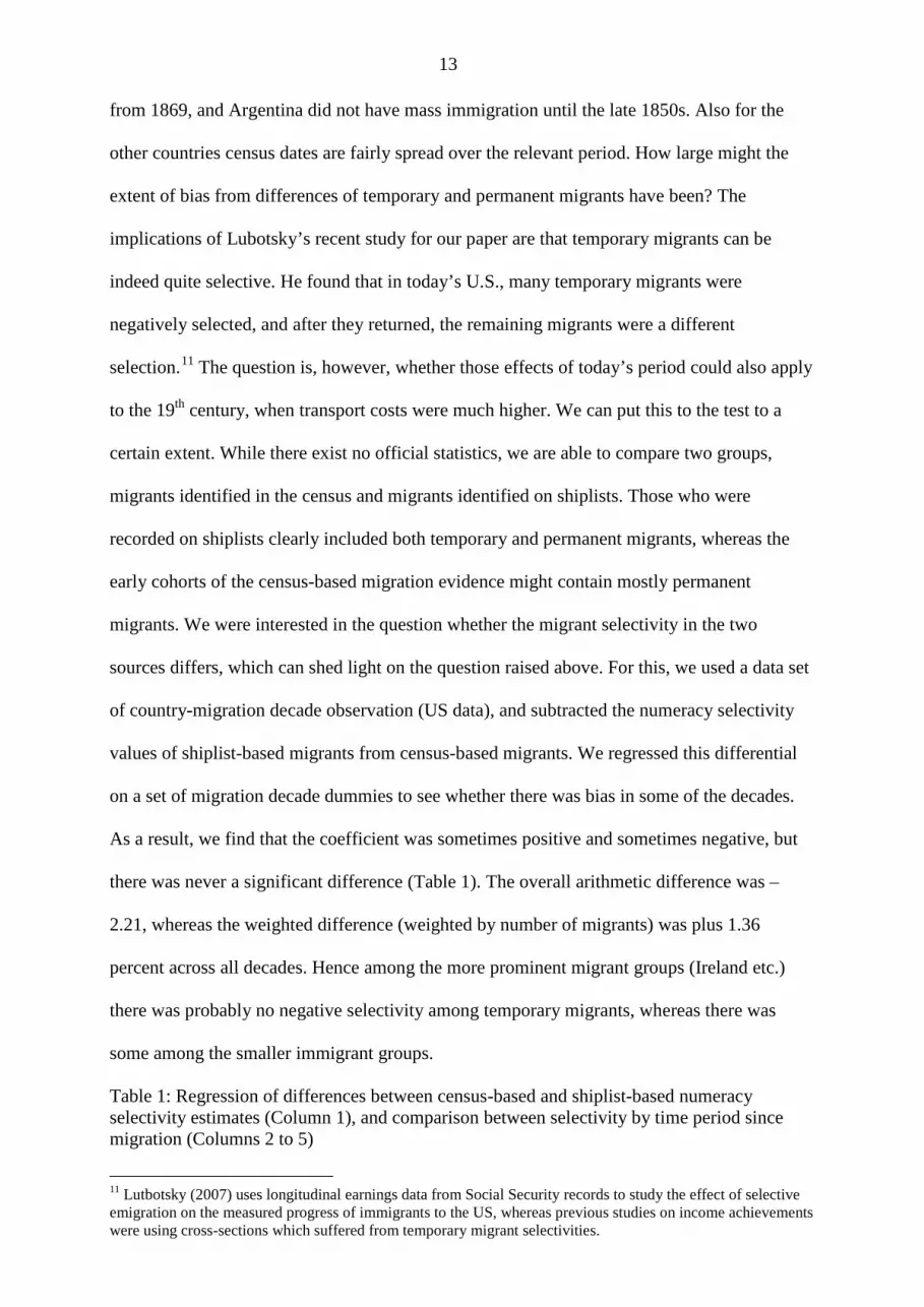
13
from 1869, and Argentina did not have mass immigration until the late 1850s. Also for the
other countries census dates are fairly spread over the relevant period. How large might the
extent of bias from differences of temporary and permanent migrants have been? The
implications of Lubotsky’s recent study for our paper are that temporary migrants can be
indeed quite selective. He found that in today’s U.S., many temporary migrants were
negatively selected, and after they returned, the remaining migrants were a different
selection.11 The question is, however, whether those effects of today’s period could also apply
to the 19th century, when transport costs were much higher. We can put this to the test to a
certain extent. While there exist no official statistics, we are able to compare two groups,
migrants identified in the census and migrants identified on shiplists. Those who were
recorded on shiplists clearly included both temporary and permanent migrants, whereas the
early cohorts of the census-based migration evidence might contain mostly permanent
migrants. We were interested in the question whether the migrant selectivity in the two
sources differs, which can shed light on the question raised above. For this, we used a data set
of country-migration decade observation (US data), and subtracted the numeracy selectivity
values of shiplist-based migrants from census-based migrants. We regressed this differential
on a set of migration decade dummies to see whether there was bias in some of the decades.
As a result, we find that the coefficient was sometimes positive and sometimes negative, but
there was never a significant difference (Table 1). The overall arithmetic difference was –
2.21, whereas the weighted difference (weighted by number of migrants) was plus 1.36
percent across all decades. Hence among the more prominent migrant groups (Ireland etc.)
there was probably no negative selectivity among temporary migrants, whereas there was
some among the smaller immigrant groups.
Table 1: Regression of differences between census-based and shiplist-based numeracy selectivity estimates (Column 1), and comparison between selectivity by time period since migration (Columns 2 to 5)
11 Lutbotsky (2007) uses longitudinal earnings data from Social Security records to study the effect of selective emigration on the measured progress of immigrants to the US, whereas previous studies on income achievements were using cross-sections which suffered from temporary migrant selectivities.
14
(1) (2) (3) (4) (5) Migration cohorts All All All All 1870s Less than 20 years
-0.96 -0.67 -0.84 -0.55
in U.S.
(0.290) (0.378) (0.291) (0.747) Migration dec 1810 -5.67
(0.523) Migration dec 1820 -1.01
(0.856)
Migration dec 1830 0.84
(0.804)
Migration dec 1840 0.58
(0.860)
Migration dec 1850 -3.41
(0.291)
Migration dec 1860 -1.85
(0.566)
Migration dec 1870 -1.99
(0.556)
Migration dec 1880 2.14
(0.641)
Migration dec 1890 -1.21
(0.637)
Country FE N N Y N N Time FE N N N Y N Constant -1.21 -2.17*** -7.53*** 0.49 -3.80
(0.637) (0.000) (0.000) (0.599) (0.005)
N 105 205 205 205 70 R-sq 0.04 0.01 0.65 0.04 0.00
In column 1, the year indicates the migration decade estimate (1810 for 1810-19 etc). Reference category is 1900s. Dependent variable is the difference between migrant selectivity according to shiplists in the U.S. (which includes both temporary and permanent migrants) and the migrant selectivity according to census. Migrant selectivity is always the difference between the numeracy of migrants and source country population in a specific decade. In column 2 to 5, the dependent variable is migrant selectivity according to the U.S. censuses of 1900 and 1910. In the column 2 to 4, both censuses are pooled, because the attention is focused on the difference between migrants more and less than 20 years in the United States. In column 5, the censuses are not pooled, because the focus is here on the comparison of migrants of the 1870s migration decade only, who were either “permanent” migrants (longer than 20 years in the U.S) or “mixed” (permanent and temporary) migrants (shorter than 20 years in the U.S.).
Moreover, we used the time of migration variable which is available in the U.S.
censuses of 1900 and 1910. We distinguished migrants who were less than 20 years and those
who were more than 20 years in the United States, which is a frequently used threshold.
Within those two groups, we calculated the difference between their ABCC value and the one
of the country and birth decade they came from. This yielded 205 country-cohort
observations, each expressed as the difference between migrant ABCC and source country
ABCC. This variable was regressed on a dummy variable “Less than 20 years in the U.S.”,
whereas the reference categories were migrants who were at the time of the census more than
15
20 years in the United States (Table 1, Col. 2-4). As we do not know whether the former
migrants stayed later-on, it is a comparison between both permanent and temporary migrants
on the one hand and permanent migrants on the other. There is always a small negative effect
of less than 1 percent ABCC, but it is never significant.12 In sum, if there was an issue of
return migrant selectivity, it was probably small for this period.
3b. Estimating Inequality
A second methodological question was the measurement of relative inequality. Although
Borjas’ original model looks at the standard deviation of wages, most recent studies on the
model use Gini coefficients of the income distribution, because they are available for a large
number of countries since about 1980. The underlying assumption is that wage variation and
overall income Gini coefficients correlate.13 For the 19th century, data on inequality is scarce
(see van Zanden et al., 2011; Blum and Baten, 2011), therefore we use an innovative approach
to capture this independent variable, that builds on the work of these authors.
Our core independent variable is inequality in the destination country minus inequality
in the source country, constructed with an anthropometric method. Baten (2000) argued that
the coefficient of variation of human stature is correlated with overall inequality in a society,
and that it can be used as proxy measure, especially where income inequality indicators are
lacking. The correlation has been confirmed in further analyses, for example by Pradhan et al.
(2003), Moradi and Baten (2005) and van Zanden et al. (2011). This method has been widely
used in the economic history literature (Sunder, 2003; Guntupalli and Baten, 2006). The idea
is that heights reflect nutritional conditions during early childhood and youth. As wealthier
people have better access to food, medical resources and shelter, their children tend to be
taller than those of the poorer strata of the population. Hence, the variation of height of a
certain cohort may be indicative of income distribution during the decade of their birth.
12 Another test compared those who were in the U.S. for 10-20 years and those in the U.S. 20-30 years taking them from the two censuses of 1900 and 1910 separately. The migration took place in both cases during the 1870s. As result, the mixed group had a selectivity of -0.55 percent, compared to “permanent” group. 13 Belot and Hatton (2011) use wage differences measured in the wages for occupations that normally require some skills versus some that do not
16
Yet, while a correlation with income does exist, this correlation is only partial, since
some important inputs are not traded on markets but are provided as public goods. These lead
to modest deviations between purchasing power-based and height-based inequality measures.
Deaton (2003) and Pradhan et al. (2003) have highlighted the importance of measures of
health inequality in general. Heights capture important biological aspects of the standard of
living (Komlos, 1985; Steckel, 1995). Also in migration decisions a proxy that captures
overall welfare is relevant, because individuals not only maximize their income but also
health and longevity.14
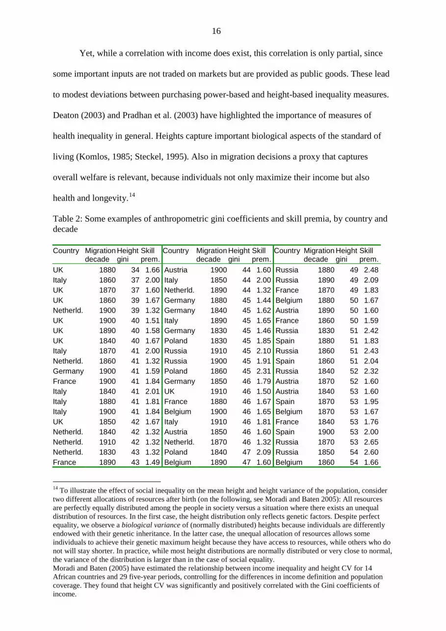
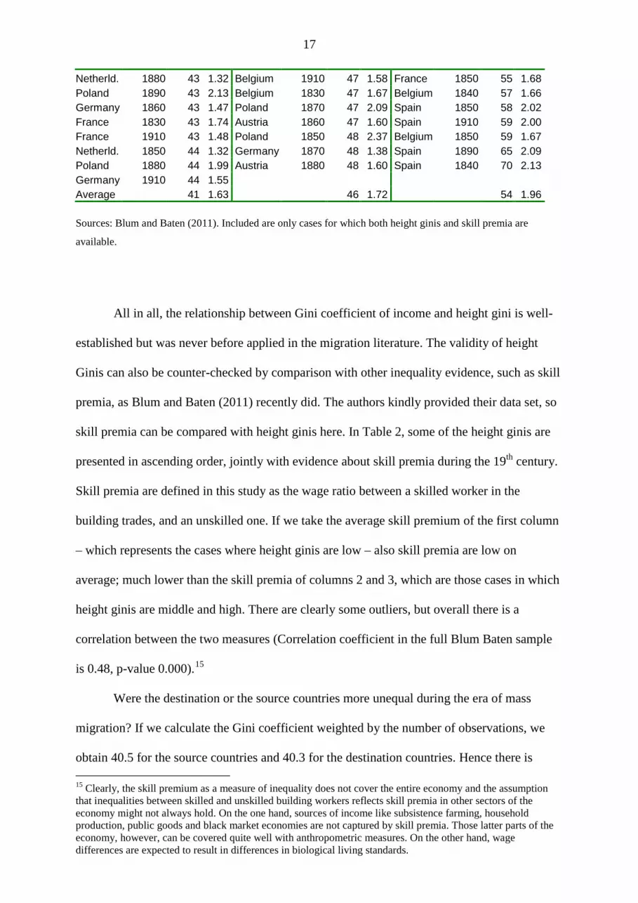
Table 2: Some examples of anthropometric gini coefficients and skill premia, by country and decade Country
Migration decade
Height gini
Skill prem.
Country
Migration decade
Height gini
Skill prem.
Country
Migration decade
Height gini
Skill prem.
UK 1880 34 1.66 Austria 1900 44 1.60 Russia 1880 49 2.48 Italy 1860 37 2.00 Italy 1850 44 2.00 Russia 1890 49 2.09 UK 1870 37 1.60 Netherld. 1890 44 1.32 France 1870 49 1.83 UK 1860 39 1.67 Germany 1880 45 1.44 Belgium 1880 50 1.67 Netherld. 1900 39 1.32 Germany 1840 45 1.62 Austria 1890 50 1.60 UK 1900 40 1.51 Italy 1890 45 1.65 France 1860 50 1.59 UK 1890 40 1.58 Germany 1830 45 1.46 Russia 1830 51 2.42 UK 1840 40 1.67 Poland 1830 45 1.85 Spain 1880 51 1.83 Italy 1870 41 2.00 Russia 1910 45 2.10 Russia 1860 51 2.43 Netherld. 1860 41 1.32 Russia 1900 45 1.91 Spain 1860 51 2.04 Germany 1900 41 1.59 Poland 1860 45 2.31 Russia 1840 52 2.32 France 1900 41 1.84 Germany 1850 46 1.79 Austria 1870 52 1.60 Italy 1840 41 2.01 UK 1910 46 1.50 Austria 1840 53 1.60 Italy 1880 41 1.81 France 1880 46 1.67 Spain 1870 53 1.95 Italy 1900 41 1.84 Belgium 1900 46 1.65 Belgium 1870 53 1.67 UK 1850 42 1.67 Italy 1910 46 1.81 France 1840 53 1.76 Netherld. 1840 42 1.32 Austria 1850 46 1.60 Spain 1900 53 2.00 Netherld. 1910 42 1.32 Netherld. 1870 46 1.32 Russia 1870 53 2.65 Netherld. 1830 43 1.32 Poland 1840 47 2.09 Russia 1850 54 2.60 France 1890 43 1.49 Belgium 1890 47 1.60 Belgium 1860 54 1.66
14 To illustrate the effect of social inequality on the mean height and height variance of the population, consider two different allocations of resources after birth (on the following, see Moradi and Baten 2005): All resources are perfectly equally distributed among the people in society versus a situation where there exists an unequal distribution of resources. In the first case, the height distribution only reflects genetic factors. Despite perfect equality, we observe a biological variance of (normally distributed) heights because individuals are differently endowed with their genetic inheritance. In the latter case, the unequal allocation of resources allows some individuals to achieve their genetic maximum height because they have access to resources, while others who do not will stay shorter. In practice, while most height distributions are normally distributed or very close to normal, the variance of the distribution is larger than in the case of social equality. Moradi and Baten (2005) have estimated the relationship between income inequality and height CV for 14 African countries and 29 five-year periods, controlling for the differences in income definition and population coverage. They found that height CV was significantly and positively correlated with the Gini coefficients of income.
17
Netherld. 1880 43 1.32 Belgium 1910 47 1.58 France 1850 55 1.68 Poland 1890 43 2.13 Belgium 1830 47 1.67 Belgium 1840 57 1.66 Germany 1860 43 1.47 Poland 1870 47 2.09 Spain 1850 58 2.02 France 1830 43 1.74 Austria 1860 47 1.60 Spain 1910 59 2.00 France 1910 43 1.48 Poland 1850 48 2.37 Belgium 1850 59 1.67 Netherld. 1850 44 1.32 Germany 1870 48 1.38 Spain 1890 65 2.09 Poland 1880 44 1.99 Austria 1880 48 1.60 Spain 1840 70 2.13 Germany 1910 44 1.55 Average 41 1.63 46 1.72 54 1.96 Sources: Blum and Baten (2011). Included are only cases for which both height ginis and skill premia are
available.
All in all, the relationship between Gini coefficient of income and height gini is well-
established but was never before applied in the migration literature. The validity of height
Ginis can also be counter-checked by comparison with other inequality evidence, such as skill
premia, as Blum and Baten (2011) recently did. The authors kindly provided their data set, so
skill premia can be compared with height ginis here. In Table 2, some of the height ginis are
presented in ascending order, jointly with evidence about skill premia during the 19th century.
Skill premia are defined in this study as the wage ratio between a skilled worker in the
building trades, and an unskilled one. If we take the average skill premium of the first column
– which represents the cases where height ginis are low – also skill premia are low on
average; much lower than the skill premia of columns 2 and 3, which are those cases in which
height ginis are middle and high. There are clearly some outliers, but overall there is a
correlation between the two measures (Correlation coefficient in the full Blum Baten sample
is 0.48, p-value 0.000).15
Were the destination or the source countries more unequal during the era of mass
migration? If we calculate the Gini coefficient weighted by the number of observations, we
obtain 40.5 for the source countries and 40.3 for the destination countries. Hence there is 15 Clearly, the skill premium as a measure of inequality does not cover the entire economy and the assumption that inequalities between skilled and unskilled building workers reflects skill premia in other sectors of the economy might not always hold. On the one hand, sources of income like subsistence farming, household production, public goods and black market economies are not captured by skill premia. Those latter parts of the economy, however, can be covered quite well with anthropometric measures. On the other hand, wage differences are expected to result in differences in biological living standards.

18
almost no difference between the two. If we include only those observations which can be
included in the regressions below (Table 5, Column 1), the result is identical.
Among the destination countries not represented in the skill premia data set, Norway
and Canada had low anthropometric inequalities with values between 41 and 48, whereas the
U.S. inequality was not low. Unfortunately, we do not have skill premia for Ireland
separately, so we cannot compare this important source country. The overall inequality of UK
was in the medium range. Poland, for example, had relatively low inequality. As the UK had
higher inequality than Poland, we would expect more skilled migration from Poland to the
UK.
While the anthropometric inequality measures allow to cover many countries and
decades, we were curious whether the results would be confirmed with other, non-
anthropometric inequality measures, even if those might be only available for a subset of
observations. Those are based on direct income gini coefficients, ginis estimated based on the
wage-to-GDP proxy suggested by Williamson, and the share of income received by the richest
fraction of the population (van Zanden et al., 2011, explain how those indicators are
transformed to become comparable). We test below whether those non-anthropometric
inequality measures yields the same results as our basic specification.
4. Data
For measuring human capital selectivity of migrants, it is necessary to measure both the
human capital of migrants and of the population of the source country. For the migrants, we
use data sets from the IPUMS and the North Atlantic Population Projects that provide 100
percent census samples for the late 19th century for a number of countries, and smaller
samples for other countries.16 We only use information on individuals that are older than 23,
because younger people still are more aware of their age. For numeracy of source countries,
16 See data appendix.
19
we use published national censuses of a great number of countries that were originally
compiled by Crayen and Baten (2010a).17
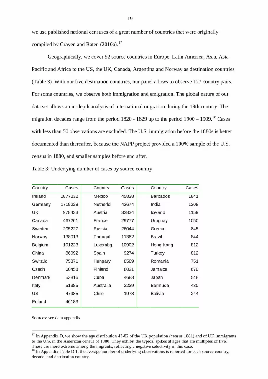
Geographically, we cover 52 source countries in Europe, Latin America, Asia, Asia-
Pacific and Africa to the US, the UK, Canada, Argentina and Norway as destination countries
(Table 3). With our five destination countries, our panel allows to observe 127 country pairs.
For some countries, we observe both immigration and emigration. The global nature of our
data set allows an in-depth analysis of international migration during the 19th century. The
migration decades range from the period 1820 - 1829 up to the period 1900 – 1909.18 Cases
with less than 50 observations are excluded. The U.S. immigration before the 1880s is better
documented than thereafter, because the NAPP project provided a 100% sample of the U.S.
census in 1880, and smaller samples before and after.
Table 3: Underlying number of cases by source country
Country Cases Country Cases Country Cases
Ireland 1877232 Mexico 45828 Barbados 1841
Germany 1719228 Netherld. 42674 India 1208
UK 978433 Austria 32834 Iceland 1159
Canada 467201 France 29777 Uruguay 1050
Sweden 205227 Russia 26044 Greece 845
Norway 138013 Portugal 11362 Brazil 844
Belgium 101223 Luxembg. 10902 Hong Kong 812
China 86092 Spain 9274 Turkey 812
Switz.ld 75371 Hungary 8589 Romania 751
Czech 60458 Finland 8021 Jamaica 670
Denmark 53816 Cuba 4683 Japan 548
Italy 51385 Australia 2229 Bermuda 430
US 47985 Chile 1978 Bolivia 244
Poland 46183
Sources: see data appendix.
17 In Appendix D, we show the age distribution 43-82 of the UK population (census 1881) and of UK immigrants to the U.S. in the American census of 1880. They exhibit the typical spikes at ages that are multiples of five. These are more extreme among the migrants, reflecting a negative selectivity in this case. 18 In Appendix Table D.1, the average number of underlying observations is reported for each source country, decade, and destination country.
20
5a. How did migrant selectivity develop during this period?
We first take a closer look at our dependent variable, which is defined as the numeracy of
migrants minus the numeracy in the source country (both in percent). For the investigated
period, average numeracy was almost equal in the source countries (90 percent), and in the
destination countries (89 percent). The average numeracy of migrants was slightly lower,
namely 87 percent (arithmetic mean by source country), or 86 percent (mean weighted by
migrant numbers). On average, there was, thus, no numeracy brain drain, but rather a
mathematical brain gain for the source countries, because migrants who left in the 19th and
early 20th century were slightly less numerate than the remaining population. The difference
is, however, small so that it is more meaningful to look at the variation of brain drain and
brain gain between countries and over time and to study the determinants. In the following,
we analyze some prominent examples of emigrant countries sending migrants to the U.S. and
UK. We arrange all numeracy values by migration decade.
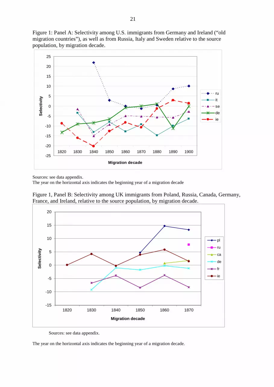
The largest migrant flows to the United States in this period came from Germany and
Ireland. These migrants were mainly negatively selected for the early cohorts of our sample
(Figure 1, Panel A).19 We actually find 6-13 percent lower numeracy among those Germans
migrating during the 1820s-1850s. Irish migrants display a stronger negative selectivity,
perhaps due to the Great Famine years, since remittances sent over by previous migrants were
also used by the less educated to leave the country. Those who migrated in the “hungry
1840s” display a value that is 20 percent lower than those, who stayed in Ireland. Over time,
this negative selectivity diminishes and eventually dissolves completely for the migration
cohorts 1880-1900.20
19 We consider Ireland separately, although it was part of the British Empire, because the characteristics of Irish migrants were different. 20 Except for the small dip in German selectivity, this might have been caused by the economic crisis of the early 1890s initiated by the Baring crisis.
21
Figure 1: Panel A: Selectivity among U.S. immigrants from Germany and Ireland (“old migration countries”), as well as from Russia, Italy and Sweden relative to the source population, by migration decade.
Sources: see data appendix. The year on the horizontal axis indicates the beginning year of a migration decade Figure 1, Panel B: Selectivity among UK immigrants from Poland, Russia, Canada, Germany, France, and Ireland, relative to the source population, by migration decade.
Sources: see data appendix.
The year on the horizontal axis indicates the beginning year of a migration decade.
-25
-20
-15
-10
-5
0
5
10
15
20
25
1820 1830 1840 1850 1860 1870 1880 1890 1900
Migration decade
Sele
ctiv
ity
ruitsedeie
-15
-10
-5
0
5
10
15
20
1820 1830 1840 1850 1860 1870
Sele
ctiv
ity
Migration decade
pl
ru
ca
de
fr
ie
22
Among the “new immigration areas” in Eastern and Southern Europe – and the Nordic
countries such as Sweden – the development is quite different (Figure 1, panel A). The
Swedes and Italians show a modest negative selectivity over the whole period with no major
changes. In contrast, the Russian immigrants initially are very positively selected (although
numbers of migrants were small). The earliest cohorts migrating in the 1840s are more than
20% more numerate than their compatriots staying at home.21 This is partly due to the fact
that large shares of Russian immigrants were Jews, who have a reputation for being better
educated than the overall population. Additionally, the high costs of migration from Eastern
Europe translated in highly skilled first-wave migrants. Afterwards, there are probably strong
“friends and relatives”-effects at work, also supported by remittances, as illustrated by the fact
that the strong positive selectivity of the first decades decreases among the later cohorts.
As a second example of a migration destination, England is a particularly interesting
case (Figure 1, Panel B). Here, immigration is predominantly Irish in the first cohorts. These
individuals are on average slightly positively selected (between 0 and 5 percent). Therefore,
Ireland experiences some brain drain to England, but a brain gain migration to the US. Also,
Poland and Russia, and to a lesser extent Canada suffer from brain drain effects due to
migration to England. France and Germany, in contrast, did not experience brain drain with
their modest migration flows to England.
In sum, although migrants are on average slightly negative selected, the variation
between countries is large. Especially during the mid-19th century waves of migration, some
of the main source countries display negative migrant selectivity partly caused by payments of
source country government institutions who wanted to send away the poorest, and partly
financed by remittances of earlier migrants (especially important for the Irish migration, see
Cohn 2009, for the German case see Bade 2008). In contrast, Eastern European migrants are
quite positively selected.
21 The immigration cohort of the 1830s would have been even more positively selected, but we removed it from the figure due to quite small sample size, in order not to provide an inadequate impression. Thanks to Ray Cohn for his important comment on this.
23
5b. What determines migrant selectivity?
We first estimate the factors determining migrant selectivity in an OLS framework using the
following equation:
(3) Sijt = Inequijt + log(Migijt-1) + PovConstit+ Log (Distij) + PovConstit * Log (Distij)
+ Demijt + Languageij + Colonyij + Civil Warit + Relative Democracyijt +
Fixed Effectsi + Fixed Effectsj+ Fixed Effectst
Skill-selectivity of migrants Sijt observed in destination country j from source country i in
migration decade t is our dependent variable. The prominent explanatory variable is Inequijt,
which is the relative Gini coefficient from destination and source country in a given migration
decade. This is the coefficient of interest, when analyzing the Roy-Borjas relationship. Next,
we control for a set of standard migration variables that could also impact on migrant
selectivity, such as the friends-and-relatives-effect, which we proxy with the log of the
absolute immigrants observed in destination country j from source country i in t-1, log(Migijt-
1) that is, in the decade previous to the estimated migration decade. PovConstit is a variable
that controls for the development level of the source country i as a possible poverty constraint.
The log distance, Log (Distij), between the capitals of source and destination countries is also
included. The poverty constraint is also interacted with log distance, since we would expect
the poverty constraint to be more binding in case of a transatlantic journey then in the case of
intra-European migration because of the lower material and psychological migration costs in
the latter case. Additionally, we control for common language, Languageij and colonial ties,
Colonyij.22 And finally, we control for Relative Democracyijt of source and destination country
and Civil Warit at the time of emigration in the source country.
Descriptive statistics are displayed in Table 4. The migrant selectivity variable is
distributed between -27.9 and +52.0 numeracy points with an unweighted mean of -4.3,
indicating that on average, migrants were slightly negatively selected. Relative Gini
22 http://www.cepii.fr/anglaisgraph/bdd/distances.htm, last accessed 15.10.2010

24
coefficients are distributed between -28 and 22. The raw migrant share variable displayed
some left skewness, which is why we take the logs.
Table 4: Descriptive statistics
Variable Obs Mean Std. Dev. Min Max
Migrant selectivity 303 -4.3 8.2 -27.9 52.0
Relative inequality
(anthrop.) 303 -3.9 8.2 -28.0 22.0
Relative inequality
(non anthrop.) 82 1.0 12.7 -42.4 28.6
Ln migrant share 303 0.6 2.1 -5.0 4.6
Poverty constraint 303 0.9 0.3 0.0 2.1
Ln distance 303 3.0 1.1 0.5 4.6
Ln dist*pov. constr. 303 2.7 1.6 0.0 8.3
Relative democr. 303 1.3 3.5 -5.7 10.0
Common language 303 0.2 0.4 0.0 1.0
Colonial r'ship 303 0.2 0.4 0.0 1.0
Note: only the cases are included for which all explanatory variables (Table 5, Col 1) did not contain
missing values. The variable “Relative inequality (non anthrop.)” refers to Table 7, Column 1. Sources: see data
appendix.
In our estimations, we always employ destination and source country fixed effects to
capture country specific political and socio-cultural characteristics as well as the income
situation in destination and source countries.
As a result, relative inequality plays a consistent role in determining migrant
selectivity (Table 5). The coefficients of this variable are positive and have the expected sign
in all five specifications. The results confirm the relationship proposed by Roy (1951) and
Borjas (1987). In the first regression, we include the Russian emigration, although it might
have been partly determined by religious factors, as explained in the previous section. In the
second to fifth column, it is excluded and our results remain the same. In column 2, 4 and 5
we tested fixed effects models in order to control for unobserved heterogeneity (which is
otherwise controlled with country dummies). The coefficient for relative inequality is robust
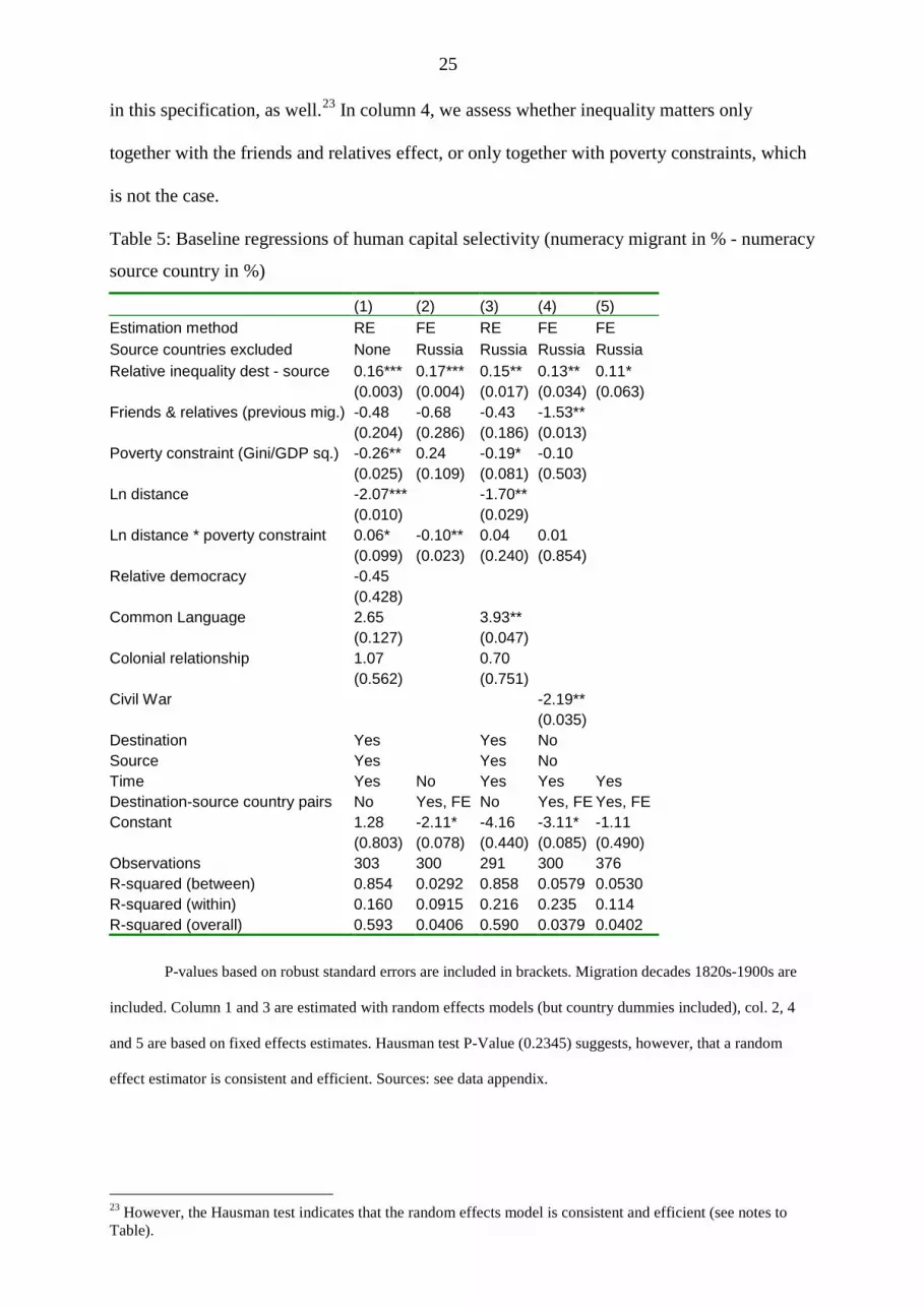
25
in this specification, as well.23 In column 4, we assess whether inequality matters only
together with the friends and relatives effect, or only together with poverty constraints, which
is not the case.
Table 5: Baseline regressions of human capital selectivity (numeracy migrant in % - numeracy
source country in %)
(1) (2) (3) (4) (5) Estimation method RE FE RE FE FE Source countries excluded None Russia Russia Russia Russia Relative inequality dest - source 0.16*** 0.17*** 0.15** 0.13** 0.11* (0.003) (0.004) (0.017) (0.034) (0.063) Friends & relatives (previous mig.) -0.48 -0.68 -0.43 -1.53** (0.204) (0.286) (0.186) (0.013) Poverty constraint (Gini/GDP sq.) -0.26** 0.24 -0.19* -0.10 (0.025) (0.109) (0.081) (0.503) Ln distance -2.07*** -1.70** (0.010) (0.029) Ln distance * poverty constraint 0.06* -0.10** 0.04 0.01 (0.099) (0.023) (0.240) (0.854) Relative democracy -0.45 (0.428) Common Language 2.65 3.93** (0.127) (0.047) Colonial relationship 1.07 0.70 (0.562) (0.751) Civil War -2.19** (0.035) Destination Yes Yes No Source Yes Yes No Time Yes No Yes Yes Yes Destination-source country pairs No Yes, FE No Yes, FE Yes, FE Constant 1.28 -2.11* -4.16 -3.11* -1.11 (0.803) (0.078) (0.440) (0.085) (0.490) Observations 303 300 291 300 376 R-squared (between) 0.854 0.0292 0.858 0.0579 0.0530 R-squared (within) 0.160 0.0915 0.216 0.235 0.114 R-squared (overall) 0.593 0.0406 0.590 0.0379 0.0402
P-values based on robust standard errors are included in brackets. Migration decades 1820s-1900s are
included. Column 1 and 3 are estimated with random effects models (but country dummies included), col. 2, 4
and 5 are based on fixed effects estimates. Hausman test P-Value (0.2345) suggests, however, that a random
effect estimator is consistent and efficient. Sources: see data appendix.
23 However, the Hausman test indicates that the random effects model is consistent and efficient (see notes to Table).
26
Is the coefficient of relative inequality economically meaningful? One method of
measuring economic significance is to consider the effects of one standard deviation of the
explanatory variable. If we multiply the standard deviation of inequality (8.21) with its
coefficient (0.17, col. 2 in Table 5), we obtain 1.39. This is roughly 17% of the standard
deviation of the dependent variable (standard deviation: 8.16), which means that it can explain
roughly one sixth of the standard deviation of the dependent variable. This amount is not very
large, but it is also not negligible. If we do the same with the coefficient of the non-
anthropometric relative inequality variable below (Table 7, column 1: 0.29, and Table 4, line
3), we obtain 3.68, which is around 45% of the standard deviation of the dependent variable.
This is a substantial share, indicating economic significance.
The other variables had much less consistent effects. The friends and relatives effect
has always the expected negative sign, but is only statistically significant in specification 4,
Table 5 (and in Appendix Table D.2, column 1). This indicates some impact of already
existing networks on the skill selectivity of new migrants, but the insignificance of many
coefficients suggests that this effect was not very systematic. The provision of information
and remittances might have encouraged also less positively selected individuals to migrate in
some of the cases.
The poverty constraint variable renders also no consistent results. It mainly has a
negative sign and is twice significant. While Hatton and Williamson (1998) found that it was
a determinant of migration flows, but human capital selectivity does not seem to be
consistently related to this variable.
We calculated a time variant measure of economic distance costs.24 The strong decline
of transport cost with the arrival of the steamship innovation features prominently here. Log
(Distij) has a negative sign and becomes significant. This result might seem counter-intuitive,
but the result might be due to the fact that the majority of the variance in the distance variable
24 We took the passenger cost estimates by Sanchez-Alonso (2008), and calculated the cost for distance unit for each decade. This is then multiplied with actual distances between population centres in the countries. (distance measures from http://www.cepii.fr/)

27
stems from the difference in trans-Atlantic versus intra- European migration. We observe
better selected individuals in European destination countries than in the U.S. or Argentina, for
example, perhaps because the risky environment of the New World deterred skilled
migrants.25
Relative democracy is controlled for based on the estimates of democracy produced by
the Polity IV project.26 It indicates the openness of democratic institutions in a country and is
measured on a scale of -10 (low) to 10 (high). We subtracted the democracy score of the
destination country from the one of the source country to obtain the relative democracy
variable. One might expect that the more educated were attracted by higher democracy values
in the destination country, relative to the source country (on the significant attraction of
migrants of any skill, see Bertocchi and Strozzi 2008). This variable turns out to be
insignificant, too. The politically motivated migration might have been too small in number
during the 19th century, or it was probably not sufficiently restricted to the more educated
strata.
Finally, we tested common language and colonial relationships, and found positive
effects for language. A common language might have been more useful for the more educated
who usually have a comparative advantage with words and skills, rather than with brawn.
Colonial ties do not seem to matter. Finally, in column 4 of Table 5 we test for a potential
effect of civil war in the country of origin, which turns out negative and significant. This
25 This is supported by the fact that when old world destinations are not included below in Column 5 of Appendix Table D.2, the variable gets a large positive value (p-value 0.103). As a second possible explanation, it could be speculated that migrants within Europe expected more skill competition in European destination labor markets. Figures 1 and 2 indicate this particularly for the case of Irish emigrants. We also include an interaction term between economic distance and poverty constraint, but it turns out mostly insignificant. In Table B.2 in the appendix we also tested whether the effect of distance and poverty constraint differ in the first half of the 19th century, because as shipping technology improved, travelling across the Atlantic became less time consuming and costly. Therefore an interaction term of distance and the time dummies of the first half of the 19th century was included (Appendix Table B.2). The result was a significant negative coefficient, indicating that in the early period, when migration was more costly, the impact of distance on migrant selectivity was even more negative than thereafter. This might be slightly more in line with the risk interpretation above, because in the early period the New World was still perceived as a risky world. An interaction term with the poverty measure and the first half of the 19th century did not render significant results. 26 Marshall, Monty G., and Jaggers, K. (2008): Polity IV Project: data set. http://www.systemicpeace.org/polity/polity4.htm

28
variable is taken from the Correlates of War Project and Uppsala Conflict Data Project. It is
coded as a dummy variable, turning 1 if civil war broke out in a given country and period. 27
5c. Tests of robustness, WLS, and direction of causality issues
As a first test for robustness, we omitted the German, Irish and English migrants to test if our
result were mainly driven by these very large immigrant groups. The results do not differ very
much, and the Roy-Borjas forces remain strong (Appendix Table D.2, columns 1-3).28
An alternative robustness test is to weigh the observations with the square root of the
number of migrants underlying each unit in a WLS regression which leads to more efficient
estimates. The results in Table 6, column 1 to 4, are consistent with previous estimates: the
relative inequality is a significant determinant of migrant selectivity. One potential
disadvantage of weighted regressions is that a few source countries account for the majority of
migrants; and thus they receive most of the weight in the estimates.29
Finally in column 5 of Table 6, we test the alternative measure for the friends-and-
relatives effect that we described in the notes to the Table, namely the number of migrants
relative to home country population. Using this different specification does not change the
27 Civil war is defined as sustained combat with at least 1,000 battle-related deaths per year that takes place between the armed forces of a government and forces of another entity for central control or for local issues. Military and civilian deaths are counted. Source: Correlates of War Project and Uppsala Conflict Data Project. http://www.correlatesofwar.org/ 28 If the Irish are omitted, the friends-and-relatives effects turns small and insignificant, this is neatly consistent with the literature that argued that this effect was particularly important for Irish migration (Cohn 2009). Next, we exclude the Irish and the Italian migrants, because here, the migration flows were very large in comparison to the home country population. Another way of validating the robustness of our results is to exclude migration to European destination countries (Appendix Table D.2, column 5). The result is that even if we look at only transatlantic migration, our results stay robust. 29 While in the OLS estimations, common language had a positive effect on human capital selectivity, the WLS regressions suggest the opposite. Here the Irish, who were negatively selected and shared a common language with North Americans, gain a strong weight, because their N was large. A former colonial relationship also seems to be of importance in WLS: this variable turns highly significant and positive in all estimations, indicating that people, who migrated into a country to which they were linked by colonial ties, were more positively selected than migrants moving to other destination countries. This might have been caused partly by re-migration of the families of former colonial officials or similar special factors of the colonial administration. We also assessed whether the difference between migrant numeracy and source country numeracy might depend on the level of source country numeracy. Those coming from a high education background might have been more likely to be negatively selected, even if we have seen many counter-examples in the Figures discussed above. We therefore include a term “ABCC level source country”, which indeed turns significant but did not change the main results (Table 6, column 3). In a similar exercise to evaluate the properties of the dependent variable, we included only those in which the source country numeracy deviates from the optimum of 100 percent (Table 6, column 4). This removes some 35 cases, relative to column 2, but again the coefficients do not change.
29
significance of the Borjas variable, and most other significance levels also do not change
(distance is the exception).
A comprehensive test of the properties of time series indicated that the main series as
well as the residuals do not display unit root problems. The Fisher test for unbalanced panels,
as well as the Hadri-LM-test for the three largest source countries in a balanced panel, were
calculated and suggest that our series do not suffer from non-stationarity.
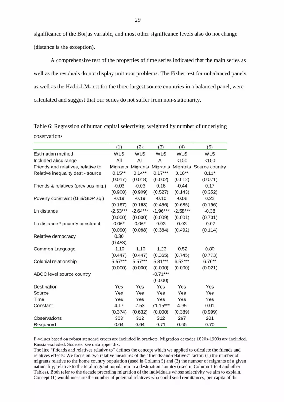
Table 6: Regression of human capital selectivity, weighted by number of underlying
observations
(1) (2) (3) (4) (5) Estimation method WLS WLS WLS WLS WLS Included abcc range All All All <100 <100 Friends and relatives, relative to Migrants Migrants Migrants Migrants Source country Relative inequality dest - source 0.15** 0.14** 0.17*** 0.16** 0.11* (0.017) (0.018) (0.002) (0.012) (0.071) Friends & relatives (previous mig.) -0.03 -0.03 0.16 -0.44 0.17 (0.908) (0.909) (0.527) (0.143) (0.352) Poverty constraint (Gini/GDP sq.) -0.19 -0.19 -0.10 -0.08 0.22 (0.167) (0.163) (0.456) (0.685) (0.196) Ln distance -2.63*** -2.64*** -1.96*** -2.58*** -0.38 (0.000) (0.000) (0.009) (0.001) (0.701) Ln distance * poverty constraint 0.06* 0.06* 0.03 0.03 -0.07 (0.090) (0.088) (0.384) (0.492) (0.114) Relative democracy 0.30 (0.453) Common Language -1.10 -1.10 -1.23 -0.52 0.80 (0.447) (0.447) (0.365) (0.745) (0.773) Colonial relationship 5.57*** 5.57*** 5.81*** 6.52*** 6.76** (0.000) (0.000) (0.000) (0.000) (0.021) ABCC level source country -0.71*** (0.000) Destination Yes Yes Yes Yes Yes Source Yes Yes Yes Yes Yes Time Yes Yes Yes Yes Yes Constant 4.17 2.53 71.15*** 4.95 0.01 (0.374) (0.632) (0.000) (0.389) (0.999) Observations 303 312 312 267 201 R-squared 0.64 0.64 0.71 0.65 0.70
P-values based on robust standard errors are included in brackets. Migration decades 1820s-1900s are included. Russia excluded. Sources: see data appendix. The line “Friends and relatives relative to” defines the concept which we applied to calculate the friends and relatives effects: We focus on two relative measures of the “friends-and-relatives” factor: (1) the number of migrants relative to the home country population (used in Column 5) and (2) the number of migrants of a given nationality, relative to the total migrant population in a destination country (used in Column 1 to 4 and other Tables). Both refer to the decade preceding migration of the individuals whose selectivity we aim to explain. Concept (1) would measure the number of potential relatives who could send remittances, per capita of the

30
source country. Assuming that the wealth of all previous immigrants would be similar, this is a convincing indicator. However, it has considerable data requirements, and population estimates in some of the source countries are not available. We could construct this measure only for 201 country pairs, for which relative inequality and other explanatory variables were available.

31
Table 7: Regression of human capital selectivity on non-anthropometric inequality measures (1) (2) (3) (4) (5) (6) Estimation method RE RE FE WLS WLS WLS Relative inequality dest - source 0.29** 0.28* 0.24** 0.34* 0.34* 0.38* (0.024) (0.058) (0.029) (0.097) (0.097) (0.080) Friends & relatives (previous mig.) -0.24 -0.23 -0.24 0.16 0.16 0.37 (0.657) (0.729) (0.813) (0.738) (0.738) (0.391) Poverty constraint (Gini/GDP sq.) -11.47** -11.53** -5.49 -16.74** -16.74** -11.84 (0.043) (0.021) (0.321) (0.032) (0.032) (0.146) Ln distance -1.95 -2.12 -4.13*** -4.13*** -3.58** (0.244) (0.213) (0.008) (0.008) (0.012) Ln distance * poverty constraint 2.26 2.41 0.23 5.93*** 5.93*** 5.02** (0.269) (0.235) (0.928) (0.006) (0.006) (0.023) Relative democracy -0.38 1.61* -0.47 (0.745) (0.068) (0.540) Common Language 0.74 0.64 -0.08 -0.08 -1.45 (0.835) (0.887) (0.981) (0.981) (0.603) Colonial relationship -1.78 -1.87 -2.08 -2.08 -1.25 (0.537) (0.691) (0.411) (0.411) (0.622) Civil War -1.10 -0.50 (0.668) (0.841) ABCC level source country -0.74 (0.103) Destination Yes Yes No Yes Yes Yes Source Yes Yes Yes, FE Yes Yes Yes Time No No No Yes Yes Yes Constant -4.34 7.79 -0.84 5.35 61.01*** 87.60*** (0.632) (0.390) (0.789) (0.424) (0.000) (0.000) Observations 82 82 82 82 82 82 R-square between 0.866 0.867 0.0275 R-square within 0.215 0.216 0.232 R-square overall 0.788 0.789 0.0318 0.79 0.79 0.81 Source: Sources: see data appendix. Van Zanden et al. (2011) recently presented estimates of global inequality based on both anthropometric and non-anthropometric inequality measures, and they kindly provided the latter to us.
32
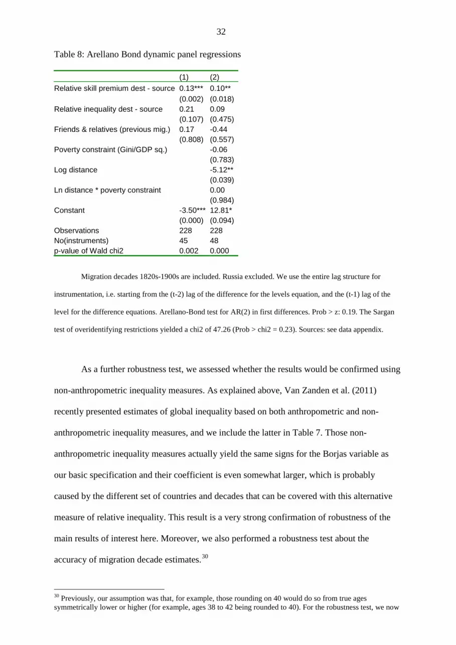
Table 8: Arellano Bond dynamic panel regressions (1) (2) Relative skill premium dest - source 0.13*** 0.10** (0.002) (0.018) Relative inequality dest - source 0.21 0.09 (0.107) (0.475) Friends & relatives (previous mig.) 0.17 -0.44 (0.808) (0.557) Poverty constraint (Gini/GDP sq.) -0.06 (0.783) Log distance -5.12** (0.039) Ln distance * poverty constraint 0.00 (0.984) Constant -3.50*** 12.81* (0.000) (0.094) Observations 228 228 No(instruments) 45 48 p-value of Wald chi2 0.002 0.000
Migration decades 1820s-1900s are included. Russia excluded. We use the entire lag structure for
instrumentation, i.e. starting from the (t-2) lag of the difference for the levels equation, and the (t-1) lag of the
level for the difference equations. Arellano-Bond test for AR(2) in first differences. Prob > z: 0.19. The Sargan
test of overidentifying restrictions yielded a chi2 of 47.26 (Prob > chi2 = 0.23). Sources: see data appendix.
As a further robustness test, we assessed whether the results would be confirmed using
non-anthropometric inequality measures. As explained above, Van Zanden et al. (2011)
recently presented estimates of global inequality based on both anthropometric and non-
anthropometric inequality measures, and we include the latter in Table 7. Those non-
anthropometric inequality measures actually yield the same signs for the Borjas variable as
our basic specification and their coefficient is even somewhat larger, which is probably
caused by the different set of countries and decades that can be covered with this alternative
measure of relative inequality. This result is a very strong confirmation of robustness of the
main results of interest here. Moreover, we also performed a robustness test about the
accuracy of migration decade estimates.30
30 Previously, our assumption was that, for example, those rounding on 40 would do so from true ages symmetrically lower or higher (for example, ages 38 to 42 being rounded to 40). For the robustness test, we now
33
Next we considered the problem of endogeneity. Theoretically, one could imagine that a
massive exodus of a large and highly selected part of a population would influence relative
inequality of the source country, since relative inequality should ceteris paribus decline, if, for
example, a large share of unskilled workers leaves. In most countries, however, the
requirement of a large share of the population leaving is not fulfilled, since emigration rates
were normally below 5 percent per decade. Exceptions are Ireland, from where in some
decades more than 10 percent left, and Italy right before WWI (Hatton and Williamson,
1998). This means that a problem of reverse causality might arise as a large, and strongly
selective migrant flow might in turn affect income distribution in the source country. The only
migration flows that were so large are the Irish and the Italian. If we exclude them from our
regressions, the results stay robust (Appendix Table D.2, column 4). Hence, we conclude that
the direction of causality issue is not affecting our results generally.
Finally, we tested whether our results also hold when a Generalized Method of
Moments estimator is applied (Arellano and Bond, 1991). While this method is
conventionally used in dynamic settings to account for the likely endogeneity of lagged
dependent variables, it basically generates a large number of instrumental variables from
lagged first difference values of the dependent variable. This estimation in first differences is
of advantage, because it allows us to make sure that trend correlation is not a problem here.
Again, the relative inequality coefficients turn out robust (Table 8).
To conclude, a wide range of econometric techniques suggests that relative inequality
had an effect on migrant selectivity as measured by relative numeracy with the age heaping
method. There is some evidence -- although more limited -- on friends-and relatives-effects,
hypothesized that only ages 37 to 41 rounded to 40. In a second step, we did the same with 39 to 43. We are well aware that this introduces artificial measurement error, because the symmetric rounding is the more likely factual behavior. Hence the results would be expected to yield slightly less significant results, but a small variation should not completely change the results. This is exactly what happened. Of the coefficients, 100 percent kept the same sign and the same order of magniturde, and almost all remained significant. In very few cases, the p-values of statistical significance went slightly over 0.10, as we would have expected since we are introducing artificial measurement error in this robustness test.

34
colonial relationships and common language, whereas counteracting forces might have
rendered the effects of economic distance and democracy mostly insignificant.
Conclusion
In this study, we assessed the selectivity of migrants in the era of mass migration. We focus
not only on the main transatlantic migration destinations, but also on two European
destination countries, the UK and Norway. No less than 52 source countries could be
included, with 127 country pair flows. The underlying data set is based on 6.2 million
individual migrants.
The main model tested is the Roy Model of self-selection (1951) that Borjas applied to
the process of migration (1987). It states a relationship between skill selectivity of migrants
and relative inequality of source and destination countries, measured with an anthropometric
indicator here. We confirm the influence of these economic migration incentives after
controlling for a large number of other variables such as “friends and relatives effects”,
poverty constraints, economic distance, relative democracy, common language and colonial
relationships. Even if we used non-anthropometric inequality measures, regressions actually
yield the same signs for the Borjas variable as our basic specification and the coefficient is
even somewhat larger. This study has been the first general assessment of migrant selectivity
during this most crucial period of human migration history, using large samples that included
a variety of different source and destination countries.
It is crucial to understand the brain-drain processes between source and destination
countries, because the stock of human capital determines future growth capabilities. Brain
drain effects have not been systematically studied for the era of mass migration of the mid-to-
late 19th century with large international samples before. In the case of mid-19th century mass
migration history, we also noted some arithmetic brain gains for the source countries, since
those who left Scandinavia or central Europe around mid-century were often less numerate
than the remaining population. There could have been, for instance, marginal positive human
capital growth effects in Germany or in some Scandinavian countries, because the average

35
numeracy should have increased with migration, due to negatively selected emigration. In
contrast, Eastern Europe lost a large number of the numerate population, and the migration
effects might have been ceteris paribus negative. Clearly, also a large number of other factors
were at work, which is why these effects should not be seen in isolation.
Can we draw a wider pricture, comparing today’s migration with the era of mass
migration? Two main differences are obvious. Firstly, in the world today, immigration
policies play a much stronger role than in the 19th century, making it very hard for many
unskilled potential migrants to jump over immigration hurdles. Hence each consideration of
relative inequality incentives has to be ceteris paribus. A second major difference in this big
picture is that today many migrants come from countries with higher inequality. This fact
fueled the Borjas debate about potentially problematic selectivity of migrants coming from
Mexico to the United States in the recent past. In the 19th and early 20th century, this was
clearly different, because source and destination country inequalities were almost equal.
However, the debate about migrant education in the U.S. before WWI was also mostly
motivated by immigration from countries in Southern and Eastern Europe which were
characterised by relatively high inequality. Even if the absolute level of education was the
main issue of debate, the Borjas forces were also influential in the background. In sum, when
designing immigration policies today, both the recent and the historical experience can
provide important insights about the economic forces which determine the selectivity of
migration.
36
References
Abramitzky, R., Boustan, L.P., Eriksson, K. 2009. Measuring Selectivity and Returns in the
age of Mass Migration. NBER Working Paper 15684.
Arellano, M., and S. Bond. 1991. Some tests of specification for panel data: Monte Carlo
evidence and an application to employment equations. Review of Economic Studies
58: 277-297.
Bachi, R., 1951. The tendency to round off age returns: measurement and correction. Bulletin
of the International Statistical Institute 33, 195-221
Bade, K.J. (ed.), 2008. Enzyklopädie Migration in Europa: vom 17. Jh. bis zur Gegenwart.
Stuttgart.
A’Hearn, B., Baten, J., Crayen, D., 2009. Quantifying Quantitative Literacy: Age Heaping
and the History of Human Capital. The Journal of Economic History 69/3, 783-808.
Baten, J., 2000. Economic Development and the Distribution of Nutritional Resources in
Bavaria, 1797-1839, Journal of Income Distribution 9, 89-106.
Baten, J., Blum, M., 2012. Growing Taller, but Unequal: Biological Well-Being in World
Regions and Its Determinants, 1810-1989, Economic History of Developing Regions
(forthcoming 2012).
Belot, M.V.K., Hatton, T.J., 2011. Immigrant Selection in the OECD. Scandinavian Journal of
Economics, forthcoming.
Bertocchi, G. and Strozzi, C., 2008. International Migration and the Role of Institutions,
Public Choice, 137, 81-102.
Blum, M. and Baten, J., 2011. Estimating Inequality with Anthropometric Indicators, Review
for Economics – Jahrbuch für Wirtschaftswissenschaften, 62-2, 107-138.
Borjas, G.J., 1987. Self-Selection and the Earnings of Immigrants. The American Economic
Review 77/4, 531-553.
Boustan, L.P., 2007. Were Jews political refugees or economic migrants? Assessing the
persecution theory of Jewish emigration, 1881–1914. In: T.J.Hatton, K.H.O'Rourke
37
and A.M.Taylor (eds.), The New Comparative Economic History: Essays in Honor of
Jeffrey G. Williamson. MIT Press. Cambridge.
Bruecker H., Defoort, C., 2006. The Self-Selection of International Migrants Reconsidered:
Theory and New Evidence. IZA Discussion Paper Series. IZA DP 2052.
Chiswick, B.R., 2005. High Skilled Immigration in the International Arena. IZA Discussion
Paper Series. IZA DP 1782.
Cinnirella, F., 2008. Optimists or pessimists? A reconsideration of nutritional status in Britain,
1740–1865. European Review of Economic History 2008/12, 325-354.
Clark, G., 2007. A Farewell to Alms: A Brief Economic History of the World. Princeton UP.
Cohn, R.L., 2009. Mass Migration under Sail: European Immigration to the Antebellum
United States. Cambridge University Press. Cambridge.
Crayen, D., Baten, J., 2010a. Global Trends in Numeracy 1820–1949 and its Implications for
Long-term Growth. Explorations in Economic History 47/1, 82-99.
Crayen, D., Baten, J., 2010b. New Evidence and New Methods to Measure Human Capital
Inequality before and during the Industrial Revolution: France and the US in the
Seventeenth to Nineteenth centuries. Economic History Review 53-2, 452-478.
Chiquiar, D., Hanson, G., 2005. International migration, self-selection, and the distribution of
wages: evidence from Mexico and the United States. Journal of Political Economy
113-2, 239–281.
Deaton, A., 2003. Health, Inequality and Economic Development, Journal of Economic
Literature, XLI, 112–158.
De Moor, T. and Van Zanden, J.-L., 2008. Uit fouten kun je leren. Tijdschrift voor
Economische en Sociale Geschiedenis 5-4: 55-86.
Docquier, F., 2006. Brain Drain and Inequality Across Nations. IZA Discussion Paper Series.
IZA DP 2440.
Feliciano, C., 2005. Educational Selectivity in U.S. Immigration: How Do Immigrants
Compare to those left behind? Demography 42/1, 131-152.

38
Ferenczi, I., Willcox, W.F., 1929. International Migrations, Vol I&II. New York.
Flora, P., 1983. State, Economy and Society in Western Europe: 1815-1975. A data handbook
in two Volumes. Frankfurt, M. Campus.
Fogel, R., 1994. Economic Growth, Population Theory, and Physiology: The Bearing of
Long-Term Processes on the Making of Economic Policy. American Economic
Review 84: 369-95.
Grogger, J. and Hanson, G.H., 2011. Income maximization and the selection and sorting of
international migrants. Journal of Development Economics 95, 42-57.
Guntupalli, A.M., Baten, J., 2006: The development and inequality of heights in North, West
and East India, 1915-1944, Explorations in Economic History 43-4, 578-608.
Hatton, T.J., 2010. The Cliometrics of International Migration: A Survey. Journal of
Economic Surveys 24, no. 5, 941-969.
Hatton, T.J., Williamson, J.G. 1998. The Age of Mass Migration: Causes and Economic
Impact. Oxford University Press. New York.
Hatton, T.J., Williamson, J.G. 2002. What Fundamentals Drive World Migration? NBER
Working Paper No. 9159.
Hatton, T.J., Williamson, J.G. 2008. Global Migration and the World Economy: two
Centuries of Policy and Performance. MIT Press. Michigan.
Hippel, W.v., 1984. Auswanderung aus Südwestdeutschland. Studien zur Württembergischen
Auswanderung und Auswanderungspolitik im 18. und 19. Jahrhundert. Stuttgart.
Humphries, J., Leunig, T., 2009. Was Dick Whittington taller than those he left behind?
Anthropometric measures, migration and the quality of life in early nineteenth century
London? Explorations in Economic History 46/1, 120-131.
Liebig, T., Sousa-Poza, A., 2004. Migration, Self-Selection and Income Inequality: An
International Analysis. Kyklos, Vol. 57/1, 125-147
39
Long, J., Ferrie, J., 2010. British, American, and British-American Social Mobility:
Intergenerational Occupational Change Among Migrants and Non-Migrants in the
Late 19th Century. Working Paper Colby College/Northwestern University.
Lubotsky, D., 2007. Chutes or Ladders? A Longitudinal Analysis of Immigrant Earnings.
Journal of Political Economy, 115/5, 820-867.
Kamphoefner, W., 2009. Mass Migration under Sail: European Immigration to the
Antebellum United States. By Raymond L. Cohn. Book Review. Journal of
Interdisciplinary History 40/4, 621-622.
Komlos, J., 1985. Stature and Nutrition in the Habsburg Monarchy. The American Historical
Review Vol. 90, No. 5, 1149-1161.
Komlos, J., Baten, J., (eds.), 1998. The Biological Standard of Living in Comparative
Perspectives. Stuttgart: Steiner.
Maddison, A., 2009. The World Economy: a Millennial Perspective. OECD Publ. 2001.
Marshall, M.G., Jaggers, K. 2008. Polity IV Project: Political Regime Characteristics and
Transitions, 1800-2008. Center for Systemic Peace and Center for Global Policy at
George Mason University.
Myers, R., 1954. Accuracy of age reporting in the 1950 United States census. Journal of the
American Statistical Association XLIX, 826-831.
Moradi, A., Baten, J., 2005. Inequality in Sub-Saharan Africa: New Data and New Insights
from Anthropometric Estimates. World Development Vol. 33, No. 8, 1233-1265.
Moraga, J., 2011. New Evidence of Emigrant Selection. Review of Economics and Statistics
93-1, 72-96.
Mills, E.J., Schabas, W.A., Volmink, J., Walker, R., Ford, N., Katabira, E., Anema, A.,
Joffres, M., Cahn, P., Montaner, J., 2008. Should active recruitment of health workers
from sub-Saharan Africa be viewed as a crime? The Lancet 371, 685-88.
Mokyr, J., 1983. Why Ireland starved: a quantitative and analytical history of the Irish
economy, 1800-1850, London and Boston.
40
O’Grada, C., 1986. Across the Briny Ocean: some thoughts on the Irish emigration to
America 1800-1850. Migrations across time and nations. New York, 79-94.
O’Grada, C., 2006. Dublin Jewish Demography a Century Ago. The Economic and Social
Review 37-2, 123-147.
O’Rourke, K., Williamson, J., 1999. Globalization and History. Cambridge, Ma. And London.
Pradhan, M., Sahn D.E., Younger, S.D., 2003. Decomposing World Health Inequality. Journal
of Health Economics 22/2, 271-293.
Roy, A., 1951. Some thoughts on the distribution of earnings. Oxford Economic Papers 3,
135–46.
Sanchez Alonso, B., 2008. The Other Europeans: Immigration into Latin America and the
International Labour Market, 1870-1930. Revista de Historia Económica25-3, 395-426
Singer, J.D., Small, M., 1972. The Wages of War, 1816-1965: A Statistical Handbook. New
York. Or see http://www.correlatesofwar.org, last accessed March 31st, 2010.
Steckel, R., 1995. Stature and the Standard of Living. Journal of Economic Literature 33,
1903-1940.
Sunder, M., 2003. The Making of Giants in a Welfare State: The Norwegian Experience in the
20th Century. Economics & Human Biology, 1(2), 267-276.
Timmer, A.S., Williamson, J.G., 1996. Racism, Xenophobia or Markets? The Political
Economy of Immigration Policy Prior to the Thirties. NBER Working Paper W5867.
Van Zanden, J.L., 2009. The skill premium and the Great Divergence, European Review of
Economic History 13, 121-153.
Van Zanden, J.L., Baten, J., Foldvari, P., Leeuwen, B.v., 2011. World Income Inequality
1820-2000. Working Paper Univ. Utrecht/Tuebingen.
Wegge, S.A., 2002. Occupational Self-selection of Nineteenth-Century German Emigrants:
Evidence from the Principality of Hesse-Cassel. European Review of Economic
History 6 (3), 365-394.
41
Appendix A (not to be included in the published version, but available in the internet) Data Appendix
Migrant numeracy: Difference between the numeracy of migrants and the joint weighted numeracy of stayers
and migrants (except for countries in which migration was small, see the longer footnote in the ‘skill selectivity’
section). Numeracy in the source countries are from Crayen and Baten (2010a). On the sources of migrants:
Census evidence was available for Argentina (1869, 1895) – sample of circa 2 percent; Canada (1871, 1881-
100%, 1901); Norway (1865, 1875, 1900); England (1851, 1881); US (1850, 1860, 1870, 1880-100%, 1900,
1910). Sources of those censuses: On the U.S. except 1880: Ruggles, Steven, Matthew Sobek, and Trent
Alexander, et al. Integrated Public Use Microdata Series: Version 3.0 [Machine-readable database].
Minneapolis, MN: Minnesota Population Center [producer and distributor], 2004. On Argentina: Somoza, J. and
Lattes, A. (1967. Muestras de los dos primeros censos nacionales de población, 1869 y 1895. Documento de
Trabajo No 46, Instituto T. Di Tella, CIS, Buenos Aires. On all other samples: North Atlantic Population Project
and Minnesota Population Center. NAPP: Complete Count Microdata. NAPP Version 2.0 [computer files].
Minneapolis, MN: Minnesota Population Center [distributor], 2008. [http://www.nappdata.org].
We used the migration numbers in Ferenczi and Willcox to identify the countries in which the migration rate
exceeded one percent per decade to a given target country (in most cases, there was only one target country with
such substantial migration). For the periods before 1870, we used the stock of migrants in the target countries,
and compared overlapping numbers between Ferenczi and Willcox and census data in order to make sure that the
differences in counting (Ferenczi and Willcox focus on migration statistics, hence an Irish migrant to Canada
might have finally gone to the U.S; the census stock excludes those who died between migration and census
taking). But the correspondence between both sources was quite good. For example, for the 1860s Ferenczi and
Willcox list some 700,000 migrants from the UK (incl. Ireland) to the U.S., whereas the stock in the 1880s that
we estimated to have migrated during the 1860s was 660,000. We then calculated the weighted average of
numeracy of stayers and migrants. Only for very few cases we had to assume similar values to the ones of other
migrants (for example, we assumed that Spanish migration to Brazil in the 1880s was similar to the one to
Argentina in the 1880s etc.).
Relative Inequality Dest-Source (anthrop.):: height gini of the destination county minus the height gini of the
source county, from Blum and Baten (2012), Estimating Inequality with Anthropometric Indicators, for an online
version, see http://www.wiwi.uni-tuebingen.de/cms/fileadmin/ Uploads/Schulung/Schulung5/
Joerg/Baten_Blum_skpr100331a.pdf, last accessed March 31st, 2010.
Moradi and Baten (2005) recommended the following formula for translating height CVs into ‘height ginis’
(ibid: p.29), which we will use below:
(3) Giniit=-33.5+20.5*CVit
Relative Inequality (non-anthrop.): Gini coefficients of income inequality of the destination county minus the
Gini coefficient of the source county, from van Zanden et al. (2011), friendly provided by the authors. The
authors include all estimates of income inequality: direct estimates based on tax and other statistical surveys,
indirect estimates based on the share of income of the richest fraction of the population, and indirect estimates
based on the ratio between average income and the wages of unskilled workers (the ‘Williamson method’).

42
Friends and relatives (previous mig.): The share of migrants from one source country in one destination country,
relative to the total number of migrants in this destination country. It was calculated with migrant data sets cited
above under Migrant numeracy. In Table 6, column 5, this variable is defined as the number of migrants in
country j from country i, relative to the population in country i. Population comes from Maddison (2009). When
census years were less than two decades from each other, we used linear interpolation for the number of migrants
for the latter measure, and population figures were also interpolated between Maddison’s years of observation,
but only if sensible start year population figures were available.
Poverty constraint: Height ginis divided by GDP per capita squared (multiplied with 1 million), Height ginis are
based on Blum and Baten (2011, see Relative above), GDP on Maddison (2009), and for those countries for
which values were lacking we used the imputations first done by Baten and Blum (2010), see
http://www.wiwi.uni-
tuebingen.de/cms/fileadmin/Uploads/Schulung/Schulung5/Joerg/baten_blum_ht_100331a.pdf last accessed
March 31st, 2010.
Distance: Log distance is taken from http://www.cepii.fr/anglaisgraph/bdd/distances.htm last accessed March
31st, 2010. The distance was then multiplied with the passenger cost estimates by Sanchez-Alonso (2008) to
account for the decline in distance costs.
Colonial ties: see distance; it is a dummy which is one if source and destination countries had a colonial
relationship at some point in time.
Common language: see distance. It is a dummy which is one if the population majority in the source and
destination countries had the same language.
Relative democracy: Evidence from the Polity IV project, see Marshall, Monty G., and Jaggers, K.(2008): Polity
IV Project: data set. http://www.systemicpeace.org/polity/polity4.htm last accessed March 31st, 2010. We took
the overall democracy index. The values vary between –10 and 10, and we took the value in the destination
country minus the one of the source country.
Civil War data is from the Correlates of War Project, see Singer, J. David and Melvin Small (1972): The Wages
of War, 1816-1965: A Statistical Handbook. New York. Or see http://www.correlatesofwar.org last accessed
March 31st, 2010. It is a dummy variable which is 1 if a country had a civil war conflict with at least 1,000 battle
deaths per year.
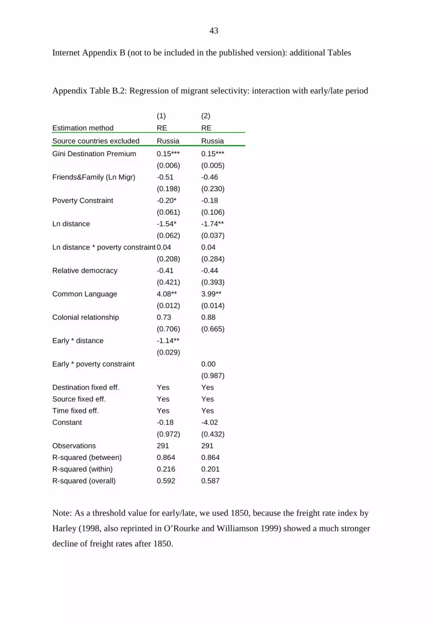
43
Internet Appendix B (not to be included in the published version): additional Tables
Appendix Table B.2: Regression of migrant selectivity: interaction with early/late period
(1) (2) Estimation method RE RE
Source countries excluded Russia Russia
Gini Destination Premium 0.15*** 0.15*** (0.006) (0.005) Friends&Family (Ln Migr) -0.51 -0.46 (0.198) (0.230) Poverty Constraint -0.20* -0.18 (0.061) (0.106) Ln distance -1.54* -1.74** (0.062) (0.037) Ln distance * poverty constraint 0.04 0.04 (0.208) (0.284) Relative democracy -0.41 -0.44 (0.421) (0.393) Common Language 4.08** 3.99** (0.012) (0.014) Colonial relationship 0.73 0.88 (0.706) (0.665) Early * distance -1.14** (0.029) Early * poverty constraint 0.00 (0.987) Destination fixed eff. Yes Yes Source fixed eff. Yes Yes Time fixed eff. Yes Yes Constant -0.18 -4.02 (0.972) (0.432) Observations 291 291 R-squared (between) 0.864 0.864 R-squared (within) 0.216 0.201 R-squared (overall) 0.592 0.587
Note: As a threshold value for early/late, we used 1850, because the freight rate index by
Harley (1998, also reprinted in O’Rourke and Williamson 1999) showed a much stronger
decline of freight rates after 1850.

44
Not for publication: Appendix C: Methodology and basic concepts of age heaping
(Internet Appendix)
We study numerical abilities in this article, which are an important component of overall
human capital. In order to provide estimates of very basic components of numeracy, we will
apply the age heaping methodology.31 The idea is that in less developed countries of the past,
only a certain share of the population was able to report the own age exactly when census-
takers, army recruitment officers, or prison officials asked for it. The remaining population
reported a rounded age, for example, 40, when they were in fact 39 or 41. In today’s world of
obligatory schooling, passports, universities, birth documents, and bureaucracy, it is hard to
imagine that people did not know their exact age. But in early and less organized societies this
was clearly different. The typical result is an age distribution with spikes at ages ending in a
five or a zero and an underrepresentation of other ages, which does not reflect the true age
distribution. There was also some heaping on multiples of two, which was quite widespread
among children and teenagers and to a lesser extent among young adults in their twenties.
This shows that most individuals actually knew their age as teenagers, but only in well-
educated societies were they able to remember or calculate their exact age again later in life.32
To give an example of rounding on multiples of five, the census of Mexico City 1790
reports 410 people aged 40, but only 42 aged 41. This was clearly caused by age heaping.
Apolant (1975, p. 333) gives individual examples of age misreporting: Joseph Milan, who
appeared in February 1747 as a witness in an Uruguayan court, should have been 48 years old,
according to one judicial record. However, in the same year, but in another judicial record, he
declares his age to be ’45 years’. Demographers see this age misreporting as a problem when
calculating life expectancies and other population statistics. But exactly this misreporting
enables us to approximate numerical abilities of historical populations. The ratio between the
preferred ages and the others can be calculated by using several indices, one of them being the
Whipple index.33 To calculate the Whipple index of age heaping, the number of persons
reporting a rounded age ending with 0 or 5 is divided by the total number of people, and this
is subsequently multiplied by 500. Thus, the index measures the proportion of people who
31 For more detailed surveys on the age heaping methodology see A’Hearn, Baten and Crayen (2009). 32 At higher ages, this heaping pattern is mostly negligible, but interestingly somewhat stronger among populations who are numerate enough not to round on multiples of five. 33 A’Hearn, Baten and Crayen (2009) found that this index is the only one that fulfils the desired properties of scale independence (a linear response to the degree of heaping), and that it ranks samples with different degrees of heaping reliably.
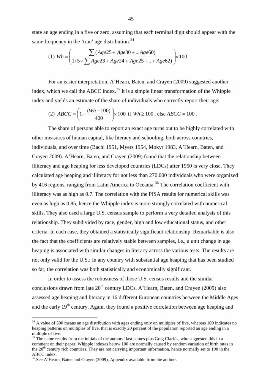
45
state an age ending in a five or zero, assuming that each terminal digit should appear with the
same frequency in the ‘true’ age distribution.34
(1) 100)62..2524235/1
)60...3025(×
++++×
++=
∑∑
AgeAgeAgeAgeAgeAgeAge
Wh
For an easier interpretation, A’Hearn, Baten, and Crayen (2009) suggested another
index, which we call the ABCC index.35 It is a simple linear transformation of the Whipple
index and yields an estimate of the share of individuals who correctly report their age:
(2) 100400
)100(1 ×
−−=
WhABCC if 100≥Wh ; else 100=ABCC .
The share of persons able to report an exact age turns out to be highly correlated with
other measures of human capital, like literacy and schooling, both across countries,
individuals, and over time (Bachi 1951, Myers 1954, Mokyr 1983, A’Hearn, Baten, and
Crayen 2009). A’Hearn, Baten, and Crayen (2009) found that the relationship between
illiteracy and age heaping for less developed countries (LDCs) after 1950 is very close. They
calculated age heaping and illiteracy for not less than 270,000 individuals who were organized
by 416 regions, ranging from Latin America to Oceania.36 The correlation coefficient with
illiteracy was as high as 0.7. The correlation with the PISA results for numerical skills was
even as high as 0.85, hence the Whipple index is more strongly correlated with numerical
skills. They also used a large U.S. census sample to perform a very detailed analysis of this
relationship. They subdivided by race, gender, high and low educational status, and other
criteria. In each case, they obtained a statistically significant relationship. Remarkable is also
the fact that the coefficients are relatively stable between samples, i.e., a unit change in age
heaping is associated with similar changes in literacy across the various tests. The results are
not only valid for the U.S.: In any country with substantial age heaping that has been studied
so far, the correlation was both statistically and economically significant.
In order to assess the robustness of those U.S. census results and the similar
conclusions drawn from late 20th century LDCs, A’Hearn, Baten, and Crayen (2009) also
assessed age heaping and literacy in 16 different European countries between the Middle Ages
and the early 19th century. Again, they found a positive correlation between age heaping and
34 A value of 500 means an age distribution with ages ending only on multiples of five, whereas 100 indicates no heaping patterns on multiples of five, that is exactly 20 percent of the population reported an age ending in a multiple of five. 35 The name results from the initials of the authors’ last names plus Greg Clark’s, who suggested this in a comment on their paper. Whipple indexes below 100 are normally caused by random variation of birth rates in the 20th century rich countries. They are not carrying important information, hence normally set to 100 in the ABCC index. 36 See A’Hearn, Baten and Crayen (2009), Appendix available from the authors.
46
literacy, although the relationship was somewhat weaker than for the 19th or 20th century data.
It is likely that the unavoidable measurement error when using early modern data caused the
lower statistical significance.
Age heaping has also been compared to other human capital indicators, for example,
primary schooling rates. The widest geographical sample studied so far was created by Crayen
and Baten (2010a), who were able to include 70 countries for which both age heaping and
schooling data (as well as other explanatory variables) were available. They found in a series
of cross-sections between the 1880s and 1940s that primary schooling and age heaping were
closely correlated, with R-squares between 0.55 and 0.76 (including other control variables;
see below). Again, the coefficients were relatively stable over time. This large sample also
allowed the examination of various other potential determinants of age heaping. To assess
whether the degree of bureaucracy, birth registration, and government interaction with citizens
are likely to influence the knowledge of one’s exact age, independently of personal education,
the authors used the number of censuses performed for each individual country for the period
under study as an explanatory variable for their age heaping measure. Except for countries
with a very long history of census-taking, all variations of this variable turned out
insignificant, which would suggest that an independent bureaucracy effect was rather weak. In
other words, it is sometimes the case that societies with a high number of censuses had high
age awareness. But, at the same time, these societies were also early in introducing schooling
and this variable clearly had more explanatory power in a joint regression than the
independent bureaucracy effect. Crayen and Baten also tested whether the general standard of
living had an influence on age heaping tendencies (using height as well as GDP per capita to
serve as a proxy for welfare) and found a varying influence: in some decades, there was a
statistically significant correlation, but in others there was none. Cultural determinants of age
heaping were also observable, but their strongest influence was visible in East Asia, not in the
Latin American countries under study in this article.
In this article, we employ the ABCC measure of age heaping, computing indexes for
different countries and birth decades. In order to do so, we use the age groups 23-32, 33-42,
etc.37 we omitted the age range from 63 to 72, as this age group offers too few observations,
especially for the 17th and 18th centuries, when mortality was relatively high.38
37 An advantage of this method is to spread the preferred ages, such as 25 or 30, more evenly within the age groups and it adjusts also for the fact that more people will be alive at age 50 than at age 54 or at age 55 than at age 59 (Crayen and Baten 2010b). 38 Given that young adults aged 23 to 32 round partly on multiples of two rather than five, we use the adjustment method suggested by Crayen and Baten (2010a) to increase the Whipple value (minus 100) by 24 percent, before calculating the ABCC measure.

47
An advantage of the age heaping methodology is that age statements are more widely
available than other human capital proxies like signature ability or school attendance. As Reis
(2008) argues, the age heaping measure is a very basic measure of human capital. Therefore,
it is especially valid to study human capital development in Latin America in the 17th and 18th
centuries when more advanced human capital indicators were quite scarce and reflected only
the skills of the elite.
48
Not for publication: Appendix C: Literacy as an alternative measure of skill selectivity
Interestingly, while some specialized studies have used the occupational structure and age
heaping of migrants as indicators, literacy of migrants was not used before. Unfortunately,
literacy of immigrants at arrival was only assessed in the U.S. starting in 1899, when the U.S.
public grew concerned with the educational status of recent mass immigration from Southern
and Eastern Europe, and those lists are not available as individual data sets.
Literacy was also recorded in the censuses between 1850 and 1910, but the comparison
between the literacy of immigrants in the U.S. and the population in the source country is
difficult for a number of reasons. Firstly, literacy in source countries was recorded using a
number of different definitions. Some sources recorded literacy of the adult population,
whereas the majority recorded those aged 15 and older, 10 and older or even six years and
older.1 Many statistics report just one number for the whole population which makes it
impossible to calculate literacy of age groups or to obtain time series by birth cohorts.
Secondly, literacy of individuals coming from different linguistic backgrounds is always
difficult to measure. Even if census takers were instructed to record literacy in any language
and not only in the official language of the destination country, migrants from different
language families could still have declared themselves illiterate when they were asked by
census takers. We compared literacy and age heaping from the census data of the different
migrant groups in the United States directly. Migrants with a Romanic-language background,
namely Italy and Portugal, displayed average numeracy values. However, they had
significantly lower literacy rates than one would expect according to their average numeracy.
Thirdly, although the vast majority arrived as young adults, a part of the migrants came as
children and teenagers to the United States. Already for the mid-19th century, Cohn (2009)
reports roughly one quarter arriving as children. When we look at the literacy of persons with
migration background in the census some years later, we therefore have to be aware that many
of them acquired literacy when they already lived in the United States. So the literacy
performance is not only influenced by selective migration but also by age structure and
schooling possibilities for migrants. To make things even more complicated, the U.S. was
often the destination for migrants coming from countries with lower schooling (Eastern and
Southern Europe), but also from countries with better schooling than the U.S., such as
Sweden, Norway and so on. The children of those migrant families might have “lost” some of
the schooling they would have obtained in their source countries if they had not migrated.
Therefore, there exist various biases of different directions which are difficult to quantify. For
these reasons, the study of U.S. migrant selectivity based on literacy is too difficult at the

49
present stage of knowledge. Fortunately, the age heaping techniques provides a feasible
alternative to study this important issue.

50
Appendix D Appendix Table D.1: Average number of underlying cases for each decade, destination and
source country, by migration decade and destination country
Destination 1820 1830 1840 1850 1860 1870 1880 1890 1900
Argentina 109 265 428 721 655 623
Canada 197 10664 8723 7228 5220 4352 381 421
Norway 527 878 1490 2511 2120 2002 1798 1655
UK 1451 1208 1611 515 411 376
US 915 13006 24900 32064 35651 30703 989 941 655
Notes: For example, 109 was the average number of cases of all source countries that provided migrants to
Argentina in the 1830s.
Sources: see data appendix.
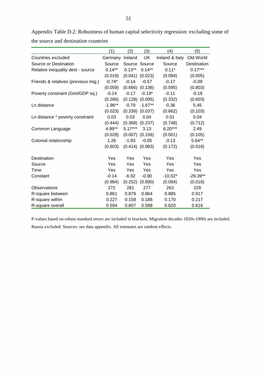
51
Appendix Table D.2: Robustness of human capital selectivity regression: excluding some of
the source and destination countries
(1) (2) (3) (4) (5) Countries excluded Germany Ireland UK Ireland & Italy Old World Source or Destination Source Source Source Source Destination Relative inequality dest - source 0.14** 0.13** 0.14** 0.11* 0.17*** (0.019) (0.041) (0.023) (0.084) (0.005) Friends & relatives (previous mig.) -0.74* -0.14 -0.57 -0.17 -0.09 (0.059) (0.666) (0.136) (0.595) (0.803) Poverty constraint (Gini/GDP sq.) -0.14 -0.17 -0.19* -0.11 -0.18 (0.286) (0.128) (0.095) (0.332) (0.603) Ln distance -1.96** -0.79 -1.67** -0.36 5.45 (0.023) (0.339) (0.037) (0.662) (0.103) Ln distance * poverty constraint 0.03 0.03 0.04 0.01 0.04 (0.444) (0.368) (0.237) (0.748) (0.712) Common Language 4.99** 5.17*** 3.13 6.20*** 2.49 (0.028) (0.007) (0.156) (0.001) (0.105) Colonial relationship 1.26 -1.93 -0.05 -3.13 5.64** (0.603) (0.414) (0.983) (0.172) (0.018) Destination Yes Yes Yes Yes Yes Source Yes Yes Yes Yes Yes Time Yes Yes Yes Yes Yes Constant -0.14 -6.92 -0.90 -10.02* -29.39** (0.984) (0.252) (0.890) (0.094) (0.018) Observations 272 281 277 263 229 R-square between 0.861 0.879 0.864 0.885 0.917 R-square within 0.227 0.158 0.188 0.170 0.217 R-square overall 0.594 0.607 0.588 0.620 0.616
P-values based on robust standard errors are included in brackets. Migration decades 1820s-1900s are included.
Russia excluded. Sources: see data appendix. All estimates are random effects.
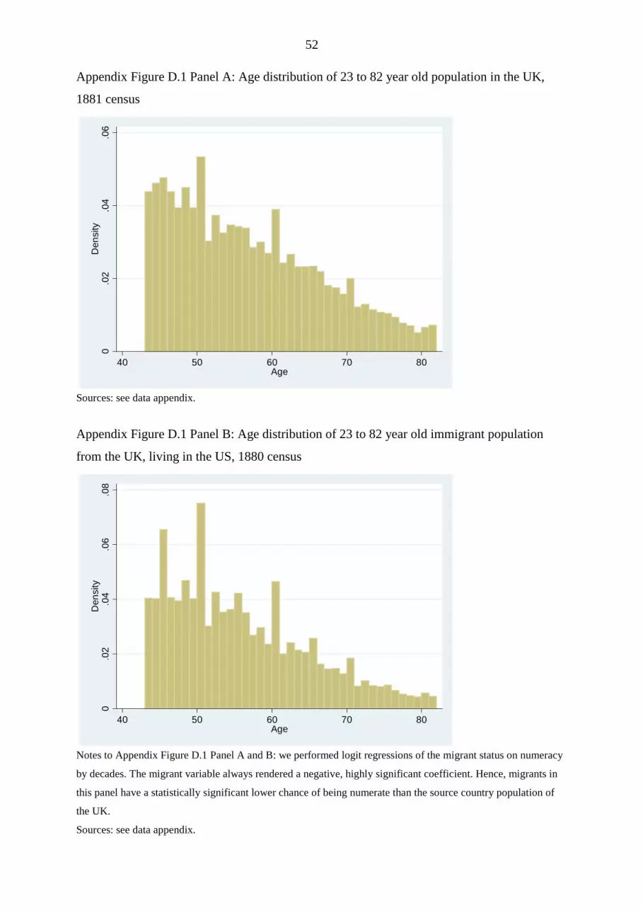
52
Appendix Figure D.1 Panel A: Age distribution of 23 to 82 year old population in the UK,
1881 census
Sources: see data appendix.
Appendix Figure D.1 Panel B: Age distribution of 23 to 82 year old immigrant population
from the UK, living in the US, 1880 census
Notes to Appendix Figure D.1 Panel A and B: we performed logit regressions of the migrant status on numeracy
by decades. The migrant variable always rendered a negative, highly significant coefficient. Hence, migrants in
this panel have a statistically significant lower chance of being numerate than the source country population of
the UK.
Sources: see data appendix.
0.0
2.0
4.0
6D
ensi
ty
40 50 60 70 80Age
0.0
2.0
4.0
6.0
8D
ensi
ty
40 50 60 70 80Age