bottleneck oriented card-based production control for push repetitive manufacturing system

Journal of Advanced Mechanical Design,

Systems, and

Manufacturing

Vol. 7, No. 3, 2013

1

Bottleneck Oriented Card-Based Production Control for Push Repetitive Manufacturing

Systems*

M. H. AZIZ**, Erik BOHEZ**, Yuichi KANDA***, Hironori HIBINO**** and Toru SAKUMA*****

** Industrial & Manufacturing Engineering, Asian Institute of Technology Klong Luang 4, Pathum Thani 12120, Thailand

E-mail: [email protected] *** Graduate School of Engineering, Toyo University

5-28-20, Hakusan, Bunkyo-ku, Tokyo, Japan **** Production Engineering Department, Technical Research Institute, JSPMI

1-1-12, Hachiman-cho, Higashikurume, Tokyo, Japan **** Mechanical System Engineering, Tokyo University of Agriculture & Technology

2-24-16, Naka-cho, Koganei-shi, Tokyo, Japan Abstract One of the major problems of the push Repetitive Manufacturing Systems (RMS) is the Work In Process (WIP) buildups between the stations due to the push nature of the flow of material. Card-based pull or push-pull production control systems offered smooth production flow with reduced WIP. But, applying these systems to push production environment requires huge cost for major cultural and operational changes. We propose a solution to WIP buildups, without altering the basic structure of operation of the push production system. We propose a bottleneck oriented card-based production control system for push RMS. In our system parts release on the shop floor according to the customer demand whereas the material flow is constrained with the Production Authorization Cards (PAC). The PAC circulates between the first station and the bottleneck station in the form of a loop, reducing WIP buildups between the stations. We have conducted simulation based case studies to demonstrate the efficacy of our approach.

Key words: Repetitive Manufacturing Systems, Card-Based Production Control, Work In Process, Bottleneck, Buffer, Simulation

1. Introduction

In the push RMS, orders are released on the shop floor based on external demand. Afterwards, parts are pushed to the next work station once they finish their operation on the previous workstation, without considering the congestion of the downstream workstation. This phenomena results in the requirement for more buffer space, long lead times and sometime even to line stoppage. Consequences are alarming for the companies using push production control systems with MRP or MRP II, which are already on limited profit margins because of the tough competitions and where most of the work is done by human labor. These companies face a dilemma. On one hand they need to be cost effective and competitive by reducing WIP buildups. But, on the other hand – despite of the low WIP inventory offered by pull or push-pull card-based production control systems – these companies cannot afford to convert to a new production control system, because of the high capital cost requirements for installing new system, for altering floor layout, for training the

*Received 27 Aug., 2012 (No. 12-0346) [DOI: 10.1299/jamdsm.7.x]

Copyright © 2013 by JSME

Journal of Advanced Mechanical Design,Systems, and Manufacturing

Vol. 7, No. 3, 2013

2

workers and for spreading the change to their suppliers and buyers. They need an easy to implement and easy to use system with minimum cost and minimum worker training, which would reduce WIP buildups between the stations, without altering the basic structure of their existing push production control system.

For this purpose, we propose a bottleneck oriented card-based Production Control (PC) system for the push Repetitive Manufacturing Systems (RMS). Our card based system is neither a pull system nor a push-pull system, it is simply a push-hold-push system, where parts release on the shop floor according to the customer demand and the material flow is constraint with the Production Authorization Cards (PAC). The PACs circulate between the first station and the bottleneck station in the form of a loop, constraining the unnecessary WIP from accumulating between the stations. Because, in RMS the bottleneck remains the same unless there is a machine failure or a change of product mix, and the bottleneck station is the one with the WIP buildup. In this way our proposed system reduces the WIP build-ups between the stations without changing the basic structure and the working of the existing push production control system.

Section 2 is for related literature review. In section 3 we have explained the bottleneck oriented card-based PC system for push RMS. For the evaluation of our system, in section 4 we have conducted case studies and have simulated our model in Witness software. The paper has been concluded in section 5.

2. Literature Review

In the push RMS, orders are released on the shop floor based on external demand, process plan, inventory levels and pre-determined lead times. Afterwards parts are pushed to the next work station once they finish their operation on the previous workstation, without considering the congestion of the downstream workstation(1). Whereas, the value of WIP increases down the stream of production process, as labor, time, energy and resources added to it(2). Thus depending upon the processing cost at each stage, the WIP at the first stage has lower cost than the one at the later stages. The possibility of large WIP buildups between the workstations is high in the push system, which causes high variability in cycle time with an increased cost in terms of inventory buildup(3). Moreover, it requires more buffer space, and could even lead to line stoppage in highly variable demands. Whereas, for an efficient production; reduction of the WIP inventory between the processes and decrease in the line stoppage are essential(4), along with the reduction of buffer space, reduction of manufacturing lead-time and constriction of unnecessary WIP at the earlier stages of production.

Card-base Production Control (PC) techniques emerged to deal with the problems of shop floor congestion, huge buffer space, long lead-times and large WIP buildups. According to Ref.(5) detailed workload computation strategy for each work centre is efficient in reducing WIP, but, it requires the implementation of the data collection system and requires the data reporting activities concerning each machine centre. Where, the workload computed by each work centre includes; workload on hand, workload in transit and released workload. These complexities could be overcome by card-based material control, in which once the number of cards is calculated then cards automatically control the workload on hand, workload in transit and released workload.

. Card-based PC techniques could be either pull such as; Kanban(6)., Generalised Kanban(7), Base Stock(8), and Extended Kanban(9) or pull-push such as; CONWIP(10), POLCA(11), E-POLCA(1), Generic POLCA(12) and Load-Based POLCA(13). Although these techniques have many advantages in certain conditions, but none of them is flawless. For instance in case of kanban in varying demand and high variety situations, direct relation between card signal and product type would lead to large number of different bins or intermediate stock(14) thus affecting the core objectives of minimizing the WIP and


Vol. 7, No. 3, 2013

3

minimizing the buffer space. Generalised Kanban, Base Stock and Extended Kanban are no exception. Similarly, for POLCA or E-POLCA or Generic POLCA or Load-Based POLCA as the numbers of station and part routs variety increase, the number of card types increase double fold, because POLCA system requires two type of cards to be attached with each part or lot. This results into a complex network of cards along with a need of card storage bins and immediate stock at each station. Whereas in case of CONWIP according to Ref.(15) the disadvantage is that the inventory levels inside the system are not controlled individually; high inventories can appear in front of the bottleneck station and when a machine breaks down. Our system has the advantage of low WIP inventory at every station including the bottleneck station. CONWIP and PAC loop would be the same at times when the bottleneck would be the last station, still there would be a difference of time buffer. We have shown these effects in the case studies in section 4.

The concept of bottleneck oriented scheduling was introduced in Theory Of Constraint (TOC). Although, the PAC and the TOC, both are bottleneck oriented that is; as soon as a part would finish processing at a bottleneck station a new part would enter into the production line. In this way the production rate of non-bottleneck stations would be synchronized with that of the bottleneck station. However, the intent of the development of PAC varies from that of TOC. In TOC the intent is to achieve maximum production by first identifying the constraint resource and then exploiting the constraint resource by utilizing it maximum(5) by providing it abundant supply of material. On the other hand the intent of the PAC is to minimize the parts queue at each station including the bottleneck station by providing just the required supply of material just at the right time at the bottleneck. Therefore, in TOC the emphasis is on spacious physical buffer at the bottleneck, whereas in PAC the emphasis is to minimize all the physical buffers including the one at the bottleneck.

Furthermore, to achieve the objective of minimized WIP stocks between the stations, the PAC differs from the TOC at operational level. Drum Buffer Rope (DBR) is the technique to realize the concept of TOC. There may be different variants of DBR; an example could be found in Ref.(16). But, in its basic form the DBR uses Optimized Production Technology (OPT) for scheduling. OPT schedules the constraint resource and the non-constraint resources separately and uses forward scheduling logic(17). Forward scheduling logic releases parts at the earliest to maximize production, which results in excess finished goods inventory. In this way DBR uses time buffer along with the physical buffer and material release decision is based on the estimated time for the time buffer. On the other hand, the PAC is for the systems using MRP or MRP II. These systems use backward scheduling logic, while considering capacity to be available. The material release decision is based on due dates and pre-determined lead times(17). After the release, the material is constraint with PACs. Converting a push RMS based on MRP into OPT requires either a parallel scheduling system or a complete replacement of the existing production control system. Therefore we proposed the use of PAC without altering the functioning of MRP or MRP II system. It is a low cost approach to minimize the WIP build-ups at all stations including the bottleneck station.

These techniques are suited only to their respective pull or push-pull environments. According to Ref.(18) applying these techniques to a factory running on a push production control system requires significant changes in the culture and the operating structure of that factory. These changes require capital cost. Cost for hiring external consultants for a period of six months to one year or may be more depending upon the magnitude of the change. Cost for the proper training of higher management as well as labor according to the new system’s requirements. If required, cost for altering the shop floor layout. Cost for the installation of new production management system, whether it replaces the old system or works in parallel with the old one. Cost for expansion of the new system to the suppliers and the buyers. After all that spending, success is still a matter of luck as have been


Vol. 7, No. 3, 2013

4

observed in many cases. On the other hand, our proposed system is a low cost solution to reduce WIP with the

ease of implementation on the shop floor and with the ease of usage by the workers. Thus suited for companies using push production control with MRP or MRP II and where part loading and dispatching is supervised by human labor. Because, PAC system does not require any extra production management system to be installed in the factory, nor it requires any advanced level training of the management and the workers, nor it uses complex algorithms and dispatching rules ever prone to changes and to errors in real time production. Our system works in the presence of existing push production control system, which release the material according to its computed schedule and sequence. PACs only constrain the unnecessary WIP before the first station and keep it from accumulating between the work stations. PACs achieve this by circulating between the first station and the bottleneck station. In the next section, we have developed the bottleneck oriented card-based PC system for RMS.

3. Model of RMS with PAC

Repetitive Manufacturing System (RMS), often called as cyclic production system is the one which produces products at a constant frequency. Where a set of resources such as machines, labor, robot etc. repeatedly performs a set of certain tasks and the system produces a set of certain products each cycle with same or similar products produced over a lengthy period of time(19).

Layout of these systems is in the form of flow shop and/or serial line, where parts move to next station after finishing operation at one station in a pre-defined sequence on a pre-defined route. Planning and control is carried out in time buckets, where time bucket for strategic capacity planning is of two to five years, time bucket for aggregate planning is of ten months to one year and for Master Production Scheduling (MPS) the planning horizon is of four to six weeks(20). Sequencing is used for scheduling which simplifies the dispatching process. Repetitive manufacturing can be use for Make To Stock (MTO) as well as for Make To Order (MTO) production. Similarly, could be push or pull or hybrid.

Our proposed system is applicable to push RMS where parts are released on the shop floor based on external demand, bill of material/process plan, inventory levels and pre-determined lead times. Those companies have MRP or MRP II systems in place to release the orders. Once the scheduling and the sequencing process are complete the bottleneck remains the same in these systems, unless there is a machine failure or a change of product mix. The bottleneck station is the one with the high WIP accumulation because of the push nature of material flow. Which results in large buffer space requirement and longer lead times. Consequently, it is possible to reduce WIP accumulation at the bottleneck station; if the queues of WIP at the bottleneck station could be shifted toward the first station by constraining more and more WIP inventory before the first station.

Therefore, the material is released according to the schedule and in a sequence, but the first machine station does not start processing the part unless the PAC is attached with it, thus keeping the downstream stations from unnecessary WIP. When a PAC attaches with a part, then the first station starts processing that part. The PAC remains attached with a part until it finishes its operation at the bottleneck station. After detaching from a part after the bottleneck station, the PAC moves back to the first station. Here the PAC stays idle for some time and then attached with another part, thus circulates in a loop from the first station to the bottleneck station along the rout of the parts. Therefore, if a PAC is not available at the first station, it means that the bottleneck station is working at its full capacity and is not available to process more parts at the time when these parts are suppose to reach the bottleneck. In this way, we constrain the unnecessary WIP from accumulating between the stations.


Vol. 7, No. 3, 2013

5

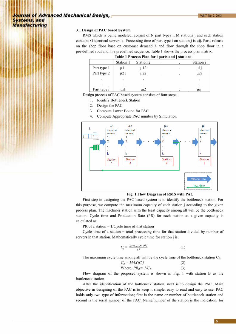
3.1 Design of PAC based System RMS which is being modeled, consist of N part types i, M stations j and each station

contains O identical servers k. Processing time of part type i on station j is μij. Parts release on the shop floor base on customer demand λ and flow through the shop floor in a pre-defined rout and in a predefined sequence. Table 1 shows the process plan matrix.

Table 1 Process Plan for i parts and j stations Station 1 Station 2 . . Station j

Part type 1 μ11 μ12 . . μ1j Part type 2 μ21 μ22 . . μ2j

. . . .

. . . . Part type i μi1 μi2 . . μij

Design process of PAC based system consists of four steps; 1. Identify Bottleneck Station 2. Design the PAC 3. Compute Lower Bound for PAC 4. Compute Appropriate PAC number by Simulation

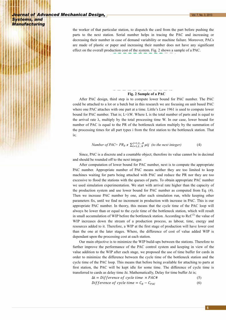
Fig. 1 Flow Diagram of RMS with PAC First step in designing the PAC based system is to identify the bottleneck station. For

this purpose, we compute the maximum capacity of each station j according to the given process plan. The machines station with the least capacity among all will be the bottleneck station. Cycle time and Production Rate (PR) for each station at a given capacity is calculated as;

PR of a station = 1/Cycle time of that station Cycle time of a station = total processing time for that station divided by number of

servers in that station. Mathematically cycle time for station j is;

Cj = ∑ , ,… (1)

The maximum cycle time among all will be the cycle time of the bottleneck station CB. CB = MAX{Cj} (2) Where, PRB = 1/CB (3)

Flow diagram of the proposed system is shown in Fig. 1 with station B as the bottleneck station.

After the identification of the bottleneck station, next is to design the PAC. Main objective in designing of the PAC is to keep it simple, easy to read and easy to use. PAC holds only two type of information; first is the name or number of bottleneck station and second is the serial number of the PAC. Name/number of the station is the indication, for

Journal of Advanced MechanicSystems, and Manufacturing

the woparts decreaare meffect

Acould whereboundthe arnumbethe pris;

Siand sh

APAC nmachiexcesswe usthe prThen paramappropalwayin smaWIP iresourthan tdepen

Ofurthevalue order cycle first stransfe

cal Design,

orker of that particular station, to dispatch the card fto the next station. Serial number helps in tracin

asing their number in case of demand variability or mmade of plastic or paper and increasing their numbe

on the overall production cost of the system. Fig. 2 sh

Fig. 2 Sample of a PACAfter PAC design, third step is to compute lower bo

be attached to a lot or a batch but in this research wee one PAC attaches with one part at a time. Little’s Lawd for PAC number. That is; L=λW. Where L is the totarrival rate λ, multiply by the total processing time Wer of PAC is equal to the PR of the bottleneck statioocessing times for all part types i from the first statio

Number of PAC= PRB x ∑ , ,…, … (to the n

ince, PAC is a discrete and a countable object; therefohould be rounded off to the next integer.

After computation of lower bound for PAC number, nenumber. Appropriate number of PAC means neitheines waiting for parts being attached with PAC and sive to flood the stations with the queues of parts. Toed simulation experimentation. We start with arrival

roduction system and use lower bound for PAC numwe increase PAC number by one, after each simu

meters fix, until we find no increment in production wpriate PAC number. In theory, this means that the c

ys be lower than or equal to the cycle time of the bottall accumulation of WIP before the bottleneck station.increases down the stream of a production procesrces added to it. Therefore, a WIP at the first stage ofthe one at the later stages. Where, the difference

ndant upon the processing cost at each station. Our main objective is to minimize the WIP build-ups b

r improve the performance of the PAC control systaddition to the WIP after each stage, we proposed thto minimize the difference between the cycle time otime of the PAC loop. This means that before being a

station, the PAC will be kept idle for some time. Tferred to cards as delay time Δt. Mathematically, DelayΔt #

Vol. 7, No. 3, 2013

6

from the part before pushing the ng the PAC and increasing or

machine failure. Moreover, PACs er does not have any significant hows a sample of a PAC.

C und for PAC number. The PAC

e are focusing on unit based PAC w 1961 is used to compute lower al number of parts and is equal to W. In our case, lower bound for on multiply by the summation of on to the bottleneck station. That

next integer) (4)

ore its value cannot be in decimal

ext is to compute the appropriate er they are too limited to keep reduce the PR nor they are too obtain appropriate PAC number rate higher than the capacity of

mber as computed from Eq. (4). ulation run, while keeping other with increase in PAC. This is our cycle time of the PAC loop will tleneck station, which will result According to Ref.(2) the value of

ss, as labour, time, energy and f production will have lower cost of cost of value added WIP is

etween the stations. Therefore to tem and keeping in view of the he use of time buffer for cards in of the bottleneck station and the available for attaching to parts at The difference of cycle time is y for time buffer Δt is;

(5) (6)

Journal of Advanced MechanicSystems, and Manufacturing

W

Wbottlen

PATh

with th

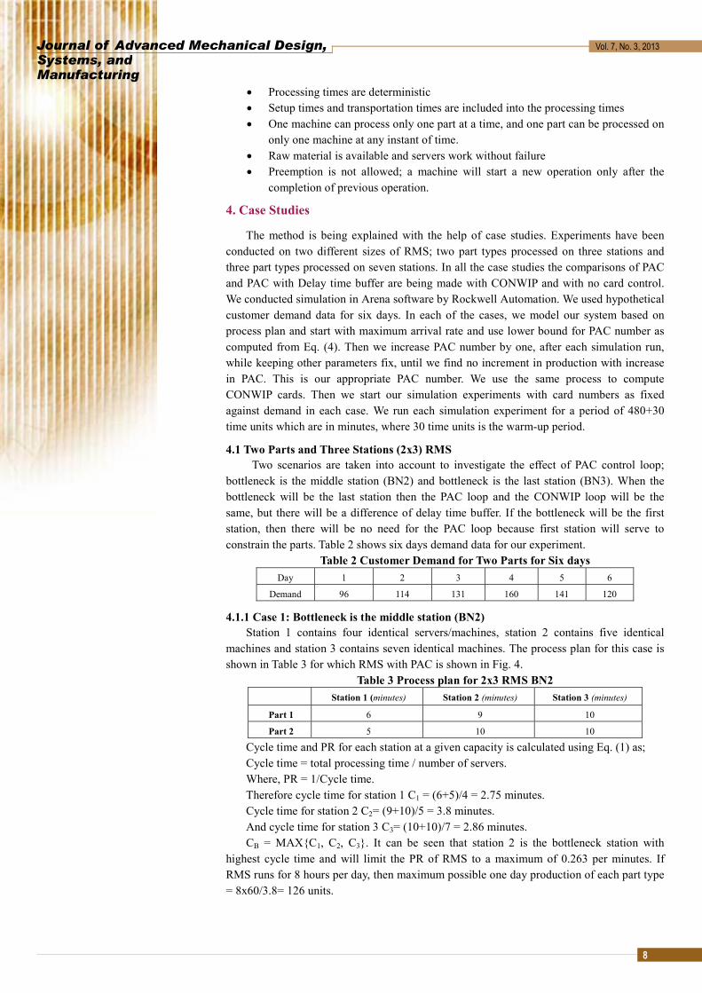
Bone obshop fimplemnote thwoulde-cardhumanmateriemploa smafreed bin to the timinto th

TomanufwhethsystemDue tsimula

Dbottlenqueueaveragin the

cal Design,

Cycle time of the bottleneck station ∑

Where, ∑ , ,… is the processing time of all p are the total identical servers at bottleneck station.

Cycle time of PAC loop ∑ , ,…, … #

Where, ∑ , ,…, … is the processing time of all paneck station. AC# are the total number of PACs in the loop. hus, in theory, the delay for time buffer Δt is equal tohe bottleneck cycle time and subtracted with the total Δt # ∑ , ,…, …

ut in practice, Δt will be computed by iteration and wbtained from Eq (9), because there are many factors wfloor. The delay for time buffer Δt, once computed, thementing it to cards at the shop floor, such as; a timer he time delay for each card or an electronic card syste

d be much simpler. However, in this research we areds, because our scope is on the production systems whn labour. The disadvantage of e-cards is the loss of ial and information, which might lead to less con

oyees and might lead to errors(21). In case of physical cll conveyer belt at the input of the PAC storage bin bfrom parts will be placed on one end of the conveyebe attached with new parts as in Fig. 3. The speed of

me difference when the PAC would be placed on the he bin should be equal to the required delay for time bu Δt

Fig. 3 Delay Mechanism for Timo validate our approach, we have conducted simfacturing system simulation is an efficient tool for

her it is layout design or number of equipment desm design such as kanban and so on(22). Simulation sato this reason, there is plenty of literature on manation such as Refs.(23)(24)(25) and (26).

During simulation, we varied customer demand anneck station. The simulation results give us the totas of parts waiting between different station, averagge utilization of each station. To demonstrate our apprnext section. Assumptions made in this research are;

Vol. 7, No. 3, 2013

7

, ,… (7)

part types at the bottleneck.

(8)

art types from station 1 till the

o the product of the PAC number processing time in a PAC loop.

(9)

would be slightly lower than the which can cause variation on the en there could be many means of clock or an employee who could em. In case of electronic cards, it e using physical cards instead of here most of the work is done by connection between the flow of nfidence in the system by the

cards, one such way is to think of before the first station. The PAC er and will be collected from the f the conveyer would be such that conveyer and when it would fell uffer, that is;

(10)

me Buffer mulation experiments. Because r manufacturing system design, sign or production management

aves the cost as well as the time. nufacturing system design using

nd changed the position of the al production of each part type, ge throughput time of parts and roach, case studies are presented


Vol. 7, No. 3, 2013

8

• Processing times are deterministic • Setup times and transportation times are included into the processing times • One machine can process only one part at a time, and one part can be processed on

only one machine at any instant of time. • Raw material is available and servers work without failure • Preemption is not allowed; a machine will start a new operation only after the

completion of previous operation.

4. Case Studies

The method is being explained with the help of case studies. Experiments have been conducted on two different sizes of RMS; two part types processed on three stations and three part types processed on seven stations. In all the case studies the comparisons of PAC and PAC with Delay time buffer are being made with CONWIP and with no card control. We conducted simulation in Arena software by Rockwell Automation. We used hypothetical customer demand data for six days. In each of the cases, we model our system based on process plan and start with maximum arrival rate and use lower bound for PAC number as computed from Eq. (4). Then we increase PAC number by one, after each simulation run, while keeping other parameters fix, until we find no increment in production with increase in PAC. This is our appropriate PAC number. We use the same process to compute CONWIP cards. Then we start our simulation experiments with card numbers as fixed against demand in each case. We run each simulation experiment for a period of 480+30 time units which are in minutes, where 30 time units is the warm-up period.

4.1 Two Parts and Three Stations (2x3) RMS Two scenarios are taken into account to investigate the effect of PAC control loop;

bottleneck is the middle station (BN2) and bottleneck is the last station (BN3). When the bottleneck will be the last station then the PAC loop and the CONWIP loop will be the same, but there will be a difference of delay time buffer. If the bottleneck will be the first station, then there will be no need for the PAC loop because first station will serve to constrain the parts. Table 2 shows six days demand data for our experiment.

Table 2 Customer Demand for Two Parts for Six days Day 1 2 3 4 5 6

Demand 96 114 131 160 141 120

4.1.1 Case 1: Bottleneck is the middle station (BN2) Station 1 contains four identical servers/machines, station 2 contains five identical

machines and station 3 contains seven identical machines. The process plan for this case is shown in Table 3 for which RMS with PAC is shown in Fig. 4.

Table 3 Process plan for 2x3 RMS BN2 Station 1 (minutes) Station 2 (minutes) Station 3 (minutes)

Part 1 6 9 10

Part 2 5 10 10

Cycle time and PR for each station at a given capacity is calculated using Eq. (1) as; Cycle time = total processing time / number of servers. Where, PR = 1/Cycle time. Therefore cycle time for station 1 C1 = (6+5)/4 = 2.75 minutes. Cycle time for station 2 C2= (9+10)/5 = 3.8 minutes. And cycle time for station 3 C3= (10+10)/7 = 2.86 minutes. CB = MAX{C1, C2, C3}. It can be seen that station 2 is the bottleneck station with

highest cycle time and will limit the PR of RMS to a maximum of 0.263 per minutes. If RMS runs for 8 hours per day, then maximum possible one day production of each part type = 8x60/3.8= 126 units.


Vol. 7, No. 3, 2013

9

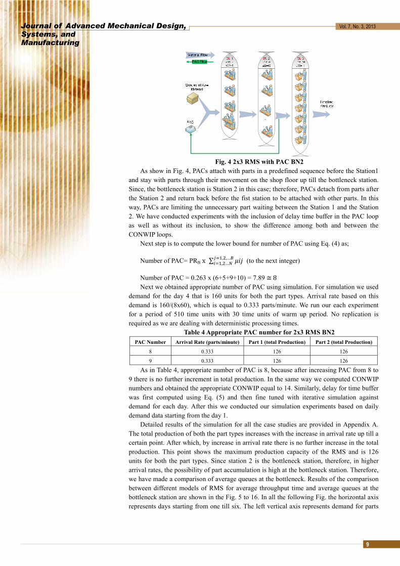
Fig. 4 2x3 RMS with PAC BN2 As show in Fig. 4, PACs attach with parts in a predefined sequence before the Station1

and stay with parts through their movement on the shop floor up till the bottleneck station. Since, the bottleneck station is Station 2 in this case; therefore, PACs detach from parts after the Station 2 and return back before the fist station to be attached with other parts. In this way, PACs are limiting the unnecessary part waiting between the Station 1 and the Station 2. We have conducted experiments with the inclusion of delay time buffer in the PAC loop as well as without its inclusion, to show the difference among both and between the CONWIP loops.

Next step is to compute the lower bound for number of PAC using Eq. (4) as;

Number of PAC= PRB x ∑ , ,…, … (to the next integer)

Number of PAC = 0.263 x (6+5+9+10) = 7.89 ≅ 8 Next we obtained appropriate number of PAC using simulation. For simulation we used

demand for the day 4 that is 160 units for both the part types. Arrival rate based on this demand is 160/(8x60), which is equal to 0.333 parts/minute. We run our each experiment for a period of 510 time units with 30 time units of warm up period. No replication is required as we are dealing with deterministic processing times.

Table 4 Appropriate PAC number for 2x3 RMS BN2 PAC Number Arrival Rate (parts/minute) Part 1 (total Production) Part 2 (total Production)

8 0.333 126 126

9 0.333 126 126

As in Table 4, appropriate number of PAC is 8, because after increasing PAC from 8 to 9 there is no further increment in total production. In the same way we computed CONWIP numbers and obtained the appropriate CONWIP equal to 14. Similarly, delay for time buffer was first computed using Eq. (5) and then fine tuned with iterative simulation against demand for each day. After this we conducted our simulation experiments based on daily demand data starting from the day 1.

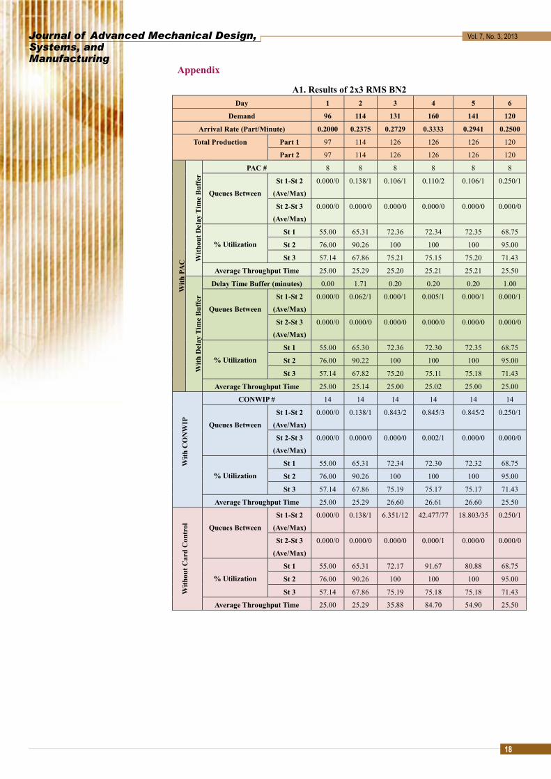
Detailed results of the simulation for all the case studies are provided in Appendix A. The total production of both the part types increases with the increase in arrival rate up till a certain point. After which, by increase in arrival rate there is no further increase in the total production. This point shows the maximum production capacity of the RMS and is 126 units for both the part types. Since station 2 is the bottleneck station, therefore, in higher arrival rates, the possibility of part accumulation is high at the bottleneck station. Therefore, we have made a comparison of average queues at the bottleneck. Results of the comparison between different models of RMS for average throughput time and average queues at the bottleneck station are shown in the Fig. 5 to 16. In all the following Fig. the horizontal axis represents days starting from one till six. The left vertical axis represents demand for parts


Vol. 7, No. 3, 2013

10

increasing from bottom to top. Demand for each day is represented by rectangular bars with a horizontal line perpendicular to these bars representing the maximum production capacity of the RMS under consideration. The right vertical axis represents either the average throughput time in minutes or the average queue at the bottleneck station, depending on the type of comparison.

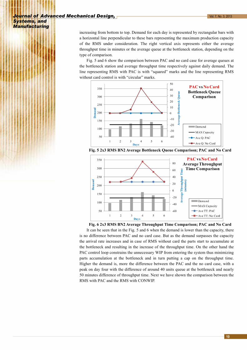
Fig. 5 and 6 show the comparison between PAC and no card case for average queues at the bottleneck station and average throughput time respectively against daily demand. The line representing RMS with PAC is with “squared” marks and the line representing RMS without card control is with “circular” marks.

Fig. 5 2x3 RMS BN2 Average Bottleneck Queue Comparison; PAC and No Card

Fig. 6 2x3 RMS BN2 Average Throughput Time Comparison; PAC and No Card It can be seen that in the Fig. 5 and 6 when the demand is lower than the capacity, there

is no difference between PAC and no card case. But as the demand surpasses the capacity the arrival rate increases and in case of RMS without card the parts start to accumulate at the bottleneck and resulting in the increase of the throughput time. On the other hand the PAC control loop constrains the unnecessary WIP from entering the system thus minimizing parts accumulation at the bottleneck and in turn putting a cap on the throughput time. Higher the demand is, more the difference between the PAC and the no card case, with a peak on day four with the difference of around 40 units queue at the bottleneck and nearly 50 minutes difference of throughput time. Next we have shown the comparison between the RMS with PAC and the RMS with CONWIP.


Vol. 7, No. 3, 2013

11

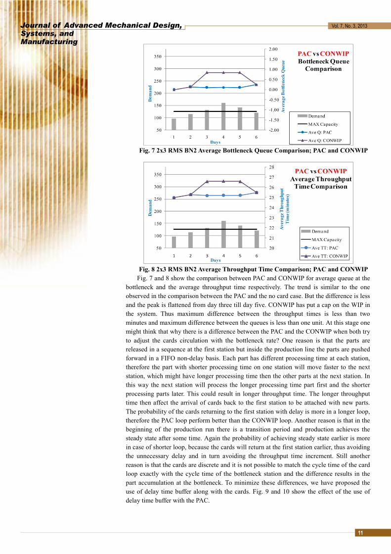
Fig. 7 2x3 RMS BN2 Average Bottleneck Queue Comparison; PAC and CONWIP

Fig. 8 2x3 RMS BN2 Average Throughput Time Comparison; PAC and CONWIP Fig. 7 and 8 show the comparison between PAC and CONWIP for average queue at the

bottleneck and the average throughput time respectively. The trend is similar to the one observed in the comparison between the PAC and the no card case. But the difference is less and the peak is flattened from day three till day five. CONWIP has put a cap on the WIP in the system. Thus maximum difference between the throughput times is less than two minutes and maximum difference between the queues is less than one unit. At this stage one might think that why there is a difference between the PAC and the CONWIP when both try to adjust the cards circulation with the bottleneck rate? One reason is that the parts are released in a sequence at the first station but inside the production line the parts are pushed forward in a FIFO non-delay basis. Each part has different processing time at each station, therefore the part with shorter processing time on one station will move faster to the next station, which might have longer processing time then the other parts at the next station. In this way the next station will process the longer processing time part first and the shorter processing parts later. This could result in longer throughput time. The longer throughput time then affect the arrival of cards back to the first station to be attached with new parts. The probability of the cards returning to the first station with delay is more in a longer loop, therefore the PAC loop perform better than the CONWIP loop. Another reason is that in the beginning of the production run there is a transition period and production achieves the steady state after some time. Again the probability of achieving steady state earlier is more in case of shorter loop, because the cards will return at the first station earlier, thus avoiding the unnecessary delay and in turn avoiding the throughput time increment. Still another reason is that the cards are discrete and it is not possible to match the cycle time of the card loop exactly with the cycle time of the bottleneck station and the difference results in the part accumulation at the bottleneck. To minimize these differences, we have proposed the use of delay time buffer along with the cards. Fig. 9 and 10 show the effect of the use of delay time buffer with the PAC.


Vol. 7, No. 3, 2013

12

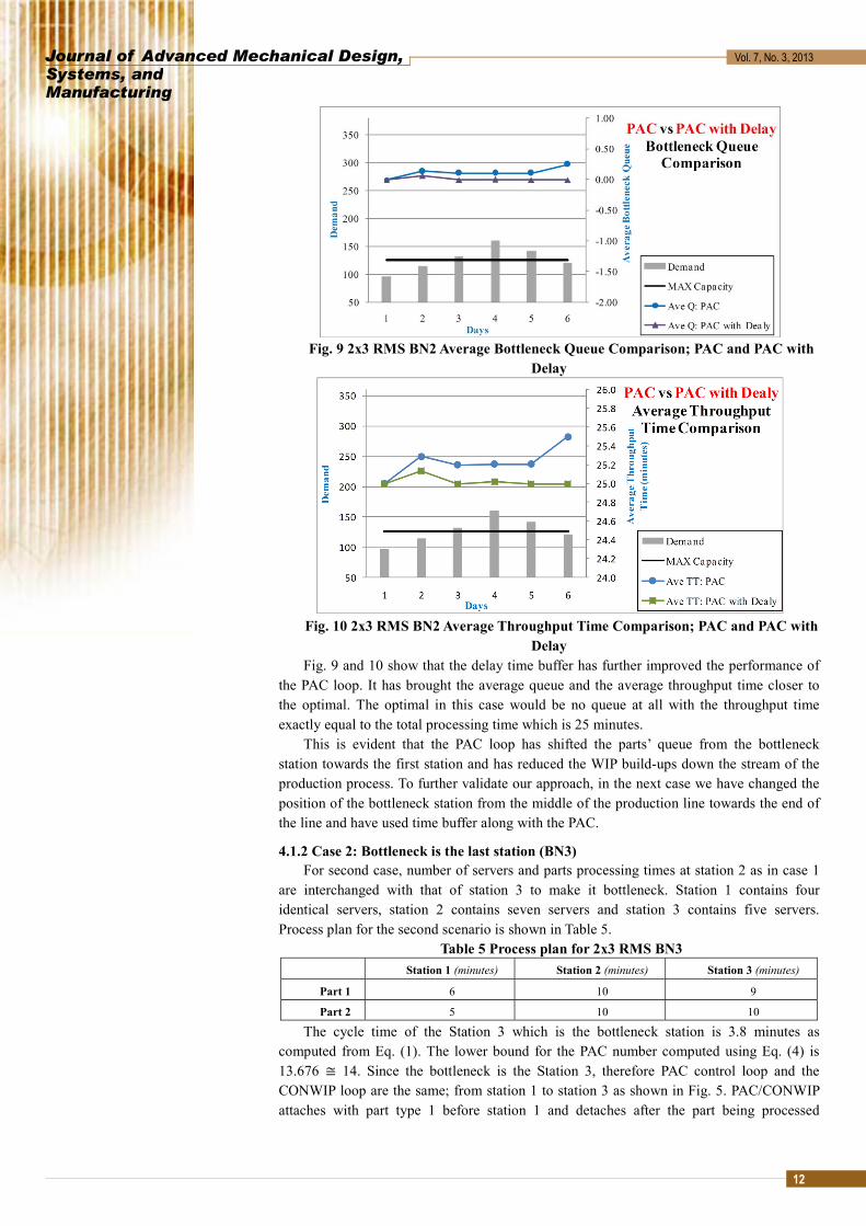
Fig. 9 2x3 RMS BN2 Average Bottleneck Queue Comparison; PAC and PAC with Delay

Fig. 10 2x3 RMS BN2 Average Throughput Time Comparison; PAC and PAC with Delay

Fig. 9 and 10 show that the delay time buffer has further improved the performance of the PAC loop. It has brought the average queue and the average throughput time closer to the optimal. The optimal in this case would be no queue at all with the throughput time exactly equal to the total processing time which is 25 minutes.

This is evident that the PAC loop has shifted the parts’ queue from the bottleneck station towards the first station and has reduced the WIP build-ups down the stream of the production process. To further validate our approach, in the next case we have changed the position of the bottleneck station from the middle of the production line towards the end of the line and have used time buffer along with the PAC.

4.1.2 Case 2: Bottleneck is the last station (BN3) For second case, number of servers and parts processing times at station 2 as in case 1

are interchanged with that of station 3 to make it bottleneck. Station 1 contains four identical servers, station 2 contains seven servers and station 3 contains five servers. Process plan for the second scenario is shown in Table 5.

Table 5 Process plan for 2x3 RMS BN3 Station 1 (minutes) Station 2 (minutes) Station 3 (minutes)

Part 1 6 10 9

Part 2 5 10 10

The cycle time of the Station 3 which is the bottleneck station is 3.8 minutes as computed from Eq. (1). The lower bound for the PAC number computed using Eq. (4) is 13.676 ≅ 14. Since the bottleneck is the Station 3, therefore PAC control loop and the CONWIP loop are the same; from station 1 to station 3 as shown in Fig. 5. PAC/CONWIP attaches with part type 1 before station 1 and detaches after the part being processed


Vol. 7, No. 3, 2013

13

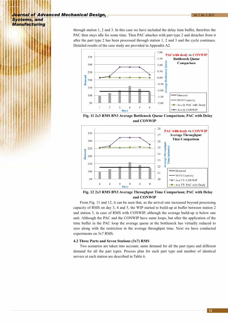
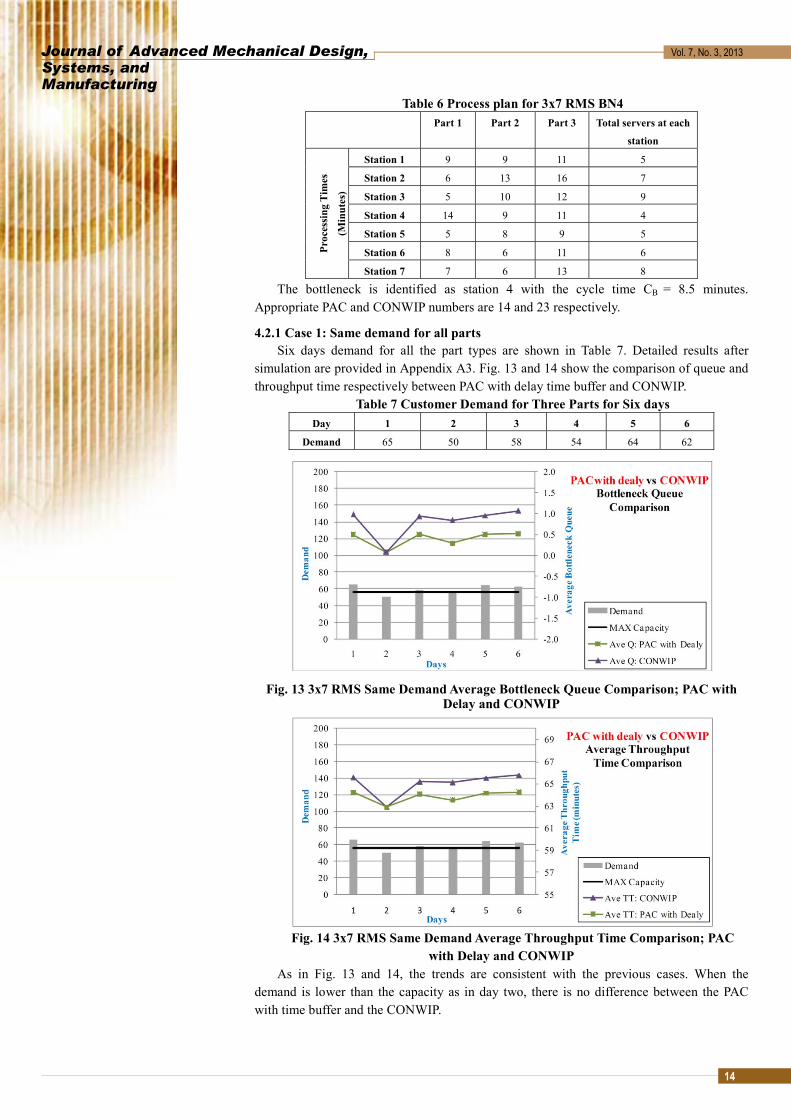
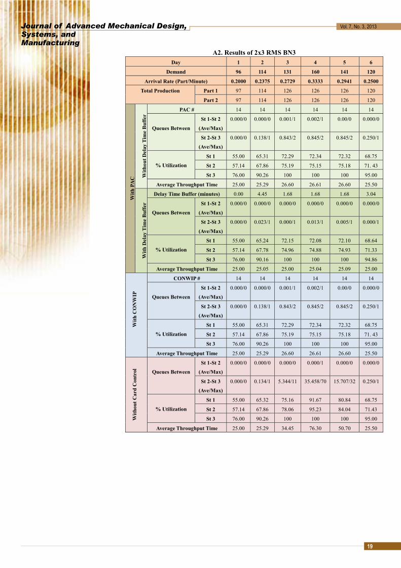
through station 1, 2 and 3. In this case we have included the delay time buffer, therefore the PAC then stays idle for some time. Then PAC attaches with part type 2 and detaches from it after the part type 2 has been processed through station 1, 2 and 3 and the cycle continues. Detailed results of the case study are provided in Appendix A2.

Fig. 11 2x3 RMS BN3 Average Bottleneck Queue Comparison; PAC with Delay and CONWIP

Fig. 12 2x3 RMS BN3 Average Throughput Time Comparison; PAC with Delay and CONWIP

From Fig. 11 and 12, it can be seen that, as the arrival rate increased beyond processing capacity of RMS on day 3, 4 and 5, the WIP started to build-up at buffer between station 2 and station 3, in case of RMS with CONWIP, although the average build-up is below one unit. Although the PAC and the CONWIP have same loops, but after the application of the time buffer in the PAC loop the average queue at the bottleneck has virtually reduced to zero along with the restriction in the average throughput time. Next we have conducted experiments on 3x7 RMS.

4.2 Three Parts and Seven Stations (3x7) RMS Two scenarios are taken into account; same demand for all the part types and different

demand for all the part types. Process plan for each part type and number of identical servers at each station are described in Table 6.


Vol. 7, No. 3, 2013

14

Table 6 Process plan for 3x7 RMS BN4 Part 1 Part 2 Part 3 Total servers at each

station

Proc

essi

ng T

imes

(Min

utes

)

Station 1 9 9 11 5

Station 2 6 13 16 7

Station 3 5 10 12 9

Station 4 14 9 11 4

Station 5 5 8 9 5

Station 6 8 6 11 6

Station 7 7 6 13 8

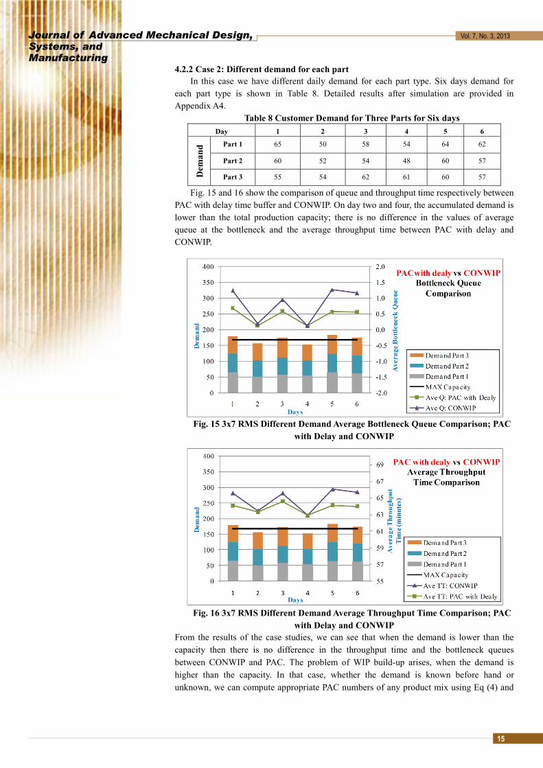
The bottleneck is identified as station 4 with the cycle time CB = 8.5 minutes. Appropriate PAC and CONWIP numbers are 14 and 23 respectively.

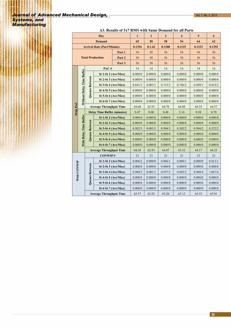
4.2.1 Case 1: Same demand for all parts Six days demand for all the part types are shown in Table 7. Detailed results after

simulation are provided in Appendix A3. Fig. 13 and 14 show the comparison of queue and throughput time respectively between PAC with delay time buffer and CONWIP.

Table 7 Customer Demand for Three Parts for Six days Day 1 2 3 4 5 6

Demand 65 50 58 54 64 62

Fig. 13 3x7 RMS Same Demand Average Bottleneck Queue Comparison; PAC with Delay and CONWIP

Fig. 14 3x7 RMS Same Demand Average Throughput Time Comparison; PAC with Delay and CONWIP

As in Fig. 13 and 14, the trends are consistent with the previous cases. When the demand is lower than the capacity as in day two, there is no difference between the PAC with time buffer and the CONWIP.


Vol. 7, No. 3, 2013

15

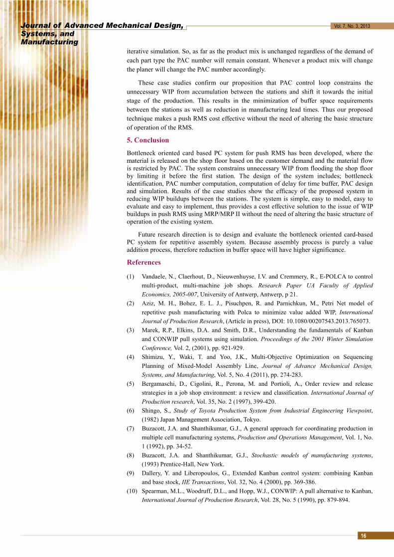
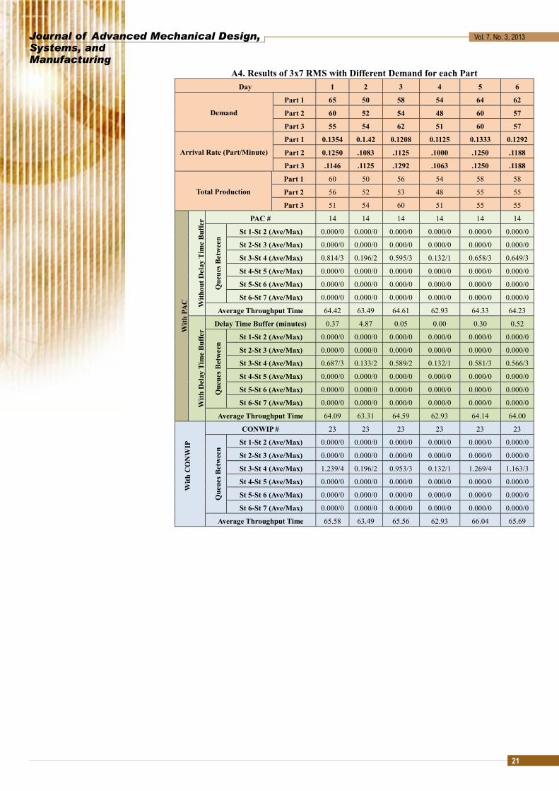
4.2.2 Case 2: Different demand for each part In this case we have different daily demand for each part type. Six days demand for

each part type is shown in Table 8. Detailed results after simulation are provided in Appendix A4.

Table 8 Customer Demand for Three Parts for Six days Day 1 2 3 4 5 6

Dem

and Part 1 65 50 58 54 64 62

Part 2 60 52 54 48 60 57

Part 3 55 54 62 61 60 57

Fig. 15 and 16 show the comparison of queue and throughput time respectively between PAC with delay time buffer and CONWIP. On day two and four, the accumulated demand is lower than the total production capacity; there is no difference in the values of average queue at the bottleneck and the average throughput time between PAC with delay and CONWIP.

Fig. 15 3x7 RMS Different Demand Average Bottleneck Queue Comparison; PAC with Delay and CONWIP

Fig. 16 3x7 RMS Different Demand Average Throughput Time Comparison; PAC with Delay and CONWIP

From the results of the case studies, we can see that when the demand is lower than the capacity then there is no difference in the throughput time and the bottleneck queues between CONWIP and PAC. The problem of WIP build-up arises, when the demand is higher than the capacity. In that case, whether the demand is known before hand or unknown, we can compute appropriate PAC numbers of any product mix using Eq (4) and


Vol. 7, No. 3, 2013

16

iterative simulation. So, as far as the product mix is unchanged regardless of the demand of each part type the PAC number will remain constant. Whenever a product mix will change the planer will change the PAC number accordingly.

These case studies confirm our proposition that PAC control loop constrains the unnecessary WIP from accumulation between the stations and shift it towards the initial stage of the production. This results in the minimization of buffer space requirements between the stations as well as reduction in manufacturing lead times. Thus our proposed technique makes a push RMS cost effective without the need of altering the basic structure of operation of the RMS.

5. Conclusion

Bottleneck oriented card based PC system for push RMS has been developed, where the material is released on the shop floor based on the customer demand and the material flow is restricted by PAC. The system constrains unnecessary WIP from flooding the shop floor by limiting it before the first station. The design of the system includes; bottleneck identification, PAC number computation, computation of delay for time buffer, PAC design and simulation. Results of the case studies show the efficacy of the proposed system in reducing WIP buildups between the stations. The system is simple, easy to model, easy to evaluate and easy to implement, thus provides a cost effective solution to the issue of WIP buildups in push RMS using MRP/MRP II without the need of altering the basic structure of operation of the existing system.

Future research direction is to design and evaluate the bottleneck oriented card-based PC system for repetitive assembly system. Because assembly process is purely a value addition process, therefore reduction in buffer space will have higher significance.

References

(1) Vandaele, N., Claerhout, D., Nieuwenhuyse, I.V. and Cremmery, R., E-POLCA to control multi-product, multi-machine job shops. Research Paper UA Faculty of Applied Economics, 2005-007, University of Antwerp, Antwerp, p 21.

(2) Aziz, M. H., Bohez, E. L. J., Pisuchpen, R. and Parnichkun, M., Petri Net model of repetitive push manufacturing with Polca to minimize value added WIP, International Journal of Production Research, (Article in press), DOI: 10.1080/00207543.2013.765073.

(3) Marek, R.P., Elkins, D.A. and Smith, D.R., Understanding the fundamentals of Kanban and CONWIP pull systems using simulation. Proceedings of the 2001 Winter Simulation Conference, Vol. 2, (2001), pp. 921-929.

(4) Shimizu, Y., Waki, T. and Yoo, J.K., Multi-Objective Optimization on Sequencing Planning of Mixed-Model Assembly Line, Journal of Advance Mechanical Design, Systems, and Manufacturing, Vol. 5, No. 4 (2011), pp. 274-283.

(5) Bergamaschi, D., Cigolini, R., Perona, M. and Portioli, A., Order review and release strategies in a job shop environment: a review and classification. International Journal of Production research, Vol. 35, No. 2 (1997), 399-420.

(6) Shingo, S., Study of Toyota Production System from Industrial Engineering Viewpoint, (1982) Japan Management Association, Tokyo.

(7) Buzacott, J.A. and Shanthikumar, G.J., A general approach for coordinating production in multiple cell manufacturing systems, Production and Operations Management, Vol. 1, No. 1 (1992), pp. 34-52.

(8) Buzacott, J.A. and Shanthikumar, G.J., Stochastic models of manufacturing systems, (1993) Prentice-Hall, New York.

(9) Dallery, Y. and Liberopoulos, G., Extended Kanban control system: combining Kanban and base stock, IIE Transactions, Vol. 32, No. 4 (2000), pp. 369-386.

(10) Spearman, M.L., Woodruff, D.L., and Hopp, W.J., CONWIP: A pull alternative to Kanban, International Journal of Production Research, Vol. 28, No. 5 (1990), pp. 879-894.


Vol. 7, No. 3, 2013

17

(11) Krishnamurthy, A. and Suri, R., Planning and implementing POLCA: a card-based control system for high variety or custom engineered products, Production Planning & Control, Vol. 20, No. 7 (2009), pp. 596-610.

(12) Fernandes, N.O. and Silva, S.C., Generic POLCA – A production and materials flow control mechanism for quick response manufacturing, International Journal of Production Economics, 104 (1), 74-84. Vol. 104, No. 1 (2006), pp. 74-84.

(13) Vandaele, N, Nieuwenhuyse, I. Van, Claerhout, D. and Cremmery, R., Load-Based POLCA: An Integrated Material Control System for Multiproduct, Multimachine Job Shops, Manufacturing & Service Operations Management, Vol. 10, No. 2 (2008), pp. 181-197.

(14) Riezebos J., Design of POLCA material control system, International Journal of Production research, Vol. 48, No. 5 (2010), pp. 1455-1477.

(15) Gaury, E.G.A., Pierreval, H. and Kleijnen, J.P.C., An evolutionary approach to select a pull system among Kanban, CONWIP and hybrid, Journal of Intelligent. Manufacturing, Vol. 11, No. 2 (2000), pp. 157-167.

(16) Takahashi, K., Morikawa, K. and Chen, Y., Comparing Kanban Control with the Theory Of Constraints using Markov Chains, International Journal of Production Research, Vol. 45, No. 16, (2007), pp. 3599-3617.

(17) Baudin, M., Manufacturing Systems Analysis with Application to Production Scheduling, (1990), Yourdon Press, Prentice-Hall, Inc. New Jersey.

(18) Younies, H. and Barhem, B., A Review of the Adoption of Just-In-Time Method and its Effect on Efficiency, Public Administration and Management: An Interactive Journal, Vol. 12, No. 2 (2007), pp. 25-46.

(19) Kamoun, H. and Sriskandarajah, C., The complexity of scheduling jobs in repetitive manufacturing systems, European Journal of Operational Research, Vol. 70, No. 3 (1993), pp. 350-364.

(20) Gaither, N. and Frazier, G., Operations Management (8 ed.), (2001), South-Western, Mason, Ohio.

(21) Riezebos, J., Design of POLCA material control system, International Journal of Production Research, Vol. 48, No. 5, (2010), pp. 1455-1477.

(22) Hibino, H., Instrument Engineers' Handbook, Volume 3: Process Software and Digital Networks, Fourth Edition: Virtual Plants: Process Simulation and Emulation, Chapter 24, (2011), CRC Press, New York.

(23) Inukai, T., Hibino, H. and Fukuda, Y., Simulation Environment Synchronizing Real Equipment for Manufacturing Cell, Journal of Advance Mechanical Design, Systems, and Manufacturing, Vol. 1, No. 2 (2007), pp. 238-249.

(24) Abu Qudeiri, J., Yamamoto, H., Ramli, R. and Al-Momani, K.R., Development of Production Simulator for Buffer Size Decisions in Complex Production Systems Using Genetic Algorithm, Journal of Advance Mechanical Design, Systems, and Manufacturing, Vol. 1, No. 3 (2007), pp. 418-429.

(25) Sakaguchi, T., Kamimura, T. and Shirase, K., Computational Simulation for Decision of Scheduling Period in Reactive Scheduling, Journal of Advance Mechanical Design, Systems, and Manufacturing, Vol. 2, No. 4 (2008), pp. 753-761.

(26) Tateyama, T., Tateno, T. and Shimizu, K., Dynamic Work Planning by Using Simulation-based Optimization in Consideration of Workers’ Skill and Training, Journal of Advance Mechanical Design, Systems, and Manufacturing, Vol. 4, No. 3 (2010), pp. 597-604.


Vol. 7, No. 3, 2013

18

Appendix

A1. Results of 2x3 RMS BN2 Day 1 2 3 4 5 6

Demand 96 114 131 160 141 120

Arrival Rate (Part/Minute) 0.2000 0.2375 0.2729 0.3333 0.2941 0.2500

Total Production Part 1 97 114 126 126 126 120

Part 2 97 114 126 126 126 120

With

PA

C W

ithou

t Del

ay T

ime

Buf

fer

PAC # 8 8 8 8 8 8

Queues Between

St 1-St 2

(Ave/Max)

0.000/0 0.138/1 0.106/1 0.110/2 0.106/1 0.250/1

St 2-St 3

(Ave/Max)

0.000/0 0.000/0 0.000/0 0.000/0 0.000/0 0.000/0

% Utilization

St 1 55.00 65.31 72.36 72.34 72.35 68.75

St 2 76.00 90.26 100 100 100 95.00

St 3 57.14 67.86 75.21 75.15 75.20 71.43

Average Throughput Time 25.00 25.29 25.20 25.21 25.21 25.50

With

Del

ay T

ime

Buf

fer

Delay Time Buffer (minutes) 0.00 1.71 0.20 0.20 0.20 1.00

Queues Between

St 1-St 2

(Ave/Max)

0.000/0 0.062/1 0.000/1 0.005/1 0.000/1 0.000/1

St 2-St 3

(Ave/Max)

0.000/0 0.000/0 0.000/0 0.000/0 0.000/0 0.000/0

% Utilization

St 1 55.00 65.30 72.36 72.30 72.35 68.75

St 2 76.00 90.22 100 100 100 95.00

St 3 57.14 67.82 75.20 75.11 75.18 71.43


With

CO

NW

IP

CONWIP # 14 14 14 14 14 14

Queues Between

St 1-St 2

(Ave/Max)

0.000/0 0.138/1 0.843/2 0.845/3 0.845/2 0.250/1

St 2-St 3

(Ave/Max)

0.000/0 0.000/0 0.000/0 0.002/1 0.000/0 0.000/0

% Utilization

St 1 55.00 65.31 72.34 72.30 72.32 68.75

St 2 76.00 90.26 100 100 100 95.00

St 3 57.14 67.86 75.19 75.17 75.17 71.43


With

out C

ard

Con

trol

Queues Between

St 1-St 2

(Ave/Max)

0.000/0 0.138/1 6.351/12 42.477/77 18.803/35 0.250/1

St 2-St 3

(Ave/Max)

0.000/0 0.000/0 0.000/0 0.000/1 0.000/0 0.000/0

% Utilization

St 1 55.00 65.31 72.17 91.67 80.88 68.75

St 2 76.00 90.26 100 100 100 95.00

St 3 57.14 67.86 75.19 75.18 75.18 71.43



Vol. 7, No. 3, 2013

19

A2. Results of 2x3 RMS BN3 Day 1 2 3 4 5 6

Demand 96 114 131 160 141 120

Arrival Rate (Part/Minute) 0.2000 0.2375 0.2729 0.3333 0.2941 0.2500

Total Production Part 1 97 114 126 126 126 120

Part 2 97 114 126 126 126 120

With

PA

C W

ithou

t Del

ay T

ime

Buf

fer

PAC # 14 14 14 14 14 14

Queues Between

St 1-St 2

(Ave/Max)

0.000/0 0.000/0 0.001/1 0.002/1 0.00/0 0.000/0

St 2-St 3

(Ave/Max)

0.000/0 0.138/1 0.843/2 0.845/2 0.845/2 0.250/1

% Utilization

St 1 55.00 65.31 72.29 72.34 72.32 68.75

St 2 57.14 67.86 75.19 75.15 75.18 71. 43

St 3 76.00 90.26 100 100 100 95.00


With

Del

ay T

ime

Buf

fer


Queues Between

St 1-St 2

(Ave/Max)

0.000/0 0.000/0 0.000/0 0.000/0 0.000/0 0.000/0

St 2-St 3

(Ave/Max)

0.000/0 0.023/1 0.000/1 0.013/1 0.005/1 0.000/1

% Utilization

St 1 55.00 65.24 72.15 72.08 72.10 68.64

St 2 57.14 67.78 74.96 74.88 74.93 71.33

St 3 76.00 90.16 100 100 100 94.86


With

CO

NW

IP

CONWIP # 14 14 14 14 14 14

Queues Between

St 1-St 2

(Ave/Max)

0.000/0 0.000/0 0.001/1 0.002/1 0.00/0 0.000/0

St 2-St 3

(Ave/Max)

0.000/0 0.138/1 0.843/2 0.845/2 0.845/2 0.250/1

% Utilization

St 1 55.00 65.31 72.29 72.34 72.32 68.75

St 2 57.14 67.86 75.19 75.15 75.18 71. 43

St 3 76.00 90.26 100 100 100 95.00


With

out C

ard

Con

trol

Queues Between

St 1-St 2

(Ave/Max)

0.000/0 0.000/0 0.000/0 0.000/1 0.000/0 0.000/0

St 2-St 3

(Ave/Max)

0.000/0 0.134/1 5.344/11 35.458/70 15.707/32 0.250/1

% Utilization

St 1 55.00 65.32 75.16 91.67 80.84 68.75

St 2 57.14 67.86 78.06 95.23 84.04 71.43

St 3 76.00 90.26 100 100 100 95.00



Vol. 7, No. 3, 2013

20

A3. Results of 3x7 RMS with Same Demand for all Parts Day 1 2 3 4 5 6

Demand 65 50 58 54 64 62

Arrival Rate (Part/Minute) 0.1354 0.1.42 0.1208 0.1125 0.1333 0.1292

Total Production

Part 1 56 50 56 54 56 56

Part 2 56 50 56 54 56 56

Part 3 56 50 56 54 56 56

With

PA

C

With

out D

elay

Tim

e B

uffe

r PAC # 14 14 14 14 14 14

Que

ues B

etw

een

St 1-St 2 (Ave/Max) 0.000/0 0.000/0 0.000/0 0.000/0 0.000/0 0.000/0

St 2-St 3 (Ave/Max) 0.000/0 0.000/0 0.000/0 0.000/0 0.000/0 0.000/0

St 3-St 4 (Ave/Max) 0.641/2 0.083/1 0.715/3 0.746/2 0.569/3 0.635/2

St 4-St 5 (Ave/Max) 0.000/0 0.000/0 0.000/0 0.000/0 0.000/0 0.000/0

St 5-St 6 (Ave/Max) 0.000/0 0.000/0 0.000/0 0.000/0 0.000/0 0.000/0

St 6-St 7 (Ave/Max) 0.000/0 0.000/0 0.000/0 0.000/0 0.000/0 0.000/0


With

Del

ay T

ime

Buf

fer


Que

ues B

etw

een

St 1-St 2 (Ave/Max) 0.000/0 0.000/0 0.000/0 0.000/0 0.000/0 0.000/0

St 2-St 3 (Ave/Max) 0.000/0 0.000/0 0.000/0 0.000/0 0.000/0 0.000/0

St 3-St 4 (Ave/Max) 0.502/3 0.083/1 0.504/3 0.302/2 0.504/2 0.522/2

St 4-St 5 (Ave/Max) 0.000/0 0.000/0 0.000/0 0.000/0 0.000/0 0.000/0

St 5-St 6 (Ave/Max) 0.000/0 0.000/0 0.000/0 0.000/0 0.000/0 0.000/0

St 6-St 7 (Ave/Max) 0.000/0 0.000/0 0.000/0 0.000/0 0.000/0 0.000/0


With

CO

NW

IP

CONWIP # 23 23 23 23 23 23

Que

ues B

etw

een

St 1-St 2 (Ave/Max) 0.006/2 0.000/0 0.006/1 0.000/1 0.000/0 0.013/1

St 2-St 3 (Ave/Max) 0.000/0 0.000/0 0.000/0 0.000/0 0.000/0 0.000/0

St 3-St 4 (Ave/Max) 0.984/3 0.083/1 0.937/3 0.845/2 0.960/4 1.067/4

St 4-St 5 (Ave/Max) 0.000/0 0.000/0 0.000/0 0.000/0 0.000/0 0.000/0

St 5-St 6 (Ave/Max) 0.000/0 0.000/0 0.000/0 0.000/0 0.000/0 0.000/0

St 6-St 7 (Ave/Max) 0.000/0 0.000/0 0.000/0 0.000/0 0.000/0 0.000/0



Vol. 7, No. 3, 2013

21

A4. Results of 3x7 RMS with Different Demand for each Part Day 1 2 3 4 5 6

Demand

Part 1 65 50 58 54 64 62

Part 2 60 52 54 48 60 57

Part 3 55 54 62 51 60 57

Arrival Rate (Part/Minute)

Part 1 0.1354 0.1.42 0.1208 0.1125 0.1333 0.1292

Part 2 0.1250 .1083 .1125 .1000 .1250 .1188

Part 3 .1146 .1125 .1292 .1063 .1250 .1188

Total Production

Part 1 60 50 56 54 58 58

Part 2 56 52 53 48 55 55

Part 3 51 54 60 51 55 55

With

PA

C

With

out D

elay

Tim

e B

uffe

r PAC # 14 14 14 14 14 14 Q

ueue

s Bet

wee

n

St 1-St 2 (Ave/Max) 0.000/0 0.000/0 0.000/0 0.000/0 0.000/0 0.000/0

St 2-St 3 (Ave/Max) 0.000/0 0.000/0 0.000/0 0.000/0 0.000/0 0.000/0

St 3-St 4 (Ave/Max) 0.814/3 0.196/2 0.595/3 0.132/1 0.658/3 0.649/3

St 4-St 5 (Ave/Max) 0.000/0 0.000/0 0.000/0 0.000/0 0.000/0 0.000/0

St 5-St 6 (Ave/Max) 0.000/0 0.000/0 0.000/0 0.000/0 0.000/0 0.000/0

St 6-St 7 (Ave/Max) 0.000/0 0.000/0 0.000/0 0.000/0 0.000/0 0.000/0


With

Del

ay T

ime

Buf

fer


Que

ues B

etw

een

St 1-St 2 (Ave/Max) 0.000/0 0.000/0 0.000/0 0.000/0 0.000/0 0.000/0

St 2-St 3 (Ave/Max) 0.000/0 0.000/0 0.000/0 0.000/0 0.000/0 0.000/0

St 3-St 4 (Ave/Max) 0.687/3 0.133/2 0.589/2 0.132/1 0.581/3 0.566/3

St 4-St 5 (Ave/Max) 0.000/0 0.000/0 0.000/0 0.000/0 0.000/0 0.000/0

St 5-St 6 (Ave/Max) 0.000/0 0.000/0 0.000/0 0.000/0 0.000/0 0.000/0

St 6-St 7 (Ave/Max) 0.000/0 0.000/0 0.000/0 0.000/0 0.000/0 0.000/0


With

CO

NW

IP

CONWIP # 23 23 23 23 23 23

Que

ues B

etw

een

St 1-St 2 (Ave/Max) 0.000/0 0.000/0 0.000/0 0.000/0 0.000/0 0.000/0

St 2-St 3 (Ave/Max) 0.000/0 0.000/0 0.000/0 0.000/0 0.000/0 0.000/0

St 3-St 4 (Ave/Max) 1.239/4 0.196/2 0.953/3 0.132/1 1.269/4 1.163/3

St 4-St 5 (Ave/Max) 0.000/0 0.000/0 0.000/0 0.000/0 0.000/0 0.000/0

St 5-St 6 (Ave/Max) 0.000/0 0.000/0 0.000/0 0.000/0 0.000/0 0.000/0

St 6-St 7 (Ave/Max) 0.000/0 0.000/0 0.000/0 0.000/0 0.000/0 0.000/0


bottleneck oriented card-based production control for push repetitive manufacturing system

Documents