bootstrap generation and evaluation of an fmri simulation database
TRANSCRIPT
Bootstrap generation and evaluation of an fMRI simulationdatabase
Pierre Belleca,*, Vincent Perlbargb,c, and Alan C. EvansaaMcConnell Brain Imaging Centre, Montreal Neurological Institute, McGill University, H3A2B4,Montreal, CanadabInserm, UMR_S 678, Laboratoire d’Imagerie Fonctionnelle, F-75634, Paris, FrancecUPMC Univ Paris 06, UMR_S 678, Laboratoire d’Imagerie Fonctionnelle, F-75634, Paris, France
AbstractComputer simulations have played a critical role in functional magnetic resonance imaging (fMRI)research, notably in the validation of new data analysis methods. Many approaches have been usedto generate fMRI simulations, but there is currently no generic framework to assess how realisticeach one of these approaches may be. In this paper, a statistical technique called parametric bootstrapwas used to generate a simulation database that mimicked the parameters found in a real database,which comprised 40 subjects and 5 tasks. The simulations were evaluated by comparing thedistributions of a battery of stastical measures between the real and simulated databases. Two popularsimulation models were evaluated for the first time by applying the bootstrap framework. The firstmodel was an additive mixture of multiple components and the second one implemented a non-linearmotion process. In both models, the simulated components included the following brain dynamics :a baseline, physiological noise, neural activation and random noise. These models were found tosuccessfully reproduce the relative variance of the components and the temporal autocorrelation ofthe fMRI time series. By contrast, the level of spatial autocorrelation was found to be drastically lowusing the additive model. Interestingly, the motion process in the second model intrisically generatedsome slow time drifts and increased the level of spatial autocorrelations. These experimentsdemonstrated that the bootstrap framework is a powerful new tool that can pinpoint the respectivestrengths and limitations of simulation models.
Keywordsbootstrap; evaluation; fMRI; motion; parametric model; simulation
1 IntroductionFunctional magnetic resonance imaging (fMRI) measures the hemodynamic correlates of brainneural activity [1,2]. This modality had a deep impact on human cognitive neuroscience andclinical research over the past fifteen years [3,Figure 1]. Computer simulations have criticallycontributed to advance fMRI research in at least two directions. They have first been used to
© 2009 Elsevier Inc. All rights reserved.*Corresponding author. Fax: +1-514-398-8948. E-mail address: [email protected] is a PDF file of an unedited manuscript that has been accepted for publication. As a service to our customers we are providing thisearly version of the manuscript. The manuscript will undergo copyediting, typesetting, and review of the resulting proof before it ispublished in its final citable form. Please note that during the production process errors may be discovered which could affect the content,and all legal disclaimers that apply to the journal pertain.
NIH Public AccessAuthor ManuscriptMagn Reson Imaging. Author manuscript; available in PMC 2010 December 1.
Published in final edited form as:Magn Reson Imaging. 2009 December ; 27(10): 1382–1396. doi:10.1016/j.mri.2009.05.034.
NIH
-PA Author Manuscript
NIH
-PA Author Manuscript
NIH
-PA Author Manuscript
evaluate the performance of some data analysis methods in a completely controlledenvironment, e.g. fMRI data preprocessing [4], hypothesis testing strategies [5,6], activationdetection techniques [7–10] or motion-correction algorithms [11–14]. Simulations have alsoplayed a key role in uncovering some of the underlying mechanisms of the fMRI data-generating process, both on the aspects of neural dynamics [15,16], brain metabolism [17,18]and MR physics [19].
There has been a wide variety of approaches to generate fMRI simulations : a new ad hocenvironment has essentially been developed for each particular study. As a consequence, it hasbeen difficult so far to compare the simulation results reported by different groups working onthe same question. To fully appreciate the potential value of the results reported in a givensimulation study, the fMRI research community would need a rigorous and comprehensiveevaluation of the strengths and limitations of employed simulation framework. Some groupshave used an additive model with three main components : a constant baseline, a signal ofinterest called activation and a random noise, e.g. [20,7,4,8,21–23,9,24,5,6]. Such additivemodels essentially gave access to the signal-to-noise ratio and the shape of activated regions.The investigators mostly did not question whether the simulations were realistic as long assome plausible values were assigned to the parameters of the simulation model.
More elaborate approaches included motion as part of the data-generating process, eitherthrough spatial interpolation [11–13] or using a first-principle model of the MR physics [19,25,26]. Such models gave access to the motion parameters and in some cases to the pulsesequence parameters. They were also much more computationally demanding, requiring hoursor even days of computation on a single workstation. Unfortunately, whether these modelsgenerated realistic simulations has not yet been quantitatively assessed. Rather, the evaluationwas a qualitative examination, i.e. a visual check of the presence or the shape of known artefactson static images [19].
This paper presents a principled framework to generate an fMRI simulation database andevaluate its strengths and limitations. In general, the proximity between a simulation databaseand real fMRI acquisitions depends on the quality of the simulation model, but is also relatedto the way the simulation parameters are selected to generate the database. Obviously, if theparameters themselves strongly deviate from realistic values, the most accurate model of thefMRI data-generating process would lead to simulations of poor quality.
We developed a flexible method to address these issues which could in theory be applied toany parametric simulation model. The rationale of our method was to replicate a real fMRIdatabase by systematically using the parameters estimated on the real data to set up theparameters of the simulations. This approach was a direct application of a statistical techniquecalled parametric bootstrap. Iterating this process on each subject of a large database ensuredthat the variability of the simulated parameters precisely mimicked the variability found in thereal database under scrutiny, for example in terms of brain anatomy or signal-to-noise ratio.The evaluation of the quality of the simulated database proceeded by assessing which statisticalproperties of fMRI data were well replicated and which ones were not. Specifically, a batteryof statistical measures was estimated on each individual dataset and group-level summarieswere derived. The significance of the differences between the real and simulated group-levelsummaries were established using a non-parametric bootstrap of the subjects found in thedatabase.
We applied the bootstrap framework on two simulation models that encapsulated the mainfeatures of common models used in literature, namely an additive (ADD) model and a simplemotion (SM) model. These experiments were designed to demonstrate that the bootstrapapproach is feasible on recent popular models. To the best of our knowledge, it was also the
Bellec et al. Page 2
Magn Reson Imaging. Author manuscript; available in PMC 2010 December 1.
NIH
-PA Author Manuscript
NIH
-PA Author Manuscript
NIH
-PA Author Manuscript
first quantitative evaluation conducted on an fMRI simulation database. The simulatedcomponents included a baseline, slow time drifts, physiological noise, neural activation andrandom noise. This range of brain dynamics is as large or even larger than what has beenconsidered thus far by other groups working on fMRI simulations. Parametric bootstrap wasused to replicate a real database, the so-called functional reference battery (FRB), featuring alarge population (N = 40 subjects) and 5 tasks designed to engage a broad range of brainsystems. The FRB database was replicated using each model, resulting into two simulationdatabases, respectively called FRB-ADD and FRB-SM. We evaluated the quality of eachsimulation database by investigating the following individual statistical measures : respectivevariance of the estimated components of the model, the spatial and temporal autocorrelation,as well as the distribution of the variance in a principal component analysis.
2 Bootstrap generation and evaluation of an fMRI simulation database2.1 Parametric bootstrap generation of an fMRI simulation database
The most critical ingredient in a computer-based simulation study is the data-generatingprocess (DGP). The DGP f describes the mechanisms used to generate a data sample y of arandom variable Y. For example, f could represent the process of drawing multiple independentsamples from a Gaussian random number generator. The DGP f is perfectly known andcontrolled in a simulation study, yet simulations are also generally intended to replicate a realexperiment. In the case of brain imaging, y would be an individual set of fMRI time series,Y would represent a subject and f would be a model of the random process that goes from theindividual brain functional architecture to a digital BOLD measure of the brain activityacquired during an MRI session. The real DGP f or its parameters θ are actually unknown andthe investigator is bound to rely on a more or less elaborate approximation f^. The bootstrapis a general statistical method to perform this estimation that relies on a real data sample y toderive a bootstrap estimated DGP f^y.
The other main ingredient in computer simulations is a function m that can be estimated oneach data sample y, resulting into one measurement m(y) (see figure C.1). The measure m (y)could for example be a set of maps of regression coefficients estimated in a linear model ortheir associated level of significance against a null hypothesis, i.e. a statistical map. One basicobjective in a computer simulation study would be to uncover the distribution of the measuresm (y) when y follows the DGP f. This can be formally done through Monte-Carlo simulationswhich consists in drawing from f a number B of independent and identically distributed (i.i.d.)
data replicates and use these samples to derive an estimate Ĝ of the (left-sided)cumulative distribution function (cdf) G of m(y) :
(1)
where # is the cardinality of a set and the symbol ≐ means that the two terms are asymptoticallyequal as B tends toward infinity.
Some further explicit parametric assumptions on the DGP would allow to raise even moreinteresting questions. A parametric model provides the investigator with an explicit control onthe different aspects of the DGP, such as the localisation of truly activated regions or the signal-to-noise ratio. Formally, the DGP takes a closed-form expression fθ which depends on a set ofground-truth parameters θ. In our case, these parameters would represent all the features ofbrain dynamics included in the model, e.g. brain anatomy, characteristics of brain tissues,modulations of related to the metabolic response to neural activity, motion, etc. Under sucha parametric assumption, the parametric bootstrap simulation (PBS) consists in replacing the
Bellec et al. Page 3
Magn Reson Imaging. Author manuscript; available in PMC 2010 December 1.
NIH
-PA Author Manuscript
NIH
-PA Author Manuscript
NIH
-PA Author Manuscript
real unknown parameters θ by some estimate θ ̂ derived from a real dataset y. Section 3 willdescribe some particular models in details but the techniques presented here are general. Onepossible application of a parametric DGP would be to perform a sensitivity analysis, i.e.determine which is the influence of one parameter in θ on G(x). To build on the previousexamples, it would be interesting to assess how the signal-to-noise ratio affects the estimatedstatistics in the activated regions. Moreover, if m(y) was an estimator θ^ of the parameters θ,it would be possible to investigate the accuracy of the estimator and even to compare theaccuracy of different estimators as it was commonly done using receiver-operatingcharacteristic (ROC) curves [27].
The parametric bootstrap can be extended to a full fMRI database. An fMRI database is acollection of individual datasets collected for a number N of subjects. Those subjectsare independent samples of a specific population, for example adults with no history ofneurological or psychiatric disorder between the age of 20 and 40. Each fMRI dataset yn ismodeled as one sample drawn from a subject-specific random variable Yn with some subject-specific distribution fθn. Replicating the real database using PBS simply consists in estimatingthe parameter θ ̂n for each subject Yn and generating a PBS replicate from fθ̂n. The PBSmethod to replicate an fMRI simulation database was summarised in the central part of FigureC.2.
2.2 Non-parametric bootstrap evaluation of an fMRI simulation databaseThere are a number of concerns with the theoretical foundation of PBS in the context ofindividual fMRI simulations. The chief concern that would actually stand for any parametricapproach is the validity of the parametric model. Other possible shortcomings are the qualityof the procedure used to estimate the parameters of the model, or the applicability of thebootstrap approach itself that depends on the properties of the measure m. As a consequence,it is crucial to evaluate whether an fMRI simulation database generated through PBS exhibitssome realistic statistical features. Our evaluation strategy was to compare the distribution of abattery of statistical features between the real fMRI database and its PBS replication.
For a particular statistical feature mn = m(yn), the evaluation of the quality of the simulationdatabase boils down to compare the approximate distribution of the measure derived with realsamples to the distribution of their simulated replications . For thatpurpose, it is possible to derive some summary statistics s(m1 …, mn) of the distribution suchas the mean, median, 0.05% upper and lower percentiles and compare this summary s* to thevalue s* derived on the simulation database. To assess statistically any departure between s*and s*, we resorted to non-parametric bootstrap of the subjects of the database. Those subjectsare independent and identically distributed (i.i.d.) and in addition our summary statistics aresmooth functions of the mean, so the most standard version of non-parametric bootstrap isadapted to that problem, see for example [28] p. 80–90. Non-parametric bootstrap consists indrawing subjects with replacement from the population, and derive a new replicate of thesummary statistics s*b for this surrogate population. By repeating this step a large number B
of times, the bootstrap replicates can be used to derive a two-sided symmetric boostrapconfidence interval on s* based on the bootstrap cdf defined in Equation (1) [29]. If the realsummary statistics s did not fall within the bootstrap confidence interval for s* at a reasonablelevel of confidence, e.g. p < 0.01, we would conclude to a significant departure between thereal and simulated data. The whole evaluation procedure was summarised in the Figure C.2.
Ideally, the proposed evaluation method would be performed on the very same measure(s) ofinterest as the one(s) investigated in the simulation study. Unfortunately, such measure musually relies on the ground truth parameters θn. In such case, it would not be possible to derive
Bellec et al. Page 4
Magn Reson Imaging. Author manuscript; available in PMC 2010 December 1.
NIH
-PA Author Manuscript
NIH
-PA Author Manuscript
NIH
-PA Author Manuscript
the samples on the real data because the ground-truth parameters would be unknown.The evaluation method alternatively relies on a battery of different statistical features m thatcan be estimated both on the real and simulated data. The list of statistical features would coverthe most salient aspects that can potentially affect a data analysis method. The features usedin this work were listed in Section 4.2.
3 Parametric models of fMRI simulation3.1 A general form
The following notations were used to describe the models of fMRI data generation :
(2)
where Y, B, D, P, A and E were matrices and ϕ was a function. The matrix Y was a 3D+tdataset of size T × S that represented the simulated fMRI time series, with T and S standingfor the number of time samples and voxels, respectively. The other matrices, of size T × R withR eventually greater than S for high spatial resolution, each represented one component of themodel :
• B was a constant baseline reflecting the brain anatomy,
• D described slow time drifts of the baseline,
• P represented fluctuations induced by physiological noise such as breathing and heartbeat,
• A described the hemodynamic fluctuations related to neural activity,
• E was a random measurement error.
The function ϕ was simulating the MR imaging process, and could be either a linear or a non-linear function. This function was potentially dependent on additional unknown parameters,e.g. the motion parameters.
3.2 Simulation model ADDThe ADD simulations were based on a linear mixture model with a Gaussian noise :
(3)
where XC and βC respectively were the temporal and spatial distribution of component C, withC standing for any of the components B, D, P or A. The T × S matrix E* was a sample of aGaussian random variable independent in time and space, with a zero mean and a voxel-specificvariance for all voxels υ. A diagram representation of Equation (3) can be found in FigureC.3. The following parameters were a fixed, known part of the parametric model :
• XB was a constant vector of size T × 1.
• XD was a basis of discrete cosines covering the frequency window [0, 0.01] Hz, ofsize T × KD. The number KD depended on the sampling rate and the length of thefMRI time series, and in our case was equal to 6.
• XA was the modeled BOLD response to an experiment. In this work, it was a singleboxcar experiment convolved with a fixed hemodynamic response function.
Bellec et al. Page 5
Magn Reson Imaging. Author manuscript; available in PMC 2010 December 1.
NIH
-PA Author Manuscript
NIH
-PA Author Manuscript
NIH
-PA Author Manuscript
The following parameters of the model were unknown and had to be estimated using a realdataset :
• The spatial distributions of all components (βB, βD, βP and βA). Their respective sizeswere 1 × S, KD × S, KP × S and 1 × S. The number of physiological noise covariatesKP was itself a parameter estimated on the data.
• The physiological noise temporal distribution XP.
• The map of the variance of the Gaussian noise, of size 1 × S.
Both the spatial and temporal distributions of the physiological noise had to be estimated, whichis a blind source estimation problem. As a consequence, the estimation of the parameters ofmodel ADD was addressed using an iterative procedure mixing some least-square linear fitsand an independent component analysis. The outline of the estimation pipeline was:
1. The raw functional data was corrected for rigid-body motion and slice timing.
2. The spatial distribution of slow time drifts was estimated using a least-square linearfit.
3. The residuals of the fit were decomposed into spatially independent components, andan automatic method called CORSICA was used to identify the components relatedto physiological noise [30]. Those components XP were subtracted from the fMRIdata to produce a physiology-corrected dataset.
4. A least-square linear fit of XA was performed on the physiology-corrected dataset ateach voxel. A t-map of significance was also derived and a bilateral threshold of p< 0.001 uncorrected for multiple comparisons was applied to this map. The estimateof βa was 0 for non-significant voxels, and the least-square estimate everywhere else.
5. The variance of the residuals was corrected for the total number of covariates in the
model to provide an estimation of the variance of the Gaussian noise .
6. Based on the estimate of the noise variance, a shrinkage correction [31] was appliedto the estimates of βD and βP. This step was performed to improve the accuracy ofthe variance distribution of these components.
The parameter estimation pipeline was described in further details in Annex A. This procedurewas not standard and notably relied on an approximation for the estimation of the noisevariance. The components B, A and E* of the model were commonly used in fMRI simulations,e.g. [4]. By contrast with a common approach, e.g. [23,5,6,22], the noise was not modeled asa random process exhibiting dependencies in both time and space. Alternatively, the slow timedrifts and physiological noise components were added as deterministic mixtures, as was donefor example in [20,21]. Lund et al [32] showed that adding components in the linear modelwould account for the temporal autocorrelation of the noise, even though this result cannot bedirectly translated to the ADD model because the study by Lund et al did not use ICA to identifythe physiological noise. The slow time drifts and physiological noise may also account for thespatial correlations in the fMRI noise, but this question is to our knowledge still opened. Allthe questions and potential concerns raised in this paragraph were investigated in the evaluationof the ADD simulation database presented in Section 4.
3.3 Simulation model SMThe simulation model SM took the following form :
(4)
Bellec et al. Page 6
Magn Reson Imaging. Author manuscript; available in PMC 2010 December 1.
NIH
-PA Author Manuscript
NIH
-PA Author Manuscript
NIH
-PA Author Manuscript
The deterministic components of the model, i.e. B = Xbβb, P = XPβP and A = Xaβa, were firstadded to generate a motion-free and noise-free space-time dataset Yref of size T × R. The spatialdimension R was significantly higher than the native functional spatial dimension S, e.g. a high-resolution voxel size of 1 × 1 × 1 mm3 for Yhigh compared to a native functional resolution of4 × 4 × 4 mm3 for Y. A simple rigid-body motion process ϕSM was then applied on Yhigh usingthe translation parameters τ and rotation parameters ρ. For each slice and each volume of thefMRI dataset, a cubic interpolation was performed in time on Yhigh, τ and ρ to derive a brainvolume V of size 1 × R and a set of six motion parameters that precisely corresponded to thetime of acquisition of this slice and this volume. The rigid-body transformation was applied toV using a tricubic interpolation scheme1. For each voxel of the slice at the native functionalresolution, the value of all high-resolution voxels inside the low-resolution voxel wereaveraged. This process was iterated over all slices and volumes to produce a low-resolutiondataset Ylow of size T × S. A Gaussian noise E* of size T × S was finally added to Ylow togenerate a sample of fMRI simulation with a size T × S. The flowchart of the SM modelwas depicted in Figure C.4.
The parameters XB and XA were known and defined in the same way as for the ADD model.The unknown parameters of the model SM were almost the same as for the ADD model. Thedifferences were that SM did not have a slow time drifts component but included instead someunknown motion parameters τ and ρ, both of size T × 3, for a total of 6 parameters per volumeof the time-space fMRI dataset.
The parameters of the model SM were estimated using essentially the same pipeline as formodel ADD. This pipeline actually featured a motion parameter estimation, even thoughmotion was not included in ADD. The main additional step was to oversample the spatialdistributions βB, βP and βA at the high spatial dimension R. This was done through nearest-neighbour interpolation for the physiological noise and the activation components. The high-resolution baseline spatial distribution was derived by combining a segmentation of a T1 imageof the subject and the ADD estimate β ̂B, see annex B for details.
As was noted for the model ADD, the method used to estimate the parameters of the modelSM relied on a number of approximations. First, the nearest-neighbour oversampling of thespatial distribution of P and A neglected the partial-volume effects in the low-resolutionestimates of the ADD model. Second, the high-resolution baseline was derived by assuming aone-to-one correspondence between the T1 and coefficients, which may not be accurate.Note also that the transformation (ϕSM was very similar to some other transformationspreviously used in the literature [12,11], with small differences : Freire et al. used a low-resolution space to simulate the motion and both this group and Ardekani et al did not includethe slice timing effects, i.e. the same volume and transformation was used to generate all theslices in each volume of the fMRI simulation. To our knowledge, none of the studies that haveused a model of motion have considered a structured noise such as P in addition to the baseline.Another important modelling choice was to exclude the slow time drifts component from theSM model. The origin of these slow time drifts is somewhat controversial, and they probablyrepresent a mixture of motion/physiological noise and scanner drifts. We postulated that themotion process could account for the most part of the drifts. Excluding the drifts wouldtherefore be regarded as the lesser of two evils, because adding an extra slow time driftscomponent on top of the motion-induced drifts would result in a far too large total amount ofslow time drifts. The potential concerns raised in this paragraph were investigated in theevaluation of the SM simulation database presented in Section 4.
1This process was actually restricted to a neighbourhood of the slice of interest to save computation time.
Bellec et al. Page 7
Magn Reson Imaging. Author manuscript; available in PMC 2010 December 1.
NIH
-PA Author Manuscript
NIH
-PA Author Manuscript
NIH
-PA Author Manuscript
4 The ADD-FRB and SM-FRB simulation databases4.1 The functional reference battery (FRB) database
The PBS framework relies on a large number of real datasets acquired following a specificscanning protocol, such that the variability of the simulation parameters would berepresentative of the characteristics found in this protocol. For this purpose, we used the so-called functional reference battery (FRB) database, which has been designed and acquired bythe International Consortium for Brain Mapping (ICBM)2 . Forty right-handed healthyvolunteers (20 men, 20 women; age ranging from 20 to 38 years, median 25 years) haveparticipated in this study which was approved by the local ethic committee. Subjects had nohistory of neurological or psychological disorders. Functional data was acquired while subjectsperformed five different tasks, i.e. auditory naming, AN; external ordering, EO, which is aworking memory task; hand imitation, HA, a visuo-motor task; an oculomotor task, OM, anda verbal generation task, VG. The control condition used for all tasks was to fixate a smallarrow at the centre of a screen and press a button when the arrow pointed to the left (veryinfrequently). An extensive description of the stimuli and tasks can be found on the internet3 .
For each functional run, 88 brain volumes of blood oxygenation level dependent signals wererecorded on a 1.5T Siemens Sonatavision MRI scanner at the McConnel Brain Imaging Centerin Montreal, using a 2D echo-planar imaging sequence and the following parameters: TR/TE= 4 s/50 ms, 64 × 64 matrix, in-plane resolution 4mm×4mm, 26 non-contiguous slices, with a1 mm slice gap, FOV = 256 mm×256 mm, slice thickness 4 mm and flip angle = 90º. A high-resolution T1-weighted scan was also acquired using the following FLASH gradient echosequence: TR/TE = 22 ms/9.2 ms, 192 × 256 × 256 matrix, FOV = 192 mm×256 mm×256 mmand flip angle = 30º. Subjects performed on-off block paradigms, with 28-sec (7 vol.) longblocks. There were 12 blocks per run (6 ‘off-on’), 3 volumes at the beginning of the run to waitfor magnetisation stabilisation, and one extra volume at the end which was ‘off’.
In total, there were 200 fMRI datasets in the FRB database (40 subjects times 5 tasks). Togenerate the simulation databases, the parameters of data simulation were estimated for eachdataset, and plugged into the simulation engines ADD and SM to derive one parametricbootstrap replication. The resulting simulation databases comprised 200 datasets each and werecalled FRB-ADD and FRB-SM respectively.
4.2 List of the statistical features for evaluationThe following statistical features were investigated to evaluate the quality of the simulationdatabases. The first set of features aimed at quantifying the empirical signal-to-noise ratio. Thesame processing pipeline that was applied to estimate the parameters of the ADD model onthe real FRB database was used again on the FRB-ADD and FRB-SM simulation databases.Maps of relative percentage of variance were derived for each component of the model. Forexample, the variance map of slow time drifts was defined as the absolute difference betweenthe variance of the functional data before and after temporal filtering, divided at each voxel bythe total variance of the time series after motion correction and slice timing. The sameprocedure was applied for the physiological noise and the activation. The relative variance ofthe residuals was defined in a similar way, except it simply involved the variance map of theresiduals rather than a difference between two variance maps.
2http://www.loni.ucla.edu/ICBM/3http://www.loni.ucla.edu/ICBM/Downloads/Downloads_FRB.shtml
Bellec et al. Page 8
Magn Reson Imaging. Author manuscript; available in PMC 2010 December 1.
NIH
-PA Author Manuscript
NIH
-PA Author Manuscript
NIH
-PA Author Manuscript
Another batch of measures was used to investigate the amount of correlation structure presentin the data. First, local spatial autocorrelation maps were derived, i.e. the average correlationbetween the time series associated with each voxel and its 6 spatial neighbours, as well as thetemporal (lag 1) autocorrelation maps. These maps were derived at the very beginning of theprocessing pipeline, i.e. on motion-corrected data, and also on the residuals of the linear model.To get an insight into correlations regardless of the spatial scale, the repartition of the variancein the 60 first components of a spatial principal component analysis (PCA) relative to the totalvariance explained by these components was also derived.
For all measures that took the form of a map, a group-level average was computed after non-linear coregistration in the MNI space. Axial slices of these averages were presented in thefigures for qualitative evaluation. The corresponding slices were also generated on a structuralaverage for anatomical localisation, see Figure C.5. For each individual map, some quantitativesummaries were derived, i.e. the 0.01%, 0.25%, 0.50%, 0.75% and 0.99% percentiles withinthe brain. The summary at the group level was the mean of the individual summaries. Regardingthe PCA variance curves, the group-level summary was also the average curve. The bootstraptest described in Section 2.2 was applied to assess any statistical departure between the group-level summaries derived from the FRB and FRB-ADD/FRB-SM databases. The text gives aconcise report of the main results and a comprehensive description can be found in the tables.
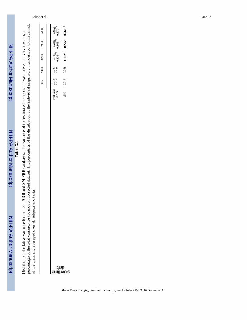
4.3 Evaluation4.3.1 Percentage of variance—The percentage of relative variance of each component ofthe model for the real and simulation databases can be found in Table C.1 and Figure C.6.
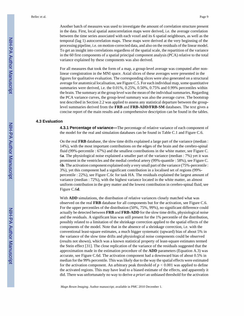
On the real FRB database, the slow time drifts explained a large part of the variance (median :14%), with the most important contributions on the edges of the brain and the cerebro-spinalfluid (99%-percentile : 67%) and the smallest contributions in the white matter, see Figure C.6a. The physiological noise explained a smaller part of the variance (median : 7%) yet it wasprominent in the ventricles and the medial cerebral artery (99%-quantile : 58%), see Figure C.6b. The activation component explained only a very small part of the variance (75%-percentile :3%), yet this component had a significant contribution in a localised set of regions (99%-percentile : 22%), see Figure C.6c for task HA. The residuals explained the largest amount ofvariance (median : 72%), with the highest variance located in the white matter, an almostuniform contribution in the grey matter and the lowest contribution in cerebro-spinal fluid, seeFigure C.6d.
With ADD simulations, the distribution of relative variances closely matched what wasobserved on the real FRB database for all components but for the activation, see Figure C.6.For the upper percentiles of the distribution (50%, 75%, 99%), no significant difference couldactually be detected between FRB and FRB-ADD for the slow time drifts, physiological noiseand the residuals. A significant bias was still present for the 1% percentile of the distribution,possibly related to a limitation of the shrinkage correction applied to the spatial effects of thecomponents of the model. Note that in the absence of a shrinkage correction, i.e. with theconventional least-square estimates, a much bigger systematic (upward) bias of about 5% inthe variance of the slow time drifts and physiological noise components could be observed(results not shown), which was a known statistical property of least-square estimates termedthe Stein effect [31]. The close replication of the variance of the residuals suggested that theapproximation made in the estimation procedure of the ADD parameters (Equation A.3) wasaccurate, see Figure C.6d. The activation component had a downward bias of about 0.5% inmedian for the 99% percentile. This was likely due to the way the spatial effects were estimatedfor the activation component. An arbitrary peak threshold of p < 0.001 was applied to definethe activated regions. This may have lead to a biased estimate of the effects, and apparently itdid. There was unfortunately no way to derive a priori an unbiased threshold for the activation
Bellec et al. Page 9
Magn Reson Imaging. Author manuscript; available in PMC 2010 December 1.
NIH
-PA Author Manuscript
NIH
-PA Author Manuscript
NIH
-PA Author Manuscript
component, as the effect size and the real activated regions were unknown. Shrinkageestimation would have been a way to avoid this problem, but it would have resulted in somevery large activated regions which were not physiologically plausible. The bootstrap evaluationproved able to identify this shortcoming of the parameter estimation procedure.
Interestingly on the FRB-SM database, a significant amount of variance was explained by theslow time drifts (median : 12%) even though the SM model did not explicitly include thiscomponent. The motion process induced a spatial distribution of drifts prominent in the edgesof the brain and the ventricles which shared some similarities with what was observed on thereal database, see Figure C.6a. However, some clear departures could be observed for examplein the white matter. In quantitative terms, all percentiles of the slow time drifts variancesignificantly departed between FRB-SM and FRB. The size of the bias was still smaller than5% of the real estimate for the upper percentiles (50%, 75%, 99%)4 . Regarding thephysiological noise, there was a clear downward bias, even though the bias was still less than5% of the FRB estimate. This was probably a consequence of neglecting the partial volumeeffects in the estimation procedure of the SM parameters. The partial-volume effects alsoslightly reduced the variance of task-induced fluctuations, see Figure C.6c. These multipledepartures caused a biased variance for the residuals, but still in the range of 5% of the realestimates except for the first 1% percentile.
As a whole, the evaluation performed on the FRB database demonstrated that the FRB-ADD database had a realistic repartition of the relative variance among the differentcomponents of the model, and that the FRB-SM had only a small bias in its relative variancedistribution. This bias could probably be neglected for most applications. As an interesting by-product, this experiment also demonstrated the accuracy of the approximation made to estimatethe parameters of the ADD model, at least for the range of parameters present in the FRBdatabase. The FRB-SM database also confirmed the hypothesis that the sole motion couldinduce slow time drifts to a quite realistic level without having to add any type of arbitraryfluctuations in the slow frequency band.
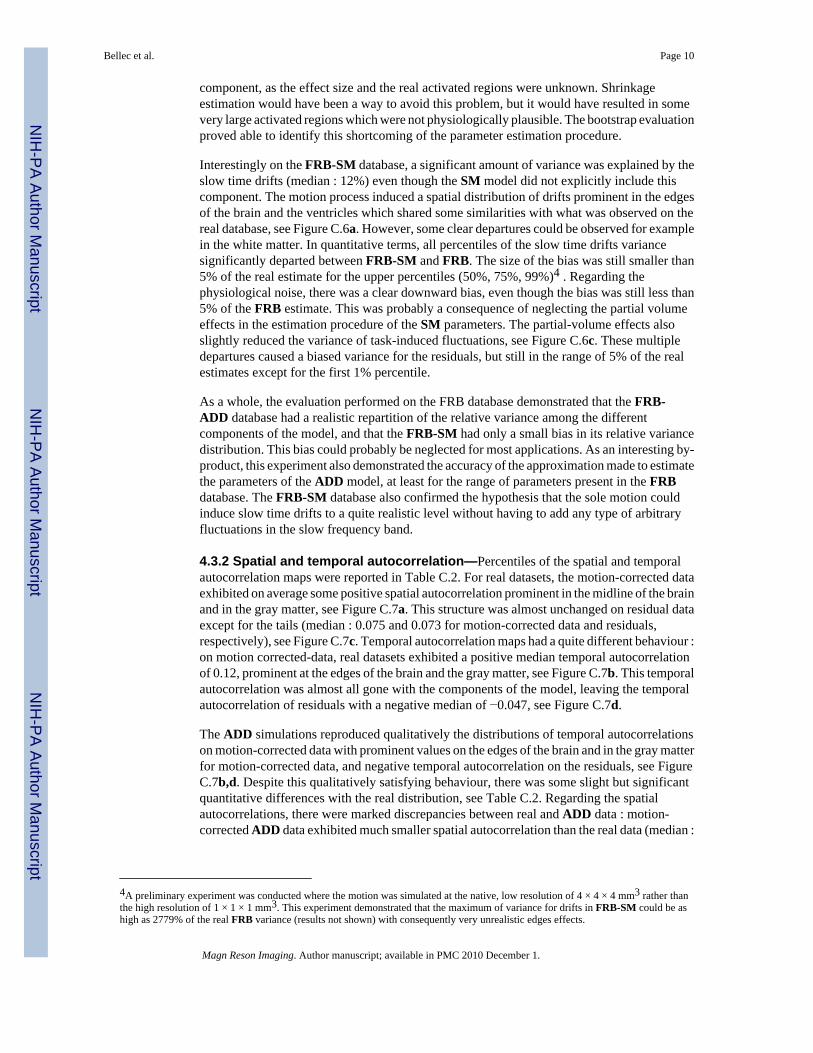
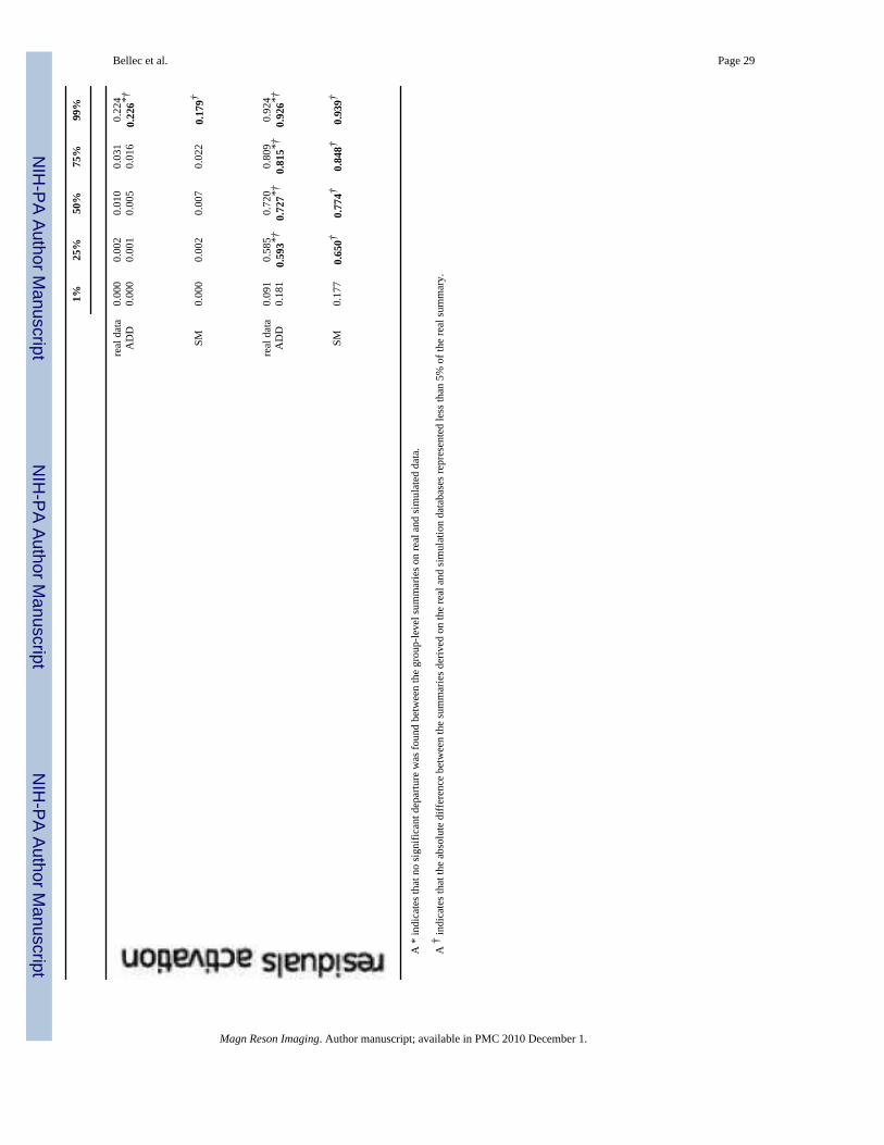
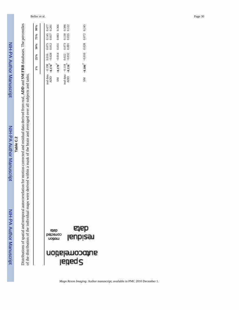
4.3.2 Spatial and temporal autocorrelation—Percentiles of the spatial and temporalautocorrelation maps were reported in Table C.2. For real datasets, the motion-corrected dataexhibited on average some positive spatial autocorrelation prominent in the midline of the brainand in the gray matter, see Figure C.7a. This structure was almost unchanged on residual dataexcept for the tails (median : 0.075 and 0.073 for motion-corrected data and residuals,respectively), see Figure C.7c. Temporal autocorrelation maps had a quite different behaviour :on motion corrected-data, real datasets exhibited a positive median temporal autocorrelationof 0.12, prominent at the edges of the brain and the gray matter, see Figure C.7b. This temporalautocorrelation was almost all gone with the components of the model, leaving the temporalautocorrelation of residuals with a negative median of −0.047, see Figure C.7d.
The ADD simulations reproduced qualitatively the distributions of temporal autocorrelationson motion-corrected data with prominent values on the edges of the brain and in the gray matterfor motion-corrected data, and negative temporal autocorrelation on the residuals, see FigureC.7b,d. Despite this qualitatively satisfying behaviour, there was some slight but significantquantitative differences with the real distribution, see Table C.2. Regarding the spatialautocorrelations, there were marked discrepancies between real and ADD data : motion-corrected ADD data exhibited much smaller spatial autocorrelation than the real data (median :
4A preliminary experiment was conducted where the motion was simulated at the native, low resolution of 4 × 4 × 4 mm3 rather thanthe high resolution of 1 × 1 × 1 mm3. This experiment demonstrated that the maximum of variance for drifts in FRB-SM could be ashigh as 2779% of the real FRB variance (results not shown) with consequently very unrealistic edges effects.
Bellec et al. Page 10
Magn Reson Imaging. Author manuscript; available in PMC 2010 December 1.
NIH
-PA Author Manuscript
NIH
-PA Author Manuscript
NIH
-PA Author Manuscript
0.012 and 0.075 respectively), see Figure C.7a, and the effect was drastic on residuals (median :0.001 and 0.073 respectively), see Figure C.7b.
The spatial autocorrelations of motion-corrected SM data was closer of those observed on realdatasets (median : 0.031 and 0.075, respectively). In a similar way to what was observed onreal data, the spatial autocorrelation on residuals was very close of the one derived on motion-corrected data (median : 0.031 and 0.028 for SM motion-corrected data and residuals,respectively). As a consequence, on residuals, the spatial autocorrelation of FRB-SM wasmuch closer of FRB than FRB-ADD was (median : 0.073, 0.001 and 0.028 for FRB, FRB-ADD and FRB-SM respectively). Despite this improvement, there was still some significantdifferences between the spatial autocorrelations of FRB and FRB-SM, see Table C.2. Thebehaviour of the temporal autocorrelations was very similar between FRB-ADD and FRB-SM. The distribution on motion-corrected data was actually a bit closer of the real databasefor FRB-SM, with no significant difference detected on the 99% percentile (0.703 and 0.698for FRB and FRB-SM respectively).
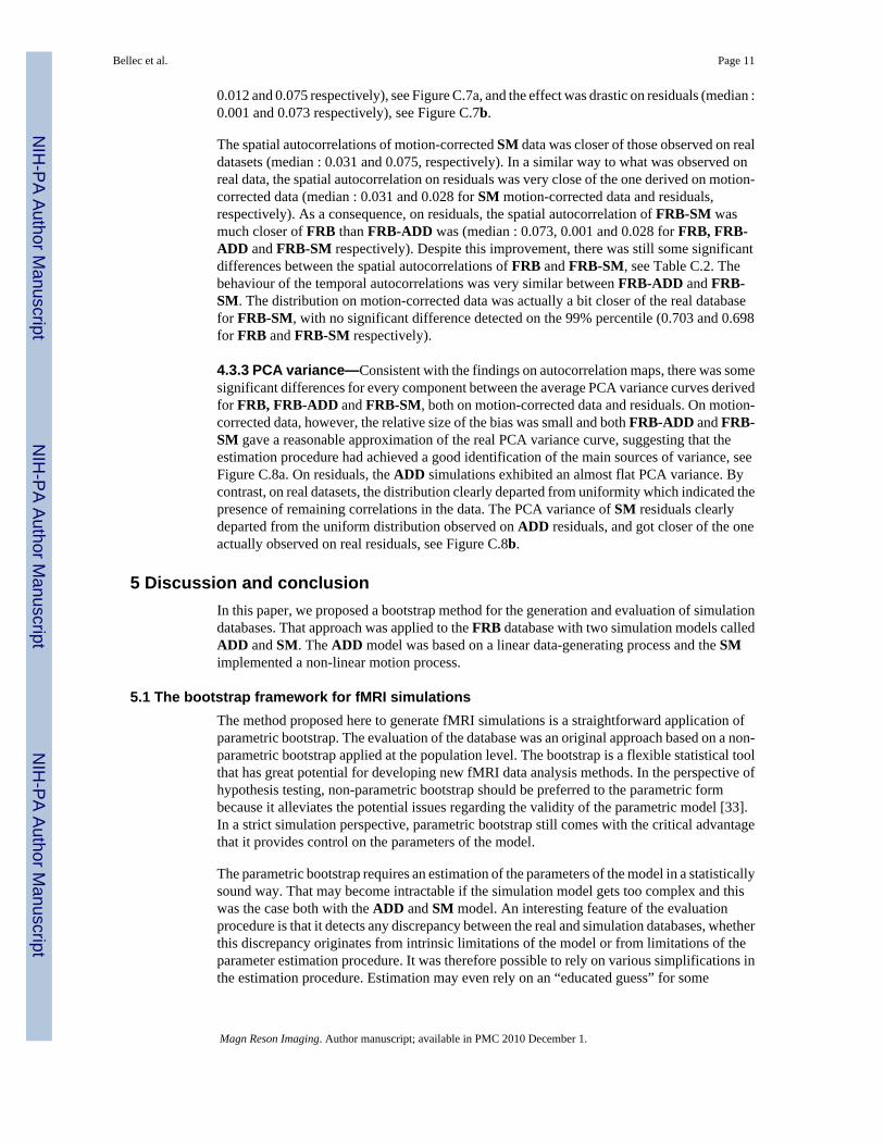
4.3.3 PCA variance—Consistent with the findings on autocorrelation maps, there was somesignificant differences for every component between the average PCA variance curves derivedfor FRB, FRB-ADD and FRB-SM, both on motion-corrected data and residuals. On motion-corrected data, however, the relative size of the bias was small and both FRB-ADD and FRB-SM gave a reasonable approximation of the real PCA variance curve, suggesting that theestimation procedure had achieved a good identification of the main sources of variance, seeFigure C.8a. On residuals, the ADD simulations exhibited an almost flat PCA variance. Bycontrast, on real datasets, the distribution clearly departed from uniformity which indicated thepresence of remaining correlations in the data. The PCA variance of SM residuals clearlydeparted from the uniform distribution observed on ADD residuals, and got closer of the oneactually observed on real residuals, see Figure C.8b.
5 Discussion and conclusionIn this paper, we proposed a bootstrap method for the generation and evaluation of simulationdatabases. That approach was applied to the FRB database with two simulation models calledADD and SM. The ADD model was based on a linear data-generating process and the SMimplemented a non-linear motion process.
5.1 The bootstrap framework for fMRI simulationsThe method proposed here to generate fMRI simulations is a straightforward application ofparametric bootstrap. The evaluation of the database was an original approach based on a non-parametric bootstrap applied at the population level. The bootstrap is a flexible statistical toolthat has great potential for developing new fMRI data analysis methods. In the perspective ofhypothesis testing, non-parametric bootstrap should be preferred to the parametric formbecause it alleviates the potential issues regarding the validity of the parametric model [33].In a strict simulation perspective, parametric bootstrap still comes with the critical advantagethat it provides control on the parameters of the model.
The parametric bootstrap requires an estimation of the parameters of the model in a statisticallysound way. That may become intractable if the simulation model gets too complex and thiswas the case both with the ADD and SM model. An interesting feature of the evaluationprocedure is that it detects any discrepancy between the real and simulation databases, whetherthis discrepancy originates from intrinsic limitations of the model or from limitations of theparameter estimation procedure. It was therefore possible to rely on various simplifications inthe estimation procedure. Estimation may even rely on an “educated guess” for some
Bellec et al. Page 11
Magn Reson Imaging. Author manuscript; available in PMC 2010 December 1.
NIH
-PA Author Manuscript
NIH
-PA Author Manuscript
NIH
-PA Author Manuscript
parameters, i.e. using values found in the literature as it is commonly done in the simulationcommunity.
If the procedure of parameter estimation was correct, the evaluation of the simulation databasecould be viewed as a diagnostic study of the model of the fMRI data-generating process. Sucha diagnostic tool would have a wider application range than existing tools specifically tailoredfor linear models [34]. This flexibility comes at the price of a large increase in computationalcost because the database needs to be fully replicated and reanalysed in the bootstrap approach.However, the purpose of the evaluation procedure was not to demonstrate that a given modelof fMRI simulation would be able to perfectly reproduce any type of statistical measure on areal dataset. One may argue that such an analytical model probably does not exist anyway.Rather than just testing for the presence of a significant deviation between the real and thesimulation databases, the bootstrap evaluation method provided an estimation of the potentialbias regarding a set list of statistical measures. This approach was designed to assess thestrengths and limitations of a model using different perspectives, rather than strictlydemonstrating the validity of the model.
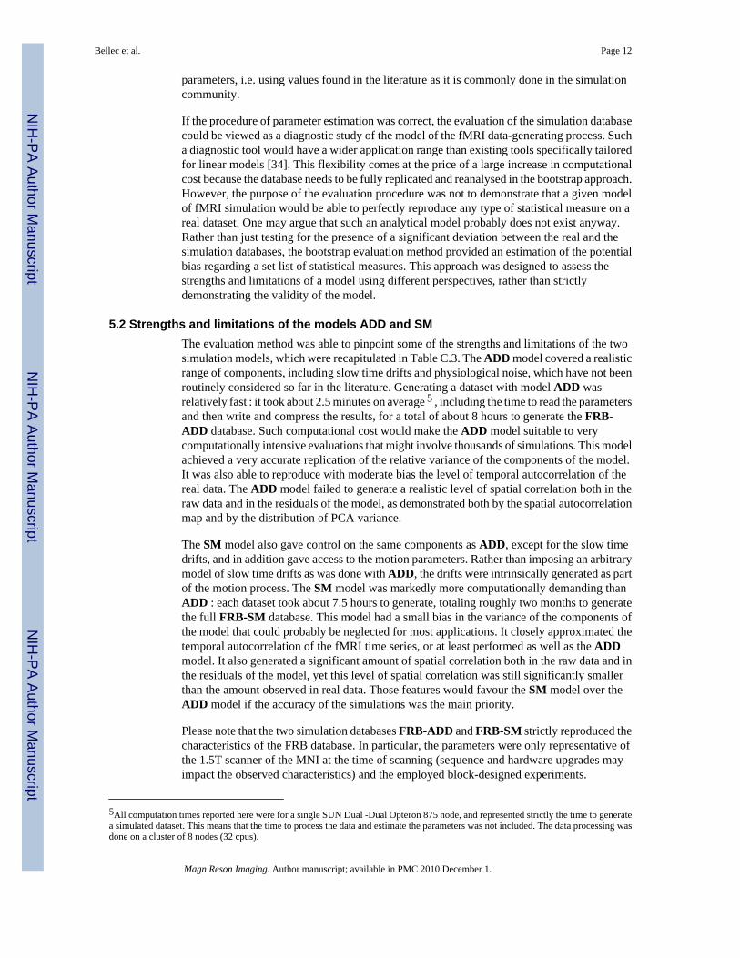
5.2 Strengths and limitations of the models ADD and SMThe evaluation method was able to pinpoint some of the strengths and limitations of the twosimulation models, which were recapitulated in Table C.3. The ADD model covered a realisticrange of components, including slow time drifts and physiological noise, which have not beenroutinely considered so far in the literature. Generating a dataset with model ADD wasrelatively fast : it took about 2.5 minutes on average 5 , including the time to read the parametersand then write and compress the results, for a total of about 8 hours to generate the FRB-ADD database. Such computational cost would make the ADD model suitable to verycomputationally intensive evaluations that might involve thousands of simulations. This modelachieved a very accurate replication of the relative variance of the components of the model.It was also able to reproduce with moderate bias the level of temporal autocorrelation of thereal data. The ADD model failed to generate a realistic level of spatial correlation both in theraw data and in the residuals of the model, as demonstrated both by the spatial autocorrelationmap and by the distribution of PCA variance.
The SM model also gave control on the same components as ADD, except for the slow timedrifts, and in addition gave access to the motion parameters. Rather than imposing an arbitrarymodel of slow time drifts as was done with ADD, the drifts were intrinsically generated as partof the motion process. The SM model was markedly more computationally demanding thanADD : each dataset took about 7.5 hours to generate, totaling roughly two months to generatethe full FRB-SM database. This model had a small bias in the variance of the components ofthe model that could probably be neglected for most applications. It closely approximated thetemporal autocorrelation of the fMRI time series, or at least performed as well as the ADDmodel. It also generated a significant amount of spatial correlation both in the raw data and inthe residuals of the model, yet this level of spatial correlation was still significantly smallerthan the amount observed in real data. Those features would favour the SM model over theADD model if the accuracy of the simulations was the main priority.
Please note that the two simulation databases FRB-ADD and FRB-SM strictly reproduced thecharacteristics of the FRB database. In particular, the parameters were only representative ofthe 1.5T scanner of the MNI at the time of scanning (sequence and hardware upgrades mayimpact the observed characteristics) and the employed block-designed experiments.
5All computation times reported here were for a single SUN Dual -Dual Opteron 875 node, and represented strictly the time to generatea simulated dataset. This means that the time to process the data and estimate the parameters was not included. The data processing wasdone on a cluster of 8 nodes (32 cpus).
Bellec et al. Page 12
Magn Reson Imaging. Author manuscript; available in PMC 2010 December 1.
NIH
-PA Author Manuscript
NIH
-PA Author Manuscript
NIH
-PA Author Manuscript
Investigating the variability of simulation parameters across field strengths, scanning sites andexperimental designs will be a major direction for future work.
5.3 Expanding the modelsThere are at least three promising directions to expand the proposed models of simulations andpotentially fix some of their limitations. Rather than generating a single task-related large-scalenetwork, some other networks could be included, e.g. the default-mode network [35], by usingan exploratory identification method [22,36].
The simulations could also be expanded to include more realistic models of large-scale networkactivity and the associated response of brain metabolism and hemodynamic, such as the modelof Riera et al. [37]. However, at this stage, and despite some promising results [38], estimatingthe parameters for such models is still challenging when a large number of regions is involved.In this case, parameters of the model would have to be fixed in an arbitrary way by theinvestigator, yet a study based on linear models could still provide estimates of the varianceof fMRI activity.
Another direction would be to include a realistic simulation engine, such as the one recentlyproposed by Drobnjak et al [19]. Special attention would then need to be given to the residuals.The estimated residual variance in the current approach is mixing the random measurementnoise with, notably, some unmodelled generation artefacts. The variance related to the random(Rician) measurement noise could be more specifically estimated using regions of interestoutside the brain [25] and the realistic engine would then take the scanner artefacts into account.
5.4 MIDASThis work is part of a larger effort made by a consortium, named MIDAS6 [39], formed by ourgroup at Montreal, a group at FMRIB, Oxford, and a group at the University of Hawaii(formerly at the University of Pittsburgh). The aims of this consortium are to build a webinterface that would make accessible some pregenerated simulated databases and allow torequest for customised simulations. Multiple choices for the simulation model and the databaseof reference will be made available. In particular, additional simulation databases will begenerated to cover a wide range of scanning protocols. Public simulation databases wouldcritically help to standardise the benchmarking of new data analysis methods and would alsogrant access to some elaborate simulation models for the fMRI community at large. Thebootstrap method presented here provides a rigorous framework to generate and evaluate suchfMRI simulation databases.
AcknowledgmentsThe authors would like to thank Habib Benali, Christophe Grova and Keith Worsley for fruitful discussions, and toacknowledge the work of Roger Woods, Tomas Paus and the International Consortium for Brain Mapping (ICBM)fMRI community in creating the FRB database. This research has been supported in part by CLUMEQ7, which isfunded in part by NSERC (MRS), FQRNT, and McGill University. Pierre Bellec was supported partly by NIH (NIFTI)grant R01 MH67172-01 and partly by an FRSQ-Inserm fellowship.
References1. Ogawa S, Lee TM, Kay AR, Tank DW. Brain magnetic resonance imaging with contrast dependent
on blood oxygenation. Proc Natl Acad Sci U S A 1990;87:9868–9872. [PubMed: 2124706]
6http://midas-online.org/7http://www.clumeq.mcgill.ca/
Bellec et al. Page 13
Magn Reson Imaging. Author manuscript; available in PMC 2010 December 1.
NIH
-PA Author Manuscript
NIH
-PA Author Manuscript
NIH
-PA Author Manuscript
2. Logothetis NK, Pauls J, Augath M, Trinath T, Oeltermann A. Neurophysiological investigation of thebasis of the fMRI signal. Nature 2001;412:150–157. [PubMed: 11449264]
3. Fox PT, Laird AR, Lancaster JL. Coordinate-based voxel-wise metaanalysis:dividends of spatialnormalization Report of a virtual workshop. Hum Brain Mapp 2005;25:1–5. [PubMed: 15846826]
4. Della-Maggiore V, Chau W, Peres-Neto PR, McIntosh AR. An empirical comparison of SPMpreprocessing parameters to the analysis of fMRI data. Neuroimage 2002;17:19–28. [PubMed:12482065]
5. Logan BR, Rowe DB. An evaluation of thresholding techniques in fMRI analysis. Neuroimage2004;22:95–108. [PubMed: 15110000]
6. Marchini J, Presanis A. Comparing methods of analyzing fMRI statistical parametric maps.Neuroimage 2004;22:1203–1213. [PubMed: 15219592]
7. Baumgartner R, Ryner L, Richter W, Summers R, Jarmasz M, Somorjai R. Comparison of twoexploratory data analysis methods for fMRI: fuzzy clustering vs. principal component analysis. MagnRes Imaging 2000;18:89–94.
8. Lu Y, Jiang T, Zang Y. Region growing method for the analysis of functional MRI data. Neuroimage2003;20:455–465. [PubMed: 14527606]
9. Dimitriadou E, Barth M, Windischberger C, Hornik K, Moser E. A quantitative comparison offunctional MRI cluster analysis. Artif Intell Med 2004;31:57–71. [PubMed: 15182847]
10. Worsley KJ, Chen JI, Lerch J, Evans AC. Comparing functional connectivity via thresholdingcorrelations and singular value decomposition. Philos Trans R Soc Lond B Biol Sci 2005;360:913–920. [PubMed: 16087436]
11. Ardekani BA, Bachman AH, Helpern JA. A quantitative comparison of motion detection algorithmsin fMRI. Magn Res Imaging 2001;19:959–963.
12. Freire L, Mangin JF. Motion correction algorithms may create spurious brain activations in theabsence of subject motion. Neuroimage 2001;14:709–722. [PubMed: 11506543]
13. Pickens DR, Li Y, Morgan VL, Dawant BM. Development of computer-generated phantoms for fMRIsoftware evaluation. Magn Reson Imaging 2005;23:653–663. [PubMed: 16051040]
14. Morgan VL, Dawant BM, Li Y, Pickens DR. Comparison of fMRI statistical software packages andstrategies for analysis of images containing random and stimulus-correlated motion. Comput MedImaging Graph 2007;31:436–446. [PubMed: 17574816]
15. Honey CJ, K¨otter R, Breakspear M, Sporns O. Network structure of cerebral cortex shapes functionalconnectivity on multiple time scales. Proc Natl Acad Sci U S A 2007;104:10240–10245. [PubMed:17548818]
16. Ghosh A, Rho Y, McIntosh AR, K¨otter R, Jirsa VK. Cortical network dynamics with time delaysreveals functional connectivity in the resting brain. Cogn Neurodyn 2008;2:115–120. [PubMed:19003478]
17. Buxton RB, Wong EC, Frank LR. Dynamics of blood flow and oxygenation changes during brainactivation:The balloon model. Magn Res Med 1998;39:855–864.
18. Aubert A, Costalat R. A model of the coupling between brain electrical activity, metabolism, andhemodynamics:Application to the interpretation of functional neuroimaging. Neuroimage2002;17:1162–1181. [PubMed: 12414257]
19. Drobnjak I, Gavaghan D, Süli E, Pitt-Francis J, Jenkinson M. Development of a functional magneticresonance imaging simulator for modeling realistic rigid-body motion artifacts. Magn Reson Med2006;56:364–380. [PubMed: 16841304]
20. Baumgartner R, Windischberger C, Moser E. Quantification in functional magnetic resonanceimaging:Fuzzy clustering vs correlation analysis. Magn Res Imaging 1998;16:115–125.
21. Beckmann CF, Smith SM. Probabilistic independent component analysis for functional magneticresonance imaging. IEEE Trans Med Imaging 2004;23:137–152. [PubMed: 14964560]
22. Bellec P, Perlbarg V, Jbabdi S, P´el´egrini-Issac M, Anton J, Doyon J, Benali H. Identification oflarge-scale networks in the brain using fMRI. Neuroimage 2006;29:1231–1243. [PubMed:16246590]
23. Bullmore E, Long C, Suckling J, Fadili J, Calvert G, Zelaya F, Carpenter TA, Brammer M. Colorednoise and computational inference in neurophysiological (fMRI) time series analysis:resamplingmethods in time and wavelet domains. Hum Brain Mapp 2001;12:61–78. [PubMed: 11169871]
Bellec et al. Page 14
Magn Reson Imaging. Author manuscript; available in PMC 2010 December 1.
NIH
-PA Author Manuscript
NIH
-PA Author Manuscript
NIH
-PA Author Manuscript
24. Jahanian H, Hossein-Zadeh GA, Soltanian-Zadeh H, Ardekani BA. Controlling the false positive ratein fuzzy clustering using randomization:application to fMRI activation detection. Magn Res Imaging2004;22:631–638.
25. Xu Y, Wu G, Rowe DB, Ma Y, Zhang R, Xu G, Li SJ. Complex-model-based estimation of thermalnoise for fMRI data in the presence of artifacts. Magn Res Imaging 2007;25:1079–1088.
26. Kim B, Yeo DT, Bhagalia R. Comprehensive mathematical simulation of functional magneticresonance imaging time series including motion-related image distortion and spin saturation effect.Magn Res Imaging 2008;26:147–159.
27. Sorenson JA, Wang X. ROC methods for evaluation of fMRI techniques. Magn Res Med1996;36:737–744.
28. Shao, J.; Tu, D. Springer; 1995. The Jackknife and Bootstrap.29. Efron, B.; Tibshirani, RJ. CRC: Chapman &Hall; 1994. An Introduction to the Bootstrap.30. Perlbarg V, Bellec P, Anton JL, Pelegrini-Issac M, Doyon J, Benali H. CORSICA:correction of
structured noise in fMRI by automatic identification of ICA components. Magn Res Imaging2007;25:35–46.
31. Stein, C. Proceedings of the Third Berkeley Symposium on Mathematical Statistics and Probability.Vol. Volume 1. Berkeley and Los Angeles: University of California Press; 1956. Inadmissibility ofthe usual estimator for the mean of a multivariate normal distribution; p. 197-206.
32. Lund TE, Madsen KH, Sidaros K, Luo WL, Nichols TE. Non-white noise in fMRI: Does modellinghave an impact? Neuroimage 2006:54–66. [PubMed: 16099175]
33. Bellec P, Marrelec G, Benali H. A bootstrap test to investigate changes in brain connectivity forfunctional MRI. Stat Sin 2008;18:1253–1268.
34. Luo WL, Nichols TE. Diagnosis and exploration of massively univariate neuroimaging models.Neuroimage 2003;19:1014–1032. [PubMed: 12880829]
35. Greicius MD, Krasnow B, Reiss AL, Menon V. Functional connectivity in the resting brain: A networkanalysis of the default mode hypothesis. Proc Natl Acad Sci U S A 2003;100:253–258. [PubMed:12506194]
36. De Luca M, Beckmann CF, De Stefano N, Matthews PM, Smith SM. fMRI resting state networksdefine distinct modes of long-distance interactions in the human brain. Neuroimage 2006;29:1359–1367. [PubMed: 16260155]
37. Riera JJ, Wan X, Jimenez JC, Kawashima R. Nonlinear local electrovascular coupling. A theoreticalmodel. Hum Brain Mapp 2006;27:896–914. [PubMed: 16729288]
38. Riera JJ, Jimenez JC, Wan X, Kawashima R, Ozaki T. Nonlinear local electrovascular coupling. II:From data to neuronal masses. Hum Brain Mapp 2007;28:335–354. [PubMed: 16933303]
39. Boada F, Collins D, Drobnjak Eddy W, Evans A, Griffin M, Jenkinson M, Noll D, Pike B, Shi H,Shroff D, Stenger V, Worsley K. MIDAS-a multi–site fMRI simulator consortium Tenth Int Confon Functional. Mapping of the Human Brain. 2004
40. Collins DL, Neelin P, Peters TM, Evans AC. Automatic 3D intersubject registration of MR volumetricdata in standardized talairach space. J Comput Assist Tomogr 1994;18:192–205. [PubMed: 8126267]
41. McKeown MJ, Makeig S, Brown GG, Jung TP, Kindermann SS, Bell AJ, Sejnowski TJ. Analysis offMRI data by blind separation into independent spatial components. Hum Brain Mapp 1998;6:160–188. [PubMed: 9673671]
42. Thomas CG, Harshman RA, Menon RS. Noise reduction in BOLD-based fMRI using componentanalysis. Neuroimage 2002;17:1521–1537. [PubMed: 12414291]
43. Bell AJ, Sejnowski TJ. An information-maximization approach to blind separation and blinddeconvolution. Neural Comput 1995;7:1129–1159. [PubMed: 7584893]
44. Judge GG, Hill CR, Bock ME. An adaptive empirical Bayes estimator of the multivariate normalmean under quadratic loss. J Econom 1990;44:189–213.
Bellec et al. Page 15
Magn Reson Imaging. Author manuscript; available in PMC 2010 December 1.
NIH
-PA Author Manuscript
NIH
-PA Author Manuscript
NIH
-PA Author Manuscript
A Parameter estimation for the ADD modelThe components in the model ADD were estimated iteratively in the following order: βB and
βD; βP, XP and . The notations and an outline of the estimation pipeline weredescribed in Section 3 and the details of each stage of the pipeline were given below.
A.1 Motion and slice-timing correctionThe first volumes corresponding to approximately 10 seconds of acquisition were discardedto allow the magnetisation to reach equilibrium. For each subject and each functional run, sometranslation parameters τ̂ and rotation parameters ρ ̂ were estimated on the gradient of eachvolume using MINC-TRACC [40] with the gradient of the volume acquired in the middle ofthe first functional run of the subject as a target reference. The estimated withinrun rigid-bodytransformation was inverted and applied to each volume using sinc spatial interpolation. Rawfunctional data were then corrected for interslice acquisition time delay with theimplementation found in SPM28, using sinc temporal interpolation. The resulting motion-corrected and slice-timing corrected dataset was denoted Ym.
A.2 Baseline B and slow time drifts DThe baseline and slow time drifts were modelled using a discrete cosine basis [32]:
(A.1)
where T is the number of volumes in the motion-corrected dataset Ym. The frequency associatedwith Xd(k) was k/(2T × TR) Hz, where TR is the repetition time in seconds. To model the slowtime drifts in the [0, fc] band, k thus ranged from 0 to Kd, the integer division of 2T × TR by1/fc. In our case, with TR = 4 s, T = 85 and fc = 0.01 Hz, the basis to model slow time driftswas composed of Kd + 1 = 7 discrete cosines. Note that the baseline Xb was the constant cosineXd(k) for k = 0. The spatial distributions of the baseline β ̂B and slow time drifts β ̂D wereestimated through least-square fitting of the slow time drifts on Ym. The drifts-corrected datasetYd was the motion-corrected dataset Ym minus the estimated contributions of the baselineB^ = XBβ ̂B and the slow time drifts D ̂ = XDβ ̂D.
A.3 Physiological noise PSpatial independent component analysis (ICA) can achieve blind identification ofphysiological noise related to heart beat and respiration in fMRI data [41,42]. A spatial ICAof Yd into 60 components was estimated by optimising the spatial independence using theInfoMax algorithm9, starting from an initial decomposition into principal components withhighest variance [43]. A procedure called CORSICA [30] was used to identify the ICAcomponents related to physiological noise X ̂p, along with the spatial distributions β ̂p. Thismethod finds components with predominant influence in areas known a priori to be corruptedin a systematic fashion by physiological noise. The physiology-corrected dataset Ypis thedrifts-corrected dataset Yd minus the estimated contributions of physiological noise P̂ =X ̂Pβp.
8http://www.fil.ion.ucl.ac.uk/spm/spm2.html9http://www.sccn.ucsd.edu/fmrlab/
Bellec et al. Page 16
Magn Reson Imaging. Author manuscript; available in PMC 2010 December 1.
NIH
-PA Author Manuscript
NIH
-PA Author Manuscript
NIH
-PA Author Manuscript
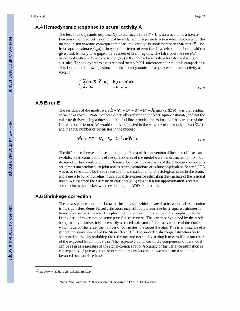
A.4 Hemodynamic response to neural activity AThe local hemodynamic response XA to the task, of size T × 1, is assumed to be a boxcarfunction convolved with a canonical hemodynamic response function which accounts for themetabolic and vascular consequences of neural activity, as implemented in fMRIstat 10. Theleast-square estimate β ̂A(υ) is in general different of zero for all voxels υ in the brain, while agiven task is likely to engage only a subset of brain regions. The false-positive rate p(υ)associated with a null hypothesis that β(υ) = 0 at a voxel υ was therefore derived using t-statistics. The null hypothesis was rejected for p < 0.001, uncorrected for multiple comparisons.This lead to the following estimate of the hemodynamic consequences of neural activity atvoxel υ:
(A.2)
A.5 Error EThe residuals of the model were Ê = Ym – B^ – D^ – P^ – Â, and var(Ê(υ)) was the residualvariance at voxel υ. Note that here  actually referred to the least-square estimate, and not theestimate derived using a threshold. In a full linear model, the estimate of the variance of theGaussian error term σ2(υ) would simply be related to the variance of the residuals var(Ê(υ))and the total number of covariates in the model :
(A.3)
The differences between this estimation pipeline and the conventional linear model case aretwofold. First, contributions of the components of the model were not estimated jointly, butiteratively. This is only a minor difference, because the covariates of the different componentsare almost uncorrelated, so joint and iterative estimations are almost equivalent. Second, ICAwas used to estimate both the space and time distribution of physiological noise in the brain,and there is to our knowledge no analytical derivation for estimating the variance of the residualnoise. We assumed the estimate of equation (A.3) was still a fair approximation, and thisassumption was checked when evaluating the ADD simulations.
A.6 Shrinkage correctionThe least-square estimator is known to be unbiased, which means that its statistical expectationis the true value. Some biased estimators may still outperform the least-square estimator interms of variance accuracy. This phenomenon is clear on the following example. Considerfitting a set of covariates on some pure Gaussian noise. The variance explained by the modelbeing strictly positive, it is necessarily a biased estimator of the true variance of the modelwhich is zero. The larger the number of covariates, the larger the bias. This is an instance of ageneral phenomenon called the Stein effect [31]. The so-called shrinkage estimators try toaddress that issue by shrinking the estimator and eventually setting it to zero if it is too closeof the expected level in the noise. The respective variances of the components of the modelcan be seen as a measure of the signal-to-noise ratio. Accuracy of the variance estimation isconsequently of primary interest in computer simulations and we advocate it should befavoured over unbiasedness.
10http://www.math.mcgill.ca/keith/fmristat/
Bellec et al. Page 17
Magn Reson Imaging. Author manuscript; available in PMC 2010 December 1.
NIH
-PA Author Manuscript
NIH
-PA Author Manuscript
NIH
-PA Author Manuscript
A James-Stein shrinkage correction [44] was applied to the components of the model involvingmore than two covariates, i.e. the slow time drifts and the physiological noise. To simplifynotations, the correction was described below for D but it was applied in the same fashion toP. Let the the following correction factor be defined at every voxel υ :
(A.4)
Let be defined as max(0, ĈD(υ)). The James-Stein corrected estimate of βD(υ) was
.
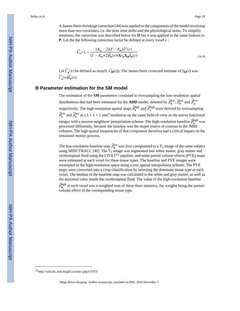
B Parameter estimation for the SM modelThe estimation of the SM parameters consisted in oversampling the low-resolution spatial
distributions that had been estimated for the ADD model, denoted by and
respectively. The high-resolution spatial maps and were derived by oversampling
and at a 1 × 1 × 1 mm3 resolution on the same field-of-view as the native functional
images with a nearest-neighbour interpolation scheme. The high-resolution baseline wasprocessed differently, because the baseline was the major source of contrast in the fMRIvolumes. The high spatial frequencies of that component therefore had a critical impact on thesimulated motion process.
The low-resolution baseline map was first coregistered to a T1 image of the same subjectusing MINCTRACC [40]. The T1 image was segmented into white matter, gray matter andcerebrospinal fluid using the CIVET11 pipeline, and some partial volume effects (PVE) mapswere estimated at each voxel for these tissue types. The baseline and PVE images wereresampled in the high-resolution space using a sinc spatial interpolation scheme. The PVEmaps were converted into a crisp classification by selecting the dominant tissue type at eachvoxel. The median of the baseline map was calculated in the white and gray matter, as well asthe maximal value inside the cerebrospinal fluid. The value of the high-resolution baseline
at each voxel was a weighted sum of these three statistics, the weights being the partial-volume effect of the corresponding tissue type.
11http://wiki.bic.mni.mcgill.ca/index.php/CIVET
Bellec et al. Page 18
Magn Reson Imaging. Author manuscript; available in PMC 2010 December 1.
NIH
-PA Author Manuscript
NIH
-PA Author Manuscript
NIH
-PA Author Manuscript
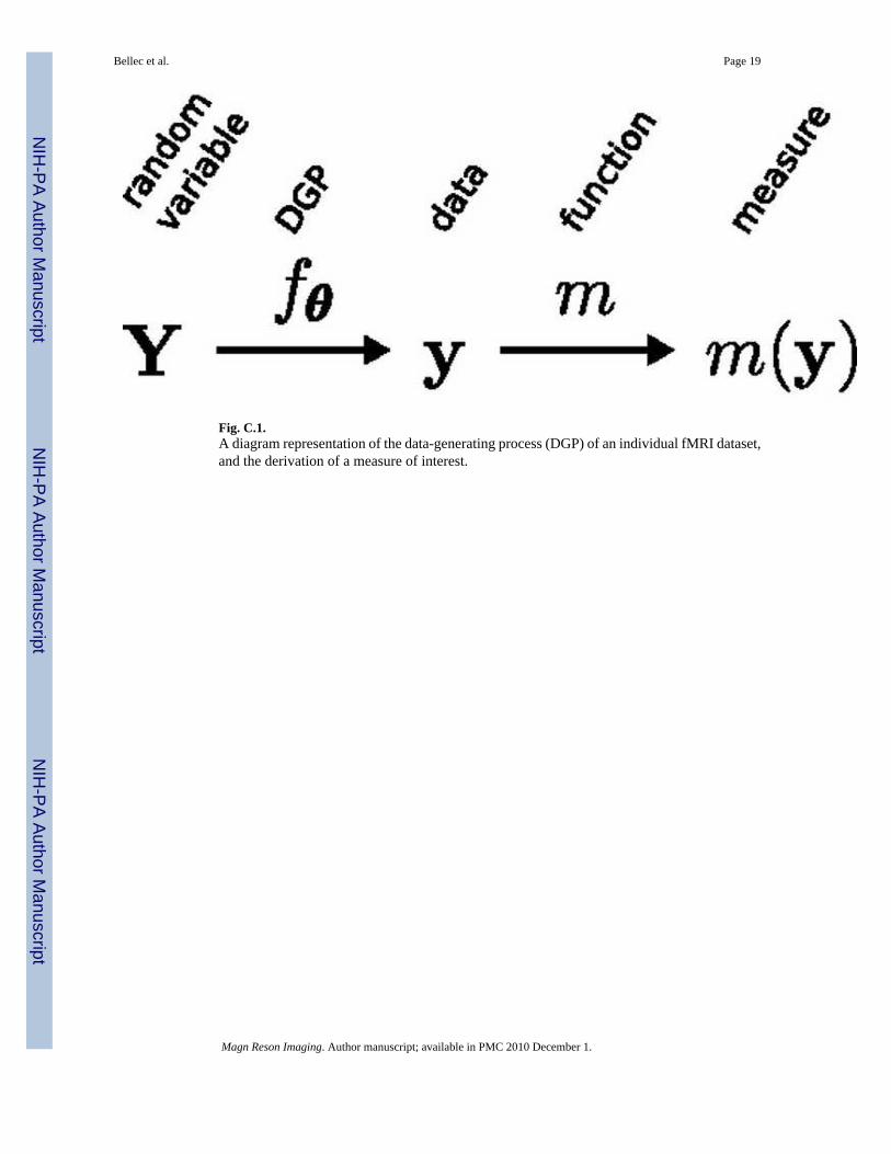
Fig. C.1.A diagram representation of the data-generating process (DGP) of an individual fMRI dataset,and the derivation of a measure of interest.
Bellec et al. Page 19
Magn Reson Imaging. Author manuscript; available in PMC 2010 December 1.
NIH
-PA Author Manuscript
NIH
-PA Author Manuscript
NIH
-PA Author Manuscript
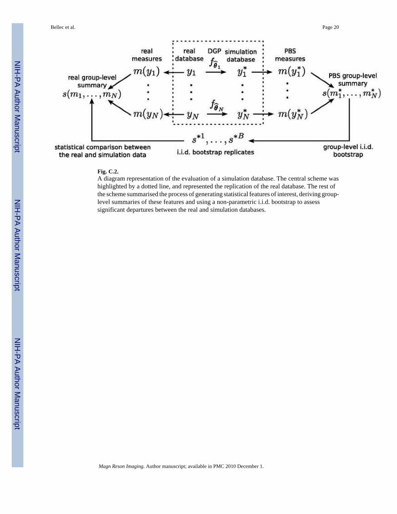
Fig. C.2.A diagram representation of the evaluation of a simulation database. The central scheme washighlighted by a dotted line, and represented the replication of the real database. The rest ofthe scheme summarised the process of generating statistical features of interest, deriving group-level summaries of these features and using a non-parametric i.i.d. bootstrap to assesssignificant departures between the real and simulation databases.
Bellec et al. Page 20
Magn Reson Imaging. Author manuscript; available in PMC 2010 December 1.
NIH
-PA Author Manuscript
NIH
-PA Author Manuscript
NIH
-PA Author Manuscript
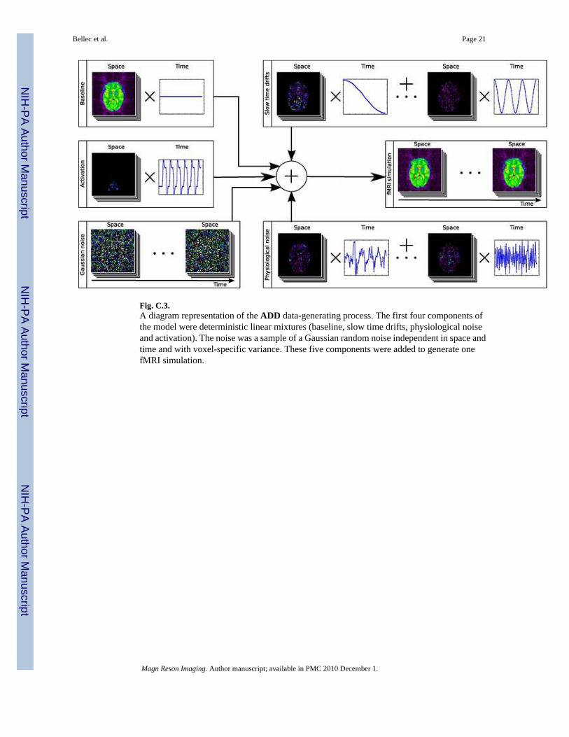
Fig. C.3.A diagram representation of the ADD data-generating process. The first four components ofthe model were deterministic linear mixtures (baseline, slow time drifts, physiological noiseand activation). The noise was a sample of a Gaussian random noise independent in space andtime and with voxel-specific variance. These five components were added to generate onefMRI simulation.
Bellec et al. Page 21
Magn Reson Imaging. Author manuscript; available in PMC 2010 December 1.
NIH
-PA Author Manuscript
NIH
-PA Author Manuscript
NIH
-PA Author Manuscript
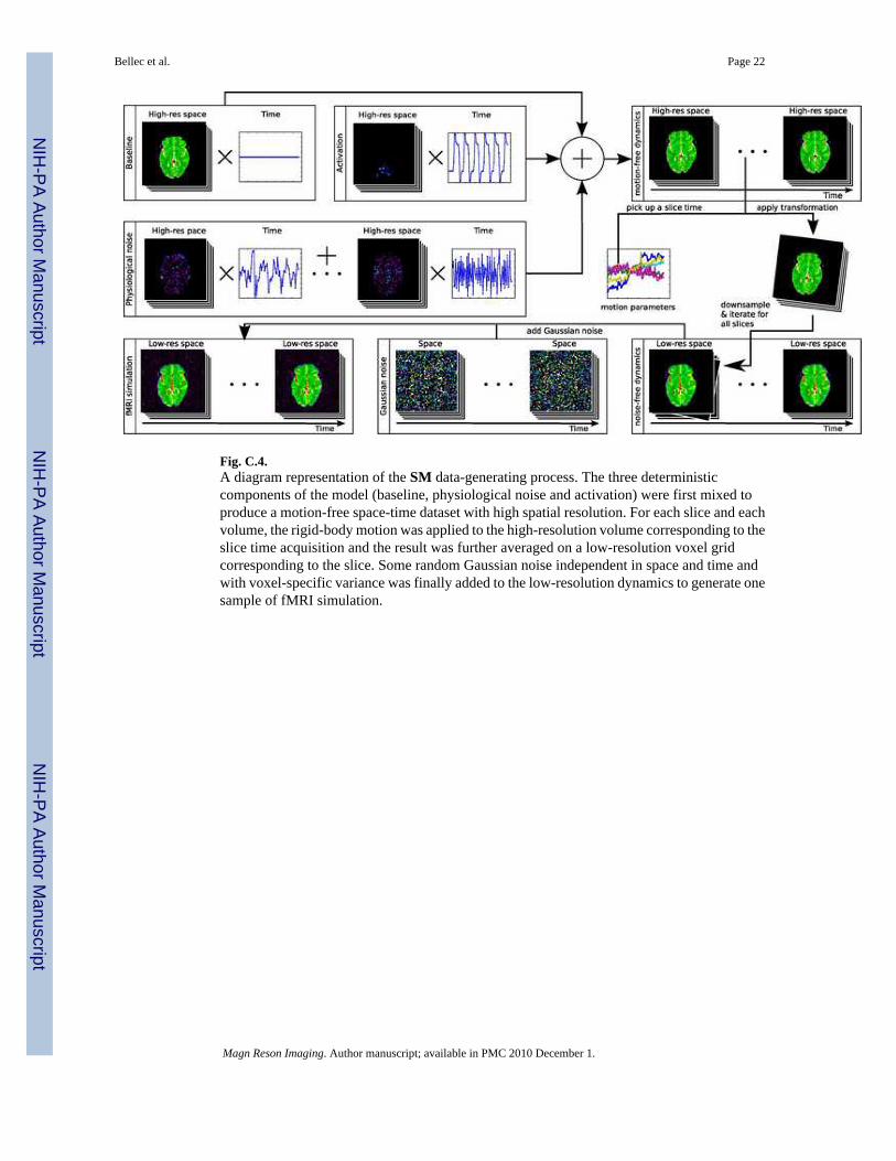
Fig. C.4.A diagram representation of the SM data-generating process. The three deterministiccomponents of the model (baseline, physiological noise and activation) were first mixed toproduce a motion-free space-time dataset with high spatial resolution. For each slice and eachvolume, the rigid-body motion was applied to the high-resolution volume corresponding to theslice time acquisition and the result was further averaged on a low-resolution voxel gridcorresponding to the slice. Some random Gaussian noise independent in space and time andwith voxel-specific variance was finally added to the low-resolution dynamics to generate onesample of fMRI simulation.
Bellec et al. Page 22
Magn Reson Imaging. Author manuscript; available in PMC 2010 December 1.
NIH
-PA Author Manuscript
NIH
-PA Author Manuscript
NIH
-PA Author Manuscript
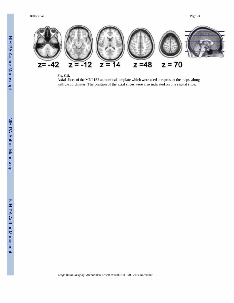
Fig. C.5.Axial slices of the MNI 152 anatomical template which were used to represent the maps, alongwith z-coordinates. The position of the axial slices were also indicated on one sagital slice.
Bellec et al. Page 23
Magn Reson Imaging. Author manuscript; available in PMC 2010 December 1.
NIH
-PA Author Manuscript
NIH
-PA Author Manuscript
NIH
-PA Author Manuscript
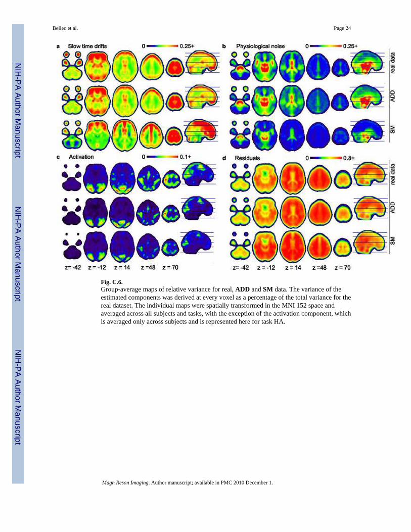
Fig. C.6.Group-average maps of relative variance for real, ADD and SM data. The variance of theestimated components was derived at every voxel as a percentage of the total variance for thereal dataset. The individual maps were spatially transformed in the MNI 152 space andaveraged across all subjects and tasks, with the exception of the activation component, whichis averaged only across subjects and is represented here for task HA.
Bellec et al. Page 24
Magn Reson Imaging. Author manuscript; available in PMC 2010 December 1.
NIH
-PA Author Manuscript
NIH
-PA Author Manuscript
NIH
-PA Author Manuscript
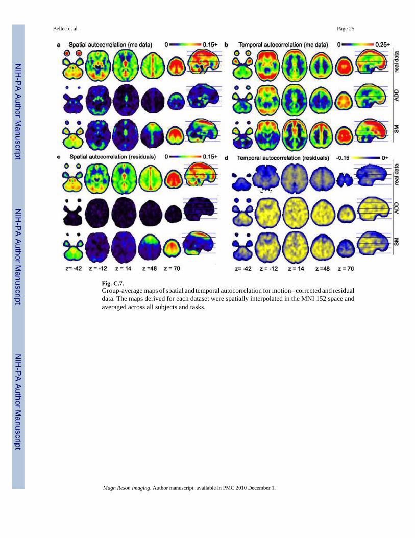
Fig. C.7.Group-average maps of spatial and temporal autocorrelation for motion– corrected and residualdata. The maps derived for each dataset were spatially interpolated in the MNI 152 space andaveraged across all subjects and tasks.
Bellec et al. Page 25
Magn Reson Imaging. Author manuscript; available in PMC 2010 December 1.
NIH
-PA Author Manuscript
NIH
-PA Author Manuscript
NIH
-PA Author Manuscript
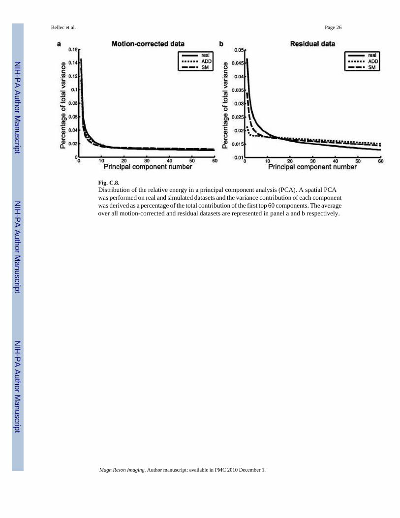
Fig. C.8.Distribution of the relative energy in a principal component analysis (PCA). A spatial PCAwas performed on real and simulated datasets and the variance contribution of each componentwas derived as a percentage of the total contribution of the first top 60 components. The averageover all motion-corrected and residual datasets are represented in panel a and b respectively.
Bellec et al. Page 26
Magn Reson Imaging. Author manuscript; available in PMC 2010 December 1.
NIH
-PA Author Manuscript
NIH
-PA Author Manuscript
NIH
-PA Author Manuscript
NIH
-PA Author Manuscript
NIH
-PA Author Manuscript
NIH
-PA Author Manuscript
Bellec et al. Page 27Ta
ble
C.1
Dis
tribu
tion
of re
lativ
e va
rianc
e fo
r the
real
, AD
D a
nd S
M F
RB
dat
abas
es. T
he v
aria
nce
of th
e es
timat
ed c
ompo
nent
s was
der
ived
at e
very
vox
el a
s ape
rcen
tage
of t
he to
tal v
aria
nce
for t
he m
otio
n-co
rrec
ted
data
set.
The
perc
entil
es o
f the
dis
tribu
tion
of th
e in
divi
dual
map
s wer
e th
en d
eriv
ed w
ithin
a m
ask
of th
e br
ain
and
aver
aged
ove
r all
subj
ects
and
task
s.
1%25
%50
%75
%99
%
real
dat
a0.
018
0.08
10.
141
0.24
80.
672
AD
D0.
016
0.07
50.
136*†
0.24
6*†0.
670*†
SM0.
016
0.06
90.
122†
0.22
5†0.
666*†
Magn Reson Imaging. Author manuscript; available in PMC 2010 December 1.

NIH
-PA Author Manuscript
NIH
-PA Author Manuscript
NIH
-PA Author Manuscript
Bellec et al. Page 281%
25%
50%
75%
99%
real
dat
a0.
000
0.03
80.
070
0.12
60.
579
AD
D0.
005
0.03
8*†0.
071*†
0.12
9*†0.
559*†
SM0.
001*
0.02
4†0.
048†
0.09
0†0.
462†
Magn Reson Imaging. Author manuscript; available in PMC 2010 December 1.
NIH
-PA Author Manuscript
NIH
-PA Author Manuscript
NIH
-PA Author Manuscript
Bellec et al. Page 291%
25%
50%
75%
99%
real
dat
a0.
000
0.00
20.
010
0.03
10.
224
AD
D0.
000
0.00
10.
005
0.01
60.
226*†
SM0.
000
0.00
20.
007
0.02
20.
179†
real
dat
a0.
091
0.58
50.
720
0.80
90.
924
AD
D0.
181
0.59
3*†0.
727*†
0.81
5*†0.
926*†
SM0.
177
0.65
0†0.
774†
0.84
8†0.
939†
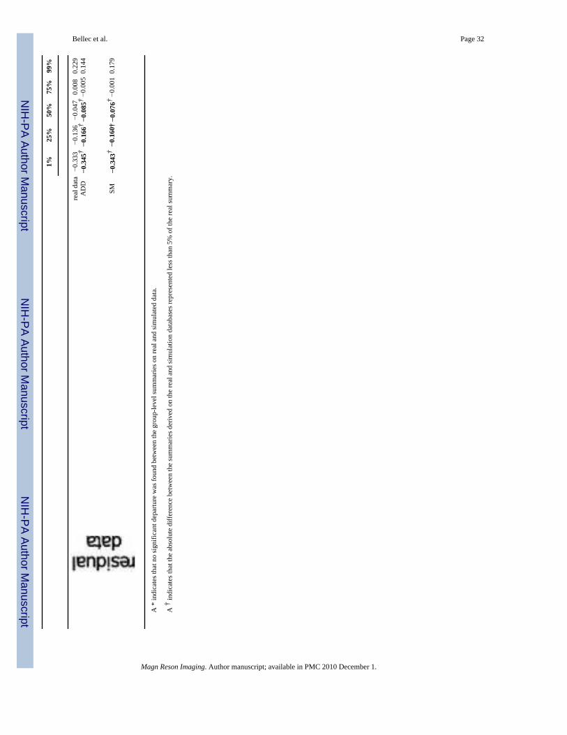
A *
indi
cate
s tha
t no
sign
ifica
nt d
epar
ture
was
foun
d be
twee
n th
e gr
oup-
leve
l sum
mar
ies o
n re
al a
nd si
mul
ated
dat
a.
A †
indi
cate
s tha
t the
abs
olut
e di
ffer
ence
bet
wee
n th
e su
mm
arie
s der
ived
on
the
real
and
sim
ulat
ion
data
base
s rep
rese
nted
less
than
5%
of t
he re
al su
mm
ary.
Magn Reson Imaging. Author manuscript; available in PMC 2010 December 1.
NIH
-PA Author Manuscript
NIH
-PA Author Manuscript
NIH
-PA Author Manuscript
Bellec et al. Page 30Ta
ble
C.2
Dis
tribu
tions
of s
patia
l and
tem
pora
l aut
ocor
rela
tion
for m
otio
n-co
rrec
ted
and
resi
dual
dat
a der
ived
from
real
, AD
D an
d SM
FR
B d
atab
ases
. The
per
cent
iles
of th
e di
strib
utio
n of
the
indi
vidu
al m
aps w
ere
deriv
ed w
ithin
a m
ask
of th
e br
ain
and
aver
aged
ove
r all
subj
ects
and
task
s.
1%25
%50
%75
%99
%
real
dat
a−0
.198
0.01
60.
075
0.14
50.
477
AD
D−0
.174
†−0
.028
0.01
20.
057
0.28
1
SM−0
.170
†−0
.014
0.03
10.
083
0.36
6
real
dat
a−0
.118
0.02
20.
073
0.13
00.
386
AD
D−0
.116
†−0
.032
0.00
10.
035
0.12
2
SM−0
.106
†−0
.010
0.02
80.
072
0.24
5
Magn Reson Imaging. Author manuscript; available in PMC 2010 December 1.

NIH
-PA Author Manuscript
NIH
-PA Author Manuscript
NIH
-PA Author Manuscript
Bellec et al. Page 311%
25%
50%
75%
99%
real
dat
a−0
.237
0.00
90.
124
0.27
10.
703
AD
D−0
.245
*†−0
.019
0.08
80.
224
0.65
5
SM−0
.227
†−0
.015
0.09
00.
230
0.69
8*
Magn Reson Imaging. Author manuscript; available in PMC 2010 December 1.
NIH
-PA Author Manuscript
NIH
-PA Author Manuscript
NIH
-PA Author Manuscript
Bellec et al. Page 321%
25%
50%
75%
99%
real
dat
a−0
.333
−0.1
36−0
.047
0.00
80.
229
AD
D−0
.345
†−0
.166
†−0
.085
†−0
.005
0.14
4
SM−0
.343
†−0
.160
†−0
.076
†−0
.001
0.17
9
A *
indi
cate
s tha
t no
sign
ifica
nt d
epar
ture
was
foun
d be
twee
n th
e gr
oup-
leve
l sum
mar
ies o
n re
al a
nd si
mul
ated
dat
a.
A †
indi
cate
s tha
t the
abs
olut
e di
ffer
ence
bet
wee
n th
e su
mm
arie
s der
ived
on
the
real
and
sim
ulat
ion
data
base
s rep
rese
nted
less
than
5%
of t
he re
al su
mm
ary.
Magn Reson Imaging. Author manuscript; available in PMC 2010 December 1.
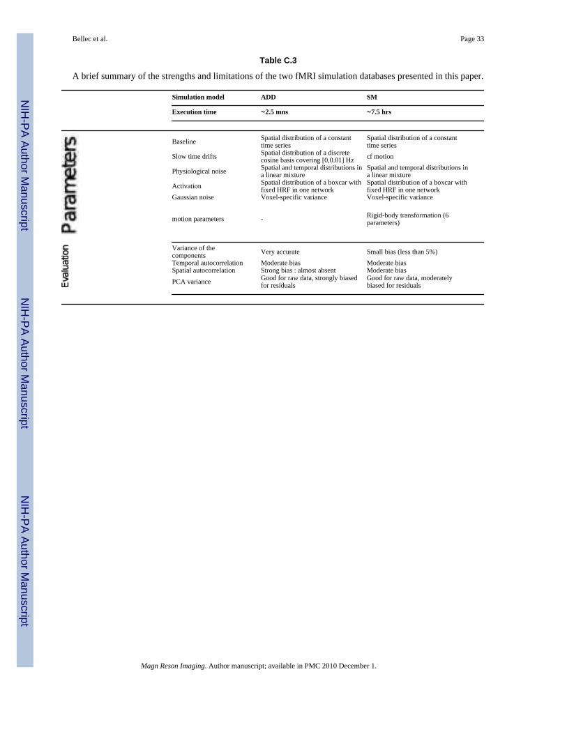
NIH
-PA Author Manuscript
NIH
-PA Author Manuscript
NIH
-PA Author Manuscript
Bellec et al. Page 33
Table C.3
A brief summary of the strengths and limitations of the two fMRI simulation databases presented in this paper.
Simulation model ADD SM
Execution time ∼2.5 mns ∼7.5 hrs
Baseline Spatial distribution of a constanttime series
Spatial distribution of a constanttime series
Slow time drifts Spatial distribution of a discretecosine basis covering [0,0.01] Hz cf motion
Physiological noise Spatial and temporal distributions ina linear mixture
Spatial and temporal distributions ina linear mixture
Activation Spatial distribution of a boxcar withfixed HRF in one network
Spatial distribution of a boxcar withfixed HRF in one network
Gaussian noise Voxel-specific variance Voxel-specific variance
motion parameters - Rigid-body transformation (6parameters)
Variance of thecomponents Very accurate Small bias (less than 5%)Temporal autocorrelation Moderate bias Moderate biasSpatial autocorrelation Strong bias : almost absent Moderate biasPCA variance Good for raw data, strongly biased
for residualsGood for raw data, moderatelybiased for residuals
Magn Reson Imaging. Author manuscript; available in PMC 2010 December 1.