Beggar-Thy-Women:Foreign Brides and the Domestic Front – The Case of

Taiwan ∗

Lena Edlund†

Elaine M. Liu‡

Jin-Tan Liu§

July 8, 2013

Abstract

In 2003, one in four marriages in Taiwan involved a bride from a foreign, and of-ten substantially poorer, country. We examine the impact of foreign brides on nativewomen using administrative data covering the period 1998 to 2006. Our identificationstrategy exploits a 2003 policy that tightened visa requirements combined with the ob-servation that rural or poorly educated men were more prone to marry foreign brides.Our difference-in-differences estimates suggest a positive fertility response among do-mestic women from the presence of foreign brides. We also find divorce risk to decline, aperhaps counter-intuitive finding but one consistent with children stabilizing marriage.

JEL Classification: : J12, O15, D1

∗We thank Ted Bergstrom, Aimee Chin, Andrew Foster, Scott Hankins, Jeanne LaFortune, Jee Lehmann,Aloysius Siow, John Strauss, Laura Zimmermann, Andy Zuppann and seminar and conference participantsat Boston College, IFPRI, Vanderbilt University, University of Toronto, USC, UCI, UH, Dalhousie Univer-sity, University of Maryland-School of Public Policy, Peking University Guanghua School of Management,Tsinghua University, SWUFE, National Taiwan University, Texas STATA conference, EDW, PAA, NEUDCand MIEDC for their comments and suggestions. David Gross provided excellent language editing services.Elaine M. Liu thanks Chiang Ching-kuo Foundation for financial support.

†Department of Economics, Columbia University.‡Corresponding Author. Department of Economics, University of Houston.§Department of Economics, National Taiwan University and NBER.

1 Introduction

In Taiwan, 29% of brides in 2003 were foreign born, a sharp increase from the mere 2% in

1990.1 Over the past decade, developed East Asian countries have received more than half

a million foreign brides, the vast majority from substantially poorer countries such as the

People’s Republic of China (henceforth, China), Vietnam, Indonesia and the Philippines.

The phenomenon is not isolated to East Asia. Poorer or less educated women marrying

richer or better educated men is a part of a longstanding pattern in which women marry

up. However, the magnitude and the scope of this dramatic rise in foreign brides are un-

precedented and have been met with apprehension in the receiving countries. The existing

literature has linked the phenomenon to notions of male superiority within the social context

of the receiving countries. It has also chronicled the motives and (mis-)fortunes of the brides

and grooms [Hsia, 1997, 2006, Luoh, 2006, Kim, 2009, 2012, Kawaguchi & Lee, 2012] and

highlighted the benefits to the natal families of the foreign brides [Belanger et al. , 2011,

Belanger & Linh, 2011]. However, little attention has been given to the impact on women

in the receiving countries.2

A priori, it is plausible that domestic women would be negatively affected by the inflow

of foreign brides. Foreign women constitute low-cost competition similar to the presence

of immigrant workers in the labor market. However, there are two principal reasons to

believe that the impact on domestic women in the marriage market is more severe than

the impact that immigrant workers have on the native workers in the labor market. First,

considering the core services provided by wives: sex and children [Edlund & Korn, 2002],

1During the same time period, the proportion of marriages involving foreign grooms remained stablearound 3%.

2Weiss et al. [2012] is a recent exception.

1

the substitutability between foreign and domestic women as wives may be high, especially if

they are of similar ethnicity.3 Second, although the possibility of complementarities between

the immigrant and domestic workers imply that the immigrant worker may not necessarily

displace a domestic worker in the labor market, this scenario is less likely on the marriage

market where complementarities are with the opposite, not the same, sex.

How domestic women fare in the face of low-cost competition in the form of foreign brides

is a question of high policy relevance for a number of reasons. First, a large number of brides

from poor countries likely undermine the status of women – directly through a compositional

change and indirectly through the effect on native women’s status – and as a consequence,

children’s outcomes may suffer.4

Second, the rapid growth of foreign brides in East Asian countries has been primarily

driven by the rise of so called ”mail-order brides” and the prevalence of this type of marriage

should be highly responsive to policy changes such as visa requirements and regulations of

matrimonial agencies. Marriages involving mail-order brides are concluded after only a few

meetings, are brokered by a third party and involve a bride from a poor country who upon

marriage settles in the groom’s substantially richer country. Although marriages between

bride and groom of different nationalities have been on the rise in recent years in part due to

lower travel costs and increasing integration of social and economic networks across countries,

the majority of cross-border marriages taking place in the developed countries of East Asia

like Taiwan stand out because of their transactional characteristic.5

3The greater the emphasis on child quality and companionship the less interchangeable domestic andforeign women are likely to be. Although a foreign background could be a coveted feature in a wife andmother, newspaper testimony from foreign brides suggests otherwise. Foreign brides are expected to adaptto the host country and to not pass on the language or other aspects of their native country’s culture.

4See Duflo [2011] for a review of the literature on women’s status and their children’s outcome.5International marriages have also become more common in Europe, e.g. nearly half the marriages in

2

Third, the topic of mail-order brides is likely to emerge as a salient policy issue as the

close to 15 million surplus males under the age 20 in China begin to look for wives. Importing

foreign brides has been touted as a solution to the looming bride deficit [Sharygin et al. ,

2012]. Feasibility notwithstanding, importing women for marriage would undo the advantage

that son preference gave domestic women through relative scarcity in the marriage market.

In this paper, we study Taiwan. In the fall of 2003 the Taiwanese government reversed

course and tightened visa requirements for brides coming from China.6 The changes included

the introduction of an interview designed to screen out mail-order brides (who were asked

detailed questions about the husband and his family). As a result, it became much more

difficult to marry Chinese brides and the number of Chinese brides halved between 2003 and

2004. In 2005, a similar policy was applied to Vietnamese brides and the flow of Vietnamese

brides was similarly stemmed. By 2006, foreign brides were one-quarter of the number in

2003. This drastic change in policies governing the flow of foreign brides into Taiwan presents

us with a unique opportunity to evaluate the social impact of foreign brides on the domestic

population of women.

In particular, we focus on local women’s fertility response to the inflow of foreign brides.

Fertility is well below replacement level in East Asia’s developed countries and Taiwan is

no exception. Fertility is a prime example of a joint decision and therefore subject to intra-

household bargaining.7 Although it can be debated whether wives or husbands want children

“more,” low fertility in developed East Asian countries today is commonly attributed to

Switzerland are international. Yet in Europe the gender of foreign spouses is rather balanced; in East Asia,foreign spouses are predominantly women.

6For a number of reasons including concern that the foreign brides fed prostitution rings, led to thedevaluing of women and threatened national security.

7For early contributions see Mancer & Brown [1980], Horney & McElroy [1988], McElroy [1990], Bour-guignon et al. [1994], Lundberg & Pollak [1993].

3

modern women’s reluctance to assume the traditional roles of subservience and domesticity

expected in marriage and motherhood [Frejka et al. , 2010]. Therefore, in the context at

hand, fertility can be seen as an inverse measure of women’s bargaining power.8 Assuming

that the inflow of foreign brides undercuts domestic women’s bargaining power we would

therefore expect foreign brides to increase domestic women’s fertility.

However, the predicted effect on divorce is less clear. On the one hand, foreign brides

make divorce and remarriage for men more attractive. On the other hand, if fertility increases

and the presence of young children stabilize marriages, then the net effect of foreign brides

on divorce is ambiguous.

We analyze Taiwanese government administrative records covering the universe of mar-

riage, divorce and birth registries for the period of 1998 to 2006. We limit our attention to

couples who married in between 1998 and 2003 (before the tightening of visa requirements)

and link to their subsequent fertility and divorce outcomes through 2006.9 The merged

dataset contains information on the bride’s and groom’s respective birth date and educa-

tion level, the couple’s marriage date, divorce date, marriage history, place of residence, and

detailed birth records of children born between 1998 and 2006.

Our main identification strategy is a difference-in-differences approach where the first

difference exploits the 2003 policy change that resulted in a drastic reduction in the entry

of foreign brides. For the second difference we note that foreign brides affect “marginal”

8For evidence that women desire lower fertility than their spouses, see Ashraf et al. [2012]. Francis [2011]found that when Taiwanese women have more bargaining power, fertility declines. A government reportbased on a nationally representative survey in 2006 in Taiwan found that the ideal number of children ishigher for married men (2.5) than for married women (2.4) and for single men (1.93) than for signal women(1.88).

9Our analysis is restricted to couples who married before the visa-tightening policy went into effect sincethe policy could have changed the type of natives that got married.

4

marriage markets more. Foreign brides have been much more prevalent in poor rural areas

and among less educated men, so-called mail-order brides being all but absent among the

better educated. We seek to classify localities according to their reliance on foreign brides.

To that end, we use the adult sex ratio in the locality as a gauge of its standing in the national

marriage market. The rationale for this proxy is that internal migration patterns mirror those

of cross-border marriages: young women leave poor rural areas to seek a better life. This is

a general pattern and one of the authors has argued elsewhere that more young women than

young men are leaving economically depressed areas due to the marriage market [Edlund,

2005]. Young women may be viewed as a scarce resource, whose allocation is determined by

demand. Since, by and large, rich areas have rich men, young women are disproportionately

found there. Moreover, in Taiwan the eldest son is supposed to co-reside with his aging

parents, further reducing male mobility. Therefore, adult sex ratios (male-to-female) may

serve as a measure of the ability of men to marry domestic women and thus the demand for

foreign brides.

We find that native couples in areas with high sex ratios are less likely to have children

and are more likely to divorce after 2003 relative to couples in low sex-ratio townships.

Moreover, we exploit the fact that few men with a college degree married foreign brides;

especially mail-order brides. The incidence of foreign brides among college educated grooms

was largely unaffected by the more strict visa requirements post-2003. Therefore, couples in

which the husband is college educated may serve as another comparison group. Similarly,

we find that native women with less educated husbands are less likely to have children and

are more likely to divorce after 2003 relative to couples with college educated husbands.

Next, we present evidence on intra-household bargaining power from the Social Devel-

5

opment Trends Survey. The results are consistent with the fertility results. We find that

wives are more likely to be the decision maker on household expenditure and child-rearing

decisions in areas with high sex ratios after 2003 relative to those in low sex-ratio townships.

A limitation of these data is a small sample size (albeit nationally representative) and only

a two-year availability of questions on decision making in the household.

Other than the marriage market channel, it is possible that foreign women displace native

women in the labor market. If local women have lower income as a result of foreign brides,

that could also lower their bargaining power at home. However, examining native women’s

labor force participation, earnings, and hours worked, we find no evidence of labor market

effects.

The remainder of this paper is structured as follows: Section 2 discusses background and

existing literature on foreign brides, Section 3 describes the data, Section 4 presents the

specification for regression analysis and discusses the results, and Section 5 concludes.

In the Appendix, we make a theoretical case for increased competition leading to higher

fertility among domestic women and, possibly, changes to divorce rates.

2 Background and Literature Review

Women marrying up is a common and possibly long standing feature of human mating

systems [Oota et al. , 2001]. The marrying-up often has a geographic component, with

poorer areas losing their young women to richer areas [Fan & Huang, 1998, Edlund, 2005].

A modern-day version is the so-called mail-order brides phenomenon whereby a man in a rich

country marries a woman from a poor country after very few preliminaries, casting marriage

6

in a venal and transactional light. Pejoratively termed, the phenomenon is generally looked

down upon by the receiving country and was minimally pursued in the past.

Internet penetration and cheaper transportation has undoubtedly been important cata-

lysts for the rise in cross-border marriages. However, the prevalence of cross-border marriages

in the developed East Asian countries suggests additional factors.

First, East Asia shares a common culture defined by its Confucian heritage. While in

the past century Confucianism has been superseded by other ideologies, notably nationalism

and communism, it still has a grip on family values. One example is the persistence of a son

preference culture. Confucianism also places great emphasis on filial behavior; “being disre-

spectful towards inlaws” remains grounds for divorce in Taiwan, echoing a similar precept in

traditional Chinese family law.10 Tellingly, a recent Korean survey found that 53.5 percent

of Korean husbands answered “obedience to parents” as their foremost reason for marrying

Vietnamese brides, followed by “similar appearance to Koreans” [Kim, 2012, p. 552].

Another reason mail-order brides have become prevalent in East Asian developed coun-

tries is that marriage in the Confucian tradition is very clearly a transaction through which a

woman is purchased to deliver progeny, preferably sons. In most of East Asia until the 1950s

marriages were arranged by the parents of the prospective spouses and companionship, as

emphasized in the West [Glendon, 1996], was disdained. Thus, while Western culture has

idealized and practiced companionate marriage, the Confucian marriage has the outright

flavor of a purchase contract, whereby the wife is acquired to render reproductive and other

services.

10“Disobedience towards husband’s parents” was the first out of seven grounds for divorce in traditionalChinese family law.

7

While Western-inspired family law has been adhered to since the mid 1900s, male-oriented

attitudes towards family formation remains in East Asia and may be one reason greater

educational attainment and concomitant ability to be economically self-sufficient has led

many women in richer East Asian countries to opt-out of marriage. With fewer women in

the marriage market, men at the bottom of socioeconomic status have found it difficult to

find a domestic wife and have turned to substantially poorer, but culturally and ethnically

similar, women from China or Vietnam. Although the premise of male chauvinist values

begs the question why attitudes have not changed, the gender structure in the host countries

is often pointed to as an explanation for the appeal of foreign brides [Kim, 2012, Kawaguchi

& Lee, 2012].

Additionally, the countries composing East Asia are economically heterogeneous; coun-

tries such as Singapore and Japan have per capita incomes above USD40,000 as compared

to Vietnam which despite almost two decades of economic reforms remains relatively poor

at a per capita GDP of around USD1,400. Taiwan (GDP per capita is about USD20,000),

while not as rich as Singapore or even Korea, is clearly richer than China (USD4,000 per

capita GDP) or Vietnam.

In the case of Taiwan, the cultural proximity to China contributed to the high levels

of foreign brides. In 1987, Taiwan lifted martial law and in 1992 allowed entry of Chinese

spouses [Liaw et al. , 2011]. Following the thawing of bi-lateral relationships, the number of

Chinese brides steadily increased. In 2003, close to 29,000 Taiwanese men married Chinese

brides. For comparison, in the same year about 110,000 Taiwanese men married a compatriot.

Vietnam has been the second largest source country of foreign brides. Greater Taiwanese

business interests in Vietnam in the 1990s provided the impetus for the marriage of some

8

110,000 Vietnamese women to Taiwanese men in the following decade [Belanger & Linh,

2011].

During the 1980s and 1990s, Taiwan’s economy was growing rapidly, especially relative

to some of its East Asian neighbors. By 1990, Taiwan’s GDP per capita was 19 times higher

than China’s, 10 times higher than Indonesia’s and 22 times higher than Vietnam’s. As the

Taiwanese government encouraged investment throughout Southeast Asia in the early 1990s,

Taiwanese businessmen went to Vietnam and Indonesia to seek cheap labor but also saw the

potential of marriage brokerage [Jiang & Huang, 2004].

These brokers charge the prospective groom a lump-sum of USD7,000-10,000 [Wang &

Chang, 2002].11 The brokers manage the entire process, including arranging the groom’s trip

abroad and his meeting with potential brides. Once a groom chooses his bride, the broker

arranges a wedding banquet in the bride’s hometown, prepares all the documents for the

bride’s visa application, and arranges the trip to Taiwan. The process takes less than a week

for the groom, while the bride often has to wait for a couple months before she receives the

proper visa to enter Taiwan.12 According to the Survey Report of the 2002 Living Conditions

of Foreign and Mainland Spouses produced by the Taiwanese government containing data

collected from 175,000 foreign spouses, 37.8% of all Southeast Asian brides were introduced

to their spouses via commercial marriage brokers and 46% met through friends and relatives

[Ministry of Interior, 2004].13 Table 1 describes the composition of foreign brides by country

11The average wedding in Taiwan costs USD26,000, more than the annual per capita income, and expensesare usually paid by groom.

12For more in depth report on the process of bride selection see Wang & Chang [2002].13The high share of foreign brides being introduced through friends and relatives have two implications.

First is that a high share of foreign brides do prefer their foreign marriage arrangement over staying in theirhome countries, so that they would introduce their friends and families to marry a Taiwanese man. Second,this is parallel to the findings in the immigration literature where new immigrants could benefit from theexisting network of immigrants in the host countries [Beaman, 2012].

9

of origin. China, Vietnam and Indonesia are among the largest bride exporting countries.

Why would these foreign brides want to marry abroad? According to a survey done in 2004

in Vietnam of 650 households with one or more daughters married to Taiwanese men, the

overwhelming reason is material gain. Nearly 80% of households cite “to help the family,”

“for a better life,” or “to make parents happy” as the main reason.14 The Vietnamese bride’s

family receive USD1,000-2,000 at the time of the wedding in addition to later remittances

[Wang & Chang, 2002, Belanger et al. , 2011].15 After the Taiwanese government lifted

the restriction in 1992 on Chinese brides entering Taiwan the marriage brokerage business

expanded to China.

The number of foreign brides starts to increase in the mid-1990s. By the time our dataset

begins in 1998, every one in eight marriages involves a foreign bride and the percentage

keeps rising through 2003 (see Figure 1). On September 1, 2003 the Taiwanese government

implemented more stringent screening of newly married Chinese brides seeking entry. Prior

to the policy, Chinese brides only needed to provide a valid marriage certificate in order

to obtain a visa. After the policy, three interviews were required: prior to entry, at the

port of entry, and finally at the place of residence. Brides could be refused entry or be

repatriated immediately if the marriage was deemed illegitimate [Wu, 2004, Lu, 2008].16

Thus, entry became arbitrary and solely dependent on the interviewers.17 This new rule

implicitly increased the cost of marrying Chinese brides.18 Figure 2 separates Chinese and

14There was no case of parents having sold their daughter [Ngu, 2005].15The UN/World Bank estimates nominal 2011 GDP per capita in Vietnam at around USD1,400.16Announced on August 28, 2003 by the Immigration Office, Ministry of Interior, and published on the

front page of the China Times, the Liberty Times and the United Daily Newspaper on August 29, 2003.17According to Wu [2004], nearly 10% of Chinese brides were turned away in the first four months of the

policy’s implementation.18Lu [2008] suggests that one of the main reasons why the policy was implemented is due to the negative

media attention surrounding several crackdowns on prostitution rings that consisted mostly of Chinese brides.

10

Southeast Asian brides. It is clear that the policy was enforced since we observe a dramatic

decline of Chinese brides starting in the winter of 2004. The decline in Southeast Asian brides

starts in 2005 when the Taiwanese embassy in Vietnam switched to one-on-one interviews

instead of bulk processing, reducing the number of visas from hundreds to 20-30 a day

(Dajiyuan News, 2005).

2.1 Existing Literature

The foreign-bride phenomenon in Taiwan has been widely studied since early work by Hsia

[1997]. However, most of the studies have been ethnographic in nature. In this section, we

only discuss the studies that have drawn on large-scale data sets and thus are closest to our

paper.

Tsay [2005] provided an overview of the trends of the foreign bride phenomenon from 1991

to 2003 in Taiwan. Drawing on aggregate-level datasets provided by the central government,

he describes the rising trend, country-composition and settlement patterns of foreign brides.

His paper is one of the first to identify the regional variation in the demand and supply of

brides. Luoh [2006] furthered the analysis by combining the Labor Force Participation survey

with the 2000 Census survey to examine the relationship between the groom’s education

level and the likelihood of marrying a foreign bride. He found that foreign brides had

disproportionately married grooms with less extensive education. Among men with less

than a middle-school education, foreign brides outnumbered Taiwanese brides. He also found

that foreign brides are disproportionately located in the southern, less-developed, parts of

Chang [2002] estimated that a total of 1,800 Chinese brides have been convicted of prostitution. Yet, thescale of this problem does not seem large when one considers that there were more than 300,000 foreignbrides in Taiwan during this time period.

11

the island (such as Ponghu, Chiayi and Nantou Counties) while the metropolitan areas (such

as Taipei and Taichung City) had very few foreign brides. These differences will be used in

our paper for the difference-in-differences analysis.

Liaw et al. [2011] analyzed the 2003 Survey of Foreign and Mainland Spouses’ Life Status.

The main focus of their paper was to examine determinants of fertility among foreign brides.

They estimated the total fertility rate of foreign brides to be 1.58 children, substantially

above the 2003 national average of 1.23 [Chen, 2005].

Kawaguchi & Lee [2012] asked why men in developed East Asian countries have turned to

countries such as China and Vietnam for brides in such numbers. They pointed to reluctance

of increasingly well-educated domestic women to enter wedlock. However, tension between

women’s education and willingness to marry can be resolved in a number of ways. In the

West, there has been a radical shift in gender roles allowing women to combine marriage and

work, reversing the once negative relationship between education and marriage.

The literature on society-wide effects is small. The study closest to ours, Tsai et al.

[2010], examined the impact of foreign brides on out-of-wedlock fertility among Taiwanese

women. Using the 1990 and 2000 censuses, they found a positive association with out-of-

wedlock fertility by comparing areas that were major recipients of foreign brides to areas

receiving fewer foreign brides. However, a challenge when interpreting this association as

causal is that the factors that drove local men to turn to foreign wives are likely to be closely

related to local women’s decision to bear children outside of marriage. Weiss et al. [2012]

studied the gender differential impact of the rise in marriages between a Hong Kong man

and a Mainland woman after the 1997 re-unification. They argued that Hong Kong women

(men) were less (more) likely to ever be married, currently married, or the household head;

12

and more (less) likely to be currently divorced or a single parent. In their analysis they use

Taiwan as a control group, thus their findings are relative to Taiwanese men and women.

3 Data

For our main analysis, we link Taiwanese marriage, divorce and birth registries for the years

1998 through 2006. From each marriage record we obtain information on education, date of

birth, country of origin, and marriage history of the bride and the groom. The birth registry

contains information on sex, birth weight, gestation length, birth order, and birth place.

Thus, for each couple married between 1998 and 2006 we have information on fertility and

divorce outcomes through 2006.

The policy change we exploit took place in the fall of 2003. By making it more difficult to

marry mail-order brides the policy likely changed the type of native couples who got married.

Therefore, we limit our sample couples where both husband and wife are Taiwanese, non-

aboriginal, nationals who married between 1998-2003.19 Furthermore, we require the wife

to be between the ages of 20 and 45 and the husband to be born between 1928 and 1987.

That is, a couple would be observed until divorce or the wife turning 46. Since fertility has

a 9-month lead-time, 2005 is the first year we expect the policy change to show in natality

data. We omit year 2004, a transitional year, leaving us with six years of pre-treatment and

two years of post-treatment data.

We exclude a couple of remote islands mainly used as military bases (less than 0.1% of

total observations), leaving us with 356 townships in 23 counties.

19Couples in which the groom is foreign or the bride or groom is aboriginal constituted 5% of the totalsample.

13

Thus, we arrive at an analysis sample of 691,216 couples on average observed over five

years, or 3,563,957 couple-year observations.

3.1 Descriptive Statistics

Table 2 provides summary statistics of couples married between 1998 and 2003, broken

down by the bride’s origin: Taiwan, China, South East Asia or Other. Here, China includes

Macao, Hong Kong and mainland China. Southeast Asia includes Vietnam, Indonesia,

Malaysia, Thailand, Cambodia, Singapore, The Philippines and Laos. This table provides

characteristics of our analysis sample (Column 1) as well as illustrates how the foreign brides

and their grooms differ from native couples.

We see that the majority of foreign brides are from China, 61%, followed by Southeast

Asian brides, 33% (an underestimate as the remaining 6% of brides include Chinese and

Southeast Asian brides who entered in 1998 and 1999, see note to Table 2).

The spousal age gap is 11-13 years among couples where the bride is foreign. Among

Taiwanese couples, the gap is three years. Not only are foreign brides younger than local

brides but the Taiwanese men who marry them are also substantially older. As for education,

grooms who marry Chinese or Southeast Asian brides are less educated than those who marry

native women. Conditional on reporting, the education level of Chinese brides is higher than

those of Southeast Asian brides. Perhaps unsurprisingly, the marriages involving foreign

brides were also more unstable. While 10% of couples in which the bride (and the groom)

were Taiwanese had divorced by 2006, the numbers for Chinese brides and Southeast Asian

brides who had divorced were 28% and 17%, respectively. 6.21% of Chinese brides were

14

marrying to a divorcee, while this rate is much lower for domestic brides (less than 1%). It

is quite common for (male) divorcees to remarry foreign brides. 20

Figure 3 displays the share of foreign brides over time by groom’s education level. There

is a clear negative gradient, consistent with previous findings. The majority of men who

marry foreign brides have at most a middle-school education. Grooms with a four-year

college degree almost exclusively marry a fellow Taiwanese woman.

4 Empirical Analysis

In this section, we investigate the effect of foreign women on domestic women. To that end,

we focus on the fertility and divorce outcomes of Taiwanese-born married women. Lastly, we

utilize two rounds of the nationally representative Social Development Trends Survey and

its information on household decision making.

4.1 Identification

For our analysis using administrative data, we pursue a difference-in-differences approach

using the 2003 policy change combined with the assumption that less attractive men would

be more affected by the more stringent visa requirement.

For the second difference, we use two features of the marriage market, the adult sex ratio

in the township and the education level of the groom. The rationale for using the township

sex ratio is that women of family-forming age migrate to better marriage markets, resulting

20These statistics likely overstate the stability of marriages with foreign brides since they are more likelythan domestic brides to abscond without seeking a formal divorce. Foreign brides are only eligible forcitizenship after three years of residence. On average it takes about eight years to receive citizenship.

15

in poor marriage markets also having a surplus of men. In fact, the township sex ratios

(ages 20-50) range from 0.84 (men to women) to 1.67, where the richer, metropolitan areas

generally have a surplus of women, and poorer rural areas have a surplus of men (see Figures

4 and 5). We classify townships according to their sex-ratio quartile (population based, 2000

census).21

Figure 6 presents the share of foreign brides by quartile for each year relative to the peak

year 2003. As expected, townships in the fourth quartile have the sharpest increase in foreign

brides leading up to the 2003 policy, as well as the sharpest decline. Figure 7 presents the

geographic distribution of foreign brides from 1998 to 2006.

We separately analyze the seven administrative metropolitan areas (which contain about

a quarter of the total population). These areas are less comparable to the rest of Taiwan for

the following four reasons: (i) Our main analysis relies on the assumption that an individual’s

marriage market would mostly depend on the adult sex ratio in his/her township. The

highly integrated transportation and labor market in these metropolitan areas renders the

township distinction less meaningful. For example, Taipei City, which area-wise is smaller

than Manhattan, has 12 townships. (ii) The 2003 SARS outbreak was known to hit big

cities (more densely populated) in Taiwan the hardest. SARS, as an infectious disease, was

known to be more prevalent in hospitals, possibly affecting fertility plans. Thus, SARS is an

example of a factor affecting fertility in metropolitan areas for which neither year fixed effects

nor linear time trends would account.22 (iii) The higher housing costs and greater population

density affect fertility levels. (iv) Townships in metropolitan areas would cluster mostly in

21Ideally, 2003 township sex ratio would best reflect a town’s female deficit and marriage market compe-tition at the onset of visa tightening policy. However, 2003 sex ratio at township level is not available.

22One reason SARS might have affected fertility is that people sought to avoid outpatient medical careduring the epidemic [Bennett et al. , 2011].

16

the first sex ratio quartile. If we kept metropolitan areas in our analysis, the comparison we

made between those in the second/third/fourth quartiles to first quartile would be not only

about local sex ratio but also about the differences in urbanization of these areas.

Therefore, we separate these largest metropolitan areas – special municipalities (Taipei,

Kaohsiung) and provincial cities (Keelung, Hsinchu, Taichung, Chiayi, Tainan cities) – and

pursue slightly different approaches for the metropolitan and non-metropolitan sub-samples.

For the non-metropolitan areas, we let township sex ratio provide the second difference, the

idea being that high sex ratio townships will be more affected.

For the metropolitan areas, since townships are highly integrated, we let husband’s ed-

ucation form the second difference, the assumption being that college educated men are

unaffected by the availability of foreign brides, the mail-order variety in particular.

As can be seen in Figure 3 college educated men are the least likely to marry a foreign

bride, and the sharp decline seen after the 2003 policy is barely noticeable suggesting that the

mail-order brides are a rarity among college educated men. College educated men outrank

lesser educated men in the marriage market and the most straightforward explanation for

their affinity for fellow Taiwanese as spouses is positive assortative mating (e.g., from public

goods in marriage) and foreign spouses ranking below Taiwanese women on the (Taiwanese)

marriage market. However, this does not imply that the college educated are insulated

from the influence of foreign brides and the difference is likely one of degrees rather than

absolutes. Marriage provides men with sex and children and the ability of a woman to

perform those tasks does not rely on a common language. However, marriage may also

provide companionship, and for this, domestic brides have a distinct advantage. The greater

the weight on personal compatibility, the lower the substitutability bias introduced is one of

17

attenuation. That is, if foreign brides also reduce the bargaining power of women married

to educated men, the difference-in-differences would provide a lower bound estimate of the

impact.

4.2 Regression Model

For the non-metropolitan areas, we estimate a regression model of the form:

Yivt = β1I(Post03)t +4∑

j=2

βjI(SexRatioQj)v × I(Post03)t

+4∑

j=2

I(SexRatioQj)v +Xivt + t× LOCALITYv

+ τt + πv + εivt (1)

where Yivt is an indicator variable, 1 if couple i in township v in year t had a child or divorced.

I(Post03) is an indicator variable, 1 if t > 2003. I(SexRatioQj)v indicates township v’s sex-

ratio quartile. Xivt includes wife’s age, age 2, husband’s education (9-15 years, 16 or more

years), whether the couple has a son, and a set of dummies controlling for duration of

marriages (in years). τt is a vector of year dummies, and LOCALITY is a vector of county

or township dummies. We cluster standard errors at the township level.

The main coefficients of interest are β2, β3, β4 which capture the heterogeneous impact of

the 2003 policy on the likelihood of fertility or divorce across sex-ratio quartiles.

We focus on the coefficients β2, β3, andβ4 rather than β1. The coefficient on I(Post03)t,

β1, captures not only changes in low sex-ratio townships driven by the policy but also any

18

changes in country-wide contemporaneous factors affecting the outcome in question. These

coefficients are also sensitive to which year is excluded from the year fixed effects.23

As a preliminary, Figure 8 shows the probability of a birth in the years leading up to the

2003 policy, by sex-ratio quartile. This figure is restricted to only those who married before

2003. Before the policy, the higher sex-quartiles have higher fertility and we observe parallel

decreasing trends across the four quartiles. After the policy, fertility drops more in the high

sex-ratio areas.

For the metropolitan areas we let husband’s education level provide the second difference

and estimate a regression model of the form:

Yivt = β1I(Post03)t + β2I(Post03)t ×MIDDLEi

+β3I(Post03)t × LOWi +MIDDLEi + LOWi

+Xivt + τt × LOCALITYiv + πv + εivt (2)

whereMIDDLE is an indicator variable that takes on the value 1 if the husband has nine

to fifteen years of education, and LOW is an indicator variable that is 1 if the husband has

eight years or less of schooling. The reference category is four-year college degree or more.

The coefficients of interests are β2 and β3 and in the case of fertility we expect β3 < β2 < 0.

23Between controlling for year of marriage, marriage duration, and year, we can choose two. We haveopted for marriage duration and year, the reason being that we believe these two to have a stronger linkto fertility (and divorce) than year of marriage. For instance, fertility is likely influenced by economy wideevents like unemployment (2000 and 2001 were recession years) or auspicious years for the Chinese Zodiac.The presence of idiosyncratic factors also means that fertility trends are poorly captured by, say, a polynomialin year.

19

4.2.1 Fertility Outcomes – Non-Metropolitan Areas

We start by estimating Equation 1 without the county-specific time trends (only year effects)

on couples in non-metropolitan areas (see Table 3 for results). In Column 1, all education

groups are pooled, whereas Columns 2-4 present results by husband’s education. We see that

relative to couples in the first (township sex-ratio) quartile, fertility falls after the 2003 policy

and, as hypothesized, the decline is greater in the townships with higher male sex ratios. For

couples in the fourth sex-ratio quartile townships there is a 4 percentage point reduction in

fertility. Coefficients on second quartiles SexRatioQ2 and third quartiles SexRatioQ3 are

statistically different, as are the SexRatioQ3 and SexRatioQ4 coefficients

Turning to the effects by education (Columns 2-4), we see that within each education

category, there is a greater reduction in fertility among couples in higher sex-ratio townships

after the policy. Comparing across education groups, the ordering of the effect sizes are as

hypothesized, larger among the less educated.

The coefficient on I(Post03) is negative but is hard to interpret due to the inclusion of

year dummies. Consequently, going forward, we will omit this coefficient from the tables to

focus on the difference-in-differences results.

In Table 4 we present results allowing for county- and township-specific time trends

respectively as well as county-year fixed effects, Panels A-C. In Panel A we allow for different

fertility trends by county; the results are qualitatively similar. For the whole sample and

within each education group, the effect is greater in higher sex-ratio areas. Quantitatively,

the results are somewhat muted. Next, we turn to a more demanding specification by

substituting township-specific for county-specific time trends (there are 308 townships and

20

16 counties in non-metropolitan areas), see Panel B. The qualitative pattern found earlier

remains however reduced in magnitude. Finally, we control for county-year fixed effects

(Panel C) and the results are similar to the specification including county-specific time

trends. For ease of comparison, the coefficients across specifications are graphed in Figures

9 and 10.

4.2.2 Fertility Outcomes – Metropolitan Areas

We now turn to the results for the seven metropolitan areas, home to about a quarter of

our sample. For the reasons outlined previously, the township sex ratios provide a less

meaningful distinction here. Instead, we group couples according to husband’s education

level, the assumption being that the policy mainly impacted men with less education leaving

college educated men largely unaffected.

Table 5 presents the results from estimating Equation 2 for the metropolitan areas. As

hypothesized, relative to the college group (defined by husband’s education), lower education

groups reduced their fertility post-policy. In the basic specification, Column 1, relative to

the most educated group, the middle and lowest education groups reduced their fertility by

0.062 and 0.074 respectively (the difference is statistically significant at the 1% level). While

the effect size may appear small, the baseline fertility risk is only 0.19. Columns 2-4 allow

for location specific time trends and city-year fixed effects, and the difference-in-differences

results remain almost unchanged, consistent with metropolitan areas being geographically

highly integrated and homogeneous.

21

4.3 Divorce Outcomes

Next we examine divorce outcome (Tables 6-8). While the results are not as clear as in the

case of fertility, the picture that emerges is that foreign brides stabilized marriage – a seem-

ingly counterintuitive finding. Theory suggests that more women would make remarriage

more attractive for men, thereby having a destabilizing effect. While this might still be the

case over the longer term, in the short term the higher fertility of Taiwanese wives, and thus

the presence of young children (as documented above), suggests an alternative explanation.

We sketch the argument here (for a more detailed exposition, see the Appendix). Assume

that in marriage men hire women to produce children (see Edlund [forthcoming]) and do-

mestic and foreign women are substitutes. In return, in marriage, men provide resources to

women. Furthermore, suppose that fertility is uncertain, depending on the woman’s unveri-

fiable effort and a stochastic term. If the production of children is costly to women, women

have an incentive to shirk. Divorce may be a disciplining device, triggered by low fertility

(failure to bear children was the second of the seven ground for divorce in Chinese family

law).24

Foreign brides in this setting can have two effects. Faced with a better alternative,

men’s divorce threshold may shift, triggering divorce at a higher fertility level. Faced with

heightened risk of marriage termination, women might increase effort, resulting in a rightward

shift in the fertility distribution. Thus, the prediction is that fertility would increase whereas

the net effect on divorce risk is ambiguous.

24Taiwan was part of China 1683-1895.

22

4.4 Robustness

To check robustness to functional form assumptions, we also estimate the policy impact on

fertility and divorce using duration analysis with a Weibull hazard function. We find similar

results for both fertility and divorce. As for fertility, those residing in the third and the

fourth sex-ratio quartiles respectively were 3.6% and 5.8% less likely to give birth after the

2003 policy than couples in townships with lowest sex-ratio quartile (statistically significant

at 1%). We also find that the likelihood of divorce increased for couples in the fourth quartile

by 8% relative to the couples in the first quartile. Since the findings are in line with those of

the OLS analysis, we do not include the tables in the interest of space (but they are available

from the authors upon request).

We also estimate a triple-difference model, in which we are interested in whether fertility

reduction by lower educated men is greater in higher adult sex ratio areas (and conversely

for divorce). The results are largely supportive (see Appendix Table A.1).

4.5 Decision Making Within Households

While we interpret our findings so far as being consistent with domestic women losing bar-

gaining power due to the greater availability of foreign brides, in this section we seek some

direct evidence of lower bargaining power using the Social Trend Survey. The survey is na-

tionally representative and in 2002 and 2006 it asked of both husbands and wives: “Within

your household, who is making each of the following decision: expenditures, savings, and

child rearing.” Options are: self, spouse, both, others or not applicable. We employ the

same difference-in-differences strategy as before, grouping respondents according to the lo-

23

cal (adult) sex ratio. Our outcome of interest is a dummy variable that takes the value 1 if

the wife is reported as the main decision maker.25 Columns 1 to 3 of Table 9 show results

using the husband’s responses and Columns 4 to 6 show results using the wife’s responses.

Both husbands and wives report that, after the policy, wives are more likely to decide how

to manage savings and expenditure in areas with higher adult sex ratios. The pattern for

child-rearing is less clear. Still, consistently, after the policy, women in the highest sex-ratio

quartile gained on women in the lowest sex-ratio quartile.

4.6 Discussion

We have shown that as a consequence of the immigration policy change in 2003, native

married women reduce fertility and increase divorce rates. Our findings in Section 4.5 suggest

that these results may be due to a shift of bargaining power from husband to wife. However,

there could be other channels through which the policy affects the welfare of native brides,

namely the labor market competition. For example, foreign brides can become a low cost

substitute for native women in the labor market. Consequently, the tightened immigration

policy in 2003 could have affected native women labor market outcomes and indirectly affect

native women’s fertility and divorce outcomes.

To explore this alternative hypothesis, we use the Labor Force Participation Survey (1998

to 2006), a nationally representative survey collected annually by the Taiwanese government

to examine employment status, wages and hours worked in the previous week for married

women. Similar to the analysis on fertility and divorce, if there is an impact on the labor

25We decide to focus on the choice that wives as the main decision makers (rather than both as choice)since it is a more clear indicator of wife’s status rising at home.

24

market due to the 2003 policy, we expect (i) the least educated native women to be more

affected since they are closer substitutes to foreign women, and (ii) areas with higher foreign

bride inflow to be more affected. Yet, neither of these patterns emerge in Table 10.26 These

results are not surprising for two reasons. First, foreign brides are prohibited from working

until they receive permanent residence status which usually takes several years, so we do

not expect an immediate impact on the labor market. If foreign brides work regardless of

legality, we would expect them to work in the informal labor market, competing primarily

with domestic low-skilled women if at all. Second, Angrist [2002] found high sex ratios to

be associated with lower female labor force participation. Therefore, while there may be a

higher demand for female labor after the 2003 policy, it is not clear whether married women

prefer to work or not. In sum, the absence of a labor market effect suggests that the marriage

market is the main channel through which foreign brides affected domestic women.

Hitherto, we have focused on native women. However, there is no reason to believe

foreign wives to be insulated from the overseas competition and in Table 11 we present results

estimating Equation 1. Panel A presents results for Chinese wives and Panel B results for

Southeast Asian wives. For both groups, the changes in fertility are driven by couples where

the groom is less educated. Among Chinese wives we find no affect among couples with a

college educated husband. Among Southeast Asian wives, the effect is of the “wrong” sign

– couples residing in the highest sex-ratio areas had relatively higher fertility post-policy.

As already discussed, the foreign bride phenomenon decrease with the groom’s education

and college educated men were likely unaffected by the change in visa requirements. The

26The results presented in Panels B and C include the entire sample of married women regardless ofemployment status. We also tried various alternative specifications including restricting the sample to thosewho were employed and using log(income) as the dependent variable – the results are still statisticallyinsignificant. These results are not presented in the interest of space but are available upon request.

25

impact is smaller among Southeast Asian brides than among Chinese brides. A couple of

factors may have contributed to this differential effect. First, the announcement of the policy

was publicized on the front page of major local newspapers in the fall of 2003. Since most

Southeast Asian brides do not read Chinese, information dispersion was likely slower among

this group. Second, the policy change in 2003 was designed to curtail the inflow of Chinese

mail-order brides – the inflow of Southeast Asian brides was stemmed later.

5 Conclusion

In 2003, 29% of marriages in Taiwan involved a foreign bride. Taiwan is not alone, in that

the practice is on the rise throughout East Asia. Women marrying up, within or across

countries, is a long standing practice. What is new is the larger scale on which this practice

is now occurring, fueled by lower transaction costs (the internet, cheaper air travel, etc.),

stark economic disparities and in the case of East Asia, a shared cultural heritage.

We examine the impact of the foreign bride on Taiwanese married women exploiting

a policy change initiated in 2003 which increased the difficulty of marrying foreign brides.

Using administrative data, we estimate that foreign brides increased fertility of domestic

women and reduced divorce rates. Our findings are likely to generalize to South Korea and

Japan, also countries where men have turned to foreign brides in large numbers.

East Asian developed countries struggle with fertility levels well below replacement level,

a phenomenon commonly linked to domestic women’s reluctance to marry, especially if

educated. In 2010, Taiwan recorded a total fertility rate of 0.90 children per woman and

the numbers for Korea and Japan were similarly low at 1.21 and 1.39 respectively. The

26

popularity of foreign brides from substantially poorer countries offers additional evidence of

womens roles in marriage trailing the progress made in other domains such as education and

the workplace.

27

References

2005. Proc. Marriage Migration between Vietnam and Taiwan: A View from Vietnam

(Singapore, 5-7 December 2005).

Angrist, Joshua. 2002. How do sex ratios affect marriage and labor markets? Evidence from

America’s second generation. Quarterly Journal of Economics, 117(3), 997–1038.

Ashraf, Nava, Field, Erica, & Lee, Jean. 2012. Household Bargaining and Excess Fertility:

An Experimental Study in Zambia. Duke and Harvard University.

Beaman, Lori A. 2012. Social Networks and the Dynamics of Labour Market Outcomes:

Evidence from Refugees Resettled in the U.S. The Review of Economic Studies, 79(1),

128–161.

Belanger, Daniele, & Linh, Tran Giang. 2011. The impact of transnational migration on

gender and marriage in sending communities of Vietnam. Current Sociology, 59(1), 59–

77.

Belanger, Daniele, Linh, Tran Giang, & Duong, Le Bach. 2011. Marriage Migrants as

Emigrants. Asian Population Studies, 7(2), 89–105.

Bennett, Daniel, Chiang, Chun-Fang, & Malani, Anup. 2011 (April). Learning During a

Crisis: the SARS Epidemic in Taiwan. Working Paper 16955. National Bureau of Economic

Research.

Bourguignon, Francois, Browning, Martin, Chiappori, Pierre-Andre, & Lechene, Valerie.

1994. Incomes and Outcomes: a Structural Model of Intra-Household Allocation. Journal

of Political Economy, 102(6), 1067–1096.

Chang, Shu-Ming. 2002 (May). Marketing International Marriages: Cross-Border Marriage

Business in Vietnam and Taiwan. M.Phil. thesis, Tamkang University, Taiwan. in Chinese.

Chen, Chaonan. 2005. Perspectives of Taiwan’s Population and Potency of Alternative

Policies. The Japanese Journal of Population, 3(1), 58–75.

Duflo, Esther. 2011 (December). Womens Empowerment and Economic Development. Work-

ing Paper 17702. National Bureau of Economic Research.

Edlund, Lena. 2005. Sex and the City. Scandinavian Journal of Economics, 107, 25–44.

Edlund, Lena. 2006. Marriage: Past, Present, Future? CESifo Economics Studies, 52(4),

621–639.

Edlund, Lena. forthcoming. The Role of Paternity Presumption and Custodial Rights for

Understanding Marriage Patterns. Economica.

Edlund, Lena, & Korn, Evelyn. 2002. A Theory of Prostitution. Journal of Political Economy,

110(1), 181–214.

Fan, Cindy F., & Huang, Youqin. 1998. Waves of rural brides: Female marriage migration

28

in China. Annals of the Association of American Geographers, 88(June), 227–251.

Francis, AndrewM. 2011. Sex ratios and the red dragon: using the Chinese Communist

Revolution to explore the effect of the sex ratio on women and children in Taiwan. Journal

of Population Economics, 24(3), 813–837.

Frejka, Tomas, Jones, Gavin W, & Sardon, Jean-Paul. 2010. East Asian childbearing patterns

and policy developments. Population and Development Review, 36(3), 579–606.

Glendon, Mary Ann. 1996. The Transformation of Family Law: State, Law and Family in

the United States and Western Europe. Chicago: University of Chicago Press.

Horney, M. J., & McElroy, Marjorie B. 1988. The Household Allocation Problem: Results

from a Bargaining Model. Pages 15–38 of: Schultz, T. Paul (ed), Research in Population

Economics, vol. 6. Greenwich: JAI Press.

Hsia, Hsiao-Chuan. 1997. Selfing and Othering in the “Foreign Bride” Phenomenon -A Study

of Class, Gender and Ethnicity in the Transnational Marriages between Taiwanese Men

and Indonesian Women. Ph.D. thesis, University of Florida.

Hsia, Hsiao-Chuan. 2006. Empowering ”Foreign Brides” and Community through Praxis-

Oriented Research. Societies Without Borders, 115(1), 93–111.

Jiang, YL; Chen YJ, & Huang, YT. 2004. A Study of Life Adjustment of the Mainland

China Spouses and Foreign Spouses. Community Development Quarterly, 105(1), 66–89.

Kawaguchi, Daiji, & Lee, Soohyung. 2012 (March). Brides for Sale: Cross-Border Marriages

and Female Immigration.

Kim, Andrew Enungi. 2009. Global Migration and South Korea: Foreign Workers, Foreign

Brides and the Making of a Multicultural Society. Ethnic and Racial Studies, 32(1), 70–92.

Kim, Hee-Kang. 2012. Marriage Migration Between South Korea and Vietnam: A Gender

Perspective. Asian perspective, 36(3), 531–563.

Liaw, Kao-Lee, Lin, Ji-Ping, & Liu, Chien-Chia. 2011. Reproductive contributions of Tai-

wan’s foreign wives from the top five source countries. Demographic Research, 24-26(April

27, 2011).

Lu, Melody Chia-Wen. 2008. Gender, Marriage and Migration: Contemporary Marriages

Between Mainland China and Taiwan. Ph.D. thesis, Proefschrift Universiteit Leiden,

Leiden, The Netherlands.

Lundberg, Shelly, & Pollak, Robert A. 1993. Separate spheres bargaining and the marriage

market. Journal of Political Economy, 988–1010.

Luoh, Ming-Ching. 2006. Gender Differences in Educational Attainment and International

Marriages. Taiwan Economic Review, 34(1), 79–115. in Chinese.

Mancer, Marilyn, & Brown, Murray. 1980. Marriage and Household Decision-Making: A

Bargaining Analysis. International Economic Review, 21(1), 31–44.

29

McElroy, Marjorie. 1990. The Emperical Content of Nash-Bargained Household Behavior.

Journal of Human Resources, 25(4), 559–583.

Ministry of Interior, ROC. 2004. Survey Report of the Living Conditions of Foreign and

Mainland Spouses. Tech. rept. in Chinese.

Oota, Hioki, Settheetham-Ishida, Wannapa, Tiwawech, Danai, Ishida, Takafumi, & Stonek-

ing, Mark. 2001. Human mtDNA and Y-Chromosome Variation is Correlated with Ma-

trilocal versus Patrilocal Residence. Nature Genetics, 29.

Shapiro, Carl, & Stiglitz, Joseph E. 1984. Equilibrium Unemployment as a Worker Discipline

Device. The American Economic Review, 74(3), pp. 433–444.

Sharygin, Ethan, Ebenstein, Avraham, & Das Gupta, Monica. 2012. Implications of China’s

future bride shortage for the geographical distribution and social protection needs of never-

married men. Population studies, 1–21.

Tsai, Wehn-jyuan, Liu, J.T., & Hockenberry, J. 2010. Do Foreign Brides Crowd Out

Domestic Unwed Women? A Study of Nonmarital Fertility in Taiwan.

Tsay, Ching-lung. 2005. Marriage migration of women from China and Southeast Asia to

Taiwan. In: Jones, Gavin W., & Ramdas, Kamalini (eds), (Un)tying the Knot: Ideal and

Reality in Asian Marriage. Singapore: Asia Research Institute. National University of

Singapore.

Wang, Hong-zen, & Chang, Shu-ming. 2002. The commodification of international marriages:

Cross-border marriage business in Taiwan and Viet Nam. International Migration, 40(6),

93–114.

Weiss, Yoram, Yi, Junjian, & Zhang, Junsen. 2012. Hypergamy, Cross-boundary Marriages,

and Family Behavior. Mimeo.

Wu, Shen. 2004. Study of Chinese Female Spouses Life Adaptation in Taiwan A case study

of the Chinese Female Spouses in Taipei County. M.Phil. thesis, National Sun Yat-Sen

University, Taiwan. in Chinese.

30

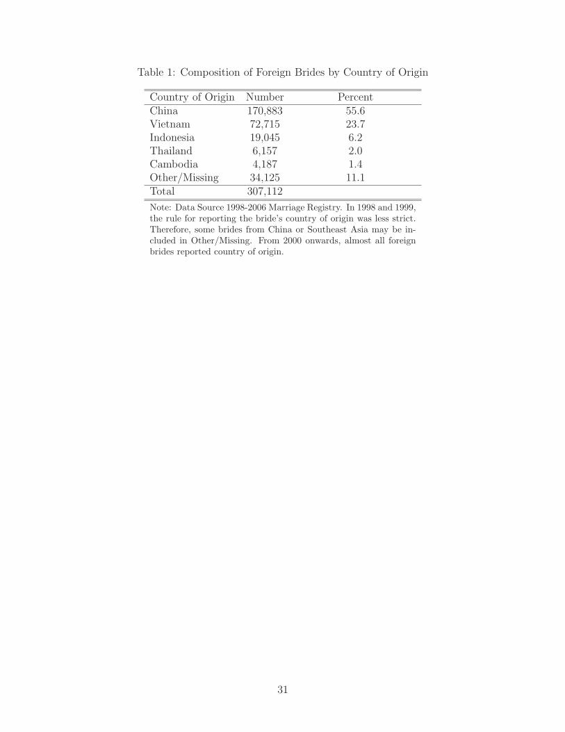
Table 1: Composition of Foreign Brides by Country of Origin

Country of Origin Number PercentChina 170,883 55.6Vietnam 72,715 23.7Indonesia 19,045 6.2Thailand 6,157 2.0Cambodia 4,187 1.4Other/Missing 34,125 11.1Total 307,112

Note: Data Source 1998-2006 Marriage Registry. In 1998 and 1999,the rule for reporting the bride’s country of origin was less strict.Therefore, some brides from China or Southeast Asia may be in-cluded in Other/Missing. From 2000 onwards, almost all foreignbrides reported country of origin.

31

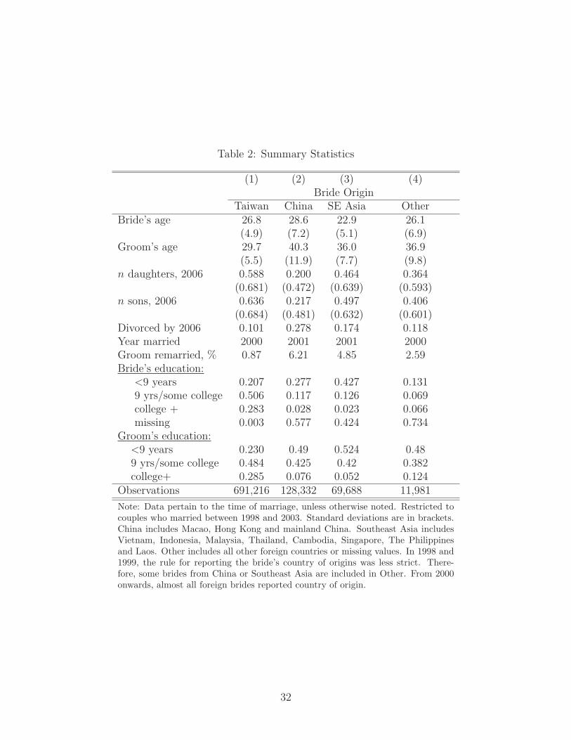
Table 2: Summary Statistics

(1) (2) (3) (4)Bride Origin

Taiwan China SE Asia OtherBride’s age 26.8 28.6 22.9 26.1

(4.9) (7.2) (5.1) (6.9)Groom’s age 29.7 40.3 36.0 36.9

(5.5) (11.9) (7.7) (9.8)n daughters, 2006 0.588 0.200 0.464 0.364

(0.681) (0.472) (0.639) (0.593)n sons, 2006 0.636 0.217 0.497 0.406

(0.684) (0.481) (0.632) (0.601)Divorced by 2006 0.101 0.278 0.174 0.118Year married 2000 2001 2001 2000Groom remarried, % 0.87 6.21 4.85 2.59Bride’s education:

<9 years 0.207 0.277 0.427 0.1319 yrs/some college 0.506 0.117 0.126 0.069college + 0.283 0.028 0.023 0.066missing 0.003 0.577 0.424 0.734

Groom’s education:<9 years 0.230 0.49 0.524 0.489 yrs/some college 0.484 0.425 0.42 0.382college+ 0.285 0.076 0.052 0.124

Observations 691,216 128,332 69,688 11,981

Note: Data pertain to the time of marriage, unless otherwise noted. Restricted tocouples who married between 1998 and 2003. Standard deviations are in brackets.China includes Macao, Hong Kong and mainland China. Southeast Asia includesVietnam, Indonesia, Malaysia, Thailand, Cambodia, Singapore, The Philippinesand Laos. Other includes all other foreign countries or missing values. In 1998 and1999, the rule for reporting the bride’s country of origins was less strict. There-fore, some brides from China or Southeast Asia are included in Other. From 2000onwards, almost all foreign brides reported country of origin.

32

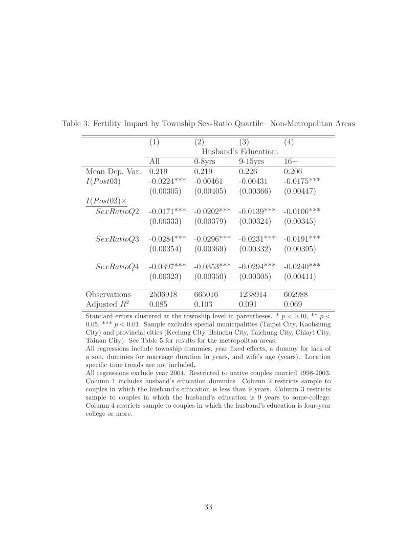
Table 3: Fertility Impact by Township Sex-Ratio Quartile– Non-Metropolitan Areas

(1) (2) (3) (4)Husband’s Education:

All 0-8yrs 9-15yrs 16+Mean Dep. Var. 0.219 0.219 0.226 0.206I(Post03) -0.0224*** -0.00461 -0.00431 -0.0175***

(0.00305) (0.00405) (0.00366) (0.00447)I(Post03)×

SexRatioQ2 -0.0171*** -0.0202*** -0.0139*** -0.0106***(0.00333) (0.00379) (0.00324) (0.00345)

SexRatioQ3 -0.0284*** -0.0296*** -0.0231*** -0.0191***(0.00354) (0.00369) (0.00332) (0.00395)

SexRatioQ4 -0.0397*** -0.0353*** -0.0294*** -0.0240***(0.00323) (0.00350) (0.00305) (0.00411)

Observations 2506918 665016 1238914 602988Adjusted R2 0.085 0.103 0.091 0.069

Standard errors clustered at the township level in parentheses. * p < 0.10, ** p <0.05, *** p < 0.01. Sample excludes special municipalities (Taipei City, KaohsiungCity) and provincial cities (Keelung City, Hsinchu City, Taichung City, Chiayi City,Tainan City). See Table 5 for results for the metropolitan areas.All regressions include township dummies, year fixed effects, a dummy for lack ofa son, dummies for marriage duration in years, and wife’s age (years). Locationspecific time trends are not included.All regressions exclude year 2004. Restricted to native couples married 1998-2003.Column 1 includes husband’s education dummies. Column 2 restricts sample tocouples in which the husband’s education is less than 9 years. Column 3 restrictssample to couples in which the husband’s education is 9 years to some-college.Column 4 restricts sample to couples in which the husband’s education is four-yearcollege or more.

33

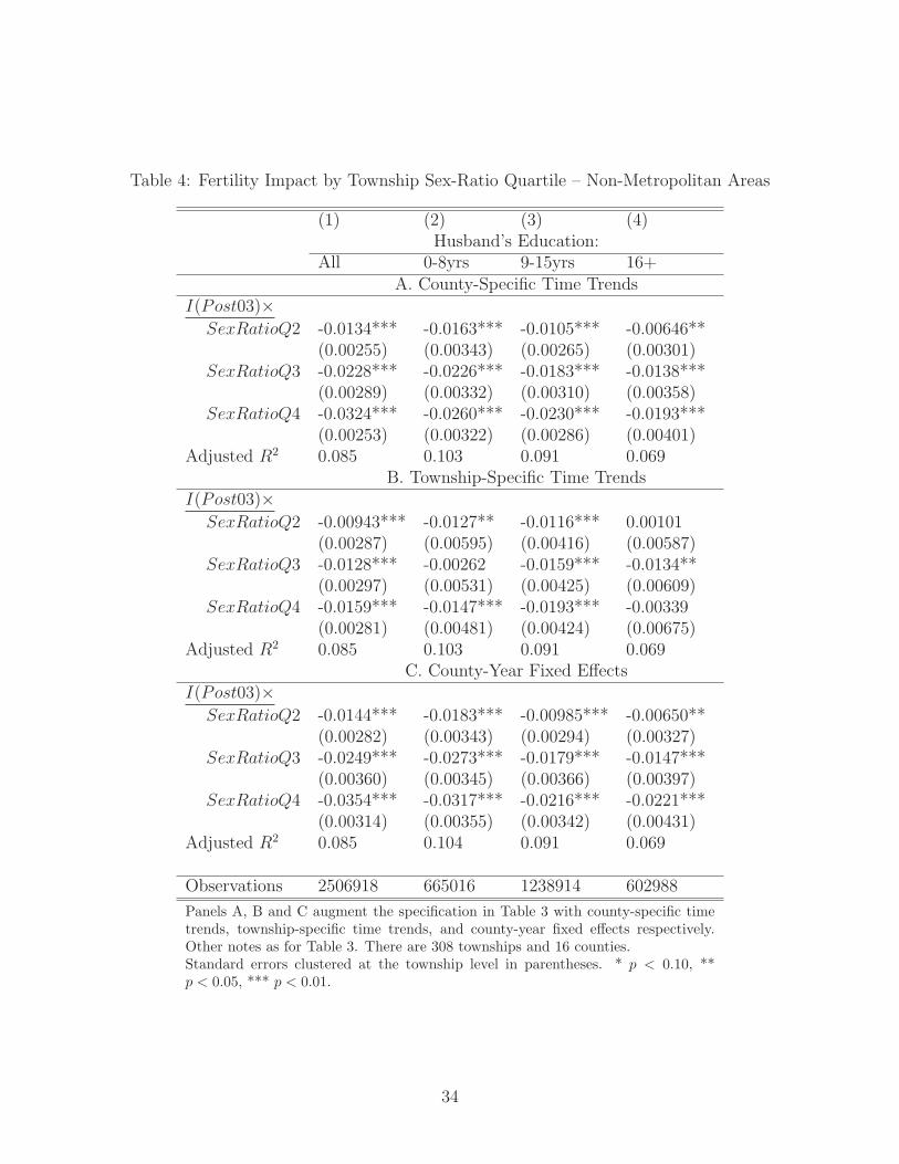
Table 4: Fertility Impact by Township Sex-Ratio Quartile – Non-Metropolitan Areas

(1) (2) (3) (4)Husband’s Education:

All 0-8yrs 9-15yrs 16+A. County-Specific Time Trends

I(Post03)×SexRatioQ2 -0.0134*** -0.0163*** -0.0105*** -0.00646**

(0.00255) (0.00343) (0.00265) (0.00301)SexRatioQ3 -0.0228*** -0.0226*** -0.0183*** -0.0138***

(0.00289) (0.00332) (0.00310) (0.00358)SexRatioQ4 -0.0324*** -0.0260*** -0.0230*** -0.0193***

(0.00253) (0.00322) (0.00286) (0.00401)Adjusted R2 0.085 0.103 0.091 0.069

B. Township-Specific Time TrendsI(Post03)×

SexRatioQ2 -0.00943*** -0.0127** -0.0116*** 0.00101(0.00287) (0.00595) (0.00416) (0.00587)

SexRatioQ3 -0.0128*** -0.00262 -0.0159*** -0.0134**(0.00297) (0.00531) (0.00425) (0.00609)

SexRatioQ4 -0.0159*** -0.0147*** -0.0193*** -0.00339(0.00281) (0.00481) (0.00424) (0.00675)

Adjusted R2 0.085 0.103 0.091 0.069C. County-Year Fixed Effects

I(Post03)×SexRatioQ2 -0.0144*** -0.0183*** -0.00985*** -0.00650**

(0.00282) (0.00343) (0.00294) (0.00327)SexRatioQ3 -0.0249*** -0.0273*** -0.0179*** -0.0147***

(0.00360) (0.00345) (0.00366) (0.00397)SexRatioQ4 -0.0354*** -0.0317*** -0.0216*** -0.0221***

(0.00314) (0.00355) (0.00342) (0.00431)Adjusted R2 0.085 0.104 0.091 0.069

Observations 2506918 665016 1238914 602988

Panels A, B and C augment the specification in Table 3 with county-specific timetrends, township-specific time trends, and county-year fixed effects respectively.Other notes as for Table 3. There are 308 townships and 16 counties.Standard errors clustered at the township level in parentheses. * p < 0.10, **p < 0.05, *** p < 0.01.

34

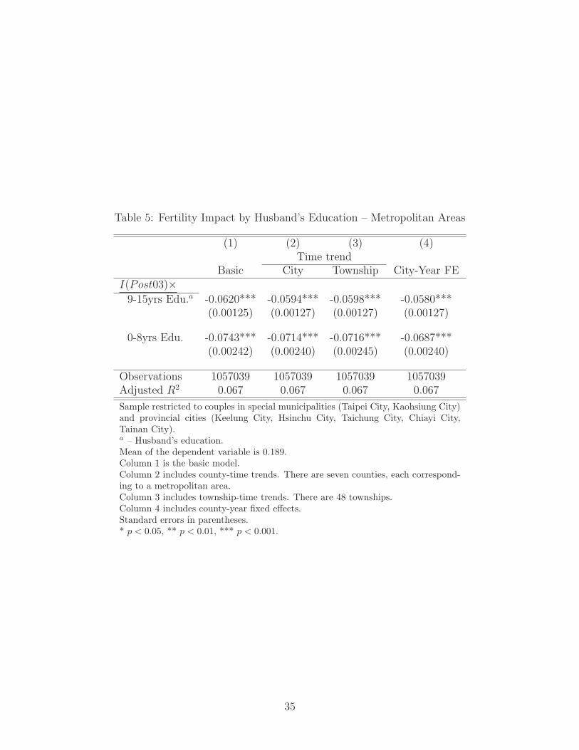
Table 5: Fertility Impact by Husband’s Education – Metropolitan Areas

(1) (2) (3) (4)Time trend

Basic City Township City-Year FEI(Post03)×9-15yrs Edu.a -0.0620*** -0.0594*** -0.0598*** -0.0580***

(0.00125) (0.00127) (0.00127) (0.00127)

0-8yrs Edu. -0.0743*** -0.0714*** -0.0716*** -0.0687***(0.00242) (0.00240) (0.00245) (0.00240)

Observations 1057039 1057039 1057039 1057039Adjusted R2 0.067 0.067 0.067 0.067

Sample restricted to couples in special municipalities (Taipei City, Kaohsiung City)and provincial cities (Keelung City, Hsinchu City, Taichung City, Chiayi City,Tainan City).a – Husband’s education.Mean of the dependent variable is 0.189.Column 1 is the basic model.Column 2 includes county-time trends. There are seven counties, each correspond-ing to a metropolitan area.Column 3 includes township-time trends. There are 48 townships.Column 4 includes county-year fixed effects.Standard errors in parentheses.* p < 0.05, ** p < 0.01, *** p < 0.001.

35

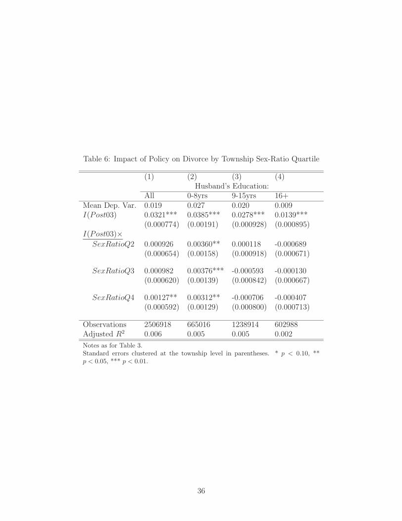
Table 6: Impact of Policy on Divorce by Township Sex-Ratio Quartile

(1) (2) (3) (4)Husband’s Education:

All 0-8yrs 9-15yrs 16+Mean Dep. Var. 0.019 0.027 0.020 0.009I(Post03) 0.0321*** 0.0385*** 0.0278*** 0.0139***

(0.000774) (0.00191) (0.000928) (0.000895)I(Post03)×

SexRatioQ2 0.000926 0.00360** 0.000118 -0.000689(0.000654) (0.00158) (0.000918) (0.000671)

SexRatioQ3 0.000982 0.00376*** -0.000593 -0.000130(0.000620) (0.00139) (0.000842) (0.000667)

SexRatioQ4 0.00127** 0.00312** -0.000706 -0.000407(0.000592) (0.00129) (0.000800) (0.000713)

Observations 2506918 665016 1238914 602988Adjusted R2 0.006 0.005 0.005 0.002

Notes as for Table 3.Standard errors clustered at the township level in parentheses. * p < 0.10, **p < 0.05, *** p < 0.01.

36

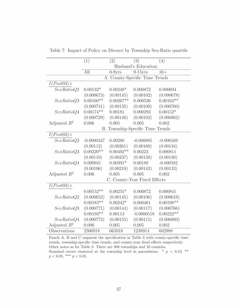
Table 7: Impact of Policy on Divorce by Township Sex-Ratio quartile

(1) (2) (3) (4)Husband’s Education:

All 0-8yrs 9-15yrs 16+A. County-Specific Time Trends

I(Post03)×SexRatioQ2 0.00132* 0.00248* 0.000872 0.000694

(0.000673) (0.00145) (0.00102) (0.000678)SexRatioQ3 0.00160** 0.00267** 0.000536 0.00163**

(0.000741) (0.00135) (0.00109) (0.000760)SexRatioQ4 0.00174** 0.00181 0.000293 0.00152*

(0.000729) (0.00140) (0.00102) (0.000862)Adjusted R2 0.006 0.005 0.005 0.002

B. Township-Specific Time TrendsI(Post03)×

SexRatioQ2 -0.0000347 0.00280 -0.000885 -0.000169(0.00112) (0.00261) (0.00160) (0.00134)

SexRatioQ3 0.00220** 0.00492** 0.00223 0.000811(0.00110) (0.00237) (0.00150) (0.00130)

SexRatioQ4 0.000941 0.00391* 0.00180 -0.000582(0.00106) (0.00210) (0.00142) (0.00133)

Adjusted R2 0.006 0.005 0.005 0.002C. County-Year Fixed Effects

I(Post03)×0.00152** 0.00255* 0.000872 0.000841

SexRatioQ2 (0.000652) (0.00145) (0.00106) (0.000616)0.00183** 0.00242* 0.000461 0.00198**

SexRatioQ3 (0.000771) (0.00144) (0.00117) (0.000766)0.00193** 0.00113 -0.0000518 0.00222**

SexRatioQ4 (0.000773) (0.00155) (0.00115) (0.000893)Adjusted R2 0.006 0.005 0.005 0.002Observations 2506918 665016 1238914 602988

Panels A, B and C augment the specification in Table 3 with county-specific timetrends, township-specific time trends, and county-year fixed effects respectively.Other notes as for Table 3. There are 308 townships and 16 counties.Standard errors clustered at the township level in parentheses. * p < 0.10, **p < 0.05, *** p < 0.01.

37

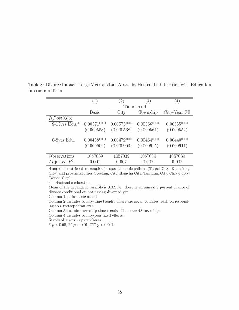
Table 8: Divorce Impact, Large Metropolitan Areas, by Husband’s Education with EducationInteraction Term

(1) (2) (3) (4)Time trend

Basic City Township City-Year FEI(Post03)×9-15yrs Edu.a 0.00571*** 0.00575*** 0.00566*** 0.00555***

(0.000558) (0.000568) (0.000561) (0.000552)

0-8yrs Edu. 0.00458*** 0.00472*** 0.00464*** 0.00440***(0.000902) (0.000903) (0.000915) (0.000911)

Observations 1057039 1057039 1057039 1057039Adjusted R2 0.007 0.007 0.007 0.007

Sample is restricted to couples in special municipalities (Taipei City, KaohsiungCity) and provincial cities (Keelung City, Hsinchu City, Taichung City, Chiayi City,Tainan City).a – Husband’s education.Mean of the dependent variable is 0.02, i.e., there is an annual 2-percent chance ofdivorce conditional on not having divorced yet.Column 1 is the basic model.Column 2 includes county-time trends. There are seven counties, each correspond-ing to a metropolitan area.Column 3 includes township-time trends. There are 48 townships.Column 4 includes county-year fixed effects.Standard errors in parentheses.* p < 0.05, ** p < 0.01, *** p < 0.001.

38

Tab

le9:

Impactof

Policyon

Intra-Hou

seholdDecisionMak

ingbySex-R

atio

Quartile

WifeDecides:

HeSays

SheSays

Spending

Savings

Children

Spending

Savings

Children

MeanDep.Var.

0.228

0.189

0.130

0.279

0.258

0.137

I(P

ost03)×

Sex

RatioQ

20.0293

0.0530***

0.00296

-0.0219

0.0624**

-0.00178

(0.0322)

(0.0107)

(0.0209)

(0.0385)

(0.0288)

(0.0161)

Sex

RatioQ

30.0308

0.0196

0.0238

-0.0176

0.0245

0.0182*

(0.0307)

(0.0129)

(0.0178)

(0.0174)

(0.0221)

(0.00989)

Sex

RatioQ

40.0741*

0.0678***

0.0565**

0.0549*

0.0729**

0.0255

(0.0405)

(0.0172)

(0.0221)

(0.0281)

(0.0263)

(0.0174)

Observations

12162

12162

11472

13835

13835

13147

Adjusted

R2

0.027

0.014

0.015

0.016

0.011

0.005

Standard

errors

inparentheses.*p<

0.10

,**

p<

0.05

,**

*p<

0.01.Outcomes

are

only

surveyed

in2002and2006.Allregressionsincludecounty

dummies,

asetofagedummies,

educationdummies,

adummyforem

ploymentstatus,

adummyindicatingwhether

theinterviewee

isthemain

earner.

Allregressionsareweightedusingsample

weight.

Sex

ratiosan

dthequartiles

aredefined

atthe

county

level

since

township

ofresiden

ceis

notavailable

inthedataset.

Restrictto

coupleswhogot

marriedbefore

2004.Columns1to

3restricted

tohusband’s

response.Column4to

6restricted

towife’sresponse.Columns1and4presentwhether

wifeis

themain

decision-m

aker

forexpenditure

decisions.

Columns2and5presentwhether

wifeis

themain

decision-m

aker

forsavingan

dasset

investmentdecisions.

Columns3and6presentwhether

wifeis

themain

decision-m

aker

forchild-

rearingdecisions.

39

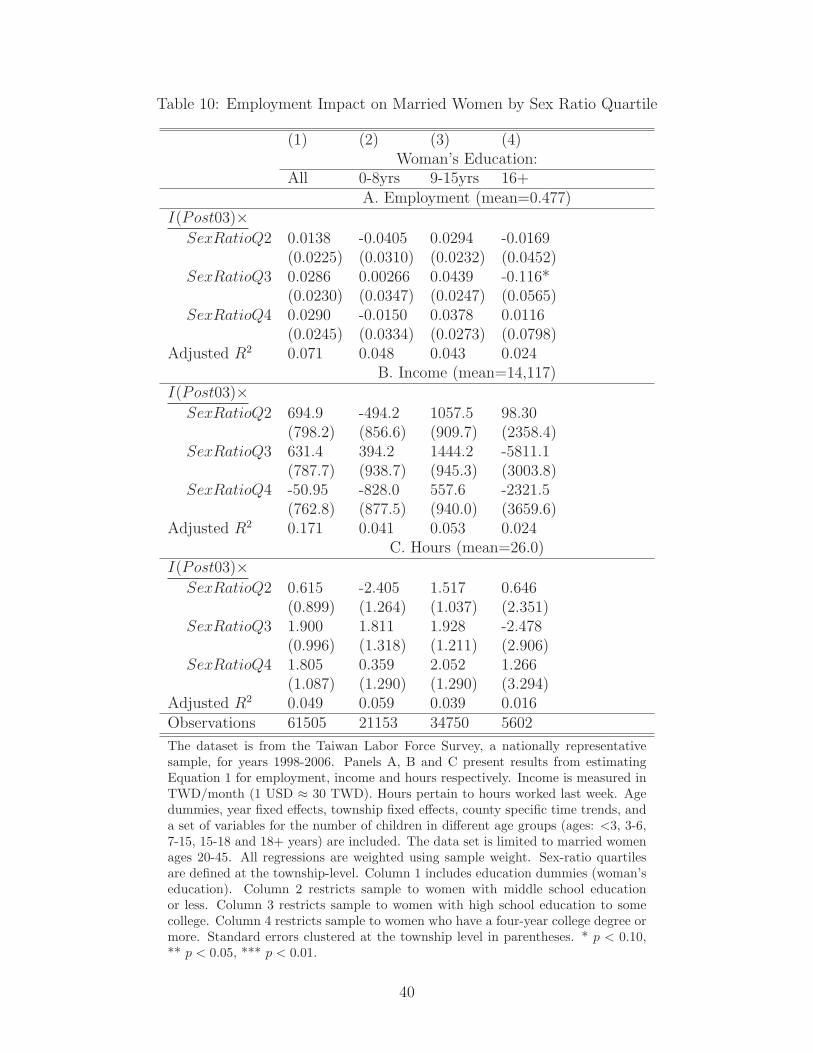
Table 10: Employment Impact on Married Women by Sex Ratio Quartile

(1) (2) (3) (4)Woman’s Education:

All 0-8yrs 9-15yrs 16+A. Employment (mean=0.477)

I(Post03)×SexRatioQ2 0.0138 -0.0405 0.0294 -0.0169

(0.0225) (0.0310) (0.0232) (0.0452)SexRatioQ3 0.0286 0.00266 0.0439 -0.116*

(0.0230) (0.0347) (0.0247) (0.0565)SexRatioQ4 0.0290 -0.0150 0.0378 0.0116

(0.0245) (0.0334) (0.0273) (0.0798)Adjusted R2 0.071 0.048 0.043 0.024

B. Income (mean=14,117)I(Post03)×

SexRatioQ2 694.9 -494.2 1057.5 98.30(798.2) (856.6) (909.7) (2358.4)

SexRatioQ3 631.4 394.2 1444.2 -5811.1(787.7) (938.7) (945.3) (3003.8)

SexRatioQ4 -50.95 -828.0 557.6 -2321.5(762.8) (877.5) (940.0) (3659.6)

Adjusted R2 0.171 0.041 0.053 0.024C. Hours (mean=26.0)

I(Post03)×SexRatioQ2 0.615 -2.405 1.517 0.646

(0.899) (1.264) (1.037) (2.351)SexRatioQ3 1.900 1.811 1.928 -2.478

(0.996) (1.318) (1.211) (2.906)SexRatioQ4 1.805 0.359 2.052 1.266

(1.087) (1.290) (1.290) (3.294)Adjusted R2 0.049 0.059 0.039 0.016Observations 61505 21153 34750 5602

The dataset is from the Taiwan Labor Force Survey, a nationally representativesample, for years 1998-2006. Panels A, B and C present results from estimatingEquation 1 for employment, income and hours respectively. Income is measured inTWD/month (1 USD ≈ 30 TWD). Hours pertain to hours worked last week. Agedummies, year fixed effects, township fixed effects, county specific time trends, anda set of variables for the number of children in different age groups (ages: <3, 3-6,7-15, 15-18 and 18+ years) are included. The data set is limited to married womenages 20-45. All regressions are weighted using sample weight. Sex-ratio quartilesare defined at the township-level. Column 1 includes education dummies (woman’seducation). Column 2 restricts sample to women with middle school educationor less. Column 3 restricts sample to women with high school education to somecollege. Column 4 restricts sample to women who have a four-year college degree ormore. Standard errors clustered at the township level in parentheses. * p < 0.10,** p < 0.05, *** p < 0.01.

40

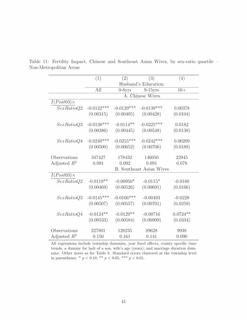
Table 11: Fertility Impact, Chinese and Southeast Asian Wives, by sex-ratio quartile –Non-Metropolitan Areas

(1) (2) (3) (4)Husband’s Education:

All 0-8yrs 9-15yrs 16+A. Chinese Wives

I(Post03)×SexRatioQ2 -0.0122*** -0.0129*** -0.0139*** 0.00378

(0.00315) (0.00405) (0.00428) (0.0104)

SexRatioQ3 -0.0138*** -0.0114** -0.0225*** 0.0182(0.00386) (0.00445) (0.00548) (0.0138)

SexRatioQ4 -0.0240*** -0.0255*** -0.0242*** 0.00209(0.00500) (0.00652) (0.00706) (0.0188)

Observations 347427 178432 146050 22945Adjusted R2 0.091 0.092 0.091 0.078

B. Southeast Asian WivesI(Post03)×

SexRatioQ2 -0.0119** -0.00950* -0.0115* -0.0180(0.00469) (0.00526) (0.00691) (0.0166)

SexRatioQ3 -0.0145*** -0.0166*** -0.00493 -0.0228(0.00507) (0.00557) (0.00701) (0.0259)

SexRatioQ4 -0.0124** -0.0129** -0.00716 0.0724**(0.00533) (0.00584) (0.00909) (0.0334)

Observations 227801 128235 89628 9938Adjusted R2 0.150 0.161 0.141 0.090

All regressions include township dummies, year fixed effects, county specific timetrends, a dummy for lack of a son, wife’s age (years), and marriage duration dum-mies. Other notes as for Table 3. Standard errors clustered at the township levelin parentheses. * p < 0.10, ** p < 0.05, *** p < 0.01.

41

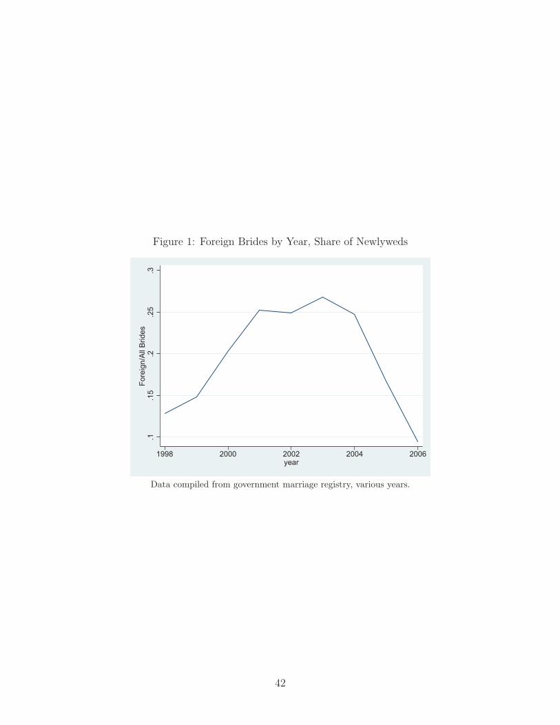
Figure 1: Foreign Brides by Year, Share of Newlyweds

.1.1

5.2

.25

.3Fo

reig

n/A

ll B

rides

1998 2000 2002 2004 2006year

Data compiled from government marriage registry, various years.

42

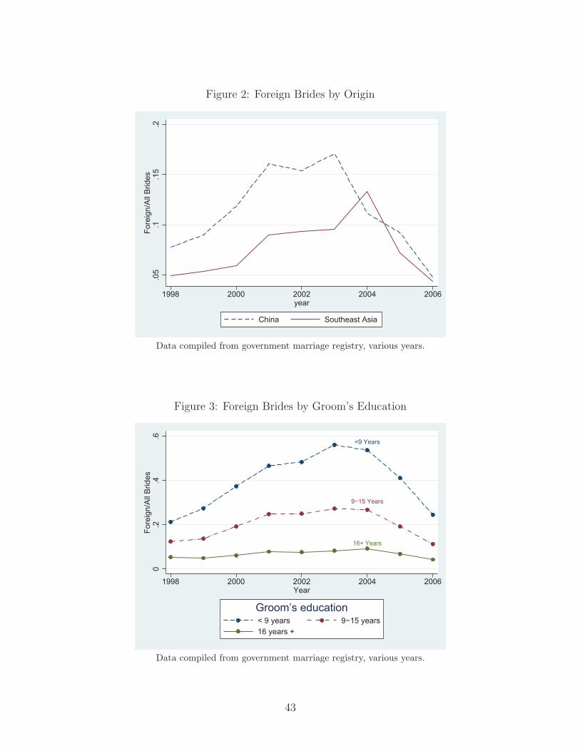
Figure 2: Foreign Brides by Origin

.05

.1.1

5.2

Fore

ign/

All

Brid

es

1998 2000 2002 2004 2006year

China Southeast Asia

Data compiled from government marriage registry, various years.

Figure 3: Foreign Brides by Groom’s Education

<9 Years

9−15 Years

16+ Years

0.2

.4.6

Fore

ign/

All

Brid

es

1998 2000 2002 2004 2006Year

< 9 years 9−15 years16 years +

Groom’s education

Data compiled from government marriage registry, various years.

43

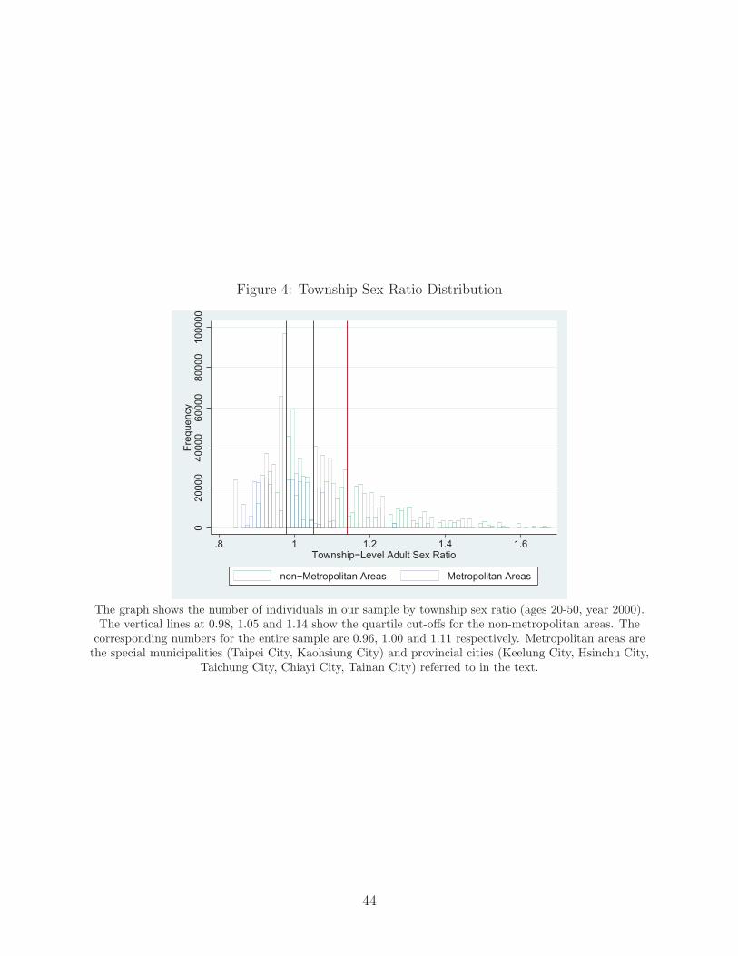
Figure 4: Township Sex Ratio Distribution

020

000

4000

060

000

8000

010

0000

Freq

uenc

y

.8 1 1.2 1.4 1.6Township−Level Adult Sex Ratio

non−Metropolitan Areas Metropolitan Areas

The graph shows the number of individuals in our sample by township sex ratio (ages 20-50, year 2000).The vertical lines at 0.98, 1.05 and 1.14 show the quartile cut-offs for the non-metropolitan areas. Thecorresponding numbers for the entire sample are 0.96, 1.00 and 1.11 respectively. Metropolitan areas arethe special municipalities (Taipei City, Kaohsiung City) and provincial cities (Keelung City, Hsinchu City,

Taichung City, Chiayi City, Tainan City) referred to in the text.

44

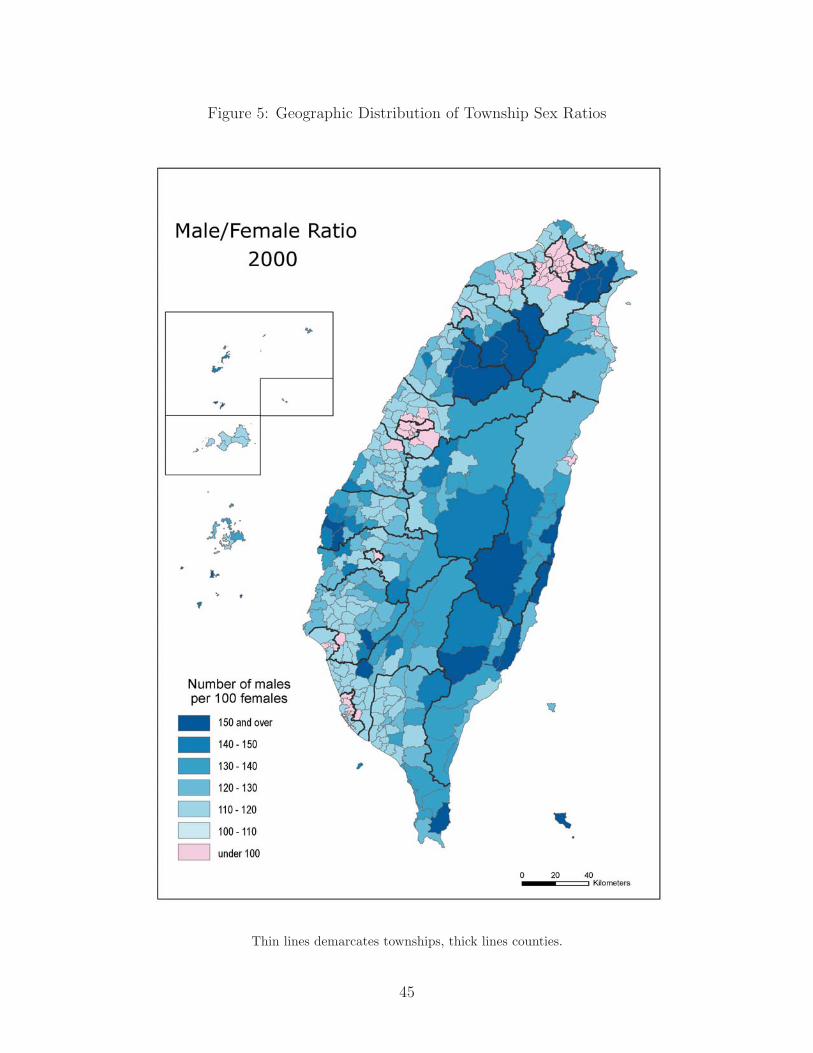
Figure 5: Geographic Distribution of Township Sex Ratios

Thin lines demarcates townships, thick lines counties.

45

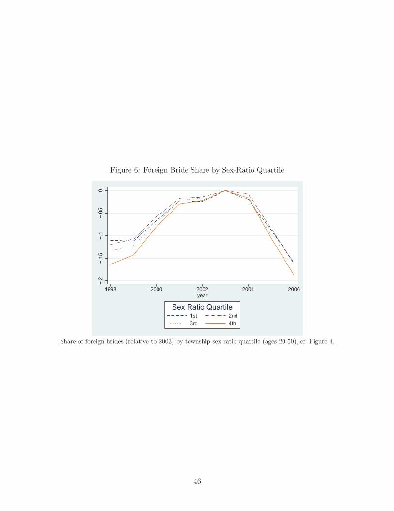
Figure 6: Foreign Bride Share by Sex-Ratio Quartile

−.2

−.15

−.1

−.05

0

1998 2000 2002 2004 2006year

1st 2nd3rd 4th

Sex Ratio Quartile

Share of foreign brides (relative to 2003) by township sex-ratio quartile (ages 20-50), cf. Figure 4.

46

Figure

7:Geograp

hic

Distribution

ofForeign

BrideShare1998-2006–Fmap

1998

1999

2000

2001

2002

2003

2004

2005

2006

Thin

lines

dem

arcatestownships,

thicklines

counties.

47

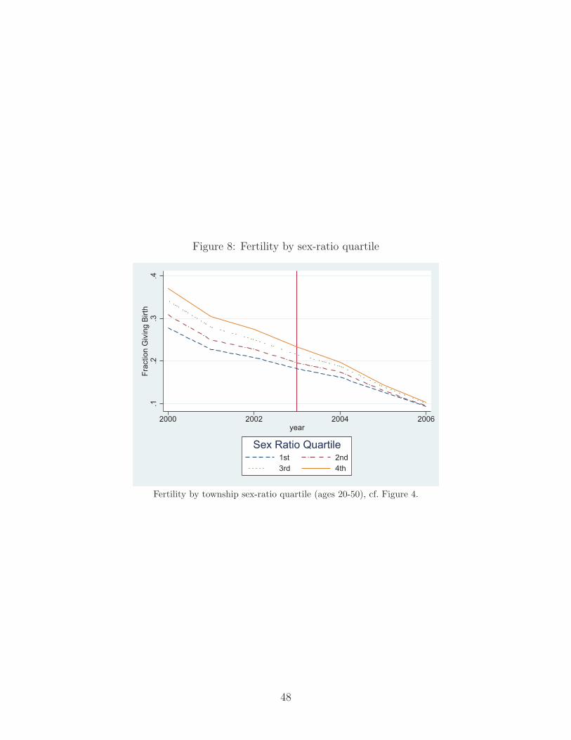
Figure 8: Fertility by sex-ratio quartile

.1.2

.3.4

Frac

tion

Giv

ing

Birt

h

2000 2002 2004 2006year

1st 2nd3rd 4th

Sex Ratio Quartile

Fertility by township sex-ratio quartile (ages 20-50), cf. Figure 4.

48

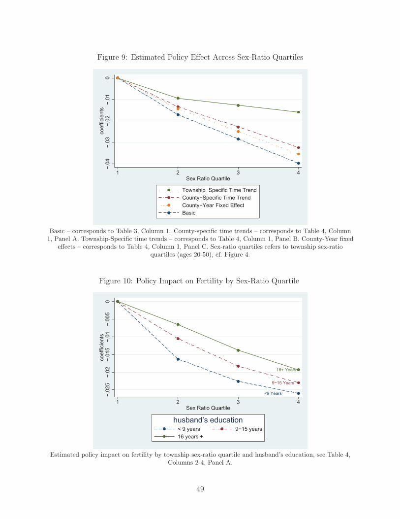
Figure 9: Estimated Policy Effect Across Sex-Ratio Quartiles

−.04

−.03

−.02

−.01

0co

effic

ient

s

1 2 3 4Sex Ratio Quartile

Township−Specific Time TrendCounty−Specific Time TrendCounty−Year Fixed EffectBasic

Basic – corresponds to Table 3, Column 1. County-specific time trends – corresponds to Table 4, Column1, Panel A. Township-Specific time trends – corresponds to Table 4, Column 1, Panel B. County-Year fixed

effects – corresponds to Table 4, Column 1, Panel C. Sex-ratio quartiles refers to township sex-ratioquartiles (ages 20-50), cf. Figure 4.

Figure 10: Policy Impact on Fertility by Sex-Ratio Quartile

<9 Years

9−15 Years

16+ Years

−.02

5−.

02−.

015

−.01

−.00

50

coef

ficie

nts

1 2 3 4Sex Ratio Quartile

< 9 years 9−15 years16 years +

husband’s education

Estimated policy impact on fertility by township sex-ratio quartile and husband’s education, see Table 4,Columns 2-4, Panel A.

49

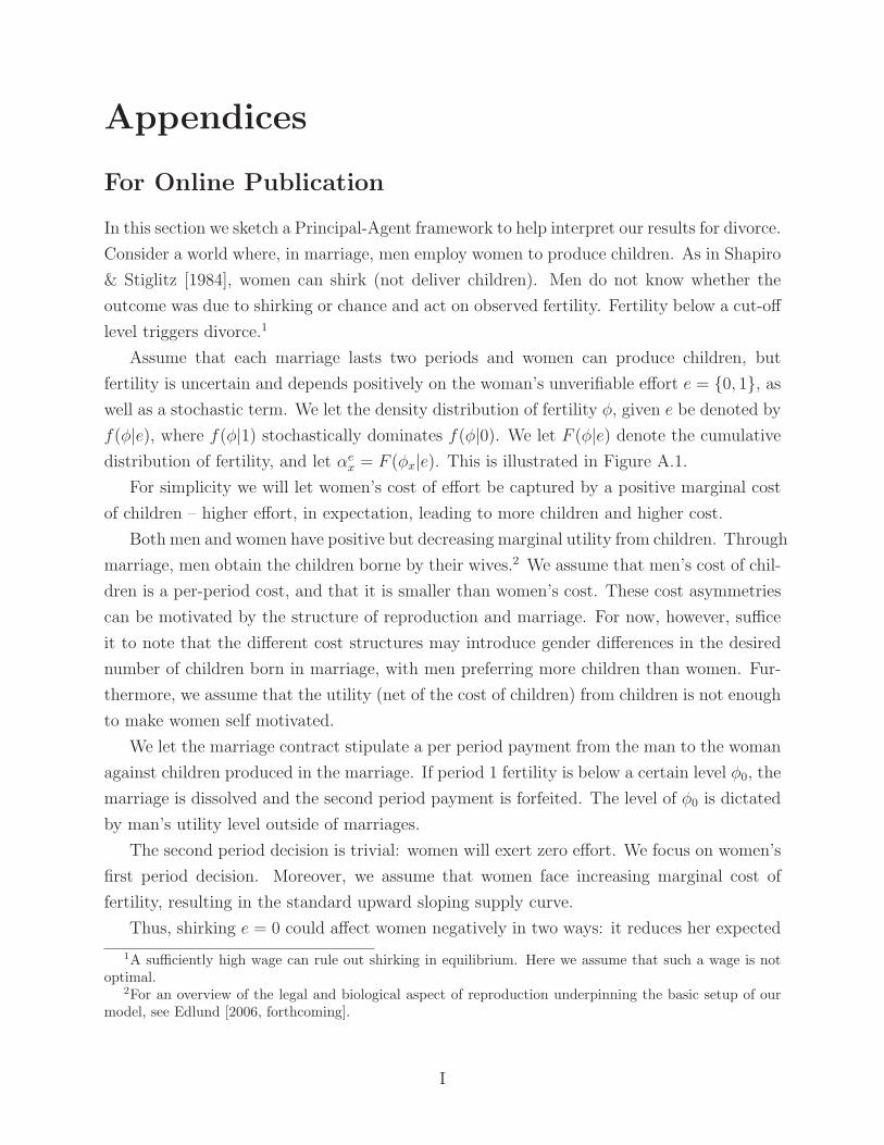
Appendices

For Online Publication

In this section we sketch a Principal-Agent framework to help interpret our results for divorce.

Consider a world where, in marriage, men employ women to produce children. As in Shapiro

& Stiglitz [1984], women can shirk (not deliver children). Men do not know whether the

outcome was due to shirking or chance and act on observed fertility. Fertility below a cut-off

level triggers divorce.1

Assume that each marriage lasts two periods and women can produce children, but

fertility is uncertain and depends positively on the woman’s unverifiable effort e = {0, 1}, aswell as a stochastic term. We let the density distribution of fertility φ, given e be denoted by

f(φ|e), where f(φ|1) stochastically dominates f(φ|0). We let F (φ|e) denote the cumulative

distribution of fertility, and let αex = F (φx|e). This is illustrated in Figure A.1.

For simplicity we will let women’s cost of effort be captured by a positive marginal cost

of children – higher effort, in expectation, leading to more children and higher cost.

Both men and women have positive but decreasing marginal utility from children. Through

marriage, men obtain the children borne by their wives.2 We assume that men’s cost of chil-

dren is a per-period cost, and that it is smaller than women’s cost. These cost asymmetries

can be motivated by the structure of reproduction and marriage. For now, however, suffice

it to note that the different cost structures may introduce gender differences in the desired

number of children born in marriage, with men preferring more children than women. Fur-

thermore, we assume that the utility (net of the cost of children) from children is not enough

to make women self motivated.

We let the marriage contract stipulate a per period payment from the man to the woman

against children produced in the marriage. If period 1 fertility is below a certain level φ0, the

marriage is dissolved and the second period payment is forfeited. The level of φ0 is dictated

by man’s utility level outside of marriages.

The second period decision is trivial: women will exert zero effort. We focus on women’s

first period decision. Moreover, we assume that women face increasing marginal cost of

fertility, resulting in the standard upward sloping supply curve.

Thus, shirking e = 0 could affect women negatively in two ways: it reduces her expected

1A sufficiently high wage can rule out shirking in equilibrium. Here we assume that such a wage is notoptimal.

2For an overview of the legal and biological aspect of reproduction underpinning the basic setup of ourmodel, see Edlund [2006, forthcoming].

I

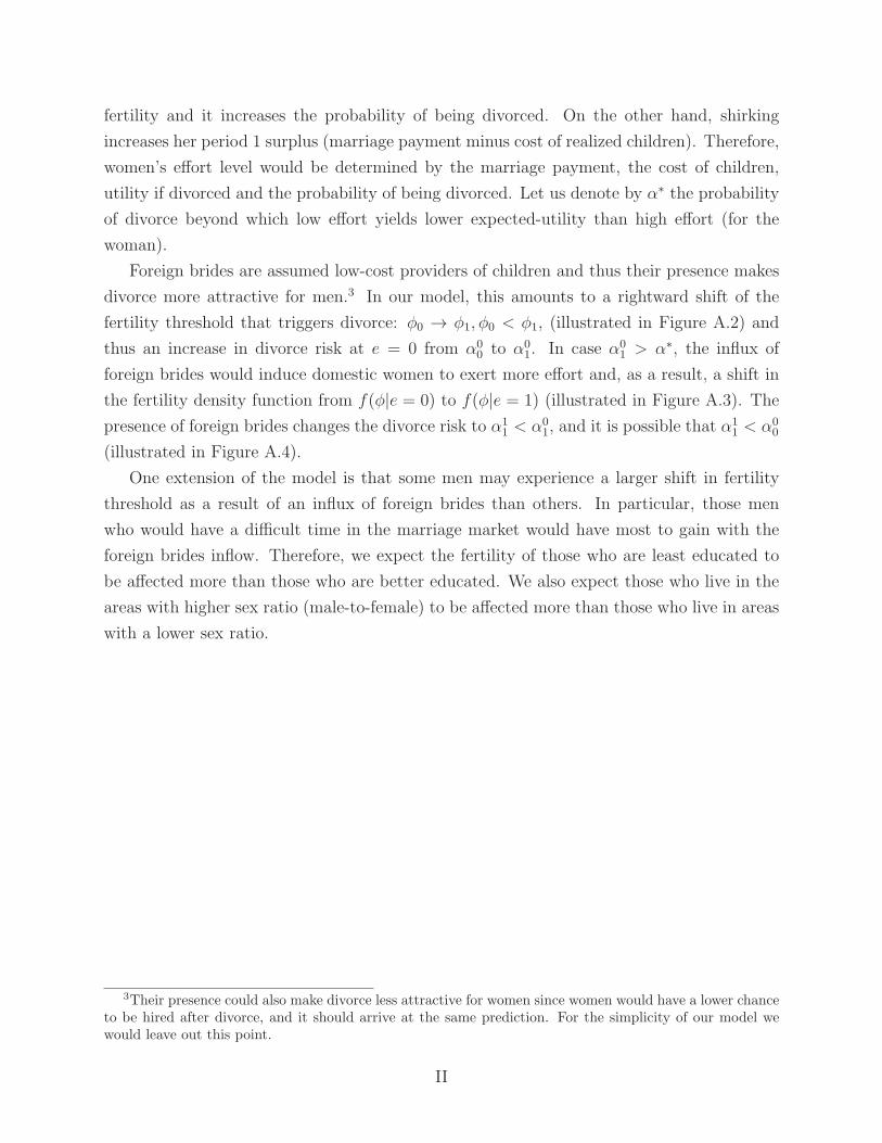
fertility and it increases the probability of being divorced. On the other hand, shirking

increases her period 1 surplus (marriage payment minus cost of realized children). Therefore,

women’s effort level would be determined by the marriage payment, the cost of children,

utility if divorced and the probability of being divorced. Let us denote by α∗ the probability

of divorce beyond which low effort yields lower expected-utility than high effort (for the

woman).

Foreign brides are assumed low-cost providers of children and thus their presence makes

divorce more attractive for men.3 In our model, this amounts to a rightward shift of the

fertility threshold that triggers divorce: φ0 → φ1, φ0 < φ1, (illustrated in Figure A.2) and

thus an increase in divorce risk at e = 0 from α00 to α0

1. In case α01 > α∗, the influx of

foreign brides would induce domestic women to exert more effort and, as a result, a shift in

the fertility density function from f(φ|e = 0) to f(φ|e = 1) (illustrated in Figure A.3). The

presence of foreign brides changes the divorce risk to α11 < α0

1, and it is possible that α11 < α0

0

(illustrated in Figure A.4).

One extension of the model is that some men may experience a larger shift in fertility

threshold as a result of an influx of foreign brides than others. In particular, those men

who would have a difficult time in the marriage market would have most to gain with the

foreign brides inflow. Therefore, we expect the fertility of those who are least educated to

be affected more than those who are better educated. We also expect those who live in the

areas with higher sex ratio (male-to-female) to be affected more than those who live in areas

with a lower sex ratio.

3Their presence could also make divorce less attractive for women since women would have a lower chanceto be hired after divorce, and it should arrive at the same prediction. For the simplicity of our model wewould leave out this point.

II

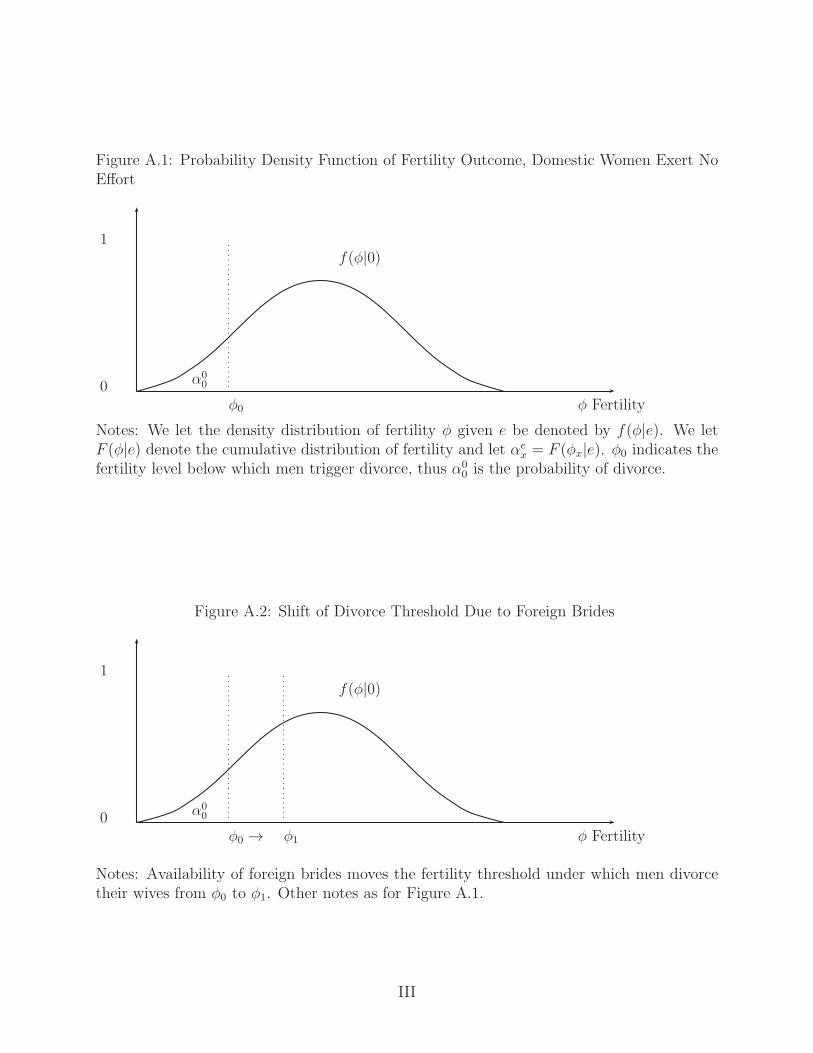
Figure A.1: Probability Density Function of Fertility Outcome, Domestic Women Exert NoEffort

φ0 φ Fertility

f(φ|0)

0

1

α00

Notes: We let the density distribution of fertility φ given e be denoted by f(φ|e). We letF (φ|e) denote the cumulative distribution of fertility and let αe

x = F (φx|e). φ0 indicates thefertility level below which men trigger divorce, thus α0

0 is the probability of divorce.

Figure A.2: Shift of Divorce Threshold Due to Foreign Brides

φ0 → φ Fertility

f(φ|0)

0

1

α00

φ1

Notes: Availability of foreign brides moves the fertility threshold under which men divorcetheir wives from φ0 to φ1. Other notes as for Figure A.1.

III

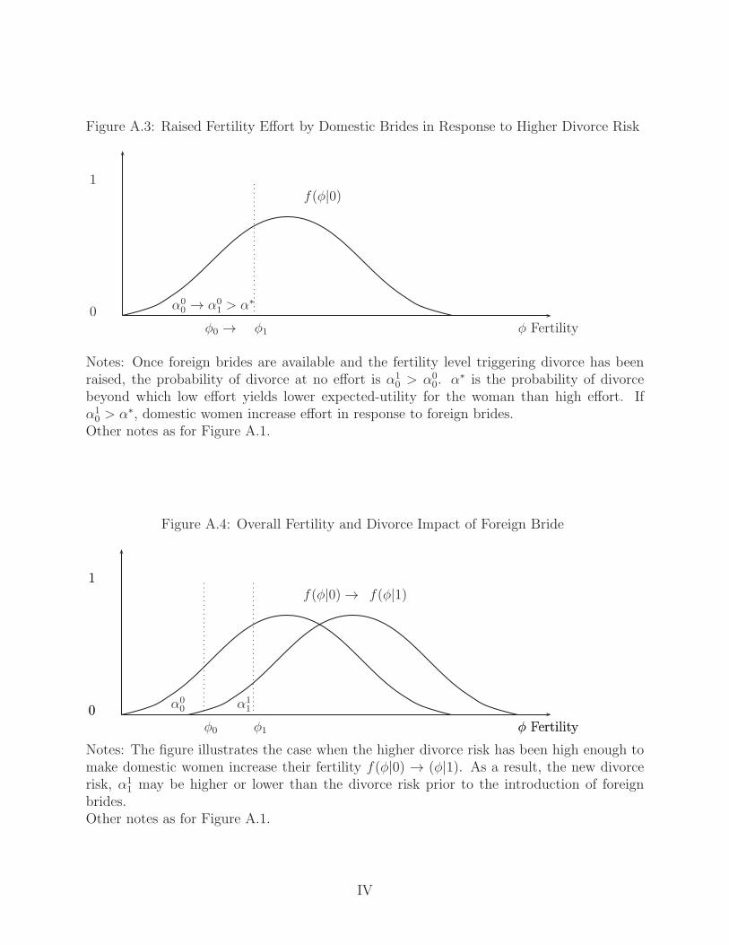
Figure A.3: Raised Fertility Effort by Domestic Brides in Response to Higher Divorce Risk

φ0 → φ Fertility

f(φ|0)

0

1

α00 → α0

1 > α∗

φ1

Notes: Once foreign brides are available and the fertility level triggering divorce has beenraised, the probability of divorce at no effort is α1

0 > α00. α∗ is the probability of divorce

beyond which low effort yields lower expected-utility for the woman than high effort. Ifα10 > α∗, domestic women increase effort in response to foreign brides.

Other notes as for Figure A.1.

Figure A.4: Overall Fertility and Divorce Impact of Foreign Bride

φ0 φ Fertility

f(φ|0) →

0

1

α00

φ1 φ Fertility

f(φ|1)

0

1

α11

Notes: The figure illustrates the case when the higher divorce risk has been high enough tomake domestic women increase their fertility f(φ|0) → (φ|1). As a result, the new divorcerisk, α1

1 may be higher or lower than the divorce risk prior to the introduction of foreignbrides.Other notes as for Figure A.1.

IV

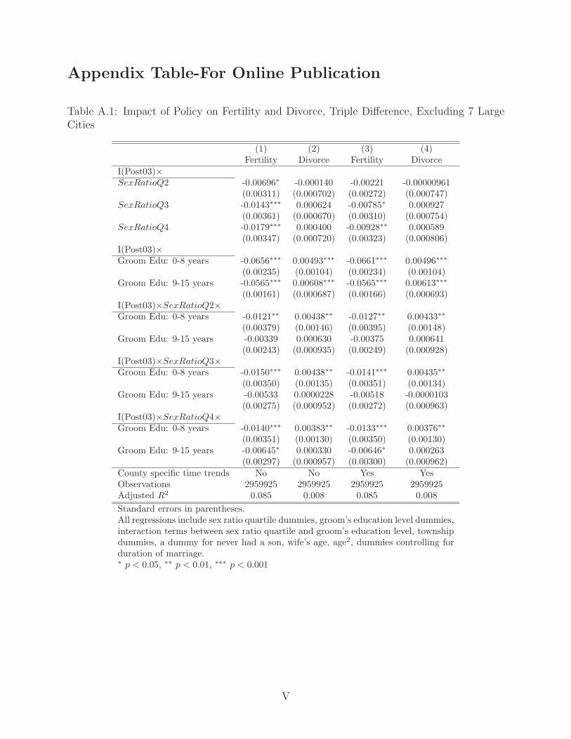
Appendix Table-For Online Publication

Table A.1: Impact of Policy on Fertility and Divorce, Triple Difference, Excluding 7 LargeCities

(1) (2) (3) (4)Fertility Divorce Fertility Divorce

I(Post03)×SexRatioQ2 -0.00696∗ -0.000140 -0.00221 -0.00000961

(0.00311) (0.000702) (0.00272) (0.000747)SexRatioQ3 -0.0143∗∗∗ 0.000624 -0.00785∗ 0.000927

(0.00361) (0.000670) (0.00310) (0.000754)SexRatioQ4 -0.0179∗∗∗ 0.000400 -0.00928∗∗ 0.000589

(0.00347) (0.000720) (0.00323) (0.000806)I(Post03)×Groom Edu: 0-8 years -0.0656∗∗∗ 0.00493∗∗∗ -0.0661∗∗∗ 0.00496∗∗∗

(0.00235) (0.00104) (0.00234) (0.00104)Groom Edu: 9-15 years -0.0565∗∗∗ 0.00608∗∗∗ -0.0565∗∗∗ 0.00613∗∗∗

(0.00161) (0.000687) (0.00166) (0.000693)I(Post03)×SexRatioQ2×Groom Edu: 0-8 years -0.0121∗∗ 0.00438∗∗ -0.0127∗∗ 0.00433∗∗

(0.00379) (0.00146) (0.00395) (0.00148)Groom Edu: 9-15 years -0.00339 0.000630 -0.00375 0.000641

(0.00243) (0.000935) (0.00249) (0.000928)I(Post03)×SexRatioQ3×Groom Edu: 0-8 years -0.0150∗∗∗ 0.00438∗∗ -0.0141∗∗∗ 0.00435∗∗

(0.00350) (0.00135) (0.00351) (0.00134)Groom Edu: 9-15 years -0.00533 0.0000228 -0.00518 -0.0000103

(0.00275) (0.000952) (0.00272) (0.000963)I(Post03)×SexRatioQ4×Groom Edu: 0-8 years -0.0140∗∗∗ 0.00383∗∗ -0.0133∗∗∗ 0.00376∗∗

(0.00351) (0.00130) (0.00350) (0.00130)Groom Edu: 9-15 years -0.00645∗ 0.000330 -0.00646∗ 0.000263

(0.00297) (0.000957) (0.00300) (0.000962)County specific time trends No No Yes YesObservations 2959925 2959925 2959925 2959925Adjusted R2 0.085 0.008 0.085 0.008

Standard errors in parentheses.All regressions include sex ratio quartile dummies, groom’s education level dummies,interaction terms between sex ratio quartile and groom’s education level, townshipdummies, a dummy for never had a son, wife’s age, age2, dummies controlling forduration of marriage.∗ p < 0.05, ∗∗ p < 0.01, ∗∗∗ p < 0.001

V