www.elsevier.com/locate/yjbin

Journal of Biomedical Informatics 36 (2003) 389–399

Methodological Review

Bayesian networks for knowledge discovery in large datasets:basics for nurse researchers

Sun-Mi Leea,* and Patricia A. Abbottb

a School of Nursing, University of Maryland at Baltimore, 655 W. Lombard, Baltimore, MD, USAb School of Nursing, Johns Hopkins University, 525 North Wolfe Street, Baltimore, MD, USA

Received 18 March 2003

Abstract

The growth of nursing databases necessitates new approaches to data analyses. These databases, which are known to be massive

and multidimensional, easily exceed the capabilities of both human cognition and traditional analytical approaches. One innovative

approach, knowledge discovery in large databases (KDD), allows investigators to analyze very large data sets more comprehensively

in an automatic or a semi-automatic manner. Among KDD techniques, Bayesian networks, a state-of-the art representation of

probabilistic knowledge by a graphical diagram, has emerged in recent years as essential for pattern recognition and classification in

the healthcare field. Unlike some data mining techniques, Bayesian networks allow investigators to combine domain knowledge with

statistical data, enabling nurse researchers to incorporate clinical and theoretical knowledge into the process of knowledge discovery

in large datasets. This tailored discussion presents the basic concepts of Bayesian networks and their use as knowledge discovery

tools for nurse researchers.

� 2003 Elsevier Inc. All rights reserved.

Keywords: Bayesian network; Data mining; Knowledge discovery; Nursing research

1. Background

In today�s health care environment, large clinical and

administration databases have grown as hospital infor-

mation systems become more commonplace. The de-

velopment of standardized nursing terminologies used

to document nursing diagnoses, nursing interventions,

nursing outcomes, and nursing goals in electronic sys-

tems contributes to the growth of such data collections.The challenge facing nursing researchers is how effec-

tively and efficiently knowledge can be extracted from

the large collections of valuable nursing/healthcare data

that are generated. Knowledge discovery in large data-

bases (KDD) allows investigators to assess very large

data more comprehensively [1]. Abbott [2] defines KDD

in healthcare as the process of ‘‘the melding of human

expertise with statistical and machine learning tech-

* Corresponding author. Fax: 1-410-706-0190.

E-mail address: Sun-mi@son.umaryland.edu (S.-M. Lee).

1532-0464/$ - see front matter � 2003 Elsevier Inc. All rights reserved.

doi:10.1016/j.jbi.2003.09.022

niques to identify features, patterns, and underlyingrules in large collections of health care data’’ (p. 142).

KDD is a multi-step process that makes use of data

manipulation and mining methods. To uncover novel,

interesting, and useful knowledge in databases, investi-

gators use data mining techniques to transform over-

whelming volumes of data through the discovery of

associations or patterns, segmentation (or clustering) of

records based on the similarity between variables andthe values, or creation of predictive (or classification)

models [3]. Data mining approaches have been used for

an extended period of time in the financial industry, but

they are relatively new in the medical domain, and their

use in nursing is quite rare.

In the healthcare/medical domain, commonly used

data mining tools for knowledge discovery include

neural networks, decision trees, and classification andregression trees (CART). Neural networks are known as

connectionist, meaning that they parallel distributed

processing models or artificial intelligence and are

designed to mimic the parallel processing ability of

the human brain [4]. Decision trees create a binary tree

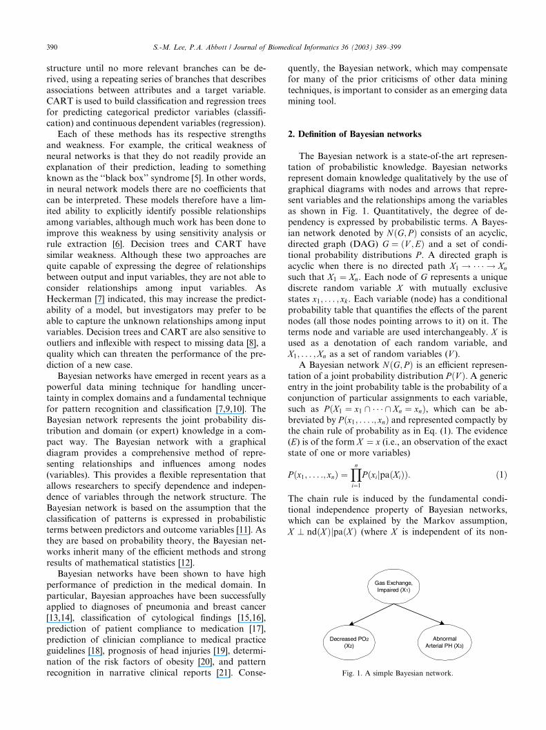
Fig. 1. A simple Bayesian network.

390 S.-M. Lee, P.A. Abbott / Journal of Biomedical Informatics 36 (2003) 389–399

structure until no more relevant branches can be de-rived, using a repeating series of branches that describes

associations between attributes and a target variable.

CART is used to build classification and regression trees

for predicting categorical predictor variables (classifi-

cation) and continuous dependent variables (regression).

Each of these methods has its respective strengths

and weakness. For example, the critical weakness of

neural networks is that they do not readily provide anexplanation of their prediction, leading to something

known as the ‘‘black box’’ syndrome [5]. In other words,

in neural network models there are no coefficients that

can be interpreted. These models therefore have a lim-

ited ability to explicitly identify possible relationships

among variables, although much work has been done to

improve this weakness by using sensitivity analysis or

rule extraction [6]. Decision trees and CART havesimilar weakness. Although these two approaches are

quite capable of expressing the degree of relationships

between output and input variables, they are not able to

consider relationships among input variables. As

Heckerman [7] indicated, this may increase the predict-

ability of a model, but investigators may prefer to be

able to capture the unknown relationships among input

variables. Decision trees and CART are also sensitive tooutliers and inflexible with respect to missing data [8], a

quality which can threaten the performance of the pre-

diction of a new case.

Bayesian networks have emerged in recent years as a

powerful data mining technique for handling uncer-

tainty in complex domains and a fundamental technique

for pattern recognition and classification [7,9,10]. The

Bayesian network represents the joint probability dis-tribution and domain (or expert) knowledge in a com-

pact way. The Bayesian network with a graphical

diagram provides a comprehensive method of repre-

senting relationships and influences among nodes

(variables). This provides a flexible representation that

allows researchers to specify dependence and indepen-

dence of variables through the network structure. The

Bayesian network is based on the assumption that theclassification of patterns is expressed in probabilistic

terms between predictors and outcome variables [11]. As

they are based on probability theory, the Bayesian net-

works inherit many of the efficient methods and strong

results of mathematical statistics [12].

Bayesian networks have been shown to have high

performance of prediction in the medical domain. In

particular, Bayesian approaches have been successfullyapplied to diagnoses of pneumonia and breast cancer

[13,14], classification of cytological findings [15,16],

prediction of patient compliance to medication [17],

prediction of clinician compliance to medical practice

guidelines [18], prognosis of head injuries [19], determi-

nation of the risk factors of obesity [20], and pattern

recognition in narrative clinical reports [21]. Conse-

quently, the Bayesian network, which may compensatefor many of the prior criticisms of other data mining

techniques, is important to consider as an emerging data

mining tool.

2. Definition of Bayesian networks

The Bayesian network is a state-of-the art represen-tation of probabilistic knowledge. Bayesian networks

represent domain knowledge qualitatively by the use of

graphical diagrams with nodes and arrows that repre-

sent variables and the relationships among the variables

as shown in Fig. 1. Quantitatively, the degree of de-

pendency is expressed by probabilistic terms. A Bayes-

ian network denoted by NðG; P Þ consists of an acyclic,

directed graph (DAG) G ¼ ðV ;EÞ and a set of condi-tional probability distributions P . A directed graph is

acyclic when there is no directed path X1 ! � � � ! Xn

such that X1 ¼ Xn. Each node of G represents a unique

discrete random variable X with mutually exclusive

states x1; . . . ; xk. Each variable (node) has a conditional

probability table that quantifies the effects of the parent

nodes (all those nodes pointing arrows to it) on it. The

terms node and variable are used interchangeably. X isused as a denotation of each random variable, and

X1; . . . ;Xn as a set of random variables (V ).A Bayesian network NðG; P Þ is an efficient represen-

tation of a joint probability distribution P ðV Þ. A generic

entry in the joint probability table is the probability of a

conjunction of particular assignments to each variable,

such as P ðX1 ¼ x1 \ � � � \ Xn ¼ xnÞ, which can be ab-

breviated by Pðx1; . . . :; xnÞ and represented compactly bythe chain rule of probability as in Eq. (1). The evidence

(E) is of the form X ¼ x (i.e., an observation of the exact

state of one or more variables)

P ðx1; . . . :; xnÞ ¼Yn

i¼1P ðxijpaðXiÞÞ: ð1Þ

The chain rule is induced by the fundamental condi-

tional independence property of Bayesian networks,

which can be explained by the Markov assumption,

X ? ndðX ÞjpaðX Þ (where X is independent of its non-

S.-M. Lee, P.A. Abbott / Journal of Biomedical Informatics 36 (2003) 389–399 391

descendents ðndðX ÞÞ given the parents paðX Þ). This as-sumption discussed in detail in Section 6.

3. Advantages of Bayesian network as data mining tool

Although a few disadvantages exist, such as lack of

commercially available Bayesian network learning al-

gorithms or computational complexity, several signifi-cant advantages in the process employing Bayesian

networks can be argued [7,8,22]. First, Bayesian net-

works allow investigators to use their domain expert

knowledge in the discovery process, while other tech-

niques rely primarily on coded data to extract

knowledge. Second, Bayesian network models can be

more easily understood than many of the other tech-

niques via the use of nodes and arrows. These repre-sent the variables of interest and the relationships of

variables, respectively. Researchers can easily encode

domain expert knowledge through the use of these

graphical diagrams, and thus more easily understand

and interpret the output of the Bayesian network. In

addition, Bayesian network algorithms capitalize on

this encoded knowledge to increase their efficiency in

modeling process and accuracy in its predictive per-formance.

Bayesian networks are also superior in capturing in-

teractions among input variables. In some situations,

decision trees or CART may appear to produce more

accurate classifications because they consider only rela-

tionships between output and input variables. However,

ability to capture the relationships among input vari-

ables has tremendous value in exploring data. Next,Bayesian networks are flexible in regards to missing in-

formation. Bayesian network models can produce rela-

tively accurate prediction even in the situation where

complete data are not available. Last, because Bayesian

networks can incorporate domain knowledge into sta-

tistical data, Bayesian networks are less influenced by

small sample size [23].

It is believed that they may be well suited for nursingresearch, particularly in knowledge discovery in nursing

databases. A more detailed discussion will enhance the

understanding of how Bayesian networks operate and

why they are particularly well-suited to the discovery of

new nursing knowledge.

Table 1

Summary of notations

Notations Descriptions

P ðAÞ Prior probability of occurring eve

P ð^AÞ Prior probability of not occurring

P ðAjBÞ or P ðA;BÞ Posterior (conditional) probability

P ðA \ BÞ Intersection of events A and BP ðA [ BÞ Union of events A and B: P ðA [ B

4. Basic probabilistic concepts

Fundamentally, Bayesian networks are designed to,

through the complex application of the well-developed

Bayesian probability theory (Bayes�rule), obtain proba-

bilities of unknown variables from known probabilistic

relationships [10,24]. To understand Bayesian networks,

basic concepts such as the Bayesian probability ap-

proach, prior (or unconditional) probability, posterior(or conditional) probability, joint probability distribu-

tion, and Bayes� rule, need to be discussed. Table 1

summarizes the notation that will be used throughout

the following sections.

4.1. Bayesian probability vs. classical probability

As Heckerman [25] discusses, there are differencesbetween Bayesian probability and classical probability.

The Bayesian probability of an event is a person�s degreeof belief in that event; the classical probability is the

probability that an event will occur. Contrary to clas-

sical probability, we do not need repeated trials to

measure the Bayesian probability. Thus, Bayesian

probability based on personal belief is useful where the

probability cannot be measured, even by repeated ex-periments.

4.2. Prior, conditional, and joint probability distribution

4.2.1. Prior probability

In a situation when no other information (evidence) is

available, the probability of an event occurring is a prior

or unconditional probability. The commonly used de-notation of prior probability is P ðAÞ, where the event ofA is occurring. Prior probability, PðAÞ, is used only when

no other information is available. Also, denotation,

P ð^AÞ, can be used to represent the prior probability of

an event not occurring. For example, suppose Ineffective

Airway Clearance denotes a binary variable whether or

not a particular patient admitted in hospital has a

nursing diagnosis of Ineffective Airway Clearance. Theprior probability of Ineffective Airway Clearance may be

expressed (estimated) as P (Ineffective Airway Clear-

ance)¼ 0.15, meaning that without the presence of any

other evidence (information), a nurse may assume that

a particular patient has a 15% chance of having an

nt Aevent A: P ðAÞ þ P ð^AÞ ¼ 1

of occurring event A, given B

Þ ¼ PðAÞ þ P ðBÞ � PðA \ BÞ

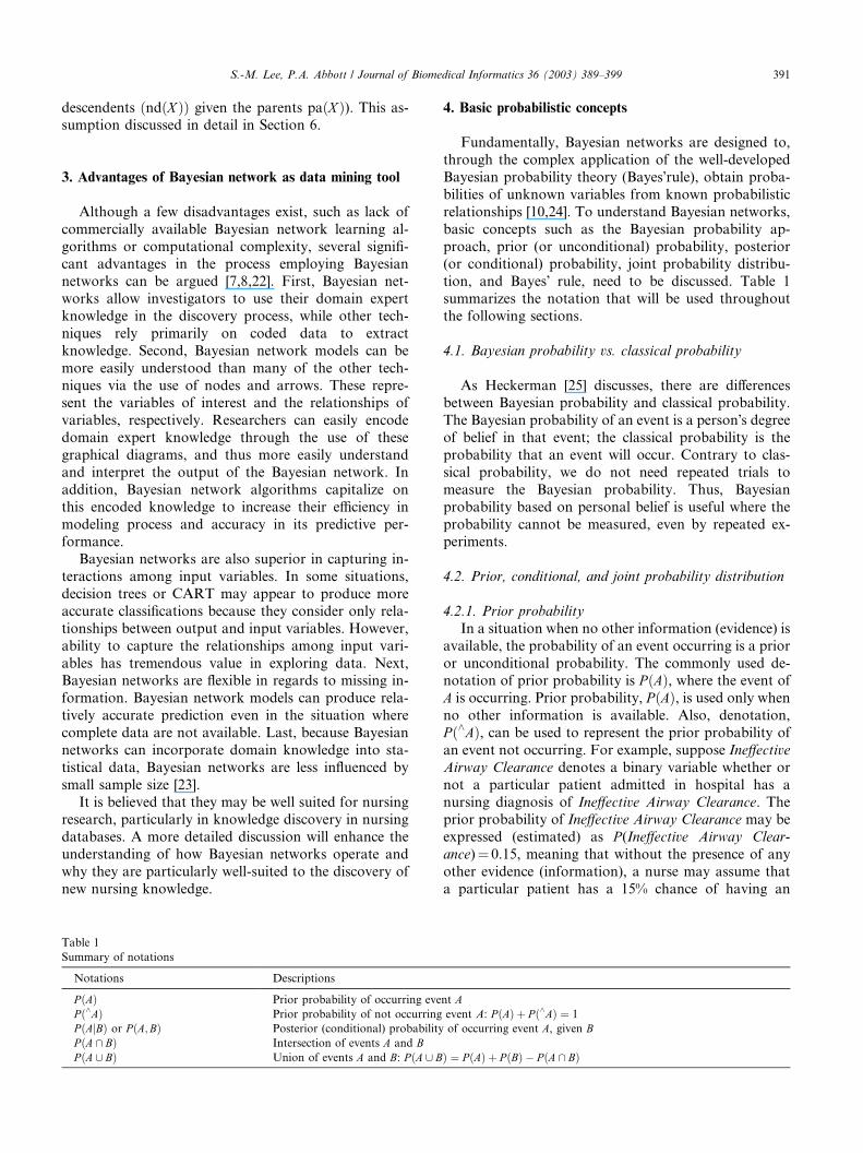
Fig. 2. A simple example of Bayesian network in causal relationship.

Table 2

Joint probability distribution

Pain Satisfaction with care

High Middle Low

Level I 0.30 0.15 0.01

Level II 0.15 0.20 0.04

Level III 0.05 0.03 0.07

392 S.-M. Lee, P.A. Abbott / Journal of Biomedical Informatics 36 (2003) 389–399

Ineffective Airway Clearance. In this example of P (Inef-fective Airway Clearance), we can assume that they can

have values such as present or absent. Thus, P (Ineffec-tive Airway Clearance) is viewed as P (Ineffective Airway

Clearance¼ present), and P (^Ineffective Airway Clear-

ance) as P (Ineffective Airway Clearance¼ absent).

A probability term is also used to express random

variables with multi-values in the nursing domain. For

example, if we are interested in the random variableCognition of a patient, this variable may have several

possible values, such as very good, good, poor, and very

poor. We might estimate them based on experience as:

P (Cognition¼ very good)¼ 0.60; P (Cognition¼ good)¼0.30; P (Cognition¼ poor)¼ 0.08; and P (Cognition¼very poor)¼ 0.02. We can also state all the possible

values of the random variable, Cognition, as P (Cogni-tion)¼ (0.6, 0.3, 0.08, and 0.02), which can be definedas a probability distribution for the random variable

Cognition.

4.2.2. Conditional probability

As discussed earlier, the probability of an event oc-

curring is expressed as a prior or unconditional proba-

bility; once the evidence is obtained, it becomes

posterior or conditional probability. Once we have newinformation B, we can use the conditional probability of

A given B instead of P ðAÞ, which can be denoted as

PðAjBÞ. This means ‘‘the probability of A, given B’’ [24].Suppose P (Ineffective Airway ClearancejGrunting) is es-

timated to be 0.60. This proposes that if a patient is

observed to have a Grunting breathing sound, and no

other information is available, and then the probability

of the patient having an Ineffective Airway Clearance

will be changed from 0.15 to 0.60. That is, without

considering the presence of Grunting, the probability of

Ineffective Airway Clearance (prior probability) is 0.15;

while considering the presence of Grunting, the proba-

bility of Ineffective Airway Clearance (posterior proba-

bility) becomes 0.60.

4.2.3. Joint probability distribution

The joint probability distribution expresses all the

probabilities of all combinations of different values of

random variables. As mentioned in the Cognition ex-

ample, the probability distribution of Cognition is a one-

dimensional vector of probability for all possible values

of a variable. The joint probability distribution is ex-

pressed as an n-dimensional table ðn > 1Þ, which is

called the joint probability table. The joint probabilitytable consists of the probabilities of all possible events

occurring. Table 2 illustrates an example of joint prob-

ability distribution with a two-dimensional table of the

two variables Pain and Satisfaction with Care in the

nursing care domain, in which each variable has three

values. Because all events are mutually exclusive, the

sum of all the cells is �1� in the joint probability table.

This distribution can answer any probabilistic statement

of interest. Adding across a row or column gives the

prior probability of a variable; for example, P(Pain

¼Level I) ¼ 0.3 + 0.15 + 0.01 ¼ 0.46. P (Pain¼Level I

\ Satisfaction with Care¼High) can also be obtained

which is 0.3.

4.3. Bayes’ rule

This section demonstrates the details of updating

prior probability to conditional (posterior) probability

using Bayes� rule. Conditional probabilities can be re-

defined in Eq. (2) [24]

P ðAjBÞ ¼ P ðA \ BÞPðBÞ : ð2Þ

This equation can also be written as:

P ðA \ BÞ ¼ PðA;BÞ ¼ P ðAjBÞPðBÞ; ð3Þ

P ðA \ BÞ ¼ PðA;BÞ ¼ P ðBjAÞPðAÞ: ð4ÞBased on two equations (Eqs. (3) and (4)), we can induce

the equation known as Bayes� rule in Eq. (5) (also Bayes�law or Bayes� theorem) [24], by equating the two right-hand sides and dividing by P ðBÞ > 0

P ðAjBÞ ¼ P ðBjAÞP ðAÞPðBÞ : ð5Þ

Bayes� rule is useful in practice to estimate unknown

P ðAjBÞ from three probability terms (i.e., P ðBjAÞ, P ðAÞ,and P ðBÞ) that nurses may be able to easily estimate in a

domain. In a task estimating the probability of Ineffec-

tive Airway Clearance, there can be conditional proba-

bilities on causal relationships as in Fig. 2. Nurses may

want to derive a nursing diagnosis given information byGrunting. A nurse knows that Ineffective Airway Clear-

ance may cause a patient to have a Grunting breathing

sound (an estimated 40% of the time). The nurse also

knows some unconditional facts: suppose the prior

S.-M. Lee, P.A. Abbott / Journal of Biomedical Informatics 36 (2003) 389–399 393

probability of a patient having Ineffective Airway

Clearance is 0.15, and the prior probability of any pa-

tient having Grunting is 0.10. When a nurse would like to

estimate P (Ineffective Airway ClearancejGrunting) whichmay not be well-known probability, conditional proba-

bilities can be induced based on Bayes� rule in Eq. (5)

P (GruntingjIneffective Airway Clearance)¼ 0.40

P (Ineffective Airway Clearance)¼ 0.15

P (Grunting)¼ 0.10According to these three probabilities

P ðIneffective Airway Clearancej GruntingÞ¼ ðP ðGruntingjIneffective Airway ClearanceÞ� P ðIneffective Airway ClearanceÞÞ=ðPðGruntingÞÞ

¼ 0:40� 0:15

0:10¼ 0:60:

This simple example of Bayes� rule demonstrates howunknown probabilities can be computed from the

known.

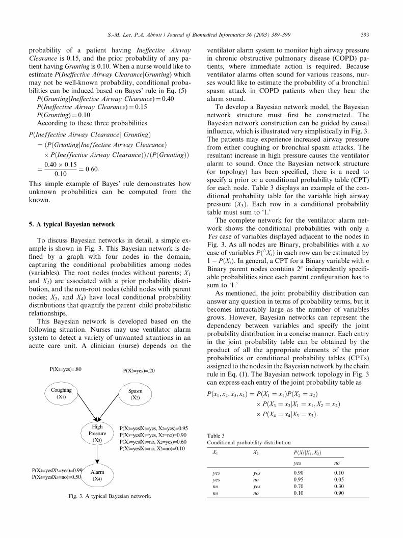
5. A typical Bayesian network

To discuss Bayesian networks in detail, a simple ex-

ample is shown in Fig. 3. This Bayesian network is de-fined by a graph with four nodes in the domain,

capturing the conditional probabilities among nodes

(variables). The root nodes (nodes without parents; X1

and X2) are associated with a prior probability distri-

bution, and the non-root nodes (child nodes with parent

nodes; X3, and X4) have local conditional probability

distributions that quantify the parent–child probabilistic

relationships.This Bayesian network is developed based on the

following situation. Nurses may use ventilator alarm

system to detect a variety of unwanted situations in an

acute care unit. A clinician (nurse) depends on the

Fig. 3. A typical Bayesian network.

ventilator alarm system to monitor high airway pressurein chronic obstructive pulmonary disease (COPD) pa-

tients, where immediate action is required. Because

ventilator alarms often sound for various reasons, nur-

ses would like to estimate the probability of a bronchial

spasm attack in COPD patients when they hear the

alarm sound.

To develop a Bayesian network model, the Bayesian

network structure must first be constructed. TheBayesian network construction can be guided by causal

influence, which is illustrated very simplistically in Fig. 3.

The patients may experience increased airway pressure

from either coughing or bronchial spasm attacks. The

resultant increase in high pressure causes the ventilator

alarm to sound. Once the Bayesian network structure

(or topology) has been specified, there is a need to

specify a prior or a conditional probability table (CPT)for each node. Table 3 displays an example of the con-

ditional probability table for the variable high airway

pressure ðX3Þ. Each row in a conditional probability

table must sum to �1.�The complete network for the ventilator alarm net-

work shows the conditional probabilities with only a

Yes case of variables displayed adjacent to the nodes in

Fig. 3. As all nodes are Binary, probabilities with a no

case of variables P ð^XiÞ in each row can be estimated by

1� P ðXiÞ. In general, a CPT for a Binary variable with nBinary parent nodes contains 2n independently specifi-

able probabilities since each parent configuration has to

sum to �1.�As mentioned, the joint probability distribution can

answer any question in terms of probability terms, but it

becomes intractably large as the number of variablesgrows. However, Bayesian networks can represent the

dependency between variables and specify the joint

probability distribution in a concise manner. Each entry

in the joint probability table can be obtained by the

product of all the appropriate elements of the prior

probabilities or conditional probability tables (CPTs)

assigned to the nodes in theBayesiannetworkby the chain

rule in Eq. (1). The Bayesian network topology in Fig. 3can express each entry of the joint probability table as

P ðx1; x2; x3; x4Þ ¼ PðX1 ¼ x1ÞP ðX2 ¼ x2Þ� P ðX3 ¼ x3jX1 ¼ x1;X2 ¼ x2Þ� P ðX4 ¼ x4jX3 ¼ x3Þ:

Table 3

Conditional probability distribution

X1 X2 P ðX3jX1;X2Þ

yes no

yes yes 0.90 0.10

yes no 0.95 0.05

no yes 0.70 0.30

no no 0.10 0.90

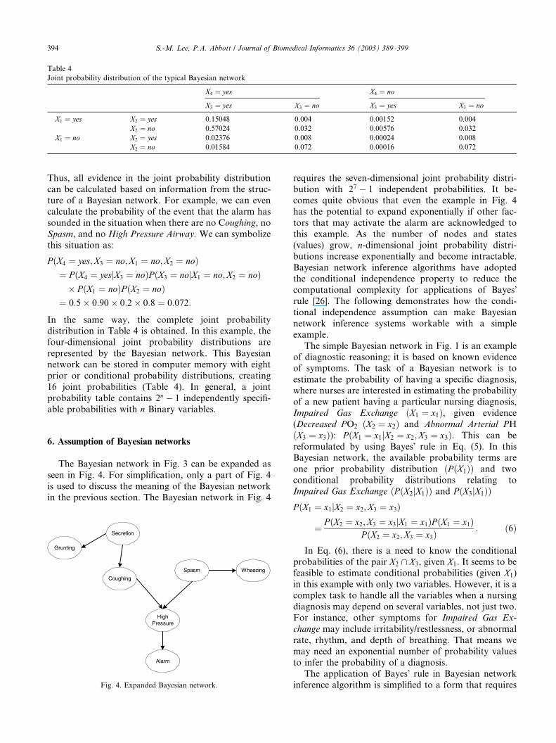
Table 4

Joint probability distribution of the typical Bayesian network

X4 ¼ yes X4 ¼ no

X3 ¼ yes X3 ¼ no X3 ¼ yes X3 ¼ no

X1 ¼ yes X2 ¼ yes 0.15048 0.004 0.00152 0.004

X2 ¼ no 0.57024 0.032 0.00576 0.032

X1 ¼ no X2 ¼ yes 0.02376 0.008 0.00024 0.008

X2 ¼ no 0.01584 0.072 0.00016 0.072

394 S.-M. Lee, P.A. Abbott / Journal of Biomedical Informatics 36 (2003) 389–399

Thus, all evidence in the joint probability distributioncan be calculated based on information from the struc-

ture of a Bayesian network. For example, we can even

calculate the probability of the event that the alarm has

sounded in the situation when there are no Coughing, no

Spasm, and no High Pressure Airway. We can symbolize

this situation as:

PðX4 ¼ yes;X3 ¼ no;X1 ¼ no;X2 ¼ noÞ¼ PðX4 ¼ yesjX3 ¼ noÞP ðX3 ¼ nojX1 ¼ no;X2 ¼ noÞ� P ðX1 ¼ noÞP ðX2 ¼ noÞ¼ 0:5� 0:90� 0:2� 0:8 ¼ 0:072:

In the same way, the complete joint probability

distribution in Table 4 is obtained. In this example, thefour-dimensional joint probability distributions are

represented by the Bayesian network. This Bayesian

network can be stored in computer memory with eight

prior or conditional probability distributions, creating

16 joint probabilities (Table 4). In general, a joint

probability table contains 2n � 1 independently specifi-

able probabilities with n Binary variables.

6. Assumption of Bayesian networks

The Bayesian network in Fig. 3 can be expanded as

seen in Fig. 4. For simplification, only a part of Fig. 4

is used to discuss the meaning of the Bayesian network

in the previous section. The Bayesian network in Fig. 4

Fig. 4. Expanded Bayesian network.

requires the seven-dimensional joint probability distri-bution with 27 � 1 independent probabilities. It be-

comes quite obvious that even the example in Fig. 4

has the potential to expand exponentially if other fac-

tors that may activate the alarm are acknowledged to

this example. As the number of nodes and states

(values) grow, n-dimensional joint probability distri-

butions increase exponentially and become intractable.

Bayesian network inference algorithms have adoptedthe conditional independence property to reduce the

computational complexity for applications of Bayes�rule [26]. The following demonstrates how the condi-

tional independence assumption can make Bayesian

network inference systems workable with a simple

example.

The simple Bayesian network in Fig. 1 is an example

of diagnostic reasoning; it is based on known evidenceof symptoms. The task of a Bayesian network is to

estimate the probability of having a specific diagnosis,

where nurses are interested in estimating the probability

of a new patient having a particular nursing diagnosis,

Impaired Gas Exchange ðX1 ¼ x1Þ, given evidence

(Decreased PO2 ðX2 ¼ x2Þ and Abnormal Arterial PH

ðX3 ¼ x3Þ): PðX1 ¼ x1jX2 ¼ x2;X3 ¼ x3Þ. This can be

reformulated by using Bayes� rule in Eq. (5). In thisBayesian network, the available probability terms are

one prior probability distribution ðP ðX1ÞÞ and two

conditional probability distributions relating to

Impaired Gas Exchange ðP ðX2jX1ÞÞ and P ðX3jX1ÞÞP ðX1 ¼ x1jX2 ¼ x2;X3 ¼ x3Þ

¼ P ðX2 ¼ x2;X3 ¼ x3jX1 ¼ x1ÞP ðX1 ¼ x1ÞP ðX2 ¼ x2;X3 ¼ x3Þ

: ð6Þ

In Eq. (6), there is a need to know the conditional

probabilities of the pair X2 \ X3, given X1. It seems to be

feasible to estimate conditional probabilities (given X1)in this example with only two variables. However, it is a

complex task to handle all the variables when a nursing

diagnosis may depend on several variables, not just two.

For instance, other symptoms for Impaired Gas Ex-

change may include irritability/restlessness, or abnormal

rate, rhythm, and depth of breathing. That means we

may need an exponential number of probability values

to infer the probability of a diagnosis.The application of Bayes� rule in Bayesian network

inference algorithm is simplified to a form that requires

S.-M. Lee, P.A. Abbott / Journal of Biomedical Informatics 36 (2003) 389–399 395

fewer probabilities to produce a result by introducingthe assumption of conditional independence. To rede-

fine Eq. (6), a conditionalized version of the general

product rule is applied (Eq. (7)); it is useful when some

general background evidence is available, rather than in

the complete absence of information. Eq. (7) is drawn

from the general product rule in Eqs. (3) and (4)

P ðA;BjEÞ ¼ PðAjB;EÞP ðBjEÞ ¼ P ðBjA;EÞP ðAjEÞ: ð7ÞThe process for proving the conditionalized version

of the general product rule is omitted here. Readers who

are interested in this process can refer to Jensen [24].Based on those rules, (Eqs. (4) and (7)), Eq. (6) is

reformulated in Eq. (8)

P ðX1 ¼ x1jX2 ¼ x2;X3 ¼ x3Þ

¼ P ðX2 ¼ x2;X3 ¼ x3jX1 ¼ x1ÞP ðX1 ¼ x1ÞP ðX2 ¼ x2;X3 ¼ x3Þ

¼ P ðX3 ¼ x3jX2 ¼ x2;X1 ¼ x1ÞP ðX2 ¼ x2jX1 ¼ x1ÞP ðX1 ¼ x1ÞP ðX3 ¼ x3jX2 ¼ x2ÞP ðX2 ¼ x2Þ

:

ð8Þ

Yet estimating a value for the numerator,

P ðX3 ¼ x3jX2 ¼ x2;X1 ¼ x1Þ, is no easier than finding a

value for PðX2 ¼ x2;X3 ¼ x3jX1 ¼ x1Þ. To simplify the

expressions, we need to make an assumption. The X1 is

the direct cause of both the X2 and the X3. Once we

know the patient has an X1, the probability of the X3 are

not dependent on the presence of an X2; similarly, X2

does not change the probability that X1 is causing X3.

These properties can be denoted as:

P ðX3jX1;X2Þ ¼ P ðX3jX1Þ;

P ðX2jX1;X3Þ ¼ P ðX2jX1Þ:These equations express the conditional independence of

X2 and X3, given X1. Given conditional independence,

now we can simplify Eq. (8) for Bayesian probability

updating into Eq. (9)

P ðX1 ¼ x1jX2 ¼ x2;X3 ¼ x3Þ

¼ P ðX3 ¼ x3jX1 ¼ x1ÞP ðX2 ¼ x2jX1 ¼ x1ÞP ðX1 ¼ x1ÞP ðX3 ¼ x3jX2 ¼ x2ÞP ðX2 ¼ x2Þ

:

ð9Þ

There is still the term PðX3 ¼ x3jX2 ¼ x2Þ, which mightbecome complex by considering all symptoms those

which are not represented in the network as an example.

However, this term can be eliminated by normalization

in Eq. (10)

ðX1 ¼ x1jX2 ¼ x2;X3 ¼ x3Þ

¼ 1

PðX3 ¼ x3jX2 ¼ x2ÞPðX2 ¼ x2Þ� P ðX3 ¼ x3jX1 ¼ x1ÞP ðX2 ¼ x2jX1 ¼ x1ÞP ðX1 ¼ x1Þ¼ aPðX3 ¼ x3jX1 ¼ x1ÞPðX2 ¼ x2jX1 ¼ x1ÞP ðX1 ¼ x1Þ;

P

ð10Þ

where a ¼ 1=ðPðX3 ¼ x3jX2 ¼ x2ÞPðX2 ¼ x2ÞÞ is nothingbut a constant, which is referred to as the normalization

constant. It normalizes the distribution to sum to �1.�In the context of using Bayes� rule, conditional in-

dependence relationships among variables can simplify

the Bayesian network inference for a queried variable;

also, it can greatly reduce the number of conditional

probabilities under assumption of conditional indepen-

dence with normalization process. Conditional inde-pendence is an important concept in designing a

Bayesian network and constructing a Bayesian inference

algorithm [10,24,26]. Also, the conditional independence

properties enable us to perform inference without con-

sidering the entire joint distribution.

The d-separation properties can be used to easily

distinguish whether a X is independent of another node

Y . Nodes X and Y are d-separated (conditionally inde-pendent) if among paths connecting X and Y there is an

intermediate node Z that fulfills one of the following

statements:

• Z is the middle node in a serial connection

(X ! Z ! Y or X Z Y ) and then Z is instanti-

ated by the evidence. For example from Fig. 4, pa-

tient findings of Wheezing breath sounds and

Grunting breath sounds are independent, given evi-dence about whether the patient has Coughing epi-

sodes.

• Z has a diverging connection between X and YðX Z ! Y Þ and then Z is instantiated by the evi-

dence. In Fig. 4, if we know that the patient has Se-

cretions in the airway, Grunting and Wheezing are

independent.

• Z is the middle node in a converging connectionðX ! Z Y Þ and neither Z nor any of its descen-

dants have received evidence; Grunting and Spasm

are independent if we do not have any evidence. They

are dependent, however, under evidence of High

Pressure. For example, if High Pressure, then a

Grunting breathing sound is increased evidence that

the patient does not have Spasm.

7. Inferences in Bayesian network

As illustrated earlier, Bayes� rule is a fundamental

theorem applied to Bayesian network inference systems.

The fundamental task of a Bayesian network is to an-

swer the probability of unknown (query) variable by

providing the posterior probability distribution, givensome values of evidence variables [26]. In other words,

the inference task is often defined as computing all

posterior marginal probabilities given the evidence or

solving a query Q ¼ ðT ; eÞ where T is the target set and eis the evidence. A Bayesian network is flexible in that we

can chose any node as an output (target) variable for

inferences, unlike any other techniques, such as neural

396 S.-M. Lee, P.A. Abbott / Journal of Biomedical Informatics 36 (2003) 389–399

networks, decision trees, CART, or conventional sta-tistical methods.

Bayes� rule helps to predict the outcomes of events

that are dependent on other events, when events (vari-

ables) are linked in the form of a network. Russell and

Norvig [26] demonstrated four different task scenarios:

(1) diagnostic inferences, (2) causal inferences, (3) in-

tercausal inferences, and (4) mixed inferences. Diag-

nostic reasoning is conducted for inferences of causesfrom effects. Causal and intercausal inferences are con-

ducted from causes to effects, and between causes of a

common effect, respectively. Mixed inferences are the

combination of two or more of the other three types of

inferences. Using the examples of the Bayesian network

in Fig. 3, we can demonstrate these principles: (1)

diagnostic inference is conducted when a ventilator

Alarm goes off and nurses would like to estimate theprobability that a patient is having a bronchial Spasm

i.e., P ðX2 ¼ yesjX4 ¼ yesÞ; (2) given Coughing, the

probability of the ventilator Alarm going off is obtained

by causal inference i.e., P ðX4 ¼ yesjX1 ¼ yesÞ; (3) givenHigh Pressure with evidence of Coughing, P ðX2 ¼yesjX1 ¼ yes;X3 ¼ yesÞ, intercausal inference is con-

ducted to answer the probability of Spasm; and (4) the

queries to calculate PðX3 ¼ yesjX4 ¼ yes;X2 ¼ noÞ andPðX2 ¼ yesjX4 ¼ yes;X1 ¼ noÞ are the examples of the

mixed inferences.

8. Bayesian networks as a knowledge discovery tool

In this section, the KDD process and how the

Bayesian networks can be used in knowledge discoveryas a data mining tool will be discussed.

8.1. Knowledge discovery process

The KDD process consists of five basic steps: (1)

problem identification; (2) data extraction; (3) data

preprocessing; (4) data mining, and; (5) pattern inter-

pretation and presentation [1]. The initial step of KDDis the development of an understanding of the applica-

tion domain, the relevant prior knowledge, and the

goals of the knowledge discovery. The data extraction

process includes selecting a dataset with variables of

interest focusing on the exploration to be performed.

Data preprocessing involves cleaning the data to ex-

amine the impact of outliers and noise on the data set,

and deciding on strategies for handling missing datafields. Also, in this step, dimension reduction or trans-

formation methods are considered to reduce the effective

number of variables under consideration, or to find in-

variant representations for the data.

The data mining step includes choosing the data min-

ing task and algorithm and the active investigation of the

transformed data set for interesting patterns. The main

tasks of data mining in healthcare may include (1)discovering associations, (2) clustering, or (3) creating

predictive (classification/regression)models.Datamining

algorithms refer to the method to be used in actual data

mining. After interpretingmined patterns, it is possible to

return to any of previous steps for further iteration.

8.2. Data mining with Bayesian network

Actual data mining process using Bayesian networks

consists primarily of two phases. The first phase is the

construction of a directed acyclic graph, called a

Bayesian network structure, which encodes probabilistic

relationships among variables. The second phase is the

assessment of the prior and local conditional (posterior)

probabilities, the so-called parameters. The second step

is conducted by training and testing a network structureby using an existing observational dataset.

8.2.1. Constructing Bayesian network structure

After deciding what variables and states (values) to

model, researchers can build a Bayesian network struc-

ture by using two different approaches: (1) manual

construction using expert knowledge or (2) automatic or

semi-automatic construction by learning (training) al-gorithms. The first method of building a Bayesian net-

work structure solely relies on a domain expert

knowledge (experience and observation). In this step,

researchers can construct the Bayesian network by

causal influence considering conditional independence

similar to the Bayesian network in Fig. 3. The second

method allows the researchers to be assisted by Bayesian

network learning algorithms, which can be applied tothe process of knowledge discovery from large datasets.

These algorithms are designed to automatically (or

semi-automatically) determine the dependence and in-

dependence of variables by finding direct relationships

between the nodes. A potential consequence of the

structural learning is that hidden or unknown structure

in the domain, frequently missed by investigators using

conventional statistical methods, is identified.There are two different approaches in finding an op-

timal structure: a search-and-score-based and con-

straint-based algorithms. A search-and-score-based

algorithm searches for the best model structure using a

scoring metric, which reflects the goodness-of-fit of the

structure to the data. Examples of systems that imple-

ment a search-and-score-based algorithm include the

Bayesian Knowledge Discoverer [27], and BayesianLab[28]. A constraint-based algorithm searches a best pos-

sible structure by finding all the possible conditional

independence and dependencies with a statistical test

(e.g., v2 test). Systems that implement this algorithm

include HUGIN [29], BN PowerConstructor and BN

PowerPredictor [30–32], and TETRAD [33]. Constraint-

based approaches allow the researcher to specify the

S.-M. Lee, P.A. Abbott / Journal of Biomedical Informatics 36 (2003) 389–399 397

relationships between variables using domain knowl-edge in learning a structure. The use of constraints in the

learning phase enables the investigators to feed the

learning algorithm with existing and well-established

structural knowledge of the domain. That is, the learn-

ing algorithms allow researchers to specify available

knowledge about dependence or independence among

pairs of variables in the data set, which is useful in

guiding the learning algorithm towards the best possiblemodel. In this step, nurse researchers can incorporate

domain knowledge obtained by a theoretical research

framework, literature, or observational experience.

8.2.2. Assessing parameters

Once a satisfactory dependence structure is obtained,

the next step is to estimate the parameters of the model

encoding the strengths of the dependencies among nodes(variables). Assessing parameters develops the condi-

tional probability relationships at each node, given the

network structure and the data. The parameters can be

assigned by expert knowledge. Alternately, by inducing

a learning algorithm, the parameters can be learned

from data. These methods can also be combined, which

may strengthen the performance of a model. If a data-

base includes fully observed data (no missing data), theestimation of parameters is simple and can be done just

by calculating (counting and dividing) the prior or

conditional probabilities, given the Bayesian network

structure. However, missing data commonly exists in

real world, especially in the healthcare domain. This

requires the use of parameter estimation methods that

address missing data.

The most commonly used parameter algorithm is theexpectation-maximization (EM) algorithm [34]. This

approach is useful for estimating the parameters of the

conditional probability distributions in the case of

missing data. The EM algorithm is an iterative algo-

rithm that given a network structure and a database of

cases, determines a local maximum estimate of the pa-

rameters by assuming the pattern of missing data is

uninformative (missing at random or missing completelyat random). Maximum a posterior (MAP) is estimated

in this situation when initial knowledge about the pa-

rameters is assigned; maximum likelihood (ML) is esti-

mated in the situation when non-informative (default)

prior beliefs are used. The software programs, such as

HUGIN and Netica, provide the parameter learning

algorithms.

The parameter learning step is accomplished with arandomly assigned set of raw data designated as the

‘‘training’’ set. The next step of the testing phase is to

validate a trained network on new cases in a test set. The

assigned test set is comprised of the remaining cases

(those not used to actually estimate the parameters in

the first place) in the overall dataset. These cases are

considered ‘‘unseen,’’ and thus, performance measures

should be generated from a test set results, which givesome insights into the usefulness of the models. In the

next section, several performance measures of the

models in classification problems are described.

8.3. Performance measures in classification problems

The performance of predictive models should be

evaluated by their abilities of discrimination and cali-bration [35]. Discrimination measures how much the

model is able to separate cases with positive outcome

value from those with negative outcome value. Cali-

bration is a measure of how close the predicted values

are to the real outcomes, measuring whether they are

high or low when compared to the real outcomes. The

discriminatory power of the models can be analyzed by

using an area under the receiver operating characteristic(ROC) curve, a graphical representation of the dis-

criminatory power of the model. Calibration of the

models can be measured by construction of calibration

curve or computation of the Hosmer–Lemeshow good-

ness-of-fit v2 statistic [36].

The ROC curve is a plot of the sensitivity versus

(1) specificity) of a model in a binary classification task

[37]. Sensitivity is defined as the number of correctlyclassified cases as positives divided by the total number

of actual positive cases. Specificity is defined as the

number of correctly classified cases as negatives divided

by the total number of actual negative cases. As each

sensitivity and specificity is dependent upon the choice

of cut-off point, the ROC curve can be plotted through

various cut-off values. The area under this curve then

gives a definitive measure of the classifier�s discrimina-tion ability that is not dependent on the choice of cut-off

point value [38]. Accuracy is calculated using a threshold

that minimizes the sum of (1) sensitivity)2 and

(1) specificity)2. This threshold determines the point in

the ROC curve that is closest to (0, 1) [39]. Also, positive

predictive value (PPV) and negative predictive value

(NPV) cannot be ignored in reporting in the results.

PPV is the proportion of cases that the network classifiesas positive that actually are positive, and NPV is the

proportion of cases that the net classifies as negative that

are actually negative.

9. Discussion

As mentioned earlier, Bayesian networks are anemerging knowledge discovery approach that has sev-

eral advantages over other techniques. The most at-

tractive advantage to nurse researchers is that they can

use domain knowledge in the process of knowledge

discovery in a graphical format. At the same time,

however, the Bayesian network approach can be more

robust to errors in the researcher�s prior knowledge

398 S.-M. Lee, P.A. Abbott / Journal of Biomedical Informatics 36 (2003) 389–399

through the learning phase than other conventionalstatistical modeling methods. For instance, hidden re-

lationships among variables that a researcher might

omit can be detected by the structural learning algo-

rithm. In general, based on statistical data and learning

rules, Bayesian networks can improve the reliability of a

model [40]. Consequently, it may be useful as an ex-

ploratory data analysis tool capturing the relationships

among variables.Bayesian networks can be used in various ways in

nursing research. For instance, structural learning of

Bayesian networks can assist researchers in identifying

the contributing factors relating to a specific patient

outcome. Those identified contributing factors can be

used to build a model to predict patients� outcome,

which allows for modification of nursing actions to

improve quality of care. In today�s healthcare environ-ment, with the emphasis on healthcare costs, quality

improvement, and patient outcomes, it becomes im-

portant to fully understand all aspects of care and the

impact on patient outcomes. In order to fully under-

stand the causes and effects of clinical care a compre-

hensive analysis of complex interactions that occur in

the patient care process is required. Prior studies of

nursing interventions do exist, however, they are oftensporadic in nature and narrow in scope. This may be due

to limitations of the data available for such studies or

the constraints of traditional analytic techniques. Such

studies, while commendable, are conducted on small

samples and may not produce significant nor general-

izable results. Knowledge discovery in large databases

that contain data of value to nursing researchers via a

Bayesian network modeling technique may provide newevidence of the nursing contribution to patient out-

comes.

References

[1] Fayyad U, Piatesesky-Shapiro G, Smyth P, Uthurusamy R.

Advances in knowledge discovery and data mining. Cambridge,

MA: MIT Press; 1996.

[2] Abbott P. Knowledge discovery in large data sets: a primer for

data mining applications in health care. In: Ball MJ, Hannah KJ,

Newbold SK, Douglas JV, editors. Nursing informatics: where

caring and technology meet. New York: Springer; 2000. p. 139–48.

[3] Cios KJ. Medical data mining and knowledge discovery. New

York: Physica-Verlag; 2001.

[4] Rumelhart DE, Hinton GE, Williams RJ. Learning internal

representation by error propagation. In: Rumelhart DE, McClel-

land JL, editors. Parallel distributed processing. Cambridge: MIT

Press; 1986.

[5] Tu JV. Advantages and disadvantages of using artificial neural

networks versus logistic regression for predicting medical out-

comes. J Clin Epidemiol 1996;49:1225–32.

[6] Penny W, Frost D. Neural networks in clinical medicine. Med

Decis Making 1996;16(4):386–98.

[7] Heckerman D. Bayesian networks for data mining. Data Min

Knowl Disc 1997;1:79–119.

[8] Cowell RG, Dawid AP, Lauritzen SL, Spiegelhalter DJ.

Probabilistic networks and expert systems. New York: Springer;

1999.

[9] Heckerman DE. Bayesian networks for knowledge discovery. In:

Fayyad UM, Piatetsky-Shapiro G, Smyth P, Uthurusamy R,

editors. Advances in knowledge discovery and data mining. Menlo

Park, CA: The MIT Press; 1996. p. 273–305.

[10] Pearl J. Probabilistic reasoning in intelligent systems: networks of

plausible inference. San Francisco, CA: Morgan Kaufmann

Publishers; 1988.

[11] Luttrell SP. Partitioned mixture distribution: An adaptive Bayes-

ian network for low-level image processing. IEE Proc Vision,

Image Signal Process 1994;141(4):251–60.

[12] Sox HC, Blatt MA, Higgins MC, Marton KI. Medical decision

making. Boston: Butterworths; 1988.

[13] Aronsky D, Haug PJ. Automatic identification of patients eligible

for a pneumonia guideline. Proc/AMIA Annu Symp 2000:

12–6.

[14] Burnside E, Rubin D, Shachter R. A Bayesian network for

mammography. Proc/AMIA Annu Symp 2000:106–10.

[15] Hamilton PW, Montironi R, Abmayr W, et al. Clinical applica-

tions of Bayesian belief networks in pathology. Pathologica

1995;87(3):237–45.

[16] Montironi R, Bartels PH, Thompson D, Scarpelli M, Hamilton

PW. Prostatic intraepithelial neoplasia (PIN). Performance of

Bayesian belief network for diagnosis and grading. J Pathol

1995;177(2):153–62.

[17] Korrapati R, Mukherjee S, Chalam KV. A Bayesian framework

to determine patient compliance in glaucoma cases. Proc/AMIA

Annu Fall Symp 2000:1050.

[18] Abston KC, Pryor TA, Haug PJ, Anderson JL. Inducing practice

guidelines from a hospital database. Proc/AMIA Annu Fall Symp

1997:168–72.

[19] Sakellaropoulos GC, Nikiforidis GC. Development of a

Bayesian network for the prognosis of head injuries using

graphical model selection techniques. Methods Inf Med 1999;

38(1):37–42.

[20] Bunn CC, Du M, Niu K, Johnson TR, Poston WSC, Foreyt JP.

Predicting the risk of obesity using a Bayesian network. Proc/

AMIA Annu Symp 1999:1035.

[21] Wilcox A, Hripcsak G. Classification algorithms applied to

narrative reports. Proc/AMIA Annu Symp 1999:455–9.

[22] Heckerman DE. Learning Bayesian networks: The combination of

knowledge and statistical data. MSR-TR-94-09. 1995. Redmond,

WA, Microsoft Research.

[23] Eisenstein EL, Alemi F. A comparison of three techniques for

rapid model development: an application in patient risk-stratifi-

cation. Proc/AMIA Annu Fall Symp 1996:443–7.

[24] Jensen FV. An introduction to Bayesian networks. New York:

UCL Press; 1996.

[25] Heckerman DE. A tutorial on learning with Bayesian networks.

MSR-TR-95-06. 1996. Redmond, WA, Microsoft Research.

[26] Russell S, Norvig P. Artificial intelligence: a modern approach.

Englewood Cliffs, New Jersey: Prentice-Hall; 1995.

[27] Ramoni M, Sebastiani P. Learning Bayesian networks from

incomplete databases. KMI-TR-43. 1997. UK, Knowledge Media

Institute.

[28] BayesiaLab. France: Bayesia SA; 2003.

[29] Jensen FV, Kjaerulff UB, Lang M, Madsen AL. HUGIN-The tool

for Bayesian networks and influence diagrams. Proc First Eur

Workshop Probabilistic Graph Models 2002:212–21.

[30] Cheng J, Bell DA, Liu W. An algorithm for Bayesian belief

network construction from data. Proc AI & STAT 1997:83–90.

[31] Cheng J. BN PowerConstructor. Available from: http://www.cs.

ualberta.ca/~jcheng/bnpc.htm. 1998.

[32] Cheng J. BN PowerPredictor. Available from: http://www.cs.

ualberta.ca/~jcheng/bnpp.htm. 2000.

S.-M. Lee, P.A. Abbott / Journal of Biomedical Informatics 36 (2003) 389–399 399

[33] Spirtes P, Glymour C, Scheine R. Causation, prediction, and

search. 2nd ed. Cambridge, MA: The MIT Press; 2000.

[34] Lauritzen SL. The EM algorithm for graphical association models

with missing data. Comput Statistics Data Anal 1995;19:

191–201.

[35] Hanley JA, McNeil BJ. A method of comparing the areas under

receiver operating characteristic curves derived from the same

cases. Radiology 1983;148(3):839–43.

[36] Glantz SA. Primer of applied regression and analysis of variance.

New York: McGraw-Hill; 1990.

[37] Hanley JA, McNeil BJ. The meaning and use of the area under a

receiver operating characteristic (ROC) curve. Radiology

1982;143(1):29–36.

[38] Turner DA. An intuitive approach to receiver operating charac-

teristic curve analysis. J Nuclear Med 1978;19(2):213–20.

[39] Rowland T, Ohno-Machado L, Ohrn A. Comparison of multiple

prediction models for ambulation following spinal cord injury.

Proc/AMIA Annu Symp 1998:528–32.

[40] Suermondt HJ, Cooper GF. An evaluation of explanations of

probabilistic inference. Comput Biomed Res 1993;26(3):242–54.