baryon acoustic oscillations and primordial non-gaussianities
TRANSCRIPT
Dissertationsubmitted to the
Combined Faculties of the Natural Sciences and Mathematicsof the Ruperto-Carola-University of Heidelberg, Germany
for the degree ofDoctor of Natural Sciences
Put forward byAlessandra Grassi
born in: Arezzo, Italyoral examination: July 25th, 2013


B A RY O N A C O U S T I C O S C I L L AT I O N S A N DP R I M O R D I A L N O N - G A U S S I A N I T I E S W I T H W E A K
L E N S I N G
Referees: Prof. Dr. Björn Malte SchäferProf. Dr. Luca Amendola


A Fedee alle nostre pagine bianche


A B S T R A C T- Z U S A M M E N FA S S U N G
This work introduces two investigations on possible new weak lens-ing applications. In the first part, I present a study on the possibilityof detecting baryon acoustic oscillations by means of 3d weak lensing(3dWL). Basing our analysis on a Fisher matrix approach, we quan-tify the uncertainty on inferring the amplitude of the power spectrumwiggles with 3dWL. Ultimately, we find that surveys like Euclid andDES should be able to detect, respectively, the first four and three os-cillations, with errors reaching the 1% or 10% of the amplitude for thefirst two wiggles in the case of Euclid. The second part of this workfocuses on the study of primordial non-Gaussianities with a classicalweak lensing approach. We study inflationary bi- and trispectra, thestrentgh of their signals, and the consequences of fitting data witha wrong type of bispectrum on the inferred on fNL. We concludethat contraints on fNL are not competitive with the ones from CMB,but nonetheless valuable in case of a scale-dependent fNL. Lastly, wequantify lensing ability to test the Suyama-Yamaguchi inequality, andascertain that Euclid could give evidence in favour or against the in-equality for large non-Gaussianity values (τNL > 105 or fNL > 102).
In dieser Arbeit untersuche ich zwei neue Anwendungsmöglich-keiten des schwachen kosmischen Linseneffekts. In dem ersten Teilmeiner Dissertation zeige ich die Ergebnisse einer statistische Studie,die den Fisher-Formalismus verwendet, ob baryonische Oszillationenin dreidimensionalen Abbildungen der kosmischen Struktur über denLinseneffekt detektiert werden können. Mein Ergebnisse zeigen, dassDurchmusterungen wie Euclid und DES die ersten vier oder dreiOszillationen erkennen, wobei die Amplitude der ersten beiden Os-zillationen statistische Fehler im Prozentbereich haben. Im zweitenTeil untersuche ich primordiale nicht-Gaußianitäten durch den klas-sischen Linseneffekt, insbesondere inflationäre Bi- und Trispektren,deren Signalstärke und die Auswirkungen einer falschen Modellwahlauf die Messung von Parametern wie fNL. Ich zeige, dass Einschränkun-gen auf fNL nicht mit dem CMB konkurrenzfähig sind, es sei denn dienicht-Gaußianitäten wären skalenabhängig. Schließlich untersuche ichdie Möglichkeit, mit dem Linseneffekt die Suyama-Yamaguchi-Un-gleichung zu testen, wobei Euclid in der Lage sein sollte, statistischeTests im Parameterbereich τNL > 105 und fNL > 102 durchzuführen.
vii


C O N T E N T S
List of Figures xiiList of Tables xiv
Preface xvii
i introduction to cosmology 1
1 foundations of cosmology 3
1.1 Describing a homogeneous Universe . . . . . . . . . . . 4
1.1.1 Robertson-Walker metric . . . . . . . . . . . . . 4
1.1.2 Metric’s dynamics and density parameters . . . 5
1.1.3 Redshift . . . . . . . . . . . . . . . . . . . . . . . 6
1.1.4 Cosmological distances . . . . . . . . . . . . . . 7
1.2 Introducing inhomogeneities . . . . . . . . . . . . . . . 8
1.2.1 Linear description of perturbations . . . . . . . 8
1.2.2 Statistical description of inhomogeneities: Thepower spectrum . . . . . . . . . . . . . . . . . . . 9
1.3 A timeline of the Cosmos evolution . . . . . . . . . . . 11
2 gravitational lensing 15
2.1 Light deflection by gravitation . . . . . . . . . . . . . . 17
2.1.1 Lens equation . . . . . . . . . . . . . . . . . . . . 17
2.1.2 Image distortion . . . . . . . . . . . . . . . . . . 20
2.2 Cosmological weak lensing . . . . . . . . . . . . . . . . 21
2.2.1 Angular power spectrum . . . . . . . . . . . . . 22
2.2.2 Measuring the lensing distortions . . . . . . . . 23
2.3 3d weak lensing . . . . . . . . . . . . . . . . . . . . . . . 24
ii detecting baryon acoustic oscillations by 3d weak
lensing 27
3 baryon acoustic oscillations 29
3.1 The physics of baryon acoustic oscillations . . . . . . . 30
3.1.1 The plasma era . . . . . . . . . . . . . . . . . . . 30
3.1.2 After recombination . . . . . . . . . . . . . . . . 31
3.2 BAO as a cosmological tool . . . . . . . . . . . . . . . . 35
3.2.1 What is a statistical standard ruler . . . . . . . . 35
3.2.2 Constraining cosmological parameters with baryonacoustic oscillations . . . . . . . . . . . . . . . . 38
3.2.3 Nonlinear effects and observational complications 40
4 baryon acoustic oscillations with 3d weak lens-ing 43
4.1 Introduction . . . . . . . . . . . . . . . . . . . . . . . . . 44
ix

x contents
4.2 Cosmology and structure formation . . . . . . . . . . . 46
4.2.1 Dark energy cosmologies . . . . . . . . . . . . . 46
4.2.2 CDM power spectrum . . . . . . . . . . . . . . . 46
4.2.3 Structure growth . . . . . . . . . . . . . . . . . . 47
4.2.4 Weak gravitational lensing . . . . . . . . . . . . 47
4.3 3d weak lensing . . . . . . . . . . . . . . . . . . . . . . . 48
4.4 Detecting BAO wiggles . . . . . . . . . . . . . . . . . . . 51
4.4.1 Construction of the Fisher matrix . . . . . . . . 51
4.4.2 Statistical errors . . . . . . . . . . . . . . . . . . . 54
4.4.3 Detectability of BAO wiggles . . . . . . . . . . . 57
4.5 Summary and conclusions . . . . . . . . . . . . . . . . . 65
iii probing primordial non-gaussianities with weak
lensing 67
5 inflation and primordial non-gaussianities 69
5.1 The inflationary paradigm . . . . . . . . . . . . . . . . . 70
5.1.1 Standard model: successes and issues . . . . . . 70
5.1.2 The inflationary solution . . . . . . . . . . . . . 72
5.2 Primordial non-Gaussianities . . . . . . . . . . . . . . . 74
5.2.1 Shapes of non-Gaussianities . . . . . . . . . . . . 75
5.2.2 The Suyama-Yamaguchi inequality . . . . . . . 78
5.2.3 Measuring primordial non-Gaussianities . . . . 79
6 a weak lensing view on primordial non-gaussia-nities 81
6.1 Weak lensing convergence bispectrum . . . . . . . . . . 82
6.2 Expected signal to noise ratio . . . . . . . . . . . . . . . 83
6.3 Consequences of a wrong bispectrum choice . . . . . . 86
6.4 Subtraction of structure formation bispectrum . . . . . 88
6.5 Conclusions . . . . . . . . . . . . . . . . . . . . . . . . . 90
7 a test of the suyama-yamaguchi inequality 91
7.1 Introduction . . . . . . . . . . . . . . . . . . . . . . . . . 92
7.2 Cosmology and structure formation . . . . . . . . . . . 94
7.3 Non-Gaussianities . . . . . . . . . . . . . . . . . . . . . . 95
7.4 Weak gravitational lensing . . . . . . . . . . . . . . . . . 97
7.4.1 Weak lensing potential and convergence . . . . 97
7.4.2 Convergence polyspectra . . . . . . . . . . . . . 97
7.4.3 Relative magnitudes of weak lensing polyspectra 100
7.5 Signal to noise-ratios . . . . . . . . . . . . . . . . . . . . 100
7.6 Degeneracies in the trispectrum . . . . . . . . . . . . . . 102
7.7 Testing the Suyama-Yamaguchi-inequality . . . . . . . 104
7.8 Analytical distributions . . . . . . . . . . . . . . . . . . 106
7.9 Summary . . . . . . . . . . . . . . . . . . . . . . . . . . . 108
contents xi
iv summary and conclusions 113
Appendix 119
a calculation of 3dwl covariance 121
bibliography 123

L I S T O F F I G U R E S
Figure 1.1 Snapshots of the Millennium simulation. . . . 13
Figure 2.1 Giant arcs due to gravitational lensing. . . . . 16
Figure 2.2 Simplified lensing mechanism. . . . . . . . . . 17
Figure 2.3 Multiple images due to lensing. . . . . . . . . . 19
Figure 3.1 Evolving spherical density perturbation . . . . 33
Figure 3.2 BAO in the matter power spectrum . . . . . . . 35
Figure 3.3 Evidence of an accelerating Universe . . . . . . 36
Figure 3.4 Statistical standard rulers: The concept . . . . . 38
Figure 3.5 Observations of BAO and baryonic peak . . . . 39
Figure 4.1 The BAO wiggles considered in the analysis. . 52
Figure 4.2 BAO wiggles increment used in the calculationof the Fisher matrix. . . . . . . . . . . . . . . . . 53
Figure 4.3 Marginalized errors. . . . . . . . . . . . . . . . 55
Figure 4.4 Sensitivity of marginalized errors for BAO wig-gles on shape noise σε . . . . . . . . . . . . . . 56
Figure 4.5 Sensitivity of marginalized errors for BAO wig-gles on photometric redshift error σz . . . . . . 57
Figure 4.6 Sensitivity of marginalized errors for BAO wig-gles on median redshift zmed . . . . . . . . . . . 58
Figure 4.7 Conditional and marginalized relative errorson BAO wiggles on different surveys. . . . . . 58
Figure 4.8 Confidence ellipses for the first four BAO wig-gles (Euclid). . . . . . . . . . . . . . . . . . . . . 59
Figure 4.9 Confidence ellipses for the first four BAO wig-gles (DES). . . . . . . . . . . . . . . . . . . . . . 60
Figure 4.10 Confidence ellipses for the first four BAO wig-gles (DEEP). . . . . . . . . . . . . . . . . . . . . 60
Figure 4.11 Marginalized errors on BAO wiggles in the wiggle-only power spectrum (Euclid) . . . . . . . . . . 61
Figure 4.12 Marginalized errors on BAO wiggles in the wiggle-only power spectrum (DES) . . . . . . . . . . . 62
Figure 4.13 Marginalized errors on BAO wiggles in the wiggle-only power spectrum (DEEP) . . . . . . . . . . 62
Figure 4.14 Marginalized errors on BAO wiggles as a func-tion of nw (DEEP and Euclid) . . . . . . . . . . 64
Figure 4.15 Marginalized errors on BAO wiggles as a func-tion of nw (DES and Euclid) . . . . . . . . . . . 64
Figure 5.1 Shapes of non-Gaussianities: local, equilateral,and orthogonal. . . . . . . . . . . . . . . . . . . 76
xii

List of Figures xiii
Figure 6.1 Bispectra for local, equilateral, and orthogonaln-G . . . . . . . . . . . . . . . . . . . . . . . . . 84
Figure 6.2 Signal-to-noise ratio computation with CUBAlibrary. . . . . . . . . . . . . . . . . . . . . . . . 85
Figure 6.3 Dimensionless signal-to-noise ratio for local, equi-lateral, and orthogonal n-G. . . . . . . . . . . . 87
Figure 6.4 Misestimation of fNL when a wrong n-G modelis chosen to fit the data. . . . . . . . . . . . . . 88
Figure 6.5 Bias on fNL when from the structure formationbispectrum. . . . . . . . . . . . . . . . . . . . . . 89
Figure 7.1 Weak lensing spectrum, bispectrum and trispec-trum. . . . . . . . . . . . . . . . . . . . . . . . . 99
Figure 7.2 Contributions to the weak lensing polyspectraas a function of comoving distance. . . . . . . . 99
Figure 7.3 Parameters K(`), S(`) and Q(`). . . . . . . . . . 101
Figure 7.4 Noise-weighted weak lensing spectrum, bispec-trum, and trispectrum. . . . . . . . . . . . . . . 103
Figure 7.5 Cumulative signal to noise-ratios for spectrum,bispectrum and trispectrum. . . . . . . . . . . . 103
Figure 7.6 Degeneracies in the gNL-τNL-plane for a Euclidmeasurement. . . . . . . . . . . . . . . . . . . . 105
Figure 7.7 Bayesian evidence α(fNL, τNL). . . . . . . . . . 107
Figure 7.8 Probability distribution of Q = (6/5fNL)2/τNL. 109
Figure 7.9 Probability distribution p(Q) as a function ofQ, for fixed fNL and τNL. . . . . . . . . . . . . . 109
Figure 7.10 Signal-to-noise for bi- and trispectrum with to-mography. . . . . . . . . . . . . . . . . . . . . . 112

L I S T O F TA B L E S
Table 1.1 Cosmological parameter from Planck. . . . . . 13
Table 4.1 Euclid, DES, and DEEP survey characteristics. 54
xiv

A C R O N Y M S
3dWL 3d weak lensing
BAO Baryon Acoustic Oscillations
BOSS Baryon Oscillation Spectroscopic Survey
CMB Cosmological Microwave Background
DES Dark Energy Survey
LSS Large Scale Structure
n-G non-Gaussianities
SDSS Sloan Digital Sky Survey
SY Suyama-Yamaguchi
xv


P R E FA C E
Many steps have been made since 1915, when Albert Einstein firstpublished his work on a relativistic theory of gravity, marking thebirth of modern cosmology. Back then, it was thought that our Uni-verse coincided with the Milky Way, and there was no reason to doubtits staticity. In a decade, both conceptions would have been provenwrong: Observations by Edwin Hubble and, before him, Vesto Slipher,suggested in 1924 that our galaxy was just one among many, and thatsuch distant objects were receding from us, as if the Universe wasexpanding. Friedmann’s equations, derived a couple of years earlierfrom Einstein’s general relativity under the assumptions of homo-geneity and isotropy of the Universe, had been themselves implicitly- and, back then, surprisingly - supporting an expanding Cosmos.This was just the beginning of the series of processes that led manycommon conceptions about our Universe to be revolutionized.
In less than one century, we came to learn that the initial assump-tions of homogeneity and isotropy were well-grounded, as the discov-ery of an extremely uniform background blackbody radiation (CMB)proved in 1965. We are now familiar with the idea of an expand-ing Universe, and we are able to make predictions about the rate ofthis motion, both in the past and in the future, and infer some ofthe consequences it may have on the properties, and the evolution,of the Cosmos’ content. Overall, we developed a comprehensive stan-dard model able to describe such properties, and parametrize them bymeans of some quantities that are being measured with ever-growingprecision: the cosmological parameters.
Regardless of all its successes, though, the study of our Universeis far from being a closed issue. Many questions still remain unan-swered. We still do not know anything about the true nature of darkmatter, postulated to account for several problems: flat rotationalcurves in spiral galaxies, dynamical properties of galaxy clusters, orthe small amplitude of primordial density fluctuations, as observedfrom the CMB. Such perturbations would not have led to structureformation as we observe it today, had baryonic matter been the onlygravitationally interacting species. Our understanding of the non-linear regime of structure formation is also incomplete. In addition,the origin of the seeds of structure formation, i. e. the primordial dis-tribution of density fluctuations, is not known, and such a distribu-tion must be given as an initial condition in the framework of the stan-dard model. A possible solution to this last issue is given by inflation,also gracefully solving the problem of the excessive flatness of our
xvii

xviii preface
Universe as well as the CMB problem, in which isotropy is also ob-served on scales that should not have been causally connected. Infla-tion postulates the existence of an early period in which the Universehas undergone an accelerated expansion. Many inflationary modelsexist, and all of them naturally predict the genesis of density fluctua-tions. Furthermore, observations dating back to 1998 detected for thefirst time an - unexpected - acceleration of the Universe, opening anew series of unresolved questions regarding the mechanism that isdriving this peculiar type of expansion. Possible solutions could bea modified theory of gravity that on larger scales acts differently togeneral relativity, or some kind of energy whose properties mimic, insome sense, the effect of a repulsive gravity. Such a component is usu-ally referred to as dark energy, and its contribution could either varyor be uniform with time; in the last case, dark energy would havethe same effect of a cosmological constant Λ, originally introducedby Einstein in his field equations. These are only a fraction of the stillopen questions, and the amount of the understanding we lack makescosmology one of the most fecund sciences of our time.
This work, in particular, focuses on two of these unsolved issues.We know that constraints on the nature and properties of dark en-ergy, for instance, can be obtained by an accurate description of theUniverse’s expansion history. Such a description can be provided bystandard rulers: objects or properties of known size, and for whomwe can easily retrieve the distance-redshift relation. Baryon acousticoscillations, frozen relics of the time when matter and radiation werecoupled together, are promising candidates to the role of standardrulers, and could indeed help us understanding more about the na-ture of dark energy. The other problem here addressed involves theinflationary paradigm. It turns out that many different models of in-flation predict diverse degrees of deviation from Gaussianity in thedistribution of primordial density fluctuations. A detection of suchdeviation, and of its entity, could tell us something about the leadingmechanism responsible for inflation.
Both baryon acoustic oscillations and primordial non-Gaussianitiesare observable properties of the matter distribution. The purpose ofthis work is then to understand what kind of contribution could aweak lensing analysis give to the quest for the detection, and mea-surement, of these two quantities. The weak lensing method, in effect,can infer informations about the cosmological density field. It does soby exploiting the relativistic deflection of light due to variations of thegravitational potential, and hence of the mass distribution.
This thesis is articulated in three parts. Part i has a twofold, in-troductory purpose. A collection of the main results of modern cos-mology will be given in Chapter 1, in order to frame the originalresearch of this work in a wider picture. Here I will review a de-scription of the Universe’s metric and dynamical properties, when

preface xix
homogeneity and isotropy are assumed to be valid on large scales.Growth of primordial perturbations and their statistical descriptionwill also be concisely addressed, as well as a schematic chronology ofthe Universe from its very first instants up to now. The second aim ofthis introductory part is to introduce gravitational lensing both gener-ically, as a relativistic effect, and as a cosmological tool, especially inits weak limit. A special mention to 3d weak lensing, able to producea 3-dimensional shear map by using photometric redshift of galaxiesas an estimate of their distance, will also be given in this chapter.
The following parts will present our two investigations. Part ii willfocus on the possibility of detecting baryon acoustic oscillations bymeans of 3d weak lensing. It constitutes of Chapter 3, where I firstexamine the physics governing the baryon oscillations genesis. I willcontinue by introducing the concept of standard rulers, proving thatbaryon acoustic oscillations can be considered such, hence providingmotivation for the scientific community interest in these cosmolog-ical tool. In Chapter 4, I will propose a novel method for their de-tection. Our method is inspired by some of weak lensing interestingproperties such as, most importantly, its sensitivity to both dark andbaryonic matter, its well understood physics, and its independencyfrom other methods, especially regarding probed redshift or scales,but also systematic errors and degeneracies. Unfortunately, the wideline-of-sight weighting functions arising from the source projectionon the sky plane, renders narrowband features of the matter powerspectrum unobservable with classical weak lensing. A 3d lensing ap-proach, though, provides a direct estimate of the 3-dimensional mat-ter distribution. Our study, here reproduced as in Grassi and Schäfer[2013], quantifies the statistical power of this approach on inferringthe presence of one or more baryon acoustic wiggles, and the preci-sion that it allows for constraining the spectrum at the oscillationswavelengths. Such analyses are carried out for future surveys like Eu-clid, DES, or the hypothetical DEEP. Lastly, our study investigateshow much the uncertainties on the determination of the power spec-trum are sensitive to some typical survey parameters.
Part ii will be centered on the investigation of primordial non-Gaussianities with classical weak lensing, starting with an introduc-tion of such features of the primordial density distribution in Chap-ter 5. Here I will briefly explain the common traits of inflationarytheories, and why the assumption of a period with an accelerated ex-pansion made its way over the years in explaining some of the stan-dard cosmological model contradictions. Moreover, I will enumeratethe possible parametrizations of the deviations from Gaussianity pre-dicted by some inflationary models, and explain why those devia-tions can be devised as a means to study the mechanism behind infla-tion. Thereafter, I will review in Chapter 6 the results we obtained inSchäfer et al. [2012], where the statistical sensitivity of the weak lens-

xx preface
ing bispectrum to the signal from the three main shapes of primordialnon-Gaussianity is tested. Finally, in Chapter 7, I will propose weaklensing as a method for testing the Suyama-Yamaguchi inequality: Itis a fundamental relation that links two of the non-linear parametersthat describe and parametrize the degree of primordial non-Gauss-ianities. Although such inequality is a general result, violations arepredicted among certain inflationary models. Being in the conditionto detect this kind of anomalies could indeed help to discriminatebetween different, competing models of inflation. Our investigationstarts from the study of the weak lensing bi- and trispectrum and thecomputation of the relative signal-to-noise ratio. We give an analyticalexpression for the probability of the inequality to be exactly fulfilled,and we finally estimate the degree of primordial non-Gaussianity al-lowing to make a reliable statement about the relation.
Chapter iv will ultimately summarize the main results of this thesis,and Appendix A will briefly outline the numerical method used inthe computation of the 3d weak lensing covariance matrices.
Part of the content presented in this thesis has appeared already, orwill soon appear, in the following publications:
• Detecting baryon acoustic oscillations by 3d weak lensingA. Grassi and B. M. Schäfer,submitted to MNRAS, under revision,arXiv:1303.1024;
• A weak lensing view on primordial non-GaussianitiesB. M. Schäfer, A. Grassi, M. Gerstenlauer and C. Byrnes,MNRAS, 421:797-807;
• A test for the Suyama-Yamaguchi inequality from weak lensingA. Grassi, L. Heisenberg, C. Byrnes and B. M. Schäfer,in preparation

Part I
I N T R O D U C T I O N T O C O S M O L O G Y


1F O U N D AT I O N S O F C O S M O L O G Y
This chapter intends to be a collection of the main results obtained inCosmology. For a more detailed dissertation on the main aspects ofmodern cosmology I refer to Coles and Lucchin [2002], Padmanabhan[1993], Bartelmann [2010b], and to Bartelmann [2012] for an analysisof the evolution of this discipline over time1.
Before starting, it could be worthwhile pointing out that all along dark and baryonicmatterthis chapter and this Thesis I will refer to ordinary2 matter as baryonic.
By matter, on the other hand, I will mean both baryons and dark matter.The existence of a type of matter that could only interact by gravityand possibly by weak force, has been speculated to account for ro-tation curves of spiral galaxies, inconsistencies betwbeen cluster ofgalaxies mass estimates and other probes. Unfortunately, there is stillno direct evidence for a particle with such characteristics, althoughmany efforts are being done to detect it. For some recent reviewson the subject, please see Del Popolo [2013], Frenk and White [2012],Peter [2012], or Einasto [2011].
The present chapter is organized as follows. Section 1.1 will startfrom the Cosmological principle and derive the main properties pos-sessed by a homogeneous and isotropic Universe. In particular, it willdeduce a metric for such a system, define distances, and parametrizethe density of the Cosmos content. Section 1.2, instead, will focusmore on the inhomogeneous part of our Universe, namely on how
1 among the others, I would like to mention Prof. Bartelmann’s lecture notes on Cos-mology, kindly provided on:ita.uni-heidelberg.de/research/bartelmann/Lectures/cosmology/.
2 meaning, by ordinary: Able to interact gravitationally and electromagnetically.
3

4 foundations of cosmology
density perturbations are supposed to evolve, and how they can bestatistically described. Lastly, Section 1.3 will present a schematictimeline of the Universe, from the first instants after the big bang,until the beginning of structure formation.
1.1 describing a homogeneous universe
A great part of modern cosmology is based on two very simple as-sumptions:
1. the properties of the Universe are independent of the direc-tion when averaged over large scales, therefore the Universeis isotropic;
2. we are not special or favored observers in any way, and ourposition in the Universe is supposed to be comparable with anyother (Copernican principle).
The two statements above imply that the Universe is both homoge-Cosmologicalprinciple neous and isotropic, and are usually referred to as the Cosmological
principle.In addition, we assume that gravity is described by Einstein’s gen-general relativity
eral relativity. Since the other three fundamental forces (weak, strong,and electromagnetic) are either intrinsically acting on very small scales(weak and strong forces), or have their scales limited by charge shield-ing (electromagnetic force), gravity, whose action is not negligibleeven at very large scales, is indeed the most relevant type of inter-action in the cosmological framework.
1.1.1 Robertson-Walker metric
In general relativity, the line element can be written as ds2 = gijdxidxj.As soon as the Cosmological-principle ansatz is adopted, it can beshown that g0i = 0 (isotropy would be violated, otherwise), andg00 = c2 (the Copernican principle imposes that all fundamental ob-servers3 witness the same properties and evolution of the Universe),so that ds2 = c2dt2 + gijdxidxj. Spacetime can therefore be decom-posed in spatial hypersurfaces at constant time. To preserve isotropy,these surfaces should only be multiplied by a scale function a(t):
ds2 = c2dt2 − a2(t)dl2. (1.1)
By convention, the scale factor a(t) is normalized in such a way thata(t0) = a0 = 1, where t0 corresponds to today.
In spherical coordinates l = (r, θ,φ), Equation 1.1 readsRobertson-Walkermetric
3 by fundamental one means free-fall observers, or, equivalently, observers placed inan inertial frame of reference.

1.1 describing a homogeneous universe 5
ds2 = c2dt2 − a2(t)[dr2 + f2K(r)dω
2]
, (1.2)
where dω is the solid angle element. The previous equation describesthe metric of a homogeneous and isotropic universe, and is called theRobertson-Walker metric. The quantity fK is a function that is restrictedby homogeneity to the values
fK(r) =
K−1/2sin(K−1/2r) K > 0, spherical,
r K = 0, flat,
|K−1/2|sinh(|K−1/2|r) K > 0, hyperbolic,
(1.3)
with K being a constant value describing spatial curvature.
1.1.2 Metric’s dynamics and density parameters
Homogeneity turns out to be useful also in determining the dynami- ideal fluid:dissipationless,subject to pressurebut not to shearstress
cal properties of the metric, i. e. the dynamical properties of a(t). Infact, by assuming that pressure p and density ρ of the Universe con-tent - assumed as an ideal fluid - only depend on time, one can makeuse of the Robertson-Walker metric to solve Einstein’s field equations:
Gµν =8πG
c2Tµν +Λgµν, (1.4)
where Tµν is the energy momentum tensor, depending on the densityand pressure of the fluid, G is the gravitational constant, Gµν theEinstein-tensor, linked to the second derivatives of the metric, and Λis the cosmological constant. The result is then Friedmann’s
equations(a
a
)2=8πG
3ρ−
Kc2
a2+Λ
3, (1.5)
a
a= −
4πG
3
(ρ+ 3
p
c2
)+Λ
3. (1.6)
These two relations are called Friedmann’s equations, and they are notnecessarily independent. In effect, the first equation can be recoveredfrom the integration of the second if the expansion is considered tobe adiabatic, i. e.
d
dt(a3ρc2) + p
d
dt(a3) = 0. (1.7)
We can define the logarithmic derivative of the scale factor a(t) as Hubble parameter
the Hubble parameter
H(t) ≡ aa
, (1.8)

6 foundations of cosmology
whose dimension is of course the inverse of a time (the dotted quan-tity will be intended as derivatives with respect to t).
Starting from the first Friedmann’s equation (Equation 1.5) one cansee that there exists a critical quantity, called ρcr, that, for a Uni-critical density
verse with no cosmological constant, defines the density the Universeshould have to be exactly flat:
ρcr(t) ≡3H2(t)
8πG. (1.9)
In some sense, a sphere containing matter at the critical density isforced to have a perfect balance between gravitational potential andkinetic energy, causing the expansion to be constant, and the curva-ture is equal to 1.
It is convenient to express the energy density at a given t of thedensity parameters
species contained in the Universe as a ratio between their densityand ρcr(t), namely the density parameter:
Ωi(t) ≡ρi(t)
ρcr(t). (1.10)
In particular, we can define such a parameter also for the cosmologi-cal constant Λ,
ΩΛ(t) =Λ
3H2(t), (1.11)
and the curvature K,
ΩK ≡ 1−Ωm0 −Ωr0 −ΩΛ0 = −Kc2
H20, (1.12)
where the subscripts 0 indicate that the quantity must be evaluatedtoday, i. e. t = t0.
Once that the density parameters are defined, one can express thefirst Friedmann’s equation in terms of the Ωi, yieldingexpansion function
H2(a) = H20[Ωr0a
−4 +Ωm0a−3 +ΩKa
−2 +ΩΛ0]
≡ H20E2(a). (1.13)
The quantity E(a) is called the expansion function, and carries informa-tion about the expansion history.
1.1.3 Redshift
One key quantity in cosmology is the redshift, that is the relativechange in wavelength of the light emitted by a source and later de-tected by an observer. If λs is the wavelength emitted by the source,and λo the one observed, then the redshift is
z ≡ λo − λs
λs. (1.14)

1.1 describing a homogeneous universe 7
Since this stretching of waves on the fly is given by the recession of the relation betweenredshift and scalefactor
source due to cosmic expansion, it comes naturally that z is linked tothe ratio of the scale factors at emission and observation, respectivelyas and ao. In particular, we have
1+ z =ao
as. (1.15)
1.1.4 Cosmological distances
While a Euclidean description of space-time would allow for a uni-vocal definition of the distance between two given objects, this is notanymore true in cosmology. In addition, differently from a static, Eu-clidean framework, distances will depend on the scale factor, as well.As it will be shown in this section, there are several ways to define dis-tance, and although they tend to each other in the limit of a Euclideanspace, they can substantially differ in a more general context.
proper distance (dprop ) is the distance measured by the time ittakes for a light ray to travel from a source placed at a redshiftz2 to an observer put at z1 :
ddprop = −cdt = −cdaa
, (1.16)
yielding
dprop(z1 , z2) = c
∫ a(z2)a(z1)
daa
. (1.17)
comoving distance (dcom ) is the distance that is comoving withthe cosmic flow, therefore evaluated at t = const. It is the dif-ference of coordinates l (see Equation 1.1) between the sourceand the observer along the geodesic ds = 0, giving −cdt =
addcom and
dcom(z1 , z2) = c
∫ a(z2)a(z1)
daaa
. (1.18)
angular diameter distance (dA ) is defined as the ratio betweenthe true size of a given source and its angular size as perceivedby the observer. The angular size also depends on the spatialcurvature, and it can be proved that
dA(z1 , z2) =a(z2)
a(z1)fK [dcom(z1 , z2)] . (1.19)
Since the quantity a(z2) gets smaller as the source is placed angular diameterdistance is notmonotonic
farther away, the angular diameter distance has the interestingproperty of not being monotonically increasing with dcom: Asa result, after a certain z depending on the cosmology objectstend to look bigger as they are farther.

8 foundations of cosmology
luminosity distance (dL ), on the other hand, comes from therelation existing between the intrinsic luminosity of a sourceand the flux received by an observer. It is linked to the angulardiameter distance via the Etherington relation
dl(z1, z2) =(L
4πF
)2=
(a(z2)
a(z1)
)2dA(z1, z2), (1.20)
valid in very kind of space time.
1.2 introducing inhomogeneities
The Universe can indeed be considered homogeneous on large scales.On the other hand, structures like clusters, galaxies, stars, or life it-self, show that on smaller scale, we have some inhomogeneities to ac-count for. The origin of the primordial distribution of perturbations isstill subject of debate, although inflation, i. e. a period of acceleratedexpansion, may be the source mechanism for such fluctuations (formore details on this topic, please see Section 5.2). This section willgive a brief overview on how density perturbations evolve with timeand how they can be described statistically.
1.2.1 Linear description of perturbations
For small inhomogeneities, a Newtonian treatment of the problem isstill considered a good approximation. A non-relativistic fluid can bedescribed by the continuity and Euler equations,continuity, Euler,
and Poissonequations ∂ρ
∂t+∇ · ρv = 0, (1.21)
∂v∂t
+ (v · ∇)v +1
ρ∇p+∇Φ = 0, (1.22)
formulating, respectively, mass and momentum conservation. In ad-dition, the gravitational potential Φ should also satisfy the Poissonequation
∇2Φ = 4πGρ, (1.23)
that links it to the density field.Density perturbations can be described via of the density contrastdensity contrast
δ(x, t) ≡ ρ(x, t) − ρ(t)ρ(t)
, (1.24)
. By means of linear perturbation theory, from Equation 1.21, Equa-tion 1.22 and Equation 1.23 it is possible to derive the time evolutionof the density contrast δ:
δ(x, t) + 2Hδ(x, t) −c2sa2∇2δ(x, t) − 4πGρ0δ(x, t) = 0, (1.25)

1.2 introducing inhomogeneities 9
or its equivalent form in Fourier space
δ(k, t) + 2Hδ(k, t) + δ(k, t)(c2sa2k2 − 4πGρ0
)= 0, (1.26)
where a transformation to comoving coordinates r = ax was per-formed. The term cs, present in both equations, is the sound speed,such that δp = c2sδρ.
Equation 1.26 naturally defines a scale, called Jeans length Jeans length
λJ ≡2π
kJ=
√c2sπ
Gρ0, (1.27)
telling us something about the threshold under which pressure bal-ances gravitational attraction. It turns out that every perturbationwhose scale is smaller than λJ oscillates, whereas those whose scaleis larger, grow or decay.
It is interesting to notice that perturbations grow at a different rate perturbationsgrowth ratedepending on which species is dominating the overall Universe en-
ergy density. In particular, it can be found that δ ∝ a2 in the radiation-dominated era, and δ ∝ a in the matter-dominated epoch.
The linear growth function D+(a) traces the evolution of the density growth function
contrast with respect to the scale factor a,
D+(a) ≡δ(a)
δ(a0)≡ δ(a)δ(1)
(1.28)
There is a good fitting formula for the growth factor in case of aΛCDM model, that reads [Carroll et al., 1992]
D+(a) =5a
2Ωm
[Ω4/7m −ΩΛ +
(1+
Ωm
2
)(1+
ΩΛ70
)]−1. (1.29)
1.2.2 Statistical description of inhomogeneities: The power spectrum
The density contrast δ(x), introduced in the previous section, can be density contrast as astochastic fieldseen as a homogeneous and isotropic stochastic field, thanks to the
Cosmological Principle. Our Universe, on the other hand, can be de-vised as a product of a statistical realization of such a field. What weare interested in, is a study of the properties of the field δ(x).
One conceptual problem arises as we notice that we are allowed toobserve only one realization of the stochastic field. A way out to thislimitation is making use of the ergodic hypothesis, stating: ergodic hypothesis
• averaging a given stochastic field at a fixed point over the entireensemble of realizations is equivalent to carrying out a spatialaverage on its own realizations.

10 foundations of cosmology
It can be proved that a stochastic field is ergodic if the field can bedescribed by a Gaussian statistics and if its power spectrum is contin-uous [Adler, 1981].
The density fluctuations can indeed be assumed to be Gaussian(some amount of deviations from Gaussianity is predicted by someinflationary theories, topic that will be treated in much more detailover all Part iii; nevertheless, Gaussianity remains a good first approx-imation for the field δ(x)). Moreover, it is known that a Gaussian fieldis completely defined by its mean and variance. Since the mean of thedensity contrast field is null by construction (see Equation 1.24), thevariance is all we need to exhaustively describe the field δ(x).
The variance of a field σ2, is related to that field’s correlation func-correlation function
tion
ξ(r) ≡ 〈δ(x)δ(x + r)〉, (1.30)
describing how much a given field’s realization moves away from apurely Poissonian realization; in other words, how much a field tendsto be correlated on certain scales. In fact, the variance σ2 coincideswith the correlation function when r = 0. If we define the powerspectrum to be the correlation function’s equivalent in Fourier space,power spectrum
as follows
〈δ(k)δ∗(k ′)〉 = (2π)3Pδ(k)δD(k − k ′), (1.31)
(valid if the random field is homogeneous) it is straightforward to seethat there is a particular link between variance and power spectrum:
σ2 = 4π
∫k2dk
(2π)3P(k). (1.32)
As a consequence, the two-point statistics ξ(r) and P(k) are sufficientto describe the properties of the field.
There are several reasons why the power spectrum is often pre-why using the powerspectrum? ferred over the correlation function. Among the advantages of using
P(k), for instance, we can acknowledge the fact that, for homogeneousGaussian perturbations, estimates of the power spectrum at differentk are uncorrelated, while this does not hold for the correlation func-tion. Also, from definitions in Equation 1.31 and Equation 1.30, itis easy to see that the covariance matrix of δ(k) is a diagonal matrix,whereas in configuration space it is not. Most importantly, if the back-ground of a field has some kind of symmetry, the most natural choicefor expanding perturbations of the field is in eigenmodes of that sym-metry. Due to our hypotheses of isotropy and homogeneity, we canstate the background field to be symmetric under translations, andFourier modes are exactly the eigenmodes of the translation operator[Hamilton, 2009].
Inflationary theories generally predict a primordial power spec-trum of the type
P(k) ∝ kns , (1.33)

1.3 a timeline of the cosmos evolution 11
where ns is called spectral index and is very close to 1 (see also Ta-ble 1.1 for the latest constraints on ns).
The power spectrum that we observe today has a dependence on kthat goes like
P(k) ∝
k (k < k0),
k−3 (k k0),(1.34)
where k0 depends on the time of equality between matter and radia-tion, and on when a perturbation of a given scale enters the horizon.Such behavior of the power spectrum on the smaller scales is due tothe growth suppression for modes entering the horizon when radia-tion is still dominating.
1.3 a timeline of the cosmos evolution
In this last section, some key events in the Universe history will bepresented as we follow the timeline of the cosmic evolution. Pleasenote that the time intervals indicated on the margins are purely in-dicative.
the early universe The events of the very early Universe are first fractions ofsecondknown until a certain extent. This epoch is thought to be de-
scribed by grand unification theories, stating a unification be-tween electroweak and strong forces. As the temperature drops,due to the cosmic expansion, these forces gradually separate,until, lastly, electromagnetic and weak interactions detach.
The very first fractions of second of the Cosmos history couldhave witnessed an accelerated expansion of the Universe, calledinflation. Such a mechanism was postulated in order to explain inflation
some problems arising in the standard cosmological model, andit is thought to be responsible for the existence of primordialperturbation of the density field. Section 5.1 will address thistopic in more detail.
radiation domination Looking at Equation 1.13 it is straight- from 1 s to∼ 50 kyrsforward to see that the dominant quantity at early times (small
a(t)) is the radiation term. During that time the approximation
dadt
= H0a−1Ω
1/2r0 (1.35)
holds, and by solving the equation one finds that, while radia-tion dominates, the expansion of the Universe scales like
a ∝√t. (1.36)
Nucleosynthesis takes place in this epoch: In fact, the reachedtemperature range allows for the formation of the lightest nuclei

12 foundations of cosmology
via a two-body collision process. The production stops at Lithi-um, due to the fact that as coulomb barriers become stronger,synthesis of heavier nuclei gets more inefficient. The standardmodel is able to predict the light elements abundances due tonucleosynthesis with a good precision.
During radiation-dominated epoch, and part of the matter-dom-inated era, (baryonic) matter and radiation are coupled via Thom-son scattering.
matter domination The equality time teq is defined as the mo-from ∼ 50 kyrs to∼ 9.5 Gyrs ment when a transition from a radiation-dominated to a matter-
dominated Universe occurs. From Equation 1.13 it follows thatteq is such that a(teq) ≡ aeq = Ωr0/Ωm0. During this time wehave
dadt
= H0a−1/2Ω
1/2m0 , (1.37)
hence yielding
a ∝ t2/3. (1.38)
All along matter domination, some quite important events oc-cur.
• Recombination and decoupling. As previously said, during∼ 300 kyrs
the first stages of the cosmic history, baryonic matter andradiation are coupled via a mechanism called Thomsonscattering, due to the continuous interactions between elec-trons and photons. As the temperature decreases, nucleiand electrons start to combine for the first time, and matterand radiation gradually decouple from each other, evolv-ing separately. This mechanism and one of its most im-portant consequences, i. e. the origin of baryon acousticBAO
oscillations (BAO), are crucial for this Thesis and will bedescribed in Chapter 3.
Another fundamental consequence of this period is thegenesis of the cosmological microwave background (CMB),a thermal radiation (corresponding to a black-body radi-ation of 2.7 K) filling the entire observable Universe, andoriginated in the moment when the Cosmos became trans-parent to radiation. First detected in 1965 [Penzias andWilson, 1965], the CMB initially proved that we live in aUniverse that is undoubtedly homogeneous on large scales.On the other hand, the study of the anisotropies observedon the CMB temperature or polarization map is one of themost fertile branch of the entire cosmology, yielding proba-bly the most stringent constraints on cosmological param-eters. For some of the latest constraints coming from the
1.3 a timeline of the cosmos evolution 13
parameter Planck Planck+lensing Planck+WMAP pol.
Ωm0 0.314± 0.020 0.307± 0.019 0.315+0.016−0.018
ΩΛ0 0.686± 0.020 0.693± 0.019 0.685+0.018−0.016
Ωb0h2 0.02207± 0.00033 0.02217± 0.00033 0.02205± 0.00028
H0 67.4± 1.4 67.9± 1.5 67.3± 1.2ns 0.9616± 0.0094 0.9635± 0.0094 0.9603± 0.0073σ8 0.834± 0.027 0.823± 0.018 0.829± 0.012zeq 3386± 69 3362± 69 3391± 60zdrag 1059.29± 0.65 1059.43± 0.64 1059.25± 0.58Age [Gyr] 13.813± 0.058 13.796± 0.058 13.817± 0.048
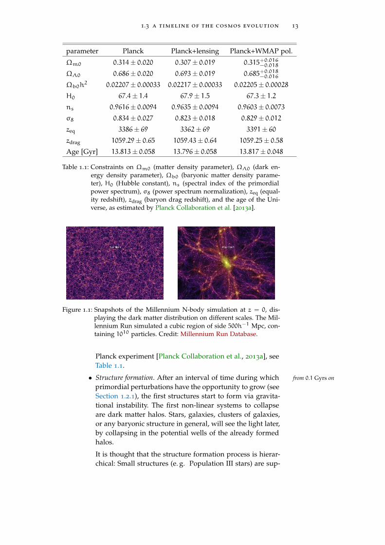
Table 1.1: Constraints on Ωm0 (matter density parameter), ΩΛ0 (dark en-ergy density parameter), Ωb0 (baryonic matter density parame-ter), H0 (Hubble constant), ns (spectral index of the primordialpower spectrum), σ8 (power spectrum normalization), zeq (equal-ity redshift), zdrag (baryon drag redshift), and the age of the Uni-verse, as estimated by Planck Collaboration et al. [2013a].
Figure 1.1: Snapshots of the Millennium N-body simulation at z = 0, dis-playing the dark matter distribution on different scales. The Mil-lennium Run simulated a cubic region of side 500h−1 Mpc, con-taining 1010 particles. Credit: Millennium Run Database.
Planck experiment [Planck Collaboration et al., 2013a], seeTable 1.1.
• Structure formation. After an interval of time during which from 0.1 Gyrs on
primordial perturbations have the opportunity to grow (seeSection 1.2.1), the first structures start to form via gravita-tional instability. The first non-linear systems to collapseare dark matter halos. Stars, galaxies, clusters of galaxies,or any baryonic structure in general, will see the light later,by collapsing in the potential wells of the already formedhalos.
It is thought that the structure formation process is hierar-chical: Small structures (e. g. Population III stars) are sup-

14 foundations of cosmology
posed to form earlier, whereas larger objects should appearlater via a clustering mechanism.
As density fluctuations grow, there comes one point whenthe small-perturbations approximation does not hold any-more. Even though simplified models exist, able to havepredictions about the statistical properties of collapsed ob-jects (e. g. the Press-Schechter mass function [Press andSchechter, 1974]), the description of what happens in thenon-linear regime of gravitational collapse needs to be ad-dressed by means of tools such as numerical N-body sim-ulations (see Figure 1.1).
dark energy domination Observation coming from Type Ia su-from ∼ 9.5 Gyrs tonow pernovae showed that the Universe is right now undergoing an
accelerated expansion, yielding the scientific community to be-lieve that there exists a non-zero dark energy (or cosmologicalconstant, in its simplest form) component. A domination of theterm ΩΛ gives
dadt
= H0aΩ1/2Λ , (1.39)
hence bringing
a ∝ et. (1.40)
Recent constrains on ΩΛ lead to believe that the dark energycomponent started to dominate the Universe energy density ina recent time, whose correspondent redshift seems to be of theorder of the unity.
In this chapter I gave a synthetic overview of the most importantresults obtained in Cosmology. The main purpose was giving a widercontext to better collocate the original work that will be presented inPart ii and Part ii. The background, however, would not be completewithout a proper introduction to the method that has been used in theoriginal investigations addressed in this Thesis: gravitational weaklensing. I will present this topic in the following chapter.

2G R AV I TAT I O N A L L E N S I N G
The main purpose of modern cosmology is the understanding of Uni-verse’s evolution over time, from its very beginning to its fate, know-ing the Cosmos’ statistical properties and how structures developedor how they will evolve. Most of this is done by means of some the-oretical models and via quantities that, defined within such models,parametrize the most important properties of the cosmos: These quan-tities are called the cosmological parameters. Constraints on the cos-mological parameters can be placed in a multiplicity of ways, rangingfrom the study of the cosmological microwave background, to statis-tics of the galaxy distribution or of high-redshift objects such as TypeIa supernovae. Diverse methods often probe different scales, are sub-ject to independent systematics, or are sensitive to different cosmo-logical parameters. Gravitational lensing is one of this methods, andhas been proposed as a cosmological tool over the last years.
The lensing effect from gravitation is a relativistic phenomenon,due to the fact that, as matter produces curvature in space-time, it alsodistorts geodesics of that given space-time, causing light trajectoriesto bend. In cosmology we observe gravitational lensing when lightcoming from a distant source, e. g. a galaxy or a quasar, passes closeto massive objects like clusters of galaxies. As a result, the image ofthe source galaxy gets distorted. This deformation can be minimal, asin weak lensing, or considerable, like the giant arcs or the Einsteinrings produced by strong lensing (see for instance Figure 2.1).
It is intuitive that the amount of deflection that different light bun-dles will undergo, or, equivalently, the amount of distortion suffered
15

16 gravitational lensing
Figure 2.1: Giant arcs due to the effect of gravitational lensing. The clus-ter RCS2 032727-132623 acts as a lens for a background galaxy,whose image gets extremely magnified and stretched. Credit:NASA, ESA/Hubble.
by a source image, will depend on the mass distribution that liesbetween the observer and the source. Weak lensing can therefore beused to study the statistics of such a distribution, and infer constraintson cosmological parameter from it. One important advantage of lens-ing, is that it is sensitive to both baryonic and dark matter, and it istherefore immune, for instance, to systematic errors due to the galaxybias.
The aim of this Chapter is to give an overview of gravitational lens-ing. A special attention was devoted to weak lensing, that we adoptedas a method for detection of baryon acoustic oscillations and primor-dial non-Gaussianities of the density distribution (Part ii and Part iii,respectively). In Section 2.1, I will present the basic idea and physicsbehind lensing, as defined in a quite general context. A declinationof the lensing formalism for the specific case of cosmological weaklensing will be treated in Section 2.2. A particular kind of formal-ism, aiming to derive a 3-dimensional map of the cosmic shear, isintroduced in Section 2.3. This method, called 3d weak lensing, is ofparticular interest for this Thesis, since it was proposed by our workas a tool for detecting baryon acoustic oscillations in the matter powerspectrum, as we will see in Part ii.
The content of this chapter is based on Bartelmann and Schneider[2001], Refregier [2003], Bartelmann [2010a], and I refer to these re-views for a more accurate and extended analysis of the topic.

2.1 light deflection by gravitation 17
source plane
lens plane
↵
Ds
Dds
Dd
observer
Figure 2.2: The basic lensing process acting when a point-like source is sub-ject to the effect of a single lens.
2.1 light deflection by gravitation
2.1.1 Lens equation
The simplest situation that involves the lensing mechanism is drawnin Figure 2.2. Here we have an observer, a source placed at the angulardiameter distance Ds and a mass concentration placed in between thetwo, at distance Dd from the observer and Dds from the source.
If the dimension of the lens is negligible with respect to the dis- thin lens and Bornapproximationstances Ds, Dds, and Dd, we can use the thin-lens approximation. In this
framework, the deflection is assumed to take place instantaneouslyon the lens plane, a surface perpendicular to the line-of-sight andpassing through the lens. The Born approximation, also often used,supposes that the slightly curved light-ray path can be replaced bya single straight ray.
The path of the light ray traveling to the observer is bent by theaction of the lens. As a consequence, the source object will appearat a different position, now subtending an angle β (and not θ, as itwould be without the lens) with the line-of-sight.

18 gravitational lensing
The deflection is quantified by the angle α (see Figure 2.2), that isdeflection angle
predicted by general relativity and reads
α =4GM
c2ξ
|ξ|2, (2.1)
where ξ is the impact parameter, denoting the distance from the lens,defined on the lens plane1.
Once we define the relations
θ =ξ
Ddand β =
η
Ds, (2.2)
then the relation, called lens equation, that the geometry of the lightlens equation
ray path has to fulfill is
β ≡ θ−Dds
Dsα(Ddθ) = θ−α(θ), (2.3)
with α being defined as in the equation, and called the reduced deflec-tion angle.
If we choose to abandon the simplified model of deflection by asingle mass, and
• consider instead a mass distribution, characterized by a densityρ(ξ, z),
• assume that deflection angles are small, i. e. we are dealing witha weak gravitational field,
• make use of the Born approximation,
then in the continuum limit, the vectorial sum of all the small deflec-tions can be written as an integral that looks like
α(ξ) =4G
c2
∫d2ξ ′
∫dz ′ρ(ξ, z)
ξ− ξ ′
|ξ− ξ|2. (2.4)
It is possible to show that the deflection angle can be expressed asdeflection angle asthe gradient of a
potentiala gradient of a potential ψ. In order to do that, we should first definethe surface mass density as the mass density projected on a surface thatis perpendicular to the line-of-sight:
Σ(ξ) ≡∫
dz ρ(ξ, z). (2.5)
Similarly, one can introduce the quantity
Σcr =c2
4πG
Ds
DdDds, (2.6)
called critical surface mass density. This term allows us to write a di-convergence
1 this prediction holds only in case the impact parameter is much larger than theSchwarzschild radius, RS ≡ 2GM/c2, of the lens.

2.1 light deflection by gravitation 19
Figure 2.3: The famous Einstein’s cross. The quasar QSO 2237+0305 is sub-ject to the lensing by a foreground galaxy, producing four sepa-rate images. Credit: ESA/Hubble.
mensionless Σ(ξ), such that
κ(θ) ≡ Σ(Ddθ)
Σcr, (2.7)
that is now depending on the angle θ, rather than on the absolutedistance ξ from the lens.
The quantity κ(θ) is called convergence. Having κ > 1 is a sufficientcondition (although not necessary) for the lens equation to have mul-tiple solutions. In other words, a surface mass density larger than the multiple images
threshold value Σcr, brings to the development of multiple images(see Figure 2.3). The situation κ = 1 poses a limit for the discrimi-nation between weak and strong gravitational lensing. Whenever the weak and strong
lensingconvergence is larger than, or of the order of unity, we have stronglensing, featuring multiple images or somewhat extreme distortionsof the source image, such as the giant arcs pictured in Figure 2.1;weak lensing, instead, takes place when κ 1, and is characterizedby small image deformations, usually of the order of 2%.
Eventually, it is possible to write the total deflection angle in termsof the convergence κ and the angle θ on which it depends:
α(θ) =1
π
∫d2θ ′κ(θ ′)
θ−θ ′
|θ−θ ′|2. (2.8)
The previous relation makes obvious that the deflection angle canindeed be expressed as a 2-dimensional gradient of a potential ψ,
α(θ) = ∇ψ(θ), (2.9)
where lensing potential

20 gravitational lensing
ψ(θ) ≡ 1
π
∫d2θ ′κ(θ ′) ln |θ−θ|. (2.10)
The quantity ψ is called lensing potential, and it can be seen as the lens-ing equivalent of the Newtonian gravitational potential. Moreover, itsatisfies the Poisson equation
∇2ψ(θ) = 2κ(θ). (2.11)
2.1.2 Image distortion
A point-like source whose light experiences gravitational lensing bya given mass distribution, will be perceived by an observer as if itwas shifted on the plane perpendicular to the line of sight. Thingsimage deformation
of extended sources are slightly more complicated for a source of finite size. In this case,light rays coming from different parts of the source will be subjectto deflections that do not necessarily have to be of the same entity,depending on the values assumed by the lensing potential on theplane.
In general, light bundles that are deflected differentially will pro-duce distorted images of the source that emitted them. This distortioncan be qualitatively and quantitatively described by the Jacobian ma-trix of the lens equation:
A(θ) =∂β
∂θ(2.12)
In case we assume the source to be considerably smaller than thescale on which the properties of the lens change, we can expand thelens equation and truncate it at the first order, yielding
A(θ) =
(δij −
∂2ψ(θ)
∂θi∂θj
)=
(1− κ− γ1 −γ2
−γ2 1− κ+ γ1
). (2.13)
In the previous equation, a new complex quantity has been intro-complex shear
duced: The shear γ, that can be written in terms of γ1 and γ2 asγ ≡ γ1 + iγ2, or equivalently γ = |γ|exp(2iϕ), where the factor oftwo in the exponential reminds us that the shear is a spin-2 field. Theshear components are related to the second derivatives of the lensingpotential via the relations
γ1 =1
2
(∂2ψ
∂θ21−∂2ψ
∂θ22
), γ2 =
∂2ψ
∂θ1∂θ2. (2.14)
It is particularly interesting to have a look at A(θ) once we divideisotropic and anisotropic distortions. In fact, Equation 2.13 can be re-written as
A(θ) = (1− κ)
(1− g1 −g2
−g2 1+ g1
). (2.15)

2.2 cosmological weak lensing 21
The term (1− κ) acts in a homogeneous fashion, re-scaling the sizeof the lensed object. The matrix, on the other hand, will produce a reduced shear
distortion of the image through the action of the components of theso called reduced shear g, by definition:
gi ≡γi1− κ
. (2.16)
Please note that, in principle, the deformation depends on both shearand convergence, although in the limit of weak lensing (κ 1), wehave gi ∼ γi.
It can be seen that for a generic, circular source, the distortion due distortion of acircular sourceto gravitational lensing will produce an elliptical image, whose major
and minor axes are given, respectively, by the relations
a =r
1− κ− |γ|and b =
r
1− κ+ |γ|, (2.17)
where |γ| is, of course, the modulus of the complex shear γ.Lensing is just a geometrical effect, and there is no absorption or
emission of photons once the light bundle has left the source. As aconsequence, the surface brightness of the source is conserved. Fluxis not, though, and a quantification of how much the observed flux magnification
differs from the one the source would have without lensing, is givenby the magnification µ of the light bundle,
µ ≡ 1
|detA|=
1
(1− κ) − |γ|2, (2.18)
that results to be the inverse of the determinant of the Jacobian matrixA(θ). Magnification is caused by both convergence and shear, thanksto isotropic and anisotropic focusing of light, respectively.
2.2 cosmological weak lensing
In this section, cosmological weak lensing will be analyzed, and allthe results obtained so far will be generalized to the case where thelens deflecting light ray paths is not a single mass, but instead thelarge scale structure of the Universe.
In this framework, the deflection angle is given by an integral of deflection angle forLSS-induced lensingthe gradient of the potential, or better the component perpendicular
to the line-of-sight. This integral is weighted, though, by the ratio oftwo angular diameter distances: The one between lens and source,over the one between observer and source. In fact,
α(θ,χ) =2
c2
∫χ0
dχ ′fK(χ− χ
′)
fK(χ)∇θΦ[fK(χ
′)θ,χ ′], (2.19)
where χ is a comoving coordinate.Similarly as before, it is possible to define an effective convergence effective convergence

22 gravitational lensing
κeff, and express it in terms of the density contrast making use of thePoisson equation
∇2Φ =3H20Ωm0
2aδ. (2.20)
The effective convergence is given by
κeff(θ,χ) =1
2∇θα(θ,χ), (2.21)
hence depending, in principle, on a 2-dimensional Laplacian ∇θ · ∇θ
of the gravitational potential (see Equation 2.19). It is possible topromote this Laplacian to a 3-dimensional one by adding a factor∂2Φ/∂χ2. The legitimacy of the operation comes from the fact thatderivatives along the line-of-sight average to zero2; its convenience,on the other hand, comes from the fact that it permits the exploita-tion of the Poisson equation, i. e. κeff to be written in terms of thedensity contrast:
κeff(θ,χ) =3Ωm0
2χ2H
∫χ0
dχfK(χ)fK(χ− χ
′)
fK(χ)
δ[fK(χ)θ,χ]a(χ)
, (2.22)
with χH = c/H0 being the Hubble distance.Assumed that the sources are not all at the same distance χ, but areaveraged effective
convergence placed according to a redshift distribution n(χ), one can constructan effective convergence that is averaged over n(χ), therefore onlydepending on the angular coordinates θ:
κeff(θ) =3Ωm0
2χ2H
∫χH0
dχGκ(χ)fK(χ)δ[fK(χ)θ,χ]
a(χ), (2.23)
and Gκ a weighting function such that
Gκ(χ) ≡∫χHχ
dχ ′n(χ ′)fK(χ− χ
′)
fK(χ), (2.24)
with n(χ ′) as the redshift distribution of the sources. Thus, the (aver-aged) effective convergence is an integral of the cosmological densitycontrast, all along the unperturbed light path, conveniently weightedby the function Gκ.
2.2.1 Angular power spectrum
Although we cannot exactly predict the exact amount of light deflec-tion for a given source, we can infer something about the statisticalproperties of these deflections. In effect, we have seen that it is pos-sible to express the quantities responsible for image distortions in
2 White and Hu [2000] verified the validity of this statement with numerical simula-tions.

2.2 cosmological weak lensing 23
terms of δ (the effective shear can also be defined in a similar way,although calculations are slightly more complex than for the conver-gence). The density contrast, as already mentioned in the previouschapter (see Section 1.2.2), can be assimilated to a stochastic field andis well described by its two-point statistics.
Is it possible to construct such statistics also in weak lensing? The Limber’s equation
answer is yes, and it is given by Limber’s equation. Suppose we havea generic, Gaussian stochastic field ϕ defined in the sky and its powerspectrum Pϕ(k). Then, given any projection of ϕ on the plane perpen-dicular to the line-of-sight that can be written as
g(θ) =
∫χ0
dχ ′q(χ ′)ϕ(χ ′θ), (2.25)
(where q(χ) is a certain weighting function along the line-of-sight)this projection allows its own power spectrum to be written
Pg(`)m =
∫χ0
dχ ′q2(χ ′)
χ ′2P
(k =
`
χ ′
). (2.26)
This result holds as far as the weighting function q(χ) is compara-tively smooth with respect to the scales on which the density contrastis expected to vary [Limber, 1953].
The Limber equation can be applied also in our case, in particularif we consider the effective convergence as a projection of the densityfield δ, and Gκ, or better its rescaling
Wκ(χ) =3Ωm0
2χ2H
G(χ)fK(χ)
a, (2.27)
as its weighting function. These assumptions bring us to the follow- angular powerspectruming expression for the angular power spectrum of the lensing conver-
gence
Cκ(`) =
∫χH0
dχW2κ(χ)
χ2Pδ
(k =
`
fK(χ)
). (2.28)
Moreover, a elementary Fourier analysis can show that the shearpower spectrum, derived in an analogous way, is exactly identicalto the convergence one
Cκ(`) ≡ Cγ(`), (2.29)
since both κ and γ depend on the second derivative of the lensingpotential.
2.2.2 Measuring the lensing distortions
The lensing convergence (or shear) angular power spectrum defined power spectrumsensitivity tocosmologicalparameters
in Equation 2.28 is particularly interesting because of its sensitivity to

24 gravitational lensing
cosmological parameters, via theΩm factor and of course via the den-sity contrast two-point statistics Pδ(k), and its evolution with time.
In principle, there is no way to know exactly how, and by howmuch, the image of a single galaxy is distorted by gravitational lens-ing. Nonetheless, one can still infer statistical deformations once thereshear from ellipticity
measurements is a larger sample of galaxies. Suppose that the observed ellipticity ofa galaxy is a sum of two effects: Its intrinsic ellipticity, and the shearγ (we are in the weak-lensing limit, therefore κ 1 and its effect onthe image shape distortion is negligible). In such a case, the two-pointcorrelation function of the observed ellipticity εobs
i can be written
〈εobsi εobs
j 〉 = 〈(εinti + γi)(ε
intj + γj)〉
= 〈εinti ε
intj 〉+ 〈εint
i γj〉+ 〈γiεintj 〉+ 〈γiγj〉
' 〈γiγj〉, (2.30)
where εint is the intrinsic ellipticity. The main assumption done inweak lensing (and in the last equivalence of the previous equation) isthat there are neither correlations between the intrinsic ellipticities ofgalaxies (〈εintεint〉), nor between εint
i and the surrounding tidal field(〈εintγ〉). In this way, the correlation function between observed ellip-ticities equals the shear two-point statistics.
In reality, this simplification is not completely exact. Intrinsic align-intrinsic alignments
ments between galaxies that formed in a common environment doexist, and can partly contaminate the results if not properly takeninto account. See Schäfer [2009] for a review on the subject.
2.3 3d weak lensing
The expression for the effective covariance in terms of the densitycontrast (Equation 2.22) shows that, originally, this is a 3-dimensionalquantity, depending on the distance χ between the source and theobserver. Averaging κeff over the supposed redshift distribution ofline-of-sight
averaging is notnecessary
the sources has become common practice over the years, leading toanalyses of 2-dimensional shear fields. Performing this simplificationhas been a mere consequence of poor measurements of individualgalaxy distances.
This weighing, though, is not necessary if we can know such dis-tances with good approximation. Upcoming surveys such as Euclid3
or DES4, able to measure galaxy photometric redshift with high accu-racy, allow to use this z as a good and precise estimate of individualgalaxy distances.
Heavens [2003] was the first to develop a framework to fully ex-3d expansion oflensing observables ploit the gain of information coming from a 3d weak lensing analysis.
The main idea is to perform a special spectral expansion of lensing
3 euclid-ec.org4 darkenergysurvey.org

2.3 3d weak lensing 25
observables, like the convergence or the shear5 (a detailed descriptionof the theory can be found in Castro et al. [2005], Massey et al. [2007],Heavens et al. [2006], Kitching et al. [2008a]).
A combination of spherical harmonics and spherical Bessel func- spherical harmonicsand spherical Besselfunctions
tions, respectively taking care of the angular and radial components,is the most natural choice for a Fourier expansion in spherical coordi-nates. In fact, such a combination is an eigenfunction of the Laplacianin spherical coordinates, and turns out to be particularly useful whenwe want to express all the lensing quantities in terms of the densityfield. For a generic scalar field f(r), such an expansion reads
f`m(k) ≡√2
π
∫d3r f(r) j`(kr)Y∗`m(θ), (2.31)
where j` and Y`m are, respectively, a spherical Bessel function of thefirst kind and a spherical harmonic.
Quantities like the lensing potential, the shear, or the convergencecan thus be decomposed and expressed in terms of coefficients of thisexpansion. For the convergence, for instance, we have:
κ`m(k) ≡√2
π
∫χ2dχ dθ κ(θ,χ) j`(kχ)Y∗`m(θ). (2.32)
An estimator of κ`m can be constructed, that in the case of a full-skysurvey of galaxies is given by the relation
κ`m(k) =3Ωm
2χ2H
`(`+ 1)
2
B`(k,k ′′)(k ′′)2
δ`m(k ′′). (2.33)
As we will see in Section 4.3 (Part ii), where a more detailed deriva- mode-couplingmatrixtion of this quantity will be provided, the matrix B`(k,k ′′) carries
all the information on additional mode couplings coming from lens-ing, the galaxy redshift distribution, and uncertainties in the measure-ment of the photometric redshift.
Statistics of the convergence (or shear, of course) coefficients6 in theconsidered 3d expansion depend on that of the coefficients δ`m with-out any averaging along the line-of-sight distribution of galaxies. Thepower spectrum of δ`m is exactly equal to the spectrum of the densitycontrast itself [Castro et al., 2005], and therefore inherits its sensitivityto cosmological parameters. Moreover, the absence of a line-of-sightweighing results in a more direct correspondence between a 3d lens-ing statistics and the underlying matter power spectrum, at least withrespect to the classical 2d weak lensing approach.
It has been shown [Heavens et al., 2006] that a 3d analysis would be valuable tool fordark energy study
5 please note that such observables depend on the gravitational potential, that evolveswith time and is not perceived as homogeneous by galaxies that are lensed underits effect. It is more correct, then, to refer to the transform of such quantities as thetransform of the corresponding, homogeneous fields that exist in correspondence ofthe time on which the galaxy emitted its light [Castro et al., 2005]
6 in this work only 3d two-point statistics have been considered; for higher orderstatistics please refer to Munshi et al. [2011].

26 gravitational lensing
of particular interest regarding constraints on the dark energy equa-tion of state, providing a reduction of the marginalized errors on itscoefficients w0 and wa, especially when combined to measurementsfrom CMB and baryon acoustic oscillations experiments.
The lack of an averaging along the line-of-sight source distribution,on the other hand, resulting as already said in a tighter relation be-tween the 3d weak lensing and the matter power spectra, leads to theidea of exploiting this kind of approach for detecting localized fea-possible application
for baryon acousticcoscillations
tures of the matter P(k), e. g. baryon acoustic oscillations (that will beintroduced in the next chapter). Such features are usually smoothedout from the classical weak lensing power spectrum, due to the pres-ence of the weighting function defined in Equation 2.24. On the con-trary, they are inherited by the 3d weak lensing spectrum, and theirdetectability depends on the sensitivity of the 3d method. In Part iiof this Thesis, I will give an overview on baryon acoustic oscillationsas a cosmological tool, and on our predictions regarding the feasibil-ity of their detection with a 3d weak lensing approach [Grassi andSchäfer, 2013].

Part II
D E T E C T I N G B A RY O N A C O U S T I CO S C I L L AT I O N S B Y 3 D W E A K L E N S I N G


3B A RY O N A C O U S T I C O S C I L L AT I O N S
Baryon acoustic oscillations are features of the matter power spec-trum P(k), where they show up as a damped series of peaks andtroughs. As the power spectrum is defined in Fourier space, it makessense to identify a BAO counterpart in configuration space: the baryonacoustic peak, namely a bump-shaped feature of the two-point mat-ter correlation function. Both this peak and BAO are manifestationof the same phenomenon: In fact, they originate during the decou-pling between matter and radiation, and represent a preferred clus-tering scale in the global matter distribution. As we will see, BAOhave been suggested to be among the most powerful and promisingnew cosmological tools for cosmological parameter constraining. Inparticular, they can help us studying and determining our Universe’sexpansion history. For a recent review, please see Bassett and Hlozek[2010].
In this Chapter, I will briefly introduce baryon acoustic oscillationsby explaining, in Section 3.1, what kind of physical processes theyoriginate from, whereas in Section 3.2 I will analyze BAO’s poten-tialities as a cosmological tool and, more specifically, as a statisticalstandard ruler.
29

30 baryon acoustic oscillations
3.1 the physics of baryon acoustic oscillations
3.1.1 The plasma era
During the first 300−400 kyrs of the Universe, the baryonic and radia-tion components of the Cosmos are in the form of a hot, dense plasmaA plasma is defined
as a globally neutralcollection of
free-moving chargedparticles
composed by electrons, nuclei and photons. All along this epoch, ra-diation and baryons result tightly coupled thanks to Thomson scatter-ing by electrons, a mechanism describing an elastic collision betweena free charged particle and a photon. As long as the timescale ofthe scattering is much smaller than the expansion timescale tH(z) =H(z)−1, we observe a continuous momentum transfer between bary-onic matter and radiation, causing them to be in thermal equilibrium.If we define the average time between two Thomson scatterings to be
ts =1
σTne, (3.1)
where σT is the Thomson cross section and ne the number density offree electrons, it is clear that, as long as ne is large enough to make therelation ts tH hold, baryons and photons will be coupled, and theirtemperatures will evolve in the same manner. This state of coursecauses the plasma to be opaque to electromagnetic radiation.
One important consequence of coupling between baryons and radi-acoustic waves inthe primordialphoton-baryon
plasma
ation, is that any perturbation in the plasma behaves like an acousticwave, thanks to the competing forces of gravity and radiation pres-sure. In simple words:
1. given a certain, primordial, perturbation in density, e. g. anoverdensity, gravitation acts to compress the plasma in corre-spondence of the overdensity itself;
2. this process also increases photon density;
3. the temperature rises, and so does the radiation pressure,
4. causing the plasma to expand.
A more rigorous analysis can be found in Eisenstein et al. [2007b],where they remind that, given the rapidity of the scattering comparedto time it takes to travel along the wavelength of a generic perturba-tion, the Euler equation can be expanded in powers of the term k/τ,namely the Compton free path λs = τ−1, over a wavelength λ ∝ k−1,where k is the perturbation’s wavenumber, τ = aσTne is the differ-ential optical depth, and the dot denotes a derivative with respectto conformal time η =
∫dt/a, while a is, as usual, the scale factor
[Montanari and Durrer, 2011]. In this way it is possible to write the

3.1 the physics of baryon acoustic oscillations 31
evolution of a single Fourier mode of the plasma perturbation in theso called tight coupling approximation:
d
dη[(1+ R)δ] +
k2
3δ = −k2(1+ R)Φ−
d
dη[3(1+ R)Ψ], (3.2)
[Peebles and Yu, 1970; Doroshkevich et al., 1978; Ma and Bertschinger,1995] where Φ is the gravitational potential, Ψ the perturbation ofspatial curvature and
R ≡ 3ρb4ργ
(3.3)
is the ratio between baryon and photon momentum density. It is easyto see that Equation 3.2 describes a driven oscillator with originalfrequency csk, where cs is defined as the sound speed
cs =c√
3(1+ R), (3.4)
and can assume at most the value of c/√3. The period decay can
anyway be neglected for small values of R, typical for the range ofredshifts here considered (z >∼ 1000).
3.1.2 After recombination
When considering the timeline of Universe’s evolution, some events,more than others, mark exceptional changes in the state and physi-cal properties of the Cosmos’s content. The epoch of recombinationand decoupling is undoubtedly part of this category. We have seenthat during the plasma era, perturbations are not allowed to grow inamplitude, on the contrary they propagate as acoustic waves with acertain sound speed (Equation 3.4); there comes a moment, though,when things change. As both temperature and density of the plasma Recombination
decrease due to cosmic expansion, the equilibrium state for baryonsmoves towards a situation where nuclei and electrons combine to-gether [Zeldovich et al., 1969; Peebles, 1968], no longer being ionized:
H+ + e− H + γ. (3.5)
By convention, the instant when 50% of baryonic matter is in theform of neutral atoms is called recombination time trec ∼ 360000 yrs,corresponding to a redshift of zrec ∼ 1090 [Komatsu et al., 2011; PlanckCollaboration et al., 2013a].
Shortly after this process begins to take place, scattering betweenphotons and electrons starts to become more and more sporadic. Inother words: The Hubble distance is now comparable or even smallerthan the photon mean free path. Photons gradually stop noticing the Decoupling and
drag epoch

32 baryon acoustic oscillations
presence of baryons, meaning that they decouple from them and thatthe total optical depth up to the present becomes smaller than one.This is when last scattering and cosmic microwave background origi-nate. As a consequence of recombination, also baryons stop noticingphotons, although these two specular processes do not necessarilyhave to take place at the same time. In fact, since there are vastlymore γ than baryons, photon’s optical depth approaches 1 earlierthan baryon’s τb. The moment when the baryon optical depth
τb(η) ≡∫η0η
dητ
(1+ R)(3.6)
drops below unity, is when baryons are released from the drag ofphotons due to Compton scattering, and is usually called drag epoch[Hu and Sugiyama, 1996]. From this time on, matter and radiationevolve separately: Photons now freely propagate, the Universe is al-ready transparent to electromagnetic radiation, and baryons mustnow be treated as a pressureless species, meaning that they can nowcool down at a different rate compared to photons, and eventuallycollapse. Of course the tight coupling approximation seen in Equa-tion 3.2 doesn’t hold anymore, and perturbations in the baryon den-sity can no longer propagate as acoustic waves after decoupling. Thedrag epoch doesn’t coincide, in principle, with recombination, al-though the two moments are comparable and both depend on Ωmand Ωb. A fitting formula for the derivation of the drag redshift wasproposed by Eisenstein and Hu [1998]:
zdrag = 1291(Ωmh
2)0.251
1+ 0.659(Ωmh2)0.828
(1+ b1(Ωbh
2)b2)
, (3.7)
with
b1 = 0.313(Ωmh2)−0.419[1+ 0.607(Ωmh2)0.674],
b2 = 0.238(Ωmh2)0.223. (3.8)
An interesting and instructive analysis of the evolution of a point-Evolution of apoint-like density
perturbationlike overdensity in configuration space was carried out by Eisensteinet al. [2007b], as shown in Figure 3.1. Here they analyze the massprofile behavior of such an overdensity with respect to a radial coor-dinate, as time passes by (different panels). The density perturbationis initially present in all species, i. e. dark matter, photons, baryons,and neutrinos. The figure clearly displays how, while at first thewave propagates through baryons and photons as a single pulse, afterz ∼ 1100 (time of recombination) this starts to be not valid anymore.In fact, after recombination photons can freely propagate, not supply-ing radiation pressure to baryons; the sound speed obviously dropsand this causes the baryons perturbation to slow down and even-tually freeze. Not only does the perturbation stall, but it grows bygravitational instability.

3.1 the physics of baryon acoustic oscillations 33
(a) z = 6824, t ∼ 1.4 · 104yrs (b) z = 1440, t ∼ 2.3 · 105yrs
(c) z = 848, t ∼ 5.7 · 105yrs (d) z = 478, t ∼ 1.45 · 106yrs
(e) z = 79, t ∼ 2.3 · 107yrs (f) z = 10, t ∼ 4.7 · 108yrs
Figure 3.1: The evolution with time of the radial mass profile of a point-likeoverdensity initially located at r = 0. Different panels display themass profiles at chosen redshifts, while the colors represent massprofiles of dark matter (black), baryons (blue), photons (red), neu-trinos (green). Time increases (and z gets smaller) as we look atpanels from left to right, and from top to bottom. The first twopanels show how coupling between baryons and photons makesthe perturbation evolve in an identical way for the two species.A smoothing of the DM overdensity over r > 0, due to gravita-tional interaction with the plasma, is also visible from Figure 3.1bon. After Figure 3.1c it becomes evident that photons have al-ready decoupled from matter and start streaming away, whilethe baryon perturbation gradually stops at a radius ∼ 150 Mpc.Both baryon and DM overdensity grow in amplitude and inter-act gravitationally, yelding a double-peaked mass profile like theone in Figure 3.1f. Figure taken from Eisenstein et al. [2007b].
In this scenario, what remains after recombination and decouplingare two overdensities:
• the CDM’s one, located at the center;

34 baryon acoustic oscillations
• the baryons’ one, that from t0 to trec managed to travel up to adistance rs from the center, and that now forms a shell aroundthe origin.
The distance covered by the baryons perturbation, i. e. the radius ofthe overdensity spherical shell, is of course related to the size of thesound horizon at the drag epoch, that is assumed to be comparableto the sound horizon at recombination [Eisenstein and White, 2004]:
rs =
∫trec
0
cS(1+ z)dt
=1√ΩmH
20
2c√3zeqReq
ln
[√1+ Rrec +
√Rrec + Req
1+√Req
], (3.9)
where zeq is the redshift at the moment of equality between matterand radiation, and Req, Rrec are the baryon-photon momentum den-sity ratios for, respectively, equality and recombination, giving rS ofthe order of 150 Mpc. Interacting via gravitation, CDM and baryonsdrag each other, eventually reaching the intermediate situation shownin the last panel of Figure 3.1, where the final radial mass profile fea-tures a peak close to the perturbation origin, and a secondary onelocated at the distance the baryon-photon acoustic wave could travelbefore recombination.
Galaxies and collapsed objects tend to form in correspondence ofoverdensities. As a consequence, the scale of the sound horizon at re-combination remains as a characteristic separation length in the mat-ter distribution, because there is where galaxies will be more likelyto form. In other words, it can be considered as a preferred scale formatter clustering. Since, of course, the overall baryon distribution willconsist in a superposition of perturbations similar to the one consid-ered, this length can only be recovered statistically. In effect, it willappear in the correlation function as a peak1 around the scale rs.
The power spectrum and the two-point correlation function of thematter distribution form a Fourier pair. Therefore, since the transformof a single bump gives a harmonic sequence, the baryon acoustic peakwill be visible in P(k) as wiggles (BAO) whose wavelength is strictlyrelated to the sound horizon scale at the time of recombination kS =
2π/rS. Power spectra with and without the presence of a baryoniccomponents are plotted in Figure 3.2.
1 it is a peak because we are dealing with an excess of clustering at a certain scale; ascarcity of clustering, on the other hand, would produce a dip.

3.2 bao as a cosmological tool 35
10-3 10-2 10-1
k [h · 1/Mpc]
103
104
105
P(k
)
PBAO
Ps
PCDM
Figure 3.2: The difference between a CDM-only power spectrum (black,solid line), a power spectrum where also a baryonic presencewas considered, in the amount of Ωb = 0.44 (magenta line) andthe corresponding smooth spectrum (black, dashed line). We canalso observe that the presence of baryons acts as an overall sup-pression in intermediate and small scales. The spectra were cal-culated using the prescription by Eisenstein and Hu [1998]
3.2 baryon acoustic oscillations as a cosmological tool
3.2.1 What is a statistical standard ruler
Since Riess et al. [1998] and Perlmutter et al. [1999] proved for the firsttime that the Universe was accelerating (see Figure 3.3), cosmologistshave strived for years aiming to explain what kind of mechanism isbehind this peculiar type of expansion. Whether be this phenomenonrelated to the cosmological constant, or to a dark energy with some stillunknown equation of state, there is no doubt that the understandingof the expansion of the Universe relies on our ability to investigate theredshift-distance relation, unless we consider, for instance, modified-gravity theories.
The expansion rate in function of redshift, i. e. the Hubble parame-ter H(z), can be inferred by measuring quantities such as the angulardiameter distance
dA =c
1+ z
∫z0
dz
H(z)(3.10)
or the luminosity distance (see Section 1.1.4)
dL ≡√
L
4πF
= (1+ z)2dA. (3.11)

36 baryon acoustic oscillations
34
36
38
40
42
44
1M=0.24, 1R=0.76
1M=0.20, 1R=0.00
1M=1.00, 1R=0.00
m-M
(mag
)
MLCS
0.01 0.10 1.00z
-0.5
0.0
0.5
6(m
-M) (
mag
)
Figure 3.3: Difference between relative and absolute magnitude (top panel)for a sample of Type Ia supernova as a function of their redshift.The lines represent the expected behavior for different cosmolo-gies, while the bottom panel displays the residuals with respectto the reference model, characterized by Ωm = 0.2 and ΩΛ = 0.The data appear to give evidence for a flat Universe with a non-zero Λ-component, implying an acceleration of the cosmic ex-pansion. Figure taken from Riess et al. [1998].
If we assume the expansion to be ascribable to the effect of darkenergy, and described by its density parameter ΩΛ and its equationof state (assumed that it can be treated as an ideal fluid)
w(z) =pΛρΛ
∣∣∣∣z
, (3.12)
then the Hubble parameter for a flat, matter and dark-energy domi-Hubble parameter asa proxy for dark
energy contributionnated universe can be written:
H(z) = H0
√Ωm0(1+ z)3 +ΩΛ0 exp
[3
∫z0
1+w(z)
1+ zdz
], (3.13)
where H0, Ωm0, and ΩΛ0 are, respectively, the expansion rate pa-rameter, the matter density and dark energy density parameters atpresent time. The Hubble parameter is thus the fundamental observ-able related to ΩΛ0 and w(z).
To measure quantities like dL and dA and their trend with redshift,standard candlesand standard rulers

3.2 bao as a cosmological tool 37
though, we need respectively
• standard candles: Objects whose absolute magnitude, or luminos-ity, is known or, alternatively, whose luminosity change withredshift in a well understood way;
• standard rulers: Objects of known absolute size, or whose size-redshift relation is well acknowledged.
Rulers and candles are especially useful, in cosmology, for solvingissues related to the degeneracy that exists between radial distance,intrinsic size (or luminosity) of the object, and space curvature. Infact, if we observe an object to be small (or faint), theoretically we arenot allowed to know whether it is intrinsically small (faint), whetherit looks like this because it is very far away from us, or whether spacecurvature acts as a lens and distorts its shape. Standard rulers andcandles can, in principle, break this degeneracy.
Several examples of this two very special category of objects canbe found in cosmology. Type Ia supernovae (SNIa) are probably themost famous among standard candles : Since their collapse always oc-curs at the Chandrasekar mass, they happen to have a characteristicbrightness at the peak of their light curve, that can be used as stan-dard candle after appropriate calibrations. Unlike other standard can-dles (e. g. Cepheids, RR Lyrae), Type Ia supernovae are particularlysuited for cosmology thanks to their extremely high brightness, thatmakes them visible even at cosmologically relevant distances. Riesset al. [1998], for instance, used supernovae up to z ∼ 1 in their study,corresponding to a distance of the order of the Gpc.
Concerning cosmological standard rulers, some have been proposedover the years: Double-lobed [Buchalter et al., 1998] and ultra-compactradio sources [Kellermann, 1993; Gurvits, 1994; Jackson and Dodgson,1997], or even galaxy clusters [Allen et al., 2002; Schäfer et al., 2005;Mantz et al., 2008]. All of them gave results similar or at least com-patible with the ones obtained by Riess et al. [1998] from SNIa.
A slightly different class of standard rulers also exists. Imagine to statistical standardrulershave, rather than an object, a particular behavior or phenomenon that
has a characteristic, known scale, e. g. clustering of galaxies. In thiscase we are not dealing with one single object of known size, butinstead with a certain distribution whose characteristic scale can berecovered only statistically (see Figure 3.4): Such a tool is called statis-tical standard ruler.
The ideal (statistical) standard ruler allows for very accurate con- 3 rules for theperfect standardruler
straints on H(z), and in order to achieve that it should satisfy thefollowing properties2:
2 these considerations are based on Martin White’s lectures on BAO, that he kindlyprovides on mwhite.berkeley.edu

38 baryon acoustic oscillations
Figure 3.4: The concept behind statistical standard rulers, taken from Bas-sett and Hlozek [2010]. It shows a very simple, two-dimensionalgalaxy distribution featuring a preferred clustering scale. In theleft panel, the relatively small number of galaxies makes the cor-relation visible to the naked eye. The right panel, instead, showsa distribution with the same characteristics but where the num-ber of galaxies is much larger: In this case, the distribution’s char-acteristic scale is not obvious anymore and can only be regainedstatistically, by means of a correlation function.
• it should be possible to calibrate the ruler over the largest possi-ble redshift interval (i. e. we can precisely predict how the rulersize evolves with z);
• the ruler size should be small enough to be measured with highstatistical accuracy over the volume of the surveys;
• it should be possible to get a high-precision measurement of theruler.
We will see in the following sections that baryonic features in thematter distribution statistics can satisfy all of these properties.
3.2.2 Constraining cosmological parameters with baryon acoustic oscilla-tions
Since BAO and the baryon acoustic peak are manifestations of the ex-istence of a preferred clustering scale, and since this scale’s absolutevalue can be relatively easily calculated from theory, they make ex-cellent statistical standard rulers, as it was first suggested by Coorayet al. [2001] and later developed in more detail by Eisenstein [2003]and Blake and Glazebrook [2003].
By measuring both the transverse, angular size of the BAO featureand its interval in redshifts at different z (namely, transverse and ra-dial Fourier modes of the matter distribution) we can get estimatesof, respectively, dA(z) and H(z). Since the physical, absolute scale ofBAO is known, they are not considered an Alcock-Paczynski test [Al-cock and Paczynski, 1979] and the two quantities themselves, ratherthan their product, can be inferred separately.

3.2 bao as a cosmological tool 39
Baryon acoustic oscillations fulfill, in theory, all the characteristicsof a good ruler, in fact:
• within a certain grade of accuracy, BAO scale is predicted bywell understood, linear theory and depends mainly on matterand baryon density, meaning that CMB constrains on Ωm andΩb, for instance, can be used to accurately calibrate the BAOruler;
• recent galaxy surveys have reached sufficiently large volumesso that BAO features can be detected in the galaxy density dis-tribution;
• the oscillatory behavior (peak) of the matter power spectrum(two-point correlation function) is a relatively sharp and easilyrecognizable feature to detect.
3.2.2.1 Observing baryon acoustic oscillations
(a) (b)
Figure 3.5: On the left, the baryon acoustic peak in the correlation functionof a SDSS galaxy sample. The three upper lines represent mod-els with, from top to bottom, Ωmh2 = 0.12, 0.13, 0.14, while forall three Ωbh2 = 0.024; the bottom line shows a model with nobaryons, and therefore no acoustic peak. The right panel, on theother hand, exhibits a power spectrum derived from an SDSS(top curve) and an LRG (bottom curve) galaxy sample. Solidand dashed lines represent, respectively, a ΛCDM fit to WMAP3
[Spergel et al., 2007] data, and a fit that includes also non-linearcorrections. Left and right panels are taken respectively fromEisenstein et al. [2005] and Tegmark et al. [2006].
The two primary channels for observing a baryon acoustic signa-ture are the power spectrum of CMB temperature anisotropies andstatistics of galaxy distributions. While oscillatory features in the CMBpower spectrum were already observed by WMAP [Hinshaw et al.,2003, 2007; Nolta et al., 2009; Larson et al., 2011], BAO signatures in
40 baryon acoustic oscillations
the galaxy distribution have been detected for the first time by Eisen-stein et al. [2005] in the SDSS survey, as shown in Figure 3.5a.
Further detection have been carried out, ever since, in particularwith SDSS [Eisenstein et al., 2005; Padmanabhan et al., 2007; Perci-val et al., 2007b, 2010; Kazin et al., 2010b; Padmanabhan et al., 2012;Mehta et al., 2012], the 2-Degree Field Galaxy Redshift Survey [2dF-GRS, Percival et al., 2007a; Beutler et al., 2011], the WiggleZ-survey[Parkinson et al., 2012] and Lyman-α forest data coming from theBaryon Oscillation Spectroscopic Survey (BOSS) [Busca et al., 2012;Slosar et al., 2013]. Moreover, [Gaztañaga et al., 2009a; Kazin et al.,2010a; Gaztañaga et al., 2009b] managed to observe both longitudinaland transverse modes in the galaxy distribution. All the observationsconfirmed what already determined in CMB measurements, namelyspatial flatness and low matter density when a flat geometry is as-sumed as a prior.
A very interesting insight on issues related to model testing andparameter estimation with baryon acoustic oscillations was made by[Cabré and Gaztañaga, 2011], who find that although BAO cannot beused for model selection, yet, they can still help to constrain cosmo-logical parameter once a specific model is assumed to be valid.
3.2.3 Nonlinear effects and observational complications
In an ideal frame, as White [2005] nicely phrased it, we should be ableto measure the linear-theory, matter power spectrum, in real space.What is usually measured, instead, is
• the non-linear,
• galaxy power spectrum,
• in redshift space.
Although it seems that BAO probably have the lowest systematic un-certainties among the methods used for studying cosmic expansion[Albrecht et al., 2006], it is clear that these three factors have repercus-sions on the detection of the BAO scale, degrading the reconstructionof the peak position, or, equivalently, of the oscillations wavelength.
Redshift space must be considered every time we take a galaxy’sredshift spacedistortions z as an estimate of its distance. In reality, a galaxy’s redshift is de-
termined not only by its distance from us, via the Hubble relation,but also by its peculiar velocity, not to mention the fact that the red-shift uncertainty of the survey, σz, also plays a role. As a result, whatwe observe is an altered version of real space, with misestimatesof true galaxy distances leading to the so called redshift space distor-tions. These kind of deformations are mainly radial, and will there-fore mostly affect measurements of the Hubble expansion rate H(z),leaving the transverse BAO scale derivation (and subsequently dA

3.2 bao as a cosmological tool 41
measurements) almost unblemished. The main effect is a suppressionof the power spectrum P(k)
Pobs(k) = P(k) exp
[−
(k||σz
1+ z
H(z)
)2], (3.14)
over the radial modes k|| [Seo and Eisenstein, 2003], where Pobs(k)is of course the resulting, observed power spectrum. This suppres-sion clearly depends on the redshift uncertainty σz, and it acts morestrongly on higher order oscillations. Its main effect is to smear outthe baryon acoustic peak in the correlation function. I refer to Blakeet al. [2006], Benitez et al. [2008], Cai et al. [2009], Simpson et al. [2009]for a more detailed analysis of the subject.
An other source of complications is undoubtedly non-linear struc- distortions due tonon-linear structureformation
ture formation. At z < 1, there is already a deviation of the non-linearP(k) from the linear one concerning wave numbers that contain acous-tic information [Eisenstein et al., 2007b]. Since non-linear collapsetend to displace matter with respect to its initial position by an or-der of ∼ 10 Mpc, due to an object’s combined interactions with all theother density fluctuations, a broadening of the baryon acoustic peakwill be observed. A broadening that adds to the natural, finite widthof the peak of ∼ 10 Mpc h−1, due to Silk damping [Silk, 1968]. InP(k), this will be observed as a damping of the oscillations at higher Silk damping:
Dissipation ofperturbations belowa given Silk scale; itis due to photonsrandomly walkingout of overdenseregions
k (smaller scales). It is straightforward that a broadening of the peakwill have important consequences in the precision with which theposition of the peak itself, i. e. the scale of the sound horizon rs, ismeasured. Mode-mode couplings in the density distribution inducedby non-linear structure formation also play a role, producing a shiftin the baryon acoustic peak. This phenomenon has been thoroughlyanalyzed by Crocce and Scoccimarro [2006b], Crocce and Scoccimarro[2006a] and Crocce and Scoccimarro [2008]. On the other hand, recon-struction methods have also been proposed [Eisenstein et al., 2007a]to account for this kind of non-linear distortion, recovering the truepeak position, and have been proved to be successful [Eisenstein et al.,2007a; Huff et al., 2007; Seo et al., 2008; Noh et al., 2009; Mehta et al.,2011]
Lastly, a further shift of the BAO peaks emerges as a consequence distortions fromgalaxy biasof the bias mechanism. Indeed, if we aim to obtain constraints on the
shape of the matter power spectrum, we should keep in mind thatobjects like galaxies or Type Ia supernovae (proposed as a target tomeasure BAO by Zhan et al. [2008]) trace the underlying dark matterdistribution in an incomplete, partially unknown way, quantified bythe bias parameter b as shown in the equation
Pobj(k) = b2(k, z)PCDM(k), (3.15)
with Pobj(k) standing for the power spectrum of the considered classof objects, PCDM(k) for the dark matter one, and where it was pointed

42 baryon acoustic oscillations
out that the bias parameter can in principle be both scale and redshiftdependent [Coles, 1993; Weinberg, 1995; Fry, 1996; Smith et al., 2007].Mehta et al. [2011] used numerical simulations to extensively analyzerepercussions of galaxy bias on BAO measurements, combined withthe reconstruction technique by Eisenstein et al. [2007a]. They findthat such shifts on the final determination of the peak position shouldnot be noticeable in current surveys, e. g. SDSS, BOSS, or the WiggleZdark energy survey. Despite that, they claim it is not excluded thatupcoming surveys like BigBOSS or Euclid could measure the BAOscale with a precision that could allow for a bias shift to be noticed.
A weak lensing measurement of the matter power spectrum wouldwhat aboutgravitational
lensing?be immune to bias mechanisms, as gravitational lensing traces theoverall matter distribution, rather than only baryons. We will see inChapter 4 that, while classical weak lensing cannot be a valuable can-didate for BAO detection due to its wide line-of-sight weighting func-tions, three-dimensional weak lensing can, instead, prove to be ableto resolve oscillatory features in P(k) [Grassi and Schäfer, 2013].

4B A RY O N A C O U S T I C O S C I L L AT I O N S W I T H 3 DW E A K L E N S I N G
This chapter reproduces the content of the paper "Detecting baryon acousticoscillations by 3d weak lensing" [Grassi and Schäfer, 2013]. The originalanalysis we carried out and the results are presented in Section 4.4 andsummarized in Section 4.5.
abstract
We investigate the possibility of detecting baryon acoustic oscilla-tion features in the cosmic matter distribution by 3d weak lensing.Baryon oscillations are inaccessible even to weak lensing tomographybecause of wide line-of-sight weighting functions and require a spe-cialized approach via 3d shear estimates. We quantify the uncertaintyof estimating the matter spectrum amplitude at the baryon oscilla-tions wave vectors by a Fisher-matrix approach with a fixed cosmol-ogy and show in this way that future weak lensing surveys such asEuclid and DES are able to pick up the first four or three wiggles,respectively, with Euclid overall giving a better precision in the mea-surement. We also provide a detailed investigation of the correlationexisting between errors and of their scaling behavior with respect tosurvey parameters such as median redshift, error on redshift, error onthe galaxy shape measurement, sky coverage, and finally with respectto the number of wiggles one is trying to determine.
43

44 baryon acoustic oscillations with 3d weak lensing
4.1 introduction
Baryon acoustic oscillation (BAO) features are modulations in thecosmic matter distribution on very large spatial scales of roughly∼ 100Mpc/h [for a review, see Bassett and Hlozek, 2010]. These BAOsare the imprint of oscillations of the photon-baryon fluid in the earlyuniverse on the matter density field driven by gravity and the equa-tion of state providing a restoring force, and they are observable intwo primary channels: through the observation of anisotropies in thecosmic microwave background (CMB) and through galaxy surveys.The most important features such as their spatial scales, their signa-ture in the CMB, their statistical properties, and their dependence oncosmological parameters is very well understood analytically [Seljakand Zaldarriaga, 1996; Hu and Sugiyama, 1996; Montanari and Dur-rer, 2011; Sutherland, 2012].
Concerning the determination of cosmological parameters, it is afortunate situation that they are observable at high redshifts throughthe primary CMB and at much lower redshifts in the galaxy distribu-tion. Due to the fact that BAOs provide a standard yardstick at twodifferent cosmological epochs, it is possible to constrain the densityparameters of cosmic fluids and the possible time evolution of theirequation of state parameters in a geometric way, breaking degenera-cies that may arise if the equations of state of cosmological fluids areallowed to change with time.
CMB observations carried out by the Cosmic Background Explorer[COBE, Bennett et al., 1994; Wright et al., 1996] first revealed aniso-tropies in the CMB, but only the Wilkinson Microwave AnisotropyProbe [WMAP, Hinshaw et al., 2003, 2007; Nolta et al., 2009; Lar-son et al., 2011] had sufficient angular resolution such that the BAOscale of ∼ 100 Mpc/h could be resolved at a comoving distance of∼ 10 Gpc/h, revealing temperature modulations of the CMB of theorder ∆T/TCMB ' 10−5 at an angular scale of roughly 2, with subse-quent higher harmonics. Likewise, galaxy surveys have now reachedsufficient depth and solid angle that BAO features could be detectedas modulations of the galaxy density of the order 10% in both radialand transverse directions. With the assumption of a galaxy biasingmodel, the longest wavelength BAO modes survive nonlinear struc-ture formation to the present epoch [Meiksin et al., 1999] and willbe targeted by future surveys for the precision determination of cos-mological parameters [Dolney et al., 2006; Angulo et al., 2008; Labatieet al., 2012], in particular dark energy [Seo and Eisenstein, 2003; Eisen-stein et al., 2007a]. Both avenues have contributed significantly to theestimation of cosmological parameters and to the selection of mostplausible cosmological models.
Specifically, there are quite a number of detection reports with on-going surveys, for instance with the Sloan Digital Sky Survey [SDSS,

4.1 introduction 45
Eisenstein et al., 2005; Padmanabhan et al., 2007; Percival et al., 2007b,2010; Kazin et al., 2010b; Padmanabhan et al., 2012; Mehta et al., 2012],the 2-Degree Field Galaxy Redshift Survey [2dFGRS, Percival et al.,2007a; Beutler et al., 2011], the WiggleZ-survey [Parkinson et al., 2012]and Lyman-α data [Busca et al., 2012] with subsequent determinationof cosmological parameters which confirm spatial flatness and thelow matter density found by CMB observations, if flatness is assumedprior to the analysis. Recent studies [Parejko et al., 2012; Zhao et al.,2012] were able to constrain neutrino masses. BAO modulations havebeen found as longitudinal as well as transverse modes in the galaxydensity [Gaztañaga et al., 2009a; Kazin et al., 2010a; Gaztañaga et al.,2009b] and their issues of model selection and parameter estimationhave been addressed thoroughly [Cabré and Gaztañaga, 2011].
The motivation for this paper is the fact that the detection of BAOs motivation
as a modulation feature in the galaxy field depends on the assump-tion of a biasing mechanism [Gaztañaga et al., 2009a; Desjacques et al.,2010] which relates the galaxy number density to the ambient densityof dark matter is well as a control of redshift space distortions effects[Nishimichi et al., 2007; Taruya et al., 2009] and it would be desirableto measure the dark matter density directly. Weak lensing would be why using 3dWL?
a prime candidate for such a measurement, but the wide line-of-sightweighting functions cause the weak lensing signal to depend ratheron the integral of the spectrum of cold dark matter (CDM) than onindividual, localized features, even in the case of tomographic lensingsurveys [Hu, 1999]. This is the reason why investigate the sensitivityof 3d weak lensing [3dWL, Heavens, 2003] for constraining the darkmatter spectrum on BAO scales: 3dWL provides a direct estimateof the 3-dimensional matter distribution and gives Gaussian errorson the amplitude of the CDM spectrum in wavelength bands fromsparsely sampled data [Leonard et al., 2012]. In this way, we aim toquantify the statistical precision at which 3dWL constraints the CDMspectrum at the BAO wavelengths, and the statistical significance forinferring the presence of one or more wiggles from 3dWL data rela-tive to the null-hypothesis of absent wiggles.
After a short compilation of basic results concerning distances, struc-ture growth, structure statistics, and conventional weak lensing inSection 4.2, we recapitulate the main results of 3dWL in Section 4.3and motivate its usage in constraining BAO wiggles. Our statisticalapproach and the estimation of statistical errors on the BAO measure-ment is given in Section 4.4, followed by a discussion of our mainresults in Section 7.9.
The reference cosmological model used is a spatially flat wCDMcosmology with Gaussian adiabatic initial perturbations in the matterdistribution. The specific parameter choices are Ωm = 0.25, ns = 1,σ8 = 0.8 and H0 = 100 h km/s/Mpc, with h = 0.72. The dark energyequation of state is set to w = −0.9 and we assume the dark energy to

46 baryon acoustic oscillations with 3d weak lensing
be smooth. The baryon density Ωb = 0.04 is used for correcting theCDM shape parameter and for predicting BAO-wiggle amplitudesand wave-vectors.
4.2 cosmology and structure formation
4.2.1 Dark energy cosmologies
In spatially flat dark energy cosmologies with the present matter den-sity Ωm, the Hubble function aH(a) = da/dt is given by
H2(a)
H20=Ωm
a3+ (1−Ωm) exp
(3
∫1a
d lna (1+w(a))
), (4.1)
with the dark energy equation of state w(a). A constant value w ≡−1 corresponds to the cosmological constant. The relation betweencomoving distance χ and scale factor a is given by
χ = c
∫1a
daa2H(a)
, (4.2)
with the Hubble distance χH = c/H0 as the cosmological distancescale. Redshift z and comoving distance are related by dz/dχ = H(z)/c
.
4.2.2 CDM power spectrum
The linear CDM-density power spectrum P(k) describes the fluctua-tion amplitude of the Gaussian homogeneous density field δ,
〈δ(k)δ(k′)∗〉 = (2π)3δD(k − k′)P(k) ∝ knsT2(k), (4.3)
with the the spectral index ns and the transfer function T(k). Therestoring force provided by the baryon-photon fluid in the early Uni-verse generates a set of wiggles in the spectrum P(k) and an overallsuppression due to diffusion. Both effects are discussed in detail byEisenstein and Hu [1998] and Eisenstein and Hu [1999] who also pro-vide a fitting formula for T(k) in terms of the density parameters Ωm,Ωb, and the Hubble parameter h.
The spectrum P(k) is normalized in such a way that it exhibits thevariance σ28 on the scale R = 8 Mpc/h,
σ2R =
∫k2dk2π2
P(k)W2(kR) (4.4)
with a Fourier transformed spherical top hat filter function, W(x) =
3j1(x)/x, where j`(x) is the spherical Bessel function of the first kindof order ` [Abramowitz and Stegun, 1972].

4.2 cosmology and structure formation 47
4.2.3 Structure growth
The growth of density fluctuations in the cosmic matter distributioncan be described as a self-gravitating hydrodynamical phenomenon,in the limit of Newtonian gravity. Homogeneous growth of the den-sity field
δ(x,a) = D+(a)δ(x,a = 1) (4.5)
in the linear regime |δ| 1 is described by the growth functionD+(a), which is the solution to the growth equation [Turner andWhite, 1997; Wang and Steinhardt, 1998; Linder and Jenkins, 2003],
d2
da2D+(a) +
1
a
(3+
d lnHd lna
)d
daD+(a) =
3
2a2Ωm(a)D+(a). (4.6)
Nonlinear structure formation leads to a strongly enhanced struc-ture growth on small scales, generates non-Gaussian features and,most importantly, wipes out BAO wiggles as features in the initialmatter distribution. This can be understood in an intuitive way ascorrections to the CDM spectrum in perturbation theory to order nassume the shape of integrals over polyspectra up to order 2n [whichseparate into a product of n spectra by application of the Wick’s the-orem, see the review by Bernardeau et al., 2002] and are thereforebecoming insensitive to localized features that are not strongly influ-encing the normalization of P(k) [Springel et al., 2005; Jeong and Ko-matsu, 2006; Pietroni, 2008; Matarrese and Pietroni, 2008; Crocce andScoccimarro, 2008; Nishimichi et al., 2009; Jeong and Komatsu, 2009;Jürgens and Bartelmann, 2012; Anselmi and Pietroni, 2012]. Since non-linear structure formation affects small scales first, we will target BAOwiggles with 3dWL beginning at the largest wavelength before pro-ceeding to successively shorter wavelengths.
4.2.4 Weak gravitational lensing
The weak lensing convergence κ provides a weighted line-of-sight av-erage of the matter density δ [for reviews, see Bartelmann and Schnei-der, 2001; Munshi et al., 2008; Hoekstra and Jain, 2008; Bartelmann,2010c],
κ =
∫χH0
dχWκ(χ)δ, (4.7)
with the weak lensing efficiency Wκ(χ) as the weighting function,
Wκ(χ) =3Ωm
2χ2H
D+
aG(χ)χ, (4.8)

48 baryon acoustic oscillations with 3d weak lensing
and the lensing efficiency weighted galaxy redshift distribution, rewrit-ten in terms of comoving distance,
G(χ) =
∫χHχ
dχ′ n(χ′)(1−
χ′
χ
). (4.9)
n(z) denotes a common parametrization of the redshift distributionof the lensed background galaxy sample,
n(z) = n0
(z
z0
)2exp
(−
(z
z0
)β)dz with
1
n0=z0βΓ
(3
β
),
(4.10)
which can be rewritten in terms of a distribution in comoving dis-tance with the relation n(χ)dχ = n(z)dz using dχ/dz = c/H(a).These expressions allow to carry out a Limber projection [Limber,1954] of the weak lensing convergence, which yields the angular con-vergence spectrum Cκ(`),
Cκ(`) =
∫χH0
dχχ2W2κ(χ)P(k = `/χ). (4.11)
We will formulate our derivations in terms of the lensing convergenceκ instead of the observable shear γ because it is a scalar quantity andpossesses identical statistical properties. Equation 4.11 illustrates whyline-of-sight averaged weak lensing spectra are ineffective in pickingup BAO wiggles (and is almost a repetition of the previous argumentwhy nonlinear structure formation destroys BAO features): They pro-vide only an integrated measure of the CDM spectrum P(k) weightedwith wide weighting functions Wκ(χ) that is very insensitive to localfeatures of the spectrum such as BAO wiggles. This argument holdseven for advanced tomographic surveys [Hu, 1999; Takada and Jain,2004] and motivates the need of a 3-dimensional mapping of the cos-mic matter distribution. With reference to Gaztañaga et al. [2009b]and Kazin et al. [2010a], we would like to emphasize that weak lens-ing, due to its sensitivity to gravitational shear components perpen-dicular to the line of sight, will provide measurements of BAO wig-gles in the transverse direction.
4.3 3d weak lensing
The method of 3dWL was introduced by Heavens [2003], who pro-posed to include distances of lensed galaxies estimated from theirphotometric redshifts to infer the 3-dimensional unprojected tidal shear,no line-of-sight
averaging in 3dWL i.e. the second derivatives of the gravitational potential perpendicularto the line-of-sight from distortions in the galaxies’ ellipticity. There-fore, this approach differs from estimations of the angular line-of-

4.3 3d weak lensing 49
sight averaged spectrum Cκ(`) or corresponding tomographic spec-tra Cijκ (`) in the important respect that the statistics of the full 3-dimensional matter distribution is inferred without any averagingof shears with the line-of-sight galaxy distribution, which has beenperformed in Equation 4.9. As such, 3dWL is particularly suited forthe problem at hand, namely to provide a precise estimate of the am-plitude of the dark matter power spectrum at the BAO wavelengths.Additionally, Heavens [2003] showed that if 3dWL is used for con-straining P(k) at a fixed cosmology, the smallest errors are expectedin the BAO regime of the CDM spectrum.
In this section, we recapitulate the main results of 3dWL in termsof the weak lensing convergence in the Fourier-convention we preferto work with; please also refer to Castro et al. [2005], Massey et al.[2007], Heavens et al. [2006], Kitching et al. [2008a] for a detailed de-scription of the theory, to Munshi et al. [2011] for higher-order statis-tics through 3dWL and to Ayaita et al. [2012] for details of our nu-merical implementation. We assume spatial flatness and lensing inlinearly evolving structures, which can be, in principle, relaxed fromthe 3dWL point of view [Pratten and Munshi, 2013]. The impact ofsystematic errors is nicely investigated by Kitching et al. [2008b], andfor an application to observational data we refer the reader to Kitch-ing et al. [2007].
The most natural choice for carrying out a Fourier transform inspherical coordinates is a combination of spherical harmonics for theangular and spherical Bessel functions for the radial dependence. We convergence
transformationcan therefore write the transformation for the convergence κ as
κ`m(k) ≡√2
π
∫χ2dχ dΩκ(χ,θ) j`(kχ)Y∗`m(θ), (4.12)
[see Ballinger et al., 1995; Heavens and Taylor, 1995], where j` andY`m are, respectively, a spherical Bessel function of the first kind anda spherical harmonic, and θ ≡ (θ,ϕ). There exist algorithms for fastcomputation of κ`m(k) [Percival et al., 2004; Rassat and Refregier,2012; Lanusse et al., 2012; Leistedt et al., 2012]. Such a transforma-tion is particularly convenient as the combination of j` and Y`m is aneigenfunction of the Laplacian in spherical coordinates, leading to aquite simple relationship between the coefficients of the density fieldδ`m(k) and the lensing convergence κ`m(k), as the observable:
κ`m(k) =3Ωm
2χ2H
`(`+ 1)
2
η`(k,k′)(k′)2
δ`m(k′), (4.13)
with the lensing-induced mode coupling η`(k,k′) mode couplinginduced by lensing
η`(k,k′) =4
π
∫∞0
χ′2dχ′
∫χ′0
dχχ′ − χ
χχ′D+
aj`(kχ
′)j`(k′χ), (4.14)
with implicit assumption of the Einstein summation convention
X(k,k ′) Y(k ′,k ′′) ≡∫∞0
k′2dk′ X(k,k ′) Y(k ′,k ′′). (4.15)

50 baryon acoustic oscillations with 3d weak lensing
It is then possible to construct an estimator for κ`m(k) by includingthe uncertainty of the galaxy distance estimates coming from errorsin the measurements of redshift. If we denote by χ the true radialcoordinate of a galaxy, and by χ ′ the one inferred by its observedredshift z′ = z(χ′), then they will be related by the probability p(χ ′|χ),which we assume to be Gaussian for simplicity:
p(χ′|χ)dχ =1√2πσ2z
exp[−(z(χ) − z(χ′))2
2σ2z
]dz′, (4.16)
where σz is the width of the distribution and is assumed to be con-stant throughout the entire galaxy sample. Furthermore, galaxies re-ceive a statistical weight according to their distribution in distancen(χ)dχ. Following the derivation in Heavens [2003], we define thetwo additional matrices
mode couplinginduced by redshift
errors and galaxydistribution
Z`(k,k′) =2
π
∫χ′2dχ′
∫dχ p(χ′|χ) j`(k′χ)j`(kχ ′), (4.17)
M`(k,k′) =2
π
∫χ2dχ n(χ) j`(kχ)j`(k′χ), (4.18)
where n(χ) is the number density of galaxies, as defined in Equa-tion 4.10. These matrices describe the correlations in spherical Fouriermodes generated by the measurement process: While η`(k,k′) de-scribes mode couplings due to weak lensing, Z`(k,k′) and M`(k,k′)define, respectively, the contributions in the mode couplings comingfrom redshift errors and from the galaxy distribution along the radialcoordinate χ.
We restrict ourselves to observations of the entire sky. In this case,full sky limit
the expression for the estimator κ`m of the convergence is then ex-pected to be
κ`m(k) =3Ωm
2χ2H
`(`+ 1)
2
B`(k,k ′′)(k ′′)2
δ`m(k ′′). (4.19)
where the mode-coupling matrix B`(k,k ′) describes two integrationsmode-couplingmatrix over k1 and k2:
B`(k,k ′′) = Z`(k,k1)M`(k1,k2)η`(k2,k ′′). (4.20)
Since the average values of a field like κ`m(k) are zero for all-skyconvergence 3dWLcovariance surveys, we can only infer information about any parameter the field
may depend on by means of its covariance,
〈κ`m(k) κ∗`m(k ′)〉 = Sκ,`(k,k ′) +Nκ,`(k,k ′) ≡ Cκ,`(k,k ′) (4.21)
which consists of a signal term Sκ,`(k,k ′) and a noise term Nκ,`(k,k ′).The signal term Sκ,` can be calculated directly from Equation 4.19:
Sκ,`(k,k ′) =(3Ωm
2χ2H
)2 [`(`+ 1)
2
]2B`(k,k ′′)(k′′)2
B`(k′,k ′′)
(k′′)2
Pδ(k′′), (4.22)

4.4 detecting bao wiggles 51
with the abbreviations
B`(k,k ′′) = Z`(k,k1)M`(k1,k2)η`(k2,k ′′) (4.23)
B`(k′,k ′′) = Z`(k
′,k3)M`(k3,k4)η`(k4,k ′′) (4.24)
with implicit integration over k1, k2 and k3, k4. The correspondingnoise part Nκ,` is given by
Nκ,`(k,k ′) =σ2ε4M`(k,k ′), (4.25)
which is proportional to the shape noise σ2ε, namely the variance ofthe galaxy ellipticity distribution. It is important to notice that Nκ,` isindependent of cosmology or variations in the CDM spectrum P(k).Intrinsic ellipticity correlations were neglected, which would greatlycomplicate the 3dWL description.
4.4 detecting bao wiggles
4.4.1 Construction of the Fisher matrix
We choose a Fisher matrix approach to determine how precisely 3dWLcan constrain baryon acoustic oscillations in the matter power spec-trum P(k). The Fisher matrix is a square matrix whose elements are Fisher matrix
definitiondefined as the expectation values of the second derivative of the loga-rithmic likelihood with respect to the fiducial parameters θα and θβ:
Fαβ = −
⟨∂2 lnL
∂θα∂θβ
⟩. (4.26)
As a general statement, if the likelihood L can be expressed as anN-dimensional Gaussian
L =1√
(2π)N det(C)exp
(−1
2~x TC−1~x
), (4.27)
where ~x is a generic data vector and C is the corresponding covari-ance, we can then write
Fαβ =1
2tr[(C−1 ∂αC)× (C−1 ∂βC)
], (4.28)
or, equivalently,
Fαβ =1
2tr[∂α lnC× ∂β lnC
], (4.29)
where ∂α and ∂β stand for the derivatives with respect to the pa-rameters θα and θβ. Given a particular experimental framework, theFisher matrix specifies what are the best errors to expect for the in-ferred parameters θα via the Cramér-Rao relation.

52 baryon acoustic oscillations with 3d weak lensing
0 0.05 0.1 0.15 0.2 0.25 0.3
k [h Mpc−1 ]
0.92
0.94
0.96
0.98
1.0
1.02
1.04
1.06
1.08
PBAO/P
sw1
w2
w3
w4
w5
w6
Figure 4.1: Ratio between the power spectrum with baryon acoustic oscilla-tions P(k) and the smooth power spectrum Ps(k). The largestwiggles in amplitude have been highlighted and labeled aswα,α = 1, ..., 6. These are the wiggles used to parametrize thepower spectrum in our Fisher matrix approach.
It can be proved that, since `-measurements are independent inthe case of full-sky coverage, we can reformulate Equation 4.28: Weconsider our estimator to be κ`m(k) and its covariance as defined inEquation 4.21, and find
Fαβ =fsky
2
`max∑`=`min
(2`+ 1) tr[(Cκ,`
−1 ∂αCκ,`)× (Cκ,`−1 ∂βCκ,`)
].
(4.30)
In our specific case, we consider the power spectrum as parametrizedour parametrizationof the spectrum not by usual cosmological parameters, such as Ωm or σ8, but rather
by its own wiggles amplitudes, namely by the values assumed byP(k) in a range of k where the wiggles wα are located. In Figure 4.1we plot the wiggle-only power spectrum, i.e. the ratio between thepower spectrum with baryon acoustic oscillations P(k) and an equiv-alent, smoothed out spectrum that has the same shape as P(k) butshows no oscillating feature, Ps(k). We highlight the wiggles thathave been used to parametrize P(k), wα,α = 1, ..., 6. By calculatingthe derivative ∂αC of the covariance with respect to a variation ofthe amplitude of a maximum number of wiggles nw, we can buildup (Equation 4.28) a Fisher matrix Fαβ, where α,β = 1, ...,nw. Sucha matrix carries information about the best errors to expect on thedetection of each wiggle wα, α = 1, ...,nw, and the cross-correlations

4.4 detecting bao wiggles 53
0 0.05 0.1 0.15 0.2 0.25 0.3
k [h Mpc−1 ]
0.92
0.94
0.96
0.98
1.0
1.02
1.04
1.06
1.08
PBAO/P
s
ratio+
ratio−
Figure 4.2: The ratio between P(k) and Ps(k). The figure shows a picto-rial representation of the variation of the amplitude of one wig-gle when calculating the derivative of the covariance matrix,∂α=2C`.
between inferred wiggle amplitudes. Given our aim, what we areactually performing in the calculation of ∂αC is a functional deriva-tive, also known as Fréchet derivative. In fact, we can imagine thepower spectrum as depending on features, i.e. the wiggles in Fig-ure 4.1. Each one of them can be approximated to a sin-like functiondefined in a range of k as wide as λ/2, where λ is the wavelength ofthe function itself. The covariance derivative is numerically estimated covariance
derivativefor one wiggle at a time as a finite difference:
∂αCκ,` =C+κ,`,α −C−
κ,`,α
2ε, (4.31)
where C±κ,`,α are the covariance matrices calculated using the powerspectra P±α (k) and ε is an arbitrarily small number. The spectra P±α (k)are equivalent to the original P(k) for all k of the domain, exceptionmade for the wave numbers belonging to the interval Iα that corre-sponds to wiggle wα. In this interval P±α (k) is then
P±α (k) = P(k)± εP(k). (4.32)
We would like to point out that, since what we are actually perform-ing by means of the spectrum variation in Equation 4.32 is in a way alogarithmic derivative of C`, the denominator in Equation 4.31 lacks afactor P(k) and is therefore just two times the fraction of the spectrumused in the variation. In Figure 4.2 we show a representation of an ex-ample of the variation performed in the calculation of the derivative
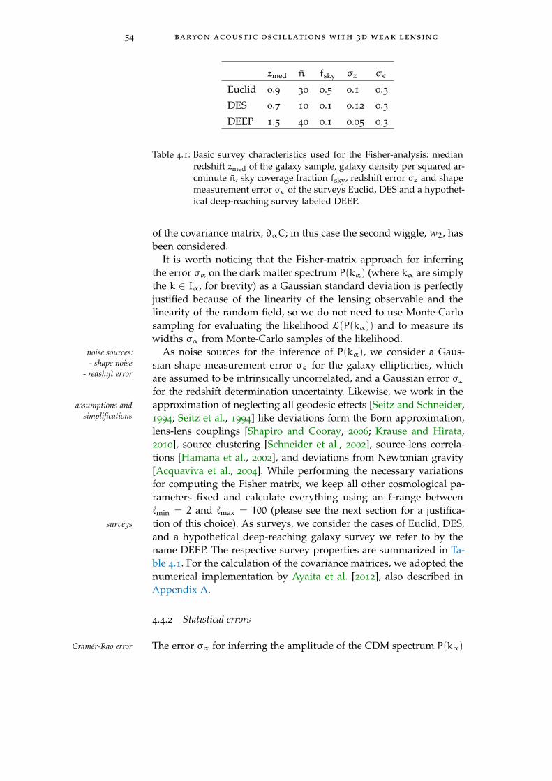
54 baryon acoustic oscillations with 3d weak lensing
zmed n fsky σz σε
Euclid 0.9 30 0.5 0.1 0.3
DES 0.7 10 0.1 0.12 0.3
DEEP 1.5 40 0.1 0.05 0.3
Table 4.1: Basic survey characteristics used for the Fisher-analysis: medianredshift zmed of the galaxy sample, galaxy density per squared ar-cminute n, sky coverage fraction fsky, redshift error σz and shapemeasurement error σε of the surveys Euclid, DES and a hypothet-ical deep-reaching survey labeled DEEP.
of the covariance matrix, ∂αC; in this case the second wiggle, w2, hasbeen considered.
It is worth noticing that the Fisher-matrix approach for inferringthe error σα on the dark matter spectrum P(kα) (where kα are simplythe k ∈ Iα, for brevity) as a Gaussian standard deviation is perfectlyjustified because of the linearity of the lensing observable and thelinearity of the random field, so we do not need to use Monte-Carlosampling for evaluating the likelihood L(P(kα)) and to measure itswidths σα from Monte-Carlo samples of the likelihood.
As noise sources for the inference of P(kα), we consider a Gaus-noise sources:- shape noise
- redshift errorsian shape measurement error σε for the galaxy ellipticities, whichare assumed to be intrinsically uncorrelated, and a Gaussian error σzfor the redshift determination uncertainty. Likewise, we work in theapproximation of neglecting all geodesic effects [Seitz and Schneider,assumptions and
simplifications1994; Seitz et al., 1994] like deviations form the Born approximation,lens-lens couplings [Shapiro and Cooray, 2006; Krause and Hirata,2010], source clustering [Schneider et al., 2002], source-lens correla-tions [Hamana et al., 2002], and deviations from Newtonian gravity[Acquaviva et al., 2004]. While performing the necessary variationsfor computing the Fisher matrix, we keep all other cosmological pa-rameters fixed and calculate everything using an `-range between`min = 2 and `max = 100 (please see the next section for a justifica-tion of this choice). As surveys, we consider the cases of Euclid, DES,surveys
and a hypothetical deep-reaching galaxy survey we refer to by thename DEEP. The respective survey properties are summarized in Ta-ble 4.1. For the calculation of the covariance matrices, we adopted thenumerical implementation by Ayaita et al. [2012], also described inAppendix A.
4.4.2 Statistical errors
The error σα for inferring the amplitude of the CDM spectrum P(kα)Cramér-Rao error

4.4 detecting bao wiggles 55
10 100 300
ℓmax
10-3
10-2
10-1
100
101
102
103
104
σα/A
α
wiggle 1wiggle 2wiggle 3wiggle 4
Figure 4.3: The marginalized errors on the first four wiggles, normalizedwith respect to their amplitude, as the maximum ` used for thecalculation of the Fisher matrix increases. It shows that choosing`max > 100 brings no particular advantage in the precision of thewiggles measurement. In the calculation of the errors we consid-ered the power spectrum as parametrized by the first 4 wiggles.
at wiggle positions kα is given by the Cramér-Rao relation,
σ2α = (F−1)αα, (4.33)
and
σ2α = 1/Fαα, (4.34)
for marginalized and conditional likelihoods, respectively.Before carrying out our analysis for surveys like Euclid, DES, and sensitivity to survey
parametersDEEP, we implement some tests in order to determine the optimalvalue for the maximum number of modes to be used in the calcula-tion of the Fisher matrix, `max. Besides, we tried to find out how andby how much are the errors sensitive to some of the usual surveyparameters, such as
1. the shape noise σε;
2. the error σz in the measurement of redshift;
3. the median redshift zmed;
4. the fraction of sky coverage fsky.
Throughout these tests, when not stated otherwise, we make use ofa default set of survey parameters such that σz = 0.02, σε = 0.3,

56 baryon acoustic oscillations with 3d weak lensing
0.1 0.2 0.3 0.6σǫ
10-4
10-3
10-2
10-1
100
101
σα/A
α
wiggle 1wiggle 2wiggle 3wiggle 4
Figure 4.4: The relative marginalized error for the first 4 wiggles, as theshape noise σε varies. Again, we assumed σz = 0.02, σε = 0.3,zmed = 0.9, fsky = 0.4 and n = 20. As we expected, larger valuesof σε bring along larger errors on the detection of the wiggles.
zmed = 0.9, fsky = 0.4 and n = 20. Additionally, we assumed we wantto constrain simultaneously the first four wiggles (see Figure 4.1).
We start our investigation by determining the errors σα, α = 1, 2, 3, 4,finding the optimal`max as the maximum number of modes `max in the summation in Equa-
tion 4.30 increases. Please refer to Figure 4.3 for a plot of the behaviorof σα normalized to the oscillation amplitude Aα, where Aα is de-fined as the maximum value of |P(k) − Ps(k)| for each wiggle. In par-ticular, we considered `max = 10, 30, 100, 300, and observe that, after`max = 100, there is practically no gain in the precision with which thefirst 4 wiggles would be constrained in a 3dWL approach. Therefore,we decide to stick to a maximum number of modes of 100 for all thesubsequent calculations. This is a fair approximation also from a theo-retical point of view: In fact, extending too much the ` interval for theFαβ summation could make us fall out of the linear regime; in addi-tion, the assumption of a Gaussian shape for the likelihood L couldnot to be anymore reasonable in such a multipole range [Heavens,2003].
In Figure 4.4, we show what happens as soon as we keep all the sur-shape-noise
vey parameters fixed and vary the shape noise σε. As one can expect,larger values of σε lead to larger σα, therefore to a greater uncertaintyin the detection of the wiggles. Moreover, the rate at which σα growswith the shape noise seems to be of the type of a power law, andseems independent of the wiggle considered, at least for the wigglessample we evaluated. The situation turns out to be similar when theredshift error
error in the determination of redshift σz is considered, in Figure 4.5:

4.4 detecting bao wiggles 57
0.01 0.05 0.1 0.2σz
10-3
10-2
10-1
100
101
σα/A
αwiggle 1wiggle 2wiggle 3wiggle 4
Figure 4.5: The relative marginalized error for the first 4 wiggles as a func-tion of the error in the measurement of the photometric redshift,σz. The sensitivity of the errors on the value of σz is not as steepas it is for the shape noise σε. In addition, the increasing rate ofσα seems to change as we consider higher order wiggles.
increasing σz still produces larger errors on all the wiggles under in-vestigation, although here the relation is somewhat slower, especiallyas long as σz . 0.1; the relation also appears to be slightly dependenton the wiggle, becoming steeper as higher order oscillations are taken.In fact, by incrementing the error on redshift from 0.01 to 0.1, we getan error larger only by a factor of ∼ 2 on the first wiggle and by a fac-tor of ∼ 8 on the second. Additionally, the correspondence between median redshift
σα and the median redshift of the survey (Figure 4.6) seems againlike a power law that gives larger errors for an increasing zmed, andis independent of the wiggle. Qualitatively, this trend makes sense inlight of the fact that, as we increase the median redshift, we keep fixedall other survey parameters such as, for example, the galaxy densityper squared arcminute n. By doing so, we consider surveys where anumber n of galaxies is distributed over a deeper cone, meaning thatwe are actually sampling the 3D convergence field in a more dilutedway, and therefore inheriting a larger noise. Naturally, varying the sky coverage
sky covarage propagates to the errors σα ∝ 1/√fsky.
4.4.3 Detectability of BAO wiggles
In this section, we would like to present the results obtained whenestimating the best errors to expect on BAO wiggles for the surveysEuclid, DES, and DEEP (please see Table 4.1 for specifications).
We started our analysis by calculating both marginalized (σα = marginalized andconditional errors

58 baryon acoustic oscillations with 3d weak lensing
0.4 0.5 0.6 0.7 0.8 0.9 1.0zmed
10-3
10-2
10-1
100
101
σα/A
α
wiggle 1wiggle 2wiggle 3wiggle 4
Figure 4.6: Relative marginalized errors on the first 4 wiggles when themedian redshift zmed of the survey increases. Since all otherparameters are kept fixed, especially the mean galaxy densityper squared arcminute, n, increasing zmed is equivalent to hav-ing more and more diluted surveys, where the same amount ofgalaxies is distributed along a deeper survey cone.
1 2 3 4wiggle
10-3
10-2
10-1
100
101
102
σα/A
α
EUCLIDDESDEEP
marginalizedconditional
Figure 4.7: Conditional (magenta lines) and marginalized relative errors(black lines) for the three surveys under investigations Euclid(solid line), DES (dashed line) and DEEP (dash-dot line) as afunction of the wiggles, when the first 4 oscillations are simulta-neously constrained.

4.4 detecting bao wiggles 59
−100 −50 0 50 100wiggle 2
−100
−50
0
50
100
wig
gle
1
-0.94 0.87 -0.82
−100 −50 0 50 100wiggle 3
−100
−50
0
50
100
wig
gle
2
-0.98 0.96
−100 −50 0 50 100wiggle 4
−100
−50
0
50
100
wig
gle
3
-0.99
Figure 4.8: Confidence ellipses for the first four wiggles in a Euclid-like sur-vey, showing that the wiggles are indeed highly correlated. Infact, taking, for example, two consecutive wiggles, such as w2and w3, we see that by increasing the amplitude of P(k) at theposition of wiggle 2, we must then have the amplitude at w3decreased in order to remain in the confidence region. The x-and y-axes show the variation of the wiggle in terms of percent-age of its amplitude Aα, the three contours areas correspond to1− 2− 3σ, and every panel shows the correlation coefficient inthe upper-right corner.

60 baryon acoustic oscillations with 3d weak lensing
−100 −50 0 50 100wiggle 2
−100
−50
0
50
100
wig
gle
1
-0.95 0.89 -0.86
−100 −50 0 50 100wiggle 3
−100
−50
0
50
100
wig
gle
2
-0.99 0.97
−100 −50 0 50 100wiggle 4
−100
−50
0
50
100
wig
gle
3
-1.00
Figure 4.9: Fisher confidence ellipses for DES, when one tries to simulta-neously constrain the first four wiggles. Again, contours areascorrespond to 1− 2− 3σ and the number in every panel is thecorrelation coefficient; the axes represent variation of wigglesin terms of their amplitude fraction. Also in this case we canobserve correlation between the amplitudes of P(k) at differentwiggles positions.
−100 −50 0 50 100wiggle 2
−100
−50
0
50
100
wig
gle
1
-0.89 0.75 -0.65
−100 −50 0 50 100wiggle 3
−100
−50
0
50
100
wig
gle
2
-0.95 0.88
−100 −50 0 50 100wiggle 4
−100
−50
0
50
100
wig
gle
3
-0.98
Figure 4.10: Confidence ellipses for the DEEP survey, with the variation ofthe oscillations in terms of the wiggle amplitude. Again, weassumed we wanted to constrain jointly the first four wiggles,contour areas stand for 1− 2− 3σ and the correlation coefficientcan be read in the panels.

4.4 detecting bao wiggles 61
0.90
0.95
1.00
1.05
1.10
PBAO/P
s
2 wiggles 3 wiggles
0 0.1 0.2 0.3 0.4
k [h Mpc−1 ]
0.90
0.95
1.00
1.05
1.10
PBAO/P
s
4 wiggles
0 0.1 0.2 0.3 0.4 0.5
k [h Mpc−1 ]
5 wiggles
Figure 4.11: The bars show the marginalized errors in the detection of thewiggles, normalized with respect to Ps(k), when the first 2 (up-per left panel), 3 (upper right panel), 4 (bottom left panel),5 (bottom right panel) wiggles are used to parametrize thepower spectrum. Here, we considered a Euclid-like survey withσz = 0.1, σε = 0.3, zmed = 0.9, fsky = 0.5 and n = 30.
√(F−1)αα) and conditional errors (σα = 1/
√Fαα) relative to the wig-
gle amplitude. These errors were computed for the three types ofsurveys, considering the first four oscillations, as shown in Figure 4.7.As we could expect, marginalized errors are always larger than thecorrespondent conditional ones, namely the σα on each wiggle whenwe assume to know precisely all the other wiggle amplitudes.
We continue the investigation considering the confidence ellipses confidence ellipses
calculated from the corresponding Fisher matrices obtained for thethree surveys. We assume we are aiming to jointly constrain the firstfour wiggles and plot the results in Figure 4.8, Figure 4.9, and Fig-ure 4.10 for, respectively, Euclid, DES, and DEEP. The sizes of the el-lipses, whose contours stand for 1−2−3σ, already tell us that, amongthe ones evaluated, Euclid will probably be the survey with largestconstraining power on the BAO wiggles. It is of particular interestnoticing the orientation of the ellipses, or their correlation coefficients(upper-right corner in every panel), that tell us something about theinterdepence between different wiggles: In fact, neighboring wigglesare anti-correlated , i.e. increasing the amplitude of the power spec-trum in correspondence to one oscillation would cause the P(k) at theposition of the adjacent wiggle to take smaller values in order to stayamong the confidence region, and vice versa, whereas the oppositeholds for alternated wiggles.

62 baryon acoustic oscillations with 3d weak lensing
0.90
0.95
1.00
1.05
1.10
PBAO/P
s
2 wiggles 3 wiggles
0 0.1 0.2 0.3 0.4
k [h Mpc−1 ]
0.90
0.95
1.00
1.05
1.10PBAO/P
s
4 wiggles
0 0.1 0.2 0.3 0.4 0.5
k [h Mpc−1 ]
5 wiggles
Figure 4.12: Marginalized errors on the detection of BAO wiggles when onetries to detect the first 2 (upper left panel), 3 (upper right panel),4 (bottom left panel), 5 (bottom right panel) wiggles at the sametime, for a DES-like survey (σz = 0.12, σε = 0.3, zmed = 1.5,fsky = 0.12 and n = 10). Again, we considered the relativemarginalized errors, dividing by Ps(k).
0.90
0.95
1.00
1.05
1.10
PBAO/P
s
2 wiggles 3 wiggles
0 0.1 0.2 0.3 0.4
k [h Mpc−1 ]
0.90
0.95
1.00
1.05
1.10
PBAO/P
s
4 wiggles
0 0.1 0.2 0.3 0.4 0.5
k [h Mpc−1 ]
5 wiggles
Figure 4.13: The marginalized errors on the detection of the wiggles in thepower spectrum, relative to Ps(k), for the hypothetical surveyDEEP, characterized by the parameters σz = 0.05, σε = 0.3,zmed = 1.5, fsky = 0.1 and n = 40.

4.4 detecting bao wiggles 63
In order to better understand whether the constraining power ofthe three surveys will allow us to detect any oscillatory feature in theCDM power spectrum, we plot the σα obtained from the Cramér-Raorelation in Equation 4.33 as error bars in the usual wiggle-only powerspectrum for DEEP (Figure 4.13), DES (Figure 4.12), and Euclid (Fig-ure 4.11). Since what is shown is a ratio between P(k) and a smoothspectrum, the σα have of course also been normalized with respectto Ps(k). The four different panels show how the errors change whenwe try to jointly constrain the first 2, 3, 4, or 5 wiggles with a 3dWLapproach.
What these and the following plots show, first of all, is an expectedfeature: As we increment the number of wiggles we expect to simul-taneously examine, the precision with which the amplitudes P(kα)would be measured gets poorer and poorer for all the oscillations.Our purpose would then be to evaluate how many BAO wiggles oneis allowed to constrain before the errors on them become too large.It can be seen that all three surveys would allow for quite good con-straints on the first 2 wiggles. The hypothetical survey DEEP alreadyshows error bars of the order of the wiggle amplitude Aα when thefirst 3 wiggles are considered, and the errors become much largerthan Aα (α > 1) as soon as one tries to detect 4 or more wiggles(Figure 4.13). On the other hand, DES and Euclid give a better per-formance, allowing for, respectively, the first 3 and 4 wiggles to besimultaneously constrained, with Euclid giving smaller errors overall(Figure 4.11).
A better comparison between the three surveys can be carried outanalyzing Figure 4.14 and Figure 4.15, where we plotted relative er-rors σα/Aα as functions of the maximum number of wiggles we wantto jointly constrain, nw, and we collate results coming from, respec-tively, DEEP and Euclid, and DES and Euclid. It becomes straight-forward that a DEEP-like survey cannot compete against Euclid: Therelative errors coming from DEEP are always larger than the latter’s,independently of the maximum number of wiggles to be constrained,and remain safely under the unity only for the first 2 wiggles.
The situation is better for DES, that seems to be at least able to de-tect the first three wiggles. However, DES gives a worse performancethan Euclid, with errors larger of a factor ∼ 6.
Concluding, Euclid seems to grant the best results, allowing forthe simultaneous detection of up to 4 wiggles with expected errorsthat are smaller than the ones predicted for both DES and, of course,DEEP, and that range between ∼ 1% and ∼ 10% (with respect to thewiggle amplitudes) for the first harmonics.

64 baryon acoustic oscillations with 3d weak lensing
2 3 4 5nw
10-3
10-2
10-1
100
101
102
103
σα/A
α
wiggle 1wiggle 2wiggle 3wiggle 4wiggle 5EUCLIDDEEP
Figure 4.14: Relative marginalized errors as a function of nw for a Euclid-like survey (solid lines) and a DEEP-like survey (dashed lines).The relative σα for a DEEP survey appear to be always largerthan the ones obtained from Euclid, independently of the max-imum number of wiggles nw we want to constrain.
2 3 4 5nw
10-3
10-2
10-1
100
101
102
103
σα/Aα
wiggle 1wiggle 2wiggle 3wiggle 4wiggle 5EUCLIDDES
Figure 4.15: Relative marginalized errors (with respect to the wiggles ampli-tude) as a function of the maximum number of wiggles that wetry to simultaneously detect, nw. Here, we show the results fora Euclid-like survey (solid lines) and a DES-like survey (dashedlines). Different colors and point types correspond to the dif-ferent wiggles on which the error σα is calculated. The relativeerrors coming from a DES-like survey turn out to be larger thanEuclid’s over all the nw interval, nevertheless still allowing DESto detect the first three wiggles simultaneously.

4.5 summary and conclusions 65
4.5 summary and conclusions
Subject of this paper has been a statistical investigation on whetherfuture weak lensing surveys are able to detect baryon acoustic oscilla-tions in the cosmic matter distribution by application of the 3d weaklensing method. For a fixedwCDM cosmology, we have estimated thestatistical precision σα on the amplitude of the CDM spectrum P(k)
at the BAO wiggle positions in a Fisher-matrix approach. Through-out, we worked under the assumption of Gaussian statistics, indepen-dent Fourier modes and in the limit of weak lensing. Noise sourceswere idealized and consisted in independent Gaussian-distributedshape-noise measurements for the lensed background galaxy sam-ple, as well as a Gaussian error for the redshift determination. Assurveys, we considered the cases of Euclid, DES and a hypotheticaldeep-reaching survey DEEP.
1. We have constructed the Fisher matrix considering our modelas parametrized by the amplitudes of the CDM power spectrumat the baryon acoustic oscillations anticipated positions. In par-ticular, we started taking the two BAO wiggles with largestamplitude and progressively increased the number of oscilla-tions considered. Keeping the cosmology fixed to a standardwCDM parameter choice, we carried out variations of P(k) thatpreserved its wiggle-shape in those wave number intervals; wethen estimated the Fisher matrix accordingly, in order to quan-tify whether the statistical power of future weak lensing surveyssuffices to place bounds on the amplitudes of the consideredharmonics. By means of the Cramér-Rao relation, we calculatedthe best errors σα to expect for the amplitudes of P(k) at wigglepositions.
2. The sensitivity of σα with respect to some typical survey-param-eters was tested. In particular, we considered the shape noiseσε, the redshift error σz, the median redshift zmed, and the skycoverage fsky. We found that, as expected, increasing the uncer-tainty in the estimate of either the redshift or the galaxy shapesbrings a larger error in the inference of the presence of wig-gles, and that the sensitivity of these errors on σz is less pro-nounced for small values of σz, although it grows as soon aswe consider higher order wiggles or large σz. An increase ofzmed leads as well to larger errors on the wiggles amplitudes, asone would expect from considering less and less populated sur-veys; for the same reason, a wider sky coverage, i.e. larger fsky,yields to higher precision in constraining the wiggle amplitudesσα ∝ 1/
√fsky.
Overall, we may conclude that the volume of a survey seem to

66 baryon acoustic oscillations with 3d weak lensing
be overcoming the importance of a high precision in the redshiftmeasurement of galaxies, at least for σz < 0.1− 0.2.
3. Finally, we evaluated the σα for the surveys under investigationand found that, among them, Euclid gave the best results, po-tentially allowing for the detection of up to the first four BAOwiggles with a good statistical confidence. Given our tests onthe sensitivity of the errors on P(kα) to certain survey parame-ters, we may conclude that Euclid’s good performance is prob-ably due to the volume of the survey in terms of total galaxynumber and sky coverage, that seem to prevail over the nega-tive effects brought by the error on redshift measurements, σz,larger than the ones predicted for the other two surveys.
Given these results, we conclude that measurements of BAO wig-gles based on future weak lensing data are entirely possible, andavoid issues related to galaxy biasing and redshift-space distortions.We forecast a detection of the first four or three wiggles with Euclidand DES by applying 3dWL techniques. Future developments fromour side include estimates of the precision that can be reached oninferring dark energy density and equation of state by including theestimate of the BAO scale at low redshifts probed by lensing to theestimates at intermediate redshift provided by galaxy surveys andthose at high redshifts such as the CMB. Additionally, we are inves-tigating the impact of systematical errors on the estimation processfrom 3dWL-data and biases in the estimation of BAO-wiggle ampli-tudes.
The next Part of this thesis will analyze another possible use of theweak lensing method: the detection of primordial non-Gaussianitiesin the density fluctuations distribution.

Part III
P R O B I N G P R I M O R D I A L N O N - G A U S S I A N I T I E SW I T H W E A K L E N S I N G


5I N F L AT I O N A N D P R I M O R D I A L N O N -G A U S S I A N I T I E S
Inflation is probably among the most controversial topics in Cos-mology. Inflation models theorize an accelerated expansion that hap-pened in the very first moments after the big bang. Such an expansioncould, in fact, solve some of the contradictions of the standard hot bigbang model, and produce the distribution of density anisotropies weobserve in the CMB, and from which the Milky Way originated.
Under the inflation paradigm, many models flourished, trying toexplain in detail the mechanism behind the expansion, and what isresponsible for it. Up to now, we still do not know if such an accel-erated expansion really took place, and what kind of fields gener-ated it. One way to help us discriminating among the wide range ofcandidate models, is measuring the amount of deviation from Gauss-ianity in the distribution of primordial density fluctuations: In fact,many inflationary models predict different degrees of non-Gaussiani-ties, making them a valuable tool.
In the present Chapter, I will schematically introduce the mainproblems of the standard big bang model, and how the hypothesisof an accelerated expansion can solve some of them in an elegant ansimple fashion (Section 5.1). In Section 5.2, I will address primordialnon-Gaussianities in the density fluctuations: how they form and howthey can be described by means of the local, equilateral, and orthogo-nal shapes.
69
70 inflation and primordial non-gaussianities
When not stated otherwise, all the content of this Chapter is basedon the reviews by Bartolo et al. [2004], Wang [2013], Chen [2010], andon Komatsu [2010], Liddle and Lyth [2000].
5.1 the inflationary paradigm
5.1.1 Standard model: successes and issues
The standard hot big bang model arises as a natural consequencewhen the following assumptions are adopted:
1. gravity is described by the theory of general relativity, and lawsof physics as we know them are also valid during the earlyUniverse;
2. the Universe is homogeneous and isotropic on large scales;CosmologicalPrinciple
3. some initial conditions must hold, in particular:
• the content of the Universe is initially in thermal equilib-rium;
• Ωtot(t = 0), i. e. the total density parameter of the Uni-verse, is very close to unity, meaning that the Universe isvery close to perfect flatness at its early stages;
• some kind of spectrum of initial fluctuations in the densitydistribution is provided.
Given these premises, one can construct a theory that easily (orstandard modelsuccesses almost easily)
1. explains the Universe’s expansion,
2. predicts the observed light-element abundances,
3. gives a natural explanation for the isotropy of the cosmic mi-crowave background,
4. provides a framework for a theory of structure formation, aim-ing to understand how the initial density fluctuations evolvedand eventually generated collapsed objects such as galaxies, orthe large scale structure.
Despite such important successes of the standard hot big bangmodel, there are still some issues that cannot find a solution in thissystem. For instance, the cosmological constant problem, that I willstandard model
issues not address here (for a review on the topic see Sahni [2002], Martin[2012], or the broader Padmanabhan [2003]), the absence of evidencefor topological defects such as magnetic monopoles [Preskill, 1979],our ignorance on what exactly constitutes dark matter (see for in-stance the reviews Einasto [2009], Silk [2013]), or the standard model’s

5.1 the inflationary paradigm 71
inability to explain the existence of primordial density fluctuations,that must be given as an initial condition. Other problems are thehorizon and the flatness ones, briefly described below.
the horizon problem The existence of a limiting velocity like ccomes naturally with the presence of a particle horizon. Theparticle horizon defines, for every point in space, the radius “ The horizon of
many people is acircle with zeroradius, which theycall their point ofview.” A. Einstein
of the sphere containing everything the point itself could havebeen in causal contact with. This means that from the momentof big bang to a generic moment t, information could travelonly a finite distance. If we imagine information to be carriedby photons with speed c, then this distance can be calculatedfrom imposing a null geodesic
0 = ds2 = c2dt2 + a2dr2, (5.1)
hence yelding
rH(t) = c
∫a(t)0
dt ′
a(t ′). (5.2)
The problem arises as soon as we estimate the particle horizonat the time of recombination rH(trec). In fact, it turns out thatthe portion of sky every point could have already been in causalcontact with, at recombination, is roughly 1/100 of our observ-able universe. This, of course, is in strong contradiction withCMB observations, clearly showing that at trec the Universe isalready homogeneous and isotropic, at least if we leave asidefluctuations of the order of ∆T/T ∼ 10−5. How can CMB spotsseparated by r > rH look like they had been casually connected?
the flatness problem As the Universe expands, its curvature evol-ves with time: the first Friedmann’s equation (Equation 1.5) canbe rewritten in terms of the total density parameter Ωtot:[
Ω−1tot (t) − 1
]ρ(t)a2(t) = −
3Kc2
8πG. (5.3)
The quantities on the right hand side of the equation are clearlyall constants, and, since ρ(t)a2(t) diminishes over time, themeaning of Equation 5.3 is that curvature cannot change qual-itatively, i. e. a Universe that is closed, flat or open for t = 0,will remain so forever. What the equation also tells us is thatcurvature does change quantitatively, though, and any initialdeviation of Ωtot from unity increases, also considerably, as tpasses by. This implies that in order for us to observe a valueof the density parameter as close to 1 as we estimate it to benowadays, Ωtot should have been (almost exactly) equal to 1,the critical value, soon after the big bang. The flatness issue istherefore a fine-tuning problem.

72 inflation and primordial non-gaussianities
5.1.2 The inflationary solution
Guth [1981] was the first to propose a way out to some of the issuesof the standard hot big bang model. The idea behind his work wasspeculating that during its early stages, and for a limited amount oftime, the Universe has undergone an accelerated expansion, calledaccelerated
expansion, a > 0 inflation. The plain assumption of the existence of a period wherea > 0 is able to solve the flatness, the horizon, and the monopoleproblems.
The flatness issue is easily addressed [Liddle and Lyth, 2000] assolution to flatnessproblem soon as we notice that if a > 0 holds, then for the definition itself
of the Hubble parameter, we have that the comoving Hubble length(Ha)−1 is such that
d
dt(Ha)−1 < 0 (5.4)
Rewriting Equation 5.3 in terms of (Ha)−1 yields
(Ωtot − 1)(Ha)2 = Kc2, (5.5)
meaning that as time goes by, and as the second term of the left handside of the equation increases, Ωtot must get closer to one. In otherwords, as a consequence of the accelerated expansion, the Universetends to look flatter. This happens because expansion made the size ofour observable universe small with respect to any original curvatureradius.
Also the solution to the horizon problem is a consequence of theshrinking comoving Hubble length during inflation. In fact, the ob-solution to horizon
problem servable Universe could have originated in a region contained in thesub-horizon scale before the accelerated expansion, hence before in-flation caused the comoving horizon scale to decrease.
Similarly, such an accelerated expansion, if long enough, wouldsolution to monopoleproblem drastically diminish the monopole density and make it compatible
with observations.
5.1.2.1 Inflation dynamics
Describing all the dynamical aspects of the main inflationary modelswould be beyond the purpose of this work. Nonetheless, I would liketo briefly describe the main aspects of the inflationary mechanism,focussing on the standard slow-roll scenario, usually associated tomodels characterized by a single field.
From the Friedmann’s Equation 1.6, it is straightforward to see thatthe condition a > 0 is met only when
ρ+3p
c2< 0, (5.6)
meaning that we need the Universe to be dominated by a species withan entity with anegative pressure
5.1 the inflationary paradigm 73
a negative pressure, i. e. w < −1/3, in order to have an exponentialexpansion.
To date, there is no indication on what exactly could be responsi-ble for inflation. Nonetheless, the most credited general hypothesisis that it could originate in conjunction with the phase transition ofa generic scalar field subject to a flat potential: As soon as the po-tential gets slightly tilted, the slowly rolling scalar field produces anegative pressure, as desired. Such a scalar is usually called inflatonand denoted by the symbol φ.
Assuming that the choice of a Robertson-Walker metric is justified, standard slow-rollscenarioand therefore that the space is homogeneous and isotropic on large
scale, and given a generic potential V(φ), the equation of motion forthe inflaton under the influence of V(φ) reads [Mukhanov, 2005]
φ+ 3Hφ+d
dφV(φ) = 0. (5.7)
This equation differs from the correspondent equation of motion inflat space in the second term, that represent the coupling of the scalarfield φ to gravity, and acts as a friction.
The H term must be known in order for Equation 5.7 to be solved.It can be proved that
H2 =8πG
3
[1
2φ2 + V(φ)
]. (5.8)
The two equations can be solved as soon as the potential form iswell known. However, more general considerations can be done, with-out any restriction on the exact shape of V(φ), if we use the slow-roll slow-roll
approximationapproximation. The slow-roll approximation allows us to solve thesystem for any choice of the potential, assumed that V(φ) is suffi-ciently flat. The assumption of flatness is quantified by the condition
|φ| 3H|φ|. (5.9)
In fact, we want the second order term of Equation 5.7 to be negligiblefor φ to slowy roll down under the potential action. On the otherhand, since the inflation pressure and density turn out to be
ρφ =φ2
2+ V(φ), pφ =
φ2
2− V(φ), (5.10)
we also need the following condition to imply a negative pressure,i. e. p ' −ρ, and therefore for inflation to take place:
1
2φ2 V(φ). (5.11)
The restrictions found in Equation 5.9 and Equation 5.11 can be ex-pressed in terms of the potential by means of the slow-roll parameters
ε(φ) ≡M2Pl
2
(V ′(φ)
V(φ)
)2 1 (5.12)
74 inflation and primordial non-gaussianities
and
|η(φ)| ≡∣∣∣∣M2
Pl
V ′′(φ)
V(φ)
∣∣∣∣ 1, (5.13)
where the primed quantities are derived with respect to φ. The condi-tion on parameter ε(φ) assures that the pressure is negative enough,while the one on η(φ) allows inflation to last as long as it should.
After the slow rolling of φ towards an equilibrium configurationφ0, it starts to oscillate around the potential minimum V(φ0), until itdecays, coupling to other fields. This process is called reheating, andits dynamical details vary quite a lot among different models (referto Bassett et al. [2006], Allahverdi et al. [2010] for reviews addressingthis topic). The reheating constitutes the threshold between inflation-ary epoch and the standard model framework; after this moment, theradiation starts to dominate.
Many alternatives to this simple scenario exist, like the curvatonmechanism [Mollerach, 1990; Enqvist and Sloth, 2002; Lyth and Wands,2002], the ekpyrotic scenario [Lehners, 2010], not to mention the en-tire class of multi field models (for a review see Wands [2008]).
5.2 primordial non-gaussianities
One of the most important successes of the inflationary scenario isthat it gives a natural explanation for the existence of primordial den-inflation generates a
primordialdistribution of
density fluctuations
sity fluctuations. What happens is that quantum fluctuations of thescalar field φ also get stretched during the accelerated expansion, andimprinted in super-Hubble scales. As soon as the inflaton decays, dur-ing the end of inflation, these fluctuations are inherited by the fieldswith which φ gets coupled, namely matter and radiation, revealingthemselves as anisotropies of their energy density field. Among thegeneric predictions that inflation models make for such density per-turbations we can find that [Chen, 2010]:
• they are almost scale invariant: In fact, during inflation, eachmode withstand a similar expansion;
• they are approximately Gaussian.
The second statement holds precisely as far as we consider the per-turbations of the scalar field to be linear: In this case the Central LimitTheorem ensures that given that modes have a random distribution,then their superposition will follow a Gaussian statistic.
Things are different, though, if the linearity hypothesis for the fielddeviations fromGaussianity perturbations must be discarded. It is the case, for example, when
we also have to consider deviations from the slow roll approxima-tion, or the contributions coming from the scalar field interactionswith itself, with other fields, or both. In that instance, deviations from

5.2 primordial non-gaussianities 75
Gaussianity could occur in the primordial density fluctuations distri-bution. As various inflationary models predict different degrees ofnon-Gaussianities, measuring the latter could lead to rule out someof these scenarios.
Unlike a normal distribution, that is completely defined by its vari-ance, and therefore by its power spectrum in Fourier space, a non-Gaussian distribution needs higher order momenta to be exhaustivelydescribed. Since the primordial distribution of density fluctuations isstill Gaussian to a good approximation, deviations can be treated per-turbatively, and in this case the bispectrum and trispectrum, defined higher order
statistics arenecessary:bispectrum,trispectrum, ...
in Fourier space as follows,
〈Φ(k1)Φ(k2)Φ(k3)〉 = (2π)3δD
( 3∑n=1
kn)BΦ(k1, k2, k3) (5.14)
〈Φ(k1)Φ(k2)Φ(k3)Φ(k4)〉 = (2π)3δD
( 4∑n=1
kn)TΦ(k1, k2, k3, k4),
(5.15)
(where Φ stands for the curvature perturbation) contain a good partof the additional information, apart from being the most accessiblehigher order momenta, both from an observational and a theoreticalpoint of view.
5.2.1 Shapes of non-Gaussianities
There are many different ways a distribution can deviate from a Gaus-sian. For this reason, non-Gaussianities are usually classified depend-ing on what modes configurations give the strongest signal. In thefollowing sections, I will give a brief description of the three mainclassifications, and provide an analytical prediction for the bispec-trum for local, equilateral, and orthogonal non-Gaussianities.
These three shapes, or a linear combination of them, cover almostthe totality of the inflationary models giving deviations from Gauss-ianity. Nonetheless, there are still some scenarios predicting peculiarshapes of non-Gaussianity, independent from the following (see forinstance Chen et al. [2007, 2008]; Barnaby [2010]).
local non-gaussianity Local-shape non-Gaussianity is probablythe most studied. In the local ansatz, the curvature perturbationΦ(x) can be written as a local expansion around a point x and local ansatz
by means of the perturbation variable Φg(x), that is assumed tosatisfy a Gaussian statistics [Wang, 2013]:
Φ(x) = Φg(x) + fNLΦ2g(x) + gNLΦ
3g(x) + ... (5.16)

76 inflation and primordial non-gaussianities
Figure 5.1: Three main shapes for the primordial bispectra, normalized asBx(k1,k2,k3)(k2/k1)2(k3/k1)2 with respect to the maximumvalue assumed, where x stands for local, equilateral, or orthog-onal. In the top-left panel, it can be seen that the local formpeaks at squeezed triangle configurations. The equilateral shape(bottom-left panel), on the other hand, provides larger bispec-trum values in correspondence of configurations where k1 'k2 ' k3, whereas the orthogonal form (top-right panel) featuresa peak at equilateral configurations, and a negative valley allalong elongated shapes, i. e. k1 = k2 + k3. Figure taken fromKomatsu [2010].
Of course this is not a general way for expanding Φ(x): In fact,in a more general picture, the non linearity parameters could de-pend on a position vector that is different from the one aroundwhich the expansion itself takes place.
This ansatz makes the study of non-Gaussianities much simplerfrom an analytical point of view. It implicitly assumes that theyarise at different spatial points in an independent way, and thatthey are generated on super-Hubble scales.
The local form bispectrum is given by the relation [Gangui et al.,1994; Verde et al., 2000; Komatsu and Spergel, 2001]
BlocalΦ (k1, k2, k3) = 2flocal
NL
[PΦ(k1)PΦ(k2) + PΦ(k2)PΦ(k3)
+PΦ(k3)PΦ(k1)]
= 2A2fNL
[kns−41 kns−42 + kns−42 kns−43
+kns−43 kns−41
], (5.17)
where the approximation PΦ(k) ' PΦg(k) was made, and wherethe coefficient
A ≡ PΦ(k)kns−4
(5.18)

5.2 primordial non-gaussianities 77
describes the departure from a scale invariant spectrum [Se-fusatti and Komatsu, 2007]. The local bispectrum given in Equa-tion 5.17 peaks among the squeezed triangle configurations, na-mely when k3 k2 ' k1 (see top-left panel of Figure 5.1).
The effect of a positive fNL would be, for instance, to enhancethe right-hand tail of the density distribution, and suppress theleft-hand one, making overdensities overall more likely to hap-pen, and on the contrary, underdensities less likely, with respectto a Gaussian distribution. Vice versa, of course, for a negativefNL.
Local shape non-Gaussianities occur, in general, in models wherenon-linearities are expected to be produced by super-horizonevolution of perturbation; this is typically expected to happenin several types of multi-field models [Lyth et al., 2003; Zaldar-riaga, 2004; Lyth and Rodríguez, 2005; Bond et al., 2009].
One peculiarity of local non-Gaussianity resides in the fact that,as Creminelli and Zaldarriaga [2004] proved, every single-inflationmodel give a bispectrum like
BlocalΦ (k1, k2, k3) =
5
3(1−ns)PΦ(k1)PΦ(k3), k3 k1,k2
(5.19)
in the squeezed triangle limit. Such a case would imply an ex- single-field modelsdo not predict localnon-Gaussianities
tremely small value for flocalNL . Detecting a flocal
NL sensibly differentfrom zero would then rule out the entire class of single-fieldinflationary.
equilateral non-gaussianity Equilateral non-Gaussianities arecharacterized by a bispectrum that peaks, as bottom-left panelof Figure 5.1 shows, at equilateral configurations (k1 ' k2 ' k3).This form is almost orthogonal to the local one, meaning thatthey can be detected independently, and its bispectrum reads[Creminelli et al., 2006]
BequilΦ (k1, k2, k3) = 6A2f
equilNL
[− 2(k1k2k3
)2(ns−4)/3−(k1k2
)ns−4 − (k2k3)ns−4 − (k3k1)ns−4+(k(ns−4)/31 k
2(ns−4)/32 kns−43
+5 perm.)]
. (5.20)
In general, a positive equilateral bispectrum corresponds to hav-ing strong overdensities encircled by large regions characterizedby a milder underdensity; on the other hand, a negative equilat-eral bispectrum describes a higher likelihood to have very con-centrated under densities surrounded by regions with a blanderoverdensity [Lewis, 2011].

78 inflation and primordial non-gaussianities
This type of non-linearities arises from several inflationary mod-els [Arkani-Hamed et al., 2004; Seery and Lidsey, 2005; Chenet al., 2007; Cheung et al., 2008; Li et al., 2008]. In general,equilateral non-Gaussianities are produced in models with non-canonical kinetic terms, such as the well known Dirac-Born-Infeld (DBI) inflation [Alishahiha et al., 2004; Silverstein andTong, 2004]. It is worth pointing out that a positive, and al-most entirely equilateral bispectrum also arises from non-linearcollapse of dense filaments in the large scale structure [Lewis,2011].
orthogonal non-gaussianity This form is constructed to beorthogonal to both local and equilateral forms, and thereforeindependent. It actually arises from a linear combination ofhigher-derivative interaction terms of the scalar field. Its bispec-trum
BorthoΦ (k1, k2, k3) = A2fortho
NL
[− 8(k1k2k3
)2(ns−4)/3−3(k1k2
)ns−4 − 3(k2k3)ns−4 − 3(k3k1)ns−4+(3k
(ns−4)/31 k
2(ns−4)/32 kns−43
+5 perm.)]
, (5.21)
when normalized in amplitude, i. e. BorthoΦ · (k2/k1)2 · (k3/k1)2,
features a peak for the equilateral configurations, and a negativetrough in correspondence of the elongated ones (k1 = k2 + k3),as Figure 5.1 displays in the top-right panel.
5.2.2 The Suyama-Yamaguchi inequality
The Suyama-Yamaguchi inequality is a very general result that linksthe two non-linearity parameters fNL and τNL, introduced and provedfor the first time by Suyama and Yamaguchi [2008].
In the local ansatz, once performed the expansion of Equation 5.16,we notice that the cubic term does not contribute to the bispectrum,instead it generates the trispectrum, that can be written as follows
T˘(k1, k2, k3, k4) = A36gNL
[kns−41 kns−42 kns−43 + 3 perm.
]+
25
18τNL
[kns−41 kns−43 |k1 + k2|ns−4
+ 11 perm.]
, (5.22)
and that depends on the parameters gNL and τNL
Generalizing the local ansatz to multi-field inflation by means ofthe δN formalism [Starobinskiı, 1985; Sasaki and Stewart, 1996], wecan expand the primordial curvature perturbation ζ, whose relationto Φ is ζ = 5Φ/3, in terms of the inflation perturbations δφ and thee-folding number

5.2 primordial non-gaussianities 79
e-folding number, defined as
N(ti, tf, r) =∫tfti
H(t, r)dt, (5.23)
namely the time integral of the Hubble parameter, evaluated locally.By means of such an expansion, it is possible to write the non-linearparameters in terms of derivatives of N with respect to the i-th in-flation perturbation δφi, i. e. Ni = ∂N/∂φi (for a detailed derivation,please see Suyama and Yamaguchi [2008]):
fNL =5∑ijNijNiNj
6(∑iN
2i )2
, gNL =25∑ijkNijkNiNjNk
54(∑iN
2i )3
, (5.24)
and
τNL =
∑ijkNijNikNjNk
(∑iN
2i )3
. (5.25)
Due to the well known Cauchy-Schwarz inequality, that can be ex-pressed as [Lin and Wang, 2010]∑
ij
(AiAi)(BjBj) >∑ij
(AiBi)(AjBj), (5.26)
it can be proved that there exists a general relation between fNL and Suyama-YamaguchiinequalityτNL,
τNL >
(6
5fNL
)2, (5.27)
called Suyama-Yamaguchi inequality.Such a relation should always hold. Nonetheless, it was calculated Suyama-Yamaguchi
inequality as a toolto discriminateamong inflationarymodels
that some inflationary models could predict a violation of the inequal-ity. Hence, detecting a departure from the condition in Equation 5.27,could help us ruling out some scenarios.
5.2.3 Measuring primordial non-Gaussianities
Many efforts have been made, over the years, to provide independentmethods able to constrain the degree of primordial non-Gaussianitiesin the density distribution. Not only do diverse approaches experi-ence different kinds of systematic errors, yielding in this way comple-mentary results: they also often probe different scales. This last fact isof fundamental importance if we consider fNL to be scale-dependent, scale-dependent fNL
as a number of studies seem to suggest [Byrnes et al., 2010a; Chen,2005; Bartolo et al., 2010; Riotto and Sloth, 2011].
The tightest constraints on primordial non-Gaussianities definitely constraints fromCMBcome from the study of CMB and the bispectrum of temperature fluc-
tuations ∆T/T [Komatsu, 2003; Casaponsa et al., 2011; Komatsu et al.,

80 inflation and primordial non-gaussianities
2011]. One undeniable advantage of this channel is that the distribu-tion of temperature anisotropies that we observe is not so affectedby deviations from Gaussianity coming from the non-linear growthof perturbations. The most recent observations constraining the non-linearity parameter fNL come from Planck [Planck Collaboration et al.,2013b] and give
flocalNL = 2.7± 5.8fequilNL = −42± 75forthoNL = −25± 39
Verde [2010] and Fedeli et al. [2011a] , among others, have workedconstraints fromLLS on the possibility to detect non-Gaussianities from large scale struc-
ture statistics. These class of methods, of course, is highly affectedby non-Gaussianities coming from structure formation, and thereforeneeds an adequate mechanism able to distinguish between primor-dial and non-primordial deviations from a normal distribution. Grav-itational lensing has also been proposed [Fedeli et al., 2011b; Paceconstraints from
lensing et al., 2011; Jeong et al., 2011], although observational constrains com-ing from this approach, so far, have focussed more on non-Gaussiani-ties generated by non-linear structure formation. A discussion on pos-sible observational constraints on primordial non-Gaussianities com-ing from weak lensing in the near future can be found in Schäfer et al.[2012] and will be presented in the next Chapter.

6A W E A K L E N S I N G V I E W O N P R I M O R D I A L N O N -G A U S S I A N I T I E S
The content of this chapter is based on the paper "A weak lensing view onprimordial non-Gaussianities" [Schäfer et al., 2012]. The development andcontribution of the author of this Thesis to the following work was testingthe numerical code and the convergence of the Monte-Carlo integration rou-tines.
A weak lensing study of primordial non-Gaussianities via conver-gence bispectrum measurements would be of great interest. In fact,lensing sums up two interesting features:
• since lensing is not affected, in principle, by galaxy bias, it hassmaller systematic errors than other large scale structure probes,such as cluster counts or the study of galaxy bispectrum;
• also, it probes smaller scales than CMB does, providing inde-pendent constraints on a possible scale dependence of the non-linearity parameter fNL, for example [Lo Verde et al., 2008].
On the other hand, classical weak lensing suffers some limitations.Among the ones that could affect the problem at hand, lies the factthat all weak lensing statistics depend on integrals along the line-of-sight. In this integration, many independent effects could sum up,hence reducing the information on the primordial non-Gaussianitiesinherited by the convergence bispectrum [Jeong et al., 2011]. As a con-sequence, we expect weak lensing to be less sensitive to primordialnon-linearities than probes like CMB.
In order to test weak lensing sensitivity, though, some questionsnaturally arise:
81

82 a weak lensing view on primordial non-gaussianities
1. Is the power of the signal of the three different shapes of primor-dial non-Gaussianity compatible with a detection by a futuresurvey like Euclid?
2. Suppose a wrong choice of the type of bispectrum (local, equi-lateral, or orthogonal) is made for fitting the data: How, and byhow much would such a mistake affect the fNL measurement?And, how likely would it be to notice such a mistake?
3. What kind of repercussions would a non-exact subtraction ofthe non-Gaussianities coming from structure formation have onthe fNL measurement?
In the present Chapter, I will recapitulate our main results pub-lished in Schäfer et al. [2012] concerning the aforementioned issues.Section 6.1 will introduce the basis of the analysis, by deriving the ob-servable convergence bispectrum and giving an estimate of the muchstronger bispectrum coming from non-linear structure formation, thathas to be subtracted from the signal in order to recover the primordialnon-Gaussianity signal. Section 6.2, Section 6.3, and Section 6.4 willgive answers to the previous questions, by means of a calculation ofthe signal-to-noise ratio, and by a statistical analysis that will try toinvestigate what kind of consequences could a wrong assumption ora wrong fit have on the measurement of fNL.
6.1 weak lensing convergence bispectrum
Before addressing the mentioned problems, let me concisely intro-duce how we get from the original bispectra coming primordial non-Gaussianities or non-linear structure formation, to the observed, weaklensing, convergence bispectrum.
I would like to start from the statistics coming from primordial de-viations from Gaussianity. Given the bispectrum with respect to thedistribution of the potential BΦ(k1, k2, k3), defined for local, equi-lateral and orthogonal non-Gaussianities as shown in Equation 5.17,Equation 5.20, and Equation 5.21, then the bispectrum of the densitydensity bispectrum
field reads
Bδ(k1, k2, k3,a) =3∏i=1
(2D+(a)
3ΩmT(ki)(χHki)
2
)BΦ(k1, k2, k3), (6.1)
with T(k) and D+(a) as, respectively, the transfer function and thegrowth function. This result is of course obtained by means of thecomoving Poisson equation [Munshi et al., 2012], linking the potentialdistribution to the density field δ(k,a):
∇2Φ =3Ωm0
2χ2H
D+(a)
aδ. (6.2)

6.2 expected signal to noise ratio 83
Once obtained Bδ(k1, k2, k3,a), the projection of the flat-sky conver- convergencebispectrumgence bispectrum Bκ is then [Schneider et al., 1998; Takada and Jain,
2003a,b, 2004; Dodelson and Zhang, 2005]
Bκ(`1, `2, `3) =∫χH0
dχχ4W3(χ)Bδ(k1, k2, k3,a), (6.3)
where the Limber equation was used [Limber, 1954], and ki = `i/χfor i = 1, 2, 3. Unfortunately, since a weak lensing approach impliesa line-of-sight integration, we can already forecast that many, inde-pendent effects will add up to the information, therefore reducingthe power of the non-Gaussian signal because of the Central Limittheorem [Jeong et al., 2011].
The observed spherical convergence bispectrum is obtained from sphericalconvergencebispectrum
Bκ(`1, `2, `3) via the following relation
Bκ(`1, `2, `3) '
(`1 `2 `3
0 0 0
)√∏3p=1(2`p + 1)
4πBκ(`1, `2, `3), (6.4)
where the first term on the right hand side of the equation is theWigner-3j symbol, whose purpose is to select only the configurationsthat satisfy the triangle inequality, and set the bispectrum to zerofor all the others. A 3d representation of the values assumed by the(dimensionless) bispectra Bκ is shown in Figure 6.1.
As already mentioned, primordial non-Gaussianities are not theonly source of deviations from normality. In fact, non-linearities com-ing from structure formation also generate a non-Gaussian contribu- structure formation
bispectrumtion to the density field statistics, that can be described by the bispec-trum term [Buchert, 1994; Bernardeau et al., 2002]
BSFδ (k1, k2, k3,a) =
3∑i,j=1(i 6=j)
D4+(a)M(ki, kj)P(ki)P(kj), (6.5)
with M(ki, kj) describing the coupling between modes:
M(ki, kj) =10
7+
(kikj
+kj
ki
)kikjkikj
+4
7
(kikjkikj
)2. (6.6)
The quantity M(ki, kj) assumes the largest values when the vectorski and kj are parallel, i. e. x = 1, so that the strongest non-Gaussiancontribute comes from squeezed configurations. Since BSF
δ is muchstronger than the primordial non-Gaussianities bispectrum, this con-tribution must be subtracted in order to recover the signal comingfrom primordial non-linearities.
6.2 expected signal to noise ratio
Once we have the expression for the convergence bispectra, the firstquestion can be addressed: We want to find out how strong the signalcoming from primordial non-Gaussianities, and encoded in Bκ, is.

84 a weak lensing view on primordial non-gaussianities
Figure 6.1: Dimensionless convergence bispectrum (`1`2`3)4/3Bκ(`1, `2, `3)
for local (top panel), equilateral (middle panel), and orthogonalnon-Gaussianity (bottom panel), plotted in the configurationsspace. Size and colors of the blobs are proportional to the dimen-sionless bispectrum values. It is evident how the properties ofthe original bispectra are inherited by the weak lensing Bκ. Thetop and middle panel, for instance, clearly show how the corre-sponding bispectra peak for, respectively, squeezed and equilat-eral configurations.
Let the covariance be [Hu, 2001; Takada and Jain, 2003a]
cov(`1, `2, `3) =∆(`1, `2, `3)
fskyC(`1)C(`2)C(`3) (6.7)

6.2 expected signal to noise ratio 85
101
102
103
10−4
10−3
10−2
VEGAS
CUHRE
DIVONNE
SUAVE
local
ortho
equil
multipole order ℓ
sig
nal
-to
-no
ise
rati
oΣ
(ℓ)/
f NL
Figure 6.2: Cumulative signal-to-noise ratio Σ(`)/fNL as the maximum `
used in its evaluation increases. The ratio is evaluated for lo-cal (circles), orthogonal (rhombi), and equilateral (squares) non-Gaussianities. Different line-types represent the four CUBA algo-rithms, showing that they agree quite well for the calculation ofΣ(`).
The term fsky stands for the portion of sky covered by a generic survey,whereas C(`) is the observed power spectrum; both these quantity areset accordingly to Euclid predictions. On the other hand, ∆(`1, `2, `3)takes care of the triangle configurations multiplicity. Given the expres-sion for the covariance, the cumulative signal-to-noise ration can be cumulative signal-
to-noiseevaluated:
Σ2(`) =∑`1=`min
∑`2=`min
∑`3=`min
B2κ(`1, `2, `3)cov(`1, `2, `3)
. (6.8)
A direct summation of Equation 6.8 among all the possible config-urations of `1, `2, `3 would be extremely expensive from a computa-tional point of view. A way out to this problem is given by Monte-Carlo integrations. In this case, the CUBA library is used [Hahn,2005], consisting of the four different algorithms Vegas, Suave, Di-vonne, and Cuhre. The cumulative Σ(`) is calculated using the fouralgorithms, whose results seem to agree with each other, and for thethree shapes of non-Gaussianities, and its ratio with respect to thenon-linearity parameter fNL is presented in Figure 6.2. The conclu-sions that can be drawn from the plot are:
• with Euclid, the signal coming from primordial non-Gaussia-nity bispectrum can only be detected for values of fNL muchlarger than 100;
• this is true, at least, for local non-Gaussianity, that seems to bethe most easily detectable type; forms like the orthogonal onewould need an even larger degree of non-Gaussianity, and the

86 a weak lensing view on primordial non-gaussianities
equilateral type of non-Gaussianity directly follows, having thesmallest signal (almost one order of magnitude smaller than thelocal type); such a difference in the magnitude of the signal forthe three non-Gaussianity forms is also visible in Figure 6.3;
• the consequently estimated conditional Cramér-Rao bounds re-sult to be much weaker than probes like, for instance, CMB. Infact they read
σfNL =
200, local
575, orthogonal
1628, equilateral.
(6.9)
The choice of stopping the Σ(`) calculation at ` = 1000 is motivated bythe fact the the signal is not considerably increasing after this thresh-old. Moreover, ` > 1000 correspond to scales that start to be affectedby baryonic physics and intrinsic alignments [Semboloni et al., 2008,2011].
6.3 consequences of a wrong bispectrum choice
The next matter aims to understand what happens when we fit thedata with the wrong type of bispectrum. One can quantify the mises-timation of fNL by means of the multiplicative bias α, i. e. the ratiobetween the non-linearity parameter inferred from the wrong bispec-trum, fwNL, and the true ftNL. The quantity α is calculated by minimiz-ing the derivative of the functional
χ2 =∑`1=`min
∑`2=`min
∑`3=`min
[αB
wrongκ (`1, `2, `3) −Btrue
κ (`1, `2, `3)]2
cov(`1, `2, `3),
(6.10)
with respect to α itself. The superscripts t and w stand of course forthe true and wrong bispectra.
The ratio α (or better, its departure from unity) is depicted in Fig-ure 6.4a. Apparently,
• differences between the wrongly inferred fNL and the true onestart to show up as soon as relatively large multipoles are con-sidered; in fact, here is where the non-Gaussianity signal isstronger;
• the majority of the possible wrong fittings lead to an underes-timation of fNL, and the largest error (almost half an order ofmagnitude) is made when trying to fit a local non-Gaussianitywith an orthogonal one;

6.3 consequences of a wrong bispectrum choice 87
Figure 6.3: Dimensionless signal-to-noise ratio in the configurations space,Bκ(`1, `2, `3)/
√cov(`1, `2, `3). Again, size and colors of the blobs
are proportional to the bispectrum values, and the top, middle,and bottom panels depict respectively bispectra for local, equi-lateral, and orthogonal non-Gaussianity. Local non-Gaussianityshows a much higher signal-to-noise ratio for squeezed configu-rations, whereas the equilateral one presents a (weak) signal onlyfor very small values of `. Signal-to-noise coming from orthogo-nal non-Gaussianity, on the other hand, seems more uniform.
• on the other hand, an overestimate (by a factor of around ±3) offNL occurs when an equilateral bispectrum is used to fit whatis, truly, a local Bκ.

88 a weak lensing view on primordial non-gaussianities
101
102
103
−3
−2
−1
0
1
2
3
local
ortho
equil
local
ortho
equil
multipole order ℓ
rati
oar
sin
h(α
(ℓ)−1
)
(a)
101
102
103
104
10−4
10−3
10−2
10−1
100
local
ortho
equil
local
ortho
equil
non-Gaussianity parameter fNL
pro
bab
ilit
yq
(f N
L)
(b)
Figure 6.4: Left panel: ratio α(`) = fwNL/ftNL as a function of the maximum
multipole ` used in the computation of the χ2 functional. The linestyles indicate the true non-Gaussianity model: local (solid line),orthogonal (dashed line), equilateral (dash-dotted line). Markers,on the other hand, stand for the non-Gaussianity model that hasbeen wrongly chosen to fit the hypothetical data: local (circles),orthogonal (rhombi), equilateral (squares). Right panel: probabil-ity q(fNL) of obtaining data more extreme than those consideredwhen a wrong non-Gaussianity model is chosen to fit the data.Again, line types describe the true underlying model: local (solidline), orthogonal (dashed line), equilateral (dash-dotted line). Dif-ferent markers represent the wrong model chosen to explain thedata: local (circles), orthogonal (rhombi), equilateral (squares).The maximum multipole ` used for the calculation is 1000, andthe horizontal lines stand for 1, 2, 3, 4σ confidence intervals.
Hence, making a wrong ansatz regarding the type of bispectrum canlead to serious misestimates of the non-Gaussianity parameter.
Is it possible to notice such a mistake? Figure 6.4b addresses thisis it likely to noticethat a wrong
bispectrum is fittingthe data?
question by means of the quantity q(fNL), i. e. the probability - givena certain, true fNL
1 - of obtaining data more extreme than those con-sidered. The result of the analysis is that this probability starts to getconsiderably small only when the true fNL is of the order of 100 orlarger. In fact, the strength of the signal for smaller degrees of non-Gaussianity is such that no difference between data and the wrongmodel are visible.
6.4 subtraction of structure formation bispectrum
Another problem concerns the subtraction from the total bispectrumof the part bringing the contribution of structure formation BSF
κ (seeEquation 6.6). Since the prediction of this quantity depends on cos-mological parameters, our uncertainty on the constraints on the latter
1 a Gaussian likelihood was assumed.

6.4 subtraction of structure formation bispectrum 89
can propagate, yielding some possible errors in the measurement ofthe primordial non-Gaussianity degree.
In a similar way as in Section 6.3, one can define a functional de-scribing the fit of the true bispectrum Btκ
χ2 =∑`1=`min
∑`2=`min
∑`3=`min
[αBtκ(`1, `2, `3) −∆Bκ(`1, `2, `3)
]2cov(`1, `2, `3)
, (6.11)
where the quantity
∆Bκ(`1, `2, `3) = Btκ(`1, `2, `3) +Bt,SFκ (`1, `2, `3) −Bw,SF
κ (`1, `2, `3)
(6.12)
contains the information about the subtraction of the wrong structureformation bispectrum Bw,SF
κ . Again, by minimizing χ2 with respect toα = fwNL/fNL, one can calculate the distribution of the bias betweenwrong and true fNL, i. e. δ = α− 1.
−1000 −800 −600 −400 −200 0 200 400 600 800 10000
0.02
0.04
0.06
0.08
0.1
0.12
0.14
0.16
0.18
0.2
local (σ=119)
ortho (σ=372)
equil (σ=511)
bias δ in the non-Gaussianity parameter fNL
dis
trib
uti
on
p(δ
)dδ
(a)
−300 −200 −100 0 100 200 3000
0.05
0.1
0.15
0.2
0.25
local (σ=29)
ortho (σ=98)
equil (σ=149)
bias δ in the non-Gaussianity parameter fNL
dis
trib
uti
on
p(δ
)dδ
(b)
Figure 6.5: Distributions of the bias between fwNL and ftNL in the case whereuncertainties on cosmological parameter determination lead toa wrong or non complete subtraction of the structure forma-tion bispectrum for local (solid line, circles), equilateral (dash-dotted line, squares), orthogonal (dashed line, rhombi) primor-dial non-Gaussianity. The two panels show the distributions fora prior corresponding to Euclid weak lensing and BAO results(left panel), and when one adds also data coming from PLANCK’sCMB temperature and polarization analysis to the previous prior(right panel).
Figure 6.5 shows this distribution p(δ)dδ for the three non-Gauss-ianity shapes, and the two panels display different choices of prior.In particular, Figure 6.5a displays the bias distribution when a priorcoming from Euclid weak lensing and BAO results was used. On theother hand, Figure 6.5b makes use of a better prior, namely weaklensing and BAO coming from Euclid, plus the expected PLANCK’sconstraints on CMB temperature and polarization spectra.

90 a weak lensing view on primordial non-gaussianities
6.5 conclusions
Summarizing, the signal starts to dominate the noise for values offNL of 200, 575, 1628 for local, orthogonal, and equilateral non-Gauss-ianities. Also, fitting data with a wrong bispectrum type can lead tounder- or overestimates of fNL up to a factor of |3|, and such an errorwould become visible only for fNL ∼ 200 or greater. Concerning a par-tially wrong subtraction of the signal coming from structure forma-tion, it is found that the propagation on the estimate of fNL is depen-dent on the prior considered. In particular a prior consisting in datacoming from Euclid weak lensing and BAO analyses, and PLANCK’sstudy of the temperature and polarization maps, would yield typicaluncertainties of 29, 98, 149 for local, orthogonal, and equilateral non-Gaussianities, respectively. These values seem to be much less of thestatistical accuracy.
Concluding, even though a weak lensing approach to measure pri-mordial non-Gaussianity seems to have, as expected, a smaller sensi-tivity than the cosmic microwave background, it nevertheless standsout as an independent investigation, able to probe smaller scales thanCMB and hence a precious test for a possible scale dependence of fNL.
In the next chapter I will propose a more definite application ofweak lensing to the study of primordial non-Gaussianities. In partic-ular, I will treat the possibility of testing the validity of the Suyama-Yamaguchi inequality (introduced in Section 5.2.2) with weak gravi-tational lensing.

7A T E S T O F T H E S U YA M A - YA M A G U C H II N E Q U A L I T Y
This chapter exactly reproduces the content of the paper "A test of theSuyama-Yamaguchi inequality from weak lensing" [Grassi et al., 2013]. Theoriginal analysis we carried out and the results are presented in Section 7.5,Section 7.6, Section 7.7, Section 7.8, and summarized in Section 7.9.
abstract
We investigate the weak lensing signature of primordial non-Gaus-sianitites of the local type by constraining the magnitude of the weakconvergence bi- and trispectra expected for the Euclid weak lensingsurvey. Starting from expressions for the weak convergence spectra,bispectra and trispectra, whose relative magnitudes we investigateas a function of scale, we compute their respective signal to noiseratios by relating the polyspectra’s amplitude to their Gaussian co-variance using a Monte-Carlo technique for carrying out the configu-ration space integrations. In computing the Fisher-matrix on the non-Gaussianity parameters fNL, gNL, and τNL with a very similar tech-nique, we can derive Bayesian evidences for a violation of the Suyama-Yamaguchi relation τNL > (6/5fNL)
2 as a function of the true fNL andτNL-values and show that the relation can be probed down to levelsof fNL ' 102 and τNL ' 105. In a related study, we derive analyticalexpressions for the probability density that the SY-relation is exactlyfulfilled. We conclude with an outlook on the levels of non-Gaussia-nity that can be probed with tomographic lensing surveys.
91

92 a test of the suyama-yamaguchi inequality
7.1 introduction
Advances in observational cosmology made it possible to probe mod-els of the early Universe and the mechanisms that can generate smallseed perturbations in the density field from which the cosmic large-scale structure grew by gravitational instability. One of the most promi-nent of these models is inflation, in which the Universe underwent anextremely rapid exponential expansion and where small fluctuationsin the inflationary field gave rise to fluctuations in the gravitationalpotential and which then imprinted these fluctuations onto all cosmicfluids [for reviews, see Bartolo et al., 2004; Seery et al., 2007; Komatsuet al., 2009; Komatsu, 2010; Desjacques and Seljak, 2010b,a; Verde,2010; Lehners, 2010; Jeong et al., 2011; Wang, 2013; Martin et al., 2013;Lesgourgues, 2013]. Observationally, inflationary models can be dis-tinguished by the spectral index ns along with a possible scale depen-dence, the scalar to tensor-ratio r and, perhaps most importantly, thenon-Gaussian signatures, quantified by n-point correlation functionsor by polyspectra of order n in Fourier-space. They are of particularinterest as the full set of non-Gaussianity parameters can be mappedonto a Taylor-expansion of the inflaton potential, providing importantconstraints. Additionally, the configuration space dependence of thepolyspectra yields valuable information on the type of inflationarymodel [Byun and Bean, 2013].
The (possibly non-Gaussian) density fluctuations are subsequentlyimprinted in the cosmic microwave background (CMB) as tempera-ture anisotropies [Fergusson and Shellard, 2009; Fergusson and Shel-lard, 2007; Fergusson et al., 2010; Pettinari et al., 2013], in the matterdistribution which can be probed by e.g. gravitational lensing andin the number density of galaxies. Hereby it is advantageous thatthe observable is linear in the field whose statistical property we in-vestigate. In case of linear dependence the n-point functions of theobservable field can be mapped directly onto the corresponding n-point function of the primordial density perturbation, which reflectsthe microphysics of the early Universe.
The first important measurement quantifying non-Gaussianity isthe parameter fNL which describes the skewness of inflationary fluc-tuations and determines the amplitude of the bispectrum. Not onlythe bispectrum but also the trispectrum can successfully be constrainedby future precisions measurements, where the parameters gNL andτNL determine the trispectrum amplitude. The complementary anal-ysis of both the bi- and the trispectra in the future experiments willmake us able to extract more information about the mechanism ofgenerating the primordial curvature perturbations and constrain theinflationary potential. Therefore, it is an indispensable task for cos-mology to obtain the configuration space dependence for the higherpolyspectra and to make clear predictions for the non-Gaussianity

7.1 introduction 93
parameters. The non-Gaussianities are commonly expressed as per-turbations of modes of the potential ∝ kns−4/2 but can in principlehave scale dependences [Lo Verde et al., 2008; Sefusatti et al., 2009;Riotto and Sloth, 2011; Byrnes et al., 2010b; Becker et al., 2011; Byrneset al., 2010b].
The description of inflationary non-Gaussianities is done in a per-turbative way and for the relative magnitude of non-Gaussianities ofdifferent order the Suyama-Yamaguchi (SY) relation applies [Suyamaand Yamaguchi, 2008; Suyama et al., 2010; Smith et al., 2011a; Sugiyama,2012; Beltrán Almeida et al., 2013; Rodríguez et al., 2013], which in themost basic form relates the amplitudes of the bi- and of the trispec- Suyama-Yamaguchi
inequalitytrum. Recently, it has been proposed that testing for violation of theSY-inequality would make it possible to distinguish between differ-ent classes of inflationary models. In this work we focus on the re-lation between the non-Gaussianity parameters fNL and τNL for alocal model, and investigate how well the future Euclid survey canprobe the SY-relation: The question we address is how likely wouldwe believe in the SY-inequality with the infered fNL and τNL-values.We accomplish this by studying the Bayesian evidence [Trotta, 2007,2008] providing support for the SY-inequality.
Models in which a single field generates the primordial curvature single-field modelspredictionsperturbation predict an equality between one term of the trispectrum
and the bispectrum, τNL = (6fNL/5)2 (provided that the loop correc-
tions are not anomalously large, if they are then gNL should also beobservable). Violation of this consistency relation would prove thatmore than one light field present during inflation had to contributetowards the primordial curvature perturbation. However a verifica-tion of the equality would not imply single field inflation, rather thatonly one of the fields generated perturbations. In fact any detection ofnon-Gaussianity of the local form will prove that more than one fieldwas present during inflation, because single field inflation predictsnegligible levels of non-Gaussianity. A detection of τNL > (6fNL/5)
2
would prove that not only that inflation was of the multi-field variety,but also that multiple-fields contributed towards the primordial per-turbations, which are the seeds which gave rise to all the structure inthe universe today.
A violation of the Suyama-Yamaguchi inequality would come as a violation ofSY-inequalitybig surprise, since the inequality has been proved to hold for all mod-
els of inflation. Even more strongly, in the limit of an infinite volumesurvey it holds true simply by the definitions of τNL and fNL, regard-less of the theory relating to the primordial perturbations. Howeversince realistic surveys will always have a finite volume, a breaking ofthe inequality could occur. It remains unclear how one should inter-pret a breaking of the inequality, and whether any concrete scenarioscan be constructed in which this would occur. A violation may berelated to a breaking of statistical homogeneity [Smith et al., 2011a].

94 a test of the suyama-yamaguchi inequality
After a brief summary of cosmology and structure formation inSect. 7.2 we introduce primordial non-Gaussianities in Sect. 7.3 alongwith the SY-inequality relating the relative non-Gaussianity strengthsin the polyspectra of different order. The mapping of non-Gaussiani-ties by weak gravitational lensing is summarized in Sect. 7.4. Then, weinvestigate the attainable signal to noise-ratios (Sect. 7.5), address de-generacies in the measurement of gNL and τNL in (Sect. 7.6), carry outstatistical tests of the SY-inequality (Sect. 7.7) and investigate analyti-cal distributions of rations of non-Gaussianity parameters (Sect. 7.8).We summarize our main results in Sect. 7.9.
The reference cosmological model used is a spatially flat wCDMcosmology with adiabatic initial perturbations for the cold dark mat-ter. The specific parameter choices are Ωm = 0.25, ns = 1, σ8 = 0.8,Ωb = 0.04. The Hubble parameter is set to h = 0.7 and the Hubble-distance is given by c/H0 = 2996.9 Mpc/h. The dark energy equationof state is assumed to be constant with a value of w = −0.9. We preferto work with these values that differ slightly from the recent PLANCKresults [Planck Collaboration et al., 2013a] because lensing preferslower Ωm-values and larger h-values [Heymans et al., 2013]. Scale-invariance for ns was chosen for simplicity and should not stronglyaffect the conclusions as the range of angular scales probed is smalland close to the normalization scale.
The fluctuations are taken to be Gaussian perturbed with weaknon-Gaussianities of the local type, and for the weak lensing surveywe consider the case of Euclid, with a sky coverage of fsky = 1/2, amedian redshift of 0.9, a yield of n = 40 galaxies/arcmin2 and a ellip-ticity shape noise of σε = 0.3 [Amara and Réfrégier, 2007; Refregier,2009].
7.2 cosmology and structure formation
In spatially flat dark energy cosmologies with the matter density pa-rameter Ωm, the Hubble function H(a) = d lna/dt is given by
H2(a)
H20=Ωm
a3+1−Ωm
a3(1+w), (7.1)
for a constant dark energy equation of state-parameter w. Comovingdistance χ and scale factor a are related by
χ = c
∫1a
daa2H(a)
, (7.2)
given in units of the Hubble distance χH = c/H0. For the linear mat-ter power spectrum P(k) which describes the Gaussian fluctuationproperties of the linearly evolving density field δ,
〈δ(k)δ(k′)〉 = (2π)3δD(k + k′)P(k) (7.3)

7.3 non-gaussianities 95
the ansatz P(k) ∝ knsT2(k) is chosen with the transfer function T(k),which is well approximated by the fitting formula
T(q) =ln(1+ 2.34q)
2.34q×[1+ 3.89q+ (16.1q)2 + (5.46q)3
+ (6.71q)4]−1/4, (7.4)
for low-matter density cosmologies [Bardeen et al., 1986]. The wavevector k = qΓ enters rescaled by the shape parameter Γ [Sugiyama,1995],
Γ = Ωmh exp
[−Ωb
(1+
√2h
Ωm
)]. (7.5)
The fluctuation amplitude is normalized to the variance σ28,
σ2R =
∫k2dk2π2
W2R(k) P(k), (7.6)
with a Fourier-transformed spherical top-hat WR(k) = 3j1(kR)/(kR)
as the filter function operating at R = 8 Mpc/h. j`(x) denotes thespherical Bessel function of the first kind of order ` [Abramowitzand Stegun, 1972]. The linear growth of the density field, δ(x,a) =
D+(a)δ(x,a = 1), is described by the growth function D+(a), whichis the solution to the growth equation [Turner and White, 1997; Wangand Steinhardt, 1998; Linder and Jenkins, 2003],
d2
da2D+(a) +
1
a
(3+
d lnHd lna
)d
daD+(a) =
3
2a2Ωm(a)D+(a). (7.7)
From the CDM-spectrum of the density perturbation the spectrum ofthe Newtonian gravitational potential can be obtained
PΦ(k) =
(3Ωm
2χ2H
)2kns−4 T(k)2 (7.8)
by application of the Poisson-equation which reads ∆Φ = 3Ωm/(2χ2H)δ
in comoving coordinates at the current epoch, a = 1.
7.3 non-gaussianities
Inflation has been a very successful paradigm for understanding the inflationaryparadigmorigin of the perturbations we observe in different observational chan-
nels today. It explains in a very sophisticated way how the universewas smoothed during a quasi-de Sitter expansion while allowingquantum fluctuations to grow and become classical on superhorizonscales. In its simplest implementation, inflation generically predictsalmost Gaussian density perturbations close to scale-invariance. Inthe most basic models of inflation fluctuations originate from a single

96 a test of the suyama-yamaguchi inequality
scalar field in approximate slow roll and deviations from the idealorigin of n-G
Gaussian statistics is caused by deviations from the slow-roll con-ditions. Hence, a detection of non-Gaussianity would be indicativeof the shape of the inflaton potential or would imply a more elab-orate inflationary model. Although there is consensus that competi-tive constraints on the non-Gaussianity parameters will emerge fromCMB-observations and the next generation of large-scale structureexperiments, non-Gaussianities beyond the trispectrum will remaindifficult if not impossible to measure. For that reason, we focus onthe extraction of bi- and trispectra from lensing data and investigateconstraints on their relative magnitude. Furthermore, we will onlyconsider local non-Gaussianities that would follow from a single-fieldlocal ansatz
inflation model.Local non-Gaussianities are described as quadratic and cubic per-
turbations of the Gaussian potential ΦG(x) at a fixed point x, whichyields the resulting field Φ(x) [LoVerde and Smith, 2011],
ΦG(x)→ Φ(x) = ΦG(x) + fNL(Φ2G(x) − 〈Φ2G〉
)+ gNL
(Φ3G(x) − 3〈Φ2G〉ΦG(x)
), (7.9)
with the parameters fNL, gNL and τNL. These perturbations generatein Fourier-space a bispectrum 〈Φ(k1)Φ(k2)Φ(k3)〉 = (2π)3δD(k1 +bispectrum
k2 + k3)BΦ(k1, k2, k3),
BΦ(k1, k2, k3) =
(3Ωm
2χ2H
)32fNL
((k1k2)
ns−4 + 2 perm.)
· T(k1)T(k2)T(k3), (7.10)
and a trispectrum 〈Φ(k1)Φ(k2)Φ(k3)Φ(k4)〉 = (2π)3δD(k1 + k2 +trispectrum
k3 + k4) TΦ(k1, k2, k3, k4),
TΦ(k1, k2, k3, k4) =
(3Ωm
2χ2H
)4 [6gNL
((k1k2k3)
ns−4 + 3 perm.)
+25
9τNL
(kns−41 kns−43 |k1 + k2|
ns−4
+ 11 perm.)]T(k1)T(k2)T(k3)T(k4). (7.11)
The normalization of each mode Φ(k) is derived from the varianceσ28 of the CDM-spectrum P(k).
Calculating the 4-point function of (7.9) one would find the coeffi-cient (2fNL)
2 instead of the factor 25τNL/9 in eqn. (7.11) [see Byrneset al., 2006]. Since eqn. (7.9) represents single-source local non-Gauss-ianity (all of the higher order terms are fully correlated with the lin-ear term), this implies the single-source consistency relation τNL =single source:
equality (6fNL/5)2. The factor of 25/9 in eqn. (7.11) is due to the conventional
definition of τNL in terms of the curvature perturbation ζ, relatedby ζ = 5Φ/3. In more general models with multiple fields contribut-multi source:
inequality ing to Φ, the equality between the two non-linearity parameters isreplaced by the Suyama-Yamaguchi inequality τNL > (6fNL/5)
2.

7.4 weak gravitational lensing 97
7.4 weak gravitational lensing
7.4.1 Weak lensing potential and convergence
Weak gravitational lensing probes the tidal gravitational fields of thecosmic large-scale structure by the distortion of light bundles [forreviews, please refer to Bartelmann and Schneider, 2001; Bartelmann,2010c]. This distortion is measured by the correlated deformation ofgalaxy ellipticities. The projected lensing potential ψ, from which the lensing potential
distortion modes can be obtained by double differentiation,
ψ = 2
∫dχWψ(χ)Φ (7.12)
is related to the gravitational potentialΦ by projection with the weight-ing function Wψ(χ),
Wψ(χ) =D+(a)
a
G(χ)
χ. (7.13)
The distribution of the lensed galaxies in redshift is incorporated inthe function G(χ),
G(χ) =
∫χHχ
dχ′ p(χ′)dzdχ′
(1−
χ
χ′
)(7.14)
with dz/dχ′ = H(χ′)/c. It is common in the literature to use the pa-rameterization
p(z)dz = p0
(z
z0
)2exp
(−
(z
z0
)β)dz (7.15)
with
1
p0=z0βΓ
(3
β
). (7.16)
Because of the linearity of the observables following from eqn. (7.12)moments of the gravtational potential are mapped onto the same mo-ments of the observable with no mixing taking place. At this point we central limit theorem
would like to emphasis that the non-Gaussianity in the weak lensingsignal is diluted by the line of sight integration, which, according tothe central limit theorem, adds up a large number of non-Gaussianvalues for the gravitational potential with the consequence that the in-tegrated lensing potential contains weaker non-Gaussianities [Jeonget al., 2011].
7.4.2 Convergence polyspectra
Application of the Limber-equation and repeated substitution of κ =
`2ψ/2 allows the derivation of the convergence spectrum Cκ(`) from convergencespectrum

98 a test of the suyama-yamaguchi inequality
the spectrum PΦ(k) of the gravitational potential,
Cκ(`) = `4
∫χH0
dχχ2W2ψ(χ)PΦ(k), (7.17)
of the the convergence bispectrum Bκ(`1, `2, `3),bispectrum
Bκ(`1, `2, `3) = (`1`2`3)2
∫χH0
dχχ4W3ψ(χ)BΦ(k1, k2, k3) (7.18)
and of the convergence trispectrum Tκ(`1, `2, `3, `4),and trispectrum
Tκ(`1, `2, `3, `4) = (`1`2`3`4)2
∫χH0
dχχ6W4ψ(χ)TΦ(k1, k2, k3, k4). (7.19)
This relation follows from the expansion of the tensorψ = ∂2ψ/∂θi∂θjinto the basis of all symmetric 2× 2-matrices provided by the Paulimatrices σα [Abramowitz and Stegun, 1972]. In particular, the lens-ing convergence is given by κ = tr(ψσ0)/2 = ∆ψ/2 with the unitmatrix σ0. Although the actual observable in lensing are the weakshear components γ+ = tr(ψσ1)/2 and γ× = tr(ψσ3)/2, we presentall calculations in terms of the convergence, which has identical sta-tistical properties and being scalar, is easier to work with.
Fig. 7.1 shows the weak lensing spectrum and the non-Gaussianbi- and trispectra as a function of multipole order `. For the bispec-trum we choose an equilateral configuration and for the trispectruma square one. The polyspectra are multiplied with factors of (`)2n formaking them dimensionless and in that way we were able to showall spectra in a single plot, providing a better physical interpretationof variance, skewness and kurtosis per logarithmic `-interval. In ourderivation we derive the lensing potential directly from the gravita-tional potential, in which the polyspectra are expressed and subse-quently apply `2-prefactors to obtain the polyspectra in terms of theweak lensing convergence, for which the covariance and the noise ofthe measurement is most conveniently expressed. The disadvantageof this method is that the τNL-part of the trispectrum Tψ diverges forthe square configuration, because opposite sides of the square cancelin the |ki − ki+2|-terms which can not be exponentiated with a nega-tive number ns − 4. We control this by never letting the cosine of theangle between ki and ki+2 drop below −0.95. We verified that this ex-clusion cone of size ' 20 has a minor influence on the computationof signal to noise-ratios.
The contributions to the weak lensing polyspectra as a function ofcomoving distance χ are shown in Fig. 7.2, which is the derivative ofFig. 7.1 at fixed `. At the same time, the plot presents the integrandof the Limber equation and it demonstrates nicely that the largestcontribution to the weak lensing polyspectra comes from the peak ofthe galaxy distribution, with small variations with multipole order ashigher multipoles acquire contributions from slightly lower distances.

7.4 weak gravitational lensing 99
10 30 100 300 100010
−24
10−22
10−20
10−18
10−16
10−14
10−12
10−10
10−8
10−6
10−4
l2/(2π) C
κ(l)
l4/(2π)
2 B
κ(l,equilateral)
l6/(2π)
3 T
κ(l,square)
multipole order ℓ
poly
spec
traℓ2
n /(2π
)nXκ(ℓ
),X∈
C,B,T
Figure 7.1: The weak convergence spectrum Cκ(`) (red solid line), the weakconvergence bispectrum Bκ(`) for an equilateral configuration(green solid line) with fNL = 1, and the convergence trispectrumTκ(`) for a square configuration as a function of multipole order`, for gNL = 1 (blue dashed line).
30 100 300 1000 300010
−40
10−35
10−30
10−25
10−20
10−15
10−10
l2 dC/dχ
l4 dB/dχ
l6 dT/dχ
l=10
l=100
l=1000
comoving distance χ in Mpc/h
cont
ribu
tionsℓ2
n dXκ(ℓ
)/dχ
,X∈
C,B,T
Figure 7.2: Contributions dCκ(`)/dχ (red lines), dBκ(`)/dχ (green lines) forthe equilateral configuration and dTκ(`)/dχ (blue lines) for thesquare configuration, as a function of comoving distance χ. Thenon-Gaussianity parameters are chosen to be fNL = 1 and gNL =
1. We compare the contributions at ` = 10 (solid line) with ` =100 (dashed line) and ` = 1000 (dash-dotted line).

100 a test of the suyama-yamaguchi inequality
7.4.3 Relative magnitudes of weak lensing polyspectra
The strength of the non-Gaussianity introduced by nonzero values ofgNL and τNL can be quantified by taking ratios of the three polyspec-tra. We define the skewness parameter S(`) as the ratioskewness
S(`) =Bκ(`)
Cκ(`)3/2(7.20)
between the convergence bispectra for the equilateral configurationand the convergence spectrum. In analogy, we define the kurtosiskurtosis
parameter K(`),
K(`) =Tκ(`)
Cκ(`)2, (7.21)
as the ratio between the convergence trispectrum for the square con-figuration and the spectrum as a way of quantifying the size of thenon-Gaussianity. The relative magnitude of the bi- and trispectrum isgiven by the function Q(`),
Q(`) =Tκ(`)
Bκ(`)4/3. (7.22)
For computing the three parameters we set the non-Gaussianity pa-rameters to fNL = gNL = 1.
The parameters are shown in Fig. 7.3 as a function of multipole or-der `. They have been constructed such that the transfer function T(k)in each of the polyspectra is cancelled. The parameters are power-power-laws
laws because the inflationary part of the spectrum kns−4 is scale-freeand the Wick theorem reduces the polyspectra to products of that in-flationary spectrum. The amplitude of the parameters reflects the pro-portionality of the polyspectra to 3Ωm/(2χ2H) and the normalizationof each mode proportional to σ8. A noticeable outcome in the plot isthe fact that the ratio is largest on large scales as anticipated. Sincethe fluctuations in the inflationary fields give rise to fluctuations inthe gravitational potential on which the perturbation theory is built.Since the effect of the potential is on large scale and the trispectrumis proportional to the spectrum taken to the third power, the ratioK(`) should be the largest on large scales. Therefore as one can see inthe Fig. 7.3 the ratio is drops to very small numbers on small scales.Similar arguments apply to Q(`) and S(`).
7.5 signal to noise-ratios
The signal strength at which a given polyspectrum can be measured iscomputed as the ratio between that particular polyspectrum and thevariance of its estimator averaged over a Gaussian ensemble [which,in the case of structure formation non-Gaussianities, has been shown

7.5 signal to noise-ratios 101
101
102
103
10−16
10−14
10−12
10−10
10−8
10−6
10−4
10−2
kurtosis parameter K(l)
skewness parameter S(l)
ratio Q(l)
multipole order ℓ
non-
Gau
ssia
nity
ratio
sK
(ℓ),
S(ℓ
),Q
(ℓ)
Figure 7.3: Parameters K(`) (blue solid line), S(`) (green dashed line) andQ(`) (red dash-dotted line), where we chose a equilateral con-figuration for the convergence bispectrum and a square configu-ration for the trispectrum. The non-Gaussianity parameters arefNL = 1 and gNL = 1
to be a serious limitation Takada and Jain, 2009; Sato and Nishimichi,2013; Kayo et al., 2013]. We work in the flat-sky approximation be- flat-sky
cause the treatment of the bi- and trispectra involves a configuration-space average, which requires the evaluation of Wigner-symbols inmultipole space.
In the flat-sky approximation the signal to noise ratio ΣC of the spectrumsignal-to-noise ratioweak convergence spectrum Cκ(`) reads [Tegmark et al., 1997; Cooray
and Hu, 2001]
Σ2C =
∫d2`(2π)2
Cκ(`)2
covC(`), (7.23)
with the Gaussian expression for the covariance covC(`) [Hu andWhite, 2001; Takada and Hu, 2013],
covC(`) = 2× 2π fsky Cκ(`)2. (7.24)
Likewise, the signal to noise ratio ΣB of the bispectrum Bκ(`) is given bispectrumsignal-to-noise ratioby [Hu, 2000; Takada and Jain, 2004; Babich, 2005; Joachimi et al.,
2009]
Σ2B =
∫d2`1(2π)2
∫d2`2(2π)2
∫d2`3(2π)2
B2κ(`1, `2, `3)covB(`1, `2, `3)
(7.25)
where the covariance covB(`1, `2, `3) follows from
covB(`1, `2, `3) = fsky(2π)3 Cκ(`1)Cκ(`2)Cκ(`2). (7.26)

102 a test of the suyama-yamaguchi inequality
Finally, the signal to noise ratio ΣT of the convergence trispectrum Tκtrispectrumsignal-to-noise ratio results from [Zaldarriaga, 2000; Hu, 2001; Kamionkowski et al., 2011]
Σ2T =
∫d2`1(2π)2
∫d2`2(2π)2
∫d2`3(2π)2
∫d2`4(2π)2
T2κ(`1, `2, `3, `4)covT (`1, `2, `3, `4)
, (7.27)
with the expression
covT (`1, `2, `3, `4) = fsky(2π)4Cκ(`1)Cκ(`2)Cκ(`3)Cκ(`4) (7.28)
for the trispectrum covariance covT (`1, `2, `3, `4). In all covariances,the fluctuations of the weak lensing signal and the noise are takento be Gaussian and are therefore described by the noisy convergencespectrum Cκ(`),
Cκ(`) = Cκ(`) +σ2εn
, (7.29)
with the number of galaxies per steradian n and the ellipticity noiseσε.
The configuration space integrations for estimating the signal toMonte Carlointegration: CUBA noise ratios as well as for computing Fisher-matrices are carried out
in polar coordinates with a Monte-Carlo integration scheme [specifi-cally, with the CUBA-library by Hahn, 2005, who provides a range ofadaptive Monte-Carlo integration algorithms]. We obtained the bestresults with the SUAVE-algorithm that uses importance sampling forestimating the values of the integrals.
Fig. 7.4 provides a plot of the polyspectra in units of the noise oftheir respective estimators. Clearly, the measurements are dominatedby cosmic variance and show the according Poissonian dependencewith multipole `, before the galaxy shape noise limits the measure-ment on small sacles and the curves level off or, in the case of thehigher polyspectra, begin to drop on multipoles ` <∼ 300.
An observation of the polyspectra Cκ(`), Bκ and Tκ with Euclidwould yield signal to noise ratios as depicted in Fig. 7.5. Whereas theminimum values for
detection convergence spectrum Cκ(`) can be detected with high significancein integrating over the multipole range up to ` = 103, the bispectrumwould require fNL to be of the order 102 and the two trispectrumnon-Gaussianities gNL and τNL-values of the order 106 for yieldinga detection, which of course is weaker compared to CMB boundsor bounds on the parameters from large-scale structure observation.The reason lies in the non-Gaussianity supression due to the central-limit theorem in the line of sight-integration [Jeong et al., 2011]. Thiscould in principle be compensated by resorting to tomographic weaklensing (see Sect. 7.9).
7.6 degeneracies in the trispectrum
The independency of estimates of gNL and τNL from the weak lensingindependencybetween gNL and
τNL

7.6 degeneracies in the trispectrum 103
10 30 100 300 100010
−8
10−6
10−4
10−2
100
102
104
106
l2/(2π) C
κ(l)/noise
C
l4/(2π)
2 B
κ(l,equilateral)/noise
B
l6/(2π)
3 T
κ(l,square)/noise
T
multipole order ℓ
ratio
sℓ2
n /(2π
)nX
(ℓ)/√ co
v X,X∈
C,B,T
Figure 7.4: Noise-weighted weak lensing polyspectra: Cκ(`)/√
covC (redsolid line), Bκ(`)/
√covB for the equilateral configuration (green
dashed line) and Tκ(`)/√
covT (blue dash-dotted line) for thesquare configuration. The non-Gaussianity parameters are fNL =
1 and gNL = 1
101
102
103
10−10
10−8
10−6
10−4
10−2
100
102
104
ΣC
ΣB
ΣT
multipole order ℓ
cum
ulat
ive
s/n-
ratio
sΣ
C(ℓ
),Σ
B(ℓ
),Σ
T(ℓ
)
Figure 7.5: Cumulative signal to noise-ratios ΣC for the weak lensing spec-trum (red solid line), ΣB for the weak lensing bispectrum(green solid line) and ΣT for the weak lensing trispectrum, for(τNL,gNL) = (1, 1) (blue solid line), (τNL,gNL) = (1, 0) (bluedashed line) and (τNL,gNL) = (0, 1) (blue dash-dotted line).

104 a test of the suyama-yamaguchi inequality
trispectrum are depicted in Fig. 7.6 where we plot the likelihood con-tours in the gNL-τNL-plane. The likelihood L(fNL,gNL, τNL) is takento be Gaussian,
L(fNL,gNL, τNL) =
√det(F)(2π)3
exp
−12 fNL
gNL
τNL
T
F
fNL
gNL
τNL
(7.30)
which can be expected due to the linearity of the polyspectra withthe non-Gaussianity parameters. The Fisher-matrix F has been esti-mated for a purely Gaussian reference model and with a Gaussiancovariance, and its entries can be computed in analogy to the signalto noise ratios. The diagonal of the Fisher matrix is composed fromthe values ΣB and ΣT with the non-Gaussianity parameters set tounity, and the only off-diagonal elements are the two entries FgNLτNL ,
FgNLτNL =
∫d2`1(2π)2
∫d2`2(2π)2
∫d2`3(2π)2
∫d2`4(2π)2
1
covT (`1, `2, `3, `4)· Tκ
(gNL = 1, τNL = 0
)Tκ(gNL = 0, τNL = 1
), (7.31)
which again is solved by Monte-Carlo integration in polar coordi-nates. The statistical errors on fNL on one side and gNL and τNL onthe other are independent. Clearly, there is a degeneracy that gNL
can be increased at the expense of τNL and vice versa. In the remain-der of the paper, we carry out a marginalization of the Fisher-matrixmarginalization
such that the uncertainty in gNL is contained in τNL. The overall preci-sion that can be reached with lensing is about an order of magnitudeworse compared to the CMB [Smidt et al., 2010], with a very similarorientation of the degeneracy.
7.7 testing the suyama-yamaguchi-inequality
Given the fact that there are a vast of different inflationary modelsgenerating similar local-type non-Gaussianity, it is indispensable tohave a classification of these different models into some categories.This can be for instance achieved by using consistency relations amongthe non-Gaussianity parameters as the SY-relation. In the literatureone distinguishes between three main categories of models, the single-source model, the multi-source model and constrained multi-sourcemodel. As the name already reveals the single-source model is asingle-source models
model of one field causing the non-linearities. The important repre-sentatives of this category include the pure curvaton and the puremodulated reheating scenarios. It is also possible that multiple sourcesmulti-source models
are simultaneously responsible for the origin of density fluctuations.It could be for instance that both the inflaton and the curvaton fieldsare generating the non-linearities we observe today. In the case ofmulti-source models the relations between the non-linearity parame-ters are different from those for the single-source models. Finally, theconstrained
multi-source models

7.7 testing the suyama-yamaguchi-inequality 105
−1 −0.5 0 0.5 1
x 107
−1
−0.5
0
0.5
1x 10
7
probability contours
gNL
τ NL
Figure 7.6: Degeneracies in the gNL-τNL-plane for a measurement with Eu-clid: The 1σ . . . 4σ-contours of the joint likelihood are drawn,while all cosmological parameters are assumed to be known ex-actly.
constrained multi-source models are models in which the loop contri-butions in the expressions for the power spectrum and non-linearityparameters are not neglected. The classification into these three cate-gories was based on the relation between fNL and τNL. Nevertheless,this will not be enough to discriminate between the models of eachcategory. For this purpose, we will need further relations betweenfNL and gNL. Hereby, the models are distinguished by rather if gNL isproportional to fNL (fNL ∼ gNL) or enhanced or suppressed comparedto fNL. Summarizing, the fNL-τNL and fNL-gNL relations will be pow- fNL-τNL and
fNL-gNL relationserful tools to discriminate models well. In this work we are focusingon the SY-relation between fNL and τNL. The Bayesian evidence [forreviews, see Trotta, 2007, 2008] for the SY-relation τNL > (6/5fNL)
2
can be expressed as the fraction α of the likelihood L that providessupport:
α =
∫τNL>(6/5fNL)2
dτ′NL
∫df′NL L
(fNL − f′NL, τNL − τ′NL
). (7.32)
Hence α answers the question as to how likely one would believe inthe SY-inequality with inferred f′NL and τ′NL-values if the true valuesare given by fNL and τNL. Technically, α corresponds to the integralover the likelihood in the fNL-τNL-plane over the allowed region. Ifα = 1, we would fully believe in the SY-inequality, if α = 0 we would

106 a test of the suyama-yamaguchi inequality
think that the SY-relation would be violated. Correspondingly, 1− αwould provide a quantification of the violation of the SY-relation,
1−α =
∫τNL<(6/5fNL)2
dτ′NL
∫df′NL L
(fNL − f′NL, τNL − τ′NL
). (7.33)
We can formulate the integration over the allowed region as well asan integration over the full fNL-τNL-range of the likelihood multipliedwith a suitable function Π,
α =
∫dτ′NL
∫df′NL L(fNL − f′NL, τNL − τ′NL)×Π(fNL, τNL) (7.34)
with Π = θ(τNL − (6/5fNL)2). This function would play the role of a
theoretical prior in the fNL-τNL-plane. In this interpretation, α corre-sponds to the Bayesian evidence, that means the degree of belief thatdegree of belief
the SY-inequality is correct.We can test the SY-inequality τNL > (6/5fNL)
2 up to the errorson fNL and τNL provided by the lensing measurement: Fig. 7.7 showsthe test statistic α(fNL,gNL, τNL) in the fNL-τNL-plane, where the likeli-hood has been marginalized over the parameter gNL. The blue regimefNL
>∼ 10
2 is the parameter space which would not fulfill the SY-in-equality, whereas the green area τNL
>∼ 10
5 is the parameter spacethat where the SY-relation would be fulfilled. Values of fNL
<∼ 10
2 andτNL
<∼ 10
5 are inconclusive and even though non-Gaussianity param-eters may be inferred that would be in violation of the SY-relation,the wide likelihood would not allow to derive a statement. Anothernice feature is the fact that for large fNL and τNL the relation can beprobed to larger precision and the contours are more closely spaced.
7.8 analytical distributions
In this section we would like to derive the analytical expression forexactly fulfilledrelation the probability density that the SY-relation is exactly fulfilled, τNL =
(6/5fNL)2, i.e. for the case (6/5fNL)
2/τNL ≡ 1. For this purpose weexplore the properties of the distribution
p(Q)dQ with Q =(6/5fNL)
2
τNL(7.35)
where the parameters fNL and τNL are both Gaussian distributed withmeans fNL, τNL and widths σfNL and στNL .
We will split the derivation into two parts. First of all we will de-rive the distribution for the product f2NL. For this purpose we use thetransformation of the probability density:
py(y)dy = px(x)dx (7.36)

7.8 analytical distributions 107
101
102
103
104
103
104
105
106
107
108
0
0.1
0.2
0.3
0.4
0.5
0.6
0.7
0.8
0.9
1α(f
NL,τ
NL)
SY−line
fNL
τ NL
Figure 7.7: Bayesian evidence α(fNL, τNL) in the fNL-τNL-plane. Blue regionscorrespond to low, green regions to high degrees of belief. TheSY-relation τNL = (6/5fNL)
2 is indicated by the red dashed line.
with the Jacobian dxdy = 1
2√y and where x = fNL and y = x2. Thus we
can write the above equality as
py(y) =px(√y)
2√y
(7.37)
where the probability distribution px(x) is given by
px(√y) =
1√2πσ2fNL
exp
(−(√y− fNL)
2
2σ2fNL
)(7.38)
Naively written in this way, we would lose half of the distributionand do not obtain the right normalization. Therefore we have to dis-tinguish between the different signs of y. After taking care of that thedistribution of a square of a Gaussian distributed variate fNL withmean fNL and variance σfNL is given by
py(y) =1√2πσ2fNL
1
2√y
·
exp
(−
(√y−fNL)
2
2σ2fNL
),√y positive branch
exp(−
(−√−y−fNL)
2
2σ2fNL
),√y negative branch
(7.39)

108 a test of the suyama-yamaguchi inequality
with y = f2NL. In the special case of normally distributed variates, theabove expression would reduce to
py(y) =K0
(|y|
σfNLστNL
)πσfNLστNL
(7.40)
where Kn(y) is a modified Bessel function of the second kind [Abramowitzand Stegun, 1972].
The next step is now to implement the distribution eqn. (7.39) intoa ratio distribution since we are interested in the distribution of(
6fNL
5
)21
τNL
incorporating the additional factor 4. The ratio distribution can bewritten down using the Mellin transformation [Arfken and Weber,2005]:
p(Q) =
∫|α|dα py(αQ, fNL)pz(α, τNL), (7.41)
with a Gaussian distribution for z = τNL,
pz(z) =1√2πσ2z
exp(−(z− z)2
2σ2z
)(7.42)
In the special case of Gaussian distributed variates with zero meanthe distribution would be simply given by the Cauchy distribution[Marsaglia, 1965, 2006], but in the general case eqn. (7.39) needs to beevaluated analytically.
In Fig. 7.8 we are illustrating the ratio distribution as a functionof fNL and τNL for Q = 1, i.e for the case where the SY-relation be-comes an equality. The values for fNL run from 1 to 103 and τNL
runs from 1 to 106. The variances σfNL and στNL are taken fromthe output of the Fisher matrix and correspond to σfNL = 93 andστNL = 7.5× 10⁵. We would like to point out the nice outcome, thatthe distribution has a clearly visible bumped line along the the SY-equality. Similarly, Fig. 7.9 shows a number of example distributionsp(Q)dQ for a choice of non-Gaussianity parameters fNL and τNL. Welet Q run from 1 to 5 and fix the values for fNL and τNL pairwise to(fNL, τNL) = (1, 1), (5, 5), (10, 10), (20, 20), . . . , (100, 100) respectively.
7.9 summary
Topic of this paper is an investigation of inflationary bi- and trispectraby weak lensing, and testing of the SY-inequality relating the relativestrengths of the inflationary bi- and trispectrum amplitudes usingweak lensing as a mapping of the large-scale structure. Specifically,we consider the case of the projected Euclid weak lensing survey andchoose a basic wCDM-cosmology as the background model.

7.9 summary 109
Figure 7.8: The probability distribution p(Q)dQ of Q = (6/5fNL)2/τNL as a
function of the non-Gaussianity parameters fNL and τNL.
2 3 4 5
Q
0.002
0.004
0.006
0.008
0.010
pHQL
Figure 7.9: The probability distribution p(Q) as a function of Q
for fixed non-Gaussianity parameter fNL and τNL. Thecurves in descending order represent (fNL, τNL) =
(1, 1), (5, 5), (10, 10), (20, 20), . . . , (100, 100).

110 a test of the suyama-yamaguchi inequality
1. We compute weak lensing potential and weak lensing conver-gence spectra Cκ, bispectra Bκ and trispectra Tκ by Limber-projection from the CDM-polyspectra PΦ, BΦ and TΦ of theNewtonian gravitational potential Φ. The non-Gaussianity mo-del for the higher-order spectra are local non-Gaussianities para-metrised with fNL, gNL and τNL. The weak lensing polyspectrareflect in their magnitude the perturbative ansatz by which theyare generated and collect most of their amplitude at distancesof ∼ 1 Gpc/h, where the higher order polyspectra show a ten-dency to be generated at slightly smaller distances. Ratios ofpolyspectra where the transfer function has been divided out,nicly illustrate the reduction to products of spectra by appli-cation of the Wick theorem, as a pure power-law behaviour isrecovered by this construction.
2. The signal to noise ratios ΣC, ΣB and ΣT at which the polyspec-tra can be estimated with Euclid’s weak lensing data are fore-casted using a very efficient Monte-Carlo integration scheme forcarrying out the configuration space summation. These integra-tions are carried out in flat polar coordinates with a Gaussianexpression for the signal covariance. Whereas the first simplifi-cation should influence the result only weakly as most of thesignal originates from sufficiently large multipoles, the secondsimplification has been shown to be violated in the investigationof dominating structure formation non-Gaussianities, but mightbe applicable in the case of weak inflationary non-Gaussianitiesand on low multipoles.
3. With a very similar integration scheme we compute a Fisher-matrix for the set of non-Gaussianity parameters fNL, gNL andτNL such that a Gaussian likelihood L can be written down.Marginalization over gNL yields the final likelihood L(fNL, τNL)
which is the basis of the statistical investigations concerning theSY-inequality. The diagonal elements of the Fisher matrix aresimply inverse squared signal to noise ratios due to the propor-tionality Bκ ∝ fNL and Tκ ∝ τNL. For Gaussian covariances, theparameters fNL and τNL are statistically independent.
4. We quantify the degree of belief in the SY-relation with a set ofinfered values for fNL and τNL and with statistical errors σfNL
and στNL by computing the Bayesian evidence that the SY-re-lation τNL > (6/5fNL)
2 is fulfilled. Euclid data would provideevidence in favour of the relation for τNL
>∼ 10
5 and against therelation if gNL
>∼ 10
2. For fNL < 102 and τNL
<∼ 10
5 the Bayesianevidence is inconclusive and quite generally, large non-Gaussia-nities allow for a better probing of the relation.

7.9 summary 111
5. We provide a computation of the probability that the quantityQ ≡ (6/5fNL)
2/τNL is one, i.e. for an exact SY-relation. The dis-tribution can be derived by generating a χ2-distribution for f2NLand then by Mellin-transform for the ratio f2NL/τNL. We observe,that the analytical probability distribution has a clearly visiblebumped line along the SY-equality.
In summary, we would like to point out that constraining non-Gaussianities in weak lensing data is possible but the sensitivity isweaker compared to other probes. Nevertheless, for the small bis-pectrum parameter confirmed by PLANCK, τNL values of the orderof 105 would be needed to claim a satisfied SY-relation, and valuessmaller than that would not imply a violation, given the large experi-mental uncertainties.
Despite the fact that we will not be able to see a violation of theinequality, if τNL is large enough to be observed, then this togetherwith the tight observational constraints on fNL will imply that thesingle-source relation is broken and instead τNL f2NL. Even thoughthis might be allowed by inflation, such a result would come as asurprise and be of great interest, since typically even multi-sourcescenarios predict a result which is close to the single-source equality,and a strong breaking is hard to realise for known models, e.g. Pe-terson and Tegmark [2011]; Elliston et al. [2012]; Leung et al. [2013],although examples can be constructed at the expense of fine tuning[Ichikawa et al., 2008; Byrnes et al., 2009].
As an outlook we provide a very coarse projection what levels of what abouttomography?fNL and τNL can be probed by tomographic surveys with N = 2, 3, 4
redshift bins which are chosen to contain equal fractions of the galaxydistribution [Hu, 1999; Takada and Jain, 2004]. Fig. 7.10 shows the sig-nal to noise ratio ΣB and ΣT for measuring local weak lensing bi- andtrispectra, respectively, and at the same time those numbers corre-spond to the inverse statistical errors σfNL and στNL because of theproportionality Bκ ∝ fNL and Tκ ∝ τNL. If the measurement is lim-ited by statistics the constraints on the non-Gaussianity parameterscould be improved substantially, up to an statistical uncertainty ofσfNL of the order 10 and στNL of the order 104 with a correspondinglytighter probing of the SY-relation, but of course many systematical ef-fects become important, related to the measurement itself [Semboloniet al., 2011; Heymans et al., 2013], to structure formation non-Gauss-ianities at low redshifts [which can in principle be controlled withgood priors on cosmological parameters, Schäfer et al., 2012], or tothe numerics of the polyspectrum estimation [Smith et al., 2011b].

112 a test of the suyama-yamaguchi inequality
101
102
103
10−9
10−8
10−7
10−6
10−5
10−4
10−3
10−2
10−1
100
multipole l
s/n
−ra
tios Σ
B a
nd Σ
T
bispectrum
trispectrum
Figure 7.10: Cumulative signal to noise ratios ΣB (green liness) and ΣT (bluelines) for measuring the bi- and trispectrum in a tomographicweak lensing survey, with N = 1, 2, 3, 4 (bottom to top) redshiftbins.

Part IV
S U M M A RY A N D C O N C L U S I O N S


S U M M A RY A N D C O N C L U S I O N S
The relativistic effect of gravitational lensing has become, over theyears, one of the most promising cosmological tools. The well under-stood relation between light deflection and the mass that acts on itas a lens, permits to use lensing to probe the distribution of matterin our Universe, especially if we consider this phenomenon’s mostcommon regime, referred to as weak lensing.
This work intended to propose weak gravitational lensing as ameans both to detect baryon acoustic oscillations and to measurethe amount of primordial non-Gaussianities, possibly testing the re-lation that exists between some of the quantities by which they areparametrized.
Baryon acoustic oscillations are particularly interesting from a cos- BAO: Motivation
mological point of view. They originated back in the time when bary-onic matter and radiation were coupled, and can now be observed asa characteristic clustering length in the matter distribution. They areextremely good candidates to the role of statistical standard rulers,and can therefore contribute to the study of the properties and theevolution of dark energy. A lensing approach to BAO detection wouldbenefit, for instance, from weak lensing’s sensitivity to both dark mat-ter and baryons, and could probe smaller redshifts than CMB.
Primordial non-Gaussianities, on the other hand, can help to dis- primordial n-G:Motivationcriminate among competing models of inflation. In effect, some of
these models predict different amount, or different shapes of non-Gaussianity in the primordial distribution of density fluctuations. Someof them even predict a violation of the fundamental relation thatexists between two non-Gaussianity parameters: the Suyama-Yam-aguchi inequality. Detecting such violation could lead to prefer thesemodels, and the mechanisms they propose as responsible for infla-tion. The main advantage of adopting weak lensing to measure pri-mordial non-Gaussianities, would be providing an independent newmethod, subject to different systematics and, most of all, probingsmaller scales than CMB. Such a characteristics would be valuablein case of a scale-dependent non-Gaussianity.
bao with 3dwl We addressed the first of these problems by car-rying out a statistical investigation to determine whether fu-ture surveys could detect BAO with a 3d weak lensing method,with a special attention to Euclid, DES or the hypothetical deep-reaching DEEP.
To simplify the analysis, we assumed a fixed wCDM cosmology, assumptions
115

116 a test of the suyama-yamaguchi inequality
and that noise sources like the shape-noise or the photometric-redshift error could be described by independent, Gaussian statis-tics.
The model was parametrized by the amplitudes of the CDMtechnique
power spectrum P(k) at the positions of the less damped bary-onic oscillations, as they are predicted by the cosmology weassumed. By varying P(k) in a way that preserved its wiggle-shape in those wave number intervals, and by using a Fishermatrix approach, we calculated the best errors σα to expect forthe amplitudes of P(k) at such positions.
We tested the sensitivity of such statistical precisions, and esti-results
mated the best errors to expect for surveys like Euclid, DES, andDEEP. Moreover, we inferred the maximum number of wigglesthat can be simultaneously constrained with reasonably smallerrors. It was found that
1. Among all the survey characteristics, σα seemed to be par-ticularly sensitive to volume and density of the galaxy sam-ple. This held, at least, for relatively small values of theredshift error, i. e. σz < 0.1− 0.2.
2. Euclid, immediately followed by DES, gave the best per-formance. We estimated that Euclid could allow for thesimultaneous detection of the first four baryonic wiggleswith sensible precision, whereas DES is not expected to gobeyond the third harmonic.
primordial non-gaussianities with wl Our second investiga-tion focused on the study of a weak lensing approach to primor-dial non-Gaussianities.
We initially started by estimating the strength of the signal for“A weak lensingview on primordialnon-Gaussianities”
local, equilateral and orthogonal forms of primordial non-Gauss-ianities in the weak lensing bispectrum. We did so by means ofa Monte Carlo integration of the signal-to-noise ratio computa-tions. Such study proved weak lensing to have a weaker con-straining power than CMB, concluding that fNL = 200, 575, 1628(for local, orthogonal and equilateral shape, respectively) is nec-essary for weak lensing to be able to claim a detection. We alsofound that a wrong model choice in the fitting of the data bis-pectrum could lead to misestimates on fNL of the order of ±3. Inaddition, the propagation on fNL estimate of a partially wrongsubtraction of the structure formation signal, is found to be de-pendent on the prior considered. A prior consisting in Euclidweak lensing and BAO data, and PLANCK’s results on the tem-perature and polarization maps, would yield uncertainties of∼ 29, 98, 149 for local, orthogonal, and equilateral non-Gaussia-nities.

7.9 summary 117
Finally, we analyzed weak lensing sensitivity as a test for therelation that exists between fNL and τNL, i. e. the Suyama-Yam-aguchi inequality.
In the study, a wCDM cosmology was assumed; also, flat polar assumptions
coordinates and a Gaussian expression for the signal covariancewere used in the integrations of the signal-to-noise ratios. Weconsidered a local form of non-Gaussianity, parametrized byfNL, gNL and τNL, and the case of the projected Euclid weaklensing survey.
Our analysis was carried out by computing inflationary bi- and technique
trispectra by weak lensing and the correspondent signal-to-noiseratio via a very efficient Monte Carlo integration. The Fisher ma-trix of the fNL, gNL and τNL parameters was also evaluated witha similar numerical method, and from this, we derived the like-lihood of the parameters fNL and τNL.
Thanks to the likelihood L(fNL, τNL), we could estimate the results
degree of belief of the Suyama-Yamaguchi inequality, statingτNL > (6/5fNL)
2. We could conclude that data coming from asurvey like Euclid would provide a reliable statement on theinequality only for τNL
>∼ 10
5, that would give evidence for itsvalidity, and fNL
>∼ 10
2, that would instead indicate a violationof the relation.
In summary, one can conclude that measurements of baryon acous-tic oscillations with 3d weak lensing are possible. Future surveys likeEuclid or DES should allow to detect higher amplitude oscillationslike the first four or three. A 3d weak lensing approach would avoidissues related to galaxy biasing and redshift-space distortions, andtherefore be particularly valuable.
Further steps can be made to advance this work, like estimating theprecision gain on inferences about dark energy density and equationof state, when low-redshift BAO data from lensing is added to inter-mediate and high redshift probes (from galaxy distribution and CMB,respectively). An investigation of the impact of systematical errors onthe estimation process from 3dWL data and biases in the estimationof BAO-wiggle amplitudes, could also be useful.
On the other side, we acknowledge the fact that weak lensing sensi-tivity to primordial non-Gaussianities is not competitive with probeslike the CMB, and large degrees of non-Gaussianity would be neces-sary, in order to be able to observe them with such a method. Largeprimordial non-Gaussianities would be also needed for a better prob-ing of the Suyama-Yamaguchi relation. Nonetheless, weak lensingcould probe smaller scales than CMB, possibly allowing for the de-tection of a scale-dependence of the non-linearity parameters. Finally,if τNL is large enough to be observed, then the current constraints onfNL would imply τNL f2NL, hence ruling out single field inflation-

118 a test of the suyama-yamaguchi inequality
ary models, as well as many multi-field scenarios, all predicting theSuyama-Yamaguchi relation to be close to an equality.
Among the future developments to this work, I would definitelysuggest a thorough study of the improvement on τNL and fNL con-straints, coming from a tomographic analysis, that already seems par-ticularly promising.

A P P E N D I X
119


AN U M E R I C A L M E T H O D F O R T H E C A L C U L AT I O NO F T H E 3 D W E A K L E N S I N G C O VA R I A N C E
In this appendix, I will illustrate the numerical method we used forthe calculation of the covariance matrix of the 3d weak lensing con-vergence.
We have seen that the covariance Cκ,`(k,k ′) is the sum of a noisepart (Equation 4.25) and a signal part (Equation 4.22). Then Cκ,`(k,k ′)can be either calculated directly from the previous equations, that arenumerically quite demanding, or via a more efficient and more stablemethod, derived by Ayaita et al. [2012] and adopted in this work.
During this derivation, I will use the standard matrix notation, re-lating to the one used in Chapter 4 in the following way
Akk ′ = A(k,k ′)√k2∆k
√k ′2∆k ′, (A.1)
where, for a multiplication between matrix, the coefficients reproducethe summation convention1.
Since the trace operation is independent of the basis, and the Fishermatrix is given by a trace, we can choose a transformation that sim-plifies the numerical computation. Let this transformation be denotedby T `:
C` = (T `)−1C`T`, (A.2)
A natural choice for such a basis change would be an orthogonal T `,i. e. (T `)−1 = (T `)T , chosen in such a way that the transformed matrix
1
∑k k2∆k ∼
∫dkk2
121

122 calculation of 3dwl covariance
M` is diagonal. This occurs by means of the orthogonality relations ifwe define
T `kρ =
√2
π
√ρ2∆ρ
√k2∆k j`(kρ), (A.3)
where the pre-factors are given by the normalization of the eigenvec-tors.
In this way M` becomes, as desired
M`ρρ ′ = T
`ρk M
`kk ′ T
`k ′ρ ′ = n(ρ)δρρ ′ , (A.4)
whereas for the signal part, since we have S` ∝ B`kk ′ P(k ′) (B`kk ′)T ,
the transformation implies an action of T ` on the B` matrix of thetype
B`ρk ′ = T`kρB
`kk ′ . (A.5)
It can be shown that, by making use of the orthogonality relation, thefinal expression for B` is
B`ρk ′ = 2
√2
π
√ρ2∆ρ
∫∞0
dχ p(ρ|χ)n(χ) ·
·∫χ0
dχ ′ j`(k ′χ ′)χ− χ ′
χχ ′D+
a
√k ′2∆k. (A.6)
Once we have Equation A.6 we can use it for the calculation of thesignal part, while the noise part is already given by Equation A.4. Bythe sum of these two contributions, the covariance matrix for a given `can be computed and then used in the evaluation of the Fisher matrix.

B I B L I O G R A P H Y
Abramowitz, M. and Stegun, I. A. (1972). Handbook of MathematicalFunctions. Handbook of Mathematical Functions, New York: Dover,1972.
Acquaviva, V., Baccigalupi, C., and Perrotta, F. (2004). Weak lensingin generalized gravity theories. Phys. Rev. D, 70(2):023515.
Adler, R. J. (1981). The Geometry of Random Fields.
Albrecht, A., Bernstein, G., Cahn, R., Freedman, W. L., Hewitt, J., Hu,W., Huth, J., Kamionkowski, M., Kolb, E. W., Knox, L., Mather, J. C.,Staggs, S., and Suntzeff, N. B. (2006). Report of the Dark EnergyTask Force. ArXiv Astrophysics e-prints.
Alcock, C. and Paczynski, B. (1979). An evolution free test for non-zero cosmological constant. Nature, 281:358.
Alishahiha, M., Silverstein, E., and Tong, D. (2004). DBI in the sky:Non-Gaussianity from inflation with a speed limit. Phys. Rev. D,70(12):123505.
Allahverdi, R., Brandenberger, R., Cyr-Racine, F.-Y., and Mazumdar,A. (2010). Reheating in Inflationary Cosmology: Theory and Appli-cations. Annual Review of Nuclear and Particle Science, 60:27–51.
Allen, S. W., Schmidt, R. W., and Fabian, A. C. (2002). Cosmologi-cal constraints from the X-ray gas mass fraction in relaxed lensingclusters observed with Chandra. MNRAS, 334:L11–L15.
Amara, A. and Réfrégier, A. (2007). Optimal surveys for weak-lensingtomography. MNRAS, 381:1018–1026.
Angulo, R. E., Baugh, C. M., Frenk, C. S., and Lacey, C. G. (2008).The detectability of baryonic acoustic oscillations in future galaxysurveys. MNRAS, 383:755–776.
Anselmi, S. and Pietroni, M. (2012). Nonlinear Power Spectrum fromResummed Perturbation Theory: a Leap Beyond the BAO Scale.ArXiv e-prints 1205.2235.
Arfken, G. B. and Weber, H. J. (2005). Mathematical methods forphysicists 6th ed. Materials and Manufacturing Processes.
Arkani-Hamed, N., Creminelli, P., Mukohyama, S., and Zaldarriaga,M. (2004). Ghost inflation. JCAP, 4:1.
123

124 bibliography
Ayaita, Y., Schäfer, B. M., and Weber, M. (2012). Investigating clus-tering dark energy with 3D weak cosmic shear. MNRAS, 422:3056–3066.
Babich, D. (2005). Optimal estimation of non-Gaussianity. Phys. Rev.D, 72(4):043003.
Ballinger, W. E., Heavens, A. F., and Taylor, A. N. (1995). The real-space power spectrum of IRAS galaxies on large scales and theredshift distortion. MNRAS, 276:L59–L63.
Bardeen, J. M., Bond, J. R., Kaiser, N., and Szalay, A. S. (1986). Thestatistics of peaks of Gaussian random fields. ApJ, 304:15–61.
Barnaby, N. (2010). Non-Gaussianity from Particle Production duringInflation. Advances in Astronomy, 2010.
Bartelmann, M. (2010a). Gravitational Lensing. ArXiv e-prints.
Bartelmann, M. (2010b). The dark Universe. Reviews of Modern Physics,82:331–382.
Bartelmann, M. (2010c). TOPICAL REVIEW Gravitational lensing.Classical and Quantum Gravity, 27(23):233001.
Bartelmann, M. (2012). Development of Cosmology: From a Static Uni-verse to Accelerated Expansion, page 49.
Bartelmann, M. and Schneider, P. (2001). Weak gravitational lensing.Physics Reports, 340:291–472.
Bartolo, N., Fasiello, M., Matarrese, S., and Riotto, A. (2010). Tiltand running of cosmological observables in generalized single-fieldinflation. JCAP, 12:26.
Bartolo, N., Komatsu, E., Matarrese, S., and Riotto, A. (2004). Non-Gaussianity from inflation: theory and observations. Physics Re-ports, 402:103–266.
Bassett, B. and Hlozek, R. (2010). Baryon acoustic oscillations, page 246.
Bassett, B. A., Tsujikawa, S., and Wands, D. (2006). Inflation dynamicsand reheating. Reviews of Modern Physics, 78:537–589.
Becker, A., Huterer, D., and Kadota, K. (2011). Scale-Dependent Non-Gaussianity as a Generalization of the Local Model. JCAP, 1101:006.* Temporary entry *.
Beltrán Almeida, J. P., Rodríguez, Y., and Valenzuela-Toledo, C. A.(2013). The Suyama-Yamaguchi Consistency Relation in the Pres-ence of Vector Fields. Modern Physics Letters A, 28:50012.

bibliography 125
Benitez, N., Gaztanaga, E., Miquel, R., Castander, F., Moles, M.,Crocce, M., Fernandez-Soto, A., Fosalba, P., Ballesteros, F., Campa,J., Cardiel-Sas, L., Castilla, J., Cristobal-Hornillos, D., Delfino, M.,Fernandez, E., Fernandez-Sopuerta, C., Garcia-Bellido, J., Lobo, J.,Martinez, V., Ortiz, A., Pacheco, A., Paredes, S., Pons-Borderia, M.,Sanchez, E., Sanchez, S., Varela, J., and de Vicente, J. (2008). Mea-suring baryon acoustic oscillations along the line of sight with pho-tometric redshifs: the pau survey.
Bennett, C. L., Kogut, A., Hinshaw, G., Banday, A. J., Wright, E. L.,Gorski, K. M., Wilkinson, D. T., Weiss, R., and et, a. (1994). Cos-mic temperature fluctuations from two years of COBE differentialmicrowave radiometers observations. ApJ, 436:423–442.
Bernardeau, F., Colombi, S., Gaztañaga, E., and Scoccimarro, R. (2002).Large-scale structure of the Universe and cosmological perturba-tion theory. Physics Reports, 367:1–248.
Beutler, F., Blake, C., Colless, M., Jones, D. H., Staveley-Smith, L.,Campbell, L., Parker, Q., Saunders, W., and Watson, F. (2011). The6dF Galaxy Survey: baryon acoustic oscillations and the local Hub-ble constant. MNRAS, 416:3017–3032.
Blake, C. and Glazebrook, K. (2003). Probing Dark Energy Using Bary-onic Oscillations in the Galaxy Power Spectrum as a CosmologicalRuler. ApJ, 594:665–673.
Blake, C., Parkinson, D., Bassett, B., Glazebrook, K., Kunz, M., andNichol, R. C. (2006). Universal fitting formulae for baryon oscilla-tion surveys. MNRAS, 365:255–264.
Bond, J. R., Frolov, A. V., Huang, Z., and Kofman, L. (2009). Non-Gaussian Curvature Spikes from Chaotic Billiards in Inflation Pre-heating. Physical Review Letters, 103(7):071301.
Buchalter, A., Helfand, D. J., Becker, R. H., and White, R. L. (1998).Constraining Omega 0 with the Angular Size–Redshift Relation ofDouble-lobed Quasars in the FIRST Survey. ApJ, 494:503.
Buchert, T. (1994). Lagrangian Theory of Gravitational Instability ofFriedman-Lemaitre Cosmologies - a Generic Third-Order Model forNonlinear Clustering. MNRAS, 267:811.
Busca, N. G., Delubac, T., Rich, J., Bailey, S., Font-Ribera, A., Kirkby,D., Goff, J.-M. L., Pieri, M. M., Slosar, A., Aubourg, É., Bautista,J. E., Bizyaev, D., Blomqvist, M., Bolton, A. S., Bovy, J., Brewington,H., Borde, A., Brinkmann, J., Carithers, B., Croft, R. A. C., Dawson,K. S., Ebelke, G., Eisenstein, D. J., Hamilton, J.-C., Ho, S., Hogg,D. W., Honscheid, K., Lee, K.-G., Lundgren, B., Malanushenko, E.,

126 bibliography
Malanushenko, V., Margala, D., Maraston, C., Mehta, K., Miralda-Escudé, J., Myers, A. D., Nichol, R. C., Noterdaeme, P., Olmstead,M. D., Oravetz, D., Palanque-Delabrouille, N., Pan, K., Pâris, I., Per-cival, W. J., Petitjean, P., Roe, N. A., and et al. (16 additional au-thors not shown) (2012). Baryon acoustic oscillations in the ly-alphaforest of boss quasars.
Busca, N. G., Delubac, T., Rich, J., Bailey, S., Font-Ribera, A., Kirkby,D., Le Goff, J.-M., Pieri, M. M., and et, a. (2012). Baryon AcousticOscillations in the Ly-alpha forest of BOSS quasars. ArXiv e-prints1211.2616.
Byrnes, C. T., Choi, K.-Y., and Hall, L. M. (2009). Large non-Gaussianity from two-component hybrid inflation. JCAP, 0902:017.
Byrnes, C. T., Enqvist, K., and Takahashi, T. (2010a). Scale-dependence of non-Gaussianity in the curvaton model. JCAP, 9:26.
Byrnes, C. T., Gerstenlauer, M., Nurmi, S., Tasinato, G., and Wands,D. (2010b). Scale-dependent non-Gaussianity probes inflationaryphysics. JCAP, 10:4–+.
Byrnes, C. T., Sasaki, M., and Wands, D. (2006). The primordialtrispectrum from inflation. Phys.Rev., D74:123519.
Byun, J. and Bean, R. (2013). Non-Gaussian Shape Recognition. ArXive-prints 1303.3050.
Cabré, A. and Gaztañaga, E. (2011). Have baryonic acoustic oscilla-tions in the galaxy distribution really been measured? MNRAS,412:L98–L102.
Cai, Y.-C., Angulo, R. E., Baugh, C. M., Cole, S., Frenk, C. S., and Jenk-ins, A. (2009). Mock galaxy redshift catalogues from simulations:implications for Pan-STARRS1. MNRAS, 395:1185–1203.
Carroll, S. M., Press, W. H., and Turner, E. L. (1992). The cosmologicalconstant. ARA&A, 30:499–542.
Casaponsa, B., Barreiro, R. B., Curto, A., Martínez-González, E., andVielva, P. (2011). Wilkinson Microwave Anisotropy Probe 7-yr con-straints on fNL with a fast wavelet estimator. MNRAS, 411:2019–2025.
Castro, P. G., Heavens, A. F., and Kitching, T. D. (2005). Weak lensinganalysis in three dimensions. Phys. Rev. D, 72(2):023516.
Chen, X. (2005). Running non-Gaussianities in Dirac-Born-Infeld in-flation. Phys. Rev. D, 72(12):123518.
Chen, X. (2010). Primordial Non-Gaussianities from Inflation Models.Advances in Astronomy, 2010.

bibliography 127
Chen, X., Easther, R., and Lim, E. A. (2007). Large non-Gaussianitiesin single-field inflation. JCAP, 6:23.
Chen, X., Easther, R., and Lim, E. A. (2008). Generation and charac-terization of large non-Gaussianities in single field inflation. JCAP,4:10.
Cheung, C., Fitzpatrick, A. L., Kaplan, J., Senatore, L., and Creminelli,P. (2008). The effective field theory of inflation. Journal of HighEnergy Physics, 3:14–014.
Coles, P. (1993). Galaxy formation with a local bias. MNRAS,262:1065–1075.
Coles, P. and Lucchin, F. (2002). Cosmology: The Origin and Evolutionof Cosmic Structure, Second Edition.
Cooray, A. and Hu, W. (2001). Power Spectrum Covariance of WeakGravitational Lensing. ApJ, 554:56–66.
Cooray, A., Hu, W., Huterer, D., and Joffre, M. (2001). Measuring An-gular Diameter Distances through Halo Clustering. ApJL, 557:L7–L10.
Creminelli, P., Nicolis, A., Senatore, L., Tegmark, M., and Zaldarriaga,M. (2006). Limits on non-Gaussianities from WMAP data. JCAP,5:4.
Creminelli, P. and Zaldarriaga, M. (2004). A single-field consistencyrelation for the three-point function. JCAP, 10:6.
Crocce, M. and Scoccimarro, R. (2006a). Memory of initial conditionsin gravitational clustering. Phys. Rev. D, 73(6):063520.
Crocce, M. and Scoccimarro, R. (2006b). Renormalized cosmologicalperturbation theory. Phys. Rev. D, 73(6):063519.
Crocce, M. and Scoccimarro, R. (2008). Nonlinear evolution of baryonacoustic oscillations. Phys. Rev. D, 77(2):023533.
Del Popolo, A. (2013). Non-Baryonic Dark Matter in Cosmology.ArXiv e-prints.
Desjacques, V., Crocce, M., Scoccimarro, R., and Sheth, R. K. (2010).Modeling scale-dependent bias on the baryonic acoustic scale withthe statistics of peaks of Gaussian random fields. Phys. Rev. D,82(10):103529.
Desjacques, V. and Seljak, U. (2010a). Primordial non-Gaussianityfrom the large-scale structure. Classical and Quantum Gravity,27(12):124011–+.

128 bibliography
Desjacques, V. and Seljak, U. (2010b). Primordial Non-Gaussianity inthe Large-Scale Structure of the Universe. Advances in Astronomy,2010.
Dodelson, S. and Zhang, P. (2005). Weak lensing bispectrum. Phys.Rev. D, 72(8):083001.
Dolney, D., Jain, B., and Takada, M. (2006). Baryon oscillations anddark-energy constraints from imaging surveys. MNRAS, 366:884–898.
Doroshkevich, A. G., Zeldovich, Y. B., and Syunyaev, R. A. (1978).Fluctuations of the microwave background radiation in the adia-batic and entropic theories of galaxy formation. Soviet Astronomy,22:523.
Einasto, J. (2009). Dark Matter. ArXiv e-prints.
Einasto, J. (2011). Dark Matter. Baltic Astronomy, 20:231–240.
Eisenstein, D. (2003). Large-Scale Structure and Future Surveys.ArXiv Astrophysics e-prints.
Eisenstein, D. J. and Hu, W. (1998). Baryonic Features in the MatterTransfer Function. ApJ, 496:605.
Eisenstein, D. J. and Hu, W. (1999). Power Spectra for Cold DarkMatter and Its Variants. ApJ, 511:5–15.
Eisenstein, D. J., Seo, H.-J., Sirko, E., and Spergel, D. N. (2007a). Im-proving Cosmological Distance Measurements by Reconstructionof the Baryon Acoustic Peak. ApJ, 664:675–679.
Eisenstein, D. J., Seo, H.-J., and White, M. (2007b). On the robust-ness of the acoustic scale in the low-redshift clustering of matter.Astrophys.J., 664:660–674.
Eisenstein, D. J. and White, M. (2004). Theoretical uncertainty inbaryon oscillations. Phys.Rev.D, 70:103523.
Eisenstein, D. J., Zehavi, I., Hogg, D. W., Scoccimarro, R., Blanton,M. R., Nichol, R. C., Scranton, R., Seo, H.-J., and et, a. (2005). De-tection of the Baryon Acoustic Peak in the Large-Scale CorrelationFunction of SDSS Luminous Red Galaxies. ApJ, 633:560–574.
Elliston, J., Alabidi, L., Huston, I., Mulryne, D., and Tavakol, R. (2012).Large trispectrum in two-field slow-roll inflation. JCAP, 1209:001.
Enqvist, K. and Sloth, M. S. (2002). Adiabatic CMB perturbations inpre-Big-Bang string cosmology. Nuclear Physics B, 626:395–409.

bibliography 129
Fedeli, C., Carbone, C., Moscardini, L., and Cimatti, A. (2011a). Theclustering of galaxies and galaxy clusters: constraints on primor-dial non-Gaussianity from future wide-field surveys. MNRAS,414:1545–1559.
Fedeli, C., Pace, F., Moscardini, L., Grossi, M., and Dolag, K. (2011b).The effect of primordial non-Gaussianity on the skeleton of cosmicshear maps. MNRAS, 416:3098–3107.
Fergusson, J. and Shellard, E. (2009). The shape of primordial non-Gaussianity and the CMB bispectrum. Phys.Rev., D80:043510.
Fergusson, J. R., Liguori, M., and Shellard, E. P. S. (2010). GeneralCMB and primordial bispectrum estimation: Mode expansion, mapmaking, and measures of FNL. Phys. Rev. D, 82(2):023502–+.
Fergusson, J. R. and Shellard, E. P. S. (2007). Primordial non-Gaussianity and the CMB bispectrum. Phys. Rev. D, 76(8):083523–+.
Frenk, C. S. and White, S. D. M. (2012). Dark matter and cosmicstructure. Annalen der Physik, 524:507–534.
Fry, J. N. (1996). The Evolution of Bias. ApJL, 461:L65.
Gangui, A., Lucchin, F., Matarrese, S., and Mollerach, S. (1994). Thethree-point correlation function of the cosmic microwave back-ground in inflationary models. ApJ, 430:447–457.
Gaztañaga, E., Cabré, A., Castander, F., Crocce, M., and Fosalba, P.(2009a). Clustering of luminous red galaxies - III. Baryon acousticpeak in the three-point correlation. MNRAS, 399:801–811.
Gaztañaga, E., Cabré, A., and Hui, L. (2009b). Clustering of luminousred galaxies - IV. Baryon acoustic peak in the line-of-sight directionand a direct measurement of H(z). MNRAS, 399:1663–1680.
Grassi, A., Heisenberg, L., Byrnes, C. T., and Schäfer, B. M. (2013).A test of the Suyama-Yamaguchi inequality from weak lensing. inpreparation.
Grassi, A. and Schäfer, B. M. (2013). Detecting baryon acoustic oscil-lations by 3d weak lensing. ArXiv e-prints.
Gurvits, L. I. (1994). Apparent milliarcsecond sizes of active galacticnuclei and the geometry of the universe. ApJ, 425:442–449.
Guth, A. H. (1981). Inflationary universe: A possible solution to thehorizon and flatness problems. Phys. Rev. D, 23:347–356.
Hahn, T. (2005). Cuba, a library for multidimensional numerical inte-gration. Computer Physics Communications, 168(2):78 – 95.

130 bibliography
Hamana, T., Colombi, S. T., Thion, A., Devriendt, J. E. G. T., Mellier,Y., and Bernardeau, F. (2002). Source-lens clustering effects on theskewness of the lensing convergence. MNRAS, 330:365–377.
Hamilton, A. J. S. (2009). Power Spectrum Estimation. I. Basics. InMartínez, V. J., Saar, E., Martínez-González, E., and Pons-Bordería,M.-J., editors, Data Analysis in Cosmology, volume 665 of LectureNotes in Physics, Berlin Springer Verlag, pages 415–431.
Heavens, A. (2003). 3D weak lensing. MNRAS, 343:1327–1334.
Heavens, A. F., Kitching, T. D., and Taylor, A. N. (2006). Measuringdark energy properties with 3D cosmic shear. MNRAS, 373:105–120.
Heavens, A. F. and Taylor, A. N. (1995). A spherical harmonic analysisof redshift space. MNRAS, 275:483–497.
Heymans, C., Grocutt, E., Heavens, A., Kilbinger, M., Kitching, T. D.,Simpson, F., Benjamin, J., Erben, T., and et al. (2013). CFHTLenS to-mographic weak lensing cosmological parameter constraints: Mit-igating the impact of intrinsic galaxy alignments. ArXiv e-prints1303.1808.
Hinshaw, G., Nolta, M. R., Bennett, C. L., Bean, R., Doré, O., Greason,M. R., Halpern, M., Hill, R. S., and et, a. (2007). Three-Year Wilkin-son Microwave Anisotropy Probe (WMAP) Observations: Temper-ature Analysis. ApJS, 170:288–334.
Hinshaw, G., Spergel, D. N., Verde, L., Hill, R. S., Meyer, S. S., Barnes,C., Bennett, C. L., Halpern, M., and et, a. (2003). First-Year Wilkin-son Microwave Anisotropy Probe (WMAP) Observations: The An-gular Power Spectrum. ApJS, 148:135–159.
Hoekstra, H. and Jain, B. (2008). Weak Gravitational Lensing and ItsCosmological Applications. Annual Review of Nuclear and ParticleScience, 58:99–123.
Hu, W. (1999). Power Spectrum Tomography with Weak Lensing.ApJL, 522:L21–L24.
Hu, W. (2000). Weak lensing of the CMB: A harmonic approach. Phys.Rev. D, 62(4):043007.
Hu, W. (2001). Angular trispectrum of the cosmic microwave back-ground. Phys. Rev. D, 64(8):083005.
Hu, W. and Sugiyama, N. (1996). Small-Scale Cosmological Perturba-tions: an Analytic Approach. ApJ, 471:542.
Hu, W. and White, M. (2001). Power Spectra Estimation for WeakLensing. ApJ, 554:67–73.

bibliography 131
Huff, E., Schulz, A. E., White, M., Schlegel, D. J., and Warren, M. S.(2007). Simulations of baryon oscillations. Astroparticle Physics,26:351–366.
Ichikawa, K., Suyama, T., Takahashi, T., and Yamaguchi, M. (2008).Primordial Curvature Fluctuation and Its Non-Gaussianity in Mod-els with Modulated Reheating. Phys.Rev., D78:063545.
Jackson, J. C. and Dodgson, M. (1997). Deceleration without darkmatter. MNRAS, 285:806–810.
Jeong, D. and Komatsu, E. (2006). Perturbation Theory Reloaded:Analytical Calculation of Nonlinearity in Baryonic Oscillations inthe Real-Space Matter Power Spectrum. ApJ, 651:619–626.
Jeong, D. and Komatsu, E. (2009). Perturbation Theory Reloaded.II. Nonlinear Bias, Baryon Acoustic Oscillations, and MillenniumSimulation in Real Space. ApJ, 691:569–595.
Jeong, D., Schmidt, F., and Sefusatti, E. (2011). Primordial non-Gaussianity and the statistics of weak lensing and other projecteddensity fields. Phys. Rev. D, 83(12):123005.
Joachimi, B., Shi, X., and Schneider, P. (2009). Bispectrum covariancein the flat-sky limit. A&A, 508:1193–1204.
Jürgens, G. and Bartelmann, M. (2012). Perturbation Theory Trispec-trum in the Time Renormalisation Approach. ArXiv e-prints1204.6524.
Kamionkowski, M., Smith, T. L., and Heavens, A. (2011). CMB bis-pectrum, trispectrum, non-Gaussianity, and the Cramer-Rao bound.Phys. Rev. D, 83(2):023007.
Kayo, I., Takada, M., and Jain, B. (2013). Information content ofweak lensing power spectrum and bispectrum: including the non-Gaussian error covariance matrix. MNRAS, 429:344–371.
Kazin, E. A., Blanton, M. R., Scoccimarro, R., McBride, C. K., andBerlind, A. A. (2010a). Regarding the Line-of-sight Baryonic Acous-tic Feature in the Sloan Digital Sky Survey and Baryon Oscilla-tion Spectroscopic Survey Luminous Red Galaxy Samples. ApJ,719:1032–1044.
Kazin, E. A., Blanton, M. R., Scoccimarro, R., McBride, C. K., Berlind,A. A., Bahcall, N. A., Brinkmann, J., Czarapata, P., and et, a. (2010b).The Baryonic Acoustic Feature and Large-Scale Clustering in theSloan Digital Sky Survey Luminous Red Galaxy Sample. ApJ,710:1444–1461.

132 bibliography
Kellermann, K. I. (1993). The cosmological deceleration parameterestimated from the angular-size/redshift relation for compact radiosources. Nature, 361:134–136.
Kitching, T. D., Heavens, A. F., Taylor, A. N., Brown, M. L., Meisen-heimer, K., Wolf, C., Gray, M. E., and Bacon, D. J. (2007). Cosmolog-ical constraints from COMBO-17 using 3D weak lensing. MNRAS,376:771–778.
Kitching, T. D., Heavens, A. F., Verde, L., Serra, P., and Melchiorri,A. (2008a). Finding evidence for massive neutrinos using 3D weaklensing. Phys. Rev. D, 77(10):103008.
Kitching, T. D., Taylor, A. N., and Heavens, A. F. (2008b). Systematiceffects on dark energy from 3D weak shear. MNRAS, 389:173–190.
Komatsu, E. (2003). Wilkinson Microwave Anisotropy Probe con-straints on non-Gaussianity. New Astronomy, 47:797–803.
Komatsu, E. (2010). Hunting for Primordial Non-Gaussianity in theCosmic Microwave Background. Class.Quant.Grav., 27:124010.
Komatsu, E., Afshordi, N., Bartolo, N., Baumann, D., Bond, J., et al.(2009). Non-Gaussianity as a Probe of the Physics of the PrimordialUniverse and the Astrophysics of the Low Redshift Universe. arXiv0902.4759.
Komatsu, E., Smith, K. M., Dunkley, J., Bennett, C. L., Gold, B., Hin-shaw, G., Jarosik, N., Larson, D., Nolta, M. R., Page, L., Spergel,D. N., Halpern, M., Hill, R. S., Kogut, A., Limon, M., Meyer, S. S.,Odegard, N., Tucker, G. S., Weiland, J. L., Wollack, E., and Wright,E. L. (2011). Seven-year Wilkinson Microwave Anisotropy Probe(WMAP) Observations: Cosmological Interpretation. ApJS, 192:18.
Komatsu, E. and Spergel, D. N. (2001). Acoustic signatures inthe primary microwave background bispectrum. Phys. Rev. D,63(6):063002.
Krause, E. and Hirata, C. M. (2010). Weak lensing power spectrafor precision cosmology. Multiple-deflection, reduced shear, andlensing bias corrections. A&A, 523:A28.
Labatie, A., Starck, J. L., and Lachièze-Rey, M. (2012). DetectingBaryon Acoustic Oscillations. ApJ, 746:172.
Lanusse, F., Rassat, A., and Starck, J.-L. (2012). Spherical 3D isotropicwavelets. A&A, 540:A92.
Larson, D., Dunkley, J., Hinshaw, G., Komatsu, E., Nolta, M. R., Ben-nett, C. L., Gold, B., Halpern, M., and et, a. (2011). Seven-yearWilkinson Microwave Anisotropy Probe (WMAP) Observations:Power Spectra and WMAP-derived Parameters. ApJS, 192:16.

bibliography 133
Lehners, J.-L. (2010). Ekpyrotic Nongaussianity: A Review. Advancesin Astronomy, 2010.
Leistedt, B., Rassat, A., Réfrégier, A., and Starck, J.-L. (2012). 3DEX: acode for fast spherical Fourier-Bessel decomposition of 3D surveys.A&A, 540:A60.
Leonard, A., Dupé, F.-X., and Starck, J.-L. (2012). A compressed sens-ing approach to 3D weak lensing. A&A, 539:A85.
Lesgourgues, J. (2013). TASI Lectures on Cosmological Perturbations.ArXiv e-prints 1302.4640.
Leung, G., Tarrant, E. R. M., Byrnes, C. T., and Copeland, E. J. (2013).Influence of Reheating on the Trispectrum and its Scale Depen-dence.
Lewis, A. (2011). The real shape of non-Gaussianities. JCAP, 10:26.
Li, M., Wang, T., and Wang, Y. (2008). General single field inflationwith large positive non-Gaussianity. JCAP, 3:28.
Liddle, A. R. and Lyth, D. H. (2000). Cosmological Inflation and Large-Scale Structure.
Limber, D. N. (1953). The Analysis of Counts of the ExtragalacticNebulae in Terms of a Fluctuating Density Field. ApJ, 117:134.
Limber, D. N. (1954). The Analysis of Counts of the ExtragalacticNebulae in Terms of a Fluctuating Density Field. II. ApJ, 119:655–+.
Lin, C. and Wang, Y. (2010). Quadra-spectrum and quint-spectrumfrom inflation and curvaton models.
Linder, E. V. and Jenkins, A. (2003). Cosmic structure growth anddark energy. MNRAS, 346:573–583.
Lo Verde, M., Miller, A., Shandera, S., and Verde, L. (2008). Effects ofscale-dependent non-Gaussianity on cosmological structures. JCAP,4:14–+.
LoVerde, M. and Smith, K. M. (2011). The non-Gaussian halo massfunction with fNL, gNL and τNL. JCAP, 8:3.
Lyth, D. H. and Rodríguez, Y. (2005). Inflationary Prediction for Pri-mordial Non-Gaussianity. Physical Review Letters, 95(12):121302.
Lyth, D. H., Ungarelli, C., and Wands, D. (2003). Primordial densityperturbation in the curvaton scenario. Phys. Rev. D, 67(2):023503.
Lyth, D. H. and Wands, D. (2002). Generating the curvature perturba-tion without an inflaton. Physics Letters B, 524:5–14.

134 bibliography
Ma, C.-P. and Bertschinger, E. (1995). Cosmological perturbation the-ory in the synchronous and conformal newtonian gauges. Astro-phys.J., 455:7–25.
Mantz, A., Allen, S. W., Ebeling, H., and Rapetti, D. (2008). Newconstraints on dark energy from the observed growth of the mostX-ray luminous galaxy clusters. MNRAS, 387:1179–1192.
Marsaglia, G. (1965). Ratios of normal variables and ratios of sumsof uniform variables. Journal of the American Statistical Association,60(309):193–204.
Marsaglia, G. (2006). Ratios of normal variables. Journal of StatisticalSoftware, 16(4):1–10.
Martin, J. (2012). Everything you always wanted to know about thecosmological constant problem (but were afraid to ask). ComptesRendus Physique, 13:566–665.
Martin, J., Ringeval, C., and Vennin, V. (2013). Encyclopaedia Infla-tionaris. ArXiv e-prints 1303.3787.
Massey, R., Rhodes, J., Leauthaud, A., Capak, P., Ellis, R., Koekemoer,A., Réfrégier, A., Scoville, N., and et, a. (2007). COSMOS: Three-dimensional Weak Lensing and the Growth of Structure. ApJS,172:239–253.
Matarrese, S. and Pietroni, M. (2008). Baryonic Acoustic Oscillationsvia the Renormalization Group. Modern Physics Letters A, 23:25–32.
Mehta, K. T., Cuesta, A. J., Xu, X., Eisenstein, D. J., and Padmanab-han, N. (2012). A 2% Distance to z = 0.35 by Reconstructing BaryonAcoustic Oscillations - III : Cosmological Measurements and Inter-pretation. ArXiv e-prints 1202.0092.
Mehta, K. T., Seo, H.-J., Eckel, J., Eisenstein, D. J., Metchnik, M., Pinto,P., and Xu, X. (2011). Galaxy Bias and Its Effects on the BaryonAcoustic Oscillation Measurements. ApJ, 734:94.
Meiksin, A., White, M., and Peacock, J. A. (1999). Baryonic signaturesin large-scale structure. MNRAS, 304:851–864.
Mollerach, S. (1990). Isocurvature baryon perturbations and inflation.Phys. Rev. D, 42:313–325.
Montanari, F. and Durrer, R. (2011). Analytic approach to baryonacoustic oscillations. Phys. Rev. D, 84(2):023522.
Mukhanov, V. (2005). Physical Foundations of Cosmology.
Munshi, D., Heavens, A., and Coles, P. (2011). Higher-order conver-gence statistics for three-dimensional weak gravitational lensing.MNRAS, 411:2161–2185.

bibliography 135
Munshi, D., Valageas, P., van Waerbeke, L., and Heavens, A. (2008).Cosmology with weak lensing surveys. Physics Reports, 462(3):67 –121.
Munshi, D., van Waerbeke, L., Smidt, J., and Coles, P. (2012). Fromweak lensing to non-Gaussianity via Minkowski functionals. MN-RAS, 419:536–555.
Nishimichi, T., Ohmuro, H., Nakamichi, M., Taruya, A., Yahata, K.,Shirata, A., Saito, S., Nomura, H., Yamamoto, K., and Suto, Y. (2007).Characteristic Scales of Baryon Acoustic Oscillations from Pertur-bation Theory: Nonlinearity and Redshift-Space Distortion Effects.PASJ, 59:1049–.
Nishimichi, T., Shirata, A., Taruya, A., Yahata, K., Saito, S., Suto, Y.,Takahashi, R., Yoshida, N., Matsubara, T., Sugiyama, N., Kayo, I.,Jing, Y., and Yoshikawa, K. (2009). Modeling Nonlinear Evolutionof Baryon Acoustic Oscillations: Convergence Regime of N-bodySimulations and Analytic Models. PASJ, 61:321–.
Noh, Y., White, M., and Padmanabhan, N. (2009). Reconstructingbaryon oscillations. Phys. Rev. D, 80(12):123501.
Nolta, M. R., Dunkley, J., Hill, R. S., Hinshaw, G., Komatsu, E., Larson,D., Page, L., Spergel, D. N., and et, a. (2009). Five-Year WilkinsonMicrowave Anisotropy Probe Observations: Angular Power Spectra.ApJS, 180:296–305.
Pace, F., Moscardini, L., Bartelmann, M., Branchini, E., Dolag, K.,Grossi, M., and Matarrese, S. (2011). A numerical study of theeffects of primordial non-Gaussianities on weak lensing statistics.MNRAS, 411:595–606.
Padmanabhan, N., Schlegel, D. J., Seljak, U., Makarov, A., Bahcall,N. A., Blanton, M. R., Brinkmann, J., Eisenstein, D. J., and et, a.(2007). The clustering of luminous red galaxies in the Sloan DigitalSky Survey imaging data. MNRAS, 378:852–872.
Padmanabhan, N., Xu, X., Eisenstein, D. J., Scalzo, R., Cuesta, A. J.,Mehta, K. T., and Kazin, E. (2012). A 2% Distance to z=0.35 byReconstructing Baryon Acoustic Oscillations - I : Methods and Ap-plication to the Sloan Digital Sky Survey. ArXiv e-prints 1202.0090.
Padmanabhan, T. (1993). Structure Formation in the Universe.
Padmanabhan, T. (2003). Cosmological constant-the weight of thevacuum. Physics Reports, 380:235–320.
Parejko, J. K., Sunayama, T., Padmanabhan, N., Wake, D. A., Berlind,A. A., Bizyaev, D., Blanton, M., Bolton, A. S., and et, a. (2012). Theclustering of galaxies in the SDSS-III Baryon Oscillation Spectro-scopic Survey: the low redshift sample. ArXiv e-prints 1211.3976.

136 bibliography
Parkinson, D., Riemer-Sørensen, S., Blake, C., Poole, G. B., Davis,T. M., Brough, S., Colless, M., Contreras, C., and et al. (2012). Thewigglez dark energy survey: Final data release and cosmologicalresults. Phys. Rev. D, 86:103518.
Peebles, P. J. E. (1968). Recombination of the Primeval Plasma. ApJ,153:1.
Peebles, P. J. E. and Yu, J. T. (1970). Primeval Adiabatic Perturbationin an Expanding Universe. ApJ, 162:815.
Penzias, A. A. and Wilson, R. W. (1965). A Measurement of ExcessAntenna Temperature at 4080 Mc/s. ApJ, 142:419–421.
Percival, W. J., Burkey, D., Heavens, A., Taylor, A., Cole, S., Peacock,J. A., Baugh, C. M., Bland-Hawthorn, J., and et, a. (2004). The 2dFGalaxy Redshift Survey: spherical harmonics analysis of fluctua-tions in the final catalogue. MNRAS, 353:1201–1218.
Percival, W. J., Cole, S., Eisenstein, D. J., Nichol, R. C., Peacock, J. A.,Pope, A. C., and Szalay, A. S. (2007a). Measuring the Baryon Acous-tic Oscillation scale using the Sloan Digital Sky Survey and 2dFGalaxy Redshift Survey. MNRAS, 381:1053–1066.
Percival, W. J., Nichol, R. C., Eisenstein, D. J., Weinberg, D. H.,Fukugita, M., Pope, A. C., Schneider, D. P., Szalay, A. S., and et, a.(2007b). Measuring the Matter Density Using Baryon Oscillationsin the SDSS. ApJ, 657:51–55.
Percival, W. J., Reid, B. A., Eisenstein, D. J., Bahcall, N. A., Budavari,T., Frieman, J. A., Fukugita, M., Gunn, J. E., and et, a. (2010). Baryonacoustic oscillations in the Sloan Digital Sky Survey Data Release 7
galaxy sample. MNRAS, 401:2148–2168.
Perlmutter, S., Aldering, G., Goldhaber, G., Knop, R. A., Nugent, P.,Castro, P. G., Deustua, S., Fabbro, S., Goobar, A., Groom, D. E.,Hook, I. M., Kim, A. G., Kim, M. Y., Lee, J. C., Nunes, N. J., Pain,R., Pennypacker, C. R., Quimby, R., Lidman, C., Ellis, R. S., Irwin,M., McMahon, R. G., Ruiz-Lapuente, P., Walton, N., Schaefer, B.,Boyle, B. J., Filippenko, A. V., Matheson, T., Fruchter, A. S., Panagia,N., Newberg, H. J. M., Couch, W. J., and Supernova CosmologyProject (1999). Measurements of Omega and Lambda from 42 High-Redshift Supernovae. ApJ, 517:565–586.
Peter, A. H. G. (2012). Dark Matter: A Brief Review. ArXiv e-prints.
Peterson, C. M. and Tegmark, M. (2011). Non-Gaussianity in Two-Field Inflation. Phys.Rev., D84:023520.
Pettinari, G. W., Fidler, C., Crittenden, R., Koyama, K., and Wands,D. (2013). The intrinsic bispectrum of the cosmic microwave back-ground. JCAP, 4:3.

bibliography 137
Pietroni, M. (2008). Flowing with time: a new approach to non-linearcosmological perturbations. JCAP, 10:36.
Planck Collaboration, Ade, P. A. R., Aghanim, N., Armitage-Caplan,C., Arnaud, M., Ashdown, M., Atrio-Barandela, F., Aumont, J., Bac-cigalupi, C., Banday, A. J., and et al. (2013a). Planck 2013 results.XVI. Cosmological parameters. ArXiv e-prints 1303.5076.
Planck Collaboration, Ade, P. A. R., Aghanim, N., Armitage-Caplan,C., Arnaud, M., Ashdown, M., Atrio-Barandela, F., Aumont, J., Bac-cigalupi, C., Banday, A. J., and et al. (2013b). Planck 2013 Results.XXIV. Constraints on primordial non-Gaussianity. ArXiv e-prints.
Pratten, G. and Munshi, D. (2013). BAOs and Non-linearities: 3DSpherical Analysis. ArXiv e-prints.
Preskill, J. P. (1979). Cosmological production of superheavy magneticmonopoles. Physical Review Letters, 43:1365–1368.
Press, W. H. and Schechter, P. (1974). Formation of Galaxies and Clus-ters of Galaxies by Self-Similar Gravitational Condensation. ApJ,187:425–438.
Rassat, A. and Refregier, A. (2012). 3D spherical analysis of baryonacoustic oscillations. A&A, 540:A115.
Refregier, A. (2003). Weak Gravitational Lensing by Large-Scale Struc-ture. ARA&A, 41:645–668.
Refregier, A. (2009). The Dark UNiverse Explorer (DUNE): proposalto ESA’s cosmic vision. Experimental Astronomy, 23:17–37.
Riess, A. G., Filippenko, A. V., Challis, P., Clocchiatti, A., Diercks, A.,Garnavich, P. M., Gilliland, R. L., Hogan, C. J., Jha, S., Kirshner, R. P.,Leibundgut, B., Phillips, M. M., Reiss, D., Schmidt, B. P., Schommer,R. A., Smith, R. C., Spyromilio, J., Stubbs, C., Suntzeff, N. B., andTonry, J. (1998). Observational Evidence from Supernovae for anAccelerating Universe and a Cosmological Constant. AJ, 116:1009–1038.
Riotto, A. and Sloth, M. S. (2011). Strongly scale-dependent non-Gaussianity. Phys. Rev. D, 83(4):041301.
Rodríguez, Y., Beltrán Almeida, J. P., and Valenzuela-Toledo, C. A.(2013). The different varieties of the Suyama-Yamaguchi consis-tency relation and its violation as a signal of statistical inhomo-geneity. JCAP, 4:39.
Sahni, V. (2002). The cosmological constant problem and quintessence.Classical and Quantum Gravity, 19:3435–3448.

138 bibliography
Sasaki, M. and Stewart, E. D. (1996). A General Analytic Formula forthe Spectral Index of the Density Perturbations Produced duringInflation. Progress of Theoretical Physics, 95:71–78.
Sato, M. and Nishimichi, T. (2013). Impact of the non-Gaussian co-variance of the weak lensing power spectrum and bispectrum oncosmological parameter estimation. ArXiv e-prints 1301.3588.
Schäfer, B. M. (2009). Galactic Angular Momenta and Angular Mo-mentum Correlations in the Cosmological Large-Scale Structure. In-ternational Journal of Modern Physics D, 18:173–222.
Schäfer, B. M., Grassi, A., Gerstenlauer, M., and Byrnes, C. T. (2012).A weak lensing view on primordial non-Gaussianities. MNRAS,421:797–807.
Schäfer, B. M., Pfrommer, C., and Zaroubi, S. (2005). Redshift es-timation of clusters by wavelet decomposition of their Sunyaev-Zel’dovich morphology. MNRAS, 362:1418–1434.
Schneider, P., van Waerbeke, L., Jain, B., and Kruse, G. (1998). A newmeasure for cosmic shear. MNRAS, 296:873–892.
Schneider, P., van Waerbeke, L., and Mellier, Y. (2002). B-modes incosmic shear from source redshift clustering. A&A, 389:729–741.
Seery, D. and Lidsey, J. E. (2005). Primordial non-Gaussianities insingle-field inflation. JCAP, 6:3.
Seery, D., Lidsey, J. E., and Sloth, M. S. (2007). The inflationary trispec-trum. JCAP, 1:27.
Sefusatti, E. and Komatsu, E. (2007). Bispectrum of galaxies fromhigh-redshift galaxy surveys: Primordial non-Gaussianity and non-linear galaxy bias. Phys. Rev. D, 76(8):083004.
Sefusatti, E., Liguori, M., Yadav, A. P., Jackson, M. G., and Pajer, E.(2009). Constraining Running Non-Gaussianity. JCAP, 0912:022.
Seitz, S. and Schneider, P. (1994). Some remarks on multiple deflec-tion gravitational lensing. A&A, 287:349–360.
Seitz, S., Schneider, P., and Ehlers, J. (1994). Light propagation in arbi-trary spacetimes and the gravitational lens approximation. Classicaland Quantum Gravity, 11:2345–2373.
Seljak, U. and Zaldarriaga, M. (1996). A Line-of-Sight IntegrationApproach to Cosmic Microwave Background Anisotropies. ApJ,469:437.
Semboloni, E., Heymans, C., van Waerbeke, L., and Schneider, P.(2008). Sources of contamination to weak lensing three-point statis-tics: constraints from N-body simulations. MNRAS, 388:991–1000.

bibliography 139
Semboloni, E., Hoekstra, H., Schaye, J., van Daalen, M. P., and Mc-Carthy, I. G. (2011). Quantifying the effect of baryon physics onweak lensing tomography. MNRAS, 417:2020–2035.
Seo, H.-J. and Eisenstein, D. J. (2003). Probing Dark Energy withBaryonic Acoustic Oscillations from Future Large Galaxy RedshiftSurveys. ApJ, 598:720–740.
Seo, H.-J., Siegel, E. R., Eisenstein, D. J., and White, M. (2008). Non-linear Structure Formation and the Acoustic Scale. ApJ, 686:13–24.
Shapiro, C. and Cooray, A. (2006). The Born and lens lens correc-tions to weak gravitational lensing angular power spectra. Journalof Cosmology and Astro-Particle Physics, 3:7–+.
Silk, J. (1968). Cosmic Black-Body Radiation and Galaxy Formation.ApJ, 151:459.
Silk, J. (2013). Observational Status of Dark Matter. In Calcagni, G.,Papantonopoulos, L., Siopsis, G., and Tsamis, N., editors, LectureNotes in Physics, Berlin Springer Verlag, volume 863 of Lecture Notesin Physics, Berlin Springer Verlag, page 271.
Silverstein, E. and Tong, D. (2004). Scalar speed limits and cosmology:Acceleration from D-cceleration. Phys. Rev. D, 70(10):103505.
Simpson, F., Peacock, J. A., and Simon, P. (2009). Locating the baryonacoustic peak. Phys. Rev. D, 79(6):063508.
Slosar, A., Iršic, V., Kirkby, D., Bailey, S., Busca, N. G., Delubac, T.,Rich, J., Aubourg, É., Bautista, J. E., Bhardwaj, V., Blomqvist, M.,Bolton, A. S., Bovy, J., Brownstein, J., Carithers, B., Croft, R. A. C.,Dawson, K. S., Font-Ribera, A., Goff, J.-M. L., Ho, S., Honscheid,K., Lee, K.-G., Margala, D., McDonald, P., Medolin, B., Miralda-Escudé, J., Myers, A. D., Nichol, R. C., Noterdaeme, P., Palanque-Delabrouille, N., Pâris, I., Petitjean, P., Pieri, M. M., Piškur, Y., Roe,N. A., Ross, N. P., Rossi, G., Schlegel, D. J., Schneider, D. P., Sheldon,E. S., Seljak, U., Viel, M., Weinberg, D. H., and Yèche, C. (2013).Measurement of baryon acoustic oscillations in the lyman-alphaforest fluctuations in boss data release 9.
Smidt, J., Amblard, A., Byrnes, C. T., Cooray, A., Heavens, A., andMunshi, D. (2010). CMB contraints on primordial non-Gaussianityfrom the bispectrum (fNL) and trispectrum (gNL and τNL) anda new consistency test of single-field inflation. Phys. Rev. D,81(12):123007.
Smith, K. M., Loverde, M., and Zaldarriaga, M. (2011a). UniversalBound on N-Point Correlations from Inflation. Physical Review Let-ters, 107(19):191301.

140 bibliography
Smith, R. E., Scoccimarro, R., and Sheth, R. K. (2007). Scale depen-dence of halo and galaxy bias: Effects in real space. Phys. Rev. D,75(6):063512.
Smith, T. L., Kamionkowski, M., and Wandelt, B. D. (2011b). TheProbability Distribution for Non-Gaussianity Estimators. ArXiv e-prints 1104.0930.
Spergel, D. N., Bean, R., Doré, O., Nolta, M. R., Bennett, C. L., Dunk-ley, J., Hinshaw, G., Jarosik, N., Komatsu, E., Page, L., Peiris, H. V.,Verde, L., Halpern, M., Hill, R. S., Kogut, A., Limon, M., Meyer,S. S., Odegard, N., Tucker, G. S., Weiland, J. L., Wollack, E., andWright, E. L. (2007). Three-Year Wilkinson Microwave AnisotropyProbe (WMAP) Observations: Implications for Cosmology. ApJS,170:377–408.
Springel, V., White, S. D. M., Jenkins, A., Frenk, C. S., Yoshida, N.,Gao, L., Navarro, J., Thacker, R., and et, a. (2005). Simulations of theformation, evolution and clustering of galaxies and quasars. Nature,435:629–636.
Starobinskiı, A. A. (1985). Multicomponent de Sitter (inflationary)stages and the generation of perturbations. Soviet Journal of Experi-mental and Theoretical Physics Letters, 42:152.
Sugiyama, N. (1995). Cosmic Background Anisotropies in Cold DarkMatter Cosmology. ApJS, 100:281.
Sugiyama, N. S. (2012). Consistency relation for multifield inflationscenario with all loop contributions. JCAP, 5:32.
Sutherland, W. (2012). On measuring the absolute scale of baryonacoustic oscillations. MNRAS, 426:1280–1290.
Suyama, T., Takahashi, T., Yamaguchi, M., and Yokoyama, S. (2010).On classification of models of large local-type non-Gaussianity.JCAP, 12:30.
Suyama, T. and Yamaguchi, M. (2008). Non-Gaussianity in the mod-ulated reheating scenario. Phys. Rev. D, 77(2):023505.
Takada, M. and Hu, W. (2013). Power Spectrum Super-Sample Co-variance. ArXiv e-prints.
Takada, M. and Jain, B. (2003a). The three-point correlation functionin cosmology. MNRAS, 340:580–608.
Takada, M. and Jain, B. (2003b). Three-point correlations in weak lens-ing surveys: model predictions and applications. MNRAS, 344:857–886.

bibliography 141
Takada, M. and Jain, B. (2004). Cosmological parameters from lensingpower spectrum and bispectrum tomography. MNRAS, 348:897–915.
Takada, M. and Jain, B. (2009). The impact of non-Gaussian errors onweak lensing surveys. MNRAS, 395:2065–2086.
Taruya, A., Nishimichi, T., Saito, S., and Hiramatsu, T. (2009). Non-linear evolution of baryon acoustic oscillations from improvedperturbation theory in real and redshift spaces. Phys. Rev. D,80(12):123503.
Tegmark, M., Eisenstein, D. J., Strauss, M. A., Weinberg, D. H., Blan-ton, M. R., Frieman, J. A., Fukugita, M., Gunn, J. E., Hamilton,A. J. S., Knapp, G. R., Nichol, R. C., Ostriker, J. P., Padmanabhan, N.,Percival, W. J., Schlegel, D. J., Schneider, D. P., Scoccimarro, R., Sel-jak, U., Seo, H.-J., Swanson, M., Szalay, A. S., Vogeley, M. S., Yoo, J.,Zehavi, I., Abazajian, K., Anderson, S. F., Annis, J., Bahcall, N. A.,Bassett, B., Berlind, A., Brinkmann, J., Budavari, T., Castander, F.,Connolly, A., Csabai, I., Doi, M., Finkbeiner, D. P., Gillespie, B.,Glazebrook, K., Hennessy, G. S., Hogg, D. W., Ivezic, Ž., Jain, B.,Johnston, D., Kent, S., Lamb, D. Q., Lee, B. C., Lin, H., Loveday, J.,Lupton, R. H., Munn, J. A., Pan, K., Park, C., Peoples, J., Pier, J. R.,Pope, A., Richmond, M., Rockosi, C., Scranton, R., Sheth, R. K.,Stebbins, A., Stoughton, C., Szapudi, I., Tucker, D. L., vanden Berk,D. E., Yanny, B., and York, D. G. (2006). Cosmological constraintsfrom the SDSS luminous red galaxies. Phys. Rev. D, 74(12):123507.
Tegmark, M., Taylor, A. N., and Heavens, A. F. (1997). Karhunen-Loeve Eigenvalue Problems in Cosmology: How Should We TackleLarge Data Sets? ApJ, 480:22–+.
Trotta, R. (2007). Applications of Bayesian model selection to cosmo-logical parameters. MNRAS, 378:72–82.
Trotta, R. (2008). Bayes in the sky: Bayesian inference and modelselection in cosmology. Contemporary Physics, 49:71–104.
Turner, M. S. and White, M. (1997). CDM models with a smoothcomponent. Phys. Rev. D, 56:4439–+.
Verde, L. (2010). Non-Gaussianity from Large-Scale Structure Surveys.Advances in Astronomy, 2010.
Verde, L., Wang, L., Heavens, A. F., and Kamionkowski, M. (2000).Large-scale structure, the cosmic microwave background and pri-mordial non-Gaussianity. MNRAS, 313:141–147.
Wands, D. (2008). Multiple Field Inflation. In Lemoine, M., Martin, J.,and Peter, P., editors, Inflationary Cosmology, volume 738 of LectureNotes in Physics, Berlin Springer Verlag, page 275.

142 bibliography
Wang, L. and Steinhardt, P. J. (1998). Cluster Abundance Constraintsfor Cosmological Models with a Time-varying, Spatially Inhomo-geneous Energy Component with Negative Pressure. ApJ, 508:483–490.
Wang, Y. (2013). Inflation, Cosmic Perturbations and Non-Gaussianities. ArXiv e-prints 1303.1523.
Weinberg, D. H. (1995). Recovering Initial Conditions from Present-Day Structure. In American Astronomical Society Meeting Abstracts#186, volume 27 of Bulletin of the American Astronomical Society, page853.
White, M. (2005). The theory of baryon oscillations. In Probing theDark Universe with Subaru and Gemini.
White, M. and Hu, W. (2000). A New Algorithm for Computing Statis-tics of Weak Lensing by Large-Scale Structure. ApJ, 537:1–11.
Wright, E. L., Bennett, C. L., Gorski, K., Hinshaw, G., and Smoot,G. F. (1996). Angular Power Spectrum of the Cosmic MicrowaveBackground Anisotropy seen by the COBE DMR. ApJL, 464:L21.
Zaldarriaga, M. (2000). Lensing of the CMB: Non-Gaussian aspects.Phys. Rev. D, 62(6):063510.
Zaldarriaga, M. (2004). Non-Gaussianities in models with a varyinginflaton decay rate. Phys. Rev. D, 69(4):043508.
Zeldovich, Y. B., Kurt, V. G., and Syunyaev, R. A. (1969). Recombina-tion of Hydrogen in the Hot Model of the Universe. Soviet Journalof Experimental and Theoretical Physics, 28:146.
Zhan, H., Wang, L., Pinto, P., and Tyson, J. A. (2008). Measuringbaryon acoustic oscillations with millions of supernovae.
Zhao, G.-B., Saito, S., Percival, W. J., Ross, A. J., Montesano, F., Viel,M., Schneider, D. P., Ernst, D. J., and et, a. (2012). The clusteringof galaxies in the SDSS-III Baryon Oscillation Spectroscopic Survey:weighing the neutrino mass using the galaxy power spectrum ofthe CMASS sample. ArXiv e-prints 1211.3741.

A C K N O W L E D G E M E N T S
It is finally time for expressing my gratitude to everyone contributedto this journey, in one way or another.I would like to start from Prof. Joachim Wambsganß and Prof. EvaGrebel: thank you for the kind hospitality at the AstronomischesRechen-Institut throughout these years.I deeply thank the Heidelberg Graduate School for FundamentalPhysics, for the funding that made life in Heidelberg even possible.I also thank all the administrative staff of HGSFP, ARI, and ITA fortheir helpfulness and kindness.
On a more personal note: I would not be here if it was not for you,Björn. I will never be grateful enough for you giving me this won-derful opportunity. Thank you for letting me be your student. Yourenthusiasm, your unconditioned love for science, and your passionfor teaching have been, and continue to be, simply inspiring. I couldnot ask for more, and I am grateful for everything you taught me.I thank Matthias, for all his suggestions, for letting me tutor hiscourse in Cosmology, and most of all for being a daily source of learn-ing. It has been an honor working so close to you.I deeply thank Prof. Luca Amendola, for kindly accepting to be mysecond corrector, and Prof. Karlheinz Meier and Prof. Eva Grebel forgiving me the honor of joining my examination committee.A warm thank you goes to Maik Weber and Youness Ayaita, for theirprecious contribution to the work on baryon acoustic oscillations, andto Lavinia Heisenberg and Christian Byrnes for the work on primor-dial non-Gaussianities.
I am grateful to all the colleagues at the Astronomisches Rechen Insti-tut and Institut für Theoretische Astrophysik that in some way con-tributed to this work and made pleasant my everyday life. In par-ticular, my warmest thank you goes to Jan, Christian, Alex, Matteo,Mauricio, Luigi, Felix, Matthias, Gero, for the nice and funny atmo-sphere during all the ITA and ARI breaks.I also thank Aram, for our first two years here in Heidelberg, for allour stimulating discussions about philosophy, all the pasta al pestoand the laughs together. And for reminding me that most of the timesnothing lasts forever, not even friendships.Thank you Denjia, thank you Massimo, thank you sweet Gisella, andMario, and Sara: I wish we had had more time to spend together, butwho knows what future will bring us.
143

144 acknowledgements
One special thanks goes to Frederik, for the warmest of welcomingin a strange land, for all the dinners together, the board games andthe refreshing chats. Dear Fritsch, I missed your smiling face at ourdoor, in these months.Thanks to the lovely Anna and Emanuela: it has been a pleasureenjoying so many coffees with you, mie Contessine, and I am surestill many have to come, wherever we will end up.Thanks to Bobi and Laura, because laughing with you during the lastmonths in that blue-white-virtual world of ours kept me away frominsanity. Your beloved Omega-wolf.I thank Alessandro, for the words and the thoughts and the imageswe still have for each other after all these years, after all this road inbetween us. After all.And how could I forget the core of the Centrale-guys.Thank you Adi! The only thought of you makes me typing exclama-tion marks, you see? You just bring joy everywhere you go.Thanks Juri, for your awesomeness, of course, and because your placefelt like home the very first time I entered that door. spasibo, myfriend.Thank you Ana, for your support in this crazy period, for your col-ors and details, for that peculiar, red-lipped grace of yours. Andthank you, Emanuel, for all the nice friday nights together, and forwhat probably were the best lasagne I have ever had (do not tell mygrandma, though).I would also like to thank the most adorable Agnese, for her soft andshy touch, and because she smells like mum (and she knows why).Thank you, Eleonora. What would I have done without the daily doseof furry cuteness your links provided me? I am looking forward todozens of projects together, now, my sweet yet tough sewing-mate.And Jean Claude, I cannot wait to beat you at Bang!I deeply thank Angelos, for his gentle voice when needed, for thesqueezes when last expected.Francesca and Fabio. More than ten years passed, and different citiesand countries and lives. Still, I feel your shoulders next to mine, andevery time it is like we are still there, together under some porch.
A warm thank you to my whole dysfunctional, crazy and most beau-tiful family. Thank you to Silvia, Marco, i nonni, Laura, the sweetSusino, and the empress Marguttena. Thanks to every one of youfor always waiting for me, wherever I went. Thank you Emma, littlesister of mine.Thank you, mamma, for all your support along these years. Thankyou for letting me be the person I wanted to be, for letting me flyaway, and still holding me tight, always. Thank you, Gem, for beingthe best twin I could ask for, and for that shy way of yours of not un-derstanding how much you make me proud. And lastly, but perhapsmore importantly: thank you, babbo. I would not be here, had you

acknowledgements 145
not imparted me your deep love for physics. I owe all this to yourpassion, your intelligence, your patient way to teach me. Thank you.
A very, very special thank-you note goes to Federica, of course. Whatcan I say, Fede. You have been sister in the frustration and the joy, inthe accomplishments and the disappointments, and every-single-thingthis adventure brought to us. You simply filled these 1295 days withyour curly being, making me laugh as loud as I never had in myentire life. If there is one thing I know, now, in this chaotic and scaryturning point of mine, is that we will find a way to keep laughingtogether.
My last loving words are for you, Emanuele: playmate, friend, love,husband. All I recall, is the two of us flying as fast as we can, no mat-ter the distance, no matter the weariness.Thank you for waiting for me. Thank you for all our sleepy yet cheer-ful breakfasts, every single day, 600 km apart.You see? It wasn’t that far away, after all.I’m coming home, now.
[Under my breath.I thank Ciube, for 13 wagging years together. May you sleep tight,my beloved friend.]


colophon
This document was typeset using the typographical look-and-feelclassicthesis developed by André Miede. The style was inspiredby Robert Bringhurst’s seminal book on typography “The Elements ofTypographic Style”. classicthesis is available for both LATEX and LYX:
http://code.google.com/p/classicthesis/