automated computational delimitation of sst upwelling areas using fuzzy clustering

Computers & Geosciences 43 (2012) 207–216

Contents lists available at SciVerse ScienceDirect

Computers & Geosciences

0098-30

doi:10.1

n Corr

E-m

journal homepage: www.elsevier.com/locate/cageo

Automated computational delimitation of SST upwelling areas usingfuzzy clustering

Susana Nascimento a,n, Pedro Franco a, Fatima Sousa b, Joaquim Dias b, Filipe Neves b

a Department of Computer Science and Centre for Artificial Intelligence (CENTRIA), Faculdade de Ciencias e Tecnologia, Universidade Nova de Lisboa, 2829-516 Caparica, Portugalb Centro de Oceanografia and Departamento de Engenharia Geografica, Geofısica e Energia (DEGGE), Faculdade de Ciencias, Universidade de Lisboa, Campo Grande, 1749-016

Lisboa, Portugal

a r t i c l e i n f o

Article history:

Received 31 July 2011

Received in revised form

25 October 2011

Accepted 27 October 2011Available online 6 November 2011

Keywords:

Unsupervised fuzzy image segmentation

Number of clusters

Feature extraction

Fuzzy boundaries

SST images

Upwelling

04/$ - see front matter & 2011 Elsevier Ltd. A

016/j.cageo.2011.10.025

esponding author. Tel.: þ351 21 294 8536; f

ail address: [email protected] (S. Nascimento).

a b s t r a c t

In our previous work we applied fuzzy clustering to the problem of identification of upwelling areas

from Sea Surface Temperature (SST) images, and showed that the approach was promising. However,

the approach required a user-supplied information for annotation of the upwelling area on the map in

order to fine-tune parameters of the method.

In this paper, we modify the method to apply it in a fully automated manner without any pre-

specified expert knowledge. We describe a computational system, FuzzyUPWELL, that provides a

framework needed for a totally unsupervised segmentation and delimitation of upwelling areas on SST

images. The FuzzyUPWELL system integrates an unsupervised fuzzy clustering algorithm, a threshold

procedure combining a set of features extracted from clusters to determine the upwelling fronts, a

mechanism to delimitate the upwelling areas by fuzzy boundaries defined from measures of

classification uncertainty, and a Graphical User Interface (GUI).

The system has been successfully applied to a collection of 113 images obtained at the coastal ocean

of Portugal during the upwelling seasons of 1998 and 1999. The collection covers much diverse

upwelling situations. The system is shown to be robust to false positives when analysing its response

on SST images without upwelling.

& 2011 Elsevier Ltd. All rights reserved.

1. Introduction

During the summer and under the influence of northerlywinds, upwelling takes place along the west coast of Portugal.The upwelling signature is characterized by the presence at thesea surface of colder and nutrient-rich waters over the wholecontinental shelf and by filaments of upwelled waters extendinghundreds of kilometers offshore. These features have beenrepeatedly observed in visible and infrared satellite imagery(e.g., Sousa and Bricaud, 1992; Ambar and Dias, 2008).

Images of sea surface temperature (SST), obtained with thethermal infrared channels of the Advanced Very High ResolutionRadiometer (AVHRR) sensor onboard NOAA-n satellite series, arefrequently used by the oceanographers to identify the transitionzone between the colder upwelled waters near the coast and theoffshore warmer oceanic waters. Satellite image processingincludes the application of a high resolution colour scale to eachSST image. This colour scale has to be enhanced in order to get thebest contrast definition for a good visualization of the signature of

ll rights reserved.

ax: þ351 21 294 8541.

the phenomena, which is a very time-consuming process. Auto-matic detection tools are a demand due to the enormous amountof data daily collected and processed by oceanographers, and dueto the subjectivity inherent to visual inspection.

Several approaches based on neural networks have beenproposed to the automatic upwelling detection from remotesensing images: the work by Kriebel et al. (1998) focused onupwelling analysis and prediction based on neural networks usinga priori knowledge from a numerical model of coastal upwelling;in Arriaza et al. (2003) neural networks were trained for imagepre-processing, and a connectionist technique using regionalfeatures was used for the identification of oceanographic struc-tures, including upwelling, while in Chaudhari et al. (2008) aneural network was trained based on K-means clustering resultsfor labelling the SST images and a statistical coefficient used todetermine the presence of upwelling. Marcello et al. (2005)introduced a composed technique for upwelling detection, butfocused on the recognition of filament structures, based on acoarse-segmentation methodology followed by a fine-detailedgrowing process. Plattner et al. (2006) proposed a semi-auto-mated method to classify upwelling based on its statisticalcharacterization derived from wind measurements. A commoncharacteristic of most of these approaches is that they require a

www.elsevier.com/locate/cageo

www.elsevier.com/locate/cageo

dx.doi.org/10.1016/j.cageo.2011.10.025

mailto:[email protected]

dx.doi.org/10.1016/j.cageo.2011.10.025

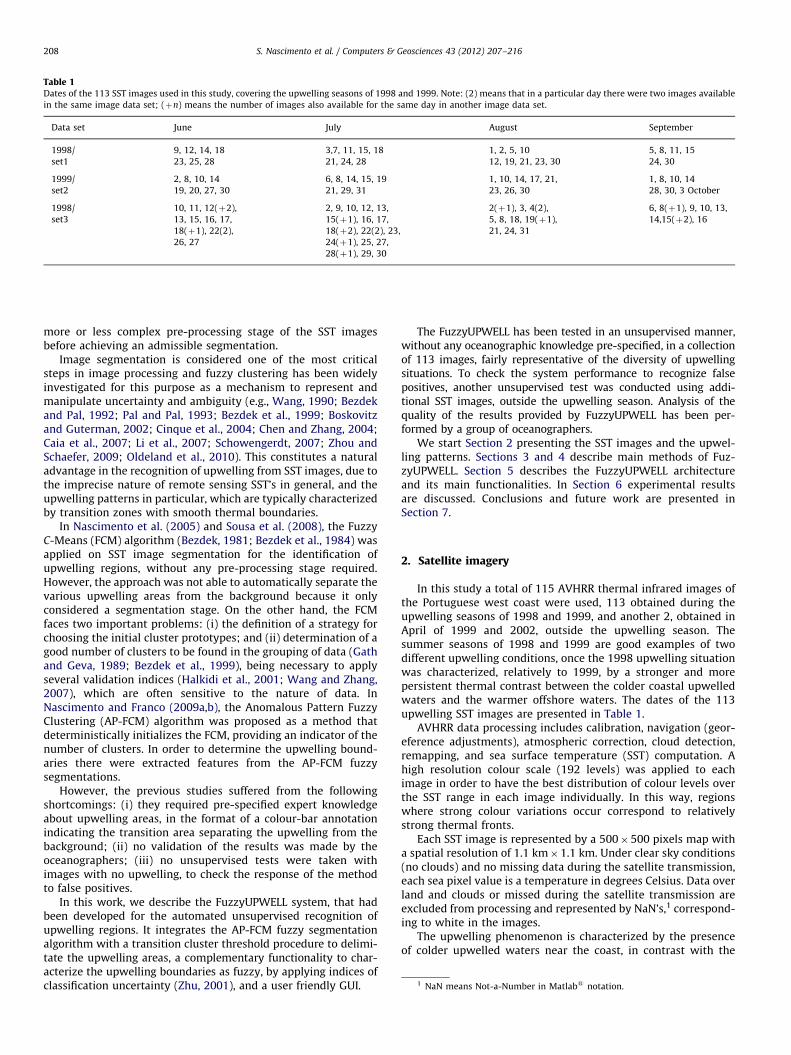
Table 1Dates of the 113 SST images used in this study, covering the upwelling seasons of 1998 and 1999. Note: (2) means that in a particular day there were two images available

in the same image data set; (þn) means the number of images also available for the same day in another image data set.

Data set June July August September

1998/ 9, 12, 14, 18 3,7, 11, 15, 18 1, 2, 5, 10 5, 8, 11, 15

set1 23, 25, 28 21, 24, 28 12, 19, 21, 23, 30 24, 30

1999/ 2, 8, 10, 14 6, 8, 14, 15, 19 1, 10, 14, 17, 21, 1, 8, 10, 14

set2 19, 20, 27, 30 21, 29, 31 23, 26, 30 28, 30, 3 October

1998/ 10, 11, 12(þ2), 2, 9, 10, 12, 13, 2(þ1), 3, 4(2), 6, 8(þ1), 9, 10, 13,

set3 13, 15, 16, 17, 15(þ1), 16, 17, 5, 8, 18, 19(þ1), 14,15(þ2), 16

18(þ1), 22(2), 18(þ2), 22(2), 23, 21, 24, 31

26, 27 24(þ1), 25, 27,

28(þ1), 29, 30

1 NaN means Not-a-Number in Matlabs notation.

S. Nascimento et al. / Computers & Geosciences 43 (2012) 207–216208

more or less complex pre-processing stage of the SST imagesbefore achieving an admissible segmentation.

Image segmentation is considered one of the most criticalsteps in image processing and fuzzy clustering has been widelyinvestigated for this purpose as a mechanism to represent andmanipulate uncertainty and ambiguity (e.g., Wang, 1990; Bezdekand Pal, 1992; Pal and Pal, 1993; Bezdek et al., 1999; Boskovitzand Guterman, 2002; Cinque et al., 2004; Chen and Zhang, 2004;Caia et al., 2007; Li et al., 2007; Schowengerdt, 2007; Zhou andSchaefer, 2009; Oldeland et al., 2010). This constitutes a naturaladvantage in the recognition of upwelling from SST images, due tothe imprecise nature of remote sensing SST’s in general, and theupwelling patterns in particular, which are typically characterizedby transition zones with smooth thermal boundaries.

In Nascimento et al. (2005) and Sousa et al. (2008), the FuzzyC-Means (FCM) algorithm (Bezdek, 1981; Bezdek et al., 1984) wasapplied on SST image segmentation for the identification ofupwelling regions, without any pre-processing stage required.However, the approach was not able to automatically separate thevarious upwelling areas from the background because it onlyconsidered a segmentation stage. On the other hand, the FCMfaces two important problems: (i) the definition of a strategy forchoosing the initial cluster prototypes; and (ii) determination of agood number of clusters to be found in the grouping of data (Gathand Geva, 1989; Bezdek et al., 1999), being necessary to applyseveral validation indices (Halkidi et al., 2001; Wang and Zhang,2007), which are often sensitive to the nature of data. InNascimento and Franco (2009a,b), the Anomalous Pattern FuzzyClustering (AP-FCM) algorithm was proposed as a method thatdeterministically initializes the FCM, providing an indicator of thenumber of clusters. In order to determine the upwelling bound-aries there were extracted features from the AP-FCM fuzzysegmentations.

However, the previous studies suffered from the followingshortcomings: (i) they required pre-specified expert knowledgeabout upwelling areas, in the format of a colour-bar annotationindicating the transition area separating the upwelling from thebackground; (ii) no validation of the results was made by theoceanographers; (iii) no unsupervised tests were taken withimages with no upwelling, to check the response of the methodto false positives.

In this work, we describe the FuzzyUPWELL system, that hadbeen developed for the automated unsupervised recognition ofupwelling regions. It integrates the AP-FCM fuzzy segmentationalgorithm with a transition cluster threshold procedure to delimi-tate the upwelling areas, a complementary functionality to char-acterize the upwelling boundaries as fuzzy, by applying indices ofclassification uncertainty (Zhu, 2001), and a user friendly GUI.

The FuzzyUPWELL has been tested in an unsupervised manner,without any oceanographic knowledge pre-specified, in a collectionof 113 images, fairly representative of the diversity of upwellingsituations. To check the system performance to recognize falsepositives, another unsupervised test was conducted using addi-tional SST images, outside the upwelling season. Analysis of thequality of the results provided by FuzzyUPWELL has been per-formed by a group of oceanographers.

We start Section 2 presenting the SST images and the upwel-ling patterns. Sections 3 and 4 describe main methods of Fuz-zyUPWELL. Section 5 describes the FuzzyUPWELL architectureand its main functionalities. In Section 6 experimental resultsare discussed. Conclusions and future work are presented inSection 7.

2. Satellite imagery

In this study a total of 115 AVHRR thermal infrared images ofthe Portuguese west coast were used, 113 obtained during theupwelling seasons of 1998 and 1999, and another 2, obtained inApril of 1999 and 2002, outside the upwelling season. Thesummer seasons of 1998 and 1999 are good examples of twodifferent upwelling conditions, once the 1998 upwelling situationwas characterized, relatively to 1999, by a stronger and morepersistent thermal contrast between the colder coastal upwelledwaters and the warmer offshore waters. The dates of the 113upwelling SST images are presented in Table 1.

AVHRR data processing includes calibration, navigation (geor-eference adjustments), atmospheric correction, cloud detection,remapping, and sea surface temperature (SST) computation. Ahigh resolution colour scale (192 levels) was applied to eachimage in order to have the best distribution of colour levels overthe SST range in each image individually. In this way, regionswhere strong colour variations occur correspond to relativelystrong thermal fronts.

Each SST image is represented by a 500�500 pixels map witha spatial resolution of 1.1 km�1.1 km. Under clear sky conditions(no clouds) and no missing data during the satellite transmission,each sea pixel value is a temperature in degrees Celsius. Data overland and clouds or missed during the satellite transmission areexcluded from processing and represented by NaN’s,1 correspond-ing to white in the images.

The upwelling phenomenon is characterized by the presenceof colder upwelled waters near the coast, in contrast with the

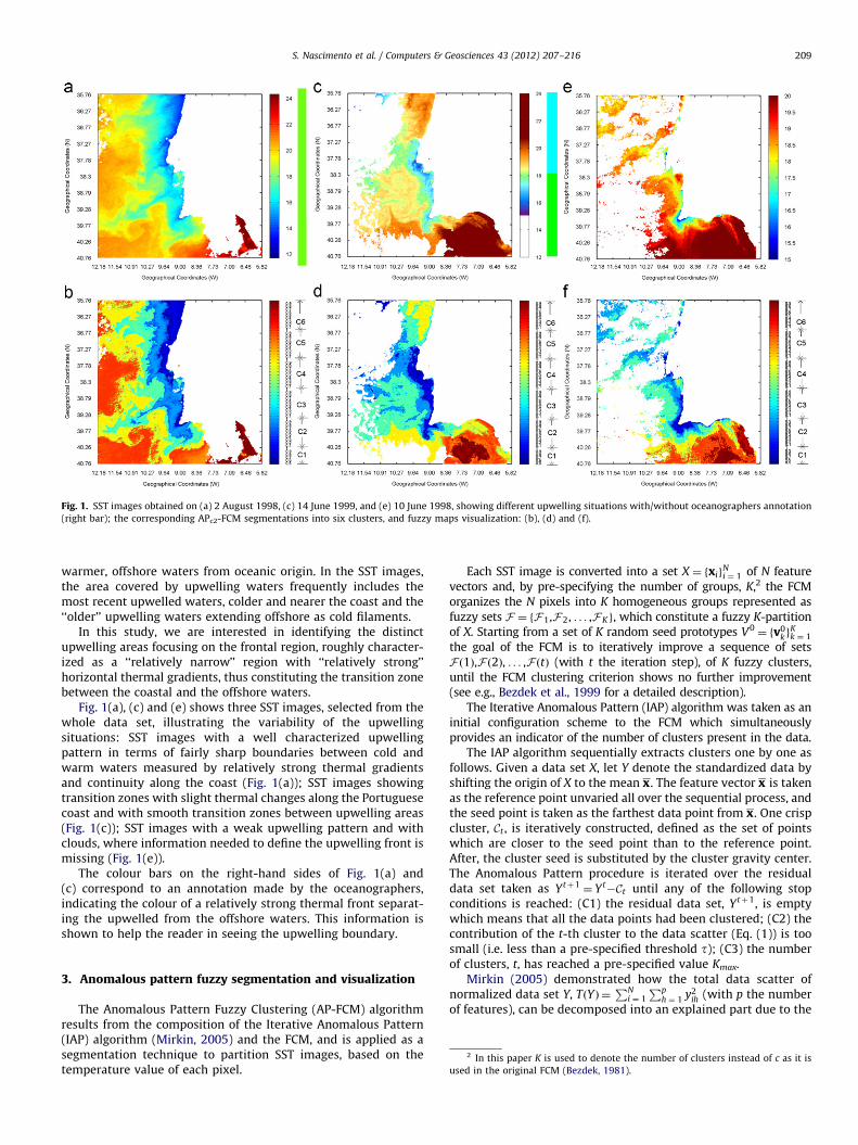
Fig. 1. SST images obtained on (a) 2 August 1998, (c) 14 June 1999, and (e) 10 June 1998, showing different upwelling situations with/without oceanographers annotation

(right bar); the corresponding APc2-FCM segmentations into six clusters, and fuzzy maps visualization: (b), (d) and (f).

S. Nascimento et al. / Computers & Geosciences 43 (2012) 207–216 209

warmer, offshore waters from oceanic origin. In the SST images,the area covered by upwelling waters frequently includes themost recent upwelled waters, colder and nearer the coast and the‘‘older’’ upwelling waters extending offshore as cold filaments.

In this study, we are interested in identifying the distinctupwelling areas focusing on the frontal region, roughly character-ized as a ‘‘relatively narrow’’ region with ‘‘relatively strong’’horizontal thermal gradients, thus constituting the transition zonebetween the coastal and the offshore waters.

Fig. 1(a), (c) and (e) shows three SST images, selected from thewhole data set, illustrating the variability of the upwellingsituations: SST images with a well characterized upwellingpattern in terms of fairly sharp boundaries between cold andwarm waters measured by relatively strong thermal gradientsand continuity along the coast (Fig. 1(a)); SST images showingtransition zones with slight thermal changes along the Portuguesecoast and with smooth transition zones between upwelling areas(Fig. 1(c)); SST images with a weak upwelling pattern and withclouds, where information needed to define the upwelling front ismissing (Fig. 1(e)).

The colour bars on the right-hand sides of Fig. 1(a) and(c) correspond to an annotation made by the oceanographers,indicating the colour of a relatively strong thermal front separat-ing the upwelled from the offshore waters. This information isshown to help the reader in seeing the upwelling boundary.

2 In this paper K is used to denote the number of clusters instead of c as it is

used in the original FCM (Bezdek, 1981).

3. Anomalous pattern fuzzy segmentation and visualization

The Anomalous Pattern Fuzzy Clustering (AP-FCM) algorithmresults from the composition of the Iterative Anomalous Pattern(IAP) algorithm (Mirkin, 2005) and the FCM, and is applied as asegmentation technique to partition SST images, based on thetemperature value of each pixel.

Each SST image is converted into a set X ¼ fxigNi ¼ 1 of N feature

vectors and, by pre-specifying the number of groups, K,2 the FCMorganizes the N pixels into K homogeneous groups represented asfuzzy sets F ¼ fF1,F 2, . . . ,FKg, which constitute a fuzzy K-partitionof X. Starting from a set of K random seed prototypes V0

¼ fv0kg

Kk ¼ 1

the goal of the FCM is to iteratively improve a sequence of setsF ð1Þ,F ð2Þ, . . . ,F ðtÞ (with t the iteration step), of K fuzzy clusters,until the FCM clustering criterion shows no further improvement(see e.g., Bezdek et al., 1999 for a detailed description).

The Iterative Anomalous Pattern (IAP) algorithm was taken as aninitial configuration scheme to the FCM which simultaneouslyprovides an indicator of the number of clusters present in the data.

The IAP algorithm sequentially extracts clusters one by one asfollows. Given a data set X, let Y denote the standardized data byshifting the origin of X to the mean x. The feature vector x is takenas the reference point unvaried all over the sequential process, andthe seed point is taken as the farthest data point from x. One crispcluster, Ct , is iteratively constructed, defined as the set of pointswhich are closer to the seed point than to the reference point.After, the cluster seed is substituted by the cluster gravity center.The Anomalous Pattern procedure is iterated over the residualdata set taken as Ytþ1

¼ Yt�Ct until any of the following stop

conditions is reached: (C1) the residual data set, Ytþ1, is emptywhich means that all the data points had been clustered; (C2) thecontribution of the t-th cluster to the data scatter (Eq. (1)) is toosmall (i.e. less than a pre-specified threshold t); (C3) the numberof clusters, t, has reached a pre-specified value Kmax.

Mirkin (2005) demonstrated how the total data scatter ofnormalized data set Y, TðYÞ ¼

PNi ¼ 1

Pph ¼ 1 y2

ih (with p the numberof features), can be decomposed into an explained part due to the

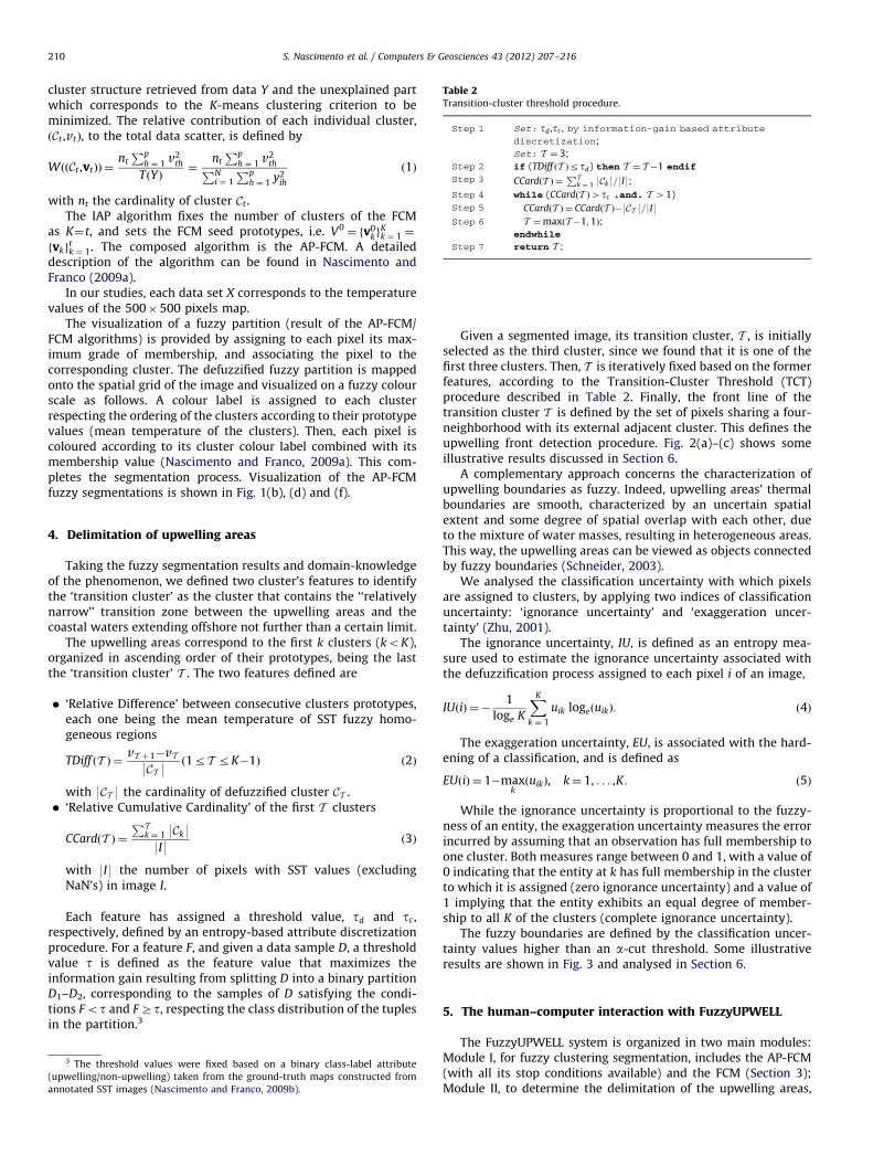
Table 2Transition-cluster threshold procedure.

Step 1 Set: td ,tc , by information-gain based attribute

discretization;

Set: T ¼ 3;

Step 2 if (TDiff ðT Þrtd) then T ¼ T �1 endif

Step 3 CCardðT Þ ¼PT

k ¼ 1 9Ck9=9I9;Step 4 while (CCardðT Þ4tc .and. T 41)

Step 5 CCardðT Þ ¼ CCardðT Þ�9CT 9=9I9Step 6 T ¼maxðT �1;1Þ;

endwhile

Step 7 return T ;


cluster structure retrieved from data Y and the unexplained partwhich corresponds to the K-means clustering criterion to beminimized. The relative contribution of each individual cluster,ðCt ,vtÞ, to the total data scatter, is defined by

WððCt ,vtÞÞ ¼ntPp

h ¼ 1 v2th

TðYÞ¼

ntPp

h ¼ 1 v2thPN

i ¼ 1

Pph ¼ 1 y2

ih

ð1Þ

with nt the cardinality of cluster Ct .The IAP algorithm fixes the number of clusters of the FCM

as K¼t, and sets the FCM seed prototypes, i.e. V0¼ fv0

kgKk ¼ 1 ¼

fvkgtk ¼ 1. The composed algorithm is the AP-FCM. A detailed

description of the algorithm can be found in Nascimento andFranco (2009a).

In our studies, each data set X corresponds to the temperaturevalues of the 500�500 pixels map.

The visualization of a fuzzy partition (result of the AP-FCM/FCM algorithms) is provided by assigning to each pixel its max-imum grade of membership, and associating the pixel to thecorresponding cluster. The defuzzified fuzzy partition is mappedonto the spatial grid of the image and visualized on a fuzzy colourscale as follows. A colour label is assigned to each clusterrespecting the ordering of the clusters according to their prototypevalues (mean temperature of the clusters). Then, each pixel iscoloured according to its cluster colour label combined with itsmembership value (Nascimento and Franco, 2009a). This com-pletes the segmentation process. Visualization of the AP-FCMfuzzy segmentations is shown in Fig. 1(b), (d) and (f).

4. Delimitation of upwelling areas

Taking the fuzzy segmentation results and domain-knowledgeof the phenomenon, we defined two cluster’s features to identifythe ‘transition cluster’ as the cluster that contains the ‘‘relativelynarrow’’ transition zone between the upwelling areas and thecoastal waters extending offshore not further than a certain limit.

The upwelling areas correspond to the first k clusters (koK),organized in ascending order of their prototypes, being the lastthe ‘transition cluster’ T . The two features defined are

�

(up

ann

‘Relative Difference’ between consecutive clusters prototypes,each one being the mean temperature of SST fuzzy homo-geneous regions

TDiff ðT Þ ¼ vT þ1�vT9CT 9

ð1rT rK�1Þ ð2Þ

with 9CT 9 the cardinality of defuzzified cluster CT .
� ‘Relative Cumulative Cardinality’ of the first T clusters
CCardðT Þ ¼PT

k ¼ 1 9Ck99I9

ð3Þ

with 9I9 the number of pixels with SST values (excludingNaN’s) in image I.

Each feature has assigned a threshold value, td and tc ,respectively, defined by an entropy-based attribute discretizationprocedure. For a feature F, and given a data sample D, a thresholdvalue t is defined as the feature value that maximizes theinformation gain resulting from splitting D into a binary partitionD1–D2, corresponding to the samples of D satisfying the condi-tions Fot and FZt, respecting the class distribution of the tuplesin the partition.3

3 The threshold values were fixed based on a binary class-label attribute

welling/non-upwelling) taken from the ground-truth maps constructed from

otated SST images (Nascimento and Franco, 2009b).

Given a segmented image, its transition cluster, T , is initiallyselected as the third cluster, since we found that it is one of thefirst three clusters. Then, T is iteratively fixed based on the formerfeatures, according to the Transition-Cluster Threshold (TCT)procedure described in Table 2. Finally, the front line of thetransition cluster T is defined by the set of pixels sharing a four-neighborhood with its external adjacent cluster. This defines theupwelling front detection procedure. Fig. 2(a)–(c) shows someillustrative results discussed in Section 6.

A complementary approach concerns the characterization ofupwelling boundaries as fuzzy. Indeed, upwelling areas’ thermalboundaries are smooth, characterized by an uncertain spatialextent and some degree of spatial overlap with each other, dueto the mixture of water masses, resulting in heterogeneous areas.This way, the upwelling areas can be viewed as objects connectedby fuzzy boundaries (Schneider, 2003).

We analysed the classification uncertainty with which pixelsare assigned to clusters, by applying two indices of classificationuncertainty: ‘ignorance uncertainty’ and ‘exaggeration uncer-tainty’ (Zhu, 2001).

The ignorance uncertainty, IU, is defined as an entropy mea-sure used to estimate the ignorance uncertainty associated withthe defuzzification process assigned to each pixel i of an image,

IUðiÞ ¼�1

loge K

XK

k ¼ 1

uik logeðuikÞ: ð4Þ

The exaggeration uncertainty, EU, is associated with the hard-ening of a classification, and is defined as

EUðiÞ ¼ 1�maxkðuikÞ, k¼ 1, . . . ,K: ð5Þ

While the ignorance uncertainty is proportional to the fuzzy-ness of an entity, the exaggeration uncertainty measures the errorincurred by assuming that an observation has full membership toone cluster. Both measures range between 0 and 1, with a value of0 indicating that the entity at k has full membership in the clusterto which it is assigned (zero ignorance uncertainty) and a value of1 implying that the entity exhibits an equal degree of member-ship to all K of the clusters (complete ignorance uncertainty).

The fuzzy boundaries are defined by the classification uncer-tainty values higher than an a-cut threshold. Some illustrativeresults are shown in Fig. 3 and analysed in Section 6.

5. The human–computer interaction with FuzzyUPWELL

The FuzzyUPWELL system is organized in two main modules:Module I, for fuzzy clustering segmentation, includes the AP-FCM(with all its stop conditions available) and the FCM (Section 3);Module II, to determine the delimitation of the upwelling areas,

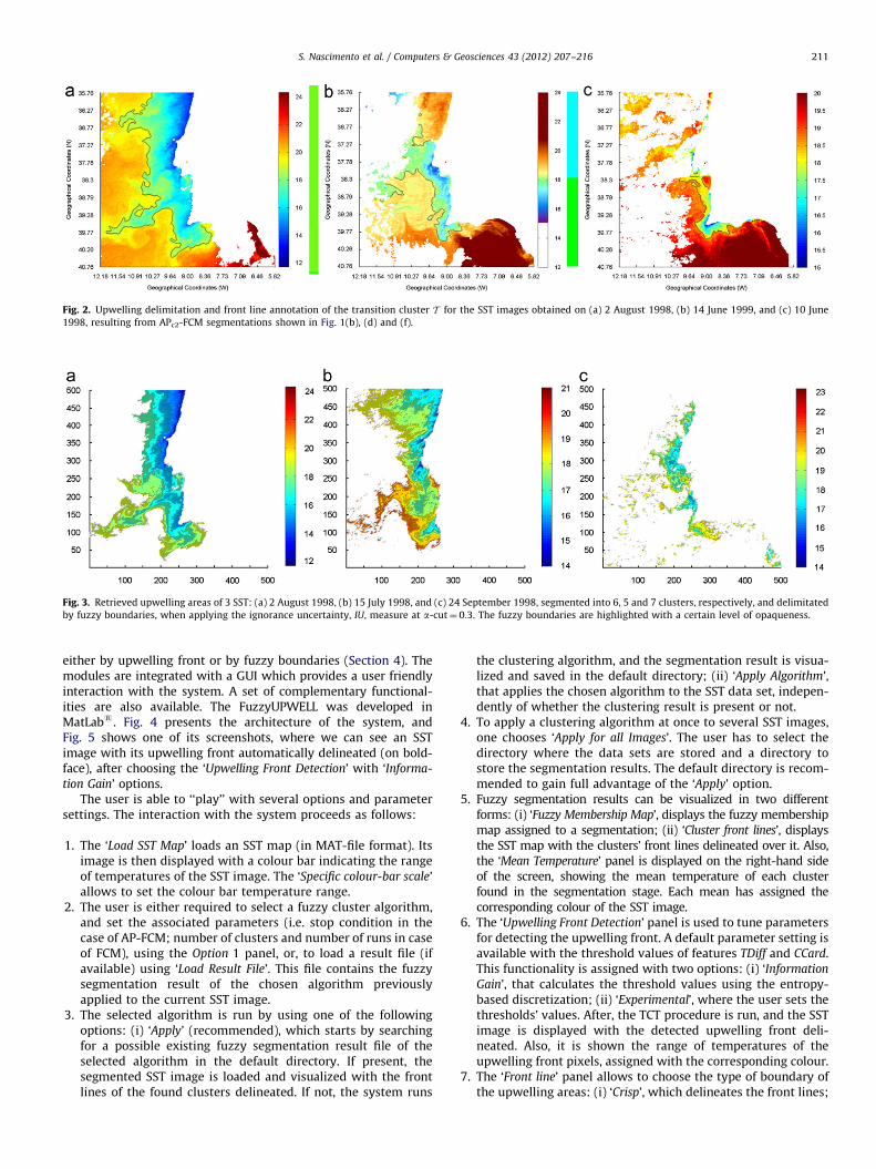
Fig. 2. Upwelling delimitation and front line annotation of the transition cluster T for the SST images obtained on (a) 2 August 1998, (b) 14 June 1999, and (c) 10 June

1998, resulting from APc2-FCM segmentations shown in Fig. 1(b), (d) and (f).

Fig. 3. Retrieved upwelling areas of 3 SST: (a) 2 August 1998, (b) 15 July 1998, and (c) 24 September 1998, segmented into 6, 5 and 7 clusters, respectively, and delimitated

by fuzzy boundaries, when applying the ignorance uncertainty, IU, measure at a-cut¼ 0:3. The fuzzy boundaries are highlighted with a certain level of opaqueness.


either by upwelling front or by fuzzy boundaries (Section 4). Themodules are integrated with a GUI which provides a user friendlyinteraction with the system. A set of complementary functional-ities are also available. The FuzzyUPWELL was developed inMatLabs. Fig. 4 presents the architecture of the system, andFig. 5 shows one of its screenshots, where we can see an SSTimage with its upwelling front automatically delineated (on bold-face), after choosing the ‘Upwelling Front Detection’ with ‘Informa-

tion Gain’ options.The user is able to ‘‘play’’ with several options and parameter

settings. The interaction with the system proceeds as follows:

1.
The ‘Load SST Map’ loads an SST map (in MAT-file format). Itsimage is then displayed with a colour bar indicating the rangeof temperatures of the SST image. The ‘Specific colour-bar scale’allows to set the colour bar temperature range.
2.
The user is either required to select a fuzzy cluster algorithm,and set the associated parameters (i.e. stop condition in thecase of AP-FCM; number of clusters and number of runs in caseof FCM), using the Option 1 panel, or, to load a result file (ifavailable) using ‘Load Result File’. This file contains the fuzzysegmentation result of the chosen algorithm previouslyapplied to the current SST image.
3.
The selected algorithm is run by using one of the followingoptions: (i) ‘Apply’ (recommended), which starts by searchingfor a possible existing fuzzy segmentation result file of theselected algorithm in the default directory. If present, thesegmented SST image is loaded and visualized with the frontlines of the found clusters delineated. If not, the system runs
the clustering algorithm, and the segmentation result is visua-lized and saved in the default directory; (ii) ‘Apply Algorithm’,that applies the chosen algorithm to the SST data set, indepen-dently of whether the clustering result is present or not.

4.
To apply a clustering algorithm at once to several SST images,one chooses ‘Apply for all Images’. The user has to select thedirectory where the data sets are stored and a directory tostore the segmentation results. The default directory is recom-mended to gain full advantage of the ‘Apply’ option.
5.
Fuzzy segmentation results can be visualized in two differentforms: (i) ‘Fuzzy Membership Map’, displays the fuzzy membershipmap assigned to a segmentation; (ii) ‘Cluster front lines’, displaysthe SST map with the clusters’ front lines delineated over it. Also,the ‘Mean Temperature’ panel is displayed on the right-hand sideof the screen, showing the mean temperature of each clusterfound in the segmentation stage. Each mean has assigned thecorresponding colour of the SST image.
6.
The ‘Upwelling Front Detection’ panel is used to tune parametersfor detecting the upwelling front. A default parameter setting isavailable with the threshold values of features TDiff and CCard.This functionality is assigned with two options: (i) ‘Information
Gain’, that calculates the threshold values using the entropy-based discretization; (ii) ‘Experimental’, where the user sets thethresholds’ values. After, the TCT procedure is run, and the SSTimage is displayed with the detected upwelling front deli-neated. Also, it is shown the range of temperatures of theupwelling front pixels, assigned with the corresponding colour.

7.
The ‘Front line’ panel allows to choose the type of boundary ofthe upwelling areas: (i) ‘Crisp’, which delineates the front lines;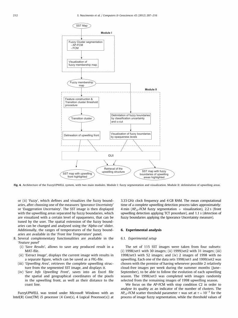

SST Map

Feature construction &Transition cluster thresholdprocedure

Visualization of fuzzy boundariesby opaqueness levels

Delimitation of fuzzy boundariesby classification uncertaintyand -cutα

Delineation of upwelling front

Fuzzy membershipmap

Transition cluster

SST map withfront highlighted

upwelling

Retrieval of theupwelling structure SST map with fuzzy

boundaries of upwellingareas highlighted

Fuzzy Cluster segmentation- AP-FCM- FCM

Visualization offuzzy membership map

Module I

Module II

GUI

Fig. 4. Architecture of the FuzzyUPWELL system, with two main modules. Module I: fuzzy segmentation and visualization. Module II: delimitation of upwelling areas.


or (ii) ‘Fuzzy’, which defines and visualizes the fuzzy bound-aries, after choosing one of the measures ‘Ignorance Uncertainty’or ‘Exaggeration Uncertainty’. The SST image is then displayedwith the upwelling areas separated by fuzzy boundaries, whichare visualized with a certain level of opaqueness, that can betuned by the user. The spatial extension of the fuzzy bound-aries can be changed and analysed using the ‘Alpha-cut’ slider.Additionally, the ranges of temperatures of the fuzzy bound-aries are available in the ‘Front line Temperature’ panel.

8.
Several complementary functionalities are available in the‘Feature panel’
(i) ‘Save Results’, allows to save any produced result in aMAT-file.

(ii) ‘Extract Image’, displays the current image with results ina separate figure, which can be saved as a FIG-file.

(iii) ‘Upwelling Area’, retrieves the complete upwelling struc-ture from the segmented SST image, and displays it.

(iv) ‘Save Info Upwelling Front’, saves into an Excel filethe spatial and geographical coordinates of the pixelsin the upwelling front, as well as their distance to thecoast line.

FuzzyUPWELL was tested under Microsoft Windows with anIntel(R) Core(TM) i5 processor (4 Core(s), 4 Logical Processor(s)) at

3.33 GHz clock frequency and 4 GB RAM. The mean computationaltime of a complete upwelling detection process takes approximately:4 min (APc2-FCM fuzzy segmentation þ visualization), 2.2 s (frontupwelling detection applying TCT procedure), and 1.1 s (detection offuzzy boundaries applying the Ignorance Uncertainty measure).

6. Experimental analysis

6.1. Experimental setup

The set of 115 SST images were taken from four subsets:(i) 1998/set1 with 30 images; (ii) 1999/set2 with 31 images; (iii)1998/set3 with 52 images; and (iv) 2 images of 1998 with noupwelling. Each one of the data sets 1998/set1 and 1999/set2 waschosen with the premise of having whenever possible 2 relativelycloud-free images per week during the summer months (June–September), to be able to follow the evolution of each upwellingseason. The 1998/set3 was completed with images randomlyselected from the remaining images of 1998 upwelling season.

We focus on the AP-FCM with stop condition C2 in order toanalyse its quality as an indicator of the number of clusters. TheAPc2-FCM scatter threshold parameter t was set at t¼ 10�3 for theprocess of image fuzzy segmentation, while the threshold values of

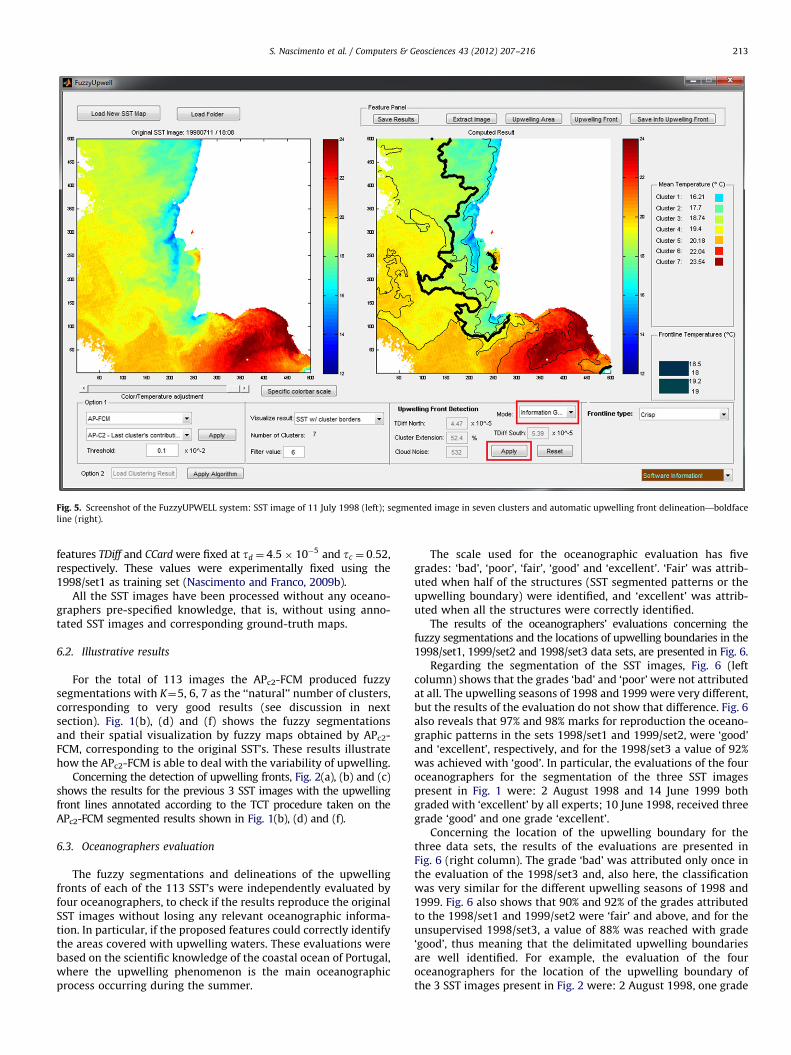
Fig. 5. Screenshot of the FuzzyUPWELL system: SST image of 11 July 1998 (left); segmented image in seven clusters and automatic upwelling front delineation—boldface

line (right).


features TDiff and CCard were fixed at td ¼ 4:5� 10�5 and tc ¼ 0:52,respectively. These values were experimentally fixed using the1998/set1 as training set (Nascimento and Franco, 2009b).

All the SST images have been processed without any oceano-graphers pre-specified knowledge, that is, without using anno-tated SST images and corresponding ground-truth maps.

6.2. Illustrative results

For the total of 113 images the APc2-FCM produced fuzzysegmentations with K¼5, 6, 7 as the ‘‘natural’’ number of clusters,corresponding to very good results (see discussion in nextsection). Fig. 1(b), (d) and (f) shows the fuzzy segmentationsand their spatial visualization by fuzzy maps obtained by APc2-FCM, corresponding to the original SST’s. These results illustratehow the APc2-FCM is able to deal with the variability of upwelling.

Concerning the detection of upwelling fronts, Fig. 2(a), (b) and (c)shows the results for the previous 3 SST images with the upwellingfront lines annotated according to the TCT procedure taken on theAPc2-FCM segmented results shown in Fig. 1(b), (d) and (f).

6.3. Oceanographers evaluation

The fuzzy segmentations and delineations of the upwellingfronts of each of the 113 SST’s were independently evaluated byfour oceanographers, to check if the results reproduce the originalSST images without losing any relevant oceanographic informa-tion. In particular, if the proposed features could correctly identifythe areas covered with upwelling waters. These evaluations werebased on the scientific knowledge of the coastal ocean of Portugal,where the upwelling phenomenon is the main oceanographicprocess occurring during the summer.

The scale used for the oceanographic evaluation has fivegrades: ‘bad’, ‘poor’, ‘fair’, ‘good’ and ‘excellent’. ‘Fair’ was attrib-uted when half of the structures (SST segmented patterns or theupwelling boundary) were identified, and ‘excellent’ was attrib-uted when all the structures were correctly identified.

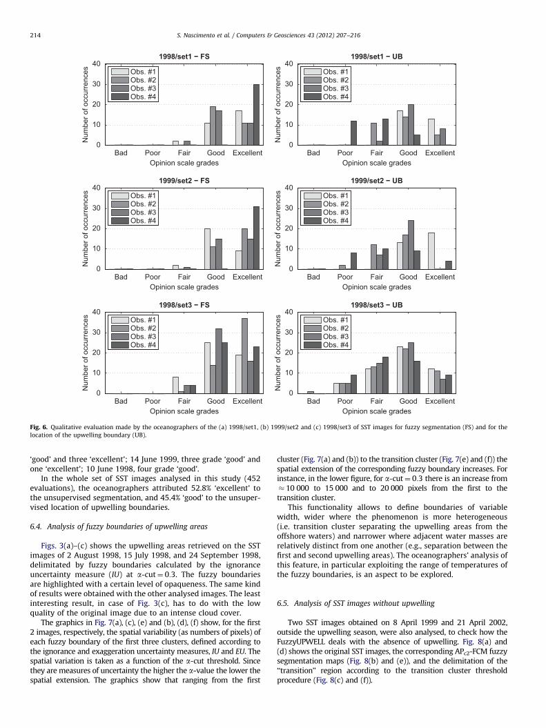
The results of the oceanographers’ evaluations concerning thefuzzy segmentations and the locations of upwelling boundaries in the1998/set1, 1999/set2 and 1998/set3 data sets, are presented in Fig. 6.

Regarding the segmentation of the SST images, Fig. 6 (leftcolumn) shows that the grades ‘bad’ and ‘poor’ were not attributedat all. The upwelling seasons of 1998 and 1999 were very different,but the results of the evaluation do not show that difference. Fig. 6also reveals that 97% and 98% marks for reproduction the oceano-graphic patterns in the sets 1998/set1 and 1999/set2, were ‘good’and ‘excellent’, respectively, and for the 1998/set3 a value of 92%was achieved with ‘good’. In particular, the evaluations of the fouroceanographers for the segmentation of the three SST imagespresent in Fig. 1 were: 2 August 1998 and 14 June 1999 bothgraded with ‘excellent’ by all experts; 10 June 1998, received threegrade ‘good’ and one grade ‘excellent’.

Concerning the location of the upwelling boundary for thethree data sets, the results of the evaluations are presented inFig. 6 (right column). The grade ‘bad’ was attributed only once inthe evaluation of the 1998/set3 and, also here, the classificationwas very similar for the different upwelling seasons of 1998 and1999. Fig. 6 also shows that 90% and 92% of the grades attributedto the 1998/set1 and 1999/set2 were ‘fair’ and above, and for theunsupervised 1998/set3, a value of 88% was reached with grade‘good’, thus meaning that the delimitated upwelling boundariesare well identified. For example, the evaluation of the fouroceanographers for the location of the upwelling boundary ofthe 3 SST images present in Fig. 2 were: 2 August 1998, one grade

Bad Poor Fair Good Excellent0

10

20

30

401998/set1 − FS

Opinion scale grades

Num

ber o

f occ

urre

nces Obs. #1

Obs. #2Obs. #3Obs. #4


10

20

30

401999/set2 − FS


Num

ber o

f occ

urre

nces Obs. #1



10

20

30

401998/set1 − UB


Num

ber o

f occ

urre

nces Obs. #1



10

20

30

401999/set2 − UB

Opinion scale gradesN

umbe

r of o

ccur

renc

es Obs. #1Obs. #2Obs. #3Obs. #4


10

20

30

401998/set3 − FS


Num

ber o

f occ

urre

nces Obs. #1



10

20

30

401998/set3 − UB


Num

ber o

f occ

urre

nces Obs. #1


Fig. 6. Qualitative evaluation made by the oceanographers of the (a) 1998/set1, (b) 1999/set2 and (c) 1998/set3 of SST images for fuzzy segmentation (FS) and for the

location of the upwelling boundary (UB).


‘good’ and three ‘excellent’; 14 June 1999, three grade ‘good’ andone ‘excellent’; 10 June 1998, four grade ‘good’.

In the whole set of SST images analysed in this study (452evaluations), the oceanographers attributed 52.8% ‘excellent’ tothe unsupervised segmentation, and 45.4% ‘good’ to the unsuper-vised location of upwelling boundaries.

6.4. Analysis of fuzzy boundaries of upwelling areas

Figs. 3(a)–(c) shows the upwelling areas retrieved on the SSTimages of 2 August 1998, 15 July 1998, and 24 September 1998,delimitated by fuzzy boundaries calculated by the ignoranceuncertainty measure (IU) at a-cut¼ 0:3. The fuzzy boundariesare highlighted with a certain level of opaqueness. The same kindof results were obtained with the other analysed images. The leastinteresting result, in case of Fig. 3(c), has to do with the lowquality of the original image due to an intense cloud cover.

The graphics in Fig. 7(a), (c), (e) and (b), (d), (f) show, for the first2 images, respectively, the spatial variability (as numbers of pixels) ofeach fuzzy boundary of the first three clusters, defined according tothe ignorance and exaggeration uncertainty measures, IU and EU. Thespatial variation is taken as a function of the a-cut threshold. Sincethey are measures of uncertainty the higher the a-value the lower thespatial extension. The graphics show that ranging from the first

cluster (Fig. 7(a) and (b)) to the transition cluster (Fig. 7(e) and (f)) thespatial extension of the corresponding fuzzy boundary increases. Forinstance, in the lower figure, for a-cut¼ 0:3 there is an increase from� 10 000 to 15 000 and to 20 000 pixels from the first to thetransition cluster.

This functionality allows to define boundaries of variablewidth, wider where the phenomenon is more heterogeneous(i.e. transition cluster separating the upwelling areas from theoffshore waters) and narrower where adjacent water masses arerelatively distinct from one another (e.g., separation between thefirst and second upwelling areas). The oceanographers’ analysis ofthis feature, in particular exploiting the range of temperatures ofthe fuzzy boundaries, is an aspect to be explored.

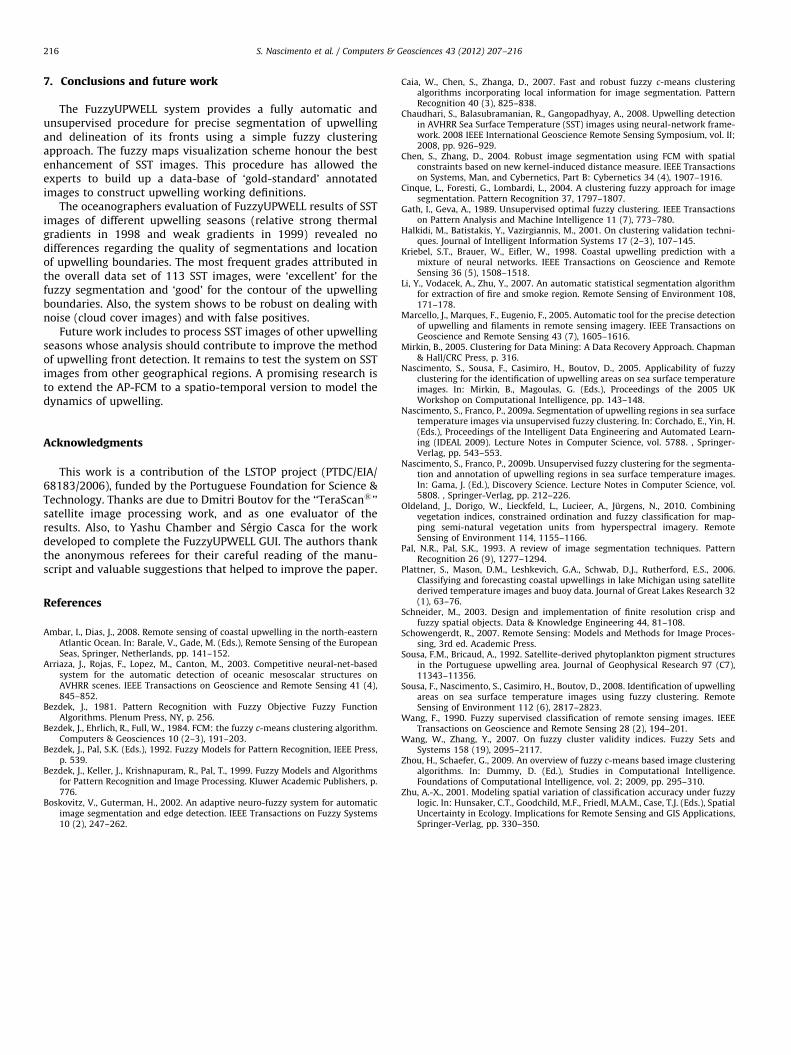
6.5. Analysis of SST images without upwelling

Two SST images obtained on 8 April 1999 and 21 April 2002,outside the upwelling season, were also analysed, to check how theFuzzyUPWELL deals with the absence of upwelling. Fig. 8(a) and(d) shows the original SST images, the corresponding APc2-FCM fuzzysegmentation maps (Fig. 8(b) and (e)), and the delimitation of the‘‘transition’’ region according to the transition cluster thresholdprocedure (Fig. 8(c) and (f)).

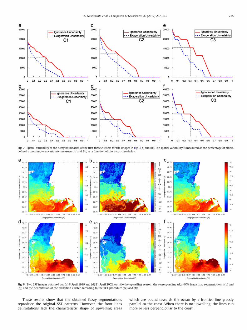
Fig. 7. Spatial variability of the fuzzy boundaries of the first three clusters for the images in Fig. 3(a) and (b). The spatial variability is measured as the percentage of pixels,

defined according to uncertainty measures IU and EU, as a function of the a-cut thresholds.

Fig. 8. Two SST images obtained on: (a) 8 April 1999 and (d) 21 April 2002, outside the upwelling season; the corresponding APc2-FCM fuzzy map segmentations ((b) and

(e)) and the delimitation of the transition cluster according to the TCT procedure ((c) and (f)).


These results show that the obtained fuzzy segmentationsreproduce the original SST patterns. However, the front linesdelimitations lack the characteristic shape of upwelling areas

which are bound towards the ocean by a frontier line grosslyparallel to the coast. When there is no upwelling, the lines runmore or less perpendicular to the coast.


7. Conclusions and future work

The FuzzyUPWELL system provides a fully automatic andunsupervised procedure for precise segmentation of upwellingand delineation of its fronts using a simple fuzzy clusteringapproach. The fuzzy maps visualization scheme honour the bestenhancement of SST images. This procedure has allowed theexperts to build up a data-base of ‘gold-standard’ annotatedimages to construct upwelling working definitions.

The oceanographers evaluation of FuzzyUPWELL results of SSTimages of different upwelling seasons (relative strong thermalgradients in 1998 and weak gradients in 1999) revealed nodifferences regarding the quality of segmentations and locationof upwelling boundaries. The most frequent grades attributed inthe overall data set of 113 SST images, were ‘excellent’ for thefuzzy segmentation and ‘good’ for the contour of the upwellingboundaries. Also, the system shows to be robust on dealing withnoise (cloud cover images) and with false positives.

Future work includes to process SST images of other upwellingseasons whose analysis should contribute to improve the methodof upwelling front detection. It remains to test the system on SSTimages from other geographical regions. A promising research isto extend the AP-FCM to a spatio-temporal version to model thedynamics of upwelling.

Acknowledgments

This work is a contribution of the LSTOP project (PTDC/EIA/68183/2006), funded by the Portuguese Foundation for Science &Technology. Thanks are due to Dmitri Boutov for the ‘‘TeraScans’’satellite image processing work, and as one evaluator of theresults. Also, to Yashu Chamber and Sergio Casca for the workdeveloped to complete the FuzzyUPWELL GUI. The authors thankthe anonymous referees for their careful reading of the manu-script and valuable suggestions that helped to improve the paper.

References

Ambar, I., Dias, J., 2008. Remote sensing of coastal upwelling in the north-easternAtlantic Ocean. In: Barale, V., Gade, M. (Eds.), Remote Sensing of the EuropeanSeas, Springer, Netherlands, pp. 141–152.

Arriaza, J., Rojas, F., Lopez, M., Canton, M., 2003. Competitive neural-net-basedsystem for the automatic detection of oceanic mesoscalar structures onAVHRR scenes. IEEE Transactions on Geoscience and Remote Sensing 41 (4),845–852.

Bezdek, J., 1981. Pattern Recognition with Fuzzy Objective Fuzzy FunctionAlgorithms. Plenum Press, NY, p. 256.

Bezdek, J., Ehrlich, R., Full, W., 1984. FCM: the fuzzy c-means clustering algorithm.Computers & Geosciences 10 (2–3), 191–203.

Bezdek, J., Pal, S.K. (Eds.), 1992. Fuzzy Models for Pattern Recognition, IEEE Press,p. 539.

Bezdek, J., Keller, J., Krishnapuram, R., Pal, T., 1999. Fuzzy Models and Algorithmsfor Pattern Recognition and Image Processing. Kluwer Academic Publishers, p.776.

Boskovitz, V., Guterman, H., 2002. An adaptive neuro-fuzzy system for automaticimage segmentation and edge detection. IEEE Transactions on Fuzzy Systems10 (2), 247–262.

Caia, W., Chen, S., Zhanga, D., 2007. Fast and robust fuzzy c-means clusteringalgorithms incorporating local information for image segmentation. PatternRecognition 40 (3), 825–838.

Chaudhari, S., Balasubramanian, R., Gangopadhyay, A., 2008. Upwelling detectionin AVHRR Sea Surface Temperature (SST) images using neural-network frame-work. 2008 IEEE International Geoscience Remote Sensing Symposium, vol. II;2008, pp. 926–929.

Chen, S., Zhang, D., 2004. Robust image segmentation using FCM with spatialconstraints based on new kernel-induced distance measure. IEEE Transactionson Systems, Man, and Cybernetics, Part B: Cybernetics 34 (4), 1907–1916.

Cinque, L., Foresti, G., Lombardi, L., 2004. A clustering fuzzy approach for imagesegmentation. Pattern Recognition 37, 1797–1807.

Gath, I., Geva, A., 1989. Unsupervised optimal fuzzy clustering. IEEE Transactionson Pattern Analysis and Machine Intelligence 11 (7), 773–780.

Halkidi, M., Batistakis, Y., Vazirgiannis, M., 2001. On clustering validation techni-ques. Journal of Intelligent Information Systems 17 (2–3), 107–145.

Kriebel, S.T., Brauer, W., Eifler, W., 1998. Coastal upwelling prediction with amixture of neural networks. IEEE Transactions on Geoscience and RemoteSensing 36 (5), 1508–1518.

Li, Y., Vodacek, A., Zhu, Y., 2007. An automatic statistical segmentation algorithmfor extraction of fire and smoke region. Remote Sensing of Environment 108,171–178.

Marcello, J., Marques, F., Eugenio, F., 2005. Automatic tool for the precise detectionof upwelling and filaments in remote sensing imagery. IEEE Transactions onGeoscience and Remote Sensing 43 (7), 1605–1616.

Mirkin, B., 2005. Clustering for Data Mining: A Data Recovery Approach. Chapman& Hall/CRC Press, p. 316.

Nascimento, S., Sousa, F., Casimiro, H., Boutov, D., 2005. Applicability of fuzzyclustering for the identification of upwelling areas on sea surface temperatureimages. In: Mirkin, B., Magoulas, G. (Eds.), Proceedings of the 2005 UKWorkshop on Computational Intelligence, pp. 143–148.

Nascimento, S., Franco, P., 2009a. Segmentation of upwelling regions in sea surfacetemperature images via unsupervised fuzzy clustering. In: Corchado, E., Yin, H.(Eds.), Proceedings of the Intelligent Data Engineering and Automated Learn-ing (IDEAL 2009). Lecture Notes in Computer Science, vol. 5788. , Springer-Verlag, pp. 543–553.

Nascimento, S., Franco, P., 2009b. Unsupervised fuzzy clustering for the segmenta-tion and annotation of upwelling regions in sea surface temperature images.In: Gama, J. (Ed.), Discovery Science. Lecture Notes in Computer Science, vol.5808. , Springer-Verlag, pp. 212–226.

Oldeland, J., Dorigo, W., Lieckfeld, L., Lucieer, A., Jurgens, N., 2010. Combiningvegetation indices, constrained ordination and fuzzy classification for map-ping semi-natural vegetation units from hyperspectral imagery. RemoteSensing of Environment 114, 1155–1166.

Pal, N.R., Pal, S.K., 1993. A review of image segmentation techniques. PatternRecognition 26 (9), 1277–1294.

Plattner, S., Mason, D.M., Leshkevich, G.A., Schwab, D.J., Rutherford, E.S., 2006.Classifying and forecasting coastal upwellings in lake Michigan using satellitederived temperature images and buoy data. Journal of Great Lakes Research 32(1), 63–76.

Schneider, M., 2003. Design and implementation of finite resolution crisp andfuzzy spatial objects. Data & Knowledge Engineering 44, 81–108.

Schowengerdt, R., 2007. Remote Sensing: Models and Methods for Image Proces-sing, 3rd ed. Academic Press.

Sousa, F.M., Bricaud, A., 1992. Satellite-derived phytoplankton pigment structuresin the Portuguese upwelling area. Journal of Geophysical Research 97 (C7),11343–11356.

Sousa, F., Nascimento, S., Casimiro, H., Boutov, D., 2008. Identification of upwellingareas on sea surface temperature images using fuzzy clustering. RemoteSensing of Environment 112 (6), 2817–2823.

Wang, F., 1990. Fuzzy supervised classification of remote sensing images. IEEETransactions on Geoscience and Remote Sensing 28 (2), 194–201.

Wang, W., Zhang, Y., 2007. On fuzzy cluster validity indices. Fuzzy Sets andSystems 158 (19), 2095–2117.

Zhou, H., Schaefer, G., 2009. An overview of fuzzy c-means based image clusteringalgorithms. In: Dummy, D. (Ed.), Studies in Computational Intelligence.Foundations of Computational Intelligence, vol. 2; 2009, pp. 295–310.

Zhu, A.-X., 2001. Modeling spatial variation of classification accuracy under fuzzylogic. In: Hunsaker, C.T., Goodchild, M.F., Friedl, M.A.M., Case, T.J. (Eds.), SpatialUncertainty in Ecology. Implications for Remote Sensing and GIS Applications,Springer-Verlag, pp. 330–350.

automated computational delimitation of sst upwelling areas using fuzzy clustering

Documents