w w w . c r c p r e s s . c o m

K26475

Atomizationand Sprays

Second Edition

Arthur H. LefebvreVincent G. McDonell

6000 Broken Sound Parkway, NW Suite 300, Boca Raton, FL 33487711 Third Avenue New York, NY 100172 Park Square, Milton Park Abingdon, Oxon OX14 4RN, UK

an informa business

w w w . c r c p r e s s . c o m

Atomization and SpraysSecond Edition

Atom

ization and SpraysLefebvre • M

cDonell

Second Edition

Cover Photo Credit: © 2016 Paul R. Kennedy, UCI Combustion Laboratory

ENGINEERING-MECHANICAL

The development of sprays from bulk liquids holds great importance in industrial processes ranging from combustion in diesel engines to spray painting and evaporative cooling procedures. In myriad industrial applications, sprays and their atomization processes inform an ever-growing, multidisciplinary field of research and production.

Grounded in the key physics of liquid breakup, transport, and evaporation, this book focuses on providing spray designers with tools to guide the design of atomizers, optimization of atomization performance, and estimations of evaporation behavior. The overarching theme of this long overdue Second Edition is founded upon the practical yet physically grounded approach taken by Arthur Lefebvre throughout his incredible career, namely, his pioneering work as an engineer of atomization and spray technology and the simple-to-use design tools he devised for achieving various spray behaviors. To this end, more attention has been given to atomizer internal flow, as recognition of the importance of this behavior has increased in the last two decades. Drawing on the key contributions made in the field over the last 25 years, additional correlations for atomizer performance and spray dispersion have been added, as well as broader considerations for advanced manufacturing methods. Finally, additional perspectives regarding instrumentation have been updated to reflect the developments in devices for quantifying spray characteristics. This book then supplies novices and experts alike with a range of engineering tools that can be used to get started on any aspect of atomization and evaporation of sprays.

This new edition:

• Summarizes various atomizer types and key principles associated with their use

• Includes examples of calculations to help ensure design tools are being correctly used

• Updates the methodological and critical perspectives from this classic text on atomization and sprays

• Provides a thorough and accessible resource for both students and professionals

Atomizationand Sprays

K26475_cover.indd 1 2/21/17 1:10 PM

Atomization and Sprays

Combustion: An International SeriesNorman Chigier, Editor

Bayvel and Orzechowski, Liquid AtomizationChigier, Combustion Measurements

Kuznetsov and Sabel’nikov, Turbulence and CombustionLefebvre, Atomization and Sprays

Atomization and Sprays

Arthur H. Lefebvre and Vincent G. McDonell

CRC PressTaylor & Francis Group6000 Broken Sound Parkway NW, Suite 300Boca Raton, FL 33487-2742

© 2017 by Taylor & Francis Group, LLC CRC Press is an imprint of Taylor & Francis Group, an Informa business

No claim to original U.S. Government works

Printed on acid-free paperVersion Date: 20161115

International Standard Book Number-13: 978-1-4987-3625-1 (Hardback)

This book contains information obtained from authentic and highly regarded sources. Reasonable efforts have been made to publish reliable data and information, but the author and publisher cannot assume responsibility for the validity of all materials or the consequences of their use. The authors and publishers have attempted to trace the copyright holders of all material reproduced in this publication and apologize to copyright holders if permission to publish in this form has not been obtained. If any copyright material has not been acknowledged please write and let us know so we may rectify in any future reprint.

Except as permitted under U.S. Copyright Law, no part of this book may be reprinted, reproduced, transmitted, or utilized in any form by any electronic, mechanical, or other means, now known or hereafter invented, including photocopying, microfilming, and recording, or in any information storage or retrieval system, without written permission from the publishers.

For permission to photocopy or use material electronically from this work, please access www.copyright.com (http://www.copyright.com/) or contact the Copyright Clearance Center, Inc. (CCC), 222 Rosewood Drive, Danvers, MA 01923,

978-750-8400. CCC is a not-for-profit organization that provides licenses and registration for a variety of users. For organizations that have been granted a photocopy license by the CCC, a separate system of payment has been arranged.

Trademark Notice: Product or corporate names may be trademarks or registered trademarks, and are used only for identification and explanation without intent to infringe.

Library of Congress Cataloging‑in‑Publication Data

Names: Lefebvre, Arthur H. (Arthur Henry), 1923–2003, author. | McDonell, Vincent G., author.Title: Atomization and sprays / Arthur H. Lefebvre and Vincent G. McDonell.Description: Second edition. | Boca Raton : Taylor & Francis, CRC Press, 2017. | Includes bibliographical references and index.Identifiers: LCCN 2016028367| ISBN 9781498736251 (hardback : alk. paper) | ISBN 9781498736268 (ebook)Subjects: LCSH: Spraying. | Atomization.Classification: LCC TP156.S6 L44 2017 | DDC 660/.2961--dc23

Visit the Taylor & Francis Web site at http://www.taylorandfrancis.com

and the CRC Press Web site at http://www.crcpress.com

v

Contents

Preface to the Second Edition ..................................................................................................................................................xiPreface to the First Edition .................................................................................................................................................... xiiiAuthors ......................................................................................................................................................................................xv

1. General Considerations .................................................................................................................................................... 1Introduction ......................................................................................................................................................................... 1Atomization ......................................................................................................................................................................... 1Atomizers ............................................................................................................................................................................. 3

Pressure Atomizers ........................................................................................................................................................ 3Rotary Atomizers ........................................................................................................................................................... 4Air-Assist Atomizers ..................................................................................................................................................... 5Airblast Atomizers ......................................................................................................................................................... 5Other Types ..................................................................................................................................................................... 5

Factors Influencing Atomization ...................................................................................................................................... 6Liquid Properties ........................................................................................................................................................... 6Ambient Conditions ...................................................................................................................................................... 9

Spray Characteristics ........................................................................................................................................................ 12Applications ....................................................................................................................................................................... 13Glossary .............................................................................................................................................................................. 13References .......................................................................................................................................................................... 16

2. Basic Processes in Atomization .................................................................................................................................... 17Introduction ....................................................................................................................................................................... 17Static Drop Formation ...................................................................................................................................................... 17Breakup of Drops .............................................................................................................................................................. 18

Drop Breakup in Flowing Air .................................................................................................................................... 18Drop Breakup in Turbulent Flow Fields ................................................................................................................... 22Drop Breakup in Viscous Flow Fields....................................................................................................................... 23

Disintegration of Liquid Jets ........................................................................................................................................... 24Influence of Jet Velocity Profile .................................................................................................................................. 29Stability Curve .............................................................................................................................................................. 32

Disintegration of Liquid Sheets ...................................................................................................................................... 39Flat Sheets...................................................................................................................................................................... 41Conical Sheets ............................................................................................................................................................... 46Fan Sheets ...................................................................................................................................................................... 46

Prompt Atomization ......................................................................................................................................................... 48Summary ............................................................................................................................................................................ 48Nomenclature .................................................................................................................................................................... 49

Subscripts ...................................................................................................................................................................... 50References .......................................................................................................................................................................... 50

3. Drop Size Distributions of Sprays ............................................................................................................................... 55Introduction ....................................................................................................................................................................... 55Graphical Representation of Drop Size Distributions ................................................................................................. 55Mathematical Distribution Functions ............................................................................................................................ 56

Normal Distribution .................................................................................................................................................... 57Log-Normal Distribution ............................................................................................................................................ 58Log-Hyperbolic Distribution ...................................................................................................................................... 58

Empirical Distribution Functions ................................................................................................................................... 58Nukiyama and Tanasawa ........................................................................................................................................... 59

vi Contents

Rosin–Rammler ............................................................................................................................................................ 59Modified Rosin–Rammler .......................................................................................................................................... 59Upper-Limit Function ................................................................................................................................................. 60Summary ....................................................................................................................................................................... 60

Mean Diameters ................................................................................................................................................................ 61Representative Diameters ................................................................................................................................................ 63Drop Size Dispersion........................................................................................................................................................ 67

Droplet Uniformity Index ........................................................................................................................................... 67Relative Span Factor ..................................................................................................................................................... 67Dispersion Index .......................................................................................................................................................... 68Dispersion Boundary Factor ....................................................................................................................................... 68

Joint Size and Velocity Distributions ............................................................................................................................. 68Concluding Remarks ........................................................................................................................................................ 68Nomenclature .................................................................................................................................................................... 69References .......................................................................................................................................................................... 69

4. Atomizers .......................................................................................................................................................................... 71Introduction ....................................................................................................................................................................... 71Atomizer Requirements ................................................................................................................................................... 71Pressure Atomizers .......................................................................................................................................................... 71

Plain Orifice .................................................................................................................................................................. 72Simplex .......................................................................................................................................................................... 75Wide-Range Nozzles ................................................................................................................................................... 79Use of Shroud Air ........................................................................................................................................................ 83Fan Spray Nozzles ........................................................................................................................................................ 84

Rotary Atomizers .............................................................................................................................................................. 86Slinger System .............................................................................................................................................................. 87

Air-Assist Atomizers ........................................................................................................................................................ 89Airblast Atomizers............................................................................................................................................................ 92Effervescent Atomizers .................................................................................................................................................... 94Electrostatic Atomizers .................................................................................................................................................... 95Ultrasonic Atomizers ....................................................................................................................................................... 96Whistle Atomizers ............................................................................................................................................................ 98Manufacturing Aspects ................................................................................................................................................... 99References .......................................................................................................................................................................... 99

5 Flow in Atomizers ......................................................................................................................................................... 105Introduction ..................................................................................................................................................................... 105Flow Number................................................................................................................................................................... 105Plain-Orifice Atomizer ................................................................................................................................................... 106

Discharge Coefficient ................................................................................................................................................ 106Pressure-Swirl Atomizer ............................................................................................................................................... 112

Discharge Coefficient .................................................................................................................................................113Film Thickness ............................................................................................................................................................117Flow Number .............................................................................................................................................................. 121Velocity Coefficient .................................................................................................................................................... 123Further Perspective .................................................................................................................................................... 125

Rotary Atomizer ............................................................................................................................................................. 126Critical Flow Rates .......................................................................................................................................................... 126Film Thickness ................................................................................................................................................................ 127Toothed Designs ............................................................................................................................................................. 127Airblast Atomizer ........................................................................................................................................................... 128Nomenclature .................................................................................................................................................................. 129References ........................................................................................................................................................................ 130

viiContents

6 Atomizer Performance ..................................................................................................................................................133Introduction ..................................................................................................................................................................... 133Plain-Orifice Atomizer ................................................................................................................................................... 133

Quiescent Environment ............................................................................................................................................ 133Crossflow ..................................................................................................................................................................... 135

Pressure-Swirl Atomizers .............................................................................................................................................. 135Effect of Variables on Mean Drop Size ................................................................................................................... 135Drop Size Relationships .............................................................................................................................................141

Rotary Atomizers ............................................................................................................................................................ 146Drop Size Equations for Smooth Flat Vane-Less Disks ........................................................................................ 147Drop Size Equations for Other Vane-Less Disks ................................................................................................... 148Drop Size Equations for Atomizer Wheels ............................................................................................................ 149Drop Size Equations for Slinger Injectors .............................................................................................................. 150

Air-Assist Atomizers ...................................................................................................................................................... 150Internal-Mixing Nozzles ........................................................................................................................................... 150External-Mixing Nozzles .......................................................................................................................................... 152

Airblast Atomizers.......................................................................................................................................................... 156Plain Jet ........................................................................................................................................................................ 156Prefilming.....................................................................................................................................................................161Miscellaneous Types .................................................................................................................................................. 166

Plain-Jet Atomization by a Crossflow ................................................................................................................ 166Plain-Jet Impingement Injector ............................................................................................................................167Other Designs .........................................................................................................................................................167

Effect of Variables on Mean Drop Size ................................................................................................................... 169Analysis of Drop Size Relationships ....................................................................................................................... 171Summary of the Main Points ................................................................................................................................... 172

Effervescent Atomizer .................................................................................................................................................... 173Electrostatic Atomizers .................................................................................................................................................. 175Ultrasonic Atomizers ..................................................................................................................................................... 175Nomenclature .................................................................................................................................................................. 177

Subscripts .................................................................................................................................................................... 177References ........................................................................................................................................................................ 178

7 External Spray Characteristics .................................................................................................................................... 183Introduction ..................................................................................................................................................................... 183Spray Properties .............................................................................................................................................................. 183

Dispersion ................................................................................................................................................................... 183Penetration .................................................................................................................................................................. 183Cone Angle .................................................................................................................................................................. 184Patternation ................................................................................................................................................................. 184Radial Liquid Distribution ....................................................................................................................................... 184Equivalent Spray Angle............................................................................................................................................. 185Circumferential Liquid Distribution ....................................................................................................................... 185Factors Influencing Spray Patternation ................................................................................................................... 186

Penetration ....................................................................................................................................................................... 186Plain Jet into Quiescent Environment ..................................................................................................................... 186Plain Jet into Crossflow ............................................................................................................................................. 188Pressure-Swirl Nozzles ............................................................................................................................................. 189

Spray Cone Angle ........................................................................................................................................................... 189Pressure-Swirl Atomizers ......................................................................................................................................... 189

Plain-Orifice Atomizers ....................................................................................................................................... 196Circumferential Liquid Distribution ........................................................................................................................... 198

Pressure-Swirl Nozzles ............................................................................................................................................. 198Airblast Atomizers .................................................................................................................................................... 198

viii Contents

Drop Drag Coefficients .................................................................................................................................................. 200Effect of Acceleration on Drag Coefficient ............................................................................................................. 202Drag Coefficients for Evaporating Drops ............................................................................................................... 202

Nomenclature .................................................................................................................................................................. 203Subscripts .................................................................................................................................................................... 203

References ........................................................................................................................................................................ 203

8 Drop Evaporation .......................................................................................................................................................... 207Introduction ..................................................................................................................................................................... 207Steady-State Evaporation ............................................................................................................................................... 207

Measurement of Evaporation Rate .......................................................................................................................... 208Theoretical Background ............................................................................................................................................ 208

Calculation of Steady-State Evaporation Rates ................................................................................................. 212Evaporation Constant ........................................................................................................................................... 213

Influence of Ambient Pressure and Temperature on Evaporation Rates ............................................................216Evaporation at High Temperatures ..........................................................................................................................216

Unsteady-State Analysis ................................................................................................................................................ 218Calculation of Heat-Up Period ................................................................................................................................. 218Influence of Pressure and Temperature on Heat-Up Period ................................................................................ 224Summary of Main Points .......................................................................................................................................... 225

Drop Lifetime .................................................................................................................................................................. 225Effect of Heat-Up Phase on Drop Lifetime ............................................................................................................. 228Effect of Prevaporization on Drop Lifetime ........................................................................................................... 228

Convective Effects on Evaporation ............................................................................................................................... 229Determination of Evaporation Constant and Drop Lifetime .............................................................................. 231Drop Lifetime ............................................................................................................................................................. 231

Calculation of Effective Evaporation Constant .......................................................................................................... 232Influence of Evaporation on Drop Size Distribution ................................................................................................. 234Drop Burning .................................................................................................................................................................. 235Multicomponent Fuel Drops ......................................................................................................................................... 237Nomenclature .................................................................................................................................................................. 239

Subscripts .................................................................................................................................................................... 239References ........................................................................................................................................................................ 240

9 Spray Size and Patternation Methods ....................................................................................................................... 243Introduction ..................................................................................................................................................................... 243Drop Sizing ...................................................................................................................................................................... 243

Drop Sizing Methods ................................................................................................................................................ 244Factors Influencing Drop Size Measurement ......................................................................................................... 244Spatial and Flux-Based Sampling ............................................................................................................................ 244

Sample Size ............................................................................................................................................................ 245Drop Saturation ..................................................................................................................................................... 246Drop Evaporation .................................................................................................................................................. 246Drop Coalescence .................................................................................................................................................. 247Sampling Location ................................................................................................................................................ 247

Mechanical Methods ................................................................................................................................................. 248Collection of Drops on Slides .............................................................................................................................. 248Collection of Drops in Cells ................................................................................................................................. 249Molten Wax Technique ......................................................................................................................................... 250Drop Freezing Techniques ................................................................................................................................... 250Cascade Impactors ................................................................................................................................................ 251

Electrical Methods ..................................................................................................................................................... 251Wicks–Dukler Technique ..................................................................................................................................... 251Charged Wire Technique ..................................................................................................................................... 252Hot Wire Technique .............................................................................................................................................. 252

ixContents

Optical Methods ......................................................................................................................................................... 252High Magnification Imaging ............................................................................................................................... 252Holography/Plenoptic .......................................................................................................................................... 254Time Gating ............................................................................................................................................................ 255X-Ray Methods ...................................................................................................................................................... 256Single-Particle Counters ....................................................................................................................................... 256Laser Diffraction Technique ................................................................................................................................ 264Intensity Ratio Method ......................................................................................................................................... 268Planar Methods ..................................................................................................................................................... 269Calibration Techniques ......................................................................................................................................... 270

Spray Pattern ................................................................................................................................................................... 271Mechanical .................................................................................................................................................................. 271Optical ......................................................................................................................................................................... 271

Imaging ................................................................................................................................................................... 271Nonimaging ........................................................................................................................................................... 272

Other Characteristics ...................................................................................................................................................... 272Comments Regarding Simulation ................................................................................................................................ 272Concluding Remarks .......................................................................................................................................................274References .........................................................................................................................................................................274

Index ........................................................................................................................................................................................ 281

xi

Preface to the Second Edition

The Second Edition of the book has been long overdue and, as a result, it has been quite challenging to even attempt to address and incorporate numerous impor-tant contributions from the spray research community since the First Edition. The overarching theme of the book’s content has remained connected to the practi-cal, yet physically grounded approach taken by Arthur Lefebvre throughout his incredible career—namely, that as an engineer or practitioner of atomization and spray technology, simple to use design tools that facilitate hardware development to achieve a particu-lar attribute in terms of spray behavior are extremely useful. While the field of atomization and sprays has expanded significantly in the last 25+ years, the guid-ing principles described in the First Edition remain in the Second Edition. As a result, contributions simply reporting observations, new methods, or even analyti-cal approaches that have not distilled the information into a form that can be readily applied are not high-lighted. While these contributions may have provided a path forward to generating a new model or design tool, emphasis has been given to the new model or tool them-selves. And preference is given for the tools in which all necessary information to apply it is readily available. While incredibly detailed information can now be gar-nered about spray performance via both measurement and simulation, it is important to realize that this infor-mation is a means to the end, which in this case is to innovate, develop, and improve atomization technology.

While Arthur Lefebvre had few peers in his field during the development of the First Edition, this is no longer the case with numerous researchers and devel-opers now very active in the field. The information he compiled from his vast research in preparing the First Edition is still very relevant, but others have, and are con-tributing. As only one of many contributors to this field, I remain humbled about the task of compiling updated information from throughout the world and trying to integrate it in a concise manner among the framework established within the First Edition. Undoubtedly, some fine work has been overlooked, and to those contribu-tors, I can only apologize in advance.

I had the honor and pleasure of knowing Arthur, having met him at ASME, AIAA, and ILASS confer-ences. He spent a few weeks each winter in Irvine where he continued to provide his course on Gas Turbine Combustion with assistance from Scott Samuelsen and Don Bahr. He relished his time meet-ing with students in the UCI Combustion Laboratory and offered many excellent suggestions regarding

research direction and analysis. Through these times I was able to get to know him better and to appreciate his perspective regarding engineering, combustion, and atomization and sprays.

In terms of the Second edition, a few points are worth mentioning. First, the criticality of liquid properties in applying the design tools contained in the book cannot be overemphasized and hence many new contributions have been made to Chapter 1. In addition, many new studies have been carried out regarding the basic prin-ciples of internal flow and spray behavior and hence Chapter 2 has a significant amount of new material.

While some efforts have been carried out in improv-ing the details and subtleties associated with describing the droplet size and size distribution, the basic tools for describing these remain largely the same as they existed in the First Edition. What has changed is the ability to rapidly determine coefficients and constants through readily available regression analysis tools. In addition, observations regarding the statistical significance of the various distributions (count, surface area, volume) have been made in regards to extracting typical statistical moments, such as standard deviation, skewness, and so on from these distributions. Chapter 3 contains this information.

In terms of atomizer types, little has changed in terms of the general classification of the various types. A few interesting concepts have evolved, but pressure-based or twin-fluid approaches remain widely used. Electrostatic and ultrasonic devices continue to be utilized. Thus, Chapter 4 remains similar to the First Edition, but consideration is given regarding innovation through advanced manufacturing methods.

The internal flow of atomizers is an area in which sig-nificant progress has been made in recent years due to novel diagnostic methods and advancements in simula-tion. Hence, Chapter 5 contains additional details asso-ciated with cases in which cavitation is now understood to play a key role in the atomization performance.

Drop size and pattern remain a critical aspect of the performance of sprays. As a result, Chapters 6 and 7 provide details on design tools that have evolved for describing these aspects. In this area, much progress has been made regarding jets in crossflow, which are used in many applications.

For combustion applications, evaporation remains a critical step. The work described in the First Edition remains highly germane, although other developments are now included. But for application to complex turbu-lent sprays in practical combustion environments, some

xii Preface to the Second Edition

of the simplifications associated with early work remain quite appropriate for design work.

Finally, Chapter 9 is dedicated to instrumentation with some consideration for simulations. It has been well established that, by working together, experimen-tal measurements and simulations combined offer the greatest insight.

I would like to thank the growing spray community as a whole and in particular the Institutes for Liquid Atomization and Spray Systems (ILASS) from around the world. The ILASS organizations, inspired and founded by the same people who inspired the First Edition of this book, remain a significant forum for bringing spray research together. Appreciation is also given to the journal Atomization and Sprays, which has provided a suitable means of archiving important spray research in a single place. Of course, many journals contain relevant works, generally they are application driven and focused, and many new contributions to diagnostic methods and simulation methods are found among numerous sources.

Ongoing discussions over the decades with Mel Roquemore, Hukam Mongia, Don Bahr, Lee Dodge, Will Bachalo, Mike Houser, Chris Edwards, Bill Sowa, Tom Jackson, Barry Kiel, Rolf Reitz, Roger Rudoff, Greg Smallwood, Michael Benjamin, Masayuki Adachi, Yannis Hardapulas, Alex Taylor, Chuck Lipp,

Scott Parrish, Randy McKinney, Doug Talley, Dom Santavicca, Jon Guen Lee, May Corn, Jeff Cohen, Corinne Lengsfeld, Norman Chigier, Jiro Senda, Paul Sojka, Marcus Herrmann, David Schmidt, Rudi Schick, Jim Drallmeier, Lee Markle, Eva Gutheil, Lee Dodge, Rick Stickles, Muh Rong Wang, and, of course, Arthur Lefebvre among many others have been helpful in establishing connections and inspiration throughout.

Thanks to Josh Holt, Ryan Ehlig, Rob Miller, Elliot Sullivan Lewis, Max Venaas, and Scott Leask for assis-tance with various aspects of this edition. Derek Dunn-Rankin, Roger Rangel, Enrique Lavernia, and Bill Sirignano have provided perspective and insight and have been an inspiration. Long-standing colleagues and collaborators Christopher Brown and Ulises Mondragon of Energy Research Consultants have also provided friendship and in depth discussions over the years. A special thank you to Scott Samuelsen who has been a great friend, colleague, and mentor. Also, I need to thank the many graduate and undergraduate students and staff of the UCI Combustion Laboratory who have provided much enjoyment and discovery.

I must also thank my family, and especially my wife, Jan, who remained encouraging and supportive during this time consuming, but rewarding process.

Vincent McDonell

xiii

Preface to the First Edition

The transformation of bulk liquid into sprays and other physical dispersions of small particles in a gaseous atmosphere is of importance in several industrial pro-cesses. These include combustion (spray combustion in furnaces, gas turbines, diesel engines, and rockets); pro-cess industries (spray drying, evaporative cooling, pow-dered metallurgy, and spray painting); agriculture (crop spraying); and many other applications in medicine and meteorology. Numerous spray devices have been devel-oped, and they are generally designated as atomizers or nozzles.

As is evident from the aforementioned applications, the subject of atomization is wide ranging and impor-tant. During the past decade, there has been a tremen-dous expansion of interest in the science and technology of atomization, which has now developed into a major international and interdisciplinary field of research. This growth of interest has been accompanied by large strides in the areas of laser diagnostics for spray anal-ysis and in a proliferation of mathematical models for spray combustion processes. It is becoming increasingly important for engineers to acquire a better understand-ing of the basic atomization process and to be fully con-versant with the capabilities and limitations of all the relevant atomization devices. In particular, it is impor-tant to know which type of atomizer is best suited for any given application and how the performance of any given atomizer is affected by variations in liquid prop-erties and operating conditions.

This book owes its inception to a highly successful short course on atomization and sprays held at Carnegie Mellon University in April 1986 under the direction of Professor Norman Chigier. As an invited lecturer to this course, my task was by no means easy because most of the relevant information on atomization is dispersed throughout a wide variety of journal articles and con-ference proceedings. A fairly thorough survey of this literature culminated in the preparation of extensive course notes. The enthusiastic response accorded to this course encouraged me to expand these notes into this book, which will serve many purposes, including those of text, design manual, and research reference in the areas of atomization and sprays.

The book begins with a general review of atomizer types and their applications, in Chapter 1. This chap-ter also includes a glossary of terms in widespread use throughout the atomization literature. Chapter 2 provides a detailed introduction to the various mecha-nisms of liquid particle breakup and to the manner in

which a liquid jet or sheet emerging from an atomizer is broken down into drops.

Owing to the heterogeneous nature of the atomiza-tion process, most practical atomizers generate drops in the size range from a few micrometers up to around 500 µm. Thus, in addition to mean drop size, which may be satisfactory for many engineering purposes, another parameter of importance in the definition of a spray is the distribution of drop sizes it contains. The various mathematical and empirical relationships that are used to characterize the distribution of drop sizes in a spray are described in Chapter 3.

In Chapter 4, the performance requirements and basic design features of the main types of atomizers in industrial and laboratory use are described. Primary emphasis is placed on the atomizers employed in indus-trial cleaning, spray cooling, and spray drying, which, along with liquid fuel–fired combustion, are their most important applications.

Chapter 5 is devoted primarily to the internal flow characteristics of plain-orifice and pressure-swirl atom-izers, but consideration is also given to the complex flow situations that arise on the surface of a rotating cup or disk. These flow characteristics are important because they govern the quality of atomization and the distribu-tion of drop sizes in the spray.

Atomization quality is usually described in terms of a mean drop size. Because the physical processes involved in atomization are not well understood, empir-ical equations have been developed for expressing the mean drop size in a spray in terms of liquid properties, gas properties, flow conditions, and atomizer dimen-sions. The equations selected for inclusion in Chapter 6 are considered to be the best available for the types of atomizers described in Chapter 4.

The function of an atomizer is not only to disintegrate a bulk liquid into small drops, but also to discharge these drops into the surrounding gas in the form of a symmetrical, uniform spray. The spray characteristics of most practical importance are discussed in Chapter 7. They include cone angle, penetration, radial liquid dis-tribution, and circumferential liquid distribution.

Although evaporation processes are not intrinsic to the subject of atomization and sprays, it cannot be overlooked that in many applications the primary pur-pose of atomization is to increase the surface area of the liquid and thereby enhance its rate of evaporation. In Chapter 8, attention is focused on the evaporation of fuel drops over wide ranges of ambient gas pressures

xiv Preface to the First Edition

and temperatures. Consideration is given to both steady-state and unsteady-state evaporation. The con-cept of an effective evaporation constant is introduced, which is shown to greatly facilitate the calculation of evaporation rates and drop lifetimes for liquid hydro-carbon fuels.

The spray patterns produced by most practical atom-izers are so complex that fairly precise measurements of drop-size distributions can be obtained only if accu-rate and reliable instrumentation and data reduction procedures are combined with a sound appreciation of their useful limits of application. In Chapter 9, the various methods employed in drop-size measurement are reviewed. Primary emphasis is placed on optical methods that have the important advantage of allow-ing size measurements to be made without the insertion of a physical probe into the spray. For ensemble mea-surements, the light diffraction method has much to commend it and is now in widespread use as a general purpose tool for spray analysis. Of the remaining meth-ods discussed, the advanced optical techniques have the capability of measuring drop velocity and number density as well as size distribution.

Much of the material covered in this book is based on knowledge acquired during my work on atom-izer design and performance over the past 30 years. However, the reader will observe that I have not hesi-tated in drawing on the considerable practical experi-ence of my industrial colleagues, notably Ted Koblish of Fuel Systems TEXTRON, Hal Simmons of the Parker

Hannifin Corporation, and Roger Tate of Delavan Incorporated. I am also deeply indebted to my gradu-ate students in the School of Mechanical Engineering at Cranfield and the Gas Turbine Combustion Laboratory at Purdue. They have made significant contributions to this book through their research, and their names appear throughout the text and in the lists of references.

Professor Norman Chigier has been an enthusiastic supporter in the writing of this book. Other friends and colleagues have kindly used their expert knowledge in reviewing and commenting on individual chapters, especially Chapter 9, which covers an area that in recent years has become the subject of fairly intense research and development. They include Dr. Will Bachalo of Aerometrics, Inc., Dr. Lee Dodge of Southwest Research Institute, Dr. Patricia Meyer of Insitec, and Professor Arthur Sterling of Louisiana State University. In the task of proofreading, I have been ably assisted by Professor Norman Chigier, Professor Ju Shan Chin, and my grad-uate student Jeff Whitlow—their help is hereby grate-fully acknowledged.

I am much indebted to Betty Gick and Angie Myers for their skillful typing of the manuscript and to Mark Bass for the high-quality artwork he provided for this book. Finally, I would like to thank my wife, Sally, for her encouragement and support during my undertak-ing of this time-consuming but enjoyable task.

Arthur H. Lefebvre

xv

Authors

Arthur H. Lefebvre (1923–2003) was Emeritus Professor at Purdue University. With industrial and academic experience spanning more than four decades, he wrote more than 150 technical papers on both fundamental and practical aspects of atomization and combustion. The honors he received include the ASME Gas Turbine and ASME R. Tom Sawyer Awards, ASME George Westinghouse Gold Medal, and the IGTI Scholar Award. He was also the first recipient of the AIAA Propellants and Combustion Award.

Vincent G. McDonell is an associate director of the UCI Combustion Laboratory at the University of California, Irvine, where he also serves as an adjunct professor in the Mechanical and Aerospace Engineering Department. He earned a PhD at the University of California, Irvine in 1990 and has served on the executive committees of ILASS-Americas and ICLASS International. He has won best paper awards from ILASS-Americas and ASME for work on atomization. He has done extensive research in the areas of atomization and combustion, holds a patent in the area, and has authored or coauthored more than 150 papers in the field.

1

1General Considerations

Introduction

The transformation of bulk liquid into sprays and other physical dispersions of small particles in a gaseous atmosphere is of importance in several industrial pro-cesses and has many other applications in agriculture, meteorology, and medicine. Numerous spray devices have been developed, which are generally designated as atomizers or nozzles. In the process of atomization, a liquid jet or sheet is disintegrated by the kinetic energy of the liquid, by the exposure to high-velocity air or gas, or by mechanical energy applied externally through a rotating or vibrating device. Because of the random nature of the atomization process, the resultant spray is usually characterized by a wide spectrum of drop sizes. The process is highly coupled and involves a wide range of characteristics that may or may not be important depending on the application. To illustrate, Figure 1.1 summarizes the processes and resultant attributes that may be found within a typical spray [1].

Natural sprays include waterfall mists, rains, and ocean sprays. At home, sprays are produced by shower heads, garden hoses, trigger sprayers for household cleaners, propellants for hair sprays, among others. They are com-monly used in applying agricultural chemicals to crops, paint spraying, spray drying of wet solids, food process-ing, cooling in various systems, including nuclear cores, gas–liquid mass transfer applications, dispersing liquid fuels for combustion, fire suppression, consumer sprays, snowmaking, and many other applications.

Combustion of liquid fuels in diesel engines, spark-ignition engines, gas turbines, rocket engines, and industrial furnaces is dependent on effective atomiza-tion to increase the specific surface area of the fuel and thereby achieve high rates of mixing and evaporation. In most combustion systems, reduction in mean fuel drop size leads to higher volumetric heat release rates, easier light up, a wider burning range, and lower exhaust con-centrations of pollutant emissions [2–4].

In other applications, however, such as crop spray-ing, small droplets must be avoided because their set-tling velocity is low and, under certain meteorological conditions, they can drift too far downwind. Drop sizes are also important in spray drying and must be closely controlled to achieve the desired rates of heat and mass transfer. When the objective is creating metal powder,

various size classes may be required for different appli-cations. For additive manufacturing, a cut between 100 and 150 microns may be desired, with material con-tained in other size particles and unusable byproduct adding cost and inefficiency if it cannot be remelted.

Efforts associated with quality control, improved utilization efficiency, pollutant emissions, precision manufacturing, and the like have elevated atomization science and technology to a major international and interdisciplinary field of research. An evolving array of applications has been accompanied by large strides in the area of advanced diagnostics for spray analysis and by resulting mathematical models and simulation of atomization and spray behavior. It is important for engineers to acquire a better understanding of the basic atomization process and to be fully conversant with the capabilities and limitations of all the relevant atomiza-tion devices. In particular, it is important to know which type of atomizer is best suited for any given applica-tion and how the performance of any given atomizer is affected by variations in liquid properties and operating conditions.

Atomization

Sprays may be produced in various ways. Several basic processes are associated with all methods of atomiza-tion, such as the hydraulics of the flow within the atom-izer, which governs the turbulence properties of the emerging liquid stream. The development of the jet or sheet and the growth of small disturbances, which eventually lead to disintegration into ligaments and then drops, are also of primary importance in deter-mining the shape and penetration of the resulting spray as well as its detailed characteristics of number density, drop velocity, and drop size distributions as functions of time and space as illustrated in Figure 1.1. All of these characteristics are markedly affected by the internal geometry of the atomizer, the properties of the gaseous medium into which the liquid stream is discharged, and the physical properties of the liquid. Perhaps the sim-plest situation is the disintegration of a liquid jet issuing from a circular orifice, where the main velocity compo-nent lies in the axial direction and the jet is in laminar

2 Atomization and Sprays

flow. Lord Rayleigh, in his classic study [5], postulated the growth of small disturbances that eventually lead to breakup of the jet into drops having a diameter nearly twice that of the jet. A fully turbulent jet can break up without the application of any external force. Once the radial components of velocity are no longer confined by the orifice walls, they are restrained only by the sur-face tension, and the jet disintegrates when the surface tension forces are overcome. The role of viscosity is to inhibit the growth of instability and generally delays the onset of disintegration. This causes atomization to occur farther downstream in regions of lower relative velocity; consequently, drop sizes are larger. In most cases, turbulence in the liquid, cavitation in the nozzle, and aerodynamic interaction with the surrounding air, which increases with air density, all contribute to atomization.

Many applications call for a conical or flat spray pattern to achieve the desired dispersion of drops for liquid–gas mixing. Conical sheets may be produced by pressure-swirl nozzles in which a circular discharge orifice is preceded by a chamber in which tangential holes or slots are used to impart a swirling motion to the liquid as it leaves the nozzle. Flat sheets are generally produced either by forc-ing the liquid through a narrow annulus, as in fan spray nozzles, or by feeding it to the center of a rotating disk or cup. To expand the sheet against the contracting force of surface tension, a minimum sheet velocity is required and

is produced by pressure in pressure-swirl and fan spray nozzles and by centrifugal force in rotary atomizers. Regardless of how the sheet is formed, its initial hydro-dynamic instabilities are augmented by aerodynamic dis-turbances, so as the sheet expands away from the nozzle and its thickness declines, perforations are formed that expand toward one an other and coalesce to form threads and ligaments. As these ligaments vary widely in diame-ter, when they collapse the drops formed also vary widely in diameter. Some of the larger drops created by this pro-cess disintegrate further into smaller droplets. Eventually, a range of drop sizes is produced whose average diam-eter depends mainly on the initial thickness of the liquid sheet, its velocity relative to the surrounding gas, and the liquid properties of viscosity and surface tension.

A liquid sheet moving at high velocity can also disin-tegrate in the absence of perforations by a mechanism known as wavy-sheet disintegration, whereby the crests of the waves created by aerodynamic interaction with the surrounding gas are torn away in patches. Finally, at very high liquid velocities, corresponding to high injec-tion pressures, sheet disintegration occurs close to the nozzle exit. However, although several modes of sheet disintegration have been identified, in all cases the final atomization process is one in which ligaments break up into drops according to the Rayleigh mechanism.

With prefilming airblast atomizers, a high relative velocity is achieved by exposing a slow-moving sheet of

Pumping characteristics, flowin tubes and channels, internalgeometry, and flow fieldLiquid properties, dischargecoefficient, sheet, cone angle,thickness, velocity, shearflow, and turbulence characteristics

Wave instabilities inthe liquid sheet mechanismsfor sheet primary breakup

Breakup length

Drop deformation andbreakupSecondary breakupdrop collisions and coalescenceDrop size, velocity, number density,and volume flux distributions

Drop dynamics, drop slip velocities,induced air flow field, gas phaseflow field with swirl, reversedflow, and turbulence

Spray interactions with turbulenteddies, cluster formation, dropheat transfer and evaporation

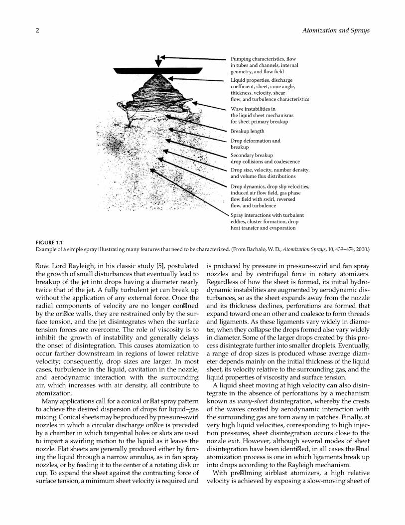
FIGURE 1.1Example of a simple spray illustrating many features that need to be characterized. (From Bachalo, W. D., Atomization Sprays, 10, 439–474, 2000.)

3General Considerations

liquid to high-velocity air. Photographic evidence sug-gests that for low-viscosity liquids the basic mechanisms involved are essentially the same as those observed in pressure atomization, namely the production of drops from ligaments created by perforated-sheet and/or wavy-sheet disintegration.

A typical spray includes a wide range of drop sizes. Some knowledge of drop size distribution is helpful in evaluating process applications in sprays, especially in calculations of heat or mass transfer between the dispersed liquid and the surrounding gas. Unfortunately, no complete theory has yet been developed to describe the hydrodynamic and aerody-namic processes involved when jet and sheet disinte-gration occurs under normal atomizing conditions, so that only empirical correlations are available for predicting mean drop sizes and drop size distribu-tions. Comparison of the distribution parameters in common use reveals that all of them have deficien-cies of one kind or another. In one the maximum drop diameter is unlimited; in others the minimum possi-ble diameter is zero or even negative. So far, no single parameter has emerged that has clear advantages over the others. For any given application the best distri-bution function is one that is easy to manipulate and provides the best fit to the experimental data.

The difficulties in specifying drop size distribu-tions in sprays have led to widespread use of various mean or median diameters. A median droplet diam-eter divides the spray into two equal parts by number, length, surface area, or volume [6]. Median diameters may be determined from different types of cumulative distribution curves shown in Figure 3.6. In a typical spray, the value of the median diameter, expressed in micrometers, will vary by a factor of about four depending on the median diameter selected for use. It is important therefore to decide which measure is the most suitable for a particular application. Some diam-eters are easier to visualize and comprehend, while others may appear in prediction equations that have been derived from theory or experiment. Some drop size measurement techniques yield a result in terms of one particular median diameter. In some cases, a given median diameter is selected to emphasize some impor-tant characteristic, such as the total surface area in the spray. For liquid fuel fired combustion systems and other applications involving heat and mass transfer to liquid drops, the Sauter mean diameter, which repre-sents the ratio of the volume to the surface area of the spray, is often preferred. The mass median diameter, which is about 15%–25% larger than the Sauter mean diameter, is also widely used. As Tate [6] has pointed out, the ratio of these two diameters is a measure of the spread of drop sizes in the spray.

Atomizers

An atomizer is generally used to produce a spray. Essentially, all that is needed is a high relative velocity between the liquid to be atomized and the surrounding air or gas. Some atomizers accomplish this by discharg-ing the liquid at high velocity into a relatively slow-moving stream of air or gas. Notable examples include the various forms of pressure atomizers and also rotary atomizers, which eject the liquid at high velocity from the periphery of a rotating cup or disk. An alternative approach is to expose the relatively slow-moving liquid to a high- velocity airstream. The latter method is gener-ally known as twin-fluid, air-assist, or airblast atomization. Other examples may involve heterogeneous processes in which air bubbles or liquid vapor become involved in disrupting the liquid phase during the injection process.

Pressure Atomizers

When a liquid is discharged through a small aperture under high applied pressure, the pressure energy is converted into the kinetic energy (velocity). For a typi-cal hydrocarbon fuel, in the absence of frictional losses a nozzle pressure drop of 138 kPa (20 psi) produces an exit velocity of 18.6 m/s. As velocity increases as the square root of the pressure, at 689 kPa (100 psi) a velocity of 41.5 m/s is obtained, while 5.5 MPa (800 psi) produces 117 m/s.

Plain Orifice. A simple circular orifice is used to inject a round jet of liquid into the surrounding air. The finest atomization is achieved with small orifices but, in practice, the difficulty of keeping liquids free from for-eign particles usually limits the minimum orifice size to around 0.3 mm. Combustion applications for plain-orifice atomizers include turbojet afterburners, ramjets, diesel engines, and rocket engines.

Pressure-Swirl (Simplex). A circular outlet orifice is preceded by a swirl chamber into which liquid flows through a number of tangential holes or slots. The swirl-ing liquid creates a core of air or gas that extends from the discharge orifice to the rear of the swirl chamber. The liquid emerges from the discharge orifice as an annular sheet, which spreads radially outward to form a hollow conical spray. Included spray angles range from 30° to almost 180°, depending on the application. Atomization performance is generally good. The finest atomization occurs at high delivery pressures and wide spray angles.

For some applications a spray in the form of a solid cone is preferred. This can be achieved using an axial jet or some other device to inject droplets into the center of the hollow conical spray pattern produced by the swirl

4 Atomization and Sprays

chamber. These two modes of injection create a bimodal distribution of drop sizes, droplets at the center of the spray being generally larger than those near the edge.

Square Spray. This is essentially a solid-cone nozzle, but the outlet orifice is specially shaped to distort the conical spray into a pattern that is roughly in the form of a square. Atomization quality is not as high as the conventional hollow-cone nozzles but, when used in multiple-nozzle combinations, a fairly uniform coverage of large areas can be achieved.

Duplex. A drawback of all types of pressure nozzles is that the liquid flow rate is proportional to the square root of the injection pressure differential. In practice, this limits the flow range of simplex nozzles to about 10:1. The duplex nozzle overcomes this limitation by feeding the swirl chamber through two sets of distribu-tor slots, each having its own separate liquid supply. One set of slots is much smaller in cross-sectional area than the other. The small slots are termed primary and the large slots secondary. At low flow rates all the liquid to be atomized flows into the swirl chamber through the primary slots. As the flow rate increases, the injec-tion pressure increases. At some predetermined pres-sure level a valve opens and admits liquid into the swirl chamber through the secondary slots.

Duplex nozzles allow good atomization to be achieved over a range of liquid flow rates of about 40:1 without the need to resort to excessively high delivery pressures. However, near the point where the secondary liquid is first admitted into the swirl chamber, there is a small range of flow rates over which atomization quality is poor. Moreover, the spray cone angle changes with flow rate, being widest at the lowest flow rate and becoming narrower as the flow rate is increased.

Dual Orifice. This is similar to the duplex nozzle except that two separate swirl chambers are provided, one for the primary flow and the other for the secondary flow. The two swirl chambers are housed concentrically within a single nozzle body to form a nozzle within a nozzle. At low flow rates all the liquid passes through the inner primary nozzle. At high flow rates liquid continues to flow through the primary nozzle, but most of the liquid is passed through the outer secondary nozzle that is designed for a much larger flow rate. As with the duplex nozzle, there is a transition phase, just after the pressurizing valve opens, when the secondary spray draws its energy for atomiza-tion from the primary spray, so the overall atomization quality is relatively poor.

Dual-orifice nozzles offer more flexibility than the duplex nozzles. For example, if desired, the primary and secondary sprays can be merged just downstream of the nozzle to form a single spray. Alternatively, the primary and secondary nozzles can be designed to produce dif-ferent spray angles, the former being optimized for low flow rates and the latter optimized for high flow rates.

Spill Return. This is essentially a simplex nozzle, but with a return flow line at the rear or side of the swirl chamber and a valve to control the quantity of liquid removed from the swirl chamber and returned to sup-ply. Very high turndown ratios are attainable with this design. Atomization quality is always good because the supply pressure is held constant at a high value, reduc-tions in flow rate being accommodated by adjusting the valve in the spill return line. This construction provides a hollow-cone spray pattern, with some increase in the spray angle as the flow is reduced.

Fan Spray. Several different concepts are used to pro-duce flat or fan-shaped sprays. The most popular type of nozzle is one in which the orifice is formed by the intersection of a V groove with a hemispheric cavity communicating with a cylindrical liquid inlet [6]. It pro-duces a liquid sheet parallel to the major axis of the ori-fice, which disintegrates into a narrow elliptical spray.

An alternative method of producing a fan spray is by discharging the liquid through a plain circular hole onto a curved deflector plate. The deflector method pro-duces a somewhat coarser spray pattern. Wide spray angles and high flow rates are attainable with this type of nozzle. Because the nozzle flow passages are rela-tively large, the problem of plugging is minimized.

A fan spray can also be produced by the collision of impinging jets. If two liquid jets are arranged to collide outside the nozzle, a flat liquid sheet is formed that is perpendicular to the plane of the jets. The atomization performance of this type of injector is relatively poor, and high stream velocities are necessary to approach the spray quality obtainable with other types of pres-sure nozzles. Extreme care must be taken to ensure that the jets are properly aligned. The main advantage of this method of atomization is the isolation of different liquids until they collide outside the nozzle. These are commonly used for hypergolic propellant systems in which an oxidizer and fuel component will react upon contact

Rotary Atomizers

One widely used type of rotary atomizer comprises a high-speed rotating disk with means for introducing liquid at its center. The liquid flows radially outward across the disk and is discharged at high velocity from its periphery. The disk may be smooth and flat or may have vanes or slots to guide the liquid to the periphery. At low flow rates, droplets form near the edge of the disk. At high flow rates, ligaments or sheets are gener-ated at the edge and disintegrate into droplets. Small disks operating at high rotational speeds and low flow rates are capable of producing sprays in which drop sizes are fairly uniform. A 360° spray pattern is devel-oped by rotating disks that are usually installed in a

5General Considerations

cylindrical or conical chamber where an umbrella-like spray is created by downward gas currents [6].

Some rotary atomizers employ a cup instead of a disk. The cup is usually smaller in diameter and is shaped like an elongated bowl. In some designs, the edge of the cup is serrated to encourage a more uniform drop size distribution in the spray. A flow of air around the periphery is sometimes used to shape the spray and to assist in transporting the droplets away from the atom-izer. In contrast to pressure nozzles, rotary atomizers allow independent variation of flow rate and disk speed, thereby providing more flexibility in operation.

Air-Assist Atomizers

In this type of nozzle, the liquid is exposed to a stream of air or steam flowing at high velocity. In the internal-mixing configuration, gas and liquid are mixed within the nozzle before discharging through the outlet orifice. The liquid is sometimes supplied through tangential slots to encourage a conical discharge pattern. However, the maximum spray angle is limited to about 60°. The device tends to be energy inefficient, but it can produce a finer spray than simple pressure nozzles.

As its name suggests, in the external-mixing form of air-assist nozzle the high-velocity gas or steam impinges on the liquid at or outside the liquid discharge orifice. Its advantage over the internal-mixing type is that problems of back pressures are avoided because there is no internal communication between gas and liquid. However, it is less efficient than the internal-mixing concept, and higher gas flow rates are needed to achieve the same degree of atomization. Both types of nozzles can atomize high-viscosity liquids effectively.

Airblast Atomizers

These devices function in a very similar manner to air-assist nozzles, and both types fall in the general category of twin-fluid atomizers. The main difference between air-assist and airblast atomizers is that the former use relatively small quantities of air or steam flowing at very high velocities (usually sonic), whereas the latter employ large amounts of air flowing at much lower velocities (<100 m/s). Airblast nozzles are thus ideally suited for atomizing liquid fuels in continuous-flow combustion systems, such as gas turbines, where air velocities of this magnitude are usually readily available. The most com-mon form of airblast atomizer is one in which the liquid is first spread into a thin conical sheet and then exposed to high-velocity airstreams on both sides of the sheet. The atomization performance of this prefilming type of airblast nozzle is superior to that of the alternative plain-jet airblast nozzle, in which the liquid is injected into the airstream in the form of one or more discrete jets.

Other Types

Most practical atomizers are of the pressure, rotary, or twin-fluid type. However, many other forms of atomizers have been developed that are useful in special applications.

Electrostatic. A liquid jet or film is exposed to an intense electrical pressure that tends to expand its area. This expansion is opposed by the surface tension forces. If the electrical pressure predominates, droplets are formed. Droplet size is a function of the electrical pres-sure, the liquid flow rate, and the physical and electrical properties of the liquid. The low liquid flow rates asso-ciated with electrostatic atomizers have tended to limit their practical applications to electrostatic painting and nonimpact printing.

Ultrasonic. The liquid to be atomized is fed through or over a transducer and horn, which vibrates at ultra-sonic frequencies to produce the short wavelengths necessary for fine atomization. The system requires a high-frequency electrical input, two piezoelectric trans-ducers, and a stepped horn. The concept is well suited for applications that require very fine atomization and a low spray velocity. At present, an important application of ultrasonic atomizers (nebulizers) is for medical inha-lation therapy, where very fine sprays and the absence of gas to effect atomization are important attributes.

Sonic (Whistle). Gas is accelerated within the device to sonic velocity and impinges on a plate or annular cav-ity (resonation chamber). The sound waves produced are reflected into the path of the incoming liquid [7]. The frequency of the sound waves is around 20 kHz, and this serves to disintegrate the liquid into small droplets ranging downward in size from 50 μm. The sonic and pneumatic effects are difficult to isolate from each other. Efforts have been made to design nozzles that operate above the audible frequency limit to reduce the nuisance of noise [8]. However, in some applications the attendant sound field may benefit the process (e.g., combustion) for which the resultant spray is required.

Windmill. Many aerial applications of pesticides require a narrow spectrum of drop sizes. The conven-tional rotary disk atomizers can provide such a spec-trum, but only when operating in the ligament mode at low flow rates. By making radial cuts at the periph-ery of a disk and twisting the tips of the segments, the disk can be converted into a windmill that will rotate rapidly when inserted into an airflow at aircraft flight speed. According to Spillmann and Sanderson [9], the disk windmill constitutes an ideal rotary atomizer for the aerial application of pesticides. It provides a narrow spectrum of drop sizes in the range most suitable for herbicides, at relatively high flow rates.

Vibrating Capillary. This type of droplet generator was first used to study the collision and coalescence of small water droplets. It consists of a hypodermic needle

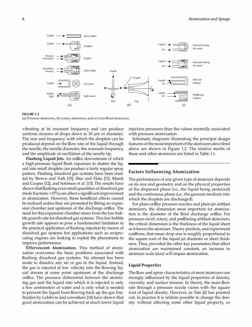
6 Atomization and Sprays

vibrating at its resonant frequency and can produce uniform streams of drops down to 30 μm in diameter. The size and frequency with which the droplets can be produced depend on the flow rate of the liquid through the needle, the needle diameter, the resonant frequency, and the amplitude of oscillation of the needle tip.

Flashing Liquid Jets. An orifice downstream of which a high-pressure liquid flash vaporizes to shatter the liq-uid into small droplets can produce a fairly regular spray pattern. Flashing dissolved gas systems have been stud-ied by Brown and York [10], Sher and Elata [11], Marek and Cooper [12], and Solomon et al. [13]. The results have shown that flashing even small quantities of dissolved gas (mole fractions <15%) can effect a significant improvement in atomization. However, these beneficial effects cannot be realized unless they are promoted by fitting an expan-sion chamber just upstream of the discharge orifice. The need for this expansion chamber stems from the low bub-ble growth rate for dissolved gas systems. This low bubble growth rate appears to pose a fundamental limitation to the practical application of flashing injection by means of dissolved gas systems but applications such as recipro-cating engines are looking to exploit the phenomena to improve performance.

Effervescent Atomization. This method of atomi-zation overcomes the basic problems associated with flashing dissolved gas systems. No attempt has been made to dissolve any air or gas in the liquid. Instead, the gas is injected at low velocity into the flowing liq-uid stream at some point upstream of the discharge orifice. The pressure differential between the atomiz-ing gas and the liquid into which it is injected is only a few centimeters of water and is only what is needed to prevent the liquid from flowing back up the gas line. Studies by Lefebvre and coworkers [14] have shown that good atomization can be achieved at much lower liquid

injection pressures than the values normally associated with pressure atomization.

Schematic diagrams illustrating the principal design features of the most important of the atomizers described above are shown in Figure 1.2. The relative merits of these and other atomizers are listed in Table 1.1.

Factors Influencing Atomization

The performance of any given type of atomizer depends on its size and geometry and on the physical properties of the dispersed phase (i.e., the liquid being atomized) and the continuous phase (i.e., the gaseous medium into which the droplets are discharged).

For plain-orifice pressure nozzles and plain-jet airblast atomizers, the dimension most important for atomiza-tion is the diameter of the final discharge orifice. For pressure-swirl, rotary, and prefilming airblast atomizers, the critical dimension is the thickness of the liquid sheet as it leaves the atomizer. Theory predicts, and experiment confirms, that mean drop size is roughly proportional to the square root of the liquid jet diameter or sheet thick-ness. Thus, provided the other key parameters that affect atomization are maintained constant, an increase in atomizer scale (size) will impair atomization.

Liquid Properties

The flow and spray characteristics of most atomizers are strongly influenced by the liquid properties of density, viscosity, and surface tension. In theory, the mass flow rate through a pressure nozzle varies with the square root of liquid density. However, as Tate [6] has pointed out, in practice it is seldom possible to change the den-sity without affecting some other liquid property, so

(a) (b) (c)

Liquid

Liquid

Liquid

Liquid

Air assist

Air assist

Airblast

Airblast

Plain-jet

Prelming

Internal-mixing

External-mixing

Air

Air

Air

Air

Plain-orice

Dual-orice

Fan spray

Spill return

Simplex

Duplex

Liquid

Liquid

Liquid

SupplySpill

Primary

Primary

Secondary

SecondaryLiquid

Liquid

Disk Cup

FIGURE 1.2(a) Pressure atomizers, (b) rotary atomizers, and (c) twin-fluid atomizers.

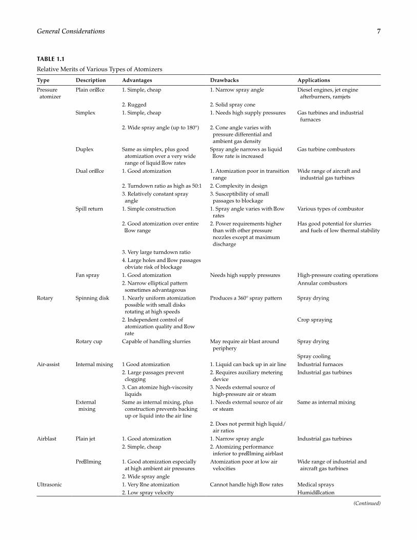
7General Considerations

TABLE 1.1

Relative Merits of Various Types of Atomizers

Type Description Advantages Drawbacks Applications

Pressure atomizer

Plain orifice 1. Simple, cheap 1. Narrow spray angle Diesel engines, jet engine afterburners, ramjets

2. Rugged 2. Solid spray coneSimplex 1. Simple, cheap 1. Needs high supply pressures Gas turbines and industrial

furnaces2. Wide spray angle (up to 180°) 2. Cone angle varies with

pressure differential and ambient gas density

Duplex Same as simplex, plus good atomization over a very wide range of liquid flow rates

Spray angle narrows as liquid flow rate is increased

Gas turbine combustors

Dual orifice 1. Good atomization 1. Atomization poor in transition range

Wide range of aircraft and industrial gas turbines

2. Turndown ratio as high as 50:1 2. Complexity in design3. Relatively constant spray angle

3. Susceptibility of small passages to blockage

Spill return 1. Simple construction 1. Spray angle varies with flow rates

Various types of combustor

2. Good atomization over entire flow range

2. Power requirements higher than with other pressure nozzles except at maximum discharge

Has good potential for slurries and fuels of low thermal stability

3. Very large turndown ratio4. Large holes and flow passages obviate risk of blockage

Fan spray 1. Good atomization Needs high supply pressures High-pressure coating operations2. Narrow elliptical pattern sometimes advantageous

Annular combustors

Rotary Spinning disk 1. Nearly uniform atomization possible with small disks rotating at high speeds

Produces a 360° spray pattern Spray drying

2. Independent control of atomization quality and flow rate

Crop spraying

Rotary cup Capable of handling slurries May require air blast around periphery

Spray drying

Spray coolingAir-assist Internal mixing 1 Good atomization 1. Liquid can back up in air line Industrial furnaces

2. Large passages prevent clogging

2. Requires auxiliary metering device

Industrial gas turbines

3. Can atomize high-viscosity liquids

3. Needs external source of high-pressure air or steam

External mixing

Same as internal mixing, plus construction prevents backing up or liquid into the air line

1. Needs external source of air or steam

Same as internal mixing

2. Does not permit high liquid/air ratios

Airblast Plain jet 1. Good atomization 1. Narrow spray angle Industrial gas turbines2. Simple, cheap 2. Atomizing performance

inferior to prefilming airblastPrefilming 1. Good atomization especially

at high ambient air pressuresAtomization poor at low air velocities

Wide range of industrial and aircraft gas turbines

2. Wide spray angleUltrasonic 1. Very fine atomization Cannot handle high flow rates Medical sprays

2. Low spray velocity Humidification

(Continued)

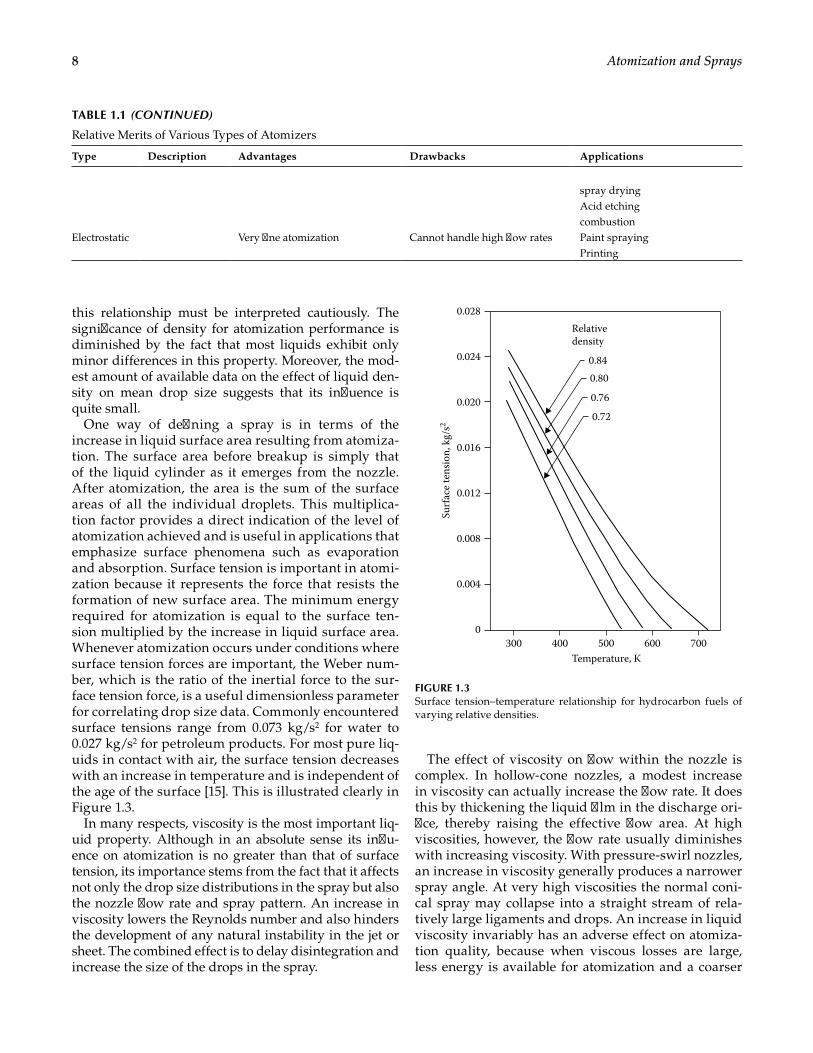
8 Atomization and Sprays

this relationship must be interpreted cautiously. The significance of density for atomization performance is diminished by the fact that most liquids exhibit only minor differences in this property. Moreover, the mod-est amount of available data on the effect of liquid den-sity on mean drop size suggests that its influence is quite small.

One way of defining a spray is in terms of the increase in liquid surface area resulting from atomiza-tion. The surface area before breakup is simply that of the liquid cylinder as it emerges from the nozzle. After atomization, the area is the sum of the surface areas of all the individual droplets. This multiplica-tion factor provides a direct indication of the level of atomization achieved and is useful in applications that emphasize surface phenomena such as evaporation and absorption. Surface tension is important in atomi-zation because it represents the force that resists the formation of new surface area. The minimum energy required for atomization is equal to the surface ten-sion multiplied by the increase in liquid surface area. Whenever atomization occurs under conditions where surface tension forces are important, the Weber num-ber, which is the ratio of the inertial force to the sur-face tension force, is a useful dimensionless parameter for correlating drop size data. Commonly encountered surface tensions range from 0.073 kg/s2 for water to 0.027 kg/s2 for petroleum products. For most pure liq-uids in contact with air, the surface tension decreases with an increase in temperature and is independent of the age of the surface [15]. This is illustrated clearly in Figure 1.3.

In many respects, viscosity is the most important liq-uid property. Although in an absolute sense its influ-ence on atomization is no greater than that of surface tension, its importance stems from the fact that it affects not only the drop size distributions in the spray but also the nozzle flow rate and spray pattern. An increase in viscosity lowers the Reynolds number and also hinders the development of any natural instability in the jet or sheet. The combined effect is to delay disintegration and increase the size of the drops in the spray.

The effect of viscosity on flow within the nozzle is complex. In hollow-cone nozzles, a modest increase in viscosity can actually increase the flow rate. It does this by thickening the liquid film in the discharge ori-fice, thereby raising the effective flow area. At high viscosities, however, the flow rate usually diminishes with increasing viscosity. With pressure-swirl nozzles, an increase in viscosity generally produces a narrower spray angle. At very high viscosities the normal coni-cal spray may collapse into a straight stream of rela-tively large ligaments and drops. An increase in liquid viscosity invariably has an adverse effect on atomiza-tion quality, because when viscous losses are large, less energy is available for atomization and a coarser

(CONTINUED)TABLE 1.1

Relative Merits of Various Types of Atomizers

Type Description Advantages Drawbacks Applications

spray dryingAcid etchingcombustion

Electrostatic Very fine atomization Cannot handle high flow rates Paint sprayingPrinting

Relativedensity

0.84

0.028

0.024

0.020

0.016

0.012

0.008

0.004

0300 400 500 600 700

Temperature, K

Surf

ace

tens

ion,

kg/

s2

0.80

0.76

0.72

FIGURE 1.3Surface tension–temperature relationship for hydrocarbon fuels of varying relative densities.

9General Considerations

spray results. In airblast atomizers, liquid velocities are usually much lower than in pressure nozzles. In con-sequence, the drop sizes produced by airblast nozzles tend to be less sensitive to variations in liquid viscosity.

Table 1.2 lists the relevant physical properties of some of the liquids used in spray applications. The viscosity of these liquids ranges from 0.001 kg/m·s for water to 0.5 kg/m·s for heavy fuel oil. The viscosity of liquids generally decreases with an increase in temperature. It is customary to heat up many of the heavier fuel oils, partly to reduce pumping power requirements but also to improve atomization.

Some fluids, for example slurries of liquids and solid powders, are characterized by a nonlinear relationship between shear stress and shear strain rate. For such liq-uids, which are called non-Newtonian, it is necessary to specify the shear rate with the viscosity. The apparent reduction in viscosity with increasing shear rate high-lights the need to minimize pressure losses in the supply lines and nozzles. This reduction is also desirable because the viscosities of non-Newtonian fluids have less effect on atomization if a high shear rate is produced in the liq-uid film formed by the nozzle [15]. Very little secondary atomization will occur once the drops are formed, due to the increase in apparent viscosity at the lower shear rate.

To successfully correlate or simulate atomization behavior, it is imperative to know the key physical prop-erties at the point of atomization. Table 1.2 provides some information for an array of liquids as a starting point. However, for many applications, the temperature dependency must be established. Also, in the case of mixtures of pure liquids, the behavior of the mixture must be understood. In some cases, the properties of the mixture are simple mass weighted averages, but for some liquids (e.g., alcohols) an azeotrope may result, which has highly nonlinear behavior. Hence, for the best results, the researcher/end-user is urged to estab-lish measurement capability for the physical proper-ties using various ASTM, ISO, or SAE methods (e.g., ASTM D 1343-93 for viscosity, ASTM D971; D3825-09 or D7541-11 for surface tension; ASTM D4052 for density). Extensive information (CRC Report 635) is available for the temperature-dependent properties of jet fuels due to its critical role in aircraft and associated need for ensur-ing safety [16]. Yet, as an illustration of the importance of knowing the actual physical properties of the liquids being worked with, the information in CRC 635 is still only representative and the variability in properties from batch to batch of jet fuel still requires an independent measurement to have full confidence in the actual prop-erties of the jet fuel being worked with.

In summary, it is imperative that the physical proper-ties of the liquids used are well understood in order to apply the concepts within this book.

Ambient Conditions

The ambient gas into which sprays are injected can vary widely in pressure and temperature. This is especially true of liquid fuel fired combustion systems. In diesel engines, critical and supercritical pressure and temper-ature conditions are encountered. In gas turbine com-bustors, fuel sprays are injected into highly turbulent, swirling recirculating streams of reacting gases. In indus-trial furnaces, the fuel is sprayed into high-temperature flames of recirculating combustion products. With pres-sure-swirl atomizers, the spray angle decreases markedly with increase in ambient gas density until a minimum angle is reached beyond which any further increase in the ambient gas density has no effect on the spray angle. The ambient gas density also has a strong influence on the mean drop sizes produced by pressure-swirl atom-izers. If the ambient pressure is raised continuously above the normal atmospheric value, the mean drop size increases initially until a maximum value is reached and then slowly declines. The reasons for this unusual rela-tionship between ambient pressure and mean drop size are discussed in Chapter 6.

The spray patterns generated by pressure-swirl atom-izers are also affected by the liquid injection pressure differential ∆PL. The ejector action of the high-velocity spray generates air currents, which causes the spray angle to contract. This effect is aggravated by the increase in spray velocity that accompanies an increase in ∆PL. Thus, although increasing ∆PL has no effect on the spray angle immediately downstream of the nozzle, it causes appreciable contraction of the spray pattern farther downstream.

With plain-orifice atomizers an increase in the ambi-ent gas density leads to a wider spray angle. This is because the increase in aerodynamic drag on the drop-lets, created by an increase in gas density, tends to pro-duce a greater deceleration in the axial direction than in the radial direction.

The spray patterns produced by airblast atomizers tend to be fairly insensitive to variations in the ambient gas density. All but the largest drops in the spray tend to follow the streamlines of the airflow pattern generated at the nozzle exit by the various swirlers and shaped pas-sages within the nozzle. This airflow pattern generally remains fixed and independent of air density, apart from second-order Reynolds number and Mach number effects. However, if the natural cone angle of the spray, that is, the spray angle with no air flowing, is markedly different from that of the air, then the change in aerodynamic drag forces produced by a change in air density will affect the resulting spray pattern. In general, an increase in air den-sity will cause the spray pattern to adhere more closely to the streamlines of the atomizing air.

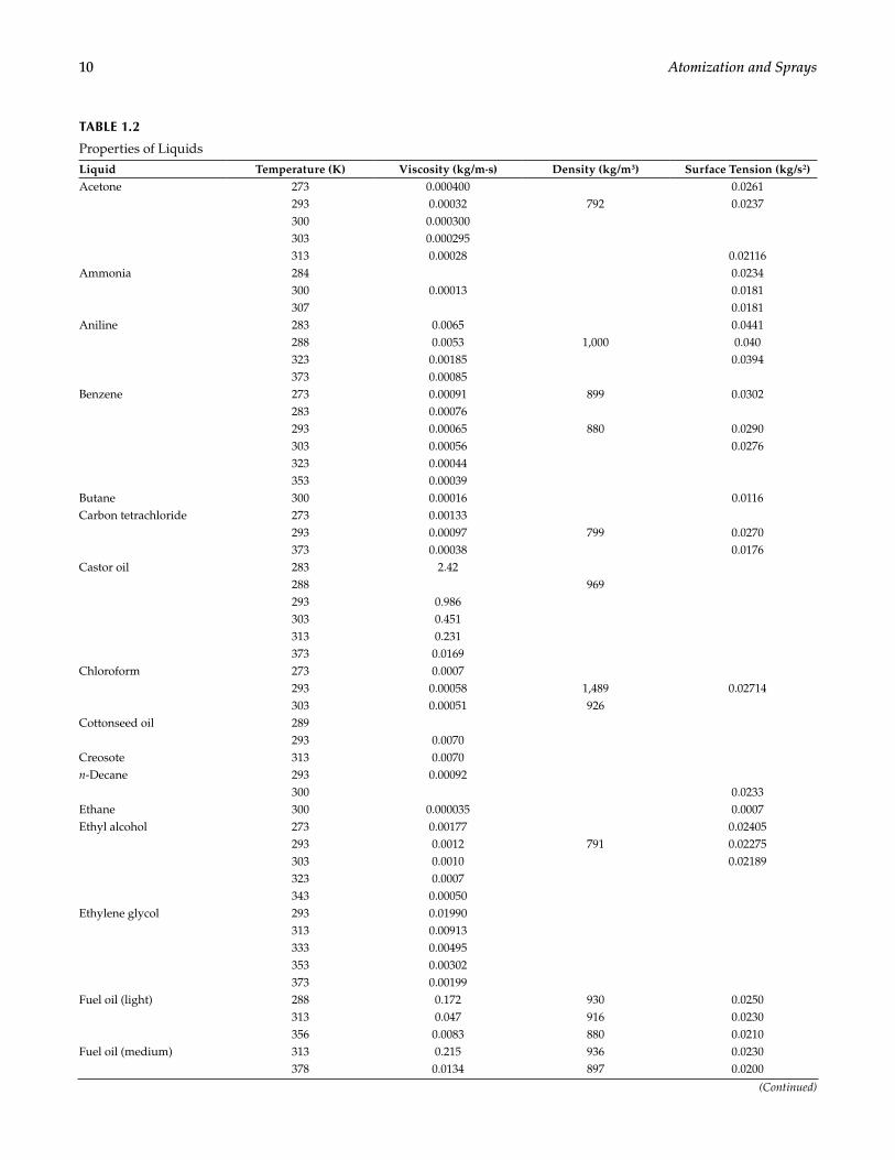
10 Atomization and Sprays

TABLE 1.2

Properties of Liquids

Liquid Temperature (K) Viscosity (kg/m·s) Density (kg/m3) Surface Tension (kg/s2)Acetone 273 0.000400 0.0261

293 0.00032 792 0.0237300 0.000300303 0.000295313 0.00028 0.02116

Ammonia 284 0.0234300 0.00013 0.0181307 0.0181

Aniline 283 0.0065 0.0441288 0.0053 1,000 0.040323 0.00185 0.0394373 0.00085

Benzene 273 0.00091 899 0.0302283 0.00076293 0.00065 880 0.0290303 0.00056 0.0276323 0.00044353 0.00039

Butane 300 0.00016 0.0116Carbon tetrachloride 273 0.00133

293 0.00097 799 0.0270373 0.00038 0.0176

Castor oil 283 2.42288 969293 0.986303 0.451313 0.231373 0.0169

Chloroform 273 0.0007293 0.00058 1,489 0.02714303 0.00051 926

Cottonseed oil 289293 0.0070

Creosote 313 0.0070n-Decane 293 0.00092

300 0.0233Ethane 300 0.000035 0.0007Ethyl alcohol 273 0.00177 0.02405

293 0.0012 791 0.02275303 0.0010 0.02189323 0.0007343 0.00050

Ethylene glycol 293 0.01990313 0.00913333 0.00495353 0.00302373 0.00199

Fuel oil (light) 288 0.172 930 0.0250313 0.047 916 0.0230356 0.0083 880 0.0210

Fuel oil (medium) 313 0.215 936 0.0230378 0.0134 897 0.0200

(Continued)

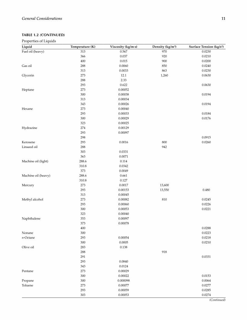
11General Considerations

TABLE 1.2 (CONTINUED)

Properties of Liquids

Liquid Temperature (K) Viscosity (kg/m·s) Density (kg/m3) Surface Tension (kg/s2)Fuel oil (heavy) 313 0.567 970 0.0230

366 0.037 920 0.0210400 0.015 900 0.0200

Gas oil 288 0.0060 850 0.0240313 0.0033 863 0.0230

Glycerin 273 12.1 1,260 0.0630288 2.33293 0.622 0.0630

Heptane 273 0.00052300 0.00038 0.0194313 0.00034343 0.00026 0.0194

Hexane 273 0.00040293 0.00033 0.0184300 0.00029 0.0176323 0.00025

Hydrazine 274 0.00129293 0.00097298 0.0915

Kerosene 293 0.0016 800 0.0260Linseed oil 288 942

303 0.0331363 0.0071

Machine oil (light) 288.6 0.114310.8 0.0342373 0.0049

Machine oil (heavy) 288.6 0.661310.8 0.127

Mercury 273 0.0017 13,600293 0.00153 13,550 0.480313 0.00045

Methyl alcohol 273 0.00082 810 0.0245293 0.00060 0.0226300 0.00053 0.0221323 0.00040

Naphthalene 353 0.00097373 0.00078400 0.0288

Nonane 300 0.0223n-Octane 293 0.00054 0.0218

300 0.0005 0.0210Olive oil 283 0.138

288 918291 0.0331293 0.0840343 0.0124

Pentane 273 0.00029300 0.00022 0.0153

Propane 300 0.000098 0.0064Toluene 273 0.00077 0.0277

293 0.00059 0.0285303 0.00053 0.0274

(Continued)

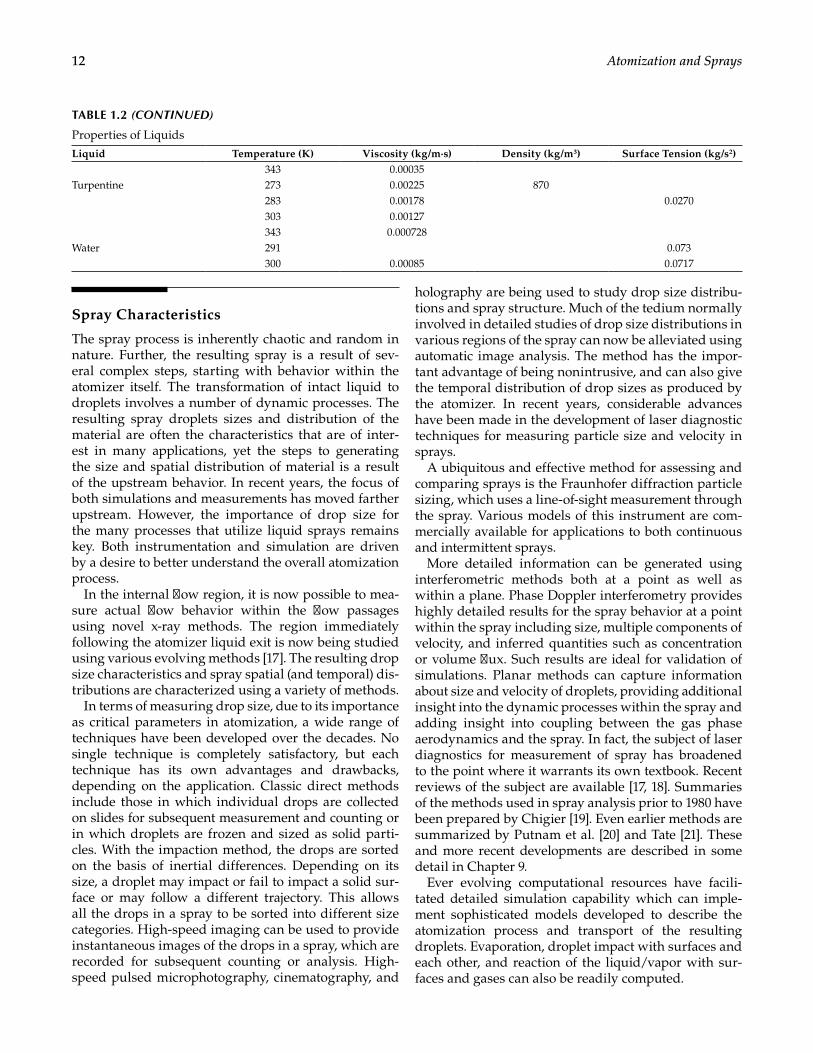
12 Atomization and Sprays

Spray Characteristics

The spray process is inherently chaotic and random in nature. Further, the resulting spray is a result of sev-eral complex steps, starting with behavior within the atomizer itself. The transformation of intact liquid to droplets involves a number of dynamic processes. The resulting spray droplets sizes and distribution of the material are often the characteristics that are of inter-est in many applications, yet the steps to generating the size and spatial distribution of material is a result of the upstream behavior. In recent years, the focus of both simulations and measurements has moved farther upstream. However, the importance of drop size for the many processes that utilize liquid sprays remains key. Both instrumentation and simulation are driven by a desire to better understand the overall atomization process.

In the internal flow region, it is now possible to mea-sure actual flow behavior within the flow passages using novel x-ray methods. The region immediately following the atomizer liquid exit is now being studied using various evolving methods [17]. The resulting drop size characteristics and spray spatial (and temporal) dis-tributions are characterized using a variety of methods.

In terms of measuring drop size, due to its importance as critical parameters in atomization, a wide range of techniques have been developed over the decades. No single technique is completely satisfactory, but each technique has its own advantages and drawbacks, depending on the application. Classic direct methods include those in which individual drops are collected on slides for subsequent measurement and counting or in which droplets are frozen and sized as solid parti-cles. With the impaction method, the drops are sorted on the basis of inertial differences. Depending on its size, a droplet may impact or fail to impact a solid sur-face or may follow a different trajectory. This allows all the drops in a spray to be sorted into different size categories. High-speed imaging can be used to provide instantaneous images of the drops in a spray, which are recorded for subsequent counting or analysis. High-speed pulsed microphotography, cinematography, and

holography are being used to study drop size distribu-tions and spray structure. Much of the tedium normally involved in detailed studies of drop size distributions in various regions of the spray can now be alleviated using automatic image analysis. The method has the impor-tant advantage of being nonintrusive, and can also give the temporal distribution of drop sizes as produced by the atomizer. In recent years, considerable advances have been made in the development of laser diagnostic techniques for measuring particle size and velocity in sprays.

A ubiquitous and effective method for assessing and comparing sprays is the Fraunhofer diffraction particle sizing, which uses a line-of-sight measurement through the spray. Various models of this instrument are com-mercially available for applications to both continuous and intermittent sprays.

More detailed information can be generated using interferometric methods both at a point as well as within a plane. Phase Doppler interferometry provides highly detailed results for the spray behavior at a point within the spray including size, multiple components of velocity, and inferred quantities such as concentration or volume flux. Such results are ideal for validation of simulations. Planar methods can capture information about size and velocity of droplets, providing additional insight into the dynamic processes within the spray and adding insight into coupling between the gas phase aerodynamics and the spray. In fact, the subject of laser diagnostics for measurement of spray has broadened to the point where it warrants its own textbook. Recent reviews of the subject are available [17, 18]. Summaries of the methods used in spray analysis prior to 1980 have been prepared by Chigier [19]. Even earlier methods are summarized by Putnam et al. [20] and Tate [21]. These and more recent developments are described in some detail in Chapter 9.

Ever evolving computational resources have facili-tated detailed simulation capability which can imple-ment sophisticated models developed to describe the atomization process and transport of the resulting droplets. Evaporation, droplet impact with surfaces and each other, and reaction of the liquid/vapor with sur-faces and gases can also be readily computed.

TABLE 1.2 (CONTINUED)

Properties of Liquids

Liquid Temperature (K) Viscosity (kg/m·s) Density (kg/m3) Surface Tension (kg/s2)343 0.00035

Turpentine 273 0.00225 870283 0.00178 0.0270303 0.00127343 0.000728

Water 291 0.073300 0.00085 0.0717

13General Considerations

Applications

A compilation by Tate [6] of some of the most important applications is contained in Table 1.3. While this per-spective is more than four decades old, it is still quite relevant. As the cost, complexity, atomizing perfor-mance, and energy consumption vary widely between different types of atomizers, it is important to select the best atomizer for any given application. The following factors enter into the proper selection: properties of the liquid to be atomized, for example, density, viscosity, surface tension, and temperature; ambient gas proper-ties, such as pressure, temperature, and flow pattern; particle sizes and percent solids in suspensions, slur-ries, and pastes; maximum flow rate; range of flow rates

(turndown ratio); required mean drop size and drop size distribution; liquid or gas pressures available for nozzles, or power required for rotary atomizers; condi-tions that may contribute to wear and corrosion; size and shape of vessel, enclosure, or combustor containing spray; economics of spray operation taking into account initial cost, operating expenses, and depreciation; and safety considerations [6].

Glossary

Some of the terms frequently used in descriptions of atomizers and sprays are defined in the following. These definitions are necessarily brief, and no attempt has been made to include all qualifying considerations.

Air-assist nozzle: Nozzle in which high-velocity air or steam is used to enhance pressure atomization at low liquid flow rates.

Airblast atomizer: Atomizer in which a liquid jet or sheet is exposed to air flowing at high velocity.

Air core: Cylindrical void space within the rotating liq-uid in a simplex swirl chamber.

Arithmetic mean diameter: Linear mean diameter of drops in spray.

Atomization: Process whereby a volume of liquid is dis-integrated into a multiplicity of small drops.

Beam steering: Refraction of a laser beam due to den-sity gradients in the continuous phase.

Breakup length: Length of continuous portion of jet measured from nozzle exit to point where breakup occurs.

Cavitation: Formation of bubbles by gas or vapor released in flow regions of low static pressure; affects discharge coefficient and jet breakup.

Cavitation number: Ratio of pressure differential to downstream pressure; indicator of propensity for cavitation.

Combined spray: Spray produced when both stages flow simultaneously in a dual-orifice or piloted-airblast nozzle.

Continuous phase: Medium, usually gaseous, in which atomization occurs.

Critical flow rate: Liquid flow rate corresponding to the transition from one mode of atomization to another.

Critical Weber number: Value of Weber number above which a single drop will split into two or more drops.

Cumulative distribution: Plot of percentage by num-ber, surface area, or volume of drops whose diameter is less than a given drop diameter.

TABLE 1.3

Spray Applications

Production or processingSpray drying (dairy products, coffee and tea, starch pharmaceuticals, soaps and detergents, pigments, etc.)

Spray coolingSpray reactions (absorption, roasting, etc.)Atomized suspension technique (effluents, waste liquors, etc.)Powdered metalsTreatmentEvaporation and aerationCooling (spray ponds, towers, reactors, etc.)Humidification and mistingAir and gas washing and scrubbingIndustrial washing and cleaningCoatingSurface treatmentSpraypainting (pneumatic, airless, and electrostatic)Flame sprayingInsulation, fibers, and undercoating materialsMulticomponent resins (urethanes, epoxies, polyesters, etc.)Particle coating and encapsulationCombustionOil burners (furnaces and heaters, industrial and marine boilers)Diesel fuel injectionGas turbines (aircraft, marine, automotive, etc.)Rocket fuel injectionMiscellaneousMedicinal spraysDispersion of chemical agentsAgricultural spraying (insecticides, herbicides, fertilizer solutions, etc.)

Foam and fog suppressionPrintingAcid etching

Source: Tate, R. W.: Sprays, Kirk-Othmer Encyclopedia of Chemical Technology. pp. 634–654. 1969. Copyright Wiley-VCH Verlag GmbH & Co. KGaA.

14 Atomization and Sprays

Discharge coefficient: Ratio of actual flow rate to theo-retical flow rate.

Discharge orifice: Final orifice through which liquid is discharged into the ambient gas.

Dispersed phase: Liquid to be atomized.Dispersion: Ratio of the volume of a spray to the vol-

ume of the liquid contained within it.Drooling: Sluggish dripping of liquid from a nozzle

while spraying, usually caused by impingement of the spray on some surface other than the ori-fice from which the liquid is discharging [22].

Drop coalescence: Collision of two drops to form a sin-gle drop.

Droplet size: Diameter of a spherical droplet, usually expressed in micrometers.

Droplet uniformity index: Indication of the range of drop sizes in a spray relative to the median diameter.

Drop saturation: Droplet population exceeding the capability of the sizing instrument or method.

Dual-orifice atomizer: Atomizer consisting of two sim-plex nozzles fitted concentrically one inside other.

Duplex nozzle: Nozzle featuring a swirl chamber with two sets of tangential swirl ports, one set being the primary ports for low flows and the other the larger secondary ports for handling high flow rates.

Effective evaporation constant: Value of evaporation constant that includes heat-up period and con-vective effects.

Electrostatic atomizer: Atomizer in which electrical pressure is used to overcome surface tension forces and achieve atomization.

Equivalent spray angle: Angle formed by drawing two straight lines from the nozzle discharge orifice through the center of the liquid mass in the left and right lobes of the spray.

Evaporation constant: Indication of the rate of change of drop surface area during steady-state evaporation.

External mixing nozzle: Air-assist atomizer in which high-velocity gas impinges on a liquid at or out-side the final orifice.

Extinction: Percentage of light removed from original direction; indicator of the extent to which mea-surements of mean drop size are affected by multiple scattering. Also termed obscuration.

Fan spray: Spray in the shape of a sector of a circle of about 75° angle; elliptical in cross section.

Film thickness: Thickness of annular liquid sheet as it discharges from the atomizer.

Flat spray: Same as fan spray.Flow number: Effective flow area of a nozzle, usually

expressed as the ratio of mass or volumetric

flow rate to the square root of injection pressure differential.

Flow rate: Amount of liquid discharged during a given period of time; normally identified with all fac-tors that affect flow rate, such as pressure dif-ferential and liquid density.

Frequency distribution curve: Plot of liquid volume per size class.

Heat transfer number: Indicator of rate of evaporation due to heat transfer to droplet from surround-ing gas.

Heat-up period: Initial phase of droplet evaporation prior to attainment of steady-state conditions.

Hollow-cone spray: Spray in which most of the droplets are concentrated at the outer edge of a conical spray pattern.

Impingement: Collision of two round liquid jets or colli-sion of a jet of liquid with a stationary deflector.

Impinging jet atomizer: Atomizer in which two liquid jets collide outside the nozzle to produce a liq-uid sheet perpendicular to the plane of the jets.

Internal mixing nozzle: Air-assist atomizer in which gas and liquid mix within the nozzle before dis-charging through the outlet orifice.

Mass transfer number: Indicator of rate of evaporation due to mass transfer.

Mass (volume) median diameter: Diameter of a drop below or above which 50% of the total mass (volume) of drops lies.

Mean drop size: A given spray is replaced by a ficti-tious one in which all the drops have the same diameter while retaining certain characteristics of the original spray.

Monodisperse spray: Spray containing drops of uni-form size.

Multiple scattering: When spray number density is high some drops obscure part of signal gen-erated by others, leading to biased diffraction patterns.

Normal distribution: Distribution of drop sizes based on the random occurrence of a given drop size.

Obscuration: Percentage of light removed from original direction; indicator of the extent to which mea-surements of mean drop size are affected by multiple scattering. Also known as extinction.

Ohnesorge number: Dimensionless group obtained by dividing the square root of the Weber num-ber by the Reynolds number, which eliminates velocity from both; indicator of jet or sheet stability.

Patternation: A measure of the uniformity of the cir-cumferential distribution of liquid in a conical spray. The term radial patternation is also used to describe the radial distribution of liquid within a conical spray.

15General Considerations

Patternator: Two types are available: one designed to measure the radial liquid distribution in a coni-cal spray, the other to measure the uniformity of the circumferential liquid distribution.

Plain-orifice atomizer: Atomizer in which liquid is ejected at high velocity through a small round hole; the best known example is a diesel injector.

Polydisperse spray: Spray containing drops of different sizes.

Prefilmer: Solid surface on which a thin continuous liq-uid film is formed.

Pressure atomizer: Single-fluid atomizer in which the conversion of pressure to kinetic energy results in a high relative velocity between the liquid and the surrounding gas.

Relative density: Ratio of the mass of a given volume of liquid to the mass of an equal volume of water; the temperature of both liquids must be stated. For example, relative density = 0.81 at 289/277 K indicates that the mass of the liquid was mea-sured at 289 K and divided by the mass of an equal volume of water at 277 K. Formerly called specific gravity.

Relative span factor: Indicator of the range of drop sizes relative to the mass median diameter.

Reynolds number: Dimensionless ratio of inertial force to viscous force.

Rosin–Rammler distribution: Drop size distribution described in terms of two parameters, one of which provides a measure of the spread of drop sizes.

Rotary atomizer: Atomizer in which liquid is dis-charged from the edge of a rotating disk, cup, or slotted wheel.

Sauter mean diameter: Diameter of a droplet whose surface-to-volume ratio is equal to that of the entire spray.

Shroud air: A flow of air over the atomizer face to pre-vent deposition of carbon; also used to modify spray characteristics at low flow rates.

Simplex nozzle: Nozzle that employs a single swirl chamber to produce a well-atomized spray of wide cone angle.

Skewness: The axis of the nozzle spray cone is not colin-ear with the central axis of the nozzle; the maxi-mum departure is stated in degrees [22].

Slinger system: Rotary atomizer employed in some small gas turbines.

Solid-cone spray: Spray in which the droplets are fairly uniformly distributed throughout a conical spray volume.

Spatial sampling: Measurement of drops contained within a volume under conditions such that contents of volume do not change during any single measurement.

Spill-return nozzle: Basically a simplex atomizer with provision for liquid to be removed from the swirl chamber and returned to supply; provides good atomization even at lowest flow rates.

Spitting: Large, irregular drops of liquid intermittently produced by otherwise uniformly fine spray; sometimes caused by internal flow leaks within the nozzle [22].

Spray angle: Angle formed by two straight lines drawn from the discharge orifice to cut the spray con-tours at a specific distance from the atomizer face.

Spray axis: Intersection of two planes of symmetry of the spray [6]; for symmetrical sprays the spray axis coincides with the centerline of the angle.

Stability curve: Graph showing relationship between jet velocity and breakup length.

Streak: Very narrow sector of the spray with more or less than the average concentration of droplets.

Surface tension: Property that resists expansion of liq-uid surface area. Surface tension forces must be overcome by aerodynamic, centrifugal, or pres-sure forces to achieve atomization.

Swirl chamber: Conical or cylindrical cavity having tangential inlets that impart a swirling motion to the liquid.

Temporal sampling: Measurement of drops that pass through a fixed area during a specific time interval.

Transition range: Small flow range of a dual-stage nozzle over which atomization quality is relatively poor; occurs when the pressurizing valve first opens to allow secondary liquid flow into the nozzle.

Turndown ratio: Ratio of maximum rated liquid flow to minimum rated liquid flow.

Twin-fluid atomizer: Generic term encompassing all nozzle types in which atomization is achieved using high-velocity air, gas, or steam.

Ultrasonic atomizer: Atomizer in which a vibrating surface is used to make a liquid film unstable and disintegrate into drops.

Upper critical point: Point on stability curve where breakup changes from varicose to sinuous.

Varicose: Term used to describe appearance of liquid jet during breakup without interaction with air.

Velocity coefficient: Ratio of actual discharge velocity to the theoretical velocity corresponding to the total pressure differential across the nozzle.

Viscosity: Liquid property that has a marked effect on atomization quality and spray angle and also affects pumping power requirements; very dependent on liquid temperature.

Visibility technique: Drop sizing interferometry used in conjunction with laser Doppler anemometry to measure both drop size and velocity.

16 Atomization and Sprays

Weber number: Dimensionless ratio of momentum force to surface tension force.

Web bulb temperature: Droplet surface temperature during steady-state evaporation.

Whistle atomizer: Atomizer in which sound waves are used to shatter a liquid jet into droplets.

Wide-range nozzle: Nozzle designed to provide good atomization over a wide range of liquid flow rates; best known example is dual-orifice nozzle.

Windmill atomizer: Rotary atomizer used for aerial application of pesticides; unique feature is use of wind forces to provide rotary motion.

References

1. Bachalo, W. D., Spray diagnostics for the twenty-first century, Atomization Sprays, Vol. 10, 2000, pp. 439–474.

2. Lefebvre, A. H., Fuel effects on gas turbine combustion—Ignition, stability, and combustion efficiency, ASME J. Eng. Gas Turbines Power, Vol. 107, 1985, pp. 24–37.

3. Reeves, C. M., and Lefebvre, A. H., Fuel effects on air-craft combustor emissions, ASME Paper 86-GT-212, 1986.

4. Rink, K. K., and Lefebvre, A. H., Influence of fuel drop size and combustor operating conditions on pollutant emissions, SAE Technical Paper 861541, 1986.

5. Rayleigh, L., On the instability of jets, Proc. London Math. Soc., Vol. 10, 1878, pp. 4–13.

6. Tate, R. W., Sprays, Kirk-Othmer Encyclopedia of Chemical Technology, Vol. 18, 2nd ed., New York: John Wiley & Sons, 1969, pp. 634–654.

7. Fair, J., Sprays, Kirk-Othmer Encyclopedia of Chemical Engineering, Vol. 21, 3rd ed., New York: John Wiley & Sons, 1983, pp. 466–483.

8. Topp, M. N., Ultrasonic atomization—A photographic study of the mechanism of disintegration, J. Aerosol Sci., Vol. 4, 1973, pp. 17–25.

9. Spillmann, J., and Sanderson, R., A disc-windmill atomizer for the aerial application of pesticides, in: Proceedings of the 2nd International Conference on Liquid Atomization and Spray Systems, Madison, Wisconsin, 1982, pp. 169–172.

10. Brown, R., and York, J. L., Sprays formed by flashing liq-uid jets, AIChE J., Vol. 8, No. 2, 1962, pp. 149–153.

11. Sher, E., and Elata, C., Spray formation from pressure cans by flashing, Ind. Eng. Chem. Process Des. Dev., Vol. 16, 1977, pp. 237–242.

12. Marek, C. J., and Cooper, L. P., U.S. Patent No. 4,189,914, 1980.

13. Solomon, A. S. P., Rupprecht, S. D., Chen, L. D., and Faeth, G. M., Flow and atomization in flashing injectors, Atomization Spray Technol., Vol. 1, 1985, pp. 53–76.

14. Sovani, S. D., Sojka, P. E., and Lefebvre, A. H., Effervescent atomization, Prog. Energy Combust. Sci., Vol. 27, 2001, pp. 483–521.

15. Christensen, L. S., and Steely, S. L., Monodisperse atom-izers for agricultural aviation applications, NACA CR-159777, February 1980.

16. Coordinating Research Council. Handbook of aviation fuel properties, Coordinating Research Council Report 635, 2004.

17. Linne, M., Imaging in the optically dense regions of a spray: A review of developing techniques, Prog. Energy Combust. Sci., Vol. 39, 2013, pp. 403–440.

18. Fansler, T. D., and Parrish, S. E., Spray measurement technology: A review, Meas. Sci. Technol., Vol. 26, 2015, pp. 1–34.

19. Chigier, N., Drop size and velocity instrumentation, Prog. Energy Combust. Sci., Vol. 9, 1983, pp. 155–177.

20. Putnam, A. A., Miesse, C. C, and Pilcher, J. M., Injection and combustion of liquid fuels, Battelle Memorial Institute, WADC Technical Report 56–344, 1957.

21. Tate, R. W., and Olsen, E. O., Techniques for Measuring Droplet Size in Sprays, West Des Moines, IA: Delavan Manufacturing Co., 1964.

22. Anon., Atomizing Nozzles for Combustion Nozzles, West Des Moines, IA: Delavan Manufacturing Co., 1968.

17

2Basic Processes in Atomization

Introduction

The atomization process is essentially one in which bulk liquid is converted into small drops. Basically, it can be considered as a disruption of the consolidating influence of surface tension by the action of internal and external forces. In the absence of such disruptive forces, surface tension tends to pull the liquid into the form of a sphere, since this has the minimum surface energy. Liquid viscosity exerts a stabilizing influ-ence by opposing any change in system geometry. On the other hand, aerodynamic forces acting on the liquid surface may promote the disruption process by applying an external distorting force to the bulk liquid. Breakup occurs when the magnitude of the disruptive force just exceeds the consolidating surface tension force.

Many of the larger drops produced in the initial disin-tegration process are unstable and undergo further dis-ruption into smaller drops. Thus, the final range of drop sizes produced in a spray depends not only on the drop sizes produced in primary atomization, but also on the extent to which these drops are further disintegrated during secondary atomization.

This chapter is devoted primarily to review some of the mechanisms that have been proposed to account for the manner in which a jet or sheet emerging from an atomizer is broken down into drops. This is a rich field of research as continued emphasis on predicting drop sizes and atomization necessitates use of models of these processes that can be implemented into both low- and high-order calculations of the key processes. The process of jet disintegration is of primary impor-tance for the design of different types of plain-orifice atomizers used extensively in diesel and rocket engines. The mechanisms of sheet disintegration have direct relevance to the design of rotary atomizers for spray drying and to the performance of pressure-swirl and prefilming airblast atomizers that are widely used in oil burners and gas turbine combustors. In view of their importance in the overall atomization process, the various mechanisms of liquid particle breakup are considered first.

Static Drop Formation

Before embarking on a discussion of practical atomi-zation processes, it is worthwhile to consider briefly the most elementary form of atomization, which is the quasi-static case of the hanging or pendant drop. This is exemplified by the slow discharge of a liquid from the end of a burette or a dripping faucet. When the gravity force on the liquid exceeds the attaching surface tension force, the liquid is pulled away from its attachment and a drop forms. The mass of the drop formed is deter-mined by equating the gravitational and surface tension forces on the drop. For the slow emission of liquid from a thin circular tube of diameter do, the mass of the drop formed is

Do= π σ

mdg

(2.1)

The size of the spherical drop corresponding to this mass is given by

6 o

L

1 3

= σρ

Dd

g (2.2)

For a sharp-edged opening 1 mm in diameter, Equation 2.2 would predict drop sizes of 3.6 and 2.6 mm for water and kerosene, respectively. If the hole size were reduced to 10 μm in diameter, the predicted drop sizes for the two liquids would be 784 and 560 μm, respectively.

For the breakaway of a drop from a flat horizontal wetted surface, which involves a more complex balance of gravitational and surface tension forces, Tamada and Shibaoka [1] derived the following expression for drop size:

3.3L

0.5

= σρ

Dg

(2.3)

This equation predicts that drops formed slowly by the action of gravity on a liquid film would have diame-ters of 9 and 5 mm for water and kerosene, respectively.

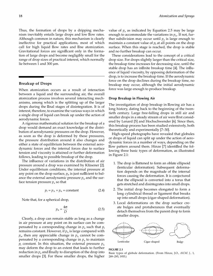
18 Atomization and Sprays

Thus, the formation of drops by a dripping mecha-nism inevitably entails large drops and low flow rates. Although common in nature, this mechanism is clearly ineffective for practical applications, most of which call for high liquid flow rates and fine atomization. Gravitational forces are significant only in the forma-tion of large drops and become negligibly small for the range of drop sizes of practical interest, which normally lie between 1 and 300 μm.

Breakup of Drops

When atomization occurs as a result of interaction between a liquid and the surrounding air, the overall atomization process involves several interacting mech-anisms, among which is the splitting up of the larger drops during the final stages of disintegration. It is of interest, therefore, to examine the various ways in which a single drop of liquid can break up under the action of aerodynamic forces.

A rigorous mathematical solution for the breakup of a drop would demand an exact knowledge of the distri-bution of aerodynamic pressures on the drop. However, as soon as the drop is deformed by these pressures, the pressure distribution around it also changes and either a state of equilibrium between the external aero-dynamic forces and the internal forces due to surface tension and viscosity is attained or further deformation follows, leading to possible breakup of the drop.

The influence of variations in the distribution of air pressure around a drop was examined by Klüsener [2]. Under equilibrium conditions, the internal pressure at any point on the drop surface, pI, is just sufficient to bal-ance the external aerodynamic pressure pA and the sur-face tension pressure pσ so that

constantI A= + =σp p p (2.4)

Note that, for a spherical drop,

4= σ

σpD

(2.5)

Clearly, a drop can remain stable as long as a change in air pressure at any point on its surface can be com-pensated by a corresponding change in pσ such that pI remains constant. However, if pA is large compared with pσ, then any appreciable change in pA cannot be com-pensated by a corresponding change in pσ to maintain pI constant. In this situation, the external pressure pA may deform the drop to an extent that leads to further reduction in pσ and finally to disruption of the drop into smaller drops [3]. For these smaller drops, the higher

value of pσ as indicated by Equation 2.5 may be large enough to accommodate the variations in pA. If not, fur-ther subdivision may occur until pσ is large enough to maintain a constant value of pI at all points on the drop surface. When this stage is reached, the drop is stable and no further breakup can occur.

These considerations lead to the concept of a critical drop size. For drops slightly larger than the critical size, the breakup time increases for decreasing size, until the stable drop has an infinite breakup time [4]. The influ-ence of liquid viscosity, by opposing deformation of the drop, is to increase the breakup time. If the aerodynamic force on the drop declines during the breakup time, no breakup may occur, although the initial aerodynamic force was large enough to produce breakup.

Drop Breakup in Flowing Air

The investigation of drop breakup in flowing air has a long history, dating back to the beginning of the twen-tieth century. Large free-falling drops in still air and smaller drops in a steady stream of air were first consid-ered by Lenard [5] and Hochschwender [6]. Since then, this breakup process has been studied extensively, both theoretically and experimentally [7–30].

High-speed photographs have revealed that globules or drops of liquid can split up under the action of aero-dynamic forces in a number of ways, depending on the flow pattern around them. Hinze [7] identified the fol-lowing three basic types of deformation, as illustrated in Figure 2.1:

1. The drop is flattened to form an oblate ellipsoid (lenticular deformation). Subsequent deforma-tion depends on the magnitude of the internal forces causing the deformation. It is conjectured that the ellipsoid is converted into a torus that gets stretched and disintegrates into small drops.

2. The initial drop becomes elongated to form a long cylindrical thread or ligament that breaks up into small drops (cigar-shaped deformation).

3. Local deformations on the drop surface cre-ate bulges and protuberances that eventually detach themselves from the parent drop to form smaller drops.

Lenticular Cigar-shaped Bulgy

FIGURE 2.1Basic types of globule deformation. (From Hinze, J.O., AlChE J., 1, 289–295, 1955.)

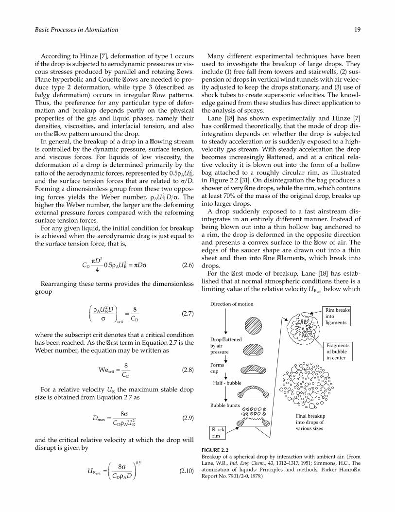
19Basic Processes in Atomization

According to Hinze [7], deformation of type 1 occurs if the drop is subjected to aerodynamic pressures or vis-cous stresses produced by parallel and rotating flows. Plane hyperbolic and Couette flows are needed to pro-duce type 2 deformation, while type 3 (described as bulgy deformation) occurs in irregular flow patterns. Thus, the preference for any particular type of defor-mation and breakup depends partly on the physical properties of the gas and liquid phases, namely their densities, viscosities, and interfacial tension, and also on the flow pattern around the drop.

In general, the breakup of a drop in a flowing stream is controlled by the dynamic pressure, surface tension, and viscous forces. For liquids of low viscosity, the deformation of a drop is determined primarily by the ratio of the aerodynamic forces, represented by 0.5 A R

2ρ U , and the surface tension forces that are related to σ/D. Forming a dimensionless group from these two oppos-ing forces yields the Weber number, A R

2ρ σU D . The higher the Weber number, the larger are the deforming external pressure forces compared with the reforming surface tension forces.

For any given liquid, the initial condition for breakup is achieved when the aerodynamic drag is just equal to the surface tension force, that is,

4

0.5D

2

A R2π ρ = π σC

DU D (2.6)

Rearranging these terms provides the dimensionless group

8A R

2

crit D

ρσ

=U DC

(2.7)

where the subscript crit denotes that a critical condition has been reached. As the first term in Equation 2.7 is the Weber number, the equation may be written as

We8

critD

=C

(2.8)

For a relative velocity UR the maximum stable drop size is obtained from Equation 2.7 as

8

maxD A R

2= σρ

DC U

(2.9)

and the critical relative velocity at which the drop will disrupt is given by

8

RD A

0.5

crit = σρ

UC D

(2.10)

Many different experimental techniques have been used to investigate the breakup of large drops. They include (1) free fall from towers and stairwells, (2) sus-pension of drops in vertical wind tunnels with air veloc-ity adjusted to keep the drops stationary, and (3) use of shock tubes to create supersonic velocities. The knowl-edge gained from these studies has direct application to the analysis of sprays.

Lane [18] has shown experimentally and Hinze [7] has confirmed theoretically, that the mode of drop dis-integration depends on whether the drop is subjected to steady acceleration or is suddenly exposed to a high-velocity gas stream. With steady acceleration the drop becomes increasingly flattened, and at a critical rela-tive velocity it is blown out into the form of a hollow bag attached to a roughly circular rim, as illustrated in Figure 2.2 [31]. On disintegration the bag produces a shower of very fine drops, while the rim, which contains at least 70% of the mass of the original drop, breaks up into larger drops.

A drop suddenly exposed to a fast airstream dis-integrates in an entirely different manner. Instead of being blown out into a thin hollow bag anchored to a rim, the drop is deformed in the opposite direction and presents a convex surface to the flow of air. The edges of the saucer shape are drawn out into a thin sheet and then into fine filaments, which break into drops.

For the first mode of breakup, Lane [18] has estab-lished that at normal atmospheric conditions there is a limiting value of the relative velocity RcritU below which

Direction of motion

Drop attenedby airpressure

Formscup

Half - bubble

Bubble bursts

ickrim

Final breakupinto drops ofvarious sizes

Fragmentsof bubblein center

Rim breaksintoligaments

FIGURE 2.2Breakup of a spherical drop by interaction with ambient air. (From Lane, W.R., Ind. Eng. Chem., 43, 1312–1317, 1951; Simmons, H.C., The atomization of liquids: Principles and methods, Parker Hannifin Report No. 7901/2-0, 1979.)

20 Atomization and Sprays

breakup does not occur. For liquids whose surface ten-sions lie in the range 0.028–0.475 kg/s2, the relationship is given by

R

0.5

crit ασ

U

D (2.11)

This equation should be compared with Equation 2.10. For water, Equation 2.11 becomes

784

Rcrit =UD

(2.12)

where UR is in meters per second and d in micrometers.From the data of Merrington and Richardson [9] and

Hinze [7] estimated that Wecrit to be 22 for a free-falling drop. For low-viscosity liquid drops suddenly exposed to a high-velocity airstream, the critical value of the Weber number was estimated to be 13.

Taylor [10] has provided an explanation for the obser-vation that critical Weber numbers for drops subjected to a steady stream are almost twice as high as those for drops suddenly exposed to an airflow at a constant speed. According to Taylor, the reason for this may be seen by considering the drop as a vibrating system and comparing the suddenly applied force FT and the gradu-ally increasing force Fs required to produce the same extension. The maximum distortion the drop can sus-tain without breaking occurs when FT = 0.5FS.

Hinze’s value of 13 for the critical Weber number may be compared with 8/CD from Equation 2.8, 10.6 from the data of Lane [18], 10.3 for mercury drops in air obtained by Haas [19], and 7.2–16.8 (with an average of about 13.0) for water, methyl alcohol, and a low-viscosity silicone oil obtained by Hanson et al. [20].

To account for the influence of liquid viscosity on drop breakup, Hinze [7] used a viscosity group defined as

WeRe

=Z (2.13)

This dimensionless group represents the ratio of an internal viscosity force to an interfacial surface tension force [13]. Some idea of the significance of the group may be gained by examining these forces [21]. The interfacial tension force per unit area is represented by σ/D, while the friction force per unit area, τ, is given by the product of liquid viscosity and the velocity gradient within the drop, that is, μL δ U/ δ x. If the drop is oscillating at its nat-ural frequency of vibration,  ω , then τ is of the order μL ω . The frequency is related to the properties of the drop by

2 1 1 2

[ 1 ]2

2 3L A

( )( )( )( )ω = σ + − +

π ρ + + ρn n n nD n n

(2.14)

where n depends on the mode of vibration. The most important mode is the first, for which n = 2. Since the density of the liquid is usually much higher than that of the surrounding air, for n = 2 Equation 2.14 becomes

4

LL

L

0.5

τ = µ ω ≈ µπ

σρ

D D

(2.15)

The ratio of the friction force to the surface tension force is thus

4 4

OhL

L0.5( )

τσ

=π

µρ σ

=π

D D

(2.16)

This equation illustrates the relevance of the Ohnesorge number (Oh) to the atomization process. However, as Sleicher [21] has pointed out, before the drops break up they are likely to become distorted to an extent far beyond the linear region of validity of Equation 2.15. Therefore, the viscosity forces repre-sented in this group may not be as important as those that resist the stretching of the drop by the flow field.

According to Hinze [7], the effect of viscosity on the critical Weber number can be expressed by a relation of the following form

We We 1 Ohcrit crit ( )= + f (2.17)

where Wecrit is the critical Weber number for zero viscosity.

This form is considered acceptable because, in the lim-iting case, Oh goes to zero as μL goes to zero. Thus, when μL is so small that it offers no resistance to drop defor-mation, the initial value of the Weber number, as given by Equation 2.17, reverts to the value for zero viscosity.

The data of Hanson et al. [20] provide qualitative sup-port for Equation 2.17 but do not agree in detail. Brodkey [22] has proposed the following empirical relationship for Oh < 10:

We We 1.077Ohcrit crit1.6= + (2.18)

which is claimed to be accurate within 20%.Others proposed similar forms suggest that the appar-

ent role of viscosity is to delay breakup. These include Gelfand [23] who proposed, for Oh < 4:

We We 1.5Ohcrit crit0.74= + (2.19)

By inspection, the varying coefficients in Equations 2.18 and 2.19 lead to results that differ in terms of the role of Oh. Hence the precise role of Oh remained a somewhat open question. Further experimental work by Faeth and coworkers led to the development of a regime map based on We and Oh [24], which clarifies the role of these two

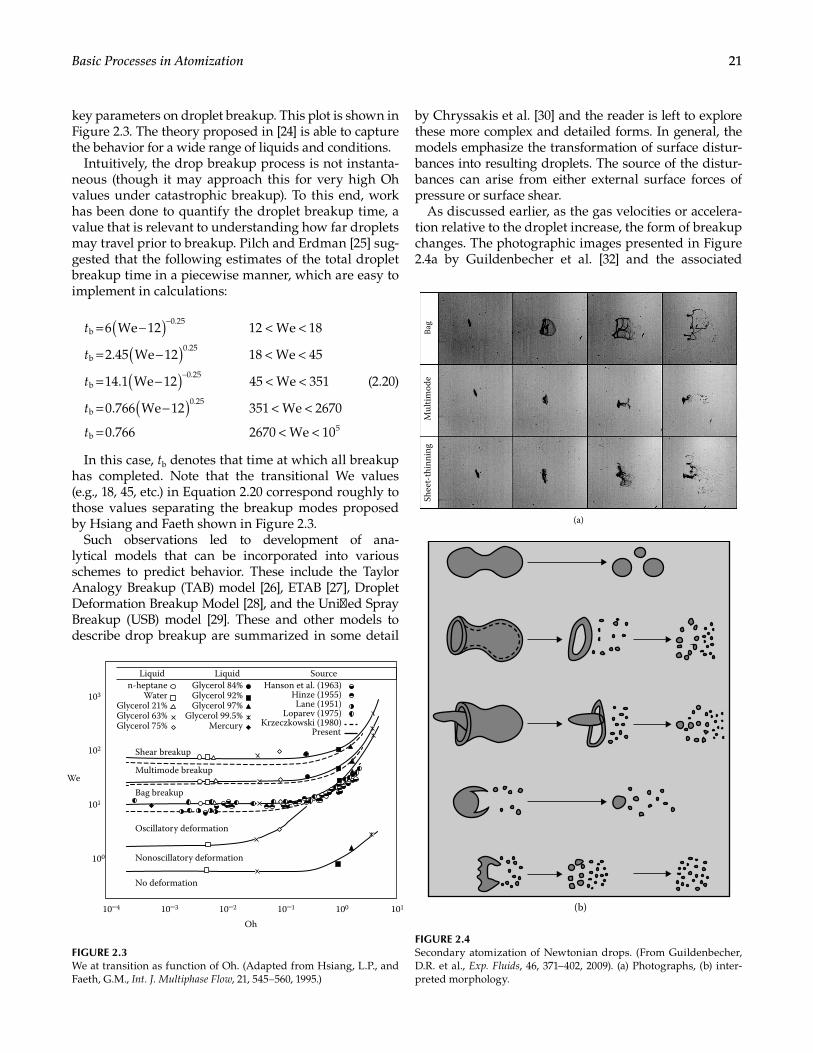
21Basic Processes in Atomization

key parameters on droplet breakup. This plot is shown in Figure 2.3. The theory proposed in [24] is able to capture the behavior for a wide range of liquids and conditions.

Intuitively, the drop breakup process is not instanta-neous (though it may approach this for very high Oh values under catastrophic breakup). To this end, work has been done to quantify the droplet breakup time, a value that is relevant to understanding how far droplets may travel prior to breakup. Pilch and Erdman [25] sug-gested that the following estimates of the total droplet breakup time in a piecewise manner, which are easy to implement in calculations:

6 We 12 12 We 18

2.45 We 12 18 We 45

14.1 We 12 45 We 351

0.766 We 12 351 We 2670

0.766 2670 We 10

b0.25

b0.25

b0.25

b0.25

b5

( )( )( )

( )

= − < <

= − < <

= − < <

= − < <

= < <

−

−

t

t

t

t

t

(2.20)

In this case, tb denotes that time at which all breakup has completed. Note that the transitional We values (e.g., 18, 45, etc.) in Equation 2.20 correspond roughly to those values separating the breakup modes proposed by Hsiang and Faeth shown in Figure 2.3.

Such observations led to development of ana-lytical models that can be incorporated into various schemes to predict behavior. These include the Taylor Analogy Breakup (TAB) model [26], ETAB [27], Droplet Deformation Breakup Model [28], and the Unified Spray Breakup (USB) model [29]. These and other models to describe drop breakup are summarized in some detail

by Chryssakis et al. [30] and the reader is left to explore these more complex and detailed forms. In general, the models emphasize the transformation of surface distur-bances into resulting droplets. The source of the distur-bances can arise from either external surface forces of pressure or surface shear.

As discussed earlier, as the gas velocities or accelera-tion relative to the droplet increase, the form of breakup changes. The photographic images presented in Figure 2.4a by Guildenbecher et al. [32] and the associated

Shee

t-th

inni

ngBa

gM

ultim

ode

(a)

(b)

FIGURE 2.4Secondary atomization of Newtonian drops. (From Guildenbecher, D.R. et al., Exp. Fluids, 46, 371–402, 2009). (a) Photographs, (b) inter-preted morphology.

Liquid

103

102

101

100

10–4 10–3 10–2 10–1 100 101

n-heptaneWater

Glycerol 21%

Glycerol 84% Hanson et al. (1963)Hinze (1955)Lane (1951)

Loparev (1975)Krzeczkowski (1980)

Present

Glycerol 92%Glycerol 97%

Glycerol 99.5%Mercury

Glycerol 63%Glycerol 75%

Shear breakup

Multimode breakup

Bag breakup

Oscillatory deformation

Nonoscillatory deformation

No deformation

We

Oh

Liquid Source

FIGURE 2.3We at transition as function of Oh. (Adapted from Hsiang, L.P., and Faeth, G.M., Int. J. Multiphase Flow, 21, 545–560, 1995.)

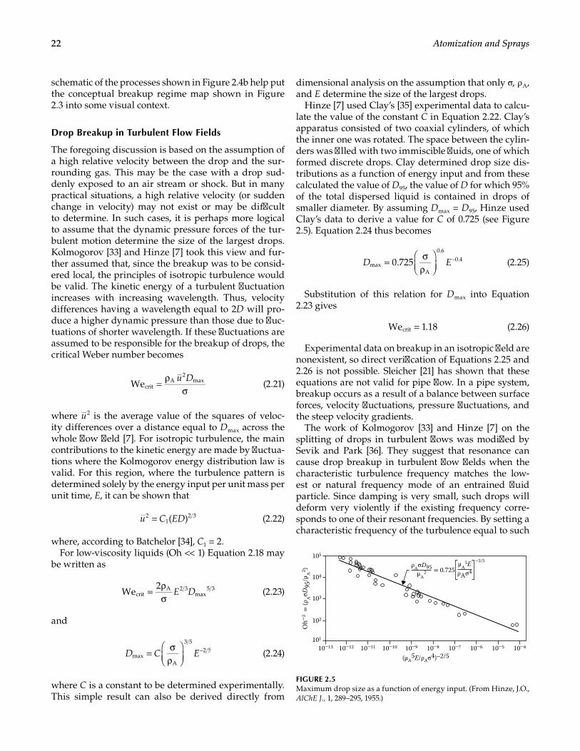
22 Atomization and Sprays

schematic of the processes shown in Figure 2.4b help put the conceptual breakup regime map shown in Figure 2.3 into some visual context.

Drop Breakup in Turbulent Flow Fields

The foregoing discussion is based on the assumption of a high relative velocity between the drop and the sur-rounding gas. This may be the case with a drop sud-denly exposed to an air stream or shock. But in many practical situations, a high relative velocity (or sudden change in velocity) may not exist or may be difficult to determine. In such cases, it is perhaps more logical to assume that the dynamic pressure forces of the tur-bulent motion determine the size of the largest drops. Kolmogorov [33] and Hinze [7] took this view and fur-ther assumed that, since the breakup was to be consid-ered local, the principles of isotropic turbulence would be valid. The kinetic energy of a turbulent fluctuation increases with increasing wavelength. Thus, velocity differences having a wavelength equal to 2D will pro-duce a higher dynamic pressure than those due to fluc-tuations of shorter wavelength. If these fluctuations are assumed to be responsible for the breakup of drops, the critical Weber number becomes

WecritA

2max= ρ

σu D

(2.21)

where 2u is the average value of the squares of veloc-ity differences over a distance equal to Dmax across the whole flow field [7]. For isotropic turbulence, the main contributions to the kinetic energy are made by fluctua-tions where the Kolmogorov energy distribution law is valid. For this region, where the turbulence pattern is determined solely by the energy input per unit mass per unit time, E, it can be shown that

( )21

2 3=u C ED (2.22)

where, according to Batchelor [34], C1 = 2.For low-viscosity liquids (Oh << 1) Equation 2.18 may

be written as

We2

critA 2 3

max5 3= ρ

σE D (2.23)

and

maxA

3 52 5= σ

ρ

−D C E (2.24)

where C is a constant to be determined experimentally. This simple result can also be derived directly from

dimensional analysis on the assumption that only σ, ρ A, and E determine the size of the largest drops.

Hinze [7] used Clay’s [35] experimental data to calcu-late the value of the constant C in Equation 2.22. Clay’s apparatus consisted of two coaxial cylinders, of which the inner one was rotated. The space between the cylin-ders was filled with two immiscible fluids, one of which formed discrete drops. Clay determined drop size dis-tributions as a function of energy input and from these calculated the value of D95, the value of D for which 95% of the total dispersed liquid is contained in drops of smaller diameter. By assuming Dmax = D95, Hinze used Clay’s data to derive a value for C of 0.725 (see Figure 2.5). Equation 2.24 thus becomes

0.725maxA

0.60.4= σ

ρ

−D E (2.25)

Substitution of this relation for Dmax into Equation 2.23 gives

We 1.18crit = (2.26)

Experimental data on breakup in an isotropic field are nonexistent, so direct verification of Equations 2.25 and 2.26 is not possible. Sleicher [21] has shown that these equations are not valid for pipe flow. In a pipe system, breakup occurs as a result of a balance between surface forces, velocity fluctuations, pressure fluctuations, and the steep velocity gradients.

The work of Kolmogorov [33] and Hinze [7] on the splitting of drops in turbulent flows was modified by Sevik and Park [36]. They suggest that resonance can cause drop breakup in turbulent flow fields when the characteristic turbulence frequency matches the low-est or natural frequency mode of an entrained fluid particle. Since damping is very small, such drops will deform very violently if the existing frequency corre-sponds to one of their resonant frequencies. By setting a characteristic frequency of the turbulence equal to such

10–13

(a)

10–12 10–11 10–10 10–9 10–8 10–7 10–6 10–5 10–4

102

101

103

104

ρAσD95μA

2μA

5EρAσ4

(μA5E/ρAσ4)–2/5

Oh–

2 =

(ρA

σD95

/μA

2 )

105

= 0.725–2/5

FIGURE 2.5Maximum drop size as a function of energy input. (From Hinze, J.O., AlChE J., 1, 289–295, 1955.)

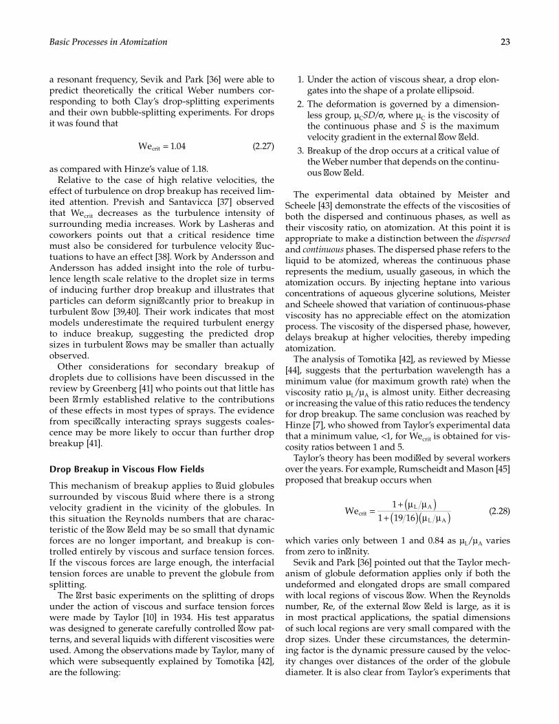
23Basic Processes in Atomization

a resonant frequency, Sevik and Park [36] were able to predict theoretically the critical Weber numbers cor-responding to both Clay’s drop-splitting experiments and their own bubble-splitting experiments. For drops it was found that

We 1.04crit = (2.27)

as compared with Hinze’s value of 1.18.Relative to the case of high relative velocities, the

effect of turbulence on drop breakup has received lim-ited attention. Prevish and Santavicca [37] observed that Wecrit decreases as the turbulence intensity of surrounding media increases. Work by Lasheras and coworkers points out that a critical residence time must also be considered for turbulence velocity fluc-tuations to have an effect [38]. Work by Andersson and Andersson has added insight into the role of turbu-lence length scale relative to the droplet size in terms of inducing further drop breakup and illustrates that particles can deform significantly prior to breakup in turbulent flow [39,40]. Their work indicates that most models underestimate the required turbulent energy to induce breakup, suggesting the predicted drop sizes in turbulent flows may be smaller than actually observed.

Other considerations for secondary breakup of droplets due to collisions have been discussed in the review by Greenberg [41] who points out that little has been firmly established relative to the contributions of these effects in most types of sprays. The evidence from specifically interacting sprays suggests coales-cence may be more likely to occur than further drop breakup [41].

Drop Breakup in Viscous Flow Fields

This mechanism of breakup applies to fluid globules surrounded by viscous fluid where there is a strong velocity gradient in the vicinity of the globules. In this situation the Reynolds numbers that are charac-teristic of the flow field may be so small that dynamic forces are no longer important, and breakup is con-trolled entirely by viscous and surface tension forces. If the viscous forces are large enough, the interfacial tension forces are unable to prevent the globule from splitting.

The first basic experiments on the splitting of drops under the action of viscous and surface tension forces were made by Taylor [10] in 1934. His test apparatus was designed to generate carefully controlled flow pat-terns, and several liquids with different viscosities were used. Among the observations made by Taylor, many of which were subsequently explained by Tomotika [42], are the following:

1. Under the action of viscous shear, a drop elon-gates into the shape of a prolate ellipsoid.

2. The deformation is governed by a dimension-less group, μCSD/σ, where μC is the viscosity of the continuous phase and S is the maximum velocity gradient in the external flow field.

3. Breakup of the drop occurs at a critical value of the Weber number that depends on the continu-ous flow field.

The experimental data obtained by Meister and Scheele [43] demonstrate the effects of the viscosities of both the dispersed and continuous phases, as well as their viscosity ratio, on atomization. At this point it is appropriate to make a distinction between the dispersed and continuous phases. The dispersed phase refers to the liquid to be atomized, whereas the continuous phase represents the medium, usually gaseous, in which the atomization occurs. By injecting heptane into various concentrations of aqueous glycerine solutions, Meister and Scheele showed that variation of continuous-phase viscosity has no appreciable effect on the atomization process. The viscosity of the dispersed phase, however, delays breakup at higher velocities, thereby impeding atomization.

The analysis of Tomotika [42], as reviewed by Miesse [44], suggests that the perturbation wavelength has a minimum value (for maximum growth rate) when the viscosity ratio μL/μA is almost unity. Either decreasing or increasing the value of this ratio reduces the tendency for drop breakup. The same conclusion was reached by Hinze [7], who showed from Taylor’s experimental data that a minimum value, <1, for Wecrit is obtained for vis-cosity ratios between 1 and 5.

Taylor’s theory has been modified by several workers over the years. For example, Rumscheidt and Mason [45] proposed that breakup occurs when

We1

1 19 16critL A

L A

( )( )( )=

+ µ µ+ µ µ

(2.28)

which varies only between 1 and 0.84 as μL/μA varies from zero to infinity.

Sevik and Park [36] pointed out that the Taylor mech-anism of globule deformation applies only if both the undeformed and elongated drops are small compared with local regions of viscous flow. When the Reynolds number, Re, of the external flow field is large, as it is in most practical applications, the spatial dimensions of such local regions are very small compared with the drop sizes. Under these circumstances, the determin-ing factor is the dynamic pressure caused by the veloc-ity changes over distances of the order of the globule diameter. It is also clear from Taylor’s experiments that

24 Atomization and Sprays

it is very difficult to atomize liquids that show a high viscosity ratio. This explains why, in practice, disper-sion by pure viscous flow is restricted to emulsification processes.

For relatively viscous drops, proposals for total breakup time of viscous droplets have been provided by Pilch and Erdman [25] who base the form on Gelfand’s expression in Equation 2.19:

4.5 1 1.2Oh We We Oh 0.3b0.74

crit( )= + ≈ <t (2.29)

Pilch and Erdman suggest Equation 2.20 is more accu-rate for lower viscosity drops. Hsiang and Faeth [24] proposed the following:

5

1Oh7

We 10 We Oh 3.5b3

crit=−

< ≈ <t (2.30)

Reasonable agreement between Equations 2.29 and 2.30 is found for low drops of high viscosity (e.g., low Oh values < 0.5).

Disintegration of Liquid Jets

When a liquid jet emerges from a nozzle as a continu-ous body of cylindrical form, the competition set up on the surface of the jet between the cohesive and disrup-tive forces gives rise to oscillations and perturbations. Under favorable conditions, the oscillations are ampli-fied and the liquid body disintegrates into drops. This process is sometimes referred to as primary atomization. If the drops so formed exceed the critical size, they fur-ther disintegrate into drops of smaller size, a process known as secondary atomization. Secondary atomiza-tion is directly related to the concepts discussed in the section above on breakup of droplets.

The phenomenon of jet disintegration has been sub-jected to theoretical and experimental investigation for more than 100 years. A comprehensive review of jet flow was made by Krzywoblocki [46], and other reviews of relevance to liquid jet flow are also available [44,47–57]. The following discussion is restricted to liq-uid jets injected into a gaseous atmosphere. It applies to any combination of liquid (the dispersed phase) and gas (the continuous phase), but for convenience the surrounding gas is usually referred to as air.

The properties of jets of most interest are the contin-uous length (which provides a measure of the growth rate of the disturbance) and the drop size (which is a

measure of the wave number of the most unstable dis-turbance). Also of interest is the manner in which the jet is disrupted. Numerous linear models describing this process have been developed over time. A review by Yoon and Heister [55] has suggested that many of these models provide very similar results. A few of these model developments, including some described by Yoon and Heister, are discussed here as a means to provide physical insight into the nature of liquid jet breakup.

The earliest investigations into jet flow phenomena appear to have been carried out by Bidone [58] and Savart [59]. Bidone’s research was concerned with the geometric forms of jets produced by nozzles of non-circular cross section, while Savart supplied the first quantitative data related to jet disintegration. His results showed that if the jet diameter is kept constant, the length of the continuous part of the jet is directly proportional to jet velocity. He also observed that, for constant jet velocity, the length of a jet is directly pro-portional to its diameter.

Plateau [60] is credited with the first theoretical investigation into jet instability. He showed that a cylindrical column of liquid is unstable if its length exceeds its perimeter; otherwise, two drops would be formed whose total surface area would be less than that of the original cylinder. Plateau’s work helped to explain the results of Savart and provided the basis for Rayleigh’s more widely known theory of jet stability.

In an early mathematical analysis, Rayleigh [11] employed the method of small disturbances to pre-dict the conditions necessary to cause the collapse of a liquid jet issuing at low velocity, for example, a low-speed water jet in air. This comprehensive analy-sis has been reviewed and summarized by McCarthy and Molloy [61].

Rayleigh compared the surface energy (directly pro-portional to the product of surface area and surface tension) of the disturbed configuration with that of the undisturbed column. He then calculated the potential energy of the disturbed configuration (relative to the equilibrium value) as

2

1s2 2 2( )= πσ γ + −E

dn bn (2.31)

where Es = potential surface energyd = jet diameterbn = constant in the Fourier series expansion γ  = dimensionless wave number = 2π/ λ  λ  = wavelength of disturbancen = any positive integer (including zero)

For nonsymmetrical disturbances, n >> 1 and Es is always positive, indicating that the system is always

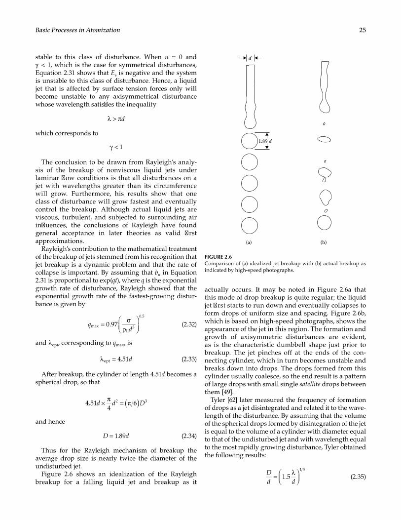
25Basic Processes in Atomization

stable to this class of disturbance. When n = 0 and γ  < 1, which is the case for symmetrical disturbances, Equation 2.31 shows that Es is negative and the system is unstable to this class of disturbance. Hence, a liquid jet that is affected by surface tension forces only will become unstable to any axisymmetrical disturbance whose wavelength satisfies the inequality

λ > πd

which corresponds to

1γ <

The conclusion to be drawn from Rayleigh’s analy-sis of the breakup of nonviscous liquid jets under laminar flow conditions is that all disturbances on a jet with wavelengths greater than its circumference will grow. Furthermore, his results show that one class of disturbance will grow fastest and eventually control the breakup. Although actual liquid jets are viscous, turbulent, and subjected to surrounding air influences, the conclusions of Rayleigh have found general acceptance in later theories as valid first approximations.

Rayleigh’s contribution to the mathematical treatment of the breakup of jets stemmed from his recognition that jet breakup is a dynamic problem and that the rate of collapse is important. By assuming that bn in Equation 2.31 is proportional to exp(qt), where q is the exponential growth rate of disturbance, Rayleigh showed that the exponential growth rate of the fastest-growing distur-bance is given by

0.97maxL

3

0.5

= σρ

qd

(2.32)

and  λ opt, corresponding to qmax, is

4.51optλ = d (2.33)

After breakup, the cylinder of length 4.51d becomes a spherical drop, so that

4.514

62 3( )× π = πd d D

and hence

1.89=D d (2.34)

Thus for the Rayleigh mechanism of breakup the average drop size is nearly twice the diameter of the undisturbed jet.

Figure 2.6 shows an idealization of the Rayleigh breakup for a falling liquid jet and breakup as it

actually occurs. It may be noted in Figure 2.6a that this mode of drop breakup is quite regular; the liquid jet first starts to run down and eventually collapses to form drops of uniform size and spacing. Figure 2.6b, which is based on high-speed photographs, shows the appearance of the jet in this region. The formation and growth of axisymmetric disturbances are evident, as is the characteristic dumbbell shape just prior to breakup. The jet pinches off at the ends of the con-necting cylinder, which in turn becomes unstable and breaks down into drops. The drops formed from this cylinder usually coalesce, so the end result is a pattern of large drops with small single satellite drops between them [49].

Tyler [62] later measured the frequency of formation of drops as a jet disintegrated and related it to the wave-length of the disturbance. By assuming that the volume of the spherical drops formed by disintegration of the jet is equal to the volume of a cylinder with diameter equal to that of the undisturbed jet and with wavelength equal to the most rapidly growing disturbance, Tyler obtained the following results:

1.51 3

= λ

Dd d

(2.35)

(a) (b)

1.89 d

d

FIGURE 2.6Comparison of (a) idealized jet breakup with (b) actual breakup as indicated by high-speed photographs.

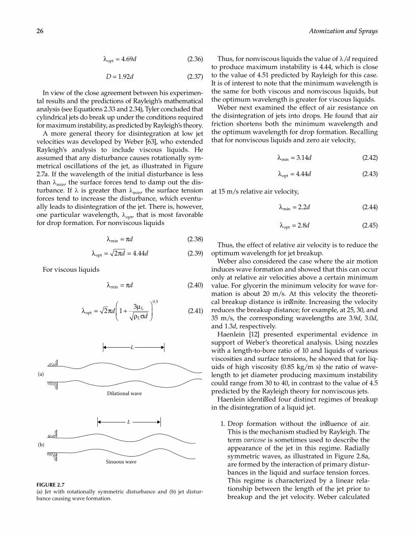
26 Atomization and Sprays

4.69optλ = d (2.36)

1.92=D d (2.37)

In view of the close agreement between his experimen-tal results and the predictions of Rayleigh’s mathematical analysis (see Equations 2.33 and 2.34), Tyler concluded that cylindrical jets do break up under the conditions required for maximum instability, as predicted by Rayleigh’s theory.

A more general theory for disintegration at low jet velocities was developed by Weber [63], who extended Rayleigh’s analysis to include viscous liquids. He assumed that any disturbance causes rotationally sym-metrical oscillations of the jet, as illustrated in Figure 2.7a. If the wavelength of the initial disturbance is less than  λ min, the surface forces tend to damp out the dis-turbance. If  λ  is greater than  λ min, the surface tension forces tend to increase the disturbance, which eventu-ally leads to disintegration of the jet. There is, however, one particular wavelength,  λ opt, that is most favorable for drop formation. For nonviscous liquids

minλ = πd (2.38)

2 4.44optλ = π =d d (2.39)

For viscous liquids

minλ = πd (2.40)

2 13

optL

L

0.5

λ = π + µρ σ

d

d (2.41)

Thus, for nonviscous liquids the value of  λ /d required to produce maximum instability is 4.44, which is close to the value of 4.51 predicted by Rayleigh for this case. It is of interest to note that the minimum wavelength is the same for both viscous and nonviscous liquids, but the optimum wavelength is greater for viscous liquids.

Weber next examined the effect of air resistance on the disintegration of jets into drops. He found that air friction shortens both the minimum wavelength and the optimum wavelength for drop formation. Recalling that for nonviscous liquids and zero air velocity,

3.14minλ = d (2.42)

4.44optλ = d (2.43)

at 15 m/s relative air velocity,

2.2minλ = d (2.44)

2.8optλ = d (2.45)

Thus, the effect of relative air velocity is to reduce the optimum wavelength for jet breakup.

Weber also considered the case where the air motion induces wave formation and showed that this can occur only at relative air velocities above a certain minimum value. For glycerin the minimum velocity for wave for-mation is about 20 m/s. At this velocity the theoreti-cal breakup distance is infinite. Increasing the velocity reduces the breakup distance; for example, at 25, 30, and 35 m/s, the corresponding wavelengths are 3.9d, 3.0d, and 1.3d, respectively.

Haenlein [12] presented experimental evidence in support of Weber’s theoretical analysis. Using nozzles with a length-to-bore ratio of 10 and liquids of various viscosities and surface tensions, he showed that for liq-uids of high viscosity (0.85 kg/m s) the ratio of wave-length to jet diameter producing maximum instability could range from 30 to 40, in contrast to the value of 4.5 predicted by the Rayleigh theory for nonviscous jets.

Haenlein identified four distinct regimes of breakup in the disintegration of a liquid jet.

1. Drop formation without the influence of air. This is the mechanism studied by Rayleigh. The term varicose is sometimes used to describe the appearance of the jet in this regime. Radially symmetric waves, as illustrated in Figure 2.8a, are formed by the interaction of primary distur-bances in the liquid and surface tension forces. This regime is characterized by a linear rela-tionship between the length of the jet prior to breakup and the jet velocity. Weber calculated

Dilational wave

Sinuous wave

(a)

(b)

L

L

FIGURE 2.7(a) Jet with rotationally symmetric disturbance and (b) jet distur-bance causing wave formation.

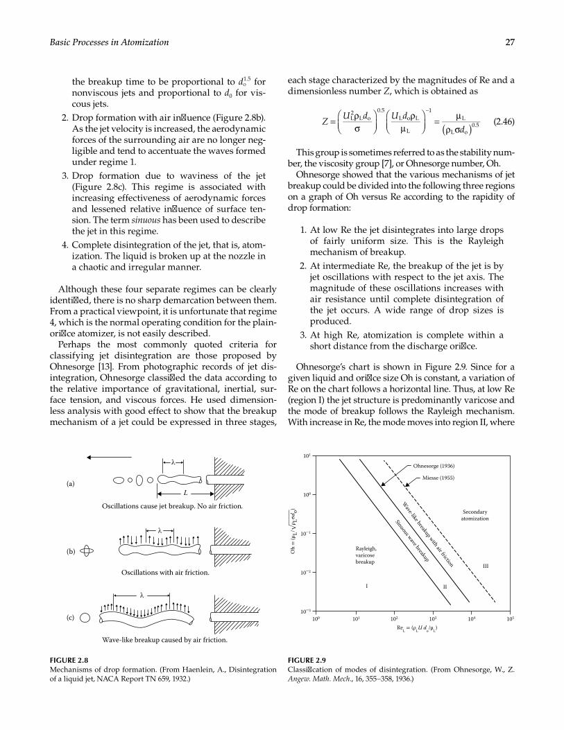
27Basic Processes in Atomization

the breakup time to be proportional to do1.5 for

nonviscous jets and proportional to d0 for vis-cous jets.

2. Drop formation with air influence (Figure 2.8b). As the jet velocity is increased, the aerodynamic forces of the surrounding air are no longer neg-ligible and tend to accentuate the waves formed under regime 1.

3. Drop formation due to waviness of the jet (Figure 2.8c). This regime is associated with increasing effectiveness of aerodynamic forces and lessened relative influence of surface ten-sion. The term sinuous has been used to describe the jet in this regime.

4. Complete disintegration of the jet, that is, atom-ization. The liquid is broken up at the nozzle in a chaotic and irregular manner.

Although these four separate regimes can be clearly identified, there is no sharp demarcation between them. From a practical viewpoint, it is unfortunate that regime 4, which is the normal operating condition for the plain-orifice atomizer, is not easily described.

Perhaps the most commonly quoted criteria for classifying jet disintegration are those proposed by Ohnesorge [13]. From photographic records of jet dis-integration, Ohnesorge classified the data according to the relative importance of gravitational, inertial, sur-face tension, and viscous forces. He used dimension-less analysis with good effect to show that the breakup mechanism of a jet could be expressed in three stages,

each stage characterized by the magnitudes of Re and a dimensionless number Z, which is obtained as

L2

L o0.5

L o L

L

1L

L o0.5( )

= ρσ

ρµ

= µρ σ

−

ZU d U d

d (2.46)

This group is sometimes referred to as the stability num-ber, the viscosity group [7], or Ohnesorge number, Oh.

Ohnesorge showed that the various mechanisms of jet breakup could be divided into the following three regions on a graph of Oh versus Re according to the rapidity of drop formation:

1. At low Re the jet disintegrates into large drops of fairly uniform size. This is the Rayleigh mechanism of breakup.

2. At intermediate Re, the breakup of the jet is by jet oscillations with respect to the jet axis. The magnitude of these oscillations increases with air resistance until complete disintegration of the jet occurs. A wide range of drop sizes is produced.

3. At high Re, atomization is complete within a short distance from the discharge orifice.

Ohnesorge’s chart is shown in Figure 2.9. Since for a given liquid and orifice size Oh is constant, a variation of Re on the chart follows a horizontal line. Thus, at low Re (region I) the jet structure is predominantly varicose and the mode of breakup follows the Rayleigh mechanism. With increase in Re, the mode moves into region II, where

(b)

(c)

(a)

λ

Oscillations cause jet breakup. No air friction.

L

Wave-like breakup caused by air friction.

λ

Oscillations with air friction.

λ

FIGURE 2.8Mechanisms of drop formation. (From Haenlein, A., Disintegration of a liquid jet, NACA Report TN 659, 1932.)

10–3

10–2

10–1

100

ReL = (ρ

LU do

/μL)

101

100 101 102 103 104 105

Rayleigh,varicosebreakup

I II

III

Sinuous wave breakup

Wave-like breakup with air friction

Ohnesorge (1936)

Miesse (1955)

Secondaryatomization

Oh =

(μL/√

ρ Lσdo)

FIGURE 2.9Classification of modes of disintegration. (From Ohnesorge, W., Z. Angew. Math. Mech., 16, 355–358, 1936.)

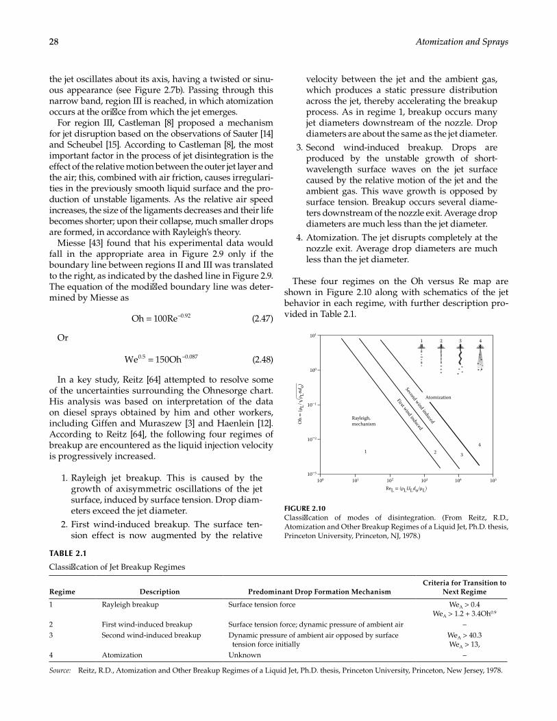
28 Atomization and Sprays

the jet oscillates about its axis, having a twisted or sinu-ous appearance (see Figure 2.7b). Passing through this narrow band, region III is reached, in which atomization occurs at the orifice from which the jet emerges.

For region III, Castleman [8] proposed a mechanism for jet disruption based on the observations of Sauter [14] and Scheubel [15]. According to Castleman [8], the most important factor in the process of jet disintegration is the effect of the relative motion between the outer jet layer and the air; this, combined with air friction, causes irregulari-ties in the previously smooth liquid surface and the pro-duction of unstable ligaments. As the relative air speed increases, the size of the ligaments decreases and their life becomes shorter; upon their collapse, much smaller drops are formed, in accordance with Rayleigh’s theory.

Miesse [43] found that his experimental data would fall in the appropriate area in Figure 2.9 only if the boundary line between regions II and III was translated to the right, as indicated by the dashed line in Figure 2.9. The equation of the modified boundary line was deter-mined by Miesse as

Oh 100Re–0.92= (2.47)

Or

We 150Oh0.5 –0.087= (2.48)

In a key study, Reitz [64] attempted to resolve some of the uncertainties surrounding the Ohnesorge chart. His analysis was based on interpretation of the data on diesel sprays obtained by him and other workers, including Giffen and Muraszew [3] and Haenlein [12]. According to Reitz [64], the following four regimes of breakup are encountered as the liquid injection velocity is progressively increased.

1. Rayleigh jet breakup. This is caused by the growth of axisymmetric oscillations of the jet surface, induced by surface tension. Drop diam-eters exceed the jet diameter.

2. First wind-induced breakup. The surface ten-sion effect is now augmented by the relative

velocity between the jet and the ambient gas, which produces a static pressure distribution across the jet, thereby accelerating the breakup process. As in regime 1, breakup occurs many jet diameters downstream of the nozzle. Drop diameters are about the same as the jet diameter.

3. Second wind-induced breakup. Drops are produced by the unstable growth of short-wavelength surface waves on the jet surface caused by the relative motion of the jet and the ambient gas. This wave growth is opposed by surface tension. Breakup occurs several diame-ters downstream of the nozzle exit. Average drop diameters are much less than the jet diameter.

4. Atomization. The jet disrupts completely at the nozzle exit. Average drop diameters are much less than the jet diameter.

These four regimes on the Oh versus Re map are shown in Figure 2.10 along with schematics of the jet behavior in each regime, with further description pro-vided in Table 2.1.

10–3

10–2

10–1

1 2 3 4

100

ReL = (ρLULdo/μL)

101

100 101 102 103 104 105

Rayleigh,mechanism

1 2 3

4

First wind induced

Second wind induced

Atomization

Oh =

(μL/√

ρ Lσdo)

FIGURE 2.10Classification of modes of disintegration. (From Reitz, R.D., Atomization and Other Breakup Regimes of a Liquid Jet, Ph.D. thesis, Princeton University, Princeton, NJ, 1978.)

TABLE 2.1

Classification of Jet Breakup Regimes

Regime Description Predominant Drop Formation MechanismCriteria for Transition to

Next Regime

1 Rayleigh breakup Surface tension force WeA > 0.4WeA > 1.2 + 3.4Oh0.9

2 First wind-induced breakup Surface tension force; dynamic pressure of ambient air –3 Second wind-induced breakup Dynamic pressure of ambient air opposed by surface

tension force initiallyWeA > 40.3WeA > 13,

4 Atomization Unknown –

Source: Reitz, R.D., Atomization and Other Breakup Regimes of a Liquid Jet, Ph.D. thesis, Princeton University, Princeton, New Jersey, 1978.

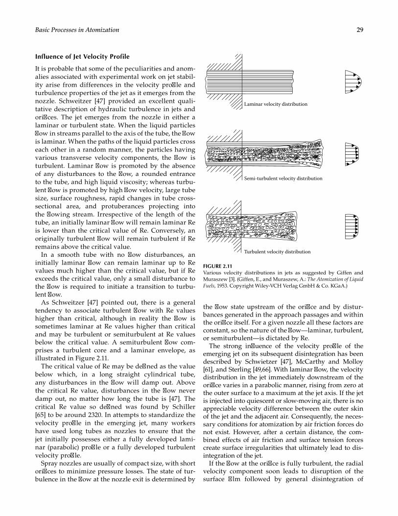
29Basic Processes in Atomization

Influence of Jet Velocity Profile

It is probable that some of the peculiarities and anom-alies associated with experimental work on jet stabil-ity arise from differences in the velocity profile and turbulence properties of the jet as it emerges from the nozzle. Schweitzer [47] provided an excellent quali-tative description of hydraulic turbulence in jets and orifices. The jet emerges from the nozzle in either a laminar or turbulent state. When the liquid particles flow in streams parallel to the axis of the tube, the flow is laminar. When the paths of the liquid particles cross each other in a random manner, the particles having various transverse velocity components, the flow is turbulent. Laminar flow is promoted by the absence of any disturbances to the flow, a rounded entrance to the tube, and high liquid viscosity; whereas turbu-lent flow is promoted by high flow velocity, large tube size, surface roughness, rapid changes in tube cross-sectional area, and protuberances projecting into the flowing stream. Irrespective of the length of the tube, an initially laminar flow will remain laminar Re is lower than the critical value of Re. Conversely, an originally turbulent flow will remain turbulent if Re remains above the critical value.

In a smooth tube with no flow disturbances, an initially laminar flow can remain laminar up to Re values much higher than the critical value, but if Re exceeds the critical value, only a small disturbance to the flow is required to initiate a transition to turbu-lent flow.

As Schweitzer [47] pointed out, there is a general tendency to associate turbulent flow with Re values higher than critical, although in reality the flow is sometimes laminar at Re values higher than critical and may be turbulent or semiturbulent at Re values below the critical value. A semiturbulent flow com-prises a turbulent core and a laminar envelope, as illustrated in Figure 2.11.

The critical value of Re may be defined as the value below which, in a long straight cylindrical tube, any disturbances in the flow will damp out. Above the critical Re value, disturbances in the flow never damp out, no matter how long the tube is [47]. The critical Re value so defined was found by Schiller [65] to be around 2320. In attempts to standardize the velocity profile in the emerging jet, many workers have used long tubes as nozzles to ensure that the jet initially possesses either a fully developed lami-nar (parabolic) profile or a fully developed turbulent velocity profile.

Spray nozzles are usually of compact size, with short orifices to minimize pressure losses. The state of tur-bulence in the flow at the nozzle exit is determined by

the flow state upstream of the orifice and by distur-bances generated in the approach passages and within the orifice itself. For a given nozzle all these factors are constant, so the nature of the flow—laminar, turbulent, or semiturbulent—is dictated by Re.

The strong influence of the velocity profile of the emerging jet on its subsequent disintegration has been described by Schwietzer [47], McCarthy and Molloy [61], and Sterling [49,66]. With laminar flow, the velocity distribution in the jet immediately downstream of the orifice varies in a parabolic manner, rising from zero at the outer surface to a maximum at the jet axis. If the jet is injected into quiescent or slow-moving air, there is no appreciable velocity difference between the outer skin of the jet and the adjacent air. Consequently, the neces-sary conditions for atomization by air friction forces do not exist. However, after a certain distance, the com-bined effects of air friction and surface tension forces create surface irregularities that ultimately lead to dis-integration of the jet.

If the flow at the orifice is fully turbulent, the radial velocity component soon leads to disruption of the surface film followed by general disintegration of

Laminar velocity distribution

Semi-turbulent velocity distribution

Turbulent velocity distribution

FIGURE 2.11Various velocity distributions in jets as suggested by Giffen and Muraszew [3]. (Giffen, E., and Muraszew, A.: The Atomization of Liquid Fuels, 1953. Copyright Wiley-VCH Verlag GmbH & Co. KGaA.)

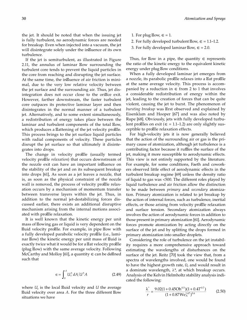
30 Atomization and Sprays

the jet. It should be noted that when the issuing jet is fully turbulent, no aerodynamic forces are needed for breakup. Even when injected into a vacuum, the jet will disintegrate solely under the influence of its own turbulence.

If the jet is semiturbulent, as illustrated in Figure 2.11, the annulus of laminar flow surrounding the turbulent core tends to prevent the liquid particles in the core from reaching and disrupting the jet surface. At the same time, the influence of air friction is mini-mal, due to the very low relative velocity between the jet surface and the surrounding air. Thus, jet dis-integration does not occur close to the orifice exit. However, farther downstream, the faster turbulent core outpaces its protective laminar layer and then disintegrates in the normal manner of a turbulent jet. Alternatively, and to some extent simultaneously, a redistribution of energy takes place between the laminar and turbulent components of the total flow, which produces a flattening of the jet velocity profile. This process brings to the jet surface liquid particles with radial components of velocity. These particles disrupt the jet surface so that ultimately it disinte-grates into drops.

The change in velocity profile (usually termed velocity profile relaxation) that occurs downstream of the nozzle exit can have an important influence on the stability of the jet and on its subsequent breakup into drops [61], As soon as a jet leaves a nozzle, that is, as soon as the physical constraint of the nozzle wall is removed, the process of velocity profile relax-ation occurs by a mechanism of momentum transfer between transverse layers within the jet. Thus, in addition to the normal jet-destabilizing forces dis-cussed earlier, there exists an additional disruptive mechanism arising from the internal motions associ-ated with profile relaxation.

It is well known that the kinetic energy per unit mass of flowing gas or liquid is very dependent on the fluid velocity profile. For example, in pipe flow with a fully developed parabolic velocity profile (i.e., lami-nar flow) the kinetic energy per unit mass of fluid is exactly twice what it would be for a flat velocity profile (plug flow) with the same average velocity. Following McCarthy and Molloy [61], a quantity  ∈  can be defined such that

∫∈= r3 3

0U dA U A

A

(2.49)

where Ur is the local fluid velocity and U the average fluid velocity over area A. For the three different flow situations we have

1. For plug flow,  ∈  = 1.

2. For fully developed turbulent flow,  ∈  = 1.1–1.2.

3. For fully developed laminar flow,  ∈  = 2.0.

Thus, for flow in a pipe, the quantity  ∈  represents the ratio of the kinetic energy to the equivalent kinetic energy under plug flow conditions.

When a fully developed laminar jet emerges from a nozzle, its parabolic profile relaxes into a flat profile at the same average velocity. This process is accom-panied by a reduction in  ∈  from 2 to 1 that involves a considerable redistribution of energy within the jet, leading to the creation of forces that can be quite violent, causing the jet to burst. The phenomenon of bursting breakup was first observed and explained by Eisenklam and Hooper [67] and was also noted by Rupe [68]. Obviously, jets with fully developed turbu-lent profiles on exit ( ∈  = 1.1–1.2) are only slightly sus-ceptible to profile relaxation effects.

For high-velocity jets it is now generally believed that the action of the surrounding air or gas is the pri-mary cause of atomization, although jet turbulence is a contributing factor because it ruffles the surface of the jet, making it more susceptible to aerodynamic effects. This view is not entirely supported by the literature. For example, for some conditions, Faeth and cowork-ers observed little effect of aerodynamic effects in the turbulent breakup regime [69] unless the density ratio of liquid to gas was <500. The different roles played by liquid turbulence and air friction allow the distinction to be made between primary and secondary atomiza-tion. Primary atomization is related to jet breakup by the action of internal forces, such as turbulence, inertial effects, or those arising from velocity profile relaxation and surface tension. Secondary atomization always involves the action of aerodynamic forces in addition to those present in primary atomization [61]. Aerodynamic forces promote atomization by acting directly on the surface of the jet and by splitting the drops formed in primary atomization into smaller droplets.

Considering the role of turbulence on the jet instabil-ity requires a more comprehensive approach toward estimating the wavelengths of disturbances on the surface of the jet. Reitz [70] took the view that, from a spectra of wavelengths involved, one would be found to have the highest growth rate, Ω, and would result in a dominate wavelength,  λ *, at which breakup occurs. Analysis of the Kelvin Helmholtz stability analysis indi-cated the following:

9.02(1 0.45Oh )(1 0.4 )(1 0.87We )

* 0.5 0.7

A1.67 0.6

λ = + ++r

T

(2.50)

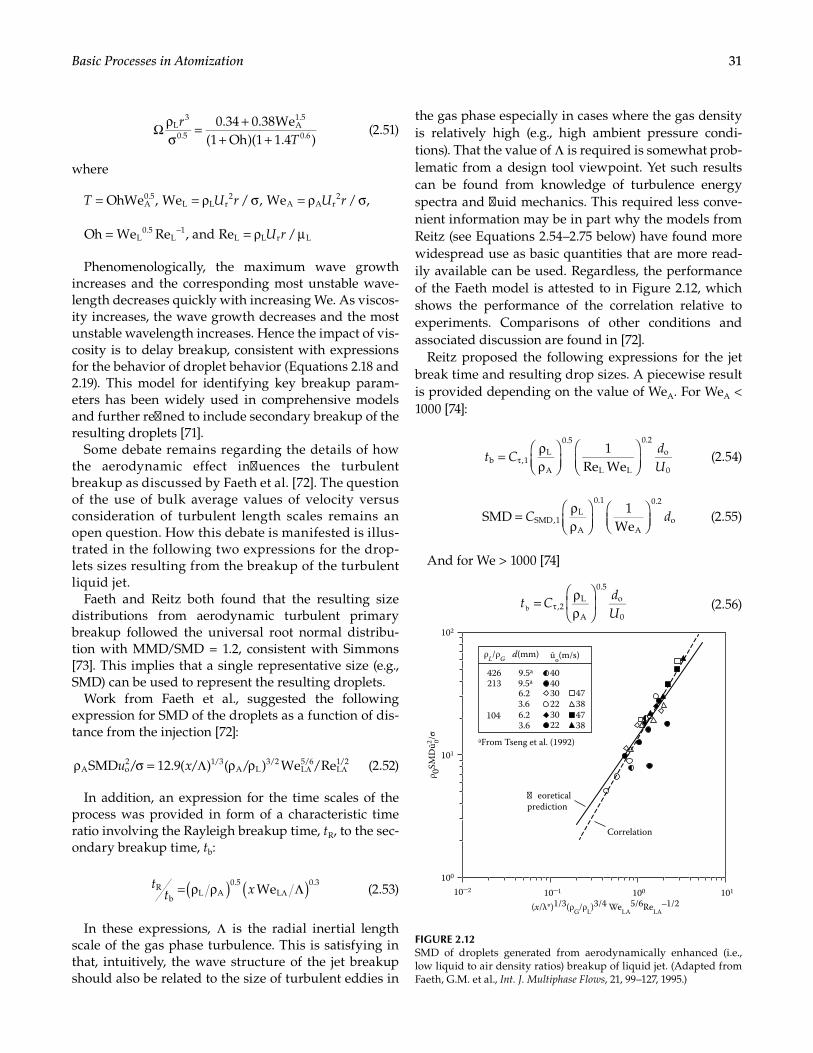
31Basic Processes in Atomization

0.34 0.38We

(1 Oh)(1 1.4 )L

3

0.5A1.5

0.6Ω ρσ

= ++ +

rT

(2.51)

where

OhWeA0.5=T , We /L L r

2= ρ σU r , We /A A r2= ρ σU r ,

Oh We ReL0.5

L1= − , and Re /L L r L= ρ µU r

Phenomenologically, the maximum wave growth increases and the corresponding most unstable wave-length decreases quickly with increasing We. As viscos-ity increases, the wave growth decreases and the most unstable wavelength increases. Hence the impact of vis-cosity is to delay breakup, consistent with expressions for the behavior of droplet behavior (Equations 2.18 and 2.19). This model for identifying key breakup param-eters has been widely used in comprehensive models and further refined to include secondary breakup of the resulting droplets [71].

Some debate remains regarding the details of how the aerodynamic effect influences the turbulent breakup as discussed by Faeth et al. [72]. The question of the use of bulk average values of velocity versus consideration of turbulent length scales remains an open question. How this debate is manifested is illus-trated in the following two expressions for the drop-lets sizes resulting from the breakup of the turbulent liquid jet.

Faeth and Reitz both found that the resulting size distributions from aerodynamic turbulent primary breakup followed the universal root normal distribu-tion with MMD/SMD = 1.2, consistent with Simmons [73]. This implies that a single representative size (e.g., SMD) can be used to represent the resulting droplets.

Work from Faeth et al., suggested the following expression for SMD of the droplets as a function of dis-tance from the injection [72]:

ρ σ = Λ ρ ρ Λ ΛSMD / 12.9( / ) ( / ) We /ReA o2 1/3

A L3/2

L5/6

L1/2u x (2.52)

In addition, an expression for the time scales of the process was provided in form of a characteristic time ratio involving the Rayleigh breakup time, tR, to the sec-ondary breakup time, tb:

WeRb

L A0.5

L0.3( ) ( )= ρ ρ ΛΛ

tt x (2.53)

In these expressions,  L  is the radial inertial length scale of the gas phase turbulence. This is satisfying in that, intuitively, the wave structure of the jet breakup should also be related to the size of turbulent eddies in

the gas phase especially in cases where the gas density is relatively high (e.g., high ambient pressure condi-tions). That the value of  L  is required is somewhat prob-lematic from a design tool viewpoint. Yet such results can be found from knowledge of turbulence energy spectra and fluid mechanics. This required less conve-nient information may be in part why the models from Reitz (see Equations 2.54–2.75 below) have found more widespread use as basic quantities that are more read-ily available can be used. Regardless, the performance of the Faeth model is attested to in Figure 2.12, which shows the performance of the correlation relative to experiments. Comparisons of other conditions and associated discussion are found in [72].

Reitz proposed the following expressions for the jet break time and resulting drop sizes. A piecewise result is provided depending on the value of WeA. For WeA < 1000 [74]:

1

Re Web ,1L

A

0.5

L L

0.2o

0t C

dU

= ρρ

τ (2.54)

SMD1

WeSMD,1L

A

0.1

A

0.2

oC d= ρρ

(2.55)

And for We > 1000 [74]

= ρρ

τ ,2

L

A

0.5o

0bt C

dU

(2.56)

d(mm) ūo(m/s)

426 40

474030

384738

223022

9.5a

9.5a

6.23.66.23.6

213

104

(x/λ*)1/3(ρG/ρL)3/4 WeLA5/6ReLA

–1/2

Correlation

aFrom Tseng et al. (1992)

eoreticalprediction

ρ 0SMD

ū2 0/σ

ρL/ρG

10–2

100

101

102

10–1 100 101

FIGURE 2.12SMD of droplets generated from aerodynamically enhanced (i.e., low liquid to air density ratios) breakup of liquid jet. (Adapted from Faeth, G.M. et al., Int. J. Multiphase Flows, 21, 99–127, 1995.)

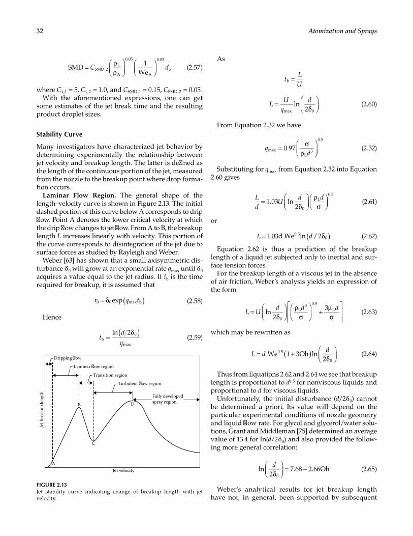
32 Atomization and Sprays

SMD1

WeSMD,2L

A

0.05

A

0.03

oC d= ρρ

(2.57)

where 5,1 =τC , 1.0,2 =τC , and 0.15SMD,1 =C , 0.05SMD,2 =C .With the aforementioned expressions, one can get

some estimates of the jet break time and the resulting product droplet sizes.

Stability Curve

Many investigators have characterized jet behavior by determining experimentally the relationship between jet velocity and breakup length. The latter is defined as the length of the continuous portion of the jet, measured from the nozzle to the breakup point where drop forma-tion occurs.

Laminar Flow Region. The general shape of the length–velocity curve is shown in Figure 2.13. The initial dashed portion of this curve below A corresponds to drip flow. Point A denotes the lower critical velocity at which the drip flow changes to jet flow. From A to B, the breakup length L increases linearly with velocity. This portion of the curve corresponds to disintegration of the jet due to surface forces as studied by Rayleigh and Weber.

Weber [63] has shown that a small axisymmetric dis-turbance  δ 0 will grow at an exponential rate qmax until  δ 0 acquires a value equal to the jet radius. If tb is the time required for breakup, it is assumed that

( )= δ exp0 0 max br q t (2.58)

Hence

ln 2

b0

max

( )=δ

tdq

(2.59)

As

b =tLU

ln2max 0

=δ

LU

qd

(2.60)

From Equation 2.32 we have

0.97maxL

3

0.5

= σρ

qd

(2.32)

Substituting for qmax from Equation 2.32 into Equation 2.60 gives

1.03 ln2 0

L0.5

=δ

ρσ

Ld

Ud d

(2.61)

or

( )= δ1.03d We ln /20.50L d (2.62)

Equation 2.62 is thus a prediction of the breakup length of a liquid jet subjected only to inertial and sur-face tension forces.

For the breakup length of a viscous jet in the absence of air friction, Weber’s analysis yields an expression of the form

ln2

3

0

L3 0.5

L=δ

ρσ

+ µσ

L Ud d d

(2.63)

which may be rewritten as

We 1 3Oh ln2

0.5

0( )= +

δ

L dd

(2.64)

Thus from Equations 2.62 and 2.64 we see that breakup length is proportional to d1.5 for nonviscous liquids and proportional to d for viscous liquids.

Unfortunately, the initial disturbance (d/2 δ 0) cannot be determined a priori. Its value will depend on the particular experimental conditions of nozzle geometry and liquid flow rate. For glycol and glycerol/water solu-tions, Grant and Middleman [75] determined an average value of 13.4 for ln(d/2 δ 0) and also provided the follow-ing more general correlation:

ln2

7.68 2.66Oh0δ

= −d (2.65)

Weber’s analytical results for jet breakup length have not, in general, been supported by subsequent

Jet velocity

C

DB

A

Dripping ow

Laminar ow region

Transition region

Turbulent ow region

Fully developedspray region

Jet b

reak

up le

ngth

FIGURE 2.13Jet stability curve indicating change of breakup length with jet velocity.

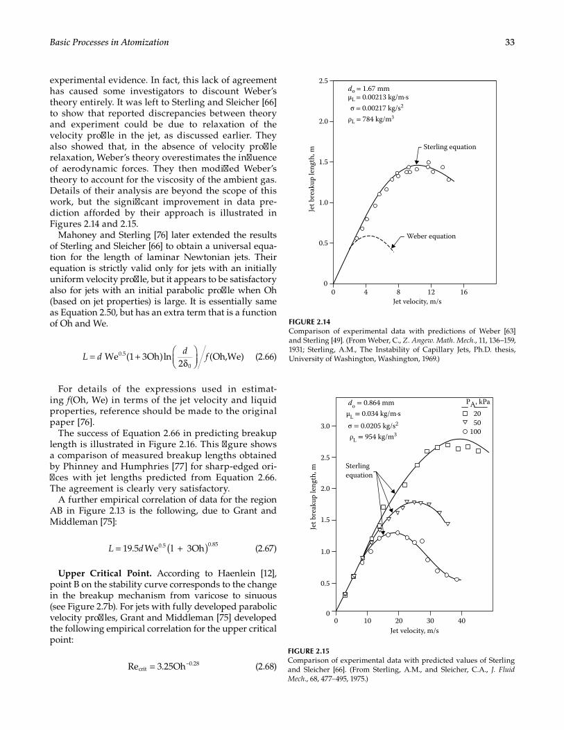
33Basic Processes in Atomization

experimental evidence. In fact, this lack of agreement has caused some investigators to discount Weber’s theory entirely. It was left to Sterling and Sleicher [66] to show that reported discrepancies between theory and experiment could be due to relaxation of the velocity profile in the jet, as discussed earlier. They also showed that, in the absence of velocity profile relaxation, Weber’s theory overestimates the influence of aerodynamic forces. They then modified Weber’s theory to account for the viscosity of the ambient gas. Details of their analysis are beyond the scope of this work, but the significant improvement in data pre-diction afforded by their approach is illustrated in Figures 2.14 and 2.15.

Mahoney and Sterling [76] later extended the results of Sterling and Sleicher [66] to obtain a universal equa-tion for the length of laminar Newtonian jets. Their equation is strictly valid only for jets with an initially uniform velocity profile, but it appears to be satisfactory also for jets with an initial parabolic profile when Oh (based on jet properties) is large. It is essentially same as Equation 2.50, but has an extra term that is a function of Oh and We.

We (1 3Oh)ln2

(Oh,We)0.5

0= +

δ

L dd

f (2.66)

For details of the expressions used in estimat-ing f(Oh, We) in terms of the jet velocity and liquid properties, reference should be made to the original paper [76].

The success of Equation 2.66 in predicting breakup length is illustrated in Figure 2.16. This figure shows a comparison of measured breakup lengths obtained by Phinney and Humphries [77] for sharp-edged ori-fices with jet lengths predicted from Equation 2.66. The agreement is clearly very satisfactory.

A further empirical correlation of data for the region AB in Figure 2.13 is the following, due to Grant and Middleman [75]:

19.5 We l 3Oh0.5 0.85( )= +L d (2.67)

Upper Critical Point. According to Haenlein [12], point B on the stability curve corresponds to the change in the breakup mechanism from varicose to sinuous (see Figure 2.7b). For jets with fully developed parabolic velocity profiles, Grant and Middleman [75] developed the following empirical correlation for the upper critical point:

Re 3.25Ohcrit–0.28= (2.68)

00

0.5

2.0

1.5

1.0

2.5

161284

Jet b

reak

up le

ngth

, m

Weber equation

Sterling equation

Jet velocity, m/s

do = 1.67 mmμL = 0.00213 kg/m·sσ = 0.00217 kg/s2

ρL = 784 kg/m3

FIGURE 2.14Comparison of experimental data with predictions of Weber [63] and Sterling [49]. (From Weber, C., Z. Angew. Math. Mech., 11, 136–159, 1931; Sterling, A.M., The Instability of Capillary Jets, Ph.D. thesis, University of Washington, Washington, 1969.)

0.5

00 302010 40

2.5Sterlingequation

2.0

1.5

1.0

3.0

Jet b

reak

up le

ngth

, m

Jet velocity, m/s

do = 0.864 mmμL = 0.034 kg/m·s

σ = 0.0205 kg/s2

ρL = 954 kg/m3

PA, kPa2050

100

FIGURE 2.15Comparison of experimental data with predicted values of Sterling and Sleicher [66]. (From Sterling, A.M., and Sleicher, C.A., J. Fluid Mech., 68, 477–495, 1975.)

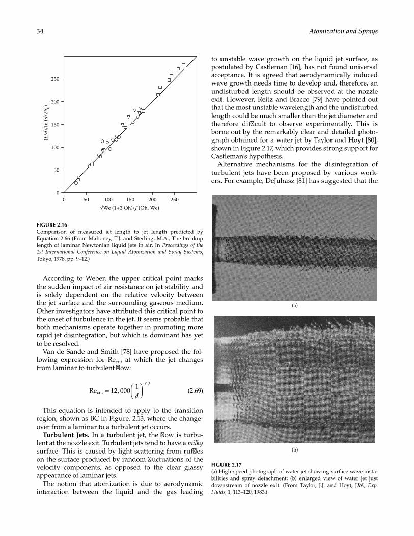
34 Atomization and Sprays

According to Weber, the upper critical point marks the sudden impact of air resistance on jet stability and is solely dependent on the relative velocity between the jet surface and the surrounding gaseous medium. Other investigators have attributed this critical point to the onset of turbulence in the jet. It seems probable that both mechanisms operate together in promoting more rapid jet disintegration, but which is dominant has yet to be resolved.

Van de Sande and Smith [78] have proposed the fol-lowing expression for Recrit at which the jet changes from laminar to turbulent flow:

Re 12,0001

crit

0.3

=

−

d (2.69)

This equation is intended to apply to the transition region, shown as BC in Figure. 2.13, where the change-over from a laminar to a turbulent jet occurs.

Turbulent Jets. In a turbulent jet, the flow is turbu-lent at the nozzle exit. Turbulent jets tend to have a milky surface. This is caused by light scattering from ruffles on the surface produced by random fluctuations of the velocity components, as opposed to the clear glassy appearance of laminar jets.

The notion that atomization is due to aerodynamic interaction between the liquid and the gas leading

to unstable wave growth on the liquid jet surface, as postulated by Castleman [16], has not found universal acceptance. It is agreed that aerodynamically induced wave growth needs time to develop and, therefore, an undisturbed length should be observed at the nozzle exit. However, Reitz and Bracco [79] have pointed out that the most unstable wavelength and the undisturbed length could be much smaller than the jet diameter and therefore difficult to observe experimentally. This is borne out by the remarkably clear and detailed photo-graph obtained for a water jet by Taylor and Hoyt [80], shown in Figure 2.17, which provides strong support for Castleman’s hypothesis.

Alternative mechanisms for the disintegration of turbulent jets have been proposed by various work-ers. For example, DeJuhasz [81] has suggested that the

(L/d

)/In

(d/2

δ 0)

00

50

250

200

150

100

25020015010050√We (1+3 Oh)/ʄ (Oh, We)

FIGURE 2.16Comparison of measured jet length to jet length predicted by Equation 2.66 (From Mahoney, T.J. and Sterling, M.A., The breakup length of laminar Newtonian liquid jets in air. In Proceedings of the 1st International Conference on Liquid Atomization and Spray Systems, Tokyo, 1978, pp. 9–12.)

(a)

(b)

FIGURE 2.17(a) High-speed photograph of water jet showing surface wave insta-bilities and spray detachment; (b) enlarged view of water jet just downstream of nozzle exit. (From Taylor, J.J. and Hoyt, J.W., Exp. Fluids, 1, 113–120, 1983.)

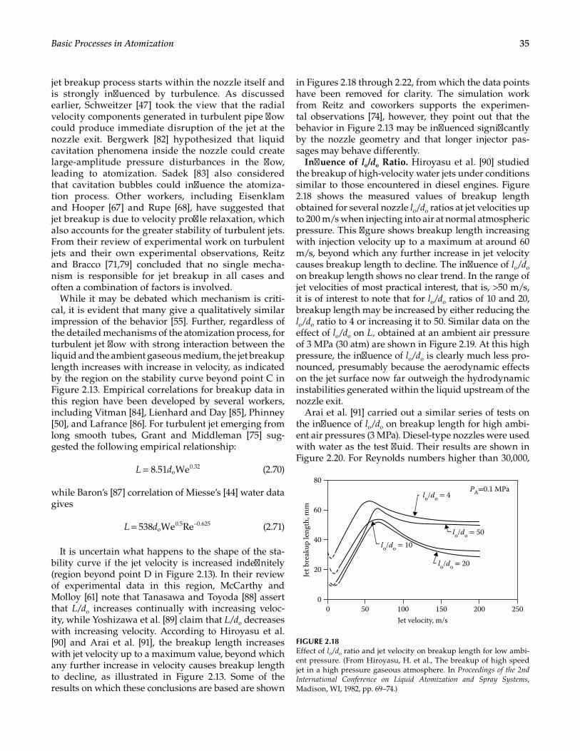
35Basic Processes in Atomization

jet breakup process starts within the nozzle itself and is strongly influenced by turbulence. As discussed earlier, Schweitzer [47] took the view that the radial velocity components generated in turbulent pipe flow could produce immediate disruption of the jet at the nozzle exit. Bergwerk [82] hypothesized that liquid cavitation phenomena inside the nozzle could create large-amplitude pressure disturbances in the flow, leading to atomization. Sadek [83] also considered that cavitation bubbles could influence the atomiza-tion process. Other workers, including Eisenklam and Hooper [67] and Rupe [68], have suggested that jet breakup is due to velocity profile relaxation, which also accounts for the greater stability of turbulent jets. From their review of experimental work on turbulent jets and their own experimental observations, Reitz and Bracco [71,79] concluded that no single mecha-nism is responsible for jet breakup in all cases and often a combination of factors is involved.

While it may be debated which mechanism is criti-cal, it is evident that many give a qualitatively similar impression of the behavior [55]. Further, regardless of the detailed mechanisms of the atomization process, for turbulent jet flow with strong interaction between the liquid and the ambient gaseous medium, the jet breakup length increases with increase in velocity, as indicated by the region on the stability curve beyond point C in Figure 2.13. Empirical correlations for breakup data in this region have been developed by several workers, including Vitman [84], Lienhard and Day [85], Phinney [50], and Lafrance [86]. For turbulent jet emerging from long smooth tubes, Grant and Middleman [75] sug-gested the following empirical relationship:

8.51 Weo0.32L d= (2.70)

while Baron’s [87] correlation of Miesse’s [44] water data gives

= 538 We Reo0.5 –0.625L d (2.71)

It is uncertain what happens to the shape of the sta-bility curve if the jet velocity is increased indefinitely (region beyond point D in Figure 2.13). In their review of experimental data in this region, McCarthy and Molloy [61] note that Tanasawa and Toyoda [88] assert that L/do increases continually with increasing veloc-ity, while Yoshizawa et al. [89] claim that L/do decreases with increasing velocity. According to Hiroyasu et al. [90] and Arai et al. [91], the breakup length increases with jet velocity up to a maximum value, beyond which any further increase in velocity causes breakup length to decline, as illustrated in Figure 2.13. Some of the results on which these conclusions are based are shown

in Figures 2.18 through 2.22, from which the data points have been removed for clarity. The simulation work from Reitz and coworkers supports the experimen-tal observations [74], however, they point out that the behavior in Figure 2.13 may be influenced significantly by the nozzle geometry and that longer injector pas-sages may behave differently.

Influence of lo/do Ratio. Hiroyasu et al. [90] studied the breakup of high-velocity water jets under conditions similar to those encountered in diesel engines. Figure 2.18 shows the measured values of breakup length obtained for several nozzle lo/do ratios at jet velocities up to 200 m/s when injecting into air at normal atmospheric pressure. This figure shows breakup length increasing with injection velocity up to a maximum at around 60 m/s, beyond which any further increase in jet velocity causes breakup length to decline. The influence of lo/do on breakup length shows no clear trend. In the range of jet velocities of most practical interest, that is, >50 m/s, it is of interest to note that for lo/do ratios of 10 and 20, breakup length may be increased by either reducing the lo/do ratio to 4 or increasing it to 50. Similar data on the effect of lo/do on L, obtained at an ambient air pressure of 3 MPa (30 atm) are shown in Figure 2.19. At this high pressure, the influence of lo/do is clearly much less pro-nounced, presumably because the aerodynamic effects on the jet surface now far outweigh the hydrodynamic instabilities generated within the liquid upstream of the nozzle exit.

Arai et al. [91] carried out a similar series of tests on the influence of lo/do on breakup length for high ambi-ent air pressures (3 MPa). Diesel-type nozzles were used with water as the test fluid. Their results are shown in Figure 2.20. For Reynolds numbers higher than 30,000,

80

60

40

20

0200150100

Jet velocity, m/s

Jet b

reak

up le

ngth

, mm

500 250

PA=0.1 MPalo/do = 4

lo/do = 50

lo/do = 10

lo/do = 20

FIGURE 2.18Effect of lo/do ratio and jet velocity on breakup length for low ambi-ent pressure. (From Hiroyasu, H. et al., The breakup of high speed jet in a high pressure gaseous atmosphere. In Proceedings of the 2nd International Conference on Liquid Atomization and Spray Systems, Madison, WI, 1982, pp. 69–74.)

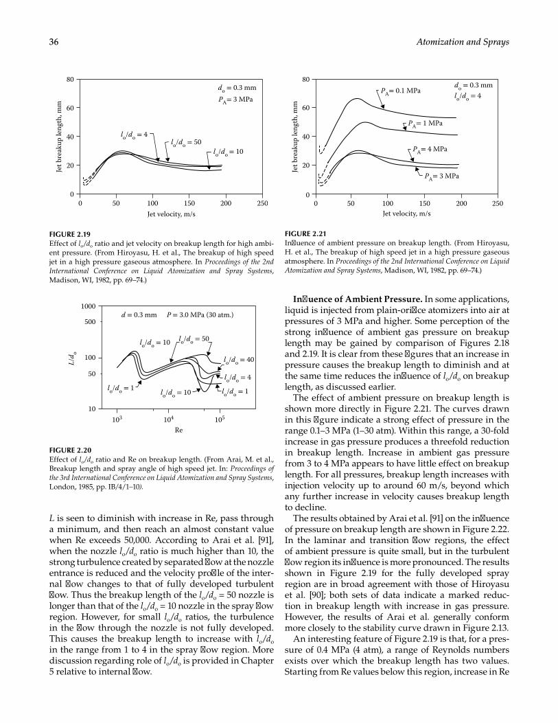
36 Atomization and Sprays

L is seen to diminish with increase in Re, pass through a minimum, and then reach an almost constant value when Re exceeds 50,000. According to Arai et al. [91], when the nozzle lo/do ratio is much higher than 10, the strong turbulence created by separated flow at the nozzle entrance is reduced and the velocity profile of the inter-nal flow changes to that of fully developed turbulent flow. Thus the breakup length of the lo/do = 50 nozzle is longer than that of the lo/do = 10 nozzle in the spray flow region. However, for small lo/do ratios, the turbulence in the flow through the nozzle is not fully developed. This causes the breakup length to increase with lo/do in the range from 1 to 4 in the spray flow region. More discussion regarding role of lo/do is provided in Chapter 5 relative to internal flow.

Influence of Ambient Pressure. In some applications, liquid is injected from plain-orifice atomizers into air at pressures of 3 MPa and higher. Some perception of the strong influence of ambient gas pressure on breakup length may be gained by comparison of Figures 2.18 and 2.19. It is clear from these figures that an increase in pressure causes the breakup length to diminish and at the same time reduces the influence of lo/do on breakup length, as discussed earlier.

The effect of ambient pressure on breakup length is shown more directly in Figure 2.21. The curves drawn in this figure indicate a strong effect of pressure in the range 0.1–3 MPa (1–30 atm). Within this range, a 30-fold increase in gas pressure produces a threefold reduction in breakup length. Increase in ambient gas pressure from 3 to 4 MPa appears to have little effect on breakup length. For all pressures, breakup length increases with injection velocity up to around 60 m/s, beyond which any further increase in velocity causes breakup length to decline.

The results obtained by Arai et al. [91] on the influence of pressure on breakup length are shown in Figure 2.22. In the laminar and transition flow regions, the effect of ambient pressure is quite small, but in the turbulent flow region its influence is more pronounced. The results shown in Figure 2.19 for the fully developed spray region are in broad agreement with those of Hiroyasu et al. [90]; both sets of data indicate a marked reduc-tion in breakup length with increase in gas pressure. However, the results of Arai et al. generally conform more closely to the stability curve drawn in Figure 2.13.

An interesting feature of Figure 2.19 is that, for a pres-sure of 0.4 MPa (4 atm), a range of Reynolds numbers exists over which the breakup length has two values. Starting from Re values below this region, increase in Re

80

60

40

20

0200150100

Jet velocity, m/s

Jet b

reak

up le

ngth

, mm

500 250

do = 0.3 mmPA= 3 MPa

lo/do = 4lo/do = 50

lo/do = 10

FIGURE 2.19Effect of lo/do ratio and jet velocity on breakup length for high ambi-ent pressure. (From Hiroyasu, H. et al., The breakup of high speed jet in a high pressure gaseous atmosphere. In Proceedings of the 2nd International Conference on Liquid Atomization and Spray Systems, Madison, WI, 1982, pp. 69–74.)

100

L/d o

500

1000

50

10105104103

Re

lo/do = 1

lo/do = 10

lo/do = 10

lo/do = 40

lo/do = 50

lo/do = 4

lo/do = 1

d = 0.3 mm P = 3.0 MPa (30 atm.)

FIGURE 2.20Effect of lo/do ratio and Re on breakup length. (From Arai, M. et al., Breakup length and spray angle of high speed jet. In: Proceedings of the 3rd International Conference on Liquid Atomization and Spray Systems, London, 1985, pp. IB/4/1–10).

40

60

80

20

020015010050

Jet velocity, m/s

Jet b

reak

up le

ngth

, mm

0 250

do = 0.3 mmlo/do = 4

PA= 0.1 MPa

PA= 1 MPa

PA= 4 MPa

PA= 3 MPa

FIGURE 2.21Influence of ambient pressure on breakup length. (From Hiroyasu, H. et al., The breakup of high speed jet in a high pressure gaseous atmosphere. In Proceedings of the 2nd International Conference on Liquid Atomization and Spray Systems, Madison, WI, 1982, pp. 69–74.)

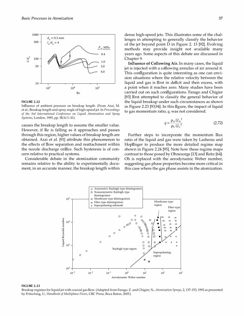
37Basic Processes in Atomization

causes the breakup length to assume the smaller value. However, if Re is falling as it approaches and passes through this region, higher values of breakup length are obtained. Arai et al. [91] attribute this phenomenon to the effects of flow separation and reattachment within the nozzle discharge orifice. Such hysteresis is of con-cern relative to practical systems.

Considerable debate in the atomization community remains relative to the ability to experimentally docu-ment, in an accurate manner, the breakup length within

dense high-speed jets. This illustrates some of the chal-lenges in attempting to generally classify the behavior of the jet beyond point D in Figure 2. 13 [92]. Evolving methods may provide insight not available many years ago. Some aspects of this debate are discussed in Chapter 9.

Influence of Coflowing Air. In many cases, the liquid jet is injected with a coflowing annulus of air around it. This configuration is quite interesting as one can envi-sion situations where the relative velocity between the liquid and gas is first in deficit and then excess, with a point when it reaches zero. Many studies have been carried out on such configurations. Farago and Chigier [93] first attempted to classify the general behavior of the liquid breakup under such circumstances as shown in Figure 2.23 [93,94]. In this figure, the impact of liquid to gas momentum ratio, q, was not considered.

A A2

L L2= ρ

ρq

UU

(2.72)

Further steps to incorporate the momentum flux ratio of the liquid and gas were taken by Lasheras and Hopfinger to produce the more detailed regime map shown in Figure 2.24 [95]. Note how these regime maps contrast to those posed by Ohnesorge [13] and Reitz [64]. Oh is replaced with the aerodynamic Weber number, suggesting gas phase properties become more critical in this case where the gas phase assists in the atomization.

1000

0.4

1.03.0

4.0

do = 0.3 mmlo/do = 4

10

Re

PA, MPa

103 104 105

50

500

100

L/d o

FIGURE 2.22Influence of ambient pressure on breakup length. (From Arai, M. et al., Breakup length and spray angle of high-speed jet. In Proceedings of the 3rd International Conference on Liquid Atomization and Spray Systems, London, 1985, pp. IB/4/1–10.)

102

103

104

105

Membrane-typeregion

Superpulsatingregion

Rayleigh-type region

Aerodynamic Weber number

Liqu

id R

eyno

lds n

umbe

r

Fiber-typeregion

10210110010–110–210–3 103

Axisymetric Rayleigh-type disintegration

Superpulsating submodeFiber-type disintegrationMembrane-type disintegration

Nonaxisymetric Rayleigh-typedisintegration

FIGURE 2.23Breakup regimes for liquid jet with coaxial gas flow. (Adapted from Farago, Z. and Chigier, N., Atomization Sprays, 2, 137–153, 1992 as presented by Fritsching, U., Handbook of Multiphase Flows, CRC Press, Boca Raton, 2005.)

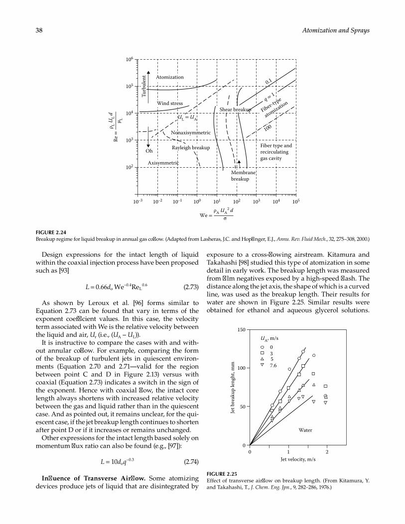
38 Atomization and Sprays

Design expressions for the intact length of liquid within the coaxial injection process have been proposed such as [93]

= −0.66 We Reo0.4

L0.6L d (2.73)

As shown by Leroux et al. [96] forms similar to Equation 2.73 can be found that vary in terms of the exponent coefficient values. In this case, the velocity term associated with We is the relative velocity between the liquid and air, Ur (i.e., (UA – UL)).

It is instructive to compare the cases with and with-out annular coflow. For example, comparing the form of the breakup of turbulent jets in quiescent environ-ments (Equation 2.70 and 2.71—valid for the region between point C and D in Figure 2.13) versus with coaxial (Equation 2.73) indicates a switch in the sign of the exponent. Hence with coaxial flow, the intact core length always shortens with increased relative velocity between the gas and liquid rather than in the quiescent case. And as pointed out, it remains unclear, for the qui-escent case, if the jet breakup length continues to shorten after point D or if it increases or remains unchanged.

Other expressions for the intact length based solely on momentum flux ratio can also be found (e.g., [97]):

10 o0.3L d q= − (2.74)

Influence of Transverse Airflow. Some atomizing devices produce jets of liquid that are disintegrated by

exposure to a cross-flowing airstream. Kitamura and Takahashi [98] studied this type of atomization in some detail in early work. The breakup length was measured from film negatives exposed by a high-speed flash. The distance along the jet axis, the shape of which is a curved line, was used as the breakup length. Their results for water are shown in Figure 2.25. Similar results were obtained for ethanol and aqueous glycerol solutions.

Atomization

Turb

ulen

t

Shear breakup

0.1

100

Fiber-type

atomizationq = 1

Wind stress

Nonaxisymmetric

Rayleigh breakupOh

Axisymmetric

Membranebreakup

Fiber type andrecirculatinggas cavity

UL = UA

10–3 10–2 10–1 100 101 102

102

105

104

103

106

103 104 105

We = σρA UA

2 d

Re =

µ L

ρ L UL d

FIGURE 2.24Breakup regime for liquid breakup in annual gas coflow. (Adapted from Lasheras, J.C. and Hopfinger, E.J., Annu. Rev. Fluid Mech., 32, 275–308, 2000.)

150

0357.6

UA, m/s

100

50

0Jet velocity, m/s

Jet b

reak

up le

nght

, mm

Water

1 20

FIGURE 2.25Effect of transverse airflow on breakup length. (From Kitamura, Y. and Takahashi, T., J. Chem. Eng. Jpn., 9, 282–286, 1976.)

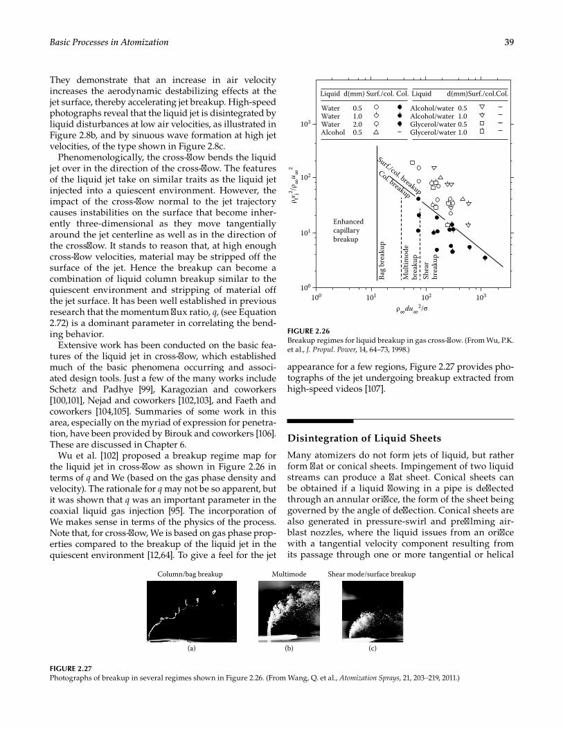
39Basic Processes in Atomization

They demonstrate that an increase in air velocity increases the aerodynamic destabilizing effects at the jet surface, thereby accelerating jet breakup. High-speed photographs reveal that the liquid jet is disintegrated by liquid disturbances at low air velocities, as illustrated in Figure 2.8b, and by sinuous wave formation at high jet velocities, of the type shown in Figure 2.8c.

Phenomenologically, the cross-flow bends the liquid jet over in the direction of the cross-flow. The features of the liquid jet take on similar traits as the liquid jet injected into a quiescent environment. However, the impact of the cross-flow normal to the jet trajectory causes instabilities on the surface that become inher-ently three-dimensional as they move tangentially around the jet centerline as well as in the direction of the crossflow. It stands to reason that, at high enough cross-flow velocities, material may be stripped off the surface of the jet. Hence the breakup can become a combination of liquid column breakup similar to the quiescent environment and stripping of material off the jet surface. It has been well established in previous research that the momentum flux ratio, q, (see Equation 2.72) is a dominant parameter in correlating the bend-ing behavior.

Extensive work has been conducted on the basic fea-tures of the liquid jet in cross-flow, which established much of the basic phenomena occurring and associ-ated design tools. Just a few of the many works include Schetz and Padhye [99], Karagozian and coworkers [100,101], Nejad and coworkers [102,103], and Faeth and coworkers [104,105]. Summaries of some work in this area, especially on the myriad of expression for penetra-tion, have been provided by Birouk and coworkers [106]. These are discussed in Chapter 6.

Wu et al. [102] proposed a breakup regime map for the liquid jet in cross-flow as shown in Figure 2.26 in terms of q and We (based on the gas phase density and velocity). The rationale for q may not be so apparent, but it was shown that q was an important parameter in the coaxial liquid gas injection [95]. The incorporation of We makes sense in terms of the physics of the process. Note that, for cross-flow, We is based on gas phase prop-erties compared to the breakup of the liquid jet in the quiescent environment [12,64]. To give a feel for the jet

appearance for a few regions, Figure 2.27 provides pho-tographs of the jet undergoing breakup extracted from high-speed videos [107].

Disintegration of Liquid Sheets

Many atomizers do not form jets of liquid, but rather form flat or conical sheets. Impingement of two liquid streams can produce a flat sheet. Conical sheets can be obtained if a liquid flowing in a pipe is deflected through an annular orifice, the form of the sheet being governed by the angle of deflection. Conical sheets are also generated in pressure-swirl and prefilming air-blast nozzles, where the liquid issues from an orifice with a tangential velocity component resulting from its passage through one or more tangential or helical

Alcohol

Enhancedcapillarybreakup

100100

101

102

103

101 102 103

Bag

brea

kup

Mul

timod

ebr

eaku

pSh

ear

brea

kup

WaterWaterWater Alcohol/water

Alcohol/waterGlycerol/waterGlycerol/water

Surf./col. breakup

Col. breakup

Liquid d(mm) Surf./col. Col. Liquid d(mm)Surf./col.Col.

0.51.02.00.5

0.51.00.51.0

ρ∞du∞2/σ

ρ fv j2 /ρ∞

u ∞2

FIGURE 2.26Breakup regimes for liquid breakup in gas cross-flow. (From Wu, P.K. et al., J. Propul. Power, 14, 64–73, 1998.)

Column/bag breakup Multimode Shear mode/surface breakup

(a) (b) (c)

FIGURE 2.27Photographs of breakup in several regimes shown in Figure 2.26. (From Wang, Q. et al., Atomization Sprays, 21, 203–219, 2011.)

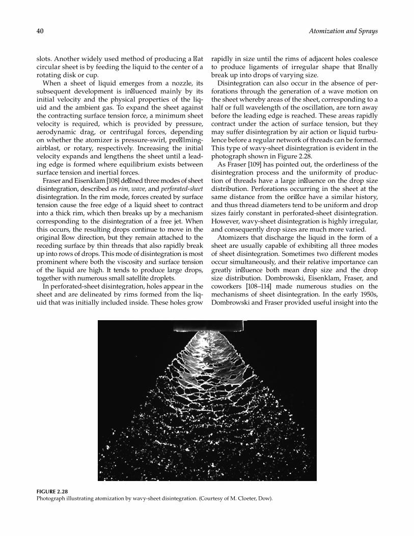
40 Atomization and Sprays

slots. Another widely used method of producing a flat circular sheet is by feeding the liquid to the center of a rotating disk or cup.

When a sheet of liquid emerges from a nozzle, its subsequent development is influenced mainly by its initial velocity and the physical properties of the liq-uid and the ambient gas. To expand the sheet against the contracting surface tension force, a minimum sheet velocity is required, which is provided by pressure, aerodynamic drag, or centrifugal forces, depending on whether the atomizer is pressure-swirl, prefilming-airblast, or rotary, respectively. Increasing the initial velocity expands and lengthens the sheet until a lead-ing edge is formed where equilibrium exists between surface tension and inertial forces.

Fraser and Eisenklam [108] defined three modes of sheet disintegration, described as rim, wave, and perforated-sheet disintegration. In the rim mode, forces created by surface tension cause the free edge of a liquid sheet to contract into a thick rim, which then breaks up by a mechanism corresponding to the disintegration of a free jet. When this occurs, the resulting drops continue to move in the original flow direction, but they remain attached to the receding surface by thin threads that also rapidly break up into rows of drops. This mode of disintegration is most prominent where both the viscosity and surface tension of the liquid are high. It tends to produce large drops, together with numerous small satellite droplets.

In perforated-sheet disintegration, holes appear in the sheet and are delineated by rims formed from the liq-uid that was initially included inside. These holes grow

rapidly in size until the rims of adjacent holes coalesce to produce ligaments of irregular shape that finally break up into drops of varying size.

Disintegration can also occur in the absence of per-forations through the generation of a wave motion on the sheet whereby areas of the sheet, corresponding to a half or full wavelength of the oscillation, are torn away before the leading edge is reached. These areas rapidly contract under the action of surface tension, but they may suffer disintegration by air action or liquid turbu-lence before a regular network of threads can be formed. This type of wavy-sheet disintegration is evident in the photograph shown in Figure 2.28.

As Fraser [109] has pointed out, the orderliness of the disintegration process and the uniformity of produc-tion of threads have a large influence on the drop size distribution. Perforations occurring in the sheet at the same distance from the orifice have a similar history, and thus thread diameters tend to be uniform and drop sizes fairly constant in perforated-sheet disintegration. However, wavy-sheet disintegration is highly irregular, and consequently drop sizes are much more varied.

Atomizers that discharge the liquid in the form of a sheet are usually capable of exhibiting all three modes of sheet disintegration. Sometimes two different modes occur simultaneously, and their relative importance can greatly influence both mean drop size and the drop size distribution. Dombrowski, Eisenklam, Fraser, and coworkers [108–114] made numerous studies on the mechanisms of sheet disintegration. In the early 1950s, Dombrowski and Fraser provided useful insight into the

FIGURE 2.28Photograph illustrating atomization by wavy-sheet disintegration. (Courtesy of M. Cloeter, Dow).

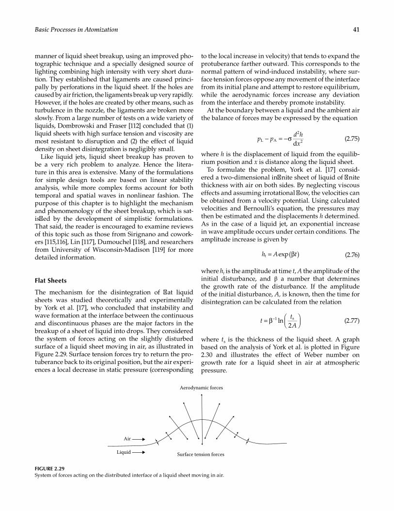
41Basic Processes in Atomization

manner of liquid sheet breakup, using an improved pho-tographic technique and a specially designed source of lighting combining high intensity with very short dura-tion. They established that ligaments are caused princi-pally by perforations in the liquid sheet. If the holes are caused by air friction, the ligaments break up very rapidly. However, if the holes are created by other means, such as turbulence in the nozzle, the ligaments are broken more slowly. From a large number of tests on a wide variety of liquids, Dombrowski and Fraser [112] concluded that (1) liquid sheets with high surface tension and viscosity are most resistant to disruption and (2) the effect of liquid density on sheet disintegration is negligibly small.

Like liquid jets, liquid sheet breakup has proven to be a very rich problem to analyze. Hence the litera-ture in this area is extensive. Many of the formulations for simple design tools are based on linear stability analysis, while more complex forms account for both temporal and spatial waves in nonlinear fashion. The purpose of this chapter is to highlight the mechanism and phenomenology of the sheet breakup, which is sat-isfied by the development of simplistic formulations. That said, the reader is encouraged to examine reviews of this topic such as those from Sirignano and cowork-ers [115,116], Lin [117], Dumouchel [118], and researchers from University of Wisconsin-Madison [119] for more detailed information.

Flat Sheets

The mechanism for the disintegration of flat liquid sheets was studied theoretically and experimentally by York et al. [17], who concluded that instability and wave formation at the interface between the continuous and discontinuous phases are the major factors in the breakup of a sheet of liquid into drops. They considered the system of forces acting on the slightly disturbed surface of a liquid sheet moving in air, as illustrated in Figure 2.29. Surface tension forces try to return the pro-tuberance back to its original position, but the air experi-ences a local decrease in static pressure (corresponding

to the local increase in velocity) that tends to expand the protuberance farther outward. This corresponds to the normal pattern of wind-induced instability, where sur-face tension forces oppose any movement of the interface from its initial plane and attempt to restore equilibrium, while the aerodynamic forces increase any deviation from the interface and thereby promote instability.

At the boundary between a liquid and the ambient air the balance of forces may be expressed by the equation

dL A

2

2− = −σp pd h

x (2.75)

where h is the displacement of liquid from the equilib-rium position and x is distance along the liquid sheet.

To formulate the problem, York et al. [17] consid-ered a two-dimensional infinite sheet of liquid of finite thickness with air on both sides. By neglecting viscous effects and assuming irrotational flow, the velocities can be obtained from a velocity potential. Using calculated velocities and Bernoulli’s equation, the pressures may then be estimated and the displacements h determined. As in the case of a liquid jet, an exponential increase in wave amplitude occurs under certain conditions. The amplitude increase is given by

( )= βexph A tt (2.76)

where ht is the amplitude at time t, A the amplitude of the initial disturbance, and  β  a number that determines the growth rate of the disturbance. If the amplitude of the initial disturbance, A, is known, then the time for disintegration can be calculated from the relation

ln2

1 s= β

−ttA

(2.77)

where ts is the thickness of the liquid sheet. A graph based on the analysis of York et al. is plotted in Figure 2.30 and illustrates the effect of Weber number on growth rate for a liquid sheet in air at atmospheric pressure.

Surface tension forces

Air

Aerodynamic forces

Liquid

FIGURE 2.29System of forces acting on the distributed interface of a liquid sheet moving in air.

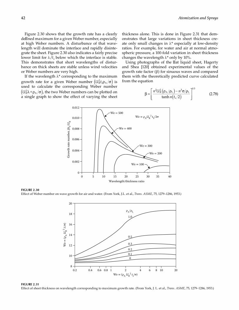
42 Atomization and Sprays

Figure 2.30 shows that the growth rate has a clearly defined maximum for a given Weber number, especially at high Weber numbers. A disturbance of that wave-length will dominate the interface and rapidly disinte-grate the sheet. Figure 2.30 also indicates a fairly precise lower limit for  λ /ts below which the interface is stable. This demonstrates that short wavelengths of distur-bance on thick sheets are stable unless wind velocities or Weber numbers are very high.

If the wavelength  λ * corresponding to the maximum growth rate for a given Weber number R

2s A( )ρ σU t is

used to calculate the corresponding Weber number

R2

A( )λ ∗ρ σU , the two Weber numbers can be plotted on a single graph to show the effect of varying the sheet

thickness alone. This is done in Figure 2.31 that dem-onstrates that large variations in sheet thickness cre-ate only small changes in  λ * especially at low-density ratios. For example, for water and air at normal atmo-spheric pressure, a 100-fold variation in sheet thickness changes the wavelength  λ * only by 10%.

Using photographs of the flat liquid sheet, Hagerty and Shea [120] obtained experimental values of the growth rate factor ( β ) for sinuous waves and compared them with the theoretically predicted curve calculated from the equation

tanh 2

2R2

A L3

L

s

0.5( )( )β =

ρ ρ − σ ρ

n U nn t

(2.78)

0.012

Gro

wth

rate

num

ber,

βtS/U

R

0.010

0.008

0.006

0.004

0.002

0353025201510

Wavelength/thickness ratio

We = 500We = ρAUR

2 tS/2σ

We = 400

We = 300

We = 200

We = 100

50 40

FIGURE 2.30Effect of Weber number on wave growth for air and water. (From York, J.L. et al., Trans. ASME, 75, 1279–1286, 1953.)

20

18

16

14

12

10

80.2

0.20.10

0.3

0.5

1.0

ρA/ρL

We = (ρA UR2 ts/σ)

We

= (ρ

A U

R2 λ/σ

)

0.4 0.6 0.8 1 2 4 6 8 10 20

FIGURE 2.31Effect of sheet thickness on wavelength corresponding to maximum growth rate. (From York, J. L. et al., Trans. ASME, 75, 1279–1286, 1953.)

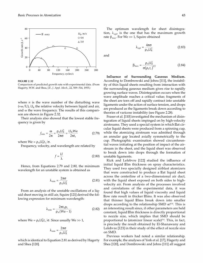
43Basic Processes in Atomization

where n is the wave number of the disturbing wave (= ω /U), UR the relative velocity between liquid and air, and  ω  the wave frequency. The results of this compari-son are shown in Figure 2.32.

Their analysis also showed that the lowest stable fre-quency is given by

2 2

We2min

A R3

R

s= ω

π= ρ

πσ=

πf

U Ut

(2.79)

where We = A R2

sρ σU t .Frequency, velocity, and wavelength are related by

=λ

fU

(2.80)

Hence, from Equations 2.79 and 2.80, the minimum wavelength for an unstable system is obtained as

2

minA R

2λ = πσρ U

(2.81)

From an analysis of the unstable oscillations of a liq-uid sheet moving in still air, Squire [121] derived the fol-lowing expression for minimum wavelength:

2 t(We 1)min

s L

Aλ = π ρ

ρ − (2.82)

where We = L R2

sρ σU t . Since usually We >> 1,

2

minA R

2λ = πσρ U

which is identical to Equation 2.81 as derived by Hagerty and Shea [120].

The optimum wavelength for sheet disintegra-tion,  λ opt, is the one that has the maximum growth rate  β max. For We >> 1, Squire obtained

4

optA R

2λ = πσρ U

(2.83)

and

maxA R

2

L s0.5( )

β = ρσ ρ

U

t (2.84)

Influence of Surrounding Gaseous Medium. According to Dombrowski and Johns [111], the instabil-ity of thin liquid sheets resulting from interaction with the surrounding gaseous medium gives rise to rapidly growing surface waves. Disintegration occurs when the wave amplitude reaches a critical value; fragments of the sheet are torn off and rapidly contract into unstable ligaments under the action of surface tension, and drops are produced as the ligaments break down according to theories of varicose instability (see Figure 2.28).

Fraser et al. [110] investigated the mechanism of disin-tegration of liquid sheets impinged on by high-velocity airstreams. They used a special system in which flat cir-cular liquid sheets were produced from a spinning cup, while the atomizing airstream was admitted through an annular gap located axially symmetrically to the cup. Photographic examination showed circumferen-tial waves initiating at the position of impact of the air-stream in the sheet, and the liquid sheet was observed to break down into drops through the formation of unstable ligaments.

Rizk and Lefebvre [122] studied the influence of initial liquid film thickness on spray characteristics. They used two specially designed airblast atomizers that were constructed to produce a flat liquid sheet across the centerline of a two-dimensional air duct, with the liquid sheet exposed on both sides to high-velocity air. From analysis of the processes involved and correlations of the experimental data, it was found that high values of liquid viscosity and liquid flow rate result in thicker films. It was also observed that thinner liquid films break down into smaller drops according to the relationship SMD  α t0.4. This is an interesting result since, if other parameters are held constant, liquid film thickness is directly proportional to nozzle size, which implies that SMD should be proportional to (atomizer linear scale)0.4. This, in fact, is precisely the result obtained by El-Shanawany and Lefebvre [123] in their study of the effect of nozzle size on SMD.

Previous workers had noted a similar relationship. For example, the analyses of York et al. [17], Hagerty and Shea [120], and Dombrowski and Johns [111] all suggest

Frequency, cycles/s

Gro

wth

rate

β, s

–1

240200160120804000

60eory

4.6UR, m/s

3.0

40

20

80

280

FIGURE 2.32Comparison of predicted growth rate with experimental data. (From Hagerty, W.W. and Shea, J.F., J. Appl. Mech., 22, 509–514, 1955.)

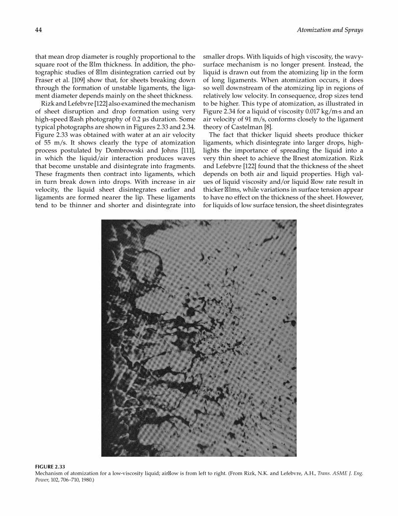
44 Atomization and Sprays

that mean drop diameter is roughly proportional to the square root of the film thickness. In addition, the pho-tographic studies of film disintegration carried out by Fraser et al. [109] show that, for sheets breaking down through the formation of unstable ligaments, the liga-ment diameter depends mainly on the sheet thickness.

Rizk and Lefebvre [122] also examined the mechanism of sheet disruption and drop formation using very high-speed flash photography of 0.2 μs duration. Some typical photographs are shown in Figures 2.33 and 2.34. Figure 2.33 was obtained with water at an air velocity of 55 m/s. It shows clearly the type of atomization process postulated by Dombrowski and Johns [111], in which the liquid/air interaction produces waves that become unstable and disintegrate into fragments. These fragments then contract into ligaments, which in turn break down into drops. With increase in air velocity, the liquid sheet disintegrates earlier and ligaments are formed nearer the lip. These ligaments tend to be thinner and shorter and disintegrate into

smaller drops. With liquids of high viscosity, the wavy-surface mechanism is no longer present. Instead, the liquid is drawn out from the atomizing lip in the form of long ligaments. When atomization occurs, it does so well downstream of the atomizing lip in regions of relatively low velocity. In consequence, drop sizes tend to be higher. This type of atomization, as illustrated in Figure 2.34 for a liquid of viscosity 0.017 kg/m·s and an air velocity of 91 m/s, conforms closely to the ligament theory of Castelman [8].

The fact that thicker liquid sheets produce thicker ligaments, which disintegrate into larger drops, high-lights the importance of spreading the liquid into a very thin sheet to achieve the finest atomization. Rizk and Lefebvre [122] found that the thickness of the sheet depends on both air and liquid properties. High val-ues of liquid viscosity and/or liquid flow rate result in thicker films, while variations in surface tension appear to have no effect on the thickness of the sheet. However, for liquids of low surface tension, the sheet disintegrates

FIGURE 2.33Mechanism of atomization for a low-viscosity liquid; airflow is from left to right. (From Rizk, N.K. and Lefebvre, A.H., Trans. ASME J. Eng. Power, 102, 706–710, 1980.)

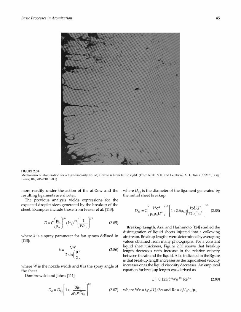
45Basic Processes in Atomization

more readily under the action of the airflow and the resulting ligaments are shorter.

The previous analysis yields expressions for the expected droplet sizes generated by the breakup of the sheet. Examples include those from Fraser et al. [113]:

( )= ρρ

D C kt 1

WeL

A

1 6

s1 3

L

1 3

(2.85)

where k is a spray parameter for fan sprays defined in [113]:

2sin

2

s≡ θ

kt W

(2.86)

where W is the nozzle width and  θ  is the spray angle of the sheet.

Dombrowski and Johns [111]:

13

d ligL

L lig

1 6

= + µρ σ

D DD

(2.87)

where Dlig is the diameter of the ligament generated by the initial sheet breakup:

1 2.672lig

2 2

L A4

1 6

LA4 7

L2 5

3

1 5

= σρ ρ

+ µ ρρ σ

D Ck

Uk U

(2.88)

Breakup Length. Arai and Hashimoto [124] studied the disintegration of liquid sheets injected into a coflowing airstream. Breakup lengths were determined by averaging values obtained from many photographs. For a constant liquid sheet thickness, Figure 2.35 shows that breakup length decreases with increase in the relative velocity between the air and the liquid. Also indicated in the figure is that breakup length increases as the liquid sheet velocity increases or as the liquid viscosity decreases. An empirical equation for breakup length was derived as

0.123 We Res0.5 0.5 0.6= −L t (2.89)

where We 2s A R2= ρ σt U and Re s L L L= ρ µt U

FIGURE 2.34Mechanism of atomization for a high-viscosity liquid; airflow is from left to right. (From Rizk, N.K. and Lefebvre, A.H., Trans. ASME J. Eng. Power, 102, 706–710, 1980.)

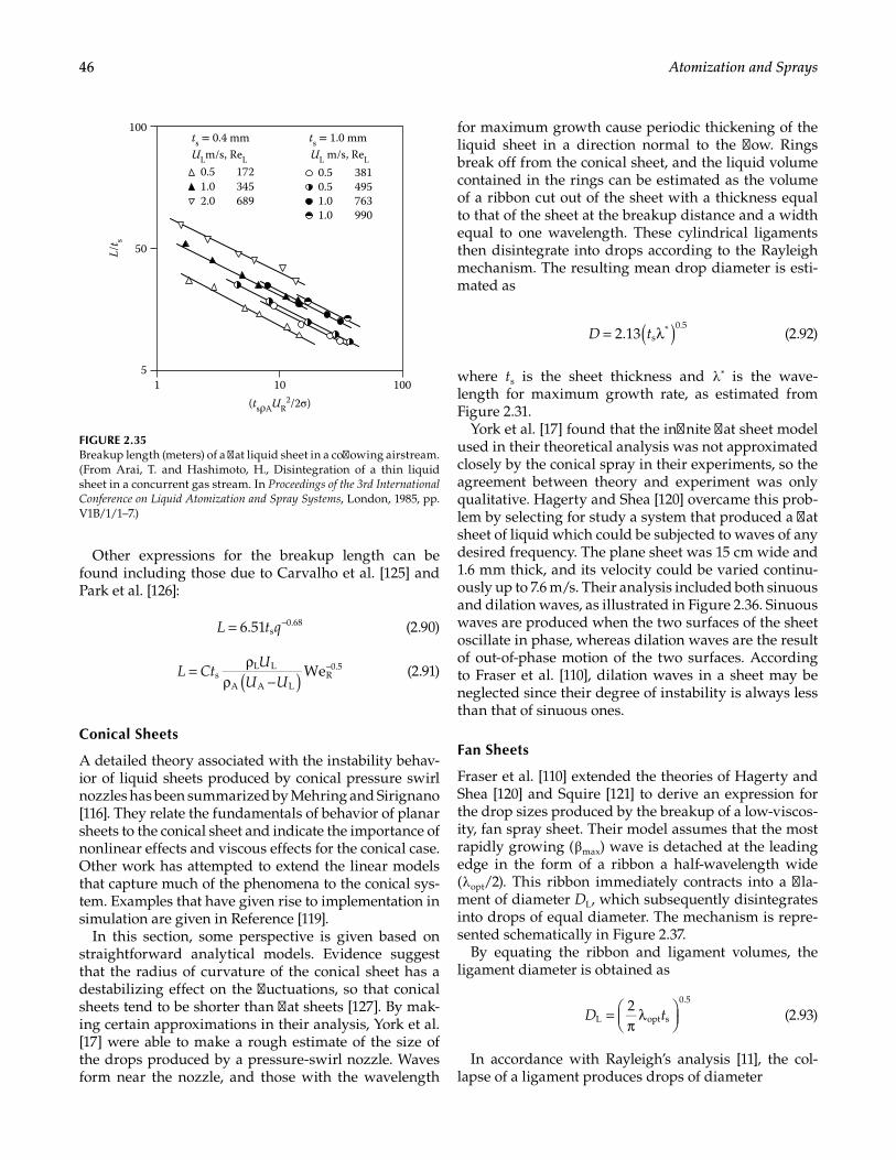
46 Atomization and Sprays

Other expressions for the breakup length can be found including those due to Carvalho et al. [125] and Park et al. [126]:

6.51 s0.68= −L t q (2.90)

WesL L

A A LR

0.5

( )= ρρ −

−L CtU

U U (2.91)

Conical Sheets

A detailed theory associated with the instability behav-ior of liquid sheets produced by conical pressure swirl nozzles has been summarized by Mehring and Sirignano [116]. They relate the fundamentals of behavior of planar sheets to the conical sheet and indicate the importance of nonlinear effects and viscous effects for the conical case. Other work has attempted to extend the linear models that capture much of the phenomena to the conical sys-tem. Examples that have given rise to implementation in simulation are given in Reference [119].

In this section, some perspective is given based on straightforward analytical models. Evidence suggest that the radius of curvature of the conical sheet has a destabilizing effect on the fluctuations, so that conical sheets tend to be shorter than flat sheets [127]. By mak-ing certain approximations in their analysis, York et al. [17] were able to make a rough estimate of the size of the drops produced by a pressure-swirl nozzle. Waves form near the nozzle, and those with the wavelength

for maximum growth cause periodic thickening of the liquid sheet in a direction normal to the flow. Rings break off from the conical sheet, and the liquid volume contained in the rings can be estimated as the volume of a ribbon cut out of the sheet with a thickness equal to that of the sheet at the breakup distance and a width equal to one wavelength. These cylindrical ligaments then disintegrate into drops according to the Rayleigh mechanism. The resulting mean drop diameter is esti-mated as

2.13 s* 0.5( )= λD t (2.92)

where ts is the sheet thickness and  λ * is the wave-length for maximum growth rate, as estimated from Figure 2.31.

York et al. [17] found that the infinite flat sheet model used in their theoretical analysis was not approximated closely by the conical spray in their experiments, so the agreement between theory and experiment was only qualitative. Hagerty and Shea [120] overcame this prob-lem by selecting for study a system that produced a flat sheet of liquid which could be subjected to waves of any desired frequency. The plane sheet was 15 cm wide and 1.6 mm thick, and its velocity could be varied continu-ously up to 7.6 m/s. Their analysis included both sinuous and dilation waves, as illustrated in Figure 2.36. Sinuous waves are produced when the two surfaces of the sheet oscillate in phase, whereas dilation waves are the result of out-of-phase motion of the two surfaces. According to Fraser et al. [110], dilation waves in a sheet may be neglected since their degree of instability is always less than that of sinuous ones.

Fan Sheets

Fraser et al. [110] extended the theories of Hagerty and Shea [120] and Squire [121] to derive an expression for the drop sizes produced by the breakup of a low-viscos-ity, fan spray sheet. Their model assumes that the most rapidly growing ( β max) wave is detached at the leading edge in the form of a ribbon a half-wavelength wide ( λ opt/2). This ribbon immediately contracts into a fila-ment of diameter DL, which subsequently disintegrates into drops of equal diameter. The mechanism is repre-sented schematically in Figure 2.37.

By equating the ribbon and ligament volumes, the ligament diameter is obtained as

2

L opt s

0.5

=π

λ

D t (2.93)

In accordance with Rayleigh’s analysis [11], the col-lapse of a ligament produces drops of diameter

0.50.5

ts = 0.4 mm ts = 1.0 mmULm/s, ReL UL m/s, ReL

1.02.0

381

51 10

(tsρAUR2/2σ)

100

50

100

172345689

495763990

0.51.01.0

L/t s

FIGURE 2.35Breakup length (meters) of a flat liquid sheet in a coflowing airstream. (From Arai, T. and Hashimoto, H., Disintegration of a thin liquid sheet in a concurrent gas stream. In Proceedings of the 3rd International Conference on Liquid Atomization and Spray Systems, London, 1985, pp. V1B/1/1–7.)

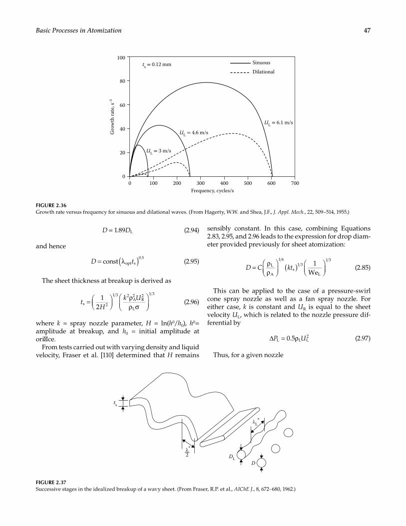
47Basic Processes in Atomization

1.89 L=D D (2.94)

and hence

const opt s0.5( )= λD t (2.95)

The sheet thickness at breakup is derived as

1

2s 2

1 3 2A2

R2

L

1 3

=

ρρ σ

tH

k U (2.96)

where k = spray nozzle parameter, H = ln(h0/h0), h0= amplitude at breakup, and h0 = initial amplitude at orifice.

From tests carried out with varying density and liquid velocity, Fraser et al. [110] determined that H remains

sensibly constant. In this case, combining Equations 2.83, 2.95, and 2.96 leads to the expression for drop diam-eter provided previously for sheet atomization:

( )= ρρ

1We

L

A

1 6

s1 3

L

1 3

D C kt (2.85)

This can be applied to the case of a pressure-swirl cone spray nozzle as well as a fan spray nozzle. For either case, k is constant and UR is equal to the sheet velocity UL, which is related to the nozzle pressure dif-ferential by

0.5L L L2∆ = ρP U (2.97)

Thus, for a given nozzle

ts = 0.12 mm

0

80

Sinuous

Dilational

UL = 4.6 m/s

UL = 3 m/s

UL = 6.1 m/s

60

40

20

100

0 600500400300200100 700Frequency, cycles/s

Gro

wth

rate

, s–1

FIGURE 2.36Growth rate versus frequency for sinuous and dilational waves. (From Hagerty, W.W. and Shea, J.F., J. Appl. Mech., 22, 509–514, 1955.)

λL*

DDL

λ*2

ts

FIGURE 2.37Successive stages in the idealized breakup of a wavy sheet. (From Fraser, R.P. et al., AIChE J., 8, 672–680, 1962.)

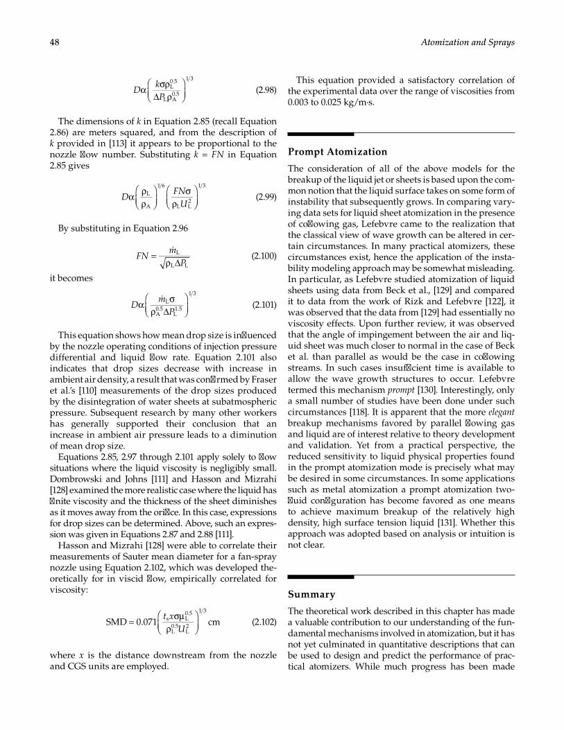
48 Atomization and Sprays

L0.5

L A0.5

1 3

α σρ∆ ρ

DkP

(2.98)

The dimensions of k in Equation 2.85 (recall Equation 2.86) are meters squared, and from the description of k provided in [113] it appears to be proportional to the nozzle flow number. Substituting k = FN in Equation 2.85 gives

L

A

1 6

L L2

1 3

α ρρ

σρ

DFN

U (2.99)

By substituting in Equation 2.96

L

L L=

ρ ∆FN

mP

(2.100)

it becomes

L

A0.5

L1.5

1 3

α σρ ∆

Dm

P (2.101)

This equation shows how mean drop size is influenced by the nozzle operating conditions of injection pressure differential and liquid flow rate. Equation 2.101 also indicates that drop sizes decrease with increase in ambient air density, a result that was confirmed by Fraser et al.’s [110] measurements of the drop sizes produced by the disintegration of water sheets at subatmospheric pressure. Subsequent research by many other workers has generally supported their conclusion that an increase in ambient air pressure leads to a diminution of mean drop size.

Equations 2.85, 2.97 through 2.101 apply solely to flow situations where the liquid viscosity is negligibly small. Dombrowski and Johns [111] and Hasson and Mizrahi [128] examined the more realistic case where the liquid has finite viscosity and the thickness of the sheet diminishes as it moves away from the orifice. In this case, expressions for drop sizes can be determined. Above, such an expres-sion was given in Equations 2.87 and 2.88 [111].

Hasson and Mizrahi [128] were able to correlate their measurements of Sauter mean diameter for a fan-spray nozzle using Equation 2.102, which was developed the-oretically for in viscid flow, empirically correlated for viscosity:

SMD 0.071 cms L0.5

L0.5

L2

1 3

= σµρ

t xU

(2.102)

where x is the distance downstream from the nozzle and CGS units are employed.

This equation provided a satisfactory correlation of the experimental data over the range of viscosities from 0.003 to 0.025 kg/m·s.

Prompt Atomization

The consideration of all of the above models for the breakup of the liquid jet or sheets is based upon the com-mon notion that the liquid surface takes on some form of instability that subsequently grows. In comparing vary-ing data sets for liquid sheet atomization in the presence of coflowing gas, Lefebvre came to the realization that the classical view of wave growth can be altered in cer-tain circumstances. In many practical atomizers, these circumstances exist, hence the application of the insta-bility modeling approach may be somewhat misleading. In particular, as Lefebvre studied atomization of liquid sheets using data from Beck et al., [129] and compared it to data from the work of Rizk and Lefebvre [122], it was observed that the data from [129] had essentially no viscosity effects. Upon further review, it was observed that the angle of impingement between the air and liq-uid sheet was much closer to normal in the case of Beck et al. than parallel as would be the case in coflowing streams. In such cases insufficient time is available to allow the wave growth structures to occur. Lefebvre termed this mechanism prompt [130]. Interestingly, only a small number of studies have been done under such circumstances [118]. It is apparent that the more elegant breakup mechanisms favored by parallel flowing gas and liquid are of interest relative to theory development and validation. Yet from a practical perspective, the reduced sensitivity to liquid physical properties found in the prompt atomization mode is precisely what may be desired in some circumstances. In some applications such as metal atomization a prompt atomization two-fluid configuration has become favored as one means to achieve maximum breakup of the relatively high density, high surface tension liquid [131]. Whether this approach was adopted based on analysis or intuition is not clear.

Summary

The theoretical work described in this chapter has made a valuable contribution to our understanding of the fun-damental mechanisms involved in atomization, but it has not yet culminated in quantitative descriptions that can be used to design and predict the performance of prac-tical atomizers. While much progress has been made

49Basic Processes in Atomization

with comprehensive modeling, prediction of the atomi-zation process from first principles remains an ongoing development. In addition, in order to do design work to screen atomizer designs, a need is apparent for simpli-fied tools. That is why most of the experimental data have been accumulated in the form of empirical and semiem-pirical equations of the type presented in Chapter 6. Nevertheless, from the theoretical, experimental, and photographic evidence now available, certain general conclusions can be drawn regarding the key factors that govern jet and sheet disintegration and the manner and extent of their influence on the drop sizes produced in the spray. It is now clear that important spray characteristics, such as mean drop size and drop size distribution, are dependent on a large number of variables such as noz-zle geometry, the physical properties of the liquid being atomized, and the physical properties, turbulence char-acteristics, and flow conditions in the surrounding gas.

The scope of this chapter has been limited to homoge-neous liquids and with generally Newtonian behavior. That said, the role of heterogeneous liquid atomization (e.g., with bubbles of gas or immiscible mixtures of oil and water) will be touched on in subsequent chapters in terms of atomization performance. Also, in some appli-cations, the liquid may be injected into an environment that is supercritical. Again, this is touched on in sub-sequent chapters, but the detailed theory underlying these cases is currently a work in progress. The reader is encouraged to consider the body of work from the Air Force Research Laboratory relative to supercritical injec-tion such as the work of Talley, Mayer, Woodward, and Cheroudi among others.

Both theoretical and experimental studies on jet and sheet disintegration have demonstrated the need to group these variables into nondimensional parameters to clarify their effects on the atomization process. As in most flow systems, the Reynolds grouping, which rep-resents the ratio of momentum forces to viscous drag forces, usefully describes the flow state of the emerg-ing jet in terms of both velocity profile and the magni-tude of the radial velocity components that promote jet disintegration. The flow characteristics most relevant to atomization are velocity, velocity profile, and turbulence properties, all of which can contribute effectively to jet or sheet disintegration, especially under conditions where aerodynamic influences are relatively small.

In reality, aerodynamic forces are seldom small, and the Weber number, which represents the ratio of the disruptive aerodynamic forces to the restoring surface tension forces, becomes very significant. In fact, for low-viscosity liquids subjected to ambient gas at high rela-tive velocities, the Weber grouping becomes dominant.

Another important dimensionless grouping is the Ohnesorge number. This group contains only the

properties of the globules formed in primary atomiza-tion before they split up into smaller drops during sec-ondary atomization. It is sometimes called a stability group because it provides an indication of the resistance of a globule to further disintegration, but it is also called a viscosity group because it accounts for the effect of liquid viscosity on the globule. Other dimensionless groups are obtained as the density ratios of the gas and liquid phases and various geometric ratios of the spray generating sys-tem. In cases where the interaction between the gas and liquid is sudden and abrupt, it is evident that many of the concepts associated with classic atomization may need to be altered. For example, the concept that viscosity acts to delay breakup may not apply.

The fundamental principle of the disintegration of a liquid consists of increasing its surface area, usually in the form of a cylindrical rod or sheet, until it becomes unstable and disintegrates into drops. If the issuing jet is in laminar flow, a vibration in the jet or an external disturbance causes disintegration as predicted by the Rayleigh breakup mechanism. If the jet is fully turbu-lent, it can break up without the application of external aerodynamic forces. Jet or sheet disintegration is pro-moted by increases in relative velocity and is impaired by increases in liquid viscosity. Regardless of all other effects, the breakup process is always accelerated by air resistance, which increases with air density. Where the air resistance is high, as in most practical applications, the mutually opposing aerodynamic and surface ten-sion forces acting on the liquid surface give rise to oscil-lations and perturbations. Under favorable conditions these oscillations are amplified and the liquid body breaks up. Jets break up into drops, while sheets disinte-grate into ligaments and then into drops. If the drops so formed exceed the stable maximum limit, they further disintegrate into smaller drops until all the drops are below the critical size.

The random nature of the atomization process means that most sprays are characterized by a wide range of drop sizes. The methods used to describe and quantify drop size distributions form the subject of Chapter 3.

Nomenclature

MMD mass median diameter (D0.5)SMD Sauter mean diameter (D32)A area, m2

CD drag coefficientD drop diameter, mDL ligament diameter, md jet diameter, mdo orifice diameter, m

50 Atomization and Sprays

E rate of energy input per unit mass, J/kg·sEs potential surface energyf frequencyg acceleration due to gravity, kg·m/s2

h displacement (amplitude) of liquid from equilibrium position, m

h0 amplitude at orifice, mh0 amplitude at breakup, mht amplitude at time t, mk nozzle factor, m2

L breakup length, ml length of jet, mlo orifice length, mmD mass of drop, kgm mass flow rate, kg/sn order of mode of vibration, or wave number

of disturbing waveOh Ohnesorge number δ PL nozzle liquid pressure differential, Papt internal pressure, Papσ surface tension pressure, Paq momentum flux ratioqmax disturbance growth rateRe Reynolds numberr jet radius, mS maximum velocity gradient in external flow fieldtb breakup time, sts sheet thickness, mU axial velocity, m/su rms value of fluctuating velocity component,

m/sx distance downstream of nozzle, mW nozzle width, mWe Weber number β  number that determines growth rate of

disturbance δ  amplitude of disturbance, m γ  dimensionless wave number ( = 2π/ λ ) λ  wavelength of disturbance, m λ * wavelength for maximum growth rate, m Λ  radial inertial length scale of gas phase, mμ, dynamic viscosity, kg/m·s ρ  density, kg/m3

σ surface tension, kg/s2

 ω  natural frequency of vibrationΩ growth rate at dominant frequencyτ friction force per unit area, kg/m·s2

Subscripts

A airD dropL liquidR relative valueo initial value

crit critical valuemax maximum valuemin minimum valueopt optimum value

References

1. Tamada, S., and Shibaoka, Y., cited in Atomization—A survey and critique of the literature, by Lapple, C. E., Henry, J. P., and Blake, D. E., Stanford Research Institute Report No. 6, 1966.

2. Klüsener, O., The injection process in compressor less diesel engines, VDI Z., Vol. 77, No. 7, 107–110 February 1933.

3. Giffen, E., and Muraszew, A., The Atomization of Liquid Fuels, New York: John Wiley & Sons, 1953.

4. Gordon, D. G., Mechanism and speed of breakup of drops, J. Appl. Phys., Vol. 30, No. 11, 1959, pp. 1759–1761.

5. Lenard, P., Uber Regen, Meteorol. Z., Vol. 21, 1904, pp. 248–262.

6. Hochschwender, E., Mechanism and Speed of Breakup of Drops, Ph.D. thesis, University of Heidelberg, Heidelberg, Germany, 1949.

7. Hinze, J. O., Fundamentals of the hydrodynamic mecha-nism of splitting in dispersion processes, AlChE J., Vol. 1, No. 3, 1955, pp. 289–295.

8. Castelman, R. A., The mechanism of the atomization of liq-uids, J. Res. Natl. Bur. Stand., Vol. 6, No. 281, 1931, pp. 369–376.

9. Merrington, A. C., and Richardson, E. G., The breakup of liquid jets, Proc. Phys. Soc. Lond., Vol. 59, No. 331, 1947, pp. 1–13.

10. Taylor, G. I., The function of emulsion in definable field flow, Proc. R. Soc. Lond. Ser. A., Vol. 146, 1934, pp. 501–523.

11. Rayleigh, L., On the instability of jets, Proc. Lond. Math. Soc., Vol. 10, 1878, pp. 4–13.

12. Haenlein, A., Disintegration of a liquid jet, NACA TN 659, 1932.

13. Ohnesorge, W., Formation of drops by nozzles and the breakup of liquid jets, Z. Angew. Math. Mech., Vol. 16, 1936, pp. 355–358.

14. Sauter, J., Determining size of drops in fuel mixture of internal combustion engines, NACA TM 390, 1926.

15. Scheubel, F. N., On atomization in carburettors, NACA TM 644, 1931.

16. Castleman, R. A., Jr., The mechanism of the atomization accompanying solid injection, NACA Report 440, 1932.

17. York, J. L., Stubbs, H. F., and Tek, M. R., The mechanism of disintegration of liquid sheets, Trans. ASME, Vol. 75, 1953, pp. 1279–1286.

18. Lane, W. R., Shatter of drops in streams of air, Ind. Eng. Chem., Vol. 43, No. 6, 1951, pp. 1312–1317.

19. Haas, F. C., Stability of droplets suddenly exposed to a high velocity gas stream, AIChE J., Vol. 10, 1964, pp. 920–924.

20. Hanson, A. R., Domich, E. G., and Adams, H. S., Shock tube investigation of the breakup of drops by air blasts, Phys. Fluids, Vol. 6, 1963, pp. 1070–1080.

51Basic Processes in Atomization

21. Sleicher, C. A., Maximum drop size in turbulent flow, AIChE J., Vol. 8, 1962, pp. 471–477.

22. Brodkey, R. A., The Phenomena of Fluid Motions, Reading, MA: Addison-Wesley, 1967.

23. Gelfand, B. E., Droplet breakup phenomena in flows with velocity lag, Prog. Energy Combust. Sci., Vol. 22, 1995, pp. 201–265.

24. Hsiang, L. P., and Faeth, G. M., Drop deformation and breakup due to shock wave and steady disturbances, Int. J. Multiphase Flow, Vol. 21, 1995, pp. 545–560.

25. Pilch, M., and Erdman, C. A., Use of breakup time data and velocity history data to predict the maximum size of stable fragments of acceleration-induced breakup of a liq-uid drop, Int. J. Multiphase Flow, Vol. 13, 1987, pp. 741–757.

26. O’Rourke, P. J., and Amsden, A. A., The TAB method for numerical calculations of spray droplet breakup, SAE Paper 872089, 1987.

27. Tanner, F. X., Liquid jet atomization and droplet breakup modeling of non-evaporating diesel fuel sprays, SAE Paper 970050, 1997.

28. Ibrahim, E. A., Yang, H. Q., and Przekwas, A. J., Modeling of spray droplets deformation and breakup, J. Prop. Power, Vol. 9, 1993, pp. 651–654.

29. Chryssakis, C., and Assanis, A., A unified fuel spray breakup model for internal combustion engine applica-tion, Atomization Sprays, Vol. 18, 2008, pp. 275–426.

30. Chryssakis, C. A., Assanis, D. N., and Tanner, F. X., Atomization models, in: Ashgriz, N. (ed.), Handbook of Atomization and Sprays: Theory and Applications, New York: Springer, 2011.

31. Simmons, H. C., The atomization of liquids: Principles and methods, Parker Hannifin Report No. 7901/2-0, 1979.

32. Guildenbecher, D. R., Lopez-Rivera, C., and Sojka, P. E., Secondary atomization, Exp. Fluids, Vol. 46, 2009, pp. 371–402.

33. Kolmogorov, A. N., On the disintegration of drops in a turbulent flow, Dokl. Akad. Nauk SSSR, Vol. 66, 1949, pp. 825–828.

34. Batchelor, G. K., The Theory of Homogeneous Turbulence, Cambridge: University Press, 1956.

35. Clay, P. H., Proc. R. Acad. Sci. (Amsterdam), Vol. 43, 1940, p. 852.

36. Sevik, M., and Park, S. H., The splitting of drops and bubbles by turbulent fluid flow, J. Fluids Eng., Vol. 95, 1973, pp. 53–60.

37. Prevish, T. D., and Santavicca, D. A., Turbulent Breakup of Hydrocarbon Droplets at Elevated Pressures, Sacramento: ILASS Americas, 1999.

38. Lasheras, J. C., Villermaux, E., and Hopfinger, E. J., Break-up and atomization of a round water jet by a high-speed annular jet, J. Fluid Mech., Vol. 357, 1998, pp. 351–379.

39. Andersson, R., and Andersson, B., On the breakup of fluid particles in turbulent flows, AIChE J., Vol. 52, 2006, pp. 2021–2030.

40. Andersson, R., and Andersson, B., Modeling the breakup of fluid particles in turbulent flows, AIChE J., Vol. 52, 2006, pp. 2031–2038.

41. Greenberg, J. B., Interacting sprays, in: Ashgriz, N. (ed.), Handbook of Atomization and Sprays: Theory and Applications, New York: Springer, 2011.

42. Tomotika, S., Breaking up of a drop of viscous liquid immersed in another viscous fluid which is extending at a uniform rate, Proc. R. Soc. London Ser. A., Vol. 153, 1936, pp. 302–320.

43. Meister, B. J., and Scheele, G. F., Drop formation from cylindrical jets in immiscible liquid system, AIChE J., Vol. 15, No. 5, 1969, pp. 700–706.

44. Miesse, C. C, Correlation of experimental data on the disintegration of liquid jets, Ind. Eng. Chem., Vol. 47, No. 9, 1955, pp. 1690–1701.

45. Rumscheidt, F. D., and Mason, S. G., Particle motion in sheared suspensions. deformation and burst of fluid drops in shear and hyperbolic flows, J. Colloid Sci., Vol. 16, 1967, pp. 238–261.

46. Krzywoblocki, M. A., Jets–Review of literature, Jet Propul., Vol. 26, 1957, pp. 760–779.

47. Schweitzer, P. H., Mechanism of disintegration of liquid jets, J. Appl. Phys., Vol. 8, 1937, pp. 513–521.

48. Marshall, W. R., Atomization and spray drying, Chem. Eng. Prog. Monogr. Ser., Vol. 50, No. 2, 1954, pp. 50–56.

49. Sterling, A. M., The Instability of Capillary Jets, Ph.D. thesis, University of Washington, Washington, 1969.

50. Phinney, R. E., The breakup of a turbulent liquid jet in a gaseous atmosphere, J. Fluid Mech., Vol. 60, 1973, pp. 689–701.

51. Bixson, L. L., and Deboi, H. H., Investigation of ratio-nal scaling procedure for liquid fuel rocket engines, Technical Documentary Report SSD-TDR-62-78, Rocket Research Laboratories, Edwards Air Force Base, California, 1962.

52. Kocamustafaogullari, G., Chen, I. Y., and Ishii, M., Unified theory for predicting maximum fluid par-ticle size for drops and bubbles, Argonne National Laboratory Report NUREG/CR-4028, 1984.

53. Lin, S. P., and Reitz, R. D., Drop and spray formation from a liquid jet, Annu. Rev. Fluid Mech., Vol. 30, 1998, pp. 85–105.

54. Lin, S. P., and Kang, D. J., Atomization of a liquid jet, Phys. Fluids, Vol. 30, 1987, pp. 2000–2006.

55. Yoon, S. S., and Heister, S. D., Categorizing linear theo-ries for atomizing round jets, Atomization Sprays, Vol. 13, 2003, pp. 499–516.

56. Birouk, M., and Lekic, N., Liquid jet breakup in quies-cent atmosphere: A review, Atomization Sprays, Vol. 19, 2009, pp. 501–528.

57. Sirignano, W. A., and Mehring, C., Review of theory of distortion and disintegration of liquid streams, Prog. Energy Combust., Vol. 26, 2000, pp. 609–655.

58. Bidone, G., Experiences sur la Forme et sur la Direction des Veines et des Courants d’Eau Lances par Diverses Ouvertures, Turin: Imprimerie Royale, 1829, pp. 1–136.

59. Savart, F., Memoire sur le choc d’une veine liquide lancee sur un plan circulaire, Ann. Chim. Phys., Vol. 53, 1833, pp. 337–386.

52 Atomization and Sprays

60. Plateau, J., Statique expérimentale et théorique des liquides soumis aux seules forces moléculaires, in: Rayleigh, L. (ed.), Theory of Sound, Vol. 2, New York: Dover Publications, 1945.

61. McCarthy, M. J., and Molloy, N. A., Review of stability of liquid jets and the influence of nozzle design, Chem. Eng. J., Vol. 7, 1974, pp. 1–20.

62. Tyler, F., Instability of liquid jets, Philos. Mag. (London), Vol. 16, 1933, pp. 504–518.

63. Weber, C., Disintegration of liquid jets, Z. Angew. Math. Mech., Vol. 11, No. 2, 1931, pp. 136–159.

64. Reitz, R. D., Atomization and Other Breakup Regimes of a Liquid Jet, Ph.D. thesis, Princeton University, Princeton, NJ, 1978.

65. Schiller, L., Untersuchungen ueber laminare und turbulente stromung, VDI Forschungsarbeit., Vol. 248, 1922, pp. 17–25.

66. Sterling, A. M., and Sleicher, C. A., The instability of cap-illary jets, J. Fluid Mech., Vol. 68, 1975, pp. 477–495.

67. Eisenklam, P., and Hooper, P. C., The flow characteristics of laminar and turbulent jets of liquid, Ministry of Supply D.G.G.W. Report/EMR/58/10, September 1958.

68. Rupe, J. H., Jet Propulsion Laboratory Report No. 32-207, January 1962.

69. Wu, P. K., Miranda, R. F., and Faeth, G. M., Effects of ini-tial flow conditions on primary breakup of non-turbu-lent and turbulent round liquid jets, Atomization Sprays, Vol. 5, 1995, pp. 175–196.

70. Reitz, R. D., Modeling atomization processes in high-pressure, vaporizing sprays, Atomization Spray Technol., Vol. 3, 1987, pp. 309–337.

71. Beale, J. C., and Reitz, R. D., Modeling spray atomiza-tion with the Kelvin-Helmholtz/Rayleigh-Taylor hybrid model, Atomization Sprays, Vol. 9, 1999, pp. 623–650.

72. Faeth, G. M., Hsiang, L. P., and Wu, P. K., Structure and breakup properties of sprays, Int. J. Multiphase Flows, Vol. 21, 1995, pp. 99–127.

73. Simmons, H. C., The correlation of drop-size distribu-tions in fuel nozzle sprays, J. Eng. Power, Vol. 99, 1977, pp. 309–319.

74. Yi, Y., and Reitz, R. D., Modeling the primary breakup of high-speed jets, Atomization Sprays, Vol. 14, 2004, pp. 53–80.

75. Grant, R. P., and Middleman, S., Newtonian jet stability, AIChE J., Vol. 12, No. 4, 1966, pp. 669–678.

76. Mahoney, T. J., and Sterling, M. A., The breakup length of laminar Newtonian liquid jets in air, in: Proceedings of the 1st International Conference on Liquid Atomization and Spray Systems, Tokyo, 1978, pp. 9–12.

77. Phinney, R. E., and Humphries, W., Stability of a Viscous Jet—Newtonian Liquids, NOLTR 70-5, January 1970, U.S. Naval Ordnance Laboratory, Silver Spring, MD.

78. Van de Sande, E., and Smith, J. M., Jet breakup and air entrainment by low-velocity turbulent jets, Chem. Eng. Sci., Vol. 31, No. 3, 1976, pp. 219–224.

79. Reitz, R. D., and Bracco, F. V., Mechanism of atomization of a liquid jet, Phys. Fluids, Vol. 25, No. 2, 1982, pp. 1730–1741.

80. Taylor, J. J., and Hoyt, J. W., Water jet photography—Techniques and methods, Exp. Fluids, Vol. 1, 1983, pp. 113–120.

81. DeJuhasz, K. J., Trans. ASME, Vol. 53, 1931, p. 65. 82. Bergwerk, W., Flow pattern in diesel nozzle spray holes,

Proc. Inst. Mech. Eng., Vol. 173, 1959, pp. 655–660. 83. Sadek, R., Communication on flow pattern in nozzle

spray holes and discharge coefficient of orifices, Proc. Inst. Mech. Eng., Vol. 173, No. 25, 1959, pp. 671–672.

84. Vitman, L. A., in: Kutateladze, S. S. (ed.), Problems of Heat Transfer and Hydraulics in Two-Phase Media, Moscow, 1961, p. 374.

85. Lienhard, J. H., and Day, J. B., The breakup of super-heated liquid jets, Trans. ASME J. Basic Eng. Ser. D., Vol. 92, No. 3, 1970, pp. 515–522.

86. Lafrance, P., The breakup length of turbulent liquid jets, Trans. ASME J. Fluids Eng., Vol 99, No. 2 June 1977, pp. 414–415.

87. Baron, T., Technical report No. 4, University of Illinois, 1949. 88. Tanasawa, Y., and Toyoda, S., On the Atomizing

Characteristics of High-Speed Jet I, Trans. Jpn. Soc. Mech., Vol. 20, 1954, p. 300.

89. Yoshizawa, Y., Kawashima, T., and Yanaida, K., Tohoku kozan, J. Tohoku Mining Soc., Vol. 11, 1964, p. 37.

90. Hiroyasu, H., Shimizu, M., and Arai, M., The breakup of high speed jet in a high pressure gaseous atmosphere, in: Proceedings of the 2nd International Conference on Liquid Atomization and Spray Systems, Madison, Wisconsin, 1982, pp. 69–74.

91. Arai, M., Shimizu, M., and Hiroyasu, H., Breakup length and spray angle of high speed jet, in: Proceedings of the 3rd International Conference on Liquid Atomization and Spray Systems, London, 1985, pp. IB/4/1–10.

92. Linne, M., Imaging in the optically dense regions of a spray: A review of developing techniques, Prog. Energ. Combust., Vol. 39, 2013, pp. 403–440.

93. Farago, Z., and Chigier, N., Morphological classifica-tion of disintegration of round liquid jets in a coaxial air stream, Atomization Sprays, Vol. 2, 1992, pp. 137–153.

94. Fritsching, U., Spray systems, in: Crowe, C. (ed.), Handbook of Multiphase Flows, Boca Raton, FL: CRC Press, 2005.

95. Lasheras, J. C., and Hopfinger, E. J., Liquid jet instability and atomization in a coaxial gas stream, Annu. Rev. Fluid Mech., Vol. 32, 2000, pp. 275–308.

96. Leroux, B., Delabroy, O., and Lacas, F., Experimental study of coaxial atomizers scaling, Part I: Dense core zone, Atomization Sprays, Vol. 17, 2007, pp. 381–407.

97. Engelbert, C., Hardalupus, Y., and Whitelaw, J., Breakup phenomena in coaxial airblast atomizers, Proc. R. Soc., Vol. 451, 1995, pp. 189–229.

98. Kitamura, Y., and Takahashi, T., Stability of a liquid jet in air flow normal to the jet axis, J. Chem. Eng. Jpn., Vol. 9, No. 4, 1976, pp. 282–286.

99. Schetz, J. A., and Padhye, A., Penetration and breakup of liquids in subsonic airstreams, AIAA J., Vol. 15, 1977, pp. 1385–1390.

100. Heister, S. D., Nguyen, T. T., and Karagozian, A. R., Modeling of liquid jets injected transversely into a super-sonic crossflow, AIAA J., Vol. 27, 1989, pp. 1727–1734.

101. Li, H. S., and Karagozian, A. R., Breakup of a liquid jet in supersonic crossflow, AIAA J., Vol. 30, 1992, pp. 1919–1921.

53Basic Processes in Atomization

102. Wu, P. K., Kirkendall, K. A., Fuller, R. P., and Nejad, A. S., Breakup processes of liquid jets in subsonic crossflow, J. Propul. Power, Vol. 14, 1998, pp. 64–73.

103. Wu, P. K., Kirkendall, K. A., Fuller, R. P., and Nejad, A. S., Spray structures of liquid jets atomized in subsonic crossflows, J. Propul. Power, Vol. 13, 1997, pp. 173–182.

104. Sallam, K. A., Aalburg, C., and Faeth, G. M., Breakup of round nonturbulent liquid jets in gaseous crossflow, AIAA J., Vol. 42, 2004, pp. 2529–2540.

105. Lee, K., Aalburg, C., Diez, F. J., Faeth, G. M, and Sallam, K. A., Primary breakup of turbulent round liquid jets in uniform crossflows, AIAA J., Vol. 45, 2007, pp. 1907–1916.

106. Wang, M., Broumand, M., and Birouk, M., Liquid jet tra-jectory in a subsonic gaseous crossflow: An analysis of published correlations, Atomization Sprays, Vol 26, No. 11, 2016, pp. 1083–1110.

107. Wang, Q., Mondragon, U. M., Brown, C. T., and McDonell, V. G., Characterization of trajectory, breakpoint, and breakpoint dynamics of a plain liquid jet in a crossflow, Atomization Sprays, Vol. 21, 2011, pp. 203–219.

108. Fraser, R. P., and Eisenklam, P., Research into the perfor-mance of atomizers for liquids, Imp. Coll. Chem. Eng. Soc. J., Vol. 7, 1953, pp. 52–68.

109. Fraser, R. P., Liquid fuel atomization, in: Sixth Symposium (International) on Combustion, Rein-hold, New York, 1957, pp. 687–701.

110. Fraser, R. P., Eisenklam, P., Dombrowski, N., and Hasson, D., Drop formation from rapidly moving sheets, AIChE J., Vol. 8, No. 5, 1962, pp. 672–680.

111. Dombrowski, N., and Johns, W. R., The aerodynamic instability and disintegration of viscous liquid sheets, Chem. Eng. Sci., Vol. 18, 1963, pp. 203–214.

112. Dombrowski, N., and Fraser, R. P., A photographic inves-tigation into the disintegration of liquid sheets, Philos. Trans. R. Soc. Lond. Ser. A Math. Phys. Sci., Vol. 247, No. 924, 1954, pp. 101–130.

113. Fraser, R. P., Dombrowski, N., and Routley, J. H., The atomization of a liquid sheet by an impinging air stream, Chem. Eng. Sci., Vol. 18, 1963, pp. 339–353.

114. Crapper, G. D., and Dombrowski, N., A note on the effect of forced disturbances on the stability of thin liquid sheets and on the resulting drop size, Int. J. Multiphase Flow, Vol. 10, No. 6, 1984, pp. 731–736.

115. Rangel, R., and Sirignano, W. A., The linear and non- linear shear instability of a fluid sheet, Phys. Fluids A., Vol. 3, 1999, pp. 2392–2400.

116. Mehring, C., and Sirignano, W. A., Review of theory of distortion and disintegration of liquid streams, Prog. Energy Combust. Sci., Vol. 26, 2000, pp. 609–655.

117. Lin, S. P., Breakup of Liquid Sheets and Jets, Cambridge: Cambridge Publishing, 2003.

118. Dumouchel, C., On the experimental investigation on primary atomization of liquid streams, Exp. Fluids, Vol. 45, 2008, pp. 371–422.

119. Senecal, P. K., Schmidt, D. P., Nouar, I., Rutland, C. J., Reitz, R. D., and Corradini, M. L., Modeling high-speed viscous liquid sheet atomization, Int. J. Multiphase Flows, Vol. 25, 1999, pp. 1073–1097.

120. Hagerty, W. W., and Shea, J. F., A study of the stability of plane fluid sheets, J. Appl. Mech., Vol. 22, No. 4, 1955, pp. 509–514.

121. Squire, H. B., Investigation of the instability of a moving liquid film, Br. J. Appl. Phys., Vol. 4, 1953, pp. 167–169.

122. Rizk, N. K., and Lefebvre, A. H., Influence of liquid film thickness on airblast atomization, Trans. ASME J. Eng. Power, Vol. 102, 1980, pp. 706–710.

123. El-Shanawany, M. S. M. R., and Lefebvre, A. H., Airblast atomization: The effect of linear scale on mean drop size, J. Energy, Vol. 4, No. 4, 1980, pp. 184–189.

124. Arai, T., and Hashimoto, H., Disintegration of a thin liquid sheet in a cocurrent gas stream, in: Proceedings of the 3rd International Conference on Liquid Atomization and Spray Systems, London, 1985, pp. V1B/1/1–7.

125. Carvalho, I. S., Heitor, M. V, and Santos, D., Liquid film disintegration regimes and proposed correlations, Int. J. Multiphase Flow, Vol. 28, 2002, pp. 773–789.

126. Park, J., Huh, K. Y., Li, X., and Renksizbulut, M., Experimental investigation on cellular breakup of a pla-nar liquid sheet from an air-blast nozzle, Phys. Fluids, Vol. 16, 2004, pp. 625–632.

127. Eisenklam, P., Recent research and development work on liquid atomization in Europe and the U.S.A., in: Paper presented at the 5th Conference on Liquid Atomization, Tokyo, 1976.

128. Hasson D., and Mizrahi, J., The drop size of fan spray nozzle, measurements by the solidifying wax method compared with those obtained by other sizing tech-niques, Trans. Inst. Chem. Eng., Vol. 39, No. 6, 1961, pp. 415–422.

129. Beck, J. E., Lefrevre, A. H., and Koblish, T. R., Airblast atomization at conditions of low air velocity, J. Prop. Power, Vol. 7, 1991, pp. 207–212.

130. Lefebvre, A. H., Energy considerations in twin-fluid atomization, J. Eng. Gas Turb. Power, Vol. 114, 1992, pp. 89–96.

131. Yule, A. J., and Dunkley, J. J., Atomization of Melts, New York: Oxford Press, 1994.

55

Introduction

A spray is generally considered as a system of drops immersed in a gaseous continuous phase. Examples of natural sprays include rain, drizzle, fog, and waterfall mists. Figure 3.1 [1] indicates the range of drop sizes as they occur in certain natural phenomena and also as commonly produced by atomizers.

Most practical atomizers generate drops in the size range from a few micrometers up to around 500 µm. Owing to the heterogeneous nature of the atomization process, the threads and ligaments formed by the various mechanisms of jet and sheet disintegration vary widely in diameter, and the resulting main drops and satellite drops vary in size correspondingly. Practical nozzles do not, therefore, pro-duce sprays of uniform drop size at any given operating condition; instead, the spray can be regarded as a spectrum of drop sizes distributed about some arbitrarily defined mean value. Only under certain special conditions (such as are obtained, e.g., with a rotary cup atomizer operating within a limited range of liquid flow rates and rotational speeds) can a fairly homogeneous spray be produced. Thus, in addition to mean drop size, another parameter of importance in the definition of a spray is the distribution of drop sizes it contains.

Graphical Representation of Drop Size Distributions

An instructive picture of drop size distribution may be obtained by plotting a histogram of drop size, each ordi-nate representing the number of drops whose dimen-sions fall between the limits D −  Δ D/2 and D +  Δ D/2. A typical histogram of this type is shown in Figure 3.2, in which  Δ D = 17 µm. If, instead of plotting the num-ber of drops, the volume of the spray corresponding to a range of drop sizes between D −  Δ D/2 and D +  Δ D/2 is plotted as a histogram of drop size, the resulting distri-bution is skewed to the right, as shown in Figure 3.3, due to the weighting effect of the larger drops.

As  Δ D is made smaller, the histogram assumes the form of a frequency curve that may be regarded as a

characteristic of the spray, provided it is based on suffi-ciently large samples. Such a curve, shown in Figure 3.4, is usually referred to as a frequency distribution curve. The ordinate values may be expressed in several alter-native ways: as the number of drops with a given diam-eter, the relative number or fraction of the total, or the fraction of the total number per size class. If the ordinate is expressed in the last manner, the area under the fre-quency distribution curve must be equal to 1.0.

It is evident that incremental frequency plots may be constructed directly from drop size distribution data by plotting  Δ Ni /N  Δ Di versus D or  Δ Qi /Q  Δ Di ver-sus D, where  Δ Ni is the number increment within  Δ Di and  Δ Qi is the volume increment within  Δ Di. The  Δ Qi can be obtained as

Q N D Di i i i∆ = ∆ π

+

6[0.5( )]3

1 2 (3.1)

where Di1 and Di2 are the upper and lower boundaries in the  Δ Di (ith) drop size class.

If the surface area or volume of the drops in the spray is plotted versus diameter, the distribution curve is again skewed to the right, as shown in Figure 3.4, due to the weighting effect of the larger diameters. Figure 3.5 [2] llustrates the use of this type of curve to demonstrate the effect on drop size distribution of a change in operating conditions, in this case an increase in air velocity through an airblast atomizer. Depending upon the application, the use of number, surface area, or volume-based distributions may be appropriate and/or of interest.

In addition to representing the drop size distribution with a frequency plot, it is also informative to use a cumu-lative distribution representation. This is essentially a plot of the integral of the frequency curve, and it may repre-sent the percentage of the total number of drops in the spray below a given size or the percentage of the total sur-face area or volume of a spray contained in drops below a given size. Cumulative distribution curves plotted on arithmetic coordinates have a general shape shown in Figure 3.6; the ordinate may be the percentage of drops by number, surface area, or volume whose diameter is less than a given drop diameter. Figure 3.7 shows cumulative distributions corresponding to the frequency distribution curves of Figure 3.5.

3Drop Size Distributions of Sprays

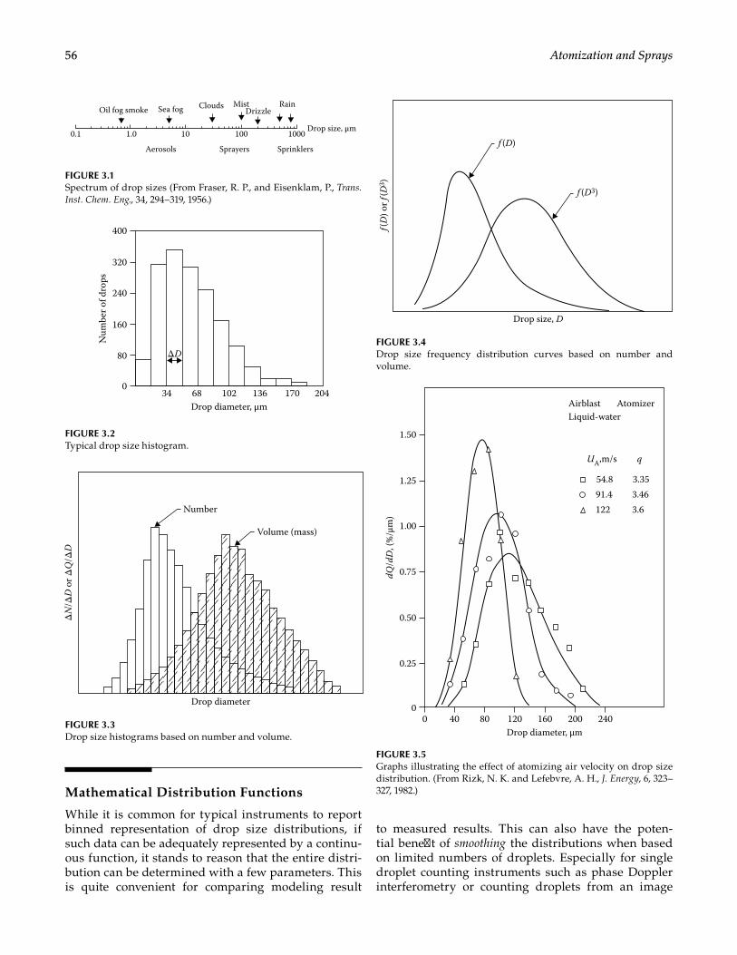
56 Atomization and Sprays

Mathematical Distribution Functions

While it is common for typical instruments to report binned representation of drop size distributions, if such data can be adequately represented by a continu-ous function, it stands to reason that the entire distri-bution can be determined with a few parameters. This is quite convenient for comparing modeling result

to measured results. This can also have the poten-tial benefit of smoothing the distributions when based on limited numbers of droplets. Especially for single droplet counting instruments such as phase Doppler interferometry or counting droplets from an image

Number

Volume (mass)

Drop diameter

ΔN

/ΔD

or Δ

Q/Δ

D

FIGURE 3.3Drop size histograms based on number and volume.

f (D)

f(D

) or f

(D3 )

f (D3)

Drop size, D

FIGURE 3.4Drop size frequency distribution curves based on number and volume.

Airblast

200160120Drop diameter, μm

dQ/d

D, (

%/μ

m)

8040

1.25

1.00

54.8

UA,m/s q

91.4122

3.353.463.6

0.75

0.50

0.25

00

1.50

240

Liquid-waterAtomizer

FIGURE 3.5Graphs illustrating the effect of atomizing air velocity on drop size distribution. (From Rizk, N. K. and Lefebvre, A. H., J. Energy, 6, 323–327, 1982.)

34

Num

ber o

f dro

ps

Drop diameter, μm

320

240

160

80

0

400

68 102 136 170 204

ΔD

FIGURE 3.2Typical drop size histogram.

CloudsSea fogOil fog smoke

0.1 1.0 10 100 1000

MistDrizzle

Rain

SprinklersSprayersAerosols

Drop size, μm

FIGURE 3.1Spectrum of drop sizes (From Fraser, R. P., and Eisenklam, P., Trans. Inst. Chem. Eng., 34, 294–319, 1956.)

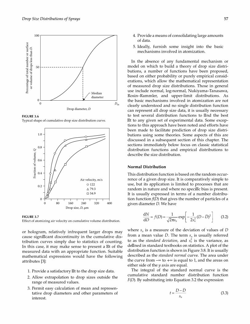
57Drop Size Distributions of Sprays

or hologram, relatively infrequent larger drops may cause significant discontinuity in the cumulative dis-tribution curves simply due to statistics of counting. In this case, it may make sense to present a fit of the measured data with an appropriate function. Suitable mathematical expressions would have the following attributes [3]:

1. Provide a satisfactory fit to the drop size data. 2. Allow extrapolation to drop sizes outside the

range of measured values. 3. Permit easy calculation of mean and represen-

tative drop diameters and other parameters of interest.

4. Provide a means of consolidating large amounts of data.

5. Ideally, furnish some insight into the basic mechanisms involved in atomization.

In the absence of any fundamental mechanism or model on which to build a theory of drop size distri-butions, a number of functions have been proposed, based on either probability or purely empirical consid-erations, which allow the mathematical representation of measured drop size distributions. Those in general use include normal, log-normal, Nukiyama–Tanasawa, Rosin–Rammler, and upper-limit distributions. As the basic mechanisms involved in atomization are not clearly understood and no single distribution function can represent all drop size data, it is usually necessary to test several distribution functions to find the best fit to any given set of experimental data. Some excep-tions to this approach have been noted and efforts have been made to facilitate prediction of drop size distri-butions using some theories. Some aspects of this are discussed in a subsequent section of this chapter. The sections immediately below focus on classic statistical distribution functions and empirical distributions to describe the size distribution.

Normal Distribution

This distribution function is based on the random occur-rence of a given drop size. It is comparatively simple to use, but its application is limited to processes that are random in nature and where no specific bias is present. It is usually expressed in terms of a number distribu-tion function f(D) that gives the number of particles of a given diameter D. We have

ND

f Ds s

D Dn n

= =π

− −

dd

( )1

2exp

12

( )22 (3.2)

where sn is a measure of the deviation of values of D from a mean value D. The term sn is usually referred to as the standard deviation, and sn

2 is the variance, as defined in standard textbooks on statistics. A plot of the distribution function is shown in Figure 3.8. It is usually described as the standard normal curve. The area under the curve from –∞ to +∞ is equal to 1, and the areas on either side of the y axis are equal.

The integral of the standard normal curve is the cumulative standard number distribution function F(D). By substituting into Equation 3.2 the expression

tD D

sn= −

(3.3)

50

Mediandiameter

Drop diameter, D

Perc

enta

ge o

f tot

al n

umbe

r or s

urfa

ceor

vol

ume

of d

rops

less

than

D.

100

00 Dm

FIGURE 3.6Typical shape of cumulative drop size distribution curve.

0.8

0.6

0.4

0.2

0

1.0

320240Drop size, D, μm

160800 400

54.979.3122

Air velocity, m/s

Frac

tion

of v

olum

e, Q

FIGURE 3.7Effect of atomizing air velocity on cumulative volume distribution.

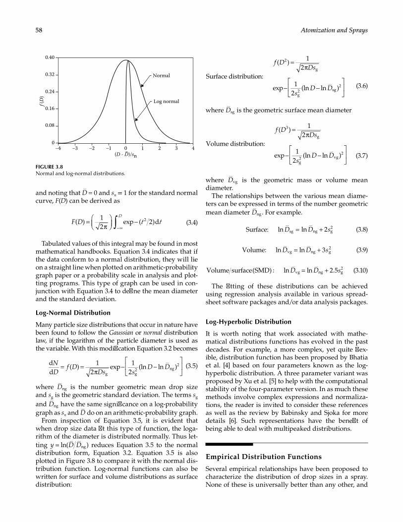
58 Atomization and Sprays

and noting that D = 0 and sn = 1 for the standard normal curve, F(D) can be derived as

t tF DD

∫=π

−−∞

( )12

exp ( 2)d2 (3.4)

Tabulated values of this integral may be found in most mathematical handbooks. Equation 3.4 indicates that if the data conform to a normal distribution, they will lie on a straight line when plotted on arithmetic- probability graph paper or a probability scale in analysis and plot-ting programs. This type of graph can be used in con-junction with Equation 3.4 to define the mean diameter and the standard deviation.

Log-Normal Distribution

Many particle size distributions that occur in nature have been found to follow the Gaussian or normal distribution law, if the logarithm of the particle diameter is used as the variable. With this modification Equation 3.2 becomes

= =π

− −

d

d( ) 1

2exp 1

2(ln ln )

g g2 ng

2ND

f DDs s

D D (3.5)

where Dng is the number geometric mean drop size and sg is the geometric standard deviation. The terms sg and Dng have the same significance on a log-probability graph as sn and D do on an arithmetic-probability graph.

From inspection of Equation 3.5, it is evident that when drop size data fit this type of function, the loga-rithm of the diameter is distributed normally. Thus let-ting y D D= ln( )ng reduces Equation 3.5 to the normal distribution form, Equation 3.2. Equation 3.5 is also plotted in Figure 3.8 to compare it with the normal dis-tribution function. Log-normal functions can also be written for surface and volume distributions as surface distribution:

=π

− −

Surface distribution:

( ) 12

exp 12

(ln ln )

2

g

g2 sg

2

f DDs

sD D (3.6)

where Dsg is the geometric surface mean diameter

=π

− −

Volume distribution:

( ) 12

exp 12

(ln ln )

3

g

g2 vg

2

f DDs

sD D (3.7)

where Dvg is the geometric mass or volume mean diameter.

The relationships between the various mean diame-ters can be expressed in terms of the number geometric mean diameter Dng. For example.

D D s= +Surface: ln ln 2sg ng g2 (3.8)

D D s= +Volume: ln ln 3vg ng g2 (3.9)

D D s= +Volume surface(SMD) : ln ln 2.5vg ng g2 (3.10)

The fitting of these distributions can be achieved using regression analysis available in various spread-sheet software packages and/or data analysis packages.

Log-Hyperbolic Distribution

It is worth noting that work associated with mathe-matical distributions functions has evolved in the past decades. For example, a more complex, yet quite flex-ible, distribution function has been proposed by Bhatia et al. [4] based on four parameters known as the log-hyperbolic distribution. A three parameter variant was proposed by Xu et al. [5] to help with the computational stability of the four-parameter version. In as much these methods involve complex expressions and normaliza-tions, the reader is invited to consider these references as well as the review by Babinsky and Sjoka for more details [6]. Such representations have the benefit of being able to deal with multipeaked distributions.

Empirical Distribution Functions

Several empirical relationships have been proposed to characterize the distribution of drop sizes in a spray. None of these is universally better than any other, and

–4 –3 –2 –1 0

0.32

0.24

0.16

f (D

)

0.08

0

0.40

1 2 3 4

Log normal

Normal

(D - D)/sn

FIGURE 3.8Normal and log-normal distributions.

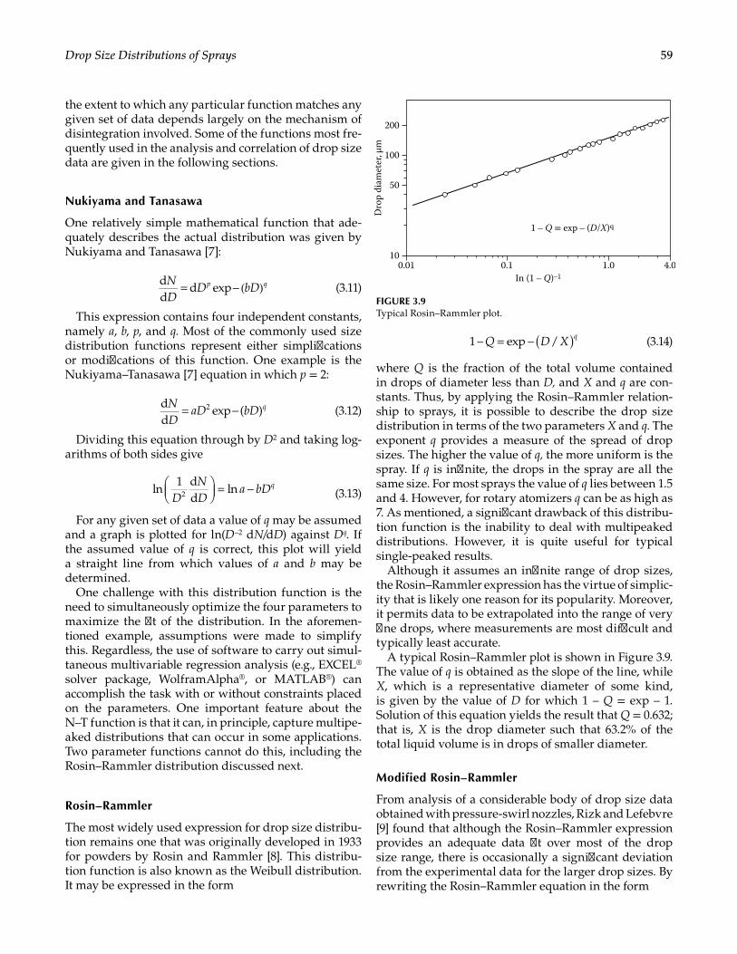
59Drop Size Distributions of Sprays

the extent to which any particular function matches any given set of data depends largely on the mechanism of disintegration involved. Some of the functions most fre-quently used in the analysis and correlation of drop size data are given in the following sections.

Nukiyama and Tanasawa

One relatively simple mathematical function that ade-quately describes the actual distribution was given by Nukiyama and Tanasawa [7]:

= − ( )dd

d expND

D bDp q (3.11)

This expression contains four independent constants, namely a, b, p, and q. Most of the commonly used size distribution functions represent either simplifications or modifications of this function. One example is the Nukiyama–Tanasawa [7] equation in which p = 2:

= −dd

exp ( )2ND

aD bD q (3.12)

Dividing this equation through by D2 and taking log-arithms of both sides give

DND

a bDq

= −ln

1 dd

ln2 (3.13)

For any given set of data a value of q may be assumed and a graph is plotted for ln(D–2 dN/dD) against Dq. If the assumed value of q is correct, this plot will yield a straight line from which values of a and b may be determined.

One challenge with this distribution function is the need to simultaneously optimize the four parameters to maximize the fit of the distribution. In the aforemen-tioned example, assumptions were made to simplify this. Regardless, the use of software to carry out simul-taneous multivariable regression analysis (e.g., EXCEL® solver package, WolframAlpha®, or MATLAB®) can accomplish the task with or without constraints placed on the parameters. One important feature about the N–T function is that it can, in principle, capture multipe-aked distributions that can occur in some applications. Two parameter functions cannot do this, including the Rosin–Rammler distribution discussed next.

Rosin–Rammler

The most widely used expression for drop size distribu-tion remains one that was originally developed in 1933 for powders by Rosin and Rammler [8]. This distribu-tion function is also known as the Weibull distribution. It may be expressed in the form

Q D X q( )=1 – exp – / (3.14)

where Q is the fraction of the total volume contained in drops of diameter less than D, and X and q are con-stants. Thus, by applying the Rosin–Rammler relation-ship to sprays, it is possible to describe the drop size distribution in terms of the two parameters X and q. The exponent q provides a measure of the spread of drop sizes. The higher the value of q, the more uniform is the spray. If q is infinite, the drops in the spray are all the same size. For most sprays the value of q lies between 1.5 and 4. However, for rotary atomizers q can be as high as 7. As mentioned, a significant drawback of this distribu-tion function is the inability to deal with multipeaked distributions. However, it is quite useful for typical single- peaked results.

Although it assumes an infinite range of drop sizes, the Rosin–Rammler expression has the virtue of simplic-ity that is likely one reason for its popularity. Moreover, it permits data to be extrapolated into the range of very fine drops, where measurements are most difficult and typically least accurate.

A typical Rosin–Rammler plot is shown in Figure 3.9. The value of q is obtained as the slope of the line, while X, which is a representative diameter of some kind, is given by the value of D for which 1 – Q = exp – 1. Solution of this equation yields the result that Q = 0.632; that is, X is the drop diameter such that 63.2% of the total liquid volume is in drops of smaller diameter.

Modified Rosin–Rammler

From analysis of a considerable body of drop size data obtained with pressure-swirl nozzles, Rizk and Lefebvre [9] found that although the Rosin–Rammler expression provides an adequate data fit over most of the drop size range, there is occasionally a significant deviation from the experimental data for the larger drop sizes. By rewriting the Rosin–Rammler equation in the form

100.01 0.1

1 – Q = exp – (D/X)q

In (1 – Q)–11.0 4.0

200

100

50

Dro

p di

amet

er, μ

m

FIGURE 3.9Typical Rosin–Rammler plot.

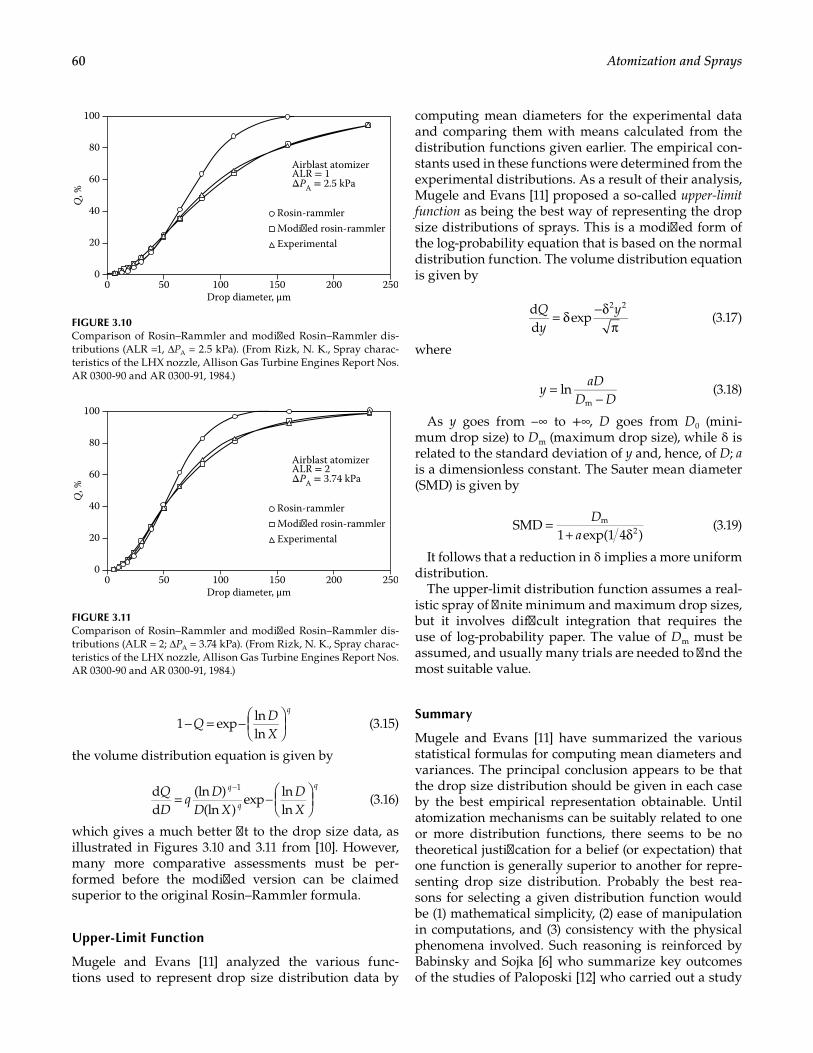
60 Atomization and Sprays

− = −

1 exp ln

lnQ

DX

q

(3.15)

the volume distribution equation is given by

= −

−dd

(ln )(ln )

exp lnln

1QD

qD

D XDX

q

q

q

(3.16)

which gives a much better fit to the drop size data, as illustrated in Figures 3.10 and 3.11 from [10]. However, many more comparative assessments must be per-formed before the modified version can be claimed superior to the original Rosin–Rammler formula.

Upper-Limit Function

Mugele and Evans [11] analyzed the various func-tions used to represent drop size distribution data by

computing mean diameters for the experimental data and comparing them with means calculated from the distribution functions given earlier. The empirical con-stants used in these functions were determined from the experimental distributions. As a result of their analysis, Mugele and Evans [11] proposed a so-called upper-limit function as being the best way of representing the drop size distributions of sprays. This is a modified form of the log-probability equation that is based on the normal distribution function. The volume distribution equation is given by

Qy

y= δ −δπ

dd

exp2 2

(3.17)

where

yaD

D D=

−ln

m (3.18)

As y goes from –∞ to +∞, D goes from D0 (mini-mum drop size) to Dm (maximum drop size), while  δ  is related to the standard deviation of y and, hence, of D; a is a dimensionless constant. The Sauter mean diameter (SMD) is given by

D

a=

+ δSMD

1 exp(1 4 )m

2 (3.19)

It follows that a reduction in  δ  implies a more uniform distribution.

The upper-limit distribution function assumes a real-istic spray of finite minimum and maximum drop sizes, but it involves difficult integration that requires the use of log-probability paper. The value of Dm must be assumed, and usually many trials are needed to find the most suitable value.

Summary

Mugele and Evans [11] have summarized the various statistical formulas for computing mean diameters and variances. The principal conclusion appears to be that the drop size distribution should be given in each case by the best empirical representation obtainable. Until atomization mechanisms can be suitably related to one or more distribution functions, there seems to be no theoretical justification for a belief (or expectation) that one function is generally superior to another for repre-senting drop size distribution. Probably the best rea-sons for selecting a given distribution function would be (1) mathematical simplicity, (2) ease of manipulation in computations, and (3) consistency with the physical phenomena involved. Such reasoning is reinforced by Babinsky and Sojka [6] who summarize key outcomes of the studies of Paloposki [12] who carried out a study

100

80

60

40

20

0200

Airblast atomizer

Rosin-rammlerModied rosin-rammlerExperimental

ALR = 1ΔPA = 2.5 kPa

150100500 250Drop diameter, μm

Q, %

FIGURE 3.10Comparison of Rosin–Rammler and modified Rosin–Rammler dis-tributions (ALR =1, DPA = 2.5 kPa). (From Rizk, N. K., Spray charac-teristics of the LHX nozzle, Allison Gas Turbine Engines Report Nos. AR 0300-90 and AR 0300-91, 1984.)

100

80

60

40

20

0200

Airblast atomizer

Rosin-rammlerModied rosin-rammlerExperimental

ALR = 2ΔPA = 3.74 kPa

150100500 250Drop diameter, μm

Q, %

FIGURE 3.11Comparison of Rosin–Rammler and modified Rosin–Rammler dis-tributions (ALR = 2; DPA = 3.74 kPa). (From Rizk, N. K., Spray charac-teristics of the LHX nozzle, Allison Gas Turbine Engines Report Nos. AR 0300-90 and AR 0300-91, 1984.)

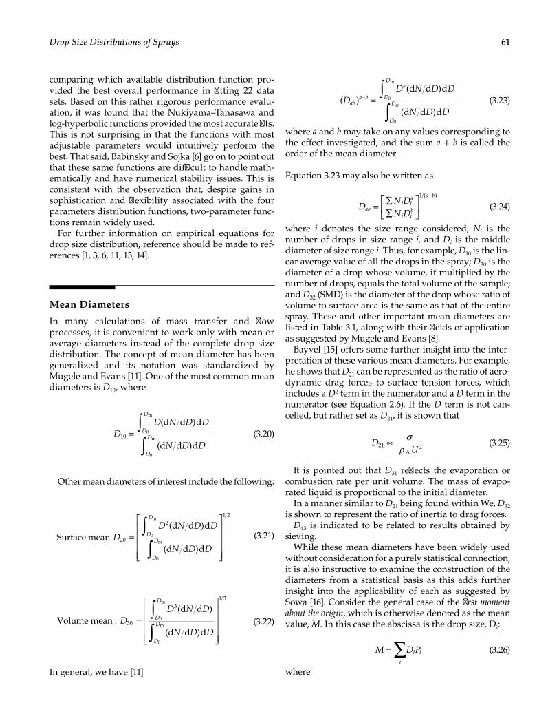
61Drop Size Distributions of Sprays

comparing which available distribution function pro-vided the best overall performance in fitting 22 data sets. Based on this rather rigorous performance evalu-ation, it was found that the Nukiyama–Tanasawa and log-hyperbolic functions provided the most accurate fits. This is not surprising in that the functions with most adjustable parameters would intuitively perform the best. That said, Babinsky and Sojka [6] go on to point out that these same functions are difficult to handle math-ematically and have numerical stability issues. This is consistent with the observation that, despite gains in sophistication and flexibility associated with the four parameters distribution functions, two- parameter func-tions remain widely used.

For further information on empirical equations for drop size distribution, reference should be made to ref-erences [1, 3, 6, 11, 13, 14].

Mean Diameters

In many calculations of mass transfer and flow processes, it is convenient to work only with mean or average diameters instead of the complete drop size distribution. The concept of mean diameter has been generalized and its notation was standardized by Mugele and Evans [11]. One of the most common mean diameters is D10, where

DD N D D

N D D

D

D

D

D

∫∫

=(d d )d

(d d )d10

0

m

0

m (3.20)

Other mean diameters of interest include the following:

DD N D D

N D D

D

D

D

D

∫∫

=

Surface mean(d d )d

(d d )d20

21 2

0

m

0

m

DD N D D

N D D

D

D

D

D

∫∫

=

Surface mean(d d )d

(d d )d20

21 2

0

m

0

m

DD N D D

N D D

D

D

D

D

∫∫

=

Surface mean(d d )d

(d d )d20

21 2

0

m

0

m (3.21)

DD N D

N D D

D

D

D

D

∫∫

=

Volume mean :(d d )

(d d )d30

31 3

0

m

0

m

DD N D

N D D

D

D

D

D

∫∫

=

Volume mean :(d d )

(d d )d30

31 3

0

m

0

m

DD N D

N D D

D

D

D

D

∫∫

=

Volume mean :(d d )

(d d )d30

31 3

0

m

0

m (3.22)

In general, we have [11]

DD N D D

N D Dab

a b

a

D

D

D

D

∫∫

=−( )(d d )d

(d d )d

0

m

0

m (3.23)

where a and b may take on any values corresponding to the effect investigated, and the sum a + b is called the order of the mean diameter.

Equation 3.23 may also be written as

DN DN D

abi i

a

i ib

a b

= ∑∑

−1 ( )

(3.24)

where i denotes the size range considered, Ni is the number of drops in size range i, and Di is the middle diameter of size range i. Thus, for example, D10 is the lin-ear average value of all the drops in the spray; D30 is the diameter of a drop whose volume, if multiplied by the number of drops, equals the total volume of the sample; and D32 (SMD) is the diameter of the drop whose ratio of volume to surface area is the same as that of the entire spray. These and other important mean diameters are listed in Table 3.1, along with their fields of application as suggested by Mugele and Evans [8].

Bayvel [15] offers some further insight into the inter-pretation of these various mean diameters. For example, he shows that D21 can be represented as the ratio of aero-dynamic drag forces to surface tension forces, which includes a D2 term in the numerator and a D term in the numerator (see Equation 2.6). If the D term is not can-celled, but rather set as D21, it is shown that

DU

σρ

∝21A

2 (3.25)

It is pointed out that D31 reflects the evaporation or combustion rate per unit volume. The mass of evapo-rated liquid is proportional to the initial diameter.

In a manner similar to D21 being found within We, D32 is shown to represent the ratio of inertia to drag forces.

D43 is indicated to be related to results obtained by sieving.

While these mean diameters have been widely used without consideration for a purely statistical connection, it is also instructive to examine the construction of the diameters from a statistical basis as this adds further insight into the applicability of each as suggested by Sowa [16]. Consider the general case of the first moment about the origin, which is otherwise denoted as the mean value, M. In this case the abscissa is the drop size, Di:

M D Pi

i i∑= (3.26)

where

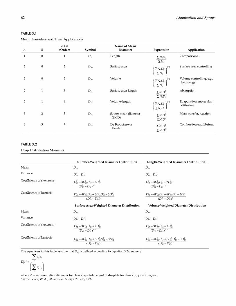
62 Atomization and Sprays

TABLE 3.1

Mean Diameters and Their Applications

A Ba + b

(Order) SymbolName of Mean

Diameter Expression Application

1 0 1 D10 Length N DN

i i

i

∑∑

Comparisons

2 0 2 D20 Surface areaN D

Ni i

i

∑∑

2 1/2 Surface area controlling

3 0 3 D30 VolumeN D

Ni i

i

∑∑

3 1/2 Volume controlling, e.g., hydrology

2 1 3 D21 Surface area-length N DN D

i i

i i

∑∑

2 Absorption

3 1 4 D31 Volume-lengthN DN D

i i

i i

∑∑

3 1/2 Evaporation, molecular diffusion

3 2 5 D32 Sauter mean diameter (SMD)

N DN D

i i

i i

∑∑

3

2

Mass transfer, reaction

4 3 7 D43 De Brouckere or Herdan

N DN D

i i

i i

∑∑

4

3

Combustion equilibrium

TABLE 3.2

Drop Distribution Moments

Number-Weighted Diameter Distribution Length-Weighted Diameter Distribution

Mean D10 D21

Variance D D−202

102 D D−31

2212

Coefficients of skewness D D D DD D− +

−3 2

( )303

202

10 103

202

102 3/2

D D D DD D− +

−3 2

( )413

312

21 213

312

212 3/2

Coefficients of kurtosis D D D D D DD D

− + −−

4 6 3( )

404

303

10 202

102

104

202

102 2

D D D D D DD D

− + −−

4 6 3( )

514

413

21 312

212

214

312

212 2

Surface Area-Weighted Diameter Distribution Volume-Weighted Diameter Distribution

Mean D32 D43

Variance D D−422

322 D D−53

2432

Coefficients of skewness D D D DD D− +

−3 2

( )523

422

32 323

422

322 3/2

D D D DD D− +

−3 2

( )633

532

43 433

532

432 3/2

Coefficients of kurtosis D D D D D DD D

− + −−

4 6 3( )

624

523

32 422

322

324

422

322 2

D D D D D DD D

− + −−

4 6 3( )

734

633

43 532

432

434

532

432 2

The equations in this table assume that Dpq is defined according to Equation 3.24, namely,

D

d n

d n

pqp q

iq

i

i

iq

i

i

∑

∑=

−

where di = representative diameter for class i; ni = total count of droplets for class i; p, q are integers.Source: Sowa, W. A., Atomization Sprays, 2, 1–15, 1992.

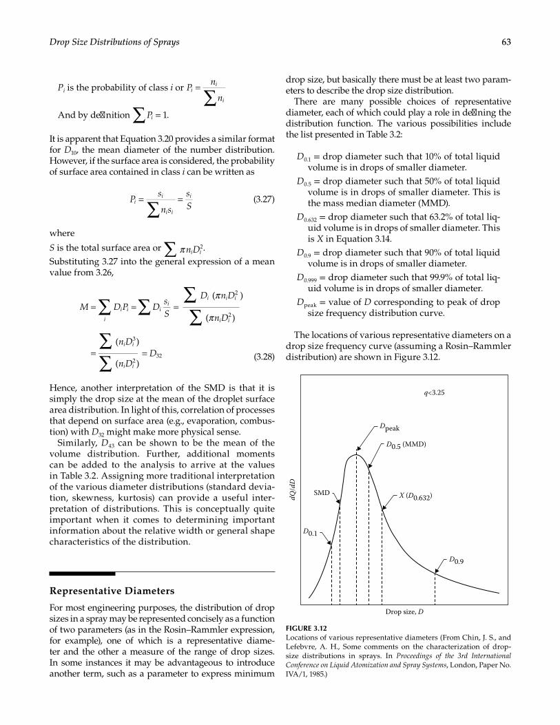
63Drop Size Distributions of Sprays

Pi is the probability of class i or Pn

ni

i

i∑=

And by definition Pi∑ = 1.

It is apparent that Equation 3.20 provides a similar format for D10, the mean diameter of the number distribution. However, if the surface area is considered, the probability of surface area contained in class i can be written as

Ps

n s

sS

ii

i i

i

∑= = (3.27)

where

S is the total surface area or n Di i∑ π 2.Substituting 3.27 into the general expression of a mean value from 3.26,

M D P DsS

D n D

n D

n D

n DD

i

i i ii

i i i

i i

i i

i i

∑ ∑∑∑

∑∑

π

π= = =

= =

( )

( )

( )

( )

2

2

3

232 (3.28)

Hence, another interpretation of the SMD is that it is simply the drop size at the mean of the droplet surface area distribution. In light of this, correlation of processes that depend on surface area (e.g., evaporation, combus-tion) with D32 might make more physical sense.

Similarly, D43 can be shown to be the mean of the volume distribution. Further, additional moments can be added to the analysis to arrive at the values in Table 3.2. Assigning more traditional interpretation of the various diameter distributions (standard devia-tion, skewness, kurtosis) can provide a useful inter-pretation of distributions. This is conceptually quite important when it comes to determining important information about the relative width or general shape characteristics of the distribution.

Representative Diameters

For most engineering purposes, the distribution of drop sizes in a spray may be represented concisely as a function of two parameters (as in the Rosin–Rammler expression, for example), one of which is a representative diame-ter and the other a measure of the range of drop sizes. In some instances it may be advantageous to introduce another term, such as a parameter to express minimum

drop size, but basically there must be at least two param-eters to describe the drop size distribution.

There are many possible choices of representative diameter, each of which could play a role in defining the distribution function. The various possibilities include the list presented in Table 3.2:

D0.1 = drop diameter such that 10% of total liquid volume is in drops of smaller diameter.

D0.5 = drop diameter such that 50% of total liquid volume is in drops of smaller diameter. This is the mass median diameter (MMD).

D0.632 = drop diameter such that 63.2% of total liq-uid volume is in drops of smaller diameter. This is X in Equation 3.14.

D0.9 = drop diameter such that 90% of total liquid volume is in drops of smaller diameter.

D0.999 = drop diameter such that 99.9% of total liq-uid volume is in drops of smaller diameter.

Dpeak = value of D corresponding to peak of drop size frequency distribution curve.

The locations of various representative diameters on a drop size frequency curve (assuming a Rosin–Rammler distribution) are shown in Figure 3.12.

Dpeak

D0.5 (MMD)

X (D0.632)

D0.9

D0.1

SMD

q<3.25

dQ/d

D

Drop size, D

FIGURE 3.12Locations of various representative diameters (From Chin, J. S., and Lefebvre, A. H., Some comments on the characterization of drop-size distributions in sprays. In Proceedings of the 3rd International Conference on Liquid Atomization and Spray Systems, London, Paper No. IVA/1, 1985.)

64 Atomization and Sprays

Chin and coworkers [17,18] have argued in support of the Rosin–Rammler distribution function, because it is simple to use and can readily be obtained using a standard drop size analyzer. A further useful advan-tage is that all the representative diameters in the spray are uniquely related to each other via the distribution parameter q. For example, we have [18]

q

q= Γ −

MMDSMD

(0.693) 111 (3.29)

where Г denotes the gamma function.This equation demonstrates that the ratio MMD/SMD

is not constant, as sometimes asserted, but is a unique function of q.

The definition of Dpeak is evident from inspection of Figure 3.12.

Clearly, at Dpeak. d2Q/dD2 = 0, so differentiation of Equation 3.14 gives

= − −

−

−

=

−

−

dd

( 1) exp

exp 0

2

2

2

1 2

q q

q

QD

DX

DX

DX

DX

q

q

q

q

q

q

(3.30)

Hence,

D

X q

q

= −

11peak

1

(3.31)

From Equation 3.14, we have

DX

q= (0.1054)0.1 1 (3.32)

DX

q= (2.3025)0.9 1 (3.33)

Also,

X

q=MMD(0.693)1 (3.34)

and

X q

= Γ −

−SMD

11

1

(3.35)

Other useful relationships are

D q=

MMD(0.152)0.1 1 (3.36)

D q=

MMD(3.32)0.9 1 (3.37)

D q=MMD

(9.968)0.999 1 (3.38)

Any of the mean diameters shown in Table 3.1 can be calculated conveniently using the following general expression:

D Xa qb q

ab a b=Γ + − Γ + −

−1 (( 3)/ )1 (( 3)/ )

(3.39)

It is of interest to examine where MMD and SMD lie on the distribution curve in relation to the peak diam-eter. From Equations 3.31 and 3.34 we have

D q

q

q

q

q

= − = −

MMD

(1 1 )(0.6931)

1.44281.4428peak

1

1

1

(3.40)

which shows that MMD = Dpeak when q = 3.2584. Referring to Figure 3.12, this means that MMD will appear on the left-hand side or the right-hand side of Dpeak depending on whether q is greater or less than 3.2584, respectively. From Equations 3.31 and 3.35 we have

D

q q

q

= −

Γ −

SMD

11

11peak

1

(3.41)

From this equation, it is apparent that Dpeak will always be larger than SMD, so SMD must always lie on the left-hand side of Dpeak.

Several representative diameters are defined in Table 3.3, and the ratios of different diameters are shown in Table 3.4 and Figures 3.13 through 3.15. Figures 3.16 and 3.17 show, respectively, the effects on the drop size frequency distribution curves and the cumulative drop size distribution curves of changes in SMD and q. These figures were calculated using Equation 3.43.

From inspection of Table 3.4, it is evident that

1. The ratio of MMD/SMD is always greater than 1. For q ≥ 3, it changes only little, as illustrated in Figure 3.15.

2. For a spray having q = 3, D0.9 is only 50% higher than D0.5, but for q ≤ 1.7, D0.9 is more than double D0.5.

3. For many sprays q lies between 2 and 2.8, and SMD is between 80% and 84% of the peak diameter.

From Equations 3.29 and 3.31 through 3.41 the general conclusion is that when the Rosin–Rammler expression is used, the ratio of any two representative diameters is always a unique function of q. In Equation 3.14, instead of using X, we can use any representative diameter and

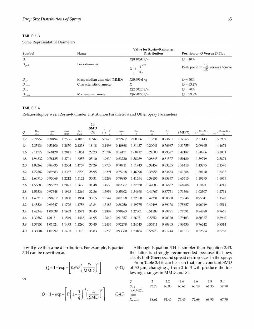
65Drop Size Distributions of Sprays

it will give the same distribution. For example, Equation 3.14 can be rewritten as

QD q

= − −

1 exp 0.693

MMD (3.42)

or

Qq

Dq q

= − − Γ −

−

1 exp 11

SMD (3.43)

Although Equation 3.14 is simpler than Equation 3.43, the latter is strongly recommended because it shows clearly both fineness and spread of drop sizes in the spray:

From Table 3.4 it can be seen that, for a constant SMD of 50 µm, changing q from 2 to 3 will produce the fol-lowing changes in MMD and X:

TABLE 3.3

Some Representative Diameters

Symbol NameValue for Rosin–Rammler

Distribution Position on Q Versus D Plot

D0.1 X(0.1054)1/q Q = 10%Dpeak Peak diameter

Xq

q

−

11

1/Peak point on

QD

dd

versus D curve

D0.5 Mass median diameter (MMD) X(0.693)1/q Q = 50%D0.632 Characteristic diameter X Q = 63.2%D0.9 X(2.3025)1/q Q = 90%D0.999 Maximum diameter X(6.9077)1/q Q = 99.9%

TABLE 3.4

Relationship between Rosin–Rammler Distribution Parameter q and Other Spray Parameters

Q DD

0.90.5

D

Dpeak

0.5

D

SMDpeak D

SMD0.5

Qat SMD (%)

q( )Γ −11 D

Xpeak D

X0.9 D

X0.1 D

X0.5 SMD/X D D

D∆ =

−0.1 0.1

0.5

D DD

∆ =−

B0.999 0.5

0.5

1.2 2.71952 0.30494 1.2506 4.1013 11.965 5.5673 0.22467 2.00376 0.15331 0.73681 0.17965 2.51143 5.7939

1.4 2.35134 0.53100 1.2870 2.4238 18.18 3.1496 0.40868 1.81437 0.20041 0.76967 0.31755 2.09695 4.1671

1.6 2.11772 0.68120 1.2841 1.8851 22.23 2.3707 0.54171 1.68417 0.24500 0.79527 0.42187 1.80966 3.2081

1.8 1.94832 0.78125 1.2701 1.6257 25.10 1.9930 0.63730 1.58939 0.28645 0.81577 0.50180 1.59719 2.5871

2.0 1.82262 0.84935 1.2534 1.4757 27.26 1.7727 0.70711 1.51743 0.32459 0.83255 0.56418 1.43275 2.1570

2.2 1.72582 0.89683 1.2367 1.3790 28.95 1.6291 0.75918 1.46098 0.35955 0.84654 0.61388 1.30110 1.8437

2.4 1.64910 0.93068 1.2212 1.3122 30.31 1.5288 0.79885 1.41554 0.39155 0.85837 0.65415 1.19295 1.6065

2.6 1.58685 0.95529 1.2071 1.2636 31.48 1.4550 0.82967 1.37820 0.42083 0.86852 0.68788 1.1023 1.4213

2.8 1.53536 0.97348 1.1943 1.2269 32.36 1.3956 0.85402 1.34698 0.44767 0.87731 0.71506 1.02507 1.2731

3.0 1.49210 0.98712 1.1830 1.1984 33.15 1.3542 0.87358 1.32050 0.47231 0.88500 0.73848 0.95841 1.1520

3.2 1.45524 0.99747 1.1726 1.1756 33.84 1.3183 0.88950 1.29775 0.49498 0.89178 0.75857 0.90019 1.0514

3.4 1.42348 1.00539 1.1633 1.1571 34.43 1.2889 0.90263 1.27801 0.51588 0.89781 0.77591 0.84888 0.9665

3.6 1.39582 1.0115 1.1549 1.1418 34.95 1.2642 0.91357 1.26071 0.5352 0.90320 0.79103 0.80327 0.8940

3.8 1.37154 1.01624 1.1473 1.1290 35.40 1.2434 0.92278 1.24543 0.55311 0.90805 0.80430 0.76242 0.8314

4.0 1.35004 1.01992 1.1403 1.118 35.83 1.2253 0.93060 1.23184 0.56973 0.91244 0.81613 0.72564 0.7768

Q 2 2.2 2.4 2.6 2.8 3.0D0.5

(MMD), µm

73.78 68.95 65.61 63.18 61.35 59.90

X, µm 88.62 81.45 76.45 72.69 69.93 67.70

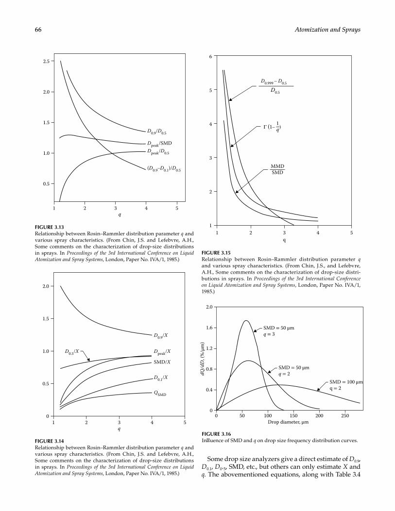
66 Atomization and Sprays

Some drop size analyzers give a direct estimate of D0.9, D0.1, D0.5, SMD, etc., but others can only estimate X and q. The abovementioned equations, along with Table 3.4

0.5

1 4

D0.9/D0.5

Dpeak/SMDDpeak/D0.5

(D0.9–D0.1)/D0.5

3q

2 5

2.0

1.5

1.0

2.5

FIGURE 3.13Relationship between Rosin–Rammler distribution parameter q and various spray characteristics. (From Chin, J.S. and Lefebvre, A.H., Some comments on the characterization of drop-size distributions in sprays. In Proceedings of the 3rd International Conference on Liquid Atomization and Spray Systems, London, Paper No. IVA/1, 1985.)

D0.9/X

D0.5/X

D0.1/X

Dpeak/X

QSMD

SMD/X

q

2.0

1

0.5

0

1.5

1.0

432 5

FIGURE 3.14Relationship between Rosin–Rammler distribution parameter q and various spray characteristics. (From Chin, J.S. and Lefebvre, A.H., Some comments on the characterization of drop-size distributions in sprays. In Proceedings of the 3rd International Conference on Liquid Atomization and Spray Systems, London, Paper No. IVA/1, 1985.)

2 3q

4 511

5

4

3

2

6

D0.999 – D0.5

D0.5

MMDSMD

(1– )1qΓ

FIGURE 3.15Relationship between Rosin–Rammler distribution parameter q and various spray characteristics. (From Chin, J.S., and Lefebvre, A.H., Some comments on the characterization of drop-size distri-butions in sprays. In Proceedings of the 3rd International Conference on Liquid Atomization and Spray Systems, London, Paper No. IVA/1, 1985.)

1.6

1.2

0.8

0.4

2.0

00 20015010050 250

Drop diameter, μm

SMD = 50 μmq = 3

SMD = 50 μmq = 2

SMD = 100 μmq = 2

dQ/d

D, (

%/μ

m)

FIGURE 3.16Influence of SMD and q on drop size frequency distribution curves.

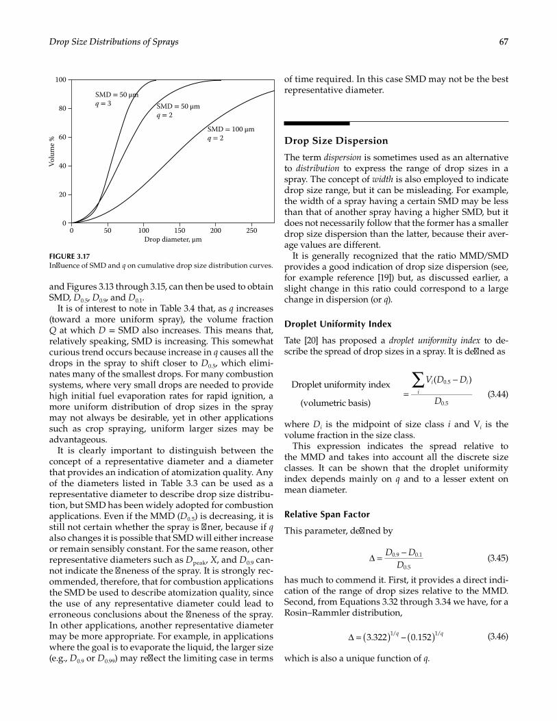
67Drop Size Distributions of Sprays

and Figures 3.13 through 3.15, can then be used to obtain SMD, D0.5, D0.9, and D0.1.

It is of interest to note in Table 3.4 that, as q increases (toward a more uniform spray), the volume fraction Q at which D = SMD also increases. This means that, relatively speaking, SMD is increasing. This somewhat curious trend occurs because increase in q causes all the drops in the spray to shift closer to D0.5, which elimi-nates many of the smallest drops. For many combustion systems, where very small drops are needed to provide high initial fuel evaporation rates for rapid ignition, a more uniform distribution of drop sizes in the spray may not always be desirable, yet in other applications such as crop spraying, uniform larger sizes may be advantageous.

It is clearly important to distinguish between the concept of a representative diameter and a diameter that provides an indication of atomization quality. Any of the diameters listed in Table 3.3 can be used as a representative diameter to describe drop size distribu-tion, but SMD has been widely adopted for combustion applications. Even if the MMD (D0.5) is decreasing, it is still not certain whether the spray is finer, because if q also changes it is possible that SMD will either increase or remain sensibly constant. For the same reason, other representative diameters such as Dpeak, X, and D0.9 can-not indicate the fineness of the spray. It is strongly rec-ommended, therefore, that for combustion applications the SMD be used to describe atomization quality, since the use of any representative diameter could lead to erroneous conclusions about the fineness of the spray. In other applications, another representative diameter may be more appropriate. For example, in applications where the goal is to evaporate the liquid, the larger size (e.g., D0.9 or D0.99) may reflect the limiting case in terms

of time required. In this case SMD may not be the best representative diameter.

Drop Size Dispersion

The term dispersion is sometimes used as an alternative to distribution to express the range of drop sizes in a spray. The concept of width is also employed to indicate drop size range, but it can be misleading. For example, the width of a spray having a certain SMD may be less than that of another spray having a higher SMD, but it does not necessarily follow that the former has a smaller drop size dispersion than the latter, because their aver-age values are different.

It is generally recognized that the ratio MMD/SMD provides a good indication of drop size dispersion (see, for example reference [19]) but, as discussed earlier, a slight change in this ratio could correspond to a large change in dispersion (or q).

Droplet Uniformity Index

Tate [20] has proposed a droplet uniformity index to de-scribe the spread of drop sizes in a spray. It is defined as

V D D

D

i i

i∑

=−Droplet uniformity index

(volumetric basis)

( )0.5

0.5 (3.44)

where Di is the midpoint of size class i and Vi is the volume fraction in the size class.

This expression indicates the spread relative to the MMD and takes into account all the discrete size classes. It can be shown that the droplet uniformity index depends mainly on q and to a lesser extent on mean diameter.

Relative Span Factor

This parameter, defined by

D D

D∆ = −0.9 0.1

0.5 (3.45)

has much to commend it. First, it provides a direct indi-cation of the range of drop sizes relative to the MMD. Second, from Equations 3.32 through 3.34 we have, for a Rosin–Rammler distribution,

q q( ) ( )∆ = 3.322 – 0.1521/ 1/ (3.46)

which is also a unique function of q.

0

80

60

40

20

0

100

20015010050 250Drop diameter, μm

SMD = 50 μmq = 3 SMD = 50 μm

q = 2

SMD = 100 μmq = 2

Volu

me

%

FIGURE 3.17Influence of SMD and q on cumulative drop size distribution curves.

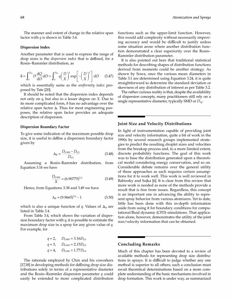
68 Atomization and Sprays

The manner and extent of change in the relative span factor with q is shown in Table 3.4.

Dispersion Index

Another parameter that is used to express the range of drop sizes is the dispersion index that is defined, for a Rosin–Rammler distribution, as

DQD

D qDX

DX

Dq qDD

∫∫δ = =

−

dd

d exp d00

mm

(3.47)

which is essentially same as the uniformity index pro-posed by Tate [20].

It should be noted that the dispersion index depends not only on q, but also to a lesser degree on X. Due to its more complicated form, δ has no advantage over the relative span factor Δ. Thus for most engineering pur-poses, the relative span factor provides an adequate description of dispersion.

Dispersion Boundary Factor

To give some indication of the maximum possible drop size, it is useful to define a dispersion boundary factor given by

D D

D∆ = −

B0.999 0.5

0.5 (3.48)

Assuming a Rosin–Rammler distribution, from Equation 3.14 we have

D

Xq= (6.90775)0.999 1 (3.49)

Hence, from Equations 3.38 and 3.49 we have

q∆ = −(9.9665) 1B1 (3.50)

which is also a unique function of q. Values of  Δ B are listed in Table 3.4.

From Table 3.4, which shows the variation of disper-sion boundary factor with q, it is possible to estimate the maximum drop size in a spray for any given value of q. For example, for

q D D

q D D

q D D

= == == =

2, 3.16

3, 2.15

4, 1.77

0.999 0.5

0.999 0.5

0.999 0.5

The rationale employed by Chin and his coworkers [17,18] in developing methods for defining drop size dis-tributions solely in terms of a representative diameter and the Rosin–Rammler dispersion parameter q could easily be extended to more complicated distribution

functions such as the upper-limit function. However, this would add complexity without necessarily improv-ing accuracy and would be difficult to justify unless some situation arose where another distribution func-tion demonstrated a clear superiority over the Rosin–Rammler distribution parameter.

It is also pointed out here that traditional statistical methods for describing shapes of distribution functions derived from moments could be another strategy. As shown by Sowa, once the various mean diameters in Table 3.1 are determined using Equation 3.24, it is quite straightforward to determine the standard deviation or skewness of any distribution of interest as per Table 3.2.

The rather curious reality is that, despite the availability of dispersion concepts, many practitioners still rely on a single representative diameter, typically SMD or D32.

Joint Size and Velocity Distributions

In light of instrumentation capable of providing joint size and velocity information, quite a bit of work in the 1990s by several research groups implemented strate-gies to predict the resulting droplet sizes and velocities from the breakup process and, to a more limited extent, discrete probability functions. The goal of this work was to base the distribution generated upon a theoreti-cal model considering energy conservation, and so on. Considerable debate remains over the general utility of these approaches as each requires certain assump-tions for it to work well. This work is well reviewed in Babinsky and Sojka [6]. It is clear from this review that more work is needed as none of the methods provide a result that is free from issues. Regardless, this concept is an important one in advancing the ability to repre-sent spray behavior from various atomizers. Yet to date, little has been done with this in-depth information aside from using it for boundary conditions for compu-tational fluid dynamic (CFD) simulations. That applica-tion alone, however, demonstrates the utility of the joint size/velocity information that can be obtained.

Concluding Remarks

Much of this chapter has been devoted to a review of available methods for representing drop size distribu-tions in sprays. It is difficult to judge whether any one method is superior to all others; such a conclusion must await theoretical determinations based on a more com-plete understanding of the basic mechanisms involved in drop formation. This work is under way, as summarized

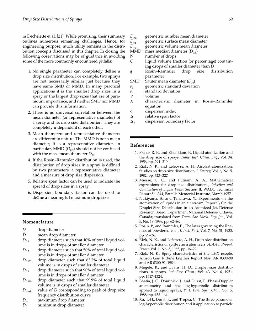
69Drop Size Distributions of Sprays

in Dechelette et al. [21]. While promising, their summary outlines numerous remaining challenges. Hence, for engineering purpose, much utility remains in the distri-bution concepts discussed in this chapter. In closing the following observations may be of guidance in avoiding some of the more commonly encountered pitfalls:

1. No single parameter can completely define a drop size distribution. For example, two sprays are not necessarily similar just because they have same SMD or MMD. In many practical applications it is the smallest drop sizes in a spray or the largest drop sizes that are of para-mount importance, and neither SMD nor MMD can provide this information.

2. There is no universal correlation between the mean diameter (or representative diameter) of a spray and its drop size distribution. They are completely independent of each other.

3. Mean diameters and representative diameters are different in nature. The MMD is not a mean diameter; it is a representative diameter. In particular, MMD (D0.5) should not be confused with the mass mean diameter D30.

4. If the Rosin–Rammler distribution is used, the distribution of drop sizes in a spray is defined by two parameters, a representative diameter and a measure of drop size dispersion.

5. Relative span factor can be used to indicate the spread of drop sizes in a spray.

6. Dispersion boundary factor can be used to define a meaningful maximum drop size.

Nomenclature

D drop diameterD mean drop diameterD0.1 drop diameter such that 10% of total liquid vol-

ume is in drops of smaller diameterD0.5 drop diameter such that 50% of total liquid vol-

ume is in drops of smaller diameterD0.632 drop diameter such that 63.2% of total liquid

volume is in drops of smaller diameterD0.9 drop diameter such that 90% of total liquid vol-

ume is in drops of smaller diameterD0.999 drop diameter such that 99.9% of total liquid

volume is in drops of smaller diameterDpeak value of D corresponding to peak of drop size

frequency distribution curveDm maximum drop diameterD0 minimum drop diameter

Dng geometric number mean diameterDsg geometric surface mean diameterDvg geometric volume mean diameterMMD mass median diameter (D0.5)N number of dropsQ liquid volume fraction (or percentage) contain-

ing drops of smaller diameter than Dq Rosin–Rammler drop size distribution

parameterSMD Sauter mean diameter (D32)sg geometric standard deviationsn standard deviationV volumeX characteristic diameter in Rosin–Rammler

equation δ  dispersion index Δ  relative span factor Δ B dispersion boundary factor

References

1. Fraser, R. P., and Eisenklam, P., Liquid atomization and the drop size of sprays, Trans. Inst. Chem. Eng., Vol. 34, 1956, pp. 294–319.

2. Rizk, N. K., and Lefebvre, A. H., Airblast atomization: Studies on drop-size distribution, J. Energy, Vol. 6, No. 5, 1982, pp. 323–327.

3. Miesse, C. C., and Putnam, A. A., Mathematical expressions for drop-size distributions, Injection and Combustion of Liquid Fuels, Section II, WADC Technical Report 56–344, Battelle Memorial Institute, March 1957.

4. Nukiyama, S., and Tanasawa, Y., Experiments on the atomization of liquids in an air stream, Report 3, On the Droplet-Size Distribution in an Atomized Jet, Defense Research Board, Department National Defense, Ottawa, Canada; translated from Trans. Soc. Mech. Eng. Jpn., Vol. 5, No. 18, 1939, pp. 62–67.

5. Rosin, P., and Rammler, E., The laws governing the fine-ness of powdered coal, J. Inst. Fuel, Vol. 7, No. 31, 1933, pp. 29–36.

6. Rizk, N. K., and Lefebvre, A. H., Drop-size distribution characteristics of spill-return atomizers, AIAA J. Propul. Power, Vol. 1, No. 3, 1985, pp. 16–22.

7. Rizk, N. K., Spray characteristics of the LHX nozzle, Allison Gas Turbine Engines Report Nos. AR 0300-90 and AR 0300-91, 1984.

8. Mugele, R., and Evans, H. D., Droplet size distribu-tions in sprays, Ind. Eng. Chem., Vol. 43, No. 6, 1951, pp. 1317–1324.

9. Bhatia, J. C., Dominick, J., and Durst, F., Phase-Doppler anemometry and the log-hyperbolic distribution applied to liquid sprays, Part. Part. Syst. Char., Vol. 5, 1988, pp. 153–164.

10. Xu, T.-H., Durst, F., and Tropea, C., The three parameter log-hyperbolic distribution and it application to particle

70 Atomization and Sprays

sizing, in: Proceedings, ICLASS-91, Gaithersburg, MD, July, 1991, pp. 316–331.

11. Babinsky, E., and Sojka, P. E., Modeling drop size distributions, Prog. Energ. Combust., Vol. 28, 2002, pp. 303–329.

12. Paloposki, T., Drop size distributions in liquid sprays, Acta Polytechnica Scandinavica: Mechanical Engineering Series, Vol. 114, Helsinki, Finland: Finnish Academy of Technology, 1994.

13. Brodkey, R. A., The Phenomena of Fluid Motions, Reading, MA: Addison-Wesley, 1967.

14. Marshall, W. R., Jr., Mathematical representations of drop-size distributions of prays. Atomization and Spray Drying, Chapter VI, Chem. Eng. Prog. Monogr. Ser., Vol. 50, No. 2, New York: American Institute of Chemical Engineers, 1954.

15. Bayvel, L.P. Liquid Atomization, Washington, DC, CRC Press, 1993.

16. Sowa, W. A., Interpreting mean drop diameters using distri-bution moments, Atomization Sprays, Vol. 2, 1992, pp. 1–15.

17. Chin, J. S., and Lefebvre, A. H., Some comments on the characterization of drop-size distributions in sprays, in: Proceedings of the 3rd International Conference on Liquid Atomization and Spray Systems, London, Paper No. IVA/1, 1985.

18. Zhao, Y. H., Hou, M. H., and Chin, J. S., Drop size distri-butions from swirl and airblast atomizers, Atomization Spray Technol., Vol. 2, 1986, pp. 3–15.

19. Martin, C. A., and Markham, D. L., Empirical correlation of drop size/volume fraction distribution in gas turbine fuel nozzle sprays, ASME Paper ASME 79-WA/GT-12, 1979.

20. Tate, R. W., Some problems associated with the accurate representation of drop-size distributions, in: Proceedings of the 2nd International Conference on Liquid Atomization and Sprays (ICLASS), Madison, WI, 1982, pp. 341–351.

21. Dechelette, A., Babinsky, E., and Sojka, P. E., Drop size distributions, in: Ashgriz, N. (ed.), Handbook of Atomization and Sprays New York: Springer, 2011.

71

4Atomizers

Introduction

Atomization is often accomplished by discharging the liquid at a high velocity into a relatively slow-moving stream of air or gas. Notable examples include the various forms of pressure atomizers and also rotary atomizers that eject the liquid at high velocity from the periphery of a rotating cup or disk. An alterna-tive approach is to expose a relatively slow-moving liquid to a high-velocity airstream. The latter method is generally known as twin-fluid, air-assist, or airblast atomization.

In this chapter, the general features of the main types of atomizers in industrial and laboratory use are described. Some emphasis is placed on the atomizers employed in combustion equipment, since this is by far their most widespread application. Most of the fuels employed in heat engines and industrial furnaces are liquids that must be atomized before being injected into the combustion zone. The process of atomization pro-duces a very high ratio of surface to mass in the liquid phase, thereby promoting rapid evaporation and high rates of combustion. The fuel injection process plays a major role in many aspects of combustion performance. It seems likely to assume even greater importance in the future, as all types of combustion equipment will be called on to burn fuels of diminishing quality, while being subjected to increasingly severe regulative stan-dards for exhaust pollutant emissions. Fuel nozzles hav-ing multifuel capability are also required.

That said, the basic atomizer concepts described herein can also be found in a wide array of applications from coatings, cleaning, spray drying, pharmaceuticals, consumer products, metal powder production, agricul-tural applications, fire suppression, and cooling among others.

Many atomizers are available commercially from companies such as Parker Hannifin, Lechler, Bete, Hago, Woodward, and Spraying Systems. In the past decades, considerable consolidation of the industry has occurred. Long-standing providers of atomizers such as Excello and Delavan have been (or parts of) absorbed by other companies such as Textron, Goodrich, and the like. Some of these have in turn been integrated into other companies such as United Technologies Corporation. This has primarily occurred in the gas turbine industry.

As a result, references to companies in example designs in this chapter may connect to names of organizations that may or may not exist as the stated entity. Regardless, the design concepts remain valid.

Atomizer Requirements

An ideal atomizer would possess all the following characteristics:

1. Ability to provide good atomization over a wide range of liquid flow rates.

2. Rapid response to changes in liquid flow rate. 3. Freedom from flow instabilities. 4. Low power requirements. 5. Capability for scaling, to provide design

flexibility. 6. Low cost, light weight, ease of maintenance,

and ease of removal for servicing. 7. Low susceptibility to damage during manufac-

ture and installation.

Fuel nozzles should have all the above features, plus the following:

1. Low susceptibility to blockage by contaminants and to carbon buildup on the nozzle face.

2. Low susceptibility to gum formation by heat soakage.

3. Uniform radial and circumferential fuel distribution.

Pressure Atomizers

As their name suggests, pressure atomizers rely on the conversion of pressure to kinetic energy to achieve a high relative velocity between the liquid and the surrounding gas. Most of the atomizers in general use are of this type. They include plain-orifice and simplex nozzles, as well as various wide range designs such as variable-geometry,

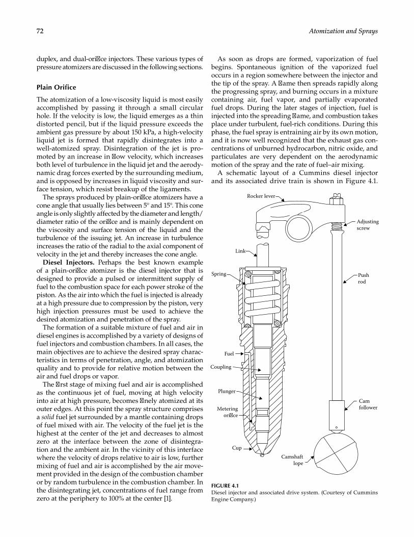
72 Atomization and Sprays

duplex, and dual-orifice injectors. These various types of pressure atomizers are discussed in the following sections.

Plain Orifice

The atomization of a low-viscosity liquid is most easily accomplished by passing it through a small circular hole. If the velocity is low, the liquid emerges as a thin distorted pencil, but if the liquid pressure exceeds the ambient gas pressure by about 150 kPa, a high- velocity liquid jet is formed that rapidly disintegrates into a well-atomized spray. Disintegration of the jet is pro-moted by an increase in flow velocity, which increases both level of turbulence in the liquid jet and the aerody-namic drag forces exerted by the surrounding medium, and is opposed by increases in liquid viscosity and sur-face tension, which resist breakup of the ligaments.

The sprays produced by plain-orifice atomizers have a cone angle that usually lies between 5° and 15°. This cone angle is only slightly affected by the diameter and length/diameter ratio of the orifice and is mainly dependent on the viscosity and surface tension of the liquid and the turbulence of the issuing jet. An increase in turbulence increases the ratio of the radial to the axial component of velocity in the jet and thereby increases the cone angle.

Diesel Injectors. Perhaps the best known example of a plain-orifice atomizer is the diesel injector that is designed to provide a pulsed or intermittent supply of fuel to the combustion space for each power stroke of the piston. As the air into which the fuel is injected is already at a high pressure due to compression by the piston, very high injection pressures must be used to achieve the desired atomization and penetration of the spray.

The formation of a suitable mixture of fuel and air in diesel engines is accomplished by a variety of designs of fuel injectors and combustion chambers. In all cases, the main objectives are to achieve the desired spray charac-teristics in terms of penetration, angle, and atomization quality and to provide for relative motion between the air and fuel drops or vapor.

The first stage of mixing fuel and air is accomplished as the continuous jet of fuel, moving at high velocity into air at high pressure, becomes finely atomized at its outer edges. At this point the spray structure comprises a solid fuel jet surrounded by a mantle containing drops of fuel mixed with air. The velocity of the fuel jet is the highest at the center of the jet and decreases to almost zero at the interface between the zone of disintegra-tion and the ambient air. In the vicinity of this interface where the velocity of drops relative to air is low, further mixing of fuel and air is accomplished by the air move-ment provided in the design of the combustion chamber or by random turbulence in the combustion chamber. In the disintegrating jet, concentrations of fuel range from zero at the periphery to 100% at the center [1].

As soon as drops are formed, vaporization of fuel begins. Spontaneous ignition of the vaporized fuel occurs in a region somewhere between the injector and the tip of the spray. A flame then spreads rapidly along the progressing spray, and burning occurs in a mixture containing air, fuel vapor, and partially evaporated fuel drops. During the later stages of injection, fuel is injected into the spreading flame, and combustion takes place under turbulent, fuel-rich conditions. During this phase, the fuel spray is entraining air by its own motion, and it is now well recognized that the exhaust gas con-centrations of unburned hydrocarbon, nitric oxide, and particulates are very dependent on the aerodynamic motion of the spray and the rate of fuel–air mixing.

A schematic layout of a Cummins diesel injector and its associated drive train is shown in Figure 4.1.

Adjustingscrew

Rocker lever

Link

Spring

Fuel

Coupling

Plunger

Meteringorice

CupCamshaft

lope

Pushrod

Camfollower

FIGURE 4.1Diesel injector and associated drive system. (Courtesy of Cummins Engine Company.)

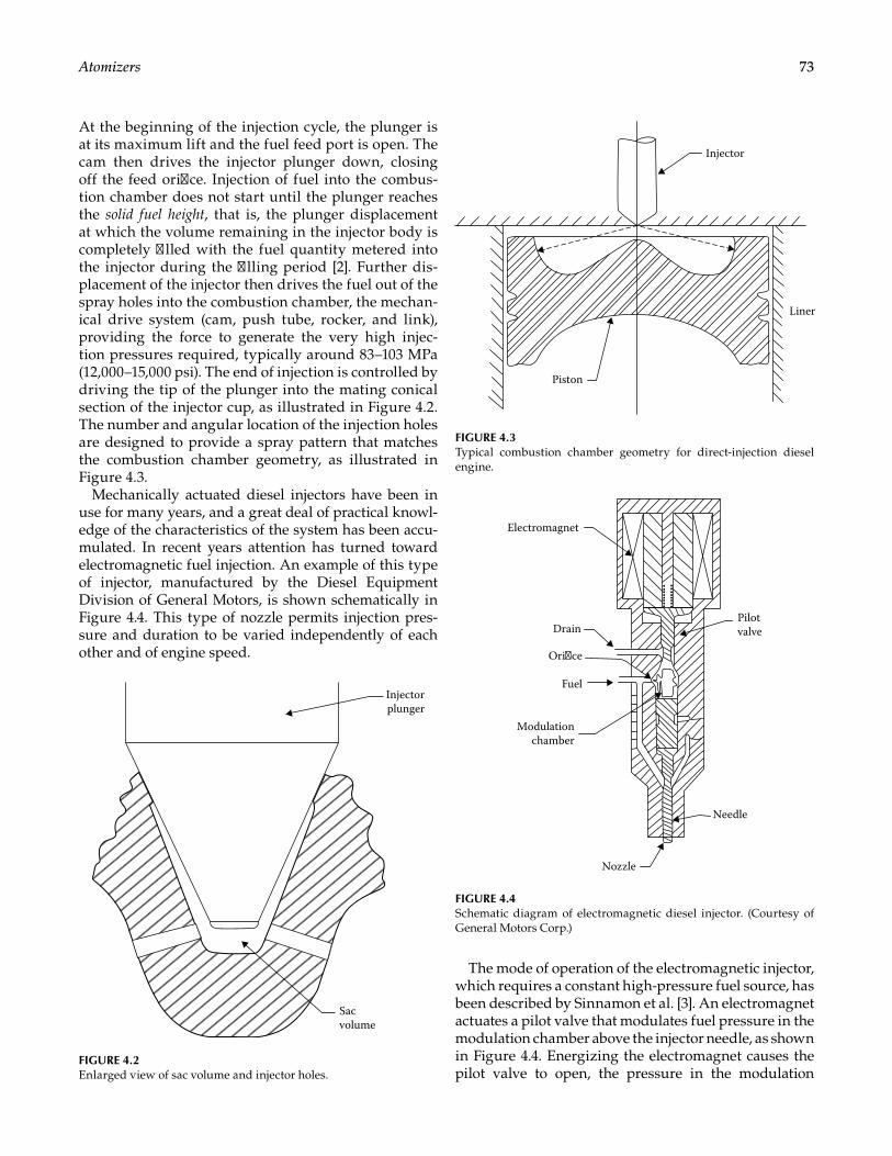
73Atomizers

At the beginning of the injection cycle, the plunger is at its maximum lift and the fuel feed port is open. The cam then drives the injector plunger down, closing off the feed orifice. Injection of fuel into the combus-tion chamber does not start until the plunger reaches the solid fuel height, that is, the plunger displacement at which the volume remaining in the injector body is completely filled with the fuel quantity metered into the injector during the filling period [2]. Further dis-placement of the injector then drives the fuel out of the spray holes into the combustion chamber, the mechan-ical drive system (cam, push tube, rocker, and link), providing the force to generate the very high injec-tion pressures required, typically around 83–103 MPa (12,000–15,000 psi). The end of injection is controlled by driving the tip of the plunger into the mating conical section of the injector cup, as illustrated in Figure 4.2. The number and angular location of the injection holes are designed to provide a spray pattern that matches the combustion chamber geometry, as illustrated in Figure 4.3.

Mechanically actuated diesel injectors have been in use for many years, and a great deal of practical knowl-edge of the characteristics of the system has been accu-mulated. In recent years attention has turned toward electromagnetic fuel injection. An example of this type of injector, manufactured by the Diesel Equipment Division of General Motors, is shown schematically in Figure 4.4. This type of nozzle permits injection pres-sure and duration to be varied independently of each other and of engine speed.

The mode of operation of the electromagnetic injector, which requires a constant high-pressure fuel source, has been described by Sinnamon et al. [3]. An electromagnet actuates a pilot valve that modulates fuel pressure in the modulation chamber above the injector needle, as shown in Figure 4.4. Energizing the electromagnet causes the pilot valve to open, the pressure in the modulation

Injectorplunger

Sacvolume

FIGURE 4.2Enlarged view of sac volume and injector holes.

Injector

Liner

Piston

FIGURE 4.3Typical combustion chamber geometry for direct-injection diesel engine.

Pilotvalve

Needle

Nozzle

Modulationchamber

Drain

Electromagnet

Orice

Fuel

FIGURE 4.4Schematic diagram of electromagnetic diesel injector. (Courtesy of General Motors Corp.)

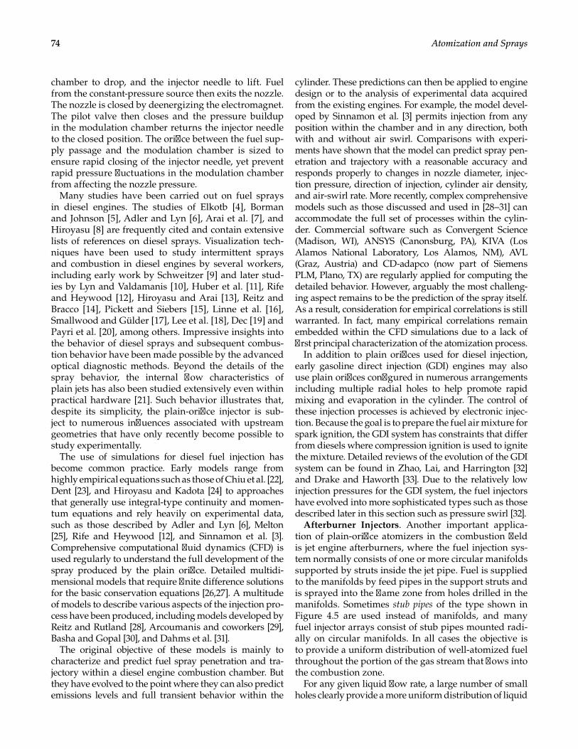
74 Atomization and Sprays

chamber to drop, and the injector needle to lift. Fuel from the constant-pressure source then exits the nozzle. The nozzle is closed by deenergizing the electromagnet. The pilot valve then closes and the pressure buildup in the modulation chamber returns the injector needle to the closed position. The orifice between the fuel sup-ply passage and the modulation chamber is sized to ensure rapid closing of the injector needle, yet prevent rapid pressure fluctuations in the modulation chamber from affecting the nozzle pressure.

Many studies have been carried out on fuel sprays in diesel engines. The studies of Elkotb [4], Borman and Johnson [5], Adler and Lyn [6], Arai et al. [7], and Hiroyasu [8] are frequently cited and contain extensive lists of references on diesel sprays. Visualization tech-niques have been used to study intermittent sprays and combustion in diesel engines by several workers, including early work by Schweitzer [9] and later stud-ies by Lyn and Valdamanis [10], Huber et al. [11], Rife and Heywood [12], Hiroyasu and Arai [13], Reitz and Bracco [14], Pickett and Siebers [15], Linne et al. [16], Smallwood and Gülder [17], Lee et al. [18], Dec [19] and Payri et al. [20], among others. Impressive insights into the behavior of diesel sprays and subsequent combus-tion behavior have been made possible by the advanced optical diagnostic methods. Beyond the details of the spray behavior, the internal flow characteristics of plain jets has also been studied extensively even within practical hardware [21]. Such behavior illustrates that, despite its simplicity, the plain-orifice injector is sub-ject to numerous influences associated with upstream geometries that have only recently become possible to study experimentally.

The use of simulations for diesel fuel injection has become common practice. Early models range from highly empirical equations such as those of Chiu et al. [22], Dent [23], and Hiroyasu and Kadota [24] to approaches that generally use integral-type continuity and momen-tum equations and rely heavily on experimental data, such as those described by Adler and Lyn [6], Melton [25], Rife and Heywood [12], and Sinnamon et al. [3]. Comprehensive computational fluid dynamics (CFD) is used regularly to understand the full development of the spray produced by the plain orifice. Detailed multidi-mensional models that require finite difference solutions for the basic conservation equations [26,27]. A multitude of models to describe various aspects of the injection pro-cess have been produced, including models developed by Reitz and Rutland [28], Arcoumanis and coworkers [29], Basha and Gopal [30], and Dahms et al. [31].

The original objective of these models is mainly to characterize and predict fuel spray penetration and tra-jectory within a diesel engine combustion chamber. But they have evolved to the point where they can also predict emissions levels and full transient behavior within the

cylinder. These predictions can then be applied to engine design or to the analysis of experimental data acquired from the existing engines. For example, the model devel-oped by Sinnamon et al. [3] permits injection from any position within the chamber and in any direction, both with and without air swirl. Comparisons with experi-ments have shown that the model can predict spray pen-etration and trajectory with a reasonable accuracy and responds properly to changes in nozzle diameter, injec-tion pressure, direction of injection, cylinder air density, and air-swirl rate. More recently, complex comprehensive models such as those discussed and used in [28–31] can accommodate the full set of processes within the cylin-der. Commercial software such as Convergent Science (Madison, WI), ANSYS (Canonsburg, PA), KIVA (Los Alamos National Laboratory, Los Alamos, NM), AVL (Graz, Austria) and CD-adapco (now part of Siemens PLM, Plano, TX) are regularly applied for computing the detailed behavior. However, arguably the most challeng-ing aspect remains to be the prediction of the spray itself. As a result, consideration for empirical correlations is still warranted. In fact, many empirical correlations remain embedded within the CFD simulations due to a lack of first principal characterization of the atomization process.

In addition to plain orifices used for diesel injection, early gasoline direct injection (GDI) engines may also use plain orifices configured in numerous arrangements including multiple radial holes to help promote rapid mixing and evaporation in the cylinder. The control of these injection processes is achieved by electronic injec-tion. Because the goal is to prepare the fuel air mixture for spark ignition, the GDI system has constraints that differ from diesels where compression ignition is used to ignite the mixture. Detailed reviews of the evolution of the GDI system can be found in Zhao, Lai, and Harrington [32] and Drake and Haworth [33]. Due to the relatively low injection pressures for the GDI system, the fuel injectors have evolved into more sophisticated types such as those described later in this section such as pressure swirl [32].

Afterburner Injectors. Another important applica-tion of plain-orifice atomizers in the combustion field is jet engine afterburners, where the fuel injection sys-tem normally consists of one or more circular manifolds supported by struts inside the jet pipe. Fuel is supplied to the manifolds by feed pipes in the support struts and is sprayed into the flame zone from holes drilled in the manifolds. Sometimes stub pipes of the type shown in Figure 4.5 are used instead of manifolds, and many fuel injector arrays consist of stub pipes mounted radi-ally on circular manifolds. In all cases the objective is to provide a uniform distribution of well-atomized fuel throughout the portion of the gas stream that flows into the combustion zone.

For any given liquid flow rate, a large number of small holes clearly provide a more uniform distribution of liquid

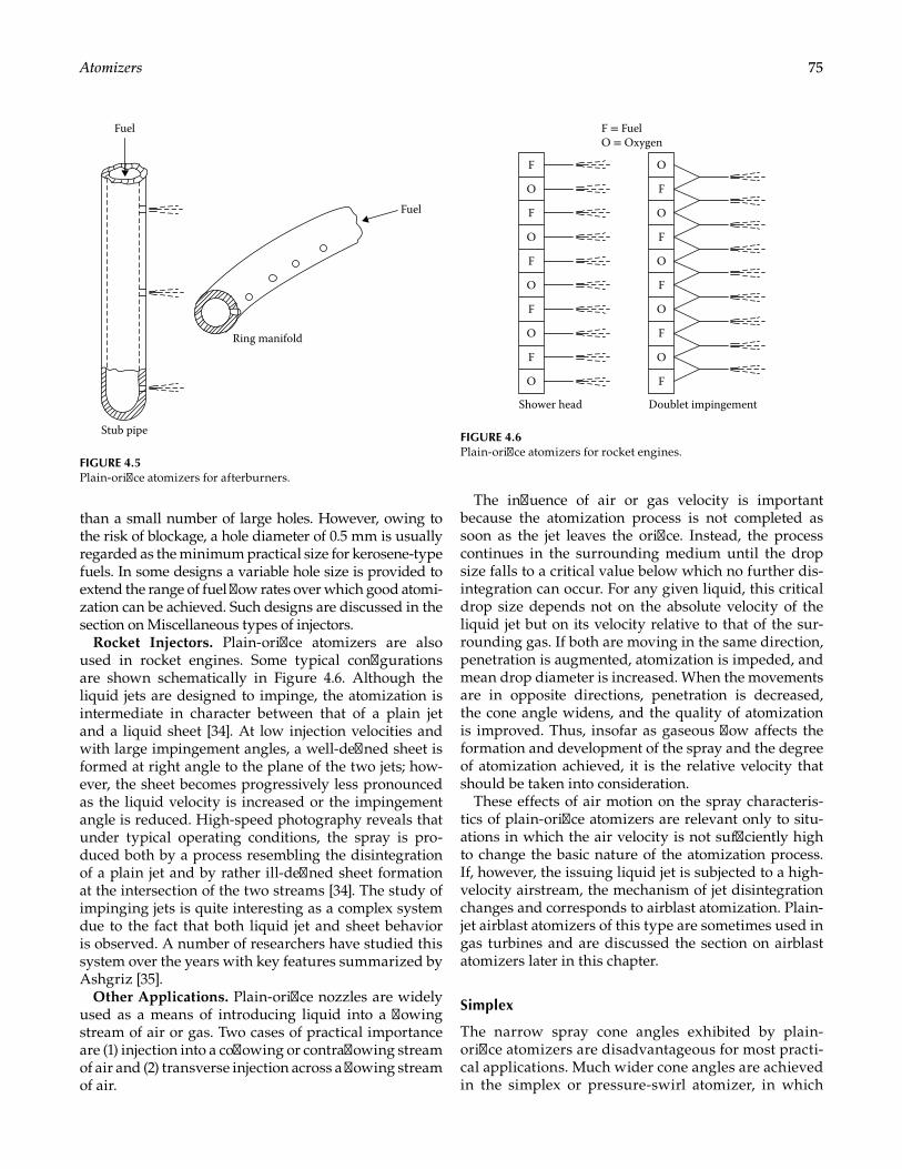
75Atomizers

than a small number of large holes. However, owing to the risk of blockage, a hole diameter of 0.5 mm is usually regarded as the minimum practical size for kerosene- type fuels. In some designs a variable hole size is provided to extend the range of fuel flow rates over which good atomi-zation can be achieved. Such designs are discussed in the section on Miscellaneous types of injectors.

Rocket Injectors. Plain-orifice atomizers are also used in rocket engines. Some typical configurations are shown schematically in Figure 4.6. Although the liquid jets are designed to impinge, the atomization is intermediate in character between that of a plain jet and a liquid sheet [34]. At low injection velocities and with large impingement angles, a well-defined sheet is formed at right angle to the plane of the two jets; how-ever, the sheet becomes progressively less pronounced as the liquid velocity is increased or the impingement angle is reduced. High-speed photography reveals that under typical operating conditions, the spray is pro-duced both by a process resembling the disintegration of a plain jet and by rather ill-defined sheet formation at the intersection of the two streams [34]. The study of impinging jets is quite interesting as a complex system due to the fact that both liquid jet and sheet behavior is observed. A number of researchers have studied this system over the years with key features summarized by Ashgriz [35].

Other Applications. Plain-orifice nozzles are widely used as a means of introducing liquid into a flowing stream of air or gas. Two cases of practical importance are (1) injection into a coflowing or contraflowing stream of air and (2) transverse injection across a flowing stream of air.

The influence of air or gas velocity is important because the atomization process is not completed as soon as the jet leaves the orifice. Instead, the process continues in the surrounding medium until the drop size falls to a critical value below which no further dis-integration can occur. For any given liquid, this critical drop size depends not on the absolute velocity of the liquid jet but on its velocity relative to that of the sur-rounding gas. If both are moving in the same direction, penetration is augmented, atomization is impeded, and mean drop diameter is increased. When the movements are in opposite directions, penetration is decreased, the cone angle widens, and the quality of atomization is improved. Thus, insofar as gaseous flow affects the formation and development of the spray and the degree of atomization achieved, it is the relative velocity that should be taken into consideration.

These effects of air motion on the spray characteris-tics of plain-orifice atomizers are relevant only to situ-ations in which the air velocity is not sufficiently high to change the basic nature of the atomization process. If, however, the issuing liquid jet is subjected to a high-velocity airstream, the mechanism of jet disintegration changes and corresponds to airblast atomization. Plain-jet airblast atomizers of this type are sometimes used in gas turbines and are discussed the section on airblast atomizers later in this chapter.

Simplex

The narrow spray cone angles exhibited by plain-orifice atomizers are disadvantageous for most practi-cal applications. Much wider cone angles are achieved in the simplex or pressure-swirl atomizer, in which

Fuel

Fuel

Ring manifold

Stub pipe

FIGURE 4.5Plain-orifice atomizers for afterburners.

Shower head Doublet impingement

F = FuelO = Oxygen

F

O

F

O

F

O

F

O

F

O

O

F

O

F

O

F

O

F

O

F

FIGURE 4.6Plain-orifice atomizers for rocket engines.

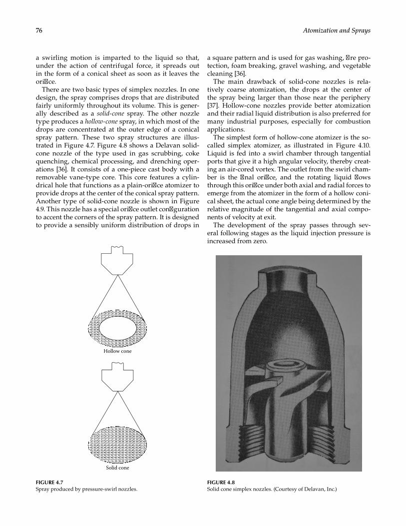
76 Atomization and Sprays

a swirling motion is imparted to the liquid so that, under the action of centrifugal force, it spreads out in the form of a conical sheet as soon as it leaves the orifice.

There are two basic types of simplex nozzles. In one design, the spray comprises drops that are distributed fairly uniformly throughout its volume. This is gener-ally described as a solid-cone spray. The other nozzle type produces a hollow-cone spray, in which most of the drops are concentrated at the outer edge of a conical spray pattern. These two spray structures are illus-trated in Figure 4.7. Figure 4.8 shows a Delavan solid-cone nozzle of the type used in gas scrubbing, coke quenching, chemical processing, and drenching oper-ations [36]. It consists of a one-piece cast body with a removable vane-type core. This core features a cylin-drical hole that functions as a plain-orifice atomizer to provide drops at the center of the conical spray pattern. Another type of solid-cone nozzle is shown in Figure 4.9. This nozzle has a special orifice outlet configuration to accent the corners of the spray pattern. It is designed to provide a sensibly uniform distribution of drops in

a square pattern and is used for gas washing, fire pro-tection, foam breaking, gravel washing, and vegetable cleaning [36].

The main drawback of solid-cone nozzles is rela-tively coarse atomization, the drops at the center of the spray being larger than those near the periphery [37]. Hollow-cone nozzles provide better atomization and their radial liquid distribution is also preferred for many industrial purposes, especially for combustion applications.

The simplest form of hollow-cone atomizer is the so-called simplex atomizer, as illustrated in Figure 4.10. Liquid is fed into a swirl chamber through tangential ports that give it a high angular velocity, thereby creat-ing an air-cored vortex. The outlet from the swirl cham-ber is the final orifice, and the rotating liquid flows through this orifice under both axial and radial forces to emerge from the atomizer in the form of a hollow coni-cal sheet, the actual cone angle being determined by the relative magnitude of the tangential and axial compo-nents of velocity at exit.

The development of the spray passes through sev-eral following stages as the liquid injection pressure is increased from zero.

Hollow cone

Solid cone

FIGURE 4.7Spray produced by pressure-swirl nozzles.

FIGURE 4.8Solid cone simplex nozzles. (Courtesy of Delavan, Inc.)

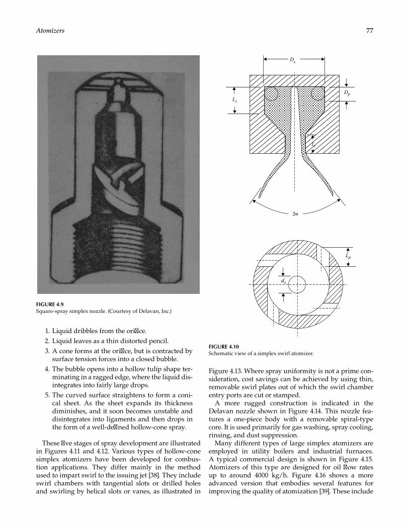
77Atomizers

1. Liquid dribbles from the orifice. 2. Liquid leaves as a thin distorted pencil. 3. A cone forms at the orifice, but is contracted by

surface tension forces into a closed bubble. 4. The bubble opens into a hollow tulip shape ter-

minating in a ragged edge, where the liquid dis-integrates into fairly large drops.

5. The curved surface straightens to form a coni-cal sheet. As the sheet expands its thickness diminishes, and it soon becomes unstable and disintegrates into ligaments and then drops in the form of a well-defined hollow-cone spray.

These five stages of spray development are illustrated in Figures 4.11 and 4.12. Various types of hollow-cone simplex atomizers have been developed for combus-tion applications. They differ mainly in the method used to impart swirl to the issuing jet [38]. They include swirl chambers with tangential slots or drilled holes and swirling by helical slots or vanes, as illustrated in

Figure 4.13. Where spray uniformity is not a prime con-sideration, cost savings can be achieved by using thin, removable swirl plates out of which the swirl chamber entry ports are cut or stamped.

A more rugged construction is indicated in the Delavan nozzle shown in Figure 4.14. This nozzle fea-tures a one-piece body with a removable spiral-type core. It is used primarily for gas washing, spray cooling, rinsing, and dust suppression.

Many different types of large simplex atomizers are employed in utility boilers and industrial furnaces. A typical commercial design is shown in Figure 4.15. Atomizers of this type are designed for oil flow rates up to around 4000 kg/h. Figure 4.16 shows a more advanced version that embodies several features for improving the quality of atomization [39]. These include

FIGURE 4.9Square-spray simplex nozzle. (Courtesy of Delavan, Inc.)

Ds

Ls

do

Lp

Dp

lo

2ѳ

FIGURE 4.10Schematic view of a simplex swirl atomizer.

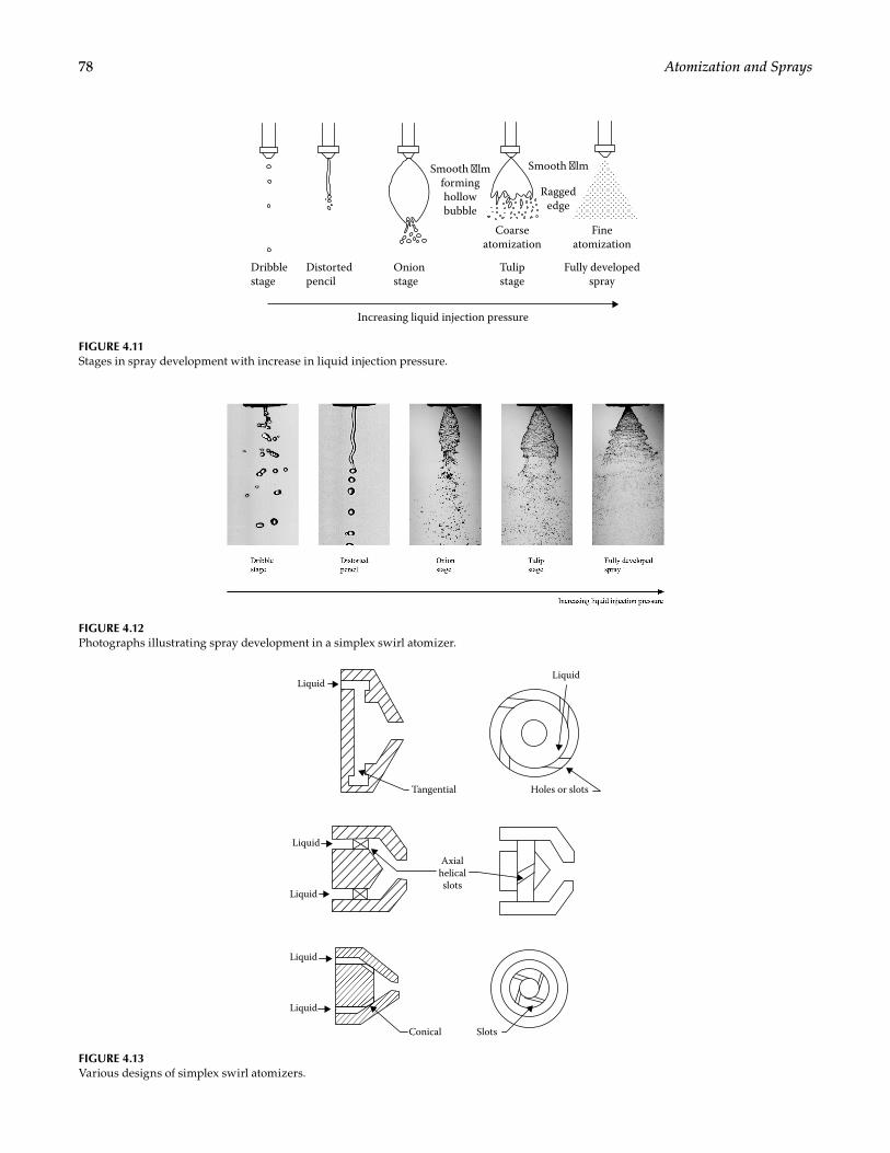
78 Atomization and Sprays

Increasing liquid injection pressure

Dribblestage

Distortedpencil

Onionstage

Tulipstage

Smooth lmforminghollowbubble

Smooth lm

Raggededge

Coarseatomization

Fineatomization

Fully developedspray

FIGURE 4.11Stages in spray development with increase in liquid injection pressure.

FIGURE 4.12Photographs illustrating spray development in a simplex swirl atomizer.

LiquidLiquid

Tangential Holes or slots

Axialhelicalslots

Conical Slots

Liquid

Liquid

Liquid

Liquid

FIGURE 4.13Various designs of simplex swirl atomizers.

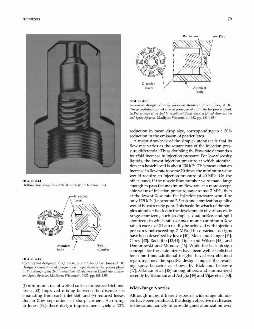
79Atomizers

(1) minimum area of wetted surface to reduce frictional losses, (2) improved mixing between the discrete jets emanating from each inlet slot, and (3) reduced losses due to flow separations at sharp corners. According to Jones [39], these design improvements yield a 12%

reduction in mean drop size, corresponding to a 30% reduction in the emission of particulates.

A major drawback of the simplex atomizer is that its flow rate varies as the square root of the injection pres-sure differential. Thus, doubling the flow rate demands a fourfold increase in injection pressure. For low- viscosity liquids, the lowest injection pressure at which atomiza-tion can be achieved is about 100 kPa. This means that an increase in flow rate to some 20 times the minimum value would require an injection pressure of 40 MPa. On the other hand, if the nozzle flow number were made large enough to pass the maximum flow rate at a more accept-able value of injection pressure, say around 7 MPa, then at the lowest flow rate the injection pressure would be only 17.5 kPa (i.e., around 2.5 psi) and atomization quality would be extremely poor. This basic drawback of the sim-plex atomizer has led to the development of various wide range atomizers, such as duplex, dual-orifice, and spill atomizers, in which ratios of maximum to minimum flow rate in excess of 20 can readily be achieved with injection pressures not exceeding 7 MPa. These various designs have been described by Joyce [40], Mock and Ganger [41], Carey [42], Radcliffe [43,44], Tipler and Wilson [45], and Dombrowski and Munday [46]. While the basic design concepts for these atomizers have been well established for some time, additional insights have been obtained regarding how the specific designs impact the result-ing spray behavior as shown by Rizk and Lefebvre [47], Sakman et al. [48] among others, and summarized recently by Eslamian and Ashgiz [49] and Vijay et al. [50].

Wide-Range Nozzles

Although many different types of wide-range atomiz-ers have been produced, the design objective in all cases is the same, namely to provide good atomization over

FIGURE 4.14Hollow-cone simplex nozzle. (Courtesy of Delavan, Inc.)

readedinsert

Swirlchamber

Atomizerbody

FIGURE 4.15Commercial design of large pressure atomizer (From Jones, A. R., Design optimization of a large pressure jet atomizer for power plant. In Proceedings of the 2nd International Conference on Liquid Atomization and Spray Systems, Madison, Wisconsin, 1982, pp. 181–185.)

readedinsert Atomizer

body

DiscRadius

FIGURE 4.16Improved design of large pressure atomizer (From Jones, A. R., Design optimization of a large pressure jet atomizer for power plant. In Proceedings of the 2nd International Conference on Liquid Atomization and Spray Systems, Madison, Wisconsin, 1982, pp. 181–185.)

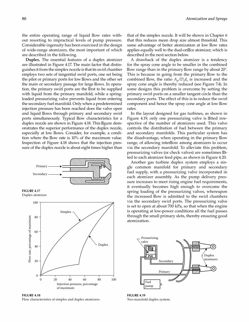
80 Atomization and Sprays

the entire operating range of liquid flow rates with-out resorting to impractical levels of pump pressure. Considerable ingenuity has been exercised in the design of wide-range atomizers, the most important of which are described in the following.

Duplex. The essential features of a duplex atomizer are illustrated in Figure 4.17. The main factor that distin-guishes it from the simplex nozzle is that its swirl chamber employs two sets of tangential swirl ports, one set being the pilot or primary ports for low flows and the other set the main or secondary passage for large flows. In opera-tion, the primary swirl ports are the first to be supplied with liquid from the primary manifold, while a spring-loaded pressurizing valve prevents liquid from entering the secondary fuel manifold. Only when a predetermined injection pressure has been reached does the valve open and liquid flows through primary and secondary swirl ports simultaneously. Typical flow characteristics for a duplex nozzle are shown in Figure 4.18. This figure dem-onstrates the superior performance of the duplex nozzle, especially at low flows. Consider, for example, a condi-tion where the flow rate is 10% of the maximum value. Inspection of Figure 4.18 shows that the injection pres-sure of the duplex nozzle is about eight times higher than

that of the simplex nozzle. It will be shown in Chapter 6 that this reduces mean drop size almost threefold. This same advantage of better atomization at low flow rates applies equally well to the dual-orifice atomizer, which is described in the next section below.

A drawback of the duplex atomizer is a tendency for the spray cone angle to be smaller in the combined flow range than in the primary flow range by about 20°. This is because in going from the primary flow to the combined flow, the ratio Ap/Dsdo is increased and the spray cone angle is thereby reduced (see Figure 7.4). In some designs this problem is overcome by setting the primary swirl ports on a smaller tangent circle than the secondary ports. The effect of this is to reduce the swirl component and hence the spray cone angle at low flow rates.

In the layout designed for gas turbines, as shown in Figure 4.19, only one pressurizing valve is fitted irre-spective of the number of atomizers used. This valve controls the distribution of fuel between the primary and secondary manifolds. This particular system has the disadvantage, when operating in the primary flow range, of allowing interflow among atomizers to occur via the secondary manifold. To alleviate this problem, pressurizing valves (or check valves) are sometimes fit-ted to each atomizer feed pipe, as shown in Figure 4.20.

Another gas turbine duplex system employs a sin-gle common manifold for primary and secondary fuel supply, with a pressurizing valve incorporated in each atomizer assembly. As the pump delivery pres-sure increases to meet rising engine fuel requirements, it eventually becomes high enough to overcome the spring loading of the pressurizing valves, whereupon the increased flow is admitted to the swirl chambers via the secondary swirl ports. The pressurizing valve is set to open at about 700 kPa, so that when the engine is operating at low-power conditions all the fuel passes through the small primary slots, thereby ensuring good atomization.

Primary

Secondary

FIGURE 4.17Duplex atomizer.

0806040200 100

80

60

40

20

100

Duplex

Injection pressure, percentageof maximum

Flow

rate

, per

cent

age

of m

axim

um

Simplex

FIGURE 4.18Flow characteristics of simplex and duplex atomizers.

Fuelpump

Primary

Pressurizingvalve

DuplexatomizersSecondary

FIGURE 4.19Two-manifold duplex system.

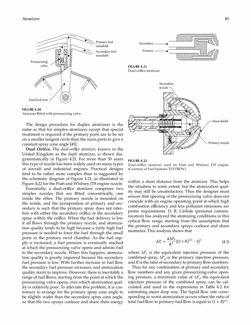
81Atomizers

The design procedure for duplex atomizers is the same as that for simplex atomizers except that special treatment is required if the primary ports are to be set on a smaller tangent circle than the main ports to give a constant spray cone angle [45].

Dual Orifice. The dual-orifice atomizer, known in the United Kingdom as the duple atomizer, is shown dia-grammatically in Figure 4.21. For more than 30 years this type of nozzle has been widely used on many types of aircraft and industrial engines. Practical designs tend to be rather more complex than is suggested by the schematic diagram of Figure 4.21, as illustrated in Figure 4.22 for the Pratt and Whitney JT8 engine nozzle.

Essentially, a dual-orifice atomizer comprises two simplex nozzles that are fitted concentrically, one inside the other. The primary nozzle is mounted on the inside, and the juxtaposition of primary and sec-ondary is such that the primary spray does not inter-fere with either the secondary orifice or the secondary spray within the orifice. When the fuel delivery is low it all flows through the primary nozzle, and atomiza-tion quality tends to be high because a fairly high fuel pressure is needed to force the fuel through the small ports in the primary swirl chamber. As the fuel sup-ply is increased, a fuel pressure is eventually reached at which the pressurizing valve opens and admits fuel to the secondary nozzle. When this happens, atomiza-tion quality is greatly impaired because the secondary fuel pressure is low. With further increase in fuel flow the secondary fuel pressure increases, and atomization quality starts to improve. However, there is inevitably a range of fuel flows, starting from the point at which the pressurizing valve opens, over which atomization qual-ity is relatively poor. To alleviate this problem, it is cus-tomary to arrange for the primary spray cone angle to be slightly wider than the secondary spray cone angle, so that the two sprays coalesce and share their energy

within a short distance from the atomizer. This helps the situation to some extent, but the atomization qual-ity may still be unsatisfactory. Thus the designer must ensure that opening of the pressurizing valve does not coincide with an engine operating point at which high combustion efficiency and less pollutant emissions are prime requirements. D. R. Carlisle (personal commu-nication) has analyzed the atomizing conditions in this critical flow range, starting from the assumption that the primary and secondary sprays coalesce and share momenta. This analysis shows that

PP

RRe

P∆ = ∆ + −4[(1 ) 1]2

0.5 2 (4.1)

where ∆Pe is the equivalent injection pressure of the combined spray, ∆Pp is the primary injection pressure, and R is the ratio of secondary to primary flow numbers.

Thus for any combination of primary and secondary flow numbers and any given pressurizing-valve open-ing pressure, a minimum value of ∆Pe, the equivalent injection pressure of the combined spray, can be cal-culated and used in the expressions in Table 6.2 for estimating mean drop size. The liquid flow rate corre-sponding to worst atomization occurs when the ratio of total fuel flow to primary fuel flow is equal to (1 + R)0.5.

Primary fuelmanifold

Secondary fuelmanifold

Pressurizingvalve

Fuel feed arm

FIGURE 4.20Atomizer fitted with pressurizing valve.

Primary

Secondary

FIGURE 4.21Dual-orifice atomizer.

Secondarynozzle

Heat shield

Primary nozzle

FIGURE 4.22Dual-orifice atomizer used on Pratt and Whitney JT8 engine. (Courtesy of Fuel Systems TEXTRON.)

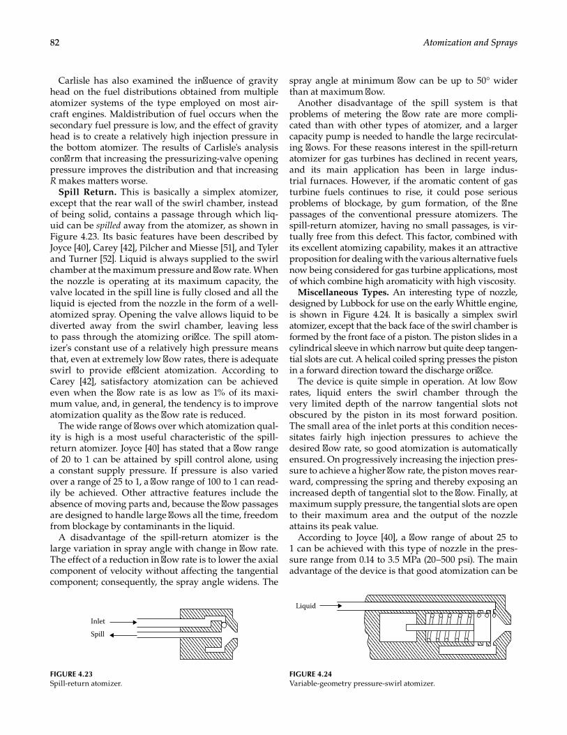
82 Atomization and Sprays

Carlisle has also examined the influence of gravity head on the fuel distributions obtained from multiple atomizer systems of the type employed on most air-craft engines. Maldistribution of fuel occurs when the secondary fuel pressure is low, and the effect of gravity head is to create a relatively high injection pressure in the bottom atomizer. The results of Carlisle's analysis confirm that increasing the pressurizing-valve opening pressure improves the distribution and that increasing R makes matters worse.

Spill Return. This is basically a simplex atomizer, except that the rear wall of the swirl chamber, instead of being solid, contains a passage through which liq-uid can be spilled away from the atomizer, as shown in Figure 4.23. Its basic features have been described by Joyce [40], Carey [42], Pilcher and Miesse [51], and Tyler and Turner [52]. Liquid is always supplied to the swirl chamber at the maximum pressure and flow rate. When the nozzle is operating at its maximum capacity, the valve located in the spill line is fully closed and all the liquid is ejected from the nozzle in the form of a well-atomized spray. Opening the valve allows liquid to be diverted away from the swirl chamber, leaving less to pass through the atomizing orifice. The spill atom-izer's constant use of a relatively high pressure means that, even at extremely low flow rates, there is adequate swirl to provide efficient atomization. According to Carey [42], satisfactory atomization can be achieved even when the flow rate is as low as 1% of its maxi-mum value, and, in general, the tendency is to improve atomization quality as the flow rate is reduced.

The wide range of flows over which atomization qual-ity is high is a most useful characteristic of the spill-return atomizer. Joyce [40] has stated that a flow range of 20 to 1 can be attained by spill control alone, using a constant supply pressure. If pressure is also varied over a range of 25 to 1, a flow range of 100 to 1 can read-ily be achieved. Other attractive features include the absence of moving parts and, because the flow passages are designed to handle large flows all the time, freedom from blockage by contaminants in the liquid.

A disadvantage of the spill-return atomizer is the large variation in spray angle with change in flow rate. The effect of a reduction in flow rate is to lower the axial component of velocity without affecting the tangential component; consequently, the spray angle widens. The

spray angle at minimum flow can be up to 50° wider than at maximum flow.

Another disadvantage of the spill system is that problems of metering the flow rate are more compli-cated than with other types of atomizer, and a larger capacity pump is needed to handle the large recirculat-ing flows. For these reasons interest in the spill-return atomizer for gas turbines has declined in recent years, and its main application has been in large indus-trial furnaces. However, if the aromatic content of gas turbine fuels continues to rise, it could pose serious problems of blockage, by gum formation, of the fine passages of the conventional pressure atomizers. The spill-return atomizer, having no small passages, is vir-tually free from this defect. This factor, combined with its excellent atomizing capability, makes it an attractive proposition for dealing with the various alternative fuels now being considered for gas turbine applications, most of which combine high aromaticity with high viscosity.

Miscellaneous Types. An interesting type of nozzle, designed by Lubbock for use on the early Whittle engine, is shown in Figure 4.24. It is basically a simplex swirl atomizer, except that the back face of the swirl chamber is formed by the front face of a piston. The piston slides in a cylindrical sleeve in which narrow but quite deep tangen-tial slots are cut. A helical coiled spring presses the piston in a forward direction toward the discharge orifice.

The device is quite simple in operation. At low flow rates, liquid enters the swirl chamber through the very limited depth of the narrow tangential slots not obscured by the piston in its most forward position. The small area of the inlet ports at this condition neces-sitates fairly high injection pressures to achieve the desired flow rate, so good atomization is automatically ensured. On progressively increasing the injection pres-sure to achieve a higher flow rate, the piston moves rear-ward, compressing the spring and thereby exposing an increased depth of tangential slot to the flow. Finally, at maximum supply pressure, the tangential slots are open to their maximum area and the output of the nozzle attains its peak value.

According to Joyce [40], a flow range of about 25 to 1 can be achieved with this type of nozzle in the pres-sure range from 0.14 to 3.5 MPa (20–500 psi). The main advantage of the device is that good atomization can be

Inlet

Spill

FIGURE 4.23Spill-return atomizer.

Liquid

FIGURE 4.24Variable-geometry pressure-swirl atomizer.

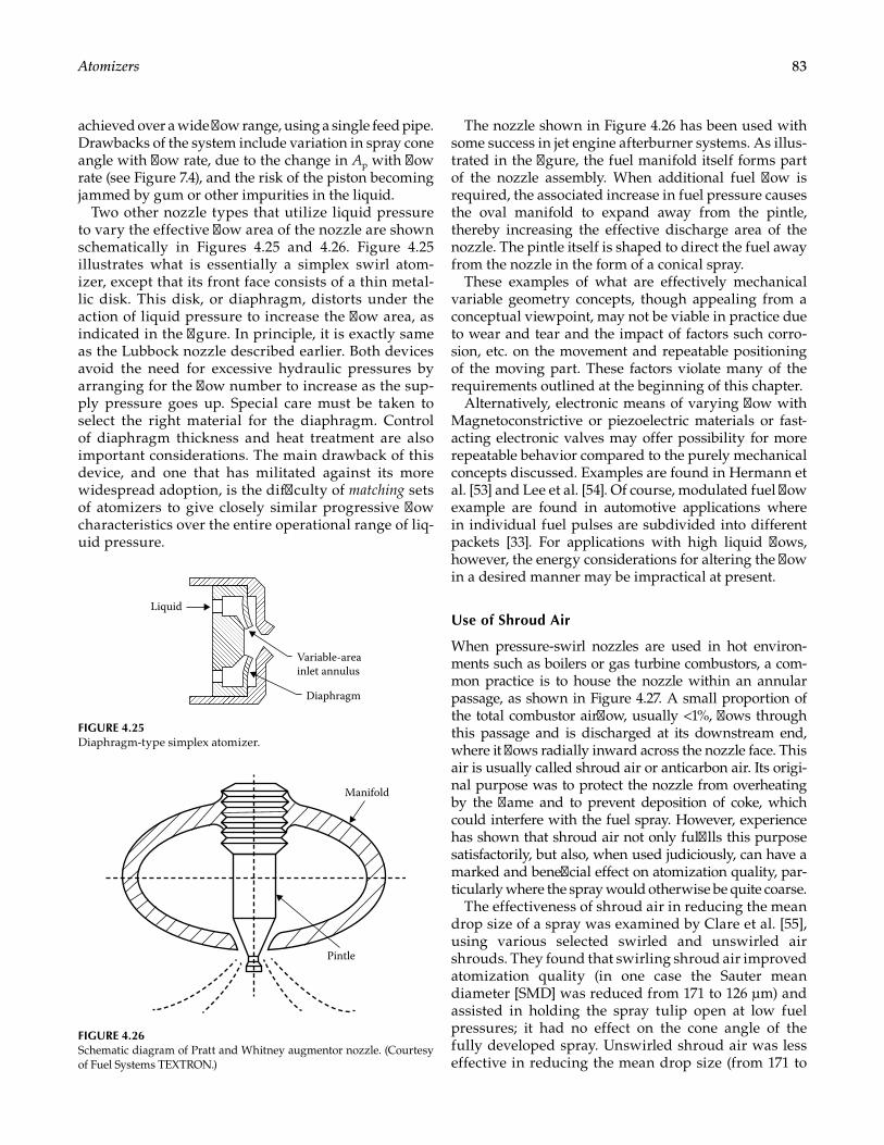
83Atomizers

achieved over a wide flow range, using a single feed pipe. Drawbacks of the system include variation in spray cone angle with flow rate, due to the change in Ap with flow rate (see Figure 7.4), and the risk of the piston becoming jammed by gum or other impurities in the liquid.

Two other nozzle types that utilize liquid pressure to vary the effective flow area of the nozzle are shown schematically in Figures 4.25 and 4.26. Figure 4.25 illustrates what is essentially a simplex swirl atom-izer, except that its front face consists of a thin metal-lic disk. This disk, or diaphragm, distorts under the action of liquid pressure to increase the flow area, as indicated in the figure. In principle, it is exactly same as the Lubbock nozzle described earlier. Both devices avoid the need for excessive hydraulic pressures by arranging for the flow number to increase as the sup-ply pressure goes up. Special care must be taken to select the right material for the diaphragm. Control of diaphragm thickness and heat treatment are also important considerations. The main drawback of this device, and one that has militated against its more widespread adoption, is the difficulty of matching sets of atomizers to give closely similar progressive flow characteristics over the entire operational range of liq-uid pressure.

The nozzle shown in Figure 4.26 has been used with some success in jet engine afterburner systems. As illus-trated in the figure, the fuel manifold itself forms part of the nozzle assembly. When additional fuel flow is required, the associated increase in fuel pressure causes the oval manifold to expand away from the pintle, thereby increasing the effective discharge area of the nozzle. The pintle itself is shaped to direct the fuel away from the nozzle in the form of a conical spray.

These examples of what are effectively mechanical variable geometry concepts, though appealing from a conceptual viewpoint, may not be viable in practice due to wear and tear and the impact of factors such corro-sion, etc. on the movement and repeatable positioning of the moving part. These factors violate many of the requirements outlined at the beginning of this chapter.

Alternatively, electronic means of varying flow with Magnetoconstrictive or piezoelectric materials or fast-acting electronic valves may offer possibility for more repeatable behavior compared to the purely mechanical concepts discussed. Examples are found in Hermann et al. [53] and Lee et al. [54]. Of course, modulated fuel flow example are found in automotive applications where in individual fuel pulses are subdivided into different packets [33]. For applications with high liquid flows, however, the energy considerations for altering the flow in a desired manner may be impractical at present.

Use of Shroud Air

When pressure-swirl nozzles are used in hot environ-ments such as boilers or gas turbine combustors, a com-mon practice is to house the nozzle within an annular passage, as shown in Figure 4.27. A small proportion of the total combustor airflow, usually <1%, flows through this passage and is discharged at its downstream end, where it flows radially inward across the nozzle face. This air is usually called shroud air or anticarbon air. Its origi-nal purpose was to protect the nozzle from overheating by the flame and to prevent deposition of coke, which could interfere with the fuel spray. However, experience has shown that shroud air not only fulfills this purpose satisfactorily, but also, when used judiciously, can have a marked and beneficial effect on atomization quality, par-ticularly where the spray would otherwise be quite coarse.

The effectiveness of shroud air in reducing the mean drop size of a spray was examined by Clare et al. [55], using various selected swirled and unswirled air shrouds. They found that swirling shroud air improved atomization quality (in one case the Sauter mean diameter [SMD] was reduced from 171 to 126 µm) and assisted in holding the spray tulip open at low fuel pressures; it had no effect on the cone angle of the fully developed spray. Unswirled shroud air was less effective in reducing the mean drop size (from 171 to

Liquid

Variable-areainlet annulus

Diaphragm

FIGURE 4.25Diaphragm-type simplex atomizer.

Manifold

Pintle

FIGURE 4.26Schematic diagram of Pratt and Whitney augmentor nozzle. (Courtesy of Fuel Systems TEXTRON.)

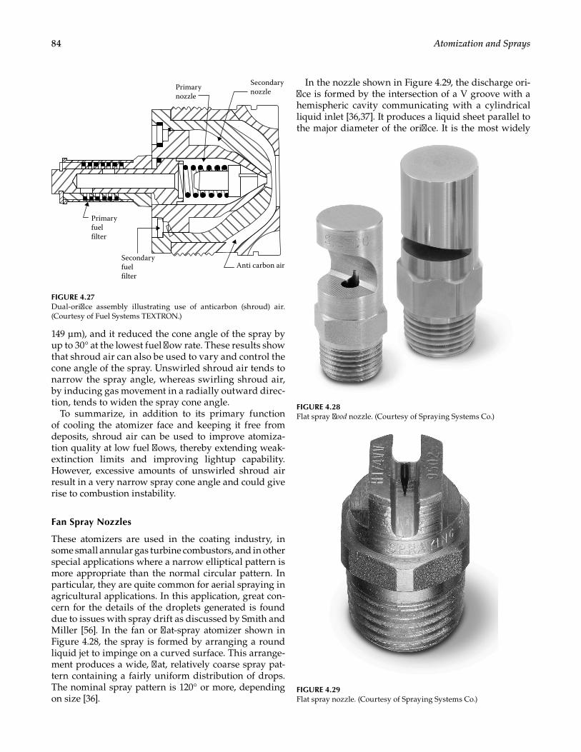
84 Atomization and Sprays

149 µm), and it reduced the cone angle of the spray by up to 30° at the lowest fuel flow rate. These results show that shroud air can also be used to vary and control the cone angle of the spray. Unswirled shroud air tends to narrow the spray angle, whereas swirling shroud air, by inducing gas movement in a radially outward direc-tion, tends to widen the spray cone angle.

To summarize, in addition to its primary function of cooling the atomizer face and keeping it free from deposits, shroud air can be used to improve atomiza-tion quality at low fuel flows, thereby extending weak-extinction limits and improving lightup capability. However, excessive amounts of unswirled shroud air result in a very narrow spray cone angle and could give rise to combustion instability.

Fan Spray Nozzles

These atomizers are used in the coating industry, in some small annular gas turbine combustors, and in other special applications where a narrow elliptical pattern is more appropriate than the normal circular pattern. In particular, they are quite common for aerial spraying in agricultural applications. In this application, great con-cern for the details of the droplets generated is found due to issues with spray drift as discussed by Smith and Miller [56]. In the fan or flat-spray atomizer shown in Figure 4.28, the spray is formed by arranging a round liquid jet to impinge on a curved surface. This arrange-ment produces a wide, flat, relatively coarse spray pat-tern containing a fairly uniform distribution of drops. The nominal spray pattern is 120° or more, depending on size [36].

In the nozzle shown in Figure 4.29, the discharge ori-fice is formed by the intersection of a V groove with a hemispheric cavity communicating with a cylindrical liquid inlet [36,37]. It produces a liquid sheet parallel to the major diameter of the orifice. It is the most widely

Primarynozzle

Primaryfuelfilter

Secondaryfuelfilter

Anti carbon air

Secondarynozzle

FIGURE 4.27Dual-orifice assembly illustrating use of anticarbon (shroud) air. (Courtesy of Fuel Systems TEXTRON.)

FIGURE 4.29Flat spray nozzle. (Courtesy of Spraying Systems Co.)

FIGURE 4.28Flat spray flood nozzle. (Courtesy of Spraying Systems Co.)

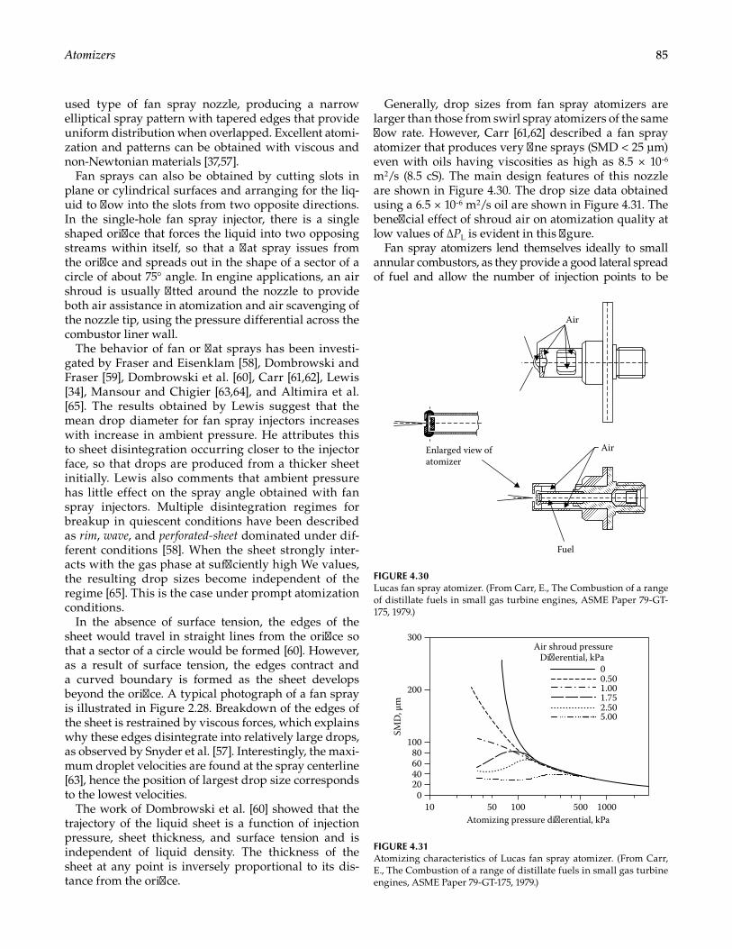
85Atomizers

used type of fan spray nozzle, producing a narrow elliptical spray pattern with tapered edges that provide uniform distribution when overlapped. Excellent atomi-zation and patterns can be obtained with viscous and non-Newtonian materials [37,57].

Fan sprays can also be obtained by cutting slots in plane or cylindrical surfaces and arranging for the liq-uid to flow into the slots from two opposite directions. In the single-hole fan spray injector, there is a single shaped orifice that forces the liquid into two opposing streams within itself, so that a flat spray issues from the orifice and spreads out in the shape of a sector of a circle of about 75° angle. In engine applications, an air shroud is usually fitted around the nozzle to provide both air assistance in atomization and air scavenging of the nozzle tip, using the pressure differential across the combustor liner wall.

The behavior of fan or flat sprays has been investi-gated by Fraser and Eisenklam [58], Dombrowski and Fraser [59], Dombrowski et al. [60], Carr [61,62], Lewis [34], Mansour and Chigier [63,64], and Altimira et al. [65]. The results obtained by Lewis suggest that the mean drop diameter for fan spray injectors increases with increase in ambient pressure. He attributes this to sheet disintegration occurring closer to the injector face, so that drops are produced from a thicker sheet initially. Lewis also comments that ambient pressure has little effect on the spray angle obtained with fan spray injectors. Multiple disintegration regimes for breakup in quiescent conditions have been described as rim, wave, and perforated-sheet dominated under dif-ferent conditions [58]. When the sheet strongly inter-acts with the gas phase at sufficiently high We values, the resulting drop sizes become independent of the regime [65]. This is the case under prompt atomization conditions.

In the absence of surface tension, the edges of the sheet would travel in straight lines from the orifice so that a sector of a circle would be formed [60]. However, as a result of surface tension, the edges contract and a curved boundary is formed as the sheet develops beyond the orifice. A typical photograph of a fan spray is illustrated in Figure 2.28. Breakdown of the edges of the sheet is restrained by viscous forces, which explains why these edges disintegrate into relatively large drops, as observed by Snyder et al. [57]. Interestingly, the maxi-mum droplet velocities are found at the spray centerline [63], hence the position of largest drop size corresponds to the lowest velocities.

The work of Dombrowski et al. [60] showed that the trajectory of the liquid sheet is a function of injection pressure, sheet thickness, and surface tension and is independent of liquid density. The thickness of the sheet at any point is inversely proportional to its dis-tance from the orifice.

Generally, drop sizes from fan spray atomizers are larger than those from swirl spray atomizers of the same flow rate. However, Carr [61,62] described a fan spray atomizer that produces very fine sprays (SMD < 25 µm) even with oils having viscosities as high as 8.5 × 10-6 m2/s (8.5 cS). The main design features of this nozzle are shown in Figure 4.30. The drop size data obtained using a 6.5 × 10-6 m2/s oil are shown in Figure 4.31. The beneficial effect of shroud air on atomization quality at low values of ∆PL is evident in this figure.

Fan spray atomizers lend themselves ideally to small annular combustors, as they provide a good lateral spread of fuel and allow the number of injection points to be

Fuel

Air

Air

Enlarged view ofatomizer

FIGURE 4.30Lucas fan spray atomizer. (From Carr, E., The Combustion of a range of distillate fuels in small gas turbine engines, ASME Paper 79-GT-175, 1979.)

10

SMD

, μm

20406080

100

200

300

050 100 500

00.501.001.752.505.00

1000Atomizing pressure dierential, kPa

Air shroud pressureDierential, kPa

FIGURE 4.31Atomizing characteristics of Lucas fan spray atomizer. (From Carr, E., The Combustion of a range of distillate fuels in small gas turbine engines, ASME Paper 79-GT-175, 1979.)

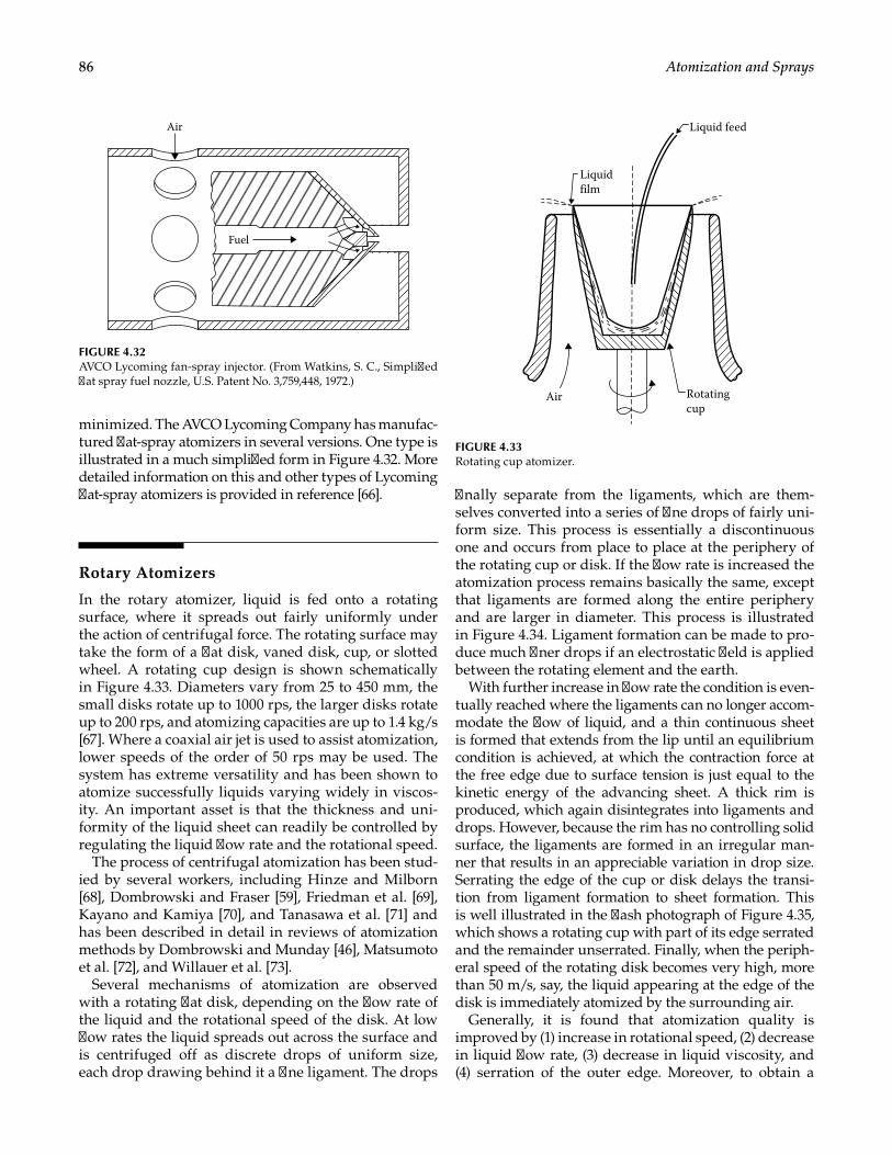
86 Atomization and Sprays

minimized. The AVCO Lycoming Company has manufac-tured flat-spray atomizers in several versions. One type is illustrated in a much simplified form in Figure 4.32. More detailed information on this and other types of Lycoming flat-spray atomizers is provided in reference [66].

Rotary Atomizers

In the rotary atomizer, liquid is fed onto a rotating surface, where it spreads out fairly uniformly under the action of centrifugal force. The rotating surface may take the form of a flat disk, vaned disk, cup, or slotted wheel. A rotating cup design is shown schematically in Figure 4.33. Diameters vary from 25 to 450 mm, the small disks rotate up to 1000 rps, the larger disks rotate up to 200 rps, and atomizing capacities are up to 1.4 kg/s [67]. Where a coaxial air jet is used to assist atomization, lower speeds of the order of 50 rps may be used. The system has extreme versatility and has been shown to atomize successfully liquids varying widely in viscos-ity. An important asset is that the thickness and uni-formity of the liquid sheet can readily be controlled by regulating the liquid flow rate and the rotational speed.

The process of centrifugal atomization has been stud-ied by several workers, including Hinze and Milborn [68], Dombrowski and Fraser [59], Friedman et al. [69], Kayano and Kamiya [70], and Tanasawa et al. [71] and has been described in detail in reviews of atomization methods by Dombrowski and Munday [46], Matsumoto et al. [72], and Willauer et al. [73].

Several mechanisms of atomization are observed with a rotating flat disk, depending on the flow rate of the liquid and the rotational speed of the disk. At low flow rates the liquid spreads out across the surface and is centrifuged off as discrete drops of uniform size, each drop drawing behind it a fine ligament. The drops

finally separate from the ligaments, which are them-selves converted into a series of fine drops of fairly uni-form size. This process is essentially a discontinuous one and occurs from place to place at the periphery of the rotating cup or disk. If the flow rate is increased the atomization process remains basically the same, except that ligaments are formed along the entire periphery and are larger in diameter. This process is illustrated in Figure 4.34. Ligament formation can be made to pro-duce much finer drops if an electrostatic field is applied between the rotating element and the earth.

With further increase in flow rate the condition is even-tually reached where the ligaments can no longer accom-modate the flow of liquid, and a thin continuous sheet is formed that extends from the lip until an equilibrium condition is achieved, at which the contraction force at the free edge due to surface tension is just equal to the kinetic energy of the advancing sheet. A thick rim is produced, which again disintegrates into ligaments and drops. However, because the rim has no controlling solid surface, the ligaments are formed in an irregular man-ner that results in an appreciable variation in drop size. Serrating the edge of the cup or disk delays the transi-tion from ligament formation to sheet formation. This is well illustrated in the flash photograph of Figure 4.35, which shows a rotating cup with part of its edge serrated and the remainder unserrated. Finally, when the periph-eral speed of the rotating disk becomes very high, more than 50 m/s, say, the liquid appearing at the edge of the disk is immediately atomized by the surrounding air.

Generally, it is found that atomization quality is improved by (1) increase in rotational speed, (2) decrease in liquid flow rate, (3) decrease in liquid viscosity, and (4) serration of the outer edge. Moreover, to obtain a

Air

Fuel

FIGURE 4.32AVCO Lycoming fan-spray injector. (From Watkins, S. C., Simplified flat spray fuel nozzle, U.S. Patent No. 3,759,448, 1972.)

Air

Liquid feed

Liquidfilm

Rotatingcup

FIGURE 4.33Rotating cup atomizer.

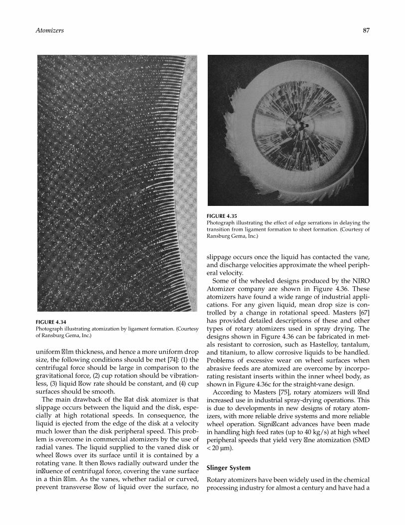
87Atomizers

uniform film thickness, and hence a more uniform drop size, the following conditions should be met [74]: (1) the centrifugal force should be large in comparison to the gravitational force, (2) cup rotation should be vibration-less, (3) liquid flow rate should be constant, and (4) cup surfaces should be smooth.

The main drawback of the flat disk atomizer is that slippage occurs between the liquid and the disk, espe-cially at high rotational speeds. In consequence, the liquid is ejected from the edge of the disk at a velocity much lower than the disk peripheral speed. This prob-lem is overcome in commercial atomizers by the use of radial vanes. The liquid supplied to the vaned disk or wheel flows over its surface until it is contained by a rotating vane. It then flows radially outward under the influence of centrifugal force, covering the vane surface in a thin film. As the vanes, whether radial or curved, prevent transverse flow of liquid over the surface, no

slippage occurs once the liquid has contacted the vane, and discharge velocities approximate the wheel periph-eral velocity.

Some of the wheeled designs produced by the NIRO Atomizer company are shown in Figure 4.36. These atomizers have found a wide range of industrial appli-cations. For any given liquid, mean drop size is con-trolled by a change in rotational speed. Masters [67] has provided detailed descriptions of these and other types of rotary atomizers used in spray drying. The designs shown in Figure 4.36 can be fabricated in met-als resistant to corrosion, such as Hastelloy, tantalum, and titanium, to allow corrosive liquids to be handled. Problems of excessive wear on wheel surfaces when abrasive feeds are atomized are overcome by incorpo-rating resistant inserts within the inner wheel body, as shown in Figure 4.36c for the straight-vane design.

According to Masters [75], rotary atomizers will find increased use in industrial spray-drying operations. This is due to developments in new designs of rotary atom-izers, with more reliable drive systems and more reliable wheel operation. Significant advances have been made in handling high feed rates (up to 40 kg/s) at high wheel peripheral speeds that yield very fine atomization (SMD < 20 µm).

Slinger System

Rotary atomizers have been widely used in the chemical processing industry for almost a century and have had a

FIGURE 4.34Photograph illustrating atomization by ligament formation. (Courtesy of Ransburg Gema, Inc.)

FIGURE 4.35Photograph illustrating the effect of edge serrations in delaying the transition from ligament formation to sheet formation. (Courtesy of Ransburg Gema, Inc.)

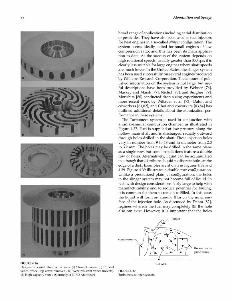
88 Atomization and Sprays

broad range of applications including aerial distribution of pesticides. They have also been used as fuel injectors for heat engines in a so-called slinger configuration. The system seems ideally suited for small engines of low compression ratio, and this has been its main applica-tion to date. As the success of the system depends on high rotational speeds, usually greater than 350 rps, it is clearly less suitable for large engines where shaft speeds are much lower. In the United States, the slinger system has been used successfully on several engines produced by Williams Research Corporation. The amount of pub-lished information on the system is not large, but use-ful descriptions have been provided by Wehner [76], Maskey and Marsh [77], Nichol [78], and Burgher [79]. Morishita [80] conducted drop sizing experiments and more recent work by Willauer et al. [73], Dahm and coworkers [81,82], and Choi and coworkers [83,84] has outlined additional details about the atomization per-formance in these systems.

The Turbomeca system is used in conjunction with a radial-annular combustion chamber, as illustrated in Figure 4.37. Fuel is supplied at low pressure along the hollow main shaft and is discharged radially outward through holes drilled in the shaft. These injection holes vary in number from 9 to 18 and in diameter from 2.0 to 3.2 mm. The holes may be drilled in the same plane as a single row, but some installations feature a double row of holes. Alternatively, liquid can be accumulated in a trough that distributes liquid to discrete holes at the edge of a disk. Examples are shown in Figures 4.38 and 4.39. Figure 4.39 illustrates a double row configuration. Unlike a pressurized plain jet configuration, the holes in the slinger system may not become full of liquid. In fact, with design considerations fairly large to help with manufacturability and to reduce potential for fouling, it is common for them to remain unfilled. In this case, the liquid will form an annular film on the inner sur-face of the injection hole. As discussed by Dahm [82], regimes wherein the fuel may completely fill the hole also can exist. However, it is important that the holes

FIGURE 4.36Designs of vaned atomizer wheels. (a) Straight vanes. (b) Curved vanes (wheel top cover removed), (c) Wear-resistant vanes (inserts). (d) High-capacity vanes. (Courtesy of NIRO Atomizer.)

Igniter

Fuel inlet

compressor

Hollow nozzleguide vanes

FIGURE 4.37Turbomeca slinger system.

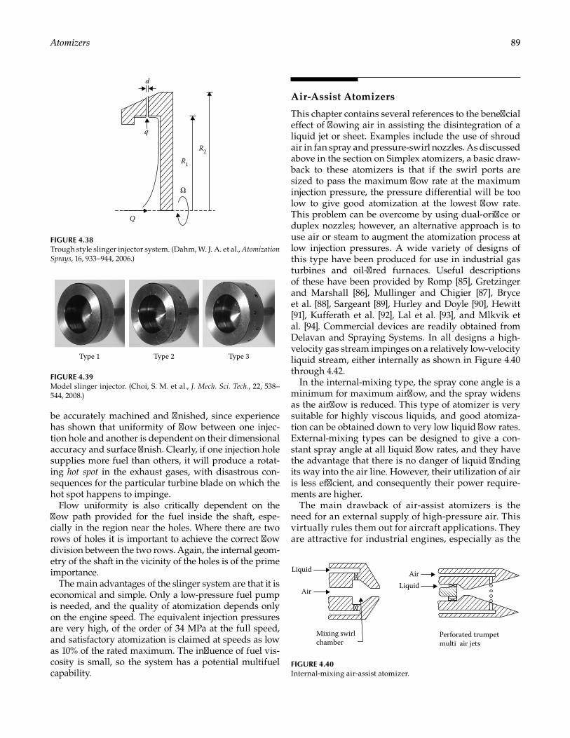
89Atomizers

be accurately machined and finished, since experience has shown that uniformity of flow between one injec-tion hole and another is dependent on their dimensional accuracy and surface finish. Clearly, if one injection hole supplies more fuel than others, it will produce a rotat-ing hot spot in the exhaust gases, with disastrous con-sequences for the particular turbine blade on which the hot spot happens to impinge.

Flow uniformity is also critically dependent on the flow path provided for the fuel inside the shaft, espe-cially in the region near the holes. Where there are two rows of holes it is important to achieve the correct flow division between the two rows. Again, the internal geom-etry of the shaft in the vicinity of the holes is of the prime importance.

The main advantages of the slinger system are that it is economical and simple. Only a low-pressure fuel pump is needed, and the quality of atomization depends only on the engine speed. The equivalent injection pressures are very high, of the order of 34 MPa at the full speed, and satisfactory atomization is claimed at speeds as low as 10% of the rated maximum. The influence of fuel vis-cosity is small, so the system has a potential multifuel capability.

Air-Assist Atomizers

This chapter contains several references to the beneficial effect of flowing air in assisting the disintegration of a liquid jet or sheet. Examples include the use of shroud air in fan spray and pressure-swirl nozzles. As discussed above in the section on Simplex atomizers, a basic draw-back to these atomizers is that if the swirl ports are sized to pass the maximum flow rate at the maximum injection pressure, the pressure differential will be too low to give good atomization at the lowest flow rate. This problem can be overcome by using dual-orifice or duplex nozzles; however, an alternative approach is to use air or steam to augment the atomization process at low injection pressures. A wide variety of designs of this type have been produced for use in industrial gas turbines and oil-fired furnaces. Useful descriptions of these have been provided by Romp [85], Gretzinger and Marshall [86], Mullinger and Chigier [87], Bryce et al. [88], Sargeant [89], Hurley and Doyle [90], Hewitt [91], Kufferath et al. [92], Lal et al. [93], and Mlkvik et al. [94]. Commercial devices are readily obtained from Delavan and Spraying Systems. In all designs a high-velocity gas stream impinges on a relatively low-velocity liquid stream, either internally as shown in Figure 4.40 through 4.42.

In the internal-mixing type, the spray cone angle is a minimum for maximum airflow, and the spray widens as the airflow is reduced. This type of atomizer is very suitable for highly viscous liquids, and good atomiza-tion can be obtained down to very low liquid flow rates. External-mixing types can be designed to give a con-stant spray angle at all liquid flow rates, and they have the advantage that there is no danger of liquid finding its way into the air line. However, their utilization of air is less efficient, and consequently their power require-ments are higher.

The main drawback of air-assist atomizers is the need for an external supply of high-pressure air. This virtually rules them out for aircraft applications. They are attractive for industrial engines, especially as the

d

q

Q

R1

R2

Ω

FIGURE 4.38 Trough style slinger injector system. (Dahm, W. J. A. et al., Atomization Sprays, 16, 933–944, 2006.)

Type 1 Type 2 Type 3

FIGURE 4.39 Model slinger injector. (Choi, S. M. et al., J. Mech. Sci. Tech., 22, 538–544, 2008.)

Liquid

Liquid Air

Air

Mixing swirlchamber

Perforated trumpetmulti air jets

FIGURE 4.40Internal-mixing air-assist atomizer.

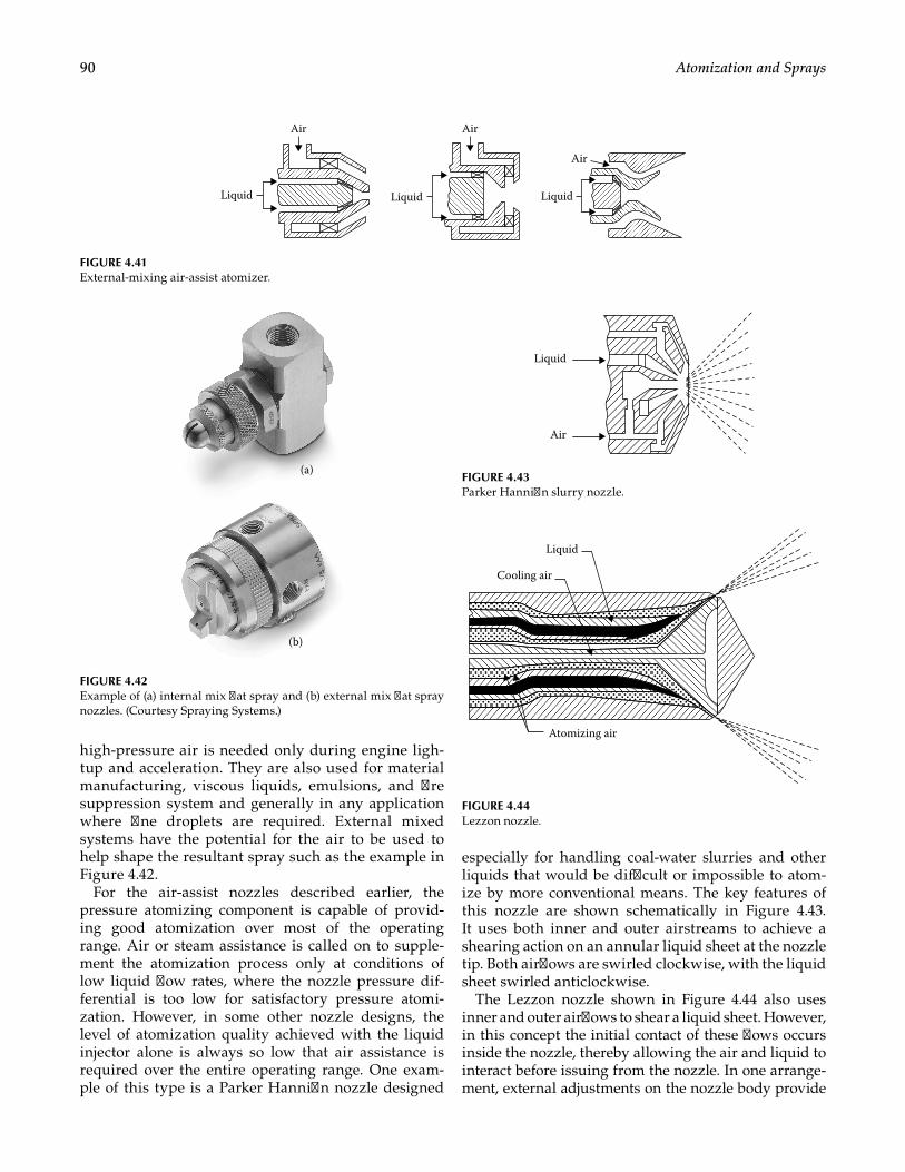
90 Atomization and Sprays

high-pressure air is needed only during engine ligh-tup and acceleration. They are also used for material manufacturing, viscous liquids, emulsions, and fire suppression system and generally in any application where fine droplets are required. External mixed systems have the potential for the air to be used to help shape the resultant spray such as the example in Figure 4.42.

For the air-assist nozzles described earlier, the pressure atomizing component is capable of provid-ing good atomization over most of the operating range. Air or steam assistance is called on to supple-ment the atomization process only at conditions of low liquid flow rates, where the nozzle pressure dif-ferential is too low for satisfactory pressure atomi-zation. However, in some other nozzle designs, the level of atomization quality achieved with the liquid injector alone is always so low that air assistance is required over the entire operating range. One exam-ple of this type is a Parker Hannifin nozzle designed

especially for handling coal-water slurries and other liquids that would be difficult or impossible to atom-ize by more conventional means. The key features of this nozzle are shown schematically in Figure 4.43. It uses both inner and outer airstreams to achieve a shearing action on an annular liquid sheet at the nozzle tip. Both airflows are swirled clockwise, with the liquid sheet swirled anticlockwise.

The Lezzon nozzle shown in Figure 4.44 also uses inner and outer airflows to shear a liquid sheet. However, in this concept the initial contact of these flows occurs inside the nozzle, thereby allowing the air and liquid to interact before issuing from the nozzle. In one arrange-ment, external adjustments on the nozzle body provide

Liquid

Air

Liquid

Air

Liquid

Air

FIGURE 4.41External-mixing air-assist atomizer.

(a)

(b)

FIGURE 4.42Example of (a) internal mix flat spray and (b) external mix flat spray nozzles. (Courtesy Spraying Systems.)

Liquid

Air

FIGURE 4.43Parker Hannifin slurry nozzle.

Liquid

Cooling air

Atomizing air

FIGURE 4.44Lezzon nozzle.

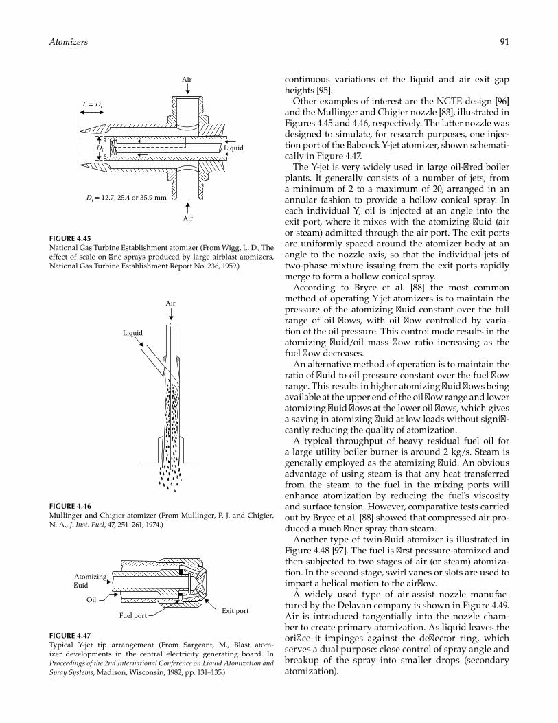
91Atomizers

continuous variations of the liquid and air exit gap heights [95].

Other examples of interest are the NGTE design [96] and the Mullinger and Chigier nozzle [83], illustrated in Figures 4.45 and 4.46, respectively. The latter nozzle was designed to simulate, for research purposes, one injec-tion port of the Babcock Y-jet atomizer, shown schemati-cally in Figure 4.47.

The Y-jet is very widely used in large oil-fired boiler plants. It generally consists of a number of jets, from a minimum of 2 to a maximum of 20, arranged in an annular fashion to provide a hollow conical spray. In each individual Y, oil is injected at an angle into the exit port, where it mixes with the atomizing fluid (air or steam) admitted through the air port. The exit ports are uniformly spaced around the atomizer body at an angle to the nozzle axis, so that the individual jets of two-phase mixture issuing from the exit ports rapidly merge to form a hollow conical spray.

According to Bryce et al. [88] the most common method of operating Y-jet atomizers is to maintain the pressure of the atomizing fluid constant over the full range of oil flows, with oil flow controlled by varia-tion of the oil pressure. This control mode results in the atomizing fluid/oil mass flow ratio increasing as the fuel flow decreases.

An alternative method of operation is to maintain the ratio of fluid to oil pressure constant over the fuel flow range. This results in higher atomizing fluid flows being available at the upper end of the oil flow range and lower atomizing fluid flows at the lower oil flows, which gives a saving in atomizing fluid at low loads without signifi-cantly reducing the quality of atomization.

A typical throughput of heavy residual fuel oil for a large utility boiler burner is around 2 kg/s. Steam is generally employed as the atomizing fluid. An obvious advantage of using steam is that any heat transferred from the steam to the fuel in the mixing ports will enhance atomization by reducing the fuel's viscosity and surface tension. However, comparative tests carried out by Bryce et al. [88] showed that compressed air pro-duced a much finer spray than steam.

Another type of twin-fluid atomizer is illustrated in Figure 4.48 [97]. The fuel is first pressure-atomized and then subjected to two stages of air (or steam) atomiza-tion. In the second stage, swirl vanes or slots are used to impart a helical motion to the airflow.

A widely used type of air-assist nozzle manufac-tured by the Delavan company is shown in Figure 4.49. Air is introduced tangentially into the nozzle cham-ber to create primary atomization. As liquid leaves the orifice it impinges against the deflector ring, which serves a dual purpose: close control of spray angle and breakup of the spray into smaller drops (secondary atomization).

Air

Air

Liquid

L = Di

Di

Di = 12.7, 25.4 or 35.9 mm

FIGURE 4.45National Gas Turbine Establishment atomizer (From Wigg, L. D., The effect of scale on fine sprays produced by large airblast atomizers, National Gas Turbine Establishment Report No. 236, 1959.)

Air

Liquid

FIGURE 4.46Mullinger and Chigier atomizer (From Mullinger, P. J. and Chigier, N. A., J. Inst. Fuel, 47, 251–261, 1974.)

Atomizinguid

Oil

Fuel port Exit port

FIGURE 4.47Typical Y-jet tip arrangement (From Sargeant, M., Blast atom-izer developments in the central electricity generating board. In Proceedings of the 2nd International Conference on Liquid Atomization and Spray Systems, Madison, Wisconsin, 1982, pp. 131–135.)

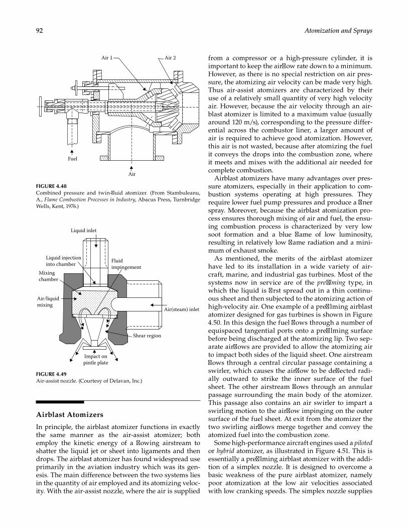
92 Atomization and Sprays

Airblast Atomizers

In principle, the airblast atomizer functions in exactly the same manner as the air-assist atomizer; both employ the kinetic energy of a flowing airstream to shatter the liquid jet or sheet into ligaments and then drops. The airblast atomizer has found widespread use primarily in the aviation industry which was its gen-esis. The main difference between the two systems lies in the quantity of air employed and its atomizing veloc-ity. With the air-assist nozzle, where the air is supplied

from a compressor or a high-pressure cylinder, it is important to keep the airflow rate down to a minimum. However, as there is no special restriction on air pres-sure, the atomizing air velocity can be made very high. Thus air-assist atomizers are characterized by their use of a relatively small quantity of very high velocity air. However, because the air velocity through an air-blast atomizer is limited to a maximum value (usually around 120 m/s), corresponding to the pressure differ-ential across the combustor liner, a larger amount of air is required to achieve good atomization. However, this air is not wasted, because after atomizing the fuel it conveys the drops into the combustion zone, where it meets and mixes with the additional air needed for complete combustion.

Airblast atomizers have many advantages over pres-sure atomizers, especially in their application to com-bustion systems operating at high pressures. They require lower fuel pump pressures and produce a finer spray. Moreover, because the airblast atomization pro-cess ensures thorough mixing of air and fuel, the ensu-ing combustion process is characterized by very low soot formation and a blue flame of low luminosity, resulting in relatively low flame radiation and a mini-mum of exhaust smoke.

As mentioned, the merits of the airblast atomizer have led to its installation in a wide variety of air-craft, marine, and industrial gas turbines. Most of the systems now in service are of the prefilming type, in which the liquid is first spread out in a thin continu-ous sheet and then subjected to the atomizing action of high- velocity air. One example of a prefilming airblast atomizer designed for gas turbines is shown in Figure 4.50. In this design the fuel flows through a number of equispaced tangential ports onto a prefilming surface before being discharged at the atomizing lip. Two sep-arate airflows are provided to allow the atomizing air to impact both sides of the liquid sheet. One airstream flows through a central circular passage containing a swirler, which causes the airflow to be deflected radi-ally outward to strike the inner surface of the fuel sheet. The other airstream flows through an annular passage surrounding the main body of the atomizer. This passage also contains an air swirler to impart a swirling motion to the airflow impinging on the outer surface of the fuel sheet. At exit from the atomizer the two swirling airflows merge together and convey the atomized fuel into the combustion zone.

Some high-performance aircraft engines used a piloted or hybrid atomizer, as illustrated in Figure 4.51. This is essentially a prefilming airblast atomizer with the addi-tion of a simplex nozzle. It is designed to overcome a basic weakness of the pure airblast atomizer, namely poor atomization at the low air velocities associated with low cranking speeds. The simplex nozzle supplies

Air 1 Air 2

Air

Fuel

FIGURE 4.48Combined pressure and twin-fluid atomizer. (From Stambuleanu, A., Flame Combustion Processes in Industry, Abacus Press, Turnbridge Wells, Kent, 1976.)

Liquid inlet

Liquid injectioninto chamber

Mixingchamber

Air/liquidmixing

Impact onpintle plate

Shear region

Air(steam) inlet

Fluidimpingement

FIGURE 4.49Air-assist nozzle. (Courtesy of Delavan, Inc.)

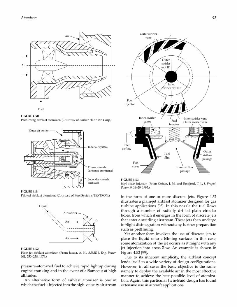
93Atomizers

pressure-atomized fuel to achieve rapid lightup during engine cranking and in the event of a flameout at high altitudes.

An alternative form of airblast atomizer is one in which the fuel is injected into the high-velocity airstream

in the form of one or more discrete jets. Figure 4.52 illustrates a plain-jet airblast atomizer designed for gas turbine applications [98]. In this nozzle the fuel flows through a number of radially drilled plain circular holes, from which it emerges in the form of discrete jets that enter a swirling airstream. These jets then undergo in-flight disintegration without any further preparation such as prefilming.

Yet another form involves the use of discrete jets to place the liquid onto a filming surface. In this case, some atomization of the jet occurs as it might with any jet injection into cross flow. An example is shown in Figure 4.53 [99].

Due to its inherent simplicity, the airblast concept lends itself to a wide variety of design configurations. However, in all cases the basic objective is the same, namely to deploy the available air in the most effective manner to achieve the best possible level of atomiza-tion. Again, this particular twin-fluid design has found extensive use in aircraft applications.

Air

Air

Fuel

FIGURE 4.50Prefilming airblast atomizer. (Courtesy of Parker Hannifin Corp.)

Outer air system

Inner air system

Primary nozzle(pressure atomizing)

Secondary nozzle(airblast)

FIGURE 4.51Piloted airblast atomizer. (Courtesy of Fuel Systems TEXTRON.)

Air swirler

Air

Air

Liquid

FIGURE 4.52Plain-jet airblast atomizer. (From Jasuja, A. K., ASME J. Eng. Power, 101, 250–258, 1979.)

Outer swirlervane

Outerswirlerexit ID

Innerswirler exit ID

Inner swirler vaneOuter swirler vaneFuel

injector

FuelInjector

Inner swirlervanes

Inletairflow

Fuelspray

Fuelfilm

Inner airflowpassage

Outerairflowpassage

FIGURE 4.53High-shear injector. (From Cohen, J. M. and Rosfjord, T. J., J. Propul. Power, 9, 16–29, 1993.)

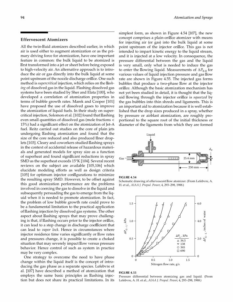
94 Atomization and Sprays

Effervescent Atomizers

All the twin-fluid atomizers described earlier, in which air is used either to augment atomization or as the pri-mary driving force for atomization, have one important feature in common: the bulk liquid to be atomized is first transformed into a jet or sheet before being exposed to high-velocity air. An alternative approach is to intro-duce the air or gas directly into the bulk liquid at some point upstream of the nozzle discharge orifice. One such method is supercritical injection, which relies on the flash-ing of dissolved gas in the liquid. Flashing dissolved gas systems have been studied by Sher and Elata [100], who developed a correlation of atomization properties in terms of bubble growth rates. Marek and Cooper [101] have proposed the use of dissolved gases to improve the atomization of liquid fuels. In their study on super-critical injection, Solomon et al. [102] found that flashing even small quantities of dissolved gas (mole fractions < 15%) had a significant effect on the atomization of Jet-A fuel. Reitz carried out studies on the core of plain jets undergoing flashing atomization and found that the size of the core reduced and also produced finer drop-lets [103]. Cleary and coworkers studied flashing sprays in the context of accidental release of hazardous materi-als and generated models for spray size as a function of superheat and found significant reductions in spray SMD as the superheat exceeds 15°K [104]. Several recent reviews on the subject are available [105,106] which elucidate modeling efforts as well as design criteria [105] for optimum injector configurations to minimize the resulting spray SMD. However, to be offset against this good atomization performance are the problems involved in coercing the gas to dissolve in the liquid and subsequently persuading the gas to emerge from the liq-uid when it is needed to promote atomization. In fact, the problem of low bubble growth rate could prove to be a fundamental limitation to the practical application of flashing injection by dissolved gas systems. The other aspect about flashing sprays that may prove challeng-ing is that, if flashing occurs prior to the injector orifice, it can lead to a step change in discharge coefficient that can lead to vapor lock. Hence in circumstances where injector residence time varies significantly or flow rates and pressures change, it is possible to create a choked situation that may severely impact flow versus pressure behavior. Hence control of such as system in practice may be very complex.

One strategy to overcome the need to have phase change within the liquid itself is the concept of intro-ducing the gas phase as a separate species. Lefebvre et al. [107] have described a method of atomization that employs the same basic principles as flashing injec-tion but does not share its practical limitations. In its

simplest form, as shown in Figure 4.54 [107], the new concept comprises a plain-orifice atomizer with means for injecting air (or gas) into the bulk liquid at some point upstream of the injector orifice. This gas is not intended to impart kinetic energy to the liquid stream, and it is injected at a low velocity. In consequence, the pressure differential between the gas and the liquid is very small, only what is needed to induce the gas to enter the flowing liquid. Measurements of ∆Pg–l for various values of liquid injection pressure and gas flow rate are shown in Figure 4.55. The injected gas forms bubbles that produce a two-phase flow at the injector orifice. Although the basic atomization mechanism has not yet been studied in detail, it is thought that the liq-uid flowing through the injector orifice is squeezed by the gas bubbles into thin shreds and ligaments. This is an important aid to atomization because it is well estab-lished that the drop sizes produced in a spray, whether by pressure or airblast atomization, are roughly pro-portional to the square root of the initial thickness or diameter of the ligaments from which they are formed

Liquid

250 mm

25.4 mmGas

do

FIGURE 4.54Schematic drawing of effervescent flow atomizer. (From Lefebvre, A. H. et al., AIAA J. Propul. Power, 4, 293–298, 1988.)

00

1.0

0.5

1.5

0

4.0

2.034.5138345690

6.0

1.0Nitrogen flow rate, g/s0.5 1.5

ΔPG

– L

, in

ches

of

wat

er

ΔPG

– L

, kP

a

ΔPL , kPa

FIGURE 4.55Pressure differential between atomizing gas and liquid. (From Lefebvre, A. H. et al., AIAA J. Propul. Power, 4, 293–298, 1988.)

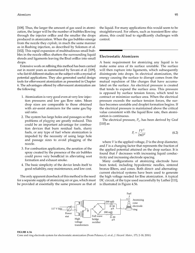
95Atomizers

[108]. Thus, the larger the amount of gas used in atomi-zation, the larger will be the number of bubbles flowing through the injector orifice and the smaller the drops produced in atomization. When the gas bubbles emerge from the nozzle they explode, in much the same manner as in flashing injection, as described by Solomon et al. [102]. This rapid expansion of multitudinous small bub-bles in the nozzle efflux shatters the surrounding liquid shreds and ligaments leaving the final orifice into small drops.

Extensive work on refining this method has been carried out in recent years as summarized by Sovani et al. [109], who list 60 different studies on the subject with a myriad of potential applications. They also generated useful design tools for effervescent atomization as presented in Chapter 6. The advantages offered by effervescent atomization are the following:

1. Atomization is very good even at very low injec-tion pressures and low gas flow rates. Mean drop sizes are comparable to those obtained with air-assist atomizers for the same gas/liq-uid ratio.

2. The system has large holes and passages so that problems of plugging are greatly reduced. This could be an important advantage for combus-tion devices that burn residual fuels, slurry fuels, or any type of fuel where atomization is impeded by the necessity of using large hole and passage sizes to avoid plugging of the nozzle.

3. For combustion applications, the aeration of the spray created by the presence of the air bubbles could prove very beneficial in alleviating soot formation and exhaust smoke.

4. The basic simplicity of the device lends itself to good reliability, easy maintenance, and low cost.

The only apparent drawback of this method is the need for a separate supply of atomizing air or gas, which must be provided at essentially the same pressure as that of

the liquid. For many applications this would seem to be straightforward. For others, such as transient flow situ-ations, this could lead to significantly challenges with control.

Electrostatic Atomizers

A basic requirement for atomizing any liquid is to make some area of its surface unstable. The surface will then rupture into ligaments, which subsequently disintegrate into drops. In electrical atomization, the energy causing the surface to disrupt comes from the mutual repulsion of like charges that have accumu-lated on the surface. An electrical pressure is created that tends to expand the surface area. This pressure is opposed by surface tension forces, which tend to contract or minimize surface area. When the electrical pressure exceeds the surface tension forces, the sur-face becomes unstable and droplet formation begins. If the electrical pressure is maintained above the critical value consistent with the liquid flow rate, then atomi-zation is continuous.

The electrical pressure, Pe, has been derived by Graf [110] as

PFV

De =

π2

2

2 (4.2)

where V is the applied voltage, D is the drop diameter, and F is a charging factor that represents the fraction of the applied potential attained on the drop surface. It is found that F decreases with increasing liquid conduc-tivity and increasing electrode spacing.

Many configurations of atomizing electrode have been tested, including hypodermic needles, sintered bronze filters, and cones. Both direct- and alternating-current electrical systems have been used to generate the high voltage needed for fine atomization. A typical DC circuit, of the type used successfully by Luther [111], is illustrated in Figure 4.56.

200 mΩ

0–30

0–30

200 mΩ

Fuel

117 V line

Powerstat

Highvoltagetransformers

Full-wavebridgerectifier

ring

Atomizingconeelectrode

+

–μA

μA

A

A

FIGURE 4.56Cone and ring electrode system for electrostatic atomization (From Polanco, G. et al., J. Hazard. Mater., 173, 2–18, 2010.)

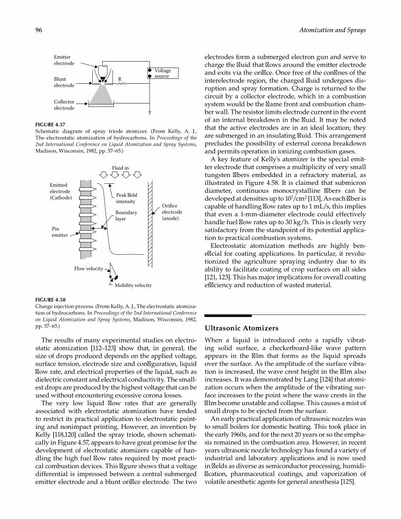
96 Atomization and Sprays

The results of many experimental studies on electro-static atomization [112–123] show that, in general, the size of drops produced depends on the applied voltage, surface tension, electrode size and configuration, liquid flow rate, and electrical properties of the liquid, such as dielectric constant and electrical conductivity. The small-est drops are produced by the highest voltage that can be used without encountering excessive corona losses.

The very low liquid flow rates that are generally associated with electrostatic atomization have tended to restrict its practical application to electrostatic paint-ing and nonimpact printing. However, an invention by Kelly [118,120] called the spray triode, shown schemati-cally in Figure 4.57, appears to have great promise for the development of electrostatic atomizers capable of han-dling the high fuel flow rates required by most practi-cal combustion devices. This figure shows that a voltage differential is impressed between a central submerged emitter electrode and a blunt orifice electrode. The two

electrodes form a submerged electron gun and serve to charge the fluid that flows around the emitter electrode and exits via the orifice. Once free of the confines of the interelectrode region, the charged fluid undergoes dis-ruption and spray formation. Charge is returned to the circuit by a collector electrode, which in a combustion system would be the flame front and combustion cham-ber wall. The resistor limits electrode current in the event of an internal breakdown in the fluid. It may be noted that the active electrodes are in an ideal location; they are submerged in an insulating fluid. This arrangement precludes the possibility of external corona breakdown and permits operation in ionizing combustion gases.

A key feature of Kelly's atomizer is the special emit-ter electrode that comprises a multiplicity of very small tungsten fibers embedded in a refractory material, as illustrated in Figure 4.58. It is claimed that submicron diameter, continuous monocrystalline fibers can be developed at densities up to 107/cm2 [113], As each fiber is capable of handling flow rates up to 1 mL/s, this implies that even a 1-mm-diameter electrode could effectively handle fuel flow rates up to 30 kg/h. This is clearly very satisfactory from the standpoint of its potential applica-tion to practical combustion systems.

Electrostatic atomization methods are highly ben-eficial for coating applications. In particular, it revolu-tionized the agriculture spraying industry due to its ability to facilitate coating of crop surfaces on all sides [121, 123]. This has major implications for overall coating efficiency and reduction of wasted material.

Ultrasonic Atomizers

When a liquid is introduced onto a rapidly vibrat-ing solid surface, a checkerboard-like wave pattern appears in the film that forms as the liquid spreads over the surface. As the amplitude of the surface vibra-tion is increased, the wave crest height in the film also increases. It was demonstrated by Lang [124] that atomi-zation occurs when the amplitude of the vibrating sur-face increases to the point where the wave crests in the film become unstable and collapse. This causes a mist of small drops to be ejected from the surface.

An early practical application of ultrasonic nozzles was to small boilers for domestic heating. This took place in the early 1960s, and for the next 20 years or so the empha-sis remained in the combustion area. However, in recent years ultrasonic nozzle technology has found a variety of industrial and laboratory applications and is now used in fields as diverse as semiconductor processing, humidi-fication, pharmaceutical coatings, and vaporization of volatile anesthetic agents for general anesthesia [125].

Emitterelectrode

Bluntelectrode

Collectorelectrode

RVoltagesource

FIGURE 4.57Schematic diagram of spray triode atomizer. (From Kelly, A. J., The electrostatic atomization of hydrocarbons. In Proceedings of the 2nd International Conference on Liquid Atomization and Spray Systems, Madison, Wisconsin, 1982, pp. 57–65.)

Fluid in

Peak eldintensity

Boundarylayer

Mobility velocity

Flow velocity

Pinemitter

Orificeelectrode(anode)

Emittedelectrode(Cathode)

FIGURE 4.58Charge injection process. (From Kelly, A. J., The electrostatic atomiza-tion of hydrocarbons. In Proceedings of the 2nd International Conference on Liquid Atomization and Spray Systems, Madison, Wisconsin, 1982, pp. 57–65.)

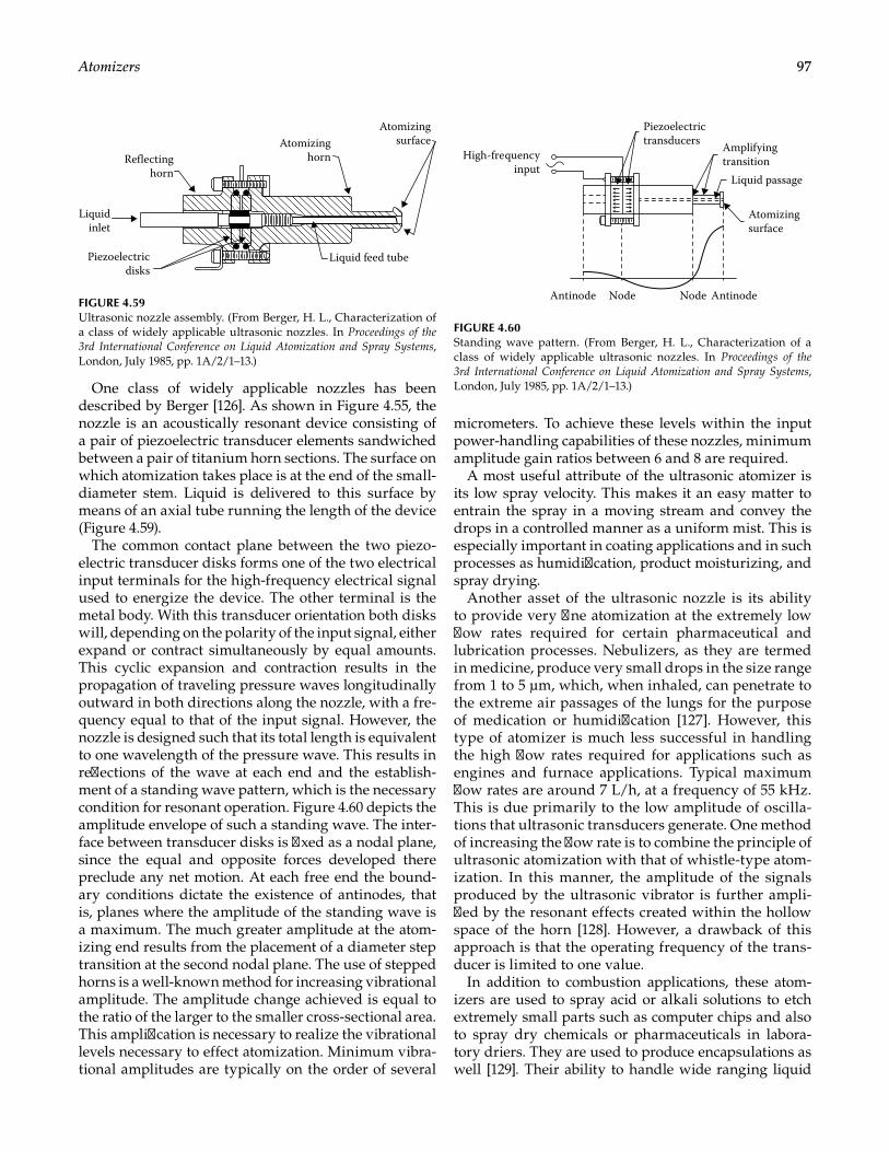
97Atomizers

One class of widely applicable nozzles has been described by Berger [126]. As shown in Figure 4.55, the nozzle is an acoustically resonant device consisting of a pair of piezoelectric transducer elements sandwiched between a pair of titanium horn sections. The surface on which atomization takes place is at the end of the small-diameter stem. Liquid is delivered to this surface by means of an axial tube running the length of the device (Figure 4.59).

The common contact plane between the two piezo-electric transducer disks forms one of the two electrical input terminals for the high-frequency electrical signal used to energize the device. The other terminal is the metal body. With this transducer orientation both disks will, depending on the polarity of the input signal, either expand or contract simultaneously by equal amounts. This cyclic expansion and contraction results in the propagation of traveling pressure waves longitudinally outward in both directions along the nozzle, with a fre-quency equal to that of the input signal. However, the nozzle is designed such that its total length is equivalent to one wavelength of the pressure wave. This results in reflections of the wave at each end and the establish-ment of a standing wave pattern, which is the necessary condition for resonant operation. Figure 4.60 depicts the amplitude envelope of such a standing wave. The inter-face between transducer disks is fixed as a nodal plane, since the equal and opposite forces developed there preclude any net motion. At each free end the bound-ary conditions dictate the existence of antinodes, that is, planes where the amplitude of the standing wave is a maximum. The much greater amplitude at the atom-izing end results from the placement of a diameter step transition at the second nodal plane. The use of stepped horns is a well-known method for increasing vibrational amplitude. The amplitude change achieved is equal to the ratio of the larger to the smaller cross-sectional area. This amplification is necessary to realize the vibrational levels necessary to effect atomization. Minimum vibra-tional amplitudes are typically on the order of several

micrometers. To achieve these levels within the input power-handling capabilities of these nozzles, minimum amplitude gain ratios between 6 and 8 are required.

A most useful attribute of the ultrasonic atomizer is its low spray velocity. This makes it an easy matter to entrain the spray in a moving stream and convey the drops in a controlled manner as a uniform mist. This is especially important in coating applications and in such processes as humidification, product moisturizing, and spray drying.

Another asset of the ultrasonic nozzle is its ability to provide very fine atomization at the extremely low flow rates required for certain pharmaceutical and lubrication processes. Nebulizers, as they are termed in medicine, produce very small drops in the size range from 1 to 5 µm, which, when inhaled, can penetrate to the extreme air passages of the lungs for the purpose of medication or humidification [127]. However, this type of atomizer is much less successful in handling the high flow rates required for applications such as engines and furnace applications. Typical maximum flow rates are around 7 L/h, at a frequency of 55 kHz. This is due primarily to the low amplitude of oscilla-tions that ultrasonic transducers generate. One method of increasing the flow rate is to combine the principle of ultrasonic atomization with that of whistle-type atom-ization. In this manner, the amplitude of the signals produced by the ultrasonic vibrator is further ampli-fied by the resonant effects created within the hollow space of the horn [128]. However, a drawback of this approach is that the operating frequency of the trans-ducer is limited to one value.

In addition to combustion applications, these atom-izers are used to spray acid or alkali solutions to etch extremely small parts such as computer chips and also to spray dry chemicals or pharmaceuticals in labora-tory driers. They are used to produce encapsulations as well [129]. Their ability to handle wide ranging liquid

Atomizinghorn

Liquid feed tube

Atomizingsurface

Reflectinghorn

Liquidinlet

Piezoelectricdisks

FIGURE 4.59Ultrasonic nozzle assembly. (From Berger, H. L., Characterization of a class of widely applicable ultrasonic nozzles. In Proceedings of the 3rd International Conference on Liquid Atomization and Spray Systems, London, July 1985, pp. 1A/2/1–13.)

Piezoelectrictransducers Amplifying

transitionLiquid passage

NodeNode

High-frequencyinput

AntinodeAntinode

Atomizingsurface

FIGURE 4.60Standing wave pattern. (From Berger, H. L., Characterization of a class of widely applicable ultrasonic nozzles. In Proceedings of the 3rd International Conference on Liquid Atomization and Spray Systems, London, July 1985, pp. 1A/2/1–13.)

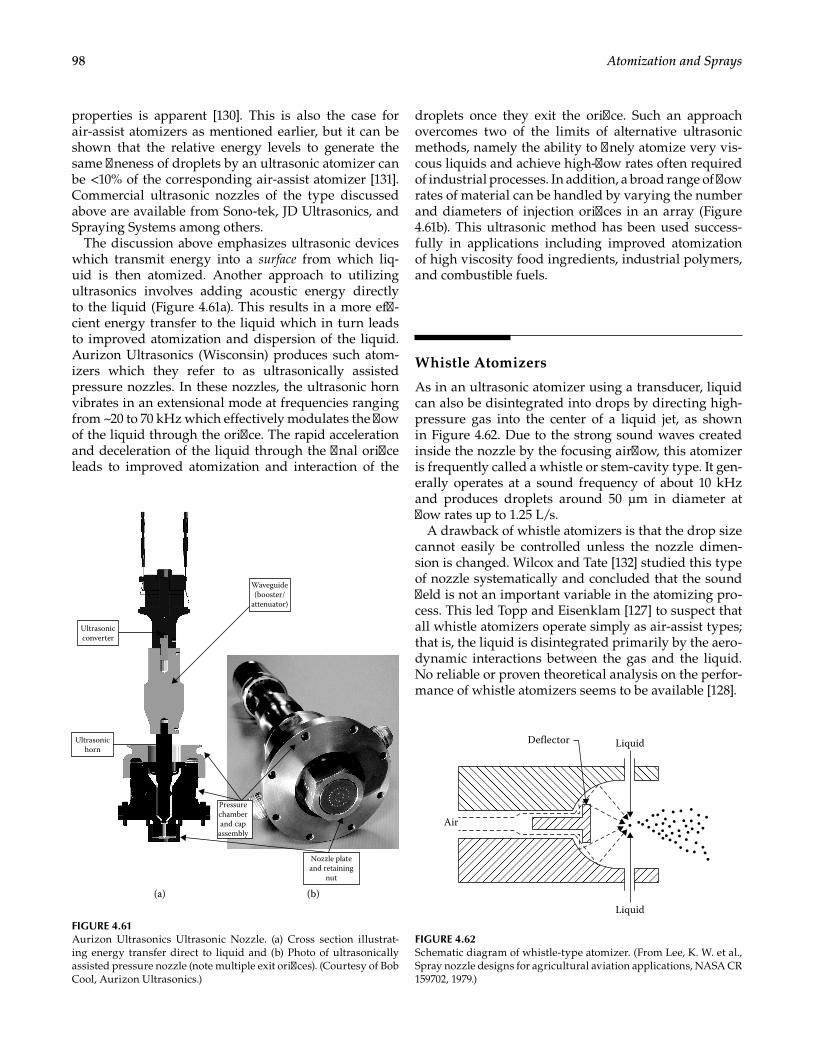
98 Atomization and Sprays

properties is apparent [130]. This is also the case for air-assist atomizers as mentioned earlier, but it can be shown that the relative energy levels to generate the same fineness of droplets by an ultrasonic atomizer can be <10% of the corresponding air-assist atomizer [131]. Commercial ultrasonic nozzles of the type discussed above are available from Sono-tek, JD Ultrasonics, and Spraying Systems among others.

The discussion above emphasizes ultrasonic devices which transmit energy into a surface from which liq-uid is then atomized. Another approach to utilizing ultrasonics involves adding acoustic energy directly to the liquid (Figure 4.61a). This results in a more effi-cient energy transfer to the liquid which in turn leads to improved atomization and dispersion of the liquid. Aurizon Ultrasonics (Wisconsin) produces such atom-izers which they refer to as ultrasonically assisted pressure nozzles. In these nozzles, the ultrasonic horn vibrates in an extensional mode at frequencies ranging from ~20 to 70 kHz which effectively modulates the flow of the liquid through the orifice. The rapid acceleration and deceleration of the liquid through the final orifice leads to improved atomization and interaction of the

droplets once they exit the orifice. Such an approach overcomes two of the limits of alternative ultrasonic methods, namely the ability to finely atomize very vis-cous liquids and achieve high-flow rates often required of industrial processes. In addition, a broad range of flow rates of material can be handled by varying the number and diameters of injection orifices in an array (Figure 4.61b). This ultrasonic method has been used success-fully in applications including improved atomization of high viscosity food ingredients, industrial polymers, and combustible fuels.

Whistle Atomizers

As in an ultrasonic atomizer using a transducer, liquid can also be disintegrated into drops by directing high-pressure gas into the center of a liquid jet, as shown in Figure 4.62. Due to the strong sound waves created inside the nozzle by the focusing airflow, this atomizer is frequently called a whistle or stem-cavity type. It gen-erally operates at a sound frequency of about 10 kHz and produces droplets around 50 µm in diameter at flow rates up to 1.25 L/s.

A drawback of whistle atomizers is that the drop size cannot easily be controlled unless the nozzle dimen-sion is changed. Wilcox and Tate [132] studied this type of nozzle systematically and concluded that the sound field is not an important variable in the atomizing pro-cess. This led Topp and Eisenklam [127] to suspect that all whistle atomizers operate simply as air-assist types; that is, the liquid is disintegrated primarily by the aero-dynamic interactions between the gas and the liquid. No reliable or proven theoretical analysis on the perfor-mance of whistle atomizers seems to be available [128].

(a)

Pressurechamberand cap

assembly

Nozzle plateand retaining

nut

(b)

Ultrasonichorn

Waveguide(booster/

attenuator)

Ultrasonicconverter

FIGURE 4.61Aurizon Ultrasonics Ultrasonic Nozzle. (a) Cross section illustrat-ing energy transfer direct to liquid and (b) Photo of ultrasonically assisted pressure nozzle (note multiple exit orifices). (Courtesy of Bob Cool, Aurizon Ultrasonics.)

Liquid

Liquid

Deflector

Air

FIGURE 4.62Schematic diagram of whistle-type atomizer. (From Lee, K. W. et al., Spray nozzle designs for agricultural aviation applications, NASA CR 159702, 1979.)

99Atomizers

Manufacturing Aspects

All of the atomizer design concepts shown require consideration for manufacturability. The ability to fabricate parts in specialized ways or with increased precision is an evolving field in its own right. Many of the designs and examples shown in this chapter can be made using the conventional machining methods. Given this as a constraint, design concepts may have been dismissed due to costs associated with manu-facturing or ability to maintain proper precision or repeatability. Yet in light of new manufacturing or machining methods, such concepts may now be viable. This has been touched on in reviews of the history of atomizer design [133].

Examples include printing methodologies or pho-toetching methods to essentially generate an atomizer in layers. So called platelet technology was used by Aerojet Corporation in the 1970s for fuel injectors, heat exchang-ers, and a myriad of other components (e.g., Reference [134]). The so-called macrolamination approach is another example of these wherein any given design that can be envisioned to be made from a series of layers can be conceived. Parker Hannifin has used this methodol-ogy to generate low-cost, highly repeatable atomizers with a wide range of flow numbers [135,136].

Another very interesting technology is additive manufacturing, wherein a part is manufactured in layers using metal powder and a laser, rather than removing material as in traditional machining. In 2015, GE Aviation gained attention for being one of the first manufacturers to have FAA approval of the LEAP Engine fuel injectors with some components made using additive manufacturing. Fuel injectors for rocket engines are also being fabricated using additive manufacturing. Examples are shown in Figure 4.63. In general, while laser sintering methods can be used to build up an injector, internal geometry and manufac-turing tolerances usually require some cleanup post fabrication.

Given the ubiquitous use of plain jets for injection liquids in various atomizer types, and the relations described in Chapter 2 regarding the dependency of the results drop sizes on injector diameters, any technology capable of providing precise, clean holes is of interest. To this end, advanced laser drilling techniques have been applied to injectors. Using picosecond laser pulses, the material that is to be removed can be done so without significant heating of the surrounding material. This allows for highly precise holes to be made at very small diameters (down to single digit micron diameters). An example from Oxford Lasers is shown in Figure 4.64.

With the recent advances in manufacturing methods and techniques, it is evident that atomizer design could

continue to evolve for many years as the understand-ing of how to design the parts to take advantage of the methods is gained.

References

1. Elliott, M. A., Combustion of diesel fuel, SAE Trans., Vol. 3, No. 3, 1949, pp. 490–497.

2. Rosselli, A., and Badgley, P., Simulation of the Cummins diesel injection system, SAE Trans., Vol. 80, Pt. 3, 1971, pp. 1870–1880.

3. Sinnamon, J. F., Lancaster, D. R., and Steiner, J. C., An experimental and analytical study of engine fuel spray trajectories, SAE Trans., Vol. 89, Sect. 1, 1980, pp. 765–783.

4. Elkotb, M. M., Fuel atomization for spray modeling, Prog. Energy Combust. Sci., Vol. 8, 1982, pp. 61–91.

5. Borman, G. L., and Johnson, J. H., Unsteady vaporiza-tion histories and trajectories of fuel drops injected into swirling air, SAE Paper 598C, 1962.

(a)

A

(b)

FIGURE 4.63Examples of fuel injectors using additive manufacturing for some elements. (a) (GE Aviation). (b) (Courtesy of NASA.)

FIGURE 4.64Example advanced laser drilling (Oxford Laser).

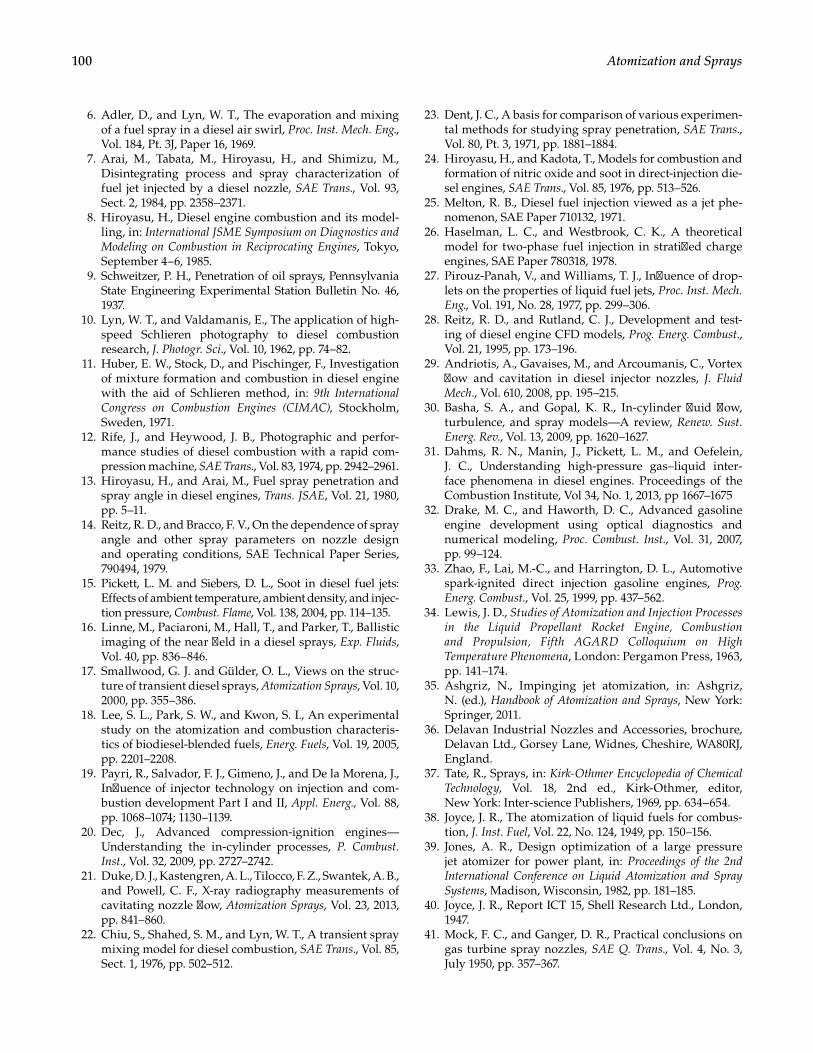
100 Atomization and Sprays

6. Adler, D., and Lyn, W. T., The evaporation and mixing of a fuel spray in a diesel air swirl, Proc. Inst. Mech. Eng., Vol. 184, Pt. 3J, Paper 16, 1969.

7. Arai, M., Tabata, M., Hiroyasu, H., and Shimizu, M., Disintegrating process and spray characterization of fuel jet injected by a diesel nozzle, SAE Trans., Vol. 93, Sect. 2, 1984, pp. 2358–2371.

8. Hiroyasu, H., Diesel engine combustion and its model-ling, in: International JSME Symposium on Diagnostics and Modeling on Combustion in Reciprocating Engines, Tokyo, September 4–6, 1985.

9. Schweitzer, P. H., Penetration of oil sprays, Pennsylvania State Engineering Experimental Station Bulletin No. 46, 1937.

10. Lyn, W. T., and Valdamanis, E., The application of high-speed Schlieren photography to diesel combustion research, J. Photogr. Sci., Vol. 10, 1962, pp. 74–82.

11. Huber, E. W., Stock, D., and Pischinger, F., Investigation of mixture formation and combustion in diesel engine with the aid of Schlieren method, in: 9th International Congress on Combustion Engines (CIMAC), Stockholm, Sweden, 1971.

12. Rife, J., and Heywood, J. B., Photographic and perfor-mance studies of diesel combustion with a rapid com-pression machine, SAE Trans., Vol. 83, 1974, pp. 2942–2961.

13. Hiroyasu, H., and Arai, M., Fuel spray penetration and spray angle in diesel engines, Trans. JSAE, Vol. 21, 1980, pp. 5–11.

14. Reitz, R. D., and Bracco, F. V., On the dependence of spray angle and other spray parameters on nozzle design and operating conditions, SAE Technical Paper Series, 790494, 1979.

15. Pickett, L. M. and Siebers, D. L., Soot in diesel fuel jets: Effects of ambient temperature, ambient density, and injec-tion pressure, Combust. Flame, Vol. 138, 2004, pp. 114–135.

16. Linne, M., Paciaroni, M., Hall, T., and Parker, T., Ballistic imaging of the near field in a diesel sprays, Exp. Fluids, Vol. 40, pp. 836–846.

17. Smallwood, G. J. and Gülder, O. L., Views on the struc-ture of transient diesel sprays, Atomization Sprays, Vol. 10, 2000, pp. 355–386.

18. Lee, S. L., Park, S. W., and Kwon, S. I., An experimental study on the atomization and combustion characteris-tics of biodiesel-blended fuels, Energ. Fuels, Vol. 19, 2005, pp. 2201–2208.

19. Payri, R., Salvador, F. J., Gimeno, J., and De la Morena, J., Influence of injector technology on injection and com-bustion development Part I and II, Appl. Energ., Vol. 88, pp. 1068–1074; 1130–1139.

20. Dec, J., Advanced compression-ignition engines—Understanding the in-cylinder processes, P. Combust. Inst., Vol. 32, 2009, pp. 2727–2742.

21. Duke, D. J., Kastengren, A. L., Tilocco, F. Z., Swantek, A. B., and Powell, C. F., X-ray radiography measurements of cavitating nozzle flow, Atomization Sprays, Vol. 23, 2013, pp. 841–860.

22. Chiu, S., Shahed, S. M., and Lyn, W. T., A transient spray mixing model for diesel combustion, SAE Trans., Vol. 85, Sect. 1, 1976, pp. 502–512.

23. Dent, J. C., A basis for comparison of various experimen-tal methods for studying spray penetration, SAE Trans., Vol. 80, Pt. 3, 1971, pp. 1881–1884.

24. Hiroyasu, H., and Kadota, T., Models for combustion and formation of nitric oxide and soot in direct-injection die-sel engines, SAE Trans., Vol. 85, 1976, pp. 513–526.

25. Melton, R. B., Diesel fuel injection viewed as a jet phe-nomenon, SAE Paper 710132, 1971.

26. Haselman, L. C., and Westbrook, C. K., A theoretical model for two-phase fuel injection in stratified charge engines, SAE Paper 780318, 1978.

27. Pirouz-Panah, V., and Williams, T. J., Influence of drop-lets on the properties of liquid fuel jets, Proc. Inst. Mech. Eng., Vol. 191, No. 28, 1977, pp. 299–306.

28. Reitz, R. D., and Rutland, C. J., Development and test-ing of diesel engine CFD models, Prog. Energ. Combust., Vol. 21, 1995, pp. 173–196.

29. Andriotis, A., Gavaises, M., and Arcoumanis, C., Vortex flow and cavitation in diesel injector nozzles, J. Fluid Mech., Vol. 610, 2008, pp. 195–215.

30. Basha, S. A., and Gopal, K. R., In-cylinder fluid flow, turbulence, and spray models—A review, Renew. Sust. Energ. Rev., Vol. 13, 2009, pp. 1620–1627.

31. Dahms, R. N., Manin, J., Pickett, L. M., and Oefelein, J. C., Understanding high-pressure gas–liquid inter-face phenomena in diesel engines. Proceedings of the Combustion Institute, Vol 34, No. 1, 2013, pp 1667–1675

32. Drake, M. C., and Haworth, D. C., Advanced gasoline engine development using optical diagnostics and numerical modeling, Proc. Combust. Inst., Vol. 31, 2007, pp. 99–124.

33. Zhao, F., Lai, M.-C., and Harrington, D. L., Automotive spark-ignited direct injection gasoline engines, Prog. Energ. Combust., Vol. 25, 1999, pp. 437–562.

34. Lewis, J. D., Studies of Atomization and Injection Processes in the Liquid Propellant Rocket Engine, Combustion and Propulsion, Fifth AGARD Colloquium on High Temperature Phenomena, London: Pergamon Press, 1963, pp. 141–174.

35. Ashgriz, N., Impinging jet atomization, in: Ashgriz, N. (ed.), Handbook of Atomization and Sprays, New York: Springer, 2011.

36. Delavan Industrial Nozzles and Accessories, brochure, Delavan Ltd., Gorsey Lane, Widnes, Cheshire, WA80RJ, England.

37. Tate, R., Sprays, in: Kirk-Othmer Encyclopedia of Chemical Technology, Vol. 18, 2nd ed., Kirk-Othmer, editor, New York: Inter-science Publishers, 1969, pp. 634–654.

38. Joyce, J. R., The atomization of liquid fuels for combus-tion, J. Inst. Fuel, Vol. 22, No. 124, 1949, pp. 150–156.

39. Jones, A. R., Design optimization of a large pressure jet atomizer for power plant, in: Proceedings of the 2nd International Conference on Liquid Atomization and Spray Systems, Madison, Wisconsin, 1982, pp. 181–185.

40. Joyce, J. R., Report ICT 15, Shell Research Ltd., London, 1947.

41. Mock, F. C., and Ganger, D. R., Practical conclusions on gas turbine spray nozzles, SAE Q. Trans., Vol. 4, No. 3, July 1950, pp. 357–367.

101Atomizers

42. Carey, F. H., The development of the spill flow burner and its control system for gas turbine engines, J. R. Aeronaut. Soc., Vol. 58, No. 527, November 1954, pp. 737–753.

43. Radcliffe, A., The performance of a type of swirl atom-izer, Proc. Inst. Mech. Eng., Vol. 169, 1955, pp. 93–106.

44. Radcliffe, A., Fuel injection, in: High Speed Aerodynamics and Jet Propulsion, Sect. D, Vol XI, Hawthorne, W.R. and Olson, W.T., editors Princeton, NJ: Princeton University Press, 1960.

45. Tipler, W., and Wilson, A. W., Combustion in gas tur-bines, Paper No. B9, in: Proceedings of the Congress International des Machines a Combustion (CIMAC), Paris, 1959, pp. 897–927.

46. Dombrowski, N., and Munday, G., Spray Drying, in: Biochemical and Biological Engineering Science, Vol 2, Chap. 16, Blakegrough, N., editor New York: Academic Press, 1968, pp. 209–320.

47. Rizk, N., and Lefebvre, A. H., Internal flow characteris-tics of simplex swirl atomizers, J. Prop Power, Vol. 1, 1985, pp. 193–199.

48. Sakman, A. T., Jog, M. A., Jeng, S. M., and Benjamin, M. A., Parametric study of simplex fuel nozzle inter-nal flow and performance, AIAA J., Vol. 38, 2000, pp. 1214–1218.

49. Eslamian, M., and Ashgriz, N., Swirl, t-jet, and vibrat-ing-mesh atomizers, in: Ashgiz, N. (ed.), Handbook of Atomization and Sprays, New York NY: Springer, 2011.

50. Vijay, G. A., Moorthi, N. S. V., and Manivannan, A., Internal and external flow characteristics of swirl atomizers: A review, Atomization Sprays, Vol. 25, 2015, pp. 153–188.

51. Pilcher, J. M., and Miesse, C. C., Methods of atomiza-tion, in: Injection and Combustion of Liquid Fuels, Chap. 2, WADC-TR-56-3 AD 118142, Columbus, Ohio: Battelle Memorial Institute, March 1957.

52. Tyler, S. R., and Turner, H. G., Fuel systems and high speed flight, Shell Aviation News, No. 233, 1957.

53. Hermann, J., Gleis, S., and Vortmeyer, D., Active Instability Control (AIC) of spray combustors by modu-lation of the liquid fuel flow rate, Combust. Sci. Technol., Vol. 118, 1996, pp. 1–25.

54. Lee, J.-Y., Lubarsky, E., and Zinn, B. T., “Slow” active con-trol of combustion instabilities by modification of liquid fuel spray properties, Proc. Combust. Inst., Vol. 30, 2005, pp. 1757–1764.

55. Clare, H., Gardiner, J. A., and Neale, M. C., Study of fuel injection in air breathing combustion cham-bers, in: Experimental Methods in Combustion Research, Surugue, J. (Editor). London: Pergamon Press, 1964, pp. 5–20.

56. Smith, R. W., and Miller, P. C. H., Drift predictions in the near nozzle region of a flat fan spray, J. Agr. Eng. Res., Vol. 59, 1994, pp. 111–120.

57. Snyder, H., Senser, D. W., Lefebvre, A. H., and Coutinho, R. S., Drop size measurements in electrostatic paint sprays, IEEE T. Ind. Appl., Vol. 25, 1989, pp. 720–727.

58. Fraser, R. P., and Eisenklam, P., Liquid atomization and the drop size of sprays, Trans. Inst. Chem. Eng., Vol. 34, 1956, pp. 295–319.

59. Dombrowski, N., and Fraser, R. P., A photographic inves-tigation into the disintegration of liquid sheets, Philos. Trans. R. Soc. Lond. Ser. A., Vol. 247, No. 924, September 1954, pp. 101–130.

60. Dombrowski, N., Hasson, D., and Ward, D. E., Some aspects of liquid flow through fan spray nozzles, Chem. Eng. Sci., Vol. 12, 1960, pp. 35–50.

61. Carr, E., The Combustion of a range of distillate fuels in small gas turbine engines, ASME Paper 79-GT-175, 1979.

62. Carr, E., Further applications of the Lucas fan spray fuel injection system, ASME Paper 85-IGT-116, 1985.

63. Mansour, A., and Chigier, N., Disintegration of liquid sheets, Phys. Fluids, Vol. 2, 1990, pp. 706–719.

64. Mansour, A., and Chigier, N., Dynamic behavior of liq-uid sheets, Phys. Fluids, Vol. 3, 1990, pp. 2971–2980.

65. Altimira, M., Rivas, A., Ramos, J. C., and Anton, R., On the disintegration of fan-shaped liquid sheets, Atomization Sprays, Vol. 22, 2012, pp. 733–755.

66. Watkins, S. C., Simplified flat spray fuel nozzle, U.S. Patent No. 3,759,448, 1972.

67. Masters, K., Spray Drying, 2nd ed., New York: John Wiley & Sons, 1976.

68. Hinze, J. O., and Milborn, H., Atomization of liquids by means of a rotating cup, ASME J. Appl. Mech., Vol. 17, No. 2, 1950, pp. 145–153.

69. Friedman, S. J., Bluckert, F. A., and Marshall, W. R., Centrifugal disk atomization, Chem. Eng. Prog., Vol. 48, 1952, pp. 181–191.

70. Kayano, A., and Kamiya, T., Calculation of the mean size of the droplets purged from the rotating disk, in: Proceedings of the 1st International Conference on Liquid Atomization and Spray Systems, Tokyo, 1978, pp. 133–143.

71. Tanasawa, Y., Miyasaka, Y., and Umehara, M., Effect of shape of rotating disks and cups on liquid atomiza-tion, in: Proceedings of the 1st International Conference on Liquid Atomization and Spray Systems, Tokyo, 1978, pp. 165–172.

72. Matsumoto, S., Crosby, E. J., and Belcher, D. W., Rotary atomizers; performance understanding and prediction, in: Proceedings of the 3rd International Conference on Liquid Atomization and Spray Systems, London, July 1985, pp. 1A/1/1–20.

73. Willauer, H. D., Mushrush, G. W., and Williams, F. W., Critical evaluation of rotary atomizer, Petrol. Sci. Technol., Vol. 24, 2006, pp. 1215–1232.

74. Karim, G. A., and Kumar, R., The atomization of liquids at low ambient pressure conditions, in: Proceedings of the 1st International Conference on Liquid Atomization and Spray Systems, Tokyo, August 1978, pp. 151–155.

75. Masters, K., Rotary atomizers, in: Proceedings of the 1st International Conference on Liquid Atomization and Spray Systems, Tokyo, August 1978, p. 456.

76. Wehner, H., Combustion chambers for turbine power plants, Interavia, Vol. 7, No. 7, 1952, pp. 395–400.

77. Maskey, H. C, and Marsh, F. X., The annular combustion chamber with centrifugal fuel injection, SAE Preprint No. 444C, 1962.

78. Nichol, I. W., The T65 and T72 shaft turbines, SAE Preprint No. 624A, 1963.

102 Atomization and Sprays

79. Burgher, M. W., Interrelated parameters of gas turbine engine design and electrical ignition systems, SAE Preprint No. 682C, 1963.

80. Morishita, T., A development of the fuel atomizing device utilizing high rotational speed, ASME Paper, 81-GT-180, New York: 1981

81. `Dahm, W. J. A., Patel, P. R., and Lerg, B. H., Experimental visualizations of liquid breakup regimes in fuel slinger atomization, Atomization Sprays, Vol. 16, 2006, pp. 933–944.

82. Dahm, W. J. A., Patel, P. R., and Lerg, B. H., Analysis of liquid breakup regimes in fuel slinger atomization, Atomization Sprays, Vol. 16, 2006.

83. Choi, S. M., Lee, D., and Park, J., Ignition and combus-tion characteristics of the gas turbine slinger combustor, J. Mech. Sci. Tech., Vol. 22, 2008, pp. 538–544.

84. Choi, S. M., Jang, S. H., Lee, D. H., and You, G. W., Spray characteristics of the rotating fuel injection system of a micro-jet engine, J. Mech. Sci. Tech., Vol. 24., 2010, pp. 551–558.

85. Romp, H. A., Oil Burning, New York: Martinus Nijhoff, The Hague; Stechert & Company, 1937.

86. Gretzinger, J., and Marshall, W. R., Jr., Characteristics of pneumatic atomization, J. Am. Inst. Chem. Eng., Vol. 7, No. 2, June 1961, pp. 312–318.

87. Mullinger, P. J., and Chigier, N. A., The design and per-formance of internal mixing multi-jet twin-fluid atom-izers, J. Inst. Fuel, Vol. 47, 1974, pp. 251–261.

88. Bryce, W. B., Cox, N. W., and Joyce, W. I., Oil droplet pro-duction and size measurement from a twin-fluid atom-izer using real fluids, in: Proceedings of the 1st International Conference on Liquid Atomization and Spray Systems, Tokyo, 1978, pp. 259–263.

89. Sargeant, M., Blast atomizer developments in the cen-tral electricity generating board, in: Proceedings of the 2nd International Conference on Liquid Atomization and Spray Systems, Madison, Wisconsin, 1982, pp. 131–135.

90. Hurley, J. F., and Doyle, B. W., Design of two-phase atom-izers for use in combustion furnaces, in: Proceedings of the 3rd International Conference on Liquid Atomization and Spray Systems, London, July 1985, pp. 1A/3/1–13.

91. Hewitt, A. J., Droplet size spectra produced by air-assisted atomizers, J. Aerosol Sci., Vol. 24, 1993, pp. 155–162.

92. Kufferath, A., Wende, B., and Leuckel, W., Influence of liquid flow conditions on spray characteristics of inter-nal-mixing twin-fluid atomizers, Int. J. Heat Fluid Flow, Vol. 20, 1999, pp. 513–519.

93. Lal, S., Kushari, A., Gupta, M., Kapoor, J. C., and Maji, S., Experimental study of an air-assisted mist generator, Exp. Therm. Fluid Sci., Vol. 34, 2010, pp. 1029–1035.

94. Mlkvik, M., Stahle, P., Schuchmann, H. P., Gaukel, V., Jedelsky, J., and Jicha, M., Twin-fluid atomization of viscous liquids: The effect of atomizer construction on breakup process, spray stability, and droplet size, Int. J. Multiphase Flows, Vol. 77, 2015, pp. 19–31.

95. Rosfjord, T. J., Atomization of coal water mixtures: Evaluation of fuel nozzles and a cellulose gum simulant, ASME Paper 85-GT-38, 1985.

96. Wigg, L. D., The effect of scale on fine sprays produced by large airblast atomizers, National Gas Turbine Establishment Report No. 236, 1959.

97. Stambuleanu, A., Flame Combustion Processes in Industry, Turnbridge Wells, Kent: Abacus Press, 1976.

98. Jasuja, A. K., Atomization of crude and residual fuel oils, ASME J. Eng. Power, Vol. 101, No. 2, 1979, pp. 250–258.

99. Cohen, J. M., and Rosfjord, T. J., Influences on the sprays formed by high-shear fuel nozzle/swirler assemblies, J. Propul. Power, Vol. 9, 1993, pp. 16–29.

100. Sher, E., and Elata, D., Spray formation from pressure cans by flashing Ind. Eng. Chem. Process Des. Dev., Vol. 16, 1977, pp. 237–242.

101. Marek, C. J., and Cooper, L. P., U.S. Patent No. 4,189,914, 1980.

102. Solomon, A. S. P., Rupprecht, S. D., Chen, L. D., and Faeth, G. M., Flow and atomization in flashing injec-tors, Atomization Spray Technol., Vol. 1, No. 1, 1985, pp. 53–76.

103. Reitz, R., A photographic study of flash-boiling atomiza-tion, Aerosol Sci. Technol., Vol. 12, 1990, pp. 561–569.

104. Witlox, H., Harper, M., Bowen, P., and Clearly, V., Flashing liquid jets and two-phase droplet dispersion: II. Comparison and validation of droplet size and rainout, J. Hazard. Mater., Vol. 142, 2007, pp. 797–809.

105. Sher, E., Bar-Kohany, T., and Rashkovan, A., Flash-boiling atomization, Prog. Energ. Combust., Vol. 34, 2008, pp. 417–439.

106. Polanco, G., Hold., A. E., and Munday, G., General review of flashing jet studies, J. Hazard. Mater., Vol. 173, 2010, pp. 2–18.

107. Lefebvre, A. H., Wang, X. F., and Martin, C. A., Spray characteristics of aerated liquid pressure atomizers, AIAA J. Propul. Power, Vol. 4, 1988, pp. 293–298.

108. Lefebvre, A. H., Gas Turbine Combustion, Hemisphere Publishing Corp, 1983.

109. Sovani, S. D., Sojka, P. E., and Lefebvre, A. H., Effervescent atomization, Prog. Energ. Combust., Vol. 27, 2001, pp. 483–521.

110. Graf, P. E., Breakup of small liquid volume by electri-cal charging, in: Proceedings of API Research Conference on Distillate Fuel Combustion, API Publication 1701, Paper CP62–4, 1962.

111. Luther, F. E., Electrostatic atomization of No. 2 heating oil, in: Proceedings of API Research Conference on Distillate Fuel Combustion, API Publication 1701, Paper CP62–3, 1962.

112. Peskin, R. L., Raco, R. J., and Morehouse, J., A study of parameters governing electrostatic atomization of fuel oil, in: Proceedings of API Research Conference on Distillate Fuel Combustion, API Publication 704, 1965.

113. Bollini, R., Sample, B., Seigal, S. D., and Boarman, J. W., Production of monodisperse charged metal particles by harmonic electrical spraying, J. Interface Sci., Vol. 51, No. 2, 1975, pp. 272–277.

114. Drozin, V. G., The electrical dispersion of liquids as aero-sols, J. Colloid Sci., Vol. 10, No. 2, 1955, pp. 158–164.

115. Macky, W. A., Some investigations on the deformation and breaking of water drops in strong electric fields, Proc. R. Soc. Lond. Ser. A, Vol. 133, 1931, pp. 565–587.

116. Nawab, M. A., and Mason, S. C., The preparation of uni-form emulsions by electrical dispersion, J. Colloid Sci., Vol. 13, 1958, pp. 179–187.

103Atomizers

117. Vonnegut, B., and Neubauer, R. L., Production of mono-disperse liquid particles by electrical atomization, J. Colloid Sci., Vol. 7, 1952, pp. 616–622.

118. Kelly, A. J., The electrostatic atomization of hydrocar-bons, in: Proceedings of the 2nd International Conference on Liquid Atomization and Spray Systems, Madison, Wisconsin, 1982, pp. 57–65.

119. Bailey, A. G., The theory and practice of electrostatic spray-ing, Atomization Spray Technol., Vol. 2, 1986, pp. 95–134.

120. Kelly, A. J., On the statistical, quantum, and practical mechanics of electrostatic sprays, J. Aerosol Sci., Vol. 25, 1994, pp. 1159–1177.

121. Law, E. S., Agricultural electrostatic spray application: A review of significant research and development dur-ing the 20th century. J. Electrostat., Vol. 51–52, 2001, pp. 25–42.

122. Shrimpton, J., and Yule, A. J. Electrohydrodynamics of charge injection atomization: Regimes and fundamental limits, Atomization Sprays, Vol. 13, 2003, pp. 173–190.

123. Maski, D., and Durairaj, D., Effects of electrode voltage, liquid flow rate, and liquid properties on spray charge-ability of an air-assisted electrostatic-induction spray-charging system, J. Electrostat., Vol. 68, 2010, pp. 152–158.

124. Lang, R. J., Ultrasonic atomization of liquids, J. Acoust. Soc. Am., Vol. 34, No. 1, 1962, pp. 6–8.

125. Cabler, P., Geddes, L. A., and Rosborough, J., The use of ultrasonic energy to vaporize anaesthetic liquids, Br. J. Aneasth., Vol. 47, 1975, pp. 541–545.

126. Berger, H. L., Characterization of a class of widely applicable ultrasonic nozzles, in: Proceedings of the 3rd International Conference on Liquid Atomization and Spray Systems, London, July 1985, pp. 1A/2/1–13.

127. Topp, M. N., and Eisenklam, P., Industrial and medical use of ultrasonic atomizers, Ultrasonics, Vol. 10, No. 3, 1972, pp. 127–133.

128. Lee, K. W., Putnam, A. A., Gieseke, J. A., Golovin, M. N., and Hale, J. A., Spray nozzle designs for agricultural aviation applications, NASA CR 159702, 1979.

129. Freitas, S., Merkle, H. P., and Gander, B., Ultrasonic atom-isation into reduced pressure atmosphere—Envisaged aseptic spray-drying for microencapsulation, J. Control. Release, Vol. 95, 2004, pp. 185–195.

130. Avvaru, B., Patil, M. N., Gogate, P. R., and Pandit, A. B., Ultrasonic atomization: Effects of liquid phase proper-ties, Ultrasonics, Vol. 44, 2006, pp. 146–158.

131. Rajan, R., and Pandit, A. B., Correlations to predict drop-let size in ultrasonic atomisation, Ultrasonics, Vol. 39, 2001, pp. 235–255.

132. Wilcox, R. L., and Tate, R. W., Liquid atomization in a high intensity sound field, J. Am. Inst. Chem. Eng., Vol. 11, No. 1, 1965, pp. 69–72.

133. Lefebvre, A., Fifty years of gas turbine fuel injection, Atomization Sprays, Vol. 10, 2000, pp. 251–276.

134. Kors, D. L., Lawver, B. R., and Addoms, J. F., Platelet-injector venture carburetor for internal combustion engines, US Patent 3,914,347, 1975.

135. Simmons, H. C., and Harvey, R. J., Spray nozzle and method of manufacturing same, US Patent 5,435,884, 1995.

136. Mansour, A., Benjamin, M., Straub, D. L., and Richards, G. A., Application of macrolamination technology to lean, premixed combustion, J. Engr. Gas Turb. Power, Vol. 123, 2001, pp. 796–802.

105

5Flow in Atomizers

Introduction

In twin-fluid atomizers of the airblast and air-assist types, atomization and spray dispersion tend to be dominated by air momentum forces, with hydrodynamic processes playing only a secondary role. With pressure-swirl nozzles, however, the internal flow characteristics are of primary importance, because they govern the thickness and uniformity of the annular liquid film formed in the final discharge orifice as well as the relative magnitude of the axial and tangential components of velocity of this film. It is therefore of great practical interest to examine the interrelationships that exist between internal flow characteristics, nozzle design variables, and important spray features such as cone angle and mean drop size. The various equations that have been derived for noz-zle discharge coefficient are discussed at some length, because this coefficient not only affects the flow rate of any given nozzle, but also can be used to calculate its velocity coefficient and spray cone angle.

It is also becoming increasingly clear that cavitation can play a complex role in both flow behavior as well as external spray characteristics. Cavitation results in a two-phase flow behavior within the injector passages and has become increasingly appreciated and under-stood through a number of advancements in imaging technologies including the ability to probe fluid flow within practical injectors.

Consideration is also given to the complex flow situa-tions that arise on the surface of a rotating cup or disk. These flow characteristics are of basic importance to the successful operation of these atomizers, because they exercise a controlling influence on the nature of the atomization process, the quality of atomization, and distribution of drop sizes in the spray.

Flow Number

The effective flow area of a pressure atomizer is usu-ally described in terms of a flow number, which is expressed as the ratio of the nozzle throughput to the square root of the fuel-injection pressure differential. Two definitions of flow number are in general use: a

British version, based on the volume flow rate, and the other is an American version, based on the mass flow rate. They are

=FNFlow rate, UK gal h

(Injection pressure differential, psid)UK 0.5 (5.1)

=FNFlow rate, lb h

(Injection pressure differential, psid)US 0.5 (5.2)

Note that 1 UK gallon = 1.2 US gallons.Equations 5.1 and 5.2 have the advantage of being

expressed in units that are in general use. Unfortunately, they are basically unsound. For example, they do not allow a fixed and constant value of flow number to be assigned to any given nozzle. Thus, although it is cus-tomary to stamp or engrave a value of flow number on the body of a simplex atomizer, this value is correct only when the nozzle is flowing a standard calibrating fluid of density 765 kg/m3. In the past, this has posed no problems with aircraft gas turbines because 765 kg/m3 roughly cor-responds to the density of aviation gasoline. However, for liquids of other densities, these two definitions of flow number could lead to appreciable errors when used to calculate liquid flow rates or injection pressures.

It should be apparent that the basic deficiency in Equations 5.1 and 5.2 is the omission of liquid density. Inclusion of this property would not only allow these equations to be rewritten in dimensionally correct form but also enable the flow number to be defined in a much more useful manner than at present, namely as the effective flow area of the nozzle. Thus the flow number of any given nozzle would have a fixed and constant value for all liquids.

By including liquid density, the flow number in square meters is obtained as

=FN Flow rate, kg s(Pressure differential, Pa) (Liquid density, kg m )0.5 3 0.5 (5.3)

The standard UK and US flow numbers may be calculated from Equation 5.3 using the formulas:

FN 0.66 10 FNUK8

L0.5= × × ρ ×− (5.4)

FN 0.66 10 FNUS6

L0.5= × × ρ × (5.5)

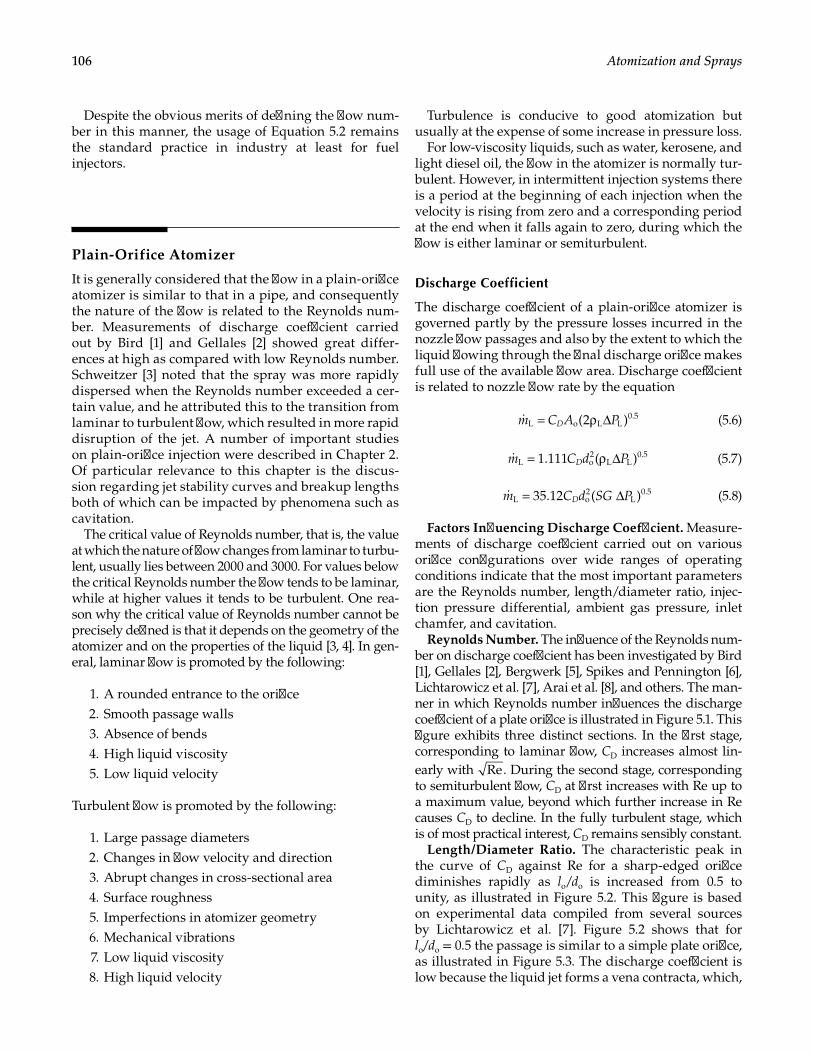
106 Atomization and Sprays

Despite the obvious merits of defining the flow num-ber in this manner, the usage of Equation 5.2 remains the standard practice in industry at least for fuel injectors.

Plain-Orifice Atomizer

It is generally considered that the flow in a plain-orifice atomizer is similar to that in a pipe, and consequently the nature of the flow is related to the Reynolds num-ber. Measurements of discharge coefficient carried out by Bird [1] and Gellales [2] showed great differ-ences at high as compared with low Reynolds number. Schweitzer [3] noted that the spray was more rapidly dispersed when the Reynolds number exceeded a cer-tain value, and he attributed this to the transition from laminar to turbulent flow, which resulted in more rapid disruption of the jet. A number of important studies on plain-orifice injection were described in Chapter 2. Of particular relevance to this chapter is the discus-sion regarding jet stability curves and breakup lengths both of which can be impacted by phenomena such as cavitation.

The critical value of Reynolds number, that is, the value at which the nature of flow changes from laminar to turbu-lent, usually lies between 2000 and 3000. For values below the critical Reynolds number the flow tends to be laminar, while at higher values it tends to be turbulent. One rea-son why the critical value of Reynolds number cannot be precisely defined is that it depends on the geometry of the atomizer and on the properties of the liquid [3, 4]. In gen-eral, laminar flow is promoted by the following:

1. A rounded entrance to the orifice 2. Smooth passage walls 3. Absence of bends 4. High liquid viscosity 5. Low liquid velocity

Turbulent flow is promoted by the following:

1. Large passage diameters 2. Changes in flow velocity and direction 3. Abrupt changes in cross-sectional area 4. Surface roughness 5. Imperfections in atomizer geometry 6. Mechanical vibrations 7. Low liquid viscosity 8. High liquid velocity

Turbulence is conducive to good atomization but usually at the expense of some increase in pressure loss.

For low-viscosity liquids, such as water, kerosene, and light diesel oil, the flow in the atomizer is normally tur-bulent. However, in intermittent injection systems there is a period at the beginning of each injection when the velocity is rising from zero and a corresponding period at the end when it falls again to zero, during which the flow is either laminar or semiturbulent.

Discharge Coefficient

The discharge coefficient of a plain-orifice atomizer is governed partly by the pressure losses incurred in the nozzle flow passages and also by the extent to which the liquid flowing through the final discharge orifice makes full use of the available flow area. Discharge coefficient is related to nozzle flow rate by the equation

m C A PD= ρ ∆(2 )L o L L0.5

(5.6)

m C d PD= ρ ∆1.111 ( )L o2

L L0.5

(5.7)

m C d SG PD= ∆35.12 ( )L o2

L0.5

(5.8)

Factors Influencing Discharge Coefficient. Measure-ments of discharge coefficient carried out on various orifice configurations over wide ranges of operating conditions indicate that the most important parameters are the Reynolds number, length/diameter ratio, injec-tion pressure differential, ambient gas pressure, inlet chamfer, and cavitation.

Reynolds Number. The influence of the Reynolds num-ber on discharge coefficient has been investigated by Bird [1], Gellales [2], Bergwerk [5], Spikes and Pennington [6], Lichtarowicz et al. [7], Arai et al. [8], and others. The man-ner in which Reynolds number influences the discharge coefficient of a plate orifice is illustrated in Figure 5.1. This figure exhibits three distinct sections. In the first stage, corresponding to laminar flow, CD increases almost lin-early with Re. During the second stage, corresponding to semiturbulent flow, CD at first increases with Re up to a maximum value, beyond which further increase in Re causes CD to decline. In the fully turbulent stage, which is of most practical interest, CD remains sensibly constant.

Length/Diameter Ratio. The characteristic peak in the curve of CD against Re for a sharp-edged orifice diminishes rapidly as lo/do is increased from 0.5 to unity, as illustrated in Figure 5.2. This figure is based on experimental data compiled from several sources by Lichtarowicz et al. [7]. Figure 5.2 shows that for lo/do = 0.5 the passage is similar to a simple plate orifice, as illustrated in Figure 5.3. The discharge coefficient is low because the liquid jet forms a vena contracta, which,

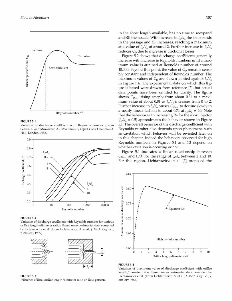
107Flow in Atomizers

in the short length available, has no time to reexpand and fill the nozzle. With increase in lo/do the jet expands in the passage and CD increases, reaching a maximum at a value of lo/do of around 2. Further increase in lo/do reduces CD due to increase in frictional losses.

Figure 5.2 shows that discharge coefficients generally increase with increase in Reynolds numbers until a max-imum value is attained at Reynolds number of around 10,000. Beyond this point, the value of CD remains sensi-bly constant and independent of Reynolds number. The maximum values of CD are shown plotted against lo/do in Figure 5.4. The experimental data on which this fig-ure is based were drawn from reference [7], but actual data points have been omitted for clarity. The figure shows CDmax rising steeply from about 0.61 to a maxi-mum value of about 0.81 as lo/do increases from 0 to 2. Further increase in lo/do causes CDmax to decline slowly in a nearly linear fashion to about 0.74 at lo/do = 10. Note that the behavior with increasing Re for the short injector (lo/do = 0.5) approximates the behavior shown in Figure 5.1. The overall behavior of the discharge coefficient with Reynolds number also depends upon phenomena such as cavitation which behavior will be revisited later on in this chapter. Indeed the behaviors observed for high Reynolds numbers in Figures 5.1 and 5.2 depend on whether caviation is occuring or not.

Figure 5.4 indicates a linear relationship between CDmax and lo/do for the range of lo/do between 2 and 10. For this region, Lichtarowicz et al. [7] proposed the

Semi-turbulent

Laminar

Turbulent

(Reynolds number)0.5

Disc

harg

e co

effic

ient

, CD

FIGURE 5.1Variation in discharge coefficient with Reynolds number. (From Giffen, E. and Muraszew, A., Atomization of Liquid Fuels, Chapman & Hall, London, 1953.)

0.2

0.3

0.4

0.5

0.6

0.7

0.8

0.9

Disc

harg

e co

effic

ient

, CD

Reynolds number10 100 1,000 10,0001

104

12

0.5

lo/do

lo/do

FIGURE 5.2Variation of discharge coefficient with Reynolds number for various orifice length/diameter ratios. Based on experimental data compiled by Lichtarowicz et al. (From Lichtarowicz, A. et al., J. Mech. Eng. Sci., 7, 210–219, 1965.)

do

lo

FIGURE 5.3Influence of final orifice length/diameter ratio on flow pattern.

1 2 3 4 5 6 7 8 9 100Orifice length/diameter ratio

0.60

0.65

0.70

0.75

0.80

0.85

Max

imum

val

ue o

f disc

harg

e co

effic

ient

High reynolds number

Equation 5.9

FIGURE 5.4Variation of maximum value of discharge coefficient with orifice length/diameter ratio. Based on experimental data compiled by Lichtarowicz et al. (From Lichtarowicz, A. et al., J. Mech. Eng. Sci., 7, 210–219, 1965.)

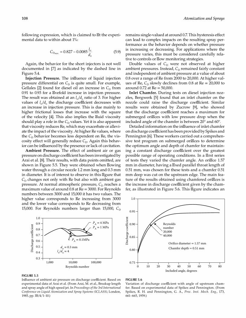
108 Atomization and Sprays

following expression, which is claimed to fit the experi-mental data to within about 1%:

Cld

= −0.827 0.0085Do

omax (5.9)

Again, the behavior for the short injectors is not well documented in [7] as indicated by the dashed line in Figure 5.4.

Injection Pressure. The influence of liquid injection pressure differential on CD is quite small. For example, Gellales [2] found for diesel oil an increase in CD from 0.91 to 0.93 for a fivefold increase in injection pressure. The result was obtained at an lo/do ratio of 3. For higher values of lo/do the discharge coefficient decreases with an increase in injection pressure. This is due mainly to higher frictional losses that increase with the square of the velocity [4]. This also implies the fluid viscosity should play a role in the CD values. Yet it is also apparent that viscosity reduces Re, which may exacerbate or allevi-ate the impact of the viscosity. At higher Re values, where the CD behavior becomes less dependent on Re, the vis-cosity effect will generally reduce CD. Again this behav-ior can be influenced by the presence or lack of cavitation.

Ambient Pressure. The effect of ambient air or gas pressure on discharge coefficient has been investigated by Arai et al. [8]. Their results, with data points omitted, are shown in Figure 5.5. They were obtained when flowing water through a circular nozzle 1.2 mm long and 0.3 mm in diameter. It is of interest to observe in this figure that CD changes not only with Re but also with ambient gas pressure. At normal atmospheric pressure, CD reaches a maximum value of around 0.8 at Re = 3000. For Reynolds numbers between 3000 and 15,000 it has two values. The higher value corresponds to Re increasing from 3000 and the lower value corresponds to Re decreasing from 15,000. For Reynolds numbers larger than 15,000, CD

remains single-valued at around 0.7. This hysteresis effect can lead to complex impacts on the resulting spray per-formance as the behavior depends on whether pressure is increasing or decreasing. For applications where the pressure varies, this must be considered carefully rela-tive to controls or flow monitoring strategies.

Double values of CD were not observed at higher ambient pressures. Instead, CD remained fairly constant and independent of ambient pressure at a value of about 0.8 over a range of Re from 2000 to 20,000. At higher val-ues of Re, CD slowly declines from 0.8 at Re = 20,000 to around 0.72 at Re = 50,000.

Inlet Chamfer. During tests on diesel injection noz-zles, Bergwerk [5] found that an inlet chamfer on the nozzle could raise the discharge coefficient. Similar results were obtained by Zucrow [9], who showed that the discharge coefficient reaches a maximum for submerged orifices with low pressure drop when the included angle of the chamfer is between 20° and 60°.

Detailed information on the influence of inlet chamfer on discharge coefficient has been provided by Spikes and Pennington [6]. These workers carried out a comprehen-sive test program on submerged orifices to determine the optimum angle and depth of chamfer for maintain-ing a constant discharge coefficient over the greatest possible range of operating conditions. In a first series of tests they varied the chamfer angle. An orifice 1.57 mm in diameter, having a fixed parallel throat length of 0.51 mm, was chosen for these tests and a chamfer 0.51 mm deep was cut on the upstream edge. The main fea-ture of the results obtained using chamfered orifices is the increase in discharge coefficient given by the cham-fer, as illustrated in Figure 5.6. This figure indicates an

1,000 10,000 100,000

0.4

0.3

0.5

0.6

0.7

0.8

0.9

1.0

Reynolds number

Disc

harg

e co

effic

ient

lo/do = 4do = 0.3 mm

PA = 0.1MPa

PA = 4 MPaPA = 1 MPa

FIGURE 5.5Influence of ambient air pressure on discharge coefficient. Based on experimental data of Arai et al. (From Arai, M. et al., Breakup length and spray angle of high speed jet. In Proceedings of the 3rd International Conference on Liquid Atomization and Spray Systems (ICLASS), London, 1985, pp. IB/4/1–10.)

0 10 20 30 40 50 60 70 80Included angle, degrees

0.75

0.80

0.85

0.90

0.95

1.0

Disc

harg

e co

effic

ient

Reynoldsnumber20,00040,000

Orifice diameter = 1.57 mmChamfer depth = 0.51 mm

FIGURE 5.6Variation of discharge coefficient with angle of upstream cham-fer. Based on experimental data of Spikes and Pennington. (From Spikes, R. H. and Pennington, G. A., Proc. Inst. Mech. Eng., 173, 661–665, 1959.)

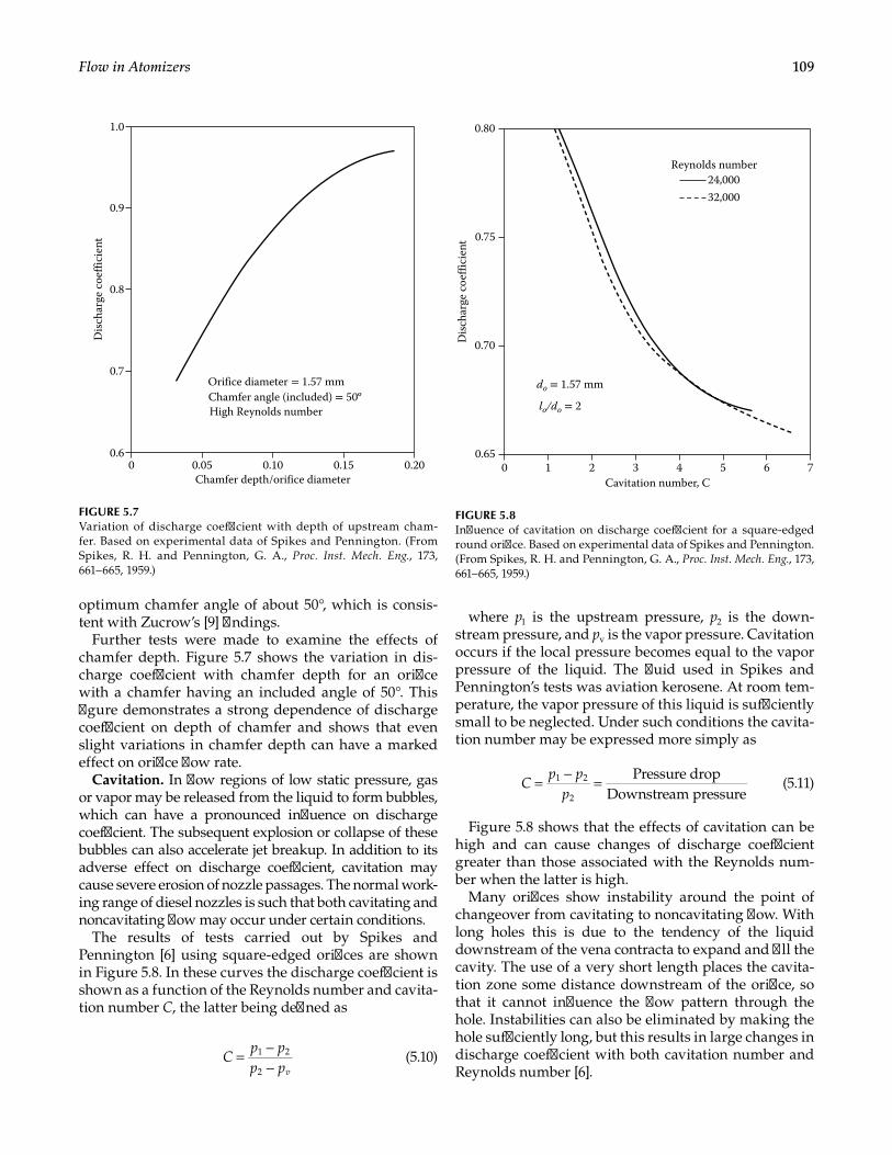
109Flow in Atomizers

optimum chamfer angle of about 50°, which is consis-tent with Zucrow’s [9] findings.

Further tests were made to examine the effects of chamfer depth. Figure 5.7 shows the variation in dis-charge coefficient with chamfer depth for an orifice with a chamfer having an included angle of 50°. This figure demonstrates a strong dependence of discharge coefficient on depth of chamfer and shows that even slight variations in chamfer depth can have a marked effect on orifice flow rate.

Cavitation. In flow regions of low static pressure, gas or vapor may be released from the liquid to form bubbles, which can have a pronounced influence on discharge coefficient. The subsequent explosion or collapse of these bubbles can also accelerate jet breakup. In addition to its adverse effect on discharge coefficient, cavitation may cause severe erosion of nozzle passages. The normal work-ing range of diesel nozzles is such that both cavitating and noncavitating flow may occur under certain conditions.

The results of tests carried out by Spikes and Pennington [6] using square-edged orifices are shown in Figure 5.8. In these curves the discharge coefficient is shown as a function of the Reynolds number and cavita-tion number C, the latter being defined as

Cp pp pv

= −−

1 2

2 (5.10)

where p1 is the upstream pressure, p2 is the down-stream pressure, and pv is the vapor pressure. Cavitation occurs if the local pressure becomes equal to the vapor pressure of the liquid. The fluid used in Spikes and Pennington’s tests was aviation kerosene. At room tem-perature, the vapor pressure of this liquid is sufficiently small to be neglected. Under such conditions the cavita-tion number may be expressed more simply as

Cp p

p= − = Pressure drop

Downstream pressure1 2

2 (5.11)

Figure 5.8 shows that the effects of cavitation can be high and can cause changes of discharge coefficient greater than those associated with the Reynolds num-ber when the latter is high.

Many orifices show instability around the point of changeover from cavitating to noncavitating flow. With long holes this is due to the tendency of the liquid downstream of the vena contracta to expand and fill the cavity. The use of a very short length places the cavita-tion zone some distance downstream of the orifice, so that it cannot influence the flow pattern through the hole. Instabilities can also be eliminated by making the hole sufficiently long, but this results in large changes in discharge coefficient with both cavitation number and Reynolds number [6].

1.0

0.05 0.15 0.200 0.10

0.9

0.8

0.7

0.6

Chamfer depth/orifice diameter

Disc

harg

e co

effic

ient

Orifice diameter = 1.57 mmChamfer angle (included) = 50ºHigh Reynolds number

FIGURE 5.7Variation of discharge coefficient with depth of upstream cham-fer. Based on experimental data of Spikes and Pennington. (From Spikes, R. H. and Pennington, G. A., Proc. Inst. Mech. Eng., 173, 661–665, 1959.)

0 1 2 3 4 5 6 7Cavitation number, C

Disc

harg

e co

effic

ient

0.65

0.70

0.75

0.80

lo/do = 2

do = 1.57 mm

Reynolds number24,00032,000

FIGURE 5.8Influence of cavitation on discharge coefficient for a square-edged round orifice. Based on experimental data of Spikes and Pennington. (From Spikes, R. H. and Pennington, G. A., Proc. Inst. Mech. Eng., 173, 661–665, 1959.)

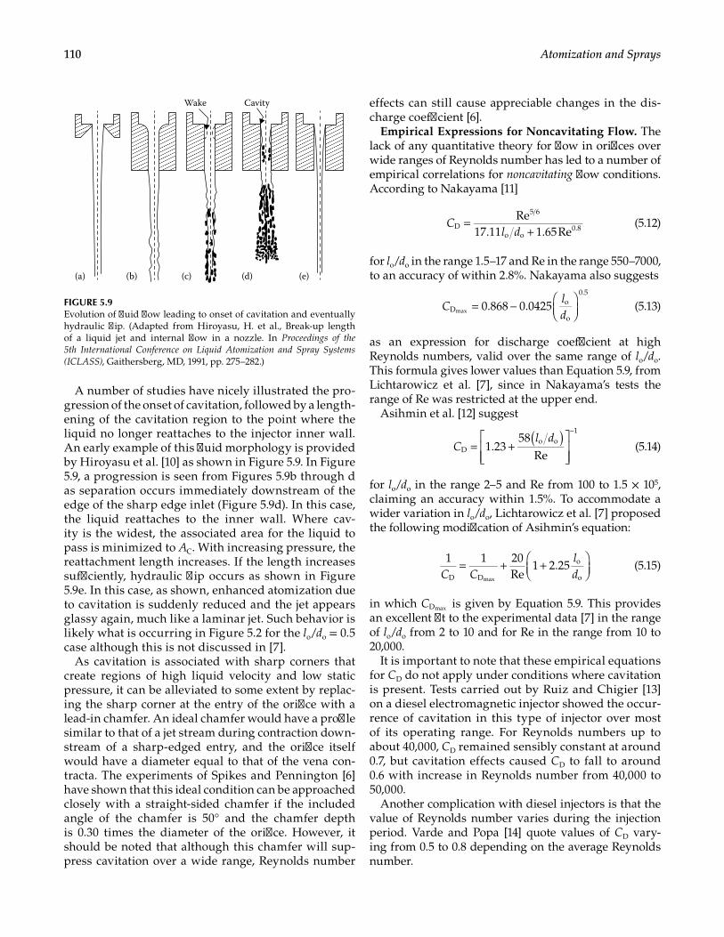
110 Atomization and Sprays

A number of studies have nicely illustrated the pro-gression of the onset of cavitation, followed by a length-ening of the cavitation region to the point where the liquid no longer reattaches to the injector inner wall. An early example of this fluid morphology is provided by Hiroyasu et al. [10] as shown in Figure 5.9. In Figure 5.9, a progression is seen from Figures 5.9b through d as separation occurs immediately downstream of the edge of the sharp edge inlet (Figure 5.9d). In this case, the liquid reattaches to the inner wall. Where cav-ity is the widest, the associated area for the liquid to pass is minimized to AC. With increasing pressure, the reattachment length increases. If the length increases sufficiently, hydraulic flip occurs as shown in Figure 5.9e. In this case, as shown, enhanced atomization due to cavitation is suddenly reduced and the jet appears glassy again, much like a laminar jet. Such behavior is likely what is occurring in Figure 5.2 for the lo/do = 0.5 case although this is not discussed in [7].

As cavitation is associated with sharp corners that create regions of high liquid velocity and low static pressure, it can be alleviated to some extent by replac-ing the sharp corner at the entry of the orifice with a lead-in chamfer. An ideal chamfer would have a profile similar to that of a jet stream during contraction down-stream of a sharp-edged entry, and the orifice itself would have a diameter equal to that of the vena con-tracta. The experiments of Spikes and Pennington [6] have shown that this ideal condition can be approached closely with a straight-sided chamfer if the included angle of the chamfer is 50° and the chamfer depth is 0.30 times the diameter of the orifice. However, it should be noted that although this chamfer will sup-press cavitation over a wide range, Reynolds number

effects can still cause appreciable changes in the dis-charge coefficient [6].

Empirical Expressions for Noncavitating Flow. The lack of any quantitative theory for flow in orifices over wide ranges of Reynolds number has led to a number of empirical correlations for noncavitating flow conditions. According to Nakayama [11]

Cl d

=+

Re17.11 1.65ReD

5 6

o o0.8 (5.12)

for lo/do in the range 1.5–17 and Re in the range 550–7000, to an accuracy of within 2.8%. Nakayama also suggests

Cld

= −

0.868 0.0425Do

o

0.5

max (5.13)

as an expression for discharge coefficient at high Reynolds numbers, valid over the same range of lo/do. This formula gives lower values than Equation 5.9, from Lichtarowicz et al. [7], since in Nakayama’s tests the range of Re was restricted at the upper end.

Asihmin et al. [12] suggest

Cl d( )= +

−

1.2358

ReDo o

1

(5.14)

for lo/do in the range 2–5 and Re from 100 to 1.5 × 105, claiming an accuracy within 1.5%. To accommodate a wider variation in lo/do, Lichtarowicz et al. [7] proposed the following modification of Asihmin’s equation:

C C

ld

= + +

1 1 20Re

1 2.25D D

o

omax

(5.15)

in which CDmax is given by Equation 5.9. This provides an excellent fit to the experimental data [7] in the range of lo/do from 2 to 10 and for Re in the range from 10 to 20,000.

It is important to note that these empirical equations for CD do not apply under conditions where cavitation is present. Tests carried out by Ruiz and Chigier [13] on a diesel electromagnetic injector showed the occur-rence of cavitation in this type of injector over most of its operating range. For Reynolds numbers up to about 40,000, CD remained sensibly constant at around 0.7, but cavitation effects caused CD to fall to around 0.6 with increase in Reynolds number from 40,000 to 50,000.

Another complication with diesel injectors is that the value of Reynolds number varies during the injection period. Varde and Popa [14] quote values of CD vary-ing from 0.5 to 0.8 depending on the average Reynolds number.

Wake

(a) (b) (c) (d) (e)

Cavity

FIGURE 5.9Evolution of fluid flow leading to onset of cavitation and eventually hydraulic flip. (Adapted from Hiroyasu, H. et al., Break-up length of a liquid jet and internal flow in a nozzle. In Proceedings of the 5th International Conference on Liquid Atomization and Spray Systems (ICLASS), Gaithersberg, MD, 1991, pp. 275–282.)

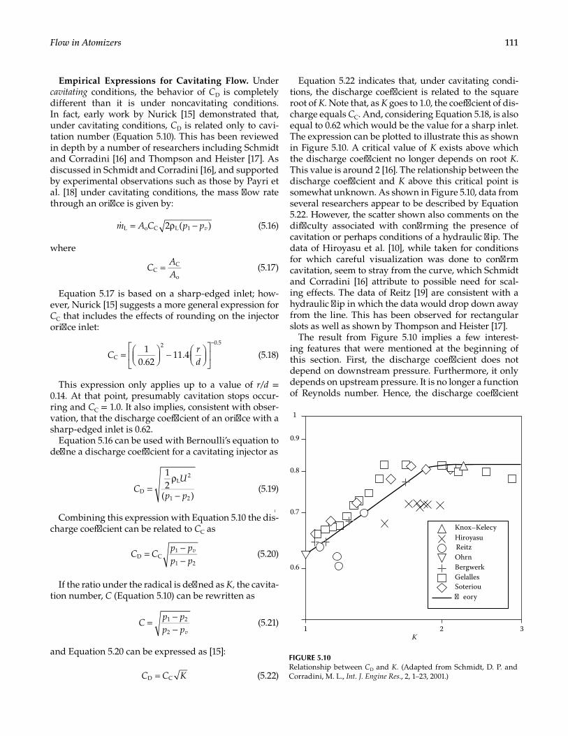
111Flow in Atomizers

Empirical Expressions for Cavitating Flow. Under cavitating conditions, the behavior of CD is completely different than it is under noncavitating conditions. In fact, early work by Nurick [15] demonstrated that, under cavitating conditions, CD is related only to cavi-tation number (Equation 5.10). This has been reviewed in depth by a number of researchers including Schmidt and Corradini [16] and Thompson and Heister [17]. As discussed in Schmidt and Corradini [16], and supported by experimental observations such as those by Payri et al. [18] under cavitating conditions, the mass flow rate through an orifice is given by:

m A C p pv= ρ −2 ( )L o C L 1 (5.16)

where

CAA

=CC

o (5.17)

Equation 5.17 is based on a sharp-edged inlet; how-ever, Nurick [15] suggests a more general expression for CC that includes the effects of rounding on the injector orifice inlet:

Crd

=

−

−1

0.6211.4C

2 0.5

(5.18)

This expression only applies up to a value of r/d = 0.14. At that point, presumably cavitation stops occur-ring and CC = 1.0. It also implies, consistent with obser-vation, that the discharge coefficient of an orifice with a sharp-edged inlet is 0.62.

Equation 5.16 can be used with Bernoulli’s equation to define a discharge coefficient for a cavitating injector as

CU

p p=

ρ

−

12

( )D

L2

1 2 (5.19)

Combining this expression with Equation 5.10 the dis-charge coefficient can be related to CC as

C Cp pp p

v= −−D C

1

1 2 (5.20)

If the ratio under the radical is defined as K, the cavita-tion number, C (Equation 5.10) can be rewritten as

Cp pp pv

= −−

1 2

2 (5.21)

and Equation 5.20 can be expressed as [15]:

C C K=D C (5.22)

Equation 5.22 indicates that, under cavitating condi-tions, the discharge coefficient is related to the square root of K. Note that, as K goes to 1.0, the coefficient of dis-charge equals CC. And, considering Equation 5.18, is also equal to 0.62 which would be the value for a sharp inlet. The expression can be plotted to illustrate this as shown in Figure 5.10. A critical value of K exists above which the discharge coefficient no longer depends on root K. This value is around 2 [16]. The relationship between the discharge coefficient and K above this critical point is somewhat unknown. As shown in Figure 5.10, data from several researchers appear to be described by Equation 5.22. However, the scatter shown also comments on the difficulty associated with confirming the presence of cavitation or perhaps conditions of a hydraulic flip. The data of Hiroyasu et al. [10], while taken for conditions for which careful visualization was done to confirm cavitation, seem to stray from the curve, which Schmidt and Corradini [16] attribute to possible need for scal-ing effects. The data of Reitz [19] are consistent with a hydraulic flip in which the data would drop down away from the line. This has been observed for rectangular slots as well as shown by Thompson and Heister [17].

The result from Figure 5.10 implies a few interest-ing features that were mentioned at the beginning of this section. First, the discharge coefficient does not depend on downstream pressure. Furthermore, it only depends on upstream pressure. It is no longer a function of Reynolds number. Hence, the discharge coefficient

Knox–KelecyHiroyasuReitzOhrnBergwerkGelallesSoterioueory

0.6

0.7

0.8

0.9

1

CD

1 2 3K

FIGURE 5.10Relationship between CD and K. (Adapted from Schmidt, D. P. and Corradini, M. L., Int. J. Engine Res., 2, 1–23, 2001.)

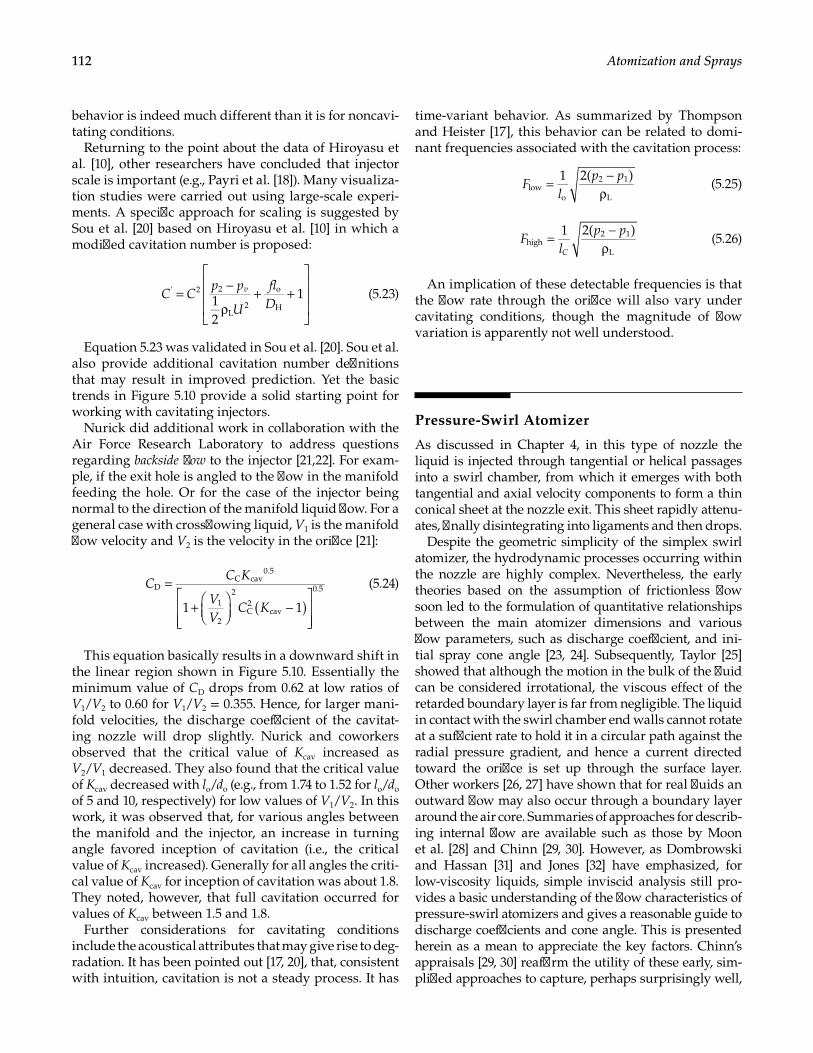
112 Atomization and Sprays

behavior is indeed much different than it is for noncavi-tating conditions.

Returning to the point about the data of Hiroyasu et al. [10], other researchers have concluded that injector scale is important (e.g., Payri et al. [18]). Many visualiza-tion studies were carried out using large-scale experi-ments. A specific approach for scaling is suggested by Sou et al. [20] based on Hiroyasu et al. [10] in which a modified cavitation number is proposed:

C Cp p

U

flD

v= −

ρ+ +

12

1' 2 2

L2

o

H (5.23)

Equation 5.23 was validated in Sou et al. [20]. Sou et al. also provide additional cavitation number definitions that may result in improved prediction. Yet the basic trends in Figure 5.10 provide a solid starting point for working with cavitating injectors.

Nurick did additional work in collaboration with the Air Force Research Laboratory to address questions regarding backside flow to the injector [21,22]. For exam-ple, if the exit hole is angled to the flow in the manifold feeding the hole. Or for the case of the injector being normal to the direction of the manifold liquid flow. For a general case with crossflowing liquid, V1 is the manifold flow velocity and V2 is the velocity in the orifice [21]:

CC K

VV

C K( )=

+

−

1 1

DC cav

0.5

1

2

2

C2

cav

0.5 (5.24)

This equation basically results in a downward shift in the linear region shown in Figure 5.10. Essentially the minimum value of CD drops from 0.62 at low ratios of V1/V2 to 0.60 for V1/V2 = 0.355. Hence, for larger mani-fold velocities, the discharge coefficient of the cavitat-ing nozzle will drop slightly. Nurick and coworkers observed that the critical value of Kcav increased as V2/V1 decreased. They also found that the critical value of Kcav decreased with lo/do (e.g., from 1.74 to 1.52 for lo/do of 5 and 10, respectively) for low values of V1/V2. In this work, it was observed that, for various angles between the manifold and the injector, an increase in turning angle favored inception of cavitation (i.e., the critical value of Kcav increased). Generally for all angles the criti-cal value of Kcav for inception of cavitation was about 1.8. They noted, however, that full cavitation occurred for values of Kcav between 1.5 and 1.8.

Further considerations for cavitating conditions include the acoustical attributes that may give rise to deg-radation. It has been pointed out [17, 20], that, consistent with intuition, cavitation is not a steady process. It has

time-variant behavior. As summarized by Thompson and Heister [17], this behavior can be related to domi-nant frequencies associated with the cavitation process:

Fl

p p= −ρ

1 2( )low

o

2 1

L (5.25)

Fl

p p

C= −

ρ1 2( )

high2 1

L (5.26)

An implication of these detectable frequencies is that the flow rate through the orifice will also vary under cavitating conditions, though the magnitude of flow variation is apparently not well understood.

Pressure-Swirl Atomizer

As discussed in Chapter 4, in this type of nozzle the liquid is injected through tangential or helical passages into a swirl chamber, from which it emerges with both tangential and axial velocity components to form a thin conical sheet at the nozzle exit. This sheet rapidly attenu-ates, finally disintegrating into ligaments and then drops.

Despite the geometric simplicity of the simplex swirl atomizer, the hydrodynamic processes occurring within the nozzle are highly complex. Nevertheless, the early theories based on the assumption of frictionless flow soon led to the formulation of quantitative relationships between the main atomizer dimensions and various flow parameters, such as discharge coefficient, and ini-tial spray cone angle [23, 24]. Subsequently, Taylor [25] showed that although the motion in the bulk of the fluid can be considered irrotational, the viscous effect of the retarded boundary layer is far from negligible. The liquid in contact with the swirl chamber end walls cannot rotate at a sufficient rate to hold it in a circular path against the radial pressure gradient, and hence a current directed toward the orifice is set up through the surface layer. Other workers [26, 27] have shown that for real fluids an outward flow may also occur through a boundary layer around the air core. Summaries of approaches for describ-ing internal flow are available such as those by Moon et al. [28] and Chinn [29, 30]. However, as Dombrowski and Hassan [31] and Jones [32] have emphasized, for low-viscosity liquids, simple inviscid analysis still pro-vides a basic understanding of the flow characteristics of pressure-swirl atomizers and gives a reasonable guide to discharge coefficients and cone angle. This is presented herein as a mean to appreciate the key factors. Chinn’s appraisals [29, 30] reaffirm the utility of these early, sim-plified approaches to capture, perhaps surprisingly well,

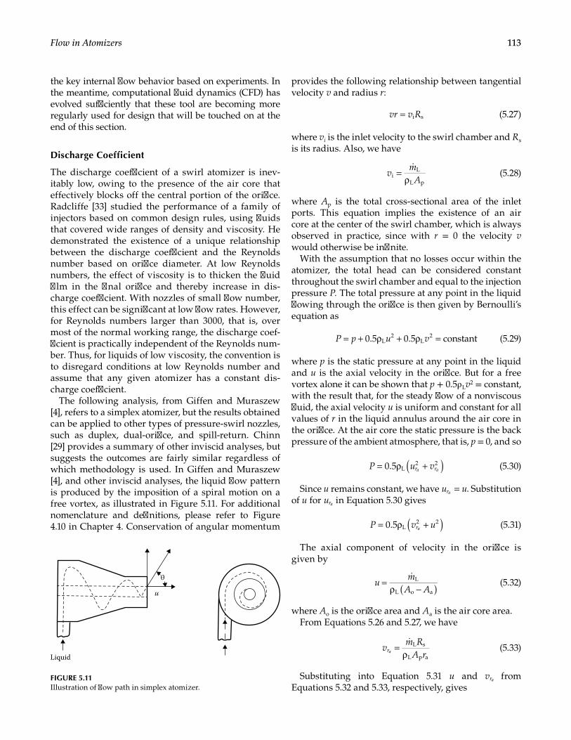
113Flow in Atomizers

the key internal flow behavior based on experiments. In the meantime, computational fluid dynamics (CFD) has evolved sufficiently that these tool are becoming more regularly used for design that will be touched on at the end of this section.

Discharge Coefficient

The discharge coefficient of a swirl atomizer is inev-itably low, owing to the presence of the air core that effectively blocks off the central portion of the orifice. Radcliffe [33] studied the performance of a family of injectors based on common design rules, using fluids that covered wide ranges of density and viscosity. He demonstrated the existence of a unique relationship between the discharge coefficient and the Reynolds number based on orifice diameter. At low Reynolds numbers, the effect of viscosity is to thicken the fluid film in the final orifice and thereby increase in dis-charge coefficient. With nozzles of small flow number, this effect can be significant at low flow rates. However, for Reynolds numbers larger than 3000, that is, over most of the normal working range, the discharge coef-ficient is practically independent of the Reynolds num-ber. Thus, for liquids of low viscosity, the convention is to disregard conditions at low Reynolds number and assume that any given atomizer has a constant dis-charge coefficient.

The following analysis, from Giffen and Muraszew [4], refers to a simplex atomizer, but the results obtained can be applied to other types of pressure-swirl nozzles, such as duplex, dual-orifice, and spill-return. Chinn [29] provides a summary of other inviscid analyses, but suggests the outcomes are fairly similar regardless of which methodology is used. In Giffen and Muraszew [4], and other inviscid analyses, the liquid flow pattern is produced by the imposition of a spiral motion on a free vortex, as illustrated in Figure 5.11. For additional nomenclature and definitions, please refer to Figure 4.10 in Chapter 4. Conservation of angular momentum

provides the following relationship between tangential velocity v and radius r:

vr v R= i s (5.27)

where vi is the inlet velocity to the swirl chamber and Rs is its radius. Also, we have

vm

A=

ρiL

L p

(5.28)

where Ap is the total cross-sectional area of the inlet ports. This equation implies the existence of an air core at the center of the swirl chamber, which is always observed in practice, since with r = 0 the velocity v would otherwise be infinite.

With the assumption that no losses occur within the atomizer, the total head can be considered constant throughout the swirl chamber and equal to the injection pressure P. The total pressure at any point in the liquid flowing through the orifice is then given by Bernoulli’s equation as

P p u v= + ρ + ρ =0.5 0.5 constantL2

L2 (5.29)

where p is the static pressure at any point in the liquid and u is the axial velocity in the orifice. But for a free vortex alone it can be shown that p + 0.5ρ Lv2 = constant, with the result that, for the steady flow of a nonviscous fluid, the axial velocity u is uniform and constant for all values of r in the liquid annulus around the air core in the orifice. At the air core the static pressure is the back pressure of the ambient atmosphere, that is, p = 0, and so

P u vr ra a( )= ρ +0.5 L2 2 (5.30)

Since u remains constant, we have u ura = . Substitution of u for ura in Equation 5.30 gives

P v ura( )= ρ +0.5 L2 2 (5.31)

The axial component of velocity in the orifice is given by

um

A A( )=ρ −

L

L o a

(5.32)

where Ao is the orifice area and Aa is the air core area.From Equations 5.26 and 5.27, we have

vm R

A rra =ρ

L s

L p a

(5.33)

Substituting into Equation 5.31 u and vra from Equations 5.32 and 5.33, respectively, gives

u

Liquid

θ

FIGURE 5.11Illustration of flow path in simplex atomizer.

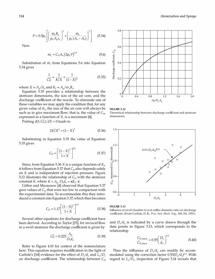
114 Atomization and Sprays

Pm R

A rm

A A= ρ

ρ

+

ρ −

0.5( )L

L s

L p a

2

L

L o a

2

(5.34)

Now

m C A PD ( )= ρ2L o L0.5

(5.6)

Substitution of mL from Equations 5.6 into Equation 5.34 gives

C K X X

= +−

1 1 1(1 )D

212 2 (5.35)

where X = Aa/Ao and K1 = Ap/πroRs.Equation 5.35 provides a relationship between the

atomizer dimensions, the size of the air core, and the discharge coefficient of the nozzle. To eliminate one of these variables we may apply the condition that, for any given value of K1, the size of the air core will always be such as to give maximum flow; that is, the value of CD, expressed as a function of X, is a maximum [4].

Putting d C dX =(1 ) 0D2 leads to

K X X( )= −2 112 2 3 (5.36)

Substituting in Equation 5.35 the value of Equation 5.35 gives

CXX

( )= −+

11D

3 0.5

(5.37)

Since, from Equation 5.36 X is a unique function of K1, it follows from Equation 5.37 that CD also depends solely on K and is independent of injection pressure. Figure 5.12 illustrates the relationship of CD with the atomizer constant K, where K A D d K= = π 4p s o 1 .

Giffen and Muraszew [4] observed that Equation 5.37 gave values of CD that were too low in comparison with the experimental data. To accommodate this they intro-duced a constant into Equation 5.37, which then becomes

CXX

= −+

1.17

(1 )1D

3 0.5

(5.38)

Several other equations for discharge coefficient have been derived. According to Taylor [25], for inviscid flow in a swirl atomizer the discharge coefficient is given by

CA

D d= 0.225D

2 p

s o (5.39)

Refer to Figure 4.10 for context of the nomenclature here. This equation requires modification in the light of Carlisle’s [34] evidence for the effect of Ds/do and Ls/Ds on discharge coefficient. The relationship between CD

and Ds/do is indicated by a curve drawn through the data points in Figure 5.13, which corresponds to the relationship

CC

Dd

=

0.55D,meas

D,theor

s

o

0.5

(5.40)

Thus the influence of Ds/do can readily be accom-modated using the correction factor 0.55(Ds/do)0.5. With regard to Ls/Ds, inspection of Figure 5.14 reveals that

0 0.4 0.8 1.2 1.6 2.00

0.2

0.4

0.6

0.8

Disc

harg

e co

effic

ient

, CD

Aρ/Ds do

FIGURE 5.12Theoretical relationship between discharge coefficient and atomizer dimensions.

0 1 2 3 4 5Ds/do

0.6

0.8

1.0

1.2

1.4

(CD

mea

sure

d)/(

CD

theo

retic

al)

0.55 (Ds/do)0.5

FIGURE 5.13Influence of swirl chamber to exit orifice diameter ratio on discharge coefficient. (From Carlisle, D. R., Proc. Inst. Mech. Eng., 169, 101, 1955.)

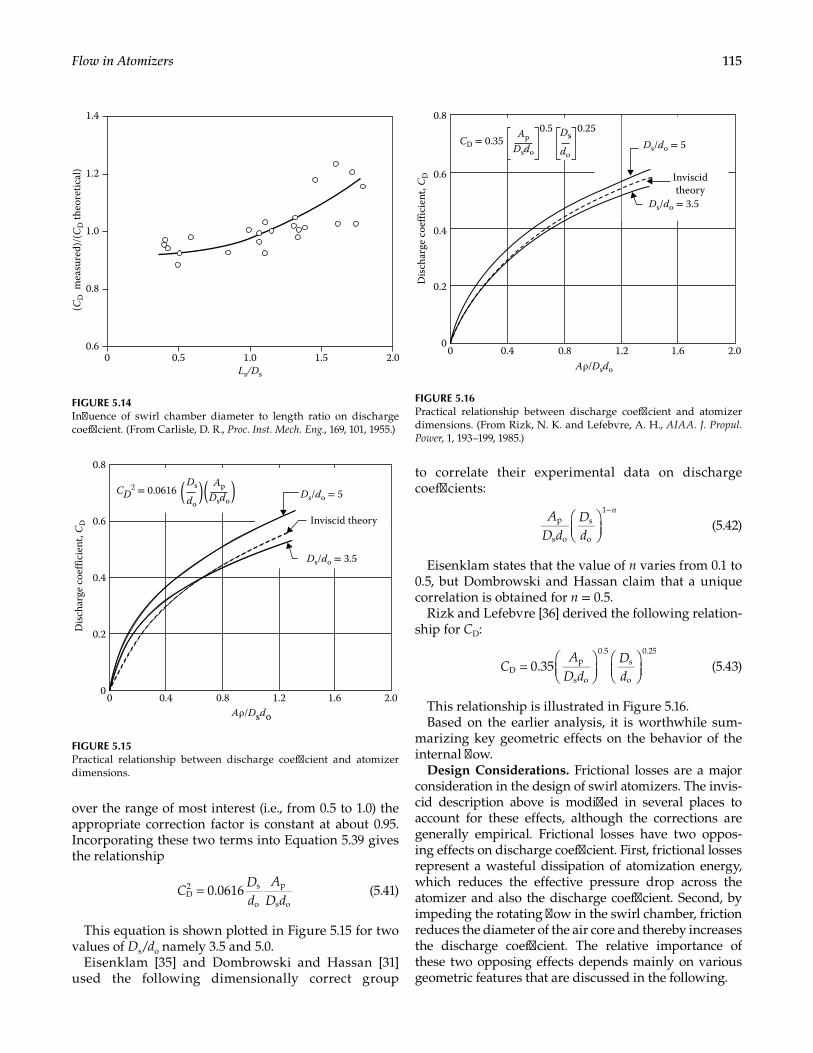
115Flow in Atomizers

over the range of most interest (i.e., from 0.5 to 1.0) the appropriate correction factor is constant at about 0.95. Incorporating these two terms into Equation 5.39 gives the relationship

CDd

AD d

= 0.0616D2 s

o

p

s o (5.41)

This equation is shown plotted in Figure 5.15 for two values of Ds/do namely 3.5 and 5.0.

Eisenklam [35] and Dombrowski and Hassan [31] used the following dimensionally correct group

to correlate their experimental data on discharge coefficients:

A

D dDd

n

−p

s o

s

o

1

(5.42)

Eisenklam states that the value of n varies from 0.1 to 0.5, but Dombrowski and Hassan claim that a unique correlation is obtained for n = 0.5.

Rizk and Lefebvre [36] derived the following relation-ship for CD:

CA

D dDd

=

0.35Dp

s o

0.5s

o

0.25

(5.43)

This relationship is illustrated in Figure 5.16.Based on the earlier analysis, it is worthwhile sum-

marizing key geometric effects on the behavior of the internal flow.

Design Considerations. Frictional losses are a major consideration in the design of swirl atomizers. The invis-cid description above is modified in several places to account for these effects, although the corrections are generally empirical. Frictional losses have two oppos-ing effects on discharge coefficient. First, frictional losses represent a wasteful dissipation of atomization energy, which reduces the effective pressure drop across the atomizer and also the discharge coefficient. Second, by impeding the rotating flow in the swirl chamber, friction reduces the diameter of the air core and thereby increases the discharge coefficient. The relative importance of these two opposing effects depends mainly on various geometric features that are discussed in the following.

0 0.5 1.0 1.5 2.00.6

0.8

1.0

1.2

1.4

(CD

mea

sure

d)/(C

D th

eore

tical

)

Ls/Ds

FIGURE 5.14Influence of swirl chamber diameter to length ratio on discharge coefficient. (From Carlisle, D. R., Proc. Inst. Mech. Eng., 169, 101, 1955.)

0 0.4 0.8 1.2 1.6 2.00

0.2

0.4

0.6

0.8

Disc

harg

e coe

ffici

ent,

CD

Aρ/Dsdo

Ds/do = 3.5

Inviscid theory

Ds/do = 5Ds

do

ApDsdo

CD2 = 0.0616

FIGURE 5.15Practical relationship between discharge coefficient and atomizer dimensions.

0 0.4 0.8 1.2 1.6 2.00

0.2

0.4

0.6

0.8

Disc

harg

e coe

ffici

ent,

CD

Aρ/Dsdo

Ds/do = 3.5

Inviscidtheory

Ds/do = 5Dsdo

ApDsdo

CD = 0.35 0.250.5

FIGURE 5.16Practical relationship between discharge coefficient and atomizer dimensions. (From Rizk, N. K. and Lefebvre, A. H., AIAA. J. Propul. Power, 1, 193–199, 1985.)

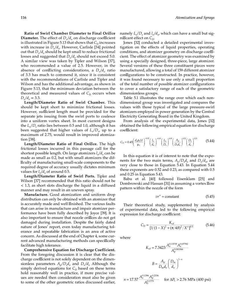
116 Atomization and Sprays

Ratio of Swirl Chamber Diameter to Final Orifice Diameter. The effect of Ds/do on discharge coefficient is illustrated in Figure 5.13 that shows that CD increases with increase in Ds/do. However, Carlisle [34] pointed out that Ds/do should be kept small to reduce frictional losses and suggested that Ds/do should not exceed 5.0. A similar view was taken by Tipler and Wilson [37], who recommended a value of 2.5. However, in the absence of conflicting considerations, a Ds/do ratio of 3.3 has much to commend it, since it is consistent with the recommendations of Carlisle and Tipler and Wilson and has the additional advantage, as shown in Figure 5.13, that the minimum deviation between the theoretical and measured values of CD occurs when Ds/do = 3.3.

Length/Diameter Ratio of Swirl Chamber. This should be kept short to minimize frictional losses. However, sufficient length must be provided for the separate jets issuing from the swirl ports to coalesce into a uniform vortex sheet. In most current designs the Ls/Ds ratio lies between 0.5 and 1.0, although it has been suggested that higher values of Ls/Ds, up to a maximum of 2.75, would result in improved atomiza-tion [38].

Length/Diameter Ratio of Final Orifice. The high frictional losses incurred in this passage call for the shortest possible length. On large atomizers lo/do can be made as small as 0.2, but with small atomizers the dif-ficulty of manufacturing small-scale components to the required degree of accuracy usually dictates minimum values for lo/do of around 0.5.

Length/Diameter Ratio of Swirl Ports. Tipler and Wilson [37] recommended that this ratio should not be < 1.3, as short slots discharge the liquid in a diffused manner and may result in an uneven spray.

Manufacture. Good atomization and uniform drop distribution can only be obtained with an atomizer that is accurately made and well finished. The various faults that can arise in manufacture and impair atomizer per-formance have been fully described by Joyce [39]. It is also important to ensure that nozzle orifices do not get damaged during installation. Despite the fairly dated nature of Jones’ report, even today manufacturing tol-erance and repeatable fabrication is an area of active concern. As discussed at the end of Chapter 4, some cur-rent advanced manufacturing methods can specifically facilitate high tolerance.

Comprehensive Equation for Discharge Coefficient. From the foregoing discussion it is clear that the dis-charge coefficient is not solely dependent on the dimen-sionless parameters Ap/Dsdo and Ds/do Although the simply derived equations for CD based on these terms hold reasonably well in practice, if more precise val-ues are needed then consideration must also be given to some of the other geometric ratios discussed earlier,

namely Ls/Ds and lo/do, which can have a small but sig-nificant effect on CD.

Jones [32] conducted a detailed experimental inves-tigation on the effects of liquid properties, operating conditions, and atomizer geometry on discharge coeffi-cient. The effect of atomizer geometry was examined by using a specially designed, three-piece, large atomizer. Several versions of these three constituent pieces were manufactured, allowing a total of 159 different atomizer configurations to be constructed. In practice, however, it was found necessary to use only a small proportion of the total number of possible atomizer configurations to cover a satisfactory range of each of the geometric dimensionless groups.

Table 5.1 illustrates the range over which each non-dimensional group was investigated and compares the values with those typical of the large pressure-swirl atomizers employed in power generation by the Central Electricity Generating Board in the United Kingdom.

From analysis of the experimental data, Jones [32] obtained the following empirical equation for discharge coefficient:

Cd U l

dLD

AD d

Dd

= ρµ

− −

0.45Do L

L

0.02o

o

0.03s

s

0.05p

s o

0.52s

o

0.23

(5.44)

In this equation it is of interest to note that the expo-nents for the two main terms, Ap/Dsdo and Ds/do, are very close to those in Equation 5.43. In Equation 5.44 these exponents are 0.52 and 0.23, as compared with 0.5 and 0.25 in Equation 5.43.

Babu et al. [40] followed Eisenklam [25] and Dombrowski and Hassan [31] in assuming a vortex flow pattern within the nozzle of the form

vrn = constant (5.45)

Their theoretical study, supplemented by analysis of experimental data, led to the following empirical expression for discharge coefficient:

CK

X B Xcd

n=− + π[1 (1 ) ( 4 ) ]D 2 2 0.5 (5.46)

where

KA A

Acd = 7.3423 o

0.13735s0.07782

p0.041066

BA

D dDd

n

=

−p

m o

m

o

1

17.57 for 2.76 MPa (400 psi)o0.1396

p0.2336

50.1775 Ln

A AA

P= ∆ >

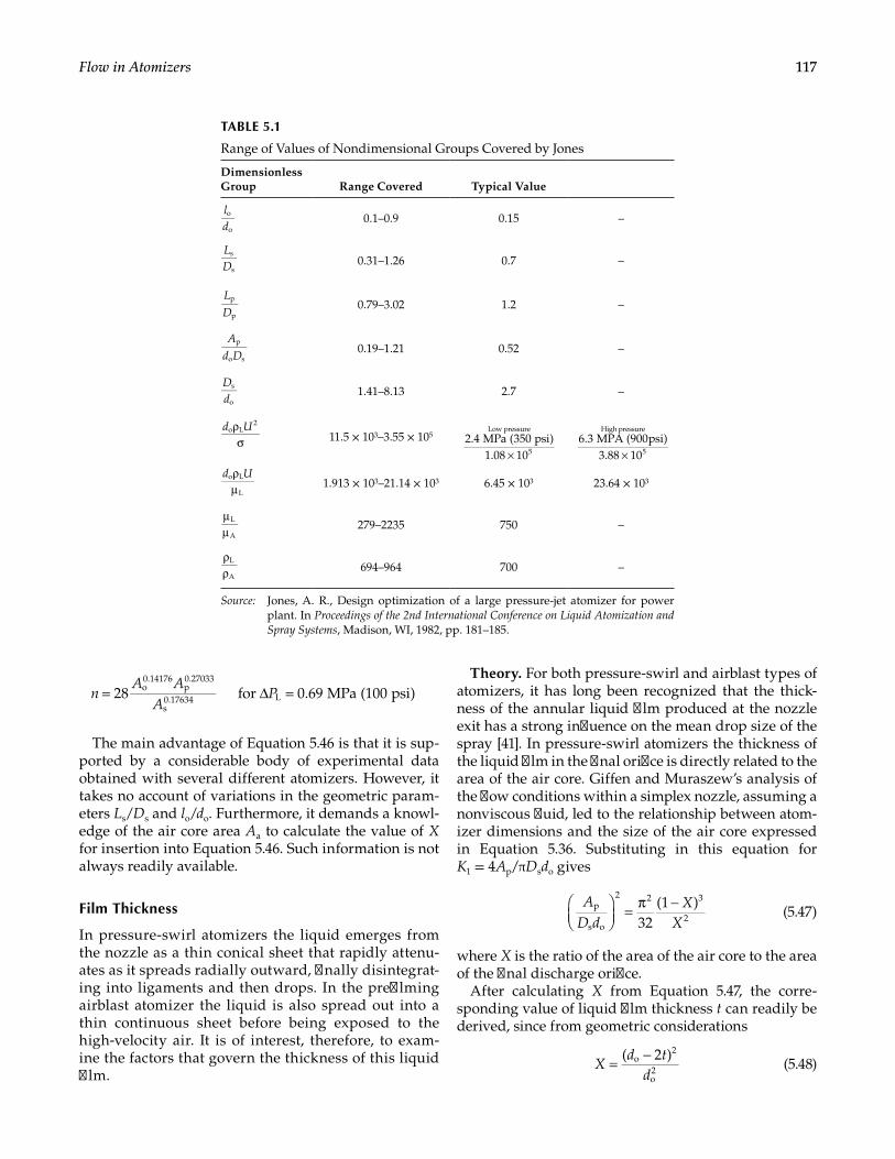
117Flow in Atomizers

nA A

AP= ∆ =28 for 0.69 MPa (100 psi)o

0.14176p0.27033

s0.17634 L

The main advantage of Equation 5.46 is that it is sup-ported by a considerable body of experimental data obtained with several different atomizers. However, it takes no account of variations in the geometric param-eters Ls/Ds and lo/do. Furthermore, it demands a knowl-edge of the air core area Aa to calculate the value of X for insertion into Equation 5.46. Such information is not always readily available.

Film Thickness

In pressure-swirl atomizers the liquid emerges from the nozzle as a thin conical sheet that rapidly attenu-ates as it spreads radially outward, finally disintegrat-ing into ligaments and then drops. In the prefilming airblast atomizer the liquid is also spread out into a thin continuous sheet before being exposed to the high-velocity air. It is of interest, therefore, to exam-ine the factors that govern the thickness of this liquid film.

Theory. For both pressure-swirl and airblast types of atomizers, it has long been recognized that the thick-ness of the annular liquid film produced at the nozzle exit has a strong influence on the mean drop size of the spray [41]. In pressure-swirl atomizers the thickness of the liquid film in the final orifice is directly related to the area of the air core. Giffen and Muraszew’s analysis of the flow conditions within a simplex nozzle, assuming a nonviscous fluid, led to the relationship between atom-izer dimensions and the size of the air core expressed in Equation 5.36. Substituting in this equation for K1 = 4Ap/πDsdo gives

A

D dX

X

= π −32

(1 )p

s o

2 2 3

2 (5.47)

where X is the ratio of the area of the air core to the area of the final discharge orifice.

After calculating X from Equation 5.47, the corre-sponding value of liquid film thickness t can readily be derived, since from geometric considerations

Xd t

d= −( 2 )o

2

o2 (5.48)

TABLE 5.1

Range of Values of Nondimensional Groups Covered by Jones

Dimensionless Group Range Covered Typical Value

ld

o

o0.1–0.9 0.15 –

LD

s

s0.31–1.26 0.7 –

LD

p

p0.79–3.02 1.2 –

Ad D

p

o s0.19–1.21 0.52 –

Dd

s

o1.41–8.13 2.7 –

d Uρσ

o L2

11.5 × 103–3.55 × 105

×2.4 MPa (350 psi)

1.08 10

Low pressure

5 ×6.3 MPA (900psi)

3.88 10

High pressure

5

d Uρµ

o L

L1.913 × 103–21.14 × 103 6.45 × 103 23.64 × 103

µµ

L

A279–2235 750 –

ρρ

L

A694–964 700 –

Source: Jones, A. R., Design optimization of a large pressure-jet atomizer for power plant. In Proceedings of the 2nd International Conference on Liquid Atomization and Spray Systems, Madison, WI, 1982, pp. 181–185.

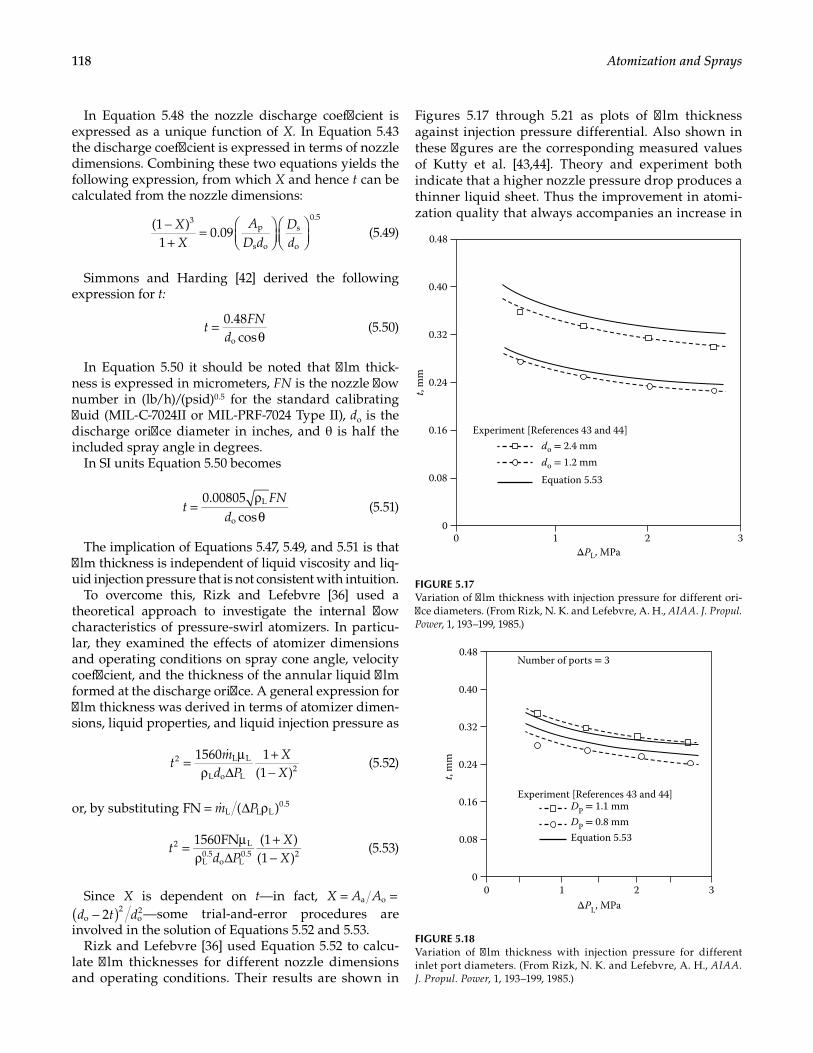
118 Atomization and Sprays

In Equation 5.48 the nozzle discharge coefficient is expressed as a unique function of X. In Equation 5.43 the discharge coefficient is expressed in terms of nozzle dimensions. Combining these two equations yields the following expression, from which X and hence t can be calculated from the nozzle dimensions:

XX

AD d

Dd

−+

=

(1 )1

0.093

p

s o

s

o

0.5

(5.49)

Simmons and Harding [42] derived the following expression for t:

tFN

d=

θ0.48

coso (5.50)

In Equation 5.50 it should be noted that film thick-ness is expressed in micrometers, FN is the nozzle flow number in (lb/h)/(psid)0.5 for the standard calibrating fluid (MIL-C-7024II or MIL-PRF-7024 Type II), do is the discharge orifice diameter in inches, and θ is half the included spray angle in degrees.

In SI units Equation 5.50 becomes

tFN

d=

ρθ

0.00805cos

L

o (5.51)

The implication of Equations 5.47, 5.49, and 5.51 is that film thickness is independent of liquid viscosity and liq-uid injection pressure that is not consistent with intuition.

To overcome this, Rizk and Lefebvre [36] used a theoretical approach to investigate the internal flow characteristics of pressure-swirl atomizers. In particu-lar, they examined the effects of atomizer dimensions and operating conditions on spray cone angle, velocity coefficient, and the thickness of the annular liquid film formed at the discharge orifice. A general expression for film thickness was derived in terms of atomizer dimen-sions, liquid properties, and liquid injection pressure as

tm

d PXX

= µρ ∆

+−

1560 1(1 )

2 L L

L o L2

(5.52)

or, by substituting m P= ∆ ρFN ( )L L L0.5

td P

XX

= µρ ∆

+−

1560FN (1 )(1 )

2 L

L0.5

o L0.5 2 (5.53)

Since X is dependent on t—in fact, X A A d t d( )= = − 2a o o2

o2

X A A d t d( )= = − 2a o o2

o2—some trial-and-error procedures are

involved in the solution of Equations 5.52 and 5.53.Rizk and Lefebvre [36] used Equation 5.52 to calcu-

late film thicknesses for different nozzle dimensions and operating conditions. Their results are shown in

Figures 5.17 through 5.21 as plots of film thickness against injection pressure differential. Also shown in these figures are the corresponding measured values of Kutty et al. [43,44]. Theory and experiment both indicate that a higher nozzle pressure drop produces a thinner liquid sheet. Thus the improvement in atomi-zation quality that always accompanies an increase in

2 30

0.08

0.16

0.24

0.32

0.40

0.48

0

do = 2.4 mmdo = 1.2 mm

Equation 5.53

t, m

mExperiment [References 43 and 44]

ΔPL, MPa1

FIGURE 5.17Variation of film thickness with injection pressure for different ori-fice diameters. (From Rizk, N. K. and Lefebvre, A. H., AIAA. J. Propul. Power, 1, 193–199, 1985.)

00

1 2 3

0.08

0.16

0.24

0.32

0.40

0.48

t, m

m

ΔPL, MPa

DP = 1.1 mmDP = 0.8 mmEquation 5.53

Experiment [References 43 and 44]

Number of ports = 3

FIGURE 5.18Variation of film thickness with injection pressure for different inlet port diameters. (From Rizk, N. K. and Lefebvre, A. H., AIAA. J. Propul. Power, 1, 193–199, 1985.)

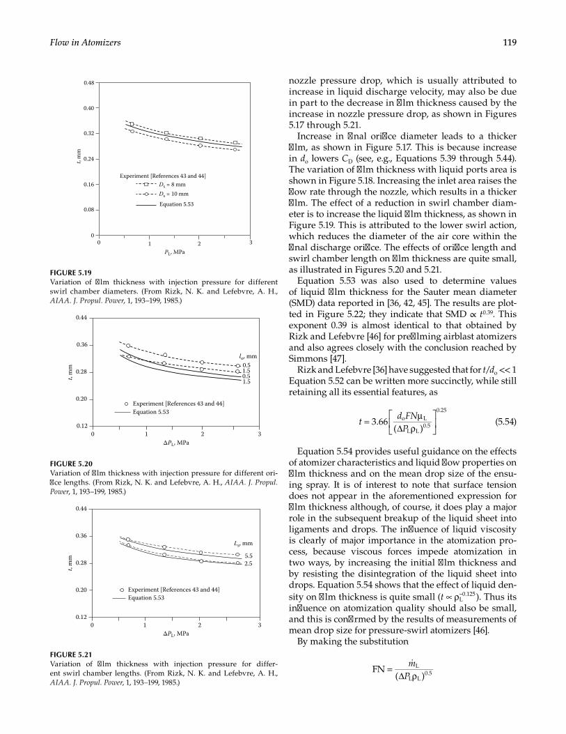
119Flow in Atomizers

nozzle pressure drop, which is usually attributed to increase in liquid discharge velocity, may also be due in part to the decrease in film thickness caused by the increase in nozzle pressure drop, as shown in Figures 5.17 through 5.21.

Increase in final orifice diameter leads to a thicker film, as shown in Figure 5.17. This is because increase in do lowers CD (see, e.g., Equations 5.39 through 5.44). The variation of film thickness with liquid ports area is shown in Figure 5.18. Increasing the inlet area raises the flow rate through the nozzle, which results in a thicker film. The effect of a reduction in swirl chamber diam-eter is to increase the liquid film thickness, as shown in Figure 5.19. This is attributed to the lower swirl action, which reduces the diameter of the air core within the final discharge orifice. The effects of orifice length and swirl chamber length on film thickness are quite small, as illustrated in Figures 5.20 and 5.21.

Equation 5.53 was also used to determine values of liquid film thickness for the Sauter mean diameter (SMD) data reported in [36, 42, 45]. The results are plot-ted in Figure 5.22; they indicate that SMD ∝ t0.39. This exponent 0.39 is almost identical to that obtained by Rizk and Lefebvre [46] for prefilming airblast atomizers and also agrees closely with the conclusion reached by Simmons [47].

Rizk and Lefebvre [36] have suggested that for t/do << 1 Equation 5.52 can be written more succinctly, while still retaining all its essential features, as

td FN

P= µ

∆ ρ

3.66

( )o L

L L0.5

0.25

(5.54)

Equation 5.54 provides useful guidance on the effects of atomizer characteristics and liquid flow properties on film thickness and on the mean drop size of the ensu-ing spray. It is of interest to note that surface tension does not appear in the aforementioned expression for film thickness although, of course, it does play a major role in the subsequent breakup of the liquid sheet into ligaments and drops. The influence of liquid viscosity is clearly of major importance in the atomization pro-cess, because viscous forces impede atomization in two ways, by increasing the initial film thickness and by resisting the disintegration of the liquid sheet into drops. Equation 5.54 shows that the effect of liquid den-sity on film thickness is quite small t ∝ ρ−( )L

0.125 . Thus its influence on atomization quality should also be small, and this is confirmed by the results of measurements of mean drop size for pressure-swirl atomizers [46].

By making the substitution

m

P=

∆ ρFN

( )L

L L0.5

00

1 2 3

0.08

0.16

0.24

0.32

0.40

0.48t,

mm

Ds = 8 mmDs = 10 mm

Equation 5.53

Experiment [References 43 and 44]

PL, MPa

FIGURE 5.19Variation of film thickness with injection pressure for different swirl chamber diameters. (From Rizk, N. K. and Lefebvre, A. H., AIAA. J. Propul. Power, 1, 193–199, 1985.)

0 1 2 30.12

0.20

0.28

0.36

0.44

t, m

m

Experiment [References 43 and 44]Equation 5.53

lo, mm0.5

0.51.5

1.5

ΔPL, MPa

FIGURE 5.20Variation of film thickness with injection pressure for different ori-fice lengths. (From Rizk, N. K. and Lefebvre, A. H., AIAA. J. Propul. Power, 1, 193–199, 1985.)

1 2 300.12

0.20

0.28

0.36

0.44

ΔPL, MPa

t, m

m

Experiment [References 43 and 44]Equation 5.53

Ls, mm

5.52.5

FIGURE 5.21Variation of film thickness with injection pressure for differ-ent swirl chamber lengths. (From Rizk, N. K. and Lefebvre, A. H., AIAA. J. Propul. Power, 1, 193–199, 1985.)

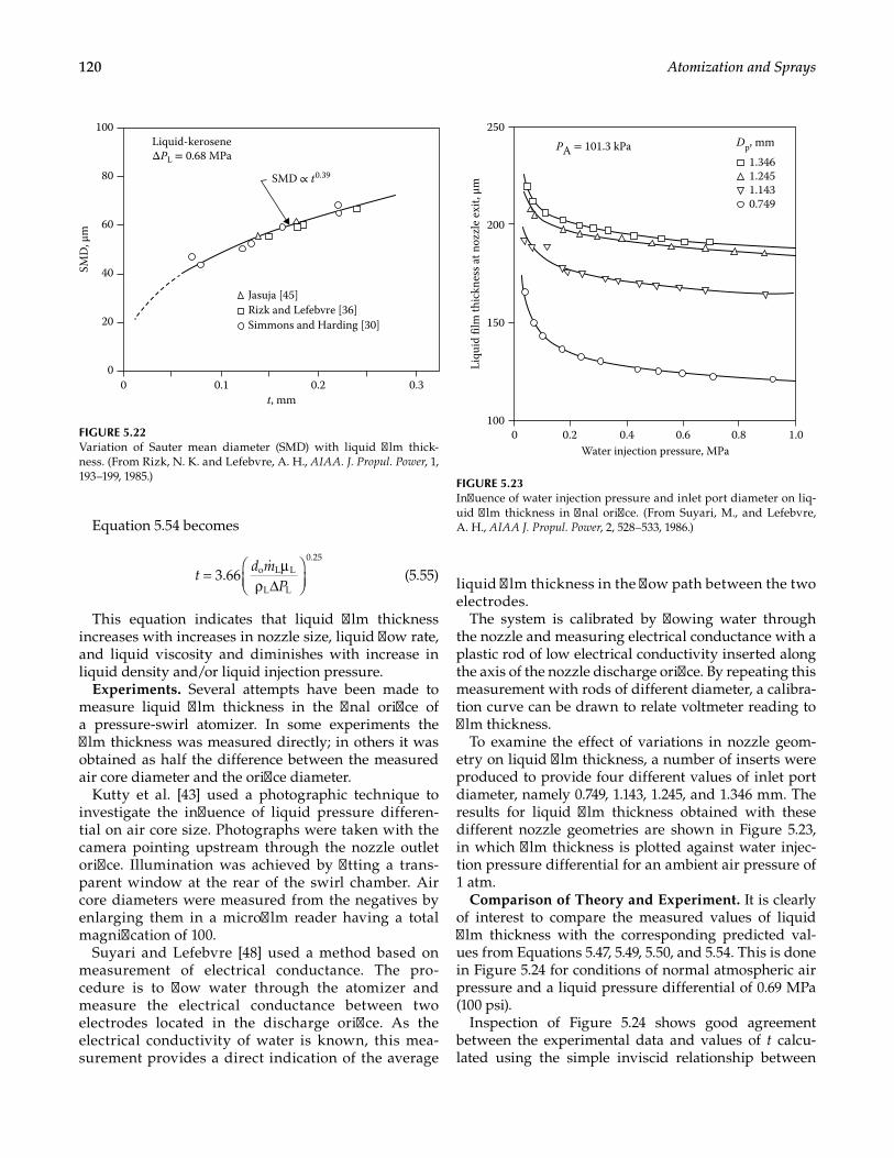
120 Atomization and Sprays

Equation 5.54 becomes

td m

P= µ

ρ ∆

3.66 o L L

L L

0.25

(5.55)

This equation indicates that liquid film thickness increases with increases in nozzle size, liquid flow rate, and liquid viscosity and diminishes with increase in liquid density and/or liquid injection pressure.

Experiments. Several attempts have been made to measure liquid film thickness in the final orifice of a pressure-swirl atomizer. In some experiments the film thickness was measured directly; in others it was obtained as half the difference between the measured air core diameter and the orifice diameter.

Kutty et al. [43] used a photographic technique to investigate the influence of liquid pressure differen-tial on air core size. Photographs were taken with the camera pointing upstream through the nozzle outlet orifice. Illumination was achieved by fitting a trans-parent window at the rear of the swirl chamber. Air core diameters were measured from the negatives by enlarging them in a microfilm reader having a total magnification of 100.

Suyari and Lefebvre [48] used a method based on measurement of electrical conductance. The pro-cedure is to flow water through the atomizer and measure the electrical conductance between two electrodes located in the discharge orifice. As the electrical conductivity of water is known, this mea-surement provides a direct indication of the average

liquid film thickness in the flow path between the two electrodes.

The system is calibrated by flowing water through the nozzle and measuring electrical conductance with a plastic rod of low electrical conductivity inserted along the axis of the nozzle discharge orifice. By repeating this measurement with rods of different diameter, a calibra-tion curve can be drawn to relate voltmeter reading to film thickness.

To examine the effect of variations in nozzle geom-etry on liquid film thickness, a number of inserts were produced to provide four different values of inlet port diameter, namely 0.749, 1.143, 1.245, and 1.346 mm. The results for liquid film thickness obtained with these different nozzle geometries are shown in Figure 5.23, in which film thickness is plotted against water injec-tion pressure differential for an ambient air pressure of 1 atm.

Comparison of Theory and Experiment. It is clearly of interest to compare the measured values of liquid film thickness with the corresponding predicted val-ues from Equations 5.47, 5.49, 5.50, and 5.54. This is done in Figure 5.24 for conditions of normal atmospheric air pressure and a liquid pressure differential of 0.69 MPa (100 psi).

Inspection of Figure 5.24 shows good agreement between the experimental data and values of t calcu-lated using the simple inviscid relationship between

0 0.1 0.2 0.30

20

40

60

80

100Liquid-keroseneΔPL = 0.68 MPa

Jasuja [45]Rizk and Lefebvre [36]Simmons and Harding [30]

SMD ∝ t0.39

SMD

, μm

t, mm

FIGURE 5.22Variation of Sauter mean diameter (SMD) with liquid film thick-ness. (From Rizk, N. K. and Lefebvre, A. H., AIAA. J. Propul. Power, 1, 193–199, 1985.)

0 0.2 0.4 0.6 0.8 1.0100

150

200

250

Liqu

id fi

lm th

ickn

ess a

t noz

zle

exit,

μm

Water injection pressure, MPa

PA = 101.3 kPa Dp, mm

1.3461.2451.1430.749

FIGURE 5.23Influence of water injection pressure and inlet port diameter on liq-uid film thickness in final orifice. (From Suyari, M., and Lefebvre, A. H., AIAA J. Propul. Power, 2, 528–533, 1986.)

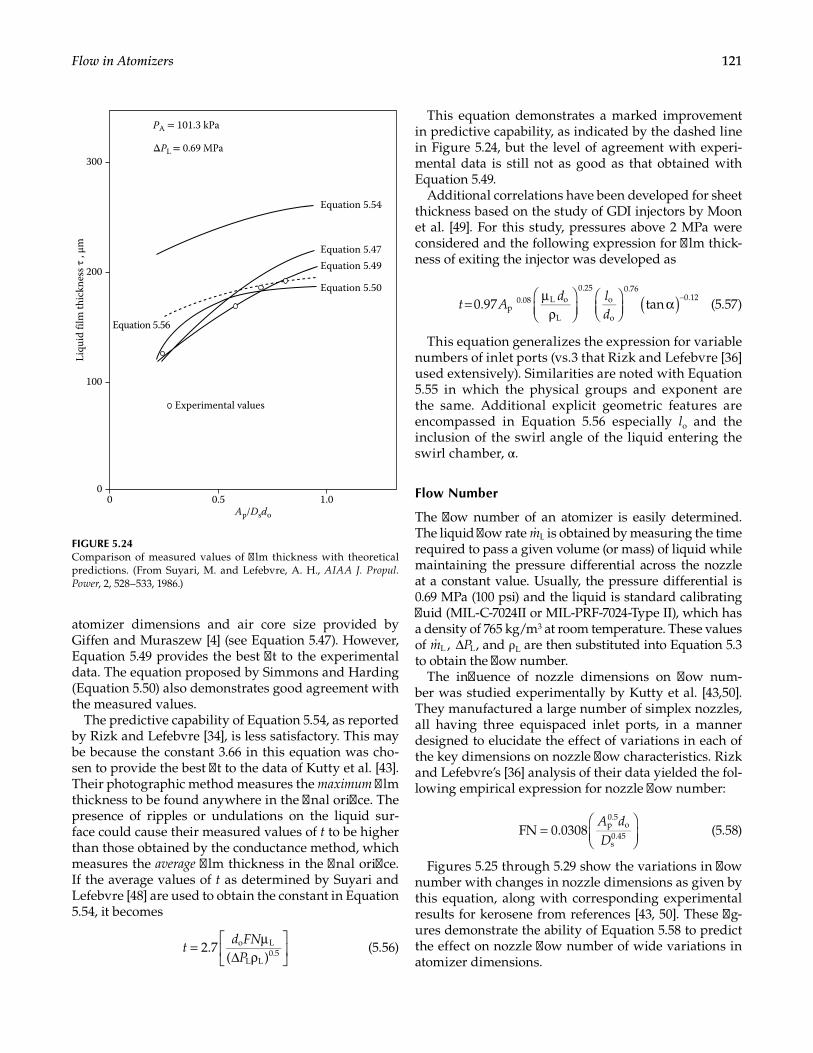
121Flow in Atomizers

atomizer dimensions and air core size provided by Giffen and Muraszew [4] (see Equation 5.47). However, Equation 5.49 provides the best fit to the experimental data. The equation proposed by Simmons and Harding (Equation 5.50) also demonstrates good agreement with the measured values.

The predictive capability of Equation 5.54, as reported by Rizk and Lefebvre [34], is less satisfactory. This may be because the constant 3.66 in this equation was cho-sen to provide the best fit to the data of Kutty et al. [43]. Their photographic method measures the maximum film thickness to be found anywhere in the final orifice. The presence of ripples or undulations on the liquid sur-face could cause their measured values of t to be higher than those obtained by the conductance method, which measures the average film thickness in the final orifice. If the average values of t as determined by Suyari and Lefebvre [48] are used to obtain the constant in Equation 5.54, it becomes

td FN

P= µ

∆ ρ

2.7

( )o L

L L0.5 (5.56)

This equation demonstrates a marked improvement in predictive capability, as indicated by the dashed line in Figure 5.24, but the level of agreement with experi-mental data is still not as good as that obtained with Equation 5.49.

Additional correlations have been developed for sheet thickness based on the study of GDI injectors by Moon et al. [49]. For this study, pressures above 2 MPa were considered and the following expression for film thick-ness of exiting the injector was developed as

t Ad l

d( )= µ

ρ

α −0.97 tanp

0.08 L o

L

0.25o

o

0.760.12

(5.57)

This equation generalizes the expression for variable numbers of inlet ports (vs.3 that Rizk and Lefebvre [36] used extensively). Similarities are noted with Equation 5.55 in which the physical groups and exponent are the same. Additional explicit geometric features are encompassed in Equation 5.56 especially lo and the inclusion of the swirl angle of the liquid entering the swirl chamber, α.

Flow Number

The flow number of an atomizer is easily determined. The liquid flow rate mL is obtained by measuring the time required to pass a given volume (or mass) of liquid while maintaining the pressure differential across the nozzle at a constant value. Usually, the pressure differential is 0.69 MPa (100 psi) and the liquid is standard calibrating fluid (MIL-C-7024II or MIL-PRF-7024-Type II), which has a density of 765 kg/m3 at room temperature. These values of m P∆,L L , and ρ L are then substituted into Equation 5.3 to obtain the flow number.

The influence of nozzle dimensions on flow num-ber was studied experimentally by Kutty et al. [43,50]. They manufactured a large number of simplex nozzles, all having three equispaced inlet ports, in a manner designed to elucidate the effect of variations in each of the key dimensions on nozzle flow characteristics. Rizk and Lefebvre’s [36] analysis of their data yielded the fol-lowing empirical expression for nozzle flow number:

A dD

=

FN 0.0308 p0.5

o

s0.45 (5.58)

Figures 5.25 through 5.29 show the variations in flow number with changes in nozzle dimensions as given by this equation, along with corresponding experimental results for kerosene from references [43, 50]. These fig-ures demonstrate the ability of Equation 5.58 to predict the effect on nozzle flow number of wide variations in atomizer dimensions.

1.00 0.5

100

200

300

Liqu

id fi

lm th

ickn

ess τ

, μm

Experimental values

Equation 5.49 Equation 5.47

Equation 5.54

Equation 5.56

Equation 5.50

PA = 101.3 kPa

ΔPL = 0.69 MPa

Ap/Dsdo

0

FIGURE 5.24Comparison of measured values of film thickness with theoretical predictions. (From Suyari, M. and Lefebvre, A. H., AIAA J. Propul. Power, 2, 528–533, 1986.)

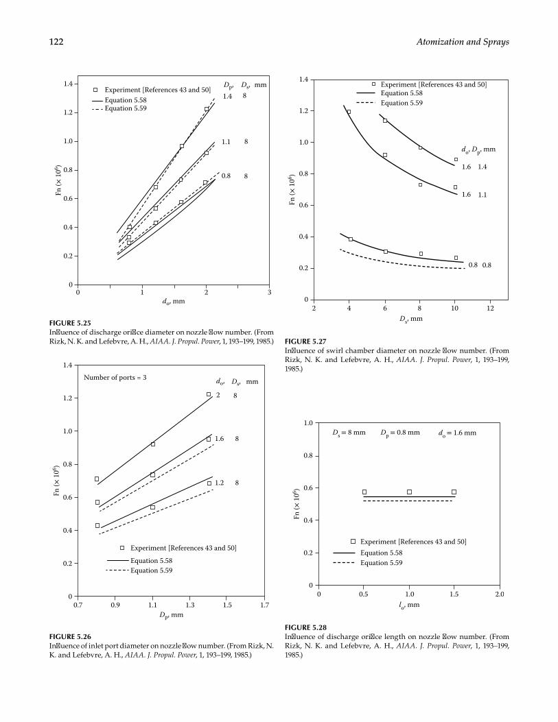
122 Atomization and Sprays

00

0.2

0.4

0.6

0.8

1.0

1.2

1.4

1 2 3

Fn (×

106 )

do, mm

Experiment [References 43 and 50]

Equation 5.59Equation 5.58

Dp, Ds, mm1.4 8

8

80.8

1.1

FIGURE 5.25Influence of discharge orifice diameter on nozzle flow number. (From Rizk, N. K. and Lefebvre, A. H., AIAA. J. Propul. Power, 1, 193–199, 1985.)

Ds, mm2 4 6 8 10 12

0

0.2

0.4

0.6

0.8

1.0

1.2

1.4

Fn (×

106 )

do, Dp, mm

1.6 1.4

1.6 1.1

Experiment [References 43 and 50]Equation 5.58Equation 5.59

0.8 0.8

FIGURE 5.27Influence of swirl chamber diameter on nozzle flow number. (From Rizk, N. K. and Lefebvre, A. H., AIAA. J. Propul. Power, 1, 193–199, 1985.)

Dp, mm

Fn (×

106 )

Experiment [References 43 and 50]

Equation 5.59Equation 5.58

do, Ds, mm

8

8

81.2

1.6

2

Number of ports = 3

0.7 0.9 1.1 1.3 1.5 1.70

0.2

0.4

0.6

0.8

1.0

1.2

1.4

FIGURE 5.26Influence of inlet port diameter on nozzle flow number. (From Rizk, N. K. and Lefebvre, A. H., AIAA. J. Propul. Power, 1, 193–199, 1985.)

0 0.5 1.0 1.5 2.0lo, mm

0

0.2

0.4

0.6

0.8

1.0

Fn (×

106 )

Ds = 8 mm Dp = 0.8 mm do = 1.6 mm

Experiment [References 43 and 50]Equation 5.58Equation 5.59

FIGURE 5.28Influence of discharge orifice length on nozzle flow number. (From Rizk, N. K. and Lefebvre, A. H., AIAA. J. Propul. Power, 1, 193–199, 1985.)

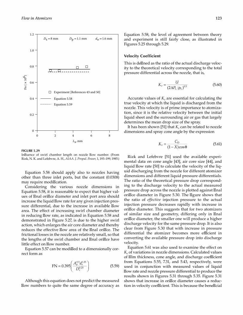
123Flow in Atomizers

Equation 5.58 should apply also to nozzles having other than three inlet ports, but the constant (0.0308) may require modification.

Considering the various nozzle dimensions in Equation 5.58, it is reasonable to expect that higher val-ues of final orifice diameter and inlet port area should increase the liquid flow rate for any given injection pres-sure differential, due to the increase in available flow area. The effect of increasing swirl chamber diameter in reducing flow rate, as indicated in Equation 5.58 and demonstrated in Figure 5.27, is due to the higher swirl action, which enlarges the air core diameter and thereby reduces the effective flow area of the final orifice. The frictional losses in the nozzle are relatively small, so that the lengths of the swirl chamber and final orifice have little effect on flow number.

Equation 5.57 can be modified to a dimensionally cor-rect form as

A d

Dp o

s=

FN 0.3950.5 1.25

0.25 (5.59)

Although this equation does not predict the measured flow numbers to quite the same degree of accuracy as

Equation 5.58, the level of agreement between theory and experiment is still fairly close, as illustrated in Figures 5.25 through 5.29.

Velocity Coefficient

This is defined as the ratio of the actual discharge veloc-ity to the theoretical velocity corresponding to the total pressure differential across the nozzle, that is,

KU

Pv =

∆ ρ(2 )L L0.5 (5.60)

Accurate values of Kv are essential for calculating the true velocity at which the liquid is discharged from the nozzle. This velocity is of prime importance to atomiza-tion, since it is the relative velocity between the initial liquid sheet and the surrounding air or gas that largely determines the mean drop size of the spray.

It has been shown [51] that Kv can be related to nozzle dimensions and spray cone angle by the expression

KCX

v =− θ(1 )cos

D (5.61)

Rizk and Lefebvre [51] used the available experi-mental data on cone angle [43], air core size [44], and liquid flow rate [50] to calculate the velocity of the liq-uid discharging from the nozzle for different atomizer dimensions and different liquid pressure differentials. The ratio of the theoretical pressure drop correspond-ing to the discharge velocity to the actual measured pressure drop across the nozzle is plotted against final orifice diameter in Figure 5.30. The figure shows that the ratio of effective injection pressure to the actual injection pressure decreases rapidly with increase in orifice diameter. This suggests that for two atomizers of similar size and geometry, differing only in final orifice diameter, the smaller one will produce a higher discharge velocity for the same pressure drop. It is also clear from Figure 5.30 that with increase in pressure differential the atomizer becomes more efficient in converting the available pressure drop into discharge velocity.

Equation 5.61 was also used to examine the effect on Kv of variations in nozzle dimensions. Calculated values of film thickness, cone angle, and discharge coefficient from Equations 5.55, 7.31, and 5.43, respectively, were used in conjunction with measured values of liquid flow rate and nozzle pressure differential to produce the results shown in Figures 5.31 through 5.35. Figure 5.31 shows that increase in orifice diameter causes a reduc-tion in velocity coefficient. This is because the beneficial

2 4 6 800

0.2

0.4

0.6

0.8

1.0

1.2

Ls, mm

Fn (

× 10

6 )

Experiment [References 43 and 50]

Equation 5.58

Equation 5.59

Ds = 8 mm Dp = 1.1 mm do = 1.6 mm

FIGURE 5.29 Influence of swirl chamber length on nozzle flow number. (From Rizk, N. K. and Lefebvre, A. H., AIAA. J. Propul. Power, 1, 193–199, 1985.)

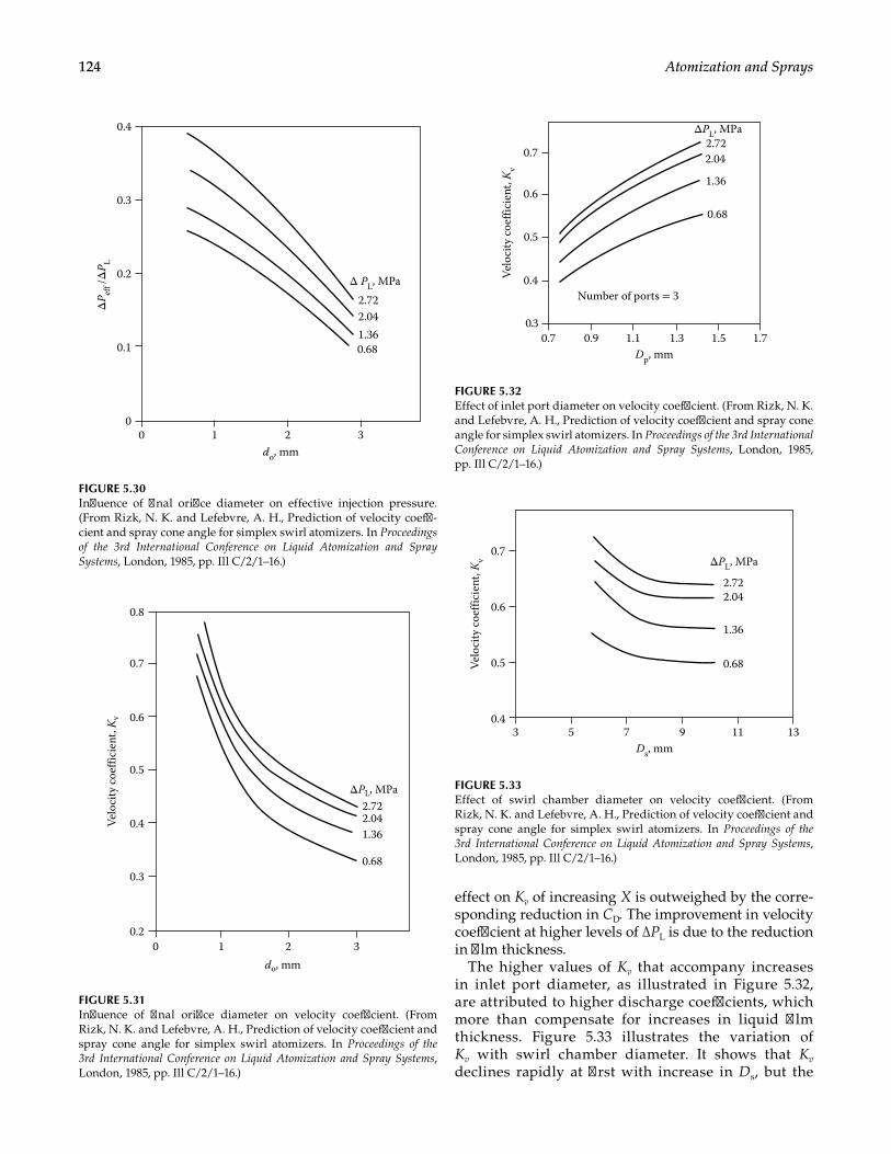
124 Atomization and Sprays

effect on Kv of increasing X is outweighed by the corre-sponding reduction in CD. The improvement in velocity coefficient at higher levels of ∆PL is due to the reduction in film thickness.

The higher values of Kv that accompany increases in inlet port diameter, as illustrated in Figure 5.32, are attributed to higher discharge coefficients, which more than compensate for increases in liquid film thickness. Figure 5.33 illustrates the variation of Kv with swirl chamber diameter. It shows that Kv declines rapidly at first with increase in Ds, but the

00

1 2 3

0.1

0.2

0.3

0.4

ΔP ef

f /ΔP L

do, mm

Δ PL, MPa2.722.041.360.68

FIGURE 5.30Influence of final orifice diameter on effective injection pressure. (From Rizk, N. K. and Lefebvre, A. H., Prediction of velocity coeffi-cient and spray cone angle for simplex swirl atomizers. In Proceedings of the 3rd International Conference on Liquid Atomization and Spray Systems, London, 1985, pp. Ill C/2/1–16.)

32100.2

0.3

0.4

0.5

0.6

0.7

0.8

Velo

city

coe

ffici

ent,

Kv

do, mm

ΔPL, MPa2.722.041.36

0.68

FIGURE 5.31Influence of final orifice diameter on velocity coefficient. (From Rizk, N. K. and Lefebvre, A. H., Prediction of velocity coefficient and spray cone angle for simplex swirl atomizers. In Proceedings of the 3rd International Conference on Liquid Atomization and Spray Systems, London, 1985, pp. Ill C/2/1–16.)

3 5 7 9 11 130.4

0.5

0.6

0.7

Velo

city

coe

ffici

ent,

Kv ΔPL, MPa

2.722.04

1.36

0.68

Ds, mm

FIGURE 5.33Effect of swirl chamber diameter on velocity coefficient. (From Rizk, N. K. and Lefebvre, A. H., Prediction of velocity coefficient and spray cone angle for simplex swirl atomizers. In Proceedings of the 3rd International Conference on Liquid Atomization and Spray Systems, London, 1985, pp. Ill C/2/1–16.)

0.7 0.9 1.1 1.3 1.5 1.70.3

0.4

0.5

0.6

0.7

Velo

city

coe

ffici

ent,

Kv

ΔPL, MPa2.722.04

1.36

0.68

Dp, mm

Number of ports = 3

FIGURE 5.32Effect of inlet port diameter on velocity coefficient. (From Rizk, N. K. and Lefebvre, A. H., Prediction of velocity coefficient and spray cone angle for simplex swirl atomizers. In Proceedings of the 3rd International Conference on Liquid Atomization and Spray Systems, London, 1985, pp. Ill C/2/1–16.)

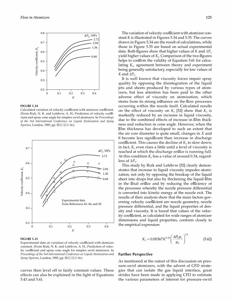
125Flow in Atomizers

curves then level off to fairly constant values. These effects can also be explained in the light of Equations 5.43 and 5.61.

The variation of velocity coefficient with atomizer con-stant K is illustrated in Figures 5.34 and 5.35. The curves drawn in Figure 5.34 are the result of calculations, while those in Figure 5.35 are based on actual experimental data. Both figures show that higher values of K and ∆PL yield higher values of Kv. Comparison of the two figures helps to confirm the validity of Equation 5.61 for calcu-lating Kv, agreement between theory and experiment being generally satisfactory, especially for low values of K and ∆PL.

It is well known that viscosity forces impair spray quality by opposing the disintegration of the liquid jets and sheets produced by various types of atom-izers, but less attention has been paid to the other adverse effect of viscosity on atomization, which stems from its strong influence on the flow processes occurring within the nozzle itself. Calculated results on the effect of viscosity on Kv [52] show that Kv is markedly reduced by an increase in liquid viscosity, due to the combined effects of increase in film thick-ness and reduction in cone angle. However, when the film thickness has developed to such an extent that the air core diameter is quite small, changes in X and θ become less significant than increase in discharge coefficient. This causes the decline of Kv to slow down; in fact, Kv even rises a little until a level of viscosity is reached at which the discharge orifice is running full. At this condition Kv has a value of around 0.34, regard-less of ∆PL.

This study by Rizk and Lefebvre [52] clearly demon-strates that increase in liquid viscosity impedes atomi-zation, not only by opposing the breakup of the liquid sheet into drops but also by thickening the liquid film in the final orifice and by reducing the efficiency of the processes whereby the nozzle pressure differential is converted into kinetic energy at the nozzle exit. The results of their analysis show that the main factors gov-erning velocity coefficient are nozzle geometry, nozzle pressure differential, and the liquid properties of den-sity and viscosity. It is found that values of the veloc-ity coefficient, as calculated for wide ranges of atomizer dimensions and liquid properties, conform closely to the empirical expression

K KP

v = ∆ ρµ

0.00367 0.29 L L

L

0.2

(5.62)

Further Perspective

As mentioned at the outset of this discussion on pres-sure-swirl atomizers, with the advent of CFD strate-gies that can isolate the gas liquid interface, great strides have been made in applying CFD to estimate the various parameters of interest for pressure-swirl

0 0.1 0.2 0.3 0.40.2

0.3

0.4

0.5

0.6

0.7

Velo

city

coe

ffici

ent,

Kv

ΔPL, MPa

2.72

2.041.36

0.68

Experimental dataFrom References 43, 44, and 50

K

FIGURE 5.35Experimental data on variation of velocity coefficient with atomizer constant. (From Rizk, N. K. and Lefebvre, A. H., Prediction of veloc-ity coefficient and spray cone angle for simplex swirl atomizers. In Proceedings of the 3rd International Conference on Liquid Atomization and Spray Systems, London, 1985, pp. Ill C/2/1–16.)

0 0.1 0.2 0.3 0.40.2

0.3

0.4

0.5

0.6

0.7

0.8

K

Velo

city

coe

ffici

ent,

Kv

ΔPL, MPa2.722.04

1.36

0.68

FIGURE 5.34Calculated variation of velocity coefficient with atomizer coefficient. (From Rizk, N. K. and Lefebvre, A. H., Prediction of velocity coeffi-cient and spray cone angle for simplex swirl atomizers. In Proceedings of the 3rd International Conference on Liquid Atomization and Spray Systems, London, 1985, pp. Ill C/2/1–16.)

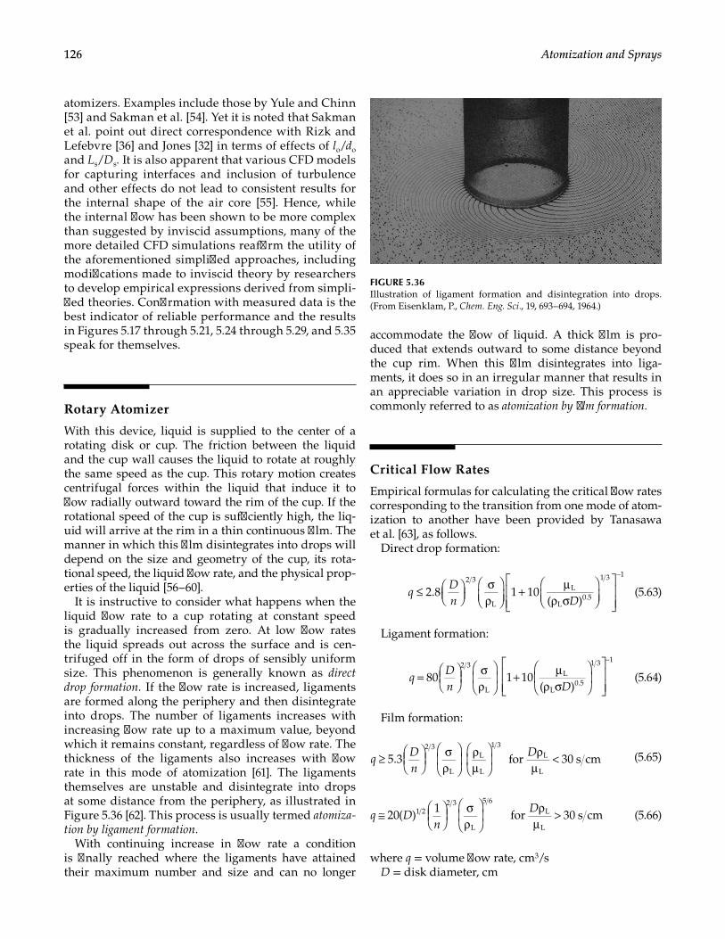
126 Atomization and Sprays

atomizers. Examples include those by Yule and Chinn [53] and Sakman et al. [54]. Yet it is noted that Sakman et al. point out direct correspondence with Rizk and Lefebvre [36] and Jones [32] in terms of effects of lo/do and Ls/Ds. It is also apparent that various CFD models for capturing interfaces and inclusion of turbulence and other effects do not lead to consistent results for the internal shape of the air core [55]. Hence, while the internal flow has been shown to be more complex than suggested by inviscid assumptions, many of the more detailed CFD simulations reaffirm the utility of the aforementioned simplified approaches, including modifications made to inviscid theory by researchers to develop empirical expressions derived from simpli-fied theories. Confirmation with measured data is the best indicator of reliable performance and the results in Figures 5.17 through 5.21, 5.24 through 5.29, and 5.35 speak for themselves.

Rotary Atomizer

With this device, liquid is supplied to the center of a rotating disk or cup. The friction between the liquid and the cup wall causes the liquid to rotate at roughly the same speed as the cup. This rotary motion creates centrifugal forces within the liquid that induce it to flow radially outward toward the rim of the cup. If the rotational speed of the cup is sufficiently high, the liq-uid will arrive at the rim in a thin continuous film. The manner in which this film disintegrates into drops will depend on the size and geometry of the cup, its rota-tional speed, the liquid flow rate, and the physical prop-erties of the liquid [56–60].

It is instructive to consider what happens when the liquid flow rate to a cup rotating at constant speed is gradually increased from zero. At low flow rates the liquid spreads out across the surface and is cen-trifuged off in the form of drops of sensibly uniform size. This phenomenon is generally known as direct drop formation. If the flow rate is increased, ligaments are formed along the periphery and then disintegrate into drops. The number of ligaments increases with increasing flow rate up to a maximum value, beyond which it remains constant, regardless of flow rate. The thickness of the ligaments also increases with flow rate in this mode of atomization [61]. The ligaments themselves are unstable and disintegrate into drops at some distance from the periphery, as illustrated in Figure 5.36 [62]. This process is usually termed atomiza-tion by ligament formation.

With continuing increase in flow rate a condition is finally reached where the ligaments have attained their maximum number and size and can no longer

accommodate the flow of liquid. A thick film is pro-duced that extends outward to some distance beyond the cup rim. When this film disintegrates into liga-ments, it does so in an irregular manner that results in an appreciable variation in drop size. This process is commonly referred to as atomization by film formation.

Critical Flow Rates

Empirical formulas for calculating the critical flow rates corresponding to the transition from one mode of atom-ization to another have been provided by Tanasawa et al. [63], as follows.

Direct drop formation:

qDn D

≤

σρ

+ µρ σ

−

2.8 1 10( )

2 3

L

L

L0.5

1 3 1

(5.63)

Ligament formation:

=

σρ

+ µ

ρ σ

−

80 1 10( )

2 3

L

L

L0.5

1 3 1

qDn D

(5.64)

Film formation:

≥

σρ

ρµ

ρµ

<5.3 for 30 s cm2 3

L

L

L

1 3L

Lq

Dn

D (5.65)

≅

σρ

ρµ

>20( ) 1 for 30 s cm1 22 3

L

5 6L

Lq D

nD (5.66)

where q = volume flow rate, cm3/sD = disk diameter, cm

FIGURE 5.36Illustration of ligament formation and disintegration into drops. (From Eisenklam, P., Chem. Eng. Sci., 19, 693–694, 1964.)

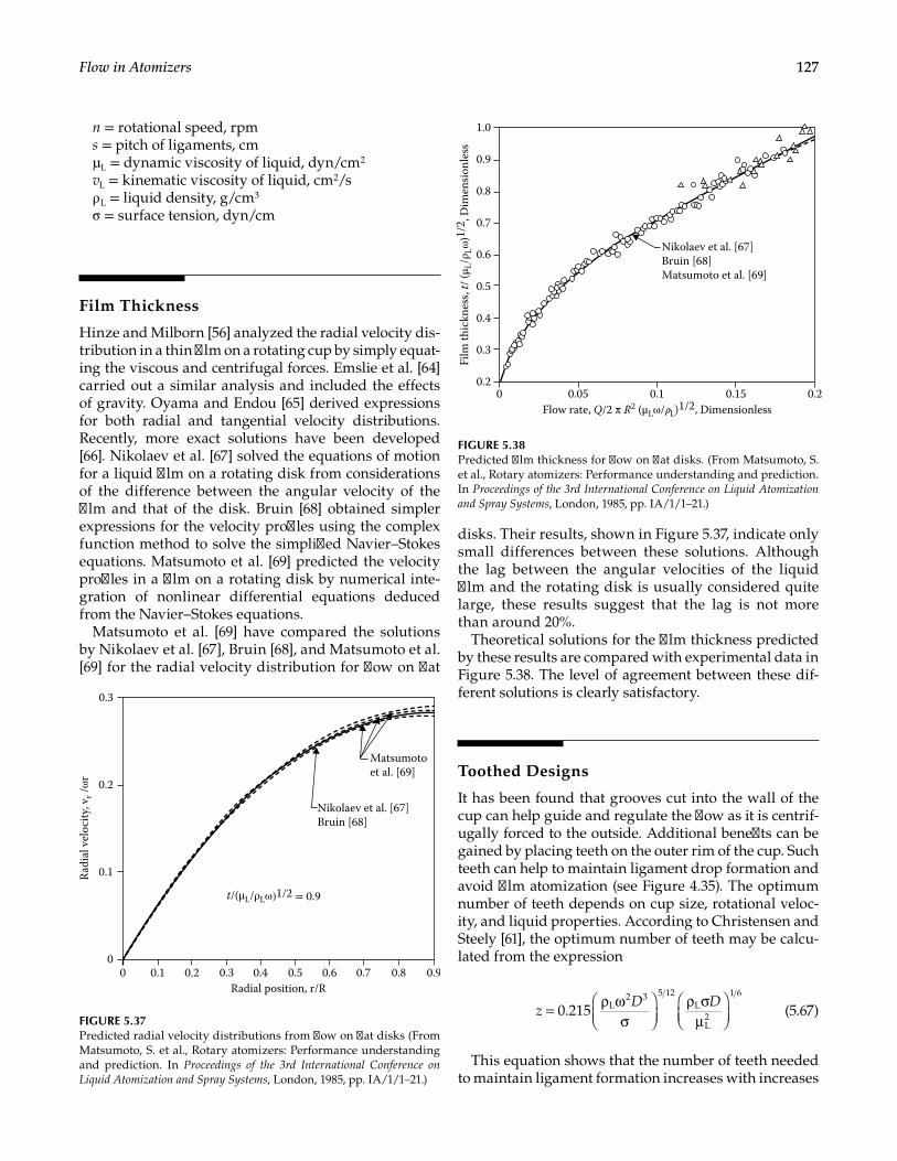
127Flow in Atomizers

n = rotational speed, rpms = pitch of ligaments, cmμL = dynamic viscosity of liquid, dyn/cm2

vL = kinematic viscosity of liquid, cm2/sρ L = liquid density, g/cm3

σ = surface tension, dyn/cm

Film Thickness

Hinze and Milborn [56] analyzed the radial velocity dis-tribution in a thin film on a rotating cup by simply equat-ing the viscous and centrifugal forces. Emslie et al. [64] carried out a similar analysis and included the effects of gravity. Oyama and Endou [65] derived expressions for both radial and tangential velocity distributions. Recently, more exact solutions have been developed [66]. Nikolaev et al. [67] solved the equations of motion for a liquid film on a rotating disk from considerations of the difference between the angular velocity of the film and that of the disk. Bruin [68] obtained simpler expressions for the velocity profiles using the complex function method to solve the simplified Navier–Stokes equations. Matsumoto et al. [69] predicted the velocity profiles in a film on a rotating disk by numerical inte-gration of nonlinear differential equations deduced from the Navier–Stokes equations.

Matsumoto et al. [69] have compared the solutions by Nikolaev et al. [67], Bruin [68], and Matsumoto et al. [69] for the radial velocity distribution for flow on flat

disks. Their results, shown in Figure 5.37, indicate only small differences between these solutions. Although the lag between the angular velocities of the liquid film and the rotating disk is usually considered quite large, these results suggest that the lag is not more than around 20%.

Theoretical solutions for the film thickness predicted by these results are compared with experimental data in Figure 5.38. The level of agreement between these dif-ferent solutions is clearly satisfactory.

Toothed Designs

It has been found that grooves cut into the wall of the cup can help guide and regulate the flow as it is centrif-ugally forced to the outside. Additional benefits can be gained by placing teeth on the outer rim of the cup. Such teeth can help to maintain ligament drop formation and avoid film atomization (see Figure 4.35). The optimum number of teeth depends on cup size, rotational veloc-ity, and liquid properties. According to Christensen and Steely [61], the optimum number of teeth may be calcu-lated from the expression

zD D= ρ ω

σ

ρ σµ

0.215 L2 3 5 12

L

L2

1 6

(5.67)

This equation shows that the number of teeth needed to maintain ligament formation increases with increases

0 0.1 0.2 0.3 0.4 0.5 0.6 0.7 0.8 0.90

0.1

0.2

0.3

Radial position, r/R

Radi

al v

eloc

ity, v

r /ωr

Matsumotoet al. [69]

Nikolaev et al. [67]Bruin [68]

t/(μL/ρLω)1/2 = 0.9

FIGURE 5.37Predicted radial velocity distributions from flow on flat disks (From Matsumoto, S. et al., Rotary atomizers: Performance understanding and prediction. In Proceedings of the 3rd International Conference on Liquid Atomization and Spray Systems, London, 1985, pp. IA/1/1–21.)

0 0.05 0.1 0.15 0.20.2

0.3

0.4

0.5

0.6

0.7

0.8

0.9

1.0

Flow rate, Q/2 π R2 (μLω/L)1/2, Dimensionless

Nikolaev et al. [67]Bruin [68]Matsumoto et al. [69]

Film

thic

knes

s, t/

(μL/

ρ Lω)

1/2 ,

Dim

ensio

nles

sFIGURE 5.38Predicted film thickness for flow on flat disks. (From Matsumoto, S. et al., Rotary atomizers: Performance understanding and prediction. In Proceedings of the 3rd International Conference on Liquid Atomization and Spray Systems, London, 1985, pp. IA/1/1–21.)

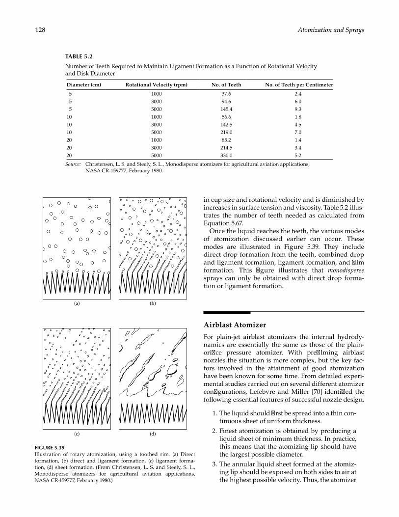
128 Atomization and Sprays

in cup size and rotational velocity and is diminished by increases in surface tension and viscosity. Table 5.2 illus-trates the number of teeth needed as calculated from Equation 5.67.

Once the liquid reaches the teeth, the various modes of atomization discussed earlier can occur. These modes are illustrated in Figure 5.39. They include direct drop formation from the teeth, combined drop and ligament formation, ligament formation, and film formation. This figure illustrates that monodisperse sprays can only be obtained with direct drop forma-tion or ligament formation.

Airblast Atomizer

For plain-jet airblast atomizers the internal hydrody-namics are essentially the same as those of the plain-orifice pressure atomizer. With prefilming airblast nozzles the situation is more complex, but the key fac-tors involved in the attainment of good atomization have been known for some time. From detailed experi-mental studies carried out on several different atomizer configurations, Lefebvre and Miller [70] identified the following essential features of successful nozzle design.

1. The liquid should first be spread into a thin con-tinuous sheet of uniform thickness.

2. Finest atomization is obtained by producing a liquid sheet of minimum thickness. In practice, this means that the atomizing lip should have the largest possible diameter.

3. The annular liquid sheet formed at the atomiz-ing lip should be exposed on both sides to air at the highest possible velocity. Thus, the atomizer

TABLE 5.2

Number of Teeth Required to Maintain Ligament Formation as a Function of Rotational Velocity and Disk Diameter

Diameter (cm) Rotational Velocity (rpm) No. of Teeth No. of Teeth per Centimeter

5 1000 37.6 2.4 5 3000 94.6 6.0 5 5000 145.4 9.310 1000 56.6 1.810 3000 142.5 4.510 5000 219.0 7.020 1000 85.2 1.420 3000 214.5 3.420 5000 330.0 5.2

Source: Christensen, L. S. and Steely, S. L., Monodisperse atomizers for agricultural aviation applications, NASA CR-159777, February 1980.

(a) (b)

(c) (d)

FIGURE 5.39Illustration of rotary atomization, using a toothed rim. (a) Direct formation, (b) direct and ligament formation, (c) ligament forma-tion, (d) sheet formation. (From Christensen, L. S. and Steely, S. L., Monodisperse atomizers for agricultural aviation applications, NASA CR-159777, February 1980.)

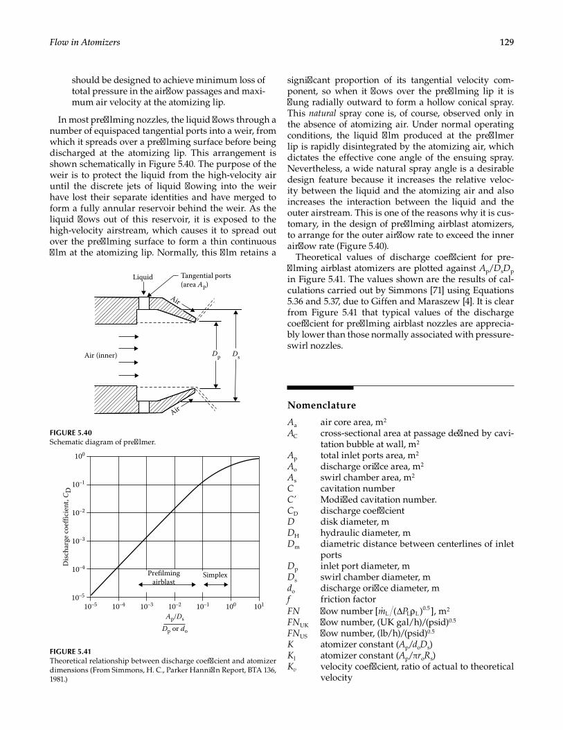
129Flow in Atomizers

should be designed to achieve minimum loss of total pressure in the airflow passages and maxi-mum air velocity at the atomizing lip.

In most prefilming nozzles, the liquid flows through a number of equispaced tangential ports into a weir, from which it spreads over a prefilming surface before being discharged at the atomizing lip. This arrangement is shown schematically in Figure 5.40. The purpose of the weir is to protect the liquid from the high-velocity air until the discrete jets of liquid flowing into the weir have lost their separate identities and have merged to form a fully annular reservoir behind the weir. As the liquid flows out of this reservoir, it is exposed to the high-velocity airstream, which causes it to spread out over the prefilming surface to form a thin continuous film at the atomizing lip. Normally, this film retains a

significant proportion of its tangential velocity com-ponent, so when it flows over the prefilming lip it is flung radially outward to form a hollow conical spray. This natural spray cone is, of course, observed only in the absence of atomizing air. Under normal operating conditions, the liquid film produced at the prefilmer lip is rapidly disintegrated by the atomizing air, which dictates the effective cone angle of the ensuing spray. Nevertheless, a wide natural spray angle is a desirable design feature because it increases the relative veloc-ity between the liquid and the atomizing air and also increases the interaction between the liquid and the outer airstream. This is one of the reasons why it is cus-tomary, in the design of prefilming airblast atomizers, to arrange for the outer airflow rate to exceed the inner airflow rate (Figure 5.40).

Theoretical values of discharge coefficient for pre-filming airblast atomizers are plotted against Ap/DsDp in Figure 5.41. The values shown are the results of cal-culations carried out by Simmons [71] using Equations 5.36 and 5.37, due to Giffen and Maraszew [4]. It is clear from Figure 5.41 that typical values of the discharge coefficient for prefilming airblast nozzles are apprecia-bly lower than those normally associated with pressure-swirl nozzles.

Nomenclature

Aa air core area, m2

AC cross-sectional area at passage defined by cavi-tation bubble at wall, m2

Ap total inlet ports area, m2

Ao discharge orifice area, m2

As swirl chamber area, m2

C cavitation numberC’ Modified cavitation number.CD discharge coefficientD disk diameter, mDH hydraulic diameter, mDm diametric distance between centerlines of inlet

portsDp inlet port diameter, mDs swirl chamber diameter, mdo discharge orifice diameter, mf friction factorFN flow number m P∆ ρ[ ( ) ]L L L

0.5 , m2

FNUK flow number, (UK gal/h)/(psid)0.5

FNUS flow number, (lb/h)/(psid)0.5

K atomizer constant (Ap/doDs)Kl atomizer constant (Ap/πroRs)Kv velocity coefficient, ratio of actual to theoretical

velocity

Tangential ports(area AP)

Liquid

Air

Air

Dp DsAir (inner)

FIGURE 5.40Schematic diagram of prefilmer.

10010–110–210–310–410–510–5

10–1

10–2

10–3

10–4

100

101

Prefilmingairblast

Simplex

Disc

harg

e co

effic

ient

, CD

Ap/Ds

Dp or do

FIGURE 5.41Theoretical relationship between discharge coefficient and atomizer dimensions (From Simmons, H. C., Parker Hannifin Report, BTA 136, 1981.)

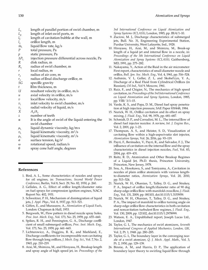
130 Atomization and Sprays

Ls length of parallel portion of swirl chamber, mLp length of inlet swirl ports, mlC length of cavitation bubble at the wall, mlo orifice length, mmL liquid flow rate, kg/sP total pressure, Pap static pressure, Pa∆PL injection pressure differential across nozzle, PaR disk radius, mRs radius of swirl chamber, mr local radius, mra radius of air core, mro radius of final discharge orifice, mSG specific gravityt film thickness, mU resultant velocity in orifice, m/su axial velocity in orifice, m/sv local flow velocity, m/svi inlet velocity to swirl chamber, m/svr radial velocity of liquid, m/sX Aa/Ao

z number of teethα It is the angle of swirl of the liquid entering the

swirl chamberμL liquid dynamic viscosity, kg/m·svL liquid kinematic viscosity, m2/sρ L liquid kinematic viscosity, m2/sσ surface tension, kg/s2

ω rotational speed, radian/sθ spray cone half angle, degrees

References

1. Bird, A. L., Some characteristics of nozzles and sprays for oil engines, in: Transactions, Second World Power Conference, Berlin, Vol 8, Sect. 29, No. 82, 1930, p. 260.

2. Gellales, A. G., Effect of orifice length/diameter ratio on fuel sprays for compression ignition engines, NACA Report No. 402, 1931.

3. Schweitzer, P. H., Mechanism of disintegration of liquid jets, J. Appl. Phys., Vol. 8, 1937, pp. 513–521.

4. Giffen, E., and Muraszew, A., Atomization of Liquid Fuels, London: Chapman & Hall, 1953.

5. Bergwerk, W., Flow pattern in diesel nozzle spray holes, Proc. Inst. Mech. Eng., Vol. 173, No. 25, 1959, pp. 655–660.

6. Spikes, R. H., and Pennington, G. A., Discharge coeffi-cient of small submerged orifices, Proc. Inst. Mech. Eng., Vol. 173, No. 25, 1959, pp. 661–665.

7. Lichtarowicz, A., Duggins, R. K., and Markland, E., Discharge coefficients for incompressible non-cavitating flow through long orifices, J. Mech. Eng. Sci., Vol. 7, No. 2, 1965, pp. 210–219.

8. Arai, M., Shimizu, M., and Hiroyasu, H., Breakup length and spray angle of high speed jet, in: Proceedings of the

3rd International Conference on Liquid Atomization and Spray Systems (ICLASS), London, 1985, pp. IB/4/1–10.

9. Zucrow, M. J., Discharge characteristics of submerged jets, Bull. No. 31, Engineering Experimental Station, Purdue University, West Lafayette, Ind., 1928.

10. Hiroyasu, H., Arai, M., and Shimizu, M., Break-up length of a liquid jet and internal flow in a nozzle, in: Proceedings of the 5th International Conference on Liquid Atomization and Spray Systems (ICLASS), Gaithersberg, MD, 1991, pp. 275–282.

11. Nakayama, Y., Action of the fluid in the air micrometer: First report, characteristics of small diameter nozzle and orifice, Bull. Jpn. Soc. Mech. Eng., Vol. 4, 1961, pp. 516–524.

12. Asihmin, V. I., Geller, Z. I., and Skobel’cyn, Y. A., Discharge of a Real Fluid from Cylindrical Orifices (in Russian), Oil Ind., Vol 9, Moscow, 1961.

13. Ruiz, F., and Chigier, N., The mechanics of high speed cavitation, in: Proceedings of the 3rd International Conference on Liquid Atomization and Spray Systems, London, 1985, pp. VIB/ 3/1–15.

14. Varde, K. S., and Popa, D. M., Diesel fuel spray penetra-tion at high injection pressure, SAE Paper 830448, 1984.

15. Nurick, W. H., Orifice cavitation and its effect on spray mixing, J. Fluid. Eng., Vol. 98, 1976, pp. 681–687.

16. Schmidt, D. P., and Corradini, M. L., The internal flow of diesel fuel injector nozzles: A review, Int. J. Engine Res., Vol. 2, 2001, pp. 1–23.

17. Thompson, A. S., and Heister, S. D., Visualization of cavitating flow within a high-aspect-ratio slot injector, Atomization Sprays, Vol. 26, 2016, pp. 93–119.

18. Payri, F., Bermudez, V., Payri, R., and Salvador, F. J., The influence of cavitation on the internal flow and the spray characteristics in diesel injection nozzles, Fuel, Vol. 83, 2004, pp. 419–431.

19. Reitz, R. D., Atomization and Other Breakup Regimes of a Liquid Jet, Ph.D. thesis, Princeton University, Princeton, New Jersey, 1978.

20. Sou, A., Hosokawa, S., and Tomiyama, A., Cavitation in nozzles of plain orifice atomizers with various length-to-diameter ratios, Atomization Sprays, Vol. 20, 2010, pp. 513–524.

21. Nurick, W. H., Ohanian, T., Talley, D. G., and Strakey, P. A., Impact of orifice length/diameter ratio of 90 deg sharp-edge orifice flow with manifold cross flow, J. Fluid. Eng., Vol. 131, 2009, pp. 081103, doi:10.1115/1.3155959.

22. Nurick, W. H., Ohanian, T., Talley, D. G., and Strakey, P. A., The impact of manifold to orifice turning angle on sharp-edge orifice flow characteristics in both cavitation and noncavitation turbulent flow regimes, J. Fluid. Eng., Vol. 130, 2009, pp. 121102, doi:10.1115/1.2978999.

23. Watson, E. A., Unpublished report, Joseph Lucas Ltd., London, 1947.

24. Taylor, G. I., The mechanics of swirl atomizers, Seventh International Congress of Applied Mechanics, London, UK, Vol. 2, Pt. 1, 1948. pp. 280–285.

25. Taylor, G. I., The boundary layer in the converging noz-zle of a swirl atomizer, Q. J. Mech. Appl. Math., Vol. 3, Pt. 2, 1950, pp. 129–139.

26. Binnie, A. M., and Harris, D. P., The application of boundary layer theory to swirling liquid flow through

131Flow in Atomizers

a nozzle, Q. J. Mech. Appl. Math., Vol. 3, Pt. 1, 1950, pp. 80–106.

27. Hodgekinson, T. G., Porton Technical Report No. 191, 1950. 28. Moon, S., Bae, C., Abo-Serie, E. F., and Cho, J., Internal

and near-nozzle flow of a pressure-swirl atomizer under varied fuel temperature, Atomization Sprays, Vol. 17, 2007, pp. 529–550.

29. Chinn, J. J., An appraisal of swirl atomizer inviscid flow analysis, Part 1: The principle of maximum flow for a swirl atomizer and its use in the exposition of early flow analyses, Atomization Sprays, Vol. 19, 2009, pp. 263–282.

30. Chinn, J. J., An appraisal of swirl atomizer inviscid flow analysis, Part 2: Inviscid spray cone angle analy-sis and comparison of inviscid methods with experi-mental results for discharge coefficient, air core radius, and spray cone angle, Atomization Sprays, Vol. 19, 2009, pp. 283–308.

31. Dombrowski, N., and Hassan, D., The flow characteris-tics of swirl centrifugal spray pressure nozzles with low viscosity liquids, AIChE J., Vol. 15, 1969, p. 604.

32. Jones, A. R., Design optimization of a large pressure-jet atomizer for power plant, in: Proceedings of the 2nd International Conference on Liquid Atomization and Spray Systems, Madison, WI, 1982, pp. 181–185.

33. Radcliffe, A., The performance of a type of swirl atom-izer, Proc. Inst. Mech. Eng., Vol. 169, 1955, pp. 93–106.

34. Carlisle, D. R., Communication on the performance of a type of swirl atomizer, by A. Radcliffe, Proc. Inst. Mech. Eng., Vol. 169, 1955, p. 101.

35. Eisenklam, P., Atomization of liquid fuels for combus-tion, J. Inst. Fuel, Vol. 34, 1961, pp. 130–143.

36. Rizk, N. K., and Lefebvre, A. H., Internal flow character-istics of simplex swirl atomizers, AIAA. J. Propul. Power, Vol. 1, No. 3, 1985, pp. 193–199.

37. Tipler, W., and Wilson, A. W., Combustion in gas turbines, Paper B9, in: Proceedings of the Congress International des Machines a Combustion (CIMAC), Paris, 1959, pp. 897–927.

38. Elkotb, M. M., Rafat, N. M., and Hanna, M. A., The influ-ence of swirl atomizer geometry on the atomization per-formance, in: Proceedings of the 1st International Conference on Liquid Atomization and Spray Systems, Tokyo, 1978, pp. 109–115.

39. Joyce, J. R., Report ICT15, Shell Research Ltd., London, 1947.

40. Babu, K. R., Narasimhan, M. V., and Narayanaswamy, K., Correlations for prediction of discharge rate, cone angle, and air core diameter of swirl spray atomizers, in: Proceedings of the 2nd International Conference on Liquid Atomization and Spray Systems, Madison, WI, 1982, pp. 91–97.

41. Lefebvre, A. H., Gas Turbine Combustion, Washington, DC: Council on Hemisphere Affairs, 1983.

42. Simmons, H. C, and Harding, C. F., Some effects of using water as a test fluid in fuel nozzle spray analysis, ASME Paper 80-GT-90, presented at ASME Gas Turbine Conference, New Orleans, 1980.

43. Sankaran Kutty, P., Narasimhan, M. V., and Narayanaswamy, K., Design and prediction of dis-charge rate, cone angle, and air core diameter of swirl

chamber atomizers, in: Proceedings of the 1st International Conference on Liquid Atomization and Spray Systems, Tokyo, 1978, pp. 93–100.

44. Narasimhan, M. V., Sankaran Kutty, P., and Narayanaswamy, K., Prediction of the air core diameter in swirl chamber atomizers, Unpublished report, 1978.

45. Jasuja, A. K., Atomization of crude and residual fuel oils, ASME J. Eng. Power, Vol. 101, No. 2, 1979, pp. 250–258.

46. Rizk, N. K., and Lefebvre, A. H., Influence of liquid film thickness on airblast atomization, ASME J. Eng. Power, Vol. 102, No. 3, 1980, pp. 706–710.

47. Simmons, H. C, The prediction of Sauter mean diameter for gas turbine fuel nozzles of different types, ASME J. Eng. Power, Vol. 102, No. 3, 1980, pp. 646–652.

48. Suyari, M., and Lefebvre, A. H., Film thickness measure-ments in a simplex swirl atomizer, AIAA J. Propul. Power, Vol. 2, No. 6, 1986, pp. 528–533.

49. Moon, S., Abo-Serie, E., and Bae, C., Liquid film thick-ness inside the high pressure swirl injectors: Real scale measurements and evaluation of analytical equations, Exp. Therm. Fluid Sci., Vol. 34, 2010, pp. 113–121.

50. Sankaran Kutty, P., Narasimhan, M. V., and Narayanaswamy, K., Prediction of the coefficient of dis-charge of swirl chamber atomizers, Unpublished work, 1978.

51. Rizk, N. K., and Lefebvre, A. H., Prediction of velocity coefficient and spray cone angle for simplex swirl atom-izers, in: Proceedings of the 3rd International Conference on Liquid Atomization and Spray Systems, London, 1985, pp. Ill C/2/1–16.

52. Rizk, N. K., and Lefebvre, A. H., Influence of liquid properties on the internal flow characteristics of simplex swirl atomizers, Atomization Spray Technol., Vol. 2, No. 3, 1986, pp. 219–233.

53. Yule, A., and Chinn, J. J., The internal flow and exit con-ditions of pressure swirl atomizers, Atomization Sprays, Vol. 10, 2000, pp. 121–146.

54. Sakman, A. T., Jog, M. A., Jeng, S. M., and Benjamin, M. A., Parametric study of simplex fuel nozzle inter-nal flow and performance, AIAA J., Vol. 38, 2000, pp. 1214–1218.

55. Vijay, G. A., Moorthi, N. S. V., and Manivannan, A., Internal and external flow characteristics of swirl atomizers: A review, Atomization Sprays, Vol. 25, 2015, pp. 153–188.

56. Hinze, J. O., and Milborn, H., Atomization of liquids by means of a rotating cup, J. Appl. Mech., Vol. 17, No. 2, 1950, pp. 145–153.

57. Adler, C. R., and Marshall, W. R., Performance of spin-ning disk atomizers, Chem. Eng. Prog., Vol. 47, 1951, pp. 515–601.

58. Fraser, R. P., Dombrowski, N., and Routley, J. H., The production of uniform liquid sheets from spinning cups; The filming by spinning cups; The atomization of a liq-uid sheet by an impinging air stream, Chem. Eng. Sci., Vol. 18, 1963, pp. 315–321, 323–337, 339–353.

59. Walton, W. H., and Prewitt, W. C., The production of sprays and mists of uniform drop size by means of spin-ning disc type sprayers, Proc. Phys. Soc., Vol. 62, Pt. 6, June 1949, pp. 341–350.

132 Atomization and Sprays

60. Willauer, H. D., Anath, R., Hoover, J. B., Mushrush, G. W., and Williams, F. W., Critical evaluation of rotary atom-izer, Petrol. Sci. Technol., Vol. 24, 2006, pp. 1215–1232.

61. Christensen, L. S., and Steely, S. L., Monodisperse Atomizers for Agricultural Aviation Applications, NASA CR-159777, February 1980.

62. Eisenklam, P., On ligament formation from spin-ning disks and cups, Chem. Eng. Sci., Vol. 19, 1964, pp. 693–694.

63. Tanasawa, Y., Miyasaka, Y., and Umehara, M., Effect of shape of rotating disks and cups on liquid atomization, in: Proceedings of the 1st International Conference on Liquid Atomization and Spray Systems, Tokyo, 1978, pp. 165–172.

64. Emslie, A. G., Benner, F. T., and Peck, L. G., J. Appl. Phys., Vol. 29, 1958, p. 858.

65. Oyama, Y., and Endou, K., On the centrifugal disk atom-ization and studies on the atomization of water drop-lets, Kagaku Kogaku, Vol. 17, 1953, pp. 256–260, 269–275 (in Japanese, English summary).

66. Matsumoto, S., Belcher, D. W., and Crosby, E. J., Rotary atomizers: Performance understanding and predic-tion, in: Proceedings of the 3rd International Conference on Liquid Atomization and Spray Systems, London, 1985, pp. IA/1/1–21.

67. Nikolaev, V. S., Vachagin, K. D., and Baryshev, Y. N., Film flow of viscous liquids over surfaces of rapidly rotating conical disks Int. Chem. Eng., Vol. 7, 1967, p. 595.

68. Bruin, S., Velocity distributions in a liquid film flowing over a rotating conical surface, Chem. Eng. Sci., Vol. 24, No. 11, 1969, pp. 1647–1654.

69. Matsumoto, S., Saito, K., and Takashima, Y., Bull Tokyo Inst. Technol., Vol. 116, 1973, p. 85.

70. Lefebvre, A. H., and Miller, D., The development of an air blast atomizer for gas turbine application, CoA-Report-AERO-193, College of Aeronautics, Cranfield, Bedford, England, June 1966.

71. Simmons, H. C., Parker Hannifin Report, BTA 136, 1981.

133

6Atomizer Performance

Introduction

Typical spray properties of importance include mean drop size, drop size distribution, radial and circumfer-ential patternation, droplet number density, cone angle, and penetration. The quality or fineness of an atomization process is usually described in terms of a mean drop size. Various definitions of mean drop size are available (see Chapter 3), of which the most widely used is the Sauter mean diameter (SMD).

Unfortunately, the physical processes involved in atomization remain insufficiently understood for mean diameters to be expressed in terms of equations derived from basic principles. The simplest case of the breakup of a liquid jet has been studied theoretically for more than a hundred years, but the results of these studies have failed to predict the spray characteristics to a sat-isfactory level of accuracy. The situation in regard to the complex sprays produced by more sophisticated types of atomizers is, understandably, even worse. As the physical structure and dynamics of a spray are the result of many interwoven complex mechanisms, none of them are fully understood, it is hardly surprising that mathematical treatments of atomization have so far defied successful development. That said, as computa-tional power compounds, implementation of high fidel-ity simulation is continually improving and numerous examples of predicting spray behavior can be found [1–5]. The advent of highly detailed data sets has pro-vided a mechanism for substantial validation [1]. Yet for engineering design, it is quite useful to provide some estimates of the relative quality or fineness of the spray generated by a given device for various conditions and liquids. While such design tools tend to be empirical in nature, they do allow general effects of liquid proper-ties, gas properties, and injector dimensions on mean drop size to be estimated.

As pointed out in Chapter 1, the properties of a liquid most relevant to atomization are surface tension, vis-cosity, and density. For a liquid injected into a gaseous medium, the only thermodynamic property generally considered of importance is the gas density. The liquid flow variables of importance are the velocity of the liq-uid jet or sheet and the turbulence in the liquid stream. The gas flow variables to be considered are the abso-lute velocity and the relative gas-to-liquid velocity. The

importance of this parameter is unfortunate, since the actual velocity field in the atomization region cannot be determined accurately. Even when liquid is sprayed into so-called quiescent air, the air velocity adjacent to the spray can attain quite high values due to the momen-tum transfer from the liquid to the surrounding air [6]. The turbulence characteristics of the air or gas may also influence atomization [7].

For plain-orifice injectors, the key geometric variables are the orifice length and diameter. Final orifice diameter is also of prime importance for pressure-swirl atomizers. For prefilming-type airblast atomizers, the dimensions that have most influence on mean drop size are the pre-filmer diameter and the hydraulic mean diameter of the atomizer air duct at the exit plane. For rotary atomizers, the only dimension of significance is the diameter of the rotating disk or cup. For all types of pneumatic or twin-fluid injectors, another variable affecting atomization is the mass ratio of liquid to air or steam.

The absence of any general theoretical treatment of the atomization process has led to the evolution of empirical equations to express the relationship between the mean drop size in a spray and the variables of liquid properties, gas properties, flow conditions, and atom-izer dimensions. Many of the drop size equations pub-lished in the literature are of somewhat dubious value. In some cases they are based on data obtained using experimental techniques that are no longer considered valid. With other equations, the insertion of appropri-ate values of gas and liquid properties yields improb-able values of SMD. The equations selected for inclusion in this chapter are considered to be the best available for engineering calculations of mean drop sizes for the types of atomizers described in Chapter 4.

Plain-Orifice Atomizer

Quiescent Environment

In plain-orifice atomizers, disintegration of the jet into drops is promoted by an increase in flow velocity, which increases both the level of turbulence in the issu-ing jet and the aerodynamic drag forces exerted by the surrounding medium; it is opposed by an increase in liquid viscosity, which delays the onset of atomization

134 Atomization and Sprays

by resisting breakup of the ligaments. Merrington and Richardson’s [8] experiments on sprays injected from a plain circular orifice into stagnant air yielded the fol-lowing relationship for mean drop size:

dU

νSMD =

500 o1.2

L0.2

L

(6.1)

Most of the research carried out on plain-orifice atom-izers has been directed toward the types of injectors employed in compression ignition (diesel) engines. With these injectors, jet breakup is due mainly to aerodynamic interaction with a highly turbulent jet. In an early study, Panasenkov [9] examined the influence of turbulence on the breakup of a liquid jet and determined mean drop sizes for jet Reynolds numbers ranging from 1,000 to 12,000. Drop sizes were correlated in terms of discharge orifice diameter and liquid Reynolds number as

dMMD 6 Re0 L0.15= − (6.2)

Harmon’s [10] equation for SMD takes account of ambi-ent gas properties as well as liquid properties. We have

d Uµ ρ σ µ ρ− − − −SMD = 330 o0.3

L0.07

L0.648 0.15

L0.55

G0.78

G0.052 (6.3)

An unusual feature of this equation is that an increase in surface tension is predicted to give finer atomization.

From their study on the effects of ambient gas density on drop size distributions, Giffen and Lamb [11] drew the following conclusions:

1. The fineness and uniformity of a spray are improved by an increase in gas density, but the rate of improvement decreases at high gas densities.

2. Gas density appears to exert little effect on the minimum drop size in the spray.

3. The maximum drop size is reduced at higher gas densities according to the relationship D .max G

0.2∝ ρ−

4. The improvement in atomization with increase in gas density is due mainly to a reduction in the number of large drops and is probably caused by subdivision of these big drops.

In 1955, Miesse [12] published his analysis of the results of previous theoretical and experimental studies on the disintegration of liquid jets. His equation for the best-fit correlation of the available experimental data is

D d We (23.5 0.000395Re )0.999 o L0.333

L= +− (6.4)

At about the same time, Tanasawa and Toyoda [13] proposed the following equation:

d Ud

SMD 47 1 331( )o L

1

G

0.25L

L o0.5= σ

ρ

+ µρ σ

− (6.5)

Some equations for the mean drop sizes produced by the diesel-type injectors are that of Hiroyasu and Katoda [14], which are of the form

Q Pρ ∆ −SMD = 2330 A0.121 0.131

L0.135 (6.6)

and that of Elkotb [15]

v P= σρ ρ ∆ −SMD 3.08 ( )L0.385

L0.737

A0.06

L0.54 (6.7)

Faeth and coworkers [16], along with Dumochel [17], emphasized the coupling of gas phase turbu-lence on the liquid breakup. This led to forms of expressions for SMD that involve the radial spatial integral length scale of turbulence, Λ, as discussed in Chapter 2 in the breakup of liquid jets. Such equa-tions have the form of

x

SMD 0.5Weex

0.5

0.53

= ΛΛ

(6.8)

In this equation, Weex refers to the Weber number at the nozzle exit based on liquid properties. In the case where nonturbulent ligaments are generated, the fol-lowing expression has been developed [16]:

x

SMD 0.72Wel

0.5

0.66

= ΛΛ

(6.9)

In this case, Wel is the Weber number based on the nonturbulent ligaments.

A similar form is suggested by Dumochel [17]:

= Λ ΛΛ

SMD 0.69/

We( / )o

0.57x

d (6.10)

It is observed that, in Equation 6.8 through 6.10, the integral length scale, Λ, must be determined in order to determine the SMD, which may or may not be straightforward.

Table 6.1 summarizes expressions for SMD for plain-orifice injectors. Expressions utilizing information that is readily available to the practitioner are emphasized. Those requiring additional information or constants or special features have not been included (e.g., Equations 6.8 through 6.10) even though they possibly may be of interest.

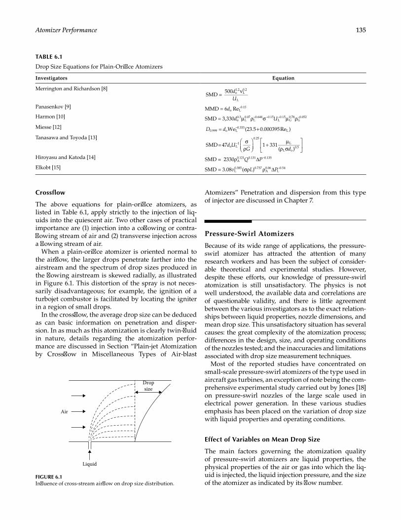
135Atomizer Performance

Crossflow

The above equations for plain-orifice atomizers, as listed in Table 6.1, apply strictly to the injection of liq-uids into the quiescent air. Two other cases of practical importance are (1) injection into a coflowing or contra-flowing stream of air and (2) transverse injection across a flowing stream of air.

When a plain-orifice atomizer is oriented normal to the airflow, the larger drops penetrate farther into the airstream and the spectrum of drop sizes produced in the flowing airstream is skewed radially, as illustrated in Figure 6.1. This distortion of the spray is not neces-sarily disadvantageous; for example, the ignition of a turbojet combustor is facilitated by locating the igniter in a region of small drops.

In the crossflow, the average drop size can be deduced as can basic information on penetration and disper-sion. In as much as this atomization is clearly twin-fluid in nature, details regarding the atomization perfor-mance are discussed in Section “Plain-jet Atomization by Crossflow in Miscellaneous Types of Air-blast

Atomizers” Penetration and dispersion from this type of injector are discussed in Chapter 7.

Pressure-Swirl Atomizers

Because of its wide range of applications, the pressure-swirl atomizer has attracted the attention of many research workers and has been the subject of consider-able theoretical and experimental studies. However, despite these efforts, our knowledge of pressure-swirl atomization is still unsatisfactory. The physics is not well understood, the available data and correlations are of questionable validity, and there is little agreement between the various investigators as to the exact relation-ships between liquid properties, nozzle dimensions, and mean drop size. This unsatisfactory situation has several causes: the great complexity of the atomization process; differences in the design, size, and operating conditions of the nozzles tested; and the inaccuracies and limitations associated with drop size measurement techniques.

Most of the reported studies have concentrated on small-scale pressure-swirl atomizers of the type used in aircraft gas turbines, an exception of note being the com-prehensive experimental study carried out by Jones [18] on pressure-swirl nozzles of the large scale used in electrical power generation. In these various studies emphasis has been placed on the variation of drop size with liquid properties and operating conditions.

Effect of Variables on Mean Drop Size

The main factors governing the atomization quality of pressure-swirl atomizers are liquid properties, the physical properties of the air or gas into which the liq-uid is injected, the liquid injection pressure, and the size of the atomizer as indicated by its flow number.

TABLE 6.1

Drop Size Equations for Plain-Orifice Atomizers

Investigators Equation

Merrington and Richardson [8] dU

νSMD =

500 o1.2

L0.2

L

Panasenkov [9] dMMD = 6 Reo L0.15−

Harmon [10] d USMD = 3,330 o0.3

L0.07

L0.15

L0.15

G0.78

G0.052µ ρ σ µ ρ−0.648 − − −

Miesse [12] = +−We (23.5 0.000395Re )0.999 o L0.333

LD d

Tanasawa and Toyoda [13]σ

ρ

+ µρ σ

−SMD=47 1 331( )

o L1

0.25L

L o0.5d U

G d

Hiroyasu and Katoda [14] Q PSMD = 2330 A0.121 0.131 0.135ρ ∆ −

Elkobt [15] v L PSMD = 3.08 ( )L0.385 0.737

A0.06

L0.54σρ ρ ∆ −

Liquid

Air

Dropsize

FIGURE 6.1Influence of cross-stream airflow on drop size distribution.

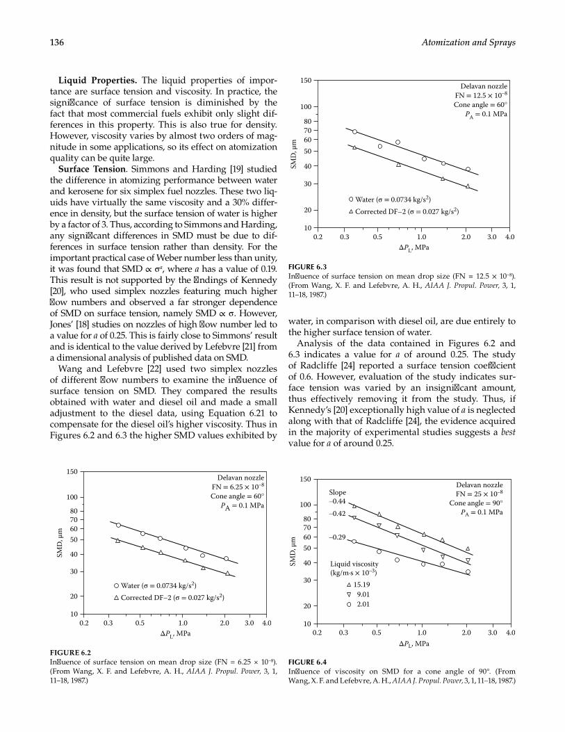
136 Atomization and Sprays

Liquid Properties. The liquid properties of impor-tance are surface tension and viscosity. In practice, the significance of surface tension is diminished by the fact that most commercial fuels exhibit only slight dif-ferences in this property. This is also true for density. However, viscosity varies by almost two orders of mag-nitude in some applications, so its effect on atomization quality can be quite large.

Surface Tension. Simmons and Harding [19] studied the difference in atomizing performance between water and kerosene for six simplex fuel nozzles. These two liq-uids have virtually the same viscosity and a 30% differ-ence in density, but the surface tension of water is higher by a factor of 3. Thus, according to Simmons and Harding, any significant differences in SMD must be due to dif-ferences in surface tension rather than density. For the important practical case of Weber number less than unity, it was found that SMD ∝  σ a, where a has a value of 0.19. This result is not supported by the findings of Kennedy [20], who used simplex nozzles featuring much higher flow numbers and observed a far stronger dependence of SMD on surface tension, namely SMD ∝  σ . However, Jones’ [18] studies on nozzles of high flow number led to a value for a of 0.25. This is fairly close to Simmons’ result and is identical to the value derived by Lefebvre [21] from a dimensional analysis of published data on SMD.

Wang and Lefebvre [22] used two simplex nozzles of different flow numbers to examine the influence of surface tension on SMD. They compared the results obtained with water and diesel oil and made a small adjustment to the diesel data, using Equation 6.21 to compensate for the diesel oil’s higher viscosity. Thus in Figures 6.2 and 6.3 the higher SMD values exhibited by

water, in comparison with diesel oil, are due entirely to the higher surface tension of water.

Analysis of the data contained in Figures 6.2 and 6.3 indicates a value for a of around 0.25. The study of Radcliffe [24] reported a surface tension coefficient of 0.6. However, evaluation of the study indicates sur-face tension was varied by an insignificant amount, thus effectively removing it from the study. Thus, if Kennedy’s [20] exceptionally high value of a is neglected along with that of Radcliffe [24], the evidence acquired in the majority of experimental studies suggests a best value for a of around 0.25.

100

80706050

40SMD

, μm

Water (σ = 0.0734 kg/s2)Corrected DF–2 (σ = 0.027 kg/s2)

ΔPL, MPa

30

20

0.2 0.3 0.5 1.0 2.0 3.0

Delavan nozzleFN = 6.25 × 10–8

Cone angle = 60°PA = 0.1 MPa

4.0

150

10

FIGURE 6.2Influence of surface tension on mean drop size (FN = 6.25 × 10–8). (From Wang, X. F. and Lefebvre, A. H., AIAA J. Propul. Power, 3, 1, 11–18, 1987.)

100

80706050

40SMD

, μm

Water (σ = 0.0734 kg/s2)Corrected DF–2 (σ = 0.027 kg/s2)

ΔPL, MPa

30

20

0.2 0.3 0.5 1.0 2.0 3.0

Delavan nozzleFN = 12.5 × 10–8

Cone angle = 60°PA = 0.1 MPa

4.0

150

10

FIGURE 6.3Influence of surface tension on mean drop size (FN = 12.5 × 10–8). (From Wang, X. F. and Lefebvre, A. H., AIAA J. Propul. Power, 3, 1, 11–18, 1987.)

100

150

80706050

40

–0.29

–0.42

–0.44Slope

SMD

, μm

Liquid viscosity(kg/m·s × 10–3)

ΔPL, MPa

30

20

0.2 0.3 0.5 1.0 2.0 3.0

Delavan nozzleFN = 25 × 10–8

Cone angle = 90°PA = 0.1 MPa

4.010

2.019.01

15.19

FIGURE 6.4Influence of viscosity on SMD for a cone angle of 90°. (From Wang, X. F. and Lefebvre, A. H., AIAA J. Propul. Power, 3, 1, 11–18, 1987.)

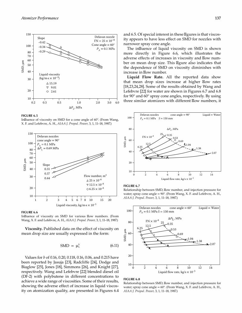
137Atomizer Performance

Viscosity. Published data on the effect of viscosity on mean drop size are usually expressed in the form:

bSMD L∝ µ (6.11)

Values for b of 0.16, 0.20, 0.118, 0.16, 0.06, and 0.215 have been reported by Jasuja [23], Radcliffe [24], Dodge and Biaglow [25], Jones [18], Simmons [26], and Knight [27], respectively. Wang and Lefebvre [22] blended diesel oil (DF-2) with polybutene in different concentrations to achieve a wide range of viscosities. Some of their results, showing the adverse effect of increase in liquid viscos-ity on atomization quality, are presented in Figures 6.4

and 6.5. Of special interest in these figures is that viscos-ity appears to have less effect on SMD for nozzles with narrower spray cone angle.

The influence of liquid viscosity on SMD is shown more directly in Figure 6.6, which illustrates the adverse effects of increases in viscosity and flow num-ber on mean drop size. This figure also indicates that the dependence of SMD on viscosity diminishes with increase in flow number.

Liquid Flow Rate. All the reported data show that mean drop sizes increase at higher flow rates [18,23,24,28]. Some of the results obtained by Wang and Lefebvre [22] for water are shown in Figures 6.7 and 6.8 for 90° and 60° spray cone angles, respectively. By using three similar atomizers with different flow numbers, it

100

150

80706050

40

–0.34–0.29

–0.42Slope

SMD

, μm

Liquid viscosity(kg/m·s × 10–3)

ΔPL, MPa

30

20

0.30.2 0.5 1.0 2.0 3.0

Delavan nozzleFN = 25 × 10–8

Cone angle = 60°PA = 0.1 MPa

4.010

9.0115.19

2.61

FIGURE 6.5Influence of viscosity on SMD for a cone angle of 60°. (From Wang, X. F. and Lefebvre, A. H., AIAA J. Propul. Power, 3, 1, 11–18, 1987.)

100

150

80706050

400.370.44

0.31Slope

SMD

, μm

Flow number, m230

20

2 3

Delavan nozzlescone angle = 90°PA = 0.1 MPaΔPL = 0.69 MPa

101 4 5 6 7 8 10 15 20

12.5 × 10–825 × 10–8

6.25 × 10–8

Liquid viscosity, kg/m·s × 10–3

FIGURE 6.6Influence of viscosity on SMD for various flow numbers. (From Wang, X. F. and Lefebvre, A. H., AIAA J. Propul. Power, 3, 1, 11–18, 1987.)

100

80

60

6.2512.5

25 0.350.53

0.691.04

1.38

2.07

SMD

, μm FN × 10–8

40

20

20 4

Delavan nozzles

106 8 10 12 14

Liquid flow rate, kg/s × 10–3

cone angle = 90° Liquid = WaterPA = 0.1 MPa

ΔPL, MPa

S = 150 mm

FIGURE 6.7Relationship between SMD, flow number, and injection pressure for water; spray cone angle = 90°. (From Wang, X. F. and Lefebvre, A. H., AIAA J. Propul. Power, 3, 1, 11–18, 1987.)

12.5

100

80

606.25

25 0.35

0.530.69

1.041.38

2.07

SMD

, μm

FN × 10–8

40

20

20 4

Delavan nozzles

106 8 10 12 14

Liquid flow rate, kg/s × 10–3

cone angle = 60° Liquid = WaterPA = 0.1 MPa

ΔPL, MPa

S = 150 mm

FIGURE 6.8Relationship between SMD, flow number, and injection pressure for water; spray cone angle = 60°. (From Wang, X. F. and Lefebvre, A. H., AIAA J. Propul. Power, 3, 1, 11–18, 1987.)

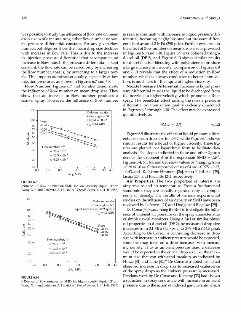
138 Atomization and Sprays

was possible to study the influence of flow rate on mean drop size while maintaining either flow number or noz-zle pressure differential constant. For any given flow number, both figures show that mean drop size declines with increase in flow rate. This is due to the increase in injection pressure differential that accompanies an increase in flow rate. If the pressure differential is kept constant, the flow rate can be raised only by increasing the flow number, that is, by switching to a larger noz-zle. This impairs atomization quality, especially at low injection pressures, as shown in Figures 6.7 and 6.8.

Flow Number. Figures 6.7 and 6.8 also demonstrate the influence of flow number on mean drop size. They show that an increase in flow number produces a coarser spray. However, the influence of flow number

is seen to diminish with increase in liquid pressure dif-ferential, becoming negligibly small at pressure differ-entials of around 2 MPa (290 psid). Further evidence on the effect of flow number on mean drop size is provided in Figures 6.9 and 6.10. Figure 6.9 was obtained using a diesel oil (DF-2), and Figure 6.10 shows similar results for diesel oil after blending with polybutene to produce a large increase in viscosity. Comparison of Figures 6.9 and 6.10 reveals that the effect of a reduction in flow number, which is always conducive to better atomiza-tion, is much less for the liquid of higher viscosity.

Nozzle Pressure Differential. Increase in liquid pres-sure differential causes the liquid to be discharged from the nozzle at a higher velocity, which promotes a finer spray. The beneficial effect raising the nozzle pressure differential on atomization quality is clearly illustrated in Figures 6.2 through 6.10. The effect may be expressed quantitatively as

PdSMD L∝ ∆ (6.12)

Figure 6.9 illustrates the effects of liquid pressure differ-ential on mean drop size for DF-2, while Figure 6.10 shows similar results for a liquid of higher viscosity. These fig-ures are plotted in a logarithmic form to facilitate data analysis. The slopes indicated in these and other figures denote the exponent d in the expression PdSMD .L∝ ∆ Figures 6.4, 6.5, 6.9, and 6.10 show values of d ranging from −0.28 to −0.44. Other reported values of d are −0.275, −0.35, −0.43, and −0.40, from Simmons [26], Abou-Ellail et al. [29], Jasuja [23], and Radcliffe [24], respectively.

Air Properties. The two properties of interest are air pressure and air temperature. From a fundamental standpoint, they are usually regarded only as compo-nents of density. The results of various experimental studies on the influence of air density on SMD have been reviewed by Lefebvre [21] and Dodge and Biaglow [25].

De Corso [30] was among the first to investigate the influ-ence of ambient air pressure on the spray characteristics of simplex swirl atomizers. Using a fuel of similar physi-cal properties to diesel oil (DF-2), he measured drop size increases from 0.1 MPa (14.5 psia) to 0.79 MPa (114.5 psia). According to De Corso, “a continuing decrease in drop size with increase in ambient pressure would be expected, since the drag force on a drop increases with increas-ing density. Thus as ambient pressure rises, a decrease would be expected in the critical drop size, i.e., the maxi-mum size that can withstand breakup, as indicated by Hinze [31] and Lane [32].” De Corso attributed his actual observed increase in drop size to increased coalescence of the spray drops as the ambient pressure is increased. Previous work by De Corso and Kemeny [33] had shown a reduction in spray cone angle with increase in ambient pressure, due to the action of induced gas currents, which

100

150

80706050

Slope

40Flow number, m2

–0.28–0.30–0.31

SMD

, μm

ΔPL, MPa

30

20

0.2 0.3 0.5 1.0 2.0 3.0

Delavan nozzlesCone angle = 60°Liquid = DF–2PA = 0.1 MPa

4.010

6.25 × 10–8

25 × 10–8

12.5 × 10–8

FIGURE 6.9Influence of flow number on SMD for low-viscosity liquid. (From Wang, X. F. and Lefebvre, A. H., AIAA J. Propul. Power, 3, 1, 11–18, 1987.)

100

150

80706050

Slope

40Flow number, m2

–0.33–0.36–0.38SM

D, μ

m

25 × 10–8

12.5 × 10–8

6.25 × 10–8

ΔPL, MPa

30

20

0.2 0.3 0.5 1.0 2.0 3.0

Delavan nozzlesCone angle = 60°

Liquid viscosity = 0.009 kg/m.sPA = 0.1 MPa

4.010

FIGURE 6.10Influence of flow number on SMD for high-viscosity liquid. (From Wang, X. F. and Lefebvre, A. H., AIAA J. Propul. Power, 3, 1, 11–18, 1987.)

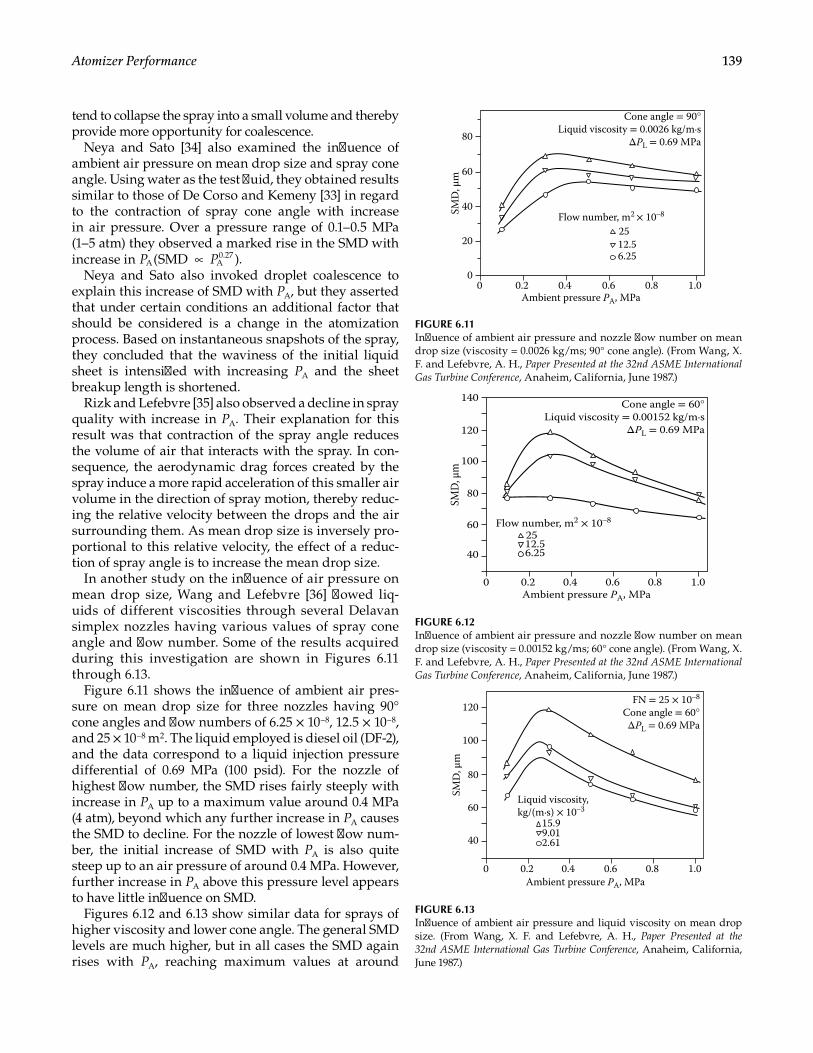
139Atomizer Performance

tend to collapse the spray into a small volume and thereby provide more opportunity for coalescence.

Neya and Sato [34] also examined the influence of ambient air pressure on mean drop size and spray cone angle. Using water as the test fluid, they obtained results similar to those of De Corso and Kemeny [33] in regard to the contraction of spray cone angle with increase in air pressure. Over a pressure range of 0.1–0.5 MPa (1–5 atm) they observed a marked rise in the SMD with increase in P P(SMD ).A A

0.27∝Neya and Sato also invoked droplet coalescence to

explain this increase of SMD with PA, but they asserted that under certain conditions an additional factor that should be considered is a change in the atomization process. Based on instantaneous snapshots of the spray, they concluded that the waviness of the initial liquid sheet is intensified with increasing PA and the sheet breakup length is shortened.

Rizk and Lefebvre [35] also observed a decline in spray quality with increase in PA. Their explanation for this result was that contraction of the spray angle reduces the volume of air that interacts with the spray. In con-sequence, the aerodynamic drag forces created by the spray induce a more rapid acceleration of this smaller air volume in the direction of spray motion, thereby reduc-ing the relative velocity between the drops and the air surrounding them. As mean drop size is inversely pro-portional to this relative velocity, the effect of a reduc-tion of spray angle is to increase the mean drop size.

In another study on the influence of air pressure on mean drop size, Wang and Lefebvre [36] flowed liq-uids of different viscosities through several Delavan simplex nozzles having various values of spray cone angle and flow number. Some of the results acquired during this investigation are shown in Figures 6.11 through 6.13.

Figure 6.11 shows the influence of ambient air pres-sure on mean drop size for three nozzles having 90° cone angles and flow numbers of 6.25 × 10–8, 12.5 × 10–8, and 25 × 10–8 m2. The liquid employed is diesel oil (DF-2), and the data correspond to a liquid injection pressure differential of 0.69 MPa (100 psid). For the nozzle of highest flow number, the SMD rises fairly steeply with increase in PA up to a maximum value around 0.4 MPa (4 atm), beyond which any further increase in PA causes the SMD to decline. For the nozzle of lowest flow num-ber, the initial increase of SMD with PA is also quite steep up to an air pressure of around 0.4 MPa. However, further increase in PA above this pressure level appears to have little influence on SMD.

Figures 6.12 and 6.13 show similar data for sprays of higher viscosity and lower cone angle. The general SMD levels are much higher, but in all cases the SMD again rises with PA, reaching maximum values at around

Flow number, m2 × 10–8SMD

, μm

2512.56.25

0.200

20

40

60

80

0.4Ambient pressure PA, MPa

0.6 0.8 1.0

Cone angle = 90°Liquid viscosity = 0.0026 kg/m·s

ΔPL = 0.69 MPa

FIGURE 6.11Influence of ambient air pressure and nozzle flow number on mean drop size (viscosity = 0.0026 kg/ms; 90° cone angle). (From Wang, X. F. and Lefebvre, A. H., Paper Presented at the 32nd ASME International Gas Turbine Conference, Anaheim, California, June 1987.)

Flow number, m2 × 10–8

SMD,

μm

0.20

40

60

80

100

120

140

0.4Ambient pressure PA, MPa

0.6 0.8 1.0

6.25

2512.5

Cone angle = 60°Liquid viscosity = 0.00152 kg/m·s

ΔPL = 0.69 MPa

FIGURE 6.12Influence of ambient air pressure and nozzle flow number on mean drop size (viscosity = 0.00152 kg/ms; 60° cone angle). (From Wang, X. F. and Lefebvre, A. H., Paper Presented at the 32nd ASME International Gas Turbine Conference, Anaheim, California, June 1987.)

Liquid viscosity,kg/(m·s) × 10–3

SMD

, μm

0.20

40

60

80

100

120

0.4Ambient pressure PA, MPa

0.6 0.8 1.0

2.61

15.99.01

FN = 25 × 10–8

Cone angle = 60°ΔPL = 0.69 MPa

FIGURE 6.13Influence of ambient air pressure and liquid viscosity on mean drop size. (From Wang, X. F. and Lefebvre, A. H., Paper Presented at the 32nd ASME International Gas Turbine Conference, Anaheim, California, June 1987.)

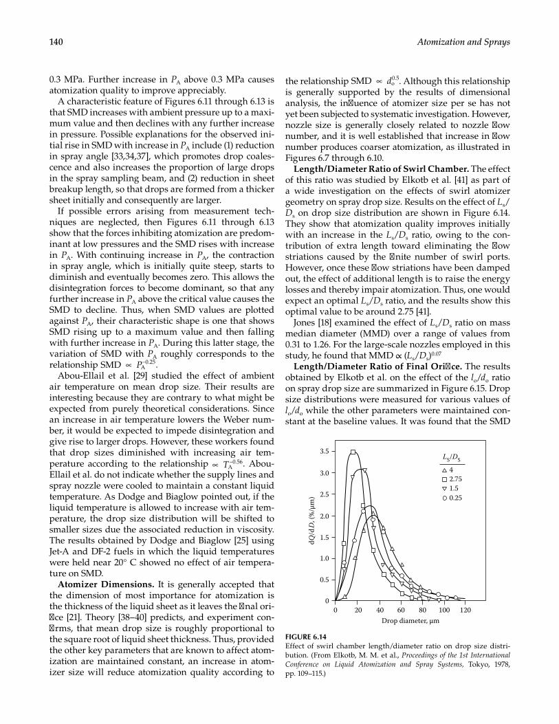
140 Atomization and Sprays

0.3 MPa. Further increase in PA above 0.3 MPa causes atomization quality to improve appreciably.

A characteristic feature of Figures 6.11 through 6.13 is that SMD increases with ambient pressure up to a maxi-mum value and then declines with any further increase in pressure. Possible explanations for the observed ini-tial rise in SMD with increase in PA include (1) reduction in spray angle [33,34,37], which promotes drop coales-cence and also increases the proportion of large drops in the spray sampling beam, and (2) reduction in sheet breakup length, so that drops are formed from a thicker sheet initially and consequently are larger.

If possible errors arising from measurement tech-niques are neglected, then Figures 6.11 through 6.13 show that the forces inhibiting atomization are predom-inant at low pressures and the SMD rises with increase in PA. With continuing increase in PA, the contraction in spray angle, which is initially quite steep, starts to diminish and eventually becomes zero. This allows the disintegration forces to become dominant, so that any further increase in PA above the critical value causes the SMD to decline. Thus, when SMD values are plotted against PA, their characteristic shape is one that shows SMD rising up to a maximum value and then falling with further increase in PA. During this latter stage, the variation of SMD with PA roughly corresponds to the relationship PSMD A

0.25∝ − .Abou-Ellail et al. [29] studied the effect of ambient

air temperature on mean drop size. Their results are interesting because they are contrary to what might be expected from purely theoretical considerations. Since an increase in air temperature lowers the Weber num-ber, it would be expected to impede disintegration and give rise to larger drops. However, these workers found that drop sizes diminished with increasing air tem-perature according to the relationship TA

0.56∝ − . Abou-Ellail et al. do not indicate whether the supply lines and spray nozzle were cooled to maintain a constant liquid temperature. As Dodge and Biaglow pointed out, if the liquid temperature is allowed to increase with air tem-perature, the drop size distribution will be shifted to smaller sizes due the associated reduction in viscosity. The results obtained by Dodge and Biaglow [25] using Jet-A and DF-2 fuels in which the liquid temperatures were held near 20° C showed no effect of air tempera-ture on SMD.

Atomizer Dimensions. It is generally accepted that the dimension of most importance for atomization is the thickness of the liquid sheet as it leaves the final ori-fice [21]. Theory [38–40] predicts, and experiment con-firms, that mean drop size is roughly proportional to the square root of liquid sheet thickness. Thus, provided the other key parameters that are known to affect atom-ization are maintained constant, an increase in atom-izer size will reduce atomization quality according to

the relationship dSMD o0.5∝ . Although this relationship

is generally supported by the results of dimensional analysis, the influence of atomizer size per se has not yet been subjected to systematic investigation. However, nozzle size is generally closely related to nozzle flow number, and it is well established that increase in flow number produces coarser atomization, as illustrated in Figures 6.7 through 6.10.

Length/Diameter Ratio of Swirl Chamber. The effect of this ratio was studied by Elkotb et al. [41] as part of a wide investigation on the effects of swirl atomizer geometry on spray drop size. Results on the effect of Ls/Ds on drop size distribution are shown in Figure 6.14. They show that atomization quality improves initially with an increase in the Ls/Ds ratio, owing to the con-tribution of extra length toward eliminating the flow striations caused by the finite number of swirl ports. However, once these flow striations have been damped out, the effect of additional length is to raise the energy losses and thereby impair atomization. Thus, one would expect an optimal Ls/Ds ratio, and the results show this optimal value to be around 2.75 [41].

Jones [18] examined the effect of Ls/Ds ratio on mass median diameter (MMD) over a range of values from 0.31 to 1.26. For the large-scale nozzles employed in this study, he found that MMD ∝ (Ls/Ds)0.07

Length/Diameter Ratio of Final Orifice. The results obtained by Elkotb et al. on the effect of the lo/do ratio on spray drop size are summarized in Figure 6.15. Drop size distributions were measured for various values of lo/do while the other parameters were maintained con-stant at the baseline values. It was found that the SMD

LS/DS

dQ/d

D, (

%/μ

m)

2000

0.5

1.0

1.5

2.0

2.5

3.0

3.5

40Drop diameter, μm

60 80 100 120

42.751.50.25

FIGURE 6.14Effect of swirl chamber length/diameter ratio on drop size distri-bution. (From Elkotb, M. M. et al., Proceedings of the 1st International Conference on Liquid Atomization and Spray Systems, Tokyo, 1978, pp. 109–115.)

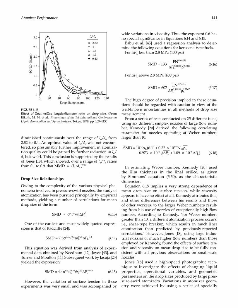
141Atomizer Performance

diminished continuously over the range of lo/do from 2.82 to 0.4. An optimal value of lo/do was not encoun-tered, so presumably further improvement in atomiza-tion quality could be gained by further reduction in lo/do below 0.4. This conclusion is supported by the results of Jones [18], which showed, over a range of lo/do ratios from 0.1 to 0.9, that l dMMD ( )o o

0.03∝ .

Drop Size Relationships

Owing to the complexity of the various physical phe-nomena involved in pressure-swirl nozzles, the study of atomization has been pursued principally by empirical methods, yielding a number of correlations for mean drop size of the form

v m Pa b c dSMD L L∝ σ ∆ (6.13)

One of the earliest and most widely quoted expres-sions is that of Radcliffe [24]:

. . . .σ ∆ −SMD = 7.3 v m P0 6

L0 2

L0 25

L0 4

(6.14)

This equation was derived from analysis of experi-mental data obtained by Needham [42], Joyce [43], and Turner and Moulton [44]. Subsequent work by Jasuja [23] yielded the expression:

v m Pσ ∆ −SMD = 4.4 0.6L0.16

L0.22

L0.43

(6.15)

However, the variation of surface tension in these experiments was very small and was accompanied by

wide variations in viscosity. Thus the exponent 0.6 has no special significance in Equations 6.14 and 6.15.

Babu et al. [45] used a regression analysis to deter-mine the following equations for kerosene-type fuels.

For ∆PL less than 2.8 MPa (400 psi)

P

SMD = 133FN0.64291

L0.22565

L0.3215∆ ρ

(6.16)

For ∆PL above 2.8 MPa (400 psi)

P

SMD = 607FN0.75344

L0.19936

L0.3767∆ ρ

(6.17)

The high degree of precision implied in these equa-tions should be regarded with caution in view of the well-known uncertainties in all methods of drop size measurement.

From a series of tests conducted on 25 different fuels, using six different simplex nozzles of large flow num-ber, Kennedy [20] derived the following correlating parameter for nozzles operating at Weber numbers larger than 10:

P Pσ + × ρ

− × ∆ + × ∆

−

− −SMD = 10 (6.11 0.32 10 FN

6.973 10 1.89 10 )

3L

5L

3L

6L (6.18)

In estimating Weber number, Kennedy [20] used the film thickness in the final orifice, as given by Simmons’ equation (5.50), as the characteristic dimension.

Equation 6.18 implies a very strong dependence of mean drop size on surface tension, while viscosity appears to have no effect at all. Kennedy attributes this, and other differences between his results and those of other workers, to the larger Weber numbers result-ing from his use of nozzles of exceptionally high flow number. According to Kennedy, “for Weber numbers greater than 10, a different atomization process occurs, i.e., shear-type breakup, which results in much finer atomization than predicted by previously-reported correlations.” However, Jones [18], using large indus-trial nozzles of much higher flow numbers than those employed by Kennedy, found the effects of surface ten-sion and viscosity on mean drop size to be fully con-sistent with all previous observations on small-scale nozzles.

Jones [18] used a high-speed photographic tech-nique to investigate the effects of changing liquid properties, operational variables, and geometric parameters on the drop sizes produced by large pres-sure-swirl atomizers. Variations in atomizer geom-etry were achieved by using a series of specially

dQ/d

D, (

%/μ

m)

0.5

1.0

00

1.5

2.0

2.5

3.0

Drop diameter, μm20 40 60 80 100

0.431.21.622.82

lo/do

140120

FIGURE 6.15Effect of final orifice length/diameter ratio on drop size. (From Elkotb, M. M. et al., Proceedings of the 1st International Conference on Liquid Atomization and Spray Systems, Tokyo, 1978, pp. 109–115.)

142 Atomization and Sprays

designed nozzle pieces that enabled 50 different geometric configurations to be studied. Analysis of the experimental data yielded the following equa-tion for mean drop size:

m P

ld

LD

AD d

Dd

∆ µ µ σ ρ

×

− − −

−

MMD = 2.47 L0.315

L0.47

L0.16

A0.04 0.25

L0.22

o

o

0.03s

s

0.07p

s o

0.13s

o

0.21 (6.19)

The ranges of variables covered in this investigation are listed in Table 5.1. Lefebvre’s [21] analysis of the flow processes in the final orifice of a simplex nozzle led to the following equation for SMD:

A d PSMD = 0.25L0.25

L0.125

o0.5

A0.25

L0.375σ µ ρ ρ ∆− − (6.20)

The value of 0.25 for the surface tension exponent is reasonably close to Simmons’ estimates (0.16–0.19) and is in exact agreement with the experimental findings of Jones [18] and Wang and Lefebvre [22]. The exponent of 0.25 for viscosity agrees fairly well with all reported val-ues. The literature suggests that the influence of liquid density on SMD is quite small. The do exponent of 0.5 is consistent with the theoretical value. The exponents for injection pressure differential and air density of −0.375 and −0.25, respectively, are identical to the experimental values obtained in the investigation by Abou-Ellail et al. [29]. Substituting d m P∝ ∆ ρ/( / )o L

0.5L L

0.25 into Equation 6.20 and using Jasuja's [23] data to determine the value of A gives

m Pσ µ ∆ ρ− −SMD = 2.25 0.25L0.25

L0.25

L0.25

A0.25

(6.21)

It is clearly unreasonable to expect any single-term parameter for SMD of the types described above, all of which are essentially derivatives or modifications of Equation 6.13, to describe adequately the complex fluid dynamic processes involved in atomization. Further objections to this type of formula can be made on purely practical grounds. For example, it does not include spray cone angle, which is known to affect mean drop size. Moreover, it implies that a nonviscous liquid should yield a spray of infinitely small drops, which seems highly unlikely from both theoretical and practi-cal considerations.

In an attempt to overcome some of the deficiencies of the existing SMD formulas and to explain some of the apparent anomalies that careful measurements often reveal, Lefebvre [46] proposed an alternative form of equation for the mean drop sizes produced by pres-sure-swirl atomizers. This equation is not the result of a mathematical treatment of the subject but is based on considerations of the basic mechanisms involved in

pressure-swirl atomization. It starts from the notion that the disintegration of a liquid jet or sheet issuing from a nozzle is not caused solely by aerodynamic forces but must be the result, at least in part, of turbulence or other disruptive forces within the liquid itself. These distur-bances within the flow have a strong influence on sheet disintegration, especially in the first stage of atomiza-tion. Subsequently, and to some extent simultaneously, the relative velocity between the liquid and the sur-rounding gas plays an important role in atomization through its influence on the development of waves on the initially smooth surface and the production of unstable ligaments. Any increase in this relative velocity causes a reduction in the size of the ligaments, so that when they disintegrate much smaller drops are produced.

As the process of atomization in pressure-swirl noz-zles is highly complex, it is convenient to subdivide it into two main stages. The first stage represents the generation of surface instabilities due to the combined effects of hydrodynamic and aerodynamic forces. The second stage is the conversion of surface protuberances into ligaments and then drops. It is recognized that this subdivision of the total atomization process into two separate and distinct stages represents an oversimplifi-cation of the mechanisms involved. However, it allows the formulation of an equation for SMD as

SMD = SMD1 + SMD2 (6.22)

Here, SMD1 represents the first stage of the atomi-zation process. Its magnitude depends partly on the Reynolds number, which provides a measure of the disruptive forces present within the liquid sheet. These forces are enhanced by increases in liquid velocity and sheet thickness and are diminished by an increase in liquid viscosity. SMD1 is also influenced by the Weber number, which governs the development of capillary waves (ripples) on the liquid surface. The rate of growth of these perturbations into projections large enough to break off and form ligaments is dependent on the ratio of the aerodynamic forces at the liquid/air interface to the consolidating surface tension forces in the liquid, that is, on Weber number.

It appears, therefore, that a suitable form of SMD1 might be one that combines both Reynolds and Weber numbers into a single parameter. Analysis of the experimental data leads to the following expression for SMD1:

txSMD

(Re We)1

s∝ × −

(6.23)

where Re is  ρ LULts/µL, We is U t ,A R2

sρ σ and ts is the ini-tial sheet thickness at the nozzle exit.

143Atomizer Performance

SMD1 should not be confused with the Z or Ohnesorge number [47], which is denoted as We /Re and rep-resents the ratio of surface tension to viscous forces operating on the liquid. In contrast, SMD1 is intended to represent the manner in which surface tension and viscous forces act together in opposing the disruptive actions of the hydrodynamic and aerodynamic momen-tum forces [46].

For both pressure and airblast nozzles, the relative velocity between the liquid and the surrounding gas has a profound effect on atomization. It generates the projections on the liquid surface that are a prerequisite to atomization and also furnishes the energy needed to convert these projections into ligaments and then drops. However, another important factor in atomiza-tion, as discussed above, is the contribution made to sheet or jet disintegration by the instabilities created within the liquid itself, which are very dependent on liquid velocity. In airblast atomization, where high-velocity air impacts on a slow-moving liquid, the only factor promoting atomization is the relative veloc-ity between the air and the liquid. This is also vitally important in pressure atomization but, by achieving this relative velocity through liquid motion instead of air motion, an important advantage is gained in that the liquid now makes an additional and independent contribution to its own disintegration, an effect that is either absent or negligibly small in airblast and air-assist atomization.

These arguments highlight the special importance of velocity in pressure atomization. The velocity at which the liquid is discharged from the nozzle has two separate effects on atomization. One important effect, which is dependent on the absolute velocity UL, is in generating the turbulence and instabilities within the bulk liquid that contribute to the first stage of the atomization process. The other effect, which depends on the relative velocity UR, is in promoting the atomization mechanisms that occur on the liquid sur-face and in the adjacent ambient gas. This means that Reynolds number, which is related to the bulk liquid, should be based on UL, while Weber number, which is associated with events occurring through the action of the surrounding gas on the liquid surface, should be based on UR.

Dividing We by Re to produce the Z number has the effect of eliminating velocity from both We and Re. This severely curtails its useful application to pressure atom-ization, where velocity is of paramount importance. In contrast, multiplying We by Re not only enhances the role of velocity, but also provides a more accurate description of how SMD is affected by changes in liquid properties as well as nozzle size and geometry.

From simple geometric considerations, the initial thickness of the liquid sheet, ts, after it is discharged

from the nozzle can be related to the film thickness within the final orifice, t, by the equation

ts = t cos  θ  (6.24)

where  θ  is half the spray cone angle.Substituting for ts from Equation 6.24 into

Equation 6.23, along with the appropriate terms for Re and We, gives

U U

tx

x∝ σ µρ ρ

θ −SMD ( cos )1

0.5L

A0.5

L R L

1 1.5 (6.25)

For the normal case of a nozzle spraying fluid into stag-nant or slow-moving air, U U .R L= Also, U P0.5 .L L

2Lρ = ∆

Hence Equation 6.25 can be simplified to

P

tx

x∝ σ µρ ∆

θ −SMD ( cos )1

0.5L

A0.5

L

1 1.5 (6.26)

The term SMD2 represents the final stage of the atomization process, in which the high relative veloc-ity induced at the liquid/air interface by the rapidly evolving conical sheet causes the surface protuberances generated in the first stage to become detached and break down into ligaments and then drops. This final disintegration is opposed by surface tension forces, but Reynolds number is no longer relevant. Thus, we have

t U t

yy

SMDWe2

s A R2

s∝ ∝ σ

ρ

− (6.27)

Substituting for ts from Equation 6.24 converts Equation 6.27 into

U

ty

ySMD ( cos )2A R

21∝ σ

ρ

θ − (6.28)

or, since UR  ≃  UL and P U0.5 ,L L L2∆ = ρ

P

ty

y∝ σρρ ∆

θ −SMD ( cos )2L

A L

1 (6.29)

Equation 6.22 thus becomes

σ µρ ∆

θ

+ σρρ ∆

θ

−

−

SMD = ( cos )

( cos )

0.5L

A0.5

L

1 1.5

L

A L

1

AP

t

BP

t

xx

yy

(6.30)

where A and B are constants whose values depend on nozzle design.

Wang and Lefebvre [22] carried out a detailed experi-mental study of the factors governing the mean drop

144 Atomization and Sprays

sizes produced by pressure-swirl atomizers. Extensive measurements of SMD were made using six simplex nozzles of different sizes and spray cone angles. Several different liquids were employed to provide a range of viscosity from 1(10–6 to 18 × 10–6 kg/m·s (1–18 c·S) and a range of surface tension from 0.027 to 0.0734 kg/s2 (27– 73.4 dyn/cm). The large amount of SMD data acquired in this investigation indicated values for x and y of 0.5 and 0.25, respectively. Moreover, the best fit to the experimental data was obtained using values of A and B of 4.52 and 0.39, respectively.

Substituting these values of x, y, A, and B into Equation 6.30 gives

Pt

Pt

σµρ ∆

θ

+ σρρ ∆

θ

SMD = 4.52 ( cos )

0.39 ( cos )

L2

A L2

0.250.25

L

A L

0.250.75 (6.31)

Inspection of Equation 6.31 reveals several interesting features of pressure-swirl atomization:

1. Increase in spray cone angle reduces mean drop size. This result is fully consistent with the experimental data shown in Figures 6.7 and 6.8 for water and in Figures 6.4 and 6.5 for special liquids of high viscosity. In both sets of figures, the comparison is made between spray angles of 90° and 60°. Equation 6.31 also suggests that an increase in spray angle should cause a stronger dependence of SMD on both viscosity and pressure differen-tial ∆PL. It does this by causing SMD2 to decline more than SMD1, thereby increasing the relative importance of the contribution made by SMD1 to the overall mean drop size. Both these effects are evident in the data shown in Figures 6.4 and 6.5. Comparison of these two figures shows that widening the spray angle not only improves atomization quality, but also increases the dependence of SMD on both viscosity and liquid injection pressure. Also worthy of note in these figures is that the exponent of ∆PL increases with increase in viscosity. This again stems directly from the added importance imparted to SMD, by increases in liquid viscosity.

2. Equation 6.31 indicates a surface tension expo-nent of 0.25. This agrees exactly with the find-ings of Jones [18] and is fairly close to Simmons and Harding’s [19] value of 0.19. The data shown in Figures 6.2 and 6.3 for water ( σ  = 0.0734 kg/s2) and corrected DF-2 ( σ  = 0.027 kg/s2) also sug-gest a surface tension exponent of 0.25.

3. As liquid density appears only in SMD2, its influence on mean drop size should generally be quite small, depending on the contribution of SMD2 to SMD. The density of commercial hydrocarbon fuels is normally between 760 and 900 kg/m3, which means that changes in fuel type are not usually accompanied by large changes in density. This fact, combined with the small dependence of SMD on  ρ L shown in Equation 6.31, implies that for most practical purposes the influence of density can usually be neglected when considering the effect of a change in fuel type on SMD.

4. As t is directly proportional to flow number (see Equation 5.50), Equation 6.31 shows that the impact of a change in flow number on SMD should be less for liquids of high viscosity. This prediction is borne out by the experimental data plotted in Figures 6.9 and 6.10 for liquid viscosi-ties of 0.0026 and 0.009 kg/m·s, respectively. The same figures also show a stronger depen-dence of SMD on injection pressure for the higher viscosity liquid. This is consistent with Equation 6.31, which indicates exponents for ∆PL varying from −0.25 for nonviscous liquids to −0.5 for liquids of high viscosity.

5. The influence of viscosity on mean drop size is demonstrated directly in Figure 6.6. This figure illustrates the diminishing effect of flow number on SMD with increase in viscosity, as discussed above, and also shows that SMD becomes less dependent on viscosity with increase in flow number, as predicted by Equation 6.31.

6. A further conclusion to be drawn from Equation 6.31 is that the impact on SMD of changes in nozzle dimensions and operating conditions will vary depending on the level of liquid viscosity. From inspection of the equation it is evident that for liquids of high viscosity SMD will be more dependent on injection pressure differential ∆PL and less dependent on nozzle flow number (via t) and spray cone angle than liquids of low viscosity.

Values of film thickness for insertion into Equation 6.31 may be obtained from Equations 5.50 or 5.51 or from Equation 5.54, with the value of the constant reduced from 3.66 to 2.7 following the recommendation of Suyari and Lefebvre [48], to give

td

P2.7

FN( )

o L

L L0.5

0.25

= µ∆ ρ

(6.32)

Drop size equations for pressure-swirl atomizers are given in Table 6.2.

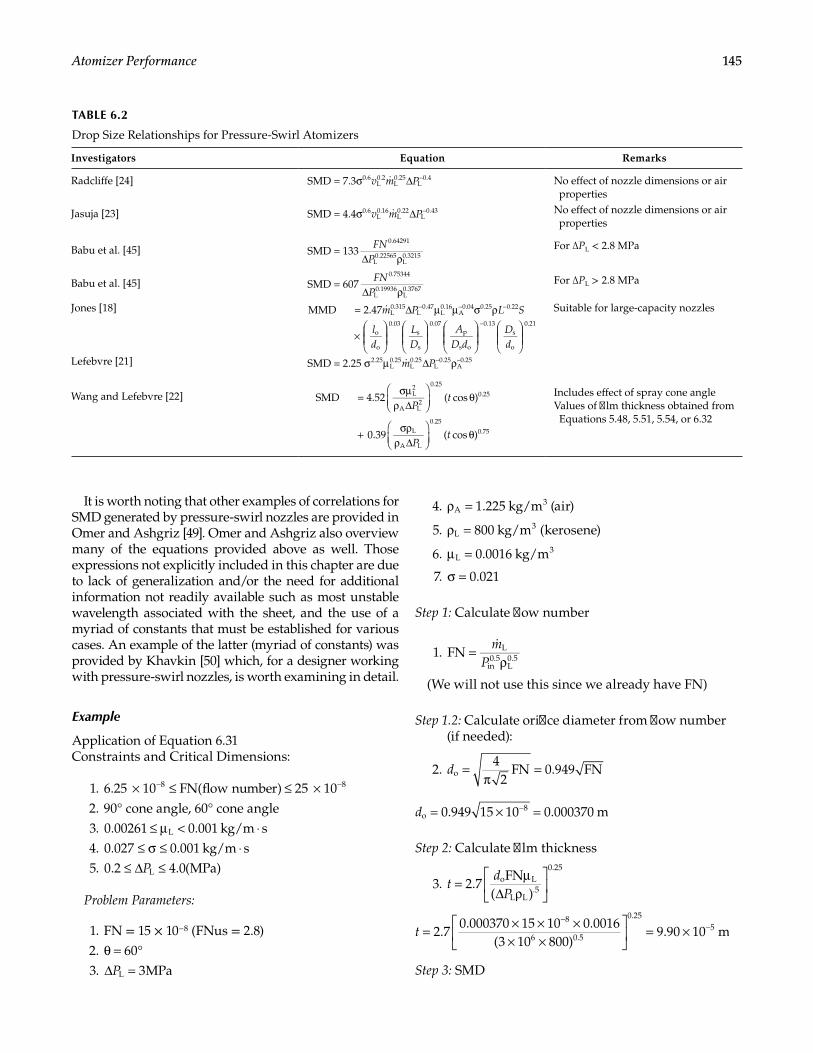
145Atomizer Performance

It is worth noting that other examples of correlations for SMD generated by pressure-swirl nozzles are provided in Omer and Ashgriz [49]. Omer and Ashgriz also overview many of the equations provided above as well. Those expressions not explicitly included in this chapter are due to lack of generalization and/or the need for additional information not readily available such as most unstable wavelength associated with the sheet, and the use of a myriad of constants that must be established for various cases. An example of the latter (myriad of constants) was provided by Khavkin [50] which, for a designer working with pressure-swirl nozzles, is worth examining in detail.

Example

Application of Equation 6.31Constraints and Critical Dimensions:

1. 6.25 10 FN(flow number) 25 108 8× ≤ ≤ ×− −

2. 90° cone angle, 60° cone angle 3. 0.00261 0.001 kg/m sL≤ µ < ⋅ 4. 0.027 0.001 kg/m s≤ σ ≤ ⋅ 5. P0.2 4.0(MPa)L≤ ∆ ≤

Problem Parameters:

1. FN = 15 × 10−8 (FNus = 2.8) 2. 60θ = ° 3. P 3MPaL∆ =

4. 1.225 kg/mA3ρ = (air)

5. 800 kg/mL3ρ = (kerosene)

6. 0.0016 kg/mL3µ =

7. 0.021σ =

Step 1: Calculate flow number

1. FN L

in0.5

L0.5

mP

=ρ

(We will not use this since we already have FN)

Step 1.2: Calculate orifice diameter from flow number (if needed):

2. d4

2FN 0.949 FNo =

π=

d 0.949 15 10 0.000370 mo8= × =−

Step 2: Calculate film thickness

3. td

P2.7

FN( )

o L

L L.5

0.25

= µ∆ ρ

t 2.70.000370 15 10 0.0016

(3 10 800)9.90 10 m

8

6 0.5

0.255= × × ×

× ×

= ×

−−

Step 3: SMD

TABLE 6.2

Drop Size Relationships for Pressure-Swirl Atomizers

Investigators Equation Remarks

Radcliffe [24] v m Pσ ∆ −SMD = 7.3 0.6L0.2

L0.25

L0.4

No effect of nozzle dimensions or air properties

Jasuja [23] v m Pσ ∆ −SMD = 4.4 0.6L0.16

L0.22

L0.43

No effect of nozzle dimensions or air properties

Babu et al. [45] FNP

SMD = 1330.64291

L0.22565

L0.3215∆ ρ

For ∆PL < 2.8 MPa

Babu et al. [45] FNP

SMD = 6070.75344

L0.19936

L0.3767∆ ρ

For ∆PL > 2.8 MPa

Jones [18] m P L S

ld

LD

AD d

Dd

∆ µ µ σ ρ

×

− − −

−

MMD = 2.47 L0.315

L0.47

L0.16

A0.04 0.25 0.22

o

o

0.03s

s

0.07p

s o

0.13s

o

0.21

Suitable for large-capacity nozzles

Lefebvre [21] m PSMD = 2.25 2.25L0.25

L0.25

L0.25

A0.25σ µ ∆ ρ− −

Wang and Lefebvre [22]P

t

Pt

SMD = 4.52 ( cos )

0.39 ( cos )

L2

A L2

0.25

0.25

L

A L

0.25

0.75

σµρ ∆

θ

+ σρρ ∆

θ

Includes effect of spray cone angleValues of film thickness obtained from Equations 5.48, 5.51, 5.54, or 6.32

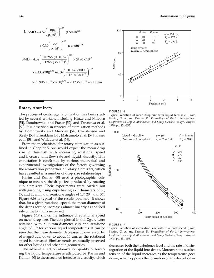
146 Atomization and Sprays

4. P

t

PtL

A L

= σµρ ∆

⋅ θ

+ σρρ ∆

⋅ θ

SMD 4.52 ( cos )

0.39 ( cos )

L2

A L2

0.250.25

0.250.75

= ×× ×

× ×

× + ×× ×

× × = × = µ

−

− −

SMD 4.520.026 (0.0016)

1.126 (3 10 )(9.90 10

COS (30)) 0.390.026 800

1.121 3 10

(9.90 10 cos 30) 2.123 10 21.1 m

6 2

0.255

0.256

0.25

5 0.75 5

Rotary Atomizers

The process of centrifugal atomization has been stud-ied by several workers, including Hinze and Milborn [51], Dombrowski and Fraser [52], and Tanasawa et al. [53]. It is described in reviews of atomization methods by Dombrowski and Munday [54], Christensen and Steely [55], Eisenklam [56], Matsumoto et al. [57], Fraser et al. [58], and Willauer et al. [59].

From the mechanisms for rotary atomization as out-lined in Chapter 5, one would expect the mean drop size to diminish with increasing rotational speed and increase with flow rate and liquid viscosity. This expectation is confirmed by various theoretical and experimental investigations of the factors governing the atomization properties of rotary atomizers, which have resulted in a number of drop size relationships.

Karim and Kumar [60] used a photographic tech-nique to measure the drop sizes produced by rotating cup atomizers. Their experiments were carried out with gasoline, using cups having exit diameters of 16, 19, and 20 mm and semicone angles of 10°, 20°, and 30°. Figure 6.16 is typical of the results obtained. It shows that, for a given rotational speed, the mean diameter of the drops formed increases almost linearly as the feed rate of the liquid is increased.

Figure 6.17 shows the influence of rotational speed on mean drop size. The data plotted in this figure were obtained with a 16-mm-diameter cup and semicone angle of 10° for various liquid temperatures. It can be seen that the mean diameter decreases by over an order of magnitude, down to about 10 µm, as the rotational speed is increased. Similar trends are usually observed for other liquids and other cup geometries.

The adverse effect on atomization quality of lower-ing the liquid temperature is attributed by Karim and Kumar [60] to the associated increase in viscosity, which

decreases both the turbulence level and the rate of disin-tegration of the liquid into drops. Moreover, the surface tension of the liquid increases as the temperature goes down, which opposes the formation of any distortion or

SMD

, μm

Feed rate, cc/s

0

40

80

Liquid = water

D, mmdeg.

102030

16N = 250 rpsTL = 277 kTA = 294 k19

20

θ,

Pressure = Atmospheric

120

0 21 3 4 5

FIGURE 6.16Typical variation of mean drop size with liquid feed rate. (From Karim, G. A. and Kumar, R., Proceedings of the 1st International Conference on Liquid Atomization and Spray Systems, Tokyo, August 1978, pp. 151–155.)

SMD

, μm

Rotary speed of cup, rps

1,000

100

TL, K

Liquid = Gasoline θ = 10ºPressure = Atmospheric Q = 65 cc/min.,

D = 16 mmTA = 278 k

293273263253

010

100 200 300 400

FIGURE 6.17Typical variation of mean drop size with rotational speed. (From Karim, G. A. and Kumar, R., Proceedings of the 1st International Conference on Liquid Atomization and Spray Systems, Tokyo, August 1978, pp. 151–155.)

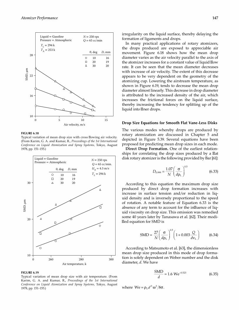
147Atomizer Performance

irregularity on the liquid surface, thereby delaying the formation of ligaments and drops.

In many practical applications of rotary atomizers, the drops produced are exposed to appreciable air movement. Figure 6.18 shows how the mean drop diameter varies as the air velocity parallel to the axis of the atomizer increases for a constant value of liquid flow rate. It can be seen that the mean diameter decreases with increase of air velocity. The extent of this decrease appears to be very dependent on the geometry of the atomizing cup. Lowering the airstream temperature, as shown in Figure 6.19, tends to decrease the mean drop diameter almost linearly. This decrease in drop diameter is attributed to the increased density of the air, which increases the frictional forces on the liquid surface, thereby increasing the tendency for splitting up of the liquid into finer drops.

Drop Size Equations for Smooth Flat Vane-Less Disks

The various modes whereby drops are produced by rotary atomization are discussed in Chapter 5 and depicted in Figure 5.39. Several equations have been proposed for predicting mean drop sizes in each mode.

Direct Drop Formation. One of the earliest relation-ships for correlating the drop sizes produced by a flat disk rotary atomizer is the following provided by Bar [61]:

DN d

1.070.999

L

0.5

= σρ

(6.33)

According to this equation the maximum drop size produced by direct drop formation increases with increase in surface tension and/or reduction in liq-uid density and is inversely proportional to the speed of rotation. A notable feature of Equation 6.33 is the absence of any term to account for the influence of liq-uid viscosity on drop size. This omission was remedied some 40 years later by Tanasawa et al. [62]. Their modi-fied equation for SMD is

N d

Qd

σρ

+ν

SMD =27

1 0.003L

0.5

L (6.34)

According to Matsumoto et al. [63], the dimensionless mean drop size produced in this mode of drop forma-tion is solely dependent on Weber number and the disk diameter, d. We have

d

SMD1.6 We 0.523= − (6.35)

where dρ ω σWe = 8 .L3 2

SMD

, μm

Air velocity, m/s

28

22

16

102030

161920

100 5 10 15

θ, deg D, mm

Liquid = GasolinePressure = Atmospheric Q = 65 cc/min

N = 250 rps

TL = 294 kTA = 253 k

FIGURE 6.18Typical variation of mean drop size with cross flowing air velocity. (From Karim, G. A. and Kumar, R., Proceedings of the 1st International Conference on Liquid Atomization and Spray Systems, Tokyo, August 1978, pp. 151–155.)

SMD

, μm

Air temperature, k

102030

161920

260010

20

30

280 300

θ, deg D, mm

Liquid = GasolinePressure = Atmospheric Q = 65 cc/min.

N = 250 rps

TL = 294 k

UA = 4.3 m/s

FIGURE 6.19Typical variation of mean drop size with air temperature. (From Karim, G. A. and Kumar, R., Proceedings of the 1st International Conference on Liquid Atomization and Spray Systems, Tokyo, August 1978, pp. 151–155.)

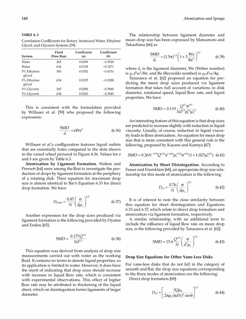
148 Atomization and Sprays

This is consistent with the formulation provided by Willauer et al. [59] who proposed the following expression:

d

a bSMDWe= (6.36)

Willauer et al.’s configuration features liquid outlets that are essentially holes compared to the slots shown in the vaned wheel pictured in Figure 4.36. Values for a and b are given by Table 6.3.

Atomization by Ligament Formation. Walton and Prewett [64] were among the first to investigate the pro-duction of drops by ligament formation at the periphery of a rotating disk. Their equation for maximum drop size is almost identical to Bar’s Equation 6.33 for direct drop formation. We have

DN d

0.870.999

L

0.5

= σρ

(6.37)

Another expression for the drop sizes produced via ligament formation is the following provided by Oyama and Endou [65]:

Q

NdSMD =

0.177 0.2

0.3 (6.38)

This equation was derived from analysis of drop size measurements carried out with water as the working fluid. It contains no terms to denote liquid properties, so its application is limited to water. However, it does have the merit of indicating that drop sizes should increase with increase in liquid flow rate, which is consistent with experimental observations. This effect of higher flow rate may be attributed to thickening of the liquid sheet, which on disintegration forms ligaments of larger diameter.

The relationship between ligament diameter and mean drop size has been expressed by Matsumoto and Takashima [66] as

d

SMD(1.5 ) 1 3

WeRe1

1 32

1 6

= π +

(6.39)

where d1 is the ligament diameter, We (Weber number) is  ρ Ld3 ω 2/8 σ , and Re (Reynolds number) is  ρ Ld2 ω /4µ.

Tanasawa et al. [62] proposed an equation for pre-dicting the mean drop sizes produced via ligament formation that takes full account of variations in disk diameter, rotational speed, liquid flow rate, and liquid properties. We have

Q

NdSMD = 0.119

0.1 0.5

0.5L0.4

L0.1

σρ µ

(6.40)

An interesting feature of this equation is that drop sizes are predicted to increase slightly with reduction in liquid viscosity. Usually, of course, reduction in liquid viscos-ity leads to finer atomization. An equation for mean drop size that is more consistent with this general rule is the following, proposed by Kayano and Kamiya [67]:

N Q dSMD = 0.26 (1 1.027 )0.79 0.32 0.69L

0.29 0.26L0.65ρ σ + µ− − − (6.41)

Atomization by Sheet Disintegration. According to Fraser and Eisenklam [68], an appropriate drop size rela-tionship for this mode of atomization is the following:

DN d

0.7610

L

0.5

= σρ

(6.42)

It is of interest to note the close similarity between this equation for sheet disintegration and Equations 6.33 and 6.37, which relate to direct drop formation and atomization via ligament formation, respectively.

A similar relationship, with an additional term to include the influence of liquid flow rate on mean drop size, is the following provided by Tanasawa et al. [62]:

QN d

SMD = 15.60.5

2L

0.4σρ

(6.43)

Drop Size Equations for Other Vane-Less Disks

For vane-less disks that do not fall in the category of smooth and flat, the drop size equations corresponding to the three modes of atomization are the following:

Direct drop formation [69]:

DQdN

32 ( ) sin10

L

L2

1 3

= µπρ π θ

(6.44)

TABLE 6.3

Correlation Coefficients for Rotary Atomized Water, Ethylene Glycol, and Glycerin Systems [59]

SystemFluid

Flow RateCoefficient

(a)Coefficient

(b)

Water 365 0.0299 −0.3920Water 634 0.0138 −0.32715% Ethylene glycol

365 0.0352 −0.4151

5% Ethylene glycol

634 0.0125 −0.3288

5% Glycerin 365 0.0296 −0.39605% Glycerin 634 0.0243 −0.3845

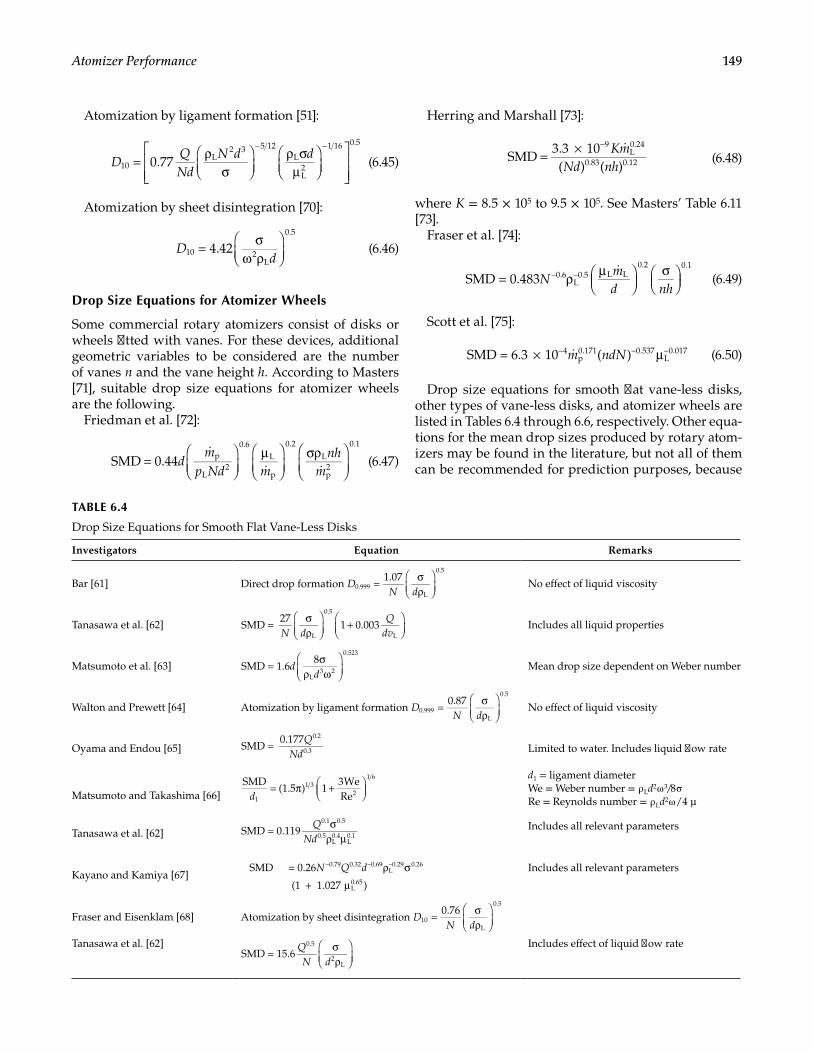
149Atomizer Performance

Atomization by ligament formation [51]:

DQNd

N d d0.7710

L2 3 5 12

L

L2

1 16 0.5

= ρσ

ρ σµ

− −

(6.45)

Atomization by sheet disintegration [70]:

Dd

4.4210 2L

0.5

= σω ρ

(6.46)

Drop Size Equations for Atomizer Wheels

Some commercial rotary atomizers consist of disks or wheels fitted with vanes. For these devices, additional geometric variables to be considered are the number of vanes n and the vane height h. According to Masters [71], suitable drop size equations for atomizer wheels are the following.

Friedman et al. [72]:

dm

p Nd mnh

m=

µ

σρ

SMD 0.44 p

L2

0.6L

p

0.2

L

p2

0.1

(6.47)

Herring and Marshall [73]:

Km

Nd nh= × −

SMD3.3 10( ) ( )

9L0.24

0.83 0.12

(6.48)

where K = 8.5 × 105 to 9.5 × 105. See Masters’ Table 6.11 [73].

Fraser et al. [74]:

Nmd nh

ρ µ

σ

− −SMD = 0.483 0.6L

0.5 L L0.2 0.1

(6.49)

Scott et al. [75]:

m ndN× µ− − −SMD = 6.3 10 ( )4p0.171 0.537

L0.017

(6.50)

Drop size equations for smooth flat vane-less disks, other types of vane-less disks, and atomizer wheels are listed in Tables 6.4 through 6.6, respectively. Other equa-tions for the mean drop sizes produced by rotary atom-izers may be found in the literature, but not all of them can be recommended for prediction purposes, because

TABLE 6.4

Drop Size Equations for Smooth Flat Vane-Less Disks

Investigators Equation Remarks

Bar [61] Direct drop formation DN d

1.070.999

L

0.5

= σρ

No effect of liquid viscosity

Tanasawa et al. [62]N d

Qdv

SMD =27

1 0.003L

0.5

L

σρ

+

Includes all liquid properties

Matsumoto et al. [63] dd

SMD = 1.68

L3 2

0.523σ

ρ ω

Mean drop size dependent on Weber number

Walton and Prewett [64] Atomization by ligament formation DN d

0.870.999

L

0.5

= σρ

No effect of liquid viscosity

Oyama and Endou [65]Q

NdSMD =

0.177 0.2

0.3 Limited to water. Includes liquid flow rate

Matsumoto and Takashima [66] dSMD

(1.5 ) 13WeRe1

1 32

1 6

= π +

d1 = ligament diameterWe = Weber number =  ρ Ld2 ω 3/8 σ Re = Reynolds number =  ρ Ld2 ω /4 µ

Tanasawa et al. [62]Q

NdSMD = 0.119

0.1 0.5

0.5L0.4

L0.1

σρ µ

Includes all relevant parameters

Kayano and Kamiya [67]N Q dSMD 0.26

(1 1.027 )

0.79 0.32 0.69L

0.29 0.26

L0.65

= ρ σ

+ µ

− − − Includes all relevant parameters

Fraser and Eisenklam [68] Atomization by sheet disintegration DN d

0.7610

L

0.5

= σρ

Tanasawa et al. [62] QN d

SMD = 15.60.5

2L

σρ

Includes effect of liquid flow rate

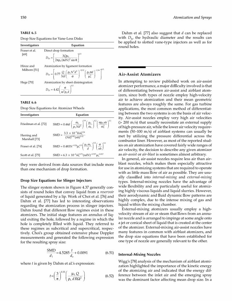
150 Atomization and Sprays

they were derived from data sources that include more than one mechanism of drop formation.

Drop Size Equations for Slinger Injectors

The slinger system shown in Figure 4.37 generally con-sists of round holes that convey liquid from a reservoir of liquid generated by a lip. Work of Choi et al. [76] and Dahm et al. [77] has led to interesting observations regarding the atomization process in slinger injectors. Dahm found that different flow regimes exist in these atomizers. The initial stage features an annulus of liq-uid exiting the hole, followed by a regime in which the hole is completely filled with liquid. They referred to these regimes as subcritical and supercritical, respec-tively. Choi’s group obtained extensive phase Doppler measurements and generated the following expression for the resulting spray size:

d

td

SMD4.5285 0.0091

l o= + (6.51)

where t is given by Dahm et al.’s expression:

tQ

dR3 0.33

L

L2=

π

µρ Ω

(6.52)

Dahm et al. [77] also suggest that d can be replaced with Dh, the hydraulic diameter and the results can be applied to slotted vane-type injectors as well as for round holes.

Air-Assist Atomizers

In attempting to review published work on air-assist atomizer performance, a major difficulty involved is that of differentiating between air-assist and airblast atom-izers, since both types of nozzle employ high-velocity air to achieve atomization and their mean geometric features are always roughly the same. For gas turbine applications, the most common method of differentiat-ing between the two systems is on the basis of air veloc-ity. Air-assist nozzles employ very high air velocities (> 200 m/s) that usually necessitate an external supply of high-pressure air, while the lower air velocity require-ments (50–100 m/s) of airblast systems can usually be met by utilizing the pressure differential across the combustor liner. However, as most of the reported stud-ies on air atomization have covered fairly wide ranges of air velocity, the decision to describe any given atomizer as air-assist or air-blast is sometimes almost arbitrary.

In general, air-assist nozzles require less air than air-blast nozzles, which makes them especially attractive for use in atomizing systems that are required to operate with as little mass flow of air as possible. They are usu-ally classified into internal-mixing and external-mixing types. Internal-mixing nozzles have the advantage of wide flexibility and are particularly useful for atomiz-ing highly viscous liquids and liquid slurries. However, their aerodynamic and fluid dynamic flow patterns are highly complex, due to the intense mixing of gas and liquid within the mixing chamber.

External-mixing atomizers usually employ a high-velocity stream of air or steam that flows from an annu-lar nozzle and is arranged to impinge at some angle onto a jet or conical sheet of liquid that is created at the center of the atomizer. External-mixing air-assist nozzles have many features in common with airblast atomizers, and the drop size equations that have been established for one type of nozzle are generally relevant to the other.

Internal-Mixing Nozzles

Wigg’s [78] analysis of the mechanism of airblast atomi-zation highlighted the importance of the kinetic energy of the atomizing air and indicated that the energy dif-ference between the inlet air and the emerging spray was the dominant factor affecting mean drop size. In a

TABLE 6.6

Drop Size Equations for Atomizer Wheels

Investigators Equation

Friedman et al. [72] dmNd m

nhmρ

µ

σρ

SMD = 0.44 L

L2

0.6L

L

0.2L

L2

0.1

Herring and Marshall [73]

KmNd nh

× −

SMD =3.3 10( ) ( )

9L0.24

0.83 0.12

Fraser et al. [74] Nmd nh

ρ µ

σ

− −SMD = 0.483 0.26L

0.5 L L0.2 0.1

Scott et al. [75] m ndN× µ− − −SMD = 6.3 10 ( )4L0.171 0.537

L0.017

TABLE 6.5

Drop Size Equations for Vane-Less Disks

Investigators Equation

Fraser et al. [69]

Direct drop formation

DQdN

32 ( ) sin

10L

L2

1 3

= µπρ π θ

Hinze and Milborn [51]

Atomization by ligament formation

DQNd

N d d0.7710

L2 3 5 12

L

L2

1 16 0.5

= ρσ

ρ σµ

− −

Hege [70] Atomization by sheet disintegration

Dd

4.4210 2L

0.5

= σω ρ

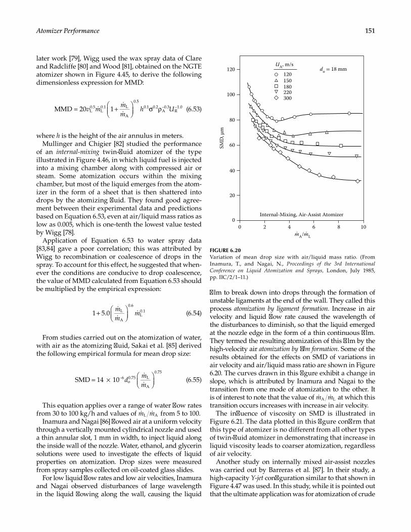
151Atomizer Performance

later work [79], Wigg used the wax spray data of Clare and Radcliffe [80] and Wood [81], obtained on the NGTE atomizer shown in Figure 4.45, to derive the following dimensionless expression for MMD:

v mmm

h U+

σ ρ− −MMD = 20 1L0.5

L0.1 L

A

0.50.1 0.2

A0.3

R1.0

(6.53)

where h is the height of the air annulus in meters.Mullinger and Chigier [82] studied the performance

of an internal-mixing twin-fluid atomizer of the type illustrated in Figure 4.46, in which liquid fuel is injected into a mixing chamber along with compressed air or steam. Some atomization occurs within the mixing chamber, but most of the liquid emerges from the atom-izer in the form of a sheet that is then shattered into drops by the atomizing fluid. They found good agree-ment between their experimental data and predictions based on Equation 6.53, even at air/liquid mass ratios as low as 0.005, which is one-tenth the lowest value tested by Wigg [78].

Application of Equation 6.53 to water spray data [83,84] gave a poor correlation; this was attributed by Wigg to recombination or coalescence of drops in the spray. To account for this effect, he suggested that when-ever the conditions are conducive to drop coalescence, the value of MMD calculated from Equation 6.53 should be multiplied by the empirical expression:

mm

m+

1 5.0 L

A

0.6

L0.1

(6.54)

From studies carried out on the atomization of water, with air as the atomizing fluid, Sakai et al. [85] derived the following empirical formula for mean drop size:

dmm

= ×

−SMD 14 10 6o0.75 L

A

0.75

(6.55)

This equation applies over a range of water flow rates from 30 to 100 kg/h and values of m m L A from 5 to 100.

Inamura and Nagai [86] flowed air at a uniform velocity through a vertically mounted cylindrical nozzle and used a thin annular slot, 1 mm in width, to inject liquid along the inside wall of the nozzle. Water, ethanol, and glycerin solutions were used to investigate the effects of liquid properties on atomization. Drop sizes were measured from spray samples collected on oil-coated glass slides.

For low liquid flow rates and low air velocities, Inamura and Nagai observed disturbances of large wavelength in the liquid flowing along the wall, causing the liquid

film to break down into drops through the formation of unstable ligaments at the end of the wall. They called this process atomization by ligament formation. Increase in air velocity and liquid flow rate caused the wavelength of the disturbances to diminish, so that the liquid emerged at the nozzle edge in the form of a thin continuous film. They termed the resulting atomization of this film by the high-velocity air atomization by film formation. Some of the results obtained for the effects on SMD of variations in air velocity and air/liquid mass ratio are shown in Figure 6.20. The curves drawn in this figure exhibit a change in slope, which is attributed by Inamura and Nagai to the transition from one mode of atomization to the other. It is of interest to note that the value of m m A L at which this transition occurs increases with increase in air velocity.

The influence of viscosity on SMD is illustrated in Figure 6.21. The data plotted in this figure confirm that this type of atomizer is no different from all other types of twin-fluid atomizer in demonstrating that increase in liquid viscosity leads to coarser atomization, regardless of air velocity.

Another study on internally mixed air-assist nozzles was carried out by Barreras et al. [87]. In their study, a high-capacity Y-jet configuration similar to that shown in Figure 4.47 was used. In this study, while it is pointed out that the ultimate application was for atomization of crude

SMD

, μm

Internal-Mixing, Air-Assist Atomizer

120150180220300

00

20

2

40

60

80

100

120

4. .

6 8 10mA/mL

UA, m/sdo = 18 mm

FIGURE 6.20Variation of mean drop size with air/liquid mass ratio. (From Inamura, T., and Nagai, N., Proceedings of the 3rd International Conference on Liquid Atomization and Sprays, London, July 1985, pp. IIC/2/1–11.)

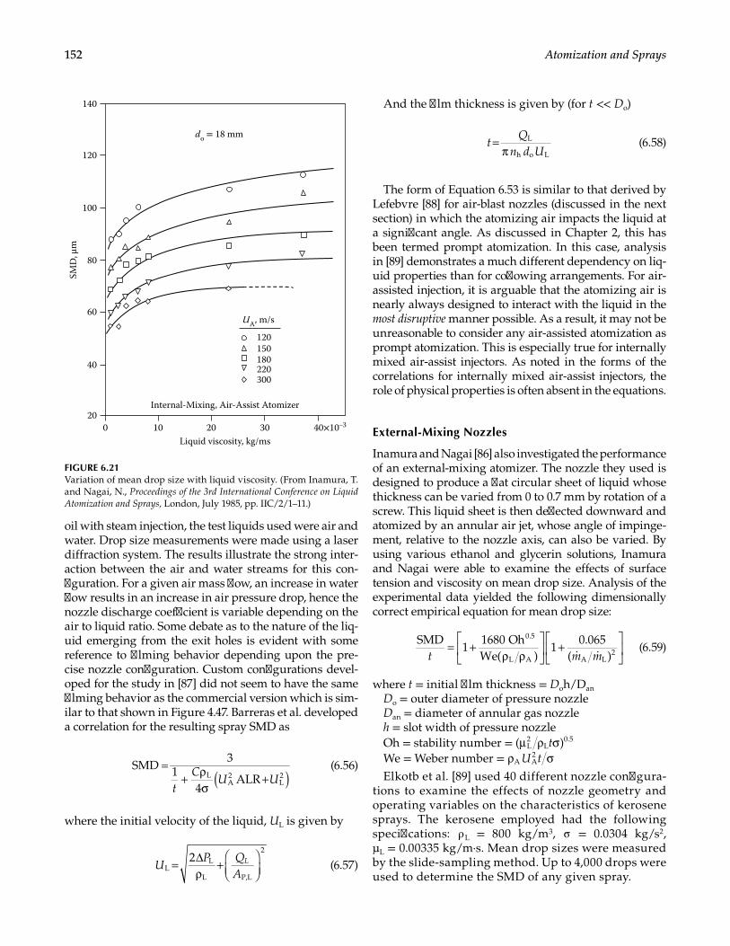
152 Atomization and Sprays

oil with steam injection, the test liquids used were air and water. Drop size measurements were made using a laser diffraction system. The results illustrate the strong inter-action between the air and water streams for this con-figuration. For a given air mass flow, an increase in water flow results in an increase in air pressure drop, hence the nozzle discharge coefficient is variable depending on the air to liquid ratio. Some debate as to the nature of the liq-uid emerging from the exit holes is evident with some reference to filming behavior depending upon the pre-cise nozzle configuration. Custom configurations devel-oped for the study in [87] did not seem to have the same filming behavior as the commercial version which is sim-ilar to that shown in Figure 4.47. Barreras et al. developed a correlation for the resulting spray SMD as

tC

U U( )=

+ ρσ

+SMD

31

4ALRL

A2

L2

(6.56)

where the initial velocity of the liquid, UL is given by

UP Q

AL2

LL

L P,L

2

= ∆ρ

+

(6.57)

And the film thickness is given by (for t << Do)

tQ

n d UL

h o L=

π (6.58)

The form of Equation 6.53 is similar to that derived by Lefebvre [88] for air-blast nozzles (discussed in the next section) in which the atomizing air impacts the liquid at a significant angle. As discussed in Chapter 2, this has been termed prompt atomization. In this case, analysis in [89] demonstrates a much different dependency on liq-uid properties than for coflowing arrangements. For air-assisted injection, it is arguable that the atomizing air is nearly always designed to interact with the liquid in the most disruptive manner possible. As a result, it may not be unreasonable to consider any air-assisted atomization as prompt atomization. This is especially true for internally mixed air-assist injectors. As noted in the forms of the correlations for internally mixed air-assist injectors, the role of physical properties is often absent in the equations.

External-Mixing Nozzles

Inamura and Nagai [86] also investigated the performance of an external-mixing atomizer. The nozzle they used is designed to produce a flat circular sheet of liquid whose thickness can be varied from 0 to 0.7 mm by rotation of a screw. This liquid sheet is then deflected downward and atomized by an annular air jet, whose angle of impinge-ment, relative to the nozzle axis, can also be varied. By using various ethanol and glycerin solutions, Inamura and Nagai were able to examine the effects of surface tension and viscosity on mean drop size. Analysis of the experimental data yielded the following dimensionally correct empirical equation for mean drop size:

t m m

= +ρ ρ

+

SMD1

1680 OhWe( )

10.065

( )

0.5

L A A L2

(6.59)

where t = initial film thickness = Doh/Dan

Do = outer diameter of pressure nozzleDan = diameter of annular gas nozzleh = slot width of pressure nozzleOh = stability number = t( )L

2L

0.5µ ρ σWe = Weber number = U tA A

2ρ σElkotb et al. [89] used 40 different nozzle configura-

tions to examine the effects of nozzle geometry and operating variables on the characteristics of kerosene sprays. The kerosene employed had the following specifications:  ρ L = 800 kg/m3,  σ  = 0.0304 kg/s2, µL = 0.00335 kg/m·s. Mean drop sizes were measured by the slide-sampling method. Up to 4,000 drops were used to determine the SMD of any given spray.

SMD

, μm

Internal-Mixing, Air-Assist Atomizer

120150180220300

020

10 20 30 40×10–3

40

60

80

100

120

140

Liquid viscosity, kg/ms

UA, m/s

do = 18 mm

FIGURE 6.21Variation of mean drop size with liquid viscosity. (From Inamura, T. and Nagai, N., Proceedings of the 3rd International Conference on Liquid Atomization and Sprays, London, July 1985, pp. IIC/2/1–11.)

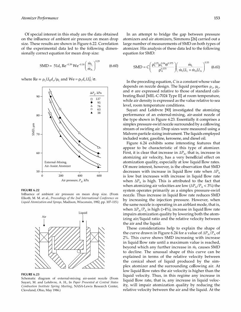
153Atomizer Performance

Of special interest in this study are the data obtained on the influence of ambient air pressure on mean drop size. These results are shown in Figure 6.22. Correlation of the experimental data led to the following dimen-sionally correct equation for mean drop size:

dmm

=

− −SMD 51 Re Weo0.39 0.18 L

A

0.29

(6.60)

where Re =  ρ LURdo/µL and d UWe .L o R2= ρ σ

In an attempt to bridge the gap between pressure atomizers and air atomizers, Simmons [26] carried out a large number of measurements of SMD on both types of atomizer. His analysis of these data led to the following equation for SMD:

Cm

m U m Uρ µ σ

ρ

+

SMD = L0.25

L0.06 0.375

A0.375

L

L L A A

0.55

(6.61)

In the preceding equation, C is a constant whose value depends on nozzle design. The liquid properties  ρ L, µL, and  σ  are expressed relative to those of standard cali-brating fluid [MIL-C-7024 Type II] at room temperature, while air density is expressed as the value relative to sea level, room temperature conditions.

Suyari and Lefebvre [90] investigated the atomizing performance of an external-mixing, air-assist nozzle of the type shown in Figure 6.23. Essentially it comprises a simplex pressure-swirl nozzle surrounded by a coflowing stream of swirling air. Drop sizes were measured using a Malvern particle sizing instrument. The liquids employed included water, gasoline, kerosene, and diesel oil.

Figure 6.24 exhibits some interesting features that appear to be characteristic of this type of atomizer. First, it is clear that increase in ∆PA, that is, increase in atomizing air velocity, has a very beneficial effect on atomization quality, especially at low liquid flow rates. Of more interest, however, is the observation that SMD decreases with increase in liquid flow rate when ∆PA is low but increases with increase in liquid flow rate when ∆PA is high. This is attributed to the fact that when atomizing air velocities are low (∆PA/PA < 3%) the system operates primarily as a simplex pressure-swirl nozzle. Thus increase in liquid flow rate reduces SMD by increasing the injection pressure. However, when the same nozzle is operating in an airblast mode, that is, when ∆PA/PA is high (>4%), increase in liquid flow rate impairs atomization quality by lowering both the atom-izing air/liquid ratio and the relative velocity between the air and the liquid.

These considerations help to explain the shape of the curve drawn in Figure 6.24 for a value of ∆PA/PA of 2%. This curve shows SMD increasing with increase in liquid flow rate until a maximum value is reached, beyond which any further increase in m L causes SMD to decline. The unusual shape of this curve can be explained in terms of the relative velocity between the conical sheet of liquid produced by the sim-plex atomizer and the surrounding coflowing air. At low liquid flow rates the air velocity is higher than the liquid velocity. Thus, in this regime any increase in liquid flow rate, that is, any increase in liquid veloc-ity, will impair atomization quality by reducing the relative velocity between the air and the liquid. At the

SMD

, μm

External-Mixing,Air-Assist Atomizer

12795766338

050

200 400 600

60

70

80

90

Air pressure, PA, kPa

ΔPL, kPa

FIGURE 6.22Influence of ambient air pressure on mean drop size. (From Elkotb, M. M. et al., Proceedings of the 2nd International Conference on Liquid Atomization and Sprays, Madison, Wisconsin, 1982, pp. 107–115.)

AirLiquid

FIGURE 6.23Schematic diagram of external-mixing air-assist nozzle (From Suyari, M. and Lefebvre, A. H., In Paper Presented at Central States Combustion Institute Spring Meeting, NASA-Lewis Research Center, Cleveland, Ohio, May 1986.)

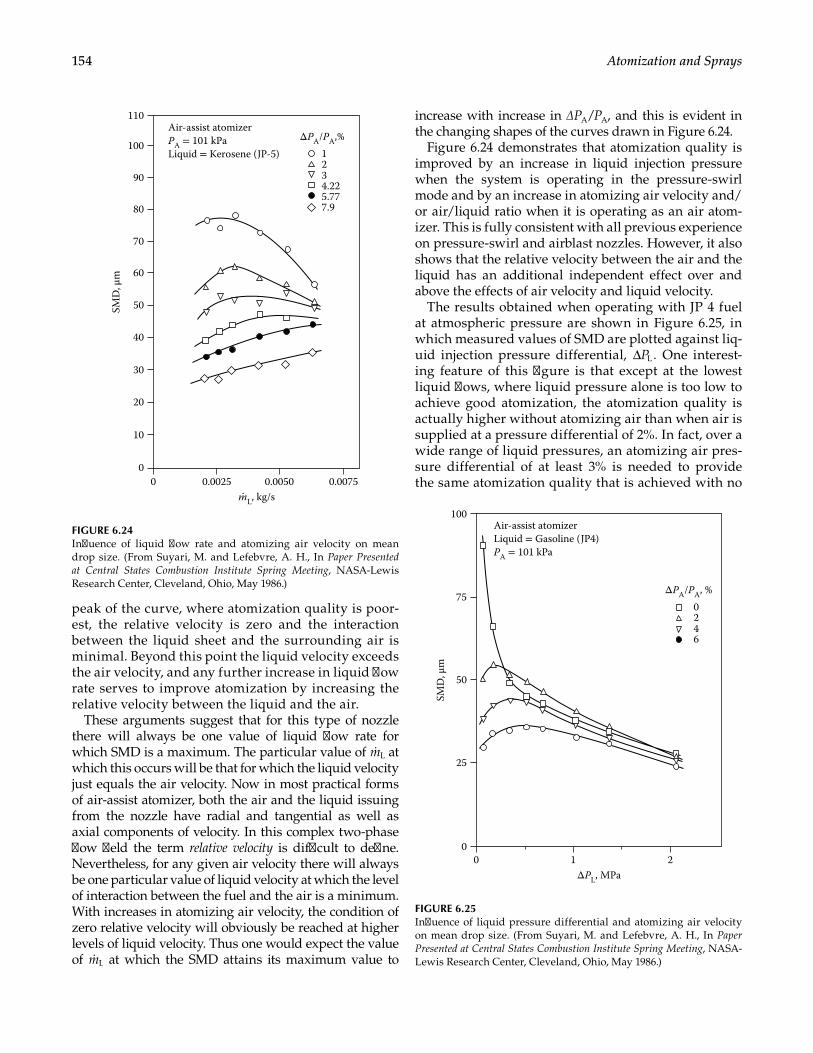
154 Atomization and Sprays

peak of the curve, where atomization quality is poor-est, the relative velocity is zero and the interaction between the liquid sheet and the surrounding air is minimal. Beyond this point the liquid velocity exceeds the air velocity, and any further increase in liquid flow rate serves to improve atomization by increasing the relative velocity between the liquid and the air.

These arguments suggest that for this type of nozzle there will always be one value of liquid flow rate for which SMD is a maximum. The particular value of m L at which this occurs will be that for which the liquid velocity just equals the air velocity. Now in most practical forms of air-assist atomizer, both the air and the liquid issuing from the nozzle have radial and tangential as well as axial components of velocity. In this complex two-phase flow field the term relative velocity is difficult to define. Nevertheless, for any given air velocity there will always be one particular value of liquid velocity at which the level of interaction between the fuel and the air is a minimum. With increases in atomizing air velocity, the condition of zero relative velocity will obviously be reached at higher levels of liquid velocity. Thus one would expect the value of m L at which the SMD attains its maximum value to

increase with increase in ∆PA/PA, and this is evident in the changing shapes of the curves drawn in Figure 6.24.

Figure 6.24 demonstrates that atomization quality is improved by an increase in liquid injection pressure when the system is operating in the pressure-swirl mode and by an increase in atomizing air velocity and/or air/liquid ratio when it is operating as an air atom-izer. This is fully consistent with all previous experience on pressure-swirl and airblast nozzles. However, it also shows that the relative velocity between the air and the liquid has an additional independent effect over and above the effects of air velocity and liquid velocity.

The results obtained when operating with JP 4 fuel at atmospheric pressure are shown in Figure 6.25, in which measured values of SMD are plotted against liq-uid injection pressure differential, P .L∆ One interest-ing feature of this figure is that except at the lowest liquid flows, where liquid pressure alone is too low to achieve good atomization, the atomization quality is actually higher without atomizing air than when air is supplied at a pressure differential of 2%. In fact, over a wide range of liquid pressures, an atomizing air pres-sure differential of at least 3% is needed to provide the same atomization quality that is achieved with no

SMD

, μm

Air-assist atomizerLiquid = Gasoline (JP4)PA = 101 kPa

100

2

0246

ΔPL, MPa

ΔPA/PA, %

25

50

75

100

FIGURE 6.25Influence of liquid pressure differential and atomizing air velocity on mean drop size. (From Suyari, M. and Lefebvre, A. H., In Paper Presented at Central States Combustion Institute Spring Meeting, NASA-Lewis Research Center, Cleveland, Ohio, May 1986.)

SMD

, μm

Air-assist atomizerPA = 101 kPaLiquid = Kerosene (JP-5)

0.0025.

00

0.0050 0.0075

10

20

30

40

50

60

70

80

90

1234.225.777.9

100

110

mL, kg/s

ΔPA/PA,%

FIGURE 6.24Influence of liquid flow rate and atomizing air velocity on mean drop size. (From Suyari, M. and Lefebvre, A. H., In Paper Presented at Central States Combustion Institute Spring Meeting, NASA-Lewis Research Center, Cleveland, Ohio, May 1986.)

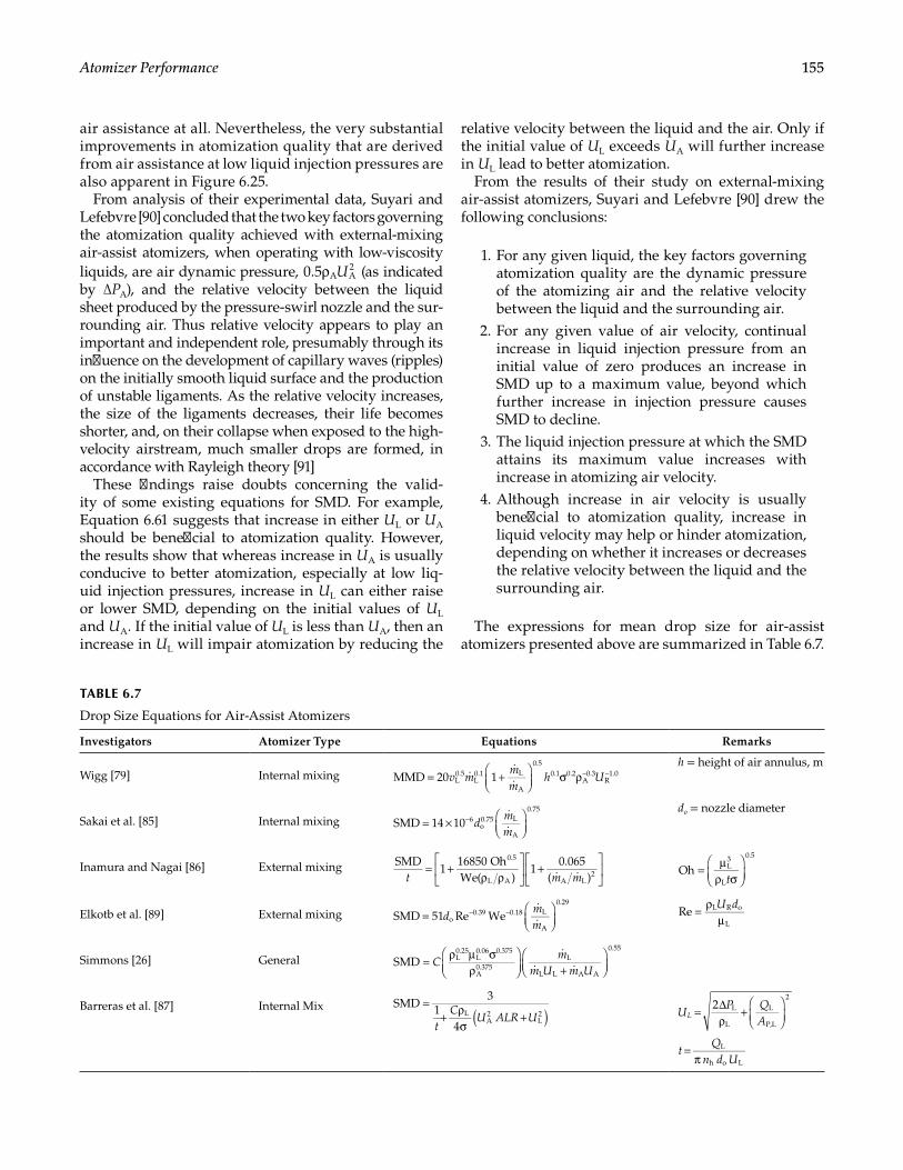
155Atomizer Performance

air assistance at all. Nevertheless, the very substantial improvements in atomization quality that are derived from air assistance at low liquid injection pressures are also apparent in Figure 6.25.

From analysis of their experimental data, Suyari and Lefebvre [90] concluded that the two key factors governing the atomization quality achieved with external-mixing air-assist atomizers, when operating with low-viscosity liquids, are air dynamic pressure, U0.5 A A

2ρ (as indicated by ∆PA), and the relative velocity between the liquid sheet produced by the pressure-swirl nozzle and the sur-rounding air. Thus relative velocity appears to play an important and independent role, presumably through its influence on the development of capillary waves (ripples) on the initially smooth liquid surface and the production of unstable ligaments. As the relative velocity increases, the size of the ligaments decreases, their life becomes shorter, and, on their collapse when exposed to the high-velocity airstream, much smaller drops are formed, in accordance with Rayleigh theory [91]

These findings raise doubts concerning the valid-ity of some existing equations for SMD. For example, Equation 6.61 suggests that increase in either UL or UA should be beneficial to atomization quality. However, the results show that whereas increase in UA is usually conducive to better atomization, especially at low liq-uid injection pressures, increase in UL can either raise or lower SMD, depending on the initial values of UL and UA. If the initial value of UL is less than UA, then an increase in UL will impair atomization by reducing the

relative velocity between the liquid and the air. Only if the initial value of UL exceeds UA will further increase in UL lead to better atomization.

From the results of their study on external-mixing air-assist atomizers, Suyari and Lefebvre [90] drew the following conclusions:

1. For any given liquid, the key factors governing atomization quality are the dynamic pressure of the atomizing air and the relative velocity between the liquid and the surrounding air.

2. For any given value of air velocity, continual increase in liquid injection pressure from an initial value of zero produces an increase in SMD up to a maximum value, beyond which further increase in injection pressure causes SMD to decline.

3. The liquid injection pressure at which the SMD attains its maximum value increases with increase in atomizing air velocity.

4. Although increase in air velocity is usually beneficial to atomization quality, increase in liquid velocity may help or hinder atomization, depending on whether it increases or decreases the relative velocity between the liquid and the surrounding air.

The expressions for mean drop size for air-assist atomizers presented above are summarized in Table 6.7.

TABLE 6.7

Drop Size Equations for Air-Assist Atomizers

Investigators Atomizer Type Equations Remarks

Wigg [79] Internal mixing v mmm

h U= +

σ ρ− −MMD 20 1L0.5

L0.1 L

A

0.50.1 0.2

A0.3

R1.0

h = height of air annulus, m

Sakai et al. [85] Internal mixing dmm

= ×

−SMD 14 10 6o0.75 L

A

0.75

do = nozzle diameter

Inamura and Nagai [86] External mixingt m m

= +ρ ρ

+

SMD1

16850 OhWe( )

10.065

( )

0.5

L A A L2

tOh L

3

L

0.5

= µρ σ

Elkotb et al. [89] External mixing dmm

=

− −SMD 51 Re Weo0.39 0.18 L

A

0.29

U dRe L R o

L= ρ

µ

Simmons [26] General Cm

m U m Uρ µ σ

ρ

+

SMD = L0.25

L0.06 0.375

A0.375

L

L L A A

0.55

Barreras et al. [87] Internal Mix

tC

U ALR USMD

31

4L

A2

L2( )

=+ ρ

σ+ U

P QA

L2 L

L

L

P,L

2

= ∆ρ

+

tQ

n d UL

h o L=

π

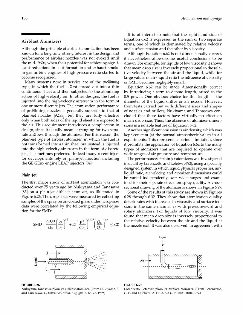
156 Atomization and Sprays

Airblast Atomizers

Although the principle of airblast atomization has been known for a long time, strong interest in the design and performance of airblast nozzles was not evoked until the mid-1960s, when their potential for achieving signif-icant reductions in soot formation and exhaust smoke in gas turbine engines of high pressure ratio started to become recognized.

Many systems now in service are of the prefilming type, in which the fuel is first spread out into a thin continuous sheet and then subjected to the atomizing action of high-velocity air. In other designs, the fuel is injected into the high-velocity airstream in the form of one or more discrete jets. The atomization performance of prefilming nozzles is generally superior to that of plain-jet nozzles [92,93], but they are fully effective only when both sides of the liquid sheet are exposed to the air. This requirement introduces a complication in design, since it usually means arranging for two sepa-rate airflows through the atomizer. For this reason, the plain-jet type of airblast atomizer, in which the fuel is not transformed into a thin sheet but instead is injected into the high-velocity airstream in the form of discrete jets, is sometimes preferred. Indeed many recent injec-tor developments rely on plain-jet injection including the GE GEnx engine LEAP injectors [94].

Plain Jet

The first major study of airblast atomization was con-ducted over 75 years ago by Nukiyama and Tanasawa [83] on a plain-jet airblast atomizer, as illustrated in Figure 6.26. The drop sizes were measured by collecting samples of the spray on oil-coated glass slides. Drop size data were correlated by the following empirical equa-tion for the SMD:

U

QQ

SMD0.585

53R L

0.5L2

L

0.225L

A

1.5

= σρ

+ µσρ

(6.62)

It is of interest to note that the right-hand side of Equation 6.62 is expressed as the sum of two separate terms, one of which is dominated by relative velocity and surface tension and the other by viscosity.

Although Equation 6.62 is not dimensionally correct, it nevertheless allows some useful conclusions to be drawn. For example, for liquids of low viscosity it shows that mean drop size is inversely proportional to the rela-tive velocity between the air and the liquid, while for large values of air/liquid ratio the influence of viscosity on SMD becomes negligibly small.

Equation 6.62 can be made dimensionally correct by introducing a term to denote length, raised to the 0.5 power. One obvious choice for this length is the diameter of the liquid orifice or air nozzle. However, from tests carried out with different sizes and shapes of nozzles and orifices, Nukiyama and Tanasawa con-cluded that these factors have virtually no effect on mean drop size. Thus, the absence of atomizer dimen-sions is a notable feature of Equation 6.62.

Another significant omission is air density, which was kept constant (at the normal atmospheric value) in all experiments. This represents a serious limitation, since it prohibits the application of Equation 6.62 to the many types of atomizers that are required to operate over wide ranges of air pressure and temperature.

The performance of plain-jet atomizers was investigated in detail by Lorenzetto and Lefebvre [92], using a specially designed system in which liquid physical properties, air/liquid ratio, air velocity, and atomizer dimensions could be varied independently over wide ranges and exam-ined for their separate effects on spray quality. A cross-sectional drawing of the atomizer is shown in Figure 6.27.

Some of the results of this study are shown in Figures 6.28 through 6.32. They show that atomization quality deteriorates with increases in viscosity and surface ten-sion, in the same manner as with pressure-swirl and rotary atomizers. For liquids of low viscosity, it was found that mean drop size is inversely proportional to the relative velocity between the air and the liquid at the nozzle exit. It was also observed, in agreement with

Air

Liqu

id

Air

FIGURE 6.26Nukiyama-Tanasawa plain-jet airblast atomizer. (From Nukiyama, S. and Tanasawa, Y., Trans. Soc. Mech. Eng. Jpn., 5, 68–75, 1939.)

Air

Liquid

FIGURE 6.27Lorenzetto–Lefebvre plain-jet airblast atomizer. (From Lorenzetto, G. E. and Lefebvre, A. H., AIAA J., 15, 1006–1010, 1977.)

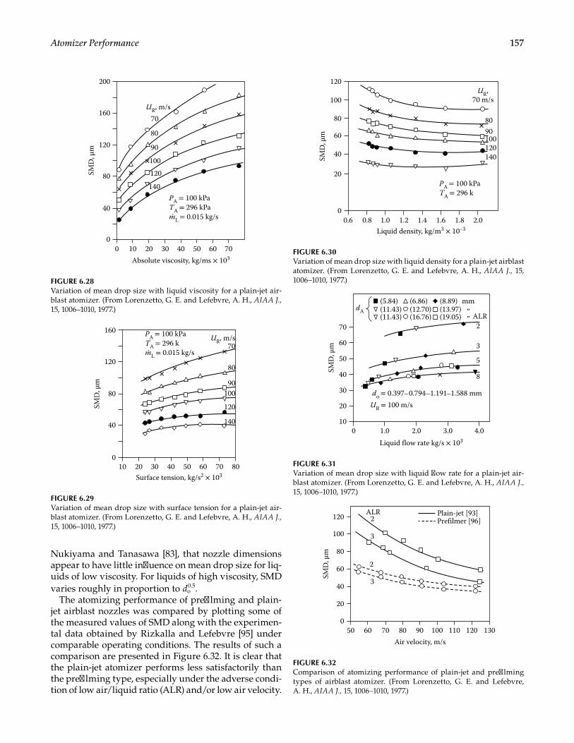
157Atomizer Performance

Nukiyama and Tanasawa [83], that nozzle dimensions appear to have little influence on mean drop size for liq-uids of low viscosity. For liquids of high viscosity, SMD varies roughly in proportion to do

0.5.The atomizing performance of prefilming and plain-

jet airblast nozzles was compared by plotting some of the measured values of SMD along with the experimen-tal data obtained by Rizkalla and Lefebvre [95] under comparable operating conditions. The results of such a comparison are presented in Figure 6.32. It is clear that the plain-jet atomizer performs less satisfactorily than the prefilming type, especially under the adverse condi-tion of low air/liquid ratio (ALR) and/or low air velocity.

SMD

, μm

PA = 100 kPaTA = 296 kPamL = 0.015 kg/s

100 20

140

.

120

100

90

80

70

Absolute viscosity, kg/ms × 10330 40 50 60 70

UR, m/s160

200

120

80

40

0

FIGURE 6.28Variation of mean drop size with liquid viscosity for a plain-jet air-blast atomizer. (From Lorenzetto, G. E. and Lefebvre, A. H., AIAA J., 15, 1006–1010, 1977.)

SMD

, μm

PA = 100 kPaTA = 296 kmL = 0.015 kg/s

140

120

10090

80

70

Surface tension, kg/s2 × 1032010 30 40 50 60 70 80

UR, m/s

40

80

120

.

160

0

FIGURE 6.29Variation of mean drop size with surface tension for a plain-jet air-blast atomizer. (From Lorenzetto, G. E. and Lefebvre, A. H., AIAA J., 15, 1006–1010, 1977.)

SMD

, μm

PA = 100 kPaTA = 296 k

8090

Liquid density, kg/m3 × 10–30.80.6 1.0 1.2 1.4 1.6 1.8 2.0

UR,70 m/s

20

0

40

60

80

100

120

100120140

FIGURE 6.30Variation of mean drop size with liquid density for a plain-jet airblast atomizer. (From Lorenzetto, G. E. and Lefebvre, A. H., AIAA J., 15, 1006–1010, 1977.)

SMD

, μm

dA

Liquid flow rate kg/s × 103

0

2

3

5

8

1.0

do = 0.397–0.794–1.191–1.588 mmUR = 100 m/s

2.0 3.0 4.0

20

10

30

40

50

60

70

(5.84) (6.86) (8.89) mm„„ ALR

(11.43) (12.70) (13.97)(11.43) (16.76) (19.05)

FIGURE 6.31Variation of mean drop size with liquid flow rate for a plain-jet air-blast atomizer. (From Lorenzetto, G. E. and Lefebvre, A. H., AIAA J., 15, 1006–1010, 1977.)

Air velocity, m/s

SMD

, μm

60 70 80 90 100 110 120 13050

20

0

40

60 2

3

3

2ALR Plain-jet [93]

Prefilmer [96]

80

100

120

FIGURE 6.32Comparison of atomizing performance of plain-jet and prefilming types of airblast atomizer. (From Lorenzetto, G. E. and Lefebvre, A. H., AIAA J., 15, 1006–1010, 1977.)

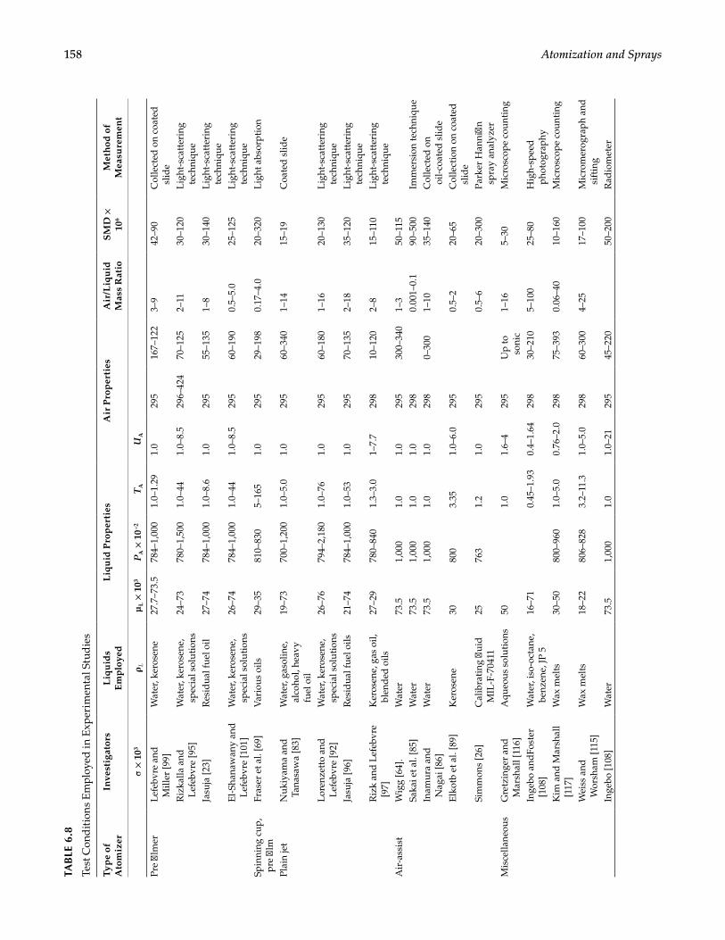
158 Atomization and SpraysTA

BLE

6.8

Test

Con

dit

ions

Em

ploy

ed in

Exp

erim

enta

l Stu

die

s

Typ

e of

A

tom

izer

Inve

stig

ator

sL

iqu

ids

Em

plo

yed

Liq

uid

Pro

per

ties

Air

Pro

per

ties

Air

/Liq

uid

M

ass

Rat

ioS

MD

×

106

Met

hod

of

Mea

sure

men

t

 σ  ×

103

 ρ  Lμ

L ×

103

PA ×

10–2

T AU

A

Pre

film

erL

efeb

vre

and

M

iller

[99]

Wat

er, k

eros

ene

27.7

–73.

578

4–1,

000

1.0–

1.29

1.0

295

167–

122

3–9

42–9

0C

olle

cted

on

coat

ed

slid

eR

izka

lla a

nd

Lef

ebvr

e [9

5]W

ater

, ker

osen

e,

spec

ial s

olut

ions

24–7

378

0–1,

500

1.0–

441.

0–8.

529

6–42

470

–125

2–11

30–1

20L

ight

-sca

tter

ing

tech

niqu

eJa

suja

[23]

Res

idua

l fue

l oil

27–7

478

4–1,

000

1.0–

8.6

1.0

295

55–1

351–

830

–140

Lig

ht-s

catt

erin

g te

chni

que

El-

Shan

awan

y an

d

Lef

ebvr

e [1

01]

Wat

er, k

eros

ene,

sp

ecia

l sol

utio

ns26

–74

784–

1,00

01.

0–44

1.0–

8.5

295

60–1

900.

5–5.

025

–125

Lig

ht-s

catt

erin

g te

chni

que

Spin

ning

cup

, pr

e fil

mFr

aser

et a

l. [6

9]V

ario

us o

ils29

–35

810–

830

5–16

51.

029

529

–198

0.17

–4.0

20–3

20L

ight

abs

orpt

ion

Plai

n je

tN

ukiy

ama

and

Ta

nasa

wa

[83]

Wat

er, g

asol

ine,

al

coho

l, he

avy

fuel

oil

19–7

370

0–1,

200

1.0–

5.0

1.0

295

60–3

401–

1415

–19

Coa

ted

slid

e

Lor

enze

tto

and

L

efeb

vre

[92]

Wat

er, k

eros

ene,

sp

ecia

l sol

utio

ns26

–76

794–

2,18

01.

0–76

1.0

295

60–1

801–

1620

–130

Lig

ht-s

catt

erin

g te

chni

que

Jasu

ja [9

6]R

esid

ual f

uel o

ils21

–74

784–

1,00

01.

0–53

1.0

295

70–1

352–

1835

–120

Lig

ht-s

catt

erin

g te

chni

que

Riz

k an

d L

efeb

vre

[97]

Ker

osen

e, g

as o

il,

blen

ded

oils

27–2

978

0–84

01.

3–3.

01–

7.7

298

10–1

202–

815

–110

Lig

ht-s

catt

erin

g te

chni

que

Air

-ass

ist

Wig

g [6

4].

Wat

er73

.51,

000

1.0

1.0

295

300–

340

1–3

50–1

15Sa

kai e

t al.

[85]

Wat

er73

.51,

000

1.0

1.0

298

0.00

1–0.

190

–500

Imm

ersi

on te

chni

que

Inam

ura

and

N

agai

[86]

Wat

er73

.51,

000

1.0

1.0

298

0–30

01–

1035

–140

Col

lect

ed o

n oi

l-co

ated

slid

eE

lkot

b et

al.

[89]

Ker

osen

e30

800

3.35

1.0–

6.0

295

0.5–

220

–65

Col

lect

ion

on c

oate

d

slid

eSi

mm

ons

[26]

Cal

ibra

ting

flui

d

MIL

-F-7

0411

2576

31.

21.

029

50.

5–6

20–3

00Pa

rker

Han

nifi

n sp

ray

anal

yzer

Mis

cella

neou

sG

retz

inge

r an

d

Mar

shal

l [11

6]A

queo

us s

olut

ions

501.

01.

6–4

295

Up

to

soni

c1–

165–

30M

icro

scop

e co

unti

ng

Inge

bo a

ndFo

ster

[1

08]

Wat

er, i

so-o

ctan

e,

benz

ene,

JP 5

16–7

10.

45–1

.93

0.4–

1.64

298

30–2

105–

100

25–8

0H

igh-

spee

d

phot

ogra

phy

Kim

and

Mar

shal

l [1

17]

Wax

mel

ts30

–50

800–

960

1.0–

5.0

0.76

–2.0

298

75–3

930.

06–4

010

–160

Mic

rosc

ope

coun

ting

Wei

ss a

nd

Wor

sham

[115

]W

ax m

elts

18–2

280

6–82

83.

2–11

.31.

0–5.

029

860

–300

4–25

17–1

00M

icro

mer

ogra

ph a

nd

sift

ing

Inge

bo [1

08]

Wat

er73

.51,

000

1.0

1.0–

2129

545

–220

50–2

00R

adio

met

er

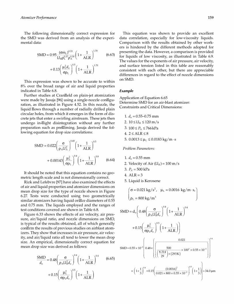
159Atomizer Performance

The following dimensionally correct expression for the SMD was derived from an analysis of the experi-mental data:

mU

d

= σρ ρ

+

+ µσρ

+

SMD 0.95( )

11

ALR

0.13 11

ALR

L0.33

R L0.37

A0.30

1.70

L2

o

L

0.5 1.70

(6.63)

This expression was shown to be accurate to within 8% over the broad range of air and liquid properties indicated in Table 6.8.

Further studies at Cranfield on plain-jet atomization were made by Jasuja [96] using a single-nozzle configu-ration, as illustrated in Figure 4.52. In this nozzle, the liquid flows through a number of radially drilled plain circular holes, from which it emerges in the form of dis-crete jets that enter a swirling airstream. These jets then undergo in-flight disintegration without any further preparation such as prefilming. Jasuja derived the fol-lowing equation for drop size correlations:

SMD 0.022 11

ALR

0.00143 11

ALR

A A2

0.45 0.5

L2

L

0.4 0.8

U= σ

ρ

+

+ µσρ

+

(6.64)

It should be noted that this equation contains no geo-metric length scale and is not dimensionally correct.

Rizk and Lefebvre [97] have also examined the effects of air and liquid properties and atomizer dimensions on mean drop size for the type of nozzle shown in Figure 6.27. Tests were conducted using two geometrically similar atomizers having liquid orifice diameters of 0.55 and 0.75 mm. The liquids employed and the ranges of test conditions covered are shown in Table 6.8.

Figure 6.33 shows the effects of air velocity, air pres-sure, air/liquid ratio, and nozzle dimensions on SMD, is typical of the results obtained, all of which generally confirm the results of previous studies on airblast atom-izers. They show that increases in air pressure, air veloc-ity, and air/liquid ratio all tend to lower the mean drop size. An empirical, dimensionally correct equation for mean drop size was derived as follows:

SMD0.48 1

1ALR

0.15 11

ALR

o A R2

o

0.4 0.4

L2

L o

0.5

d U d

d

= σρ

+

+ µσρ

+

(6.65)

This equation was shown to provide an excellent data correlation, especially for low-viscosity liquids. Comparison with the results obtained by other work-ers is hindered by the different methods adopted for presenting the data. However, a comparison is provided for liquids of low viscosity, as illustrated in Table 6.9. The values for the exponents of air pressure, air velocity, and surface tension listed in this table are reasonably consistent with each other, but there are appreciable differences in regard to the effect of nozzle dimensions on SMD.

Example

Application of Equation 6.65Determine SMD for an air-blast atomizer:Constraints and Critical Dimensions:

1. = 0.55–0.75 mmod

2. U10 120 m/sR≤ ≤ 3. ≤ ≤100 766kPaAP 4. 2 ALR 8≤ ≤ 5. 0.0013 0.0183 kg/m sL≤ µ ≤ ⋅

Problem Parameters:

1. = 0.55 mmod

2. Velocity of Air U( ) 100 m/sR = 3. PA 500 kPa= 4. ALR 3= 5. Liquid is Kerosene

0.021 kg/s , 0.0016 kg/m s,

800 kg/m

2L

L3

σ = µ = ⋅

ρ =

U d

d

= σρ

+

+ µσρ

+

SMD d 0.48 11

ALR

0.15 11

ALR

oA R

2o

0.4 0.4

L2

L o

0.5

( )

( )

= × ×

×

× × ×

× +

+

× × ×

+

= µ

−−

−

SMD 0.55 10 0.48

0.021

5008.314

29293K

100 0.55 10

113

0.150.0016

0.021 800 0.55 101

13

34.0 m

32 3

0.4

0.4 2

3

0.5

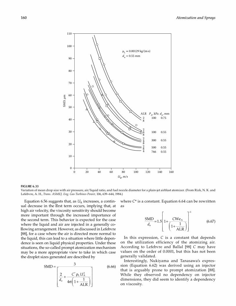
160 Atomization and Sprays

Equation 6.56 suggests that, as UR increases, a contin-ual decrease in the first term occurs, implying that, at high air velocity, the viscosity sensitivity should become more important through the increased importance of the second term. This behavior is expected for the case where the liquid and air are injected in a generally co-flowing arrangement. However, as discussed in Lefebvre [88], for a case where the air is directed more normal to the liquid, this can lead to a situation where little depen-dence is seen on liquid physical properties. Under these situations, the so-called prompt atomization mechanism may be a more appropriate view to take in which case the droplet sizes generated are described by

dC U

SMD3

2

4 11

ALRo

*L A

2

=

+ ρ

σ +

(6.66)

where C* is a constant. Equation 6.64 can be rewritten as

d

CSMD1.5 1

We

11

ALRo

A

1

= ++

−

(6.67)

In this expression, C is a constant that depends on the utilization efficiency of the atomizing air. According to Lefebvre and Ballal [98] C may have values on the order of 0.0001, but this has not been generally validated.

Interestingly, Nukiyama and Tanasawa’s expres-sion (Equation 6.62) was derived using an injector that is arguably prone to prompt atomization [88]. While they observed no dependency on injector dimensions, they did seem to identify a dependency on viscosity.

SMD

, μm

0 20 40 60 80

ALR2 100

100

300

500766

0.75

0.55

0.55

0.550.55

8

248248284

PA, kPa

UR, m/s

do, mm

100 120 140 160

10

0

20

30

40

50

60

70

80

90

100

110

μL = 0.00129 kg/(m·s)do = 0.55 mm

FIGURE 6.33Variation of mean drop size with air pressure, air/liquid ratio, and fuel nozzle diameter for a plain-jet airblast atomizer. (From Rizk, N. K. and Lefebvre, A. H., Trans. ASMEJ. Eng. Gas Turbines Power, 106, 639–644, 1984.)

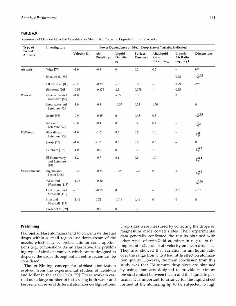
161Atomizer Performance

Prefilming

Plain-jet airblast atomizers tend to concentrate the fuel drops within a small region just downstream of the nozzle, which may be problematic for some applica-tions (e.g., combustion). As an alternative, the prefilm-ing type of airblast atomizer, which can be designed to disperse the drops throughout an entire region can be considered.

The prefilming concept for airblast atomization evolved from the experimental studies of Lefebvre and Miller in the early 1960s [99]. These workers car-ried out a large number of tests, using both water and kerosene, on several different atomizer configurations.

Drop sizes were measured by collecting the drops on magnesium oxide coated slides. Their experimental data generally confirmed the results obtained with other types of twin-fluid atomizer in regard to the important influence of air velocity on mean drop size. They also showed that variation in air/liquid ratio over the range from 3 to 9 had little effect on atomiza-tion quality. However, the main conclusion from this study was that “Minimum drop sizes are obtained by using atomizers designed to provide maximum physical contact between the air and the liquid. In par-ticular it is important to arrange for the liquid sheet formed at the atomizing lip to be subjected to high

TABLE 6.9

Summary of Data on Effect of Variables on Mean Drop Size for Liquids of Low Viscosity

Type of Twin-Fluid Atomizer

Investigators Power Dependence on Mean Drop Size of Variable Indicated

Velocity UA Air Density ρa

Liquid Density ρL

Surface Tension σ

Air/Liquid Ratio

m m(1 L A)++

Liquid/Air Ratio m m( L A)

Dimensions

Air assist Wige [79] –1.0 –0.3 0 0.2 0.5 – h0.1

Sakai et al. [85] – – – – – 0.75 do0.75

Elkotb et al. [89] –0.75 –0.39 –0.18 0.18 – 0.29 d0.43

Simmons [26] –0.55 –0.375 .25 0.375 – 0.55 –

Plain jet Nukiyama and Tanasawa [83]

–1.0 0 –0.5 0.5 0

Lorenzetto and Lefebvre [92]

–1.0 –0.3 –0.37 0.33 1.70 – 0

Jasuja [96] –0.9 –0.45 0 0.45 0.5 – do0.55

Rizk and Lefebvre [97]

–0.8 –0.4 0 0.4 0.4 –do0.6

Prefilmer Rizkalla and Lefebvre [95]

–1.0 –1.0 0.5 0.5 1.0 –Dp0.5

Jasuja [23] –1.0 –1.0 0.5 0.5 0.5 – 0

Lefebvre [118] –1.0 –0.5 0 0.5 1.0 – Dp0.5

El-Shanawany and Lefebvre [101]

–1.2 –0.7 0.1 0.6 1.0 –Dp0.4

Miscellaneous Ingebo and Foster [108]

–0.75 –0.25 –0.25 0.25 0 0Dp0.5

Weiss and Worsham [115]

–1.33 –0.30 – – – –do0.16

Gretzinger and Marshall [116]

–0.15 –0.15 0 0 – 0.6 L–0.15

Kim and Marshall [117]

–1.44 0.72 –0.16 0.41 0 0 0

Fraser et al. [69] – –0.5 0 0.5 – – –

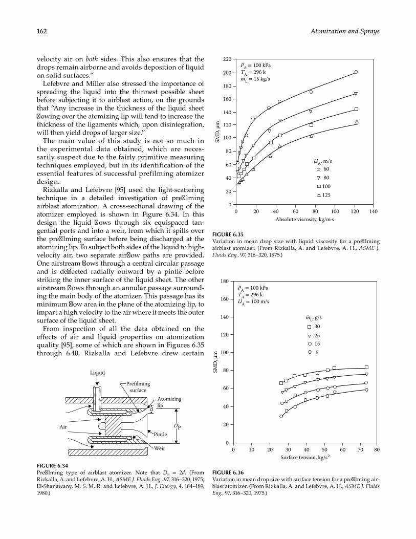
162 Atomization and Sprays

velocity air on both sides. This also ensures that the drops remain airborne and avoids deposition of liquid on solid surfaces.”

Lefebvre and Miller also stressed the importance of spreading the liquid into the thinnest possible sheet before subjecting it to airblast action, on the grounds that “Any increase in the thickness of the liquid sheet flowing over the atomizing lip will tend to increase the thickness of the ligaments which, upon disintegration, will then yield drops of larger size.”

The main value of this study is not so much in the experimental data obtained, which are neces-sarily suspect due to the fairly primitive measuring techniques employed, but in its identification of the essential features of successful prefilming atomizer design.

Rizkalla and Lefebvre [95] used the light-scattering technique in a detailed investigation of prefilming airblast atomization. A cross-sectional drawing of the atomizer employed is shown in Figure 6.34. In this design the liquid flows through six equispaced tan-gential ports and into a weir, from which it spills over the prefilming surface before being discharged at the atomizing lip. To subject both sides of the liquid to high-velocity air, two separate airflow paths are provided. One airstream flows through a central circular passage and is deflected radially outward by a pintle before striking the inner surface of the liquid sheet. The other airstream flows through an annular passage surround-ing the main body of the atomizer. This passage has its minimum flow area in the plane of the atomizing lip, to impart a high velocity to the air where it meets the outer surface of the liquid sheet.

From inspection of all the data obtained on the effects of air and liquid properties on atomization quality [95], some of which are shown in Figures 6.35 through 6.40, Rizkalla and Lefebvre drew certain

Air

d

Liquid

Prefilmingsurface

Atomizinglip

DPPintle

Weir

FIGURE 6.34Prefilming type of airblast atomizer. Note that Dh = 2d. (From Rizkalla, A. and Lefebvre, A. H., ASME J. Fluids Eng., 97, 316–320, 1975; El-Shanawany, M. S. M. R. and Lefebvre, A. H., J. Energy, 4, 184–189, 1980.)

UA, m/s

0 20 40 60Absolute viscosity, kg/m·s

80 100 120 140

20

40

60

80

100

120

140

160

180

·200

220

0

60

SMD

, μm

100125

80

PA = 100 kPaTA = 296 kmL = 15 kg/s

FIGURE 6.35Variation in mean drop size with liquid viscosity for a prefilming airblast atomizer. (From Rizkalla, A. and Lefebvre, A. H., ASME J. Fluids Eng., 97, 316–320, 1975.)

mL, g/s

Surface tension, kg/s2

30

25155

100 20 30 40 50 60 70 80

20

40

60

80

100

120

140 .

160

180

0

SMD

, μm

PA = 100 kPaTA = 296 kUA = 100 m/s

FIGURE 6.36Variation in mean drop size with surface tension for a prefilming air-blast atomizer. (From Rizkalla, A. and Lefebvre, A. H., ASME J. Fluids Eng., 97, 316–320, 1975.)

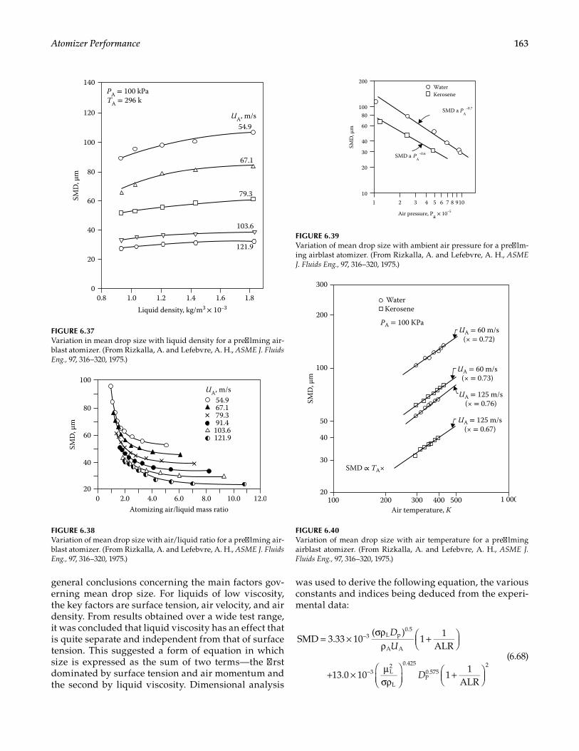
163Atomizer Performance

general conclusions concerning the main factors gov-erning mean drop size. For liquids of low viscosity, the key factors are surface tension, air velocity, and air density. From results obtained over a wide test range, it was concluded that liquid viscosity has an effect that is quite separate and independent from that of surface tension. This suggested a form of equation in which size is expressed as the sum of two terms—the first dominated by surface tension and air momentum and the second by liquid viscosity. Dimensional analysis

was used to derive the following equation, the various constants and indices being deduced from the experi-mental data:

= ×σρ

ρ+

+ × µσρ

+

−

−

SMD 3.33 10( )

11

ALR

13.0 10 11

ALR

3 L p0.5

A A

3 L2

L

0.425

P0.575

2

DU

D

(6.68)

UA, m/s

Liquid density, kg/m3 × 10–30.8 1.0 1.2 1.4 1.6 1.8

20

40

121.9

103.6

79.3

67.1

54.9

60

80

100

120

140

0

SMD

, μm

PA = 100 kPaTA = 296 k

FIGURE 6.37Variation in mean drop size with liquid density for a prefilming air-blast atomizer. (From Rizkalla, A. and Lefebvre, A. H., ASME J. Fluids Eng., 97, 316–320, 1975.)

UA, m/s

2.00 4.0Atomizing air/liquid mass ratio

6.0 8.0 10.0 12.020

40

60

80

100

SMD

, μm

54.9

91.4103.6

67.1

121.9

79.3

FIGURE 6.38Variation of mean drop size with air/liquid ratio for a prefilming air-blast atomizer. (From Rizkalla, A. and Lefebvre, A. H., ASME J. Fluids Eng., 97, 316–320, 1975.)

Air pressure, Pa × 10–5

1 2 3 4 5 6 7 8 91010

20

30

40

60

80

WaterKerosene

SMD a PA

–0.7

SMD a PA

–0.6

100

200

SMD

, μm

FIGURE 6.39Variation of mean drop size with ambient air pressure for a prefilm-ing airblast atomizer. (From Rizkalla, A. and Lefebvre, A. H., ASME J. Fluids Eng., 97, 316–320, 1975.)

Air temperature, K200100 300 400 500 1 000

20

30

40

50

100

200

300

SMD ∝ TA×

SMD

, μm

WaterKerosene

PA = 100 KPaUA = 60 m/s

(× = 0.72)

UA = 60 m/s(× = 0.73)

UA = 125 m/s(× = 0.76)

UA = 125 m/s(× = 0.67)

FIGURE 6.40Variation of mean drop size with air temperature for a prefilming airblast atomizer. (From Rizkalla, A. and Lefebvre, A. H., ASME J. Fluids Eng., 97, 316–320, 1975.)

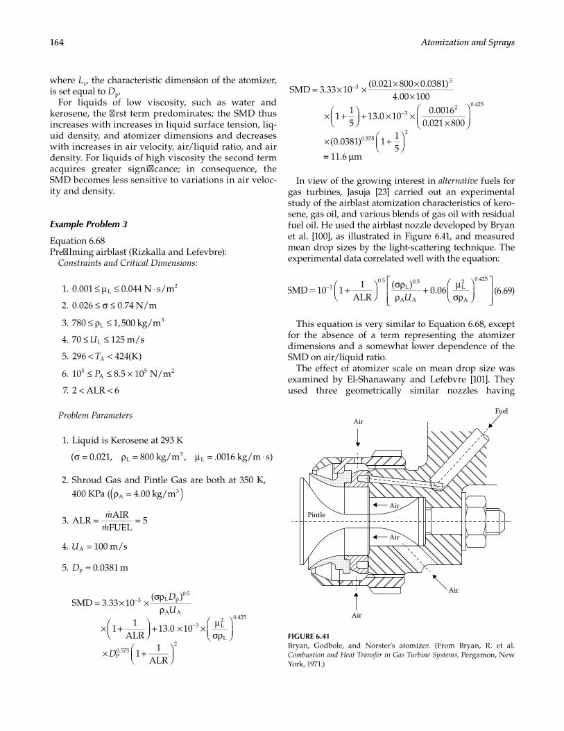
164 Atomization and Sprays

where Lc, the characteristic dimension of the atomizer, is set equal to Dp.

For liquids of low viscosity, such as water and kerosene, the first term predominates; the SMD thus increases with increases in liquid surface tension, liq-uid density, and atomizer dimensions and decreases with increases in air velocity, air/liquid ratio, and air density. For liquids of high viscosity the second term acquires greater significance; in consequence, the SMD becomes less sensitive to variations in air veloc-ity and density.

Example Problem 3

Equation 6.68Prefilming airblast (Rizkalla and Lefevbre):

Constraints and Critical Dimensions:

1. 0.001 0.044 N s/mL2≤ µ ≤ ⋅

2. 0.026 0.74 N/m≤ σ ≤

3. 780 1,500 kg/mL3≤ ρ ≤

4. U70 125 m/sL≤ ≤

5. T296 424(K)A< <

6. P10 8.5 10 N/m5A

5 2≤ ≤ ×

7. 2 ALR 6< <

Problem Parameters

1. Liquid is Kerosene at 293 K

( 0.021, 800 kg/m , .0016 kg/m s)L3

Lσ = ρ = µ = ⋅

2. Shroud Gas and Pintle Gas are both at 350 K, 400 KPa ( 4.00 kg/mA

3( )ρ =

3. m

m

ALRAIR

FUEL5= =

4. U 100 m/sA =

5. D 0.0381 mp =

SMD 3.33 10( )

11

ALR13.0 10

11

ALR

3 L p0 5

A A

3 L2

L

0.425

P0.575

2

DU

D

= × ×σρ

ρ

× +

+ × × µ

σρ

× +

−⋅

−

= × × × ××

× +

+ × ×

×

× +

µ

−

−

SMD 3.33 10(0.021 800 0.0381)

4.00 100

115

13.0 100.0016

0.021 800

(0.0381) 115

11.6 m

3.5

32 0.425

0.5752

=

In view of the growing interest in alternative fuels for gas turbines, Jasuja [23] carried out an experimental study of the airblast atomization characteristics of kero-sene, gas oil, and various blends of gas oil with residual fuel oil. He used the airblast nozzle developed by Bryan et al. [100], as illustrated in Figure 6.41, and measured mean drop sizes by the light-scattering technique. The experimental data correlated well with the equation:

U

SMD 10 11

ALR( )

0.0630.5

L0.5

A A

L2

A

0.425

= +

σρρ

+ µσρ

− (6.69)

This equation is very similar to Equation 6.68, except for the absence of a term representing the atomizer dimensions and a somewhat lower dependence of the SMD on air/liquid ratio.

The effect of atomizer scale on mean drop size was examined by El-Shanawany and Lefebvre [101]. They used three geometrically similar nozzles having

Air

Air

Air

PintleAir

FuelAir

FIGURE 6.41Bryan, Godbole, and Norster's atomizer. (From Bryan, R. et al. Combustion and Heat Transfer in Gas Turbine Systems, Pergamon, New York, 1971.)

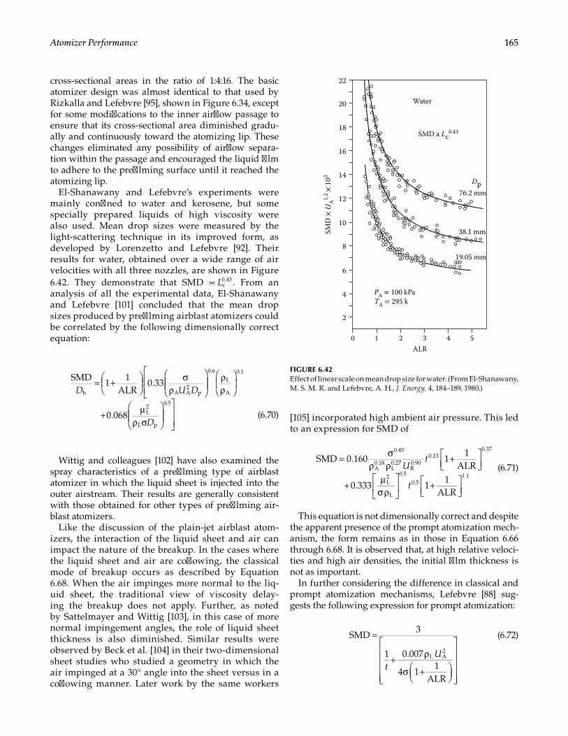
165Atomizer Performance

cross-sectional areas in the ratio of 1:4:16. The basic atomizer design was almost identical to that used by Rizkalla and Lefebvre [95], shown in Figure 6.34, except for some modifications to the inner airflow passage to ensure that its cross-sectional area diminished gradu-ally and continuously toward the atomizing lip. These changes eliminated any possibility of airflow separa-tion within the passage and encouraged the liquid film to adhere to the prefilming surface until it reached the atomizing lip.

El-Shanawany and Lefebvre’s experiments were mainly confined to water and kerosene, but some specially prepared liquids of high viscosity were also used. Mean drop sizes were measured by the light-scattering technique in its improved form, as developed by Lorenzetto and Lefebvre [92]. Their results for water, obtained over a wide range of air velocities with all three nozzles, are shown in Figure 6.42. They demonstrate that SMD Lc

0.43∝ . From an analysis of all the experimental data, El-Shanawany and Lefebvre [101] concluded that the mean drop sizes produced by prefilming airblast atomizers could be correlated by the following dimensionally correct equation:

= +

σρ

ρρ

+ µρ σ

SMD 1 1ALR

0.33

0.068

h A A2

p

0.6

L

A

0.1

L2

L p

0.5

D U D

D (6.70)

Wittig and colleagues [102] have also examined the spray characteristics of a prefilming type of airblast atomizer in which the liquid sheet is injected into the outer airstream. Their results are generally consistent with those obtained for other types of prefilming air-blast atomizers.

Like the discussion of the plain-jet airblast atom-izers, the interaction of the liquid sheet and air can impact the nature of the breakup. In the cases where the liquid sheet and air are coflowing, the classical mode of breakup occurs as described by Equation 6.68. When the air impinges more normal to the liq-uid sheet, the traditional view of viscosity delay-ing the breakup does not apply. Further, as noted by Sattelmayer and Wittig [103], in this case of more normal impingement angles, the role of liquid sheet thickness is also diminished. Similar results were observed by Beck et al. [104] in their two-dimensional sheet studies who studied a geometry in which the air impinged at a 30° angle into the sheet versus in a coflowing manner. Later work by the same workers

[105] incorporated high ambient air pressure. This led to an expression for SMD of

SMD 0.160 1

1ALR

0.333 11

ALR

0.45

A0.18

L0.27

R0.90

0.130.37

L2

L

0.5

0.51.1

Ut

t

= σρ ρ

+

+ µσρ

+

(6.71)

This equation is not dimensionally correct and despite the apparent presence of the prompt atomization mech-anism, the form remains as in those in Equation 6.66 through 6.68. It is observed that, at high relative veloci-ties and high air densities, the initial film thickness is not as important.

In further considering the difference in classical and prompt atomization mechanisms, Lefebvre [88] sug-gests the following expression for prompt atomization:

=

+ρ

σ +

SMD3

1 0.007

4 11

ALR

L A2

tU

(6.72)

0 1 2 3 4 5

2

4

6

819.05 mm

38.1 mm

76.2 mm

SMD a Lc0.43

Dp

10

12

14

16

18

20

22

ALR

Water

SMD

× U

A1.

2 ×

103

PA = 100 kPaTA = 295 k

FIGURE 6.42Effect of linear scale on mean drop size for water. (From El-Shanawany, M. S. M. R. and Lefebvre, A. H., J. Energy, 4, 184–189, 1980.)

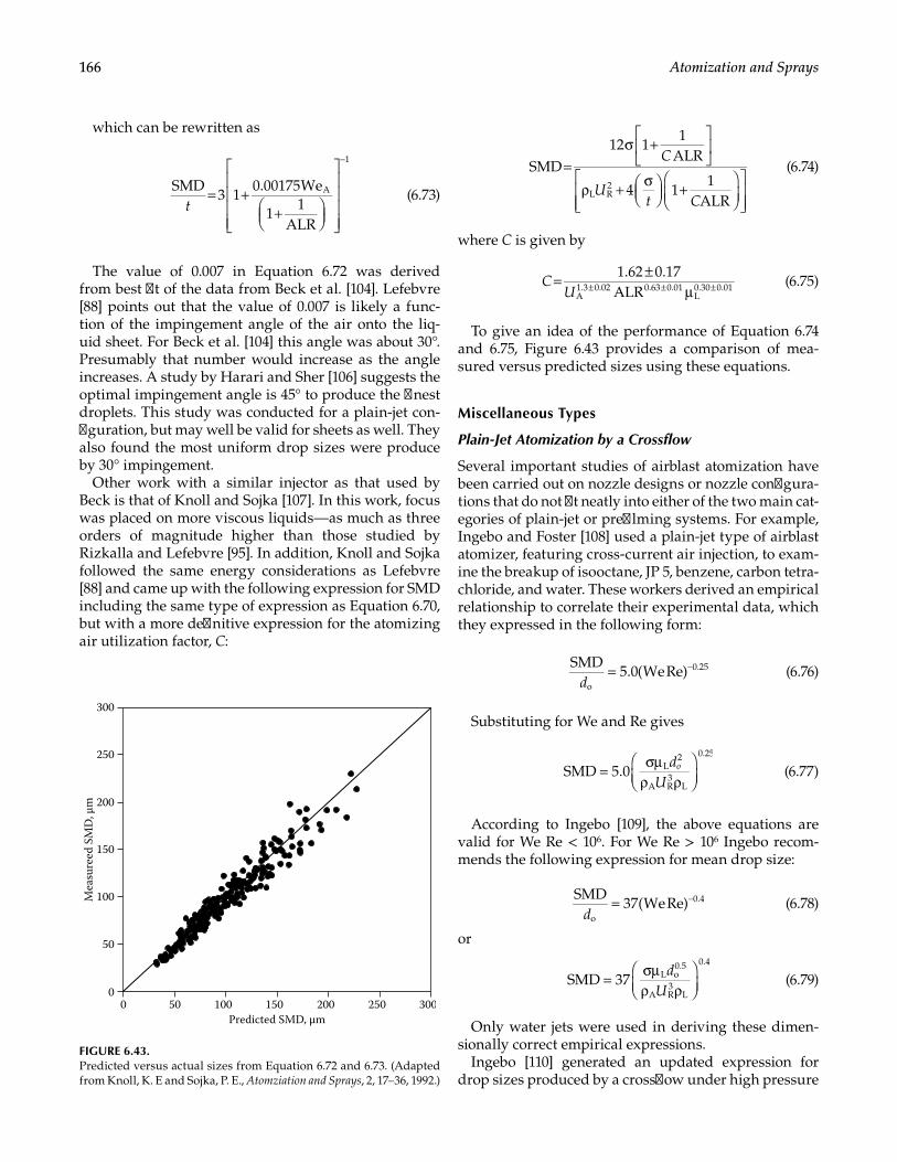
166 Atomization and Sprays

which can be rewritten as

t

SMD3 1

0.00175We

11

ALR

A

1

= ++

−

(6.73)

The value of 0.007 in Equation 6.72 was derived from best fit of the data from Beck et al. [104]. Lefebvre [88] points out that the value of 0.007 is likely a func-tion of the impingement angle of the air onto the liq-uid sheet. For Beck et al. [104] this angle was about 30°. Presumably that number would increase as the angle increases. A study by Harari and Sher [106] suggests the optimal impingement angle is 45° to produce the finest droplets. This study was conducted for a plain-jet con-figuration, but may well be valid for sheets as well. They also found the most uniform drop sizes were produce by 30° impingement.

Other work with a similar injector as that used by Beck is that of Knoll and Sojka [107]. In this work, focus was placed on more viscous liquids—as much as three orders of magnitude higher than those studied by Rizkalla and Lefebvre [95]. In addition, Knoll and Sojka followed the same energy considerations as Lefebvre [88] and came up with the following expression for SMD including the same type of expression as Equation 6.70, but with a more definitive expression for the atomizing air utilization factor, C:

C

Ut C

SMD12 1

1ALR

4 11

ALRL R2

=σ +

ρ + σ

+

(6.74)

where C is given by

CU

1.62 0.17ALRA

1.3 0.02 0.63 0.01L0.30 0.01= ±

µ± ± ± (6.75)

To give an idea of the performance of Equation 6.74 and 6.75, Figure 6.43 provides a comparison of mea-sured versus predicted sizes using these equations.

Miscellaneous Types

Plain-Jet Atomization by a Crossflow

Several important studies of airblast atomization have been carried out on nozzle designs or nozzle configura-tions that do not fit neatly into either of the two main cat-egories of plain-jet or prefilming systems. For example, Ingebo and Foster [108] used a plain-jet type of airblast atomizer, featuring cross-current air injection, to exam-ine the breakup of isooctane, JP 5, benzene, carbon tetra-chloride, and water. These workers derived an empirical relationship to correlate their experimental data, which they expressed in the following form:

d

SMD5.0(WeRe)

o

0.25= − (6.76)

Substituting for We and Re gives

d

UoSMD 5.0 L2

A R3

L

0.25

= σµρ ρ

(6.77)

According to Ingebo [109], the above equations are valid for We Re < 106. For We Re > 106 Ingebo recom-mends the following expression for mean drop size:

d

SMD37(WeRe)

o

0.4= − (6.78)

or

d

USMD 37 L o

0.5

A R3

L

0.4

= σµρ ρ

(6.79)

Only water jets were used in deriving these dimen-sionally correct empirical expressions.

Ingebo [110] generated an updated expression for drop sizes produced by a crossflow under high pressure

Mea

sure

ed S

MD

, μm

Predicted SMD, μm

300

0 50 100 150 200 250 300

250

200

150

100

50

0

FIGURE 6.43.Predicted versus actual sizes from Equation 6.72 and 6.73. (Adapted from Knoll, K. E and Sojka, P. E., Atomziation and Sprays, 2, 17–36, 1992.)

167Atomizer Performance

conditions that incorporates a new dimensionless group, the molecular scale momentum transfer group, that was found to help improve the fit of data for high pressure high velocity results:

SMD

1.4(WeRe)o 0.42

0.15d glc

=

(6.80)

This equation is quite similar to 6.78 and 6.79, but is modified by the momentum transfer term to account for density effects.

Faeth and coworkers [111] developed the following expression for the drop sizes generated by the breakup of a liquid jet in a crossflow:

x

SMD 0.56Wel

0.5

0.50

= ΛΛ

(6.81)

In this study [111], high-resolution photographs and holography were used to size the particles. This expres-sion follows directly from the development of similar forms for the injection of the liquid jet in a quiescent environment. Λ is the radial spatial integral scale of tur-bulence in the crossflow.

Another expression has been developed by Song et al. [112], based on the forms of Ingebo above:

d

qSMD

0.267 Weo 0.44 0.08 L

A

0.30L

A

0.16

= ρρ

µµ

−

(6.82)

In Song et al.’s [112] study, Jet A was the test liquid and phase Doppler interferometry was used to measure drop sizes. Noteworthy in this study was the evaluation of the effect of ambient pressure that is captured by the density ratio term. In this case, q is the liquid to cross-flow momentum flux ratio.

Another expression was developed for the SMD gener-ated by the atomization of a plain jet in a crossflow by Bolszo et al. [113]. In Bolszo et al.’s study, the injection of water, oil, and water/oil emulsions into a crossflow was considered while in the resulting equation below, the pure liquids (water and DF-2) were considered. Laser dif-fraction was used for drop sizing in this study and the flow domain up to 100 mm downstream of the point of injection was considered. The expression below is valid at a location 40 mm downstream (×) of the point of injection.

SMD

9.33 10 We Reo

71.173

0.419 1.711A

2.087= ×

− − −

dyd

q (6.83)

Equations 6.76 through 6.83 are highly relevant to the applications that employ radial fuel injection from plain-orifice atomizers into high-velocity, crossflow-ing streams of air or gas. Examples include various

air-breathing propulsion engines, such as ramjets and turbojet afterburners.

Plain-Jet Impingement Injector

In situations where transverse penetration of fuel into the gas stream is unnecessary or undesirable, a splash-plate type injector is generally preferred. With this device a round fuel jet is arranged to impinge at the cen-ter of a small plate. As the fuel flows over the edge of the plate, it is atomized by the high-velocity gas stream in which it is immersed. Essentially, the device functions as a simple prefilming airblast atomizer.

Ingebo [114] has studied the atomizing performance of this type of injector for air pressures ranging from 0.10 to 2.1 MPa (1–20 atm). His tests were confined to water, for which the effects of liquid velocity and air properties on mean drop size conformed to the relationship:

U P U PSMD 2.6 10 4.11 104L A

0.33 6A A A

0.75 1( )= × + × ρ− − − (6.84)

Weiss and Worsham [115] investigated both cross-stream and costream injection of liquid jets into high-velocity air. Their experiments covered ranges of air velocity from 60 to 300 m/s, orifice diameters from 1.2 to 4.8 mm, liquid viscosities from 0.0032 to 0.0113 kg/m·s, and air densities from 0.74 to 4.2 kg/m3. The most impor-tant factor controlling the mean drop size was found to be the relative velocity between the air and the liquid. They argued that the drop size distribution in a spray depends on the range of excitable wavelengths on the surface of a liquid sheet, the shorter-wavelength limit being due to viscous damping, while the longer wave-lengths are limited by inertia effects. Based on these assumptions, they concluded that

U d

USMD L

0.08o0.16

L0.34

A0.30

R1.33∝ µ

ρ

(6.85)

Their experimental data confirmed the dependence predicted for air velocity but gave slightly different indices for the effects of liquid properties.

Other Designs

Gretzinger and Marshall [116] studied the characteris-tics of mean drop size and drop size distribution for two different designs of airblast atomizer. One was a con-verging nozzle of the type employed by Nukiyama and Tanasawa [83], in which the liquid is first brought into contact with the atomizing airstream at the throat of an air nozzle. The other, described as an impingement noz-zle, consisted of a central circular air tube surrounded by an annular liquid duct. An impinger, mounted on a

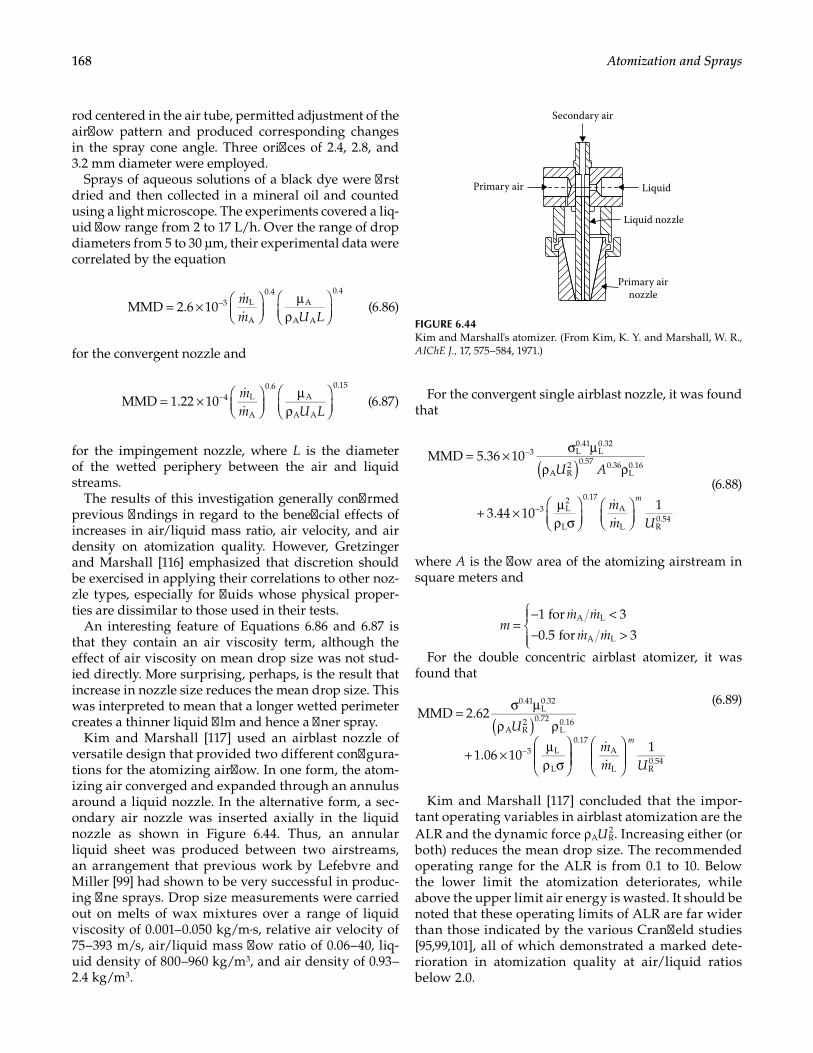
168 Atomization and Sprays

rod centered in the air tube, permitted adjustment of the airflow pattern and produced corresponding changes in the spray cone angle. Three orifices of 2.4, 2.8, and 3.2 mm diameter were employed.

Sprays of aqueous solutions of a black dye were first dried and then collected in a mineral oil and counted using a light microscope. The experiments covered a liq-uid flow range from 2 to 17 L/h. Over the range of drop diameters from 5 to 30 μm, their experimental data were correlated by the equation

mm U L

= ×

µρ

−MMD 2.6 10 3 L

A

0.4A

A A

0.4

(6.86)

for the convergent nozzle and

mm U L

= ×

µρ

−MMD 1.22 10 4 L

A

0.6A

A A

0.15

(6.87)

for the impingement nozzle, where L is the diameter of the wetted periphery between the air and liquid streams.

The results of this investigation generally confirmed previous findings in regard to the beneficial effects of increases in air/liquid mass ratio, air velocity, and air density on atomization quality. However, Gretzinger and Marshall [116] emphasized that discretion should be exercised in applying their correlations to other noz-zle types, especially for fluids whose physical proper-ties are dissimilar to those used in their tests.

An interesting feature of Equations 6.86 and 6.87 is that they contain an air viscosity term, although the effect of air viscosity on mean drop size was not stud-ied directly. More surprising, perhaps, is the result that increase in nozzle size reduces the mean drop size. This was interpreted to mean that a longer wetted perimeter creates a thinner liquid film and hence a finer spray.

Kim and Marshall [117] used an airblast nozzle of versatile design that provided two different configura-tions for the atomizing airflow. In one form, the atom-izing air converged and expanded through an annulus around a liquid nozzle. In the alternative form, a sec-ondary air nozzle was inserted axially in the liquid nozzle as shown in Figure 6.44. Thus, an annular liquid sheet was produced between two airstreams, an arrangement that previous work by Lefebvre and Miller [99] had shown to be very successful in produc-ing fine sprays. Drop size measurements were carried out on melts of wax mixtures over a range of liquid viscosity of 0.001–0.050 kg/m·s, relative air velocity of 75–393 m/s, air/liquid mass flow ratio of 0.06–40, liq-uid density of 800–960 kg/m3, and air density of 0.93–2.4 kg/m3.

For the convergent single airblast nozzle, it was found that

U A

mm U

m

( )= × σ µ

ρ ρ

+ × µρ σ

−

−

MMD 5.36 10

3.44 101

3 L0.41

L0.32

A R2 0.57 0.36

L0.16

3 L2

L

0.17A

L R0.54

(6.88)

where A is the flow area of the atomizing airstream in square meters and

1 for 3

0.5 for 3A L

A Lm

m m

m m

=− <− >

For the double concentric airblast atomizer, it was

found that

U

mm U

m( )

= σ µρ ρ

+ × µρ σ

−

MMD 2.62

1.06 101

0.41L0.32

A R2 0.72

L0.16

3 L

L

0.17A

L R0.54

(6.89)

Kim and Marshall [117] concluded that the impor-tant operating variables in airblast atomization are the ALR and the dynamic force UA R

2ρ . Increasing either (or both) reduces the mean drop size. The recommended operating range for the ALR is from 0.1 to 10. Below the lower limit the atomization deteriorates, while above the upper limit air energy is wasted. It should be noted that these operating limits of ALR are far wider than those indicated by the various Cranfield studies [95,99,101], all of which demonstrated a marked dete-rioration in atomization quality at air/liquid ratios below 2.0.

Primary air Liquid

Secondary air

Liquid nozzle

Primary airnozzle

FIGURE 6.44Kim and Marshall's atomizer. (From Kim, K. Y. and Marshall, W. R., AIChE J., 17, 575–584, 1971.)

169Atomizer Performance

It is of interest to note that the atomizer with concen-tric double air nozzles, that is, the arrangement in which the liquid sheet is entrained between two air-streams, yields only a slight improvement in atomization qual-ity over the single air nozzle. Thus, the superior perfor-mance of the former type, as observed by Lefebvre and Miller [99], was not confirmed in these experiments.

Fraser et al. [69] studied the spray characteristics of an airblast system in which a spinning cup produced flat circular liquid sheets of sensibly uniform thickness. Disintegration of the liquid sheet was accomplished by a high-velocity airstream that flowed through an annu-lar gap located axially symmetrically to the cup. They compared their experimental data with those of other workers and reported that prefilming atomizers are superior to plain-jet atomizers in producing finer sprays and that the controlled production of thin liquid sheets is a prerequisite to fine atomization. Their correlation for drop size data was derived as

vaD a

mm

QU U U

L

= ×

+ σρ +

× +

− +

−SMD 6 10

0.019( )

1 0.065(0.5 1)

6

0.5r0.21

A0.5

L2 0.25

L

A

1.5

p2

r2

r

0.5

(6.90)

where vr = kinematic viscosity ratio relative to watera = radial distance from cup lip, mDL = diameter of cup at lip, mUp = cup peripheral velocity, m/sUr = air/liquid velocity ratio = UA/UP

Fraser et al. also concluded that the air/liquid mass ratio has little effect on SMD for values exceeding 1.5. This is appreciably lower than the values of between 4 and 5 reported in subsequent investigations [95,99,101].

Many expressions for correlating and predicting the mean drop sizes of air-blast atomizers have been pro-posed. Those believed to be the most significant are listed in Tables 6.10, 6.11, and 6.12 for plain-jet, prefilm-ing, and other types of nozzles, respectively.

Effect of Variables on Mean Drop Size

The main factors influencing the mean drop size of the spray are liquid properties, air properties, and atomizer geometry.

Liquid Properties. The liquid properties of impor-tance in airblast atomization are viscosity, surface ten-sion, and density. The adverse effect on spray quality of an increase in viscosity is demonstrated in Figure 6.35, in which the SMD is plotted against viscosity for various

TABLE 6.10

Drop Size Equations for Plain-Jet Airblast Atomizers

Investigators Equations RemarksNukiyama and Tanasawa [83]

UQQ

SMD 0.585 53L R

2

0.5L2

L

0.225L

A

1.5

= σρ

+ µσρ

No effect of nozzle dimensions or air density

Lorenzetto and Lefebvre [92] mU

mm

d mm

= σρ ρ

+

+ µσρ

+

SMD 0.95( )

1

0.13 1

L0.35

L0.37

A0.30

R

L

A

1.70

L2

o

L

0.5L

A

1.70

For low-viscosity liquids SMD is independent of initial jet diameter do

Jasuja [96]SMD 0.022 1

1ALR

0.00143 11

ALR

A A2

0.45 0.5

L2

L

0.4 0.5

U= σ

ρ

+

+ µσρ

+

For cross-current breakup

Rizk and Lefebvre [97]SMD 0.48 1

1ALR

0.15 11

ALR

oA A

2c

0.4 0.4

oL2

L c

0.5

dU d

dd

= σρ

+

+ µσρ

+

Coflowing air and liquids

Lefebvre [88]

1.5 11

1o

A

1

SMDd

CWe

ALR

= ++

− Angled impingement of air upon liquid (prompt mode). C of order 0.0001

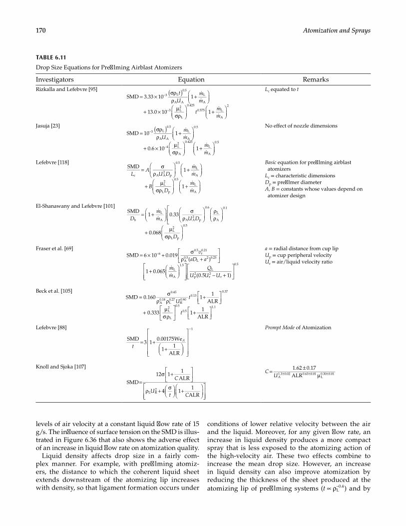
170 Atomization and Sprays

levels of air velocity at a constant liquid flow rate of 15 g/s. The influence of surface tension on the SMD is illus-trated in Figure 6.36 that also shows the adverse effect of an increase in liquid flow rate on atomization quality.

Liquid density affects drop size in a fairly com-plex manner. For example, with prefilming atomiz-ers, the distance to which the coherent liquid sheet extends downstream of the atomizing lip increases with density, so that ligament formation occurs under

conditions of lower relative velocity between the air and the liquid. Moreover, for any given flow rate, an increase in liquid density produces a more compact spray that is less exposed to the atomizing action of the high-velocity air. These two effects combine to increase the mean drop size. However, an increase in liquid density can also improve atomization by reducing the thickness of the sheet produced at the atomizing lip of prefilming systems t( )L

0.4∝ ρ− and by

TABLE 6.11

Drop Size Equations for Prefilming Airblast Atomizers

Investigators Equation RemarksRizkalla and Lefebvre [95]

SMD 3.33 10 1

13.0 10 1

3 L0.5

A A

L

A

3 L2

L

0.425

0.575 L

A

2

tU

mm

tmm

( )= ×σρρ

+

+ × µσρ

+

−

−

Lc equated to t

Jasuja [23]SMD 10 1

0.6 10 1

3 L0.5

A A

L

A

0.5

4 L2

A

0.425L

A

0.5U

mm

mm

( )=σρρ

+

+ × µσρ

+

−

−

No effect of nozzle dimensions

Lefebvre [118]SMD

1

1

c A A2

p

0.5

L

A

L2

L p

0.5

L

A

LA

U Dmm

BD

mm

= σρ

+

+ µσρ

+

Basic equation for prefilming airblast atomizers

Lc = characteristic dimensionsDp = prefilmer diameterA, B = constants whose values depend on atomizer design

El-Shanawany and Lefebvre [101]SMD

1 0.33

0.068

h

L

A A A2

p

0.6

L

A

0.1

L2

L p

0.5

Dmm U D

D

= +

σρ

ρρ

+ µσρ

Fraser et al. [69]SMD 6 10 0.019

( )

1 0.065(0.5 1)

60.5

r0.21

A0.5

L2 0.25

L

A

1.5L

p2

r2

r

0.5

vaD a

mm

QU U U

= × + σρ +

+

− +

−a = radial distance from cup lipUp = cup peripheral velocityUr = air/liquid velocity ratio

Beck et al. [105]= σ

ρ ρ+

+ µσρ

+

SMD 0.160 11

ALR

0.333 11

ALR

0.45

A0.18

L0.27

R0.90

0.130.37

L2

L

0.5

0.51.1

Ut

t

Lefebvre [88]

= ++

−

SMD3 1

0.00175We

11

ALR

1

tA

Prompt Mode of Atomization

Knoll and Sjoka [107]

SMD12 1

1ALR

4 11

ALRL R2

C

Ut C

=σ +

ρ + σ

+

CU

1.62 0.17ALRA

1.3 0.02 0.63 0.01L0.30 0.01=

±µ± ± ±

171Atomizer Performance

increasing the relative velocity UR for plain-jet noz-zles. The net effect of these conflicting factors is that the influence of liquid density on SMD is fairly small, as illustrated in Figure 6.37.

Air Properties. Of all the various factors influencing mean drop size, air velocity is undoubtedly the most important. This is very clear from inspection of Figures 6.35, 6.37, and 6.38. For low-viscosity liquids, the SMD is roughly inversely proportional to the air velocity. This underlines the importance, in airblast atomizer design, of arranging for the liquid to be exposed to the highest possible air velocity consistent with the available pres-sure drop.

The effects of air pressure and temperature on mean drop size are illustrated in Figures 6.39 and 6.40, respectively, for kerosene and water. These results, taken together, strongly suggest that for prefilming atomizers the SMD is proportional to air density to the −0.6 power.

For prefilming atomizers the SMD increases with an increase in atomizer scale (size) according to the rela-tionship SMD Lc

0.4∝ .

Analysis of Drop Size Relationships

From inspection of all the experimental data on pre-filming airblast atomizers, some general conclusions concerning the effects of air and liquid properties

on mean drop size can be drawn. For liquids of low viscosity, such as water and kerosene, the main fac-tors governing the SMD are surface tension, air den-sity, and air velocity; for liquids of high viscosity the effects of air properties are less significant, and the SMD becomes more dependent on the liquid proper-ties, especially viscosity.

The fact that viscosity has an effect quite separate from that of air velocity, as observed experimentally by Nukiyama and Tanasawa [83], Kim and Marshall [117], Lefebvre et al. [95,99,101], and Jasuja [23], suggests a form of equation in which the SMD is expressed as the sum of two terms, one dominated by air velocity and air density and the other by liquid viscosity. For prefilming types of atomizer, it can be shown [118] that

= ′ σρ

+ ′ µσρ

+

SMD

11

ALR

c A A2

p

0.5

L2

L p

0.5

LA

U D

BD

(6.91)

where A′ and B′ are constants whose value depends on the atomizer design and must be determined experimentally.

Equation 6.91 is a basic equation for the mean drop size of the prefilming airblast atomizer. It shows that

TABLE 6.12

Drop Size Equations for Miscellaneous Airblast Atomizers

Investigators Equation Remarks

Gretzinger and Marshall [116]U L

mm

MMD 2.6 10 3 A

A A

0.4L

A

0.4

= × µρ

−L = diameter of wetted peripheryDrop size independent of liquid viscosity but dependent on air viscosity

Ingebo and Foster [108] dU

SMD 5.0 L 02

A R3

L

0.25

= σµρ ρ

For cross-current breakup

Kim and Marshall [117]U A

mm

IU

m

MMD 5.36 10( )

3.44 10

30.41

L0.32

A R2 0.57 0.36

L0.16

3 L2

L

0.17A

L R0.54

= × σ µρ ρ

+ × µσρ

−

−

A = flow area of atomizing airstreamm = −1 at m m 3A L <m = −0.5 at m m 3A L >

Weiss and Worsham [115] U dU

SMD L0.08

o0.16

L0.34

A0.30

R1.33∝ µ

ρ

Cross-stream and costream injection

Ingebo [114] U P

U P

SMD 2.67 10

4.11 10

4L A

0.33

6A A A

0.75 1

()

= ×

+ × ρ

−

− −

Splash plate injector

Song et al. [112] dq= ρ

ρ

µµ

−

SMD0.267 Weo 0.44 0.08 L

A

0.30L

A

0.16 Jet in Crossflow

Bolszo et al. [113]

d

y

dq( )= × − − −SMD

9.33 10 We Reo

71.173

0.419 1.711A

2.087Jet in Crossflow

172 Atomization and Sprays

the SMD is proportional to the characteristic dimen-sion Lc, which represents the linear scale of the atom-izer. Equation 6.91 also shows that mean drop size is inversely proportional to the square root of the pre-filmer lip diameter Dp. This is not surprising; if other parameters are kept constant, an increase in Dp will reduce the liquid film thickness at the atomizing lip and hence the SMD. The implication of this result for atom-izer design is clear—for any given atomizer size (i.e., for any given value of Lc), the ratio Dp/Lc should be made as large as possible.

In practice, some secondary factors, such as liquid stream Reynolds number and airstream Mach number, affect the atomization process in a manner that is not yet fully understood. Thus, the ability of Equation 6.91 to predict mean drop diameters can be improved by rais-ing the exponent of the term U DL A A

2pσ ρ from 0.5 to 0.6.

Moreover, high-speed photographs of the atomization process have shown that for prefilming atomizers the effect of an increase in  ρ L/ ρ A is to extend the distance downstream of the atomizing lip at which sheet disinte-gration occurs, so that it takes place in a region of lower relative velocity [119]. Analysis of the experimental data shows that this effect may be accommodated by introduc-ing into Equation 6.91 the dimensionless term ( ρ L/ ρ A)0.1. With these modifications Equation 6.91 becomes

SMD1

1ALR

11

ALR

c A A2

p

0.6

L

A

0.1

L2

L p

0.5L

AU D

BD

= σρ

ρρ

+

+ µσρ

+

(6.92)

A logical choice for the characteristic dimension Lc is the hydraulic mean diameter of the atomizer air duct at its exit plane (see Figure 6.34). Equating Lc to Dh and substituting into Equation 6.92 the values of A and B derived from the experimental data of reference [101] yields Equation 6.70.

Summary of the Main Points

From the experimental data obtained by many workers on many different types of airblast atomizer, the follow-ing conclusions are drawn:

1. The mean drop size of the spray increases with increasing liquid viscosity and surface tension and with decreasing air/liquid ratio. Ideally, the air/liquid mass ratio should exceed 3, but little improvement in atomization quality is gained by raising this ratio above a value of about 5.

2. Liquid density appears to have little effect on the mean drop size. For prefilming nozzles,

the mean drop size increases slightly with an increase in liquid density; for plain-jet nozzles, the opposite effect is observed.

3. The air properties of importance in airblast atomization are density and velocity. In general, the mean drop size is roughly inversely pro-portional to air velocity. The effect of air den-sity may be expressed as SMD n

A∝ ρ− , where n is about 0.3 for plain-jet atomizers and between 0.6 and 0.7 for prefilming types.

4. For plain-jet nozzles, the initial liquid jet diam-eter has little effect on mean drop size for liq-uids of low viscosity, but for high-viscosity liquids the atomization quality deteriorates with increasing jet size.

5. For prefilming atomizers, the mean drop size increases with increasing atomizer scale (size) according to the relationship SMD Lc

0.4∝ . 6. For any given size of prefilming atomizer (i.e.,

for any fixed value of Lc), the finest atomization is obtained by making the prefilmer lip diam-eter Dp as large as possible. This is because an increase in Dp reduces the liquid film thick-ness t, which in turn reduces the mean drop size t(SMD )0.4∝ .

7. Minimum drop sizes are obtained using atom-izers designed to provide maximum physical contact between the air and the liquid. With prefilming systems the best atomization is obtained by producing the thinnest possible liq-uid sheet of uniform thickness. It is also impor-tant to ensure that the liquid sheet formed at the atomizing lip is subjected to high-velocity air on both sides. This not only provides the finest atomization, but also eliminates droplet deposi-tion on adjacent solid surfaces.

8. The performance of prefilming atomizers is superior to that of plain-jet types, especially under adverse conditions of low air/liquid ratio and/or low air velocity.

9. At least two different mechanisms are involved in airblast atomization, and the relative impor-tance of each depends mainly on the liquid vis-cosity. When a low-viscosity liquid is injected into a low-velocity airstream, waves are pro-duced on the liquid surface; this surface becomes unstable and disintegrates into fragments. The fragments then contract into ligaments, which in turn break down into drops. With increased air velocity, the liquid sheet disintegrates earlier, so ligaments are formed nearer the lip. These ligaments tend to be thinner and shorter and disintegrate into smaller drops. With liquids of

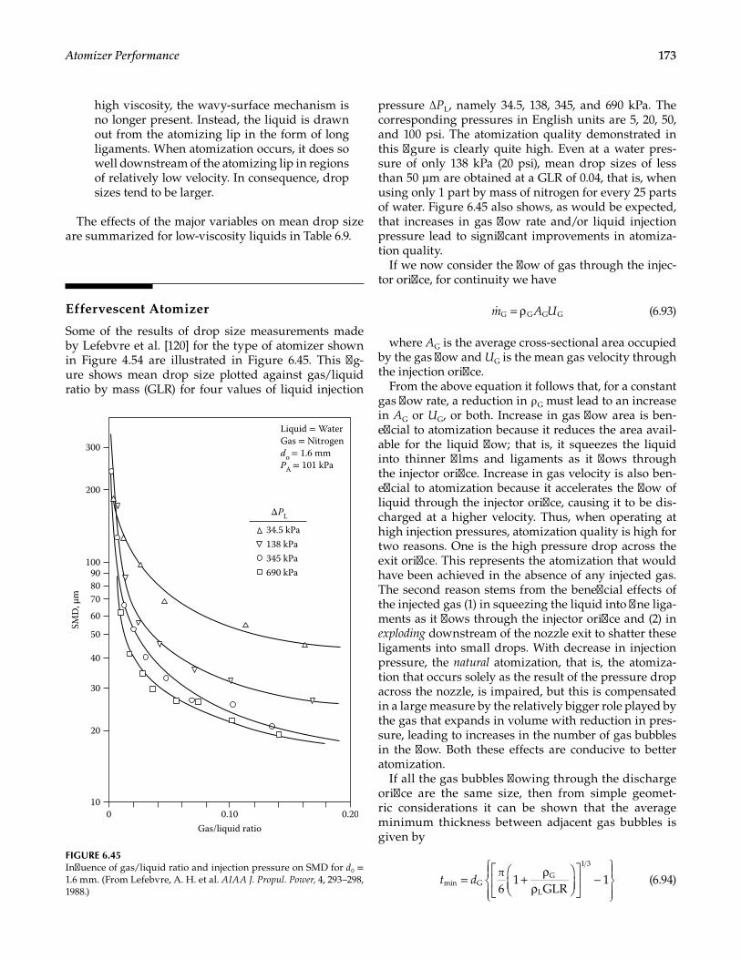
173Atomizer Performance

high viscosity, the wavy-surface mechanism is no longer present. Instead, the liquid is drawn out from the atomizing lip in the form of long ligaments. When atomization occurs, it does so well downstream of the atomizing lip in regions of relatively low velocity. In consequence, drop sizes tend to be larger.

The effects of the major variables on mean drop size are summarized for low-viscosity liquids in Table 6.9.

Effervescent Atomizer

Some of the results of drop size measurements made by Lefebvre et al. [120] for the type of atomizer shown in Figure 4.54 are illustrated in Figure 6.45. This fig-ure shows mean drop size plotted against gas/liquid ratio by mass (GLR) for four values of liquid injection

pressure ∆PL, namely 34.5, 138, 345, and 690 kPa. The corresponding pressures in English units are 5, 20, 50, and 100 psi. The atomization quality demonstrated in this figure is clearly quite high. Even at a water pres-sure of only 138 kPa (20 psi), mean drop sizes of less than 50 μm are obtained at a GLR of 0.04, that is, when using only 1 part by mass of nitrogen for every 25 parts of water. Figure 6.45 also shows, as would be expected, that increases in gas flow rate and/or liquid injection pressure lead to significant improvements in atomiza-tion quality.

If we now consider the flow of gas through the injec-tor orifice, for continuity we have

m A U= ρG G G G (6.93)

where AG is the average cross-sectional area occupied by the gas flow and UG is the mean gas velocity through the injection orifice.

From the above equation it follows that, for a constant gas flow rate, a reduction in  ρ G must lead to an increase in AG or UG, or both. Increase in gas flow area is ben-eficial to atomization because it reduces the area avail-able for the liquid flow; that is, it squeezes the liquid into thinner films and ligaments as it flows through the injector orifice. Increase in gas velocity is also ben-eficial to atomization because it accelerates the flow of liquid through the injector orifice, causing it to be dis-charged at a higher velocity. Thus, when operating at high injection pressures, atomization quality is high for two reasons. One is the high pressure drop across the exit orifice. This represents the atomization that would have been achieved in the absence of any injected gas. The second reason stems from the beneficial effects of the injected gas (1) in squeezing the liquid into fine liga-ments as it flows through the injector orifice and (2) in exploding downstream of the nozzle exit to shatter these ligaments into small drops. With decrease in injection pressure, the natural atomization, that is, the atomiza-tion that occurs solely as the result of the pressure drop across the nozzle, is impaired, but this is compensated in a large measure by the relatively bigger role played by the gas that expands in volume with reduction in pres-sure, leading to increases in the number of gas bubbles in the flow. Both these effects are conducive to better atomization.

If all the gas bubbles flowing through the discharge orifice are the same size, then from simple geomet-ric considerations it can be shown that the average minimum thickness between adjacent gas bubbles is given by

t dπ6

1GLR

1min GG

L

1 3

= + ρρ

−

(6.94)

SMD

, μm

Liquid = WaterGas = Nitrogendo = 1.6 mmPA = 101 kPa

0 0.10 0.2010

20

30

40

50

60

708090

100

200

300

Gas/liquid ratio

ΔPL

34.5 kPa138 kPa345 kPa690 kPa

FIGURE 6.45Influence of gas/liquid ratio and injection pressure on SMD for d0 = 1.6 mm. (From Lefebvre, A. H. et al. AIAA J. Propul. Power, 4, 293–298, 1988.)

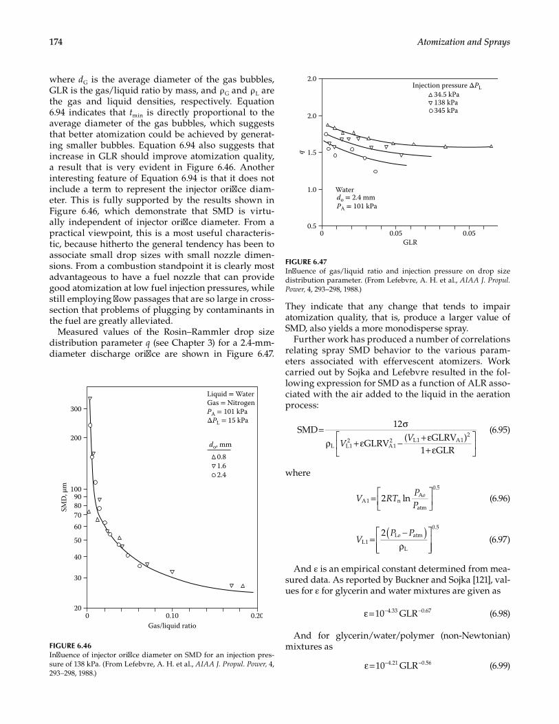
174 Atomization and Sprays

where dG is the average diameter of the gas bubbles, GLR is the gas/liquid ratio by mass, and  ρ G and  ρ L are the gas and liquid densities, respectively. Equation 6.94 indicates that tmin is directly proportional to the average diameter of the gas bubbles, which suggests that better atomization could be achieved by generat-ing smaller bubbles. Equation 6.94 also suggests that increase in GLR should improve atomization quality, a result that is very evident in Figure 6.46. Another interesting feature of Equation 6.94 is that it does not include a term to represent the injector orifice diam-eter. This is fully supported by the results shown in Figure 6.46, which demonstrate that SMD is virtu-ally independent of injector orifice diameter. From a practical viewpoint, this is a most useful characteris-tic, because hitherto the general tendency has been to associate small drop sizes with small nozzle dimen-sions. From a combustion standpoint it is clearly most advantageous to have a fuel nozzle that can provide good atomization at low fuel injection pressures, while still employing flow passages that are so large in cross-section that problems of plugging by contaminants in the fuel are greatly alleviated.

Measured values of the Rosin–Rammler drop size distribution parameter q (see Chapter 3) for a 2.4-mm-diameter discharge orifice are shown in Figure 6.47.

They indicate that any change that tends to impair atomization quality, that is, produce a larger value of SMD, also yields a more monodisperse spray.

Further work has produced a number of correlations relating spray SMD behavior to the various param-eters associated with effervescent atomizers. Work carried out by Sojka and Lefebvre resulted in the fol-lowing expression for SMD as a function of ALR asso-ciated with the air added to the liquid in the aeration process:

V

VSMD

12

GLRV( GLRV )

1 GLRL L12

A12 L1 A1

2= σ

ρ + ε − + ε+ ε

(6.95)

where

V RTPP

o2 lnA1 nA

atm

0.5

=

(6.96)

VP Po2

L1L atm

L

0.5( )=−

ρ

(6.97)

And ε is an empirical constant determined from mea-sured data. As reported by Buckner and Sojka [121], val-ues for ε for glycerin and water mixtures are given as

10 GLR4.33 0.67ε= − − (6.98)

And for glycerin/water/polymer (non-Newtonian) mixtures as

10 GLR4.21 0.56ε= − − (6.99)

Gas/liquid ratio0 0.10 0.20

20

30

40

50

60708090

100

200

300

1.60.8

2.4

Liquid = WaterGas = NitrogenPA = 101 kPaΔPL = 15 kPa

do, mm

SMD

, μm

FIGURE 6.46Influence of injector orifice diameter on SMD for an injection pres-sure of 138 kPa. (From Lefebvre, A. H. et al., AIAA J. Propul. Power, 4, 293–298, 1988.)

Injection pressure ΔPL

Water

GLR

q

0 0.05 0.050.5

1.0

1.5

2.0

2.0

345 kPa

34.5 kPa138 kPa

do = 2.4 mmPA = 101 kPa

FIGURE 6.47Influence of gas/liquid ratio and injection pressure on drop size distribution parameter. (From Lefebvre, A. H. et al., AIAA J. Propul. Power, 4, 293–298, 1988.)

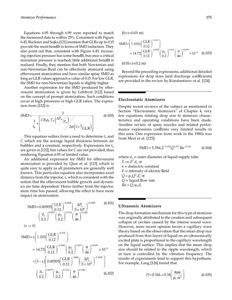
175Atomizer Performance

Equations 6.95 through 6.99 were reported to match the measured data to within 25%. Consistent with Figure 6.45, Buckner and Sojka [121] mention that GLRs up to 0.15 provide the most benefit in terms of SMD reduction. They also point out that, consistent with Figure 6.45, increas-ing injection pressure has some benefit, but once a critical minimum pressure is reached, little additional benefit is realized. Finally, they mention that both Newtonian and non-Newtonian fluid can be effectively atomized using effervescent atomization and have similar spray SMD as long as GLR values approach a value of 0.15. For low GLR, the SMD for non-Newtonian liquids is slightly higher.

Another expression for the SMD produced by effer-vescent atomization is given by Lefebvre [122] based on the concept of prompt atomization. Such conditions occur at high pressures or high GLR ratios. The expres-sion from [122] is

t

CR T PP

SMD3

12 1 1

GLRb

L AA

A( )( )

=

+ρ ∆

σ +

(6.100)

This equation suffers from a need to determine tb and C which are the average liquid thickness between air bubbles and a constant, respectively. Expressions for tb are given in [122], but values for C are not provided, thus rendering Equation 6.95 of limited value.

An additional expression for SMD for effervescent atomization is provided by Qian et al. [123] which is quite easy to apply as all parameters are generally well known. This particular equation also incorporates axial distance from the injector, x, which is consistent with the notion that the effervescent bubble growth and dynam-ics are time dependent. Hence farther from the injector, more time has passed, allowing the effect to have more impact on atomization:

SMD 0.00505

0.12 5 10

0.2 0.2 46

0.4686L

6

0.1805

o0.6675

L0.1714 0.1382

GLR P

d

=

∆×

µ

σ

− − (6.101)

(x → 0)

SMD 1.103GLR0.12

14.72GLR0.12 0.2 46

10

1 0.00505GLR0.12 5 10

0.2 0.2 46

0.218

0.3952L

0.1571 0.81994

4686L

6

0.1805

o0.6675

L0.1714 0.1382

( )

=

+

µ

σ

×

+ −

∆×

µ

σ

−

−−

− −

x

xP

d (6.102)

(0<x<0.01 m)

SMD 1.103GLR0.12

14.72GLR0.12 0.2 46

10

0.218

0.3952L

0.1571 0.81994

=

+

µ

σ

×

−

−−

x

(6.103)

(0.01<x<0.2 m)

Beyond the preceding expressions, additional detailed expressions for drop sizes (and discharge coefficients) are provided in the review by Konstantinov et al. [124].

Electrostatic Atomizers

Despite recent reviews of the subject as mentioned in Section “Electrostatic Atomizers” of Chapter 4, very few equations relating drop size to atomizer charac-teristics and operating conditions have been made. Another review of spray nozzles and related perfor-mance expressions confirms very limited results in this area. One expression from work in the 1980s was from Mori et al. [125]:

d E QSMD 5.39 Reo0.255 0.277 0.124= − − (6.104)

where do = outer diameter of liquid supply tubeE E d2

o=∈ σ∊ = dielectric constantE = intensity of electric field

L2

o3= ρ σQ Q d

Q = liquid flow rateQ doRe L= µ

Ultrasonic Atomizers

The drop formation mechanism for this type of atomizer was originally attributed to the creation and subsequent collapse of cavities caused by the intense sound wave. However, more recent opinion favors a capillary wave theory based on the observation that the mean drop size produced from thin layers of liquid on an ultrasonically excited plate is proportional to the capillary wavelength on the liquid surface. This implies that the mean drop size should be related to the ripple wavelength, which in turn is controlled by the vibration frequency. The results of experiments tend to support this hypothesis. For example, Lang [126] found that

D 0.34 0.348

L2= λ = πσ

ρ ω

(6.105)

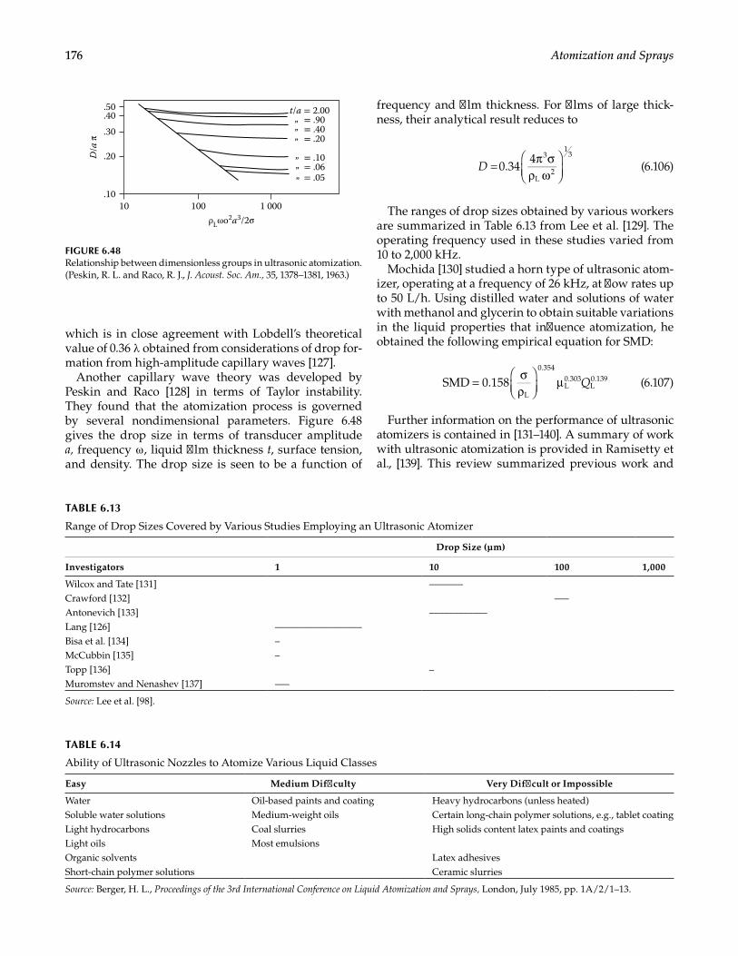
176 Atomization and Sprays

which is in close agreement with Lobdell’s theoretical value of 0.36  λ  obtained from considerations of drop for-mation from high-amplitude capillary waves [127].

Another capillary wave theory was developed by Peskin and Raco [128] in terms of Taylor instability. They found that the atomization process is governed by several nondimensional parameters. Figure 6.48 gives the drop size in terms of transducer amplitude a, frequency  ω , liquid film thickness t, surface tension, and density. The drop size is seen to be a function of

frequency and film thickness. For films of large thick-ness, their analytical result reduces to

D 0.344 3

L2

13

= π σρ ω

(6.106)

The ranges of drop sizes obtained by various workers are summarized in Table 6.13 from Lee et al. [129]. The operating frequency used in these studies varied from 10 to 2,000 kHz.

Mochida [130] studied a horn type of ultrasonic atom-izer, operating at a frequency of 26 kHz, at flow rates up to 50 L/h. Using distilled water and solutions of water with methanol and glycerin to obtain suitable variations in the liquid properties that influence atomization, he obtained the following empirical equation for SMD:

QSMD 0.158L

0.354

L0.303

L0.139= σ

ρ

µ (6.107)

Further information on the performance of ultrasonic atomizers is contained in [131–140]. A summary of work with ultrasonic atomization is provided in Ramisetty et al., [139]. This review summarized previous work and

10ρLωo2a3/2σ

D/a

π

100 1 000.10

.20

.30

.40

.50= .90

t/a = 2.00

= .40= .20

= .10= .06= .05

„„„

„„„

FIGURE 6.48Relationship between dimensionless groups in ultrasonic atomization. (Peskin, R. L. and Raco, R. J., J. Acoust. Soc. Am., 35, 1378–1381, 1963.)

TABLE 6.13

Range of Drop Sizes Covered by Various Studies Employing an Ultrasonic Atomizer

Drop Size (μm)

Investigators 1 10 100 1,000

Wilcox and Tate [131] –––––––Crawford [132] –––Antonevich [133] ––––––––––––Lang [126] ––––––––––––––––––Bisa et al. [134] –McCubbin [135] –Topp [136] –Muromstev and Nenashev [137] –––

Source: Lee et al. [98].

TABLE 6.14

Ability of Ultrasonic Nozzles to Atomize Various Liquid Classes

Easy Medium Difficulty Very Difficult or Impossible

Water Oil-based paints and coating Heavy hydrocarbons (unless heated)Soluble water solutions Medium-weight oils Certain long-chain polymer solutions, e.g., tablet coatingLight hydrocarbons Coal slurries High solids content latex paints and coatingsLight oils Most emulsionsOrganic solvents Latex adhesivesShort-chain polymer solutions Ceramic slurries

Source: Berger, H. L., Proceedings of the 3rd International Conference on Liquid Atomization and Sprays, London, July 1985, pp. 1A/2/1–13.

177Atomizer Performance

correlations and also obtained new data for a wide range of conditions. The resulting correlation produced is

D N N N=πσ

ρ ω

+πσ

ρ ω

− −0.00154 0.00154L

2

0.33

L2

0.33

Oh0.111

We0.154

In0.33

(6.108)

where

Nd

NQ

Nd

cQ= µ

ω ρ=

ω ρσ

=ω

; ;OhL

tip2

LWe

L LIn

2tip4

L

Ramisetty et al. [139] present a comparison of pre-dicted and measured drop size data for Equations 6.105, 6.106, and 6.108 along with that by Ranjan and Pandit [140]. The performance of Equation 6.108 is far superior to the other correlations in terms of matching measured data. Ramisetty et al. [139] attributes this to previous correlations developed for specific sets of atomizer con-ditions and a lack of variation in frequency in the pre-vious work. It is evident from Equation 6.108 that the frequency is very important in determining drop size.

Ultrasonic atomization can be quite flexible in terms of the liquid used. However, the degree of difficulty involved in the atomization of various classes of liquids is indicated in Table 6.14.

Nomenclature

Ao discharge orifice area, m2

Ap total inlet ports area, m2

As swirl chamber area, m2

ALR air/liquid mass ratioc root mean square molecular velocity, m/sD drop diameter, mDh hydraulic mean diameter of air exit duct, mDp prefilmer diameter, mDs swirl chamber diameter, md disk diameter, mdo discharge orifice diameter, mdl subcritical ligament diameter, mF charging factorFN flow number m P[ ( ) ]L L L

0.5= ∆ ρ , m2

g acceleration due to gravity, 0.98 m/s2

GLR gas to liquid ratio (mass)l mean free path, mLc characteristic dimension of airblast atomizer, mLs length of swirl chamber, m

MMD mass median diameter, m  flow rate, kg/snh number of holesN rotational speed, rpsP pressure, PaPAo Pressure of air within nozzle, Pa∆PL injection pressure differential across nozzle, Paq momentum flux ratio,Q volumetric flow rate, m3/sR disk radius, mRe Reynolds numberReL Reynolds number based on liquid properties

(= UL ρ Ldo /μL)RΩ2 centrifugal acceleration, m/s2

SMD Sauter mean diameter, ms downstream distance of measuring plane from

nozzleT temperature, Kt film thickness in final orifice, mts initial sheet thickness at nozzle exit, mU velocity, m/sVA1 velocity of air at nozzle exit, m/sVL1 velocity of liquid at nozzle exit, m/sWe Weber numberWeL Weber number based on liquid properties

U d( )L L2

o= ρ σ

x stream-wise distance, mw rotational speed, radians/sε fraction of air exiting nozzle that transfers all its

kinetic energy to the spray λ  wavelength, m ω  excitation frequencyμ dynamic viscosity, kg/m sΛ radial spatial integral length scale, my direction perpendicular to wall, mv kinematic viscosity, m2/s ρ  density, kg/m3

 σ  surface tension, kg/s2

Subscripts

A airL liquidR air relative to liquidG gasl ligamentex exit

178 Atomization and Sprays

References

1. Jenny, P., Roekaerts, D., and Beishuizen, N., Modeling of turbulent dilute spray combustion, Prog. Energ. Combust. Sci., Vol. 28, 2012, pp. 846–867.

2. Jiang, X., Siamas, G., Jagus, K., and Karyiannis, T., Physical modelling and advanced simulations of gas-liquid two-phase jet flows in atomization and sprays, Prog. Energ. Combust. Sci., Vol. 36, 2010 pp. 131–167.

3. Gutheil, E., Issues in computational studies of turbulent spray combustion, in: Merci, B., Roekaerts, D., Sadiki, A., (eds.), Experiments and Numerical Simulations of Diluted Spray Turbulent Combustion. New York, NY: Springer-Verlag; 2011.

4. Gorokhovski, M., and Herrmann, M., Modeling primary atomization, Annu. Rev. Fluid Mech., Vol. 40, 2008, pp. 343–366.

5. Xue, Q., Som, S., Senecal, P. K., and Pomraning, E., Large eddy simulation of fuel-spray under non-reacting IC engine conditions, Atomization Sprays, 10, 2013, pp. 925–955.

6. Rizk, N. K., and Lefebvre, A. H., Drop-size distribution characteristics of spill-return atomizers, AIAA J. Propul. Power, Vol. 1, No. 1, 1985, pp. 16–22.

7. Wu, P. -K., and Faeth, G. M., Aerodynamic effects on pri-mary breakup of turbulent liquids, Atomization Sprays, Vol. 3, 1993, pp. 265–289.

8. Merrington, A. C., and Richardson, E. G., The break-up of liquid jets, Proc. Phys. Soc. London, Vol. 59, No. 33, 1947, pp. 1–13.

9. Panasenkov, N. J., Effect of the turbulence of a liquid jet on its atomization Zh. Tekh. Fiz., Vol. 21, 1951, p. 160.

10. Harmon, D. B., Drop sizes from low-speed jets J. Franklin Inst., Vol. 259, 1955, p. 519.

11. Giffen, E., and Lamb, T. A. J., The effect of air density on spray atomization, Motor Industry Research Association Report 1953/5, 1953.

12. Miesse, C. C., Correlation of experimental data on the disintegration of liquid jets, Ind. Eng. Chem., Vol. 47, No. 9, 1955, pp. 1690–1701.

13. Tanasawa, Y., and Toyoda, S., On the atomization of a liquid jet issuing from a cylindrical nozzle, Tech. Report of Tohoku University, Japan, No. 19–2, 1955, p. 135.

14. Hiroyasu, H., and Katoda, T., Fuel droplet size distribu-tion in a diesel combustion chamber, SAE Trans., Paper 74017, 1974.

15. Elkotb, M. M., Fuel atomization for spray modeling, Prog. Energy Combust. Sci., Vol. 8, No. 1, 1982, pp. 61–91.

16. Sallam, K. A., and Faeth, G. M., Surface properties dur-ing primary breakup of turbulent liquid jets in still air, AIAA J., Vol. 41, 2003, pp. 1514–1524.

17. Dumochel, C., On the experimental investigation on pri-mary atomization of liquid streams, Exp. Fluids, Vol. 45, 2008, pp. 371–422.

18. Jones, A. R., Design optimization of a large pressure-jet atomizer for power plant, in: Proceedings of the 2nd International Conference on Liquid Atomization and Sprays, Madison, Wisconsin, 1982, pp. 181–185.

19. Simmons, H. C., and Harding, C. F., Some effects on using water as a test fluid in fuel nozzle spray analysis, ASME Paper 80-GT-90, 1980.

20. Kennedy, J. B., High weber number SMD correlations for pressure atomizers, ASME Paper 85-GT-37, 1985.

21. Lefebvre, A. H., Gas Turbine Combustion, Washington, DC: Hemisphere, 1983.

22. Wang, X. F., and Lefebvre, A. H., Mean drop sizes from pressure-swirl nozzles, AIAA J. Propul. Power, Vol. 3, No. 1, 1987, pp. 11–18.

23. Jasuja, A. K., Atomization of crude and residual fuel oils, ASME J. Eng. Power, Vol. 101, No. 2, 1979, pp. 250–258.

24. Radcliffe, A., Fuel injection, High Speed Aerodynamics and Jet Propulsion, Vol XI, Sect. D, Princeton, NJ: Princeton University Press, 1960.

25. Dodge, L. G., and Biaglow, J. A., Effect of elevated tem-perature and pressure on sprays from simplex swirl atomizers, ASME Paper 85-GT-58, 1985.

26. Simmons, H. C., The prediction of Sauter mean diameter for gas turbine fuel nozzles of different types, ASME Paper 79-WA/GT-5, 1979.

27. Knight, B. E., Communication on the performance of a type of swirl atomizer, by A. Radcliffe, Proc. Inst. Mech. Eng., Vol. 169, 1955, p. 104.

28. Rizk, N. K., and Lefebvre, A. H., Spray characteristics of simplex swirl atomizers, in: Bowen, J. R., Manson, N., Oppenheim, A. K., and Soloukhin, R. I. (eds.), Dynamics of Flames and Reactive Systems, Prog. Astronaut. Aeronaut., Vol. 95, 1985, pp. 563–580.

29. Abou-Ellail, M. M. M., Elkotb, M. M., and Rafat, N. M., Effect of fuel pressure, air pressure and air tem-perature on droplet size distribution in Hollow-Cone Kerosine sprays, in: Proceedings of the 1st International Conference on Liquid Atomization and Spray Systems, Tokyo, 1978, pp. 85–92.

30. De Corso, S. M., Effect of ambient and fuel pressure on spray drop size, ASME J. Eng. Power, Vol. 82, 1960, p. 10.

31. Hinze, J. O., Critical speeds and sizes of liquid globules, Appl. Sci. Res., Vol. VA-l, 1948, p. 273.

32. Lane, W. R., Shatter of drops in streams of air, Ind. Eng. Chem., Vol. 43, 1951, pp. 1312–1317.

33. De Corso, S. M., and Kemeny, G. A., Effect of ambient and fuel pressure on nozzle spray angle, Trans. ASME., Vol. 79, No. 3, 1957, pp. 607–615.

34. Neya, K., and Sato, S., Effect of ambient air pressure on the spray characteristics of swirl atomizers, Ship Research Institute, Tokyo, Paper 27, 1968.

35. Rizk, N. K., and Lefebvre, A. H., Spray characteristics of spill-return atomizer, AIAA J. Propul. Power, Vol. 1, No. 3, 1985, pp. 200–204.

36. Wang, X. F., and Lefebvre, A. H., Influence of ambient air pressure on pressure-swirl atomization, in: Paper Presented at the 32nd ASME International Gas Turbine Conference, Anaheim, California, June 1987.

37. Ortman, J., and Lefebvre, A. H., Fuel distributions from pressure-swirl atomizers, AIAA J. Propul. Power, Vol. 1, No. 1, 1985, pp. 11–15.

38. York, J. L., Stubbs, H. E., and Tek, M. R., The mechanism of disintegration of liquid sheets, Trans. ASME, Vol. 75, No. 7, 1953, pp. 1279–1286.

39. Hagerty, W. W., and Shea, J. F., A study of the stabil-ity of plane fluid sheets, J. Appl. Mech., Vol. 22, 1955, pp. 509–514.

179Atomizer Performance

40. Dombrowski, N., and Johns, W. R., The Aerodynamic instability and disintegration of viscous liquid sheets, Chem. Eng. Sci., Vol. 18, 1963, pp. 203–214.

41. Elkotb, M. M., Rafat, N. M., and Hanna, M. A., The influ-ence of swirl atomizer geometry on the atomization performance, in: Proceedings of the 1st International Conference on Liquid Atomization and Spray Systems, Tokyo, 1978, pp. 109–115.

42. Needham, H. C, Power Jets R&D Report, No. R1209, 1946.

43. Joyce, J. R., Report ICT 15, Shell Research Ltd., London, 1949.

44. Turner, G. M., and Moulton, R. W., Drop-size Distributions from Spray Nozzle Chem. Eng. Prog., Vol. 49, 1943, p. 185.

45. Babu, K. R., Narasimhan, M. V., and Narayanaswamy, K., Prediction of mean drop size of fuel sprays from swirl spray atomizers, in: Proceedings of the 2nd International Conference on Liquid Atomization and Sprays, Madison, Wisconsin, 1982, pp. 99–106.

46. Lefebvre, A. H., The prediction of Sauter mean diameter for simplex pressure-swirl atomizers, Atomization Spray Technol., Vol. 3, No. 1, 1987, pp. 37–51.

47. Ohnesorge, W., Formation of drops by nozzles and the breakup of liquid jets, Z. Angew. Math. Mech., Vol. 16, 1936.

48. Suyari, M., and Lefebvre, A. H., Film thickness measure-ments in a simplex swirl atomizer, AIAA J. Propul. Power, Vol. 2, No. 6, 1986, pp. 528–533.

49. Omer, K., and Ashgriz, N., Spray nozzles, in: Ashgriz, N. (ed.), in Handbook of Atomization and Sprays, Chap. 24. New York: Springer, 2011.

50. Khavkin, Y. I., Theory and Practice of Swirl Atomizers. New York: Taylor & Francis, 2004.

51. Hinze, J. O., and Milborn, H., Atomization of liquids by means of a rotating cup, ASME J. Appl. Mech., Vol. 17, No. 2, 1950, pp. 145–153.

52. Dombrowski, N., and Fraser, R. P., A photographic inves-tigation into the disintegration of liquid sheets, Philos. Trans. R. Soc. London Ser. A, Vol. 247, No. 924, September 1954, pp. 101–130.

53. Tanasawa, Y., Miyasaka, Y., and Umehara, M., On the filamentation of liquid by means of rotating discs, Trans. JSME., Vol. 25, No. 156, 1963, pp. 888–896.

54. Dombrowski, N., and Munday, G., Spray drying, in: Biochemical and Biological Engineering Science, Vol. 2, Chap. 16, New York: Academic Press, 1968, pp. 209–320.

55. Christensen, L. S., and Steely, S. L., Monodisperse atomizers for agricultural aviation applications, NASA CR-159777, February 1980.

56. Eisenklam, P., Recent research and development work on liquid atomization in Europe and the USA, in: Invited Paper to the 5th Conference on Liquid Atomization, Tokyo, 1976.

57. Matsumoto, S., Belcher, D. W., and Crosby, E. J., Rotary atomizers: Performance understanding and predic-tion, in: Proceedings of the 3rd International Conference on Liquid Atomization and Sprays, London, 1985, pp. 1A/1/1–21.

58. Fraser, R. P., Eisenklam, P., Dombrowski, N., and Hasson, D., Drop formation from rapidly moving liquid sheets, AIChEJ., Vol. 8, 1962, pp. 672–680.

59. Willauer, H. D., Mushrush, G. W., and Williams, F. W., Critical evaluation of rotary atomizer, Pet. Sci. Technol., Vo 24, 2006, pp. 1215–1232

60. Karim, G. A., and Kumar, R., The atomization of liquids at low ambient pressure conditions, in: Proceedings of the 1st International Conference on Liquid Atomization and Spray Systems, Tokyo, August 1978, pp. 151–155.

61. Bar, P., Dr. Eng. dissertation, Technical College, Karlsruhe, Germany, 1935.

62. Tanasawa, Y., Miyasaka, Y., and Umehara, M., Effect of shape of rotating disks and cups on liquid atomization, in: Proceedings of the 1st International Conference on Liquid Atomization and Spray Systems, Tokyo, 1978, pp. 165–172.

63. Matsumoto, S., Saito, K., and Takashima, Y. Phenomenal transition of liquid atomization from disk, J. Chem. Eng. Jpn., Vol. 7, 1974, p. 13.

64. Walton, W. H., and Prewett, W. G., The production of sprays and mists of uniform drop size by means of spin-ning disc type sprayers Proc. Phys. Soc. London Sect. B, Vol. 62, 1949, p. 341.

65. Oyama, Y., and Endou, K., On the centrifugal disk atom-ization and studies on the atomization of water drop-lets, Kagaku Kogaku, Vol. 17, 1953, pp. 256–260, 269–275 (in Japanese, English summary).

66. Matsumoto, S., and Takashima, Y., Kagaku Kogaku, Vol. 33, 1969, p. 357.

67. Kayano, A., and Kamiya, T., Calculation of the mean size of the droplets purged from the rotating disk, in: Proceedings of the 1st International Conference on Liquid Atomization and Sprays, Tokyo, 1978, pp. 133–143.

68. Fraser, R. P., and Eisenklam, P., Liquid atomization and the drop size of sprays, Trans. Inst. Chem. Eng., Vol. 34, 1956, pp. 294–319.

69. Fraser, R. P., Dombrowski, N., and Routley, J. H., The production of uniform liquid sheets from spinning cups; the filming by spinning cups; the atomization of a liquid sheet by an impinging air stream, Chem. Eng. Sci., Vol. 18, 1963, pp. 315–321, 323–337, 339–353.

70. Hege, H., Aufbereit. Tech., No. 3, 1969, p. 142. 71. Masters, K., Spray Drying, 2nd ed., New York: John Wiley

& Sons, 1976. 72. Friedman, S. J., Gluckert, F. A., and Marshall, W. R.,

Centrifugal disk atomization Chem. Eng. Prog., Vol. 48, No. 4, 1952, p. 181.

73. Herring, W. H., and Marshall, W. R., Performance of vaned-disk atomizers, J. Am. Inst. Chem. Eng., Vol. 1, No. 2, 1955, p. 200.

74. Fraser, R. P., Eisenklam, P., and Dombrowski, N., Complete simulation of rotary dryers, Br. Chem. Eng., Vol. 2, No. 9, 1957, p. 196.

75. Scott, M. N., Robinson, M. J., Pauls, J. F., and Lantz, R. J. Spray congealing: particle size relationships using a centrifugal wheel atomizer, J. Pharm. Sci., Vol. 53, No. 6, 1964, p. 670.

76. Choi, S. M., Jang, S. H., Lee, D. H., and You, G. W.,. Spray Characteristics of the rotating fuel injection system of a micro-jet engine. J. Mech. Sci. Technol., Vol. 24, No. 2, 2010, pp. 551–558.

180 Atomization and Sprays

77. Dahm, W. J. A., Patel, P. R., and Lerg, B. H., Analysis of liquid breakup regimes in fuel slinger atomization, Atomization and Sprays, Vol. 16, 2006, pp. 945–962.

78. Wigg, L. D., The effect of scale on fine sprays produced by large airblast atomizers, Report No. 236, National Gas Turbine Establishment, Pyestock, England, 1959.

79. Wigg, L. D., Drop-size predictions for twin fluid atom-izers, J. Inst. Fuel, Vol. 27, 1964, pp. 500–505.

80. Clare, H., and Radcliffe, A., An airblast atomizer for use with viscous fuels, J. Inst. Fuel, Vol. 27, No. 165, 1954, pp. 510–515.

81. Wood, R., unpublished work at Thornton Shell Research Center, 1954.

82. Mullinger, P. J., and Chigier, N. A., The design and per-formance of internal mixing multi-jet twin-fluid atom-izers, J. Inst. Fuel, Vol. 47, 1974, pp. 251–261.

83. Nukiyama, S., and Tanasawa, Y., Experiments on the atomization of liquids in an airstream, Trans. Soc. Mech. Eng. Jpn. Vol. 5, 1939, pp. 68–75.

84. Mayer, E., Theory of liquid atomization in high veloc-ity gas streams, Am. Rocket Soc. J., Vol. 31, 1961, pp. 1783–1785.

85. Sakai, T., Kito, M., Saito, M., and Kanbe, T., Characteristics of internal mixing twin-fluid atomizer, in: Proceedings of the 1st International Conference on Liquid Atomization and Sprays, Tokyo, 1978, pp. 235–241.

86. Inamura, T., and Nagai, N., The relative performance of externally and internally-mixed twin-fluid atomizers, in: Proceedings of the 3rd International Conference on Liquid Atomization and Sprays, London, July 1985, pp. IIC/2/1–11.

87. Barreras, F., Lozano, A., Barroso, J., and Lincheta, E., Experimental characterization of industrial twin-fluid atomizers, Atomization Sprays, Vol. 16, 2006, pp. 127–145.

88. Lefebvre, A. H., Energy considerations in twin-fluid atomization, J. Eng. Gas Turbines Power, Vol. 114, 1992, pp. 89–97.

89. Elkotb, M. M., Mahdy, M. A., and Montaser, M. E., Investigation of External-Mixing Air-blast Atomizers, in: Proceedings of the 2nd International Conference on Liquid Atomization and Sprays, Madison, Wisconsin, 1982, pp. 107–115.

90. Suyari, M., and Lefebvre, A. H., Drop-size measurements in air-assist swirl atomizer sprays, in: Paper Presented at Central States Combustion Institute Spring Meeting, NASA-Lewis Research Center, Cleveland, Ohio, May 1986.

91. Rayleigh, L., On the stability of jets, Proc. London Math. Soc., Vol. 10, 1879, pp. 4–13.

92. Lorenzetto, G. E., and Lefebvre, A. H., Measurements of drop size on a plain jet airblast atomizer, AIAA J., Vol. 15, No. 7, 1977, pp. 1006–1010.

93. Rizk, N. K., and Lefebvre, A. H., Influence of airblast atomizer design features on mean drop size, AIAA J., Vol. 21, No. 8, August 1983, pp. 1139–1142.

94. Foust, M.J., Thomsen, D., Stickles, R., Cooper, C., and Dodds, W., Development of the GE aviation low emis-sions TAPS combustor for next generation aircraft engines, Paper AIAA-2012-0936.

95. Rizkalla, A., and Lefebvre, A. H., The influence of air and liquid properties on air blast atomization, ASME J. Fluids Eng., Vol. 97, No. 3, 1975, pp. 316–320.

96. Jasuja, A. K., Plain-jet airblast atomization of alternative liquid petroleum fuels under high ambient air pressure conditions, ASME Paper 82-GT-32, 1982.

97. Rizk, N. K., and Lefebvre, A. H., Spray characteristics of plain-jet airblast atomizers, Trans. ASMEJ. Eng. Gas Turbines Power, Vol. 106, July 1984, pp. 639–644.

98. Lefebvre, A. H., and Ballal, D. R., Gas Turbine Combustion, 3rd ed. Boca Raton, FL: CRC Press.

99. Lefebvre, A. H., and Miller, D., The development of an air blast atomizer for gas turbine application, CoA-Report-AERO-193, College of Aeronautics, Cranfield, England, 1966.

100. Bryan, R., Godbole, P. S., and Norster, E. R., Characteristics of airblast atomizers, in: Norster, E. R. (ed.), Combustion and Heat Transfer in Gas Turbine Systems, Cranfield International Symp. Ser., Vol. 11. New York: Pergamon, 1971, pp. 343–359.

101. El-Shanawany, M. S. M. R., and Lefebvre, A. H., Airblast atomization: The effect of linear scale on mean drop size, J. Energy, Vol. 4, No. 4, 1980, pp. 184–189.

102. Wittig, S., Aigner, M. Sakbani, K, and Sattelmayer, T, Optical measurements of droplet size distributions: Special considerations in the parameter definition for fuel atomizers, in: Paper Presented at AGARD Meeting on Combustion Problems in Turbine Engines, Cesme, Turkey, October 1983. Also Aigner, M., and Wittig, S., Performance and optimization of an airblast nozzle, drop-size distribution and volumetric air flow, in: Proceedings of the 3rd International Conference on Liquid Atomization and Sprays, London, July 1985, pp. IIC/3/1–8.

103. Sattelmayer, T., and Wittig, S., Internal flow effects in prefilming airblast atomizers: Mechanisms of atomiza-tion and droplet spectra, J. Engr Gas Turbine and Power, Vol. 108, 1986, pp. 465–472.

104. Beck, J. E., Lefebvre, A. H., and Koblish, T. R., Airblast atomization at conditions of low air velocity, J. Propul. Power, Vol. 7, 1991, pp. 207–212.

105. Beck, J. E., Lefebvre, A. H., and Koblish, T. R., Liquid sheet disintegration by impinging air streams, Atomization Sprays, Vol. 1, 1991, pp. 155–170.

106. Harari, R., and Sher, E., Optimization of a plain-jet air-blast atomizer, Atomization Sprays, Vol. 7, 1997, pp. 97–113.

107. Knoll, K. E and Sojka, P. E., Flat-sheet twin-fluid atomi-zation of high viscosity fluids. Part I: Newtonian liquids, Atomziation Sprays, Vol. 2, 1992, pp. 17–36.

108. Ingebo, R. D., and Foster, H. H., Drop-size distribution for cross-current break-up of liquid jets in air streams, NACA TN 4087, 1957.

109. Ingebo, R. D., Capillary and acceleration wave breakup of liquid jets in axial flow air-streams, NASA Technical Paper 1791, 1981.

110. Ingebo, R.D., Aerodynamic effect of combustor inlet pressure on fuel jet atomization, J. Propul., Vol. 1, 1985, pp. 137–142.

111. Lee, K., Aalburg, C., Diez, F. J., Faeth, G. M., and Sallam, K. A., Primary breakup of turbulent round liq-uid jets in uniform crossflows, AIAA J., Vol. 45, 2007, pp. 1907–1916.

112. Song, J., Cain, C. C., and Lee, J. G., Liquid jets in subsonic air crossflow at elevated pressure, J. Engr. Gas Turbine and Power, Vol. 137, 2015, pp. 041502–1-12.

181Atomizer Performance

113. Bolszo, C. D., McDonell, V. G., Gomez, G. A., and Samuelsen, G. S., Injection of water-in-oil emulsion jets into a subsonic crossflow: An experimental study, atom-ization and sprays, 24, 2014, pp. 303–348.

114. Ingebo, R. D., Atomization of liquid sheets in high pres-sure airflow, ASME Paper HT-WA/ HT-27, 1984.

115. Weiss, M. A., and Worsham, C. H., Atomization in high velocity air-streams, J. Am. Rocket Soc., Vol. 29, No. 4, 1959, pp. 252–259.

116. Gretzinger, J., and Marshall, W. R. Jr., Characteristics of pneumatic atomization, AIChEJ., Vol. 7, No. 2, 1961, pp. 312–318.

117. Kim, K. Y., and Marshall, W. R., Drop-size distributions from pneumatic atomizers, AIChE J., Vol. 17, No. 3, 1971, pp. 575–584.

118. Lefebvre, A. H., Airblast atomization, Prog. Energy Combust. Sci., Vol. 6, 1980, pp. 233–261.

119. Rizk, N. K., and Lefebvre, A. H., Influence of liquid film thickness on airblast atomization, ASME J. Eng. Power, Vol. 102, July 1980, pp. 706–710.

120. Lefebvre, A. H., Wang, X. F., and Martin, C. A., Spray characteristics of aerated liquid pressure atomizers, AIAA J. Propul. Power, Vol. 4, No. 4, 1988, pp. 293–298.

121. Buckner, H., and Sojka, P., Effervescent atomization of high-viscosity fluids: Part II. Non-Newtonian liquids, Atomization Sprays, Vol. 3, 1993, pp. 157–170.

122. Lefebvre, A.H., Twin-fluid atomization: Factors influencing mean drop size, Atomization Sprays, Vol. 2, 1992, pp. 101–119.

123. Qian, L, Lin, J., and Hongbin, X. A fitting formula for predicting droplet mean diameter for various liquids in effervescent atomization sprays, J. Therm. Spray Technol., Vol. 19, 2010, pp. 586–601.

124. Konstantinov, D., Marsh, R., Bowen, P. and Crayford, A., Effervescent atomization of industrial energy—Technology review, Atomization Sprays, Vol. 20, 2010, pp. 525–552.

125. Mori, Y., Hijikata, K., and Nagasaki, T., Electrostatic atomization for small droplets of uniform diameter, Trans. Jpn. Soc. Mech. Eng. Ser. B, 1981, pp. 1881–1890.

126. Lang, R. S. J., Ultrasonic atomization of liquids, J. Acoust. Soc. Am., Vol. 34, No. 1, 1962, pp. 6–8.

127. Lobdell, D. D., Particle size-amplitude relation for the ultrasonic atomizer, J. Acoust. Soc. Am., Vol. 43, No. 2, 1967, pp. 229–231.

128. Peskin, R. L., and Raco, R. J., Ultrasonic atomization of liquids, J. Acoust. Soc. Am., Vol. 35, No. 9, September. 1963, pp. 1378–1381.

129. Lee, K. W., Putnam, A. A., Gieseke, J. A., Golovin, M. N., and Hale, J. A., Spray nozzle designs for agricultural aviation applications, NASA CR 159702, 1979.

130. Mochida, T., Ultrasonic atomization of liquids, in: Proceedings of the 1st International Conference on Liquid Atomization and Sprays, Tokyo, 1978, pp. 193–200.

131. Wilcox, R. L., and Tate, R. W., Liquid atomization in a high intensity sound field, AIChE J., Vol. 11, No. 1, 1965, pp. 69–72.

132. Crawford, A. E., Production of spray by high power magnetostriction transducers, J. Acoust. Soc. Am., Vol. 27, 1955, p. 176.

133. Antonevich, J., Ultrasonic atomization of liquids, IRE Trans. PGUE, Vol. 7, 1959, pp. 615.

134. Bisa, K., Dirnagl, K., and Esche, R., Zerstaubung von Flussigkeiten mit Ultraschall, Siemens Z., Vol. 28, No. 8, 1954, pp. 341–347.

135. McCubbin, T., Jr., The particle size distribution in fog produced by ultrasonic radiation, J. Acoust. Soc. Am., 1953, pp. 1013–1014.

136. Topp, M. N., Ultrasonic atomization—A photographic study of the mechanism of disintegration, Aerosol. Soc., Vol. 4, 1973, pp. 17–25.

137. Muromtsev, S. N., and Nenashev, V. P., The study of aerosols—III. An ultrasonic aerosol atomizer, J. Microbiol. Epidemiol. Immunobiol., Vol. 31, No. 10, 1960, pp. 1840–1846.

138. Berger, H. L., Characterization of a class of widely applicable ultrasonic nozzles, in: Proceedings of the 3rd International Conference on Liquid Atomization and Sprays, London, July 1985, pp. 1A/2/1–13.

139. Ramisetty, K. A., Pandit, A. B., and Gogate, P. R., Investigations into Ultrasound induced atomization, Ultrason. Sonochem., Vol. 20, 2013, pp. 254–264.

140. Ranjan, R., and Pandit, A. B., Correlations to predict droplet size in ultrasonic atomisation, Ultrasonics, Vol. 39, 2001, pp. 235–255.

183

7External Spray Characteristics

Introduction

In most applications the function of the atomizer is not only to break the liquid down into small drops but also to discharge these drops into the surrounding gaseous medium in the form of a symmetrical, uniform spray. With plain-orifice atomizers the cone angle is narrow and the drops are fairly evenly dispersed throughout the entire spray volume. Sprays of this type are often described as solid. It is possible to produce solid sprays with swirl atomizers, but for most applications the spray is usually in the form of a hollow cone of wide angle, with most of the drops concentrated at the periphery.

In both types of atomizer the liquid jet or sheet rap-idly disintegrates into drops that tend to maintain the general direction of motion of the original jet or cone. However, because of air resistance, the leading drops and the drops formed on the outside of the spray rapidly lose their momentum and form a cloud of finely atom-ized drops suspended around the main body of the spray. Their subsequent dispersion is governed mainly by the prevailing airflow pattern in the spray region.

Because plain-orifice atomizers produce a narrow, compact spray in which only a small proportion of drops are subjected to the effects of air resistance, the distribution of the spray as a whole is dictated mainly by the magnitude and direction of the velocity imparted to it at exit from the atomizer orifice. In contrast, with twin-fluid atomizers of the air-assist and airblast types, the drops are airborne at their inception, and their sub-sequent trajectories are dictated by the air movements created by air swirlers and other aerodynamic devices that form an integral part of the nozzle configuration. Thus, a feature that these atomizers have in common with plain-orifice nozzles is a lack of sensitivity of spray geometry characteristics to the physical properties of both the liquid and the surrounding gaseous medium.

The situation in regard to pressure-swirl atomizers is entirely different. With these nozzles the initial angle of the conical sheet formed at the nozzle exit is very depen-dent on nozzle design features, nozzle operating condi-tions, and liquid properties. Furthermore, even when liquid is sprayed into quiescent air, the air currents gen-erated by the ejector action of the spray itself have a pro-found influence on its physical structure. This is because the initial conical sheet incurs appreciable exposure

to the influence of the surrounding air. Normally any increase in spray cone angle will increase the extent of this exposure, leading to improved atomization. This is one reason why spray cone angle is such an important characteristic of a swirl atomizer.

This chapter is devoted mainly to the external spray characteristics of plain-orifice, pressure-swirl, and air-blast atomizers. As mean drop size and drop size distri-bution are considered in Chapter 6, the discussion in this chapter is confined to the other important spray charac-teristics, namely penetration, cone angle, radial liquid distribution, and circumferential liquid distribution.

Spray Properties

Before describing the manner and extent to which spray characteristics are influenced by liquid properties and atomizing conditions, the main properties of the spray are described.

Dispersion

The dispersion of a spray may be expressed quanti-tatively if, at any given instant, the volume of liquid within the spray is known. According to one definition, the degree of dispersion may be stated as the ratio of the volume of the spray to the volume of the liquid con-tained within it.

The advantage of good dispersion is that the liq-uid mixes rapidly with the surrounding gas, and the subsequent rates of evaporation are high. With plain-orifice atomizers of narrow spray angle, the dispersion is small. With swirl atomizers, dispersion is governed mainly by other spray characteristics, such as cone angle, mean drop size, and drop size distribution, and to a lesser extent by the physical properties of the liquid and the surrounding medium. In general, the factors that increase the spray cone angle also tend to increase the spray dispersion.

Penetration

The penetration of a spray may be defined as (1) the max-imum distance it reaches when injected into stagnant air

184 Atomization and Sprays

or (2) the maximum distance it reaches when injected into crossflowing air. In a quiescent environment, the pene-tration of an intermittent spray, such as that produced by diesel or gasoline direct injectors, is often described as a function of time. Penetration is governed by the relative magnitudes of two opposing forces: (1) the kinetic energy of the initial liquid jet and (2) the aerodynamic resistance of the surrounding gas. The initial jet velocity is usually high, but as atomization proceeds and the surface area of the spray increases, the kinetic energy of the liquid is gradually dissipated by frictional losses to the gas. When the drops have finally exhausted their kinetic energy, their subsequent trajectory is dictated mainly by gravity and/or the movement of the surrounding gas.

In general, a compact, narrow spray will have high penetration, while a well-atomized spray of wide cone angle, incurring more air resistance, will tend to have low penetration. In all cases, the penetration of a spray is much greater than that of a single drop. The first drops to be formed impart their energy to the surrounding gas that begins to move with the spray; the gas therefore offers less resistance to the following drop that conse-quently penetrate farther.

In a crossflow situation, the initial spray injection direction will be bent over as a result of the aerody-namic forces acting on the liquid/droplets produced. As discussed in Chapter 2, the key parameter influencing this bending action is the liquid to crossflow momen-tum flux ratio (Equation 2.72).

Cone Angle

A major difficulty in the definition and measurement of cone angle is that the spray cone has curved boundar-ies, owing to the effects of air interaction with the spray. To overcome this problem, the cone angle is often given as the angle formed by two straight lines drawn from the discharge orifice to cut the spray contours at some specified distance from the atomizer face. A common method of measuring spray cone angle is to record an image a silhouette of the spray at suitable magnification. Alternatively, measurements of spray width can be made at several axial locations to define the spray profile; one method is to use two probes equally spaced about the nozzle centerline that are moved until they contact the edges of the spray. One method for swirl nozzles employs linear variable displacement transducers to determine the probe positions, from which the spray angle and skew-ness of the spray about the nozzle axis are calculated [1].

Due to the importance of spray cone angle as a descrip-tion of the spray external behavior, attempts have been made to generate standard protocols to determine spray angle [2]. That such protocols are not firmly established underscores the difficulty in quantifying what appears at first to be a simple measurement. This also suggests

that any stated value for a measured cone angle should be accompanied by a clear description of exactly how it was determined.

Patternation

The symmetry of the spray pattern produced by atomizers is an important variable in many practical applications. In spray drying, for example, an asymmet-rical pattern may cause poor liquid–gas mixing, which impairs process efficiency and product quality [3]. In painting or coating of surfaces, a uniform spray pattern is essential. Patternation is also important in combus-tion apparatus such as oil burners. In combustion sys-tems, the fuel must be distributed uniformly to achieve high combustion efficiency, less pollutant emissions, and long hot section materials life. Unless spray asym-metry is severe, it may not be detected by visual inspec-tion, so quantitative determination of patternation is desirable, not only in nozzle design and development but also for quality control in specific applications [3].

Radial Liquid Distribution

Patternation is measured both radially and circumfer-entially to determine the distribution of liquid within a spray. A typical radial patternator consists of a number of small collection tubes oriented equidistant radially from the origin of the spray. The patternator shown in Figure 7.1 consists of 29 sampling tubes of square cross-section spaced 4.5° apart on an arc of 10 cm. It is mounted below the test nozzle with the nozzle axis located at the center of curvature, as illustrated in Figure 7.2.

Before a spray sample is taken, the patternator is inverted to drain away any liquid in the sampling tubes. The liquid flow rate is then adjusted until the nozzle is operating at the desired conditions. The pat-ternator is rotated to the upright position, and the sam-pling tubes begin to fill. When one of the tubes is about three-quarters full, the liquid supply is turned off and the patternator is rotated approximately 30° until a thin metal plate, which is attached to the patternator, blocks the spray. This is necessary due to the risk of liquid drib-bling after the pump is turned off.

The volume of liquid in each tube is measured by visually locating the meniscus between lines scribed into the clear plastic of the patternator. Radial distri-bution curves are made by plotting liquid volume as the ordinate and the corresponding angular location of the sampling tubes as the abscissa, as illustrated in Figure 7.2. This type of plot is useful for determining how changes in the operating parameters affect the volume flow rate of liquid at individual locations in the spray. However, comparisons cannot be made between volume flow rates at different angular positions on the

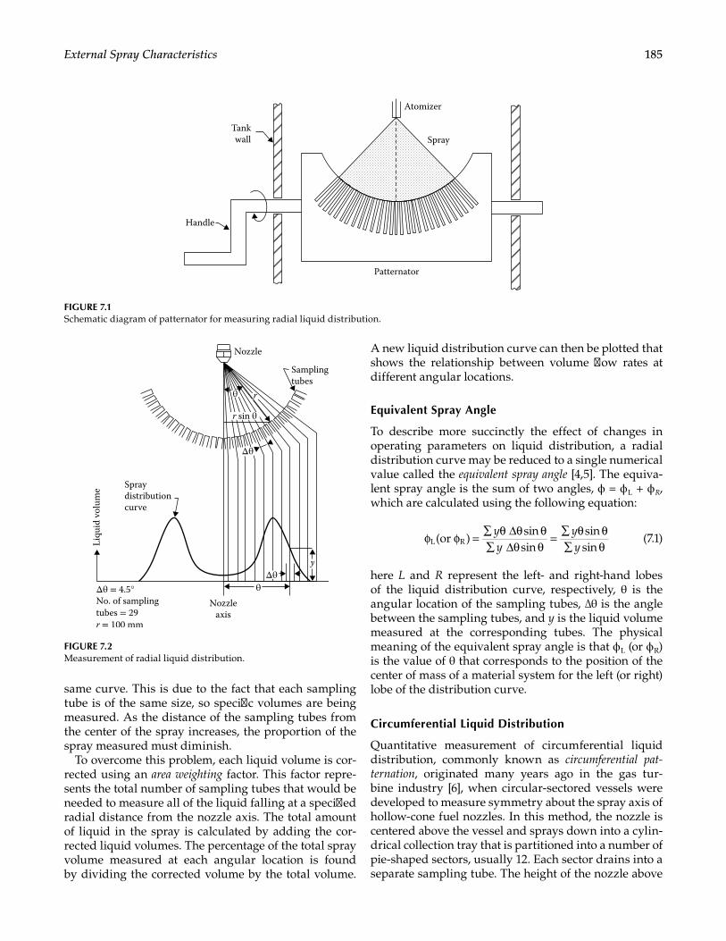
185External Spray Characteristics

same curve. This is due to the fact that each sampling tube is of the same size, so specific volumes are being measured. As the distance of the sampling tubes from the center of the spray increases, the proportion of the spray measured must diminish.

To overcome this problem, each liquid volume is cor-rected using an area weighting factor. This factor repre-sents the total number of sampling tubes that would be needed to measure all of the liquid falling at a specified radial distance from the nozzle axis. The total amount of liquid in the spray is calculated by adding the cor-rected liquid volumes. The percentage of the total spray volume measured at each angular location is found by dividing the corrected volume by the total volume.

A new liquid distribution curve can then be plotted that shows the relationship between volume flow rates at different angular locations.

Equivalent Spray Angle

To describe more succinctly the effect of changes in operating parameters on liquid distribution, a radial distribution curve may be reduced to a single numerical value called the equivalent spray angle [4,5]. The equiva-lent spray angle is the sum of two angles, ϕ = ϕ L + ϕ R, which are calculated using the following equation:

φ φ = ∑ θ ∆θ θ∑ ∆θ θ

= ∑ θ θ∑ θ

(or )sinsin

sinsinL R

yy

yy

(7.1)

here L and R represent the left- and right-hand lobes of the liquid distribution curve, respectively, θ is the angular location of the sampling tubes, ∆θ is the angle between the sampling tubes, and y is the liquid volume measured at the corresponding tubes. The physical meaning of the equivalent spray angle is that ϕ L (or ϕ R) is the value of θ that corresponds to the position of the center of mass of a material system for the left (or right) lobe of the distribution curve.

Circumferential Liquid Distribution

Quantitative measurement of circumferential liquid distribution, commonly known as circumferential pat-ternation, originated many years ago in the gas tur-bine industry [6], when circular-sectored vessels were developed to measure symmetry about the spray axis of hollow-cone fuel nozzles. In this method, the nozzle is centered above the vessel and sprays down into a cylin-drical collection tray that is partitioned into a number of pie-shaped sectors, usually 12. Each sector drains into a separate sampling tube. The height of the nozzle above

Spray

Atomizer

Patternator

Tankwall

Handle

FIGURE 7.1Schematic diagram of patternator for measuring radial liquid distribution.

θ

Δθ = 4.5°No. of samplingtubes = 29r = 100 mm

Liqu

id v

olum

e Spraydistributioncurve

Nozzle

Samplingtubes

Nozzleaxis

y

θΔθ

Δθ

r sin θ

r

FIGURE 7.2Measurement of radial liquid distribution.

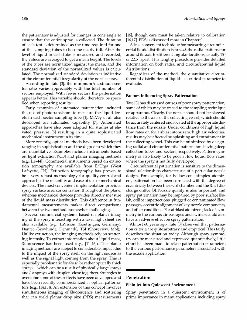
186 Atomization and Sprays

the patternator is adjusted for changes in cone angle to ensure that the entire spray is collected. The duration of each test is determined as the time required for one of the sampling tubes to become nearly full. After the level of liquid in each tube is measured and recorded, the values are averaged to get a mean height. The levels of the tubes are normalized against the mean, and the standard deviation of the normalized values is calcu-lated. The normalized standard deviation is indicative of the circumferential irregularity of the nozzle spray.

According to Tate [3], the minimum/maximum sec-tor ratio varies appreciably with the total number of sectors employed. With fewer sectors the patternation appears better. This variable should, therefore, be speci-fied when reporting results.

Early examples of automated patternation included the use of phototransistors to measure the liquid lev-els in each sector sampling tube [1]. McVey et al. also developed an automated capability [7]. Automated approaches have also been adapted for studies at ele-vated pressure [8] resulting in a quite sophisticated mechanical instrument in its time.

More recently, optical methods have been developed ranging in sophistication and the degree to which they are quantitative. Examples include instruments based on light extinction [9,10] and planar imaging methods (e.g., [11–14]). Commercial instruments based on extinc-tion tomography are available from EńUrga (West Lafayette, IN). Extinction tomography has proven to be a very robust methodology for quality control and approaches the reliability and ease of use of mechanical devices. The most convenient implementation provides spray surface area concentration throughout the plane, whereas mechanical devices provides directly measure of the liquid mass distribution. This difference in fun-damental measurements makes direct comparisons between the two methods somewhat challenging.

Several commercial systems based on planar imag-ing of the spray interacting with a laser light sheet are also available (e.g., LaVision (Goettingen, Germany), Dantec (Skovlunde, Denmark), TSI (Shoreview, MN)). Unlike extinction, the imaging methods rely on scatter-ing intensity. To extract information about liquid mass, fluorescence has been used (e.g., [11–16]). The planar imaging methods are subject to considerable impact due to the impact of the spray itself on the light source as well as the signal light coming from the spray. This is especially problematic for dense (or rather optically thick sprays—which can be a result of physically large sprays and/or sprays with droplets close together). Strategies to overcome some of these effects have been developed and have been recently commercialized as optical patterna-tors (e.g., [14,15]). An extension of this concept involves simultaneous imaging of fluorescence and scattering that can yield planar drop size (PDS) measurements

[16], though care must be taken relative to calibration [16,17]. PDS is discussed more in Chapter 9.

A less-convenient technique for measuring circumfer-ential liquid distribution is to clock the radial patternator around its axis to different angular locations, usually 15° or 22.5° apart. This lengthy procedure provides detailed information on both radial and circumferential liquid distributions.

Regardless of the method, the quantitative circum-ferential distribution of liquid is a critical parameter to evaluate.

Factors Influencing Spray Patternation

Tate [3] has discussed causes of poor spray patternation, some of which may be traced to the sampling technique or apparatus. Clearly, the nozzle should not be skewed relative to the axis of the collecting vessel, which should be accurately centered and located at the appropriate dis-tance from the nozzle. Under conditions of high liquid flow rates or, for airblast atomizers, high air velocities, results may be affected by splashing and entrainment in the collecting vessel. This can be minimized by design-ing radial and circumferential patternators having deep collection tubes and sectors, respectively. Pattern sym-metry is also likely to be poor at low liquid flow rates, where the spray is not fully developed.

Circumferential patternation is sensitive to the dimen-sional relationships characteristic of a particular nozzle design. For example, for hollow-cone simplex atomiz-ers, patternation has been correlated with the degree of eccentricity between the swirl chamber and the final dis-charge orifice [3]. Nozzle quality is also important, and spray patternation may be impaired by poor surface fin-ish, orifice imperfections, plugged or contaminated flow passages, eccentric alignment of key nozzle components, and other conditions. For airblast atomizers, lack of sym-metry in the various air passages and swirlers could also have an adverse effect on spray patternation.

Almost 60 years ago, Tate [3] observed that patterna-tion criteria are quite arbitrary and empirical. This fairly describes the situation today. Although spray symme-try can be measured and expressed quantitatively, little effort has been made to relate patternation parameters to the various performance parameters associated with the nozzle application.

Penetration

Plain Jet into Quiescent Environment

Spray penetration in a quiescent environment is of prime importance in many applications including spray

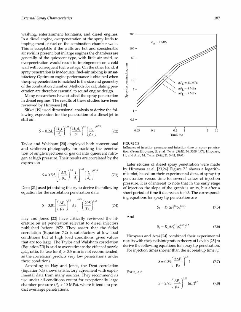
187External Spray Characteristics

washing, entertainment fountains, and diesel engines. In a diesel engine, overpenetration of the spray leads to impingement of fuel on the combustion chamber walls. This is acceptable if the walls are hot and considerable air swirl is present, but in large engines the chambers are generally of the quiescent type, with little air swirl, so overpenetration would result in impingement on a cold wall with consequent fuel wastage. On the other hand, if spray penetration is inadequate, fuel–air mixing is unsat-isfactory. Optimum engine performance is obtained when the spray penetration is matched to the size and geometry of the combustion chamber. Methods for calculating pen-etration are therefore essential to sound engine design.

Many researchers have studied the spray penetration in diesel engines. The results of these studies have been reviewed by Hiroyasu [18].

Sitkei [19] used dimensional analysis to derive the fol-lowing expression for the penetration of a diesel jet in still air.

0.2 oL

o

0.48L o

L

0.3L

A

0.35

S dU td

U dv

=

ρρ

(7.2)

Taylor and Walsham [20] employed both conventional and schlieren photography for tracking the penetra-tion of single injections of gas oil into quiescent nitro-gen at high pressure. Their results are correlated by the expression

0.5 oL

A

0.5

o

0.64

o

o

0.18

S dP t

dld

= ∆ρ

(7.3)

Dent [21] used jet mixing theory to derive the following equation for the correlation penetration data:

3.01295L

A

0.5

o

0.5

A

0.25

SP

d tT

= ∆ρ

(7.4)

Hay and Jones [22] have critically reviewed the lit-erature on jet penetration relevant to diesel injectors published before 1972. They assert that the Sitkei correlation (Equation 7.2) is satisfactory at low load conditions but at high load conditions gives values that are too large. The Taylor and Walsham correlation (Equation 7.3) is said to overestimate the effect of nozzle l0/d0 ratio. Its use for d0 > 0.5 mm is not recommended, as the correlation predicts very low penetrations under these conditions.

According to Hay and Jones, the Dent correlation (Equation 7.4) shows satisfactory agreement with exper-imental data from many sources. They recommend its use under all conditions except for exceptionally large chamber pressure (PA > 10 MPa), where it tends to pre-dict overlarge penetrations.

Later studies of diesel spray penetration were made by Hiroyasu et al. [23,24]. Figure 7.3 shows a logarith-mic plot, based on their experimental data, of spray tip penetration versus time for several values of injection pressure. It is of interest to note that in the early stage of injection the slope of the graph is unity, but after a short period of time it decreases to 0.5. The correspond-ing equations for spray tip penetration are

1 1 L0.6

A0.33S K P t= ∆ ρ− (7.5)

And

2 2 L0.1

A0.42 0.5S K P t= ∆ ρ− (7.6)

Hiroyasu and Arai [24] combined their experimental results with the jet disintegration theory of Levich [25] to derive the following equations for spray tip penetration.

For injection times shorter than the jet breakup time tb:

0.392 L

A

0.5

SP

t= ∆ρ

(7.7)

For tb < t:

2.95 ( )L

A

0.25

o0.5S

Pd t= ∆

ρ

(7.8)

0.5

1

5

10

50

100

300

0.03Sp

ray

tip p

enet

ratio

n, m

m0.1 0.5

Time, m.s1 5 10

ΔPL = 13 MPa

PA = 2 MPa

ΔPL = 8 MPaΔPL = 5 MPa

FIGURE 7.3Influence of injection pressure and injection time on spray penetra-tion. (From Hiroyasu, H. et al., Trans. JSME, 34, 3208, 1978; Hiroyasu, H., and Arai, M., Trans. JSAE, 21, 5–11, 1980.)

188 Atomization and Sprays

The jet breakup time is given by the dimensionally correct equation

28.65b L o A L–0.5

t d P( )= ρ ρ ∆ (7.9)

Sazhin et al. [26] provided a number of expres-sions for penetration based on analysis using Stokes Flow, Newton Flow, and Allen flow approximations. Their expressions are similar in nature to that of Dent (Equation 7.4); however, they require knowledge of the initial jet velocity and the droplet volume fraction, both of which are not necessarily easily determined. While velocity can be estimated from the pressure drop, it also depends on the coefficient of discharge, which can be determined if the mass flow is known for a given pres-sure drop. The volume fraction is another question that has more uncertainty.

Further work by Kostas et al. [27] used high-speed imaging to obtain time-resolved spray tip penetration data to generate simple expressions for the penetration as a function of time with emphasis on the behavior prior to breakup. The expression generated is [27]

( )3

2S t At= (7.10)

A is a function of injection pressure and ambient pres-sure and determined by best fits of the measured data. It was found that, for an injection pressure drop of 500 bar A decreased from 265 to 185 as ambient pressure increases from 1 to 50 atm. For an injection pressure drop of 1000 bar, A decreased from 570 to 480 as ambi-ent pressure increases from 1 to 50 bar. The results from Equation 7.10 indicate that Equation 7.7 overpredicts the initial penetration especially for the 500 bar injection pressure at 1 and 10 atm ambient pressures. Kostas et al. [27] point out that Equation 7.8 (post breakup time) fits the newer highly resolved data reasonably well.

Plain Jet into Crossflow

Numerous expressions exist that describe the penetra-tion of a plain liquid jet into a crossflow. These have been summarized recently in a comprehensive review by Birouk et al. [28]. Based on analysis of dozens of stud-ies carried out on liquid jets in crossflow, they propose a best fit expression to match the mean values of the cor-relations in the literature as

=

µµ

−− −

4.6 We Re0

0.4096

0

0.3635

A0.12 L

W

0.23

0

0.80

A0.01y

dq

xd

TT

(7.11)

q is the momentum flux ratio as defined by Equation 2.72. In this expression, the velocity term associated with the liquid is equal to the liquid volumetric flow rate

divided by the injector final open area. In other words, it is assumed that the coefficient of discharge, Cd = 1.

Birouk et al. [28] offer another expression (Equation 7.12) for cases where nonunity values of Cd have been used. In these cases the liquid jet velocity is the actual liq-uid jet velocity exiting the final injector orifice. However, the exact value for Cd varies between the studies exam-ined, so caution is advised when using Equation 7.12:

4.49 We0

0.4156

0

0.3254

A0.11 L

W

0.18

0

0.8yd

qxd

TT

=

µµ

−− −

(7.12)

It is worth noting that, if a particular injector geometry (e.g., chamfered inlet vs. sharp inlet, l0/d0) is used to develop a particular correlation, that correlation should work well for a new design with similar geometry features.

The penetration height of effervescent-type injec-tion into a crossflow has been studied in the context of supersonic combustion by Lin and coworkers [29].

A pair of expressions for penetration height has been provided by Ghenai et al. [30]. They studied water and methanol injected into a Mach 1.5 crossflow with amounts of gas injection into the liquid (gas to liquid ratio–GLR) ranging from 0% to 9.9% (by mass):

3.880

0.40

0

0.2yd

qxd

=

nonaerated (7.13)

( )( )− =

µρ σ

−(Equation 7.13)3.88 GLR

0nonaerated

0.28 0.32

0

0.18L

L o0.5

aerated

y yd

qxd d

(7.14)

The results indicated that aeration of the jet creates more penetration (e.g., 112% more with GLR of 8.2% for water and 70% more with GLR of 9.9% for methanol).

The aforementioned expressions are for the penetra-tion of the leading edge of the jet (windward edge). Some expression have been generated for the trajectory of the peak flux within the jet. One example is the early one by Wu et al. [31]

=

4.30

0.33

0

0.41yd

qxd

(7.15)

Besides the penetration of the leading edge of the jet injected into the crossflow, some expressions have been generated for the plume width as well as cross-sectional area that can be useful for design consideration. These have been proposed by Wu et al. [31] as

=

7.860

0.17

0

0.33zd

qxd

(7.16)

( )( )− =

µρ σ

−(Equation 7.13)3.88 GLR

0nonaerated

0.28 0.32

0

0.18L

L o0.5

aerated

y yd

qxd d

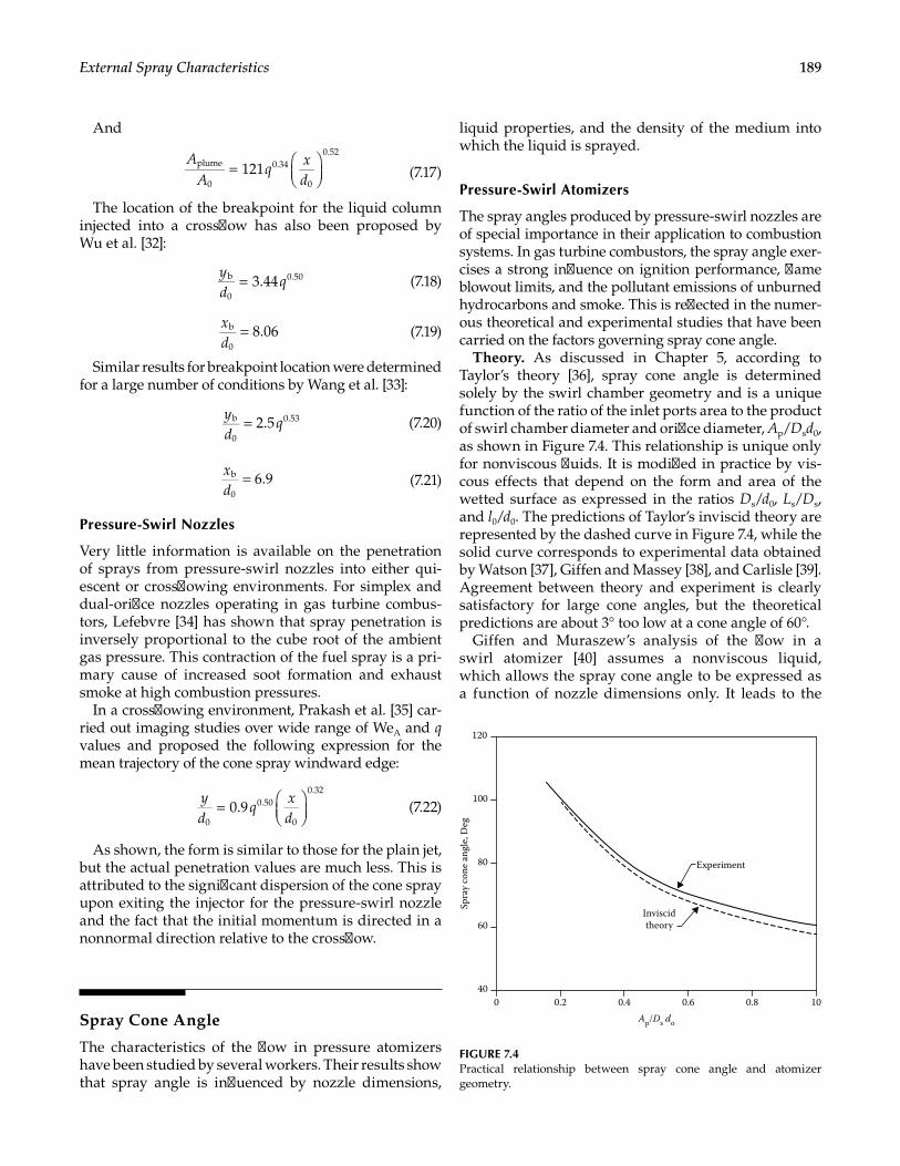
189External Spray Characteristics

And

=

121plume

0

0.34

0

0.52A

Aq

xd (7.17)

The location of the breakpoint for the liquid column injected into a crossflow has also been proposed by Wu et al. [32]:

= 3.44b

0

0.50yd

q (7.18)

xd

8.06b

0= (7.19)

Similar results for breakpoint location were determined for a large number of conditions by Wang et al. [33]:

yd

q2.5b

0

0.53= (7.20)

xd

6.9b

0= (7.21)

Pressure-Swirl Nozzles

Very little information is available on the penetration of sprays from pressure-swirl nozzles into either qui-escent or crossflowing environments. For simplex and dual-orifice nozzles operating in gas turbine combus-tors, Lefebvre [34] has shown that spray penetration is inversely proportional to the cube root of the ambient gas pressure. This contraction of the fuel spray is a pri-mary cause of increased soot formation and exhaust smoke at high combustion pressures.

In a crossflowing environment, Prakash et al. [35] car-ried out imaging studies over wide range of WeA and q values and proposed the following expression for the mean trajectory of the cone spray windward edge:

=

0.90

0.50

0

0.32yd

qxd

(7.22)

As shown, the form is similar to those for the plain jet, but the actual penetration values are much less. This is attributed to the significant dispersion of the cone spray upon exiting the injector for the pressure-swirl nozzle and the fact that the initial momentum is directed in a nonnormal direction relative to the crossflow.

Spray Cone Angle

The characteristics of the flow in pressure atomizers have been studied by several workers. Their results show that spray angle is influenced by nozzle dimensions,

liquid properties, and the density of the medium into which the liquid is sprayed.

Pressure-Swirl Atomizers

The spray angles produced by pressure-swirl nozzles are of special importance in their application to combustion systems. In gas turbine combustors, the spray angle exer-cises a strong influence on ignition performance, flame blowout limits, and the pollutant emissions of unburned hydrocarbons and smoke. This is reflected in the numer-ous theoretical and experimental studies that have been carried on the factors governing spray cone angle.

Theory. As discussed in Chapter 5, according to Taylor’s theory [36], spray cone angle is determined solely by the swirl chamber geometry and is a unique function of the ratio of the inlet ports area to the product of swirl chamber diameter and orifice diameter, Ap/Dsd0, as shown in Figure 7.4. This relationship is unique only for nonviscous fluids. It is modified in practice by vis-cous effects that depend on the form and area of the wetted surface as expressed in the ratios Ds/d0, Ls/Ds, and l0/d0. The predictions of Taylor’s inviscid theory are represented by the dashed curve in Figure 7.4, while the solid curve corresponds to experimental data obtained by Watson [37], Giffen and Massey [38], and Carlisle [39]. Agreement between theory and experiment is clearly satisfactory for large cone angles, but the theoretical predictions are about 3° too low at a cone angle of 60°.

Giffen and Muraszew’s analysis of the flow in a swirl atomizer [40] assumes a nonviscous liquid, which allows the spray cone angle to be expressed as a function of nozzle dimensions only. It leads to the

0.80.60.4Ap/Ds do

0.2

Spra

y co

ne a

ngle

, Deg

0 10

100

80 Experiment

Inviscidtheory60

40

120

FIGURE 7.4Practical relationship between spray cone angle and atomizer geometry.

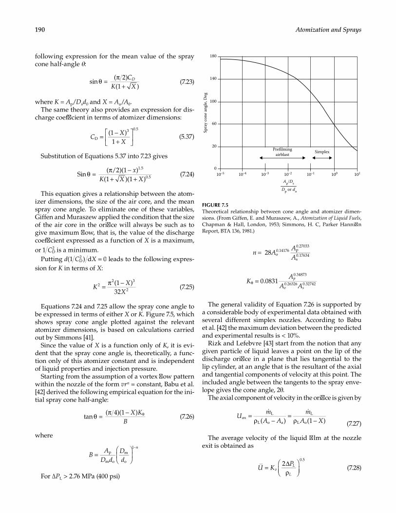
190 Atomization and Sprays

following expression for the mean value of the spray cone half-angle θ:

sin =( 2)(1 )

CK X

Dθ π+

(7.23)

where K = Ap/Dsd0 and X = Aa/A0.The same theory also provides an expression for dis-

charge coefficient in terms of atomizer dimensions:

(1 )1D

3 0.5

CXX

= −+

(5.37)

Substitution of Equations 5.37 into 7.23 gives

Sin =( /2)(1 )

(1 )(1 )

1.5

0.5

xK X X

θ π −+ +

(7.24)

This equation gives a relationship between the atom-izer dimensions, the size of the air core, and the mean spray cone angle. To eliminate one of these variables, Giffen and Muraszew applied the condition that the size of the air core in the orifice will always be such as to give maximum flow, that is, the value of the discharge coefficient expressed as a function of X is a maximum, or 1 D

2C is a minimum.Putting (1 ) d 0D

2d C X = leads to the following expres-sion for K in terms of X:

(1 )32

22 3

2KX

X= π −

(7.25)

Equations 7.24 and 7.25 allow the spray cone angle to be expressed in terms of either X or K. Figure 7.5, which shows spray cone angle plotted against the relevant atomizer dimensions, is based on calculations carried out by Simmons [41].

Since the value of X is a function only of K, it is evi-dent that the spray cone angle is, theoretically, a func-tion only of this atomizer constant and is independent of liquid properties and injection pressure.

Starting from the assumption of a vortex flow pattern within the nozzle of the form vrn = constant, Babu et al. [42] derived the following empirical equation for the ini-tial spray cone half-angle:

tan =( 4)(1 )X K

Bθ π − θ (7.26)

where

BA

D dDd

np

m o

m

o

1

=

−

For ∆PL > 2.76 MPa (400 psi)

28 o

0.14176 p0.27033

s0.17634n A

AA

=

0.0831

0.34873

0.26326 0.32742KA

A Ap

o s=θ

The general validity of Equation 7.26 is supported by a considerable body of experimental data obtained with several different simplex nozzles. According to Babu et al. [42] the maximum deviation between the predicted and experimental results is < 10%.

Rizk and Lefebvre [43] start from the notion that any given particle of liquid leaves a point on the lip of the discharge orifice in a plane that lies tangential to the lip cylinder, at an angle that is the resultant of the axial and tangential components of velocity at this point. The included angle between the tangents to the spray enve-lope gives the cone angle, 2θ.

The axial component of velocity in the orifice is given by

=

ρ −=

ρ −

( ) (1 )axL

L o a

L

L oU

mA A

mA X (7.27)

The average velocity of the liquid film at the nozzle exit is obtained as

2

0.5

U KP

vL

L= ∆

ρ

(7.28)

Prefilmingairblast Simplex

0

20

60

100

140

180

10–5 10–4 10–3 10–2 10–1 100 101

Spra

y co

ne a

ngle

, Deg

Ap/Ds

Dp or do

FIGURE 7.5Theoretical relationship between cone angle and atomizer dimen-sions. (From Giffen, E. and Muraszew, A., Atomization of Liquid Fuels, Chapman & Hall, London, 1953; Simmons, H. C, Parker Hannifin Report, BTA 136, 1981.)

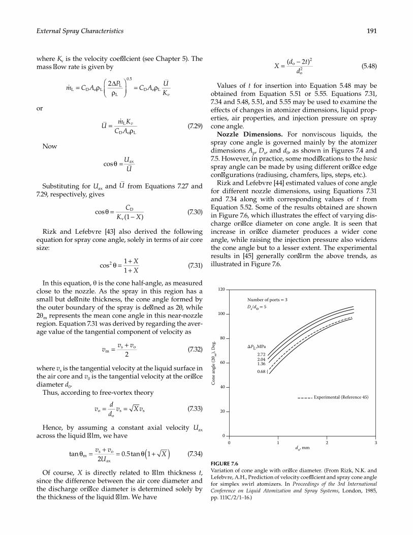
191External Spray Characteristics

where Kv is the velocity coefficient (see Chapter 5). The mass flow rate is given by

m C AP

C AUKv

= ρ ∆ρ

= ρ2L D o L

L

L

0.5

D o L

or

=ρ

L

D o LU

m KC A

v (7.29)

Now

cos = axUU

θ

Substituting for Uax and U from Equations 7.27 and 7.29, respectively, gives

cos(1 )

D

v

CK X

θ =−

(7.30)

Rizk and Lefebvre [43] also derived the following equation for spray cone angle, solely in terms of air core size:

cos11

2 XX

θ = ++

(7.31)

In this equation, θ is the cone half-angle, as measured close to the nozzle. As the spray in this region has a small but definite thickness, the cone angle formed by the outer boundary of the spray is defined as 2θ, while 2θ m represents the mean cone angle in this near-nozzle region. Equation 7.31 was derived by regarding the aver-age value of the tangential component of velocity as

2m

s ovv v= +

(7.32)

where vs is the tangential velocity at the liquid surface in the air core and v0 is the tangential velocity at the orifice diameter d0.

Thus, according to free-vortex theory

oo

s svdd

v X v= = (7.33)

Hence, by assuming a constant axial velocity Uax across the liquid film, we have

tan2

0.5tan 1ms o

ax

v vU

X( )θ = + = θ + (7.34)

Of course, X is directly related to film thickness t, since the difference between the air core diameter and the discharge orifice diameter is determined solely by the thickness of the liquid film. We have

( )o

2

o2X

d td

= − 2 (5.48)

Values of t for insertion into Equation 5.48 may be obtained from Equation 5.51 or 5.55. Equations 7.31, 7.34 and 5.48, 5.51, and 5.55 may be used to examine the effects of changes in atomizer dimensions, liquid prop-erties, air properties, and injection pressure on spray cone angle.

Nozzle Dimensions. For nonviscous liquids, the spray cone angle is governed mainly by the atomizer dimensions Ap, Ds, and d0, as shown in Figures 7.4 and 7.5. However, in practice, some modifications to the basic spray angle can be made by using different orifice edge configurations (radiusing, chamfers, lips, steps, etc.).

Rizk and Lefebvre [44] estimated values of cone angle for different nozzle dimensions, using Equations 7.31 and 7.34 along with corresponding values of t from Equation 5.52. Some of the results obtained are shown in Figure 7.6, which illustrates the effect of varying dis-charge orifice diameter on cone angle. It is seen that increase in orifice diameter produces a wider cone angle, while raising the injection pressure also widens the cone angle but to a lesser extent. The experimental results in [45] generally confirm the above trends, as illustrated in Figure 7.6.

Number of ports = 3

Experimental (Reference 45)

do, mm

Ds/do = 5

210

100

ΔPL,MPa

2.722.041.36

0.68

80

60

40

20

0

Con

e an

gle

(2θ m

), D

eg.

120

3

FIGURE 7.6Variation of cone angle with orifice diameter. (From Rizk, N.K. and Lefebvre, A.H., Prediction of velocity coefficient and spray cone angle for simplex swirl atomizers. In Proceedings of the 3rd International Conference on Liquid Atomization and Spray Systems, London, 1985, pp. 111C/2/1–16.)

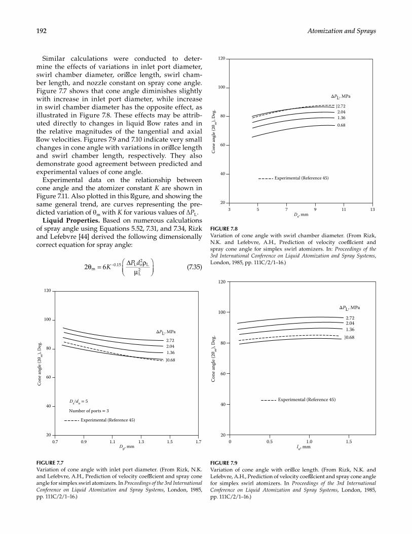
192 Atomization and Sprays

Similar calculations were conducted to deter-mine the effects of variations in inlet port diameter, swirl chamber diameter, orifice length, swirl cham-ber length, and nozzle constant on spray cone angle. Figure 7.7 shows that cone angle diminishes slightly with increase in inlet port diameter, while increase in swirl chamber diameter has the opposite effect, as illustrated in Figure 7.8. These effects may be attrib-uted directly to changes in liquid flow rates and in the relative magnitudes of the tangential and axial flow velocities. Figures 7.9 and 7.10 indicate very small changes in cone angle with variations in orifice length and swirl chamber length, respectively. They also demonstrate good agreement between predicted and experimental values of cone angle.

Experimental data on the relationship between cone angle and the atomizer constant K are shown in Figure 7.11. Also plotted in this figure, and showing the same general trend, are curves representing the pre-dicted variation of θ m with K for various values of ∆PL.

Liquid Properties. Based on numerous calculations of spray angle using Equations 5.52, 7.31, and 7.34, Rizk and Lefebvre [44] derived the following dimensionally correct equation for spray angle:

2 6m0.15 L o

2L

L2K

P dθ = ∆ ρµ

− (7.35)

Number of ports = 3

Experimental (Reference 45)

Dp, mm

Ds/do = 5

Con

e an

gle

(2θ m

), D

eg. 2.72

2.041.360.68

ΔPL, MPa

1.51.31.10.90.7

100

80

60

40

20

120

1.7

FIGURE 7.7Variation of cone angle with inlet port diameter. (From Rizk, N.K. and Lefebvre, A.H., Prediction of velocity coefficient and spray cone angle for simplex swirl atomizers. In Proceedings of the 3rd International Conference on Liquid Atomization and Spray Systems, London, 1985, pp. 111C/2/1–16.)

Experimental (Reference 45)

Ds, mmC

one

angl

e (2

θ m),

Deg

.

2.722.041.360.68

ΔPL, MPa

119753

100

80

60

40

20

120

13

FIGURE 7.8Variation of cone angle with swirl chamber diameter. (From Rizk, N.K. and Lefebvre, A.H., Prediction of velocity coefficient and spray cone angle for simplex swirl atomizers. In: Proceedings of the 3rd International Conference on Liquid Atomization and Spray Systems, London, 1985, pp. 111C/2/1–16.)

Experimental (Reference 45)

lo, mm

Con

e an

gle

(2θ m

), D

eg.

2.722.041.36

0.68

ΔPL, MPa

1.51.00.50

100

80

60

40

20

120

FIGURE 7.9Variation of cone angle with orifice length. (From Rizk, N.K. and Lefebvre, A.H., Prediction of velocity coefficient and spray cone angle for simplex swirl atomizers. In Proceedings of the 3rd International Conference on Liquid Atomization and Spray Systems, London, 1985, pp. 111C/2/1–16.)

193External Spray Characteristics

Work conducted by Ballester and Dopazo [46] also starting with inviscid theory and then adding viscous effects via experiments with injection of heavy oil, led to the following expression for cone angle:

µθ = ∆− −2 16.156m0.39

01.13

L0.9

L0.39K d P (7.36)

Comparing 7.35 with 7.36 indicates some differences in the exponents that suggest lower dependency on injector exit orifice, stronger dependency on the nozzle parameter, K, less influence on viscosity and pressure drop. However, Ballester and Dopazo [46] did not vary density or viscosity, but they did study 20 nozzles with varying orifice diameters. Given this, Equation 7.35 may be more generally indicative of the indication of the effects of liquid injection pressure and liquid properties on spray angle.

Surface Tension According to Equation 7.35, surface tension should have no effect on spray cone angle, and this is generally confirmed by experiment. Giffen and Massey [38] measured cone angles for liquids having approximately the same viscosity but a range of three to one in surface tension, and no significant effect of surface tension was observed. Wang and Lefebvre [47] compared the equivalent cone angles exhibited by sev-eral simplex swirl nozzles when flowing water and die-sel oil (DF-2). These liquids have surface tensions that differ by a factor of almost three. In all cases the spray cone angle was slightly less for diesel oil, and this was attributed to its slightly higher viscosity. As a result, Wang and Lefebvre concluded that surface tension has no appreciable effect on cone angle, thus confirming the conclusion reached by Giffen and Massey.

Density The influence of liquid density on spray cone angle is illustrated in Figure 7.12, where it can be seen that the spray angle widens slightly with increase in density. It may be noted in this figure that increase in nozzle pressure differential also causes the spray cone angle to widen. This is one of the reasons why increase in ∆PL improves atomization quality.

Viscosity The viscosity of the liquid is of great impor-tance to cone angle. It modifies the flow of an ideal liq-uid in two ways: (1) by friction in the body of the liquid and (2) by friction at the boundary between the liquid and its containing walls. Both effects are caused by the friction force created by the velocity gradient in a vis-cous liquid. The friction force produced by this veloc-ity gradient tends to reduce the tangential velocity, and this effect increases with decreasing value of atomizer radius, reaching a maximum at the air core. The higher the viscosity, the greater will be the divergence between the actual tangential velocity and the value calculated from the equation

ivr v R= (7.37)

The velocity gradient at the boundaries between the liquid and the containing walls is another source of fric-tion, and this causes the formation of a boundary layer

Experimental (Reference 45)

Ls, mm

Con

e an

gle

(2θ m

), D

eg.

2.722.041.360.68

ΔPL, MPa

6420

100

80

60

40

120

8

FIGURE 7.10Variation of cone angle with swirl chamber length. (From Rizk, N.K. and Lefebvre, A.H., Prediction of velocity coefficient and spray cone angle for simplex swirl atomizers. In Proceedings of the 3rd International Conference on Liquid Atomization and Spray Systems, London, 1985, pp. 111C/2/1–16.)

Experimental (Reference 45)

K

2.722.041.36

0.68

0.30.20.10 0.4

100

80

60

40

20

120

do = 1.6mm

ΔPL, MPa

Con

e an

gle

(2θ m

), D

eg.

FIGURE 7.11Variation of cone angle with atomizer constant. (From Rizk, N.K. and Lefebvre, A.H., Prediction of velocity coefficient and spray cone angle for simplex swirl atomizers. In Proceedings of the 3rd International Conference on Liquid Atomization and Spray Systems, London, 1985, pp. 111C/2/1–16.)

194 Atomization and Sprays

of liquid in which the velocity of the liquid changes from zero at the boundary to the ordinary velocity of the nearby liquid. The liquid in the boundary layer does not obey the same laws as the main body of liquid away from the solid boundaries, and if the thickness of the boundary layer is appreciable, a significant modification of the conditions of flow will occur [40].

Giffen and Massey [38] examined the influence of viscosity on cone angle over a range of viscosities from 2 × 10–6 to 50 × 10–6 m2/s (2–50 cS). They found that the relation between the cone half-angle and viscosity for a swirl-plate atomizer could be expressed by the empiri-cal equation:

vtan = 0.169 Lθ −0.131 (7.38)

This equation indicates a dependence of spray angle on viscosity that is roughly the same as the viscosity dependence shown in Equation 7.35.

Chen et al. [47] used blends of diesel oil (DF-2) and polybutene to examine the influence of viscosity on equivalent spray angle for a simplex nozzle. Figure 7.13 is typical of the results obtained. It shows that cone angle decreases with increase in viscosity, consistent with what Equations 7.35 and 7.38 appear to suggest.

In a swirl atomizer of the helical-groove type the liq-uid has to flow through tortuous passages before it enters the final orifice; therefore viscosity might be expected to have a greater effect in this type of atomizer. This was confirmed by Giffen and Massey [38], who found that the decrease of cone angle with increased viscosity was more pronounced than in an atomizer of the swirl-plate type. Chen et al. [47] also observed that shorter l0/d0 values resulted in greatest cone angle but that the l0/d0 influence on spray cone angle decreased as viscosity increased.

Air Properties. De Corso and Kemeny [4] carried out the first investigation on the effects of ambient gas pres-sure on spray cone angle. Their results show that, over a range of gas pressures from 10 to 800 kPa, the equivalent spray angle is an inverse function of A

1.6P . A similar study carried out by Neya and Sato [48] on water sprayed into stagnant air produced a similar result, namely that spray contraction ∆ϕ increases with A

1.2P .These studies were limited to ambient air pressure

below 1 MPa (10 atm). It should also be noted that the equivalent spray angles studied by these workers were not measured close to the nozzle but at some dis-tance downstream. In consequence, they tend to be considerably smaller than angles measured in the near-nozzle region, because as the drops move away from

2.722.041.36

0.68

do = 1.6 mm

K = 0.118

Liquid density, kg/m3

100

80

60

40

20

0

120

1,4001,2001,000800 1,600

Con

e an

gle

(2θ m

), D

eg.

ΔPL, MPa

FIGURE 7.12Effect of liquid density on initial spray cone angle. (From Rizk, N.K. and Lefebvre, A.H., Prediction of velocity coefficient and spray cone angle for simplex swirl atomizers. In Proceedings of the 3rd International Conference on Liquid Atomization and Spray Systems, London, 1985, pp. 111C/2/1–16.)

80

70

60

50

40

30

1.72 (250)1.38 (200)1.03 (150)

Eec

tive

spra

y an

gle,

deg

rees

20

10

0 121086Liquid viscosity, kg/ms

42 14 × 10–30

90 Simplex atomizer

FN = 8 × 10–8 m2

lo/do = 1.0

ΔPL, MPa (psi)

FIGURE 7.13Influence of viscosity on equivalent spray angle. (From Chen, S.K., Lefebvre, A.H., and Rollbuhler, J. J. Eng. Gas Turbines Power, 114, 97–103, 1992)

195External Spray Characteristics

the nozzle they are subjected to radial air currents gen-erated by their own kinetic energy, as described by De Corso and Kemeny [4].

Ortman and Lefebvre [5] used a radial patternator of the type shown in Figure 7.1 to examine, for four dif-ferent simplex nozzles, the effects of variations in liq-uid injection pressure and ambient air pressure on equivalent spray angle. The liquid employed was avia-tion kerosene having the following properties: ρ = 780 kg/m3, σ = 0.0275 kg/s2, µ = 0.0013 kg/m·s. Some of the results obtained are shown in Figures 7.14. through 7.17. Initially, an increase in gas pressure above nor-mal atmospheric causes the spray to contract sharply.

However, with continuing increase in gas pressure the rate of spray contraction decreases. Finally, a point is reached where further increase in ambient pressure has virtually no influence on the equivalent spray angle, as shown in Figure 7.17.

Dodge and Biaglow [49] used a Hago simplex nozzle of nominal 80° cone angle to examine the influence of atomizing conditions on spray characteristics. The liquids employed were kerosene (Jet-A) and diesel oil

45 40 35 30 25 20 15 10 5 0 5 10 15 20 25 30 35 40 45

0.10

0.20.30.40.50.60.70.80.91.0

PA, MPa0.1010.4480.792

Simplex atomizer No.1Liquid = KeroseneΔPL = 0.67 MPa

Spray half angle, Deg

Nor

mliz

ed L

iqui

d vo

lum

e

FIGURE 7.14Influence of ambient gas pressure on radial liquid distribution (Atomizer 1). (From Ortman, J. and Lefebvre, A.H., AIAA J. Propul. Power, 1, 11–15, 1985.)

4550 40 35 30 25 20 15 10 5 0 5 10 15 20 25 30 35 40 45 50

0.10

0.20.30.40.50.60.70.80.91.0

PA, MPa0.1010.3800.74

Simplex atomizer No. 2Liquid = KeroseneΔPL = 0.76 MPa

Spray half angle, Deg

Nor

mliz

ed fu

el v

olum

e

FIGURE 7.15Influence of ambient gas pressure on radial liquid distribution (Atomizer 2). (From Ortman, J. and Lefebvre, A.H., AIAA J. Propul. Power, 1, 11–15, 1985.)

00 0.60.40.2 0.8

6055504540353025201510

5

65

00 0.60.40.2 0.8

6055504540353025201510

5

65

ΔPL, MPa0.260.692.00

Simplex No. 1 Simplex No. 2

PA, MPa

Equi

vala

nt sp

ray

angl

e, D

eg.

FIGURE 7.16Influence of ambient gas pressure on equivalent spray cone angle. (From Ortman, J. and Lefebvre, A.H., AIAA J. Propul. Power, 1, 11–15, 1985.)

00 2.01.51.00.5 2.5

60

55

50

45

40

35

30

25

20

15

10

5

65

PA, MPa

Equi

vala

nt sp

ray

angl

e, D

eg.

ΔPL = 0.69 MPa

Simplex No. 3 (ϕn = 90°)

Simplex No. 4 (ϕn = 30°)

FIGURE 7.17Influence of ambient gas pressure on equivalent spray angle. (From Ortman, J. and Lefebvre, A.H., AIAA J. Propul. Power, 1, 11–15, 1985.)

196 Atomization and Sprays

(DF-2). Cone angles were measured 10 mm from the nozzle. They were defined as twice the half-angle, where the half-angle was calculated from half the total width of the spray at 10 mm divided by the distance from the nozzle plus the effective origin of the spray, which was 1.1 mm upstream of the nozzle tip. The half-cone angle θ is thus

arctanspray width (mm)

2(10 1.1)θ =

+ (7.39)

The experimental data were correlated using an expression for cone angle of the form

2 = 79.8 0.918 A

A0

θ − ρρ

(7.40)

where A0ρ is the air density at normal atmospheric pres-sure and temperature.

According to De Corso and Kemeny [4], the phenom-enon of decreasing spray angle is caused by the aero-dynamic effects due to the motion of the liquid spray through the ambient gas. The liquid emerging from the nozzle at high velocity entrains gas at the inner and outer surfaces of the spray sheath. However, the gas sup-ply to the inner portion of the spray sheath is limited by the enclosed volume in the sheath. The pressure dif-ference resulting from this effect sets up airflows that produce droplet acceleration toward the nozzle axis, thereby reducing the effective spray angle.

Injection Pressure. The influence of injection pressure on spray angle has been investigated by several work-ers including De Corso and Kemeny [4], Neya and Sato [48], Ortman and Lefebvre [5], and Dodge and Biaglow [49]. The results obtained by De Corso and Kemeny and Neya and Sato show that, over a range of injection pres-sures from 0.17 to 2.7 MPa, the equivalent spray angle is an inverse function of ∆PL.

Similar measurements were carried out by Ortman and Lefebvre [5]. Figure 7.18 is typical of the results obtained. Figure 7.19 shows that, starting from atmo-spheric pressure, increases in liquid pressure cause the spray to first widen and then contract. This phenome-non was also observed by Neya and Sato [26] but not by De Corso and Kemeny [3], so presumably it is a function of nozzle design.

Following the initial increase in spray cone angle (which occurs only with sprays injected into air at nor-mal atmospheric pressure), the spray contracts con-tinuously with further increase in liquid pressure. Eventually, a minimum spray angle is attained, and further increase in injection pressure has no discernible effect on spray angle.

To summarize, the main factors influencing spray cone angle are atomizer dimensions, especially d0,

and air density. Cone angle increases appreciably with increase in d0 and diminishes with increases in air den-sity, liquid viscosity, and liquid injection pressure.

Plain-Orifice Atomizers

The most important practical example of a plain-orifice atomizer is the fuel injector employed on diesel engines. The angle of a diesel spray is normally defined as the angle formed by two straight lines drawn from the discharge orifice to the outer periphery of the spray at a distance 60d0 downstream of the nozzle, as shown in Figure 7.20 [50]. Photographic methods are usually employed to determine this angle. Recall the earlier discussion regarding definitions of cone angle. Work resulting in [2]

4550 40 35 30 25 20 15 10 5 0 5 10 15 20 25 30 35 40 45 50

0.10

0.20.30.40.50.60.70.80.91.0

ΔPL, MPa0.310.761.97

Simplex atomizer No. 2Liquid = KerosenePA = 101 K Pa

Spray half angle, Deg

Nor

mliz

ed fu

el v

olum

e

FIGURE 7.18Influence of injection pressure on radial liquid distribution. (From Ortman, J. and Lefebvre, A.H., AIAA J. Propul. Power, 1, 11–15, 1985.)

0210 3

6055504540353025201510

5

65

0210 3

6055504540353025201510

5

65

ΔPL, MPa

ΔPL, MPa

0.1010.2760.4480.6200.793

Simplex No. 1 (75°) Simplex No. 2 (82°)

Equi

vala

nt sp

ray

angl

e, D

eg.

FIGURE 7.19Influence of injection pressure on equivalent spray angle. (From Ortman, J. and Lefebvre, A.H., AIAA J. Propul. Power, 1, 11–15, 1985.)

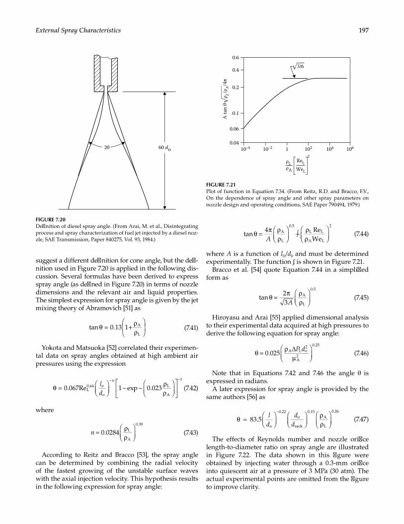
197External Spray Characteristics

suggest a different definition for cone angle, but the defi-nition used in Figure 7.20 is applied in the following dis-cussion. Several formulas have been derived to express spray angle (as defined in Figure 7.20) in terms of nozzle dimensions and the relevant air and liquid properties. The simplest expression for spray angle is given by the jet mixing theory of Abramovich [51] as

tan = 0.13 1 A

Lθ + ρ

ρ

(7.41)

Yokota and Matsuoka [52] correlated their experimen-tal data on spray angles obtained at high ambient air pressures using the expression

θ

− − ρρ

− −

= 0.067Re 1 exp 0.023L0.64 o

o

L

A

1ld

n

(7.42)

where

0.0284 L

A

0.39

n = ρρ

(7.43)

According to Reitz and Bracco [53], the spray angle can be determined by combining the radial velocity of the fastest growing of the unstable surface waves with the axial injection velocity. This hypothesis results in the following expression for spray angle:

θ π ρρ

∫ ρρ

tan =4 Re

WeA

L

0.5L L

A L

2

A (7.44)

where A is a function of l0/d0 and must be determined experimentally. The function ʄ is shown in Figure 7.21.

Bracco et al. [54] quote Equation 7.44 in a simplified form as

tan23

A

L

0.5

Aθ = π ρ

ρ

(7.45)

Hiroyasu and Arai [55] applied dimensional analysis to their experimental data acquired at high pressures to derive the following equation for spray angle:

0.025 A L o2

A2

0.25P dθ = ρ ∆

µ

(7.46)

Note that in Equations 7.42 and 7.46 the angle θ is expressed in radians.

A later expression for spray angle is provided by the same authors [56] as

θ =

ρρ

−

83.5o

0.22o

sack

0.15A

L

0.26l

dd

d (7.47)

The effects of Reynolds number and nozzle orifice length-to-diameter ratio on spray angle are illustrated in Figure 7.22. The data shown in this figure were obtained by injecting water through a 0.3-mm orifice into quiescent air at a pressure of 3 MPa (30 atm). The actual experimental points are omitted from the figure to improve clarity.

60 do2θ

FIGURE 7.20Definition of diesel spray angle. (From Arai, M. et al., Disintegrating process and spray characterization of fuel jet injected by a diesel noz-zle, SAE Transmission, Paper 840275, Vol. 93, 1984.)

10–4 10–2 102 104 10610.04

0.06

0.1

0.2

0.4

0.6

A ta

n θ√

ρ L/ρA

/4π

ρLρA

ReL

WeL

2

√3/6

FIGURE 7.21Plot of function in Equation 7.34. (From Reitz, R.D. and Bracco, F.V., On the dependence of spray angle and other spray parameters on nozzle design and operating conditions, SAE Paper 790494, 1979.)

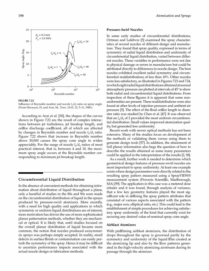
198 Atomization and Sprays

According to Arai et al. [50], the shapes of the curves shown in Figure 7.22 are the result of complex interac-tions between jet turbulence, jet breakup length, and orifice discharge coefficient, all of which are affected by changes in Reynolds number and nozzle l0/d0 ratio. Figure 7.22 shows that increase in Reynolds number above 30,000 causes the spray cone angle to widen appreciably. For the range of nozzle l0/d0 ratios of most practical interest, that is, between 4 and 10, the maxi-mum spray angle occurs at the Reynolds number cor-responding to minimum jet breakup length.

Circumferential Liquid Distribution

In the absence of convenient methods for obtaining infor-mation about distribution of liquid throughout a plane, only a handful of studies in the 80s and 90s were made on the circumferential distribution of liquid in the sprays produced by pressure-swirl atomizers. More recently, with a need for high quality and applications in which symmetric or uniform liquid distributions are of interest, more motivation has driven the use of more sophisticated planar patternation methods, whether they are mechani-cal or optical. It is likely that, until studies focused on the overall planar distribution of liquid became more common, the notion that nozzles produced axisymmet-ric sprays was perhaps simply accepted. In reality, small defects in surface finish or contamination can easily per-turb the symmetry of the spray. Hence it may be difficult to ascertain performance impacts associated with the actual nozzle design or fabrication methods.

Pressure-Swirl Nozzles

In some early studies of circumferential distributions, Ortman and Lefebvre [5] examined the spray character-istics of several nozzles of different design and manufac-ture. They found that spray quality, expressed in terms of symmetry of radial liquid distribution and uniformity of circumferential liquid distribution, varied between differ-ent nozzles. These variables in performance were not due to physical damage or errors in manufacture but could be attributed directly to differences in nozzle design. The best nozzles exhibited excellent radial symmetry and circum-ferential maldistributions of less than 10%. Other nozzles were less satisfactory, as illustrated in Figures 7.23 and 7.24, in which eight radial liquid distributions obtained at normal atmospheric pressure are plotted at intervals of 45° to show both radial and circumferential liquid distributions. From inspection of these figures it is apparent that some non-uniformities are present. These maldistributions were also found at other levels of injection pressure and ambient air pressure [5]. The effect of the final orifice length to diam-eter ratio was studied by Chen et al. [47]. It was observed that an l0/d0 of 2 provided the most uniform circumferen-tial distribution. Small values improved atomization qual-ity, but generated less uniformity.

Recent work with newer optical methods has not been extensive. Many of the studies focus on development of the methods or validating them versus using them to generate design tools [57]. In addition, the attainment of full planar information also begs the question of how to describe the results obtained as some many parameters could be applied in the interpretation of the results [2, 58].

As a result, further work is needed to determine which geometrical design features of pressure-swirl nozzles are most important to spray uniformity. At least one example exists where design parameters were directly related to the resulting spray pattern measured using a SprayVIEW® measurement system (Proveris Scientific, Marlborough, MA) [59]. The application in this case was a metered dose inhaler and it was found, through analysis of variance, that a few key geometry features played the most sig-nificant role in defining the spray pattern attributes that consisted of various aspects associated with the pattern (e.g., major axis, elliptical ratio, etc.). This could lead to the establishment of simple procedures for achieving satisfac-tory spray uniformity of the kind that currently exist for securing any desired value of nominal spray cone angle.

Airblast Atomizers

With prefilming airblast atomizers, the distribution of drops throughout the spray is governed partly by the symmetry and uniformity of the liquid film created at the atomizing lip and also by the flow patterns gener-ated in the high-velocity atomizing airstream during its passage through the atomizer.

0

5

10

10

Spra

y an

gle,

Deg

.

Reynolds number

20

25

103 104 105 106

d0 = 0.3 mmPA = 3.0 MPa

l0/d0 = 4

l0/d0 = 1 l0/d0 = 40

l0/d0 = 10

l0/d0 = 50

FIGURE 7.22Influence of Reynolds number and nozzle l0/d0 ratio on spray angle. (From Hiroyasu, H. and Arai, M., Trans. JSAE, 21, 5–11, 1980.)

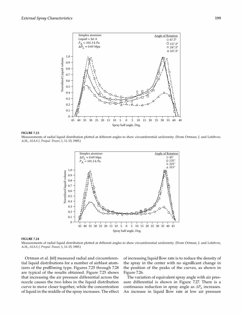
199External Spray Characteristics

Ortman et al. [60] measured radial and circumferen-tial liquid distributions for a number of airblast atom-izers of the prefilming type. Figures 7.25 through 7.28 are typical of the results obtained. Figure 7.25 shows that increasing the air pressure differential across the nozzle causes the two lobes in the liquid distribution curve to move closer together, while the concentration of liquid in the middle of the spray increases. The effect

of increasing liquid flow rate is to reduce the density of the spray in the center with no significant change in the position of the peaks of the curves, as shown in Figure 7.26.

The variation of equivalent spray angle with air pres-sure differential is shown in Figure 7.27. There is a continuous reduction in spray angle as ∆PA increases. An increase in liquid flow rate at low air pressure

45 40 35 30 25 20 15 10 5 0Spray half angle, Deg.

5 10 15 20 25 30 35 40 40

0.1

0

0.2

0.3

0.4

0.5

0.6

0.7

0.8

Angle of Rotation

Nor

mliz

ed L

iqui

d vo

lum

e0.9

1.0

67.5º157.5º247.5º337.5º

Simplex atomizerLiquid = Jet APA = 101.3 k PaΔPL = 0.69 Mpa

FIGURE 7.23Measurements of radial liquid distribution plotted at different angles to show circumferential uniformity. (From Ortman, J. and Lefebvre, A.H., AIAA J. Propul. Power, 1, 11–15, 1985.)

0.10

0.20.30.40.50.60.70.80.91.0

45 40 35 30 25 20 15 10 5 0 5 10 15 20 25 30 35 40 45

Angle of Rotation45°135°

315°225°

Spray half angle, Deg.

Nor

mliz

ed li

quid

vol

ume

Simplex atomizerΔPL = 0.69 MpaPA = 101.3 k Pa

FIGURE 7.24Measurements of radial liquid distribution plotted at different angles to show circumferential uniformity. (From Ortman, J. and Lefebvre, A.H., AIAA J. Propul. Power, 1, 11–15, 1985.)

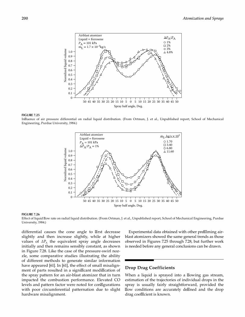
200 Atomization and Sprays

differential causes the cone angle to first decrease slightly and then increase slightly, while at higher values of ∆PA the equivalent spray angle decreases initially and then remains sensibly constant, as shown in Figure 7.28. Like the case of the pressure-swirl noz-zle, some comparative studies illustrating the ability of different methods to generate similar information have appeared [61]. In [61], the effect of small misalign-ment of parts resulted in a significant modification of the spray pattern for an air-blast atomizer that in turn impacted the combustion performance. Elevated CO levels and pattern factor were noted for configurations with poor circumferential patternation due to slight hardware misalignment.

Experimental data obtained with other prefilming air-blast atomizers showed the same general trends as those observed in Figures 7.25 through 7.28, but further work is needed before any general conclusions can be drawn.

Drop Drag Coefficients

When a liquid is sprayed into a flowing gas stream, estimation of the trajectories of individual drops in the spray is usually fairly straightforward, provided the flow conditions are accurately defined and the drop drag coefficient is known.

0.10

0.20.30.40.50.60.70.80.91.0

4550 40 35 30 25 20 15 10 5 0 5 10 15 20 25 30 35 40 45 50

1%2%

4.8%3%

Airblast atomizerLiquid = KerosenePA = 101 kPamL = 1.7 × 10–3kg/s

Spray half angle, Deg.

Nor

mliz

ed li

quid

vol

ume

ΔPA/PA

FIGURE 7.25Influence of air pressure differential on radial liquid distribution. (From Ortman, J. et al., Unpublished report, School of Mechanical Engineering, Purdue University, 1984.)

0.10

0.20.30.40.50.60.70.80.91.0

4550 40 35 30 25 20 15 10 5 0 5 10 15 20 25 30 35 40 45 50

mL, kg/s × 103

1.703.40

11.606.80

Airblast atomizerLiquid = KerosenePA = 101 kPaΔPA/PA = 1%

Spray half angle, Deg.

Nor

mliz

ed li

quid

vol

ume

.

FIGURE 7.26Effect of liquid flow rate on radial liquid distribution. (From Ortman, J. et al., Unpublished report, School of Mechanical Engineering, Purdue University, 1984.)

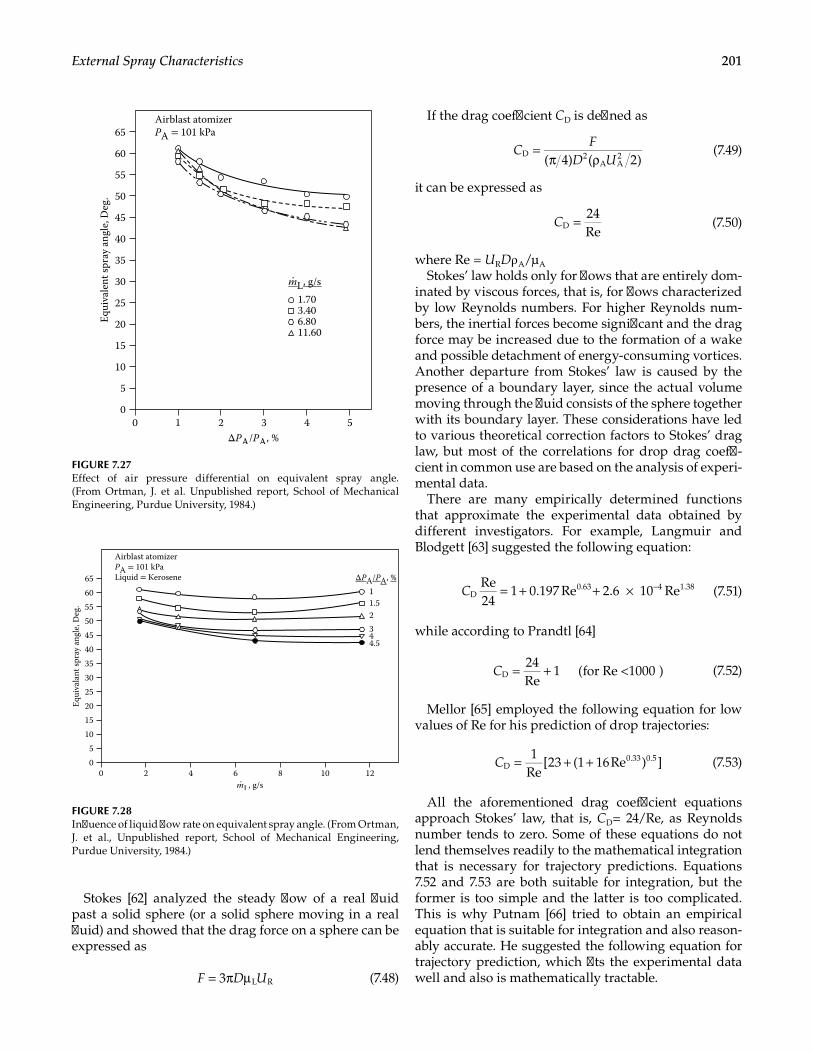
201External Spray Characteristics

Stokes [62] analyzed the steady flow of a real fluid past a solid sphere (or a solid sphere moving in a real fluid) and showed that the drag force on a sphere can be expressed as

3 L RF D U= π µ (7.48)

If the drag coefficient CD is defined as

( 4) ( 2)D 2

A A2C

FD U

=π ρ

(7.49)

it can be expressed as

24ReDC = (7.50)

where Re = URDρ A/µA

Stokes’ law holds only for flows that are entirely dom-inated by viscous forces, that is, for flows characterized by low Reynolds numbers. For higher Reynolds num-bers, the inertial forces become significant and the drag force may be increased due to the formation of a wake and possible detachment of energy-consuming vortices. Another departure from Stokes’ law is caused by the presence of a boundary layer, since the actual volume moving through the fluid consists of the sphere together with its boundary layer. These considerations have led to various theoretical correction factors to Stokes’ drag law, but most of the correlations for drop drag coeffi-cient in common use are based on the analysis of experi-mental data.

There are many empirically determined functions that approximate the experimental data obtained by different investigators. For example, Langmuir and Blodgett [63] suggested the following equation:

Re24

1 0.197 Re 2.6 10 ReD0.63 4 1.38C = + + × − (7.51)

while according to Prandtl [64]

24Re

1 (for Re <1000 )DC = + (7.52)

Mellor [65] employed the following equation for low values of Re for his prediction of drop trajectories:

1

Re[23 (1 16Re ) ]D

0.33 0.5C = + + (7.53)

All the aforementioned drag coefficient equations approach Stokes’ law, that is, CD= 24/Re, as Reynolds number tends to zero. Some of these equations do not lend themselves readily to the mathematical integration that is necessary for trajectory predictions. Equations 7.52 and 7.53 are both suitable for integration, but the former is too simple and the latter is too complicated. This is why Putnam [66] tried to obtain an empirical equation that is suitable for integration and also reason-ably accurate. He suggested the following equation for trajectory prediction, which fits the experimental data well and also is mathematically tractable.

043210 5

60

55

50

45

40

35

30

25

20

15

10

5

65

Equi

vale

nt sp

ray

angl

e, D

eg.

ΔPA/PA, %

mL, g/s

1.703.40

11.606.80

Airblast atomizerPA = 101 kPa

.

FIGURE 7.27Effect of air pressure differential on equivalent spray angle. (From Ortman, J. et al. Unpublished report, School of Mechanical Engineering, Purdue University, 1984.)

0108642

11.52344.5

0 12

6055504540353025201510

5

65 ΔPA/PA, %

Airblast atomizerPA = 101 kPaLiquid = Kerosene

mL, g/s

Equi

vala

nt sp

ray

angl

e, D

eg.

.

FIGURE 7.28Influence of liquid flow rate on equivalent spray angle. (From Ortman, J. et al., Unpublished report, School of Mechanical Engineering, Purdue University, 1984.)

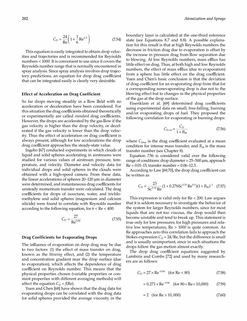
202 Atomization and Sprays

24Re

116

ReD2 3C = +

(7.54)

This equation is easily integrated to obtain drop veloc-ities and trajectories and is recommended for Reynolds numbers < 1000. It is convenient to use since it covers the Reynolds number range that is normally encountered in spray analysis. Since spray analysis involves drop trajec-tory predictions, an equation for drop drag coefficient that can be integrated easily is clearly very desirable.

Effect of Acceleration on Drag Coefficient

So far drops moving steadily in a flow field with no acceleration or deceleration have been considered. For this situation the drag coefficients obtained theoretically or experimentally are called standard drag coefficients. However, the drops are accelerated by the gas flow if the gas velocity is higher than the drop velocity, or decel-erated if the gas velocity is lower than the drop veloc-ity. Thus the effect of acceleration on drag coefficient is always present, although for low accelerations the drop drag coefficient approaches the steady-state value.

Ingebo [67] conducted experiments in which clouds of liquid and solid spheres accelerating in airstreams were studied for various values of airstream pressure, tem-perature, and velocity. Diameter and velocity data for individual drops and solid spheres in the clouds were obtained with a high-speed camera. From these data, the linear accelerations of spheres 20–120 µm in diameter were determined, and instantaneous drag coefficients for unsteady momentum transfer were calculated. The drag coefficients for drops of isooctane, water, and trichlo-roethylene and solid spheres (magnesium and calcium silicide) were found to correlate with Reynolds number according to the following equation, for 6 < Re < 400:

27

ReD 0.84C = (7.55)

Drag Coefficients for Evaporating Drops

The influence of evaporation on drop drag may be due to two factors: (1) the effect of mass transfer on drag, known as the blowing effect, and (2) the temperature and concentration gradient near the drop surface (due to evaporation), which affects the dependence of drag coefficient on Reynolds number. This means that the physical properties chosen (variable properties or con-stant properties with different averaging methods) will affect the equation CD = f(Re).

Yuen and Chen [68] have shown that the drag data for evaporating drops can be correlated with the drag data for solid spheres provided the average viscosity in the

boundary layer is calculated at the one-third reference state (see Equations 8.7 and 8.8). A possible explana-tion for this result is that at high Reynolds numbers the decrease in friction drag due to evaporation is offset by the increase in pressure drag from flow separation due to blowing. At low Reynolds numbers, mass efflux has little effect on drag. Thus, at both high and low Reynolds numbers, the effect of mass efflux (due to evaporation) from a sphere has little effect on the drag coefficient. Yuen and Chen’s basic conclusion is that the deviation of drag coefficient for an evaporating drop from that for a corresponding nonevaporating drop is due not to the blowing effect but to changes in the physical properties of the gas at the drop surface.

Eisenklam et al. [69] determined drag coefficients using experimental data on small, free-falling, burning and/or evaporating drops of fuel. They proposed the following correlation for evaporating or burning drops:

,1D

D

MC

CB

m =+

(7.56)

where CD,m is the drag coefficient evaluated at a mean condition for intense mass transfer, and BM is the mass transfer number (see Chapter 8).

Equation 7.56 is considered valid over the following range of conditions: drop diameter = 25–500 µm, approach Re = 0.01–15, transfer number = 0.06–12.3.

According to Law [69,70], the drop drag coefficient can be written as

23

Sc Re(1 0.276Sc Re )(1 )D 0.14

0.33 0.5M

1C B= + + − (7.57)

This expression is valid only for Re < 200. Law argues that it is seldom necessary to investigate the behavior of the system for larger Reynolds numbers, since for most liquids that are not too viscous, the drop would then become unstable and tend to break up. This statement is true only for low pressures; for high pressures and rela-tive low temperatures, Re > 1000 is quite common. As Re approaches zero this correlation fails to approach the Stokes expression CD = 24/Re, but the difference is small and is usually unimportant, since in such situations the drops follow the gas motion almost exactly.

The drop drag coefficient equations suggested by Lambiris and Combs [72] and used by many research-ers are as follows:

= × −27 Re (for Re < 80)D0.84C (7.58)

= × −0.271 Re (for 80 <Re< 10,000)0.84 (7.59)

= >2 (for Re 10, 000) (7.60)

203External Spray Characteristics

Finally, it can be stated that at present there is no single expression for drop drag coefficient that applies to all conditions. Until there is, the following equations are recommended. For low temperatures and Re < 1000, for easy integration use

24Re

116

ReD2 3C = +

(7.61)

And for these same conditions, it has been argued that CD can be taken to be equal to 0.44 for Re > 1000 [73].

For high temperatures (with the drop evaporating) Eisenklam’s correction can be used (Equation 7.56). More recently, using simulations with exact analysis, Chiang and Sirignano [74] proposed the following empirical expression for the drag coefficient on an evaporating droplet in a high temperature environment:

124.432ReD H

0.270.721C B( )= −

− (7.62)

where

He s

effB

h hL

= − and

ρµ

=Re A

A

DU

Nomenclature

Aplume Cross sectional area of spray plume, mRe Reynolds NumberGLR Gas to Liquid Ratioy distance from wall, myb distance from wall where breakup occurs, mx distance downstream of injection point, mxb distance downstream where breakup occursq momentum flux ratio (See Equation 2.72)Aa air core area, m2

Ap total inlet ports area, m2

A0 discharge orifice area, m2

As swirl chamber area, m2

BM mass transfer numberCD discharge coefficient or drag coefficientD diameter, m2

Dp inlet port diameter, mDs swirl chamber diameter, mdsack sack chamber diameter of nozzle holed0 discharge orifice diameter, mF drag force on sphereFN flow number ( ),L L L

0.5 2m P m= ∆ ρhe enthalpy at edge of boundary layer, kJ/kghs enthalpy at droplet surface, kJ/kgK atomizer constant (=Ap/d0Ds)

Kv velocity coefficient; ratio of actual to theoretical discharge velocity

Leff effective latent heat of evaporation, kJ/kgLs length of parallel portion of swirl chamber, ml0 orifice length, mm. L liquid flow rate, kg/sP total pressure, Pa∆P pressure differential across nozzle, PaR disk radius, mRs radius of swirl chamber, mr local radius, mS spray tip penetration, mt film thickness, m, or time, sT temperature, KU velocity, m/sU resultant velocity in orifice, m/sUax axial velocity in orifice, m/sV tangential velocity at radius r, m/svi inlet velocity to swirl chamber, m/svm mean tangential velocity, m/sv0 tangential velocity at orifice diameter d0, m/svr radial velocity of liquid, m/svs tangential velocity at liquid surface in air core,

m/sWe Weber numberX Aa/A0

θ maximum spray cone half-angle, degreesθ m mean spray cone half-angle, degreesµ absolute viscosity, kg/m sv kinematic viscosity, m2/sρ density, kg/m3

σ surface tension, kg/s2

Ф n nominal spray angle, that is, angle of spray sil-houette measured at ∆PL = 0.69 MPA (100 psi) and PA = 0.101 MPa (14.7 psia)

Ф equivalent spray angle, based on angle between centers of mass in left- and right-hand lobes of spray

Ф 0 equivalent spray angle measured at ∆PL = 0.69 MPa (100 psi) and PA = 0.101 MPa (14.7 psia)

Subscripts

A airL liquidR relative value between liquid and air

References

1. Jones, R. V., Lehtinen, J. R., and Gaag, J. M., The testing and characterization of spray nozzles, in: The manufactur-er’s viewpoint, Paper Presented at the 1st National Conference on Liquid Atomization and Spray Systems, Madison, WI, June 1987.

204 Atomization and Sprays

2. SAE International Standard J2715_200703, Gasoline Fuel Injector Spray Measurement and Characterization, 2007.

3. Tate, R. W., Spray patternation, Ind. Eng. Chem., Vol. 52, No. 10, 1960, pp. 49–52.

4. De Corso, S. M., and Kemeny, G. A., Effect of ambient and fuel pressure on nozzle spray angle, Trans. ASME, Vol. 79, No. 3, 1957, pp. 607–615.

5. Ortman, J., and Lefebvre, A. H., Fuel distributions from pressure-swirl atomizers, AIAA J. Propul. Power, Vol. 1, No. 1, 1985, pp. 11–15.

6. Joyce, J. R., Report ICT 15, Shell Research Ltd., London, 1947.

7. McVey, J. B., Russell, S., and Kennedy, J. B., High reso-lution patterator for the characterization of fuel sprays, AIAA J., Vol. 3, 1987, pp. 607–615.

8. Cohen, J. M., and Rosfjord, T. J., Spray patternation at high pressure, J. Propul. Power, Vol. 7, 1991, pp. 481–489.

9. Ullom, M. J., and Sojka, P. E., A simple optical patter-nator for evaluating spray symmetry, Rev. Sci. Instrum., Vol. 72, 2001, pp. 2472–2479.

10. Lim, J., Sivathanu, Y., Narayanan, V., and Chang, S., Optical patternation of a water spray using statistical extinction tomography, Atomization Sprays, Vol. 13, 2003, pp. 27–43.

11. Talley, D. G., Thamban, A. T. S., McDonell, V. G., and Samuelsen, G. S., Laser sheet visualization of spray structure, in: Kuo, K. K. (ed.), Recent Advances in Spray Combustion, New York: AIAA, 1995, pp. 113–141.

12. Locke, R. J., Hicks, Y. R., Anderson, R. C., and Zaller, M. M., Optical fuel injector patternation measurements in advanced liquid-fueled high pressure gas turbine com-bustors, Combust. Sci. Technol., Vol. 138, 1998, pp. 297–311.

13. McDonell, V. G., and Samuelsen, G. S., Measurement of fuel mixing and transport processes in gas turbine com-bustion, Meas. Sci. Technol., Vol. 11, 2000, pp. 870–886.

14. Brown, C. T., McDonell, V. G., and Talley, D. G., Accounting for laser extinction, signal attenuation, and secondary emission while performing optical patterna-tion in a single plane, in: Proceedings, ILASS Americas, Madison, WI, 2002.

15. Berrocal, E., Kristensson, E., Richter, M., Linne, M., and Aldén, M., Application of structured illumination for multiple scatter suppression in planar laser imaging of dense sprays, Opt. Express, Vol. 16, 2008, pp. 17870–17882.

16. Le Gal, P., Farrugia, N., and Greenhalgh, D. A., Laser sheet dropsizing of dense sprays, Opt. Laser Technol., Vol. 31, 1999, pp. 75–83.

17. Domann, R., and Hardalupas, Y., A study of parameters that influence the accuracy of the Planar Droplet Sizing (PDS) technique, Part. Part. Syst. Char., Vol. 18, 2001, pp. 3–11.

18. Hiroyasu, H., Diesel engine combustion and its mod-elling, in: Proceedings of the International Symposium on Diagnostics and Modelling of Combustion in Reciprocating Engines, Tokyo, Japan, September 1985, pp. 53–75.

19. Sitkei, G., Kraftstoffaufbereitung und Verbrennung bei Dieselmotoren, Berlin: Springer-Verlag, 1964.

20. Taylor, D. H., and Walsham, B. E., Combustion processes in a medium speed diesel engine, Proc. Inst. Mech. Eng., Vol. 184, Pt. 3J, 1970, pp. 67–76.

21. Dent, J. C., A basis for the comparison of various experi-mental methods for studying spray penetration, SAE Transmission, Paper 710571, Vol. 80, 1971.

22. Hay, N., and Jones, P. L., Comparison of the various cor-relations for spray penetration, SAE Paper 720776, 1972.

23. Hiroyasu, H., Kadota, T., and Tasaka, S., Study of the penetration of diesel spray, Trans. JSME, Vol. 34, No. 385, 1978, p. 3208.

24. Hiroyasu, H., and Arai, M., Fuel spray penetration and spray angle in diesel engines, Trans. JSAE, Vol. 21, 1980, pp. 5–11.

25. Levich, V. G., Physicochemical Hydrodynamics, Englewood Cliffs, NJ: Prentice Hall, 1962, pp. 639–650.

26. Sazhin, S. S., Feng, G., and Heikal, M. R., A model for fuel spray penetration, Fuel, Vol. 80, 2001, pp. 2171–2180.

27. Kostas, J., Honnery, D., and Soria, J., Time resolved mea-surements of the initial stages of fuel spray penetration, Fuel, Vol. 88, 2009, pp. 2225–2237.

28. Birouk, M., Wang, M., and Broumand, M., Liquid jet tra-jectory in a subsonic gaseous crossflow: An analysis of published correlations, Atomization Sprays, doi:10.1615 /AtomizSpr.2016013485

29. Lin, K. C., Kennedy, P., and Jackson, T. A., Structures of water jets in a mach 1.94 supersonic crossflow, in: Paper AIAA-2004-971, 42nd Aerospace Sciences Meeting, Reno, Nevada, 2004.

30. Ghenai, C., Sapmaz, H., and Lin, C.-X., Penetration height correlation fo non-aerated and aerated transverse liquid jets in supersonic crossflow, Exp. Fluids, Vol. 46, 2009, pp. 121–129.

31. Wu, P.-K., Kirkendall, K. A., Fuller, R. P., and Nejad, A. S., Spray structures of liquid jets atomized in subsonic crossflow, J. Propul. Power, Vol. 14, 1998, pp. 173–186.

32. Wu, P.-K., Kirkendall, K. A., Fuller, R. P., and Nejad, A. S., Breakup processes of liquid jets in subsonic crossflows, J. Propul. Power, Vol. 13, 1997, pp. 64–79.

33. Wang, Q., Mondragon, U. M., Brown, C. T., and McDonell, V. G., Characterization of trajectory, breakpoint, and break point dynamics of a plain liquid jet in a crossflow, Atomization Sprays, Vol. 21, 2011, pp. 203–220.

34. Lefebvre, A. H., Factors controlling gas turbine combustion performance at high pressures, Combustion in Advanced Gas Turbine Systems, Cranfield International Symposium Series, Vol. 10, I. E. Smith, ed., 1968, pp. 211–226.

35. Prakash, R. S., Gadgil, H., and Raghunandan, B. N., Breakup processes of pressure swirl spray in gaseous cross-flow, Int. J. Multiphas. Flow, Vol. 66, 2014, pp. 79–91.

36. Taylor, G. I., The mechanics of swirl atomizers, in: Seventh International Congress of Applied Mechanics, Vol. 2, Pt. 1, 1948, pp. 280–285.

37. Watson, E. A., Unpublished report, Joseph Lucas Ltd., London, 1947.

38. Giffen, E., and Massey, B. S., Report 1950/5, Motor Industry Research Association, England, 1950.

39. Carlisle, D. R., Communication on the performance of a type of swirl atomizer, by A. Rad cliffe, Proc. Inst. Mech. Eng., Vol. 169, 1955, p. 101.

40. Giffen, E., and Muraszew, A., Atomization of Liquid Fuels, London: Chapman & Hall, 1953.

205External Spray Characteristics

41. Simmons, H. C, Parker Hannifin Report, BTA 136, 1981. 42. Babu, K. R., Narasimhan, M. V., and Narayanaswamy,

K., Correlations for prediction of discharge rate, cone angle, and air core diameter of swirl spray atomizers, in: Proceedings of the 2nd International Conference on Liquid Atomization and Spray Systems, Madison, WI, 1982, pp. 91–97.

43. Rizk, N. K., and Lefebvre, A. H., Internal flow character-istics of simplex swirl atomizers, AIAA J. Propul. Power, Vol. 1, No. 3, 1985, pp. 193–199.

44. Rizk, N. K., and Lefebvre, A. H., Prediction of velocity coefficient and spray cone angle for simplex swirl atom-izers, in: Proceedings of the 3rd International Conference on Liquid Atomization and Spray Systems, London, 1985, pp. 111C/2/1–16.

45. Sankaran Kutty, P., Narasimhan, M. V., and Narayanaswamy, K., Design and prediction of dis-charge rate, cone angle, and air core diameter of swirl chamber atomizers, in: Proceedings of the 1st International Conference on Liquid Atomization and Spray Systems, Tokyo, 1978, pp. 93–100.

46. Ballester, J., and Dopazo, C., Discharge coefficient and spray angle measurements for small pressure-swirl noz-zles, Atomization Sprays, Vol. 4, 1994, pp. 351–367.

47. Chen, S.K., Lefebvre, A.H., and Rollbuhler, J., Journal of Engineering for Gas Turbines and Power, Vol 114, 97–102, 1992.

48. Neya, K., and Sato, S., Effect of ambient air pressure on the spray characteristics and swirl atomizers, Ship. Res. Inst., Tokyo, Paper 27, 1968.

49. Dodge, L. G., and Biaglow, J. A., Effect of elevated tem-perature and pressure on sprays from simplex swirl atomizers, in: ASME Paper 85-GT-58, presented at the 30th International Gas Turbine Conference, Houston, Texas, March 18–21, 1985.

50. Arai, M., Tabata, M., Hiroyasu, H., and Shimizu, M., Disintegrating process and spray characterization of fuel jet injected by a diesel nozzle, SAE Transmission, Paper 840275, Vol. 93, 1984.

51. Abramovich, G. N., Theory of Turbulent Jets, Cambridge, MA: MIT Press, 1963.

52. Yokota, K., and Matsuoka, S., An experimental study of fuel spray in a diesel engine, Trans. JSME, Vol. 43, No. 373, 1977, pp. 3455–3464.

53. Reitz, R. D., and Bracco, F. V., On the dependence of spray angle and other spray parameters on nozzle design and operating conditions, SAE Paper 790494, 1979.

54. Bracco, F. V., Chehroudi, B., Chen, S. H., and Onuma, Y., On the intact core of full cone sprays, SAE Transactions, Paper 850126, Vol. 94, 1985.

55. Hiroyasu, H., and Arai, M., Fuel Spray Penetration and Spray Angle in Diesel Engines, Trans. JSAE, Vol. 21, 1980, pp. 5–11.

56. Hiroyasu, H., and Aria, M., Structures of Fuel Sprays in Diesel Engines, SAE Technical Paper 900475, 1990.

57. Muliadi, A. R., Sojka, P. E., Sivathanu, Y. R, and Lim, J. A., Comparison of phase doppler analyzer (Dual-PDA)

and optical patternator data for twin-fluid and pressure-swirl atomizer sprays, J. Fluid Eng., Vol. 132, 2010, pp. 061402–1:10

58. Sheer, I. W., and Beaumont, C., A new quality methodol-ogy and metrics for spray pattern analysis, Atomization Sprays, Vol. 21, 2011, pp. 189–202.

59. Smyth, H., Brace, G., Barbour, T., Gallion, J., Grove, J., and Hickey, A. J., Spray pattern analysis for metered dose inhalers: Effect of actuator design, Pharmaceut. Res., Vol. 23, 2016, pp. 1591–1597.

60. Ortman, J., Rizk, N. K., and Lefebvre, A. H., Unpublished report, School of Mechanical Engineering, Purdue University, 1984.

61. McDonell, V. G., Arellano, L., Lee, S. W., and Samuelsen, G. S., Effect of hardware alignment on fuel distribution and combustion performance for a production engine fuel-injection assembly, in: 26th Symposium (International) on Combustion, 1996, Naples, Italy pp. 2725–2732.

62. Stokes, G. G., Scientific Papers, Cambridge: University Press, 1901.

63. Langmuir, I., and Blodgett, K., A mathematical inves-tigation of water droplet trajectories, A.A.F. Technical Report 5418, Air Material Command, Wright Patterson Air Force Base, 1946.

64. Prandtl, L., Guide to the Theory of Flow, 2nd ed., Braunschweig, Vieweg, Germany: 1944, p. 173.

65. Mellor, R., Ph.D. thesis, University of Sheffield, Sheffield, England, 1969.

66. Putnam, A., Integratable form of droplet drag coeffi-cient, J. Am. Rocket Soc., Vol. 31, 1961, pp. 1467–1468.

67. Ingebo, R. D., Drag coefficients for droplets and solid spheres in clouds accelerating in airstreams, NACA TN 3762, 1956.

68. Yuen, M. C., and Chen, L. W., On drag of evaporat-ing liquid droplets, Combust. Sci. Technol., Vol. 14, 1976, pp. 147–154.

69. Eisenklam, P., Arunachlaman, S. A., and Weston, J. A., Evaporation rates and drag resistance of burning drops, in: 11th Symposium (International) on Combustion, The Combustion Institute, 1967, pp. 715–728.

70. Law, C. K., Motion of a vaporizing droplet in a constant cross flow, Int. J. Multiphase Flow, Vol. 3, 1977, pp. 299–303.

71. Law, C. K., A theory for monodisperse spray vaporiza-tion in adiabatic and isothermal systems, Int. J. Heat Mass Transfer, Vol. 18, 1975, pp. 1285–1292.

72. Lambiris, S., and Combs, L. P., Steady state combustion measurement in a LOX RP-1 rocket chamber and related spray burning analysis, Detonation and Two Phase Flow, Prog. Astronaut. Rocketry, Vol. 6, 1962, pp. 269–304.

73. Desantes, J. M., Margot, X., Pastor, J. M, Chavez, M., and Pinzello, A., A CFD-phenomenological diesel spray analysis under evaporative conditions, Energ. Fuels, Vol. 23, 2009, pp. 3919–3929.

74. Chiang, C. H., and Sirignano, W. A., Interacting, con-vecting, vaporizing fuel droplets with variable proper-ties, Int. J. Heat Mass Transfer, Vol. 36, 1993, pp. 875–886.

207

8Drop Evaporation

Introduction

The evaporation of drops in a spray involves simultane-ous heat and mass transfer processes in which the heat for evaporation is transferred to the drop surface by con-duction and convection from the surrounding hot gas, and vapor is transferred by convection and diffusion back into the gas stream. The overall rate of evaporation depends on the pressure, temperature, and transport properties of the gas; the temperature, volatility, and diameter of the drops in the spray; and the velocity of the drops relative to that of the surrounding gas.

Much of the material contained in this chapter is rel-evant to all types of liquid sprays, but emphasis is on the evaporation of liquid hydrocarbon fuels. Examples of combustion devices burning such fuels are diesel engines, spark ignition engines, gas turbines, liquid rocket engines, and industrial furnaces. Evaporation is also important in many other processes such as spray drying, fire safety, and evaporative cooling. Many of these applications involve the evaporation of water.

The most commonly considered case in the published literature is that of droplet combustion involving a volatile liquid fuel burning in a surrounding oxidizing atmosphere. The drop evaporates and acts as a source of fuel vapor, which burns with the surrounding oxi-dant (usually air) as a diffusion flame around the drop. However, this type of heterogeneous combustion repre-sents only one extreme form of the combustion of liq-uid fuels. At the other extreme, the fuel is completely vaporized and mixed with air prior to combustion, and the combustion characteristics are essentially the same as those of fully mixed gaseous fuel–air mixtures. This type of combustion process may be described as pre-mixed or homogeneous.

In most practical combustors the fuel leaves the noz-zle in the form of ligaments or shreds that rapidly disin-tegrate into drops of varying size. The primary purpose of atomization is to increase the surface area of the fuel and thereby enhance the rate of heat transfer from the surrounding gases to the fuel. As heat transfer takes place the drops heat up (or possibly cool down, depend-ing on the ambient gas conditions and the initial fuel temperature) and, at the same time, lose part of their mass by vaporization and diffusion to the surrounding

air or gas. The rates of heat and mass transfer are mark-edly affected by the drop Reynolds number, whose value varies throughout the lifetime of the drop, since neither the drop diameter nor the drop velocity remains constant. The history of the drop velocity is determined by the relative velocity between the drop and the sur-rounding gas and also by the drop drag coefficient. The latter again depends on the Reynolds number. After a certain time has elapsed each drop attains its steady-state or wet-bulb temperature corresponding to the pre-vailing conditions.

The larger drops take longer to attain equilibrium conditions, and their trajectories are different from those of the smaller drops since they are less influenced by aerodynamic drag forces. However, the smaller drops evaporate faster and produce a cloud of vapor that moves along with the air. At some point a com-bustible mixture of air and fuel vapor is formed that is ready for ignition. In many combustion systems a source of ignition is provided by the recirculation of burned products into the reaction zone. In other sys-tems the mixture is heated by the air until it reaches its self-ignition temperature. In almost all cases the time required to produce a combustible mixture of air and fuel vapor represents a significant fraction of the total time available for completion of combustion. For this reason the subject of fuel drop evaporation merits dis-cussion in some detail.

Steady-State Evaporation

The term steady state is perhaps a misnomer when applied to drop evaporation, because a fuel drop may not attain steady-state evaporation during its lifetime. This is especially true for multicomponent fuel drops that may contain several different petroleum com-pounds, each possessing its own physical and chemi-cal properties. Nevertheless, for most light distillate fuel oils it is convenient to consider a quasi-steady gas phase that embodies the main features of the mass and ther-mal diffusion processes, which allows mass evaporation rates and drop lifetimes to be estimated to a reasonable level of accuracy.

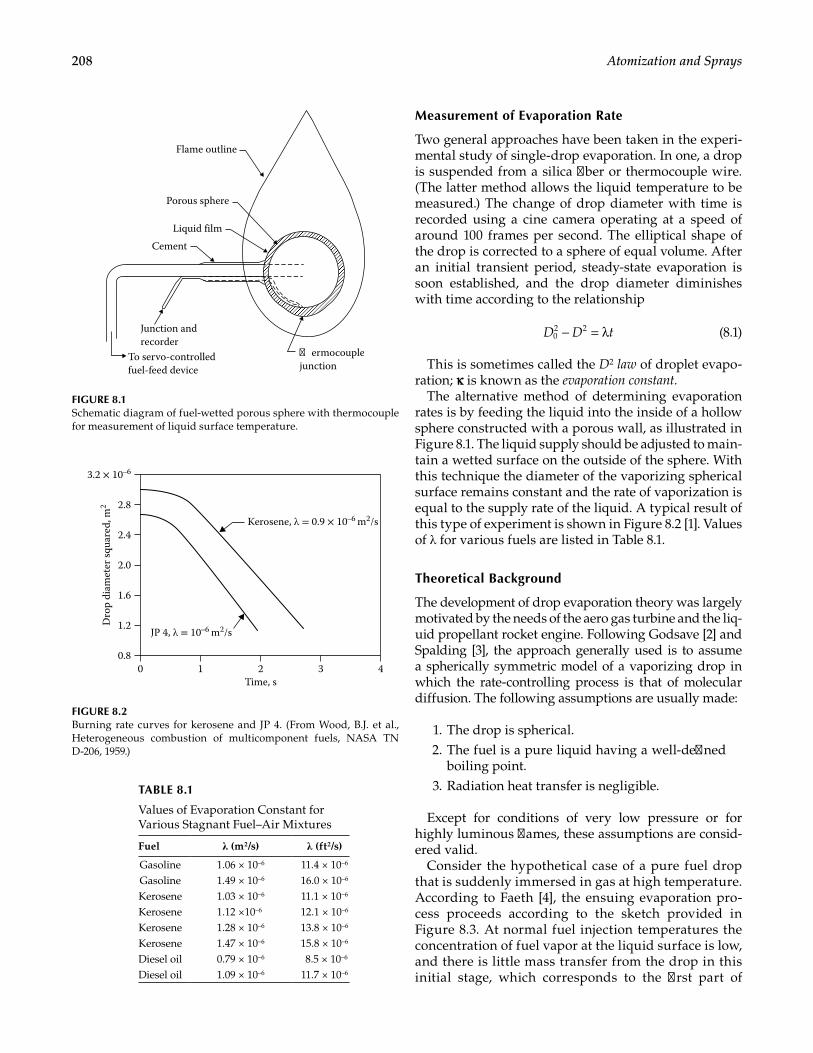
208 Atomization and Sprays

Measurement of Evaporation Rate

Two general approaches have been taken in the experi-mental study of single-drop evaporation. In one, a drop is suspended from a silica fiber or thermocouple wire. (The latter method allows the liquid temperature to be measured.) The change of drop diameter with time is recorded using a cine camera operating at a speed of around 100 frames per second. The elliptical shape of the drop is corrected to a sphere of equal volume. After an initial transient period, steady-state evaporation is soon established, and the drop diameter diminishes with time according to the relationship

02 2D D t− = λ (8.1)

This is sometimes called the D2 law of droplet evapo-ration; k is known as the evaporation constant.

The alternative method of determining evaporation rates is by feeding the liquid into the inside of a hollow sphere constructed with a porous wall, as illustrated in Figure 8.1. The liquid supply should be adjusted to main-tain a wetted surface on the outside of the sphere. With this technique the diameter of the vaporizing spherical surface remains constant and the rate of vaporization is equal to the supply rate of the liquid. A typical result of this type of experiment is shown in Figure 8.2 [1]. Values of λ for various fuels are listed in Table 8.1.

Theoretical Background

The development of drop evaporation theory was largely motivated by the needs of the aero gas turbine and the liq-uid propellant rocket engine. Following Godsave [2] and Spalding [3], the approach generally used is to assume a spherically symmetric model of a vaporizing drop in which the rate-controlling process is that of molecular diffusion. The following assumptions are usually made:

1. The drop is spherical. 2. The fuel is a pure liquid having a well-defined

boiling point. 3. Radiation heat transfer is negligible.

Except for conditions of very low pressure or for highly luminous flames, these assumptions are consid-ered valid.

Consider the hypothetical case of a pure fuel drop that is suddenly immersed in gas at high temperature. According to Faeth [4], the ensuing evaporation pro-cess proceeds according to the sketch provided in Figure 8.3. At normal fuel injection temperatures the concentration of fuel vapor at the liquid surface is low, and there is little mass transfer from the drop in this initial stage, which corresponds to the first part of

Flame outline

Porous sphere

Liquid film

Cement

Junction andrecorder

To servo-controlledfuel-feed device

ermocouplejunction

FIGURE 8.1Schematic diagram of fuel-wetted porous sphere with thermocouple for measurement of liquid surface temperature.

0.8

2.8

2.4Kerosene, λ = 0.9 × 10–6 m2/s

JP 4, λ = 10–6 m2/s

2.0

1.6

1.2

3.2 × 10–6

Dro

p di

amet

er sq

uare

d, m

2

0 32Time, s

1 4

FIGURE 8.2Burning rate curves for kerosene and JP 4. (From Wood, B.J. et al., Heterogeneous combustion of multicomponent fuels, NASA TN D-206, 1959.)

TABLE 8.1

Values of Evaporation Constant for Various Stagnant Fuel–Air Mixtures

Fuel λ (m2/s) λ (ft2/s)

Gasoline 1.06 × 10–6 11.4 × 10–6

Gasoline 1.49 × 10–6 16.0 × 10–6

Kerosene 1.03 × 10–6 11.1 × 10–6

Kerosene 1.12 ×10–6 12.1 × 10–6

Kerosene 1.28 × 10–6 13.8 × 10–6

Kerosene 1.47 × 10–6 15.8 × 10–6

Diesel oil 0.79 × 10–6 8.5 × 10–6

Diesel oil 1.09 × 10–6 11.7 × 10–6

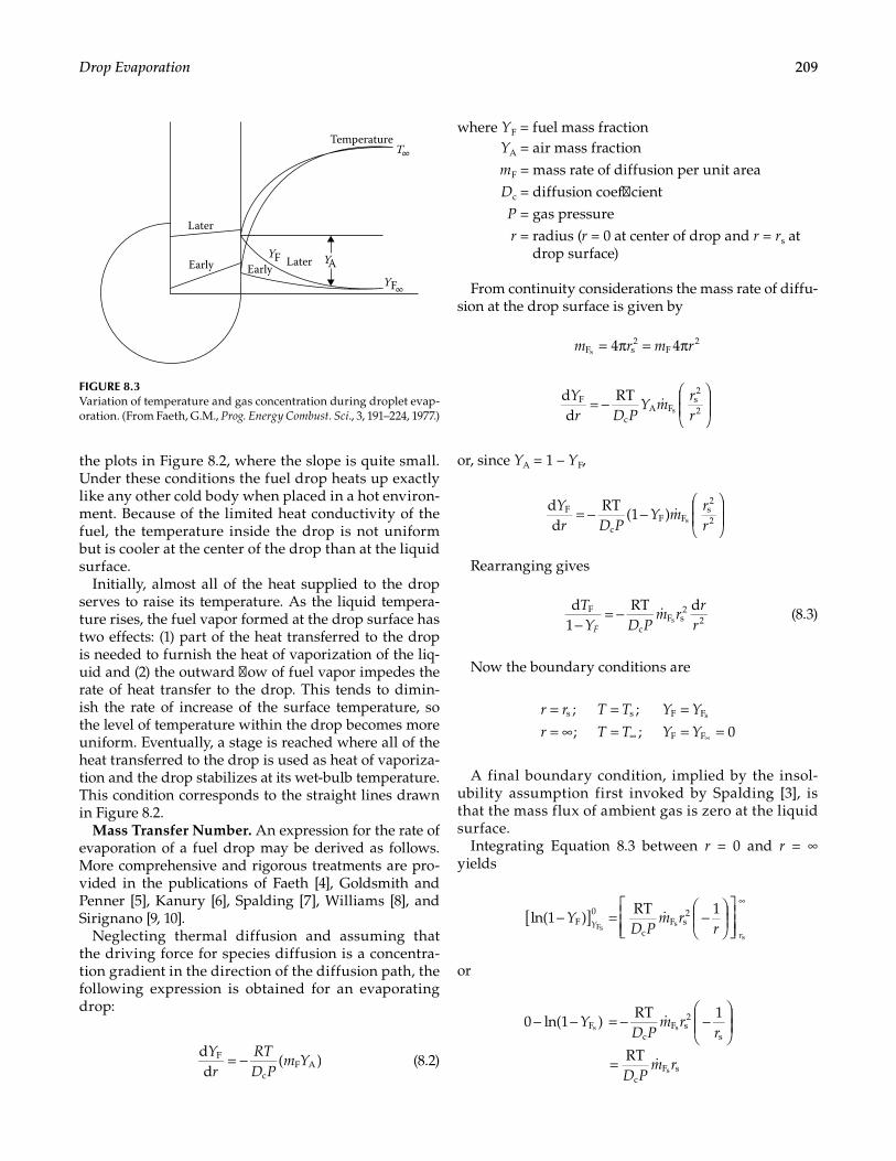
209Drop Evaporation

the plots in Figure 8.2, where the slope is quite small. Under these conditions the fuel drop heats up exactly like any other cold body when placed in a hot environ-ment. Because of the limited heat conductivity of the fuel, the temperature inside the drop is not uniform but is cooler at the center of the drop than at the liquid surface.

Initially, almost all of the heat supplied to the drop serves to raise its temperature. As the liquid tempera-ture rises, the fuel vapor formed at the drop surface has two effects: (1) part of the heat transferred to the drop is needed to furnish the heat of vaporization of the liq-uid and (2) the outward flow of fuel vapor impedes the rate of heat transfer to the drop. This tends to dimin-ish the rate of increase of the surface temperature, so the level of temperature within the drop becomes more uniform. Eventually, a stage is reached where all of the heat transferred to the drop is used as heat of vaporiza-tion and the drop stabilizes at its wet-bulb temperature. This condition corresponds to the straight lines drawn in Figure 8.2.

Mass Transfer Number. An expression for the rate of evaporation of a fuel drop may be derived as follows. More comprehensive and rigorous treatments are pro-vided in the publications of Faeth [4], Goldsmith and Penner [5], Kanury [6], Spalding [7], Williams [8], and Sirignano [9, 10].

Neglecting thermal diffusion and assuming that the driving force for species diffusion is a concentra-tion gradient in the direction of the diffusion path, the following expression is obtained for an evaporating drop:

dd

( )F

cF A

Yr

RTD P

m Y= − (8.2)

where YF = fuel mass fractionYA = air mass fractionmF = mass rate of diffusion per unit areaDc = diffusion coefficientP = gas pressurer = radius (r = 0 at center of drop and r = rs at

drop surface)

From continuity considerations the mass rate of diffu-sion at the drop surface is given by

4 4F s2

F2

sm r m r= π = π

Yr D P

Y mrr

= −

dd

RTF

cA F

s2

2s

or, since YA = 1 – YF,

Yr D P

Y mrr

= − −

dd

RT(1 )F

cF F

s2

2s

Rearranging gives

TY D P

m rr

rF−= −d

1RT dF

cF s

22s

(8.3)

Now the boundary conditions are

; ;

; ; 0s s F F

F F

sr r T T Y Y

r T T Y Y

= = == ∞ = = =∞ ∞

A final boundary condition, implied by the insol-ubility assumption first invoked by Spalding [3], is that the mass flux of ambient gas is zero at the liquid surface.

Integrating Equation 8.3 between r = 0 and r = ∞ yields

YD P

m rrY

r

[ ]− = −

∞

ln(1 )RT 1

F0

cF s

2Fs s

s

or

Y

D Pm r

r

D Pm r

− − = − −

=

0 ln(1 )RT 1

RT

Fc

F s2

s

cF s

s s

s

Temperature

Later

LaterEarlyEarly

T∞

YAYFY

F∞

FIGURE 8.3Variation of temperature and gas concentration during droplet evap-oration. (From Faeth, G.M., Prog. Energy Combust. Sci., 3, 191–224, 1977.)

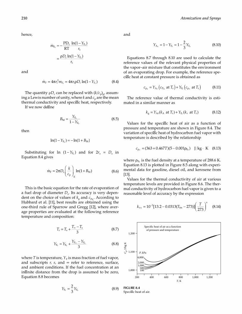
210 Atomization and Sprays

hence,

mY

r

D Yr

= − −

= ρ −

PDRT

ln(1 )

ln(1 )

Fc F

s

c F

s

ss

s

and

m r m r D YF s F s c Fs s= π = π ρ −4 4 ln(1 )2 (8.4)

The quantity ρ Dc can be replaced with (k/cp)g, assum-ing a Lewis number of unity, where k and cp are the mean thermal conductivity and specific heat, respectively.

If we now define

1M

F

F

s

s

BY

Y=

− (8.5)

then

ln(1 ) ln(1 )F MsY B− = − +

Substituting for ln (1 )FsY− and for 2rs = Ds in Equation 8.4 gives

m Dkc

B= π

+2 ln(1 )F s

p g

M (8.6)

This is the basic equation for the rate of evaporation of a fuel drop of diameter Ds. Its accuracy is very depen-dent on the choice of values of kg and pgc . According to Hubbard et al. [11], best results are obtained using the one-third rule of Sparrow and Gregg [12], where aver-age properties are evaluated at the following reference temperature and composition:

3r s

sT TT T= + −∞ (8.7)

3F F

F Fr s

sY YY Y= + −∞ (8.8)

where T is temperature, YF is mass fraction of fuel vapor, and subscripts r, s, and ∞ refer to reference, surface, and ambient conditions. If the fuel concentration at an infinite distance from the drop is assumed to be zero, Equation 8.8 becomes

23F Fr sY Y= (8.9)

and

1 123A F Fr r sY Y Y= − = − (8.10)

Equations 8.7 through 8.10 are used to calculate the reference values of the relevant physical properties of the vapor–air mixture that constitutes the environment of an evaporating drop. For example, the reference spe-cific heat at constant pressure is obtained as

at atp A P r F p rs r A r vc Y c T Y c T( )( )= + (8.11)

The reference value of thermal conductivity is esti-mated in a similar manner as

( at ) ( at )g Ar A r F v rrk Y k T Y k T= + (8.12)

Values for the specific heat of air as a function of pressure and temperature are shown in Figure 8.4. The variation of specific heat of hydrocarbon fuel vapor with temperature is described by the relationship

= + − ρ ⋅(363 0.467 )(5 0.001 ) J kg Kp Fv 0c T (8.13)

where F0ρ is the fuel density at a temperature of 288.6 K. Equation 8.13 is plotted in Figure 8.5 along with experi-mental data for gasoline, diesel oil, and kerosene from [13].

Values for the thermal conductivity of air at various temperature levels are provided in Figure 8.6. The ther-mal conductivity of hydrocarbon fuel vapor is given to a reasonable level of accuracy by the expression

10 [13.2 0.0313( 273)]273v

3bnTk T

T n

= − −

− (8.14)

1,000

200 1,000800T, K

600400

2,0001,000

500100

4,000

1,200

1,100 P, kPa

Specific heat of air as a functionof pressure and temperature

1,200

Cp,

J/kg

K

FIGURE 8.4Specific heat of air.

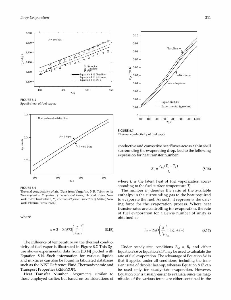
211Drop Evaporation

where

2 0.0372bn

2

nT

T= −

(8.15)

The influence of temperature on the thermal conduc-tivity of fuel vapor is illustrated in Figure 8.7. This fig-ure shows experimental data from [13,14] plotted with Equation 8.14. Such information for various liquids and mixtures can also be found in tabulated databases such as the NIST Reference Fluid Thermodynamic and Transport Properties (REFPROP).

Heat Transfer Number. Arguments similar to those employed earlier, but based on considerations of

conductive and convective heat fluxes across a thin shell surrounding the evaporating drop, lead to the following expression for heat transfer number:

=−∞( )

Tp ggB

c T T

L (8.16)

where L is the latent heat of fuel vaporization corre-sponding to the fuel surface temperature Ts.

The number BT denotes the ratio of the available enthalpy in the surrounding gas to the heat required to evaporate the fuel. As such, it represents the driv-ing force for the evaporation process. Where heat transfer rates are controlling for evaporation, the rate of fuel evaporation for a Lewis number of unity is obtained as

m Dkc

B=

+2π ln(1 )F

p g

T (8.17)

Under steady-state conditions BM = BT and either Equation 8.6 or Equation 8.17 may be used to calculate the rate of fuel evaporation. The advantage of Equation 8.6 is that it applies under all conditions, including the tran-sient state of droplet heat-up, whereas Equation 8.17 can be used only for steady-state evaporation. However, Equation 8.17 is usually easier to evaluate, since the mag-nitudes of the various terms are either contained in the

2,200

400 500

KerocineGasolineDF 2

450T, K

550

2,600

2,500

2,400

2,300

2,700

P ≏ 100 kPa

Cpv

, J/k

g K

Equation 8.13 GasolineEquation 8.13 KeroseneEquation 8.13 DF 2

FIGURE 8.5Specific heat of fuel vapor.

300

0.03

0.04

ermal conductivity of air

P = 5 Mpa

P = 0.1 Mpa

0.05

500T, K

400 600

k A, J

/ms K

FIGURE 8.6Thermal conductivity of air. (Data from Vargaftik, N.B., Tables on the Thermophysical Properties of Liquids and Gases, Halsted Press, New York, 1975; Touloukian, Y., Thermal–Physical Properties of Matter, New York, Plenum Press, 1970.)

900800700600500400

Equation 8.14

n – heptane

Kerosene

Gasoline

Experimental (gasoline)

300

0.09

0.08

0.07

0.06

0.05

0.04

0.03

0.02

0.01

0

0.10

1,000T, K

k V, J

/ms K

FIGURE 8.7Thermal conductivity of fuel vapor.

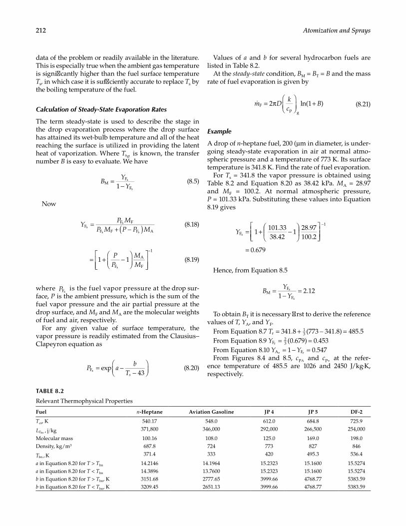
212 Atomization and Sprays

data of the problem or readily available in the literature. This is especially true when the ambient gas temperature is significantly higher than the fuel surface temperature Ts, in which case it is sufficiently accurate to replace Ts by the boiling temperature of the fuel.

Calculation of Steady-State Evaporation Rates

The term steady-state is used to describe the stage in the drop evaporation process where the drop surface has attained its wet-bulb temperature and all of the heat reaching the surface is utilized in providing the latent heat of vaporization. Where sgtT is known, the transfer number B is easy to evaluate. We have

1M

F

F

s

s

BY

Y=

− (8.5)

Now

FF F

F F F As

s

s s

YP M

P M P P M( )=+ −

(8.18)

1 1F

A

F

1

s

PP

MM

= + −

−

(8.19)

where FsP is the fuel vapor pressure at the drop sur-face, P is the ambient pressure, which is the sum of the fuel vapor pressure and the air partial pressure at the drop surface, and MF and MA are the molecular weights of fuel and air, respectively.

For any given value of surface temperature, the vapor pressure is readily estimated from the Clausius–Clapeyron equation as

exp43FsP a

bTs

= −−

(8.20)

Values of a and b for several hydrocarbon fuels are listed in Table 8.2.

At the steady-state condition, BM = BT = B and the mass rate of fuel evaporation is given by

m Dkc

B= π

+2 ln(1 )F

p g

(8.21)

Example

A drop of n-heptane fuel, 200 (μm in diameter, is under-going steady-state evaporation in air at normal atmo-spheric pressure and a temperature of 773 K. Its surface temperature is 341.8 K. Find the rate of fuel evaporation.

For Ts = 341.8 the vapor pressure is obtained using Table 8.2 and Equation 8.20 as 38.42 kPa. MA = 28.97 and MF = 100.2. At normal atmospheric pressure, P = 101.33 kPa. Substituting these values into Equation 8.19 gives

1

101.3338.42

128.97100.2

0.679

F

1

sY = + −

=

−

Hence, from Equation 8.5

1

2.12MF

F

s

s

BY

Y=

−=

To obtain BT it is necessary first to derive the reference values of T, YA, and YF.

From Equation 8.7 341.8 (773 341.8) 485.5r13T = + − =

From Equation 8.9 (0.679) 0.453F23rY = =

From Equation 8.10 1 0.547A Fr rY Y= − =From Figures 8.4 and 8.5, pAc and pvc at the refer-

ence temperature of 485.5 are 1026 and 2450 J/kg·K, respectively.

TABLE 8.2

Relevant Thermophysical Properties

Fuel n-Heptane Aviation Gasoline JP 4 JP 5 DF-2

Tcr, K 540.17 548.0 612.0 684.8 725.9

, j kgbnLT371,800 346,000 292,000 266,500 254,000

Molecular mass 100.16 108.0 125.0 169.0 198.0Density, kg/m3 687.8 724 773 827 846

, KbnT 371.4 333 420 495.3 536.4

a in Equation 8.20 for T > Tbn 14.2146 14.1964 15.2323 15.1600 15.5274a in Equation 8.20 for T < Tbn 14.3896 13.7600 15.2323 15.1600 15.5274b in Equation 8.20 for T > Tbn, K 3151.68 2777.65 3999.66 4768.77 5383.59b in Equation 8.20 for T < Tbn, K 3209.45 2651.13 3999.66 4768.77 5383.59

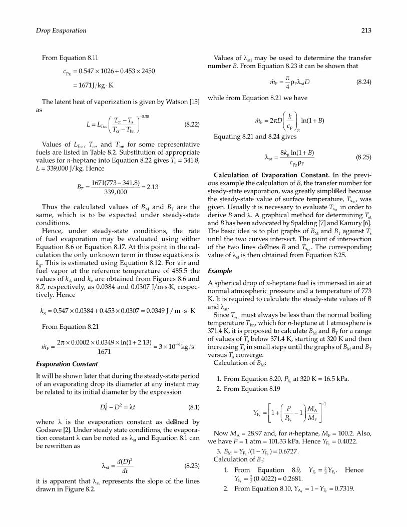
213Drop Evaporation

From Equation 8.11

= × + ×

= ⋅

0.547 1026 0.453 2450

1671J kg K

pgc

The latent heat of vaporization is given by Watson [15] as

cr s

cr bn

0.38

bnL LT TT T

T= −−

−

(8.22)

Values of bnLT , Tcr, and Tbn for some representative fuels are listed in Table 8.2. Substitution of appropriate values for n-heptane into Equation 8.22 gives Ts = 341.8, L = 339,000 J/kg. Hence

1671(773 341.8)

339, 0002.13BT = − =

Thus the calculated values of BM and BT are the same, which is to be expected under steady-state conditions.

Hence, under steady-state conditions, the rate of fuel evaporation may be evaluated using either Equation 8.6 or Equation 8.17. At this point in the cal-culation the only unknown term in these equations is kg. This is estimated using Equation 8.12. For air and fuel vapor at the reference temperature of 485.5 the values of kA and kv are obtained from Figures 8.6 and 8.7, respectively, as 0.0384 and 0.0307 J/m·s·K, respec-tively. Hence

0.547 0.0384 0.453 0.0307 0.0349 J / m s Kgk = × + × = ⋅ ⋅

From Equation 8.21

= π × × × + = × −

2 0.0002 0.0349 ln(1 2.13)1671

3 10 kg sF8m

Evaporation Constant

It will be shown later that during the steady-state period of an evaporating drop its diameter at any instant may be related to its initial diameter by the expression

− = λ02 2D D t (8.1)

where λ  is the evaporation constant as defined by Godsave [2]. Under steady state conditions, the evapora-tion constant λ  can be noted as λst and Equation 8.1 can be rewritten as

( )

st

2d Ddt

λ = (8.23)

it is apparent that λ st represents the slope of the lines drawn in Figure 8.2.

Values of λ stl may be used to determine the transfer number B. From Equation 8.23 it can be shown that

4F F stm D= π ρ λ (8.24)

while from Equation 8.21 we have

2 ln(1 )Fp g

m Dkc

B = π

+

Equating 8.21 and 8.24 gives

8 ln(1 )

stg

p Fg

k Bc

λ =+

ρ (8.25)

Calculation of Evaporation Constant. In the previ-ous example the calculation of B, the transfer number for steady-state evaporation, was greatly simplified because the steady-state value of surface temperature, sstT , was given. Usually it is necessary to evaluate sstT in order to derive B and λ . A graphical method for determining Tst and B has been advocated by Spalding [7] and Kanury [6]. The basic idea is to plot graphs of BM and BT against Ts until the two curves intersect. The point of intersection of the two lines defines B and sstT . The corresponding value of λ st is then obtained from Equation 8.25.

Example

A spherical drop of n-heptane fuel is immersed in air at normal atmospheric pressure and a temperature of 773 K. It is required to calculate the steady-state values of B and λ st.

Since stTs must always be less than the normal boiling temperature Tbn, which for n-heptane at 1 atmosphere is 371.4 K, it is proposed to calculate BM and BT for a range of values of Ts below 371.4 K, starting at 320 K and then increasing Ts in small steps until the graphs of BM and BT versus Ts converge.

Calculation of BM:

1. From Equation 8.20, FsP at 320 K = 16.5 kPa. 2. From Equation 8.19

1 1FF

A

F

1

ss

YP

PMM

= + −

−

Now MA = 28.97 and, for n-heptane, MF = 100.2. Also, we have P = 1 atm = 101.33 kPa. Hence 0.4022FsY = . 3. (1 ) 0.6727M F Fs sB Y Y= − = .

Calculation of BT:

1. From Equation 8.9, F23 Fr sY Y= . Hence

(0.4022) 0.2681F23rY = = .

2. From Equation 8.10, 1 0.7319A Fr rY Y= − = .

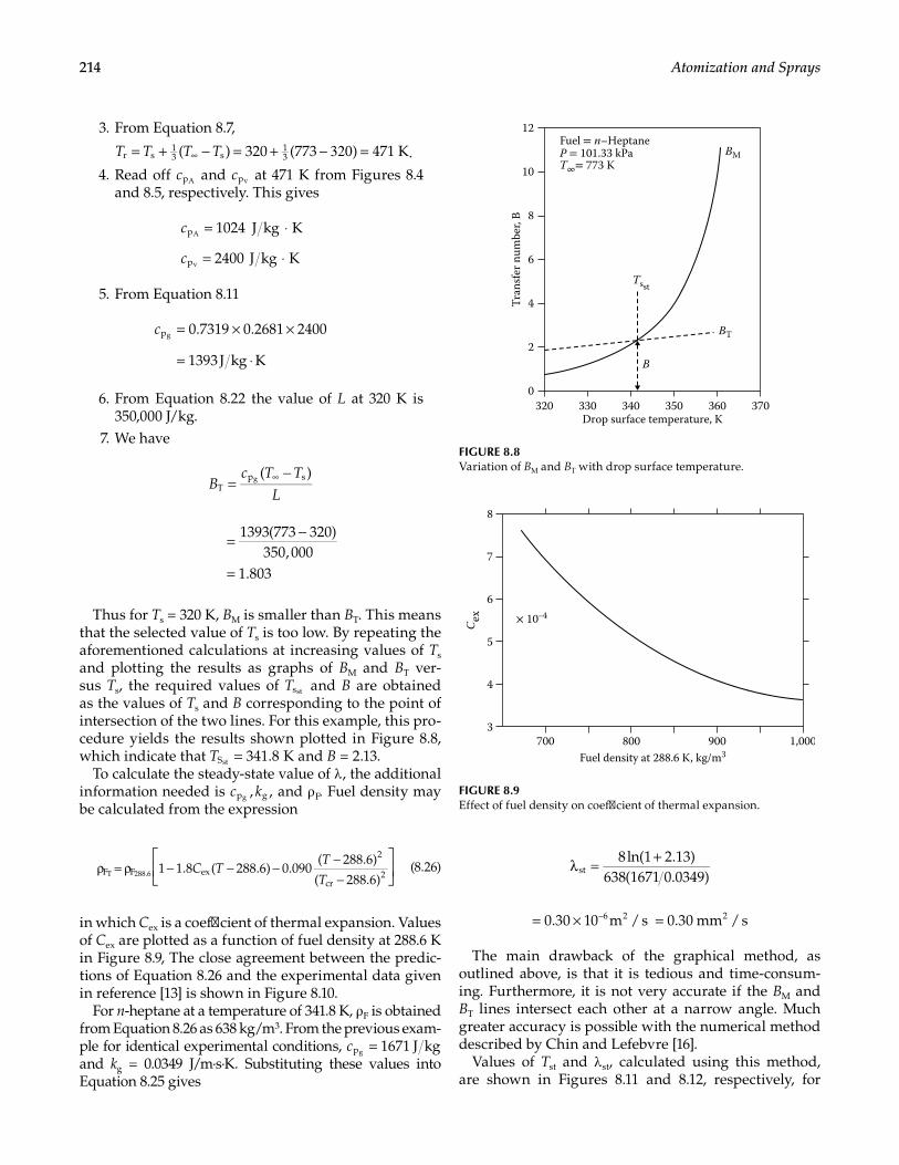
214 Atomization and Sprays

3. From Equation 8.7,

( ) 320 (773 ) 471 Kr s13 s

13T T T T= + − = + − 320 =∞ .

4. Read off pAc and pvc at 471 K from Figures 8.4 and 8.5, respectively. This gives

c

c

= ⋅

= ⋅

1024 J kg K

2400 J kg K

p

p

A

v

5. From Equation 8.11

= × ×

= ⋅

0.7319 0.2681 2400

1393J kg K

pgc

6. From Equation 8.22 the value of L at 320 K is 350,000 J/kg.

7. We have

=−∞( )

Tp sgB

c T T

L

1393(773 320)350,000

1.803

= −

=

Thus for Ts = 320 K, BM is smaller than BT. This means that the selected value of Ts is too low. By repeating the aforementioned calculations at increasing values of Ts and plotting the results as graphs of BM and BT ver-sus Ts, the required values of sstT and B are obtained as the values of Ts and B corresponding to the point of intersection of the two lines. For this example, this pro-cedure yields the results shown plotted in Figure 8.8, which indicate that 341.8SstT = K and B = 2.13.

To calculate the steady-state value of λ , the additional information needed is , ,p ggc k and ρ F. Fuel density may be calculated from the expression

ρ = ρ − − −−−

1 1.8 ( 288.6) 0.090( 288.6)

( 288.6)F F ex

2

cr2T 288.6 C T

T

T (8.26)

in which Cex is a coefficient of thermal expansion. Values of Cex are plotted as a function of fuel density at 288.6 K in Figure 8.9, The close agreement between the predic-tions of Equation 8.26 and the experimental data given in reference [13] is shown in Figure 8.10.

For n-heptane at a temperature of 341.8 K, ρ F is obtained from Equation 8.26 as 638 kg/m3. From the previous exam-ple for identical experimental conditions, 1671 J kgpgc = and kg = 0.0349 J/m·s·K. Substituting these values into Equation 8.25 gives

8ln(1 2.13)

638(1671 0.0349)stλ = +

0.30 10 m / s 0.30 mm / s–6 2 2= × =

The main drawback of the graphical method, as outlined above, is that it is tedious and time-consum-ing. Furthermore, it is not very accurate if the BM and BT lines intersect each other at a narrow angle. Much greater accuracy is possible with the numerical method described by Chin and Lefebvre [16].

Values of Tst and λ st, calculated using this method, are shown in Figures 8.11 and 8.12, respectively, for

0360 370350340330320

10

8

6

Tran

sfer

num

ber,

B

Drop surface temperature, K

Fuel = n–HeptaneP = 101.33 kPa

4

2

12

T∞= 773 KBM

BT

B

Tsst

FIGURE 8.8Variation of BM and BT with drop surface temperature.

700 900800Fuel density at 288.6 K, kg/m3

1,0003

7

6

5

4

8

× 10–4

Cex

FIGURE 8.9Effect of fuel density on coefficient of thermal expansion.

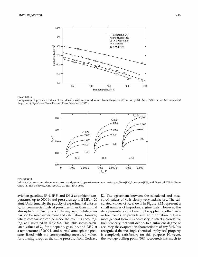
215Drop Evaporation

aviation gasoline, JP 4, JP 5, and DF-2 at ambient tem-peratures up to 2000 K and pressures up to 2 MPa (~20 atm). Unfortunately, the paucity of experimental data on λ st for commercial fuels at pressures other than normal atmospheric virtually prohibits any worthwhile com-parison between experiment and calculation. However, where comparison can be made the result is encourag-ing, as illustrated in Table 8.3. This table shows calcu-lated values of λ st for n-heptane, gasoline, and DF-2 at a temperature of 2000 K and normal atmospheric pres-sure, listed with the corresponding measured values for burning drops at the same pressure from Godsave

[2]. The agreement between the calculated and mea-sured values of λ st is clearly very satisfactory. The cal-culated values of λ st shown in Figure 8.12 represent a small number of important engine fuels. However, the data presented cannot readily be applied to other fuels or fuel blends. To provide similar information, but in a more general form, it is necessary to select a correlative fuel property that will define, to a sufficient degree of accuracy, the evaporation characteristics of any fuel. It is recognized that no single chemical or physical property is completely satisfactory for this purpose. However, the average boiling point (50% recovered) has much to

400350 500450400

Fuel temperature, K

Equation 8.26JP 5 (Kerosene)JP 4 (Gasoline)n-Octanen-Heptane

550

900

800

700

600

500

1,000

Fuel

den

sity,

kg/m

3

FIGURE 8.10Comparison of predicted values of fuel density with measured values from Vargaftik. (From Vargaftik, N.B., Tables on the Thermophysical Properties of Liquids and Gases, Halsted Press, New York, 1975.)

3000 1,000

JP 4

100

2,000P, kPa

P, kPa

P, kPa

1,000

500 100

2,000

1,000

500100

2,000

1,000

500

JP 5 DF 2

2,000 0 1,000 2,000 0 1,000 2,000

600

500

400

700

T∞, K

T sst

, K

FIGURE 8.11Influence of pressure and temperature on steady-state drop surface temperature for gasoline (JP 4), kerosene (JP 5), and diesel oil (DF-2). (From Chin, J.S. and Lefebvre, A.H., AIAA J., 21, 1437–1443, 1983.)

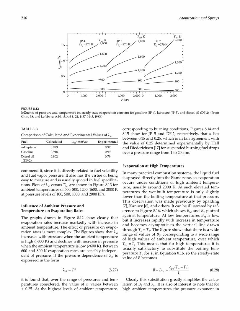
216 Atomization and Sprays

commend it, since it is directly related to fuel volatility and fuel vapor pressure. It also has the virtue of being easy to measure and is usually quoted in fuel specifica-tions. Plots of λ st versus Tbn are shown in Figure 8.13 for ambient temperatures of 500, 800, 1200, 1600, and 2000 K at pressure levels of 100, 500, 1000, and 2000 kPa.

Influence of Ambient Pressure and Temperature on Evaporation Rates

The graphs drawn in Figure 8.12 show clearly that evaporation rates increase markedly with increase in ambient temperature. The effect of pressure on evapo-ration rates is more complex. The figures show that λ st increases with pressure when the ambient temperature is high (>800 K) and declines with increase in pressure when the ambient temperature is low (<600 K). Between 600 and 800 K evaporation rates are sensibly indepen-dent of pressure. If the pressure dependence of λ st is expressed in the form

λ ∝st Pn (8.27)

it is found that, over the range of pressures and tem-peratures considered, the value of n varies between ± 0.25. At the highest levels of ambient temperature,

corresponding to burning conditions, Figures 8.14 and 8.15 show for JP 5 and DF-2, respectively, that n lies between 0.15 and 0.25, which is in fair agreement with the value of 0.25 determined experimentally by Hall and Diederichsen [17] for suspended burning fuel drops over a pressure range from 1 to 20 atm.

Evaporation at High Temperatures

In many practical combustion systems, the liquid fuel is sprayed directly into the flame zone, so evaporation occurs under conditions of high ambient tempera-ture, usually around 2000 K. At such elevated tem-peratures the wet-bulb temperature is only slightly lower than the boiling temperature at that pressure. This observation was made previously by Spalding [7], Kanury [6], and others. It can be illustrated by ref-erence to Figure 8.16, which shows BM and BT plotted against temperature. At low temperatures BM is low, but it increases rapidly with increase in temperature and becomes asymptotic to the vertical line drawn through Ts = Tb. The figure shows that there is a wide range of values of BT, corresponding to a wide range of high values of ambient temperature, over which

s bstT T= This means that for high temperatures it is usually satisfactory to substitute the boiling tem-perature Tb for Ts in Equation 8.16, so the steady-state value of B becomes

= =−∞( )

Tp b

stgB B

c T T

L (8.28)

Clearly this substitution greatly simplifies the calcu-lation of BT and λ st. It is also of interest to note that for high ambient temperatures the pressure exponent in

JP 4

500

800

1,200

1,600

1,000 2,000 0 1,000 2,000 0 1,000 2,0000

2,000

500

800

1,200

1,600

2,000

500

800

1,200

1,600

2,000

P, kPa

0

0.5

1.0

1.5 TF0 =270 K

JP 5TF0

=270 KDF 2

TF0 =270 K

T∞, KT∞, K T∞, K

λ st, m

m2 /s

FIGURE 8.12Influence of pressure and temperature on steady-state evaporation constant for gasoline (JP 4), kerosene (JP 5), and diesel oil (DF-2). (From Chin, J.S. and Lefebvre, A.H., AIAA J., 21, 1437–1443, 1983.)

TABLE 8.3

Comparison of Calculated and Experimental Values of λ st

Fuel Calculated λ st (mm2/s) Experimental

n-Heptane 0.979 0.97Gasoline 0.948 0.99Diesel oil (DF-2)

0.802 0.79

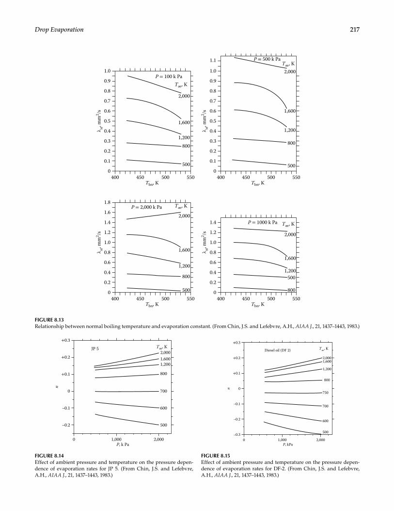
217Drop Evaporation

λ st, m

m2 /s

2,000

1,600

1,200800

500

P = 100 k Pa

P = 500 k Pa

0.9

0.8

0.7

0.6

0.5

0.4

0.3

0.2

0.1

0400 500450 550

1.0

Tbn, K

T∞, K

λ st, m

m2 /s

2,000

1,600

1,200

800

500

0.9

0.8

0.7

0.6

0.5

0.4

0.3

0.2

0.1

0400 500450 550

1.0

1.1

Tbn, K

T∞, K

λ st, m

m2 /s

2,000

1,600

1,200

800

500

P = 2,000 k Pa

P = 1000 k Pa

1.8

1.6

1.4

1.2

1.0

0.8

0.6

0.4

0.2

0400 500450 550

Tbn, K

T∞, Kλ st

, mm

2 /s 2,000

1,600

1,200500

800

1.4

1.2

1.0

0.8

0.6

0.4

0.2

0400 500450 550

Tbn, K

T∞, K

FIGURE 8.13Relationship between normal boiling temperature and evaporation constant. (From Chin, J.S. and Lefebvre, A.H., AIAA J., 21, 1437–1443, 1983.)

P, k Pa

2,000JP 5

n

1,6001,200

800

700

600

500–0.2

0 1,000 2,000

+0.2

+0.1

0

–0.1

+0.3T∞, K

FIGURE 8.14Effect of ambient pressure and temperature on the pressure depen-dence of evaporation rates for JP 5. (From Chin, J.S. and Lefebvre, A.H., AIAA J., 21, 1437–1443, 1983.)

P, kPa

1,6002,000

Diesel oil (DF 2)

1,200

800

750

700

600

500

–0.2

–0.30 1,000 2,000

+0.2

+0.1

0

–0.1

+0.3T∞, K

n

FIGURE 8.15Effect of ambient pressure and temperature on the pressure depen-dence of evaporation rates for DF-2. (From Chin, J.S. and Lefebvre, A.H., AIAA J., 21, 1437–1443, 1983.)

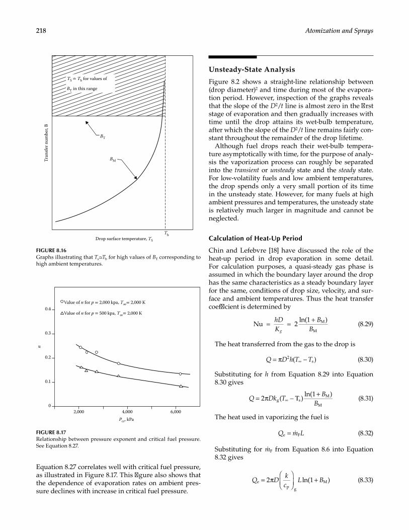
218 Atomization and Sprays

Equation 8.27 correlates well with critical fuel pressure, as illustrated in Figure 8.17. This figure also shows that the dependence of evaporation rates on ambient pres-sure declines with increase in critical fuel pressure.

Unsteady-State Analysis

Figure 8.2 shows a straight-line relationship between (drop diameter)2 and time during most of the evapora-tion period. However, inspection of the graphs reveals that the slope of the D2/t line is almost zero in the first stage of evaporation and then gradually increases with time until the drop attains its wet-bulb temperature, after which the slope of the D2/t line remains fairly con-stant throughout the remainder of the drop lifetime.

Although fuel drops reach their wet-bulb tempera-ture asymptotically with time, for the purpose of analy-sis the vaporization process can roughly be separated into the transient or unsteady state and the steady state. For low-volatility fuels and low ambient temperatures, the drop spends only a very small portion of its time in the unsteady state. However, for many fuels at high ambient pressures and temperatures, the unsteady state is relatively much larger in magnitude and cannot be neglected.

Calculation of Heat-Up Period

Chin and Lefebvre [18] have discussed the role of the heat-up period in drop evaporation in some detail. For calculation purposes, a quasi-steady gas phase is assumed in which the boundary layer around the drop has the same characteristics as a steady boundary layer for the same, conditions of drop size, velocity, and sur-face and ambient temperatures. Thus the heat transfer coefficient is determined by

= = +Nu 2

ln(1 )M

M

hDK

BBg

(8.29)

The heat transferred from the gas to the drop is

( )2sQ D h T T= π −∞ (8.30)

Substituting for h from Equation 8.29 into Equation 8.30 gives

2 ( )ln(1 )

g sM

MQ Dk T

BB

= π − Τ +∞ (8.31)

The heat used in vaporizing the fuel is

e FQ m L= (8.32)

Substituting for Fm from Equation 8.6 into Equation 8.32 gives

2 ln(1 )ep g

MQ Dkc

L B= π

+ (8.33)

Drop surface temperature, TS

BT

BMTran

sfer

num

ber,

B

Tb

BT in this range

TS ≏ Tb for values of

FIGURE 8.16Graphs illustrating that Ts≃Tb for high values of BT corresponding to high ambient temperatures.

Pcr, kPa2,000

0

0.1

0.2

0.3

0.4Value of n for p = 2,000 kpa, T∞= 2,000 K

Value of n for p = 500 kpa, T∞= 2,000 K

4,000 6,000

n

FIGURE 8.17Relationship between pressure exponent and critical fuel pressure. See Equation 8.27.

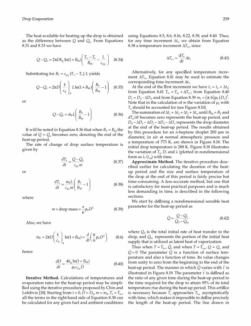
219Drop Evaporation

The heat available for heating up the drop is obtained as the difference between Q and Qe. From Equations 8.31 and 8.33 we have

− = π + − −

∞2 ln(1 )e g M

s

M pR

Q Q Dk BT T

BL

c (8.34)

Substituting for = −∞( )T p sgB c T T L yields

− = π

+ −

2 ln(1 ) 1e

p g

MT

MQ Q D

kc

L BBB

(8.35)

or

Q Q m LBB

− = −

1e F

T

M

(8.36)

It will be noted in Equation 8.36 that when BT = BM the value of Q = Qe becomes zero, denoting the end of the heat-up period.

The rate of change of drop surface temperature is given by

s e

pF

dTdt

Q Qc m

= − (8.37)

or

dTdt

m Lc m

BB

T

M= −

1s F

pF

(8.38)

where

= = ρdrop mass π6

F3m D (8.39)

Also, we have

m Dkc

Bddt

D= π

+ = π ρ

2 ln(1 )

6Fp g

M F3

(8.6)

hence

4 ln(1 )g M

F pg

dDdt

k Bc D

=+

ρ (8.40)

Iterative Method. Calculations of temperatures and evaporation rates for the heat-up period may be simpli-fied using the iterative procedure proposed by Chin and Lefebvre [18]. Starting from t = 0, D = D0, m = m0, s s0T T= , all the terms in the right-hand side of Equation 8.38 can be calculated for any given fuel and ambient conditions

using Equations 8.5, 8.6, 8.16, 8.22, 8.39, and 8.40. Thus, for any time increment ∆t1, we obtain from Equation 8.38 a temperature increment s1T∆ , since

dds

s11T

Tt

t∆ = ∆ (8.41)

Alternatively, for any specified temperature incre-ment s1T∆ , Equation 8.41 may be used to estimate the corresponding time increment 1t∆ .

At the end of the first increment we have t1 = t0 + ∆t1; from Equation 8.41 s s s1 0 1T T T= + ∆ ; from Equation 8.40 D1 = D0 - ∆D1; and from Equation 8.39 61 F 1

3m D( ) ( )= π ρ . Note that in the calculation of m the variation of ρ F with Ts should be accounted for (see Figure 8.10).

The summation of ∆t1 + ∆t2 + ∆t3 + ∆tn until BM = BT and dTs/dt becomes zero represents the heat-up period, and D0 – ∆D1 – ∆D2 – ∆D3 – ∆Dn represents the drop diameter at the end of the heat-up period. The results obtained by this procedure for an n-heptane droplet 200 μm in diameter, in air at normal atmospheric pressure and a temperature of 773 K, are shown in Figure 8.18. The initial drop temperature is 288 K. Figure 8.18 illustrates the variation of Ts, D, and λ  (plotted in nondimensional form as λ /λ st) with time.

Approximate Method. The iterative procedure desc-ribed earlier for calculating the duration of the heat-up period and the size and surface temperature of the drop at the end of this period is fairly precise but time-consuming. A less-accurate method, but one that is satisfactory for most practical purposes and is much less demanding in time, is described in the following sections.

We start by defining a nondimensional sensible heat parameter for the heat-up period as

e

0 e0

QQ Q

Q Q= −

− (8.42)

where Q0 is the total initial rate of heat transfer to the drop, and e0Q represents the portion of the initial heat supply that is utilized as latent heat of vaporization.

Thus when s0T T= , Q, and when sstT T= , Q = Qe and 0Q = The parameter Q is a function of surface tem-

perature and also a function of time. Its value changes from unity to zero from the beginning to the end of the heat-up period. The manner in which Q varies with t is illustrated in Figure 8.19. The parameter t is defined as the ratio of any given time during the heat-up period to the time required for the drop to attain 95% of its total temperature rise during the heat-up period. This artifice is necessary because Ts approaches sstT asymptotically with time, which makes it impossible to define precisely the length of the heat-up period. The line drawn in

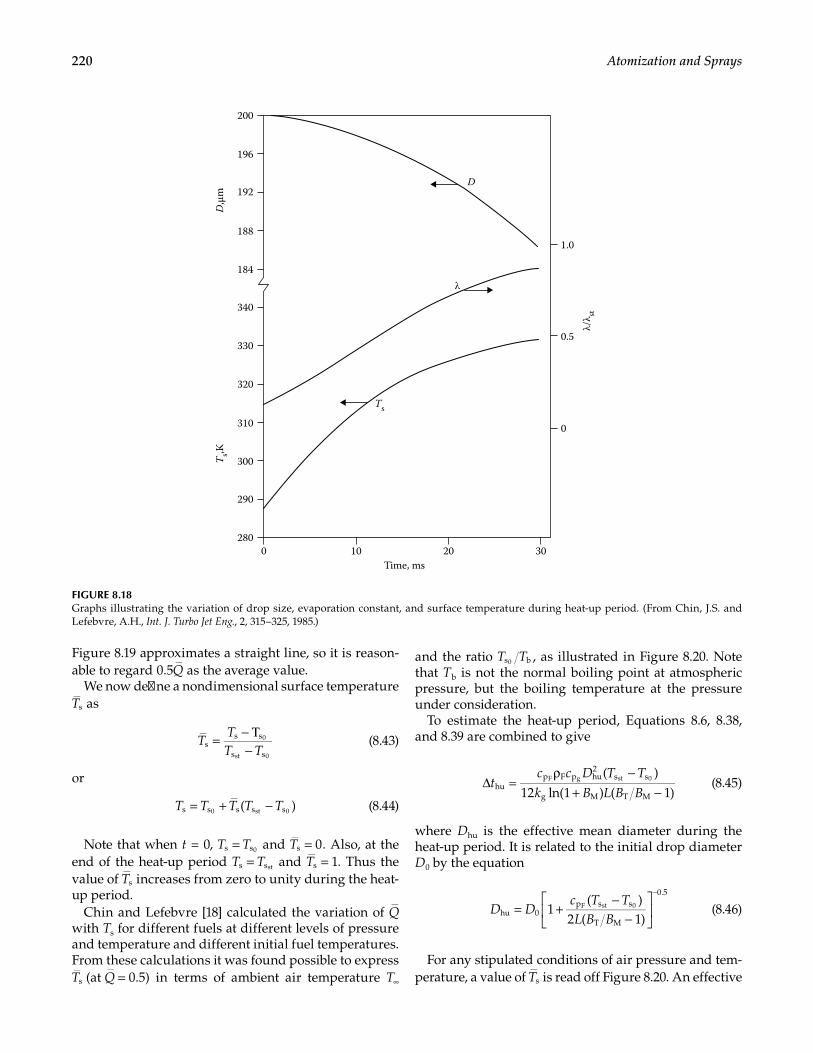
220 Atomization and Sprays

Figure 8.19 approximates a straight line, so it is reason-able to regard 0.5Q as the average value.

We now define a nondimensional surface temperature sT as

ss s

s s

0

st 0

TTT T

= − Τ−

(8.43)

or

( )s s s s s0 st 0T T T T T= + − (8.44)

Note that when t = 0, s s0T T= and 0sT = . Also, at the end of the heat-up period s sstT T= and 1sT = . Thus the value of sT increases from zero to unity during the heat-up period.

Chin and Lefebvre [18] calculated the variation of Q with Ts for different fuels at different levels of pressure and temperature and different initial fuel temperatures. From these calculations it was found possible to express

(at 0.5)sT Q = in terms of ambient air temperature T∞

and the ratio s b0T T , as illustrated in Figure 8.20. Note that Tb is not the normal boiling point at atmospheric pressure, but the boiling temperature at the pressure under consideration.

To estimate the heat-up period, Equations 8.6, 8.38, and 8.39 are combined to give

( )

12 ln(1 ) ( 1)hup F p hu

2s s

g M T M

F g st 0tc c D T T

k B L B B∆ =

ρ −+ −

(8.45)

where Dhu is the effective mean diameter during the heat-up period. It is related to the initial drop diameter D0 by the equation

1( )

2 ( 1)hu 0p s s

T M

0.5

F st 0D Dc T TL B B

= +−

−

−

(8.46)

For any stipulated conditions of air pressure and tem-perature, a value of sT is read off Figure 8.20. An effective

Time, ms

Ts

D

T s,KD

,μm

196

192

188

184

340

330

320

310

300

290

280

200

20100 30

0.5

0

1.0

λ

λ/λ st

FIGURE 8.18Graphs illustrating the variation of drop size, evaporation constant, and surface temperature during heat-up period. (From Chin, J.S. and Lefebvre, A.H., Int. J. Turbo Jet Eng., 2, 315–325, 1985.)

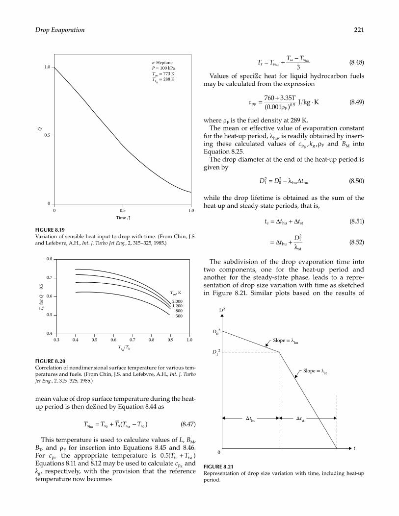
221Drop Evaporation

mean value of drop surface temperature during the heat-up period is then defined by Equation 8.44 as

( )s s s s shu 0 st 0T T T T T= + − (8.47)

This temperature is used to calculate values of L, BM, BT, and ρ F for insertion into Equations 8.45 and 8.46. For pFc the appropriate temperature is 0.5( )s s0 stT T+ Equations 8.11 and 8.12 may be used to calculate pgc and kg, respectively, with the provision that the reference temperature now becomes

3r s

shu

huT TT T= + −∞ (8.48)

Values of specific heat for liquid hydrocarbon fuels may be calculated from the expression

760 3.35(0.001 )

J kg KpF

0.5FcT= +

ρ⋅ (8.49)

where ρ F is the fuel density at 289 K.The mean or effective value of evaporation constant

for the heat-up period, λ hu, is readily obtained by insert-ing these calculated values of , ,p g Fgc k ρ and BM into Equation 8.25.

The drop diameter at the end of the heat-up period is given by

12

02

hu huD D t= − λ ∆ (8.50)

while the drop lifetime is obtained as the sum of the heat-up and steady-state periods, that is,

e hu stt t t= ∆ + ∆ (8.51)

hu12

stt

D= ∆ +λ

(8.52)

The subdivision of the drop evaporation time into two components, one for the heat-up period and another for the steady-state phase, leads to a repre-sentation of drop size variation with time as sketched in Figure 8.21. Similar plots based on the results of

n-HeptaneP = 100 kPaT∞ = 773 KTso

= 288 K

0.5

0

1.0

0 1.00.5Time ,⤒

Q

FIGURE 8.19Variation of sensible heat input to drop with time. (From Chin, J.S. and Lefebvre, A.H., Int. J. Turbo Jet Eng., 2, 315–325, 1985.)

T s for Q

= 0

.5

2,0001,200

800500

0.8 0.90.70.60.50.40.3

0.7

0.6

0.5

0.4

0.8

1.0

T∞, K

Tso/Tb

FIGURE 8.20Correlation of nondimensional surface temperature for various tem-peratures and fuels. (From Chin, J.S. and Lefebvre, A.H., Int. J. Turbo Jet Eng., 2, 315–325, 1985.)

0

Slope = λhu

Slope = λst

t

ΔtstΔthu

D02

D2

D12

FIGURE 8.21Representation of drop size variation with time, including heat-up period.

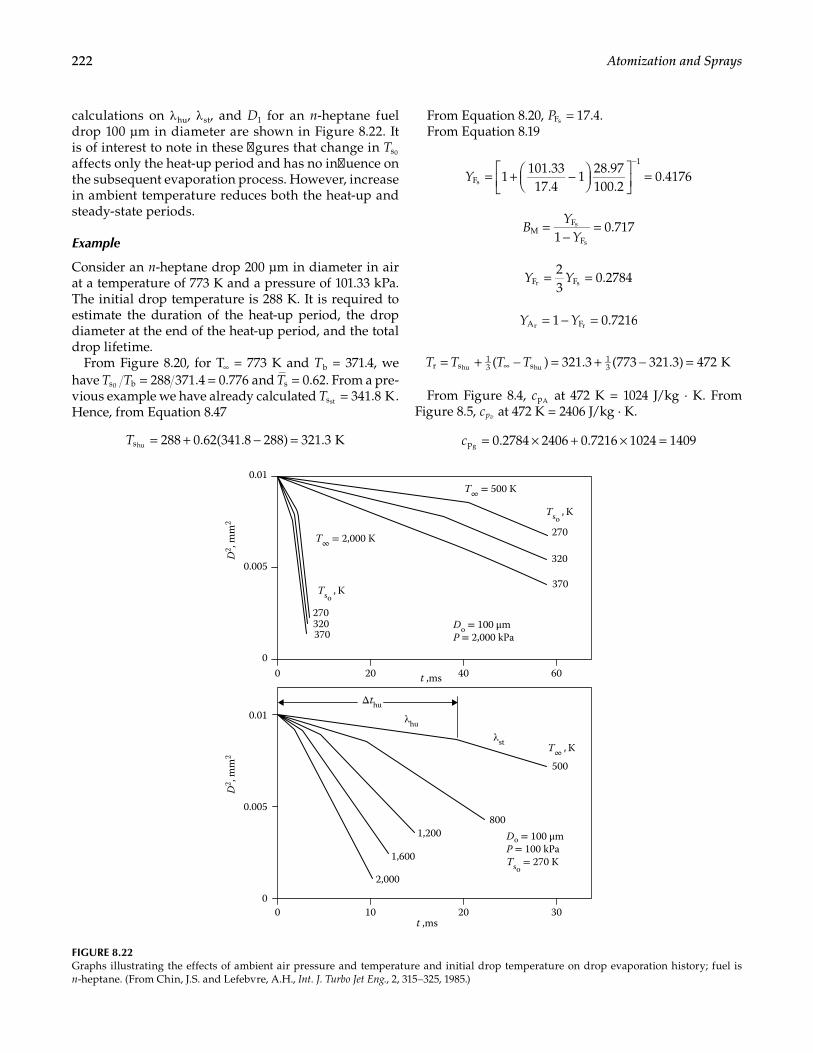
222 Atomization and Sprays

calculations on λ hu, λ st, and D1 for an n-heptane fuel drop 100 μm in diameter are shown in Figure 8.22. It is of interest to note in these figures that change in s0T affects only the heat-up period and has no influence on the subsequent evaporation process. However, increase in ambient temperature reduces both the heat-up and steady-state periods.

Example

Consider an n-heptane drop 200 μm in diameter in air at a temperature of 773 K and a pressure of 101.33 kPa. The initial drop temperature is 288 K. It is required to estimate the duration of the heat-up period, the drop diameter at the end of the heat-up period, and the total drop lifetime.

From Figure 8.20, for T∞ = 773 K and Tb = 371.4, we have 288 371.4 0.776s b0T T = = and 0.62sT = . From a pre-vious example we have already calculated 341.8 KsstT = . Hence, from Equation 8.47

288 0.62(341.8 288) 321.3 KshuT = + − =

From Equation 8.20, 17.4FsP = .From Equation 8.19

1101.3317.4

128.97100.2

0.4176F

1

sY = + −

=−

1

0.717MF

F

s

s

BY

Y=

−=

23

0.2784F Fr sY Y= =

1 0.7216A Fr rY Y= − =

= + − = + − =∞( ) 321.3 (773 321.3) 472 Kr s13 s

13hu huT T T T

From Figure 8.4, pAc at 472 K = 1024 J/kg · K. From Figure 8.5, cpv at 472 K = 2406 J/kg · K.

0.2784 2406 0.7216 1024 1409pgc = × + × =

2,000

1,600

1,200

270

270

320

320

370

370

800

500

D2 , m

m2

D2 , m

m2

t ,ms

t ,ms

00

0.005

0.01

0

0.005

0.01

20 40 60

0 10 20 30

Do = 100 μmP = 100 kPaTso

= 270 K

Do = 100 μmP = 2,000 kPa

λhu

λst

T∞ = 500 K

T∞ = 2,000 K

Tso , K

Tso , K

T∞ , K

Δthu

FIGURE 8.22Graphs illustrating the effects of ambient air pressure and temperature and initial drop temperature on drop evaporation history; fuel is n-heptane. (From Chin, J.S. and Lefebvre, A.H., Int. J. Turbo Jet Eng., 2, 315–325, 1985.)

223Drop Evaporation

From Equation 8.22, for Ts = 321.3, L = 350,000. Hence

=−

= −∞( ) 1409(773 321.3)350,000T

p sg huBc T T

L

1.818TB =

From Equation 8.49, at 0.5(288 + 341.8) = 341.9 K, 2330pFc = . From Equation 8.26, at 321.3 K, ρ F = 650 kg/m3.

From Figures 8.6 and 8.7, at 472 K, kA = 0.0376 and kv = 0.0288 J/m·s·K. Hence,

0.7216 0.0376 0.2784 0.0288

= 0.03515gk = × + ×

Substitution of these property values into Equation 8.45 gives

= × ×

∆ =× × × − ×

× × × × −

0.9375 10 s

2330 650 1409 (341.8 288)

12 0.03515 ln(1.717) 350, 000 [(1.818 0.717) 1]

6hu2

huhu2

D

tD

From Equation 8.46

D = × + −−

= ×

−−

−

200 10 12330(341.8 288)

700, 000[(1.818 0.717) 1]

187 10 m

hu6

0.5

6

hence,

t ( )∆ = × × ×

=0.9375 10 187 100.0328 s

=32.8 ms

hu6 2 –12

Thus the length of the heat-up period is 32.8 ms, during which the drop diameter is reduced from 200 to 187 μm.

The variation of drop diameter with time as obtained by the approximate method is indicated by the dashed line in Figure 8.23. Also shown in this figure is the variation in drop diameter with time as calculated by the iterative method. This approach results in a value of ∆thu of 31 ms.

The average value of λ  during the heat-up period is obtained as

D Dt

λ = −∆

= −×

= × =−

200 1870.0328 10

0.1534 10 m s 0.1534 mm s

hu02

12

hu

2 2

12

6 2 2

From the previous example, λ st = 0.30 × 10–6 m2/s. Hence, from Equation 8.51, the total drop lifetime is given by

30201000

0.034

0.036

0.038

0.040

Iterativemethod

Approximatemethod

Time, ms

32.8 ms

40

D2 , m

m2

n = HeptaneP = 100 kPaTso = 773 K

FIGURE 8.23Variation of drop diameter with time during heat-up period. (From Chin, J.S. and Lefebvre, A.H., Int. J. Turbo Jet Eng., 2, 315–325, 1985.)

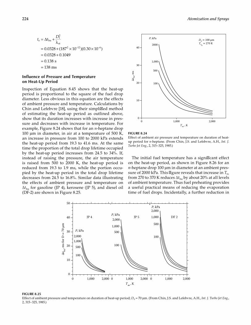
224 Atomization and Sprays

t tD= ∆ +λ

= + × ×= +==

0.0328 (187 10 )(0.30 10 )0.0328 0.10490.138 s138 ms

e hu12

st

2 –12 –6

Influence of Pressure and Temperature on Heat-Up Period

Inspection of Equation 8.45 shows that the heat-up period is proportional to the square of the fuel drop diameter. Less obvious in this equation are the effects of ambient pressure and temperature. Calculations by Chin and Lefebvre [18], using their simplified method of estimating the heat-up period as outlined above, show that its duration increases with increase in pres-sure and decreases with increase in temperature. For example, Figure 8.24 shows that for an n-heptane drop 100 μm in diameter, in air at a temperature of 500 K, an increase in pressure from 100 to 2000 kPa extends the heat-up period from 19.3 to 41.6 ms. At the same time the proportion of the total drop lifetime occupied by the heat-up period increases from 24.5 to 34%. If, instead of raising the pressure, the air temperature is raised from 500 to 2000 K, the heat-up period is reduced from 19.3 to 1.9 ms, while the portion occu-pied by the heat-up period in the total drop lifetime decreases from 24.5 to 16.8%. Similar data illustrating the effects of ambient pressure and temperature on ∆thu for gasoline (JP 4), kerosene (JP 5), and diesel oil (DF-2) are shown in Figure 8.25.

The initial fuel temperature has a significant effect on the heat-up period, as shown in Figure 8.26 for an n-heptane drop 100 μm in diameter at an ambient pres-sure of 2000 kPa. This figure reveals that increase in s0T from 270 to 370 K reduces ∆thu by about 20% at all levels of ambient temperature. Thus fuel preheating provides a useful practical means of reducing the evaporation time of fuel drops. Incidentally, a further reduction in

2000

1,000

500

100

1,0000

30

20

10

0

40

2,000

Do = 100 μmTso

= 270 K

Δt hu

, ms

T∞ , K

P, kPa

FIGURE 8.24Effect of ambient air pressure and temperature on duration of heat-up period for n-heptane. (From Chin, J.S. and Lefebvre, A.H., Int. J. Turbo Jet Eng., 2, 315–325, 1985.)

1,0002,000

2,000

2,000

1,000

1,000

500 100

00

10

20

30

40

50

1,000 2,000 0 1,000 2,000 0 1,000 2,000

500

500

100

JP 5P, kPa

P, kPa

P, kPa

DF 2JP 4

100Δt hu

, ms f

or D

= 7

0 μm

T∞ , K

FIGURE 8.25Effect of ambient pressure and temperature on duration of heat-up period; D0 = 70 μm. (From Chin, J.S. and Lefebvre, A.H., Int. J. Turbo Jet Eng., 2, 315–325, 1985.)

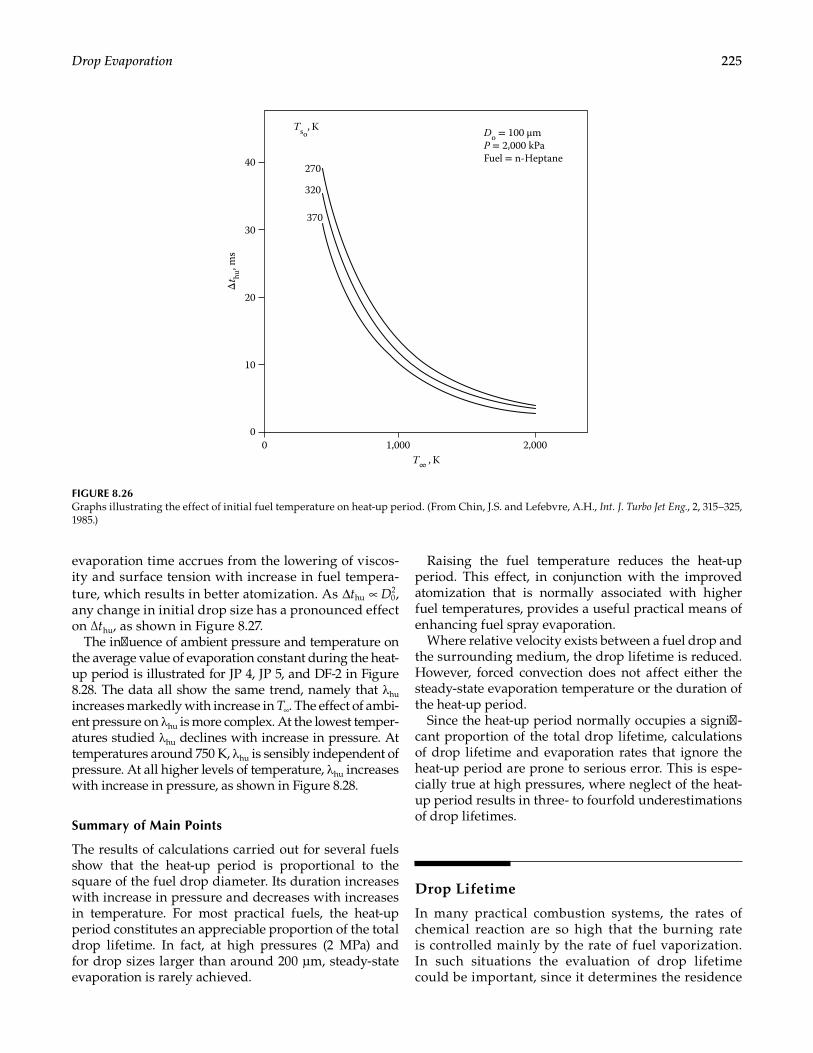
225Drop Evaporation

evaporation time accrues from the lowering of viscos-ity and surface tension with increase in fuel tempera-ture, which results in better atomization. As hu 0

2t D∆ ∝ , any change in initial drop size has a pronounced effect on ∆thu, as shown in Figure 8.27.

The influence of ambient pressure and temperature on the average value of evaporation constant during the heat-up period is illustrated for JP 4, JP 5, and DF-2 in Figure 8.28. The data all show the same trend, namely that λ hu increases markedly with increase in T∞. The effect of ambi-ent pressure on λ hu is more complex. At the lowest temper-atures studied λ hu declines with increase in pressure. At temperatures around 750 K, λ hu is sensibly independent of pressure. At all higher levels of temperature, λ hu increases with increase in pressure, as shown in Figure 8.28.

Summary of Main Points

The results of calculations carried out for several fuels show that the heat-up period is proportional to the square of the fuel drop diameter. Its duration increases with increase in pressure and decreases with increases in temperature. For most practical fuels, the heat-up period constitutes an appreciable proportion of the total drop lifetime. In fact, at high pressures (2 MPa) and for drop sizes larger than around 200 μm, steady-state evaporation is rarely achieved.

Raising the fuel temperature reduces the heat-up period. This effect, in conjunction with the improved atomization that is normally associated with higher fuel temperatures, provides a useful practical means of enhancing fuel spray evaporation.

Where relative velocity exists between a fuel drop and the surrounding medium, the drop lifetime is reduced. However, forced convection does not affect either the steady-state evaporation temperature or the duration of the heat-up period.

Since the heat-up period normally occupies a signifi-cant proportion of the total drop lifetime, calculations of drop lifetime and evaporation rates that ignore the heat-up period are prone to serious error. This is espe-cially true at high pressures, where neglect of the heat-up period results in three- to fourfold underestimations of drop lifetimes.

Drop Lifetime

In many practical combustion systems, the rates of chemical reaction are so high that the burning rate is controlled mainly by the rate of fuel vaporization. In such situations the evaluation of drop lifetime could be important, since it determines the residence

270

320

370

1,0000

30

20

10

0

40

2,000

Do = 100 μmP = 2,000 kPaFuel = n-Heptane

Δt hu

, ms

T∞ , K

Tso, K

FIGURE 8.26Graphs illustrating the effect of initial fuel temperature on heat-up period. (From Chin, J.S. and Lefebvre, A.H., Int. J. Turbo Jet Eng., 2, 315–325, 1985.)

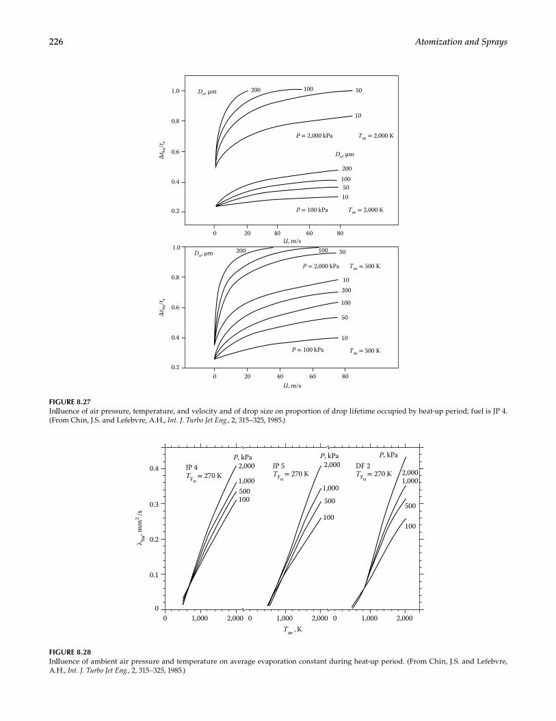
226 Atomization and Sprays

200

200

1005010

200

200

100

50

U, m/s

U, m/s

10

10

100 50

100 50

10

0

0.8

0.6

0.4

0.2

1.0

0.8

0.6

0.4

0.2

1.0

20 40 60 80

0 20 40 60 80

Δt hu

/te

Δt hu

/te

T∞ = 2,000 K

T∞ = 500 K

T∞ = 2,000 K

T∞ = 500 K

P = 2,000 kPa

P = 2,000 kPa

P = 100 kPa

P = 100 kPa

Do, μm

Do, μm

Do, μm

FIGURE 8.27Influence of air pressure, temperature, and velocity and of drop size on proportion of drop lifetime occupied by heat-up period; fuel is JP 4. (From Chin, J.S. and Lefebvre, A.H., Int. J. Turbo Jet Eng., 2, 315–325, 1985.)

2,000

1,000

00

0.1

0.2

0.3

0.4

1,000 2,000 0 1,000 2,000 0 1,000 2,000

500100

2,0002,000

1,0001,000

500 500100

100

P, kPa P, kPa P, kPaJP 5 DF 2JP 4

T∞ , K

λ hu, m

m2

/s

TFo = 270 K TFo = 270 K TFo = 270 K

FIGURE 8.28Influence of ambient air pressure and temperature on average evaporation constant during heat-up period. (From Chin, J.S. and Lefebvre, A.H., Int. J. Turbo Jet Eng., 2, 315–325, 1985.)

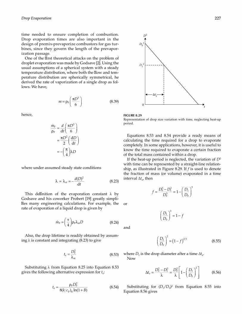
227Drop Evaporation

time needed to ensure completion of combustion. Drop evaporation times are also important in the design of premix-prevaporize combustors for gas tur-bines, since they govern the length of the prevapor-ization passage.

One of the first theoretical attacks on the problem of droplet evaporation was made by Godsave [2]. Using the usual assumptions of a spherical system with a steady temperature distribution, where both the flow and tem-perature distribution are spherically symmetrical, he derived the rate of vaporization of a single drop as fol-lows. We have,

6F

3

mD= ρ π

(8.39)

hence,

m dt

D

D Dt

D

ρ= π

= π

= − π

λ

d 6

2dd

4

F

F

3

2

where under assumed steady state conditions

λ = λ = − ( )d

2d Dt

st (8.23)

This definition of the evaporation constant λ  by Godsave and his coworker Probert [19] greatly simpli-fies many engineering calculations. For example, the rate of evaporation of a liquid drop is given by

m D=

ρ λπ

4F F st (8.24)

Also, the drop lifetime is readily obtained by assum-ing λ  is constant and integrating (8.23) to give

=λe

02

stt

D (8.53)

Substituting λ  from Equation 8.25 into Equation 8.53 gives the following alternative expression for te:

8( ) ln(1 )e

F 02

p gt

Dk c B

= ρ+

(8.54)

Equations 8.53 and 8.54 provide a ready means of calculating the time required for a drop to evaporate completely. In some applications, however, it is useful to know the time required to evaporate a certain fraction of the total mass contained within a drop.

If the heat-up period is neglected, the variation of D2 with time can be represented by a straight-line relation-ship, as illustrated in Figure 8.29. If f is used to denote the fraction of mass (or volume) evaporated in a time interval ∆te, then

103

13

03

1

0

3

fD D

DDD

= − = −

or

11

0

3DD

f

= −

and

11

0

22 3D

Df( )

= − (8.55)

where D1 is the drop diameter after a time ∆te.Now

1e02

12

02

1

0

2

tD D D D

D∆ = −

λ=

λ−

(8.56)

Substituting for (D1/D0)2 from Equation 8.55 into Equation 8.56 gives

D02

D2

D12

0 t

Δte

FIGURE 8.29Representation of drop size variation with time, neglecting heat-up period.

228 Atomization and Sprays

[1 (1 ) ]e02

2 3tD

f∆ =λ

− − (8.57)

This equation gives the time required to evaporate a fraction f of the initial mass (or volume) of a drop having an initial diameter D0.

Effect of Heat-Up Phase on Drop Lifetime

Where the heat-up period is too long to be neglected, the time required to fully evaporate the drop is obtained as the sum of the unsteady-state period and the steady-state period, that is,

e02

12

hu

12

stt

D D D= −λ

+λ

(8.58)

where D1 is the diameter of the drop at the end of the heat-up period, as illustrated in Figure 8.21. Both D1 and λ hu may be estimated using the methods described in the previous section.

For the purpose of calculating the time required to evaporate a fraction f of the initial mass (or volume) of the drop it is necessary to consider two separate cases.

Case 1. When f is small, say less than 0.1, only evapo-ration occurring during the heat-up period need be con-sidered, and the time required is given by

[1 (1 ) ]e02

hu

2 3tD

f∆ =λ

− − (8.59)

Case 2. If f is large enough to involve evaporation in both the heat-up and steady-state phases, the evapora-tion time is obtained as

[1 (1 ) ] [1 (1 ) ](1 )e02

hu1

2 3 02

st1

2 31

2 3tD

fD

f f f∆ =λ

− − +λ

− + − − (8.60)

where f1 is the fraction of the initial liquid mass that is vaporized during the heat-up period. An appropriate expression for f1 is

1( )

102

hu hu0.5

0

3

fD t

D= − − λ ∆

(8.61)

where ∆thu is the duration of the heat-up period as given by Equation 8.45.

An alternative expression for ∆te is

[1 (1 ) ](1 )e hu02

st1

2 31

2 3t tD

f f f∆ = ∆ +λ

− + − − (8.62)

Effect of Prevaporization on Drop Lifetime

We now examine for steady-state conditions the effect of prevaporization on drop evaporation time and on the time to produce any given level of vapor concentration.

Case 1. Consider first a control volume into which flows a mixture of drops, vapor, and air. The vapor con-stitutes a fraction fl of the total mass (liquid plus vapor). It is required to derive an expression for the time ∆te that the mixture must spend in the control volume to raise the vapor content from its initial value Ω to a higher value f. Let

D1 = initial drop diameterD0 = diameter of drops entering control volumeD1 = diameter of drops after time ∆te

Ω = fraction of total mass (liquid plus vapor) enter-ing control volume in vapor form

It is assumed that steady-state evaporation has been achieved by the time the drops enter the control volume.

We have, by definition,

3

03

3

D DD

i

i

− = Ω

or

103

DDi

= − Ω

or

(1 )02 2 2 3D Di= − Ω (8.63)

Also, by definition

3

13

3

D DD

fi

i

− =

and

(1 )12 2 2 3D D fi= − (8.64)

Now

e02

12

stt

D D∆ = −λ

(8.65)

Substituting for 02D from Equation 8.63 and 1

2D from Equation 8.64 intoEquation8.65 gives

[(1 ) (1 ) ]e

2

st

2 3 2 3tD

fi∆ =λ

− Ω − − (8.66)

229Drop Evaporation

or, from Equation 8.59,

111e

02

st

2 3

tD f∆ =λ

− −− Ω

(8.67)

Case 2. We now consider the situation where a mix-ture of drops, vapor, and air enters a control volume, as in case 1, except that no assumption is made concerning the origin of the vapor. It could arise from partial pre-vaporization of the existing drops, from a separate injec-tion of vapor, or from a multiplicity of vapor sources.

This situation is most readily dealt with by assuming that all the incoming vapor, regardless of its origin, is due to partial prevaporization of the drops present in the system. The time required in the control volume to raise the concentration of vapor to a fraction f of the total mass (vapor plus liquid) is again given by Equation 8.67, in which D0 is the diameter of the drops entering the control volume, Ω is the fraction of the total mass (liq-uid plus vapor) that enters the control volume as vapor, and f denotes the fraction of the total mass (liquid plus vapor) that is present in vapor form after a residence time ∆te in the control volume.

Convective Effects on Evaporation

For drop evaporation under quiescent conditions, the principal mode of heat transfer is thermal conduction. Where relative motion exists between the drop and the surrounding air or gas, the rate of evaporation is enhanced. Surprisingly, perhaps, convective effects do not change the steady-state evaporation temperature sstT . This is because forced convection affects both Q, the rate of heat transfer to the drop, and Qe, the rate of evapora-tion, to the same extent, so that under steady-state con-ditions, when Q = Qe, the two effects cancel each other. Also, from inspection of Equation 8.45 it is clear that the heat-up period ∆thu is unaffected by convective effects. However, since rates of evaporation are enhanced by convection, the total drop lifetime must diminish. Thus the effect of convection is to reduce the duration of the steady-state portion of the drop evaporation process.

If the rate of heat transfer to a drop per unit surface area per unit time is denoted by h, then

hm L

D=

πF

2

(8.68)

Substituting for Fm from Equation 8.17 gives

2( ) ln (1 )p g Th

k c L BD

=+

(8.69)

For constant fluid properties, in the absence of convec-tion, the Nusselt number is

Nu =( )s

hDk T T−∞

Substituting for h from Equation 8.69 gives

Nu = 2( )

ln(1 )p s

Tg

Lc T T

B−

+∞

or, since ( ) ,p s Tgc T L BΤ− =∞

Nu = 2ln(1 )T

T

BB+

(8.70)

As BT tends toward zero, ln(l + BT)/BT approaches unity and Nu = 2, which is the normal value for low heat transfer rates to a sphere.

In a comprehensive theoretical and experimental study, Frossling [20] showed that the effects of convec-tion on heat and mass transfer rates could be accommo-dated by a correction factor that is a function of Reynolds number and Schmidt (or Prandtl) number. Where diffu-sion rates are controlling, the correction factor is

1 0.276Re ScD0.5

g0.33+ (8.71)

Hence the vaporization rate under convective condi-tions is equal to the steady-state vaporization rate (e.g., Equation 8.24) multiplied by Equation 8.71.

For the more usual case where heat transfer rates are controlling, it becomes

1 0.276Re PrD0.5

g0.33+ (8.72)

The velocity term in ReD should be the relative veloc-ity between the drop and the surrounding gas, that is, ReD = UDρ g/μg. However, both calculations and experi-mental observations suggest that small drops rapidly attain the same velocity as the surrounding gas, after which they are susceptible only to the fluctuating com-ponent of velocity, u’. The appropriate value of Reynolds number then becomes g gu D′ ρ µ .

Another important convective heat transfer correla-tion is the following, due to Ranz and Marshall [21]:

Nu =2+0.6Re PrD0.5

g0.33 (8.73)

which corresponds to a correction factor of

1 0.3Re PrD0.5

g0.33+ (8.74)

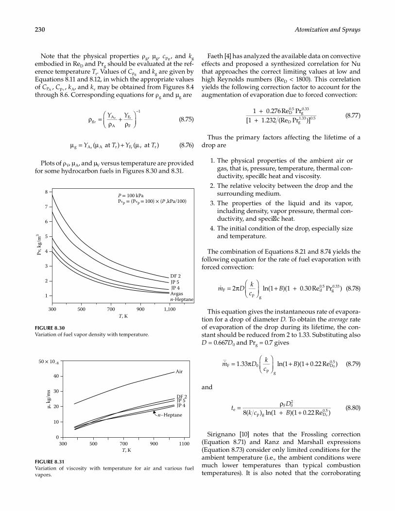
230 Atomization and Sprays

Note that the physical properties ρ g, μg, pgc , and kg embodied in ReD and Prg should be evaluated at the ref-erence temperature Tr. Values of gCρ and kg are given by Equations 8.11 and 8.12, in which the appropriate values of PAC , pvC , kA, and kv may be obtained from Figures 8.4 through 8.6. Corresponding equations for ρ g and μg are

gA

A

F

F

1

rr rY Yρ =

ρ+

ρ

−

(8.75)

( at ) ( at )g A A r F v rr rY T Y Tµ = µ + µ (8.76)

Plots of ρ V, μA, and μV versus temperature are provided for some hydrocarbon fuels in Figures 8.30 and 8.31.

Faeth [4] has analyzed the available data on convective effects and proposed a synthesized correlation for Nu that approaches the correct limiting values at low and high Reynolds numbers (ReD < 1800). This correlation yields the following correction factor to account for the augmentation of evaporation due to forced convection:

1 0.276Re Pr

[1 1.232 (Re Pr )]D0.5

g0.33

D g1.33 0.5

++

(8.77)

Thus the primary factors affecting the lifetime of a drop are

1. The physical properties of the ambient air or gas, that is, pressure, temperature, thermal con-ductivity, specific heat and viscosity.

2. The relative velocity between the drop and the surrounding medium.

3. The properties of the liquid and its vapor, including density, vapor pressure, thermal con-ductivity, and specific heat.

4. The initial condition of the drop, especially size and temperature.

The combination of Equations 8.21 and 8.74 yields the following equation for the rate of fuel evaporation with forced convection:

m Dkc

B= π

+ +2 ln(1 )(1 0.30Re Pr )F

p g

d0.5

g0.33

(8.78)

This equation gives the instantaneous rate of evapora-tion for a drop of diameter D. To obtain the average rate of evaporation of the drop during its lifetime, the con-stant should be reduced from 2 to 1.33. Substituting also D = 0.667D0 and Prg = 0.7 gives

m Dkc

B= π

+ +1.33 ln(1 )(1 0.22 Re )F 0

p g

D0.5

0 (8.79)

and

8( ) ln(1 )(1 0.22Re )e

F 02

p g D0.5t

Dk c B o

= ρ+ +

(8.80)

Sirignano [10] notes that the Frossling correction (Equation 8.71) and Ranz and Marshall expressions (Equation 8.73) consider only limited conditions for the ambient temperature (i.e., the ambient conditions were much lower temperatures than typical combustion temperatures). It is also noted that the corroborating

1

2

3

4

5

6

7

8

300

P = 100 kPa

DF 2JP 5JP 4

PvP = (PvP = 100) × (P ,kPa/100)

500 700T, K

Pv, k

g/m

3

900 1,100

Avgasn-Heptane

FIGURE 8.30Variation of fuel vapor density with temperature.

300 500 700T, K

μ, k

g/m

s

900 11000

Air

DF 2JP 5JP 4

n–Heptane10

20

30

40

50 × 10–8

FIGURE 8.31Variation of viscosity with temperature for air and various fuel vapors.

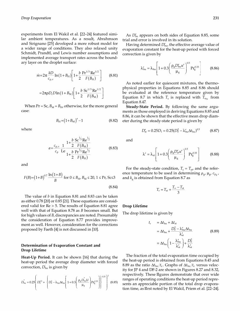
231Drop Evaporation

experiments from El Wakil et al. [22–24] featured simi-lar ambient temperatures. As a result, Abrahmson and Sirignano [25] developed a more robust model for a wider range of conditions. They also relaxed unity Schmidt, Prandtl, and Lewis number assumptions and implemented average transport rates across the bound-ary layer on the droplet surface:

mkDc

Bb

F B ( ) ( )= π + +

2 ln 1 1

2Pr Re

p,vH

1/3 1/2

H (8.81)

2 ln 1 12

Sc Rec M

1/3 1/2

MD D B

bF B

( ) ( )= πρ + +

When Pr = Sc, BM = BH, otherwise, for the more general case:

1 1H MB Ba( )= + − (8.82)

where

acc

bF B

bF B

1Le

12

Sc Re

12

Pr Re

p,v

p

13

12

M1

31

2

H

( )

( )

=+

+ (8.83)

and

( ) 1ln 10.7

F B BB

B( ) ( )= +

+ for 0 ≤ BH, BM ≤ 20, 1 ≤ Pr, Sc≤3

(8.84)

The value of b in Equation 8.81 and 8.83 can be taken as either 0.78 [20] or 0.85 [21]. These equations are consid-ered valid for Re > 5. The results of Equation 8.81 agree well with that of Equation 8.78 as B becomes small. But for high values of B, discrepancies are noted. Presumably the consideration of Equation 8.77 provides improve-ment as well. However, consideration for the corrections proposed by Faeth [4] is not discussed in [10].

Determination of Evaporation Constant and Drop Lifetime

Heat-Up Period. It can be shown [16] that during the heat-up period the average drop diameter with forced convection, hu

'D is given by

′ = + − λ ∆ +ρ ′

µ

0.25 1 0.3 Prhu 0

0.502

hu hug hu

gg0.33

0.25 2

D D D tD U (8.85)

As huD′ appears on both sides of Equation 8.85, some trial and error is involved in its solution.

Having determined huD′ , the effective average value of evaporation constant for the heat-up period with forced convection is given by

1 0.3 Prhu hug hu

g

0.5

g0.33D u

′λ = λ +ρ ′ ′

µ

(8.86)

As noted earlier for quiescent mixtures, the thermo-physical properties in Equations 8.85 and 8.86 should be evaluated at the reference temperature given by Equation 8.7 in which Ts is replaced with shuT from Equation 8.47.

Steady-State Period. By following the same argu-ments as those employed in deriving Equations 8.85 and 8.86, it can be shown that the effective mean drop diam-eter during the steady-state period is given by

0.25 0.25( )st 1 02

hu hu0.5D D D t′ = = − ′λ ∆ (8.87)

and

= 1 0.3 Prstg st

g

0.5

g0.33D u

′λ λ +ρ ′ ′

µ

(8.88)

For the steady-state condition, Ts = Tst, and the refer-ence temperature to be used in determining ρ g, μg, ,pgc and kg is obtained from Equation 8.7 as

3r st

stT TT T= + −∞

Drop Lifetime

The drop lifetime is given by

1

hu st

hu02

hu hu

st

huhu

st

02

st

t t t

tD t

tD

e = ∆ + ∆

= ∆ + − ′λ ∆′λ

= ∆ − ′λ′λ

+′λ

(8.89)

The fraction of the total evaporation time occupied by the heat-up period is obtained from Equations 8.45 and 8.89 as the ratio hu et t∆ . Graphs of hu et t∆ versus veloc-ity for JP 4 and DF-2 are shown in Figures 8.27 and 8.32, respectively. These figures demonstrate that over wide ranges of operating conditions the heat-up period repre-sents an appreciable portion of the total drop evapora-tion time, as first noted by El Wakil, Priem et al. [22–24].

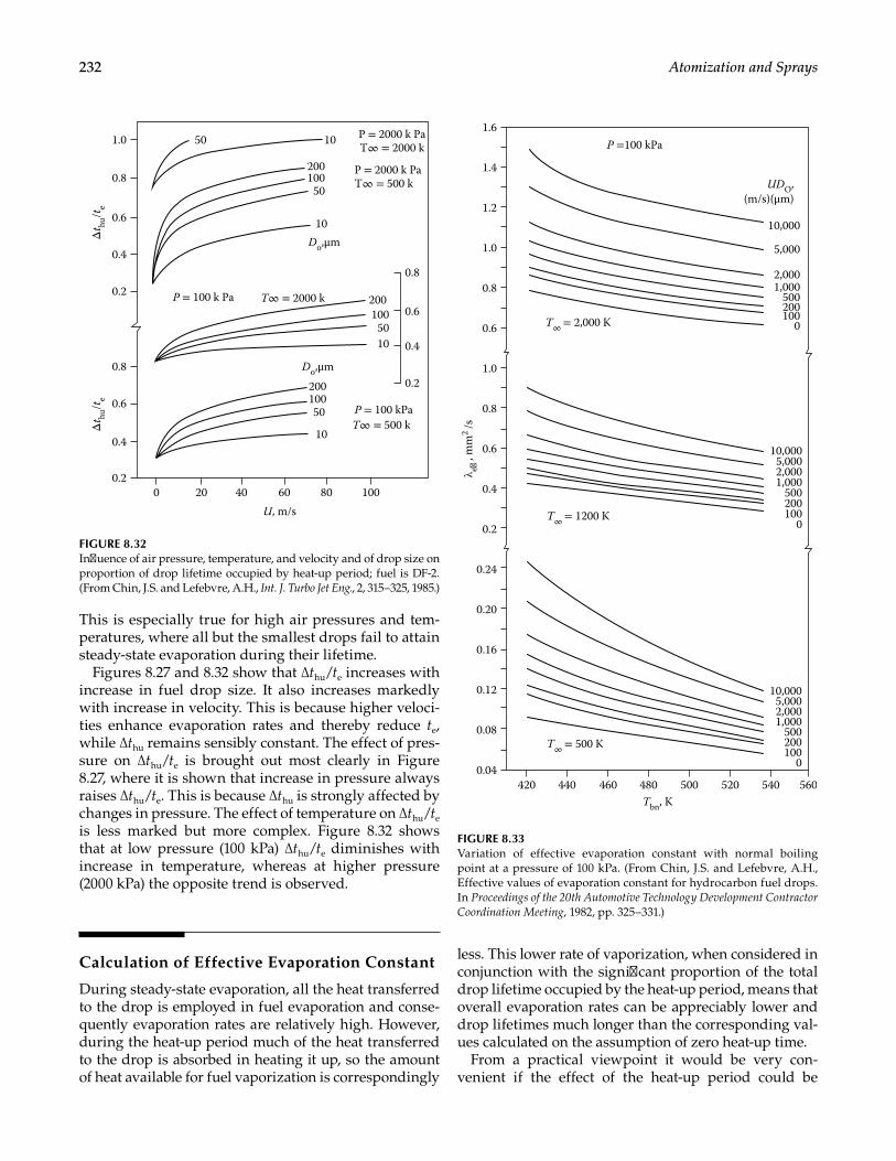
232 Atomization and Sprays

This is especially true for high air pressures and tem-peratures, where all but the smallest drops fail to attain steady-state evaporation during their lifetime.

Figures 8.27 and 8.32 show that ∆thu/te increases with increase in fuel drop size. It also increases markedly with increase in velocity. This is because higher veloci-ties enhance evaporation rates and thereby reduce te, while ∆thu remains sensibly constant. The effect of pres-sure on ∆thu/te is brought out most clearly in Figure 8.27, where it is shown that increase in pressure always raises ∆thu/te. This is because ∆thu is strongly affected by changes in pressure. The effect of temperature on ∆thu/te is less marked but more complex. Figure 8.32 shows that at low pressure (100 kPa) ∆thu/te diminishes with increase in temperature, whereas at higher pressure (2000 kPa) the opposite trend is observed.

Calculation of Effective Evaporation Constant

During steady-state evaporation, all the heat transferred to the drop is employed in fuel evaporation and conse-quently evaporation rates are relatively high. However, during the heat-up period much of the heat transferred to the drop is absorbed in heating it up, so the amount of heat available for fuel vaporization is correspondingly

less. This lower rate of vaporization, when considered in conjunction with the significant proportion of the total drop lifetime occupied by the heat-up period, means that overall evaporation rates can be appreciably lower and drop lifetimes much longer than the corresponding val-ues calculated on the assumption of zero heat-up time.

From a practical viewpoint it would be very con-venient if the effect of the heat-up period could be

0 20 40 60 80U, m/s

1000.2

Δt hu

/te

Δt hu

/te

0.4

0.6

0.8

0.2 P = 100 k Pa

P = 100 kPa

P = 2000 k Pa

200

200

1050

0.8

0.6

0.4

0.2

100

100

50

50

10

10

200

Do,μm

Do,μm

10050

10

T∞ = 2000 k

T∞ = 500 k

T∞ = 500 k

P = 2000 k PaT∞ = 2000 k

0.4

0.6

0.8

1.0

FIGURE 8.32Influence of air pressure, temperature, and velocity and of drop size on proportion of drop lifetime occupied by heat-up period; fuel is DF-2. (From Chin, J.S. and Lefebvre, A.H., Int. J. Turbo Jet Eng., 2, 315–325, 1985.)

UDO,(m/s)(μm)

540520500480Tbn, K

460440420

1.4

1.2

1.0

0.8

0.6

1.0

0.8

0.6

0.4

0.2

0.24

0.20

0.16

0.12

0.08

0.04

1.6

560

10,000

5,000

2,0001,000

500200100

10,0005,0002,0001,000

500200100

0

10,0005,0002,0001,000

500200100

0

0

P =100 kPa

λ e , m

m2

/s

T∞ = 2,000 K

T∞ = 1200 K

T∞ = 500 K

FIGURE 8.33Variation of effective evaporation constant with normal boiling point at a pressure of 100 kPa. (From Chin, J.S. and Lefebvre, A.H., Effective values of evaporation constant for hydrocarbon fuel drops. In Proceedings of the 20th Automotive Technology Development Contractor Coordination Meeting, 1982, pp. 325–331.)

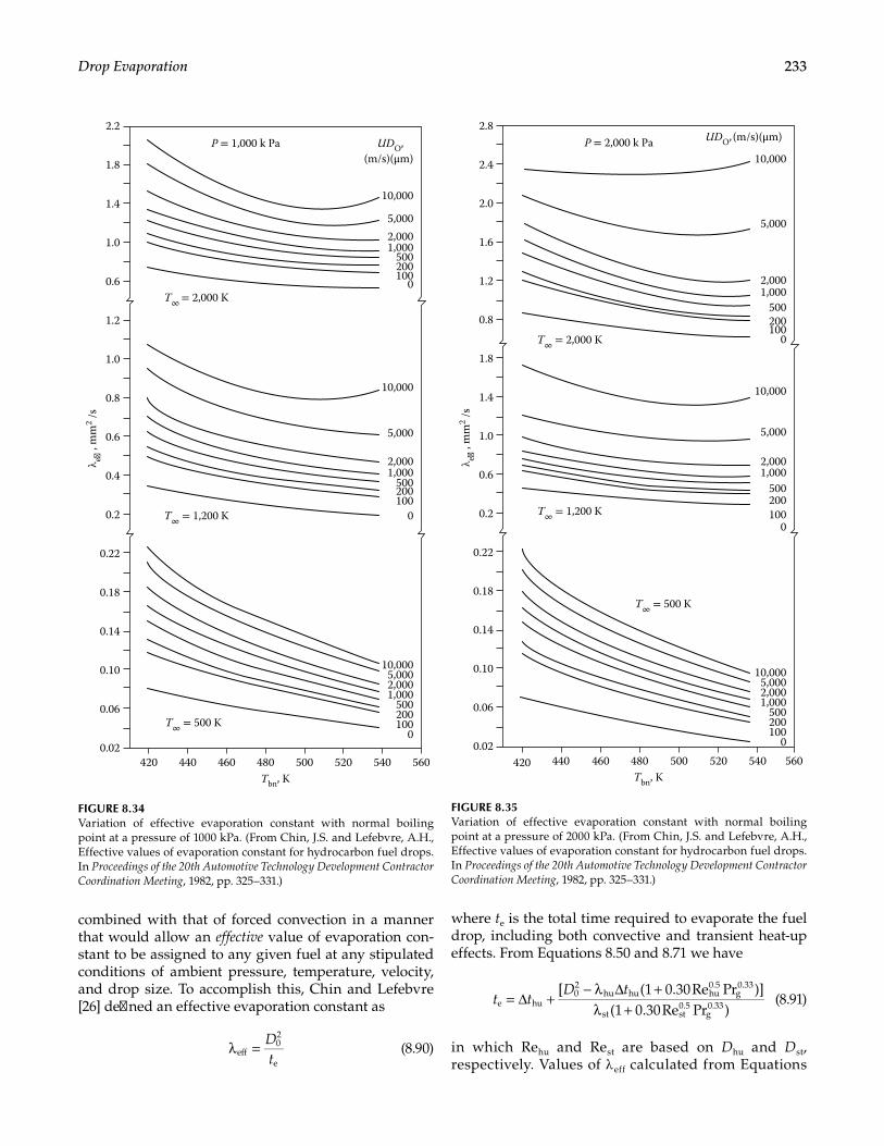
233Drop Evaporation

combined with that of forced convection in a manner that would allow an effective value of evaporation con-stant to be assigned to any given fuel at any stipulated conditions of ambient pressure, temperature, velocity, and drop size. To accomplish this, Chin and Lefebvre [26] defined an effective evaporation constant as

eff02

e

Dt

λ = (8.90)

where te is the total time required to evaporate the fuel drop, including both convective and transient heat-up effects. From Equations 8.50 and 8.71 we have

[ (1 0.30Re Pr )]

(1 0.30Re Pr )e hu02

hu hu hu0.5

g0.33

st st0.5

g0.33t t

D t= ∆ +

− λ ∆ +λ +

(8.91)

in which Rehu and Rest are based on Dhu and Dst, respectively. Values of λ eff calculated from Equations

UDO,

540520500480Tbn, K

460440420

1.8

1.4

1.0

0.6

1.2

1.0

0.8

0.6

0.4

0.2

0.22

0.18

0.14

0.10

0.06

0.02

2.2

560

10,000

5,0002,0001,000

500200100

10,000

5,000

2,0001,000

500200100

0

10,0005,0002,0001,000

500200100

0

0

P = 1,000 k Pa

λ e , m

m2 /s

T∞ = 2,000 K

T∞ = 1,200 K

T∞ = 500 K

(m/s)(μm)

FIGURE 8.34Variation of effective evaporation constant with normal boiling point at a pressure of 1000 kPa. (From Chin, J.S. and Lefebvre, A.H., Effective values of evaporation constant for hydrocarbon fuel drops. In Proceedings of the 20th Automotive Technology Development Contractor Coordination Meeting, 1982, pp. 325–331.)

540520500480Tbn, K

460440420

2.4

2.0

1.6

1.2

0.8

1.8

1.4

1.0

0.6

0.2

0.22

0.18

0.14

0.10

0.06

0.02

2.8

560

10,000

5,000

2,0001,000

500200100

10,000

5,000

2,0001,000

500200100

0

10,0005,0002,0001,000

500200100

0

0

P = 2,000 k Pa

λ e , m

m2 /s

T∞ = 2,000 K

T∞ = 1,200 K

T∞ = 500 K

UDO,(m/s)(μm)

FIGURE 8.35Variation of effective evaporation constant with normal boiling point at a pressure of 2000 kPa. (From Chin, J.S. and Lefebvre, A.H., Effective values of evaporation constant for hydrocarbon fuel drops. In Proceedings of the 20th Automotive Technology Development Contractor Coordination Meeting, 1982, pp. 325–331.)

234 Atomization and Sprays

8.90 and 8.91 are plotted in Figures 8.33 through 8.35 [26]. These figures represent plots of λ eff versus Tbn for various values of UD0 at three levels of pressure, 100, 1000, and 2000 kPa, and three levels of ambient temperature, 500, 1200, and 2000 K. While recogniz-ing that no single fuel property can fully describe the evaporation characteristics of any given fuel, the aver-age boiling point (50% recovered) has much to com-mend it for this purpose, because it is directly related to fuel volatility and vapor pressure. It also has the virtue of being easy to measure and is usually quoted in fuel specifications.

The figures show that λ eff increases with increase in ambient temperature, pressure, velocity, and drop size and diminishes with increase in normal boiling temperature.

The concept of an effective value of evaporation con-stant considerably simplifies calculations of the evapo-ration characteristics of fuel drops. For example, for any given conditions of pressure, temperature, and relative velocity, the lifetime of a fuel drop of any given size is obtained from Equation 8.90 as

e02

efft

D=λ

(8.92)

while the average rate of fuel evaporation is readily determined by dividing mF from Equation 8.39 by te from Equation 8.92 as

m D= π ρ λ6F F eff 0 (8.93)

Example

It is required to calculate the lifetime of a fuel drop 65 μm in diameter in a flowing stream where the ambient pressure and temperature are 1400 kPa and 1100 K, respectively, and the relative velocity between the air and the drop is 20 m/s. The normal boiling temperature of the fuel is 485 K, and its initial density is 810 kg/m3.

From Figure 8.34 we obtain by interpolation that the value of λ eff for P = 1000 kPa and UD0 = 20 × 65 = 1300 is 0.54 mm2/s. Similarly, we find from Figure 8.35 that for P = 2000 kPa and UD0 = 1300, λ eff is 0.59 mm2/s. Hence, by interpolation, λ eff for P = 1400 kPa is 0.56 mm2/s. From Equation 8.92

t

D=λ

= ××

= × =

−6

−

−

(65 10 )0.56 10

7.55 10 s 7.55 ms

e02

eff

2

6

3

From Equation 8.93

= π ρ λ = π × × × × ×

= ×

− −

−

6 6810 0.56 10 65 10

1.54 10 kg s

F F eff 06 6

8

m D

Influence of Evaporation on Drop Size Distribution

Although the evaporation characteristics of a single drop provide useful guidance on the evaporation history of a complete spray, there are certain key features of an evap-orating spray that can be explored only by considering the spray as a whole. For example, for the ignition of a fuel spray it is the initial rate of evaporation that is impor-tant, whereas for high combustion efficiency the time required for complete evaporation of the fuel spray is the dominant factor. Another example is provided by the lean premix-prevaporize combustor. A key feature of this concept is the attainment of complete evaporation of the fuel and complete mixing of the fuel vapor with air prior to combustion. Failure to fully vaporize the fuel results in higher NO, emissions. It is important, therefore, to know how the fraction or percentage of fuel evaporated var-ies with time, so that the best compromise can be made between the conflicting requirements of minimum NOx emissions and minimum length of premixing chamber.

It is also of interest to ascertain how the initial mean drop size and the drop size distribution (as defined by the Rosin–Rammler distribution parameter q) affect the subsequent evaporation history.

Chin et al. [27] have studied in detail the evaporation histories of JP 5 fuel sprays. The results of their calcu-lations are presented in a form that allows the time required to vaporize any given percentage of the initial spray mass to be estimated for other fuels at any stipu-lated conditions of ambient pressure and temperature.

The manner in which the mass median diameter (MMD) changes as evaporation proceeds is shown in Figure 9.1 for a JP 5 fuel spray in air at a temperature of 2000 K and a pressure of 2 MPa. This figure contains several different curves to illustrate the influence of the initial drop size distribution parameter, q0, on the variation in mean drop size with time. Over the range of values of q0 of most practical interest, Figure 9.1 shows that evaporation causes MMD to increase with time, the effect being especially pronounced for sprays having low values of q0. If time is expressed in dimen-sionless form as t90%, the time required to vaporize 90% by mass of the spray, and MMD is divided by its initial value MMD0, we can plot the nondimensional

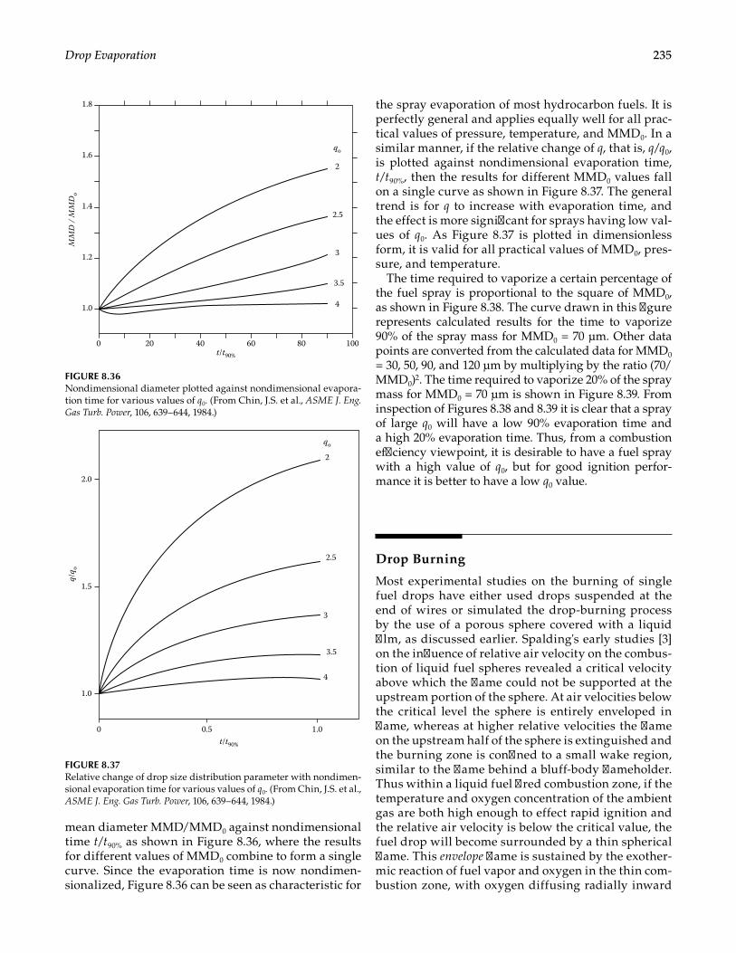
235Drop Evaporation

mean diameter MMD/MMD0 against nondimensional time t/t90% as shown in Figure 8.36, where the results for different values of MMD0 combine to form a single curve. Since the evaporation time is now nondimen-sionalized, Figure 8.36 can be seen as characteristic for

the spray evaporation of most hydrocarbon fuels. It is perfectly general and applies equally well for all prac-tical values of pressure, temperature, and MMD0. In a similar manner, if the relative change of q, that is, q/q0, is plotted against nondimensional evaporation time, t/t90%, then the results for different MMD0 values fall on a single curve as shown in Figure 8.37. The general trend is for q to increase with evaporation time, and the effect is more significant for sprays having low val-ues of q0. As Figure 8.37 is plotted in dimensionless form, it is valid for all practical values of MMD0, pres-sure, and temperature.

The time required to vaporize a certain percentage of the fuel spray is proportional to the square of MMD0, as shown in Figure 8.38. The curve drawn in this figure represents calculated results for the time to vaporize 90% of the spray mass for MMD0 = 70 μm. Other data points are converted from the calculated data for MMD0 = 30, 50, 90, and 120 μm by multiplying by the ratio (70/MMD0)2. The time required to vaporize 20% of the spray mass for MMD0 = 70 μm is shown in Figure 8.39. From inspection of Figures 8.38 and 8.39 it is clear that a spray of large q0 will have a low 90% evaporation time and a high 20% evaporation time. Thus, from a combustion efficiency viewpoint, it is desirable to have a fuel spray with a high value of q0, but for good ignition perfor-mance it is better to have a low q0 value.

Drop Burning

Most experimental studies on the burning of single fuel drops have either used drops suspended at the end of wires or simulated the drop-burning process by the use of a porous sphere covered with a liquid film, as discussed earlier. Spalding's early studies [3] on the influence of relative air velocity on the combus-tion of liquid fuel spheres revealed a critical velocity above which the flame could not be supported at the upstream portion of the sphere. At air velocities below the critical level the sphere is entirely enveloped in flame, whereas at higher relative velocities the flame on the upstream half of the sphere is extinguished and the burning zone is confined to a small wake region, similar to the flame behind a bluff-body flameholder. Thus within a liquid fuel fired combustion zone, if the temperature and oxygen concentration of the ambient gas are both high enough to effect rapid ignition and the relative air velocity is below the critical value, the fuel drop will become surrounded by a thin spherical flame. This envelope flame is sustained by the exother-mic reaction of fuel vapor and oxygen in the thin com-bustion zone, with oxygen diffusing radially inward

1.0

1.2

1.4

1.6

1.8

200 40 60 80

2

2.5

3.5

3

4

100

MM

D /

MM

Do

qo

t/t90%

FIGURE 8.36Nondimensional diameter plotted against nondimensional evapora-tion time for various values of q0. (From Chin, J.S. et al., ASME J. Eng. Gas Turb. Power, 106, 639–644, 1984.)

4

0

1.0

1.5

2.0

0.5 1.0

3.5

3

2.5

2

t/t90%

q/q o

qo

FIGURE 8.37Relative change of drop size distribution parameter with nondimen-sional evaporation time for various values of q0. (From Chin, J.S. et al., ASME J. Eng. Gas Turb. Power, 106, 639–644, 1984.)

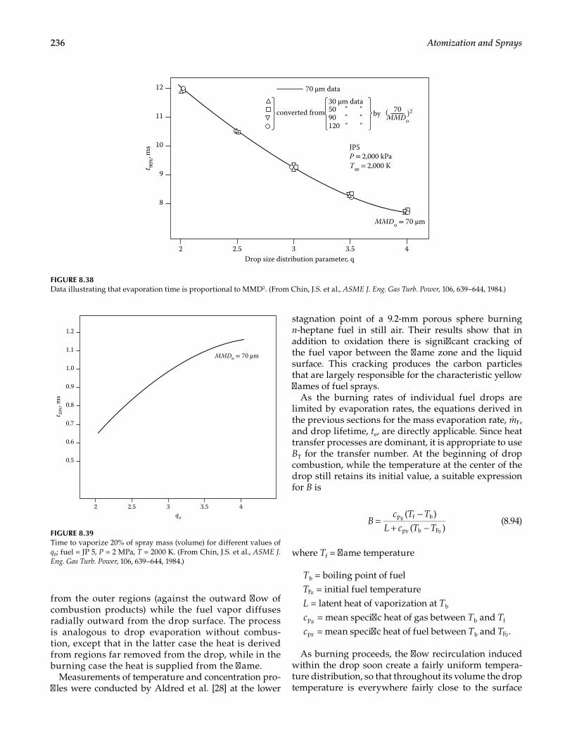
236 Atomization and Sprays

from the outer regions (against the outward flow of combustion products) while the fuel vapor diffuses radially outward from the drop surface. The process is analogous to drop evaporation without combus-tion, except that in the latter case the heat is derived from regions far removed from the drop, while in the burning case the heat is supplied from the flame.

Measurements of temperature and concentration pro-files were conducted by Aldred et al. [28] at the lower

stagnation point of a 9.2-mm porous sphere burning n-heptane fuel in still air. Their results show that in addition to oxidation there is significant cracking of the fuel vapor between the flame zone and the liquid surface. This cracking produces the carbon particles that are largely responsible for the characteristic yellow flames of fuel sprays.

As the burning rates of individual fuel drops are limited by evaporation rates, the equations derived in the previous sections for the mass evaporation rate, Fm , and drop lifetime, te, are directly applicable. Since heat transfer processes are dominant, it is appropriate to use BT for the transfer number. At the beginning of drop combustion, while the temperature at the center of the drop still retains its initial value, a suitable expression for B is

( )

( )p f b

p b F

g

F 0

Bc T T

L c T T=

−+ −

(8.94)

where Tf = flame temperature

Tb = boiling point of fuel

F0T = initial fuel temperatureL = latent heat of vaporization at Tb

pgc = mean specific heat of gas between Tb and Tf

pFc = mean specific heat of fuel between Tb and F0T .

As burning proceeds, the flow recirculation induced within the drop soon create a fairly uniform tempera-ture distribution, so that throughout its volume the drop temperature is everywhere fairly close to the surface

3.532.52

1.1

1.0

0.9

0.8

0.7

0.6

0.5

1.2

4

MMDo = 70 μm

t 20%

, ms

qo

FIGURE 8.39Time to vaporize 20% of spray mass (volume) for different values of q0; fuel = JP 5, P = 2 MPa, T = 2000 K. (From Chin, J.S. et al., ASME J. Eng. Gas Turb. Power, 106, 639–644, 1984.)

Drop size distribution parameter, q

12

converted from11

10

9

8

3.532.52 4

JP5P = 2,000 kPaT∞ = 2,000 K

MMDo = 70 μm

t 90%

, ms

70 μm data

30 μm data50 " "90 " "120 " "

by ( 70MMDo

)2

FIGURE 8.38Data illustrating that evaporation time is proportional to MMD2. (From Chin, J.S. et al., ASME J. Eng. Gas Turb. Power, 106, 639–644, 1984.)

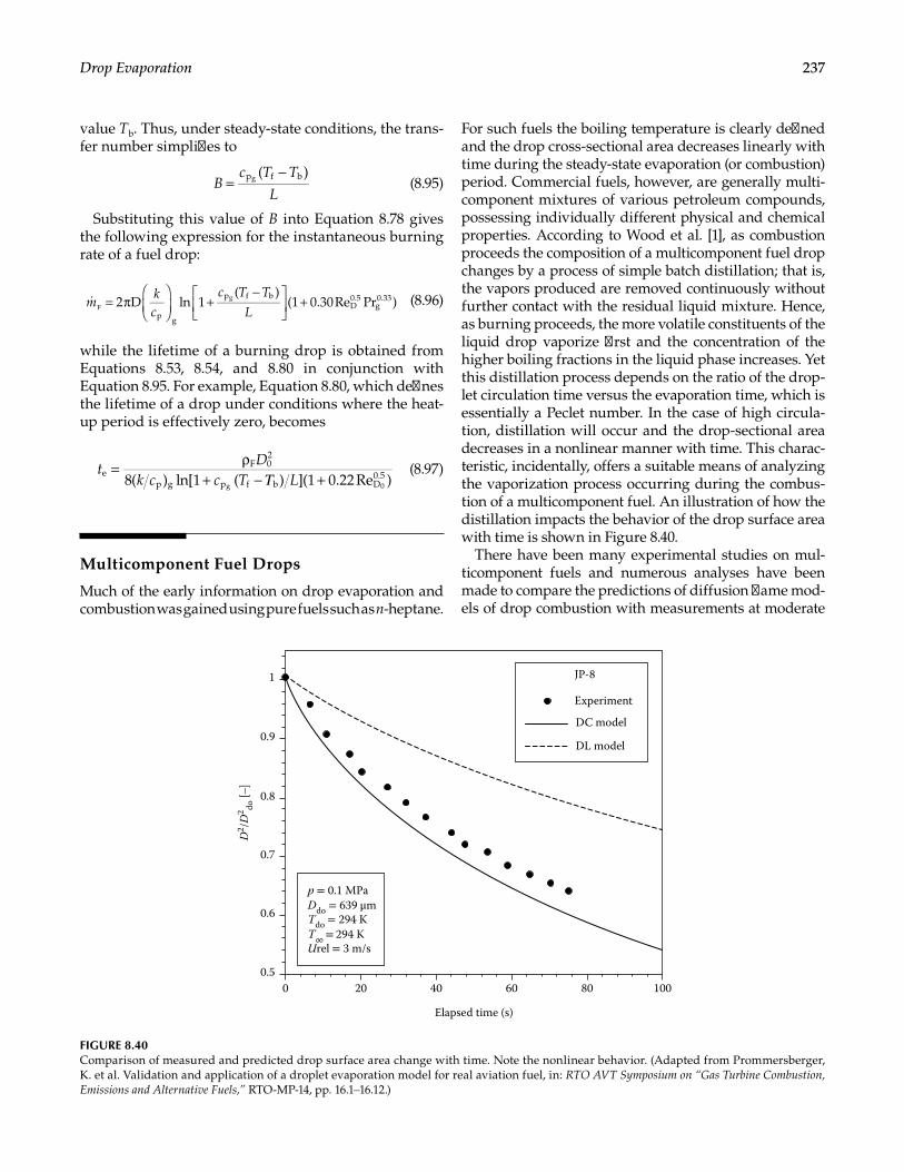
237Drop Evaporation

value Tb. Thus, under steady-state conditions, the trans-fer number simplifies to

( )p f bgB

c T T

L=

− (8.95)

Substituting this value of B into Equation 8.78 gives the following expression for the instantaneous burning rate of a fuel drop:

mkc

c T T

L = π

+

−

+2 D ln 1

( )(1 0.30Re Pr )

p g

p f bD0.5

g0.33

Fg (8.96)

while the lifetime of a burning drop is obtained from Equations 8.53, 8.54, and 8.80 in conjunction with Equation 8.95. For example, Equation 8.80, which defines the lifetime of a drop under conditions where the heat-up period is effectively zero, becomes

8( ) ln[1 ( ) ](1 0.22Re )e

F 02

p g p f b D0.5

g 0

tD

k c c T LΤ= ρ

+ − + (8.97)

Multicomponent Fuel Drops

Much of the early information on drop evaporation and combustion was gained using pure fuels such as n-heptane.

For such fuels the boiling temperature is clearly defined and the drop cross-sectional area decreases linearly with time during the steady-state evaporation (or combustion) period. Commercial fuels, however, are generally multi-component mixtures of various petroleum compounds, possessing individually different physical and chemical properties. According to Wood et al. [1], as combustion proceeds the composition of a multicomponent fuel drop changes by a process of simple batch distillation; that is, the vapors produced are removed continuously without further contact with the residual liquid mixture. Hence, as burning proceeds, the more volatile constituents of the liquid drop vaporize first and the concentration of the higher boiling fractions in the liquid phase increases. Yet this distillation process depends on the ratio of the drop-let circulation time versus the evaporation time, which is essentially a Peclet number. In the case of high circula-tion, distillation will occur and the drop-sectional area decreases in a nonlinear manner with time. This charac-teristic, incidentally, offers a suitable means of analyzing the vaporization process occurring during the combus-tion of a multicomponent fuel. An illustration of how the distillation impacts the behavior of the drop surface area with time is shown in Figure 8.40.

There have been many experimental studies on mul-ticomponent fuels and numerous analyses have been made to compare the predictions of diffusion flame mod-els of drop combustion with measurements at moderate

p = 0.1 MPaDdo = 639 μmTdo = 294 KT∞ = 294 KUrel = 3 m/s

Elapsed time (s)

D2 /D

2 do [–

]

0

0.9

0.8

0.7

0.6

0.5

1

20 40 60 80 100

JP-8

Experiment

DC model

DL model

FIGURE 8.40Comparison of measured and predicted drop surface area change with time. Note the nonlinear behavior. (Adapted from Prommersberger, K. et al. Validation and application of a droplet evaporation model for real aviation fuel, in: RTO AVT Symposium on “Gas Turbine Combustion, Emissions and Alternative Fuels,” RTO-MP-14, pp. 16.1–16.12.)

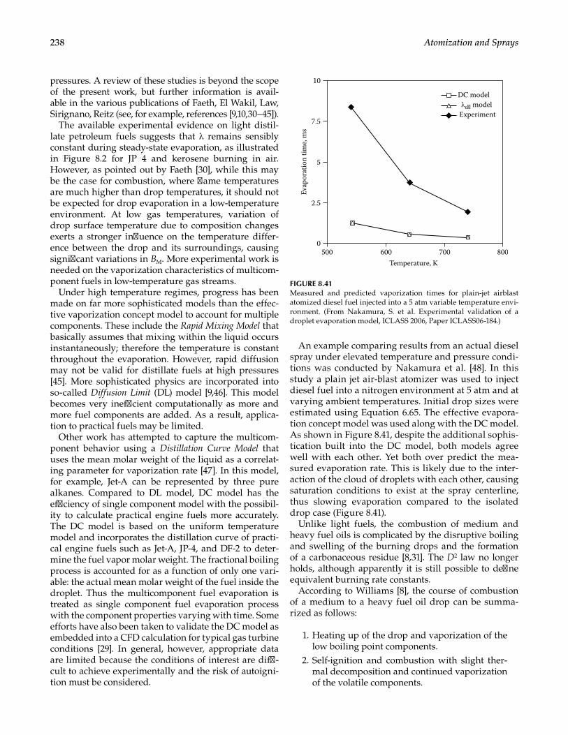
238 Atomization and Sprays

pressures. A review of these studies is beyond the scope of the present work, but further information is avail-able in the various publications of Faeth, El Wakil, Law, Sirignano, Reitz (see, for example, references [9,10,30–45]).

The available experimental evidence on light distil-late petroleum fuels suggests that λ remains sensibly constant during steady-state evaporation, as illustrated in Figure 8.2 for JP 4 and kerosene burning in air. However, as pointed out by Faeth [30], while this may be the case for combustion, where flame temperatures are much higher than drop temperatures, it should not be expected for drop evaporation in a low-temperature environment. At low gas temperatures, variation of drop surface temperature due to composition changes exerts a stronger influence on the temperature differ-ence between the drop and its surroundings, causing significant variations in BM. More experimental work is needed on the vaporization characteristics of multicom-ponent fuels in low-temperature gas streams.

Under high temperature regimes, progress has been made on far more sophisticated models than the effec-tive vaporization concept model to account for multiple components. These include the Rapid Mixing Model that basically assumes that mixing within the liquid occurs instantaneously; therefore the temperature is constant throughout the evaporation. However, rapid diffusion may not be valid for distillate fuels at high pressures [45]. More sophisticated physics are incorporated into so-called Diffusion Limit (DL) model [9,46]. This model becomes very inefficient computationally as more and more fuel components are added. As a result, applica-tion to practical fuels may be limited.

Other work has attempted to capture the multicom-ponent behavior using a Distillation Curve Model that uses the mean molar weight of the liquid as a correlat-ing parameter for vaporization rate [47]. In this model, for example, Jet-A can be represented by three pure alkanes. Compared to DL model, DC model has the efficiency of single component model with the possibil-ity to calculate practical engine fuels more accurately. The DC model is based on the uniform temperature model and incorporates the distillation curve of practi-cal engine fuels such as Jet-A, JP-4, and DF-2 to deter-mine the fuel vapor molar weight. The fractional boiling process is accounted for as a function of only one vari-able: the actual mean molar weight of the fuel inside the droplet. Thus the multicomponent fuel evaporation is treated as single component fuel evaporation process with the component properties varying with time. Some efforts have also been taken to validate the DC model as embedded into a CFD calculation for typical gas turbine conditions [29]. In general, however, appropriate data are limited because the conditions of interest are diffi-cult to achieve experimentally and the risk of autoigni-tion must be considered.

An example comparing results from an actual diesel spray under elevated temperature and pressure condi-tions was conducted by Nakamura et al. [48]. In this study a plain jet air-blast atomizer was used to inject diesel fuel into a nitrogen environment at 5 atm and at varying ambient temperatures. Initial drop sizes were estimated using Equation 6.65. The effective evapora-tion concept model was used along with the DC model. As shown in Figure 8.41, despite the additional sophis-tication built into the DC model, both models agree well with each other. Yet both over predict the mea-sured evaporation rate. This is likely due to the inter-action of the cloud of droplets with each other, causing saturation conditions to exist at the spray centerline, thus slowing evaporation compared to the isolated drop case (Figure 8.41).

Unlike light fuels, the combustion of medium and heavy fuel oils is complicated by the disruptive boiling and swelling of the burning drops and the formation of a carbonaceous residue [8,31]. The D2 law no longer holds, although apparently it is still possible to define equivalent burning rate constants.

According to Williams [8], the course of combustion of a medium to a heavy fuel oil drop can be summa-rized as follows:

1. Heating up of the drop and vaporization of the low boiling point components.

2. Self-ignition and combustion with slight ther-mal decomposition and continued vaporization of the volatile components.

0

2.5

5

Evap

orat

ion

time,

ms

Temperature, K

7.5

DC modelλe model

Experiment

10

500 600 700 800

FIGURE 8.41Measured and predicted vaporization times for plain-jet airblast atomized diesel fuel injected into a 5 atm variable temperature envi-ronment. (From Nakamura, S. et al. Experimental validation of a droplet evaporation model, ICLASS 2006, Paper ICLASS06-184.)

239Drop Evaporation

3. Extensive disruptive boiling and swelling of the drop together with considerable thermal decomposition to give a heavy tar.

4. Combustion of remaining volatile liquids and gases from the decomposition of the heavy tar, which collapses and forms a carbonaceous residue having an open structure called a cenosphere.

5. Slow heterogeneous combustion of the car-bonaceous residue at a rate of about one-tenth that of the initial drop (in terms of burning rate constants).

It is claimed that when disruptive swelling is aug-mented by emulsification of water with the fuel, extensive swelling of the drop can produce secondary atomization by smaller drops being explosively ejected from the parent drop.

Nomenclature

a, b constants in Equation 8.20 and 8.81B transfer numberBM mass transfer numberBT thermal transfer numberCex coefficient of thermal expansioncp specific heat at constant pressure, J/kg·KD drop diameter, mD0 initial drop diameter, mD1 drop diameter at end of heat-up period, mDc diffusion coefficient, m2/sDhu effective mean drop diameter during heat-up

period, mhu'D effective mean drop diameter during heat-up

period with forced convection, mst'D effective mean drop diameter during steady-

state period with forced convection, mF fraction of initial liquid mass in vapor form

after time ∆te

h heat transfer coefficient, J/m2·s·Kk thermal conductivity, J/m·s·KL latent heat of fuel vaporization, J/kgLe Lewis Number

bLT latent heat of fuel vaporization at boiling tem-perature Tb, J/kg

bnLT latent heat of vaporization at normal boiling temperature Tbn, J/kg

m mass of fuel drop, kgmF rate of fuel evaporation per unit surface area,

kg/m2·sFm rate of fuel evaporation, kg/s

M molecular weight

MMD mass median diameterNu Nusselt numbern pressure exponent of evaporation rateP ambient air pressure, kPaPcr critical pressure, kPa

FsP fuel vapor pressure at drop surface, kPaPr Prandtl numberQ rate of heat transfer to drop from surrounding

gas, J/sQe rate of heat utilization in fuel vaporization, J/sQ nondimensional sensible heat parameterq Rosin-Rammler drop size distribution param-

eter (see Equation 3.14)R gas constantr drop radius, mrs radius at drop surface, mReD drop Reynolds numberSc Schmidt numberT temperature, KTb boiling temperature, KTbn boiling temperature at normal atmospheric

pressure, K. For multicomponent fuels Tbn = average boiling point (50% recovered).

Tcr critical temperature, KTf flame temperature, KTr reference temperature, K (see Equation 8.7)Ts drop surface temperature, K

sT nondimensional surface temperature, KT∞ ambient temperature, Kt time, ste drop evaporation time, s

hut∆ duration of heat-up period, sstt∆ duration of steady-state period, s

U relative velocity between fuel drop and sur-rounding gas, m/s

u′ fluctuating component of turbulence velocity, m/s

YA mass fraction of airYF mass fraction of fuel vaporYi mass fraction of iλ  evaporation constant, m2/sλ ' evaporation constant for forced convection,

m2/sλ eff effective average value of λ  during drop life-

time, m2/sμ dynamic viscosity, kg/m·sρ  density, kg/m3

Subscripts

A airF fuelV vaporg gas0 initial value

240 Atomization and Sprays

r reference values value at drop surfacest steady-state valuehu mean or effective value during heat-up period∞ ambient value

REFERENCES

1. Wood, B. J., Wise, H., and Inami, S. H., Heterogeneous combustion of multicomponent fuels, NASA TN D-206, 1959.

2. Godsave, G. A. E., Studies of the combustion of drops in a fuel spray—The burning of single drops of fuel, in: 4th Symposium (International) on Combustion, Williams & Wilkins, Baltimore, Maryland, 1953, pp. 818–830.

3. Spalding, D. B., The combustion of liquid fuels, in: 4th Symposium (International) on Combustion, Williams & Wilkins, Baltimore, 1953, pp. 847–864.

4. Faeth, G. M., Current status of droplet and liquid combus-tion, Prog. Energy Combust. Sci., Vol. 3, 1977, pp. 191–224.

5. Goldsmith, M., and Penner, S. S., On the burning of sin-gle drops of fuel in an oxidizing atmosphere, Jet Propul., Vol. 24, 1954, pp. 245–251.

6. Kanury, A. M., Introduction to Combustion Phenomena, New York: Gordon & Breach, 1975.

7. Spalding, D. B., Some Fundamentals of Combustion, New York: Academic Press; London: Butterworths Scientific Publications, 1955.

8. Williams, A., Fundamentals of oil combustion, Prog. Energy Combust. Sci., Vol. 2, 1976, pp. 167–179.

9. Sirignano, W. A., Fuel droplet vaporization and spray com-bustion, Prog. Energy Combust., Vol. 9, 1983, pp. 291–322.

10. Sirignano, W. A., Fluid Dynamics and Transport of Droplets and Sprays, 2nd ed., Cambridge: Cambridge University Press, 2010.

11. Hubbard, G. L., Denny, V. E., and Mills, A. F., Droplet evaporation: Effects of transients and variable proper-ties, Int. J. Heat Mass Transfer., Vol. 18, 1975, pp. 1003–1008.

12. Sparrow, E. M., and Gregg, J. L., Similar solutions for free convection from a non-isothermal vertical plate, Trans ASME, Vol. 80, 1958, pp. 379–386.

13. Vargaftik, N. B., Tables on the Thermophysical Properties of Liquids and Gases, New York: Halsted Press, 1975.

14. Touloukian, Y., Thermal-Physical Properties of Matter, New York: Plenum Press, 1970.

15. Watson, K. M., Prediction of critical temperatures and heats of vaporization, Ind. Eng. Chem., Vol. 23, No. 4, 1931, pp. 360–364.

16. Chin, J. S., and Lefebvre, A. H., Steady-state evaporation characteristics of hydrocarbon fuel drops, AIAA J., Vol. 21, No. 10, 1983, pp. 1437–1443.

17. Hall, A. R., and Diederichsen, J., An experimental study of the burning of single drops of fuel in air at pressures up to 20 atmospheres, in: Fourth Symposium (International) on Combustion, Baltimore, Maryland: Williams & Wilkins, 1953, pp. 837–846.

18. Chin, J. S., and Lefebvre, A. H., The role of the heat-up period in fuel drop evaporation, Int. J. Turbo Jet Eng., Vol. 2, 1985, pp. 315–325.

19. Probert, R. P., Philos. Mag., Vol. 37, 1946, p. 94. 20. Frossling, N., On the evaporation of falling droplets,

Gerl. Beitr. Geophys., Vol. 52, 1938, pp. 170–216. 21. Ranz, W. E., and Marshall, W. R., Evaporation from

drops, Chem. Eng. Prog., Vol. 48, 1952, Part I, pp. 141–146; Part II, pp. 173–180.

22. El Wakil, M. M., Uyehara, O. A., and Myers, P. S., A theo-retical investigation of the heating-up period of injected fuel drops vaporizing in air, NACA TN 3179, 1954.

23. El Wakil, M. M., Priem, R. J., Brikowski, H. J., Myers, P. S., and Uyehara, O. A., Experimental and calculated tem-perature and mass histories of vaporizing fuel drops, NACA TN 3490, 1956.

24. Priem, R. J., Borman, G. L., El Wakil, M. M., Uyehara, O. A., and Myers, P. S., Experimental and calculated histo-ries of vaporizing fuel drops, NACA TN 3988, 1957.

25. Abramzon, B., and Sirignano, W. A., Droplet vaporiza-tion model for spray combustion calculations, Int. J. Heat Mass Tran., Vol. 32, 1989, pp. 1605–1618.

26. Chin, J. S., and Lefebvre A. H., Effective values of evaporation constant for hydrocarbon fuel drops, in: Proceedings of the 20th Automotive Technology Development Contractor Coordination Meeting, 1982, pp. 325–331.

27. Chin, J. S., Durrett, R., and Lefebvre, A. H., The interde-pendence of spray characteristics and evaporation his-tory of fuel sprays, ASME J. Eng. Gas Turb. Power, Vol. 106, July 1984, pp. 639–644.

28. Aldred, J. W., Patel, J. C., and Williams, A., The mecha-nism of combustion of droplets and spheres of liquid n-heptane, Combust. Flame, Vol. 17, 1971, pp. 139–149.

29. Faeth, G. M., Evaporation and combustion of sprays, Prog. Energ. Combust., Vol. 9, 1983, pp. 1–76.

30. Faeth, G. M., Spray combustion models—A review, AIAA Paper No. 79–0293, 1979.

31. Law, C. K., Multicomponent droplet combustion with rapid internal mixing, Combust. Flame, Vol. 26, 1976, pp. 219–233.

32. Law, C. K., Unsteady droplet combustion with droplet heating, Combust. Flame, Vol. 26, 1976, pp. 17–22.

33. Law, C. K., Recent advances in multicomponent and propellant droplet vaporization and combustion, ASME Paper 86-WA/HT-14, Presented at Winter Annual Meeting, Anaheim, California, December 1986.

34. Law, C. K., Recent advances in droplet vaporization and combustion, Prog. Energ. Combust., Vol. 8, 1982, pp. 171–201.

35. Law, C. K., Prakash, S., and Sirignano, W. A., Theory of convective, transient, multi-component droplet vaporiza-tion, in: 16th Symposium (International) on Combustion, The Combustion Institute, 1977, Cambridge, MA pp. 605–617.

36. Sirignano, W. A., and Law, C. K., Transient heating and liquid phase mass diffusion in droplet vaporization, Adv. Chem. Ser. 166, in: Zung, J. T. (ed.), Evaporation-Combustion of Fuels, American Chemical Society, Wash D.C. 1978, pp. 1–26.

37. Law, C. K., and Sirignano, W. A., Unsteady droplet com-bustion with droplet heating—II: Conduction limit, Combust. Flame, Vol. 28, 1977, pp. 175–186.

241Drop Evaporation

38. Sirignano, W. A., Theory of multicomponent fuel drop-let vaporization, Arch. Thermodyn. Combust., Vol. 9, Waterloo, Ontario 1979, pp. 235–251.

39. Lara-Urbaneja, P., and Sirignano, W. A., Theory of tran-sient multicomponent droplet vaporization in a con-vective field, in: Eighteenth Symposium (International) on Combustion, The Combustion Institute, 1981, pp. 1365–1374.

40. Sirignano, W. A., Fuel droplet vaporization and spray combustion, Prog. Energy Combust., Vol. 9, No. 4, 1983, pp. 291–322.

41. Aggarwal, S. K., and Sirignano, W. A., Ignition of fuel sprays: Deterministic calculations for idealized droplet arrays, in: 20th Symposium (International) on Combustion, The Combustion Institute, Ann Arbor, MI 1984, pp. 1773–1780.

42. Tong, A. Y., and Sirignano, W. A., Multicomponent drop-let vaporization in a high temperature gas, Combust. Flame, Vol. 66, 1986, pp. 221–235.

43. Tong, A. Y., and Sirignano, W. A., Multicomponent tran-sient droplet vaporization with internal circulation: Integral equation formulation and approximate solu-tion, Numer. Heat Transfer, Vol. 10, 1986, pp. 253–278.

44. Zhu, G.-S., and Reitz, R. D., A model for high-pressure vaporization of droplets in complex liquid mixtures using continuous thermodynamics, Int. J. Heat Mass Transfer, Vol. 45, 2002, pp. 495–507.

45. Kneer, R., Schneider, M., Noll, B., and Wittig, S., Diffusion controlled evaporation of a multicomponent droplet: Theoretical studies on the importance of variable liquid properties, Int. J. Heat Mass Transfer, Vol. 36, 1993, pp. 2403–2415.

46. Burger, M., Schmehl, R., Prommersberger, K., Schafer, O., Kock, R., and Wittig, S., Droplet evaporation mod-eling by the distillation curve model: Accounting for kerosene fuel and elevated pressures, Int. J. Heat Mass Transfer, Vol. 46, 2003, pp. 4403–4412.

47. Prommersberger, K., Maier, G., and Wittig, S., Validation and application of a droplet evaporation model for real aviation fuel, in: RTO AVT Symposium on “Gas Turbine Combustion, Emissions and Alternative Fuels,” RTO-MP-14, Lisbon, Portugal, pp. 16.1–16.12.

48. Nakamura, S., Wang, Q., McDonell, V., and Samuelsen, S. Experimental validation of a droplet evaporation model, ICLASS 2006, Paper ICLASS06-184, Kyoto, Japan.

243

9Spray Size and Patternation Methods

Introduction

The characterization of spray has evolved considerably over the last few decades. Though the size of drop-lets within a spray remains a critical characteristic of a spray, other parameters can be, and are, measured regularly. As discussed in Chapter 1 (Figure 1.1), the phenomena of interest within a spray are quite complex and varied. As instrumentation and simulation meth-ods become more capable, insights into the multitude of behaviors is becoming possible. The scope of this chap-ter focuses on drop size, but as discussed in Chapter 7, a number of highly capable methods have been devel-oped for characterizing the patternation of the spray, which has been established as another key aspect of performance. Further, methods for quantifying spray velocity, vapor phase, temperature, and other param-eters are now available. While this chapter emphasizes methods for measuring drop size and spray pattern, it touches on measurement of some of these other charac-teristics of the spray. A number of reviews on the subject of general diagnostics for characteristics of sprays are available, including those by Bachalo [1], McDonell and Samuelsen [2], Tropea [3], and most recently by Fansler and Parrish [4].

Finally, the role of simulation cannot be overlooked. While this chapter emphasizes experimental methods, some discussion is also given to simulation. It is appar-ent that simulation and experiments can (and should) go hand in hand to provide the maximum understand-ing of the complex phenomena occurring. This aspect was emphasized by Bachalo [1] as a major step required for increased understanding of spray behavior, with the suggestion that future characterization methods may directly integrate simulation with measurements. Unfortunately, because spray diagnostics and simu-lations are both substantial fields in their own right, joint efforts have been limited simply due to the scope required and the disparate background and skill sets needed. Despite this, some excellent examples that have demonstrated the utility of coupling comprehensive modeling with experiments include those by Drake and Haworth [5], the Proceedings of Measurement and Computation of Turbulent Spray Combustion Workshops [6,7], the Engine Combustion Network [8], and the over-all perspective by Jenny et al. [9]. It is apparent that

such activities are best accomplished through consortia of organizations, which often requires leadership on a national or international level.

Drop Sizing

The problem of measuring the size of very small par-ticles is encountered in many branches of engineer-ing science, and many different methods have been employed with varying degrees of success. However, special difficulties arise in the application of these meth-ods to the measurement of drop sizes in a spray and are well known to those who have attempted such measure-ments. These difficulties include (1) the very large num-ber of drops in a spray, (2) the high and varying velocity of the drops, (3) the wide range of drop sizes encoun-tered in most practical sprays (the ratio of the largest to the smallest drop diameter often exceeds 100:1), and (4) the changes in drop size with time through evaporation and coalescence. All these factors must be considered when choosing a drop size measuring technique for any given application.

Drop sizing techniques for sprays should ideally have the following characteristics:

1. Create no disturbance to the atomization process or spray pattern. Caution is required when using intrusive devices to measure drop sizes in a flowing airstream since small drops generally follow streamlines whereas large drops tend to migrate across streamlines. This phenomenon can cause a size bias in the measurements.

2. Have a size range capability of at least 10, although a factor closer to 30 is desirable in some applications. Generally, probe methods such as the hotwire technique have a size range from 1 to 600 μm and imaging techniques have a size range above about 5 μm.

3. Have the ability to measure both spatial and flux-based distributions (discussed in the fol-lowing section). The latter is generally pre-ferred, but many important optical techniques provide only spatial distributions. Conversion

244 Atomization and Sprays

from one type of distribution to the other is pos-sible if drop velocity data are also available.

4. Where appropriate, provide large representa-tive samples. To achieve a reasonably accurate measurement of size distribution, the sample should contain at least 5000 drops.

5. Tolerate wide variations in the liquid and ambi-ent gas properties. Many spray systems oper-ate at elevated pressures and temperatures. Successful development of mathematical mod-els for fuel evaporation and combustion at these arduous conditions is heavily dependent on accurate and reliable spray diagnostics.

6. Certain applications have physically large sprays. Hence ability of the diagnostic to main-tain sufficient working distance yet maintain accurate performance is often a consideration.

7. Provide rapid means of sampling and counting. Most instruments used today feature automated data acquisition and processing can accumulate results within seconds. When the number den-sity (drops/cm3) is required, the system must be fast enough to measure and record every drop passing through the probe volume. The data management system should be able to repro-duce promptly the drop size distribution in a histogram form along with the various mean diameters and standard deviations.

As it is virtually impossible to fulfill all these criteria in a single instrument, the capabilities and limitations of the various available measuring techniques must be recognized.

Drop Sizing Methods

The various methods employed in drop size measure-ment may be grouped conveniently into three broad categories—mechanical, electrical, and optical—as out-lined in the following. The third category includes opti-cal systems that have been developed in recent years and are finding an increasing range of applications. Some of these instruments have the capability of mea-suring drop velocity and number density as well as size distribution. Still other extensions incorporate more details regarding the gas phase information (e.g., vapor or continuous flow, which contains the droplets)

1. Mechanical a. Drop collection on slides or in cells b. Molten-wax and frozen-drop techniques c. Cascade impactors

2. Electrical a. Charged-wire and hot-wire techniques 3. Optical a. Imaging—photography, interferometric,

holography/plenoptic, planar, time gated, structured light

b. Nonimaging—single-particle counters, light scattering, diffraction

The growing importance of spray diagnostics has created a significant market for instrument manufac-turers to refine and improve techniques and to inno-vate new methods through research and development activities. In this chapter no attempt has been made to encompass all the techniques of relevance or with potential application to the measurement of size distri-butions in sprays. Instead, attention is focused on three main categories: methods that have been widely used in the past, those still in widespread use, and methods that are beginning to appear and seem to have promise for enhanced diagnostic capabilities in the future.

Over the years, reviews predating those in [1–4] have focused specifically on drop size measuring tech-niques and include those by Chigier [10,11], Bachalo [12], Ferrenberg [13], Hirleman [14], and Jones [15] which pro-vide a foundation for the history and developments in this area.

Factors Influencing Drop Size Measurement

All measuring techniques, whether simple or sophis-ticated, are susceptible to various errors and ambigui-ties, the nature and importance of which depend on the particular method employed. However, a number of potential sources of error in drop size measurement are common to almost all methods. They include the method of sampling (spatial or flux based), sample size, drop saturation, drop evaporation, drop coales-cence, and sampling location. In the design of instru-ments for drop size measurement, every effort is made to minimize these types of errors, but the fact remains that all techniques are subject to errors and inaccuracies associated with the basic assumptions employed, their manner of use, and the quantity of data obtained.

Spatial and Flux-Based Sampling

A key observation regarding the various measure-ment methods is associated with the inherent nature of the sampling used. Per ASTM E799-03 (2015) two types of sampling are employed to determine drop size distribution. One is spatial sampling that describes

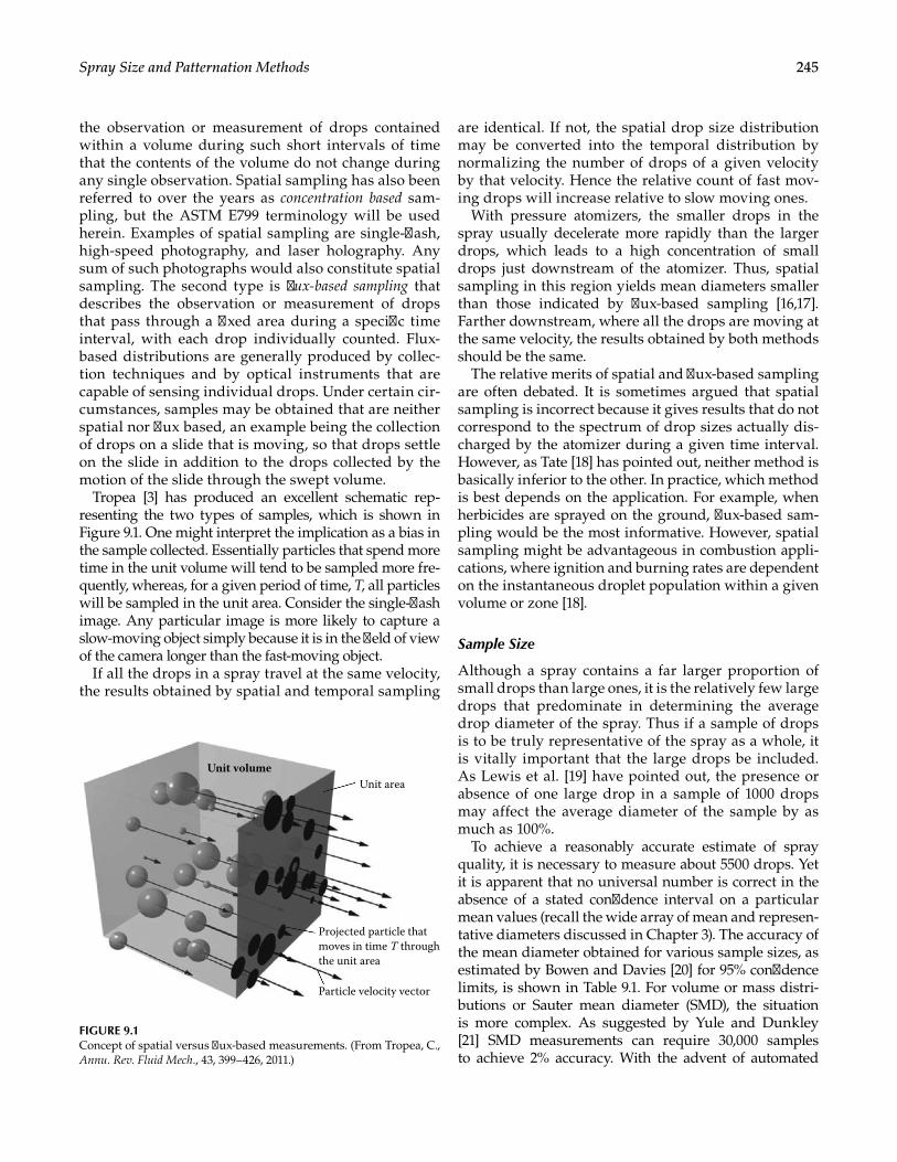
245Spray Size and Patternation Methods

the observation or measurement of drops contained within a volume during such short intervals of time that the contents of the volume do not change during any single observation. Spatial sampling has also been referred to over the years as concentration based sam-pling, but the ASTM E799 terminology will be used herein. Examples of spatial sampling are single-flash, high-speed photography, and laser holography. Any sum of such photographs would also constitute spatial sampling. The second type is flux-based sampling that describes the observation or measurement of drops that pass through a fixed area during a specific time interval, with each drop individually counted. Flux-based distributions are generally produced by collec-tion techniques and by optical instruments that are capable of sensing individual drops. Under certain cir-cumstances, samples may be obtained that are neither spatial nor flux based, an example being the collection of drops on a slide that is moving, so that drops settle on the slide in addition to the drops collected by the motion of the slide through the swept volume.

Tropea [3] has produced an excellent schematic rep-resenting the two types of samples, which is shown in Figure 9.1. One might interpret the implication as a bias in the sample collected. Essentially particles that spend more time in the unit volume will tend to be sampled more fre-quently, whereas, for a given period of time, T, all particles will be sampled in the unit area. Consider the single-flash image. Any particular image is more likely to capture a slow-moving object simply because it is in the field of view of the camera longer than the fast-moving object.

If all the drops in a spray travel at the same velocity, the results obtained by spatial and temporal sampling

are identical. If not, the spatial drop size distribution may be converted into the temporal distribution by normalizing the number of drops of a given velocity by that velocity. Hence the relative count of fast mov-ing drops will increase relative to slow moving ones.

With pressure atomizers, the smaller drops in the spray usually decelerate more rapidly than the larger drops, which leads to a high concentration of small drops just downstream of the atomizer. Thus, spatial sampling in this region yields mean diameters smaller than those indicated by flux-based sampling [16,17]. Farther downstream, where all the drops are moving at the same velocity, the results obtained by both methods should be the same.

The relative merits of spatial and flux-based sampling are often debated. It is sometimes argued that spatial sampling is incorrect because it gives results that do not correspond to the spectrum of drop sizes actually dis-charged by the atomizer during a given time interval. However, as Tate [18] has pointed out, neither method is basically inferior to the other. In practice, which method is best depends on the application. For example, when herbicides are sprayed on the ground, flux-based sam-pling would be the most informative. However, spatial sampling might be advantageous in combustion appli-cations, where ignition and burning rates are dependent on the instantaneous droplet population within a given volume or zone [18].

Sample Size

Although a spray contains a far larger proportion of small drops than large ones, it is the relatively few large drops that predominate in determining the average drop diameter of the spray. Thus if a sample of drops is to be truly representative of the spray as a whole, it is vitally important that the large drops be included. As Lewis et al. [19] have pointed out, the presence or absence of one large drop in a sample of 1000 drops may affect the average diameter of the sample by as much as 100%.

To achieve a reasonably accurate estimate of spray quality, it is necessary to measure about 5500 drops. Yet it is apparent that no universal number is correct in the absence of a stated confidence interval on a particular mean values (recall the wide array of mean and represen-tative diameters discussed in Chapter 3). The accuracy of the mean diameter obtained for various sample sizes, as estimated by Bowen and Davies [20] for 95% confidence limits, is shown in Table 9.1. For volume or mass distri-butions or Sauter mean diameter (SMD), the situation is more complex. As suggested by Yule and Dunkley [21] SMD measurements can require 30,000 samples to achieve 2% accuracy. With the advent of automated

Unit volumeUnit area

Projected particle thatmoves in time T throughthe unit area

Particle velocity vector

FIGURE 9.1Concept of spatial versus flux-based measurements. (From Tropea, C., Annu. Rev. Fluid Mech., 43, 399–426, 2011.)

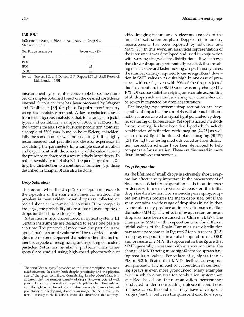
246 Atomization and Sprays

measurement systems, it is conceivable to set the num-ber of samples obtained based on the desired confidence interval. Such a concept has been proposed by Wagner and Drallmeier [22] for phase Doppler interferometry using the bootstrap method. A key conclusion drawn from their rigorous analysis is that, for a range of injector types and conditions, a sample of 10,000 is sufficient for the various means. For a four-hole production atomizer, a sample of 5500 was found to be sufficient, coinciden-tally the same number was proposed in [20]. It is highly recommended that practitioners develop experience in calculating the parameters for a sample size attribution and experiment with the sensitivity of the calculation to the presence or absence of a few relatively large drops. To reduce sensitivity to relatively infrequent large drops, fit-ting the distribution to a continuous function (e.g. those described in Chapter 3) can also be done.

Drop Saturation

This occurs when the drop flux or population exceeds the capability of the sizing instrument or method. The problem is most evident when drops are collected on coated slides or in immiscible solvents. If the sample is too large, the probability of error due to overlapping of drops (or their impressions) is high.

Saturation is also encountered in optical systems [1]. Certain instruments are designed to sense one particle at a time. The presence of more than one particle in the optical path or sample volume will be recorded as a sin-gle drop of some apparent diameter unless the instru-ment is capable of recognizing and rejecting coincident particles. Saturation is also a problem when dense sprays* are studied using high-speed photographic or

video-imaging techniques. A rigorous analysis of the impact of saturation on phase Doppler interferometry measurements has been reported by Edwards and Marx [23]. In this work, an analytical representation of the instrument was developed and used in conjunction with varying size/velocity distributions. It was shown that slower drops are preferentially rejected, thus result-ing in a bias toward faster moving drops. In many cases, the number density required to cause significant devia-tion in SMD values was quite high In one case of pres-sure-swirl nozzle, even with 90% of the drops rejected due to saturation, the SMD value was only changed by 10%. Of course statistics relying on accurate accounting of all drops such as number density or volume flux can be severely impacted by droplet saturation.

For imaging-type systems drop saturation can have significant impact as the droplets will attenuate illumi-nation sources as well as signal light generated by drop-let scattering or fluorescence. Yet sophisticated methods for overcoming this have been developed which include combination of extinction with imaging [24,25] as well as structured light illuminated planar imaging (SLIPI) [26]. For light-scattering methods based on laser diffrac-tion, correction schemes have been developed to help compensate for saturation. These are discussed in more detail in subsequent sections.

Drop Evaporation

As the lifetime of small drops is extremely short, evap-oration effect is very important in the measurement of fine sprays. Whether evaporation leads to an increase or decrease in mean drop size depends on the initial drop size distribution. For a monodisperse spray, evap-oration always reduces the mean drop size, but if the spray contains a wide range of drop sizes initially, then evaporation may produce an increase in mass median diameter (MMD). The effects of evaporation on mean drop size have been discussed by Chin et al. [27]. The changes in MMD with evaporation time for different initial values of the Rosin–Rammler size distribution parameter q are shown in Figure 9.2 for a kerosene (JP 5) fuel spray evaporating in air at a temperature of 2000 K and pressure of 2 MPa. It is apparent in this figure that MMD generally increases with evaporation time, the change of MMD being more significant for sprays hav-ing smaller qo values. For values of qo higher than 4, Figure 9.2 indicates that MMD declines as evapora-tion proceeds. The impact of evaporation in combust-ing sprays is even more pronounced. Many examples exist in which atomizers for combustion systems are specified based on their atomization performance conducted under nonreacting quiescent conditions. In these cases, the end user may have developed a transfer function between the quiescent cold flow spray

* The term “dense spray” provides an intuitive description of a satu-rated situation. In reality both droplet proximity and the physical size of the spray contribute. Considering Lambert-Beer’s law, it is apparent that the number density of drops (#/cc—associated with proximity of drops) as well as the path length in which they interact with the light (a function of physical dimensions) both impact signal, probability of overlapping drops in an image, etc. As a result, the term “optically thick” has also been used to describe a “dense spray.”

TABLE 9.1

Influence of Sample Size on Accuracy of Drop Size Measurements

No. Drops in sample Accurwacy (%)

500 ±171500 ±105500 ±535,000 ±2

Source: Bowen, I.G. and Davies, G P., Report ICT 28, Shell Research Ltd., London, 1951.

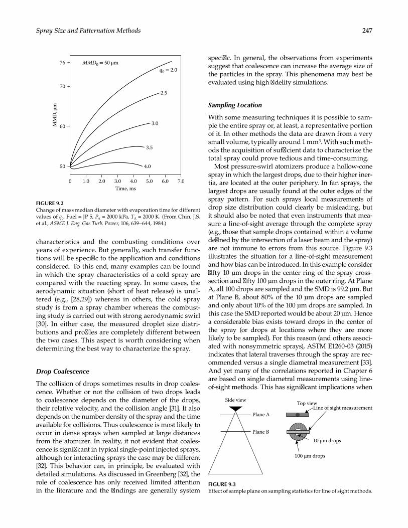
247Spray Size and Patternation Methods

characteristics and the combusting conditions over years of experience. But generally, such transfer func-tions will be specific to the application and conditions considered. To this end, many examples can be found in which the spray characteristics of a cold spray are compared with the reacting spray. In some cases, the aerodynamic situation (short of heat release) is unal-tered (e.g., [28,29]) whereas in others, the cold spray study is from a spray chamber whereas the combust-ing study is carried out with strong aerodynamic swirl [30]. In either case, the measured droplet size distri-butions and profiles are completely different between the two cases. This aspect is worth considering when determining the best way to characterize the spray.

Drop Coalescence

The collision of drops sometimes results in drop coales-cence. Whether or not the collision of two drops leads to coalescence depends on the diameter of the drops, their relative velocity, and the collision angle [31]. It also depends on the number density of the spray and the time available for collisions. Thus coalescence is most likely to occur in dense sprays when sampled at large distances from the atomizer. In reality, it not evident that coales-cence is significant in typical single-point injected sprays, although for interacting sprays the case may be different [32]. This behavior can, in principle, be evaluated with detailed simulations. As discussed in Greenberg [32], the role of coalescence has only received limited attention in the literature and the findings are generally system

specific. In general, the observations from experiments suggest that coalescence can increase the average size of the particles in the spray. This phenomena may best be evaluated using high fidelity simulations.

Sampling Location

With some measuring techniques it is possible to sam-ple the entire spray or, at least, a representative portion of it. In other methods the data are drawn from a very small volume, typically around 1 mm3. With such meth-ods the acquisition of sufficient data to characterize the total spray could prove tedious and time-consuming.

Most pressure-swirl atomizers produce a hollow-cone spray in which the largest drops, due to their higher iner-tia, are located at the outer periphery. In fan sprays, the largest drops are usually found at the outer edges of the spray pattern. For such sprays local measurements of drop size distribution could clearly be misleading, but it should also be noted that even instruments that mea-sure a line-of-sight average through the complete spray (e.g., those that sample drops contained within a volume defined by the intersection of a laser beam and the spray) are not immune to errors from this source. Figure 9.3 illustrates the situation for a line-of-sight measurement and how bias can be introduced. In this example consider fifty 10 μm drops in the center ring of the spray cross-section and fifty 100 μm drops in the outer ring. At Plane A, all 100 drops are sampled and the SMD is 99.2 μm. But at Plane B, about 80% of the 10 μm drops are sampled and only about 10% of the 100 μm drops are sampled. In this case the SMD reported would be about 20 μm. Hence a considerable bias exists toward drops in the center of the spray (or drops at locations where they are more likely to be sampled). For this reason (and others associ-ated with nonsymmetric sprays), ASTM E1260-03 (2015) indicates that lateral traverses through the spray are rec-ommended versus a single diametral measurement [33]. And yet many of the correlations reported in Chapter 6 are based on single diametral measurements using line-of-sight methods. This has significant implications when

50

60

4.0

3.5

3.0

2.570

76

0 6.05.04.03.0Time, ms

2.01.0 7.0

MMD0 = 50 μmq0 = 2.0

MM

D, μ

m

FIGURE 9.2Change of mass median diameter with evaporation time for different values of q0. Fuel = JP 5, PA = 2000 kPa, TA = 2000 K. (From Chin, J.S. et al., ASME J. Eng. Gas Turb. Power, 106, 639–644, 1984.)

Side view

Plane A

Top viewLine of sight measurement

10 μm drops

100 μm drops

Plane B

FIGURE 9.3Effect of sample plane on sampling statistics for line of sight methods.

248 Atomization and Sprays

it comes to comparing measurements by different meth-ods. At a minimum it portends a significant factor to con-sider when specifying SMD requirement for a particular atomizer if the information is based on a single line-of-sight measurement.

For low ambient temperatures, where the effects of fuel evaporation may be regarded as negligibly small, Chin et al. [17] have shown that when a liquid is injected from a pressure atomizer into a coflowing airstream, the values of mean drop size and drop size distribution, as measured by light-scattering techniques in the region downstream of the atomizer, may be appreciably differ-ent from the true values that would be measured in a plane fairly close to the nozzle where the atomization process is just complete. Unfortunately, in practice, this plane is very difficult to determine with any degree of precision, since it is very dependent on nozzle design features as well as liquid flow rate, injection pressure, and ambient air properties.

Generally, it is found that a more uniform spray (higher q) or a higher initial MMD will exhibit less variation of MMD with changing axial location. Where drop acceleration or deceleration is present, the effect on spray measurement is to increase or decrease, respec-tively, the measured value of MMD. Far downstream of the nozzle, the distance depending on the air velocity and initial MMD, all the drops attain a sensibly uniform velocity, regardless of size, so the measured MMD again approaches the initial value.

These findings suggest that measurements of nozzle spray characteristics in a flowing airstream should ideally be carried out well downstream of the nozzle (200–300 mm), using air at low temperature (<300 K) in conjunction with liquids of low volatility.

The problems outlined above with pressure atom-izers are far less pronounced with airblast atomizers, partly because of the turbulent mixing of droplets and air, but mainly because the airborne drops are trans-ported radially by the flowing air to an extent that prohibits the formation of steep drop size gradients. However, errors arising from the combined effects of coalescence and evaporation still apply to sprays gen-erated by this type of atomizer.

In general, the spray patterns produced by most practical atomizers are so complex that fairly pre-cise measurements of drop size distributions can be obtained only if accurate and reliable instrumentation and data reduction procedures are combined with a sound appreciation of their useful limits of applica-tion. As emphasized by Tate [18], the ability to rec-ognize and challenge questionable data is especially important. Thus, experience and judgment are valu-able attributes for those who measure drop sizes and use the information in the design and application of atomizing systems.

Mechanical Methods

These usually involve the capture of a sample of the spray on a solid surface or in a cell containing a special liquid. The drops are then observed, or photographed, with the aid of a microscope. The method is fairly sim-ple and has many variations.

Collection of Drops on Slides

With this technique a solid surface, usually a glass slide, is covered with a suitable coating that must be of very fine grain structure to make distinct the impressions created by very small drops [18,34]. A very fine surface may be obtained by burning a kerosene-soaked wick under the glass to produce a thin coating of soot, or by burning a magnesium ribbon to deposit a thin layer of magnesium oxide. With such coatings, drop sizes down to 3 μm in diameter can be observed and measured [35].

After the slide is exposed to the spray, the sizes of the drop impressions are measured, sometimes by means of a microscope fitted with a traversing scale. In the 1960s the advent of automated image processing resulted in a convenient instrument, the Leica Quantimet image ana-lyzer computer that made rapid, accurate assessment of particle distributions on a slide. These sizes are then converted to actual drop sizes using a correction factor derived by May [35], which accounts for the flattening of liquid on the slide. The actual diameter associated with the volume of the particle on the slide will be smaller than the perceived diameter.

Elkotb et al. [36] used soot-coated slides to measure both radial and overall drop size distributions in a spray. The sampling apparatus consists of a small- diameter cylinder with 10 holes of 5 mm diameter at different radial distances; the soot-coated glass slide is mounted on an axle fitted inside the cylinder and can be rotated around the cylinder axis by a wheel. The apparatus is placed at a distance of 60 mm from the atomizer.

Sprays injected from the atomizer and passing through the holes on the rim of the apparatus leave impressions on the soot layer deposited on the glass slide. The impressions on the slide are photographed under a microscope with a total magnification of 350. Each group of impressions represents part of the spray at a radial distance equal to that of the hole responsible for these impressions. The diameters of the impressions are measured with a scale graduated down to 0.5 μm, and the drops that have the same diameter are counted and classified into size intervals of 10-μm width. The number and diameters of the impressions obtained for each radius of the spray define the spatial and total size distributions.

One problem associated with slides is that of deter-mining what fraction of the slide area should be covered

249Spray Size and Patternation Methods

by drops. If too many drops are collected, the probabil-ity of error due to overlap is high and drop counting becomes tedious. On the other hand, if too few drops are collected, the sample may not be representative of the spray. From the standpoint of ease of measurement and counting, 0.2% coverage is satisfactory, but a cover-age as high as 1.0% can be tolerated before the problem of drop overlap becomes significant.

Other important considerations are drop evaporation and internal droplet dynamics. The lifetime of small drops is extremely short. For example, a water drop that is 10 μm in diameter has a lifetime of about 1 s in a 90% relative humidity atmosphere [37]. Thus, evapora-tion effects are very significant in the measurement of fine sprays. Similar issues arise for thermodynamically unstable situations (e.g., fine water droplets in oil as an emulsion). By the time the sample is obtained and ana-lyzed, natural particle agglomeration/separation may have occurred. Emulsification agents can help in this particular situation. If the goal is to quantify the size and number of bubbles within a drop undergoing flash-ing or effervescent atomization, the time scale associ-ated with the bubble recombination may also alter the sample prior to image analysis.

Collection efficiency is especially important with air-blast atomizers, owing to the flow field created around the collecting surface. The large drops have enough inertia to hit the surface, but the small drops tend to fol-low the streamlines. For these reasons, drop size data for airblast atomizers obtained by direct drop collection tend to indicate larger than actual sizes.

Yet another problem that arises with the collection of drops on coated slides is the determination of the cor-rection factor by which the diameter of the flattened drop must be multiplied to obtain the original diam-eter of the spherical volume. Its value depends on liquid properties, notably surface tension, and on the nature of the coating employed. For example, with oil drops the correction factor is around 0.5 for a clean glass surface and 0.86 for a magnesium-coated slide [38].

Most of the work using the impression method was performed more than 40 years ago, and the technique has now been largely supplanted by photographic and optical methods. Further, a plethora of digital image pro-cessing schemes and packages are now available to auto-matically count and size particles such as ImageJ from the National Institute of Health or commercial packages from MATLAB® or National Instruments who offer image processing add-on modules. Such software packages can be used directly with high magnification images of drops (vs. collecting them). However, in many cases with het-erogeneous liquids, physically sampling the spray may well be the best approach. An example is the quantifica-tion of discrete water particle distributions within a con-tinuous oil phase that occurs in emulsions [39]. In this

recent study, the size distribution of water drops within oil was quantified and mean values between 2 and 15 μm were obtained quite conveniently and accurately using the slide collection method that incorporated emulsion stabilizers and conducting analysis using the image pro-cessing software ImagePro® (MediaCybernetics).

Collection of Drops in Cells

An improvement on the coated-slide technique is one in which the drops are caught on a target where they are held suspended while they are counted and measured. Hausser and Strobl [40] were among the first investiga-tors to use as the target microscope slides coated with a special liquid in which the drop would not dissolve but would remain stable and suspended. An alternative approach is to collect the drops in a cell containing a suit-able immersion liquid. This method has three advantages over collection on a slide: (1) the drops remain almost per-fectly spherical, provided the density of the immersion liquid is only slightly less than that of the sprayed liquid; (2) evaporation is prevented; and (3) provided no splitting of the drop occurs on hitting the immersion liquid, the true sizes of the drops are obtained and can be measured directly. The method cannot be applied satisfactorily to coarse sprays due to the risk of disintegration of the larg-est drops on impact with the immersion liquid. The prob-lem of drop breakup can be alleviated to some extent by choosing immersion liquids of low viscosity and surface tension. Such liquids facilitate the penetration of the liquid surface by the drops. The drops then settle to the bottom of the cell, where they remain suspended and stable for an appreciable time, provided, of course, the immersion liquid is absolutely immiscible with the sprayed liquid.

Another problem with the immersion sampling method is that of drop coalescence. According to Karasawa and Kurabayashi [41], this phenomenon is often overlooked because the occurrence of coalescence is difficult to detect. The remedy is the same as that for drop breakup mentioned earlier, namely to use an immersion liquid of low viscosity [41]. Rupe [42] used this method in his investigation of sprays. The liquids employed were water and water–alcohol mixtures, and the immersion liquids were Stoddard solvent and white kerosene. The Delavan Corporation originally used this technique extensively to accumulate consid-erable data on drop size distributions in sprays [43]. The experimental procedures employed follow closely those of Rupe. Dyed water is sprayed into a cell filled with Stoddard solvent. The cell is located beneath an air-operated shutter, whose speed is adjusted to obtain a representative number of drops. After settling at the bottom of the cell, the drops are photographed at high magnification (usually 50×). The magnified drop images

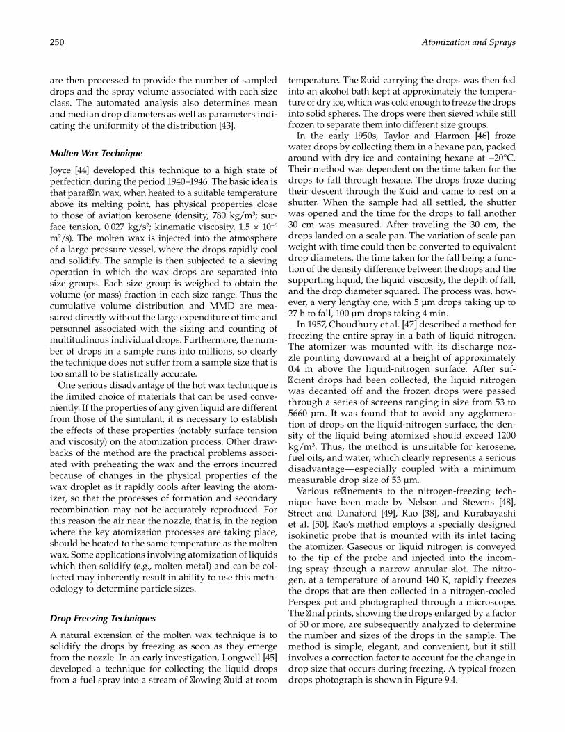
250 Atomization and Sprays

are then processed to provide the number of sampled drops and the spray volume associated with each size class. The automated analysis also determines mean and median drop diameters as well as parameters indi-cating the uniformity of the distribution [43].

Molten Wax Technique

Joyce [44] developed this technique to a high state of perfection during the period 1940–1946. The basic idea is that paraffin wax, when heated to a suitable temperature above its melting point, has physical properties close to those of aviation kerosene (density, 780 kg/m3; sur-face tension, 0.027 kg/s2; kinematic viscosity, 1.5 × 10–6 m2/s). The molten wax is injected into the atmosphere of a large pressure vessel, where the drops rapidly cool and solidify. The sample is then subjected to a sieving operation in which the wax drops are separated into size groups. Each size group is weighed to obtain the volume (or mass) fraction in each size range. Thus the cumulative volume distribution and MMD are mea-sured directly without the large expenditure of time and personnel associated with the sizing and counting of multitudinous individual drops. Furthermore, the num-ber of drops in a sample runs into millions, so clearly the technique does not suffer from a sample size that is too small to be statistically accurate.

One serious disadvantage of the hot wax technique is the limited choice of materials that can be used conve-niently. If the properties of any given liquid are different from those of the simulant, it is necessary to establish the effects of these properties (notably surface tension and viscosity) on the atomization process. Other draw-backs of the method are the practical problems associ-ated with preheating the wax and the errors incurred because of changes in the physical properties of the wax droplet as it rapidly cools after leaving the atom-izer, so that the processes of formation and secondary recombination may not be accurately reproduced. For this reason the air near the nozzle, that is, in the region where the key atomization processes are taking place, should be heated to the same temperature as the molten wax. Some applications involving atomization of liquids which then solidify (e.g., molten metal) and can be col-lected may inherently result in ability to use this meth-odology to determine particle sizes.

Drop Freezing Techniques

A natural extension of the molten wax technique is to solidify the drops by freezing as soon as they emerge from the nozzle. In an early investigation, Longwell [45] developed a technique for collecting the liquid drops from a fuel spray into a stream of flowing fluid at room

temperature. The fluid carrying the drops was then fed into an alcohol bath kept at approximately the tempera-ture of dry ice, which was cold enough to freeze the drops into solid spheres. The drops were then sieved while still frozen to separate them into different size groups.

In the early 1950s, Taylor and Harmon [46] froze water drops by collecting them in a hexane pan, packed around with dry ice and containing hexane at −20°C. Their method was dependent on the time taken for the drops to fall through hexane. The drops froze during their descent through the fluid and came to rest on a shutter. When the sample had all settled, the shutter was opened and the time for the drops to fall another 30 cm was measured. After traveling the 30 cm, the drops landed on a scale pan. The variation of scale pan weight with time could then be converted to equivalent drop diameters, the time taken for the fall being a func-tion of the density difference between the drops and the supporting liquid, the liquid viscosity, the depth of fall, and the drop diameter squared. The process was, how-ever, a very lengthy one, with 5 μm drops taking up to 27 h to fall, 100 μm drops taking 4 min.

In 1957, Choudhury et al. [47] described a method for freezing the entire spray in a bath of liquid nitrogen. The atomizer was mounted with its discharge noz-zle pointing downward at a height of approximately 0.4 m above the liquid-nitrogen surface. After suf-ficient drops had been collected, the liquid nitrogen was decanted off and the frozen drops were passed through a series of screens ranging in size from 53 to 5660 μm. It was found that to avoid any agglomera-tion of drops on the liquid-nitrogen surface, the den-sity of the liquid being atomized should exceed 1200 kg/m3. Thus, the method is unsuitable for kerosene, fuel oils, and water, which clearly represents a serious disadvantage—especially coupled with a minimum measurable drop size of 53 μm.

Various refinements to the nitrogen-freezing tech-nique have been made by Nelson and Stevens [48], Street and Danaford [49], Rao [38], and Kurabayashi et al. [50]. Rao’s method employs a specially designed isokinetic probe that is mounted with its inlet facing the atomizer. Gaseous or liquid nitrogen is conveyed to the tip of the probe and injected into the incom-ing spray through a narrow annular slot. The nitro-gen, at a temperature of around 140 K, rapidly freezes the drops that are then collected in a nitrogen-cooled Perspex pot and photographed through a microscope. The final prints, showing the drops enlarged by a factor of 50 or more, are subsequently analyzed to determine the number and sizes of the drops in the sample. The method is simple, elegant, and convenient, but it still involves a correction factor to account for the change in drop size that occurs during freezing. A typical frozen drops photograph is shown in Figure 9.4.

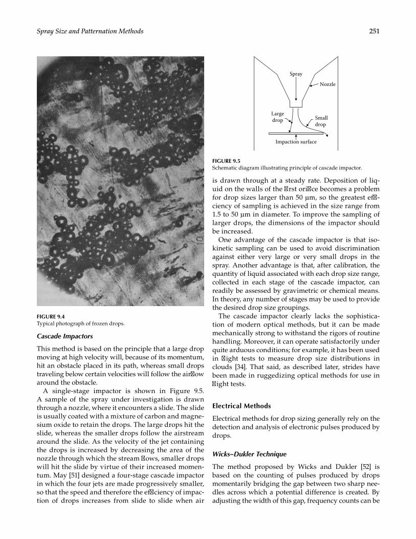
251Spray Size and Patternation Methods

Cascade Impactors

This method is based on the principle that a large drop moving at high velocity will, because of its momentum, hit an obstacle placed in its path, whereas small drops traveling below certain velocities will follow the airflow around the obstacle.

A single-stage impactor is shown in Figure 9.5. A sample of the spray under investigation is drawn through a nozzle, where it encounters a slide. The slide is usually coated with a mixture of carbon and magne-sium oxide to retain the drops. The large drops hit the slide, whereas the smaller drops follow the airstream around the slide. As the velocity of the jet containing the drops is increased by decreasing the area of the nozzle through which the stream flows, smaller drops will hit the slide by virtue of their increased momen-tum. May [51] designed a four-stage cascade impactor in which the four jets are made progressively smaller, so that the speed and therefore the efficiency of impac-tion of drops increases from slide to slide when air

is drawn through at a steady rate. Deposition of liq-uid on the walls of the first orifice becomes a problem for drop sizes larger than 50 μm, so the greatest effi-ciency of sampling is achieved in the size range from 1.5 to 50 μm in diameter. To improve the sampling of larger drops, the dimensions of the impactor should be increased.

One advantage of the cascade impactor is that iso-kinetic sampling can be used to avoid discrimination against either very large or very small drops in the spray. Another advantage is that, after calibration, the quantity of liquid associated with each drop size range, collected in each stage of the cascade impactor, can readily be assessed by gravimetric or chemical means. In theory, any number of stages may be used to provide the desired drop size groupings.

The cascade impactor clearly lacks the sophistica-tion of modern optical methods, but it can be made mechanically strong to withstand the rigors of routine handling. Moreover, it can operate satisfactorily under quite arduous conditions; for example, it has been used in flight tests to measure drop size distributions in clouds [34]. That said, as described later, strides have been made in ruggedizing optical methods for use in flight tests.

Electrical Methods

Electrical methods for drop sizing generally rely on the detection and analysis of electronic pulses produced by drops.

Wicks–Dukler Technique

The method proposed by Wicks and Dukler [52] is based on the counting of pulses produced by drops momentarily bridging the gap between two sharp nee-dles across which a potential difference is created. By adjusting the width of this gap, frequency counts can be

FIGURE 9.4Typical photograph of frozen drops.

Spray

Nozzle

Largedrop Small

drop

Impaction surface

FIGURE 9.5Schematic diagram illustrating principle of cascade impactor.

252 Atomization and Sprays

obtained in terms of gap size and then converted into drop size distributions.

Some of the problems that can arise with this type of instrument have been described by Jones [15]. It has been found that the apparent resistance of a drop bridging the gap is a function of both drop velocity and the depth of immersion of the needles into the drop. Unless a very sensitive detection and counting system is employed, a large proportion of the pulses will be below the threshold that has to be set to avoid counting pulses due to noise. This could lead to large errors in drop size distribution [15]. Furthermore, changes in drop velocities will have the same effect on count rate as changes in drop sizes, so that appar-ent changes in size distribution could occur when, in fact, only drop velocities have changed. Despite these limitations, the system might find useful application for certain types of spray, bearing in mind its ease of operation. Comparison with a proven drop sizing method would be necessary to establish its useful operating range and to identify and quantify the prin-cipal sources of error.

Charged Wire Technique

This technique operates on the principle that when a drop impinges on an electrically charged wire it removes an amount of charge that depends on its size. This allows drop sizes to be obtained by converting the charge transfer into a measurable voltage pulse.

According to Gardiner [53], the limitations of the charged wire probe appear to depend on a combination of the electrical conductivity of the liquid and the flux of drops. Liquids of low conductivity produce pulses of long duration, which increases the probability of count-ing errors due to successive impingements being super-imposed on each other. This problem appears to limit the useful application of this technique to dilute sprays of high-conductivity liquids.

Hot Wire Technique

When a liquid drop becomes attached to a heated wire, it causes local cooling of the wire as it evaporates. This phe-nomenon can be used to obtain the sizes and concentra-tions of liquid drops present in a gas stream. Essentially, the device employed is a constant- temperature hot wire anemometer. When no drops are present, the electri-cal resistance of the wire is high and sensibly uniform along its length. When a drop attaches to the wire, local cooling by the drop reduces the resistance in pro-portion to the drop size. This reduction in resistance is manifested as a voltage drop across the wire sup-ports. The constant-current electrical energy supplied

to the wire subsequently evaporates the drop, leaving the device ready to receive another drop. The entire process takes place within a time of 2 ms, depending on the drop size [54].

Mahler and Magnus [54] have described the operat-ing principles and calibration procedures of a com-mercial hot wire instrument in some detail. Under the right conditions it can yield accurate measurements of SMD, MMD, volume flow rate, and liquid concentra-tion. Although it is an intrusive technique, the platinum wire employed is only 5 μm in diameter and 1 mm long and causes very little disturbance to the flow. However, when measuring large drops the device can operate only at flow velocities below around 10 m/s because of drop shattering on the wire [12]. Moreover, the tech-nique cannot be used for liquids that leave a residue on the wire, as this affects the calibration.

For a more complete account of the hot wire tech-nique and other electrical methods for drop size mea-surements, reference should be made to the review by Jones [15]. It is worth pointing out that, often, deficien-cies of an older technique can be overcome through the advent of recent developments in materials or technology.

Optical Methods

Optical methods can be broadly divided into imag-ing and nonimaging types. The former, including flash photography and holography, are limited in practice to drop sizes larger than 5 μm. Imaging methods have the advantage of allowing the drops to be seen as they exist at the point and time where knowledge of their size is required. Another advantage is that errors that might arise from coalescence or evaporation of drops after sampling are eliminated [34].

Nonimaging methods can be subdivided into two classes—those that count and size individual drops, one at a time, and those that measure a large number of drops simultaneously. For accurate results it is impor-tant to know both drop size and velocity, and some instruments (both imaging and nonimaging) can pro-vide both sets of information.

A variety of optical methods have been employed for spray analysis. Each method has its own advantages and limitations, but they all have the important attri-bute of allowing size measurements to be made without the insertion of a physical probe into the spray.

High Magnification Imaging

Imaging is one of the most accurate and can be a least expensive techniques for the measurement of drop sizes and velocities in sprays. Usually it involves

253Spray Size and Patternation Methods

taking an image (photographs in early years, digital cameras in recent years) with a light pulse of suffi-cient intensity and sufficiently short duration to pro-duce a sharp image and then counting and sizing the images of drops recorded. Much of the development work in the application of film photography to spray analysis was carried out by Dombrowski and cowork-ers [55–57] and by Chigier and coworkers at Sheffield University [58–61].

In all imaging situations a trade-off exists between magnification (desired to get good resolution of fine particles), field of view (to isolate small regions or to capture information over a large region), image dura-tion (short pulse duration to avoid blurring or streaking of high-speed particles), and sensitivity of recording media (either film of digital sensor). In some digital imaging systems, the exposure time (currently much less than 1 μs) can be used to freeze particle motion even with a continuous light source, which is helpful for high-speed recording.

For short duration light pulses, many options are available. Mercury vapor lamps, electrical sparks, flash lights, and laser pulses are generally used to create a high-intensity light source of short duration. Flash light sources have time durations of the order of 1 μs, while common lasers can have pulse durations of the order of nanoseconds and advanced systems are achieving pico and femto second pulse durations because of technol-ogy developments.

In 1977, Jones [15] suggested that imaging (specifi-cally photography) is probably the only technique with the potential to provide drop size informa-tion from the dense, fast-moving sprays of interest in many applications. However, the method is not with-out problems, of which the most difficult is analysis of the photographic images, which always entails at least some degree of human involvement. Manual sizing is tedious and time-consuming and invariably subject to operator fatigue and bias. Automatic image analyzers, such as the Quantimet (Lieca Microsystems, Wetzlar, Germany), also call for considerable judgment on the part of the operator, who must ultimately decide which drops are in focus. With high-density sprays, the drop images may become very closely spaced on the nega-tive, or even overlapping, which detracts appreciably from the accuracy of automatic image analysis. Increase in magnification at the imaging stage tends to allevi-ate this problem and also reduces the minimum drop size that the Quantimet can reliably measure. However, these improvements can be realized only by forfeiting depth of field [15].

A calibration procedure for determining the effec-tive depth of field has been described by Chigier [61]. Particles of known size, deposited on a glass slide, are

traversed across the region of focus of the camera and photographs are taken at regular intervals. Particle images are determined by measuring each particular diameter at two different light intensity levels. The average of these measurements is related to the parti-cle diameter, and the difference between the diameters is a measure of the thickness of the blurred halo at the edge of the particle. By this means the effective depth of field is determined for each particular optical sys-tem and particle size. Standard devices are available with which to establish depth-of-field (e.g., Edmunds Scientific 5–15 Depth-of-Field target).

An early, fully automated TV camera based system was developed by Parker Hannifin in the 1960s to gain significant insight into atomizer drop size distributions [62,63]. The tedious and subjective data-processing challenges pointed out by Jones [15] were alleviated to a great extent by the TV analyzer developed by the Parker-Hannifin Corporation. This instrument used a 0.5-μs flash to photograph the drops contained within a small frame of dimensions 1.5 × 2.0 mm, approximately 1 mm in depth. The resolution of the system is within 4 μm. The rate of photography is 15 frames/s. A complete test takes about 20 min and encompasses more than 14,000 drops. The instrument is considered precise in the SMD range from 80 to 200 μm. The term precise in this context is intended to imply a repeatability of ±6%. This method was further evolved into later generation system [64]. GM Research Laboratory also developed a similar turnkey droplet sizing system using back-lighting and imaging techniques involving television standards [65]. Like the Parker system, the GM system achieved good results through careful development of algorithms for image processing to detect/isolate/size individual drops and accounting for depth of field issues.

Double exposure imaging or high-speed imaging can also be used to obtain information on drop veloci-ties. If two light pulses are generated in a rapid succes-sion, a double image is obtained of a single drop on the recording media, from which the velocity of the drop can be determined by measuring the distance trav-eled by the drop and dividing it by the time interval between the two pulses. The direction of movement of the drop can also be directly determined from the pho-tograph as an angle of flight with respect to the central axis of the spray. The method provides instantaneous measurements for individual drops, and from a series of such measurements time-average and space-average quantities can be determined as well as standard devi-ations. Measurement techniques based on this prin-ciple have been used successfully by many workers including De Corso and Kemeny [62], Mellor et al. [59], and Chigier [61].

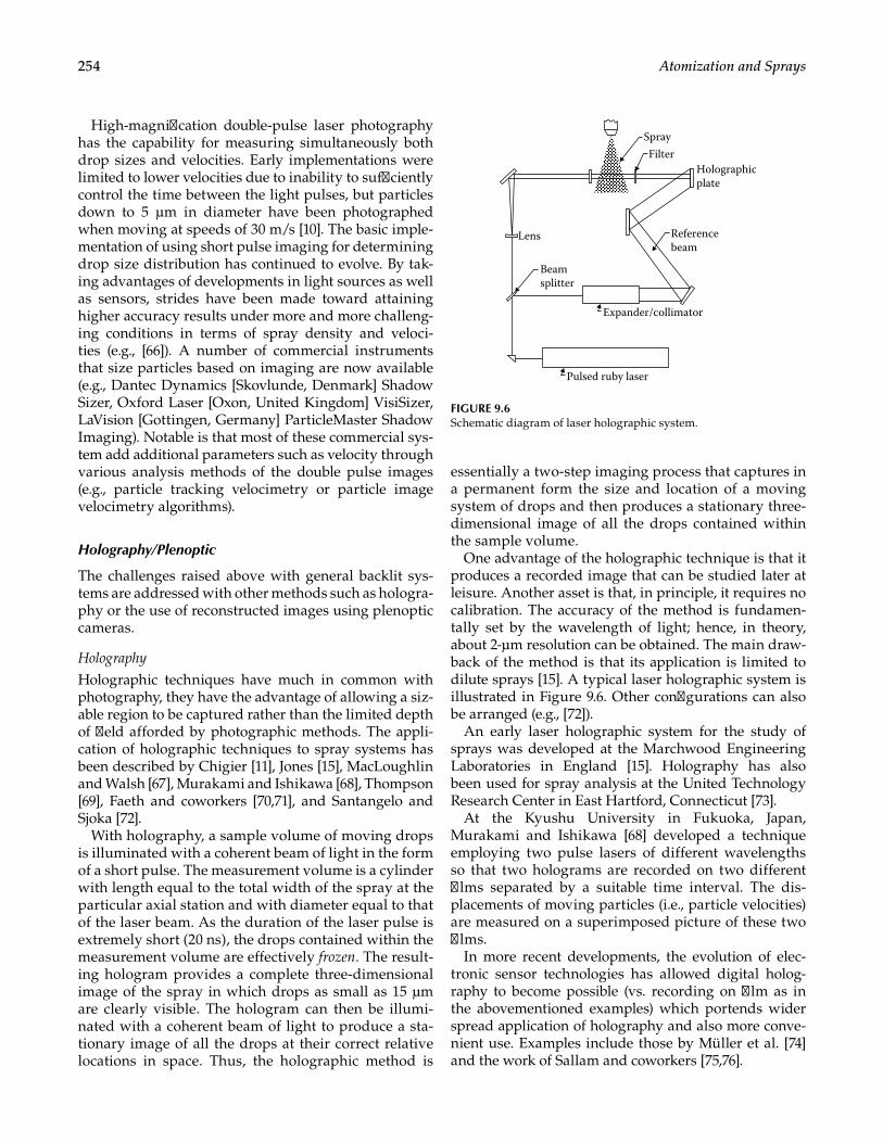
254 Atomization and Sprays

High-magnification double-pulse laser photography has the capability for measuring simultaneously both drop sizes and velocities. Early implementations were limited to lower velocities due to inability to sufficiently control the time between the light pulses, but particles down to 5 μm in diameter have been photographed when moving at speeds of 30 m/s [10]. The basic imple-mentation of using short pulse imaging for determining drop size distribution has continued to evolve. By tak-ing advantages of developments in light sources as well as sensors, strides have been made toward attaining higher accuracy results under more and more challeng-ing conditions in terms of spray density and veloci-ties (e.g., [66]). A number of commercial instruments that size particles based on imaging are now available (e.g., Dantec Dynamics [Skovlunde, Denmark] Shadow Sizer, Oxford Laser [Oxon, United Kingdom] VisiSizer, LaVision [Gottingen, Germany] ParticleMaster Shadow Imaging). Notable is that most of these commercial sys-tem add additional parameters such as velocity through various analysis methods of the double pulse images (e.g., particle tracking velocimetry or particle image velocimetry algorithms).

Holography/Plenoptic

The challenges raised above with general backlit sys-tems are addressed with other methods such as hologra-phy or the use of reconstructed images using plenoptic cameras.

Holography

Holographic techniques have much in common with photography, they have the advantage of allowing a siz-able region to be captured rather than the limited depth of field afforded by photographic methods. The appli-cation of holographic techniques to spray systems has been described by Chigier [11], Jones [15], MacLoughlin and Walsh [67], Murakami and Ishikawa [68], Thompson [69], Faeth and coworkers [70,71], and Santangelo and Sjoka [72].

With holography, a sample volume of moving drops is illuminated with a coherent beam of light in the form of a short pulse. The measurement volume is a cylinder with length equal to the total width of the spray at the particular axial station and with diameter equal to that of the laser beam. As the duration of the laser pulse is extremely short (20 ns), the drops contained within the measurement volume are effectively frozen. The result-ing hologram provides a complete three-dimensional image of the spray in which drops as small as 15 μm are clearly visible. The hologram can then be illumi-nated with a coherent beam of light to produce a sta-tionary image of all the drops at their correct relative locations in space. Thus, the holographic method is

essentially a two-step imaging process that captures in a permanent form the size and location of a moving system of drops and then produces a stationary three-dimensional image of all the drops contained within the sample volume.

One advantage of the holographic technique is that it produces a recorded image that can be studied later at leisure. Another asset is that, in principle, it requires no calibration. The accuracy of the method is fundamen-tally set by the wavelength of light; hence, in theory, about 2-μm resolution can be obtained. The main draw-back of the method is that its application is limited to dilute sprays [15]. A typical laser holographic system is illustrated in Figure 9.6. Other configurations can also be arranged (e.g., [72]).

An early laser holographic system for the study of sprays was developed at the Marchwood Engineering Laboratories in England [15]. Holography has also been used for spray analysis at the United Technology Research Center in East Hartford, Connecticut [73].

At the Kyushu University in Fukuoka, Japan, Murakami and Ishikawa [68] developed a technique employing two pulse lasers of different wavelengths so that two holograms are recorded on two different films separated by a suitable time interval. The dis-placements of moving particles (i.e., particle velocities) are measured on a superimposed picture of these two films.

In more recent developments, the evolution of elec-tronic sensor technologies has allowed digital holog-raphy to become possible (vs. recording on film as in the abovementioned examples) which portends wider spread application of holography and also more conve-nient use. Examples include those by Müller et al. [74] and the work of Sallam and coworkers [75,76].

Lens

Beamsplitter

Expander/collimator

Holographicplate

Referencebeam

FilterSpray

Pulsed ruby laser

FIGURE 9.6Schematic diagram of laser holographic system.

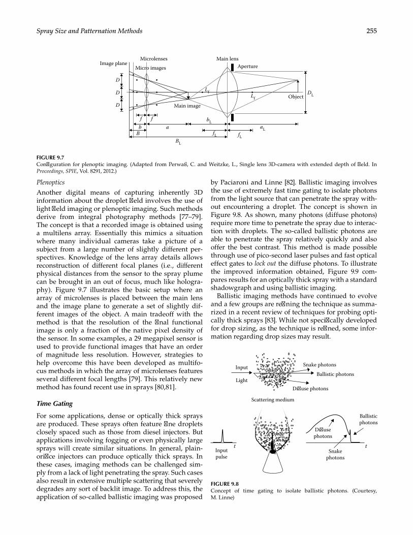
255Spray Size and Patternation Methods

Plenoptics

Another digital means of capturing inherently 3D information about the droplet field involves the use of light field imaging or plenoptic imaging. Such methods derive from integral photography methods [77–79]. The concept is that a recorded image is obtained using a multilens array. Essentially this mimics a situation where many individual cameras take a picture of a subject from a large number of slightly different per-spectives. Knowledge of the lens array details allows reconstruction of different focal planes (i.e., different physical distances from the sensor to the spray plume can be brought in an out of focus, much like hologra-phy). Figure 9.7 illustrates the basic setup where an array of microlenses is placed between the main lens and the image plane to generate a set of slightly dif-ferent images of the object. A main tradeoff with the method is that the resolution of the final functional image is only a fraction of the native pixel density of the sensor. In some examples, a 29 megapixel sensor is used to provide functional images that have an order of magnitude less resolution. However, strategies to help overcome this have been developed as multifo-cus methods in which the array of microlenses features several different focal lengths [79]. This relatively new method has found recent use in sprays [80,81].

Time Gating

For some applications, dense or optically thick sprays are produced. These sprays often feature fine droplets closely spaced such as those from diesel injectors. But applications involving fogging or even physically large sprays will create similar situations. In general, plain-orifice injectors can produce optically thick sprays. In these cases, imaging methods can be challenged sim-ply from a lack of light penetrating the spray. Such cases also result in extensive multiple scattering that severely degrades any sort of backlit image. To address this, the application of so-called ballistic imaging was proposed

by Paciaroni and Linne [82]. Ballistic imaging involves the use of extremely fast time gating to isolate photons from the light source that can penetrate the spray with-out encountering a droplet. The concept is shown in Figure 9.8. As shown, many photons (diffuse photons) require more time to penetrate the spray due to interac-tion with droplets. The so-called ballistic photons are able to penetrate the spray relatively quickly and also offer the best contrast. This method is made possible through use of pico-second laser pulses and fast optical effect gates to lock out the diffuse photons. To illustrate the improved information obtained, Figure 9.9 com-pares results for an optically thick spray with a standard shadowgraph and using ballistic imaging.

Ballistic imaging methods have continued to evolve and a few groups are refining the technique as summa-rized in a recent review of techniques for probing opti-cally thick sprays [83]. While not specifically developed for drop sizing, as the technique is refined, some infor-mation regarding drop sizes may result.

Microlenses Main lens

Main image

f fb a

bLaL

DL

fL fLBL

Lf

Lf

B

D

D

D

Aperture

Object

Micro imagesImage plane

FIGURE 9.7Configuration for plenoptic imaging. (Adapted from Perwaß, C. and Weitzke, L., Single lens 3D-camera with extended depth of field. In Proceedings, SPIE, Vol. 8291, 2012.)

Inputpulse

Scattering medium

Diuse photons

Ballistic photons

Ballisticphotons

Diusephotons

Snakephotons

tt

Snake photons

Light

Input

FIGURE 9.8Concept of time gating to isolate ballistic photons. (Courtesy, M. Linne)

256 Atomization and Sprays

X-Ray Methods

Another method that has gained considerable attention in recent years in the use of X-rays to probe both near field spray structure as well as the internal flow behav-ior within practical production atomizers. This has been made possible primarily due to the development of the Advanced Photon Source (APS) at Argonne National Laboratory. Early examples include using X-ray absorp-tion [84,85] or X-ray radiography. In this application, X-rays are absorbed via Beer's law due to mass absorp-tion. Hence radiography measures the liquid mass per unit area. While not a measurement of drop size, per se, it can provide unparalleled quantitative information about the behavior of optically dense sprays in the near field.

X-rays have also been used to image internal behav-ior using phase-contrast imaging. This has provided unique images and videos of internal flow behavior (e.g., [86,87]).

Further analysis and comparison of the X-ray and time gating methods has been provided in the recent review by Linne [83].

Single-Particle Counters

As their name implies, single-particle counters mea-sure individual particles or drops. Often these instru-ments are built around laser illumination sources. Because a single-particle counter can see only one drop at a time, the size of the measurement or probe volume sets the limitation on the drop number densi-ties in which these counters will operate accurately. In practice, the measurement volume is controlled by the diameter of the focused beam, the f number of the receiver lens and its angle to the transmitted beam, and the aperture of the photodetector [12].

Early examples of single-particle counters were lim-ited to fairly dilute sprays, but the concept of using large off-axis angles of light-scatter detection has allowed these instruments to be used in relatively dense sprays [88] approaching similar number den-sities as those to which the Fraunhofer diffraction method is restricted. Generally, single-particle coun-ters are limited by high particle number densities [23] and beam extinction, whereas diffraction instruments are limited by low number densities and by extinction in high number density environments. Since beam extinction is dependent on the optical path length and number density, in particle fields larger than around 100 mm both methods can be impacted by beam extinction.

Single-particle counters have considerable poten-tial for obtaining both size and velocity distributions directly. These distributions are based on measure-ments of individual drops and do not require the use of distribution functions. They also have the capability to perform the measurements nonintrusively with high spatial resolution over a large size range.

Optical Probe

One single-particle counting method that involves an intrusive optical sensor is the A2 Photonics (Grenoble, France) S-POP probe. Individual droplets impinging on the tip of the probe generate signals that can be used to determine particle size and velocity. It can be used in sprays as well as other types of flows. In principle, it is not limited in optical thickness. Figure 9.10 illustrates the measurement concept that involves a direct measurement of size and infers the velocity based on the slope of the light signal once the drop starts to exit the sensing tip. The method is limited to around 25 m/s and droplets larger than 15 μm.

Air: 0.01lb/s (192 m/s)Water: 0.5 GPM

Nozzle: 5 mm Exit

Air: 0.01lb/s (192 m/s)Water: 0.7 GPM

Nozzle: 5 mm Exit

Time-gatedballistic image

Shadowgram

FIGURE 9.9Comparison of regular shadowgraph and ballistic imaging images. (Courtesy, J. Gord, AFRL)

257Spray Size and Patternation Methods

Concentrations approaching 100% can be measured. While this instrument has not been widely used in sprays, for some cases it is an interesting and rela-tively low-cost option.

Light-Scattering Interferometry

With the advent of the laser Doppler velocim-eter (LDV), interest in simultaneous particle siz-ing with the system soon arose. This was due to the realization that particles were needed that could follow the flow to be measured. These con-siderations and other principles and practice of laser anemometry are outlined in the book by Durst et al. [89]. Farmer [90,91] investigated the possibility of particle sizing using the visibility of the Doppler burst signal. The analysis of Farmer, although not entirely rigorous, was accurate given the appropriate conditions on the optical parame-ters. Perhaps the greatest limitation of the technique was the requirement of using on-axis forward- or back-scattered light detection. This resulted in an excessively large sample volume and the detection of particles that passed outside the region of com-plete overlap of the two laser beams. In addition, the size range of the method was limited to a factor of 10 or less. Other efforts by Chigier and cowork-ers (e.g., [92]) sought to combine the measurement of the scattered light intensity with the LDV to obtain simultaneous particle size and velocity measure-ments. Because near-forward light-scatter detection was used, this method was also limited to very dilute

particle fields. It was not until Bachalo [88] derived the theoretical analysis for dual-beam light scattering at large off-axis angles that the method of light-scat-tering interferometry appeared to be a viable means for spray diagnostics.

Beginning with the approach of Farmer, the measure-ment of drop size and velocity is based on the obser-vation of the light scattered by drops passing through the crossover region of two intersecting laser beams. In practice, a single laser beam is split into two coher-ent beams of equal intensity and parallel polarization, which are made to cross as illustrated in Figure 9.11 [93]. Drops passing through the intersection of the two beams scatter light that produces information from which the drop velocity U is calculated as

2sin 2

DUf( )= λθ

(9.1)

where λ is the wavelength of laser light, fD the Dop-pler frequency, and θ/2 the laser beam intersection half-angle.

Size information is contained in the relative modula-tion (visibility) of the scattered signal. The term visibility may be understood by reference to Figure 9.12. It was defined by Michelson as

Visibility max min

max min

I II I

= −+

(9.2)

SprayLiquid fraction

Optoelectronic module

Velocities

Gas level

Liquid level

Time

Vol

tage

Arrival Time (A)

Exit Time (B)

End of Rise Time (C)

Chords

Opticalprobe

Optical ber link(customer-dened length)

Optical probeSensing

TipDrop

A C

B

Spray

Optoelectronic module

Velocities

Gas level

Liquid lev

Vol

tage

Arrival Time (A)

Exit Time (B)

of Rise Time (C)

Chords

Opticalprobe

Optical ber link(customer-dened length)

Optical probeSensing

TipDrop

A C

B

FIGURE 9.10A2 photonics S-POP probe and measurement concept. (Courtesy of A2 Photonic Sensors.)

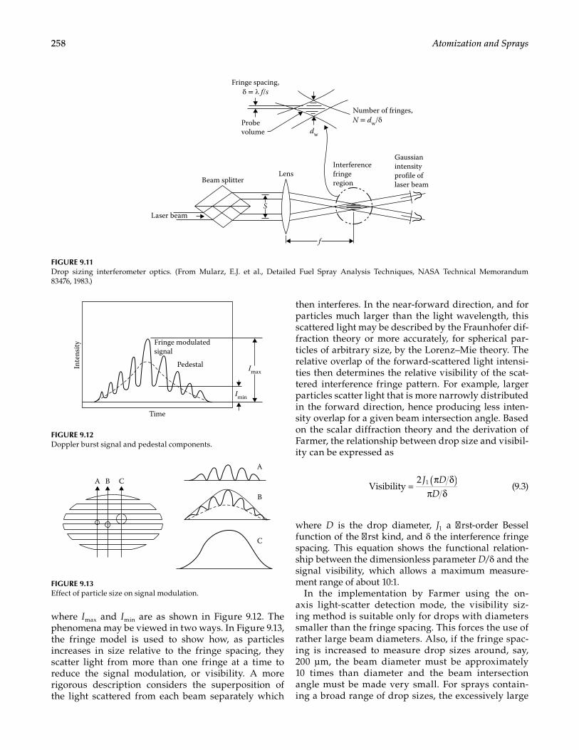
258 Atomization and Sprays

where Imax and Imin are as shown in Figure 9.12. The phenomena may be viewed in two ways. In Figure 9.13, the fringe model is used to show how, as particles increases in size relative to the fringe spacing, they scatter light from more than one fringe at a time to reduce the signal modulation, or visibility. A more rigorous description considers the superposition of the light scattered from each beam separately which

then interferes. In the near-forward direction, and for particles much larger than the light wavelength, this scattered light may be described by the Fraunhofer dif-fraction theory or more accurately, for spherical par-ticles of arbitrary size, by the Lorenz–Mie theory. The relative overlap of the forward-scattered light intensi-ties then determines the relative visibility of the scat-tered interference fringe pattern. For example, larger particles scatter light that is more narrowly distributed in the forward direction, hence producing less inten-sity overlap for a given beam intersection angle. Based on the scalar diffraction theory and the derivation of Farmer, the relationship between drop size and visibil-ity can be expressed as

( )π δπ δ

Visibility =2 1J D

D

(9.3)

where D is the drop diameter, J1 a first-order Bessel function of the first kind, and δ the interference fringe spacing. This equation shows the functional relation-ship between the dimensionless parameter D/δ and the signal visibility, which allows a maximum measure-ment range of about 10:1.

In the implementation by Farmer using the on-axis light-scatter detection mode, the visibility siz-ing method is suitable only for drops with diameters smaller than the fringe spacing. This forces the use of rather large beam diameters. Also, if the fringe spac-ing is increased to measure drop sizes around, say, 200 μm, the beam diameter must be approximately 10 times than diameter and the beam intersection angle must be made very small. For sprays contain-ing a broad range of drop sizes, the excessively large

Fringe spacing,δ = λ f/s

Number of fringes,N = dw/δProbe

volume

LensBeam splitter

Interferencefringeregion

Gaussianintensityprofile oflaser beam

Laser beam

dw

f

S

FIGURE 9.11Drop sizing interferometer optics. (From Mularz, E.J. et al., Detailed Fuel Spray Analysis Techniques, NASA Technical Memorandum 83476, 1983.)

Time

Pedestal

Fringe modulatedsignal

Inte

nsity

Imax

Imin

FIGURE 9.12Doppler burst signal and pedestal components.

A

A

B

C

B C

FIGURE 9.13Effect of particle size on signal modulation.

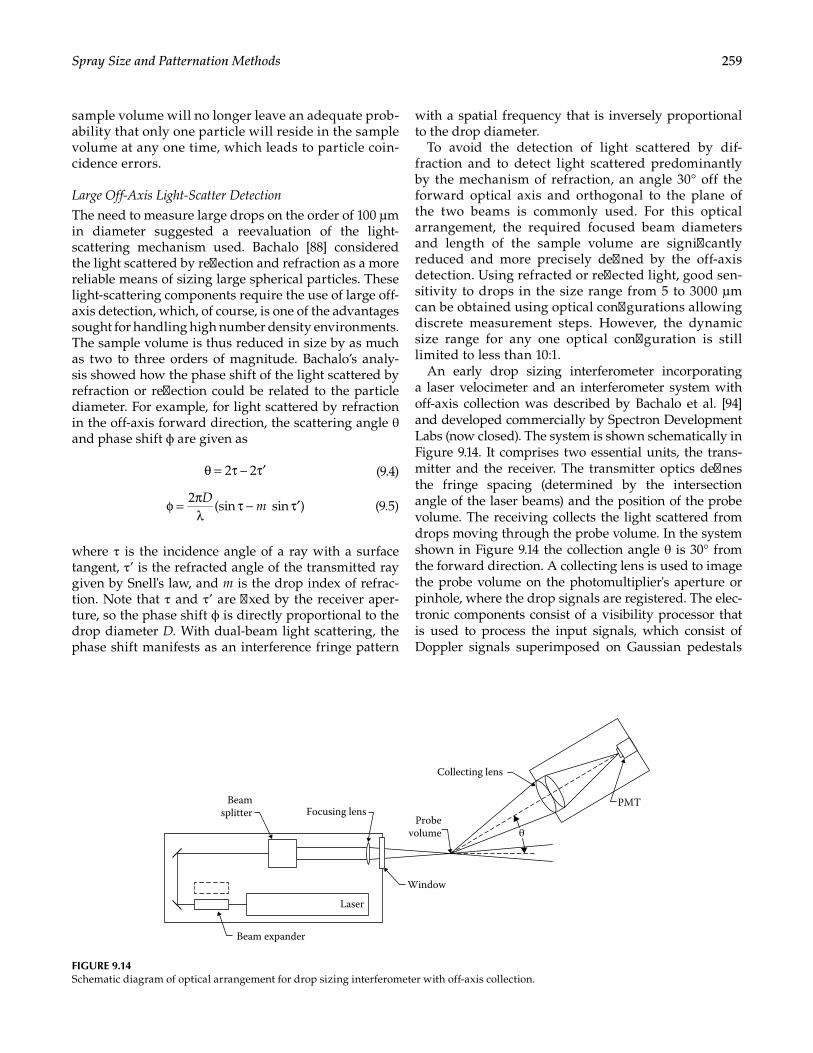
259Spray Size and Patternation Methods

sample volume will no longer leave an adequate prob-ability that only one particle will reside in the sample volume at any one time, which leads to particle coin-cidence errors.

Large Off-Axis Light-Scatter Detection

The need to measure large drops on the order of 100 μm in diameter suggested a reevaluation of the light- scattering mechanism used. Bachalo [88] considered the light scattered by reflection and refraction as a more reliable means of sizing large spherical particles. These light-scattering components require the use of large off-axis detection, which, of course, is one of the advantages sought for handling high number density environments. The sample volume is thus reduced in size by as much as two to three orders of magnitude. Bachalo’s analy-sis showed how the phase shift of the light scattered by refraction or reflection could be related to the particle diameter. For example, for light scattered by refraction in the off-axis forward direction, the scattering angle θ and phase shift ϕ are given as

2 – 2θ = τ τ′ (9.4)

2(sin sin )

Dmφ = π

λτ − τ′

(9.5)

where τ is the incidence angle of a ray with a surface tangent, τ’ is the refracted angle of the transmitted ray given by Snell's law, and m is the drop index of refrac-tion. Note that τ and τ’ are fixed by the receiver aper-ture, so the phase shift ϕ is directly proportional to the drop diameter D. With dual-beam light scattering, the phase shift manifests as an interference fringe pattern

with a spatial frequency that is inversely proportional to the drop diameter.

To avoid the detection of light scattered by dif-fraction and to detect light scattered predominantly by the mechanism of refraction, an angle 30° off the forward optical axis and orthogonal to the plane of the two beams is commonly used. For this optical arrangement, the required focused beam diameters and length of the sample volume are significantly reduced and more precisely defined by the off-axis detection. Using refracted or reflected light, good sen-sitivity to drops in the size range from 5 to 3000 μm can be obtained using optical configurations allowing discrete measurement steps. However, the dynamic size range for any one optical configuration is still limited to less than 10:1.

An early drop sizing interferometer incorporating a laser velocimeter and an interferometer system with off-axis collection was described by Bachalo et al. [94] and developed commercially by Spectron Development Labs (now closed). The system is shown schematically in Figure 9.14. It comprises two essential units, the trans-mitter and the receiver. The transmitter optics defines the fringe spacing (determined by the intersection angle of the laser beams) and the position of the probe volume. The receiving collects the light scattered from drops moving through the probe volume. In the system shown in Figure 9.14 the collection angle θ is 30° from the forward direction. A collecting lens is used to image the probe volume on the photomultiplier's aperture or pinhole, where the drop signals are registered. The elec-tronic components consist of a visibility processor that is used to process the input signals, which consist of Doppler signals superimposed on Gaussian pedestals

Beam expander

Laser

Window

Probevolume

Collecting lens

PMT

θ

Focusing lensBeam

splitter

FIGURE 9.14Schematic diagram of optical arrangement for drop sizing interferometer with off-axis collection.

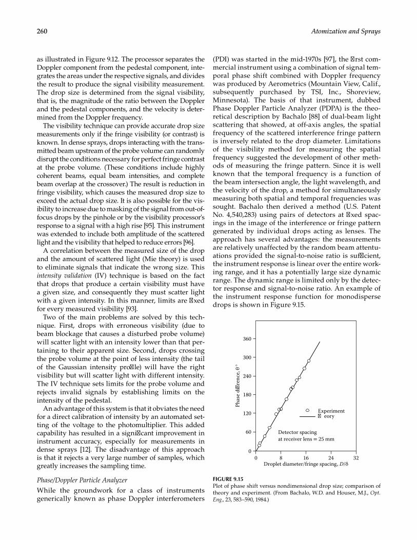
260 Atomization and Sprays

as illustrated in Figure 9.12. The processor separates the Doppler component from the pedestal component, inte-grates the areas under the respective signals, and divides the result to produce the signal visibility measurement. The drop size is determined from the signal visibility, that is, the magnitude of the ratio between the Doppler and the pedestal components, and the velocity is deter-mined from the Doppler frequency.

The visibility technique can provide accurate drop size measurements only if the fringe visibility (or contrast) is known. In dense sprays, drops interacting with the trans-mitted beam upstream of the probe volume can randomly disrupt the conditions necessary for perfect fringe contrast at the probe volume. (These conditions include highly coherent beams, equal beam intensities, and complete beam overlap at the crossover.) The result is reduction in fringe visibility, which causes the measured drop size to exceed the actual drop size. It is also possible for the vis-ibility to increase due to masking of the signal from out-of-focus drops by the pinhole or by the visibility processor's response to a signal with a high rise [95]. This instrument was extended to include both amplitude of the scattered light and the visibility that helped to reduce errors [96].

A correlation between the measured size of the drop and the amount of scattered light (Mie theory) is used to eliminate signals that indicate the wrong size. This intensity validation (IV) technique is based on the fact that drops that produce a certain visibility must have a given size, and consequently they must scatter light with a given intensity. In this manner, limits are fixed for every measured visibility [93].

Two of the main problems are solved by this tech-nique. First, drops with erroneous visibility (due to beam blockage that causes a disturbed probe volume) will scatter light with an intensity lower than that per-taining to their apparent size. Second, drops crossing the probe volume at the point of less intensity (the tail of the Gaussian intensity profile) will have the right visibility but will scatter light with different intensity. The IV technique sets limits for the probe volume and rejects invalid signals by establishing limits on the intensity of the pedestal.

An advantage of this system is that it obviates the need for a direct calibration of intensity by an automated set-ting of the voltage to the photomultiplier. This added capability has resulted in a significant improvement in instrument accuracy, especially for measurements in dense sprays [12]. The disadvantage of this approach is that it rejects a very large number of samples, which greatly increases the sampling time.

Phase/Doppler Particle Analyzer

While the groundwork for a class of instruments generically known as phase Doppler interferometers

(PDI) was started in the mid-1970s [97], the first com-mercial instrument using a combination of signal tem-poral phase shift combined with Doppler frequency was produced by Aerometrics (Mountain View, Calif., subsequently purchased by TSI, Inc., Shoreview, Minnesota). The basis of that instrument, dubbed Phase Doppler Particle Analyzer (PDPA) is the theo-retical description by Bachalo [88] of dual-beam light scattering that showed, at off-axis angles, the spatial frequency of the scattered interference fringe pattern is inversely related to the drop diameter. Limitations of the visibility method for measuring the spatial frequency suggested the development of other meth-ods of measuring the fringe pattern. Since it is well known that the temporal frequency is a function of the beam intersection angle, the light wavelength, and the velocity of the drop, a method for simultaneously measuring both spatial and temporal frequencies was sought. Bachalo then derived a method (U.S. Patent No. 4,540,283) using pairs of detectors at fixed spac-ings in the image of the interference or fringe pattern generated by individual drops acting as lenses. The approach has several advantages: the measurements are relatively unaffected by the random beam attentu-ations provided the signal-to-noise ratio is sufficient, the instrument response is linear over the entire work-ing range, and it has a potentially large size dynamic range. The dynamic range is limited only by the detec-tor response and signal-to-noise ratio. An example of the instrument response function for monodisperse drops is shown in Figure 9.15.

00

300

240

180

120

60

360

2416

Experiment

Detector spacingat receiver lens = 25 mm

8 32Droplet diameter/fringe spacing, D/δ

Phas

e di

ren

ce, θ

°

eory

FIGURE 9.15Plot of phase shift versus nondimensional drop size; comparison of theory and experiment. (From Bachalo, W.D. and Houser, M.J., Opt. Eng., 23, 583–590, 1984.)

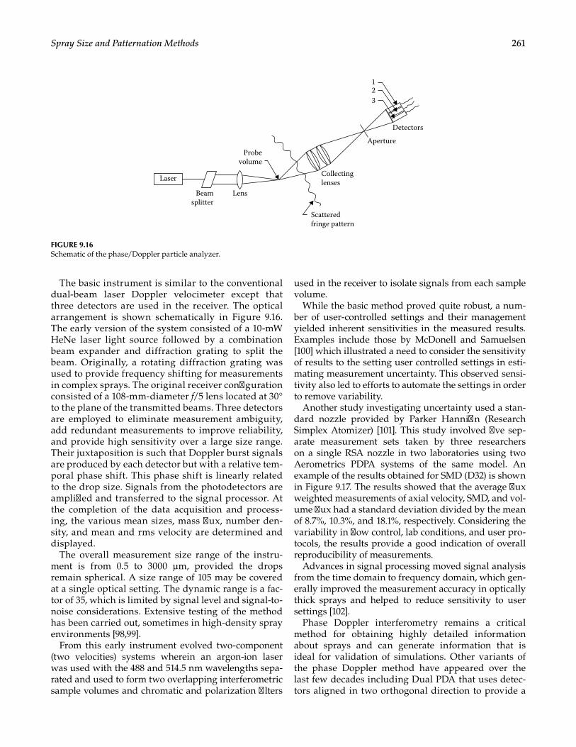
261Spray Size and Patternation Methods

The basic instrument is similar to the conventional dual-beam laser Doppler velocimeter except that three detectors are used in the receiver. The optical arrangement is shown schematically in Figure 9.16. The early version of the system consisted of a 10-mW HeNe laser light source followed by a combination beam expander and diffraction grating to split the beam. Originally, a rotating diffraction grating was used to provide frequency shifting for measurements in complex sprays. The original receiver configuration consisted of a 108-mm-diameter f/5 lens located at 30° to the plane of the transmitted beams. Three detectors are employed to eliminate measurement ambiguity, add redundant measurements to improve reliability, and provide high sensitivity over a large size range. Their juxtaposition is such that Doppler burst signals are produced by each detector but with a relative tem-poral phase shift. This phase shift is linearly related to the drop size. Signals from the photodetectors are amplified and transferred to the signal processor. At the completion of the data acquisition and process-ing, the various mean sizes, mass flux, number den-sity, and mean and rms velocity are determined and displayed.

The overall measurement size range of the instru-ment is from 0.5 to 3000 µm, provided the drops remain spherical. A size range of 105 may be covered at a single optical setting. The dynamic range is a fac-tor of 35, which is limited by signal level and signal-to-noise considerations. Extensive testing of the method has been carried out, sometimes in high-density spray environments [98,99].

From this early instrument evolved two-component (two velocities) systems wherein an argon-ion laser was used with the 488 and 514.5 nm wavelengths sepa-rated and used to form two overlapping interferometric sample volumes and chromatic and polarization filters

used in the receiver to isolate signals from each sample volume.

While the basic method proved quite robust, a num-ber of user-controlled settings and their management yielded inherent sensitivities in the measured results. Examples include those by McDonell and Samuelsen [100] which illustrated a need to consider the sensitivity of results to the setting user controlled settings in esti-mating measurement uncertainty. This observed sensi-tivity also led to efforts to automate the settings in order to remove variability.

Another study investigating uncertainty used a stan-dard nozzle provided by Parker Hannifin (Research Simplex Atomizer) [101]. This study involved five sep-arate measurement sets taken by three researchers on a single RSA nozzle in two laboratories using two Aerometrics PDPA systems of the same model. An example of the results obtained for SMD (D32) is shown in Figure 9.17. The results showed that the average flux weighted measurements of axial velocity, SMD, and vol-ume flux had a standard deviation divided by the mean of 8.7%, 10.3%, and 18.1%, respectively. Considering the variability in flow control, lab conditions, and user pro-tocols, the results provide a good indication of overall reproducibility of measurements.

Advances in signal processing moved signal analysis from the time domain to frequency domain, which gen-erally improved the measurement accuracy in optically thick sprays and helped to reduce sensitivity to user settings [102].

Phase Doppler interferometry remains a critical method for obtaining highly detailed information about sprays and can generate information that is ideal for validation of simulations. Other variants of the phase Doppler method have appeared over the last few decades including Dual PDA that uses detec-tors aligned in two orthogonal direction to provide a

Laser

LensBeamsplitter

Probevolume

123

Collectinglenses

Scatteredfringe pattern

Aperture

Detectors

FIGURE 9.16Schematic of the phase/Doppler particle analyzer.

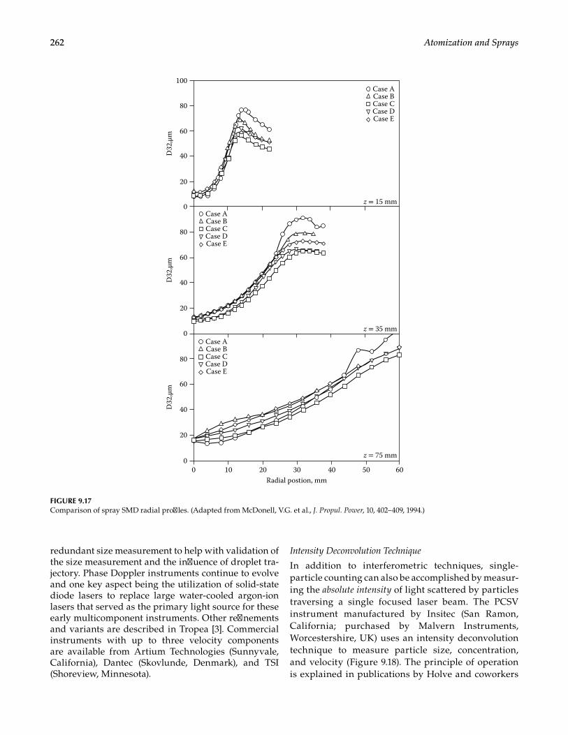
262 Atomization and Sprays

redundant size measurement to help with validation of the size measurement and the influence of droplet tra-jectory. Phase Doppler instruments continue to evolve and one key aspect being the utilization of solid-state diode lasers to replace large water-cooled argon-ion lasers that served as the primary light source for these early multicomponent instruments. Other refinements and variants are described in Tropea [3]. Commercial instruments with up to three velocity components are available from Artium Technologies (Sunnyvale, California), Dantec (Skovlunde, Denmark), and TSI (Shoreview, Minnesota).

Intensity Deconvolution Technique

In addition to interferometric techniques, single- particle counting can also be accomplished by measur-ing the absolute intensity of light scattered by particles traversing a single focused laser beam. The PCSV instrument manufactured by Insitec (San Ramon, California; purchased by Malvern Instruments, Worcestershire, UK) uses an intensity deconvolution technique to measure particle size, concentration, and velocity (Figure 9.18). The principle of operation is explained in publications by Holve and coworkers

00 10 20

Radial postion, mm30 40

z = 75 mm

z = 35 mm

z = 15 mm

50 60

20

40

60

80

0

20

40

60

80

0

20

40

60

80

100

D32

,μm

Case ECase DCase CCase BCase A

Case ECase DCase CCase BCase A

Case ECase DCase CCase BCase A

D32

,μm

D32

,μm

FIGURE 9.17Comparison of spray SMD radial profiles. (Adapted from McDonell, V.G. et al., J. Propul. Power, 10, 402–409, 1994.)

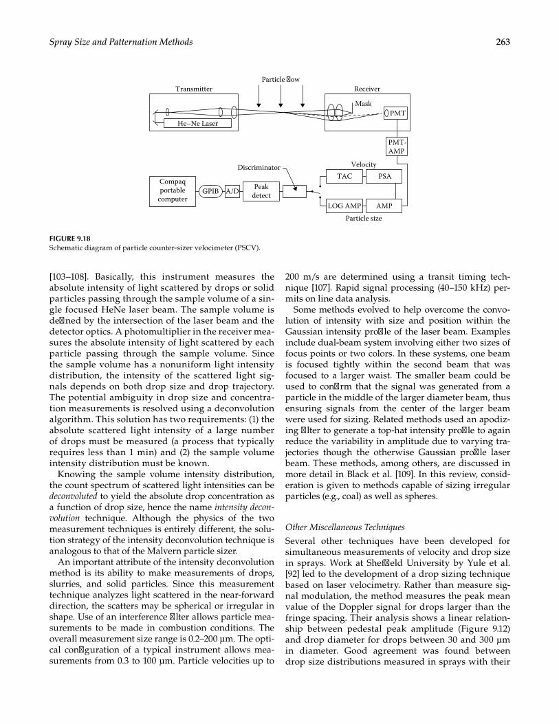
263Spray Size and Patternation Methods

[103–108]. Basically, this instrument measures the absolute intensity of light scattered by drops or solid particles passing through the sample volume of a sin-gle focused HeNe laser beam. The sample volume is defined by the intersection of the laser beam and the detector optics. A photomultiplier in the receiver mea-sures the absolute intensity of light scattered by each particle passing through the sample volume. Since the sample volume has a nonuniform light intensity distribution, the intensity of the scattered light sig-nals depends on both drop size and drop trajectory. The potential ambiguity in drop size and concentra-tion measurements is resolved using a deconvolution algorithm. This solution has two requirements: (1) the absolute scattered light intensity of a large number of drops must be measured (a process that typically requires less than 1 min) and (2) the sample volume intensity distribution must be known.

Knowing the sample volume intensity distribution, the count spectrum of scattered light intensities can be deconvoluted to yield the absolute drop concentration as a function of drop size, hence the name intensity decon-volution technique. Although the physics of the two measurement techniques is entirely different, the solu-tion strategy of the intensity deconvolution technique is analogous to that of the Malvern particle sizer.

An important attribute of the intensity deconvolution method is its ability to make measurements of drops, slurries, and solid particles. Since this measurement technique analyzes light scattered in the near-forward direction, the scatters may be spherical or irregular in shape. Use of an interference filter allows particle mea-surements to be made in combustion conditions. The overall measurement size range is 0.2–200 µm. The opti-cal configuration of a typical instrument allows mea-surements from 0.3 to 100 µm. Particle velocities up to

200 m/s are determined using a transit timing tech-nique [107]. Rapid signal processing (40–150 kHz) per-mits on line data analysis.

Some methods evolved to help overcome the convo-lution of intensity with size and position within the Gaussian intensity profile of the laser beam. Examples include dual-beam system involving either two sizes of focus points or two colors. In these systems, one beam is focused tightly within the second beam that was focused to a larger waist. The smaller beam could be used to confirm that the signal was generated from a particle in the middle of the larger diameter beam, thus ensuring signals from the center of the larger beam were used for sizing. Related methods used an apodiz-ing filter to generate a top-hat intensity profile to again reduce the variability in amplitude due to varying tra-jectories though the otherwise Gaussian profile laser beam. These methods, among others, are discussed in more detail in Black et al. [109]. In this review, consid-eration is given to methods capable of sizing irregular particles (e.g., coal) as well as spheres.

Other Miscellaneous Techniques

Several other techniques have been developed for simultaneous measurements of velocity and drop size in sprays. Work at Sheffield University by Yule et al. [92] led to the development of a drop sizing technique based on laser velocimetry. Rather than measure sig-nal modulation, the method measures the peak mean value of the Doppler signal for drops larger than the fringe spacing. Their analysis shows a linear relation-ship between pedestal peak amplitude (Figure 9.12) and drop diameter for drops between 30 and 300 µm in diameter. Good agreement was found between drop size distributions measured in sprays with their

DiscriminatorTAC

LOG AMP

Particle size

AMP

PMT-AMP

PMTMask

ReceiverParticle ow

Transmitter

He–Ne Laser

PSAVelocity

A/D Peakdetect

Compaqportable

computerGPIB

FIGURE 9.18Schematic diagram of particle counter-sizer velocimeter (PSCV).

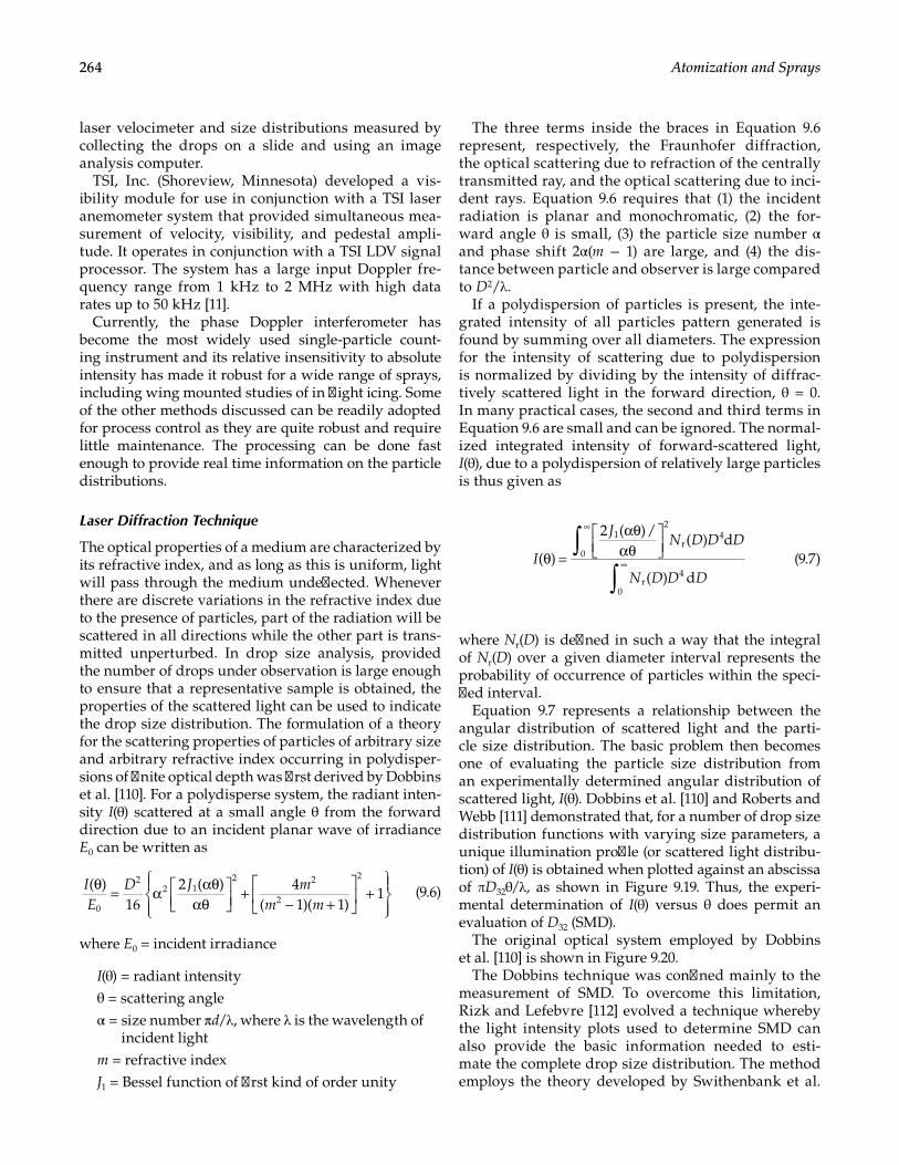
264 Atomization and Sprays

laser velocimeter and size distributions measured by collecting the drops on a slide and using an image analysis computer.

TSI, Inc. (Shoreview, Minnesota) developed a vis-ibility module for use in conjunction with a TSI laser anemometer system that provided simultaneous mea-surement of velocity, visibility, and pedestal ampli-tude. It operates in conjunction with a TSI LDV signal processor. The system has a large input Doppler fre-quency range from 1 kHz to 2 MHz with high data rates up to 50 kHz [11].

Currently, the phase Doppler interferometer has become the most widely used single-particle count-ing instrument and its relative insensitivity to absolute intensity has made it robust for a wide range of sprays, including wing mounted studies of in flight icing. Some of the other methods discussed can be readily adopted for process control as they are quite robust and require little maintenance. The processing can be done fast enough to provide real time information on the particle distributions.

Laser Diffraction Technique

The optical properties of a medium are characterized by its refractive index, and as long as this is uniform, light will pass through the medium undeflected. Whenever there are discrete variations in the refractive index due to the presence of particles, part of the radiation will be scattered in all directions while the other part is trans-mitted unperturbed. In drop size analysis, provided the number of drops under observation is large enough to ensure that a representative sample is obtained, the properties of the scattered light can be used to indicate the drop size distribution. The formulation of a theory for the scattering properties of particles of arbitrary size and arbitrary refractive index occurring in polydisper-sions of finite optical depth was first derived by Dobbins et al. [110]. For a polydisperse system, the radiant inten-sity I(θ) scattered at a small angle θ from the forward direction due to an incident planar wave of irradiance E0 can be written as

( )16

2 ( ) 4( 1)( 1)

10

22 1

2 2

2

2IE

D J mm m

θ = α αθαθ

+− +

+

(9.6)

where E0 = incident irradiance

I(θ) = radiant intensityθ = scattering angleα = size number πd/λ, where λ is the wavelength of

incident lightm = refractive indexJ1 = Bessel function of first kind of order unity

The three terms inside the braces in Equation 9.6 represent, respectively, the Fraunhofer diffraction, the optical scattering due to refraction of the centrally transmitted ray, and the optical scattering due to inci-dent rays. Equation 9.6 requires that (1) the incident radiation is planar and monochromatic, (2) the for-ward angle θ is small, (3) the particle size number α and phase shift 2α(m −  1) are large, and (4) the dis-tance between particle and observer is large compared to D2/λ.

If a polydispersion of particles is present, the inte-grated intensity of all particles pattern generated is found by summing over all diameters. The expression for the intensity of scattering due to polydispersion is normalized by dividing by the intensity of diffrac-tively scattered light in the forward direction, θ = 0. In many practical cases, the second and third terms in Equation 9.6 are small and can be ignored. The normal-ized integrated intensity of forward-scattered light, I(θ), due to a polydispersion of relatively large particles is thus given as

( )

2 ( )/( ) d

( ) d

1

0

2

r4

r4

0

I

JN D D D

N D D D

∫∫

θ =

αθαθ

∞

∞

(9.7)

where Nr(D) is defined in such a way that the integral of Nr(D) over a given diameter interval represents the probability of occurrence of particles within the speci-fied interval.

Equation 9.7 represents a relationship between the angular distribution of scattered light and the parti-cle size distribution. The basic problem then becomes one of evaluating the particle size distribution from an experimentally determined angular distribution of scattered light, I(θ). Dobbins et al. [110] and Roberts and Webb [111] demonstrated that, for a number of drop size distribution functions with varying size parameters, a unique illumination profile (or scattered light distribu-tion) of I(θ) is obtained when plotted against an abscissa of πD32θ/λ, as shown in Figure 9.19. Thus, the experi-mental determination of I(θ) versus θ does permit an evaluation of D32 (SMD).

The original optical system employed by Dobbins et al. [110] is shown in Figure 9.20.

The Dobbins technique was confined mainly to the measurement of SMD. To overcome this limitation, Rizk and Lefebvre [112] evolved a technique whereby the light intensity plots used to determine SMD can also provide the basic information needed to esti-mate the complete drop size distribution. The method employs the theory developed by Swithenbank et al.

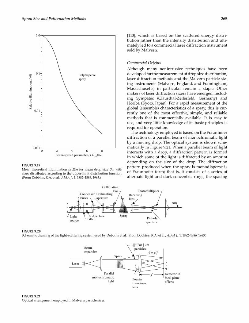
265Spray Size and Patternation Methods

[113], which is based on the scattered energy distri-bution rather than the intensity distribution and ulti-mately led to a commercial laser diffraction instrument sold by Malvern.

Commercial Origins

Although many nonintrusive techniques have been developed for the measurement of drop size distribution, laser diffraction methods and the Malvern particle siz-ing instruments (Malvern, England, and Framingham, Massachusetts) in particular remain a staple. Other makers of laser diffraction sizers have emerged, includ-ing Sympatec (Clausthal-Zellerfeld, Germany) and Horiba (Kyoto, Japan). For a rapid measurement of the global (ensemble) characteristics of a spray, this is cur-rently one of the most effective, simple, and reliable methods that is commercially available. It is easy to use, and very little knowledge of its basic principles is required for operation.

The technology employed is based on the Fraunhofer diffraction of a parallel beam of monochromatic light by a moving drop. The optical system is shown sche-matically in Figure 9.21. When a parallel beam of light interacts with a drop, a diffraction pattern is formed in which some of the light is diffracted by an amount depending on the size of the drop. The diffraction pattern produced when the spray is monodisperse is of Fraunhofer form; that is, it consists of a series of alternate light and dark concentric rings, the spacing

0 64

Polydispersespray

Beam-spread parameter, π D32 θ/λ

Rela

tive

illum

inat

ion,

I (θ

)

2 80.001

0.01

0.1

1.0

FIGURE 9.19Mean theoretical illumination profile for mean drop size D32 with sizes distributed according to the upper-limit distribution function. (From Dobbins, R.A. et al., AIAA J., 1, 1882–1886, 1963.)

Collimatinglens

Collimatingaperture

Condenserlenses

Lightsource

Receivinglens

Photomultiplier

Pinholeaperture

Aperture SprayFilter

I (θ)

FIGURE 9.20Schematic drawing of the light-scattering system used by Dobbins et al. (From Dobbins, R.A. et al., AIAA J., 1, 1882–1886, 1963.)

f

r

Beamexpander

Fouriertransformlens

Detector infocal planeof lens

Parallelmonochromatic

light

Spray

~||° For | μmparticles

Laser

θ

θ = r/f

FIGURE 9.21Optical arrangement employed in Malvern particle sizer.

266 Atomization and Sprays

of which depends on the drop diameter. However, for the more commonly encountered polydisperse sprays, a number of these Fraunhofer patterns are produced, each by a different group of drop sizes. These results in a series of overlapping diffraction rings, each of which is associated with a characteristic drop size range, depending on the focal length of the Fourier transform receiver lens. This lens focuses the diffrac-tion pattern onto a multielement photodetector that measures the light energy distribution. The photode-tector comprises 31 semicircular photosensitive rings surrounding a central circle. Each ring is therefore most sensitive to a particular small range of drop sizes. The output of the photodetector is multiplexed through an analog-to-digital converter. Interpretation of the measured light energy distribution as a drop size distribution is then carried out by a computer that provides an instant display of the measured dis-tribution. Another important attribute is that the dif-fraction pattern generated by drops is independent of the position of the drop in the light beam. This allows measurements of size distribution to be made with the drops moving at any speed.

Experience has shown that good alignment of the Malvern optical system is essential for accurate mea-surement. The correct focal length of lenses should be chosen according to the drop size range to be measured. It is also important to align the laser beam so that it is perpendicular to the spray axis at a suitable distance downstream from the atomizer.

The data may be presented in terms of a histogram or in the format of normal, lognormal, Rosin–Rammler, or model-independent modes. The raw histogram data can be post processed using any desired distribution function.

Accuracy

The Fraunhofer diffraction theory on which the instru-ment relies applies only to drops whose diameter is much larger than the wavelength of the incident light. This means that inaccuracies may be incurred when measuring drop sizes below the minimum size avail-able for a given receiver lens. It is also important to remember that the instrument is capable of measuring drop sizes only in a certain range. By a proper choice of lens, most practical sprays can be analyzed without dif-ficulty. However, the indicated histogram of drop sizes should always exhibit a definite peak. Where no peak is evident, it may mean that a significant number of drops lie outside the range of measurement capability, so the instrument cannot interpret properly the observed scat-tering pattern.

One issue that arose with early commercial systems was variability in detector sensitivity. This was noticed

through round robin testing of a standard atomizer that showed some notable outliers in measured values for some of the laboratories illustrating the value of such studies.

Dodge identified the cause of the discrepancy to an inherent limitation on the accuracy of the photo-diode detectors [114]. These detectors were assumed to have a uniform responsivity to the incident light energy but, in fact, the responsivity of different detec-tors in the same set can vary appreciably, and these variations are not repeatable between different detec-tor assemblies.

To overcome this problem, Dodge [114] devised a method that involves the separate calibration of each detector ring. Each detector is exposed to several differ-ent light levels to determine its response factor F = C/R, where C is a normalization constant that is different for each light level and R is the responsivity. The value of F determined from this procedure is then entered into the Malvern computer program to replace the existing response factor. Such calibration procedures are now taken care of in the instrument quality control checks at the factory.

Other issues associated with laser diffraction meth-ods include multiple scattering, vignetting, and beam steering.

Multiple Scattering. When spray densities are high, light that is scattered by a drop may be scattered by a second drop before reaching the detector. Since the theory for laser diffraction-based instruments assumes scattering from a single drop, this multiple scattering introduces errors in the computed size distribution.

When measuring drop sizes in a spray, most (if not all) diffraction instruments record the extinction or per-centage of the light removed from the original direction. As Dodge [115] has emphasized, extinction (sometimes called obscuration) is directly dependent on the cross-section of the drops present in the beam and is a major indicator of the extent to which the measurements are being affected by multiple scattering. The density of the spray is not a good parameter because extinction can vary over a wide range for a given density, depending on the size distribution and optical path length in the spray. The major consequence of multiple scattering is distortion of the diffraction pattern toward larger angles and a wider angle range. When the distorted data are processed, they cause the indicated drop sizes to be broader in distribution and smaller in average size than the actual distribution. The problem becomes significant when more than 50% of the incident light is scattered by the drops. However, measurements can still be performed in dense sprays where the extinction is as high as 95%, provided a correction is applied to the results.

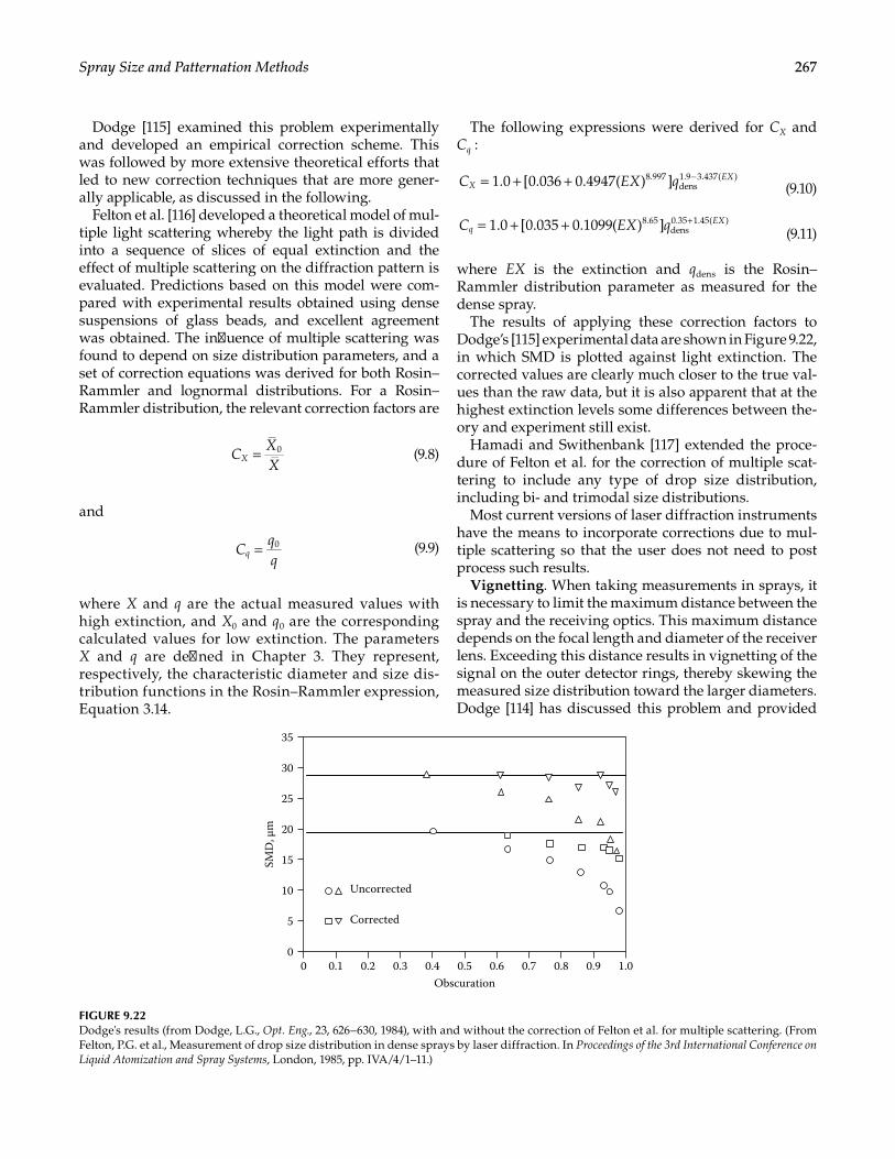
267Spray Size and Patternation Methods

Dodge [115] examined this problem experimentally and developed an empirical correction scheme. This was followed by more extensive theoretical efforts that led to new correction techniques that are more gener-ally applicable, as discussed in the following.

Felton et al. [116] developed a theoretical model of mul-tiple light scattering whereby the light path is divided into a sequence of slices of equal extinction and the effect of multiple scattering on the diffraction pattern is evaluated. Predictions based on this model were com-pared with experimental results obtained using dense suspensions of glass beads, and excellent agreement was obtained. The influence of multiple scattering was found to depend on size distribution parameters, and a set of correction equations was derived for both Rosin–Rammler and lognormal distributions. For a Rosin–Rammler distribution, the relevant correction factors are

0CXX

X =

(9.8)

and

0Cqq

q =

(9.9)

where X and q are the actual measured values with high extinction, and X0 and q0 are the corresponding calculated values for low extinction. The parameters X and q are defined in Chapter 3. They represent, respectively, the characteristic diameter and size dis-tribution functions in the Rosin–Rammler expression, Equation 3.14.

The following expressions were derived for CX and Cq :

1.0 [0.036 0.4947( ) ]8.997dens1.9 3.437( )C EX qX

EX= + + − (9.10)

1.0 [0.035 0.1099( ) ]8.65dens0.35 1.45( )C EX qq

EX= + + +

(9.11)

where EX is the extinction and qdens is the Rosin–Rammler distribution parameter as measured for the dense spray.

The results of applying these correction factors to Dodge’s [115] experimental data are shown in Figure 9.22, in which SMD is plotted against light extinction. The corrected values are clearly much closer to the true val-ues than the raw data, but it is also apparent that at the highest extinction levels some differences between the-ory and experiment still exist.

Hamadi and Swithenbank [117] extended the proce-dure of Felton et al. for the correction of multiple scat-tering to include any type of drop size distribution, including bi- and trimodal size distributions.

Most current versions of laser diffraction instruments have the means to incorporate corrections due to mul-tiple scattering so that the user does not need to post process such results.

Vignetting. When taking measurements in sprays, it is necessary to limit the maximum distance between the spray and the receiving optics. This maximum distance depends on the focal length and diameter of the receiver lens. Exceeding this distance results in vignetting of the signal on the outer detector rings, thereby skewing the measured size distribution toward the larger diameters. Dodge [114] has discussed this problem and provided

00

30

25

20

15

10

5

35

0.90.80.70.60.5Obscuration

Uncorrected

Corrected

0.40.30.20.1 1.0

SMD

, μm

FIGURE 9.22Dodge's results (from Dodge, L.G., Opt. Eng., 23, 626–630, 1984), with and without the correction of Felton et al. for multiple scattering. (From Felton, P.G. et al., Measurement of drop size distribution in dense sprays by laser diffraction. In Proceedings of the 3rd International Conference on Liquid Atomization and Spray Systems, London, 1985, pp. IVA/4/1–11.)

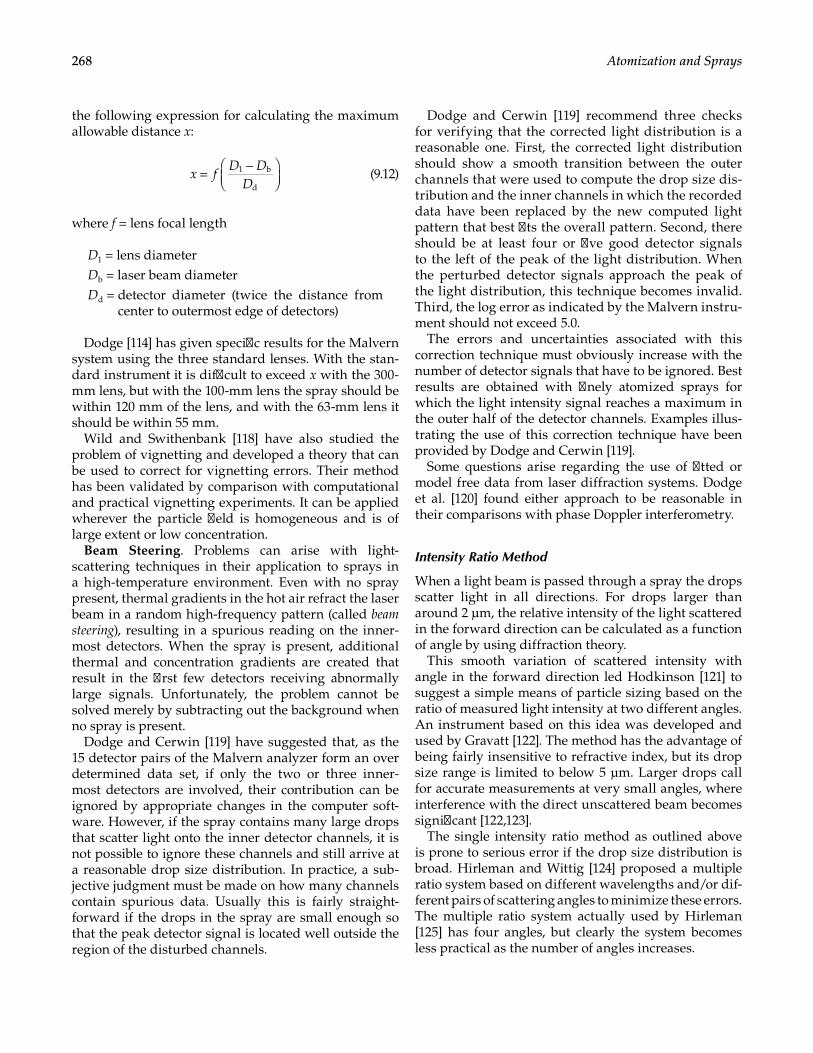
268 Atomization and Sprays

the following expression for calculating the maximum allowable distance x:

1 b

dx f

D DD

= −

(9.12)

where f = lens focal length

D1 = lens diameterDb = laser beam diameterDd = detector diameter (twice the distance from

center to outermost edge of detectors)

Dodge [114] has given specific results for the Malvern system using the three standard lenses. With the stan-dard instrument it is difficult to exceed x with the 300-mm lens, but with the 100-mm lens the spray should be within 120 mm of the lens, and with the 63-mm lens it should be within 55 mm.

Wild and Swithenbank [118] have also studied the problem of vignetting and developed a theory that can be used to correct for vignetting errors. Their method has been validated by comparison with computational and practical vignetting experiments. It can be applied wherever the particle field is homogeneous and is of large extent or low concentration.

Beam Steering. Problems can arise with light- scattering techniques in their application to sprays in a high-temperature environment. Even with no spray present, thermal gradients in the hot air refract the laser beam in a random high-frequency pattern (called beam steering), resulting in a spurious reading on the inner-most detectors. When the spray is present, additional thermal and concentration gradients are created that result in the first few detectors receiving abnormally large signals. Unfortunately, the problem cannot be solved merely by subtracting out the background when no spray is present.

Dodge and Cerwin [119] have suggested that, as the 15 detector pairs of the Malvern analyzer form an over determined data set, if only the two or three inner-most detectors are involved, their contribution can be ignored by appropriate changes in the computer soft-ware. However, if the spray contains many large drops that scatter light onto the inner detector channels, it is not possible to ignore these channels and still arrive at a reasonable drop size distribution. In practice, a sub-jective judgment must be made on how many channels contain spurious data. Usually this is fairly straight-forward if the drops in the spray are small enough so that the peak detector signal is located well outside the region of the disturbed channels.

Dodge and Cerwin [119] recommend three checks for verifying that the corrected light distribution is a reasonable one. First, the corrected light distribution should show a smooth transition between the outer channels that were used to compute the drop size dis-tribution and the inner channels in which the recorded data have been replaced by the new computed light pattern that best fits the overall pattern. Second, there should be at least four or five good detector signals to the left of the peak of the light distribution. When the perturbed detector signals approach the peak of the light distribution, this technique becomes invalid. Third, the log error as indicated by the Malvern instru-ment should not exceed 5.0.

The errors and uncertainties associated with this correction technique must obviously increase with the number of detector signals that have to be ignored. Best results are obtained with finely atomized sprays for which the light intensity signal reaches a maximum in the outer half of the detector channels. Examples illus-trating the use of this correction technique have been provided by Dodge and Cerwin [119].

Some questions arise regarding the use of fitted or model free data from laser diffraction systems. Dodge et al. [120] found either approach to be reasonable in their comparisons with phase Doppler interferometry.

Intensity Ratio Method

When a light beam is passed through a spray the drops scatter light in all directions. For drops larger than around 2 µm, the relative intensity of the light scattered in the forward direction can be calculated as a function of angle by using diffraction theory.

This smooth variation of scattered intensity with angle in the forward direction led Hodkinson [121] to suggest a simple means of particle sizing based on the ratio of measured light intensity at two different angles. An instrument based on this idea was developed and used by Gravatt [122]. The method has the advantage of being fairly insensitive to refractive index, but its drop size range is limited to below 5 μm. Larger drops call for accurate measurements at very small angles, where interference with the direct unscattered beam becomes significant [122,123].

The single intensity ratio method as outlined above is prone to serious error if the drop size distribution is broad. Hirleman and Wittig [124] proposed a multiple ratio system based on different wavelengths and/or dif-ferent pairs of scattering angles to minimize these errors. The multiple ratio system actually used by Hirleman [125] has four angles, but clearly the system becomes less practical as the number of angles increases.

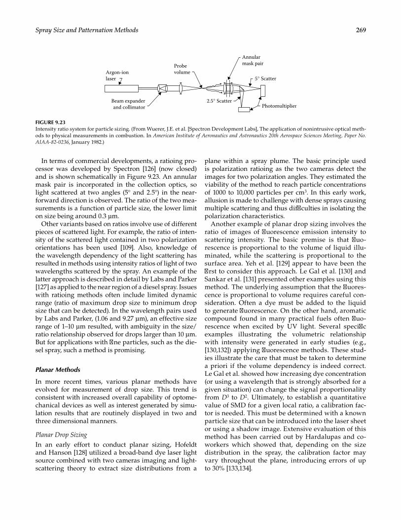
269Spray Size and Patternation Methods

In terms of commercial developments, a ratioing pro-cessor was developed by Spectron [126] (now closed) and is shown schematically in Figure 9.23. An annular mask pair is incorporated in the collection optics, so light scattered at two angles (5° and 2.5°) in the near-forward direction is observed. The ratio of the two mea-surements is a function of particle size, the lower limit on size being around 0.3 µm.

Other variants based on ratios involve use of different pieces of scattered light. For example, the ratio of inten-sity of the scattered light contained in two polarization orientations has been used [109]. Also, knowledge of the wavelength dependency of the light scattering has resulted in methods using intensity ratios of light of two wavelengths scattered by the spray. An example of the latter approach is described in detail by Labs and Parker [127] as applied to the near region of a diesel spray. Issues with ratioing methods often include limited dynamic range (ratio of maximum drop size to minimum drop size that can be detected). In the wavelength pairs used by Labs and Parker, (1.06 and 9.27 μm), an effective size range of 1–10 μm resulted, with ambiguity in the size/ratio relationship observed for drops larger than 10 μm. But for applications with fine particles, such as the die-sel spray, such a method is promising.

Planar Methods

In more recent times, various planar methods have evolved for measurement of drop size. This trend is consistent with increased overall capability of optome-chanical devices as well as interest generated by simu-lation results that are routinely displayed in two and three dimensional manners.

Planar Drop Sizing

In an early effort to conduct planar sizing, Hofeldt and Hanson [128] utilized a broad-band dye laser light source combined with two cameras imaging and light-scattering theory to extract size distributions from a

plane within a spray plume. The basic principle used is polarization ratioing as the two cameras detect the images for two polarization angles. They estimated the viability of the method to reach particle concentrations of 1000 to 10,000 particles per cm3. In this early work, allusion is made to challenge with dense sprays causing multiple scattering and thus difficulties in isolating the polarization characteristics.

Another example of planar drop sizing involves the ratio of images of fluorescence emission intensity to scattering intensity. The basic premise is that fluo-rescence is proportional to the volume of liquid illu-minated, while the scattering is proportional to the surface area. Yeh et al. [129] appear to have been the first to consider this approach. Le Gal et al. [130] and Sankar et al. [131] presented other examples using this method. The underlying assumption that the fluores-cence is proportional to volume requires careful con-sideration. Often a dye must be added to the liquid to generate fluorescence. On the other hand, aromatic compound found in many practical fuels often fluo-rescence when excited by UV light. Several specific examples illustrating the volumetric relationship with intensity were generated in early studies (e.g., [130,132]) applying fluorescence methods. These stud-ies illustrate the care that must be taken to determine a priori if the volume dependency is indeed correct. Le Gal et al. showed how increasing dye concentration (or using a wavelength that is strongly absorbed for a given situation) can change the signal proportionality from D3 to D2. Ultimately, to establish a quantitative value of SMD for a given local ratio, a calibration fac-tor is needed. This must be determined with a known particle size that can be introduced into the laser sheet or using a shadow image. Extensive evaluation of this method has been carried out by Hardalupas and co-workers which showed that, depending on the size distribution in the spray, the calibration factor may vary throughout the plane, introducing errors of up to 30% [133,134].

ProbevolumeArgon-ion

laser

Beam expanderand collimator

Annularmask pair

Photomultiplier

5° Scatter

2.5° Scatter

FIGURE 9.23Intensity ratio system for particle sizing. (From Wuerer, J.E. et al. [Spectron Development Labs], The application of nonintrusive optical meth-ods to physical measurements in combustion. In American Institute of Aeronautics and Astronautics 20th Aerospace Sciences Meeting, Paper No. AIAA-82-0236, January 1982.)

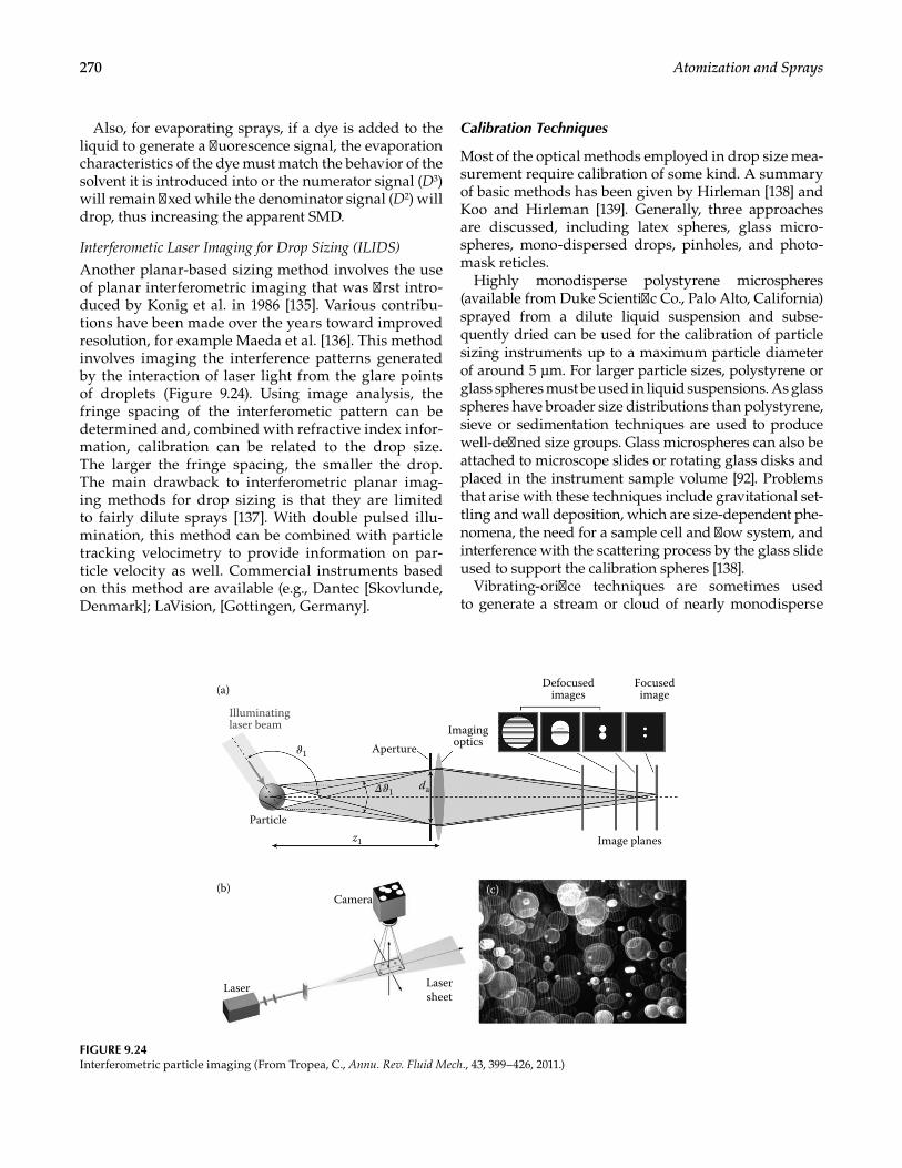
270 Atomization and Sprays

Also, for evaporating sprays, if a dye is added to the liquid to generate a fluorescence signal, the evaporation characteristics of the dye must match the behavior of the solvent it is introduced into or the numerator signal (D3) will remain fixed while the denominator signal (D2) will drop, thus increasing the apparent SMD.

Interferometic Laser Imaging for Drop Sizing (ILIDS)

Another planar-based sizing method involves the use of planar interferometric imaging that was first intro-duced by Konig et al. in 1986 [135]. Various contribu-tions have been made over the years toward improved resolution, for example Maeda et al. [136]. This method involves imaging the interference patterns generated by the interaction of laser light from the glare points of droplets (Figure 9.24). Using image analysis, the fringe spacing of the interferometic pattern can be determined and, combined with refractive index infor-mation, calibration can be related to the drop size. The larger the fringe spacing, the smaller the drop. The main drawback to interferometric planar imag-ing methods for drop sizing is that they are limited to fairly dilute sprays [137]. With double pulsed illu-mination, this method can be combined with particle tracking velocimetry to provide information on par-ticle velocity as well. Commercial instruments based on this method are available (e.g., Dantec [Skovlunde, Denmark]; LaVision, [Gottingen, Germany].

Calibration Techniques

Most of the optical methods employed in drop size mea-surement require calibration of some kind. A summary of basic methods has been given by Hirleman [138] and Koo and Hirleman [139]. Generally, three approaches are discussed, including latex spheres, glass micro-spheres, mono-dispersed drops, pinholes, and photo-mask reticles.

Highly monodisperse polystyrene microspheres (available from Duke Scientific Co., Palo Alto, California) sprayed from a dilute liquid suspension and subse-quently dried can be used for the calibration of particle sizing instruments up to a maximum particle diameter of around 5 µm. For larger particle sizes, polystyrene or glass spheres must be used in liquid suspensions. As glass spheres have broader size distributions than polystyrene, sieve or sedimentation techniques are used to produce well-defined size groups. Glass microspheres can also be attached to microscope slides or rotating glass disks and placed in the instrument sample volume [92]. Problems that arise with these techniques include gravitational set-tling and wall deposition, which are size-dependent phe-nomena, the need for a sample cell and flow system, and interference with the scattering process by the glass slide used to support the calibration spheres [138].

Vibrating-orifice techniques are sometimes used to generate a stream or cloud of nearly monodisperse

Illuminatinglaser beam

ApertureImagingoptics

Defocusedimages

Focusedimage

Image planes

Particlez1

da

Camera

Laser Lasersheet

(c)

(a)

(b)

ϑ1

Δϑ1

FIGURE 9.24Interferometric particle imaging (From Tropea, C., Annu. Rev. Fluid Mech., 43, 399–426, 2011.)

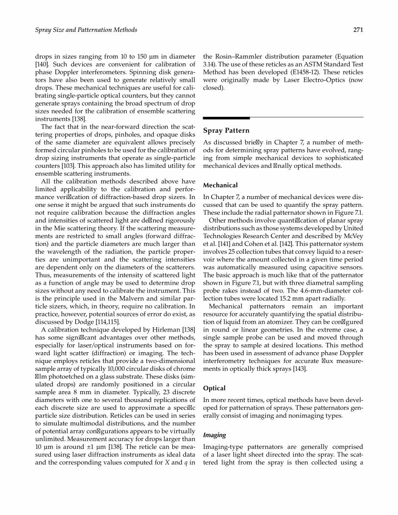
271Spray Size and Patternation Methods

drops in sizes ranging from 10 to 150 µm in diameter [140]. Such devices are convenient for calibration of phase Doppler interferometers. Spinning disk genera-tors have also been used to generate relatively small drops. These mechanical techniques are useful for cali-brating single-particle optical counters, but they cannot generate sprays containing the broad spectrum of drop sizes needed for the calibration of ensemble scattering instruments [138].

The fact that in the near-forward direction the scat-tering properties of drops, pinholes, and opaque disks of the same diameter are equivalent allows precisely formed circular pinholes to be used for the calibration of drop sizing instruments that operate as single- particle counters [103]. This approach also has limited utility for ensemble scattering instruments.

All the calibration methods described above have limited applicability to the calibration and perfor-mance verification of diffraction-based drop sizers. In one sense it might be argued that such instruments do not require calibration because the diffraction angles and intensities of scattered light are defined rigorously in the Mie scattering theory. If the scattering measure-ments are restricted to small angles (forward diffrac-tion) and the particle diameters are much larger than the wavelength of the radiation, the particle proper-ties are unimportant and the scattering intensities are dependent only on the diameters of the scatterers. Thus, measurements of the intensity of scattered light as a function of angle may be used to determine drop sizes without any need to calibrate the instrument. This is the principle used in the Malvern and similar par-ticle sizers, which, in theory, require no calibration. In practice, however, potential sources of error do exist, as discussed by Dodge [114,115].

A calibration technique developed by Hirleman [138] has some significant advantages over other methods, especially for laser/optical instruments based on for-ward light scatter (diffraction) or imaging. The tech-nique employs reticles that provide a two-dimensional sample array of typically 10,000 circular disks of chrome film photoetched on a glass substrate. These disks (sim-ulated drops) are randomly positioned in a circular sample area 8 mm in diameter. Typically, 23 discrete diameters with one to several thousand replications of each discrete size are used to approximate a specific particle size distribution. Reticles can be used in series to simulate multimodal distributions, and the number of potential array configurations appears to be virtually unlimited. Measurement accuracy for drops larger than 10 µm is around ±1 µm [138]. The reticle can be mea-sured using laser diffraction instruments as ideal data and the corresponding values computed for X and q in

the Rosin–Rammler distribution parameter (Equation 3.14). The use of these reticles as an ASTM Standard Test Method has been developed (E1458-12). These reticles were originally made by Laser Electro-Optics (now closed).

Spray Pattern

As discussed briefly in Chapter 7, a number of meth-ods for determining spray patterns have evolved, rang-ing from simple mechanical devices to sophisticated mechanical devices and finally optical methods.

Mechanical

In Chapter 7, a number of mechanical devices were dis-cussed that can be used to quantify the spray pattern. These include the radial patternator shown in Figure 7.1.

Other methods involve quantification of planar spray distributions such as those systems developed by United Technologies Research Center and described by McVey et al. [141] and Cohen et al. [142]. This patternator system involves 25 collection tubes that convey liquid to a reser-voir where the amount collected in a given time period was automatically measured using capacitive sensors. The basic approach is much like that of the patternator shown in Figure 7.1, but with three diametral sampling probe rakes instead of two. The 4.6-mm-diameter col-lection tubes were located 15.2 mm apart radially.

Mechanical patternators remain an important resource for accurately quantifying the spatial distribu-tion of liquid from an atomizer. They can be configured in round or linear geometries. In the extreme case, a single sample probe can be used and moved through the spray to sample at desired locations. This method has been used in assessment of advance phase Doppler interferometry techniques for accurate flux measure-ments in optically thick sprays [143].

Optical

In more recent times, optical methods have been devel-oped for patternation of sprays. These patternators gen-erally consist of imaging and nonimaging types.

Imaging

Imaging-type patternators are generally comprised of a laser light sheet directed into the spray. The scat-tered light from the spray is then collected using a

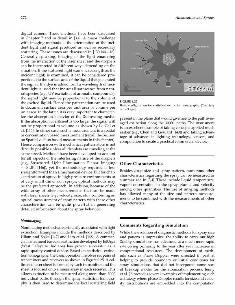
272 Atomization and Sprays

digital camera. These methods have been discussed in Chapter 7 and in detail in [3,4]. A major challenge with imaging methods is the attenutation of the inci-dent light and signal produced as well as secondary scattering. These issues are discussed in [130,144–146]. Generally speaking, imaging of the light emanating from the interaction of the laser sheet and the droplets can be interpreted in different ways depending on the situation. If the scattered light (same wavelength as the incident light) is examined, it can be considered pro-portional to the surface area of the liquid that generated the signal. If a dye is added, or if a wavelength of inci-dent light is used that induces fluorescence from natu-ral species (e.g., UV excitation of aromatic compounds), the signal light may be proportional to the volume of the excited liquid. Hence the patternation can be used to document surface area per unit area or volume per unit area. In the latter, it is very important to character-ize the absorption behavior of the fluorescing media. If the absorption coefficient is too large, the signal will not be proportional to volume as shown by Le Gal et al. [145]. In either case, such a measurement is a spatial or concentration based measurement (recall the Section on Spatial vs Flux based measurements in this chapter). Hence comparison with mechanical patternators is not directly possible unless all droplets are traveling at the same speed. Methods have been developed to account for all aspects of the interfering nature of the droplets (e.g., Structured Light Illumination Planar Imaging — SLIPI [146]), yet the methodology required is less straightforward than a mechanical device. But for char-acterization of sprays in high pressure environments or of very small dimension sprays, optical methods may be the preferred approach. In addition, because of the wide array of other measurements that can be made with laser sheets (e.g., velocity, size, etc.), combining an optical measurement of spray pattern with these other characteristics can be quite powerful in generating detailed information about the spray behavior.

Nonimaging

Nonimaging methods are primarily associated with light extinction. Examples include the methods described by Ullom and Sojka [147] and Lim et al. [148]. A commer-cial instrument based on extinction developed by EńUrga (West Lafayette, Indiana) has proven successful as a rapid quality control device. Based on statistical extinc-tion tomography, the basic operation involves six pairs of transmitters and receivers as shown in Figure 9.25. A col-limated laser sheet is formed by each transmitter and the sheet is focused onto a linear array in each receiver. This allows extinction to be measured along more than 3000 individual paths through the spray. Statistical tomogra-phy is then used to determine the local scattering field

present in the plane that would give rise to the path aver-aged extinction along the 3000+ paths. The instrument is an excellent example of taking concepts applied much earlier (e.g., Chen and Goulard [149]) and taking advan-tage of advances in lighting technology, sensors, and computation to create a practical commercial device.

Other Characteristics

Besides drop size and spray pattern, numerous other characteristics regarding the spray can be measured as summarized in [3,4]. These include liquid temperature, vapor concentration in the spray plume, and velocity among other quantities. The use of imaging methods has allowed many of the size and pattern measure-ments to be combined with the measurements of other characteristics.

Comments Regarding Simulation

While the evolution of diagnostic methods for spray size and pattern is impressive, the ability to carry out high fidelity simulations has advanced at a much more rapid rate owing primarily to the year after year increases in computational resources. The development of meth-ods such as Phase Doppler were directed in part at helping to provide boundary or initial conditions for spray simulations that did not incorporate some sort of breakup model for the atomization process. Jenny et al. [9] provides several examples of implementing such a strategy where phase Doppler results for size and veloc-ity distributions are embedded into the computation

Turbulent ow

Laser

Laser sheet

Array detector

FIGURE 9.25Basic configuration for statistical extinction tomography. (Courtesy of En’Urga.)

273Spray Size and Patternation Methods

domain. These measured particles (size and velocity) are then released into the gas phase at which point whatever coupling model used between gas and phase and liquid determines the direction the droplets travel. Examples in Jenny et al. [9] suggest that current simulations can capture the overall spray behavior with some success. In many cases, the target values for how accurately the simulations must match reality are not well defined. This leads to vague statements in some cases about reasonable agreement or good agreement between measurements and simulations. Without clear accuracy specifications, the relative agreement is difficult to comment on.

In terms of simulating the actual atomization process itself, great strides have been taken. Some simple analyti-cal breakup models are described Chapter 2, but now the capability exists to simulate the breakup process in great detail. For example, some of the methods described in Gorokhovski and Herrmann [150] can produce results that appear amazingly life-like. Figure 9.26 shows one example where the atomization of discrete fuel jets injected into a turbulent swirling crossflow is simulated using a coupled level set and volume of fluid approach [151].

Herrmann presents similar high fidelity results using a balanced force refined level set grid method for a turbulent jet injected into a crossflow [152]. The results are compared with high-speed video images and pro-vide qualitatively good agreement in terms of overall structure, breakup characteristics, and droplet behav-ior post breakup. These simulations started upstream of the injector passage using an auxiliary simulation to establish the turbulence and velocity profiles of the liquid exiting the orifice. Such result emphasizes the criticality in the boundary conditions. In most studies of jet in crossflow, little regard is given for the actual liq-uid velocity profiles of turbulence or even axial velocity, rather a bulk velocity is given which is not sufficient for such simulations.

Still others have reported highly detailed simulations of diesel sprays [153]. Interestingly, in the simulations of breakup, it has proven difficult to carry out validations. While detailed data via phase Doppler interferometry can verify the results of the breakup simulations, it does not fully validate the actual breakup details. While comparison with high-speed videos are common, more quantitative methods such as proper orthogonal decomposition or dynamic mode decomposition can be applied to both simulations and experimental results to better assess agreement.

It is evident that the most useful outcomes derived from coordinated simulation and experimental studies. This is apparent from the multiinstitutional studies such as those found in [5–9]. However, for those researchers solely con-ducting experiments, it is recommended that the experi-ment be fully documented so that the results can be useful for validation of simulations. Definition of boundary con-ditions is vital. As simulations move upstream into the injector, the detailed geometry within the injector must be provided. A suggested format for databased is given in Faeth and Samuelsen [154]. An extra 10% effort spent documenting these conditions is easily justified when considering that many detailed experiments can take a considerable time to be done carefully with quantified uncertainty. The information required is as follows:

• Facility• Configurations• Test conditions• Inlet and boundary conditions• Quantities measured• Diagnostics• Unusual methods• Experimental protocol• Quality control• Error analysis

(a)

(b) (c)

O,=65º O,=65º

x

FIGURE 9.26Comparison of computed and measured images for a complex swirl-ing air-bast injector configurations (Li, X. et al. J. Eng. Gas Turbines Power, 136, 2014)

274 Atomization and Sprays

• Availability of data• References• Data

Just keeping this list of required information in mind while planning and conducting the experiment can be helpful in ensuring its value as a suitable data set for model validation.

Concluding Remarks

It is clear that no single drop sizing method or spray pattern method is completely satisfactory. Many use-ful techniques have been developed, each with its own advantages and limitations.

Mechanical methods have the virtues of simplicity and low cost. Their main problem lies in the extraction and collection of representative spray samples.

Of the various electrical methods discussed, the hot-wire technique appears to be the most useful. However, the device can operate only at relatively low velocities (<10 m/s) due to the risk of drop breakup on impact with the wire. There is also some question about the measure-ment of liquids that could leave a residue on the wire.

Imaging systems allow the spray to be seen, but a major difficulty is the determination of the size of the viewing volume to be assigned to given drop sizes. For ensem-ble measurements the light diffraction methods are in widespread use as a general-purpose tool for spray analysis. Of the remaining optical methods discussed, phase Doppler interferometry has demonstrated signifi-cant impact on the level of detail of information that can be obtained, provided size and multiple components for velocity and mass flux in sprays produced by most prac-tical atomizers.

Planar methods are starting to make inroads owing to their highly time efficient application coupled with ease of adding complimentary measurements.

In the early days of drop sizing instruments Dodge [155] compared the performance of 17 drop size mea-suring instruments including six different types. Ten instruments were compared on one type of spray and 11 on another, with some instruments being used on both types. The results indicated systematic differences in instrument performance beyond what could be attrib-uted to problems in spray reproducibility. Differences in average drop size were as large as a factor of 5. However, good-to-excellent agreement was obtained between observations for some types of instrument. Such shoot-outs are warranted again with the development of many additional drop sizing methods and instruments.

In terms of patternation, statistical extinction tomog-raphy has demonstrated considerable promise. Optical imaging methods have evolved considerably with abil-ity to overcome incident and signal light attenuation, although the complexity of the application offsets the relative ease with which light scattered from a laser can be recorded and analyzed. Again, the question of how accurate the information needs to be considered.

In his 1995 Freeman Scholar lecture [154], Arthur Lefebvre stated:

“A drawback to advanced laser diagnostics and comprehensive modeling is that because they are both challenging and intellectually rewarding in their own right it is easy to forget that they are only means to an end. This author (A. Lefebvre) is not aware of any significant advance in atomizer or combustor technology that can be attributed to laser diagnostics or comprehensive modeling. All too often, these activities are pursued to the detri-ment of innovation and creativity, which are the two essential ingredients for progress in these areas.”

In the past 20 years this premise may still be true to some extent, yet the information being provided by laser diag-nostics and simulation is much greater in time and space resolution. Yet the atomizer designer must ultimately innovate to affect improvements in performance and should use the results to validate their creative thinking.

References

1. Bachalo, W. D., Spray diagnostics for the twenty-first century, Atomization Sprays, Vol. 10, 2000, pp. 439–474.

2. McDonell, V. G., and Samuelsen, G. S., Measurement of fuel mixing and transport processes in gas turbine com-bustion, Meas. Sci. Technol., Vol. 11, 2000, pp. 870–886.

3. Tropea, C., Optical particle characterization in flows, Annu. Rev. Fluid Mech., Vol. 43, 2011, pp. 399–426.

4. Fansler, T. D., and Parrish, S. E., Spray measurement technology: A review, Meas. Sci. Technol., Vol. 26, 2015, pp. 1–35.

5. Drake, M. C., and Haworth, D. C., Advanced gasoline engine development using optical diagnostics and numerical modeling, Proc. Combust. Inst., Vol. 31, 2007, pp. 99–124.

6. Merci, B., Roekaerts, D., and Sadiki, A., (eds.), Experiments and numerical simulations of turbulent combustion of diluted sprays, in: Proceedings of the 1st International Workshop on Turbulent Spray Combustion, Corsica, France, 2011.

7. Merci, B., and Gutheil, E., (eds.), Experiments and numerical simulations of turbulent combustion of diluted sprays, TCS 3, in: 3rd International Workshop on Turbulent Spray Combustion, Heidelberg, Germany, 2014.

275Spray Size and Patternation Methods

8. http://www.sandia.gov/ecn/ (accessed 4/30/2016) 9. Jenny, P., Roekaerts, D., and Beishuizen, N., Modeling of

turbulent dilute spray combustion, Prog. Energy Combust. Sci., Vol. 38, 2012, pp. 846–887.

10. Chigier, N. A., Instrumentation techniques for studying heterogeneous combustion, Prog. Energy Combust. Sci., Vol. 3, 1977, pp. 175–189.

11. Chigier, N. A., Drop size and velocity instrumentation, Prog. Energy Combust. Sci., Vol. 9, 1983, pp. 155–177.

12. Bachalo, W. D., Droplet analysis techniques: Their selec-tion and applications, in: Tishkoff, J. M., Ingebo, R. D., and Kennedy, J. B. (eds.), Liquid Particle Size Measurement Techniques, ASTM STP 848, West Conshohocken, US: American Society for Testing and Materials, 1984, pp. 5–21.

13. Ferrenberg, A. J., Liquid rocket injector atomization research, in: Tishkoff, J. M., Ingebo, R. D., and Kennedy, J. B. (eds.), Liquid Particle Size Measurement Techniques, ASTM STP 848, West Conshohocken, US: American Society for Testing and Materials, 1984, pp. 82–97.

14. Hirleman, E. D., Particle sizing by optical, nonimag-ing techniques, in: Tishkoff, J. M., Ingebo, R. D., and Kennedy, J. B. (eds.), Liquid Particle Size Measurement Techniques, ASTM STP 848, West Conshohocken, US: American Society for Testing and Materials, 1984, pp. 35–60.

15. Jones, A. R., A review of drop size measurement—The application of techniques to dense fuel sprays, Prog. Energy Combust. Sci., Vol. 3, 1977, pp. 225–234.

16. Wittig, S., Aigner, M., Sakbani, K. H., and Sattelmayer, T. H., Optical measurements of droplet size distribu-tions: Special considerations in the parameter definition for fuel atomizers, Paper Presented at AGARD meeting on Combustion Problems in Turbine Engines, Cesme, Turkey, October 1983.

17. Chin, J. S., Nickolaus, D., and Lefebvre, A. H., Influence of downstream distance on the spray characteristics of pressure-swirl atomizers, ASME J. Eng. Gas Turb. Power, Vol. 106, No. 1, 1986, p. 219.

18. Tate, R. W., Some problems associated with the accurate representation droplet size distributions, in: Proceedings of the 2nd International Conference on Liquid Atomization and Spray Systems, Madison, Wisconsin, June 1982, pp. 341–351.

19. Lewis, H. C., Edwards, D. G., Goglia, M. J., Rice, R. I., and Smith, L. W., Atomization of liquids in high veloc-ity gas streams, Ind. Eng. Chem., Vol. 40, No. 1, 1948, pp. 67–74.

20. Bowen, I. G., and Davies, G. P., Report ICT 28, Shell Research Ltd., London, 1951.

21. Yule, A. J., and Dunkley, J. J., Atomization of Melts for Power Production and Spray Deposition, Oxford: Clarendon Press, 1994.

22. Wagner, R. M., and Drallmeier, J. A., An approach for determining confidence intervals for common spray sta-tistics, Atomization Sprays, Vol. 11, 2001, pp. 255–268.

23. Edwards, C. F., and Marx, K. D., Analysis of the ideal phase-Doppler system: Limitations imposed by the single- particle constraint, Atomization Sprays, Vol. 2, 1992, pp. 319–366.

24. Brown, C. T., McDonell, V. G., and Talley, D. G., Accounting for laser extinction, signal attenuation, and secondary emission while performing optical patternation in a single plane, in: 15th Annual Conference on Liquid Atomization and Spray Systems, Madison, WI, 2002 (ILASS Americas 2002).

25. Koh, H., Joen, J., Kim, D., Yoon, Y., and Koo, J.-Y., Analysis of signal attenuation for quantification of planar imaging technique, Meas. Sci. Technol., Vol. 14, 2003, pp. 1829–1839.

26. Berrocal, E., Kristensson, E., Richter, M., Linne, M., and Aldén, M., Application of structured illumina-tion for multiple scattering suppression in planar laser imaging of dense sprays, Opt. Express, Vol. 16, 2008, pp. 17870–17881.

27. Chin, J. S., Durrett, R., and Lefebvre, A. H., The interde-pendence of spray characteristics and evaporation his-tory of fuel sprays, ASME J. Eng. Gas Turb. Power, Vol. 106, 1984, pp. 639–644.

28. Mao, C. P., Wang, G., and Chigier, N. A., An experi-mental study of air-assist atomizer spray flames, in: 21st Symposium (International) on Combustion, The Combustion Institute, Pittsburgh, PA, 1986, pp. 665–673.

29. McDonell, V. G., and Samuelsen, G. S., An experimental data base for the computational fluid dynamics of react-ing and non-reacting methanol sprays, J. Fluid Eng., Vol. 117, 1995, pp. 145–153.

30. McDonell, V. G., Wood, C. P., and Samuelsen, G. S., A comparison of spatially-resolved drop size and drop measurements in an isothermal spray chamber and a swirl-stabilized combustor, in: 21st Symposium (International) on Combustion, The Combustion Institute, Pittsburgh, PA, 1986, pp. 685–694.

31. Crosby, E. J., Atomization considerations in spray pro-cessing, in: Proceedings of 1st International Conference on Liquid Atomization and Spray Systems, Tokyo, August 1978, pp. 434–448.

32. Greenberg, J. B., Interacting sprays, in: Ashgriz, N. (ed.), Handbook of Atomization and Sprays: Theory and Applications, Springer, New York, 2011.

33. ASTM E1260-03, Standard test method for determining liquid drop size characteristics in a spray using optical non-imaging light-scattering instruments, 2015.

34. Pilcher, J. M., Miesse, C. C., and Putnam, A. A., Wright Air Development Technical Report WADCTR 56–344, Chapter 4, 1957.

35. May, K. R., The measurement of airborne droplets by the magnesium oxide method, J. Sci. Instrum., Vol. 27, 1950, pp. 128–130.

36. Elkotb, M. M., Rafat, N. M., and Hanna, M. A., The influ-ence of swirl atomizer geometry on the atomization per-formance, in: Proceedings of the 1st International Conference on Liquid Atomization and Spray Systems, Tokyo, 1978, pp. 109–115.

37. Kim, K. Y., and Marshall, W. R., Drop-size distributions from pneumatic atomizers, J. Am. Inst. Chem. Eng., Vol. 17, No. 3, 1971, pp. 575–584.

38. Rao, K. V. L., Liquid nitrogen cooled sampling probe for the measurement of spray drop size distribution in moving liquid-air sprays, in: Proceedings of the 1st International Conference on Liquid Atomization and Spray Systems, Tokyo, 1978, pp. 293–300.

276 Atomization and Sprays

39. Bolszo, C. D., Narvaez, A. A., McDonell, V. G., Dunn-Rankin, D., and Sirignano, W. A., Pressure-swirl atomi-zation of water-in-oil emulsions, Atomization Sprays, Vol. 201, 2011, pp. 1077–1099.

40. Hausser, F., and Strobl, G. M., Method of catching drops on a surface and defining the drop size distributions by curves, Z. Tech. Phys., Vol. 5, No. 4, 1924, pp. 154–157.

41. Karasawa, T., and Kurabayashi, T., Coalescence of drop-lets and failure of droplets to impact the sampler in the immersion sampling technique, in: Proceedings of the 2nd International Conference on Liquid Atomization and Spray Systems, Madison, Wisconsin, 1982, pp. 285–291.

42. Rupe, J. H., A technique for the investigation of spray characteristics of constant flow nozzles, in: 3rd Symposium on Combustion, Flame, and Explosion Phenomena, Williams & Wilkins, Baltimore, MD, 1949, pp. 680–694.

43. Spray Droplet Technology, Brochure, West Des Moines, IA: Delavan Manufacturing Corporation, 1982.

44. Joyce, J. R., The atomization of liquid fuels for combus-tion, J. Inst. Fuel, Vol. 22, No. 124, 1949, pp. 150–156.

45. Longwell, J. P., Fuel Oil Atomization, D.Sc. thesis, Massachusetts Institute of Technology, Massachusetts, 1943.

46. Taylor, E. H., and Harmon, D. B., Jr., Measuring drop sizes in sprays, Ind. Eng. Chem., Vol. 46, No. 7, 1954, pp. 1455–1457.

47. Choudhury, A. P. R., Lamb, G. G., and Stevens, W. F., A new technique for drop-size distribution determination, Trans. Indian Inst. Chem. Eng., Vol. 10, 1957, pp. 21–24.

48. Nelson, P. A., and Stevens, W. F., Size distribution of droplets from centrifugal spray nozzles, J. Am. Inst. Chem. Eng., Vol. 7, No. 1, 1961, pp. 80–86.

49. Street, P. J., and Danaford, V. E. J., A technique for deter-mining drop size distributions using liquid nitrogen, J. Inst. Pet. London, Vol. 54, No. 536, 1968, pp. 241–242.

50. Kurabayashi, T., Karasawa, T., and Hayano, K., Liquid nitrogen freezing method for measuring spray drop-let sizes, in: Proceedings of 1st International Conference on Liquid Atomization and Spray Systems, Tokyo, 1978, pp. 285–292.

51. May, K. R., The cascade impactor: An instrument for sampling coarse aerosols, J. Sci. Instrum., Vol. 22, 1945, pp. 187–195.

52. Wicks, M., and Dukler, A. E., Proceedings of ASME Heat Transfer Conference, Vol. V, Chicago, 1966, p. 39.

53. Gardiner, J. A., Measurement of the drop size distribu-tion in water sprays by an electrical method, Instrum. Pract., Vol. 18, 1964, p. 353.

54. Mahler, D. S., and Magnus, D. E., Hot-wire technique for droplet measurements, in: Tishkoff, J. M., Ingebo, R. D., and Kennedy, J. B. (eds.), Liquid Particle Size Measurement Techniques, ASTM STP 848, West Conshohocken, PA: American Society for Testing and Materials, 1984, pp. 153–165.

55. Dombrowski, N., and Fraser, R. P., A photographic investi-gation into the disintegration of liquid sheets, Philos. Trans. R. Soc. London Ser. A, Vol. 247, No. 924, 1954, pp. 101–130.

56. Dombrowski, N., and Johns, W. R., The aerodynamic instability and disintegration of viscous liquid sheets, Chem. Eng. Sci., Vol. 18, 1963, pp. 203–214.

57. Fraser, R. P., Dombrowski, N., and Routley, J. H., The production of uniform liquid sheets from spinning cups; The filming by spinning cups; The atomization of a liq-uid sheet by an impinging air stream, Chem. Eng. Sci., Vol. 18, 1963, pp. 315–321, 323–337, 339–353.

58. Mullinger, P. J., and Chigier, N. A., The design and per-formance of internal mixing multi-jet twin-fluid atom-izers, J. Inst. Fuel, Vol. 47, 1974, pp. 251–261.

59. Mellor, R., Chigier, N. A., and Beer, J. M., Pressure jet spray in airstreams, in: ASME Paper 70-GT-101, ASME Gas Turbine Conference, Brussels, 1970.

60. Chigier, N. A., McCreath, C. G., and Makepeace, R. W., Dynamics of droplets in burning and isothermal kero-sine sprays, Combust. Flame, Vol. 23, 1974, pp. 11–16.

61. Chigier, N. A., The atomization and burning of liquid fuel sprays, Prog. Energy Combust. Sci., Vol. 2, 1976, pp. 97–114.

62. De Corso, S. M., and Kemeny, G. A., Effect of ambient and fuel pressure on nozzle spray angle, ASME Trans., Vol. 79, No. 3, 1957, pp. 607–615.

63. Simmons, H. C., and Lapera, D. L., A high-speed spray analyzer for gas turbine fuel nozzles, Paper Presented at ASME Gas Turbine Conference, Session 2b, Cleveland, March 1969.

64. Weiss, B.A., Derov, P., DeBiase, D., and Simmons, H.C., Fluid particle sizing using a fully automated optical imag-ing system, Optical Engineering, Vol 23, 1984, pp 561–566.

65. Bertollini, G. P., Oberdier, L. M., and Lee, Y. H., Imaging processing system to analyze droplet distributions in sprays, Opt. Eng., Vol. 24, 1985, pp. 464–469.

66. Hardalupus, Y., Hishida, K., Maeda, M., Morikita, H., Taylor, A. M. K. P., and Whitelaw, J. H., Shadow Doppler technique for sizing particles of arbitrary shape, Appl. Opt., Vol. 33, 1994, pp. 8417–8426.

67. MacLoughlin, P. F., and Walsh, J. J., A holographic study of interacting liquid sprays, in: Proceedings of 1st International Conference on Liquid Atomization and Spray Systems, Tokyo, 1978, pp. 325–332.

68. Murakami, T., and Ishikawa, M., Laser holographic study on atomization processes, in: Proceedings of 1st International Conference on Liquid Atomization and Spray Systems, Tokyo, 1978, pp. 317–324.

69. Thompson, B. J., Droplet characteristics with conven-tional and holographic imaging techniques, in: Tishkoff, J. M., Ingebo, R. D., and Kennedy, J. B. (eds.), Liquid Particle Size Measurement Techniques, ASTM STP 848, West Conshohocken, PA: American Society for Testing and Materials, 1984, pp. 111–122.

70. Ruff, G. A., Bernal, L. P., and Faeth, G. M., Structure of the near-injector region of non-evaporating pressure-atomized sprays, J. Prop. Power, Vol. 7, 1991, pp. 221–230.

71. Tseng, L. E., Wu, P. K., and Faeth, G. M., Dispersed-phase structure of pressure atomized sprays, and various gas densities, J. Prop. Power, Vol. 8, 1992, pp. 1157–1166.

72. Santangelo, P. J., and Sjoka, P. E., Holographic particle diagnostics, Prog. Energy Combust. Sci., Vol. 19, 1993, pp. 587–603.

73. McVey, J. B., Kennedy, J. B., and Owen, F. K., Diagnostic techniques for measurements in burning sprays, Paper Presented at Meeting of Western States Section of the Combustion Institute, Washington, DC, October 1976.

277Spray Size and Patternation Methods

74. Müller, J., Kebbel, V., and Jüptner, W., Characterization of spatial particle distributions in a spray-forming pro-cess using digital holography, Meas. Sci. Technol., Vol. 15, 2004, pp. 706–710.

75. Lee, J., Miller, B., and Sallam, K. A., Demonstration of digital holographic diagnostics for the breakup of liquid jets using a commercial-grade CCD sensor, Atomization Sprays, Vol. 19, 2009, pp. 445–456.

76. Olinger, D. S., Sallam, K. A., Lin, K.-C., and Carter, C. D., Image processing algorithms for digital holo-graphic analysis of near-injector sprays, in: Proceedings of the ILASS-Americas, 25th Annual Conference on Liquid Atomization and Spray Systems, Pittsburgh, PA, 2013.

77. Okoshi, T., Three Dimensional Imaging Techniques, New York: Academic Press, 1976.

78. Javidi, B., and Okano, F. (eds.), Three-Dimensional Television Video and Display Technologies, Berlin: Springer-Verlag, 2002.

79. Perwaβ, C., and Weitzke, L., Single lens 3D-camera with extended depth of field, in: Proceedings, SPIE, Vol. 8291, 2012.

80. Nonn, T., Jaunet, V., and Hellman, S., Spray droplet size and velocity measurements using light-field velocimetry, in: ICLASS 2012, 12th Triennial International Conference on Liquid Atomization and Spray System, Heidelberg, Germany, 2012.

81. Lillo, P. M., Greene, M. L., and Sick, V., Plenoptic single-shot 3D imaging of in-cylinder fuel spray geometry, Z. Phys. Chem., Vol. 229, 2015, pp. 549–560.

82. Paciaroni, M., and Linne, M., Single-shot two- dimensional ballistic imaging through scattering media, Appl. Opt., Vol. 43, 2004, pp. 5100–5109.

83. Linne, M., Imaging in the optically dense regions of a spray: A review of developing techniques, Prog. Energy Combust. Sci., Vol. 39, 2013, pp. 403–440.

84. MacPhee, A. G., Tate, M. W., Powell, C. F., Yong, Y., Renzi, M. J. Ercon, A., Narayanan, S., Fontes, E., Walther, J., Shaller J. et al., X-ray imaging of shock waves generated by high-pressure fuel sprays, Science, Vol. 295, 2002, pp. 1261–1263.

85. Wang, J., S-ray vision of fuel sprays, J. Synchorotron Radiat., Vol. 12, 2005, pp. 197–207.

86. Powell, C. F., Kastengren, A. L., Liu, Z., and Fezzaa, K., The effects of diesel injector needle motion on spray structure, ASME J. Eng. Gas Turb. Power, Vol. 133, 2011, p. 012802.

87. Duke, D. J., Dastengrem, A. L. O., Tilocco, F. A., Swantek, A. B., and Powell, C. F., X-ray radiography of cavitating nozzle flow, Atomization Sprays, Vol. 23, 2013, pp. 841–860.

88. Bachalo, W. D., Method for measuring the size and veloc-ity of spheres by dual-beam light scatter interferometry, Appl. Opt., Vol. 19, No. 3, 1980, pp. 363–370.

89. Durst, F., Melling, A., and Whitelaw, J. H., Principles and Practice of Laser-Doppler Anemometry, New York: Academic Press, 1976.

90. Farmer, W. M., The interferometric observation of dynamic particle size, velocity, and number density, Ph.D. thesis, University of Tennessee, Knoxville, 1973.

91. Farmer, W. M., Sample space for particle size and veloc-ity measuring interferometers, Appl. Opt., Vol. 15, 1976, pp. 1984–1989.

92. Yule, A., Chigier, N., Atakan, S., and Ungut, A., Particle Size and Velocity Measurement by Laser Anemometry, AIAA Paper 77–214, 15th Aerospace Sciences Meeting, Los Angeles, 1977.

93. Mularz, E. J., Bosque, M. A., and Humenik, F. M., Detailed fuel spray analysis techniques, NASA Technical Memorandum 83476, 1983.

94. Bachalo, W. D., Hess, C. F., and Hartwell, C. A., An instrument for spray droplet size and velocity mea-surements, ASME Winter Annual Meeting, Paper No. 79-WA/GT-13, 1979.

95. Jackson, T. A., and Samuelson, G. S., Spatially resolved droplet size measurements, ASME Paper 85-GT-38, 1985.

96. Hess, C. F., A technique combining the visibility of a Doppler signal with the peak intensity of the pedestal to measure the size and velocity of droplets in a spray, Paper Presented at the AIAA 22nd Aerospace Sciences Meeting, Reno, NV, January 9–12, 1984.

97. Hirleman, E. D., History of development of the phase-Doppler particle sizing velocimeter, Part. Part. Syst. Char., Vol. 13, 1996, pp. 59–67.

98. Bachalo, W. D., and Houser, M. J., Phase Doppler spray analyzer for simultaneous measurements of drop size and velocity distributions, Opt. Eng., Vol. 23, No. 5, 1984, pp. 583–590.

99. Bachalo, W. D., and Houser, M. J., Spray drop size and velocity measurements using the phase/Doppler par-ticle analyzer, in: Proceedings of the 3rd International Conference on Liquid Atomization and Spray Systems, London, 1985, pp. VC/2/1–12.

100. McDonell, V.G., and Samuelsen, G. S., Sensitivity assess-ment of a phase Doppler interferometer to user con-trolled settings, in: Hirleman, E. D. (ed.), Liquid Particle Size Measurement Techniques: 2nd Volume: ASTM STP 1083, Philadelphia, PA: American Society for Testing and Materials, 1990, pp. 170–189.

101. McDonell, V. G., Samuelsen, G. S., Wang, M. R., Hong, C. H., and Lai, W. H., Interlaboratory comparison of phase Doppler measurements in a research simplex atomizer spray, J. Propul. Power, Vol. 10, 1994, pp. 402–409.

102. Zhu, J. Y., Bachalo, E. J., Rudoff, R. C., and Bachalo, W. D., and McDonell, V. G., Assessment of a Fourier-transform Doppler signal analyzer and comparison with a time-domain counter processor, Atomization Sprays, Vol. 5, 1995, pp. 585–601.

103. Holve, D. J., and Self, S. A., Optical particle sizing coun-ter for in situ measurements, Parts I and II, Appl. Opt., Vol. 18, No. 10, 1979, pp. 1632–1645.

104. Holve, D. J., In situ optical particle sizing technique, J. Energy, Vol. 4, No. 4, 1980, pp. 176–182.

105. Holve, D. J., and Annen, K., Optical particle counting and sizing using intensity deconvolution, Opt. Eng., Vol. 23, No. 5, 1984, pp. 591–603.

106. Holve, D. J., and Davis, G. W., Sample volume and align-ment analysis for an optical particle counter sizer, and other applications, Appl. Opt., Vol. 24, No. 7, 1985, pp. 998–1005.

278 Atomization and Sprays

107. Holve, D. J., Transit Timing Velocimetry (TTV) for two phase reacting flows, Combust. Flame, Vol. 48, 1982, pp. 105–108.

108. Holve, D. J., and Meyer, P. L. In-situ particle measure-ment in combustion environments, in: Chigier, N. (ed.), Combustion Measurements, Washington, DC: Hemisphere, 1991, pp. 279–299.

109. Black, D. L., McQuay, M. Q., and Bonin, M. P., Laser-based techniques for particle-size measurement: A review of sizing methods and their industrial applications, Prog. Energy Combust. Sci., Vol. 22, 1996, pp. 267–306.

110. Dobbins, R. A., Crocco, L., and Glassman, I., Measurement of mean particle sizes of sprays from diffractively scat-tered light, AIAA J., Vol. 1, No. 8, 1963, pp. 1882–1886.

111. Roberts, J. M., and Webb, M. J., Measurement of droplet size for wide range particle distribution, AIAA J., Vol. 2, No. 3, 1964, pp. 583–585.

112. Rizk, N. K., and Lefebvre, A. H., Measurement of drop-size distribution by a light-scattering technique, in: Tishkoff, J. M., Ingebo, R. D., and Kennedy, J. B. (eds.), Liquid Particle Size Measurement Techniques, ASTM STP 848, American Society for Testing and Materials, Philadelphia, PA 1984, pp. 61–71.

113. Swithenbank, J., Beer, J. M., Abbott, D., and McCreath, C. G., A laser diagnostic technique for the measurement of droplet and particle size distribution, Paper 76-69, in: 14th Aerospace Sciences Meeting, American Institute of Aeronautics and Astronautics, Washington, DC, January 26–28, 1976.

114. Dodge, L. G., Calibration of Malvern particle sizer, Appl. Opt., Vol. 23, 1984, pp. 2415–2419.

115. Dodge, L. G., Change of calibration of diffraction based particle sizes in dense sprays, Opt. Eng., Vol. 23, No. 5. 1984, pp. 626–630.

116. Felton, P. G., Hamidi, A. A., and Aigal, A. K., Measurement of drop size distribution in dense sprays by laser diffrac-tion, in: Proceedings of the 3rd International Conference on Liquid Atomization and Spray Systems, London, 1985, pp. IVA/4/1–11.

117. Hamadi, A. A., and Swithenbank, J., Treatment of mul-tiple scattering of light in laser diffraction measurement techniques in dense sprays and particle fields, J. Inst. Energy, Vol. 59, 1986. pp. 101–105.

118. Wild, P. N., and Swithenbank, J., Beam stop and vignett-ing effects in particle size measurements by laser dif-fraction, Appl. Opt., Vol. 25, No. 19, 1986, pp. 3520–3526.

119. Dodge, L. G., and Cerwin, S. A., Extending the applica-bility of diffraction-based drop sizing instruments, in: Tishkoff, J. M., Ingebo, R. D., and Kennedy, J. B. (eds.), Liquid Particle Size Measurement Techniques, ASTM STP 848, Philadelphia, PA: American Society for Testing and Materials, 1984, pp. 72–81.

120. Dodge, L. G., Rhodes, D. J., and Reitz, R. D., Comparison of Drop-Size Measurement Techniques in Fuel Sprays: Malvern Laser-Diffraction and Aerometrics Phase Doppler, Spring Meeting of Central States Section of the Combustion Institute, Cleveland, May 1986.

121. Hodkinson, J., Particle sizing by means of the forward scattering lobe, Appl. Opt., Vol. 5, 1966, pp. 839–844.

122. Gravatt, C., Real time measurement of the size distribution of particulate matter by a light scattering method, J. Air Pollut. Control Assoc., Vol. 23, No. 12, 1973, pp. 1035–1038.

123. Stevenson, W. H., Optical Measurement of Drop Size in Liquid Sprays, Gas Turbine Combustion Short Course Notes, School of Mechanical Engineering, Purdue University, West Lafayette, Indiana, 1977.

124. Hirleman, E. D., and Wittig, S. L. K., Uncertainties in particle size distributions measured with ratio-type single particle counters, in: Conference on Laser and Electro-Optical Systems, San Diego, California, May 25–27, 1976.

125. Hirleman, E. D., Optical Techniques for Particulate Characterization in Combustion Environments, Ph.D. thesis. School of Mechanical Engineering, Purdue University, West Lafayette, Indiana, 1977.

126. Wuerer, J. E., Oeding, R. G., Poon, C. C., and Hess, C. F., (Spectron Development Labs), The application of non-intrusive optical methods to physical measurements in combustion, in: American Institute of Aeronautics and Astronautics 20th Aerospace Sciences Meeting, Paper No. AIAA-82-0236, Orlando, FL January 1982.

127. Labs, J., and Parker, T., Diesel fuel spray droplet sizes and volume fractions from the region 25 mm below the orifice, Atomization Sprays, Vol. 13, 2003, pp. 425–442.

128. Hofeldt, D. L., and Hanson, R. K., Instantaneous imag-ing of particle size and spatial distribution in two-phase flows, Appl. Opt., Vol. 30, 1991, pp. 4936–4948.

129. Yeh, C. N., Kosaka, H., and Kamimoto, T., Fluorescence/scattering image technique for particle sizing in unsteady diesel spray, Trans. Jpn. Soc. Mech. Eng., Vol. 59, pp. 4008–4013, 1993.

130. Le Gal, P., Farrugia, N., and Greenhalgh, D. A., Laser sheet drop sizing of dense sprays, Opt. Laser Technol., Vol. 31, 1999, pp. 75–83.

131. Sankar, S. V., Maher, K. E., and Robart, D. M., Rapid characterization of fuel atomizers using an optical pat-ternator, ASME J. Eng. Gas Turb. Power., Vol. 121, 1999, pp. 409–414.

132. Talley, D. G., Thanban, A. T. S., McDonell, V. G., and Samuelsen, G. S., Laser sheet visualization of spray structure, Chapter 5, in: Kuo, K. K. (ed.), Recent Advances in Spray Combustion: Spray Atomization and Drop Burning Phenomena, Progress in Astronautics and Aeronautics, Vol 166, 1996, pp. 113–142.

133. Domann, R., and Hardalupas, Y., Quantitative measure-ments of planar droplet sauter mean diameter in sprays using planar droplet sizing, Part. Part. Syst. Char., Vol. 20, 2003, pp. 209–218.

134. Charalampous, G., and Hardalupas, Y., Method to reduce errors of droplet sizing based on the ratio of fluo-rescent and scattered light intensities (Laser-Induced Fluorescence/Mie Technique), Appl. Opt., Vol. 50, 2011, pp. 3622–3627.

135. Konig, G., Anders, K., and Frohn, A., A new light scat-tering technique to measure the diameter of periodically generated moving droplets, J. Aersol. Sci., Vol. 17, 1986, pp. 157–167.

279Spray Size and Patternation Methods

136. Maeda, M., Akasaka, Y., and Kawaguchi, T., Improvements of the interferometric technique for simultaneous measurement of droplet size and velocity vector field and its application to a transient spray, Exp. Fluids, Vol. 33, 2002, pp. 125–134.

137. Damaschke, N., Noback, H., and Tropea, C., Optical lim-its of particle concentration for multi-dimensional par-ticle sizing techniques in fluid mechanics, Exp. Fluids, Vol. 32, 2002, pp. 143–152.

138. Hirleman, E. D., On-line calibration technique for laser diffraction droplet sizing instruments, ASME Paper 83-GT-232, 1983.

139. Koo, J. H., and Hirleman, E. D., Review of principles of optical techniques for particle size measurements, in: Kuo, K. K. (ed.), Recent Advances in Spray Combustion: Spray Atomization and Drop Burning Phenomena, Progress in Astronautics and Aeronautics, New York: AIAA, Vol 166, 1996, pp. 3–32.

140. Berglund, R. N., and Liu, B. Y. H., Generation of mono-disperse aerosol standards, Environ. Sci. Technol., Vol. 7, 1973, pp. 147–153.

141. McVey, J. B., Russell, S., and Kennedy, J. B., High resolu-tion patternator for the characterization of fuel sprays, AIAA J., Vol. 3, 1987, pp. 607–615.

142. Cohen, J. M., and Rosfjord, T. J., Spray patternation at high pressure, J. Propul. Power, Vol. 7, 1991, pp. 481–489.

143. Strakey, P. A., Tally, D. G., Sankar, S. V., and Bachalo, W. D., Phase-Doppler interferometry with probe-to-droplet size ratios less than unity. II: Application of the technique, Appl. Opt., Vol. 39, 2000, pp. 3887–3894.

144. Talley, D. G., Thamban, A. T. S., McDonell, V. G., and Samuelsen, G. S., Laser sheet visualization of spray structure, in: Kuo, K. K. (ed.), Recent Advances in Spray Combustion, New York: AIAA, 1995, pp. 113–141.

145. Brown, C. T., McDonell, V. G., and Talley, D. G., Accounting for laser extinction, signal attenuation, and secondary emission while performing optical patter nation in a single plane, in: Proceedings, ILASS Americas, Madison, WI, 2002.

146. Berrocal, E., Kristensson, E., Richter, M., Linne, M., and Aldén, M., Application of structured illumination for multiple scatter suppression in planar laser imag-ing of dense sprays, Opt. Express, Vol. 16, 2008, pp. 17870–17882.

147. Ullom, M.J. and Sojka, P.E., A simple optical patternator for evaluating spray symmetry, Rev. Sci. Instruments, Vol 72, 2001, pp 2472–2477.

148. Lim, J., Sivathanu, Y., Narayanan, V., and Chang, S., Optical Patternation of a water spray using statistical extinction tomography, Atomiz. Sprays, Vol 13, pp 27–43, 2003.

149. Chen, F. P., and Goulard, R., Retrieval of arbitrary con-centration and temperature fields by multiangular scan-ning techniques, J. Quant. Spectrosc. Radiat. Transfer, Vol. 16, 1976, p. 819.

150. Gorokhovski, M., and Herrmann, M., Modeling primary atomization, Annu. Rev. Fluid Mech., Vol. 40, 2008, pp. 343–366.

151. Li, X., Soteriou, M. C., Kim, W., and Cohen, J. M., High fidelity simulation of the spray generated by a realistic swirling flow injector, J. Eng. Gas Turb. Power, Vol. 136, 2014, pp. 071503–1:10.

152. Herrmann, M., Detailed numerical simulations of the primary atomization of a turbulent liquid jet in cross flow, J. Eng. Gas Turb. Power, Vol. 132, 2010, pp. 061506–1:10.

153. Shinjo, J., and Umemura, A., Surface instability and primary atomization characteristics of straight liq-uid jet sprays, Int. J. Multiphase Flows, Vol. 37, 2011, pp. 1294–1304.

154. Faeth, G. M., and Samuelsen, G. S., Fast reacting non-premixed combustion, Prog. Energy Combust. Sci., Vol. 12, 1986, pp. 305–372.

155. Dodge, L. G., Comparison of performance of drop-sizing instruments, Appl. Opt., Vol. 26, No. 7, 1987, pp. 1328–1341.

156. Lefebvre, A. H., The role of fuel preparation in low- emission combustion, J. Eng. Gas Turb. Power, Vol. 117, 1995, pp. 617–653.

281

Index

A

Aerodynamic force influence, on drop breakup, 18

Aerodynamic processes, 3Afterburner injectors, 74–75Air-assist atomizers, 5, 89–92Air-assist nozzle, 91, 92, 150

external-mixing, 152–155internal-mixing, 150–152

Airblast atomizers, 5, 9, 92–93circumferential liquid distribution,

198–200drop size relationships, analysis of,

171–172flow, 128–129mean drop size, 169–171other designs, 167–169performance, 156plain-jet airblast atomizer, 156–160prefilming, 161–166

Air pressure influence, 138–140Air temperature effect, 138, 140Ambient gas, 9Ambient pressure, 216

on discharge coefficient, 108Augmentor nozzle, 83

B

Beam steering, 268Blowing effect, 202Breakup length

ambient pressure, 36–37coflowing air, 37–38lo/do ratio, 35–36Newtonian jets, 33transverse airflow, 38–39turbulent jets, 34viscous jets, 32

Breakup of jetsbreakup length, 32, 35–38, 46–47influence of jet velocity profile,

29–32jet instability, 24regimes of breakup, 26–28surrounding gaseous medium,

43–45

C

Calibration techniques, 270–271Cascade impactors, 251Cavitating flow, empirical expressions

for, 111–112

Cavitation, 2, 105influence on discharge coefficient,

109–110CFD, see Computational fluid

dynamicsCircular discharge orifice, 2Circumferential liquid distribution,

185–186airblast atomizers, 198–200pressure-swirl nozzles, 198

Circumferential patternation, see Circumferential liquid distribution

Computational fluid dynamics (CFD), 74, 125–126

Cone angle, 184air properties, 194–196injection pressure, 196liquid properties, 192–194nozzle dimensions, 191–192plain-orifice atomizers, 196–198

Conical sheets, 46Conical spray pattern, 2Critical drop size, 18Critical flow rates, 126–127Crop spraying, 1Crossflow

plain jet into, 188–189plain-orifice atomizers and, 135

Cumulative distribution curve, 55

D

Design considerations, of swirl atomizers, 115–117

Diaphragm-type simplex atomizer, 83Diesel engines, fuel sprays in, 74Diesel injectors, 72–74

jet breakup length, 32, 35–38Diffusion limit (DL) model, 238Dimension for atomization, 140Direct drop formation, 126, 147–148Discharge coefficient, 106

comprehensive equation for, 116–117

plain-orifice atomizercavitation, 109–110empirical expressions for

cavitating flow, 111–112length/diameter ratio, 106–108

pressure-swirl atomizer, 113–117Dispersion, 183

index of, 68Distillation curve model, 238DL model, see Diffusion limit model

Drop breakupin flowing air, 18–22in turbulent flow fields, 22–23viscous flow fields, 23–24

Drop burning, 235–237Drop coalescence, 247Drop collection

in cells, 249–250on slides, 248–249

Drop drag coefficients, 200–202acceleration, effect of, 202for evaporating drops, 202–203

Drop evaporation, 246–247Drop formation, 17–18Drop freezing techniques, 250–251Droplet evaporation, 227Droplet uniformity index, 67Drop lifetime

effect of heat-up phase on, 228effect of prevaporization on, 228–229

Drop saturation, 246Drop size distributions, 3

dispersion, 67–68empirical functions, 58–61graphical representation of, 55–56joint size and velocity, 68mathematical functions, 56–58mean diameters, 61–63representative diameters, 63–67

Drop size equationsfor air-assist atomizers, 155for atomizer wheels, 149–150for miscellaneous airblast atomizers,

171for other vane-less disks, 148–149for plain-jet airblast atomizers, 169for plain-orifice atomizers, 135for prefilming airblast atomizers, 170for slinger injectors, 150for smooth flat vane-less disks,

147–148Drop size measurement

cascade impactors, 251charged wire, 252collection in cells, 249–250collection on slides, 248–249drop freezing, 250–251high magnification imaging, 252–254holography, 254hot wire, 252intensity deconvolution, 262–263intensity ratio, 268–269interferometry, 257–259laser diffraction, 264–268light scattering, 248

282 Index

molten wax, 250phase/Doppler particle analyzer,

260–262Wicks–Dulder, 251–252

Drop sizing, 243–344electrical methods for, 251–252mechanical methods, 248–251optical methods for, see Optical

methods, for drop sizingrelationships, for pressure-swirl

atomizers, 141–145simulation, 272–274spray pattern, 271–272

Dual-orifice atomizer, see Duple atomizerDual orifice nozzles, 4Duple atomizer, 81–82Duplex atomizer, 80–81Duplex nozzle, 4

E

Effective evaporation constant, calculation of, 232–234

Effervescent atomization, 6Effervescent atomizers, 93–95, 173–175Electromagnetic injector, 73–74Electrostatic atomizers, 5, 95–96, 175Empirical distribution functions

modified Rosin–Rammler, 59–60Nukiyama and Tanasawa, 59upper-limit function, 60

Equivalent spray angle, 185variation of, 199–200

Evaporationambient pressure rate on, 216constant, 208

calculation of, 213–216convective effects on, 229–232on drop size distribution, 234–235measurement rate of, 208

External-mixing nozzles, 152–155

F

Fan sheets, 46–48Fan spray, 4

nozzles, 84–86Film thickness, 127

pressure-swirl atomizers, 117–121Final orifice, length/diameter ratio of,

116, 140–141Flashing liquid jets, 6Flat spray pattern, 2Flow number, 105–106

of atomizer, 121–123influence on mean drop size, 137–138

Flux-based sampling, 245Fraunhofer diffraction particle sizing, 12Frequency distribution curve, 55Fuel spray, 234

G

Gasoline direct injection (GDI) engines, 74

Gaussian distribution, see Normal distribution

GDI engines, see Gasoline direct injection engines

Gravitational force, 18

H

Heat transfer number, 211–212Heat-up period

calculation of, 218–224influence of pressure and

temperature on, 224–225Heterogeneous combustion, 207High magnification imaging, 252–254Hollow-cone

nozzles, 8–9spray, 76, 77, 79

Holography, 254Hydrodynamic processes, 3

I

ILIDS, see Interferometic laser imaging for drop sizing

Initial jet velocity, 184Injection pressure, 196Inlet chamfer, influence of, 108–109Intensity deconvolution technique,

262–263Intensity ratio method, 268–269Interferometic laser imaging for drop

sizing (ILIDS), 270Internal-mixing nozzles, 150–152

J

Jet velocity, 29–32Joint size distributions, 68

L

Laminar flow, 106Large off-axis light-scatter detection,

259–260Laser diffraction technique

accuracy, 266–268commercial origins, 265–266

Laser Doppler velocimeter (LDV), 257LDV, see Laser Doppler velocimeterLean premix-prevaporize combustor,

234Length/diameter ratio, influence of,

106–108Lezzon nozzle, 90Ligament formation, atomization by,

148, 151

Light-scattering interferometry, 257–259Liquid flow rate, mean drop size and,

137–138Liquid injection pressure, influence of,

108Liquid jets disintegration, 24–28

stability curve, see Stability curvevelocity, 29–32

Liquid sheets disintegration, 39–41conical sheets, 46fan sheets, 46–48flat sheets, 41–43surrounding gaseous medium, 43–45

Log-hyperbolic distribution, 58Log-normal distribution, 58

M

Manufacturing aspects, 99Mass median diameter (MMD), 63, 140,

142, 234, 246, 248Mass transfer number, 209Mathematical functions

log-normal, 58normal, 57–58

Mean diameters, 61–63Mechanical spray pattern, 271Median droplet diameter, 3MMD, see Mass median diameterModified Rosin–Rammler distribution,

59–60Molten wax technique, 250Momentum flux ratio, 188Multicomponent fuel drops, 237–239Multiple scattering, 266–267

N

Natural sprays, 1Noncavitating flow, empirical

expressions for, 110Non-Newtonian, 9Normal distribution, 57–58Nozzle

dimensions, 191–192pressure, 138quality of, 186

Nukiyama–Tanasawa equation, 59

O

Ohnesorge number, 20, 27Optical methods, for drop sizing

calibration techniques, 270–271high magnification imaging, 252–254holography/plenoptic, 254–255imaging spray patterns, 271–272intensity ratio method, 268–269laser diffraction technique, 264–268nonimaging spray patterns, 272

283Index

planar methods, 269–270single-particle counters, see Single-

particle counterstime gating, 255–256X-ray, 256

Optical probe, 256–257

P

Parker Hannifin nozzle, 90Patternation, 184PDPA, see Phase/Doppler particle

analyzerPenetration, 183–184

crossflow, plain jet into, 188–189pressure-swirl nozzles, 189quiescent environment, plain jet

into, 186–188Phase Doppler interferometry, 12Phase/Doppler particle analyzer

(PDPA), 260–262Piloted airblast atomizer, 92, 93Plain-jet airblast atomizer, 93, 156–160

by crossflow, 166–167drop size equations for, 169

Plain-jet impingement injector, 167Plain orifice atomizer, 3, 9, 183, 196–198

afterburner injectors, 74–75crossflow, 135diesel injectors, 72–74discharge coefficient of, 106

cavitation, 109–110empirical expressions for

cavitating flow, 111–112length/diameter ratio, 106–108

quiescent environment, 133–134rocket injectors, 75

Planar drop sizing, 269–270Planar methods, 12Platelet technology, 99Plenoptics, 255Prefilming airblast atomization, 161–166

drop size equations for, 170Prefilming airblast atomizer, 92, 93Pressure atomizers, 3–4, 71

fan spray nozzles, 84–86plain orifice, 72–75shroud air, use of, 83–84simplex nozzles, 75–79wide-range nozzles, 79–83

Pressure-swirl atomizer, 135, 189–191air properties, 194–196discharge coefficient, 113–117drop size relationships for, 141–145effect of variables on mean drop

size, 135–141example problem, 145–146film thickness, 117–121flow, 112, 121–123general considerations, 3–4

injection pressure, 196liquid properties, 192–194nozzle dimensions, 191–192plain-orifice atomizers, 196–198velocity coefficient, 123–125

Pressure-swirl nozzles, 189, 198Primary atomization, 24Prompt atomization, 48

Q

Quiescent environment, plain jet into, 186–188

R

Radial liquid distribution, 184–185Relative span factor, 67–68Representative diameters, 63–67Reynolds number

critical value of, 29on discharge coefficient, 106, 107

Rocket injectors, 75Rosin–Rammler distribution, 59, 63–69Rotary atomizer, 86–89, 126, 146

drop size equations foratomizer wheels, 149–150other vane-less disks, 148–149slinger injectors, 150smooth flat vane-less disks,

147–148general considerations, 4–5

Rotating cup atomizer, 86

S

Sample size, 245–246Sampling location, 247–248Sauter mean diameter (SMD), 60, 134

equation for, 142measurements, 245–246

Secondary atomization, 24Sheet disintegration, 148Shroud air, 83–84Simplex nozzles, 75–79Simplex swirl atomizer, 76–79Single-drop evaporation, 208Single-particle counters

intensity deconvolution technique, 262–263

large off-axis light-scatter detection, 259–260

light-scattering interferometry, 257–259

miscellaneous techniques, 263–264optical probe, 256–257phase/doppler particle analyzer,

260–262Slinger injectors, drop size equations

for, 150

Slinger system, 87–89SMD, see Sauter mean diameterSolid-cone spray, 76Sonic (whistle) atomizers, 5Spatial sampling, 244–245Spill return, 4

atomizer, 82Spray properties

circumferential liquid distribution, 185–186

dispersion, 183equivalent spray angle, 185patternation, 184penetration, 183–184radial liquid distribution,

184–185Spray triode atomizer, 95, 96Square spray, 4

simplex nozzle, 76, 77Stability curve

ambient pressure, 36–37coflowing air, 37–38laminar flow region, 32–33lo/do ratio, 35–36transverse airflow, 38–39turbulent jets, 34–35upper critical point, 33–34

Standard deviation, 57Standard drag coefficients, 202Standard normal curve, 57Static drop formation, 17–18Steady-state evaporation, 207

calculation of, 212–213Stokes’ law, 201Surface tension influence, 17, 19, 136Swirl chamber, length/diameter ratio

of, 116, 140Swirl ports, length/diameter ratio of,

116

T

Thrbulencecritical Weber number,

22–23drop breakup, 22turbulent jets, 34

Time gating, 255Toothed designs, 127–128Turbomeca system, 88Turbulent flow, 106Twin-fluid atomizer, 91, 92

U

Ultrasonic atomizers, 5, 96–98, 175–177

Unsteady-state analysis, heat-up period calculation, 218–224

Upper-limit function, 60

284 Index

V

Vaned atomizer wheels, designs of, 87, 88Variable-geometry pressure-swirl

atomizer, 82Velocity coefficient, 123–125Velocity distributions, 68Vibrating capillary droplet generator,

5–6Vignetting, 267–268Viscosity

of liquid, 193on mean drop size, 136, 137

W

Wavy-sheet disintegration, 2, 40Weber number, 20Weibull distribution, see Rosin–

Rammler distributionWet-bulb temperature, 207Whistle atomizers, 5, 98Wicks–Dukler technique,

251–252Wide-range nozzles

dual orifice, 81–82duplex, 80–81

miscellaneous types, 82–83spill return, 82

Windmill atomizers, 5

X

X-rays, 256

Y

Y-jet tip arrangement, 90, 91