This article was downloaded by: [Indian Institute of Technology Kanpur]On: 14 February 2015, At: 18:07Publisher: Taylor & FrancisInforma Ltd Registered in England and Wales Registered Number: 1072954 Registered office: Mortimer House,37-41 Mortimer Street, London W1T 3JH, UK

Statistics: A Journal of Theoretical and Applied StatisticsPublication details, including instructions for authors and subscription information:http://www.tandfonline.com/loi/gsta20

Asymptotic Theory of the Least Squares Estimators ofSinusoidal SignalDebasis Kundu aa Indian Institute of Technology , Kanpur, IndiaPublished online: 27 Jun 2007.

To cite this article: Debasis Kundu (1997) Asymptotic Theory of the Least Squares Estimators of Sinusoidal Signal, Statistics: AJournal of Theoretical and Applied Statistics, 30:3, 221-238, DOI: 10.1080/02331889708802611

To link to this article: http://dx.doi.org/10.1080/02331889708802611

PLEASE SCROLL DOWN FOR ARTICLE

Taylor & Francis makes every effort to ensure the accuracy of all the information (the “Content”) contained in thepublications on our platform. However, Taylor & Francis, our agents, and our licensors make no representations orwarranties whatsoever as to the accuracy, completeness, or suitability for any purpose of the Content. Any opinionsand views expressed in this publication are the opinions and views of the authors, and are not the views of orendorsed by Taylor & Francis. The accuracy of the Content should not be relied upon and should be independentlyverified with primary sources of information. Taylor and Francis shall not be liable for any losses, actions, claims,proceedings, demands, costs, expenses, damages, and other liabilities whatsoever or howsoever caused arisingdirectly or indirectly in connection with, in relation to or arising out of the use of the Content.

This article may be used for research, teaching, and private study purposes. Any substantial or systematicreproduction, redistribution, reselling, loan, sub-licensing, systematic supply, or distribution in any form to anyoneis expressly forbidden. Terms & Conditions of access and use can be found at http://www.tandfonline.com/page/terms-and-conditions

Srutrstrcs 30 (1997) pp 221-238 Reprrnts avadable directly from the publisher Photocopymg permitted by l~cense only

C 1997 OPA (Overseas Publrshers Association) Amsterdam B.V. Published under license

under the Gordon and Breach Science Publishers imprint.

Pr~nted In India.

ASYMPTOTIC THEORY OF THE LEAST SQUARES ESTIMATORS

OF SINUSOIDAL SIGNAL

DEBASIS KUNDU

Indian Institute of Technology Kanpur, India

(Received 25 March 1996; I n j n a l f o r m 16 June 1997)

The consistency and the asymptotic normality of the least squares estimators are de- rived of the sinusoidal model under the assumption of stationary random error. It is observed that the model does not satisfy the standard sufficient conditions of Jennrich (1969), Wu (1981) or Kundu (1991). Recently the consistency and the asymptotic nor- mality are derived for the sinusoidal signal under the assumption of normal error (Kundu; 1993) and under the assumptions of independent and identically distributed random variables in Kundu and Mitra (1996). This paper will generalize them. Hannan (1971) also considered the similar kind of model and establish the result after making the Fourier transform of the data for one parameter model. We establish the result without making the Fourier transform of the data. We give an explicit expression of the asymptotic distribution of the multiparameter case, which is not available in the litera- ture. Our approach is different from Hannan's approach. We do some simulations study to see the small sample properties of the two types of estimators.

Keywords and Phrases: Asymptotic distribution; strong consistency; least squares esti- mators and stationary distribution

A M S Subject Classifications (1985): 62502, 62C05

1. INTRODUCTION

The least squares method plays an important role in drawing the inferences about the parameters in the nonlinear regression model. In this paper we consider the least squares estimators (LSE's) of the following sinusoidal time series regression model:

Dow

nloa

ded

by [

Indi

an I

nstit

ute

of T

echn

olog

y K

anpu

r] a

t 18:

07 1

4 Fe

brua

ry 2

015

222 D. KUNDU

Here A, and B, are unknown fixed constants, o, is an unknown frequency lying between 0 and 71. X(t)'s are stationary time series satisfying the following assumption:

Assumption I

where e(t)'s are independent and identically distributed (i.i.d.) random variables with mean zero and finite variance c2 > 0. Here '=' means X(t) has that almost sure representation.

This is an important and well studied model in Time Series and Signal Processing literature. See for example Stoica (1993) for an ex- tensive list of references for different estimation procedures. Hannan (1971, 1973), Walker (1969, 1971), Kundu (1993, 1995), Kundu and Mitra (1995, 1996) also considered this or similar kind of model to study the asymptotic properties of the different estimators and some of the computational issues have been discussed in Rice and Rosen- blatt (1988). Walker (1971) considered the approximate least squares estimators (ALSE's) and proved the strong consistency and the asym- ptotic normality of the ALSE's under the assumptions that the errors are i.i.d. random variables with mean zero and finite variance. The result has been extended by Hannan (1971, 1973) to the case when the errors are stationary random variables with continuous spectrum. Kundu (1993) also considered a similar model and proved directly the consistency and the asymptotic normality of the LSE's under the assumption that X(t)'s are i.i.d. with mean zero and finite variance and they are normally distributed. The result was extended to the case of general mean zero and finite variance i i d . errors in Kundu and Mitra (1996). In this paper we generalize the result of Kundu and Mitra (1996) to the case when the errors are coming from a mean zero and finite variance stationary process. We prove directly the consistency and the asymptotic normality of the LSE's when the X(t)'s satisfy Assumption 1. It is important to observe that we do not need the continuity assumption of the spectrum. Our approach is straight for- ward and different from that of Walker (1969, 1971) or Hannan (1971, 1973). Hannan (1971, 1973) obtained the result for the one parameter

Dow

nloa

ded

by [

Indi

an I

nstit

ute

of T

echn

olog

y K

anpu

r] a

t 18:

07 1

4 Fe

brua

ry 2

015

SINUSOTDAL SIGNAL 223

case after making the Fourier transform of the data. We observe that it is not necessary to make the Fourier transform of the data. We also consider the multiparameter case and obtained the explicit expression of the asymptotic covariance matrix, which is not available in the literature. We also perform some numerical experiments to compare the small sample behavior of the ALSE's and the exact LSE's. In this paper the almost sure convergence means with respect to the usual Lebesgue measure and it will be denoted by as.. Also the notation a = O(Nb) means l a / N b J is bounded for all N.

The rest of the paper is organised as follows, in Section 2 we prove the consistency of the LSE's and establish the asymptotic normality results in Section 3. The results for the several Harmonic case are obtained in Section 4. Some numerical results are presented in Section 5 and finally we draw conclusion in Section 6.

2. CONSISTENCY OF THE LSE's

Let's denote 8, =(,&,I?,, d,) to be the LSE of 8, =(Ao, B,, o,), obtained by minimizing

with respect to 8 =(A , B , o ) . It is important to observe that the exis- tence and the uniqueness of a respective measurable function satisfy- ing (3) follows along the same line of Jennrich (1969). To prove the consistency results we need the following lemma.

LEMMA 1 Let X ( t ) be a stationary sequence which satisjies Assump- tion 1 , then

Before giving the proof in details, we would like to give a sketch of the main idea. First we show that (4) holds for the subsequence N 3 . Then

Dow

nloa

ded

by [

Indi

an I

nstit

ute

of T

echn

olog

y K

anpu

r] a

t 18:

07 1

4 Fe

brua

ry 2

015

224 D. KUNDU

we show that

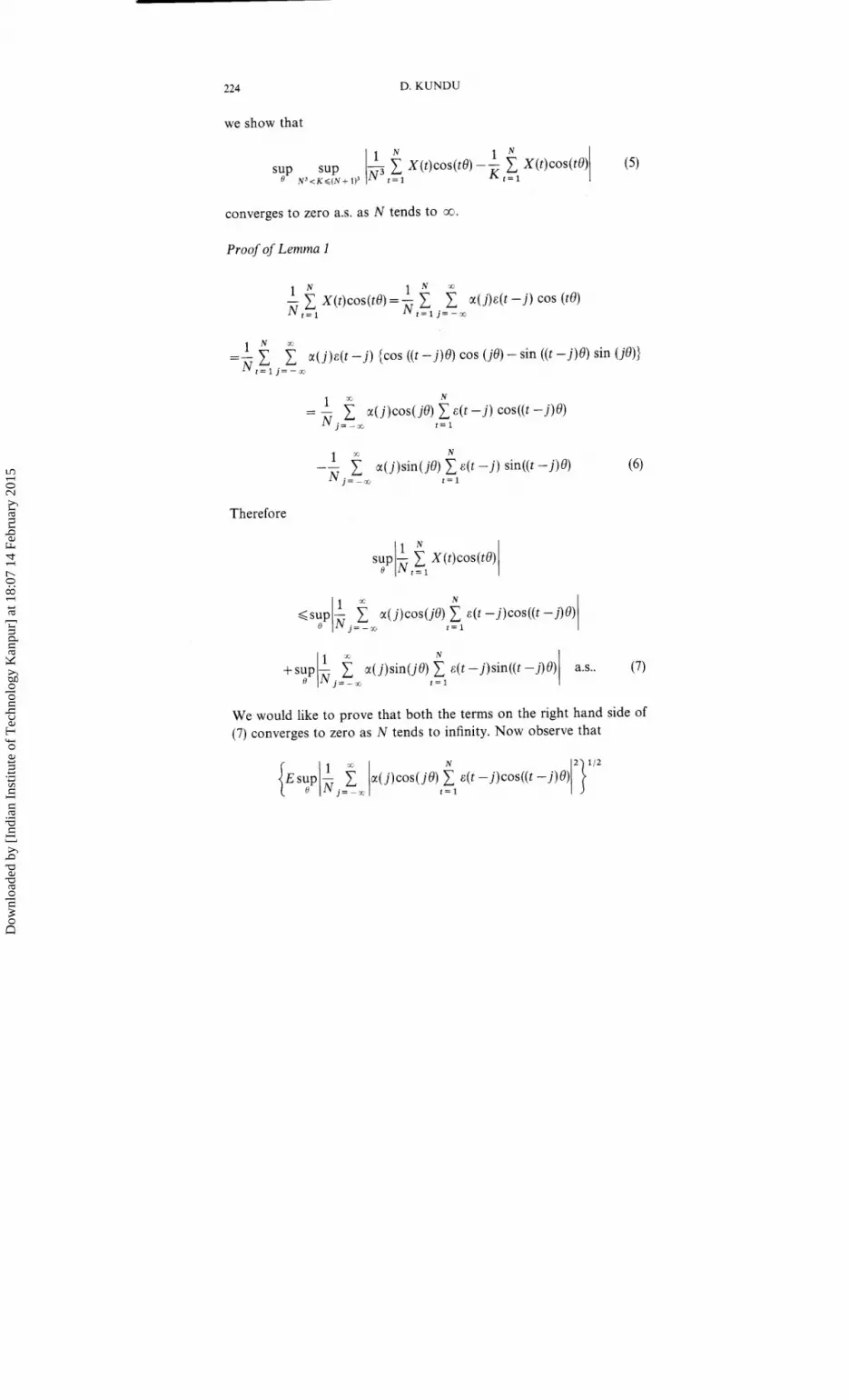
converges to zero a s . as N tends to a.

Proof of Lemma 1

1 I N - 1 X(t)cos(te) = - 2 2 a(j)&(t - j ) cos (to) N t = , N t , l j = - =

l N =- 1 c(( j ) ~ ( t - j) {COS ((t - j)O) cos (je) - sin ((t - j)e) sin (jO)}

N f = l j = - m

Therefore

We would like to prove that both the terms on the right hand (7) converges to zero as N tends to infinity. Now observe that

Dow

nloa

ded

by [

Indi

an I

nstit

ute

of T

echn

olog

y K

anpu

r] a

t 18:

07 1

4 Fe

brua

ry 2

015

SINUSOIDAL SIGNAL 225

where the sum CjV= -.+, omits the term t = 0 and the term C, is over N - It1 term (dependent on j ) . Since

(uniformly in j ) therefore (8) is O(N-'I4). Let M = N3. Therefore

Similarly the result is true if the cosine function is replaced by the sine also. Therefore

when M = N3. Now

Dow

nloa

ded

by [

Indi

an I

nstit

ute

of T

echn

olog

y K

anpu

r] a

t 18:

07 1

4 Fe

brua

ry 2

015

226 D. KUNDU

The mean squared of the first quantity on the right hand side of (12) is dominated by ( K I N 6 ) [ (N + - N3I2 = O(N- ' ) . Similarly the mean squared of the second quantity on the right hand side of (12) is dominated by K ( N 6 / N 8 ) = O ( N P 2 ) . Therefore both will converge to zero almost surely, which proves the lemma.

COROLLARY 1 The result is true i f the cosine function is replaced by the sine function.

COROLLARY 2 It can be proved similarly that i f X ( t ) is a sequence which satisjies Assumption 1 , then

Now consider

Now with the help of lemma 1, we can easily conclude that

lim sup gN(A, B, o) = 0 as . N+x O E S ~ , ~

Dow

nloa

ded

by [

Indi

an I

nstit

ute

of T

echn

olog

y K

anpu

r] a

t 18:

07 1

4 Fe

brua

ry 2

015

SINUSOIDAL SIGNAL

where the set S,,, for 6 > 0, is as follows;

therefore for all 6 > 0,

1 lim inf - [Q,(O) - Q,(Oo)] = lim sup f,(A, B, o) > 0. (17)

S ~ . M N N - + s O E S J . ~

(17) follows easily from Kundu and Mitra (1996). Here lim means limit infimum. Now suppose (a,, b,, d,) be the LSE's of (A,, B,, o,) and they are not consistent. Therefore either

Case I For all subsequences { N , ) of {N), ( 1 + lbNK/ tends to infinity or

Case I I There exists a 6 > 0 and a M < co and a subsequence { N K j such that (aNK, B ~ ~ , C;),X)ES~,~, for all K = 1,2, . . .,.

Now

as (aNK, b N K , d N K ) is the LSE of (A,, B,, w,), when N = N K . Observe that as K -t E , for both the cases, the left hand side of (18) converges to a number which is strictly positive, that is a contradiction. There- fore the LSE's of the model ( 1 ) have to be strongly consistent. There- fore we can state the following theorem:

THEOREM 1 If & = (a,, b,, d,) is the LSE of the nonlinear re- gression model (I), then it is a strongly consistent estimator of

$0 = (A,, B,, ~ 0 ) .

Dow

nloa

ded

by [

Indi

an I

nstit

ute

of T

echn

olog

y K

anpu

r] a

t 18:

07 1

4 Fe

brua

ry 2

015

228 D. KUNDU

3. ASYMPTOTIC NORMALITY

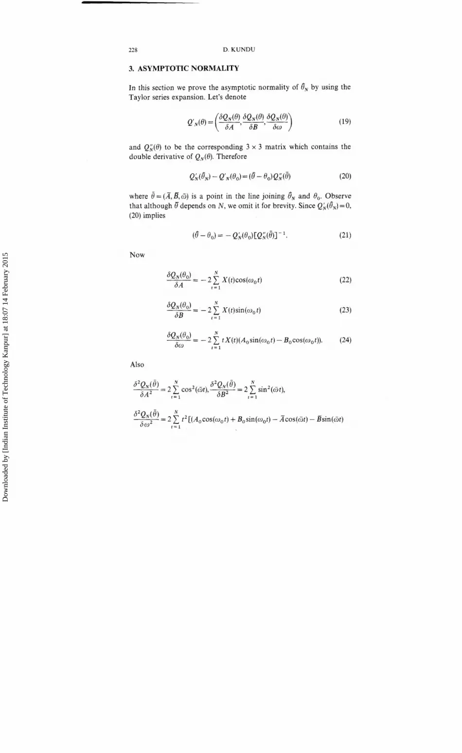
In this section we prove the asymptotic normality of 8;, by using the Taylor series expansion. Let's denote

and Q;(B) to be the corresponding 3 x 3 matrix which contains the double derivative of QN(8). Therefore

where 8 = (A,B,G) is a point in the line joining 0, and 8,. Observe that although depends on N, we omit it for brevity. Since Q;(Q,) =0, (20) implies

Now

N -- SQdeO) - - 2 tX(t)(A, sin(o,, t) - B,cos(w, t ) ) . (24) 60 i = l

Also

Dow

nloa

ded

by [

Indi

an I

nstit

ute

of T

echn

olog

y K

anpu

r] a

t 18:

07 1

4 Fe

brua

ry 2

015

SINUSOIDAL SIGNAL 229

+ X(t)) x (Acos(6t) + Bsin(6t)) + (A~in(6t)-Bcos(6t))~] (25)

- Bsin(6 t) + X(t)) - cos(6 t ) (As in(~ t ) -Bcos(6 t))] (26)

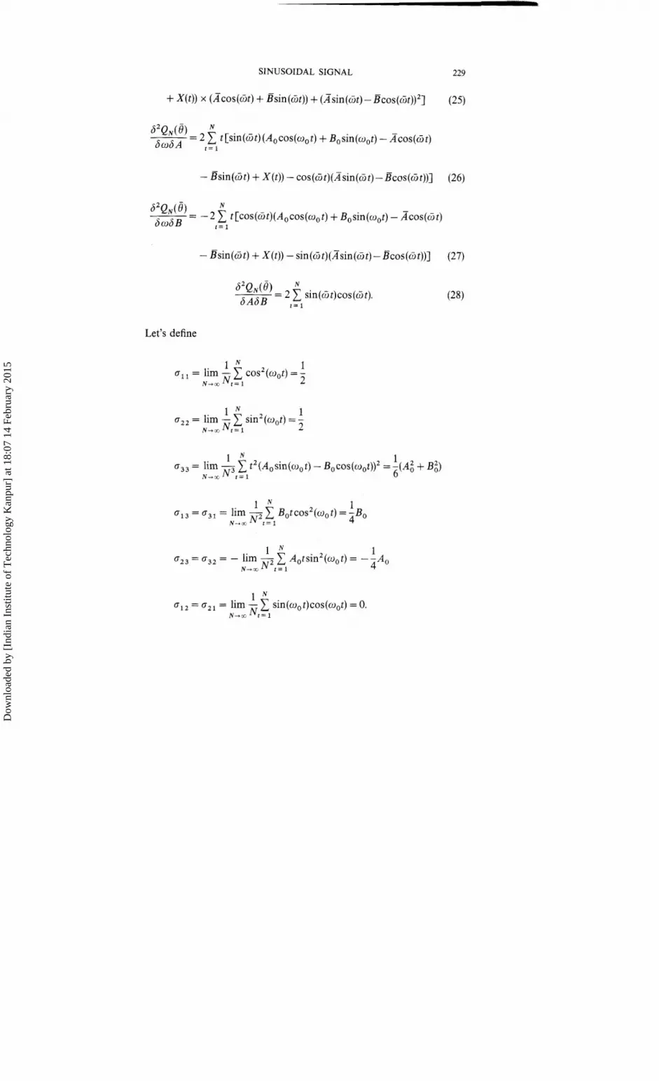
Let's define

a l = lirn L C cos2(oot) = 1 N-m Nt= 1 2

1 1 a,, = lirn - 1 sin2 (mot) = -

N-ZINt=l 2

1 1 a,, = lirn - 1 t2(Aosin(oo t) - ~ , c o s ( o , t ) ) ~ = -(A: + B;)

N-2 N 3 t = 1 6

1 1 a,, =a, , = lirn -?x Botcos2(oot) =-B,

N+XN t = 1 4

1 1 02, = a,, = - lirn - 1 Aotsin2(oot) = --Ao

N - d 2 t = 1 4

1 a12 = a21 = lirn - sin(oot)cos(wot) = 0.

N - a N t = l

Dow

nloa

ded

by [

Indi

an I

nstit

ute

of T

echn

olog

y K

anpu

r] a

t 18:

07 1

4 Fe

brua

ry 2

015

230 D. KUNDU

Now observe that as 6 + w,, A+ A, and B+B, as., we have

1 1 1 lirn - 2 cos2(ot) = lirn - C cos2(q,t) =- N-s N t = 1 N-r N t = l 2

1 1 1 lirn - 1 sin2(6t) = lim - C sin2 (coot) =- N + % ~ I = I N-r N t = 1 2

1 ~ ' Q ~ ( Q 1 lirn = lim 7 1 t2(Asin(6t) + B c o ~ ( w t ) ) ~ N + n 2~~ so2 N + 2 ~ t = l

1 = lim - 1 t2(Aosin(w, t) - B,~os(w,t))~

N-r N ~ ~ =

1 s2QN(@ 1 lirn = - lirn -Z 1 tcos(ot)(Asin(o t) - Bcos(3 t)) N+,2N2 SwSA N-z t = l

1 1 = - lim -Z 1 t ~ , s i n ~ ( o , t ) = --Ao

4 (33) N-sN t = l

1 s 2 ~ N ( @ 2 lirn ------- = lirn - 2 sin(& t)cos(G t) N+,N SAhB N-=Nt=l

2 = lim - 1 sin(o,t)cos(w,t) =O. (34)

N-cc N t = 1

Let's define the 3 x 3 matrix C = (toij)); i , j = 1,2,3 and also define the 3 x 3 diagonal matrix D as follows I) = d i a g { ~ -'I2, N- li2 N-3i2 >.

Dow

nloa

ded

by [

Indi

an I

nstit

ute

of T

echn

olog

y K

anpu

r] a

t 18:

07 1

4 Fe

brua

ry 2

015

SINUSOIDAL SIGNAL 23 1

Rewrite (21) as

(e^- 0 , ) ~ - l = - Q;(O,)D[DQ;(~)D]-I. (35)

Now from (29)-(34) we obtain

lim DQi(@)D = lim DQi(0,)D = 2C N - x N - r x

(36)

where

Now from the Central Limit theorem of Stochastic Process (see Fuller; 1976) it easily follows that QA(0,)D tends to a multivariate (3-variate) normal distribution as given below;

where

Therefore we have;

Now we can state the result as the following theorem;

Dow

nloa

ded

by [

Indi

an I

nstit

ute

of T

echn

olog

y K

anpu

r] a

t 18:

07 1

4 Fe

brua

ry 2

015

232 D. KUNDU

THEOREM 2 Under the assumptions of Theorem 1, ( ~ ' ~ ~ ( 2 , - A,), N ~ ' ~ ( B , - B,), N312(dN - a,)) converges in distribution to a 3-variate normal distribution with mean vector zero and the dispersion matrix is given by a 2 c z - ' , where c and x-' are as dejined before.

4. MULTIPARAMETER CASE

In this section we will extend the results of Section 2 and Section 3 to the following model:

where At, B t are arbitrary real numbers and o:'s are the distinct frequencies lying between 0 and 71 for K = 1, . . . , M. X(t)'s satisfy Assumption 1.

Let us use the following notations A = (A1, ..., AM), B = (B1,. . ., BM) and o = ( o l , . . . , wM). Similarly A,, B,, w, and A,, fl, and d, are also defined. We would like to investigate the consistency and the asym- ptotic normality properties of the LSE's obtained by minimizing Rd@) = ,

Y ( t ) - 1 [~ ' cos (o~ t ) + BK sin(oKt)] t = l

with respect to = (A, B, w). Now we have the following result:

THEOREM 3 ~f djN = (AN, flN, G N ) is the LSE of Do = (A,, B,, a,), then 6, is a strongly consistent estimator of 6,.

Proof of the Theorem 3 With the help of Lemma 1 and using the similar kind of techniques as that of (Kundu and Mitra; 1995), the results can be established.

Let's denote the 1 x 3M vector Rk(@) as follows:

Dow

nloa

ded

by [

Indi

an I

nstit

ute

of T

echn

olog

y K

anpu

r] a

t 18:

07 1

4 Fe

brua

ry 2

015

SINUSOIDAL SIGNAL 233

and Ri(8) denotes the 3M x 3M matrix which contains the double derivative of RN(@). Now we have

where 6 = (A, B, a) is a point in the line joining 6, and 0,. Since Rk(6,) = 0, we have

Let's define the 3M x 3M diagonal matrix V whose first 2M diagonal elements are N-'I2 and the last M diagonal elements are N-3 '2 . Therefore we can write (43) as

Now using the similar kind.of arguments as of Section 3, we can say that

where G is a 3M x 3M matrix and it has the following structure

where each of the Gij is a M x M matrix and

GI, = Gz2 = diag -c, , . . . ,-c, {: ]

Dow

nloa

ded

by [

Indi

an I

nstit

ute

of T

echn

olog

y K

anpu

r] a

t 18:

07 1

4 Fe

brua

ry 2

015

D. KUNDU

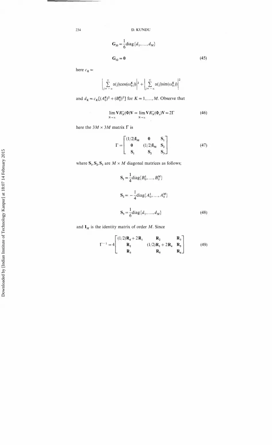
1 I G, = $diag {dl, . . . . d,,

here c, =

and d, = c, [ ( A t ) 2 + ( B t ) 2 ] for K = 1, . . . , M . Observe that

lim V Rk(@)V = lim V Rk (@,)V = 2r N - z N - x

here the 3M x 3M matrix is

where S,, S,, S, are M x M diagonal matrices as follows;

1 S, = -diag 6 {dl , . . . , d,}

and I, is the identity matrix of order M. Since

Dow

nloa

ded

by [

Indi

an I

nstit

ute

of T

echn

olog

y K

anpu

r] a

t 18:

07 1

4 Fe

brua

ry 2

015

SINUSOIDAL SIGNAL

where

we have

therefore we can state the result as the following theorem;

THEOREM 4 Under the assumptions of Theorem 3, { N ' I ~ (A, -A,), ~ " ~ ( h , - B ~ ) , N3I2(hN - w,)) converges in distribution to a 3M-variate normal distribution with mean vector zero and the dispersion matrix is given by 0 2 T - ' G T - ' .

5. N U M E R I C A L EXPERIMENTS

In this section we perform some Monte Carlo simulations to see how the asymptotic results work for small sample. We considered the fol- lowing model:

We took A, = B, = 1.5, o, = .25n(% 0.735398), .50n(% 1.570796) and .75n(% 2.356194). X ( t ) = s(t) + . 5 ~ ( t - I), where ~ ( t ) ' s are i.i.d. normal

Dow

nloa

ded

by [

Indi

an I

nstit

ute

of T

echn

olog

y K

anpu

r] a

t 18:

07 1

4 Fe

brua

ry 2

015

236 D. KUNDU

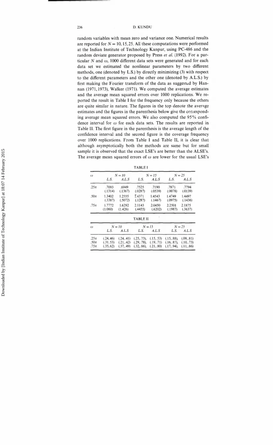
random variables with mean zero and variance one. Numerical results are reported for N = 10,15,25. All these computations were performed at the Indian Institute of Technology Kanpur, using PC-486 and the random deviate generator proposed by Press et al. (1992). For a par- ticular N and w, 1000 different data sets were generated and for each data set we estimated the nonlinear parameters by two different methods, one (denoted by L.S.) by directly minimizing (3) with respect to the different parameters and the other one (denoted by A.L.S.) by first making the Fourier transform of the data as suggested by Han- nan (1971,1973), Walker (1971). We computed the average estimates and the average mean squared errors over 1000 replications. We re- ported the result in Table I for the frequency only because the others are quite similar in nature. The figures in the top denote the average estimates and the figures in the parenthesis below give the ccnespond- ing average mean squared errors. We also computed the 95% confi- dence interval for w for each data sets. The results are reported in Table 11. The first figure in the parenthesis is the average length of the confidence interval and the second figure is the coverage frequency over 1000 replications. From Table I and Table 11, it is clear that although asymptotically both the methods are same but for small sample it is observed that the exact LSE's are better than the ALSE's. The average mean squared errors of w are lower for the usual LSE's

TABLE I

(L) N = 10 N = 15 N = 2.5 L.S. A.L.S L.S. A.L.S L.S. A.L.S

TABLE I1

co N = l O N = 1 5 N = 25 L S . A.LS L S . A.LS L.S. A.LS

Dow

nloa

ded

by [

Indi

an I

nstit

ute

of T

echn

olog

y K

anpu

r] a

t 18:

07 1

4 Fe

brua

ry 2

015

SINUSOIDAL SIGNAL 237

for almost all the sample sizes and for all w's. About the confidence intervals, it is observed that for higher values of w, the confidence interval of o obtained by using the exact LSE's usually give higher coverage probability. It is also observed that for both the methods as N increases the average length decreases and the coverage probabability increases.

6. CONCLUSIONS

In this paper we considered the one parameter and multiparameter sinusoidal model under the assumption of additive stationary errors. We obtained the asymptotic properties of the LSE's directly without making the Fourier transform of the data. We also obtained the ex- plicit expression of the covariance matrix for the multiparameter case, which is not available in the literature. From the numerical study it is observed that although asymptotically the two methods are equiva- lent but the exact LSE's are better than the ALSE's in terms of the mean squared errors. Since both the methods require the same amount of computations, therefore it is recommended not to Fourier transform the data at least for small samples to make any finite sample inference from the asymptotic results.

Acknowledgements

The author would like to thank the referee for many valuable sugges- tions.

References

[I] Fuller, W. A. (1976). Introduction to Statistical Time Series, John Wiley and Sons, New York.

121 Hannan, E. J. (1971). Nonlinear Time Series Regression, Journ. Appl. Probab., 8, 767-780.

[3] Hannan, E. J. (1973). The Estimation of Frequencies, Journ. Appl. Probab., 10, pp 510-519.

[4] Jennrich, R. I. (1969). Asymptotic Properties of Non Linear Least Squares Estima- tion, Ann. Marhem. Stat., 40, 633-543.

[5] Kundu, D. (1991). Asymptotic Properties of Complex Valued Nonlinear Regression Model, Communications in Statistics, Theory and Methods, 24, 3793-3803.

[6] Kundu, D. (1993). Asymptotic Theory of Least Squares Estimator of a Particular Nonlinear Regression Model, Statist. and Prob. Letters, 18, 13-17.

Dow

nloa

ded

by [

Indi

an I

nstit

ute

of T

echn

olog

y K

anpu

r] a

t 18:

07 1

4 Fe

brua

ry 2

015

238 D. KUNDU

[7] Kundu, D. (1995). Consistency of the Undamped Exponential Signals Model on a Restricted Parameter Space, Communication in Statistics, Theory and Methods, 24, 241-251.

[8] Kundu, D. and Mitra, A. (1995). A Note on the Consistency of the Undamped Exponetial Signals Model, Statistics, 26, 1-9.

191 Kundu, D. and Mitra, A. (1996). Asymptotic Theory of the Least Squares Es- timators of a Nonlinear Time Series Regression Model, Communications in Statis- t ic .~, Theory and Methods, 25(1), 133-141.

[lo] Press, W. H., Teukolsky, S. A,, Vellerling, W. T. and Flannery, 9. P. (1992). Nu- merical Recipies in Fortran, The Art of Scienti$c Computing, 2nd, Edition, Cam- bridge University Press.

[1 l] Rice, J. A. and Rosenblatt, M. (1988). On Frequency Estimation, Biometriku, 75, 477-484.

1121 Stoica, P. (1993). List of References on Spectral Estimation, Signal Processing, 31, 329-340.

[I31 Walker, A. M. (1969). On the Estimation of a Harmonic Components in a Time Series with Stationary Residuals, Proc. of the Intern. Stat. Inst., 43, 374-376.

[14] Walker, A. M. (1971). On the Estimation of a Harmonic Components in a Time Series with Stationary Independent Residuals, Biometrika, 58, 21-26.

[I51 Wu, C. F. J. (1981). Asymptotic Theory of Non Linear Squares Estimation, Ann. of Stat., 9, 501-513.

Debasis Kundu, Department of Mathematics,

Indian Institute of Technology, K anpur,

Pin 208016, India.

Dow

nloa

ded

by [

Indi

an I

nstit

ute

of T

echn

olog

y K

anpu

r] a

t 18:

07 1

4 Fe

brua

ry 2

015