ar2007-08.pdf - krishi icar
TRANSCRIPT
For internal use only Do not quote/cite without permission
ICAR Network Project
on
Impact, Adaptation and Vulnerability of Indian Agriculture to Climate Change
Annual Progress Report (2007-2008)
Coordinating center Indian Agricultural Research Institute, New Delhi
Collaborating centers • Central Plantation Crops Research Institute, Kasaragod
• Central Research Institute for Dryland Agriculture, Hyderabad
• Indian Institute of Horticultural Research, Bangaluru
• CSK Himachal Pradesh Agricultural University, Palampur
• Central Soil and Water Conservation Research and Training Institute, Dehradun
• ICAR Research Complex for Eastern Region, Patna
• National Dairy Research Institute, Karnal
• Central Marine Fisheries Research Institute, Cochin
• Central Inland Fisheries Research Institute, Barrackpore
• Tamil Nadu Agricultural University, Coimbatore
INDEX
SUMMARY OF THE REPORT 1 ANNEXURE 1: Co-Investigators:
• Indian Agricultural Research Institute 5
• Central Plantation Crops Research Institute, Kasaragod 5
• Central Research Institute for Dryland Agriculture, Hyderabad 6
• Indian Institute of Horticultural Research Institute, Bangalore 6
• CSK Himachal Pradesh Agricultural University, Palampur 7
• Central Soil and Water Conservation Research and Training Institute, Dehradun 7
• ICAR Research Complex for Eastern Region, Patna 7
• National Dairy Research Institute, Karnal 8
• Central Marine Fisheries Research Institute, Cochin 8
• Central Inland Fisheries Research Institute, Barrackpore 9
• Tamilnadu Agricultural University, Coimbatore 9
ANNEXURE 2: Research Associates /Senior Research Fellows
• Indian Agricultural Research Institute(Coordinating centre) 10
• Indian Agricultural Research Institute 10
• Central Plantation Crops Research Institute, Kasaragod 10
• Central Research Institute for Dryland Agriculture, Hyderabad 10
• Indian Institute of Horticultural Research Institute, Bangalore 11
• CSK Himachal Pradesh Agricultural University, Palampur 11
• Central Soil and Water Conservation Research and Training Institute, Dehradun 11
• ICAR Research Complex for Eastern Region, Patna 11
• National Dairy Research Institute, Karnal 11
• Central Marine Fisheries Research Institute, Cochin 12
• Central Inland Fisheries Research Institute, Barrackpore 12
• Tamilnadu Agricultural University, Coimbatore 12
ANNEXURE 3: Budget allocation and expenditure of different Institutes
• Indian Agricultural Research Institute 13
• Central Plantation Crops Research Institute, Kasaragod 13
• Central Research Institute for Dryland Agriculture, Hyderabad 14
• Indian Institute of Horticultural Research Institute, Bangalore 14
• CSK Himachal Pradesh Agricultural University, Palampur 15
• Central Soil and Water Conservation Research and Training Institute, Dehradun 15
• ICAR Research Complex for Eastern Region, Patna 16
• National Dairy Research Institute, Karnal 16
• Central Marine Fisheries Research Institute, Cochin 17
• Central Inland Fisheries Research Institute, Barrackpore 17
• Tamilnadu Agricultural University, Coimbatore 18
ANNEXURE 4: Specific Objectives of the individual centres
• Indian Agricultural Research Institute 19
• Central Plantation Crops Research Institute, Kasaragod 19
• Central Research Institute for Dryland Agriculture, Hyderabad 19
• Indian Institute of Horticultural Research Institute, Bangalore 20
• CSK Himachal Pradesh Agricultural University, Palampur 20
• Central Soil and Water Conservation Research and Training Institute, Dehradun 20
• ICAR Research Complex for Eastern Region, Patna 20
• National Dairy Research Institute, Karnal 21
• Central Marine Fisheries Research Institute, Cochin 21
• Central Inland Fisheries Research Institute, Barrackpore 21
• Tamilnadu Agricultural University, Coimbatore 21
ANNEXURE 5: Executive Summary by different centres
• Indian Agricultural Research Institute 22
• Central Plantation Crops Research Institute, Kasaragod 23
• Central Research Institute for Dryland Agriculture, Hyderabad 23
• Indian Institute of Horticultural Research Institute, Bangalore 24
• CSK Himachal Pradesh Agricultural University, Palampur 25
• Central Soil and Water Conservation Research and Training Institute, Dehradun 25
• ICAR Research Complex for Eastern Region, Patna 25
• National Dairy Research Institute, Karnal 25
• Central Marine Fisheries Research Institute, Cochin 26
• Central Inland Fisheries Research Institute, Barrackpore 26
• Tamilnadu Agricultural University, Coimbatore 27
ANNEXURE 6: Detailed Progress Report 28
• Indian Agricultural Research Institute 28
• Central Plantation Crops Research Institute, Kasaragod 50
• Central Research Institute for Dryland Agriculture, Hyderabad 63
• Indian Institute of Horticultural Research Institute, Bangalore 77
• CSK Himachal Pradesh Agricultural University, Palampur 88
• Central Soil and Water Conservation Research and Training Institute, Dehradun 100
• ICAR Research Complex for Eastern Region, Patna 106
• National Dairy Research Institute, Karnal 112
• Central Marine Fisheries Research Institute, Cochin 130
• Central Inland Fisheries Research Institute, Barrackpore 133
• Tamilnadu Agricultural University, Coimbatore 151
ANNEXURE 7: Papers Published
• Central Plantation Crops Research Institute, Kasaragod 192
• ICAR Research Complex for Eastern Region, Patna 192
• Central Marine Fisheries Research Institute, Cochin 193
• Tamilnadu Agricultural University, Coimbatore 193
• National Dairy Research Institute, Karnal 194
Coordinating Institute: Indian Agricultural Research Institute, New Delhi 110 012
Department /Division: Division of Environmental Sciences Principal Investigator:
Dr. P.K. Aggarwal, National Professor
Co-Investigators : Annexure 1 Names of Research Associates/ Senior Research Fellows: Annexure 2
Duration of scheme: Till 11th plan Total Cost of the scheme Rs. (in lakhs): 147.554
Budget allocation for this year and expenditure: Annexure 3 Objectives o To quantify the sensitivities of current food production systems to different scenarios
of climatic change by integrating the response of different sectors o To quantify the least-risk or ‘no regrets’ options in view of uncertainty of global
environmental change which would also be useful in sustainable agricultural development
o To determine the available management and genetic adaptation strategies for climatic change and climatic variability
o To determine the mitigation options for reducing global climatic changes in agro-ecosystems
o To provide policy support for the international negotiations on global climatic changes.
Detailed objectives of different Institutes: Annexure 4 Executive summary of the report: Annexure 5 for centre-wise summaries
1.Analysis of emissions of carbon dioxide and nitrous oxide from soil in elevated temperature indicated that the cumulative flux of N2O-N from fertilized soil increased by 21% over the ambient soil conditions in kharif season while in rabi, the cumulative flux of carbon dioxide was found to be 12% higher in elevated temperature conditions than in the ambient.
1
2. In Andhra Pradesh, the percentage of occurrence of droughts were more during 1971-1980 and 1991-2000 decades when compared to 1981-1990 decade in all agro-climatic zones except Southern and Scarce rainfall zones
3. Simulation studies using InfoCrop indicated that in Himachal Pradesh,
temperature rise by 1oC and 20C and reduction in rainfall cause decrease in maize yield by 2 to 10 %. In Bihar, maize yields are likely to go up by 13 to 38%, while a reduction in wheat and rice yield up to 25% and 37%, respectively could be expected with the climate change scenarios in 2020, 2050 and 2080.
4. In Tamil Nadu, rice production during southwest monsoon is expected to be
affected more compared to northeast monsoon due to climate change. The reduction up to 35 and 50 per cent could be noticed in 2050 and 2080, respectively, in southern region of Tamil Nadu. During northeast monsoon, crop yields are likely to increase by 5 to 15 per cent in most of the locations due to climate change. Maize and sorghum yields are likely to reduce by 2.9 to 26.4% during 2020, 2050 and 2080 from the current yield levels if adaptation strategies are not implemented.
5. Using the coconut model, climate change impacts on coconut yield are simulated for HadCM3 A2a, B2a and A1F 2020, 2050 and 2080 scenarios. Results indicate positive effect on coconut yields in west coast and parts of TN and Karnataka and negative effects on nut yield in east coast of India. However, in the event of reduced availability of irrigation, the beneficial impacts will be less or negative impacts will be more.
6. Experiments conducted in Temperature Gradient Tunnels indicated that biomass and yield of soybean, greengram and potato reduced with rise in temperature (1- 4 oC) owing to reduction in yield attributes. Compared to vegetative growth, reproductive growth showed greater sensitivity to high temperature stress in almost all the crops.
8. In chickpea, exposure to high temperature for a fortnight at flowering stage
reduced the sterility of pods, which had a beneficial effect on growth, and yield. Among the crops, wheat showed higher degree of sensitivity to high temperature as compared to legumes (greengram, soybean) and oilseeds (mustard, groundnut).
9. Elevated CO2 increased the productivity of greengram, soybean, chickpea and potato owing to increase in biomass and seed/tuber no. and their size. Groundnut crop showed positive response to elevated CO2 levels for growth and yield and the response was significantly evident at 700ppm. In groundnut moisture stress at initial stages improved the total biomass and pod yield in all the treatments and the response was more at higher levels of CO2. Tomato and onion crops showed a yield increase of 25% at elevated CO2 concentration of 550ppm.
2
11. The total consumption of castor foliage by Spodoptera litura during the entire feeding period was significantly more under elevated CO2 conditions than ambient and chamber controls indicating 39% more consumption under elevated CO2 conditions.
12. Stressful THI with 20h or more daily THI-hrs (THI >84) for several weeks affect
animal responses. The animal thermal load is not dissipated that cause economic losses. Under climate change scenario increased number of stressful days with a change in Tmax and Tmin and decline in availability of water will further impact animal productivity and health in Punjab, Rajasthan and Tamil Nadu. The change in seasonal mean temperatures and in the extreme temperatures in the future will impact animal reproductive cycles, milk yield and production The night temperature increase will not permit animals to dissipate their thermal loads and recovery to normal will be affected.
13. Analysis of historical data showed that the Indian mackerel is able to adapt to rise
in sea surface temperature by extending distribution towards northern latitudes, and by descending to depths. The mackerel was conventionally caught by surface drift gillnets by artisanal fishermen. In recent years, however, the fish is increasingly getting caught in bottom trawl nets operated by large mechanized boats at about 50 m depth. In 1985, only 2% of the total mackerel catch was from bottom trawlers. In the last five years, about 10% of the mackerel catch is by the bottom trawlers. This shows that as the sea surface temperature became warmer, the fish descended down.
14. To estimate the carbon foot print by marine fishing boats by data were collected
on the diesel consumption from about 1332 mechanized boats and 631 motorized boats in the major fishing harbors along the east and west coast of India. Initial estimates indicate that fossil fuel consumption by marine fishing boats is around 1200 million liters per year and CO2 emission by marine fishing sector is around 2.4 million tonnes per year.
15. Under controlled laboratory conditions, the fingerlings of inland fish species, L.
rohita were kept in different temperatures and ad libitum feeding. The fishes showed progressive increase upto 38% in food conversation, food consumption, specific growth and weight gain in the thermal range between 29ºC and 34ºC but the trend reversed with further increased in temperature to 35ºC.
16. Among the 11 coastal districts of Tamil Nadu, Ramnad and Nagapattinam are
most vulnerable to climatic change. Among all the 30 districts, the vulnerability to climate change is very high in the Perambalur district followed by the Nilgiris and Ramnad as compared to the other districts.
3
4
Details of Progress Report: Annexure 6
Pares Published Annexure 7 Signature of the Principal Investigator
Name: P.K. Aggarwal Designation: Network Coordinator & National Professor
ANNEXURE 1: Co-Investigators:
Indian Agricultural Research Institute, NEW DELHI
• Name : Dr. S.D. Singh, Principal Investigator
Designation : Principal Scientist, Division of Environmental Sciences
• Name : Dr. Santha Nagarajan, Designation : Principal Scientist, Nuclear Research Laboratory
• Name : Dr. R. Choudhary Designation : Principal Scientist, Division of Environmental Sciences
• Name : Dr. Madan Pal Designation : Senior Scientist, Division of Plant Physiology
• Name : Dr. Subash Chandra Designation : Senior Scientist, Entomology
• Name : Dr. Anjali Anand Designation : Senior Scientist, Nuclear Research Laboratory
• Name : Dr. Arti Bhatia Designation : Senior Scientist, Division of Environmental Sciences • Name : Dr. Niveta Jain Designation : Senior Scientist, Division of Environmental Sciences • Name : Dr. Bidisha Benerjee Designation : Scientist, Division of Environmental Sciences Central Plantation Crop Research Institute, KASARAGOD • Name : Dr. S. Naresh Kumar, Principal Investigator
Designation : Senior Scientist, Plant Physiology • Name : Dr. K.V. Kasturi Bai Designation : Principal Scientist
5
Central Research Institute for Dryland Agriculture, HYDERABAD
• Name : Dr. GGSN Rao, Principal Investigator Designation : Project Coordinator
• Name : Dr. M. Vanaja Designation : Senior Scientist, Plant Physiology
• Name : Dr. M. Srinivasa Rao Designation : Senior Scientist, Agricultural Entomology
• Name : Dr. Y.S. Ramakrishna Designation : Director
• Name : Mr. A.V.M. Subba Rao Designation : Scientist, (Agromet)
• Name : Dr. M. Maheswari Designation : Senior Scientist, Plant Physiology
• Name : Dr. N. Jyothi Laxmi Designation : Senior Scientist, Plant Physiology
Indian Institute of Horticultural Research Institute, BANGALORE
• Name : Dr.N.K. Srinivasa Rao, Principal Investigator Designation : Principal Scientist
• Name : Dr. R.M. Bhatt Designation : Principal Scientist • Name : Dr. R.H. Laxman Designation : Senior Scientist • Name : Dr. K.S. Shivashankar Designation : Senior Scientist
6
CSK Himachal Pradesh Agricultural University, PALAMPUR • Name : Dr.Ranbir Singh Rana, Principal Investigator
Designation : Scientist
• Name : Mr. Vaibhav Kalia Designation : Assistant Professor
• Name : Mr. Sanjay Sharma Designation :
Central Soil and water Conservation Research and training Institute, DEHRADUN
• Name : Dr. K.P. Tripati, Principal Investigator Designation : Principal Scientist, (Soil & WCE)
• Name : Dr. D.R.Sena Designation : Scientist Sr.Sclale, (S &WCE) at Vasad, Gujarat • Name : Dr. H.B. Singh Designation : Principal Scientist ,(Agronomy) at Vasad, Gujarat • Name : Dr. S.P.Tiwari Designation : Senior Scientist ,(Agronomy) at Vasad, Gujarat • Name : Er. Sridhara Patra Designation : Scientist ,(S& WCE) at Deharadun
ICAR Research Complex for Eastern Region, PATNA
• Name : Dr. Alok K. Sikka, Principal Investigator
• Designation : Director (upto Ist November 2007)
Dr. Abdul Haris A. (From 2nd November 2007)
• Name : Dr. A. Abdul Haris Designation : Senior Scientist • Name : Dr. Abdul Islam Designation : Senior Scientist • Name : Dr. R. Elanchezhian Designation : Senior Scientist
7
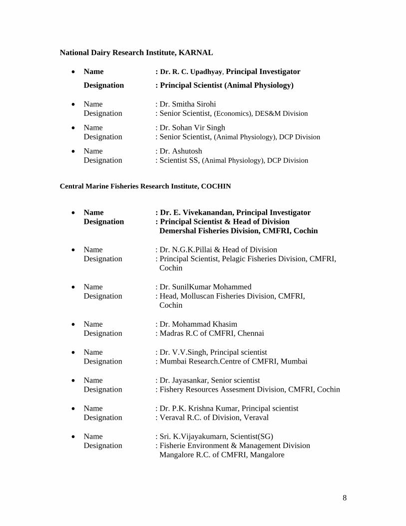
National Dairy Research Institute, KARNAL
• Name : Dr. R. C. Upadhyay, Principal Investigator
Designation : Principal Scientist (Animal Physiology)
• Name : Dr. Smitha Sirohi Designation : Senior Scientist, (Economics), DES&M Division
• Name : Dr. Sohan Vir Singh Designation : Senior Scientist, (Animal Physiology), DCP Division
• Name : Dr. Ashutosh Designation : Scientist SS, (Animal Physiology), DCP Division
Central Marine Fisheries Research Institute, COCHIN
• Name : Dr. E. Vivekanandan, Principal Investigator Designation : Principal Scientist & Head of Division Demershal Fisheries Division, CMFRI, Cochin
• Name : Dr. N.G.K.Pillai & Head of Division Designation : Principal Scientist, Pelagic Fisheries Division, CMFRI,
Cochin
• Name : Dr. SunilKumar Mohammed Designation : Head, Molluscan Fisheries Division, CMFRI,
Cochin • Name : Dr. Mohammad Khasim
Designation : Madras R.C of CMFRI, Chennai
• Name : Dr. V.V.Singh, Principal scientist Designation : Mumbai Research.Centre of CMFRI, Mumbai
• Name : Dr. Jayasankar, Senior scientist Designation : Fishery Resources Assesment Division, CMFRI, Cochin
• Name : Dr. P.K. Krishna Kumar, Principal scientist Designation : Veraval R.C. of Division, Veraval
• Name : Sri. K.Vijayakumarn, Scientist(SG) Designation : Fisherie Environment & Management Division Mangalore R.C. of CMFRI, Mangalore
8
9
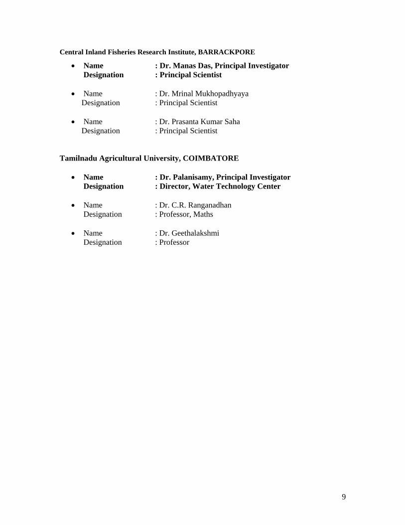
Central Inland Fisheries Research Institute, BARRACKPORE
• Name : Dr. Manas Das, Principal Investigator Designation : Principal Scientist
• Name : Dr. Mrinal Mukhopadhyaya Designation : Principal Scientist • Name : Dr. Prasanta Kumar Saha Designation : Principal Scientist
Tamilnadu Agricultural University, COIMBATORE
• Name : Dr. Palanisamy, Principal Investigator Designation : Director, Water Technology Center
• Name : Dr. C.R. Ranganadhan Designation : Professor, Maths
• Name : Dr. Geethalakshmi Designation : Professor
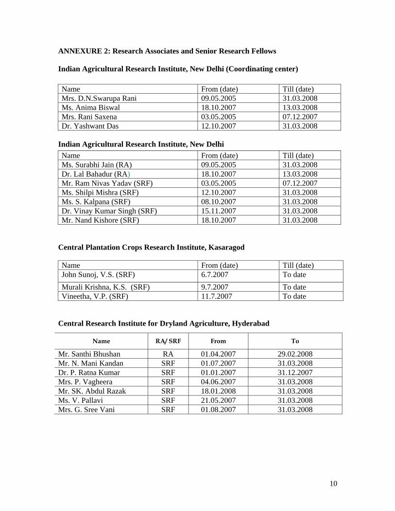
ANNEXURE 2: Research Associates and Senior Research Fellows Indian Agricultural Research Institute, New Delhi (Coordinating center)
Name From (date) Till (date) Mrs. D.N.Swarupa Rani 09.05.2005 31.03.2008 Ms. Anima Biswal 18.10.2007 13.03.2008 Mrs. Rani Saxena 03.05.2005 07.12.2007 Dr. Yashwant Das 12.10.2007 31.03.2008
Indian Agricultural Research Institute, New Delhi
Name From (date) Till (date) Ms. Surabhi Jain (RA) 09.05.2005 31.03.2008 Dr. Lal Bahadur (RA) 18.10.2007 13.03.2008 Mr. Ram Nivas Yadav (SRF) 03.05.2005 07.12.2007 Ms. Shilpi Mishra (SRF) 12.10.2007 31.03.2008 Ms. S. Kalpana (SRF) 08.10.2007 31.03.2008 Dr. Vinay Kumar Singh (SRF) 15.11.2007 31.03.2008 Mr. Nand Kishore (SRF) 18.10.2007 31.03.2008
Central Plantation Crops Research Institute, Kasaragod Name From (date) Till (date) John Sunoj, V.S. (SRF) 6.7.2007 To date Murali Krishna, K.S. (SRF) 9.7.2007 To date Vineetha, V.P. (SRF) 11.7.2007 To date
Central Research Institute for Dryland Agriculture, Hyderabad
Name RA/ SRF From To
Mr. Santhi Bhushan RA 01.04.2007 29.02.2008 Mr. N. Mani Kandan SRF 01.07.2007 31.03.2008 Dr. P. Ratna Kumar SRF 01.01.2007 31.12.2007 Mrs. P. Vagheera SRF 04.06.2007 31.03.2008 Mr. SK. Abdul Razak SRF 18.01.2008 31.03.2008 Ms. V. Pallavi SRF 21.05.2007 31.03.2008 Mrs. G. Sree Vani SRF 01.08.2007 31.03.2008
10
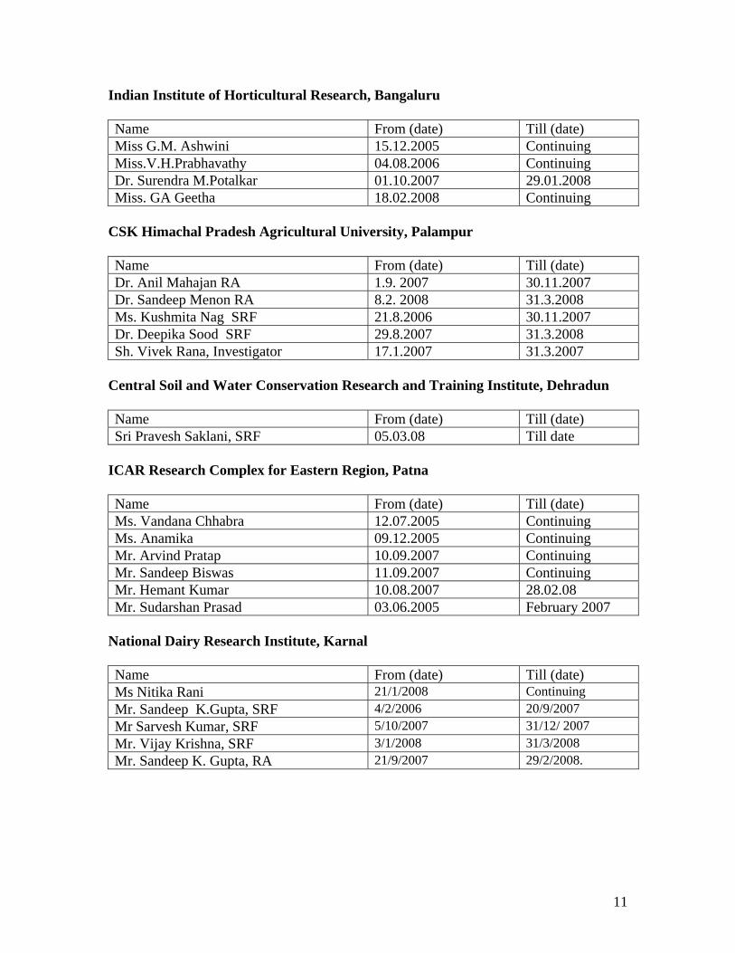
Indian Institute of Horticultural Research, Bangaluru Name From (date) Till (date) Miss G.M. Ashwini 15.12.2005 Continuing Miss.V.H.Prabhavathy 04.08.2006 Continuing Dr. Surendra M.Potalkar 01.10.2007 29.01.2008 Miss. GA Geetha 18.02.2008 Continuing
CSK Himachal Pradesh Agricultural University, Palampur Name From (date) Till (date) Dr. Anil Mahajan RA 1.9. 2007 30.11.2007 Dr. Sandeep Menon RA 8.2. 2008 31.3.2008 Ms. Kushmita Nag SRF 21.8.2006 30.11.2007 Dr. Deepika Sood SRF 29.8.2007 31.3.2008 Sh. Vivek Rana, Investigator 17.1.2007 31.3.2007
Central Soil and Water Conservation Research and Training Institute, Dehradun Name From (date) Till (date) Sri Pravesh Saklani, SRF 05.03.08 Till date
ICAR Research Complex for Eastern Region, Patna Name From (date) Till (date) Ms. Vandana Chhabra 12.07.2005 Continuing Ms. Anamika 09.12.2005 Continuing Mr. Arvind Pratap 10.09.2007 Continuing Mr. Sandeep Biswas 11.09.2007 Continuing Mr. Hemant Kumar 10.08.2007 28.02.08 Mr. Sudarshan Prasad 03.06.2005 February 2007
National Dairy Research Institute, Karnal Name From (date) Till (date) Ms Nitika Rani 21/1/2008 Continuing Mr. Sandeep K.Gupta, SRF 4/2/2006 20/9/2007 Mr Sarvesh Kumar, SRF 5/10/2007 31/12/ 2007 Mr. Vijay Krishna, SRF 3/1/2008 31/3/2008 Mr. Sandeep K. Gupta, RA 21/9/2007 29/2/2008.
11
12
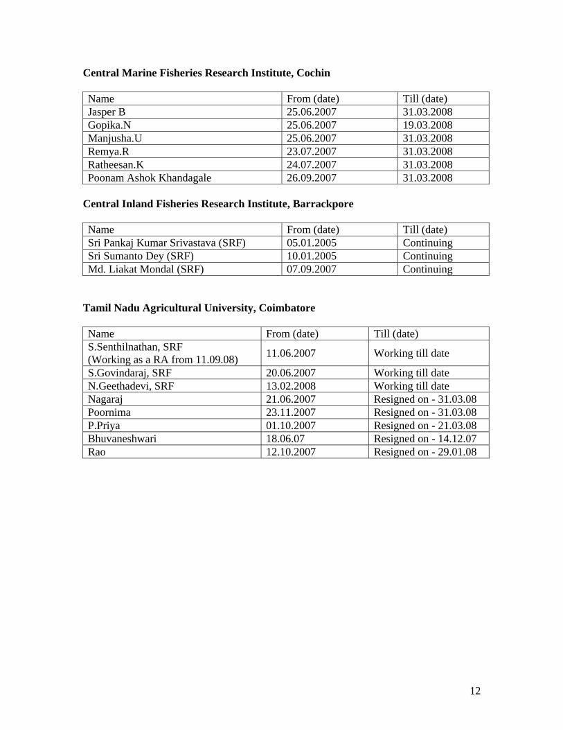
Central Marine Fisheries Research Institute, Cochin Name From (date) Till (date) Jasper B 25.06.2007 31.03.2008 Gopika.N 25.06.2007 19.03.2008 Manjusha.U 25.06.2007 31.03.2008 Remya.R 23.07.2007 31.03.2008 Ratheesan.K 24.07.2007 31.03.2008 Poonam Ashok Khandagale 26.09.2007 31.03.2008
Central Inland Fisheries Research Institute, Barrackpore
Name From (date) Till (date) Sri Pankaj Kumar Srivastava (SRF) 05.01.2005 Continuing Sri Sumanto Dey (SRF) 10.01.2005 Continuing Md. Liakat Mondal (SRF) 07.09.2007 Continuing
Tamil Nadu Agricultural University, Coimbatore Name From (date) Till (date) S.Senthilnathan, SRF (Working as a RA from 11.09.08) 11.06.2007 Working till date
S.Govindaraj, SRF 20.06.2007 Working till date N.Geethadevi, SRF 13.02.2008 Working till date Nagaraj 21.06.2007 Resigned on - 31.03.08 Poornima 23.11.2007 Resigned on - 31.03.08 P.Priya 01.10.2007 Resigned on - 21.03.08 Bhuvaneshwari 18.06.07 Resigned on - 14.12.07 Rao 12.10.2007 Resigned on - 29.01.08
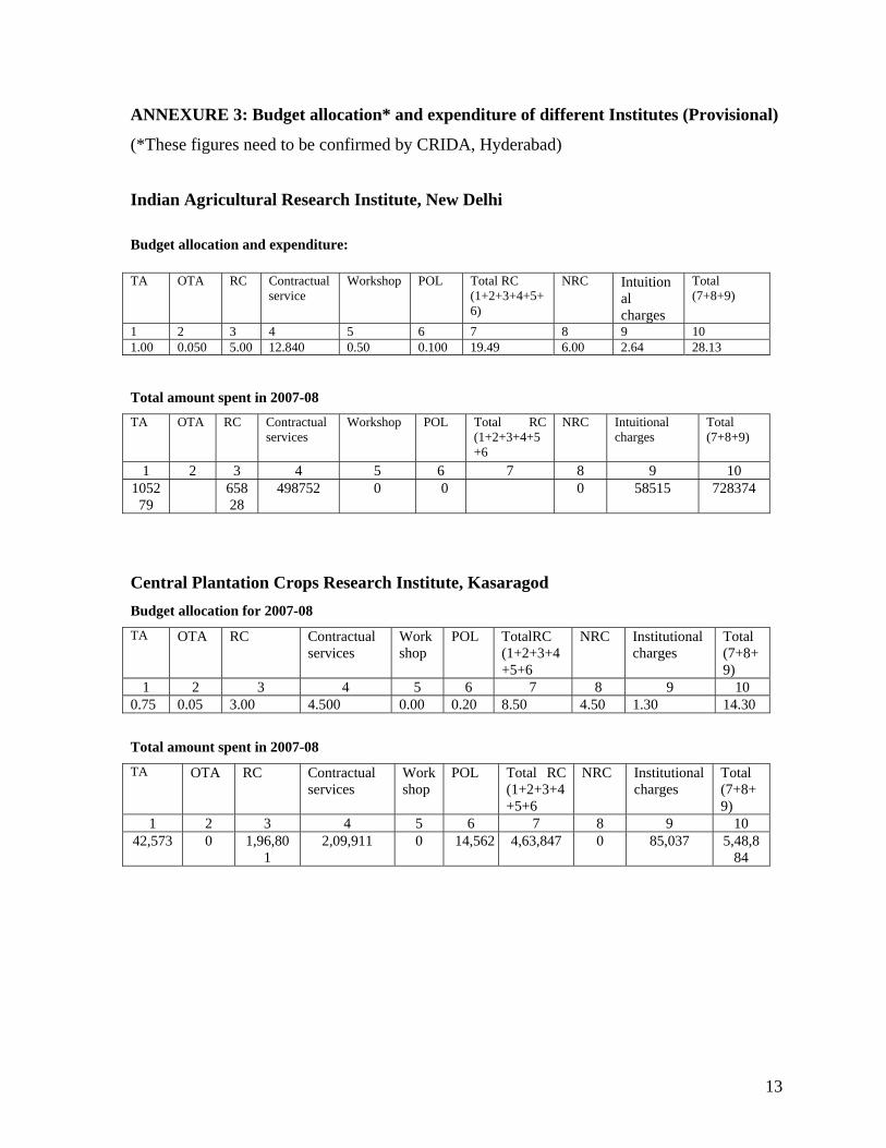
ANNEXURE 3: Budget allocation* and expenditure of different Institutes (Provisional)
(*These figures need to be confirmed by CRIDA, Hyderabad)
Indian Agricultural Research Institute, New Delhi Budget allocation and expenditure: TA OTA RC Contractual
service Workshop POL Total RC
(1+2+3+4+5+6)
NRC Intuitional charges
Total (7+8+9)
1 2 3 4 5 6 7 8 9 10 1.00 0.050 5.00 12.840 0.50 0.100 19.49 6.00 2.64 28.13 Total amount spent in 2007-08
TA OTA RC Contractual services
Workshop POL Total RC (1+2+3+4+5+6
NRC Intuitional charges
Total (7+8+9)
1 2 3 4 5 6 7 8 9 10 105279
65828
498752 0 0 0 58515 728374
Central Plantation Crops Research Institute, Kasaragod Budget allocation for 2007-08
TA OTA RC Contractual services
Work shop
POL TotalRC (1+2+3+4+5+6
NRC Institutional charges
Total (7+8+9)
1 2 3 4 5 6 7 8 9 10 0.75 0.05 3.00 4.500 0.00 0.20 8.50 4.50 1.30 14.30
Total amount spent in 2007-08
TA OTA RC Contractual services
Workshop
POL Total RC (1+2+3+4+5+6
NRC Institutional charges
Total (7+8+9)
1 2 3 4 5 6 7 8 9 10 42,573 0 1,96,80
1 2,09,911 0 14,562 4,63,847 0 85,037 5,48,8
84
13
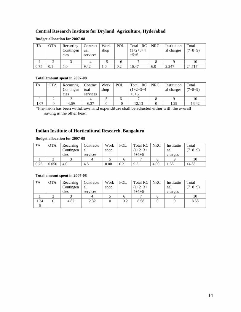
Central Research Institute for Dryland Agriculture, Hyderabad Budget allocation for 2007-08
TA OTA Recurring Contingencies
Contractual services
Work shop
POL Total RC (1+2+3+4+5+6
NRC Institutional charges
Total (7+8+9)
1 2 3 4 5 6 7 8 9 10 0.75 0.1 5.0 9.42 1.0 0.2 16.47 6.0 2.247 24.717
Total amount spent in 2007-08
TA OTA Recurring Contingencies
Contractual services
Workshop
POL Total RC (1+2+3+4+5+6
NRC Institutional charges
Total (7+8+9)
1 2 3 4 5 6 7 8 9 10 1.07 0 4.69 6.37 0 0 12.13 0 1.29 13.42 *Provision has been withdrawn and expenditure shall be adjusted either with the overall saving in the other head.
Indian Institute of Horticultural Research, Bangaluru Budget allocation for 2007-08
TA OTA Recurring Contingencies
Contractual services
Work shop
POL Total RC (1+2+3+4+5+6
NRC Institutional charges
Total (7+8+9)
1 2 3 4 5 6 7 8 9 10 0.75 0.050 4.0 4.5 0.00 0.2 9.5 4.00 1.35 14.85
Total amount spent in 2007-08
TA OTA Recurring Contingencies
Contractual services
Workshop
POL Total RC (1+2+3+4+5+6
NRC Institutional charges
Total (7+8+9)
1 2 3 4 5 6 7 8 9 10 1.24
6 0 4.82 2.32 0 0.2 8.58 0 0 8.58
14
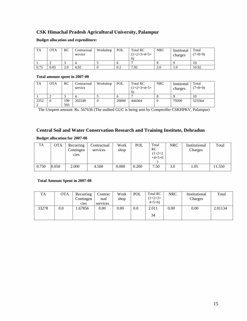
CSK Himachal Pradesh Agricultural University, Palampur Budget allocation and expenditure: TA OTA RC Contractual
service Workshop POL Total RC
(1+2+3+4+5+6)
NRC Institonal charges
Total (7+8+9)
1 2 3 4 5 6 7 8 9 10 0.75 0.05 2.0 4.92 0 0.2 7.92 2.0 1.0 10.92 Total amount spent in 2007-08
TA OTA RC Contractual service
Workshop POL Total RC (1+2+3+4+5+6)
NRC Institonal charges
Total (7+8+9)
1 2 3 4 5 6 7 8 9 10 22522
0 199593
202249 0 20000 444364 0 79200 523564
The Unspent amount: Rs. 567636 (The audited GUC is being sent by Comptroller CSKHPKV, Palampur)
Central Soil and Water Conservation Research and Training Institute, Dehradun Budget allocation for 2007-08
TA OTA Recurring Contingen
cies
Contractual services
Work shop
POL Total RC (1+2+3+4+5+6
)
NRC Institutional Charges
Total
0.750 0.050 2.000 4.500 0.000 0.200 7.50 3.0 1.05 11.550
Total Amount Spent in 2007-08
TA OTA Recurring Contingen
cies
Contractual
services
Work shop
POL Total RC (1+2+3+4+5+6)
NRC Institutional Charges
Total
33278 0.0 1.67856 0.00 0.00 0.0 2.011
34
0.00 0.00 2.01134
15
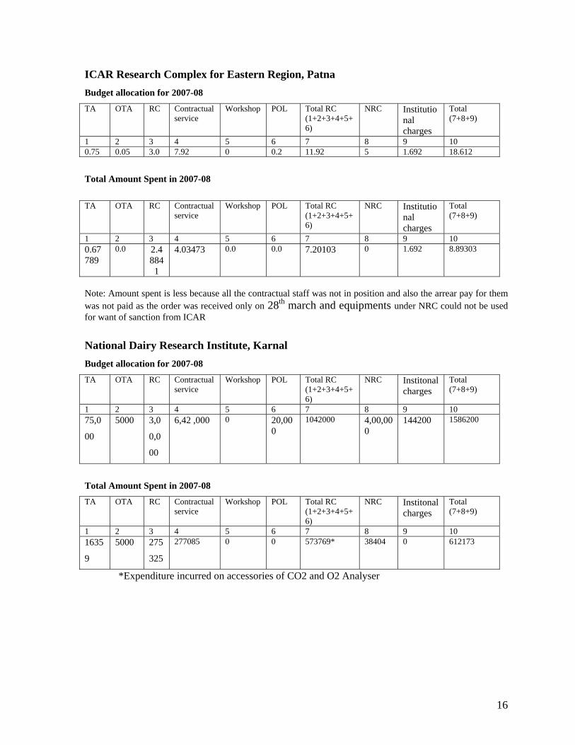
ICAR Research Complex for Eastern Region, Patna Budget allocation for 2007-08
TA OTA RC Contractual service
Workshop POL Total RC (1+2+3+4+5+6)
NRC Institutional charges
Total (7+8+9)
1 2 3 4 5 6 7 8 9 10 0.75 0.05 3.0 7.92 0 0.2 11.92 5 1.692 18.612
Total Amount Spent in 2007-08
TA OTA RC Contractual
service Workshop POL Total RC
(1+2+3+4+5+6)
NRC Institutional charges
Total (7+8+9)
1 2 3 4 5 6 7 8 9 10 0.67789
0.0 2.48841
4.03473 0.0 0.0 7.20103 0 1.692 8.89303
Note: Amount spent is less because all the contractual staff was not in position and also the arrear pay for them was not paid as the order was received only on 28th march and equipments under NRC could not be used for want of sanction from ICAR
National Dairy Research Institute, Karnal Budget allocation for 2007-08
TA OTA RC Contractual service
Workshop POL Total RC (1+2+3+4+5+6)
NRC Institonal charges
Total (7+8+9)
1 2 3 4 5 6 7 8 9 10 75,0
00
5000 3,0
0,0
00
6,42 ,000 0 20,000
1042000 4,00,000
144200 1586200
Total Amount Spent in 2007-08
TA OTA RC Contractual service
Workshop POL Total RC (1+2+3+4+5+6)
NRC Institonal charges
Total (7+8+9)
1 2 3 4 5 6 7 8 9 10 1635
9
5000 275
325
277085 0 0 573769* 38404 0 612173
*Expenditure incurred on accessories of CO2 and O2 Analyser
16
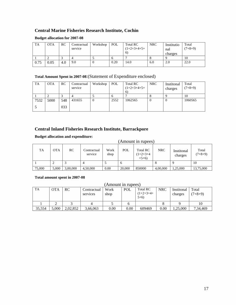
Central Marine Fisheries Research Institute, Cochin Budget allocation for 2007-08 TA OTA RC Contractual
service Workshop POL Total RC
(1+2+3+4+5+6)
NRC Institutional charges
Total (7+8+9)
1 2 3 4 5 6 7 8 9 10 0.75 0.05 4.0 9.0 0 0.20 14.0 6.0 2.0 22.0
Total Amount Spent in 2007-08:(Statement of Expenditure enclosed) TA OTA RC Contractual
service Workshop POL Total RC
(1+2+3+4+5+6)
NRC Institonal charges
Total (7+8+9)
1 2 3 4 5 6 7 8 9 10 7532
5
5000 548
033
431655 0 2552 1062565 0 0 1060565
Central Inland Fisheries Research Institute, Barrackpore Budget allocation and expenditure: (Amount in rupees)
TA
OTA
RC
Contractual
service
Work shop
POL
Total RC (1+2+3+4
+5+6)
NRC
Institonal charges
Total
(7+8+9)
1 2 3 4 5 6 8 9 10 75,000 5,000 3,00,000 4,50,000 0.00 20,000 850000 4,00,000 1,25,000 13,75,000 Total amount spent in 2007-08
(Amount in rupees) TA OTA RC Contractual
services Work shop
POL Total RC (1+2+3+4+5+6)
NRC Institonal charges
Total (7+8+9)
1 2 3 4 5 6 8 9 10 35,554 5,000 2,02,852 3,66,063 0.00 0.00 609469 0.00 1,25,000 7,34,469
17
18
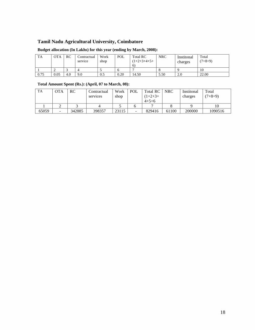
Tamil Nadu Agricultural University, Coimbatore Budget allocation (In Lakhs) for this year (ending by March, 2008):
TA OTA RC Contractual service
Work shop
POL Total RC (1+2+3+4+5+6)
NRC Institonal charges
Total (7+8+9)
1 2 3 4 5 6 7 8 9 10 0.75 0.05 4.0 9.0 0.5 0.20 14.50 5.50 2.0 22.00 Total Amount Spent (Rs.): (April, 07 to March, 08):
TA OTA RC Contractual services
Workshop
POL Total RC (1+2+3+4+5+6
NRC Institonal charges
Total (7+8+9)
1 2 3 4 5 6 7 8 9 10 65059 - 342885 398357 23115 - 829416 61100 200000 1090516
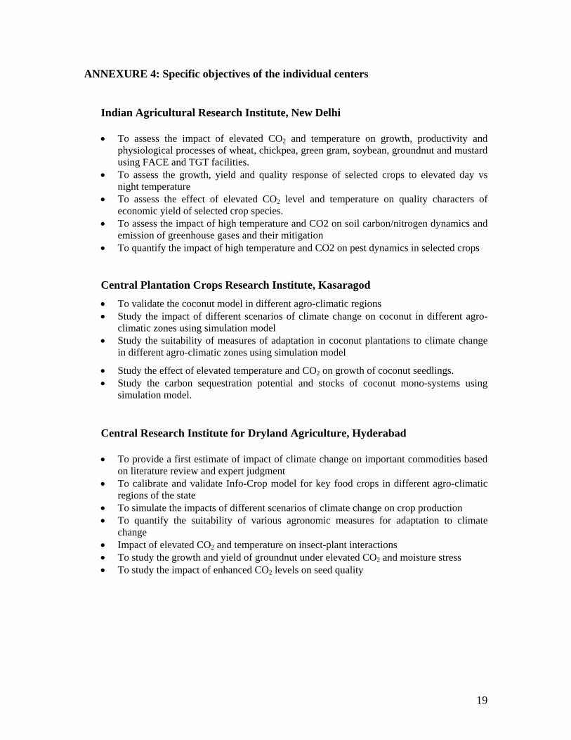
ANNEXURE 4: Specific objectives of the individual centers
Indian Agricultural Research Institute, New Delhi
• To assess the impact of elevated CO2 and temperature on growth, productivity and physiological processes of wheat, chickpea, green gram, soybean, groundnut and mustard using FACE and TGT facilities.
• To assess the growth, yield and quality response of selected crops to elevated day vs night temperature
• To assess the effect of elevated CO2 level and temperature on quality characters of economic yield of selected crop species.
• To assess the impact of high temperature and CO2 on soil carbon/nitrogen dynamics and emission of greenhouse gases and their mitigation
• To quantify the impact of high temperature and CO2 on pest dynamics in selected crops
Central Plantation Crops Research Institute, Kasaragod • To validate the coconut model in different agro-climatic regions • Study the impact of different scenarios of climate change on coconut in different agro-
climatic zones using simulation model • Study the suitability of measures of adaptation in coconut plantations to climate change
in different agro-climatic zones using simulation model
• Study the effect of elevated temperature and CO2 on growth of coconut seedlings. • Study the carbon sequestration potential and stocks of coconut mono-systems using
simulation model.
Central Research Institute for Dryland Agriculture, Hyderabad • To provide a first estimate of impact of climate change on important commodities based
on literature review and expert judgment • To calibrate and validate Info-Crop model for key food crops in different agro-climatic
regions of the state • To simulate the impacts of different scenarios of climate change on crop production • To quantify the suitability of various agronomic measures for adaptation to climate
change • Impact of elevated CO2 and temperature on insect-plant interactions • To study the growth and yield of groundnut under elevated CO2 and moisture stress • To study the impact of enhanced CO2 levels on seed quality
19
Indian Institute of Horticultural Research, Bangaluru • To study the effects of elevated CO2, temperature, water stress on growth, water use
efficiency, quality and yield of tomato and onion. • To correlate prevailing climatic conditions to phenology, crop performance and quality of
grape fruits and wine from different grape growing regions. • To assess the impact of climate change on onion and tomato using validated InfoCrop
model and working out adaptation strategies and assessing vulnerability of these crops under different agro-climatic regions.
• Linking different climate change scenarios with the models to quantify the impact in different agro-climatic regions and GIS mapping of spatial distribution of impacts.
CSK Himachal Pradesh Agricultural University, Palampur • To provide a first estimate of impact of climate change on important commodities based
on literature review and expert judgment. • To calibrate and validate INFOCROP for key food crops (Maize, wheat and rice) in
different agro-climatic region of the state. • To simulate the impacts of different scenarios of climate change on crop production. • To quantify the suitability of various agronomic measures for adaptation to climate
change Central Soil and Water Conservation Research and Training Institute, Dehradun
• To provide a first estimate of impact of climate change (run-off and soil loss) on
important commodities of selected Watersheds of India based on literature review and expert judgment.
• To calibrate and validate AVSWAT / Info-crop model for runoff, soil loss for key food crops in different Watersheds of the country.
• To simulate the impacts of different scenarios of climate change (run-off and soil loss) on crop production through MGLP/optimization
• To quantify the suitability of various Watershed Management measures for adaptation to climate change (run-off and soil loss).
ICAR Research Complex for Eastern Region, Patna • To calibrate and validate Infocrop model for key food crops in different agro climatic
regions of Bihar. • 2. To simulate the impacts of different scenarios of climate change on crop production in
Bihar • 3. To quantify the suitability of various agronomic and land and water management
measures for adaptation to climate change • 4. To develop integrated modeling framework for coupling hydrologic model with crop
water demand, water allocation and socio-economic models
20
21
National Dairy Research Institute, Karnal • To provide a first estimate of impact of sudden weather changes on livestock growth and
milk production based on literature review and expert judgment • To identify and calibrate NRC model for suitability in Indian dairy animals incorporating
changes in temperature and feed intake • To quantify magnitude of milk production decline in relation to cumulative THI load
during hot period and wind chill effects during cold months. • To quantify the suitability of various thermal stress alleviating measures for adaptation to
climate changes Central Marine Fisheries Research Institute, Cochin
• To assess the adaptability and vulnerability of marine organisms to elevated seawater temperature.
• To assess the impact on primary and secondary producers. • To evaluate socioeconomic conditions of coastal communities in the changed
scenarios. • To evolve adaptation and mitigation measures to sustain Indian marine fisheries.
Central Inland Fisheries Research Institute, Barrackpore • To survey the fish seed hatcheries in the districts of Puri, Khurda, Balasore, Mayurbhanj
in Orissa. • To study the species richness of rivers Mahanadi and Brahamani in districts of Cuttak,
Jajpur and Angul. • To develop a predictive regression model, based on the data of eight macro ecological
parameters related to fisheries of 14 major Indian rivers. • To study the effect of different range of temperature on the growth of fingerlings of L.
rohita Tamil Nadu Agricultural University, Coimbatore • Construction of Composite Vulnerability Index • Multi Goal Linear Programming (MGLP) for sustainable food security • To calibrate and validate InfoCrop / DSSAT models for key food crops in
different agroclimatic regions of Tamil Nadu. • To quantify the impacts of different scenarios of climate change on key crops
growth and production. • To quantify the suitability of various agronomic measures for adaptation to
climate change
ANNEXURE 5: Executive Summary by each centre
Indian Agricultural Research Institute, New Delhi
• The structural, operational and functional performances of infrastructure facilities
(FACE, OTC and TGT) were found to be satisfactory and minor problems could be rectified through further calibration. Results indicated that elevated temperature (+2-3oC) caused differential extent of reduction in growth and yield of different crops viz., rice, greengram, soybean, groundnut, wheat, and chickpea. Among the crops, wheat showed higher degree of sensitivity to high temperature as compared to legumes (greengram, soybean) and oilseeds (mustard, groundnut).
• Biomass and yield of soybean, greengram and potato reduced markedly with rise in
temperature (1- 4oC) owing to reduction in yield attributes. Among the yield components, 1000 grain/seed weight showed less sensitivity to high temperature.
• In experiments on exposure to high temperatures ether during day or night, soybean,
greengram, groundnut and potato showed reduction in yield under high daytime temperaure, while except potato other three crops yielded more under elevated night temp. In chickpea, exposure to high temperature for a fortnight at flowering stage reduced the sterility of pods, which had a beneficial effect on growth, and yield of crop.
• Elevated CO2 registered marked increase in the productivity of greengram, soybean,
chickpea and potato owing to increase in biomass and seed/tuber no. and their size. • Analysis on quality parameters in grains/tubers of crops (rice, green gram, soybean
and potato) indicated that increased temperature reduced carbohydrate content, while enhanced the level of protein in the grains and tubers. In general, seedling vigour is affected due to elevated temperature. Elevated CO2, on the other hand, increased sugar and starch contents and decreased protein content in potato. In soybean and green gram also there was reduction in protein content of grain due to elevated CO2.
• Analysis on emissions of carbon dioxide and nitrous oxide from soil in elevated
temperature indicated that the cumulative flux of carbon dioxide did not significantly increase with an average increase of temperature by 3.6oC over a period of 100 days in the kharif season. The cumulative flux of N2O-N from fertilized soil over 100 days increased by 21% over the ambient soil conditions. In the rabi season, the cumulative flux of carbon dioxide was found to be 12% higher in elevated temperature conditions than the ambient over a period of 115 days.
• Generic insect population dynamics models were developed based on the concept of
thermal times for different phenological stages. The model was validated for holometabolous, hemimetabolous and viviparous type of insect life cycles.
22
Central Plantation Crops Research Institute, Kasaragod
• Coconut simulation model is developed and validated to different agro-climatic zones. Simulated coconut potential total dry matter production varied across the agro-climatic zones from around 52 t.ha-1.year-1 in central southern plateau and hill zone of Karnataka to 62 t.ha-1.year-1 at south of southern plateau and hills zone of Tamil Nadu. Potential yields varied from 25 to 30 t.ha-1.year-1 depending on the agro-climatic zone.
• Using the coconut model, climate change impacts on coconut yield are simulated for HadCM3 A2a, B2a and A1F 2020, 2050 and 2080 scenarios. Results indicate positive effect on coconut yields in west coast and parts of TN and Karnataka and negative effects on nut yield in east coast of India. However, in the event of reduced availability of irrigation, the beneficial impacts will be less or negative impacts will be more.
• In Open Top Chamber (OTC) studies on coconut seedlings, morpho-physiological and biochemical analysis indicated initial responses of coconut seedlings to elevated temperature (+3 oC) and CO2 (550 and 700 ppm) as compared to chamber control. Seedlings grown in elevated CO2 have higher root dry matter, specific leaf area, chlorophyll a/b ratio, collar girth, shoot height, and shoot dry matter and leaf area as compared to those grown in chamber control. Seedlings exposed to elevated temperature have high shoot height; root length, collar girth and root dry matter and volume as compared to those in chamber control. Starch and reducing sugars were higher in seedlings grown in elevated CO2 condition as compared to the chamber control seedlings.
• Initial results indicate that elevated temperature during storage adversely effected oil quality in terms of free fatty acids, acid value and peroxide value.
Central Research Institute for Dryland Agriculture, Hyderabad
• The rainfall data of 174 stations well spread over Andhra Pradesh with a period ranging from 1871 to 2004 years was analysed and the significant trends were identified using the Mann Kendall test of significance. Using these values a rainfall trend map of Andhra Pradesh was generated. The percentage of occurrence of droughts was more during 1971-1980 and 1991-2000 decades when compared to 1981-1990 decade in all agro-climatic zones except Southern and Scarce rainfall zones.
• The total consumption of castor foliage by Spodoptera litura during the entire feeding period was significantly more under elevated CO2 conditions than ambient and chamber controls indicating 39% more consumption under elevated CO2 conditions.
• Groundnut crop showed positive response to elevated CO2 levels for growth and yield and the response was significantly evident at 700ppm. Moisture stress at initial stages improved the total biomass and pod yield in all the treatments and the response was
23
more at higher levels of CO2. The seed weight increased with moisture stress due to higher number of pods and seeds, however reduced 100 seed weight was observed with moisture stress. Both elevated CO2 levels increased the oil content and the response was more prominent at higher level.
• The unsaturated fatty acids increased over saturated fatty acids with elevated CO2 levels. It was also observed that the content of Oleic acid showed increasing trend with elevated CO2 levels where as the reverse trend was with linolenic acid fraction.
Indian Institute of Horticultural Research, Bangaluru
• The InfoCrop model was further calibrated from the data obtained from field experiments for determinate and indeterminate cultivars in tomato and four important cultivars of onion, grown under potential conditions during 1988-89 at Indian Institute of Horticultural Research, Bangalore.
• Validation of the models was taken up with the inputs from experiments conducted at different agro-ecological regions for different seasons, nitrogen and irrigation levels. The data from experiments conducted at Bangalore, Hyderabad, Hisar, New Delhi, Dharwad and Nasik were used for validating onion model and Bangalore, Karnal, Ludhiana, Bhubaneshwar and Hisar for tomato model.
• The preliminary sensitivity analysis of the validated models was done to quantify the impact of increase in temperature and CO2 on yield. It was observed that the yield reduction in tomato was only up to 20% when the temperature increased up to 5°C. In onion the yield reduction was up to 40% with increase in temperature of 3°C and 75% reduction with 4°C increase
• The analysis of the impact of climate change in terms of deviations in yield for 2020, 2050 and 2080 from base years for both onion and tomato was done. The model outputs on onion showed that, in Nasik region of Maharashtra, a major onion growing region, yields reductions would be more in Kharif season followed by Late Kharif season. Yield reductions would be lowest in Rabi season in 2020, 2050 and 2080 for the all the scenarios studied.
• Response of onion and tomato to elevated CO2 (550ppm) was studied in Open Top chambers. Tomato recorded a yield increase of 24.4% and onion recorded an increase of 25.9% at elevated CO2 concentration of 550ppm.
• In wine grape cv. Cabernet Sauvignon the relationship between mean maximum and minimum temperature prevailing during veraison to fruit maturity and berry anthocyanin and total flavonoids content showed a negative relationship. The difference between maximum and minimum temperature during the fruit maturation stage was found to have very high influence on berry anthocyanin content.
24
CSK Himachal Pradesh Agricultural University, Palampur
• Impact of elevated CO2 levels of 420 ppm and 470 ppm on maize crop under potential conditions and rainfed recommended condition showed an increase of 3.0% and 5.4% and 4.3 and 8.1% in 10th June sown crop respectively. Temperature rise by 1oC and 20C and reduction in rainfall caused decrease in maize yield by 2 to 10 %.
• In wheat, results indicated an increase in yield with elevated levels of CO2 to the tune of 4.9 to 7.3 % in early sown conditions (15th October).
Central Soil and Water Conservation Research and Training Institute, Dehradun • The relevant toposheets of the seven study watersheds (Almus, Tehri Garhwal; Belura,
Maharashtra; Pogalur,Coimbatore; Jonainala, Orissa; Udhagaman-dalam, TamilNadu; Umiam, Meghalaya; Antisar, Kheda,Gujrat) have been scanned, geo-referenced on UTM projection: datum WGS 84.The watershed boundary has been delineated and the contours and the boundary has digitized. The DEM has also been generated on Arc-view. The data of soil and land use, groundwater level and daily weather has been compiled for use in hydrological and crop models.
ICAR Research Complex for Eastern Region, Patna
• Projection using climate change scenarios indicate a likely increase in maize yields ranging from 13 to 38% while a reduction in wheat and rice yield is likely up to 25% and 37%, respectively with the climate change scenarios in 2020, 2050 and 2080 at Pusa. At Sabour a reduction up to 50% is projected for wheat yields and 15% reduction in rice yields.
• Analysis of past data indicated a decreasing trend in mean monthly streamflow in Upper Bhavani basin (lying upstream of the Bhavanisagar Reservoir with the two main rivers the Bhavani and the Moyar) in almost all the months except May and Jan was observed.
National Dairy Research Institute, Karnal
• Very high and low environmental temperatures and lack of prior conditioning result in to low production of livestock managed in unprotected or open or partially protected buildings. Heat and Cold wave with high wind velocity can push vulnerable animals beyond their survival threshold limits of high and low temperature. The consequences of exposure to extreme cold could be severe particularly in Indian animals not adapted to severe cold with high wind velocity. Covering of animals with loose, lightweight and warm jute materials (gunny bags clothing) can help in protection and excessive heat loss from body. Tightly-woven and water-repellant outer covers can further protect them from wet winters and wind chill effects.
• Stressful THI with 20h or more daily THI-hrs (THI >84) for several weeks affect animal responses. The animal thermal load is not dissipated that cause economic losses. Under climate change scenario increased number of stressful days with a change in Tmax and Tmin and decline in availability of water will further impact
25
animal productivity and health in Punjab, Rajasthan and Tamil Nadu. The change in seasonal mean temperatures and in the extreme temperatures in the future will impact animal reproductive cycles, milk yield and production The night temperature increase will not permit animals to dissipate their thermal loads and recovery to normal will be affected.
Central Marine Fisheries Research Institute, Cochin
• The Indian mackerel Rastrelliger kanagurta, one of the commercially important pelagic fish, is able to adapt to rise in sea surface temperature by extending distribution towards northern latitudes, and by descending to depths. During 1961-76, the mackerel catch along the northwest coast of India contributed about 7.5% to the all India mackerel catch, which increased to 18% during 1997-06. In the northeast coast, the mackerel catch contributed 0.4% to the all India mackerel catch during 1961-76, which increased to 1.7% during 1997-06. The mackerel was conventionally caught by surface drift gillnets by artisanal fishermen. In recent years, however, the fish is increasingly getting caught in bottom trawl nets operated by large mechanized boats at about 50 m depth. In 1985, only 2% of the total mackerel catch was from bottom trawlers. In the last five years, about 10% of the mackerel catch is by the bottom trawlers. This shows that the fish descends down to overcome warmer surface waters.
• To estimate the carbon foot print by marine fishing boats by data were collected on the diesel consumption from about 1332 mechanized boats and 631 motorized boats in the major fishing harbors along the east and west coast of India. Initial estimates indicate that fossil fuel consumption by marine fishing boats is around 1200 million liters per year and CO2 emission by marine fishing sector is around 2.4 million tonnes per year.
• Many of the coastal fishing villages are vulnerable to sea level rise as they are located close to the seashore. To identify the most vulnerable villages, a survey on the distance from high-tide line (HTL) to each fishing village was undertaken. Demographic details and infrastructure available in the fishing villages of maritime states were collected. There are about 2643 fishing villages along the Indian coast, out of which 458 are within 100m from the high tide line. The largest number of coastal fishing villages, (about 200) within 100m, are in Kerala. The population in the 458 coastal fishing villages is around 1 million. The data on vulnerable fishing villages will be helpful for estimating the cost of relocating the villages; and sensitize the fishing communities on the perils of rising sea level.
.
Central Inland Fisheries Research Institute, Barrackpore
• Under controlled laboratory conditions, the fingerlings of L. rohita were kept in different temperatures and ad libitum feeding. They showed conspicuous responses for their food conversation, food consumption, specific growth and weight gain with thermal variations in ambient waters. The fishes at the end 92 days exposure showed
26
27
progressive increase in above mentioned values in the thermal range between 29ºC and 34ºC but the trend reversed with further increased in temperature to 35ºC. With 4ºC increase in temperature from 29ºC to 33ºC the values raised by 12.29 % and when the ambient temperature of the fishes was increased to 34ºC the improvement was to the tune of 38.69%. However, when fishes exposed to 35ºC the weight was declined by 30.10% compared to that at 34ºC.
Tamil Nadu Agricultural University, Coimbatore
• Among the 11 coastal districts of Tamil Nadu, Ramnad and Nagapattinam are most vulnerable to climatic change. Among all the 30 districts, the vulnerability to climate change is very high in the Perambalur district followed by the Nilgiris and Ramnad as compared to the other districts.
• Analysis using the multi-linear goal programming model, indicated that possibility of increasing the total rice production by 1.58 million tonnes, which accounts for 31.23 per cent more than the existing current level from the different agro climatic regions of Tamil Nadu even by imposing all the constraints. At State level, even with all constraints are included, the farm income can be increased by about 51 billion rupees which is 108 per cent higher than the existing level of income earned by the farmers.
• Future changes in rainfall, maximum temperature and minimum temperature for 2020, 2040 and 2080 over the baseline data (2000) for Tamil Nadu region indicates that the precipitation may increase by 10 to 15 per cent during southwest monsoon season (June – September) while, there may be a slight reduction in rainfall in the south western zone alone during northeast monsoon season. With respect to temperature, there is an increase of 2.5 to 5°C is expected in both the seasons and more increase is expected in minimum temperature compared to maximum temperature.
• Study on impacts of climate change on rice production indicated that the rice production during southwest monsoon is expected to be affected more compared to northeast monsoon due to climate change. The reduction up to 35 and 50 per cent could be noticed in 2050 and 2080, respectively, in southern region of Tamil Nadu. The central eastern zone is the next vulnerable zone contributing 20 and 35 per cent yield reduction during 2050 and 2080, respectively. It is quite interesting to note that there is an increase in yield of 5 to 15 per cent in most of the locations during 2020 in northeast monsoon. During 2050, there is a slight reduction (10 – 15 %) in yield is expected in the southern zone. During 2080, in almost all the zones reduction would be 20 to 35 per cent.
• Analysis on the maize crop indicated that due to global warming, maize yields will decrease by 2.9, 10.1 and 20.4 per cent respectively during 2020, 2050 and 2080 from the current yield levels. The results of sorghum crop revealed that the expected decline in yields is 4.6, 15 and 24.6 per cent respectively during 2020, 2050 and 2080 from the current yield levels if no management intervention is made.
28
ANNEXURE 6: Detailed Progress Report
Indian Agricultural Research Institute, New Delhi
Objective 1. To assess the impact of elevated temperature and CO2 on growth and
productivity of different crops
Calibration of Free Air Carbon dioxide Enrichment (FACE) and Temperature
Gradient Tunnel (TGT) facility in field
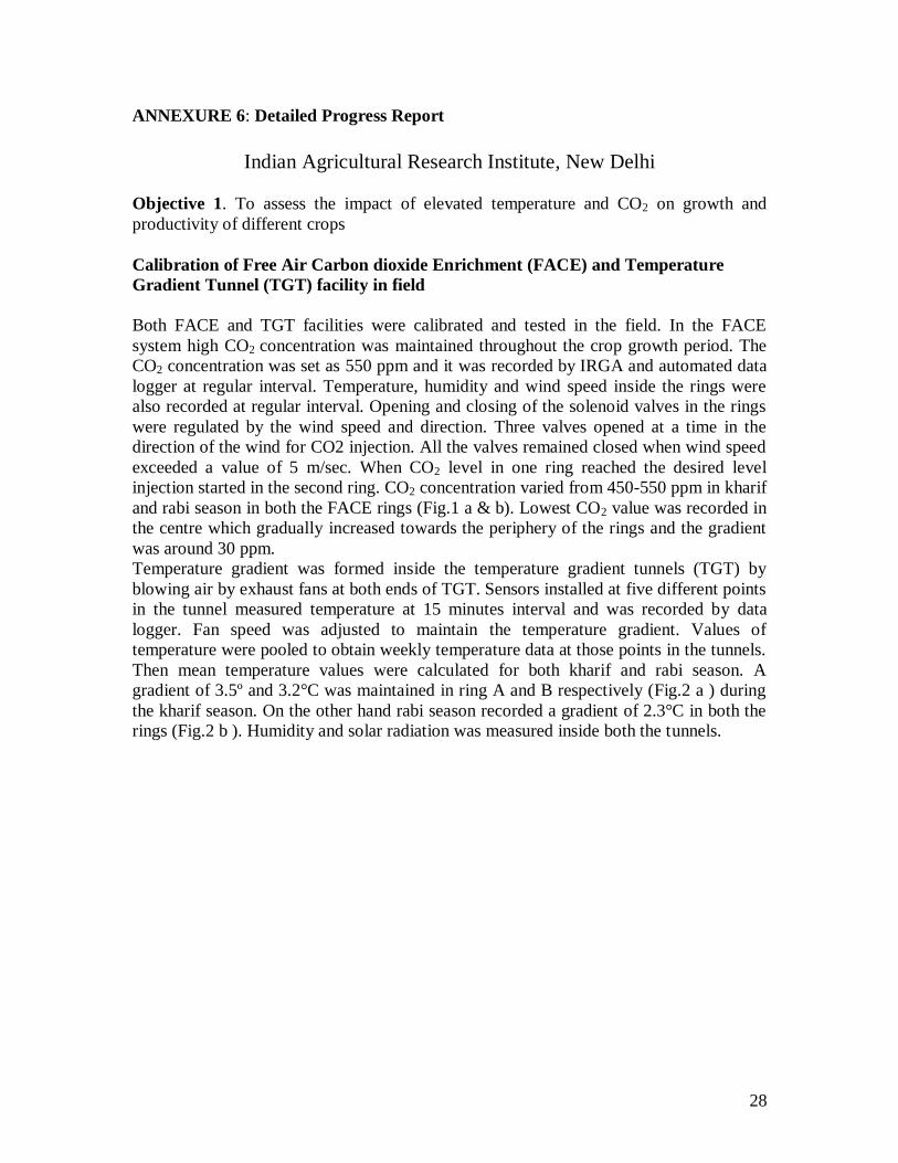
Both FACE and TGT facilities were calibrated and tested in the field. In the FACE
system high CO2 concentration was maintained throughout the crop growth period. The
CO2 concentration was set as 550 ppm and it was recorded by IRGA and automated data
logger at regular interval. Temperature, humidity and wind speed inside the rings were
also recorded at regular interval. Opening and closing of the solenoid valves in the rings
were regulated by the wind speed and direction. Three valves opened at a time in the
direction of the wind for CO2 injection. All the valves remained closed when wind speed
exceeded a value of 5 m/sec. When CO2 level in one ring reached the desired level
injection started in the second ring. CO2 concentration varied from 450-550 ppm in kharif
and rabi season in both the FACE rings (Fig.1 a & b). Lowest CO2 value was recorded in
the centre which gradually increased towards the periphery of the rings and the gradient
was around 30 ppm.
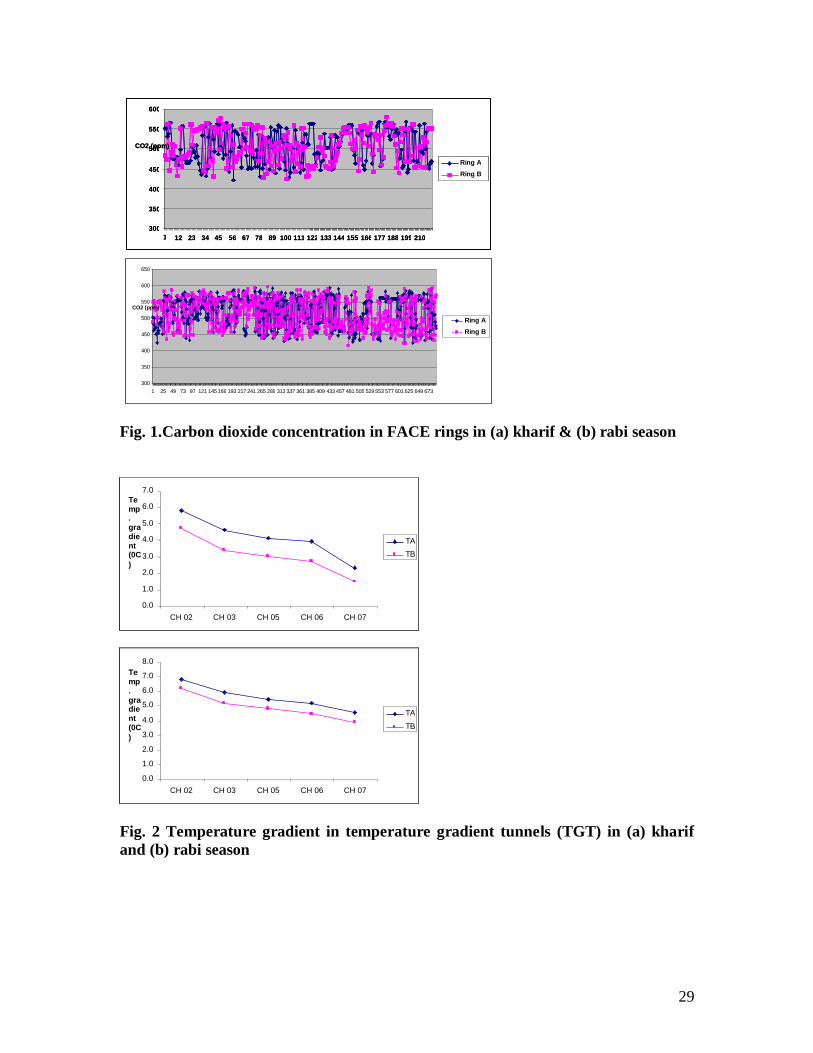
Temperature gradient was formed inside the temperature gradient tunnels (TGT) by
blowing air by exhaust fans at both ends of TGT. Sensors installed at five different points
in the tunnel measured temperature at 15 minutes interval and was recorded by data
logger. Fan speed was adjusted to maintain the temperature gradient. Values of
temperature were pooled to obtain weekly temperature data at those points in the tunnels.
Then mean temperature values were calculated for both kharif and rabi season. A
gradient of 3.5º and 3.2°C was maintained in ring A and B respectively (Fig.2 a ) during
the kharif season. On the other hand rabi season recorded a gradient of 2.3°C in both the
rings (Fig.2 b ). Humidity and solar radiation was measured inside both the tunnels.
29
Fig. 1.Carbon dioxide concentration in FACE rings in (a) kharif & (b) rabi season
0.0 1.0 2.0 3.0 4.0 5.0 6.0 7.0
CH 02 CH 03 CH 05 CH 06 CH 07
Temp. gradient (0C
)
TA TB
0.0 1.0 2.0 3.0 4.0 5.0 6.0 7.0 8.0
CH 02 CH 03 CH 05 CH 06 CH 07
Temp. gradient (0C
)
TA TB
0.0 1.0 2.0 3.0 4.0 5.0 6.0 7.0
CH 02 CH 03 CH 05 CH 06 CH 07
Temp. gradient (0C
)
TA TB
0.0 1.0 2.0 3.0 4.0 5.0 6.0 7.0 8.0
CH 02 CH 03 CH 05 CH 06 CH 07
Temp. gradient (0C
)
TA TB
Fig. 2 Temperature gradient in temperature gradient tunnels (TGT) in (a) kharif
and (b) rabi season
300
350
400
450
500
550
600
1 12 23 34 45 56 67 78 89 100 111 122 133 144 155 166 177 188 199 210
CO2 (ppm) Ring A Ring B
300
350
400
450
500
550
600
1 12 23 34 45 56 67 78 89 100 111 122 133 144 155 166 177 188 199 210
CO2 (ppm) Ring A Ring B
300 350 400 450 500 550 600 650
1 25 49 73 97 121 145 169 193 217 241 265 289 313 337 361 385 409 433 457 481 505 529 553 577 601 625 649 673
CO2 (ppm) Ring A Ring B
30
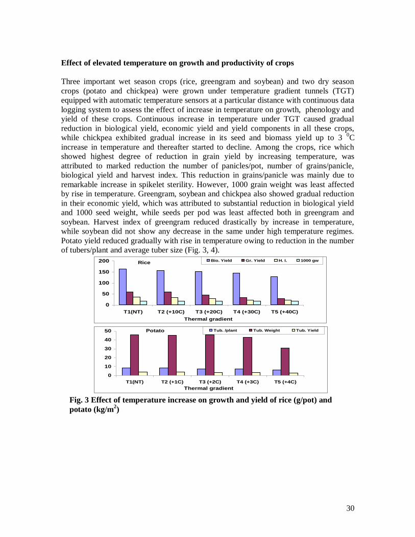
Effect of elevated temperature on growth and productivity of crops
Three important wet season crops (rice, greengram and soybean) and two dry season
crops (potato and chickpea) were grown under temperature gradient tunnels (TGT)
equipped with automatic temperature sensors at a particular distance with continuous data
logging system to assess the effect of increase in temperature on growth, phenology and
yield of these crops. Continuous increase in temperature under TGT caused gradual
reduction in biological yield, economic yield and yield components in all these crops,
while chickpea exhibited gradual increase in its seed and biomass yield up to 3 0C
increase in temperature and thereafter started to decline. Among the crops, rice which
showed highest degree of reduction in grain yield by increasing temperature, was
attributed to marked reduction the number of panicles/pot, number of grains/panicle,
biological yield and harvest index. This reduction in grains/panicle was mainly due to
remarkable increase in spikelet sterility. However, 1000 grain weight was least affected
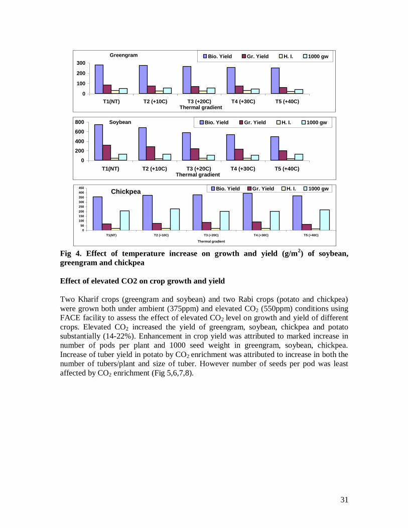
by rise in temperature. Greengram, soybean and chickpea also showed gradual reduction
in their economic yield, which was attributed to substantial reduction in biological yield
and 1000 seed weight, while seeds per pod was least affected both in greengram and
soybean. Harvest index of greengram reduced drastically by increase in temperature,
while soybean did not show any decrease in the same under high temperature regimes.
Potato yield reduced gradually with rise in temperature owing to reduction in the number
of tubers/plant and average tuber size (Fig. 3, 4).
Potato
0
10
20
30
40
50
T1(NT) T2 (+1C) T3 (+2C) T4 (+3C) T5 (+4C)
Thermal gradient
Tub. /plant Tub. Weight Tub. Yield
Rice
0
50
100
150
200
T1(NT) T2 (+10C) T3 (+20C) T4 (+30C) T5 (+40C)
Thermal gradient
Bio. Yield Gr. Yield H. I. 1000 gw
Fig. 3 Effect of temperature increase on growth and yield of rice (g/pot) and
potato (kg/m2)
31
Greengram
0
100
200
300
T1(NT) T2 (+10C) T3 (+20C) T4 (+30C) T5 (+40C)Thermal gradient
Bio. Yield Gr. Yield H. I. 1000 gw
Soybean
0
200
400
600
800
T1(NT) T2 (+10C) T3 (+20C) T4 (+30C) T5 (+40C)Thermal gradient
Bio. Yield Gr. Yield H. I. 1000 gw
0
50
100
150
200
250
300
350
400
450
T1(NT) T2 (+10C) T3 (+20C) T4 (+30C) T5 (+40C)
Thermal gradient
Bio. Yield Gr. Yield H. I. 1000 gwChickpea
Fig 4. Effect of temperature increase on growth and yield (g/m
2) of soybean,
greengram and chickpea
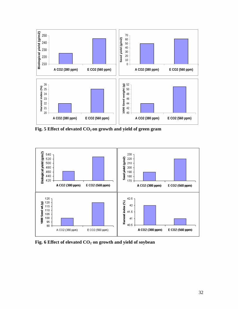
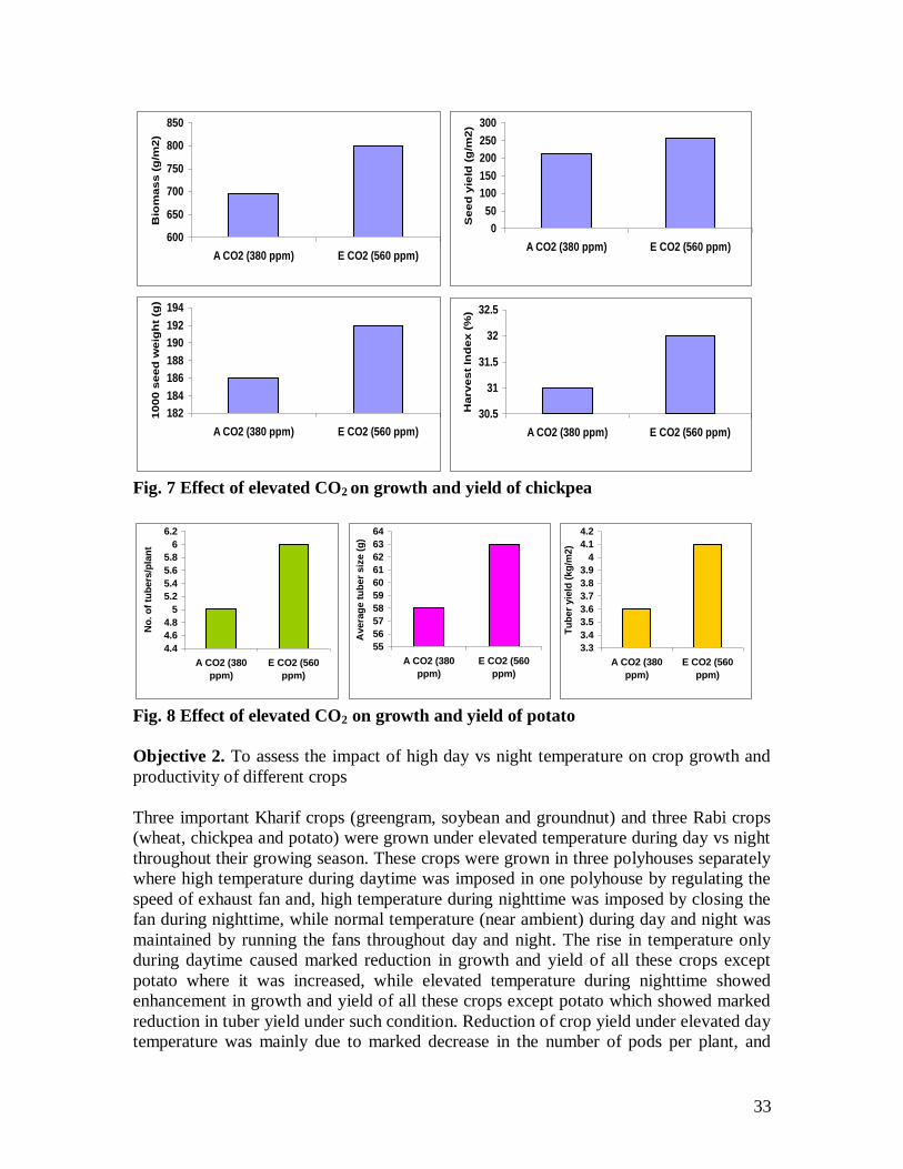
Effect of elevated CO2 on crop growth and yield
Two Kharif crops (greengram and soybean) and two Rabi crops (potato and chickpea)
were grown both under ambient (375ppm) and elevated CO2 (550ppm) conditions using
FACE facility to assess the effect of elevated CO2 level on growth and yield of different
crops. Elevated CO2 increased the yield of greengram, soybean, chickpea and potato
substantially (14-22%). Enhancement in crop yield was attributed to marked increase in
number of pods per plant and 1000 seed weight in greengram, soybean, chickpea.
Increase of tuber yield in potato by CO2 enrichment was attributed to increase in both the
number of tubers/plant and size of tuber. However number of seeds per pod was least
affected by CO2 enrichment (Fig 5,6,7,8).
32
210
220
230
240
250
A CO2 (380 ppm) E CO2 (560 ppm)Bio
log
ical
yie
ld (
g/m
2)
0
10
20
30
40
50
60
70
A CO2 (380 ppm) E CO2 (560 ppm)
Seed
yie
ld (
g/m
2)
20
21
22
23
24
25
26
A CO2 (380 ppm) E CO2 (560 ppm)
Harvest
ind
ex (
%)
40
42
44
46
48
50
52
A CO2 (380 ppm) E CO2 (560 ppm)
1000 S
eed
weig
ht
(g)
Fig. 5 Effect of elevated CO2 on growth and yield of green gram
Fig. 6 Effect of elevated CO2 on growth and yield of soybean
33
600
650
700
750
800
850
A CO2 (380 ppm) E CO2 (560 ppm)
Bio
ma
ss
(g
/m2
)
0
50
100
150
200
250
300
A CO2 (380 ppm) E CO2 (560 ppm)
Se
ed
yie
ld (
g/m
2)
30.5
31
31.5
32
32.5
A CO2 (380 ppm) E CO2 (560 ppm)
Ha
rve
st
Ind
ex
(%
)
182
184
186
188
190
192
194
A CO2 (380 ppm) E CO2 (560 ppm)
10
00
se
ed
we
igh
t (g
)
Fig. 7 Effect of elevated CO2 on growth and yield of chickpea
4.4
4.6
4.8
5
5.2
5.4
5.6
5.8
6
6.2
A CO2 (380
ppm)
E CO2 (560
ppm)
No
. o
f tu
bers
/pla
nt
55
56
57
58
59
60
61
62
63
64
A CO2 (380
ppm)
E CO2 (560
ppm)
Avera
ge t
ub
er
siz
e (
g)
3.3
3.4
3.5
3.6
3.7
3.8
3.9
4
4.1
4.2
A CO2 (380
ppm)
E CO2 (560
ppm)
Tu
ber
yie
ld (
kg
/m2)
Fig. 8 Effect of elevated CO2 on growth and yield of potato
Objective 2. To assess the impact of high day vs night temperature on crop growth and
productivity of different crops
Three important Kharif crops (greengram, soybean and groundnut) and three Rabi crops
(wheat, chickpea and potato) were grown under elevated temperature during day vs night
throughout their growing season. These crops were grown in three polyhouses separately
where high temperature during daytime was imposed in one polyhouse by regulating the
speed of exhaust fan and, high temperature during nighttime was imposed by closing the
fan during nighttime, while normal temperature (near ambient) during day and night was
maintained by running the fans throughout day and night. The rise in temperature only
during daytime caused marked reduction in growth and yield of all these crops except
potato where it was increased, while elevated temperature during nighttime showed
enhancement in growth and yield of all these crops except potato which showed marked
reduction in tuber yield under such condition. Reduction of crop yield under elevated day
temperature was mainly due to marked decrease in the number of pods per plant, and
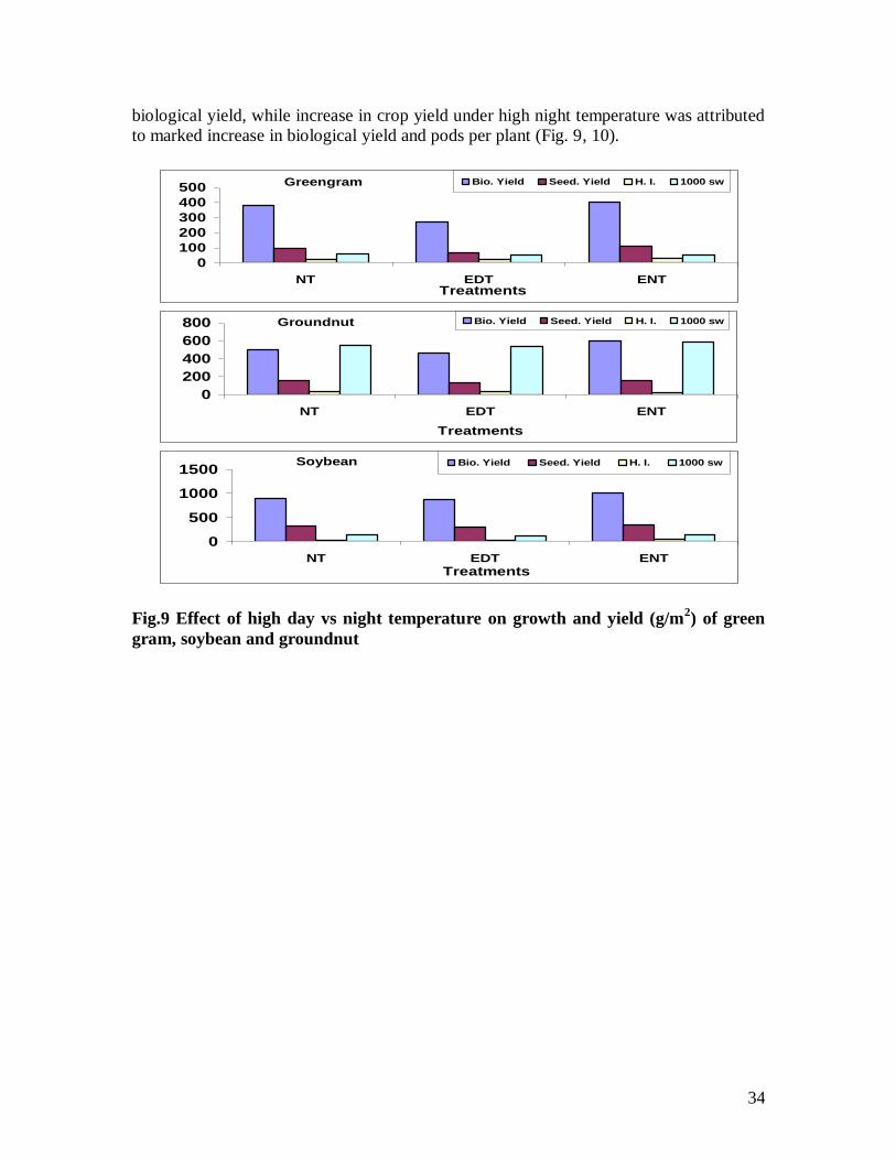
34
biological yield, while increase in crop yield under high night temperature was attributed
to marked increase in biological yield and pods per plant (Fig. 9, 10).
Greengram
0
100
200
300
400
500
NT EDT ENTTreatments
Bio. Yield Seed. Yield H. I. 1000 sw
Soybean
0
500
1000
1500
NT EDT ENT
Treatments
Bio. Yield Seed. Yield H. I. 1000 sw
Groundnut
0
200
400
600
800
NT EDT ENT
Treatments
Bio. Yield Seed. Yield H. I. 1000 sw
Fig.9 Effect of high day vs night temperature on growth and yield (g/m2) of green
gram, soybean and groundnut
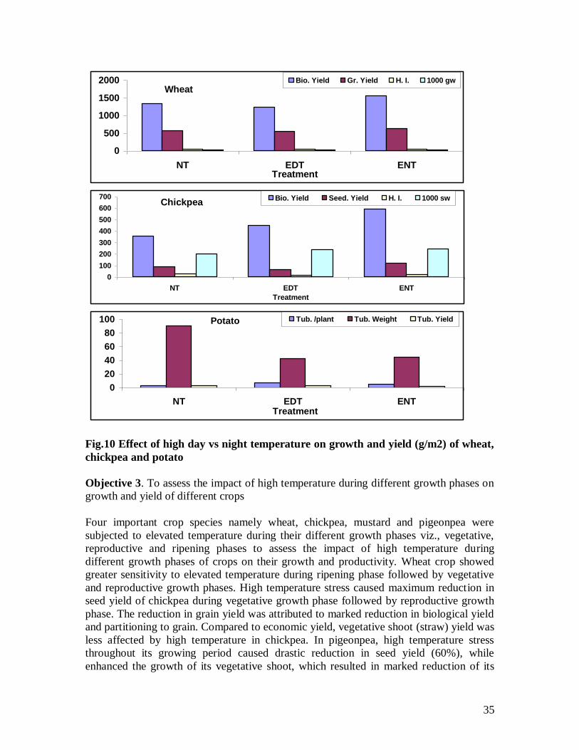
35
Wheat
0
500
1000
1500
2000
NT EDT ENTTreatment
Bio. Yield Gr. Yield H. I. 1000 gw
Chickpea
0
100
200
300
400
500
600
700
NT EDT ENT
Treatment
Bio. Yield Seed. Yield H. I. 1000 sw
Potato
0
20
40
60
80
100
NT EDT ENTTreatment
Tub. /plant Tub. Weight Tub. Yield
Fig.10 Effect of high day vs night temperature on growth and yield (g/m2) of wheat,
chickpea and potato
Objective 3. To assess the impact of high temperature during different growth phases on
growth and yield of different crops
Four important crop species namely wheat, chickpea, mustard and pigeonpea were
subjected to elevated temperature during their different growth phases viz., vegetative,
reproductive and ripening phases to assess the impact of high temperature during
different growth phases of crops on their growth and productivity. Wheat crop showed
greater sensitivity to elevated temperature during ripening phase followed by vegetative
and reproductive growth phases. High temperature stress caused maximum reduction in
seed yield of chickpea during vegetative growth phase followed by reproductive growth
phase. The reduction in grain yield was attributed to marked reduction in biological yield
and partitioning to grain. Compared to economic yield, vegetative shoot (straw) yield was
less affected by high temperature in chickpea. In pigeonpea, high temperature stress
throughout its growing period caused drastic reduction in seed yield (60%), while
enhanced the growth of its vegetative shoot, which resulted in marked reduction of its
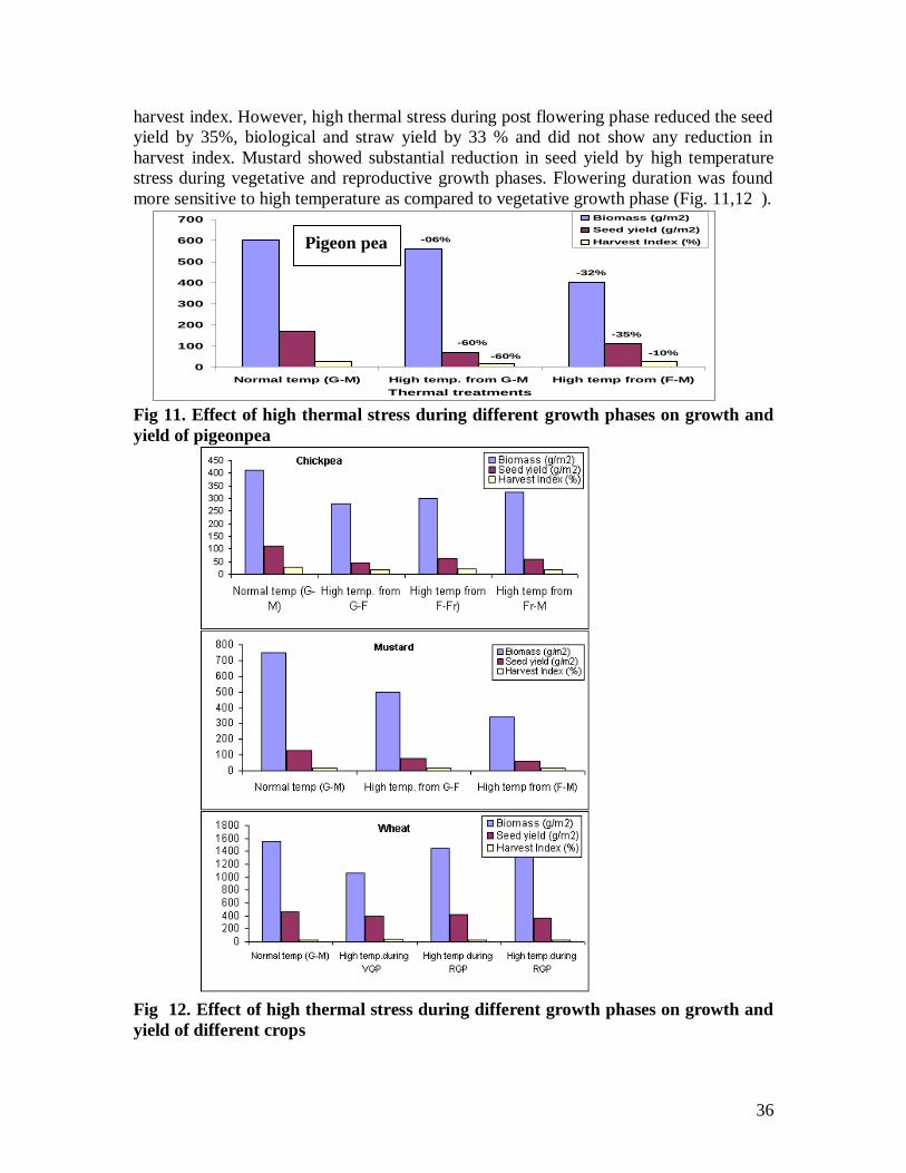
36
harvest index. However, high thermal stress during post flowering phase reduced the seed
yield by 35%, biological and straw yield by 33 % and did not show any reduction in
harvest index. Mustard showed substantial reduction in seed yield by high temperature
stress during vegetative and reproductive growth phases. Flowering duration was found
more sensitive to high temperature as compared to vegetative growth phase (Fig. 11,12 ).
0
100
200
300
400
500
600
700
Normal temp (G-M) High temp. from G-M High temp from (F-M)
Thermal treatments
Biomass (g/m2)
Seed yield (g/m2)
Harvest Index (%)-06%
-60%
-60%
-32%
-35%
-10%
Fig 11. Effect of high thermal stress during different growth phases on growth and
yield of pigeonpea
Fig 12. Effect of high thermal stress during different growth phases on growth and
yield of different crops
Pigeon pea
37
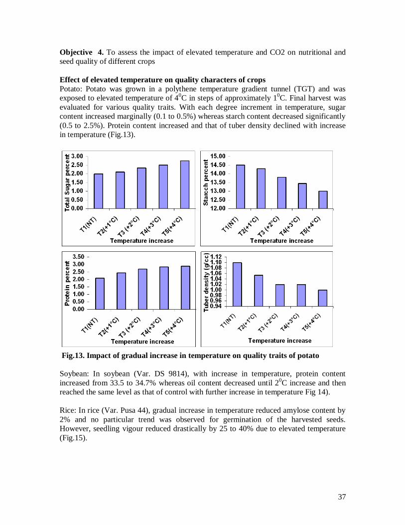
Objective 4. To assess the impact of elevated temperature and CO2 on nutritional and
seed quality of different crops
Effect of elevated temperature on quality characters of crops
Potato: Potato was grown in a polythene temperature gradient tunnel (TGT) and was
exposed to elevated temperature of 40C in steps of approximately 1
0C. Final harvest was
evaluated for various quality traits. With each degree increment in temperature, sugar
content increased marginally (0.1 to 0.5%) whereas starch content decreased significantly
(0.5 to 2.5%). Protein content increased and that of tuber density declined with increase
in temperature (Fig.13).
Fig.13. Impact of gradual increase in temperature on quality traits of potato
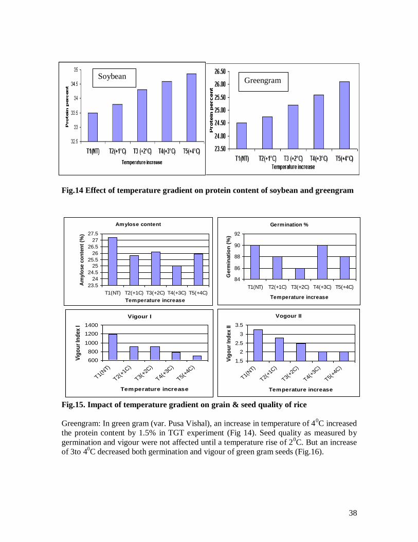
Soybean: In soybean (Var. DS 9814), with increase in temperature, protein content
increased from 33.5 to 34.7% whereas oil content decreased until 20C increase and then
reached the same level as that of control with further increase in temperature Fig 14).
Rice: In rice (Var. Pusa 44), gradual increase in temperature reduced amylose content by
2% and no particular trend was observed for germination of the harvested seeds.
However, seedling vigour reduced drastically by 25 to 40% due to elevated temperature
(Fig.15).
38
Amylose content
23.5
24
24.5
25
25.5
26
26.5
27
27.5
T1(NT) T2(+1C) T3(+2C) T4(+3C) T5(+4C)
Temperature increase
Am
ylo
se c
on
ten
t (%
)
Germination %
84
86
88
90
92
T1(NT) T2(+1C) T3(+2C) T4(+3C) T5(+4C)
Temperature increase
Germ
inati
on
(%
)
Vigour I
600
800
1000
1200
1400
T1(NT)
T2(+1
C)
T3(+2
C)
T4(+3
C)
T5(+4
C)
Temperature increase
Vig
ou
r In
dex I
Vogour II
1.5
2
2.5
3
3.5
T1(NT)
T2(+1
C)
T3(+2
C)
T4(+3
C)
T5(+4
C)
Temperature increase
Vig
ou
r In
dex II
Fig.14 Effect of temperature gradient on protein content of soybean and greengram
Fig.15. Impact of temperature gradient on grain & seed quality of rice
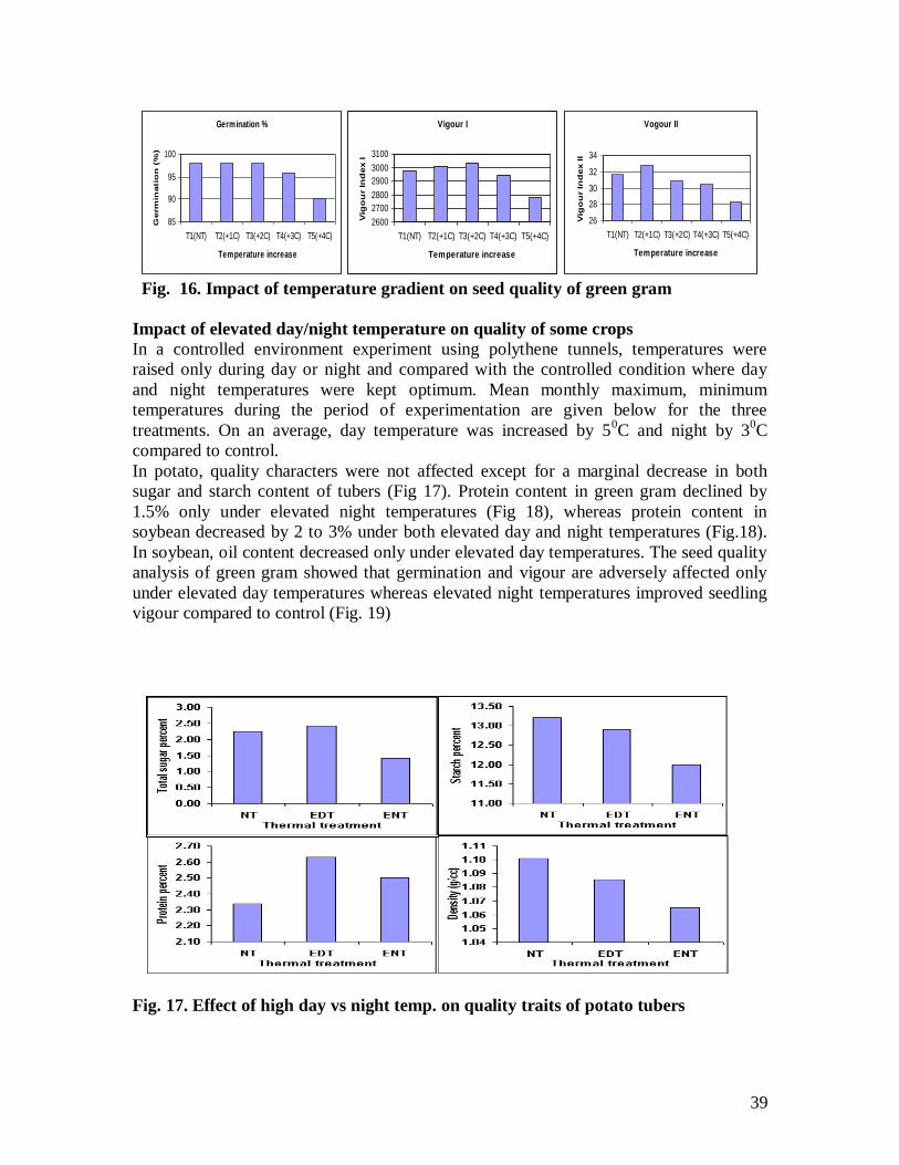
Greengram: In green gram (var. Pusa Vishal), an increase in temperature of 40C increased
the protein content by 1.5% in TGT experiment (Fig 14). Seed quality as measured by
germination and vigour were not affected until a temperature rise of 20C. But an increase
of 3to 40C decreased both germination and vigour of green gram seeds (Fig.16).
Soybean Greengram
39
Fig. 16. Impact of temperature gradient on seed quality of green gram
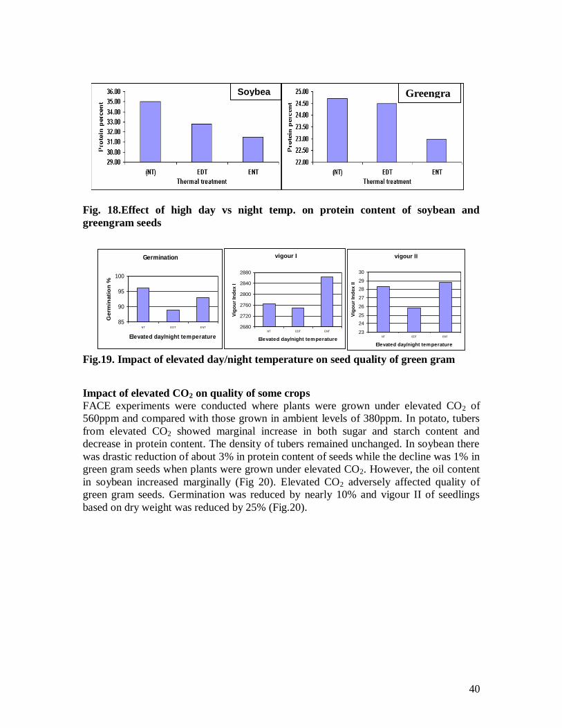
Impact of elevated day/night temperature on quality of some crops
In a controlled environment experiment using polythene tunnels, temperatures were
raised only during day or night and compared with the controlled condition where day
and night temperatures were kept optimum. Mean monthly maximum, minimum
temperatures during the period of experimentation are given below for the three
treatments. On an average, day temperature was increased by 50C and night by 3
0C
compared to control.
In potato, quality characters were not affected except for a marginal decrease in both
sugar and starch content of tubers (Fig 17). Protein content in green gram declined by
1.5% only under elevated night temperatures (Fig 18), whereas protein content in
soybean decreased by 2 to 3% under both elevated day and night temperatures (Fig.18).
In soybean, oil content decreased only under elevated day temperatures. The seed quality
analysis of green gram showed that germination and vigour are adversely affected only
under elevated day temperatures whereas elevated night temperatures improved seedling
vigour compared to control (Fig. 19)
Fig. 17. Effect of high day vs night temp. on quality traits of potato tubers
Germination %
85
90
95
100
T1(NT) T2(+1C) T3(+2C) T4(+3C) T5(+4C)
Temperature increase
Germ
inatio
n (
%)
Vigour I
2600
2700
2800
2900
3000
3100
T1(NT) T2(+1C) T3(+2C) T4(+3C) T5(+4C)
Temperature increase
Vig
ou
r In
dex I
Vogour II
26
28
30
32
34
T1(NT) T2(+1C) T3(+2C) T4(+3C) T5(+4C)
Temperature increase
Vig
ou
r In
dex II
40
Fig. 18.Effect of high day vs night temp. on protein content of soybean and
greengram seeds
Fig.19. Impact of elevated day/night temperature on seed quality of green gram
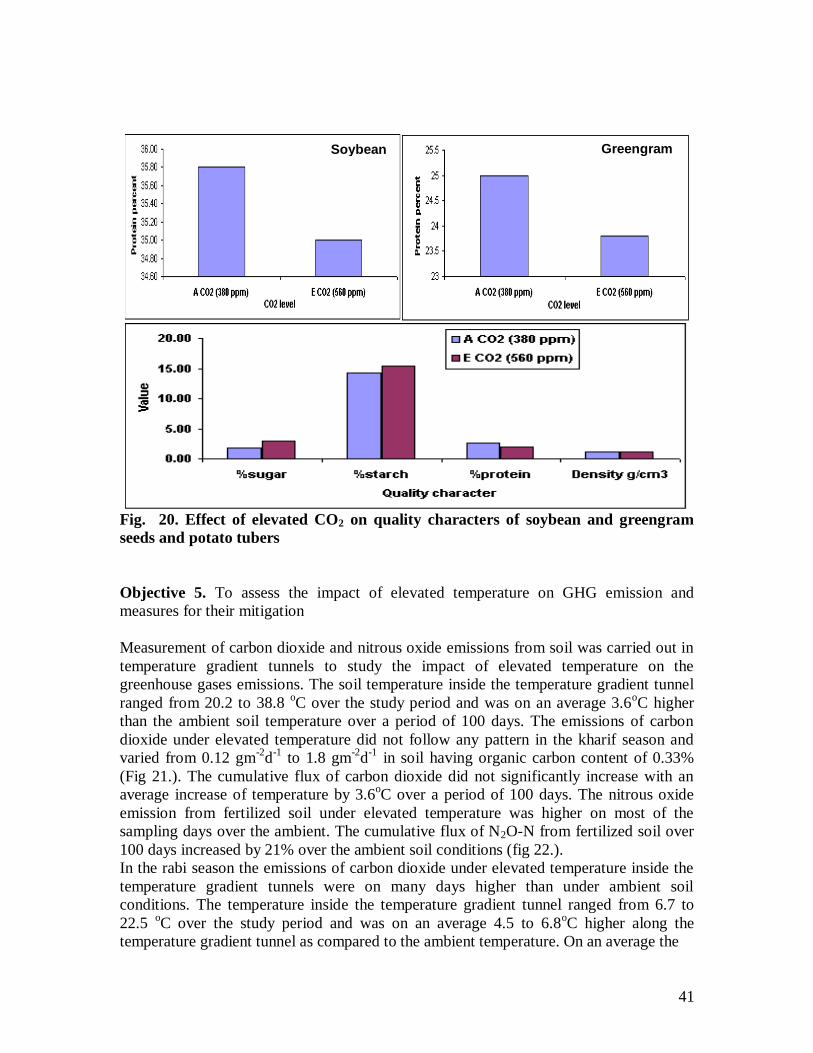
Impact of elevated CO2 on quality of some crops
FACE experiments were conducted where plants were grown under elevated CO2 of
560ppm and compared with those grown in ambient levels of 380ppm. In potato, tubers
from elevated CO2 showed marginal increase in both sugar and starch content and
decrease in protein content. The density of tubers remained unchanged. In soybean there
was drastic reduction of about 3% in protein content of seeds while the decline was 1% in
green gram seeds when plants were grown under elevated CO2. However, the oil content
in soybean increased marginally (Fig 20). Elevated CO2 adversely affected quality of
green gram seeds. Germination was reduced by nearly 10% and vigour II of seedlings
based on dry weight was reduced by 25% (Fig.20).
vigour II
23
24
25
26
27
28
29
30
NT EDT ENT
Elevated day/night temperature
Vig
ou
r In
dex II
Germination
85
90
95
100
NT EDT ENT
Elevated day/night temperature
Germ
inati
on
%
vigour I
2680
2720
2760
2800
2840
2880
NT EDT ENT
Elevated day/night temperature
Vig
ou
r In
dex I
Soybeannn
Greengra
m
41
Fig. 20. Effect of elevated CO2 on quality characters of soybean and greengram
seeds and potato tubers
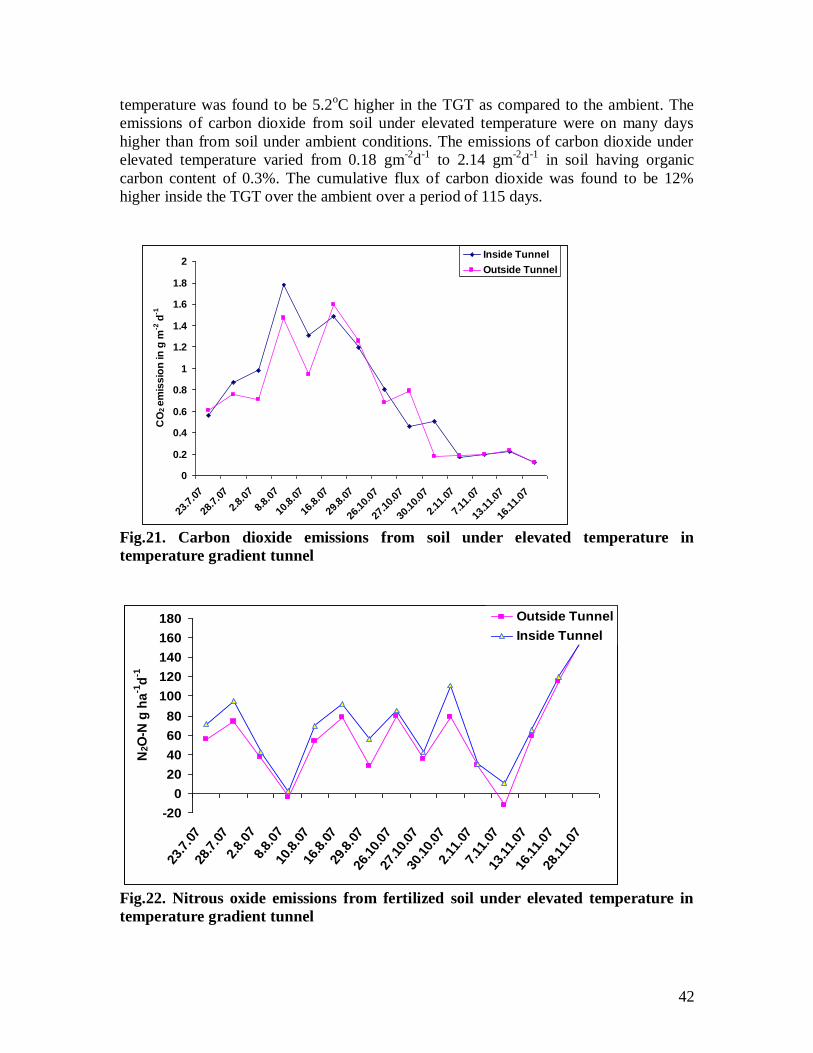
Objective 5. To assess the impact of elevated temperature on GHG emission and
measures for their mitigation
Measurement of carbon dioxide and nitrous oxide emissions from soil was carried out in
temperature gradient tunnels to study the impact of elevated temperature on the
greenhouse gases emissions. The soil temperature inside the temperature gradient tunnel
ranged from 20.2 to 38.8 oC over the study period and was on an average 3.6
oC higher
than the ambient soil temperature over a period of 100 days. The emissions of carbon
dioxide under elevated temperature did not follow any pattern in the kharif season and
varied from 0.12 gm-2
d-1
to 1.8 gm-2
d-1
in soil having organic carbon content of 0.33%
(Fig 21.). The cumulative flux of carbon dioxide did not significantly increase with an
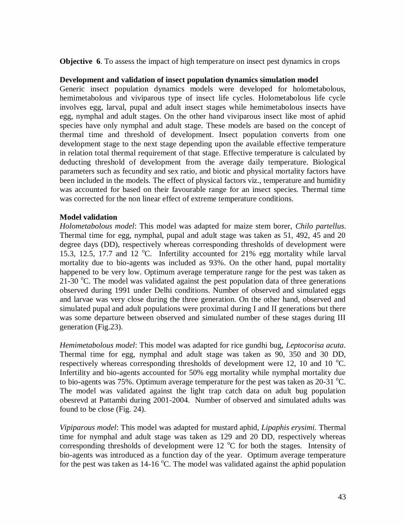
average increase of temperature by 3.6oC over a period of 100 days. The nitrous oxide
emission from fertilized soil under elevated temperature was higher on most of the
sampling days over the ambient. The cumulative flux of N2O-N from fertilized soil over
100 days increased by 21% over the ambient soil conditions (fig 22.).
In the rabi season the emissions of carbon dioxide under elevated temperature inside the
temperature gradient tunnels were on many days higher than under ambient soil
conditions. The temperature inside the temperature gradient tunnel ranged from 6.7 to
22.5 oC over the study period and was on an average 4.5 to 6.8
oC higher along the
temperature gradient tunnel as compared to the ambient temperature. On an average the
Greengram Soybean
42
temperature was found to be 5.2oC higher in the TGT as compared to the ambient. The
emissions of carbon dioxide from soil under elevated temperature were on many days
higher than from soil under ambient conditions. The emissions of carbon dioxide under
elevated temperature varied from 0.18 gm-2
d-1
to 2.14 gm-2
d-1
in soil having organic
carbon content of 0.3%. The cumulative flux of carbon dioxide was found to be 12%
higher inside the TGT over the ambient over a period of 115 days.
0
0.2
0.4
0.6
0.8
1
1.2
1.4
1.6
1.8
2
23.7
.07
28.7
.07
2.8.
07
8.8.
07
10.8
.07
16.8
.07
29.8
.07
26.1
0.07
27.1
0.07
30.1
0.07
2.11
.07
7.11
.07
13.1
1.07
16.1
1.07
CO
2 e
mis
sio
n in
g m
-2 d
-1
Inside Tunnel
Outside Tunnel
Fig.21. Carbon dioxide emissions from soil under elevated temperature in
temperature gradient tunnel
-20
0
20
40
60
80
100
120
140
160
180
23.7
.07
28.7
.07
2.8.
078.
8.07
10.8
.07
16.8
.07
29.8
.07
26.1
0.07
27.1
0.07
30.1
0.07
2.11
.07
7.11
.07
13.1
1.07
16.1
1.07
28.1
1.07
N2O
-N g
ha
-1d
-1
Outside Tunnel
Inside Tunnel
Fig.22. Nitrous oxide emissions from fertilized soil under elevated temperature in
temperature gradient tunnel
43
Objective 6. To assess the impact of high temperature on insect pest dynamics in crops
Development and validation of insect population dynamics simulation model
Generic insect population dynamics models were developed for holometabolous,
hemimetabolous and viviparous type of insect life cycles. Holometabolous life cycle
involves egg, larval, pupal and adult insect stages while hemimetabolous insects have
egg, nymphal and adult stages. On the other hand viviparous insect like most of aphid
species have only nymphal and adult stage. These models are based on the concept of
thermal time and threshold of development. Insect population converts from one
development stage to the next stage depending upon the available effective temperature
in relation total thermal requirement of that stage. Effective temperature is calculated by
deducting threshold of development from the average daily temperature. Biological
parameters such as fecundity and sex ratio, and biotic and physical mortality factors have
been included in the models. The effect of physical factors viz., temperature and humidity
was accounted for based on their favourable range for an insect species. Thermal time
was corrected for the non linear effect of extreme temperature conditions.
Model validation
Holometabolous model: This model was adapted for maize stem borer, Chilo partellus.
Thermal time for egg, nymphal, pupal and adult stage was taken as 51, 492, 45 and 20
degree days (DD), respectively whereas corresponding thresholds of development were
15.3, 12.5, 17.7 and 12 oC. Infertility accounted for 21% egg mortality while larval
mortality due to bio-agents was included as 93%. On the other hand, pupal mortality
happened to be very low. Optimum average temperature range for the pest was taken as
21-30 oC. The model was validated against the pest population data of three generations
observed during 1991 under Delhi conditions. Number of observed and simulated eggs
and larvae was very close during the three generation. On the other hand, observed and
simulated pupal and adult populations were proximal during I and II generations but there
was some departure between observed and simulated number of these stages during III
generation (Fig.23).
Hemimetabolous model: This model was adapted for rice gundhi bug, Leptocorisa acuta.
Thermal time for egg, nymphal and adult stage was taken as 90, 350 and 30 DD,
respectively whereas corresponding thresholds of development were 12, 10 and 10 oC.
Infertility and bio-agents accounted for 50% egg mortality while nymphal mortality due
to bio-agents was 75%. Optimum average temperature for the pest was taken as 20-31 oC.
The model was validated against the light trap catch data on adult bug population
obesrevd at Pattambi during 2001-2004. Number of observed and simulated adults was
found to be close (Fig. 24).
Vipiparous model: This model was adapted for mustard aphid, Lipaphis erysimi. Thermal
time for nymphal and adult stage was taken as 129 and 20 DD, respectively whereas
corresponding thresholds of development were 12 oC for both the stages. Intensity of
bio-agents was introduced as a function day of the year. Optimum average temperature
for the pest was taken as 14-16 oC. The model was validated against the aphid population
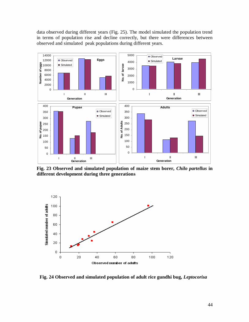
44
data observed during different years (Fig. 25). The model simulated the population trend
in terms of population rise and decline correctly, but there were differences between
observed and simulated peak populations during different years.
Eggs
0
2000
4000
6000
8000
10000
12000
14000
I II III
Generation
Nu
mb
er
of
eg
gs
Observed
Simulated
Larvae
0
1000
2000
3000
4000
5000
I II III
Generation
No
. o
f la
rva
e
Observed
Simulated
Pupae
0
50
100
150
200
250
300
350
400
I II IIIGeneration
No
. o
f p
up
ae
Observed
Simulated
Adults
0
50
100
150
200
250
300
350
400
I II IIIGeneration
No
. o
f A
du
lts
Observed
Simulated
Fig. 23 Observed and simulated population of maize stem borer, Chilo partellus in
different development during three generations
Fig. 24 Observed and simulated population of adult rice gundhi bug, Leptocorisa acuta
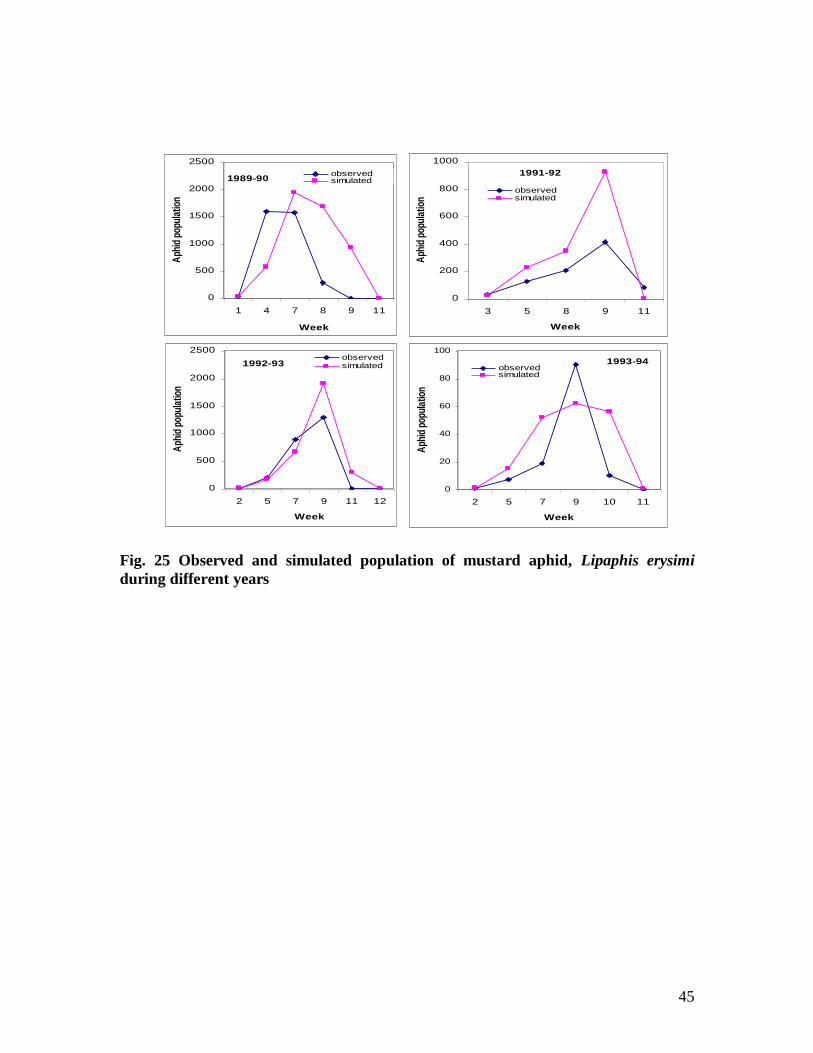
45
1989-90
0
500
1000
1500
2000
2500
1 4 7 8 9 11
Week
Aph
id p
opul
atio
nobservedsimulated
1991-92
0
200
400
600
800
1000
3 5 8 9 11
Week
Aph
id p
opul
atio
n
observedsimulated
1992-93
0
500
1000
1500
2000
2500
2 5 7 9 11 12
Week
Aph
id p
opul
atio
n
observedsimulated
1993-94
0
20
40
60
80
100
2 5 7 9 10 11
Week
Aph
id p
opul
atio
n
observedsimulated
Fig. 25 Observed and simulated population of mustard aphid, Lipaphis erysimi
during different years
46
Effect of high temperature on physiological characteristics and yield of chickpea
(Cicer arietinum L.) cultivars.
Two chickpea cultivars (Pusa 1053 and Pusa 1108) were raised in earthen pots in pot
culture of the Division of Plant Physiology. Recommended cultural practices were
followed. One set of plants was grown under natural environment (ambient temperature)
while other set of plants was grown inside a polycover and exposed to high temperature
(ranged between 3-4 o
C, above ambient temperature) from germination till maturity of
the crop. A third set of plants was exposed to high temperature during flowering stage
and fourth set was exposed to high temperature only during pod filling stage by
transferring the pots inside poly cover. Observations were recorded on membrane
stability index, carbohydrates and proline at vegetative, flowering and pod filling stages
and yield attributes were recorded at harvest of the crop.
Membrane stability index (MSI) varied significantly at different stages of growth in both
the cultivars. At vegetative and pod filling stage, no significant changes occurred in MSI
under high temperature. However, at flowering stage both the cultivars showed
significantly higher MSI due to elevated temperature. No significant effect of high
temperature occurred on concentration of total sugars in both the cultivars at vegetative
and flowering stage but Pusa 1108 showed significant reduction n total sugars during pod
filling stage under high temperature. Proline content was significantly higher in high
temperature grown chickpea plants of cultivar Pusa 1108 while no significant changes
occurred in Pusa 1053 (Fig. 24). The effect of high temperature on yield attributes varied
among both the cultivars exposed to high temperature throughout the growth period. No
significant changes occurred in yield attributes of Pusa 1108 due to exposure to high
temperature either throughout the growth period or at different stages. On the other hand,
Pusa 1053 plant exposed to high temperature only during flowering stage responded
positively and produced higher seed number and grains per plant compared to the plants
grown under high temperature throughout the growth period and exposed only during pod
filling stage (Table 1). This study concludes that 3-4 o
C increase in temperature may not
affect the yield of chickpea plants and even short spells of increased temperature
particularly during flowering period may have positive effect on growth and
development. However, further studies are required to confirm these findings particularly
under field conditions.
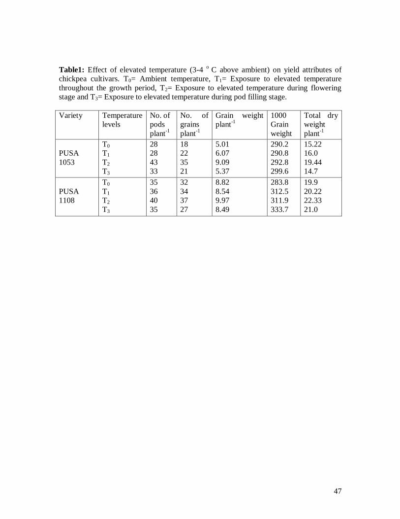
47
Table1: Effect of elevated temperature (3-4 o
C above ambient) on yield attributes of
chickpea cultivars. T0= Ambient temperature, T1= Exposure to elevated temperature
throughout the growth period, T2= Exposure to elevated temperature during flowering
stage and T3= Exposure to elevated temperature during pod filling stage.
Variety Temperature
levels
No. of
pods
plant-1
No. of
grains
plant-1
Grain weight
plant-1
1000
Grain
weight
Total dry
weight
plant-1
PUSA
1053
T0
T1
T2
T3
28
28
43
33
18
22
35
21
5.01
6.07
9.09
5.37
290.2
290.8
292.8
299.6
15.22
16.0
19.44
14.7
PUSA
1108
T0
T1
T2
T3
35
36
40
35
32
34
37
27
8.82
8.54
9.97
8.49
283.8
312.5
311.9
333.7
19.9
20.22
22.33
21.0
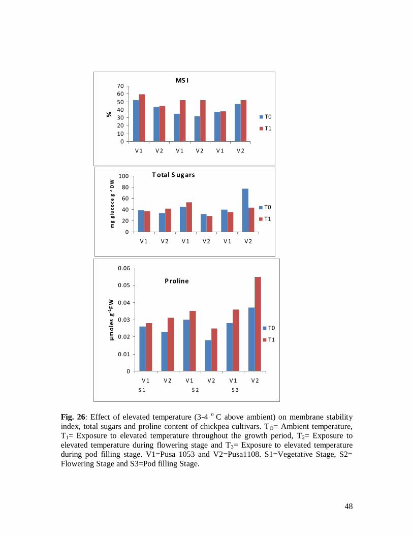
48
Fig. 26: Effect of elevated temperature (3-4 o
C above ambient) on membrane stability
index, total sugars and proline content of chickpea cultivars. TO= Ambient temperature,
T1= Exposure to elevated temperature throughout the growth period, T2= Exposure to
elevated temperature during flowering stage and T3= Exposure to elevated temperature
during pod filling stage. V1=Pusa 1053 and V2=Pusa1108. S1=Vegetative Stage, S2=
Flowering Stage and S3=Pod filling Stage.
0
0.01
0.02
0.03
0.04
0.05
0.06
V 1 V 2 V 1 V 2 V 1 V 2
µm
ole
s g
-1F
W
T0
T1
P roline
S 1 S 2 S 3
010
20304050
6070
V 1 V 2 V 1 V 2 V 1 V 2
% T0
T1
MS I
0
20
40
60
80
100
V 1 V 2 V 1 V 2 V 1 V 2
mg
glu
co
ce
g-1
DW
T0
T1
T otal S ug ars
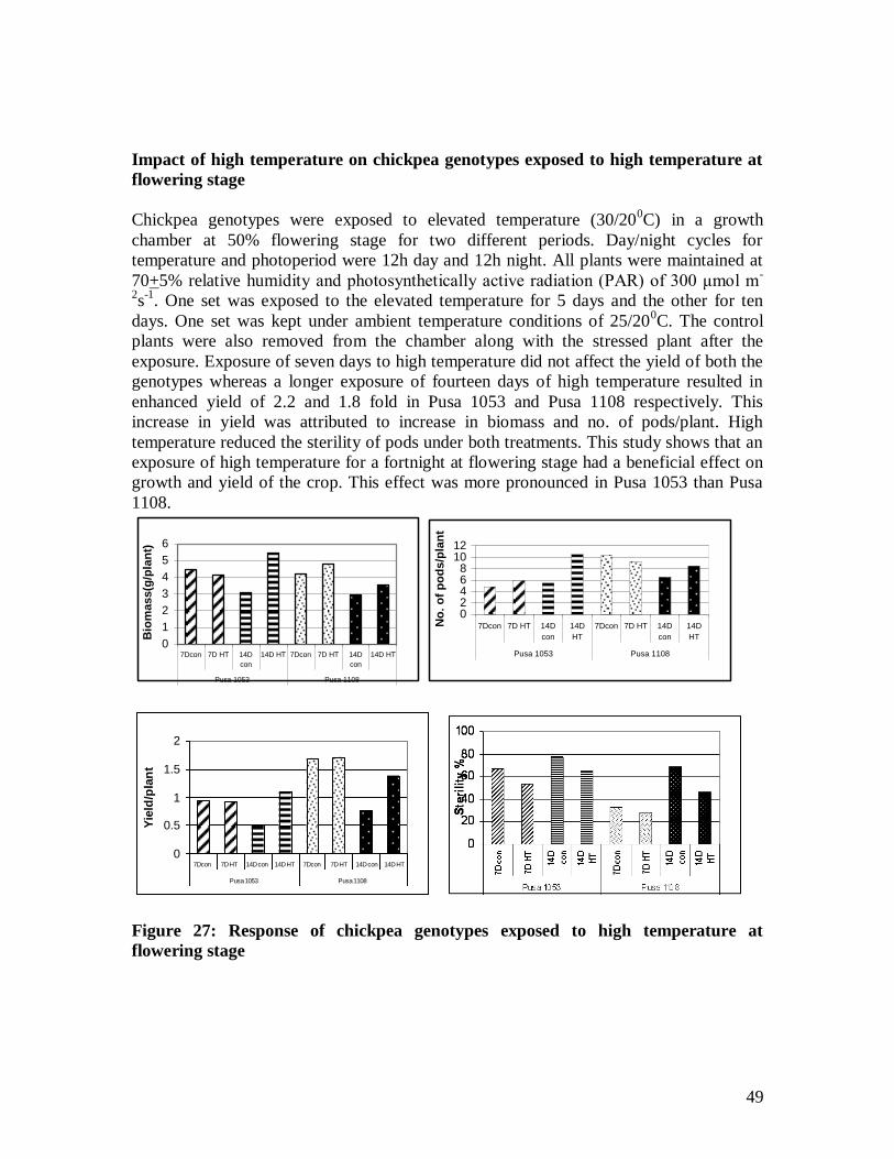
49
Impact of high temperature on chickpea genotypes exposed to high temperature at
flowering stage
Chickpea genotypes were exposed to elevated temperature (30/200C) in a growth
chamber at 50% flowering stage for two different periods. Day/night cycles for
temperature and photoperiod were 12h day and 12h night. All plants were maintained at
70+5% relative humidity and photosynthetically active radiation (PAR) of 300 μmol m-
2s
-1. One set was exposed to the elevated temperature for 5 days and the other for ten
days. One set was kept under ambient temperature conditions of 25/200C. The control
plants were also removed from the chamber along with the stressed plant after the
exposure. Exposure of seven days to high temperature did not affect the yield of both the
genotypes whereas a longer exposure of fourteen days of high temperature resulted in
enhanced yield of 2.2 and 1.8 fold in Pusa 1053 and Pusa 1108 respectively. This
increase in yield was attributed to increase in biomass and no. of pods/plant. High
temperature reduced the sterility of pods under both treatments. This study shows that an
exposure of high temperature for a fortnight at flowering stage had a beneficial effect on
growth and yield of the crop. This effect was more pronounced in Pusa 1053 than Pusa
1108.
0
1
2
3
4
5
6
7Dcon 7D HT 14D
con
14D HT 7Dcon 7D HT 14D
con
14D HT
Pusa 1053 Pusa 1108
Bio
mass(g
/pla
nt)
02468
1012
7Dcon 7D HT 14D
con
14D
HT
7Dcon 7D HT 14D
con
14D
HT
Pusa 1053 Pusa 1108
No
. o
f p
od
s/p
lan
t
0
0.5
1
1.5
2
7Dcon 7D HT 14D con 14D HT 7Dcon 7D HT 14D con 14D HT
Pusa 1053 Pusa 1108
Yie
ld/p
lan
t
Figure 27: Response of chickpea genotypes exposed to high temperature at
flowering stage
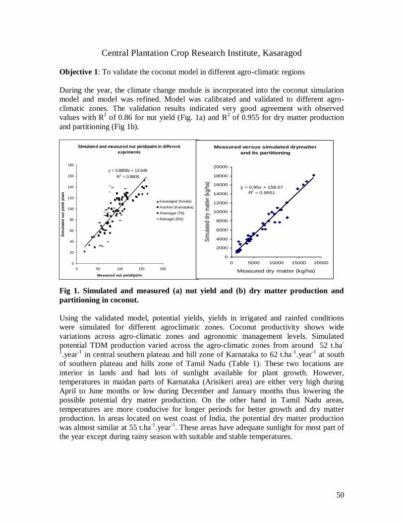
50
SImulated and measured nut yield/palm in different
expriments
y = 0.8858x + 13.649
R2 = 0.8609
0
20
40
60
80
100
120
140
160
180
0 50 100 150 200
Measured nut yield/palm
Sim
ula
ted
nu
t yie
ld/
pla
m
Kasaragod (Kerala)
Arisikeri (Karnataka)
Aliarnagar (TN)
Ratnagiri (MS)
Measured versus simulated drymatter
and its partitioning
y = 0.95x + 158.07
R2 = 0.9551
0
2000
4000
6000
8000
10000
12000
14000
16000
18000
20000
0 5000 10000 15000 20000
Measured dry matter (kg/ha)
Sim
ulat
ed d
ry m
atte
r (k
g/ha
)
Central Plantation Crop Research Institute, Kasaragod
Objective 1: To validate the coconut model in different agro-climatic regions
During the year, the climate change module is incorporated into the coconut simulation
model and model was refined. Model was calibrated and validated to different agro-
climatic zones. The validation results indicated very good agreement with observed
values with R2 of 0.86 for nut yield (Fig. 1a) and R
2 of 0.955 for dry matter production
and partitioning (Fig 1b).
Fig 1. Simulated and measured (a) nut yield and (b) dry matter production and
partitioning in coconut.
Using the validated model, potential yields, yields in irrigated and rainfed conditions
were simulated for different agroclimatic zones. Coconut productivity shows wide
variations across agro-climatic zones and agronomic management levels. Simulated
potential TDM production varied across the agro-climatic zones from around 52 t.ha-
1.year
-1 in central southern plateau and hill zone of Karnataka to 62 t.ha
-1.year
-1 at south
of southern plateau and hills zone of Tamil Nadu (Table 1). These two locations are
interior in lands and had lots of sunlight available for plant growth. However,
temperatures in maidan parts of Karnataka (Arisikeri area) are either very high during
April to June months or low during December and January months thus lowering the
possible potential dry matter production. On the other hand in Tamil Nadu areas,
temperatures are more conducive for longer periods for better growth and dry matter
production. In areas located on west coast of India, the potential dry matter production
was almost similar at 55 t.ha-1
.year-1
. These areas have adequate sunlight for most part of
the year except during rainy season with suitable and stable temperatures.
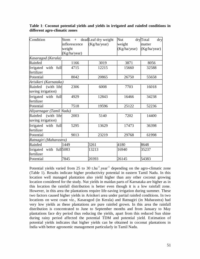
51
Table 1: Coconut potential yields and yields in irrigated and rainfed conditions in
different agro-climatic zones
Condition Stem + dead
inflorescence
weight
(Kg/ha/year)
Leaf dry weight
(Kg/ha/year)
Nut dry
weight
(Kg/ha/year)
Total dry
matter
(Kg/ha/year)
Kasaragod (Kerala)
Rainfed 1166 3019 3871 8056
Irrigated with full
fertilizer
4715 12215 15660 32588
Potential 8042 20865 26750 55658
Arisikeri (Karnataka)
Rainfed (with life
saving irrigation)
2306 6008 7703 16018
Irrigated with full
fertilizer
4929 12843 16466 34238
Potential 7518 19596 25122 52236
Aliyarnagar (Tamil Nadu)
Rainfed (with life
saving irrigation)
2003 5140 7202 14400
Irrigated with full
fertilizer
5295 13629 17473 36398
Potential 9013 23219 29768 61998
Ratnagiri (Maharastra)
Rainfed 1449 3261 4180 8648
Irrigated with full
fertilizer
5083 13213 16940 35237
Potential 7845 20393 26145 54383
Potential yields varied from 25 to 30 t.ha-1
.year-1
depending on the agro-climatic zone
(Table 1). Results indicate higher productivity potential in eastern Tamil Nadu. In this
location well managed plantation also yield higher than any other coconut growing
location considered for the study. Nut yields in maidan parts of Karnataka are higher as in
this location the rainfall distribution is better even though it is a low rainfall zone.
However, in this area the plantations require life-saving irrigation during summer. These
two factors caused higher yields in Arisikeri area under partial rainfed conditions. In two
locations on west coast viz., Kasaragod (in Kerala) and Ratnagiri (in Maharastra) had
very low yields as these plantations are pure rainfed grown. In this area the rainfall
distribution is concentrated to June to September months and from January to May
plantations face dry period thus reducing the yields, apart from this reduced Sun shine
during rainy period affected the potential TDM and potential yield. Estimation of
potential yields indicates that higher yields can be obtained in coconut plantations in
India with better agronomic management particularly in Tamil Nadu.
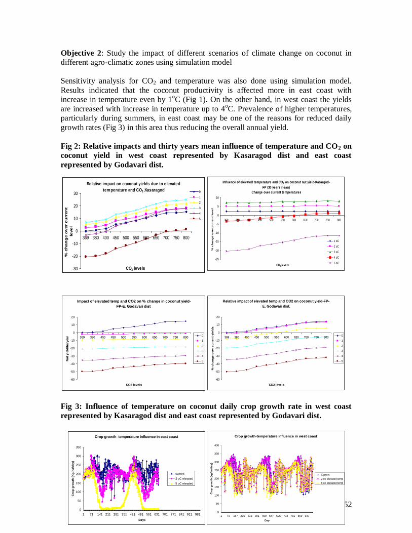
52
Relative impact of elevated temp and CO2 on coconut yield-FP-
E. Godavari dist.
-60
-50
-40
-30
-20
-10
0
10
20
369 380 400 450 500 550 600 650 700 750 800
CO2 levels
% c
han
ge o
ver
cu
rren
t yie
lds
0
1
2
3
4
5
Relative impact on coconut yields due to elevated
temperature and CO2 -Kasaragod
-30
-20
-10
0
10
20
30
369 380 400 450 500 550 600 650 700 750 800
CO2 levels
% c
han
ge o
ver
cu
rren
t
level
0
1
2
3
4
5
Influence of elevated temperature and CO2 on coconut nut yield-Kasargod-
FP (30 years mean)
Change over current temperatures
-25
-20
-15
-10
-5
0
5
10
369 380 400 450 500 550 600 650 700 750 800
CO2 levels
% c
han
ge o
ver
cu
rren
t le
vel
1 oC
2 oC
3 oC
4 oC
5 oC
Impact of elevated temp and CO2 on % change in coconut yield-
FP-E. Godavari dist
-60
-50
-40
-30
-20
-10
0
10
20
369 380 400 450 500 550 600 650 700 750 800
CO2 levels
Nu
t yie
ld/h
a/y
ear 0
1
2
3
4
5
Objective 2: Study the impact of different scenarios of climate change on coconut in
different agro-climatic zones using simulation model
Sensitivity analysis for CO2 and temperature was also done using simulation model.
Results indicated that the coconut productivity is affected more in east coast with
increase in temperature even by 1oC (Fig 1). On the other hand, in west coast the yields
are increased with increase in temperature up to 4oC. Prevalence of higher temperatures,
particularly during summers, in east coast may be one of the reasons for reduced daily
growth rates (Fig 3) in this area thus reducing the overall annual yield.
Fig 2: Relative impacts and thirty years mean influence of temperature and CO2 on
coconut yield in west coast represented by Kasaragod dist and east coast
represented by Godavari dist.
Fig 3: Influence of temperature on coconut daily crop growth rate in west coast
represented by Kasaragod dist and east coast represented by Godavari dist.
Crop growth- temperature influence in east coast
0
50
100
150
200
250
300
350
1 71 141 211 281 351 421 491 561 631 701 771 841 911 981
Days
Cro
p g
row
th (
Kg
/ha/d
ay)
current
2 oC elevated
5 oC elevated
Crop growth-temperature influence in west coast
0
50
100
150
200
250
300
350
400
1 79 157 235 313 391 469 547 625 703 781 859 937
Day
Cro
p g
rwo
th (
kg
/ha
/da
y)
Current
2 oc elevated temp
5 oc elevated temp
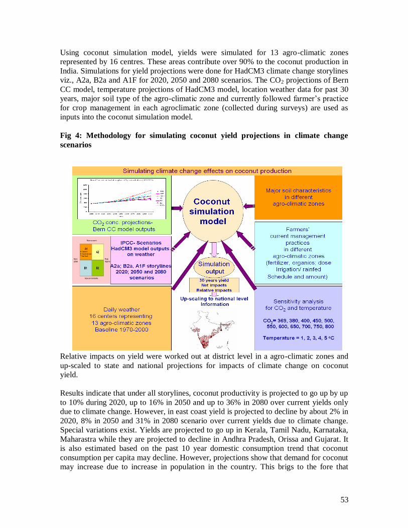
53
Using coconut simulation model, yields were simulated for 13 agro-climatic zones
represented by 16 centres. These areas contribute over 90% to the coconut production in
India. Simulations for yield projections were done for HadCM3 climate change storylines
viz., A2a, B2a and A1F for 2020, 2050 and 2080 scenarios. The CO2 projections of Bern
CC model, temperature projections of HadCM3 model, location weather data for past 30
years, major soil type of the agro-climatic zone and currently followed farmer‟s practice
for crop management in each agroclimatic zone (collected during surveys) are used as
inputs into the coconut simulation model.
Fig 4: Methodology for simulating coconut yield projections in climate change
scenarios
Relative impacts on yield were worked out at district level in a agro-climatic zones and
up-scaled to state and national projections for impacts of climate change on coconut
yield.
Results indicate that under all storylines, coconut productivity is projected to go up by up
to 10% during 2020, up to 16% in 2050 and up to 36% in 2080 over current yields only
due to climate change. However, in east coast yield is projected to decline by about 2% in
2020, 8% in 2050 and 31% in 2080 scenario over current yields due to climate change.
Special variations exist. Yields are projected to go up in Kerala, Tamil Nadu, Karnataka,
Maharastra while they are projected to decline in Andhra Pradesh, Orissa and Gujarat. It
is also estimated based on the past 10 year domestic consumption trend that coconut
consumption per capita may decline. However, projections show that demand for coconut
may increase due to increase in population in the country. This brigs to the fore that
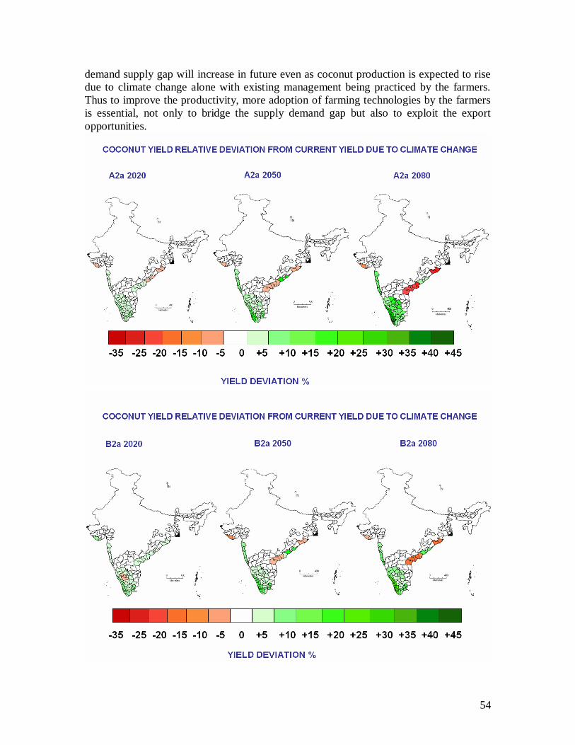
54
demand supply gap will increase in future even as coconut production is expected to rise
due to climate change alone with existing management being practiced by the farmers.
Thus to improve the productivity, more adoption of farming technologies by the farmers
is essential, not only to bridge the supply demand gap but also to exploit the export
opportunities.
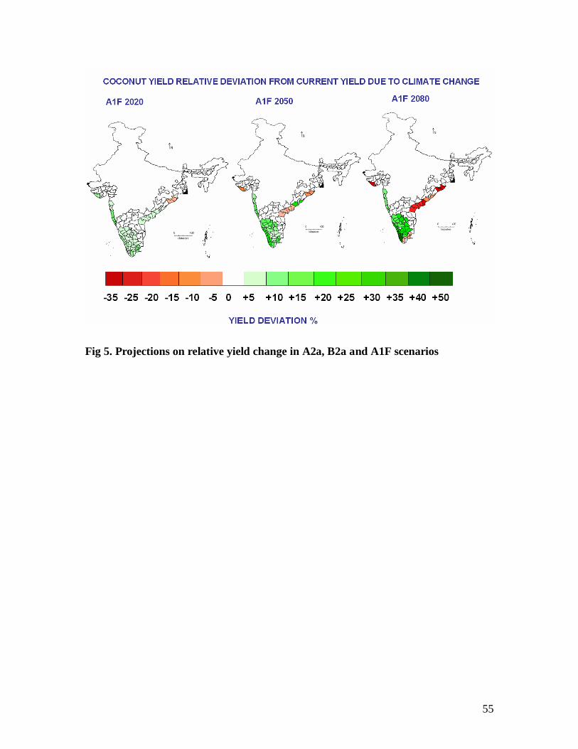
55
Fig 5. Projections on relative yield change in A2a, B2a and A1F scenarios
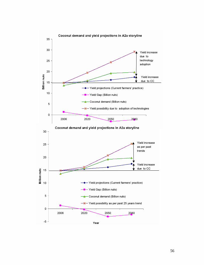
56
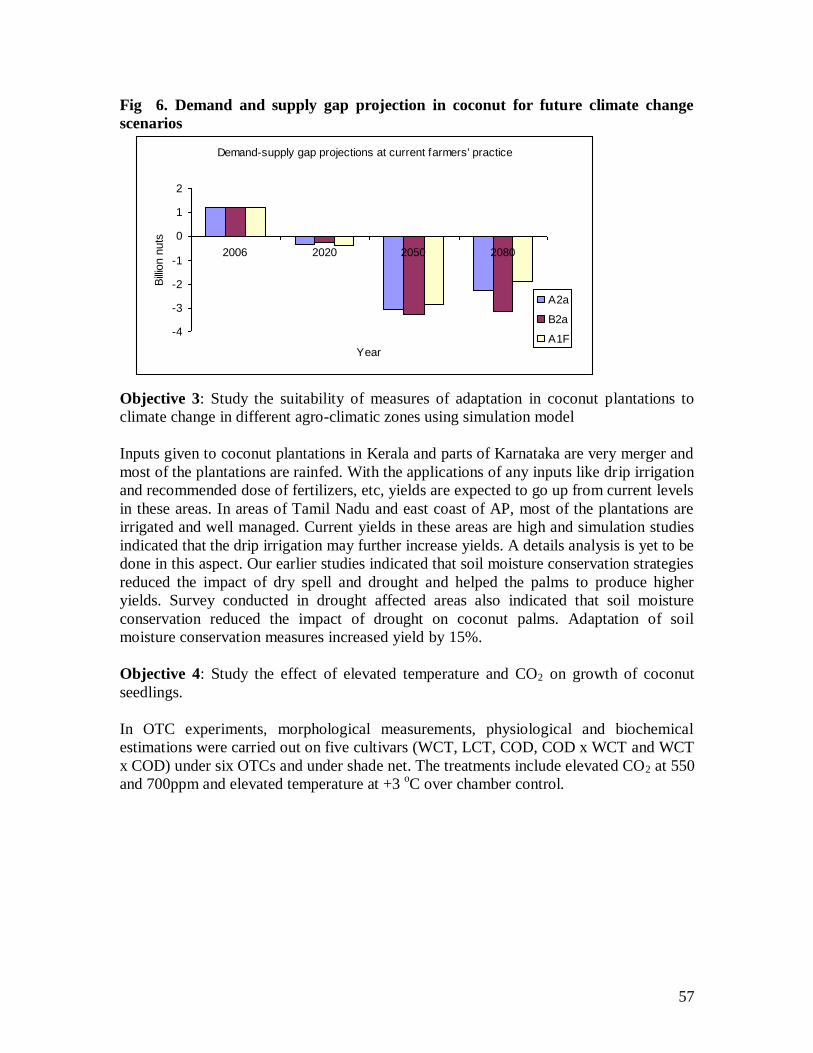
57
Demand-supply gap projections at current farmers' practice
-4
-3
-2
-1
0
1
2
2006 2020 2050 2080
Year
Billio
n n
uts
A2a
B2a
A1F
Fig 6. Demand and supply gap projection in coconut for future climate change
scenarios
Objective 3: Study the suitability of measures of adaptation in coconut plantations to
climate change in different agro-climatic zones using simulation model
Inputs given to coconut plantations in Kerala and parts of Karnataka are very merger and
most of the plantations are rainfed. With the applications of any inputs like drip irrigation
and recommended dose of fertilizers, etc, yields are expected to go up from current levels
in these areas. In areas of Tamil Nadu and east coast of AP, most of the plantations are
irrigated and well managed. Current yields in these areas are high and simulation studies
indicated that the drip irrigation may further increase yields. A details analysis is yet to be
done in this aspect. Our earlier studies indicated that soil moisture conservation strategies
reduced the impact of dry spell and drought and helped the palms to produce higher
yields. Survey conducted in drought affected areas also indicated that soil moisture
conservation reduced the impact of drought on coconut palms. Adaptation of soil
moisture conservation measures increased yield by 15%.
Objective 4: Study the effect of elevated temperature and CO2 on growth of coconut
seedlings.
In OTC experiments, morphological measurements, physiological and biochemical
estimations were carried out on five cultivars (WCT, LCT, COD, COD x WCT and WCT
x COD) under six OTCs and under shade net. The treatments include elevated CO2 at 550
and 700ppm and elevated temperature at +3 oC over chamber control.
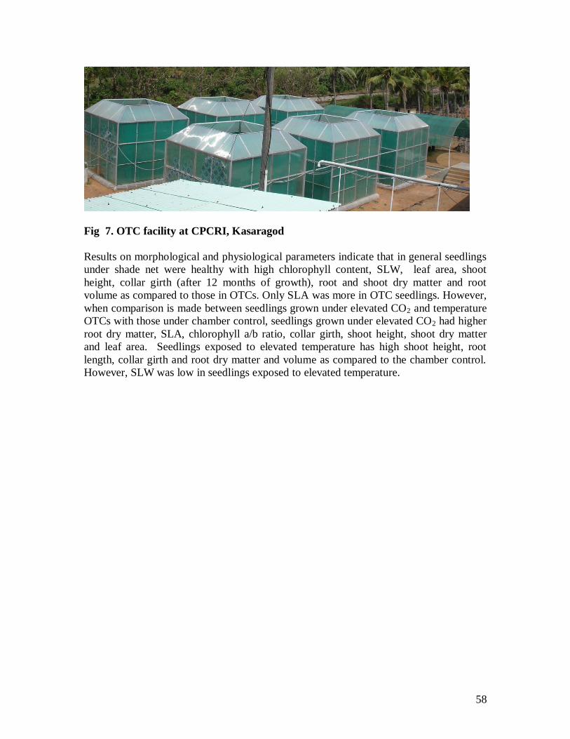
58
Fig 7. OTC facility at CPCRI, Kasaragod
Results on morphological and physiological parameters indicate that in general seedlings
under shade net were healthy with high chlorophyll content, SLW, leaf area, shoot
height, collar girth (after 12 months of growth), root and shoot dry matter and root
volume as compared to those in OTCs. Only SLA was more in OTC seedlings. However,
when comparison is made between seedlings grown under elevated CO2 and temperature
OTCs with those under chamber control, seedlings grown under elevated CO2 had higher
root dry matter, SLA, chlorophyll a/b ratio, collar girth, shoot height, shoot dry matter
and leaf area. Seedlings exposed to elevated temperature has high shoot height, root
length, collar girth and root dry matter and volume as compared to the chamber control.
However, SLW was low in seedlings exposed to elevated temperature.
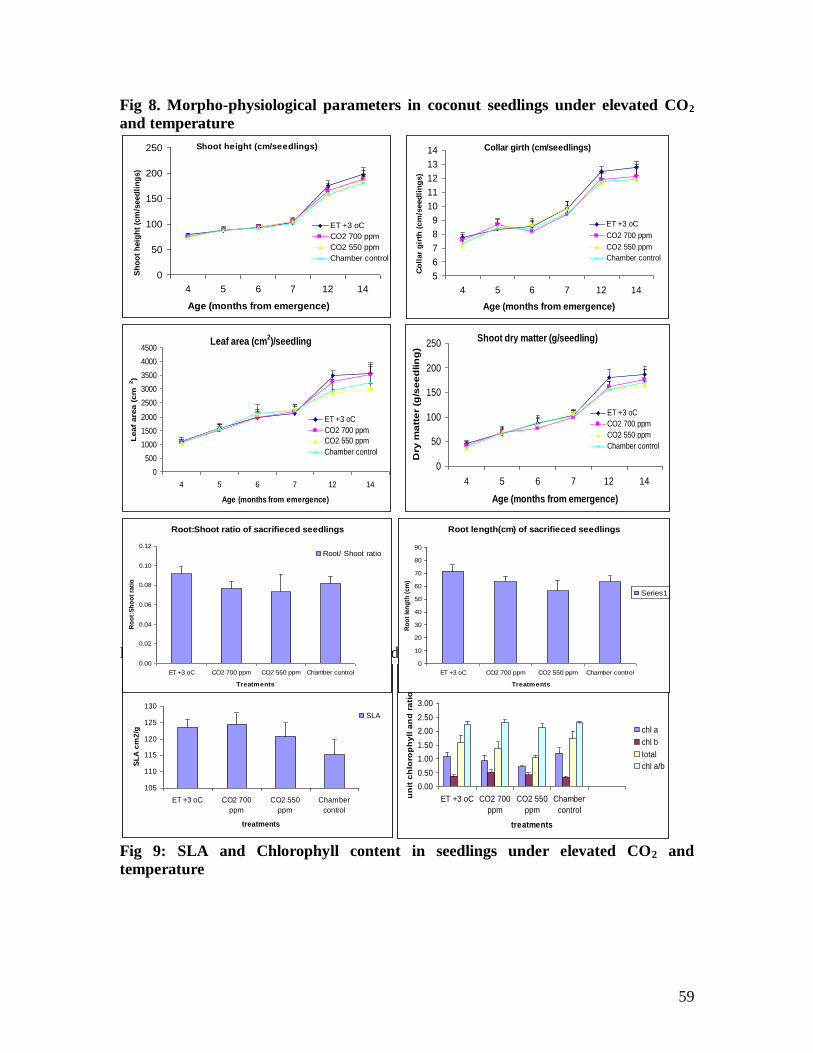
59
Fig 8. Morpho-physiological parameters in coconut seedlings under elevated CO2
and temperature
Fig 9: SLA and Chlorophyll content in seedlings under elevated CO2 and temperature
Fig 9: SLA and Chlorophyll content in seedlings under elevated CO2 and
temperature
Specific leaf area cm2/g leaf tissue
105
110
115
120
125
130
ET +3 oC CO2 700
ppm
CO2 550
ppm
Chamber
control
treatments
SL
A c
m2
/g
SLA
Chlorophyll pigments / g of fresh leaf tissue
0.00
0.50
1.00
1.50
2.00
2.50
3.00
ET +3 oC CO2 700
ppm
CO2 550
ppm
Chamber
control
treatments
un
it c
hlo
rop
hy
ll a
nd
ra
tio
chl a
chl b
total
chl a/b
Shoot height (cm/seedlings)
0
50
100
150
200
250
4 5 6 7 12 14
Age (months from emergence)
Sh
oo
t h
eig
ht
(cm
/seed
lin
gs)
ET +3 oC
CO2 700 ppm
CO2 550 ppm
Chamber control
Collar girth (cm/seedlings)
5
6
7
8
9
10
11
12
13
14
4 5 6 7 12 14
Age (months from emergence)
Co
llar
gir
th (
cm
/seed
lin
gs)
ET +3 oC
CO2 700 ppm
CO2 550 ppm
Chamber control
Leaf area (cm2)/seedling
0
500
1000
1500
2000
2500
3000
3500
4000
4500
4 5 6 7 12 14
Age (months from emergence)
Leaf
are
a (
cm
2)
ET +3 oC
CO2 700 ppm
CO2 550 ppm
Chamber control
Shoot dry matter (g/seedling)
0
50
100
150
200
250
4 5 6 7 12 14
Age (months from emergence)
Dry
ma
tte
r (g
/se
ed
lin
g)
ET +3 oC
CO2 700 ppm
CO2 550 ppm
Chamber control
Root:Shoot ratio of sacrifieced seedlings
0.00
0.02
0.04
0.06
0.08
0.10
0.12
ET +3 oC CO2 700 ppm CO2 550 ppm Chamber control
Treatments
Ro
ot:
Sh
oo
t ra
tio
Root/ Shoot ratio
Root length(cm) of sacrifieced seedlings
0
10
20
30
40
50
60
70
80
90
ET +3 oC CO2 700 ppm CO2 550 ppm Chamber control
Treatments
Ro
ot
len
gth
(cm
)
Series1
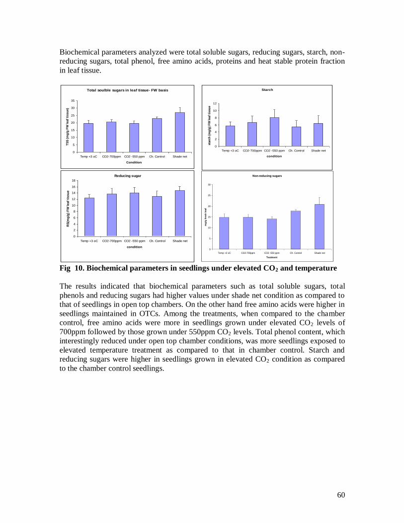
60
Biochemical parameters analyzed were total soluble sugars, reducing sugars, starch, non-
reducing sugars, total phenol, free amino acids, proteins and heat stable protein fraction
in leaf tissue.
Fig 10. Biochemical parameters in seedlings under elevated CO2 and temperature
The results indicated that biochemical parameters such as total soluble sugars, total
phenols and reducing sugars had higher values under shade net condition as compared to
that of seedlings in open top chambers. On the other hand free amino acids were higher in
seedlings maintained in OTCs. Among the treatments, when compared to the chamber
control, free amino acids were more in seedlings grown under elevated CO2 levels of
700ppm followed by those grown under 550ppm CO2 levels. Total phenol content, which
interestingly reduced under open top chamber conditions, was more seedlings exposed to
elevated temperature treatment as compared to that in chamber control. Starch and
reducing sugars were higher in seedlings grown in elevated CO2 condition as compared
to the chamber control seedlings.
Total soulble sugars in leaf tissue- FW basis
0
5
10
15
20
25
30
35
Temp +3 oC CO2-700ppm CO2 -550 ppm Ch. Control Shade net
Condition
TS
S (
mg
/g F
W leaf
tissu
e)
Starch
0
2
4
6
8
10
12
Temp +3 oC CO2-700ppm CO2 -550 ppm Ch. Control Shade net
condition
sta
rch
(m
g/g
) F
W leaf
tissu
e
Reducing sugar
0
2
4
6
8
10
12
14
16
18
Temp +3 oC CO2-700ppm CO2 -550 ppm Ch. Control Shade net
condition
RS
(mg
/g)
FW
leaf
tissu
e
Non-reducing sugars
0
5
10
15
20
25
30
Temp +3 oC CO2-700ppm CO2 -550 ppm Ch. Control Shade net
Teatment
mg
/g f
resh
leaf
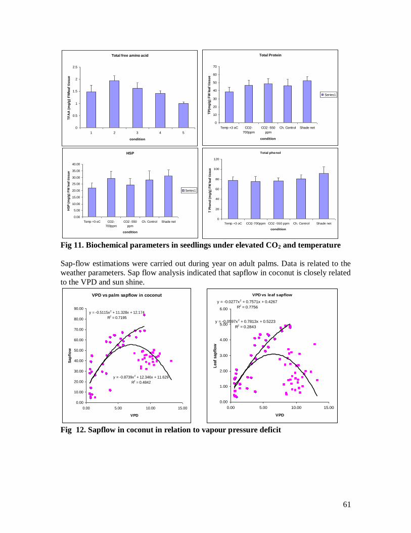
61
Fig 11. Biochemical parameters in seedlings under elevated CO2 and temperature
Sap-flow estimations were carried out during year on adult palms. Data is related to the
weather parameters. Sap flow analysis indicated that sapflow in coconut is closely related
to the VPD and sun shine.
Fig 12. Sapflow in coconut in relation to vapour pressure deficit
VPD vs palm sapflow in coconut
y = -0.5115x2 + 11.328x + 12.174
R2 = 0.7195
y = -0.8739x2 + 12.346x + 11.629
R2 = 0.4842
0.00
10.00
20.00
30.00
40.00
50.00
60.00
70.00
80.00
90.00
0.00 5.00 10.00 15.00
VPD
Sap
flo
w
VPD vs leaf sapflow
y = -0.0277x2 + 0.7571x + 0.4267
R2 = 0.7756
y = -0.0597x2 + 0.7813x + 0.5223
R2 = 0.2843
0.00
1.00
2.00
3.00
4.00
5.00
6.00
0.00 5.00 10.00 15.00
VPD
Leaf
sap
flo
w
Total free amino acid
0
0.5
1
1.5
2
2.5
1 2 3 4 5
condition
TF
AA
(m
g/g
) F
Wle
af
tissu
e
Total Protein
0
10
20
30
40
50
60
70
Temp +3 oC CO2-
700ppm
CO2 -550
ppm
Ch. Control Shade net
condition
TP
(mg
/g)
FW
leaf
tissu
e
Series1
HSP
0.00
5.00
10.00
15.00
20.00
25.00
30.00
35.00
40.00
Temp +3 oC CO2-
700ppm
CO2 -550
ppm
Ch. Control Shade net
condition
HS
P (
mg
/g)
FW
leaf
tissu
e
Series1
Total phenol
0
20
40
60
80
100
120
Temp +3 oC CO2-700ppm CO2 -550 ppm Ch. Control Shade net
condition
T P
hen
ol (m
g/g
) F
W leaf
tissu
e
62
Objective 5. Study the carbon sequestration potential and stocks of coconut mono-
systems using simulation model.
Estimations on carbon sequestration potential and stock in coconut plantations under
different management conditions and agro-climatic zones were continued. The net
primary production (NPP) estimations of coconut monocrop in different agro-climatic
zones indicated annual carbon sequestration potential of coconut above ground biomass
ranged from 8 to 32 t CO2/ha/year depending on cultivar, agro-climatic zone, soil type
and management. Further work on estimations for entire life cycle of coconut using
coconut simulation model and up-scaling to national potentials are under progress.
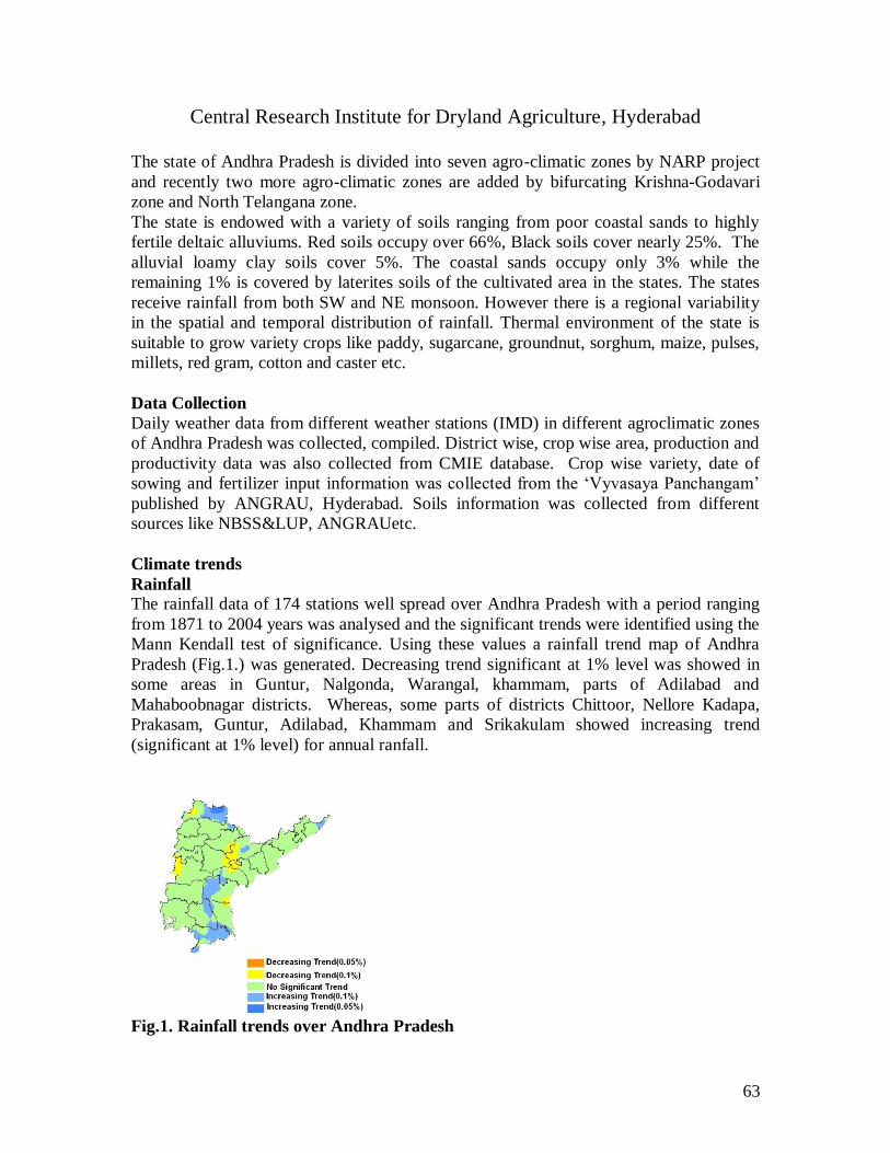
63
Central Research Institute for Dryland Agriculture, Hyderabad
The state of Andhra Pradesh is divided into seven agro-climatic zones by NARP project
and recently two more agro-climatic zones are added by bifurcating Krishna-Godavari
zone and North Telangana zone.
The state is endowed with a variety of soils ranging from poor coastal sands to highly
fertile deltaic alluviums. Red soils occupy over 66%, Black soils cover nearly 25%. The
alluvial loamy clay soils cover 5%. The coastal sands occupy only 3% while the
remaining 1% is covered by laterites soils of the cultivated area in the states. The states
receive rainfall from both SW and NE monsoon. However there is a regional variability
in the spatial and temporal distribution of rainfall. Thermal environment of the state is
suitable to grow variety crops like paddy, sugarcane, groundnut, sorghum, maize, pulses,
millets, red gram, cotton and caster etc.
Data Collection
Daily weather data from different weather stations (IMD) in different agroclimatic zones
of Andhra Pradesh was collected, compiled. District wise, crop wise area, production and
productivity data was also collected from CMIE database. Crop wise variety, date of
sowing and fertilizer input information was collected from the „Vyvasaya Panchangam‟
published by ANGRAU, Hyderabad. Soils information was collected from different
sources like NBSS&LUP, ANGRAUetc.
Climate trends
Rainfall
The rainfall data of 174 stations well spread over Andhra Pradesh with a period ranging
from 1871 to 2004 years was analysed and the significant trends were identified using the
Mann Kendall test of significance. Using these values a rainfall trend map of Andhra
Pradesh (Fig.1.) was generated. Decreasing trend significant at 1% level was showed in
some areas in Guntur, Nalgonda, Warangal, khammam, parts of Adilabad and
Mahaboobnagar districts. Whereas, some parts of districts Chittoor, Nellore Kadapa,
Prakasam, Guntur, Adilabad, Khammam and Srikakulam showed increasing trend
(significant at 1% level) for annual ranfall.
Fig.1. Rainfall trends over Andhra Pradesh
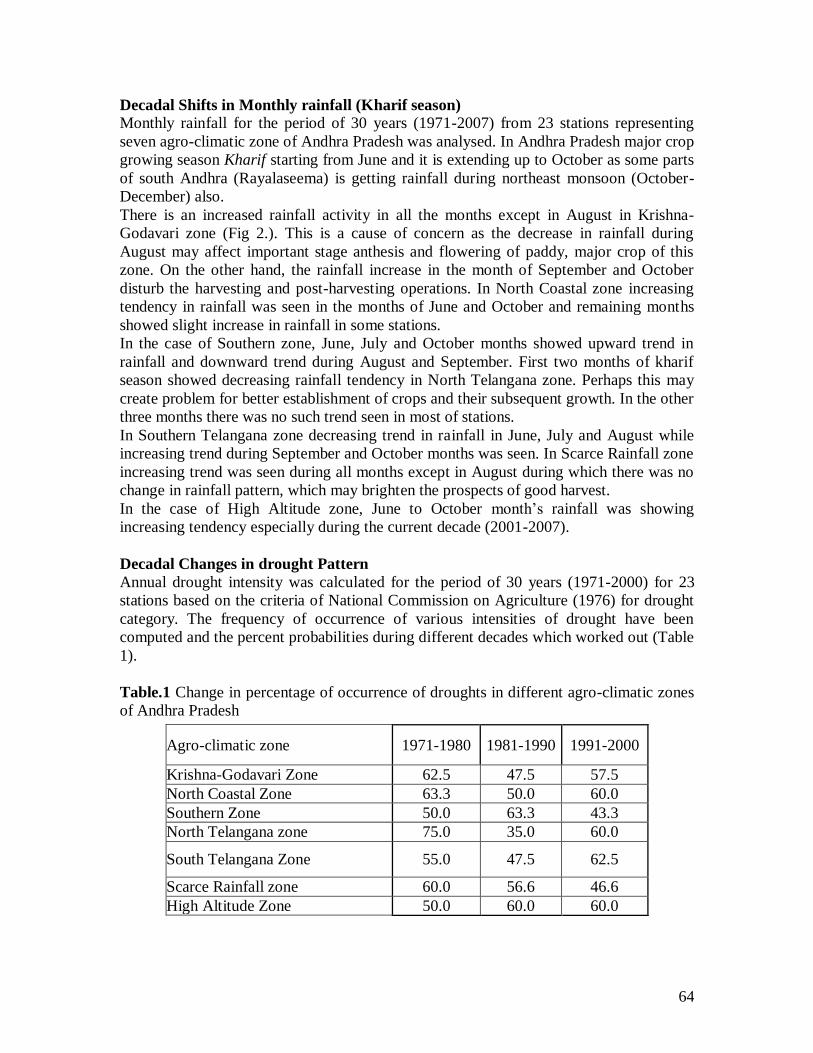
64
Decadal Shifts in Monthly rainfall (Kharif season)
Monthly rainfall for the period of 30 years (1971-2007) from 23 stations representing
seven agro-climatic zone of Andhra Pradesh was analysed. In Andhra Pradesh major crop
growing season Kharif starting from June and it is extending up to October as some parts
of south Andhra (Rayalaseema) is getting rainfall during northeast monsoon (October-
December) also.
There is an increased rainfall activity in all the months except in August in Krishna-
Godavari zone (Fig 2.). This is a cause of concern as the decrease in rainfall during
August may affect important stage anthesis and flowering of paddy, major crop of this
zone. On the other hand, the rainfall increase in the month of September and October
disturb the harvesting and post-harvesting operations. In North Coastal zone increasing
tendency in rainfall was seen in the months of June and October and remaining months
showed slight increase in rainfall in some stations.
In the case of Southern zone, June, July and October months showed upward trend in
rainfall and downward trend during August and September. First two months of kharif
season showed decreasing rainfall tendency in North Telangana zone. Perhaps this may
create problem for better establishment of crops and their subsequent growth. In the other
three months there was no such trend seen in most of stations.
In Southern Telangana zone decreasing trend in rainfall in June, July and August while
increasing trend during September and October months was seen. In Scarce Rainfall zone
increasing trend was seen during all months except in August during which there was no
change in rainfall pattern, which may brighten the prospects of good harvest.
In the case of High Altitude zone, June to October month‟s rainfall was showing
increasing tendency especially during the current decade (2001-2007).
Decadal Changes in drought Pattern
Annual drought intensity was calculated for the period of 30 years (1971-2000) for 23
stations based on the criteria of National Commission on Agriculture (1976) for drought
category. The frequency of occurrence of various intensities of drought have been
computed and the percent probabilities during different decades which worked out (Table
1).
Table.1 Change in percentage of occurrence of droughts in different agro-climatic zones
of Andhra Pradesh
Agro-climatic zone 1971-1980 1981-1990 1991-2000
Krishna-Godavari Zone 62.5 47.5 57.5
North Coastal Zone 63.3 50.0 60.0
Southern Zone 50.0 63.3 43.3
North Telangana zone 75.0 35.0 60.0
South Telangana Zone 55.0 47.5 62.5
Scarce Rainfall zone 60.0 56.6 46.6
High Altitude Zone 50.0 60.0 60.0
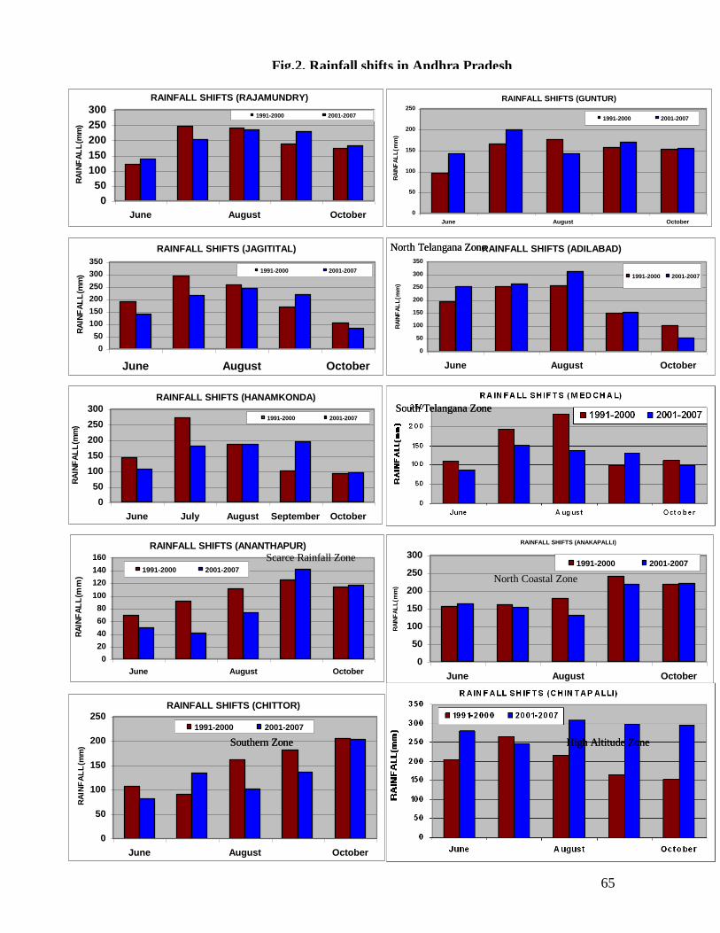
65
RAINFALL SHIFTS (RAJAMUNDRY)
0
50
100
150
200
250
300
June August October
RA
INF
AL
L(m
m)
1991-2000 2001-2007
RAINFALL SHIFTS (GUNTUR)
0
50
100
150
200
250
June August October
RA
INF
AL
L(m
m)
1991-2000 2001-2007
RAINFALL SHIFTS (ADILABAD)
0
50
100
150
200
250
300
350
June August October
RA
INF
AL
L(m
m)
1991-2000 2001-2007
RAINFALL SHIFTS (JAGITITAL)
0
50
100
150
200
250
300
350
June August October
RA
INF
AL
L(m
m)
1991-2000 2001-2007
Fig.2. Rainfall shifts in Andhra Pradesh
North Telangana Zone
RAINFALL SHIFTS (HANAMKONDA)
0
50
100
150
200
250
300
June July August September October
RA
INF
AL
L(m
m)
1991-2000 2001-2007
South Telangana Zone
RAINFALL SHIFTS (ANANTHAPUR)
0
20
40
60
80
100
120
140
160
June August October
RA
INF
AL
L(m
m)
1991-2000 2001-2007
Scarce Rainfall Zone
RAINFALL SHIFTS (ANAKAPALLI)
0
50
100
150
200
250
300
June August October
RA
INF
AL
L(m
m)
1991-2000 2001-2007
RAINFALL SHIFTS (CHITTOR)
0
50
100
150
200
250
June August October
RA
INF
AL
L(m
m)
1991-2000 2001-2007
Southern Zone High Altitude Zone
North Telangana Zone
South Telangana Zone
North Coastal Zone
Southern Zone High Altitude Zone
66
The results revealed that the highest (75%) and lowest (35%) percentage of occurrence of
drought was noticed in North Telangana zone during the decade of 1971-1980 and 1981-
1990, respectively. The percentage of occurrence of droughts were more during 1971-
1980 and 1991-2000 decades when compared to 1981-1990 decade in all agro-climatic
zones except Southern and Scarce rainfall zones (Table.1). In these two zones percentage
of drought were more in 1971-1980 and 1981-0990 decade than recent decade 1991-
2000.
Temperature trends:
Temperature (maximum, minimum and average) data of 30 years were analysed for
different locations in Andhra Pradesh. The results revealed that the temperatures had
shown considerable increase in day, night and also average annual temperatures. But at
Khammam, the day time temperatures had shown considerable decreasing trend where as
night temperatures showed an increasing trend. Overall the average annual temperature
has shown a decreasing trend. Whereas at Visakhapatnam daytime temperatures have
shown increasing and while night time temperatures showed decreasing trend, overall the
average annual temperature showed an increasing temperature at many locations in the
state.
Effect of rainfall and temperature on crop yields:
The yields of various crops like rice, sorghum, groundnut, etc. versus rainfall and
temperature trends were analysed for all the districts. A few significant relationships are
given below. The relationship between rainfall and sorghum production at Anantapur
showed a negative relationship with rainfall in most of the years which may be attributed
to uneven distribution of rainfall during the crop growth period. In case of temperature
whenever the seasonal average temperature increases production reduced. The paddy
production in Visakhapatnam had direct relationship with rainfall during most of the
years, whereas average annual temperature had indirect relationship with the paddy
production. There was direct relationship between rainfall and production of sorghum
in Ranga Reddy. At Mahaboobnagar also the sorghum production has direct relationship
with rainfall. Though there was negative relationship between temperature and
production. Positive relationship was found between groundnut production and rainfall at
Kurnool in most of years. There was clear-cut negative relationship between temperature
and groundnut production. At Warangal rainfall during the crop growth period positively
influenced the paddy production. There was not much variation in temperature at
Warangal and it was found that the production was not affected either positively or
negatively by temperature. There was an indirect relationship between paddy production
and rainfall at Khammam at the same time positive relationship was seen between
temperature and paddy production.
Validation of InfoCrop model output:
Validation of InfoCrop model for rainfed crops viz., sorghum, pearlmillet, maize, cotton
and redgram at different stations located in 7 agroclimatic zones of Andhra Pradesh were
carried out. Station-wise weather data of Anantapur, Karimnagar (Jagityal) and
Rangareddy was used in the InfoCrop programme after converting them into model
format. The district-wise observed yield data for the same period was collected. After the

67
simulation, the yields of simulated and observed were compared. The root mean square
error values were very high in the case of maize, cotton and redgram. The simulated
yields of sorghum and millet have shown a close relationship with the observed yields as
the root mean square error values were smaller.
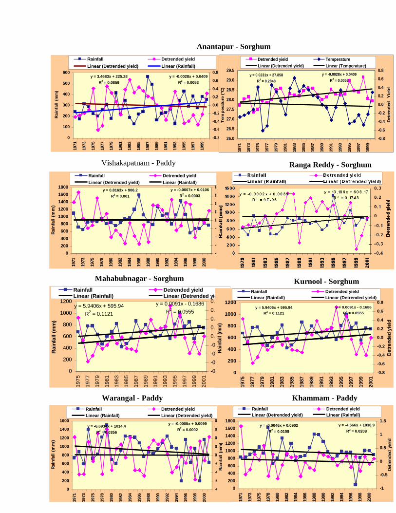
68
square error values were smaller.
y = -0.0028x + 0.0409
R2 = 0.0053
y = 3.4683x + 225.28
R2 = 0.0859
0
100
200
300
400
500
6001971
1973
1975
1977
1979
1981
1983
1985
1987
1989
1991
1993
1995
1997
1999
Rain
fall
(m
m)
-0.8
-0.6
-0.4
-0.2
0.0
0.2
0.4
0.6
0.8
Detr
en
ded
Yie
ld
Rainfall Detrended yield
Linear (Detrended yield) Linear (Rainfall)
y = 0.0231x + 27.858
R2 = 0.2848
y = -0.0028x + 0.0409
R2 = 0.0053
26.0
26.5
27.0
27.5
28.0
28.5
29.0
29.5
1971
1973
1975
1977
1979
1981
1983
1985
1987
1989
1991
1993
1995
1997
1999
Tem
pera
ture
(°C
)
-0.8
-0.6
-0.4
-0.2
0.0
0.2
0.4
0.6
0.8
Detr
en
ded
Y
ield
Detrended yield Temperature
Linear (Detrended yield) Linear (Temperature)
Anantapur - Sorghum
y = -0.0007x + 0.0106
R2 = 0.0003
y = 0.8163x + 906.2
R2 = 0.001
0
200
400
600
800
1000
1200
1400
1600
1800
1971
1973
1975
1978
1980
1982
1984
1986
1988
1990
1992
1994
1996
1998
2000
Rain
fall
(m
m)
-0.8
-0.6
-0.4
-0.2
0.0
0.2
0.4
0.6
0.8
Detr
en
ded
yie
ld
Rainfall Detrended yield
Linear (Detrended yield) Linear (Rainfall)
Vishakapatnam - Paddy Ranga Reddy - Sorghum
y = 5.9406x + 595.94
R2 = 0.1121
y = 0.0091x - 0.1686
R2 = 0.0555
0
200
400
600
800
1000
1200
197
5
197
7
197
9
198
1
198
3
198
5
198
7
198
9
199
1
199
3
199
5
199
7
199
9
200
1
Ra
infa
ll (m
m)
-0.8
-0.6
-0.4
-0.2
0.0
0.2
0.4
0.6
0.8
De
tre
nd
ed y
ield
Rainfall Detrended yieldLinear (Rainfall) Linear (Detrended yield)
Mahabubnagar - Sorghum
y = 5.9406x + 595.94
R2 = 0.1121
y = 0.0091x - 0.1686
R2 = 0.0555
0
200
400
600
800
1000
1200
19
75
19
77
19
79
19
81
19
83
19
85
19
87
19
89
19
91
19
93
19
95
19
97
19
99
20
01
Ra
infa
ll (
mm
)
-0.8
-0.6
-0.4
-0.2
0.0
0.2
0.4
0.6
0.8
De
tre
nd
ed y
ield
Rainfall Detrended yield
Linear (Rainfall) Linear (Detrended yield)
Kurnool - Sorghum
y = -6.6934x + 1014.4
R2 = 0.0356
y = -0.0005x + 0.0099
R2 = 0.0002
0
200
400
600
800
1000
1200
1400
1600
1971
1973
1975
1978
1980
1982
1984
1986
1988
1990
1992
1994
1996
1998
2000
Rain
fall
(m
m)
-0.8
-0.6
-0.4
-0.2
0
0.2
0.4
0.6
0.8
Detr
en
ded
yie
ld
Rainfall Detrended yield
Linear (Rainfall) Linear (Detrended yield)
Warangal - Paddy
y = -0.0046x + 0.0902
R2 = 0.0109
y = -4.566x + 1038.9
R2 = 0.0208
0
200
400
600
800
1000
1200
1400
1600
1800
1971
1973
1975
1978
1980
1982
1984
1986
1988
1990
1992
1994
1996
1998
2000
Rain
fall
(m
m)
-1
-0.5
0
0.5
1
1.5
Detr
en
ded
yie
ld
Rainfall Detrended yield
Linear (Detrended yield) Linear (Rainfall)
Khammam - Paddy
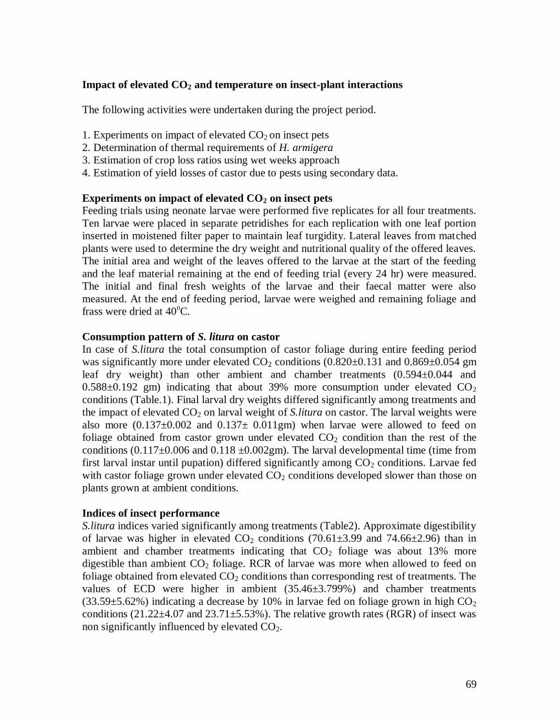
69
Impact of elevated CO2 and temperature on insect-plant interactions
The following activities were undertaken during the project period.
1. Experiments on impact of elevated CO2 on insect pets
2. Determination of thermal requirements of H. armigera
3. Estimation of crop loss ratios using wet weeks approach
4. Estimation of yield losses of castor due to pests using secondary data.
Experiments on impact of elevated CO2 on insect pets
Feeding trials using neonate larvae were performed five replicates for all four treatments.
Ten larvae were placed in separate petridishes for each replication with one leaf portion
inserted in moistened filter paper to maintain leaf turgidity. Lateral leaves from matched
plants were used to determine the dry weight and nutritional quality of the offered leaves.
The initial area and weight of the leaves offered to the larvae at the start of the feeding
and the leaf material remaining at the end of feeding trial (every 24 hr) were measured.
The initial and final fresh weights of the larvae and their faecal matter were also
measured. At the end of feeding period, larvae were weighed and remaining foliage and
frass were dried at 40oC.
Consumption pattern of S. litura on castor
In case of S.litura the total consumption of castor foliage during entire feeding period
was significantly more under elevated CO2 conditions (0.820±0.131 and 0.869±0.054 gm
leaf dry weight) than other ambient and chamber treatments (0.594±0.044 and
0.588±0.192 gm) indicating that about 39% more consumption under elevated CO2
conditions (Table.1). Final larval dry weights differed significantly among treatments and
the impact of elevated CO2 on larval weight of S.litura on castor. The larval weights were
also more (0.137±0.002 and 0.137± 0.011gm) when larvae were allowed to feed on
foliage obtained from castor grown under elevated CO2 condition than the rest of the
conditions (0.117±0.006 and 0.118 ±0.002gm). The larval developmental time (time from
first larval instar until pupation) differed significantly among CO2 conditions. Larvae fed
with castor foliage grown under elevated CO2 conditions developed slower than those on
plants grown at ambient conditions.
Indices of insect performance
S.litura indices varied significantly among treatments (Table2). Approximate digestibility
of larvae was higher in elevated CO2 conditions (70.61±3.99 and 74.66±2.96) than in
ambient and chamber treatments indicating that CO2 foliage was about 13% more
digestible than ambient CO2 foliage. RCR of larvae was more when allowed to feed on
foliage obtained from elevated CO2 conditions than corresponding rest of treatments. The
values of ECD were higher in ambient (35.46±3.799%) and chamber treatments
(33.59±5.62%) indicating a decrease by 10% in larvae fed on foliage grown in high CO2
conditions (21.22±4.07 and 23.71±5.53%). The relative growth rates (RGR) of insect was
non significantly influenced by elevated CO2.
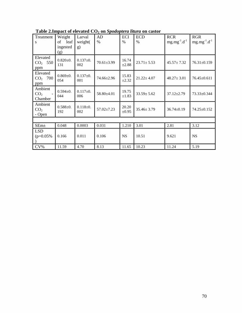
70
Table 2.Impact of elevated CO2 on Spodoptera litura on castor
Treatments
Weight of leaf
ingested
(g)
Larval weight(
g)
AD %
ECI %
ECD %
RCR mg.mg
-1.d
-1
RGR mg.mg
-1.d
-1
Elevated
CO2 550 ppm
0.820±0.
131
0.137±0.
002 70.61±3.99
16.74
±2.88 23.71± 5.53 45.57± 7.32 76.31±0.159
Elevated
CO2 700
ppm
0.869±0.
054
0.137±0.
001 74.66±2.96
15.83
±2.32 21.22± 4.07 48.27± 3.01 76.45±0.611
Ambient CO2 -
Chamber
0.594±0.
044
0.117±0.
006 58.80±4.01
19.75
±1.83 33.59± 5.62 37.12±2.79 73.33±0.344
Ambient
CO2
- Open
0.588±0.
192
0.118±0.
002 57.02±7.23
20.20
±0.95 35.46± 3.79 36.74±0.19 74.25±0.152
SEm± 0.048 0.0003 0.031 1.210 3.01 2.81 3.12
LSD
(p=0.05%
)
0.166 0.011 0.106 NS 10.51 9.621 NS
CV% 11.59 4.70 8.13 11.65 10.23 11.24 5.19
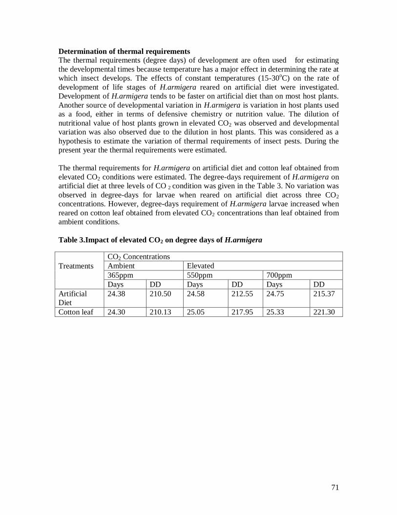
71
Determination of thermal requirements
The thermal requirements (degree days) of development are often used for estimating
the developmental times because temperature has a major effect in determining the rate at
which insect develops. The effects of constant temperatures (15-30oC) on the rate of
development of life stages of H.armigera reared on artificial diet were investigated.
Development of H.armigera tends to be faster on artificial diet than on most host plants.
Another source of developmental variation in H.armigera is variation in host plants used
as a food, either in terms of defensive chemistry or nutrition value. The dilution of
nutritional value of host plants grown in elevated CO2 was observed and developmental
variation was also observed due to the dilution in host plants. This was considered as a
hypothesis to estimate the variation of thermal requirements of insect pests. During the
present year the thermal requirements were estimated.
The thermal requirements for H.armigera on artificial diet and cotton leaf obtained from
elevated CO2 conditions were estimated. The degree-days requirement of H.armigera on
artificial diet at three levels of CO 2 condition was given in the Table 3. No variation was
observed in degree-days for larvae when reared on artificial diet across three CO2
concentrations. However, degree-days requirement of H.armigera larvae increased when
reared on cotton leaf obtained from elevated CO2 concentrations than leaf obtained from
ambient conditions.
Table 3.Impact of elevated CO2 on degree days of H.armigera
Treatments
CO2 Concentrations
Ambient Elevated
365ppm 550ppm 700ppm
Days DD Days DD Days DD
Artificial
Diet
24.38 210.50 24.58 212.55 24.75 215.37
Cotton leaf 24.30 210.13 25.05 217.95 25.33 221.30
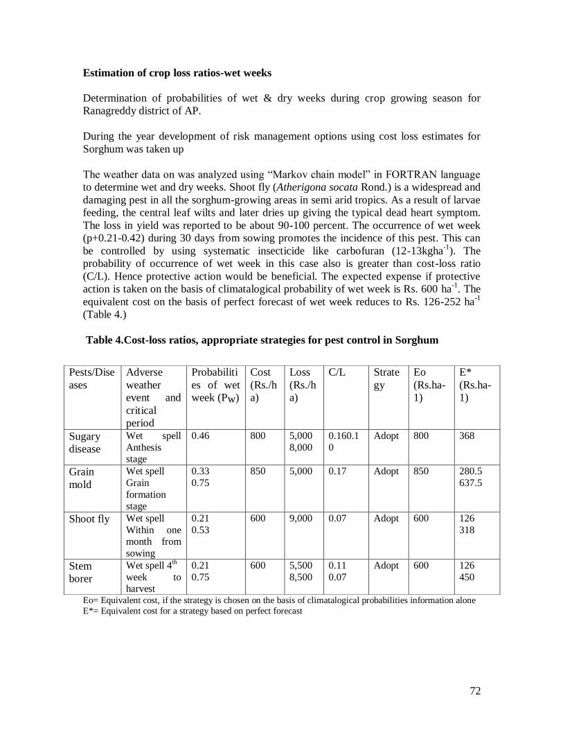
72
Estimation of crop loss ratios-wet weeks
Determination of probabilities of wet & dry weeks during crop growing season for
Ranagreddy district of AP.
During the year development of risk management options using cost loss estimates for
Sorghum was taken up
The weather data on was analyzed using “Markov chain model” in FORTRAN language
to determine wet and dry weeks. Shoot fly (Atherigona socata Rond.) is a widespread and
damaging pest in all the sorghum-growing areas in semi arid tropics. As a result of larvae
feeding, the central leaf wilts and later dries up giving the typical dead heart symptom.
The loss in yield was reported to be about 90-100 percent. The occurrence of wet week
(p+0.21-0.42) during 30 days from sowing promotes the incidence of this pest. This can
be controlled by using systematic insecticide like carbofuran (12-13kgha-1
). The
probability of occurrence of wet week in this case also is greater than cost-loss ratio
(C/L). Hence protective action would be beneficial. The expected expense if protective
action is taken on the basis of climatalogical probability of wet week is Rs. 600 ha-1
. The
equivalent cost on the basis of perfect forecast of wet week reduces to Rs. 126-252 ha-1
(Table 4.)
Table 4.Cost-loss ratios, appropriate strategies for pest control in Sorghum
Eo= Equivalent cost, if the strategy is chosen on the basis of climatalogical probabilities information alone
E*= Equivalent cost for a strategy based on perfect forecast
Pests/Dise
ases
Adverse
weather
event and
critical
period
Probabiliti
es of wet
week (Pw)
Cost
(Rs./h
a)
Loss
(Rs./h
a)
C/L Strate
gy
Eo
(Rs.ha-
1)
E*
(Rs.ha-
1)
Sugary
disease
Wet spell
Anthesis stage
0.46 800 5,000
8,000
0.160.1
0
Adopt 800 368
Grain
mold
Wet spell
Grain
formation stage
0.33
0.75
850 5,000
0.17 Adopt 850 280.5
637.5
Shoot fly Wet spell
Within one month from
sowing
0.21
0.53
600 9,000 0.07 Adopt 600 126
318
Stem
borer
Wet spell 4th
week to harvest
0.21
0.75
600 5,500
8,500
0.11
0.07
Adopt 600 126
450
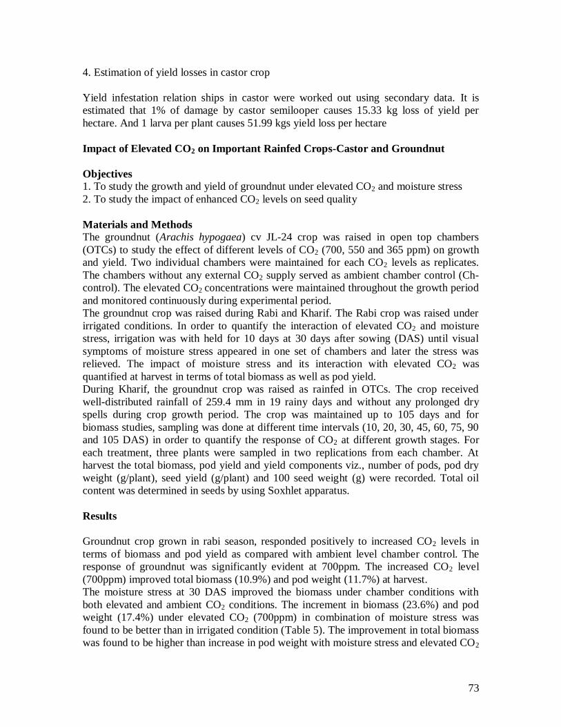
73
4. Estimation of yield losses in castor crop
Yield infestation relation ships in castor were worked out using secondary data. It is
estimated that 1% of damage by castor semilooper causes 15.33 kg loss of yield per
hectare. And 1 larva per plant causes 51.99 kgs yield loss per hectare
Impact of Elevated CO2 on Important Rainfed Crops-Castor and Groundnut
Objectives
1. To study the growth and yield of groundnut under elevated CO2 and moisture stress
2. To study the impact of enhanced CO2 levels on seed quality
Materials and Methods
The groundnut (Arachis hypogaea) cv JL-24 crop was raised in open top chambers
(OTCs) to study the effect of different levels of CO2 (700, 550 and 365 ppm) on growth
and yield. Two individual chambers were maintained for each CO2 levels as replicates.
The chambers without any external CO2 supply served as ambient chamber control (Ch-
control). The elevated CO2 concentrations were maintained throughout the growth period
and monitored continuously during experimental period.
The groundnut crop was raised during Rabi and Kharif. The Rabi crop was raised under
irrigated conditions. In order to quantify the interaction of elevated CO2 and moisture
stress, irrigation was with held for 10 days at 30 days after sowing (DAS) until visual
symptoms of moisture stress appeared in one set of chambers and later the stress was
relieved. The impact of moisture stress and its interaction with elevated CO2 was
quantified at harvest in terms of total biomass as well as pod yield.
During Kharif, the groundnut crop was raised as rainfed in OTCs. The crop received
well-distributed rainfall of 259.4 mm in 19 rainy days and without any prolonged dry
spells during crop growth period. The crop was maintained up to 105 days and for
biomass studies, sampling was done at different time intervals (10, 20, 30, 45, 60, 75, 90
and 105 DAS) in order to quantify the response of CO2 at different growth stages. For
each treatment, three plants were sampled in two replications from each chamber. At
harvest the total biomass, pod yield and yield components viz., number of pods, pod dry
weight (g/plant), seed yield (g/plant) and 100 seed weight (g) were recorded. Total oil
content was determined in seeds by using Soxhlet apparatus.
Results
Groundnut crop grown in rabi season, responded positively to increased CO2 levels in
terms of biomass and pod yield as compared with ambient level chamber control. The
response of groundnut was significantly evident at 700ppm. The increased CO2 level
(700ppm) improved total biomass (10.9%) and pod weight (11.7%) at harvest.
The moisture stress at 30 DAS improved the biomass under chamber conditions with
both elevated and ambient CO2 conditions. The increment in biomass (23.6%) and pod
weight (17.4%) under elevated CO2 (700ppm) in combination of moisture stress was
found to be better than in irrigated condition (Table 5). The improvement in total biomass
was found to be higher than increase in pod weight with moisture stress and elevated CO2
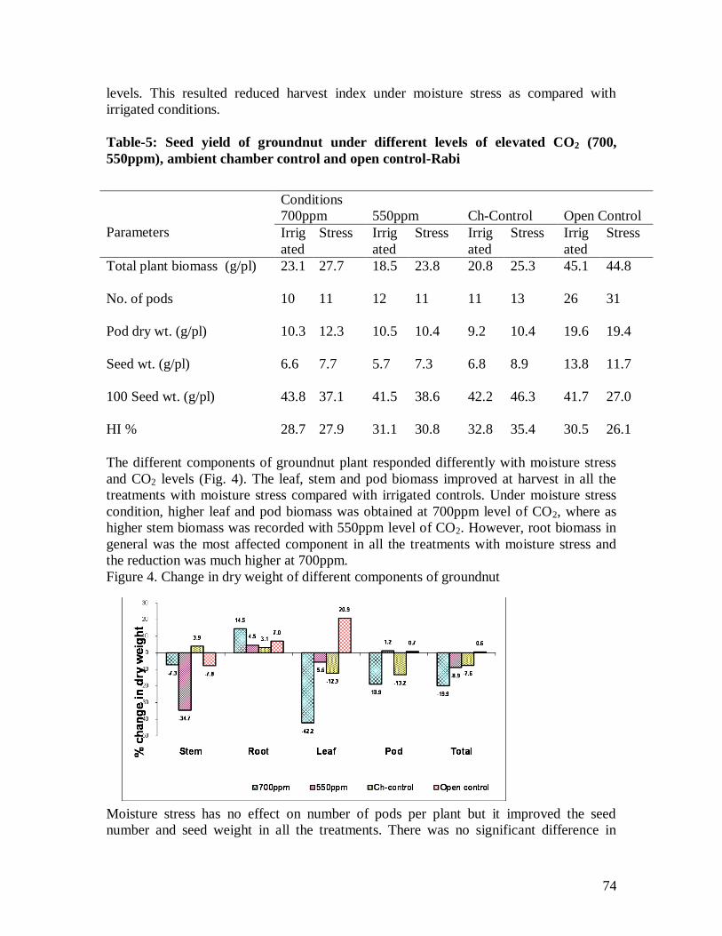
74
levels. This resulted reduced harvest index under moisture stress as compared with
irrigated conditions.
Table-5: Seed yield of groundnut under different levels of elevated CO2 (700,
550ppm), ambient chamber control and open control-Rabi
The different components of groundnut plant responded differently with moisture stress
and CO2 levels (Fig. 4). The leaf, stem and pod biomass improved at harvest in all the
treatments with moisture stress compared with irrigated controls. Under moisture stress
condition, higher leaf and pod biomass was obtained at 700ppm level of CO2, where as
higher stem biomass was recorded with 550ppm level of CO2. However, root biomass in
general was the most affected component in all the treatments with moisture stress and
the reduction was much higher at 700ppm.
Figure 4. Change in dry weight of different components of groundnut
Moisture stress has no effect on number of pods per plant but it improved the seed
number and seed weight in all the treatments. There was no significant difference in
Parameters
Conditions
700ppm 550ppm Ch-Control Open Control
Irrig
ated
Stress Irrig
ated
Stress Irrig
ated
Stress Irrig
ated
Stress
Total plant biomass (g/pl) 23.1 27.7 18.5 23.8 20.8 25.3 45.1 44.8
No. of pods 10 11 12 11 11 13 26 31
Pod dry wt. (g/pl) 10.3 12.3 10.5 10.4 9.2 10.4 19.6 19.4
Seed wt. (g/pl) 6.6 7.7 5.7 7.3 6.8 8.9 13.8 11.7
100 Seed wt. (g/pl) 43.8 37.1 41.5 38.6 42.2 46.3 41.7 27.0
HI % 28.7 27.9 31.1 30.8 32.8 35.4 30.5 26.1
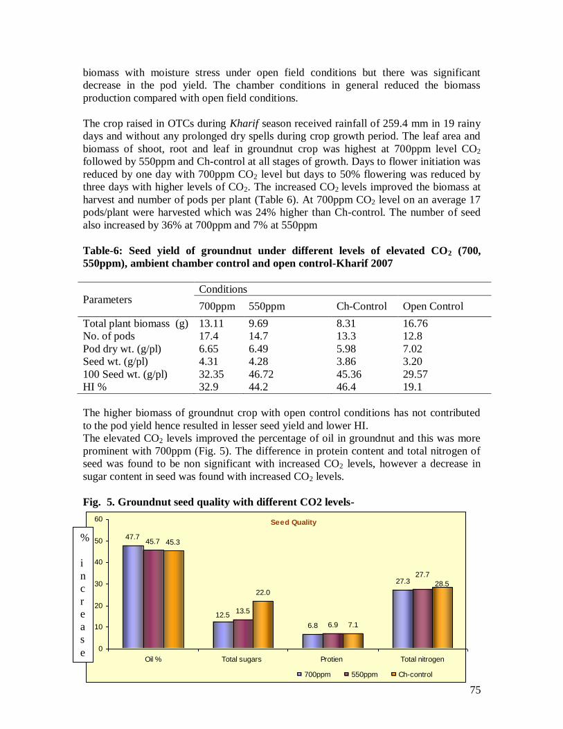
75
biomass with moisture stress under open field conditions but there was significant
decrease in the pod yield. The chamber conditions in general reduced the biomass
production compared with open field conditions.
The crop raised in OTCs during Kharif season received rainfall of 259.4 mm in 19 rainy
days and without any prolonged dry spells during crop growth period. The leaf area and
biomass of shoot, root and leaf in groundnut crop was highest at 700ppm level CO2
followed by 550ppm and Ch-control at all stages of growth. Days to flower initiation was
reduced by one day with 700ppm CO2 level but days to 50% flowering was reduced by
three days with higher levels of CO2. The increased CO2 levels improved the biomass at
harvest and number of pods per plant (Table 6). At 700ppm CO2 level on an average 17
pods/plant were harvested which was 24% higher than Ch-control. The number of seed
also increased by 36% at 700ppm and 7% at 550ppm
Table-6: Seed yield of groundnut under different levels of elevated CO2 (700,
550ppm), ambient chamber control and open control-Kharif 2007
Parameters Conditions
700ppm 550ppm Ch-Control Open Control
Total plant biomass (g) 13.11 9.69 8.31 16.76
No. of pods 17.4 14.7 13.3 12.8
Pod dry wt. (g/pl) 6.65 6.49 5.98 7.02
Seed wt. (g/pl) 4.31 4.28 3.86 3.20
100 Seed wt. (g/pl) 32.35 46.72 45.36 29.57
HI % 32.9 44.2 46.4 19.1
The higher biomass of groundnut crop with open control conditions has not contributed
to the pod yield hence resulted in lesser seed yield and lower HI.
The elevated CO2 levels improved the percentage of oil in groundnut and this was more
prominent with 700ppm (Fig. 5). The difference in protein content and total nitrogen of
seed was found to be non significant with increased CO2 levels, however a decrease in
sugar content in seed was found with increased CO2 levels.
Fig. 5. Groundnut seed quality with different CO2 levels-
Seed Quality
47.7
6.8
27.3
45.7
13.5
6.9
45.3
22.0
7.1
12.5
27.7
28.5
0
10
20
30
40
50
60
Oil % Total sugars Protien Total nitrogen
700ppm 550ppm Ch-control
%
i
n
c
r
e
a
s
e
76
N summary, groundnut crop showed positive response to elevated CO2 levels for growth
and yield and the response was significantly evident at 700ppm. The responses of
different plant components of groundnut crop were found to be different with CO2 levels
and moisture stress. Moisture stress at initial stages improved the total biomass and pod
yield in all the treatments and the response was more at higher levels of CO2.The seed
weight increased with moisture stress due to higher number of pods and seeds, however
reduced 100 seed weight was observed with moisture stress. Both elevated CO2 levels
increased the oil content and the response was more prominent at higher level.
The unsaturated fatty acids increased over saturated fatty acids with elevated CO2 levels.
It was also observed that the content of Oleic acid showed increasing trend with elevated
CO2 levels where as the reverse trend was with linolenic acid fraction.The chamber
conditions in general reduced the biomass production (up to 50%) during both Rabi and
Kharif seasons compared with open field conditions.
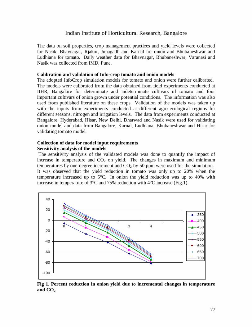
77
Indian Institute of Horticultural Research, Bangalore
The data on soil properties, crop management practices and yield levels were collected
for Nasik, Bhavnagar, Rjakot, Junagadh and Karnal for onion and Bhubaneshwar and
Ludhiana for tomato. Daily weather data for Bhavnagar, Bhubaneshwar, Varanasi and
Nasik was collected from IMD, Pune.
Calibration and validation of Info-crop tomato and onion models
The adopted InfoCrop simulation models for tomato and onion were further calibrated.
The models were calibrated from the data obtained from field experiments conducted at
IIHR, Bangalore for determinate and indeterminate cultivars of tomato and four
important cultivars of onion grown under potential conditions. The information was also
used from published literature on these crops. Validation of the models was taken up
with the inputs from experiments conducted at different agro-ecological regions for
different seasons, nitrogen and irrigation levels. The data from experiments conducted at
Bangalore, Hyderabad, Hisar, New Delhi, Dharwad and Nasik were used for validating
onion model and data from Bangalore, Karnal, Ludhiana, Bhubaneshwar and Hisar for
validating tomato model.
Collection of data for model input requirements
Sensitivity analysis of the models
The sensitivity analysis of the validated models was done to quantify the impact of
increase in temperature and CO2 on yield. The changes in maximum and minimum
temperatures by one-degree increment and CO2 by 50 ppm were used for the simulation.
It was observed that the yield reduction in tomato was only up to 20% when the
temperature increased up to 5°C. In onion the yield reduction was up to 40% with
increase in temperature of 3°C and 75% reduction with 4°C increase (Fig.1).
-100
-80
-60
-40
-20
0
20
40
0 1 2 3 4
350
400
450
500
550
600
650
700
Fig 1. Percent reduction in onion yield due to incremental changes in temperature
and CO2
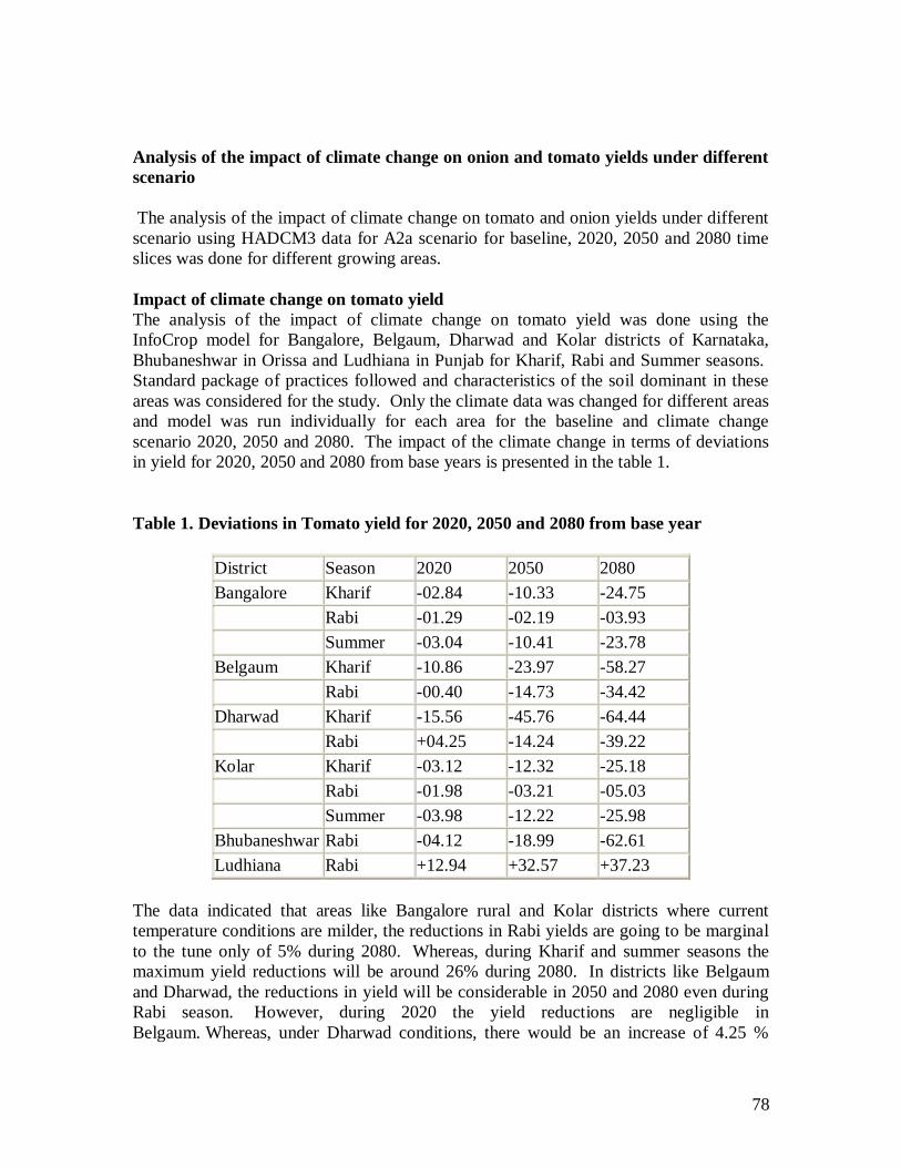
78
Analysis of the impact of climate change on onion and tomato yields under different
scenario
The analysis of the impact of climate change on tomato and onion yields under different
scenario using HADCM3 data for A2a scenario for baseline, 2020, 2050 and 2080 time
slices was done for different growing areas.
Impact of climate change on tomato yield
The analysis of the impact of climate change on tomato yield was done using the
InfoCrop model for Bangalore, Belgaum, Dharwad and Kolar districts of Karnataka,
Bhubaneshwar in Orissa and Ludhiana in Punjab for Kharif, Rabi and Summer seasons.
Standard package of practices followed and characteristics of the soil dominant in these
areas was considered for the study. Only the climate data was changed for different areas
and model was run individually for each area for the baseline and climate change
scenario 2020, 2050 and 2080. The impact of the climate change in terms of deviations
in yield for 2020, 2050 and 2080 from base years is presented in the table 1.
Table 1. Deviations in Tomato yield for 2020, 2050 and 2080 from base year
District Season 2020 2050 2080
Bangalore Kharif -02.84 -10.33 -24.75
Rabi -01.29 -02.19 -03.93
Summer -03.04 -10.41 -23.78
Belgaum Kharif -10.86 -23.97 -58.27
Rabi -00.40 -14.73 -34.42
Dharwad Kharif -15.56 -45.76 -64.44
Rabi +04.25 -14.24 -39.22
Kolar Kharif -03.12 -12.32 -25.18
Rabi -01.98 -03.21 -05.03
Summer -03.98 -12.22 -25.98
Bhubaneshwar Rabi -04.12 -18.99 -62.61
Ludhiana Rabi +12.94 +32.57 +37.23
The data indicated that areas like Bangalore rural and Kolar districts where current
temperature conditions are milder, the reductions in Rabi yields are going to be marginal
to the tune only of 5% during 2080. Whereas, during Kharif and summer seasons the
maximum yield reductions will be around 26% during 2080. In districts like Belgaum
and Dharwad, the reductions in yield will be considerable in 2050 and 2080 even during
Rabi season. However, during 2020 the yield reductions are negligible in
Belgaum. Whereas, under Dharwad conditions, there would be an increase of 4.25 %
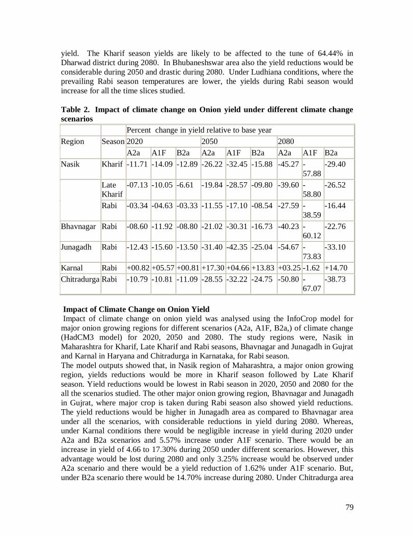
79
yield. The Kharif season yields are likely to be affected to the tune of 64.44% in
Dharwad district during 2080. In Bhubaneshswar area also the yield reductions would be
considerable during 2050 and drastic during 2080. Under Ludhiana conditions, where the
prevailing Rabi season temperatures are lower, the yields during Rabi season would
increase for all the time slices studied.
Table 2. Impact of climate change on Onion yield under different climate change
scenarios
Percent change in yield relative to base year
Region Season 2020 2050 2080
A2a A1F B2a A2a A1F B2a A2a A1F B2a
Nasik Kharif -11.71 -14.09 -12.89 -26.22 -32.45 -15.88 -45.27 -
57.88
-29.40
Late
Kharif
-07.13 -10.05 -6.61 -19.84 -28.57 -09.80 -39.60 -
58.80
-26.52
Rabi -03.34 -04.63 -03.33 -11.55 -17.10 -08.54 -27.59 -
38.59
-16.44
Bhavnagar Rabi -08.60 -11.92 -08.80 -21.02 -30.31 -16.73 -40.23 -
60.12
-22.76
Junagadh Rabi -12.43 -15.60 -13.50 -31.40 -42.35 -25.04 -54.67 -
73.83
-33.10
Karnal Rabi +00.82 +05.57 +00.81 +17.30 +04.66 +13.83 +03.25 -1.62 +14.70
Chitradurga Rabi -10.79 -10.81 -11.09 -28.55 -32.22 -24.75 -50.80 -
67.07
-38.73
Impact of Climate Change on Onion Yield
Impact of climate change on onion yield was analysed using the InfoCrop model for
major onion growing regions for different scenarios (A2a, A1F, B2a,) of climate change
(HadCM3 model) for 2020, 2050 and 2080. The study regions were, Nasik in
Maharashtra for Kharif, Late Kharif and Rabi seasons, Bhavnagar and Junagadh in Gujrat
and Karnal in Haryana and Chitradurga in Karnataka, for Rabi season.
The model outputs showed that, in Nasik region of Maharashtra, a major onion growing
region, yields reductions would be more in Kharif season followed by Late Kharif
season. Yield reductions would be lowest in Rabi season in 2020, 2050 and 2080 for the
all the scenarios studied. The other major onion growing region, Bhavnagar and Junagadh
in Gujrat, where major crop is taken during Rabi season also showed yield reductions.
The yield reductions would be higher in Junagadh area as compared to Bhavnagar area
under all the scenarios, with considerable reductions in yield during 2080. Whereas,
under Karnal conditions there would be negligible increase in yield during 2020 under
A2a and B2a scenarios and 5.57% increase under A1F scenario. There would be an
increase in yield of 4.66 to 17.30% during 2050 under different scenarios. However, this
advantage would be lost during 2080 and only 3.25% increase would be observed under
A2a scenario and there would be a yield reduction of 1.62% under A1F scenario. But,
under B2a scenario there would be 14.70% increase during 2080. Under Chitradurga area
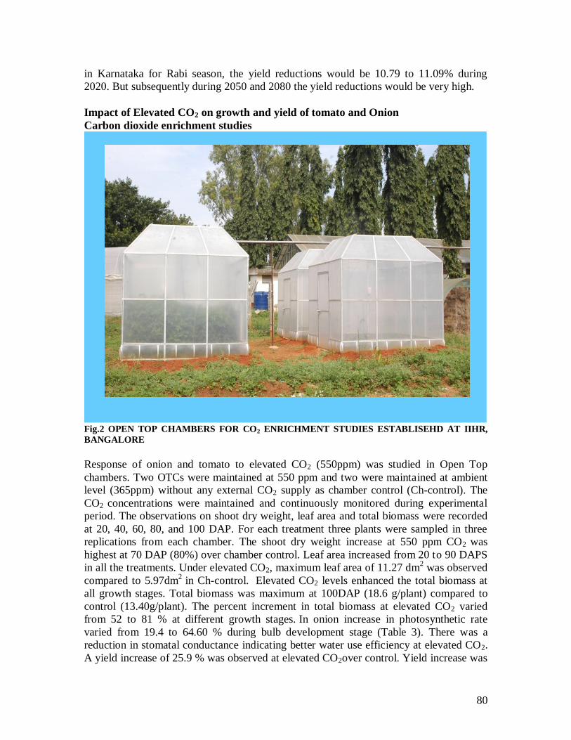
80
in Karnataka for Rabi season, the yield reductions would be 10.79 to 11.09% during
2020. But subsequently during 2050 and 2080 the yield reductions would be very high.
Impact of Elevated CO2 on growth and yield of tomato and Onion
Carbon dioxide enrichment studies
Fig.2 OPEN TOP CHAMBERS FOR CO2 ENRICHMENT STUDIES ESTABLISEHD AT IIHR,
BANGALORE
Response of onion and tomato to elevated CO2 (550ppm) was studied in Open Top
chambers. Two OTCs were maintained at 550 ppm and two were maintained at ambient
level (365ppm) without any external CO2 supply as chamber control (Ch-control). The
CO2 concentrations were maintained and continuously monitored during experimental
period. The observations on shoot dry weight, leaf area and total biomass were recorded
at 20, 40, 60, 80, and 100 DAP. For each treatment three plants were sampled in three
replications from each chamber. The shoot dry weight increase at 550 ppm CO2 was
highest at 70 DAP (80%) over chamber control. Leaf area increased from 20 to 90 DAPS
in all the treatments. Under elevated CO2, maximum leaf area of 11.27 dm2 was observed
compared to 5.97dm2
in Ch-control. Elevated CO2 levels enhanced the total biomass at
all growth stages. Total biomass was maximum at 100DAP (18.6 g/plant) compared to
control (13.40g/plant). The percent increment in total biomass at elevated CO2 varied
from 52 to 81 % at different growth stages. In onion increase in photosynthetic rate
varied from 19.4 to 64.60 % during bulb development stage (Table 3). There was a
reduction in stomatal conductance indicating better water use efficiency at elevated CO2.
A yield increase of 25.9 % was observed at elevated CO2over control. Yield increase was
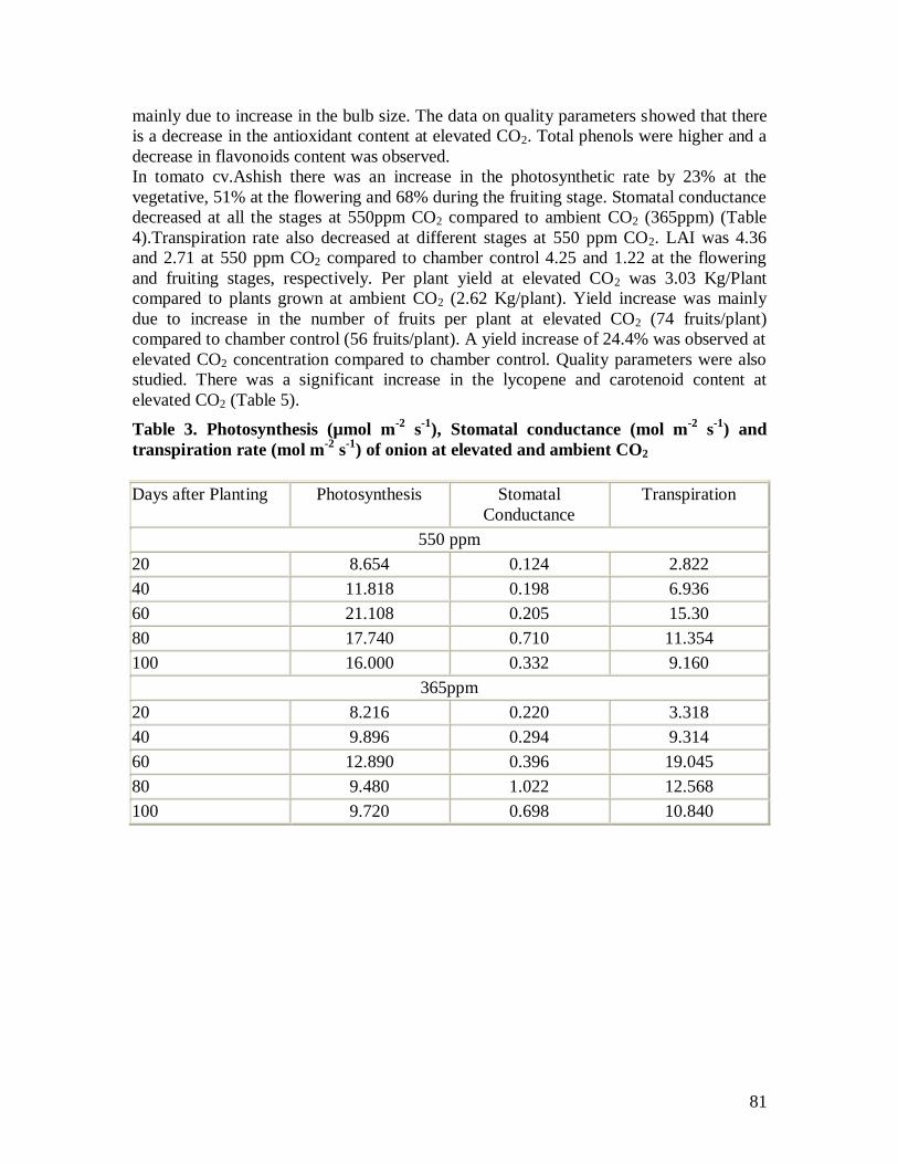
81
mainly due to increase in the bulb size. The data on quality parameters showed that there
is a decrease in the antioxidant content at elevated CO2. Total phenols were higher and a
decrease in flavonoids content was observed.
In tomato cv.Ashish there was an increase in the photosynthetic rate by 23% at the
vegetative, 51% at the flowering and 68% during the fruiting stage. Stomatal conductance
decreased at all the stages at 550ppm CO2 compared to ambient CO2 (365ppm) (Table
4).Transpiration rate also decreased at different stages at 550 ppm CO2. LAI was 4.36
and 2.71 at 550 ppm CO2 compared to chamber control 4.25 and 1.22 at the flowering
and fruiting stages, respectively. Per plant yield at elevated CO2 was 3.03 Kg/Plant
compared to plants grown at ambient CO2 (2.62 Kg/plant). Yield increase was mainly
due to increase in the number of fruits per plant at elevated CO2 (74 fruits/plant)
compared to chamber control (56 fruits/plant). A yield increase of 24.4% was observed at
elevated CO2 concentration compared to chamber control. Quality parameters were also
studied. There was a significant increase in the lycopene and carotenoid content at
elevated CO2 (Table 5).
Table 3. Photosynthesis (µmol m-2
s-1
), Stomatal conductance (mol m-2
s-1
) and
transpiration rate (mol m-2
s-1
) of onion at elevated and ambient CO2
Days after Planting Photosynthesis Stomatal
Conductance
Transpiration
550 ppm
20 8.654 0.124 2.822
40 11.818 0.198 6.936
60 21.108 0.205 15.30
80 17.740 0.710 11.354
100 16.000 0.332 9.160
365ppm
20 8.216 0.220 3.318
40 9.896 0.294 9.314
60 12.890 0.396 19.045
80 9.480 1.022 12.568
100 9.720 0.698 10.840
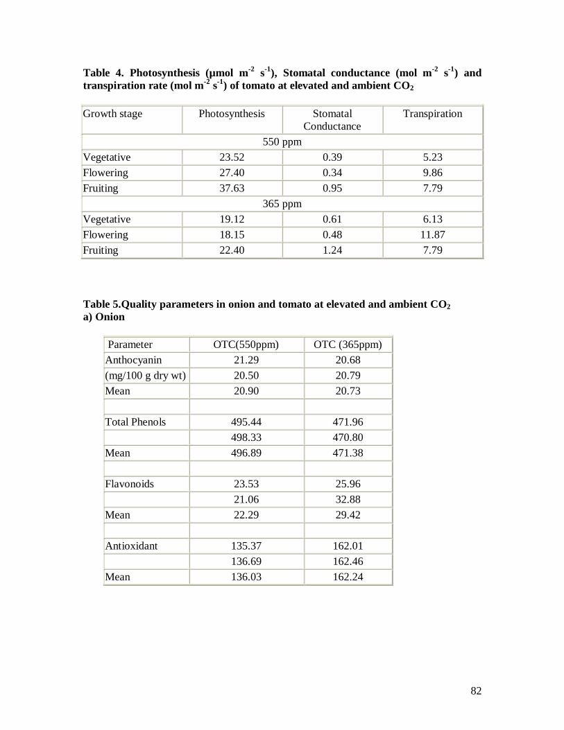
82
Table 4. Photosynthesis (µmol m-2
s-1
), Stomatal conductance (mol m-2
s-1
) and
transpiration rate (mol m-2
s-1
) of tomato at elevated and ambient CO2
Growth stage Photosynthesis Stomatal
Conductance
Transpiration
550 ppm
Vegetative 23.52 0.39 5.23
Flowering 27.40 0.34 9.86
Fruiting 37.63 0.95 7.79
365 ppm
Vegetative 19.12 0.61 6.13
Flowering 18.15 0.48 11.87
Fruiting 22.40 1.24 7.79
Table 5.Quality parameters in onion and tomato at elevated and ambient CO2
a) Onion
Parameter OTC(550ppm) OTC (365ppm)
Anthocyanin 21.29 20.68
(mg/100 g dry wt) 20.50 20.79
Mean 20.90 20.73
Total Phenols 495.44 471.96
498.33 470.80
Mean 496.89 471.38
Flavonoids 23.53 25.96
21.06 32.88
Mean 22.29 29.42
Antioxidant 135.37 162.01
136.69 162.46
Mean 136.03 162.24
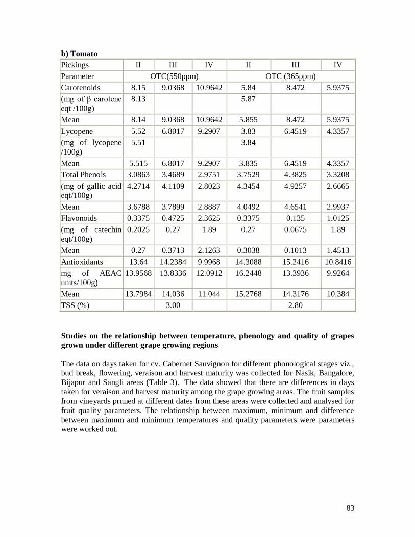
83
b) Tomato
Pickings II III IV II III IV
Parameter OTC(550ppm) OTC (365ppm)
Carotenoids 8.15 9.0368 10.9642 5.84 8.472 5.9375
(mg of β carotene
eqt /100g)
8.13 5.87
Mean 8.14 9.0368 10.9642 5.855 8.472 5.9375
Lycopene 5.52 6.8017 9.2907 3.83 6.4519 4.3357
(mg of lycopene
/100g)
5.51 3.84
Mean 5.515 6.8017 9.2907 3.835 6.4519 4.3357
Total Phenols 3.0863 3.4689 2.9751 3.7529 4.3825 3.3208
(mg of gallic acid
eqt/100g)
4.2714 4.1109 2.8023 4.3454 4.9257 2.6665
Mean 3.6788 3.7899 2.8887 4.0492 4.6541 2.9937
Flavonoids 0.3375 0.4725 2.3625 0.3375 0.135 1.0125
(mg of catechin
eqt/100g)
0.2025 0.27 1.89 0.27 0.0675 1.89
Mean 0.27 0.3713 2.1263 0.3038 0.1013 1.4513
Antioxidants 13.64 14.2384 9.9968 14.3088 15.2416 10.8416
mg of AEAC
units/100g)
13.9568 13.8336 12.0912 16.2448 13.3936 9.9264
Mean 13.7984 14.036 11.044 15.2768 14.3176 10.384
TSS (%) 3.00 2.80
Studies on the relationship between temperature, phenology and quality of grapes
grown under different grape growing regions
The data on days taken for cv. Cabernet Sauvignon for different phonological stages viz.,
bud break, flowering, veraison and harvest maturity was collected for Nasik, Bangalore,
Bijapur and Sangli areas (Table 3). The data showed that there are differences in days
taken for veraison and harvest maturity among the grape growing areas. The fruit samples
from vineyards pruned at different dates from these areas were collected and analysed for
fruit quality parameters. The relationship between maximum, minimum and difference
between maximum and minimum temperatures and quality parameters were parameters
were worked out.
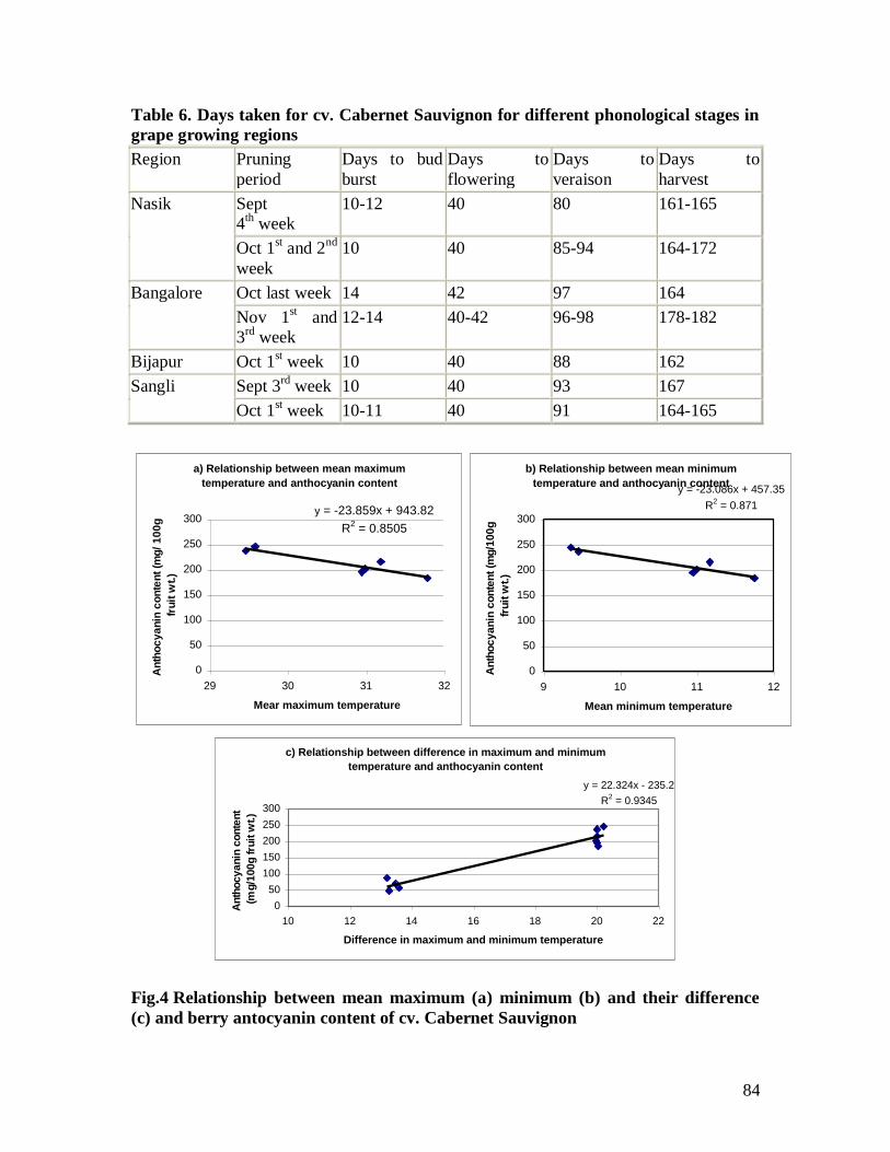
84
Table 6. Days taken for cv. Cabernet Sauvignon for different phonological stages in
grape growing regions
Region Pruning
period
Days to bud
burst
Days to
flowering
Days to
veraison
Days to
harvest
Nasik Sept
4th week
10-12 40 80 161-165
Oct 1st and 2
nd
week
10 40 85-94 164-172
Bangalore Oct last week 14 42 97 164
Nov 1st and
3rd
week
12-14 40-42 96-98 178-182
Bijapur Oct 1st week 10 40 88 162
Sangli Sept 3rd
week 10 40 93 167
Oct 1st week 10-11 40 91 164-165
Fig.4 Relationship between mean maximum (a) minimum (b) and their difference
(c) and berry antocyanin content of cv. Cabernet Sauvignon
a) Relationship between mean maximum
temperature and anthocyanin content
y = -23.859x + 943.82
R2 = 0.8505
0
50
100
150
200
250
300
29 30 31 32
Mear maximum temperature
An
tho
cy
an
in c
on
ten
t (m
g/
10
0g
fru
it w
t.)
b) Relationship between mean minimum
temperature and anthocyanin contenty = -23.086x + 457.35
R2 = 0.871
0
50
100
150
200
250
300
9 10 11 12
Mean minimum temperature
An
tho
cy
an
in c
on
ten
t (m
g/1
00
g
fru
it w
t.)
c) Relationship between difference in maximum and minimum
temperature and anthocyanin content
y = 22.324x - 235.2
R2 = 0.9345
0
50
100
150
200
250
300
10 12 14 16 18 20 22
Difference in maximum and minimum temperature
Anth
ocyanin
conte
nt
(mg/1
00g fru
it w
t.)
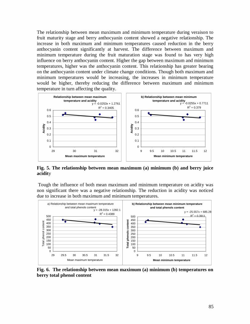
85
The relationship between mean maximum and minimum temperature during veraison to
fruit maturity stage and berry anthocyanin content showed a negative relationship. The
increase in both maximum and minimum temperatures caused reduction in the berry
anthocyanin content significantly at harvest. The difference between maximum and
minimum temperature during the fruit maturation stage was found to has very high
influence on berry anthocyanin content. Higher the gap between maximum and minimum
temperatures, higher was the anthocyanin content. This relationship has greater bearing
on the anthocyanin content under climate change conditions. Though both maximum and
minimum temperatures would be increasing, the increases in minimum temperature
would be higher, thereby reducing the difference between maximum and minimum
temperature in turn affecting the quality.
Fig. 5. The relationship between mean maximum (a) minimum (b) and berry juice
acidity
Tough the influence of both mean maximum and minimum temperature on acidity was
non significant there was a negative relationship. The reduction in acidity was noticed
due to increase in both maximum and minimum temperatures.
Fig. 6. The relationship between mean maximum (a) minimum (b) temperatures on
berry total phenol content
Relationship between mean maximum
temperature and acidity y = -0.0253x + 1.2761
R2 = 0.3405
0
0.1
0.2
0.3
0.4
0.5
0.6
29 30 31 32
Mean maximum temperature
Ac
idit
y
b) Relationship between mean minimum
temperature and acidity y = -0.0255x + 0.7711
R2 = 0.379
0
0.1
0.2
0.3
0.4
0.5
0.6
9 9.5 10 10.5 11 11.5 12
Mean minimum temperature
Ac
idit
y
a) Relationship between mean maximum temperature
and total phenols contenty = -28.315x + 1282.1
R2 = 0.4389
0
50
100
150
200
250
300
350
400
450
500
29 29.5 30 30.5 31 31.5 32
Mean maximum temperature
Tota
l ph
en
ol
co
nte
nt
b) Relationship between mean minimum temperature
and total phenols content
y = -25.557x + 685.28
R2 = 0.3911
0
50
100
150
200
250
300
350
400
450
500
9 9.5 10 10.5 11 11.5 12
Mean minimum temperature
To
tal
ph
en
ols
co
nte
nt
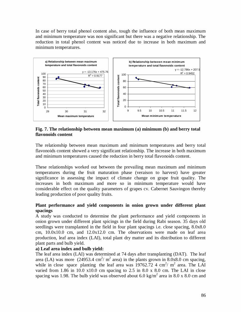
86
In case of berry total phenol content also, tough the influence of both mean maximum
and minimum temperature was non significant but there was a negative relationship. The
reduction in total phenol content was noticed due to increase in both maximum and
minimum temperatures.
Fig. 7. The relationship between mean maximum (a) minimum (b) and berry total
flavonoids content
The relationship between mean maximum and minimum temperatures and berry total
flavonoids content showed a very significant relationship. The increase in both maximum
and minimum temperatures caused the reduction in berry total flavonoids content.
These relationships worked out between the prevailing mean maximum and minimum
temperatures during the fruit maturation phase (veraison to harvest) have greater
significance in assessing the impact of climate change on grape fruit quality. The
increases in both maximum and more so in minimum temperature would have
considerable effect on the quality parameters of grapes cv. Cabernet Sauvingon thereby
leading production of poor quality fruits.
Plant performance and yield components in onion grown under different plant
spacings
A study was conducted to determine the plant performance and yield components in
onion grown under different plant spicings in the field during Rabi season. 35 days old
seedlings were transplanted in the field in four plant spacings i.e. close spacing, 8.0x8.0
cm, 10.0x10.0 cm, and 12.0x12.0 cm. The observations were made on leaf area
production, leaf area index (LAI), total plant dry matter and its distribution to different
plant parts and bulb yield.
a) Leaf area index and bulb yield:
The leaf area index (LAI) was determined at 74 days after transplanting (DAT). The leaf
area (LA) was more (24953.4 cm2/ m
2 area) in the plants grown in 8.0x8.0 cm spacing,
while in close space planting the leaf area was 19762.72 4 cm2/ m
2 area. The LAI
varied from 1.86 in 10.0 x10.0 cm spacing to 2.5 in 8.0 x 8.0 cm. The LAI in close
spacing was 1.98. The bulb yield was observed about 6.0 kg/m2 area in 8.0 x 8.0 cm and
a) Relationship between mean maximum
temperature and total flavonoids content
y = -13.176x + 475.76
R2 = 0.9177
0
10
20
30
40
50
60
70
80
90
100
29 30 31 32
Mean maximum temperature
To
tal
fla
von
oid
s c
on
ten
t
b) Relationship between mean minimum
temperature and total flavonoids content
y = -12.786x + 207.5
R2 = 0.9452
0
20
40
60
80
100
9 9.5 10 10.5 11 11.5 12
Mean minimum temperatureT
ota
l fl
avo
no
ids c
on
ten
t
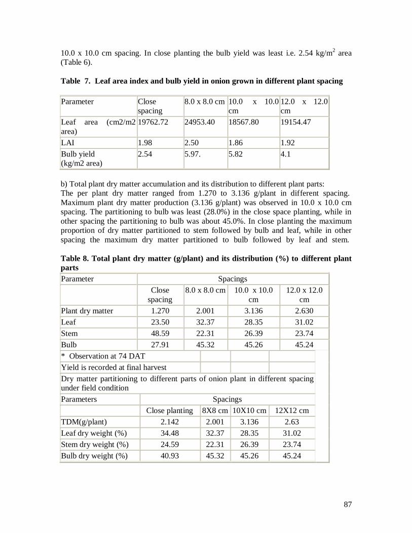
87
10.0 x 10.0 cm spacing. In close planting the bulb yield was least i.e. 2.54 kg/m2 area
(Table 6).
Table 7. Leaf area index and bulb yield in onion grown in different plant spacing
Parameter Close
spacing
8.0 x 8.0 cm 10.0 x 10.0
cm
12.0 x 12.0
cm
Leaf area (cm2/m2
area)
19762.72 24953.40 18567.80 19154.47
LAI 1.98 2.50 1.86 1.92
Bulb yield
(kg/m2 area)
2.54 5.97. 5.82 4.1
b) Total plant dry matter accumulation and its distribution to different plant parts:
The per plant dry matter ranged from 1.270 to 3.136 g/plant in different spacing.
Maximum plant dry matter production (3.136 g/plant) was observed in 10.0 x 10.0 cm
spacing. The partitioning to bulb was least (28.0%) in the close space planting, while in
other spacing the partitioning to bulb was about 45.0%. In close planting the maximum
proportion of dry matter partitioned to stem followed by bulb and leaf, while in other
spacing the maximum dry matter partitioned to bulb followed by leaf and stem.
Table 8. Total plant dry matter (g/plant) and its distribution (%) to different plant
parts
Parameter Spacings
Close
spacing
8.0 x 8.0 cm 10.0 x 10.0
cm
12.0 x 12.0
cm
Plant dry matter 1.270 2.001 3.136 2.630
Leaf 23.50 32.37 28.35 31.02
Stem 48.59 22.31 26.39 23.74
Bulb 27.91 45.32 45.26 45.24
* Observation at 74 DAT
Yield is recorded at final harvest
Dry matter partitioning to different parts of onion plant in different spacing
under field condition
Parameters Spacings
Close planting 8X8 cm 10X10 cm 12X12 cm
TDM(g/plant) 2.142 2.001 3.136 2.63
Leaf dry weight (%) 34.48 32.37 28.35 31.02
Stem dry weight (%) 24.59 22.31 26.39 23.74
Bulb dry weight (%) 40.93 45.32 45.26 45.24
88
CSK Himachal Pradesh Agricultural University, Palampur
Impact of climate change on crops:
Maize:
The INFOCROP-maize model was validated using the historical data generated by the
research trials at Palampur. The weather data and soil data already generated was used.
Impact of elevated CO2 on maize yield was simulated under both potential i.e., no
resource limitation and rainfed under recommended package and practices under sub
humid and subtropical region of Palampur. Results showed that the magnitude of impact
of elevated Co2 was more under rainfed conditions. Under potential conditions, an
increase in CO2 to 420ppm and 470ppm levels indicated an increase of more than 3.0%
and 5.4% in 10th
June sown crop over current CO2 levels (Table 1 & Fig 1). The
subsequent planting windows on 20th June showed 3.8 and 6.3% increase in yield under
420ppm and 470ppm CO2 levels.
The highest yields under potential conditions were obtained on 10th
June sown crop at all
levels of CO2 based on Probability Distribution Function. Similarly under Rainfed
Conditions the best planting was 10th June. It is also supported by the weather data of the
region as Palampur region receives pre-monsoon rains during first week of June which is
best for sowing of crop.
Under rainfed conditions 420ppm and 470ppm levels indicated an increase of more than
4.3 and 8.1% in 10th
June sown crop (Table 2).The elevated CO2 levels i.e. 420 and 470
ppm showed an increase in yield. The rainfed crop was simulated under recommended
packages and practices.
Table 1. Impact of elevated CO2 on Maize Yield under No Resource Limitation in Sub
Humid Subtropical Conditions. (Based on 20 Years).
Date of
Sowing
CO2 Impact Percent Change in Yield
370 420 470 420 ppm 470 ppm
10th June
Mean 6448.35±1096 6643.07±1042 6794 ±1252 3.0 5.4
Maximum 10989 113450 12446
Minimum 5610 5834.0 5937.0
20th June
Mean 6000.0±1288 6230.0±1083 6379.0±1259 3.80 6.3
Maximum 10132 12306.0 1241.0
Minimum 5795 6263.0 6802.0
30th June
Mean 5892.0±1273 6094±1110 6149.0±1245 3.4 4.4
Maximum 8997 98763.0 99270
Minimum 5858 5913.0 6058.0
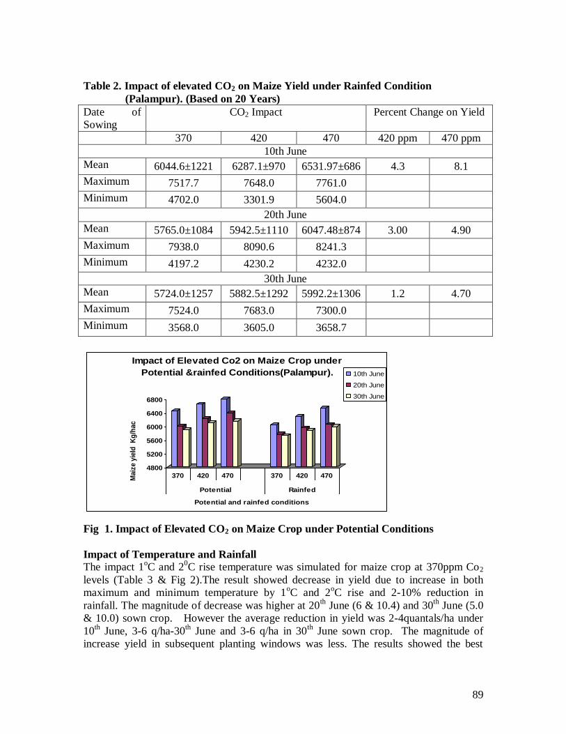
89
Table 2. Impact of elevated CO2 on Maize Yield under Rainfed Condition
(Palampur). (Based on 20 Years)
Date of
Sowing
CO2 Impact Percent Change on Yield
370 420 470 420 ppm 470 ppm
10th June
Mean 6044.6±1221 6287.1±970 6531.97±686 4.3 8.1
Maximum 7517.7 7648.0 7761.0
Minimum 4702.0 3301.9 5604.0
20th June
Mean 5765.0±1084 5942.5±1110 6047.48±874 3.00 4.90
Maximum 7938.0 8090.6 8241.3
Minimum 4197.2 4230.2 4232.0
30th June
Mean 5724.0±1257 5882.5±1292 5992.2±1306 1.2 4.70
Maximum 7524.0 7683.0 7300.0
Minimum 3568.0 3605.0 3658.7
Fig 1. Impact of Elevated CO2 on Maize Crop under Potential Conditions
Impact of Temperature and Rainfall
The impact 1oC and 2
0C rise temperature was simulated for maize crop at 370ppm Co2
levels (Table 3 & Fig 2).The result showed decrease in yield due to increase in both
maximum and minimum temperature by 1oC and 2
oC rise and 2-10% reduction in
rainfall. The magnitude of decrease was higher at 20th June (6 & 10.4) and 30
th June (5.0
& 10.0) sown crop. However the average reduction in yield was 2-4quantals/ha under
10th June, 3-6 q/ha-30
th June and 3-6 q/ha in 30
th June sown crop. The magnitude of
increase yield in subsequent planting windows was less. The results showed the best
4800
5200
5600
6000
6400
6800
Maiz
e y
ield
K
g/h
ac
370 420 470 370 420 470
Potential Rainfed
Potential and rainfed conditions
Impact of Elevated Co2 on Maize Crop under
Potential &rainfed Conditions(Palampur). 10th June
20th June
30th June
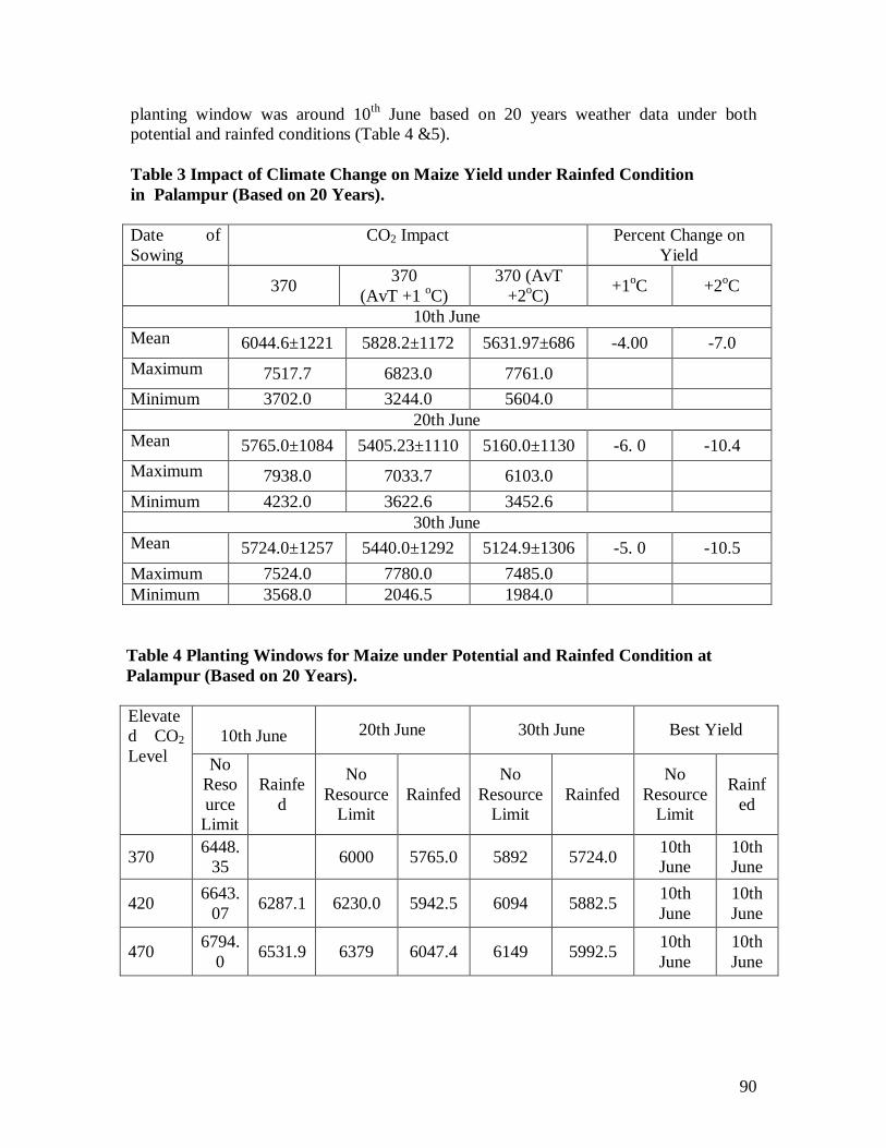
90
planting window was around 10th
June based on 20 years weather data under both
potential and rainfed conditions (Table 4 &5).
Table 3 Impact of Climate Change on Maize Yield under Rainfed Condition
in Palampur (Based on 20 Years).
Date of
Sowing
CO2 Impact Percent Change on
Yield
370
370
(AvT +1 oC)
370 (AvT
+2oC)
+1oC +2
oC
10th June
Mean 6044.6±1221 5828.2±1172 5631.97±686 -4.00 -7.0
Maximum 7517.7 6823.0 7761.0
Minimum 3702.0 3244.0 5604.0
20th June
Mean 5765.0±1084 5405.23±1110 5160.0±1130 -6. 0 -10.4
Maximum 7938.0 7033.7 6103.0
Minimum 4232.0 3622.6 3452.6
30th June
Mean 5724.0±1257 5440.0±1292 5124.9±1306 -5. 0 -10.5
Maximum 7524.0 7780.0 7485.0
Minimum 3568.0 2046.5 1984.0
Table 4 Planting Windows for Maize under Potential and Rainfed Condition at
Palampur (Based on 20 Years).
Elevate
d CO2
Level
10th June 20th June 30th June Best Yield
No
Reso
urce
Limit
Rainfe
d
No
Resource
Limit
Rainfed
No
Resource
Limit
Rainfed
No
Resource
Limit
Rainf
ed
370 6448.
35 6000 5765.0 5892 5724.0
10th
June
10th
June
420 6643.
07 6287.1 6230.0 5942.5 6094 5882.5
10th
June
10th
June
470 6794.
0 6531.9 6379 6047.4 6149 5992.5
10th
June
10th
June
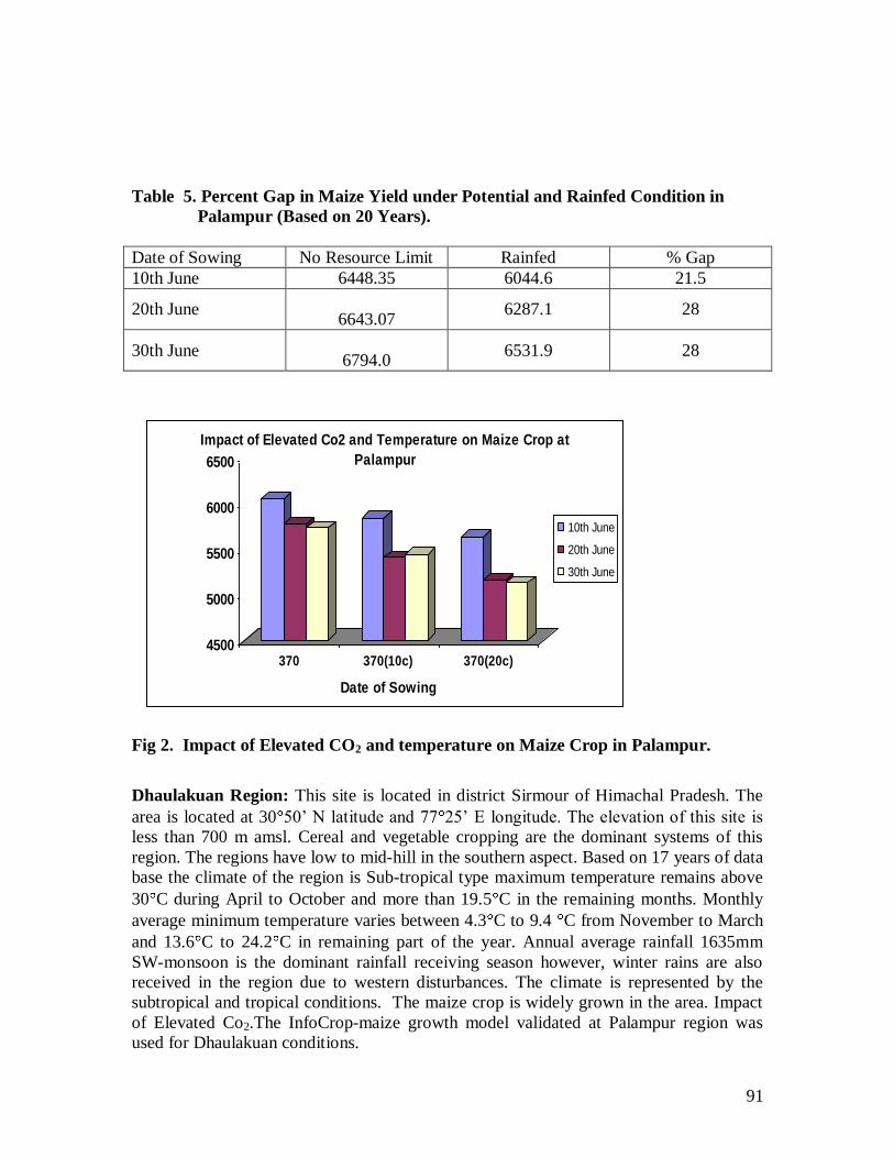
91
Table 5. Percent Gap in Maize Yield under Potential and Rainfed Condition in
Palampur (Based on 20 Years).
Date of Sowing No Resource Limit Rainfed % Gap
10th June 6448.35 6044.6 21.5
20th June
6643.07 6287.1 28
30th June
6794.0 6531.9 28
Fig 2. Impact of Elevated CO2 and temperature on Maize Crop in Palampur.
Dhaulakuan Region: This site is located in district Sirmour of Himachal Pradesh. The
area is located at 30 50‟ N latitude and 77 25‟ E longitude. The elevation of this site is
less than 700 m amsl. Cereal and vegetable cropping are the dominant systems of this
region. The regions have low to mid-hill in the southern aspect. Based on 17 years of data
base the climate of the region is Sub-tropical type maximum temperature remains above
30 C during April to October and more than 19.5 C in the remaining months. Monthly
average minimum temperature varies between 4.3 C to 9.4 C from November to March
and 13.6 C to 24.2 C in remaining part of the year. Annual average rainfall 1635mm
SW-monsoon is the dominant rainfall receiving season however, winter rains are also
received in the region due to western disturbances. The climate is represented by the
subtropical and tropical conditions. The maize crop is widely grown in the area. Impact
of Elevated Co2.The InfoCrop-maize growth model validated at Palampur region was
used for Dhaulakuan conditions.
4500
5000
5500
6000
6500
370 370(10c) 370(20c)
Date of Sowing
Impact of Elevated Co2 and Temperature on Maize Crop at
Palampur
10th June
20th June
30th June
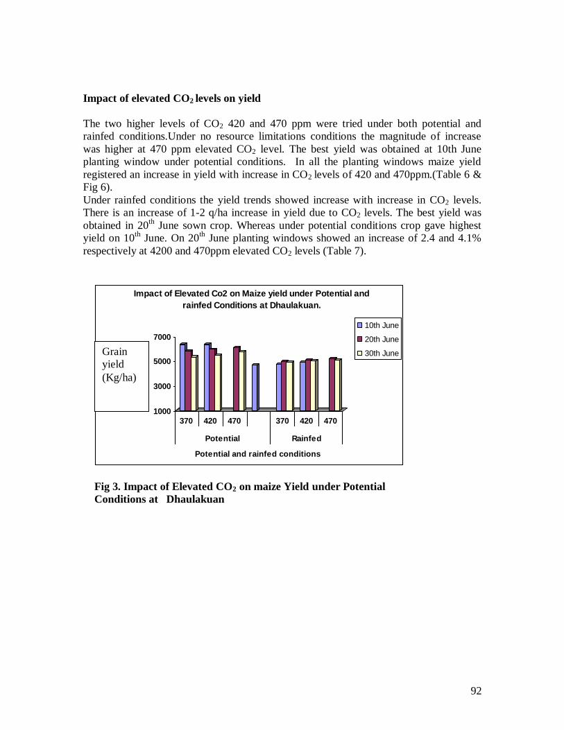
92
Impact of elevated CO2 levels on yield
The two higher levels of CO2 420 and 470 ppm were tried under both potential and
rainfed conditions.Under no resource limitations conditions the magnitude of increase
was higher at 470 ppm elevated CO2 level. The best yield was obtained at 10th June
planting window under potential conditions. In all the planting windows maize yield
registered an increase in yield with increase in CO2 levels of 420 and 470ppm.(Table 6 &
Fig 6).
Under rainfed conditions the yield trends showed increase with increase in CO2 levels.
There is an increase of 1-2 q/ha increase in yield due to CO2 levels. The best yield was
obtained in 20th
June sown crop. Whereas under potential conditions crop gave highest
yield on 10th
June. On 20th June planting windows showed an increase of 2.4 and 4.1%
respectively at 4200 and 470ppm elevated CO2 levels (Table 7).
Fig 3. Impact of Elevated CO2 on maize Yield under Potential
Conditions at Dhaulakuan
1000
3000
5000
7000
370 420 470 370 420 470
Potential Rainfed
Potential and rainfed conditions
Impact of Elevated Co2 on Maize yield under Potential and
rainfed Conditions at Dhaulakuan.
10th June
20th June
30th JuneGrain
yield
(Kg/ha)
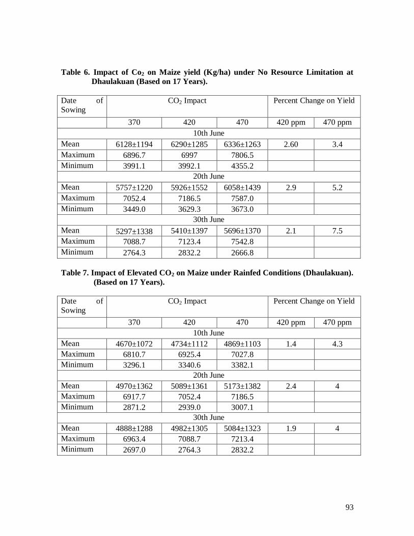
93
Table 6. Impact of Co2 on Maize yield (Kg/ha) under No Resource Limitation at
Dhaulakuan (Based on 17 Years).
Date of
Sowing
CO2 Impact Percent Change on Yield
370 420 470 420 ppm 470 ppm
10th June
Mean 6128±1194 6290±1285 6336±1263 2.60 3.4
Maximum 6896.7 6997 7806.5
Minimum 3991.1 3992.1 4355.2
20th June
Mean 5757±1220 5926±1552 6058±1439 2.9 5.2
Maximum 7052.4 7186.5 7587.0
Minimum 3449.0 3629.3 3673.0
30th June
Mean 5297±1338 5410±1397 5696±1370 2.1 7.5
Maximum 7088.7 7123.4 7542.8
Minimum 2764.3 2832.2 2666.8
Table 7. Impact of Elevated CO2 on Maize under Rainfed Conditions (Dhaulakuan).
(Based on 17 Years).
Date of
Sowing
CO2 Impact Percent Change on Yield
370 420 470 420 ppm 470 ppm
10th June
Mean 4670±1072 4734±1112 4869±1103 1.4 4.3
Maximum 6810.7 6925.4 7027.8
Minimum 3296.1 3340.6 3382.1
20th June
Mean 4970±1362 5089±1361 5173±1382 2.4 4
Maximum 6917.7 7052.4 7186.5
Minimum 2871.2 2939.0 3007.1
30th June
Mean 4888±1288 4982±1305 5084±1323 1.9 4
Maximum 6963.4 7088.7 7213.4
Minimum 2697.0 2764.3 2832.2
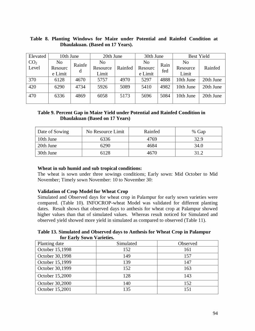
94
Table 8. Planting Windows for Maize under Potential and Rainfed Condition at
Dhaulakuan. (Based on 17 Years).
Elevated
CO2
Level
10th June 20th June 30th June Best Yield
No
Resourc
e Limit
Rainfe
d
No
Resource
Limit
Rainfed
No
Resourc
e Limit
Rain
fed
No
Resource
Limit
Rainfed
370 6128 4670 5757 4970 5297 4888 10th June 20th June
420 6290 4734 5926 5089 5410 4982 10th June 20th June
470 6336 4869 6058 5173 5696 5084 10th June 20th June
Table 9. Percent Gap in Maize Yield under Potential and Rainfed Condition in
Dhaulakuan (Based on 17 Years)
Date of Sowing No Resource Limit Rainfed % Gap
10th June 6336 4769 32.9
20th June 6290 4684 34.0
30th June 6128 4670 31.2
Wheat in sub humid and sub tropical conditions:
The wheat is sown under three sowings conditions; Early sown: Mid October to Mid
November; Timely sown November: 10 to November 30:
Validation of Crop Model for Wheat Crop
Simulated and Observed days for wheat crop in Palampur for early sown varieties were
compared. (Table 10). INFOCROP-wheat Model was validated for different planting
dates. Result shows that observed days to anthesis for wheat crop at Palampur showed
higher values than that of simulated values. Whereas result noticed for Simulated and
observed yield showed more yield in simulated as compared to observed (Table 11).
Table 13. Simulated and Observed days to Anthesis for Wheat Crop in Palampur
for Early Sown Varieties.
Planting date Simulated Observed
October 15,1998 152 161
October 30,1998 149 157
October 15,1999 139 147
October 30,1999 152 163
October 15,2000 128 143
October 30,2000 140 152
October 15,2001 135 151

95
October 30,2001 145 159
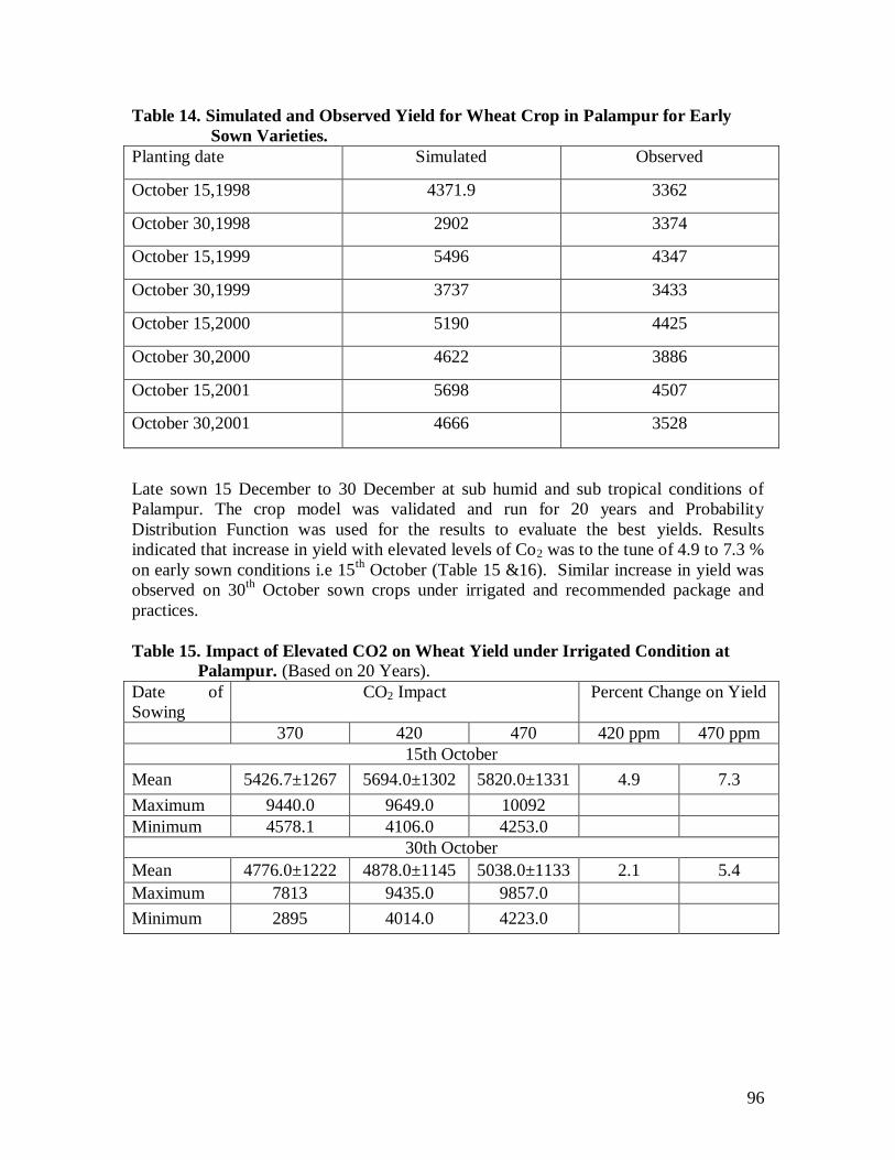
96
Table 14. Simulated and Observed Yield for Wheat Crop in Palampur for Early
Sown Varieties.
Planting date Simulated Observed
October 15,1998 4371.9 3362
October 30,1998 2902 3374
October 15,1999 5496 4347
October 30,1999 3737 3433
October 15,2000 5190 4425
October 30,2000 4622 3886
October 15,2001 5698 4507
October 30,2001 4666 3528
Late sown 15 December to 30 December at sub humid and sub tropical conditions of
Palampur. The crop model was validated and run for 20 years and Probability
Distribution Function was used for the results to evaluate the best yields. Results
indicated that increase in yield with elevated levels of Co2 was to the tune of 4.9 to 7.3 %
on early sown conditions i.e 15th
October (Table 15 &16). Similar increase in yield was
observed on 30th
October sown crops under irrigated and recommended package and
practices.
Table 15. Impact of Elevated CO2 on Wheat Yield under Irrigated Condition at
Palampur. (Based on 20 Years).
Date of
Sowing
CO2 Impact Percent Change on Yield
370 420 470 420 ppm 470 ppm
15th October
Mean 5426.7±1267 5694.0±1302 5820.0±1331 4.9 7.3
Maximum 9440.0 9649.0 10092
Minimum 4578.1 4106.0 4253.0
30th October
Mean 4776.0±1222 4878.0±1145 5038.0±1133 2.1 5.4
Maximum 7813 9435.0 9857.0
Minimum 2895 4014.0 4223.0
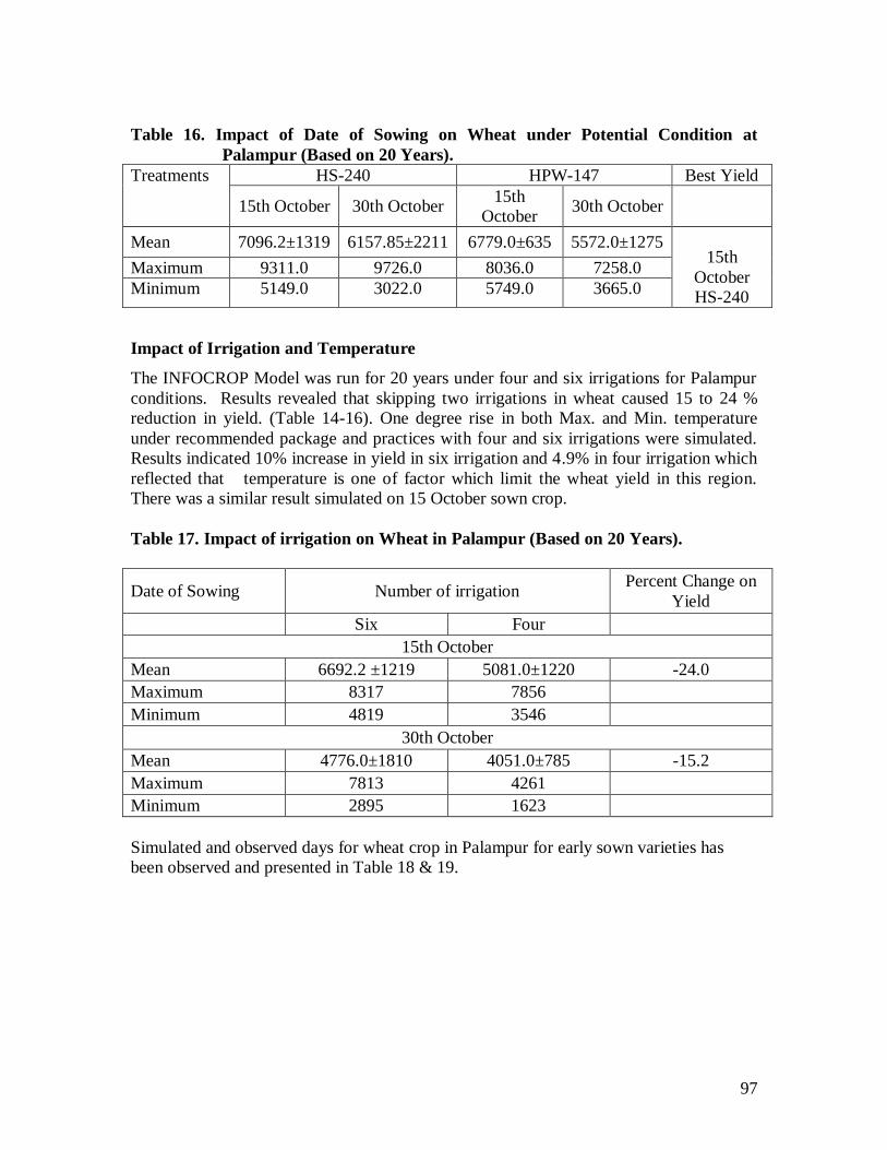
97
Table 16. Impact of Date of Sowing on Wheat under Potential Condition at
Palampur (Based on 20 Years).
Treatments HS-240 HPW-147 Best Yield
15th October 30th October 15th
October 30th October
Mean 7096.2±1319 6157.85±2211 6779.0±635 5572.0±1275
15th
October
HS-240
Maximum 9311.0 9726.0 8036.0 7258.0
Minimum 5149.0 3022.0 5749.0 3665.0
Impact of Irrigation and Temperature
The INFOCROP Model was run for 20 years under four and six irrigations for Palampur
conditions. Results revealed that skipping two irrigations in wheat caused 15 to 24 %
reduction in yield. (Table 14-16). One degree rise in both Max. and Min. temperature
under recommended package and practices with four and six irrigations were simulated.
Results indicated 10% increase in yield in six irrigation and 4.9% in four irrigation which
reflected that temperature is one of factor which limit the wheat yield in this region.
There was a similar result simulated on 15 October sown crop.
Table 17. Impact of irrigation on Wheat in Palampur (Based on 20 Years).
Date of Sowing Number of irrigation Percent Change on
Yield
Six Four
15th October
Mean 6692.2 ±1219 5081.0±1220 -24.0
Maximum 8317 7856
Minimum 4819 3546
30th October
Mean 4776.0±1810 4051.0±785 -15.2
Maximum 7813 4261
Minimum 2895 1623
Simulated and observed days for wheat crop in Palampur for early sown varieties has
been observed and presented in Table 18 & 19.
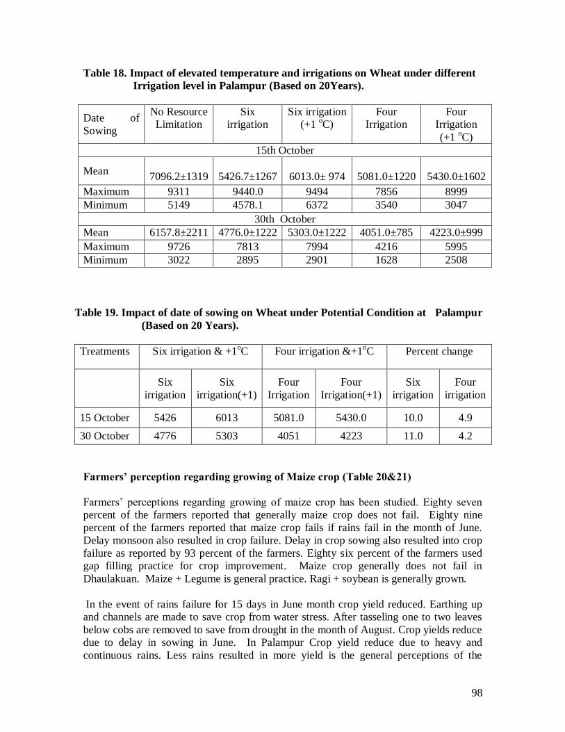
98
Table 18. Impact of elevated temperature and irrigations on Wheat under different
Irrigation level in Palampur (Based on 20Years).
Date of
Sowing
No Resource
Limitation
Six
irrigation
Six irrigation
(+1 oC)
Four
Irrigation
Four
Irrigation
(+1 oC)
15th October
Mean
7096.2±1319
5426.7±1267
6013.0± 974
5081.0±1220
5430.0±1602
Maximum 9311 9440.0 9494 7856 8999
Minimum 5149 4578.1 6372 3540 3047
30th October
Mean 6157.8±2211 4776.0±1222 5303.0±1222 4051.0±785 4223.0±999
Maximum 9726 7813 7994 4216 5995
Minimum 3022 2895 2901 1628 2508
Table 19. Impact of date of sowing on Wheat under Potential Condition at Palampur
(Based on 20 Years).
Treatments Six irrigation & +1oC Four irrigation &+1
oC Percent change
Six
irrigation
Six
irrigation(+1)
Four
Irrigation
Four
Irrigation(+1)
Six
irrigation
Four
irrigation
15 October 5426 6013 5081.0 5430.0 10.0 4.9
30 October 4776 5303 4051 4223 11.0 4.2
Farmers’ perception regarding growing of Maize crop (Table 20&21)
Farmers‟ perceptions regarding growing of maize crop has been studied. Eighty seven
percent of the farmers reported that generally maize crop does not fail. Eighty nine
percent of the farmers reported that maize crop fails if rains fail in the month of June.
Delay monsoon also resulted in crop failure. Delay in crop sowing also resulted into crop
failure as reported by 93 percent of the farmers. Eighty six percent of the farmers used
gap filling practice for crop improvement. Maize crop generally does not fail in
Dhaulakuan. Maize + Legume is general practice. Ragi + soybean is generally grown.
In the event of rains failure for 15 days in June month crop yield reduced. Earthing up
and channels are made to save crop from water stress. After tasseling one to two leaves
below cobs are removed to save from drought in the month of August. Crop yields reduce
due to delay in sowing in June. In Palampur Crop yield reduce due to heavy and
continuous rains. Less rains resulted in more yield is the general perceptions of the

99
farmers of the region. Delay in sowing cause the major reduction in yield. Leaves
removal is one of the practices if dry spell occurs in August. Less time available in SW
monsoon for intercultural operations due to heavy rains. The farmer perceptions indicated
that if dry spell occur in July than Earthing up and Gap Filling is done. Where in August,
the leave below cobs immediately after tasseling are recommended to mitigate the stress.
100
Central Soil and Water Conservation Research and Training Institute - Dehradun
Introduction
During the period under report, preliminary work related with the study was undertaken. The
review of literature reveals that AVSWAT and EPIC models have been used by most of the
workers to assess the hydrological parameters of the watersheds. EPIC gives soil erosion and crop
productivity both. There appears to be significant variation in the methodology adapted by the
workers all over the world. An integrated approach has been observed in most of the studies
including generation of daily (scaling down) projected weather data from GCM using RCM and
finally computing projected crop yield with input of not only precipitation but temperature and
CO2 .This not only warrants the knowledge of running the model but thorough basic concept of
hydrology, soil, crop physiology and off course climate.
In Indian context only general information of effect of climate change over hydrology and crop
production is available. Quantitative information on this aspect is rarely available. The model used
for any study needs to be calibrated and validated before applied for generating projected output.
The non availability of data on runoff and soil loss from watersheds of about 500 ha also puts
additional use of sub model for calibration and validation.
One of the common requirements of any model for hydrological study is developing input layer of
DEM, soil and land use. In order to develop DEM layer, the relevant toposheets of the study
watersheds (7 numbers, Table 1) were scanned, geo-referenced on UTM projection: datum WGS
84.The watershed boundary was delineated and the contours and the boundary were digitized. The
DEM was then generated on Arc-view (Fig1).
The models also need tabular data on additional parameters. Some of these data has been compiled
from secondary sources as published in various literatures (Table 2). The daily weather data of the
stations adjoining nearer to the study area as available with the India meteorological Department
(IMD) , ICAR institutes or SAUs has been collected for a duration of 5 years ( mostly for the
period between 1990 -2005).This will be required for hydrological and crop models.
Groundwater recharge
The aspect of ground water recharge (a component of the rainfall –runoff relationship) is being
studied at CSWCRTI, Regional Station Vasad, Gujrat since 2002-2003. This data will be used to
calibrate and validate the hydrological model. The data is being reorganized/reanalyzed keeping in
view the model requirement. Under this;
The data on groundwater level from 2002 September to March, 2008 have been collected
(fortnightly and weekly basis). Suitable models like SWAT (Arc-view interface), and WEAP
(Water Evaluation Assessment Project) has been chosen to be used for running the climate change
scenario‟s effect on water resources. Another model GMS (Groundwater Modeling System) also
has been procured to find out the groundwater recharge scenario consequent upon the climate
change. The detailed geological survey is in progress using electrical resistivity method.
Geological formation data (well log data) for 3 piezometers installed in the project area have been
collected. A representative well log data (Fig 2.) reveals that the watershed has four aquifers of
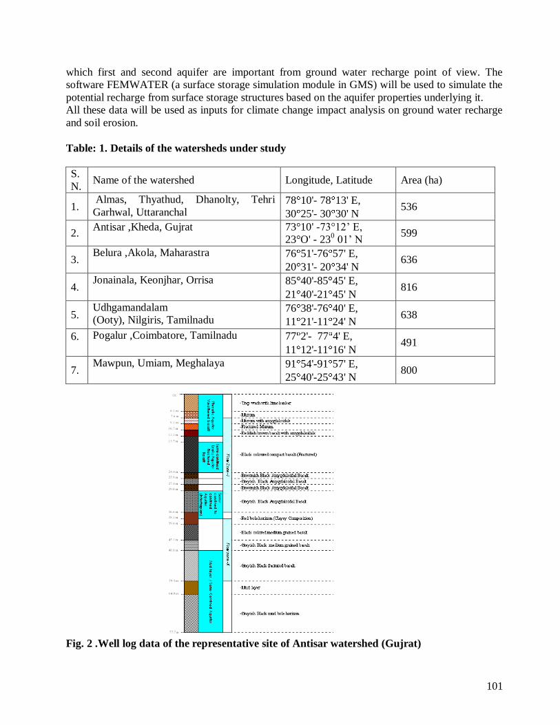
101
which first and second aquifer are important from ground water recharge point of view. The
software FEMWATER (a surface storage simulation module in GMS) will be used to simulate the
potential recharge from surface storage structures based on the aquifer properties underlying it.
All these data will be used as inputs for climate change impact analysis on ground water recharge
and soil erosion.
Table: 1. Details of the watersheds under study
S.
N. Name of the watershed Longitude, Latitude Area (ha)
1. Almas, Thyathud, Dhanolty, Tehri
Garhwal, Uttaranchal 78 10'- 78 13' E,
30 25'- 30 30' N 536
2. Antisar ,Kheda, Gujrat 73°10' -73°12‟ E,
23°O' - 230 01‟ N
599
3. Belura ,Akola, Maharastra 76 51'-76 57' E,
20 31'- 20 34' N 636
4. Jonainala, Keonjhar, Orrisa 85 40'-85 45' E,
21 40'-21 45' N 816
5. Udhgamandalam
(Ooty), Nilgiris, Tamilnadu 76 38'-76 40' E,
11 21'-11 24' N 638
6.
Pogalur ,Coimbatore, Tamilnadu 77 2'- 77 4' E,
11 12'-11 16' N 491
7. Mawpun, Umiam, Meghalaya 91 54'-91 57' E,
25 40'-25 43' N 800
Fig. 2 .Well log data of the representative site of Antisar watershed (Gujrat)
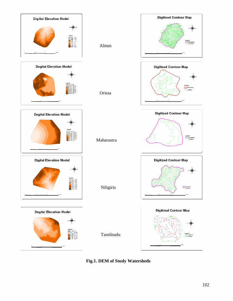
102
Almas
Orissa
Maharastra
Niligiris
Tamilnadu
Fig.1. DEM of Study Watersheds
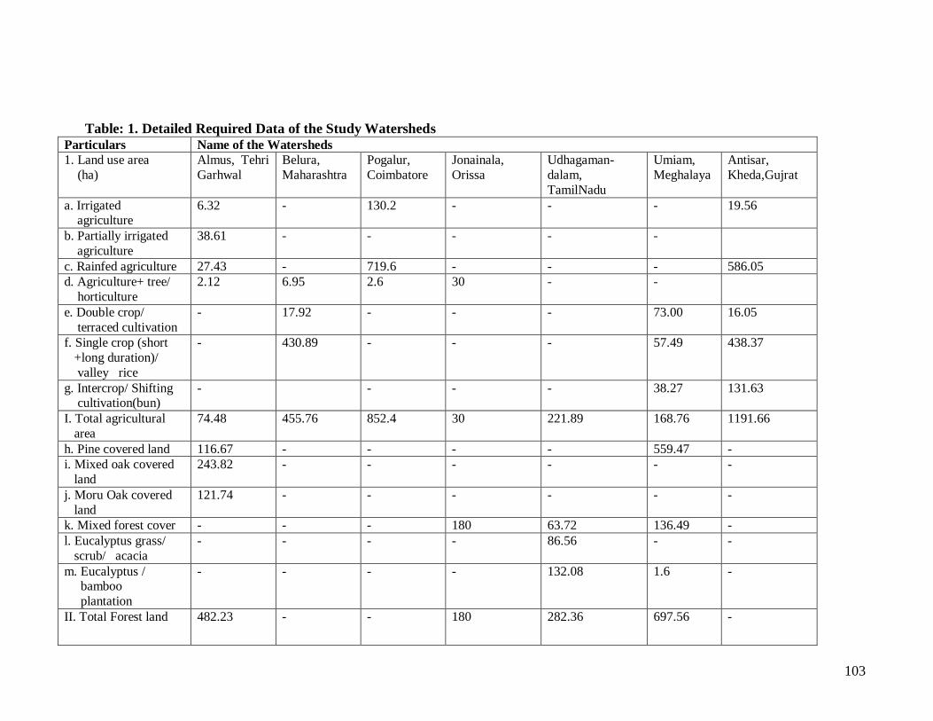
103
Table: 1. Detailed Required Data of the Study Watersheds
Particulars Name of the Watersheds
1. Land use area
(ha)
Almus, Tehri
Garhwal
Belura,
Maharashtra
Pogalur,
Coimbatore
Jonainala,
Orissa
Udhagaman-
dalam,
TamilNadu
Umiam,
Meghalaya
Antisar,
Kheda,Gujrat
a. Irrigated agriculture
6.32 - 130.2 - - - 19.56
b. Partially irrigated
agriculture
38.61 - - - - -
c. Rainfed agriculture 27.43 - 719.6 - - - 586.05
d. Agriculture+ tree/
horticulture
2.12 6.95 2.6 30 - -
e. Double crop/
terraced cultivation
- 17.92 - - - 73.00 16.05
f. Single crop (short
+long duration)/
valley rice
- 430.89 - - - 57.49 438.37
g. Intercrop/ Shifting cultivation(bun)
- - - - 38.27 131.63
I. Total agricultural
area
74.48 455.76 852.4 30 221.89 168.76 1191.66
h. Pine covered land 116.67 - - - - 559.47 -
i. Mixed oak covered
land
243.82 - - - - - -
j. Moru Oak covered
land
121.74 - - - - - -
k. Mixed forest cover - - - 180 63.72 136.49 -
l. Eucalyptus grass/
scrub/ acacia
- - - - 86.56 - -
m. Eucalyptus / bamboo
plantation
- - - - 132.08 1.6 -
II. Total Forest land 482.23 - - 180 282.36 697.56 -
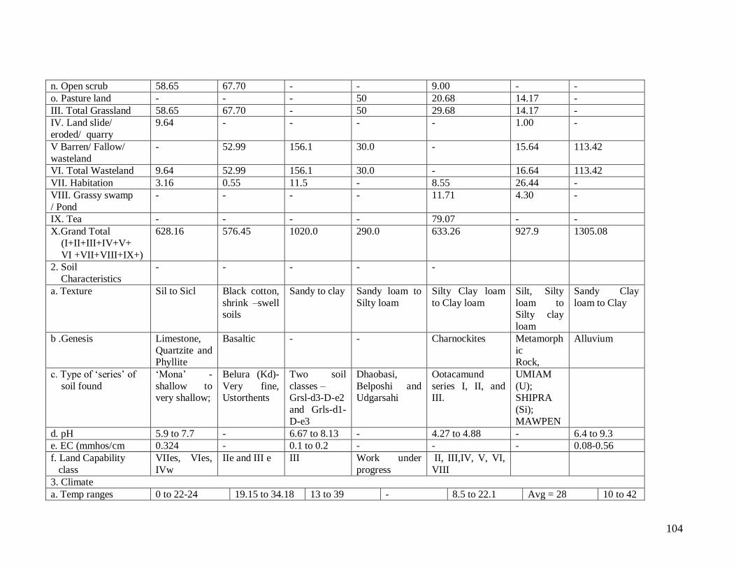
104
n. Open scrub 58.65 67.70 - - 9.00 - -
o. Pasture land - - - 50 20.68 14.17 -
III. Total Grassland 58.65 67.70 - 50 29.68 14.17 -
IV. Land slide/
eroded/ quarry
9.64 - - - - 1.00 -
V Barren/ Fallow/
wasteland
- 52.99 156.1 30.0 - 15.64 113.42
VI. Total Wasteland 9.64 52.99 156.1 30.0 - 16.64 113.42
VII. Habitation 3.16 0.55 11.5 - 8.55 26.44 -
VIII. Grassy swamp
/ Pond
- - - - 11.71 4.30 -
IX. Tea - - - - 79.07 - -
X.Grand Total
(I+II+III+IV+V+
VI +VII+VIII+IX+)
628.16 576.45 1020.0 290.0 633.26 927.9 1305.08
2. Soil
Characteristics
- - - - -
a. Texture Sil to Sicl Black cotton,
shrink –swell soils
Sandy to clay Sandy loam to
Silty loam
Silty Clay loam
to Clay loam
Silt, Silty
loam to Silty clay
loam
Sandy Clay
loam to Clay
b .Genesis Limestone,
Quartzite and Phyllite
Basaltic - - Charnockites Metamorph
ic Rock,
Alluvium
c. Type of „series‟ of
soil found
„Mona‟ -
shallow to very shallow;
Belura (Kd)-
Very fine, Ustorthents
Two soil
classes – Grsl-d3-D-e2
and Grls-d1-
D-e3
Dhaobasi,
Belposhi and Udgarsahi
Ootacamund
series I, II, and III.
UMIAM
(U); SHIPRA
(Si);
MAWPEN
d. pH 5.9 to 7.7 - 6.67 to 8.13 - 4.27 to 4.88 - 6.4 to 9.3
e. EC (mmhos/cm 0.324 - 0.1 to 0.2 - - - 0.08-0.56
f. Land Capability
class
VIIes, VIes,
IVw
IIe and III e III Work under
progress
II, III,IV, V, VI,
VIII
3. Climate
a. Temp ranges 0 to 22-24 19.15 to 34.18 13 to 39 - 8.5 to 22.1 Avg = 28 10 to 42
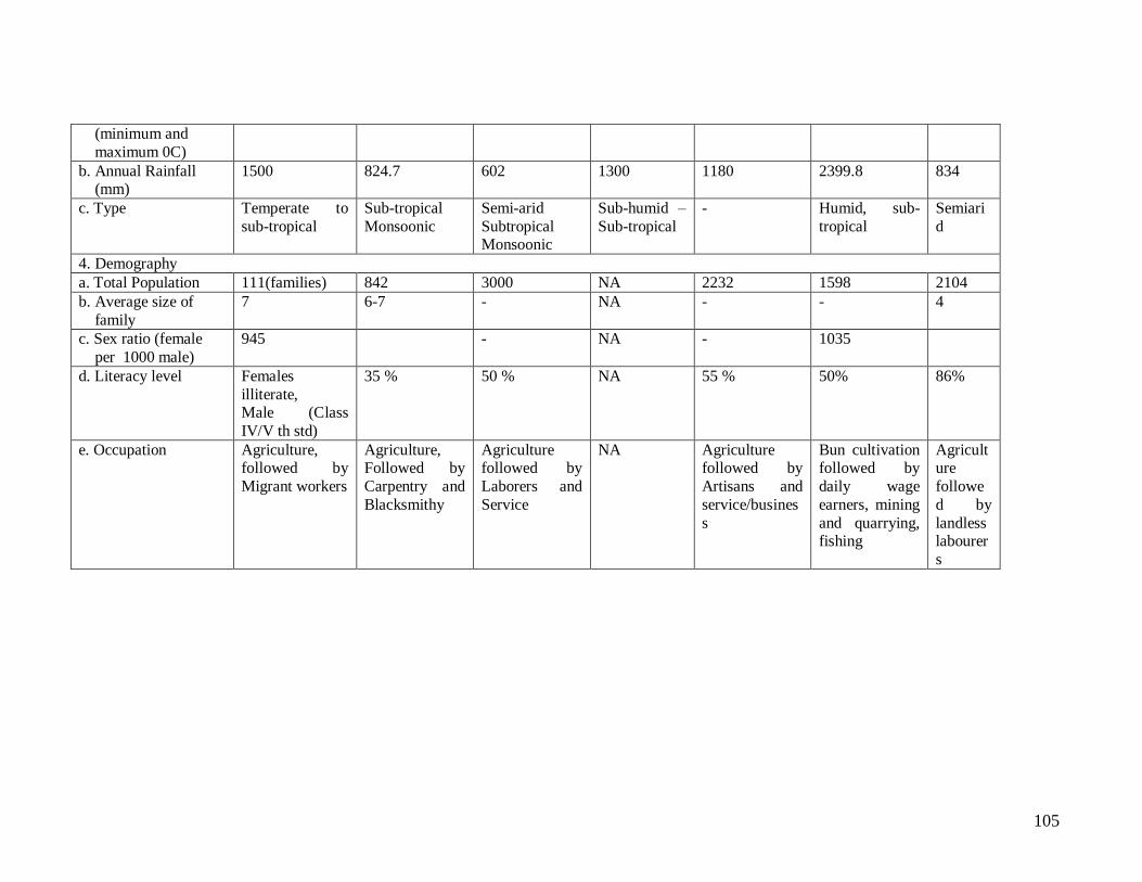
105
(minimum and
maximum 0C)
b. Annual Rainfall (mm)
1500 824.7 602 1300 1180 2399.8 834
c. Type Temperate to
sub-tropical
Sub-tropical
Monsoonic
Semi-arid
Subtropical Monsoonic
Sub-humid –
Sub-tropical
- Humid, sub-
tropical
Semiari
d
4. Demography
a. Total Population 111(families) 842 3000 NA 2232 1598 2104
b. Average size of
family
7 6-7 - NA - - 4
c. Sex ratio (female
per 1000 male)
945 - NA - 1035
d. Literacy level Females
illiterate, Male (Class
IV/V th std)
35 % 50 % NA 55 % 50% 86%
e. Occupation Agriculture, followed by
Migrant workers
Agriculture, Followed by
Carpentry and
Blacksmithy
Agriculture followed by
Laborers and
Service
NA Agriculture followed by
Artisans and
service/busines
s
Bun cultivation followed by
daily wage
earners, mining
and quarrying, fishing
Agriculture
followe
d by
landless labourer
s
106
ICAR Research Complex for Eastern Region, Patna
A. Assessment of impact, adaptation and mitigation of climate change on major crops of
Bihar
(a) Trend Analysis of Agro-meteorological variables: Rainfall, temperature and
potential evapotranspiration (PET) are investigated for studying the significant features of
climatic variability at three centres viz. Sabour, Pusa and Patna of Bihar in Eastern India.
These centres are present in Zone III B, Zone I, and Zone III A of Bihar. Annual,
seasonal and monthly rainfall, temperature and potential evapotranspiration (PET) were
analyzed by using M-K Test, SP Rho test and linear regression test. The results of trend
analysis of different agro- meteorological variables are summarized below:
Monthly Trend: At Sabour, monthly rainfall showed an increasing trend but significant
increase at 5 percent is observed during the month of April only. As temperature
(maximum and minimum temperature) is concerned, it also shows increasing trend in all
of the months except during January and April- June month. However, for most of the
months PET shows a downward trend. At Pusa, rainfall show upward trend in most of the
months but significant increase in rainfall is observed for April, November and December
months. A significant increase in minimum temperature is observed for all of the months
except March and June. Six out of twelve months show a downward trend in maximum
temperature and, significant decrease during January and March is observed. PET follows
the same trend as maximum temperature but shows significant decrease during January
and significant increase during August month as shown in table 1. In Patna, a decrease in
maximum temperature from January to July and in minimum temperature from April to
October is observed. However, this decrease in maximum temperature is significant
during January and May months and significant decrease during April, July and
September in minimum temperature is observed. Majority of months show increase in
rainfall and PET for Patna.
Seasonal Trend: Seasonal rainfall shows an increasing trend during all of the seasons
however, significant increase during summer and monsoon season at Sabour. Maximum
temperature showed decreasing trend during winter and summer season but increasing
trend in other two seasons. Minimum temperature showed an increasing trend except
during summers. Monsoon and post-monsoon seasons show increased PET. At Pusa,
rainfall showed downward trend during post-monsoon period and minimum temperature
shows significant increase during all the four seasons. However, maximum temperature
increased in monsoon and post monsoon seasons. At Patna, on seasonal basis,
temperature showed decreasing trend during winter, summer and monsoon season except
significant increase in minimum temperature during winter season (December, January
and February). An increase in maximum as well as minimum temperature is observed
during post –monsoon period. Rainfall showed decreasing trend during summer and post-
monsoon period but increased during other two seasons. Potential evapotranspiration
however showed an increasing trend for summer and monsoon season but downward
trend during winter and post –monsoon.
Annual trend: Annual rainfall shows an increasing trend for all of the stations.
Maximum as well as minimum temperature showed an upward trend at Sabour. At Pusa
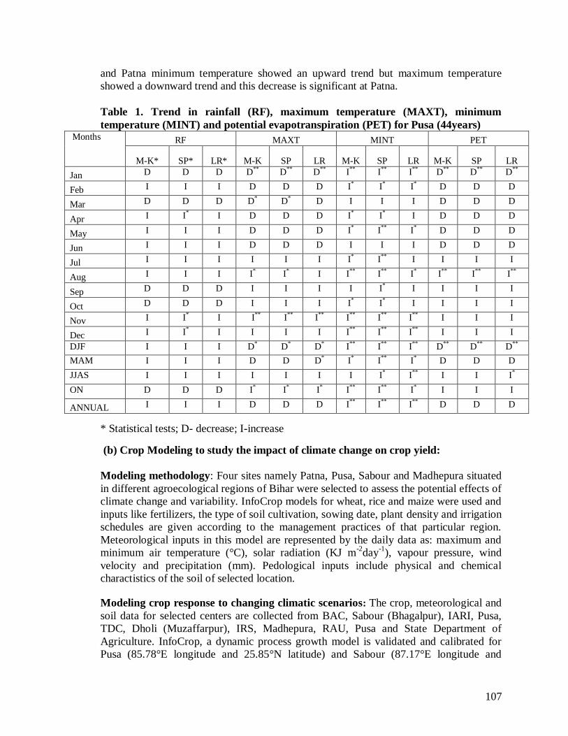
107
and Patna minimum temperature showed an upward trend but maximum temperature
showed a downward trend and this decrease is significant at Patna.
Table 1. Trend in rainfall (RF), maximum temperature (MAXT), minimum
temperature (MINT) and potential evapotranspiration (PET) for Pusa (44years) Months RF MAXT MINT PET
M-K* SP* LR* M-K SP LR M-K SP LR M-K SP LR
Jan D D D D** D** D** I** I** I** D** D** D**
Feb I I I D D D I* I* I* D D D
Mar D D D D* D* D I I I D D D
Apr I I* I D D D I* I* I D D D
May I I I D D D I* I** I* D D D
Jun I I I D D D I I I D D D
Jul I I I I I I I* I** I I I I
Aug I I I I* I* I I** I** I* I** I** I**
Sep D D D I I I I I* I I I I
Oct D D D I I I I* I* I I I I
Nov I I* I I** I** I** I** I** I** I I I
Dec I I* I I I I I** I** I** I I I
DJF I I I D* D* D* I** I** I** D** D** D**
MAM I I I D D D* I* I** I* D D D
JJAS I I I I I I I I* I** I I I*
ON D D D I* I* I* I** I** I* I I I
ANNUAL I I I D D D I** I** I** D D D
* Statistical tests; D- decrease; I-increase
(b) Crop Modeling to study the impact of climate change on crop yield:
Modeling methodology: Four sites namely Patna, Pusa, Sabour and Madhepura situated
in different agroecological regions of Bihar were selected to assess the potential effects of
climate change and variability. InfoCrop models for wheat, rice and maize were used and
inputs like fertilizers, the type of soil cultivation, sowing date, plant density and irrigation
schedules are given according to the management practices of that particular region.
Meteorological inputs in this model are represented by the daily data as: maximum and
minimum air temperature (°C), solar radiation (KJ m-2
day-1
), vapour pressure, wind
velocity and precipitation (mm). Pedological inputs include physical and chemical
charactistics of the soil of selected location.
Modeling crop response to changing climatic scenarios: The crop, meteorological and
soil data for selected centers are collected from BAC, Sabour (Bhagalpur), IARI, Pusa,
TDC, Dholi (Muzaffarpur), IRS, Madhepura, RAU, Pusa and State Department of
Agriculture. InfoCrop, a dynamic process growth model is validated and calibrated for
Pusa (85.78°E longitude and 25.85°N latitude) and Sabour (87.17°E longitude and
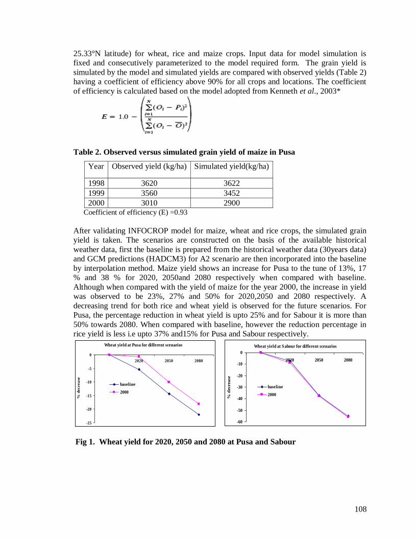
108
Wheat yield at Pusa for different scenarios
-25
-20
-15
-10
-5
0
2020 2050 2080
% d
ecrea
se
baseline
2000
25.33°N latitude) for wheat, rice and maize crops. Input data for model simulation is
fixed and consecutively parameterized to the model required form. The grain yield is
simulated by the model and simulated yields are compared with observed yields (Table 2)
having a coefficient of efficiency above 90% for all crops and locations. The coefficient
of efficiency is calculated based on the model adopted from Kenneth et al., 2003*
Table 2. Observed versus simulated grain yield of maize in Pusa
Year Observed yield (kg/ha) Simulated yield(kg/ha)
1998 3620 3622
1999 3560 3452
2000 3010 2900 Coefficient of efficiency (E) =0.93
After validating INFOCROP model for maize, wheat and rice crops, the simulated grain
yield is taken. The scenarios are constructed on the basis of the available historical
weather data, first the baseline is prepared from the historical weather data (30years data)
and GCM predictions (HADCM3) for A2 scenario are then incorporated into the baseline
by interpolation method. Maize yield shows an increase for Pusa to the tune of 13%, 17
% and 38 % for 2020, 2050and 2080 respectively when compared with baseline.
Although when compared with the yield of maize for the year 2000, the increase in yield
was observed to be 23%, 27% and 50% for 2020,2050 and 2080 respectively. A
decreasing trend for both rice and wheat yield is observed for the future scenarios. For
Pusa, the percentage reduction in wheat yield is upto 25% and for Sabour it is more than
50% towards 2080. When compared with baseline, however the reduction percentage in
rice yield is less i.e upto 37% and15% for Pusa and Sabour respectively.
Wheat yield at Sabour for different scenarios
-60
-50
-40
-30
-20
-10
0
2020 2050 2080
% d
ecrease
baseline
2000
Fig 1. Wheat yield for 2020, 2050 and 2080 at Pusa and Sabour
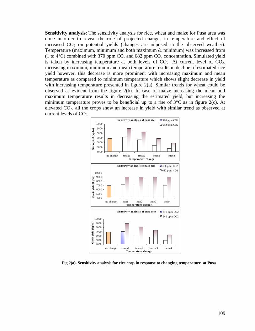
109
Sensitivity analysis: The sensitivity analysis for rice, wheat and maize for Pusa area was
done in order to reveal the role of projected changes in temperature and effect of
increased CO2 on potential yields (changes are imposed in the observed weather).
Temperature (maximum, minimum and both maximum & minimum) was increased from
(1 to 4°C) combined with 370 ppm CO2 and 682 ppm CO2 concentration. Simulated yield
is taken by increasing temperature at both levels of CO2. At current level of CO2,
increasing maximum, minimum and mean temperature results in decline of estimated rice
yield however, this decrease is more prominent with increasing maximum and mean
temperature as compared to minimum temperature which shows slight decrease in yield
with increasing temperature presented in figure 2(a). Similar trends for wheat could be
observed as evident from the figure 2(b). In case of maize increasing the mean and
maximum temperature results in decreasing the estimated yield, but increasing the
minimum temperature proves to be beneficial up to a rise of 3°C as in figure 2(c). At
elevated CO2, all the crops show an increase in yield with similar trend as observed at
current levels of CO2. Senstivity analysis of pusa rice
4000
5000
6000
7000
8000
9000
10000
no change tmax1 tmax2 tmax3 tmax4
Temperature change
Ga
rin
yie
ld (
kg
/ha
)
370 ppm CO2
682 ppm CO2
Senstivity analysis of pusa rice
4000
5000
6000
7000
8000
9000
10000
no change tmin1 tmin2 tmin3 tmin4
Temperature change
Ga
rin
yie
ld (
kg
/ha
)
370 ppm CO2
682 ppm CO2
Senstivity analysis of pusa rice
4000
5000
6000
7000
8000
9000
10000
no change tmean1 tmean2 tmean3 tmean4
Temperature change
Ga
rin
yie
ld (
kg
/ha
)
370 ppm CO2
682 ppm CO2
Fig 2(a). Sensitivity analysis for rice crop in response to changing temperature at Pusa
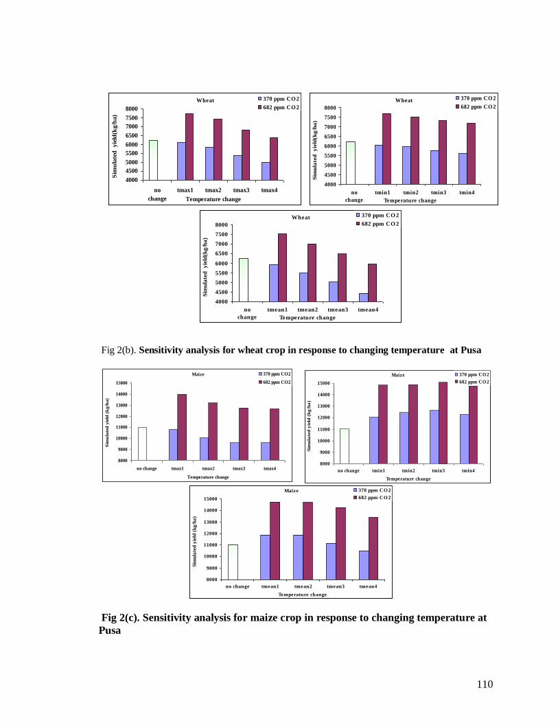
110
Maize
8000
9000
10000
11000
12000
13000
14000
15000
no change tmax1 tmax2 tmax3 tmax4
Temperature change
Sim
ula
ted
yie
ld (
kg/h
a)
370 ppm CO2
682 ppm CO2
Wheat
4000
4500
5000
5500
6000
6500
7000
7500
8000
no
change
tmin1 tmin2 tmin3 tmin4
Temperature change
Sim
ula
ted
y
ield
(kg
/ha
)
370 ppm CO 2
682 ppm CO 2Wheat
4000
4500
5000
5500
6000
6500
7000
7500
8000
no
change
tmax1 tmax2 tmax3 tmax4
Temperature change
Sim
ula
ted
yie
ld(k
g/h
a)
370 ppm CO 2
682 ppm CO 2
Maize
8000
9000
10000
11000
12000
13000
14000
15000
no change tmin1 tmin2 tmin3 tmin4
Temperature change
Sim
ula
ted
yie
ld (
kg
/ha
)
370 ppm CO 2
682 ppm CO 2
Wheat
4000
4500
5000
5500
6000
6500
7000
7500
8000
no
change
tmean1 tmean2 tmean3 tmean4
Temperature change
Sim
ula
ted
y
ield
(kg
/ha
)
370 ppm CO 2
682 ppm CO 2
Maize
8000
9000
10000
11000
12000
13000
14000
15000
no change tmean1 tmean2 tmean3 tmean4
Temperature change
Sim
ula
ted
yie
ld (
kg
/ha
)
370 ppm CO 2
682 ppm CO 2
Fig 2(b). Sensitivity analysis for wheat crop in response to changing temperature at Pusa
Fig 2(c). Sensitivity analysis for maize crop in response to changing temperature at
Pusa

111
B. Climate change impact assessment on water resource availability for developing
suitable water management strategy under projected climate change
Hydrological Modeling for Assessing Climate Change Impact in Bhavani Basin
In the second phase of the ICAR Network project on climate change “Impact, Adaptation
and Vulnerability of Indian Agriculture to climate Change”, the Upper Bhavani basin
lying upstream of the Bhavanisagar Reservoir with the two main rivers the Bhavani and
the Moyar was selected for assessing the climate change impact on hydrology and water
resources availability in the basin. The basin has a total area of 4100 km2 and is a high
altitude area at the confluence of the eastern and western Ghats with topography that is
undulating in lower plateau and uplands and rugged in western parts. The elevation
ranges from 300 m above msl on the plains to 2600 m above msl on the Nilgiris plateau.
The mean annual precipitation varies from 700 m on the low lands to over 3000m in the
hills. The main part of the basin experiences a humid equatorial climate, although the
lowland plains are sub-humid. Before studying the impact of climate change on water
resources availability in the basin under different climate change scenarios, an attempt
was made to study the trend in stream flow using past historical data. For this purpose,
stream flow data of three gauging stations, namely, Nellithurai, Thengumarahada, and
Savandapur for the period 1978-2005 were collected and analyzed. Four different
statistical tests, namely, linear regression test, Spearman‟s Rho test, Mann-Kendall test,
and Sen‟s estimator of slope were employed for the purpose. All the four tests showed
similar trend. Decreasing trend in mean monthly streamflow was observed throughout the
basin in all most all the months except May (in all 3 stations) and Jan (in Savandapur).
However, the decrease is significant during Jul-Oct, and Dec-Jan in Nelluthari, and Oct-
Dec in Savandapur at 5% significance level (Fig. 3). For delineation of basin into
different hydrological response units (HRUs) for distributed hydrological modeling, total
12 toposheets (1:50,000 scale) covering the basin were georeferenced for digitizing.
-4
-3
-2
-1
0
1
2
3
4
Jan Feb Mar Apr May Jun Jul Aug Sep Oct Nov Dec
Month
MK
Sta
tist
ics
(Z)
Nellithurai Thengumarahada Savandapur
Fig. 3. Mann-Kendall test statistics for streamflow trend in Bhavani basin.
112
NATIONAL DAIRY RESEARCH INSTITUTE, KARNAL
1.0 Impact of cold wave and wind chill on growth and milk production
1.1 Impact of cold wave
The cold assessed on the basis of outside air temperature doesn‟t indicate about the true
coldness and comfort to enable protection of livestock from winter conditions. Climatic
factors like wind speed, relative humidity and sunshine play important roles in
determining the intensity of cold outside and comfort in cold. A description of coldness
was proposed in the form of "wind chill index" to describe the relative
discomfort/danger resulting from the combination of wind and temperature. (Siple and
Passel Index,1945). Wind chill temperature is a measure of the combined cooling effect
of wind and temperature. As wind velocity increases, heat is carried away from the
animal body at a faster rate, driving down both the skin temperature and eventually the
internal body temperature below their normal temperature and to a state of hypothermia.
The Wind Chill Temperature index is thus the measure of this relationship. The Wind
Chill Temperature index was computed for Karnal on the basis of air temperature and
wind velocity that prevailed during winter of 2006-07, 2007-08. In the present study WCI
was used to assess production loss with an assumption that thermal losses from skin of
animals are similar to that of man.
During 2007 cold wave swept from Jan 1 to 5 in the North India. Impact of cold wave
lashed during January 2007 was analyzed on milk production of cattle and buffaloes.
Tmin and wind chill factors were correlated with decline in milk production. The decline
in milk production ranged from 1-27% in crossbred cattle. 32.0% cows reduced their
milk production by about 5% and 36% cows declined their production in the range of 5-
10%, however loss in production of cows was observed between 15-20% in 5.0% cows.
About 27% cows did not change their milk production and cold wave effect was not
observed in these cows.
During 2008 cold wave in the North India resulted for much longer period than observed
during last several years and the cold wave event continued for several weeks. The
extended periods, five and fifteen days of the cold wave (Jan 1 –5 and Jan 19-28) when
the wind chill factor was low with temperatures 5-7° C below normal near freezing point
and wind chill factor less than 2. The milk production losses were more than 20%. One
contributing factor to the production losses was the continuous exposure to chilly wind
with Wind Chill Index below 0, so there was no opportunity for recovery during daytime
(an important element in coping with cold stress). A partly cloud cover and inadequate
solar radiation during the day and low to moderate winds speeds were further
contributing factors. For cattle and buffaloes in Northern India with low chill factor
(ranging from 2 to –2.0) push animals living in open conditions to shiver and to
"Emergency" situation, the animal thermal balance is hardly maintained by shivering and
increased feed intake. Of the 157 cows monitored for production changes during cold
wave of 2008, 49% cows declined their production about 5% and in 28% cows loss in
113
production was between 5-10% and more than 5.0% declined their production between
10-15% and 18% animals did not exhibit a decline or observed to increase in milk
production (Table1).
Low environmental temperatures and lack of prior conditioning result in to low
production and death of livestock managed in unprotected or open or partially protected
buildings. Cold wave with high wind velocity can push vulnerable animals beyond their
survival threshold limits of low temperature. The consequences of exposure to cold could
be severe particularly in Indian animals not adapted to severe cold with high wind
velocity. The importance of the wind chill index in context of livestock production is that
it can help in reducing impact of winter weather. In managing livestock in cold weather
an important factor that need to be kept in mind is that surrounding hot air and body heat
produced by animals may be used to protect against the cold. Covering of animals with
loose, lightweight and warm jute materials (gunny bags clothing) can help in protection
and excessive heat loss from body. Tightly- woven and water-repellant outer covers can
further protect them from wet winters and wind chill effects.
1.2 Impact of Heat waves
High ambient temperatures during summers can result in production and death losses for
un adapted livestock. High temperatures with high wind velocity (Heat waves) cause
losses to vulnerable cattle and buffaloes. Continuous exposure of animals, at THI higher
than 75, during the heat waves decrease opportunity for recovery at night. Low
temperature during night is an important element in coping with heat stress. High
temperature accompanying with high solar radiation loads, on clear skies days and low to
moderate wind speeds further contribute to risk.
Heat wave during summer negatively impacted milk yield of cattle and buffaloes. On an
average loss in production occurred by more than 3.0% accounting 650 lit during 30 days
June period. The loss in production due to heat waves on length of lactation has not been
considered as some of the buffaloes are impacted in the form of lactation length and
reproductive functions. The impact of heat wave was observed to be more on the milk
yield of heifers than other cows and buffaloes with an average yield decline of 3.2%. The
impact of heat wave during summer on milk yield and production of cows and heifers
ranged from 2- 15 %. Heifers and cows were equally sensitive to thermal stress and heat
waves swept during June. On an average a decline of 2.5% in milk production of cows
occurred and caused a loss of 3200 lit during June.
(Table2)
High ambient temperatures cause production losses in livestock. Temperature rise from
January to March have a positive impact on milk yield and increase production of cattle
and buffaloes. But temperature rise from March to June reduce yield and production.
Heat waves that occur during April to June with ambient temperature above 38- 40 ° C
severely impact animal health and productivity. Heat waves in the months of May and
June in Northern India, ranging from few days to several weeks, with temperature
extremes of 45 °C and wind velocity of 7-8 Km/h negatively impact milk production to
about 20-30%. High solar radiation during the day further causes thermal stress. During
summer, particularly in May and June months hourly THI values exceeded more than 80
114
during the day and night. After onset of monsoon in July, air humidity increases and low
difference in dry and wet bulb temperatures reduces efficiency of evaporative cooling.
Since livestock production system in India is based on small and marginal farmers the
production losses during summers and during heat waves could be more in terms of yield
per day, health and well being than the organized farms where the heat mitigating
measures could be adopted. Heat wave impact assessment studies on milk production of
cattle indicate low to moderate loss in yield and production of both cattle and buffaloes.
Inadequate protection during heat waves and lack of water availability to livestock often
result in production loss and cause health problem in young and unconditioned livestock.
1.3 Feed Intake and growth
Cold exposure of animals also influence feed intake of animals. Feed intake of animals
increase during winter months as compared to comfortable months (March and October)
and increase in growing animals is higher than adult animals. A sudden drop in
temperature during cold wave was observed to reduce their feed intake and Zebu,
crossbreds and buffaloes were uncomfortable under open housing system particularly
from 5 PM to 9 AM indicating that animals experience cold during night hours. Some of
the animals were observed to shiver during early morning that continued till rise of
ambient temperature to 15 ° C.
High ambient temperature of May and June depress feed intake and growth rate of
animals as compared to comfortable conditions. Dry matter intake decline with rise in
THI has been presented graphically (Fig2)
1.4 Impact of temperature on energy expenditure and pulmonary functions
Energy expenditure and methane emissions from cattle and buffaloes were assessed after
exposing animals to different temperatures in climatic chamber. The expired air was
collected in Douglas bags from individual animal. Volume of air was measured by
passing through Wet test meter and analyzed for O2, CO2 and methane. The RQ was
computed after STPD correction and energy expenditure was calculated. Methane
emissions were measured in exhausted air from methane content change and airflow rate.
Exposure of cattle and buffaloes increased their metabolic rate and ventilation volume.
The impact of temperature was observed to be more at 35° C than that observed at 40° C
indicating that animal response to temperatures are variable. At 32° C heat production
increased marginally but at 35° C the response was much more pronounced. Exposure
of cattle and buffaloes increased pulmonary ventilation volume of animals and CO2
content in expired air increased, CO2 increment declined and O2 retained increased
(Table3 &4). Methane emissions in expired air varied from 0.03 to 0.11% and no
temperature effects were noticed on methane emissions. The results indicate that
temperature rise impacts animal metabolism and affects pulmonary activity. The rise in
respiratory frequency at high temperature impacts CO2 content of expired air and oxygen
uptake of animals.
2.0 THI variations at Karnal
115
Increase in THI due to temperature rise affects animal growth and productivity but
animals are able to dissipate body heat because of higher difference in dry bulb and wet
bulb temperature. Dry heat waves often referred as “loo” during May and June reduce
productivity but difference in night and day temperatures (10-12 ° C) help in alleviation
of thermal loads. The situation changes with onset of monsoon or due to storms or other
weather changes. A low difference between T db and T wb decreases efficiency of
evaporative cooling and increases animal discomfort.
Air temperature variations occurring every 10 min were recorded at Karnal on a
meteorological station. THI for Karnal data based on hourly air temperature and relative
humidity records were analyzed and results have presented in Fig. 3. The data revealed
that THI levels are below 70 throughout the day and night of January and February. The
night time temperature are low thus THI were <65 during major part of January and
February. During March day temperature increase elevated THI and daytime THI
increased to70- 80 particularly in the afternoon. In April THI exceeded 80 during
afternoon for 2-3 hours period. Low ambient temperature during night (T min) permit
heat dissipation from skin and animals dissipate heat gained during night at low THI. But
in May the values of THI exceed 80 for 83.5% of the 24h period and for more than 4-6
hours animals were in distress with THI higher than 85. During May and June 45-50% of
the daytime THI was more than 85 thus animals were under severe stress and gained heat
from environment. Increase in air humidity with onset of monsoon caused a rise in THI
and animals were uncomfortable mainly due to decline in difference in temperature. In
the months of July and August hourly THI values were higher than 75 and more than
45% of the time temperature humidity conditions were distressful and THI values were
>85. Ambient temperature started declining from September onwards and animals were
comfortable and their productivity improved.
In order to estimate duration of uncomfort during different days of the year and variations
THI were computed from hourly records of dry bulb and humidity for the twelve months
and summer period of April to June and rainy season of July to September. The analysis
revealed that THI starts increasing in afternoon from Feb onwards and exceed 75 for 2-3
h in the afternoon from March onwards. For more than 1500 h during the year THI
ranges between 76-80 and for other 1500 h between 81-85. THI exceeding 85 (86-95) are
observed during May for more than 115 h and total number of hours exceeding 86
increases to 300-350 h during July and August. The severe stress days with THI > 85 are
predominantly observed from May to August. After onset of monsoon in June/ July
difference between morning and evening THI is reduced and animals get limited
opportunity for recovery from thermal stress due to higher humidity. During summer
months (May and June) THI with a value of 80 or more increase by more than 450% as
compared to comfortable March (65 h Vs 295 h). Decline in THI during night in summer
months (April and May) due to low temperature during night provide opportunity to
animals for heat dissipation.
For crossbred cattle and buffaloes in Northern India and place like Karnal or other places
with 20 h or more daily THI-hrs (THI _ 84) for several weeks, the animal heat load is
not dissipated that cause economic and health losses. The increased number of days by
about 260% from existing 40 to 104 days with a change Tmax and Tmin will further
116
impact animal thermal balance affecting productivity and health. Under climate change
situations the rise in temperature with a decline in precipitation in Punjab, Rajasthan and
Tamil Nadu is likely to cause severe impacts on livestock production due to decline in
availability of water. The state is already experiencing severe water shortage for intensive
agriculture production system. The all-round warming likely to occur in the seasonal
mean temperatures and in the extreme temperatures also and both the days and nights
higher temperatures in the future will impact animal reproductive cycles and therefore
will affect milk yield and production due to decline in difference in Day and night
temperature. The night temperatures will be increasing at much higher rates than the day
temperatures. The lowest minimum temperatures are expected to be warmer by more than
5°C over most parts of the India; the highest maximum temperatures show an increase of
only 2°C. The recent evidence indicates that the minimum temperatures are increasing
more rapidly than the maximum temperatures not only over India, but also across several
regions in the world.
The projected changes in the T min and T max extremes will affect thermal balance of
animals working in field and animals grazing during day time in hot humid conditions in
Northern India. The night temperature increase at much higher rates than the day
temperatures will not permit animals to dissipate their thermal loads and recovery to
normal will be affected.
2.1 THI stress due to climate change during 2080-2100
Analysis of stress on livestock on the basis of THI calculated for different days of the
years 2005 and 2006 revealed that for 160-165 days THI was less than 65 in northern
India and for about 50 days the THI ranged between 66-70. THI was more than 70 for
about 40-42 days and THI ranged between 75 and 80 for 95-100 days during the year.
The uncomfortable THI (>80) due to high temperature are observed for about 40 days.
The results further indicated that the congenial THI for production are only about 40 %
and more than 30 percent of time the THI exceed 80 and 13% of the days with THI> 85
are distressful to livestock production (Fig 4). The temperature rise as per HADCM3
projections is likely to increase uncomfortable days with THI>80 from existing 40 days
(10.9%) to 104 days (28.5%) for A2 scenario and 89 days for B2 scenario for time slices
2080-2100. the results further indicate that number of days with THI >80 will increase by
260 % causing severe economic loss to farmers.
3.0 Identification and calibration of NRC model for suitability in Indian dairy
animals incorporating changes in temperature and feed intake
NRC model has been widely used for calculating nutrient requirements of livestock.
Though suitability of NRC model for livestock of India has limitedly been investigated,
an attempt has been made to assess suitability of NRC standards for cattle with emphasis
on compensation for temperature changes. The requirements for energy and protein
increase with change in temperature.
Energy requirements for maintenance as per NRC, 2001 is : 0.080 Mcal/kg BW 0.75
117
Energy requirements for maintenance as per NRC, 1976 is : 129 kcal/kg BW 0.75
Energy requirements for maintenance as per Kearl: 118 Kcal/Kg BW 0.75
Mild to severe heat stress has been observed to increase maintenance requirements by 7-
25% that is equal to 0.7 to 2.4 Mcal/day.
NRC standards take into account high metabolic activity and requirements for milk
production of temperate breeds of cattle. The requirements of Zebu and crossbreds cattle
are lower than NRC and have been observed to be different (Kearl, 1982). We have
considered both of these and observed that nutrient requirements as per NRC are 27-30%
higher than Kearl or actual requirements due to their metabolic activity at lower level and
low heat expenditure per unit surface area. The energy expanded by Indian cattle and
buffaloes under stressful conditions based on NRC, therefore are likely to be unrealistic.
The work is in progress on the measurements and likely to provide information suitable
for use in CC impact studies.
4.0 Suitability of various thermal alleviating measures
The suitability of alleviating measures was assessed during different months of summer
and rainy seasons. Cooling efficiency was computed from dry and wet bulb differences.
The impact of heat stress on production of crossbred cattle and buffaloes has limitedly
been evaluated. Recently efforts have been made to alleviate heat stress of cows using
heat abatement system such as shades, fans, fog misters, and sprinklers. These systems
differ in efficacy of cooling and thus create variation in thermal conditions to which
animals are exposed. Thermal relief provided by these devices differs significantly at
different places and have not been evaluated. Climatic conditions in the Northern India
from March to June (Summer) are characterized by high air temperature and dry air.
During rainy season from July to September high temperature is associated with high
humidity. These hot and humid conditions particularly after monsoon onset significantly
compromise evaporative heat loss from animals. The evaporative cooling of cows is more
successful from April to June when dry bulb temperature is high and humidity levels are
low compared to July to September when humidity levels are more with temperature.
Methodology
The temperature difference between the T db and T wb is referred as Wet bulb depression
indicates the maximum decrease of air temperature by evaporation. The wet bulb
depression helps in prediction of evaporative cooling on the basis of decline in
temperature. The cooling power of air is related to wet bulb temperature and evaporative
efficiency. Evaporative efficiency is the reduction in dry bulb temperature as a
percentage of the difference between the dry bulb temperature and the wet bulb
temperature. Assuming efficiency of the evaporative cooling system (60,70 and 80%), the
temperature of the cooled air has been calculated and presented below:
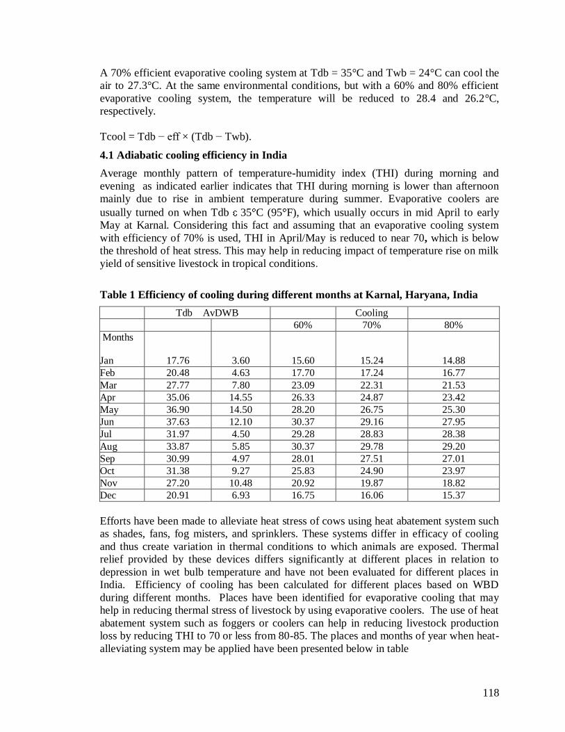
118
A 70% efficient evaporative cooling system at Tdb = 35°C and Twb = 24°C can cool the
air to 27.3°C. At the same environmental conditions, but with a 60% and 80% efficient
evaporative cooling system, the temperature will be reduced to 28.4 and 26.2°C,
respectively.
Tcool = Tdb − eff × (Tdb − Twb).
4.1 Adiabatic cooling efficiency in India
Average monthly pattern of temperature-humidity index (THI) during morning and
evening as indicated earlier indicates that THI during morning is lower than afternoon
mainly due to rise in ambient temperature during summer. Evaporative coolers are
usually turned on when Tdb 35 C (95 F), which usually occurs in mid April to early
May at Karnal. Considering this fact and assuming that an evaporative cooling system
with efficiency of 70% is used, THI in April/May is reduced to near 70, which is below
the threshold of heat stress. This may help in reducing impact of temperature rise on milk
yield of sensitive livestock in tropical conditions.
Table 1 Efficiency of cooling during different months at Karnal, Haryana, India
Tdb AvDWB Cooling
60% 70% 80%
Months
Jan 17.76 3.60 15.60 15.24 14.88
Feb 20.48 4.63 17.70 17.24 16.77
Mar 27.77 7.80 23.09 22.31 21.53
Apr 35.06 14.55 26.33 24.87 23.42
May 36.90 14.50 28.20 26.75 25.30
Jun 37.63 12.10 30.37 29.16 27.95
Jul 31.97 4.50 29.28 28.83 28.38
Aug 33.87 5.85 30.37 29.78 29.20
Sep 30.99 4.97 28.01 27.51 27.01
Oct 31.38 9.27 25.83 24.90 23.97
Nov 27.20 10.48 20.92 19.87 18.82
Dec 20.91 6.93 16.75 16.06 15.37
Efforts have been made to alleviate heat stress of cows using heat abatement system such
as shades, fans, fog misters, and sprinklers. These systems differ in efficacy of cooling
and thus create variation in thermal conditions to which animals are exposed. Thermal
relief provided by these devices differs significantly at different places in relation to
depression in wet bulb temperature and have not been evaluated for different places in
India. Efficiency of cooling has been calculated for different places based on WBD
during different months. Places have been identified for evaporative cooling that may
help in reducing thermal stress of livestock by using evaporative coolers. The use of heat
abatement system such as foggers or coolers can help in reducing livestock production
loss by reducing THI to 70 or less from 80-85. The places and months of year when heat-
alleviating system may be applied have been presented below in table
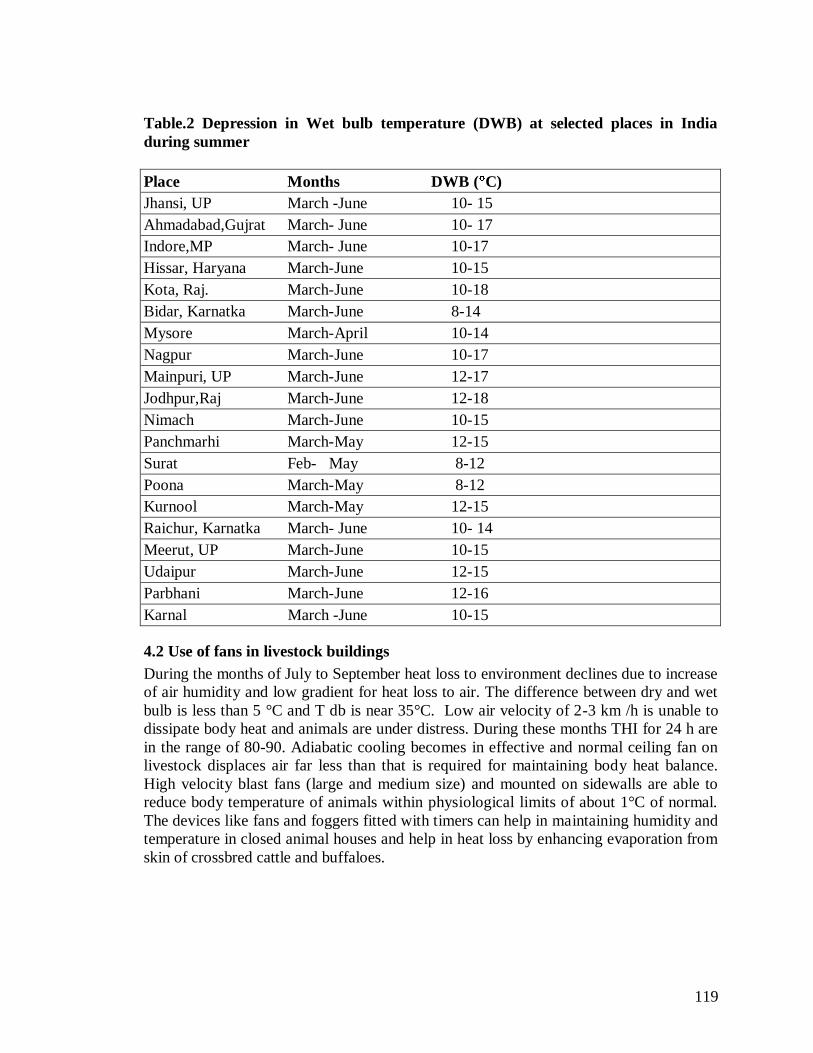
119
Table.2 Depression in Wet bulb temperature (DWB) at selected places in India
during summer
Place Months DWB ( C)
Jhansi, UP March -June 10- 15
Ahmadabad,Gujrat March- June 10- 17
Indore,MP March- June 10-17
Hissar, Haryana March-June 10-15
Kota, Raj. March-June 10-18
Bidar, Karnatka March-June 8-14
Mysore March-April 10-14
Nagpur March-June 10-17
Mainpuri, UP March-June 12-17
Jodhpur,Raj March-June 12-18
Nimach March-June 10-15
Panchmarhi March-May 12-15
Surat Feb- May 8-12
Poona March-May 8-12
Kurnool March-May 12-15
Raichur, Karnatka March- June 10- 14
Meerut, UP March-June 10-15
Udaipur March-June 12-15
Parbhani March-June 12-16
Karnal March -June 10-15
4.2 Use of fans in livestock buildings
During the months of July to September heat loss to environment declines due to increase
of air humidity and low gradient for heat loss to air. The difference between dry and wet
bulb is less than 5 °C and T db is near 35°C. Low air velocity of 2-3 km /h is unable to
dissipate body heat and animals are under distress. During these months THI for 24 h are
in the range of 80-90. Adiabatic cooling becomes in effective and normal ceiling fan on
livestock displaces air far less than that is required for maintaining body heat balance.
High velocity blast fans (large and medium size) and mounted on sidewalls are able to
reduce body temperature of animals within physiological limits of about 1°C of normal.
The devices like fans and foggers fitted with timers can help in maintaining humidity and
temperature in closed animal houses and help in heat loss by enhancing evaporation from
skin of crossbred cattle and buffaloes.
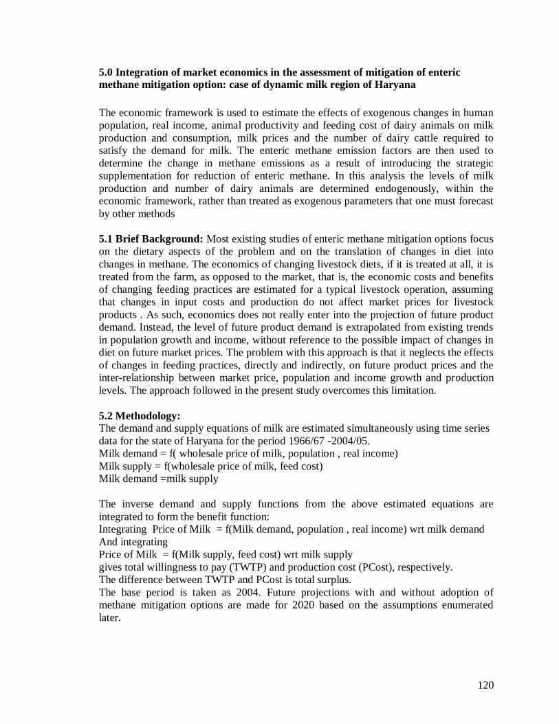
120
5.0 Integration of market economics in the assessment of mitigation of enteric
methane mitigation option: case of dynamic milk region of Haryana
The economic framework is used to estimate the effects of exogenous changes in human
population, real income, animal productivity and feeding cost of dairy animals on milk
production and consumption, milk prices and the number of dairy cattle required to
satisfy the demand for milk. The enteric methane emission factors are then used to
determine the change in methane emissions as a result of introducing the strategic
supplementation for reduction of enteric methane. In this analysis the levels of milk
production and number of dairy animals are determined endogenously, within the
economic framework, rather than treated as exogenous parameters that one must forecast
by other methods
5.1 Brief Background: Most existing studies of enteric methane mitigation options focus
on the dietary aspects of the problem and on the translation of changes in diet into
changes in methane. The economics of changing livestock diets, if it is treated at all, it is
treated from the farm, as opposed to the market, that is, the economic costs and benefits
of changing feeding practices are estimated for a typical livestock operation, assuming
that changes in input costs and production do not affect market prices for livestock
products . As such, economics does not really enter into the projection of future product
demand. Instead, the level of future product demand is extrapolated from existing trends
in population growth and income, without reference to the possible impact of changes in
diet on future market prices. The problem with this approach is that it neglects the effects
of changes in feeding practices, directly and indirectly, on future product prices and the
inter-relationship between market price, population and income growth and production
levels. The approach followed in the present study overcomes this limitation.
5.2 Methodology:
The demand and supply equations of milk are estimated simultaneously using time series
data for the state of Haryana for the period 1966/67 -2004/05.
Milk demand = f( wholesale price of milk, population , real income)
Milk supply = f(wholesale price of milk, feed cost)
Milk demand =milk supply
The inverse demand and supply functions from the above estimated equations are
integrated to form the benefit function:
Integrating Price of Milk = f(Milk demand, population , real income) wrt milk demand
And integrating
Price of Milk = f(Milk supply, feed cost) wrt milk supply
gives total willingness to pay (TWTP) and production cost (PCost), respectively.
The difference between TWTP and PCost is total surplus.
The base period is taken as 2004. Future projections with and without adoption of
methane mitigation options are made for 2020 based on the assumptions enumerated
later.
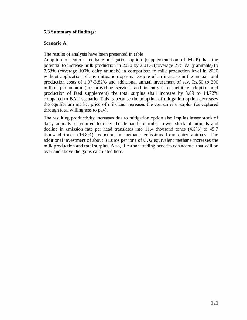
121
5.3 Summary of findings:
Scenario A
The results of analysis have been presented in table
Adoption of enteric methane mitigation option (supplementation of MUP) has the
potential to increase milk production in 2020 by 2.01% (coverage 25% dairy animals) to
7.53% (coverage 100% dairy animals) in comparison to milk production level in 2020
without application of any mitigation option. Despite of an increase in the annual total
production costs of 1.07-3.82% and additional annual investment of say, Rs.50 to 200
million per annum (for providing services and incentives to facilitate adoption and
production of feed supplement) the total surplus shall increase by 3.89 to 14.72%
compared to BAU scenario. This is because the adoption of mitigation option decreases
the equilibrium market price of milk and increases the consumer‟s surplus (as captured
through total willingness to pay).
The resulting productivity increases due to mitigation option also implies lesser stock of
dairy animals is required to meet the demand for milk. Lower stock of animals and
decline in emission rate per head translates into 11.4 thousand tones (4.2%) to 45.7
thousand tones (16.8%) reduction in methane emissions from dairy animals. The
additional investment of about 3 Euros per tone of CO2 equivalent methane increases the
milk production and total surplus. Also, if carbon-trading benefits can accrue, that will be
over and above the gains calculated here.
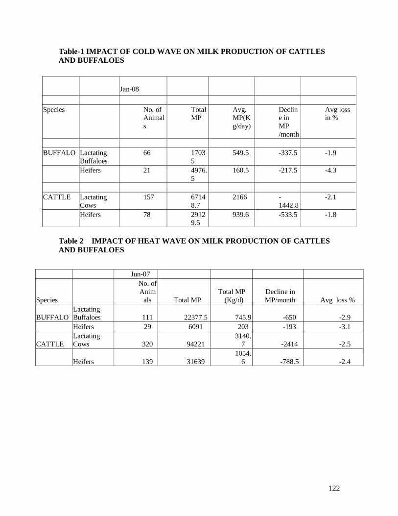
122
Table-1 IMPACT OF COLD WAVE ON MILK PRODUCTION OF CATTLES
AND BUFFALOES
Table 2 IMPACT OF HEAT WAVE ON MILK PRODUCTION OF CATTLES
AND BUFFALOES
Jan-08
Species No. of Animal
s
Total MP
Avg. MP(K
g/day)
Decline in
MP
/month
Avg loss in %
BUFFALO Lactating
Buffaloes
66 1703
5
549.5 -337.5 -1.9
Heifers 21 4976.
5
160.5 -217.5 -4.3
CATTLE Lactating
Cows
157 6714
8.7
2166 -
1442.8
-2.1
Heifers 78 29129.5
939.6 -533.5 -1.8
Jun-07
Species
No. of
Anim
als Total MP
Total MP
(Kg/d)
Decline in
MP/month Avg loss %
BUFFALO Lactating Buffaloes 111 22377.5 745.9 -650 -2.9
Heifers 29 6091 203 -193 -3.1
CATTLE Lactating Cows 320 94221
3140.7 -2414 -2.5
Heifers 139 31639
1054.
6 -788.5 -2.4
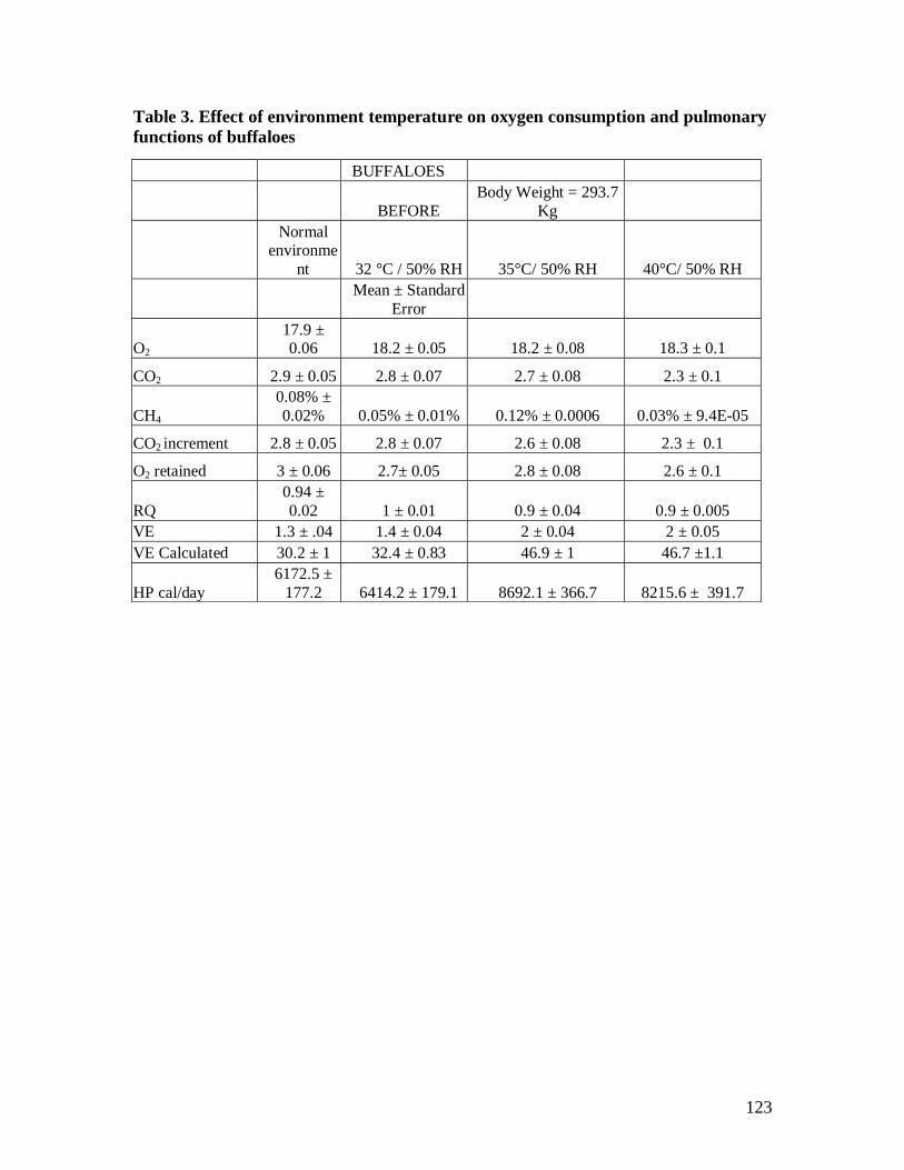
123
Table 3. Effect of environment temperature on oxygen consumption and pulmonary
functions of buffaloes
BUFFALOES
BEFORE
Body Weight = 293.7
Kg
Normal environme
nt 32 °C / 50% RH 35°C/ 50% RH 40°C/ 50% RH
Mean ± Standard
Error
O2 17.9 ± 0.06 18.2 ± 0.05 18.2 ± 0.08 18.3 ± 0.1
CO2 2.9 ± 0.05 2.8 ± 0.07 2.7 ± 0.08 2.3 ± 0.1
CH4
0.08% ±
0.02% 0.05% ± 0.01% 0.12% ± 0.0006 0.03% ± 9.4E-05
CO2 increment 2.8 ± 0.05 2.8 ± 0.07 2.6 ± 0.08 2.3 ± 0.1
O2 retained 3 ± 0.06 2.7± 0.05 2.8 ± 0.08 2.6 ± 0.1
RQ
0.94 ±
0.02 1 ± 0.01 0.9 ± 0.04 0.9 ± 0.005
VE 1.3 ± .04 1.4 ± 0.04 2 ± 0.04 2 ± 0.05
VE Calculated 30.2 ± 1 32.4 ± 0.83 46.9 ± 1 46.7 ±1.1
HP cal/day
6172.5 ±
177.2 6414.2 ± 179.1 8692.1 ± 366.7 8215.6 ± 391.7
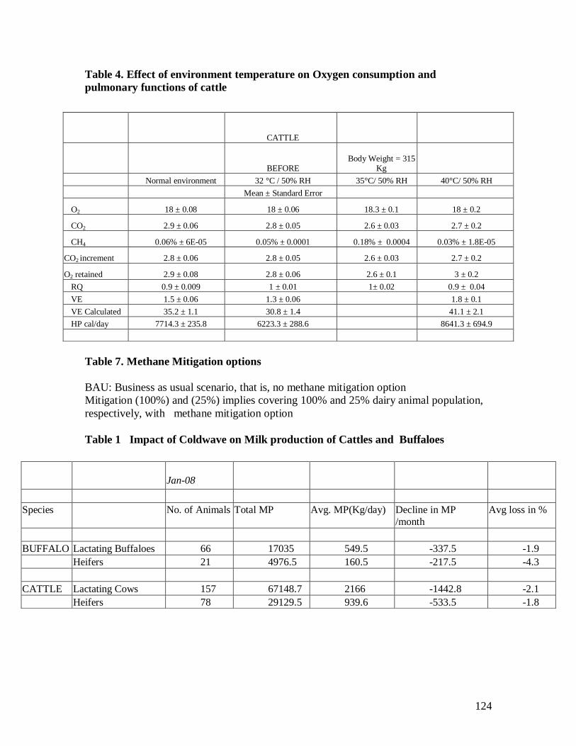
124
Table 4. Effect of environment temperature on Oxygen consumption and
pulmonary functions of cattle
Table 7. Methane Mitigation options
BAU: Business as usual scenario, that is, no methane mitigation option
Mitigation (100%) and (25%) implies covering 100% and 25% dairy animal population,
respectively, with methane mitigation option
Table 1 Impact of Coldwave on Milk production of Cattles and Buffaloes
CATTLE
BEFORE
Body Weight = 315
Kg
Normal environment 32 °C / 50% RH 35°C/ 50% RH 40°C/ 50% RH
Mean ± Standard Error
O2 18 ± 0.08 18 ± 0.06 18.3 ± 0.1 18 ± 0.2
CO2 2.9 ± 0.06 2.8 ± 0.05 2.6 ± 0.03 2.7 ± 0.2
CH4 0.06% ± 6E-05 0.05% ± 0.0001 0.18% ± 0.0004 0.03% ± 1.8E-05
CO2 increment 2.8 ± 0.06 2.8 ± 0.05 2.6 ± 0.03 2.7 ± 0.2
O2 retained 2.9 ± 0.08 2.8 ± 0.06 2.6 ± 0.1 3 ± 0.2
RQ 0.9 ± 0.009 1 ± 0.01 1± 0.02 0.9 ± 0.04
VE 1.5 ± 0.06 1.3 ± 0.06 1.8 ± 0.1
VE Calculated 35.2 ± 1.1 30.8 ± 1.4 41.1 ± 2.1
HP cal/day 7714.3 ± 235.8 6223.3 ± 288.6 8641.3 ± 694.9
Jan-08
Species No. of Animals Total MP Avg. MP(Kg/day) Decline in MP
/month
Avg loss in %
BUFFALO Lactating Buffaloes 66 17035 549.5 -337.5 -1.9
Heifers 21 4976.5 160.5 -217.5 -4.3
CATTLE Lactating Cows 157 67148.7 2166 -1442.8 -2.1
Heifers 78 29129.5 939.6 -533.5 -1.8
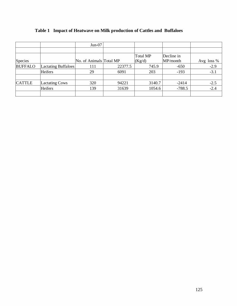
125
Table 1 Impact of Heatwave on Milk production of Cattles and Buffaloes
Jun-07
Species No. of Animals Total MP Total MP (Kg/d)
Decline in MP/month Avg loss %
BUFFALO Lactating Buffaloes 111 22377.5 745.9 -650 -2.9
Heifers 29 6091 203 -193 -3.1
CATTLE Lactating Cows 320 94221 3140.7 -2414 -2.5
Heifers 139 31639 1054.6 -788.5 -2.4
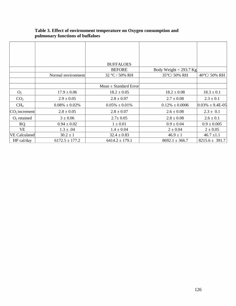
126
Table 3. Effect of environment temperature on Oxygen consumption and
pulmonary functions of buffaloes
BUFFALOES
BEFORE Body Weight = 293.7 Kg
Normal environment 32 °C / 50% RH 35°C/ 50% RH 40°C/ 50% RH
Mean ± Standard Error
O2 17.9 ± 0.06 18.2 ± 0.05 18.2 ± 0.08 18.3 ± 0.1
CO2 2.9 ± 0.05 2.8 ± 0.07 2.7 ± 0.08 2.3 ± 0.1
CH4 0.08% ± 0.02% 0.05% ± 0.01% 0.12% ± 0.0006 0.03% ± 9.4E-05
CO2 increment 2.8 ± 0.05 2.8 ± 0.07 2.6 ± 0.08 2.3 ± 0.1
O2 retained 3 ± 0.06 2.7± 0.05 2.8 ± 0.08 2.6 ± 0.1
RQ 0.94 ± 0.02 1 ± 0.01 0.9 ± 0.04 0.9 ± 0.005
VE 1.3 ± .04 1.4 ± 0.04 2 ± 0.04 2 ± 0.05
VE Calculated 30.2 ± 1 32.4 ± 0.83 46.9 ± 1 46.7 ±1.1
HP cal/day 6172.5 ± 177.2 6414.2 ± 179.1 8692.1 ± 366.7 8215.6 ± 391.7
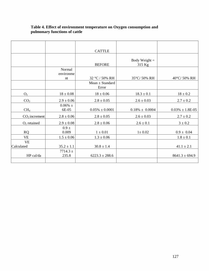
127
Table 4. Effect of environment temperature on Oxygen consumption and
pulmonary functions of cattle
CATTLE
BEFORE
Body Weight =
315 Kg
Normal environme
nt 32 °C / 50% RH 35°C/ 50% RH 40°C/ 50% RH
Mean ± Standard
Error
O2 18 ± 0.08 18 ± 0.06 18.3 ± 0.1 18 ± 0.2
CO2 2.9 ± 0.06 2.8 ± 0.05 2.6 ± 0.03 2.7 ± 0.2
CH4
0.06% ±
6E-05 0.05% ± 0.0001 0.18% ± 0.0004 0.03% ± 1.8E-05
CO2 increment 2.8 ± 0.06 2.8 ± 0.05 2.6 ± 0.03 2.7 ± 0.2
O2 retained 2.9 ± 0.08 2.8 ± 0.06 2.6 ± 0.1 3 ± 0.2
RQ 0.9 ± 0.009 1 ± 0.01 1± 0.02 0.9 ± 0.04
VE 1.5 ± 0.06 1.3 ± 0.06 1.8 ± 0.1
VE Calculated 35.2 ± 1.1 30.8 ± 1.4 41.1 ± 2.1
HP cal/da
7714.3 ±
235.8 6223.3 ± 288.6 8641.3 ± 694.9
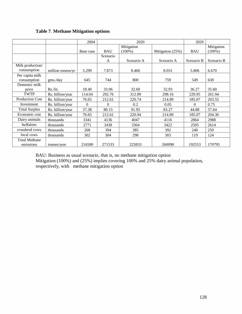
128
Table 7. Methane Mitigation options
BAU: Business as usual scenario, that is, no methane mitigation option
Mitigation (100%) and (25%) implies covering 100% and 25% dairy animal population,
respectively, with methane mitigation option
2004 2020 2020
Base case BAU
Mitigation
(100%) Mitigation (25%) BAU
Mitigation
(100%)
Scenario
A Scenario A Scenario A Scenario B Scenario B
Milk production/
consumption million tonnes/yr 5.299 7.873 8.466 8.031 5.806 6.670
Per capita milk
consumption gms./day 645 744 800 759 549 630
Domestic milk
price Rs./lit. 18.40 33.06 32.60 32.93 36.27 35.60
TWTP Rs. billion/year 114.04 292.76 312.89 298.16 229.95 261.94
Production Cost Rs. billion/year 76.65 212.61 220.74 214.89 185.07 203.55
Investment Rs. billion/year 0 0 0.2 0.05 0 0.75
Total Surplus Rs. billion/year 37.38 80.15 91.95 83.27 44.88 57.64
Economic cost Rs. billion/year 76.65 212.61 220.94 214.89 185.07 204.30
Dairy animals thousands 3341 4136 4047 4116 2864 2988
buffaloes thousands 2771 3438 3364 3422 2505 2614
crossbred cows thousands 268 394 385 392 240 250
local cows thousands 302 304 298 303 119 124
Total Methane
emissions tonnes/year 216500 271533 225833 260098 192553 170795
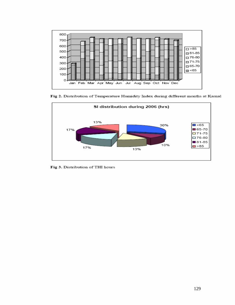
129
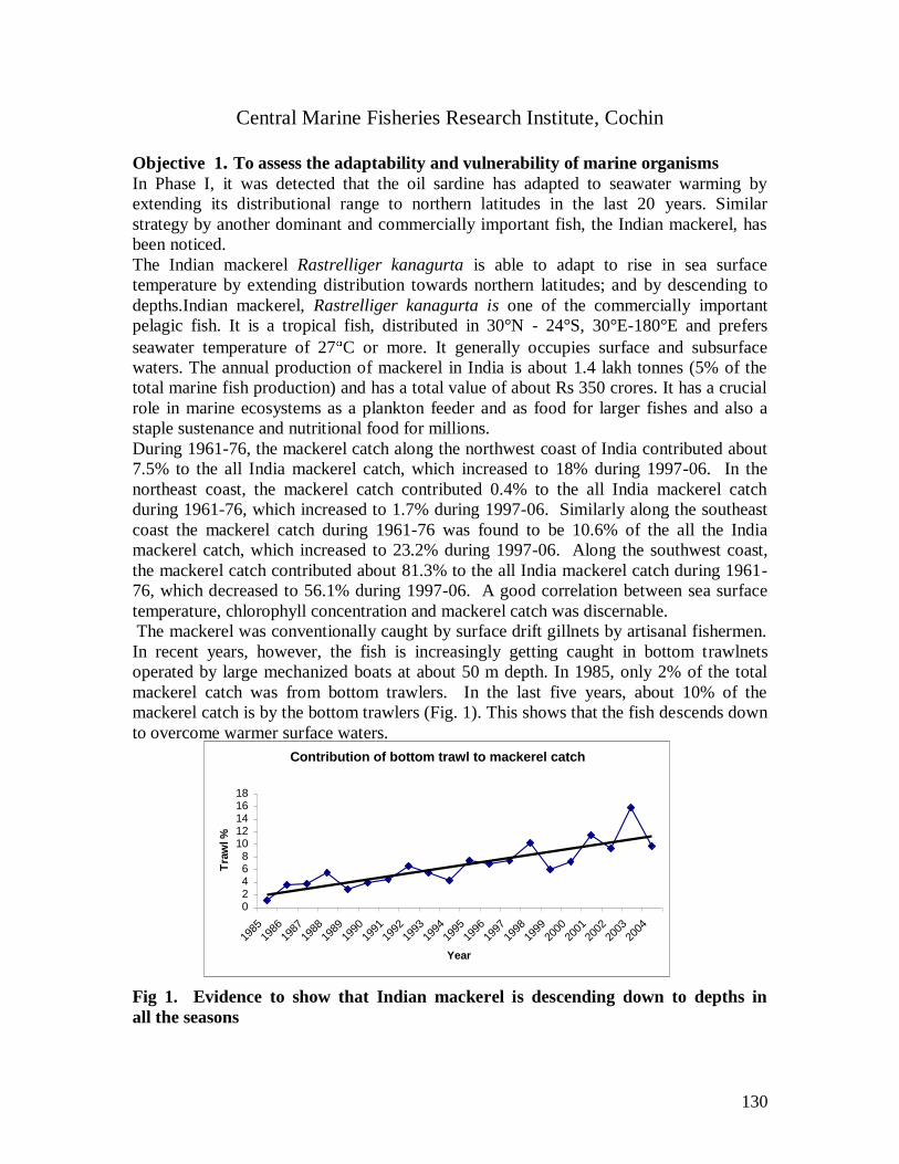
130
Central Marine Fisheries Research Institute, Cochin
Objective 1. To assess the adaptability and vulnerability of marine organisms
In Phase I, it was detected that the oil sardine has adapted to seawater warming by
extending its distributional range to northern latitudes in the last 20 years. Similar
strategy by another dominant and commercially important fish, the Indian mackerel, has
been noticed.
The Indian mackerel Rastrelliger kanagurta is able to adapt to rise in sea surface
temperature by extending distribution towards northern latitudes; and by descending to
depths.Indian mackerel, Rastrelliger kanagurta is one of the commercially important
pelagic fish. It is a tropical fish, distributed in 30°N - 24°S, 30°E-180°E and prefers
seawater temperature of 27 C or more. It generally occupies surface and subsurface
waters. The annual production of mackerel in India is about 1.4 lakh tonnes (5% of the
total marine fish production) and has a total value of about Rs 350 crores. It has a crucial
role in marine ecosystems as a plankton feeder and as food for larger fishes and also a
staple sustenance and nutritional food for millions.
During 1961-76, the mackerel catch along the northwest coast of India contributed about
7.5% to the all India mackerel catch, which increased to 18% during 1997-06. In the
northeast coast, the mackerel catch contributed 0.4% to the all India mackerel catch
during 1961-76, which increased to 1.7% during 1997-06. Similarly along the southeast
coast the mackerel catch during 1961-76 was found to be 10.6% of the all the India
mackerel catch, which increased to 23.2% during 1997-06. Along the southwest coast,
the mackerel catch contributed about 81.3% to the all India mackerel catch during 1961-
76, which decreased to 56.1% during 1997-06. A good correlation between sea surface
temperature, chlorophyll concentration and mackerel catch was discernable.
The mackerel was conventionally caught by surface drift gillnets by artisanal fishermen.
In recent years, however, the fish is increasingly getting caught in bottom trawlnets
operated by large mechanized boats at about 50 m depth. In 1985, only 2% of the total
mackerel catch was from bottom trawlers. In the last five years, about 10% of the
mackerel catch is by the bottom trawlers (Fig. 1). This shows that the fish descends down
to overcome warmer surface waters.
Fig 1. Evidence to show that Indian mackerel is descending down to depths in
all the seasons
Contribution of bottom trawl to mackerel catch
02468
1012141618
1985
1986
1987
1988
1989
1990
1991
1992
1993
1994
1995
1996
1997
1998
1999
2000
2001
2002
2003
2004
Year
Tra
wl %
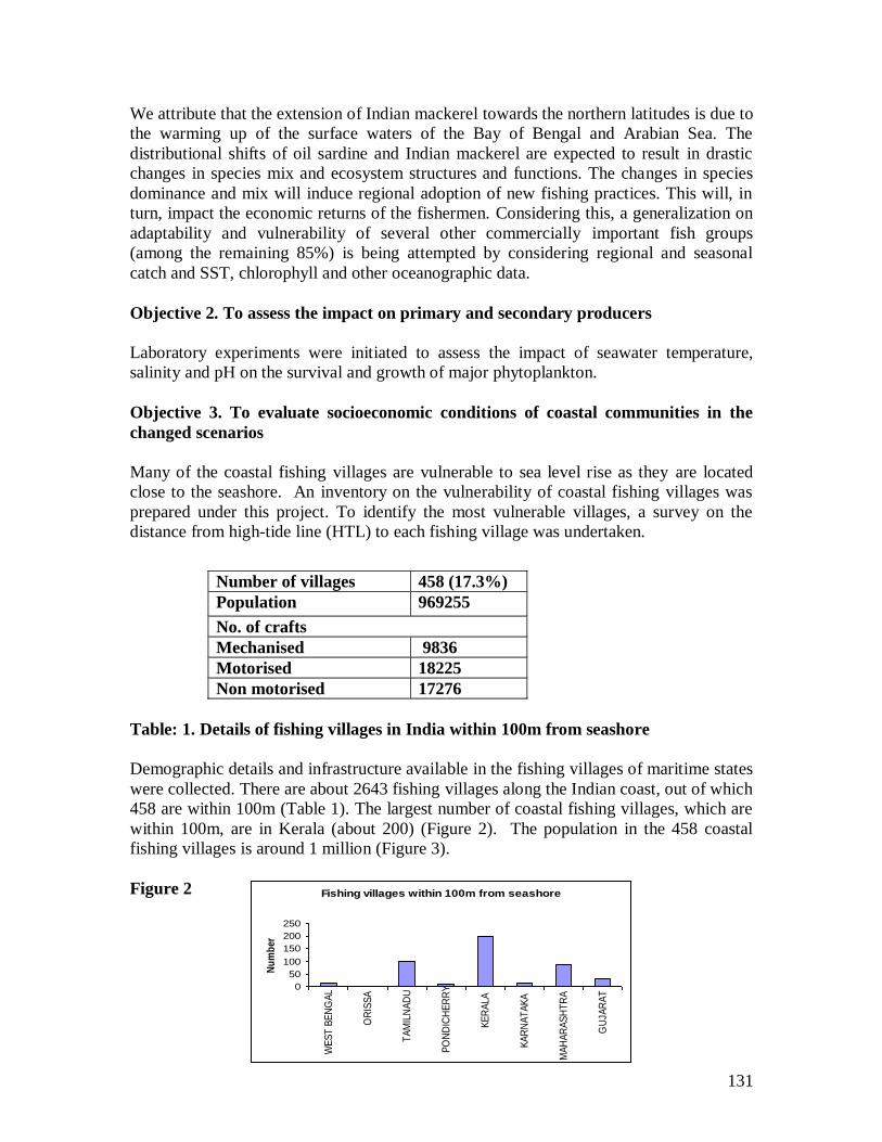
131
We attribute that the extension of Indian mackerel towards the northern latitudes is due to
the warming up of the surface waters of the Bay of Bengal and Arabian Sea. The
distributional shifts of oil sardine and Indian mackerel are expected to result in drastic
changes in species mix and ecosystem structures and functions. The changes in species
dominance and mix will induce regional adoption of new fishing practices. This will, in
turn, impact the economic returns of the fishermen. Considering this, a generalization on
adaptability and vulnerability of several other commercially important fish groups
(among the remaining 85%) is being attempted by considering regional and seasonal
catch and SST, chlorophyll and other oceanographic data.
Objective 2. To assess the impact on primary and secondary producers
Laboratory experiments were initiated to assess the impact of seawater temperature,
salinity and pH on the survival and growth of major phytoplankton.
Objective 3. To evaluate socioeconomic conditions of coastal communities in the
changed scenarios
Many of the coastal fishing villages are vulnerable to sea level rise as they are located
close to the seashore. An inventory on the vulnerability of coastal fishing villages was
prepared under this project. To identify the most vulnerable villages, a survey on the
distance from high-tide line (HTL) to each fishing village was undertaken.
Table: 1. Details of fishing villages in India within 100m from seashore
Demographic details and infrastructure available in the fishing villages of maritime states
were collected. There are about 2643 fishing villages along the Indian coast, out of which
458 are within 100m (Table 1). The largest number of coastal fishing villages, which are
within 100m, are in Kerala (about 200) (Figure 2). The population in the 458 coastal
fishing villages is around 1 million (Figure 3).
Figure 2
Fishing villages within 100m from seashore
0
50
100
150
200
250
WE
ST
BE
NG
AL
OR
ISS
A
TA
MIL
NA
DU
PO
ND
ICH
ER
RY
KE
RA
LA
KA
RN
AT
AK
A
MA
HA
RA
SH
TR
A
GU
JAR
AT
Nu
mb
er
Number of villages 458 (17.3%)
Population 969255
No. of crafts
Mechanised 9836
Motorised 18225
Non motorised 17276
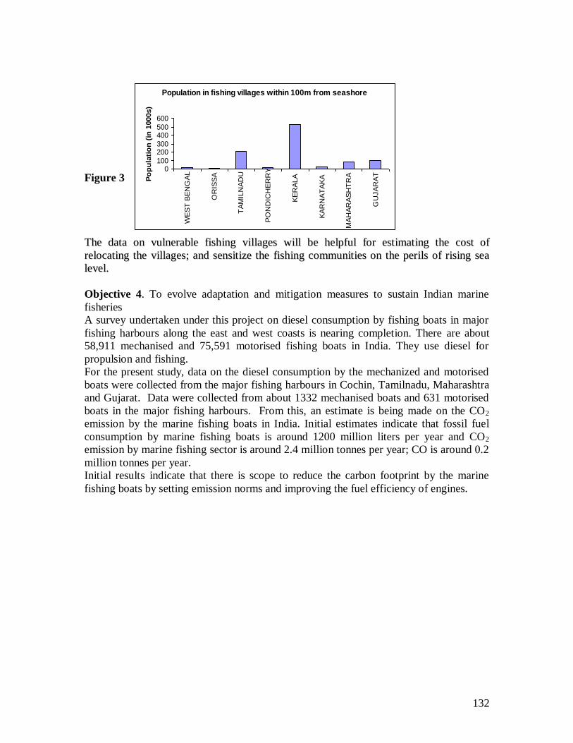
132
Figure 3
TThhee ddaattaa oonn vvuullnneerraabbllee ffiisshhiinngg vviillllaaggeess wwiillll bbee hheellppffuull ffoorr eessttiimmaattiinngg tthhee ccoosstt ooff
rreellooccaattiinngg tthhee vviillllaaggeess;; aanndd sseennssiittiizzee tthhee ffiisshhiinngg ccoommmmuunniittiieess oonn tthhee ppeerriillss ooff rriissiinngg sseeaa
lleevveell..
Objective 4. To evolve adaptation and mitigation measures to sustain Indian marine
fisheries
A survey undertaken under this project on diesel consumption by fishing boats in major
fishing harbours along the east and west coasts is nearing completion. There are about
58,911 mechanised and 75,591 motorised fishing boats in India. They use diesel for
propulsion and fishing.
For the present study, data on the diesel consumption by the mechanized and motorised
boats were collected from the major fishing harbours in Cochin, Tamilnadu, Maharashtra
and Gujarat. Data were collected from about 1332 mechanised boats and 631 motorised
boats in the major fishing harbours. From this, an estimate is being made on the CO2
emission by the marine fishing boats in India. Initial estimates indicate that fossil fuel
consumption by marine fishing boats is around 1200 million liters per year and CO2
emission by marine fishing sector is around 2.4 million tonnes per year; CO is around 0.2
million tonnes per year.
Initial results indicate that there is scope to reduce the carbon footprint by the marine
fishing boats by setting emission norms and improving the fuel efficiency of engines.
Population in fishing villages within 100m from seashore
0100
200300
400500
600
WE
ST
BE
NG
AL
OR
ISS
A
TA
MIL
NA
DU
PO
ND
ICH
ER
RY
KE
RA
LA
KA
RN
AT
AK
A
MA
HA
RA
SH
TR
A
GU
JA
RA
T
Po
pu
lati
on
(in
1000s)
133
CENTRAL INLAND FISHRIES RESEARCH INSTITUTE, BARRAKPORE
Objective 1.
Impact of temperature and rainfall on the breeding of Indian major carps in Fish
seed hatcheries of Orissa.
Aquaculture practice of breeding in captivity of fishes viz. Indian major carps, C. catla,
L. rohita and C. mrigala by the technique of hypophysation and their spawning occurs
during the monsoon season (June-July) and extends till September. However, in recent
years the phenomenon of IMC maturing and spawning as early as March is observed, as a
result it has been possible to breed them twice in a year at an interval ranging from 30-60
days. It is of significance to note that the climate is showing perceptible changes in India
on a regional scale over the years. Temperature is one of the dominant factors influencing
the reproductive cycle in fishes. During these 6 months (January to June) temperatures in
India gradually increase and reach their maximum by May-June. This environmental
factor along with rainfall and photoperiod stimulate the endocrine glands which help in
the maturation of gonads of carp. In Orissa the average temperature is on the rise over the
last 30years. The average maximum and minimum temperature throughout the state
during the time period 1975-2000 has increased by 0.57ºC. and 0.11ºC while the average
rainfall has decreased. A perusal of the records reveals that the South West Monsoon
comes at the earliest by 26th
May and latest by 26th
June. If 7th
June is taken as the
commencement of monsoon; the tendency of monsoon coming late is increasing. Thus
the natural phenomenon which decreases the temperature is getting delayed every year.
Consequently its impact is being felt in the inland water bodies and on inland fish.
With this background investigation was conducted to ascertain the impact of temperature
on the breeding of Indian major carps in the fish hatcheries in four districts of Orissa.
The study was having objectives to analyze i) the climatic changes viz. increase in
temperature and rainfall pattern some districts of Orissa, ii) impact of elevated
temperature on the breeding of Indian major carps and impact on the fishers.
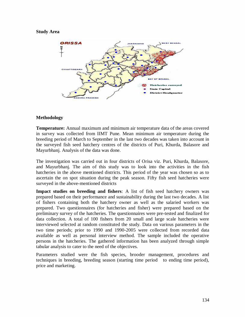
134
Study Area
Methodology
Temperature: Annual maximum and minimum air temperature data of the areas covered
in survey was collected from IIMT Pune. Mean minimum air temperature during the
breeding period of March to September in the last two decades was taken into account in
the surveyed fish seed hatchery centres of the districts of Puri, Khurda, Balasore and
Mayurbhanj. Analysis of the data was done.
The investigation was carried out in four districts of Orisa viz. Puri, Khurda, Balasore,
and Mayurbhanj. The aim of this study was to look into the activities in the fish
hatcheries in the above mentioned districts. This period of the year was chosen so as to
ascertain the on spot situation during the peak season. Fifty fish seed hatcheries were
surveyed in the above-mentioned districts
Impact studies on breeding and fishers: A list of fish seed hatchery owners was
prepared based on their performance and sustainability during the last two decades. A list
of fishers containing both the hatchery owner as well as the salaried workers was
prepared. Two questionnaires (for hatcheries and fisher) were prepared based on the
preliminary survey of the hatcheries. The questionnaires were pre-tested and finalized for
data collection. A total of 100 fishers from 20 small and large scale hatcheries were
interviewed selected at random constituted the study. Data on various parameters in the
two time periods; prior to 1990 and 1990-2005 were collected from recorded data
available as well as personal interview method. The sample included the operative
persons in the hatcheries. The gathered information has been analyzed through simple
tabular analysis to cater to the need of the objectives.
Parameters studied were the fish species, brooder management, procedures and
techniques in breeding, breeding season (starting time period to ending time period),
price and marketing.
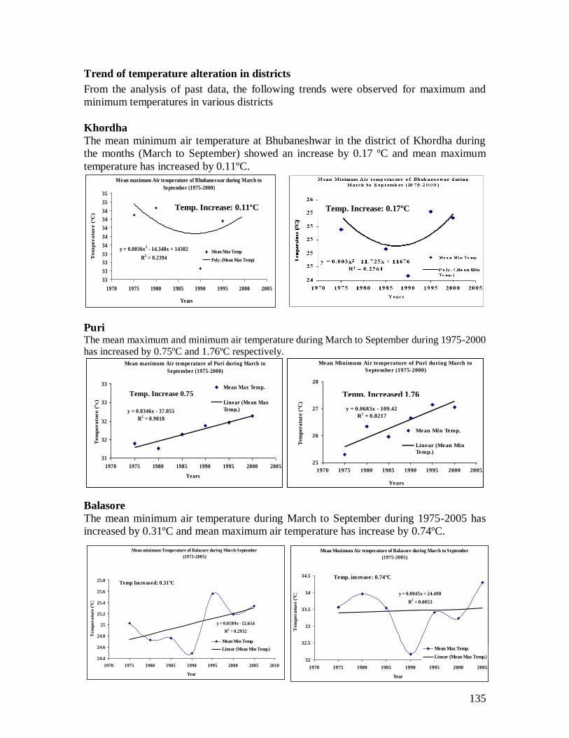
135
Mean maximum Air temperature of Puri during March to
September (1975-2000)
y = 0.0346x - 37.055
R2 = 0.9018
31
32
32
33
33
1970 1975 1980 1985 1990 1995 2000 2005
Years
Tem
pera
ture (
ºc)
Mean Max Temp.
Linear (Mean Max
Temp.)
Mean Minimum Air temperature of Puri during March to
September (1975-2000)
y = 0.0683x - 109.42
R2 = 0.8217
25
26
27
28
1970 1975 1980 1985 1990 1995 2000 2005
Years
Tem
per
atu
re (
ºC)
Mean Min Temp.
Linear (Mean Min
Temp.)
Trend of temperature alteration in districts
From the analysis of past data, the following trends were observed for maximum and
minimum temperatures in various districts
Khordha
The mean minimum air temperature at Bhubaneshwar in the district of Khordha during
the months (March to September) showed an increase by 0.17 ºC and mean maximum
temperature has increased by 0.11ºC. Mean maximum Air temperature of Bhubaneswar during March to
September (1975-2000)
y = 0.0036x2 - 14.348x + 14302
R2 = 0.2394
33
33
33
33
34
34
34
34
34
35
35
1970 1975 1980 1985 1990 1995 2000 2005
Years
Tem
pera
ture (
ºC)
Mean Max Temp
Poly. (Mean Max Temp)
Puri The mean maximum and minimum air temperature during March to September during 1975-2000 has increased by 0.75ºC and 1.76ºC respectively.
Balasore
The mean minimum air temperature during March to September during 1975-2005 has
increased by 0.31ºC and mean maximum air temperature has increase by 0.74ºC.
Mean minimum Temperature of Balasore during March-September
(1975-2005)
y = 0.0189x - 12.654
R2 = 0.2932
24.4
24.6
24.8
25
25.2
25.4
25.6
25.8
1970 1975 1980 1985 1990 1995 2000 2005 2010
Year
Tem
pera
ture (
ºC)
Mean Min Temp.
Linear (Mean Min Temp.)
Temp Increased: 0.31ºC
Mean Maximum Air temperature of Balasore during March to September
(1975-2005)
y = 0.0045x + 24.498
R2 = 0.0053
32
32.5
33
33.5
34
34.5
1970 1975 1980 1985 1990 1995 2000 2005
Year
Tem
pera
ture (
ºC)
Mean Max Temp.
Linear (Mean Max Temp.)
Temp. increase: 0.74ºC
Temp. Increase: 0.11ºC
Temp. Increase 0.75 Temp. Increased 1.76
Temp. Increase: 0.17ºC
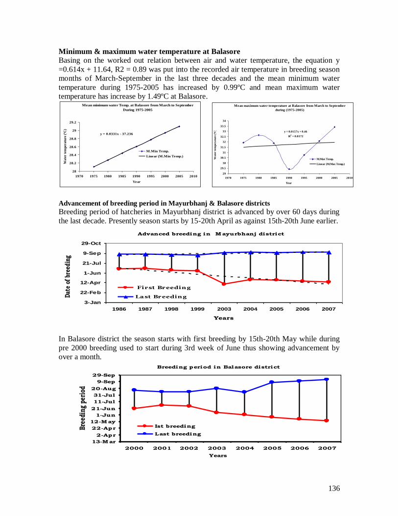
136
Minimum & maximum water temperature at Balasore
Basing on the worked out relation between air and water temperature, the equation y
=0.614x + 11.64, R2 = 0.89 was put into the recorded air temperature in breeding season
months of March-September in the last three decades and the mean minimum water
temperature during 1975-2005 has increased by 0.99ºC and mean maximum water
temperature has increase by 1.49ºC at Balasore.
Advancement of breeding period in Mayurbhanj & Balasore districts
Breeding period of hatcheries in Mayurbhanj district is advanced by over 60 days during
the last decade. Presently season starts by 15-20th April as against 15th-20th June earlier.
In Balasore district the season starts with first breeding by 15th-20th May while during
pre 2000 breeding used to start during 3rd week of June thus showing advancement by
over a month.
Mean minimum water Temp. at Balasore from March to September
During 1975-2005
y = 0.0331x - 37.236
28
28.2
28.4
28.6
28.8
29
29.2
1970 1975 1980 1985 1990 1995 2000 2005 2010
Year
Wa
ter
tem
per
atu
re (
ºC)
M.Min Temp.
Linear (M.Min Temp.)
Mean maximum water temperature at Balasore from March to September
during (1975-2005)
y = 0.0157x + 0.46
R2 = 0.0172
29
29.5
30
30.5
31
31.5
32
32.5
33
33.5
34
1970 1975 1980 1985 1990 1995 2000 2005 2010
Year
Wa
ter
tem
per
atu
re (
ºC)
M.Max Temp.
Linear (M.Max Temp.)
Advanced breeding in Mayurbhanj district
3-Jan
22-Feb
12-Apr
1-Jun
21-Jul
9-Sep
29-Oct
1986 1987 1998 1999 2003 2004 2005 2006 2007
Years
Dat
e of
bre
edin
g
First Breedin g
La st Breedin g
Breeding period in Balasore district
13-Mar
2-Apr
22-Apr
12-May
1-Jun
21-Jun
11-Jul
31-Jul
20-Aug
9-Sep
29-Sep
2000 2001 2002 2003 2004 2005 2006 2007
Years
Bre
edin
g pe
riod
Ist breeding
Last breeding
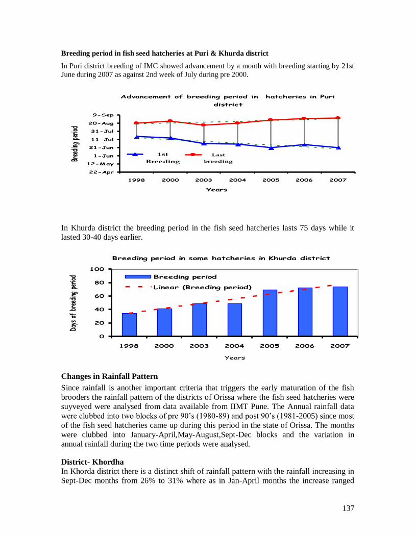
137
Breeding period in fish seed hatcheries at Puri & Khurda district
In Puri district breeding of IMC showed advancement by a month with breeding starting by 21st
June during 2007 as against 2nd week of July during pre 2000.
In Khurda district the breeding period in the fish seed hatcheries lasts 75 days while it
lasted 30-40 days earlier.
Changes in Rainfall Pattern
Since rainfall is another important criteria that triggers the early maturation of the fish
brooders the rainfall pattern of the districts of Orissa where the fish seed hatcheries were
suyveyed were analysed from data available from IIMT Pune. The Annual rainfall data
were clubbed into two blocks of pre 90‟s (1980-89) and post 90‟s (1981-2005) since most
of the fish seed hatcheries came up during this period in the state of Orissa. The months
were clubbed into January-April,May-August,Sept-Dec blocks and the variation in
annual rainfall during the two time periods were analysed.
District- Khordha
In Khorda district there is a distinct shift of rainfall pattern with the rainfall increasing in
Sept-Dec months from 26% to 31% where as in Jan-April months the increase ranged
Advancement of breeding period in hatcheries in Puri
district
1st
Breeding
Last
breeding
22-Apr
12-May
1-Jun
21-Jun
11-Jul
31-Jul
20-Aug
9-Sep
1998 2000 2003 2004 2005 2006 2007
Years
Bree
ding
per
iod
Breeding period in some hatcheries in Khurda district
0
20
40
60
80
100
1998 2000 2003 2004 2005 2006 2007
Years
Days
of
bree
ding
perio
d Breeding period
Linear (Breeding period)
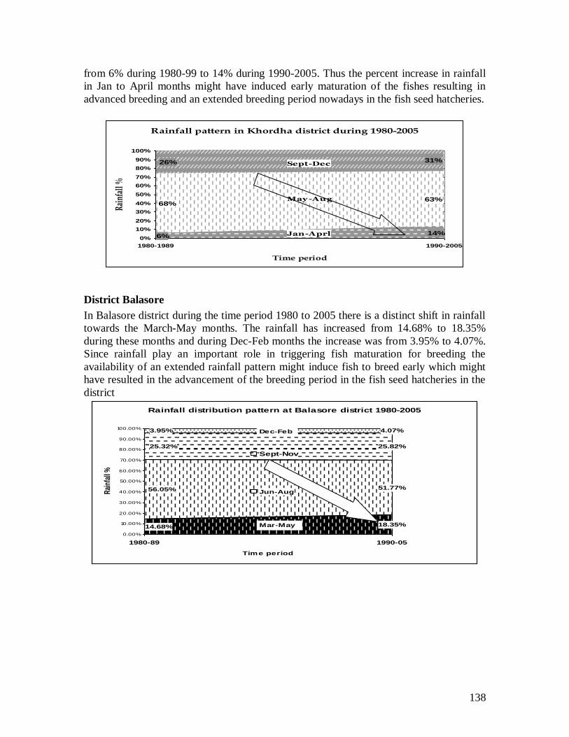
138
from 6% during 1980-99 to 14% during 1990-2005. Thus the percent increase in rainfall
in Jan to April months might have induced early maturation of the fishes resulting in
advanced breeding and an extended breeding period nowadays in the fish seed hatcheries.
Rainfall pattern in Khordha district during 1980-2005
14%6%
63%68%
31%26%
0%
10%
20%
30%
40%
50%
60%
70%
80%
90%
100%
1980-1989 1990-2005
Time period
Rain
fall
%
Sept-Dec
May -Aug
Jan-Aprl
District Balasore
In Balasore district during the time period 1980 to 2005 there is a distinct shift in rainfall
towards the March-May months. The rainfall has increased from 14.68% to 18.35%
during these months and during Dec-Feb months the increase was from 3.95% to 4.07%.
Since rainfall play an important role in triggering fish maturation for breeding the
availability of an extended rainfall pattern might induce fish to breed early which might
have resulted in the advancement of the breeding period in the fish seed hatcheries in the
district
Rainfall distribution pattern at Balasore district 1980-2005
18.35%
51.77%
25.82%
4.07%
14.68%
56.05%
25.32%
3.95%
0.00%
10.00%
20.00%
30.00%
40.00%
50.00%
60.00%
70.00%
80.00%
90.00%
100.00%
1980-89 1990-05
Time period
Rai
nfal
l %
Sept-Nov
Jun-Aug
Mar-May
Dec-Feb
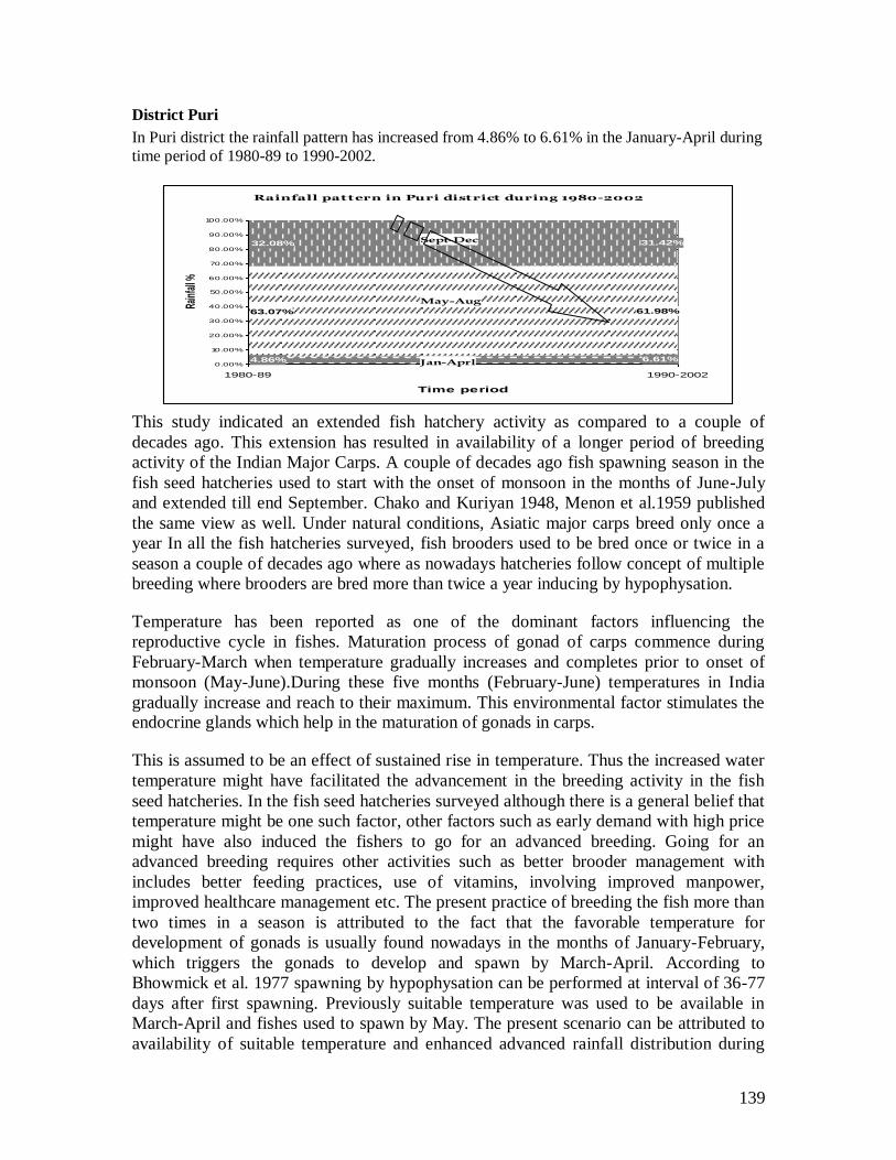
139
District Puri
In Puri district the rainfall pattern has increased from 4.86% to 6.61% in the January-April during
time period of 1980-89 to 1990-2002.
Rainfall pattern in Puri district during 1980-2002
6.61%4.86%
61.98%63.07%
32.08% 31.42%
0.00%
10.00%
20.00%
30.00%
40.00%
50.00%
60.00%
70.00%
80.00%
90.00%
100.00%
1980-89 1990-2002
Time period
Rain
fall %
Sept-Dec
May-Aug
Jan-Aprl
This study indicated an extended fish hatchery activity as compared to a couple of
decades ago. This extension has resulted in availability of a longer period of breeding
activity of the Indian Major Carps. A couple of decades ago fish spawning season in the
fish seed hatcheries used to start with the onset of monsoon in the months of June-July
and extended till end September. Chako and Kuriyan 1948, Menon et al.1959 published
the same view as well. Under natural conditions, Asiatic major carps breed only once a
year In all the fish hatcheries surveyed, fish brooders used to be bred once or twice in a
season a couple of decades ago where as nowadays hatcheries follow concept of multiple
breeding where brooders are bred more than twice a year inducing by hypophysation.
Temperature has been reported as one of the dominant factors influencing the
reproductive cycle in fishes. Maturation process of gonad of carps commence during
February-March when temperature gradually increases and completes prior to onset of
monsoon (May-June).During these five months (February-June) temperatures in India
gradually increase and reach to their maximum. This environmental factor stimulates the endocrine glands which help in the maturation of gonads in carps.
This is assumed to be an effect of sustained rise in temperature. Thus the increased water
temperature might have facilitated the advancement in the breeding activity in the fish
seed hatcheries. In the fish seed hatcheries surveyed although there is a general belief that
temperature might be one such factor, other factors such as early demand with high price
might have also induced the fishers to go for an advanced breeding. Going for an
advanced breeding requires other activities such as better brooder management with
includes better feeding practices, use of vitamins, involving improved manpower,
improved healthcare management etc. The present practice of breeding the fish more than
two times in a season is attributed to the fact that the favorable temperature for
development of gonads is usually found nowadays in the months of January-February,
which triggers the gonads to develop and spawn by March-April. According to
Bhowmick et al. 1977 spawning by hypophysation can be performed at interval of 36-77
days after first spawning. Previously suitable temperature was used to be available in
March-April and fishes used to spawn by May. The present scenario can be attributed to
availability of suitable temperature and enhanced advanced rainfall distribution during
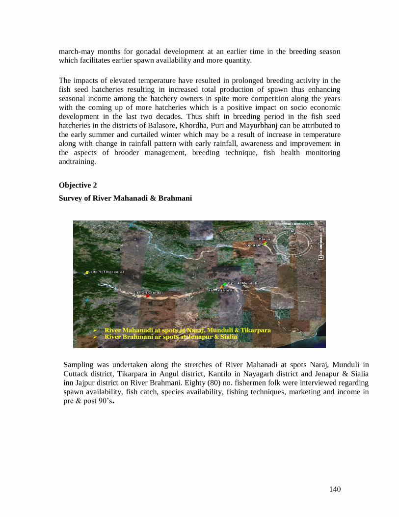
140
march-may months for gonadal development at an earlier time in the breeding season which facilitates earlier spawn availability and more quantity.
The impacts of elevated temperature have resulted in prolonged breeding activity in the
fish seed hatcheries resulting in increased total production of spawn thus enhancing
seasonal income among the hatchery owners in spite more competition along the years
with the coming up of more hatcheries which is a positive impact on socio economic
development in the last two decades. Thus shift in breeding period in the fish seed
hatcheries in the districts of Balasore, Khordha, Puri and Mayurbhanj can be attributed to
the early summer and curtailed winter which may be a result of increase in temperature
along with change in rainfall pattern with early rainfall, awareness and improvement in
the aspects of brooder management, breeding technique, fish health monitoring
andtraining.
Objective 2
Survey of River Mahanadi & Brahmani
River Mahanadi at spots at Naraj, Munduli & Tikarpara River Brahmani ar spots at Jenapur & Sialia
Sampling was undertaken along the stretches of River Mahanadi at spots Naraj, Munduli in
Cuttack district, Tikarpara in Angul district, Kantilo in Nayagarh district and Jenapur & Sialia
inn Jajpur district on River Brahmani. Eighty (80) no. fishermen folk were interviewed regarding
spawn availability, fish catch, species availability, fishing techniques, marketing and income in
pre & post 90‟s.
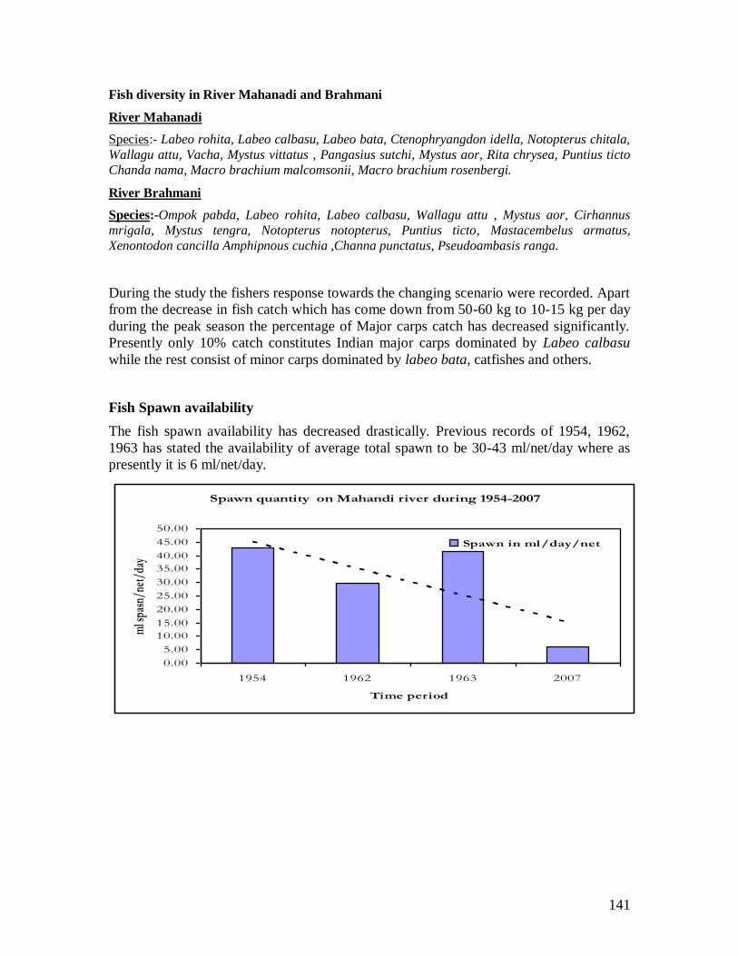
141
Fish diversity in River Mahanadi and Brahmani
River Mahanadi
Species:- Labeo rohita, Labeo calbasu, Labeo bata, Ctenophryangdon idella, Notopterus chitala,
Wallagu attu, Vacha, Mystus vittatus , Pangasius sutchi, Mystus aor, Rita chrysea, Puntius ticto
Chanda nama, Macro brachium malcomsonii, Macro brachium rosenbergi.
River Brahmani
Species:-Ompok pabda, Labeo rohita, Labeo calbasu, Wallagu attu , Mystus aor, Cirhannus
mrigala, Mystus tengra, Notopterus notopterus, Puntius ticto, Mastacembelus armatus,
Xenontodon cancilla Amphipnous cuchia ,Channa punctatus, Pseudoambasis ranga.
During the study the fishers response towards the changing scenario were recorded. Apart
from the decrease in fish catch which has come down from 50-60 kg to 10-15 kg per day
during the peak season the percentage of Major carps catch has decreased significantly.
Presently only 10% catch constitutes Indian major carps dominated by Labeo calbasu
while the rest consist of minor carps dominated by labeo bata, catfishes and others.
Fish Spawn availability
The fish spawn availability has decreased drastically. Previous records of 1954, 1962,
1963 has stated the availability of average total spawn to be 30-43 ml/net/day where as
presently it is 6 ml/net/day.
Spawn quantity on Mahandi river during 1954-2007
0.00
5.00
10.00
15.00
20.00
25.00
30.00
35.00
40.00
45.00
50.00
1954 1962 1963 2007
Time period
ml s
pasn
/net
/day
Spawn in ml/day/net
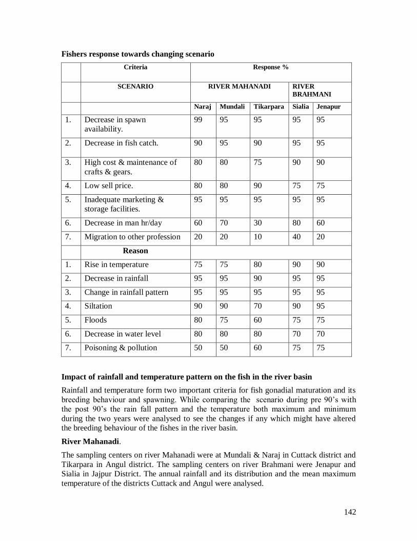
142
Fishers response towards changing scenario
Criteria Response %
SCENARIO RIVER MAHANADI RIVER
BRAHMANI
Naraj Mundali Tikarpara Sialia Jenapur
1. Decrease in spawn
availability.
99 95 95 95 95
2. Decrease in fish catch. 90 95 90 95 95
3. High cost & maintenance of
crafts & gears.
80 80 75 90 90
4. Low sell price. 80 80 90 75 75
5. Inadequate marketing &
storage facilities.
95 95 95 95 95
6. Decrease in man hr/day 60 70 30 80 60
7. Migration to other profession 20 20 10 40 20
Reason
1. Rise in temperature 75 75 80 90 90
2. Decrease in rainfall 95 95 90 95 95
3. Change in rainfall pattern 95 95 95 95 95
4. Siltation 90 90 70 90 95
5. Floods 80 75 60 75 75
6. Decrease in water level 80 80 80 70 70
7. Poisoning & pollution 50 50 60 75 75
Impact of rainfall and temperature pattern on the fish in the river basin
Rainfall and temperature form two important criteria for fish gonadial maturation and its
breeding behaviour and spawning. While comparing the scenario during pre 90‟s with
the post 90‟s the rain fall pattern and the temperature both maximum and minimum
during the two years were analysed to see the changes if any which might have altered
the breeding behaviour of the fishes in the river basin.
River Mahanadi.
The sampling centers on river Mahanadi were at Mundali & Naraj in Cuttack district and
Tikarpara in Angul district. The sampling centers on river Brahmani were Jenapur and
Sialia in Jajpur District. The annual rainfall and its distribution and the mean maximum
temperature of the districts Cuttack and Angul were analysed.
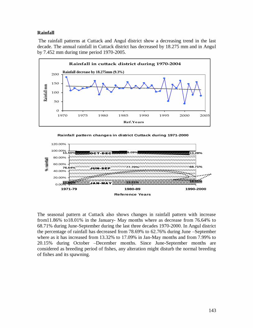
143
Rainfall
The rainfall patterns at Cuttack and Angul district show a decreasing trend in the last
decade. The annual rainfall in Cuttack district has decreased by 18.275 mm and in Angul
by 7.452 mm during time period 1970-2005.
Rainfall in cuttack district during 1970-2004
0
50
100
150
200
1970 1975 1980 1985 1990 1995 2000 2005
Ref.Years
Rain
fall
mm
Rainfall pattern changes in district Cuttack during 1971-2000
11.86% 13.21% 18.01%
76.64% 77.70% 68.71%
11.50% 9.09% 13.28%
0.00%
20.00%
40.00%
60.00%
80.00%
100.00%
120.00%
1971-79 1980-89 1990-2000
Reference Years
% ra
infa
ll
OCT-DEC
JUN-SEP
JAN-MAY
The seasonal pattern at Cuttack also shows changes in rainfall pattern with increase
from11.86% to18.01% in the January- May months where as decrease from 76.64% to
68.71% during June-September during the last three decades 1970-2000. In Angul district
the percentage of rainfall has decreased from 78.69% to 62.76% during June –September
where as it has increased from 13.32% to 17.09% in Jan-May months and from 7.99% to
20.15% during October –December months. Since June-September months are
considered as breeding period of fishes, any alteration might disturb the normal breeding
of fishes and its spawning.
Rainfall decrease by 18.275mm (9.3%)
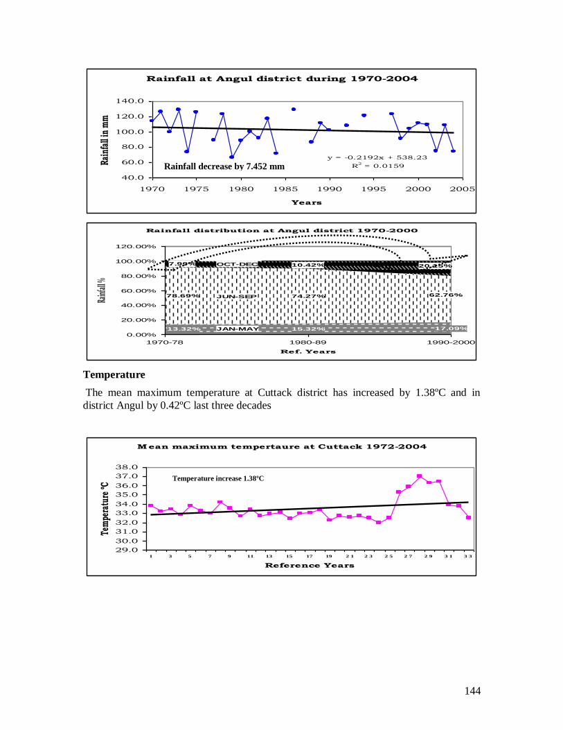
144
Rainfall at Angul district during 1970-2004
y = -0.2192x + 538.23
R2 = 0.0159
40.0
60.0
80.0
100.0
120.0
140.0
1970 1975 1980 1985 1990 1995 2000 2005
Years
Rai
nfal
l in
mm
Rainfall distribution at Angul district 1970-2000
15.32% 17.09%
74.27%
10.42%
13.32%
78.69% 62.76%
7.99% 20.15%
0.00%
20.00%
40.00%
60.00%
80.00%
100.00%
120.00%
1970-78 1980-89 1990-2000
Ref. Years
Rainf
all %
OCT-DEC
JUN-SEP
JAN-MAY
Temperature
The mean maximum temperature at Cuttack district has increased by 1.38ºC and in
district Angul by 0.42ºC last three decades
Mean maximum tempertaure at Cuttack 1972-2004
y = 0.0432x + 32.793
R2 = 0.1074
29.0
30.0
31.0
32.0
33.0
34.0
35.0
36.0
37.0
38.0
1 3 5 7 9 11 13 15 17 19 2 1 2 3 2 5 2 7 2 9 3 1 3 3
Reference Years
Tem
pera
ture
ºC
Rainfall decrease by 7.452 mm
Temperature increase 1.38ºC
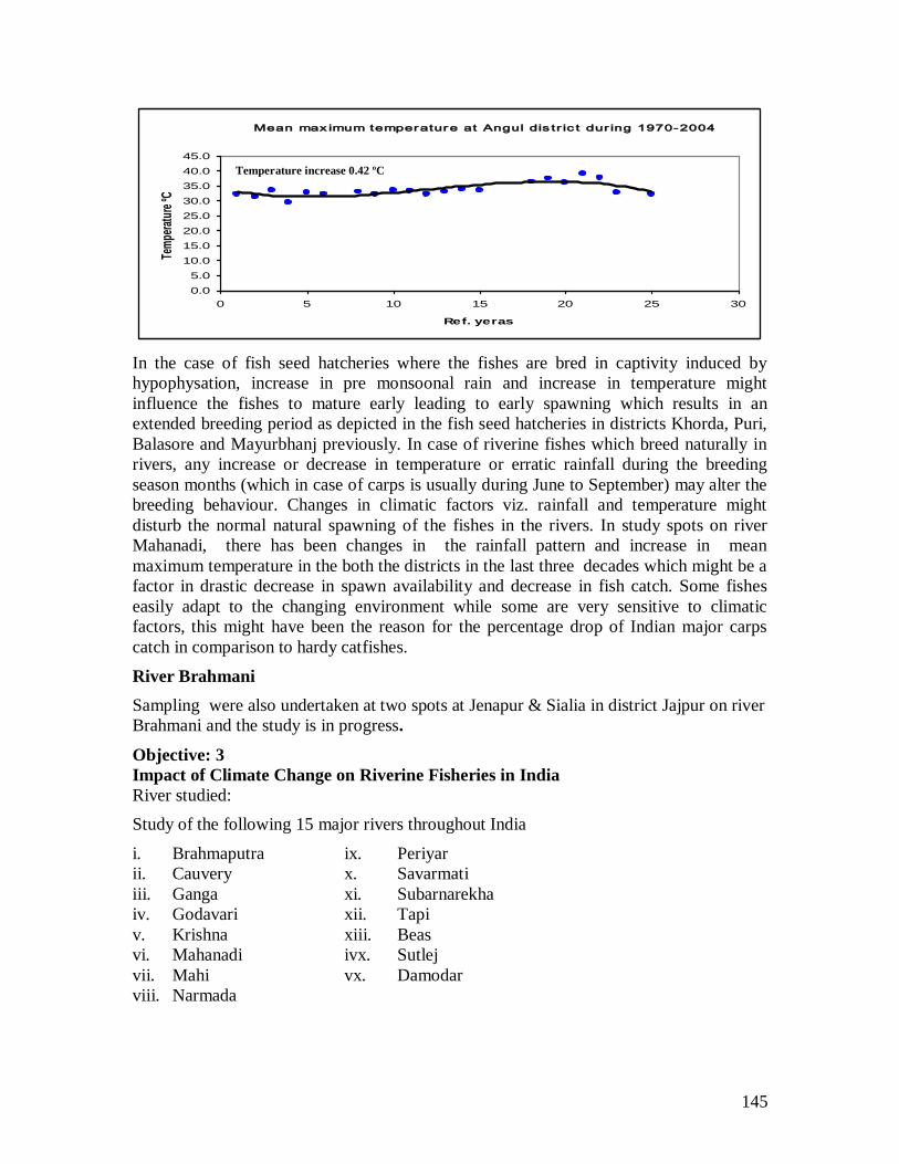
145
Mean max imum temperature at Angul dis tr ic t dur ing 1970-2004
y = -0.0037x3 + 0.1363x2 - 1.1176x + 33.96
R2 = 0.6168
0.0
5.0
10.0
15.0
20.0
25.0
30.0
35.0
40.0
45.0
0 5 10 15 20 25 30
Ref. yeras
Tem
pera
ture
ºC
In the case of fish seed hatcheries where the fishes are bred in captivity induced by
hypophysation, increase in pre monsoonal rain and increase in temperature might
influence the fishes to mature early leading to early spawning which results in an
extended breeding period as depicted in the fish seed hatcheries in districts Khorda, Puri,
Balasore and Mayurbhanj previously. In case of riverine fishes which breed naturally in
rivers, any increase or decrease in temperature or erratic rainfall during the breeding
season months (which in case of carps is usually during June to September) may alter the
breeding behaviour. Changes in climatic factors viz. rainfall and temperature might
disturb the normal natural spawning of the fishes in the rivers. In study spots on river
Mahanadi, there has been changes in the rainfall pattern and increase in mean
maximum temperature in the both the districts in the last three decades which might be a
factor in drastic decrease in spawn availability and decrease in fish catch. Some fishes
easily adapt to the changing environment while some are very sensitive to climatic
factors, this might have been the reason for the percentage drop of Indian major carps
catch in comparison to hardy catfishes.
River Brahmani
Sampling were also undertaken at two spots at Jenapur & Sialia in district Jajpur on river
Brahmani and the study is in progress.
Objective: 3
Impact of Climate Change on Riverine Fisheries in India
River studied:
Study of the following 15 major rivers throughout India
i. Brahmaputra ix. Periyar
ii. Cauvery x. Savarmati
iii. Ganga xi. Subarnarekha
iv. Godavari xii. Tapi
v. Krishna xiii. Beas
vi. Mahanadi ivx. Sutlej
vii. Mahi vx. Damodar
viii. Narmada
Temperature increase 0.42 ºC
146
Data:
The data were collected for each river from different published sources. Since the data on
the parameters for different rivers were not available for each year, we considered the
data for the year from1994 to2007, almost all the parameters for each river were available
within this period. i.e. Our study period was 1994-2007, about one and half decade.
Along with fish species richness, we determined the following parameters as variables
obtained from different websites and published literature within the study period for
middle stretch of each river.
i. The mean annual water temperature (in ºC)
ii. Mean annual water temperature range (in ºC)
iii. Annual total rainfall (in mm)
iv. Mean annual discharge (m3/s)
v. Mean annual sediment load (000 MT/Km2/Yr)
vi. Mean annual runoff (B.C.M):
vii. Climatic zones: The climate of India was classified into four major zones
based on amount of rainfall and its pattern. The zones were ranked using
Likert`z scaling procedure by considering various characteristics, which are
suitable for fish population in the zones. The climatic zone assigned to each
river corresponds to the largest climatic area drained by the middle part of the
river.
viii. Mean latitude (Degree and second) of river basin was taken as average of
latitude and was weighted by its length. The values for mean latitude are for
the center of each river basin.
and
ix. Total area of drainage basin (Km2).
The main objective was to find out a best possible combination or subset of independent
variables expressing the dependent variable among fish species richness of river with
relatively greater multiple R2-value. Relations between the variables were tested by
standard regression, using a set of linear contrasts for each variable. In “statistical
methods” the order in which the predictor variables are entered into (or taken out of) the
model is determined according to the strength of their correlation with the criterion
variable. Several versions of such method include forward selection, backward
elimination and stepwise selection regression techniques to derive the optimum subset of
the independent variables with maximum contribution to the among-river variation in fish
species richness. The R2 - statistic provides the proportion of variance in the criterion
variable, which is accounted for by the regression model. Using SPSS package performed
all these statistical analyses were performed.
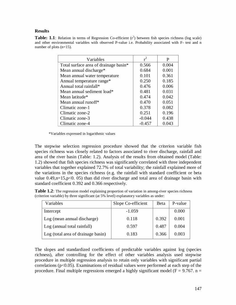
147
Results
Table: 1.1: Relation in terms of Regression Co-efficient (r2) between fish species richness (log scale)
and other environmental variables with observed P-value i.e. Probability associated with F- test and n
number of plots (n=15).
*Variables expressed in logarithmic values
The stepwise selection regression procedure showed that the criterion variable fish
species richness was closely related to factors associated to river discharge, rainfall and
area of the river basin (Table: 1.2). Analysis of the results from obtained model (Table:
1.2) showed that fish species richness was significantly correlated with three independent
variables that together explained 72.7% of total variability; the rainfall explained more of
the variations in the species richness (e.g. the rainfall with standard coefficient or beta
value 0.49,n=15,p<0. 05) than did river discharge and total area of drainage basin with
standard coefficient 0.392 and 0.366 respectively.
Table 1.2: The regression model explaining proportion of variation in among-river species richness
(criterion variable) by three significant (at 5% level) explanatory variables as under:
Variables Slope Co-efficient Beta P-value
Intercept
Log (mean annual discharge)
Log (annual total rainfall)
Log (total area of drainage basin)
-1.059
0.118
0.597
0.183
0.392
0.487
0.366
0.000
0.001
0.004
0.003
The slopes and standardized coefficients of predictable variables against log (species
richness), after controlling for the effect of other variables analysis used stepwise
procedure in multiple regression analysis to retain only variables with significant partial
correlations (p<0.05). Examinations of residual values were performed at each step of the
procedure. Final multiple regressions emerged a highly significant model (F = 9.767. n =
Variables r2 P
Total surface area of drainage basin*
Mean annual discharge*
Mean annual water temperature
Annual temperature range*
Annual total rainfall*
Mean annual sediment load*
Mean latitude*
Mean annual runoff*
Climatic zone-1
Climatic zone-2
Climatic zone-3
Climatic zone-4
0.566
0.684
0.101
0.250
0.476
0.481
0.474
0.470
0.378
0.251
-0.044
-0.457
0.004
0.001
0.361
0.185
0.006
0.031
0.042
0.051
0.082
0.196
0.438
0.043
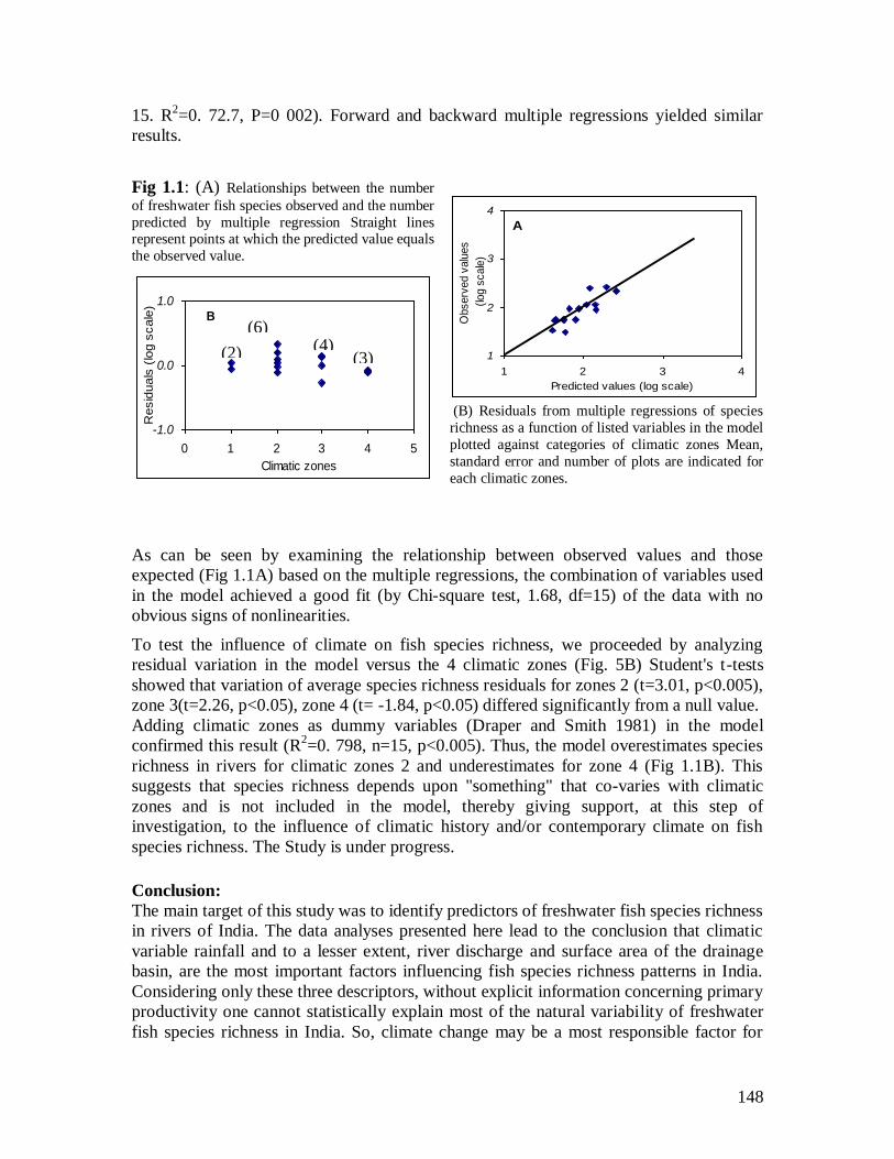
148
15. R2=0. 72.7, P=0 002). Forward and backward multiple regressions yielded similar
results.
Fig 1.1: (A) Relationships between the number
of freshwater fish species observed and the number
predicted by multiple regression Straight lines represent points at which the predicted value equals
the observed value.
(B) Residuals from multiple regressions of species
richness as a function of listed variables in the model
plotted against categories of climatic zones Mean,
standard error and number of plots are indicated for
each climatic zones.
As can be seen by examining the relationship between observed values and those
expected (Fig 1.1A) based on the multiple regressions, the combination of variables used
in the model achieved a good fit (by Chi-square test, 1.68, df=15) of the data with no
obvious signs of nonlinearities.
To test the influence of climate on fish species richness, we proceeded by analyzing
residual variation in the model versus the 4 climatic zones (Fig. 5B) Student's t-tests
showed that variation of average species richness residuals for zones 2 (t=3.01, p<0.005),
zone 3(t=2.26, p<0.05), zone 4 (t= -1.84, p<0.05) differed significantly from a null value.
Adding climatic zones as dummy variables (Draper and Smith 1981) in the model
confirmed this result (R2=0. 798, n=15, p<0.005). Thus, the model overestimates species
richness in rivers for climatic zones 2 and underestimates for zone 4 (Fig 1.1B). This
suggests that species richness depends upon "something" that co-varies with climatic
zones and is not included in the model, thereby giving support, at this step of
investigation, to the influence of climatic history and/or contemporary climate on fish
species richness. The Study is under progress.
Conclusion:
The main target of this study was to identify predictors of freshwater fish species richness
in rivers of India. The data analyses presented here lead to the conclusion that climatic
variable rainfall and to a lesser extent, river discharge and surface area of the drainage
basin, are the most important factors influencing fish species richness patterns in India.
Considering only these three descriptors, without explicit information concerning primary
productivity one cannot statistically explain most of the natural variability of freshwater
fish species richness in India. So, climate change may be a most responsible factor for
A
1
2
3
4
1 2 3 4
Predicted values (log scale)
Observ
ed v
alu
es
(lo
g s
cale
)
B
-1.0
0.0
1.0
0 1 2 3 4 5
Climatic zones
Resid
uals
(lo
g s
cale
)
(2)
(6) (4)
(3)
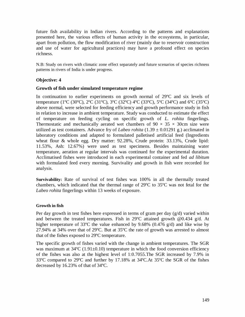
149
future fish availability in Indian rivers. According to the patterns and explanations
presented here, the various effects of human activity in the ecosystems, in particular,
apart from pollution, the flow modification of river (mainly due to reservoir construction
and use of water for agricultural practices) may have a profound effect on species
richness.
N.B: Study on rivers with climatic zone effect separately and future scenarios of species richness
patterns in rivers of India is under progress.
Objective: 4
Growth of fish under simulated temperature regime
In continuation to earlier experiments on growth normal of 29ºC and six levels of
temperature (1ºC (30ºC), 2ºC (31ºC), 3ºC (32ºC) 4ºC (33ºC), 5ºC (34ºC) and 6ºC (35ºC)
above normal, were selected for feeding efficiency and growth performance study in fish
in relation to increase in ambient temperature. Study was conducted to estimate the effect
of temperature on feeding cycling on specific growth of L. rohita fingerlings.
Thermostatic and mechanically aerated wet chambers of 90 × 35 × 30cm size were
utilized as test containers. Advance fry of Labeo rohita (1.39 ± 0.01291 g.) acclimated in
laboratory conditions and adapted to formulated palletised artificial feed (Ingredients
wheat flour & whole egg. Dry matter: 92.28%, Crude protein: 33.13%, Crude lipid:
11.53%, Ash: 12.67%) were used as test specimens. Besides maintaining water
temperature, aeration at regular intervals was continued for the experimental duration.
Acclimatised fishes were introduced in each experimental container and fed ad libitum
with formulated feed every morning. Survivality and growth in fish were recorded for
analysis.
Survivability: Rate of survival of test fishes was 100% in all the thermally treated
chambers, which indicated that the thermal range of 29ºC to 35ºC was not fetal for the
Labeo rohita fingerlings within 13 weeks of exposure.
Growth in fish
Per day growth in test fishes here expressed in terms of gram per day (g/d) varied within
and between the treated temperatures. Fish in 29ºC attained growth @0.434 g/d. At
higher temperature of 33ºC the value enhanced by 9.68% (0.476 g/d) and like wise by
27.94% at 34% over that of 29ºC. But at 35ºC the rate of growth was arrested to almost
that of the fishes exposed to 29ºC temperature.
The specific growth of fishes varied with the change in ambient temperatures. The SGR
was maximum at 34ºC (1.91±0.10) temperature in which the food conversion efficiency
of the fishes was also at the highest level of 1:0.7055.The SGR increased by 7.9% in
33ºC compared to 29ºC and further by 17.18% at 34ºC.At 35ºC the SGR of the fishes
decreased by 16.23% of that of 34ºC.
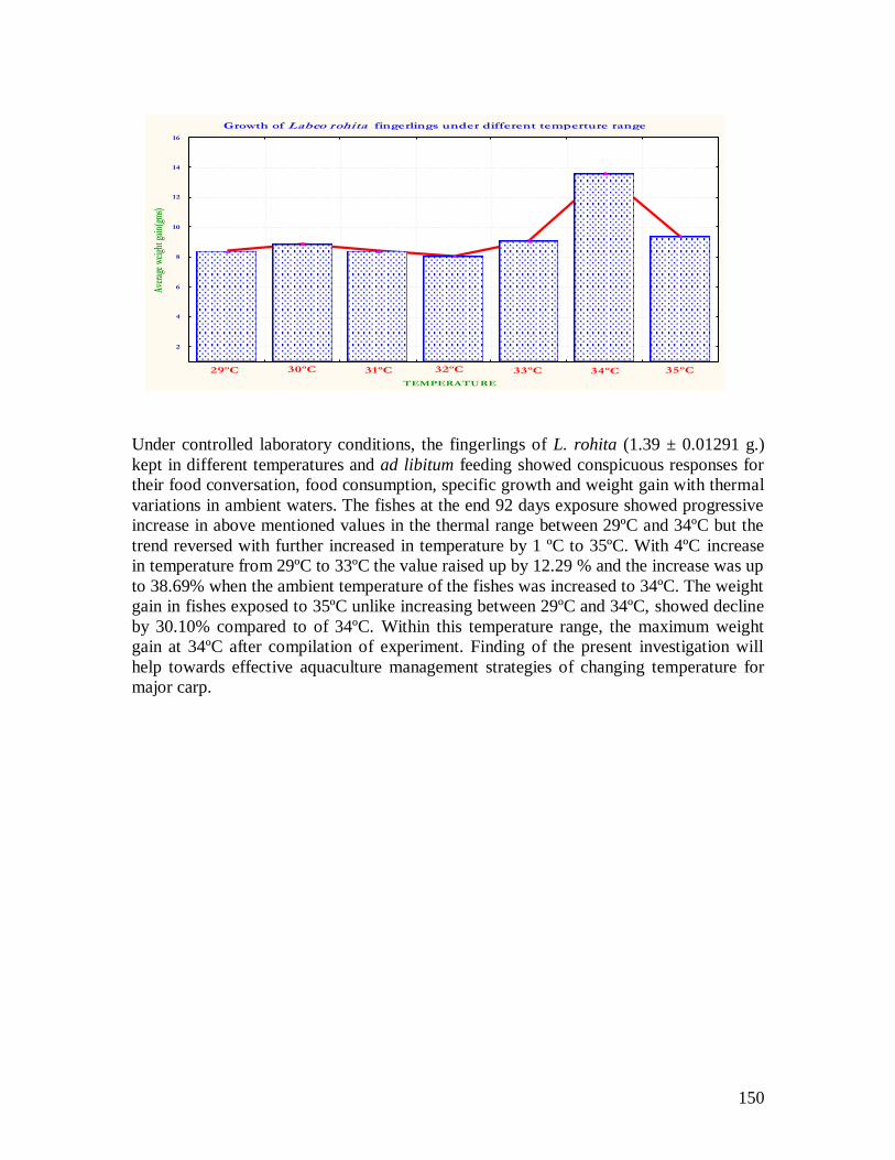
150
Under controlled laboratory conditions, the fingerlings of L. rohita (1.39 ± 0.01291 g.)
kept in different temperatures and ad libitum feeding showed conspicuous responses for
their food conversation, food consumption, specific growth and weight gain with thermal
variations in ambient waters. The fishes at the end 92 days exposure showed progressive
increase in above mentioned values in the thermal range between 29ºC and 34ºC but the
trend reversed with further increased in temperature by 1 ºC to 35ºC. With 4ºC increase
in temperature from 29ºC to 33ºC the value raised up by 12.29 % and the increase was up
to 38.69% when the ambient temperature of the fishes was increased to 34ºC. The weight
gain in fishes exposed to 35ºC unlike increasing between 29ºC and 34ºC, showed decline
by 30.10% compared to of 34ºC. Within this temperature range, the maximum weight
gain at 34ºC after compilation of experiment. Finding of the present investigation will
help towards effective aquaculture management strategies of changing temperature for
major carp.
Growth of Labeo rohita fingerlings under different temperture range
Case 1 Case 2 Case 3 Case 4 Case 5 Case 6 Case 7
TEMPERATURE
2
4
6
8
10
12
14
16
Aver
age
weig
ht g
ain(
gms)
29ºC 35ºC30ºC 31ºC 32ºC 33ºC 34ºC
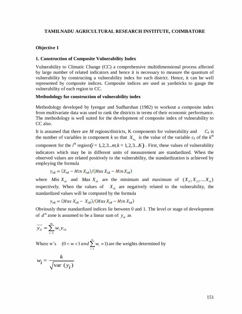
151
TAMILNADU AGRICULTURAL RESEARCH INSTITUTE, COIMBATORE
Objective 1
1. Construction of Composite Vulnerability Index
Vulnerability to Climatic Change (CC) a comprehensive multidimensional process affected
by large number of related indicators and hence it is necessary to measure the quantum of
vulnerability by constructing a vulnerability index for each district. Hence, it can be well
represented by composite indices. Composite indices are used as yardsticks to gauge the
vulnerability of each region to CC.
Methodology for construction of vulnerability index
Methodology developed by Iyengar and Sudharshan (1982) to workout a composite index
from multivariate data was used to rank the districts in terms of their economic performance.
The methodology is well suited for the development of composite index of vulnerability to
CC also.
It is assumed that there are M regions/districts, K components for vulnerability and Ck is
the number of variables in component k so that kicX is the value of the variable ck of the k
th
component for the ith region( )1,2,3... ; 1,2,3...i m k K= = . First, these values of vulnerability
indicators which may be in different units of measurement are standardized. When the
observed values are related positively to the vulnerability, the standardization is achieved by
employing the formula
where idMin X and
idMax X are the minimum and maximum of 1 2( , ,.... )i i inX X X
respectively. When the values of idX are negatively related to the vulnerability, the
standardized values will be computed by the formula
Obviously these standardized indices lie between 0 and 1. The level or stage of development
of thd zone is assumed to be a linear sum of idy as
id
m
i
id ywy1
Where w‟s n
i
iwandw1
)110( are the weights determined by
var ( )
kwi
yi
=
152
1
1 )(
1n
i iyVark
The choice of the weights in this manner would ensure that large variation in any one of the
indicators would not unduly dominate the contribution of the rest of the indicators and distort
inter zone comparisons.
For classificatory purposes, a simple ranking of the zone indices viz., dy would be enough.
However for a meaningful characterization of the different stages of vulnerability, suitable
fractile classification from an assumed distribution is needed. One probability distribution,
which is widely used in this context, is the Beta distribution. This distribution is defined by
1 1( ) (1 ) / ( , ), 0 1 , 0.a bf z x x a b x and a bb- -= - £ £ >
This distribution has two parameters a and b. They can be estimated either by using the
method described in Iyengar and Sudharshan (1982) or by using software packages. The Beta
distribution is skewed. Let 1 1 2 2 2 3 4(0, ),( , ),( , ),( , )z z z z z z z and
4( ,1)z be the linear intervals
such that each interval has the same probability weight of 20 per cent. These fractile intervals
can be used to characterize the various stages of vulnerability.
1. Less vulnerable If 10 dy z< <
2. Moderately Vulnerable If 1 2dz y z< <
3. Vulnerable If 2 3dz y z< <
4. Highly vulnerable If 3 4dz y z< <
5. Very highly vulnerable If 4 1dz y< <
This index is a composite one constructed on the basis of several factors, which are prone to
be affected by climatic change. Following Patnaik and Narayanan (2005), these factors can
be grouped into five components namely, 1.Demographic 2. Climatic 3. Agriculture 4.
Occupational and 5. Geographic. Each one of these components can have several sub-
indicators. The vulnerability indices derived by applying statistical techniques can be used to
classify the coastal districts into five different categories namely, less vulnerable, moderately
vulnerable, vulnerable, highly vulnerable and very highly vulnerable.
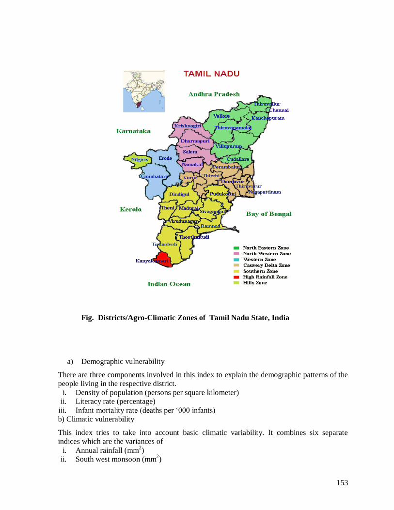
153
Fig. Districts/Agro-Climatic Zones of Tamil Nadu State, India
a) Demographic vulnerability
There are three components involved in this index to explain the demographic patterns of the
people living in the respective district.
i. Density of population (persons per square kilometer)
ii. Literacy rate (percentage)
iii. Infant mortality rate (deaths per „000 infants)
b) Climatic vulnerability
This index tries to take into account basic climatic variability. It combines six separate
indices which are the variances of
i. Annual rainfall (mm2)
ii. South west monsoon (mm2)
154
iii. North east monsoon (mm2)
iv. Maximum temperature (oC
2)
v. Minimum temperature (oC
2)
vi. Diurnal temperature variation (oC
2)
c) Agricultural vulnerability
This includes the following variables to predict the vulnerability related to agricultural
activities.
i. Production of food grains (tonnes / hectare)
ii. Productivity of major crops (tonnes/ hectare)
iii. Cropping intensity (percentage)
iv. Irrigation intensity (percentage)
v. Livestock population (Number per hectare of net sown area)
vi. Forest area(percentage geographic area)
d) Occupational vulnerability
Six indicators were taken to calculate the vulnerability related to occupational characteristics
of people and all these variables are converted into per hectare of net sown area.
i. Number of cultivators
ii. Total main workers
iii. Agricultural labourers
iv. Marginal workers
v. Industrial workers
vi. Non workers e) Geographic vulnerability
i. Coastal length (kilometer)
ii. Geographical area (hectare)
Measuring vulnerability for different agro climatic zones of Tamil Nadu
The values of the vulnerability index and the corresponding ranks of the different agro
climatic regions of Tamil Nadu are shown in Table1. It can be observed that the vulnerability
of the people to climate change is very high in the hilly zone followed by southern zone as
compared to the other agro climatic zones. Table 2 and 3 gives the ranks of the agro climatic
zones for different components of vulnerability and their classification in terms of
vulnerability.
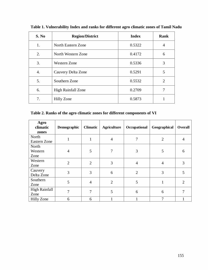
155
Table 1. Vulnerability Index and ranks for different agro climatic zones of Tamil Nadu
S. No Region/District Index Rank
1. North Eastern Zone 0.5322 4
2. North Western Zone 0.4172 6
3. Western Zone 0.5336 3
4. Cauvery Delta Zone 0.5291 5
5. Southern Zone 0.5532 2
6. High Rainfall Zone 0.2709 7
7. Hilly Zone 0.5873 1
Table 2. Ranks of the agro climatic zones for different components of VI
Agro
climatic
zones
Demographic Climatic Agriculture Occupational Geographical Overall
North
Eastern Zone 1 1 4 7 2 4
North
Western
Zone
4 5 7 3 5 6
Western
Zone 2 2 3 4 4 3
Cauvery
Delta Zone 3 3 6 2 3 5
Southern
Zone 5 4 2 5 1 2
High Rainfall
Zone 7 7 5 6 6 7
Hilly Zone 6 6 1 1 7 1
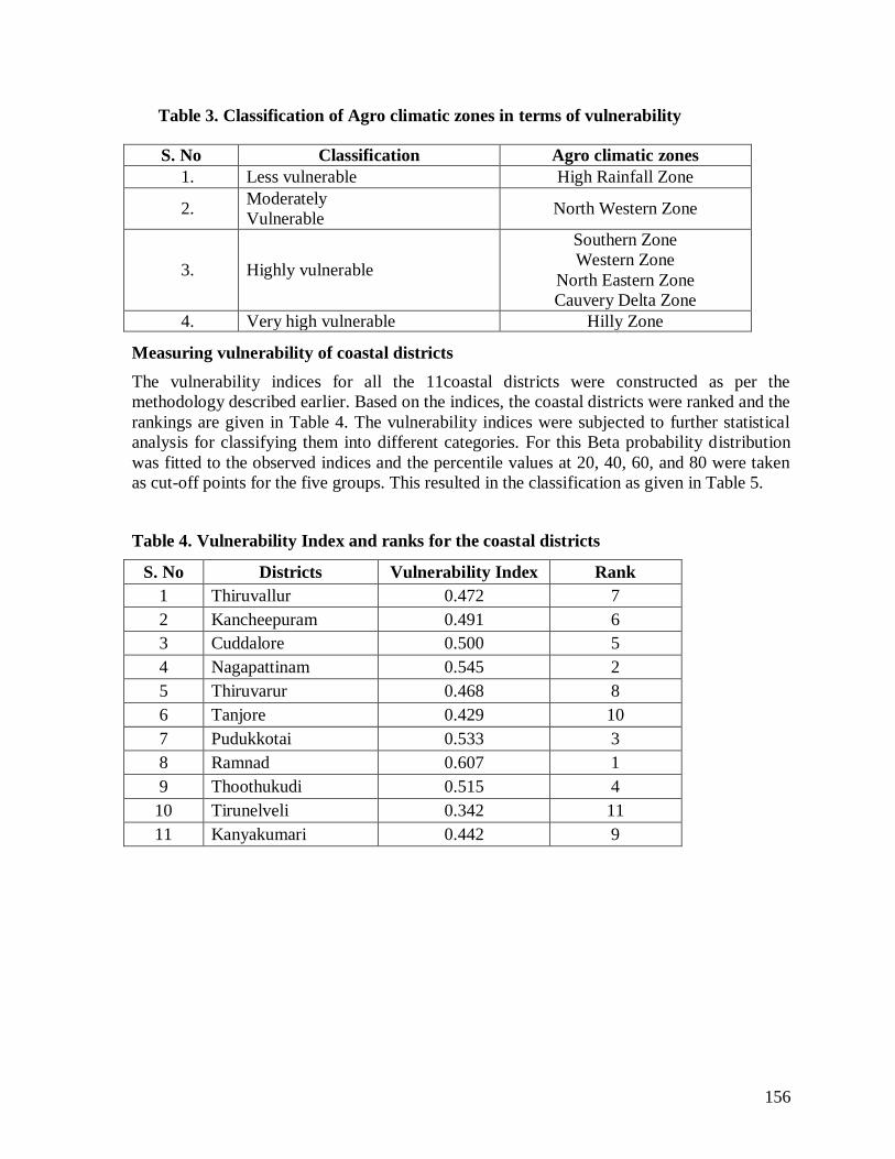
156
Table 3. Classification of Agro climatic zones in terms of vulnerability
S. No Classification Agro climatic zones
1. Less vulnerable High Rainfall Zone
2. Moderately
Vulnerable North Western Zone
3. Highly vulnerable
Southern Zone
Western Zone
North Eastern Zone
Cauvery Delta Zone
4. Very high vulnerable Hilly Zone
Measuring vulnerability of coastal districts
The vulnerability indices for all the 11coastal districts were constructed as per the
methodology described earlier. Based on the indices, the coastal districts were ranked and the
rankings are given in Table 4. The vulnerability indices were subjected to further statistical
analysis for classifying them into different categories. For this Beta probability distribution
was fitted to the observed indices and the percentile values at 20, 40, 60, and 80 were taken
as cut-off points for the five groups. This resulted in the classification as given in Table 5.
Table 4. Vulnerability Index and ranks for the coastal districts
S. No Districts Vulnerability Index Rank
1 Thiruvallur 0.472 7
2 Kancheepuram 0.491 6
3 Cuddalore 0.500 5
4 Nagapattinam 0.545 2
5 Thiruvarur 0.468 8
6 Tanjore 0.429 10
7 Pudukkotai 0.533 3
8 Ramnad 0.607 1
9 Thoothukudi 0.515 4
10 Tirunelveli 0.342 11
11 Kanyakumari 0.442 9
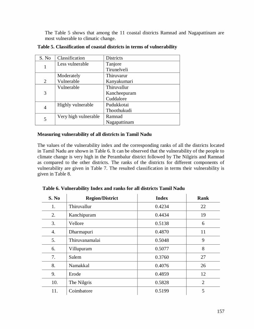
157
The Table 5 shows that among the 11 coastal districts Ramnad and Nagapattinam are
most vulnerable to climatic change.
Table 5. Classification of coastal districts in terms of vulnerability
S. No Classification Districts
1 Less vulnerable Tanjore
Tirunelveli
2
Moderately
Vulnerable
Thiruvarur
Kanyakumari
3
Vulnerable Thiruvallur
Kancheepuram
Cuddalore
4 Highly vulnerable Pudukkotai
Thoothukudi
5 Very high vulnerable Ramnad
Nagapattinam
Measuring vulnerability of all districts in Tamil Nadu
The values of the vulnerability index and the corresponding ranks of all the districts located
in Tamil Nadu are shown in Table 6. It can be observed that the vulnerability of the people to
climate change is very high in the Perambalur district followed by The Nilgiris and Ramnad
as compared to the other districts. The ranks of the districts for different components of
vulnerability are given in Table 7. The resulted classification in terms their vulnerability is
given in Table 8.
Table 6. Vulnerability Index and ranks for all districts Tamil Nadu
S. No Region/District Index Rank
1. Thiruvallur 0.4234 22
2. Kanchipuram 0.4434 19
3. Vellore 0.5138 6
4. Dharmapuri 0.4870 11
5. Thiruvanamalai 0.5048 9
6. Villupuram 0.5077 8
7. Salem 0.3760 27
8. Namakkal 0.4076 26
9. Erode 0.4859 12
10. The Nilgris 0.5828 2
11. Coimbatore 0.5199 5
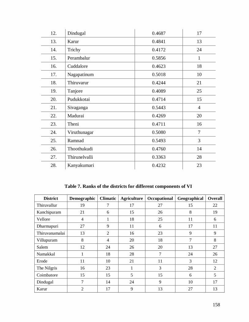
158
12. Dindugal 0.4687 17
13. Karur 0.4841 13
14. Trichy 0.4172 24
15. Perambalur 0.5856 1
16. Cuddalore 0.4623 18
17. Nagapatinum 0.5018 10
18. Thiruvarur 0.4244 21
19. Tanjore 0.4089 25
20. Pudukkotai 0.4714 15
21. Sivaganga 0.5443 4
22. Madurai 0.4269 20
23. Theni 0.4711 16
24. Viruthunagar 0.5080 7
25. Ramnad 0.5493 3
26. Thoothukudi 0.4760 14
27. Thirunelvalli 0.3363 28
28. Kanyakumari 0.4232 23
Table 7. Ranks of the districts for different components of VI
District Demographic Climatic Agriculture Occupational Geographical Overall
Thiruvallur 19 7 17 27 15 22
Kanchipuram 21 6 15 26 8 19
Vellore 4 1 18 25 11 6
Dharmapuri 27 9 11 6 17 11
Thiruvanamalai 13 2 16 23 9 9
Villupuram 8 4 20 18 7 8
Salem 12 24 26 20 13 27
Namakkal 1 18 28 7 24 26
Erode 11 10 21 11 3 12
The Nilgris 16 23 1 3 28 2
Coimbatore 15 15 5 15 6 5
Dindugal 7 14 24 9 10 17
Karur 2 17 9 13 27 13
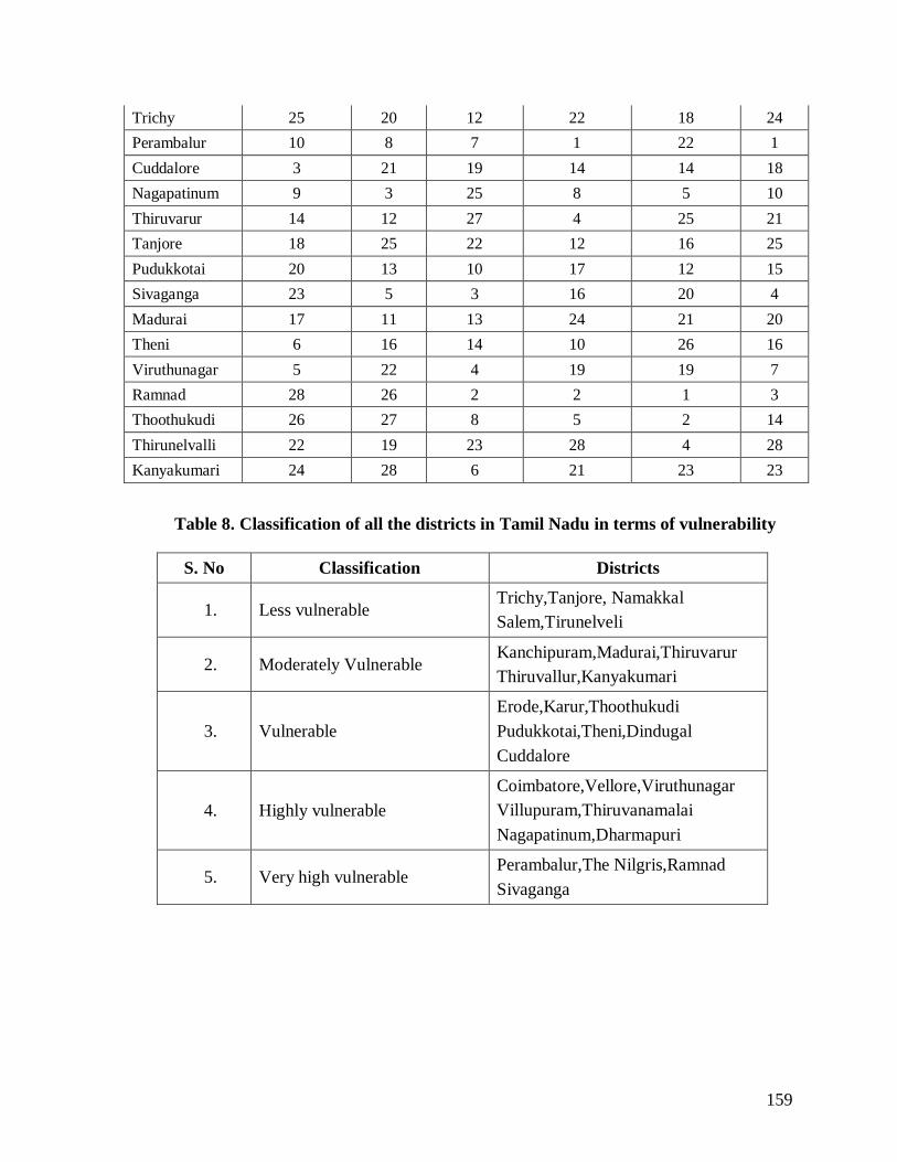
159
Trichy 25 20 12 22 18 24
Perambalur 10 8 7 1 22 1
Cuddalore 3 21 19 14 14 18
Nagapatinum 9 3 25 8 5 10
Thiruvarur 14 12 27 4 25 21
Tanjore 18 25 22 12 16 25
Pudukkotai 20 13 10 17 12 15
Sivaganga 23 5 3 16 20 4
Madurai 17 11 13 24 21 20
Theni 6 16 14 10 26 16
Viruthunagar 5 22 4 19 19 7
Ramnad 28 26 2 2 1 3
Thoothukudi 26 27 8 5 2 14
Thirunelvalli 22 19 23 28 4 28
Kanyakumari 24 28 6 21 23 23
Table 8. Classification of all the districts in Tamil Nadu in terms of vulnerability
S. No Classification Districts
1. Less vulnerable Trichy,Tanjore, Namakkal
Salem,Tirunelveli
2. Moderately Vulnerable Kanchipuram,Madurai,Thiruvarur
Thiruvallur,Kanyakumari
3. Vulnerable
Erode,Karur,Thoothukudi
Pudukkotai,Theni,Dindugal
Cuddalore
4. Highly vulnerable
Coimbatore,Vellore,Viruthunagar
Villupuram,Thiruvanamalai
Nagapatinum,Dharmapuri
5. Very high vulnerable Perambalur,The Nilgris,Ramnad
Sivaganga
160
Objective 2
Multi Goal Linear Programming (MGLP) for sustainable food security
Multi Goal Linear Programming (MGLP) model
The Ricardian model is used to project the area, production and productivity of major crops
under existing and different climate change scenarios. These projected values can be used to
estimate maximum possible production in different climate change scenarios by fitting the
suitable optimization model. Hence, the multi goal linear programming is a suitable tool to
predict the possible changes in the food grain production and utilization of resources under
different climate change scenarios.
For planning the sustainable food security and their resource requirements in the different
agro climatic zones of Tamil Nadu, the MGLP model can be used. The MGLP model for
Tamil Nadu covers all the 30 districts, which can be viewed as a combination of the different
agro climatic regions. This model has been used in several studies for land use planning at
the state level (Aggarwal et al., 2001), sub-regional and regional level (Schipper et al., 1995;
Veeneklaas et al., 1991), village level (Huizing and Bronsveld, 1994) and farm level (Schans,
1991). The model is developed using MATLAB a mathematical modeling and optimization
software. The model used for the present study is as follows.
General symbols used in the model
Land Units: l= 1, 2,... L
Seasons: s=1, 2,,…S
Crops: c =1, 2,...C
Technologies: t=1, 2,…T
SC = Set of selected crops for maximum production.
cP Current production of crop c in Tamil Nadu.
Available resources
l sA =Available land area (ha) in land unit l in season s.
l sW = Available water (m3) in land unit l in season s.
lsL = Total labour (in man days) available at the land unit l in season s.
l sC = Capital availability (Rs) in land unit l in season s.
Technological coefficients
lsctx Land area used in land unit l, in season s, for crop c under technology t.
lscty Productivity of crop c, in season s in land unit l under technology t.
lsctw Water requirement per unit area for crop c in season s in land unit l under
technology t.
lsctl Labour requirement per unit area for crop c in season s in land unit l under
technology t.
lsctc Capital requirement per unit area for crop c in season s in land unit l under
technology t.
lsctr Net return from crop c, in season s in land unit l under technology t.
161
Objective functions
The proposed multi goal linear programming model has the five social, economic and
environmental objectives. They are a) Maximizing food grain production, b) Maximizing net
income, c)Maximizing employment d) Minimizing agricultural area and e) Minimizing water
use
For each of the above objective we included the following constraints one by one:
Land is the only constraint,
Land and Water are the constraints
Land and Technology are the constraints
Land, Water and Technology are the constraints
Land, Water, Technology and Labour are the constraints
Land, Water, Technology and Capital are the constraints
Land, Water, Technology , Labour and Capital are the constraints
Area under each annual crop is same in all the seasons in each land unit
Estimation of resources availability include
Estimation of land resources
Estimation of water resources availability
Estimation of labour availability
Yield estimation at different technology levels
Yield estimation at technology level 1
This methodology was same as followed by Aggarwal et al., (2001). They estimated
potential yield at technology level 5 using the various crop growth simulation models and
current yield level for technology 1. The required data were collected from them through
ICAR Climate Change Network Project and used for the present analysis.
Yields estimation at technology level 2, 3 and 4
The difference between the adjusted potential yield and the calculated current yield in each
agro climatic zone was considered as the attainable yield gap for that respective crop. Target
yields were set at bridging 25, 50 and 75 per cent of the yield gap for these technology levels
of 2, 3 and 4 respectively.
Yield estimation at technology level 5
The measured yields at this level of technology in different agro climatic zones are not
available. However, the yield at technology level 5 estimated and simulated by
the Aggarwal et al., and the same was collected and used in the present study.
Aggarwal et al., (2001) used a variety of crop growth simulation models for the different
crops to estimate the potential yields that can be attained in the different agro climatic zones.
A complete standard calibration and validation was impossible for the other crops such as
162
cotton, groundnut and sugarcane. The potential yields were simulated for these crops and
further judged on the basis of expert knowledge.
Sowing dates for the different crops were selected depending on the prevailing cropping
pattern in the respective agro climatic zones. In general, even under the best management,
marketable yield is lower than potential yield because of unavoidable losses through pests
and diseases, during harvesting, transportation and processing. These losses were assumed to
result in a 10 per cent reduction in potential yield. Therefore, realizable potential yield of an
area has been set at 90 per cent of potential yield and these yields were allotted to different
agro climatic zones.
Estimation of input requirements for the yields at different technology levels
Calculation of costs of inputs like seed, irrigation, fertilizer and labour were done for
different technology levels.
Calculation of byproduct value
The total amount of byproducts produced from the various crop activities were estimated
from the target yield and crop specific harvest indices. It can be assumed that 20 per cent of
the total byproducts were lost during harvesting and transportation and this will not be
available for use. Use the following formula to calculate the total byproduct produced by the
different crops.
Byproduct = Target yield × 0.8 / Harvest Index
Crop suitability
Crop suitability is based on their cultivated area for past more than five years in particular
season in their respective agro climatic zone. If the particular crop is suitable give 1,
otherwise 0.
Description of resources
The natural and socio economic resources available in Tamil Nadu, different technological
adaptation followed by various categories of farmers and estimation of potential yield of
major crops at different technology levels were elaborately discussed.
Availability of land resources, water resources, capital availability and labour availability
were worked out.
Technology description to attain target yields
Technology level in this study is defined as the complete description of the production
activity, which includes the target yield level plus all inputs required to realize this target
output and all additional outputs such as byproducts of the crops. A major aim is to planning
for sustainable food security that combined with the various goals of maximizing food grain
production, maximizing farm income from agriculture, maximizing the employment
opportunities and others. Thus, the selected different technology levels in the future may
exhibit higher yields than the current systems. The various technologies are described in brief
as follows.
163
Technology level 5
This is the maximum potential attainable yield level that could be achieved by the large
farmers only. This technology is currently not practiced in Tamil Nadu.
It represents knowledge based and intensive mechanized crop production. Target yield are set
equal to potential yields. It can be assumed that some well endowed resource rich farmers of
Tamil Nadu might adopt this technology in the future. Concepts of precision farming may be
used to maximize input use efficiency through high-tech agriculture including site specific
and integrated nutrient, water and pest management. It can be made use of special equipment
such as tractor-mounted implements and micro and high volume chemical applicators in
combination with liquid fertilizers. It has been assumed that the full cost of all implements
will not be borne by the farmers directly. This heavy and costly equipment will be made
available to them from the government organizations and farmer‟s cooperative societies. The
cost of hiring this equipment has been included at a rate of rupees 4,000 per hectare per crop.
In view of high mechanization activities, human labour use is assumed to decrease up to 40
per cent. Overall, this technology is expected to result in a considerable increase in food
production and net income of the farmers although the capital requirement is also much
higher.
Technology level 4
Target yield for this technology in the various zones for different crops was set to current
yield plus bridging the 75 per cent of the yield gap. This is also similar to technology 5 with
more input use efficiency and knowledge intensive technology but this is followed with
partially mechanized crop production has been assumed for technology 4. Input use
efficiencies are higher than in technologies 1, 2 and 3, but slightly lower than the technology
5 and also it requires relatively lower capital.
Technology level 3
This technology can be achieved by target yields are set to current yield plus 50 per cent of
the yield gap for the particular crops in each zone. Again, these higher yields are supported
by input intensification, in proportion to the increase in yield.
Technology level 2
Target yields were achieved in this technology were set to the current yield plus bridging the
25 per cent of the yield gap. Agricultural practices similar to these in technology 1 were
assumed. The higher yields were obtained by assuming the intensification of input use in
proportion to the increase in yield.
Technology level 1
This technology is current practice followed by the farmers in different agro climatic zones
of Tamil Nadu and this is considered as the baseline level. The average yield rate of major
crops in Tamil Nadu is higher than the national average. The farmers depending on their land
resources and capital availability they will select the different production techniques. In this
study, however, we have used the average conditions of the farming activities in the state to
define this technology. In general, the mechanization level is medium, ploughing is usually
done with a tractor and tillage implements and levelling of fields is done at a very rough
scale. Sowing and application of fertilizers are mostly done with manually. The use of
164
organic manure is low on an average, farmer use less than one tonne of farmyard manure per
hectare.
Maximizing food grain production
Land is the only constraint
Rice is the major food grain in Tamil Nadu with the total production of about
5 million tonnes per year in a total area of 18.73 lakh hectares. The maximum attainable rice
production in Tamil Nadu is 16.19 million tonnes from the current level of production of five
million tonnes with production of other crops maintained at their current level. To produce
this level of output, Tamil Nadu has to use 100 per cent of cultivable land, needs 50.43
billion m3 of water, 52.61 billion rupees of capital, 272 million labour days of employment,
0.49,
0.19 and 0.11 million tonnes of nitrogen, phosphorus and potash respectively. If these
resources are made available, farmers could generate an income of 116.91 billion rupees
from the current level of 47.09 billion rupees per annum and this is higher by about
70 billion rupees from the current income of our farmers. These resource requirements are
several times higher than the current availability of resources and hence this level cannot be
achieved in practice.
Land and water are the constraints
In addition to land, the available water is added as an additional constraint to determine the
maximum possible rice production in all the agro climatic regions of Tamil Nadu. Under this
constraint, rice being the largest consumer of water in the state, rice production dropped to
7.06 million tonnes – a reduction of 9.13 million tonnes from maximum production under
when land alone is the constraint, keeping production of other crops at their current level. As
shown in Table 28, to realize this level of rice production Tamil Nadu needs 23.96 billion m3
of water, 73.91 percentage of land area, 33.69 billion rupees of capital, 245.38 million labour
days. It will generate a net income of 66.49 billion rupees against 116.91 billion rupees when
land alone is the constraint. Further fertilizer requirements drastically dropped to 0.39 million
tonnes from 0.79 million tonnes. The above results show that water is the major limiting
factor for agriculture in Tamil Nadu. The above level of rice production is possible only
when 44 per cent of the land area is allotted to technology level 5.
Land and technology are the constraints
In the third stage, technology adoption by various categories of farmers is introduced as
another constraint in addition to the land resources. In this case, maximum attainable rice
production will be 14.51 million tonnes. Water requirement is nearly doubled which is 45.64
billion m3 compared to current availability because water is not added as the constraint in the
model. Capital and net income of the farmers decreased about 10 and 7 per cent respectively.
However, employment opportunities increased to 10 per cent compared to the first case.
Fertilizer requirement also decreased compared to first case (a). This level is also not
possible because water is the major limiting factor.
Land, water, technology and labour are the constraints
When land, water and technology adoption were simultaneously introduced as constraints,
the rice production decreased to 7.06 million tonnes. About 77 per cent of available
cultivated land, 34 billion rupees of capital, 24 billion m3 of water and
165
264 million labour days of employment are needed to produce this level of output. This will
give 66 billion rupees of net income annually to our farmers in the different agro climatic
zones of Tamil Nadu. When labour also included, there is no change in the level of rice
production which shows that labour is not a limiting factor.
Land, water, technology, labour and capital are the constraints
Capital is a major socio economic resource for the marginal and small farmers. When this is
also included as a constraint, the rice production is further decreased to 6.64 million tonnes
compared to all other cases. Here the land utilization is only 70 per cent of the available land.
The utilization of all other resources considerably reduced. Figure 2 shows the land use
pattern when all the constraints were taken into account.
Finally to summarize the above results indicate that it is possible to increase the total rice
production by 1.58 million tonnes, which accounts for 31.23 per cent more than the existing
current level from the different agro climatic regions of Tamil Nadu even by imposing all the
constraints. Net income of the farmers will also increase from 47.09 to 65.20 billion rupees.
This is higher by 18.11 billion rupees and shares 38.45 per cent more income to our farmers
in Tamil Nadu compared to what they are earning at present.
It can be observed that when land is the only constraint, all land area is utilized under the
highest technology level (Tech 5), which gives maximum productivity. When water is
included as a constraint, technology 5 gets only 44 per cent of the land area while other
technologies get around 13 per cent of the land each and about 26 per cent of the land area is
left unutilized. But when all the constraints are included technology 5 gets only 36 per cent
and about 30 per cent of land area becomes unutilized, technology 4 gets 27 per cent of the
land and about 12 per cent of the land is obtained by each one of the other three technologies.
When water is not included as a constraint the MGLP model utilizes the 100 per cent of the
land area. This again emphasizes the conclusion that water is the major constraint for
agricultural production in Tamil Nadu.
Maximizing farm net income
Land is the only constraint
Farm net income of the farmers from major crops in Tamil Nadu would reach a maximum of
198.90 billion rupees from the current level of earning of 47.09 billion rupees, which is about
152 billion rupees higher, and this is 322 per cent higher than the existing level of income.
Also in this scenario, the production of all crops will be greater than or equal to their current
level. To generate this level of net income, Tamil Nadu needs 100 per cent of available land,
51.96 billion rupees of capital, 48.58 billion m3
of water and 280.56 million labour days.
Cotton production will reach 18.99 million bales compared to current level of 0.19 million
bales and sugarcane production will also increase from 24.46 to 29.56 million tonnes and
other crops will maintain their current level of production.
To achieve this level of net income, the capital level has to increase from
36 billion rupees to 52 billion rupees. Similarly, water available should be increase from 24
billion m3
to 48.58 billion m3.
These resources are neither currently available nor they do
become available (especially water) in the next two or three decades and hence this level of
maximum net income is not possible.
166
Land and water are the constraints
When availability of irrigation water is include as a constraint, the net income drops to 124
billion rupees, which accounts for a decrease of 37.71 per cent of the net income when land
is the only constraint. In this scenario, only 85 per cent of land will be utilized and
requirements of capital, water and labour are below the levels needed when land is the
constraint. To generate 123.89 billion rupees of net income, the resource requirements are 23.71
billion m3
of water, 41.89 billion rupees of capital and 210.07 million labour days of employment.
The production of groundnut will be five times more than the current level and sugarcane
production will also from 24.46 to 33.72 million tonnes.
Except capital all other resources are within the available limits and 5 billion rupees of extra
capital are needed and farmers should go to technology level 5 which will give maximum
productivity. Thus, this is achievable only the farmers to adopt the largest technology (Tech
5) with additional capital.
Land and technology are the constraints
With technology adoption constraint in addition to constraint on land, the net income of the
farmers can be maximized to 174.77 billion rupees by cultivating all the land area. This
scenario will produce maximum cotton and sugarcane and the production of other crops will
be maintained at current level. One important feature of this scenario is the increase in the
employment opportunities (312.37 million labour days), this is higher than the corresponding
values for other scenarios. The capital and water requirements are respectively 48.34 billion
rupees and 42.28 billion m3, fertilizer consumption will be more than the current level of
consumption. But this solution seems to be infeasible because of extremely high amount of
resources needed which are not currently available especially water.
Land, water, technology, labour and capital are the constraints
The addition of labour and capital as constraints reduce the farm income. The net income of
the farm decreases to 121.19 billion rupees when labour is also a constraint, whereas the farm
income will come down to 98.29 billion rupees when capital is also added. Employment
generation will decrease to 246.82 and 205.87 million labour days due to the addition of
respective constraints.
When these two resources (labour and capital) are together included as a constraints, the farm
income drops to 98.29 billion rupees. The resource requirements of 22.05 billion m3 of water,
34.16 billion rupees of capital and 205.87 million labour days are needed to achieve this level
of farm income. When all the constraints are introduced, the percentage contribution by
different crops to net income and area under different crops when farm income is maximized
indicate that, at the aggregate State level, even with all constraints are included, the farm
income is higher by about 51 billion rupees which constitutes 108 per cent higher than the
existing level of income.
Percentage land area under different technology levels, when farm income maximized
indicated that almost all the land area is used by highest technology level 5, when land is the
only constraint. Irrigation water requirement has introduced an additional constraint, the land
utilization is distributed about 82, 15 and 3 per cent to technology level 5, 4 and 2
respectively and remaining 15 per cent of the land is left unutilized.
167
When all the constraints are included, technology 5 gets only 32 per cent and technology 4
gets 54 per cent of the land and about 9 and 5 per cent of the land is utilized by technology 3
and 4 respectively. About 20 per cent of land area becomes unutilized and this also clearly
indicates that water is the major limiting factor for crop production in Tamil Nadu. This
solution seems to be feasible as the requirement of all the resources are within the available
limits and farmers have to practice the modern technologies (Tech 4 and 5).
Maximizing employment
Land is the only constraint
Maximization of employment opportunities in agricultural sector is another social objective
of the present study. Production of major crops and their resource requirements for Tamil
Nadu at an aggregated level is presented in Table 32, when employment is maximized. The
maximum employment potential in different agro climatic regions of Tamil Nadu is about
527.92 million labour days, when land is the only constraint. This is associated with 5.73
million tonnes of rice production compared to the current level of 5.06 million tonnes. The
production of cotton will increase from 0.19 million bales to 5.74 million bales and
groundnut production will also increase to 1.78 million tonnes from the current level of 1.01
million tonnes and production of other crops is maintained at their current level. To generate
this level of employment, 100 per cent of the agricultural land, 29.98 billion meter3 of water
and 52.22 billion rupees of capital will be needed. In addition to increased employment, this
will generate an annual income of 98.48 billion rupees. Fertilizer consumption will be more
than the current level of consumption. This is not feasible because addition of 5 billion
meter3 of water and addition of capital is required.
Land and water are the constraints
In addition to land resource, water availability is included as a constraint, the employment
opportunities will reduce to 472 million labour days. Rice production will be maintained at
current level along with other crops except cotton and groundnut which will increase relative
to the current level of production. This is due to an increased area under labour intensive and
water use efficient cotton and groundnut crops. Annual farm income also decreased to 69.74
billion rupees, utilizing the resource requirements of 46.55 billion rupees of capital and 22.67
billion meter3 of water. Fertilizer consumption will increase to 0.19, 0.08 and 0.05 million
tonnes of nitrogen, phosphorus and potash respectively when compared to current
consumption. Area under technology 1, 2 and 3 is predominantly utilized when land and
water are the constraints. This solution is feasible only when capital is increased to another
10 billion rupees and farmer shift from current technology to technologies 2 and 3.
Land and technology are the constraints
When technology adoption and land are the only constraints, the employment opportunities
will be generated at the same level when land alone was the constraint. Rice production will
not undergo any change and it will be the same level of 5.73 million tonnes when land alone
was the constraint. Cotton production will reach up to 5.74 million bales compared to current
level of 0.19 million bales and groundnut production will also increase from 1.01 to 1.78
million tonnes and other crops will maintain their current level of production. Fertilizer
consumption will increase to 0.40 million tonnes from the current consumption level of 0.10
168
million tonnes. In this scenario the resource requirements of water, capital and fertilizer
consumption is high when compared to current level, so this is not feasible solution.
Land, water and technology are the constraints
When technology adoption is included along with land and water constraints, employment
generation will drop to 472 million labour days from 528 million labour days when land
alone is the constraint. Rice production will decline to their current level along with other
crops except for cotton and groundnut, which will increase relative to the current level. To
generate this level of employment, the resource requirements are 22.67 billion m3
of water
and 46.55 billion rupees of capital. This will give 69.74 billion rupees of net income annually
to our farmers in Tamil Nadu compared to current level of 47.09 billion rupees. This solution
is feasible only if there is an increase of 30 per cent of capital.
Land, water, technology, labour and capital are the constraints
When labour is added as a constraint, employment generation is dropped to 350 million
labour days by utilizing the 94 per cent of the land. It will generate a net income of 73 billion
rupees against the current income of 47 billion rupees but it requires 41 billion rupees of
capital and 0.42 million tonnes of fertilizer which is higher than the current level. Whereas
capital is added as a constraint, the employment opportunities will be marginally increased to
365 million labour days compared to current level of employment. This requires 18.79 billion
m3 of water and 35.81 billion rupees of capital which is lower than the current level.
When labour and capital are together added as constraints, the employment opportunities
were drastically reduced to 350 million labour days from the maximum level of about 528
million labour days when land alone is the constraint. For this, it needs 19.81 billion m3 of
water, 87.95 per cent of land resources and 35.73 billion rupees of capital, which generates a
net income of 57.44 billion rupees of agricultural per year. Fertilizer consumption will
increase to 0.13, 0.04 and 0.05 million tonnes of nitrogen, phosphorus and potash
respectively when compared to current level. By introduction of all the constraints the per
cent contribution by different crops to the total employment are given .
Percentage area of agricultural land under different technology levels are presented in Table
33 and Figure 7, when employment is maximized. It can be observed that when land is the
only constraint, all land area is utilized under the technology level 3 which requires
maximum labour. This is due to technology 3 requires maximum number of labour days
compared to first two levels of technologies and last two technologies (Tech 4 and 5) will
comes under mechanization. When water is included as a constraint, technology 3 gets only
78 per cent of the land area while technology level 1 and 2 gets 20 and 2 per cent of land area
respectively. But when all the constraints are included technology 3 gets only 34 per cent,
technology 1 gets 37 per cent of the land and about 27 per cent of the land is obtained by
technology level 2. When water is not included as a constraint, the model utilizes the 100 per
cent of the land area under the technology level 3. This again emphasizes water is the major
constraint for agricultural production in Tamil Nadu.
169
Minimizing agricultural area
Land is the only constraint
Agricultural area was minimized while targets of production of all crops were kept at their
current levels. This objective gains importance in view of the need for additional land
requirement for housing, industry and infrastructural facilities due to increase in population.
Table 34 provides production and area of the six crops and utilization of all resources when
agricultural area is minimized. When land is the only constraint, the current output of the
major crops can be obtained only by utilizing only 44.45 per cent of the agricultural land. It
is also interesting to note that in this scenario, farm income in different agro climatic zones of
Tamil Nadu will be 32.81 per cent higher than the current net income earned by our farmers.
To achieve this Tamil Nadu requires 24.17 billion rupees of capital, 18.49 billion m3 of water
and 120 million labour days. Interestingly, this resource requirement is lower than the current
availability. But there is a considerable loss of employment opportunities from agriculture
due to reduction in agricultural area. As expected, 100 per cent of the land area is cultivated
under highest level of technology (Tech 5), which consumes less labour and gives more
productivity to give the maximum production from the minimum area. This solution is
feasible only when the farmers adopt the highest technology level 5 to maintain current
production of crops by utilizing only 45 per cent of its currently cultivated area.
Land and water are the constraints
When irrigation water is included as a constraint, the land area is marginally increased to
45.16 from 44.45 per cent when land alone is the constraint. In this scenario, the employment
opportunities will decline by 8 million labour days and this will generate a net income 62.48
billion rupees. Fertilizer consumption will increase to 0.23, 0.09 and 0.08 million tonnes of
nitrogen, phosphorus and potash respectively when compared to current consumption.
Land, water and technology are the constraints
In addition to land, when constraint of technology adoption is included, the required
minimum agriculture area to maintain the current level production will increase from 1672 to
1735 thousand hectares. One important feature of this scenario is the increase in the
employment opportunities to 130.33 million labour days, which is higher than the
corresponding values for other scenarios. This target can be achieved from
24 billion rupees of capital and 18.54 billion m3 of water and it will generate a net income of
63 billion rupees.
Land, water, technology, labour and capital are the constraints
When labour and capital are introduced as constraints separately to the previous case (c), the
minimum agricultural area increases to 1767 and 1769 thousand hectares respectively when
compared to land is the only constraint (1672 thousand hectares). In both the scenarios, it
utilizes 18 billion m3 of water, 23 billion rupees of capital and 122 million labour days of
capital to generate a net income of 65 billion rupees.
When these two resources of labour and capital are together added as constraints, the
minimum agricultural area will increase to 47.03 per cent from the 44.45 per cent when land
alone is the constraint. This will generate the maximum farm income of 65 billion rupees to
the farmers from the agricultural activities when compared to all other cases. This is 38 per
170
cent higher than the current income generated by our farmers by utilizing only 47 per cent of
the currently cultivated area. To generate this level of net income, the resource requirements
are 18.27 billion m3
of water, 22.98 billion rupees of capital and 122.91 million labour days
of employment. All these resource requirements are less than the current consumption levels.
To summarize the above results, in all the scenarios of area minimization, the resource
requirements will be less (land area, capital, water and labour days) when compared to
current level of utilization. Also, the net income will increase by about
15 billion rupees in all the cases which is higher than the existing level of income generated
by our farmers. However, the employment potential will reduce drastically when compared
to current level of employment opportunities. Thus, this solution is feasible only when the
farmers to adopt the modern technology levels of 4 and 5.
Percentage area of agricultural land under different technology levels are presented in Table
35, when agricultural area is minimized. As expected, all the 100 per cent of cultivated land
area will distribute to the modern technologies (Technology 4 and 5) in all the scenarios. This
is due to the reason that technologies 4 and 5 will give the maximum level of productivity.
Minimizing water use
Land is the only constraint
The earlier scenario analyses revealed that water availability was the major constraint to
increase food grain production in the State of Tamil Nadu. Therefore, in this scenario a
minimum water requirement was determined to produce current levels of crop production. In
this situation, the model generates higher net income by utilizing lesser amount of capital and
land area when compared to current level. At the same time, resource requirements are 18.24
billion m3 of water, 234.61 million labour days and 0.30 million tonnes of fertilizer
consumption.
Land and water are the constraints
In addition to land, the available water is added as an additional constraint to determine the
minimum possible water requirement for agriculture in all the agro climatic regions of Tamil
Nadu. Under this constraint, rice consumes about 51 per cent of the total water requirement to
maintain current level of its production. Other crops will utilize the remaining amount of water and
the production will be at their current level.
Land and technology are the constraints
Technology adoption by various categories of farmers is included as a constraint in addition
to the land resources. In this case, to realize this current level of crop production Tamil Nadu
needs 18.24 billion m3 of water, 65.72 per cent of land area, 28.91 billion rupees of capital and
237.97 million labour days. Fertilizer consumption will also increase from 0.1 million tones to 0.29
million tonnes when compared to current level. It will generate a net income of 57.13 billion rupees
against 47.09 billion rupees of current level
171
Land, water, technology, labour and capital are the constraints
When all constraints are gradually added to land resource constraint, there was no change in
water use to maintain the current level of production of all crops. Water consumption will still
remain as 18.24 billion m3 in the entire scenario which shows that this will be the minimum water
requirement for agricultural activities in Tamil Nadu. However, this is 26.27 per cent lower than the
current water requirement. But the resource requirements of capital, labour, land and fertilizer
changed when constraints are added.
When all the constraints are included simultaneously, the resource requirements are 18.24
billion m3
of water, 27.92 billion rupees of capital and 63.39 per cent of the land area. All
these resource requirements are lesser than the current consumption level. However the
employment potential will drop to 217.64 million labour days from the 360.66 million labour
days of employment when compared to current level. This will generate a net income of
58.29 billion rupees against the current level income of 47.09 billion rupees per annum to the
farmers in Tamil Nadu. This needs 0.18, 0.07 and 0.06 million tonnes of nitrogen, hosphorus
and potash fertilizers respectively which is higher than the current level of consumption.
To summarize all the above results discussed here, in all the scenarios, water minimization
will require less amount of resources such as land area, capital, water and labour days when
compared to current level of utilization. Also, the net income will increase by around 10
billion rupees in all the cases which is higher than the existing level of income generated by
our farmers in Tamil Nadu. However, the employment potential will reduce marginally when
compared to current level of employment opportunities. Thus, this solution is feasible only
when the farmers adopt all the technologies equally, less water consuming crops and should
follow the water saving technologies to minimize the wastage of water.
Percentage area of agricultural land under different technology levels are presented in Table
37, when minimizing the irrigation water. While minimizing the water use, maximum area
under cultivation will go to technology 1, because it consumes lesser amount of water
compared to other technologies. In this scenario of water minimization, by adding the
constraints one by one, percentage of cultivated area has distributed more or less equal to all
the technologies except technology level 1 has marginally more area compared to other
technologies.
Out of the five objectives discussed, the point of view of food security, the first objective
namely, maximizing food grain production should given top most priority and this objective
should considered when constraints on all resources are imposed. In this situation, the food
grain production were increased from about 5 million tonnes to 6.64 million tonnes for which
only the fertilizer consumption will be more and current level of all other resources are
sufficient. This seems to be a feasible solution if farmers adopt modern technologies
(Technology 4 and 5) for which proper planning has to be made.
Water sharing options
Water is the most precious resource for agriculture in Tamil Nadu. Hence, four different
scenarios of water sharing are included in the model:
1. No sharing of water between land units and between seasons
2. Sharing of water allowed between seasons in each land unit.
172
3. Sharing of water allowed between land units in each season.
4. Sharing of water allowed between land units and between seasons
The results from the study are summarized below.
When food grain production is maximized and water is not shared between land units and
seasons the maximum food grain production is 6.64 million tonnes. When it is shared
between land units and between seasons it increases to 7.3 million tonnes. Since the current
level production is 5.01 million tonnes, there is a possibility to increase the fod production by
50 percent by sharing water between land units in all the seasons.
Similarly, maximum farm net income will range between 98.90 to 121.25 billion rupees
against the current level of 47.05 billion rupees. But, there is not much appreciable increase
in the employment due to sharing of water. The reason is adoption of technologies which
require minimum quantum of labour are selected for adoption (Technologies 1,4 and 5).
When no water is shared the minimum agriculture area required for producing at Least the
current level of production of all crops is 1769.09 thousand ha against the current level of
3761.90 th. Ha. There is a marginal decrease in agricultural area when water is shared. A
model predicts a minimum water requirement of 18.24 billion m3 (current level 24.73 billion
m3) under all scenarios of water sharing to meet at least the current level of production of al
the crops considered in the model.
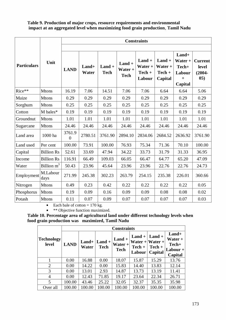
173
Table 9. Production of major crops, resource requirements and environmental
impact at an aggregated level when maximizing food grain production, Tamil Nadu
Each bale of cotton = 170 kg.
** Objective function maximized.
Table 10. Percentage area of agricultural land under different technology levels when
food grain production was maximized, Tamil Nadu
Technology
level
Constraints
LAND Land+
Water
Land +
Tech
Land +
Water +
Tech
Land +
Water +
Tech +
Labour
Land +
Water +
Tech +
Capital
Land+
Water +
Tech+
Labour +
Capital
1 0.00 16.88 0.00 18.07 15.87 15.29 13.76
2 0.00 14.22 0.00 15.83 14.40 13.83 12.14
3 0.00 13.01 2.93 14.87 13.73 13.19 11.41
4 0.00 12.43 71.85 19.17 23.64 22.34 26.71
5 100.00 43.46 25.22 32.05 32.37 35.35 35.98
Over all 100.00 100.00 100.00 100.00 100.00 100.00 100.00
Particulars Unit
Constraints
LAND Land+
Water
Land +
Tech
Land +
Water +
Tech
Land +
Water +
Tech +
Labour
Land +
Water +
Tech +
Capital
Land+
Water +
Tech+
Labour
+
Capital
Current
level
(2004-
05)
Rice** Mtons 16.19 7.06 14.51 7.06 7.06 6.64 6.64 5.06
Maize Mtons 0.29 0.29 0.29 0.29 0.29 0.29 0.29 0.29
Sorghum Mtons 0.25 0.25 0.25 0.25 0.25 0.25 0.25 0.25
Cotton M bales* 0.19 0.19 0.19 0.19 0.19 0.19 0.19 0.19
Groundnut Mtons 1.01 1.01 1.01 1.01 1.01 1.01 1.01 1.01
Sugarcane Mtons 24.46 24.46 24.46 24.46 24.46 24.46 24.46 24.46
Land area 1000 ha 3761.9
0 2780.51 3761.90 2894.10 2834.06 2684.52 2636.92 3761.90
Land used Per cent 100.00 73.91 100.00 76.93 75.34 71.36 70.10 100.00
Capital Billion Rs 52.61 33.69 47.94 34.22 33.73 31.79 31.33 36.95
Income Billion Rs 116.91 66.49 109.03 66.05 66.47 64.77 65.20 47.09
Water Billion m3 50.43 23.96 45.64 23.96 23.96 22.76 22.76 24.73
Employment M.Labour
days 271.99 245.38 302.23 263.79 254.15 235.38 226.01 360.66
Nitrogen Mtons 0.49 0.23 0.42 0.22 0.22 0.22 0.22 0.05
Phosphorus Mtons 0.19 0.09 0.16 0.09 0.09 0.08 0.08 0.02
Potash Mtons 0.11 0.07 0.09 0.07 0.07 0.07 0.07 0.03
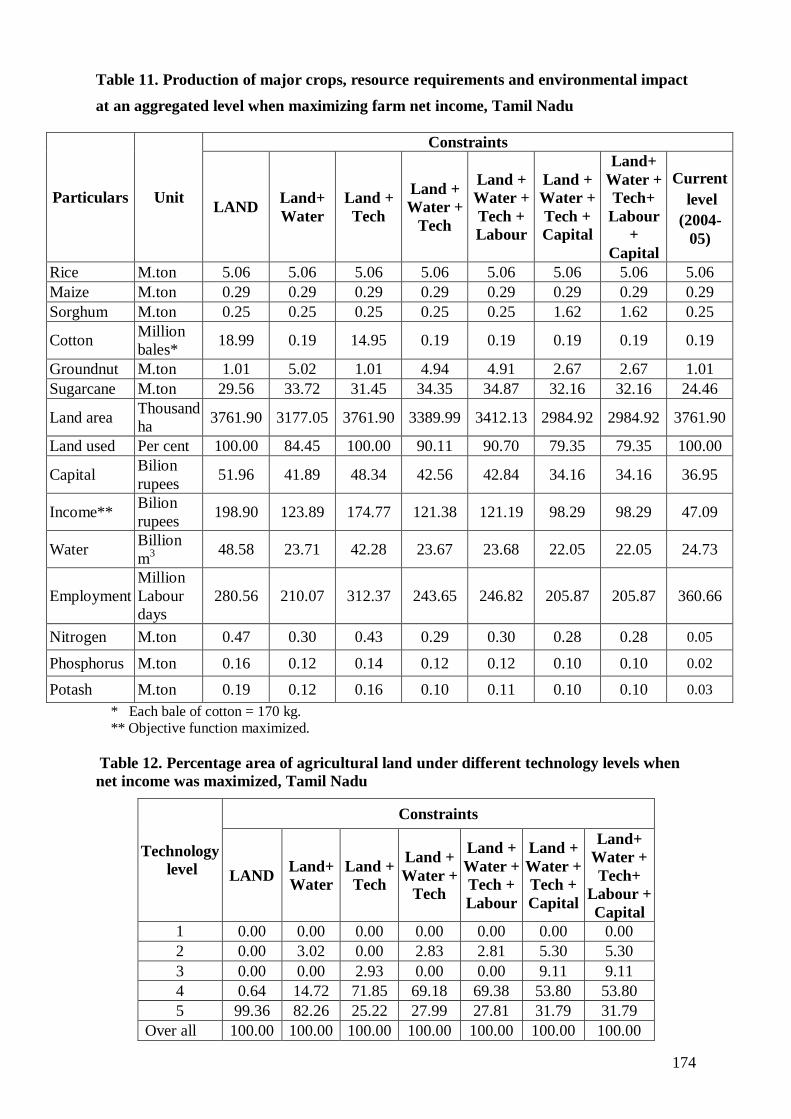
174
Table 11. Production of major crops, resource requirements and environmental impact
at an aggregated level when maximizing farm net income, Tamil Nadu
Particulars Unit
Constraints
LAND Land+
Water
Land +
Tech
Land +
Water +
Tech
Land +
Water +
Tech +
Labour
Land +
Water +
Tech +
Capital
Land+
Water +
Tech+
Labour
+
Capital
Current
level
(2004-
05)
Rice M.ton 5.06 5.06 5.06 5.06 5.06 5.06 5.06 5.06
Maize M.ton 0.29 0.29 0.29 0.29 0.29 0.29 0.29 0.29
Sorghum M.ton 0.25 0.25 0.25 0.25 0.25 1.62 1.62 0.25
Cotton Million
bales* 18.99 0.19 14.95 0.19 0.19 0.19 0.19 0.19
Groundnut M.ton 1.01 5.02 1.01 4.94 4.91 2.67 2.67 1.01
Sugarcane M.ton 29.56 33.72 31.45 34.35 34.87 32.16 32.16 24.46
Land area Thousand
ha 3761.90 3177.05 3761.90 3389.99 3412.13 2984.92 2984.92 3761.90
Land used Per cent 100.00 84.45 100.00 90.11 90.70 79.35 79.35 100.00
Capital Bilion
rupees 51.96 41.89 48.34 42.56 42.84 34.16 34.16 36.95
Income** Bilion
rupees 198.90 123.89 174.77 121.38 121.19 98.29 98.29 47.09
Water Billion
m3
48.58 23.71 42.28 23.67 23.68 22.05 22.05 24.73
Employment
Million
Labour
days
280.56 210.07 312.37 243.65 246.82 205.87 205.87 360.66
Nitrogen M.ton 0.47 0.30 0.43 0.29 0.30 0.28 0.28 0.05
Phosphorus M.ton 0.16 0.12 0.14 0.12 0.12 0.10 0.10 0.02
Potash M.ton 0.19 0.12 0.16 0.10 0.11 0.10 0.10 0.03
* Each bale of cotton = 170 kg. ** Objective function maximized.
Table 12. Percentage area of agricultural land under different technology levels when
net income was maximized, Tamil Nadu
Technology
level
Constraints
LAND Land+
Water
Land +
Tech
Land +
Water +
Tech
Land +
Water +
Tech +
Labour
Land +
Water +
Tech +
Capital
Land+
Water +
Tech+
Labour +
Capital
1 0.00 0.00 0.00 0.00 0.00 0.00 0.00
2 0.00 3.02 0.00 2.83 2.81 5.30 5.30
3 0.00 0.00 2.93 0.00 0.00 9.11 9.11
4 0.64 14.72 71.85 69.18 69.38 53.80 53.80
5 99.36 82.26 25.22 27.99 27.81 31.79 31.79
Over all 100.00 100.00 100.00 100.00 100.00 100.00 100.00
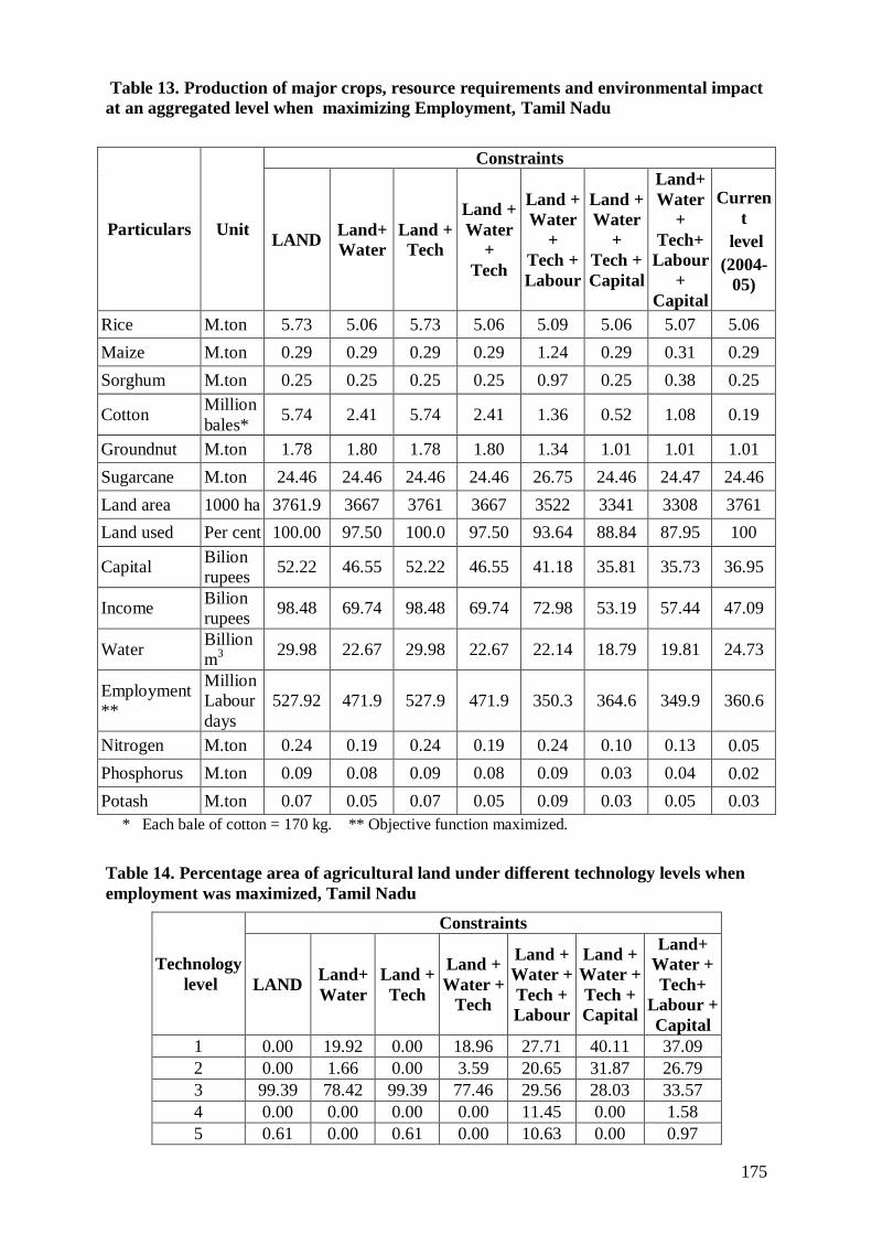
175
Table 13. Production of major crops, resource requirements and environmental impact
at an aggregated level when maximizing Employment, Tamil Nadu
Particulars Unit
Constraints
LAND Land+
Water
Land +
Tech
Land +
Water
+
Tech
Land +
Water
+
Tech +
Labour
Land +
Water
+
Tech +
Capital
Land+
Water
+
Tech+
Labour
+
Capital
Curren
t
level
(2004-
05)
Rice M.ton 5.73 5.06 5.73 5.06 5.09 5.06 5.07 5.06
Maize M.ton 0.29 0.29 0.29 0.29 1.24 0.29 0.31 0.29
Sorghum M.ton 0.25 0.25 0.25 0.25 0.97 0.25 0.38 0.25
Cotton Million
bales* 5.74 2.41 5.74 2.41 1.36 0.52 1.08 0.19
Groundnut M.ton 1.78 1.80 1.78 1.80 1.34 1.01 1.01 1.01
Sugarcane M.ton 24.46 24.46 24.46 24.46 26.75 24.46 24.47 24.46
Land area 1000 ha 3761.9 3667 3761 3667 3522 3341 3308 3761
Land used Per cent 100.00 97.50 100.0 97.50 93.64 88.84 87.95 100
Capital Bilion
rupees 52.22 46.55 52.22 46.55 41.18 35.81 35.73 36.95
Income Bilion
rupees 98.48 69.74 98.48 69.74 72.98 53.19 57.44 47.09
Water Billion
m3
29.98 22.67 29.98 22.67 22.14 18.79 19.81 24.73
Employment
**
Million
Labour
days
527.92 471.9 527.9 471.9 350.3 364.6 349.9 360.6
Nitrogen M.ton 0.24 0.19 0.24 0.19 0.24 0.10 0.13 0.05
Phosphorus M.ton 0.09 0.08 0.09 0.08 0.09 0.03 0.04 0.02
Potash M.ton 0.07 0.05 0.07 0.05 0.09 0.03 0.05 0.03
* Each bale of cotton = 170 kg. ** Objective function maximized.
Table 14. Percentage area of agricultural land under different technology levels when
employment was maximized, Tamil Nadu
Technology
level
Constraints
LAND Land+
Water
Land +
Tech
Land +
Water +
Tech
Land +
Water +
Tech +
Labour
Land +
Water +
Tech +
Capital
Land+
Water +
Tech+
Labour +
Capital
1 0.00 19.92 0.00 18.96 27.71 40.11 37.09
2 0.00 1.66 0.00 3.59 20.65 31.87 26.79
3 99.39 78.42 99.39 77.46 29.56 28.03 33.57
4 0.00 0.00 0.00 0.00 11.45 0.00 1.58
5 0.61 0.00 0.61 0.00 10.63 0.00 0.97

176
Over all 100.00 100.00 100.00 100.00 100.00 100.00 100.00
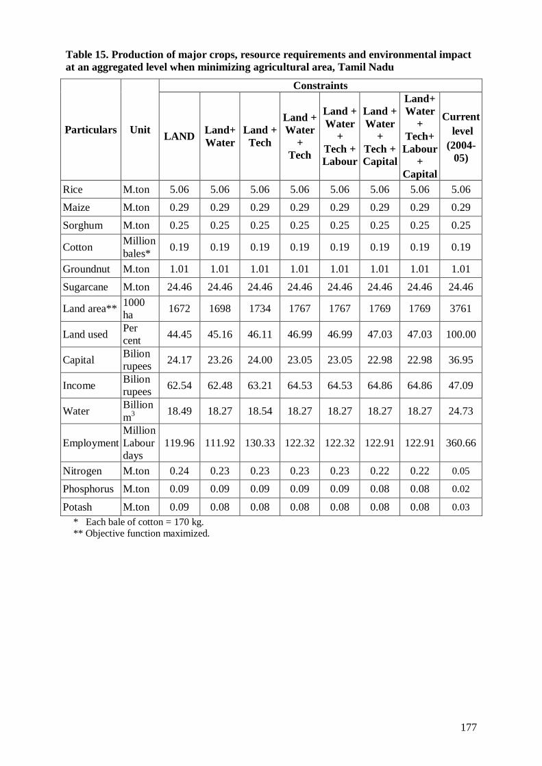
177
Table 15. Production of major crops, resource requirements and environmental impact
at an aggregated level when minimizing agricultural area, Tamil Nadu
Particulars Unit
Constraints
LAND Land+
Water
Land +
Tech
Land +
Water
+
Tech
Land +
Water
+
Tech +
Labour
Land +
Water
+
Tech +
Capital
Land+
Water
+
Tech+
Labour
+
Capital
Current
level
(2004-
05)
Rice M.ton 5.06 5.06 5.06 5.06 5.06 5.06 5.06 5.06
Maize M.ton 0.29 0.29 0.29 0.29 0.29 0.29 0.29 0.29
Sorghum M.ton 0.25 0.25 0.25 0.25 0.25 0.25 0.25 0.25
Cotton Million
bales* 0.19 0.19 0.19 0.19 0.19 0.19 0.19 0.19
Groundnut M.ton 1.01 1.01 1.01 1.01 1.01 1.01 1.01 1.01
Sugarcane M.ton 24.46 24.46 24.46 24.46 24.46 24.46 24.46 24.46
Land area** 1000
ha 1672 1698 1734 1767 1767 1769 1769 3761
Land used Per
cent 44.45 45.16 46.11 46.99 46.99 47.03 47.03 100.00
Capital Bilion
rupees 24.17 23.26 24.00 23.05 23.05 22.98 22.98 36.95
Income Bilion
rupees 62.54 62.48 63.21 64.53 64.53 64.86 64.86 47.09
Water Billion
m3
18.49 18.27 18.54 18.27 18.27 18.27 18.27 24.73
Employment
Million
Labour
days
119.96 111.92 130.33 122.32 122.32 122.91 122.91 360.66
Nitrogen M.ton 0.24 0.23 0.23 0.23 0.23 0.22 0.22 0.05
Phosphorus M.ton 0.09 0.09 0.09 0.09 0.09 0.08 0.08 0.02
Potash M.ton 0.09 0.08 0.08 0.08 0.08 0.08 0.08 0.03
* Each bale of cotton = 170 kg. ** Objective function maximized.
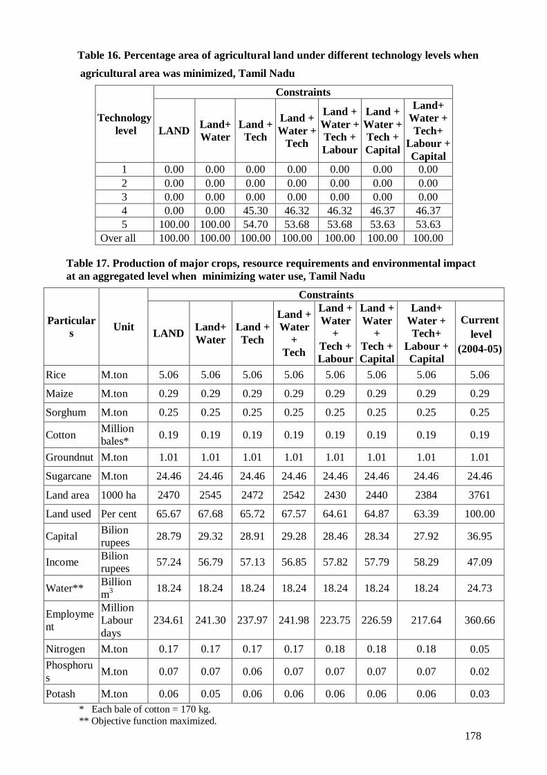
178
Table 16. Percentage area of agricultural land under different technology levels when
agricultural area was minimized, Tamil Nadu
Technology
level
Constraints
LAND Land+
Water
Land +
Tech
Land +
Water +
Tech
Land +
Water +
Tech +
Labour
Land +
Water +
Tech +
Capital
Land+
Water +
Tech+
Labour +
Capital
1 0.00 0.00 0.00 0.00 0.00 0.00 0.00
2 0.00 0.00 0.00 0.00 0.00 0.00 0.00
3 0.00 0.00 0.00 0.00 0.00 0.00 0.00
4 0.00 0.00 45.30 46.32 46.32 46.37 46.37
5 100.00 100.00 54.70 53.68 53.68 53.63 53.63
Over all 100.00 100.00 100.00 100.00 100.00 100.00 100.00
Table 17. Production of major crops, resource requirements and environmental impact
at an aggregated level when minimizing water use, Tamil Nadu
Particular
s Unit
Constraints
LAND Land+
Water
Land +
Tech
Land +
Water
+
Tech
Land +
Water
+
Tech +
Labour
Land +
Water
+
Tech +
Capital
Land+
Water +
Tech+
Labour +
Capital
Current
level
(2004-05)
Rice M.ton 5.06 5.06 5.06 5.06 5.06 5.06 5.06 5.06
Maize M.ton 0.29 0.29 0.29 0.29 0.29 0.29 0.29 0.29
Sorghum M.ton 0.25 0.25 0.25 0.25 0.25 0.25 0.25 0.25
Cotton Million
bales* 0.19 0.19 0.19 0.19 0.19 0.19 0.19 0.19
Groundnut M.ton 1.01 1.01 1.01 1.01 1.01 1.01 1.01 1.01
Sugarcane M.ton 24.46 24.46 24.46 24.46 24.46 24.46 24.46 24.46
Land area 1000 ha 2470 2545 2472 2542 2430 2440 2384 3761
Land used Per cent 65.67 67.68 65.72 67.57 64.61 64.87 63.39 100.00
Capital Bilion
rupees 28.79 29.32 28.91 29.28 28.46 28.34 27.92 36.95
Income Bilion
rupees 57.24 56.79 57.13 56.85 57.82 57.79 58.29 47.09
Water** Billion
m3
18.24 18.24 18.24 18.24 18.24 18.24 18.24 24.73
Employme
nt
Million
Labour
days
234.61 241.30 237.97 241.98 223.75 226.59 217.64 360.66
Nitrogen M.ton 0.17 0.17 0.17 0.17 0.18 0.18 0.18 0.05
Phosphoru
s M.ton 0.07 0.07 0.06 0.07 0.07 0.07 0.07 0.02
Potash M.ton 0.06 0.05 0.06 0.06 0.06 0.06 0.06 0.03
* Each bale of cotton = 170 kg.
** Objective function maximized.
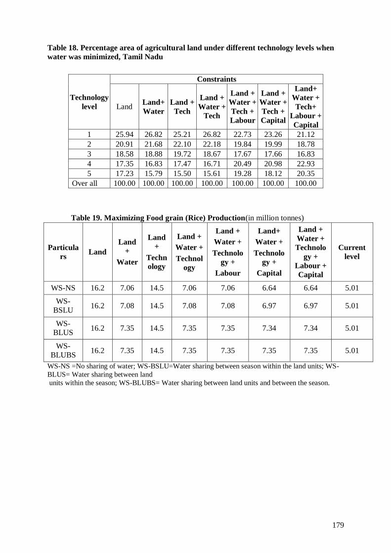
179
Table 18. Percentage area of agricultural land under different technology levels when
water was minimized, Tamil Nadu
Technology
level
Constraints
Land Land+
Water
Land +
Tech
Land +
Water +
Tech
Land +
Water +
Tech +
Labour
Land +
Water +
Tech +
Capital
Land+
Water +
Tech+
Labour +
Capital
1 25.94 26.82 25.21 26.82 22.73 23.26 21.12
2 20.91 21.68 22.10 22.18 19.84 19.99 18.78
3 18.58 18.88 19.72 18.67 17.67 17.66 16.83
4 17.35 16.83 17.47 16.71 20.49 20.98 22.93
5 17.23 15.79 15.50 15.61 19.28 18.12 20.35
Over all 100.00 100.00 100.00 100.00 100.00 100.00 100.00
Table 19. Maximizing Food grain (Rice) Production(in million tonnes)
Particula
rs Land
Land
+
Water
Land
+
Techn
ology
Land +
Water +
Technol
ogy
Land +
Water +
Technolo
gy +
Labour
Land+
Water +
Technolo
gy +
Capital
Land +
Water +
Technolo
gy +
Labour +
Capital
Current
level
WS-NS 16.2 7.06 14.5 7.06 7.06 6.64 6.64 5.01
WS-
BSLU 16.2 7.08 14.5 7.08 7.08 6.97 6.97 5.01
WS-
BLUS 16.2 7.35 14.5 7.35 7.35 7.34 7.34 5.01
WS-
BLUBS 16.2 7.35 14.5 7.35 7.35 7.35 7.35 5.01
WS-NS =No sharing of water; WS-BSLU=Water sharing between season within the land units; WS-
BLUS= Water sharing between land
units within the season; WS-BLUBS= Water sharing between land units and between the season.
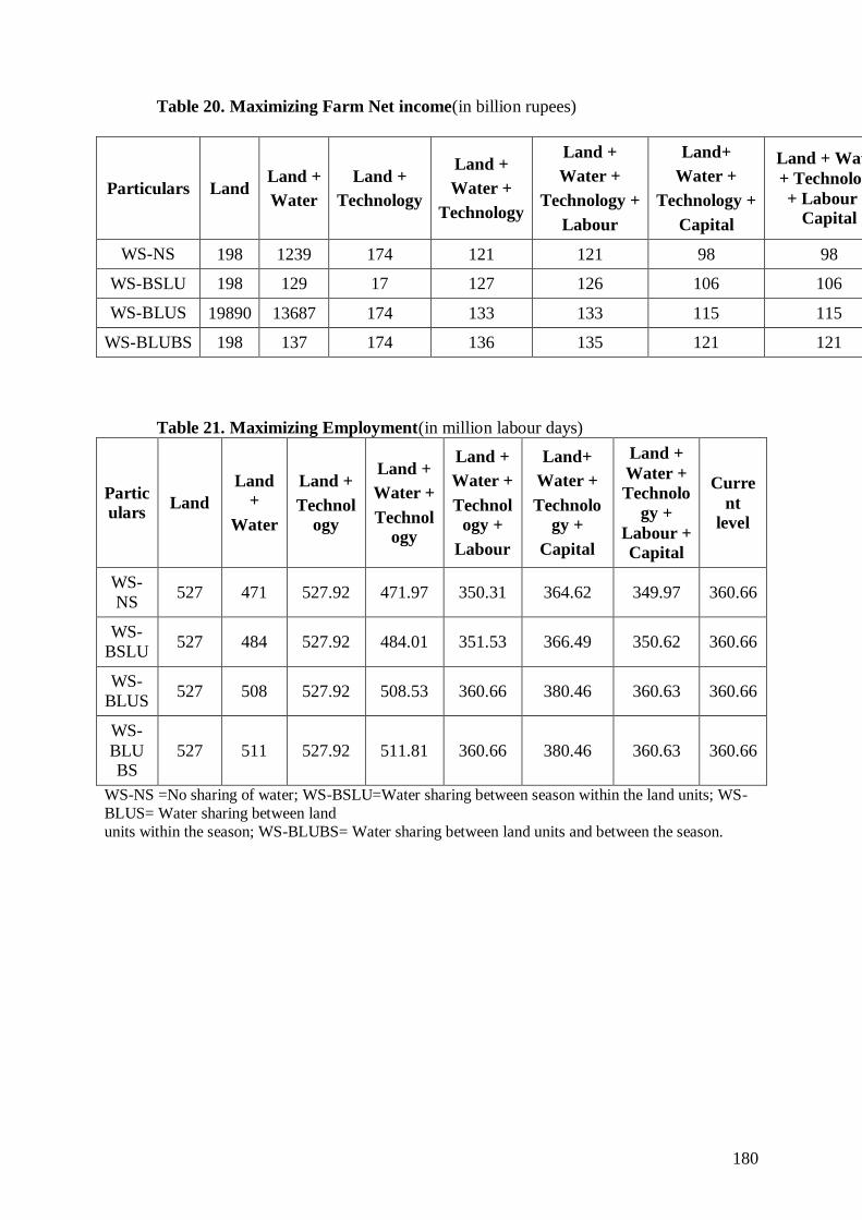
180
Table 20. Maximizing Farm Net income(in billion rupees)
Particulars Land Land +
Water
Land +
Technology
Land +
Water +
Technology
Land +
Water +
Technology +
Labour
Land+
Water +
Technology +
Capital
Land + Water
+ Technology
+ Labour +
Capital
Current
level
WS-NS 198 1239 174 121 121 98 98 47
WS-BSLU 198 129 17 127 126 106 106 47
WS-BLUS 19890 13687 174 133 133 115 115 47
WS-BLUBS 198 137 174 136 135 121 121 47
Table 21. Maximizing Employment(in million labour days)
Partic
ulars Land
Land
+
Water
Land +
Technol
ogy
Land +
Water +
Technol
ogy
Land +
Water +
Technol
ogy +
Labour
Land+
Water +
Technolo
gy +
Capital
Land +
Water +
Technolo
gy +
Labour +
Capital
Curre
nt
level
WS-
NS 527 471 527.92 471.97 350.31 364.62 349.97 360.66
WS-
BSLU 527 484 527.92 484.01 351.53 366.49 350.62 360.66
WS-
BLUS 527 508 527.92 508.53 360.66 380.46 360.63 360.66
WS-
BLUBS
527 511 527.92 511.81 360.66 380.46 360.63 360.66
WS-NS =No sharing of water; WS-BSLU=Water sharing between season within the land units; WS-
BLUS= Water sharing between land
units within the season; WS-BLUBS= Water sharing between land units and between the season.
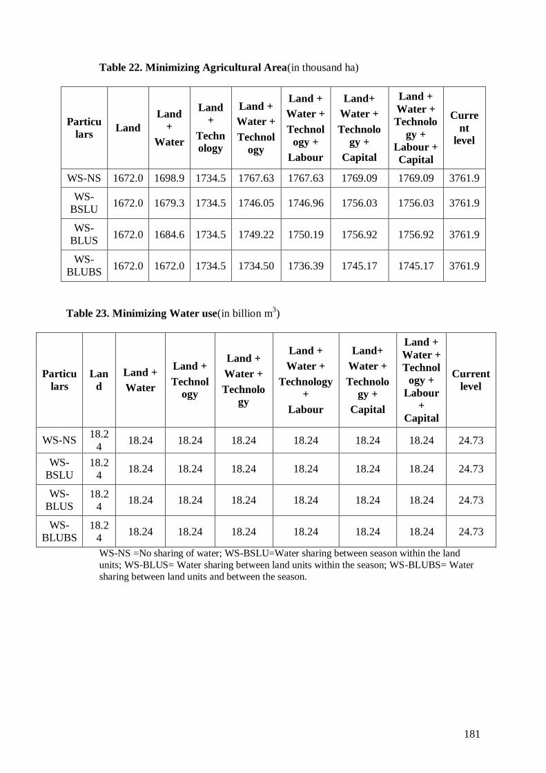
181
Table 22. Minimizing Agricultural Area(in thousand ha)
Particu
lars Land
Land
+
Water
Land
+
Techn
ology
Land +
Water +
Technol
ogy
Land +
Water +
Technol
ogy +
Labour
Land+
Water +
Technolo
gy +
Capital
Land +
Water +
Technolo
gy +
Labour +
Capital
Curre
nt
level
WS-NS 1672.0 1698.9 1734.5 1767.63 1767.63 1769.09 1769.09 3761.9
WS-
BSLU 1672.0 1679.3 1734.5 1746.05 1746.96 1756.03 1756.03 3761.9
WS-
BLUS 1672.0 1684.6 1734.5 1749.22 1750.19 1756.92 1756.92 3761.9
WS-
BLUBS 1672.0 1672.0 1734.5 1734.50 1736.39 1745.17 1745.17 3761.9
Table 23. Minimizing Water use(in billion m3)
Particu
lars
Lan
d
Land +
Water
Land +
Technol
ogy
Land +
Water +
Technolo
gy
Land +
Water +
Technology
+
Labour
Land+
Water +
Technolo
gy +
Capital
Land +
Water +
Technol
ogy +
Labour
+
Capital
Current
level
WS-NS 18.2
4 18.24 18.24 18.24 18.24 18.24 18.24 24.73
WS-
BSLU 18.2
4 18.24 18.24 18.24 18.24 18.24 18.24 24.73
WS-
BLUS 18.2
4 18.24 18.24 18.24 18.24 18.24 18.24 24.73
WS-
BLUBS 18.2
4 18.24 18.24 18.24 18.24 18.24 18.24 24.73
WS-NS =No sharing of water; WS-BSLU=Water sharing between season within the land
units; WS-BLUS= Water sharing between land units within the season; WS-BLUBS= Water
sharing between land units and between the season.
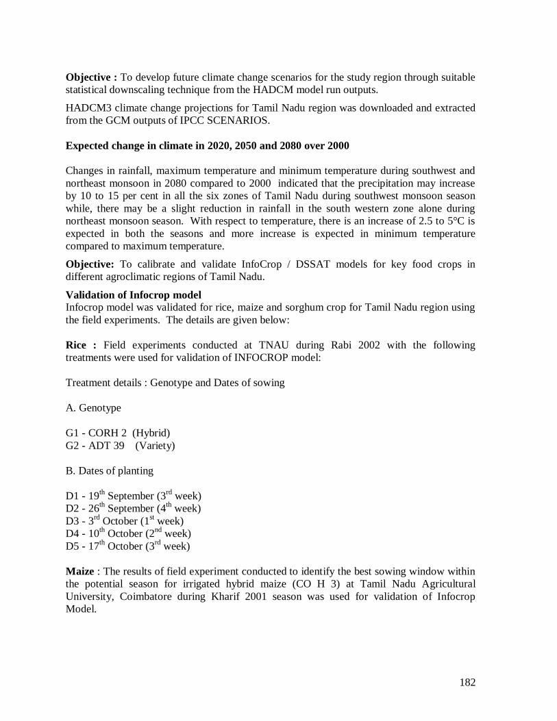
182
Objective : To develop future climate change scenarios for the study region through suitable
statistical downscaling technique from the HADCM model run outputs.
HADCM3 climate change projections for Tamil Nadu region was downloaded and extracted
from the GCM outputs of IPCC SCENARIOS.
Expected change in climate in 2020, 2050 and 2080 over 2000
Changes in rainfall, maximum temperature and minimum temperature during southwest and
northeast monsoon in 2080 compared to 2000 indicated that the precipitation may increase
by 10 to 15 per cent in all the six zones of Tamil Nadu during southwest monsoon season
while, there may be a slight reduction in rainfall in the south western zone alone during
northeast monsoon season. With respect to temperature, there is an increase of 2.5 to 5°C is
expected in both the seasons and more increase is expected in minimum temperature
compared to maximum temperature.
Objective: To calibrate and validate InfoCrop / DSSAT models for key food crops in
different agroclimatic regions of Tamil Nadu.
Validation of Infocrop model
Infocrop model was validated for rice, maize and sorghum crop for Tamil Nadu region using
the field experiments. The details are given below:
Rice : Field experiments conducted at TNAU during Rabi 2002 with the following
treatments were used for validation of INFOCROP model:
Treatment details : Genotype and Dates of sowing
A. Genotype
G1 - CORH 2 (Hybrid)
G2 - ADT 39 (Variety)
B. Dates of planting
D1 - 19th September (3
rd week)
D2 - 26th September (4
th week)
D3 - 3rd
October (1st week)
D4 - 10th October (2
nd week)
D5 - 17th October (3
rd week)
Maize : The results of field experiment conducted to identify the best sowing window within
the potential season for irrigated hybrid maize (CO H 3) at Tamil Nadu Agricultural
University, Coimbatore during Kharif 2001 season was used for validation of Infocrop
Model.
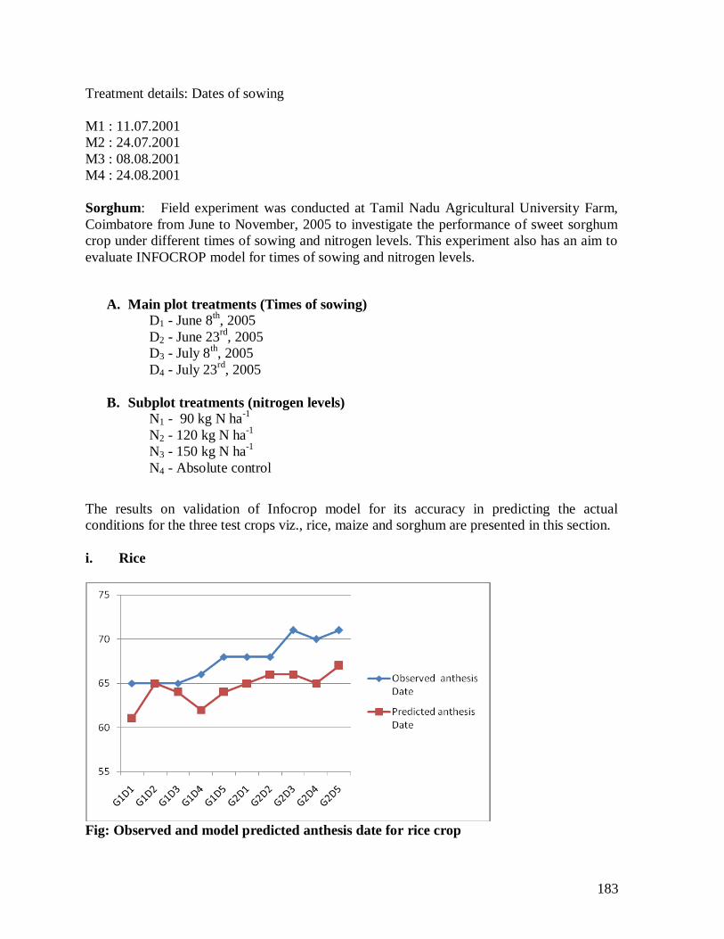
183
Treatment details: Dates of sowing
M1 : 11.07.2001
M2 : 24.07.2001
M3 : 08.08.2001
M4 : 24.08.2001
Sorghum: Field experiment was conducted at Tamil Nadu Agricultural University Farm,
Coimbatore from June to November, 2005 to investigate the performance of sweet sorghum
crop under different times of sowing and nitrogen levels. This experiment also has an aim to
evaluate INFOCROP model for times of sowing and nitrogen levels.
A. Main plot treatments (Times of sowing)
D1 - June 8th, 2005
D2 - June 23rd
, 2005
D3 - July 8th, 2005
D4 - July 23rd
, 2005
B. Subplot treatments (nitrogen levels)
N1 - 90 kg N ha-1
N2 - 120 kg N ha-1
N3 - 150 kg N ha-1
N4 - Absolute control
The results on validation of Infocrop model for its accuracy in predicting the actual
conditions for the three test crops viz., rice, maize and sorghum are presented in this section.
i. Rice
Fig: Observed and model predicted anthesis date for rice crop
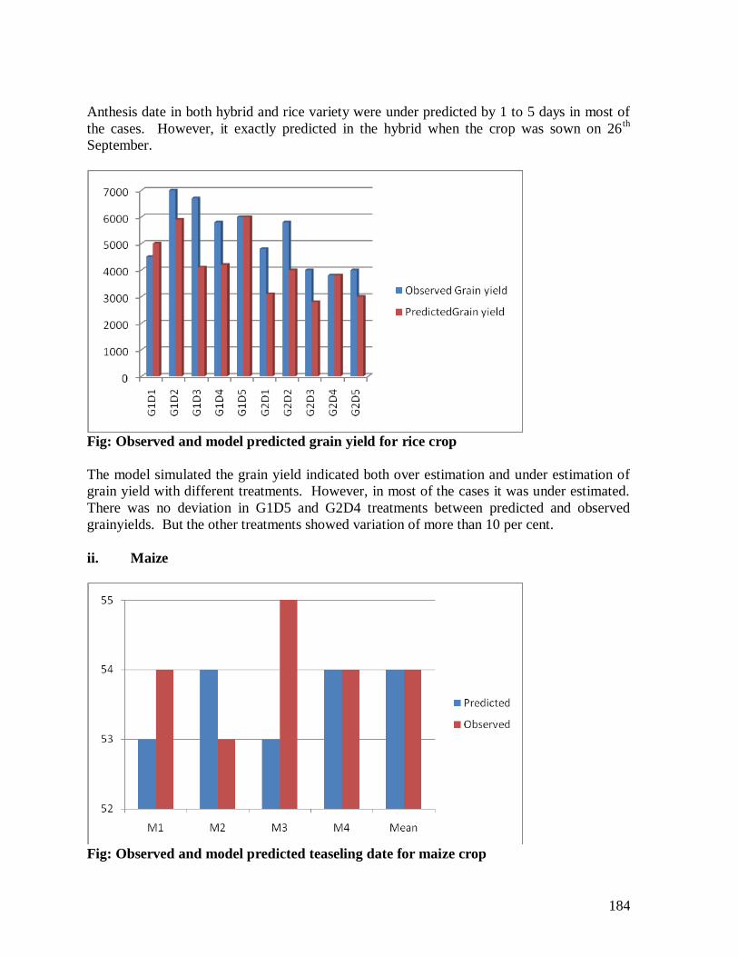
184
Anthesis date in both hybrid and rice variety were under predicted by 1 to 5 days in most of
the cases. However, it exactly predicted in the hybrid when the crop was sown on 26th
September.
Fig: Observed and model predicted grain yield for rice crop
The model simulated the grain yield indicated both over estimation and under estimation of
grain yield with different treatments. However, in most of the cases it was under estimated.
There was no deviation in G1D5 and G2D4 treatments between predicted and observed
grainyields. But the other treatments showed variation of more than 10 per cent.
ii. Maize
Fig: Observed and model predicted teaseling date for maize crop
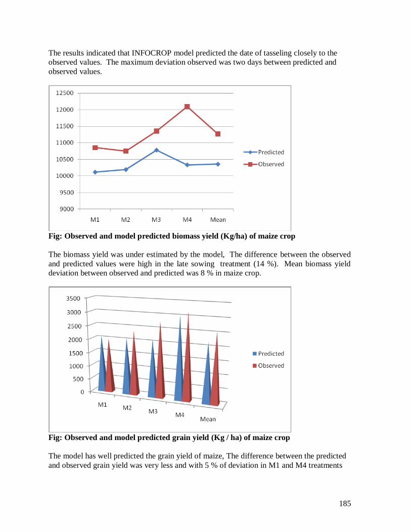
185
The results indicated that INFOCROP model predicted the date of tasseling closely to the
observed values. The maximum deviation observed was two days between predicted and
observed values.
Fig: Observed and model predicted biomass yield (Kg/ha) of maize crop
The biomass yield was under estimated by the model, The difference between the observed
and predicted values were high in the late sowing treatment (14 %). Mean biomass yield
deviation between observed and predicted was 8 % in maize crop.
Fig: Observed and model predicted grain yield (Kg / ha) of maize crop
The model has well predicted the grain yield of maize, The difference between the predicted
and observed grain yield was very less and with 5 % of deviation in M1 and M4 treatments
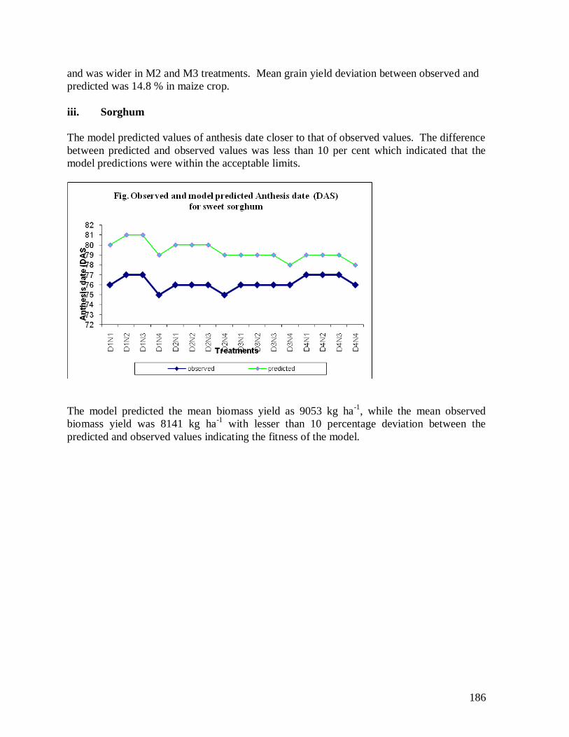
186
and was wider in M2 and M3 treatments. Mean grain yield deviation between observed and
predicted was 14.8 % in maize crop.
iii. Sorghum
The model predicted values of anthesis date closer to that of observed values. The difference
between predicted and observed values was less than 10 per cent which indicated that the
model predictions were within the acceptable limits.
The model predicted the mean biomass yield as 9053 kg ha-1
, while the mean observed
biomass yield was 8141 kg ha-1
with lesser than 10 percentage deviation between the
predicted and observed values indicating the fitness of the model.
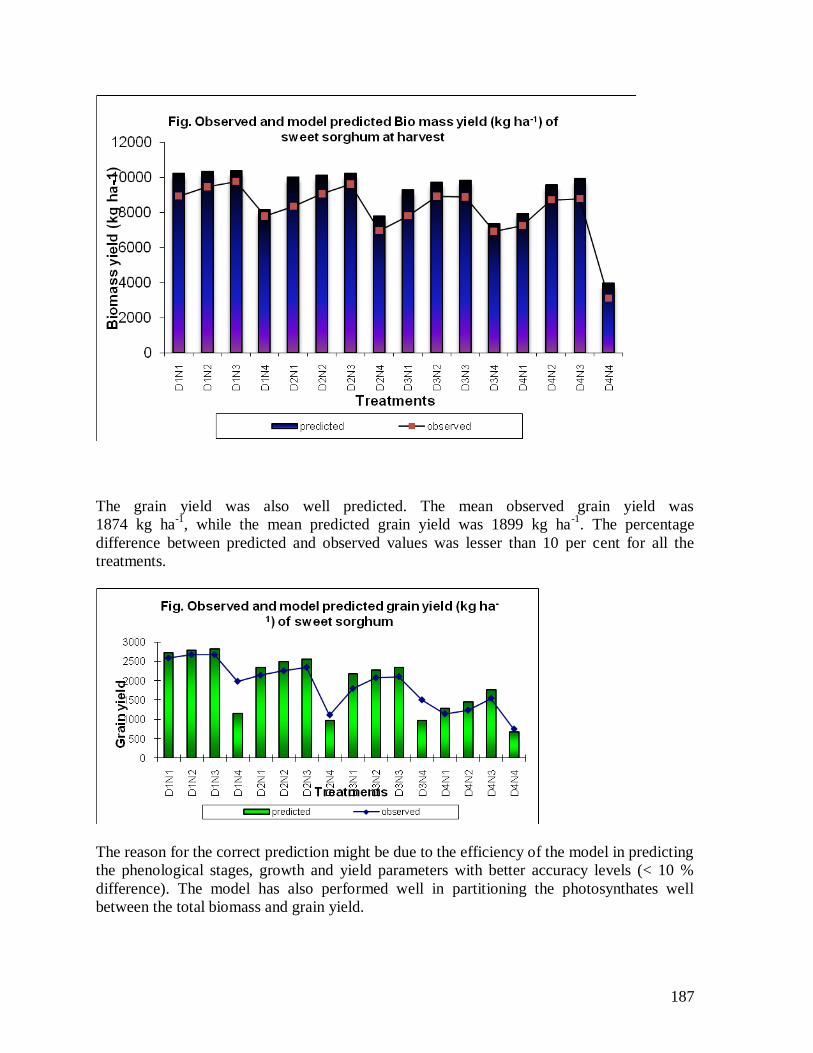
187
The grain yield was also well predicted. The mean observed grain yield was
1874 kg ha-1
, while the mean predicted grain yield was 1899 kg ha-1
. The percentage
difference between predicted and observed values was lesser than 10 per cent for all the
treatments.
The reason for the correct prediction might be due to the efficiency of the model in predicting
the phenological stages, growth and yield parameters with better accuracy levels (< 10 %
difference). The model has also performed well in partitioning the photosynthates well
between the total biomass and grain yield.
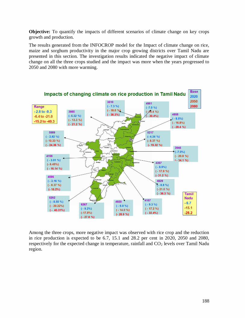
188
Objective: To quantify the impacts of different scenarios of climate change on key crops
growth and production.
The results generated from the INFOCROP model for the Impact of climate change on rice,
maize and sorghum productivity in the major crop growing districts over Tamil Nadu are
presented in this section. The investigation results indicated the negative impact of climate
change on all the three crops studied and the impact was more when the years progressed to
2050 and 2080 with more warming.
Among the three crops, more negative impact was observed with rice crop and the reduction
in rice production is expected to be 6.7, 15.1 and 28.2 per cent in 2020, 2050 and 2080,
respectively for the expected change in temperature, rainfall and CO2 levels over Tamil Nadu
region.
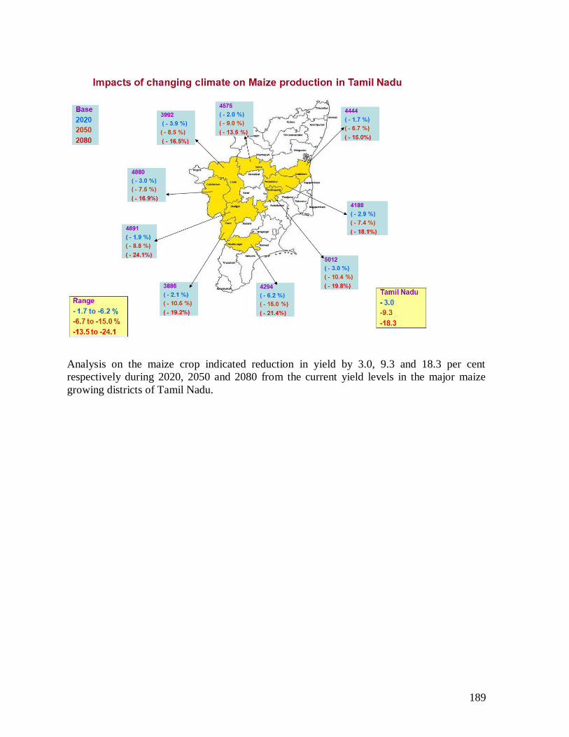
189
Analysis on the maize crop indicated reduction in yield by 3.0, 9.3 and 18.3 per cent
respectively during 2020, 2050 and 2080 from the current yield levels in the major maize
growing districts of Tamil Nadu.
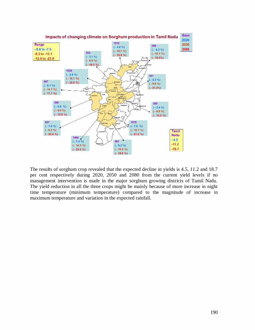
190
The results of sorghum crop revealed that the expected decline in yields is 4.5, 11.2 and 18.7
per cent respectively during 2020, 2050 and 2080 from the current yield levels if no
management intervention is made in the major sorghum growing districts of Tamil Nadu.
The yield reduction in all the three crops might be mainly because of more increase in night
time temperature (minimum temperature) compared to the magnitude of increase in
maximum temperature and variation in the expected rainfall.
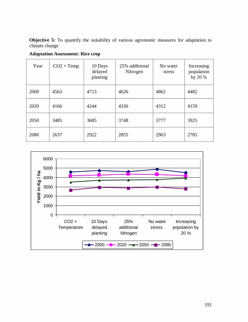
191
Objective 5: To quantify the suitability of various agronomic measures for adaptation to
climate change
Adaptation Assessment: Rice crop
Year CO2 + Temp. 10 Days
delayed
planting
25% additional
Nitrogen
No water
stress
Increasing
population
by 20 %
2000 4563 4713 4626 4862 4482
2020 4166 4244 4336 4312 4159
2050 3485 3685 3748 3777 3925
2080 2637 2922 2855 2963 2785
0
1000
2000
3000
4000
5000
6000
CO2 +
Temperature
10 Days
delayed
planting
25%
additional
Nitrogen
No water
stress
Increasing
population by
20 %
Yie
ld i
n K
g /
ha
2000 2020 2050 2080
ANNEXURE 7: Papers published:
Central Plantation Crops Research institute, Kasargod
Naresh Kumar, S., Kasturi Bai, K. V. Rajagopal V. and Aggarwal, P.K. 2008. Simulating coconut growth, development and yield using InfoCrop-coconut model. Tree Physiology (Canada)-In press
Naresh Kumar, S., M.S. Rajeev and Vinayan D.D. Nagvekar, R. Venkitaswamy,
D.V. Raghava Rao, B. Boraiah, , M. S.Gawankar, R. Dhanapal, D.V. Patil and K.V. Kasturi Bai. 2007. Trends in weather and yield changes in past in coconut growing areas in India. Oral presentation at National Conference on “Impact of Climate Change with Paricular Reference to Agriculture” at TNAU, Coimbatore from 22-24, August, 2007.
ICAR Research Complex for Eastern Region,Patna
Adlul Islam, Alok K Sikka and S Prasad 2007. Investigation of streamflow trend in Brahmani Basin. Hydrological Sciences Journal (Paper No: 2978).
Islam, A., A. K Sikka, B. Saha, and Anamika 2007. Application of GIS and Image
Processing in Distributed Hydrological Modeling. Institute Bulletin (Bulletin No: R-26/PAT-15).
Abdul Haris, R. Elanchezhian, A.K. Sikka, Vandna Chhabra, Arvind Pratap and
Sandeep Biswas.Estimation of climate change impact on rice yield (var.Sita) in Bihar 2008. A.. (accepted for Bihar Science Congress,2008).
A.Abdul Haris, A.K.Sikka, R.Elanchezhian, Sandeep Biswas, Vandna Chhabra and
Arvind Pratap. Impact of climate change on wheat and maize yield at Pusa in Bihar 2008.. (accepted for Bihar Science Congress,2008).
A.Abdul Haris, R. Elanchezhian, R.K Batta, Vandna Chhabra, Sandeep Biswas and Arvind Pratap. Sensitivity of crop yield to temperature under different CO2
scenarios through Infocrop model. 2008.. (accepted for Bihar Science Congress,2008).
192
CENTRAL Marine Fisheries Research Institute, Cochin Vivekanandan, E., N.G.K. Pillai and M. Rajagopalan. 2008. Adaptation of the oil sardine Sardinella longiceps to seawater warming along the Indian coast. In: Glimpses of Aquatic Biodiversity, Rajiv Gandhi Chair Spl. Publ., 111-119. Vivekanandan, E. and J. Jayasankar. 2008. Impact of climate change on Indian marine fisheries. Proc. Winter School, CMFRI, Cochin, 302 pp.
1. Participation in seminars 2. Conducted ICAR sponsored Winter School “Impact of Climate Change on India
Marine Fisheries” for 22 participants from Universities, colleges and ICAR Institutions for 21 days from 18.1.2008 to 7.2.2008 at CMFRI, Cochin.
3. Participated in the National Conference on climate change and made a presentation at NASC Complex, New Delhi on October 12 & 13, 2007.
4. Participated and presented a paper on Climate Change organized by Press Club of India on October 24, 2007 at Cochin
5. Participated and presented a paper “Issues in vulnerability assessment and adaptation in India” in the workshop organized by NATCOM Project Management Cell of MoE&F, Government of India on November 1 & 2, 2007 at New Delhi.
6. Participated and presented a paper “Environmental Issues and Capture Fisheries Sustainability” in the workshop organized by Cochin University on November, 16, 2007 at Cochin.
7. Participated and presented a paper “Climate change impacts in fisheries in Kerala” orgainsed by Kerala Agricultural University at Fisheries College, Panangad on December 14, 2007.
8. Participated and presented a paper Climate Change and Food Security with special reference to Marine Fisheries in the International Symposium conducted at CRIDA on February 18 & 19, 2008 at Hyderabad.
Tamilnadu Agricultural Reserch Institute, TNAU
Palanisami, K., P.Paramasivam, C.R.Ranganathan P.K. Aggarwal, and
S.Senthilnathan, 2009. “Quantifying Vulnerability and Impact of Climate Change on Production of Major Crops in Tamil Nadu, India”, From Headwaters to the Ocean-Hydrological changes and Watershed Management, Taylor & Francis Group, London, U.K, ISBN 978-0-415-47279-1 pp 509-514.
Palanisami, K., P.K. Aggarwal, S.Natarajan, C.R.Ranganathan, R.Sivasamy, P.Paramasivam, V.Geethalakshmi and S.Senthilnathan, 2007. “Quantifying the Impact of Climate Change on Production of Major Crops in Tamil Nadu”, CARDS Series 30, Pp 49.
Palanisami.K, C.Ranganathan, S.Senthilnathan and Chieko Umetsu, 2008. “Developing the Composite Vulnerability Index relating to Climate Change
for the Different Agro Climatic Zones of Tamil Nadu”, Inter-University Research Institute Corporation, National Institutes for the Humanities,
193
Research Institute for Humanity and Nature, Japan, Pp 127-137. ISBN: 978-4-902325-28-7
V. Geethalakshmi, S. Kokilavani, R. Nagarajan, C. Babu and S. Poornima. 2008.
Impacts of Climate Change on rice and ascertaining adaptation opportunities for Tamil Nadu state. In the proceedings of the International symposium on Agrometeorology and Food security conducted by CRIDA, Hyderabad between 18 – 21, February, 2008 : pp: 21 - 22.
V. Geethalakshmi and Ga. Dheebakaran. 2008. Impact of climate change on
agriculture over Tamil Nadu. In: Climate Change and Agriculture over India. Published by AICRP on Agrometeorology. Pp: 79 – 93.
V. Geethalakshmi, S. Kokilavani, R. Nagarajan, C. Babu and S. Poornima. 2008.
Impacts of Climate Change on rice and ascertaining adaptation opportunities for Tamil Nadu state. In the proceedings of the International symposium on Agrometeorology and Food security conducted by CRIDA, Hyderabad between 18 – 21, February, 2008 : pp: 21 - 22.
National Dairy research Institute, Karnal
R.C.Upadhyay, S.V.Singh, Ashok Kumar, Sandeep K. Gupta, Ashutosh, (2007). Impact of Climate change on Milk production of Murrah buffaloes. Italian J Anim. Science, 6, (Suppl. 2), 1329-1332
R.C. Upadhyay, S.V. Singh, and Ashutosh (2008) Impact of climate change on
livestock. Indian Dairyman 60(3): 98-102. C.Devraj and R.C.Upadhyay (2007) Effect of catecholamines and thermal exposure
on lymphocyte proliferation, IL-1α & β in buffaloes, 8 th World Buffalo Congress, Caserta, Italy, Oct 19-22, 2007
R. C Upadhyay; Ashutosh and S.V. Singh (2007) Impact of temperature rise and
climate change on growth and milk productivity of livestock. (Invited Paper) In: International Tropical Ecology Congress held at Dehradun, December 2-5, 2007. (Abstract) page 54.
R.C; Upadhyay, S.V. Singh, and Ashutosh (2008) Impact of climate change on
livestock. (Invited Paper): In: XXXVI Dairy Industry conference held at Banaras Hindu University, Varanasi (U.P.). Proceedings, PP. 68-73.
R.C. Upadhyay, A. Kumar, Ashutosh, S.V. Singh and S.K. Gupta (2007). Impact of
climate change on milk productivity of Indian livestock. In: National
194
195
Conference on Impact of Climate Change with Particular Reference to Agriculture held at TNAU Coimbatore from August 22-24, 2007.
K.S.Roy and R.C.Upadhyay (2007) Methane emissions in expired air of buffaloes.
International Tropical Animal Nutrition Conference, Volume II, Abstracts of the papers presented, October 4-7, 2007, NDRI, Karnal, Page 261.