anomalies, dualities, and topology of d = 6 n = 1 superstring vacua
TRANSCRIPT
arX
iv:h
ep-t
h/96
0518
4v1
25
May
199
6
RU-96-16NSF-ITP-96-21CALT-68-2057
IASSNS-HEP-96/53hep-th/9605184
Anomalies, Dualities, and Topologyof D = 6 N = 1 Superstring Vacua
Micha Berkooz,1 Robert G. Leigh,1 Joseph Polchinski,2
John H. Schwarz,3 Nathan Seiberg,1 and Edward Witten4
1Department of Physics, Rutgers University, Piscataway, NJ 08855-08492Institute for Theoretical Physics, University of California,
Santa Barbara, CA 93106-40303California Institute of Technology, Pasadena, CA 911254Institute for Advanced Study, Princeton, NJ 08540
Abstract
We consider various aspects of compactifications of the Type I/heterotic
Spin(32)/Z2 theory on K3. One family of such compactifications in-
cludes the standard embedding of the spin connection in the gauge
group, and is on the same moduli space as the compactification of
the heterotic E8 × E8 theory on K3 with instanton numbers (8,16).
Another class, which includes an orbifold of the Type I theory re-
cently constructed by Gimon and Polchinski and whose field theory
limit involves some topological novelties, is on the moduli space of
the heterotic E8 × E8 theory on K3 with instanton numbers (12,12).
These connections between Spin(32)/Z2 and E8 × E8 models can be
demonstrated by T duality, and permit a better understanding of non-
perturbative gauge fields in the (12,12) model. In the transformation
between Spin(32)/Z2 and E8 × E8 models, the strong/weak coupling
duality of the (12,12) E8 × E8 model is mapped to T duality in the
Type I theory. The gauge and gravitational anomalies in the Type I
theory are canceled by an extension of the Green-Schwarz mechanism.
1 Introduction
In the ongoing development of string duality, six-dimensional vacua with
N = 1 supersymmetry have been a recent focus of interest. In such vacua,
supersymmetry plus Lorentz invariance are not so strong as to prevent in-
teresting dynamics, but are strong enough to allow much of the dynamics
to be understood. This was exploited, for example, in the study of small
instantons in the SO(32) heterotic string [1].
There have been three broad categories of approaches developed for ob-
taining six-dimensional string vacua with N=1 supersymmetry. One begins
with the E8 × E8 theory compactified on K3. Using the recently developed
11-dimensional understanding of this string theory [2], this approach has a
natural extension to M-theory compactified on K3× S1/Z2. The second ap-
proach begins with the SO(32) theory compactified on K3. Here, one has
the option of viewing the SO(32) theory either as a heterotic string theory or
a Type I superstring theory, since they are nonperturbatively equivalent [3].
The third and most recent approach, which goes under the name of F-theory,
begins with the Type IIB superstring in ten dimensions [4]. By associating a
two-torus to the complex scalar field of this theory, and allowing it to vary in
non-trivial ways over a four-dimensional base space B, one forms a Calabi-
Yau space with an elliptic fibration. Many different classes of vacua can be
constructed by each of these approaches, and in many cases it is clear that
constructions obtained by the various different approaches are dual to one
another – i.e., nonperturbatively equivalent.
Six-dimensional theories with N=1 supersymmetry contain four distinct
kinds of massless multiplets: the gravity multiplet, tensor multiplets, vector
multiplets, and hypermultiplets. The vector multiplets are characterized by
the choice of a gauge group and the hypermultiplets by the choice of a rep-
resentation of the group. A tensor multiplet, which is always a singlet of the
group, contains a two-form potential with an anti-self-dual field strength.
Since the gravity multiplet contains a two-form potential with a self-dual
field strength, it is only possible to give a manifestly covariant effective ac-
tion when there is exactly one tensor multiplet. In this case the self-dual
1
and anti-self-dual tensors can be described together by a single two-form B
or a three-form field strength H . In traditional compactifications of string
theory from ten dimensions there is exactly one tensor multiplet. Additional
tensor multiplets are obtained in compactifications of M-theory by adding
small instantons, which can also be interpreted as five-branes. In the SO(32)
approach, on the other hand, the addition of small instantons (or five-branes)
leads to additional vector multiplets and enhanced gauge symmetry, but no
additional tensor multiplets [1]. In the F-theory constructions there are also
vacua without any tensor multiplet [5]. Here we will only consider vacua
with one tensor multiplet.
Since all N=1 models in six dimensions are chiral, the cancellation of
anomalies is an important requirement. In particular, in the case of one ten-
sor multiplet, a necessary requirement is that the 8-form anomaly polynomial
factorize in the product of two 4-forms: I8 ∼ X4∧X4, where X4 and X4 have
the structure
X4 = trR2 −∑
α
vαtrF 2α (1.1)
X4 = trR2 −∑
α
vαtrF 2α (1.2)
and α labels the various factors in the gauge group. Actually, as we will
discuss in the next section, there can also be additional terms in I8 of the
form X2 ∧X6 when the group contains U(1) factors. As is well-known, the
four-forms also appear in the Bianchi identity dH = X4 and field equation
d ∗ H = X4. It has been realized recently that whenever any of the vα’s is
negative there is a value of the dilaton for which the coupling constant of the
corresponding gauge group diverges. This singularity is believed to signal a
phase transition associated with the appearance of tensionless strings [5, 6].
This is a very interesting phenomenon, which is the subject of much current
discussion. However, in most of this paper we will focus on models (or
parameter ranges) for which this phenomenon does not occur.
In this paper we would like to elaborate on two recently-discussed classes
of D = 6, N = 1 vacua and to establish the connection between them. The
first class is the SO(32) Type I string on K3 in the T 4/Z2 orbifold limit [7].
The second is the E8×E8 heterotic string on K3, with symmetric embedding
2
of the instantons in the two E8’s [8]. For convenience we will refer to these
as GP and DMW vacua respectively. Along the way we will also consider the
E8 × E8 string with other embeddings, and other vacua of the Spin(32)/Z2
heterotic string.
In ref. [7], consistency conditions for open superstring compactifications
were studied, and the general solution was found for the case of a T 4/Z2
orbifold. Cancellation of tadpoles for massless Ramond-Ramond 10-form
and 6-form potentials required 32 Chan-Paton nine-brane indices and 32
five-brane indices, the five-branes oriented so as to fill the 6-dimensional
spacetime).1 The gauge group associated with nine-branes was found to be
U(16) (or a combination of unitary and symplectic subgroups, obtained by
adding Wilson lines) and the same for the five-branes with the five-brane
positions playing the role of the Wilson lines.
The world-sheet consistency conditions, from closure of the operator prod-
uct expansion and cancellation of one-loop divergences, were conjectured to
be a complete set. If so, spacetime gauge and gravitational anomaly cancella-
tion, normally a tight constraint on the spectra of D = 6, N = 1 Yang-Mills
theories, will hold automatically. In ref. [7] the quartic terms in the spacetime
anomalies were found to cancel for all GP models.
In section 2 we study the full anomaly; as expected, the GP models are
(perturbatively) consistent, but the details are interesting. As is familiar from
refs. [9], in order that the anomalies be canceled in the usual way (via tree-
level exchange of the 2-form Bµν), the anomaly 8-form for the non-abelian
gauge fields and gravity must factorize into a product of two 4-forms. In
the consistent models of ref. [7], we find that part of the anomaly polynomial
involving abelian gauge fields does not factorize in this fashion. We identify an
extended version of the GS mechanism in which the anomalies involving U(1)
gauge fields are canceled by tree-level exchange of certain 0-form fields. These
1There is a semantic problem in this subject. In the GP models the five-brane Chan-Paton index takes 32 values, but half can be regarded as the images of the others underthe orbifold Z2, and (as discussed in refs. [1, 7]) half again can be regarded as imagesunder world-sheet parity Ω. Thus there are only 8 dynamical five-branes, each havingthe minimum unit of 6-form charge. So we will refer to five-branes when, as will usuallybe the case, we mean the dynamical objects, and to ‘indices’ when we count the imagesseparately.
3
fields are identified as R-R closed string twisted sector states. The requisite
inhomogeneous transformation of these fields under gauge transformations
leads to spontaneous symmetry breaking of some of the U(1) factors (just
as occurs for the Green-Schwarz mechanism in four dimensions [10]), so that
some of the states identified as massless in ref. [7] receive masses of order the
open string coupling.
Although the world-sheet considerations of ref. [7] evidently guarantee a
perturbatively consistent theory, we show that there is a potential nonper-
turbative inconsistency. For many of the GP models, spinors of the gauge
group cannot be defined. Such spinors do not exist in perturbation theory
but do arise nonperturbatively as D-branes, so the inconsistency appears first
in this way.
In the GP construction there are two types of gauge groups: those car-
ried by open strings that connect pairs of five-branes and those carried by
open strings that connect pairs of nine-branes. As we will explain, there is
a T duality that interchanges the five-branes and nine-branes and thereby
interchanges the two types of open strings and the gauge groups that they
carry.
We will claim that these theories are on the same moduli space as the class
of vacua considered by DMW. The latter exhibit an interesting phenomenon:
heterotic/heterotic string duality. That is, they have an S-duality symme-
try that interchanges perturbative heterotic strings with non-perturbative
heterotic strings.
We will argue that the GP and DMW are equivalent under a sort of ‘U-
duality’ that maps the S-duality of the DMW description to the T duality
of the GP description. This is an example of the widespread phenomenon
of “duality of dualities.” Several pieces of evidence support the proposed
correspondence between these models. One of these is a comparison of the
structure of the factorized anomaly polynomials in each case. Another is the
construction of solitonic strings in the GP setup with the correct properties to
be identified with the two kinds of heterotic strings in the DMW description.
Finally, we will exhibit at the end of this paper a direct proof of this relation
using T duality between certain orbifolds.
4
By integrating the Bianchi identity over K3 one learns that, of n1 and
n2 are the number of instantons in the two factors, then E8 × E8 compact-
ifications must satisfy n1 + n2 + n5 = 24. As we have already said, setting
n5, the number of E8 × E8 fivebranes, to zero ensures that there is just one
tensor multiplet. The DMW models correspond to the symmetric embedding
n1 = n2 = 12. In the case of the SO(32) theory compactified on K3, there
is a similar requirement, namely n1 + n5 = 24, where n1 is the number of
instantons embedded in the SO(32) group and n5 is the number of SO(32)
five-branes (magnetic duals of the heterotic string in ten dimensions). Per-
turbative string vacua have n5 = 0, of course, but by now we have become
accustomed to considering non-perturbative possibilities. The GP construc-
tion uses the K3 orbifold T 4/Z2, rather than a smooth K3. It turns out that
the 16 orbifold singularities each contain a “hidden” instanton, a fact that we
will demonstrate by studying the behavior upon blowing up the singularity.
The models constructed by GP satisfy the counting rule by introducing eight
five-branes in addition to the hidden instantons.
In section 3, we use D = 10 heterotic - Type I duality [3] to relate the GP
models to the SO(32) heterotic string on K3. From the anomaly polynomial
one learns that the nine-brane gauge group maps to a perturbative gauge
symmetry of the heterotic theory, and the five-brane gauge group to a non-
perturbative gauge symmetry. It is therefore not surprising that Type I
T-duality, which interchanges the nine- and five-branes (for a review see
ref. [11]), maps to the heterotic weak/strong duality discussed in ref. [12]
and realized in the DMW construction. As discussed in ref. [12], the dual
heterotic string is a wrapped five-brane; in the Type I theory we construct
both the heterotic string and its dual as D-branes [13]. Finally, we show that
for one particular GP model, the heterotic dual can be constructed as a free
orbifold.
In section 4 we consider the effect of blowing up the Z2 fixed points by
turning on twisted sector fields. A count of instanton number implies that
there must be one instanton hidden at each fixed point. The gauge bundle
that results when the fixed point is blown up is a Spin(32)/Z2 bundle but
not an SO(32) bundle. That is, fields in the vector representation of SO(32)
5
cannot be defined. This is not an inconsistency because the Type I string
has only tensor representations (in perturbation theory) and one class of
spinor representation (nonperturbatively).2 A calculation of the dimension
of instanton moduli space agrees with the GP spectrum.
In section 5 we consider T -duality between the SO(32) and E8 × E8
heterotic strings on K3. We first classify Z2 subgroups of Spin(32)/Z2 and
E8 × E8. We then discuss Spin(32)/Z2 and E8 × E8 bundles (of instanton
number 24) on K3 and the possible T -dualities between them. We resolve
a puzzle remaining from ref. [8]. The nonperturbative gauge symmetries of
the DMW model, which had been tentatively attributed to small E8 × E8
instantons, in fact arise from small Spin(32)/Z2 instantons in the T -dual
theory. Finally, we construct explicitly the T -duality between the SO(32)
and E8 × E8 strings on T 4/Z2 orbifolds, with various embeddings of Z2 in
the gauge groups, and in particular complete the connection between the GP
and DMW models.
Although we shall not explore the subject here, we should point out that
this class of models has also been constructed in F-theory [14]. The key there
is to choose the base space of the elliptic fibration to be P1 × P1. In this
description the inversion of heterotic string coupling is realized geometrically
as the interchange of the two P1 factors.
2 Anomalies
2.1 Anomalies in the U(16) × U(16) Model
Reference [7] constructed a class of N = 1 six-dimensional Type I superstring
vacua with maximal gauge group U(16)9 × U(16)5. The first U(16)9 factor
comes from nine-branes while the second arises when all 8 five-branes are
at a single fixed point of the orbifold. The massless spectrum includes the
hypermultiplets
2× (120, 1)(2/4,0)
1× (16, 16)(1/4,1/4)
2In the heterotic dual the same representations appear, but all perturbatively.
6
2× (1, 120)(0,2/4) (2.1)
4× (1, 1)(0,0)
16× (1, 1)(0,0)
where the subscripts refer to the U(1) charges.3 In this section we will il-
lustrate the cancellation of anomalies for this special case of maximal gauge
group, and in the next we will consider the general case.
In order for the anomalies of the theory (2.1) to be canceled by the stan-
dard GS mechanism [9], it is necessary that the anomaly 8-form factorize into
a product of two 4-forms. The anomaly is then canceled, in the low energy
theory, by the appearance of a gauge-variant counterterm coupling the field
Bµν to one of the two 4-forms.
Recall that for N=1 models in six dimensions cancellation of the coeffi-
cient of the tr R4 term in the anomaly polynomial requires that nH − nV =
273−29nT , where nH , nV , and nT are the number of hyper multiplets, vector
multiplets, and tensor multiplets, respectively. In this paper we will only be
considering models with nT = 1. In addition, the hypermultiplet representa-
tions have to appear in such a way as to ensure that all tr F 4 terms can be
eliminated. In the theory with the field content given above, the tr R4 and
tr F 4 terms do cancel, and the full gravitational + gauge anomaly may be
written, using standard formulas, [15, 16], in the form
I8 = X(9)4 ∧X
(5)4 +X2 ∧X
(9)6 +X ′
2 ∧X(5)6 . (2.2)
The last two terms can appear only in the presence of U(1) factors, because
they involve tr F , which is nonvanishing for U(1) only. The various forms
appearing here are
X(a)4 = tr F 2
a −1
2tr R2
X(a)6 =
8
3
(
−1
4tr R2 · tr Fa + tr F 3
a −9
4tr Fa · tr F
2a +
3
2(tr Fa)
3)
X2 = 4 tr F9 + tr F5 (2.3)
X ′2 = 4 tr F5 + tr F9
3The U(1) charges are obtained by noting that the endpoints transform as a 16 + 16
of U(16); the factor of 1/4 is included in order to give a canonical normalization.
7
where Fa with a = 5, 9 refer to the two U(16) field strength two-forms in
the fundamental (16-dimensional) representation. A term of the form tr Fa
only involves the U(1) subalgebra. We note that this is not of the usual
factorized form, and thus the full anomaly cannot be canceled by exchange
of a two-form, which involves GS interactions of the familiar form
Γc.t. =∫
B2 ∧X(5)4 + a0
∫
X(9)3 ∧X
(5)3 (2.4)
for some (scheme-dependent) constant a0. The B2 field is the 2-form with
gauge invariant field strength H = dB2 −X(9)3 where X
(a)4 = dX
(a)3 .
The counterterm (2.4) succeeds in canceling the first term in (2.2). The
remaining two terms may be canceled by additional counterterms (up to
gauge-dependent terms)
Γ′c.t. =
∫
B(9)0 X
(9)6 +
∫
B(5)0 X
(5)6 (2.5)
if we assign the anomalous transformation laws:
B(9)0 → B
(9)0 + 4ǫ9 + ǫ5 (2.6)
B(5)0 → B
(5)0 + 4ǫ5 + ǫ9
under the U(1) gauge transformations Aa → Aa + dǫa. It follows that the
scalar fields B0 must appear in the low energy Lagrangian in the combina-
tions dB(a)0 −qa,bA(b), where qa,b are the coefficients of the shifts in (2.6). The
inhomogeneity of the transformation laws (2.6) implies that the two U(1)’s
are spontaneously broken, just as in four-dimensional theories with anoma-
lous U(1)’s where a similar mechanism appears [10]. The unbroken symmetry
is therefore only SU(16) × SU(16). The B0 fields are linear combinations of
R-R twisted-sector scalars, which we will refer to as φI , I = 1, . . . , 16 labeling
the orbifold fixed points. By examining string amplitudes, we may identify
the fields B0 more concretely and deduce their kinetic terms and anomalous
couplings (2.5). These all appear at disk order, as does the standard GS
term (2.4). In the next section, we will see that these couplings arise also in
the (equivalent) boundary-state tadpole formalism. It is easy to infer from
diagrams that the B0 fields that cancel the U(1) anomalies are twisted sector
R-R states. Consider the mixing of a scalar mode with a U(1) gauge boson.
8
The Chan-Paton factor of the U(1) gauge boson is a matrix in the algebra
of SO(32) of the form:
λ ≡M =(
0 I16−I16 0
)
(2.7)
(I16 is a 16 × 16 unit matrix). The orbifold projection R acts on the Chan-
Paton indices as matrices γR,a, which are identical in form to M ; again the
index a denotes either the nine- or five-brane sector. Consider first a coupling
of an untwisted closed-string mode to a U(1) gauge boson. Such an amplitude
is proportional to tr λ, and hence it vanishes trivially. However, insertion
of a twist operator in the interior of the disk creates a cut which must be
taken to run from its insertion point to the boundary. The fields jump across
the cut by the orbifold operation R, which includes the matrix γR,a on the
Chan-Paton degrees of freedom. The disk amplitude is then proportional to
tr γR,aλ 6= 0. The R-R twisted state associated to a given fixed point then
couples to the U(1) at that fixed point, while each of the sixteen R-R twisted
states couple to the U(1)9 gauge boson. We can therefore identify
B(5)0 = φ1 (2.8)
B(9)0 =
1
4
16∑
I=1
φI .
This ensures that eqs. (2.6) are consistent, if φ1 refers to the special fixed
point and each of the other 15 twisted fields shift by φI → φI + ǫ9. These
rules generalize in a straightforward way to all other models in Ref. [7], as
we will see in the next section. Incidentally, the 4-to-1 ratio of charges in
(2.6) has a simple explanation: given the natural normalization of fields in
(2.8), it is the only choice consistent with 5 ↔ 9 T -duality.
At each fixed point the twisted sector includes three NS-NS scalars and
one R-R scalar. They belong to a single N = 1 D = 6 hypermultiplet,
transforming as an SU(2)R doublet Φ. Because supersymmetry remains un-
broken, the Higgs mechanism that gives mass to the vector boson by eating
the R-R field must also give mass to the NS-NS superpartners; let us see how
this arises from the D-terms. For any U(1) gauge symmetry supersymmetry
requires that the three one-forms
2IAǫ = iδΦ∗σAdΦ − idΦ∗σAδΦ (2.9)
9
be closed. The SU(2)R-triplet D-terms are then defined by dDA = IA. For a
linearly realized U(1), δΦ = iǫqΦ and DA = qΦ∗σAΦ. For the spontaneously
broken U(1),
δΦ = ǫv ≡ ǫ
[
10
]
. (2.10)
Parameterizing the doublet by Φ = (φ − iHAσA)v, this gives δφ = ǫ and
DA = HA, so that D2 is a mass term for H .
We will consider details of blowing up the orbifold points in section 4.
Let us note briefly here the following. Because of the above remarks, the
D-term contains a term linear in HA as well as the usual quadratic terms for
charged fields. In particular the D-term for the 9-brane U(1) contains the
sum of all the HAI . Let us go to a generic point in the K3 moduli space by
giving vevs to all the geometric moduli of K3. Since the sum of HAI is not
(generically) zero, then D-flatness requires the gauge groups to be broken, at
least to Sp(8). We are now on a large smooth K3, and we can try to identify
the remaining massless modes in the σ-model classical limit. SO(32) has an
SU(2)×Sp(8) maximal subgroup and it is easy to check that if we assume we
have 2 instantons in SU(2) we obtain the correct spectrum. This corresponds
to the following topological fact. As we will explain in section 4, the point
in GP moduli space at which the unbroken gauge group is U(16) (or SU(16)
allowing for the mechanism above) corresponds to a certain U(1) instanton
of instanton number 16, embedded in a very particular way in Spin(32)/Z2,
on the K3 orbifold. It can be shown that on a smooth K3 manifold, there
is no abelian instanton with the given instanton number and embedding in
Spin(32)/Z2 (this is equivalent to the fact that upon blowing up, the orbifold
singularities are replaced by two-spheres whose cohomology classes are not
anti-self-dual) so the SU(16) must be “Higgsed” if one turns on twisted sector
modes to blow up the singularities of the K3 orbifold.4 The “SU(2) instanton
of instanton number two” mentioned above is really an SO(3) instanton; for
SU(2) instantons on a smooth K3 surface, the minimum instanton number is
4, but for an SO(3) instanton (of non-zero second Stiefel-Whitney class) the
minimum instanton number is 2. (These last assertions can be understood
4This is an assertion about K3; the smooth, ALE Eguchi-Hansen manifold discussedin section four does have a self-dual holomorphic two-sphere and abelian instanton.
10
using an argument given – in the SO(32) case – at the end of section 5.2.)
Repeating the analysis for the 5-branes, and using the U(1)5 D-term,
we obtain an Sp(8) unbroken 5-brane group after turning on twisted sector
modes, as expected from eight 5-branes on a smooth K3.
2.2 Anomalies in the General Case
We now consider the problem in more generality. Ref. [7] described models
with nine-brane gauge group U(16) and five-brane gauge group∏
I U(mI) ×∏
J Sp(n′J). The five-brane unitary factors arise from mI/2 five-branes at
fixed point I, while the symplectic factors are from 5-branes away from fixed
points. The maximum rank is achieved when all 8 five-branes sit at fixed
points. We will focus on this case, since the more general case is obtained by
spontaneous breaking (moving 5-branes off the fixed points). In particular,
we will consider the U(1)16 subgroup of the five-brane gauge group, coming
from open strings with both ends on the same five-brane.
T -duality interchanges five-branes and nine-branes, but the groups above
are not T -dual because we have omitted the Wilson lines that are dual to
the five-brane positions [7]. Let us now rectify this. The Wilson lines in the
directions m = 6, 7, 8, 9 must satisfy
[Wm,Wn] = 0, MWmM−1 = W−1
m , (2.11)
i.e. flatness and the orbifold projection. Here M is the matrix in (2.7), but
it is now regarded as an element of the group. We can take a basis in which
the Wm are made up of blocks of two types
Wm =
R2(θ).
±1.
R−12 (θ)
.±1
.
(2.12)
where R2(θ) is a 2 × 2 rotation matrix. The structure of large and small
blocks must be the same for all m, by flatness. The large 2 × 2 blocks are
11
T -dual to the motions of five-branes in the bulk of the orbifold, while the
small blocks are T -dual to half-five-branes fixed at orbifold points.
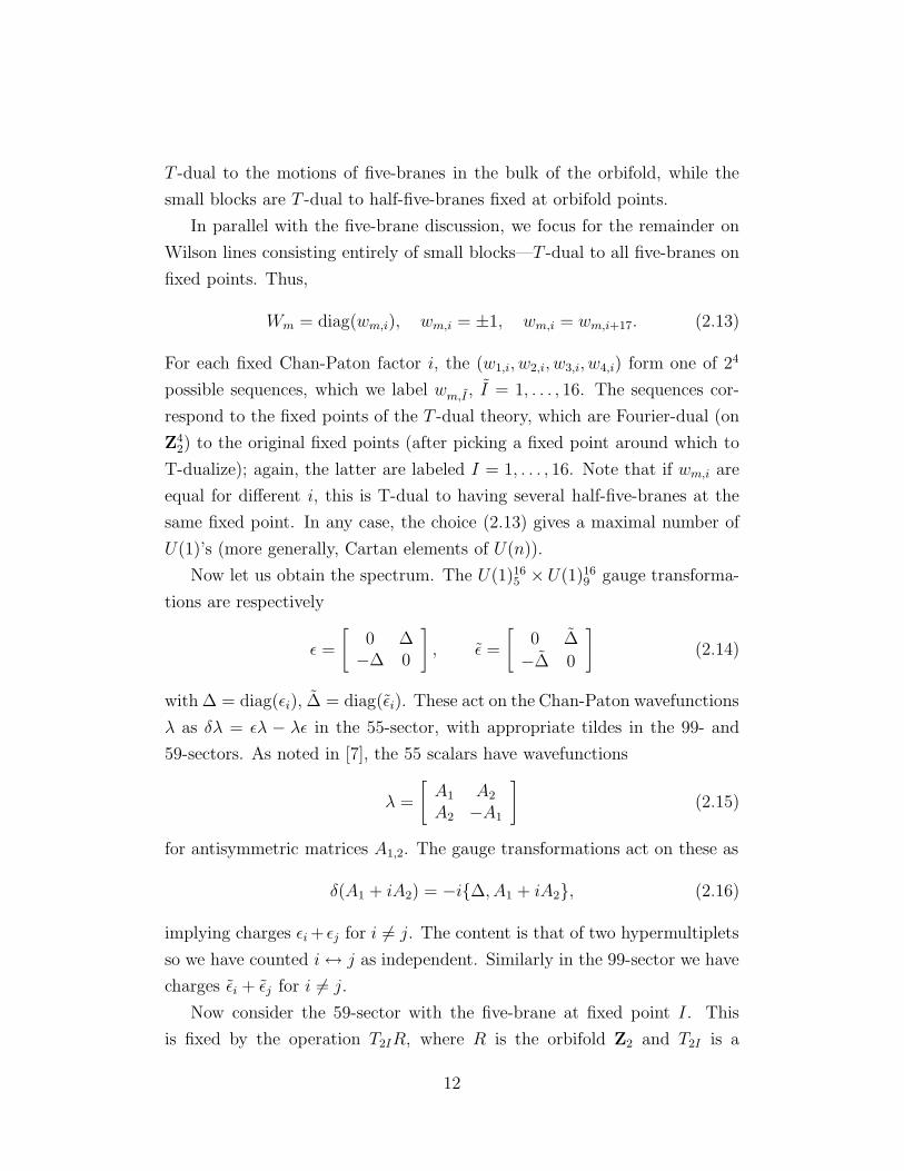
In parallel with the five-brane discussion, we focus for the remainder on
Wilson lines consisting entirely of small blocks—T -dual to all five-branes on
fixed points. Thus,
Wm = diag(wm,i), wm,i = ±1, wm,i = wm,i+17. (2.13)
For each fixed Chan-Paton factor i, the (w1,i, w2,i, w3,i, w4,i) form one of 24
possible sequences, which we label wm,I , I = 1, . . . , 16. The sequences cor-
respond to the fixed points of the T -dual theory, which are Fourier-dual (on
Z42) to the original fixed points (after picking a fixed point around which to
T-dualize); again, the latter are labeled I = 1, . . . , 16. Note that if wm,i are
equal for different i, this is T-dual to having several half-five-branes at the
same fixed point. In any case, the choice (2.13) gives a maximal number of
U(1)’s (more generally, Cartan elements of U(n)).
Now let us obtain the spectrum. The U(1)165 ×U(1)16
9 gauge transforma-
tions are respectively
ǫ =
[
0 ∆−∆ 0
]
, ǫ =
[
0 ∆
−∆ 0
]
(2.14)
with ∆ = diag(ǫi), ∆ = diag(ǫi). These act on the Chan-Paton wavefunctions
λ as δλ = ǫλ − λǫ in the 55-sector, with appropriate tildes in the 99- and
59-sectors. As noted in [7], the 55 scalars have wavefunctions
λ =
[
A1 A2
A2 −A1
]
(2.15)
for antisymmetric matrices A1,2. The gauge transformations act on these as
δ(A1 + iA2) = −i∆, A1 + iA2, (2.16)
implying charges ǫi + ǫj for i 6= j. The content is that of two hypermultiplets
so we have counted i↔ j as independent. Similarly in the 99-sector we have
charges ǫi + ǫj for i 6= j.
Now consider the 59-sector with the five-brane at fixed point I. This
is fixed by the operation T2IR, where R is the orbifold Z2 and T2I is a
12
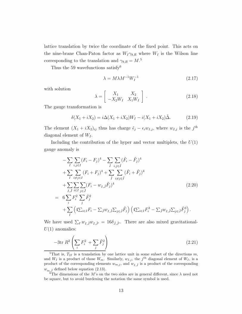
lattice translation by twice the coordinate of the fixed point. This acts on
the nine-brane Chan-Paton factor as WIγ9,R where WI is the Wilson line
corresponding to the translation and γ9,R = M .5
Thus the 59 wavefunctions satisfy6
λ = MλM−1W−1I (2.17)
with solution
λ =
[
X1 X2
−X2WI X1WI
]
. (2.18)
The gauge transformation is
δ(X1 + iX2) = i∆(X1 + iX2)WI − i(X1 + iX2)∆. (2.19)
The element (X1 + iX2)ij thus has charge ǫj − ǫiwI,j, where wI,j is the jth
diagonal element of WI .
Including the contribution of the hyper and vector multiplets, the U(1)
gauge anomaly is
−∑
I
∑
i,j∈I
(Fi − Fj)4 −
∑
I
∑
i,j∈I
(Fi − Fj)4
+∑
I
∑
i6=j∈I
(Fi + Fj)4 +
∑
I
∑
i6=j∈I
(Fi + Fj)4
+∑
I,J
∑
i∈I
∑
j∈J
(Fi − wI,J Fj)4 (2.20)
= 6∑
i
F 2i
∑
j
F 2j
+∑
I
(
4∑
i∈IFi −∑
JwI,J
∑
j∈J Fj
) (
4∑
i∈IF3i −
∑
JwI,J
∑
j∈J F3j
)
.
We have used∑
I wI,JwI,J ′ = 16δJ ,J ′. There are also mixed gravitational-
U(1) anomalies:
−3tr R2
∑
i
F 2i +
∑
j
F 2j
(2.21)
5That is, T2I is a translation by one lattice unit in some subset of the directions m,and WI is a product of those Wm. Similarly, wI,j , the jth diagonal element of WI , is aproduct of the corresponding elements wm,j , and wI,J is a product of the corresponding
wm,J
defined below equation (2.13).6The dimensions of the M ’s on the two sides are in general different, since λ need not
be square, but to avoid burdening the notation the same symbol is used.
13
−1
16tr R2
∑
I
(
4∑
i∈IFi −∑
JwI,J
∑
j∈J Fj
) (
4∑
i∈IFi −∑
JwI,J
∑
j∈J Fj
)
.
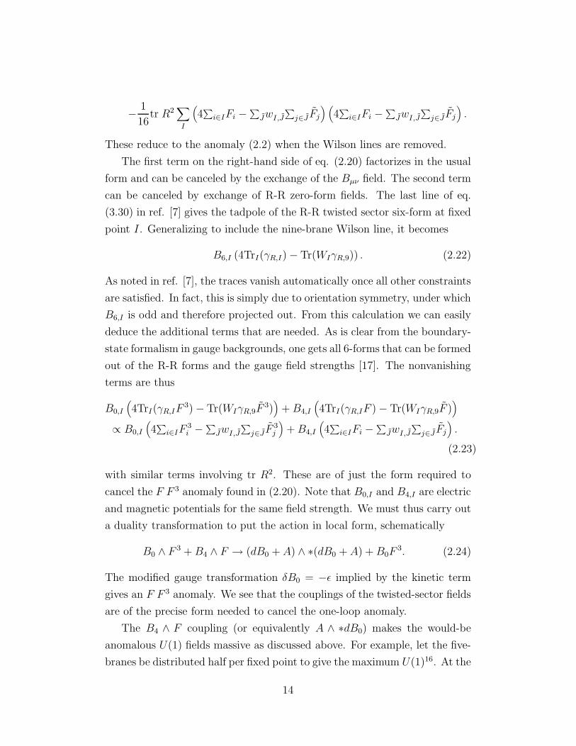
These reduce to the anomaly (2.2) when the Wilson lines are removed.
The first term on the right-hand side of eq. (2.20) factorizes in the usual
form and can be canceled by the exchange of the Bµν field. The second term
can be canceled by exchange of R-R zero-form fields. The last line of eq.
(3.30) in ref. [7] gives the tadpole of the R-R twisted sector six-form at fixed
point I. Generalizing to include the nine-brane Wilson line, it becomes
B6,I (4TrI(γR,I) − Tr(WIγR,9)) . (2.22)
As noted in ref. [7], the traces vanish automatically once all other constraints
are satisfied. In fact, this is simply due to orientation symmetry, under which
B6,I is odd and therefore projected out. From this calculation we can easily
deduce the additional terms that are needed. As is clear from the boundary-
state formalism in gauge backgrounds, one gets all 6-forms that can be formed
out of the R-R forms and the gauge field strengths [17]. The nonvanishing
terms are thus
B0,I
(
4TrI(γR,IF3) − Tr(WIγR,9F
3))
+B4,I
(
4TrI(γR,IF ) − Tr(WIγR,9F ))
∝ B0,I
(
4∑
i∈IF3i −
∑
JwI,J
∑
j∈J F3j
)
+B4,I
(
4∑
i∈IFi −∑
JwI,J
∑
j∈J Fj
)
.
(2.23)
with similar terms involving tr R2. These are of just the form required to
cancel the F F 3 anomaly found in (2.20). Note that B0,I and B4,I are electric
and magnetic potentials for the same field strength. We must thus carry out
a duality transformation to put the action in local form, schematically
B0 ∧ F3 +B4 ∧ F → (dB0 + A) ∧ ∗(dB0 + A) +B0F
3. (2.24)
The modified gauge transformation δB0 = −ǫ implied by the kinetic term
gives an F F 3 anomaly. We see that the couplings of the twisted-sector fields
are of the precise form needed to cancel the one-loop anomaly.
The B4 ∧ F coupling (or equivalently A ∧ ∗dB0) makes the would-be
anomalous U(1) fields massive as discussed above. For example, let the five-
branes be distributed half per fixed point to give the maximum U(1)16. At the
14
massless level one can think of B4,I as a Lagrange multiplier determining the
gauge field FI in terms of the five-brane fields, so the gauge group is identical
to the nine-brane group, though the actual fields are linear combinations of
the five- and nine-brane fields. We are considering models with a rank-32
group, which contains at least two U(1)’s (the case considered in the previous
section) and at most 32 (when there is one five-brane at each I and one nine-
brane with each I). One can see that if there are 16 or fewer U(1)’s, all are
broken, while if there are more than 16, exactly 16 are broken.
2.3 A Nonperturbative Anomaly
The models described in the previous section fall into several classes. The
number of half five-branes on each of the 16 fixed points can be odd or even,
and this is fixed because only whole five-branes can move off the fixed point.
Similarly, the number of Chan-Paton factors with each I can be odd or even.
Although these models are all consistent in perturbation theory, there is a
nonperturbative inconsistency in most of the classes. Consider transporting
a charged field around the fixed point at Xm = 0, from Xm to −Xm. On
this nontrivial path the field picks up the SO(32) transformation M .7 Now
transport a field twice around the fixed point, so that it comes back to itself
times M2. This path is topologically trivial so fields must come back to their
original values. Now M2 = −1, but this is no problem because this is in the
SO(32) vector representation, and there are no fields in this representation.
The matrix M can be thought of as a rotation by 12π in each of the 16 planes
(k, k + 16). It follows that M2 is +1 in one spinor representation and −1 in
the other. This is precisely the spectrum given by the GSO projection, so
the holonomy is consistent.
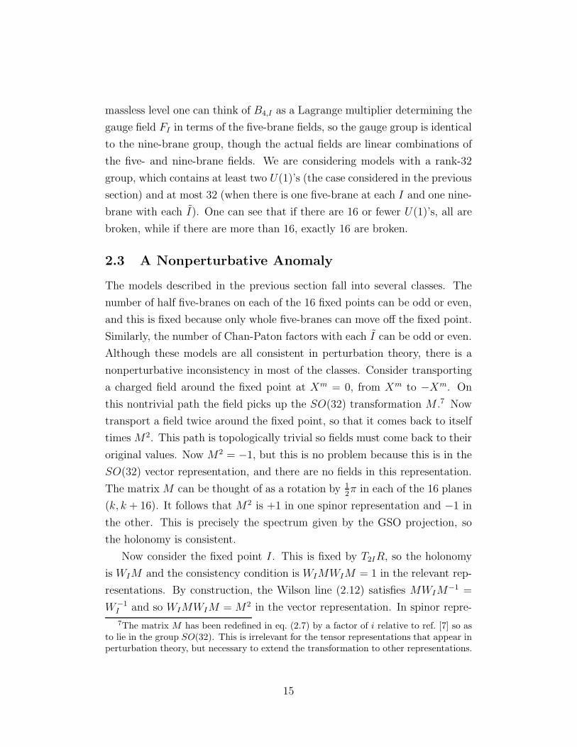
Now consider the fixed point I. This is fixed by T2IR, so the holonomy
is WIM and the consistency condition is WIMWIM = 1 in the relevant rep-
resentations. By construction, the Wilson line (2.12) satisfies MWIM−1 =
W−1I and so WIMWIM = M2 in the vector representation. In spinor repre-
7The matrix M has been redefined in eq. (2.7) by a factor of i relative to ref. [7] so asto lie in the group SO(32). This is irrelevant for the tensor representations that appear inperturbation theory, but necessary to extend the transformation to other representations.
15
sentations it is not hard to see that the large blocks (being connected to the
identity) have no net effect. Consider a small block with −1’s in rows k and
k+16. One can think of this as a rotation by π in the plane (k, k+16). This
commutes with M and squares to a 2π rotation. Thus it is trivial in the vec-
tor representation but −1 in both spinors. If there are an odd number of such
blocks, then WIMWIM = −M2 in the spinor representation and there is no
spinor representation that can be consistently defined at both fixed points.
Consistency of the model thus requires that for all I the number of small
−1 blocks is even. The T -dual statement for the five-branes is this: consider
any 8 fixed points lying in a 3-plane (such as the 3-plane x6 = 0). The total
number of five-branes on these fixed points must be integer.
Since the spinor representations appear only as D-branes, this is a non-
perturbative inconsistency. In section 5 we will see that it has a simple
topological interpretation, and we will actually find a slightly stronger con-
dition: consider any 4 fixed points lying in a 2-plane (such as the 2-plane
x6 = x7 = 0). The total number of five-branes on these fixed points must be
integer.
Taking into account the nonperturbative constraint, there appear to be
six connected sets of GP orbifolds. There can be zero half-five-branes, 8
half-five-branes in a 3-plane, or 16 half-five-branes, times the corresponding
three sectors of Wilson lines, giving nine sectors that are reduced to six by
T-duality. We will see in section 5 that all of them are connected via smooth
K3’s.
The topological interpretation of the non-perturbative inconsistency that
we have described really has to do with the second Stiefel-Whitney class
w2 of the SO(32) bundle. In the above discussion, the key point was that a
reflection R of R4 and a translation TI in the I th direction obey geometrically
RTI = T−1I R.
In dividing by the group G generated by R and TI to make a K3 orbifold
from T4, we represented T and TI in the gauge group SO(32) by matrices
M and WI , in such a way that the desired relation
MWI = W−1I M,
16
is satisfied in SO(32) but not after lifting to Spin(32)/Z2. In such a situation,
if G acted freely on R4, then after dividing R4 by G, one would get a smooth
manifold R4/G with a flat SO(32) bundle of non-zero w2. Here, we are
dealing with a somewhat more abstract string-theoretic version of w2, as the
G action is not free.
3 Duality1: Type I and Heterotic SO(32)
In ten dimensions the SO(32) Type I and heterotic strings are dual with a
specific transformation of the metric and other fields [3], and so they remain
equivalent when compactified on corresponding smooth manifolds. Finding
the dual of an orbifold compactification is less straightforward. In the limit
of a large orbifold, one can use the adiabatic principle [18]: the dual theory
looks geometrically like an orbifold away from the fixed point. Also, by
transporting charged fields around a fixed point, it follows that the gauge
holonomy (here M) is the same in both theories. But it need not be that a
free orbifold CFT in one theory maps to a free orbifold theory in the other—
there might, for example, be twisted-state backgrounds. This arose in ref. [7],
where the heterotic orbifold with spin and gauge connections equal did not
have a free-CFT Type I dual. In the present case, we can see immediately
that most of the Type I models do not have a free-CFT dual. The point is
that the antisymmetric tensor 6-form charge is canceled locally only for one
set of models, the U(1)165 models with a half-five-brane at each fixed point.
For the other models there is a local charge, hence a field strength and a
dilaton gradient. This is a higher order (disk) effect in the Type I CFT, but
tree level in the heterotic dual.
In section 3.1 we first consider some generalities that do not depend on
such details, specifically the relation between Type I T -duality and heterotic
weak/strong duality [12, 8]. In section 3.2 we study those models which do
have free-CFT heterotic duals.
17
3.1 Type I - Heterotic Duality
The quadratic-quadratic anomaly polynomial is
(tr R2 − 2tr F 2)(tr R2 − 2tr F 2), (3.1)
where (as before) a tilde is used for the nine-brane fields, though now the
trace is in the fundamental representation of U(m) rather than the Chan-
Paton representation. In the heterotic string description, either F or F is
identified as a perturbative gauge field at level one, whereas the other is
identified as a nonperturbative gauge field [19, 8]. It follows that T -duality,
which interchanges F and F in the Type I description, maps to strong/weak
duality [12, 8] in the heterotic description.
To develop this further, let us identify some of the scalars that appear in
heterotic and Type I compactifications to six dimensions. The main point
is to organize them in terms of supersymmetry multiplets. This gives a pre-
ferred (and most convenient) basis. Field redefinitions are constrained by
gauge invariance and supersymmetry. Since the tensor multiplet includes a
gauge field, the scalar φ in the multiplet cannot be redefined by an infinitesi-
mal transformation. The only freedom is to multiply the tensor multiplet by
minus one, which acts on the bosons in the multiplet as
φ→ −φ, B− → −B−. (3.2)
This transformation on B− is equivalent to a duality transformation on the
two-form B. In general, this duality transformation is not a symmetry of the
Lagrangian. It maps it to another Lagrangian.
We are now going to identify a particular scalar field φ (and one hyper-
multiplet) in two cases:
1. The heterotic string on K3. The hypermultiplets include the moduli
of K3, including the radius rh. Since supersymmetry transformations
act simply on the background fields in the world-sheet sigma model,
rh is the radius in the heterotic string metric. The ten dimensional
dilaton Dh affects the scalar φ in the tensor multiplet—the latter is
a function of Dh and rh. To identify φ, consider the ten dimensional
18
Lagrangian expressed in terms of the heterotic string metric. One of
the terms there is e−2DhH ·H . Therefore, the coefficient of H ·H in the
six dimensional Lagrangian in the string metric is r4he
−2Dh . Since this
term is Weyl invariant, this is also the answer in the Einstein metric,
and hence
r4he
−2Dh = e−2φ. (3.3)
2. The Type I theory on K3. The scalar φ is again a function of two
scalars: the ten dimensional dilaton DI and the radius of K3, rI , in
the Type I string metric. To identify φ, consider the ten dimensional
Lagrangian expressed in terms of the Type I string metric. Since B
is a RR field, the H · H term in that Lagrangian is not multiplied by
an exponential of DI . Therefore, the coefficient of H · H in the six
dimensional Lagrangian in the string metric is r4I . Since this term is
Weyl invariant, this is also the answer in the Einstein metric, and hence
r4I = e−2φ. (3.4)
Note that φ is independent of the ten dimensional dilatonDI . The same
conclusion can also be reached by studying the action of spacetime
supersymmetry transformations on the world-sheet sigma model. It
acts on the moduli without mixing with DI which multiplies the two
dimensional curvature term. Therefore, rI should appear as a field
in a separate multiplet. The ten dimensional dilaton DI affects the
hypermultiplets. A straightforward dimensional reduction shows that
the appropriate combination is e−2DIr4I .
In fact, given the identification of the fields in the heterotic compactifica-
tion we could have derived it in the Type I compactification using the change
of variables in the ten dimensional Lagrangian used in heterotic/Type I dual-
ity (for this purpose we need only the change of variables, not the assumption
of complete duality)
r2I = r2
he−Dh, DI = −Dh, (3.5)
19
which identifies the two fields as
e−2φ = r4I = r4
he−2Dh , r4
Ie−2DI = r4
h, (3.6)
i.e. as the Type I radius and the heterotic radius.
The duality transformation (3.2) in the Type I variables inverts the Type
I radius rI while holding rh = rIe−DI/2 fixed. This is precisely the action
of T duality in this theory. So Type I T -duality is the image of heterotic
weak/strong duality, which inverts the six-dimensional heterotic coupling
eφ. Note that the fact that rh is held fixed and therefore DI transforms is
standard in T duality, which keeps the Newton constant GN = r4h = r4
Ie−2DI
fixed.
Heterotic duality gives two different perturbative heterotic limits of the
GP theory. The latter should therefore have two different heterotic string
solitons, one carrying the current algebra of the nine-brane gauge group and
one that of the five-brane gauge group, and these should be interchanged
by T -duality. The first is just the Dirichlet one-brane, extended in a non-
compact direction. Its T -dual is the Dirichlet five-brane, wrapped in the
compact directions and extended in one non-compact direction. The analysis
in GP can be extended to include these objects. The Chan-Paton algebra
gives
γΩ,1 = γΩR,5′ = I, γR,1 = γΩR,1 = γR,5′ = γΩ,1 = M. (3.7)
There are no constraints from divergences, because the R-R flux is free to
spread in the non-compact directions. A prime is used to distinguish the
heterotic five′-branes, which are wrapped on the K3 and localized in four
non-compact directions, from the GP five-branes, which are extended in all
the non-compact directions. Since M is even-dimensional, the minimal five′-
brane thus has a two-valued Chan-Paton index as found in refs. [1, 7]. The
minimal one-brane also has a two-valued Chan-Paton index; this simply la-
bels the one-brane, at a given point on the compact space, and its image
under R.
Quantization of the one-brane is precisely as in ref. [20], as long as the
one-brane is not coincident with a fixed point or five-brane. One finds right-
and left-moving oscillations, in both the noncompact and compact directions,
20
together with right-moving Green-Schwarz superpartners. There are also
real left-moving fermions ¿from the 19- open strings. These carry the 32-
valued nine-brane index. They generate an SO(32) current algebra, since
the Wilson lines and orbifold projections do not affect the local structure on
the macroscopic one-brane. There is no current algebra from the 15-strings
because these are massive, being stretched.
When the one-brane sits at a fixed point there are additional massless
degrees of freedom from strings stretched between the one-brane and its
image. These are found to be a U(1) gauge field on the one-brane; also,
the oscillations in the compact directions are enlarged to a complex field
carrying the U(1). Their right-moving superpartners also become complex,
and a real left-moving fermion appears. Similarly, when the one-brane is
coincident with a five-brane there are massless right- and left-moving fields
in the 15 sector. These carry the 32-valued five-brane index, and the NS
and R strings transform respectively as spinors 2 under the noncompact and
compact SO(4) tangent groups. Quantum fluctuations of a one-dimensional
object will take it away from these special points, but it may be possible to
fix it by turning on vev’s of the non-generic massless fields, and in this way
find new strings.
For the five′-brane everything is the same by T -duality, with the five-
branes and nine-branes interchanged. In particular, the transverse position
of the one-brane in the compact direction is related by T -duality to a U(1)
gauge field living on the five′-brane tangent to the non-compact directions.
It is straightforward to calculate the tension of the two strings. In the
Type I theory the electric heterotic string (the ten-dimensional one-brane)
has tension
Te =1
λI
= e−DI =r2h
r2I
. (3.8)
The magnetic heterotic string (the ten-dimensional five-brane) wraps around
K3 and therefore its tension is proportional to the volume of K3
Tm =r4I
λI= r4
I e−DI = r2
hr2I . (3.9)
Clearly, they are exchanged under rI → 1/rI holding rh fixed, which is our
duality transformation.
21
3.2 An Orbifold Dual
The only GP theories for which the H charge is canceled locally, and which
therefore might map to free theories on the heterotic side, are those with
the eight five-branes distributed half per fixed point. Indeed, as we will now
describe, there is a consistent T4/Z2 orbifold of the heterotic string, con-
structed by embedding Z2 in Spin(32)/Z2 using the matrix M ; its massless
spectrum matches that of a GP model with half a five-brane at each fixed
point.
Let us focus on the case with no Wilson lines. First we describe what one
sees on the Type I side. The Type I gauge group, taking into account the
results of section 2, is SU(16) × U(1). Turning to the hyper multiplets, the
99-sector contributes two antisymmetric 120’s, and the 59-sector contributes
a 16 for each fixed point. The 16 at fixed point I couples to the U(1) linear
combination AI +A. It follows from section 2 that the massless gauge bosons
have AI = −4A, so the 16 couples to −3A; the U(1) charge of each 16 is
−3, where that of each 120 is +2.
Now we consider the heterotic string orbifold in which dividing by the
reflection R is accompanied by a transformation M in the gauge group. In
the untwisted sector, the projection to R-invariant states reduces the gauge
group from SO(32) to U(16), while the surviving hypermultiplets (coming
from the components of the gauge field tangent to R4) are two 120’s. Note
that the holonomy is order 4 in the twisted sector, M2 = −1 being the current
algebra GSO projection. The current algebra fermions are thus moded in
integers+14
and the zero point energy on the left side is
−32
192−
4
24+
4
48= −
1
4. (3.10)
This is level-matched, the massless level having one λa−1/4 excitation with a
an SU(16) 16 index, showing the consistency of the theory. The zero point
shift of the U(1) charge is −164, giving the net −3 as above. Similarly the
sector twisted by M3 gives the 16 with charge +3. So the twisted sector
massless states agree with what is found in the Type I description.
22
4 Topology Of The GP Model
The GP models are, of course, Type I orbifolds with target space R6×T4/Z2.
One expects intuitively that the twisted sector fields supported at the Z2 fixed
points should include blowing up modes associated with a deformation from
T4/Z2 to a smooth K3 surface; indeed, the closed string spectrum found
in [7] contains appropriate twisted sector fields to do the job. There are,
however, a variety of puzzles about the connection of the GP model with K3
compactifications that we wish to unravel here.
To explain the issues, we may start by noting the following. A smooth
K3 compactification needs a vacuum SO(32) gauge bundle with instanton
number 24, to make it possible to obey the familiar equation dH = tr R ∧
R − tr F ∧ F . The GP model does not have any explicit instantons in
the vacuum. Rather than instantons, the model has five-branes; there are
eight five-branes, at arbitrary positions on T4/Z2.8 Since a Type I five-brane
is equivalent to the small size limit of an instanton [1], eight instantons are
implicit in the five-branes of the GP model. Since 24 are expected, 24−8 = 16
seem to be missing.
As there are 16 Z2 orbifold singularities in T4/Z2, one might intuitively
think that one instanton is “hiding” at each singularity, and that blowing up
one of these singularities will bring an instanton out into the open. Under-
standing this will be our first goal.
The construction in [7], as we have explained above, involves a twist
operator that acts on the SO(32) Chan-Paton label by multiplication by a
32 × 32 matrix which in 16 × 16 blocks looks like
M =
(
0 I−I 0
)
. (4.1)
As noted earlier, this matrix obeys not M2 = 1, as one might expect in
constructing a Z2 orbifold, but M2 = −1. Thus, this orbifold would not be
possible if the gauge group of the Type I superstring were really SO(32). Its
viability depends on the fact that the gauge group is really Spin(32)/Z2. The
8As noted in footnote 1, these eight five-branes come from 32 Chan-Paton indices,counting the images under the orbifold Z2 and world-sheet parity Ω.
23
Z2 in question is generated by an element w of the center of Spin(32) that
acts as −1 on the 32 dimensional vector representation, −1 on one spinor,
of, say, negative chirality, and +1 on the other spinor. Only representations
with w = 1 are present in the Spin(32)/Z2 heterotic string, or equivalently,
in the Type I superstring. The matrix M obeys M2 = w, and in the Type I
or Spin(32)/Z2 heterotic theory, this is equivalent to M2 = 1.
Thus, a Z2 orbifold such as this one is possible. But its existence depends
on the fact that the gauge group is Spin(32)/Z2 rather than SO(32), and
we will have to use this fact in comparing the model to what can be seen
geometrically.
We begin with some remarks about the difference between SO(32) and
Spin(32)/Z2 vector bundles on a manifold X. It is possible to have a
Spin(32)/Z2 vector bundle that is not associated with any SO(32) vector
bundle. This can be achieved if on some two-cycle S ⊂ X, Dirac quantiza-
tion is obeyed for the adjoint representation, and the positive chirality spinor,
but not for the vector or negative chirality spinor. If for some Spin(32)/Z2
bundle, precisely the representations that are present for Spin(32)/Z2 obey
Dirac quantization, then this bundle cannot be derived from an SO(32) bun-
dle. For an explicit example, suppose that the gauge field lives in an abelian
subgroup of Spin(32)/Z2, generated by a matrix Q which is the sum of 16
copies of(
0 1−1 0
)
. (4.2)
Suppose moreover that the integrated magnetic flux is π – that is precisely
one-half of a Dirac quantum. Then Dirac quantization is violated for the vec-
tor, but is obeyed for the adjoint or the positive chirality spinor (for which
the sum of the 16 U(1) charges is even). This is the basic example of a
Spin(32)/Z2 bundle that is not associated with an SO(32) bundle. Note
that the fact that F/2π has a half-integral number of Dirac quanta for every
element of the vector representation is essential in ensuring that Dirac quan-
tization is obeyed for the adjoint and positive chirality spinor representations.
This is the reason for using the embedding via Q.
Given a Spin(32)/Z2 bundle E, one can define a mod two cohomology
class w2(E), which assigns the value +1 to a two-cycle on which Dirac quan-
24
tization is obeyed for the vector representation and −1 to a two-cycle on
which it is not obeyed. Thus w2(E) ∈ H2(X,Z2) measures the obstruction
to associating E with an SO(32) bundle. The notation w2 is motivated by
the fact that the obstruction to deriving a Spin(n) bundle from an SO(n)
bundle F is conventionally called w2(F ) (w2 is the second Stiefel-Whitney
class). w2 is quite analogous to w2; in fact, for n = 8, Spin(8) triality ex-
changes them. One might describe w2 as the obstruction to a bundle having
“vector structure,” just as w2 is the obstruction to “spin structure.”
4.1 Blow-Up of a Z2 Orbifold Singularity
Now we want to consider the behavior of a Spin(32)/Z2 bundle near one of
the Z2 orbifold singularities P ∈ T4/Z2. If P is blown up, one gets a two-
sphere S, of self-intersection number S ·S = −2. The structure near S looks
like the Eguchi-Hansen space, which is an ALE hyper-Kahler manifold X
with fundamental group at infinity Z2. We will call the fundamental group
at infinity π1(X). We want to guess what kind of gauge theory on X one gets
as a local description near S after just slightly blowing up the singularities
of the GP model.
First of all, the Eguchi-Hansen space admits a U(1) instanton field A
whose field strength F = dA vanishes at infinity. If we think of S as the
complex manifold P1, then X can be regarded as a complex line bundle over
S; in fact, X is the total space of the line bundle O(−2). This means that if
Y is a fiber of X → S, then
∫
S
F
2π= −2
∫
Y
F
2π. (4.3)
We want to eventually embed the U(1) instanton in Spin(32)/Z2, using the
matrix Q, in such a way that Dirac quantization is obeyed for the adjoint
or positive chirality spinor but not for the vector. With this in mind, we
normalize F so that∫
S
F
2π=
1
2, (4.4)
and hence∫
Y
F
2π= −
1
4. (4.5)
25
Therefore∫
X
F ∧ F
16π2= −
1
32. (4.6)
(In doing the integral, one can, using (4.5), think of one factor of F/2π as
−1/4 of a delta function supported on S, after which the integral over S is
done using (4.4).)
If now this gauge field is embedded in Spin(32)/Z2 via the embedding Q
of the U(1) Lie algebra into SO(32) (that is, using the sum of sixteen copies
of (4.2)), then the SO(32) instanton number becomes
∫
X
tr F ∧ F
16π2= 1. (4.7)
Thus, this is an instanton of instanton number one that obeys Dirac quanti-
zation for the adjoint or the spinor, but not for the vector. It is an instanton
without “vector structure.”
Because F is square-integrable, this instanton approaches a flat connec-
tion at infinity. We can determine which flat connection it is. The generator
of the fundamental group at infinity π1(X) is simply a large circle at infin-
ity in Y . The monodromy W of the connection around this circle is simply
exp∫
Y F , and with the embedding (4.2) and the factor of −1/4 in (4.5), this
is equivalent to
W = M,
with M the twisting matrix (4.1) used in [7].
The gauge field that is related – upon slight blowing up – to the GP model
must have monodromy M around the generator of π1(X), since in dividing
by the Z2 that creates this cycle, the Chan-Paton factors were multiplied by
the matrix M . We also expect this gauge field to have instanton number one,
since as we explained above, in the GP construction there seems to be one
“missing” instanton buried in each fixed point. Moreover, it is very natural
to suspect that this gauge field must commute with a U(16) subgroup of
SO(32), because GP models get an unbroken U(16) gauge symmetry from
the nine-branes. (The U(16) is broken to SU(16) by quantum corrections
discussed in section 2.) The instanton we have constructed does indeed break
SO(32) to U(16), because U(16) is the subgroup of SO(32) that commutes
26
with Q. Moreover, for a U(16)-invariant instanton that admits spinors but
not vectors, the minimum instanton number is one, since in (4.4) we used the
smallest half-integer. (From the analysis below of the dimension of instanton
moduli space, it will be clear that an instanton E on X with w2(E) 6= 0
has instanton number at least one even if one does not assume unbroken
U(16).) The field we have constructed is clearly the unique U(16)-invariant
instanton with instanton number one and monodromy M at infinity, and
moreover is overdetermined by those properties. We regard these facts as
compelling evidence that this is the gauge field related, after slight blow-up,
to the structure of the GP model near the orbifold singularities.
4.2 Dimension Of The Moduli Space
To probe somewhat more deeply, we will need to understand some facts about
instanton moduli spaces both on the non-compact hyper-Kahler manifold X
and on a compact K3 manifold. In general, with a simple gauge group G
on a compact four-manifold Y without boundary, the index formula for the
dimension of instanton moduli space for instanton number k is
dimMk = 4hk − dimG(
b0 − b1 + b+2)
, (4.8)
where h is the dual Coxeter number of G, b0 and b1 are the dimensions of the
spaces of harmonic zero-forms and one-forms on Y , and b+2 is the dimension
of the space of self-dual harmonic two-forms on Y . On K3, b0 = 1, b1 = 0,
and b+2 = 3, so the formula becomes
dimMk = 4hk − 4dimG. (4.9)
Actually, the formulas (4.8) and (4.9) only coincide with the actual dimension
of instanton moduli space if the generic instanton number k field completely
breaks the gauge symmetry; this will be so if k is large enough.
Note that if π1(G) 6= 0, giving the instanton number k does not uniquely
fix the topological class of the instanton; one will also meet two-dimensional
characteristic classes such as w2 and w2. (If G is not connected, one also
meets one-dimensional characteristic classes.) These do not, however, appear
27
in the index formula (4.8) (except indirectly via the fact that k is sometimes
shifted from integral values when classes such as w2 are present).
Now if one wants to consider not a compact manifold Y but an ALE
hyper-Kahler manifold X, there are a few modifications in the formula. The
moduli problem we want is one in which the instanton is required to be flat
at infinity. Also, we do not want to divide by global gauge transformations
at infinity; this has the happy consequence that moduli space always has the
dimension suggested by the index formula, since there are no constant gauge
transformations to worry about (and the relevant H2 group can likewise be
shown to vanish using the fact that the metric is hyper-Kahler).
Another change is that k might not be an integer (even when π1(G) = 0).
In fact, in addition to specifying k (and classes such as w2), a component of
instanton moduli space is labeled by the choice of a flat connection at infinity,
or equivalently the choice of a representation ρ (in G) of the fundamental
group at infinity π1(X). The values of k are shifted from integers by an
amount equal to the Chern-Simons invariant of the flat connection. This
has the intuitively expected consequence that if the fundamental group at
infinity is Zn (corresponding to the blow-up of a Zn orbifold singularity),
then k is not necessarily an integer but takes values in Z/n. Note, though,
that (for appropriate G) several choices of ρ may give the same shift in k (we
give examples later), so specifying k does not determine the problem.
Finally, and crucially in what follows, the index formula on an ALE space
is not obtained simply by shifting k as needed. There is a crucial contribution
involving the eta invariant (for the operator d + d∗ restricted to self-dual
forms) of the flat connection ρ at infinity. This contribution depends only on
ρ (and not on the instanton number or other characteristic classes); in fact,
it only depends on how the adjoint representation of G transforms under ρ.
Further, the quantities b0, b1, and b+2 cannot simply be replaced by their L2
counterparts (which in fact vanish). One must go back to the index theorem,
and use the R2 curvature integral which on a compact manifold would equal
b0 − b1 + b+2 , or equivalently the eta invariant of the trivial flat connection at
infinity.
In this paper, the only ALE space that we will consider in detail is the
28
Eguchi-Hansen manifold X, with fundamental group at infinity Z2. The
representation ρ just corresponds to the choice of an element x ∈ G with
x2 = 1. The eta invariant is a linear combination of the numbers n+ and n−
of generators of G that are even or odd under x; of course, n+ +n− = dimG.
The R2 curvature integral gives a contribution proportional to dimG. So the
terms mentioned in the last paragraph are linear combinations of n+ and n−.
The coefficient of n+ is actually zero, since for abelian G the moduli space
has dimension zero. The coefficient of n− is actually such that the dimension
of moduli space is
dimMk = 4hk −1
2n−. (4.10)
As an example, take G = Spin(32)/Z2, and set x equal to the matrix M
that appeared earlier. As M breaks Spin(32) to U(16), and dim Spin(32) =
496, dim U(16) = 256, we have n− = 496 − 256 = 240. Also, for Spin(32),
h = 30. The formula thus becomes in this case
dimMk = 120(k − 1). (4.11)
So the k = 1 instanton that we constructed earlier with monodromy M at
infinity has no moduli. Indeed, none were manifest in the construction of
this instanton (and it is not hard to prove directly that there are none).
Moreover, the spectrum of the GP model, when all five-branes are safely
away from the orbifold singularities, contains no massless U(16) non-singlets
that would be naturally interpreted as moduli of the instanton gauge bundle
at the singularity. So the fact that in this case dimM1 = 0 is further evidence
that the instanton we constructed is related to the gauge bundle of the GP
model.
5 Duality2: Heterotic SO(32) and E8 × E8
5.1 Instantons On The ALE Space
For further illustration of these idea, we will need to understand the various
types of E8 or Spin(32)/Z2 instantons on the ALE space with fundamental
group Z2 at infinity. For a recent discussion on instantons on ALE spaces
from the point of view of string theory see [21].
29
We will need to classify Z2 subgroups of Spin(32)/Z2 and E8, since the
monodromy of the instanton at infinity generates such a subgroup. First,
begin with Spin(32)/Z2. There are two types of elements of order two in
Spin(32)/Z2: those that would square to one in SO(32), and those that
would square to −1 in SO(32). A basic topological fact is that the mon-
odromy at infinity on the ALE space is of the second kind – it squares to
−1 in SO(32) – if and only if the bundle does not have vector structure,
that is w2(E) 6= 0. One might suspect this intuitively, and a proof can go as
follows. The region T at infinity in the Eguchi-Hansen space is homotopic to
a circle bundle over the two-sphere S; this circle bundle has Euler class −2
(because S · S = −2). Since the Euler class of the bundle reduces to 0 mod
2, the spectral sequence (for the fibration T → S) that computes the mod
2 cohomology of T is trivial, and the pullback H2(S,Z2) → H2(T,Z2) is an
isomorphism. So the bundle lacks vector structure when restricted to T if
and only if it lacks vector structure when restricted to S. A flat bundle at in-
finity with monodromy that squares to one in SO(32) obviously corresponds
to a bundle with vector structure at infinity, and from the special case we
examined of an instanton without vector structure on S with monodromy
M at infinity, it is clear that monodromy that squares to −1 corresponds to
lack of vector structure at infinity. So in short, the monodromy at infinity
squares to −1 in SO(32) if and only if w2(E) 6= 0.
Now to classify the Z2 subgroups, consider first the case of a bundle with
vector structure where we are dealing with Z2 subgroups of SO(32). Such a
group is generated by a matrix that we can take to be
x = diag(−1,−1, . . . ,−1, 1, 1, . . . , 1) (5.1)
with p eigenvalues −1 and 32 − p eigenvalues 1. For this to be in SO(32)
rather than O(32), p must be even. Requiring x to be of order 2 (and not
order 4) when lifted to Spin(32), p must be divisible by four; after dividing
by Z2 to get Spin(32)/Z2, we can identify x with −x and so take p ≤ 16.
The non-trivial cases are thus p = 4, 8, 12, and 16. This gives four choices of
Z2 subgroup. Of course n− = p(32 − p).
We now want to show that with such monodromy at infinity, the instanton
number is k = p/8 mod Z (so that integer k corresponds to the three cases
30
p = 0, 8, 16 and half-integer k corresponds to the two cases p = 4, 12). One
method to do this is to simply exhibit a special case of an instanton with that
instanton number modulo Z. Take the gauge group to be SO(4), and ask
for the monodromy at infinity to be −1. With SO(4) regarded as (SU(2) ×
SU(2))/Z2, take a standard SU(2) one-instanton solution on R4, centered
at the origin, and embedded in one of the SU(2) factors of SO(4). Such
a field is invariant under the Z2 symmetry xi → −xi of R4, and descends
to an instanton number 1/2 field on R4/Z2 with monodromy at infinity
−1 ∈ SO(4).9 Thus if the monodromy at infinity has 4 eigenvalues −1, the
instanton number is 1/2 modulo Z. With 4n eigenvalues −1 at infinity, one
can take n copies of the half-instanton just described in commuting SU(2)
subgroups of SO(4n), giving instanton number n/2 modulo Z, in agreement
with the claim above. The same method, applied to an SO(16) subgroup of
E8, can be used to justify the claims made presently for E8.
In this analysis of Z2 subgroups of SO(32), there is one subtlety that we
do not have to face. The SO(32) element x can be lifted to Spin(32)/Z2
in two different ways (depending on the sign of the action on spinors), but
because the gauge bundle with monodromy x can be considered as an SO(32)
bundle, the instanton number and eta invariant can be computed in SO(32),
and one does not need to worry about the choice of lifting. For bundles
without vector structure, the choice of lifting does matter.
Now we consider elements of order two in Spin(32)/Z2 that square to −1
in SO(32). An SO(32) matrix that squares to −1 is equivalent to the matrix
M . M can be lifted to Spin(32)/Z2 in two ways, giving two group elements
that we will call M and M ′. Note that the formula (4.11) applies equally
well to M or M ′ (as they act the same way in the adjoint representation), so
in either case the eta invariant shifts the effective instanton number by −1.
However, M and M ′ have different values of the allowed instanton number.
Recall that we constructed above an explicit instanton with monodromy M
9The following facts, which make this clear, may be familiar. The region at infinityin R
4 is homotopic to S3, which is isomorphic to SU(2). The SU(2) one-instanton is
asymptotic at infinity to a pure gauge A = dg · g−1, where in a suitable gauge g is the“identity map” from the S
3. Therefore, under the Z2 transformation of R4 or S
3, whichacts by “multiplication by −1,” one has g → −g, making clear that the monodromy atinfinity, after dividing by this Z2, is the element −1 of SU(2) or equivalently of SO(4).
31
and instanton number 1. This was done by taking in SO(32) a total of 16
commuting copies of an SO(2) instanton with magnetic flux
∫
Y
F
2π=
1
4
(
0 1−1 0
)
. (5.2)
Each SO(2) factor contributed 1/16 to the instanton number. Now to get
monodromy M ′ instead of M , we want to make at infinity an extra 2π ro-
tation in one of the SO(2) subgroups. This will occur if we add one Dirac
quantum to the magnetic flux (integrated over Y ) in that subgroup, so that
one will have∫
Y
F
2π=
5
4
(
0 1−1 0
)
. (5.3)
This subgroup will now contribute 52/16 to the instanton number, so in going
from M to M ′ the instanton number has changed by (52 − 12)/16 = 3/2,
showing that with monodromy M ′ at infinity, the instanton number is half-
integral.
Now we move on to E8. E8 actually has only two subgroups of order two.
One of them is obtained by considering a subgroup (SU(2) × E7)/Z2 of E8
and taking the Z2 generated by the element −1 of SU(2). This breaks E8
to (SU(2) × E7)/Z2 and gives half-integer k and n− = 112. The other case
is obtained by taking the Z2 to be the center of a Spin(16)/Z2 subgroup of
E8, breaking E8 to Spin(16)/Z2. This gives integer k and n− = 128.
To prove that these are the only Z2 subgroups of E8, note that one can
assume that the generator x of Z2 is in Spin(16)/Z2, which contains a max-
imal torus. If x2 = 1 in SO(16), even without dividing by the Z2, then as
above one can realize x as a diagonal SO(16) matrix with p eigenvalues −1
and 16 − p eigenvalues 1. By arguments as above, the only cases that one
needs to consider are p = 4 and p = 8. These can be seen to correspond
respectively to the unbroken groups (SU(2)×E7)/Z2 and Spin(16)/Z2. One
can also consider the case in which in SO(16), x2 = −1, so that x2 = 1 only
in Spin(32)/Z2. This corresponds to the case that x is a matrix N which is
the sum of eight blocks of the form
(
0 1−1 0
)
(5.4)
32
(analogous to the SO(32) matrix M that entered earlier). The subgroup
of SO(16) left unbroken by N is U(8), but additional unbroken symmetries
come from generators of E8 in the spinor of SO(16). In defining the action
of N on the spinor representation of SO(16), there is an arbitrary minus
sign, and what unbroken group one gets depends on how this sign is chosen.
With one choice of sign one gets the unbroken (SU(2)×E7)/Z2 seen earlier,
while the other choice gives another way to construct the Z2 symmetry with
unbroken Spin(16)/Z2. We will label these two lifts of N to E8 as N and N ′,
respectively. This uniform construction of the two inequivalent Z2 subgroups
of E8, differing only by how the action of N is lifted to spinors, will be
convenient when we analyze T -dualities.
The Nonperturbative Inconsistency
We can now obtain a better understanding of the nonperturbative in-
consistency found in section 2.3. Thus far we have considered the Dirac
quantization condition on the small two-sphere S located at each orbifold
point. There are other closed 2-cycles on K3. Consider four fixed points
lying in a plane (for example x6 = x7 = 0); label them by α. There is sphere
S ′ which intersects each of the Sα once. It follows that
∫
S′
F
2π=∑
α
∫
Yα
F
2π. (5.5)
For holonomy M , this is just the matrix (5.4) in each U(1) and so is integer-
valued in the positive chirality spinor. However, if m of the fixed points have
holonomy M ′, then in one O(2) one obtains (m+ 1) times (5.4), shifting the
value in the spinor by ±m/2. It follows that for m odd the positive chirality
spinor does not satisfy Dirac quantization on S ′; there is an obstruction w2.
From the discussion above, the number of instantons in the plane is m/2
plus an integer, so the condition for the positive chirality spinor to exist is
that the number of instantons in each plane be an integer. This is slightly
stronger than the (T -dual of the) condition found in section 2.3.
To summarize, the nonperturbative inconsistency has a simple origin.
A vector bundle which admits tensors but not spinors of SO(32) can be a
33
consistent background for the Type I string in perturbation theory, but not
nonperturbatively.
5.2 Spin(32)/Z2 Instantons on K3
We would now like to study in more detail Spin(32)/Z2 instantons on K3.
In addition to the instanton number k, a Spin(32)/Z2 bundle E on K3 is
classified by the characteristic class w2(E), which is the obstruction to E
admitting “vector structure.” w2(E) takes values in H2(K3,Z2), which has
222 elements, so for a fixed K3 there are 222 topological classes of E to
consider, for given k. However, if one classifies E’s only up to diffeomorphism
(which may be appropriate if one plans to let the gravitational moduli of the
K3 vary arbitrarily), there are only a few cases. In fact, being a mod two
cohomology class, w2 can be lifted to an integral cohomology class that is well-
defined modulo two. Its square (which is even because K3 is a spin manifold)
is therefore well-defined modulo four. K3 has a very large diffeomorphism
group (see for instance chapter six of [22]), and it can be shown that if w2
is non-zero, its only invariant is the value of w22 modulo four. So there are
three cases: w2 = 0, which corresponds to the SO(32) bundles that have
been assumed in the past; w2 non-zero and w22 congruent to 2 modulo four;
and w2 non-zero but w22 congruent to 0 modulo four. Of the three cases, we
will only study two in this paper: the conventional case with w2 = 0, and the
bundle relevant to the GP model, which (with w2 supported on two-spheres
obtained by blowing up 16 Z2 fixed points) has w2 6= 0, but w22 congruent to
0 modulo four.
The index formula for the dimension of instanton moduli space says that
(regardless of the value of w2)
dimMk = 120k − 992, (5.6)
for k large enough that the generic instanton completely breaks the gauge
symmetry. Is this true for the value k = 24 that is relevant to K3 compact-
ification of the Spin(32)/Z2 heterotic string? A necessary but not sufficient
condition is that the right hand side of (5.6) should be positive. For the
physical value, k = 24, the necessary condition is obeyed, but nonetheless
34
complete breaking of the symmetry is not possible for the standard bundle
with w2 = 0. This has been argued as follows. Take an SU(2) instan-
ton of instanton number 24, embedded in SO(32) so as to break SO(32) to
SU(2)×SO(28). This gives an SU(2)×SO(28) theory with 10 copies of the
(2, 28) of SU(2) × SO(28), a spectrum that makes possible Higgsing to an
SO(8) without charged fields.
This argument shows that there is a branch of the moduli space on which
the generic unbroken gauge group is SO(8), but does not show that there
is not another branch with, for instance, complete symmetry breaking. The
following simple argument shows this and exhibits directly that “vector struc-
ture” is the key issue.
Given an SO(32) bundle E over K3 with instanton number k, let D be the
Dirac operator on spinors with values in the vector representation of SO(32).
One of the two spin bundles of K3 is trivial; let us call this the bundle of
positive chirality spinors. The index of D, that is the number of zero modes
of positive chirality minus the number with negative chirality, is from the
index theorem
I = 2(32 − k). (5.7)
For k < 32 there are thus at least 2(32 − k) positive chirality zero modes.
Let ψ be such a mode. Using the fact that the curvature of K3 and of the
instanton bundle are both anti-self-dual and that ψ has positive chirality, one
gets
0 =∫
K3(Dψ,Dψ) =
∫
K3(ψ,D2ψ) = −
∫
K3(ψ,DαD
αψ) =∫
K3(Dαψ,D
αψ),
(5.8)
with the gamma matrix terms canceling out (since for instance ψΓαβFαβψ = 0
because of considerations of self-duality and chirality). So such a zero mode
is covariantly constant, Dαψ = 0. Since the positive chirality spin bundle
of K3 is of rank two, to get 2(32 − k) covariantly constant positive chirality
spinors, the structure group of the gauge connection on E must leave fixed a
32 − k dimensional subspace of the vector representation of SO(32). So for
any k ≤ 30, there is always an unbroken SO(32− k).
This argument clearly uses heavily the existence of vector structure, and
one may ask what happens for w2 6= 0. For the k = 24 bundle relevant to
35
the GP model, complete Higgsing is possible; this is clear from the explicit
spectrum found in ref. [7]. This is also true for a k = 24 bundle with w22
congruent to two modulo four. In fact, one can construct such a bundle
with 23 SO(32) instantons, breaking to SO(9); the last instanton can be
a Spin(32)/Z2 instanton, supported on a two-sphere S of S · S = −2, as
constructed above, and breaking Spin(32)/Z2 to U(16). If the SO(9) and
U(16) are aligned generically in Spin(32)/Z2, their intersection is trivial,
showing that complete Higgsing is possible.
5.3 Comparison to E8 Instantons
Upon toroidal compactification, the SO(32) heterotic string is equivalent to
the E8 × E8 heterotic string. One may ask to what extent that is also true
upon K3 compactification.
In E8 × E8 compactification on K3, one may place 12 + n instantons in
one E8 and 12 − n in the other, with 0 ≤ n ≤ 12. The generic unbroken
gauge symmetry depends on n. One generically has complete Higgsing for
n = 0, 1, 2, while for n > 2 there is a generic unbroken gauge group. The
n = 0 and n = 2 models are actually equivalent. This is known from F -
theory [14], though it is conceivable that there might exist a more down-to-
earth explanation via some sort of T -duality.
We would like to know whether the various Spin(32)/Z2 models are equiv-
alent to some of the E8 × E8 models. The conventional model based on the
SO(32) bundle with vector structure has – as we have explained above –
a generic unbroken SO(8) symmetry, with no massless charged hypermulti-
plets. The E8×E8 model with those characteristics is the n = 4 model, so one
is led to conjecture that (as independently suggested in [14]) the Spin(32)/Z2
model with vector structure is equivalent to the E8×E8 model with instanton
numbers (16, 8). Later we will demonstrate, via T -duality, that this is so.
We would also like to identify GP models with E8 × E8 models. In
particular, a special case of the GP models, as explained in section 4.2, has
a description as a Spin(32)/Z2 heterotic string orbifold. This model has the
gauge group completely broken generically, so the E8 × E8 models to which
it might be equivalent are n = 0 and 1. In fact, we will argue later using
36
T -duality that this particular Spin(32)/Z2 model is equivalent to the n = 0
model, that is to the E8×E8 model with equal instanton numbers in the two
E8’s.
Comparison to E8 × E8 Perturbation Theory
This last-mentioned equivalence actually makes it possible to resolve some
puzzles that were left hanging in [8]. We will pause to explain this here, be-
fore going on in the next subsection to construct the T -dualities by which the
Spin(32)/Z2 and E8 × E8 models can be related. In [8], it was shown that
the E8 × E8 model with n = 0, that is with instanton numbers (12, 12), has
a strong-weak coupling duality that exchanges perturbative massless gauge
fields, which arise via conventional symmetry restoration when Higgs ex-
pectation values are turned off, with massless gauge fields that arise non-
perturbatively at singularities.
An attempt was made in section 4 of [8] to match particular unbroken
gauge groups with particular singularities, associated with small instantons.
The paradox is that extensive numerical evidence was offered for such match-
ing, which however was based on assumptions that did not appear sound.
For example, it was proposed that un-Higgsing of a perturbative Sp(n)
gauge group for n = 1, 2, 3 was dual to the collapse of n small instantons at a
point. This proposal neatly fits the facts if the small instantons in question
generate just the non-perturbative gauge groups that actually arise [1] from
small Spin(32)/Z2 instantons. Since the model in question was an E8 × E8
model, it was assumed in [8] that the small instantons would have to be small
E8 instantons. But it is now clear [23, 5] that small E8 instantons behave in
a very different (and more exotic) way than small Spin(32)/Z2 instantons.
The fact that the (12, 12) E8 × E8 model turns out to be equivalent to a
Spin(32)/Z2 model resolves the contradiction. Because of this relation, in
addition to singularities due to small E8 instantons, the model also has sin-
gularities due to small Spin(32)/Z2 instantons. The facts presented in [8] all
fit neatly if we reinterpret the claim to be that the restoration of a pertur-
bative Sp(n) symmetry is dual to the collapse of n coincident Spin(32)/Z2
instantons.
Another contradiction in [8] concerned the special case of n = 3, that is
37
un-Higgsing of an Sp(3) subgroup. This should be dual to collapse of three
instantons at a point. If they are E8 instantons, then in the (12, 12) model,
this leaves only 9 instantons in one of the two E8’s, which would lead to
the un-Higgsing of a perturbative SU(3) group that is not predicted by the
duality. Resolutions of this puzzle suggested in [8] were not very convincing,
but the situation is now clear: the instantons in question are Spin(32)/Z2
instantons, and collapse of three of them need not lead to restoration of any
perturbative gauge symmetry.
We can likewise now resolve a number of contradictions in the discussion
in [8] of the restoration of an SU(n) gauge symmetry, for n = 3, . . . , 6. This
was interpreted in terms of the collapse of n/2 instantons at a Z2 orbifold
singularity. The difficulty here is that in the numerical evidence in [8], it
was necessary to claim that the moduli space of E8 instantons of instanton
number n/2 on the Eguchi-Hansen space has dimension 60n, for even or odd
n. While this is true for even n (provided we take the monodromy at infinity
to be trivial – recall that there is another choice that gives integral instanton
number), it is, because of the correction involving the eta invariant, false
for odd n. The correction is −n−/2 = −56, given that n− = 112 for the
monodromy at infinity that gives half-integral instanton number.
If, however, one reinterprets the discussion in terms of Spin(32)/Z2 in-
stantons, then all becomes clear. We consider in the neighborhood of a Z2
orbifold singularity a bundle without vector structure (since that is the sort
of bundle that arises in the GP model near orbifold singularities, as we have
discussed). The monodromy at infinity can therefore be M or M ′, corre-
sponding as we have seen to integer or half-integer instanton number. The
eta invariant is not zero, but has the effect, as we calculated in (4.11), of
shifting the instanton number by one. Thus, we modify the proposal in [8]
to assert that the un-Higgsing of an SU(n) perturbative gauge symmetry,
for n = 3, . . . , 6, is dual to collapse of 1 + n/2 Spin(32)/Z2 instantons at
a Z2 orbifold singularity without vector structure. Not only is this revised
proposal free of the previous contradictions, but (given the T -duality that
we will discuss in the next subsection) it is indeed in agreement with the
spectrum found in ref. [7]. There it was found (without restriction to n ≤ 6)
38
that with n/2 five-branes (equivalent to 2n Chan-Paton indices) at an A1
orbifold singularity without vector structure, one gets an SU(n) gauge sym-
metry. We claim that there is an instanton hidden in this kind of orbifold
singularity even before five-branes come near, so the total instanton number
carried by the orbifold singularity to give SU(n) symmetry is indeed 1+n/2.
5.4 T -Dualities between K3 Compactifications
Here we will, finally, justify the claims made earlier about T -dualities be-
tween certain K3 compactifications of the Spin(32)/Z2 and E8×E8 heterotic
strings.
It is helpful first to recall how the Spin(32)/Z2 and E8 ×E8 theories are
related after compactification on R9×S1. One can interpolate in three steps
from the vacuum with unbroken Spin(32)/Z2 to the vacuum with unbroken
E8 ×E8:
(a) Starting with unbroken Spin(32)/Z2 with a very large S1, one con-
tinuously turns on a Wilson line that breaks this group to a subgroup that
is locally SO(16) × SO(16). The requisite Wilson line is a diagonal matrix
W = diag(1, . . . , 1,−1, . . . ,−1) with 16 eigenvalues 1 and 16 eigenvalues −1.
(b) Then one makes an r → 1/r transformation on the S1. In other words,
one continuously reduces the radius of the S1 until it is very small; at that
point, the theory is better described via a T -duality transformation which
makes r large again. The dual theory is an E8×E8 theory with a Wilson line
W ′ that breaks E8 ×E8 to a subgroup that is locally SO(16)×SO(16). The
Wilson line in question is a product, in each E8, of the group element (−1)F
corresponding to a 2π rotation in an SO(16) subgroup; this group element
acts as +1 in the part of the adjoint representation of E8 that transforms as
the adjoint of SO(16), and −1 on the rest.
(c) Finally, one can continuously turn off the Wilson line W ′ and restore
the E8 ×E8 gauge symmetry.
Note that, though all three steps are needed to interpolate from unbroken
Spin(32)/Z2 to unbroken E8 × E8, step (b) is the only step that is really
necessary to show that the Spin(32)/Z2 and E8×E8 theories are equivalent.
Step (b) shows by itself that the Spin(32)/Z2 theory with the gauge group
39
weakly broken by a certain Wilson line (Wilson line symmetry breaking is
weak if r is large) is continuously connected to the E8 ×E8 theory with the
gauge group similarly weakly broken. We mention this because, when we get
to K3 orbifolds, there may be an obstruction to steps (a) or (c); it is only
step (b) that we need to implement.
Model with Vector Structure
In actually studying T -dualities between Spin(32)/Z2 and E8 × E8 het-
erotic strings, we will consider K3 manifolds constructed as Z2 orbifolds of a
four-torus T4. On the four-torus we will sometimes have Wilson lines.
When one divides the four-torus by Z2, one must also make a Z2 twist in
the gauge group in order to preserve level matching. We first consider the
case of a Spin(32)/Z2 model with vector structure, so that the generator x
of the Z2 twist can be regarded as an element of SO(32) (but x is equivalent
to −x because the gauge group is really Spin(32)/Z2). In the fermionic
construction of the Spin(32)/Z2 heterotic string, the SO(32) is carried by
32 left-moving Majorana-Weyl fermions, and the twist simply multiplies p
of them by −1; because x is equivalent to −x we can take p ≤ 16. For
level matching, p must be congruent to 4 modulo 8, so the possibilities are
p = 4 and p = 12. p = 4 corresponds to the “standard embedding of the
spin connection in the gauge group” (and breaks SO(32) to SO(28)×SO(4),
which becomes SO(28)×SU(2) if one replaces the orbifold by a smooth K3),
but we will here consider the other case p = 12.
The p = 12 model has unbroken SO(20) × SO(12) (where the two fac-
tors act respectively on left-moving fermions that are even or odd under x).
The spectrum of massless hypermultiplets consists of a (20, 12) from the un-
twisted sector and sixteen (1, 32) half-hypermultiplets from twisted sectors
(the 32 is a chiral spinor of SO(12)). The unbroken gauge group of this model
after generic Higgsing (at least on one obvious branch) is easily determined.
After using the (1, 32)’s to completely break the SO(12), the (20, 12) suf-
fices to break SO(20) down to SO(8). So the model, at least on this branch,
has a generic unbroken SO(8), as expected for a K3 compactification of the
Spin(32)/Z2 heterotic string with vector structure.
Now we want to turn on a Wilson line W that breaks SO(32) to SO(16)×
40
SO(16) (and together with x breaks SO(32) to a smaller group). To contin-
uously turn on W , we write
W = exp(πb), (5.9)
where b is an SO(32) generator that is conjugate to eight copies of(
0 1−1 0
)
(5.10)
plus a 16× 16 identity matrix. Since x multiplies all four coordinates of the
four-torus by −1, we can continuously turn on W by setting Wt = exp(πtb),
0 ≤ t ≤ 1, provided
xb = −bx. (5.11)
This can be achieved as follows. Break up the 32 fermions of the Spin(32)/Z2
heterotic string into two groups of 16, where x has four eigenvalues −1 in
the first group and eight in the second group. Take b to be zero in the first
group, and in the second group (in a basis in which x is −1 on the first eight
basis elements and +1 on the others) take b to be the matrix
b =
(
0 I−I 0
)
(5.12)
in eight by eight blocks. This b has the desired properties.
So starting with this Z2 orbifold of the Spin(32)/Z2 heterotic string,
we can continuously turn on the Wilson line W , implementing step (a) in
the above scenario. Then we can implement the crucial step (b), making
an r → 1/r transformation on the circle that has the Wilson line, thereby
mapping the Spin(32)/Z2 model to an E8 × E8 model.
The E8 × E8 heterotic string has a convenient fermionic construction
with two groups of 16 left-moving free fermions and a separate GSO-like
projection on each. When the E8 × E8 model is obtained as just described,
the matrix x acts with four eigenvalues −1 on the first group and with eight
on the second. Such elements of E8 were discussed in our classification of Z2
subgroups of E8, and break E8 to SU(2)×E7 and SO(16), respectively. After
arriving at an E8 ×E8 model in this fashion, we also have a Wilson line that
would break E8 ×E8 to SO(16)× SO(16) and breaks SU(2)×E7 × SO(16)
41
to SU(2) × SU(2) × SO(12) × SO(8) × SO(8). (Note that the unbroken
subgroup of the second E8 is SO(8)×SO(8), since this is the intersection of
the two SO(16)’s that commute respectively with x and with W .)
One may ask whether the Wilson line symmetry breaking can be turned
off to get a pure Z2 orbifold of the E8 ×E8 heterotic string. To do this, one
wants to write in each E8
(−1)F = eπb, (5.13)
where b is an E8 generator with xb = −bx; this enables one to interpolate
from the 1 to (−1)F via Wt = exp(πtb), as before. In a basis in which the
−1 eigenvalues of x are the first four of the first group of sixteen fermions
and the first eight in the second group, one can take b to generate a rotation
of the 4-5 plane of the first group and the 8-9 plane of the second.
Model without Vector Structure
Now we want to relate E8 ×E8 compactification with instanton numbers
(12, 12) to a Spin(32)/Z2 model without vector structure.
It will be convenient to start on the E8×E8 side. The way we will ensure
that an orbifold corresponds to a (12, 12) compactification is by showing that
it is symmetric between the two E8’s.
There is actually no Z2 orbifold of the four-torus that is symmetric in
the two E8’s. To see this, use the fermionic construction of E8 × E8, with
two groups of sixteen fermions. The two possible Z2 generators of E8, say N
and N ′, can be realized by matrices that act as −1 on four or eight fermions,
respectively, breaking E8 to SU(2)×E7 or SO(16). Level matching requires
that the number of twisted fermions is 4 modulo 8, so the possible Z2 twists
are N × 1 (the standard embedding of the spin connection in the gauge
group, with instanton numbers (24, 0)) or N × N ′, with unbroken gauge
group SU(2)×E7 × SO(16). No level-matched choice is symmetric between
the two E8’s.
There is, however, a Z2 orbifold with an additional Z2 Wilson line (one
might describe it as a Z2 × Z2 orbifold) that is symmetric in the two E8’s.
(This was pointed out independently in [24].) To see this, use another con-
struction ofN andN ′ that was described in our classification of Z2 subgroups.
42
In this construction, N is an SO(16) matrix that breaks SO(16) to U(8), and
N ′ = (−1)FN .
Consider a Z2 orbifold of T4 with the Z2 acting on gauge fermions by
N ×N ′. This is equivalent to the model described two paragraphs ago with
unbroken gauge group SU(2)×E7 ×SO(16), though the unbroken subgroup
of SO(16) × SO(16) is only U(8) × U(8). It is not symmetric in the two
E8’s. Consider, however, a related model with in addition a Z2 Wilson line
(−1)F × (−1)F in, say, the x10 direction, which we take to have period one.
Thus, the transformation x10 → −x10 (with also inversion of x7, . . . , x9)
acts in E8 × E8 as N × N ′. The transformation x10 → x10 + 1 acts as
(−1)F × (−1)F . The combined transformation x10 → −x10 +1 therefore acts
as N(−1)F × N ′(−1)F . But this equals N ′ ×N , which differs from N × N ′
by exchange of the two E8’s. Moreover, x10 → −x10 + 1 is conjugated to
x10 → −x10 by the symmetry x10 → x10 + 1/2. The conclusion, then, is that
this particular Z2 ×Z2 orbifold (or Z2 orbifold with Wilson line) is invariant
under exchange of the two E8’s accompanied by x10 → x10+1/2. Therefore, it
corresponds to a K3 compactification with equal instanton numbers (12, 12).
(One can verify that the massless hypermultiplet spectrum makes complete
Higgsing possible.)
Moreover, because the Wilson line we used is just the one that by itself
would break E8 × E8 to SO(16) × SO(16), we are in the right situation to
interpolate to Spin(32)/Z2: all we need to do is to make the usual r →
1/r transformation in the direction with the Wilson line. In the resulting
Spin(32)/Z2 model, the twist N×N ′ (which is represented on the 32 fermions
by the direct sum of 16 copies of the 2×2 matrix in (5.10)) is our friendM , the
Z2 twist of Spin(32)/Z2 that forbids vector structure. So we have succeeded
in showing that the E8 ×E8 compactification with equal instanton numbers
is equivalent to a Spin(32)/Z2 compactification without vector structure.
6 Acknowledgments
The research of MB, RGL and NS was supported in part by DOE grant #DE-
FG02-96ER40559; that of JP by NSF grants #PHY91-16964 and #PHY94-
43
07194; that of JHS by DOE grant #DE-FG03-92-ER40701; and that of EW
by NSF grant #PHY95-13835.
44
References
[1] E. Witten, “Small Instantons in String Theory,” Nucl. Phys. B460
(1996) 541, hep-th/9511030.
[2] P. Horava and E. Witten, “Heterotic and Type I String Dynamics from
Eleven Dimensions,” Nucl. Phys. B460 (1996) 506, hep-th/9510209;
“Eleven-Dimensional Supergravity on a Manifold with Boundary,”
IASSNS-HEP-96-17, hep-th/9603142.
[3] E. Witten, “String Theory Dynamics In Various Dimensions,” Nucl.
Phys. B433 (1995) 85, hep-th/9503124.
[4] C. Vafa, “Evidence for F Theory,” HUTP-96-A004, hep-th/9602022.
[5] N. Seiberg and E. Witten, “Comments on String Dynamics in Six Di-
mensions,” RU-96-12, hep-th/9603003.
[6] M. Duff, H. Lu and C.N. Pope, “Heterotic Phase Transitions and
Singularities of The Gauge Dyonic String,” CTP-TAMU-9-96, hep-
th/9603037.
[7] E.G. Gimon and J. Polchinski, “Consistency Conditions for Orientifolds
and D-Manifolds,” NSF-ITP-96-01, hep-th/9601038.
[8] M.J. Duff, R. Minasian and E. Witten, “Evidence for Het-
erotic/Heterotic Duality,” CTP-TAMU-54/95, hep-th/9601036.
[9] M.B. Green and J.H. Schwarz, “Anomaly Cancellations in Supersym-
metric D = 10 Gauge Theory and Superstring Theory,” Phys. Lett.
149B (1984) 117; “Infinity Cancellation in SO(32) Superstring The-
ory,” Phys. Lett. 151B (1985) 21; “The Hexagon Gauge Anomaly in
Type I Superstring Theory,” Nucl. Phys. B255 (1985) 93.
[10] E. Witten, “Some Properties of O(32) Superstrings,” Phys. Lett. 149B
(1984) 351; M. Dine, N. Seiberg, and E. Witten, “Fayet-Iliopoulos Terms
in String Theory,” Nucl. Phys. B289 (1987) 589.
45
[11] J. Polchinski, S. Chaudhuri, and C. V. Johnson, “Notes on D-Branes,”
NSF-ITP-96-03, hep-th/9602052.
[12] M. J. Duff, “Strong/Weak Coupling Duality from the Dual String,” Nucl.
Phys. B442 (1995) 47, hep-th/9501030.
[13] J. Polchinski, “Dirichlet-Branes and Ramond-Ramond Charges,” Phys.
Rev. Lett. 75 (1995) 4724, hep-th/9510017; J. Dai, R.G. Leigh and
J. Polchinski, “New Connections between String Theories,” Mod. Phys.
Lett. A4 (1989) 2073.
[14] D. Morrison and C. Vafa, “Compactifications of F-Theory on Calabi-
Yau Three-Folds – I and II,” DUKE-TH-96-106, hep-th/9602114, and
DUKE-TH-96-107, hep-th/9603161.
[15] L. Alvarez-Gaume and E. Witten, “Gravitational Anomalies,” Nucl.
Phys. B234 (1983) 269.
[16] M.B. Green, J.H. Schwarz and E. Witten, “Superstring Theory,” Cam-
bridge University Press, 1987.
[17] M. Li, “Boundary States of D-Branes and Dy-Branes,” Nucl. Phys.
B460 (1996) 351, hep-th/9510161; M. Douglas, “Branes Within
Branes,” RU-95-92, hep-th/9512077.
[18] C. Vafa and E. Witten, “Dual String Pairs with N = 1 and N = 2
Supersymmetry in Four Dimensions,” HUTP-95-A023, hep-th/9507050.
[19] A. Sagnotti, “A Note on the Green-Schwarz Mechanism in Open-String
Theory,” Phys. Lett. 294B (1992) 196.
[20] J. Polchinski and E. Witten, “Evidence for Heterotic – Type I Duality,”
Nucl. Phys. B460 (1996) 525, hep-th/9510169.
[21] M.R. Douglas and G. Moore, “D-branes, Quivers and ALE Instantons”
hep-th/9603167.
[22] R. Friedman and J. W. Morgan, “Smooth Four-Manifolds And Complex
Surfaces,” (Springer-Verlag, 1994).)
46
[23] O. J. Ganor and A. Hanany, “Small E8 Instantons and Tensionless Non-
critical Strings,” IASSNS-HEP-96-12, hep-th/9602120.
[24] G. Aldazabal, A. Font, L.E. Ibanez, and F. Quevedo, “Het-
erotic/Heterotic Duality in D = 6 and D = 4,” CERN-TH-96-35, hep-
th/9602097.
47