animal health and welfare and environmental impact of
TRANSCRIPT
University of Natural Resources and Life Sciences, Vienna
Department for Sustainable Agricultural Systems
Division of Livestock Science
Animal health and welfare and environmental impact of different husbandry systems in organic
pig farming in selected European countries
DI Gwendolyn Rudolph
Supervisor: Univ.Prof.Dr. Christoph Winckler
Advisory team: Prof. Sandra Edwards
Dr. Sabine Dippel Ass.Prof.Dr. Christine Leeb
Ao.Univ.Prof.Dr. Werner Zollitsch
A doctoral thesis submitted to the University of Natural Resources and Life Sciences, Vienna, Austria for the award of the Doctor rerum naturalium technicarum degree
Vienna, July 2015
Dedicated to the loving memory of Andreas Missner
Acknowledgement
This thesis represents not only my work during the farm visits and at the keyboard, but also intensive work of all people involved in the ProPIG project in the one or other way.
I gratefully thank all farmers participating in the study for their time and effort.
Obviously, the project and my thesis would not have been possible without our project coordinator Tina Leeb. Thanks for your tireless effort, which was “as easy as herding cats”!
Special thanks goes to my main supervisor Christoph Winckler, who always maintained the overview of my thesis and supported me whenever needed. I have been able to gain valuable experiences in the topic of animal health and welfare and additional skills for scientific working.
My consulting team Sabine Dippel, Sandra Edwards, Tina Leeb and Werner Zollitsch is thanked for providing valuable expert input, useful comments and especially for always having an open ear for me. Thanks for always having time to brainstorm or give comments and helping me when not seeing the wood for the trees. I want to express my particular gratitude to Sabine for her tireless guidance on statistics and handling of complex data sets.
Many researchers across eight European countries were involved in ProPIG. Thanks for developing the project, collecting the valuable data on farm and Jean-Yves Dourmad for providing the LCA tool. I enjoyed our collective work, workshops and numerous discussions. Thanks for sharing your knowledge with me!
Indispensable for the completion of the present thesis were conversations and discussions with colleagues, especially with Anke Gutmann, Stefan Hörtenhuber, Katharina Schodl and Lukas Tremetsberger. Additionally, Michaela Bürtlmair and Daniela Kottik have to be mentioned, as they are the ones in the background at our division, keeping everything up and running. I want to thank my three master students Roland Brandhofer, Katharina Fohringer and Ines Taschl who did their master thesis within ProPIG. Furthermore, our student assistants Anja Eichinger and Roswitha Heigl supported me whenever needed in various ways. Apart from the solid scientific experience I made within the PhD, a special personal outcome is, that wonderful friendships have developed.
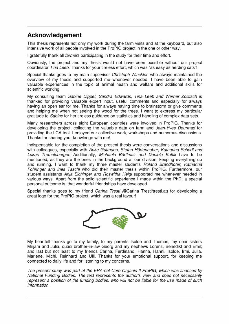
Special thanks goes to my friend Carina Trestl (©Carina Trestl/trestl.at) for developing a great logo for the ProPIG project, which was a real favour!
My heartfelt thanks go to my family, to my parents Isolde and Thomas, my dear sisters Mirjam and Julia, quasi brother-in-law Georg and my nephews Lorenz, Benedikt and Emil; and last but not least to my friends Carina, Ferdinand, Hanna, Hanni, Isolde, Irmi, Julia, Marlene, Michi, Reinhard and Ulli. Thanks for your emotional support, for keeping me connected to daily life and for listening to my concerns.
The present study was part of the ERA-net Core Organic II ProPIG, which was financed by National Funding Bodies. The text represents the author’s view and does not necessarily represent a position of the funding bodies, who will not be liable for the use made of such information.
Table of contents
List of tables .............................................................................................................. I
List of figures ........................................................................................................... IV
List of abbreviations ............................................................................................... IV
Summary .................................................................................................................. VI
Zusammenfassung ................................................................................................. VII
1 Introduction ......................................................................................................... 1
1.1 Animal health and welfare (AHW) of organic pigs.................................................... 1
1.1.1 Importance of farm animal welfare ...................................................................... 1
1.1.2 Concepts of animal health and welfare in farm animals ...................................... 2
1.1.3 On farm animal health and welfare assessment ................................................. 2
1.1.4 Animal health and welfare of organic pigs........................................................... 3
1.2 Environmental impact (ENV) of organic pig husbandry systems ........................... 9
1.3 Association between AHW and ENV of organic pig husbandry systems ..............12
1.4 ERA-net Core Organic II project ProPIG ..................................................................14
2 Objectives of the thesis .................................................................................... 15
3 Animals, Materials and Methods ..................................................................... 16
3.1 Overall study design .................................................................................................16
3.2 Inclusion criteria for participating farms .................................................................17
3.3 Data collection on farm .............................................................................................17
3.3.1 On farm data collection tool ...............................................................................17
3.3.2 Animal health and welfare (AHW) ......................................................................18
3.3.2.1 Animal-based parameters ...........................................................................18
3.3.2.2 Resource-based parameters .......................................................................21
3.3.2.3 Parameters further describing the husbandry system ..................................22
3.3.3 Environmental impact (ENV)..............................................................................23
3.4 Environmental impact – Life cycle assessment methodology ...............................24
3.4.1 System boundaries and functional unit ..............................................................24
3.4.2 Production chains (PC) ......................................................................................24
3.4.3 Additional calculations and assumptions regarding performance parameters ....25
3.4.3.1 Live weight ..................................................................................................25
III
3.4.3.2 Feed intake and Feed conversion rate ........................................................25
3.4.4 Additional calculations for system comparison ...................................................27
3.4.5 Overview of sources of emissions .....................................................................28
3.4.6 Environmental impact of feed production ...........................................................28
3.4.7 Environmental impact of pig management .........................................................30
3.4.7.1 CH4 emissions .............................................................................................30
3.4.7.2 Retention and Excretion of N and P ............................................................31
3.4.7.3 Livestock manure ........................................................................................31
3.4.7.4 Livestock manure outdoors .........................................................................32
3.4.8 Characteristics of the husbandry system investigated ........................................33
3.4.8.1 Animal performance and production data ....................................................33
3.4.8.2 Housing (floor type) and manure management ...........................................36
3.5 Associations between AHW and ENV ......................................................................39
3.6 Data analysis .............................................................................................................41
3.6.1 Animal health and welfare (AHW) ......................................................................41
3.6.1.1 Data management and statistics .................................................................41
3.6.1.2 Inter-observer reliability ...............................................................................41
3.6.2 Environmental impact (ENV)..............................................................................42
3.6.2.1 System comparison .....................................................................................42
3.6.2.2 Correlations .................................................................................................42
3.6.2.3 Hierarchical cluster analysis ........................................................................42
3.6.3 Associations between AHW and ENV ................................................................45
4 Results and discussion .................................................................................... 46
4.1 Animal health and welfare (AHW) .............................................................................46
4.1.1 Inter-observer reliability (IOR) ............................................................................46
4.1.2 Descriptive farm characteristics .........................................................................47
4.1.3 AHW at current location level .............................................................................50
4.1.4 AHW at farm system level .................................................................................51
4.1.5 Correlation between AHW and productivity ........................................................53
4.1.6 Discussion .........................................................................................................59
4.1.7 Conclusions .......................................................................................................66
4.2 Environmental impact (ENV) .....................................................................................67
4.2.1 ENV of production chains in different husbandry systems .................................67

IV
4.2.2 Correlation between farm characteristics and ENV ............................................69
4.2.3 Cluster analysis regarding ENV of organic pig husbandry systems....................71
4.2.4 Discussion .........................................................................................................78
4.2.5 Conclusion .........................................................................................................82
4.3 Associations between AHW and ENV ......................................................................83
4.3.1 Environmental cluster characteristics (GHGE, AP and EP) ................................83
4.3.2 AHW in the ENV clusters ...................................................................................84
4.3.2.1 GOOD% at PC level of ENV clusters ..........................................................84
4.3.2.2 GOOD% per animal category (SO, WE, FA) of ENV clusters ......................84
4.3.2.3 Individual AHW parameters of ENV clusters ...............................................84
4.3.3 Correlation between ENV and GOOD% ............................................................86
4.3.4 Discussion .........................................................................................................86
4.3.5 Conclusion .........................................................................................................91
5 General discussion ........................................................................................... 92
5.1 Main results of the study ..........................................................................................92
5.2 Methodological considerations ................................................................................93
5.2.1 Challenges of a multidisciplinary approach ........................................................94
5.2.2 Farm selection ...................................................................................................95
5.2.3 Number of farms per system..............................................................................95
5.2.4 ‘Husbandry system’ as level of assessment .......................................................96
5.2.5 Sampling strategy on farm .................................................................................96
5.2.6 Inter-observer reliability and exclusion of AHW parameters ...............................97
5.3 Overall conclusions...................................................................................................98
References ............................................................................................................ 101
Appendix 1 – Definitions of animal-based parameters ..................................... 110
Appendix 2 – Additional Tasks Accomplished During the PhD Study Period 116
I
List of tables
Table 1: Prevalences of selected animal-based parameters reported in studies of on-farm assessment of pregnant and lactating sows, weaners and fatteners (AC= animal categories with SO=pregnant sows, LS= Lactating sows, WE= weaners, FA=fatteners; Prevalence (% [mean or median; if both were mentioned in a study, median was included here]), n animals= number of animals included in study, depending on information in the study, total number of animals and/or minimum – maximum number of animals, n farms= number of farms included in the study; System C=Conventional, O=organic, na=not specified) ......................................................................................... 6
Table 2: Characteristics and greenhouse gas emissions (GHGE, kg CO2-eq/FU), acidification potential (AP, g SO2-eq/FU) and eutrophication potential (EP, g PO4-eq/FU) of selected LCA studies on pig production (FU=Functional unit) ......................................................11
Table 3: Definition of the three organic pig husbandry systems indoor, outdoor and partly outdoor. .........................................................................................................................16
Table 4: Scoring scales for animal-based parameters used in the study (WE = Weaner, FA = Fattener, SO = Pregnant sows. .....................................................................................19
Table 5: Overview of selected resource parameters assessed in the study (WE=Weaner, FA=Fattener, SO= Pregnant sows) ...............................................................................21
Table 6: Description of production chains by husbandry system ...........................................25
Table 7: Characterisation of feedstuff of fattener diets ..........................................................27
Table 8: Recommendation for digestible lysine (Alibert, 2014) .............................................27
Table 9: Categories of sources of environmental impact of pig production according to Dourmad et al. (2014) ...................................................................................................28
Table 10: Emission factors depending on manure type and litter quality (variation factor) occurring during animal keeping (in-house storage) according to Rigolot et al. (2010b) 32
Table 11: Emission factors for manure storage depending on manure type and storage period (variation factor) according to Rigolot et al. (2010b) and Dourmad et al. (2014) .32
Table 12: Emission factors for manure spreading depending on manure type and spreading type (variation factor) (Rigolot et al., 2010b, Dourmad et al., 2014) ...............................32
Table 13: Emission factors for NH3, N2O, N2 and N03 in outdoor paddocks ..........................33
Table 14: System characteristics for LSU (number of livestock unit), number of sows present at the production chain visit, number of slaughtered fattening pigs/year and Livestock Unit. N=Number of production chains. ...........................................................................33
Table 15: Characteristics of the animal production stages by system. N=Number of production chains. .........................................................................................................34
Table 16: Characteristics of dietary nutrient content and feed consumption by system. FCR=Feed conversion rate, N=Number of production chains. .......................................36
Table 17: Frequency and percentages of floor type for lactating and pregnant sows, weaners and fattening pigs kept in the systems indoor (IN) and partly outdoor (POUT) (shares above 20% are in bold characters; the floor type of percentage of animal categories that are kept within one production chain partly outdoors, are highlighted in square brackets). N=Number of production chains. ...................................................................................37
Table 18: Type and frequency of manure treatment by system. N=Number of production chains. ...........................................................................................................................38
II
Table 19: Results from inter-observer reliability tests before farm visits from in total three training/IOR sessions (same trainer/gold standard but different trainees each). Exact percentage agreement is given as median (min - max) across all observer - gold standard pairs. Agreement for categorical parameters (respiratory problems and diarrhoea) was based on separate scores, i.e. diarrhoea score 0, 1, 2. Median number of groups observed was 10 (range 7 to 10) for all sow parameters but pigs needing hospitalisation (n = 7, range 4 to 10), and 10 (range 10 to 21) for weaner and fattener parameters except ectoparasites (n = 10, range 6 to 21). Prevalence = median gold standard prevalence (Q25, Q75; n of groups; for G prevalence at group level and n only) across all three tests. For prevalence of categorical parameters (respiratory problems and diarrhoea) score 1 and 2 were combined. Data where observers did not reach 70 % agreement are not included, to show exactly the IOR data relevant for AHW data used in the results. A/G= assessed at animal (A) or group (G) level; SO = sows, WE = weaners, FA = fatteners................................................................................................................46
Table 20: Results from repeated inter-observer reliability tests of selected resource-based parameters before farm visits. Exact agreement is given as median (min - max) across all observer - gold standard pairs. The categorical parameter feed supply was not combined, i.e. ad libitum 0 and 1 were kept as such and compared to gold standard. Prevalence = median gold standard prevalence (for G prevalence at group level and n only). For prevalence of categorical parameters (feed supply) percentage of groups not fed ad libitum is presented. Median number of groups observed for feed supply and number of drinkers was 10 (FA/WE: range 10 to 21; SO feed supply: range 7 to 10, SO number of drinkers: range 6 to 10). G = assessed at group level; SO = sows, WE = weaners, FA = fatteners. ...............................................................................................47
Table 21: Numbers of farms per country and husbandry system. AT = Austria, CH = Switzerland, DE = Germany, IT = Italy, CZ = Czech Republic, DK = Denmark, FR = France, UK = United Kingdom. ......................................................................................47
Table 22: Percentage (%) of animals kept outdoors per animal category on partly outdoor farms (SO = sows, WE = weaners, FA = fatteners; LS= lactating sows). .......................47
Table 23: Number and percentage (%) of farms per husbandry system and numbers of farms per production type (animal categories on farm: SO = sows, WE = weaners, FA = fatteners). Number of animals relate to animals present at farm visit. Breed C = conventional, U = unconventional, M = C and U or crosses between the two. ...............48
Table 24: Number of farms where animals (SO = sows, WE = weaners, FA = fatteners) were assessed indoors, outdoors or both by animal category. Both = n farms where animals of a stage were assessed indoor and outdoor (n is included in indoor and outdoor). Total number of farms = 74. ...................................................................................................48
Table 25: Characteristics (number of farms, Median, minimum and maximum) of farm size and management related aspects per system (IN, POUT, OUT) ...................................49
Table 26: Number of farms per system conducting different management practices in suckling piglets per system (na= not assessed in OUT) ................................................49
Table 27: Number of assessed groups and number of animals (min, median, max) per assessed group/farm and characteristics of resources by animal category and system (SO=pregnant sows, WE=weaners, FA=fatteners; mdn= median) .................................50
Table 28: Median prevalences and Q25, Q75 for animals assessed indoors or outdoors, respectively, and results of Wilcoxon rank sum tests for current location effect (p). Prevalences with different superscripts within a row differ at p ≤ 0.05. Significant differences are highlighted in bold. AC = animal category (SO = sows, SP= Suckling piglet, WE = weaners, FA = fatteners). %a = percent of affected animals, %g = percent of affected groups. na = not tested for differences. N=number of farms .........................54
III
Table 29: Median (Mdn) prevalences and Q25, Q75 for assessed animals per farm system (IN: indoor, POUT: partly outdoor, OUT: outdoor). p = result of global Kruskal-Wallis test for system effect. Prevalences with different superscripts within a row differ at p ≤ 0.05 in a pairwise system comparison with Wilcoxon rank sum tests and Bonferroni-Holm correction for three tests. AC = animal category (SO = sows, SP= Suckling piglets, WE = weaners, FA = fatteners). %a = percent of affected animals, %g = percent of affected groups. na = not tested for differences. N= number of farms .........................................56
Table 30: Spearman’s Rho’s correlations (r [Spearman Rho´s correlation coefficient], p [ns=not significant; *=p<0.05; **=p<0.01; ***=p<0.001], (n [number of observations]) between performance measures and selected animal-based parameters. (SO= sow, SP= Suckling piglets, WE=weaners, FA=fatteners) .......................................................58
Table 31: Environmental impact of organic pig production in three husbandry systems (IN, POUT, OUT): GHGE, AP and EP per 1000 kg live weight at slaughter .........................67
Table 32: Correlations (Spearman’s Rho’s correlation test) between farm characteristics (rows) and environmental impact indicators (columns) for 61 production chains (three production chains had to be excluded due to a missing animal category at farm) ..........70
Table 33: Number of production chains per system (IN, POUT, OUT) in clusters (clusters subjected to further statistical tests are highlighted in grey; number of production chains per system in Cluster 14, Cluster 2 and Cluster 3 did not differ significantly (p=0.13)) ...71
Table 34: Environmental impacts in GHGE, AP and EP per 1000kg live weight at slaughter by cluster (total N=59 production chains) (clusters subjected to further statistical tests are highlighted in grey) ..................................................................................................72
Table 35: Cluster characteristics regarding number of sows on PC at farm visit, average number of slaughtered fattening pigs/year and number of livestock units (LSU) ............73
Table 36: Characteristics of the animal production stages by cluster ....................................74
Table 37: Characteristics of dietary nutrient content and feed consumption by cluster .........75
Table 38: Relative contribution of feed stuff category in the different clusters .......................76
Table 39: Classification of production chains per cluster according to deficient, excess or sufficient amount of digestible lysine in the diets for growers and finishers; N=total number of PC per cluster ...............................................................................................77
Table 40: GHGE, AP and EP per 1000kg live weight at slaughter by ENV clusters (n=38 PCs) ..............................................................................................................................83
Table 41: GOOD% per ENV cluster (N = number of PCs; Kruskal-Wallis test) .....................84
Table 42: GOOD% by animal category (SO = sows, WE = weaners, FA = fatteners) per ENV cluster (N = number of PCs; Kruskal-Wallis test). ..........................................................84
Table 43: Median prevalences (Q25, Q75; n) of animal health and welfare parameters per ENV cluster (Kruskal-Wallis test) (AC= Animal category, SO = sows, WE = weaners, FA = fatteners). %a = percent of animals, %g = percent of groups. na = not tested ............85

IV
List of figures
Figure 1: Description of weaning and fattening (=growers and finishers) stages (source: Brandhofer (2014), adapted) .........................................................................................26
Figure 2: Hierarchical cluster analysis of 59 PCs on the basis of PC specific AP, EP and GHGE; shown is the selection criteria R-Squared for possible number of Clusters (R-Squared*Number of Clusters)........................................................................................43
Figure 3: Hierarchical cluster analysis of 59 PCs on the basis of PC specific AP, EP and GHGE; shown are the selection criteria Pseudo T-Squared and pseudo F statistics for possible number of Clusters ..........................................................................................43
Figure 4: Hierarchical cluster analysis of 59 PCs on the basis of PC specific AP, EP and GHGE; shown is the dendrogram of average linkage cluster analysis with all possible number of clusters. The green lines indicate the two levels chosen for cluster description and further statistical analysis, respectively. ..................................................................44
Figure 5: Mean relative contribution of the different sources to GHGE, AP and EP based on data from IN (n=24), POUT (n=30) and OUT (n=10) production chains .........................68
Figure 6: Mean relative contribution of the different animal categories to GHGE, AP and EP based on data from IN (n=24), POUT (n=30) and OUT (n=10) production chains .........69
Figure 7: Mean relative contribution of the different sources to GHGE, AP and EP by cluster (total n=59; CL1=Cluster 1 (n=18), CL2=Cluster 2 (low ENV cluster) (n=21), CL3=Cluster 3 (high ENV cluster) (n=14), CL4= Cluster 4 (n=4), CL5=Cluster 5 (n=2), CL 14= Cluster 14 (intermediate ENV cluster) (n=22) ....................................................72
Figure 8: GHGE (left), AP (centre), and EP (right) plotted against GOOD% (vertical axis) (n=38 PCs) ....................................................................................................................86
List of abbreviations
AC Animal category
AHW Animal health and welfare
AP Acidification potential
AT Austria
BCS Body condition score (with low BCS= thin and high BCS= fat)
CH Switzerland
CP Crude protein (in g/kg)
CW Carcass weight (kg)
CZ Czech Republic
DE Germany
DK Denmark
dLys Digestible lysine
ENV Environmental impact
EP Eutrophication potential
Eq Equivalents
FA Fattening pig
FR France
V
GHG Greenhouse gas
GHGE Greenhouse gas emission (global warming potential)
GOOD% Animal health and welfare summary score
IN Indoor with concrete outdoor run
IT Italy
Kg Kilogram
LCA Life Cycle Assessment
LSU Livestock Unit (LSU) per farm or production chain: calculated on the basis of present pigs (other animals were not taken into account) on farm at the farm or production chain level, by using the following rates for converting numbers of animals into LSU: Lactating or pregnant sow = 0.3 LSU, weaner = 0.07 LSU, fattener = 0.15 LSU
LW Live weight at slaughter (kg)
ME Metabolisable Energy (ME content in MJ ME/kg)
N Number
OUT Outdoors
PC Production chain
POUT Partly outdoors
t Tons
Tot P Total phosphorus (in g/kg)
Yr year
C Carbon
CH4 Methane
CO2 Carbon dioxide
LUC Land Use Change
MCF Methane Conversion Factor
N Nitrogen
N2 Molecular nitrogen
NH3 Ammonia
NOX Nitrogen oxides
NO3 Nitrate
N2O Nitrous oxide (laughing gas)
P Phosphorus
SO Sow
UK United Kingdom
WE Weaner
VI
Summary
Organic pig husbandry systems in Europe are diverse - ranging from indoor systems with concrete outside run to outdoor systems all year round. The level of animal health and welfare (AHW) and environmental impact (ENV) has never been quantified for those systems using on-farm data. Furthermore it is often discussed, that husbandry systems common in organic farming (e.g. outdoor systems) enhance AHW but impair ENV.
In this thesis (1) AHW, (2) ENV and (3) the association between AHW and ENV was assessed for three different organic pig husbandry systems. In total 74 pig farms in eight European countries were included. The husbandry systems were defined as indoor (IN; n=34), partly outdoor (POUT; n=28) and outdoor (OUT; n=12).
(1) AHW was assessed in pregnant sows (SO), weaners (WE) and fattening pigs (FA). Across systems, prevalences of most AHW areas were low; exceptions were respiratory problems (IN, POUT), diarrhoea (IN), vulva deformation (IN, OUT) and short tails (IN, POUT). Total suckling piglet losses should be improved in all three systems. OUT had advantages regarding several areas of AHW, which could be explained by the outdoor specific environment, e.g. respiratory problems (better air quality), diarrhoea (less exposure to faeces) and lameness (softer lying and walking surfaces). POUT farms kept SO in most cases outdoors and WE/ FA similar to IN farms, which was reflected in the AHW results.
(2) A life cycle assessment (LCA) was conducted to quantify ENV for the criteria greenhouse gas emissions, acidification and eutrophication potential of the three husbandry systems. LCA was calculated for 64 production chains (PC), consisting mainly of farrow to finish farms or combined breeding and fattening only farms. Emissions were influenced mainly by feed and direct emissions from excreta with the fattening stage as the main contributor. Regarding greenhouse gas emissions, no differences were found between systems. POUT showed lower acidification potential than IN and lower eutrophication potential than OUT. Hierarchical cluster analysis revealed three clusters: a ‘low ENV’ cluster (lowest median for all criteria); an ‘intermediate ENV’ cluster (intermediate medians for all criteria) and a ‘high ENV’ cluster (highest median for all criteria). One of the main differences was a significantly lower fatteners' feed conversion rate in the low ENV cluster.
(3) No significant association was found between AHW and ENV when comparing the ENV clusters with regard to an overall AHW summary score (GOOD%), summary scores per animal category (GOOD%_SO, GOOD%_WE or GOOD%_FA) and single animal-based parameters or correlations between GHGE, AP, EP and GOOD%. The main reasons for a lack of associations between AHW and ENV may be the fact that LCA includes impact areas (e.g. manure storage and spreading, emissions during feed production), which do not necessarily relate to AHW.
It can be concluded, that European organic pigs kept in all three types of husbandry systems (IN/POUT/OUT) may experience high levels of AHW and have low ENV. The variation of both, AHW and ENV, was in most cases higher within a husbandry system than between, indicating a potential for improvement in all systems e.g. through farm (PC) individual management strategies. Furthermore the results show advantages of POUT regarding ENV and OUT regarding AHW, which may serve as a basis for the further development of organic pig husbandry systems. The lack of association between AHW and ENV found in this study does not necessarily mean that no association exists. Still, this study generated a starting point to explore associations between AHW and ENV to be tested either on a larger number of PC or between specific AHW and ENV areas.

VII
Zusammenfassung
Die Haltung von Bioschweinen in Europa rangiert von ganzjähriger Freilandhaltung bis zu reinen Stallhaltungssystemen mit Auslauf. Tiergesundheit und Wohlergehen sowie Umweltwirkung dieser Haltungssysteme wurden bislang nicht anhand von einzelbetrieblichen Daten quantifiziert. Ziel der Dissertation war (1) die Tiergesundheit und Wohlergehen (AHW), (2) die Umweltwirkung (ENV) und (3) den Zusammenhang zwischen AHW und ENV von Schweinen in drei verschiedenen Bio - Haltungssystemen zu erheben und zu analysieren. Dazu wurden Daten von insgesamt 74 Betrieben in acht europäischen Ländern erhoben. Die Haltungssysteme wurden folgendermaßen definiert: Stallhaltung mit Auslauf (IN; n=34), teilweise Freilandhaltung (POUT; n=28) und Freilandhaltung (OUT; n=12).
(1) AHW wurde anhand von tierbezogenen Parametern bei tragenden Sauen (SO), Aufzuchtferkeln (WE) und Mastschweinen (FA) erfasst. Über die Systeme hinweg waren die Prävalenzen in den meisten AHW Bereichen niedrig, mit Ausnahme von Atemwegsproblemen (IN, POUT), Durchfall (IN), Vulvavernarbungen (IN, OUT) und kurzen Schwänzen (IN, POUT). In allen Haltungssystemen bedarf es Verbesserungen hinsichtlich der Saugferkelverluste. In einigen Parametern gab es keine Unterschiede zwischen den Systemen. OUT hatte Vorteile in Bezug auf Atemwegsgesundheit und Durchfall (WE, FA), sowie Lahmheit (SO), die auf die spezifische Haltungsumwelt im Freiland (z.B. bessere Luftqualität und weichere Liegeflächen) zurückgeführt werden können. In POUT wurden vorrangig SO im Freiland gehalten, WE und FA hingegen ähnlich wie in IN; dies spiegelte sich in den Ergebnissen wider.
(2) Eine Lebenszyklusanalyse (LCA) wurde zur Quantifizierung der Umweltwirkung (ENV) für die Kriterien Treibhausgase, Eutrophierungspotential und Versauerungspotential) der drei Bioschweine - Haltungssysteme durchgeführt. Für die Bewertung der Produktionsphase (Aufzucht bis zum Hoftor) wurden spezialisierte Ferkelaufzucht- und Mastbetriebe als Produktionskette (PC) kombiniert; insgesamt wurde die LCA für 64 PC berechnet. Futtermittel und direkte Emissionen aus den Exkrementen sind die Hauptemissionsquellen, wobei die Mastschweine den größten Anteil verursachen. Treibhausgase unterschieden sich nicht signifikant zwischen den Haltungssystemen. POUT hatte ein signifikant niedrigeres Versauerungspotenzial als IN und geringeres Eutrophierungspotenzial als OUT. Eine hierarchische Clusteranalyse ergab drei Cluster: einen ‚niedrigen ENV’ Cluster mit den niedrigsten Medianen in allen Kriterien, einen ‚mittleren ENV’ Cluster mit mittleren Medianen in allen Kriterien und einen ‚hohen ENV’ Cluster mit den höchsten Medianen in allen Kriterien. Der Hauptunterschied war die bessere Futterverwertung der Mastschweine im Cluster mit niedriger ENV.
(3) Im Vergleich der ENV Cluster mit AHW anhand eines Summenparameters für Tiergesundheit und Wohlergehen (Gesamtscore GOOD% und GOOD% für die einzelnen Tierkategorien), einzelner tierbezogener Parameter sowie Korrelationen zwischen den ENV Kriterien und GOOD% wurde kein signifikanter Zusammenhang gefunden. Wesentlich für das Fehlen eines Zusammenhangs zwischen AHW und ENV dürfte die gesamtbetriebliche Lebenszyklusanalyse sein, die Bereiche inkludiert, die nicht notwendigerweise Auswirkung auf AHW haben (z.B. Wirtschaftsdüngerlagerung, Emissionen aus der Futtermittelproduktion).
Alle drei Bioschweine–Haltungssysteme haben grundsätzlich das Potential, gute Tiergesundheit und Wohlergehen und geringe Umweltwirkungen zu gewährleisten. Die Variation von AHW und ENV war meist innerhalb der Systeme größer als zwischen den Systemen und deutet damit auf ein allgemeines Optimierungspotenzial in allen Systemen, z.B. durch betriebsspezifische Managementmaßnahmen, hin. Die Ergebnisse zeigen, dass POUT hinsichtlich ENV und OUT hinsichtlich AHW als Anregung für die Entwicklung der biologischen Schweinehaltung dienen können. Die vorliegende Arbeit stellt weiterhin eine Ausgangsbasis für zukünftige Untersuchungen anhand größerer Stichproben oder zwischen spezifischen AHW- und ENV-Bereichen dar.

1
1 Introduction
Since the 1990´s, organic farming has rapidly developed in almost all European countries (Früh et al., 2014). This general development was supported by financial aids within agri-environmental programs (e.g. EC No. 2078/92). Also organic pig farming has gained interest in Europe, but the pork sector still ranks relatively low within organic livestock production and particularly in comparison to the sheep and bovine sector (Lernoud and Willer, 2015). In the European Union the number of organic pigs has increased (Früh et al., 2014, Lernoud and Willer, 2015); e.g. between 2007 and 2013 the organic pig sector grew by 31 %, and with about 0.7 million animals it represented 0.5 % of the total number of pigs in the European Union in 2013 (Lernoud and Willer, 2015).
Within Europe, organic pigs are produced according to the general principles of organic farming (IFOAM, 2014) and national and international regulations (e.g. EC No. 834/2007 and 889/2008) as well as private standards (Edwards et al., 2014b). The COREPIG project, which was performed in six European countries (from 2007 to 2010), showed that the housing conditions of pigs and breeds vary between countries. Pigs may be kept completely outdoors, as in most UK farms, or always indoors with access to an outdoor run, e.g. in most farms in German speaking countries. Furthermore, both systems, indoor and outdoor, may be combined on one farm for different production stages or during different seasons in different production stages or seasons for example in Denmark (Früh et al., 2014, Prunier et al., 2014a).
Animal farming faces various challenges – climate change as well as animal health and welfare are keywords reflecting the ongoing public and scientific discussion within the livestock sector (Goodland and Anhang, 2009, De Vries and de Boer, 2010, Gerber et al., 2013, Jacques, 2014). Doubts about environmental impact of agricultural production systems and deficits in animal health and welfare have led to increased awareness and discussions among consumers, scientists and, last but not least, farmers. The principles of organic agriculture (IFOAM, 2014) shall address the consumers’ demands and perceptions of healthy animals (Eurobarometer, 2007) which are able to perform natural behaviours and cause little environmental impact.
In the last decades, the ongoing sustainability debate is characterized by different sustainability frameworks, ranging from environmental and social standards to corporate social responsibility and codes of good practices developed by universities, civil society, corporations and national and international institutions. The SAFA Guidelines (Sustainability Assessment of Food and Agriculture systems) were developed as an international reference document, a benchmark that defines the elements of sustainability. The SAFA guidelines highlight, that sustainability consists of four dimensions of sustainability: good governance, environmental integrity, economic resilience and social well-being. In the section environmental integrity the following themes are addressed: Atmosphere, Water, Land, Materials and Energy, Biodiversity and Animal Welfare (FAO, 2014b). The complexity of sustainability underlines the importance of multi-criteria assessments including the on-farm assessment of animal health and welfare and environmental impact of husbandry systems.
1.1 Animal health and welfare (AHW) of organic pigs
1.1.1 Importance of farm animal welfare
In general, the welfare status of farm animals has gained increased importance for consumers (Blokhuis et al., 2003). Especially at the European level, animal welfare has received growing attention within the last decades (Eurobarometer, 2007). Consumers in European countries associate organic animal husbandry and the related products with a high level of animal welfare (Spoolder, 2007, Zander and Hamm, 2010, Eurobarometer, 2007, Gade, 2002). As Cagienard et al. (2005) indicate, there is currently a trend in Europe to
2
provide consumers with meat produced in husbandry systems that are especially well adjusted to meet the behavioural needs of farm animals. The development of animal welfare standards is more advanced than standards regarding the environmental impact of meat production (de Jonge and van Trijp, 2013). For instance, in the UK the “Freedom Food” scheme was launched as cooperation between RSPCA (Royal Society for the Prevention of Cruelty to Animals) and the industry to improve animal welfare by setting housing standards considered benefiting animal welfare. In 1994, Bowes of Norfolk signed up as the first pig enterprise. Connected to “Freedom Food” is the Assurewel project, which is a collaboration between RSPCA, Soil Association and the University of Bristol and aims at developing a farm assurance scheme by assessing the health, physical condition and behaviour of farm animals. The Assurewel project includes the assessment of animal-based parameters (Freedom Food, 2015).
Due to the use of animal-based parameters included in the farm assurance scheme, the Freedom Food and Assurewel project approach can be regarded as advantageous. For a long-term market positioning of products related to higher animal health and welfare, this needs to be demonstrable in objective terms by assessing animal health and welfare on the basis of animal-based parameters on farm.
1.1.2 Concepts of animal health and welfare in farm animals
Organic animal husbandry is explicitly linked to underlying concepts of animal health and welfare (Vaarst and Alrøe, 2012). The principles of organic farming (health, ecology, fairness and care) explicitly and implicitly address the aim of a high animal health and welfare status. As a guiding principle of organic livestock husbandry, health is ‘not simply the absence of illness, but the maintenance of physical, mental, social and ecological well-being’, and ‘health’ is defined as ‘the wholeness and integrity of living systems’ (IFOAM, 2014).
Animal welfare science emerged in the 1970s, initially stimulated by public concern over the welfare of animals kept in the then new confinement production systems. Research originally intended to solve problems in confinement production systems, but many of the scientific methods have been proven applicable to animals in different systems (Fraser et al., 2013). Animal welfare requires value-based judgements when applied to any farming system (Edwards et al., 2014b). Broom (2011) states, that welfare scientists agreed that animal welfare is a scientific concept, as the term describes a potentially measurable quality of a living animal at a certain time. On the basis of intensive discussions amongst animal welfare scientists, different concepts of animal welfare have been developed during recent decades, emphasising the biological functioning of the animal (health, growth, productivity), the affective states of the animals (pain, suffering and other feelings and emotions) and naturalness (to live in as natural circumstances as possible, where animals can express their normal behaviour) (Fraser, 2003, Verhoog et al., 2007, Broom, 2011). Most approaches combine all three concepts, e.g. the Farm Animal Welfare Council suggests considering the ‘five freedoms’, representing ideal states of animals' welfare on farm (FAWC, 2009, Edwards et al., 2014b).
1.1.3 On farm animal health and welfare assessment
It is generally accepted, that the most valid on-farm assessment of animal welfare is obtained by using comprehensive animal health and welfare assessment systems, considering welfare issues that go beyond animal health (Johnsen et al., 2001, Sørensen and Fraser, 2010). Several protocols for farm animal welfare assessment at herd level have been developed and are currently available (Bracke et al., 2004, Main et al., 2007, Goossens et al., 2008, Welfare Quality®, 2009). The on-farm assessment of animal health and welfare is mainly based on a range of parameters, divided roughly into two categories: environment (resource)-based parameters, such as features of the housing system and management procedures, and animal-based parameters including behaviour, animal health measures and
3
physiological states, assessed directly at the animal or through farm specific records on performance or treatment data (e.g. losses, treatment incidences or replacement rate).
On-farm assessment should therefore include valid parameters that actually reflect the animals’ welfare state; animal-based parameters measure more validly than resource-based parameters the actual welfare state of the animals (Whay et al., 2007). The selection of widely accepted criteria is a challenging issue, due to the different views of animal welfare between individuals, e.g. between animal producers and non-producers (Sørensen and Fraser, 2010).
On farm assessment of animal health and welfare may be challenging, e.g. assessment of animal-based parameters is often time consuming (Andreasen et al., 2013) and requires sufficient training of the observers (Dippel et al., 2014b). The assessment of environmental (resource) parameters (e.g. length of stalls, feeding and drinking facilities) is considered as “fairly uncomplicated” and repeatability of resource-based parameters is usually not considered as a problem (Johnsen et al., 2001).
1.1.4 Animal health and welfare of organic pigs
Scientific studies addressing the main health and welfare concerns in organic pigs have recently been reviewed (Hovi et al., 2003, Bonde and Sørensen, 2004, Kijlstra and Eijck, 2006, Leeb et al., 2014, Lindgren et al., 2014, Edwards et al., 2014a, Sutherland et al., 2013). Due to the limited availability of on-farm assessment data, these studies gathered information on the animal health and welfare status of organic pigs in Europe using different sources of information. Information was either gained through farmer questionnaires (e.g. Herzog et al., 2006), clinical measures taken directly on the animal (e.g. Day et al., 2003, Leeb et al., 2010, Dippel et al., 2014b) or by slaughterhouse findings (e.g. Baumgartner et al., 2003, Etterlin et al., 2014). Even though interest in on-farm animal health and welfare increased in the last decades, limited data from on-farm assessment of animal-based parameters is available for animals kept in different husbandry systems within organic pig production in Europe. So far, on-farm assessments were conducted either only in one husbandry system (e.g. Day et al., 2003), or combined data from organic farms with different husbandry systems but differences in pig health and welfare between systems were not in the studies’ focus (e.g. Leeb et al., 2010, Dippel et al., 2014b). Data from organic and conventional farms were even combined (Scott et al., 2009). It is remarkable, that authors of on-farm assessment studies repeatedly reported high variability in prevalences of animal-based parameters (across different animal categories) between farms (Whay et al., 2007, Dippel et al., 2014b).
Adequate feeding of animals is considered as a challenge in organic livestock production as some nutritional inputs may be scarce (Zollitsch, 2007). One sign for inadequate feeding can be deviations from the optimal body condition score in sows. Poor body condition of organic sows ranged from not significantly different from accepted target values during pregnancy, at farrowing or at weaning (Day et al., 2003), 10.4% (Leeb et al., 2010) up to 18.8% (Dippel et al., 2014b). The definitions of poor body condition used in these three studies are very similar, but the studies differ between husbandry systems assessed. Day et al. (2003), assessed sows in 9 UK organic outdoor farms, while Dippel et al. (2014b) who identified thinness as the most frequent problem in organic sows, assessed organic sows across 100 European farms, both indoor and outdoor husbandry systems. As well in the survey of Leeb et al. (2010) organic sows across 40 organic Austrian pig farms in both indoor and outdoor husbandry systems (mainly indoor, few outdoor farms) have been reported. Other studies, which did not differentiate between organic and conventional systems found lower prevalences, e.g. a smaller survey conducted on seven organic and conventional label farms found 6% thin sows (Winckler et al., 2001), still higher in comparison with findings of Scott et al. (2009) with 5% of sows being either thin or over-fat in 82 organic or conventional farms (both indoor and outdoor) in the UK and the Netherlands.
4
However, overfeeding of sows resulting in fat sows is as well reported as a health and welfare problem, with 4.9% and 14.2%, respectively (Dippel et al., 2014b, Leeb et al., 2010). Regarding shoulder lesions, which are associated with low body condition, a median prevalence of 0.0% was reported in the mentioned survey from Leeb et al. (2010) with a maximum on one farm of 12.5%. Another animal-based parameter associated with nutrition and especially competition for food or restricted water access are vulva lesions and deformations due to vulva biting (Leeb et al., 2001). Vulva lesions and vulva deformations were rarely seen in organic sows (40 farms in Austria) with a median prevalence of 4.3% and 3.2%, respectively (Dippel et al., 2014b, Leeb et al., 2010). Dippel et al. (2014b) report a median prevalence of 3.5% for a combined vulva lesion and deformation score.
Lameness is a common disorder in sows (Nalon et al., 2013) and considered as a relevant welfare indicator, which as well represents an economic challenge to pig producers due to premature culling of sows and increased labour and medical treatment (Knage-Rasmussen et al., 2014, Nalon et al., 2013). Lameness is a multifactorial condition, depending both on management and sow genetics (Nalon et al., 2013). In the survey of Leeb et al. (2010) a median of 12.1% pregnant sows were reported as severely lame and 52.6% mildly lame, while almost no lame weaners and fatteners were found (0.0% and 1.8%, respectively). However, in a survey conducted a few years later, lameness was rarely found in organic outdoor sows with a median prevalence of 0.0% (Day et al., 2003, Dippel et al., 2014b), but prevalence varied considerably between farms, indicating that on some farms the problem is present (Dippel et al., 2014b). Knage-Rasmussen et al. (2014) assessed pregnant sows in 9 organic outdoor herds in Denmark; an average prevalence of 4.6% was found in winter (with 24.4% in conventional herds assessed in the same study), while in summer the average prevalence was higher (11%). Similar prevalences (mean 7%) were reported in a German study on lameness in organic pregnant sows (excluding lactating sows, including sows not pregnant yet) across 40 farms. The authors highlight the influence of on-farm management primarily through detection of lameness at an early stage and targeted prevention on the occurrence of lameness in sows (March et al., 2014)
Lesions arise either during fighting when unfamiliar pigs are mixed or as already described in the context of vulva lesions, due to competition for feed and other resources. Body lesions (skin damage) were rarely seen in weaners and growing/finishing pigs and sows outdoors kept outdoors in England (Day et al., 2003). In contrast, Leeb et al. (2010) report a median of 9.7% body lesions in weaners and 12.6% in fatteners, which were mainly kept indoors. Dippel et al. (2014b) report 12.5% and 7.9%, respectively, in organic sows injuries on anterior and hind body parts, in contrast to very low prevalences found by Leeb et al. (2010). Definitions of lesions used in Day et al. (2003) refer to an older study and are not mentioned in the study itself, while Dippel et al. (2014b) refer to Welfare Quality® (2009). Leeb et al. (2010) mention in general similar definitions as used in the latter study, but lesions were defined slightly larger, e.g. longish lesions had to be larger than 3 cm and round lesions >1 x 1 cm, while Dippel et al. (2014b) take also smaller lesions into account. These differences in the definitions can be considered as a reason for lower prevalences found in the Austrian study.
Tail lesions and consequently short tails may be a result of tail biting, which is considered as on of the main challenges in pigs kept indoors. Other reasons for short tails than tail-biting are also discussed, but difficult to examine, similarly the aetiology of ear necrosis is complex and diverse causes (e.g. microorganisms, environmental factors, immunosuppressive agents as well as mycotoxins) are reviewed by Pejsak et al. (2011). Additionally, Jaeger (2013) mentioned in a popular scientific article on tail biting, that mycotoxins in feedstuff cause necrosis, e.g. tail necrosis. Leeb et al. (2010), found tail necrosis already in suckling piglets, it might be assumed, that in these young piglets tail necrosis’ was not caused by tail-biting but by other causes, similarly to the aetiology of ear necrosis. In the same study conducted by Leeb et al. (2010), relatively low prevalences of tail lesions and short tails were found in weaners with a median of 0.0% and 3.4% (39 farms), respectively; however higher
5
prevalences were reported for fatteners with 0.5% and 13.3% (33 farms), respectively. This increase in short tails from weaners to fatteners may indicate that either in the growing period problems occur which result in an increased number of short tails, but as well it might be that the fatteners had more short tails due to other causes during their suckling and weaning period.
Diarrhoea is a multifactorial disease, which results from a challenged digestive system, challenged immune system and various stressors, especially during the weaning process (Leeb et al., 2014). The risk of post-weaning diarrhoea has been shown to decrease with increasing weaning weight and age. Different pathogens (e.g. E.coli) as well e.g. cleanliness of the weaning pen, low creep feed intake, temperature of the weaning pen, stocking procedure and air quality have been identified as risk factors for post-weaning diarrhoea, as reviewed in Leeb et al. (2014). Generally the minimum weaning age of 40 days in organic pig farming can be considered as advantageous regarding the occurrence of diarrhoea. In weaner and fattener groups on organic farms in Austria, diarrhoea was in median rarely seen, but the authors report a considerable variation between farms (range 0-100%, respectively) (Leeb et al., 2010). Differences between pig husbandry systems (indoor vs. outdoor) where not considered in the study.
Respiratory problems are also considered as an important welfare indicator, which should be assessed across animal categories. While respiratory problems were rarely seen in organic sows, median prevalence in weaner groups was 50.0% and 42.9% in fattener groups across Austrian organic pig farms (39 and 33 farms, respectively), however these prevalences represent the sum of signs of conjunctivitis, eye discharge and other signs of respiratory problems (Leeb et al., 2010). Respiratory problems were as well rarely seen in organic sows in another study (Dippel et al., 2014b), but the authors conclude, that signs of respiratory problems are difficult to detect outdoors, which was the case for about half of the sows assessed in the study.
One of the most widely discussed problems in organic sows are endo- and ectoparasites, due to the housing conditions and restrictions on prophylactic chemical measures (Edwards et al., 2014a). Baumgartner et al. (2003) found ectoparasites (detected in skin scrapings) in 29% (n=48 farms) of organic Austrian farms with sow units and in 59% (n=51 farms) of farms with finishing units. Similar results were presented for sows kept outdoors in the smaller survey by Day et al. (2003) in the UK. In contrast, Carstensen et al. (2002) did not find any clinical signs for ectoparasites in a Danish survey on 9 organic farms (weaners, fatteners and sows). However, infections of gastrointestinal pig endoparasites were repeatedly reported in different studies (Baumgartner et al., 2003, Etterlin et al., 2014).
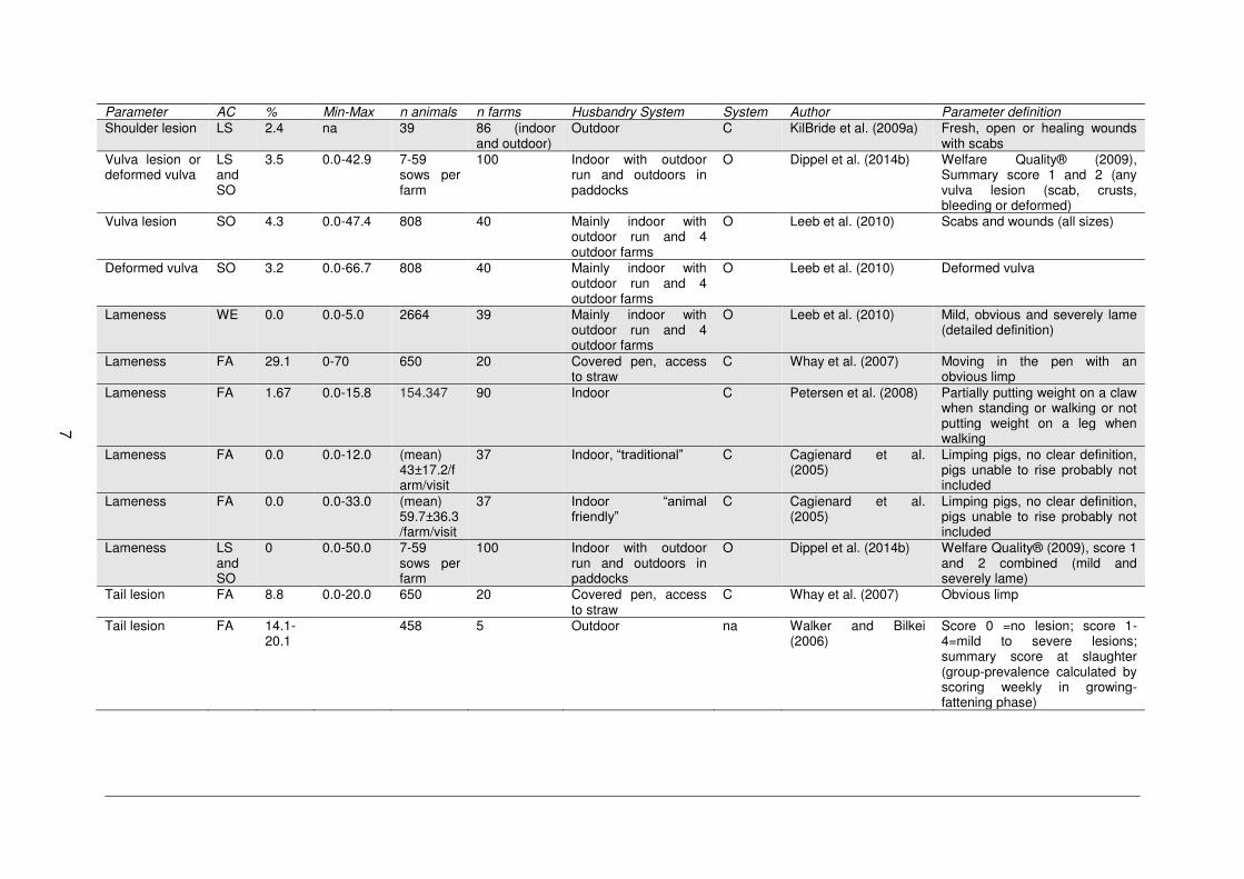
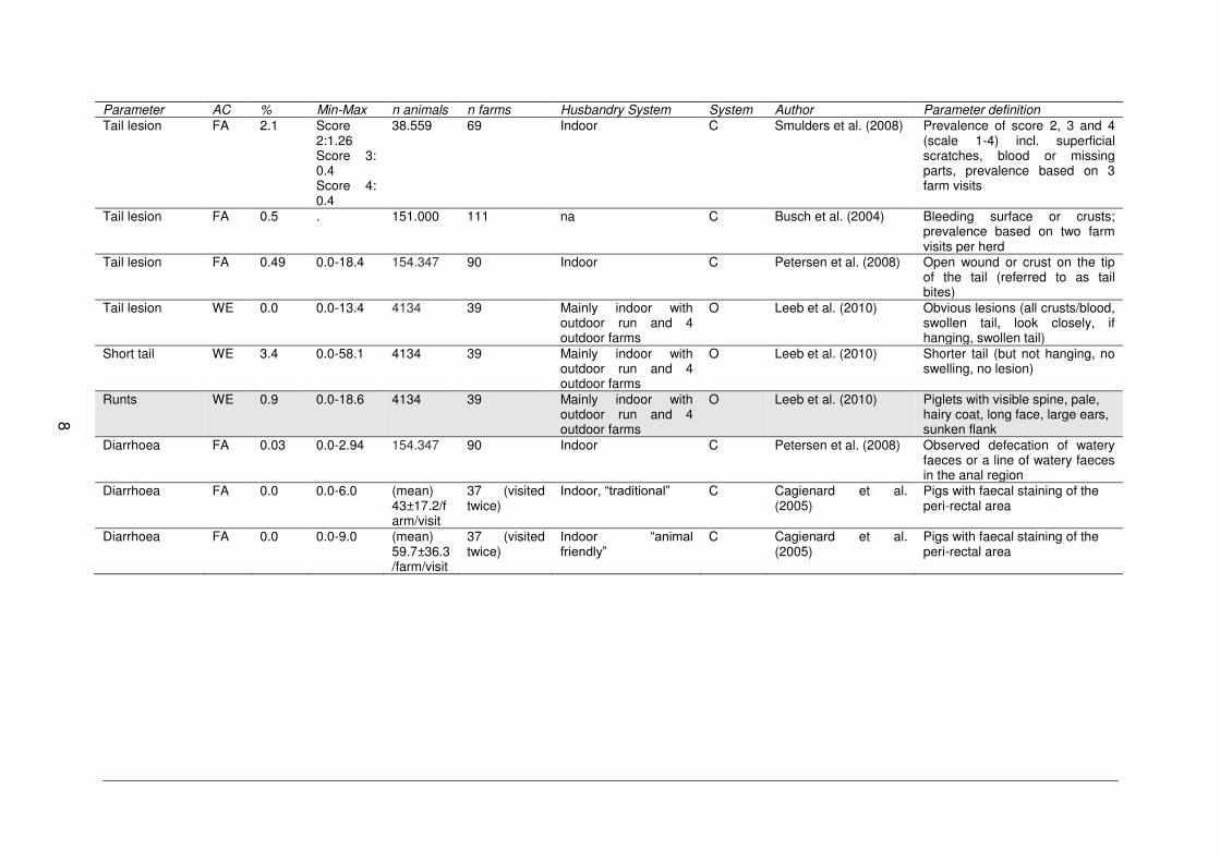
Table 1reports prevalences of selected clinical measures taken directly on the animal during on-farm assessments on organic and conventional farms. The present study focus is on AHW of organic pigs in different organic pig husbandry systems, a comparison to conventional husbandry systems was not intended. Still, some conventional studies were included in the following table for the interested reader. Some studies assessed pigs in different husbandry systems within one study, for example KilBride et al. (2009a) and Cagienard et al. (2005), others focused on one husbandry system, for example Zurbrigg (2006). Generally, this summary should not be assumed to be complete; rather it is intended to allow a comparison of the definitions used and of the results obtained. However, it has to be noted, that definitions of animal-based parameters vary between studies and therefore direct comparison is not always appropriate.
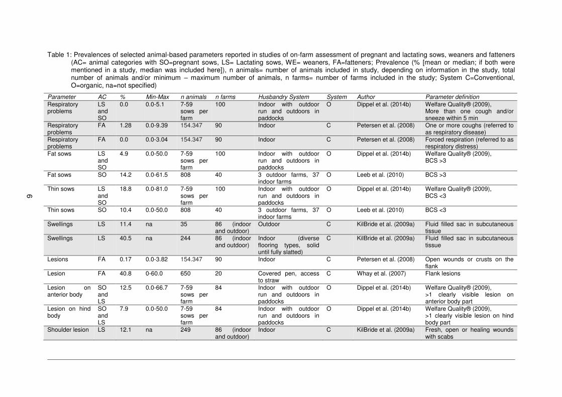
6
Table 1: Prevalences of selected animal-based parameters reported in studies of on-farm assessment of pregnant and lactating sows, weaners and fatteners (AC= animal categories with SO=pregnant sows, LS= Lactating sows, WE= weaners, FA=fatteners; Prevalence (% [mean or median; if both were mentioned in a study, median was included here]), n animals= number of animals included in study, depending on information in the study, total number of animals and/or minimum – maximum number of animals, n farms= number of farms included in the study; System C=Conventional, O=organic, na=not specified)
Parameter AC % Min-Max n animals n farms Husbandry System System Author Parameter definition Respiratory problems
LS and SO
0.0 0.0-5.1 7-59 sows per farm
100 Indoor with outdoor run and outdoors in paddocks
O Dippel et al. (2014b) Welfare Quality® (2009), More than one cough and/or sneeze within 5 min
Respiratory problems
FA 1.28 0.0-9.39 154.347 90 Indoor C Petersen et al. (2008) One or more coughs (referred to as respiratory disease)
Respiratory problems
FA 0.0 0.0-3.04 154.347 90 Indoor C Petersen et al. (2008) Forced respiration (referred to as respiratory distress)
Fat sows LS and SO
4.9 0.0-50.0 7-59 sows per farm
100 Indoor with outdoor run and outdoors in paddocks
O Dippel et al. (2014b) Welfare Quality® (2009), BCS >3
Fat sows SO 14.2 0.0-61.5 808 40 3 outdoor farms, 37 indoor farms
O Leeb et al. (2010) BCS >3
Thin sows LS and SO
18.8 0.0-81.0 7-59 sows per farm
100 Indoor with outdoor run and outdoors in paddocks
O Dippel et al. (2014b) Welfare Quality® (2009), BCS <3
Thin sows SO 10.4 0.0-50.0 808 40 3 outdoor farms, 37 indoor farms
O Leeb et al. (2010) BCS <3
Swellings LS 11.4 na 35 86 (indoor and outdoor)
Outdoor C KilBride et al. (2009a) Fluid filled sac in subcutaneous tissue
Swellings LS 40.5 na 244 86 (indoor and outdoor)
Indoor (diverse flooring types, solid until fully slatted)
C KilBride et al. (2009a) Fluid filled sac in subcutaneous tissue
Lesions FA 0.17 0.0-3.82 154.347 90 Indoor C Petersen et al. (2008) Open wounds or crusts on the flank
Lesion FA 40.8 0-60.0 650 20 Covered pen, access to straw
C Whay et al. (2007) Flank lesions
Lesion on anterior body
SO and LS
12.5 0.0-66.7 7-59 sows per farm
84 Indoor with outdoor run and outdoors in paddocks
O Dippel et al. (2014b) Welfare Quality® (2009), >1 clearly visible lesion on anterior body part
Lesion on hind body
SO and LS
7.9 0.0-50.0 7-59 sows per farm
84 Indoor with outdoor run and outdoors in paddocks
O Dippel et al. (2014b) Welfare Quality® (2009), >1 clearly visible lesion on hind body part
Shoulder lesion LS 12.1 na 249 86 (indoor and outdoor)
Indoor C KilBride et al. (2009a) Fresh, open or healing wounds with scabs
7
Parameter AC % Min-Max n animals n farms Husbandry System System Author Parameter definition Shoulder lesion LS 2.4 na 39 86 (indoor
and outdoor) Outdoor C KilBride et al. (2009a) Fresh, open or healing wounds
with scabs Vulva lesion or deformed vulva
LS and SO
3.5 0.0-42.9 7-59 sows per farm
100 Indoor with outdoor run and outdoors in paddocks
O Dippel et al. (2014b) Welfare Quality® (2009), Summary score 1 and 2 (any vulva lesion (scab, crusts, bleeding or deformed)
Vulva lesion SO 4.3 0.0-47.4 808 40 Mainly indoor with outdoor run and 4 outdoor farms
O Leeb et al. (2010) Scabs and wounds (all sizes)
Deformed vulva SO 3.2 0.0-66.7 808 40 Mainly indoor with outdoor run and 4 outdoor farms
O Leeb et al. (2010) Deformed vulva
Lameness WE 0.0 0.0-5.0 2664 39 Mainly indoor with outdoor run and 4 outdoor farms
O Leeb et al. (2010) Mild, obvious and severely lame (detailed definition)
Lameness FA 29.1 0-70 650 20 Covered pen, access to straw
C Whay et al. (2007) Moving in the pen with an obvious limp
Lameness FA 1.67 0.0-15.8 154.347 90 Indoor C Petersen et al. (2008) Partially putting weight on a claw when standing or walking or not putting weight on a leg when walking
Lameness FA 0.0 0.0-12.0 (mean) 43±17.2/farm/visit
37 Indoor, “traditional” C Cagienard et al. (2005)
Limping pigs, no clear definition, pigs unable to rise probably not included
Lameness FA 0.0 0.0-33.0 (mean) 59.7±36.3/farm/visit
37 Indoor “animal friendly”
C Cagienard et al. (2005)
Limping pigs, no clear definition, pigs unable to rise probably not included
Lameness LS and SO
0 0.0-50.0 7-59 sows per farm
100 Indoor with outdoor run and outdoors in paddocks
O Dippel et al. (2014b) Welfare Quality® (2009), score 1 and 2 combined (mild and severely lame)
Tail lesion FA 8.8 0.0-20.0 650 20 Covered pen, access to straw
C Whay et al. (2007) Obvious limp
Tail lesion FA 14.1-20.1
458 5 Outdoor na Walker and Bilkei (2006)
Score 0 =no lesion; score 1-4=mild to severe lesions; summary score at slaughter (group-prevalence calculated by scoring weekly in growing-fattening phase)
8
Parameter AC % Min-Max n animals n farms Husbandry System System Author Parameter definition Tail lesion FA 2.1 Score
2:1.26 Score 3: 0.4 Score 4: 0.4
38.559 69 Indoor C Smulders et al. (2008) Prevalence of score 2, 3 and 4 (scale 1-4) incl. superficial scratches, blood or missing parts, prevalence based on 3 farm visits
Tail lesion FA 0.5 . 151.000 111 na C Busch et al. (2004) Bleeding surface or crusts; prevalence based on two farm visits per herd
Tail lesion FA 0.49 0.0-18.4 154.347 90 Indoor C Petersen et al. (2008) Open wound or crust on the tip of the tail (referred to as tail bites)
Tail lesion WE 0.0 0.0-13.4 4134 39 Mainly indoor with outdoor run and 4 outdoor farms
O Leeb et al. (2010) Obvious lesions (all crusts/blood, swollen tail, look closely, if hanging, swollen tail)
Short tail WE 3.4 0.0-58.1 4134 39 Mainly indoor with outdoor run and 4 outdoor farms
O Leeb et al. (2010) Shorter tail (but not hanging, no swelling, no lesion)
Runts WE 0.9 0.0-18.6 4134 39 Mainly indoor with outdoor run and 4 outdoor farms
O Leeb et al. (2010) Piglets with visible spine, pale, hairy coat, long face, large ears, sunken flank
Diarrhoea FA 0.03 0.0-2.94 154.347 90 Indoor C Petersen et al. (2008) Observed defecation of watery faeces or a line of watery faeces in the anal region
Diarrhoea FA 0.0 0.0-6.0 (mean) 43±17.2/farm/visit
37 (visited twice)
Indoor, “traditional” C Cagienard et al. (2005)
Pigs with faecal staining of the peri-rectal area
Diarrhoea FA 0.0 0.0-9.0 (mean) 59.7±36.3/farm/visit
37 (visited twice)
Indoor “animal friendly”
C Cagienard et al. (2005)
Pigs with faecal staining of the peri-rectal area
9
1.2 Environmental impact (ENV) of organic pig husbandry systems
Numerous studies have already demonstrated that considerable environmental impact arises from agriculture. Livestock production exerts severe impact on air, water and soil quality due to the related emissions (De Vries and de Boer, 2010). According to FAO (2014a) the world´s livestock sector contributes 18 % of global greenhouse gas emissions.
Life cycle assessment (LCA) provides a valuable and consistent methodological framework to quantify the environmental impact within the life cycle of a product (Guinée et al., 2002, Basset-Mens et al., 2007). Hence several life cycle assessments (LCA) have been conducted during recent years to quantify the environmental impact, mainly greenhouse gas emissions (GHGE), acidification potential (AP) and eutrophication potential (EP) of animal husbandry systems (Dolman et al., 2012, Basset-Mens and van der Werf, 2005, Halberg et al., 2010). Due to high CH4 emissions from enteric fermentation, ruminants were in the focus of LCA, but GHGE of pork production has also to be considered in the light of high consumption of pork and pork products in the European Union.
LCA relates the environmental impact of a product to a functional unit (e.g. kg live weight at slaughter or kg product (e.g. pork)) (De Vries and de Boer, 2010), different system boundaries can be chosen for calculations, e.g. a cradle-to-farm gate or cradle-to-slaughterhouse or supermarket. Variations in chosen system boundaries, functional units and inventory input and output data (representative data, resources and emission factors used in the calculations) make it difficult to compare results of different LCA studies. To analyse the environmental impact of different pig husbandry systems, a cradle-to-farm gate calculation is suitable, as the post-farm gate stages of production most likely do not differ
between pigs reared in different systems – unless the carcasses are processed in a different way. Furthermore, according to Dalgaard et al. (2007), in a LCA of Danish pork production the contribution of emissions originating from processes in the slaughterhouse was the second smallest contributor to GHGE.
As Dolman et al. (2012) state, LCA studies so far have commonly been based on model scenarios or a small number of farms, which did not always cover farm-specific data from cradle to farm gate. Since livestock production is almost entirely non-organic within OECD countries, the majority of LCA studies published cover non-organic livestock products (De Vries and de Boer, 2010). De Vries and de Boer (2010) state that non-organic pork production systems within the OECD countries are usually homogeneous because of their rather standardised production method. Due to the limited availability of specific data for non-conventional production methods and farmers’ practices, general scenario data are often used in LCAs of farming systems (Basset-Mens et al., 2007). However, organic pig production is currently a relatively small, but nevertheless rapidly developing production system in the European countries. The production methods and husbandry systems for organic pigs in Europe vary more widely than within non-organic production systems. For instance, as already mentioned, a survey across eight European countries revealed that husbandry systems for organic pigs may vary from complete outdoor production on pasture to completely indoors with access to an outdoor run only (Früh et al., 2014). However, the environmental impact of organic pig production has rarely been assessed. Until now, no study has been conducted which has analysed the greenhouse gas emissions (GHGE), acidification and eutrophication potential (AP and EP, respectively) of a large number of organic farrowing to finishing pig farms across several European countries based on individual farm production and detailed housing system data.
10
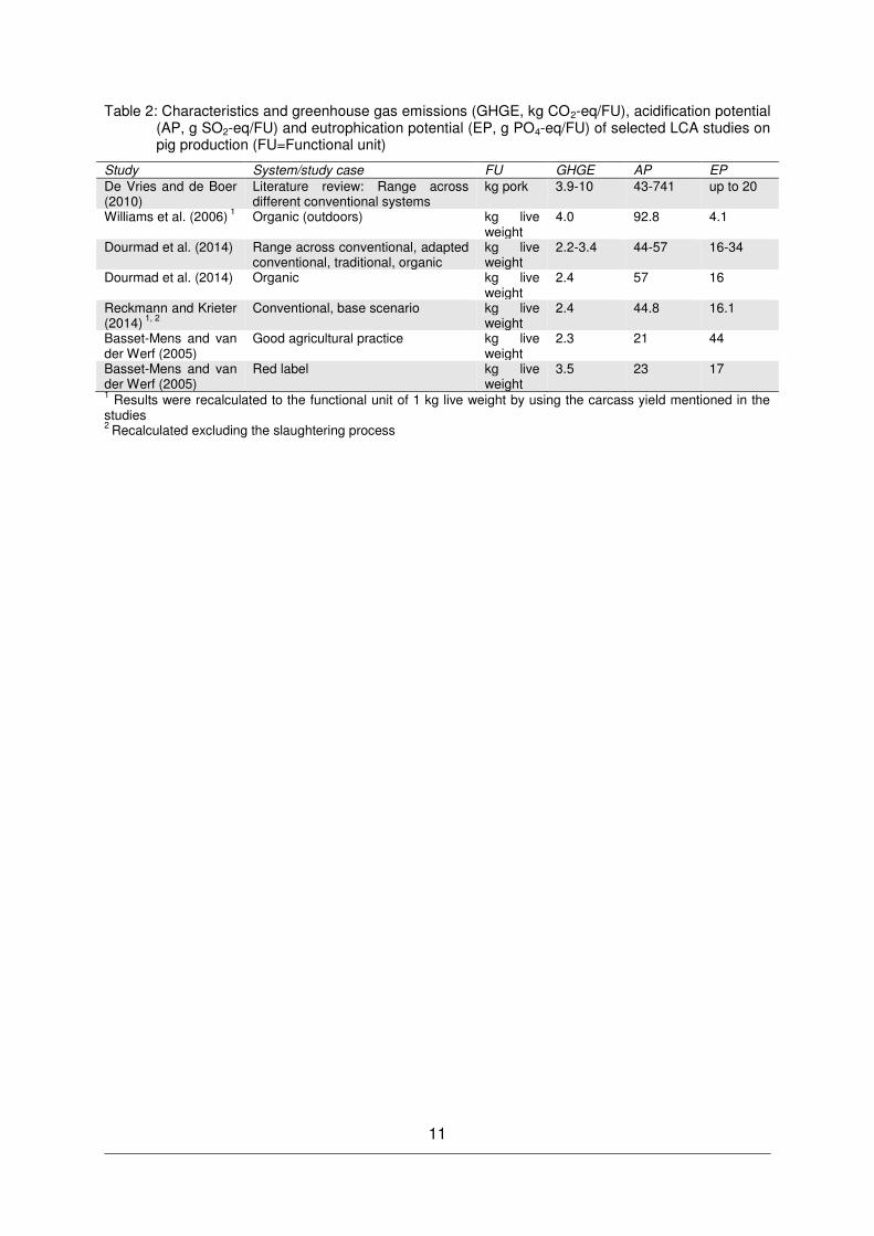
De Vries and de Boer (2010) reviewed (besides other livestock products) six comparable LCA studies of pork products (criteria: OECD country, non-organic production, type of LCA methodology, allocation method used, definition of system boundaries). When recalculating the results to the same functional unit (kg pork product), the production of 1 kg of pork (product) resulted in 3.9-10 kg CO2-eq, 43-741 g SO2-eq and up to 20 g PO4-eq (Table 2). Large variation was found, especially regarding acidification and eutrophication potential.
The study conducted by Williams et al. (2006), who analysed the environmental impact organic and conventional pig production, was considered in De Vries and de Boer (2010) literature review. However, as the calculations for the organic production systems were not taken into account, the results are listed additionally here. GHGE and AP were higher than in Dourmad et al. (2014), but EP remarkably lower. Dourmad et al. (2014) evaluated the environmental impact of 15 European pig farming systems from 5 European countries in the European Union Q-PorkChains project. For each pig farming system data from 5-10 farms were obtained from surveys and systems were categorised into conventional, adapted conventional, traditional and organic. Organic systems resulted in 2.4 kg CO2-eq, 57 g SO2-eq and 16 g PO4-eq per kg live weight. Feed production contributed less to EP in organic systems than in the others. Animal housing, feed production, manure storage and spreading resulted in higher absolute values in organic systems than in conventional ones. Similar to the results of De Vries and de Boer (2010), large variation of the environmental impact was found over all systems.
Lammers (2011) reviewed LCAs of different farrow-to-finish pig systems (inclusion criteria: all production stages prior to farm gate evaluated, studies that analysed stages after the farm gate were included if recalculation to cradle-to-farm gate was possible). All results were recalculated to a functional unit of 1 kg of live weight. The main focus of the review was to highlight resource or impact intense sources within the studied systems. Pig diets were identified as having the largest influence on environmental impact. The author highlights the importance of improvement of production performance and utilization of pig manure as well as on-farm energy production. Differences between systems in acidification and eutrophication were explained by assumptions made for manure management.
To explore differences in environmental performance among farms, Dolman et al. (2012) quantified the environmental performance of 27 specialised conventional pig fattening farms (off farm production of piglets and feed included); the results were within the range of studies included in the above mentioned literature review (De Vries and de Boer, 2010). A high variation among farms was found, as individual farm characteristics influenced the environmental impacts. These results reflect the importance of farm specific calculations of the environmental impact. Additionally, Dolman et al. (2012) calculated correlations between farm characteristics and environmental impact. All environmental indicators highly positively correlated with the amount of feed intake adjusted per functional unit and the type of feed. Negative correlations were found between the average number of fattening pigs and environmental impact indicators, but this relationship is not considered as causal (e.g. the authors state that it might be the case that better entrepreneurs manage the larger farms in their sample).
Reckmann and Krieter (2014) conducted a LCA of typical German pork production to identify farm parameters which had most impact on the LCA results. By varying performance parameters, alternative scenarios were constructed. Parameters which had most impact on the LCA results were identified as: number of piglets born alive per litter, carcass lean-meat content and feed conversion rate. The authors stated that the fertility of sows and the feeding management of fatteners should be optimized to mitigate environmental impacts at pig farm level.
11
Table 2: Characteristics and greenhouse gas emissions (GHGE, kg CO2-eq/FU), acidification potential (AP, g SO2-eq/FU) and eutrophication potential (EP, g PO4-eq/FU) of selected LCA studies on pig production (FU=Functional unit)
Study System/study case FU GHGE AP EP De Vries and de Boer (2010)
Literature review: Range across different conventional systems
kg pork 3.9-10 43-741 up to 20
Williams et al. (2006) 1 Organic (outdoors) kg live weight
4.0 92.8 4.1
Dourmad et al. (2014) Range across conventional, adapted conventional, traditional, organic
kg live weight
2.2-3.4 44-57 16-34
Dourmad et al. (2014) Organic kg live weight
2.4 57 16
Reckmann and Krieter (2014) 1, 2
Conventional, base scenario kg live weight
2.4 44.8 16.1
Basset-Mens and van der Werf (2005)
Good agricultural practice kg live weight
2.3 21 44
Basset-Mens and van der Werf (2005)
Red label kg live weight
3.5 23 17
1 Results were recalculated to the functional unit of 1 kg live weight by using the carcass yield mentioned in the studies 2 Recalculated excluding the slaughtering process
12
1.3 Association between AHW and ENV of organic pig husbandry systems
Organic livestock farming pursues the goal of environmentally friendly production and sustainment of good animal health and welfare (IFOAM, 2014). However, whether both aspects can be equally achieved within organic livestock farming is debated (e.g. Sundrum, 2001). Generally, in livestock production different policy objectives might emerge. For instance, the European Environment Agency (EEA, 2013) mentioned, that greater requirements for animal welfare and the housing of animals may contribute to increased emissions (so called “pollution – swapping”). The World Society for the Protection of Animals recommends to include animal welfare in discussions on sustainable agriculture and climate change (WSPA, 2008).
It might be generally assumed that a healthy and well-being pig is also more environmentally friendly, with fewer veterinary treatments and better utilization of feed, but more extensive production may also carry negative environmental costs. To date, knowledge on the extent to which provision for increased animal welfare is linked to environmental costs in organic husbandry systems is scarce. Until now, the association between AHW and ENV has mainly been discussed indirectly with regard to husbandry systems. Edwards (2005) discussed aspects of outdoor pig production in terms of AHW and ENV starting from the consumer perception of outdoor pig production as being more environmental friendly and enhanced in animal welfare than indoor systems. Additionally, aspects which might influence AHW and ENV, e.g. availability and quality of resources (for instance straw) were mainly reported independently from each other in studies either mentioning their impact on AHW (Cagienard et al., 2005, Scott et al., 2006) or ENV (Amon et al., 2005) and are described in more detail in the following.
Keeping pigs outdoors on paddocks may serve as an example of a possible and complex dilemma between AHW and ENV at system level. According to Edwards (2005), outdoor pig husbandry systems are often perceived to be more environmentally friendly (i.e. generating less pollution than especially slurry-based production) and also considered as a near to optimal husbandry system for pigs in terms of allowing natural behaviours such as rooting. However, the latter behaviour can cause damage to the grass cover (Watson et al., 2003) and consequently soil erosion and nutrient losses can occur. Also, feed efficiency may be poorer in climatic extremes, causing also increased losses of nutrients (Edwards, 2005). Despite the fact that nose-ringing is a painful procedure which impacts the welfare of the animals by preventing their normal rooting behaviour (Edwards, 2007), in some countries (e.g. Denmark) nose-ringing of organic pigs is allowed to prevent rooting and thus to reduce soil erosion and nutrient losses (Früh, 2011, Edwards, 2005). IFOAM norms for organic farming comprise efforts to maintain good vegetation cover (IFOAM, 2014) such as low animal density and crop rotation including pigs. Keeping pigs indoors will on the one hand reduce environmental impact through less soil erosion and nutrient losses, but on the other hand it increases environmental impact through emissions during manure storage and spreading and might reduce animal welfare through reduced opportunities for behaviour activities (Lindgren et al., 2014).
An example for a possible association between AHW and ENV is the use of straw as bedding or enrichment. Straw is used for several reasons, e.g. to avoid lesions of various types, swellings and lameness as well as to satisfy the pigs’ need of exploratory activity (Tuyttens, 2005). Straw bedding, as required in the organic standards (EG Nr. 889/2008), is mainly considered as beneficial for animal health (e.g. Cagienard et al., 2005), given that the litter is clean and dry, but is reported as risk factor for respiratory problems (Scott et al., 2006) if straw quality is poor (e.g. wet and dirty or dusty). The environmental impact as regards NH3 emissions may differ between systems (slatted floors vs. bedded floor) as well as within systems, as in both systems various variants and adaptations can be found with consequently a range of emission levels for each system (Philippe et al., 2011). Recent
13
studies have shown that straw-based systems can cause less impact on the environment if lying and excretion areas are divided (Amon et al., 2005) and consequently straw bedding is maintained clean and dry. Therefore, farmer practices regarding pen cleaning have significant effects on gaseous emissions from pig excreta (Rigolot et al., 2010b) and simultaneously on animal health (Banhazi et al., 2008).
In general, one of the main challenges in organic pig production is providing all animal categories with physiologically appropriate diets according to the organic farming regulations (e.g. Zollitsch, 2007). In a review paper, Kijlstra and Eijck (2006) mention that almost all nutrients in a diet are important to maintain an optimal immune response, therefore inadequate feeding of pigs can result in negative consequences for the immune status and the susceptibility to different pathogens. Although many aspects of the role of feeding in animal health are not yet understood, inadequate feeding is frequently seen as one cause of health and welfare disorders, e.g. weaning diarrhoea (Zollitsch, 2007), tail–biting (Taylor et al., 2010) and occurrence of stereotypies (Philippe et al., 2015). An appropriate amount of fibre in diets can be taken as one example for adequate feeding, which influences animal health and welfare. Diets low in volume and fibre may have negative effects on AHW as they increase the risk of constipation and thus the risk of bacterial toxins to be absorbed and target the udder (Oliviero et al., 2009). This may be considered as a risk factor for MMA (mastitis - metritis - agalactia syndrome). In terms of behaviour, group-housed gilts fed ad libitum high-fibre-diets containing unmolassed sugarbeet pulp show reduced abnormal oral behaviour (Brouns et al., 1994). Philippe et al. (2015) analysed the effects of a high-fibre diet on ammonia and greenhouse gas emissions from gestating sows and fattening pigs under barn conditions and reported reduced NH3 emissions with high-fibre diets, while N2O and CO2 emissions were not impacted by fibrous content in diets and CH4 emissions increased with higher amounts of fibre.
Organic farms have, compared to conventional ones, the potential to be more efficient in the use of nutrients on farm level, because of the markedly lower nutrient inputs; lower farm level nutrient inputs go along with reduced nutrient input in the environment, which can be considered as beneficial regarding environmental impact (Sundrum et al., 2007). While the latter refers to the total level of nutrients in a farming system, also the specific use of nutrients may have an environmental impact. For example, pig diets exceeding the physiological demand can be a risk factor for the environment, e.g. when only one diet is used for dry and lactating sows and e.g. a nitrogen surplus is excreted. Furthermore, nutrient inputs in soil could be high, especially when pigs are kept outdoors due to high nutrient inputs in specific excretory areas (Edwards, 2007). Furthermore, higher feed wastage (e.g. feeders without lid), especially in outdoor systems, may not directly concern animal health (assuming that animals are provided with enough feed), but represent significant nutrient losses, which can increase the environmental impact (Edwards, 2007).
Endoparasites have been reported for domestic pigs in all kind of husbandry systems (reviewed in Roepstorff et al., 2011, Lindgren et al., 2014), but access to an outdoor area may predispose animals to parasitic infections (Andersen et al., 2014). Especially Ascaris suum and Trichuris suis are transmitted by hard-shelled eggs which remain alive and infective in soil for up to 10 years as reviewed e.g. by Thamsborg et al. (2010) and Roepstorff et al. (2011). However, indoor pig pens with plenty of straw bedding, with continuous flow between batches, will also lead to increased levels of parasites, as reviewed in Thamsborg et al. (2010). Impacts of parasitic infections may vary between individual pigs (Lindgren et al., 2014), but in general can lead to poor animal performance and poorer feed efficiency and, at the same time, affect animal welfare due to clinical diseases (e.g. Carstensen et al., 2002, Roepstorff et al., 2011). Poorer feed conversion rate affects the environmental impact, as already discussed in the previous chapters of the present thesis and reported by several authors (e.g. Dolman et al., 2012). Ectoparasites, especially mange (caused by Sarcoptes scabiei var. suis) which is considered as the most widespread ectoparasite disease in pigs, cause itching and skin lesions, which influence the pig’s welfare
14
(Jensen et al., 2002). Ivermectin is the most widely used avermectin (pesticide) to control ectoparasites in livestock, but on the other hand many macrocyclic lactones, including ivermectin, are substances of high concern with regard to their environmental impact due to their potential effects on non-target organisms (Lumaret et al., 2012). Mange eradication can therefore be considered as beneficial for the animals and in the short term disadvantageous for the environment. In the long term it may even be advantageous for the environment, as macrocyclic lactones are no longer required with successful eradication. Overall, regarding infections with parasites, dilemmas between AHW and ENV may be less pronounced, as long as targeted treatment with macrocyclic lactones is used.
1.4 ERA-net Core Organic II project ProPIG
The present thesis was conducted within the project “ProPIG” (period 2011-2014), which is part of the European transnational research cooperation CoreOrganic II. The main idea of Core Organic 2 is the coordination of research programmes between partner countries in order to benefit from the shared efforts.
The overall aim of ProPIG (www.coreorganic2.org/propig) was to examine the relationship between health, welfare and environmental impact in order to improve both aspects of organic pig production, as competitive organic pig production needs to encompass low environmental impacts and good animal health and welfare. In theory, improving animal health and welfare reduces environmental impacts through decreased medicine use, improved growth rates and feed conversion efficiency. However, as data on environmental impacts are scarce, the extent of such improvement has never been verified on commercial farms. In the ProPIG project, on-farm assessment protocols to assess animal health and welfare and environmental impact were carried out on 74 farms in three pig husbandry systems (indoor with concrete outside run (IN), outdoor (OUT), partly outdoor (POUT)) in eight European countries. Results were fed back and used by the farmers to decide farm specific goals and strategies to achieve these goals. As an outcome, all farms created their individual health and welfare plans, which were reviewed after one year to allow continuous development.
The project took a holistic approach and combined several key objectives: management of outdoor areas, disease prevention, optimizing nutrition and innovative interacting strategies for improvement to support extension services.
15
2 Objectives of the thesis
Until now few studies have been published on the environmental impact (ENV) (e.g. Williams et al., 2006, Dourmad et al., 2014) or the animal health and welfare (AHW) status (e.g. Day et al., 2003, Dippel et al., 2014b) of organic pig production systems. Until now, multi-criteria assessments including the on-farm assessment of animal health and welfare (AHW) on the basis of animal-based parameters directly taken on the animal and environmental impact (ENV) of different organic pig husbandry systems are to my knowledge lacking. The association between AHW and ENV has not been analysed on the basis of specific on-farm AHW assessments and farm-specific ENV calculations (life cycle assessment).
This knowledge gap is the motivation to develop a method to assess both aspects and to examine in follow the association between AHW and ENV. Although, as discussed above, the direction of association between AHW and ENV may differ for specific aspects, the hypothesis that farms with good animal health and welfare will have lower environmental impact was formulated on the basis of the organic farming principles (IFOAM, 2014).
Therefore the objectives of the present thesis are to explore the animal health and welfare status, the environmental impact and the potential associations between them for three different organic pig husbandry systems which are common in Europe: indoor (IN), partly outdoor (POUT) and outdoor (OUT). The specific aims of the present thesis are:
(1) Animal health and welfare status (AHW) in three different organic pig husbandry systems in eight European countries
To assess and describe animal health and welfare status on the basis of measures taken directly in the animals and related production and treatment records
To compare the animal health and welfare status in three organic pig husbandry systems
Hypothesis: There is more variation between farms within systems than between systems
Each farm can ensure good animal health and welfare, independently of the husbandry system.
(2) Environmental impact (ENV) as regards greenhouse gas emissions (GHGE), acidification potential (AP) and eutrophication potential (EP) in three different organic pig husbandry systems in eight European countries
To calculate GHGE, AP and EP at production chain level (cradle-to-farm gate)
To describe and compare GHGE, AP and EP of three different organic pig husbandry systems
To explore the main GHGE, AP and EP sources at system level
Hypothesis:
There is more variation between farms within systems than between systems There are no differences between husbandry systems regarding environmental
impact
(3) Association of Animal health and welfare status and Environmental impact
To characterise the associations between animal health and welfare and environmental impact
Hypothesis: Farms with good animal health and welfare have a lower environmental impact
16
3 Animals, Materials and Methods
3.1 Overall study design
The present results are based on data assessed during the first farm visit, which took place in 74 pig farms (representing three different husbandry systems) in eight different European countries during summer/autumn 2012 (Austria, Czech Republic, France, Italy, Switzerland) and autumn/winter 2012 (Denmark) until spring 2013 (United Kingdom, Germany). Per country, all assessments were carried out by one trained observer each, with the Swiss observer also performing assessments in France. The different husbandry systems were defined as indoor (IN), partly outdoor (POUT) and outdoor (OUT) (Table 3).
Table 3: Definition of the three organic pig husbandry systems indoor, outdoor and partly outdoor.
system abbreviation definition outdoor OUT Pigs live permanently outdoors in paddocks with shelter (temporary hut or
permanent building) but unrestricted access to the soil. The paddock is usually integrated in a crop rotation and not just a sacrifice area for permanent use by pigs.
indoor IN Pigs live in buildings with access to an outdoor run of concrete, or to an outdoor run of soil, which is a small sacrifice area for permanent pig use and is not integrated into a crop rotation.
partly outdoor
POUT Pigs spend part of the production cycle indoor and another part outdoors. This can be at least one production stage (dry sows, lactating sows, group suckling, weaned piglets or finishing pigs) being housed in one system while the rest is housed in the other system, or pigs spending part of the year in one system and the rest in the other system (seasonal housing).
remarks Weaned piglets kept in an enclosure directly on soil in fields are considered outdoor if only the lying area is roofed, and considered indoor if the entire enclosure is roofed. If only a small percentage of the animals (<10% in herds of in total 300 pigs or less, or <5% in larger herds) are kept in a different system, the farm is classified according to the system that is more common.
On-farm animal-based parameters were assessed in pregnant (gestating) sows (SO), weaners (WE) and fatteners (FA), with the following definition of animal categories:
Pregnant sows: sows or gilts from 1st insemination onwards in service area or pregnant sow accommodation
Weaners: pigs from weaning until transfer to fattening at ~ 35 kg Fatteners: pigs >35 kg (also including possible replacement gilts)
Lactating sows were excluded from direct assessments in order to avoid disturbances of the animals resulting from unknown persons entering the farrowing pen. Furthermore, most problems in lactating sows are assumed to be reflected in the state of the pregnant sows (e.g. swellings). Data from treatment records (e.g. MMA) were analysed and selected resource-based parameters were assessed from outside the farrowing pen (e.g. type of drinker).
17
3.2 Inclusion criteria for participating farms
The overall requirement for farm recruitment was the farmer’s motivation to participate, as a positive attitude was regarded essential for the successful implementation of improvement strategies to be evaluated in the project. Organic pig farmers were provided with information regarding the opportunity to participate in ProPIG through organic farming advisors, producer associations, agricultural journals and their websites or, if necessary, personal contacts (not all approaches applicable to all countries). Criteria for participation and exclusion of farms were:
Certified organic for at least two years preference for combined farrow-finish farms with more than 20 sows in the herd and
100 finishing places small farms with less than 10 sows in the herd, farrowing only or finishing only farms
were avoided if possible special needs person’s farms, research and teaching farms were excluded
Recruitment of farms was finally also based on the type of husbandry system, as the project objective was to compare the three different organic pig husbandry systems.
3.3 Data collection on farm
At the beginning of the farm visit, the assessor outlined the aim of the project and informed the farmer about the overall project (i.e. in total 3 farm visits with different approaches). At the end of the farm visit a brief feedback was given to the farmer and a time frame for the next farm visit was given.
3.3.1 On farm data collection tool
Based on literature (Dippel et al., 2014b, Leeb et al., 2010, Welfare Quality®, 2009) and expert knowledge, a standardised on-farm assessment protocol was developed by the ProPIG consortium. Additionally, a supplementary dictionary was established to define/clarify terms to ensure that all assessors correctly interpret the parameters.
The protocol was integrated into ‘PigSurfer’ (=PIG SURveillance, FEedback and Reporting), a custom-made Software tool. It enables direct on-farm data collection via tablet PC. The first PigSurfer version was pilot tested in Austria (for indoor systems) and Italy and Denmark (for outdoor systems). The tool was then further revised by taking this first practical experience into account. The English version of the PigSurfer protocol was translated into German and Italian by persons who were included in the development of the protocol to avoid mistakes due to the translation.
The final PigSurfer protocol is structured in 5 thematic sections:
Interview (Farm management, Manure management, detailed information of animals kept (floor type)
Records (productivity data and treatments) Land use (crop production) Diets composition and diets content Direct observations of weaners, fatteners, pregnant sows (animal-based parameters
and resources) and lactating sows (resources only)
Menu items within the sections provide (where meaningful) the choice between husbandry systems (indoor, outdoor, partly outdoor) and animal categories (lactating and pregnant sows, weaners and fatteners) to present only items relevant for the observed husbandry system and animal group. Questions on farm specific data covered the 12 months prior to the farm visit.

18
3.3.2 Animal health and welfare (AHW)
3.3.2.1 Animal-based parameters
The animal-based parameters were selected based on their indicative value for the presence (or absence) of health and welfare problems (Dippel et al., 2014b). The assessment was adapted from previous protocols of animal-based parameters (Dippel et al., 2014b, Leeb et al., 2010, Welfare Quality®, 2009). All animal-based parameters are described in Table 4 and supported by pictures (see Annex 1).
Behavioural observations
Exploratory behaviour of standing and sitting pigs was assessed in each pen or paddock using a single scan sampling from outside the pen with good visibility of the whole pen/paddock; the method followed Mullan et al. (2009) and included also expert opinion (especially regarding stone chewing). In systems with restricted feeding, observation was not carried out immediately before or after feeding. Observations started after a 2-minute waiting period to allow pigs to adapt to the presence of the observer. First, the total number of animals in the pen/paddock was recorded. Then the number of standing and sitting pigs, which had their snout in contact with a manipulable material was recorded (positive enrichment-directed behaviour) and the number of standing or sitting pigs manipulating penmates, pen fittings or muck (negative behaviour) was recorded. Furthermore, the number of standing or sitting pigs manipulating a stone with the snout was assessed. Pigs drinking or feeding were not included. The exploratory behaviour was defined in detail as follows:
manipulating enrichment: investigation of a manipulable material (e. g. straw, hay, wood (chip), sawdust, mushroom, compost, peat, roughage; grazing or rooting in soil) or in contact with an object (“toy”) such as hanging object or ball
manipulating pig, pen or muck: Manipulating other pig, pen fittings or muck (e.g. manipulating any part of another pig, with muck or the floor, fixtures or fittings of the pen; empty chewing, tongue rolling)
manipulating stones: manipulation of a stone with the snout or mouth (often audible)
Clinical measures directly taken in the animal
Direct clinical measures were either assessed as presence of a given severity level of the respective parameter in the group (respiratory problems, diarrhoea and pigs requiring hospitalisation) or as prevalence based on observation of individual animals (e.g. lameness, short tails). In general, the assessment was carried out visually from a distance of approximately 0.5 m. Only one side of each animal was assessed, i.e. for half of the pigs the left, and for the other half the right side.
All clinical measures were expressed at group level. If possible, the animal-based parameters were assessed in all animals in all pens/paddocks of a given farm. If this was not possible, the following sampling strategy was applied:
<10 pens/paddocks: full sampling 10-25 pens/paddocks: 10 pens/paddocks (as random as possible choice of pens
across fields/buildings/animal categories etc.) >25 pens/paddocks: 15 pens/paddocks (as random as possible choice of pens across
fields/buildings/animal categories etc.) <25 animals in pen/paddock: full sampling 25-100 pigs in pen/paddock: 25 animals (randomly 5 pigs in 5 different places) >100 pigs in pen/paddock: 50 animals (randomly 5 pigs in 10 different places)
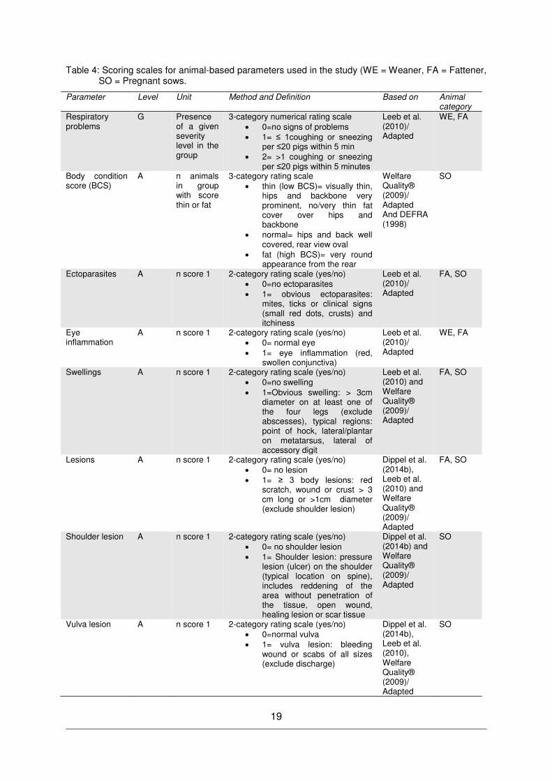
19
Table 4: Scoring scales for animal-based parameters used in the study (WE = Weaner, FA = Fattener, SO = Pregnant sows.
Parameter Level Unit Method and Definition Based on Animal category
Respiratory problems
G Presence of a given severity level in the group
3-category numerical rating scale 0=no signs of problems 1= ≤ 1coughing or sneezing
per ≤20 pigs within 5 min 2= >1 coughing or sneezing
per ≤20 pigs within 5 minutes
Leeb et al. (2010)/ Adapted
WE, FA
Body condition score (BCS)
A n animals in group with score thin or fat
3-category rating scale thin (low BCS)= visually thin,
hips and backbone very prominent, no/very thin fat cover over hips and backbone
normal= hips and back well covered, rear view oval
fat (high BCS)= very round appearance from the rear
Welfare Quality® (2009)/ Adapted And DEFRA (1998)
SO
Ectoparasites A n score 1 2-category rating scale (yes/no) 0=no ectoparasites 1= obvious ectoparasites:
mites, ticks or clinical signs (small red dots, crusts) and itchiness
Leeb et al. (2010)/ Adapted
FA, SO
Eye inflammation
A n score 1 2-category rating scale (yes/no) 0= normal eye 1= eye inflammation (red,
swollen conjunctiva)
Leeb et al. (2010)/ Adapted
WE, FA
Swellings A n score 1 2-category rating scale (yes/no) 0=no swelling 1=Obvious swelling: > 3cm
diameter on at least one of the four legs (exclude abscesses), typical regions: point of hock, lateral/plantar on metatarsus, lateral of accessory digit
Leeb et al. (2010) and Welfare Quality® (2009)/ Adapted
FA, SO
Lesions A n score 1 2-category rating scale (yes/no) 0= no lesion 1= ≥ 3 body lesions: red
scratch, wound or crust > 3 cm long or >1cm diameter (exclude shoulder lesion)
Dippel et al. (2014b), Leeb et al. (2010) and Welfare Quality® (2009)/ Adapted
FA, SO
Shoulder lesion A n score 1 2-category rating scale (yes/no) 0= no shoulder lesion 1= Shoulder lesion: pressure
lesion (ulcer) on the shoulder (typical location on spine), includes reddening of the area without penetration of the tissue, open wound, healing lesion or scar tissue
Dippel et al. (2014b) and Welfare Quality® (2009)/ Adapted
SO
Vulva lesion A n score 1 2-category rating scale (yes/no) 0=normal vulva 1= vulva lesion: bleeding
wound or scabs of all sizes (exclude discharge)
Dippel et al. (2014b), Leeb et al. (2010), Welfare Quality® (2009)/ Adapted
SO
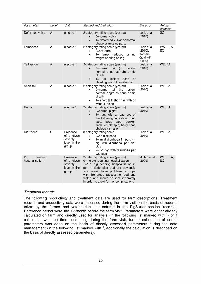
20
Parameter Level Unit Method and Definition Based on Animal category
Deformed vulva A n score 1 2-category rating scale (yes/no) 0=normal vulva 1= deformed vulva: abnormal
shape or missing parts
Leeb et al. (2010)
SO
Lameness A n score 1 2-category rating scale (yes/no) 0=not lame 1= lame: reduced or no
weight bearing on leg
Leeb et al. (2010), Welfare Quality® (2009)
WA, FA, SO
Tail lesion A n score 1 2-category rating scale (yes/no) 0=normal tail (no lesion,
normal length as hairs on tip of tail)
1= tail lesion: scab or bleeding wound, swollen tail
Leeb et al. (2010)
WE, FA
Short tail A n score 1 2-category rating scale (yes/no) 0=normal tail (no lesion,
normal length as hairs on tip of tail)
1= short tail: short tail with or without lesion
Leeb et al. (2010)
WE, FA
Runts A n score 1 2-category rating scale (yes/no) 0=normal piglet 1= runt: with at least two of
the following indicators: long face, large ears, sunken flank, visible spin, hairy coat, obviously smaller
Leeb et al. (2010)
WE, FA
Diarrhoea G Presence of a given severity level in the group
3-category rating scale 0=no diarrhoea 1= mild diarrhoea in pen: ≤1
pig with diarrhoea per ≤20 pigs
2= >1 pig with diarrhoea per ≤20 pigs
Leeb et al. (2010)
WE, FA
Pig needing hospitalisation
Presence of a given severity level in the group
2-category rating scale (yes/no) 0= no pig requiring hospitalisation 1=≥ 1 pig needing hospitalisation in pen: include pigs that are obviously sick, weak, have problems to cope with the group (access to food and water) and should be kept separately in order to avoid further complications
Mullan et al. (2009)
WE, FA, SO
Treatment records
The following productivity and treatment data are used for farm descriptions. Treatment records and productivity data were assessed during the farm visit on the basis of records taken by the farmer and veterinarian and entered in the PigSurfer section ‘records’. Reference period were the 12-month before the farm visit. Parameters were either already calculated on farm and directly used for analysis (in the following list marked with 1) or if calculation was too time consuming during the farm visit, further calculation of useful parameters was done on the basis of directly assessed parameters during the data management (in the following list marked with 2, additionally the calculation is described on the basis of directly assessed parameters):
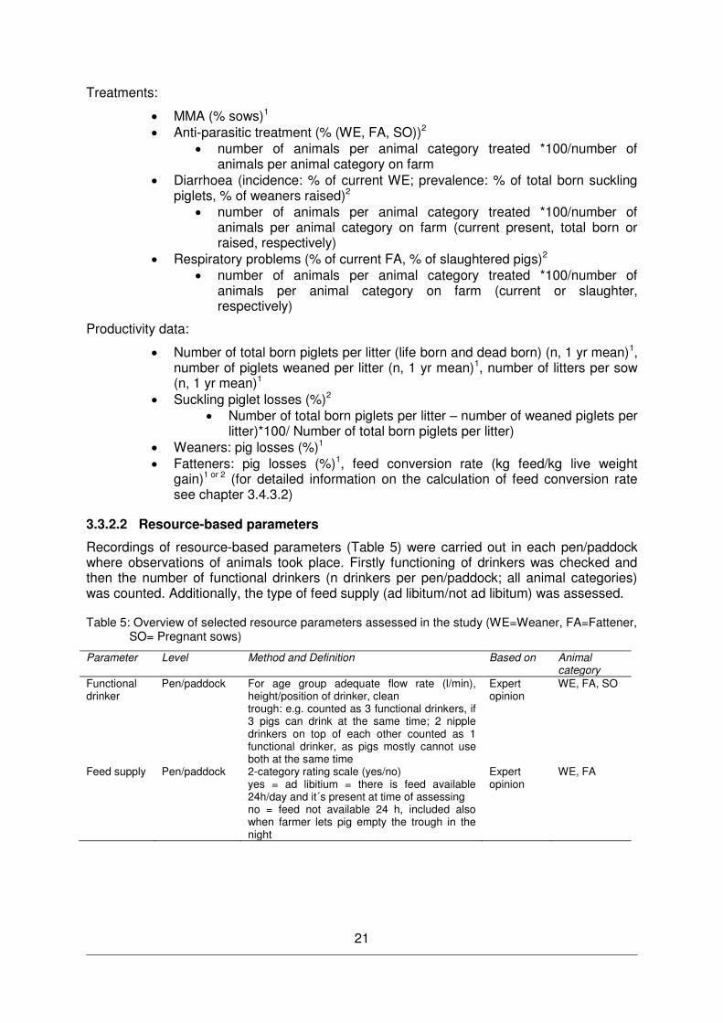
21
Treatments:
MMA (% sows)1 Anti-parasitic treatment (% (WE, FA, SO))2
number of animals per animal category treated *100/number of animals per animal category on farm
Diarrhoea (incidence: % of current WE; prevalence: % of total born suckling piglets, % of weaners raised)2
number of animals per animal category treated *100/number of animals per animal category on farm (current present, total born or raised, respectively)
Respiratory problems (% of current FA, % of slaughtered pigs)2 number of animals per animal category treated *100/number of
animals per animal category on farm (current or slaughter, respectively)
Productivity data:
Number of total born piglets per litter (life born and dead born) (n, 1 yr mean)1, number of piglets weaned per litter (n, 1 yr mean)1, number of litters per sow (n, 1 yr mean)1
Suckling piglet losses (%)2 Number of total born piglets per litter – number of weaned piglets per
litter)*100/ Number of total born piglets per litter) Weaners: pig losses (%)1 Fatteners: pig losses (%)1, feed conversion rate (kg feed/kg live weight
gain)1 or 2 (for detailed information on the calculation of feed conversion rate see chapter 3.4.3.2)
3.3.2.2 Resource-based parameters
Recordings of resource-based parameters (Table 5) were carried out in each pen/paddock where observations of animals took place. Firstly functioning of drinkers was checked and then the number of functional drinkers (n drinkers per pen/paddock; all animal categories) was counted. Additionally, the type of feed supply (ad libitum/not ad libitum) was assessed.
Table 5: Overview of selected resource parameters assessed in the study (WE=Weaner, FA=Fattener, SO= Pregnant sows)
Parameter Level Method and Definition Based on Animal category
Functional drinker
Pen/paddock For age group adequate flow rate (l/min), height/position of drinker, clean trough: e.g. counted as 3 functional drinkers, if 3 pigs can drink at the same time; 2 nipple drinkers on top of each other counted as 1 functional drinker, as pigs mostly cannot use both at the same time
Expert opinion
WE, FA, SO
Feed supply Pen/paddock 2-category rating scale (yes/no) yes = ad libitium = there is feed available 24h/day and it´s present at time of assessing no = feed not available 24 h, included also when farmer lets pig empty the trough in the night
Expert opinion
WE, FA
22
3.3.2.3 Parameters further describing the husbandry system
General
number of slaughtered fatteners (n/year), carcass weight (kg, 1 yr mean)
Breed
The breeds used were recorded separately for sows and boars (or semen in the case of artificial insemination) and categorized as follows:
conventional (CONV = Large White, Landrace, Hybrid sows) unconventional (UNCONV = traditional, indigenous breeds, usually low producing,
e.g. Cinta senese, Mangalitza) cross CONV * UNCONV cross UNCONV * UNCONV
Herd management
number of days pre-farrowing the sow is moved to the farrowing accommodation (n days pre-farrowing)
average age of sows at culling (n farrowings before slaughter, 1 yr mean) replacement rate (%) management practices in piglets (castration, supplementation of iron, teeth grinding,
cross-fostering) age of piglets at castration (days) and age at weaning (days) amount of straw used in pig unit (t/year)

23
3.3.3 Environmental impact (ENV)
Data recording for the evaluation of the environmental impact was based on Dourmad et al. (2014). The following items of the PigSurfer sections ‘interview’, ‘records’, ‘diets composition and diets content’ and ‘direct animal observations’ were used for analysis of environmental impact of organic pig husbandry systems:
(i) Sow performance: number of weaned piglets/sow/year, replacement rate (%), live weight at slaughter (kg), feed intake during gestation and lactation period (kg/period), duration of lactation period (days)
(ii) Weaner performance: weight at weaning (kg), piglet mortality (%), daily feed intake (kg), feed conversion rate (kg feed/kg live weight gain)
(iii) Fattener performance: weight at beginning of fattening phase (kg), mortality (%), daily feed intake (kg), feed conversion rate (kg feed/kg live weight gain), daily weight gain (kg/day), live weight at slaughter (kg), age at slaughter (days)
(iv) Diets: diets composition (% of individual ingredients in diet), diet nutrient and energy content (metabolisable energy (MJ ME/kg), crude protein (CP), phosphorus (P)
(v) Animal husbandry: type of system (Outdoor, Partly outdoor, Indoor with outside run), type of floor (solid floor, slats/partly slatted (%), deep litter)
(vi) Litter quality was assessed at pen level based on the following litter quality scale; based on the litter quality score at pen level, a mean litter quality score was calculated at farm level for further analysis:
i. Very good: 100% of litter is clean, dry and not mouldy ii. Good: >50 % of litter is clean, dry and not mouldy iii. Poor: >50% of litter is dirty, wet or mouldy iv. Very poor: 100% of litter is dirty, wet or mouldy
(vii) Manure: manure type (liquid, solid), manure handling (cleaning frequency), manure storage (type and duration), manure treatment (composting, anaerobic/aerobic digestion, type and distance of spreading (wide spreading, injection), mean distance of manure transport to place of spreading; Crop rotation and stocking rate (animals/ha)
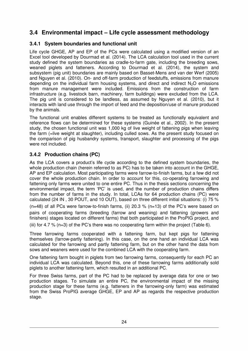
24
3.4 Environmental impact – Life cycle assessment methodology
3.4.1 System boundaries and functional unit
Life cycle GHGE, AP and EP of the PCs were calculated using a modified version of an Excel tool developed by Dourmad et al. (2014). The LCA calculation tool used in the current study defined the system boundaries as cradle-to-farm gate, including the breeding sows, weaned piglets and fatteners. According to Dourmad et al. (2014), the system and subsystem (pig unit) boundaries are mainly based on Basset-Mens and van der Werf (2005) and Nguyen et al. (2010). On- and off-farm production of feedstuffs, emissions from manure depending on the individual farm housing systems, and direct and indirect N2O emissions from manure management were included. Emissions from the construction of farm infrastructure (e.g. livestock barn, machinery, farm buildings) were excluded from the LCA. The pig unit is considered to be landless, as assumed by Nguyen et al. (2010), but it interacts with land use through the import of feed and the deposition/use of manure produced by the animals.
The functional unit enables different systems to be treated as functionally equivalent and reference flows can be determined for these systems (Guinée et al., 2002). In the present study, the chosen functional unit was 1,000 kg of live weight of fattening pigs when leaving the farm (=live weight at slaughter), including culled sows. As the present study focused on the comparison of pig husbandry systems, transport, slaughter and processing of the pigs were not included.
3.4.2 Production chains (PC)
As the LCA covers a product’s life cycle according to the defined system boundaries, the whole production chain (herein referred to as PC) has to be taken into account in the GHGE, AP and EP calculation. Most participating farms were farrow-to-finish farms, but a few did not cover the whole production chain. In order to account for this, co-operating farrowing and fattening only farms were united to one entire PC. Thus in the thesis sections concerning the environmental impact, the term ‘PC’ is used, and the number of production chains differs from the number of farms in the study. In total, LCAs for 64 production chains (PC) were calculated (24 IN , 30 POUT, and 10 OUT), based on three different initial situations: (i) 75 %
(n=48) of all PCs were farrow-to-finish farms, (ii) 20.3 % (n=13) of the PC s were based on pairs of cooperating farms (breeding (farrow and weaning) and fattening (growers and finishers) stages located on different farms) that both participated in the ProPIG project, and
(iii) for 4.7 % (n=3) of the PC s there was no cooperating farm within the project (Table 6).
Three farrowing farms cooperated with a fattening farm, but kept pigs for fattening themselves (farrow-partly fattening). In this case, on the one hand an individual LCA was calculated for the farrowing and partly fattening farm, but on the other hand the data from sows and weaners were used for the combined LCA with the cooperating farm.
One fattening farm bought in piglets from two farrowing farms, consequently for each PC an individual LCA was calculated. Beyond this, one of these farrowing farms additionally sold piglets to another fattening farm, which resulted in an additional PC.
For three Swiss farms, part of the PC had to be replaced by average data for one or two production stages. To simulate an entire PC, the environmental impact of the missing production stage for these farms (e.g. fatteners in the farrowing-only farm) was estimated from the Swiss ProPIG average GHGE, EP and AP as regards the respective production stage.
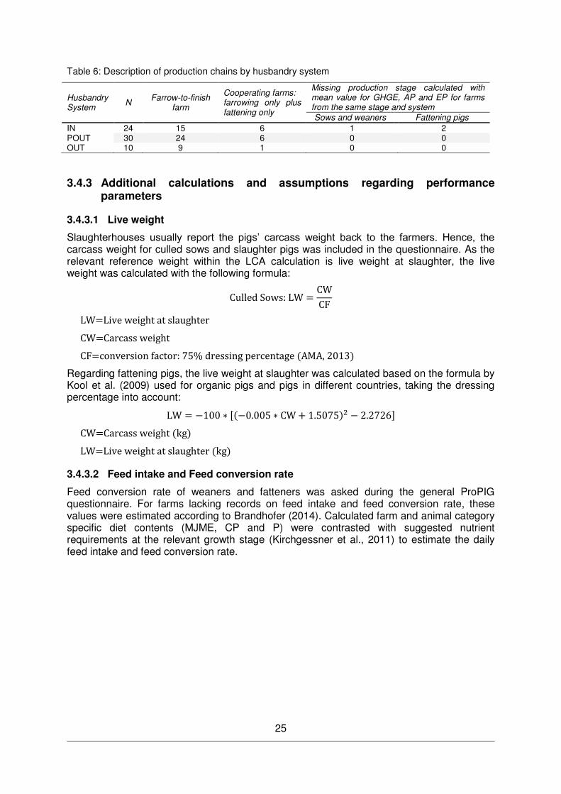
25
Table 6: Description of production chains by husbandry system
Husbandry System
N Farrow-to-finish
farm
Cooperating farms: farrowing only plus fattening only
Missing production stage calculated with mean value for GHGE, AP and EP for farms from the same stage and system Sows and weaners Fattening pigs
IN 24 15 6 1 2 POUT 30 24 6 0 0 OUT 10 9 1 0 0
3.4.3 Additional calculations and assumptions regarding performance parameters
3.4.3.1 Live weight
Slaughterhouses usually report the pigs’ carcass weight back to the farmers. Hence, the carcass weight for culled sows and slaughter pigs was included in the questionnaire. As the relevant reference weight within the LCA calculation is live weight at slaughter, the live weight was calculated with the following formula: Culled Sows: LW = CWCF
LW=Live weight at slaughter
CW=Carcass weight
CF=conversion factor: 75% dressing percentage (AMA, 2013)
Regarding fattening pigs, the live weight at slaughter was calculated based on the formula by Kool et al. (2009) used for organic pigs and pigs in different countries, taking the dressing percentage into account: LW = − ∗ [ − . ∗ CW + . − . ]
CW=Carcass weight (kg)
LW=Live weight at slaughter (kg)
3.4.3.2 Feed intake and Feed conversion rate
Feed conversion rate of weaners and fatteners was asked during the general ProPIG questionnaire. For farms lacking records on feed intake and feed conversion rate, these values were estimated according to Brandhofer (2014). Calculated farm and animal category specific diet contents (MJME, CP and P) were contrasted with suggested nutrient requirements at the relevant growth stage (Kirchgessner et al., 2011) to estimate the daily feed intake and feed conversion rate.
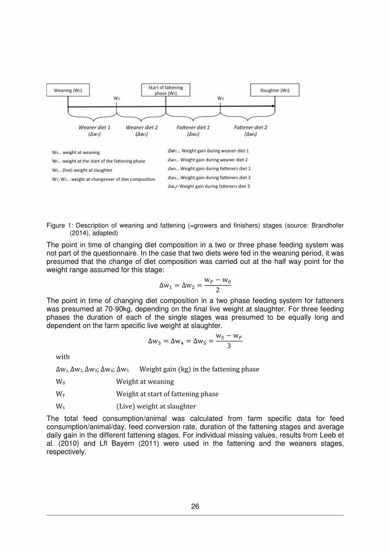
26
Figure 1: Description of weaning and fattening (=growers and finishers) stages (source: Brandhofer (2014), adapted)
The point in time of changing diet composition in a two or three phase feeding system was not part of the questionnaire. In the case that two diets were fed in the weaning period, it was presumed that the change of diet composition was carried out at the half way point for the weight range assumed for this stage: Δw = Δw = w� − w
The point in time of changing diet composition in a two phase feeding system for fatteners was presumed at 70-90kg, depending on the final live weight at slaughter. For three feeding phases the duration of each of the single stages was presumed to be equally long and dependent on the farm specific live weight at slaughter. Δw = Δw = Δw = w� − w�
with Δw1, Δw2, Δw3; Δw4; Δw5 Weight gain (kg) in the fattening phase
W0 Weight at weaning
WF Weight at start of fattening phase
WS (Live) weight at slaughter
The total feed consumption/animal was calculated from farm specific data for feed consumption/animal/day, feed conversion rate, duration of the fattening stages and average daily gain in the different fattening stages. For individual missing values, results from Leeb et al. (2010) and Lfl Bayern (2011) were used in the fattening and the weaners stages, respectively.
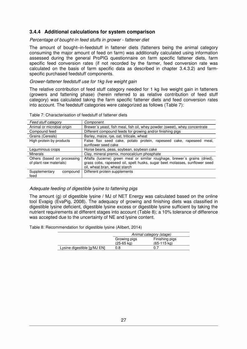
27
3.4.4 Additional calculations for system comparison
Percentage of bought-in feed stuffs in grower - fattener diet
The amount of bought–in-feedstuff in fattener diets (fatteners being the animal category consuming the major amount of feed on farm) was additionally calculated using information assessed during the general ProPIG questionnaire on farm specific fattener diets, farm specific feed conversion rates (if not recorded by the farmer, feed conversion rate was calculated on the basis of farm specific data as described in chapter 3.4.3.2) and farm-specific purchased feedstuff components.
Grower-fattener feedstuff use for 1kg live weight gain
The relative contribution of feed stuff category needed for 1 kg live weight gain in fatteners (growers and fattening phase) (herein referred to as relative contribution of feed stuff category) was calculated taking the farm specific fattener diets and feed conversion rates into account. The feedstuff categories were categorized as follows (Table 7):
Table 7: Characterisation of feedstuff of fattener diets
Feed stuff category Component Animal or microbial origin Brewer´s yeast, fish meal, fish oil, whey powder (sweet), whey concentrate Compound feed Different compound feeds for growing and/or finishing pigs Grains (Cereals) Barley, maize, rye, oat, triticale, wheat High protein by products False flax seed cake, potato protein, rapeseed cake, rapeseed meal,
sunflower seed cake Leguminous crops Horse beans, peas, soybean, soybean cake Minerals Clay, mineral premix, monocalcium phosphate Others (based on processing of plant raw materials)
Alfalfa (lucerne) green meal or similar roughage, brewer´s grains (dried), grass cobs, rapeseed oil, spelt husks, sugar beet molasses, sunflower seed oil, wheat bran, wheat starch
Supplementary compound feed
Different protein supplements
Adequate feeding of digestible lysine to fattening pigs
The amount (g) of digestible lysine / MJ of NET Energy was calculated based on the online tool Evapig (EvaPig, 2008). The adequacy of growing and finishing diets was classified in digestible lysine deficient, digestible lysine excess or digestible lysine sufficient by taking the nutrient requirements at different stages into account (Table 8); a 10% tolerance of difference was accepted due to the uncertainty of NE and lysine content.
Table 8: Recommendation for digestible lysine (Alibert, 2014)
Animal category (stage) Growing pigs
(25-65 kg) Finishing pigs (65-115 kg)
Lysine digestible [g/MJ EN] 0.8 0.7
28
3.4.5 Overview of sources of emissions
According to the calculation method used (Dourmad et al., 2014), the environmental impact indicators GHGE, AP and EP can be attributed to different sources, presented in Table 9.
Table 9: Categories of sources of environmental impact of pig production according to Dourmad et al. (2014)
Source Definition Feed Direct and indirect emissions (crop production, land use change, energy
consumption, processing) Housing Direct emissions of excreta occurring during keeping of animals in pens indoors or
paddocks outdoors and energy (electricity) consumption Manure storage Direct emissions of excreta during storage (depending on type and duration of
storage) Manure treatment Direct emissions depending on type of treatment (if applied) Manure spreading Direct emissions during manure spreading, depending on type of spreading
3.4.6 Environmental impact of feed production
Greenhouse gas emissions
Feedstuffs were either produced on farm or bought in. As the participating farms were situated in eight different European countries, the feed components were produced in different locations under varying climatic conditions. Also, divergent local methods of production and heterogeneous levels of yields were found across all farms. Due to this variability in the origin of feeds, the large number of different components used across all farms and furthermore the poor availability of data on potential greenhouse gas emissions of feed ingredient production within the eight countries, the following approach was applied regarding the greenhouse gas emissions from the feed supply chain:
In general all feedstuffs were regarded as bought-in. GHGE of all feedstuffs except fishmeal and fish oil are based on Hörtenhuber et al. (2011), who analysed the GHGE for alternative protein-rich feedstuffs produced in Austria (e.g. grain legumes, by-products from oilseeds or grains) in comparison to solvent-extracted soybean meal, taking the effects of the LUC (land use change) into account. GHGE for eight protein-rich feedstuffs were calculated within a LCA, including the most important processes leading to GHGE. The total GHGE were summed as CO2-eq using the conversion factors 25 kg CO2-eq for 1kg methane and 298 kg CO2-eq for 1kg nitrous oxide as described in IPCC (2007). GHGE associated to agricultural production, transport, production of mineral fertilizers and pesticides and emissions from soil and LUC as well as industrial processing of feedstuffs and allocation of GHGE to products are considered; see Hörtenhuber et al. (2011) for methodological details. Hörtenhuber (2013b) additionally calculated the GHGE for all feedstuffs used in diets fed at farms in the project by using the method described in Hörtenhuber et al. (2011). GHGE of the rarely used components fishmeal and fish oil originate from Samuel-Fitwi et al. (2013). GHGE, AP and EP for monocalcium phosphate and mineral premix are based on the Danish LCA food database (LCA Food database, 2007).
Acidification and eutrophication potential of feed production
Eutrophication potential (EP) indicates the influence of N- and P-losses on aquatic and terrestrial environments. The EP of feed ingredients was calculated by Hörtenhuber (2013a). To achieve the NO3-N-emissions related to feed ingredients, mean quantities of applied N from manure and commercial fertilizers on organic farms in Austria (published in Hörtenhuber et al. (2010) and Hörtenhuber et al. (2011) or calculated using the same method) were multiplied with factors of NO3-N leaching of various farming systems and intensities identified by Kolbe (2002). For the P-losses it was assumed, that on average a surplus of 5 % regarding the plant requirements according to yield were applied. These 5 % were considered as potentially lost. The EP (N- and P-losses summarized) was expressed
29
by Hörtenhuber (2013a) in g PO4-eq/kg feedstuff component (Hörtenhuber, 2013a) by using conversion factors as suggested by Hausschild and Wenzel (1998).
To calculate the acidifying potential (AP) effects of substances on the environment, their acid formation potential was calculated and expressed as SO2-eq. The following conversion factors were used according to Hausschild and Wenzel (1998): 1 for SO2, 0.7 for NOX and 1.88 for NH3.
In crop cultivation NH3 is the main form of gaseous, acidifying substance. SO2 does not significantly contribute to the feedstuffs’ AP. The small amount of likely gaseous N-losses in the form of NOX was not considered; otherwise all losses were calculated with standard values according to IPCC (2006). For organic N-fertilisers 20% gaseous N-losses after the application were assumed. The applied amounts of N-fertilisers are based, in the same way as the EP, on the mean quantities used on organic farms in Austria (Hörtenhuber et al., 2010).
30
3.4.7 Environmental impact of pig management
Gaseous emissions from animal housing and manure storage were calculated for NH3
(Rigolot et al., 2010a, Rigolot et al., 2010b), N2O (IPCC, 2006), NOx (Nemecek and Kägi, 2007) and CH4 (Rigolot et al., 2010a, Rigolot et al., 2010b). The indicator result for each impact category was determined by multiplying the aggregated resources used and the aggregated emissions of each individual substance with a characterisation factor for each impact category to which it may potentially contribute (Dourmad et al., 2014).
GHGE, AP and EP of the pig production were calculated using the CML2 “baseline” and “all categories” 2001 characterisation methods as implemented in the Ecoinvent v2.0 database. GHGE were calculated according to 100-year global warming potential factors expressed in kg CO2-eq, according to IPCC (2006): CH4: 25, N20: 298, CO2: 1. EP was expressed in kg PO4-eq, calculated using the following generic EP factors: NH3: 0.35, NO3: 0.1, NO2: 0.13, NOX:0.13, PO4:1 (Guinée et al., 2002). AP was expressed in kg SO2-eq, using average European AP factors: NH3: 1.6, NOx: 0.5, SOx: 1.2.
The following detailed explanations regarding emissions occurring during pig production are based on the LCA calculation tool described in Dourmad et al. (2014).
3.4.7.1 CH4 emissions
Regarding CH4 emissions from enteric fermentation and manure management, the calculations were based on Rigolot et al. (2010a), Rigolot et al. (2010b) and IPCC (2006): The amount of CH4 emitted due to enteric fermentation is calculated from E(CH4) as the energy associated with CH4 production, which constitutes part of the difference between digestible energy (DE) and metabolisable energy (ME). CH = E CH. MJkg∗
*=CH4 calorific value equal to 56.65 MJ/kg
The amount of E(CH4) depends on the animals’ physiological status and the amount of digestible fibre ingested (ResD), which was estimated as the difference between digested OM and digested protein, fat, starch and sugar (see Rigolot et al. (2010a)). To obtain the loss of energy as CH4, ResD is multiplied by 670J/g for weaners and fattening pigs and 1370J/g for sows according to Noblet et al. (2004).
CH4 emissions from manure storage were calculated on the basis of the IPCC “Tier2” method with some adaptions (Rigolot et al., 2010b): CH _ kg = VS ∗ Bo ∗ MCF
VS= volatile solids (kg) (considered as OM amount (kg))
B0= maximum CH4 producing capacity (m³/kg DM)
MCF= CH4 conversion factor for the management system considered
VS is calculated by Rigolot et al. (2010b) as OM amount (organic matter, kg) in the excreta. The amount of excreted OM depends on the OM amount in diets fed and their digestibility. As these values are not known at the individual farm level, an average of 11.5% was assumed for the percentage of OM excreted (Dourmad et al., 2014). B0 and MCF were taken from IPCC (2006), with some adaptions of MCF to integrate farm specific practices related to manure collection and handling (type of manure, frequency of removal, duration of storage, processing).
31
3.4.7.2 Retention and Excretion of N and P
The amount of N excreted is calculated as the difference between intake and retention, whereby the dietary CP (crude protein) contents form the basis for the N content in the feedstuffs. N kg = N − N According to Kjeldahl, CP consists of 16% N. A constant average N content of 2.56% (16% protein in body weight) is assumed for the calculation of N retention (adapted from Rigolot et al. (2010b)). For weaners and fatteners N retention is then calculated as: N kg = . x (LW − LW ) N _ kg = . x LW − LW
with N _ = retained nitrogen kg LW = Live weight of pigs at the beginning of the fattening stage kg LW_ = Live weight of piglets at weaning kg LW_ = Live weight of pigs at slaughter kg
For sows, N retention is calculated per year as N retention over their lifetime (from first insemination up to culling), multiplied by the replacement rate: Nbody kg = . x LW_slaughter − LW_first insemination x R
with
R =farm specific replacement rate (%) LW_slaughter - LW_first_insemination= estimated as 110kg
In the calculation of nitrogen excretion of sows, the amount retained in piglets up to weaning has also to be added: Nbody = N x LW x .
with N = Number of weaned piglets/sow/year
The P excretion follows the same principle, using 4.3 g P per kg body weight (Rigolot et al., 2010b, Brandhofer, 2014).
3.4.7.3 Livestock manure
Direct N20-N emissions from manure during in-house and outdoor storage and field application were calculated according to IPCC (2006). Emissions of NOX were estimated according to Nemecek and Kägi (2007). NH3-N emissions during in-house storage, outside storage and field application of manure were calculated according to Rigolot et al. (2010b) according to type of effluent (slurry, solid manure), litter quality in deep litter systems (as farm specific variation factor), duration and type of storage and method of spreading (Table 10, Table 11, Table 12). Ambient and house temperatures were not measured at farm, but were estimated according to mean temperatures estimated for each country.
P losses during manure storage, treatment and spreading (Rigolot et al., 2010b) were assumed to be negligible and therefore not taken into account.

32
Table 10: Emission factors depending on manure type and litter quality (variation factor) occurring during animal keeping (in-house storage) according to Rigolot et al. (2010b)
NH3-N (kg/kg N)
N2O-N (kg/kg N)
N2-N (kg/kg N)
Floor type and manure management Slatted floor: slurry (evacuation after each batch) 0.242 0.002 0.006 Solid flooring: solid manure 0.142 0.002 0.006 Deep litter depending on litter quality:
very good 0.080 0.012 0.589 good 0.100 0.024 0.496 poor 0.220 0.038 0.305
very poor 0.440 0.008 0.116
Table 11: Emission factors for manure storage depending on manure type and storage period (variation factor) according to Rigolot et al. (2010b) and Dourmad et al. (2014)
NH3-N (kg/kg N)
N2O-N (kg/kg N)
N2-N (kg/kg N)
Criteria manure storage* variation factor Solid manure (manure pile) 0.07 0.01 0.03 Slurry storage:
covered 0.05 0.001 - uncovered- storage period <180 days 0.05 0.001 -
uncovered- storage period > 180 days 0.10 0.001 - uncovered- storage period 180-365 days 0.15 0.001 -
Emissions occurring due to manure treatment were included on the basis of factors reported by Rigolot et al. (2010b). As detailed information on farm specific practices was not available (e.g. number of turnings in the case of composting), additional variation was not taken into account.
Emissions due to manure spreading are related to the kind of manure (slurry, solid manure) and the method of spreading (wide spreading, injection), also according to Rigolot et al. (2010b).
Table 12: Emission factors for manure spreading depending on manure type and spreading type (variation factor) (Rigolot et al., 2010b, Dourmad et al., 2014)
NH3-N (kg/kg N)
N2O-N (kg/kg N)
NO3-N (kg/kg N)
Manure spreading Solid manure and compost [kg/kg applied manure] 0.05 0.0010 0.05 Slurry spreading – wide spreading [kg/kg applied slurry] 0.20 0.0024 0.05 Slurry spreading – injection [kg/kg applied slurry] 0.08 0.00126 0.05
Energy use in the building for lighting, heating and ventilation was considered, but not the emissions and resources used for the construction of buildings. Veterinary and cleaning products were also excluded. CO2 emissions due to metabolic activity of pigs were not taken into account (Rigolot et al., 2010b, IPCC, 2006).
3.4.7.4 Livestock manure outdoors
For animals kept on outdoor paddocks, emission factors were based on Basset-Mens et al. (2007), adapted according to Dourmad (2013). The amount of N excreted was calculated according to the type and number of pigs per ha of paddock at a given time. Emission factors (Table 13) were then applied to estimate NH3, N2O, N2 and NO3 losses to the environment.
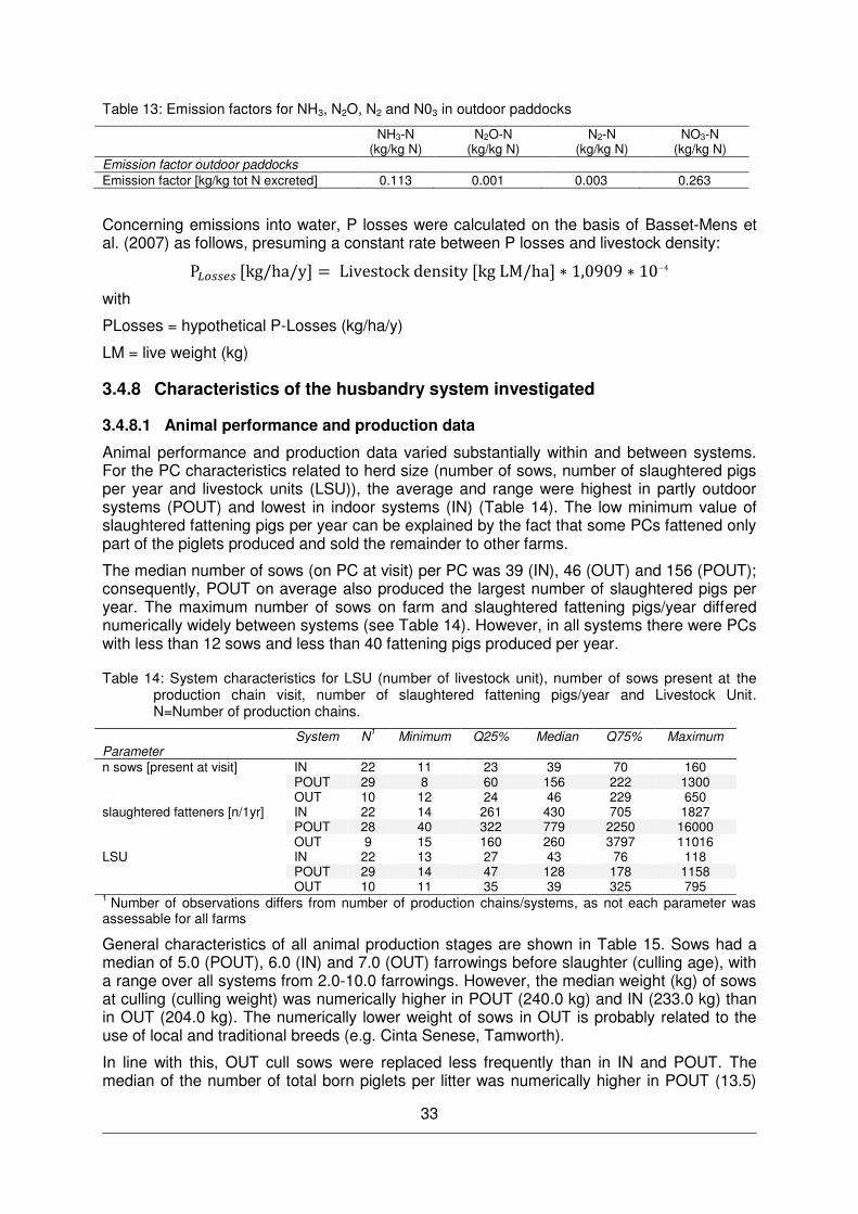
33
Table 13: Emission factors for NH3, N2O, N2 and N03 in outdoor paddocks
NH3-N (kg/kg N)
N2O-N (kg/kg N)
N2-N (kg/kg N)
NO3-N (kg/kg N)
Emission factor outdoor paddocks Emission factor [kg/kg tot N excreted] 0.113 0.001 0.003 0.263
Concerning emissions into water, P losses were calculated on the basis of Basset-Mens et al. (2007) as follows, presuming a constant rate between P losses and livestock density: P������ [kg/ha/y] = Livestock density [kg LM/ha] ∗ , 9 9 ∗ −
with
PLosses = hypothetical P-Losses (kg/ha/y)
LM = live weight (kg)
3.4.8 Characteristics of the husbandry system investigated
3.4.8.1 Animal performance and production data
Animal performance and production data varied substantially within and between systems. For the PC characteristics related to herd size (number of sows, number of slaughtered pigs per year and livestock units (LSU)), the average and range were highest in partly outdoor systems (POUT) and lowest in indoor systems (IN) (Table 14). The low minimum value of slaughtered fattening pigs per year can be explained by the fact that some PCs fattened only part of the piglets produced and sold the remainder to other farms.
The median number of sows (on PC at visit) per PC was 39 (IN), 46 (OUT) and 156 (POUT); consequently, POUT on average also produced the largest number of slaughtered pigs per year. The maximum number of sows on farm and slaughtered fattening pigs/year differed numerically widely between systems (see Table 14). However, in all systems there were PCs with less than 12 sows and less than 40 fattening pigs produced per year.
Table 14: System characteristics for LSU (number of livestock unit), number of sows present at the production chain visit, number of slaughtered fattening pigs/year and Livestock Unit. N=Number of production chains.
System N1 Minimum Q25% Median Q75% Maximum Parameter n sows [present at visit] IN 22 11 23 39 70 160
POUT 29 8 60 156 222 1300 OUT 10 12 24 46 229 650
slaughtered fatteners [n/1yr] IN 22 14 261 430 705 1827 POUT 28 40 322 779 2250 16000 OUT 9 15 160 260 3797 11016
LSU IN 22 13 27 43 76 118 POUT 29 14 47 128 178 1158 OUT 10 11 35 39 325 795
1 Number of observations differs from number of production chains/systems, as not each parameter was assessable for all farms
General characteristics of all animal production stages are shown in Table 15. Sows had a median of 5.0 (POUT), 6.0 (IN) and 7.0 (OUT) farrowings before slaughter (culling age), with a range over all systems from 2.0-10.0 farrowings. However, the median weight (kg) of sows at culling (culling weight) was numerically higher in POUT (240.0 kg) and IN (233.0 kg) than in OUT (204.0 kg). The numerically lower weight of sows in OUT is probably related to the use of local and traditional breeds (e.g. Cinta Senese, Tamworth).
In line with this, OUT cull sows were replaced less frequently than in IN and POUT. The median of the number of total born piglets per litter was numerically higher in POUT (13.5)
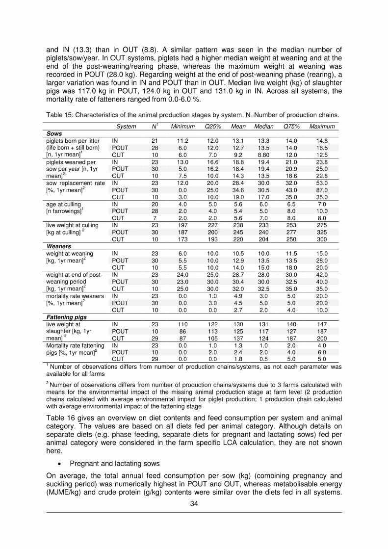
34
and IN (13.3) than in OUT (8.8). A similar pattern was seen in the median number of piglets/sow/year. In OUT systems, piglets had a higher median weight at weaning and at the end of the post-weaning/rearing phase, whereas the maximum weight at weaning was recorded in POUT (28.0 kg). Regarding weight at the end of post-weaning phase (rearing), a larger variation was found in IN and POUT than in OUT. Median live weight (kg) of slaughter pigs was 117.0 kg in POUT, 124.0 kg in OUT and 131.0 kg in IN. Across all systems, the mortality rate of fatteners ranged from 0.0-6.0 %.
Table 15: Characteristics of the animal production stages by system. N=Number of production chains.
System N1 Minimum Q25% Mean Median Q75% Maximum Sows piglets born per litter (life born + still born) [n, 1yr mean]1
IN 21 11.2 12.0 13.1 13.3 14.0 14.8 POUT 28 6.0 12.0 12.7 13.5 14.0 16.5 OUT 10 6.0 7.0 9.2 8.80 12.0 12.5
piglets weaned per sow per year [n, 1yr mean]2
IN 23 13.0 16.6 18.8 19.4 21.0 23.8 POUT 30 5.0 16.2 18.4 19.4 20.9 25.0 OUT 10 7.5 10.0 14.3 13.5 18.6 22.8
sow replacement rate [%, 1yr mean]2
IN 23 12.0 20.0 28.4 30.0 32.0 53.0 POUT 30 0.0 25.0 34.6 30.5 43.0 87.0 OUT 10 3.0 10.0 19.0 17.0 35.0 35.0
age at culling [n farrowings]1
IN 20 4.0 5.0 5.6 6.0 6.5 7.0 POUT 28 2.0 4.0 5.4 5.0 8.0 10.0 OUT 7 2.0 2.0 5.6 7.0 8.0 8.0
live weight at culling [kg at culling] 2
IN 23 197 227 238 233 253 275 POUT 30 187 200 245 240 277 325 OUT 10 173 193 220 204 250 300
Weaners weight at weaning [kg, 1yr mean]2
IN 23 6.0 10.0 10.5 10.0 11.5 15.0 POUT 30 5.5 10.0 12.9 13.5 13.5 28.0 OUT 10 5.5 10.0 14.0 15.0 18.0 20.0
weight at end of post-weaning period [kg, 1yr mean]2
IN 23 24.0 25.0 28.7 28.0 30.0 42.0 POUT 30 23.0 30.0 30.4 30.0 32.5 40.0 OUT 10 25.0 30.0 32.0 32.5 35.0 35.0
mortality rate weaners [%, 1yr mean]2
IN 23 0.0 1.0 4.9 3.0 5.0 20.0 POUT 30 0.0 3.0 4.5 5.0 5.0 20.0 OUT 10 0.0 0.0 2.7 2.0 4.0 10.0
Fattening pigs live weight at slaughter [kg, 1yr mean] 2
IN 23 110 122 130 131 140 147 POUT 10 86 113 125 117 127 187 OUT 29 87 105 137 124 187 200
Mortality rate fattening pigs [%, 1yr mean]2
IN 23 0.0 1.0 1.3 1.0 2.0 4.0 POUT 10 0.0 2.0 2.4 2.0 4.0 6.0 OUT 29 0.0 0.0 1.8 0.5 5.0 5.0
1 Number of observations differs from number of production chains/systems, as not each parameter was available for all farms 2 Number of observations differs from number of production chains/systems due to 3 farms calculated with means for the environmental impact of the missing animal production stage at farm level (2 production chains calculated with average environmental impact for piglet production; 1 production chain calculated with average environmental impact of the fattening stage
Table 16 gives an overview on diet contents and feed consumption per system and animal category. The values are based on all diets fed per animal category. Although details on separate diets (e.g. phase feeding, separate diets for pregnant and lactating sows) fed per animal category were considered in the farm specific LCA calculation, they are not shown here.
Pregnant and lactating sows
On average, the total annual feed consumption per sow (kg) (combining pregnancy and suckling period) was numerically highest in POUT and OUT, whereas metabolisable energy (MJME/kg) and crude protein (g/kg) contents were similar over the diets fed in all systems.
35
The median total phosphorus (g/kg) content in feed for sows was lower in OUT than in POUT and IN.
Weaners
The median kg feed use per weaner was numerically higher in OUT (50) than in IN and POUT (both 39 kg). Crude protein (g/kg) and total phosphorus (g/kg) in feed for weaners was on average (median) numerically lowest in OUT, with similar values recorded in IN and POUT. However, similar values regarding metabolisable energy (MJ ME/kg) were recorded over all systems.
Fatteners
The median feed use per produced fattening pig as well as the feed conversion rate were numerically highest in OUT. Crude protein (g/kg) and total phosphorus (g/kg) contents were numerically lower in OUT and higher in IN and POUT. Similar metabolisable energy (MJME/kg) values were recorded over all systems.

36
Table 16: Characteristics of dietary nutrient content and feed consumption by system. FCR=Feed conversion rate, N=Number of production chains.
Parameter System N Minimum Q25% Median Q75% Maximum Pregnant and lactating sows
Feed per sow [kg/year] IN 23 923 1059 1277 1419 1733 POUT 30 675 1440 1680 1946 2236 OUT 10 827 1379 1468 1604 1825
Average pregnant and lactating sow dietary content of1: ME MJ/kg IN 23 11.8 12.3 12.5 13.0 13.1
POUT 30 10.6 12.5 12.7 12.9 13.7 OUT 10 9.6 9.6 12.9 13.3 14.7
CP [g/kg] IN 23 124 148 153 162 185 POUT 30 124 142 151 160 171 OUT 10 112 123 154 164 165
total P [g/kg] IN 23 4.0 5.1 5.5 6.0 6.6 POUT 30 3.3 4.5 5.5 5.9 7.8 OUT 10 0.8 3.0 3.3 4.6 6.1
Weaners Feed per weaner produced [kg/weaner]
IN 23 18 28 39 45 60 POUT 30 12 33 39 45 99 OUT 10 21 34 50 70 111
Average post-weaning dietary content of1: ME MJ/kg IN 23 12.0 12.6 12.8 13.2 13.5
POUT 30 12.0 12.8 13.1 13.3 13.5 OUT 10 9.5 9.5 12.8 13.4 14.7
CP [g/kg] IN 23 138 171 180 184 207 POUT 30 130 173 185 190 208 OUT 10 112 144 158 198 198
total P [g/kg] IN 23 3.7 5.0 5.8 6.0 6.9 POUT 30 3.4 4.7 5.8 6.2 8.9 OUT 10 0.8 3.5 3.5 5.4 6.4
Fattening pig Feed per fattening pig produced [kg/fattener]
IN 23 220 259 331 387 494 POUT 29 158 251 300 364 1132 OUT 10 209 217 393 871 986
Fattening pig FCR [kg/kg pig]
IN 23 2.4 2.9 3.3 3.8 4.4 POUT 29 2.7 3.0 3.2 3.7 7.0 OUT 10 2.8 2.9 4.9 6.5 7.5
Average fattening pig dietary content of1: ME MJ/kg IN 23 12.0 12.5 12.7 13.0 14.8
POUT 29 12.0 12.8 12.9 13.0 13.4 OUT 10 9.5 9.5 13.0 13.5 14.7
CP [g/kg] IN 23 118 154 159 170 190 POUT 29 130 144 168 177 202 OUT 10 112 114 151 170 186
total P [g/kg] IN 23 3.3 4.40 5.0 5.5 6.4 POUT 29 3.4 3.7 4.9 5.5 6.4 OUT 10 0.8 2.4 3.2 3.7 6.4
3.4.8.2 Housing (floor type) and manure management
The housing, and consequently manure management, only varied between the individual PCs in IN and POUT, while in OUT all animals where kept outdoors. In indoor pens, animals were kept with bedding or deep litter and partly slatted floor and constant access to a concrete outdoor run. Table 17 reports detailed information on housing (floor type) for all animal categories in the PCs studied. All animal categories in IN were mainly kept on concrete floors with bedding or concrete with partly slatted floors. In POUT mainly lactating sows were kept outdoors throughout the year (i.e. on 82.7% of PCs), and the proportion of
1 Average dietary content over all diets fed to the animal group.
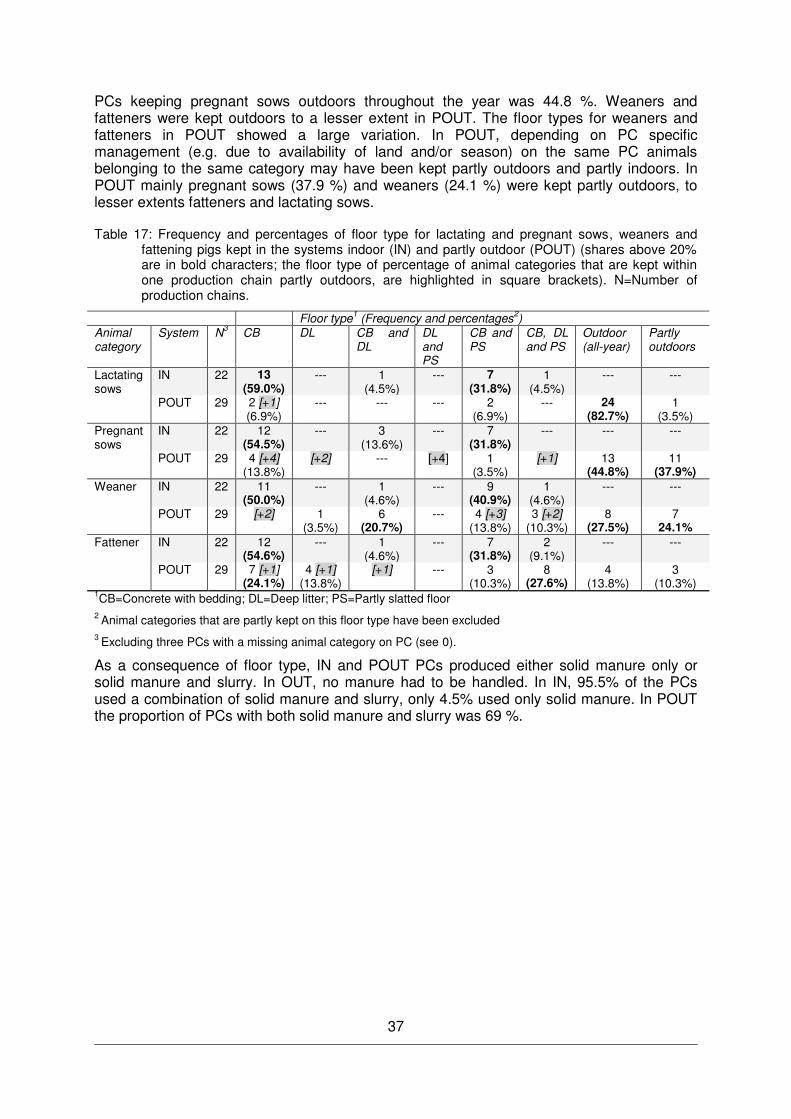
37
PCs keeping pregnant sows outdoors throughout the year was 44.8 %. Weaners and fatteners were kept outdoors to a lesser extent in POUT. The floor types for weaners and fatteners in POUT showed a large variation. In POUT, depending on PC specific management (e.g. due to availability of land and/or season) on the same PC animals belonging to the same category may have been kept partly outdoors and partly indoors. In POUT mainly pregnant sows (37.9 %) and weaners (24.1 %) were kept partly outdoors, to lesser extents fatteners and lactating sows.
Table 17: Frequency and percentages of floor type for lactating and pregnant sows, weaners and fattening pigs kept in the systems indoor (IN) and partly outdoor (POUT) (shares above 20% are in bold characters; the floor type of percentage of animal categories that are kept within one production chain partly outdoors, are highlighted in square brackets). N=Number of production chains.
Floor type1 (Frequency and percentages2) Animal category
System N3 CB DL CB and DL
DL and PS
CB and PS
CB, DL and PS
Outdoor (all-year)
Partly outdoors
Lactating sows
IN 22 13 (59.0%)
--- 1 (4.5%)
--- 7 (31.8%)
1 (4.5%)
--- ---
POUT 29 2 [+1] (6.9%)
--- --- --- 2 (6.9%)
--- 24 (82.7%)
1 (3.5%)
Pregnant sows
IN 22 12 (54.5%)
--- 3 (13.6%)
--- 7 (31.8%)
--- --- ---
POUT 29 4 [+4] (13.8%)
[+2] --- [+4] 1 (3.5%)
[+1] 13 (44.8%)
11 (37.9%)
Weaner IN 22 11 (50.0%)
--- 1 (4.6%)
--- 9 (40.9%)
1 (4.6%)
--- ---
POUT 29 [+2] 1 (3.5%)
6 (20.7%)
--- 4 [+3] (13.8%)
3 [+2] (10.3%)
8 (27.5%)
7 24.1%
Fattener IN 22 12 (54.6%)
--- 1 (4.6%)
--- 7 (31.8%)
2 (9.1%)
--- ---
POUT 29 7 [+1] (24.1%)
4 [+1] (13.8%)
[+1] --- 3 (10.3%)
8 (27.6%)
4 (13.8%)
3 (10.3%)
1CB=Concrete with bedding; DL=Deep litter; PS=Partly slatted floor 2 Animal categories that are partly kept on this floor type have been excluded 3 Excluding three PCs with a missing animal category on PC (see 0).
As a consequence of floor type, IN and POUT PCs produced either solid manure only or solid manure and slurry. In OUT, no manure had to be handled. In IN, 95.5% of the PCs used a combination of solid manure and slurry, only 4.5% used only solid manure. In POUT the proportion of PCs with both solid manure and slurry was 69 %.
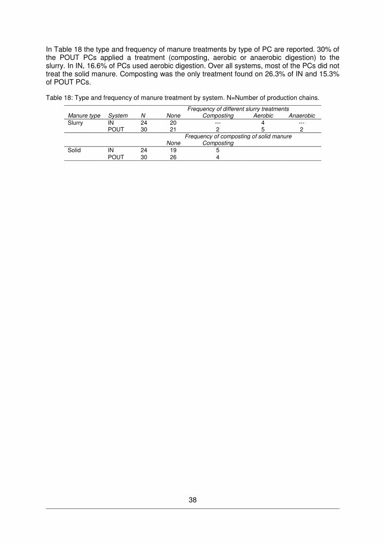
38
In Table 18 the type and frequency of manure treatments by type of PC are reported. 30% of the POUT PCs applied a treatment (composting, aerobic or anaerobic digestion) to the slurry. In IN, 16.6% of PCs used aerobic digestion. Over all systems, most of the PCs did not treat the solid manure. Composting was the only treatment found on 26.3% of IN and 15.3% of POUT PCs.
Table 18: Type and frequency of manure treatment by system. N=Number of production chains.
Frequency of different slurry treatments Manure type System N None Composting Aerobic Anaerobic Slurry IN 24 20 --- 4 ---
POUT 30 21 2 5 2 Frequency of composting of solid manure None Composting Solid IN 24 19 5
POUT 30 26 4

39
3.5 Associations between AHW and ENV
For a detailed description of the overall study design, definition of husbandry systems (IN, POUT, OUT), farm selection, data collection on farm, definition of animal health and welfare parameters, as well as life cycle assessment see the above given method description in chapter 3, results for inter-observer reliability tests are given in chapter 4.1.1
Animal health and welfare parameters at production chain level
Animal-based parameters were selected based on their indicative value for the presence (or absence) of health and welfare problems (Dippel et al., 2014b); for detailed definitions of the animal-based parameters see chapter 3.3.2.1. The assessment was adapted from previous protocols of animal-based parameters (Dippel et al., 2014b, Leeb et al., 2010, Welfare Quality®, 2009). Animal-based parameters were assessed as prevalences or scores at pen level in pregnant (gestating) sows (SO), weaners (WE) and fatteners (FA). As the comparison with ENV parameters required AHW to be at PC level, prevalences of animal-based parameters were re-calculated for each animal category on PC level:
animal level (A): % of animals with finding per animal category (SO, WE, FA); data averaged across groups
group level (G): % of groups observed with finding per animal category Scores 1 and 2 of respiratory problems and diarrhoea were additionally combined
for analysis.
Summary score GOOD% and GOOD% per animal category
As ENV calculations yielded one value per environmental impact indicator and production chain or a cluster association reflecting overall ENV for each PC, also information on animal-based parameters had to be combined. This was done by creating a summary score (GOOD%) without weighting factors. An expert panel (ProPIG consortium) decided to exclude the following animal-based parameters described in 3.3.2.1in the summary score GOOD%:
Feed conversion rate of WE and FA: Feed conversion rate of FA was already identified in ENV as the most important influencing factor with regard to environmental impact
Replacement rate and number of farrowings per sow before culling as well as information on treatments: these parameters mainly depend on PC management
Vulva lesions in SO: the prevalence of vulva deformations was considered sufficient to reflect problems with aggressive behaviour as they are reflecting long term problems
Application of nose rings: only found in SO kept outdoors and mainly depending on PC management
Regarding diarrhoea and respiratory problem scores, the sum of animals with score 1 and 2 was taken into account in GOOD%, but not scores 1 and 2 separately. Furthermore, only parameters for which information was available for more than 80 % of the PCs were used for calculations. For this reason, losses in WE and FA were excluded. The parameters lesions and swellings in SO and FA as well as low BCS in SO were excluded due to low inter-observer agreement (see chapter 4.1.1).
Finally, all animal-based parameters listed in Table 43 were used for the calculation of GOOD%. GOOD% was thus based on 15 animal-based parameters, which yielded 28 values per PC due to their applicability to one, two or three animal categories (SO and WE: 9 animal-based parameters, respectively, FA: 10 animal-based parameters).
GOOD% was calculated as follows: Median prevalences were calculated for each parameter and animal category across all PCs as benchmarking values. Per PC, values for each animal category were then compared against the respective median. When the value was smaller or
40
equal to the median the PC value was classified as ‘good’. Regarding manipulation of enrichment, values greater than or equal to the median were considered as good. Finally, GOOD% was calculated by dividing the number of parameters rated ‘good’ by the total number of parameters for each PC (missing values not considered), with a possible range of GOOD% from 0 to 100 %. Only GOOD% scores for PCs with ≤ 10% missing values were considered in the analysis.
Within the LCA calculation (see chapter 4.2) the main contribution to the environmental impact arose from the fattening phase. Furthermore, as described in detail in AHW, most differences between husbandry systems and consequently farms were found in WE and FA, but rarely in SO. Consequently, GOOD% was additionally calculated for each animal category (SO, WE, FA), as within the overall GOOD% compensation between animal categories would have been possible. To calculate GOOD% within each animal category (SO, WE, FA), the same approach as for GOOD% was used, except for each PC only animal categories with maximum 1 missing parameter per category were used for cluster description and tested between ENV clusters.
41
3.6 Data analysis
All calculations were performed with SAS 9.2 and 9.3. When a significant effect was revealed (p<0.05) in the global test (Kruskal-Wallis), pairwise comparisons were performed using the Wilcoxon Two-Sample (Rank sum) test, p-values were adjusted for multiple comparisons using Bonferroni correction. Furthermore, p<0.05 was established as significance level regarding Spearman correlations.
3.6.1 Animal health and welfare (AHW)
3.6.1.1 Data management and statistics
Animal-based parameters were expressed according to the husbandry system the animals were located in at the time of data collection (herein referred to as ‘current location’). Furthermore, animal-based and resource-based parameters as well as parameters describing the system were analysed at farm level according to the husbandry system (IN, POUT, OUT).
Calculation of prevalences:
animal level (A): % of animals with finding per animal category (SO, WE, FA) based on total number of animals scored
group level (G): % of groups observed with finding per animal category Scores 1 and 2 of respiratory problems and diarrhoea were additionally combined for
analysis. pen/paddock level: % of pens/paddocks where animals are fed ad libitum; median
number of drinkers/pen or paddock/farm
In order to explore differences in animal health and welfare between the three husbandry systems, a non-parametric Kruskal-Wallis test was used. When a significant effect of the husbandry system was revealed, pairwise comparisons between husbandry systems were performed using the Wilcoxon Two-Sample (Rank sum) test. Furthermore, Spearman correlations were calculated between selected performance parameters and selected clinical measures.
3.6.1.2 Inter-observer reliability
Clinical measures directly taken on the animal
The observer who was the most experienced pig assessor (CL) trained the 7 observers from the different countries. The observer training included classroom training and joint scoring of animals and parameter discussions. The following training and inter-observer reliability (IOR) test procedure was applied:
One two-day observer training and IOR test with all observers present took place before the start of data collection on farms. As IOR was unsatisfactory for the majority of parameters, training and IOR testing were repeated at three different dates and locations due to logistical constraints. These training and testing sessions took place before the start of farm visits and included the gold standard (CL) and two (twice in AT) to three observers (DK). Only results from repeated IOR tests are presented here.
IOR was calculated as exact agreement between observers and gold standard and thresholds for sufficient reliability were set at an agreement of ≥ 70 %. Because most parameters had very low prevalences, correlations were not calculated as they are not meaningful when a high proportion of observations are equal.
Data for single parameters from observers with < 70 % agreement were omitted from analysis. Furthermore, parameters for which ≥ 3 observers did not reach the threshold
42
(lesions and swellings in sows, weaners and fatteners, low BCS in sows) were excluded in order to avoid bias due to variation introduced by the observers.
Resource-based parameters
Regarding training and IOR of husbandry resource-based parameters, in general the same procedure as for animal-based parameters was applied, but although observer agreement was not achieved regarding number of animals per drinker, results are shown to highlight the importance of detailed training of resource-based parameters.
3.6.2 Environmental impact (ENV)
3.6.2.1 System comparison
In order to explore differences in the environmental impact between organic pig husbandry systems, statistical analysis was performed using a non-parametric Kruskal-Wallis test due to the non-normal distribution of the variables concerning environmental impact (AP, EP and GHGE). Boxplots with whiskers were created to graphically depict groups for the numerical environmental impact indicators. When a husbandry effect was shown to be significant, pairwise comparisons between husbandry systems were performed using the Wilcoxon Two-Sample (Rank sum) test.
3.6.2.2 Correlations
Additionally, Spearman correlations were calculated between farm characteristics, which were not directly included in the LCA calculation and the environmental indicators AP, EP and GHGE. Furthermore, the following farm characteristics were considered in correlations, although directly used in the calculation of AP, EP and GHGE: piglets weaned per sow per year [n, 1yr mean], carcass weight [kg, 1yr mean].
3.6.2.3 Hierarchical cluster analysis
Since AP, EP and GHGE did not significantly correlate with each other, they were subjected to a hierarchical cluster analysis using the average linkage method (SAS). For this analysis, outliers were excluded, resulting in 59 PCs finally included in the cluster analysis.
In average linkage, the distance between two clusters is the average distance between pairs of observations, one in each cluster. Due to the different units of the variables, the variables were standardized by mean (procedure stdize). The number of clusters was chosen based on R-Squared (SAS_Institute, 2008) (Figure 2), Pseudo F and Pseudo t2 statistics (Figure 3). Additionally, the average distance between the clusters was graphically checked in the dendrogram (Figure 4).
R-squared is the proportion of variance accounted for by the clusters. Figure 2 shows that R-squared is at 79.9% when the data are grouped into 5 clusters and at 74.5% when grouped into 4 clusters. Relatively large numbers of the Pseudo F statistic indicate good numbers of clusters: grouping the data in 4 as well as grouping them in 5 clusters showed a high value of Pseudo F statistics (Figure 3), indicating appropriate clustering.
To interpret pseudo t2 statistic, SAS_Institute (2008) recommends to look at the plot from right to left until the first value is markedly larger than the previous value, then move back to the right in the plot by one step in the cluster history. In turn, grouping in 4 as well as grouping in 5 and 8 clusters fulfils these requirements of the pseudo t2 statistic.

43
Figure 2: Hierarchical cluster analysis of 59 PCs on the basis of PC specific AP, EP and GHGE; shown is the selection criteria R-Squared for possible number of Clusters (R-Squared*Number of Clusters)
Figure 3: Hierarchical cluster analysis of 59 PCs on the basis of PC specific AP, EP and GHGE; shown are the selection criteria Pseudo T-Squared and pseudo F statistics for possible number of Clusters
Due to R-Squared, Pseudo F and Pseudo t2 statistics two levels of cluster classification are suitable for cluster classification, i.e. choosing either 5 clusters (herein referred to as level A) or four clusters (herein referred to as level B) (Figure 4). Cluster 2, Cluster 3 and Cluster 5 are the same on both levels.
When choosing the level A classification (i.e. Cluster 1, Cluster 2, Cluster 3, Cluster 4, Cluster 5), two of them, i.e. Cluster 4 and Cluster 5, contain only a low number of PCs (n= 4 and 2, respectively), therefore further statistical analysis to explore differences between clusters was not considered as appropriate on this level. But as R-Squared and Pseudo t2
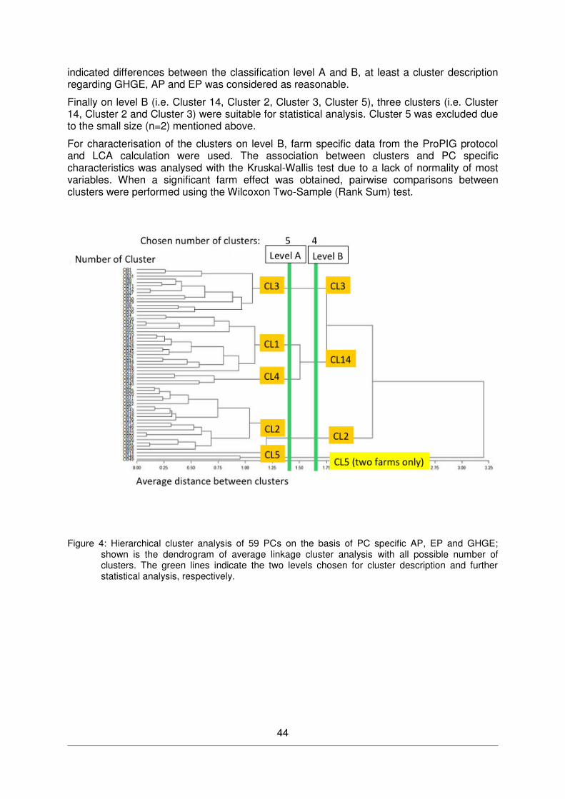
44
indicated differences between the classification level A and B, at least a cluster description regarding GHGE, AP and EP was considered as reasonable.
Finally on level B (i.e. Cluster 14, Cluster 2, Cluster 3, Cluster 5), three clusters (i.e. Cluster 14, Cluster 2 and Cluster 3) were suitable for statistical analysis. Cluster 5 was excluded due to the small size (n=2) mentioned above.
For characterisation of the clusters on level B, farm specific data from the ProPIG protocol and LCA calculation were used. The association between clusters and PC specific characteristics was analysed with the Kruskal-Wallis test due to a lack of normality of most variables. When a significant farm effect was obtained, pairwise comparisons between clusters were performed using the Wilcoxon Two-Sample (Rank Sum) test.
Figure 4: Hierarchical cluster analysis of 59 PCs on the basis of PC specific AP, EP and GHGE; shown is the dendrogram of average linkage cluster analysis with all possible number of clusters. The green lines indicate the two levels chosen for cluster description and further statistical analysis, respectively.
45
3.6.3 Associations between AHW and ENV
For chapter 4.3 a reduced sub-dataset was used only containing PCs for which ENV and GOOD% was possible to calculate. The reduced sub-dataset contained 38 PCs across ENV clusters (n=13, 12 and 13 per cluster, respectively), which represents 59 % of the original PCs in the intermediate ENV cluster, 62 % of the low ENV cluster and 86 % of the high ENV cluster.
In order to explore the association between AHW and ENV two different approaches were chosen:
1. The ENV clusters were tested regarding differences in GOOD %, GOOD% per animal category (SO, WE, FA) as well as each AHW parameter separately.
2. The second approach explored the strength and direction of associations between AHW and ENV by correlating GOOD% with the environmental impact indicators GHGE, AP and EP.
Comparisons between clusters were carried out using a non-parametric Kruskal-Wallis test. Furthermore, Spearman rank correlations were calculated between GOOD% and AP, EP and GHGE, respectively.

46
4 Results and discussion
4.1 Animal health and welfare (AHW)
4.1.1 Inter-observer reliability (IOR)
Table 19 contains results from the inter-observer reliability tests (as described in chapter 3.6.1.2), of clinical measures taken on the animal, which were done at three different dates and locations due to logistical constraints. For most of the parameters low median prevalences were found. The sows available for IOR testing did not show ectoparasites, poor body condition, shoulder lesions, vulva deformations or lesions, or require hospitalisation. In WE and FA, only diarrhoea (score 1 and 2 combined), respiratory problems (score 1 and 2) and pigs needing hospitalisation had a median prevalence > 0. Lowest agreement was found in the parameters respiratory problems in WE and FA and lameness in SO (71% agreement, respectively). Although for some parameters the prevalence recorded in the reliability test was zero for all observers, the parameters were kept in the analysis, as the observers agreed on problem absence (similar to Dippel et al. (2014b).
Table 19: Results from inter-observer reliability tests before farm visits from in total three training/IOR sessions (same trainer/gold standard but different trainees each). Exact percentage agreement is given as median (min - max) across all observer - gold standard pairs. Agreement for categorical parameters (respiratory problems and diarrhoea) was based on separate scores, i.e. diarrhoea score 0, 1, 2. Median number of groups observed was 10 (range 7 to 10) for all sow parameters but pigs needing hospitalisation (n = 7, range 4 to 10), and 10 (range 10 to 21) for weaner and fattener parameters except ectoparasites (n = 10, range 6 to 21). Prevalence = median gold standard prevalence (Q25, Q75; n of groups; for G prevalence at group level and n only) across all three tests. For prevalence of categorical parameters (respiratory problems and diarrhoea) score 1 and 2 were combined. Data where observers did not reach 70 % agreement are not included, to show exactly the IOR data relevant for AHW data used in the results. A/G= assessed at animal (A) or group (G) level; SO = sows, WE = weaners, FA = fatteners.
animal category
parameter level agreement prevalence
Median Min Max Median Q25 Q75 n SO ectoparasites A 100 71 100 0 0 0 27
BCS: fat sows A 86 71 100 0 0 0 27 lameness A 71 70 90 0 0 20 27 shoulder lesions A 100 86 100 0 0 0 27 vulva deformation A 83 71 100 0 0 0 27 vulva lesions A 86 71 100 0 0 0 27 pigs needing hospitalisation
G 100 86 100 0 . . 27
WE and FA ectoparasites A 100 100 100 0 0 0 37 eye inflammation A 100 70 100 0 0 0 41 lameness A 90 80 100 0 0 0 41 runts A 90 80 100 0 0 0 41 tail lesions A 90 80 100 0 0 0 41 tail short A 81 70 100 0 0 5 41 diarrhoea (0,1,2) G 90 70 100 17 . . 41 respiratory problems (0,1,2)
G 71 70 100 39 . . 41
pigs needing hospitalisation
G 100 90 100 2.4 . . 41
Table 20 reports results from the repeated inter-observer reliability tests of selected resource-based parameters. For feed supply, sufficient agreement was achieved across animal categories, but for the number of drinkers in SO 4 out of 7 observers did not achieve sufficient agreement with the gold standard. However, agreement regarding number of
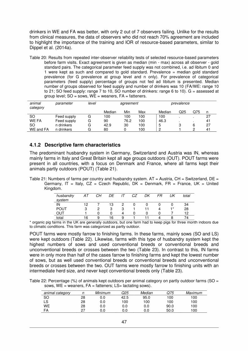
47
drinkers in WE and FA was better, with only 2 out of 7 observers failing. Unlike for the results from clinical measures, the data of observers who did not reach 70% agreement are included to highlight the importance of the training and IOR of resource-based parameters, similar to Dippel et al. (2014a).
Table 20: Results from repeated inter-observer reliability tests of selected resource-based parameters before farm visits. Exact agreement is given as median (min - max) across all observer - gold standard pairs. The categorical parameter feed supply was not combined, i.e. ad libitum 0 and 1 were kept as such and compared to gold standard. Prevalence = median gold standard prevalence (for G prevalence at group level and n only). For prevalence of categorical parameters (feed supply) percentage of groups not fed ad libitum is presented. Median number of groups observed for feed supply and number of drinkers was 10 (FA/WE: range 10 to 21; SO feed supply: range 7 to 10, SO number of drinkers: range 6 to 10). G = assessed at group level; SO = sows, WE = weaners, FA = fatteners.
animal category
parameter level agreement prevalence
Median Min Max Median Q25 Q75 n SO Feed supply G 100 100 100 100 . . 27 WE FA Feed supply G 90 76.2 100 46.3 . . 41 SO n drinkers G 42.9 30 100 5 3 6 27 WE and FA n drinkers G 80 0 100 2 1 2 41
4.1.2 Descriptive farm characteristics
The predominant husbandry system in Germany, Switzerland and Austria was IN, whereas mainly farms in Italy and Great Britain kept all age groups outdoors (OUT). POUT farms were present in all countries, with a focus on Denmark and France, where all farms kept their animals partly outdoors (POUT) (Table 21).
Table 21: Numbers of farms per country and husbandry system. AT = Austria, CH = Switzerland, DE = Germany, IT = Italy, CZ = Czech Republic, DK = Denmark, FR = France, UK = United Kingdom.
husbandry system
AT CH DE IT CZ DK FR UK total
IN 12 7 13 2 0 0 0 0 34 POUT 3 2 3 3 1 11 4 1* 28 OUT 1 0 0 4 0 0 0 7 12 total 16 9 16 9 1 11 4 8 74
* organic pig farms in the UK are generally outdoors, but one farm had to keep pigs for three month indoors due to climatic conditions. This farm was categorized as partly outdoor.
POUT farms were mostly farrow to finishing farms. In these farms, mainly sows (SO and LS) were kept outdoors (Table 22). Likewise, farms with this type of husbandry system kept the highest numbers of sows and used conventional breeds or conventional breeds and unconventional breeds or crosses between the two (Table 23). In contrast to this, IN farms were in only more than half of the cases farrow to finishing farms and kept the lowest number of sows, but as well used conventional breeds or conventional breeds and unconventional breeds or crosses between the two. OUT farms were mostly farrow to finishing units with an intermediate herd size, and never kept conventional breeds only (Table 23).
Table 22: Percentage (%) of animals kept outdoors per animal category on partly outdoor farms (SO = sows, WE = weaners, FA = fatteners; LS= lactating sows).
animal category n Minimum Q25 Median Q75 Maximum SO 28 0.0 42.5 95.0 100 100 LS 28 0.0 100 100 100 100 WE 28 0.0 0.0 0.0 90.0 100 FA 27 0.0 0.0 0.0 50.0 100

48
Table 23: Number and percentage (%) of farms per husbandry system and numbers of farms per production type (animal categories on farm: SO = sows, WE = weaners, FA = fatteners). Number of animals relate to animals present at farm visit. Breed C = conventional, U = unconventional, M = C and U or crosses between the two.
production type n animals (median (Q25 - Q75)) breed
system N farms (%)
SO WE FA
SO SOWE
WEFA
FA SO WE FA C M U
IN 34 (46) 16 0 7 1 10
39 (26-73)
82 (47-140)
140 (82-300) 23 11 0
POUT 28 (38) 26 0 2 0 0
141 (52-216)
250 (80-400)
338 (74-720) 23 4 1
OUT 12 (16) 9 1 0 1 1
53 (37-248)
49 (17-350)
154 (51-1166) 0 6 6
overall 51 1 9 2 11 65
(30-150) 105
(47-310) 187
(80-455) 0 0 0
In addition to the analysis of animal-based parameters on farm level (IN, POUT, OUT), a summary of the current location level (indoor / outdoor) of animal groups was done (Table 24). On the same farm, pregnant sows were most frequently assessed indoors as well as outdoors.
Table 24: Number of farms where animals (SO = sows, WE = weaners, FA = fatteners) were assessed indoors, outdoors or both by animal category. Both = n farms where animals of a stage were assessed indoor and outdoor (n is included in indoor and outdoor). Total number of farms = 74.
animal category assessed indoor
assessed outdoor
both
SO 36 34 9 WE 43 15 1 FA 51 16 4
Farm size related aspects (Table 25) showed wider variation within systems than between systems, whereby POUT had the highest median number of ha and LSU. The annual amount of straw (litter and enrichment material) used per LSU was highest in POUT and lowest in OUT. The highest amount was recorded in POUT and probably related to deep litter systems, which were more commonly used in POUT. With a median of 1700 slaughtered fatteners per year, POUT produced a higher amount of pigs than IN and OUT. Across systems, the lowest fatteners carcass weight was found in OUT, but in all systems some farms fattened the pigs up to 150 kg. POUT had the median lowest carcass weight. In median the sows were moved to farrowing accommodation 7 (IN, OUT) and 10 (POUT) days before farrowing, but also higher values were recorded especially in POUT and OUT, which were related to uncommon and complex farm management strategies, e.g. moving pregnant sows 90 days before farrowing together to a joint farrowing system as found in OUT. Median age at weaning was lowest (42 days) in IN and higher in POUT and OUT (49 and 50 days respectively). Again, higher values (age at weaning) found across all systems did not represent the common structure in organic pig systems.
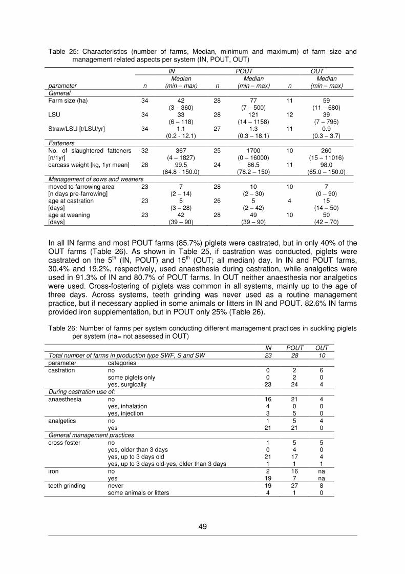
49
Table 25: Characteristics (number of farms, Median, minimum and maximum) of farm size and management related aspects per system (IN, POUT, OUT)
IN POUT OUT
parameter n Median
(min – max) n Median
(min – max) n Median
(min – max) General Farm size (ha) 34 42
(3 – 360) 28 77
(7 – 500) 11 59
(11 – 680) LSU 34 33
(6 – 118) 28 121
(14 – 1158) 12 39
(7 – 795) Straw/LSU [t/LSU/yr] 34 1.1
(0.2 - 12.1) 27 1.3
(0.3 – 18.1) 11 0.9
(0.3 – 3.7) Fatteners No. of slaughtered fatteners [n/1yr]
32 367 (4 – 1827)
25 1700 (0 – 16000)
10 260 (15 – 11016)
carcass weight [kg, 1yr mean] 28 99.5 (84.8 - 150.0)
24 86.5 (78.2 – 150)
11 98.0 (65.0 – 150.0)
Management of sows and weaners moved to farrowing area [n days pre-farrowing]
23 7 (2 – 14)
28 10 (2 – 30)
10 7 (0 – 90)
age at castration [days]
23 5 (3 – 28)
26 5 (2 – 42)
4 15 (14 – 50)
age at weaning [days]
23 42 (39 – 90)
28 49 (39 – 90)
10 50 (42 – 70)
In all IN farms and most POUT farms (85.7%) piglets were castrated, but in only 40% of the OUT farms (Table 26). As shown in Table 25, if castration was conducted, piglets were castrated on the 5th (IN, POUT) and 15th (OUT; all median) day. In IN and POUT farms, 30.4% and 19.2%, respectively, used anaesthesia during castration, while analgetics were used in 91.3% of IN and 80.7% of POUT farms. In OUT neither anaesthesia nor analgetics were used. Cross-fostering of piglets was common in all systems, mainly up to the age of three days. Across systems, teeth grinding was never used as a routine management practice, but if necessary applied in some animals or litters in IN and POUT. 82.6% IN farms provided iron supplementation, but in POUT only 25% (Table 26).
Table 26: Number of farms per system conducting different management practices in suckling piglets per system (na= not assessed in OUT)
IN POUT OUT Total number of farms in production type SWF, S and SW 23 28 10 parameter categories castration no 0 2 6 some piglets only 0 2 0 yes, surgically 23 24 4 During castration use of: anaesthesia no 16 21 4
yes, inhalation 4 0 0 yes, injection 3 5 0
analgetics no 1 5 4 yes 21 21 0 General management practices cross-foster no 1 5 5 yes, older than 3 days 0 4 0 yes, up to 3 days old 21 17 4 yes, up to 3 days old-yes, older than 3 days 1 1 1 iron no 2 16 na yes 19 7 na teeth grinding never 19 27 8 some animals or litters 4 1 0
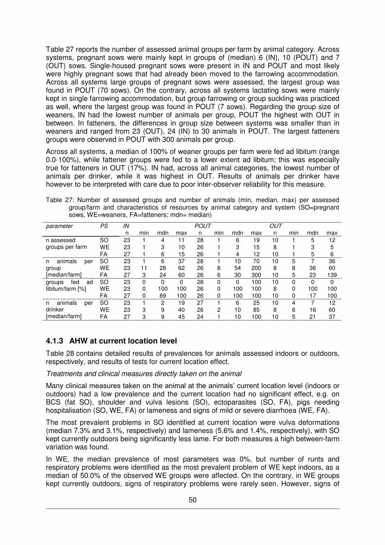
50
Table 27 reports the number of assessed animal groups per farm by animal category. Across systems, pregnant sows were mainly kept in groups of (median) 6 (IN), 10 (POUT) and 7 (OUT) sows. Single-housed pregnant sows were present in IN and POUT and most likely were highly pregnant sows that had already been moved to the farrowing accommodation. Across all systems large groups of pregnant sows were assessed, the largest group was found in POUT (70 sows). On the contrary, across all systems lactating sows were mainly kept in single farrowing accommodation, but group farrowing or group suckling was practiced as well, where the largest group was found in POUT (7 sows). Regarding the group size of weaners, IN had the lowest number of animals per group, POUT the highest with OUT in between. In fatteners, the differences in group size between systems was smaller than in weaners and ranged from 23 (OUT), 24 (IN) to 30 animals in POUT. The largest fatteners groups were observed in POUT with 300 animals per group.
Across all systems, a median of 100% of weaner groups per farm were fed ad libitum (range 0.0-100%), while fattener groups were fed to a lower extent ad libitum; this was especially true for fatteners in OUT (17%). IN had, across all animal categories, the lowest number of animals per drinker, while it was highest in OUT. Results of animals per drinker have however to be interpreted with care due to poor inter-observer reliability for this measure.
Table 27: Number of assessed groups and number of animals (min, median, max) per assessed group/farm and characteristics of resources by animal category and system (SO=pregnant sows, WE=weaners, FA=fatteners; mdn= median)
parameter PS IN POUT OUT n min mdn max n min mdn max n min mdn max
n assessed groups per farm
SO 23 1 4 11 28 1 6 19 10 1 5 12 WE 23 1 3 10 26 1 3 15 8 1 3 5 FA 27 1 6 15 26 1 4 12 10 1 5 6
n animals per group [median/farm]
SO 23 1 6 37 28 1 10 70 10 5 7 36 WE 23 11 28 62 26 8 54 200 8 8 36 60 FA 27 3 24 60 26 6 30 300 10 5 23 139
groups fed ad libitum/farm [%]
SO 23 0 0 0 28 0 0 100 10 0 0 0 WE 23 0 100 100 26 0 100 100 8 0 100 100 FA 27 0 89 100 26 0 100 100 10 0 17 100
n animals per drinker [median/farm]
SO 23 1 2 19 27 1 6 25 10 4 7 12 WE 23 3 9 40 26 2 10 85 8 6 16 60 FA 27 3 9 45 24 1 10 100 10 5 21 37
4.1.3 AHW at current location level
Table 28 contains detailed results of prevalences for animals assessed indoors or outdoors, respectively, and results of tests for current location effect.
Treatments and clinical measures directly taken on the animal
Many clinical measures taken on the animal at the animals’ current location level (indoors or outdoors) had a low prevalence and the current location had no significant effect, e.g. on BCS (fat SO), shoulder and vulva lesions (SO), ectoparasites (SO, FA), pigs needing hospitalisation (SO, WE, FA) or lameness and signs of mild or severe diarrhoea (WE, FA).
The most prevalent problems in SO identified at current location were vulva deformations (median 7.3% and 3.1%, respectively) and lameness (5.6% and 1.4%, respectively), with SO kept currently outdoors being significantly less lame. For both measures a high between-farm variation was found.
In WE, the median prevalence of most parameters was 0%, but number of runts and respiratory problems were identified as the most prevalent problem of WE kept indoors, as a median of 50.0% of the observed WE groups were affected. On the contrary, in WE groups kept currently outdoors, signs of respiratory problems were rarely seen. However, signs of
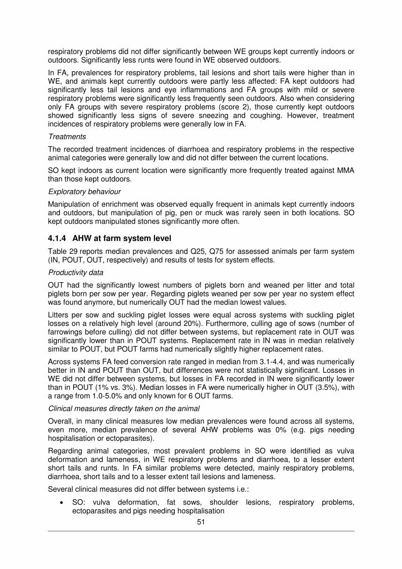
51
respiratory problems did not differ significantly between WE groups kept currently indoors or outdoors. Significantly less runts were found in WE observed outdoors.
In FA, prevalences for respiratory problems, tail lesions and short tails were higher than in WE, and animals kept currently outdoors were partly less affected: FA kept outdoors had significantly less tail lesions and eye inflammations and FA groups with mild or severe respiratory problems were significantly less frequently seen outdoors. Also when considering only FA groups with severe respiratory problems (score 2), those currently kept outdoors showed significantly less signs of severe sneezing and coughing. However, treatment incidences of respiratory problems were generally low in FA.
Treatments
The recorded treatment incidences of diarrhoea and respiratory problems in the respective animal categories were generally low and did not differ between the current locations.
SO kept indoors as current location were significantly more frequently treated against MMA than those kept outdoors.
Exploratory behaviour
Manipulation of enrichment was observed equally frequent in animals kept currently indoors and outdoors, but manipulation of pig, pen or muck was rarely seen in both locations. SO kept outdoors manipulated stones significantly more often.
4.1.4 AHW at farm system level
Table 29 reports median prevalences and Q25, Q75 for assessed animals per farm system (IN, POUT, OUT, respectively) and results of tests for system effects.
Productivity data
OUT had the significantly lowest numbers of piglets born and weaned per litter and total piglets born per sow per year. Regarding piglets weaned per sow per year no system effect was found anymore, but numerically OUT had the median lowest values.
Litters per sow and suckling piglet losses were equal across systems with suckling piglet losses on a relatively high level (around 20%). Furthermore, culling age of sows (number of farrowings before culling) did not differ between systems, but replacement rate in OUT was significantly lower than in POUT systems. Replacement rate in IN was in median relatively similar to POUT, but POUT farms had numerically slightly higher replacement rates.
Across systems FA feed conversion rate ranged in median from 3.1-4.4, and was numerically better in IN and POUT than OUT, but differences were not statistically significant. Losses in WE did not differ between systems, but losses in FA recorded in IN were significantly lower than in POUT (1% vs. 3%). Median losses in FA were numerically higher in OUT (3.5%), with a range from 1.0-5.0% and only known for 6 OUT farms.
Clinical measures directly taken on the animal
Overall, in many clinical measures low median prevalences were found across all systems, even more, median prevalence of several AHW problems was 0% (e.g. pigs needing hospitalisation or ectoparasites).
Regarding animal categories, most prevalent problems in SO were identified as vulva deformation and lameness, in WE respiratory problems and diarrhoea, to a lesser extent short tails and runts. In FA similar problems were detected, mainly respiratory problems, diarrhoea, short tails and to a lesser extent tail lesions and lameness.
Several clinical measures did not differ between systems i.e.:
SO: vulva deformation, fat sows, shoulder lesions, respiratory problems, ectoparasites and pigs needing hospitalisation

52
WE: short tails, lame animals, diarrhoea and respiratory problems score 2, respectively, and pigs needing hospitalisation
FA: short tails, lame animals, diarrhoea score 2, ectoparasites, runts and pigs needing hospitalisation
In several AHW problems, OUT had significantly lower prevalences. The more commonly observed problems were mild and severe respiratory problems (coughing and sneezing) in WE and FA, in both animal categories in OUT significantly less groups were affected (both 0% OUT, >60 % POUT, IN). Furthermore, prevalence of severe respiratory problems (score 2 only) was significantly lower in FA groups in OUT than in IN while POUT FA groups differed neither from IN nor from OUT. As well, significantly less FA with eye inflammation were seen in OUT compared to IN and POUT.
Signs of diarrhoea (score 1 + 2) were less frequently seen in WE groups in OUT (0%) compared to IN (25.0%), while POUT groups differed neither from IN nor from OUT. However prevalence of diarrhoea (score 1 + 2) in FA groups in OUT were lower than in POUT and in IN (0%, 0%, 8.3%, respectively). However, signs of severe diarrhoea were rarely seen at all.
Almost no fresh tail lesions were seen in all systems, but in FA the significantly lowest number was seen in OUT compared to IN and POUT. However, short tails were seen more often than tail lesions, especially in FA, but independently from the system. OUT had, compared to IN and POUT, the lowest number of runts in WE, but across all systems almost no runts in FA were observed anymore.
OUT and POUT had fewer lame sows compared to IN (0%, 3.4%, 7.1%, respectively). Across all systems vulva lesions were almost never recorded, even though a significant difference was found: OUT sows had significantly less vulva lesions than sows in POUT, while IN differed neither from OUT nor from POUT. However, vulva deformation was observed in all three systems, whereby no system effect was found.
Treatments
Regarding treatment of MMA all systems differed significantly from each other, IN had the highest incidence of treatment of MMA in SO, intermediate incidences were recorded in POUT and lowest in OUT. Furthermore, the number of treatment prevalence against diarrhoea in suckling piglets (SP), WE and FA as well as treatment incidences of respiratory problems was low and did not differ between systems.
Anti-parasite treatment of sows did not differ between systems. Most sows, at least in IN and POUT, were treated once a year against parasites, which may have contributed in these systems to the fact that no signs of ectoparasites were observed on SO and FA. OUT sows were treated numerically less frequently against parasites, but no signs of ectoparasites were found.
Exploratory behaviour
Manipulation of enrichment was seen in all animal categories in all three systems, but manipulation of pen/muck/ other pigs was rarely seen in any system. However, manipulating stones was found in sows more frequently in OUT than in IN, but POUT differed neither from IN nor from OUT.
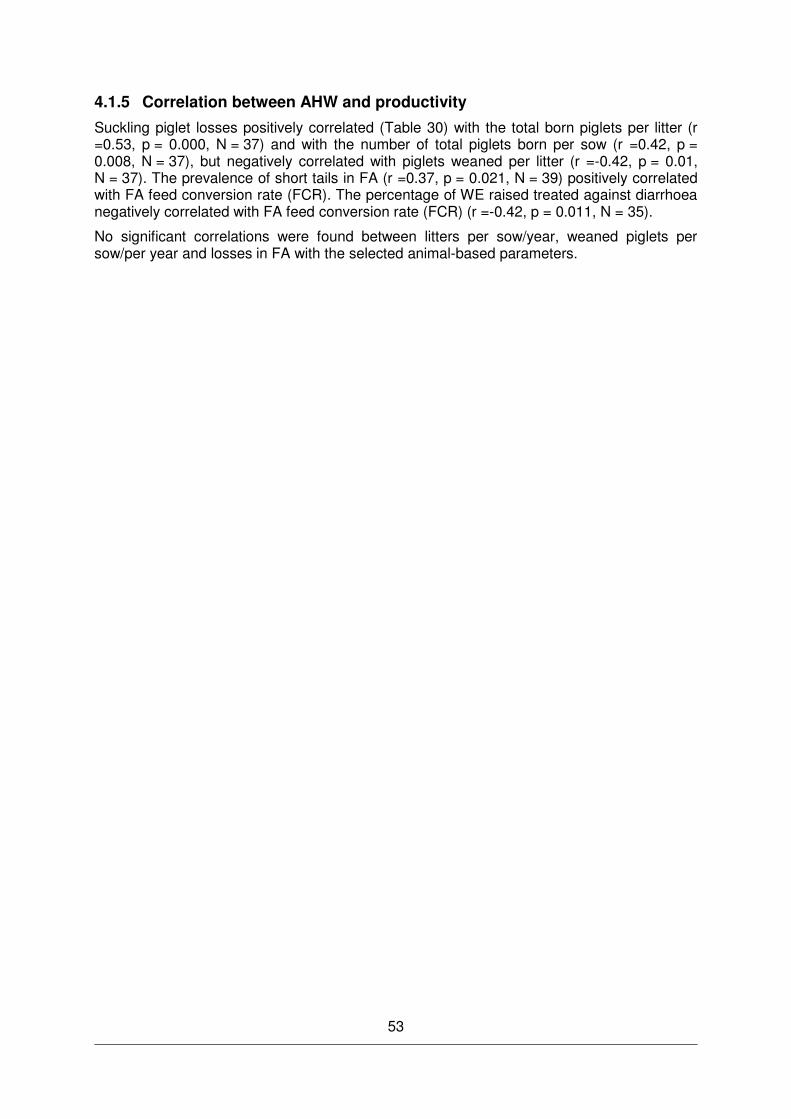
53
4.1.5 Correlation between AHW and productivity
Suckling piglet losses positively correlated (Table 30) with the total born piglets per litter (r =0.53, p = 0.000, N = 37) and with the number of total piglets born per sow (r =0.42, p = 0.008, N = 37), but negatively correlated with piglets weaned per litter (r =-0.42, p = 0.01, N = 37). The prevalence of short tails in FA (r =0.37, p = 0.021, N = 39) positively correlated with FA feed conversion rate (FCR). The percentage of WE raised treated against diarrhoea negatively correlated with FA feed conversion rate (FCR) (r =-0.42, p = 0.011, N = 35).
No significant correlations were found between litters per sow/year, weaned piglets per sow/per year and losses in FA with the selected animal-based parameters.
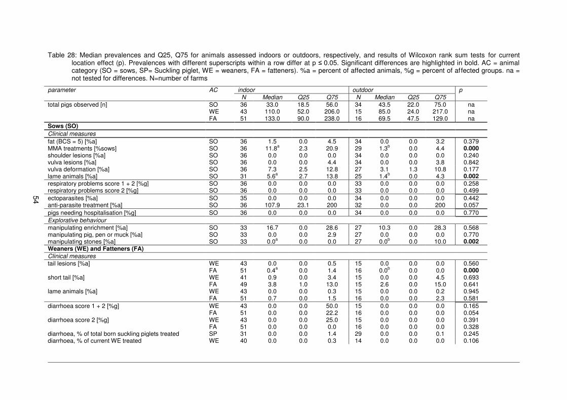
54
Table 28: Median prevalences and Q25, Q75 for animals assessed indoors or outdoors, respectively, and results of Wilcoxon rank sum tests for current location effect (p). Prevalences with different superscripts within a row differ at p ≤ 0.05. Significant differences are highlighted in bold. AC = animal category (SO = sows, SP= Suckling piglet, WE = weaners, FA = fatteners). %a = percent of affected animals, %g = percent of affected groups. na = not tested for differences. N=number of farms
parameter AC indoor outdoor p N Median Q25 Q75 N Median Q25 Q75
total pigs observed [n] SO 36 33.0 18.5 56.0 34 43.5 22.0 75.0 na WE 43 110.0 52.0 206.0 15 85.0 24.0 217.0 na FA 51 133.0 90.0 238.0 16 69.5 47.5 129.0 na Sows (SO)
Clinical measures
fat (BCS = 5) [%a] SO 36 1.5 0.0 4.5 34 0.0 0.0 3.2 0.379 MMA treatments [%sows] SO 36 11.8a 2.3 20.9 29 1.3b 0.0 4.4 0.000 shoulder lesions [%a] SO 36 0.0 0.0 0.0 34 0.0 0.0 0.0 0.240 vulva lesions [%a] SO 36 0.0 0.0 4.4 34 0.0 0.0 3.8 0.842 vulva deformation [%a] SO 36 7.3 2.5 12.8 27 3.1 1.3 10.8 0.177 lame animals [%a] SO 31 5.6a 2.7 13.8 25 1.4b 0.0 4.3 0.002 respiratory problems score 1 + 2 [%g] SO 36 0.0 0.0 0.0 33 0.0 0.0 0.0 0.258 respiratory problems score 2 [%g] SO 36 0.0 0.0 0.0 33 0.0 0.0 0.0 0.499 ectoparasites [%a] SO 35 0.0 0.0 0.0 34 0.0 0.0 0.0 0.442 anti-parasite treatment [%a] SO 36 107.9 23.1 200 32 0.0 0.0 200 0.057 pigs needing hospitalisation [%g] SO 36 0.0 0.0 0.0 34 0.0 0.0 0.0 0.770 Explorative behaviour manipulating enrichment [%a] SO 33 16.7 0.0 28.6 27 10.3 0.0 28.3 0.568 manipulating pig, pen or muck [%a] SO 33 0.0 0.0 2.9 27 0.0 0.0 0.0 0.770 manipulating stones [%a] SO 33 0.0a 0.0 0.0 27 0.0b 0.0 10.0 0.002 Weaners (WE) and Fatteners (FA) Clinical measures tail lesions [%a] WE 43 0.0 0.0 0.5 15 0.0 0.0 0.0 0.560
FA 51 0.4a 0.0 1.4 16 0.0b 0.0 0.0 0.000 short tail [%a] WE 41 0.9 0.0 3.4 15 0.0 0.0 4.5 0.693
FA 49 3.8 1.0 13.0 15 2.6 0.0 15.0 0.641 lame animals [%a] WE 43 0.0 0.0 0.3 15 0.0 0.0 0.2 0.945 FA 51 0.7 0.0 1.5 16 0.0 0.0 2.3 0.581 diarrhoea score 1 + 2 [%g] WE 43 0.0 0.0 50.0 15 0.0 0.0 0.0 0.165
FA 51 0.0 0.0 22.2 16 0.0 0.0 0.0 0.054 diarrhoea score 2 [%g] WE 43 0.0 0.0 25.0 15 0.0 0.0 0.0 0.391
FA 51 0.0 0.0 0.0 16 0.0 0.0 0.0 0.328 diarrhoea, % of total born suckling piglets treated SP 31 0.0 0.0 1.4 29 0.0 0.0 0.1 0.245 diarrhoea, % of current WE treated WE 40 0.0 0.0 0.3 14 0.0 0.0 0.0 0.106
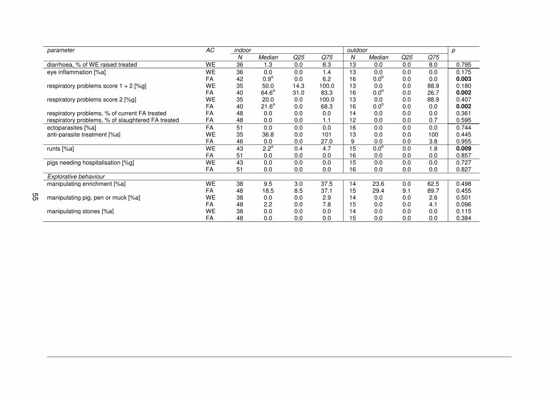
55
parameter AC indoor outdoor p N Median Q25 Q75 N Median Q25 Q75
diarrhoea, % of WE raised treated WE 36 1.3 0.0 8.3 13 0.0 0.0 8.0 0.795 eye inflammation [%a] WE 36 0.0 0.0 1.4 13 0.0 0.0 0.0 0.175
FA 42 0.9a 0.0 6.2 16 0.0b 0.0 0.0 0.003 respiratory problems score 1 + 2 [%g] WE 35 50.0 14.3 100.0 13 0.0 0.0 88.9 0.180 FA 40 64.6a 31.0 83.3 16 0.0b 0.0 26.7 0.002 respiratory problems score 2 [%g] WE 35 20.0 0.0 100.0 13 0.0 0.0 88.9 0.407 FA 40 21.6a 0.0 68.3 16 0.0b 0.0 0.0 0.002 respiratory problems, % of current FA treated FA 48 0.0 0.0 0.0 14 0.0 0.0 0.0 0.361 respiratory problems, % of slaughtered FA treated FA 48 0.0 0.0 1.1 12 0.0 0.0 0.7 0.595 ectoparasites [%a] FA 51 0.0 0.0 0.0 16 0.0 0.0 0.0 0.744 anti-parasite treatment [%a] WE 35 36.8 0.0 101 13 0.0 0.0 100 0.445 FA 46 0.0 0.0 27.0 9 0.0 0.0 3.8 0.955 runts [%a] WE 43 2.2a 0.4 4.7 15 0.0b 0.0 1.8 0.009
FA 51 0.0 0.0 0.0 16 0.0 0.0 0.0 0.857 pigs needing hospitalisation [%g] WE 43 0.0 0.0 0.0 15 0.0 0.0 0.0 0.727 FA 51 0.0 0.0 0.0 16 0.0 0.0 0.0 0.827 Explorative behaviour manipulating enrichment [%a] WE 38 9.5 3.0 37.5 14 23.6 0.0 62.5 0.498 FA 48 18.5 8.5 37.1 15 29.4 9.1 89.7 0.455 manipulating pig, pen or muck [%a] WE 38 0.0 0.0 2.9 14 0.0 0.0 2.6 0.501 FA 48 2.2 0.0 7.8 15 0.0 0.0 4.1 0.096 manipulating stones [%a] WE 38 0.0 0.0 0.0 14 0.0 0.0 0.0 0.115 FA 48 0.0 0.0 0.0 15 0.0 0.0 0.0 0.384
56
Table 29: Median (Mdn) prevalences and Q25, Q75 for assessed animals per farm system (IN: indoor, POUT: partly outdoor, OUT: outdoor). p = result of global Kruskal-Wallis test for system effect. Prevalences with different superscripts within a row differ at p ≤ 0.05 in a pairwise system comparison with Wilcoxon rank sum tests and Bonferroni-Holm correction for three tests. AC = animal category (SO = sows, SP= Suckling piglets, WE = weaners, FA = fatteners). %a = percent of affected animals, %g = percent of affected groups. na = not tested for differences. N= number of farms
parameter AC IN POUT OUT p N Mdn Q25 Q75 N Mdn Q25 Q75 N Mdn Q25 Q75
total pigs observed [n] SO 23 24.0 18.0 54.0 28 68.5 29.5 94.0 10 43.0 29.0 57.0 na WE 23 83.0 40.0 142.0 26 171.5 72.0 250.0 8 52.5 29.0 142.0 na FA 27 148.0 90.0 262.0 26 111.0 91.0 227.0 10 94.0 49.0 154.0 na Productivity data and treatments piglets born per litter (life born + still born) [n, 1yr mean]
SO 21 13.0a 12.0 14.0 26 13.4a 12.0 14.0 10 8.8b 7.0 12.0 0.001
piglets weaned per litter [n, 1yr mean] SO 22 9.7a 9.0 10.3 27 9.8a 9.0 11.0 10 7.3b 5.0 9.6 0.015 litters per sow [n, 1yr mean] SO 22 2.0 1.9 2.1 27 2.0 1.9 2.0 10 2.0 1.7 2.0 0.403 total piglets born per sow [n, 1yr mean] SO 21 26.8a 24.0 28.1 26 26.6a 22.8 28.6 10 16.6b 11.1 24.0 0.002 piglets weaned per sow per year [n, 1yr mean] SO 23 19.4 16.6 21.0 27 19.0 16.0 21.0 10 13.5 10.0 18.6 0.049 suckling piglet losses [%, 1yr mean] SO 21 21.3 19.6 32.1 26 21.6 16.5 28.6 10 19.2 14.9 27.3 0.156 MMA treatments [%sows] SO 23 16.5a 8.0 43.8 26 1.6b 0.0 5.3 7 0.0c 0.0 0.0 0.000 sow replacement rate [%, 1yr mean] SO 23 30.0ab 20.0 33.0 27 31.0a 25.0 45.0 10 17.0b 10.0 35.0 0.009 culling age [n farrowings] SO 19 6.0 5.0 7.0 27 5.0 4.0 8.0 7 7.0 2.0 8.0 0.805 losses [%, 1yr mean] WE 20 3.5 1.5 5.0 24 5.0 3.0 5.0 6 4.0 3.0 5.0 0.882
FA 22 1.0a 1.0 3.0 21 3.0b 2.0 4.0 6 3.5ab 1.0 5.0 0.005 feed conversion rate FA 26 3.2 2.9 3.6 24 3.3 3.0 3.9 11 4.4 2.9 6.5 0.061 Sows (SO) Clinical measures fat (BCS = 5) [%a] SO 23 1.7 0.0 4.7 28 0.3 0.0 3.2 10 0.0 0.0 5.6 0.633 shoulder lesions [%a] SO 23 0.0 0.0 0.0 28 0.0 0.0 0.0 10 0.0 0.0 0.0 0.326 vulva lesions [%a] SO 23 0.0ab 0.0 4.3 28 1.9a 0.0 4.2 10 0.0b 0.0 0.0 0.040 vulva deformation [%a] SO 23 8.7 4.5 14.3 27 3.0 1.4 10.8 4 10.7 3.8 18.1 0.074 lame animals [%a] SO 23 7.1a 4.3 16.2 17 3.4b 0.0 4.9 10 0.0b 0.0 1.7 0.001 respiratory problems score 1 + 2 [%g] SO 23 0.0 0.0 0.0 27 0.0 0.0 0.0 10 0.0 0.0 0.0 0.412 respiratory problems score 2 [%g] SO 23 0.0 0.0 0.0 27 0.0 0.0 0.0 10 0.0 0.0 0.0 0.650
ectoparasites [%a] SO 22 0.0 0.0 0.0 28 0.0 0.0 0.0 10 0.0 0.0 0.0 0.178 anti-parasite treatment [%a] SO 23 187.5 60.0 200.0 28 100.0 0.0 200.0 8 0.0 0.0 100.0 0.054 pigs needing hospitalisation [%g] SO 23 0.0 0.0 0.0 28 0.0 0.0 0.0 10 0.0 0.0 0.0 0.777 Exploratory behaviour (SO) manipulating enrichment [%a] SO 22 11.9 0.0 25.0 24 17.6 0.0 28.5 9 5.7 0.0 71.4 0.874 manipulating pig, pen or muck [%a] SO 22 0.0 0.0 0.0 24 0.0 0.0 0.0 9 2.1 0.0 24.1 0.066 manipulating stones [%a] SO 22 0.0a 0.0 0.0 24 0.0ab 0.0 0.8 9 0.0b 0.0 10.0 0.029
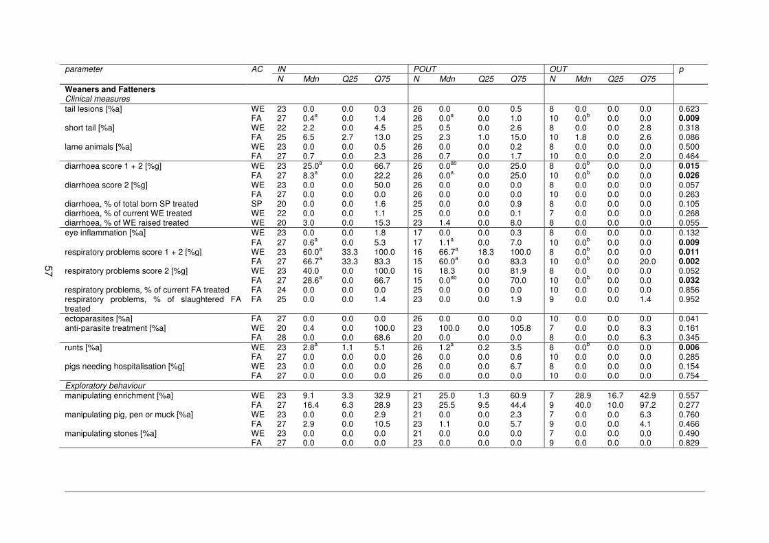
57
parameter AC IN POUT OUT p N Mdn Q25 Q75 N Mdn Q25 Q75 N Mdn Q25 Q75
Weaners and Fatteners Clinical measures
tail lesions [%a] WE 23 0.0 0.0 0.3 26 0.0 0.0 0.5 8 0.0 0.0 0.0 0.623 FA 27 0.4a 0.0 1.4 26 0.0a 0.0 1.0 10 0.0b 0.0 0.0 0.009
short tail [%a] WE 22 2.2 0.0 4.5 25 0.5 0.0 2.6 8 0.0 0.0 2.8 0.318 FA 25 6.5 2.7 13.0 25 2.3 1.0 15.0 10 1.8 0.0 2.6 0.086
lame animals [%a] WE 23 0.0 0.0 0.5 26 0.0 0.0 0.2 8 0.0 0.0 0.0 0.500 FA 27 0.7 0.0 2.3 26 0.7 0.0 1.7 10 0.0 0.0 2.0 0.464 diarrhoea score 1 + 2 [%g] WE 23 25.0a 0.0 66.7 26 0.0ab 0.0 25.0 8 0.0b 0.0 0.0 0.015
FA 27 8.3a 0.0 22.2 26 0.0a 0.0 25.0 10 0.0b 0.0 0.0 0.026 diarrhoea score 2 [%g] WE 23 0.0 0.0 50.0 26 0.0 0.0 0.0 8 0.0 0.0 0.0 0.057
FA 27 0.0 0.0 0.0 26 0.0 0.0 0.0 10 0.0 0.0 0.0 0.263 diarrhoea, % of total born SP treated SP 20 0.0 0.0 1.6 25 0.0 0.0 0.9 8 0.0 0.0 0.0 0.105 diarrhoea, % of current WE treated WE 22 0.0 0.0 1.1 25 0.0 0.0 0.1 7 0.0 0.0 0.0 0.268 diarrhoea, % of WE raised treated WE 20 3.0 0.0 15.3 23 1.4 0.0 8.0 8 0.0 0.0 0.0 0.055 eye inflammation [%a] WE 23 0.0 0.0 1.8 17 0.0 0.0 0.3 8 0.0 0.0 0.0 0.132
FA 27 0.6a 0.0 5.3 17 1.1a 0.0 7.0 10 0.0b 0.0 0.0 0.009 respiratory problems score 1 + 2 [%g] WE 23 60.0a 33.3 100.0 16 66.7a 18.3 100.0 8 0.0b 0.0 0.0 0.011 FA 27 66.7a 33.3 83.3 15 60.0a 0.0 83.3 10 0.0b 0.0 20.0 0.002 respiratory problems score 2 [%g] WE 23 40.0 0.0 100.0 16 18.3 0.0 81.9 8 0.0 0.0 0.0 0.052 FA 27 28.6a 0.0 66.7 15 0.0ab 0.0 70.0 10 0.0b 0.0 0.0 0.032 respiratory problems, % of current FA treated FA 24 0.0 0.0 0.0 25 0.0 0.0 0.0 10 0.0 0.0 0.0 0.856 respiratory problems, % of slaughtered FA treated
FA 25 0.0 0.0 1.4 23 0.0 0.0 1.9 9 0.0 0.0 1.4 0.952
ectoparasites [%a] FA 27 0.0 0.0 0.0 26 0.0 0.0 0.0 10 0.0 0.0 0.0 0.041 anti-parasite treatment [%a] WE 20 0.4 0.0 100.0 23 100.0 0.0 105.8 7 0.0 0.0 8.3 0.161 FA 28 0.0 0.0 68.6 20 0.0 0.0 0.0 8 0.0 0.0 6.3 0.345 runts [%a] WE 23 2.8a 1.1 5.1 26 1.2a 0.2 3.5 8 0.0b 0.0 0.0 0.006
FA 27 0.0 0.0 0.0 26 0.0 0.0 0.6 10 0.0 0.0 0.0 0.285 pigs needing hospitalisation [%g] WE 23 0.0 0.0 0.0 26 0.0 0.0 6.7 8 0.0 0.0 0.0 0.154 FA 27 0.0 0.0 0.0 26 0.0 0.0 0.0 10 0.0 0.0 0.0 0.754 Exploratory behaviour manipulating enrichment [%a] WE 23 9.1 3.3 32.9 21 25.0 1.3 60.9 7 28.9 16.7 42.9 0.557 FA 27 16.4 6.3 28.9 23 25.5 9.5 44.4 9 40.0 10.0 97.2 0.277 manipulating pig, pen or muck [%a] WE 23 0.0 0.0 2.9 21 0.0 0.0 2.3 7 0.0 0.0 6.3 0.760 FA 27 2.9 0.0 10.5 23 1.1 0.0 5.7 9 0.0 0.0 4.1 0.466 manipulating stones [%a] WE 23 0.0 0.0 0.0 21 0.0 0.0 0.0 7 0.0 0.0 0.0 0.490 FA 27 0.0 0.0 0.0 23 0.0 0.0 0.0 9 0.0 0.0 0.0 0.829
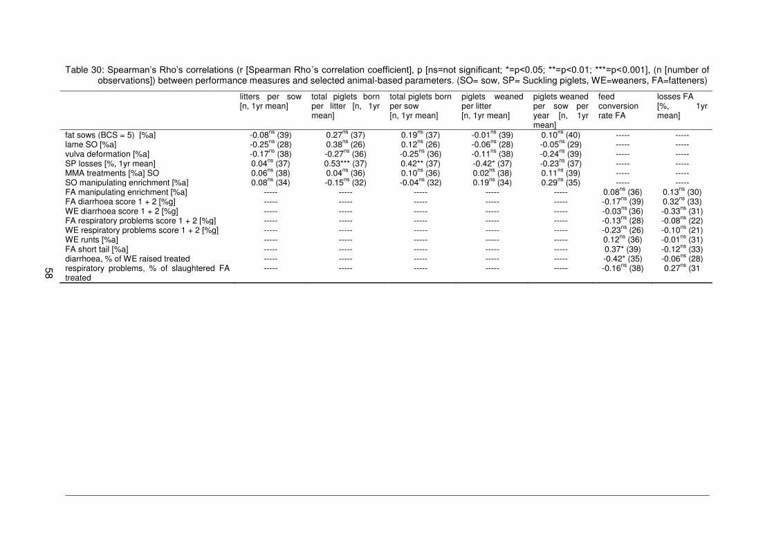
58
Table 30: Spearman’s Rho’s correlations (r [Spearman Rho´s correlation coefficient], p [ns=not significant; *=p<0.05; **=p<0.01; ***=p<0.001], (n [number of observations]) between performance measures and selected animal-based parameters. (SO= sow, SP= Suckling piglets, WE=weaners, FA=fatteners)
litters per sow [n, 1yr mean]
total piglets born per litter [n, 1yr mean]
total piglets born per sow [n, 1yr mean]
piglets weaned per litter [n, 1yr mean]
piglets weaned per sow per year [n, 1yr mean]
feed conversion rate FA
losses FA [%, 1yr mean]
fat sows (BCS = 5) [%a] -0.08ns (39) 0.27ns (37) 0.19ns (37) -0.01ns (39) 0.10ns (40) ----- ----- lame SO [%a] -0.25ns (28) 0.38ns (26) 0.12ns (26) -0.06ns (28) -0.05ns (29) ----- ----- vulva deformation [%a] -0.17ns (38) -0.27ns (36) -0.25ns (36) -0.11ns (38) -0.24ns (39) ----- ----- SP losses [%, 1yr mean] 0.04ns (37) 0.53*** (37) 0.42** (37) -0.42* (37) -0.23ns (37) ----- ----- MMA treatments [%a] SO 0.06ns (38) 0.04ns (36) 0.10ns (36) 0.02ns (38) 0.11ns (39) ----- ----- SO manipulating enrichment [%a] 0.08ns (34) -0.15ns (32) -0.04ns (32) 0.19ns (34) 0.29ns (35) ----- ----- FA manipulating enrichment [%a] ----- ----- ----- ----- ----- 0.08ns (36) 0.13ns (30) FA diarrhoea score 1 + 2 [%g] ----- ----- ----- ----- ----- -0.17ns (39) 0.32ns (33) WE diarrhoea score 1 + 2 [%g] ----- ----- ----- ----- ----- -0.03ns (36) -0.33ns (31) FA respiratory problems score 1 + 2 [%g] ----- ----- ----- ----- ----- -0.13ns (28) -0.08ns (22) WE respiratory problems score 1 + 2 [%g] ----- ----- ----- ----- ----- -0.23ns (26) -0.10ns (21) WE runts [%a] ----- ----- ----- ----- ----- 0.12ns (36) -0.01ns (31) FA short tail [%a] ----- ----- ----- ----- ----- 0.37* (39) -0.12ns (33) diarrhoea, % of WE raised treated ----- ----- ----- ----- ----- -0.42* (35) -0.06ns (28) respiratory problems, % of slaughtered FA treated
----- ----- ----- ----- ----- -0.16ns (38) 0.27ns (31
59
4.1.6 Discussion
Brief description of results
AHW was assessed in pregnant sows (SO), weaners (WE) and fattening pigs (FA). Across systems, prevalences of most AHW areas were low; exceptions were respiratory problems (IN, POUT), diarrhoea (IN), vulva deformation (IN, OUT) and short tails (IN, POUT). Total suckling piglet losses should be improved in all three systems. OUT had advantages regarding several areas of AHW, which could be explained by the outdoor specific environment, e.g. respiratory problems (better air quality), diarrhoea (less exposure to faeces) and lameness (softer lying and walking surfaces). POUT farms kept SO in most cases outdoors and WE/ FA similar to IN farms, which was reflected in the AHW results.
Design of the study
Information on prevalences of organic pig health and welfare problems is limited, as few large-scale published on-farm assessment studies exist. Therefore the present study applied a comprehensive animal health and welfare protocol, mainly consisting of animal-based parameters, on 74 organic pig farms with three different husbandry systems (IN (n=34), POUT (n=28), OUT (n=12)) across 8 European countries. The results of the present study give a detailed overview of the health and welfare status of organic sows (SO), weaners (WE) and fatteners (FA) in the three husbandry systems. The sample of farms is not necessarily completely representative for organic pig production, as farms having problems regarding animal health and welfare were specifically invited to participate in the project. On the other hand also ambitious farmers might have responded to this call. These two groups of farmers together might lead to a relatively representative sample, which is supported by the fact that the found prevalences are in the range of other studies.
Since the study’s focus was on comparison of the three systems and there were different numbers of farms and systems per country, no tests for statistical difference between countries were carried out. However, national regulations and common local strategies (e.g. age at weaning, duration of fattening period) or general level of endemic health within a country may influence herd health on a national level (Hovi et al., 2003, Edwards et al., 2014a).
A standardised on-farm assessment protocol was developed and integrated into ‘PigSurfer’, a Software tool enabling direct digital on-farm data collection via tablet pc. The animal-based welfare indicators used in this protocol were based on the Welfare Quality protocol (Welfare Quality®, 2009) and experiences from previous studies (Leeb et al., 2010, Dippel et al., 2014b). They were adapted to present a picture, as complete as possible, of pig health and welfare within a one-day visit. An observational assessment of lactating sows and suckling piglets was considered as not feasible, instead farm records were used for these animal categories. Furthermore, due to the comprehensive approach the ProPIG questionnaire included additional farm specific data regarding type of farm and diverse management aspects (e.g. diets composition and content, land use, manure handling), which are not presented here in detail. Therefore, the assessment of AHW data directly taken on the animal had to be restricted, e.g. only little behavioural assessment was conducted due to time limitations.
In accordance with the established scientific opinion, the most experienced observer in assessing pig health and welfare trained the 7 observers, who visited the farms. Training was divided into two sessions, during the first session scoring systems and definitions of all animal-based parameters to be assessed in the project were shown and discussed among observers on the basis of photos. In the second session, assessment was performed directly on animals on organic pig farms. IOR tests are based on the results from the second session conducted in the repeated testing sessions before the start of farm visit.
60
Satisfactory agreement between observers regarding animal-based parameters is regarded as a challenge (Whay, 2007), but considered as feasible with sufficient training (Knierim and Winckler, 2009). Some animal-based parameters had low prevalences in the IOR testing sample in the present study. The observers agreed on non-existence of findings, which does not necessarily mean that they would detect the problems. In IOR tests, exact observer agreement was applied, which might be too strict, but considered as reasonable in the present study, as the aim was to compare husbandry systems on the basis of animal-based parameters assessed by different observers. However, such a strict approach might not be necessary for e.g. IOR tests for advisors, as here the most important factor is to identify main weaknesses on farm to develop farm specific improvement strategies. In such a situation, an agreement tolerating plus/minus one could be considered instead.
Despite repeated observer training and retraining, it was not possible to achieve satisfactory agreement with regard to the assessment of thin sows, as well as body lesions and swellings in SO and FA. Hence, these parameters were excluded from further analysis in order to avoid a potential bias when exploring differences between the husbandry systems. Mullan et al. (2011) found as well that a measure for body lesions showed a large spread of difference in observer scores compared to those of the trainer. In the present study this could be due to the fact, that assessment of lesions of individual – constantly moving – pigs is a challenge. Furthermore, the indicators of respiratory problems (sneezing, coughing) may change over time (within the IOR session) and therefore it may be assumed, that the lower agreement in respiratory problems can be attributed to different observation times.
Johnsen et al. (2001) mention that assessment of environmental (resource) parameters (e.g. length of stalls, feeding and drinking facilities) is uncomplicated and usually highly repeatable. In contrast, the inter-observer reliability for environmental parameters in the present study suggests training even simple resource parameters similar to trainings of animal-based parameters. Overall, it can be concluded, that in further studies sufficient time for observer training and retraining should be scheduled. Furthermore, a better sample for IOR tests should be assessed, which includes all severity levels of the animal-based parameter scores. To ensure an optimal sample for IOR tests, it is suggested to visit the farms used for IOR tests beforehand and assess the prevalences of the animal-based parameters in advance.
Data analysis showed, that in POUT mainly sows were kept outdoors and weaners and fatteners only to a lesser extent. Though, as in the farm system POUT some animal categories (mainly SO) were kept outdoors, others indoors (with WE and FA), animal health and welfare status was analysed on two levels: current location, where the animal was assessed at farm visit (indoor vs. outdoor) and farm system level (IN, POUT, OUT).
Productivity and treatments
Farm specific productivity data and some animal-based parameters (e.g. treatments of mastitis) were assessed from farm records taken by the farmer and veterinarian. However, for some farms records were incomplete. Prunier et al. (2014a) state that in their study nearly half of the farmers had no electronic records of their data; while in the present study, 62.5% of the Austrian farms already had electronic records (for farms in the other seven countries this information was not recorded).
Overall, piglet production levels in the present study were in the range of previous studies in organic pig farms (Prunier et al., 2014a). OUT had significantly lowest numbers of piglets born and weaned per litter and total piglets born per sow, while no husbandry system effect was found on litters per sow and suckling piglet losses. Suckling piglet losses in all three systems amounted to about 20%, showing this to be an area in need of improvement in organic pig production, as also reported by Prunier et al. (2014b). To identify reasons for suckling piglet losses was not aim of this study, but regarding IN and POUT it might be assumed that the larger litter size in these systems influences suckling piglet losses, again as reported in Prunier et al. (2014b). Our results support findings in Prunier et al. (2014b),
61
that regarding piglet survival positive and negative factors were present in each type of farm with the system not being the main influencing factor. Prunier et al. (2014a) classified the farms as “indoor” or “outdoor” based on where sows were kept during the first 2 weeks after farrowing. Outdoor farrowing was not associated with lower production levels. Though, the studies’ farm classification method has to be taken into account, as their classification “outdoor” corresponds to a combination of POUT (with sows outdoors) and OUT in the present study.
The culling age of sows was between 5 and 7 litters across systems, with a significantly lower replacement rate in OUT than in POUT; in IN the replacement rate was similar to POUT. These results indicate, that sows have a longer lifespan in OUT. In outdoor husbandry systems, extensive breeds are more commonly used. The data show in accordance with Edwards (2005), the use of more extensive breeds in outdoor pig husbandry systems is more common than in indoor systems and could be a reason for the lower replacement rate in OUT and as well for the higher AHW status of pigs kept outdoors.
Moving sows to the farrowing area at a median of 7 to 10 days before birth agrees with findings of Prunier et al. (2014a), who report that 67% of the analysed indoor farms move the sow ≥ 5 days before birth to the farrowing area. Moving the sows earlier than that to the farrowing area was recorded especially in POUT and OUT, which was related to farm specific complex management strategies, e.g. moving pregnant sows 90 days before farrowing to an area which is used during gestation and lactation as found in OUT.
Fatteners feed conversion rate ranged from 3.1-4.4 kg, and was numerically better in IN and POUT than OUT. This result might be expected due to the more extensive breeds, higher activity and greater climatic challenge in OUT, but differences were not statistically significant. Losses of fatteners recorded in IN were significantly lower than in POUT (1% vs. 3%), OUT had numerically the highest losses in FA but differed neither from IN nor from POUT. When animals are kept indoors, the farmer may more easily detect pigs needing hospitalisation due to the smaller area available for pigs, but FA needing hospitalisation did not differ between systems. Another reason could be that farmers in IN intervene earlier in the event of pigs’ illness, but this could not be proved by the data, as treatment incidences and prevalences of diarrhoea and respiratory problems did not differ between systems. However, diarrhoea treatment of WE raised was numerically higher in IN.
Procedures applied on piglets
Castration of piglets is clearly a painful procedure (von Borell et al., 2009). The majority of IN and POUT farms used analgetics and in few cases also anaesthesia. Only 4 OUT farms castrated piglets, but used neither analgesics nor anaesthesia. In OUT, fattening of boars is more common (e.g. in the UK). Discussions on pain reduction (Sutherland, 2015) during piglet castration mainly arose in countries, where IN and POUT systems are found more frequently (Heid et al., 2011). These developments have influenced the guidelines of organic farming associations, e.g. in Austria and Switzerland, as seen in the more frequent use of analgetics and anaesthesia in IN and POUT than in OUT.
Across systems, teeth grinding was never used as a standard management practice, but if necessary applied to some animals or litters in IN and POUT. In contrast, Prunier et al. (2014a) reported that 59.1% of indoor farms in a European study performed teeth grinding, which could show a reduction of this management procedure in organic pig farming.
Animal-based parameters
Across systems in the present study in many clinical measures median prevalence of several AHW problems was 0% (e.g. pigs needing hospitalisation or ectoparasites). Overall, regardless of differences between husbandry systems, vulva deformations and lameness were identified as the most prevalent problems in SO, while in WE it were respiratory problems and diarrhoea, and to a lesser extent short tails and runts. In FA, similar problems,
62
i.e. mainly respiratory problems, diarrhoea, short tails and to a lesser extent tail lesions and lameness were detected.
Several animal-based parameters assessed in the present study showed a marked variation between farms. Levels of physical conditions varied greatly between herds, as similarly reported in comparable studies (Whay et al., 2007, Leeb et al., 2010, Dippel et al., 2014b). In general, Dippel et al. (2014b) found similar levels of health and welfare in organic sows. In fact, differences to the Dippel et al. (2014b) study can mainly be attributed to different definitions of parameters. However, the most prevalent problems in SO identified in the latter study were, besides vulva lesions, thinness and body lesions, which had to be excluded in the present study due to bad IOR results.
As described in the results, several clinical measures directly taken on the animal did not differ between husbandry systems. Regarding sows, this concerns prevalences of vulva deformation, fat sows, shoulder lesions, respiratory problems, ectoparasites and pigs needing hospitalisation. In WE and FA, prevalences of short tails, lame animals, severe diarrhoea (score 2) and pigs needing hospitalisation were similar across systems, just as respiratory problems score 2 in WE and ectoparasites and runts in FA. Furthermore, with the exception of manipulating stones in SO, exploratory behaviour of pigs, did not differ between systems. In the following section, exploratory behaviour, prevalences of shoulder lesions and ectoparasites will be discussed as an example for parameters, which did not differ between systems.
Exploratory behaviour probably did not differ between systems, as at least straw is, according to the European organic regulations, available for pigs in all organic husbandry systems. A similar study (Temple et al., 2011), looking at intensively and extensively kept Iberian pigs, found also no difference regarding manipulation of material between the two systems. In SO, the higher frequency of stone chewing is on the one hand explained by the availability of stones in OUT and POUT only, but on the other hand it can be speculated that this abnormal behaviour relates to the absence of any other appropriate material to explore, when paddocks are lacking vegetation (Braund et al., 1998). Similarly, Bolhuis et al. (2006) state that the availability of enrichment material may affect the behaviour of pigs. However, the definitions of exploratory behaviour in the present study have to be taken into account. It may be suggested, that if a more detailed observation of exploratory behaviour would be applied (e.g. rooting and digging), husbandry system might be differentiated.
Prevalences of shoulder lesions in the present study were even lower than in comparable studies (Leeb et al., 2010) and the husbandry system did not influence the prevalence. This result is in contrast to KilBride et al. (2009a), who found differences between farms and as well as between systems: shoulder lesions in lactating sows were assessed on sows kept in- or outdoors in 86 herds in the United Kingdom, with much lower prevalences in sows kept outdoors (2.4% outdoors vs. 12.1% indoors). The low prevalences of shoulder lesions found across all three husbandry systems in the present study can probably be attributed to the obligatory straw bedding in organic pig farming.
Ecto- and endoparasites are often found in organic pig production (Simoneit et al., 2012) and are repeatedly reported to be a special challenge for outdoor pig production (Carstensen et al., 2002, Day et al., 2003, Papatsiros, 2011, Roepstorff et al., 2011, Van der Giessen et al., 2007). Baumgartner et al. (2003) for example found ectoparasites (detected in skin scrapings) in 29% of organic indoor farms with sow units and in 59% farms with indoor finishing units. In contrast, in the present study across the three husbandry systems very few signs of ectoparasites were observed on FA and SO. Faecal samples were not taken, but anti-parasite treatments were recorded as a relevant animal-based parameter. Almost all sows were treated once a year against parasites, which may have contributed to the fact that very few signs of ectoparasites were observed on finishers and sows.
63
However, OUT demonstrated significantly lower prevalences for several AHW parameters compared to IN and POUT:
mild and severe respiratory problems (WE, FA) eye inflammation (FA) diarrhoea (score 1 + 2) (FA groups) fresh tail lesions (FA) runts (WE) MMA treatment incidences
The following animal-based parameters differed significantly only between OUT and IN, with lower prevalences in OUT:
severe respiratory problems (FA) signs of diarrhoea (WE)
In one animal-based parameters OUT and POUT had significantly lower prevalences compared to IN:
lame sows
While regarding vulva lesions, OUT sows had significantly less vulva lesions than sows in POUT, while IN differed neither from OUT nor from POUT.
Advantages for pigs kept outdoors were already reported as well by Guy et al. (2002) who compared health conditions of different genotypes of fattening pigs kept in three different husbandry systems (straw yards, fully slatted pens and outdoor paddocks). However, outdoor paddocks in their study were not consequently run under an organic farming label, as in the UK pigs in conventional systems are partly kept outdoors as well. In the following the beneficial effect of keeping pigs outdoors will be discussed on the basis of individual animal-based parameters, which had significantly lower prevalences in OUT.
The higher treatment incidence of MMA in IN and POUT can be explained by less possibilities to move around and to separate dunging and lying area in an indoor situation, which can lead to constipation and/or increased soiling of the udder with E.coli – both risk factors for MMA (Oliviero et al., 2009, Gerjets and Kemper, 2009). Additionally, sows are easier to reach and to treat in indoor conditions, which might contribute to the higher actual number of treatments. However, lower treatment incidences in OUT may be discussed controversial as well, as it does not necessarily mean, that less MMA occurs outdoors, but farmers might observe MMA less easily and therefore treat less.
Similarly to MMA, diarrhoea can be related to poorer hygiene as well, which is more of a challenge in restricted indoor conditions. IN had significantly higher prevalences of diarrhoea score 1 + 2 compared to OUT, while POUT did not differ from IN nor from OUT, but was numerically closer to OUT. Outdoor piglets might benefit from earlier exposure to different kinds of food and exposure to soil, leading to fewer problems around weaning (Leeb et al., 2014), as well as a potentially higher weaning age in OUT (8 weeks rather than 6). WE in POUT still might have some advantages through the suckling period in outdoor paddocks (as most of lactating and pregnant sows in POUT are kept outdoors). Much lower prevalences of diarrhoea in both animal categories were found by Leeb et al. (2010). Ad libitum feeding of WE is known as a risk factor for weaning diarrhoea; in the present study a high percentage of WE groups per farm were fed ad libitum across all systems. This feeding management could in general influence the prevalence of diarrhoea seen on farm. However, in IN this feeding management might have been more influencing than in OUT and POUT, maybe due to cumulative effects occurring indoors. However, in the present study treatment incidence of diarrhoea in WE was low and might indicate either prudent use of antibiotics, diarrhoea being not an essential problem or a low awareness of diarrhoea problems by IN farmers. It must be mentioned though, that assessing diarrhoea outdoors is more difficult and could have
64
influenced the results, as observers could have missed signs of diarrhoea in outdoor paddocks (due to the size of paddocks and mud).
Competition around feeding, especially if malfunctioning electronic sow feeders or non-lockable feeding stalls are used, may lead to vulva lesions and, in the long term, vulva deformations. Few fresh vulva lesions were found on the farms in comparison to other studies (Leeb et al., 2010, Dippel et al., 2014b), but they occurred mainly in POUT, indicating that these farms had current problems with vulva-biting. But overall, the prevalence of vulva deformations was equal across systems generally indicating room for improvement, as the problem is more dependent on feeding strategies than on husbandry system (Leeb et al., 2001). Prevalences of vulva deformation were higher than reported in another study (Leeb et al., 2010, Dippel et al., 2014b), although the definition of vulva deformation used in both studies is similar. Farms in the present study seem to have more conflicting situations around feeding in the past, which resulted in higher prevalences, but as only few farms are struggling with current injured vulvas (vulva lesions), most of the farmers already set actions to improve the situation, e.g. by installing individual and lockable feeding stalls. Still, these findings underline the importance of including vulva deformations in assessment protocols, as the indicator vulva lesion might not fully reflect whether or not a problem exists, as lesions might heal relatively quickly, but still represent a serious welfare problem.
Lameness restricts the animal from performing appropriate behaviour (KilBride et al., 2009b), affects animal welfare, causes considerable economic losses to farmers and is frequently encountered in many conventional herds (Heinonen et al., 2013). Lameness in sows is also reported as a common reason for premature culling of sows (KilBride et al., 2009b). High lameness prevalence (8.8%, 16.9%, respectively) in conventional sows was reported by Heinonen et al. (2006) in sows kept in loose-housed herds in Finland (including gilts, lactating and pregnant sows) and by KilBride et al. (2009b) in conventional pregnant sows in England. In contrast, in studies on organic pig farms lameness was rarely seen in sows (Day et al., 2003, Dippel et al., 2014b), but varied between farms (Dippel et al., 2014b). In the present study, almost no lame WE and FA were found in any of the three systems, lameness affected mainly sows kept in IN. SO kept in OUT were significantly less lame and POUT sows were mainly kept in outdoor paddocks, thus experiencing the same advantages of the husbandry system as OUT sows. This result of advantages for SO kept in paddocks is supported by the additional analysis on the current location level, which showed, that SO currently kept outdoors were significantly less lame than SO currently kept indoors. These findings fit to results from Day et al. (2003), who did not find lame sows in outdoor paddocks as well. KilBride et al. (2009a) report an increased risk of lameness in pigs housed on partly/fully slatted floors or floors with sparse bedding. Even though straw bedding is obligatory in organic husbandry systems, the results of the present study show a higher risk for lameness for sows kept in IN than in POUT or OUT.
The lower levels of negative social behaviour in extensively kept pigs (Temple et al., 2011) might fit to the observation of less tail lesions of FA in OUT in the present study, although here exploratory behaviour did not differ between systems. Furthermore, the analysis on the current location level showed as well advantages for FA currently kept outdoors regarding prevalences of tail lesions. According to the literature, tail-biting (Taylor et al., 2010, Taylor et al., 2012) and manipulating other pigs (Lyons et al., 1995) is more frequently observed in pigs in intensive indoor systems, but was seen in pigs kept outdoors as well (Walker and Bilkei, 2006). Tail-biting has negative impact on animal welfare, but as well related costs can be high for the farmer due to reduced weight gain, veterinary treatment and carcass condemnation.
The high group prevalence of respiratory problems in WE and FA, has to be seen in the light of the definitions used for the assessment. The signs observed were mostly coughing and sneezing of individual animals within a group, which may be regarded a low threshold. The difference between mild and severe problems only related to the frequency observed – any pig with clinical pneumonia would have been additionally included in the category “animals
65
needing hospitalisation”. However, the increased respiratory problems in IN and POUT (where in two thirds of the farms WE as well as FA were kept indoors) and significantly higher median prevalences of eye inflammations in FA in IN and POUT may be explained by higher levels of dust caused by dry feeding as well as through straw (Kijlstra and Eijck, 2006). It could be speculated, that the ventilation systems also might not always have worked perfectly well. As a result, air quality would never be as good in indoor systems as outdoors. These results are supported by the analysis on the current location level, as FA currently outdoors also showed significantly less signs of respiratory problems and eye inflammations. According to Scott et al. (2006), who analysed animal health of fattening pigs on fully-slatted floor and straw-bedding accommodation, pigs kept on straw tend to have more respiratory symptoms. Petersen et al. (2008) reported low prevalence of respiratory disease in finishing pigs kept in commercial indoor pens, but Baumgartner et al. (2003) found less pneumonic lesions in organic pigs in Austria than reported in a comparable study on conventional pigs. We suggest, that the use of straw of good quality (and consequently less dust in the pens) may have a beneficial effect on the prevalence of respiratory problems. The general importance of straw use for pig husbandry and wide variety of positive effects on pigs due to straw use has already been reported (Cagienard et al., 2005, Tuyttens, 2005).
Regarding respiratory problems, animals were only treated individually with antibiotics, which demonstrates as already discussed regarding diarrhoea treatments either prudent use of drugs in organic systems or indicates that respiratory problems and eye inflammation are not an essential problem or a low awareness of respiratory problems by IN farmers. Furthermore, the low threshold for respiratory problems in the present study has to be taken into account.
Across systems, farms with a high number of animals per drinker were seen. Due to poor IOR, the numbers have to be interpreted carefully, as single farms with 100 animals per drinker are unlikely, even with bad water management on farm, indicating that observers did not follow the definitions. However, median number of drinkers per animal were definitely too low on some farms. Water availability is essential for animals and influences as well performance of the animals. Therefore the number of functioning and adequate drinkers deserves further attention and should be highlighted by organic advisors, common recommendations are one drinker/10 weaners or fatteners and 1 drinker/5 sows (group housing) (BMGF, 2006).
Correlations
Correlations were calculated between selected clinical measures directly taken on the animal and production data. The intention was to investigate an association between animal health and welfare and productivity. The influence of litter size on piglet mortality is known (Prunier et al., 2014a) and therefore the following results were somehow expected: suckling piglet losses positively correlated with the total born piglets per litter and with the number of total piglets born per sow and negatively correlated with piglets weaned per litter.
The prevalence of short tails in FA (r =0.37, p = 0.021, N = 39) positively correlated with the feed conversion rate (FCR) of fatteners. Median FCR in OUT was numerically higher than IN and POUT. Therefore this result was somehow unexpected, as tail-biting is usually more frequently observed in intensive housing systems with barren environments and therefore a negative correlation between the prevalence of short tails and feed conversion rate (which was numerically lower in IN and POUT) was expected. But tail-biting might not be the only reason for short tails, as already discussed, for instance mycotoxins could lead to tail necrosis and consequently to short tails (Jaeger, 2013), which might influence pig health and feed conversion rate. It may be assumed, that OUT farms have more problems with e.g. mycotoxins or other factors leading to short tails than IN or POUT beside tail-biting, although in one reviewed study tail-biting was reported to occur outdoors as well (Walker and Bilkei, 2006). However, the positive correlation was relatively weak.
66
The percentage of WE treated against diarrhoea negatively correlated with FA feed conversion rate (FCR), which might indicate that untreated diarrhoea problems during weaning period have an impact on the FCR in the fattening period. The analysed farm data showed, that OUT had a numerically higher median FCR and numerically lower median prevalences of WE treated against diarrhoea than IN and POUT. It may be assumed, that IN and POUT, which can be considered as more intensive farms than OUT, are prone to treat more frequently.
4.1.7 Conclusions
This study is unique in comparing, using the same animal-based indicators, three different husbandry systems (IN, POUT, OUT), in which pigs are kept under the same EU organic regulations. The hypothesis, that in all three systems good health and welfare can be ensured can only be confirmed for some health and welfare areas. In many aspects good health and welfare was found when looking at the clinical measures assessed in all three systems. Conditions, which should not be found even on individuals, as they cause pain and suffering (e.g. animals requiring hospitalisation, shoulder lesions, runts), were rarely seen. The results showed that, across systems, prevalences of most AHW areas except respiratory problems in IN and POUT and diarrhoea in IN, vulva deformation (IN and OUT) and short tails (IN, POUT) were low. There was definitely room for improvement regarding total suckling piglet losses in all systems.
Beyond that, OUT appeared definitely to be the best system regarding several areas of AHW, which could be explained by the environmental conditions, e.g. respiratory problems (better air quality), diarrhoea (less exposure to faeces) and lameness (softer flooring and lying surfaces). POUT farms in most cases kept SO outdoors and WE and FA similar to IN farms, and this was reflected in the results obtained for these animal categories. In terms of AHW, keeping pigs outdoors can definitely be considered preferable, even if just a part of the herd is kept outdoors or only seasonal outdoor keeping is performed.
Overall the results from on-farm assessment of clinical measures show on the one side the main health challenges in organic pigs (e.g. respiratory problems) and the benefits of keeping pigs outdoors. But as Edwards et al. (2014a) already summarised regarding organic sows as well, the health and welfare of pigs will depend on several aspects – the general level of disease in a country or region, the extent to which organic standards influence health and welfare risks as well as individual farm factors such as herd size, husbandry system and quality of the management and stockmanship.
It may be suggested, that some animal-based parameters were more influenced by general organic regulations (e.g. obligatory availability of straw bedding) and specific farm management (e.g. anti-parasite-treatment) than by husbandry system. These results support the studies’ hypothesis that basically each farm can ensure good animal health and welfare regarding those parameters, which did not differ between systems, but outdoor keeping of animals definitely had advantages in AHW.
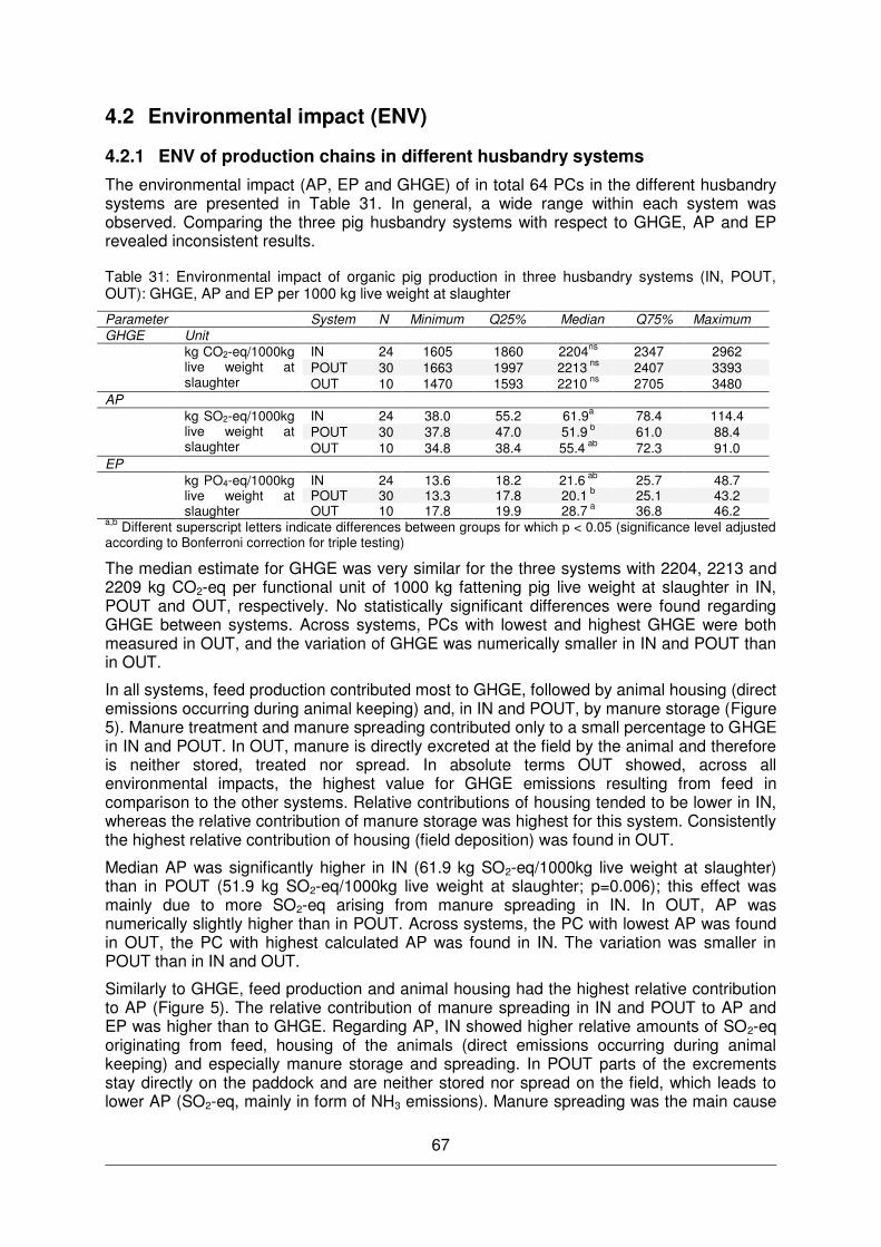
67
4.2 Environmental impact (ENV)
4.2.1 ENV of production chains in different husbandry systems
The environmental impact (AP, EP and GHGE) of in total 64 PCs in the different husbandry systems are presented in Table 31. In general, a wide range within each system was observed. Comparing the three pig husbandry systems with respect to GHGE, AP and EP revealed inconsistent results.
Table 31: Environmental impact of organic pig production in three husbandry systems (IN, POUT, OUT): GHGE, AP and EP per 1000 kg live weight at slaughter
Parameter System N Minimum Q25% Median Q75% Maximum GHGE Unit kg CO2-eq/1000kg
live weight at slaughter
IN 24 1605 1860 2204ns 2347 2962 POUT 30 1663 1997 2213 ns 2407 3393 OUT 10 1470 1593 2210 ns 2705 3480
AP kg SO2-eq/1000kg
live weight at slaughter
IN 24 38.0 55.2 61.9a 78.4 114.4 POUT 30 37.8 47.0 51.9 b 61.0 88.4 OUT 10 34.8 38.4 55.4 ab 72.3 91.0
EP kg PO4-eq/1000kg
live weight at slaughter
IN 24 13.6 18.2 21.6 ab 25.7 48.7 POUT 30 13.3 17.8 20.1 b 25.1 43.2 OUT 10 17.8 19.9 28.7 a 36.8 46.2
a,b Different superscript letters indicate differences between groups for which p < 0.05 (significance level adjusted according to Bonferroni correction for triple testing)
The median estimate for GHGE was very similar for the three systems with 2204, 2213 and 2209 kg CO2-eq per functional unit of 1000 kg fattening pig live weight at slaughter in IN, POUT and OUT, respectively. No statistically significant differences were found regarding GHGE between systems. Across systems, PCs with lowest and highest GHGE were both measured in OUT, and the variation of GHGE was numerically smaller in IN and POUT than in OUT.
In all systems, feed production contributed most to GHGE, followed by animal housing (direct emissions occurring during animal keeping) and, in IN and POUT, by manure storage (Figure 5). Manure treatment and manure spreading contributed only to a small percentage to GHGE in IN and POUT. In OUT, manure is directly excreted at the field by the animal and therefore is neither stored, treated nor spread. In absolute terms OUT showed, across all environmental impacts, the highest value for GHGE emissions resulting from feed in comparison to the other systems. Relative contributions of housing tended to be lower in IN, whereas the relative contribution of manure storage was highest for this system. Consistently the highest relative contribution of housing (field deposition) was found in OUT.
Median AP was significantly higher in IN (61.9 kg SO2-eq/1000kg live weight at slaughter) than in POUT (51.9 kg SO2-eq/1000kg live weight at slaughter; p=0.006); this effect was mainly due to more SO2-eq arising from manure spreading in IN. In OUT, AP was numerically slightly higher than in POUT. Across systems, the PC with lowest AP was found in OUT, the PC with highest calculated AP was found in IN. The variation was smaller in POUT than in IN and OUT.
Similarly to GHGE, feed production and animal housing had the highest relative contribution to AP (Figure 5). The relative contribution of manure spreading in IN and POUT to AP and EP was higher than to GHGE. Regarding AP, IN showed higher relative amounts of SO2-eq originating from feed, housing of the animals (direct emissions occurring during animal keeping) and especially manure storage and spreading. In POUT parts of the excrements stay directly on the paddock and are neither stored nor spread on the field, which leads to lower AP (SO2-eq, mainly in form of NH3 emissions). Manure spreading was the main cause
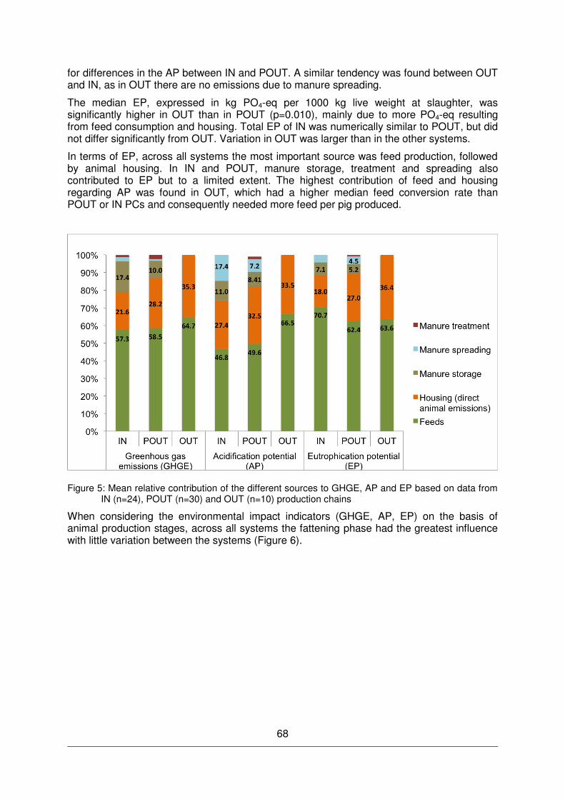
68
for differences in the AP between IN and POUT. A similar tendency was found between OUT and IN, as in OUT there are no emissions due to manure spreading.
The median EP, expressed in kg PO4-eq per 1000 kg live weight at slaughter, was significantly higher in OUT than in POUT (p=0.010), mainly due to more PO4-eq resulting from feed consumption and housing. Total EP of IN was numerically similar to POUT, but did not differ significantly from OUT. Variation in OUT was larger than in the other systems.
In terms of EP, across all systems the most important source was feed production, followed by animal housing. In IN and POUT, manure storage, treatment and spreading also contributed to EP but to a limited extent. The highest contribution of feed and housing regarding AP was found in OUT, which had a higher median feed conversion rate than POUT or IN PCs and consequently needed more feed per pig produced.
Figure 5: Mean relative contribution of the different sources to GHGE, AP and EP based on data from IN (n=24), POUT (n=30) and OUT (n=10) production chains
When considering the environmental impact indicators (GHGE, AP, EP) on the basis of animal production stages, across all systems the fattening phase had the greatest influence with little variation between the systems (Figure 6).
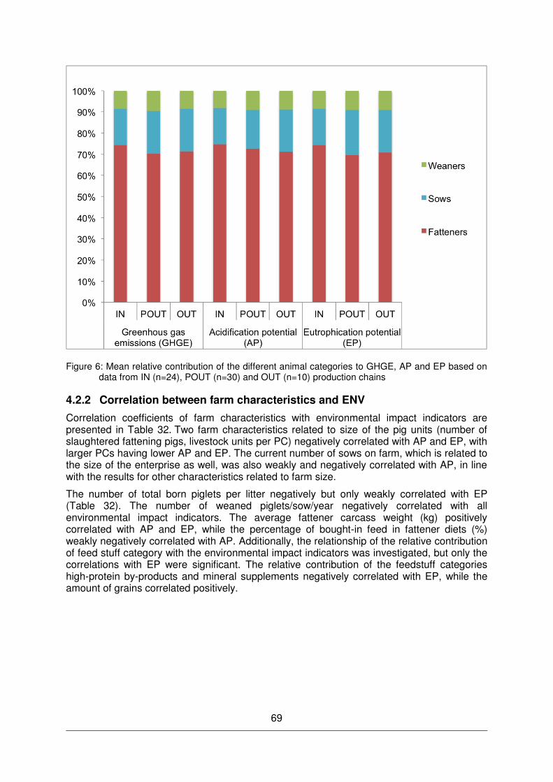
69
Figure 6: Mean relative contribution of the different animal categories to GHGE, AP and EP based on data from IN (n=24), POUT (n=30) and OUT (n=10) production chains
4.2.2 Correlation between farm characteristics and ENV
Correlation coefficients of farm characteristics with environmental impact indicators are presented in Table 32. Two farm characteristics related to size of the pig units (number of slaughtered fattening pigs, livestock units per PC) negatively correlated with AP and EP, with larger PCs having lower AP and EP. The current number of sows on farm, which is related to the size of the enterprise as well, was also weakly and negatively correlated with AP, in line with the results for other characteristics related to farm size.
The number of total born piglets per litter negatively but only weakly correlated with EP (Table 32). The number of weaned piglets/sow/year negatively correlated with all environmental impact indicators. The average fattener carcass weight (kg) positively correlated with AP and EP, while the percentage of bought-in feed in fattener diets (%) weakly negatively correlated with AP. Additionally, the relationship of the relative contribution of feed stuff category with the environmental impact indicators was investigated, but only the correlations with EP were significant. The relative contribution of the feedstuff categories high-protein by-products and mineral supplements negatively correlated with EP, while the amount of grains correlated positively.
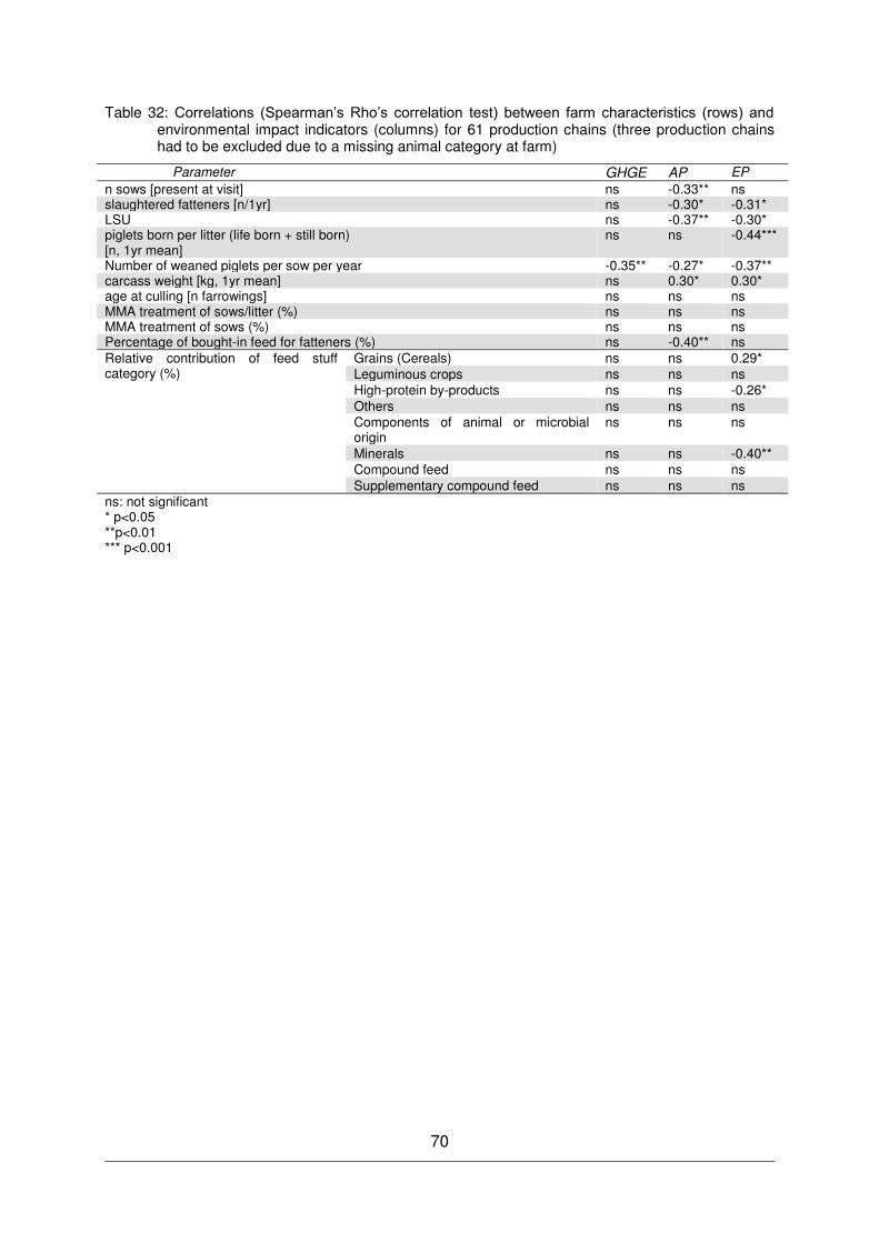
70
Table 32: Correlations (Spearman’s Rho’s correlation test) between farm characteristics (rows) and environmental impact indicators (columns) for 61 production chains (three production chains had to be excluded due to a missing animal category at farm)
Parameter GHGE AP EP n sows [present at visit] ns -0.33** ns slaughtered fatteners [n/1yr] ns -0.30* -0.31* LSU ns -0.37** -0.30* piglets born per litter (life born + still born) [n, 1yr mean]
ns ns -0.44***
Number of weaned piglets per sow per year -0.35** -0.27* -0.37** carcass weight [kg, 1yr mean] ns 0.30* 0.30* age at culling [n farrowings] ns ns ns MMA treatment of sows/litter (%) ns ns ns MMA treatment of sows (%) ns ns ns Percentage of bought-in feed for fatteners (%) ns -0.40** ns Relative contribution of feed stuff category (%)
Grains (Cereals) ns ns 0.29* Leguminous crops ns ns ns High-protein by-products ns ns -0.26* Others ns ns ns Components of animal or microbial origin
ns ns ns
Minerals ns ns -0.40** Compound feed ns ns ns Supplementary compound feed ns ns ns
ns: not significant * p<0.05 **p<0.01 *** p<0.001
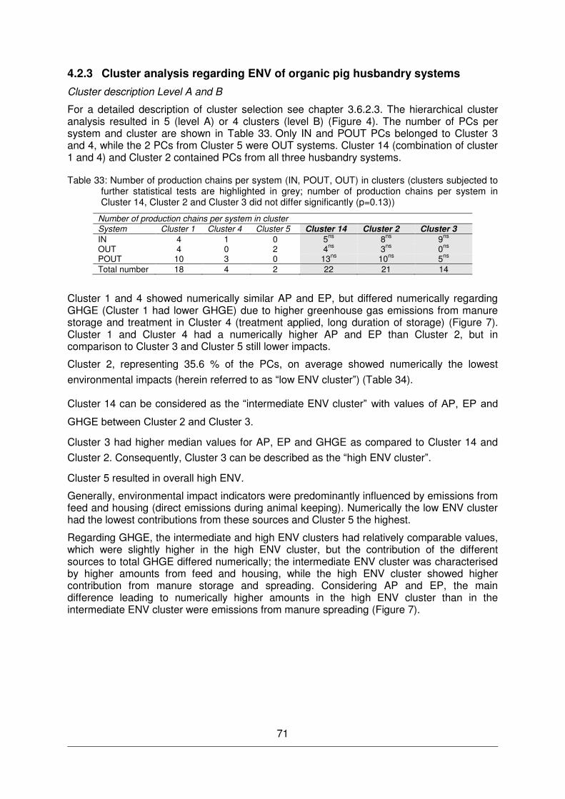
71
4.2.3 Cluster analysis regarding ENV of organic pig husbandry systems
Cluster description Level A and B
For a detailed description of cluster selection see chapter 3.6.2.3. The hierarchical cluster analysis resulted in 5 (level A) or 4 clusters (level B) (Figure 4). The number of PCs per system and cluster are shown in Table 33. Only IN and POUT PCs belonged to Cluster 3 and 4, while the 2 PCs from Cluster 5 were OUT systems. Cluster 14 (combination of cluster 1 and 4) and Cluster 2 contained PCs from all three husbandry systems.
Table 33: Number of production chains per system (IN, POUT, OUT) in clusters (clusters subjected to further statistical tests are highlighted in grey; number of production chains per system in Cluster 14, Cluster 2 and Cluster 3 did not differ significantly (p=0.13))
Number of production chains per system in cluster System Cluster 1 Cluster 4 Cluster 5 Cluster 14 Cluster 2 Cluster 3
IN 4 1 0 5ns 8ns 9ns OUT 4 0 2 4ns 3ns 0ns POUT 10 3 0 13ns 10ns 5ns Total number 18 4 2 22 21 14
Cluster 1 and 4 showed numerically similar AP and EP, but differed numerically regarding GHGE (Cluster 1 had lower GHGE) due to higher greenhouse gas emissions from manure storage and treatment in Cluster 4 (treatment applied, long duration of storage) (Figure 7). Cluster 1 and Cluster 4 had a numerically higher AP and EP than Cluster 2, but in comparison to Cluster 3 and Cluster 5 still lower impacts.
Cluster 2, representing 35.6 % of the PCs, on average showed numerically the lowest
environmental impacts (herein referred to as low ENV cluster ) (Table 34).
Cluster 14 can be considered as the intermediate ENV cluster with values of AP, EP and
GHGE between Cluster 2 and Cluster 3.
Cluster 3 had higher median values for AP, EP and GHGE as compared to Cluster 14 and
Cluster 2. Consequently, Cluster 3 can be described as the high ENV cluster .
Cluster 5 resulted in overall high ENV.
Generally, environmental impact indicators were predominantly influenced by emissions from feed and housing (direct emissions during animal keeping). Numerically the low ENV cluster had the lowest contributions from these sources and Cluster 5 the highest.
Regarding GHGE, the intermediate and high ENV clusters had relatively comparable values, which were slightly higher in the high ENV cluster, but the contribution of the different sources to total GHGE differed numerically; the intermediate ENV cluster was characterised by higher amounts from feed and housing, while the high ENV cluster showed higher contribution from manure storage and spreading. Considering AP and EP, the main difference leading to numerically higher amounts in the high ENV cluster than in the intermediate ENV cluster were emissions from manure spreading (Figure 7).
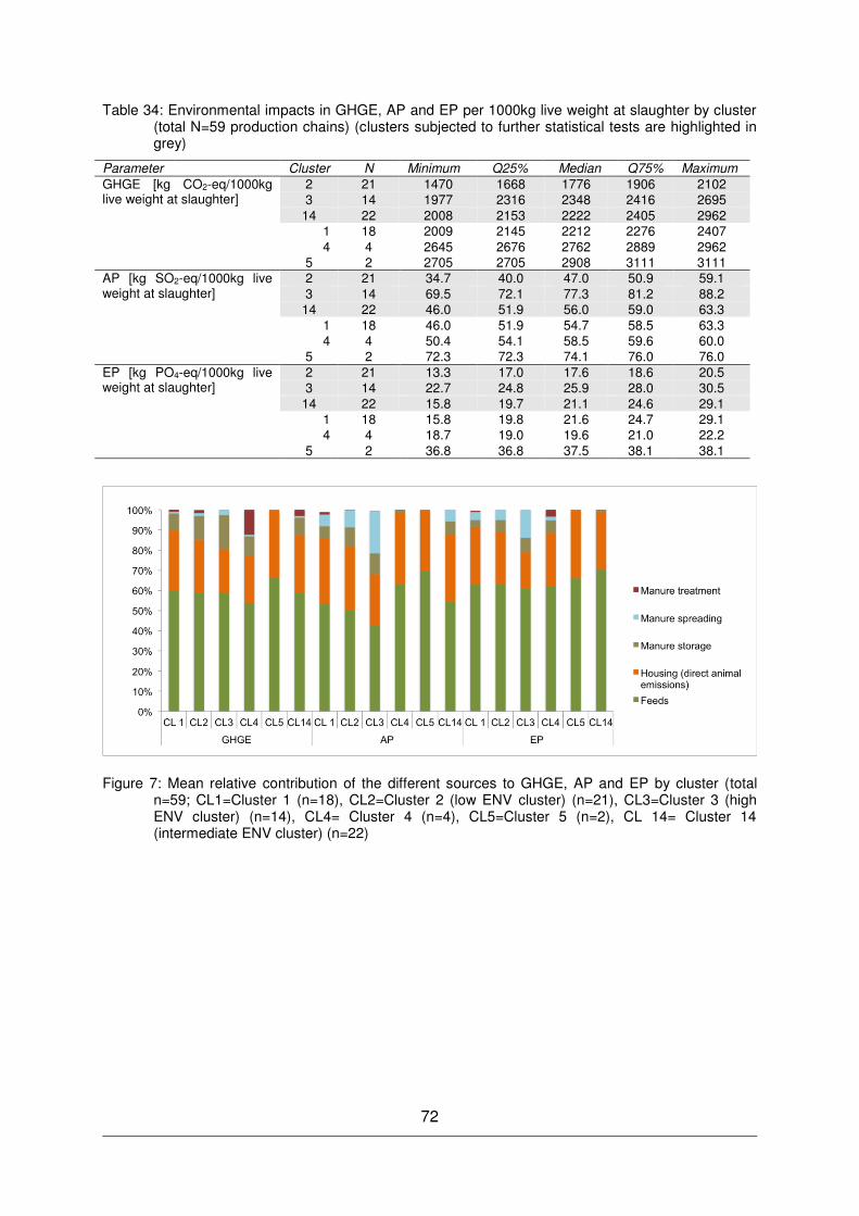
72
Table 34: Environmental impacts in GHGE, AP and EP per 1000kg live weight at slaughter by cluster (total N=59 production chains) (clusters subjected to further statistical tests are highlighted in grey)
Parameter Cluster N Minimum Q25% Median Q75% Maximum GHGE [kg CO2-eq/1000kg live weight at slaughter]
2 21 1470 1668 1776 1906 2102 3 14 1977 2316 2348 2416 2695
14 22 2008 2153 2222 2405 2962 1 18 2009 2145 2212 2276 2407 4 4 2645 2676 2762 2889 2962
5 2 2705 2705 2908 3111 3111 AP [kg SO2-eq/1000kg live weight at slaughter]
2 21 34.7 40.0 47.0 50.9 59.1 3 14 69.5 72.1 77.3 81.2 88.2
14 22 46.0 51.9 56.0 59.0 63.3 1 18 46.0 51.9 54.7 58.5 63.3 4 4 50.4 54.1 58.5 59.6 60.0
5 2 72.3 72.3 74.1 76.0 76.0 EP [kg PO4-eq/1000kg live weight at slaughter]
2 21 13.3 17.0 17.6 18.6 20.5 3 14 22.7 24.8 25.9 28.0 30.5
14 22 15.8 19.7 21.1 24.6 29.1 1 18 15.8 19.8 21.6 24.7 29.1 4 4 18.7 19.0 19.6 21.0 22.2
5 2 36.8 36.8 37.5 38.1 38.1
Figure 7: Mean relative contribution of the different sources to GHGE, AP and EP by cluster (total n=59; CL1=Cluster 1 (n=18), CL2=Cluster 2 (low ENV cluster) (n=21), CL3=Cluster 3 (high ENV cluster) (n=14), CL4= Cluster 4 (n=4), CL5=Cluster 5 (n=2), CL 14= Cluster 14 (intermediate ENV cluster) (n=22)
73
Differences between clusters (Level B)
Differences in factors potentially influencing environmental impact indicators were tested on Level B (between the low ENV cluster (Cluster 2), the intermediate ENV cluster (Cluster 14) and the high ENV cluster (Cluster 3)). Farm size related characteristics (as shown in Table 35) did not differ significantly between individual clusters. Regarding LSU/ha the global test revealed a significant effect, but no statistically significant differences were detected between individually cluster in the pairwise comparisons.
Characteristics related to farm size were numerically lowest for PCs in the high ENV cluster, while the highest average farm size related values were found in the intermediate ENV cluster (Table 35). The low ENV cluster, characterised by the lowest overall environmental impact, had on average 80 sows, 659 slaughtered fattening pigs/year and 118 LSU. These values range between those for the intermediate and high ENV cluster.
Table 35: Cluster characteristics regarding number of sows on PC at farm visit, average number of slaughtered fattening pigs/year and number of livestock units (LSU)
Parameter Cluster N1 Minimum Q25% Mean Median Q75% Maximum n sows [present at visit]
Low ENV [2] 19 12 50 158 80ns 180 650 Intermediate ENV [14] 21 8 35 203 110 ns 222 1300
High ENV [3] 14 15 20 77 28 ns 160 249 slaughtered fatteners [n/1yr]
Low ENV [2] 18 65 417 1936 659 ns 1827 11016 Intermediate ENV [14] 20 15 317 2633 859 ns 3199 16000
High ENV [3] 14 14 261 598 324 ns 687 3100 LSU Low ENV [2] 19 14 44 167 118 ns 138 795
Intermediate ENV [14] 21 11 43 187 121 ns 192 1158 High ENV [3] 14 13 18 57 38 ns 106 184
1 Number of observations differs from number of production chains/systems, as not each parameter was available for all production chains ns not significant
The average weight (kg) of weaners at the end of the post-weaning period (Table 36) differed significantly between clusters. In the intermediate ENV cluster significantly heavier (p=0.012) pigs entered the fattening phase than in the high ENV cluster. Starting fattening of piglets at a lower weight had a negative effect on environmental impact indicators. Fatteners’ feed conversion rate in the low ENV cluster was significantly lower (p=0.000) than in the intermediate and high ENV clusters. In line with this, the total amount of feed per fattening pig produced (kg) was significantly lower in the low ENV cluster in comparison to the high ENV cluster (p=0.000) and to the intermediate ENV cluster (p=0.006) (Table 37). Improved feed conversion rate and lower feed consumption in the low ENV cluster had a beneficial effect on environmental impacts. However, mortality of fatteners was significantly higher in the low ENV cluster (p=0.000) than in the high ENV cluster (Table 36). Regarding the percentage of bought-in feed components in fattener diets (Table 38), significantly lower values were found for the high ENV cluster in comparison to the low ENV cluster (p=0.000) and the intermediate cluster (p=0.000). Additionally, the relative contribution of feedstuff category was tested; in the low and high ENV cluster significantly higher percentages of leguminous crops were used in the diets than in the intermediate ENV cluster.
74
Table 36: Characteristics of the animal production stages by cluster
Cluster3 N Min. Q25% Mean Median Q75% Max. Sows piglets born per litter (life born + still born) [n, 1yr mean]1
Low ENV [2] 19 12.0 12.1 13.2 13.3ns 14.0 14.5 Intermediate ENV [14] 20 6.0 10.8 12.1 12.3 ns 14.0 16.5
High ENV [3] 13 8.0 12.0 12.8 13.3 ns 14.0 14.5
piglets weaned per sow per year [n, 1yr mean]2
Low ENV [2] 20 10.0 18.2 19.2 19.9 ns 21.1 25.0 Intermediate ENV [14] 22 10.0 16.0 18.3 19.0 ns 21.0 23.8
High ENV [3] 14 14.0 16.0 18.3 19.1 ns 19.7 25.0
sow replacement rate [%, 1yr mean]2
Low ENV [2] 20 12.0 26.0 31.8 30.5 ns 35.0 50.0 Intermediate ENV [14] 22 8.0 20.0 32.5 28.0 ns 45.0 87.0
High ENV [3] 14 20.0 20.0 29.0 26.5 ns 33.0 53.0
live weight at culling [kg at culling]2
Low ENV [2] 20 187 200 237 240 ns 257 310 Intermediate ENV [14] 22 180 220 249 245 ns 275 325
High ENV [3] 14 197 200 234 233 ns 253 277 Weaners weight at weaning [kg, 1yr mean]2
Low ENV [2] 20 0.0 10.0 11.3 10.7 ns 13.5 22.0 Intermediate ENV [14] 22 5.5 10.0 13.1 12.5 ns 15.0 28.0
High ENV [3] 14 8.0 10.0 11.5 10.9 ns 12.5 22.0 weight at end of post-weaning
[kg, 1yr mean]2
Low ENV [2] 20 24.0 25.8 29.4 30.0ab 30.0 42.0 Intermediate ENV [14] 22 25.0 30.0 31.6 31.5b 35.0 40.0
High ENV [3] 14 23.0 25.0 28.3 29.0a 30.0 34.0
mortality rate weaners [%, 1yr mean]2
Low ENV [2] 20 0.0 3.5 5.7 5.0ns 5.0 20.0 Intermediate ENV [14] 22 0.0 1.0 3.2 3.0 ns 5.0 10.0
High ENV [3] 14 0.0 1.0 3.1 3.0ns 5.0 5.0 Fattening pigs live weight at slaughter [kg, 1yr mean]2
Low ENV [2] 20 104 112 124 117 ns 129 165 Intermediate ENV [14] 21 86 112 128 120 ns 136 200
High ENV [3] 14 116 121 131 129 ns 140 150 Mortality rate fattening pigs
[%, 1yr mean]2
Low ENV [2] 20 1.0 1.5 2.9 3.0a 4.0 5.0 Intermediate ENV [14] 21 0.0 1.0 1.9 2.0 ab 2.0 6.0
High ENV [3] 14 0.0 0.0 1.0 1.0b 1.0 4.0 1 Number of observations differs from number of production chains/systems, as not each parameter was assessable for all farms 2 Number of observations differ from number of production chains/system due to 3 farms calculated with means for the environmental impact of the missing animal production stage at farm level (2 production chains calculated with average environmental impact for piglet production; 1 production chain calculated with average environmental impact of the fattening stage 3 parameters, which showed significant differences between clusters are highlighted in bold a,b Different superscript letters indicate differences between groups for which p < 0.05 (significance level adjusted according to Bonferroni correction for triple testing). ns not significant
75
Table 37: Characteristics of dietary nutrient content and feed consumption by cluster
Cluster1 N Min. Q25% Mean Median Q75% Max. Sows Feed per sow [kg/year]
Low ENV [2] 20 675 1028 1415 1458 ns 1595 2053 Intermediate ENV [14] 22 827 1332 1603 1702 ns 1834 2236
High ENV [3] 14 1060 1203 1383 1385 ns 1473 1946
Average sow dietary content of MJ ME/kg Low ENV [2] 20 9.6 11.9 12.1 12.5 ns 12.9 13.1
Intermediate ENV [14] 22 12.0 12.3 12.7 12.7 ns 12.9 13.7 High ENV [3] 14 11.8 12.4 12.6 12.6 ns 13.0 13.3
CP [g/kg] Low ENV [2] 20 124 148 155 155 ns 164 185 Intermediate ENV [14] 22 112 137 149 152 ns 162 180 High ENV [3] 14 133 146 150 151 ns 157 165
tot P [g/kg] Low ENV [2] 20 3.0 4.7 5.2 5.5 ns 5.9 7.8 Intermediate ENV [14] 22 3.1 4.5 5.4 5.8 ns 6.1 6.5 High ENV [3] 14 3.3 4.4 5.0 5.3 ns 5.5 6.0
Weaners Feed per weaner produced [kg/weaner]
Low ENV [2] 20 18 30 38 39 ns 45 56 Intermediate ENV [14] 22 12 33 43 38 ns 50 111 High ENV [3] 14 20 30 37 36 ns 45 59
Average post-weaning dietary content of MJ ME/kg Low ENV [2] 20 9.5 12.5 12.4 12.8 ns 13.1 13.4
Intermediate ENV [14] 22 12.0 12.6 12.9 12.9 ns 13.2 13.6 High ENV [3] 14 12.0 12.9 13.0 13.1 ns 13.4 13.5
CP [g/kg] Low ENV [2] 20 138 168 177 179ns 189 203 Intermediate ENV [14] 22 112 170 176 181 ns 195 208 High ENV [3] 14 147 172 180 182ns 188 208
tot P [g/kg] Low ENV [2] 20 3.5 3.8 5.2 5.7 ns 6.0 6.8 Intermediate ENV [14] 22 3.1 5.5 5.6 6.0 ns 6.2 6.9 High ENV [3] 14 3.5 4.7 5.5 5.5 ns 5.8 8.9
Fattening pig Feed per fattening pig produced [kg/fattener]
Low ENV [2] 20 209 222 269 242a 322 378 Intermediate ENV [14] 21 159 266 381 337 ab 385 981 High ENV [3] 14 291 323 384 390 b 443 494
Percentage of bought-in feed stuff in fattener diets
Low ENV [2] 18 20 58 79 100 a 100 100 Intermediate ENV [14] 19 30 100 87 100 a 100 100 High ENV [3] 14 0 7 35 25 b 69 100
Fattening pig FCR [kg/kg pig]
Low ENV [2] 20 2.4 2.7 2.9 2.8a 3.0 3.3 Intermediate ENV [14] 21 3.0 3.2 3.8 3.6 b 4.2 6.0 High ENV [3] 14 3.1 3.3 3.7 3.8 b 4.0 4.6
Average fattening pig dietary content of MJ ME/kg Low ENV [2] 20 9.5 12.5 12.3 12.8 ns 12.9 13.2
Intermediate ENV [14] 21 12.0 12.6 13.0 12.9 ns 13.2 14.5 High ENV [3] 14 12.0 12.7 13.0 12.9 ns 13.0 14.8
CP [g/kg] Low ENV [2] 20 139 153 163 165 ns 172 190 Intermediate ENV [14] 21 112 144 162 171 ns 183 202 High ENV [3] 14 118 153 157 158 ns 164 177
tot P [g/kg] Low ENV [2] 20 2.4 3.6 4.5 4.9 ns 5.1 6.0 Intermediate ENV [14] 21 3.1 4.0 5.0 5.5ns 5.8 6.4 High ENV [3] 14 3.3 4.0 4.6 4.8 ns 5.1 6.0
a,b Different superscript letters indicate differences between groups for which p < 0.05 (significance level adjusted according to Bonferroni correction for triple testing) ns not significant 1 parameters, which showed significant differences between clusters are highlighted in bold
76
Table 38: Relative contribution of feed stuff category in the different clusters
Cluster1 N Min. Q25% Mean Median Q75% Max. Parameter Grains Low ENV [2] 19 0.0 50.0 53.2 61.8 ns 67.8 74.5
Intermediate ENV [14] 21 0.0 50.0 53.8 65.0 ns 71.4 90.0 High ENV [3] 14 41.4 65.0 67.2 68.1 ns 71.8 85.5
Leguminous crops
Low ENV [2] 19 0.0 16.4 20.9 25.0 ab 27.5 31.6 Intermediate ENV [14] 21 0.0 7.5 16.3 17.4 b 21.9 44.4
High ENV [3] 14 14.5 20.5 26.0 23.1 a 31.0 44.5 High-protein by-products
Low ENV [2] 19 0.0 2.0 5.3 4.7 ns 8.4 13.1 Intermediate ENV [14] 21 0.0 0.0 3.3 1.1 ns 4.2 13.8
High ENV [3] 14 0.0 0.0 2.7 1.6 ns 6.4 6.9 Others Low ENV [2] 19 0.0 0.0 7.2 3.0 ns 6.8 80.2
Intermediate ENV [14] 20 0.0 0.0 3.9 0.1 ns 5.1 17.1 High ENV [3] 14 0.0 0.0 1.0 0.0 ns 1.1 5.1
Components of animal or microbial origin
Low ENV [2] 19 0.0 0.0 0.4 0.0 ns 1.0 3.2 Intermediate ENV [14] 21 0.0 0.0 2.3 0.0 ns 0.0 42.3
High ENV [3] 14 0.0 0.0 0.0 0.0 ns 0.0 0.0 Minerals Low ENV [2] 19 0.0 2.0 2.6 2.7 ns 3.1 5.4
Intermediate ENV [14] 21 0.0 0.0 1.6 1.6 ns 2.8 5.6 High ENV [3] 14 0.0 2.0 2.2 2.4 ns 2.9 4.0
Compound feed Low ENV [2] 19 0.0 0.0 10.5 0.0 ns 0.0 100
Intermediate ENV [14] 21 0.0 0.0 19.1 0.0 ns 0.0 100 High ENV [3] 14 0.0 0.0 0.0 0.0 ns 0.0 0.0
Supplementary compound feed
Low ENV [2] 19 0.0 0.0 0.0 0.0 ns 0.0 0.0 Intermediate ENV [14] 21 0.0 0.0 0.0 0.0 ns 0.0 0.0
High ENV [3] 14 0.0 0.0 1.0 0.0 ns 0.0 11.4 a,b Different superscript letters within columns indicate differences between groups per parameter for which p < 0.05 (significance level adjusted according to Bonferroni correction for triple testing) ns not significant 1 parameters which showed significant differences between clusters are highlighted in bold
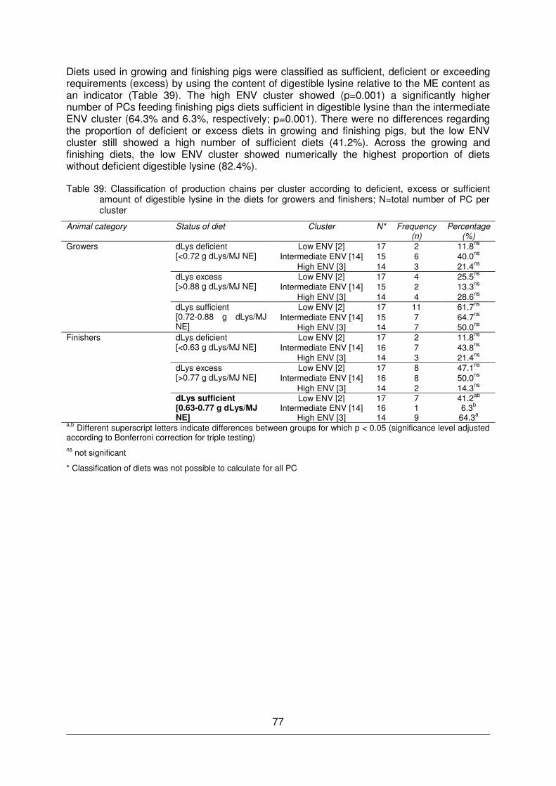
77
Diets used in growing and finishing pigs were classified as sufficient, deficient or exceeding requirements (excess) by using the content of digestible lysine relative to the ME content as an indicator (Table 39). The high ENV cluster showed (p=0.001) a significantly higher number of PCs feeding finishing pigs diets sufficient in digestible lysine than the intermediate ENV cluster (64.3% and 6.3%, respectively; p=0.001). There were no differences regarding the proportion of deficient or excess diets in growing and finishing pigs, but the low ENV cluster still showed a high number of sufficient diets (41.2%). Across the growing and finishing diets, the low ENV cluster showed numerically the highest proportion of diets without deficient digestible lysine (82.4%).
Table 39: Classification of production chains per cluster according to deficient, excess or sufficient amount of digestible lysine in the diets for growers and finishers; N=total number of PC per cluster
Animal category Status of diet Cluster N* Frequency (n)
Percentage (%)
Growers dLys deficient [<0.72 g dLys/MJ NE]
Low ENV [2] 17 2 11.8ns
Intermediate ENV [14] 15 6 40.0ns High ENV [3] 14 3 21.4ns dLys excess
[>0.88 g dLys/MJ NE] Low ENV [2] 17 4 25.5ns
Intermediate ENV [14] 15 2 13.3ns
High ENV [3] 14 4 28.6ns
dLys sufficient [0.72-0.88 g dLys/MJ NE]
Low ENV [2] 17 11 61.7ns
Intermediate ENV [14] 15 7 64.7ns
High ENV [3] 14 7 50.0ns
Finishers dLys deficient [<0.63 g dLys/MJ NE]
Low ENV [2] 17 2 11.8ns
Intermediate ENV [14] 16 7 43.8ns
High ENV [3] 14 3 21.4ns
dLys excess [>0.77 g dLys/MJ NE]
Low ENV [2] 17 8 47.1ns
Intermediate ENV [14] 16 8 50.0ns
High ENV [3] 14 2 14.3ns
dLys sufficient [0.63-0.77 g dLys/MJ NE]
Low ENV [2] 17 7 41.2ab Intermediate ENV [14] 16 1 6.3b High ENV [3] 14 9 64.3a a,b Different superscript letters indicate differences between groups for which p < 0.05 (significance level adjusted according to Bonferroni correction for triple testing) ns not significant
* Classification of diets was not possible to calculate for all PC
78
4.2.4 Discussion
Brief description of results
A life cycle assessment (LCA) was conducted to quantify the environmental impact with regard to greenhouse gas emissions (GHGE), acidification potential (AP) and eutrophication potential (AP) of the three husbandry systems. Emissions were influenced mainly by feed, followed by housing (direct emissions of excreta occurring during keeping of animals in pens indoors or paddocks outdoors and energy (electricity) consumption). Most emissions were associated with the fattening stage. Variation within a husbandry system was higher than between systems, indicating that good values can be achieved in all systems. Regarding GHGE, no statistically significant differences were found between IN, POUT and OUT. Regarding AP and EP, POUT has the lowest impact. Considering AP, higher emissions were found in IN than in POUT (OUT differed neither from IN nor from POUT), mainly due to emissions from manure storage and spreading. OUT showed numerically lower AP than IN as well, but the high emissions from feeds compensated for the lack of emissions from manure storage and spreading. OUT had significantly higher EP than POUT and numerically higher EP than IN (IN differed neither from OUT nor from POUT). A hierarchical cluster analysis identified a low, intermedium and high ENV cluster. Feed conversion rate in FA and FA feed consumption was significantly lower in the low ENV cluster.
Study design
LCAs of livestock (products) so far have focussed mainly on ruminants, but also included pig production. Direct comparisons of different LCA studies always should be done with caution due to differences in underlying methodological assumptions and chosen system boundaries (Lammers, 2011). Nevertheless, LCA studies with similar assumptions and the same system boundaries may assist in interpreting and comparing results. Until now, most of the conducted LCAs were based on model scenarios or a small number of farms was evaluated, which were not always based on farm specific data from cradle to farm gate (Dolman et al., 2012). In accordance with Dolman et al. (2012) there was a high variation in environmental impact among farms in the present study, indicating that individual farm characteristics influenced the environmental impact. These results reflect the importance of farm specific calculations, rather than generalised scenarios. The environmental impact of different organic pig husbandry systems on the basis of production chain specific data across several European countries was investigated here for the first time. The focus on cradle-to-farm-gate on the basis of farm specific data was found appropriate for identifying the main sources of environmental impact of PC as well as for husbandry system comparisons (IN, OUT, POUT).
The LCA calculation tool used (Dourmad et al., 2014) offers the possibility to investigate the PC specific environmental impact along a full pig production cycle up to the farm gate. Besides the influence of the PC specific characteristics, LCA results depend on underlying methodological assumptions (e.g. emission factors for different floor types, allocation approach etc.). The degree of uncertainty for estimates revealed from these assumptions might vary between PCs and could eventually be not fully appropriate for the diverse housing systems in organic pig farming (e.g. outdoor climate stable).
In case of emissions from feed production, a degree of uncertainty for estimates exists, as the emissions were based on data for organic feed production in Austria. This approach was considered as best option, as otherwise insufficient data for all the variety of feedstuff used in organic pig diets are available, which are specifically calculated for regional conditions of crop production. For some feedstuff components LCA was specifically calculated for the purpose of the present study, as an LCA expert calculated the emissions for all components used in diets by ProPIG farms. For the aim of this study, to compare the husbandry systems with regard to ENV, this approach can therefore be regarded as ambitious and suitable. The calculated LCA represents a balanced picture of the emissions from feed per PCs.
79
Furthermore it has to be considered, that LCA results are influenced by assumptions or measurements regarding pig production and farm management characteristics, which depend on availability and quality of data (e.g. consistent records on feed consumption). Furthermore, feed conversion rate calculation is based on feed use (kg feed fed per day) as reported by the farmers; losses of feed occurring especially outdoors, were probably not taken into consideration by the farmer. Therefore the calculated feed conversion rate might be higher than the true feed conversion rate, but in terms of environmental impact the feed applied should be taken into account anyway, if consumed by the pigs or lost. But improving feeding strategies to avoid losses and consequently the amount of feed needed can be considered as beneficial effect on ENV.
Relevant PC specific data were assessed during farm visits, as precisely as possible, but on-farm surveys may often not be carried out as exactly as experimental studies. Furthermore, the PC specific data used in the present study are based on inventory data covering a period of 12 months prior to the PC visit. The calculated LCAs reflect retrospectively the situation and environmental impact based on this time period, which may differ from the current situation on a given PC (e.g. lower number of weaned piglets/sow/year due to the occurrence of a disease). At the same time, the actual state on the day of the PC visit may not fully reflect the common farm situation. For example, litter quality, which was assessed on the day of the PC visit, may not reflect the PC’s average litter quality throughout the year. Some aspects, especially regarding the condition of outdoor paddocks (e.g. the fields gradient, soil type, proximity to lakes or other waters, can be considered as insufficiently studied and were therefore not included in the calculation tool yet.
These limitations are highlighted as possible improvements for future studies. As the limitations concern all husbandry systems they are not considered as influencing the analysis of differences between husbandry systems. Furthermore, LCA takes numerous aspects into account, if weaknesses concern single aspects, this does not reduce the meaningfulness of the calculation. Finally, it has to be mentioned, that despite these limitations, the data available for the present thesis and the calculation of a high number of organic pig PC specific cradle-to-farm gate LCA taking different husbandry systems into account is unique.
Comparison with other studies
Few studies on the environmental impact of organic pig production have been conducted so far. Direct comparison with other studies is difficult e.g. due to different underlying assumptions. But our results for the environmental impact (GHGE, AP, EP) are in line with other studies (reviewed in De Vries and de Boer, 2010), especially with the results for organic systems reported by Dourmad et al. (2014), using a similar methodology and system boundaries. GHGE was 2.4 kg CO2-eq/kg live weight for organic pig production, while the median obtained in the present study is 2.2 kg CO2-eq/kg live weight for IN, OUT and POUT.
Regarding AP, Dourmad et al. (2014) found 57 g SO2-eq/kg live weight for organic pig production, while in the present study AP ranges in median from 51.9-61.9 g SO2-eq/kg live weight: The lower medians for POUT and OUT than for organic systems in Dourmad et al. (2014) are likely due to less or no emissions from manure management. The higher median AP found in IN (61.9) as compared to Dourmad et al. (2014), may be attributed to higher emissions from the source feed in IN, which resulted mainly from a poorer feed conversion rate in fatteners in the present study compared to this previous study.
Regarding EP, in the present study the medians range from 20.1-28.7 g PO4-eq/kg live weight and therefore exceed the values for organic farms found by Dourmad et al. (2014) (16g) but are in the range of conventional systems (16-34 g) (Dourmad et al., 2014). The higher EP in the present study is due to the source feed, likely based on a poorer median feed conversion rate in IN, POUT and OUT than found by Dourmad et al. (2014).
Lammers (2011) also highlights the importance of an improvement of production performance and the utilization of pig manure for the reduction of the environmental impact
80
of farms. Differences between systems in acidification and eutrophication potential were explained by underlying assumptions made for crop nutrient management and manure management (storage and utilization). These assumptions influence the amount of emissions, e.g. emissions are reported to be lower when pigs are housed in system relying on bedding with manure handled as a composting solid, this is likely due more to the cropping system than pig manure management or husbandry system per se.
Across all environmental impact indicators in the present study, the wide variation (minimum- maximum) has to be emphasized. These LCA results correspond with literature findings showing as well high variation in the environmental impact, especially regarding AP and EP (De Vries and de Boer, 2010, Dourmad et al., 2014, Dolman et al., 2012) between farms or model scenario calculations.
Environmental impact of three organic pig husbandry systems (IN, POUT, OUT)
One of the aims of the present study was to identify main sources and relevant animal stages for emissions in the three different organic pig husbandry systems. Regarding sources, across GHGE, AP and EP, emissions from feeds contributed most to the total environmental impact. Regarding animal production stages, most emissions were allocated to the fattening phase. These results agree with other LCA studies highlighting emissions of feeds consumed by animals as having considerable impact on the amount of emissions (Basset-Mens and van der Werf, 2005, Basset-Mens et al., 2007, Pelletier et al., 2010, Alig et al., 2012, Reckmann and Krieter, 2014).
Within husbandry systems, a considerable variation between individual PCs was found for all environmental impact indicators. Regarding GHGE, no statistically significant differences were found between IN, POUT and OUT. Higher AP was found in IN compared to POUT (OUT differed neither from IN nor from POUT) and higher EP in OUT than in POUT (IN differed neither from IN nor from POUT). As other authors (e.g. Dalgaard et al., 2007) also report similar GHGE for different systems or countries, but different AP and EP, it might be that GHGE is a less sensitive indicator for finding differences between systems or countries, as GHGE of feedstuffs do not differ in a wide range (apart from those with high emissions related to land use change), while regarding AP and EP emission factors are more divers between animals kept indoors or outdoors.
Considering AP, higher emissions were found in IN than in POUT, mainly due to emissions from manure storage and spreading. OUT showed numerically lower AP than IN as well, but due to high emissions from feeds, but the high emissions from feeds compensated for the lack of emissions from manure storage and spreading. OUT had significantly higher EP than POUT and numerically higher EP than IN. The main likely differences are the higher emissions from feed and direct emissions from animals. OUT showed a relatively high feed consumption and poorer feed conversion rate in fatteners, which likely has increased EP.
The results highlight the importance of manure storage and manure spreading in IN and the potential for reducing environmental impact in OUT by improving the feed conversion rate especially in fatteners. The poorer feed conversion rate in OUT was partly influenced by heavier pigs at the end of the fattening phase in some PCs (see Table 15).
Patterns of environmental impact
Comparing the environmental impacts with respect to GHGE, AP and EP across the three pig husbandry systems showed inconsistent results. The results however indicate that factors other than the husbandry system mainly influenced the PCs’ specific environmental impact. In order to explore this, the PCs were clustered regarding their GHGE, AP and EP values. The clustering resulted in a “low ENV” cluster (Cluster 2), which is characterised by overall lowest median GHGE, AP and EP. Furthermore an “intermediate ENV” cluster (Cluster 14) with intermediate median GHGE, AP and EP and last but not least a “high ENV” cluster (Cluster 3) with highest median GHGE, AP and EP was identified. The number of
81
PCs per husbandry system in the clusters did not differ significantly, but the high ENV cluster did not contain OUT PCs.
It was assumed, that PC characteristics would provide insight into the environmental impact and lead specifically to better explanation of the calculated values. Regarding PC characteristics, feed conversion rate in fatteners and fatteners feed consumption was lower in the low environmental impact cluster. Also Reckmann and Krieter (2014) identified feed conversion rate in finishers as the parameter with greatest influence on feed used to produce pork and consequently on the LCA outcomes. Furthermore, fertility of sows, especially number of piglets born alive per litter was described as an important influencing factor. Similar findings were found earlier in Dalgaard et al. (2007), but in the present study only weak correlations regarding sow fertility and environmental impact were found. In general, only weak correlations were found between PCs’ characteristics and their environmental impact in the present study.
Two farm characteristics related to the size of the pig units (number of slaughtered pigs, livestock units per PC) negatively correlated with AP and EP, with larger PCs having lower AP and EP. Again, the association was weak only. The current number of sows per PC, which is related to size of the enterprise as well, was also weakly, negatively correlated with AP, in line with the results of other farm size related characteristics. These results may indicate that larger farms were more efficient in managing their pig husbandry or that they were managed by farmers with greater experience and better training (Dolman et al., 2012).
The number of total born (still and life born) piglets per litter negatively correlated with EP. However, the correlation coefficient indicated again only a weak relationship, therefore the results do not allow strong conclusions, as for instance that PCs with larger litter sizes have lower EP. Emissions occurring during keeping the sows are allocated to their offspring and therefore higher litter sizes may be regarded as beneficial as long as all piglets survive and grow adequate. However, the influence of litter size on piglet mortality is known (Prunier et al., 2014a), therefore it should be suggested to focus on an adequate litter size with robust, viable and growing well piglets. This suggestion fits to the number of piglets/sow/year negatively correlated with all environmental impact indicators, which may indicate that farms with good management and productivity are at an advantage.
The percentage of bought-in feed in fattener diets (%) was weakly negatively correlated with AP. This might indicate that, even if PCs purchased a higher amount of feed components for fattener diets, these feeds either were loaded with relatively low AP or contribute otherwise to a slightly reduced AP (e.g. contributed to a better balanced diet and hence improved feed conversion).
Regarding the relative contribution (%) of feedstuff categories to the environmental impact indicators, significant correlations were only found for EP. High-protein by-products and minerals negatively correlated with EP, while the amount of grains was positively correlated. This might indicate that high protein by products and minerals contribute to a better balanced diet. The average fattener carcass weight (kg) was positively correlated with AP and EP, as during the fattening stage a large proportion of emissions arise. Towards the end of the fattening period the amount of feed needed for 1 kg weight gain increases in comparison to earlier growing stages (Kirchgessner et al., 2011).
82
4.2.5 Conclusion
Regarding environmental impact a substantial variation was found between individual PCs within systems. The ranking of the husbandry systems depends on the environmental impact indicator. The huge variation of the environmental impact indicators across PCs indicate that LCAs based on mean values of model scenarios will not always be representative for all farms in the modelled scenario.
In all husbandry systems, PCs with low environmental impacts were found, indicating that IN, POUT as well as OUT may be managed in an environmentally friendly way. However, a lack of consistent differences between husbandry systems as well as results from cluster analysis indicate, that factors other than the husbandry system are influencing the environmental impact of organic pig production.
Emerging emissions due to the source ‘feed’, which are depending on the amount and type of feedstuff components and housing (direct emissions of excreta) contribute to a large share to a PCs ENV. Regarding the production stages, most emissions were associated with the fattening stage, therefore, the fattening pigs feed conversion rate is of particular importance. By improving the feed conversion rate, emissions in the sources feed and housing can be decreased simultaneously.
The low ENV cluster was characterised by the lowest median AP, EP and GHGE. Across the growing and finishing diets, the low ENV cluster showed numerically the highest proportion of diets with appropriate digestible lysine content (82.4%). EP negatively correlated with the
dietary percentage of the feed components high-protein by-products and mineral
supplements , while the proportion of bought-in feed in fattener diets (%) weakly negatively correlated with AP. Therefore, it can be suggested that avoiding amino acid-deficient diets may improve the environmental impact besides animal performance. In situations where farm management options, such as crop rotation, feed allocation etc. were insufficient for achieving optimum dietary nutrient profiles, buying in specific high-protein feed components may be regarded as suitable optimisation measure. However, if overstressed, this option may contradict to the approach of organic farming (BMEL, 2015) to prefer home-grown feedstuffs.
Furthermore, manure management (storage and spreading) were identified as main sources of emissions, especially the high ENV cluster was characterised by higher amounts of emissions due to manure management. Therefore losses of emissions from this source need to be avoided by e.g. use of covered slurry tanks and direct application of manure to the soil.
The results indicate that the combination of overall good farm management in several aspects influences the environmental impact to a higher extent than high productivity levels. These aspects should be optimised to mitigate environmental impacts at pig farm level.

83
4.3 Associations between AHW and ENV
In the first part of this thesis, AHW of organic pig husbandry systems was analysed on farm level (n = 74) (see chapter 4.1). Animal-based parameters, including clinical measures directly taken on the animals as well as behaviour observations (active pigs manipulating either manipulable materials or other pigs or pen fittings), were selected by an expert panel to represent animal health and welfare status of organic pigs (see chapter 3.3.2.1). The results showed that good AHW can be achieved in all three husbandry systems (for description of husbandry systems see Table 3, page 16), with advantages for OUT in relation to several animal-based parameters, but disadvantages regarding mortality of fattening pigs.
In the second part of the thesis, ENV of the three organic pig husbandry systems was analysed on the basis of emissions of pollutants which contribute to the three environmental impact categories: greenhouse gas emissions (GHGE), acidification potential (AP) and eutrophication potential within a life cycle assessment (LCA) (see chapter 4.2). As the LCA covers a product’s life cycle according to the defined system boundaries, the whole production chain (herein referred to as PC) has to be taken into account in the GHGE, AP and EP calculation. A hierarchical cluster analysis (n=59 PCs) revealed three clusters, a ‘low ENV’ cluster, which had the lowest median GHGE, AP and EP, an ‘intermediate ENV’ cluster and a ‘high ENV’ cluster with highest median GHGE, AP and EP.
For exploring the associations between AHW and ENV in this chapter a reduced sub-dataset was used only containing PCs for which ENV and GOOD% was possible to calculate (see chapter 3.6.3). The reduced sub-dataset contained 38 PCs across ENV clusters (n=13, 12 and 13 per cluster, respectively), which represents 59 % of the original PCs in the intermediate ENV cluster, 62 % of the low ENV cluster and 86 % of the high ENV cluster.
4.3.1 Environmental cluster characteristics (GHGE, AP and EP)
Table 40 reports the environmental impact in the three clusters based on the 38 PCs used for analysis in this chapter. While PCs in the low ENV cluster (cluster 2) generally had the lowest environmental impact regarding AP, EP and GHGE, and PCs in the high ENV cluster (cluster 3) had the highest median GHGE, AP and EP, values for all three impact indicators were intermediate in the intermediate ENV cluster (cluster 14). There was a large variation of GHGE, AP and EP within each cluster. Although cluster 3 is considered as the high ENV cluster, the numerically highest GHGE for a single PC was found in cluster 14.
Table 40: GHGE, AP and EP per 1000kg live weight at slaughter by ENV clusters (n=38 PCs)
Parameter cluster n Min Q25 Median Q75 Max GHGE [kg CO2-eq/1000kg live weight at slaughter]
High ENV [3*] 12 1977 2264 2338 2406 2695 Intermediate ENV [14*] 13 2008 2209 2224 2369 2962
Low ENV [2*] 13 1565 1663 1709 1802 2044 AP [kg SO2-eq/1000kg live weight at slaughter]
High ENV [3*] 12 69.7 73.0 77.3 80.8 88.2 Intermediate ENV [14*] 13 46.0 49.4 52.4 58.4 60.6
Low ENV [2*] 13 37.3 38.4 47.0 52.0 59.1 EP [kg PO4-eq/1000kg live weight at slaughter]
High ENV [3*] 12 22.7 24.2 26.0 28.2 30.6 Intermediate ENV [14*] 13 17.8 19.7 22.2 24.7 29.1
Low ENV [2*] 13 13.6 17.0 17.6 19.3 20.5 * cluster labels used in chapter 4.2
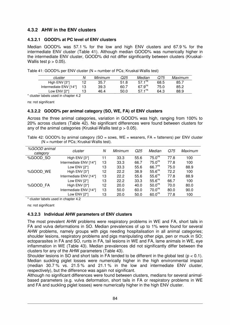
84
4.3.2 AHW in the ENV clusters
4.3.2.1 GOOD% at PC level of ENV clusters
Median GOOD% was 57.1 % for the low and high ENV clusters and 67.9 % for the intermediate ENV cluster (Table 41). Although median GOOD% was numerically higher in the intermediate ENV cluster, GOOD% did not differ significantly between clusters (Kruskal-Wallis test p > 0.05).
Table 41: GOOD% per ENV cluster (N = number of PCs; Kruskal-Wallis test)
cluster N Minimum Q25 Median Q75 Maximum High ENV [3*] 12 35.7 51.8 57.1ns 68.5 85.7
Intermediate ENV [14*] 13 39.3 60.7 67.9ns 75.0 85.2 Low ENV [2*] 13 46.4 50.0 57.1ns 64.3 88.9
* cluster labels used in chapter 4.2
ns: not significant
4.3.2.2 GOOD% per animal category (SO, WE, FA) of ENV clusters
Across the three animal categories, variation in GOOD% was high, ranging from 100% to 20% across clusters (Table 42). No significant differences were found between clusters for any of the animal categories (Kruskal-Wallis test p > 0.05).
Table 42: GOOD% by animal category (SO = sows, WE = weaners, FA = fatteners) per ENV cluster (N = number of PCs; Kruskal-Wallis test).
%GOOD animal category
cluster N Minimum Q25 Median Q75 Maximum
%GOOD_SO High ENV [3*] 11 33.3 55.6 75.0ns 77.8 100 Intermediate ENV [14*] 13 33.3 66.7 75.0ns 77.8 100
Low ENV [2*] 13 33.3 55.6 66.7ns 75.0 88.9 %GOOD_WE High ENV [3*] 12 22.2 38.9 55.6ns 72.2 100
Intermediate ENV [14*] 13 22.2 55.6 55.6ns 77.8 88.9 Low ENV [2*] 13 22.2 33.3 55.6ns 66.7 100
%GOOD_FA High ENV [3*] 12 20.0 40.0 50.0ns 70.0 80.0 Intermediate ENV [14*] 13 50.0 60.0 70.0ns 80.0 90.0
Low ENV [2*] 13 20.0 50.0 60.0ns 77.8 100 * cluster labels used in chapter 4.2
ns: not significant
4.3.2.3 Individual AHW parameters of ENV clusters
The most prevalent AHW problems were respiratory problems in WE and FA, short tails in FA and vulva deformations in SO. Median prevalences of up to 1% were found for several AHW problems, namely groups with pigs needing hospitalisation in all animal categories; shoulder lesions, respiratory problems and pigs manipulating other pigs, pen or muck in SO; ectoparasites in FA and SO, runts in FA, tail lesions in WE and FA, lame animals in WE, eye inflammation in WE (Table 43). Median prevalences did not significantly differ between the clusters for any of the AHW parameters (Table 43). Shoulder lesions in SO and short tails in FA tended to be different in the global test (p < 0.1). Median suckling piglet losses were numerically higher in the high environmental impact (median 30.7 % vs. 21.5 % and 21.1 % in the low and intermediate ENV cluster, respectively), but the difference was again not significant. Although no significant differences were found between clusters, medians for several animal-based parameters (e.g. vulva deformation, short tails in FA or respiratory problems in WE and FA and suckling piglet losses) were numerically higher in the high ENV cluster.
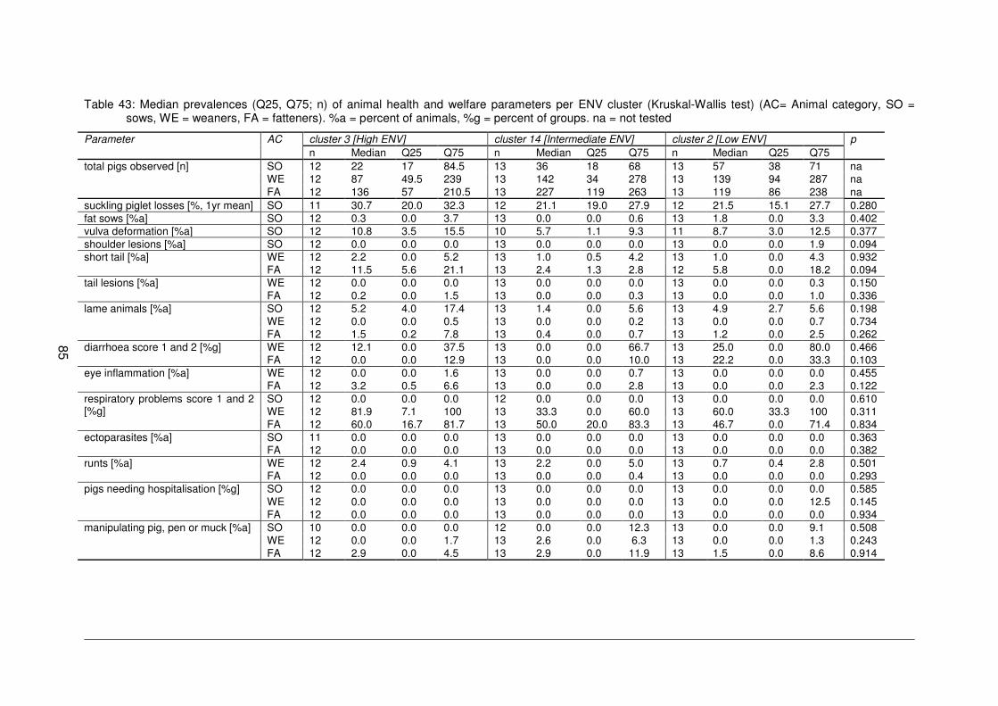
85
Table 43: Median prevalences (Q25, Q75; n) of animal health and welfare parameters per ENV cluster (Kruskal-Wallis test) (AC= Animal category, SO = sows, WE = weaners, FA = fatteners). %a = percent of animals, %g = percent of groups. na = not tested
Parameter AC cluster 3 [High ENV] cluster 14 [Intermediate ENV] cluster 2 [Low ENV] p n Median Q25 Q75 n Median Q25 Q75 n Median Q25 Q75
total pigs observed [n] SO 12 22 17 84.5 13 36 18 68 13 57 38 71 na WE 12 87 49.5 239 13 142 34 278 13 139 94 287 na FA 12 136 57 210.5 13 227 119 263 13 119 86 238 na
suckling piglet losses [%, 1yr mean] SO 11 30.7 20.0 32.3 12 21.1 19.0 27.9 12 21.5 15.1 27.7 0.280 fat sows [%a] SO 12 0.3 0.0 3.7 13 0.0 0.0 0.6 13 1.8 0.0 3.3 0.402 vulva deformation [%a] SO 12 10.8 3.5 15.5 10 5.7 1.1 9.3 11 8.7 3.0 12.5 0.377 shoulder lesions [%a] SO 12 0.0 0.0 0.0 13 0.0 0.0 0.0 13 0.0 0.0 1.9 0.094 short tail [%a] WE 12 2.2 0.0 5.2 13 1.0 0.5 4.2 13 1.0 0.0 4.3 0.932
FA 12 11.5 5.6 21.1 13 2.4 1.3 2.8 12 5.8 0.0 18.2 0.094 tail lesions [%a] WE 12 0.0 0.0 0.0 13 0.0 0.0 0.0 13 0.0 0.0 0.3 0.150
FA 12 0.2 0.0 1.5 13 0.0 0.0 0.3 13 0.0 0.0 1.0 0.336 lame animals [%a] SO 12 5.2 4.0 17.4 13 1.4 0.0 5.6 13 4.9 2.7 5.6 0.198
WE 12 0.0 0.0 0.5 13 0.0 0.0 0.2 13 0.0 0.0 0.7 0.734 FA 12 1.5 0.2 7.8 13 0.4 0.0 0.7 13 1.2 0.0 2.5 0.262
diarrhoea score 1 and 2 [%g] WE 12 12.1 0.0 37.5 13 0.0 0.0 66.7 13 25.0 0.0 80.0 0.466 FA 12 0.0 0.0 12.9 13 0.0 0.0 10.0 13 22.2 0.0 33.3 0.103
eye inflammation [%a] WE 12 0.0 0.0 1.6 13 0.0 0.0 0.7 13 0.0 0.0 0.0 0.455 FA 12 3.2 0.5 6.6 13 0.0 0.0 2.8 13 0.0 0.0 2.3 0.122
respiratory problems score 1 and 2 [%g]
SO 12 0.0 0.0 0.0 12 0.0 0.0 0.0 13 0.0 0.0 0.0 0.610 WE 12 81.9 7.1 100 13 33.3 0.0 60.0 13 60.0 33.3 100 0.311 FA 12 60.0 16.7 81.7 13 50.0 20.0 83.3 13 46.7 0.0 71.4 0.834
ectoparasites [%a] SO 11 0.0 0.0 0.0 13 0.0 0.0 0.0 13 0.0 0.0 0.0 0.363 FA 12 0.0 0.0 0.0 13 0.0 0.0 0.0 13 0.0 0.0 0.0 0.382
runts [%a] WE 12 2.4 0.9 4.1 13 2.2 0.0 5.0 13 0.7 0.4 2.8 0.501 FA 12 0.0 0.0 0.0 13 0.0 0.0 0.4 13 0.0 0.0 0.0 0.293
pigs needing hospitalisation [%g] SO 12 0.0 0.0 0.0 13 0.0 0.0 0.0 13 0.0 0.0 0.0 0.585 WE 12 0.0 0.0 0.0 13 0.0 0.0 0.0 13 0.0 0.0 12.5 0.145 FA 12 0.0 0.0 0.0 13 0.0 0.0 0.0 13 0.0 0.0 0.0 0.934
manipulating pig, pen or muck [%a] SO 10 0.0 0.0 0.0 12 0.0 0.0 12.3 13 0.0 0.0 9.1 0.508 WE 12 0.0 0.0 1.7 13 2.6 0.0 6.3 13 0.0 0.0 1.3 0.243 FA 12 2.9 0.0 4.5 13 2.9 0.0 11.9 13 1.5 0.0 8.6 0.914
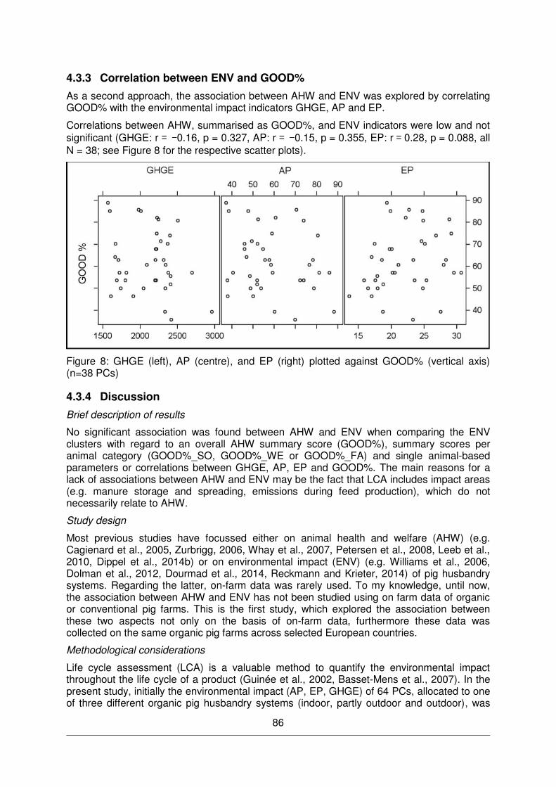
86
4.3.3 Correlation between ENV and GOOD%
As a second approach, the association between AHW and ENV was explored by correlating GOOD% with the environmental impact indicators GHGE, AP and EP.
Correlations between AHW, summarised as GOOD%, and ENV indicators were low and not significant (GHGE: r = -0.16, p = 0.327, AP: r = -0.15, p = 0.355, EP: r = 0.28, p = 0.088, all N = 38; see Figure 8 for the respective scatter plots).
Figure 8: GHGE (left), AP (centre), and EP (right) plotted against GOOD% (vertical axis) (n=38 PCs)
4.3.4 Discussion
Brief description of results
No significant association was found between AHW and ENV when comparing the ENV clusters with regard to an overall AHW summary score (GOOD%), summary scores per animal category (GOOD%_SO, GOOD%_WE or GOOD%_FA) and single animal-based parameters or correlations between GHGE, AP, EP and GOOD%. The main reasons for a lack of associations between AHW and ENV may be the fact that LCA includes impact areas (e.g. manure storage and spreading, emissions during feed production), which do not necessarily relate to AHW.
Study design
Most previous studies have focussed either on animal health and welfare (AHW) (e.g. Cagienard et al., 2005, Zurbrigg, 2006, Whay et al., 2007, Petersen et al., 2008, Leeb et al., 2010, Dippel et al., 2014b) or on environmental impact (ENV) (e.g. Williams et al., 2006, Dolman et al., 2012, Dourmad et al., 2014, Reckmann and Krieter, 2014) of pig husbandry systems. Regarding the latter, on-farm data was rarely used. To my knowledge, until now, the association between AHW and ENV has not been studied using on farm data of organic or conventional pig farms. This is the first study, which explored the association between these two aspects not only on the basis of on-farm data, furthermore these data was collected on the same organic pig farms across selected European countries.
Methodological considerations
Life cycle assessment (LCA) is a valuable method to quantify the environmental impact throughout the life cycle of a product (Guinée et al., 2002, Basset-Mens et al., 2007). In the present study, initially the environmental impact (AP, EP, GHGE) of 64 PCs, allocated to one of three different organic pig husbandry systems (indoor, partly outdoor and outdoor), was
87
assessed (see chapter 4.2.1). For the present chapter a reduced sub-dataset was used, due to limitations further discussed below. All median values of the environmental impact indicators were in the range of a comparable other study (Dourmad et al., 2014). Cluster differences between the intermediate and the high ENV cluster in the reduced sub-dataset used in this chapter were not as clear as in the original data set (see 4.2.3), especially regarding GHGE. However, despite of less pronounced differences in GHGE the original (see 4.2.3) cluster description as low, intermediate and high was regarded acceptable also for the present chapter. But as GHGE may be a less sensitive indicator for finding differences between systems, it was assumed that it may be a less sensitive indicator as well for analysing the association between AHW and ENV.
AHW status for the sub-dataset of 38 PCs was similarly characterised by mainly low prevalences (< 1.0%) of AHW problems in general, and few parameters like diarrhoea, respiratory problems, and suckling piglet losses had higher prevalences.
For exploring the association between AHW and ENV, some of the animal-based parameters were excluded because they were either more influenced by PC management than by the husbandry system (replacement rate and number of farrowings per sow before culling, application of nose rings as well as treatments), had already been identified in ENV as important influencing factor with regard to environmental impact (feed conversion rate in WE and FA), appeared to be sufficiently reflected by another animal based parameter (vulva lesions in SO) or were not available for more than 80 % of PC (losses in WE and FA).
Finally, 15 animal-based parameters were retained, which due to their applicability to one, two or three animal categories (SO, WE, FA), yielded up to 28 values per PC (SO and WE: 9 animal-based parameters, respectively, FA: 10 animal-based parameters). Summarising these selected AHW parameters into one AHW summary score “GOOD%” was regarded as advantageous in order to avoid errors due to multiple testing. There are several approaches to combine the results from animal welfare measures in an overall outcome (Botreau et al., 2007). Almost all of them require informed decisions and weighting of results, which can impact the outcome (e.g. Scott et al., 2001, Bracke et al., 2002). A rather complex approach for creating an integrated animal welfare score has been developed for the Welfare Quality® protocol (Welfare Quality®, 2009). However, the Welfare Quality® approach could not be used for the present analysis because some additional animal-based parameters were used in the present study (e.g. red eyes) or were defined differently (e.g. definitions of social behaviour). As it was not in the scope of this study to develop a new welfare summary score, an approach was chosen that did not involve any weighting of parameters and used robust (median instead of mean) summary calculations. This seemed to be the closest possible approximation to an unbiased AHW summary score. Alternatively, lower and upper quartiles instead of the median may be used as thresholds for sum score calculations in further studies.
As only animal-based parameters for which information was available for more than 80 % of the PCs were used for calculations, due to missing data losses in WE and FA were not taken into account. Again, losses may be considered as important for AHW (e.g. Prunier et al., 2014b) as well as for ENV, as fertility and number of piglets born alive per litter were identified by Reckmann and Krieter (2014) as influencing ENV and within LCA in the present study emissions occurring during keeping the sows are allocated to their offspring.
Despite these limitations, the remaining 28 AHW values were still considered as representing a balanced picture of a PC’s status quo of animal health and welfare - similar to the LCA, which represents as well a balanced picture of a PC’s environmental impact. However, it cannot be excluded that the summary AHW would change if other or more AHW parameters were taken into account and consequently may also affect the results regarding associations between AHW and ENV.
As only GOOD% scores for PCs with ≤ 10% missing values were considered as acceptable for further analysis, in this chapter a reduced sub-dataset was used for comparing AHW with
88
ENV compared to overall ENV analysis (38 vs. 64 PCs, respectively) for which the calculation of the environmental impact (GHGE, AP and EP) as well as animal health and welfare status (summarized in GOOD%) was available. Hence, statistical power was lower for exploring the association between AHW and ENV. It could be assumed that the reduced sub dataset available for the present chapter was insufficient for exploring associations between AHW and ENV. Due to the high number of factors and outcomes involved, more than 38 PCs might be beneficial for in-depth analysis of possible associations between AHW and ENV.
Association between environmental impact and animal health and welfare
The principles of organic farming (IFOAM, 2014) include the maintenance of good AHW and low ENV (IFOAM, 2014). Furthermore the two aspects are linked to each other, as specific aspects of pig production can impact on AHW and ENV (e.g. quantity and quality of food). The question which was investigated here, was if and in which direction an association between actually exists. It might be generally assumed that a healthy and well-being pig is also more environmentally friendly, with fewer veterinary treatments and better utilization of feed (e.g. feed conversion rate), but more extensive production may also carry negative environmental costs. Therefore, in this study for the first time, both aspects were examined on the basis of on-farm assessment and related to each other.
For several animal-based parameters median prevalence was low (0 to 1%) across PCs and consequently across ENV clusters. This finding corresponds to other AHW studies, e.g. in the case of respiratory problems in SO (Dippel et al., 2014b), shoulder lesions in SO (Leeb et al., 2010), ectoparasites in FA and SO (Carstensen et al., 2002) or tail lesions in WE and FA and lame WE (Leeb et al., 2010). Therefore, across all PCs (n=38) considered in this part of the thesis, low prevalences of several animal based parameters indicate good animal health and welfare status in these aspects. However, the most prevalent AHW problems across clusters were respiratory problems and diarrhoea in WE and FA, short tails in FA and vulva deformations in SO, which have been identified in other studies as well (Leeb et al., 2010).
Neither the overall animal health and welfare summary score GOOD% per PC nor GOOD% per animal category (SO, WE, FA, respectively) differed between the clusters representing low, intermediate and high ENV. Although GOOD% was numerically higher in the intermediate ENV cluster, due to the high variation within clusters, GOOD% did not differ significantly between clusters. Furthermore, no meaningful associations (Spearman rank correlations) between GOOD% and the environmental impact indicators AP, EP and GHGE were found. As discussed in the previous chapter (see chapter 4.2.3) one characteristic of the high ENV cluster were high emissions from manure storage and spreading; these emissions influence the total amount of emissions and therefore ENV, but are actually not of major importance for AHW. This may contribute to the fact that GOOD% did not differ between ENV clusters.
However, as by summarizing the animal based parameters to GOOD% per PC and GOOD% per animal category per PC, associations between AHW and ENV might have become less distinct, additionally the prevalences of each animal based parameter were tested between clusters. Regarding animal categories, the fattening phase contributes most to the PCs’ emissions. Therefore, it was assumed, that AHW of FA may differ between ENV clusters. Again no differences between clusters were found for the prevalences of the single animal-based parameters.
The prevalences of only two animal-based parameters tended to be different in the global test between the clusters, i.e. shoulder lesions in SO and short tails in FA (Kruskal Wallis test, p = 0.094). Pairwise comparisons however did not reveal significant differences anymore. Median prevalence of short tails in FA was numerically highest in the high ENV cluster. To identify the causes for short tails was not aim of the present study. The literature shows, that short tails may result from previous tail-biting (Moinard et al., 2003), but as well short tails may be a result of other causes than tail-biting, e.g. necrosis (Jaeger, 2013).
89
Earlier results (Wallgren and Lindahl, 1996) indicate that tail-biting affects the growth rate of pigs, these results were confirmed by Sinisalo et al. (2012). Feed conversion rate is substantially different between the ENV clusters and significantly poorer in the high ENV cluster. It may be speculated, that in the high ENV cluster, more factors which could lead to short tails, either associated with tail-biting, e.g. high stocking density or use of feeding systems with 5 or more growing pigs per feed space (e.g. Moinard et al., 2003, EFSA, 2007), or other factors causing short tails (e.g. mycotoxins) occur than in the other clusters. The measurement of the effect of tail-biting or other causes for short tails on production is difficult, because it requires a large dataset and detailed information on numerous parameters, there still might be some association between short tails and feed conversion rate.
Shoulder lesions in SO were generally rarely seen, but the numerically highest prevalence was found in the upper quartile (Q75) in the low ENV cluster. This indicates, that only few PCs and sows were affected and therefore the result should not be overestimated, as it was probably a PC specific problem with individual sows. However, as shoulder lesions may occur more often in thin sows, it may be presumed, that SO in the low ENV cluster could be thinner. This aspect could not be analysed due to poor inter-observer agreement regarding thin sows.
Across clusters (see chapter 4.2.3), environmental impact indicators were dominated by emissions from feed and housing (direct emissions during animal keeping). Numerically, the low ENV cluster had the lowest contributions from these sources. PCs in the low ENV cluster may use rations/amounts of feed, which merely fulfil the sows’ nutrients requirements, indirectly resulting from time to time in shoulder lesions. Contrary to this hypothesis, earlier in the present thesis (see chapter 4.2.3) it was shown, that there were no differences regarding the proportion of deficient or excess diets in growing and finishing pigs between clusters, but the low ENV cluster showed a high number of sufficient diets (41.18%). It is notable, that across the growing and finishing diets, the low ENV cluster showed numerically the highest proportion of diets (fattening pigs) without deficient digestible lysine (82.35%). Still, it might be, that regarding sows a different picture emerges, but this cannot be confirmed in the present thesis, as the focus regarding deficient or excess diets in SO was not tested between clusters. Likewise, contrary to the theory, that there might be more shoulder lesions due to thinner sows, the low ENV cluster had numerically the highest number of fat sows. Fat sows may be seen negative from an environmental impact view due to higher potential nutrient losses; the (numerical) result is therefore somehow unexpected in the low ENV cluster and as well opposed to the theory of numerically more shoulder lesions due to thinner sows in the low ENV cluster.
Unexpectedly, the low ENV cluster had numerically the highest medians of diarrhoea in FA and WE. Diarrhoea and reduced growth are both reported as accompanying weaning (Lallès et al., 2007), and therefore poorer feed conversion rate (at least in WE) could be expected in the low ENV cluster. However a conflicting result was found previously in this thesis (see chapter 4.2.3), as the low ENV cluster had, at least in FA, significantly the lowest feed conversion rate. Feed conversion rate in WE was not tested between clusters earlier in this thesis, as FA contributed considerably more to ENV than SO and WE together. More diarrhoea problems were found in more intensive farms with greater productivity, which has been described in the literature as important influencing factor for ENV (Lammers, 2011). However, an association between productivity and ENV could not be proven earlier in the present thesis see chapter 4.2.2) as only a weak correlation regarding sow fertility and environmental impact was found. The low ENV cluster may be affected by more diarrhoea problems, but as no runts were observed in the low ENV cluster, the farmers in this cluster seem to be able to minimise the negative effects of diarrhoea on the performance of WE and FA and still achieve better feed conversion rates, which positively influence a PCs ENV.
In the intermediate ENV cluster, the median prevalences for the majority of the parameters (60.7 % of all assessed parameters) across FA, SO and WE were 0.0 %. WE and FA in the intermediate ENV cluster had numerically the lowest median prevalences of respiratory
90
problems. This higher proportion of low prevalences in several AHW parameters may indicate, that PCs in this cluster managed factors better, that influence especially AHW but as well ENV. This might for example concern litter quality, as clean and dry litter may be advantageous for AHW and ENV as already discussed. However, as at least regarding GHGE and EP the intermediate ENV cluster is closer to the high ENV cluster than to the low ENV cluster, this explanation appears to be less meaningful. To identify PC specific factors in the intermediate ENV cluster, which somehow are beneficial for AHW and in a certain amount as well for ENV, further investigation is needed.
The high ENV cluster had numerically the highest medians in more animal-based parameters as compared to the other clusters, and it is the only cluster in which median prevalences of eye inflammation and tail lesions in FA were higher than 0.0%. Numerically highest median prevalences of respiratory problems in WE and FA were observed for PCs in the high ENV cluster. As shown in the second part of this thesis (see chapter 4.2.3), direct emissions from excreta, e.g. NH3, occurring during housing (keeping of animals in pens indoors or paddocks outdoors) were higher in the high and intermediate ENV cluster than in the low ENV cluster (based on the original data set including 59 PC). The higher amount of emissions could be one out of several causes for the numerically higher median prevalences of eye inflammation, respiratory problems and tail lesions in FA in the high ENV cluster, as NH3 irritates the pigs’ eyes and respiratory system and is furthermore considered as one risk factor for tail-biting (as reviewed in Banhazi et al., 2008). As emissions from housing were similar in the high and intermediate ENV cluster, the same numerically number of highest medians in animal-based parameters could have been expected in both clusters. One explanation might be that other influencing factors on these AHW parameters occur more often in the high ENV cluster than in the intermediate ENV cluster (e.g. draught air). Furthermore, emissions from housing may be similar in the high and intermediate ENV cluster, but still have different impact on AHW, for instance if the air change rate and consequently the concentrations of NH3 affecting the pigs differ between the two clusters. However, these aspects were not considered in the present study.
Furthermore, suckling piglet losses were high across all clusters, though the numerically highest median was found in the high ENV cluster (30.7%). Although it is known, that suckling piglet losses are an area requiring improvement in organic production, (Prunier et al., 2014b), this numerically higher prevalence in the high ENV cluster might indicate that these PCs especially experience problems in the suckling period. Improvement in production performance, as highlighted by Lammers (2011), is therefore important to reduce the environmental impact, as emissions occurring during the sow’s life are allocated to the number of piglets per sow.
Across all ENV clusters, PCs with high GOOD%, indicating good animal health and welfare, were found. Although no associations between AHW and ENV were found in the present study, it is notable, that the numerically lowest GOOD% was found in the high ENV cluster, while the numerically highest GOOD% was found in the low ENV cluster. The increased number of animal based parameters with numerically highest medians in the high ENV cluster could be cautiously interpreted as an indication of an association between higher ENV and lower AHW. However, an improved feed conversion rate and lower feed consumption distinguished the low ENV cluster from the intermediate and high ENV cluster, which had a beneficial effect on environmental impacts. Poorer feed conversion rate may be a result of a disease, as e.g. it is known that weaning diarrhoea influences pigs growth rate (Nyachoti et al., 2006). Poorer feed conversion rate may be a result of management strategies as well, e.g. a prolonged fattening period if heavier slaughter weights are desired. Therefore a low feed conversion rate does not always necessarily represent animals having AHW problems. The interaction between animal health and welfare problems and feed conversion rate might therefore be an interesting starting point for further investigations.
However, much more essential for explanation is, that LCA represents an overall PC environmental impact assessment, which covers the whole cradle to farm gate, including
91
areas not important for AHW, mainly manure storage and spreading, or areas not always necessarily connected to poor AHW, e.g. poorer feed conversion rate due to prolonged fattening period. Furthermore, as shown in the second part of this thesis (see chapter 4.2.1) emissions due to the source “feed” (which is depending on the amount and type of feedstuff components) contribute to a large share to a PC’s ENV; however, feed production does not concern AHW directly, as long as the animals are fed appropriate. These aspects are probably the main reasons, why no associations between AHW and ENV were detected.
4.3.5 Conclusion
The objective of the present chapter was to investigate the associations between AHW and ENV of different pig husbandry systems across selected European countries. The results demonstrated a high variation of both AHW and ENV status. The hypothesis of the study, that PCs with low environmental impact also have good animal health and welfare was confirmed, at the same time it was shown, that PCs with higher environmental impact also can have good animal health and welfare. However, some trends point towards a positive correlation between AHW and ENV, e.g. more animal based parameters with numerically highest medians (indicating lower AHW) were found in the high ENV.
ENV assessment of PCs considers impact areas (e.g. manure storage and spreading, emissions during feed production), which do not directly affect AHW, and it may be assumed that this is the main reason for the lack of associations between AHW and ENV. Furthermore, due to the high number of factors and outcomes involved, more than 38 PCs might be beneficial for in-depth analysis of possible associations between AHW and ENV. Still, this study generated a starting point to explore associations between AHW and ENV to be tested either on a larger number of PC or between specific AHW problems and feed conversion rate.
92
5 General discussion
This section focuses on a short summary of the main results followed by a discussion of the general project set up as well as methodological aspects, which were so far only briefly or not discussed. Furthermore, building on the findings and experiences made in the course of the present thesis, conclusions will be drawn and suggestions on further research be made.
5.1 Main results of the study
(1) The first part of the present thesis (see chapter 4.1) presents an on-farm study across 8 European countries on animal health and welfare status of pregnant sows, weaners and fattening pigs in three different organic pig husbandry systems: indoor with concrete outdoor run (IN), partly outdoor (POUT) and outdoor (OUT). Seventy-four organic pig farms were included in the study, i.e. 34 IN, 28 POUT and 12 OUT. The assessment included primarily animal-based parameters and a limited number of resource-based parameters.
In general, a comparatively high level of animal health and welfare was found in most farms, as prevalences were low for most AHW areas with the exception of respiratory problems in IN and POUT and diarrhoea in IN, vulva lesions (IN and OUT) and short tails (IN, POUT). OUT appeared to provide beneficial environmental conditions with regard to several aspects of AHW such as respiratory problems (better air quality), diarrhoea (less exposure to faeces) and lameness (softer flooring of activity and lying areas). POUT farms in most cases kept SO outdoors and WE and FA similar to IN farms, and this was reflected in the results obtained for these animal categories. These results agree with other studies, which for example highlight low prevalences for lameness in sows when kept outdoors (Day et al., 2003, Knage-Rasmussen et al., 2014), however, Bonde and Sørensen (2004) mention, that prevalence of leg disorders and other clinical diseases in outdoor herds might be under-estimated because diagnosis in outdoor herds is more difficult.
Total suckling piglet losses were found to be a problem across all systems, which confirms the findings of Prunier et al. (2014a). Furthermore, also the level of respiratory problems in weaners and fatteners agree with similar studies, e.g, (Leeb et al., 2010) but regarding diarrhoea in WE and FA in the present study higher prevalences were found than by Leeb et al. (2010). Although vulva lesions belong to the animal-based parameters with comparatively higher prevalences, few vulva lesions were found on the farms in comparison to other studies (Leeb et al., 2010, Dippel et al., 2014b).
(2) In the second part of the thesis (see chapter 4.2), a life cycle assessment (LCA) was conducted for all farms using farm specific data to quantify the environmental impact categories greenhouse gas emissions (GHGE), eutrophication potential (EP) and acidification potential (AP). To implement the LCA system boundary “cradle to farm gate” for specialised farms (breeding only and fattening only farms) had to be combined to a production chain (in total 64 PCs).
For GHGE, AP and EP, emissions resulting from feeds contributed most to the total environmental impact, and within the analysed PCs most emissions originated from the fattening period. These results agree with reviewed LCA studies, which highlighted that the emissions from feeds consumed by animals had considerable impact on the total amount of emissions (Basset-Mens and van der Werf, 2005, Basset-Mens et al., 2007, Pelletier et al., 2010, Alig et al., 2012, Reckmann and Krieter, 2014).
Regarding GHGE, no statistically significant differences were found between husbandry systems. POUT had the lowest median values regarding AP and EP; AP in POUT differed significantly from IN, while EP in POUT differed significantly from OUT. Therefore POUT may be considered as preferable system regarding ENV in the present sample.
AP was significantly lower in POUT compared to IN mainly due to fewer emissions from manure storage and spreading (OUT differed neither from IN nor from POUT). OUT showed
93
numerically lower AP than IN as well, but due to high emissions from feeds, the benefit regarding the absence of manure storage and spreading was lost. POUT had significantly lower EP than OUT (and numerically lower EP than IN, but IN differed neither from IN nor from POUT), mainly due to a relatively high feed consumption and poorer feed conversion rate in fatteners in OUT, which increased emissions from feed and direct emissions from animals. Overall, the results highlight the impact of manure storage and spreading in IN and the high potential for reducing environmental impact in OUT by improving the feed conversion ratio, especially in fatteners. The poorer feed conversion ratio in OUT was partly influenced by the longer duration of the fattening phase in some PCs due to the production of heavier pigs.
Comparing the three pig husbandry systems with respect to GHGE, AP and EP revealed inconsistent results. Therefore the PCs were subjected to a hierarchical cluster analysis using the average linkage method (SAS). For this analysis, outliers were excluded, resulting in 59 PCs finally included in the cluster analysis. Clustering revealed three clusters, a ‘low ENV’ cluster, which had the lowest median GHGE, AP and EP, an ‘intermediate ENV’ cluster and a ‘high ENV’ cluster with highest median GHGE, AP and EP. The number of PCs per husbandry system in the clusters did not differ significantly, although the high ENV cluster did not contain PCs belonging to OUT. One of the main differences between the clusters was a significantly lower fatteners' feed conversion rate in the low ENV cluster.
(3) In the third part of the thesis, associations between AHW and ENV were investigated. For this purpose, an AHW summary score (GOOD%) was introduced at production chain (PC) and animal category level, taking into account whether a PC or animal category (SO, FA, WE) exceeded the respective median value or not (for details see chapter 3.5). Due to data availability and the methodological approach of GOOD% calculation, a reduced data sub-set was used containing 38 PC. Neither GOOD% per PC, GOOD% per animal category nor individual animal-based parameters differed between the ENV clusters.
5.2 Methodological considerations
In the present study, a large number of farms (n=74) representing three different husbandry systems were visited across eight different European countries. The sample size of 74 farms in the present study is in the upper range of other studies on AHW of organic pigs (AHW studies on conventional pigs were not taken into account in the present thesis). Sample size of on-farm AHW assessment studies varies considerably between studies, for example Day et al. (2003) visited 9 farms in the UK, Leeb et al. (2010) 60 farms in Austria and Dippel et al. (2014b) 101 farms across 6 European countries. To my knowledge, the present study is the first one, which examines differences between three different organic pig husbandry systems.
The majority of on-farm assessments were conducted either only in one husbandry system (e.g. Day et al., 2003), or combined data from organic farms with different husbandry systems but differences in pig health and welfare between systems were not in the studies’ focus (e.g. Leeb et al., 2010, Dippel et al., 2014b) or even combined data from organic and conventional farms (Scott et al., 2009). Therefore specific results of AHW assessments are rarely available for different husbandry systems.
LCA studies so far have commonly been based on model scenarios (e.g Reckmann and Krieter, 2014) or a small number of farms, often not considering farm specific data from cradle to farm gate (Dolman et al., 2012). One exception is the study by Dolman et al. (2012), who took farm specific data from 27 specialised fattening farms in Denmark into account, but environmental impact from sows and weaners was based on national average figures of specialised rearing farms. Although using data from 3 – 13 farms for each of in total 15 contrasting pig farming systems in five countries, Dourmad et al. (2014) built an average model system for each farming system (see also Bonneau et al. (2014)). Therefore, the number of PC specific LCA calculations in the present thesis can be considered
94
considerably large and unique for life cycle assessment in pig production. The huge variation found for the environmental impact indicators across PCs indicate that LCAs based on mean values of model scenarios may not be representative for all farms in the modelled scenario.
As stated above, studies focus mostly on either AHW or ENV. One exception is the EU-funded project Quality-PorkChain (Bonneau et al., 2014, Dourmad et al., 2014), in which an integrated evaluation of eight sustainability issues in a single tool was developed. However, based on the published data (Bonneau et al., 2014), it is not clear how the AHW assessment was taken into account in detail. The tool developed was mainly based on interviews with farmers and/or their employees. To the author’s knowledge, so far no study was conducted with a multidisciplinary approach to simultaneously quantify AHW and ENV in different organic pig husbandry systems and the attempt to identify association between both aspects.
5.2.1 Challenges of a multidisciplinary approach
In order to achieve the thesis’ objectives, farm visits with comprehensive tasks were conducted which go partly far beyond the objectives of most other studies focussing on either AHW (e.g. Day et al., 2003, Zurbrigg, 2006, Leeb et al., 2010, Dippel et al., 2014b) or ENV (e.g. Basset-Mens and van der Werf, 2005, Williams et al., 2006, Dolman et al., 2012).
Generally, on-farm assessment of animal health and welfare alone may be already challenging, e.g. assessment of animal-based parameters is often time consuming (Andreasen et al., 2013), especially if clinical measures are taken directly on the animals and additionally records on treatments are assessed. Several circumstances have to be taken into account when structuring the farm visits: e.g. behavioural observations should not be conducted close to feeding times and the observers have to be able to assess the animal-based parameters regardless of interfering factors, e.g. disturbances by farm employees. Especially weaning and fattening pigs might move around quickly in the pens, passing from the indoor pen to the outdoor run and vice versa, which makes the assessment challenging. Nevertheless, the observers have to work conscientiously and calm, trying to minimize stressful situations for the pigs, which could result in pigs moving even more around and influencing even AHW parameters, e.g. signs of diarrhoea on the floor might disappear.
Well-trained observers adjusting on farm specific circumstances are important, therefore observer training in the present study took mainly place under practical conditions on common organic pig farms. Besides training of animal-based parameters, all data to be collected on farm should be discussed during observer trainings to ensure, that all observers agree on the intention of the data. This was done in the present projects observer trainings’, additionally a dictionary was established to define/clarify terms to ensure that all assessors correctly interpret the parameters (e.g. calculation of replacement rate, definition of age groups, e.g. gilts).
Regarding on-farm collection of records, it has to be taken into account that on each farm a more or less individual strategy is applied how records on pig’s productivity, treatments and other farm management (e.g. land use) are noted, which can be a demanding and time-consuming task. Therefore it is important, to be as well prepared as possible by e.g. the simple measures of taking a functional desktop calculator and fully charged tablet with you. Furthermore, it can be recommended to be familiar with software tools (e.g. records for herd management) commonly used on pig farms. This knowledge where and how to find data needed makes communication with farmers and data collection easier.
Collecting all data relevant for PC specific LCA calculations and on-farm AHW assessment of sows, weaners and fatteners within a one-day farm visit can therefore be regarded as challenging. Despite the multidisciplinary approach, sample size and quantity and quality of data assessed are comparable with or rather even higher to other studies (Day et al., 2003, Leeb et al., 2010, Dolman et al., 2012, Dippel et al., 2014b, Dourmad et al., 2014) focussing only on one of the both aspects. Representative results were obtained for AHW and ENV of different organic pig husbandry systems.
95
The present thesis shows that evaluation of AHW and ENV of different organic pig husbandry systems can be performed across several countries and on a large scale. This finding fits to conclusions by Rydhmer et al. (2014), who showed, that evaluation of sustainability of pig breeding activities for different conventional and organic farm systems can be performed across several countries and on a large scale.
5.2.2 Farm selection
In many studies, farm selection criteria have not been described (Day et al., 2003, Baumgartner et al., 2003) or are solely based on farm size and type (Prunier et al., 2014a). Besides general selection criteria (e.g. farm size and type), in the present project the farmer’s motivation to participate was considered as important as requirement for farm recruitment. A positive attitude towards the project was regarded essential for an additional project aspect, which is not included in the present thesis, namely the successful implementation of improvement strategies to be evaluated as a part of the project. Also Leeb et al. (2010), in a animal health plan study on 60 Austrian organic pig farms, stressed the farmers’ motivation as possible farm selection criteria; the authors estimated that 65 % of the farmers participated on the basis of their own motivation.
It may be argued, that motivated farmers are more interested in their farms’ ENV and AHW and therefore are more likely to have an above-average status of ENV and AHW on their farm. As one of the project aims was to improve AHW, farmers confronted with specific problems on their farms (e.g. weaning diarrhoea or fertility problems), were especially invited to participate. These farmers still might be considered as motivated, as they are aware of specific AHW problems. Therefore, the sample of farms is not necessarily completely representative for organic pig production, still as the found AHW prevalences are in the range of other studies it can be assumed, that an appropriate sample of farms was included.
5.2.3 Number of farms per system
An equal distribution of farms across the three husbandry systems, which was initially aimed at, was not completely achieved. The number of assessed farms per husbandry system differed, as it was more difficult as expected to find OUT farms. This is due to a decreasing number of organic pig farms in the UK (UK Department for Environment and Food and Rural Affairs, 2013) and additionally farms initially categorized as OUT had to be classified as POUT after the first farm visit, as e.g. one animal category was kept indoors for a longer period than 10 % of the year. Nevertheless, the final sample size was considered as appropriate as each husbandry system consisted of a sufficient number of farms to be analysed statistically. Furthermore, analysis of AHW data was conducted at two levels, i.e. at the system level (IN, POUT, OUT) and according to the location of the animals at the time of the assessment (i.e. indoors or outdoors). The results of both levels of analysis point into the same direction, i.e. in several animal-based parameters it is advantageous for the AHW status of pigs to be kept outdoors ((in OUT or POUT, respectively).
Nevertheless it has to be pointed out, that due to the lower number of OUT farms the analyses on husbandry system level has less statistical power. Due to the substantial variation in several animal-based parameters and ENV between farms (PCs), differences between systems might have become less distinct, but this does not necessarily mean that for a larger sample actually no system effect exists.
96
5.2.4 ‘Husbandry system’ as level of assessment
As a first step in the initial phase of the ProPIG project, a definition of the three husbandry systems indoor with concrete outdoor run (IN), partly outdoor (POUT) and outdoor (OUT) (Table 3, see page 16) was generated. The definitions focus on details on where the animals are kept. More detailed characteristics e.g. concerning breed were not included in the system definitions, but assessed in the questionnaire to be used in system descriptions (see Table 23, page 48 and Table 25, page 49). Of course husbandry systems are not only characterised by the location where the animals are kept, but as well by other factors as e.g. breed, country, farm size or desired carcass weight of fattening pigs. These additional factors characterising farms and their husbandry system only concerned few farms, respectively. To split one husbandry system, e.g. outdoor farms, in sub-groups because they differed partly in other factors was not considered as appropriate, as the sample size within each sub-group would have been small and reduce statistical power.
However, as each system is described in detail, interpretation of results can take these additional characteristics of husbandry systems into account. In many cases it can be assumed, that no bias occurred due to the presence of those additional characteristics. Nevertheless in same cases specific farm (PC) characteristics can have an impact on AHW and ENV. For instance on some OUT farms the fattening period was prolonged to achieve carcasses with different qualities, which might explain the overall poorer feed conversion rate of fattening pigs in OUT.
Farm (PC) specific management strategies (as e.g. the given example regarding prolonged fattening period) might have influenced especially ENV. As an example, this is emphasized by the particular impact of feed conversion rate in FA on ENV criteria and the average carcass weight (kg) which was positively correlated with AP and EP (p<0.05, r = 0.30, respectively), as during the prolonged fattening period a large proportion of emissions arise from the amount of feed needed. Prolonged fattening periods resulting in poorer feed conversion rate concerned mainly the husbandry system OUT, but less IN and POUT.
Overall it was assumed, that the environmental conditions reflected in husbandry system definitions (e.g. type of floor) are the most important but not the only factors influencing AHW and ENV. However, additional farm (PC) characteristics are given to allow interpretation of results, therefore the level of husbandry system was considered as adequate.
5.2.5 Sampling strategy on farm
Farm size and consequently number of animals differed substantially between farms. If possible, all animals in all pens/paddocks of a given farm were assessed. If this approach was not possible due to large numbers of pen/paddocks or animals, a sampling strategy (see chapter 3.3.2.1) was applied for feasibility reasons.
The sampling strategy has impact on the quality of estimates of prevalences of animal-based parameters for individual farms. Therefore, the true prevalence for animal-based parameters was assessed on smaller ProPIG farms where all animals were assessed, while for farms where the sampling strategy was applied, the prevalences were only estimated. Mullan et al. (2009) investigated the effect of sampling strategy on the estimates of prevalence for selected animal-based parameters on different farms. The authors addressed the importance of choosing a large enough sample size to be able to estimate the true prevalence of both physiological and behavioural traits on farms. Depending on the animal-based parameter and farm (prevalences were assessed on six different farms varying in size) different numbers of pens had to be assessed to approach the true prevalence. Especially for parameters with low prevalences, e.g. lameness with prevalences <6.0%, even a large sample did not achieve the true prevalence of those parameters. For instance, in the case of body lesions a sample of 10 pens would give a range of 22% prevalence for one farm, but only 9% for another farm, despite similar true farm prevalences of 14.3 % and 13.0%, respectively. According to the findings of Mullan et al. (2009) the applied sampling strategy in
97
the project has to be considered as not large enough. However, the median number of animals present on farm indicates that in most cases all groups and animals were assessed: for instance, median number of sows ranging from 39 to 141 would mean, that considering common management, a maximum of six groups of pregnant sows consisting of 5 to 18 sows each, was on farm. This means, when applying the sampling strategy, all groups and all animals were assessed. Still, specifically in large groups of animals the sampling strategy might not be sufficient, but best estimates were achieved. Furthermore, the applied sampling strategy goes far beyond the approach used by Welfare Quality® (2009), which was also applied e.g. in Leeb et al. (2010) and Dippel et al. (2014b).
For feasibility reasons, increasing the number of assessed animals and pens was not possible within the present study. Assessing all animals and pens on large farms would have made it impossible to carry out the entire on-farm protocol within a one-day farm visit. The applied sampling strategy is in the upper range of comparable other studies, for instance had Dippel et al. (2014b) the aim to score 5 groups of weaned piglets, independently of the number of pens on farm. The effect of sampling strategy and consequently the derivation of true versus estimated prevalences will probably always be a challenge of on-farm assessments. Anyhow, applied on farm research does not claim to be a controlled experiment. Still, a consensus of sampling strategy in on-farm studies should be discussed elsewhere for future studies and if a sampling strategy was applied, the reliability of estimates should be taken into account in the interpretation.
5.2.6 Inter-observer reliability and exclusion of AHW parameters
Assessment of animal-based parameters requires sufficient training of the observers (Dippel et al., 2014b). The assessment of environmental (resource) parameters (e.g. length of stalls, feeding and drinking facilities) is considered as uncomplicated and repeatable without difficulty by Johnsen et al. (2001); however, Dippel et al. (2014a) report contrary experiences made in the present study.
Inter-observer reliability is not always a standard procedure applied in on-farm assessment studies or at least not described in materials and methods (e.g. Day et al., 2003, Knage-Rasmussen et al., 2014), but is of great importance if the assessment is done by different assessors (Knierim and Winckler, 2009). In the present study, inter-observer reliability (IOR) regarding the animal-based parameters was tested based on live scoring of the animals. It may be argued, that repeated IOR tests based on videos may result in improved intra- und inter-observer agreement of experienced observers in single parameters than IOR tests based on live scoring (e.g. (Schlageter-Tello et al., 2015) for lameness in cattle). But in the present study it was decided to test the IOR under practical farm conditions, as this is the situation observers have to handle during the farm visits, including e.g. pigs moving around in the pen, background noise or observers being manipulated by pigs during on-farm assessment.
Despite repeated observer trainings and retraining, it was not possible to achieve satisfactory agreement for all animal-based parameters. Firstly, data for single parameters from specific observers, who had < 70 % agreement were omitted from analysis, and secondly animal-based parameters for which ≥ 3 observers did not reach the threshold of agreement (thresholds for sufficient reliability were set at an agreement of ≥ 70 %) were excluded in order to avoid bias due to variation introduced by the observers. Therefore, lesions and swellings in SO and FA and thin sows (low body condition score) were not further considered in the analysis of AHW and the association between AHW and ENV.
Of course omitting these three parameters from the analysis was not desired, as all animal-based parameters were initially selected based on their indicative value for the presence (or absence) of health and welfare problems (Dippel et al., 2014b). The present thesis’ aim was to investigate AHW as complete as possible and to cover all aspects of AHW. Only a relatively small number of parameters had to be excluded (5 out of in total 41 animal-based
98
parameters). The excluded parameters would have given additional information on body condition, social behaviour and lying comfort. These aspects are at least partly covered by other parameters, e.g. shoulder lesions can be observed in thin sows.
However, the use of reliable data only is of great importance. The decision to exclude animal-based parameters for which observers did not reach the threshold, is easily possible in data analysis and ensures data quality. Still, it would be possible to analyse the excluded animal-based parameters on a national level only without creating a joined dataset, as each country was assessed by one observer.
Furthermore, it has to be questioned, why in some parameters lower agreement was achieved. As already discussed briefly in the first part of the thesis (see chapter 4.1.6), one reason for the low observer agreement for some parameters could be the varying initial levels of knowledge on pig health and behaviour among observers, as assumed also by Dippel et al. (2014b). Schlageter-Tello et al. (2015) found that different levels of experience of observers can influence IOR. It may therefore be suggested to take the different observer levels of knowledge on pig health into account when planning the trainings, as some observers might need more training than others in order to achieve the same level of inter observer agreement.
5.3 Overall conclusions
The present study offers an immense amount of detailed data and information on AHW and ENV of different organic pig husbandry systems. It is unique in comparing three different organic pig husbandry systems (IN, POUT, OUT) throughout Europe, using animal-based parameters assessed on farm and data relevant for the environmental impact from the same organic pig farms. Nevertheless, some aspects of the present study may be improved and the following suggestions could be implemented in future studies as well as in attempts to improve the organic pig farming sector.
Scientific research
Regarding AHW, future studies may benefit from expanding the observer training and from taking the different observer levels of knowledge on pig health into account when planning the trainings. This will ensure that less experienced observers have the possibility to achieve the threshold for inter-observer agreement and likely avoid the exclusion of animal-based parameters due to poor inter-observer agreement. Furthermore, as reaching adequate sample sizes most likely will remain a challenge in on-farm research, it is important to clearly describe the sampling strategy applied in a study and to cautiously interpret the findings taking the reliability of the estimated prevalences into account.
Regarding ENV, the following aspects of the LCA calculation shall be addressed as they still provide room for further discussions and investigations. Due to a lack of emission factors for all types of housing, e.g. no distinction between indoor area and outdoor run was made when calculating emissions from housing in IN. In outdoor paddocks, specific soil condition, proportion of the vegetation cover and paddock slope was not taken into account as well. If in basic research studies additional measurements for different situations of pigs kept in organic pig husbandry systems would be conducted, these could be integrated in applied LCAs. This is similarly the case for emission factors for feedstuff components: For further studies it would be very useful to have a collection of emission factors for feedstuff components in organic quality available, which is potentially based on the approach of the LCA Food database (2007), but continuously expanded with available emission factors.
For farms lacking records on feed conversion rate in WE and FA, these values were estimated from PC specific data (e.g. duration of the fattening stages, carcass weight, amount of feed fed etc.). If PC specific data needed for the calculation of the feed conversion rate was not available, no LCA was conducted. Feed conversion rate proved to be essential for a PCs ENV, therefore it is important to take PC specific feed conversion rates into
99
account and estimations should only be done if reasonable data is available. One option for improvement would be a longer time period between farm recruitment and first farm visit connected with a request to the farmer to take detailed records in this period.
Regarding the association between AHW and ENV, some further considerations may be stressed. Firstly, it could be assumed that the reduced sub-dataset was not appropriate for exploring associations between AHW and ENV sufficiently. Due to the high number of factors and outcomes involved, more than 38 PCs might be needed for in-depth analysis of possible associations between AHW and ENV. Statistical power was lower and associations between AHW and ENV therefore might have become less obvious and not statistically significant. Secondly, very essential for explanation of the lack of association is, that LCA represents an overall PC environmental impact assessment, which covers the whole cradle to farm gate, including areas not necessarily important for AHW (e.g. manure management) or areas not always necessarily connected to poor AHW (e.g. poorer feed conversion rate due to prolonged fattening period).
Three options for further research on the association between AHW and ENV could be:
To test GOOD% within systems including only PCs with similar management strategies regarding duration of the fattening phase, as it may be difficult to detect associations between AHW and ENV, if the reason for poorer FCR is not an AHW problem, but results from the management strategy.
Risk factor analysis regarding AHW and ENV could be conducted to compare identified risk factors for both aspects with each other. This would allow analysing the relationships between factors influencing both AHW and ENV.
As feed conversion rate was already identified as influencing ENV, it may be worth to investigate direct associations between animal based parameters and feed conversion rate. For example, Garnett et al. (2013) state, that many aspects of animal welfare can increase productivity, especially when low productivity is caused by disease, insufficient feed and other causes of poor health. Post-weaning diarrhoea and the associated reductions in growth rates, resulting in poorer feed conversion rate, are considered as one of the main challenges in pig production (Nyachoti et al., 2006). Therefore, it is interesting to examine the association between feed conversion rate and AHW, for instance during controlled experiments on the impact of health and welfare problems (e.g. respiratory problems) on the feed conversion rate.
It can be recommended, that the projects approach to use on-farm data from a large number of farms is meaningful also for further studies on AHW and ENV, due to the large variation between farms regarding AHW and ENV. This is supported by similar findings of comparable studies (Leeb et al., 2010, Bonneau et al., 2014, Dippel et al., 2014b). Especially the huge variation of the environmental impact indicators across PCs indicate that LCAs based on mean values of model scenarios will not always be representative for all farms in modelled scenarios.
Despite the challenges of the multidisciplinary approach taken in this study (e.g. collection of data on AHW and ENV within one day), it can be recommended to follow a similar approach also in future studies. Firstly, data collection is very efficient as several parameters can be used for both aspects. Secondly, analysing AHW and ENV on the basis of the same sample of individual farms (PCs) enables a more holistic insight and interpretation of organic pig husbandry systems. Comprehensive studies like the one presented here, with a joint effort needed from scientists across several countries and disciplines, can probably only be ensured in international projects with a suitable funding background.
Farmers and advisory services
The variation of AHW and ENV between farms and PCs highlights the individuality of issues for each farm and also the potential for improvement within each husbandry system.
100
This can be taken up by different improvement strategies, such as advisory activities, farmer group discussions or self-evaluation. To support implementation of improvement strategies, two practical tools for further use by advisors and farmers were created within ProPIG (but not part of the present thesis):
A ‘Handbook for organic pig farmers’ based on expert opinion as well as farmers improvement strategies regarding AHW in the format of a hard cover ring-binder and available online as pdf, allowing practical application on farm.
A ‘Decision support tool for environmental impact’ (‘EDST’) in the form of an interactive spreadsheet, which identifies areas of possible improvement regarding ENV through a structured questionnaire and suggests improvement measures.
Additionally, the already mentioned advanced data collection tool ‘Pigsurfer’ was especially developed for advisors and scientists to make assessing, analysing and feedback (benchmarking) of animal based parameters during few hours on farm feasible.
General future perspective
The results of the present study on AHW, ENV and the associations between AHW and ENV in three organic pig husbandry systems across Europe together with the three tools 2 represent a good starting point for farm (PC) specific improvements regarding AHW and ENV. Furthermore the results show advantages of POUT regarding ENV and OUT regarding AHW, which may serve as a basis for the further development of organic pig husbandry systems.
2 Information on the availability of the tools may be found online: either on http://www.coreorganic2.org/propig or on www.orgprints.org by using the keyword ProPIG
101
References
ALIBERT, L. 2014. Besoins alimentaires des animaux en fonction du stade physiologique [Online]. Available: http://www.itab.asso.fr/downloads/porc-bio/cahier_porc_0.pdf [Accessed 10.12.2014 2014].
ALIG, M., GRANDL, F., MIELEITNER, J., NEMECEK, T. & GAILLARD, G. 2012. Life Cycle Assessment of Beef, Pork and Poultry, Executive Summary. Reckenholz-Tänikon, Switzerland.
AMA. 2013. Agrarmarkt Austria Lebend- und Schlachtgewichte, Schlachtausbeute, Schlachtungen, Fleischanfall 2011-2012 Stand April 2013 [Online]. AgrarMarkt Austria Available: http://www.ama.at/Portal.Node/ama/public?gentics.rm=PCP&gentics.pm=gti_full&p.contentid=10008.120536&220_schlachtgew.pdf [Accessed 01.12.2013 2013].
AMON, B., FRÖHLICH, M., KRYVORUCHKO, V. & AMON, T. 2005. Messen und Mindern von Ammoniak-, Lachgas- und Methanemissionen aus einem Schrägbodenstall für Mastschweine. Endbericht GZ 21.210/10-II/1/03. Universität für Bodenkultur Wien. Im Auftrag des BMLFUW.
ANDERSEN, H. M. L., DYBKJÆR, L. & HERSKIN, M. S. 2014. Growing pigs’ drinking behaviour: number of visits, duration, water intake and diurnal variation. Animal, 8, 1881-1888.
ANDREASEN, S. N., WEMELSFELDER, F., SANDØE, P. & FORKMAN, B. 2013. The correlation of Qualitative Behavior Assessments with Welfare Quality® protocol outcomes in on-farm welfare assessment of dairy cattle. Applied Animal Behaviour Science, 143, 9-17.
BANHAZI, T. M., SEEDORF, J., RUTLEY, D. L. & PITCHFORD, W. S. 2008. Identification of Risk Factors for Sub-Optimal Housing Conditions in Australian Piggeries: Part 1. Study Justification and Design. 14.
BASSET-MENS, C. & VAN DER WERF, H. M. G. 2005. Scenario-based environmental assessment of farming systems: the case of pig production in France. Agriculture, Ecosystems & Environment, 105, 127-144.
BASSET-MENS, C., VAN DER WERF, H. M. G., ROBIN, P., MORVAN, T., HASSOUNA, M., PAILLAT, J. M. & VERTÈS, F. 2007. Methods and data for the environmental inventory of contrasting pig production systems. Journal of Cleaner Production, 15, 1395-1405.
BAUMGARTNER, J., LEEB, T., GRUBER, T. & TIEFENBACHER, R. 2003. Husbandry and animal health on organic pig farms in Austria. Animal Welfare, 12, 631-635.
BLOKHUIS, H. J., JONES, R. B., GEERS, R., MIELE, M. & VEISSIER, I. 2003. Measuring and monitoring animal welfare: transparency in the food product quality chain. Animal Welfare, 12, 445-455.
BMEL 2015. Organic Farming in Germany. Bonn: Federal Ministry of Food and Agriculture BMGF 2006. Selbstevaluierung Handbuch Schweine. Vienna: Bundesministerium für
Gesundheit und Frauen im Einvernehmen mit Bundesministerium für Land- und Forstwirtschaft, Umwelt und Wasserwirtschaft.
BOLHUIS, J. E., SCHOUTEN, W. G. P., SCHRAMA, J. W. & WIEGANT, V. M. 2006. Effects of rearing and housing environment on behaviour and performance of pigs with different coping characteristics. Applied Animal Behaviour Science, 101, 68-85.
BONDE, M. & SØRENSEN, J. T. 2004. Herd health management in organic pig production using a quality assurance system based on Hazard Analysis and Critical Control Points. NJAS - Wageningen Journal of Life Sciences, 52, 133-143.
BONNEAU, M., KLAUKE, T. N., GONZÀLEZ, J., RYDHMER, L., ILARI-ANTOINE, E., DOURMAD, J. Y., DE GREEF, K., HOUWERS, H. W. J., CINAR, M. U., FÀBREGA, E., ZIMMER, C., HVIID, M., VAN DER OEVER, B. & EDWARDS, S. A. 2014. Evaluation of the sustainability of contrasted pig farming systems: integrated evaluation. Animal, 8, 2058-2068.
102
BOTREAU, R., BONDE, M., BUTTERWORTH, A., PERNY, P., BRACKE, M. B. M., CAPDEVILLE, J. & VEISSIER, I. 2007. Aggregation of measures to produce an overall assessment of animal welfare. Part 1: a review of existing methods. Animal, 1, 1179-1187.
BRACKE, M. B. M., HULSEGGE, B., KEELING, L. & BLOKHUIS, H. J. 2004. Decision support system with semantic model to assess the risk of tail biting in pigs: 1. Modelling. Applied Animal Behaviour Science, 87, 31-44.
BRACKE, M. B. M., SPRUIJT, B. M., METZ, J. H. M. & SCHOUTEN, W. G. P. 2002. Decision support system for overall welfare assessment in pregnant sows A: Model structure and weighting procedure. Journal of Animal Science, 80, 1819-1834.
BRANDHOFER, R. 2014. Umweltwirkungen biologischer Schweinehaltung: Vergleich zweier Haltungssysteme auf Basis des Treibhausgas-Potenzials sowie einer Stickstoff und Phosphorbilanz. Master thesis in preparation, University of Natural Resources and Life Sciences.
BRAUND, J. P., EDWARDS, S. A., RIDDOCH, I. & BUCKNER, L. J. 1998. Modification of foraging behaviour and pasture damage by dietary manipulation in outdoor sows. Applied Animal Behaviour Science, 56, 173-186.
BROOM, D. 2011. A History of Animal Welfare Science. Acta Biotheoretica, 59, 121-137. BROUNS, F., EDWARDS, S. A. & ENGLISH, P. R. 1994. Effect of dietary fibre and feeding
system on activity and oral behaviour of group housed gilts. Applied Animal Behaviour Science, 39, 215-223.
BUSCH, M. E., WACHMANN, H., NIELSEN, E. O., PETERSEN, H. H. & NIELSEN, J. P. Tail biting - can routine meat inspection data be used for classification of herds? 18th IPVS Congress, 2004 Hamburg, Germany.
CAGIENARD, A., REGULA, G. & DANUSER, J. 2005. The impact of different housing systems on health and welfare of grower and finisher pigs in Switzerland. Preventive Veterinary Medicine, 68, 49-61.
CARSTENSEN, L., VAARST, M. & ROEPSTORFF, A. 2002. Helminth infections in Danish organic swine herds. Veterinary Parasitology, 106, 253-264.
DALGAARD, R., HALBERG, N. & HERMANSEN, J. E. 2007. Danish Pork Production - An Environmental Assessment. DJF Animal Science. Tjele, Denmark: University of Aarhus.
DAY, J. E. L., KELLY, H., MARTINS, A. & EDWARDS, S. A. 2003. Towards a baseline assessment of organic pig welfare. Animal Welfare, 12, 637-641.
DE JONGE, J. & VAN TRIJP, H. M. 2013. Meeting Heterogeneity in Consumer Demand for Animal Welfare: A Reflection on Existing Knowledge and Implications for the Meat Sector. Journal of Agricultural and Environmental Ethics, 26, 629-661.
DE VRIES, M. & DE BOER, I. J. M. 2010. Comparing environmental impacts for livestock products: A review of life cycle assessments. Livestock Science, 128, 1-11.
DEFRA 1998. Condition scoring of pigs, Defra publications 3480. London, UK. DIPPEL, S., BOCHICCHIO, D., HAUN POULSEN, P., HOLINGER, M., HOLMES, D., KNOP,
D., PRUNIER, A., RUDOLPH, G., SILEROVA, J. & LEEB, C. Trough or bowl: observers need training for assessing resource as well as clinical parameters. In: MOUNIER, L. & VEISSIER, I., eds. WAFL-6th International Conference on the Assessment of Animal Welfare at Farm and Group Level, 3-5 September, 2014a Clermont-Ferrand, France. 182.
DIPPEL, S., LEEB, C., BOCHICCHIO, D., BONDE, M., DIETZE, K., GUNNARSSON, S., LINDGREN, K., SUNDRUM, A., WIBERG, S., WINCKLER, C. & PRUNIER, A. 2014b. Health and welfare of organic pigs in Europe assessed with animal-based parameters. Organic Agriculture, 4, 149-161.
DOLMAN, M. A., VROLIJK, H. C. J. & DE BOER, I. J. M. 2012. Exploring variation in economic, environmental and societal performance among Dutch fattening pig farms. Livestock Science, 149, 143-154.

103
DOURMAD, J. Y. 24.04.2013 2013. RE: Livestock manure outdoors. Type to BRANDHOFER, R.
DOURMAD, J. Y., RYSCHAWY, J., TROUSSON, T., BONNEAU, M., GONZÀLEZ, J., HOUWERS, H. W. J., HVIID, M., ZIMMER, C., NGUYEN, T. L. T. & MORGENSEN, L. 2014. Evaluating environmental impacts of contrasting pig farming systems with life cycle assessment. Animal, 8, 2072-2037.
EDWARDS, S., MEJER, H., ROEPSTORFF, A. & PRUNIER, A. 2014a. Animal health, welfare and production problems in organic pregnant and lactating sows. Organic Agriculture, 4, 93-105.
EDWARDS, S. A. 2005. Product quality attributes associated with outdoor pig production. Livestock Production Science, 94, 5-14.
EDWARDS, S. A. Nutritional approaches to reducing the environmental impact of outdoor pigs. 41st University of Nottingham Feed Conference 3rd - 5th September 2007 2007 Loughborough, UK.
EDWARDS, S. A., PRUNIER, A., BONDE, M. & STOCKDALE, E. A. 2014b. Special issue—organic pig production in Europe—animal health, welfare and production challenges. Organic Agriculture, 4, 79-81.
EEA 2013. Annual European Union greenhouse gas inventory 1990-2011 and inventory report 2013, Technical report. European Commission, DG Climate Action European Environment Agency.
EFSA 2007. Scientific Opinion of the Panel on Animal Health and Welfare on a request from Commission on the risks associated with tail biting in pigs and possible means to reduce the need for tail docking considering the different housing and husbandry systems. EFSA Journal, 611.
ETTERLIN, P. E., YTREHUS, B., LUNDEHEIM, N., HELDMER, E., ÖSTERBERG, J. & EKMAN, S. 2014. Effects of free-range and confined housing on joint health in a herd of fattening pigs. BMC Veterinary Research, 10.
EUROBAROMETER 2007. Attitudes of EU citizens towards Animal Welfare. Special Eurobarometer 270/Wave 66.1 - TNS Opinion & Social
EVAPIG 2008. A calculator of energy, amino acid and phosphorus values of ingredients and diets for growing and adult pigs. INRA, Ajinomoto Eurolysine SAS, AFZ.
FAO. 2014a. The role of livestock in climate change [Online]. Food and Agriculture Organization of the United Nations. Available: http://www.fao.org/agriculture/lead/themes0/climate/en/ [Accessed 08.07.2014.
FAO 2014b. SAFA Sustainability Assessment of Food and Agriculture Systems Guidelines Version 3.0. Rome.
FAWC 2009. Farm Animal Welfare in Great Britain: Past, Present and Future. London. FRASER, D. 2003. Assessing animal welfare at the farm and group level: the interplay of
science and values. Animal Welfare, 12, 433-443. FRASER, D., DUNCAN, I. J. H., EDWARDS, S. A., GRANDIN, T., GREGORY, N. G.,
GUYONNET, V., HEMSWORTH, P. H., HUERTAS, S. M., HUZZEY, J. M., MELLOR, D. J., MENCH, J. A., ŠPINKA, M. & WHAY, H. R. 2013. General Principles for the welfare of animals in production systems: The underlying science and its application. The Veterinary Journal, 198, 19-27.
FREEDOM FOOD 2015. Freedom Food Impact Report. West Sussex: Freedom Food Dedicated to farm animal welfare.
FRÜH, B. 2011. Organic Pig Production in Europe. Health Management in Common Organic Pig Farming. Frick, Sitzerland: Research Institute of Organic Agriculture.
FRÜH, B., BOCHICCHIO, D., EDWARDS, S., HEGELUND, L., LEEB, C., SUNDRUM, A., WERNE, S., WIBERG, S. & PRUNIER, A. 2014. Description of organic pig production in Europe. Organic Agriculture, 4, 83-92.
GADE, P. B. 2002. Welfare of animal production in intensive and organic systems with special reference to Danish organic pig production. Meat Science, 62, 353-358.
104
GARNETT, T., APPLEBY, M. C., BALMFORD, A., BATEMAN, I. J., BENTON, T. G., BLOOMER, P., BURLINGAME, B., DAWKINS, M., DOLAN, L., FRASER, D., HERRERO, M., HOFFMANN, I., SMITH, P., THORNTON, P. K., TOULMIN, C., VERMEULEN, S. J. & GODFRAY, H. C. J. 2013. Sustainable Intensification in Agriculture: Premises and Policies. Science, 341, 33-34.
GERBER, P. J., STEINFELD, H., HENDERSON, B., MOTTET, A., OPIO, C., DIJKMAN, J., FALCUCCI, A. & TEMPIO, G. 2013. Tackling climate change through livestock – A global assessment of emissions and mitigation opportunities. Rome.
GERJETS, I. & KEMPER, N. 2009. Coliform mastitis in sows: A review. Journal of Swine Health and Production, 17, 97-105.
GOODLAND, R. & ANHANG, J. 2009. Livestock and Climate Change, what if the key actors in climate change are... cows, pigs and chicken? . World Watch Magazine.
GOOSSENS, X., SOBRY, L., DBERG, F., TUYTTENS, F., MAES, D., DE SMET, S., NEVENS, F., OPSOMER, G., LOMMELEN, F. & GEERS, R. 2008. A population-based on-farm evaluation protocol for comparing the welfare of pigs between farms. Animal Welfare, 17, 35-41.
GUINÉE, J. B., GORRÉE, M., HEIJUNGS, R., HUPPES, G., KLEIJN, R., KONING, A. D., OERS, L. V., WEGENER SLEESWIJK, A., SUH, S., UDO DE HAES, H. A., BRUIJN, H. D., DUIN, R. V. & HUIJBREGTS, M. A. J. 2002. Handbook on life cycle assessment. Operational guide to the ISO standards. Dordrecht.
GUY, J. H., ROWLINSON, P., CHADWICK, J. P. & ELLIS, M. 2002. Health conditions of two genotypes of growing-finishing pig in three different housing systems: implications for welfare. Livestock Production Science, 75, 233-243.
HALBERG, N., HERMANSEN, J. E., KRISTENSEN, I. S., ERIKSEN, J., TVEDEGAARD, N. & PETERSEN, B. M. 2010. Impact of organic pig production systems on CO2 emission, C sequestration and nitrate pollution. Agronomy for Sustainable Development, 30, 721-731.
HAUSSCHILD, M. & WENZEL, H. 1998. Environmental assessments of products. Scientific background, London, UK, Chapman & Hall.
HEID, A., BRENNINKMEYER, C., KNIERIM, U. & HAMM, U. 2011. Alternativen zur betubungslosen Ferkelkastration im kologischen Landbau - Analyse der Auswirkungen alternativer Verfahren auf die Akzeptanz bei Verbrauchern und Produzenten (Alternatives to castration of piglets without anaesthesia in organic farming – Analysis of the impacts of alternative methods on the acceptance by consumers and producers. BÖL Bericht 18652. Witzenhausen, Germany: BÖL Bundesprogramm Ökologischer Landbau.
HEINONEN, M., ORAVAINEN, J., ORRO, T., SEPPÄ-LASSILA, L., ALA-KURIKKA, E., VIROLAINEN, J., TAST, A. & PELTONIEMI, O. A. T. 2006. Lameness and fertility of sows and gilts in randomly selected loose-housed herds in Finland. Veterinary Record, 159, 383-387.
HEINONEN, M., PELTONIEMI, O. & VALROS, A. 2013. Impact of lameness and claw lesions in sows on welfare, health and production. Livestock Science, 156, 2-9.
HERZOG, S., FRÜH, B. & NOTZ, C. 2006. Schweinehaltung: Beratung zurzeit dringlicher als Forschung. . Bioaktuell, Nr. 8.
HÖRTENHUBER, S., LINDENTHAL, T., AMON, B., MARKUT, T., KIRNER, L. & ZOLLITSCH, W. 2010. Greenhouse gas emissions from selected Austrian dairy production systems—model calculations considering the effects of land use change. Renewable Agriculture and Food Systems, 25, 316-329.
HÖRTENHUBER, S. J. 24.10.2013 2013a. RE: Calculation of acidification and eutrophication potential. Type to RUDOLPH, G.
HÖRTENHUBER, S. J. 2013b. RE: Greenhouse gas emissions from feedstuffs. Type to BRANDHOFER, R. & RUDOLPH, G.
HÖRTENHUBER, S. J., LINDENTHAL, T. & ZOLLITSCH, W. 2011. Reduction of greenhouse gas emissions from feed supply chains by utilizing regionally produced
105
protein sources: the case of Austrian dairy production. Journal of the Science of Food and Agriculture, 91, 1118-1127.
HOVI, M., SUNDRUM, A. & THAMSBORG, S. M. 2003. Animal health and welfare in organic livestock production in Europe: current state and future challenges. Livestock Production Science, 80, 41-53.
IFOAM 2014. The IFOAM NORMS for Organic Production and Processing Version 2014, Germany, IFOAM.
IPCC 2006. Guidelines for national greenhouse gas inventories. . In: EGGLESTON, S., BUENDIA, L., MIWA, K., NGARA, T., TANABE, K. (ed.).
IPCC 2007. Climate Change 2007 - The Physical Science Basis: Working Group I Contribution to the Fourth Assessment Report of the IPCC, Cambridge University Press.
JACQUES, S. 2014. Science and animal welfare in France and European Union: Rules, constraints, achievements. Meat Science, 98, 484-489.
JAEGER, F. 2013. Das Projekt "intakter Ringelschwanz" beim Schwein - stehen wir vor dem Durchbruch? . Tierärztl. Umschau, 68, 3-11.
JENSEN, J. C. E., NIELSEN, L. H., ARNASON, T. & CRACKNELL, V. 2002. Elimination of mange mites Sarcoptes scabiei var. suis from two naturally infested Danish sow herds using a single injection regime with doramectin. Acta Veterinaria Scandinavica, 43, 75-84.
JOHNSEN, P. F., JOHANNESSON, T. & SANDØE, P. 2001. Assessment of Farm Animal Welfare at Herd Level: Many Goals, Many Methods. Acta Agriculturae Scandinavica, Section A — Animal Science, 51, 26-33.
KIJLSTRA, A. & EIJCK, I. A. J. M. 2006. Animal health in organic livestock production systems: a review. NJAS - Wageningen Journal of Life Sciences, 54, 77-94.
KILBRIDE, A., GILLMAN, C. & GREEN, L. 2009a. A cross sectional study of the prevalence, risk factors and population attributable fractions for limb and body lesions in lactating sows on commercial farms in England. BMC Veterinary Research, 5, 30.
KILBRIDE, A. L., GILLMAN, C. E. & GREEN, L. E. 2009b. A cross-sectional study of the prevalence of lameness in finishing pigs, gilts and pregnant sows and associations with limb lesions and floor types on commercial farms in England. Animal Welfare, 18, 215-224.
KIRCHGESSNER, M., ROTH, F. X., SCHWARZ, F. J. & STANGL, G. 2011. Tierernährung, Weihenstephan, DLG Verlag.
KNAGE-RASMUSSEN, K. M., HOUE, H., ROUSING, T. & SØRENSEN, J. T. 2014. Herd- and sow-related risk factors for lameness in organic and conventional sow herds. animal, 8, 121-127.
KNIERIM, U. & WINCKLER, C. 2009. On-farm welfare assessment in cattle: validity, reliability and feasibility issues and future perspectives with special regard to the Welfare Quality® approach. Animal Welfare, 18, 451-458.
KOLBE, H. 2002. Wasserbelastung in Abhängigkeit von der Landnutzung Ökologie und Landbau
KOOL, A., BLONK, H., PONSIOEN, T., SUKKEL, W., VERMEER, H., DE VRIES, J. W. & HOSTE, R. 2009. Carbon Footprints of conventional and organic pigs – Assessment of typical production systems in the Netherlands, Denmark, England and Germany. Wageningen.
LALLÈS, J.-P., BOSI, P., SMIDT, H. & STOKES, C. R. 2007. Weaning — A challenge to gut physiologists. Livestock Science, 108, 82-93.
LAMMERS, P. J. 2011. Life-cycle assessment of farrow-to-finish pig production systems: A review. CAB Reviews: Perspectives in Agriculture, Veterinary Science, Nutrition and Natural Resources, 6, 1-8.
LCA FOOD DATABASE. 2007. LCA Food database [Online]. Available: http://www.lcafood.dk/ [Accessed 15.10 2013].

106
LEEB, B., LEEB., C., TROXLER, J. & SCHUH, M. 2001. Skin Lesions and Callosities in Group-Housed Pregnant Sows: Animal-Related Welfare Indicators. Acta Agriculturae Scandinavica, Section A - Animal Science, Suppl. 30, 82-87.
LEEB, C., BERNARDI, F. & WINCKLER, C. 2010. Einführung und Monitoring von BetriebsEntwicklungsPlänen (BEP) Tiergesundheit und Wohlbefinden in österreichischen Bioschweinebetrieben Wien.
LEEB, C., HEGELUND, L., EDWARDS, S., MEJER, H., ROEPSTORFF, A., ROUSING, T., SUNDRUM, A. & BONDE, M. 2014. Animal health, welfare and production problems in organic weaner pigs. Organic Agriculture, 4, 123-133.
LERNOUD, J. & WILLER, H. 2015. Current Statistics on Organic Agriculture Worldwide: Organic Area, Producers, Markets and Selected Crops. In: WILLER, H., LERNOURD, J. (ed.) The World of Organic Agriculture. Statistics and Emerging Trends 2015. Frick, Bonn: Research Institute of Organic Agriculture (FiBL) and IFOAM- Organic International.
LFL BAYERN 2011. Schweinefütterung am Ökobetrieb II - Fütterungsversuche, Fütterungsempfehlungen. Poing: LfL Bayern
LINDGREN, K., BOCHICCHIO, D., HEGELUND, L., LEEB, C., MEJER, H., ROEPSTORFF, A. & SUNDRUM, A. 2014. Animal health and welfare in production systems for organic fattening pigs. Organic Agriculture, 4, 135-147.
LUMARET, J. P., ERROUISSI, F., FLOATE, K., RÖMBKE, J. & WARDHAUGH, K. 2012. A review on the toxicity and non-target effects of macrocyclic lactones in terrestrial and aquatic environments. Current Pharmaceutical Biotechnology, 13, 1004-1060.
LYONS, C. A. P., BRUCE, J. M., FOWLER, V. R. & ENGLISH, P. R. 1995. A comparison of productivity and welfare of growing pigs in four intensive systems. Livestock Production Science, 43, 265-274.
MAIN, D. C. J., WHAY, H. R., LEEB, C. & WEBSTER, A. J. F. 2007. Formal animal-based welfare assessment in UK certification schemes. Animal Welfare, 16, 233-236.
MARCH, S., BRINKMANN, J., DIPPEL, S., LEEB, C., SCHWALM, A., WEISSMAN, F. & WINCKLER, C. 2014. Lahmheiten bei Zuchtsauen - auch im Ökolandbau? Welche Ursachen stecken dahinter und wie kann die Praxis reagieren? BÖLN-Projekt Nr. 11 OE 098, Germany.
MOINARD, C., MENDL, M., NICOL, C. J. & GREEN, L. E. 2003. A case control study of on-farm risk factors for tail biting in pigs. Applied Animal Behaviour Science, 81, 333-355.
MULLAN, S., BROWNE, W. J., EDWARDS, S. A., BUTTERWORTH, A., WHAY, H. R. & MAIN, D. C. J. 2009. The effect of sampling strategy on the estimated prevalence of welfare outcome measures on finishing pig farms. Applied Animal Behaviour Science, 119, 39-48.
MULLAN, S., EDWARDS, S. A., BUTTERWORTH, A., WHAY, H. R. & MAIN, D. C. J. 2011. Inter-observer reliability testing of pig welfare outcome measures proposed for inclusion within farm assurance schemes. The Veterinary Journal, 190, e100-e109.
NALON, E., CONTE, S., MAES, D., TUYTTENS, F. A. M. & DEVILLERS, N. 2013. Assessment of lameness and claw lesions in sows. Livestock Science, 156, 10-23.
NEMECEK, T. & KÄGI, T. 2007. Life cyce inventories of Swiss and European Agricultural production systems. Final report ecoinvent report v2.0., no 15. Zürich and Dübendorf, Switzerland.
NGUYEN, T. L. T., HERMANSEN, J. E. & MOGENSEN, L. 2010. Fossil energy and GHG saving potentials of pig farming in the EU. Energy Policy, 38, 2561-2571.
NOBLET, J., SEVE, B. & JONDREVILLE, C. 2004. Nutritional value for pigs. . In: SAUVAN, D., PEREZ, J. M. & TRAN, G. (eds.) Tables of composition and nutritional value of feed materials: pigs, poultry, cattle, sheep, goats, rabbits, horses, fish. Versailles, France: INRA Editions.
NYACHOTI, C. M., OMOGBENIGUN, F. O., RADEMACHER, M. & BLANK, G. 2006. Performance responses and indicators of gastrointestinal health in early-weaned pigs
107
fed low-protein amino acid-supplemented diets. Journal of Animal Science, 84, 125-134.
OLIVIERO, C., KOKKONEN, T., HEINONEN, M., SANKARI, S. & PELTONIEMI, O. 2009. Feeding sows with high fibre diet around farrowing and early lactation: Impact on intestinal activity, energy balance related parameters and litter performance. Research in Veterinary Science, 86, 314-319.
PAPATSIROS, V. G. 2011. Impact of animal health management on organic pig farming in greece. Biotechnology in Animal Husbandry, 27, 115-125.
PEJSAK, Z., MARKOWSKA-DANIEL, I., POMORSKA-MÓL, M., POROWSKI, M. & KOŁACZ, R. 2011. Ear necrosis reduction in pigs after vaccination against PCV2. Research in Veterinary Science, 91, 125-128.
PELLETIER, N., LAMMERS, P., STENDER, D. & PIROG, R. 2010. Life cycle assessment of high- and low-profitability commodity and deep-bedded niche swine production systems in the Upper Midwestern United States. Agricultural Systems, 103, 599-608.
PETERSEN, H. H., NIELSEN, E. O., HASSING, A.-G., ERSBØLL, A. K. & NIELSEN, J. P. 2008. Prevalence of clinical signs of disease in Danish finisher pigs. Veterinary Record, 162, 377-382.
PHILIPPE, F. X., CABARAUX, J. F. & NICKS, B. 2011. Ammonia emissions from pig houses: Influencing factors and mitigation techniques. Agriculture, Ecosystems and Environment, 141, 245-260.
PHILIPPE, F. X., LAITAT, M., WAVREILLE, J., NICKS, B. & CABARAUX, J. F. 2015. Effects of a high-fibre diet on ammonia and greenhouse gas emissions from gestating sows and fattening pigs. Atmospheric Environment, 109, 197-204.
PRUNIER, A., DIPPEL, S., BOCHICCHIO, D., EDWARDS, S., LEEB, C., LINDGREN, K., SUNDRUM, A., DIETZE, K. & BONDE, M. 2014a. Characteristics of organic pig farms in selected European countries and their possible influence on litter size and piglet mortality. Organic Agriculture, 4, 163-173.
PRUNIER, A., LUBAC, S., MEJER, H., ROEPSTORFF, A. & EDWARDS, S. 2014b. Health, welfare and production problems in organic suckling piglets. Organic Agriculture, 4, 107-121.
RECKMANN, K. & KRIETER, J. 2014. Environmental impacts of the pork supply chain with regard to farm performance. Journal of Agricultural Science.
RIGOLOT, C., ESPAGNOL, S., POMAR, C. & DOURMAD, J. Y. 2010a. Modelling of manure production by pigs and NH3, N2O and CH4 emissions. Part I: animal excretion and enteric CH4, effect of feeding and performance. Animal, 4, 1401-1412.
RIGOLOT, C., ESPAGNOL, S., ROBIN, P., HASSOUNA, M., BÉLINE, F., PAILLAT, J. M. & DOURMAD, J. Y. 2010b. Modelling of manure production by pigs and NH3, N2O and CH4 emissions. Part II: effect of animal housing, manure storage and treatment practices. Animal, 4, 1413-1424.
ROEPSTORFF, A., MEJER, H., NEJSUM, P. & THAMSBORG, S. M. 2011. Helminth parasites in pigs: New challenges in pig production and current research highlights. Veterinary Parasitology, 180, 72-81.
RYDHMER, L., GOURDINE, J. L., DE GREEF, K. & BONNEAU, M. 2014. Evaluation of the sustainability of contrasted pig farming systems: breeding programmes. Animal, 8, 2016-2026.
SAMUEL-FITWI, B., MEYER, S., RECKMANN, K., SCHROEDER, J. P. & SCHULZ, C. 2013. Aspiring for environmentally conscious aquafeed: comparative LCA of aquafeed manufacturing using different protein sources. Journal of Cleaner Production, 52, 225-233.
SAS_INSTITUTE 2008. SAS/STAT 9.s2 User´s Guide, Cary, NC, USA, SAS Institute Inc. SCHLAGETER-TELLO, A., BOKKERS, E. A. M., KOERKAMP, P. W. G. G., VAN HERTEM,
T., VIAZZI, S., ROMANINI, C. E. B., HALACHMI, I., BAHR, C., BERCKMANS, D. & LOKHORST, K. 2015. Comparison of locomotion scoring for dairy cows by
108
experienced and inexperienced raters using live or video observation methods. Animal Welfare, 24, 69-79.
SCOTT, E. M., NOLAN, A. M. & FITZPATRICK, J. L. 2001. Conceptual and Methodological Issues Related to Welfare Assessment: A Framework for Measurement. Acta Agriculturae Scandinavica, Section A — Animal Science, 51, 5-10.
SCOTT, K., BINNENDIJK, G. P., EDWARDS, S. A., GUY, J. H., KIEZEBRINK, M. C. & VERMEER, H. M. 2009. Preliminary evaluation of a prototype welfare monitoring system for sows and piglets (Welfare Quality<sup>®</sup> project). Animal Welfare, 18, 441-449.
SCOTT, K., CHENNELLS, D. J., CAMPBELL, F. M., HUNT, B., ARMSTRONG, D., TAYLOR, L., GILL, B. P. & EDWARDS, S. A. 2006. The welfare of finishing pigs in two contrasting housing systems: Fully-slatted versus straw-bedded accommodation. Livestock Science, 103, 104-115.
SIMONEIT, C., BENDER, S. & KOOPMANN, R. 2012. Quantitative and qualitative overview and assessment of literature on animal health in organic farming between 1991 and 2011 - Part II: Pigs, poultry, others. Landbauforschung Volkenrode, 62, 105-110.
SINISALO, A., NIEMI, J. K., HEINONEN, M. & VALROS, A. 2012. Tail biting and production performance in fattening pigs. Livestock Science, 143, 220-225.
SMULDERS, D., HAUTEKIET, V., VERBEKE, G. & GEERS, R. 2008. Tail and ear biting lesions in pigs: an epidemiological study. Animal Welfare, 17, 61-69.
SØRENSEN, J. T. & FRASER, D. 2010. On-farm welfare assessment for regulatory purposes: Issues and possible solutions. Livestock Science, 131, 1-7.
SPOOLDER, H. A. M. 2007. Animal welfare in organic farming systems. Journal of the Science of Food and Agriculture, 87, 2741-2746.
SUNDRUM, A. 2001. Organic livestock farming: A critical review. Livestock Production Science, 67, 207-215.
SUNDRUM, A., NICHOLAS, P. & PADEL, S. Organic farming: challenges for farmers and feed suppliers. 41st University of Nottingham Feed Conference 3rd - 5th September 2007 Loughborough, UK.
SUTHERLAND, M. A. 2015. Welfare implications of invasive piglet husbandry procedures, methods of alleviation and alternatives: a review. New Zealand Veterinary Journal, 63, 52-57.
SUTHERLAND, M. A., WEBSTER, J. & SUTHERLAND, I. 2013. Animal health and welfare issues facing organic production systems. Animals, 3, 1021-1035.
TAYLOR, N. R., MAIN, D. C. J., MENDL, M. & EDWARDS, S. A. 2010. Tail-biting: A new perspective. The Veterinary Journal, 186, 137-147.
TAYLOR, N. R., PARKER, R. M. A., MENDL, M., EDWARDS, S. A. & MAIN, D. C. J. 2012. Prevalence of risk factors for tail biting on commercial farms and intervention strategies. The Veterinary Journal, 194, 77-83.
TEMPLE, D., MANTECA, X., VELARDE, A. & DALMAU, A. 2011. Assessment of animal welfare through behavioural parameters in Iberian pigs in intensive and extensive conditions. Applied Animal Behaviour Science, 131, 29-39.
THAMSBORG, S., ROEPSTORFF, A., NEJSUM, P. & MEJER, H. 2010. Alternative approaches to control of parasites in livestock: Nordic and Baltic perspectives. Acta Veterinaria Scandinavica, 52, S27.
TUYTTENS, F. A. M. 2005. The importance of straw for pig and cattle welfare: A review. Applied Animal Behaviour Science, 92, 261-282.
UK DEPARTMENT FOR ENVIRONMENT AND FOOD AND RURAL AFFAIRS. 2013. UK Statistics 2012 United Kingdom [Online]. Available: https://http://www.gov.uk/government/uploads/system/uploads/attachment_data/file/206688/organics-statsnotice-13jun13.pdf [Accessed 21.07 2015].
VAARST, M. & ALRØE, H. 2012. Concepts of Animal Health and Welfare in Organic Livestock Systems. Journal of Agricultural and Environmental Ethics, 25, 333-347.

109
VAN DER GIESSEN, J., FONVILLE, M., BOUWKNEGT, M., LANGELAAR, M. & VOLLEMA, A. 2007. Seroprevalence of Trichinella spiralis and Toxoplasma gondii in pigs from different housing systems in The Netherlands. Veterinary Parasitology, 148, 371-374.
VERHOOG, H., LAMMERTS VAN BUEREN, E. T., MATZE, M. & BAARS, T. 2007. The value of ‘naturalness’ in organic agriculture. NJAS - Wageningen Journal of Life Sciences, 54, 333-345.
VON BORELL, E., BAUMGARTNER, J., GIERSING, M., JÄGGIN, N., PRUNIER, A., TUYTTENS, F. A. M. & EDWARDS, S. A. 2009. Animal welfare implications of surgical castration and its alternatives in pigs. Animal, 3, 1488-1496.
WALKER, P. K. & BILKEI, G. 2006. Tail-biting in outdoor pig production. The Veterinary Journal, 171, 367-369.
WALLGREN, P. & LINDAHL, E. 1996. The Influence of Tail Biting on Performance of Fattening Pigs. Acta Veterinaria Scandinavica, 37, 453-460.
WATSON, C. A., ATKINS, T., BENTO, S., EDWARDS, A. C. & EDWARDS, S. A. 2003. Appropriateness of nutrient budgets for environmental risk assessment: a case study of outdoor pig production. European Journal of Agronomy, 20, 117-126.
WELFARE QUALITY® 2009. Welfare Quality® assessment protocol for pigs (sows and piglets, growing and finishing pigs). In: CONSORTIUM, W. Q. (ed.). Lelystad, Netherlands.
WHAY, H. R. 2007. The journey to animal welfare improvement. Animal Welfare, 16, 117-122.
WHAY, H. R., LEEB, C., MAIN, D. C. J., GREEN, L. E. & WEBSTER, A. J. F. 2007. Preliminary assessment of finishing pig welfare using animal-based measurements. Animal Welfare, 16, 209-211.
WILLIAMS, A. G., AUDSLEY, E. & SANDARS, D. L. 2006. Determining the environmental burdens and resource use in the production of agricultural and horticultural commodities. Main Report. Defra Research Project IS0205. . Bedford: Cranfield University and Defra.
WINCKLER, C., BÜHNEMANN, A., SEIDEL, K., KÜFMANN, K. & FENNEKER, A. Label pig production and organic pig farming - a pilot study on housing an welfare related parameters in sows. CIGR Symposium Animal Welfare Considerations in Livestock Housing Systems, 24.10.2001 2001 Szklarska Poreba, Polen. 479-490.
WSPA 2008. Eating our Future. The environmental impact of industrial animal agriculture (by Appleby, M.C.). London: World Society for the Protection of Animals.
ZANDER, K. & HAMM, U. 2010. Consumer preferences for additional ethical attributes of organic food. Food Quality and Preference, 21, 495-503.
ZOLLITSCH, W. 2007. Challenges in the nutrition of organic pigs. Journal of the Science of Food and Agriculture, 87, 2747-2750.
ZURBRIGG, K. 2006. Sow shoulder lesions: Risk factors and treatment effects on an Ontario farm1. Journal of Animal Science, 2509-2514.
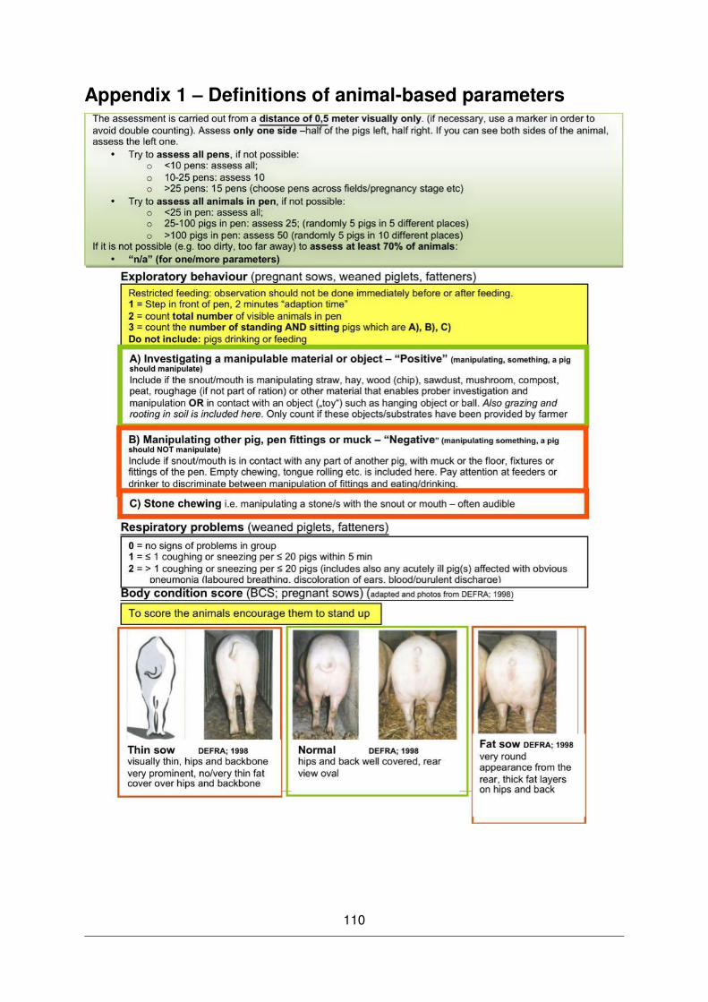
110
Appendix 1 – Definitions of animal-based parameters

111
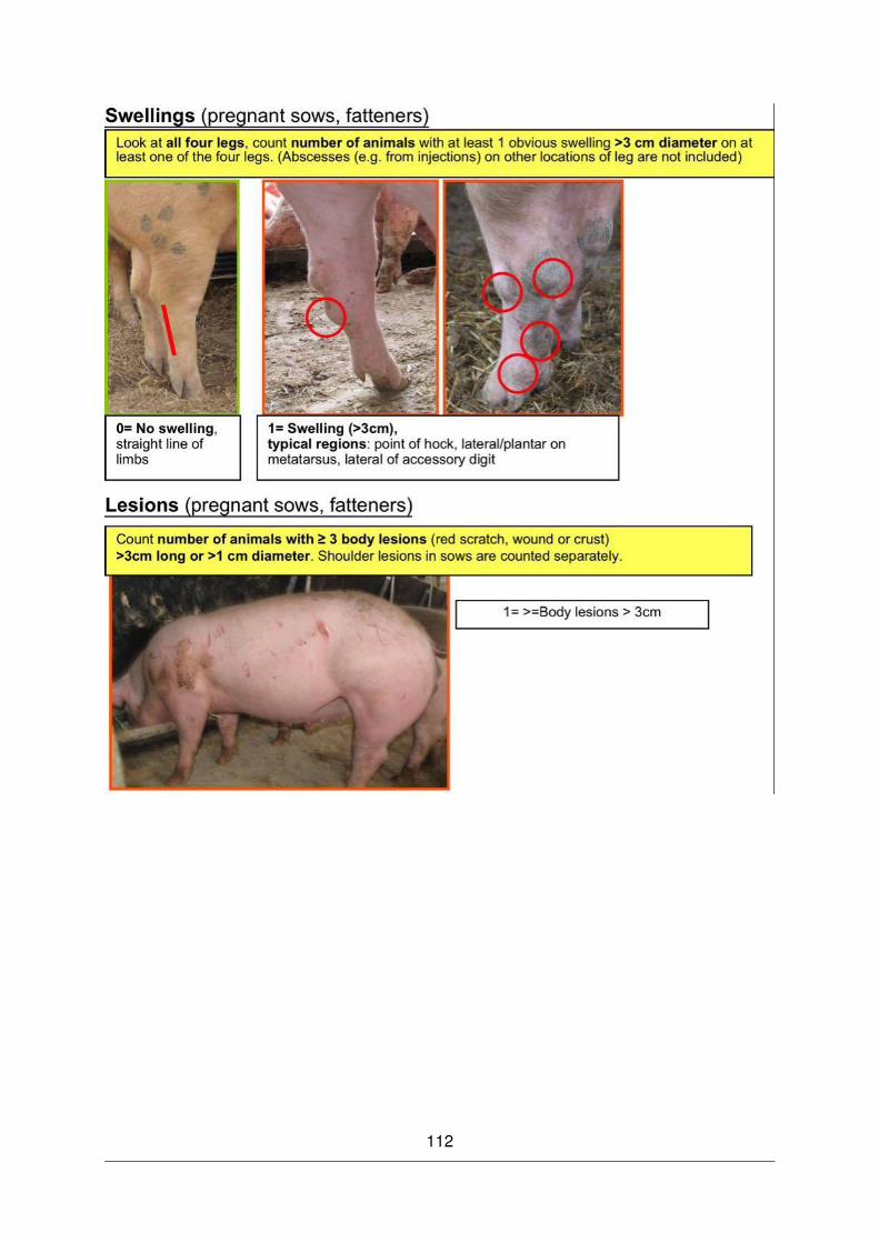
112

113

114
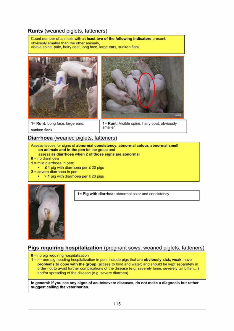
115
116
Appendix 2 – Additional Tasks Accomplished During the PhD Study Period
Contribution to Conferences:
Prunier, A., Bochicchio, D., Butler, G., Dippel, S., Dourmad, J.Y., Edwards, S., Rousing, T., Rudolph, G., Illmann, G., Leeb, C. (2015): Presentation du projet ProPIG et des principaux resultats. Available at http://orgprints.org/28257
Leeb, C., Rudolph, G., Bochicchio, D., Butler, G., Dippel, S., Dourmad, J.Y., Edwards, S., Früh, B., Illmann, G., Prunier, A., Rousing, T., Winckler, C. (2014): Betriebsspezifische Strategien zur Reduktion des Umwelteinflusses durch Verbesserung von Tiergesundheit, Wohlergehen und Ernährung von Bioschweinen. Fachtagung für biologische Landwirtschaft 2014, HBLFA Raumberg-Gumpenstein, Austria. (Talk). Available at http://orgprints.org/27988
Prunier, A., Rudolph, G., Bochicchio, D., Butler, G., Dippel, S., Leeb, C. (2014): Nutritional characteristics of the diets in organic pig production. In: Book of Abstracts of the 65th Annual Meeting of the European Federation of Animal Science, Wageningen Academic Publishers, Wageningen, Netherlands (Talk). Available at http://orgprints.org/26945
Rudolph, G., Dippel, S., Leeb, C., Winckler, C. (2014): Was erkunden Bioschweine in Freiland- und Stallhaltung? In: Freiland Verband (Ed.), Tierhaltung und Beschäftigung bei Tieren, Vienna, Austria (Talk).
Leeb, C., Bochicchio, D., Butler, G., Edwards, S., Früh, B., Illmann, G., Prunier, A., Rousing, T., Rudolph, G., Dippel, S. (2014): PigSurfer – SURveillance, FEedback & Reporting within ProPIG for communication with 75 pig farmers. In: Mounier, L., Veissier, I. (Eds.), Proceedings of the 6th International Conference on the Assessment of Animal Welfare at Farm and Group Level, Wageningen Academic Publishers, Wageningen, Netherlands. (Poster). Available at http://orgprints.org/26922
Dippel, S., Bochicchio, D. Holinger, M., Holmes, D. Knop, D., Prunier, A. Rudolph, G. Silerova, J., Leeb, C. (2014): Trough or bowl? Observers need training for assessing resource as well as clinical parameters. In: Mounier, L., Veissier, I. (Eds.), Proceedings of the 6th International Conference on the Assessment of Animal Welfare at Farm and Group Level, Wageningen Academic Publishers, Wageningen, Netherlands. (Poster). Available at http://orgprints.org/26928
Rudolph, G., Brandhofer, R., Leeb, C. (2014): Wie Treibhausgase vermindern? Ergebnisse und Erkenntnisse aus der Praxis. Bio Austria Bauerntage 2014, Wels (Talk). Available at http://orgprints.org/25570
Rudolph, G., Bochicchio, D. Brandhofer, R., Berner, A., Butler, G., Dippel, S., Dourmad, J.Y., Edwards, S., Früh, B., Holinger, M., Holmes, D., Illmann, G., Knop, D., Meier, M., Prunier, A., Rousing, T., Salomon, E.; Silerova, J., Sorensen, J.T., Urban, J., Vertes, F., Winckler, C., Leeb, C. (2014): ‘ProPIG’ Challenges and opportunities for on farm pig researchers: How to collect sound scientific data on animal health, welfare, nutrition and environmental impact AND act as a facilitator to improve these aspects at the same time? The 11th European IFSA Symposium, Berlin, 1.4. - 4.4.2014 (Poster). Available at http://orgprints.org/25627
Rudolph, G., Bochicchio, D., Butler, G., Dippel, S., Dourmad, J.Y., Edwards, S., Früh, B., Illmann, G., Meier, M., Prunier, A., Rousing, T., Salomon, E., Silerova, J., Sorensen, J.T.; Urban, J., Vertes, F., Winckler, C., Leeb, C. (2012): ProPIG - Organic pig health, welfare and environmental impact across Europe. Minding Animals, Utrecht, The Netherlands, 4-6 Juli 2012 (Poster). Available at http://orgprints.org/22582
Rudolph, G., Bochicchio, D., Butler, G., Dippel, S., Dourmad, J.Y., Edwards, S., Früh, B., Illmann, G., Meier, M., Prunier, A., Rousing, T., Silerova, J., Salomon, E., Sorensen, J.T., Urban, J., Vertes, F., Winckler, C., Leeb, C., (2012): ProPIG – Betriebsspezifische Strategien
117
zur Reduktion der Umweltauswirkung von Bioschweine Betrieben durch Verbesserung von Tiergesundheit, Wohlergehen und Ernährung von Bioschweinen. Tagung Forschung und Lehre zur Ökologischen Landwirtschaft an der Universität für Bodenkultur, Vienna, Austria, 18.10.2012 (Poster). Available at http://orgprints.org/22616
Tools:
Handbook for farmers:
Holinger, M., Ayrle, H., Bochicchio, D., Butler, G., Dippel, S., Edwards, S., Holmes, D., Illmann, G., Leeb, C., Maupertuis, F., Meliov, M., Prunier, A., Rousing, T., Rudolph, G., Früh, B. (2015): Improving Health and Welfare of Pigs – A Handbook for organic farmers. Available online for free at https://www.fibl.org/de/shop/artikel/c/schweine/p/1676-handbook-propig.html
Environmental decision support tool and PigSurfer:
The link to the environmental decision support tool and PigSurfer is available through the website link www.coreorganic2.org/propig.