DOCUMENT RESUME

ED 104 933 TM 004 389

AUTHOR Hall, Charles E.; And OthersTITLE VARAN2: A Linear Model Variance Analysis Program.

Second Edition. Research Memorandum.INSTITUTION Educational Testing Service, Princeton, N.J.

REPORT NO RM-73-30PUB DATE Nov 73NOTE 124p.; Not available in hard copy due to marginal

legibility of originality document

EDRS PRICE MF-$0.76 HC Not Available from EDRS..PLUS POSTAGE

DESCRIPTORS- *Analysis of Variance; *Computer Programs;*Correlation; Discriminant Analysis; Electronic DataProcessing; Factor Analysis; Iliothesis Testing;Input Output; *Manuals; MathematiCa3Applications;Matrices; Orthogonal Rotation; Programing Languages;*Statistical Analysis; Tests of Significance

ABSTRACTThe VARAN (variance Analysis) program is an addition

to a series of computer programs for multivariate analysis ofvariance. The development of VARAN exploits the full linear model.

Analysis of variance, univariate and multivariate, is the programs

main target. Correlation analysis of all types is available with

printout in the vernacular of correlation. The hybrid of these,

homogeneity of regression, has been added with as much flexibility as

can be currently mustered. In addition to these, VARAN includes

several styles of factor and component analysis complete with tests

of factorization and rotation techniques. This research memorandum is

the manual for the second'edition of VARAN, an enlargement of the

first edition. The mainstream of the program is essentially unchanged

but several additions have been made and three small programming

errors have been corrected. The most extensive addition has been in

serial correlation analysis. (Author/RC)

N

o RESEARCH

MEMORANDUM4

e

US DEPARTMENT OF HEALTHEDUCATION 6 WELFARENATIONAL INSTITUTE OF

EDUCATIONDO, JME .A BEE RE .'RC.

07 (CO EXAC A RE cc, IRCM

THE PE RSON OR00';AN ZA 'NOR ,N

At,NC, PO f NvONS

STATE (10 NOT NEC f SsAQRE PRk

- SENT Off ,C A. NA' ' F

EOM CATION PO, r ON p

PERM 75`,ON 10 REPROOLCE THI$

-ORYR7OHTED MATERIAL BY MICRO

FICHE ONLY HAS BEEN GRANTED OT

f./i,c71Ezi- /A!?.zI ER C SND OR(AEBIATIONS OUFRAT

,N,uNDER AGREE- MEN'5 WITH THE NA

',)vAL NS"11111 O1 EDUCATIONI THER REPRODUc f.f OUTSIDE

THE ERIC 'EM t7EQUtftfc FERMIS,)N Of THE COPYR7C,HT OWNER

VARAN:z:

A LINEAR MODEL VARIANCE ANALYSIS PROGRAM

Second Edition-J

Charles E. hail

Katherine Kornhauser

and

:)orothy T. Thayer

BEST C77 iAlAriABLE.41is Memorandum is for interoffice use.

4:7) Tt is n'Dt to bf.. cited !Is published

00 rtlort witnut :Ipt.cific permission

the auth,r.

C42>

n't1 ::ervice

.;,,rsey

lcYN

RM-73-30

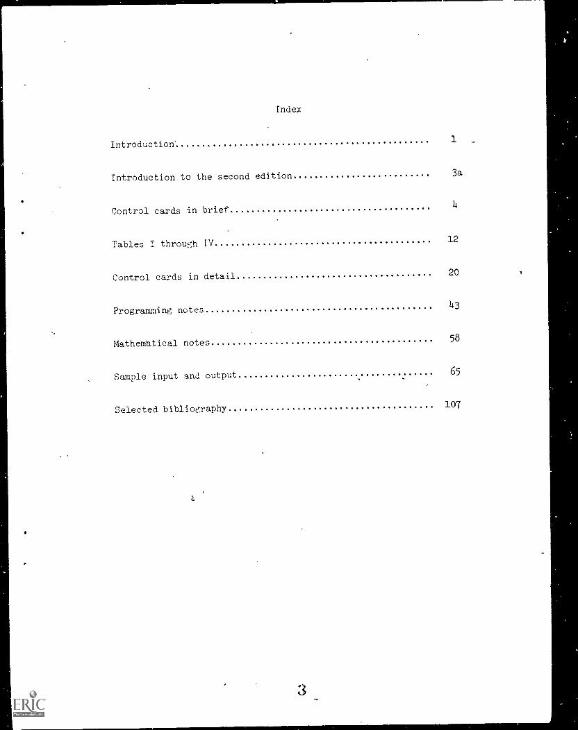
Index

Introduction'1

Introduction to the second edition 3a

Control cards in brief14

Tables I through IV12

Control cards in detail 20

Programming notes43

Mathematical notes58

Sample input and output65

Selected bibliography107

3

Introduction

This memorandum is the manual for the VARAN program. (The acronym

comes from the words VARiance ANalysis)

The VARAN program is the latest-addition to a series of computer

programs for multivariate analysis of variai ,e which originated about 1957.

About that time R. Darrell Bock had a MANOVA type program running on the

UNIVAC at the University of North Carolina. Bock's original program

handled only a few variables and was otherwise quite restricted and was

not in much general use. Later, in 1962, C. E. Hall and Elliot Cramer

with Bock's assistance published a program called MANOVA in FORTRAN 2 which

was internationally circulated. The program handled 25 variables and 100

degrees of freedom for hypothesis.

The wide use of this program prompted further development by Cramer

and by Bock and Finn. In 1966 Cramer published a program called MANOVA

in FORTRAN 4 followed by Finn and Bock's program MULTIVARIANCE also in

FORTRAN 4. The development of these two programs greatly increased the

scope of multivariate analyses which could be performed on computers.

MULTIVARIANCE was the first of the programs in this series that

utilized the full linear model. The earlier programs had been restricted

to models of the cell means in their main streams of calculation. Other

variations on the linear model, like canonical correlation, were of an

"accidental" nature. With the development. of MULTIVARIANCE, the series

turned to the flexibility of the full linear model.

The development of VARAN continues this series in the exploitation

of the full linear model. Analysis of variance, univariate and multivariate,

is the main target of the program as with the earlier programs. Corre-

lation analysis of all types is available with printout in the vernacular

of correlation. The hybrid of 6lese, homogeneity of regression, has been

4

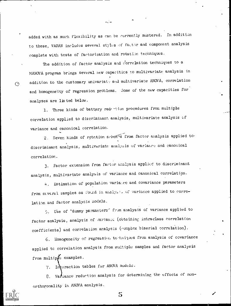
added with as much flexibility as can be currently mustered. In addition

to these, VARAN includes several styles of factor and component analysis

complete with tests of factorization and rotatiDn techniques.

The addition of factor analysis and correlation techniques to a

MANOVA program brings several new capacities to multivariate analysis in

0 addition to the customary univariat multivaria*,e ANOVA, correlation

and homogeneity of regression problems. Some of the new capacities for

analyses are listed below.

1. Three kinds of battery redi?tion procedures from multiple

correlation applied to discriminant analysis, multivariate analysis of

variance and canonical correlation.

2. Seven kinds of rotation: schs from factor analysis applied to

discriminant analysis, multivariate analysis of variance and canonical

correlation.

3. Factor extension from factor analysis applied to discriminant

analysis, multivariate analysis of variance and canonical correlation.

u. Estimation of population variance and covariance parameters

from scveral samples as ound in analysL of variance applied to corre-

lation and factor analysis models.

5. USe of "dummy parameters" from analysis of variance applied to

factor analysis, analysis of iarian,:c (obtaining intraclass correlation

coefficients) and correlation analysis (complex biserial correlation).

6. Homogeneity of regression te,hnilues from analysis of covariance

applied tc correlation analysis from multiple samples and factor analysis

from multip e examples.

In eraction tables fur ANOVA models.

8. Va lance reduction analysis for determining the effects of non-

orthogonality in ANOVA analysis.

5

-3-

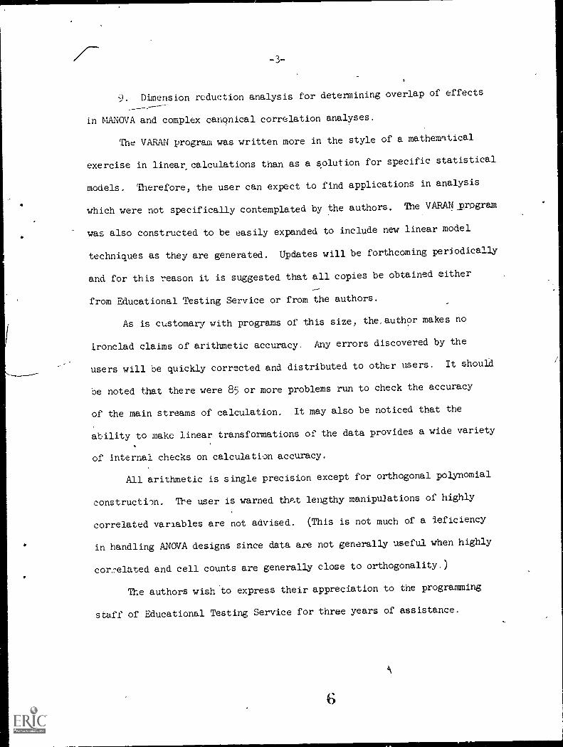
9. Dimension reduction analysis for determining overlap of effects

in MANOVA and complex canonical correlation analyses.

The VARAN program was written more in the style of a mathenntical

exercise in linear_ calculations than as a solution for specific statistical

models. Therefore, the user can expect to find applications in analysis

which were not specifically contemplated by the authors. The VARAN _program

was also constructed to be easily expanded to include new linear model

techniques as they are generated. Updates will be forthcoming periodically

and for this reason it is suggested that all copies be obtained either

from Educational Testing Service or from the authors.

As is customary with programs of this size, the author makes no

ironclad claims of arithmetic accuracy. Any errors discovered by the

users will be quickly corrected and distributed to other users. It should

be noted that there were 85 or more problems run to check the accuracy

of the main streams of calculation. It may also be noticed that the

ability to make linear transformations of the data provides a wide variety

of internal checks on calculation accuracy.

All arithmetic is single precision except for orthogonal polynomial

constructim. The user is warned that lengthy manipulations of highly

correlated variables are not advised. (This is not much of a ieficiency

in handling ANOVA designs since data are not generally useful when highly

cor.7elated and cell counts are generally close to orthogonality.)

The authors wish to express their appreciation to the programming

staff of Educational Testing Service for three years of assistance.

-3a-

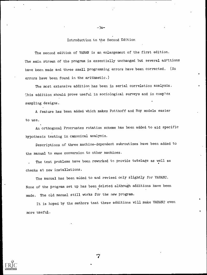
Introduction to the Second Edition

The second editioh of VARAN is an enlargement of the first edition.

The main stream of the program is essentially unchanged but several additions

have been made and three small programming errors have been corrected. (No

errors have been found in the arithmetic.)

The most extensive addition has been in serial correlation analysis.

This addition should prove useful in sociological surveys and in complex

sampling designs.

A feature has been added which makes Potthoff and Roy models easier

to use.

An orthogonal Procrustes rotation scheme has been added to aid specific

hypothesis testing in canonical analysis.

Descriptions of three machine-dependent subroutines have been added to

the manual to ease conversion to other machines.

The test problems have been reworked to provide tutelage as well as

checks at new installations.

The manual has been added to and revised only slightly for VARAN2.

None of the program set up has been deleted although additions have been

made. The old manual still works for the new program.

It is hoped by the authors tnat these additions will make VARAN2 even

more useful.

-4-

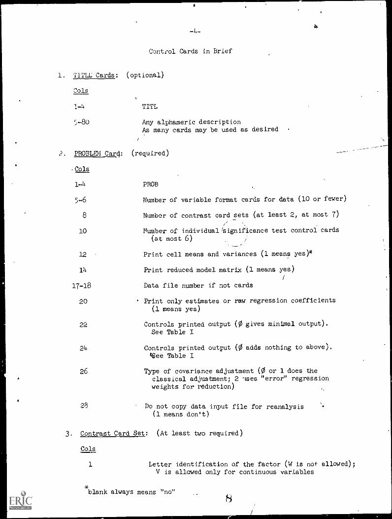
Control Cards in Brief

1. T1T.LL Cards: (optional)

Cols

1-4 TITL

5-80 Any alphameric descriptionAs many cards may be used as desired

2. PROBLEM Card: (required)

.Cols

1-4 PROB

5-6

8

10

12

14

17-18

Number of variable format cards for data (10 or fewer)

Number of contrast card sets (at least 2, at most 7)

Number of individual/Significance test control cards(at most 6)

Print cell means and variances (1 means yes)*

Print reduced model matrix (1 means yes)

Data file number if not cards

20 Print only estimates or raw regression coefficients(1 means yes)

22 Controls printed output (0 gives minimal output).See Table I

24 Controls printed output (0 adds nothing to above).$ee Table I

26 Type of covariance adjustment (0 or 1 does theclassical adjustment; 2 ses "error" regressionweights for reduction)

28 Do not copy data input file for reanalysis(1 means don't)

3. Contrast Card Set: (At least two required)

Cols

1 Letter identification of the factor (W is not allowed);V is allowed only for continuous variables

blank always means "no"

8

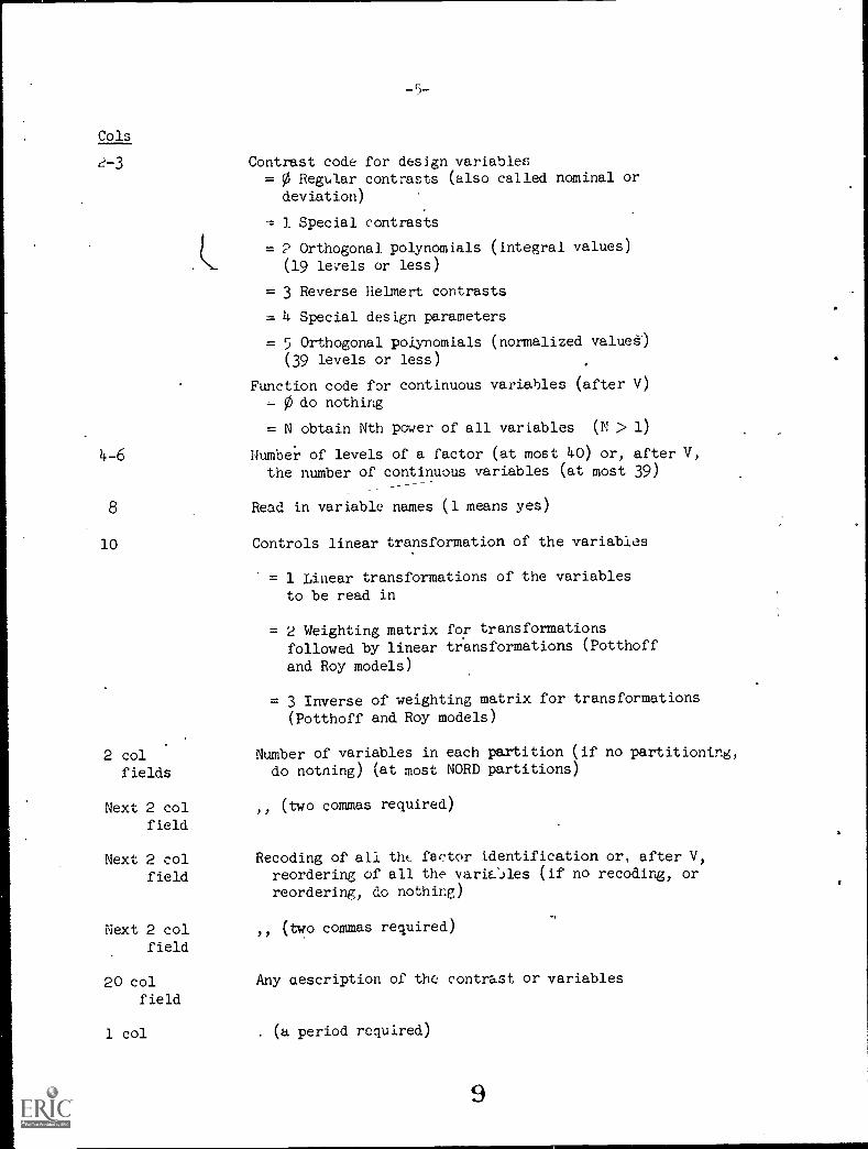
Cols

-5-

Contrast code for design variables= 0 Regular contrasts (also called nominal or

deviation)

1 Special contrasts

= 2 Orthogonal polynomials (integral values)

(19 levels or less)

= 3 Reverse Helmert contrasts

= 4 Special design parameters

= 5 Orthogonal polynomials (normalized valueS)

(39 levels or less)

Function code for continuous variables (after V)0 do nothing

N obtain Nth power of all variables (N > 1)

4-6 Number of levels of a factor (at most 40) or, after V,the number of continuous variables (at most 39)

8 Read in variable names (1 means yes)

10

2 colfields

Next 2 colfield

Next 2 colfield

Next 2 colfield

20 colfield

1 col

0

Controls linear transformation of the variables

= 1 Linear transformations of the variablesto be read in

= 2 Weighting matrix for transformations

followed by linear transformations (Potthoff

and Roy models)

= 3 Inverse of weighting matrix for transformations

(Potthoff and Roy models)

Number of variables in each partition (if no partitioning,do notning) (at most NORD partitions)

(two commas required)

Recoding of all tht factor identification or, after V,reordering of all the variCiles (if no recoding, orreordering, do nothing)

00 (two commas required)

Any description of the contrast or variables

. (a period required)

-6-

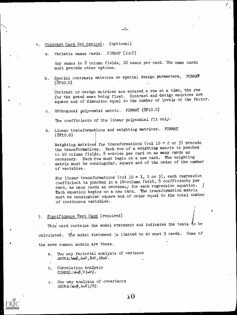
4. Contrast Card Set Option:;: (optional)

a. Variable names cards. FORMAT (10i13)

Any names in 8 column fields, 10 names per card. The name cards

must precede other options.

b. Special contrasts matrices or special design parameters. FORMAT

(8F10.0)

Contrast or design matrices are entered a row at a time, the row

for the grand mean being first. Contrast and design matrices are

square and of dimension equal to the number of levels of the factor.

c. Orthogonal polynomial metric. FORMAT (8F10.0)

The coefficients of the linear polynomial fit only.

d. Linear transformations and weighting matrices. FORMAT

(8F10.0)

Weighting matrices for transformations (col 10 = 2 or 3) precede

the transformations. Each row of a weighting matrix is punched

in 10 column fielfis, 8 entries per card on as many cards as

necessary. Eachrow must begin on a new card. The weighting

matrix must be nonsingular, square and of the order of the number

of variables.

For linear transformations (col 10 = 1, 2 or 3), each regression

coefficient is punched in a 10-column field, 8 coefficients per

card, as many cards as necessary for each regression equation. )

Each equation begins on a new card. The transformation matrix

must be nonsingular square and of order equal to the total number

of continuous variables.

5. Significance Test Card (required)

This card contains the model statement and indicates the tests o be

calculated. T}ie model statement .s limited to at most 9 cards. Some of

the more common models are these.

a. Two way factorial analysis of variance

ANOVA:W4,A.V,EW,AB=V.

b. Correlation analysisCORREL:W=0,V1=V2.

c. One way analysis of covarianceANOVA:W=0,X=V1/V2.

4

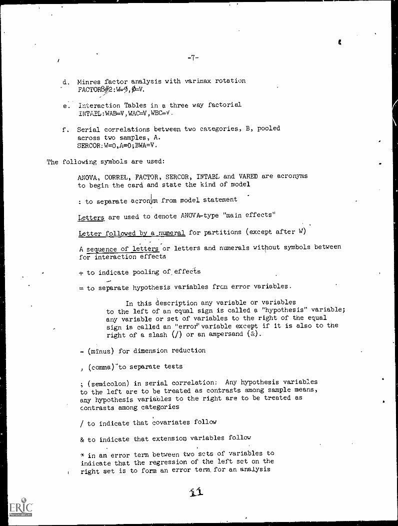
-7-

d. Minres factor analysis with varimax rotationFACTOR :W4,PV.

e. Interaction Tables in a three way factorial

INTA2L:WAB=V,WAC=V,WBC.V.

f. Serial correlations between two categories, B, pooled

across two samples, A.SERCOR:W=0,A=0;BWA=V.

The following symbols are used:

ANOVA, CORREL, FACTOR, SERCOR, INTABL and VARED are acronymsto begin the card and state the kind of model

1

: to separate acronym from model statement

Letters are used to denote ANOVA -type "main effects"

Letter followed by a numeral for partitions (except after w)

A sequence of letters or letters and numerals without symbols between

for interaction effects

+ to indicate pooling of_effedis

= to separate hypothesis variables frcm error variables.

In this description any variable or variables

to the left of an equal sign is called a "hypothesis" variable;

any variable or set of variables to the right of the equal

sign is called an "error'' variable except if it is also to the

right of a slash (/) or an ampersand (&).

- (minus) for dimension reduction

, (comma)-to separate tests

; (semicolon) in serial correlation: Any hypothesis variables

to the left are to be treated as contrasts among sample means,

any hypothesis variables to the right are to be treated as

contrasts among categories

/ to indicate that covariates follow

& to indicate that extension variables follow

* in an error term between two sets of variables to

indicate that the regression of the left set on the

1right set is to form an error term, for an analysis

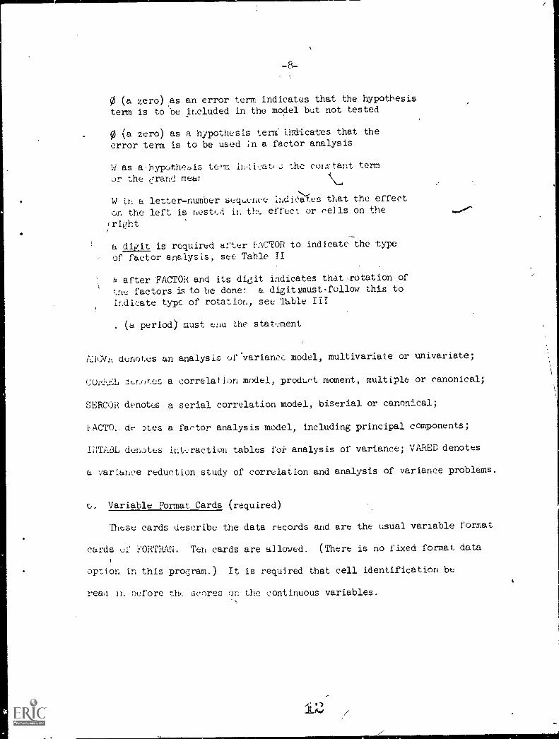
-8-

0 (a zero) as an error term indicates that the hypothesis

term is to be included in the model but not tested

0 (a zero) as a hypothesis term indicates that theerror term is to be used ;n a factor analysis

W as a,hypothe:)is term indicat,J the conFtant term

or the Brand meal.

.

W in a letter-number se eqL,nce inai(ates that the effect

on the left is nested in the effect or cells on the

i right

a digit is required after F:kCTOR to indicate the type

of factor analysis, see Table Il

after FACTOR and its digit indicates that rotation oftne factors is to be done: a digitimust follow this to

indicate type of rotation, set Table III

.(a period) must en(' the statement

it;i0V:, denotes an analysis orvariance model, multivariate or univariate;

aenotes a correlation model, product moment, multiple or canonical;

SERCOi denotes a serial correlation model, biserial or canonical;

'FACTO.. dr Dtes a factor analysis model, including principal components;

INTA31, denotes interaction tables for analysis of variance; VARED denotes

a variance reduction study of correlation and analysis of variance problems.

Variable Format Cards (required)

These cards describe the data records and are the usual variable format

cards of FORTRAN. Ten cards are allowed. (There is no fixed format data

option in this program.) It is required that cell identification be

real In before th(_ scores on the continuous variables.

10

0

-8a-

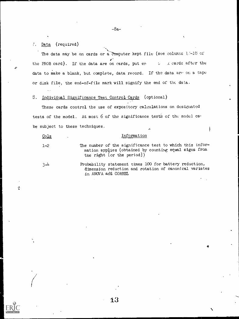
7. Data (required)

The data may be on cards or a computer kept file (see columns 1:-18 of

the PROB card). If the data are on cards, put en x cards after tht

data to make a blank, but complete, data record. If the data are on a tape

or disk file, the end-of-file mark will signify the end of the data.

8. Individual Significance Test Control-Cards (optional)

These cards control the use of expository calculations on designated

tests of the model. At most 6 of the significance testis of the model ca-

be subject to these techniques.A

Cols Information

1-2 The number of the significance test to which this infor-mation applies (obtained by counting equal signs fromthe right [or the period))

3-4 Probability statement times 100 for battery reduction,dimension reduction and rotation of canonical variatesin ANOVA arid. CORBEL

-9-

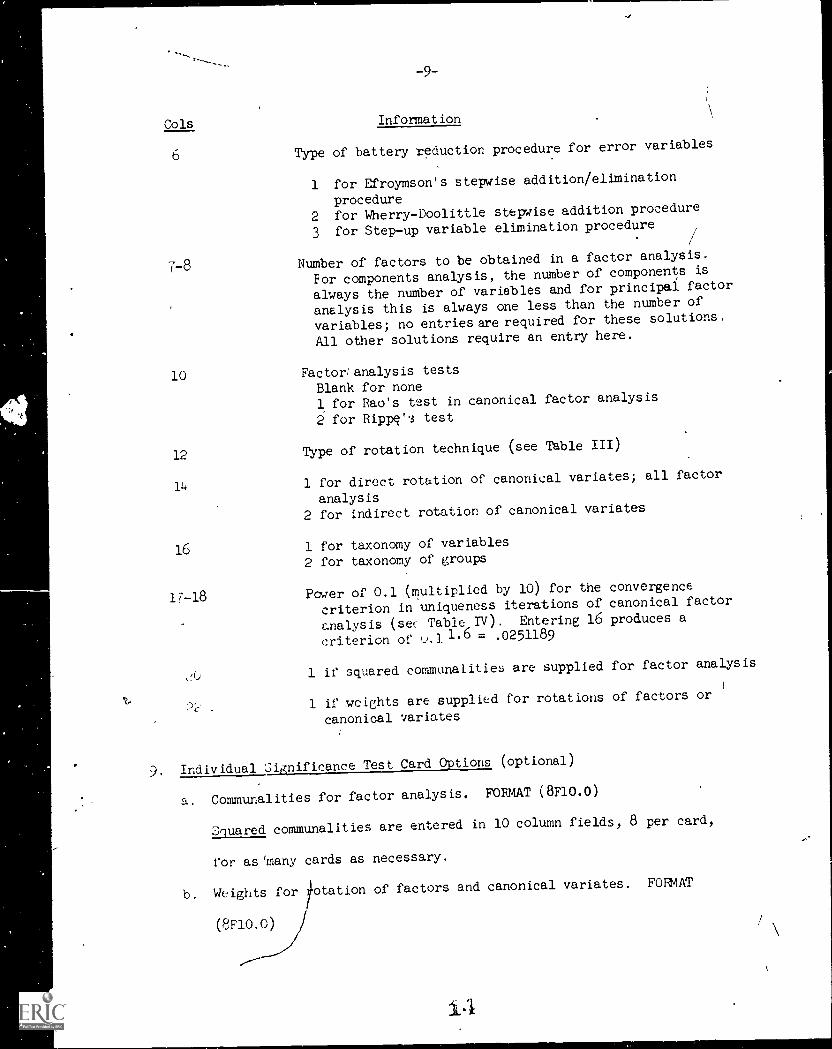
Cols Information

Type of battery reduction procedure for error variables

1 for Efroymson's stepwise addition/elimination

procedure2 for Wherry-Doolittle stepwise addition procedure

3 for Step-up variable elimination procedure

7-8 Number of factors to be obtained in a factor analysis.

For components analysis, the number of components is

always the number of variables and for principal factor

analysis this is always one less than the number of

variables; no entriesare required for these solutions.

All other solutions require an entry here.

10 Factor; analysis testsBlank for none1 for Rao's test in canonical factor analysis

2 for Rippe's test

12 Type of rotation technique (see Table III)

14 1 for direct rotation of canonical variates; all factor

analysis2 for indirect rotation of canonical variates

16 1 for taxonomy of variables

2 for taxonomy of groups

1F-18 Power of 0.1 (multiplied by 10) for the convergence

criterion in uniqueness iterations of canonical factor

cnalysis (se( Table IV). Entering 16 produces a

criterion of u.1 1.6 = .0251189

1 if squared communalities are supplied for factor analysis

2.

1 if weights are supplied for rotations of factors or

canonical variates

9 Individual Significance Test Card Options (optional)

a. Communalities for factor analysis. FORMAT (8F10.0)

Squared communalities are entered in 10 column fields, 8 per card,

for as'many cards as necessary.

b. Weights for totation of factors and canonical variates. FORMAT

(8F10.0)

-10-

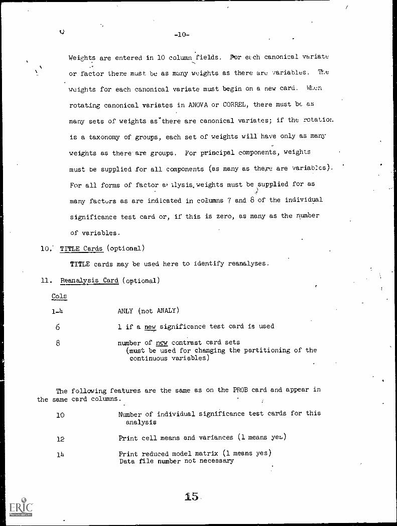
Weights are entered in 10 column fields. Por each canonical variate

or factor there must be as many weights as there are variables. The

weights for each canonical variate must begin on a new card. When

rotating canonical variates in ANOVA or CORREL, there must be as

many sets of weights as-there are canonical variates; if the rotation

is a taxonomy of groups, each set of weights will' have only as many

weights as there'are groups. For principal components, weights

must be supplied for all components (as many as there are variables).

For all forms of factor a/ llysis.weights must be supplied for as4

many factors as are indicated in columns 7 and 8 of the individual

significance test card or, if this is zero, as many as the number

of variables.

10: TITLE Cards (optional)

TITLE cards may be used here to identify reanalyses.

11. Reanalysis Card (optional)

Cols

1-4 ANLY (not ANALY)

6 1 if a new significance test card is used

8 number of new contrast card sets(must be used for changing the partitioning of thecontinuous variables)

The following features are the same as on the PROB card and appear in

the same card columns.

10 Number of individual significance test cards for this

analysis

12 Print cell means and variances (1 means-yeL)

14 Print reduced model matrix (1 means yes)Data file number not necessary

15

Cols

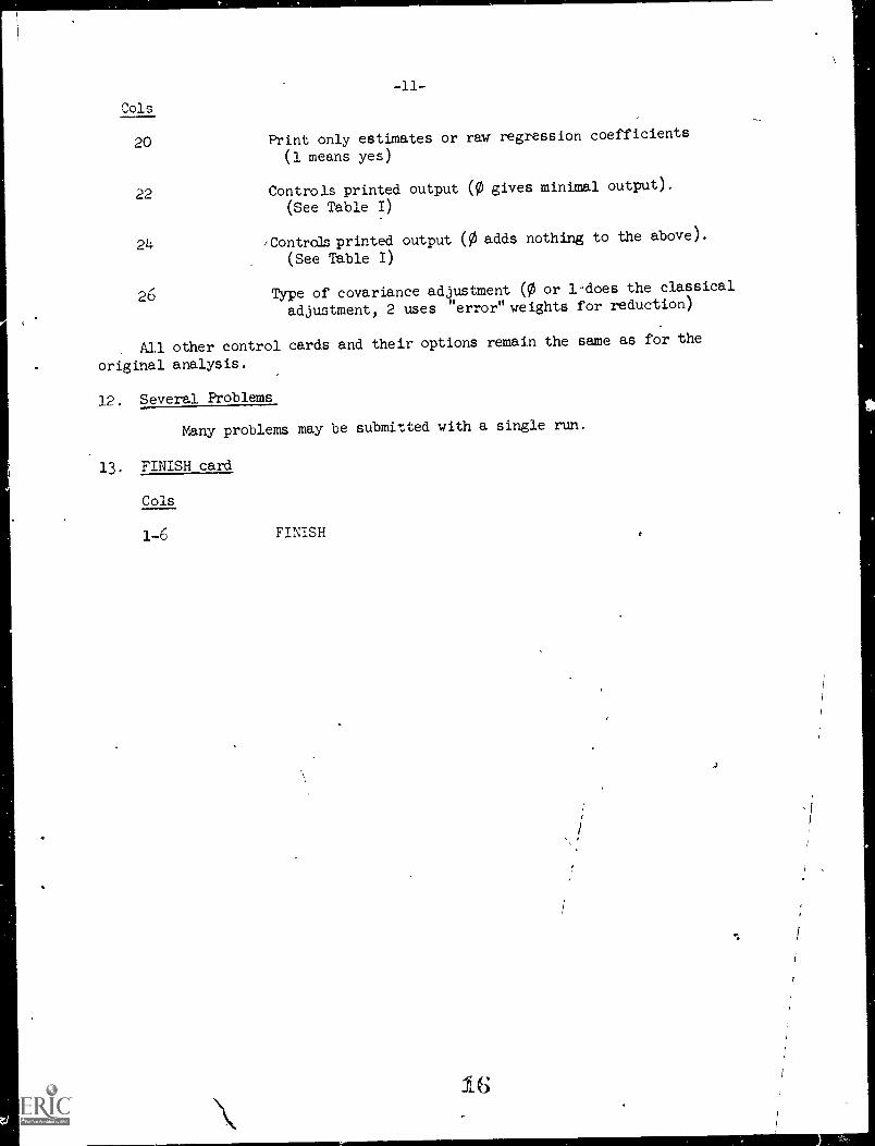
20 Print only estimates or raw regression coefficients

(1 means yes)

22 Controls printed output (0 gives minimal output).

(See Table I)

24 /Controls printed output (0 adds nothing to the above).

(See Table I)

26 Type of covariance adjustment (0 or 1-does the classical

adjustment, 2 uses "error" weights for reduction)

All other control cards and their options remain the same as for the

original analysis.

12. Several Problems

Many problems may be submitted with a single run.

13. FINISH card

Cols

1-6 FINISH

1-/

-12-

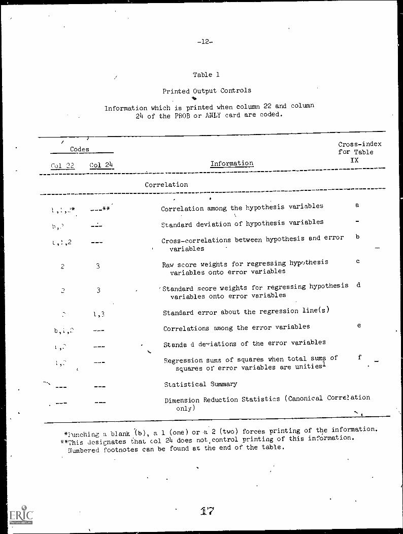
Table 1

Printed Output Controls41,

Information which is printed when column 22 and column

24 of the PROB or ANLY card are coded.

CodesCross-indexfor Table

Col 22 Col 24 Information IX

Correlation

11 '* ___** Correlation among the hypothesis variables a

1),2 Standard deviation of hypothesis variables -

L,1,2 Cross-correlations between hypothesis and error b

variables

2 3 Raw score weights for regressing hypothesis

variables onto error variables

3'Standard score weights for regressing hypothesis d

variables onto error variables

1,3 Standard error about the regression line(s)

b,1,2 Correlations among the error variables

Standa d de,riations of the error variables

Regression sums of squares when total sums of

squares of error variables are unitiesl

Statistical Summary

e

Dimension Reduction Statistics (Canonical Correlation

only)

*Punching a blank (b), a 1 (one) or 'a 2 (two) forces printing of the information.

**This designates that col 24 does not,control printing of this information.

Numbered footnotes can be found at the end of the table.

17

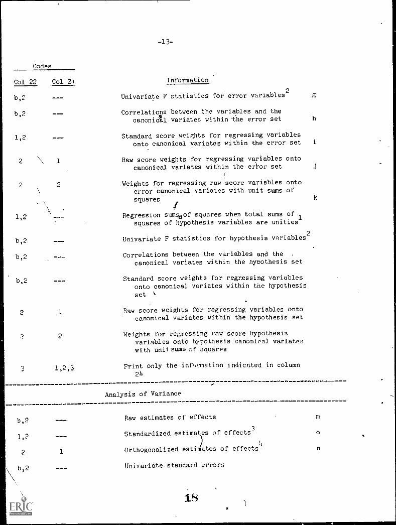
-13-

Codes

Col 22 Col 24 Information

b,2 Univariate F statistics for error variables2

b,2 Correlations between the variables and thecanonical variates within the error set

1,2

2 1

2

Standard score weights for regressing variablesonto canonical variates within the error set

Raw score weights for regressing variables ontocanonical variates within the error set

Weights for regressing raw score variables ontoerror canonical variates with unit sums of

squares

4'

1,2 Regression sums0of squares when total sums of

squares of hypothesis variables are unities

b,2 Univariate F statistics for hypothesis variables2

b,2 Correlations between the variables and the .

canonical variates within the hypothesis set

b,2

2 1

2 2

Standard score weights for regressing variablesonto canonical variates within the hypothesis

set 't

Raw score weights for regressing variables ontocanonical variates within the hypothesis set

Weights for regressing raw score hypothesisvariables onto hypothesis canonical variateswith unit sums of squares

g

h

J

3 1,2,3 Print only the information indicated in column

24

----------------------------------------------------- ----------------------------------

Analysis of Variance

b,2

1,2

2

b,2

1

- -

Raw estimates of effects

Standardized estima es of effects-

)

'1

Orthogonalized estimates of effects4

Univariate standard errors

18

0

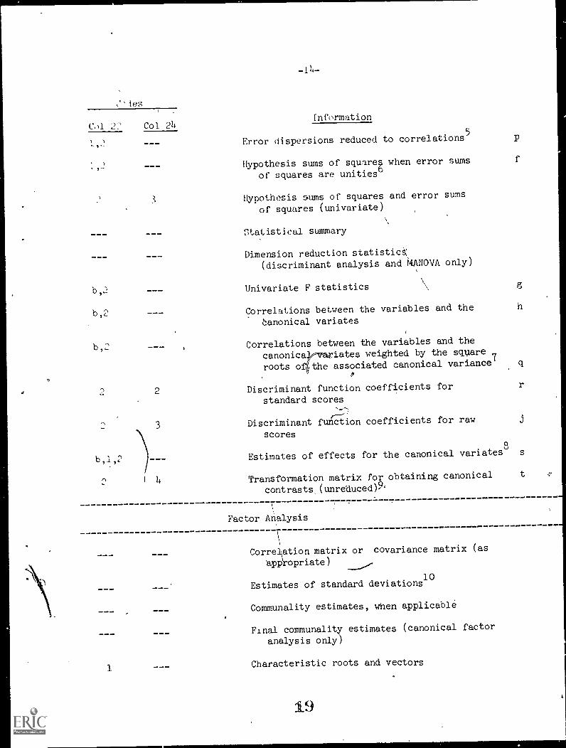
Col 2?

L,2

Col 2/1

114

Information

Error dispersions reduced to correlations5

Hypothesis sums of square when error sums

of squares are unities°

3Hypothesis sums of squares and error sums

of squares (univariate)

statistical summary

Dimension reduction statistic(discriminant analysis and MANOVA only)

b,2 Univariate F statistics \\ g

b,2 Correlations between the variables and the h

canonical variates

b,2 Correlations between the variables and the

canonical fates weighted by the square

roots o the associated canonical variance

2 Discriminant function coefficients for

standard scores

Discriminant function coefficients for raw

scores3

b,1,2 Estimates of effects for the canonical variates8

s

2 4 Transformation matrix for obtaining canonical t

0contrasts (unreduced),

Factor Analysis

Correlation matrix or covariance matrix (as

app/ropriate)

Estimates of standard deviations10

Communality estimates, when applicable

Final communality estimates (canonical factor

analysis only)

1Characteristic roots and vectors

19

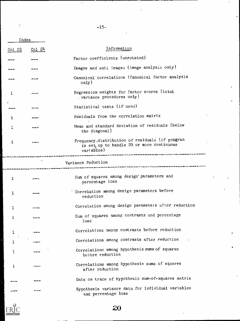
Codes

-15-

Information

Factor coefficients (unrotated)

Images and anti images (image analysis only)

Canonical correlations (Canonical factor analysis

only)

Regression weights for factor scores (total

.variance procedures only)

Statistical tests (if used)

1Residuals from the correlation matrix

Mean and standard deviation of residuals (below

the diagonal)

1Frequency,distribution of residuals (if program

is setup to handle 20 or more continuous

variables)

Variance Reduction

Sum of squares among design-parameters and

percentage loss

Correlation among design parameters before

reduction

Correlation among design parameters after reduction

Sum of squares among contrasts and percentage

loss

Correlations among contrasts before reduction

Correlations among contrasts after reduction

Correlations among hypothesis SIWW30/f squares

before reduction

Correlations among hypothesis sums of squares

after reduction

Data on trace of hypothesis sum-of-squares matrix

Hypothesis variance data for individual variables

and percentage loss

20

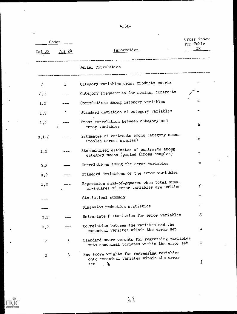
-15a-

CodesCross indexfor Table

Col 22 Col 24 Information IX

Serial Correlation

1 Category variables cross products matrix'

Category frequencies for nominal contrasts

1,2 Correlations among category variables

1,2 1 Standard deviation of category variables

1,2 Cross correlation between category and

ti error variables

0,1,2 Estimates of contrasts among category means

(pooled across samples)

1,2 Standardized estimates of .contrasts among

category means (pooled across samples)

0,2 Correlations among the error variables

0,2 Standard deviations of the error variables

1,2 Regression sums-of-squares when total sums-

of-squares of error variables are unities

Statistical summary

Dimension reduction statistics

0,2 Univariate F statistics for error variables

0,2 Correlation between the variates and the

canonical variates within the error set

2 3 Standard score weights for regressing variables

onto canonical ,ariates within the error set

0 3 Raw score weights for regressing variables2

onto canonical variates within the error

set 4

a

b

j

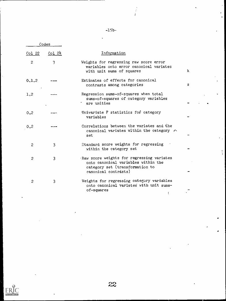
-15b-

Codes

Col 22 Col 24 Information

2 3 Weights for regressing raw score errorvariables onto error canonical variateswith unit sums of squares

0,1,2 Estimates of effects for canonicalcontrasts among categories

1,2 Regression sums-of-squares when totalSums-of-squares of category variablesare unities

0,2 Univariate F statistics foi categoryvariables

0,2

2 3

2 3

2 3

Correlations between the variates and thecanonical variates within the category r.s.

set

Standard score weights for regressingwithin the category set

Raw score weights for regressing variatesonto canonical variables within thecategory set (transformation tocanonical contrasts)

Weights for regressing category variablesonto canonical variates with unit sums-of-squares

22

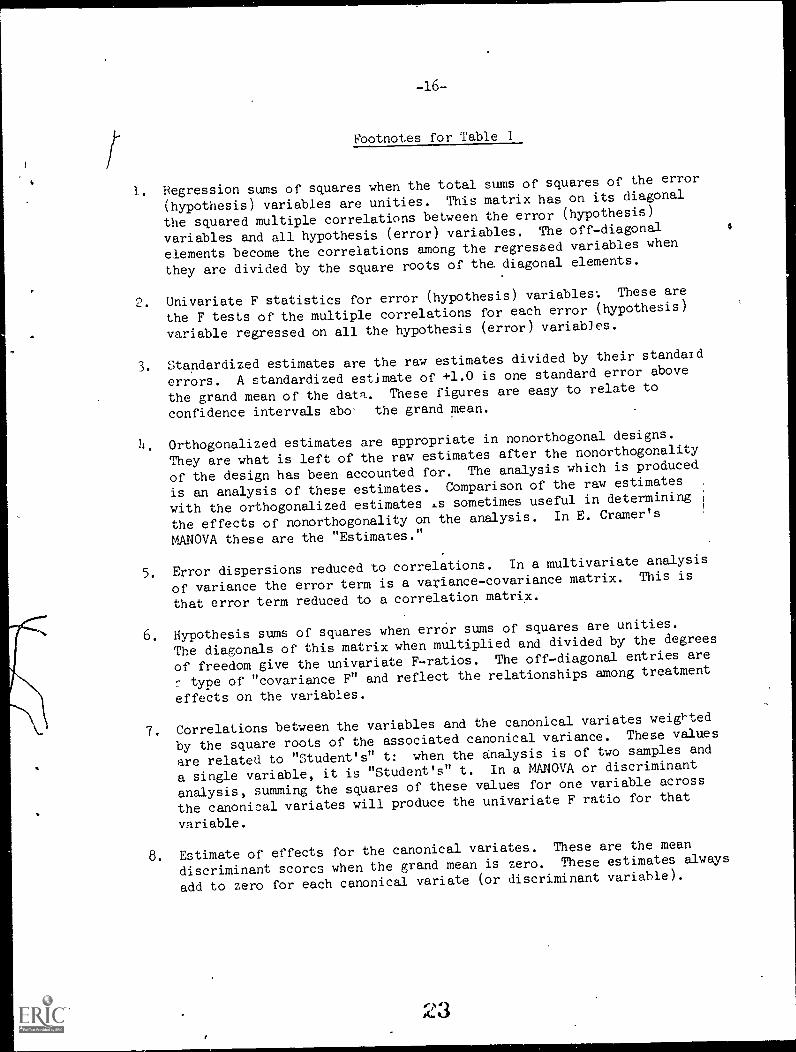
-16-

Footnotes for Table I

1. Regression sums of squares when the total sums of squares of the error

(hypothesis) variables are unities. This matrix has on its diagonal

the squared multiple correlations between the error (hypothesis)

variables and all hypothesis (error) variables. The offdiagonal

elements become the correlations among the regressed variables when

they are divided by the square roots of the, diagonal elements.

2. Univariate F statistics for error (hypothesis) variables. These are

the F tests of the multiple correlations for each error (hypothesis)

variable regressed on all the hypothesis (error) variab3es.

3. Standardized estimates are the raw estimates divided by their standard

errors. A standardized estimate of +1.0 is one standard error above

the grand mean of the data. These figures are easy to relate to

confidence intervals abo- the grand mean.

4. Orthogonalized estimates are appropriate in nonorthogonal designs.

They are what is left of the raw estimates after the nonorthogonality

of the design has been accounted for. The analysis which is produced

is an analysis of these estimates. Comparison of the raw estimates

with the orthogonalized estimates sometimes useful in determining

the effects of nonorthogonality on the analysis. In E. Cramer's

MANOVA these are the "Estimates."

5. Error dispersions reduced to correlations. In a multivariate analysis

of variance the error term is a variancecovariance matrix. This is

that error term reduced to a correlation matrix.

6. Hypothesis sums of squares when error sums of squares are unities.

The diagonals of this matrix when multiplied and divided by the degrees

of freedom give the univariate Fratios. The offdiagonal entries are

type of "covariance F" and reflect the relationships among treatment

effects on the variables.

7. Correlations between the variables and the canonical variates weieted

by the square roots of the associated canonical variance. These values

are related to "Student's" t: when the analysis is of two samples and

a single variable, it is "Student's" t. In a MANOVA or discriminant

analysis, summing the squares of these values for one variable across

the canonical variates will produce the univariate F ratio for that

variable.

8. Estimate of effects for the canonical variates. These are the mean

discriminant scores when the grand mean is zero. These estimates always

add to zero for each canonical variate (or discriminant variable).

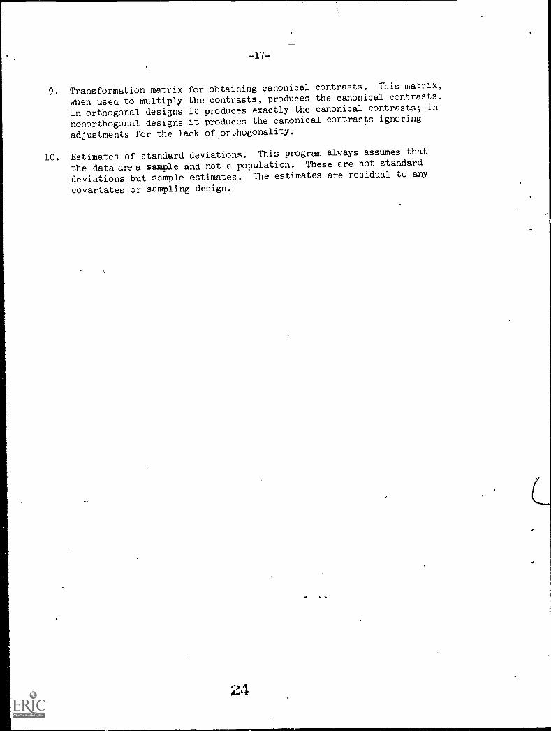
-17-

9. Transformation matrix for obtaining canonical contrasts. This matrix,

when used to multiply the contrasts, produces the canonical contrasts.

In orthogonal designs it produces exactly the canonical contrasts; in

nonorthogonal designs it produces the canonical contrasts ignoring

adjustments for the lack of orthogonality.

10. Estimates of standard deviations. This program always assumes that

the data area sample and not a population. These are not standard

deviations but sample estimates. The estimates are residual to any

covariates or sampling design.

24

-18-

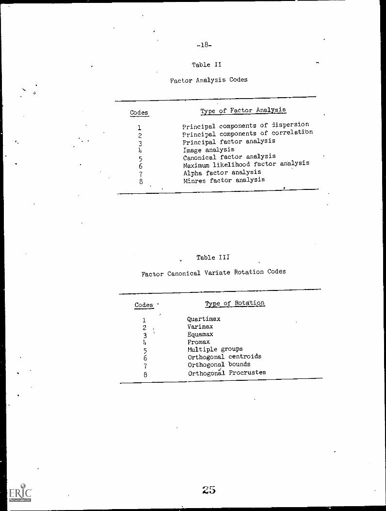
Table II

Factor Analysis Codes

Codes ape of Factor Analysis

1 Principal components of dispersion

2 Principal components of correlation

3 Principal factor analysis

Image analysis

5Canonical factor analysis

6 Maximum likelihood factor analysis

7 Alpha factor analysis

8 Minres factor analysis

Table III

Factor Canonical Variate Rotation Codes

Codes Type of Rotation

1 Quartimax

2 ,Varimax

3 Equamax

4 Promax

5 Multiple groups

6 Orthogonal centroids

7 Orthogonal bounds

8 Orthogonal Procrustes

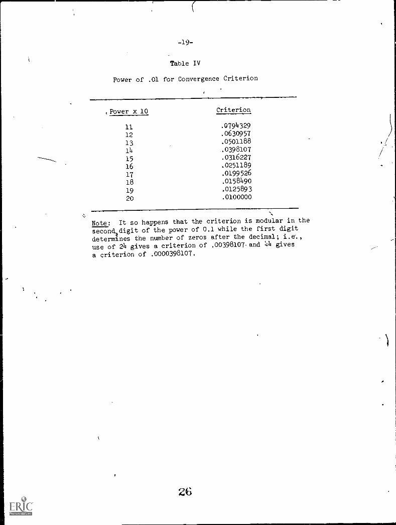
-19-

Table IV

Power of .01 for Convergence Criterion

;Power x 10 Criterion

11 .W94329

12 .0630957

13 .0501188

14 .0398107

15 .0316227

16 .0251189

17 .0199526

18 .0158490

19 .0125893

20 .0100000

Note: It so happens that the criterion is modular in the

second4digit of the power of 0.1 while the first digit

determines the number of zeros after the decimal; i.e.,

use of 24 gives a criterion of .00398107 and 44 gives

a criterion of .0000398107.

26

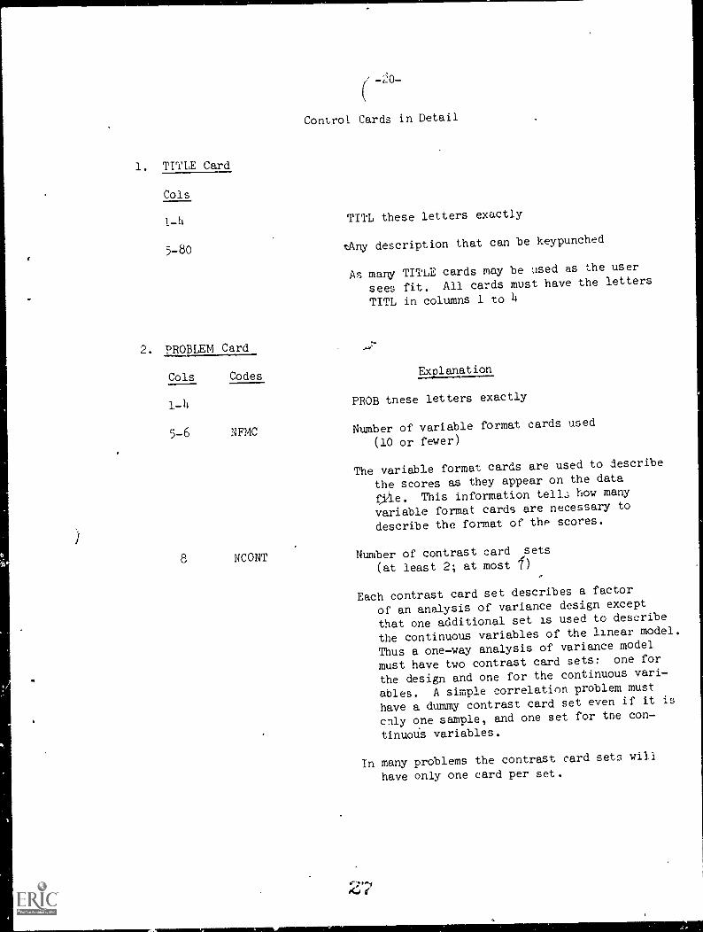
1. TITLE Card

Cols

1-4

5-8o

2. PROBLEM Card

Control Cards in Detail

TITL these letters exactly

'zAny description that can be keypunched

As many TITLE cards may be used as the user

sees fit. All cards must have the letters

TITL in columns 1 to 4

Cols Codes Explanation

1-4 PROB tnese letters exactly

5-6 NFMC Number of variable format cards used

(10 or fewer)

8 NCONT

The variable format cards are used to describe

the scores as they appear on the data

f*le. This information tells how many

variable format cards are necessary to

describe the format of the scores.

Number of contrast card ,sets

(at least 2; at most 7)

Each contrast card set describes a factor

of an analysis of variance design except

that one additional set is used to describe

the continuous variables of the linear model.

Thus a one-way analysis of variance model

must have two contrast card sets: one for

the design and one for the continuous vari-

ables. A simple correlation problem must

have a dummy contrast card set even if it is

cnly one sample, and one set for the con-

tinuous variables.

In many problems the contrast card sets will

have only one card per set.

2

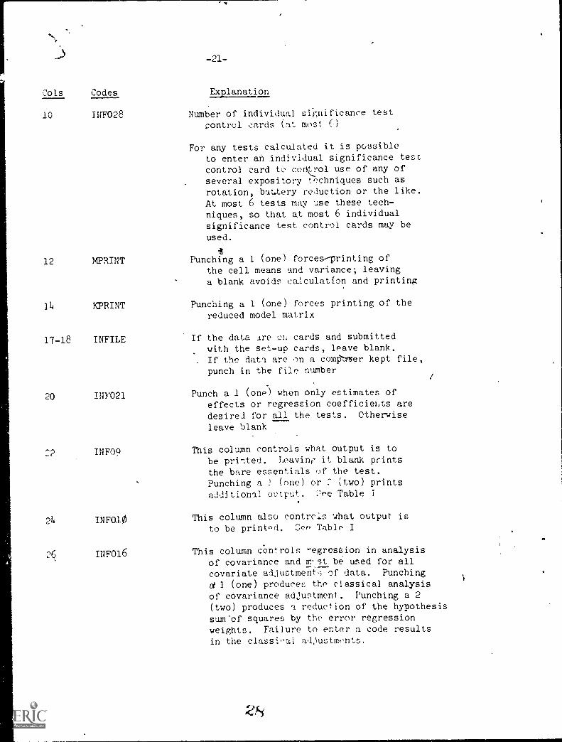
-21-

Cols Codes Explanation

10 INF028 Number of individual significance testcontrol cards (at most 6)

For any tests calculated it is possibleto enter an individual significance testcontrol card to coy rol use of any ofseveral expository techniques such asrotation, bat.tery reduction or the like.

At most 6 tests may use these tech-niques, so that at most 6 individualsignificance test control cards may be

used.

12 MPRINT Punching a 1 (one) forces-printing ofthe cell means and variance; leavinga blank avoids calculation and printing

14 KPRINT Punching a 1 (one) forces printing of thereduced model matrix

17-18 INFILE If the data Are on cards and submittedwith the set-up cards, leave blank.

. If the data are on a comPaler kept file,punch in the file number

20 INFO21 Punch a 1 (one) when only estimates ofeffects or regression coefficiehts aredesired for all the tests. Otherwise

leave blank

22 INFO9 This column controls what output is to

be printed. Leaving it blank printsthe bare essentials Qt' the test.Punching a 2 (one) or : (two) prints

additional output. :7ee Table I

24 INF010 This column also controls what output is

to be printed. See Table I

INF016 This column controls -egression in analysisof covariance and r'st be used for allcovariate adjustment,; of data. Punching

d 1 (one) produces the classical analysis

of covariance adjustment. Punching a 2(two) produces a reduction of the hypothesissum'of squares by the error regression

weights. Failure to enter a code results

in the classi,al adJustmnts.

-21a-

Cols Codes Explanation

28 INE035 Punching a 1 in this column prevents copying

of the data file for reanalysis. This is

particularly useful for large data setswhen no reanalysis is to be done; it saves

time on the machine.

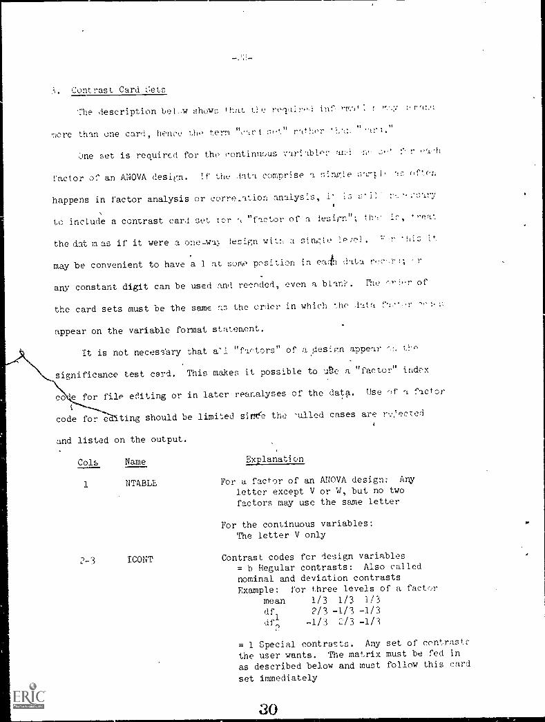
3. Contrast Card sets

The description belw show; that tle regal fin' r ar.,1

more than one card, hence the term "cart set" rather '?,an "

One set is required for the eontinuc,us variables and r ea,h

factor of an ANOVA design. If the data comprise a single sarql, as ofen

happens in factor analysis or corre-ation analysis, is s.

to include a contrast card set tor a "factor of a iesirn"; th'1* re a

the dat m as if it were a one-wa:, lesign wit:, a single lefel. Is

may be convenient to have a 1 at some position in ea data rec',r:; r

any constant digit can be used and recoiled, even a blank. I'he of

the card sets must be the same as the order in which the data fa-r

appear on the variable format statement.

It is not necess'ary that a'l " factors" of aliesipl appear 1,1'0

significance test card. This makes it possible to use a "factor" index

co e for file editing or in later reanalyses of the data. Use ' >f a factor

code fc7;ealting should be limited since the -ulled cases are r,'ected

and listed on the output.

Cols Name Explanation

1 NTABLE For a factor of an ANOVA design: Any

letter except V or W, but no twofactors may use the same letter

For the continuous variables:The letter V only

2-3 ICONT Contrast codes fcr design variables= b Regular contrasts: Also called

nominal and deviation contrasts

Example: for three levels of a factor

mean 1/3 1/3 1/3

df 2/3 -1/3 -1/3df

1-1/3 2/3 -1/3

2

= 1 Special contrasts. Any set of contrasts

the user wants. The matrix must be fed in

as described below and must follow this card

set immediately

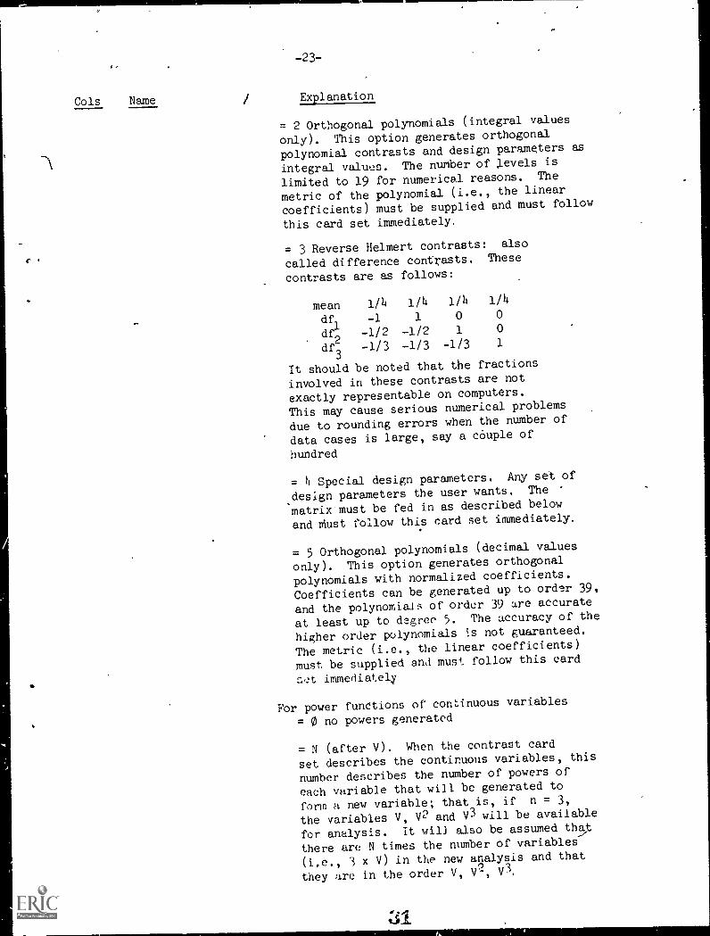
Cols Name Explanation

= 2 Orthogonal polynomials (integral values

only). This option generates orthogonal

polynomial contrasts and design parameters as

integral values. The number of Levels is

limited to 19 for numerical reasons. The

metric of the polynomial (i.e., the linear

coefficients) must be supplied and must follow

this card set immediately.

= 3 Reverse Helmert contrasts: also

called difference contrasts. These

contrasts are as follows:

meandf

1df

2df

3

1/4

-1

-1/2-1/3

1/4

1

-1/2-1/3

1/40

1

-1/3

1/4

0

0

1

It should be noted that the fractions

involved in these contrasts are not

exactly representable on computers.

This may cause serious numerical problems

due to rounding errors when the number of

data cases is large, say a couple of

hundred

= 4 Special design parameters. Any set of

design parameters the user wants. The

matrix'must be fed in as described below

and Must follow this card set immediately.

= 5 Orthogonal polynomials (decimal values

only). This option generates orthogonal

polynomials with normalized coefficients.

Coefficients can be generated up to order 39,

and the polynomials of order 39 are accurate

at least up to degree 5. The accuracy of the

higher order polynomials is not guaranteed.

The metric (i.e., the linear coefficients)

must be supplied ana must follow this card

immediately

For power functions of continuous variables

= 0 no powers generated

= N (after V). When the contrast card

set describes the continuous variables, this

number describes the number of powers of

each variable that will be generated to

form a new variable; that is, if n = 3,

the variables V, V2 and V3 will be available

for analysis. It wilJ also be assumed th5t.

there are N times the number of variables

(i.e., 3 x V) in the new analysis and thatV3they are in the order V, V2,

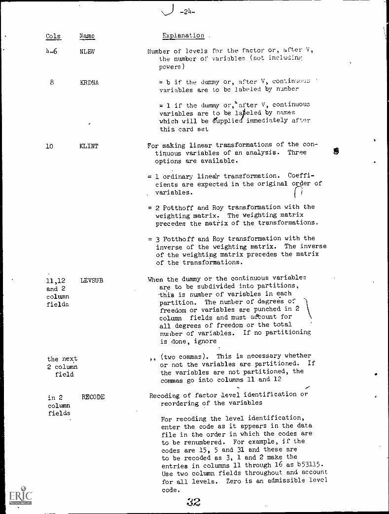
-24-

Cols Name Explanation ,

4-6 NLEV Number of levels for the factor or, after V,the number of variables (not includinfr,

powers)

8 KRDNA = b if the dummy or, after V, continuous

variables are to be labeled by number

= 1 if the dummy or,1*after V, continuous

variables are to be l4eled by nameswhich will be ffupplie immediately after

this card set

10 KLINT For making linear transformations of the con-tinuous variables of an analysis. Three

options are available.

= 1 ordinary linear transformation. Coeffi-

cients are expected in the original order of

variables.

= 2 Potthoff and Roy transformation with the

weighting matrix. The weighting matrixprecedes the matrix of the transformations.

= 3 Potthoff and Roy transformation with the

inverse of the weighting matrix. The inverseof the weighting matrix precedes the matrixof the transformations.

11,12 LEVSUB When the dummy or the continuous variables

and 2 are to be subdivided into partitions,

column this is number of variables in each

fields partition. The number of degrees offreedom or variables are punched in 2

column fields and must account forall degrees of freedom or the totalnumber of variables. If no partitioning

is done, ignore

the next2 column

field

,, (two commas). This is necessary whether

or not the variables are partitioned. If

the variables are not partitioned, thecommas go into columns 11 and 12

in 2 RECODE Recoding of factor level identification or

column reordering of the variables

fieldsFor recoding the level identification,enter the code as it appears in the datafile in the order in which the codes are

to be renumbered. For example, if the

codes are 15, 5 and 31 and these areto be recoded as 3, 1 and 2 make theentries in columns 11 through 16 as b53115.Use two column fields throughout and account

for all levels. Zero is an admissible level

code.

42

-25.-

Cols Name Explanation

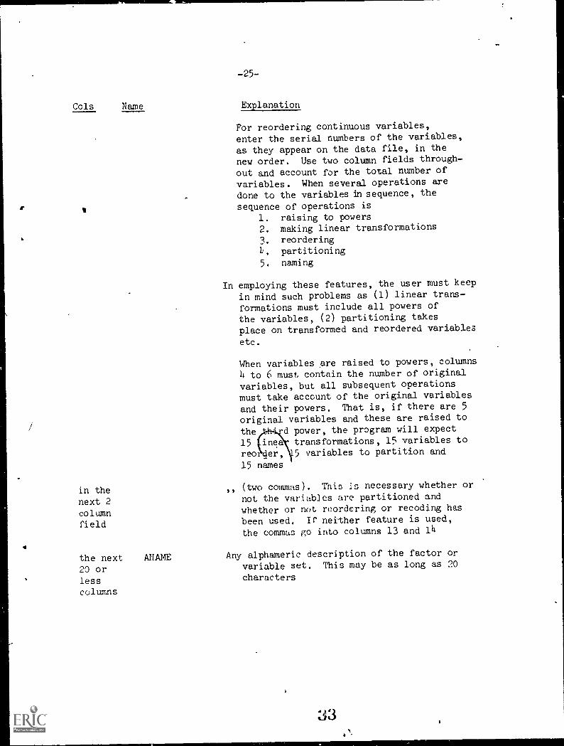
in thenext 2columnfield

For reordering continuous variables,enter the serial numbers of the variables,

as they appear on the data file, in the

new order. Use two column fields throughout and account for the total number of

variables. When several operations are

done to the variables in sequence, thesequence of operations is

1. raising to powers

2. making linear transformations

3. reordering

Z. partitioning

5. naming

In employing these features, the user must keep

in mind such problems as (1) linear transformations must include all powers ofthe variables, (2) partitioning takes

place on transformed and reordered variables

etc.

When variables are raised to powers, columns

h to 6 must contain the number of originalvariables, but all subsequent operationsmust take account of the original variables

and their powers. That is, if there are 5original variables and these are raised to

the d power, the program will expect

15 inea transformations, 15 variables to

reo 4er, 5 variables to partition and

15 names

(two commas). This is necessary whether or

not the variables are partitioned andwhether or not reordering or recoding has

been used. It' neither feature is used,

the commas go into columns 13 and 14

the next ANAME Any alphameric description of the factor or

20 or variable set. This may be as long as 20

less characters

columns

-26-

Cols Name Explanation

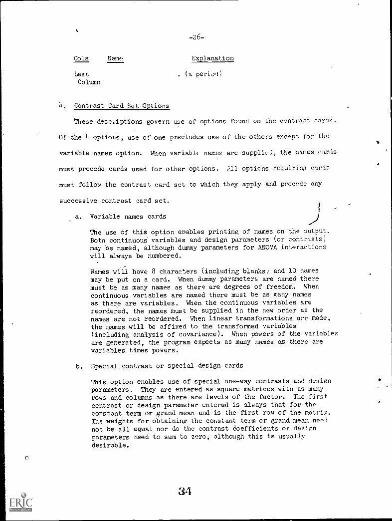
Last . (a period)

Column

it. Contrast Card Set Options

These descriptions govern use of options found on the contrast cards.

Of the 4 options, use of one precludes use of the others except for the

variable names option. When variable names are supplicl, the names cards

must precede cards used for other options; All opticns requirinfr cards

must follow the contrast card set to which they apply and precede any

successive contrast card set.

a. Variable names cards

The use of this option enables printing of names on the output.Both continuous variables and design parameters (or contrasts)may be named, although dummy parameters for ANOVA interactionswill always be numbered.

Names will have 8 characters (including blanks) and 10 namesmay be put on a card. When dummy parameters are named there

must be as many names as there are degrees of freedom. When

continuous variables are named there must be as many names

as there are variables. When the continuous variables arereordered, the names must be supplied in the new order as the

names are not reordered. When linear transformations are made,

the names will be affixed to the transformed variables(including analysis of covariance). When powers of the variablesare generated, the program expects as many names as there arevariables times powers.

b. Special contrast or special design cards

This option enables use of special one-way contrasts and designparameters. They are entered as square matrices with as manyrows and columns as there are levels of the factor. The firstccntrast or design parameter entered is always that for theconstant term or grand mean and is the first row of the matrix.The weights for obtaining the constant term or grand mean neednot be all equal nor do the contrast Coefficients or designparameters need to sum to zero, although this is usually

desirable.

34

-27-

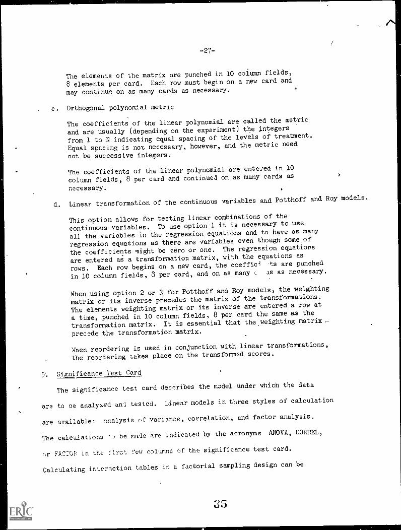
The elements of the matrix are punched in 10 column fields,

8 elements per card. Each row must begin on a new card and

may continue on as many cards as necessary. 4

c. Orthogonal polynomial metric

The coefficients of the linear polynomial are called the metric

and are usually (depending on the experiment) the integers

from 1 to N indicating equal spacing of the levels of treatment.

Equal spacing is not necessary, however, and the metric need

not be successive integers.

The coefficients of the linear polynomial are entered in 10

column fields, 8 per card and continued on as many cards as

necessary.

d. Linear transformation of the continuous variables and Potthoff and Roy models.

This option allows for testing linear combinations of the

continuous variables. To use option 1 it is necessary to use

all the variables in the regression equations and to have as many

regression equations as there are variables even though some of

the coefficients might be zero or one. The regression equations

are entered as a transformation matrix, with the equations as

rows. Each row begins on a new card, the coeffici is are punched

in 10 column fields, 8 per card, and on as many c as as necessary.

When using option 2 or 3 for Potthoff and Roy models, the weighting

matrix or its inverse precedes the matrix of the transformations.

The elements weighting matrix or its inverse are entered a row at

a time, punched in 10 column fields, 8 per card the same as the

transformation matrix. It is essential that the_weighting matrix,

precede the transformation matrix.

When reordering is used in conjunction with linear transformations,

the reordering takes place on the transformed scores.

5. Significance Test Card

The significance test card describes the model under which the data

are to oe analyzed and tested. Linear models in three styles of calculation

are available: analysis of variance, correlation, and factor analysis.

the calculations be made are indicated by the acronyms ANOVA, CORREL,

or FAC'20Fc in the tirzt few calumns of the significance test card.

Calculating interaction tables in a factorial sampling design can be

-27a-

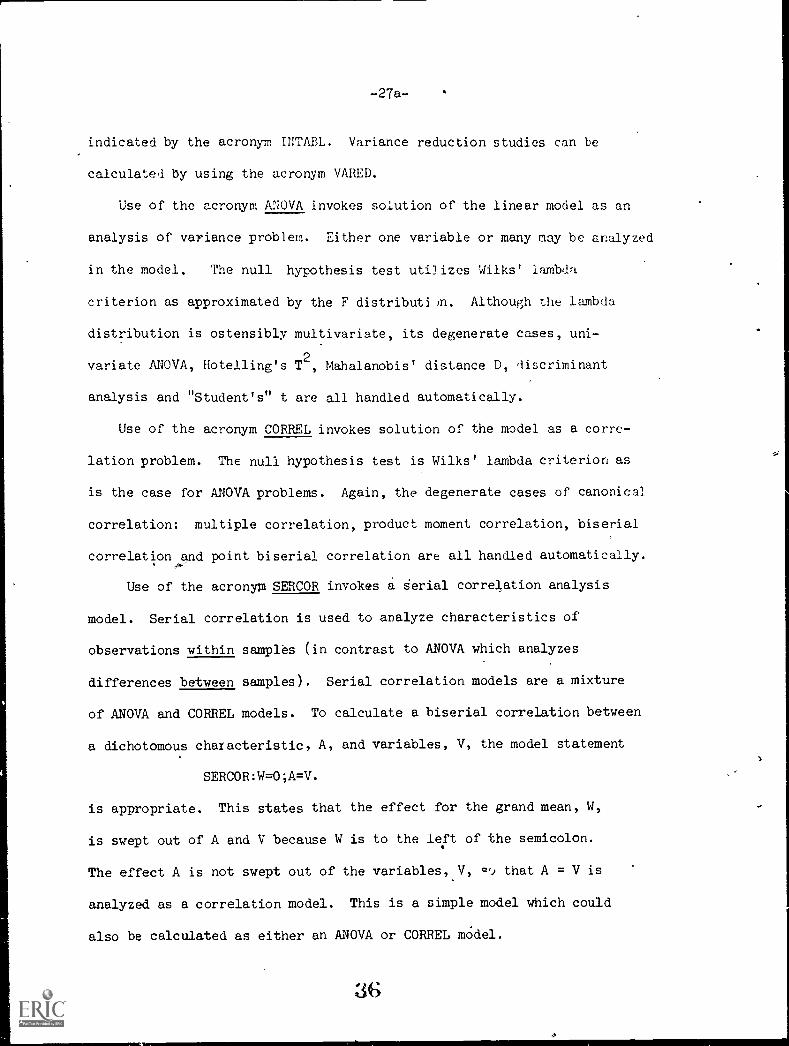
indicated by the acronym IUTABL. Variance reduction studies can be

calculated by using the acronym VARED.

Use of the acronym ANOVA invokes solution of the linear model as an

analysis of variance problem. Either one variable or many may be analyzed

in the model. The null hypothesis test uti3izes Wilks' lambda

criterion as approximated by the F distributi al. Although the lambda

distribution is ostensibly multivariate, its degenerate cases, uni-

variate ANOVA, Hotelling's T2

, Mahalanobis' distance D, discriminant

analysis and "Student's" t are all handled automatically.

Use of the acronym CORREL invokes solution of the model as a corre-

lation problem. The null hypothesis test is Wilks' lambda criterion as

is the case for ANOVA problems. Again, the degenerate cases of canonical

correlation: multiple correlation, product moment correlation, biserial

correlation and point biserial correlation are all handled automatically.,00,-

Use of the acronym SERCOR invokes a Serial correlation analysis

model. Serial correlation is used to analyze characteristics of

observations within samples (in contrast to ANOVA which analyzes

differences between samples). Serial correlation models are a mixture

of ANOVA and CORBEL models. To calculate a biserial correlation between

a dichotomous characteristic, A, and variables, V, the model statement

SERCOR:W=0;A=V.

is appropriate. This states that the effect for the grand mean, W,

is swept out of A and V because W is to the left of the semicolon.

The effect A is not swept out of the variables, V, Q,./ that A = V is

analyzed as a correlation model. This is a simple model which could

also be calculated as either an ANOVA or CORREL model.

366

-28-

More complex serial correlation models are common for a model with

several samples, A, and one characteristic, B, common over the samples

the following model is appropriate

SERCOR:W=0,A=0;B=V,AB=V .

Here W and A are to the left of the semicolon to remove the effects of

grand mean and between sample variation from the data before analyzing

the characteristic B. The effects for B are not removed from AB and V

because they are to the right of the semicolon; likewise AB is not removed

from V. The effect AB=V is a test to check the homogeneity of regression

of B onto V in the various samples of A. Further discussion of the uses

of serial correlation is found in the reference cited in the bibliography.

Serial correlations can be performed with all the variations of the linear

model: covariates, rotation of canonical variates, Potthoff and Roy models,

dimension reduction, etc.

Use of the ac..onym FACTOR invokes a factor-analytic decomposition of

the data. ',;everal types of solutions are available as displayed in

Table II. The acronym FACTOR must be immediately followed by a digit

from Table II to denote which factor decomposition is to be used. It

is possible to denote a rotation procedure by following this digit with

a number sign (#) and another digit to denote type of rotation. When

communality procedures other than squared multiple correlations are used,

the individual significance test card also must be used. When less

than all the factors are to be extracted, the individual significance

test card must be used.

3,7

-28a-

Use of the acronym INTABL generates interaction tables for ANOVA

problems. Interaction tables are generated as a nesting procedure with-

out including the grand mean in the model. Thus the statement, ,WAB=V1,

generates all the means of the variables in V for the AB interaction

of an ANOVA model. It is possible to generate many interaction tables

in the same model statement.. The estimates used for constructing

:38

-29-

interaction tables are the raw estimates and are not subject to analysis

>of covariance adjustments. Interaction tables adjusted for covariates

may be obtained by using regression transformations on the original'

variables.

Use of the acronym VARED generates a study of the sum of squares °

for hypothesis before and after reduction of the mode to orthogonality.

Model statements follow the rules for ANOVA and CORREL models. VARED

studies are not subject to analysis of covariance adjUstments except

by ,asing regression transformations on the original variables.

On the remainder of the card, special symbols, letters and numbers

are used to designate the model to be analyzed.

Letters. The letters used are those from the contrast card set.

That is, 'Ise oftne /_etter A assumes that there is an effect and a factor

Jf the design to be called A and that there is a contrast card set that

nas "A" plAnche.d in column I.

There is also a contrast .:.ard set for the continuous variables which

has a "V" in column 1. When the phrase ,A=V, is punched into the card,

1 il- of sq,arer: for t'w A effect will be generated and tested for its

rerescion the va-Y1 L]es V.

If the design is a factorial, there may also be a B effect to test.

,r this we punch the phrase ,B=V, in the significance test card. To

Des the i4eraction effect we punch the phrase ,AB=V, in the card.

111, une of two or more letters al,laent generates the Kronecker product

7,f he main e'rect ,lesign parameters necessary for testing interactions.

r)rder of Kronecker product. This prof/ram generates Kronecker products

in the order letermined by the order of the contrast card sets and

39

-30-

ultimately by the input data record. Consider the term Al:. 1r !),(1

contrast cards set for Nctor A precedes that for factor s (whi-.

say the identification code for factor A is to the left of 4,1%0 i!t-nti-

fication code for factor F on the data file) the AB dummy parameter., are

generated and the estimates printed in the order albi, a2b1, abl,...,

anbi, alb2, ..,anbm . The same order is generated

whether the interaction term is written BA or AF.

Eguals15n. An equal sign (=) is used to separate the hypothesis

variables from the error variables. The hypothesis variables are

designated by letters and numbers to the left of the equal sign; the

-error variables are designated by letters and numbers to the right of

the equal sign.

Commas, colons, and periods. Commas (,) are used to separate the

tests from each other. A colon (:) is used to separate the model

acronym frpm the teats; and a period (.) is always the last character

in a model statement.

Grand mean and zero. The constant term or grand mean may be included

in the model by using the phrase ,W=0, where W indicates the constant

term as a hypothesis and 0 (a zero) indicates that there are no error

variables for the hypothesis and no test to be made. The use of zero

as an error term is the way in which a set of variables may be included

in the model as if they were hypothesis variables but not tested.

When 0 is used as a hypothesis, it indicates that the error term is

to be subjected to factor analysis.

With this information it is possible to write a significance

test card for a simple factorial analysis of variance:

(a) ANOVA:W=0,A=V,B=V,AB=,..

a sigdlificance test car! fear a factor ahalys:s:

(b) FACTniii:W-,0 V.

::umbered partitions. The contrast card optical for partitions mak s

t possible to subdivide the sets -r parameters and continuous

variables into several subsets, The iartitions are written on the

.significance test card as Al , A2, or %I, V3, isje, etc the number

referring naturally to the oidinal position of the partition (this use

f numbers can be easily oonfusei with the use of numbers in nested

moiels).

With this information it is possib:e to write the following models

aat many Lthers,

(c) Partitionoi anal,:,is of variance (such as orthogonal

polynomial test,;)

A:i0VA:W=0,A1=-V,A =V,B=V,AlltztV,A213=V.

orrelatipn 7,ode.s

in a one-way design

A::)VA:W=4,A=0,V1-4,AV.r-Vr'.

(r) A priacipa_. factor Analysis on several samples

FACT0F /.114./

(g) Currelatit a 'inaly:

Jsr :11ares.

rrom :.;t2ver1.1 samples

l u ; _ i g a 1 3 . S i t po several effects to pr(sduce

an analysis r varlanoe with several factors, one

-le Interaction: and tet them simultanenusly flr the

1 +V',

For instance,

(n) ,A!.4Ac+i,c+Apc..vify

When orthogonal polynomial.1 are partili')ned, this .t:1:o ii ow

pooling of high ord polynomials for simkiltaneou: testing, as

,r1=v,p;,=v,p3+r4-1-,..v.

When + is used between two sets of variables, the variables are

pooled before any other operation takes place: For example V1/1::+1.--

indicates that both V? and V3 at-. tntly 0,1variates for VI.

When the parameters for a give. effect are used both singly

in some tests and pooled in other tests, the order in which the

parameters are presented on the significance test earl must always

be the'same for every test in which the parameters are used,

W and numbers for nested analyses. The letter W is commonly used

in statistical literature to indicate nesting; BWA indicates that

several samples, B, are nested in each of the levels or samples of f.

This notation is expanded slightly here as follows.

(j) ,BWA1=V, Indicates a test of B within the first

level of A.

(k) ,BWAl+BWA2=V, indicates a pooled test of B within

only the first two levels of A.

(1) ,BWA=V, indicates a test of B pooled for all levels

of A.

(m) ,BWAC, indicates a test ''f B pooled over all cells

of a two-factor design, A-.

(n) ,V1WA1=V2, indicates a teat cf the correlation betweenV1 and V2 within the first level of factor A.

Here, a number, used after a letter which follows a W, indicates

the level, not a partition. A number used after a letter but before

a W (or in the absence of a W) indicates a partition.

-33-

Slash (/) for analysis of covariance. The use of a slash indicates

that all variates after the slash and before the next comma (or colon

or period or minus) are to be covariates for the test indicated. A

slash and variables immediately following the acronym indicates that

all the tests in

makes possible th

e model have those variables as covariates. This

following types of models.

\..) Analysis of covariance in a factorial analysis of

variance

ANOVA:W=0,A=V1/V2,B=V1/V2,AB=V1/V2. or

AlIOVA/V2:W=0,A=V1,B=V1,AB=V1.

(p) Partial correlation

CORBEL:W=0,V1=V2/V3.

(q) Principal components analysis with covariates

FACTOR1/V2:W=0,0=V1.

(r) AllOVA:W=0,A=V1,3=V1/V2,AB=V1/V2+V3.

Ampersand (&) for extension. The use of an ampersand indicates

that all the variables after the ampersand and before the next comma

' p2riod cr minus) are to be used as extension variables

the r'anonial variates of the test indicated. An ampersand immediately

rolluwina, the crc)nym inuicates that extension is to be done to all

the canonical variates in all the tests in the model statement. This

Akes It p,,dssible to write the following models.

is) Iiiscriminant analysis of V1 and A extended to V2

ANnVA:W=4,A=Vl&V2. or

ANOVAW:W=0,A=V1.

43

(t ) Canoni, rrelati.n 1,.'ween P and VI extf.nae,!

V.' and V

i'ORPEL :W=0 , P= V &V, +V 4.

Cu) Factor Vi t:xtended to V.

FACTnr .11 :',1=0 ,O=V .

Number sign ('N) f,)r rotation. The use of /1 after the acronym

FACTOR and its iigit in ticat es ' h it factors are to he rotated. A

digit must follow to denote which rotation scheme is to be used.

Table ITI lists the types ,f r tations available. This makes it possible

to write the model.

( v ) Alpha factor analys i with equamax rotation

PACTOE7#

(Potation of canonical variates in ANOVA or CORBELcan be done only by using the individual significanc(

test card.)

Asterisk (*) for couonents of variance. In many components of

variance models, the error term for a test can be generated as a

regression sum t.,f squares. More simply, the sum of squares for hypothesis

of one test may be the sum of squares for errors of another test.

Therefore, to make it easy to cal _il ate the sum of squares for error

we use the notation A*V tc denote the regression of continuous variables

V on dummy parameters A to form an error term. This notation is allowed

only on the right of an equal sign where errors are designated.

It should be noted that, this Frutram will not solve multivariate

components of variance models where the number of continuous variables

V is more than the number of dummy parameters A or degrees of freedom

"^r c'rrr)r,

-34a-

Minus (-) for dimension reduction. In multivariate models, it may

be desirable to remove the significant canonical variates of one effect

from the variables to be analyzed for another effect: to wit, the

significant canonical variates of an ANOVA interaction r,..loved from con-

sideration in a test of a main effect. If A and B are main effects in

an ANOVA design and AB their interaction the statement

,A=V-AB=V.

will generate a test for A independent of any significant interaction

effects.

Semicolon (0 for limiting sweeps in serial correlation. In ANOVA

and CORREL models all hypothesis terms in the model statement are swept

out sequentially from left to right leaving a residual sum-of-squares of

the variables. In serial correlation, the hypothesis terms which lie to

the left of the semicolon are swept out but those hypothesis terms to the

right of the semicolon are not swept. The assumption being that hypothesis

statements to the right of the semicolon refer to characteristics of the

observations in the samples or populations.

-35-

Special notes.

(a) When effects are partitioned and repooled (for example V1 +V3)

the pooling must always be presented on the significance test card

in the same order. That is, you cannot state A=V1+V3 and B=V3+V1

in the same model. You must state A=V1+V3 and B=V1+V3. Also, when

effects are partitioned, they must stay partitioned: i.e., A=V is not

an alternative for Al+A2=V when A has been partitioned.

(b) In one model statement, a set of parameters may be used only

for a hypothesis, an error, an extension or a covariate but not for

two of these.

6. Variable Fermat Cards

These cards describe the way in which the data on the observations

appear on the data file. There may be as many as 10 cards to describe

the format. The use of the variable format follows the customary

FORTRAN restrictions.

Suppose the data appeared as follows:

Cols. 1-5 information to be ignored

6 level number the first factor

7information to be ignored

8-9 level identification of the second factor

10-13 a datum on the first continuous variable

14-18 a datum on the second continuous variable

19-21 information to be ignored

22-25 a datum on the third continuous variable

26-to end information to be ignored

-36-

The information on these records can be read with the following

variable format statement

(5X,I1,1X,I2,F4.0:F5.0,3X,F4.0)

It will be noticed that all identification numbers are expected in

fixed (I, integer) format while all continuous variable scores are

expected in floating (F, decimal) format.

About factor identification. The reading of factor level identification

must precede the reading of variable scores. In the above e..;.ample the

data record is arranged so that this occurs naturally. It is possible

that the factor level identification is interspersed among the variable

stores; in this case the "tab" feature of format statements may be used to

read the factor level identificationbefore the variable scores. If this

cannot be done the data will reed to be rearranged to put level codes first

in the records.

All records must contain factor level information. When single

samples are analyzed, it will be necessary either to include a constant

on the file or to fake a factor with one level. This may be done by

reading a number off the record and recoding it to 1 or b reading a

(blank on the record and recoding it to 1.

On IBM machines it will also be necessary to note the following

comment abo'at reading integer variable scores in F format: for example

reading the score 12 as F2.0.

The score 12 read as F2.0 occupies 2 characters. When the program

copies this score to save it for reanalysis, it copies 12.0 in two

characters 2.0 which does not include the 1: The copy is overflowed.

When the copy file is read for reanalysis the program will register an

-37-

overflow in subroutine DATVEC. To prevent this disability either

manufacture the original file as 012 and read it as F3.0 or manufacture

the original file as 12. and read' it as F3.0.

7. Data

The data may be on any file as long as the file is designated on

the problem card by a two-digit number in columns 17 and 18. Blanks

in these columns indicate the data are on cards and follow the variable

format statement.

If the data are on cards, a blank data record must follow the data:

there must be as many blank cards as there are cards in the data record

of one observation. If the data are on a tape or disk file an ordinary

end-of-file mark will do.

I .

lAs a rule it is simpler to arrange factor level identification codes

first on the data record before the continuous variable scores because

these codes must be read in first in the record. This expedient is

not a necessity on many machines because of the 'tab" feature of

FORTRAN IV compilers.

8. Individual Significance Test Control Card

The individual significance test cards are used to control procedures

which can be applied to particular significance tests and not to others.

These procedures are expository in nature and not usually subject to

statistical testing. Arbitrarily, the number of statistical tests

in the model to which these procedures can be applied is limited to six.

Each individual significance test control card is presented with

the options which apply to it. The control cards are presented in the

reverse order from the order of the tests on the significance test

card (i.e., last to first).

48

-38-

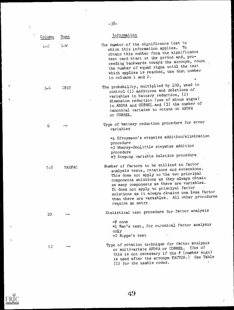
Column Name Information

1-2 NOW The number of the significance test to

which this information applies. To

obtain this number from the significance

test card start at the period and, pro-

ceeding backwards toward the acronym, count

the number of equal signs until the test

which applies is reached, use that number

in columns 1 and 2.

3-h CRIT The probability, multiplied by 100, used to

control (1) additions and deletions of

variables in battery reduction, (2)

dimension reduction (use of minus signs)

in ANOVA and CORREL and (3) the number of

canonical variates to rotate in ANOVA

or CORREL.

6 Type of battery reduction procedure for error

variables

=1 Efroymson's stepwise addition/elimination

procedure=2 Wherry-Doolittle stepwise addition

procedure=3 Step-up variable deletion procedure

7-8 MAXFAC Number of factors to be utilized in factor

analysis tests, rotations and extensions.

This does not apply to-the two principal

components solutions as they always obtain

as many components as there are variables.

It does not apply to principal factor

solutions as it always obtains one less factor

than there are variables. All other procedures

require an entry.

10Statistical test procedure for factor analysis

12

=0 none=1 Rao's test, for conical factor analysis

only=2 Rippe's test

Type of rotation technique for factor analysis

or multivariate ANOVA or CORREL. (Use of

this is not necessary if the // (number sign)

is used after the acronym FACTOR.) See Table

III for the usable codes.

49

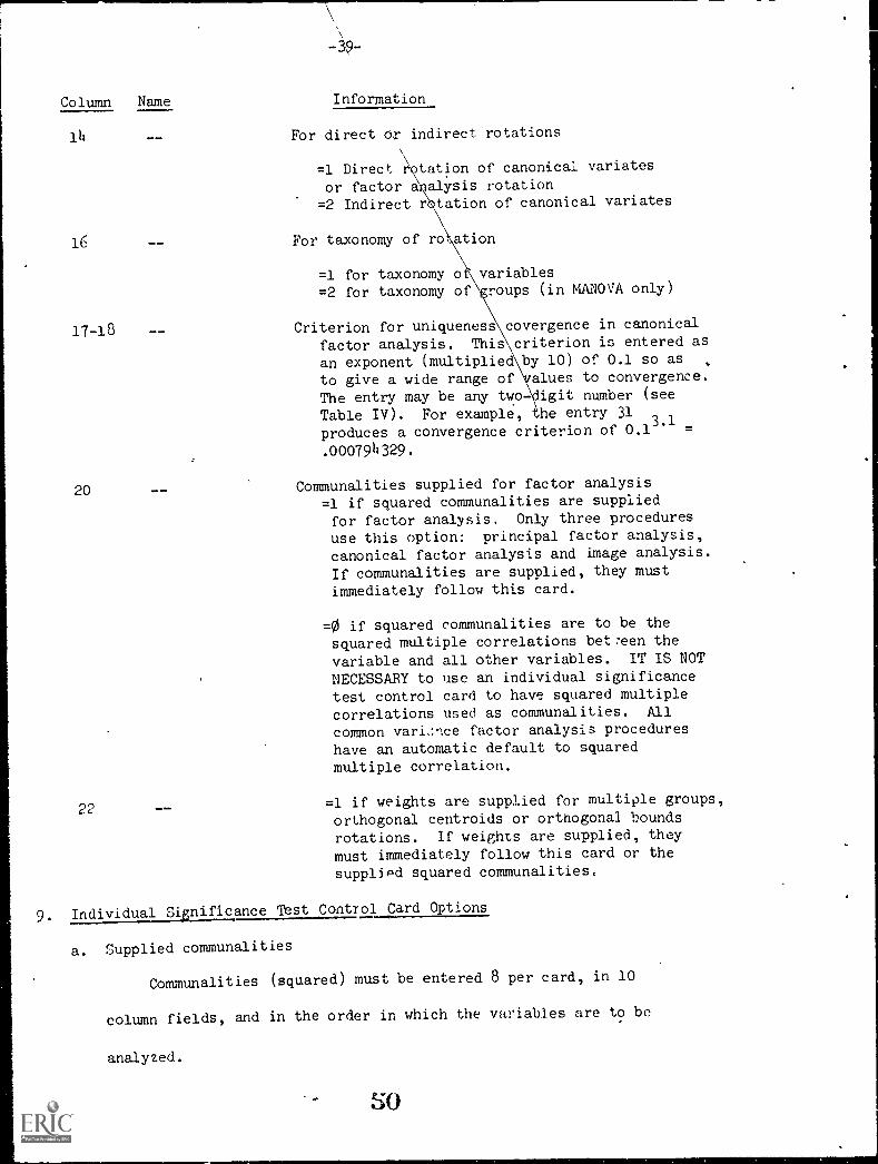
Column Name

-39-

Information

For direct or indirect rotations

=1 Direct tation of canonical variatesor factor a alysis rotation=2 Indirect r tation of canonical variates

16 For taxonomy of ro ation

=1 for taxonomy o variables

=2 for taxonomy of roups (in MANOVA only)

17-18 Criterion for uniqueness covergence in canonical

factor analysis. This criterion is entered as

an exponent (multiplied by 10) of 0.1 so as

to give a wide range of alues to convergence.

The entry may be any two- igit number (see

Table IV). For example, be entry 31produces a convergence criterion of 0.13'1 =

.000794329.

20

22

Communalities supplied for factor analysis

=1 if squared communalities are suppliedfor factor analysis. Only three procedures

use this option: principal factor analysis,

canonical factor analysis and image analysis.If communalities are supplied, they mustimmediately follow this card.

=0 if squared communalities are to be thesquared multiple correlations bet:een thevariable and all other variables. IT IS NOT

NECESSARY to use an individual significancetest control card to have squared multiplecorrelations used as communalities. All

common vari.:nce factor analysis procedures

have an automatic default to squaredmultiple correlation.

=1 if weights are supplied for multiple groups,orthogonal centroids or orthogonal bounds

rotations. If weights are supplied, theymust immediately follow this card or the

supplied squared communalities.

9. Individual Significance Test Control Card Options

a. Supplied communalities

Communalities (squared) must be entered 8 per card, in 10

column fields, and in the order in which the variables are to be

analyzed.

SO

-140-

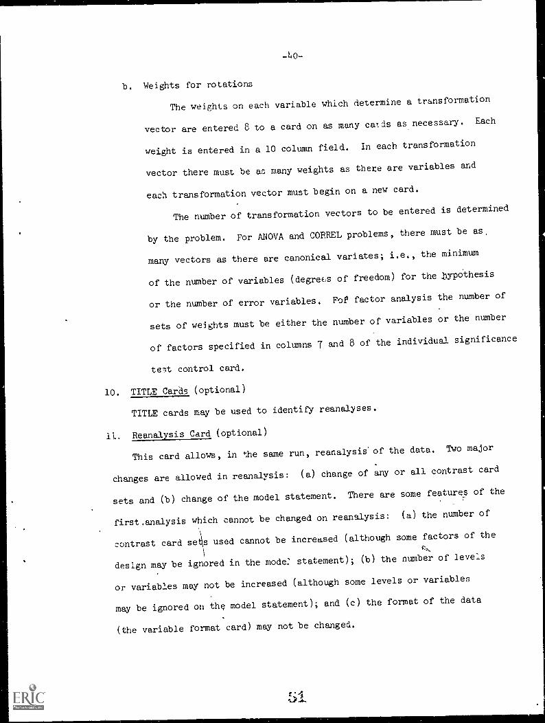
b. Weights for rotations

The weights on each variable which determine a transformation

vector are entered 8 to a card on as many cards as necessary. Each

weight is entered in a 10 column field. In each transformation

vector there must be as many weights as there are variables and

each transformation vector must begin on a new card.

The number of transformation vectors to be entered is determined

by the problem. For ANOVA and CORREL problems, there must be as,

many vectors as there are canonical variates; i.e., the minimum

of the number of variables (degrees of freedom) for the bypo'thesis

or the number of error variables. For factor analysis the number of

sets of weights must be either the number of variables or the number

of factors specified in columns 7 and 8 of the individual significance

telt control card.

10. TITLE Cards (optional)

TITLE cards may be used to identify reanalyses.

11. Reanalysis Card (optional)

This card allows, in the same run, reanalysis' of the data. Two major

changes are allowed in reanalysis: (a) change of any or all contrast card

sets and (b) change of the model statement. There are some features of the

first.analysis which cannot be changed on reanalysis: (a) the number of

contrast card sets used cannot be increased (although some factors of the

design may be ignored in the mode: statement); (b) the number of levels

or variables may not be increased (although some levels or variables

may be ignored on the model statement); and (c) the format of the data

(the variable format card) may not be changed.

Cols

1-4

6

8

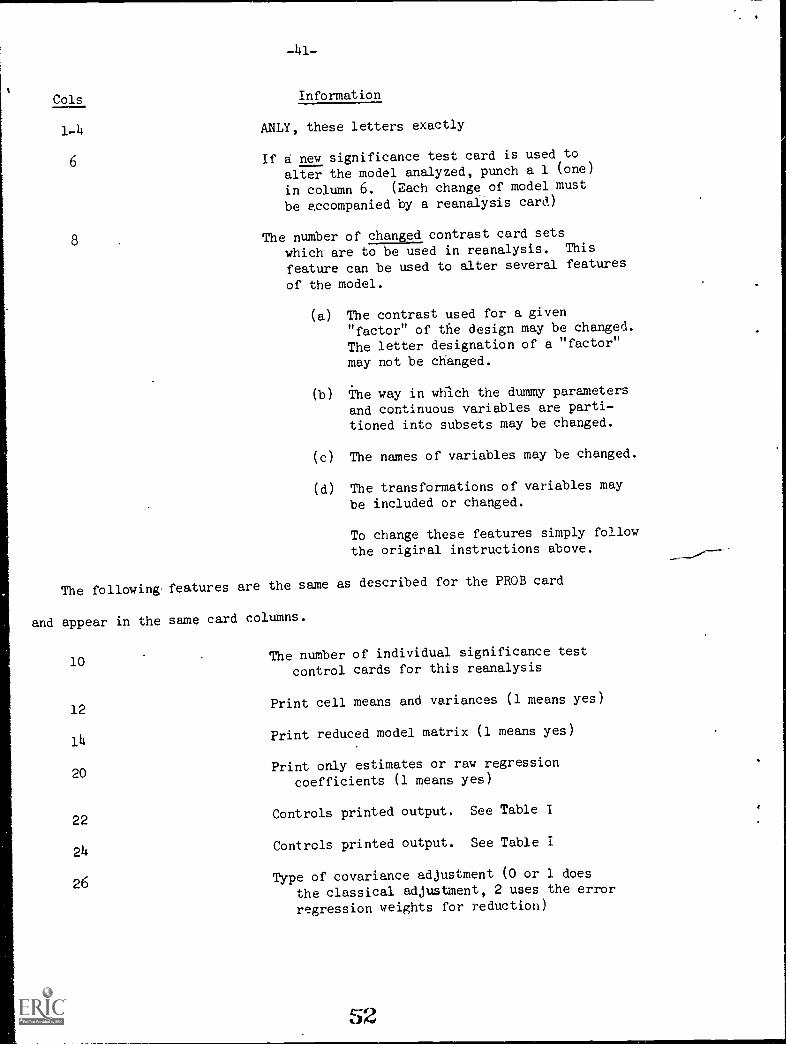
-141-

Information

ANLY, these letters exactly

If a new significance test card is used to

alter the model analyzed, punch a 1 (one)

in column 6. (Each change of model must

be accompanied by a reanalysis card)

The number of changed contrast card sets

which are to be used in reanalysis. This

feature can be used to alter several features

of the model.

(a) The contrast used for a given"factor" of the design may be changed.The letter designation of a "factor"

may not be changed.

(b) The way in which the dummy parametersand continuous variables are partitioned into subsets may be changed.

(c) The names of variables may be changed.

(d) The transformations of variables may

be included or changed.

To change these features simply follow

the original instructions above.

The following features are the same as described for the PROB card

and appear in the same card columns.

10

12

14

20

22

24

26

The number of individual significance test

control cards for this reanalysis

Print cell means and variances (1 means yes)

Print reduced model matrix (1 means yes)

Print only estimates or raw regression

coefficients (1 means yes)

Controls printed output. See Table I

Controls printed output. See Table I

Type of covariance adjustment (0 or 1 does

the classical adjustment, 2 uses the error

regression weights for reduction)

52

-42-

The options of columns 10 to 26 must be reinstated for each reanalysis

because doing a reanalysis erases the controls of the previous analysis.

12. Several Problems

Many sets of data may be analyzed in one run. The cards for each set

may follow each other.

13. FINISH Card NA card with FINISH in columns 1-6 may follow the last problem.

-43-

Programming Notts

The VARAN program is written in FORTRAN IV for an IBM 360-65 computer.

Insofa as possible it is written to be compatible with any computer which

uses FORTRAN-like compilers. Such features as may nee3 changing are

accessible without much labor. The following list shows some of these

features.

1. All multiple precision statements are titled "DOUBLE PRECISION."

All input-output units are designated by integer constants which

can be changed in the main program.

3. All dimensioning constants for changing the size of arrays are

centralized in tne main program and four executive subroutines.

This allows for easy changing of size parameters and adaption of

the program to special problems. The arrays and their dimensioning

constants are listed in Tables VI through VIII. The program is

distributed in three sizes, Tiny, Standard, and Large. The FORTRAN

decks are the standard size while instructions are on the tape

for implementing the tiny and large sizes.

The program is put together in two basic sections, one for the clerical

part of setting up the model, and another for doing the mathematics of the

solution. .The clerical section is controlled by the executive subroutines

nisEX1, 3UBEX3 and SUBEXL. The mathematical section is controlled by the

e::ecutive subroutine SUBEX2 with the factor analysis subsection controlled

by iUBEX5. Table V lists each of the subroutines with a brief description

its purpose. This table lists each major executive subroutine and after

it. the miscellaneous subroutines used oy it as well as the major subroutines

54

-1414-

which are called by the executive subroutine. The order of the listing

roughly dictated by the following considerations:

1. the order in which the program executes

2. the order in which the overlay structure is put together, and

3. V-e. of which the FORTRAN decks are listed on the mailer

tape (the :exception here is that th' executive subroutines are

at the heal of the mailer tape)

Comment cards a- quite liberally to explain the functions of

subroutines. A' T aead of each subroutine there are several comment cards

which describe the function of the subroutine and how it operates.

Accuracy of calculations. The programming sequence was arranged in such

a way as to be convenient and accurate for multivariate problems. Therefore

some of the univariate side statistics have been manipulated excessively

outside the main flow of calculations and do noi: serve as checks for

riL,Ierical accuracy. Accuracy checks should be made on the multivariate

calculations.

-44a-

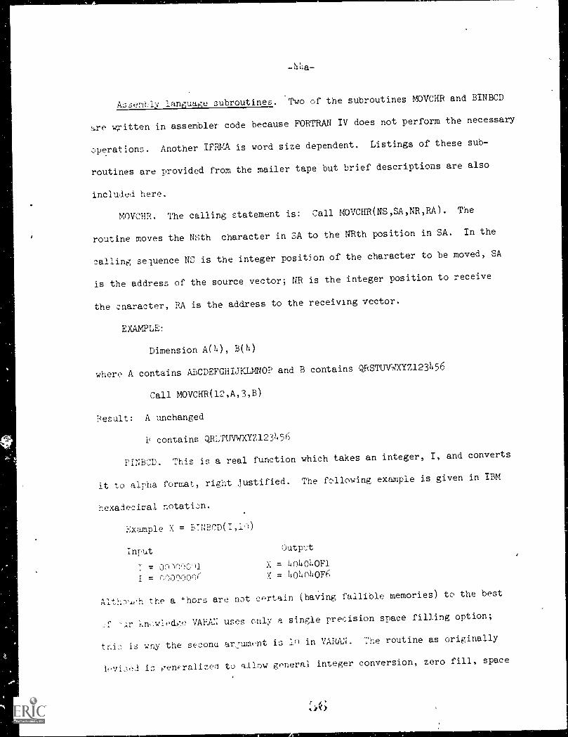
Assemt:ly language subroutines. Two of the subroutines MOVCHR and BINBCD

51re written in assembler code because FORTRAN IV does not perform the necessary

operations. Another IFRMA is word size dependent. Listings of these sub-

routines are provided from the mailer tape but brief descriptions are also

included here.

MOVCHR. The calling statement is: Call MOVCHR(NS,SA,NR,RA). The

routine moves the NSth character in SA to the NRth position in SA. In the

calling sequence NS is the integer position of the character to be moved, SA

is the address of the source vector; NR is the integer position to receive

the cnaracter, RA is the address to the receiving vector.

EXAMPLE:

Dimension A(4), B(4)

where A contains ABCDEFGHIJKLMNOP and B contains QRSTUWXYZ123456

Call MOVCHR(12,A,3,B)

Result: A unchanged

? contains QRLTUVWXYZ123456

PINBCD. This is a real function which takes an integer, I, and converts

it to alpha format, right justified. The following example is given in IBM

hexadecimal notation.

Example X = KNBCD(I,l.-))

anrut Output

= on ")M0')1 X = 404040F1

I = n00000n( = 404n40F6

Alth.T.h the a *-hors are not certain (having fallible memories) to the best

knuwledp-,e VARAN uses only a single precision space filling option;

trio is wry the second a,ument is In in VAW1N. The routine as originally

levi,;ed is p'encralizeci to allow general integer conversion, zero fill, space

f' 6

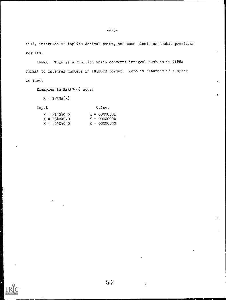
-414b-

fill, insertion of implied decimal point, and uses single or double precision

results.

IFRMA. This is a function which converts integral numf-,ers in AIPHA

format to integral numbers in INTEGER format. Zero is returned if a space

is input

Examples in HEX(360) code:

K = IFRMA(X)

Input Output

X = F1404040 K = 00000001

X = F64134040 K = 00000006x = 4040404o K = 00000000

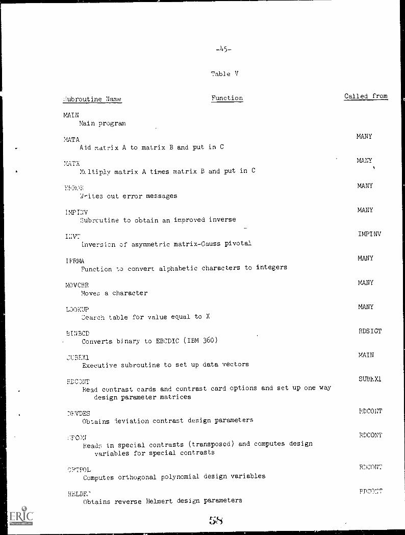
Aibroutine Name

-45-

Table V

Function

MAINMain program

MATAAid matrix A to matrix B and put in C

MATXMtltiply matrix A times matrix B and put in C

ERRORwrites out error messages

IMPINVSubrcutine to obtain an improved inverse

INN:Inversion of asymmetric matrix-Gauss pivotal

IFRMAFunction to convert alphabetic characters to integers

MOVCHRMoves a character

LOOKUPsearch table for value equal to X

BINBCDConverts binary to EBCDIC (IBM 360)

.:UBEX1Executive subroutine to set up data vectors

RDCOUTRead contrast cards and contrast card options and set up one way

design parameter matrices

Called from

MANY

MANY

MANY

MANY

IMPINV

MANY

MANY

MANY

RDSIGT

MAIN

SUBEX1

DEVDES RDCONT

Obtains deviation contrast design parameters

:TCON RDCONT

Reads in special contrasts (transposed) and computes design

variables for special contrasts

.')RTPOLRDCONT

Computes orthogonal polynomial design variables

HELDE,' PDC=Obtains reverse Helmert design parameters

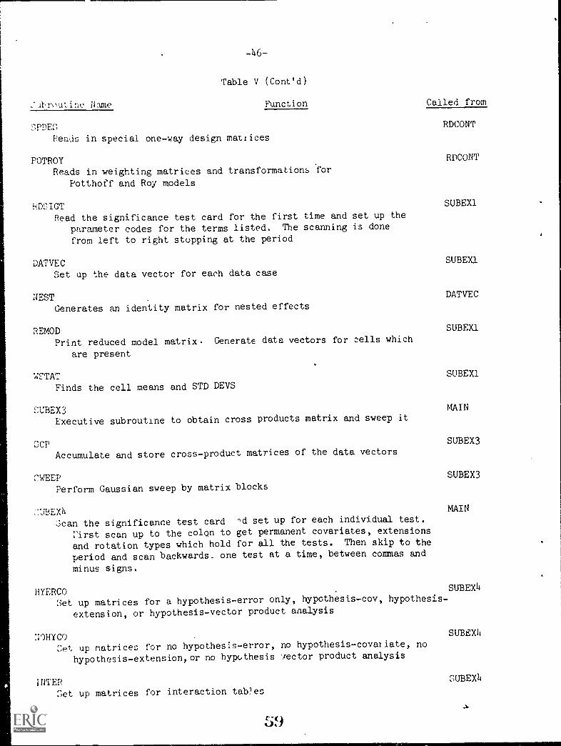
It,routi:le Name

SPDES

-46-

Table V (Cont'd)

Function Called from

RDCONT

Reads in special one-way design matrices

POTROYReadsin weighting matrices and transformations for

Potthoff and Roy models

RDSIGTRead the significance test card for the first time and set up the

parameter codes for the terms listed. The scanning is done

from left to right stopping at the period

DATVECSet up the data vector for each data case

NESTGenerates an identity matrix for nested effects

REMODPrint reduced model matrix. Generate data vectors for cells which

are present

Finds the cell means and STD DEVS

UBEX3Executive subroutine to obtain cross products matrix and sweep it

OCPAccumulate and store cross-product matrices of the data vectors

WEEPPerform Gaussian sweep by matrix blocks

SUBEX4Scan the significance test card set up for each individual test.

rirst scan up to the colon to get permanent covariates, extensions

and rotation types which hold for all the tests. Then skip to the

period and scan backwards_ one test at a time, between commas and

minus signs.

RDCONT

SUBEXI

SUBEX1

DATVEC

SUBEX1

SUBEXI

MAIN

SUBEX3

SUBEX3

MAIN

HYERCO SUBEX4

Set up matrices for a hypothesis-error only, hypothesis-cov, hypothesis-

extension, or hypothesis-vector product analysis

NOHYCOSet up matrices for no hypothesis-error, no hypothesis-covarlate, no

hypothesis - extension, or no hypothesis ',rector product analysis

TNTERSet up matrices for interaction tab?es

59

SUBEX4

SUBEX4

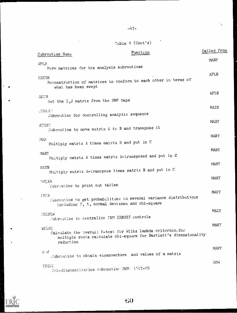
Subroutine Name

-147-

Table V (Cont'd)

Function Called from

APLBMANY

Form matrices for the analysis subroutines

1ECONReconstruction of matrices to conform to each other in terms of

what has been swept

APLB

GETMAPLB

Get the I,J matrix from the SWP tape

MAIN

21broutine for controlling analytic sequence

ATOBTMANY

2.ubroutine to move matrix A to B and transpose it

MLABMANY

Multiply matrix A times matrix B and put in C

MkBTMANY

Multiply matrix A times matrix B-transposed and put in C

MATBMANY

Multiply matrix A-transpose times matrix B and put in C

OUTABMANY

'ubrDutine to print out tables

PROBMANY

:'7ubroutine to get probabilities in several variance distributions

including F, t, normal deviates and chi-square

UNDFLWMANY

.:lbroutine to centralize IBM ERRSET controls

WILKE;MANY

Calculate the overall F-test for Wilks lambda criterion, for

multiple roots calculate chi-square for Bartlett's dimensionality

reduction

ti' fiMANY

ubroutine to obtain eigenvectors and values of a matrix

HOW

Fri-diagonalization subroutiw' DM 1';17-IJB

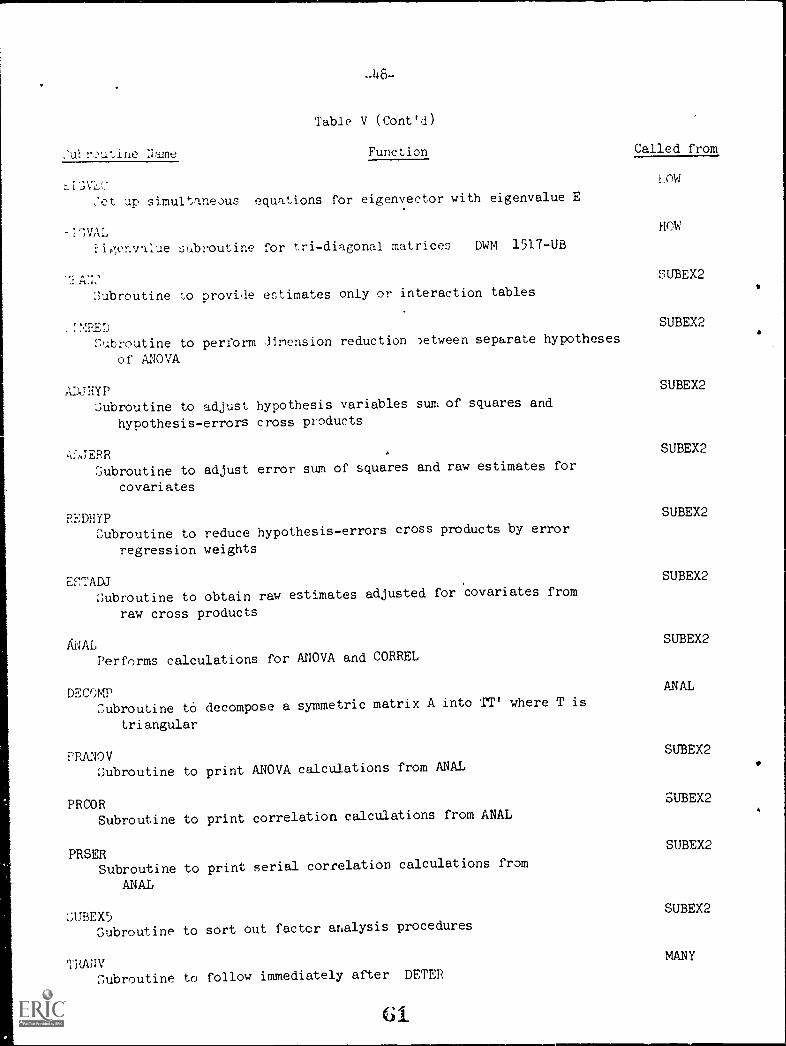
Name

Table V (Cont'd)

Function Called from

h OW

:et up simultaneous equations for eigenvector with eigenvalue E

I;VAL:igenvalue subroutine for tri-diagonal matrices DWM 1517-UB

Subroutine to provide estimates only or interaction tables

TY.RED

Subroutine to perform dimension reduction )etween separate hypotheses

of ANOVA

ADJHYPSubroutine to adjust hypothesis variables sum of squares and

hypothesis-errors cross products

:JATEPRSubroutine to adjust error sum of squares and raw estimates for

covariates

REDHYPSubroutine to reduce hypothesis-errors cross products by error

regression weights

E:::TADJ

Subroutine to obtain raw estimates adjusted for covariates from

raw cross products

HOW

SUBEX2

SUBEX2

SUBEX2

SUBEX2

SUBEX2

SUBEX2

ANAL SUBEX2

Performs calculations for ANOVA and CORREL

DECOMPANAL

Subroutine to decompose a symmetric matrix A into TT' where T is

triangular

PRAMV SUBEX2

Subroutine to print ANOVA calculations from ANAL

PRCORSUBEX2

Subroutine to print correlation calculations from ANAL

PRSERSUBEX2

Subroutine to print serial correlation calculations from

ANAL

SUBEX5SUBEX2

Subroutine to sort out factor analysis procedures

TRANVMANY

Subroutine to follow immediately after DETER

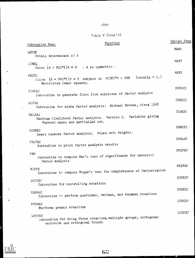
Subroutine Name

Table V (Cont'd)

FunctionCalled from

DETERMANY

Obtain determinant of A

SIMEQSolve (A PHI*I)X = B . A is symmetric .

RI:SOL

Solve. (A PHI*I)V = X subject to V(TR)*V = CON (usually = 1.)

Restricted least squares.

MANY

MANY

FIREACSUBEX5

Subroutine to generate first five solutions of factor analysis

ALPHASUBEX5

Subroutine for alpha factor analysis: Michael Browne, circa 1968

MALFAIMaximum likelihood factor analysis. Version 2. Variables giving

Heywood cases are partialled out.

SUBEX5

MINRESSUBEX5

Least squares factor analysis. Fixed unit weights.

PRIFACSUBEX5

Subroutine to print factor analysis results

RAOPRIFAC

Subroutine to compute Rao's test of significance for canonical

factor analysis

RIPPEPRIFAC

Subroutine to compute Rippe's test for completeness of factorization

ROTCONSUBEX2

Subroutine for controlling rotations

VARMAXSUBEX2

Subroutine t-) perform quartimax, varimax, and eauamax rotations

PPOMAXSUBEX2

Performs prom( rotations

WATCENSubroutine for doing three rotations, multiple groups, orthogonal

centroids and orthogonal bounds

SUBEX2

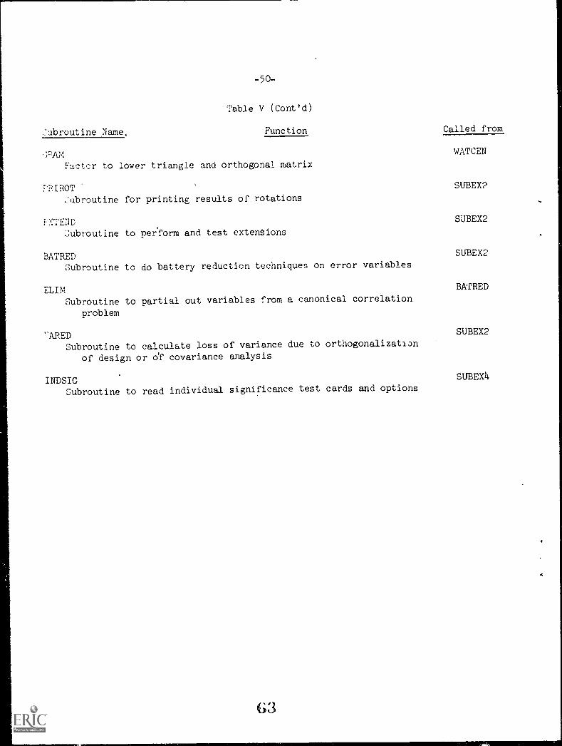
:ubroutine Name,

-50-

Table V (Cont'd)

Function Called from

WATCEN

Factor to lower triangle and orthogonal matrix

PRIROT SUBEX2

subroutine for printing results of rotations

:XTEND SUBEX2

Subroutine to per:form and test extensions

BATRED SUBEX2

Subroutine to do battery reduction techniques on error variables

ELI;

Subroutine to partial out variables from a canonical correlation

problem

-APEDSubroutine to calculate loss of variance due to orthogonalization

of design or of covariance analysis

INDSIGSubroutine to read individual significance test cards and options

63

BATRED

SUBEX2

SUBEXI4

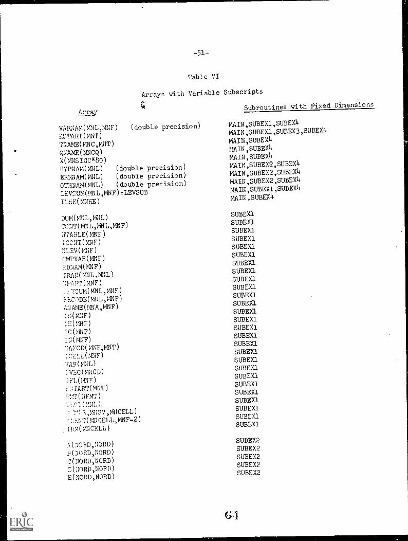
-51--

Table VI

Arrays with Variable Subscripts

Array

VARNAM(MNL,MNF) (double precision)

KSTART(h1NT)

TNAME(MNC,MIIT)

QNAME(MNCQ)x(nNsIcc*8o)HYPNAM(MNL) (double precision)

ERRNAM(MNL) (double precision)

OTHNAM(MNL) (double precision)

LEVCUM(MNL,MNF).LEVSUBLliE( )

DUM(MNL,ML)CCNT(MNL,MNL,MNF)NTABLE(MNF)ICONT(MNF)NLEV(MIJF)

CMPVAR(KNF)FDNAM(MNF)TRAN(nNL,ML)7.PAFT(MNF)

.:7CUM(MNL,MNF):ECODE(MNL,MNF)ANAME(i NA,MNF)

..;(IMF)

IE(MNF)

IC(MN7)IN(1CF)'IAFCD(MNF,MNT)

I CELL ( MNF )

AP(MNL)VEC (MCI))FL 04NF

i.7..",PART(MNT)

FM(NFMT)ECT(MNL)

::ENT(MNCELL,MNF-2)71M(MTICELL)

AMRD,NORD)NNORD,NORD)c( NORD,NORD)

:,(NORD,NORD)

E(NORD,NORD)

6.

Subroutines with Fixed Dimensions

MAIN,SUBEX1,SUBEX4MAIN,SUBEX1,SUBEX3,SUBEX4MAIN,SUBEX4MAIN,SUBEAMAIN,SUBEX4MAIN,SUBEX2,SUBEX4MAIN,SUBEX2,SUBEX4MAIN,SUBEX2,SUBEX4MAIN,SUBEX1,SUBEX4MAIN,SUBEX4

SUBEX1SUBEX1SUBEX1SUBEX1SUBEX1SUBEX1SUBEX1SUBEX1SUBEX1SUBEX1SUBEX1SUBEX1SUBEX1SUBEX1SUBEX1SUBEX1SUBEX1SUBEX1SUBEX1SUBEX1SUBEX1SUBEX1SUBEX1SUBEX1SUBEX1SUBEX1SUBEX1

SUBEX2SUBEX2SUBEX2SUBEX2SUBEX2

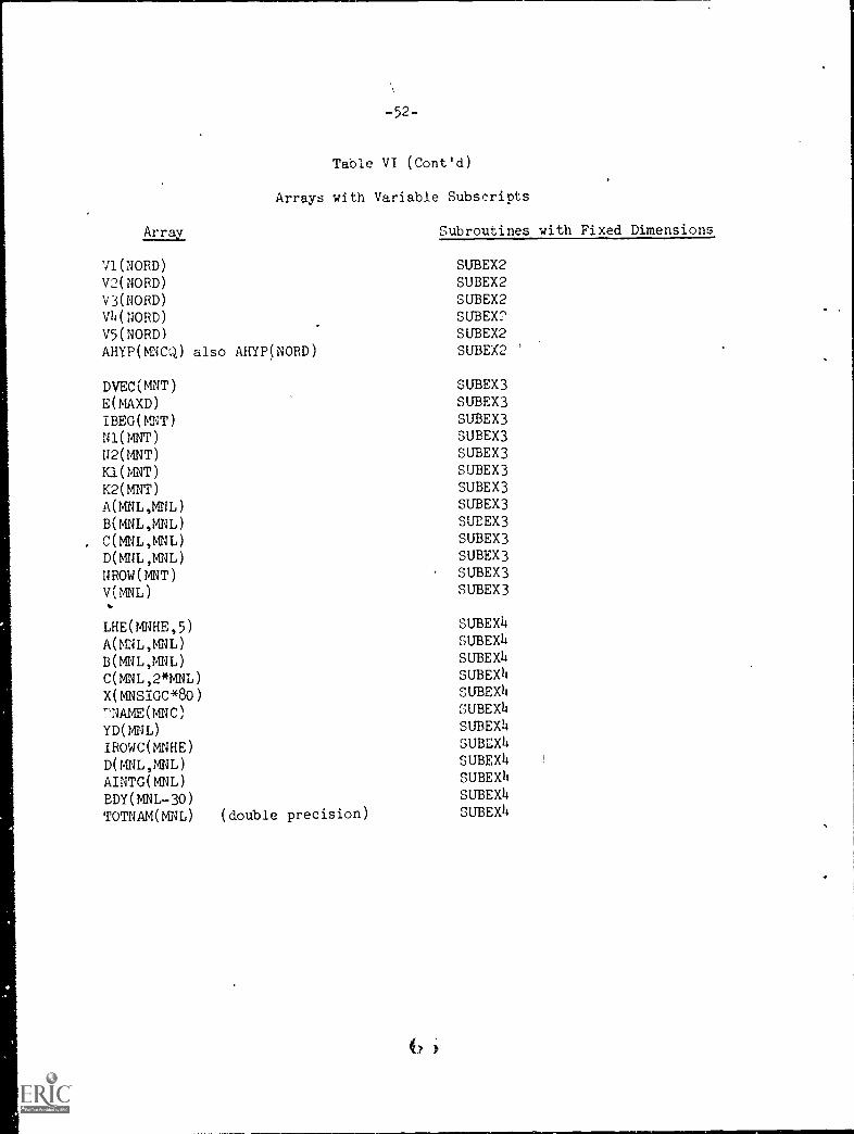
-52-

Table VI (Cont'd)

Arrays with Variable Subscripts

Array Subroutines with Fixed Dimensions

V1(NORD) SUBEX2

V2(NORD) SUBEX2

V3(NORD) SUBEX2Vh(NORD) SUBEX2V5(NORD) SUBEX2

AHYP(MNCQ) also AHYP(NORD) SUBEX2

DVEC(MNT) SUBEX3

E(MAXD) SUBEX3

IBEG(MNT) SUBEX3

N1( KNT ) SUBEX3

U2(MNT) SUBEX3

Kl(MNT) SUBEX3

K2(MNT) SUBEX3

A(MNL,MNL) SUBEX3

B(MNL,MNL) SUBEX3

C(MNL,MNL) SUBEX3

D(MNL,MNL) SUBEX3

UROW(MNT) SUBEX3

V(KNL) SUBEX3

LHE(MNHE,5) SUBEX4

A(MNL,MNL) SUBEX4

B(MNL,MNL) SUBEX4

C(MNL,2*MNL) SUBEX4

X(MNSIGC*80) SUBEX4

7NAME(MNC) SUBEX4

YD(MNL) SUBEX4

IROWC(MNHE) SUBEX4

D(MNL,MNL) SUBEX4

AINTG(MNL) SUBEX4

BDY(MNL-30) SUBEX4

TOTNAM(MNL) (double precision) SUBEX4

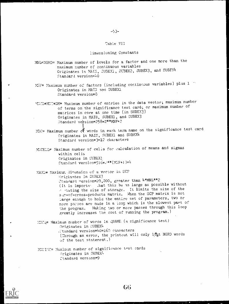
-53-

`able VII

Limensioning Constants

MNL=NORD= Maximum number of levels for a factor and one more than the

maximum number of continuous variablesOriginates in MAIN, SUBEX1, SUBEX2, SUBEX3, and SUBEX4

Standard version=li0

MNF= Maximum number of factors (including continuous variables) plus 1

Originates in MAIN and SUBEX1Standard version=8

m.N.C.D=1:`:=NM= Maximum number of entries in the data vector; maximum number

of terms on the significance test card; or maximum number of

matrices in core at one time (in SUBEX3)

Originates in MAIN, SUBEX1, and SUBEX3Standard velsion=258=2**MNF+2

MIC= Maximum number 0' words in each term name on the significance test card

Originates in MAIN, SUBEX1 and SUBEXL

Standard version=3=12 characters

MNCELL= Maximum number of cells for ,alculation of means and sigmas

within cellsOriginates in SUBEX1Standard versicn=516=,'"(MNF+1)+4

MAXD= Maximum di,nension of a vector in SCPOriginates in SUBEX3Standard ,rersion=20,000, greater than 4*MNL**2

(It is importa _hat this be as large as possible without

q.ating the size of storage. It limits the size of the

sum-of-cross-products matrix. When the SCP matrix is not

large enough to hold the entire set of parameters, two or

more pares are made in a lool: which is the slowest part of

the program. Making two or more passes through this loopgreatly increases the cost of running the program.)

M:;C=. Maximum number of words in QNAME (a significance test)

Originates in SUBEX4standard version =hO =160 characters(Through an error, the printout will only 14t NORD words

of the test statement.)

MNSI(;(7= Maximum number of significance test cards

Originates in SUBEXI.

Standard version=9

66

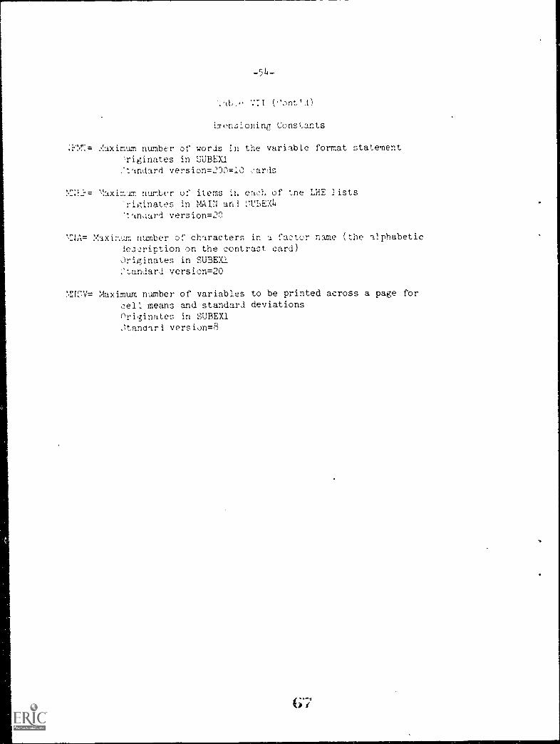
',ab:e VII (''ont11)

irrenzioning Constants

..laximum number of words in the variable format statement)riginates in SUBEXI:tandard version=2")0=10 ,artis

Maxim= number of items it. eacl. of tne LHE ists

'rig,inates in MAIN aril L',I:15EXIE

'1-andard version=:20

M:1A= ,aximu..rn number of characters in a factor name (the alphabetic

lescription on the contrast card)Originates in SUBEX1:standard version=20

Maximum number of variables to be printed across a page for

cell means and standard deviationsnriginates in SUBEX1.tanuari vers ion=8

67

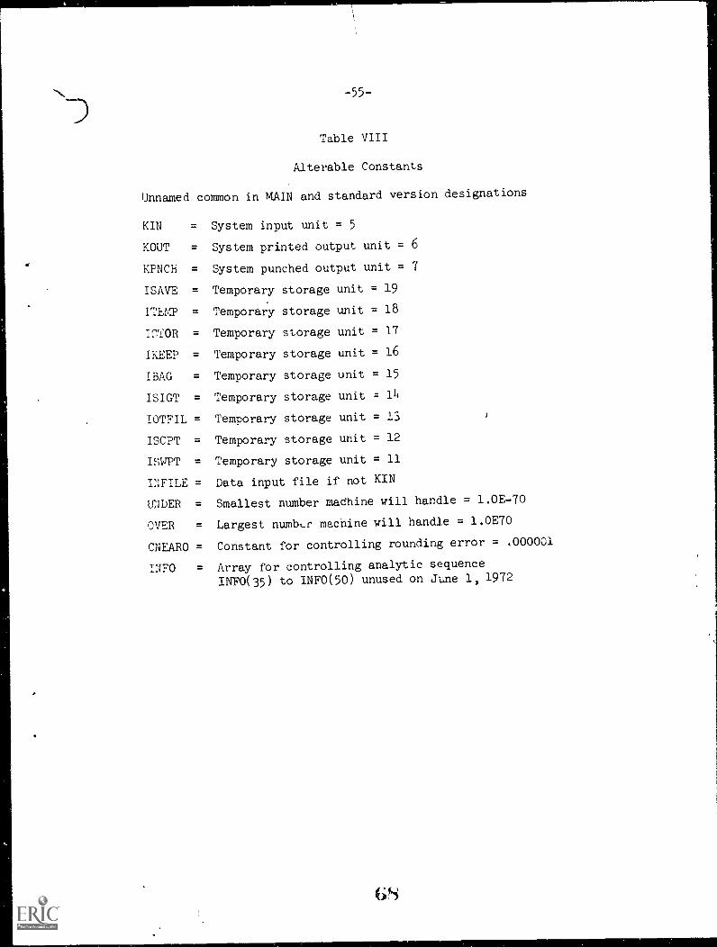
-55-

Table VIII

Alterable Constants

Unnamed common in MAIN and standard version

KIN = System input unit = 5

KOUT = System printed output unit = 6

KPNCH = System punched output unit = 7

ISAVE = Temporary storage unit = 19

ITEM? = Temporary storage unit = 18

IGTOR = Temporary storage unit = 17

IKEEP = Temporary storage unit = 16

IBAG = Temporary storage unit = 15

ISIGT = Temporary storage unit = 14

IOTFIL = Temporary storage unit = 13

ISCPT = Temporary storage unit = 12

ISCPT = Temporary storage unit = 11

INFILE = Data input file if not KIN

UNDER = Smallest number machine will handle = 1.0E-70

OVER = Largest numbtx machine will handle = 1.0E70

CNEARO = Constant for controlling rounding error = .000001

INFO = Array for controlling analytic sequenceINFO(35) to INFO(50) unused on June 1, 1972

designations

GH

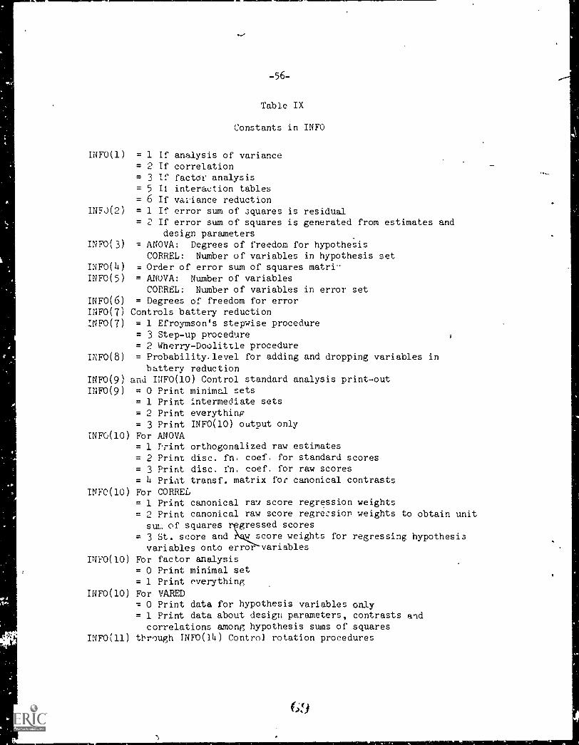
Table IX

Constants in INFO

INFO(1) = 1 If analysis of variance= 2 If correlation= 3 If factor analysis= 5 II interaction tables= 6 If valiance reduction

INFJ(2) = 1 If error sum of squares is residual= 2 If error sum of squares is generated from estimates and

design parametersINFO(3) = ANOVA: Degrees of freedom for hypothesis

CORREL: Number of variables in hypothesis setINFO @) = Order of error sum of squares matri-INFO(5) = ANOVA: Number of variables

CORREL: Number of variables in error setINFO(6) = Degrees of freedom for errorINFO(7) Controls battery reductionnuo(7) = 1 Efroymson's stepwise procedure

= 3 Step-up procedure= 2 Wherry-Doolittle procedure

INFO(8) = Probability.level for adding and dropping variables inbattery reduction

INFO(9) and INFO(10) Control standard analysis print-outINFO(9) = 0 Print minimal sets

= 1 Print intermediate sets= 2 Print everything= 3 Print INFO(10) output only

INFO(10) For ANOVA= 1 Print orthogonalized raw estimates= 2 Print disc. fn. coef. for standard scores= 3 Print disc. fn. coef. for raw scores= 4 Print transf. matrix for canonical contrasts

INFO(10) For CORREL= 1 Print canonical raw score regression weights= 2 Print canonical raw score regression weights to obtain unitsutt of squares regressed scores

= 3 St. score and w score weights for regressing hypothesisvariables onto error variables

INFO(10) For factor analysis= 0 Print minimal set= 1 Print everything

INFO(10) For VARED= 0 Print data for hypothesis variables only= 1 Print data about design parameters, contrasts andcorrelations among hypothesis sums of squares

INFO(11) tbrough INFO(14) Control rotation procedures

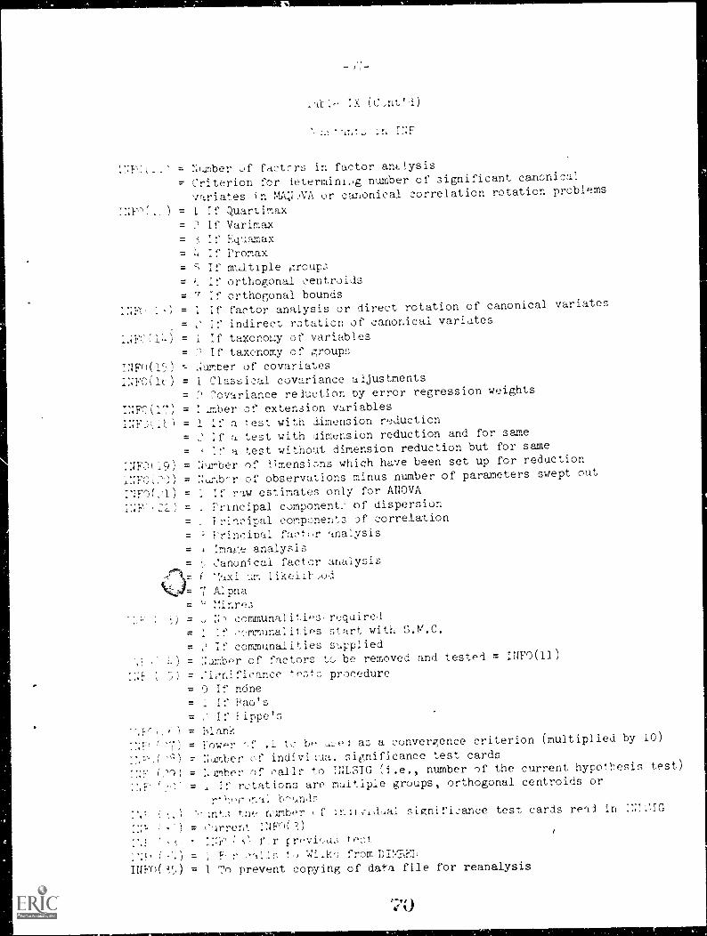
= Number of factors in factor an/Jysis

= Criterion for tetermini.Ag number of significant canonical

variates in WiJVA or canonical correlation rotation problems

iNP'.. ) = 1 If Quartimax= 2 If Varimax

= t if Equamax

= if Promax

= If multiple group:,

= If orthogonal centroids

= If orthogonal bounds

l'; = 1 if factor analysis or direct rotation of canonical variates

= If indirect rotation of canonical variates

1.+Ff:'14) = 1 :f taxonomy of variables= 2 If taxonomy of groups

INF)(15) .:umber of covariates

INFO(1t) = 1 Classical covariance adjustments= 2 Covariance reduction try error regression weights

INFC(17) = : .tuber of extension variables

INFJL_t = I If a test with dimension reduction

= If a test with dimension reduction and for same

= a test without dimension reduction but for same

:NFJ1(19) = Number of iimensio,ns which have been set up for reduction

iNFO:2O) = :;us b-r of observations minus number of parameters swept out

iNM(Z1) = 1 If raw estimates only for ANOVA

1:;F:,21) = 1Principal component: of dispersionirincipal components of correlation

= Principal factor analysis

= j image analysis

= Canonical factor analysis

= ( 'Iaxi um likel_11-,od

Alpna= ' !!inre3

t,) = J communalities, required

= 1 if ,'..,mmuoalities start with S."0.C.

= If communalities supplied= Number of factors to be removed and tested = INFO(11)

= :ignificance te5t;,, procedure

= 0 If ndne= 1 if Pao's

= 2 If Pippe's= Islank

' '7) = Power tY,' .1 to be use: as a convergence criterion (multiplied by 10)

r Number of indivitua, significance test cards

IF (00) = :.1mber of calls to :NLSIG number of the current hypothesis test)

= If rotations are multiple groups, orthogonal centroids or

r'tor)nal bn,AndF

Int3 toe number t f inii,t.dual significance test cards read in

= current INFo(''.)

:11 f_ r

IF. r ,.'all:- to Wi2te.,; from Drr,-,,EP

INFo(t') = 1 To prevent copying of data file for reanalysis

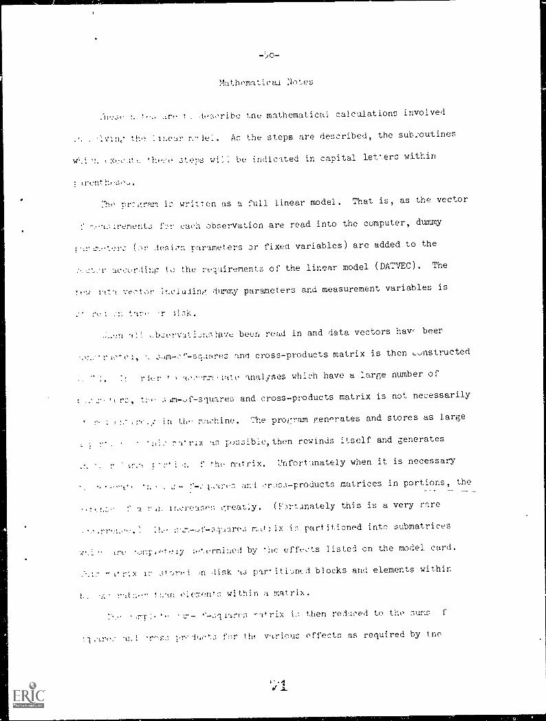
Mathematical Notes

n_te, are t_ describe tne mathematical calculations involved

'lying the :Inear Ao the steps are described, the subooutines

'n xectitt_ these steps will be indicated in capital letters within

trent nese,J.

1,7he pr-gram is written as a full linear model. That is, as the vector

-..-trement3 f'r each observation are read into the computer, dummy

t..tleter.:, (or design parameters or fixed variables) are added to the

r accurding to the requirements of the linear model (DATVEC). The

t t'it'. veotor 1hclulinr dummy parameters and measurement variables is

sel zrt t are. or _tick.

en al? t_b3ervatiphol-ave been read in and data vectors hay, beer

cam-of-sq.lbres and cross-products matrix is then t..onstructed

rier ao,'omm,tate analyses which have a large number of

3,T1-,C-squares and cross-products matrix is not necessarily

nttre.y in the machine. The program generates and stores as large

ratrix as possible, then rewinds itself and generates

1 ,n the mat rix. Unfortunately when it is necessary

1,areS and cros.3-products matrices in portions, the

increases greatly. (Fprtdnately this is a very rare

:he sam-uf-square3 mattix is partitioned into submatrices

tre tetermined by the effects listed on the model card.

ttrix is Jt'orei ,n disk '13 partiti-Jrac_d blocks and elements within

rather t nan elements within a matrix.

watrix then reduced to the sums -f

ani preducts for tilt_ various effects as required by the

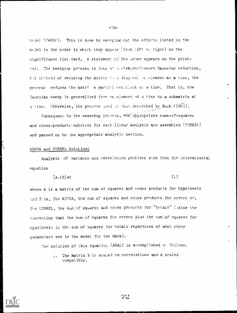
-59--

model (;VEEP). This is done by sweeping out the effects listed in the

model in the order in which they appear from left to right) on the

significance list card. A statement of the orier appears on the print-

ut. The sweeping process is done a- a straightforward Gaussian reduction,

bit instead of reducing the matrix t) a liag(_nal In element at a time, the

process reduces the mats: a partiti red t:lock a, a time. That is the

Gaussian sweep is generalized from an element at a time to a submatrix at

a time. Otherwise, the process Ased is that described by Boc1 -(196 3).

Subsequent to the sweeping process,-the appropriate sums-of-squares

and cross-products matrices for each linear analysis are assembled (MIBEX4)

and passed on to :he appropriate analytic section.

ANOVA and CORREL Solutions

Analysis of variance and correlation problems stem from the determinants'

equation

IA-ABI=0 (1)

where A is a matrix of the sum of squares and cross products for hypothesis

ant B is, for ANnVA, the sum of squares and cross products for errors or,

fnr CORREL, the su.r1 of squares and cross products for "totals" (Asing the

convention that the sum of squares for errors plus the sum of squares for

hypothesis is the sum of squares for totals regardless of what other

parameters are in the model for the data).

The solution of this equation (ANAL) is accomplished as follows.

The matrix B is scaled to correlations and A scaled

compatibly.

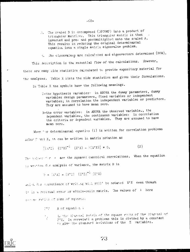
-60-

The scaled B is decomposed (LECOMP) into a product of

triangular matrices. This triangular matrix is then

inverted and pre- and postmultiplied onto the scaled A.

This results in reducing the original determinantal

equation into a single matrix eigenvalue problem.

f. .'he eigenvalue.s are calculated and eigenvectors determined (HOW).

This des,:ription is the essential flow of the calculations. However,

there are many side statistics calculated to provide expository material for

the analyses. Table X lists the side statistics and gives their formulations.

In Table X the symbols have the following meanings.

Z-the hypothesis variables: in ANOVA the dummy parameters, dummy

variables design parameters, fixed variables or independent

variables; in correlation the independent variables or predictors.

They are assumed to have mean zero.

X-the error variables: in ANOVA the observed variable.., the

dependent variables, the continuous variables: in correlation

the criteria or dependent variables. They are assumed to have

mean zero.

When 'ae determinantal equation (1) is written for correlation problems

lsinr ani X, it can be written in matrix notation as

(7,'x)-1 (vx) - '(X'x)1 = o.

v11-_.es a are the squared canonical correlations. When the equation

written f[_r analysis of variance, the matrix B is

PX) - (X12) (Z1 Z)-1 (7:X)

wni.h for ,--lvenience of writ_ng wlil sail' be notated X'X even though

is a residual error or witnin-cells matrix. The values of X here

rat sims of squ=ir(,6.

A of equati, n 1

L tLe iiap7c,nal matrix of the square roots of the Jiarr-nal of

?'Z. In correlati n problems this is divided by a constant

to give the standard deviations of the Z variables.

73

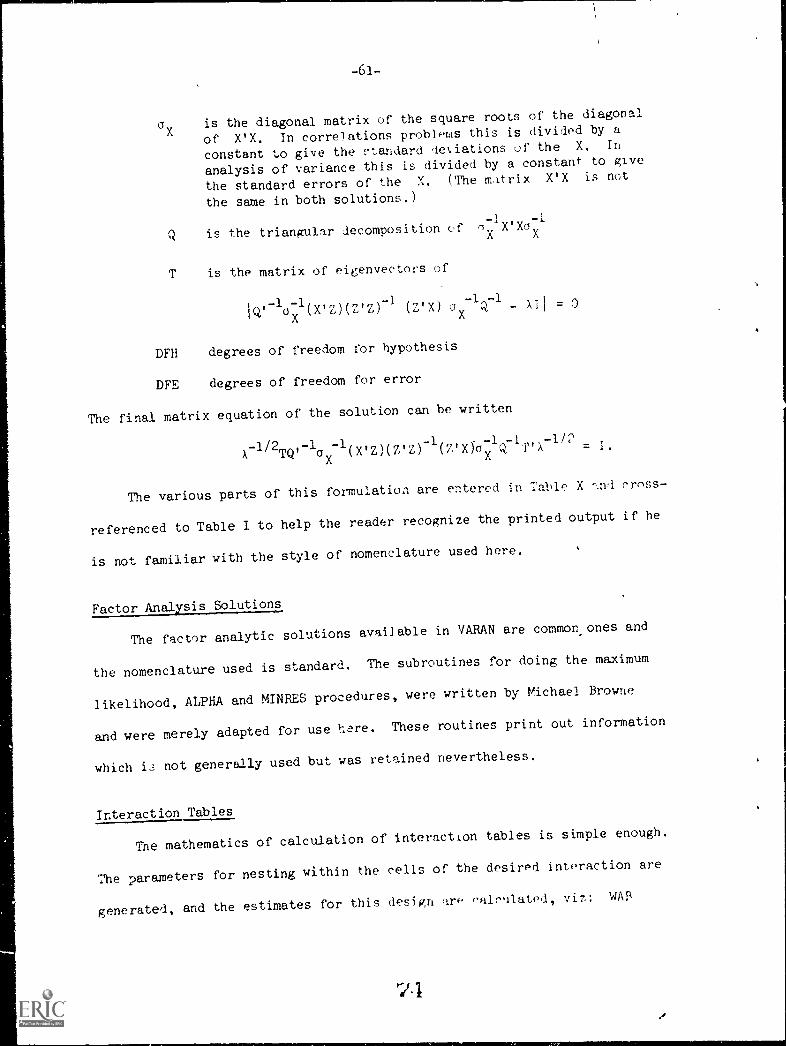
-61-

oX

is the diagonal matrix of the square roots of the diagonal

of X'X. In correlations problems this is divided by a

constant to give the ctandard de'.iations of the X. In

analysis of variance this is divided by a constant to give

the standard errors of the X. (The mitrix X'X is nct

the same in both solutions.)

Q is the triangular decomposition of (11XiXo-1X X

T is the matrix of eigenvectors of

1Q,-1u_,,x1tx 7,)(7)7,)-1 (7,1X)

x1Q-1 -

DFH degrees of freedom for hypothesis

DFE degrees of freedom for error

The final matrix equation of the solution can be written

= 0

1

A-1/2

TQ'-1

ox

-1(X°Z)(7.'7.)

-1(7'X).(1-"Q7

1

T'X = I.X

The various parts of this formulation are entered in Table X %nd cross-

referenced to Table I to help the reader recognize the printed output if he

is not familiar with the style of nomenclature used here.

Factor Analysis Solutions

The factor analytic solutions available in VARAN are common ones and

the nomenclature used is standard. The subroutines for doing the maximum

likelihood, ALPHA and MINRES procedures, were written by Michael Browne

and were merely adapted for use tare. These routines print out information

which i not generally used but was retained nevertheless.

Interaction Tables

The mathematics ofcalculation of interaction tables is simple enough.

The parameters for nesting within the cells of the desired interaction are

generated, and the estimates for this design oftlo,ilated, viz: WAR

7.1

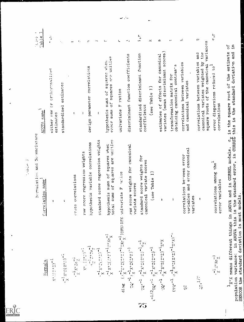
Formula

-1X'

X

:01_

X1 X

k

-1

I.c-rmulatio sand Noenclature

Correlation name

1ANOVA name

cress correlations

raw score regression weights

hypothesis variable correlations

standard score regression weights

hypothesis sums of squares when

total sums of squares are unities

ding

'',(- 7.)

Z>to

univariate F

A \-

TQ,-1 J-lx,z(z,z)-10-1

-1/2

-1

-1

XTQ'

ox

X'7,(17.12.)-1

-1

Tq,

0x-x,z(z,z)-17,7x

(TQ'-1

0-1X'7,(Z1Z) 121X)--

1/

,-

Xo1

raw score weights for

canonical

variate scores

standard score weights for

canonical variate scores

(see Table I)

correlations between error

variables and error canonical

variates

correlations among the1

error variables

either raw or orthognalized

estimates

standardized estimates

design parameter correlations

hypothesis sums of squares wten

error sums of squares a

unities

univariate F ratios

discriminant function coefficients

standardized discriminant function

coefficients

(see Table I)

estimates of effects for canonical

variates (mean discriminant scores)

transformation matrix for

obtaining canonical contrasts

correlations between variables

and canonical variates

7able

correlations between variables and

canonical variates weighted by the

square roots of the canonical

variances

error dispersions reduced

tot

correlations

1X1X means different things in ANOVA and inCORBEL models.

av is the square root of the

estimate of

population variance:

in ANOVA this is the standard error, in

CORREt this is the standard deviation and in

SERCOR the standard deviation in most models.

i,r

k h e9T

-63-

1 roduces the estimates for the cell:, cf the AP face of a factorial design.

gran: lean mult .,led 1ri i141/1.1-7

The acronym IITAPL cc: rides -.jut when e

ave been -..)b+ained, then pT1rt3 them °lit.

Varience Peduction Analysis

ance re iucti on %in`1.1,y > i3 pro,edure for evaluiting the

efcct of i.i,baIanye in an tesign iu t.l unf :al cell sizes. Basically,

hypothesis sums of .,Tian -; r the given test is generated both before

an after taking account of the inequality of cell sizes. (The grand mean

is not removed from the data.) The "before" sums of squares is assumed

to be 100 per cent of the data available. When the "after" sums o" squares

is larger than the "before" a negative loss is indicated.

Dimension Reduction Analysis

ills feature is 'available through the significance test card and is

indicated by a minus sign (-). In use it pertains to a feature of multi-

variate analysis of variance and canonical correlation which has no uni-

variate ar,1

To explain its '1'3(', ';',f,ry)sf- we are giver two independent statistical

hypotheses, both involving the same error variables, such as an interaction

a main effects test in a MANOVA resign if variables. '2uppose the

interaction test, AP.:-V, has r < p significant dimensions (or roots).

hest. r limensions of the p ,3imensions of error have the sruie

iers les as r vari obi e- in r uni variate analyses and suggest that

effects r i rn-t tp,r 9,)w-

-ver, tt,c. remaining p-r iimensions of er rd. are not interact ,e and can

reas-nably ' este I over th, main et* fe A.

a

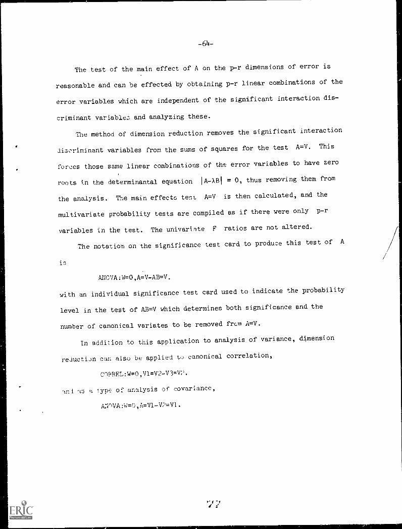
-611-

The test of the main effect of A on the p-r dimensions of error is

reasonable and can be effected by obtaining p-r linear combinations of the

error variables which are independent of the significant interaction dis-

criminant variable:, and analyzing these.

The method of dimension reduction removes the significant interaction

discriminant variables from the sums of squares for the test A=V. This

forces those same linear combinations of the error variables to have zero

roots in the determinantal equation IA -ABI = 0, thus removing them from

the analysis. The main effects test A=V is then calculated, and the

multivariate probability tests are compiled as if there were only p-r

variables in the test. The univarinte F ratios are not altered.

The notation on the significance test card to produce this test of A

is

ANOVA:14=0,A=V-AB=V.

with an individual significance test card used to indicate the probability

level in the test of AB=V which determines both significance and the

number of canonical variates to be removed from A=V.

In addition to this application to analysis of variance, dimension

reuctiDn can also be applied to canonical correlation,

CnPREL:W=0,V1=V2-V3=VP.

ts a type of analysis of covariance,

ANnVA:W=0,A=V1-W=V1.

-64a-

Rotation Procedures for Canonical Variates and Factors

Eight rotation procedures are available for multivariate solutions to

linear models. Four of these are familiar techniques of factor analysis:

Quartimax, Varimax, Equamax and Promax. These four techniques apply

mathematical criteria to the solutions and rotate the correlations between

the canonical variates and the variables to a solution that is presumably

more comprehensible to the researcher.

The remaining four rotation procedures apply external criteria to the

rotational procedure. In multiple groups, orthogonal centroids and orthog-

onal bounds, a set of regression weights are entered and used to determine

the correlations between the rotated canonical variates and the variables.

This makes all these procedures Procrustian in form; however, they are not

explicitly Procrustian in that they use regression weights, not target co-

efficient matrices. The multiple groups procedure obtains an oblique

solution. The orthogonal centroids scheme is similar but uses the first set

of weights optimally, then uses the second set of weights optimally but

orthogonal to the first set. Successive weights are fitted optimally but

orthogonal to all the previously fitted weights.

Orthogonal bounds is Procrustian in form also. First a multiple group

oblique solution is found then an orthogonal envelope is found which has a

least squares fit about the multiple group solution. The correlations

between the canonical variates and the variables are rotated to the envelope.

Thr orthogonal Procrustes scheme is due to Norman Cliff and is

r'ferenced in the bibliography. The calculation scheme is due to Roger

P-tnnell. Here the weights supplied are the "target" matrix of coefficients

and not regression weights.

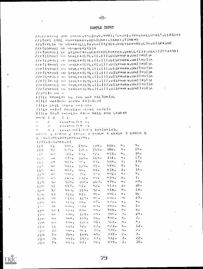
-65-

SAMPLE INPUT

/ /L1 -111 U/ Jori Innoo,55,10,9,999),'04161,11-m,hALLCHASI,CLASS=t//T/7.1-)1 tX1-C ,,6N=VAkAN,KtGIUN=1,1(36k),11Mt=5//itPLIn 00 oSN=HALLLIti,UNI1=2314,V0L=StR=RLSL1h,01$1)=HR//t-TU51-Oul o0 0oAJANt=sysiN//rT061-01 00 SYS001=A,uLt5=(i-q-ChP1=1-hA,LKELL=133,oLKSIZI-7-345H)//rT11rou1 00 SPACr=(LYL,(1,1))-9U1SP=NI-w,uNI1=0JK//h1101 oo SPACh=(CYL9(1,1)),U1SP=New,UNI1=uISN1/F7'1 3i-001 PO ',-,PALF=(GYL,(1,1)),DISP=NFVOUNII=OISN,

//h114M)01 )11) SPALL=(LYL,(1,1)),U1S1'=NFW,UNIT=UISK//t-T15UU1 011 SPAU-=(LYLI(111)),DISP=Nt"W,UNIT=LASK//1-1161-0U1 HU SPACr=1CYL,(1,1)),U1SP=10-w,U1'iIT=DISK//1-T17t-im) v )-'AL1-=(CYL11111))tuiSP=NI-w,UN11=UIShc

oo .ACr=1CYL,(1,1)),U1SP=Nbw,UNI1=DISK//1-119roo1 01) 1-ALr=1LYL,(1,1)),u1SP= 'v1vitUNI1=0IK//YSIN oo111Lt o, 1WU 1vASY 1-ALTUNIAL11ILt- vigx1r0H k:oitvA 1-Kiw11.01

111Lr Lt-LL

MO* ProoLt-0 wuorL A11-(1A111Lc T17.1 rko,,Lrp- hktim HALL APlu CRAI,.0evktlh 1 3 1 1

,,,,t -4 A.

(2 I 1,1o,k thh-C).U)

,;) 1//4KIAhLtS.3 tkKOH 4 tKKUk 5 El-KRUK 6

117 41 7411/4, 1 )b. 1u4. Sub. 4. 9.

117 41 4/5. 1/0. 105. 360. 4. 16.

!17 H, *41. r15. 16.

//'4. 104. 331. 4. 17.

11 )737 to-. 51. 5h4. 3. 13

11 4" 11c, 71 `)19. 5. 5.

1in 41 Y4)1. kni 49. 41b. 3. 16.

II') <sr, 119t` 7"s. 492. 4. 9.

1 i

iin4" r-t.

50-).

i1/ion.

m9,

Z01.479.474.

7.

4.1.

-9.

-)1 '351. 91. 513. 3. 26.

1(,) 51 64/. 114 5Z. 41b. 4. 16.

1(n 53 /14. rl. 7U. 491. 4. U.

1/n 12-). MU. 0/U. 1. Z5.

1/ /11. 67. 4/I. 4. 4.

h4. 45. 4. 7.

1 /s' 7/ t . 740. 4. b.

11'- 'pr-c 1/5 m7. 4h4. 4. 24.

qnr-t. i0(4 Y4. 1,,)4.. 4!It") '1,14 /( Yl ,t)3 4.

11 /1 47. 1/. n7. h/3. 4. 12.

1 1/ m4M 9t. 4)49. 4. /.

11H 73 104. 1W-4. 47 355. /. 114 (465. 14/. hl. 432. 3. LL.

/1t4 75 'v-». 91. 497. 16.

79

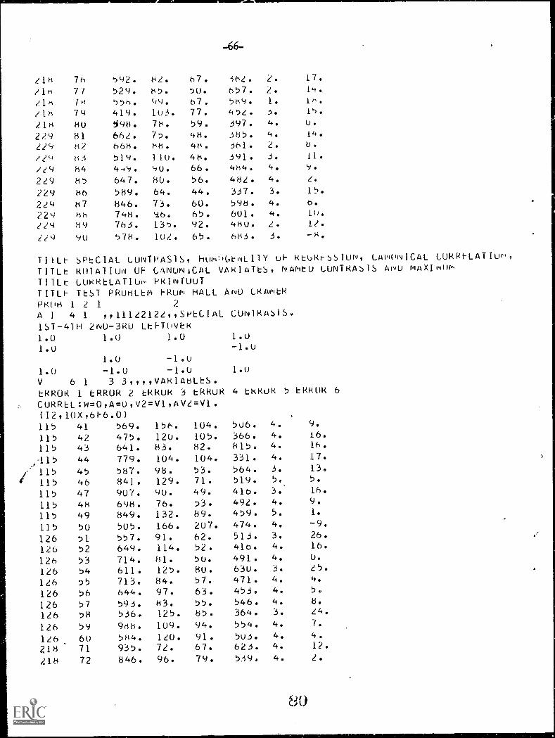
218/1811h218218229229

/29/192292292292292292e9

7h 592. 82. 67.77 529. e5. 50.

1+ ,-)56. 99. 67.79 419. 103. 77.

80 598. 7e. 59.

81 662. 75. 48.8? hhh. 88. 48.

83 519. 110. 48.84 4-t9. 90. 66.85 647. 80. 56.

86 589. 64. 44.

87 846. 73. 60.)1h 748. 9.5. 65.89 763. 135. 92.

90 578. 102. 65.

-66-

362. 2. 17.

657. 2. 14.

589. 1. 18.

47C. J. 15.

397. 4. U.

385. 4. 14.

361. 2. 8.

391. 3. 11.

484. 4. v.

482. 4. 2.

337. 3. 15.

596. 4. 6.

601. 4. 10.

480. 2. II.

683. 3. -8.

THLt- SPtC1AL LUNTRAS1S, Hurl 1(,b4L11Y OF REuRrsSIUN, CAI 1,1 11\1 ICAL CURkt-LATIw,

TITLE RulAl1uN OF CANONICAL VARIATES, NANtO LuNTRAsls ANU HAMNomTITLE_ LORRELATIo0 PR1NFUUTTITLF TEST PRUtiLEf' FROM HALL AM) GkAmERPR08 1 2 1 2

A 1 4 1 11122122 SPECIAL LUN1RAS1S.1ST-4TH 2N0-3R0 LEFTOVER1.0 1.0 1.0 1.0

1.0 -1.01.0 -1.0

1.0 -1.0 -1.0 1.0

V 6 1 3 3,,,,VAk1A8LES.ERROR 1 ERROR 2 tkkuk 3 ERROR 4 ERROR 5 ERROR 6

CURRLL:W=0,A=0,V2=V1IAV2=V1.(12,10X,6F-6.0)115 41 569. 156. 104. 506. 4. 9.

115 42 475. 120. 105. 366. 4. 16.

115 43 641. 83. 82. 815. 4. 16.

,115 44 779. 104. 104. 331. 4. 17.

115 45 587. 98. 53. 564. 3. 13.

115 46 841. 129. 71. 519. 5. 5.

115 47 907. 90. 49. 416. 3. 16.

115 48 698. 76. 53. 492. 4. 9.

115 49 849. 132. 89. 459. 5. 1.

115 50 505. 166. 207. 474. 4. -9.

126 51 557. 91. 62. 513. 3. 26.

126 52 649. 114. 52. 41a. 4. 16.

126 53 714. 81. 50. 491. 4. U.

126 54 611. 125. 80. 630. 3. 25.

126 55 713. 84. 57. 471. 4. 4.

126 56 644. 97. 63. 453. 4. 5.

126 57 593. 83. 55. 546. 4. 8.

126 58 536. 125. 85. 364. 3. 24.

126 59 988. 109. 94. 554. 4. 7.

126 60 584. 120. 91. 503. 4. 4.

218 71 935. 72. 67. 623. 4. I?.

218 72 846. 96. 79. 549. 4. 2.

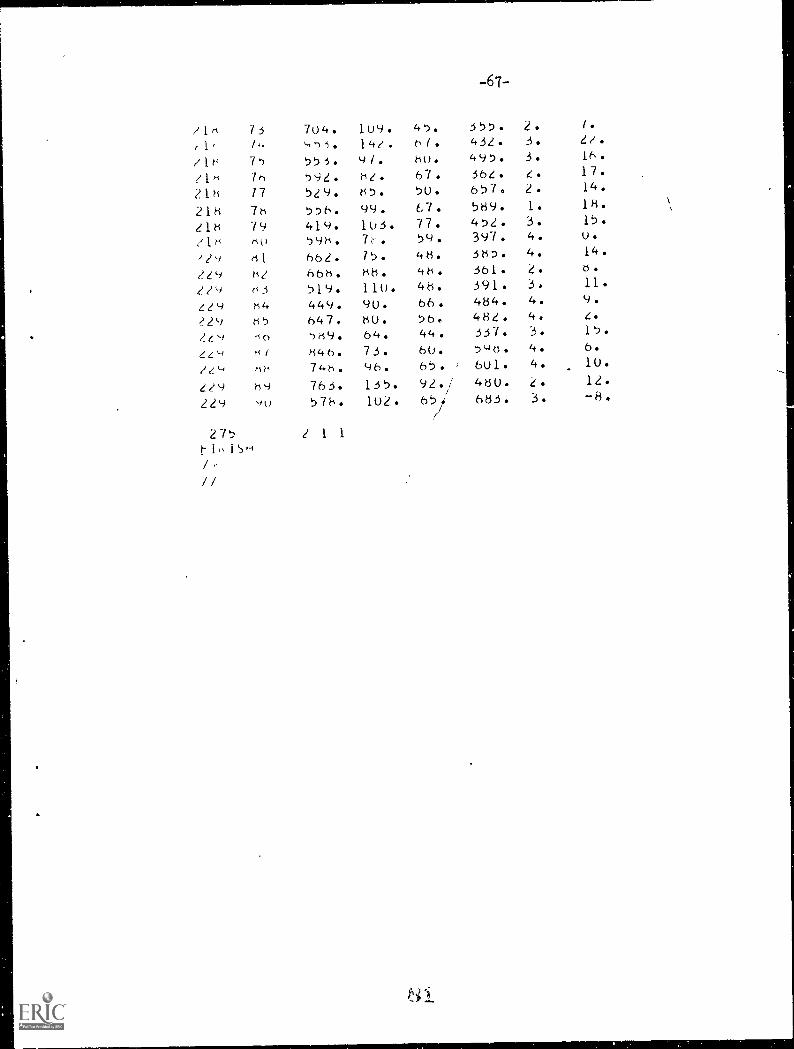
-67-

/1,s /3 704. 109. 45. 355. 2. I.(1' 14-. .,.-)3. 14?. t,i. 432. 3. 2/.

/it' 75 55.5. 97, 80. 495. 3. 16.

11m 7h 592. h/. 67. 362. Z. 17.21h 17 529. 85. 5U. 657. 2. 14.

218 7h 556. 99. E 7. 589. 1. 18.218 74 419. 103. 71. 452. 3. 15.4'18 80 598. / . 59. 397. 4. U.

)1) 81 662. /5. 48. 385. 4. 14.

1 z 9 82 668. m8. 48. 361. 2. d.

2I9 ti i 519. 110. 48. 391. 3. 11.

229 84 449. 9U. 66. 484. 4. 9.

?29 85 647. 8U. 56. 482. 4. L.

?e9 ,-0 589. 64. 44. 337. 3. 15.4'-i 7' 846. 73. 60. 590. 4. 6.

,,,,,u po, 71-0-1. 96. 65. 601. 4. 10.

2/9 89 763. 135. 92.1 480. Z. 12.229 90 578. 102. 65/ 683. 3. -8.

275 2 1 1

8I .15H-+

/

//

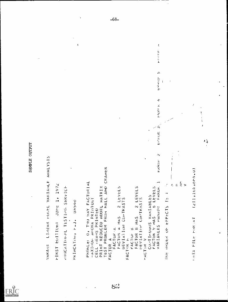
SA

MP

LE O

UT

PU

T

VARAN:

LMEAR NUoE=L VARIANCE- ANALYSIS

t-IRST hOITION:

JUP.B 1, 1972

rDOCATINNPL TESTING- SERVICE

PRINCETON, N.J.

0854

0

PkOhLEI

0, T'4O 1:IAY FACTORIAL

AXINU ANOVA PRINIOUT

CELL NEANS PRINTED

PRINT REDUCED MODEL MATRIX

TEST PROBLEM FROM HALL AND CRAER

FACTOR A

41X

FACTuP-A

FACTOR A HAS

2 LEVELS

DEVIAI011 CONTRASTS

FACTOR h

FACTOR

FACTOR B HAS

2 LEVELS

WEVIATIllw CuoTRASIS

+-ACToR V

CLI.JTINOu0S VARIABLES

FACTOR V HAS

6 LEVELS

VARIABLES NAIED:

ERkOK

ItRkOr 2

touR

t-I<P1 I:

4

THE ORDEr' OF EFFECTS IS

:

h V

r,LITA

FILE-

E144';LIT

(c11,10X,6F6.0)

tQ.lip

5,

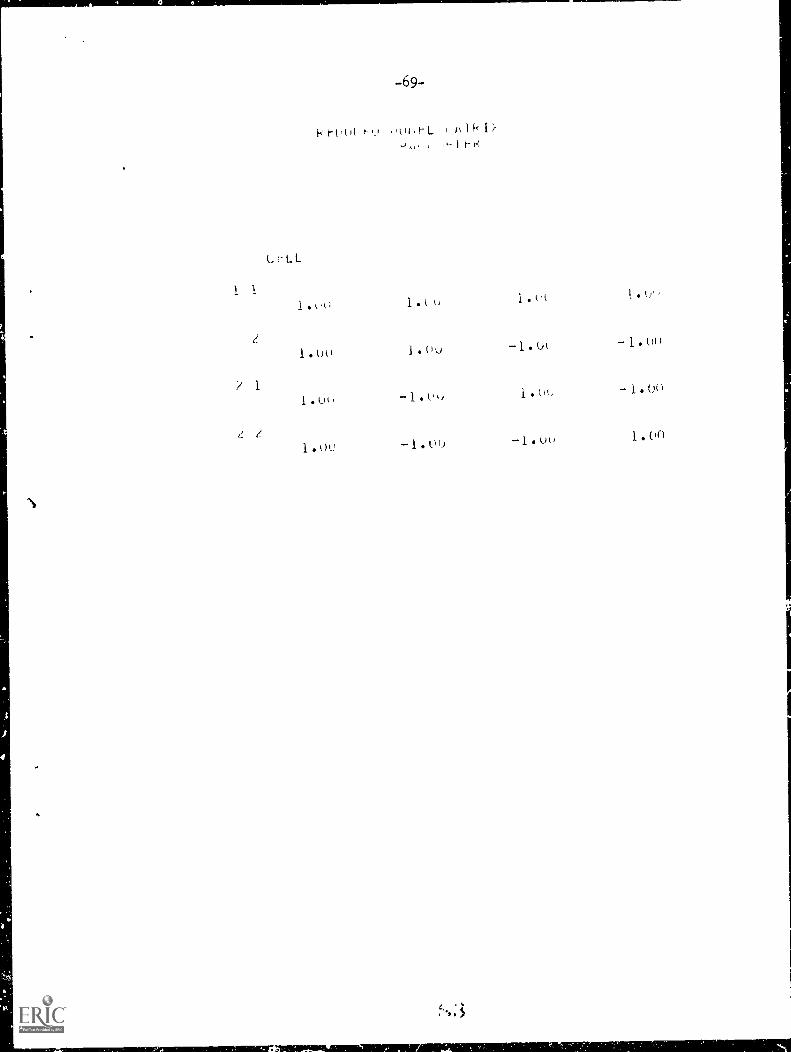
-69.-

iqN)PP/'

1

?

/_

1

(I-LL

1.00

1.0o

1.00

1.0u

1 c 0

1.0u

-100

-1.0)

1.00

1.0

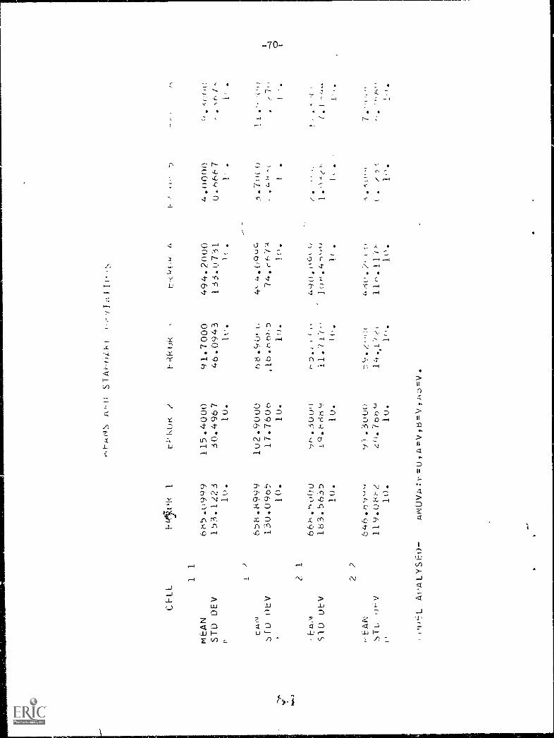
AfD STAH,)4k(

MEAN

STO 0EV

1

f-A

Dk

1

685.0999

153.1223

10.

t;-'ut<

r

115.4000

30.4967

10.

8kkok

91.7000

46.0943

tu.

t-K

kc,u

494.2000

133.0731 .

4.0000

0.6667

1'

..

CA

N658.8999

102.9000

68.901 t,

44.0QuQ

510 0EV

130.0965

17.7606

74.rf,7-4

.7

-410.

10.

1(1.

0

21

668.5000

D.,

+,

4040

.00k

c,/.

SID uEV

183.5635

19.8889

It).L

tnt.4

ki/ .

)

10.

10.

I(..

.

22

-EAN

646.89-9

9).3000

.1(

7.

ST(. 01-V

119.08r2

20.7bou

11(-

.111

.10.

10.

10.

10

Al-ALYSED-

ANOVA:1.,=0,A=V03=V,Ab=v.

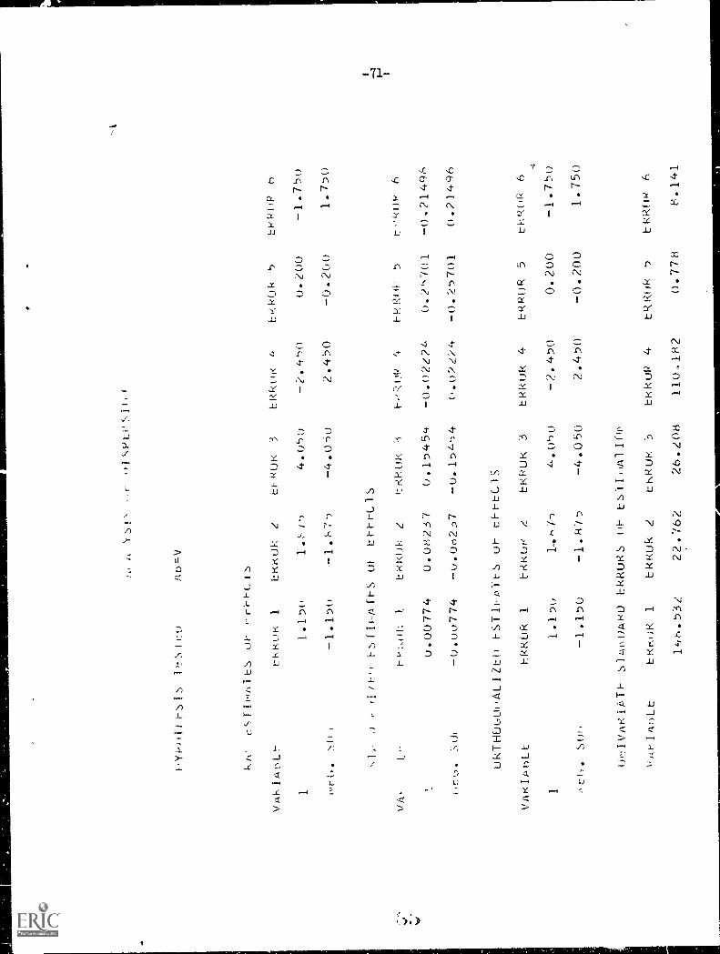
S!

r

itSfrO

Aor-V

kfc

cSIDAltS oF

.--1-1-1-.Gis

VARIAnLt

FKKu8

1EKKOk 2

ti-POR

3FRkOr< 4

El-i.P0k

51:78P0R h

11.170

1.')

4.050

2.4')0

0.200

1.750

oi-0.

)1J,

1.150

1.F-75

4.050

2.450

0.200

1.770

1[-S111-,A11-S ut

Li-Fr-OS

\1/A,'

L-

f-4-':.01(

1EkKI_W

217r(P.01.

)(--,';Ig)

4el-).$1P

51:'k01-,

6

U.00774

0.08237

0.15454

0.02224

0.2",701

0.21496

it,,,.

30r

0.00774 0.0627 0.15454

0.0224

0.25701

0.21496

ukTHO0u1.ALIZEO ESTII-pYrs ur tFrtCIS

VAkIAoLt

rkkUR 1

ertkut<

2bRPuk 3

ERROR 4

LRR0R 5

ti-OZOR

6--4

11.150

1,.?"7n

4.050

2.450

0.200

1.75u

t-_(,.

Sul.

1.150

1.875

4.050

2.450

0.200

1.750

U0AVArZikTF slpougH0 FkRUKS

Ls-1111/0'11v

14,6.534

22.762 AIM&

26.208

110.182

EKkuP 4

tRf.Oik

5EkROP 6

0.778

8.141

kgvIgriLt

ERI-JJK

1ERRLik 2

tt.R0K

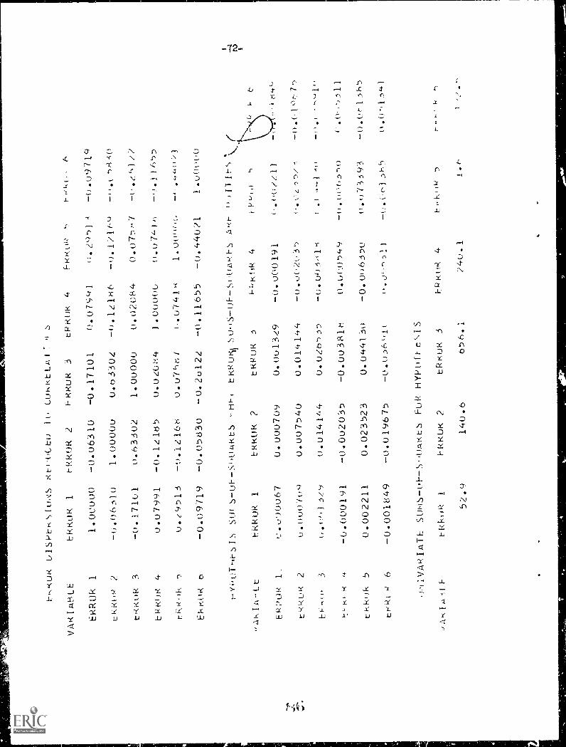
t71.RUR

VARIW3LE

01.SPSI(JS

ERROR

1

Rti'0060 10

rkkOR 2

COKKbLA17

17RRuR 3

tRRoR 4

F-KRIR

ti

kkar,

6

ERROR

11.0CUU11

-0.06310

-0.17101

0.07Y-I1

0./.9')14

-0.09714

rkkW4

2-0.06310

1.00000

0.03302

-0.12186

-0.12169

-0.L58-i0

ERK0k

3-0.17101

u.63302

1.00000

0.02084

0.07587

-0.1112

e0K0R

40.07991

-0.12165

0.020 ?t4

7.00000

0.074)

-0.11655

rRkiik

5u.e9513

-0.12168

0.0Thr;I

(,.07418

-,.44f1;,)

EkKoR

o-0.09719

-0.0563U

-0.20122

-0.11655

-0.440?1

1.00000

t-iy

i-,0T

HI-

SU

( S

-01-

-S0O

AK

tS -

t-0-

1

o'

,_.is, I A - L t

t-i k k U k

1ERROR 2

EI-OR 1.

,....v00067

0.000709

tuR 2

0.000-/o9

0.007540

E f- , 1

i .

3ii,

,l;,.)

3,!_

`J0.014144

-t-

o1

H,-

4.-0.000191

-0.002035

tRkuk 5

0.002211

0.023523

t+ R(k 6

-0.001849

-0.019675

,wrIVARIATL SONS-01--S0OARtS FoR

LRRrit

1FRKOR 2

E.KRuN Ski0S-01--S01(ARF-

t RP UR 3

1-f,K11(.!

4

0.0u1329

-0.000191

0.014144

-0.002(,3')

0.026535

-0.00318

-0.003816

0.0(,0549

0.0441

-0.0063,0

-0.036,f it

0.0.311

HYPtiftcc,IS

tRRuR 3

11-PRi(R 4

,11'<

" ) IT I i-

t-1-'1-1,$

`'.

00/211

i,)e-)5./.

t./

t.,1 AI.

-0.tw6.3n0

0.073393

-0.0r1385 n

kt,

.1'1844

_m.1,-,,p,

c.0,,-)3.11

-0.0e1385

.,4

0.0 131 h

52.9

140.6

656.1

240.1

1.r

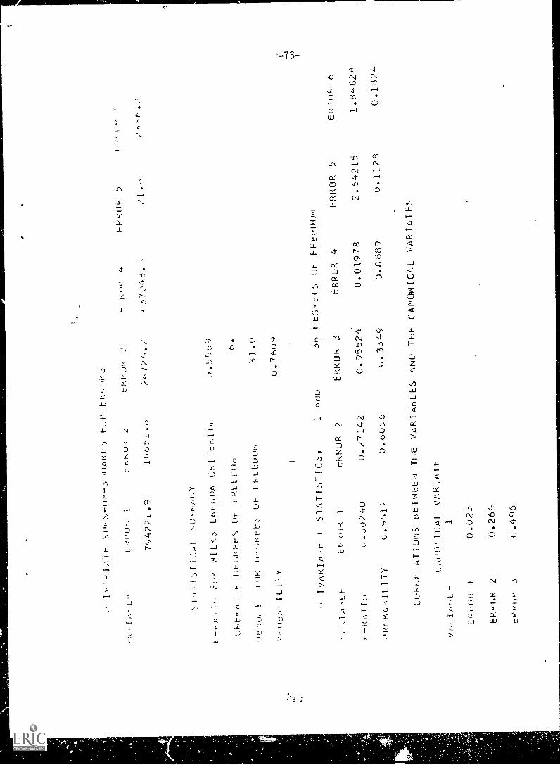
ATt-

1,HAI<LS

t-UP

Alr.Lr

tRIdu,,,

1

794221.9

rNhAJK 2

tP,r0t,

5

16651.6

?6-121,./

\01,AKY

hr.41!1, ,=08

OILKS LAI.THJA Ct<ITtklOH

0.5569

DthRttS 0F FKLE-Dy0

6.

iHk

L.11-=

V1-(LLULlh

3).0

ILI1Y

0.7609

IVARIAir h SlATITICS,

4hI-e-0Ik

5

o37043. s

11.

1AHD

5t)

I.EGRE-ES uF

.IA'L h

e'P.RtiK

1tkRuR 2

3ERROR 4

ERROR 5

ERROP 6

t--KAlltt

u.00240

0.27142

0.95524

0.01978

2.64215

1.84828

PktiriA',11LITY

0.'1612

0.6056

.3349

0.8889

0.1128

0.1824

GOr4KLLATIOHS bETWEEN THE

VARIAbLES AND THE CANONIUL

VARIATES

Cwill\ICAL VARIATt

1

ERr-mR

10.025

ERROR 2

0.264

cowl,

50.4Q6

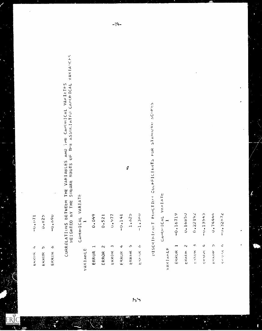
1-RRoR

ERROR 5

ERROR 6

-0.071

0.825

-O.69u

CORRELATIONS BETWEEN THE VARIABLES AND iHt C1-000NICAL

VARIATFS

WEIGHTED by THE SOUARE ROUTS OF THE ASSOLIATFO CANONICAL

vARIACFc

VARIABLE

CA1"01«ICAL

1

VARIATE

ERROR

10.049

ERROR

20.521

ERROR

30.977

ERROR

4-0.141

.11,

4

ERROR

51.625

tRi-oR

6-1.360

oISCRINIoAI,T FONCTIoq CuLFFICIENTS FuR sTANwRo

.CoPt.s

Cw"OwICAL VAI<IATt

VARIABLE

1

ERROR

1-0.16719

EkkoR

20.16850

E.ckoR

0.22192

=1,1-:

4-

u.13

543

tk:K1W

0.74444

60.3274

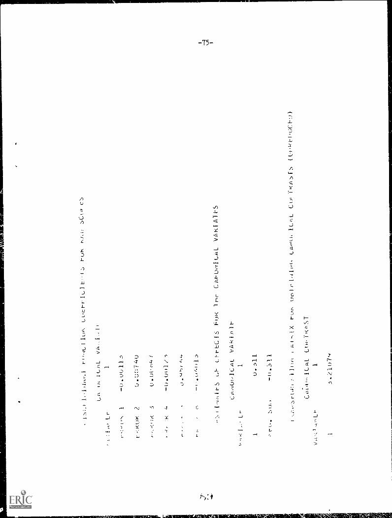
GA

ai C

AL

VA

,. l,;

r

1

,kT

cuur

-rIc

itn1;

)F\AL

FIJK lmc Ci.woolGAL V4KIATt-S

CilmAJICAL VAkiA1t-

1

u.:511

IIt%

I'N

Xt-

UF

N1.

411'

('C

o. 1

P<

As

(

_ LAI

ICA

!.C

Ut`

iK«S

T

1

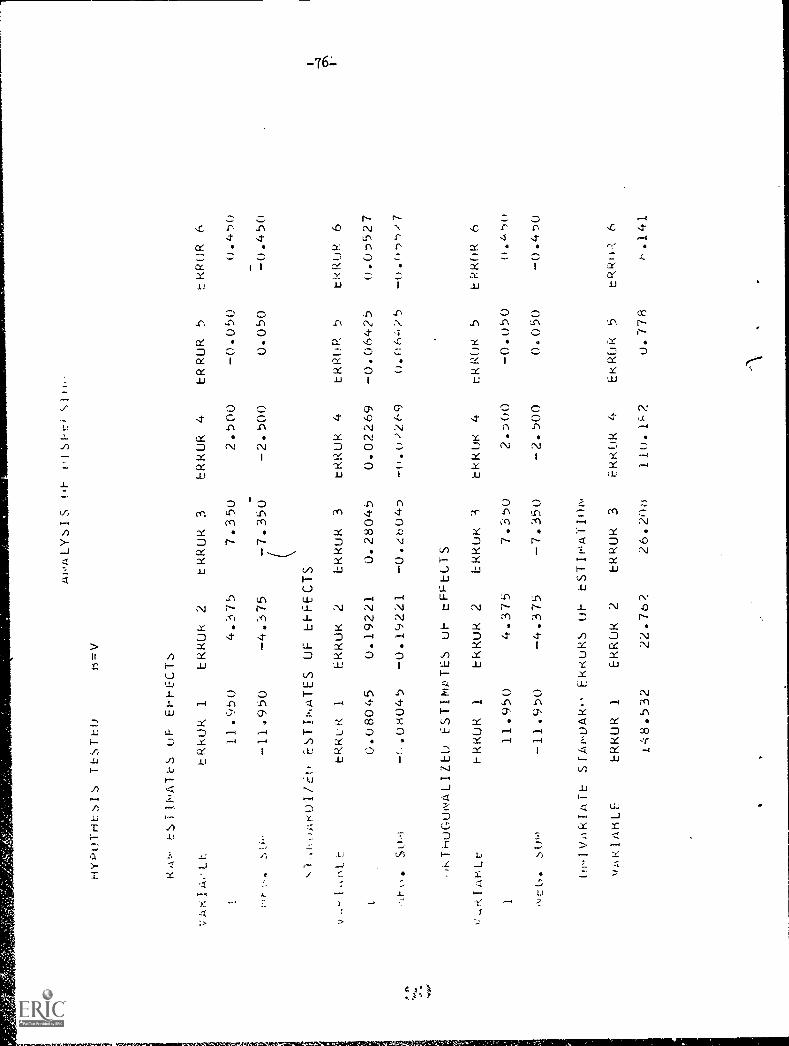
VA

K

r

Alo

ix L

YS

I $tO

F01

S(

-t:i

Si

HY0oTHEsIs TESThO

b=V

RAt tSfli.A.PCS uF EhhECTs

ERROR 1

ERROR 2

tkRUk 3

ERROR 4

ERROR 5

ERROR 6

11.950

4.375

7.350

2.500

-0.050

-11.950

-4.375

-7.350

-2.500

0.050

L,N0AKOI/Eo ESTINATES OF EFFECTS

0.450

-0.450

v--1A,r,LE

tRkuk

1EkkOK 2

ERROR 3

ERROR 4

ERROR 5

tRROR 6

St,1

0.08045

0.19221

0.28045

0.02269

-0.06425

0.05527

-f-08045

-0.19221

-0.26045

-0.0)269

0_(6425

-0.07,)/7

.)KThioGONALIZEO ESTIMPTES oh tPPECTS

KIA,,t_c

ERROR 1

Ekkuk 2

EkkOK 3

tkkOK 4

rkROK 5

ERROR 6

111.95()

4.375

7.350

2.500

-0.050

0.i.-50

\4EG.

SUS}

-11.950

-4.375

-7.350

-2.500

0.050

-0.450

ONIVARIATt

vAKIAbLE

SfAwuAk.

ERkUR 1

FRKokS oh

ERROR 2

ESTImATIo6,

ERROR 3

EkKOk 4

EKROR 5

ERRo

6

J.-48.532

22.762

26.200

110.12

0.778

h.141

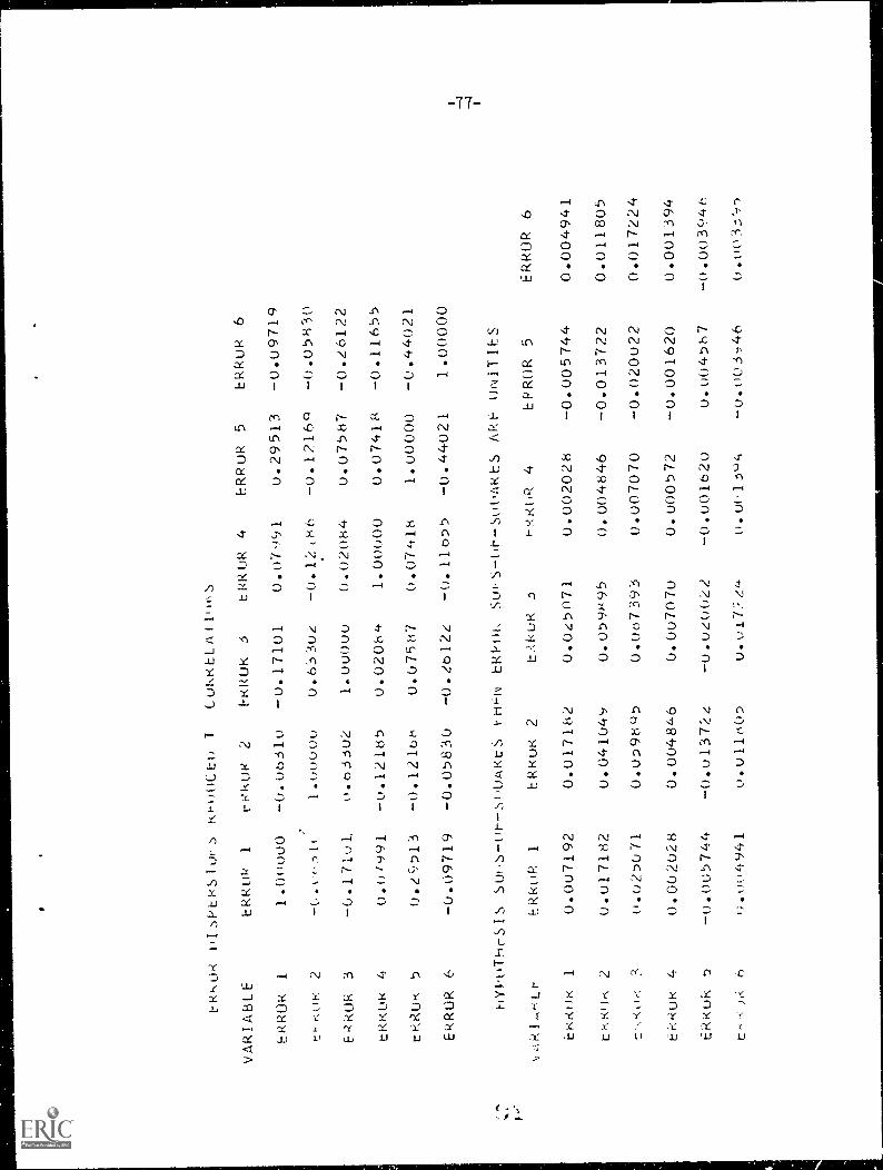
9476000

4769,100'0

4777.LIO*0

SO8ITO*0

.147647000

9 d0H2H

947z-c'000-

1_9<470(10

OF9I000

ZZ007.0'0

ZZLCIO'0

4747L5000

S )302fdR

,,t,cIono

oF9TOn'O

eL0000

OLOLOO*0

947R4700.0

RFOZOO*0

47

-,17:aTO

*0

?7,0070.0

0LoL000

q6c:Lon*0

c68h<00

ILu70*()

c

cOoTTO0

94794700'0

<0q69:00

4070"1470.0

?s4.1/..10'0

>4(1)42.H

S=JIIINn 71W/ SR>WOOS-AO-SInS '411,1AR

M:41-4

1476711()fr

4747LcnO'n

R?re00'0

itoc7r)-0

"ePTL100

Z6TL000

I't)OW-1

00000°T

IZ04747'0

ccoTT°0

77.1970

OCR<0*0 61L600

9

Iz047470

000001

4"147L00

/.4..oo

,4QTFT0

c,"1c,)70

5),(1?

r3.147L0*0

00000I

+7907,0'0

T7T0---

ThL0'0

47

).0>2)p

ZeT97*0

L8cL0*0

47u00()

00000-1

fl999o

In1LT()

C21(1012-3

Oc.L$10'0

o9I-eT*0

70c,c90

noon6-1

)-(

C ,)r)

r")...

61L60'0

C.156?0

16i,)0'0

TOILT°0 0"19900

00000'I

I)(2ir:4

9 dnddR

G Widi:A

47

21-12M1

9Aro124A

781-1.-)

16(12121R

19,101SmAdQ10

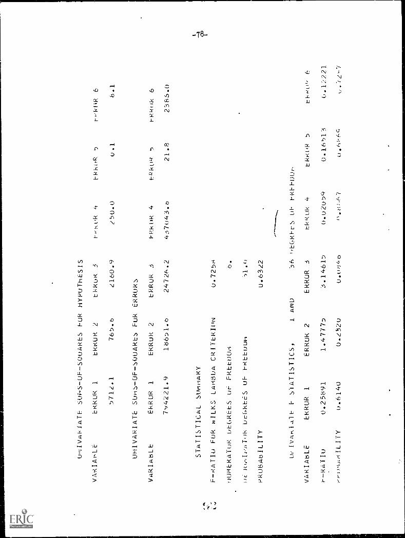
0NAVARIATE SUIS-OF-SOOARES FOR HYPOTHESIS

VARIAbLE

ERROR

1ERROR 2

5712.1

765.6

tkRoR 3

rwR0R 4

2160.9

250.0

UMIVARIATE SUils-OF-SUUARES Fuk ERRORS

VARIABLE

ERROR 1

ERROR 2

794221.9

18671.6

STATISTICAL SUmARY

F-RATIO FUR wILKS LAMBDA CRITERION

tJUMERAToR 0E6REES or FREE00m

0tlueih,ATIIR 0E0REES OF FREEuum

PROBAbILITY

OeiVARIalr F STATISTICS,

VARIABLE

ERROR

1

r-RATIO

0.25891

0.6140

ERROR 2

1.4777)

0.2520

A1\11)

ERROR 3

ERROR 4

24726.2

457043.6

0.7256 b.

-11.0

0.6322

ERROR 3

3.14615

0.0646

rkkoR 5

rwkOR 6

ERROR 5

rPRok 6

0EGRErS OF FIO-FHOri

rkRuk 4

0.02059

().6h67

21.8

2385.0

ERROR 5

0.16513

0.6;(..c4

tkr4oL? 6

0.12221

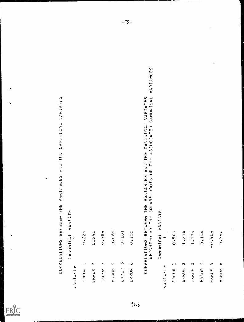
CORRELATIONS btl-t:LEN THE VARIABLES AM) THE CANONICAL vARIATcS

vAr.IA.,Li:

CANONICAL VARIATE

1

tKKOm

10.226

ERROR

20.541

tkNoR

50.789

trMUK

40.064

ERROR

50.181

ERROR

6U.155

CORRELATIONS BETWEEN THE VARIABLES AM) THE CANONICAL VARIATES

WEIGHTED BY THE SQUARE ROUTS OF THE ASSUCIATED CANUNICAL VARIANCES

VARIAL-

CANONICAL VARIATE

1

EkkOR

10.509

Fc+.ROR

21.216

L:R,..oR

31.774

ERROR

40.144

ERROR

50.406

til.KOK

6i1.3s0

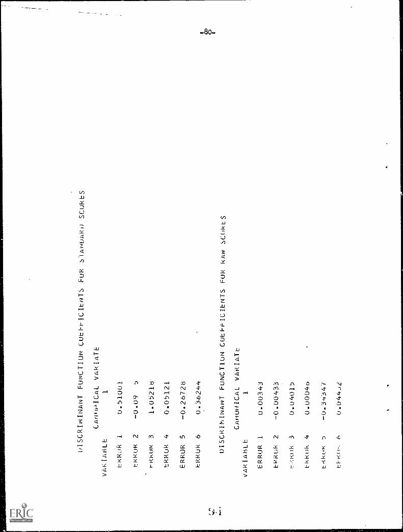
DISCRIMINANT FUNCTION COEFFICIENTS FUR SIANDAR1) SCORES

CANONICAL VARIATE

VARIABLE

1

ERROR

10.51001

ERRuk

20.09

5

7-0.cUR

31.05218

ERROR

40.05121

ERROR

50.26728

ERROR

60.36244

DISCRIMINANT FUNCTION COEFFICIENTS FUR kAw SCORES

vARIABLE

CANuNICAL VARIATE

1

ERROR

1U.00343

EPRok

20.00433

,:,-kk

30.04015

ERROR

40.0004o

ERRIJR

50.34347

EPRIJ,

o0.044.'2

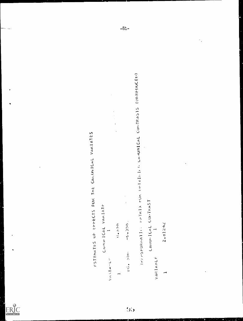
ESTIATES UF EI-I-ECTS

FUR THE CAkUNICAL

VARIATES

CA001,ICAL VARIATE

vs, : I

J-1

,Lf-

1

10.:))(-)

t-G.

::,0,-

-0.i)6_

Tti-I-SEUkvIATIt..

11-,TRIX frUK OpigIi,11(- Cm,AJNICAL

Cul,,TRAS1S (01,.RF0UCE0)

CAnurvICAL CUI.TRAST

VARIAbLE

1

12.b124z

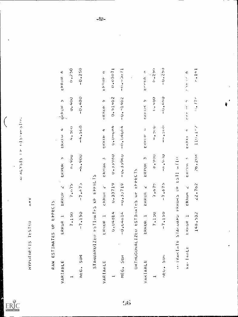
ALYsIS

tt 015 -co.,

HYPOFFiEcIS TESTH)

/4=

-- V

RAW ESTIMATES OF EFFECTS

VARIABLE

ERROR

1ERRuP 2

EkRuk 3

EkK('rl

4t,RPOP

5tRRuk 6

17.150

7.675

8.900

4. 50()

0.400

0.250

NEG. SUM

7.150

7.675

8.900

4.500

0.400

0.250

STANOARUIZEO ESTINATFS UF EFFi:CTS

VARIABLE

ER'cuR

1cKKOR L

ckRuk 3

tRKUk 4

tRkok 5

tPRtli-

10.U4314

0.33719

0.33960

0.04084

0.51402

0.03071

NEG. SUM

0.04r14,

U.3.-)719

u.3.596u

0.04084

0.-1402

0.4)2,071

ORTHUGONALIZEO tSTIATES uF tFFECTS

VARIABLE

ERKUR

1hKRUP, 4

ERPuk 3

17.150

6.90U

Suo

7.15O

7.675

7-%.900

0'IVARIATt SiAr.0APU F-kRuRS uF

VA- I4hLt

tr.i--<UR

1tRkuR G

tR-'Ut.%

148.532

2.2.762

2'6.208

11u.1 F,?

t1-0,0

5t,'wok 6

0.400

0.250

0.400

0.250

Cr'

tr.

'0% ,

6

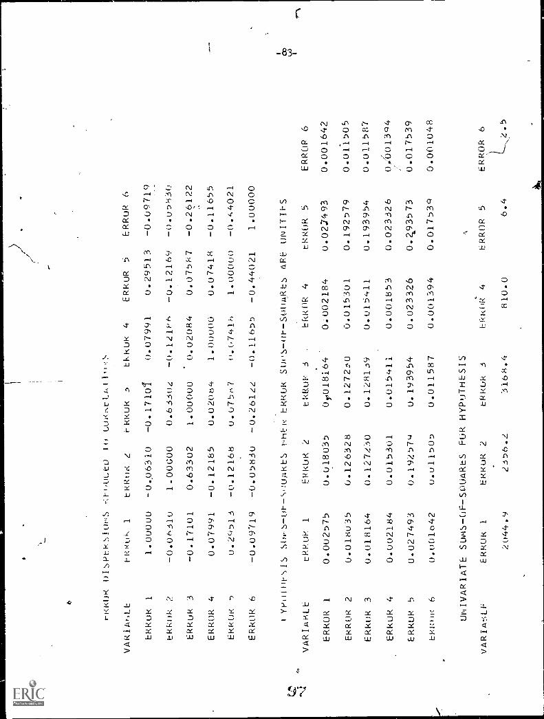
rRKOR

VARIAt,LE

OISPHKSIONS

tlZtlUF.

1

Ki-o)ULtO

Itr

tRRQK 2

ULMKtLAII.

i-RKUR

tkRUK 4

ERROR n

ERROR 6

Ekkuk

11.00000

-0,06310

-0.17101

0.07991

0.29513

-0.0971Q

tkkiik

2-0.0631u

1.00000

0.63302

-0.121P6

-0.12169

-0.05830

ERkuk

3-0.17101

0.63302

1.00000

0.02084

0.07587

-0.26122

ERkuR

40.07991

-0.12185

0.02064

1.00000

0.07418

-0.11655

Ekkok

0.2(4713

-Q.12168

U.075h7

(1. 0

741h

1.00

000

-0.4,4021

ERROR

6-0.09719

-0.0583Q

-0.26122

-0.11655

- U.44021

1.00000

l'it'llIPIS 4,i1J-Ilt--'N

VARIANCE

tRfUk

1

MAKES thF-i,

FPRUk 2

ERROR so' s-m-4,(i iARts ARE

tkRut

3ERROR 4

01\111-II-S

ERROR 5

ERROR 6

ERROR

10.002575

0.018035

07,018164

0.002184

0.02J493

0.001642

ERROR 2

0.018035

0.126328

0.1272:N0

0.015301

0.192579

0.011505

ERkuk 3

0.018164

0.1272-0

0.128139

0.015411

0.193954

0.011587

ERkuk 4

0.002184

0.015301

0.015411

0.001853

0.023326

0A001394

ERROR 5

0.027493

0.192579

0.193954

0.023326

0.4,93573

0.017539

Eki:111,

60.001642

0.011505

0.011587

0.001394

0.017539

0.001048

UhIVARIATE SUmS-OP-SOUARES FUR

HYPuTHESIS

VAR1A8LE

ERROR 1

ERROR 2

Ekkiik 3

EkROR 4

ERROR 5

ERROR 6

2044.9

2376.!

3168.4

810.0

6.4

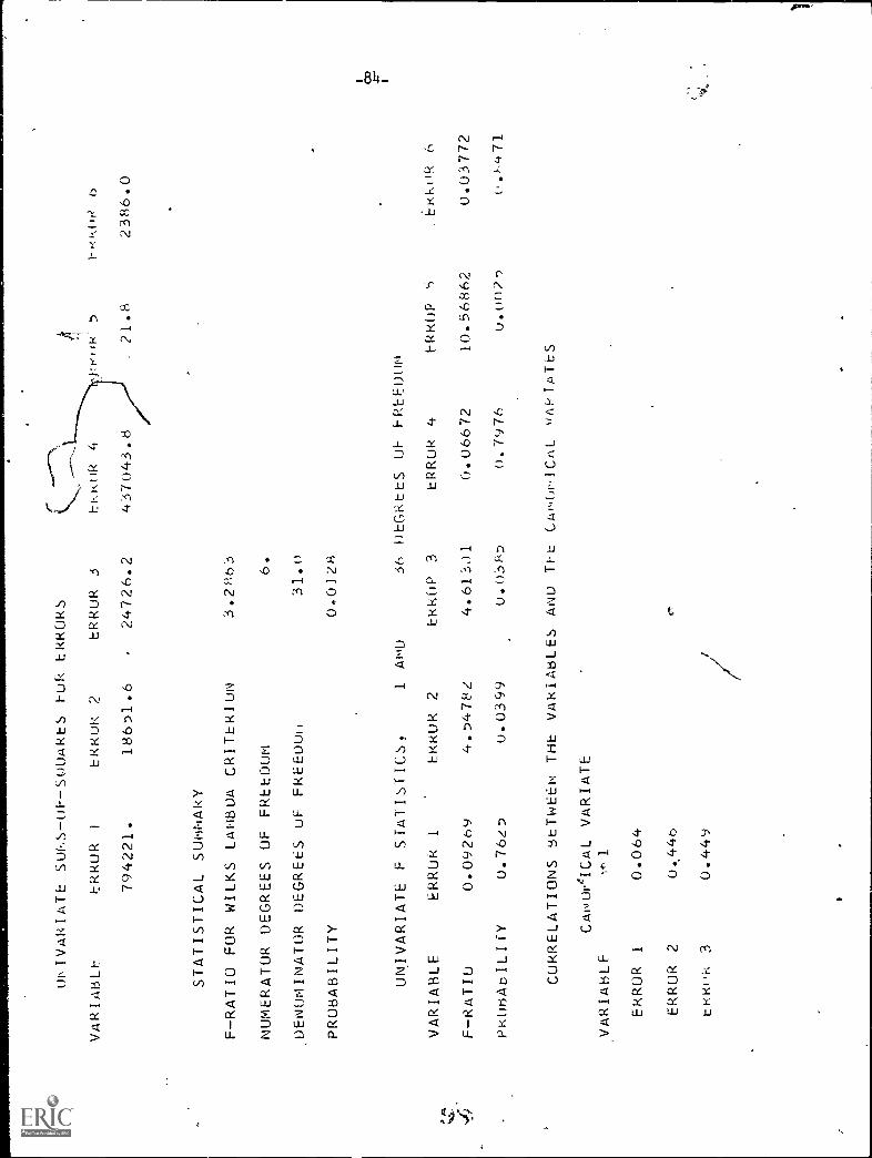
01\IVARIATE SUkS-0ES0OARES FUR

VARIABLE?

ERROR

1ERkuk 2

ERRORS

ERROR 3

794221.

18651.6

24726.2

STATISTICAL SUNNARY

FRATIO FOR WILKS LAMBDA CRITERION

3.2863

NUMERATOR DEGREES OF FREEDOM

6.

DENOMINATOR DEGREES uF FREEOull

31.0

PROBABILITY

000)28

UNIVARIATE F STATISTICS,

t.ef $1-4' 5

t-- .(KCW b

1AND

36 DEGREES OF FREF:DOm

21.8

2386.0

VARIABLE

ERROR 1

ERROR 2

EkROP 3

ERRok 4

FRRUP

')

Ekkok 6

FRATIO

0.09269

4.5478 2

4.613,)1

(i.06672

10.56862

0.03772

PkOnAEILIfY

0.7625

u.0399

0.0385

0.7976

0.002-)

t,471

CORRELATIONS BETWEEN THE VARIABLES AND Ti-E CA0.0r,ICAL %/APIATES

CAImUr4ICAL VARIATE

VARIAIALF

Nel

ERROR

10.064

ERROR

20.446

CKRI'N

30.449

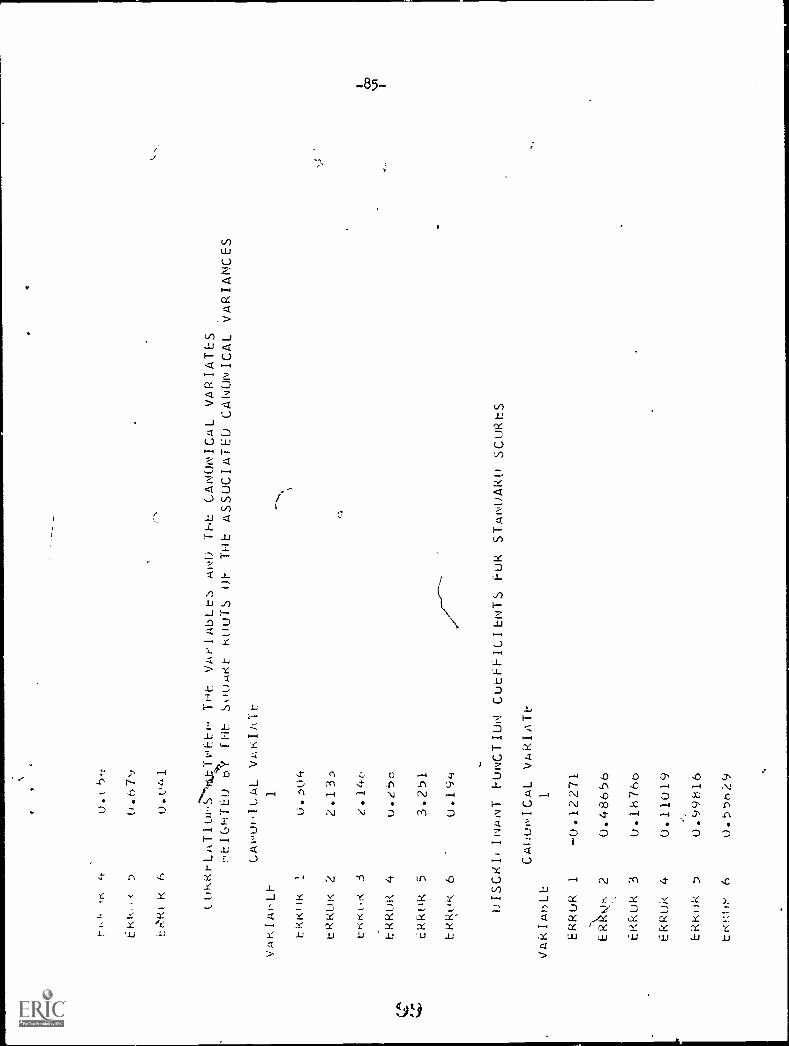
u.t 64

0.679

tORRFLATIOJoEho- THh VAPIAbLtS miv0

TFiI

CANONICAL VAR IATES

,:,FIGHTED DY f0E So0uRt- RDoTS OF THE ASSOCIATED CANONICAL VARIANCES

CAI-0011,AL VAr:IATh

vgRiArLh

1

hkroIK

IU.04

hRRUK 2

2.13

ckr<t,r<

32.146

IRRUR

40.256

eRkuk

53.251

ER0i:

60.

194

DISCRI# INANT FUNCTION CuEFFICIENTS FUR STANDARD SCORtS

VARIA6LE

CADuNICAL VARIATF

1

ERRUR

1U.12271

E-1.41-\

20.48656

ERROR

30.18760

ERRUR

40.11019

ERKok

50.9916

tr:t7Ow

60.55629

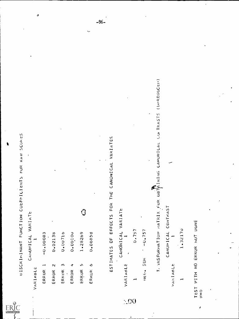
u1SCRlistINANT FUNCTION CLJEFFICIENTS FUR RAW SCURcS

CAN

VARIATE

vARIABLE

1

ERROR

10.00083

ERROR

20.02138

.

ERROR

30.00716

ERROR

40.0010u

ERROR

51.28269

C101

ERkoR

60.06858

ESTIMATES OF EFFECTS FUR ThE CANONICAL VAkIATES

CANONICAL VARIATE

,.,

VARIAbLE

1

C1

0.757

NE(,.

Slim

0.757

T. INSFORATION rIATRIX Fuk UB

CANONICAL CUNTRAST

/ARIABLh

1

11.3217u

TEST WITH NO ERROR NUT uuNE

.,

0=0

INING CANUNICAL LuiTkASTS (lwREOUCLU)

t

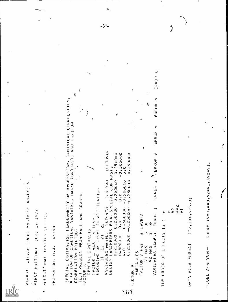
VARAA:

LIi

°biu

tJULL VAklAvcr A,ALYsIS

FIRST EVITIoN:

JUlot 1, 1972

tOOCATiliAL TrSTIpq, St--<v;LA7

PRIvICtION, [..J.

Ut:)40

SPECIAL CoNTRASTS, HumuCENEDY uF ktt,RESSION, CANONICAL

CURRELATIoN,

RoTATION Of- CANONICAL VARIA1E, NAhEu CUNUASTS

ANU mAxIUo

CORRELATION PRINTOUT

.44

TEST PRubLEM FRUm HALL AND CRAHER

FACTOR A

SPECIAL CONTRASTS

FACTOR A HAS

4 LEVELS

RECuUING uF LEvFL

11

12

21

22

VARIABLES NAED:

1ST-4TH

200-3k0

LEFTuvER

PARA(ETERS FRUIT SPECIAL CONTRASTS

0.250000

0.250000

0.250000

0.250000

A0.500000

0.0

0.0

-0.500000

0.0

0.500000

-0.500000

u.0

0.250000

-0.250000

-0.250000

0.250000

rFACTOR V

VARIABLES

FACTOR V HAS

6 LEVELS

VI HAS

3DF

V2 HAS

3OF

es"

VARIABLES NAf.ED:

ERROR 1

ERROR 2

EkkUk 3

ERROR 4

ERROR 5

ERROR 6

THE ORDER OF EFFECTS IS

:

A V2Avg

VI

DATA FILE FORHAI

(I2,10X,61-6.0)

,;u0EL Al!ALYSED-

CuRREL:1-4=0,A=0,V2=V1,AV2=V1.

1

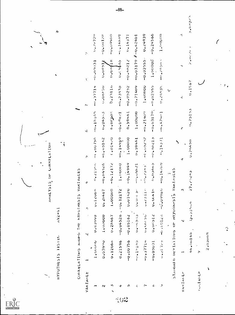
AmALYSIS Or Lokkl:Wis1 lull

HYPUTHLS1S

1 tS 1 tl.

AV2 =1,1

C01,KtLATIO0S Avtoi,q,

hYrUlri1:SIS VARIA6LES

I

VAR1MoLt

1

*2

34

67

11.00000

U.G3990

u.1206

0./15,-6

-(.0o/)6

-6.1£,105

-11.

7714

-0.05031

0.2o

72,)

20.

0399

u1.00000

0.2647

-0.045e6

-0.05162

0.045,,3

0.o6kt,0

.08

1-0.001?v

30.12066

0.28467

1.00000

-0.1217/

(.014/0

6.083

0.2-4110

0.08

18

-0.0,491

)

40.21596

-0.04526

.-0.12172

1.00000

-0.14Ww)9

-0.008/.1

-6.234

0.(

5116D

5-0.00756

-0.05162

0.01420

-0.14949

1.00000

0.59461

-0.05252

-0.66212

0.14371

-0.11,16

u.,45,s)

U. l

)-(

_.),

-0.09821

0.59461

1.00000

-0.21409

-0.031791-0.42401

7-0.37714

U.1

,t)r

:,,t.,

'..0

(:)1

1('

-0.2140')

1.00000

-0.02555,

0.24939

is

-0.05031

0.0)ip12

u. lik,41

0.05465

-0.03179

-0.02555

1.00006

-0.24566

0.e17/-.)

-6,1z6

-6.09900

6,1/-./1

-0.4?401

1.00000

STA0DA1-0 Otv1A)100s Or mYpoirirSlj VAKILtS

vw<1A6Lr

12

34

,)

6/

8

44.61)14;1

1,2.

:.).;(

it;).

27.1

51ti

u.?0450

0.2515.1

0.1(.67

?.t)

:',1(

)a.w4;-,,,,1-)

9

2.030;58

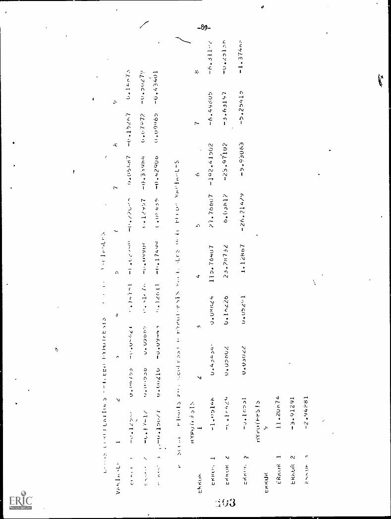
I.<I t-LAI IYrI S

I, rt,,

1.Y1-111rt:

'11,01L1 -3

1e

(7

fs9

P0.1014

!)5

.14,

i-(

0.0567

-0.15167

0.14673

-(,.1

7-1/

Q.0

:ob5

0.12-y57

-0.311964

0.07972

-0.5u27

p0,"

),,-

(t .1

50/(

U.0

02IU

-0.0

944'

)".1Z611

-0.1749Q

(.W435

-0.42906

0.09965

-0.43401

05(

r14

,01

Ji

I1'N

ES

.iY

» 1

I-r.

't t't

.11-

r1-111,,

VIA

tRkor.

HYP0114-.51:.5

11

34

56

78

co

rt:R0-5

1-1.05146

0.43434-

0.0'48.24

115.76407

27.76607'

-192.41502

-6.49805

-6.311-e

I

trikuR

-.164119

0.05602

0.1426

23.28732

6.03812

- 23.97102

-3.63197

-0.25136

ct.6...

7?

-0.16531

0.03022

0.052t,1

1.12867

-26.21419

-5.93063

-5.25415

-1.3746:-

HYt)00,6S13

EKKUR

9

Ekr(uk

111.20674

Ekkok

2-3.91291

i:rst.01-

-5

-2.94881

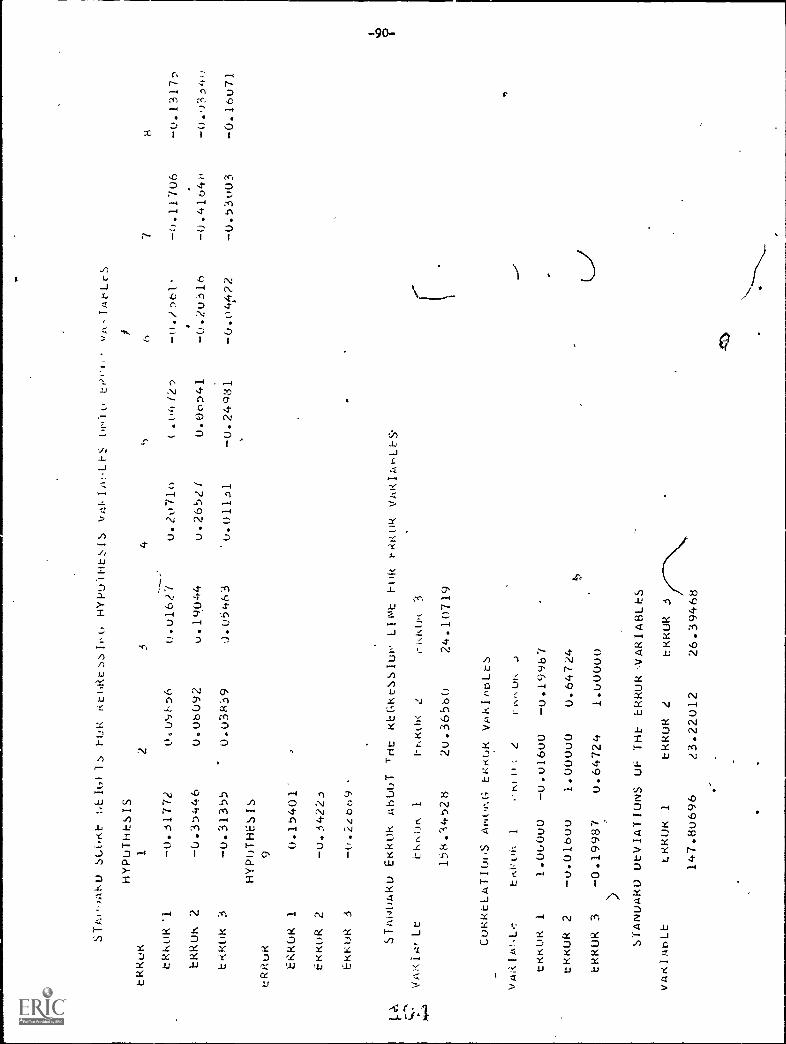
STkooAK0 SLOKt 14ElullS

HYPUTHESIS

tRRuK

1

Flat: KcoRtssIoo HYPuiHtSiS NrAkI8:4.FS

24

,)

v8-IAtlrS

(-)

78

tkR0R

-0..31772

0.ul,D6

0.01627

0.20710

(.o4/2

-0.t1'

-0.11706

-0.1317n

..

1-tRUIN 2

-0.35446

0.0b092

v.19044

0.26521

0.06541

-0.20316

-0.41648

-0.033i#,J

E,0:0k 3

-0.31355

0.03K39

J.05463

'0.01131

-0.24981

-0.04.p2

-0.53003

-0.16071

HYPOTHESIS

tRRuR

9

ERROR 1

0.15401'

EKKOR 2

-v.34223

EkKoR 3

-0.2co69

STAw0Aku EKkuk AbU0T THt KC,KtSSluo Llot F.0k rkKoR

`":"

VARIgrLt

ti.o.om

1tro<OK

ci.k0<

3

158.-44528

20.36580

24.10719

CoRktLATIOoS ANor.G tkr<GR VAkImILS

VARIW.LC

trcok

1ni

iz

r

tKKOK

11.00000

-0.01600

-0.19967

tRKUR

2-0.0160o

1.00000

0.64724

ERROR

3-0.19987

0.64724

1.00000

STANUARO UtVIATIUNS OF THt EKKURVARIABLES

vAKImoLt

LRKOK 1

tkRUR 2

17KRUR 3/-"\

147.80696

23.22012

26.39468

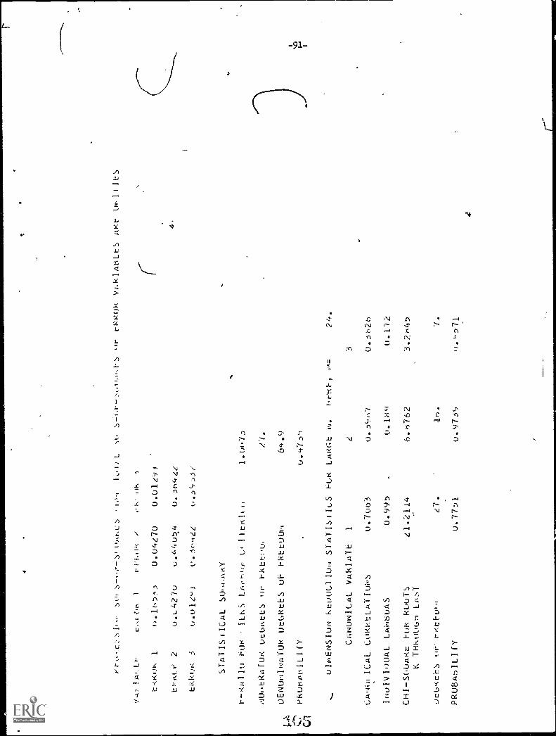
1.11

w't

rRROk VARIABLt7S Ahtt 01,11ILS

AI-IALt

L'.0 0K

1FE'-,l,

/.-}.

,If.

,1

t{r(

Ok

10.163

0.04L70

0.01G91

Li,m_P 2

u.+,42 7u

0.44054

0.J044/

EKPAJK 3

0.01Z"1

C.3o4zz

k,.3(:,:)3/

STATIS1ICAL SUIY

1---(ATIti Foe

ILLS LAop Ut

MUI.ERAIUK Utbittn

1-ktt:g.),

OENUNINAfUK Ut6KtES u1 hkEtOU

PkUtiPtLIfY

CR

ulHENSIuN ktu0c1 iufq STATIsILLS hiJR LARGE h.

10=

24.

CANUNICAL VARIATE

1

CAq(21 ICAL CORRtLAIIl&S

U.7003

IhUIVIOUAL LANbUAS

0.995

CHI-S(.UARE FOK ROUTS

41.21i4

K THRo0bm LilaT

OEUKEES

t-,:tEu0.1

PRUBAnILIfY

3 0.3026

U.

0.1Iz

6.8762

3.2845

e7.

lo.

7.

0.7751

0.973g

0.k571

4.

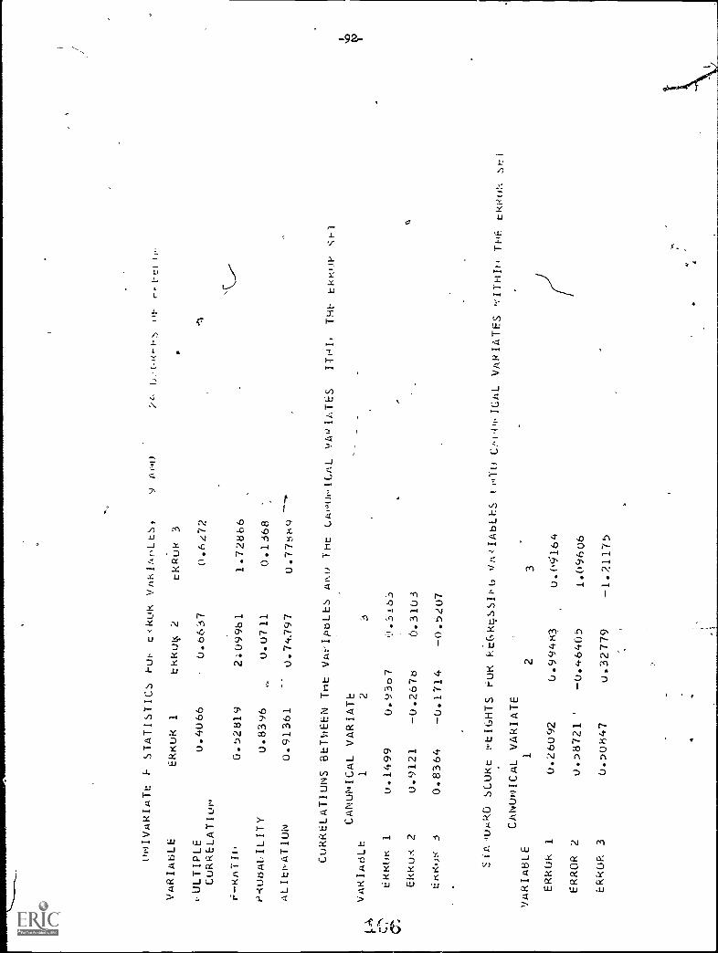
(119IVARIATt F STATISTICS Fut cRkuk

VARIAnLtS,

9 /\00

,t-r:11,..

VARIABLE

ERKUR 1

tkkutic 2

tkPuk 3

pULTIPLE

0.4066

0.6637

0.6t72

CuRRELATILIN

H-RATA'

0.52819

2:09961

1.72866

P-cursAIALITY

0.8396

0.0711

0.1368

ALItivATION

0.91361

0.74397

0.7788q ---"'

CuRRELATIUNS BETWEEN Tmt VAi'Ip6LEs

AM) THC CgiotwICAL VA0IATES

ITHIt

THF bkh.1.11)

Shl

CANUNICAL VARIATE

'

VARIA6Lt

12

3

ERKOK 1

0.1499

0.93o7

1).3).63

EkkuA 2

0.9121

-0.2678

0.3103

EKKuK 3

0.8364

-0.1714

-0.5207

-t)

SiA'UARD SCUKt ttIGHTS ruk ktGkqSSII(2

vioIAbLES tNTO Cf.1,01,ICAL

VAPIATES

THh tkku!--, St1

CANO0ICAL VAkIATE

vARIA8LE

12

3

ERkOk

10.26092

0.99483

u.0164

ERROR

20.58721

'

-0.46405

1.09606

tRkOk

30.50847

u.32779

-1.21175

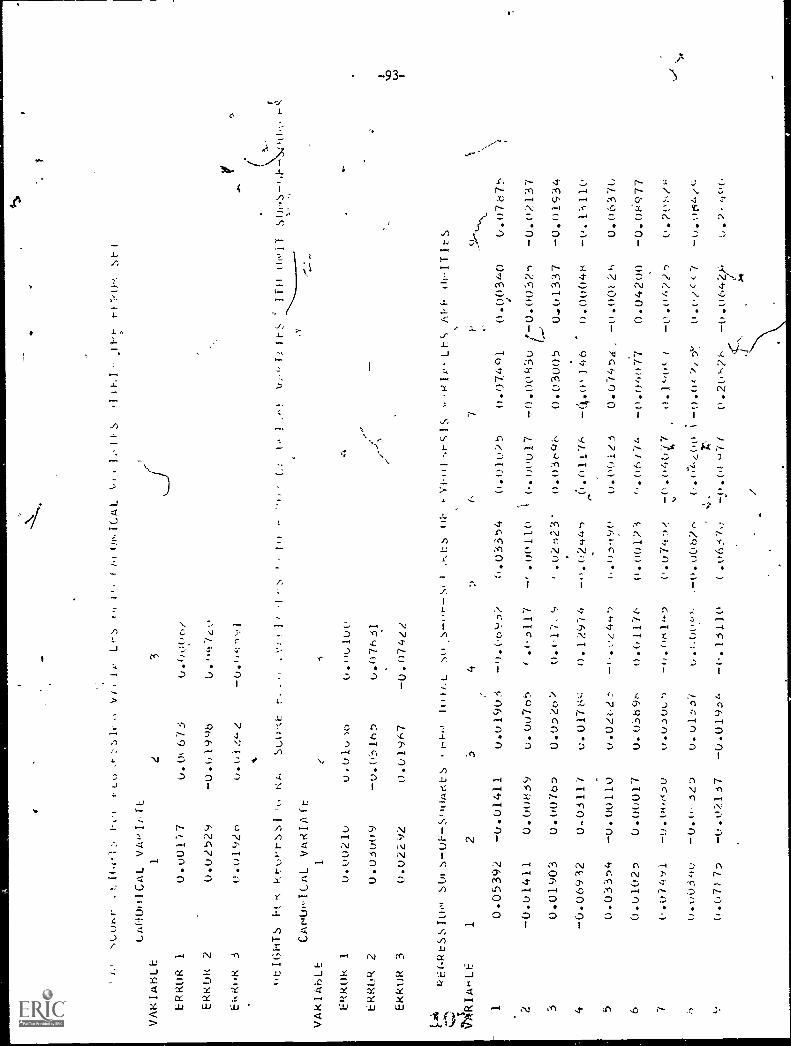
slcursr

t-ct

vi

Li-S

(ICAL

I IFS

t-t

St- I

GAOuICAL

VARIABLE

1

ERROR 1

0.00177

ERROR 2

0.01529

Ei..RoR

30.01(120

U. UI 673

-0.019(-R5

U.

'PLIGHTS Ft c kto'r-ssl

SL0KI:

CAH.,,ICAL VARIAft

VARIAbLL

1ti

00.(

0k1

0.0021u

v.01t,

)(-)

0.Yulue

ERROR 2

U.03009

-0.03165

v.07631

EkkoR 3

0.02292

0.0197,7

-0.074//

.I

'o- 1

-!

\r;"-T,'. 11-S

ITI1 oloi 7

Sli.s-',F--S410-.

/A

kE(42tSSI(1,

SUi

s-0-

-S,1

0Ae.

kSk.

....,

.-4-.0

101/

.LS

-"r-

I,..

: s O

h*Y1-11

-+t-

S IS

''K

Ip-L1",

i\ P

h111'I T

I rs

q'gR

IALE

12

34

:,

67

P.9.--,..\_

10.05391

-0.01411

u.01901

-0.(.0u3/

(,.03354

0.01025

0.07491

0.00340

0.0767's

Q

,

2-0.01411

0.00t-<39

0.0076')

(.(..,117

-1.00110

, 0.00017

-0.00i30

t-0.0032n

-0.0'137

I....,

30.01903

0.00765

0.0526%

0.e17.,-,

,.01,123'

0.03600

0.03005

0..01337

-U.01934

4-0.06932

0,0311/

u. u176

0.1/.94

-Y.02,4701

,-.

0.011.77-

-4.0'146

-

0.0004t-<

-0.1311e

50.03354

-0.00110

0.0[6[!,

1..1,34,10

0.001z3

0.0745a,

U.06376

60.

0102

50.

0001

70.03b9r-

0.01176

0.00121

06 7A

-.0.

0407

70.

0420

0OP<?77

-0.00(1

('.U74!)!

-0.04047

o.P-oct

-0.0A?2.)

0.003,w

U.

0062e,

o.4.z,/o0

7,'5`:

.o/c (7

-o.ory.,/c

(1.07175

-0.02137

-0.1

)193

z--0

.131

10(

-0.(

00.

20,-

,?-

- 0.

0642

/.cf

oo

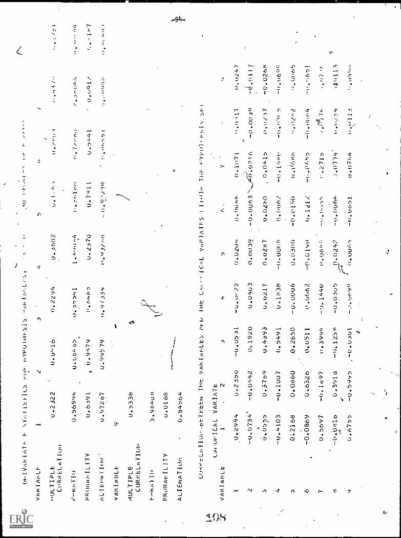
01VAkIATF F

ru!- nYP0IHFSIS

VAklArLh

13

1.1ULTIPLE

0.2322

0.016

C0RkELATIut/

f-RATIO

0.56994

U.U8465

,PRImmhILITY

0.6391

, 0.9679

ALIEw411uN'

0.97267

0.99579

VARIABLE

9

MULTIPLE

0.5338

CURRELATILIN

F-kA1 I0

3.98408

PROBAbILITY

0.0168

ALIEMATIOm

0.84564

CO-(tLATILWotTV:tEN

THt

VAKIAhLtS Pvt.,

VARIAtiLt

LA) UPICAL VARIArt

12

3

10.2994

0.2350

-0.0531

2-0.0734'

- 0.0442

0.1920

,.

30.05?,

0.37b9

0.4393

4-0.4103

-0.1007

0.5491

,0.2168

0.0660

0.2650

6-0.0869

0.6326

0.0511

70.5697

-0.1697

0.3994

8-0.0816

0.3918

-0.123

..

.e,

90.6755

-0.5995

-0.0301 9

4

0.2294

0.3602

0..55541

1,4.

o-,4

0.6485

0.2370

0.9/334

0.93/ %'8

k('

5

.30 0F,<I-,-.

iJ)

I

/ rt,

3

0.:4

1100

0.7/

(-64

)

0.7811

0.5441

INt L'Af"i 1C1L VRPIATS 1 1101w THF t-,YPtIl-rsl' 5F I

45

A7

t,

II

4

-0.0,22

0.0403

0.0217

0.1838

-0.0006

0.0062

-0.1440

-0.0305

-..069°

0.0204

0.003

0.0287

-0.0004,

o.othoo

-0,6190

0.06k

0.0247

..,;_-r

j0.0005

0.004t-

0.1071

-0.0063N,.4e.0216

0.0280

0.0415

-0.14

-0,01,4)

0.0688

0.121/

-1 .01,55

-, .015'1

4 .271

-0.0064

1.0774'

-0.0651

0.0M4

0

".1)-11-i

-0.0039

0.0,-)7

-1)."A°

I.02z1

-0.00(-4

t'4i/4

0.t,/n4

0.0113

\

-4.0117

-0.0268

).0065

-0.t1651

)i6113

f .0590

(J.-1e7

,..,

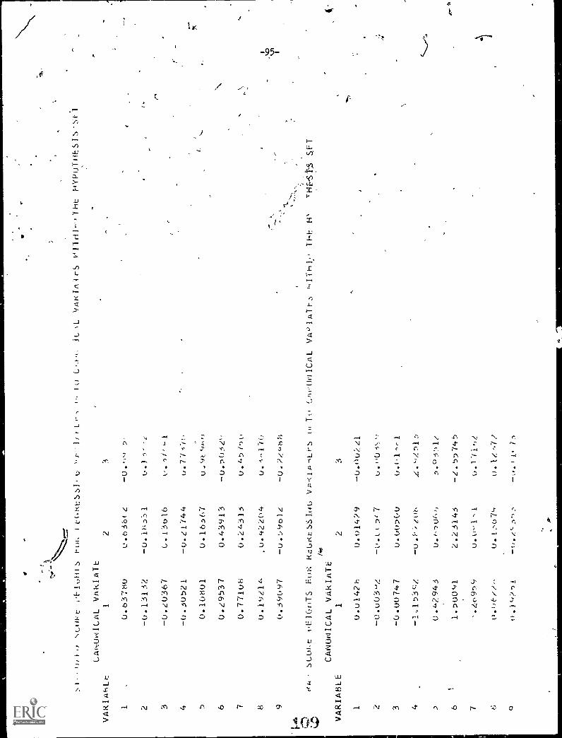
I,

IH i

./(,

Ili t

6'1-

1,,tti S

E (A,

it(, to.: S S I

.t.

'° P

'"1; t

L - ,

1,,

GANuNIGAL VARIATE

VARIABLE

12

3

10.637H0

0.636(2

-0.,,k,

2,

2-0.13132

-0.1r;331

u..)7,-

3-0.20367

(.13616

u. 1 /.-.,

4-0.30521

-0.21744

0.77.

50.10H01

0.16367

0.9t. 9mu

60.29537

0.43913

-0.5(132"

70.77108

0.24313

0.450)o

80.1 9114

,u.42204

u-4i-170

90.39097

-u.i961z

-0.2z4h8

IC,J.L

ll, rL VAKIAIES

HypuTHEsjs-:51-

SOOt\t oFIGrJS Fug RcukESSIul, VA <tABLEs u4 T0

1,011ICAL VA0IATEs

THE H'

THkiLS $.FT

VARIABLE

1

CANONICAL VAkIATE

1

0.u142h

2

0.014?9

3

-0.00221

2-0.003'-'2

-0.((5z7

u . "03". ,f

3-0.00747

0.00500

0.(.1-,1

4-1,153q2

-0.i.",1u6

1. ',/.. pl 3

)0.42943

U.r.,nUA,,

3.9351/

61.50091

2.23143

-L.55745

7.20959

u. u- 1^ 1

0.1-11,-,2

60.0(-//-

U.L.-N079

u. l

-7?

C4

0.1(

4?')1

-u.,f"nn,

mil.. /n

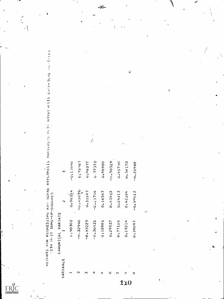
NEF,HTS t-('R REGRESSING Riv! SCI'kt

"ITH wIT SOmS-0ESQUAKES

CANONICAL VARIATE

VARIABLE

12

hYPuTHESIS VAKIorIL-:-..

it! Ti. HYPia-it-STS

3

Cto tio 1L/1

-t,

' 1,

10.90302

0.904

0.13946

20_32940

0.4979,-

0.33t167

I"

30.53229

0.35587

0.98377

,._..

40.30521

0.21744

0.77370

50.10801

0.16367

0.98980

60.29537

0.43913

0.50329

70.77108

0.24313

U.45750

80.19214

0.42204

U.38170

..f..,

90.39097

0.59612

U.22488

1 r :),

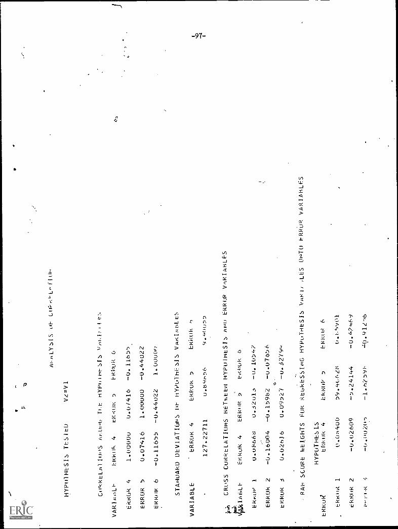
Al.

tkLY SI S

Lot-

LW*,

HYPOTHESIS TESIED

V2=V1

CokKLLA1100S Av.01A, TLE HYPoihrSIs vAkI!flt

VARIA60-

Ekkok 4

tRKuk 5

FRPuR 6

EkROR

41.0000u

0.01416

0.1165')

ERROR

50.07416

1.00000

0.44022

EkKok

60.11655

0.44022

1.0uuw:

STANuARD DEVIATIONS

HYPOThSIS VAKIAoLtS

VARIABLE

ERROR 4

EKRuk 5

Ekkok

127.22711

U.d

geo)

69.

40u5

!)

CROSS CURRLLATIUNS bETv.tbil HYPUIHtSIs Am, ERROR

VqkIABLES

44IAMA-

ERkuk 4

ERRIIR 5

EKkuk 6

EkKor,

1

ERROR 2

tRkuk

0.08668

0.32013

0.10542

0.16004 0.15962

u.07656

c>,

0.026)6

0.09527 u. 3219 -i

RAl SCORE WE&GHTS FUR REbRESSING HYPuTHESIS VAKI/

,LES ONTO ERRuR VARIABLES

HYPOTHESES

bRkuk 4

0.W1400

0.02609

0.(0202

EkkoP 5

EKkOR 6

59.4(.628

0.0901

5.24144

0.42469

1.11'259t-

=0.912 n6

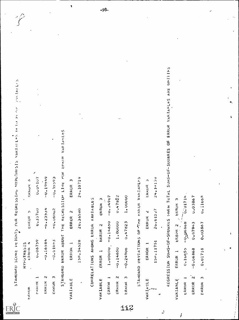
ERRUR

STANDARD SCoRE otIGNTS FuR REGRESSIwu HYPuTHPSIs "ARIA1LPS 14,10 pf

HYPOTHESIS

tkkok 4

ERRUR 5

ERkuk 6

pkkuR 1

0.06759

0.33760

0.0')107

ERROR 2

-0.16584

-0.23554

-0.19949

ERRUR 3

-0.010r,3

-0.06002

STANDARD ERROR ABOUT THE REGRESSION LINE FUR EvkuR VARIALES

VARIABLE

ERROk 1

ERROR 2

ERROR 3

158.34528

20.36580

24.10719

CORRELATIONS ANONG ERRUR VARIABLES

VARLABLE

ERROR 1

ERROR 2

ERRUR 3

ERROR

11.00000,

-0.14650

-0.24907

ERRuR

2-0.14650

1.00000

0.47822

VA

14'

ERRUR

3-0.24906

0.47823

1.0000Q

STANDARD DEVIATIONS OF,Int ERkUk VAklARLFS

VARIAeLE

ERROR 1

15r1.11751

ERRUR 2

ERRUR 3

20.01227

24.I11139

J'osiArLI-S

REGRESSION SUNS-OF-SOUARES I,HEN TOTAL SUNS-OF-SOUARES OF ERRUR VARIABLES ARE UNI1IFS

VARIABLE

ERROR

1ERROR 2

ERRUR 3

ERROR

10.1085

-0.06868

0.01718.

ERROR

2-0.06868

0.07943

u.03867

FRROR

30.01718

0.03867

0.11068

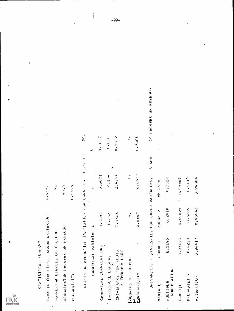
SIATISTICAL SUvw.ARY

FRATIO FOR wILKS LANBUA

-0.I:KATOR Ot.q.,KEtS OF FRtEVON

OENuIoATOk Dcbkths OF t-liEr0011

PRO6ABILITY

U.A

GL,

4

Rtuouflui, 5IA1I3II0S FUR LARGt v.

HI-KF, N=

24.

CAI4ONICAL VAkIATt

IG

CAI uw1GAL CUkRtLATIUNS

0.4692

0..1071

II,0IVI0UAL LANbloAS

0.'1?

0.104

CHISAkt FOR kbUTS

7.'16o6

G.4.,')4

K THROUbh LASI

143EG,-tt!!S uF FRtEuu

9.

CekuviAhILIfY

0.ot.:17

3 0.1017

O.( 10

0.231? 1.

UNIVARIATt F STATISTICS FU}

tRklik VARIAbLtS,

3 Awl)

24 OEC,REES OF FRLEDO1s.

VARIAhLt

r.ULTIPLE

CORRELATION

tkRUR 1

LkkUR e

0.3295

0.e818

tRkoR 3

0.3327

FRATIU

0.97413

0.69025

'0.99567

PRUrtAbILITY

0.4213

0.669

0,4111

ALIt1')ATIOq.

0.94417

0.95946

0.94304

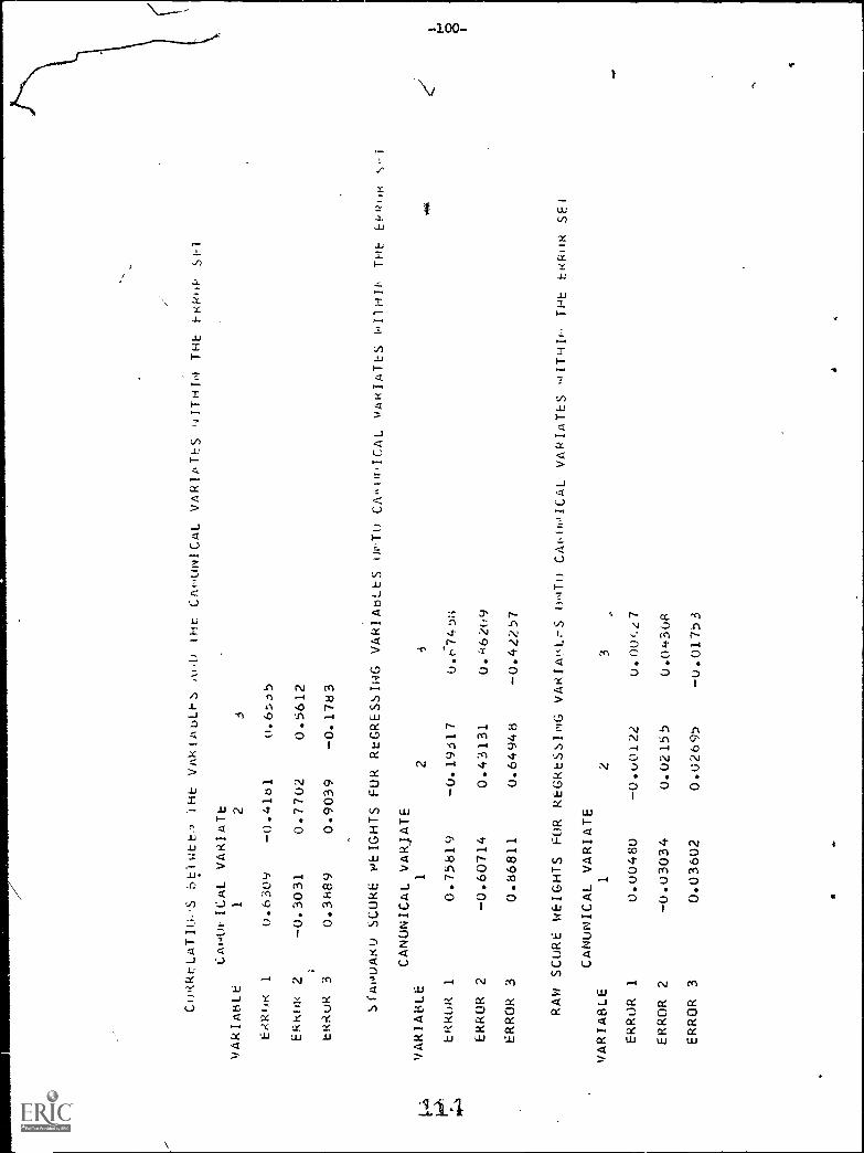
CoRtLATItiS btiwtt,'J IHt VARtAbLEs

!Hr. CAt.UNICAL VARIPTtS 'iITHIA THE El.<F6IP

VARIABLE

CA1401-ICAL

1

VARIATt 2

3

E.,420k

10.6309

0.4181

0.6s35

ERROR

20.3031

0.7702

0.5612

tRRuR

30.3889

0.9039

0.1783

1-4.4

SiA0UARU SCORE wEIGHTS

CANONICAL VARIATE

VARIABLE

1

FUR RtGRESSING VARIA6LLS (WTO CA-ur.ICAL vARIATES

1.111HII,

THE EkPloK

23

1'4

4.1.

ERROR 1

0.75819

0.19317

0.6-7456

ERROR 2

0.60714

0.43131

0.k6209

ERROR 3

0.86811

0.64948

0.42257

RAW SCORE WEIGHTS FUR REGRtSSING VARIAt.L.-S 0070 CAI,110ICAL

VAkIATES

THL hkROR SEI

CANONICAL VARIATE

VARIABLE

12

3

ERROR 1

0.00480

0.00122

0.00e.27

ERROR 2

0.03034

0.02155

0.04608

ERROR 3

0.03602

0.02695

0.01753

,, T

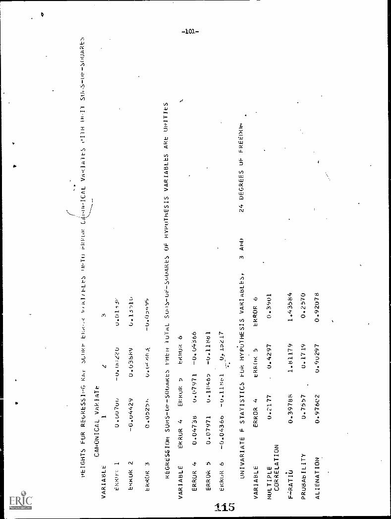
ri-

HEIGHTS FUR REGRESSING Rht suNkr

RI/I,Li7s ilt\u FPPaik kilNICAL VAIATt-S 0I1H in,Ii SU.;SNrSNUARES

CANONICAL VARIATE

VARIABLE

ERRO.:

1

EKKuk 2

ERROR 3

U.0070

0.04429

O.U525

-0.O

GZ

jo

U.03889

U. (

a (;

3

0.0113

0.16')1U

0.03499

REGRESSION SUMS-0ESOOARtS vHEN luTAL SthISuFSQUARES OF HYPOTHESIS

VARIABLES Ake UNITItS

VARIABLE

ERROR 4

EL:Kok 5

ERROR 6

ERROR 4

0.04738

0.07971

0.04366

ERROR 5

0.07971

0.1846

0.11881

ERROR 6

0.04366 0.118o1

0.12i-r

-

cn

UNIVARIATE F STATISTICS FOk

HYPOTHESIS VARIABLES,

3 AND

24 DEGREES uF FREED.ON

VARIABLE

ERROR 4

tRkOR 5

ERROR 6

MULTIPLE

0.;s177

-0.4297

0.3901

CORRELATION

F -RATIO

0.39788

1.81179

1.43584

PROBABILITY

0.7557

U.1719

0.2570

ALIENATION

0.97602

0.9u297

0.92078

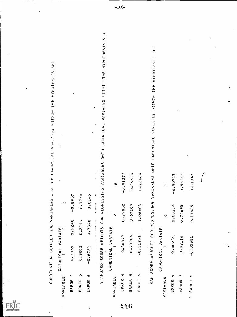
COPRELATIo0 bETDEEN THE \sARIAhLES

iHE cm"oNICAL vARIA1ES

Ikh HYPoTHESIS SE1

CANONICAL VARIATE

VARIABLE

12

3

ERROR 4

0.3955

0.7240

0.8907

ERROR 5

0.9003

0.224.;

0.370

ERROR 6

0.6781

0.7348

0.0145

STANDARD SCORE WEIGHTS FUR REGRESSING VARIABLES

ONTO CANONICAL VARIATES ITNI. THE

HYPOTHESIS SET

CANONICAL VARIATE

VARIABLE

.1

23

* 4-, 0 N

[A

ERROR 4

0.30377

0.29832

0.91278

0:

ERROR 5

0.73786

0.67107

0.45640

ERRuk 6

0.31786

1.06D03

0.12664

RAO SCORE WEIGHTS FUR REGRESSING VARIABLES UNTOLANoNICAL VARIATES olTHIN THE HYPoTrESIS SET

CANUICAL VARIATE

VARIA8LE

12

ERROR 4

0.00239_

0.00234

0.00717

EkRuR 5

0.82116

0.74683

u.S5243

EkRUk 6

0.03381

0.11329

0.01347

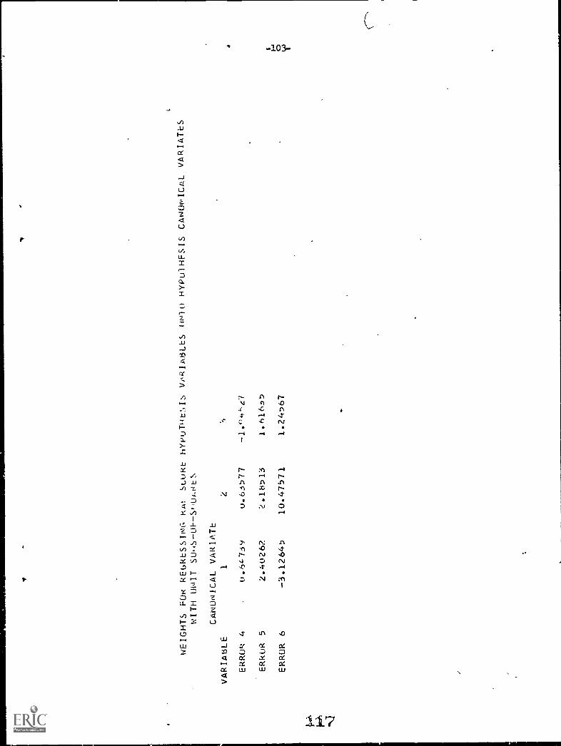
WEIGHTS FOR REGRESSINC, Rat

Suukt hYPuTutSIs VARIABLES (11010 HYPulHFSIS CANONICAL VARIATES

WITH UNIT SU.ISOFSHUAktS

CANONICAL VARIATE

VARIABLE

ERROk 4

ERROR 5

ERROR 6

1

0.6L739

2.40262

3.12645

2

0.63577

2.1813

10.47571

1.fl,te7

1.61655

1.24567

: 1- 0 Y

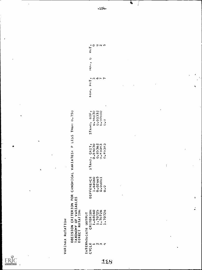
VARINAX ROTATION

DECISION CRITERION FOR CANONICAL

TAXONOMY OF VARIABLES

DIRECT ROTATION

INTERNEuIATE UUTPUT

CYCLE

CRITERION

DIFFERENCE

VARIATES: P LESS THAN 0.750

STAND. GRIT.

STAND. DIE.

Nom. PDT.

Ntivq. 0

RUT.

11.68060

1.68060

0.84030

0.84030

30

21.70725

0.02665

0.85362

0.01332

60

31.70726

0.00001

0.85363

0.00000

72

41.70726

0.0

0.85363

0.0

75

A

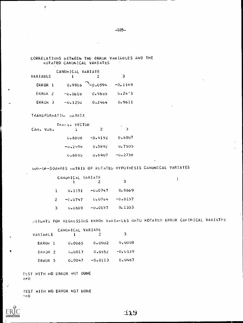
e

-105-

CORRELATIONS bETWEEN THE ERRORROTATED CANONICAL VARIATES

CANONICAL VARIATEVARIABLE 1 2

ERROR 1 0.9916 -N-0.0594

ERROR 2 -0.061b 0.96b7

ERROR 3 -0.1250 0.2464

VARIABLES AND THE

3

-0.1149

6.24'3

0.9611

TRANSFORNATIoi 1,,ATRIX

Ti-CA0o VECTORCAN. VAR. 1 2 3

0.6808 -0.4192 0.6007

-0.2',94 0.5892 0.7505

0.6665 0.6907 -0.2756

SUI',-UF-SOUARES MATRIX OF ROTATEu HYPOTHESIS CANONICAL VARIATES

CANONICAL VARIATF1 2 3

1 0.1151 -0.0747 0.0669

2 -0.0747 0.0764 -0.0157

3 0.0669 -0.0157 0.1333

0E1oHTS FOk REGRESSING EkkOR VARIAr,LES ONTO ROTATED ERROR CANONICAL VARIATES

CANONICAL VARIATtVARIABLE 1 2 3

ERROR 1 0.0065 0.0002 0.0008

ERROR 2 0.0017 0.0552 -0.0139

ERROR 3 0.0047 -0.0113 0.0467

TEST WITH NO ERROR NOT DONEA=0

TEST WITH NO ERROR NOT DONE'q=0

'119

-106-

VARA.q: LINEAR mODEL VARIANCE ANALYSIS

FIRST EDITION: JUNE 1, 1972

FOOCATI004,L TESTING SERVICE

PRINCETON, N.J. 08540

END OF PROBLEMS

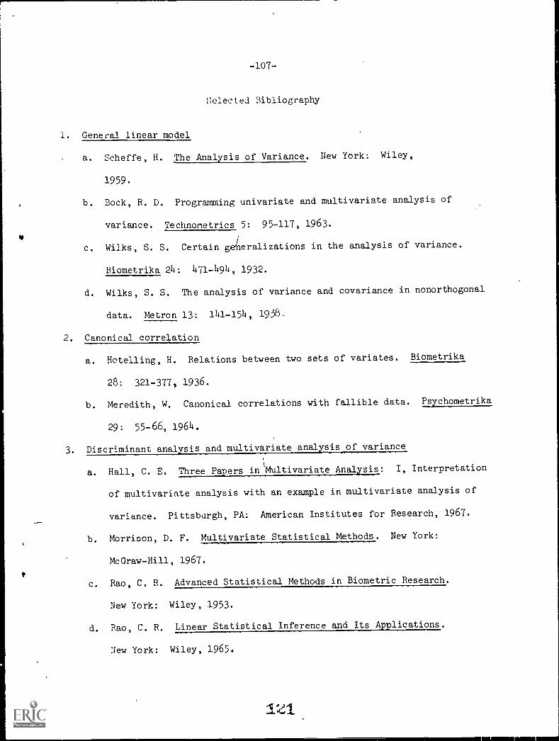
-107-

Selected Bibliography

1. General linear model

a. Scheffe, H. The Analysis of Variance. New York: Wiley,

1959.

b. Bock, R. D. Programming univariate and multivariate analysis of

variance. Technonetrics 5: 95-117, 1963.

c. Wilks, S. S. Certain g ieralizations in the analysis of variance.

Riometrika 24: 471-494, 1932.

d. Wilks, S. S. The analysis of variance and covariance in nonorthogonal

data. Matron 13: 141-154, 19.58.

2. Canonical correlation

a. Hotelling, H. Relations between two sets of variates. Biometrika

28: 321-377, 1936.

b. Meredith, W. Canonical correlations with fallible data. Psychometrika

29: 55-66, 1964.

3. Discriminant analysis and multivariate analysis of variance

a. Hall, C. E. Three Papers in'Multivariate Analysis: I, Interpretation

of multivariate analysis with an example in multivariate analysis of

variance. Pittsburgh, PA: American Institutes for Research, 1967.

b. Morrison, D. F. Multivariate Statistical Methods. New York:

McGraw-Hill, 1967.

c. Rao, C. R. Advanced Statistical Methods in Biometric Research.

New York: Wiley, 1953.

d. Rao, C. R. Linear Statistical Inference and Its Applications.

New York: Wiley, 1965.

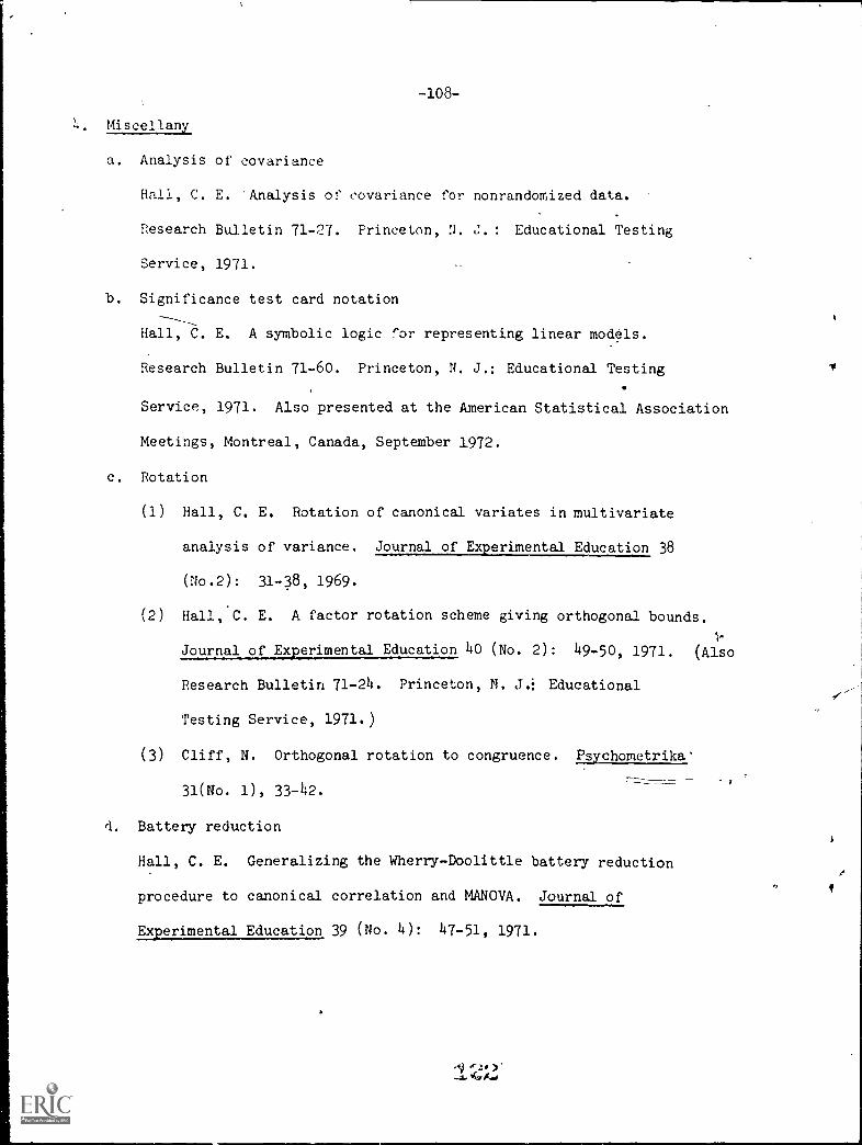
-108-

4. Miscellany

a. Analysis of covariance

Hall, C. E. 'Analysis of covariance for nonrandomized data.

Research Bulletin 71-27. Princeton, N. J. : Educational Testing

Service, 1971.

b. Significance test card notation

Hall, C. E. A symbolic logic for representing linear models.

Research Bulletin 71-60. Princeton, N. J.: Educational Testing

Service, 1971. Also presented at the American Statistical Association

Meetings, Montreal, Canada, September 1972.

c. Rotation

(1) Hall, C. E. Rotation of canonical variates in multivariate

analysis of variance. Journal of Experimental Education 38

(No.2): 31-38, 1969.

(2) Hall, C. E. A factor rotation scheme giving orthogonal bounds.

Journal of Experimental Education 40 (No. 2): 49-50, 1971. (Also

Research Bulletin 71-24. Princeton, N. J.: Educational

Testing Service, 1971.)

(3) Cliff, N. Orthogonal rotation to congruence. Psychometrika'

31(No. 1), 33-42.

d. Battery reduction

Hall, C. E. Generalizing the Wherry-Doolittle battery reduction

procedure to canonical correlation and MANOVA. Journal of

Experimental Education 39 (No. 4): 47-51, 1971.

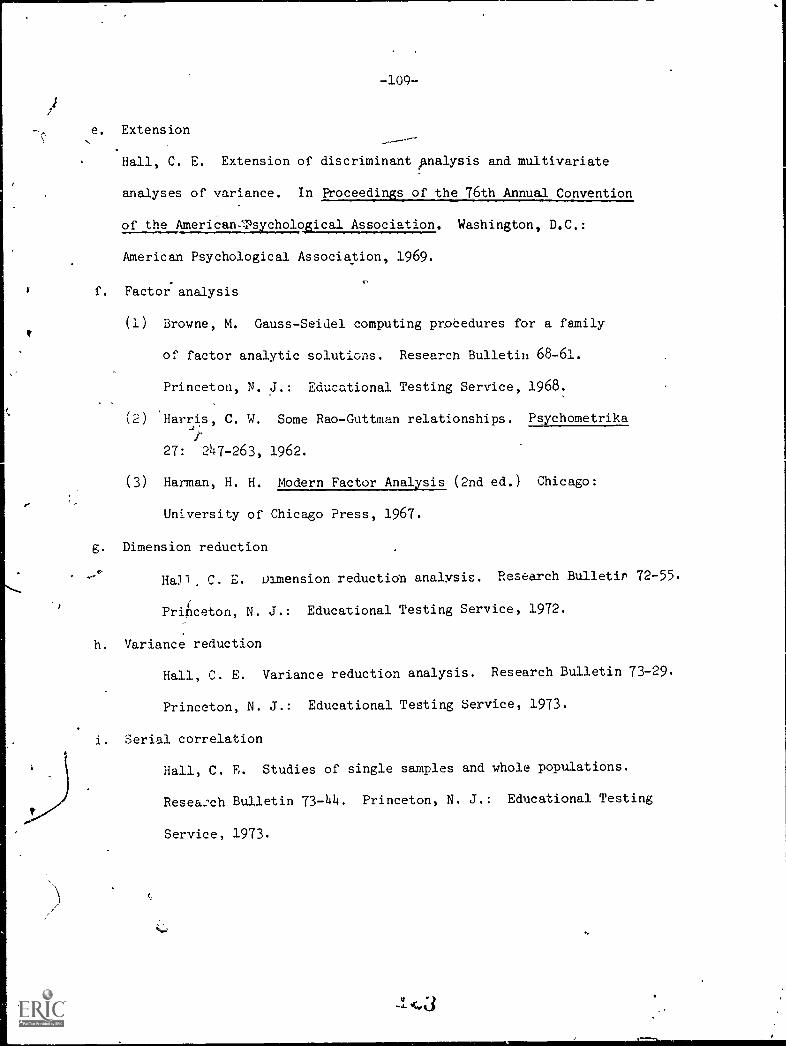
-109-

e. Extension

Hall, C. E. Extension of discriminant analysis and multivariate

analyses of variance. In Proceedings of the 76th Annual Convention

of the American.Tsycholozical Association. Washington, D.C.:

American Psychological Association, 1969.

f. Factor analysis

(1) Browne, M. Gauss-Seidel computing probedures for a family

of factor analytic solutions. Research Bulletin 68-61.

Princeton, N. J.: Educational Testing Service, 1968.

g

(2) Harris, C. W. Some Rao-Guttman relationships. Psychometrika

27: 247-263, 1962.

(3) Harman, H. H. Modern Factor Analysis (2nd ed.) Chicago:

University of Chicago Press, 1967.

Dimension reduction

Ha)), C. E. Dimension reduction analysis. Research Bulletin 72-55.

(Princeton, N. J.: Educational Testing Service, 1972.

h. Variance reduction

Hall, C. E. Variance reduction analysis. Research Bulletin 73-29.

Princeton, N. J.: Educational Testing Service, 1973.

1. Serial correlation

Hall, C. E. Studies of single samples and whole populations.

Research Bulletin 73-44. Princeton, N. J.: Educational Testing

Service, 1973.

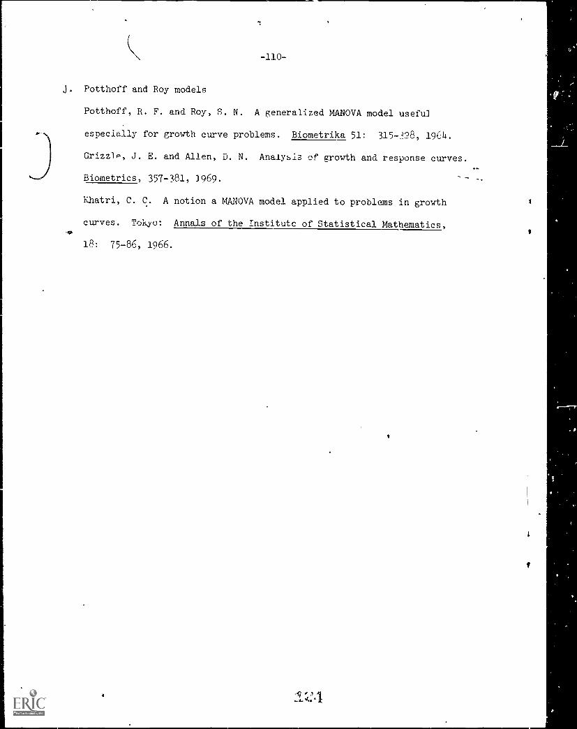
-110-

j. Potthoff and Roy models

Potthoff, R. F. and Roy, S. N. A generalized MANOVA model useful

especially for growth curve problems. Biometrika 51: 315-28, 1964.

-G.

Grizzle, J. E. and Allen, D. N. Analysis of arowth and response curves.

Biometrics, 357-381, 7969.

Khatri, C. C. A notion a MANOVA model applied to problems in growth

curves. Tokyo: Annals of the Institutc of Statistical Mathematics,

18: 75-86, 1966.