analyzing the techniques that improve fault tolerance of aggregation trees in sensor networks

Analyzing techniques for improving fault toleranceof aggregation trees in sensor networks*

LAUKIK CHITNIS

University of Florida

ALIN DOBRA


and

SANJAY RANKA


The potential gains of deploying sensor networks for large scale applications are being realized.One of the basic operations in sensor networks is in-network aggregation. Among the various ap-

proaches to in-network aggregation, such as gossip and tree, including the hash-based techniques,

the tree-based approaches have better performance and energy-saving characteristics. How-ever, sensor networks are highly prone to failures. Numerous techniques suggested in literature

to counteract the effect of failures have not been analyzed in depth. In this paper, we focus on

the performance of these tree-based aggregation techniques in the presence of failures. First, weidentify a fault model that captures the important failure traits of the system. Then, we analyze

the correctness of simple tree aggregation with our fault model. We then use the same fault model

to analyze the techniques that utilize redundant trees to improve the variance. The impact oftechniques for maintaining the correctness under faults, such as rebuilding or locally fixing the

tree, is then studied under the same fault model. We also do the cost-benefit analysis of using

the hash-based schemes which are based on FM sketches. We conclude that these fault toler-ance techniques for tree aggregation do not necessarily result in substantial improvement in fault

tolerance.

Categories and Subject Descriptors: C.2.4 [COMPUTER-COMMUNICATION NETWORKS]:

Distributed Systems—Distributed applications; G.3 [Probability and Statistics]: —probabilis-tic algorithms (including Monte Carlo); H.2.4 [DATABASE MANAGEMENT]: Systems—

Query processing; I.6.4 [SIMULATION; MODELING]: Model Validation and Analysis

General Terms: Algorithms, Design, Performance, Reliability

Additional Key Words and Phrases: In-network processing and aggregation, Fault tolerance,

Sensor fusion and distributed inference, Modeling faults

Author’s address: Laukik Chitnis,

CSE Building Room E402, University of Florida, Gainesville, FL 32611-6120 [email protected]

*A short version of this paper, titled Analyzing the multiple aggregation trees technique for fault

tolerance in sensor networks, is to appear in the Proc. of International Conference on InformationSystems, Technology and Management (ICISTM 2007), New Delhi, India, March 2007.This work is supported in part by the National Science Foundation under Grant ITR 0325459,

NSF-CAREER-IIS-0448264 and NSF Grant number 0312038 (under a subcontract from FIU)Permission to make digital/hard copy of all or part of this material without fee for personal

or classroom use provided that the copies are not made or distributed for profit or commercial

advantage, the ACM copyright/server notice, the title of the publication, and its date appear, andnotice is given that copying is by permission of the ACM, Inc. To copy otherwise, to republish,to post on servers, or to redistribute to lists requires prior specific permission and/or a fee.c© 2007 ACM 0000-0000/2007/0000-0001 $5.00

ACM Journal Name, Vol. V, No. N, January 2007, Pages 1–23.

2 ·

1. INTRODUCTION

A wireless sensor network consists of untethered sensor nodes forming an ad-hocwireless network to co-operatively perform sensing, and may be even actuating,operations[Zhao and Guibas 2004][Culler et al. 2004]. Today, sensor networks findapplication in various areas ranging from environment monitoring to battlefieldsurveillance. In addition to one or more sensors, for monitoring say temperature,pressure or motion, each sensor node typically consists of a wireless communicationdevice, such as a radio transceiver, and a microcontroller, all powered by a battery.The size of each sensor node, though, may be as small as a grain of dust [Warnekeet al. 2001][Koushanfar et al. 2004]. With applications such as hurricane modelingand tracking envisioned to utilize tens of thousands of such small sensor nodes,the cost of each sensor node is constrained. Due to significant constraints on thecost, and therefore the quality of sensor motes, and the often hostile environmentsin which they are deployed, sensor networks are prone to failures. Size and costconstraints on sensor nodes result in corresponding constraints on resources such asenergy, memory, computational speed and bandwidth [Koushanfar et al. 2004][Zhaoand Guibas 2004]. As a result, fault tolerance and optimal resource utilization arethe important challenges in the field of algorithms in sensor network.

An important class of algorithms in sensor networks is aggregation. The problemof data aggregation includes calculating an aggregate of the readings from all or asubset of the sensors. Examples of data aggregation include calculating the averagetemperature of a particular region in habitat monitoring or calculating the maxi-mum pressure exerted on a plane. Aggregate operations such as count, sum, averageand quantiles fall in this category. An important characteristic of this class of algo-rithms is that, knowing the algorithm for a one aggregate operator such as average,similar algorithms can be developed for many other aggregate operations[Kempeet al. 2003]. In-network aggregation approaches, such as tree, gossip or hash-basedalgorithms are used to minimize the energy spent in aggregation operation.

In this paper, we focus on the accuracy and scalability of tree-based aggregationtechniques in the presence of failures. Such analysis would typically be applicablein cases of deployment of large scale sensor networks in hostile environments. In theabsence of failures, the tree based aggregation schemes are known to excel – smallconstant factor associated with their O(log n) performance, in fact, makes it the bestavailable in sensor networks. This, along with their ease of construction, are amongthe reasons why tree based techniques such as [Madden et al. 2002] are preferred inpractical implementations for aggregation in sensor networks [Gehrke and Madden2004] [Mainwaring et al. 2002]. Other in-network aggregation techniques, such asgossip-based algorithms [Kempe et al. 2003] [Chen et al. 2005], though offer similarO(log n) asymptotic performance, usually have a large constant factor associatedwith them[Chen et al. 2005][Chitnis et al. 2006]. However, the performance ofaggregation trees in the presence of failures remain largely unexplored. A fewsolutions are suggested in literature [Madden et al. 2002][Jia et al. 2006][Considineet al. 2004][Nath et al. 2004] to counteract the effect of failures in aggregationACM Journal Name, Vol. V, No. N, January 2007.

· 3

trees. These proposed tactics, though appear very intuitive, are not analyzed indepth. The focus of this paper is on analyzing these suggestions qualitatively andquantitatively.

In particular, we focus on fault tolerance in terms of performance and correctness.Failures usually result in increase in resource utilization in terms of, say, time tocompletion and energy utilized. Longer time to completion means degradation inperformance. Failures also result in degradation in correctness of algorithms. Aswe will soon see, the presence of failures results in a bias between the true valueof the aggregate and the aggregate value returned by the algorithm. Failures alsoinduce variance in the calculated aggregate value. Thus, improving fault tolerancecan also be seen as decreasing the bias and/or the variance of the aggregate value.

A naive approach is to just neglect the effect of failures. However, neglectingthe effects of failure of an intermediate tree node would entail neglecting not onlythe value of the failed node from the aggregate calculation, but also neglecting thevalues of all the nodes in the subtree rooted at this failed node. Not surprisingly,such a naive strategy does not guarantee any form of correctness [Bawa et al.2003] [Chitnis et al. 2006]. The inaccuracy introduced due to failures might beprohibitively large.

The other options discussed in literature include maintaining multiple trees [Mad-den et al. 2002][Considine et al. 2004], fixing the trees locally before proceedingwith aggregation [Jia et al. 2006][Gobriel et al. 2006] and using order-independent,duplicate-insensitive multimaps [Nath et al. 2004] [Considine et al. 2004][Manjhiet al. 2005] (based primarily on FM sketches [Flajolet and Martin 1985]). Anotheroption is rebuilding the aggregation tree when a failure is detected during the ag-gregation process [Chitnis et al. 2006]. We analyze each of these options in furtherdetail in the following sections. We start with identifying a simple fault model inSection 2 to be consistently applied in our analysis. We then carefully analyze, firsttheoretically and then experimentally, the impact of using multiple trees on faulttolerance of the tree aggregation in Section 4. Then we analyze the simple globalrestart technique in Section 5 followed by the study of impact of using local fixeson fault tolerance in Section 6. We also discuss the applicability of sketch basedtechniques in Section 7.

The main thrust of this paper is on conceptually analyzing the fault tolerance,scalability – and hence the applicability – and accuracy of the different techniques.We first analyze theoretically the extent to which the fault tolerance of an aggre-gation tree can be improved using each of the techniques. The analysis suggeststhat the gains of using these techniques might not be as high as previously believedto be. We back our conceptual analysis with results from experiments simulatingdifferent failure conditions using the fault model for various sizes of sensor net-works. We identify high level trends in fault tolerance, scalability and accuracy ofthe various tree-based techniques which would enable informed decision-making indesigning aggregation algorithms for sensor networks.

2. FAILURE MODEL

A common aspect of applications in sensor networks is the presence of failures.The amount of failures vary over a wide range [Eckhardt and Steenkiste 1996],

ACM Journal Name, Vol. V, No. N, January 2007.

4 ·

depending, primarily, on the environment and the size and cost of hardware used.This is due to the following reasons:

—Large scale applications involving sensor networks usually call for thousandsof untethered nodes spread across the system. To constrain the overall cost,as a design decision, the sensor nodes typically consist of inexpensive hard-ware[Koushanfar et al. 2004] [Warneke et al. 2001]. Also, the energy sourceof sensor nodes is typically non-rechargeable. The idea is to improve the over-allfault tolerance of the system using redundancy, while keeping the system costdown. However, these factors make the sensor nodes more fault-prone.

—The applications of sensor networks often require the nodes to be deployed in un-controlled environments. In fact, with applications usually ranging from habitatmonitoring, coastal and hurricane monitoring to sewage control and deploymentin battlefields, the environment is usually hostile. This results in impairments ofsensor nodes or communication, thus resulting in higher probability of failure.

Hence, it becomes quite imperative to analyze the behavior of algorithms in faultyenvironments to better understand the implications and estimate their performancebefore being actually deployed. For testing the fault tolerance and scalability ofalgorithms in sensor networks, we need a model which captures the fault behavioreffectively. The fault-model should be simple enough to analyze, but also sophisti-cated enough to capture the actual fault behavior effectively. This calls for limitingthe number of parameters in the fault model to the most relevant, so that they canbe fairly accurately estimated. The fault model discussed here is thus an expandedversion of the one discussed in our previous work [Chitnis et al. 2006]. We haveincorporated additional parameters in order to accurately analyze the impact ofthe actual fault behavior on the techniques discussed in this paper. We identify thefollowing sources of failures in our simple fault model:

—Node failures: As discussed before, the need for deployment of tens of thousandsof sensor nodes usually calls for the use of untethered nodes having high proba-bility of failure. This parameter can be captured as the probability of failure of asensor node in unit time. This parameter models the kind of failures wherein thenodes appear to be inactive throughout the span of an aggregation operation. Wealso note that sensor nodes are often put in sleep mode to save energy. Any nodethat sleeps through the aggregation operation, accidentally or by design, alsowould count as node failure from the point of view of this aggregation operation[Koushanfar et al. 2004]. For ease of analysis, instead of using multiple inputparameters such as number of failures per second and the time in seconds peraggregation operation, we use a span of an aggregation operation as the time unitfor expressing node failures. We note that knowing the per second failure rateand an estimate of the aggregation time, we can easily estimate this parameter.

—Link failures: The hostile environments in which sensor networks are usuallydeployed imply a weak signal to noise ratio for wireless communication. Coupledwith obstructions and other factors, the failure to communicate with another livenode in the network is highly possible. Also, the use of lightweight protocols inwireless sensor networks means that usually there are no delivery confirmations oracknowledgments. As a result, the probability of link failure is another important


· 5

parameter and is thus considered in our fault model. Since a link failure isrelevant only during communication attempts, we model the link failure per unittime as the probability of link failure in the time it takes for transmission ofa message. Knowing the probability of link failure, say per second, and thestandard message length and communication data-rate, this parameter can beeasily estimated. Once again, this results in reduction of free parameters in ourfault model leading to easier analysis without compromising on quality of results.

In this paper, we focus on investigating if significant gains can be achieved byutilizing the techniques suggested in literature for improving fault tolerance. Hence,as an adversarial approach, we have to provide the best case scenarios for each ofthe techniques analyzed in this paper by making the following assumptions in ourfault model:

—We ignore the transient failures – these may be, for example in a retransmis-sion communication paradigm, failures due to message being garbled on initialcommunication attempts, but eventually leading to a successful transmission.Such failures end up delaying the entire process overall and affects each of thestrategies discussed in the paper equally.

—Each failure is assumed to be independent. We do not consider correlation be-tween failures. Though correlation is an undeniable occurrence, it is difficult tocapture correlation with the limited capabilities of sensor motes. Also, simplefault models neglecting correlation between failures have been shown to modelrealistic scenarios with correlation quite effectively [Chitnis et al. 2006].

—Byzantine failures are not considered.

We now apply this fault model in the analysis of each of the proposed techniquesfor improving fault tolerance of an aggregation tree. We begin with the techniqueproposed for reducing the variance of the aggregation operation, namely, usingmultiple trees in Section 4. We then analyze the techniques that strive to maintainthe correctness of the aggregation operation in the presence of failures, namely,rebuilding the tree in Section 5 and fixing the aggregation tree locally in Section 6.But first, we discuss the preliminaries of tree-based aggregation and model the lossof information in an aggregation tree due to failures.

3. PRELIMINARIES: TREE AGGREGATION

In tree based aggregation techniques, depicted in Figure 1, the main idea is toorganize all the sensor nodes into a spanning tree – called aggregation tree[Maddenet al. 2002]. The root of the tree is the node where the query is injected andwhere the aggregation result is retrieved. The query/request is propagated fromparent to children. The leaf nodes send the value of the measurement to the parent.Intermediate nodes wait for values from the children, do a local aggregation of thesevalues and its own measurement and send the aggregate to the parent. The rootnode computes in the same manner as any intermediate node and presents thevalue of the overall aggregate to the user. The algorithm requires a spanning-treeamong the sensor nodes [Madden et al. 2002] [Madden et al. 2003] [Bawa et al.2003] [Gupta et al. 2001]. The efficiency of the algorithm depends on the longestroute from root to the leaf, i.e how balanced this tree is.


6 ·

��

��

��

��

��query

aggregate

Fig. 1. Tree-based aggregation

However, when a failure occurs, the result returned at the root node may not becorrect [Chitnis et al. 2006]. Unless the faulty node is a leaf, the information in thesubtree rooted at the faulty node is not aggregated, i.e. not only the informationof the faulty node is lost, but the information in the entire subtree is lost.

3.1 Partial Aggregation

In this section, we characterize the loss of information in an aggregation tree dueto failures. Assuming a uniform probability of failure, pn for node failure and pl

for link failure, as defined in the simple fault model, we formulate the expressionsfor average information loss and the expected variance. These values also dependon the actual aggregation operation performed. We model the behavior for simplesum operation, with count considered as a simple case, and note that a large rangeof aggregate operators can be tackled similarly [Kempe et al. 2003].

We model the failure of nodes in the sensor network of size N as a 0/1 randomvariable X.

Xi ={

1 if node i is alive0 otherwise

Similarly, let Y be the 0/1 random variable modeling the link failure. Thus,

Yij = Yji ={

1 if communication link between nodes i and j is up0 otherwise

Hence, if pn is the probability of node failure and pl is the probability of linkfailure,

E(X) = 0(pn) + 1(1− pn) = 1− pn

E(Y ) = 0(pl) + 1(1− pl) = 1− pl


· 7

Let Vi be the random variable denoting the value accumulated at node i. Thus,Vi is the partial aggregation value which includes the value at node i. If the valuessensed at each individual node i is xi, then for every leaf node in the aggregationtree, Vleaf = xleaf . For the summation aggregation operation, the value at eachintermediate node j, it is defined as

Vj = xj +∑

all children c

VcXcYcj (1)

Equation 1 accounts for the fact that for each child node c, the value Vc reachesits parent node j only if (a) the child node is alive (Xc = 1), and (b) node c cancommunicate its partial aggregate Vc to its parent j (Ycj = 1).

The aggregated value as seen at the root node R is then VR and the averageinformation loss for summation is then

∑xi − E(VR). Note that the root node is

usually a very reliable node such as the base station, and hence XR can be assumedto be 1.

From simple induction, we get an expression for VR as

VR =∑

all nodes i

xi

∏nodes Xn along path to root

Xn

∏

links Yl along path to root

Yl

As explained in the failure model explained in section 2, the failures are assumed

to be independent. Hence, on taking the expected value, we get

E(VR) =∑

all nodes i

xi{(1− pn)(1− pl)}len(i,R)

where

len(i,R) is the length of the path from node i to root R

To get a better intuition about the problem, consider a perfectly balanced treeas a case-study. Let us first consider the scenario where ∀i, xi = 1 (this is thecount query). Each sensor node reachable from the root would contribute 1 to theaggregate and hence the expected value of VR yields the expected value of the countof nodes alive and reachable from the root node.

E(VR) =log N∑d=1

(number of nodes at depth d){(1− pn)(1− pl)}d

For a binary tree, it can be expressed as

E(VR) =log N∑d=1

2d{(1− pn)(1− pl)}d

Another important statistic to be considered in such cases is the variance of therandom variable. We calculate the variance of the random variable VR by firstobserving that


8 ·

V 2R =

∑all nodes i

xi

∏nodes XiR

n along path to root R

XiRn

∏

links Y iRl along path to root R

Y iRl

×

∑all nodes j

xj

∏nodes XjR

n along path to root R

XjRn

∏

links Y jRl along path to root R

Y jRl

V 2R =

∑all nodes i and j

xixj

∏unique nodes Xn along paths to root

Xn

∏

unique links Yl along paths to root

Yl

This is because X and Y are 0/1 random variables and hence Xi×Xi = Xi. The

variance of the final aggregate can then be evaluated as

V ar(VR) = E(V 2R)− [E(VR)]2

We corroborate the estimates of the bias and variance as predicted by this modelwith experimental results.

3.2 Experimental evaluation

The experiments we present in this paper are performed on simulated sensor net-works wherein the N sensor nodes are placed randomly in a unit square field. Aunit-disc communication graph is used – each sensor can communicate with onlythose sensors which lie within its radius of communication. Thus, the communi-cation graph is undirected. This two dimensional space is characteristic of deploy-ments in most sensor network applications. A spanning quad-tree is formed amongthe participating nodes by starting with the root node, splitting the space into4 regions, selecting a random node in each part to be the child of this node andrecursing until no nodes are left. This method of splitting produces a reasonablybalanced tree with good locality for the lower part of the tree. This approach issimilar to the method of [Gupta et al. 2001]. The trees formed in this way also havethe additional advantage of being group independent while answering queries[Jiaet al. 2006]. An alternative is to use flooding – as in [Madden et al. 2002] – in whichcase the communication between parent and children will be more efficient but thetree may be unbalanced. Aggregation begins with the leaf nodes sending their val-ues to their respective parents. Intermediate nodes collect values from all the childnodes it could reach to – failure of a node or communication link is ignored; performpartial aggregation (including its own value) and forward the partial aggregate toits parent. The process of one aggregation operation culminates with the partialaggregates reaching the root node and the root node estimating the final aggregatevalue.

In figure 2, we have plotted the expected aggregate returned by a count queryand its corresponding variance for various probabilities of link failure plink. Wealso note that a similar trend is observed for all the different network sizes N andnode failures pnode. As the probability of failure increases, there is an increase inACM Journal Name, Vol. V, No. N, January 2007.

· 9

0

2000

4000

6000

8000

10000

1e-04 0.001 0.01 0.1

Ave

rage

cou

nt w

ith 1

σ

plink

Count

Fig. 2. The mean and standard deviation of the count aggregate using one tree as a function of

the probability of link failure for a sensor network of size N=8192 at pnode = 0.00016

the bias and variance of the estimate. The behavior trend observed in Figure 2corroborates with the behavior as predicted by our simple theoretical analysis.Thus, these results vindicate the simple theoretical model used.

4. REDUCING VARIANCE USING MULTIPLE AGGREGATION TREES

Multiple decision trees have been utilized in data mining to improve robustness[Kargupta et al. 2006] [Kwok and Carter 1990]. In such cases, the use of multipletrees has been shown to reduce the variance. Using multiple aggregation trees atthe same time has been proposed [Madden et al. 2003] [Considine et al. 2004] as away of reducing variance. The main idea here is that if two trees are independent,the variance of a linear combination of the two final aggregates would be half of thevariance of the individual aggregate from a single tree. Consider the example of aquery for finding the count of the nodes alive in the network. Two aggregation treesare constructed independently and the aggregation operation occurs simultaneouslyin both the trees. The final estimate of the count of the sensors is calculated as theaverage of the results returned by the two trees. It is easy to see that the expectedvalue of this final aggregate is same as the expected value of the individual aggregatefrom each of the trees.

E(X1 + X2

2) = E(

X1

2+

X2

2) = E(

X1

2) + E(

X2

2)

=12(E(X1) + E(X2)) =

12(2E(X))

= E(X) (2)

Now, consider the variance of the final aggregate, assuming the two trees areindependent


10 ·

V ar(X1 + X2

2) = V ar(

X1

2+

X2

2) = V ar(

X1

2) + V ar(

X2

2)

=14(V ar(X1) + V ar(X2)) =

14(2 ∗ V ar(X))

=V ar(X)

2(3)

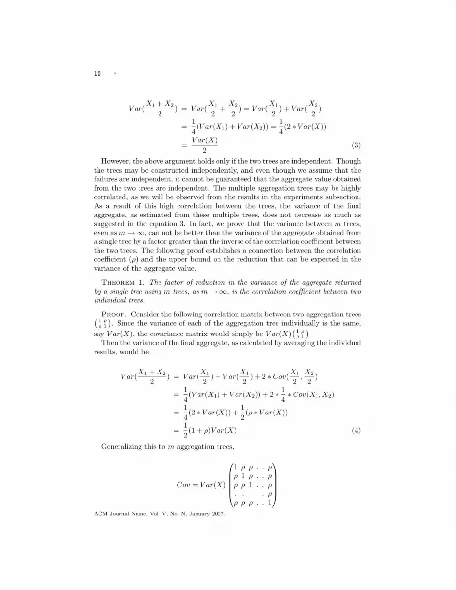
However, the above argument holds only if the two trees are independent. Thoughthe trees may be constructed independently, and even though we assume that thefailures are independent, it cannot be guaranteed that the aggregate value obtainedfrom the two trees are independent. The multiple aggregation trees may be highlycorrelated, as we will be observed from the results in the experiments subsection.As a result of this high correlation between the trees, the variance of the finalaggregate, as estimated from these multiple trees, does not decrease as much assuggested in the equation 3. In fact, we prove that the variance between m trees,even as m →∞, can not be better than the variance of the aggregate obtained froma single tree by a factor greater than the inverse of the correlation coefficient betweenthe two trees. The following proof establishes a connection between the correlationcoefficient (ρ) and the upper bound on the reduction that can be expected in thevariance of the aggregate value.

Theorem 1. The factor of reduction in the variance of the aggregate returnedby a single tree using m trees, as m →∞, is the correlation coefficient between twoindividual trees.

Proof. Consider the following correlation matrix between two aggregation trees( 1 ρρ 1

). Since the variance of each of the aggregation tree individually is the same,

say V ar(X), the covariance matrix would simply be V ar(X)( 1 ρ

ρ 1

)Then the variance of the final aggregate, as calculated by averaging the individual

results, would be

V ar(X1 + X2

2) = V ar(

X1

2) + V ar(

X1

2) + 2 ∗ Cov(

X1

2,X2

2)

=14(V ar(X1) + V ar(X2)) + 2 ∗ 1

4∗ Cov(X1, X2)

=14(2 ∗ V ar(X)) +

12(ρ ∗ V ar(X))

=12(1 + ρ)V ar(X) (4)

Generalizing this to m aggregation trees,

Cov = V ar(X)

1 ρ ρ . . ρρ 1 ρ . . ρρ ρ 1 . . ρ. . . ρρ ρ ρ . . 1


· 11

And the variance of the final aggregate would be

V ar(X1 + X2 + · · ·+ Xm

m) =

1m∗ V ar(X) + (m2 −m)

ρ

m2V ar(X)

=1 + (m− 1)ρ

mV ar(X) (5)

Hence, as m →∞, 1m → 0 and m−1

m → 1, and so

limm→∞

V ar(X1 + X2 + · · ·+ Xm

m) = ρ× V ar(X)

This immediately has the following implications:

(1) The use of multiple aggregation trees is not going to reduce the variance of theaggregate by a factor greater than the correlation between two trees. So, if thecorrelation coefficient between two trees is high, the reduced variance may notbe worth the overhead cost of maintaining multiple trees.

(2) Plotting the factor of reduction in variance (1+(m−1)ρm ) for different values of

m and ρ, we note that most of the reduction in variance (of the maximumpossible) is achieved using as few as 5 to 7 trees – the returns diminish withincreasing number of trees.

In the following experimental evaluation, we show that the correlation coefficient,and hence the reduction in variance obtained by using multiple trees, is dependenton the way the multiple trees are constructed. We also analyze the impact ofconstructing and maintaining those multitree structures on the fault tolerance ofthe aggregation system.

Experiments and Results

In this section, we perform experiments to determine the possible correlation be-tween the aggregate values for different models suggested in literature utilizingmultiple trees. As explained in the previous section, it is necessary to ascertain theamount of independence, or equivalently, the correlation between multiple trees. Ifthere is a high amount of correlation between multiple trees, the reduction in vari-ance is limited and may not be worth the additional cost of multiple trees, especiallywhen energy is at a premium. In particular, we study the trade-off between thecost of multiple trees and the advantages they provide in terms of controlling thevariance. We consider the following models of tree-based aggregation techniqueswhich use multiple trees:

—Levelized multitrees: We categorize a multiple tree structure, where all the par-ents of a node lie in the same level, as levelized trees. The multiple tree structurediscussed in [Madden et al. 2002] has two parents in the level just above thechild node and thus falls in this category. The multitree structure discussed in[Considine et al. 2004] has up to 3 parent nodes, all at the same level. Thus, ineffect, the level of each of the nodes is the same in each of the trees in such cases.


12 ·

Fig. 3. Levelized multitree structure. Ag-gregates are split equally along the solid and

dashed paths from a node.

Fig. 4. Arbitrary multitree structure. Thesolid and dashed arrows represent two differ-

ent trees (shown partially here). Final esti-

mate is obtained by aggregating at the singleroot node the estimates from the two trees.

—Arbitrary multitrees: These are the multitree structures created without anyrestrictions on the position of the parent in any other tree. Thus, in this case,the node is free to be at any of the levels in the different trees. Multiple treesformed independently using any tree generating algorithm, such as GIST [Jiaet al. 2006], would fall in this category.

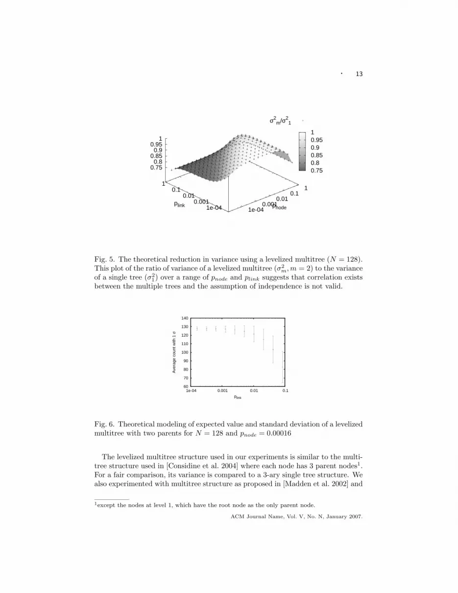
Extending the theoretical analysis for the expected value and variance of theaggregate for a single tree in the previous section to levelized multitree, we plot theexpected value and standard deviation for a levelized multitree having two parentsfor each node in Figure 6. We also plot the reduction in the variance when comparedto a single binary tree of the same size (N = 128) in Figure 5. We observe that,theoretically, the reduction obtained in the variance is not uniform over the rangeof node and link failures. The ratio of the variance of the multitree to the varianceof a single tree is observed to be nearly as high as 1 in some cases. Also, theminimum of the ratio is much greater than 0.5, the value which corresponds to thecorrelation between the two trees being zero (ρ = 0). This proves that correlationexists between the multiple trees and the assumption of independence between thevalues returned by multiple trees [Madden et al. 2002][Considine et al. 2004] is notentirely valid over the entire range of node and link failures.

To ascertain the results of our theoretical model, we also perform simulationexperiments. In our experiments, we study the correlation between two trees wherethe mulitree structure is (a) a levelized multitree, and (b) an arbitrary multitree.We observe the variance of a single tree, and the variance of the multitree in eachcase. The reduction in the variance obtained using multiple trees can be usedto estimate the correlation between the two trees. The ratio of the variance ofmultitrees to a single tree is plotted for a levelized multitree in Figure 7 and for anarbitrary multitree in Figure 8.ACM Journal Name, Vol. V, No. N, January 2007.

· 13

0.75 0.8 0.85 0.9 0.95 1

1e-04 0.001

0.01 0.1

1

1e-04 0.001

0.01 0.1

1

0.75 0.8

0.85 0.9

0.95 1

σ2m/σ2

1

pnodeplink

Fig. 5. The theoretical reduction in variance using a levelized multitree (N = 128).This plot of the ratio of variance of a levelized multitree (σ2

m,m = 2) to the varianceof a single tree (σ2

1) over a range of pnode and plink suggests that correlation existsbetween the multiple trees and the assumption of independence is not valid.

60

70

80

90

100

110

120

130

140

1e-04 0.001 0.01 0.1

Ave

rage

cou

nt w

ith 1

σ

plink

Fig. 6. Theoretical modeling of expected value and standard deviation of a levelizedmultitree with two parents for N = 128 and pnode = 0.00016

The levelized multitree structure used in our experiments is similar to the multi-tree structure used in [Considine et al. 2004] where each node has 3 parent nodes1.For a fair comparison, its variance is compared to a 3-ary single tree structure. Wealso experimented with multitree structure as proposed in [Madden et al. 2002] and

1except the nodes at level 1, which have the root node as the only parent node.


14 ·

0

0.2

0.4

0.6

0.8

1

1.2

1e-04 0.001 0.01 0.1

Red

uctio

n in

var

ianc

e

plink

ρ=0.75ρ=0.25

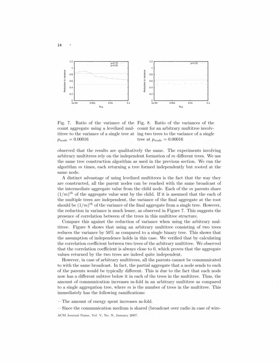
Fig. 7. Ratio of the variance of thecount aggregate using a levelized mul-titree to the variance of a single tree atpnode = 0.00016

0

0.2

0.4

0.6

0.8

1

1.2

1e-04 0.001 0.01 0.1

Red

uctio

n in

var

ianc

e

plink

ρ=0.25

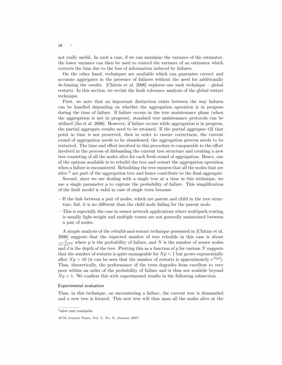
Fig. 8. Ratio of the variances of thecount for an arbitrary multitree involv-ing two trees to the variance of a singletree at pnode = 0.00016

observed that the results are qualitatively the same. The experiments involvingarbitrary multitrees rely on the independent formation of m different trees. We usethe same tree construction algorithm as used in the previous section. We run thealgorithm m times, each returning a tree formed independently but rooted at thesame node.

A distinct advantage of using levelized multitrees is the fact that the way theyare constructed, all the parent nodes can be reached with the same broadcast ofthe intermediate aggregate value from the child node. Each of the m parents share(1/m)th of the aggregate value sent by the child. If it is assumed that the each ofthe multiple trees are independent, the variance of the final aggregate at the rootshould be (1/m)th of the variance of the final aggregate from a single tree. However,the reduction in variance is much lesser, as observed in Figure 7. This suggests thepresence of correlation between of the trees in this multitree structure.

Compare this against the reduction of variance when using the arbitrary mul-titree. Figure 8 shows that using an arbitrary multitree consisting of two treesreduces the variance by 50% as compared to a single binary tree. This shows thatthe assumption of independence holds in this case. We verified that by calculatingthe correlation coefficient between two trees of the arbitrary multitree. We observedthat the correlation coefficient is always close to 0, which proves that the aggregatevalues returned by the two trees are indeed quite independent.

However, in case of arbitrary multitrees, all the parents cannot be communicatedto with the same broadcast. In fact, the partial aggregate that a node sends to eachof the parents would be typically different. This is due to the fact that each nodenow has a different subtree below it in each of the trees in the multitree. Thus, theamount of communication increases m-fold in an arbitrary multitree as comparedto a single aggregation tree, where m is the number of trees in the multitree. Thisimmediately has the following ramifications:

—The amount of energy spent increases m-fold.—Since the communication medium is shared (broadcast over radio in case of wire-ACM Journal Name, Vol. V, No. N, January 2007.

· 15

less sensor networks) and each node has to send and receive m times the messages,the communication has to be serialized.

—Since the communication needs to be serialized, the total time required for ag-gregation can also be assumed to increase m times.

—The probability of node failure is calculated as the probability of the node stayingalive in the time period of an aggregation operation. Now if the aggregation timeincreases, more nodes would fail in this interval. Thus, the probability of nodefailure can be assumed to increase m times too.

3500

4000

4500

5000

5500

6000

6500

7000

7500

8000

8500

1e-04 0.001 0.01 0.1

Ave

rage

cou

nt w

ith 1

σ

pnode

Fig. 9. The mean and standard deviation of the count aggregate as a function of the probability

of node failure for a sensor network of size N = 8192 and plink = 0.00016

We note that, as the probability of node failure increases, (a)the bias from the trueaggregate value increases, and (b)the variance increases, as observed in Figure 9.Thus, the reduction in the variance due to independence between trees is somewhatcounteracted by

—the increase in the variance due to effective m-fold increase in probability of nodefailure pnode

—if bias correction is to be applied, the increased bias due to increase in pnode alsoincreases the variance

Since the probability of link failure depends on the time per transmission, theincrease in the aggregation time for the arbitrary multitrees does not have anydirect impact on the probability of link failure. However, the increased energyexpenditure leads to weakening of transmission power over longer range of timeand thus indirectly affects the probability of link failure.

5. REBUILDING

Using multiple trees dealt with reducing the variance of the aggregate value returnedat the root node. The hope was that, knowing the trends of the bias in the estimatedaggregate as a function of the probability of failure and the number of sensors, thefinal aggregate estimation can just be unscaled appropriately to compensate forthe bias. However, this would also increase the variance of the result and hence is


16 ·

not really useful. In such a case, if we can minimize the variance of the estimator,the lower variance can then be used to control the variance of an estimator whichcorrects the bias due to the loss of information induced by failures.

On the other hand, techniques are available which can guarantee correct andaccurate aggregates in the presence of failures without the need for additionallyde-biasing the results. [Chitnis et al. 2006] explores one such technique – globalrestarts. In this section, we revisit the fault tolerance analysis of the global restarttechnique.

First, we note that an important distinction exists between the way failurescan be handled depending on whether the aggregation operation is in progressduring the time of failure. If failure occurs in the tree maintenance phase (whenthe aggregation is not in progress), standard tree maintenance protocols can beutilized [Jia et al. 2006]. However, if failure occurs while aggregation is in progress,the partial aggregate results need to be retained. If the partial aggregate till thatpoint in time is not preserved, then in order to ensure correctness, the currentround of aggregation needs to be abandoned; the aggregation process needs to berestarted. The time and effort involved in this procedure is comparable to the effortinvolved in the process of disbanding the current tree structure and creating a newtree consisting of all the nodes alive for each fresh round of aggregation. Hence, oneof the options available is to rebuild the tree and restart the aggregation operationwhen a failure is encountered. Rebuilding the tree ensures that all the nodes that arealive 2 are part of the aggregation tree and hence contribute to the final aggregate.

Second, since we are dealing with a single tree at a time in this technique, weuse a single parameter p to capture the probability of failure. This simplificationof the fault model is valid in case of single trees because:

—If the link between a pair of nodes, which are parent and child in the tree struc-ture, fail, it is no different than the child node failing for the parent node.

—This is especially the case in sensor network applications where multipath routingis usually light-weight and multiple routes are not generally maintained betweena pair of nodes.

A simple analysis of the rebuild-and-restart technique presented in [Chitnis et al.2006] suggests that the expected number of tree rebuilds in this case is about

1(1−p)Nd where p is the probability of failure, and N is the number of sensor nodesand d is the depth of the tree. Plotting this as a function of p for various N suggeststhat the number of restarts is quite manageable for Np < 1 but grows exponentiallyafter Np > 10 (it can be seen that the number of restarts is approximately eNpd).Thus, theoretically, the performance of the trees degrades from excellent to verypoor within an order of the probability of failure and is thus not scalable beyondNp > 1. We confirm this with experimental results in the following subsection.

Experimental evaluation

Thus, in this technique, on encountering a failure, the current tree is dismantledand a new tree is formed. This new tree will thus span all the nodes alive at the

2alive and reachable


· 17

time of reconstruction and the aggregation processed is triggered. Since the treeis reconstructed every time a failure is encountered, if and when the aggregationoperation does manage to run to completion, it implies that all the nodes that arealive are accounted for in the aggregation query result.

We use the same experimental setup as explained in the previous section. Oncethe tree is constructed, the aggregation operation begins at the leaf nodes andpropagates up the tree. The query dissemination is assumed to have occurredduring tree construction. As an adversarial approach to proving the limitationsin fault tolerance of these techniques, we consider the minimum cost that can beincurred by these techniques. Hence,

—The cost of building the tree is assumed to be zero. This also makes our analysisindependent of any tree construction algorithm – a most ideal, though practicallyunrealizable, construction cost is assumed.

—The detection of failure is assumed also to be free of cost. On detecting a failure,the tree is reconstructed and the aggregation operation is restarted.

The cost of reconstructing the tree is also assumed to be zero. Hence the onlycost counted is the time spent (or the number of messages sent) in the aggregationprocess.

10

100

1000

10000

100000

1e-05 1e-04 0.001 0.01

Ave

rage

tim

e to

com

plet

ion

Probability of failure (p)

N=1024N=4096N=8192

Fig. 10. The time to completion in rounds plotted against the probability of failure when usingthe global restart technique

The results in Figure 10, which plots the average time to completion versusthe probability of failure for various sizes of the network, show that as long asNp < 1, the aggregation trees have excellent performance. But once the probabilityof failure starts to increase beyond p > 1/N , the expected time to completion growsexponentially. An important observation here is that the performance of the tree-based technique turns from best to worst within an order of magnitude increase ofthe probability of failure p for any given network of size N .

These results confirm the theoretical analysis presented earlier about the expo-nentially increasing number of restarts after Np > 1. This proves that, given a


18 ·

sensor network of size N , the tree-based aggregation provides robustly correct re-sults with exceptional performance until p is small, such that Np < 1. However, asp increases further, the performance of this technique degrades exponentially andother alternatives need to be explored.

6. LOCAL FIXING

From the discussion in the previous section, it follows that, unlike general treemaintenance protocols, the failures occurring during the aggregation phase shouldnot impede the partial aggregates from being retained. In the case of fixing thetrees locally to tide over failures, the children of the failed node, basically, need toreattach themselves to another node in the network which still has an unimpededpath to the root node. Note that satisfying this condition implies that the orphanedchildren cannot attach themselves to the descendant nodes in their own subtree,thus avoiding creation of cycles. However, since their partial aggregates must bepreserved, an additional condition to be satisfied is that they cannot attach to anynode which has already sent out its own partial aggregate.

Satisfying these conditions makes fixing trees locally during the aggregation phasemore difficult than fixing during just the maintenance phase, which is the commoncase discussed in general tree-based algorithms like routing or subscription-basedprotocols.

Thus, in the advent of multiple failures, fixing the tree locally to compensate forall these failures might actually cost more than rebuilding the tree. Depending onthe number of failures that can be sustained before rebuilding the tree becomescost-effective, the tree reconstruction can be delayed. Once again, since we wantto prove that even the best of these techniques do not substantially improve thefault tolerance of the aggregation tree, we assume that the cost of each local fixis zero. This is also a good way of steering clear of the specifics of local fault-fixing algorithms since, with zero cost, it is as ideal, though probably practicallyunrealizable, as it can be.

We can extend the expression for the number of global restarts from the previoussection to allow up to k local fixes before a rebuild-and-restart is triggered. Thenumber of restarts in case of k local fixes can thus be approximated to

1k∑

i=0

nCkpi(1− p)n−i

Note that we have discounted the depth d of the tree from the formula – this onlymakes the local-fixing algorithm look better and thus, again, provide a best-casescenario. To visualize this theoretical model, we plot the number of restarts, ascalculated from this approximate estimate, for values of k ranging from 0, which isequivalent to global restart, to k > log(n) for a sensor network of size n = 8192 inFigure 11.

Redundancy can be used to take corrective actions, as discussed in the RideShar-ing [Gobriel et al. 2006] approach to fault tolerant aggregation. This approach ex-emplifies a minimal overhead for local fixes paradigm, using the concept of backupparents. The approach performs best if transmission ordering is enforced alongwith parent-clique formation and co-tracking (we encourage the readers to lookupACM Journal Name, Vol. V, No. N, January 2007.

· 19

[Gobriel et al. 2006] for further details) – this requires additional work during treeconstruction. However, not all losses are guaranteed to be accounted for in thisapproach. Also, node failures are ignored in this approach.

In the following section, we conduct experiments to study the effect on faulttolerance of having the ability to sustain k local fixes before triggering a tree re-construction and restarting the aggregation operation.

1

100

10000

1e+06

1e+08

1e+10

1e+12

1e-05 1e-04 0.001 0.01

Est

imat

ed r

esta

rts

Probability of failure (p)

k=0 (global restart)k=2k=8

k=16 (> log N)

Fig. 11. Theoretical prediction of im-provement in fault-tolerance using klocal fixes for sensor network of sizeN=8192

10

100

1000

10000

100000

1e-05 1e-04 0.001 0.01A

vera

ge ti

me

to c

ompl

etio

nProbability of failure (p)

k=0 (global restart)k=2k=8

k=16 (log N)

Fig. 12. The time to completion plot-ted against the probability of failurewhen the maximum number of localfixes allowed is k=0, 2, 8 and 16

Experimental evaluation

From the results of the experiments in the previous section concerning globalrestarts, it can be argued that this exceptionally bad behavior of the tree maybe due to the stringent requirement that the tree be reconstructed on encounteringthe first failure in the aggregation process. A general belief expressed in the litera-ture [Jia et al. 2006] [Madden et al. 2002] is that fixing tree structures to overcomethe faults locally would provide a better performance at higher probabilities of fail-ure. In this set of experiments, we use the same setup as used in the previous setof experiments, except the fact that we now allow up to k failures to occur beforewe reconstruct the tree. Using k as a free variable, we see the effect on the fault-tolerance of the tree structure of being able to sustain varying number of failures.Here, we also assume that the cost of fixing each fault (up to k faults) is zero. Thisguarantees the best possible performance of the aggregation tree using local faultfixing techniques, though this may be practically unrealizable.

Figure 12 reflects the fault-tolerance of the aggregation tree for different valuesof k - it plots the average time to completion for different values of k as a functionof p. The point of focus is the threshold p beyond which the performance degradesexponentially. By observing this plot for increasing values of k, we can study theeffectiveness of allowing local fixes - the later this threshold is reached on the paxis, the better it is for fault tolerance. We vary k from 0, case of global restart,to k = log(n). We observe that, even with the maximum sustainable number


20 ·

of failures before restart as high as log(n) and beyond, the fault-tolerance of theaggregation tree is improved by only an order of magnitude in p.

This shows that, even after assuming no cost for local fixes, having the abilityto sustain very high number of failures before reconstruction does not transform toconsiderable gain in fault tolerance.

7. SKETCH BASED TECHNIQUES

Sketch based methods have been proposed in literature [Nath et al. 2004] [Con-sidine et al. 2004] as fault-tolerant aggregation techniques. These techniques areessentially based on the duplicate-insensitive counting FM-sketches [Flajolet andMartin 1985]. Each sensor node maintains a sketch - a bitmap vector - indicativeof the number of distinct sensor nodes it has heard about. When a sensor nodereceives a sketch from a neighboring node, the union of the incoming sketch withits current sketch yields a bitmap vector which approximates the count of the unionof nodes seen by these two communicating sensors. By ensuring that the sketchesare sent along a tree structure to the root node, at the end of the process, the rootnode has a good estimate of the total count. This idea has been further extendedby [Nath et al. 2004] and [Considine et al. 2004] to calculate the sum of values, inparticular, and hence a lot of other aggregate operations too, in general.

Sketches for increasing fault tolerance

This sketching technique for aggregation operation is inherently fault tolerant tonode and link failures in sensor networks due to its property of being duplicate-insensitive. The same bitmap vector can be transmitted to more than one parentnodes at a time. Since the process is insensitive to duplicates, this does not affectthe aggregate value, however, it improves the fault tolerance of the aggregationnetwork. This is primarily because for a node to be counted in the aggregation,there needs to be an uninterrupted path from that node to the root node. Andso, by creating multiple paths, the fault tolerance is greatly improved. Thus, theimmunity of the sketch-based techniques to multipath algorithms, and the fact thata single copy of the sketch finding its way to the root is good enough, make thistechnique a good candidate for aggregation.

However, as is the case with approximate techniques, this scheme also suffers frominaccuracies. The accuracy of the technique can be improved by using multiple bitvectors (each utilizing different hash functions) instead of a single vector formingthe sketch. The improvement in accuracy with increasing number of bitmap vectorsm, as observed in the decreasing percentage standard error in [Flajolet and Martin1985], is listed in Table 7

For accommodating aggregates of large scale sensor networks of size rangingfrom tens of thousands to million nodes, a safe size of a single bit vector can be32 bits, as assumed in [Nath et al. 2004]. The standard packet size of messagesis, by default [TinyOS 2006], 36 bytes3. With this message length, we can barelyuse m = 8 bit vectors, which would bring the standard error down to just about30%, as seen in Table 7. To limit the standard error to within 10%, the numberof bit vectors required to be maintained and transmitted in each message is m =

3including the headers


· 21

Table I. Standard Error of Counting sketches for several values of m, the number of bitmap vectors,

as reported in [Flajolet and Martin 1985]

m % standard error

2 61.0

4 40.98 28.2

16 19.6

32 13.864 9.7

128 6.8256 4.8

512 3.4

1024 2.4

64. The number of bit vectors required to get the standard error within 2% isgreater than m = 1024. Even after employing some of the space saving techniquessuch as run-length encoding utilized in [Considine et al. 2004], the size of eachsketch message would be around 4KB. Communication of packets of this lengthin the low-bandwidth and low-energy paradigm of sensor networks is currentlyunrealizable and, in fact, is a challenge even for ethernet-based ad-hoc networks.As a result, even though sketch-based aggregation techniques are most immuneto node and link failures in sensor networks, the inaccuracies introduced due tothe innate approximation nature of the technique render it difficult to realize forfairly accurate aggregate calculations. Also, by construction, sketches can only dealwith integer calculations and adaptation to floating point aggregation would leadto additional loss of precision.

8. OBSERVATIONS AND CONCLUSION

In this paper, we have evaluated, qualitatively and quantitatively, the different tree-based techniques for aggregation in sensor network from the point of view of faulttolerance and scalability. We make the following observations:

—The global restarts technique, though ensures correctness, renders the trees un-usable at Np > 10

—Having the ability to sustain k local fixes before triggering a tree reconstructionand restarting the aggregation operation hardly improves the fault-tolerance byan order of magnitude – and this was under the extreme assumption that localfixes occur instantaneously and do not incur any cost of their own.

—The amount of correlation between multiple trees differs depending on the waythe multitree structures are created. Localized multitree structures, like thelevelized multitrees which have minimal aggregation operation time overhead,have higher correlation.

—If the multiple trees are truly arbitrary, as is the requirement for truly indepen-dent trees, the gains in minimizing the variance come at the cost of increasingthe overall probability of failure which, invariably, results in an increase in thevariance.


22 ·

This shows that there is no one pure tree-based aggregation technique that canbe fault-tolerant in all cases of network sizes and probabilities of failures. A morecomprehensive hybrid approach, like the methodology devised in [Chitnis et al.2006], needs to be considered to optimize on performance in all cases.

REFERENCES

Bawa, M., Garcia-Molina, H., Gionis, A., and Motwani, R. 2003. Estimating aggregates on

a peer-to-peer network.

Chen, J.-Y., Pandurangan, G., and Xu, D. 2005. Robust aggregates computation in wire-

less sensor networks. In Proceedings of the Fourth International Conference on Information

Processing in Sensor Networks (IPSN). IEEE, Los Angeles, California, USA.

Chitnis, L., Dobra, A., and Ranka, S. 2006. Aggregation methods for large scale sensor net-

works. Technical report rep-2006-292, CISE, University of Florida.

Considine, J., Li, F., Kollios, G., and Byers, J. 2004. Approximate aggregation techniques

for sensor databases. In ICDE ’04: Proceedings of the 20th International Conference on DataEngineering. IEEE Computer Society, Washington, DC, USA, 449.

Culler, D., Estrin, D., and Srivastava, M. 2004. Overview of wireless sensor networks.

Eckhardt, D. and Steenkiste, P. 1996. Measurement and analysis of the error characteristics

of an in-building wireless network. In SIGCOMM. 243–254.

Flajolet, P. and Martin, G. 1985. Probabilistic counting algorithms for database applications.

Gehrke, J. and Madden, S. 2004. Query processing in sensor networks. IEEE Pervasive Com-

puting 03, 1, 46–55.

Gobriel, S., Khattab, S., Daniel Mosse, J. B., and Melhem, R. 2006. Ridesharing: Fault

tolerant aggregation in sensor networks using corrective actions. In SECON’06, Third An-

nual IEEE Communications Society Conference on Sensor and Ad Hoc Communications andNetworks. IEEE, Reston, VA.

Gupta, I., van Renesse, R., and Birman, K. 2001. Scalable fault-tolerant aggregation in largeprocess groups.

Jia, L., Noubir, G., Rajaraman, R., and Sundaram, R. 2006. Group-independent spanningtree for data aggregation in dense sensor networks. In International Conference on Distributed

Computing in Sensor Systems (DCOSS). Springer Berlin / Heidelberg, San Francisco, CA,

USA.

Kargupta, H., Park, B.-H., and Dutta, H. 2006. Orthogonal decision trees. IEEE Transactionson Knowledge and Data Engineering 18, 8, 1028–1042.

Kempe, D., Dobra, A., and Gehrke, J. 2003. Gossip-based computation of aggregate informa-tion. In 44th Annual IEEE Symposium on Foundations of Computer Science. IEEE Computer

Society, Cambridge, MA, USA.

Koushanfar, F., Potkonjak, M., and Sangiovanni-Vincentelli, A. 2004. Handbook of Sensor

Networks. Number 36. CRC press, Chapter Fault-Tolerance in Sensor Networks.

Kwok, S. W. and Carter, C. 1990. Multiple decision trees. In UAI ’88: Proceedings of the

Fourth Annual Conference on Uncertainty in Artificial Intelligence. North-Holland, 327–338.

Madden, S., Franklin, M. J., Hellerstein, J. M., and Hong, W. 2002. Tag: a tiny aggregation

service for ad-hoc sensor networks. SIGOPS Oper. Syst. Rev. 36, SI, 131–146.

Madden, S., Franklin, M. J., Hellerstein, J. M., and Hong, W. 2003. The design of an

acquisitional query processor for sensor networks. In SIGMOD Conference. ACM, San Diego,

California, 491–502.

Mainwaring, A., Polastre, J., Szewczyk, R., Culler, D., and Anderson, J. 2002. Wireless

sensor networks for habitat monitoring. In ACM Workshop on Wireless Sensor Networks andApplications (WSNA’02). ACM, Atlanta, GA.

Manjhi, A., Nath, S., and Gibbons, P. B. 2005. Tributaries and deltas: efficient and robust ag-gregation in sensor network streams. In SIGMOD ’05: Proceedings of the 2005 ACM SIGMOD

conference on Management of data. ACM Press, New York, NY, USA, 287–298.


· 23

Nath, S., Gibbons, P. B., Seshan, S., and Anderson, Z. R. 2004. Synopsis diffusion for robust

aggregation in sensor networks. In SenSys ’04: Proceedings of the 2nd Conference on Embeddednetworked sensor systems. ACM Press, New York, NY, USA, 250–262.

TinyOS, F. 2006. Tinyos frequently asked questions.

Warneke, B., Last, M., Liebowitz, B., and Pister, K. S. J. 2001. Smart dust: Communicating

with a cubic-millimeter computer. Computer 34, 1, 44–51.

Zhao, F. and Guibas, L. 2004. Wireless Sensor Networks: An Information Processing Approach.Morgan Kaufmann.


analyzing the techniques that improve fault tolerance of aggregation trees in sensor networks

Documents