analytical stress functions applied to hydraulic fracturing
TRANSCRIPT
1
1. INTRODUCTION
The expressions commonly used for elastic stress in
studies to predict borehole breakouts and hydraulic
fracture patterns for well stimulation have been developed by Ernst Gustav Kirsch, a 19
th Century
German Engineer, and published over a century ago. The
Kirsch [1] formulas of 1898 properly account for the stresses around so-called balanced boreholes, where the
drilling fluid supports no deviatoric stress but provides a
median pressure on the well bore that equals the lithostatic pressure. When the borehole is pressurized
either more or less than the ambient confining pressure
in the host rock, the effect of over-pressure or under-
pressure on the stress pattern induced in the vicinity of the wellbore can be profound.
A set of analytical equations derived here from the superposition of a comprehensive pair of stress functions
accurately models the interaction of hydraulically induced
pressures on a borehole with and without a regional
tectonic background stress. Previous work on borehole breakout has accounted for unbalanced pressures in
boreholes [2, 3]. These earlier solutions incorporate an
elasto-plastic solution for shear stress concentrations that
determine the locations of actual plastic slip. In this study,
a different approach is taken, starting from simple stress function superposition to arrive at an elastic solution that
accounts for the stress trajectories around pressurized
wellbores.
The approach taken here seeks analytical simplicity by
adopting the following model assumptions:
(i) Elastic rock behavior is assumed. Elasto-plastic extensions are possible [2, 3], but not necessary
for the initiation of elastic failure and pressure opening
of pre-existing surfaces of failure, the application focus
of this study. (ii) Unlike the assumption in previous studies
that require communication between pore fluid in the
host rock and the drilling fluid (e.g., [4]), such a connection is not essential in the approach outlined here.
The drilling fluid in this study simply exerts a static
pressure on the inner wellbore surface with an elastic response of the wall rock. In fact, the applicability of
elasto-plastic solutions to the impervious rock
formations that host unconventional gas (tight sandstone,
ARMA 11-598
Analytical Stress Functions applied to Hydraulic Fracturing:
Scaling the Interaction of Tectonic Stress and Unbalanced Borehole
Pressures
Weijermars, R.
Juarez, J.
Copyright 2011 ARMA, American Rock Mechanics Association
This paper was prepared for presentation at the 45th US Rock Mechanics / Geomechanics Symposium held in San Francisco, CA, June 26–29,
2011.
This paper was selected for presentation at the symposium by an ARMA Technical Program Committee based on a technical and critical review of the paper by a minimum of two technical reviewers. The material, as presented, does not necessarily reflect any position of ARMA, its officers, or members. Electronic reproduction, distribution, or storage of any part of this paper for commercial purposes without the written consent of ARMA is prohibited. Permission to reproduce in print is restricted to an abstract of not more than 300 words; illustrations may not be copied. The abstract must contain conspicuous acknowledgement of where and by whom the paper was presented.
ABSTRACT: Some 19,000 new oil and gas wells were drilled in the US alone in 2010, and many need hydraulic fracturing aimed at improving well productivity. The Kirsch equations have been widely applied to model borehole stresses; in the basic formulation these
equations are valid only for isotropic elastic media with a non-pressurized hole. A stress function, from which the Kirsch equations can
be derived, is developed here to account for the effect of hydraulic pressure on the cylindrical surface of the wellbore. The concise
solution via the stress function superposition is simpler than any previous analytical derivation. The function can be scaled to map the
typical stress patterns for unbalanced hydraulic well bore pressures and provides a more comprehensive solution than the early Kirsch
equations. The stress fields visualized can account for both over-pressurized and under-pressurized boreholes - with and without a
tectonic background stress - and are valid for horizontal and vertical borehole sections. These analytical solutions allow fast mapping
of stress trajectories around wellbores, which is useful for applications that aim to optimize hydraulic fracturing and thereby improve
oil and gas well productivity. The analytical insight developed here may also contribute to develop better visual images (using stress
trajectories) to prevent blow-outs and loss of drilling fluid in damaged formations.
2
gas shales) is likely to be invalid – no pore connectivity
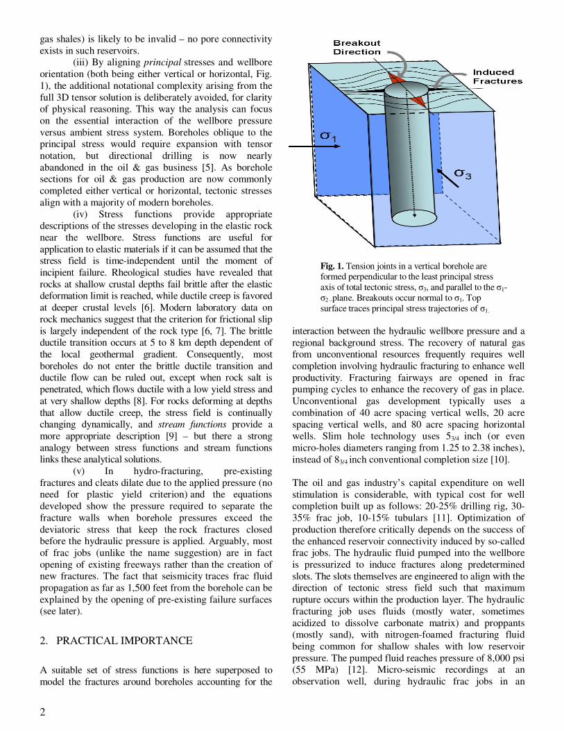
exists in such reservoirs. (iii) By aligning principal stresses and wellbore
orientation (both being either vertical or horizontal, Fig.
1), the additional notational complexity arising from the
full 3D tensor solution is deliberately avoided, for clarity of physical reasoning. This way the analysis can focus
on the essential interaction of the wellbore pressure
versus ambient stress system. Boreholes oblique to the principal stress would require expansion with tensor
notation, but directional drilling is now nearly
abandoned in the oil & gas business [5]. As borehole sections for oil & gas production are now commonly
completed either vertical or horizontal, tectonic stresses
align with a majority of modern boreholes.
(iv) Stress functions provide appropriate descriptions of the stresses developing in the elastic rock
near the wellbore. Stress functions are useful for
application to elastic materials if it can be assumed that the stress field is time-independent until the moment of
incipient failure. Rheological studies have revealed that
rocks at shallow crustal depths fail brittle after the elastic deformation limit is reached, while ductile creep is favored
at deeper crustal levels [6]. Modern laboratory data on
rock mechanics suggest that the criterion for frictional slip
is largely independent of the rock type [6, 7]. The brittle ductile transition occurs at 5 to 8 km depth dependent of
the local geothermal gradient. Consequently, most
boreholes do not enter the brittle ductile transition and ductile flow can be ruled out, except when rock salt is
penetrated, which flows ductile with a low yield stress and
at very shallow depths [8]. For rocks deforming at depths
that allow ductile creep, the stress field is continually changing dynamically, and stream functions provide a
more appropriate description [9] – but there a strong
analogy between stress functions and stream functions links these analytical solutions.
(v) In hydro-fracturing, pre-existing
fractures and cleats dilate due to the applied pressure (no need for plastic yield criterion) and the equations
developed show the pressure required to separate the
fracture walls when borehole pressures exceed the
deviatoric stress that keep the rock fractures closed before the hydraulic pressure is applied. Arguably, most
of frac jobs (unlike the name suggestion) are in fact
opening of existing freeways rather than the creation of new fractures. The fact that seismicity traces frac fluid
propagation as far as 1,500 feet from the borehole can be
explained by the opening of pre-existing failure surfaces (see later).
2. PRACTICAL IMPORTANCE
A suitable set of stress functions is here superposed to
model the fractures around boreholes accounting for the
interaction between the hydraulic wellbore pressure and a
regional background stress. The recovery of natural gas from unconventional resources frequently requires well
completion involving hydraulic fracturing to enhance well
productivity. Fracturing fairways are opened in frac pumping cycles to enhance the recovery of gas in place.
Unconventional gas development typically uses a
combination of 40 acre spacing vertical wells, 20 acre
spacing vertical wells, and 80 acre spacing horizontal wells. Slim hole technology uses 53/4 inch (or even
micro-holes diameters ranging from 1.25 to 2.38 inches),
instead of 83/4 inch conventional completion size [10].
The oil and gas industry’s capital expenditure on well
stimulation is considerable, with typical cost for well completion built up as follows: 20-25% drilling rig, 30-
35% frac job, 10-15% tubulars [11]. Optimization of
production therefore critically depends on the success of
the enhanced reservoir connectivity induced by so-called frac jobs. The hydraulic fluid pumped into the wellbore
is pressurized to induce fractures along predetermined
slots. The slots themselves are engineered to align with the direction of tectonic stress field such that maximum
rupture occurs within the production layer. The hydraulic
fracturing job uses fluids (mostly water, sometimes
acidized to dissolve carbonate matrix) and proppants (mostly sand), with nitrogen-foamed fracturing fluid
being common for shallow shales with low reservoir
pressure. The pumped fluid reaches pressure of 8,000 psi (55 MPa) [12]. Micro-seismic recordings at an
observation well, during hydraulic frac jobs in an
Fig. 1. Tension joints in a vertical borehole are formed perpendicular to the least principal stress
axis of total tectonic stress, σ3, and parallel to the σ1-
σ2 –plane. Breakouts occur normal to σ1. Top
surface traces principal stress trajectories of σ1.
3
adjacent vertical well, have revealed that fractures
propagate (or pre-existing fissures dilate) in shale formations [13] and tight sands [14] as much as 1,500
feet (~0.5 km) in lateral directions.
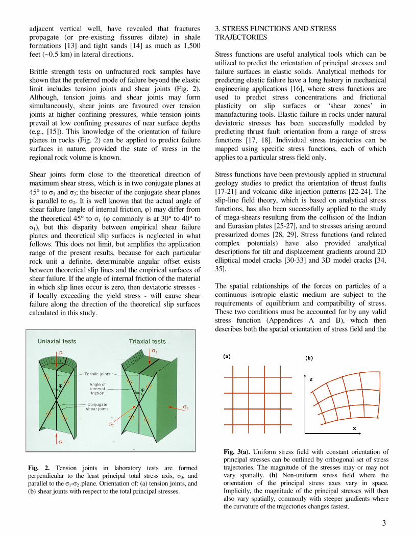
Brittle strength tests on unfractured rock samples have shown that the preferred mode of failure beyond the elastic
limit includes tension joints and shear joints (Fig. 2).
Although, tension joints and shear joints may form simultaneously, shear joints are favoured over tension
joints at higher confining pressures, while tension joints
prevail at low confining pressures of near surface depths (e.g., [15]). This knowledge of the orientation of failure
planes in rocks (Fig. 2) can be applied to predict failure
surfaces in nature, provided the state of stress in the
regional rock volume is known.
Shear joints form close to the theoretical direction of
maximum shear stress, which is in two conjugate planes at
45° to σ1 and σ3; the bisector of the conjugate shear planes
is parallel to σ2. It is well known that the actual angle of shear failure (angle of internal friction, φ) may differ from
the theoretical 45° to σ1 (φ commonly is at 30° to 40° to σ1), but this disparity between empirical shear failure
planes and theoretical slip surfaces is neglected in what follows. This does not limit, but amplifies the application
range of the present results, because for each particular
rock unit a definite, determinable angular offset exists
between theoretical slip lines and the empirical surfaces of shear failure. If the angle of internal friction of the material
in which slip lines occur is zero, then deviatoric stresses -
if locally exceeding the yield stress - will cause shear failure along the direction of the theoretical slip surfaces
calculated in this study.
3. STRESS FUNCTIONS AND STRESS
TRAJECTORIES
Stress functions are useful analytical tools which can be
utilized to predict the orientation of principal stresses and
failure surfaces in elastic solids. Analytical methods for predicting elastic failure have a long history in mechanical
engineering applications [16], where stress functions are
used to predict stress concentrations and frictional plasticity on slip surfaces or ‘shear zones’ in
manufacturing tools. Elastic failure in rocks under natural
deviatoric stresses has been successfully modeled by predicting thrust fault orientation from a range of stress
functions [17, 18]. Individual stress trajectories can be
mapped using specific stress functions, each of which
applies to a particular stress field only.
Stress functions have been previously applied in structural
geology studies to predict the orientation of thrust faults [17-21] and volcanic dike injection patterns [22-24]. The
slip-line field theory, which is based on analytical stress
functions, has also been successfully applied to the study of mega-shears resulting from the collision of the Indian
and Eurasian plates [25-27], and to stresses arising around
pressurized domes [28, 29]. Stress functions (and related
complex potentials) have also provided analytical descriptions for tilt and displacement gradients around 2D
elliptical model cracks [30-33] and 3D model cracks [34,
35].
The spatial relationships of the forces on particles of a
continuous isotropic elastic medium are subject to the
requirements of equilibrium and compatibility of stress. These two conditions must be accounted for by any valid
stress function (Appendices A and B), which then
describes both the spatial orientation of stress field and the
Fig. 2. Tension joints in laboratory tests are formed
perpendicular to the least principal total stress axis, σ3, and parallel to the σ1-σ2 -plane. Orientation of: (a) tension joints, and
(b) shear joints with respect to the total principal stresses.
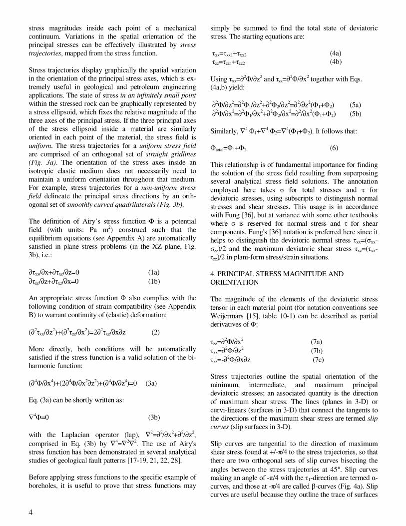
Fig. 3(a). Uniform stress field with constant orientation of principal stresses can be outlined by orthogonal set of stress
trajectories. The magnitude of the stresses may or may not
vary spatially. (b) Non-uniform stress field where the
orientation of the principal stress axes vary in space.
Implicitly, the magnitude of the principal stresses will then
also vary spatially, commonly with steeper gradients where
the curvature of the trajectories changes fastest.
4
stress magnitudes inside each point of a mechanical
continuum. Variations in the spatial orientation of the principal stresses can be effectively illustrated by stress
trajectories, mapped from the stress function.
Stress trajectories display graphically the spatial variation in the orientation of the principal stress axes, which is ex-
tremely useful in geological and petroleum engineering
applications. The state of stress in an infinitely small point
within the stressed rock can be graphically represented by
a stress ellipsoid, which fixes the relative magnitude of the
three axes of the principal stress. If the three principal axes of the stress ellipsoid inside a material are similarly
oriented in each point of the material, the stress field is
uniform. The stress trajectories for a uniform stress field
are comprised of an orthogonal set of straight gridlines
(Fig. 3a). The orientation of the stress axes inside an
isotropic elastic medium does not necessarily need to
maintain a uniform orientation throughout that medium. For example, stress trajectories for a non-uniform stress
field delineate the principal stress directions by an orth-
ogonal set of smoothly curved quadrilaterals (Fig. 3b).
The definition of Airy’s stress function Φ is a potential
field (with units: Pa m2) construed such that the
equilibrium equations (see Appendix A) are automatically satisfied in plane stress problems (in the XZ plane, Fig.
3b), i.e.:
∂τxx/∂x+∂τxz/∂z=0 (1a)
∂τzz/∂z+∂τxz/∂x=0 (1b)
An appropriate stress function Φ also complies with the
following condition of strain compatibility (see Appendix
B) to warrant continuity of (elastic) deformation:
(∂2τxx/∂z
2)+(∂
2τzz/∂x
2)=2∂
2τxz/∂x∂z (2)
More directly, both conditions will be automatically
satisfied if the stress function is a valid solution of the bi-harmonic function:
(∂4Φ/∂x
4)+(2∂
4Φ/∂x
2∂z
2)+(∂
4Φ/∂z
4)=0 (3a)
Eq. (3a) can be shortly written as:
∇4Φ=0 (3b)
with the Laplacian operator (lap), ∇2=∂
2/∂x
2+∂
2/∂z
2,
comprised in Eq. (3b) by ∇4=∇
2∇
2. The use of Airy's
stress function has been demonstrated in several analytical
studies of geological fault patterns [17-19, 21, 22, 28].
Before applying stress functions to the specific example of
boreholes, it is useful to prove that stress functions may
simply be summed to find the total state of deviatoric
stress. The starting equations are:
τxx=τxx1+τxx2 (4a)
τzz=τzz1+τzz2 (4b)
Using τxx=∂2Φ/∂z
2 and τzz=∂
2Φ/∂x
2 together with Eqs.
(4a,b) yield:
∂2Φ/∂z
2=∂
2Φ1/∂z
2+∂
2Φ2/∂z
2=∂
2/∂z
2(Φ1+Φ2) (5a)
∂2Φ/∂x
2=∂
2Φ1/∂x
2+∂
2Φ2/∂x
2=∂
2/∂x
2(Φ1+Φ2) (5b)
Similarly, ∇4 Φ1+∇
4 Φ2=∇
4(Φ1+Φ2). It follows that:
Φtotal=Φ1+Φ2 (6)
This relationship is of fundamental importance for finding
the solution of the stress field resulting from superposing several analytical stress field solutions. The annotation
employed here takes σ for total stresses and τ for
deviatoric stresses, using subscripts to distinguish normal
stresses and shear stresses. This usage is in accordance with Fung [36], but at variance with some other textbooks
where σ is reserved for normal stress and τ for shear
components. Fung's [36] notation is preferred here since it helps to distinguish the deviatoric normal stress τxx=(σxx-
σzz)/2 and the maximum deviatoric shear stress τxz=(τxx-
τzz)/2 in plani-form stress/strain situations.
4. PRINCIPAL STRESS MAGNITUDE AND
ORIENTATION
The magnitude of the elements of the deviatoric stress
tensor in each material point (for notation conventions see
Weijermars [15], table 10-1) can be described as partial derivatives of Φ:
τzz=∂2Φ/∂x
2 (7a)
τxx=∂2Φ/∂z
2 (7b)
τxz=-∂2Φ/∂x∂z (7c)
Stress trajectories outline the spatial orientation of the
minimum, intermediate, and maximum principal deviatoric stresses; an associated quantity is the direction
of maximum shear stress. The lines (planes in 3-D) or
curvi-linears (surfaces in 3-D) that connect the tangents to the directions of the maximum shear stress are termed slip
curves (slip surfaces in 3-D).
Slip curves are tangential to the direction of maximum shear stress found at +/-π/4 to the stress trajectories, so that
there are two orthogonal sets of slip curves bisecting the
angles between the stress trajectories at 45°. Slip curves making an angle of -π/4 with the τ1-direction are termed α-
curves, and those at -π/4 are called β-curves (Fig. 4a). Slip curves are useful because they outline the trace of surfaces
5
of potential shear failure (relevant for wellbore breakouts).
No shear failure is likely when α-curves intersect at some point A (Fig. 4b). The curvature of β-curves becomes
infinite near A and approaches a circle. Such singular
points only possess neutral stress or pressure (deviatoric
stresses vanish) and therefore are termed neutral points. The concept of slip curves has been successfully applied to
explain the fault pattern associated with indentation of
mainland Asia by the Indian subcontinent [25-27]. The angular relationships of the slip curves are subject to
Hencky’s Theorems (Appendix C). Upon fracture
initiation the elastic stress field will be perturbed around the propagating fracture as modeled elsewhere [37, 38].
5. STRESS FUNCTION FOR REGIONAL TECTONIC
STRESS WITHOUT PRESENCE OF BOREHOLE
A uniaxial regional compression (i.e., τ1 is horizontal and
τ3 is vertical, normal to the ground surface, while τ2=0) can
be represented by a stress function for a uniaxial deviatoric compression within an isotropic elastic plate without a
hole (Fig. 5):
Φ1(x,y)=(τ1/2)y2
(8a)
which expressed in cylindrical coordinates corresponds to:
Φ1(r,θ)=(τ1/2)r2sin
2 θ (8b)
This translates to geological situations where deviatoric tectonic stresses may reach up to 100 to 1,000 MPa [39,
40], where the regional uni-axial compression generates a
deviatoric stress τxx=τ1 and total stress σ1=2τ1.
6. STRESS FUNCTION FOR A PRESSURIZED
BOREHOLE WITHOUT A REGIONAL STRESS
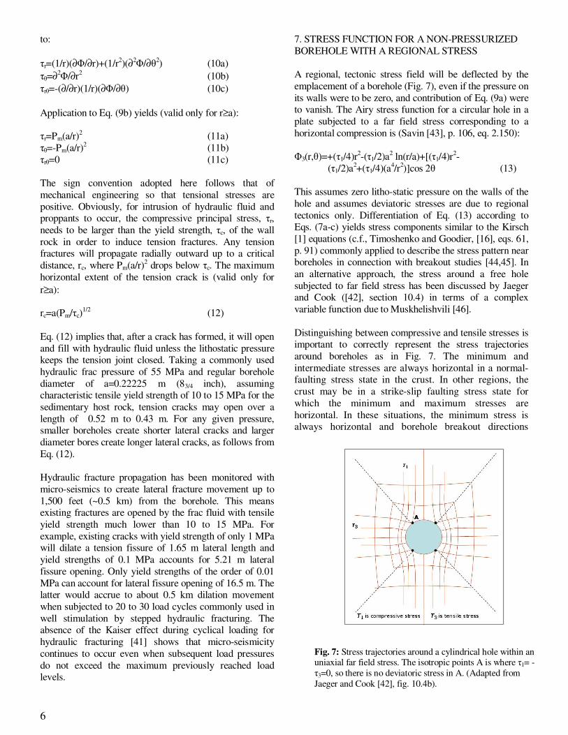
The state of stress around a circular borehole solely subject
to pressure from a wellbore fluid (mud, or hydraulic fluid
in a frac job) is axially symmetric and characterized by a
stress trajectory pattern of radial lines and concentric circles defining a spider-web pattern (Fig. 6). This stress
field can be described by a simple stress function in a 2-D
cylindrical or polar reference frame (r,θ) (after Timoshenko and Goodier [16]):
Φ2(r,θ) = A ln r (9a)
The value of the parameter A can be expressed as a
function of the hydraulic pressure, Pm, and the radius of the
drill hole, ’a’. Because the radial stress equals the hydraulic pressure, Pm, at r=a it can be shown that A=Pm a
2
in order to satisfy this boundary condition. Consequently,
Eq. (9a) can be rewritten as:
Φ2(r,θ)=Pma2ln r (9b)
The two normal and symmetric shear elements of the stress tensor are obtained by differentiation according to
Eqs. (1a to c), which in cylindrical coordinates transform
Fig. 6: Stress trajectories around an internally pressurized
circular borehole.
Fig. 4(a). Principal directions of stress (solid) and theoretical slip-curves (dashed). (b) Family of α-curves
meeting at a singular point A.
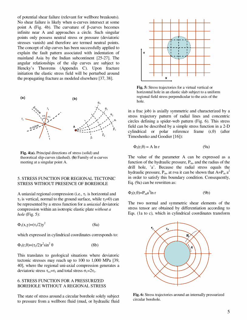
Fig. 5: Stress trajectories for a virtual vertical or horizontal hole in an elastic slab subject to a uniform
regional field stress perpendicular to the axis of the
hole.
6
to:
τr=(1/r)(∂Φ/∂r)+(1/r2)(∂
2Φ/∂θ
2) (10a)
τθ=∂2Φ/∂r
2(10b)
τrθ=-(∂/∂r)(1/r)(∂Φ/∂θ) (10c)
Application to Eq. (9b) yields (valid only for r≥a):
τr=Pm(a/r)2
(11a)
τθ=-Pm(a/r)2
(11b)
τrθ=0 (11c)
The sign convention adopted here follows that of
mechanical engineering so that tensional stresses are
positive. Obviously, for intrusion of hydraulic fluid and proppants to occur, the compressive principal stress, τr,
needs to be larger than the yield strength, τc, of the wall
rock in order to induce tension fractures. Any tension fractures will propagate radially outward up to a critical
distance, rc, where Pm(a/r)2 drops below τc. The maximum
horizontal extent of the tension crack is (valid only for
r≥a):
rc=a(Pm/τc)1/2
(12)
Eq. (12) implies that, after a crack has formed, it will open
and fill with hydraulic fluid unless the lithostatic pressure keeps the tension joint closed. Taking a commonly used
hydraulic frac pressure of 55 MPa and regular borehole
diameter of a=0.22225 m (83/4 inch), assuming characteristic tensile yield strength of 10 to 15 MPa for the
sedimentary host rock, tension cracks may open over a
length of 0.52 m to 0.43 m. For any given pressure, smaller boreholes create shorter lateral cracks and larger
diameter bores create longer lateral cracks, as follows from
Eq. (12).
Hydraulic fracture propagation has been monitored with
micro-seismics to create lateral fracture movement up to
1,500 feet (~0.5 km) from the borehole. This means existing fractures are opened by the frac fluid with tensile
yield strength much lower than 10 to 15 MPa. For
example, existing cracks with yield strength of only 1 MPa will dilate a tension fissure of 1.65 m lateral length and
yield strengths of 0.1 MPa accounts for 5.21 m lateral
fissure opening. Only yield strengths of the order of 0.01
MPa can account for lateral fissure opening of 16.5 m. The latter would accrue to about 0.5 km dilation movement
when subjected to 20 to 30 load cycles commonly used in
well stimulation by stepped hydraulic fracturing. The absence of the Kaiser effect during cyclical loading for
hydraulic fracturing [41] shows that micro-seismicity
continues to occur even when subsequent load pressures
do not exceed the maximum previously reached load levels.
7. STRESS FUNCTION FOR A NON-PRESSURIZED
BOREHOLE WITH A REGIONAL STRESS
A regional, tectonic stress field will be deflected by the
emplacement of a borehole (Fig. 7), even if the pressure on
its walls were to be zero, and contribution of Eq. (9a) were to vanish. The Airy stress function for a circular hole in a
plate subjected to a far field stress corresponding to a
horizontal compression is (Savin [43], p. 106, eq. 2.150):
Φ3(r,θ)=+(τ1/4)r2-(τ1/2)a
2 ln(r/a)+[(τ1/4)r
2-
(τ1/2)a2+(τ1/4)(a
4/r
2)]cos 2θ (13)
This assumes zero litho-static pressure on the walls of the
hole and assumes deviatoric stresses are due to regional
tectonics only. Differentiation of Eq. (13) according to Eqs. (7a-c) yields stress components similar to the Kirsch
[1] equations (c.f., Timoshenko and Goodier, [16], eqs. 61,
p. 91) commonly applied to describe the stress pattern near boreholes in connection with breakout studies [44,45]. In
an alternative approach, the stress around a free hole
subjected to far field stress has been discussed by Jaeger and Cook ([42], section 10.4) in terms of a complex
variable function due to Muskhelishvili [46].
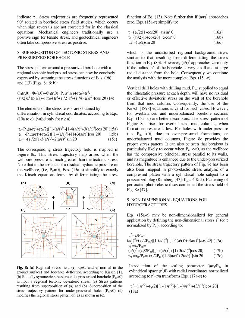
Distinguishing between compressive and tensile stresses is important to correctly represent the stress trajectories
around boreholes as in Fig. 7. The minimum and
intermediate stresses are always horizontal in a normal-faulting stress state in the crust. In other regions, the
crust may be in a strike-slip faulting stress state for
which the minimum and maximum stresses are
horizontal. In these situations, the minimum stress is always horizontal and borehole breakout directions
Fig. 7: Stress trajectories around a cylindrical hole within an uniaxial far field stress. The isotropic points A is where τ1= -
τ3=0, so there is no deviatoric stress in A. (Adapted from
Jaeger and Cook [42], fig. 10.4b).
7
indicate τ3. Stress trajectories are frequently represented
90° rotated in borehole stress field studies, which occurs when sign reversals are not corrected for in the classical
equations. Mechanical engineers traditionally use a
positive sign for tensile stress, and geotechnical engineers
often take compressive stress as positive.
8. SUPERPOSITON OF TECTONIC STRESS AND
PRESSURIZED BOREHOLE
The stress pattern around a pressurized borehole with a
regional tectonic background stress can now be concisely expressed by summing the stress functions of Eqs. (9b)
and (13) (Figs. 8a & b):
Φ4(r,θ)=Φ2(r,θ)+Φ3(r,θ)=Pma2ln r+(τ1/4)r
2-
(τ1/2)a2 ln(r/a)+[(τ1/4)r
2-(τ1/2)a
2+(τ1/4)(a
4/r
2)]cos 2θ (14)
The elements of the stress tensor are obtained by differentiation in cylindrical coordinates, according to Eqs.
(10a to c), (valid only for r ≥ a):
τr=Pm(a/r)2+(τ1/2)[[1-(a/r)
2]-[1-4(a/r)
2+3(a/r)
4]cos 2θ](15a)
τθ= -Pm(a/r)2+(τ1/2)[[1+(a/r)
2]+[1+3(a/r)
4]cos 2θ] (15b)
τrθ= -(τ1/2)[1-3(a/r)4+2(a/r)
2]sin 2θ (15c)
The corresponding stress trajectory field is mapped in Figure 8c. This stress trajectory map arises when the
wellbore pressure is much greater than the tectonic stress.
Note that in the absence of a residual hydraulic pressure on
the wellbore, (i.e, Pm=0), Eqs. (15a-c) simplify to exactly the Kirsch equations found by differentiating the stress
function of Eq. (13). Note further that if (a/r)2 approaches
zero, Eqs. (15a-c) simplify to:
τr=(τ1/2)[1-cos2θ]=τ1sin2 θ (16a)
τθ=(τ1/2)[1+cos2θ]=τ1cos2 θ (16b)
τrθ=-(τ1/2)sin 2θ (16c)
which is the undisturbed regional background stress
similar to that resulting from differentiating the stress function in Eq. (8b). However, (a/r)
2 approaches zero only
if the radius ’a’ of the borehole is very small and at large
radial distance from the hole. Consequently we continue the analysis with the more complete Eqs. (15a-c).
Vertical drill holes with drilling mud, Pm, supplied to equal
the lithostatic pressure at each depth, will have no residual or effective deviatoric stress on the wall of the borehole
from that mud column. Consequently, the use of the
Kirsch [1898] equations is valid for such cases. However, for overbalanced and underbalanced borehole sections
Eqs. (15a –c) are better descriptors. The stress pattern of
Figure 8c arises for overbalanced mud columns, when formation pressure is low. For holes with under-pressure
(i.e. Pm <0), due to over-pressured formations, or
underbalanced mud columns, Figure 8e provides the
proper stress pattern. It can also be seen that breakout is particularly likely to occur when Pm <<0, as the wellbore
has the compressive principal stress parallel to its walls,
and its magnitude is enhanced due to the under-pressurized borehole. The stress trajectory pattern of Fig. 8c has been
also been mapped in photo-elastic stress analysis of a
compressed platen with a cylindrical hole subject to a
pressurized plug (Ramberg [47], figs. 4 & 5). Flattening of perforated photo-elastic discs confirmed the stress field of
Fig. 8e [47].
9. NON-DIMENSIONAL EQUATIONS FOR
HYDROFRACTURES
Eqs. (15a-c) may be non-dimensionalized for general
application by defining the non-dimensional stress τ* (or τ
normalized by Pm), according to:
τr*=τr/Pm=
(a/r)2+(τ1/2Pm)[[1-(a/r)
2]-[1-4(a/r)
2+3(a/r)
4]cos 2θ] (17a)
τθ*=τθ/Pm=
-(a/r)2+(τ1/2Pm)[[1+(a/r)
2]+[1+3(a/r)
4]cos 2θ] (17b)
τrθ*=τrθ/Pm=-(τ1/2Pm)[1-3(a/r)
4+2(a/r)
2]sin 2θ (17c)
Introduction of the scaling parameter ζ=τ1/Pm in
cylindrical space (r*,θ) with radial coordinates normalized
according to r*=r/a transforms Eqs. (17a-c) to:
τr*=(1/r
*2)+(ζ/2)[[1-(1/r
*2)]-[1-(4/r
*2)+(3/r
*4)]cos 2θ]
(18a)
Fig. 8: (a) Regional stress field (τ1, τ2=0, and τ3 normal to the ground surface) and borehole deflection according to Kirsch [1],
(b) Radially symmetric stress around a pressurized borehole (Pm>0)
without a regional tectonic deviatoric stress. (c) Stress patterns
resulting from superposition of (a) and (b). Superposition of the
stress trajectory pattern for under-pressured holes (Pm<0) (d)
modifies the regional stress pattern of (a) as shown in (e).
8
τθ*=-(1/r
*2)+(ζ/2)[[1+(1/r
*2)]+[1+(3/r
*4)]cos 2θ] (18b)
τrθ*=-(ζ/2)[1-(3/r
*4)+(2/r
*2)]sin 2θ (18c)
The scaling parameter ζ is the non-dimensional ratio of the
tectonic background stress τ1 and the hydraulic pressure,
Pm, on the walls of the borehole.
The stress trajectories may now be mapped in (r*,θ)-space
using various ratios of hydraulic pressure Pm and regional far field stress τ1 as expressed in the scaling factor ζ. The
inclination β of a stress trajectory with respect to the r*-
axes may be determined from:
tan 2β=2τrθ*/(τr
*-τθ
*) (19)
with two solution for β separated by π/2. A continuous solution of Eq. (19) in a particular space outlines the stress
trajectories.
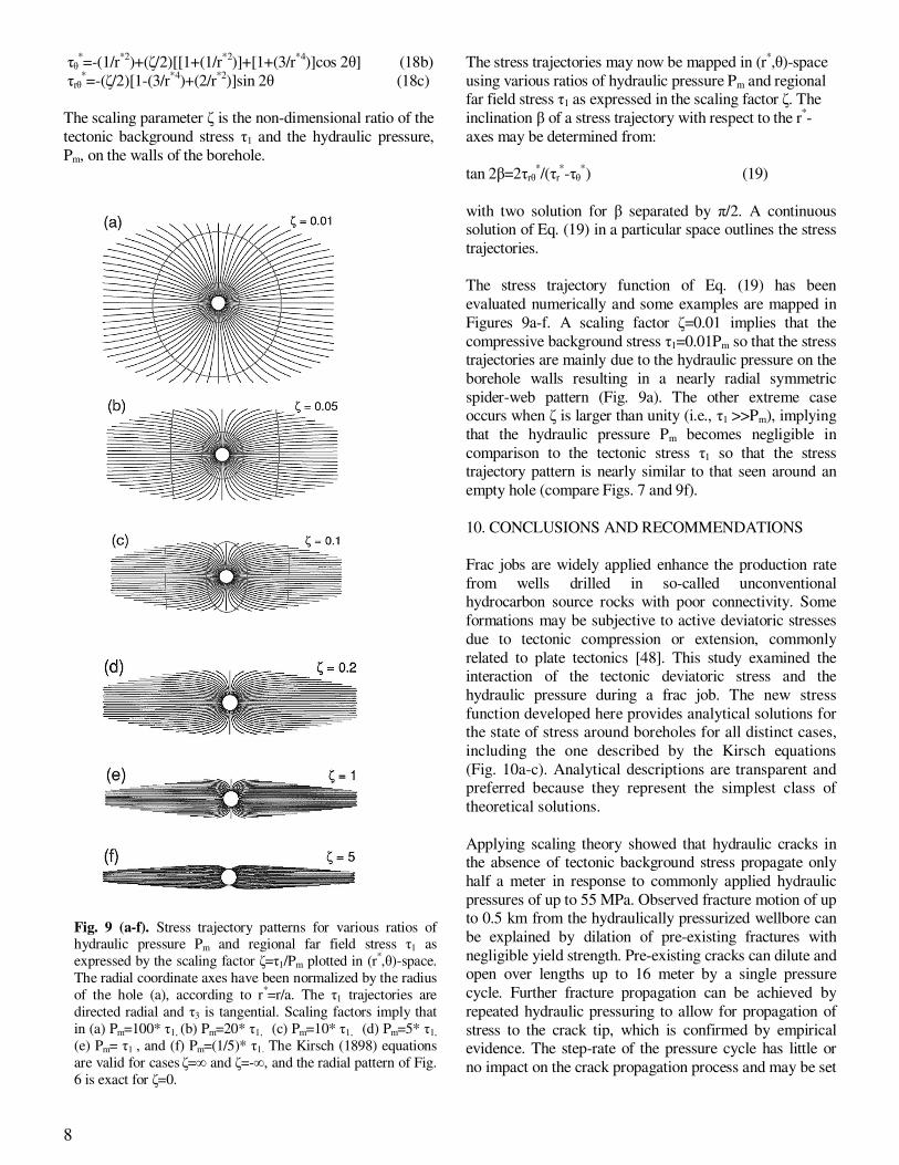
The stress trajectory function of Eq. (19) has been
evaluated numerically and some examples are mapped in
Figures 9a-f. A scaling factor ζ=0.01 implies that the
compressive background stress τ1=0.01Pm so that the stress trajectories are mainly due to the hydraulic pressure on the
borehole walls resulting in a nearly radial symmetric
spider-web pattern (Fig. 9a). The other extreme case occurs when ζ is larger than unity (i.e., τ1 >>Pm), implying
that the hydraulic pressure Pm becomes negligible in
comparison to the tectonic stress τ1 so that the stress trajectory pattern is nearly similar to that seen around an
empty hole (compare Figs. 7 and 9f).
10. CONCLUSIONS AND RECOMMENDATIONS
Frac jobs are widely applied enhance the production rate
from wells drilled in so-called unconventional hydrocarbon source rocks with poor connectivity. Some
formations may be subjective to active deviatoric stresses
due to tectonic compression or extension, commonly
related to plate tectonics [48]. This study examined the interaction of the tectonic deviatoric stress and the
hydraulic pressure during a frac job. The new stress
function developed here provides analytical solutions for the state of stress around boreholes for all distinct cases,
including the one described by the Kirsch equations
(Fig. 10a-c). Analytical descriptions are transparent and preferred because they represent the simplest class of
theoretical solutions.
Applying scaling theory showed that hydraulic cracks in the absence of tectonic background stress propagate only
half a meter in response to commonly applied hydraulic
pressures of up to 55 MPa. Observed fracture motion of up to 0.5 km from the hydraulically pressurized wellbore can
be explained by dilation of pre-existing fractures with
negligible yield strength. Pre-existing cracks can dilute and open over lengths up to 16 meter by a single pressure
cycle. Further fracture propagation can be achieved by
repeated hydraulic pressuring to allow for propagation of
stress to the crack tip, which is confirmed by empirical evidence. The step-rate of the pressure cycle has little or
no impact on the crack propagation process and may be set
Fig. 9 (a-f). Stress trajectory patterns for various ratios of hydraulic pressure Pm and regional far field stress τ1 as
expressed by the scaling factor ζ=τ1/Pm plotted in (r*,θ)-space.
The radial coordinate axes have been normalized by the radius
of the hole (a), according to r*=r/a. The τ1 trajectories are
directed radial and τ3 is tangential. Scaling factors imply that
in (a) Pm=100* τ1, (b) Pm=20* τ1, (c) Pm=10* τ1, (d) Pm=5* τ1,
(e) Pm= τ1 , and (f) Pm=(1/5)* τ1. The Kirsch (1898) equations
are valid for cases ζ=∞ and ζ=-∞, and the radial pattern of Fig.
6 is exact for ζ=0.
9
as high as practically achievable to complete the well
stimulation job fastest from a cost point of view.
Another insight resulting from this study is that hydraulic
frac jobs will deflect the stress trajectories around the
pressurized borehole such that the tectonic background stress has little effect on the failure direction in the
immediate vicinity of the borehole. A final practical
recommendation is that steep pressure drops during the frac cycle must be avoided as such drops induce shear
failure breakout of the borehole walls, which may obstruct
the connectivity required for effective production. Shear failure can be prevented by lowering suction pressures and
a slower flowback rate. In practice well completions
involve perforations in the casing that will focus hydraulic
pressure on predetermined sections of the borehole in the pay zone. High viscosity frac fluid such as gels will not
only better carry proppants, but also buffer steep pressure
drops and are therefore preferred when shear failure handicaps completion jobs.
The stress function developed here can also account for natural overpressures which may jeopardize drilling
activities when the well bore crosses rock formations
with extremely high or low formation pressures not
balanced by the weight of the drilling mud column. The
wall rock then frequently washes out and break outs
damage the wellbore integrity. The 2010 Macondo well damage drilled by Deep Horizon for BP in the Gulf of
Mexico is an example of an unbalanced wellbore. The
simple analytical solutions developed here may help to
prevent blow-outs and loss of drilling fluid in damaged formations; under-pressures are also accounted for by
the analytical description. Better fracture placement is
therefore possible in frac jobs, which typically account for 30% of well development cost, using the analytical
solutions provided here using a comprehensive stress
function. Such better fracture fairways then enhance well productivity and thus help bring down the cost per unit
of recovered gas. This is now much needed to stem
growing concerns of oil business analysts about the
economic gap caused by depressed natural gas prices [49] – gas is currently sold below production cost by
many unconventional gas companies in the US.
Acknowledgement: An earlier draft of this manuscript was
kindly reviewed by Dr. Maria Nikolinakou and Dr. Gang Luo at
the Bureau of Economic Geology, Austin. The plots of Eq. (19)
in Figs.(9a-f) were completed by Dr. Dan Schultz-Ela (a former
colleague at the Bureau of Economic Geology now at
Department of Computer Science, Mathematics & Statistics,
Mesa State College, Colorado), who kindly granted permission
for their use.
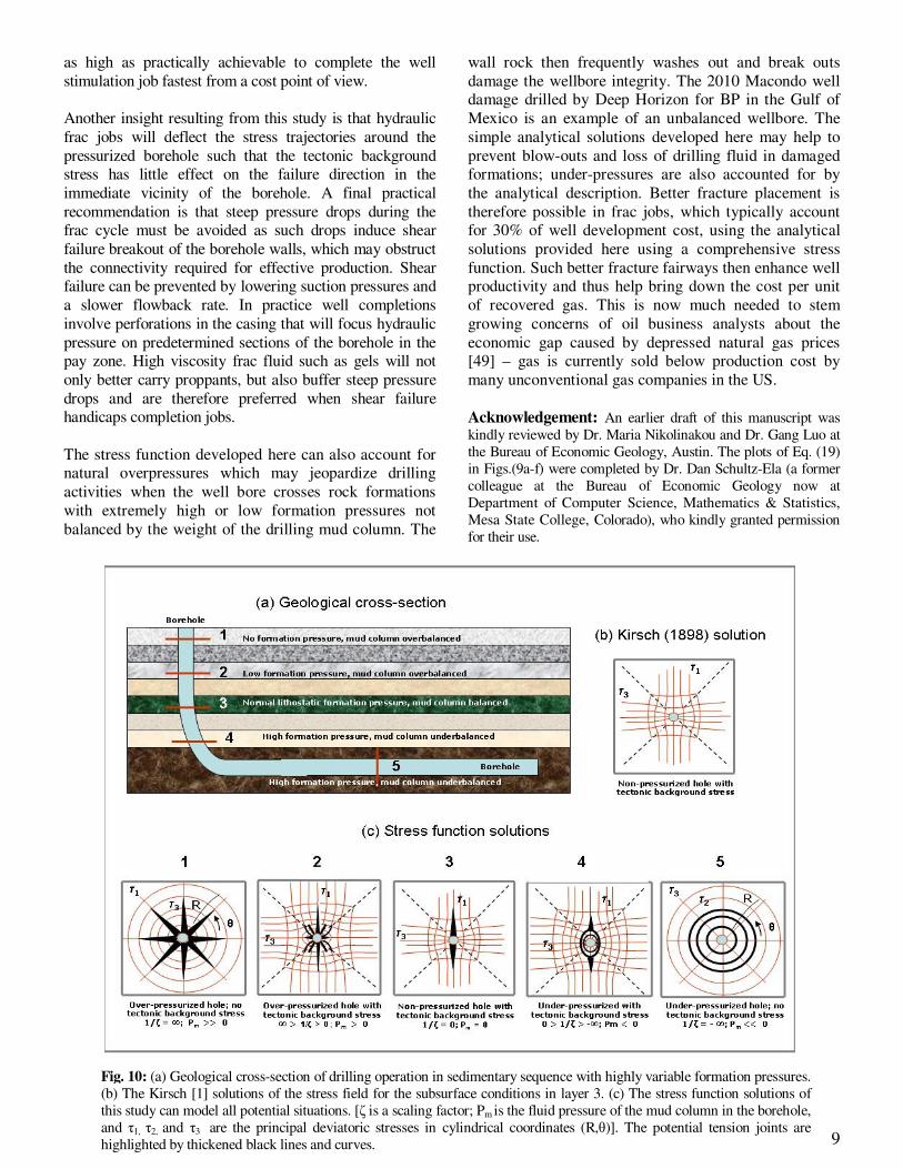
Fig. 10: (a) Geological cross-section of drilling operation in sedimentary sequence with highly variable formation pressures.
(b) The Kirsch [1] solutions of the stress field for the subsurface conditions in layer 3. (c) The stress function solutions of
this study can model all potential situations. [ζ is a scaling factor; Pm is the fluid pressure of the mud column in the borehole,
and τ1, τ2, and τ3 are the principal deviatoric stresses in cylindrical coordinates (R,θ)]. The potential tension joints are
highlighted by thickened black lines and curves.
10
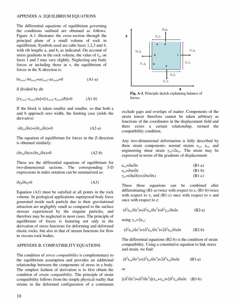
APPENDIX A: EQUILIBRIUM EQUATIONS
The differential equations of equilibrium governing
the conditions outlined are obtained as follows.
Figure A-1 illustrates the cross-section through the
principal plane of a small volume of rock in equilibrium. Symbols used are cube faces 1,2,3 and 4,
with rib lengths a, and b, as indicated. On account of
stress gradients in the rock volume, the value of τxx on faces 1 and 3 may vary slightly. Neglecting any body
forces or including those in τ, the equilibrium of
forces in the X-direction is:
bτ(xx)1-bτ(xx)3+aτ(xz)2-aτ(xz)4=0 (A1-a)
if divided by ab:
[(τ(xx)1-τ(xx)3)/a]+[(τ(xz)2-τ(xz)4)/b]=0 (A1-b)
If the block is taken smaller and smaller, so that both a
and b approach zero width, the limiting case yields the
derivative:
(∂τxx/∂x)+(∂τxz/∂z)=0 (A2-a)
The equation of equilibrium for forces in the Z-direction
is obtained similarly:
(∂τzz/∂z)+(∂τxz/∂x)=0 (A2-b)
These are the differential equations of equilibrium for
two-dimensional sections. The corresponding 3-D expressions in index notation can be summarized as:
∂τji/∂xj=0 (A3)
Equation (A3) must be satisfied at all points in the rock volume. In geological applications superposed body force
generated inside each particle due to their gravitational
attraction are negligibly small as compared to the surface stresses experienced by the singular particles, and
therefore may be neglected in most cases. The principle of
equilibrium of forces is featuring not only in the
derivation of stress functions for deforming and deformed elastic rocks, but also in that of stream functions for flow
in viscous rock bodies.
APPENDIX B: COMPATIBILITY EQUATIONS
The condition of stress compatibility is complementary to
the equilibrium assumption and provides an additional relationship between the components of stress in a body.
The simplest fashion of derivation is to first obtain the
condition of strain compatibility. The principle of strain compatibility follows from the simple physical reality that
strains in the deformed configuration of a continuum
exclude gaps and overlaps of matter. Components of the
strain tensor therefore cannot be taken arbitrary as
functions of the coordinates in the displacement field and
there exists a certain relationship, termed the compatibility condition.
Any two-dimensional deformation is fully described by three strain components: normal strains exx, ezz, and
engineering shear strain γxz=2exz. The strain may be
expressed in terms of the gradients of displacement:
exx=∂u/∂x (B1-a)
ezz=∂w/∂z (B1-b)
γxz=(∂u/∂z)+(∂w/∂x) (B1-c)
These three equations can be combined after
differentiating (B1-a) twice with respect to z, (B1-b) twice
with respect to x, and (B1-c) once with respect to x and once with respect to z:
(∂2exx/∂z
2)+(∂
2ezz/∂x
2)=∂
2γxz/∂x∂z (B2-a)
using γxz=2exz:
(∂2exx/∂z
2)+(∂
2ezz/∂x
2)=2∂
2exz/∂x∂z (B2-b)
The differential equations (B2-b) is the condition of strain
compatibility. Using a constitutive equation to link stress and strain, we find:
(∂2τxx/∂z
2)+(∂
2τzz/∂x
2)=2∂
2τxz/∂x∂z (B3-a)
or
[(∂2/∂z
2)+(∂
2/∂x
2)](τxx+τzz)=2∂
2τxz/∂x∂z (B3-b)
Fig. A-1. Principle sketch explaining balance of
forces.
11
Equation (B3-a) implies that the normal and shear
displacements caused by the stress have to be internally compatible in the material considered. For the three-
dimensional case, the condition of strain compatibility is
made up of six independent expressions contained in the
tensor equation:
(∂2τij/∂xmxn)+(∂
2τmn/∂xi∂xj)-(∂
2τim/∂xjxn)+(∂
2τjn/∂xi∂xm)=0
(B4)
For example, consider a block of rock subjected to a pure
shear deformation, with boundary forces such that
deviatoric stresses τxx=-τzz and τxz=0. This is a valid
boundary condition, and there is no spatial gradient in any of the stress components. The equilibrium and
compatibility conditions are fulfilled in any point of the
block.
APPENDIX C: HENCKY’S THEOREMS FOR STRESS
TRAJECTORIES AND SLIP CURVES
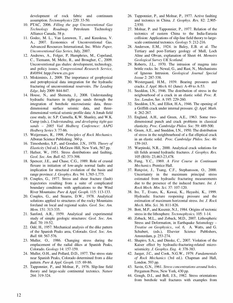
Hencky (see Hill [50]) has formulated two practical
theorems related to some special properties of stress
trajectories and slip-curve fields, after considering a curvilinear quadrilateral ABCD (Fig. C-1).
The first theorem refers to angles of the grid intersections. If the orientation of any two given β-
curves (e.g., AD and BC) is changing, the associated two
α-curves (e.g., AB and DC) rotate through the same angle θ. It follows that:
θB-θA=θC-θD (C1)
θC-θB=θD-θA (C2)
If orthogonal curvilinear coordinates are chosen in the
node points of one of the corners of the quadrilateral, Hencky's first theorem achieves great practical value.
The unknown angle γ follows from the known angles α
and β:
θC=θB+θD (C3)
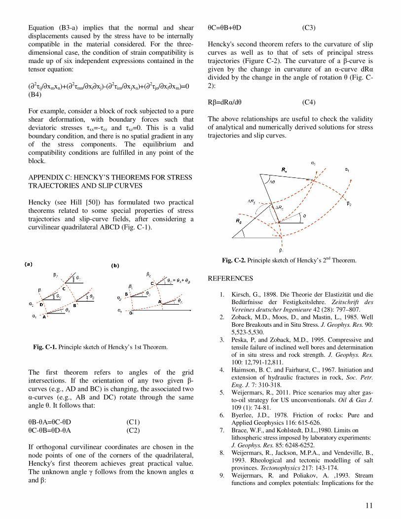
Hencky's second theorem refers to the curvature of slip
curves as well as to that of sets of principal stress
trajectories (Figure C-2). The curvature of a β-curve is
given by the change in curvature of an α-curve dRα divided by the change in the angle of rotation θ (Fig. C-
2):
Rβ=dRα/dθ (C4)
The above relationships are useful to check the validity of analytical and numerically derived solutions for stress
trajectories and slip curves.
REFERENCES
1. Kirsch, G., 1898. Die Theorie der Elastizität und die
Bedürfnisse der Festigkeitslehre. Zeitschrift des
Vereines deutscher Ingenieure 42 (28): 797–807.
2. Zoback, M.D., Moos, D., and Mastin, L., 1985. Well
Bore Breakouts and in Situ Stress. J. Geophys. Res. 90:
5,523-5,530.
3. Peska, P, and Zoback, M.D., 1995. Compressive and
tensile failure of inclined well bores and determinationof in situ stress and rock strength. J. Geophys. Res.
100: 12,791-12,811.
4. Haimson, B. C. and Fairhurst, C., 1967. Initiation and
extension of hydraulic fractures in rock, Soc. Petr.
Eng. J. 7: 310-318.
5. Weijermars, R., 2011. Price scenarios may alter gas-
to-oil strategy for US unconventionals. Oil & Gas J.
109 (1): 74-81.
6. Byerlee, J.D., 1978. Friction of rocks: Pure and
Applied Geophysics 116: 615-626.
7. Brace, W.F., and Kohlstedt, D.L.,1980. Limits onlithospheric stress imposed by laboratory experiments:
J. Geophys. Res. 85: 6248-6252.
8. Weijermars, R., Jackson, M.P.A., and Vendeville, B.,
1993. Rheological and tectonic modelling of salt
provinces. Tectonophysics 217: 143-174.
9. Weijermars, R. and Poliakov, A. ,1993. Stream
functions and complex potentials: Implications for the
Fig. C-2. Principle sketch of Hencky’s 2nd Theorem.
Fig. C-1. Principle sketch of Hencky’s 1st Theorem.
12
development of rock fabric and continuum
assumption. Tectonophysics 220: 33-50.
10. PTAC, 2006. Filling the gap Unconventional Gas
Technology Roadmap. Petroleum Technology
Alliance Canada, 58 p.
11. Godec, M. L., Van Leeuwen, T., and Kuuskraa, V.A., 2007. Economics of Unconventional Gas.
Advanced Resources International, Inc. White Paper,
Unconventional Gas Series, July, 2007.
12. Andrews, A., Folger, P, Humphries, M., Copeland,
C., Tiemann, M, Meltz, R., and Brougher, C., 2009.
Unconventional gas shales: development, technology,
and policy issues. Congressional Research Service,
R40894. htpp://www.crs.gov
13. Miskiminis, J., 2009. The importance of geophysical
and petrophysical data integration for the hydraulic
fracturing of unconventional reservoirs. The Leading
Edge, July 2009: 844-847.14. House, N., and Shemeta, J., 2008. Understanding
hydraulic fractures in tight-gas sands through the
integration of borehole microseismic data, three-
dimensional surface seismic data, and three-
dimensional vertical seismic profile data: A Jonah field
case study, in: S.P. Cumella, K.W. Shanley, and W.K.
Camp (eds.), Understanding, and developing tight-gas
sands – 2005 Vail Hedberg Conference: AAPG
Hedberg Series 3: 77-86.
15. Weijermars, R., 1998. Principles of Rock Mechanics.
Alboran Science Publishing. 360 p.16. Timoshenko, S.P., and Goodier, J.N., 1970. Theory of
Elasticity (3rd ed.). McGraw-Hill, New York, 567 pp.
17. Hafner, W., 1951. Stress distributions and faulting,
Geol. Soc. Am. Bull. 62: 373-398.
18. Spencer, J.E., and Chase, C.G., 1989. Role of crustal
flexure in initiation of low-angle normal faults and
implication for structural evolution of the basin and
range province: J. Geophys. Res. 94: 1,765-1,775.
19. Couples, G., 1977. Stress and shear fracture (fault)
trajectories resulting from a suite of complicated
boundary conditions with applications to the Wind
River Mountains: Pure & Appl. Geoph. 115: 113-133.20. Couples, G., and Stearns, D.W., 1978. Analytical
solutions applied to structures of the rocky Mountains
foreland on local and regional scales. Geol. Soc. Am.
Mem. 151: 313-335.
21. Sanford, A.R., 1959. Analytical and experimental
study of simple geologic structures: Geol. Soc. Am.
Bull. 70: 19-52.
22. Odé, H., 1957. Mechanical analysis of the dike pattern
of the Spanish Peaks area, Colorado. Geol. Soc. Am.
Bull. 68: 567-576.
23. Muller, O., 1986. Changing stress during theemplacement of the radial dikes at Spanish Peaks,
Colorado. Geology 14: 157-159.
24. Muller, O.H., and Pollard, D.D., 1977. The stress state
near Spanish Peaks, Colorado determined from a dike
pattern. Pure & Appl. Geoph. 115: 69-86.
25. Tapponnier, P., and Molnar, P., 1976. Slip-line field
theory and large-scale continental tectonics. Nature
264: 319-324.
26. Tapponnier, P., and Molnar, P., 1977. Active faulting
and tectonics in China. J. Geophys. Res. 82: 2,905-
2,930.
27. Molnar, P. and Tapponnier, P., 1977. Relation of the
tectonics of eastern China to the India-Eurasia
collision: Applications of slip-line field theory to large-scale continental tectonics. Geology 5: 212-216.
28. Anderson, E.M., 1924. in Baley, E.B. et al. The
Tertiary and post-Tertiary geology of Mull, Loch
Aline and Obvan, explanation of Sheet 44. Memoirs
Geological Survey UK Scotland.
29. Roberts, J.L., 1970. The intrusion of magma into
brittle rocks. In: Newal, G., and Rast, N., Mechanisms
of Igneous Intrusion. Geological Journal Special
Isssue 2: 287-338.
30. Westergaard, H.M., 1939. Bearing pressures and
cracks. J. Appl. Mech. 61 (June): A-49 to A-53.
31. Sneddon, I.N., 1946. The distribution of stress in theneigbourhood of a crack in an elastic solid. Proc. R.
Soc. London, Ser. A 195: 229-260.
32. Sneddon, I.N., and Elliot, H.A., 1946. The opening of
a Griffith crack under internal pressure. Q. Appl. Math.
4: 262-267.
33. England, A.H., and Green, A.E., 1963. Some two-
dimensional punch and crack problems in classical
elasticity. Proc. Cambridge Philos. Soc. 59: 489-500.
34. Green, A.E., and Sneddon, I.N., 1950. The distribution
of stress in the neighbourhood of a flat elliptical crack
in an elastic solid. Proc. Cambridge Philos. Soc. 46:159-163.
35. Warpinski, N.R.., 2000. Analytical crack solutions for
tilt fields around hydraulic fractures. J. Geophys. Res.
105 (B10): 23,463-23,478.
36. Fung, Y.C., 1969. A First Course in Continuum
Mechanics. Prentice Hall.
37. Rutqvist, J., Tsang, C.F., Stephansson, O., 2000.
Uncertainty in the maximum principal stress
estimated from hydraulic fracturing measurements
due to the presence of the induced fracture. Int. J.
Rock Mech. Min. Sci. 37: 107-120.
38. Ito, T., Evans, K., Kawai, K., Hayashi, K., 1999.Hydraulic fracture reopening pressure and the
estimation of maximum horizontal stress. Int. J. Rock
Mech. Min. Sci. 36: 811-826.
39. Bott, M.P., and Kusznir, N.J., 1984. Origins of tectonic
stress in the lithosphere. Tectonophysics, 105: 1-14.
40. Zoback, M.L., and Zoback, M.D., 2007. Lithospheric
Stress and Deformation, in Earthquake Seismology –
Treatise on Geophysics., vol. 6, A. Watts, and G.
Schubert, (eds.), Elsevier Science Publishers,
Amsterdam, p. 253-274.
41. Shapiro, S.A., and Dinske, C., 2007. Violation of theKaiser effect by hydraulic-fracturing-related micro-
seismicity. J. Geophys. Eng. 4: 378-383.
42. Jaeger, J.C., and Cook, N.G.W., 1979. Fundamentals
of Rock Mechanics (3rd ed.). Chapman and Hall,
London. 593 pp.
43. Savin, G.N., 1961. Stress concentrations around holes.
Pergamon Press, New York, 430 pp.
44. Gough, D.I., and Bell, J.S., 1982. Stress orientations
from borehole wall fractures with examples from
13
Colorado, east Texas, and northern Canada. Can. J.
Earth Sci. 19: 1,358-1,370.
45. Zheng, Z., Kemeny, J., and Cook, N.G. , 1989.
Analysis of borehole breakouts. J. Geophys. Res. 94:
7,171-7,182.
46. Muskhelishvili, N.I., 1954. Some Basic Problems of
the Mathematical Theory of Elasticity, Noordhof
Ltd., Groningen, The Netherlands.
47. Ramberg, H., 1961. Artificial and natural photo-elastic
effects in quartz and feldspars. The American
Mineralogist 46: 934-951
48. Fossen, H., 2010. Structural Geology. Cambridge
University Press.
49. Weijermars, R., 2010. Why untenable US natural gas
boom may soon need wellhead price-floor regulation
for industry survival. First Break 28(9): 33-38.
50. Hill, R., 1950. Mathematical Theory of Plasticity.
Oxford University Press.