analysing and modelling urban land cover change for run-off modelling in kampala, uganda
TRANSCRIPT

ANALYSING AND MODELLING
URBAN LAND COVER CHANGE
FOR RUN-OFF MODELLING IN
KAMPALA, UGANDA
GEZEHAGN DEBEBE FURA
March, 2013
SUPERVISORS:
Dr. Richard Sliuzas
Dr. Johannes Flacke


Thesis submitted to the Faculty of Geo-Information Science and Earth
Observation of the University of Twente in partial fulfilment of the
requirements for the degree of Master of Science in Geo-information Science
and Earth Observation.
Specialization: Urban Planning and Management
SUPERVISORS:
Dr. Richard Sliuzas
Dr. Johannes Flacke
THESIS ASSESSMENT BOARD: Prof. Dr. Ir. M.F.A.M. van Maarseveen (Chair)
MSc. Ms. Olena Dubovyk (External Examiner, University of Bonn)
Dr. Richard Sliuzas (1st Supervisor)
Dr. Johannes Flacke (2nd Supervisor)
ANALYSING AND MODELLING
URBAN LAND COVER CHANGE
FOR RUN-OFF MODELLING IN
KAMPALA, UGANDA
GEZEHAGN DEBEBE FURA
Enschede, The Netherlands, March, 2013

DISCLAIMER
This document describes work undertaken as part of a programme of study at the Faculty of Geo-Information Science and
Earth Observation of the University of Twente. All views and opinions expressed therein remain the sole responsibility of the
author, and do not necessarily represent those of the Faculty.

i
ABSTRACT
Land cover change (LCC) is amongst the most widely increasing and significant sources of todays’ change
in the earth’s land surface. It results in the degradation of natural vegetation and significant increases in
impervious surfaces. This particularly create several problems and become an issue in the rapidly
urbanizing cities of developing countries, such as Kampala, coupled with the high population growth rate
leading to modification or complete replacement of the land surface contributing to increased run-off
rates thereby. This study, analyse and model the LCC over space and time in the Upper Lubigi catchment
area (ULCA) of Kampala city by using the potential of remote sensing, geo-information systems (GIS),
and logistic regression modelling (LRM) techniques forming a partial contribution to Integrated Flood
Management (IFM) (run-off simulation and prediction) in the city. The study basically focused on
analysing the composition and proportion of land covers, the rate and determinants of the LCC, and
possible future growth location and various growth scenarios for the built-up land cover in the study area
in the course of preparing land cover data for run-off modelling.
The outcome of the analyses mainly revealed that the built-up, bare soil, and various roads land cover
classes have significantly increased at the expense of decrease in the vegetation land covers in the period
2004-2010. The built-up land cover has increased in area from about 5.59km2 in 2004 to 7.79km2 in 2010
while the vegetation land cover decreased from about 11.29km2 to 8.89km2 and the bare soil is
considerably remain high in both years containing about 9.27km2 (more than one third of the study area).
The built-up land cover increases at annual growth rate of 6.85% and the vegetation decrease at the
decreasing rate of 3.5% in the period. The significant physical driving forces of the LCC are evaluated
based on expertise rating score and statistically quantified using LRM. The proportion of urban land in a
surrounding area, distance to CBD, distance to minor roads, distance to industrial sites, and distance to
major roads attract the growth while the variables slope, distance to market centres, distance to streams,
and proportion of undeveloped land in a surrounding area are influentially prohibiting the growth. The
prediction of the built-up based on trend growth interpolation in the LRM has also revealed that the built-
up land cover area will increase from 7.79km2 in the year 2010 to 11.56km2, 15.26km2 and 18.96km2 by
the year 2020, 2030 and 2040 respectively. The cumulative impacts of the existing built-up, minor roads,
major roads and industrial sites have played significant role in the manifestation of the development in all
prediction periods. Furthermore, all the three scenarios: the trend growth, the high growth, and the low
growth scenarios constructed based on the daily demand for built-up area for the year 2020 in this study
have shown much of the available open spaces and wetlands in the study area are placed under boundless
pressure, with the increase in the built-up contributing to the increase in the imperviousness of the land
surface. In the trend growth scenario the built-up land has increased to about 3.78km2 while in the high
growth it has increased to about 5.03km2, and the low growth is obtained decreased to about 2.91km2.
Further, the predicted change in the land cover and the results of the scenarios alongside the estimation of
the proportion of the other remaining land cover types are compiled and mapped as required in run-off
modelling. The obtained results and approaches stretched in this study can help to improve understanding
of the phenomena of the LCC at micro-scale to contribute to the process of decision making for urban
planners and managers to be able to forecast and ultimately mitigate and/or reduce risks of flooding
associated with the increase in impervious land surfaces at the defined geographic province.
Key words: analyse and model land cover change; logistic regression modelling; GIS and remote
sensing; Integrated Flood Management; run-off modelling; Kampala
ii
ACKNOWLEDGEMENTS
For the completion of this thesis and on the course of my study enthusiastic support have provided by
individuals, members of the UPM and ITC staff, and The Netherlands Fellowship Program (NPF). First
and foremost, it is with immense gratitude that I acknowledge the NFP who generously granted the
funding for my study and let me to attain my career intension and professional goal. This thesis would not
happen to be possible without the generous grant they offered. It gives me great pleasure in
acknowledging the help and dedication of all the lecturers and staffs in ITC since the moment I start my
study in the institute, which had made me to feel home and get the spirit of working hard with inspiration.
I wish to thank the academic staff members of UPM including secretaries and other supporting staff,
whose guidance and inspiration let me pursue my study with bravery. I am exceptionally indebted to my
supervisors, Dr. Richard Sliuzas and Dr. Johannes Flacke, whose guidance is invaluable and who gave me
an opportunity to work with and learn from them besides their good advice, constructive criticism,
support, and endurance during the thesis writing. I would like to extend my special thanks to Dr. Richard
Sliuzas for facilitating Apartment housing, respondents, and organizing a workshop during the fieldwork
for all ITC students in Kampala. I am also indebted to Dr. Shuwab Lwasa and all staff members of the
Outspan primary school of Kampala, and the staff members of KCCA, whose their contributions are
countless in facilitating respondents and providing all the necessary support in need during the entire
period of the field work. I owe my deepest gratitude to all respondents Baker Sengendo, Godwin Othieno,
John Kisembo, Kisembo Teddy, Kuyiga Maximus, Lutaaga Hassan, Mpanga Musassa, Nakoko
Emmanuel, Nalule Harriet, Nambassi Moses, Prince Kanaakulya, and Dr. Shuwab Lwasa for their kind
participation in conducting the questionnaire. I wish to thank my institute, Ethiopian Civil Service
University for their support in allowing me to attend my professional study at ITC. I consider it an honour
to work with all UPM students who are helped me to arrive at the end of this thesis. I share the credit of
my work with my family who have shoulder all my responsibility at my absence. Last but not least, I
cannot find words to express my gratitude to my love Menbi (Jerrye) and my child Yisahak who have paid
the most sacrifice by enduring my long absence from home.

iii
TABLE OF CONTENTS
1. Introduction ........................................................................................................................................................... 1
1.1. Background and Justification ....................................................................................................................................1 1.2. Research problem ........................................................................................................................................................4 1.3. Research objective .......................................................................................................................................................5 1.4. Conceptual framework ...............................................................................................................................................6 1.5. Research design matrix ...............................................................................................................................................7 1.6. Research design and methodology ...........................................................................................................................8 1.7. Structure of the thesis .................................................................................................................................................9
2. Land cover change modelling and the drivers in Kampala ..........................................................................11
2.1. Introduction .............................................................................................................................................................. 11 2.2. Land cover change (LCC) ....................................................................................................................................... 11 2.3. Urbanization and land cover change in kampala ................................................................................................ 11 2.4. Land cover change and its environmental impact in Kampala ........................................................................ 12 2.5. Drivers of urban land cover changes ................................................................................................................... 13 2.6. Drivers of land cover change in Kampala ........................................................................................................... 15 2.7. Spatial characteristics of land cover change in Kampala ................................................................................... 15 2.8. Spatial policies and land cover change in Kampala ............................................................................................ 16 2.9. Models and modelling land cover change ............................................................................................................ 17 2.10. Modelling and issues of spatial resolutions ......................................................................................................... 21 2.11. Scenarios development ............................................................................................................................................ 22 2.12. Link between land covers and run-off models.................................................................................................... 23 2.13. Previous studies to linking LCC with run-off modelling ................................................................................. 24
3. The study area .....................................................................................................................................................27
3.1. Introduction .............................................................................................................................................................. 27 3.2. Physical characterstics and the land covers in Lubigi catchment..................................................................... 27 3.3. Land cover change and its impacts in Lubigi catchment .................................................................................. 28 3.4. Major socio-economic characterstics of the Lubigi catchment ........................................................................ 28 3.5. Characteristics of existing land use and the issues in Lubigi catchment......................................................... 30
4. Data and Methodology .....................................................................................................................................31
4.1. Introduction .............................................................................................................................................................. 31 4.2. Data source and qualities ........................................................................................................................................ 31 4.3. Land cover maps preparation and methodology ................................................................................................ 33 4.4. Analysing and quantifiying the LCC in the ULCA 2004 – 2010...................................................................... 39 4.5. Methodological selection to model the LCC in the study area ........................................................................ 41 4.6. Determining and quantifying the driving forces of LCC .................................................................................. 41 4.7. Prediction of future locations of LCC .................................................................................................................. 48 4.8. Scenarios development ............................................................................................................................................ 48 4.9. Assumptions and possible source of errors........................................................................................................ 52
5. Results and Discussions .....................................................................................................................................53
5.1. Introduction .............................................................................................................................................................. 53 5.2. Quantification of the land cover and LCC in the ULCA in the period 2004 - 2010 ................................. 53 5.3. Evaluation of the methodological approach and data preparation for run-off modelling .......................... 60 5.4. Evaluating and determining the probable driving forces of the LCC............................................................. 60 5.5. Determining and quantifying the driving forces of the LCC in LR M ..................................................... 62 5.6. Probability location maps of built-up area ........................................................................................................... 67 5.7. Scenarios development ............................................................................................................................................ 70
6. Conclusion and Recommendations .................................................................................................................78

iv
6.1. Sumary of key findings ............................................................................................................................................ 78 6.2. Specific conclusions ................................................................................................................................................. 79 6.3. Further research directions ..................................................................................................................................... 80
7. List of references ................................................................................................................................................ 82
8. Appendix.............................................................................................................................................................. 86

v
LIST OF FIGURES
Figure 1-1: Impact of built-up surfaces on urban water flow................................................................................. 2
Figure 1-2: Map of the upper Lubigi catchment and Kampala City Administrative Areas ............................... 3
Figure 1-3: Conceptual frame work ............................................................................................................................ 6
Figure 1-4: Research design and methods ................................................................................................................. 8
Figure 2-1: Growth of Kampala and its Environs 1980 and 2001 ......................................................................13
Figure 2-2: Urban expansion and assessed probabilities for new built-up area.................................................16
Figure 2-3: Two-dimensional cellular automata......................................................................................................20
Figure 2-4: Effect of variation in spatial resolution on models result. ................................................................22
Figure 3-1: The study area, (Aerial photographs of the study area in the right side) ........................................27
Figure 3-2: Population growth trend in Kampala 1969-2002 ...............................................................................29
Figure 4-1: Process workflow for the preparation of land cover maps ..............................................................34
Figure 4-2: Partial view (block-3) of the process of extracting the missed building in 2004...........................35
Figure 4-3: Partial view of the digitized points on the mosaic image 2004 ........................................................37
Figure 4-4: Over view of methodological approaches to LRM and Scenarios ..................................................42
Figure 5-1: Lubigi catchment area land cover class 2004 and 2010 ....................................................................54
Figure 5-2: The percentage of the land covers in the ULCA between the year 2004 and 2010 .....................55
Figure 5-3: Location of LCC in the Lubigi catchment area in the period 2004 – 2010 ...................................56
Figure 5-4: Distribution of the built-up LCC across the Lubigi parishes in 2004 - 2010 ...............................56
Figure 5-5: Comparison of the distribution of the built-up LCC across the parishes in 2004 – 2010 ..........57
Figure 5-6: The proportional distribution of each impervious land cover classes in the ULCA ....................58
Figure 5-7: The proportional distribution of the impervious land cover class in the ULCA ..........................59
Figure 5-8: The comparative distribution of impervious land covers across parishes in 2004 & 2010 .........59
Figure 5-9: Raster layers of independent variables. ................................................................................................62
Figure 5-10: The topography and predicted probability maps of built-up 2010-2040 .....................................68
Figure 5-11: Probable location maps and the patterns of trend growth 2010-2040 .........................................69
Figure 5-12: Comparative location of existing and the predicted built-up by 2020-2040 across parishes ....69
Figure 5-13: The location of built-up for the trend growth scenario 2020 ........................................................71
Figure 5-14: The location of built-up for the high growth scenario 2020 ..........................................................72
Figure 5-15: The location of built-up for the low growth scenario 2020 ...........................................................73
Figure 5-16: Comparison of the allocated built-up per parishes for the various scenarios by 2020 ..............73
Figure 5-17: Locational patterns of the growth in built-up for the various scenarios 2020 ............................74
Figure 5-18: Proportion of the bare soil land cover per unit of the allocated cell for the scenarios .............75
Figure 8-1: Partial view comparing the existing and updated building footprints ............................................87
Figure 8-2: Partial view indicating the process of digitizing the missed building footprints 2004. ................88
Figure 8-3: Comparing the converted polygon with the existing and missed built-up on image. ..................89
Figure 8-4: Comparison of land cover 2004 before and after digitizing the missed built-up in raster. .........90
Figure 8-5: Consideration of neighbourhood effect for proximity characteristics ...........................................96
Figure 8-6: Suitability layer .........................................................................................................................................97
Figure 8-7: Land cover map for the Trend growth scenario 2020 ......................................................................97
Figure 8-8: Land cover map for the Low growth scenario 2020 .........................................................................98
Figure 8-9: Land cover map for the High growth scenario 2020 ........................................................................98

vi

vii
LIST OF TABLES
Table 1-1: Research design matrix .............................................................................................................................. 7
Table 2-1: Comparison of multi-regression, log-linear and logistic regression..................................................19
Table 3-1: Population distribution by division........................................................................................................29
Table 4-1: Summary of lists of the spatial and non-spatial data used in the study............................................32
Table 4-2: Rules of classification of land covers based on surface characteristics ............................................40
Table 5-1: Rate of the LCC in the ULCA between the year 2004 and 2010 ......................................................55
Table 5-2: List of variables scores according to the respondents ........................................................................61
Table 5-3: List of variables included in LRM ..........................................................................................................61
Table 5-4: Result of multicollinearity analysis .........................................................................................................63
Table 5-5: Parameters of factors of LCC .................................................................................................................64
Table 5-6: Accuracy evaluation of the model ..........................................................................................................66
Table 5-7: Proportion of the land covers for the three scenarios 2020 ..............................................................74
Table 8-1: List of data and data sources used .........................................................................................................86
Table 8-2: Summary of lists of driving factors of LCC /land use change based on literature ........................91
Table 8-3: Template of questionnaire sheet ............................................................................................................92
Table 8-4: Rated responses of the key informants (Probable driving force of land cover changes)..............95
Table 8-5: Rated responses of the key informants (possible available developable land locations) ...............95
Table 8-6: Rated responses of the key informants (Expected Scenarios for land cover changes) .................96
Table 8-7: Lists of key informants ............................................................................................................................96

viii

ix
LIST OF ACRONYM
CA Cellular Automata
CBD Central Business District
CCCI Cities and Climate Change Initiative
CI Confidence Interval
CLUE-S Conversion of Land Use and its Effects
DEM Digital Elevation Model
DF-C Driving Forces-Land Cover Change
GIS Geographic Information System
KCC Kampala City Councils
KCCA Kampala Capital City Authority
KIFM Kampala’s Integrated Flood Management
KPDP Kampala Physical Development Plan
IFM Integrated Flood risk Management
ITC ITC International Training Centre, (currently, Faculty of Geo-Information Science and Earth Observation, University of Twente
LCC Land Cover Change
LISEM Limburg Soil Erosion Model
LR Logistic Regression
LRM Logistic Regression Model
LRMs Logistic Regression Models
NSDFs National Slum Development Federations
PCP Percentage of Correct Predictions
PDCs Parishes Development Committees
SPSS Statistical Package for Social Science
UBOS Uganda Bureau of Statistics
ULCA Upper Lubigi Catchment Area
VHR Very High Resolution imagery
VIF Variance Inflation Factor

x

ANALYSING AND MODELLING URBAN LAND COVER CHANGE FOR RUN-OFF MODELLING IN KAMPALA, UGANDA
1
1. INTRODUCTION
Urban land cover changes are mainly characterized by the increase in impervious land surface covers that result
in the increase in surface water run-off (Praskievicz & Chang, 2009). To be able to forecast and ultimately
mitigate and/or reduce risks of flooding associated with the increase in impervious land surfaces
methodological approach to analysis and model urban land cover change for run-off modelling is required.
This research aims to analyse and model land cover change (LCC) over space and time in Kampala city; in
the Upper Lubigi catchment area (ULCA), by using the potential of remote sensing, geo-information
systems (GIS) and various modelling techniques forming a partial contribution to Integrated Flood
Management (IFM) in the city. The analysis explores trends and future location of LCC in the study area
through the use of various growth scenarios. The result of the analyses are considered to be valuable in
process of run-off modelling in the catchment and to deepen the understanding of the land cover changes in
the study area and elsewhere in the city for purposes of similar application as well.
To begin with the research, this chapter introduces and explains the background justification, identification of
the research problem leading to the research objectives and the corresponding research questions. It also
presents the conceptual framework and research design matrix pertained to the research topic in which the
study attempts to achieve the identified research objectives. The chapter winds up by providing detailed
descriptions of the research design and methodological approaches followed by brief explanation of the
structure of the thesis.
1.1. Background and Justification
LCC is amongst the most widely increasing and significant sources of todays’ change in the earth’s land
surface (Houet, Verburg, & Loveland, 2010; Lambin et al., 2001). In urban areas, much LCC is the result
of degradation of urban natural vegetation and intensification of impervious surfaces (built-up, bare soil
and other impermeable artificial and natural surfaces), which leads to modification or complete
replacement of the cover of the land surface due to the rapid urbanization coupled with high population
growth rate. Currently, in the cities of developing countries, where more than 90 per cent of the world’s
urban population growth is taking place and expected to continue, the impact of urbanization and climate
change are converging in dangerous ways causing extreme environmental and socio-economic
deteriorations (Blanco et al., 2009; UN-Habitat, 2011). Urbanization degrades and fragments natural
habitats (e.g. loss of biodiversity, agricultural land and open space), which in turn cause change in climate
condition (e.g. rise in temperature) and environmental pollutions (e.g. ground water pollution) (Berling-
Wolff & Wu, 2004), while climate change increase vulnerability of the people and their properties (e.g.
flooding or rise in sea level, heat-related illness or mortality) (UN-Habitat, 2011).
Urban LCC may cause the degradation of the natural environments including: soil erosion, reduced rain
fall, reduced capacity of soil to hold water and increased frequency and severity of flooding (Houghton,
1994) amongst others. Subsequently, such changes determine the vulnerability of places and people to
climatic or socio-economic problems (Verburg, Koomen, Hilferink, Pérez-Soba, & Lesschen, 2012). For
instance, the potential for surface run-off is strongly affected by the condition of LCC (Van Rompaey, Govers,
& Puttemans, 2002). Different land covers have different nature to absorb or retain rain water, for example
impervious surfaces do not allow or allow little percentage of rain water to retain than grassed surfaces.

ANALYSING AND MODELLING URBAN LAND COVER CHANGE FOR RUN-OFF MODELLING IN KAMPALA, UGANDA
2
LCC is a consequence of complex interaction of different actors, driving forces, and the land itself (Verburg,
2006; Verburg et al., 2002). It is mostly seen as the result of the complex interaction (due to the interaction of
decision making at different levels) between changes in social and economic opportunities linked with the
biophysical environment (Koomen, Rietveld, & Nijs, 2008; Verburg & Lesschen, 2006). The various interacting
components that take place over a wide range of space and time and driven by one or more factors (e.g.
availability of road network, land suitability) that influence the actions of the actors involved in the system
(Alberti & Waddell, 2000; Verburg et al., 2002). A combination of increasing urbanization and increasing per
capita land consumption in cities leads to unprecedented rate of land cover conversion (Berling-Wolff & Wu,
2004; Verburg & Lesschen, 2006).
Planners seek to influence land developments through a set of interventions that either constrain or favour
certain developments (Koomen et al., 2008), so that land configurations are achieving balanced environmental
and stakeholder needs (Verburg et al., 2012; Verburg et al., 2002). Environmental managers and land use
planners need information about the dynamics of LCC (Verburg et al., 2002), policy makers need to understand
the trade-offs between different policy options and the mechanisms that cause LCC; planners therefore need
to provide appropriate information to policy makers (Verburg & Lesschen, 2006). Thus, in the study of urban
development process quantifying and analysing urban LCC over space and time is essential for appropriate
policy intervention, particularly for development programs.
LCC is a main issue in studies of sustainable development and integrated assessment of environmental
problems (van der Veen & Otter, 2001). Apart from the economic point of view that is concerned with land
value in terms of spatial process (location choices) as discussed by van der Veen and Otter (2001), urban
development (buildings, roads etc.) entails substantial public and private investments with long economic life
spans. So any urban development that greatly increases imperviousness will also have significant and long
lasting environmental impacts, such as increased run-off. This view is supported by Arnold and James (1996);
Alberti and Waddell (2000). For instance, the amount of run-off and water retention is highly depends on the
condition of land covers and so that it is important to integrate development programs with impacts of LCC on
the developments in the current and the future time. The physical condition of land surface covers, the pattern
and intensity of the surface of the land cover types determine the balance of the water basin (Praskievicz &
Chang, 2009). Figure 1-1 below show relationship between impervious surfaces and run-off.
Figure 1-1: Impact of built-up surfaces on urban water flow
The better understanding of LCC process and the driving factors helps to identify policy measures that can be
used to efficiently modify or mitigate issues related to land development and also helps to project possible
future LCC trajectories and conditions of land cover patterns under different scenarios (Koomen & Stillwell,
2007; Verburg & Lesschen, 2006). This can be achieved through the use of different modelling approaches,
Source: IWA Water Wiki,
http://www.iwawaterwiki.org/xwi
ki/bin/view/Articles/Stormwater
Runoff; International Resource &
Hub for the Global Water
Community.

ANALYSING AND MODELLING URBAN LAND COVER CHANGE FOR RUN-OFF MODELLING IN KAMPALA, UGANDA
3
such as Logistic Regression Model (LRM), Cellular Automata (CA) models, Conversion of Land Use and its
Effects (CLUE-S) dynamic models.
Spatial models that predict LCC are required to help evaluation of the long run impacts of development
patterns on the structure of landscapes and the values derived from them (Wear & Bolstad, 1998). A
numbers of LCC modelling approaches and their domain of application areas have been widely discussed
among many researchers (see for example, Koomen et al., 2008; van der Veen & Otter, 2001; Verburg,
Kok, Pontius, & Veldkamp, 2006; Verburg, Schot, Dijst, & Veldkamp, 2004). For instance, Lambin
(1997), have discussed that LCC models can be used to either statistically estimate the transition
probabilities of LCC from a sample of transitions occurring during some time interval or be introduced by
switching between stationary transitions matrices at certain intervals or can be used to model dynamic
transition probabilities by the contribution of exogenous or endogenous variables to the transitions.
Moreover, Koomen and Stillwell (2007) have also made very extensive discussion of the most common
LCC or land use change models and their theoretical backgrounds (see section 2.9 for the details).
Kampala is one of the African cities, that is growing rapidly where social, economic and environmental
challenges are several posing pressure on the quality of life of the inhabitants (UN-Habitat, 2009), with
annual growth rates of 5.6% (Vermeiren, Van Rompaey, Loopmans, Serwajja, & Mukwaya, 2012). As
reported in UN-Habitat (2009), Kampala’s annual population growth rate is 3.7%, faster than that of any
other urban area in Uganda in 2009, and the city is also highly vulnerable to effects of flooding and heavy
storms that cause destruction of houses, social services and livelihoods of urban dwellers, while the city’s
vulnerability to various climatic and socio-economic problems is expected to rise and continue. One of the
flooding hotspots, Bwaise in the division of Kawempe, is located on a former wetland land with high risk
of flash flooding induced from the ULCA (NEMA, 2009). (See Figure 1-2 below)
Figure 1-2: Map of the upper Lubigi catchment and Kampala City Administrative Areas

ANALYSING AND MODELLING URBAN LAND COVER CHANGE FOR RUN-OFF MODELLING IN KAMPALA, UGANDA
4
Kampala’s Integrated Flood Management (KIFM) project, supported by UN-HABITAT's Cities and
Climate Change Initiative (CCCI) and Kampala Capital City Authority (KCCA), addresses many
stakeholders and aims at two spatial levels; administrative city-wide and neighbourhoods (for introducing
an integrated flood management approach in Kampala) with main focus of inception, data collection,
flood modelling and analysis and strategic development (Sliuzas, 2012). Run-off and flood modelling
analysis in this project require intensive data inputs of which current land cover and the built environment
are among the required data; as one of the important contributors of flash floods leading to increased rates
of run-off in the Kampala city is the increases in impervious surfaces. Information data about the land
cover will also be a base, for example to examine “ building and planning regulations to identify
opportunities for increasing rain water harvesting and infiltration options which will help to reduce the
amount and speed of run-off ” (Sliuzas, 2012).
The intensive construction of development in the ULCA in favour of unplanned settlements linked with
climate change and drainage related problems has contributed to flash flood vulnerability of the lowland
settlements, such as Bwaise (NEMA, 2009). The flooding problem calls for an exploration and analysis of
LCC in the catchment, the key driving factors of the LCC, and the future locations of LCC over space and
time, which are very essential sources of information for sustainable policy interventions related to issues
of flood risk management. This research is intends to analyse and model urban LCC over space and time
for the upper Lubigi catchment for run-off modelling using the potential of remote sensing, LRM and
GIS techniques forming a partial contribution to IFM in this area.
1.2. Research problem
According to NEMA (2009), the Lubigi catchment area is characterized by intensive developments of
housing, industries, institutions and commercial buildings through the conversion of wetland and clearing
of the buffer zones and open spaces from being a potential area for urban ecosystem conservation. As
impervious surface area increases, the entire water balance of the catchment will be altered. The increase
in the intensity of impervious surfaces in the ULCA has led to the increase high storm waters in the
lowland settlements of the catchment; in Bwaise (NEMA, 2009). This is the most significant impact of
urban land development (Praskievicz & Chang, 2009). It causes an increase in the overall surface run-off
and quick flashing of the storm water and therefore causing an increase in the level of vulnerability of
urban land to the effect of climate change. The magnitude and the level of surfaces run-off and flash
floods are directly or indirectly impacted by the types of the physical condition of land surface covers, the
pattern and intensity of the surface of the land cover types (e.g. impervious surfaces; built-up, asphalt
road, and pervious surfaces; vegetation, grass land) among others.
Lwasa (2010), and NEMA (2009) have discussed a number of LCC related impacts in this catchment, such
as the increase in surface run-off and flood vulnerability. So far there is no research done regarding LCC
modelling to predict the future location of the LCC as an influential driver of surface water runoff for the
study area. Currently, there is the need for information about predicted location of LCC for run-off
modelling for the IFM in the catchment.
Hence, this research aims to develop methods for analysing and modelling urban LCC for the ULCA in
Kampala city. It will explore different LCC scenarios based on trend growth, high growth and low growth
policy options to determine future location of the LCC. The out-put of the study is believed to be useful

ANALYSING AND MODELLING URBAN LAND COVER CHANGE FOR RUN-OFF MODELLING IN KAMPALA, UGANDA
5
as an input for the Integrated Flood risk Management project program. This study could also give insight
in to the understanding of the LCC in Kampala and the impact of various adaption measures to reduce or
mitigate impacts related to LCC Lwasa (2010), for sustainable land development and management in the
catchment. The method can be successfully applied to other catchments in Kampala and elsewhere.
1.3. Research objective
The main objective of this research is to develop methods to analyse and model urban land cover change
for Integrated Flood Management in Kampala
Specific objectives and research questions 1.3.1.
In order to achieve the main research objective the following specific objectives are identified and
corresponding research questions will be answered.
1. To analyse the proportion of LCC over the period 2004 - 2010.
1.1. What is the composition of the land cover types in the study area?
1.2. What are the proportions of these LCC over the periods?
1.3. What are the rate of change and the spatial distributions of impervious land covers?
2. To determine an appropriate method to model LCC for run-off modelling
2.1. What type of LCC data is required for run-off modelling?
2.2. How does the spatial resolution requirement for surface water modelling affect the LCC
modelling process?
2.3. What is an appropriate modelling approach for simulating the LCC?
3. To determine and quantify the driving forces of LCC for the period 2004 - 2010.
3.1. What are the key driving factors of the LCC for the period?
3.2. How did the driving forces contribute to the LCC?
4. To determine possible future location of LCC for various growth scenarios.
4.1. What are relevant growth scenarios for the study area?
4.2. Where are probable future locations of impervious land for the different scenarios?
4.3. What implications do the outcomes have for urban development policy?
4.4. What implications do the outcomes have for flood management policy?

ANALYSING AND MODELLING URBAN LAND COVER CHANGE FOR RUN-OFF MODELLING IN KAMPALA, UGANDA
6
1.4. Conceptual framework
LCC research conceptualization is essential to help to focus on particular aspects of a study and to make
the underlining assumption clear (Hersperger, Gennaio, Verburg, & Burgi, 2010). As such, based on the
interrelations among the three main components (determinants) of LCC: driving forces, actors, and the
land itself, Hersperger et al. (2010) have developed four conceptual frameworks that underlie different
approaches of LCC analysis, referring to different past experiences of relevant research literatures. Driving
forces are the forces that interact with actors to shape the land change; create complex system and affect a
whole range of spatial and temporal state of the components, and actors (e.g. farmers, individuals or
groups who own the land and affect it directly; primary actors) make decisions; act accordingly and
influence other actors (e.g. policy makers who indirectly influence the primary actor by either prohibiting
or promoting the land to change; secondary actors) and the environment with in their actions, while LCC
refers to change in the state of the land; land developments as a result of the interactions. Figure 1-3
below show the conceptual model (DF-C) and link between driving forces of LCC. Limited to the
objective of this study, here it is acknowledged that the other three LCC models, of which more focuses,
are on the causal relationship between actors and driving forces to change are not discussed and the detail
description of the models can be found in Hersperger et al. (2010).
The DF-C model is a generalised model that seeks to correlate driving forces with observed LCC without
considering the role of land users and other actors in determining LCC i.e. the driving forces directly
affects the location and nature of LCC. Causal relationships between drivers and LCC are not primary
concern to explore; rather, the connections within wide, spatially explicit data sets of key explanatory
variables are the primary interest (Hersperger et al., 2010), and it also help to explore past trends or
potential future changes and allow to answer questions, such as which driving forces associate with
change; which of the driving forces contribute to change and how much. DF-C is useful for exploratory
analysis that is fully based on statistical methods that are related to the definition of theoretical relations
among driving forces and LCC (that are calibrated based on empirical data) and while the relation between
driving forces and LCC can be hypothesized, the DF-C is also applicable at several spatial scales
(Hersperger et al., 2010), making it quite flexible in use.
Figure 1-3: Conceptual frame work
The conceptual model for Linking LCC with driving forces, the arrows indicate only the main directions
of influence (Source: Hersperger et al., 2010; Fig: 1).

ANALYSING AND MODELLING URBAN LAND COVER CHANGE FOR RUN-OFF MODELLING IN KAMPALA, UGANDA
7
1.5. Research design matrix
Table 1-1: Research design matrix

ANALYSING AND MODELLING URBAN LAND COVER CHANGE FOR RUN-OFF MODELLING IN KAMPALA, UGANDA
8
1.6. Research design and methodology
The main phases of the study are summarized in the Figure 1-4 below. The research process generally
contains six main steps. It starts with definition of research problem supported by literature review from
relevant topic. This served as a basis to develop conceptual framework in which the depth and extent of
the research is defined. Data acquisition, data preparations, data analysis and modelling, scenario
development and result communication are the other steps of the research process in which the study try
to address the research problem and communicate the results. During these steps available data
preparation, processing and analysis using different modelling techniques and approaches are employed to
achieve the main objective of the research.
Figure 1-4: Research design and methods

ANALYSING AND MODELLING URBAN LAND COVER CHANGE FOR RUN-OFF MODELLING IN KAMPALA, UGANDA
9
1.7. Structure of the thesis
This thesis is organised into six successive chapters. Chapter-1: Introduction, this chapter introduces and
explains the background justification and research problem area leading to the identification of the
research objectives and the corresponding research questions. It also presents the conceptual framework
and research design matrix pertinent to the research topic in which the study tries to achieve the identified
research objectives. Chapter-2: Literature review, discuss the theoretical background information about
LCC, the driving forces, and LCC modelling and the approaches in in details. Chapter-3: Study Area,
this provides background information about the study area. The chapter review LCC practises in Lubigi
catchment and illustrates the general profile of the existing main land cover types. Chapter-4: Data
processing and Methodology, describe the bases and processes within which this study is considered
and executed. It describes the data source, tools, and approaches employed to determine key driving
forces of LCC and scenarios development in the case study. Generally, it frameworks the overall research
methodological approach and data analysis underpin the study to achieve the research objective. Chapter-
5: Results and Discussion, present results analysis of the LCC along with the detailed discussion and
evaluations of the results. Chapter-6: Conclusion and Recommendations, this chapter provide the
main concluding remarks of the study and recommendations on further research directions.


ANALYSING AND MODELLING URBAN LAND COVER CHANGE FOR RUN-OFF MODELLING IN KAMPALA, UGANDA
11
2. LAND COVER CHANGE MODELLING AND THE DRIVERS IN KAMPALA
2.1. Introduction
This chapter presents the general review of literature that compiles information on the topic of land cover,
LCC, and models and modelling issues. It discusses the theoretical background information on definition
and bases for the classification of land covers in the context of this study, impacts of urbanization and the
LCC in Kampala, driving forces of LCC, LCC modelling approaches, theoretical concepts of scenarios,
and links between land cover and run-off modelling in details. The chapter concludes by providing short
review on methodological approaches from previous studies; review of few selected studies from the
scientific research in the domain to link the studies of LCC with run-off modelling.
2.2. Land cover change (LCC)
The land used by human leads to changes in land cover that can negatively impact biodiversity (Verburg &
Lesschen, 2006). Land that is intensively developed as built-up structure decreases the amount of available
natural habitat and cause habitat fragmentation. Land cover refers to the physical conditions of earth
surfaces, such as vegetation; trees, grass or built-up structures: buildings, paved land, road or other
features that cover the land surfaces, such as bare soil, water, etc., while LCC refers to the change in the
state or the condition of the land surfaces. Land covers can be classified in various ways based on different
conditions, such as the nature of the surfaces, and purposes of the underlining study (see e.g. Anderson,
Hardy, Rocah, & Witmer, 1976). To this end, in this study land cover class are considered as impervious
surfaces (e.g. building footprint, bare soil, and road) and vegetation land; pervious surfaces (e.g. grassland,
agricultural land and open-green space), as required in run-off modelling (see also section 2.12and 4.3).
According to Arnold and James (1996), impervious surfaces can defined as any material that prevents the
infiltration of water into the ground soil. Mostly, it includes: roads, rooftops, bedrocks and compacted
soil. They do not allow rainwater to infiltrate into the ground soil; it generates more run-off than the
natural undeveloped surfaces (Arnold & James, 1996). Unlike the impervious surfaces, pervious surfaces
are surfaces that allow rainwater to infiltrate into the ground soil; it helps to reduce the impacts of
impervious surfaces (e.g. dense forest covers slows down water flow; flow resistance) and it includes
grasslands, agricultural and open-green spaces (Figure 1-1). The intensification of impervious surfaces
therefore, causes the increase in volume and velocity of surface run-off and gives rise to physical and
ecological impacts. Urbanization has been characterized by the increase in impervious land cover
addressing complex environmental and health issues (Arnold & James, 1996). This is particularly a
concern for rapidly growing cities of the world, such as Kampala without or with less control on the urban
development.
2.3. Urbanization and land cover change in kampala
The current evolution of Kampala city from small town of 8 km2 square in 1906 to 195km2 is occurring
in a haphazard manner (Oonyu & Esaete, 2012). The city history can be traced back to the time when it

ANALYSING AND MODELLING URBAN LAND COVER CHANGE FOR RUN-OFF MODELLING IN KAMPALA, UGANDA
12
was established as the capital of Buganda Kingdom and while the city has served as a political and
administrative capital until 1894; when the British declared Uganda a Protectorate and transferred the
capital to Entebbe. It was returned as capital city in 1962 at Uganda's independence (Omolo-Okalebo,
Haas, Werner, & Sengendo, 2010).
Initially, the modern structural plan for Kampala was developed in 1912, covering Nakasero and Old
Kampala hills, an area of 56.7 square kilometres with a population of about 2850 people (Omolo-Okalebo
et al., 2010). This was followed by other planning schemes of 1919, 1930, 1951, 1968, 1972 and the latest
in 1994 successively (Omolo-Okalebo et al., 2010; Oonyu & Esaete, 2012). After Kampala become the
capital city of Uganda, the city has experienced to grow sprawl from a city of 7 hills on to 25 different hills
separated by wide valleys and has been served as centre of rapid economic growth centre after 1970s
(Oonyu & Esaete, 2012). According to the authors, this result in the increased demand for employment,
land for housing, social services and infrastructure that have stimulated the urban development and
industrialization attracting about 55% of population from rural areas.
The unprecedented population growth in Kampala city has become a challenge for natural environment of
the metropolitan area (NEMA, 2009; Nyakaana, Sengendo, & Lwasa, 2007). According to NEMA (2009),
the natural environment, such as the wetlands, buffer zones of forests and open spaces has continued to
face degradation for industrial and housing developments, agricultural use, as well as pollution from
industrial and domestic waste. The intensive building construction, the paved land, and infrastructure
development have therefore put countless impact on the forests, open spaces, and the wetland vegetation
in the city area (Lwasa, 2010; NEMA, 2009; Nyakaana et al., 2007).
2.4. Land cover change and its environmental impact in Kampala
Kampala has been experiencing rapid physical expansion of land use pattern and land cover changes as the
result of the increase in urban population, industrialization, and associated demand for housing (Nyakaana
et al., 2007). According to the authors, the main land cover types in urban area of the city include built-up,
open spaces, wetlands and agriculture, which was predominantly occupied by agricultural activities in
1980s. However, as the analysis of the authors indicates, in the 1990s the situation was dramatically
changed in a way that built-up areas were increased by more than double while the agricultural land tends
to decline by quarter. Similarly the wetlands have severely reduced with complete change in some parts of
the city while facing continuous and serious degradation due to its being the only available and cheap land
for development (Nyakaana et al., 2007). Figure 2-1 below shows urban expansion of Kampala between
the year 1980 and 2002.
The land cover changes in Kampala as the result of wetlands, open spaces and forest lands encroachment
and destruction for housing and infrastructure development causes reducing in the ecological services of
the natural environment (NEMA, 2009; Nyakaana et al., 2007). The vastly increased built-up area and
paved surfaces in the city leads to reduced water infiltration contributing to the increase in the level of
storm water, which causes flooding in the low-laying area of the city such as Bwasie (NEMA, 2009). The
heavy run-off leading to continuous flooding has been exacerbated by the increased urbanisation through
the encroachment and deforestation of wetlands in several places in the city (NEMA, 2009; Nyakaana et
al., 2007). The shrinkage of wetland system, for instance the Lubigi wetland in the upper part of the
catchment due to the increase in the densely populated settlements, has caused the increase in the water
retention time during rainy season resulting in to flooding (NEMA, 2009; Nyakaana et al., 2007).
There has been wide coverage of wetlands, dense forest buffer zone and quality drinking water streams
and natural springs in many parts of the city in the 1960s (NEMA, 2009). However, this is completely

ANALYSING AND MODELLING URBAN LAND COVER CHANGE FOR RUN-OFF MODELLING IN KAMPALA, UGANDA
13
changed and deteriorated as the result of waste disposal from the construction sites and industries
constructed nearby water ways through the clearing of buffer zones that serve as natural filtration of
wastes before it reaches the water basin (NEMA, 2009; Nyakaana et al., 2007). According to Nyakaana et
al. (2007), this situation is worsen since 1993 and appears to be dramatic change after the year 1999.
As the wetland systems that offer environmental services to the in habitants exposed to complete
degradation, there has been vulnerability of the settlers in the wetlands to the increased floods that has
threatened their livelihood, which has also caused disturbance to the wild life in the areas (Nyakaana et al.,
2007). The increased in the removal of vegetation covers and development of hilltops have also loads silt
and organic matters in the low-laying channels, such as Nakivubo and Bwaise, which adversely changed
the environmental quality and caused the increase in the water pollution and surface run-off (Nyakaana et
al., 2007). These quick changes in land cover in Kampala city can be attributed to several factors.
Figure 2-1: Growth of Kampala and its Environs 1980 and 2002
Urban built-up 1980 (drak black), and 2002( in gray) (Source: Nyakaana et al., 2007, p. 16)
2.5. Drivers of urban land cover changes
Driving forces are factors that cause change in the phenomenon of spatial features and are influential in
the evolution processes of the land surfaces (Burgi, Hersperger, & Schneeberger, 2004). Spatial change,
such as LCC is a consequence of natural, socioeconomic, political, and technological factors that drive and
influence the development of spatial structure of a place (Burgi et al., 2004; Dietzel, Herold, Hemphill, &
Clarke, 2005). Researchers in various fields of studies have categorized the different driving forces of LCC
into various types based on the purpose and case being studied. Understanding the fundamental types of
the driving factors is one of a basic requirement to identify the most important drivers of change to
develop realistic models of LCC (Veldkamp & Lambin, 2001).

ANALYSING AND MODELLING URBAN LAND COVER CHANGE FOR RUN-OFF MODELLING IN KAMPALA, UGANDA
14
According to Barredo, Kasanko, McCormick, and Lavalle (2003), and Burgi et al. (2004), the driving
factors can be identified as: (1) environmental factors; (2) local scale neighbourhood factors; (3) spatial
factors (accessibility); (4) level of economic development; and (5) urban and regional planning policies,
which can be further categorized as site characteristics, neighbourhood characteristics, and proximity
characteristics (Dubovyk, Sliuzas, & Flacke, 2011; Huang, Zhang, & Wu, 2009). These are discussed in the
following sections in details.
Site characteristics 2.5.1.
Environmental factors: these drivers are natural factors which includes site factors, such as topography, soil
characteristics, climate, and natural hazards, such as flooding risk, volcanic events, and landslides (Burgi et al.,
2004). They are all related to the biophysical characteristics of land, such as terrain and water bodies. The
environmental characteristics may be represented as constraints for urban land development (e.g. quality of
slopes, prone areas to natural hazards and natural barriers) or opportunities to a development (e.g. physical
suitability of soil, slope, aesthetic or view of the landscape to attract land users). These are termed as “site
selection” factors that concerns the issue of spatial site characteristics in the allocation of certain land uses to
put in the contexts of Cheng and Masser (2004).
Urban and regional planning policies: urban and regional planning policies are policies that are related to
zoning, which regulates urban space (locations) to be occupied by a land cover type over space and time
(Barredo et al., 2003). These factors can be generally considered as constraints. According to the author, zoning
is a core driving factor in urban development process, for example introducing protection of forest land cover
may affect the location of urban residential lands.
Socio-economic development: these driving forces are basically associated with issues of economy and social
behaviour (Burgi et al., 2004). It comprises factors that are related to level of economic development, individual
preferences, and socio-economic and political system that are basically related to human decision making
processes (Barredo et al., 2003; Burgi et al., 2004).
Neighbourhood characteristics 2.5.2.
Local scale neighbourhood factors: these factors refer to the correlation and causality of certain land cover
or land use types up on the neighbouring land cover in the immediate surroundings. These are related to the
effects of one or more land cover types up on the others as a function of distance decay (Barredo et al., 2003).
For instances forest land cover near or adjacent to existing built-up areas has high probability to change to
built-up area than those that are located at far.
Proximity characteristics 2.5.3.
Spatial factors (Accessibility): these are factors related to the locational characteristics of the land uses, such
as flows or transport networks, distance to the centre, accessibility, and others utilities lines (Barredo et al.,
2003). They are factors related to technology (e.g. railroads and highways) that has highly shaped the landscape
and affect patterns of land use (Burgi et al., 2004). For instance, a new links in the road network introduced
somewhere in or around a city might cause enormous urban dynamics as an attractor for urban development.
In general, the socioeconomic, natural, and technological driving factors can be constraining and non-
constraining factors. The constraining factors indicate limitations posed on the urban development due to
policy impact and/or the physical characteristics of the land cover, such as, conserved land, government lands,
and water bodies. They do not have any development potential. While, in contrast, the non-constraining factors
are factor that promote LCC. For instance, proximity factors, such as distance to road, distance to city core,
and other factors, such as contiguous neighbourhood, and availability of usable land among others. However,
the nature of the influences of these factors depends on various spatial and temporal dimensions (the scale of

ANALYSING AND MODELLING URBAN LAND COVER CHANGE FOR RUN-OFF MODELLING IN KAMPALA, UGANDA
15
analysis and time steps), and the case under study (the geographical region) (De Koning, Veldkamp, &
Fresco, 1998; Hu & Lo, 2007; Verburg, De Koning, Kok, Veldkamp, & Bouma, 1999); and (Cheng &
Masser, 2004).
2.6. Drivers of land cover change in Kampala
LCC in Kampala city can be attributed to several biophysical, socio-economics, and management system.
In the first instance population dynamics are the most significant driving factor of LCC (urban expansion)
in the city (Lwasa & Nyakaana, 2004; NEMA, 2009; Nyakaana et al., 2007). The rural urban migration and
the natural fertility rate have stimulated urban spatial development and industrialization, leading to rapid
environmental changes (NEMA, 2009). Policies for the economic transformation of Uganda that declares
Kampala as centre for economic development through industrialization is the second main driving forces
of the urban expansion (Lwasa & Nyakaana, 2004; Nyakaana et al., 2007). Associated with economic
transformation, several driving forces such as market forces, commodification of land and
informalization of the land acquisition has been the conversion factors of environmentally sensitive land
in the urban area (Lwasa & Nyakaana, 2004). Apart from these, LCC in the city are also initiated by the
development of various new infrastructures across the city. For instances, the construction of the northern
bypass highway and traverses to the eastern length of Lubigi wetlands have made boundless contributions
to the degradation of the surrounding natural environments (Kityo & Pomeroy, 2006).
2.7. Spatial characteristics of land cover change in Kampala
The LCC in Kampala is mainly characterized by the consumption of wetlands and agricultural lands for
industrial development and unplanned settlements (NEMA, 2009; Nyakaana et al., 2007). According to
Nyakaana et al. (2007), industrial built-up has changed at the increasing rate of 8.9%, and built-up land at
15.7% while forestland has change decreasingly at the rate of 11.4% in the year between 1980 and 2002
(Figure 2-1 above). Furthermore, a study done by Vermeiren et al. (2012), for the years between 1989 and
2010 indicate that the growth of the Kampala city has increased exponentially from 71 km2 to 386 km2
densely along the main roads and the already built-up urban centres. This expansion of the city has been
taken place through the encroachment of wetlands, such as Kinawataka wetland, between Nakawa, Ntinda
and Kireka and part of Nalukolongo for industrial activities, and while unplanned developments, such as
Nsooba, Bulyera, Kiyanja, Kansanga, Kyetinda, Mayanja and Nakivubohas have severely caused
degradation of the land cover in these parts of the city (Nyakaana et al., 2007). The recent study conducted
by Vermeiren et al. (2012), has indicated the probability of the city to grow increasingly in the surrounding
area based on various policy assumptions (Figure 2-2). This can be an indication of a caution of the
continuation of the city growth through the encroachment of the wetlands and over the available
pre-urban lands, given that situations are not mantained.
According to Vermeiren et al. (2012) prediction models, based on three various policy scenarios (business
as usual, restrictive, and visioning scenarios) and assumption that the current population growth rate
(5.6%) remain constant, the total built-up area of the city is expected to increase from 386 km2 in 2010 up
to 653 km2 in 2020 and to 1000 km2 in 2030. The authors also revealed that, in the year between 1989 and
2010 much of the city growth were take place in the low-laying areas hosting about 61% of the built-up
area while the hilltops form green low-density, upper class neighbourhoods and hosts 18% of built-up
area. The remaining 21% of the present built-up area is occurred in the low lying wetlands.

ANALYSING AND MODELLING URBAN LAND COVER CHANGE FOR RUN-OFF MODELLING IN KAMPALA, UGANDA
16
Figure 2-2: Urban expansion and assessed probabilities for new built-up area.
(a) Observed urban expansion between 1989 and 2010 in the Kampala metropolitan area. (b) Assessed
probabilities for new built-up in the metropolitan. (Source: Vermeiren et al., 2012, p. 203 figure 4)
2.8. Spatial policies and land cover change in Kampala
Since 1903, when the legal framework for the planned growth of Kampala was laid down, a number of
rules and regulations governing the physical development of the city’s area were also outlined
(UN-Habitat, 2007). However, according to UN-Habitat (2007) report, all development plans prior to the
1972 were characterized by impartiality of urban settlements; mainly the plans were considered targeting
the Europeans and Asians in planning the provision of spacious and expensive residential areas along with
well laid out administrative, commercial and industrial areas. This results in high density per-urban slum
settlements, which adversely put pressure on the surrounding environments. Following the 1972
development plan, the 1994 structural plan was developed. However, challenges of rapid urbanisation and
the individual land tenure rights assigned across the city have left the Kampala City Councils (KCC), the
currently named Kampala Capital City Authority (KCCA), powerless in enforcing planning as well.
The land issues in Kampala city are most complex thereby contributing to the increase in
uncontrolled/unplanned development vastly. The multiple land tenure system (Mailo, Leasehold, Freehold
and Customary tenure system) has complicated the issues of land tenure system, in such a way that an
“individual or different individuals can hold different layered interests on the same piece of land either as
plot owners, tenants, lawful or bonafide occupants” (UN-Habitat, 2007). These create a big challenge for
KCCA to implement the development control and plans. Although the KCCA has the mandate to control
development in the City, the lack of the ownership or jurisdiction over all the land put great pressure on
the development of the city. This can be witnessed from the way in which the city development pattern
has been evolved.

ANALYSING AND MODELLING URBAN LAND COVER CHANGE FOR RUN-OFF MODELLING IN KAMPALA, UGANDA
17
2.9. Models and modelling land cover change
Models are simplified and logical representation of realities. They are instruments used to mimic and
provide the better understanding of process or phenomenon, such as urban expansion. Although they are
simplified representation, models are powerful tools to simulate and predict the implication of certain
actions in the future (Couclelis, 2005). Models can be used to predict and forecast future based on logical
assumptions. They are tools to facilitate thinking (Couclelis, 2005). However, the form of the representation
depends on the underlying theories and methods (Hersperger et al., 2010; Koomen & Stillwell, 2007). Bhatta
(2010); Koomen et al. (2008); Koomen and Stillwell (2007) have made extensive discussion of the most
common LCC or land use change models and their theoretical backgrounds.
Classifications models 2.9.1.
Many researchers have proposed various models and modelling conceptual frame works as a base for
models classification, see for example (Hersperger et al., 2010; Koomen & Stillwell, 2007). Although the
fundamental goal and concept of models are to understand the causes and consequences of change in the
earth’s surfaces, yet there is no unifying theory of the land evolution models are attained (Hersperger et al.,
2010). However, since theory, interpretations, and models are essential and indispensable components in
the study of land related issues (Hersperger et al., 2010), conceptualization and explanation of the system
under study is also equally important to focus on particular aspects.
Hersperger et al. (2010), have made brief summary of three main traditions of theorizing land use change
/LCC models referring to Briassoulis (2000). These includes: urban and regional economics and regional
science, sociological and political economy, and nature-society theories (Hersperger et al., 2010). The
sociological and political economy model emphasize on the importance of human agency, social
relationships, social networks, and socio-cultural change. The urban and regional economics, which are
mostly know as von Thunen’s agricultural land rent and Alonso’s urban land rent theories are used either
independently or in combination with other theories while the nature-society theories refer to a holistic
view of the human causes of environmental change and deal with the totality of interactions between
natural environment, economy, society, technology, and culture. On the other hands, based on the
function/ purpose of the models, Hersperger et al. (2010) have also classified models in to two general
categorizes: Descriptive and Prescriptive models.
Descriptive models are predictive models that are used to explore the effects of possible future
(Hersperger et al., 2010). They are explanatory models used to simulate a process or a system (the causes
and consequences) to predict the future. Predictive models are used for extrapolation of trends, evaluation
of scenarios, and the prediction of future states (Christian & Andrew, 2006). The prescriptive models are
exploratory models that are used to test how best match a set of goals and objectives to a certain standard
or assumption (Hersperger et al., 2010). Descriptive models are mathematical process of describing land
use change or LCC and the factors that are responsible for the change and they are used to support the
better understanding of the process of the land use change or LCC while prescriptive models are
normative models used to test the extent of agreements between theory and reality. They are used to
support planning and policy development; they are used to explore theory and generate hypotheses
(Christian & Andrew, 2006; Itami, 1994).
Furthermore, models can be classified as static or dynamic models, transformation or allocation models,
deterministic or probabilistic models, sector-specific or integrated models, and zones or grids models

ANALYSING AND MODELLING URBAN LAND COVER CHANGE FOR RUN-OFF MODELLING IN KAMPALA, UGANDA
18
based on a certain theories and principles to allocate land use (Koomen & Stillwell, 2007). However, these
classifications of models do not imply that they are homogenously grouped and no matter how the models
are classified, understanding the purpose and the characteristics of a good model is essential.
Characteristics of good models 2.9.2.
As the number and the types of models and modelling approaches are many, understanding the
characteristics of good models on which the relevance of the models will be evaluated are important.
According to Cecchini; (1999) cited by Blecic, Cecchini, and Trunfio (2008), a good model characteristics
should satisfy the following conditions: 1) Model should not be a black-box; it is essential for a model to
be understood how it works and why; 2) Model should be enabling the assessment of as many alternatives
as possible, as well as the understanding of them and the differences between them; 3) Model should be
compatible with other models, even if differing in formulation and techniques used; 4) Model should not
require an excessive number of variables, amount of data or computational power; 5) Model should be
flexible for different situations and contexts, and should allow processing and handling with what is at
hand; 6) Model should be fast to build, at least with respect to the schedules of the project the model is
built for (Blecic et al., 2008). However, in the fields of land use/land cover studies, the selections of
relevant and appropriate models are essentially depend on basic principles and theories of allocating land
(Koomen & Stillwell, 2007) and the subject under study (Hersperger et al., 2010).
Modelling land cover change 2.9.3.
Spatial models that predict LCC are required to help evaluation of the long run impacts of development
patterns on the structure of landscapes and the values derived from them (Wear & Bolstad, 1998). As such, a
numbers of LCC modelling approaches and their domain of application areas have been widely discussed in
many literatures (see for example, Koomen et al., 2008; van der Veen & Otter, 2001; Verburg, Kok, et al., 2006;
Verburg, Schot, et al., 2004). For instance, Lambin (1997), has described that models can be used either to
statistically estimate the transition probabilities of land covers from a sample of transitions occurring during
some time interval or by switching between stationary transitions matrices at certain time intervals (e.g. Logistic
Regression Model (LRM), as in Hu and Lo (2007); Huang et al. (2009) and Verburg et al. (2002)) or they can
be used to model dynamic transition probabilities of the land covers by introducing exogenous or endogenous
variables to the transitions in to a model (e.g. Cellular Automata models (CA), as in Alberti and Waddell
(2000)). However, the selection among the different modelling approaches and tools also depend on the
purpose and the spatial extent of the study, and the data characteristics (Verburg et al., 1999). The next
sections will discuss some of the LCC models and their characteristics.
Logistic regression modelling 2.9.4.
Logistic regression model (LRM) is mathematical estimation of the relationships between urban expansion and
the drivers from historical data through the use of statistical techniques to generate probability location maps of
urban growth and can be used to identify the influence of the driving forces as well as to provide a degree of
confidence regarding their contribution in the process of predicting the future urban expansion pattern (Cheng
& Masser, 2003; Hu & Lo, 2007; Lambin, 1997). It has been extensively and yet widely used in the processes
that involve pattern analysis. For instance, Cheng and Masser (2003); Hu and Lo (2007), Huang et al. (2009);
and Verburg, van Eck, de Nijs, Dijst, and Schot (2004) among others, have appreciated the potential of
LRM to determine the probable locations of LCC and the drivers associated to the changes. As such,
LRMs are helpful to understand the complex process of LCC to obtain valuable information on possible future
locations and patterns of land covers. Moreover, LRM is advantageous over other modelling approaches in that
it consume less time during the process of data calibration compared to other modelling approaches, such as
CA modelling (Hu & Lo, 2007).

ANALYSING AND MODELLING URBAN LAND COVER CHANGE FOR RUN-OFF MODELLING IN KAMPALA, UGANDA
19
However, a LRM has its own limitations. One of the limitation is that the probability map can only indicate
where urban development will take place, but not when it to take place (lack of temporal dynamics) and do not
incorporate effects of some factors, such as personal preferences (Dubovyk et al., 2011; Hu & Lo, 2007).
Second, in LRM the empirical estimation to select the predicting variables are based on data driven; rather than
knowledge based. Despite of this limitations, LRM is spatially explicit and appropriate for multi-scale analysis
and intrinsically it allow much deeper understanding of the driving forces of LCC and the spatial pattern (Hu &
Lo, 2007), as a result.
In the process that involves complex system, such as LCC or urban expansion process, LR models are
advantageous in explaining dependent variables (urban expansion or densification; land to change), explanatory
variables (factors that cause the land to change) and normality assumption than other statistical analysis
techniques, such as linear regression and log-linear regression (Cheng & Masser, 2003). Table 2-1 below
indicates comparisons of the different regression analysis.
Table 2-1: Comparison of multi-regression, log-linear and logistic regression
Source: (Cheng & Masser, 2003, p. 202 table 1)
In urban expansion process the driving factors are mostly the combinations of continuous and categorical
variables (Cheng & Masser, 2003). However, the nature of urban LCC (the dependent variables) can be
understand as dichotomous ( the presence of change or no change) and can be described using binary
values (1 or 0) indicating the presence of change (1) or absence of change (0) (Cheng & Masser, 2003; Hu
& Lo, 2007). Furthermore, to correlate urban expansion (LCC) with the driving forces and to generate a
probability map of LCC, the logistic regressions can be generally described by the mathimatical equations
(Cheng & Masser, 2003):
Where x1, x2, x3. . . xm are explanatory variables, y is the dependent variable which can be expressed as a linear
combination function of the explanatory variables representing a linear relationship (Eq. (1)). The parameter a
is a constant; b1, b2 . . . bm are the regression coefficients to be estimated. If the dependent variable, y is
represented as a binary (0 or 1), the value close to 1 means the high likely occurrence of new cell (e.g. transition
from non-urban to urban cell), and the value close to 0 means the less likely a change to occur.
The function y can be also represented as logit (P), i.e. the log (to base e) of the odds or likelihood ratio that
the dependent variable y is 1 (Eq. (2)). The P implies the probability of occurrence of a change. The probability
value P can be defined as a non-linear regression of the explanatory variables (Eq. (3)). This implies that the
probability value P will strictly increase with the increase in the value of y (following the logistic curve).
Regression coefficients b1, b2 . . . bm indicate effect of each explanatory variables on the value of P. A positive
sign of a coefficient imply that the explanatory variable will contribute to increase in the probability of change
to occur where as a negative sign imply the opposite effect.

ANALYSING AND MODELLING URBAN LAND COVER CHANGE FOR RUN-OFF MODELLING IN KAMPALA, UGANDA
20
Cellular Automata Modelling 2.9.5.
Cellular Automata (CA) models are cells based dynamic models that change the state of cells according to
a specific transition rules as a function of their original state and local neighbourhoods (Alberti & Waddell,
2000; Itami, 1994; Torrens, 2000). CA is potential platform to explore complexity (Torrens, 2000). CA is a
grid based iterative array aroused by placing copies of similar sequential machines at each of the grid cells
in one dimension (1D) (a single row of identical cells), two dimension (2D) (cells that are composed of a
matrix of identical cells regularly arranged in rows and columns.) or three dimensional (3D) grid spaces in
a uniform fashion (Itami, 1994).
Fundamentally CA is characterized by five defining elements (Itami, 1994; Torrens, 2000): 1) Girds cells, a
discrete lattice of sites; 2) Temporal space, discrete time steps; 3) Cells state, a finite set of possible values;
4) Transition rules, deterministic rules; 5) Surrounding neighbourhoods, a local neighbourhood of sites.
The concept of the two dimensional CA originally developed in 1950s by John Von Neumann and his
colleague (Itami, 1994). This is further introduced as a game theory called “Conway’s Game of Life” by
Martin Gardner in 1970s (Torrens, 2000). In this game of life (played on 2D grids of cells) the cells exist
either dead (0) or alive (1) states, indicating presence or absence of change in state (new generation) in
Moore neighbourhood cells. For example, the change from non- urban to urban based on the transition
rules in the next time period can be described as change from dead (0) to alive (1) states, given that the
state zero and one representing non-urban and urban cells respectively. In the next time period the state
of each cell is dependent on the original state of the cell itself and its nearest neighbours within a radius of
eight cells in the current time period which can be affected by the transition rules as well. Figure 2-3 below
shows the two most common way of describing neighbourhood: the von Neumann neighbourhood (4-
cells) and the Moore neighbourhood (8-cells) in 2D cellular automata.
The transition rules of the game are defined as: (1) survivals, every live cell (one) within two or three live
neighbours survives into the next time steps; (2) deaths, every live cell within four or more live
neighbours, or less than two, dies (zero); (3) births, every dead cell within exactly three live neighbours
becomes live in the next time steps. More detailed explanation of this concepts can be found in Itami
(1994); Torrens (2000). From these simple transition rules coupled with the original state of the cells and
its neighbours effect greater variety and complexity of behaviour evolves over time.
Figure 2-3: Two-dimensional cellular automata
Source: (Torrens, 2000, p. 22 Figure 3)

ANALYSING AND MODELLING URBAN LAND COVER CHANGE FOR RUN-OFF MODELLING IN KAMPALA, UGANDA
21
To start the game, some of the live cells (1) are originally seeded randomly (matrix of live cells) in the
lattice sites. Up on the beginning of the game, the transition rules are applied to each cell in the lattice
spaces. Through time steps and over space, the results are displayed graphically on the screen in regular or
chaotic patterns, and the process continuous iteratively until the action is stop. On the process of
evolution, the cells may collapse into extinction, or they may produce the self-replicating structures. These
result in complex behaviour emerged from iterative simulations that can be used generally to represent the
complexity of the natural systems, but some modifications are required (Itami, 1994; Torrens, 2000).
CA models have been widely used in different fields of disciplines for various purposes. CA has been
primarily applied in the exploration of the natural and physical sciences at a wide range (Itami, 1994). For
instance, among many researchers, Alberti and Waddell (2000), have applied a CA prototype to predict
human induced environmental pressures; land conversion, in a dynamic and spatially explicit framework
that links human decisions to changes; Itami (1994); Wu (2002), have also explained the potential of CA
models to simulate the complexity of LCC process in a sequence of steps through a set of states. CA
models are relatively easy generally to represent natural systems, such as urban system (Itami, 1994;
Torrens, 2000), and advantages in modelling spatial dynamics in particular (Itami, 1994). However, CA
models are very dependent on the initial state of the cells and the transition functions that define their
behaviour, and therefore may not have the capacity to accurately predict the change (Itami, 1994).
Calibration of CA models are also not simple; depicted to its stochastic nature each time a CA model is
run the result will be different (Itami, 1994; Ward, Murray, & Phinn, 2003).
2.10. Modelling and issues of spatial resolutions
Among some scientific requirements of modelling process, one is the spatial resolution (scale) dependency
of explanatory variables (Gibson, Ostrom, & Ahn, 2000; Hu & Lo, 2007; Veldkamp & Fresco, 1997;
Veldkamp & Lambin, 2001; Verburg, Schot, et al., 2004). Gibson et al. (2000), have defined the term scale
as the spatial, temporal, quantitative, or analytical dimensions used to measure and study any phenomenon
whereas resolution is defined as the precision used in the measurement while they refers level as a region
along a measurement dimension or locations along a scale. Scale, resolution and level are all can be
interpreted in terms of space, time or phenomenon. For instance, the terms: micro, meso, and macro
levels can be used as to refer to small, medium, and large sized spatial scale of a phenomena. Likewise,
levels can be related to time as to refer to short, medium, and long term time durations. Furthermore,
scale, extent and resolution are all interdependent (Gibson et al., 2000); may not be distinguished
explicitly.
Problems of scaling can be associated with issues of scale and/or level; extent and resolution (Gibson et
al., 2000). As described in Gibson et al. (2000), the extent (degree of a dimension used in quantifying a
phenomenon) defines the limit of the measured phenomenon while resolution used to observe quantity
depends on the extent. Therefore, issues related to scale are very important in all scientific inquiry
explicitly or implicitly in order to identify impacts of scale, extent, and resolution on pattern of a particular
subject under study. This is predominantly true in urban studies, ecology and landscape modelling.
Models result and the interpretation are therefore determined by scale of analysis at which phenomena are
explained. For instance, in statistical analysis, such as multiple regression analysis, there are turning points
(the optimal scale) where the scale of spatial resolutions are no longer significant for the models to
perform good (Hu & Lo, 2007). This idea is also supported and explained by De Koning et al. (1998),
based on their practical cased study in Ecuador. During their investigation of land use change with various

ANALYSING AND MODELLING URBAN LAND COVER CHANGE FOR RUN-OFF MODELLING IN KAMPALA, UGANDA
22
independent variables at six aggregation levels, the authors found that at the high spatial scale (coarser
resolutions) model fits decrease quite strongly for all land use types. Furthermore , De Koning et al.
(1998) have cautioned and suggested that it is very essential to consider different level of aggregations for
different geographic regions in the process of describing and explaining effects of scale in explaining
effects of different driving forces on land use change. Figure 2-4 below shows effect of variation in spatial
resolution on models result.
Figure 2-4: Effect of variation in spatial resolution on models result.
Simulation results at various scale A) at coarse resolution; B) at fine resolution (Source: Verburg et al., 1999, p. 55).
2.11. Scenarios development
Although, different definitions for the concept scenario were noted, Couclelis (2005), has made a brief
summary of the definition referring to different scholars. Scenario is “hypothetical sequences of events
constructed for the purpose of focusing attention on casual process and decision points;… projection of
both wishes and fears regarding the future;….tools to reach one’s understanding of the world;…and
description of a future situation and courses of events…”(Couclelis, 2005, p. 1363), to remark some from
the lists of given definitions to the concept. Scenarios are essential and powerful means of interpreting and
understanding planning and policy analysis (Barredo et al., 2003; Couclelis, 2005; Guhathakurta, 2002 ;
Itami, 1994). According to Guhathakurta (2002 ), scenario is “important in securing and endorsing the
premises needed to make decisions under conditions of uncertainty and complexity….they shape the
course of a discourse by reshaping the initial positions of the actors concerned….and need not be factual
at all” (Guhathakurta, 2002 p. 896). Enforcing to this, Couclelis (2005), has made a notion that state
“future can be understood as a coherent and plausible story” and scenarios are the most important
toolbox in this regards (Couclelis, 2005). Based on various assumptions, different scenarios can be
constructed. However a common way of constructing scenarios is the consideration of population growth
trends: Trend growth scenario, High growth scenario, and Low growth scenario assumptions to predict
the future possible situation, such as location of built-up land covers based on demand calculation.

ANALYSING AND MODELLING URBAN LAND COVER CHANGE FOR RUN-OFF MODELLING IN KAMPALA, UGANDA
23
Trend growth scenario: trend extrapolation also called “business as usual scenario” is a technique of
projecting past trends based on historical data (historical time series); the assumption that past growth rate
remain unchanged to the future. It assumes no change in the structure of the underling factors and
conditions in general. It considers the probable of future growth with no significant externalities or
intervention. This approaches of predicting future change is expected to be useful for the analysis of short
term change as it does not necessitate explanation of causality. However, the different conditions and
assumptions can be influenced by many variables to remain unchanged (e.g. demand for built-up area,
which is highly dependent on level economic development and demographic characteristics).
High growth scenario: high growth scenario also known as “worst case scenario” is the assumption that
based on the expectation of accelerated demographic growth will happen driven by external factors such
as increased uncontrolled birth rate and rural in-migration.
Low growth scenario: this is the assumption based on the expectation of there will very significant
radical intervention to be undertaken to ensure the future sustainable growth. It is also called “best case
scenario” were by sustainable urban growth is expected. This scenario considers, the reduced population
growth rate; birth rate and rural in-migration, administrative reforms, effective development regularisation
and appropriate services in all sectors to achieve a balanced urban system. The fundamental preconditions
for this assumption is that major structural reforms.
2.12. Link between land covers and run-off models
Among many variables that are required for run-off modelling, land cover data is the most prerequisite
(De Roo & Jetten, 1999). For example, land cover data, such as building rooftops, vegetation, asphalt
road, murrum (compacted soil) and bare soil are essential for runoff modelling in Limburg Soil Erosion
Model (LISEM). All input maps in LISEM are prepared in raster format. This raster GIS is produced by
PCRaster environmental software (a software which is an integration of C++ code, GIS operations,
mathematical operations and hydrological functions used to easily produce and displayed the input and
output maps for LISEM as raster maps format) and these data are useful to drive information about the
nature of interception (water on tops of roof or leaf), infiltration (water on ground) and surface roughness;
surfaces resistance and water storage in the process of determining overland flow or surface water run-off
(http://www.itc.nl/lisem/).
Now days, there are several run off modelling tools available devised by researchers (Jetten, De Roo, &
Favis-Mortlock, 1999; Nearing et al., 2005). The models are designed to take different advantages of
spatial variations to simulate runoff and erosion yield within spatial unit (Nearing et al., 2005). The models
have been developed to simulate run-off dynamics of larger and more complex catchments to put it in the
words of (Jetten, Govers, & Hessel, 2003). However, for the IFM project program in the study area,
LISEM is the proposed run-off modelling tool.
Limburg Soil Erosion Model and its data requirements 2.12.1.
LISEM is can be used to simulate the effects of the current land cover or land use on the surface run-off
(De Roo & Jetten, 1999). It is a process based model used to model run-off for the better understanding
location of run-off hotspots to predict and to evaluate the effects of different overland flow and water
conservation measures as well (Hessel, Jetten, Liu, & Qiu, 2010). The model incorporated basic processes
that are used to determine overland flow and channel flow among others (http://www.itc.nl/lisem/).

ANALYSING AND MODELLING URBAN LAND COVER CHANGE FOR RUN-OFF MODELLING IN KAMPALA, UGANDA
24
LISEM is used to simulate surface run-off (overflow) by calculating the discharge flux of land cover types
based on the average water height in the grid cells of the raster land cover maps using a kinematic wave of
the water leading to the outlet (http://www.itc.nl/lisem/). As discussed in on the web site, LISEM can
simulate several types of surface, such as paved surface, coated and compacted surface, vegetation surface,
for each raster cell of the land cover types. Different infiltration rates are applied to the water height on
each surface type and the surface weighted average is then taken as the representative water height. Thus,
the infiltration process is applied separately to all surface types in the grid cell, which results in different
water heights on each surface type. The infiltration characteristics vary according to the surface and the
infiltration is calculated for each type. LISEM needs various types of maps depending on the input
options which can be derived from four basic maps that include: DEM, land use, soils, and roads
(http://www.itc.nl/lisem/). Therefore, the land cover maps are among the fundamental data required in
LISEM to simulate surface run-off. Further and detail information about LISEM model can be obtained
from the website (http://www.itc.nl/lisem/). Moreover, LISEM require definite spatial resolution (grid
cell size).
According to Nearing et al. (2005), in spatial modelling the scale of analysis affects models result and thus
models should be based on an analysis of the process at various spatial and temporal scales. Spatial
resolution (cell size) is one of the most arbitrary choices made by the researchers (Jetten et al., 2003).
LISEM is designed for small scale areas (50 m2 to 5 km2) and all input and output data are processed in
the form of raster maps with grid cell resolution that usually various between 2 and 20 meters (Nearing et
al., 2005). In simulation models the spatial resolutions are among one of the determinants of the models
result. This also holds true in the case of LISEM model. However, the selection of spatial resolutions of a
model depends on the application, area studied and data availability (Verburg et al., 1999; Walsh,
Crawford, Welsh, & Crews-Meyer, 2001).
2.13. Previous studies to linking LCC with run-off modelling
Through the use of opportunities provided by both remote sensing and GIS numerous amount of
research studies have been done to map urban impervious and open space for the determination of run-
off modelling at various conceptual and spatial level and extent over different geographic space. To
mention few, Thanapura et al. (2007); Solin, Feranec, and Novacek (2011); Van Dessel, Van Rompaey,
Poelmans, and Szilassi (2008); Van Rompaey et al. (2002) are amongst others.
For instance, Thanapura et al. (2007), presented a methodological approach to derive land cover data from
remote sensing imagery in GIS spatial modelling environment. The authors introduced the use of
Normalized Difference Vegetation Index (NDVI) to map urban land cover data from high spatial
resolution satellite imagery. They make the use of Quick-Bird imagery band reflectance characteristics; the
red (630 to 690 nm) and NIR (760 to 900 nm) bands, and the NDIV image classification scheme
(algorism) to assess categories of open space and impervious urban areas. According to the authors the
methodological approach was very effective and efficient to extract urban land cover data that are useful
to determine run-off modelling. This method could have used to derive the land cover data for this case
study. However, the method is not relevant for the study for two reasons: One is the method makes use
of high spatial resolution of Quick-Bird imagery with specific bands characteristics, which is not available
for the study area. The second reason is the levels of the land cover classes required for run-off modelling
for this case study is in a much more detail as discussed in the previous sections.

ANALYSING AND MODELLING URBAN LAND COVER CHANGE FOR RUN-OFF MODELLING IN KAMPALA, UGANDA
25
On the other hands, Van Dessel et al. (2008) have used high resolution land cover maps to measure soil
connectivity and erosion rate for the Lake Balaton catchment in Hungary for over 25 years (1981-2005).
In their case study, the authors have delineated the land covers maps in a more detailed way which
includes: built-up area, arable land, vineyard, grassland and forest. The level of the land cover classification
was logical as the study was done in agricultural landscape, where a number matrix of land conversion are
possible among the aforementioned land cover classes, but is not relevant in urban environment like
Kampala, where in most cases the land conversion is from any non-built-up to built-up. After their detail
study on the trends of the land cover conversion in the catchment (rate of change in the land covers in the
past) the authors have develop a land cover scenarios using LRM.
The LCC scenarios developed by Van Dessel et al. (2008), was to assess the conversion probabilities of
the land covers as the function of physical and socio-economic driving forces and to estimate future levels
of sediment input into the Lake in the future. During the scenarios development, the authors use trend
extrapolation to construct future land cover maps for over the periods of 25 years (2010-2030) at an
interval of 10-years periods. The study of Van Dessel et al. (2008), is pretty similar to the approaches
preferred in this case study. However, the level of consideration of the land conversions and the scenarios
development are exceptional.


ANALYSING AND MODELLING URBAN LAND COVER CHANGE FOR RUN-OFF MODELLING IN KAMPALA, UGANDA
27
3. THE STUDY AREA
3.1. Introduction
This chapter provides background information on the study area. It explains the physical characteristics
and the condition of land covers in the study area. It also provides an overview of the challenges of the
settlements and the surrounding environment in the study area. The chapter concludes with brief
explanation on the socio-economic activities and the main types of land use in the catchment.
3.2. Physical characterstics and the land covers in Lubigi catchment
The natural environment in Kampala has generally faced continuous degradation with the increase in
population growth rate, which has put enormous pressure on natural resources neighbouring districts. The
increase in highly paved built up areas have caused to reduced water infiltration and generation of high storm
water (NEMA, 2009). As reported in NEMA (2009), the wetlands in Kampala has been degraded for industrial
and housing developments, agricultural use as well as pollution from industrial, construction dumps and
domestic waste. This is particularly a case of wetlands located in the Lubigi catchment area.
Figure 3-1: The study area, (Aerial photographs of the study area in the right side)

ANALYSING AND MODELLING URBAN LAND COVER CHANGE FOR RUN-OFF MODELLING IN KAMPALA, UGANDA
28
The Lubigi catchment is located about 7.5km on the west of Kampala city (Namakambo (2000), as cited
by Kityo & Pomeroy, 2006). According to Kityo and Pomeroy (2006), Lubigi contains the largest wetlands
and extend through Lubaga and Kawempe. However large portion of Lubigi catchment is found in
Kawempe division, while the remains of parts are located in Nakawa and Lubaga and covers about 33
square kilometres (see section 1.1, Figure 1-2). The wetlands could be accessed at several locations on
Masaka, Hoima, Mityana and Sentema roads and surrounded by highly populated sub urban villages that
includes: Busega, Natete, Bulenga, Nakuwadde, Lubanyi, Masanafu, Kawala, Nganda and Namungoona
with high impacts on the condition of the wetland near to them (Kityo & Pomeroy, 2006). At the time
writing the authors, Lubigi wetland has no conservation status in any part of it and while the new northern
bypass highway and construction traverses the eastern length of Lubigi wetlands have resulted in the
infilling of those sections of the swamp crossed by the highway. The topography of Lubigi catchment is
characterized by hills and valleys with a slope lying from zero per cent along Lubigi primary channel to 42
per cent to the hill tops. It contain permanent water logged wetlands and several streams drains into and
forms part of the Lake Kyoga system (Kampala District State of Environment Report, 1997). Figure 3-1
above shows the study area and its topographic characteristics.
3.3. Land cover change and its impacts in Lubigi catchment
The vegetation covers of Lubigi catchment is dominated by papyrus as reported in the Kampala District
State of Environment Report (Kampala District State of Environment Report, 1997). In the 1980s, much
of the land cover was wetlands, which was gradually cleared from 1986 onward as the population
increased (Nyakaana et al., 2007). As reported in Kampala District State of Environment, this
“…..Wetlands act as large sponges which absorb water from the run-off and release it steadily through
evaporation into the atmosphere and through gravity drainage into rivers and streams. The hydraulic
resistance of the vegetation diminishes the force and amount of flooding downstream and where the
vegetation has been disturbed or removed flooding is bound to occur as in some suburbs like Bwaise….”
(Kampala District State of Environment Report, 1997, p. 22). As many of the land covers in other parts
of the city, the vegetation land covers and wetlands in this catchment has been degraded for industrial
development and to host the informal settlements.
The degradation of these land covers in the upper Lubigi catchment have caused the increase in the
magnitude and the level of surfaces run-off and flash floods that directly or indirectly impacted the
livelihood of the low-laying settlements, such as Bwasie areas (Nyakaana et al., 2007). The increase in
storm water run-off causes destruction of properties and pollution of drinking water (Kampala District
State of Environment Report, 1997).
3.4. Major socio-economic characterstics of the Lubigi catchment
Lubigi catchment area, which includes parts of Kawempe, Nakawa and Lubaga administrative divisions is
characterized by high industrial and housing development witnessing the issues of inadequate
infrastructure and basics services in the city. Kampala city, the centre of industrial and commercial
economic activities of Uganda in addition to being the capital city of the country, is generally characterized
by poor infrastructure and services provisions, including road network, water supply and sewer systems,
unreliable supply of energy and poor rail access that virtually remained unimproved (IHC, 2009; UN-
Habitat, 2009).

ANALYSING AND MODELLING URBAN LAND COVER CHANGE FOR RUN-OFF MODELLING IN KAMPALA, UGANDA
29
The industries in Kampala are simulators of development in the city serving also as the location of job
opportunities for majority of labour forces including untrained, low skilled and semiskilled employee with
low salaries/ wages earning (Nyakaana et al., 2007). According to the authors, however, the industries
produce below capacity to provide goods with high production cost for local consumption, which result in
low consumption rates of the domestic products given that most of the inhabitant, earn low income to
afford the market. This has made Kampala a centre of imported goods that contributed to the low rates of
economic development (Nyakaana et al., 2007).
Although, there is a variation in level of economic development and infrastructure distribution in the city
(Nyakaana et al., 2007), the characteristics of economic activities in Kawempe, Nakawa and Lubaga
administrative division are generally similar. The divisions are mushroomed by a number of businesses
such as, industries, retail shops, a blooming farmers market, institutional buildings (universities and
hospitals), and residential housing. According to Nyakaana et al. (2007), Nakawa is dominated by
industrial establishments while Lubaga dominated by residential facilities and Kawempe has a number of
industries, commercial establishments, and residential facilities.
All the three divisions are relatively characterized by high population distributions compared to the rest of
the divisions in the city according to the 2002 census data. Lubaga, Kawempe and Nakawa have hosted
about 25, 22, and 20 per cent of the total population in the city respectively by the year 2002. Table 3-1
and shows population distribution in the five divisions and Figure 3-2 shows the Kampala city growth
trend in the year 1969 to 2042 projected based on the 2002 National Population Census Reports.
Table 3-1: Population distribution by division
Division 1969 1980 1991 2002 2011 2022 2031 2042
Lubaga 74,098 103,846 179,328 302,105 417,000 603,000 1,055,656 1,848,107
Kawempe 60,259 82,885 161,316 268,659 425,000 555,000 971,623 1,700,994
Nakawa 59,711 81,913 133,813 246,298 354,000 542,000 948,864 1,661,151
Makindye 40,155 113,304 186,997 301,090 450,000 609,000 1,066,160 1,866,496
Central 56,168 76,655 112,787 90,392 104,000 139,000 243,343 426,015
Total 290,391 458,603 774,241 1,208,544 1,750,000 2,448,000 4,285,646 7,502,763
Figure 3-2: Population growth trend in Kampala 1969-2002
*Projection accessed from KPDP Draft Final Report (2012), ** own projection based on annual growth rates.

ANALYSING AND MODELLING URBAN LAND COVER CHANGE FOR RUN-OFF MODELLING IN KAMPALA, UGANDA
30
3.5. Characteristics of existing land use and the issues in Lubigi catchment
The main land use in Kampala generally include: residential settlement, industrial plots, commercial, open
spaces, agriculture, and wetlands (Nyakaana et al., 2007). These land uses are on land under the Mailo,
Freehold, Leasehold and Customary tenure systems in a most complicated manner influencing planning
and controlling development in the city (Nyakaana et al., 2007; UN-Habitat, 2007).
Residential housing is among the most intensively increasing land use located on different parts of the city.
Following the rapid population growth as discussed in the preceding section, the demand for housing is
exceeding any other time in the city since the time the “Uganda Government has facilitated macro-
economic stability, economic liberalization, security, infrastructural development, constitutional land
tenure reform which have greatly improved the performance of the sector” (Nyakaana et al., 2007).
According to the authors, this causes the spreading of unplanned residential housing development at the
peripherals of the city forming fast growing slums, particularly around institutional facilities including
Kikoni, Katanga, Kivulu, Kagugube slums around Mekerere University while the Central Business District
(CBD) has been changed into shopping arcades, hotels, apartments and office buildings.
The industrial land use has significantly influenced the natural environment and the structure of the city;
being a centre for employment both for the population in and outside of the city (Nyakaana et al., 2007).
According to Nyakaana et al. (2007), the industrial land use has both informal and formal nature
accommodating 93 per cent of the county total industrial area in parts of the city, in which Nakawa and
Kawempe are the two hot spots and the industrial development has conversely attracted by the
liberalization of investment and macro-economic policies.
As a result of the uncontrolled and unplanned industrial and residential development, the agricultural and
wetlands, such as Lubigi which contains the largest wetlands in the city are under extreme pressure
(NEMA, 2009; Nyakaana et al., 2007). According to Nyakaana et al. (2007) the wetlands, such as Nakawa-
Kyambogo, Nalukolongo, and Kinawataka wetland, between Nakawa, Ntinda and Kireka, and part of
Nalukolongo are consumed by industrial developments, while Ndeeba, Bwaise areas, Nateete and Katanga
in Wandegeya among others are consumed by housing construction and other socio-economic activities.

ANALYSING AND MODELLING URBAN LAND COVER CHANGE FOR RUN-OFF MODELLING IN KAMPALA, UGANDA
31
4. DATA AND METHODOLOGY
4.1. Introduction
This chapter is mainly devoted to provide the overall research methodological approach and data analysis
details that underpin the study. After providing briefs on data sources and the data quality issues, it
describes the research methodology adopted to attain the objectives of the study and explain the details of
data analysis and processing on the main phases of the research progress. The chapter also provide
summary on possible sources of errors in the courses of the study process.
4.2. Data source and qualities
The data used during the courses of this study are accessed from two main sources: ITC’s data archive and
field work survey. Most of the spatial data are obtained from ITC’s data archive. While some of them are
raw data (not processed) and generated by own data processing, a number of other data are derived from
these originally processed and available data. The remained spatial and information data were collected
through field survey, later from which other substantial data are derived. Table 4-1 below shows an over
view of lists of all data used in the study along with the data sources and the data characteristics.
Generally, lists of provisional required data were collected from both primary and secondary data sources.
Primary data collection 4.2.1.
To collect primary data, such as qualitative information and expert opinions that cannot be derived from
the secondary data, but are most important elements to determine the relevance of the proposed analysis,
questionnaire method was chosen and deployed. Questionnaires were prepared before field work and
distributed to key informants and experts (Appendix-C). The questionnaires mainly aims: 1) to evaluate
the significance of the collected probable driving forces of LCC to the context of study area, 2) to
determine the relevance of the proposed scenarios as well as to identify possible future growth location in
the study area. The key informants were local people and experts selected from various institutes of
KCCA and experts from academic staff (Appendix-G Table 8-7). The key informants from KCCA
includes: KCCA physical planner, Kawempe division environmental officer, and the representatives of the
parishes’ development committee (who possess local knowledge and are responsible for development
control in the selected parishes). The academic staffs were selected from Mekerere University and include
a specialist (who has done a significant research on various issues related to the urban growth and the land
covers of the Kampala city) and students (from department of geography who have participated in the
preparation of land use map for 2010).
Apart from questionnaires, combinations of formal and informal discussions on various issues of urban
growth of Kampala; issues related to the urban development and flood in the study area in particular, were
held with different groups of people collected from various institutes in the city. The informal discussion
was conducted with a group of committee from National Slum Development Federations (NSDFs). The
formal discussion on a workshop was spanned for a day with various expertise, specialists and local people
invited from various institutes. As a main source of information, the discussions were very essential to

ANALYSING AND MODELLING URBAN LAND COVER CHANGE FOR RUN-OFF MODELLING IN KAMPALA, UGANDA
32
gain deeper understanding of the issues of urban growth of the Kampala city (opportunities and impacts)
over time.
Secondary data collection 4.2.2.
Most of the secondary data were compiled during pre-field work phase of this study. The datasets, which
include: building footprint of 2004 and 2010, roads network 1993 and 2004, and stream (river) lines, are
originally processed and available. The data are obtained from ITC’s archive. The aerial photograph of the
year 2010 and the mosaic image of the year 2004 from which land cover class of the respective years are
processed, and the digital elevation model (DEM); from which slope is generated, are also obtained from
ITC’s archive. The recent population information data is available only for year 2002 and accessed from
the 2002 census statistics; Uganda Bureau of Statistics (UBOS) report available online.
All the data are geo-referenced to the same geographic coordinate system; (GCS) Clarke1880 =
Arc_1960_UTM_Zone_36N, D_Arc_1960 (Datum), Clarke_1880_RGS (Spheroid). See also Appendix-A,
Table 8-1 for the detailed description of the data and data sources.
Table 4-1: Summary of lists of the spatial and non-spatial data used in the study.
Data types Data format year Own derive Data sources
Sp
ati
al
Building footprints Vector 2004 & 2010 Proportions of built-up ITC
Road Vector 1993 & 2004 proximity factor maps ITC
Rivers/streams Vector 10yrs flood level Proximity factor map ITC
Aerial photograph Image 2010 Land cover map 2010 ITC
Mosaic image Image 2004 Land cover map 2004 ITC
Land use map vector 2010 Industrial site locations ITC &KCCA
DEM Raster 2010 Slope map ITC
CBD vector 2012 Proximity factor map Google earth 2012
Market centres Vector 2012 Proximity factor map Field survey & Google earth
No
n
spati
al
Population data Table/pdf 2002/2012 Population projection UBOS/KPDP
Lists of probable driving factors
Questionnaire
2012
Probable driving forces
Field survey & Literature/Expertise
Data accessibility and quality issues 4.2.3.
Although currently there is a great progress, the accessibility of spatial data in cities of developing
countries, such as African is not simple (Barredo, Demicheli, Lavalle, Kasanko, & McCormick, 2004).
Kampala is not exceptional. Unfortunately, there is no secondary spatial data available about spatial policy,
such as maps of protected area and risk zones, and land cover map for the study area. However, there is
land use map of 2002 available, which is not verified through fieldwork (as described in the metadata) and
therefore cannot be used for the purpose of this study. Land use map of 2010 is currently under planning.
Thus, land cover maps for the years 2004 and 2010 are not available and need to be prepared consistent
with the building footprints of the two years.
Besides to the inaccessibility of spatial data, the data inconsistences among some of the available data are
apparent, as the sources of these data are from various institutions prepared across different periods of
time for various purposes. In addition, the difficulty of producing absolute and accurate data from remote
sensing data can contribute to the inconsistence in data quality. The variability of the data source could
also introduce some errors into the data. Therefore, the compilation of primary and other secondary data

ANALYSING AND MODELLING URBAN LAND COVER CHANGE FOR RUN-OFF MODELLING IN KAMPALA, UGANDA
33
requires the establishment of inevitable errors to avoid or reduce the risk of expected errors for further
processing and analysis.
Being aware of these issues, to maintain the data quality and inconstancy, the period of study of the LCC
of past trends for this research was limited to the year between 2004 and 2010. Most of the required data
for this study are available for the period. The data consistency was possibly able to be maintained for this
period. This was particularly beneficial to process land cover maps of 2004 and 2010 (see section 4.2.3) at
relatively the same resolution (cell size of 0.5 meters). This enable to get comparable information about
the land covers at the same scale of analysis. It is also valuable to maintain data consistence between land
cover classes and the available building footprints, which were derived from the topographic maps of the
respective years at the same resolution. The limitation of the study to this period was also equally
important to update the roads data set (see section 4.2.2.). However, it should be noted that the issues of
data inconsistence is not new and simple and cannot be absolutely avoided rather it remains in the form of
“salt and pepper” as discussed in many literatures. Nevertheless, to maintain the data quality of and
consistency, necessary and sufficient steps and decisions were considered referring to relevant literatures
and with the help of expertise knowledge as discussed in the respective sections as part of data preparation
and processing.
4.3. Land cover maps preparation and methodology
In this study, the land cover maps preparation generally comprises two major steps: the general
classification and the detailed classification. The general classification is the classification of land cover
maps from remote sensing data. This is referred to as the Level-1 in this study. The detailed classification
is obtained by overlying the vector layers of building footprints and roads with the classification at level-1
and this is denoted as Level-2. Figure 4-1 below summarizes the methodological approach to the
preparation of land cover maps from the remote sensing data and the vector layers.
Preparation of land cover maps from remote sensing data 4.3.1.
The preparation of the land cover maps of the year 2004 and 2010 are processed at two levels. First, the
two major classes: vegetation and impervious land covers were derived from the Very High Resolution
(VHR) imagery of the respective years using supervised classification. This is useful to identify the
impervious from vegetation to step to next level. In the second level, the two major classes were
combined with the vector layers to obtain the detailed classification using vector overlay techniques in
ArcGIS environment for each year (Figure 4-1: below).
Land cover map of the year 2004 was derived from mosaic image of 0.6 meter ground resolution
(resampled to 0.5m) while the land cover map of the year 2010 was derived from aerial photograph of
resolution 0.5 meter using maximum likelihood classification in ERDAS-imagine 2011 software package.
The land cover classes for the two years are categorized in to two main groups: (1) impervious, which
includes bare soil, paved land, roads, and all built-up structures; (2) vegetation which includes, forests,
wetlands and grass lands. This is useful later to overlay it with the available vector layers of the building
footprints (section 4.3.2 and 4.3.4). The classification accuracy of the land cover maps was assessed. The
classification accuracy for the land cover map 2010 was about 93% while that of 2004 was 83%. The
accuracy assessment was performed based on 125 randomly collected ground control points from Google
earth 2010 with the help the VHR images. The VHR images were used to validate the reference points.

ANALYSING AND MODELLING URBAN LAND COVER CHANGE FOR RUN-OFF MODELLING IN KAMPALA, UGANDA
34
The obtained kappa index values are 0.65 and 0.85 for the year 2004 and 2010 indicating the random
agreement among the assessed maps and the reference points are above 65% and 85% respectively.
Due to problem related to seasonal variation (end or beginning of rainy season; not defined), when the
image was taken, the quality of the mosaic image is less. The roof tops and the grass have reddish soil
colour similar to bare soil. This makes the classification of the land cover 2004 relatively challenging. The
greater similarity in the reflectance of bare soil and corroded roof tops of corrugated iron sheet and the
confusion from grass grow on the roof tops of the building as well as the heterogeneity of the coloured
roof tiles makes the classification process difficult. As a result, the classification accuracy of the image
2004 was low compared to the 2010. These result in less average kappa index of the classes for this year.
Nevertheless, the vegetation and the impervious surfaces were sufficiently classified to meet the objective
of this study. Besides to this, to improve the quality of the classifications, majority filter were applied using
window size of 4x4 neighbourhood cells for the two maps during post classification. This was useful to
merge pixels that are located dispersal with the large class area. The effect of shadow is not taken into
consideration during the classification of the land cover maps for both years. Furthermore, as a separate
process, to reduce the problem of mix in the built-up with bare soil a number of computations were
performed. These are discussed in details in the next section.
Figure 4-1: Process workflow for the preparation of land cover maps
Mosaic Image 2004
Classification level-1
Accuracy Level
-Vegetation-Roof tops-Bare Soil-Road
Impervious surfaces
Vegetation
Unsatisfied
Satisfied
Classification Level-2
Trend Analysis2004 - 2010
supervised
Visual interpretation
Satisfied
Classification level-1
-Vegetation-Roof tops-Bare Soil-Road
Impervious surfaces
Vegetation
Classification Level-2
Based on spectral valueand
Visual comparisons
Vector Overly
Roof Tops & Roads layers2004 & 2010
Aerial photograph 2010
Geometric correction
UnsatisfiedGeometric correction
Based on spectral valueand
Visual comparisons
Maps showing land cover
distribution
Tables & figuresShowing rate and proportion
of LCC
Acceptable
Not acceptable

ANALYSING AND MODELLING URBAN LAND COVER CHANGE FOR RUN-OFF MODELLING IN KAMPALA, UGANDA
35
Updating building footprints 4.3.2.
Although building footprints of the year 2004 and 2010 are available, further processing of the data
required establishing the inconsistence among them. Using visual comparison of the building footprint
2004 with the VHR mosaic image, it is found that some of the rooftops in the 2004 are not well extracted
(missing) while it is relatively well extracted in the year 2010. Some of the buildings that exist in the 2004
are also missed in the year 2010. This might be due to two reasons and need to be maintained.
One of the reasons could be attributed to the error that can occur during the process of extracting the
building footprints itself while the other might be due to the removal (demolishing) of the buildings in the
2004 in the period as a result of new development, such as the newly constructed northern by pass road
and other cases, such as updating (reconstructing) the structures through the modification of its location.
Therefore, maintaining this gap is very essential. This is processed at three successive stages in ArcGIS
environment. These are discussed in details in the following few paragraphs.
In the first stage, the building footprints that are missing in the year 2004, but exist on the 2010 were
updated. The missed building footprints were refined and extracted manually with the help of a
combination of the building footprint 2010 with the aerial photograph of the year 2010, and the building
footprint 2004 with that of the mosaic image of the year 2004. The updating process was carried out using
of series of steps as follows.
First, the layers of the four aforementioned data are positioned one on the top of the other as follows.
The building footprint 2010 is placed on the top of the mosaic image 2004. The layer of the building
footprint 2010 (brown) is set to sufficient display transparency so that it is easy to see clearly the building
lay-out on the mosaic image 2004. Next, the layer of the building footprint 2004 (yellow) was set to other
different display colour to the 2010, so that it will easy the process of differentiating the missed building
footprint in 2004 from the mosaic image; placed on the top of the building footprint 2010.
Figure 4-2: Partial view (block-3) of the process of extracting the missed building in 2004

ANALYSING AND MODELLING URBAN LAND COVER CHANGE FOR RUN-OFF MODELLING IN KAMPALA, UGANDA
36
Finally, the missed building footprints in 2004 that are available on the 2010 layer are selected (brown;
cyan edged) and exported as a layer. The selections of the missed building footprints are guided with the
help of blocks of grids (13-blocks of 2000m x 2000m uniform grid that cover the study area). A block of
the girds represents a layer of missed building footprint. This approach was useful to avoid and/or reduce
the overpassing of missed building footprints during the selection. Figure 4-2 above shows the partial view
of the process of extracting the missed building footprints in 2004 (block-3 of the grid at the right lower
corner). To avoid confusion, whenever necessary during the selection of the missed building, the selection
processes was further supported by visual comparison of the aerial photograph 2010 with building
footprint of 2010. However, some of buildings that are available on mosaic image 2004 are also missed
from the building footprints of both years. The updating process for this case was treated in the third
stage (see Figure 4-3, and Appendix-C). Some attempt was also made to maintain the geometric
inconsistence among the building footprints of the two years. This was computed in the second stage.
In the second stage, geometric inconsistency and the quality of the building footprints were triggered to be
maintained for both years. This is useful to reduce the over or under estimation of built-up areas (building
footprints) in the process of analysing the land cover changes. Geometric inconsistence in the building
footprints of the two years might arouse from shadows in between the buildings that are extracted as
building footprint and the difference in characteristics of the images due to the difference in their sources.
To reduce or eliminate this effect some techniques of the data (building footprints) manipulation were
applied in ArcGIS environment.
The geometric calibration of the building footprints were processed through the use of overlay tools with
the help of both visual interpretation and technical approaches. In the first place, the building footprints
for each of the two years were aggregated (dissolved) using the attributes “ID” for building footprint 2004
and building structure “Type” for the 2010. This allows merging the smaller area into one large group.
Subsequently, the building footprint 2004 is subtracted (erased) from that of the 2010. The result hence
belongs to the change in the built-up area. The 2004 building footprint was then combined with the
obtained change in the built-up area to give the updated building footprint 2010. The partial view of the
process of maintaining the geometric inconsistence in the building footprints are show in (Appendix-C).
In final the stage of the process of updating the building footprints, the 2004 building footprints that were
not well extracted from the image are digitized manually. This is important as many of the building
footprints for this year remain un-extracted; particularly in the area of low-laying wetlands and area of old
roof topped locations. In the process, both the existing building footprints of the two years and the 2004
classified land cover map containing the two main classes (level-1) were used. The computation process
was done through a series of steps in ArcGIS environment. The process of digitizing and the finally
updated building footprints for the two years illustrated in Figure 4-3 below (see also Appendix-C).
Initially, the 2004 land covers map that was classified as vegetation and impervious is converted into
polygon. The impervious land cover class contains bare soil and built-up are selected. Other land covers
classes, such as the different road types were originally erased from this class. Therefore, the impervious
land cover assumed contains only the bare soil and built-up (building footprints). The 2004 existing
building footprints are erased from the class bare soil and built-up. The remained layer then contains only
the bare soil. The detail process of separating the classes is discussed in next section (section 4.3.4).
ANALYSING AND MODELLING URBAN LAND COVER CHANGE FOR RUN-OFF MODELLING IN KAMPALA, UGANDA
37
Figure 4-3: Partial view of the digitized points on the mosaic image 2004
The polygon layer of the class bare soil is converted into a raster layer of cell size 10mx10m.The 10m cell
size is selected for computation purpose and assuming that it can represent the smallest building size. The
raster layer is converted in to points so that each of the raster cells is represented by its centroid. The
points are then located on the top of the building footprint 2004 and the mosaic image 2004 at a time. By
using the option “select feature by location” in ArcGIS, all the points that are located on the top of the
existing building footprints are selected and excluded from the remaining points to be digitized. This
simplifies the process of digitizing the remained points; those points that are located outside the existing
building footprints but located on the mosaic image. Accordingly, all the points that are on the mosaic
image and meet the following guiding rules were digitized. The defining rules are represented as follows:
Rule-1: If a point is located on the top of the building on the mosaic image then the point is built-up.
Rule-2: If 50% a point is located on the top of the building, then the point is the built-up.
Rule-3: If a point is not located on the top of the building on the mosaic image, but appears to be built-up
…….compared to the surrounding, then the point represents the built-up.
Rule-4: If a pairs of point is located either horizontally or vertically following the gird but not on the top
…….of the building and fulfilling the above rules, then the pair of point that define the building
…….represents the built-up (Figure 4-3above).

ANALYSING AND MODELLING URBAN LAND COVER CHANGE FOR RUN-OFF MODELLING IN KAMPALA, UGANDA
38
In addition, the considerations of other different cases were also made based on the situation of the
surrounding cells. The digitized points are then converted to raster of the same cell size as the original.
This was finally converted to equivalent polygon to combine it with the available building footprints.
After erasing the layer of the building footprint 2004 and the road layers from the converted polygon; the
polygon obtained from the digitized points, the remained layer is combined with the built-up 2004, which
gives the finally updated building footprint of this year. In same manner the digitized polygon is updated
to the 2010 building footprints due to all the building exist on the 2004 assumed to be also on the 2010.
However, some consideration is also made here. The buildings that are located along the northern by pass
and do not exist on the building 2010 are omitted (see Appendix-C).
Updating roads networks 4.3.3.
The road networks available for the year 1993 and 2004 are used to derive roads data in this study. Road
centrelines of the year 1993 are used for centreline references. There is no centreline available for the road
layer 2004. Therefore, the 1993 roads centrelines were updated to the road 2004. In addition, some of the
road networks for the year 2004 were also updated through manual digitizing from the aerial photograph
2010. The newly constructed northern by-pass roads were also included into the process. Finally all the
roads layer were updated to the year 2010 with the help of the aerial photograph 2010. This updated roads
layer was used through the entire periods of this study.
The roads type were not clearly defined and categorised in the available road data. The road layer was
classified into major roads and minor roads with the help of the aerial photograph. Similarly, these roads
network were also further classified as tarmac, gravel and earth roads for the purpose of this study (needed
at these class levels for run-off modelling). Finally, the roads were converted into respective polygon layers
using the roads centreline as a reference. The dimensions of the roads were measured from the aerial
photograph for the respective road types. The widths of the roads were considered to be uniform for the
tarmac, gravel and earth road types. However, some variations in the width for the northern by-pass road
were considered per segments of the road. Finally, the roads were combined into one layer.
Compilation of the land cover maps 4.3.4.
The primarily classified land cover maps (level-1) and the two vector layers (the road and building
footprints) were compiled in to a detailed land covers data that includes: vegetation (VG), bare soil (BS),
roads (RD) and building footprints (BF). This level (level-2) of the land covers class is required for run-off
modelling in the study area. Accordingly, the primarily classified land cover maps (level-1 classification)
were combined with the updated building footprints and the road layers for both years separately using
vector overlay tools. The classification of the land covers at this detailed level is useful to determine the
proportion of the land covers in the study area. The assumption is that the sum of all the land cover types
per unit of a cell of defined size summed up to give 100%. This proportion of each of the land covers
class: RD, BU, VG, and BS per unit of a cell of defined resolution (e.g. 10m x 10m) can be formulated by
the equation (Eq.5) so that the proportion of each of the land cover types per a cell of certain size for the
period of 2004 and 2010 can be estimated. These land cover data are useful to drive input data as required
in LISEM model using PCRaster environmental software (see section 2.12).

ANALYSING AND MODELLING URBAN LAND COVER CHANGE FOR RUN-OFF MODELLING IN KAMPALA, UGANDA
39
4.4. Analysing and quantifiying the LCC in the ULCA 2004 – 2010
The process of analysing and quantifying the land covers and the LCC in the study area are executed in
ArcGIS environment. The combination of various land covers data obtained from different sources are
used to generate the land cover maps as required in LISEM model, as discussed in the previous sections.
In order to predict the future location of the land cover, understanding the composition and trends of the
land covers and LCC in the past are essential. The following subsections are therefore devoted to provide
the detail discussions on the methodological approaches implemented to quantify and analyse the trends
of land covers change and its distribution across the study area.
The composition of the land cover types 4.4.1.
The identification of the composition of the land cover types are determined based on the land cover data
requirement in LISEM model (see section 2.12). The currently needed data for this specific study is the
detailed land cover maps obtained at the level-2. Therefore, land cover classes in the ULCA are identified
as vegetation (VG), bare soil (BS), roads (RD), and building footprints (BF) obtained through the
combination of the various the land cover data (section 4.2.3). The land cover maps derived from remote
sensing data are overlaid with the vector layers of building footprints (section 4.2.1) and road networks
(section 4.2.2) for both of the year 2004 and 2010 in ArcGIS environment. The overlying of the land
cover maps (containing two classes; vegetation and impervious surfaces) with building footprints and the
road layers for the year 2004 and 2010 were employed as follows.
First, the building footprints of the corresponding years were subtracted from the land cover maps that
comprise the two main classes derived at level-1. The remained layer hence contains vegetation, bare soil,
and roads. Second, the roads of various classes (tarmac, gravel and earth roads) were overlaid with (erased)
form the remained layer aforementioned so that the resulting layer contains only bare soil and vegetation
classes. Finally, all the layers; building footprints, roads, and the layer that contain vegetation and bare soil
are combined (union) in to one layer for each of the two years to get a layer that contains all the land
cover classes. This allows computing the proportion of the land covers classes in the study area.
The proportions of the LCC types in the period 2004 – 2010 4.4.2.
The quantification of the proportions of the LCC was analysed in the percentage of change in the total
land area of each land cover classes in the study area for the period 2004-2010. The proportions of the
LCC for the period were calculated through the use of ArcGIS and statistical analysis (Microsoft-excel)
(Table 5-1; section 5.2.2). The map of the LCC was produced by overlaying (subtracting) the layers of the
two maps (Figure 5-3, section 5.2.2). The LCC map here shows the general change in the land cover from
non-built-up (vegetation) to built-up (building footprints, roads and bare soil). The road networks used for
the year 2004 remains unchanged through the entire periods of the study. However, the newly constructed
northern by-pass road in the time period was considered as an addition for the 2010 land cover map as
discussed in previous sections. In the process, there are also some gravel roads in the 2004 that are
changed into tarmac road in the year 2010. The proportions of change in the land cover were calculated
using the equation (Eq. 6):
(
)
Where, A1 and A2 are the area of the land cover at the year 2004 and 2010 respectively.

ANALYSING AND MODELLING URBAN LAND COVER CHANGE FOR RUN-OFF MODELLING IN KAMPALA, UGANDA
40
The rate of change of impervious surfaces 4.4.3.
The quantification of the rate of change (%) of the land cover types for the year between 2004 and 2010
were calculated by applying the formula (Eq. 7) per year.
(
)
Where, Y1 and Y2 are the area of the impervious land cover type at the year 2004 and 2010 respectively,
and is the total number of year in the period.
The spatial distributions of impervious surfaces 4.4.4.
The proportion of the spatial distribution of the land cover classes for the year 2004 and 2010 were
calculated by using a uniform rectangular grid of area 10m x 10m. The rectangular grid was created in
ArcGIS using “create feature” tool (fishnet). The grid was overlaid (intersected) with the land cover maps
of respective years. Then, the proportion of each land cover types per unit of the grid cells were calculated
as discussed in the previous section (section 4.3.4). The proportional distributions of each class are
therefore illustrated (Figure 5-6). The maps were visualized using quantile of five classes. In addition, the
classification of the proportion of the land covers (as impervious and vegetation) were computed based on
the rules of land cover classification proposed by Thanapura et al. (2007), for the determination of run-off
coefficient (Table 4-2). This was convenient to understand the general location of the impervious surfaces
in the study area. The maps showing the spatial distributions of the proportion of the land covers were
visualized in ArcGIS using the attribute that shows proportion of each class. These maps were visualized
in quantile of three class (section 5.2.3; Figure 5-5 a, and b).
Table 4-2: Rules of classification of land covers based on surface characteristics
Land-cover Labels Rules
Impervious Area If land area has < 25% covered with areas characterized by vegetative open spaces, then Impervious Area
If land area > 75% characterized by impervious surfaces (e.g., Asphalt, concrete, buildings), then Impervious Area
If land area >75% covered by bare land (e.g., Bare rock, gravel, silt, clay, dirt, and sand or any other earthen materials), then Impervious Area.
Vegetation If land area < 25% covered with areas characterized by impervious surfaces, then vegetation
If land area >75% covered with vegetation naturally existing or planted [e.g., grass, plants, tree (leaf-on/leaf-off), forest, shrub, and scrub], then vegetation Else Impervious Area
Source: Adapted from (Thanapura et al., 2007)

ANALYSING AND MODELLING URBAN LAND COVER CHANGE FOR RUN-OFF MODELLING IN KAMPALA, UGANDA
41
4.5. Methodological selection to model the LCC in the study area
The methodological selection of a study of LCC depends on various conditions (Verburg et al., 1999). The
data requirement, the purposes of the study, the geographic location of the study area, and the spatial scale
of analysis are the primary determinants of the selection of appropriate method in the study of issues
related to land cover changes (see for example Cheng & Masser, 2004; Koomen & Stillwell, 2007;
Veldkamp & Fresco, 1997; Veldkamp & Lambin, 2001). As such, based on the data requirement for run-
off modelling and the available data for the study area a combinations of a number of LCC modelling
approaches are selected as discussed in the previous sections of this chapter. All the methodological
approaches deployed in the preceding sections are based on the attempts to generate the data required in
LISEM model in the process of determining surface water modelling. The main data required for surface
water modelling in LISEM model are disused in section 2.12 in details.
The next sections also focus on the process of identifying and determining the key driving forces of the
LCC in the study area. After explaining the procedure of input data preparation for LRM and issues of
scale selection, it describes the process of quantifying the key driving factors and model evaluations so as
to achieve the second objectives of this study. The over view of the justification of the methodological
selection of LRM discussed in the previous section (section 2.9.4) is also drawn. The section also discussed
the methodological approach to develop scenarios of locations of the built-up land cover in the near
future based on the trend growth. Figure 4-4 below shows an overview of work flow and methodological
approaches to determine the driving forces of LCC and scenarios developments.
4.6. Determining and quantifying the driving forces of LCC
In the process of determining and quantifying the driving forces of LCC in the study area, a combination
of two approaches were applied: (1) consultation of literatures and expertise opinions, and (2), LRM
techniques. Qualitative information about the driving forces of the LCC was generally obtained from
literature review and expertise opinions (Appendix-D; Table 8-2) and translated into quantitative data with
the help of questionnaires survey based on rating scale (Appendix-F; Table 8-4). The questionnaire was
used to evaluate the relevance of the driving forces to the study area. Finally, the lists of the driving factors
were subjected to LRM to statistically quantify and determine the significance level of the factors as
proposed by Cheng and Masser (2003); Hu and Lo (2007) among others. This is valuable to achieve
reliable anticipated scenarios development based on trend growth, which later could be used for the
prediction of run-off model in LISEM, a separate research project on going currently.
Compilation of the list of factors for LCC modelling 4.6.1.
Based on literature review, lists of probable driving factors of LCC were collected (Appendix-D: Table
8-2). The factors were grouped in to three categories: site specific characteristics, proximity characteristics,
and neighbourhood characteristics (section 2.5). Evaluating the relevance of the collected driving factors
to context of the study area prior to the modelling process is essential as suggested in many literatures
(see for example Lambin et al., 2001; Turner & Robbins, 2008; Veldkamp & Fresco, 1997). Therefore, the
lists of driving forces were subjected to key informants (section 4.2.1 and Appendix –E, Table 8-3) and
the responses of the respondent were rated based on Likert scale (Appendix –F, Table 8-4).

ANALYSING AND MODELLING URBAN LAND COVER CHANGE FOR RUN-OFF MODELLING IN KAMPALA, UGANDA
42
Figure 4-4: Over view of methodological approaches to LRM and Scenarios
Although, the consideration of socio-economic factors are very essential and have significant impacts on
the process of LCC (Burgi et al., 2004; Bürgi & Turner, 2002; Lambin et al., 2001), due to the lack of data
in these regards, factors considered in this study were limited to only lists of the physical driving forces.

ANALYSING AND MODELLING URBAN LAND COVER CHANGE FOR RUN-OFF MODELLING IN KAMPALA, UGANDA
43
Despite of this, the limited number of variables in a model is also valuable to understand phenomena that
involves complex process and to identify the factor that are more attributed to the process (Bürgi &
Turner, 2002; Huang et al., 2009). To this end, a list of 14 probable physical driving factors were subjected
to endogenous knowledge (local people and expert opinion) via questionnaire method to evaluate their
relevance to the study area based on the opinion of local expertise (Appendix-E, Table 8-3, Appendix -D,
Table 8-2). During the field work, 20 questionnaires were prepared to be distributed to different expertise
selected from various institutes of KCCA and academic staff from Mekerere University (see Appendix-G).
However, only 12 questionnaires were able to be completed and collected successfully from the
respondents (section 4.2.1 and Appendix-F, Table 8-4).
Although, the numbers of the collected questionnaires are arguably low, the information collected from
these respondents was sufficient to evaluate the relevance of the factors to the context of the study area.
This was helpful to give the impression that whether the factors are important factors or not to proceed to
the process of identifying and determining the key driving factors of the LCC in LRM and later to
compare the model result with expertise opinion in the discussion part to further evaluate their agreement
and the views of the expertise about the factors.
Preparation of input data for LR modelling 4.6.2.
The input data required for LR modelling are identified as dependent variables and independent variables
(Table 5-3). The dependent variables are the land cover maps prepared for the year 2004 and 2010
(themes to be explained by the determining factors). They are represented as binary maps (1, indicating
presence of change; 0, absence of change). The built-up land cover is given the binary code (1) and all the
other land cover classes (vegetation, bare, and the roads) are given (0) code and named “vegetation”,
assuming that all road classes remain unchanged. However, later after the process of prediction, the road
classes are subtracted from the category “vegetation” as it is already developed land in reality. The
independent variables are factor maps of the driving forces (determining factors) and all of them are
represented as continuous maps with value normalized to the same range (value ranging from 0 – 1 as
required in Change Analysis Software package for computation purpose. All maps of the dependent and
the independent variables are originally converted to raster maps of 2.5m x 2.5m cell size and masked to
the same spatial extent (the study area) to avoid data inconsistencies.
Selection of cell size: after performing a number of models run on various cell size (varying from
2.5m x 2.5m to 20m x20m), which earned less or no significance to a number of variables as the cell size
get coarse, the 2.5m x 2.5m cell size was selected. Although, the cell size with10m resolution is required
spatial resolution for run-off modelling for the study area in LISEM, the model performance at the 2.5m x
2.5m spatial scale is found significant for all the variables in the model. However, the 2.5m cell resolution
is also suitable for the run-off modelling in LISEM (Nearing et al., 2005). Originally, the cell size 2.5m is
selected based on the consideration of the cell size of most of the data used in this study. In most cases,
the majority of the data used in this case study are derived from VHR imagery (0.5m) aerial photograph
(e.g. DEM, building footprints and land cover maps). Therefore, the selection of the 2.5m cell size is
valuable to reduce problems related to issues of scaling as suggested by Hu and Lo (2007). All the data
were prepared in ArcGIS environment. Moreover, the detail preparations of the factor maps for the
independent variables are executed under the three categories: the site specific, proximity, and
neighbourhood characteristics.

ANALYSING AND MODELLING URBAN LAND COVER CHANGE FOR RUN-OFF MODELLING IN KAMPALA, UGANDA
44
Site specific characteristics: slope is the only representative of site specific characteristic considered in
this study. It is most important factor in determining the nature of urban expansion (Cheng & Masser,
2003). This factor map is generated from the DEM of 0.5m resolution and represented as a percentage.
Proximity characteristics: these are represented by distance to major roads, distance to minor roads
distance to industrial sites, distance to streams, distance to market centre, and distance to CBD. Proximity
factors are primary causes of urban expansion (Cheng & Masser, 2003). The recent study of Vermeiren et
al. (2012), indicate that at the Kampala metropolitan level proximity to CBD, existing built-up and major
roads are significant factors influencing the city growth between the year 2003 and 2010. As agreed by
expertise (see Appendix-F) most of these factors are considered to be significantly impact the patterns of
urban development in the study area.
To this end, two categorise of road layers: the major and minor roads are identified from the updated road
data. The newly constructed northern by-pass road between the year 2005 and 2009 was digitized
manually with the help of the aerial photograph 2010. Moreover, all the road layers assumed to remain
unchanged for the entire periods of the study. The market centres that are located within and/or adjacent
to the study area (assumed to have influences) are identified and digitized with the help of expertise and
Google earth during the field work. The locations of each industrial site, located within and/or around the
study area (Appendix- H, Figure 8-5), were generated from land use map 2010 and represented by a
corresponding central point (median of each block of industrial sites). For both CBD and industrial site
the nearest distance to the existing built-up are calculated. The factor map for all other proximity factors
are calculated from the respective layers based on Euclidean distances measured to the selected factor
(Huang et al., 2009).
Neighbourhood characteristics: these include two factor maps representing proportion of built-up and
proportion of non-built-up in the base year 2004. They are prepared to incorporate the effects spatial
interaction between developed and undeveloped area around a central cell of circular neighbourhood of
radius 7 cells containing a cell size 10m x 10m. The most commonly used neighbourhood window size in
the studies of simulation models range from 3 x 3, 5 x 5, or 7 x 7 (Hu & Lo, 2007). In most of similar
studies, the 7 cell radius window size is preferred to define neighbourhood size; for instance Cheng and
Masser (2003) with cell size of 10mx10m, Hu and Lo (2007) with cell size 20mx20m.
Executing LR modelling 4.6.3.
To recall, LRM has been used to model the connection between the driving forces (independent variables)
and the LCC (dependent variables) based on historic data. As it is mentioned in the previous section
(section 2.9.4), it also used to identify the influence of independent variables by statistically computing a
degree of confidence about their contribution (Hu & Lo, 2007). Mathematically, logistic regression model
can be given by the equation (Eq.3) discussed in section 2.9.4. This technique is a multivariate estimation
method in examining the relative strength and significance of the explanatory variables and can be also
explained as (Hu & Lo, 2007):
P(y) is the probability of a dependent variable y to occur, as the function of the base natural logarithms e,
a constant 𝒂, a coefficient attached to explanatory variable , and an explanatory variable .

ANALYSING AND MODELLING URBAN LAND COVER CHANGE FOR RUN-OFF MODELLING IN KAMPALA, UGANDA
45
Multicollinearity analysis 4.6.4.
Multicollinearity occurs when one or more of the independent variables are linear related to each other’s
(Field, 2009). Thus, analysing the effect of spatial correlation among the independent variables is very
essential (Cheng & Masser, 2003; Huang et al., 2009). The existence of high degree of multicollinearity
between spatial factors consequently causes disproportionately high values of standard deviation of
regression coefficients in the model (Cheng & Masser, 2003; Field, 2009). This can lead to wrong
interpretation and conclusion of the models result. Therefore, it is essential to eliminate the variables with
high degree of multicollinearity in the LRM (Field, 2009; Van Dessel et al., 2008). This can be done by
applying Variance Inflation Factor (VIF) test (Field, 2009), expressed by the formula:
where, is a square of standard error of the explanatory variables, the explanatory variables with VIF
greater than 10 indicate the existence of multicollinearity among the variables (Field, 2009). Therefore,
only variables with VIF less than 10 will be incorporated in to the model. Hence, multicollinearity analyses
were performed for the sets of the independent variables to evaluate the degree of spatial correlation
among them.
Sampling scheme 4.6.5.
Once spatial correlation between the independent variables were established, it is also equally important to
deal with spatial autocorrelation across or with in the dependent variables (Cheng & Masser, 2003; Irwin
& Geoghegan, 2001). As its name indicates, the spatial dependency among variables arouses from the
spatial contiguity ‘‘adjacent-neighbour” (Bell & Bockstael, 2000). This is sated as “everything is related to
everything else, but near things are more related than distant things” Tobler’s first law of geography. This
can affect the results of analysis and lead to conclusion of accepting wrong hypothesis; as regression
coefficient and significance level are highly sensitive to the effects of neighbouring cells “sphere of
influence” (Bell & Bockstael, 2000; Irwin & Geoghegan, 2001). The sources and levels of the problems of
spatial dependency can vary with the estimation of sampling sizes (Bell & Bockstael, 2000). For instance,
the higher the sample results in the higher variation in the values of the variables hence help to reduce the
spatial auto correlation among the variables. Therefore, the selection of sampling size and sampling
approaches in representing the population size involved in the interaction is very essential.
In LRM, the two commonly used approaches are either systematic sampling or random sampling. These
are sampling schemes designed to reduce spatial autocorrelation in LRM (Cheng & Masser, 2003).
Systematic sampling is efficient to represent spatial dependence reduction but may lose data on adjacent
neighbours if population is heterogeneous while the stratified sampling is efficient to represent a
population but not to reduce spatial dependence (Cheng & Masser, 2003; Huang et al., 2009). To this end,
in this case study, to determine the optimal window size at which the model can perform good systematic
unbalanced sampling method was preferred and performed. This has allowed to repeatedly perform and
evaluate the searching for a matrix of widow size (varying from fine; 2x2 to coarse; 20x20) that good fit to
estimate the maximum likelihood model as suggested by Bell and Bockstael (2000).

ANALYSING AND MODELLING URBAN LAND COVER CHANGE FOR RUN-OFF MODELLING IN KAMPALA, UGANDA
46
Logistic regression parameters 4.6.6.
The empirical parameters in LRM that can be used to describe the influences of independent variables to
explain the dependent variable includes: coefficient ( ), odds ratios, chi-square statistics and T-Wald
statistics (z-value) among others.
Parameters of the models ( ):
These are the coefficients of explanatory variables estimated from LRM by applying maximum likelihood
algorithm to determine the best fit of the explanatory variables in explaining the occurrence of the
outcome variable (Cheng & Masser, 2003; Huang et al., 2009). According to Cheng and Masser (2003);
and Huang et al. (2009), the (+) positive and (-) negative signs of the coefficients indicates the nature of
correlation of the explanatory variables to the dependent variable.
Odds ratios:
These are parameter used to estimate the nature of relation of the explanatory variables to the dependent
variable from their coefficients in explaining the occurrence of the dependent variable. They are described
by the ratio of an event occurring in a model of a group of explanatory variables compared to another
model group and it is expressed as
. They are odds of the model’s successful performance. The
value of the odds range from zero (0) to positive infinity. It increases with the increase in the value of the
coefficients or decreases otherwise. The odds value greater than one (increase in odds ratio value), implies
the increase in the chance of occurrence of the dependent variable.
Chi-square statistics:
Chi-square is the parameter that can be used to evaluate goodness of fit of LRM. It is used to indicate
accuracy or reliability of the model (Cheng & Masser, 2003; Huang et al., 2009). It used to test whether the
variables are associated with the outcome of the model or not. Statistically it can be described by the
formula:
∑
Where stands for chi-square, observed and predicted count are observed and predicted values of the
same cell in the model respectively.
The larger the value of the chi-square implies the explanatory variables have significant influence on the
model outcome. The assumption of the null hypothesis, ( ) that all the explanatory variables are
insignificant (has zero value of coefficients) to explain the dependent variable, hence, can be statistically
verified by comparing the corresponding p-value estimated with the selected significance level ( ). In this
case study the selected significance level is, = 0.05 and confidence interval (CI), is 95%; as the model
was built on the base of these assumptions. If the estimated p-value is less than the selected , then is
rejected implying that there exist at least one explanatory variable that has an influence on the outcome of
the model (Field, 2009).

ANALYSING AND MODELLING URBAN LAND COVER CHANGE FOR RUN-OFF MODELLING IN KAMPALA, UGANDA
47
T-Wald statistics (z-value):
These are parameter obtained by dividing the value of a regression coefficient of the variables to their
respective standard error. Wald statistics are used to test the significance of explanatory variables to
explain the dependent variable (Cheng & Masser, 2003; Hu & Lo, 2007); they are used to evaluate whether
the coefficient of an independent variable is significantly different from zero. If the values are significant,
the variables contribute to the model outcome.
Where is Wald statistics, is a coefficient of the variables, is a standard error the respective variables
Model evaluation 4.6.7.
As model evaluations is an essential aspect of modelling process, the evaluation of the model was executed
based on the Percentage of Correct Predictions (PCP) among a number of possible measures available to
assess models reliability and performances. In most literatures of similar studies, the commonly used
approaches are: 1) Percentage of Correct Predictions (PCP), for example used in Huang et al. (2009), 2);
(Berling-Wolff & Wu, 2004); Cheng and Masser (2003), Relative Operating Characteristics (ROC) used in
Verburg, van Eck, et al. (2004); Dubovyk et al. (2011), and 3), Cohen’s Kappa, used in Verburg et al.
(2002); Millington, George L. W. Perry, and Rau´ l Romero-Calcerrada (2007); van Vliet, White, and
Dragicevic (2009), measures amongst others. The next paragraphs discuss few of the characteristics of
these measures explained in the various literatures.
Percentage of correct predictions (PCP):
The PCP measures is the central and the most widely used measure of accuracy assessment (Foody, 2002).
It is a measure of the percentage of total number of correctly predicted against the ground (real) reference
data computed based on contingency table. Although, there is no single universally accepted measures
exist to assess accuracy of a prediction or classification, the confusion matrix approaches, such as PCP are
preferred among most researchers as it is based on the assessment of perfect co-registration of data set
Foody (2002). PCP measure gives a quick indication of the model performance and it is available
incorporated with the Change Analyst Software package used to execute the regression modelling for this
case study.
Relative Operating Characteristics (ROC):
ROC also known as “receiver operating characteristics” is performance graphing technique used to
evaluate and compare algorithms (Fawcett, 2006). It is a graph curve plot on a two-dimensional plane in
which correctly classified and wrongly classified values are plotted along the Y-axis and X-axis
respectively, and the area under the ROC curve indicates how well the classification are performed to
represent the expected value (Fawcett, 2006); probabilities assigned to the locations to be correctly
represented as built-up in this case. It equates the value of the actual map with the simulated probability
map through a succession of 2x2 contingency tables (confusion matrix) and calculate ratios of true-
positives and false-positives values that are plotted in the form of graph curve (Fawcett, 2006).

ANALYSING AND MODELLING URBAN LAND COVER CHANGE FOR RUN-OFF MODELLING IN KAMPALA, UGANDA
48
As discussed in a deep detail by Fawcett (2006), these values are compared to a certain threshold (which
conceptually vary from and need careful analyses to make decision) taken from the ROC
space and ranked to accept or reject the assessment. The values of the ROC are therefore, interpreted as
the percentage of all possible pairs of cases in the model assigned with a higher probability to a correct
case than to an incorrect case. The produces the point (0, 0) while as the threshold reduced and
finally get produces (1, 1) and these values are rated between 0 to 1 and plotted along the respective
axis, as it is aforementioned, so that the value under the cure ( area value) will also range from 0 to1
indicating the high (1) to poor (0) classification accuracy (Fawcett, 2006). However, as it was mentioned by
the author, no area under the curve has a value less than 0.5 in principle. Moreover, although it able to
provide a richer measure of classification performance, ROC methods of performance evaluation has also
its limitations in that it is “sensitive to class distributions and error costs, and this formulation of area
under the curve as well” (Fawcett, 2006).
Cohen’s Kappa (K):
The Kappa statistic is a pixel by pixel statistic measures to assess the goodness of fit between two nominal
datasets (van Vliet et al., 2009). It used to assess the goodness of fit between the model outcome and the
real land cover map at the end of the simulation period based on K values. The K values range from
positive (+1) to negative (-1) indicating the better agreement (+1) and a worse agreement (-1) based on the
expected output (van Vliet et al., 2009). However, as it is discussed in van Vliet et al. (2009), K measure is
highly dependent on the number of cells that change; a simulation with small changing pixels will result in
high K value when the absolute value of K is used. The K statics is also sensitive to locational precisions
of pixels in the model; small deviation in location of a pixel will result in incorrect classification of the
pixel. Despite of this, K measure can be used for accuracy assessment to evaluate agreement between the
modelled map and the real reference map based on a direct pixel by pixel map comparison.
4.7. Prediction of future locations of LCC
Probability maps 4.7.1.
The prediction of the probable location of the LCC change was simulated based on the extrapolation of
the past trend of change in the land covers for three decades in the future. The extrapolation of the trend
was made by setting the simulation option provided with in the Change Analyst model to high probability
mode to accommodate the change. The predictions were made by fitting all the significant parameters of
the LRM for the years 2020, 2030 and 2040 to explain how the patterns of the growth take place at an
interval of 10-years as well. Based on these predicted probability maps and demand calculated from trend
growth for various scenarios assumption the possible location of the built-up land was identify on the
predicted probability, which is later to be used for prediction of run-off modelling as separate study.
4.8. Scenarios development
In this study, three different scenarios are considered to allocate a certain amount of demand for built-up
land onto the predicted probability map. The constructed scenarios are: Trend growth scenario, High
growth scenario, and Low growth scenario assumptions. These scenarios are established based on the
“Alternative Development Scenarios” proposed by KCCA “Updated Kampala Structure Plan and
Upgrading Draft Final Report” September 2012 or KPDP as well as the expertise opinion. As discussed in
the report, the anticipated scenarios for the Kampala metropolitan area are made to assess the future
needs and constraints of the metropolitan based on the consideration of various assumptions, such as

ANALYSING AND MODELLING URBAN LAND COVER CHANGE FOR RUN-OFF MODELLING IN KAMPALA, UGANDA
49
in-migration rates and policies regulations at the very detailed level. However, the scenarios considered
here in this study are fabricated based on the assumption that the demand for the built-up area is straight
linked to the population growth, and hence the building footprints are considered as in the KPDP report.
Certainly, no consideration of demographic and policies issues are apprehended in this case study for the
scenarios development. The assumption made here is that the demand for the built-up area can be linearly
associated to the population growth. The built-up area referred to this study is also the built footprint.
Besides to this, the purposes of the scenarios are here to assign an overall built-up area on the predicted
location (section 4.7) systematically. The predicted location of the built-up based on the LRM only gives
the probability location map of the built-up in the future based on the trend growth. In addition, all
parcels (a unit grid cell) of the land assumed to be fully developed in so doing. Therefore, the anticipated
scenarios are aimed at allocating the various projected demand for the built-up area based on the values of
the predicted probable location map. The capacity of each parcel of land (grid cells) then can be defined to
accommodate only a restricted amount of the calculated demand per unit of a defined parcel size. Hence,
the past trend of change in the built-up area is considered to compute the demand for land to construct
the anticipated scenarios. The outcomes of the scenarios are thus expected to be used for the prediction of
surface run-off in separate research study.
Future demand calculation for built-up land 4.8.1.
Based on the annual growth rate of the built-up area in the period 2004 – 2010, the estimated demand for
built-up land for the trend growth scenario is calculated using the formula (Eq.11):
Where, is the built-up area at a certain year in the future, is the daily demand for built-up area, is
the number of year between two time steps, and is the base year (2010).
The projection of demand for the built-up for the remaining two scenarios are thus computed based on
the calculation of this initial demand for the trend growth scenario. The next few paragraphs describe the
assumptions considered to construct the three scenarios in this study (see also section 2.11).
Trend growth scenario: trend extrapolation also called “business as usual scenario” is calculated based
on historical data. The assumption is that past growth rate remains unchanged in the future. It assumes no
change in the structure of the underling factors and conditions in general. It considers the probable of
future growth with no significant externalities or intervention. It is anticipated to be the feasible scenario
for future Kampala, discussed in the KPDP report. The feasibility of the scenario for this case study is
also the expectation of the respondents (Appendix –F’ Table 8-6). Therefore, the trend growth is
extrapolated based on the calculation of the daily demand for land from observed growth in the period
2004-2010. The daily demand for land is calculated by using the equation (Eq.12):
(
)
Where, is the daily demand for built-up area, is the built-up area at the year 2010, the built-up are
at the year 2004, and is the number of year between the two time steps.
Therefore, by substituting the value of in to equation (eq.11) the demand for the trend growth scenario
at certain year was calculated. This is used as a base for the estimation of demand for the built-up for the
other two scenarios at the same point of time period.

ANALYSING AND MODELLING URBAN LAND COVER CHANGE FOR RUN-OFF MODELLING IN KAMPALA, UGANDA
50
High growth scenario: high growth scenario also known as “worst case scenario” is a type of scenario
usually constructed based on the assumption that accelerated demographic growth will happen driven by
external factors, such as increased uncontrolled birth rate and rural in-migration as well as economic
development. Mentioned in many literatures, the population of the Kampala is expected to double itself
by the year 2020 (see section 3.4, Table 3-1). According to the report in the KPDP this scenario has
relevance for the future Kampala metropolitan. It is also highly agreed by the expertise that the scenario is
feasible for this study area too (Appendix–F,
Table 8-6). Accordingly, the demand for the built-up area (building footprint) for this scenario is
calculated based on the computed demand for the trend growth and referring to the “Alternative
Development Scenarios” proposed by KCCA.
To adopt the assumption made by KCCA to this study, the proportion of the projected building footprint
for the long-term period for the three scenarios was considered. The proportion of the projected demand
for the building footprint was calculated and compared. Accordingly, it was found that the proportions
(%) of the building footprints of the trend scenario to the high and low growth scenarios are about 33%
and -23% respectively from the report. Therefore, the proportion 33% is assumed to be apt for the high
growth scenario and the -23% for the low growth as well in this case study. However, to estimate the
future increase in the built-up for the proposed scenarios, it is mentioned in the report that the scale of
population and economic activity affect the scale of the calculated footprint and the gross landmass area
to be developed significantly in a diverged way.
Low growth scenario: also called “best case scenario” is mostly based on the assumption that the
population growth rate will be reduced. According to the KCCA report, this assumption made based on
the birth rate and rural in-migration, administrative reforms, effective development regularisation and
appropriate services in all sectors need to be maintained to achieve a balanced urban system. This scenario
is less feasible for this case study according to the response collected from the expertise (Appendix –F:
Table 8-6). However, the scenario is projected to see its comparative effect. Hence, in this study the low
growth scenario is assumed to be less by 23% compared to the trend growth at the same point in time.
Allocation of the demand 4.8.2.
The allocations of the calculated demand for the three scenarios are performed using the ArcGIS
extension package known as “CommunityViz planning software”. The “Scenario 360” is a powerful
analysis and interactive tools of the package used to comprehend planning, site selection and evaluation,
and to build-out various analyses among others (CommunityViz Scenario 360 help). To this end, here in
this case study, the scenario 360 is used to allocate the calculated demand on the predicted map obtained
from the LRM using the flexible and robust option provided by the software; “the allocation wizard”
build-out analysis.
To allocate the calculated demand the following procedures are performed. First, a 10mx10m fishnet (grid
layer) was created and overlaid with the probability map. Then all the grid areas equal to 80m2 and above
are selected as suitable layer to house the calculated demand. This assumption is made based on the
average minimum amount of standard plot size proposed to be occupied by different housing units (own
calculation) in the future based on the KPDP report. However, the existing built-up area and other areas
that are designate as open space (predefined open areas) were eliminated from this layer (see Appendix-I).
The exclusion of the grid cells with area below 80m2 from the layer was also served as creation of buffer
zone between the existing built-up and the land to be allocated. Nevertheless, no other policy restriction
or physical suitability of the land is taken into account in the process of allocation.

ANALYSING AND MODELLING URBAN LAND COVER CHANGE FOR RUN-OFF MODELLING IN KAMPALA, UGANDA
51
Second, from the predicted probability map, the probability values of the map are extracted and stored as
an attribute to be used to assign suitability value to the suitability layer. Thus, the grid cells with the higher
the probability values will have the higher priority to be allocated to accommodate the demand. The
extraction of the probability values from the raster map was done through the conversion of the raster
layer into vector format. Third, the scoring capacity of each gird cell to accommodate the calculated
demand is computed. This was done by adding an attribute table to the suitability layer. In this attribute
table, the capacity of each cells are limited to be only 50% of its total (the area of the respective cell). This
assumption is also selected based on the maximum amount of built footprint area proposed to be
developed according to KPDP report. Finally, in the allocation wizard, allocation of the calculated demand
is performed for each of the scenarios using strict allocation order.
Compiling the land cover data for the prediction of run-off by the year 2020 for the scenarios 4.8.3.
To assemble the land covers map for the different scenarios, in the courses of preparing the land cover
data required for the prediction of surface run-off, the consideration of the increase in the proportion of
the bare soil as the result of the increase in building footprint is essential. The underlining assumption is
that the increase the amount of settlements in urban area can cause the parallel increase in the quantity of
bare soil or paved land. Of course; it should be noted that the causes of bare surfaces can be attributed to
many natural phenomenon and human actives, such as outdoor walking paths, construction and domestic
waste soil damp, over cropping or grazing, quarrying of sand and clay for construction and pottery works,
improperly managed playing ground and various activities on open areas, landslides, volcanic eruptions,
eroded soils, fire risk, and others. However, for this case analysis (regarding the scenarios development)
the estimation of the bare soil is made by considering only the bare soil that could be generated near to or
around the building footprints as a result of activities, such as outdoor walking paths. This could help to
estimate the quantity of bare soil in the cells that were allocated only to the 50% of its total area.
As such, to estimate the amount of bare soil that could evolve in the period 2010-2020, the volume of the
bare soil in the period 2004-2010 that are around the building footprints of the two years are considered.
First, a 10m x10m grid layer was overlaid (intersect) with the layer of bare soil land cover in the study area
for both years separately. The 10m x10m grid is selected as the allocation model is desired to be at this
spatial resolution. Second, all grid cells that intersect the building footprints were selected. This represents
the bare soil around the building footprints for each year. Third, the amount of change in the selected bare
soil was computed. Then, the change in the amount of bare soil located around the building footprint is
compared to the amount of change in the building footprints in the period 2004-2010. This help to
associate the bare soil to be estimated to the increase in the building footprints for each scenario. Finally,
the proportional increase in the total amount bare soil is calculated for each of the scenarios (the various
increases in building footprints) using the equation (Eq. 13). Therefore, the total increases in the area of
bare soil are used to compute the proportion of bare soil in each of the allocated cells for the various
respective scenarios. All the computation processes are executed in ArcGIS environment.
⁄
where, is the area of building footprints allocated to each cell, is the total area of the estimated
bare soil, and is the total building footprints predicted for the respective scenarios.

ANALYSING AND MODELLING URBAN LAND COVER CHANGE FOR RUN-OFF MODELLING IN KAMPALA, UGANDA
52
4.9. Assumptions and possible source of errors
There may be errors occurred associated with some assumptions and data quality themselves in the
courses of data processing. The assumptions that the building footprints are fully extracted and
representative of the actual existing roof tops for the period, the consideration of the limited physical
drivers as the only causative factors in the LRM, the being the study area is an “island” in which the
concern of the influences of neighbouring factors might not be sufficient, and the exemption of data
conversion problems to different format to be far may introduce hidden errors. Besides to this, effort
made to compensate the lack of data (e.g. manual digitizing of some road and built-up area), the data
inconsistences issues as discussed in the previous sections (section 4.2 & 4.3), and cumulative errors that
might arise from computation power of the employed soft wares should not be underestimated. The lack
of the current data to validate the predicted probability locations of built-up and the lack of reliable
method to calculate the projection of demand for land in the cases of scenarios developed and the
simplicity of estimating the proportion of bare soil for the scenarios also should be considered.

ANALYSING AND MODELLING URBAN LAND COVER CHANGE FOR RUN-OFF MODELLING IN KAMPALA, UGANDA
53
5. RESULTS AND DISCUSSIONS
5.1. Introduction
This chapter presents overview of methods employed to analyse the land cover and LCC, and the results
of the analysis along with the detailed discussions and evaluations of the results. It presents the main
research findings on analysing and quantifying the LCC, determining and quantifying the driving forces,
prediction of the future growth location of the built-up, and the implications of the growth for urban
development and flood management policies in detail leading to the concluding chapter of this study.
5.2. Quantification of the land cover and LCC in the ULCA in the period 2004 - 2010
The composition of the land cover types 5.2.1.
The composition of the land covers in the catchment was identified into six classes: built-up, vegetation,
bare soil, earth road, tarmac road, and gravel road (Figure 5-1). The classification accuracy of the land
covers maps for both years were reasonably good and sufficient to conclude the result is acceptable.
However, it should be noted that there are problems that might arise from the issues of data quality and
processing. Although, the land cover maps derived from remote sensing are potential sources of
information, it is also judged to be insufficient quality for some operational applications (Foody, 2002; Lu
& Weng, 2006). Many researchers underline different possible sources of errors. According to Foody
(2002), disagreements among the data and the ground reference are expected to be typical sources of
errors; the spatial autocorrelation among the different classes of land cover pixels are also considered to be
a problem, particularly during the use of high resolution images to drive land covers data (Friedl et al.,
2000). The issues of scale of the image (spatial resolution) from which the data is derived determines the
accuracy of the classification (Small, 2004). The temporal and atmospheric issues are also the concerns for
the causes (Spruce et al., 2011).
As discussed in the previous section (section 4.3.2) there was some mix of the land covers which can
introduce a basis of exaggerating or underestimating the land covers. This problem is expected particularly
among the built-up and bare soil land covers due to their complete similarity in some parts of the study
area. To maintain this problem, some digitization processes are implemented (see section 4.3.2). It was not
easy to overcome the problem owing to the existence of densely populated buildings besides to their high
variability in pattern, size and shape in most parts of the study area using the proposed techniques in the
aforementioned section. However, the applied technique was potentially sufficient to reduce the effects
and has helped to attain more reliable results (Appendix-C). Much of the built-up are classified as bare are
able to be extracted and reclassified as built-up. In addition, some of the building footprints that remained
un-extracted in the 2004 and exist on the building footprints of the 2010 are also updated with the help of
the high resolution images and calibrated for the two years to improve the data consistency. Therefore, the
obtained result is sufficient to achieve the objective of this study.

ANALYSING AND MODELLING URBAN LAND COVER CHANGE FOR RUN-OFF MODELLING IN KAMPALA, UGANDA
54
Figure 5-1: Lubigi catchment area land cover class 2004 and 2010
a) Land cover class 2004 derived from mosaic image 2004
b) Land cover class 2010 derived from aerial photograph 2010

ANALYSING AND MODELLING URBAN LAND COVER CHANGE FOR RUN-OFF MODELLING IN KAMPALA, UGANDA
55
The proportions of the land cover changes in the period 2004-2010 5.2.2.
The calculation of the proportion of the LCC for the year between 2004 and 2010 was performed using
vector overlay and statistical analysis techniques. The proportions of the LCC for the period were found
considerably significant. High proportions of the built-up, tarmac and vegetation LCC between the two
years were observed while the other classes were relatively show slight change or remains unchanged
(Figure 5-2). The built-up land cover shows an increase in area from about 5.59km2 in 2004 to 7.79km2 in
2010 while the vegetation land cover shows a decrease from about 11.29km2 to 8.89km2 conversely of the
27.34km2 total area of land in the study area. The gravel road show slight decrease while the tarmac road
was doubled in area. The increase in the tarmac road is owing to the addition of newly constructed
northern by-pass road. The rest of the land covers relatively remains unchanged.
Table 5-1: Rate of the LCC in the ULCA between the year 2004 and 2010
Land covers types 2004 Area (m2)
2010 Area (m2)
Proportion of LCC in the period
Rate of LCC (per year)
Bare soil 9271850 9280956 0.01% 0.02%
Building footprint 5519610 7789440 41.1% 6.85%
Earth road 570478 570098 0.0% -0.01%
Gravel 390235 379097 -2.9% -0.48%
Tarmac 315455 438004 38.8% 6.47%
Vegetation 11286327 8891168 -21.2% -3.54%
Total 27348761 27348761 - -
Figure 5-2: The percentage of the land covers in the ULCA between the year 2004 and 2010
The rate of the land cover changes in the period 2004-2010 5.2.3.
The rate of the LCC for the built-up, tarmac road and vegetation land covers were relatively significant in
the period. The built-up land cover changes at an increasing annual growth rate of 6.85% contributing to
the increase in the built-up by about 41.1% in the 2010 while the tarmac road increased at a rate of 6.47%.
The vegetation land cover changes at a decreasing rate of 3.5% during the period. It shows a decreased by
about 20.3% in the same year (Table 5-1). The result shows that the nature of the observed LCC is both
densification and expansion type. Surrounding the existing built-up in the upper parts of the catchment
along the low laying land, more developments were observed in parts of Kawempe I, Kyebando, Kikaya,
Bukoto-I, Kanyanya, Kasubi, Kamwokya II, Mulugo III, Kamwokya II, Bukoto II, Bwaise I, Bwaise II,
Mekerere III, Mekerere I, Mulugo II, Nakulabye, Mulugo I, Bwaise III and Wandegeya parishes in the
form of intensification and expansion while scattered types of both newly emerging settlements are
observed expanding on the Bulyera wetlands of Kikaya and Bukoto II, Kawempe I and Kanyanya
parishes (Figure 5-3 & 5-4). The pulling or pushing effects of the various factors has role for the LCC.

ANALYSING AND MODELLING URBAN LAND COVER CHANGE FOR RUN-OFF MODELLING IN KAMPALA, UGANDA
56
The impacts of neighbourhood, proximity to road and availability of land appear to be the observable
factors for the growth to happen in these parishes. Although, there are no sufficient roads in most parts of
these parishes; where the increased in the development are observed, and the land is swampy (not suitable)
the developments are much more in these locations than in other parishes both in the form of expansion
and densifications in the period along the existing road lines and on the low-laying land. Figure 5-3 and
Figure 5-4 below shows the distribution of the LCC in the study area.
Figure 5-3: Location of LCC in the Lubigi catchment area in the period 2004 – 2010
Figure 5-4: Distribution of the built-up LCC across the Lubigi parishes in 2004 - 2010

ANALYSING AND MODELLING URBAN LAND COVER CHANGE FOR RUN-OFF MODELLING IN KAMPALA, UGANDA
57
Figure 5-5: Comparison of the distribution of the built-up LCC across the parishes in 2004 – 2010
As it can be observed from the maps (Figure 5-3 and 5-4) and the graph (Figure 5-5) Kawempe I,
Kyebando, Kikaya, Kanyanya, Bukoto I, Kasubi, Kazo, Mekerere II, and Mulago III are the most
developed parishes accommodating the change in the area of the built-up by 0.29, 0.28, 0.26, 0.19, 0.17,
0.13, 0.1 and 0.9 in kilometre squares respectively between the year 2004 and 2010 contributing about
1.51 km2 (66.52%) of the total 2.27 km2 observed change in built-up in the period.
The spatial distributions of impervious surfaces 5.2.4.
The spatial distribution of the impervious surfaces were calculated and mapped based on the theoretical
assumptions discussed in section 4.3.4. The proportion of each impervious surface: the built-up, bare soil
and the roads were computed per 10m x10m grid cells for the year 2004 and 2010. The distributions of
each class are mapped in ArcGIS environment. Similarly the distribution of the vegetation land cover was
also calculated. The maps are visualized in percentage of five quantile divisions (Figure 5-6 a, and b). This
is the information data required to be used to model surface water run-off in LISEM. The result of the
analysis shows that the spatial distributions of the impervious surfaces are significant in the year 2010 than
that of the 2004 (Figure 5-6 a, and b). Bare soil contributes much of the impervious surfaces in both years.
The increase in amount of this naked surface is due to the presence of quarried land for clay searching,
open fields for playground, market centres and parking lots that are not well managed, damped soil waste,
agricultural land, and eroded mud soil from the quarry and other bare surfaces.
Further, based on the methodological approach proposed by Thanapura et al. (2007), the analysis of the
distribution of the land cover classes was employed. The impervious surfaces were classified in to three
categories based on the percentage of each of the land cover classes per unit of the grid cell (see section
4.4.4 Table 4-2). This can essentially provide valuable information in mapping the general location of the
intensity of the impervious land covers over space in the study area (Figure 5-7). Moreover, this methods
of classifying the land covers can be useful to calculate run-off coefficient that could be used as an input
parameter in the most commonly used “rational method” for storm water run-off calculation as well
storm drainage design and analysis (Thanapura et al., 2007). From the result of the analysis much of the
impervious surfaces are located in the upper parts of the catchment, such as Kawempe I, Kyebando,
Kikaya, Kanyanya, Bukoto I, and Kazo parishes (Figure 5-8). For instance, in Kawempe-I there is about
2.5km2 impervious land out of the 2.90km2 total land area in the parish in the year 2010, which is about
more than 90% of the total of the area parish. Similarly, Kyebando, Kikaya, Kanyanya, Bukoto I, and
Kazo parishes contain about 2.85, 2.34, 1.83, 1.65, and 1.06 km2 are covered by impervious surfaces,
which account about 84%, 66%, 81%, 84% and 89% of the parishes’ respective total area respectively.

ANALYSING AND MODELLING URBAN LAND COVER CHANGE FOR RUN-OFF MODELLING IN KAMPALA, UGANDA
58
In the previous analysis, it was indicated that these parishes are the most developed parishes in the study
area in the same year. Kololo-I is the parish with the least percentage of impervious land cover observed
(60.3%) in the study area, compared to the total land of the parish. As a whole the result indicates that the
increase in imperviousness of the land is highly related to the urban development, which has an
implication on the increase in surface run-off.
Figure 5-6: The proportional distribution of each impervious land cover classes in the ULCA
a) Proportional distribution of the impervious land covers classes in 2004
b) Proportional distribution of the impervious land covers classes in 2010

ANALYSING AND MODELLING URBAN LAND COVER CHANGE FOR RUN-OFF MODELLING IN KAMPALA, UGANDA
59
Figure 5-7: The proportional distribution of the impervious land cover class in the ULCA
a), Proportion of impervious land covers 2004
b), Proportion of impervious land covers 2010
Figure 5-8: The comparative distribution of impervious land covers across parishes in 2004 & 2010

ANALYSING AND MODELLING URBAN LAND COVER CHANGE FOR RUN-OFF MODELLING IN KAMPALA, UGANDA
60
5.3. Evaluation of the methodological approach and data preparation for run-off modelling
In this study, different methodological approaches were adapted and proposed to generate the land cover
data for run-off modelling as required in LISEM modelling platform based on the available data. As
discussed in the previous sections (section 2.12, 4.4.3, 5.2.4, and 5.2.1), the land cover information
required in LISEM model are at the detailed level of the classification. In LISEM the proportion of each
land covers per unit of a cell size varying from 2m to 20m are required in a separate layer as explained in
Nearing et al. (2005). The model is very sensitive to the selection of cell size (resolution) and perform
better at the lower cell size (Jetten et al., 2003). The model result improved with more spatial information
in a given landscape. Therefore, given the requirements of the model, all the methodological approaches
implemented and the scales of analysis selected are constructed based on the considerations of the model
characteristics.
Although, uncertainties are always inherent in the process of modelling, the methodological approaches
proposed and implemented so far sufficiently allowed to prepare the land cover data required in LISEM
model. The selected scale of analysis: the cell size 2.5m for LRM (section 5.2.1) and the cell size 10m for
the calculation of the proportion of the land covers are found to be suitable complied with the land cover
maps, the building footprints, and other data, such as DEM used in this study. In addition, the 2.5m cell
size is virtually the minimum cell size required in LISEM model. Subsequently, the land cover data are
prepared at the 0.5m resolution. The 2.5m cell size therefore could offer relatively the less aggregated
information in the process of determining the driving forces and the predicted location of the LCC. The
10m gird cell was used to calculate the proportion of each land cover types per unit of the cell on separate
layer (Figure 5-6). Therefore, it does not have any implication on the composition of the land cover.
However, it should be noted that the appropriateness of the cell size are evaluated only in the context of
this study. Acknowledged the variability of the data sources and its scarcity for the study area, the obtained
result could be used in the quantification of surface run-off in the study area adequately.
5.4. Evaluating and determining the probable driving forces of the LCC
Probable driving factors of LCC in the study area based on expert opinion 5.4.1.
According to the response obtained from the key informants except the variable “spatial policy”, all the
selected variables have scored a rating score equal or greater than half out of the reference rating score 5;
the maximum significance level considered for this study (Table 5-2). Most of the variables scored above
2.5 out of 5 (very significant) but the variables: Master plan, spatial policies, and distance to rivers/streams
have relatively scored less. This could be an indication that these factors have the negative influence on
the development in the study area, which is not foreseen by the expertise. Luckily, all the variables scored
above 2.5 were incorporated in to the LRM, but due to the lack of data to define locational suitability,
zoning, distance to bus stops, and master plan these factors are not included in the LRM. It worth good
had they were incorporated in to the model. Accordingly, all the remained 9 factors were incorporated in
to the LRM. Table 5-2 below shows the rating score and the variables included into the LRM.

ANALYSING AND MODELLING URBAN LAND COVER CHANGE FOR RUN-OFF MODELLING IN KAMPALA, UGANDA
61
Table 5-2: List of variables scores according to the respondents
Driving factors
Respondent rating scores Rating Score
Total Respondent
Remark Rating 5 4 3 2 1
Sit
e
ch
ara
cters
Slope 2 5 1 1 3 3.2 12
Zoning status of the land 2 2 2 3 3 2.8 12 Not in LRM
Master plan 1 1 4 3 3 2.5 12 Not in LRM
Suitability of the land 6 2 3 1 - 4.1
12 Not in LRM
Neig
hb
ou
r
ho
od
s
Proportion of undeveloped land 4 3 - 3 2 3.3 12
Proportion of urban land 5 5 1 - 1 4.1 12
Spatial policies - 1 - 3 8 1.5 12 Not in LRM
Pro
xim
ity
ch
ara
cteri
stic
s
Distance to major roads 10 2 - - - 4.8 12
Distance to minor roads 3 3 3 3 - 3.5 12
Distance to industrial sites 2 3 1 3 3 2.8 12
Distance to minor city centres 3 5 2 2 3.4 12
Distance to rivers/ streams 2 1 3 1 5 2.5 12
Distance to market centres 5 5 1 1 4.0 12
Distance to bus stops 2 2 2 - 6 2.5 12 Not in LRM
In addition to the aforementioned physical factors, there are also other socio-economic factors that were
recommended by the respondents to be considered as the drivers of the LCC in the study area. Factors,
such as land values, economic development of the individuals, population density, migration rate, presence
of social communities and individual preferences are considered to be important drivers of the LCC.
These factors are also suggested to be the main drivers of LCC in various geographic regions in many
literature (see forexample, Cheng & Masser, 2003; Hu & Lo, 2007; Schneeberger, Bürgi, Hersperger, &
Ewald, 2007), explicitly to the study area (Lwasa & Nyakaana, 2004; Nyakaana et al., 2007) among others.
However, due to lack of data the factors are not considered in the model. Based on the expertise opinion
and data availability the factor maps of the probable driving forces were prepared. Table 5-3 and
Figure 5-8 below, shows the descriptions of the variables in the LRM and the factor maps of the
independent variables respectively.
Table 5-3: List of variables included in LRM
Types of variable Variable Description Nature of Variable
Dependent Y
1- Built-up (building footprints) 0 – Vegetation (others)
Dichotomous
Independent X
Site specific characteristics X1 Slope continuous
Neighbourhood characteristics X2 Proportion of undeveloped land in a surrounding area
continuous
X3 Proportion of urban land in a surrounding area
continuous
Proximity characteristics
X4 Distance to major roads
continuous
X5 Distance to minor roads continuous
X6 Distance to rivers/ streams continuous
X7 Distance to industrial sites continuous
X8 Distance to market centres continuous
X9 Distance to CBD continuous

ANALYSING AND MODELLING URBAN LAND COVER CHANGE FOR RUN-OFF MODELLING IN KAMPALA, UGANDA
62
Figure 5-9: Raster layers of independent variables.
5.5. Determining and quantifying the driving forces of the LCC in LR M
Multicollinearity analysis 5.5.1.
Multicollinearity diagnosis was performed for the lists of the independent variables. In many literatures of
similar study, for instance (Cheng & Masser, 2003; Dubovyk et al., 2011; Hu & Lo, 2007; Huang et al.,
2009; Van Dessel et al., 2008), it is suggested that the analysis of causative dependence among specific
factors are very important. Therefore, the VIF was calculated for each of the variables. As the result of the
analysis shows (Table 5-4) there was no significant multicollinearity observed among the sets of the
variables in the model. All the variables score VIF less 10; the threshold level suggested to deal with the
multicollinearity (Field, 2009). Since the lists of the variables are relatively few, the absences significant
collinearity is not surprise. Therefore, the entire variables were incorporated into the model.

ANALYSING AND MODELLING URBAN LAND COVER CHANGE FOR RUN-OFF MODELLING IN KAMPALA, UGANDA
63
Table 5-4: Result of multicollinearity analysis
Description Variable Label VIF
Slope X1 1.257
Proportion of undeveloped land in a surrounding area X2 1.295
Proportion of urban land in a surrounding area X3 1.269
Distance to major roads X4 1.277
Distance to minor roads X5 1.291
Distance to rivers/ streams X6 1.258
Distance to industrial sites X7 1.200
Distance to market centres X8 1.196
Distance to main CBD X9 1.128
Sampling scheme and scale sensitivity 5.5.2.
Sampling is a very important process that needs caution to analyse the influences of factors and effects of
neighbourhoods in determining and predicting spatial changes (Bell & Bockstael, 2000; Hu & Lo, 2007;
Irwin & Geoghegan, 2001) while the consideration of the scale sensitivity of the variables are also
important (Bell & Bockstael, 2000; De Koning et al., 1998; Hu & Lo, 2007; Verburg et al., 1999). To deal
with the neighbourhood effect and the scale sensitivity of the model, a number of sampling schemes and
scale of analysis were considered by varying the sampling window size from 3x3, 5x5, 7x7 and 9x9 for
each of the 2.5mx2.5m, 5mx5m, 10mx10m,15mx15m and 20mx20m grid cells of the model run. The
model revealed that the variables are highly sensitive to both the change in the window size to select the
sampling size (neighbourhood effects) and the grid cell size (spatial resolution). In this study, the
significance of the variables in the model decreases with an increase in sampling windows size from 3x3 to
9x9 for each of the 2.5m x2.5m to 20mx20m grids space in general. For instance, by holding the
2.5mx2.5m gird space size constant, and varying the sampling window size from 3x3 to 7x7, it was found
that the values of the odds ratio of the variables X1, and X8 ; both significant at p-value = 0.0000, shows
slight decreased, but it results in insignificant t-test value of these explanatory variables: 0.8018 and 0.0545
respectively at the defined confidence interval indicating the less predictability of the outcome variable as
the effect of these predicting variables (Cheng & Masser, 2003).
To obtain the optimal resolution at which a model performs best different approaches are proposed by
different scholars. For instance, Hu and Lo (2007), have proposed the use of fractal dimension analysis
calculated form the residual of the predictions. However, according to the authors obtaining true fractal
dimension to evaluate the models at all scale are not possible. In this study, the optimal scale at which the
model is powerful to predict the change was evaluated on the base of the statistical values, such as PCP
cells obtained from the model. To reduce the effects of neighbourhoods, the selection of the sampling size
was performed by varying the sampling widow size.
To select sampling size Hu and Lo (2007); Bell and Bockstael (2000) have proposed different approaches.
For instance, Bell and Bockstael (2000); Cheng and Masser (2003) have suggested that systematic and
unbalanced sampling method is appropriate to deal with effect neighbourhood influence at micro level
while Hu and Lo (2007) have mentioned three step approch: applying data aggregation and pixel thinning
functions, including spatial coordinates of data points into the list of independent variables, and sampling.
In this study, the systematic and unbalanced sampling approach was used to determine the population size
in the interaction. After several simulation of the model for all others sampling window and grid cell size

ANALYSING AND MODELLING URBAN LAND COVER CHANGE FOR RUN-OFF MODELLING IN KAMPALA, UGANDA
64
combinations, the predictability performance of the variables in the model was obtained best at the 3x3
sampling window size and the 2.5mx2.5m grid space with PCP value of 91.81% (Table 5-6 below).
Logistic regression modelling 5.5.3.
LRM was applied to analyse and determine influence of the driving factors of the LCC and to predict
future location of the built-up land cover in the study area. LRM is effective method to analyse and
understand land cover changes and the influencing factors (Hu & Lo, 2007; Huang et al., 2009; Veldkamp
& Lambin, 2001). It is a powerful technique to explore the relationships between the explanatory variables
and the dependent variable in spatially explicit manner to determine the observed change as a
consequence (Hu & Lo, 2007; Huang et al., 2009). However, the causative effect of these variables
depends on various conditions and the case under study. The scale of analysis and the spatial level,
(De Koning et al., 1998; Hu & Lo, 2007; Verburg et al., 1999), the temporal dimension; time steps (Cheng
& Masser, 2004), context of the geographical region; culture of the specific area under study (Cheng &
Masser, 2004; Huang et al., 2009), are some of the factors that influence the significance level of driving
forces in determining the observed change. Nevertheless, LRM is valuable to explain the relationship
between the driving forces and the LCC that may allow a better understanding of the process in space and
time (Hu & Lo, 2007; Huang et al., 2009; Verburg et al., 1999); for urban planners and policy makers
(Hersperger et al., 2010). In this study, binary logistic regression model was applied and the model has
revealed the significant of driving forces of the LCC form the lists of the variables in the model suggested
by literature and expertise (Table 5-2 above). The model result is summarized as follows and the
parameters of the model are presented in the Table 5-5 below.
Model summary: Sample size = 4368080, P-value = 0.0000, PCP: 91.81%, Log Likelihood = -125004.8405
Overall Model Fit: Chi Square = 17893.2984, df = 27, Threshold value= 0.102467
Table 5-5: Parameters of factors of LCC
Variable Coefficient Standard Error z-value t-test(p) Odds-ratio
X1 -0.191486 0.092351 -2.073455 0.0381* 0.82573
X2 -0.757909 0.062346 -12.156570 0.0000* 0.46865
X3 3.168508 0.047049 67.345343 0.0000* 23.7720
X4 0.366353 0.026924 13.606951 0.0000* 1.44246
X5 0.508823 0.044717 11.378683 0.0000* 1.66333
X6 -0.597565 0.037281 -16.028856 0.0000* 0.55015
X7 0.400489 0.027835 14.388009 0.0000* 1.49256
X8 -0.306679 0.036884 -8.314808 0.0000* 0.73589
X9 0.739585 0.039323 18.807919 0.0000* 2.09507
-3.0088 - - - -
is the constant , *Variables are significant at α =0.05
The result of the LRM indicated that all the factors in the model are significant determinants of the LCC
at the significance level α = 0.05 and p-value 0.0000, but the variable X1, has gained p-value = 0.0381. The
variables: proportion of urban land in a surrounding area (X3), distance to CBD (X9), distance to minor
roads (X5), distance to industrial sites (X7), and distance to major roads (X4), are positively related to the
change while slope (X1), distance to market centres (X8), distance to rivers/streams (X6), and proportion
of undeveloped land in a surrounding area (X2) are negatively related to the change. The relative
significance of each of the driving forces and the nature of their influences can be analyzed from the odds
ratio value and the value of coefficients of the variables obtained from the model respectively.

ANALYSING AND MODELLING URBAN LAND COVER CHANGE FOR RUN-OFF MODELLING IN KAMPALA, UGANDA
65
Key driving factors of LCC and their nature of influences 5.5.4.
From the result of the model it can be deduced that the variables from X1 to X9 are all significant factors of
the LCC for the period 2004 - 2010. The variables: proportion of urban land in a surrounding are (X3),
distance to CBD (X9), distance to minor roads (X5), distance to industrial sites (X7), and distance to major
roads (X4) contributes to development positively (promote growth) with odd ratio of 23.77200, 2.095067,
1.66333, 1.49256, and 1.44246 respectively; all with odd ratio >1, which indicates that at the presence of
these variables the probability of the land covers to change is high while slope (X1), distance to market
centres (X8), distance to rivers/streams (X6), and proportion of undeveloped land in a surrounding area
(X2) contribute negatively to the growth (prohibit the growth) all with odd ratio <1(Table 5-5 above). In
most cases, the model results have agreement with the suggestion given by the respondents.
Although comparing the statistical parameters of the model with the scoring of expertise is hollow, the
information given by the expertise about the nature and existence of the link between the influencing
factors and the outcome variable are found to be good indicators. Verburg, Schot, et al. (2004) have noted
that, expert knowledge can be used as a method to quantify the relations between driving forces and LCC.
According to the expertise opinion, the distance to major roads (score 4.8), proportion of urban land in
the surrounding area (4.1), distance to minor roads (3.5), and distance to minor city centres (3.4) are the
main promoters of the growth in the study area. However, distance to market centre with high expertise
rating score (4.1) was found to be negatively related to the growth according to the model result. On the
other hands the relatively low score of the expertise rating value for the variables: slope (3.2), distance to
rivers/streams (2.5), and proportion of undeveloped land in a surrounding area (3.3) could be an indicator
of the negative influences of the factors on the growth (Table 5-2 above).
From the result of the model, the variable distance to CBD (X9) is found to be very significant factors
next to the variable proportion of urban land in a surrounding area (X3). This variable was not in the
expertise model. It was included into the model based on the study of Vermeiren et al. (2012). According
to Vermeiren et al. (2012) for the Kampala metropolitan area the distance to CBD was found to be one of
the major drivers of the city growth in addition to distance to the major roads and distance to the existing
building negatively influencing the growth. However, in this study the model revealed that the distance to
CBD is found the growth positively in contradiction.
An interesting observation revealed by the model is that the proportion of undeveloped land in a
surrounding area (X2) has significantly negative relation to the development, which could be an indication
that the available land is not suitable for development. From the previous analysis (section 5.2.2; 5.2.3 &
5.2.4), it is observed that much of the undeveloped land are found in the low laying area of the study and
most part of this land belongs to the wetlands (Figure 5-5). The negative association of the undeveloped
land to the growth could be therefore for the reason that the land is not suitable for development as it is
swampy. However, there is much development remain taking place in this location as the only available
land for development is the wetlands (Lwasa & Nyakaana, 2004; NEMA, 2009).
The remaining variables in the model revealed similar outcomes with other comparable studies. The
variables proportion of urban land in a surrounding area (X3), distance to minor roads (X5), distance to
major roads (X4), and distance to industrial sites (X7) attract growth while distance to rivers/streams (X6),
and slope (X1) prohibit development in most cases (Cheng & Masser, 2003; Dubovyk et al., 2011; Hu &
Lo, 2007; Verburg et al., 1999). However the effects of these variables depend on various conditions and
the cases under study as discussed in the early sections (section 2.10 and 5.2.3).

ANALYSING AND MODELLING URBAN LAND COVER CHANGE FOR RUN-OFF MODELLING IN KAMPALA, UGANDA
66
Model evaluation and interpretations 5.5.5.
The evaluation and interpretation of the results and the fit of the LRM are based on the estimated value of
the model parameters associated with the corresponding variables that can best explain the connection
among the variables in the model as suggested by (Cheng & Masser, 2003; Field, 2009; Hu & Lo, 2007)
among others. Discussed in the previous section (section 4.6.5), the estimated coefficient value and the
associated odds ratio for the corresponding variable, the chi-square and the corresponding p-value
estimated and compared with significance level can be used to interpret the model results while the
percentage of correct predictions; PCP used to evaluate the model fit and performance.
To proceed to the interpretation of the model result, the performance of LRM was first evaluated based
on the observation of the reality and the PCP value of the model. The predicated residual map obtained
from the model for the year between 2004 and 2010 was visually compared with the actual land covers
map 2010. It has been found that there was high agreement among the maps, but there were some pixels
which are not present on the predicted map while they are on the actual map 2010. Nevertheless, form
the model parameter, the PCP cells was found to be 91.81% for the same prediction period endorsing the
agreement between the maps are high. Compared to results of similar approaches used by previous studies
(Cheng & Masser, 2003; Huang, Xie, & Tay, 2010; Huang et al., 2009), the obtained PCP value was found
to be magnificent. For instance, for three different models, Cheng and Masser (2003) had a model with
maximum PCP equal to 83%, and also Huang et al. (2009), had similarly a model with maximum PCP
equal to75.62% among three distinct models. Hence, the interpretation of the model outcome was
preceded. Table 5-6 shows summary the model assessment.
Table 5-6: Accuracy evaluation of the model
Predicted Correct Prediction : 4010368 Wrong Prediction : 357712 Percentage of Correct Prediction (PCP) = 91.81%
Observed 0 1 Total
0 3105104 3216 3108320
1 354496 905264 1259760
Total 3459600 908480 4368080
Entirely, all the driving forces considered in the model are found to be associated with the LCC in the
study area. The driving force: proportion of urban land in a surrounding area (X3), distance to CBD (X9),
distance to minor roads (X5), distance to industrial sites (X7), and distance to major roads (X4) contributes
to the development positively. All are significant at = 0.05, p-value 0.0000 with odd ratio of: 23.77200,
2.095067, 1.66333, 1.49256, and 1.44246 respectively. The odds ratio of the driving force (X3), proportion
of urban land in the surrounding area, indicates that the existence of built-up area tends to attract much
growth in the area. To state it statistically, the log odds of being built-up area for a location around the
existing built-up will increase by about 23.8% for a unit increase in the coefficient of the variable holding
the value of all the other independent variables constant. In another word, for any non-built-up land
around the existing built-up the probability of the land to be changed in to built-up will be by about 23.8
times higher than that of the land at far or less built-up. This implies that the probability of a location
existing nearby built-up area is 95.97%. Similarly, the effects of the rest of the driving forces attracting
growth (promote the LCC) can be interpreted. The proximity factors: distance to CBD (X9), distance to
minor roads (X5), distance to industrial sites (X7), and distance to major roads(X4) are all contributes to the
increase in the built-up in the period. The respective contribution of the factors to the log odds of being
the built-up at a location is about 109%, 66%, 49%, and 44% respectively indicating that the influences of
the factors to attract growth are significant (Table 5-5).

ANALYSING AND MODELLING URBAN LAND COVER CHANGE FOR RUN-OFF MODELLING IN KAMPALA, UGANDA
67
On the other hand, the variables slope (X1), distance to market centres (X8), distance to rivers/streams
(X6), and proportion of undeveloped land in a surrounding area (X2) are negatively associated to the LCC.
They prohibit growth to take place in the study area. All are significant at = 0.05 and odd ratio: 0.82573,
0.735887, 0.55015, and 0.46865 respectively. This logit transformation of the outcome variable, which has
linear relationship with the predictor variable, indicates that for a unit increase in the distance to
rivers/streams (X6), holding the other variables value constant, the odds of being a built-up area for a
location will decrease by about 55.02%. The odds value 0.55015 or 1/1.81769 indicates that a location one
unit away from river/stream would have a probability of 1.81769 times higher than a location at one unit
near to the river/stream to be built-up. Similarly, the variable distance to market centres indicate that for
every unit distance increase in proximity to market centres the odds of a plot being built-up would fall by
73.59%.
The urban growth (built-up) tends to develop near to the low lying land in the year 2004 -2010. As it can
be observed from the odds of the variable, the odds of being built-up for a location will decrease by about
82.57% for every 1% increase in slope. This result of the model also complies with the opinion of the
expertise. According to the expertise, much of the slums are settled in the low lying area of the Kampala
city in general. The land value is cheap and the construction of building is relatively simple in this area. On
the other hand, the presence of high proportion of undeveloped land in the surrounding area of built-up
land has also shown the pushing effect on the built-up area in a location by about 46.87%; i.e. the odds of
a location being built-up surrounding the available land will be 0.53135 time less than otherwise. Given
that the policy to protect the available land is loose this might not be the case, particularly in urban area.
Here, the incident could be hypothesized as, most of the available land in the study area are swampy and
not suitable for built-up besides to its being prone to flooding. During the field observation made in the
study area it is also witnessed that most of the currently available lands surrounding the existing built-up in
the study area are entirely wetlands that are unsuitable for development t are covered by “papyrus” plant.
Generally, the LRM model parameters was enabled to identify the causative and influential factors that
determine the location of built-up land covers in the study area in the period. Although the time period of
the study in the past fall short and span few, the model result could be a base for the indication that the
identified factors are potential determinants of the LCC in the period and help to predict where the
probable growth area tends to be in the future rigorously; particularly for the short term development
plan. Among the physical driving factors in the model, proportion of urban land in a surrounding area
(X3), distance to CBD (X9), distance to minor roads (X5), distance to industrial sites (X7), and distance to
major roads (X4) are the most significant factors of the land cover changes with positive connection to the
change in declining order while the variables slope (X1), distance to market centres (X8), distance to
rivers/streams (X6), and proportion of undeveloped land in a surrounding area (X2) are significant
negatively linked to the change in diminishing order as well.
5.6. Probability location maps of built-up area
Probable location maps 5.6.1.
The predicted probability location maps of the built-up for the next three decades were interpolated in the
Change Analyst based on the trend growth. The result the model shows that the built-up area will increase
relatively at a constant rate from the 7.79km2 in 2010 to 11.56km2, 15.26km2 and 18.96km2 by the year
2020, 2030 and 2040 respectively. The result also indicates that the pattern of the growth in the catchment
generally follows the 2010 layout having more of densification types of development for the first two

ANALYSING AND MODELLING URBAN LAND COVER CHANGE FOR RUN-OFF MODELLING IN KAMPALA, UGANDA
68
periods while it appears an expansion types of development on the available land by the 2030 and entirely
expansion sort of new development by the year 2040 as an extension of existing built-up at an average
annual growth rate of 6.85% (Figure 5-8).
Figure 5-10: The topography and predicted probability maps of built-up 2010-2040
The predicted map also shows development is pushed by the available open space (wetlands) and slope.
However, much of the new development appears to be on the low-lying lands following the base of the
hills along the edge of the wetlands in the upper part of the catchment. The cumulative impacts of the
existing built-up, minor roads, major roads and industrial sites have played significant role in the
manifestation of the development in all prediction periods. Furthermore, as it can be comprehended from
the maps (Figure 5-8 and Figure 5-11) the presence of minor roads appears to be most influential than
other factors in this case. This is particularly true for the short term prediction (2020). The proximity to
industrial sites also seems to be influential for the predicted location remotely. These ensure the
implication that the needs for accessibility and employment or job are encouraging a settlement to happen
at certain location.

ANALYSING AND MODELLING URBAN LAND COVER CHANGE FOR RUN-OFF MODELLING IN KAMPALA, UGANDA
69
Figure 5-11: Probable location maps and the patterns of trend growth 2010-2040
Figure 5-12: Comparative location of existing and the predicted built-up by 2020-2040 across parishes
The graph (Figure 5-12) shows comparative location of the predicted growth across the parishes. Similar
to the past trend (growth trend in the period 2004-2010), much of the growth are still hosted by the
parishes: Kawempe I, Kyebando, Kikaya, Kanyanya, Bukoto I, Kasubi, Kazo, Bwasie I Mekerere II
Bwasie II, Mulago III and Bukoto II in all prediction periods. In most cases, the predicted location of the
growth across the parishes has high agreement with the view of the expertise. According to the expertise
rating score much growth are expected in the near future in the parishes: Kanyanya (4.0), Kikaya (3.8),

ANALYSING AND MODELLING URBAN LAND COVER CHANGE FOR RUN-OFF MODELLING IN KAMPALA, UGANDA
70
Kyebando (3.8), Kazo (3.4), Bwaise III (3.3), Mekerere II (3.2), Bwaise II (3.1), Mekerere I (3.1), Mulago
III (3.0), Kawempe I (2.9), and Bukoto I (2.6). The predicted location of the growth in the parishes
Kawempe I, Kyebando, Kikaya, and Kanyanya is most significant. This could be for the fact that most of
the available land for development exist in these parishes.
Model validation 5.6.2.
Model validation is a crucial component of a spatially explicit simulation model to know the model
prediction accuracy (Pontius Jr & Schneider, 2001). The model validation could have been made by
comparing the map that show actual change and no changed against predicted change and no change
based on contingency table. However, given the prediction was made based on the extrapolation of past
trends and the absence of comparable recent data, which is not in the model, in this study the validation of
the model is remained unexplained.
5.7. Scenarios development
In this study three different scenarios were constructed. The scenario includes: trend growth, high growth,
and low growth scenarios. The relevance of the scenarios was evaluated based on expertise opinion and
referring to the KPDP report. According to both the expertise and the report, the trend growth and high
growth scenarios are realistic for the future Kampala. Explicit to the study area, out of the 12 respondents
11 of them highly agree that the growth will be accelerated depicted to the several factors while 7 expect
the trend growth will continue as well and 1 respondent agree the low growth can happen (Appendix-F,
Table 8-6). Accordingly, the projection of demand for the three scenarios was performed based on the
assumptions discussed in the previous section (section 4.8.1). The scenarios are projected up to the year
2020. The period of the scenarios is selected for it is required to predict the surface run-off for the study
area in the near future. Thus, the demand for the scenarios was calculated for the period and the
allocations of the calculated demand for each scenario were executed in the CommunityViz as discussed
the early section (section 4.8.2).
Trend growth scenario 5.7.1.
The demand for the trend growth scenario was calculated based on growth in the building footprint for
the period 2004 -2010. The demand calculated for the built-up for the year 2020 is about 3.78km2. This
demand was allocated on the predicted location of the built-up area obtained from the LRM. The strict
ordered allocation of the demand in the CommunityViz was enabled to identify the location of the built-
up area by the year 2020. During the process of allocation only 50% of each gird cells were allowed to
house the demand (section 4.8.2). Compiled with the predicted probable location of the built-up in the
LRM, the allocation of the demand has witnessed that there will be high growth in the parishes, such as
Kikaya, Kanyanya, Kawempe I, Kyebando, Bukoto I, Kazo, Bukoto II, Bwasie I, Mulago III, Mekerere II,
Bwasie II, and Kasubi among others, if the trend growth remains continuous. Of the total amount of the
computed demand for this period about 3.09km2 were allocated in these parishes. This is about 81.89%
of the allocated demand in the study area in the period. Strictly speaking, all the aforementioned parishes
will host about 0.56, 0.48, 0.46, 0.34, 0.32, 0.23, 0.17, 0.16, 0.14, 0.13, and 0.11 areas in square kilometres
respectively (Figure 5-13, Figure 5-16, and Figure 5-17).
The presence of minor roads and existing built-up area seems to be significant to influence the growth.
Much of the “vacant land or open space” (wetlands) surrounding the existing built-up and located nearby
the minor roads tends to have high probability to lodge the demand. Thus, the trend growth appears to be

ANALYSING AND MODELLING URBAN LAND COVER CHANGE FOR RUN-OFF MODELLING IN KAMPALA, UGANDA
71
more of infill and densification type with relatively minor expansion for the period. This impacts of minor
roads and existing built-up is more observable and can be witnessed by the high growth scenario. The
priority of a plot of land near to minor roads and the existing built-up to host the allocated land is the
same in location as the trend scenario for the equivalent demand while the additional demand for the high
growth scenario is located in the form of expansion as a continuation of the trend scenario (Figure 5-16).
Figure 5-13: The location of built-up for the trend growth scenario 2020
High growth scenario 5.7.2.
The demand for the high growth scenario was computed based on the trend growth. The calculated
demand for this scenario is about 5.03km2. Similar to the trend growth, strict ordered allocation of the
demand was performed to define the location of the built-up area by the year 2020. Accordingly,
there will be high growth to be absorbed in Kikaya, Kanyanya, Kawempe I, Kyebando, Bukoto I, Kazo,
Bukoto II, Bwasie I, Mulago III, Mekerere II, Bwasie II, and Kasubi parishes similar to the trend growth
scenario. However, this growth scenario shows the additional development (33%) to the trend growth has
a form of complete expansion stretching out from the existing built-up. The expansion appears to be
much in Kikaya, Kanyanya, Kawempe I, Kyebando, Mekerere II, Mulago III, Bukoto II, and Bukoto I
parishes, particularly on the Bulyera wetlands and along the edge of northern by-pass road (Figure 5-14,
Figure 5-16, and Figure 5-17). Much of the wetlands and the open space remain under high pressure of
the development. These parishes host an area between 0.69km2 and 0.42km2 in diminishing order, which
is about 68.42% of the projected growth for this scenario. This is particularly true for the low-laying land
in the upper part of the catchment. Most of these parishes are the parishes suggested by the expertise
with high affinity to embrace growth in the future (Appendix-F, Table 8-4).

ANALYSING AND MODELLING URBAN LAND COVER CHANGE FOR RUN-OFF MODELLING IN KAMPALA, UGANDA
72
Figure 5-14: The location of built-up for the high growth scenario 2020
Low growth scenario 5.7.3.
Similar to the high growth scenario demand for the trend scenario was computed based on the trend
growth. The calculated demand for this scenario is about 2.91km2, which is about 23% less than the trend
growth (see section 4.8.2). The strict ordered allocation producer was performed to allocate the demand to
define the location of the built-up area for the year 2020. In this scenario, much of the allocated built-up
tend to development entirely as infilling and intensifying type of growth on the available “vacant land and
open space” with few expansion as an extended edge of the existing built-up. Still, the Kikaya, Kawempe
I, Kanyanya, Bukoto I, Kyebando, Kazo, Mulago III, Bwasie II, Bukoto II, and Mekerere II, parishes
remains attracting much of the growth in diminishing order all hosting the additional development by an
area varying between 0.41km2 to 0.07km2, which is about 70.71% of the planned demand (2.91km2) for
the scenario (Figure 5-15, Figure 5-16, and Figure 5-17). The wetlands give the impression to be relieved
from being not encroached for the development in this scenario. Nevertheless, the amount of the
available open space consumed by the development is significantly high. All the scenarios result in
contributing high amount of built-up land to study area.

ANALYSING AND MODELLING URBAN LAND COVER CHANGE FOR RUN-OFF MODELLING IN KAMPALA, UGANDA
73
Figure 5-15: The location of built-up for the low growth scenario 2020
In all scenarios, it was observed that much of the available open spaces and wetlands in the study area are
placed under boundless pressure, with the increase in the built-up contributing to the increase in the
imperviousness of the land surface. Given the amount of available land is very low and the remained
wetlands itself is very important for balancing the associated ecosystems, besides to its being substantial
for ecological value (to offer greenness to the city) the increase in the built-up is significantly high. This
increase in the built-up is assumed to be only the building footprints. However, the amount of land to be
paved and other impervious surfaces to be emerged as the result of the new development are not
considered in this case (see the next section). The consideration of these facts could have substantial
implication on the surrounding natural environment and eco-system as a whole and the management
system thereby. The next two sub-sections have discussed the implication of the various scenarios (the
increase in the built-up) developed for the study area for urban development and management policy.
Figure 5-16: Comparison of the allocated built-up per parishes for the various scenarios by 2020

ANALYSING AND MODELLING URBAN LAND COVER CHANGE FOR RUN-OFF MODELLING IN KAMPALA, UGANDA
74
Figure 5-17: Locational patterns of the growth in built-up for the various scenarios 2020
Compilation of the land cover data for the prediction of run-off by the year 2020 for the scenarios 5.7.4.
The predicted and allocated land cover maps for the year 2020 were compiled for the various scenarios as
required for run-off modelling. In addition to the allocated built-up the quantity and proportion of the
vegetation, and the bare soil land cover classes were calculated. Table 5-7 below shows the amount of the
land covers in area for the different scenarios in the year 2020.
Table 5-7: Proportion of the land covers for the three scenarios 2020
Land cover type
Base year 2010
Trend growth Year 2020
Low growth Year 2020
High growth Year 2020
Area (m2) Area (m2) Area (m2) Area (m2)
Bare soil in the allocated cell *975824 1626373 1252307 2163077
Bare soil 9280956 5614642 5523260 4817919
Building in the allocated cell *2269829 3783049 2912948 5031455
Building footprint 7789440 7789440 7789440 7789440
Earth Road 570098 570098 570098 570098
Gravel 379097 379097 379097 379097
Tarmac 438004 438004 438004 438004
Vegetation in the allocated cell * 2055931 3255421 2366266
Vegetation 8891168 5092127 5228186 3793405
Total 27348761 27348761 27348761 27348761
*Areas that are already in the respective cells (land covers) of the base year 2010

ANALYSING AND MODELLING URBAN LAND COVER CHANGE FOR RUN-OFF MODELLING IN KAMPALA, UGANDA
75
The estimated bare soil with in the total allocated cells was found to be about 1.63Km2, 1.25km2, and
2.16km2 while the remaining proportion, which is accounted for the vegetation land covers, is obtained to
be about 2.06Km2, 3.26km2, and 2.37km2 for the trend growth, low growth and high growth scenarios
respectively. The earth road, tarmac road, and gravel road assumed to remain unchanged in all scenarios.
The proportion of the bare soil in the allocated cells for various scenarios and its spatial distribution were
computed and displayed (Figure 5-18). The maximum calculated percentage of the bare soil in the
allocated cell is about 21.50% while the minimum is 4.73%. The spatial distribution of the land covers for
the various scenarios are compiled in to a layer and displayed as a map (see Appendix-I: Figure 8-7, Figure
8-8, and Figure 8-9).
Figure 5-18: Proportion of the bare soil land cover per unit of the allocated cell for the scenarios

ANALYSING AND MODELLING URBAN LAND COVER CHANGE FOR RUN-OFF MODELLING IN KAMPALA, UGANDA
76
Implications of the growth for urban development policy 5.7.5.
The various scenarios are considered in this study to understand development situations in the study area,
which can also help to understand situation in the other parts of the Kampala city as well. The scenarios
are different only in the amount of demand calculated for the built-up area for the next eight years to
identify where will be the demand located assuming that the outside world remain unchanged over the
period. Each scenario has shown significantly different demand for land.
However, all the growth scenarios relatively show high growth development in the built-up through
infilling of the available open spaces and encroaching the wetlands located at the edge of the existing built-
up. Most of the remained wetlands and open spaces will disappear and will suffer from disturbance. Given
the trend growth and the loose policy regulation to control the growth agreed to continue, the wetlands
are expected to fail to bear all the pressure imposed by the development. Besides to this, the density of the
settlements in this area is extremely high. These might result in several social problems and high slum
creation with bulk of the population causing more pressure on the surrounding environment.
On the other hand, there is also a situation where a form of fragmented (new settlement) and incremental
growth are seen in all scenarios, particularly for the trend and the high growth scenarios. The increase in
the growth might have put burden on the existing infrastructure and complicate the issues of accessibility
causing high traffic congestion in the city at the large scale resulting in social instability and poor quality of
life and living conditions thereby. Accessibility to various services will be problematic given that the
current condition is remained continuous and unsolved or unimproved in conjunction with the significant
overcrowding of the settlements. As the result, access to public services, opportunities, and employment
will require commuting high cost both in terms of time, distance and other resources. This is particularly
true for the high growth scenario, which shows more extended types of growth at the edge of the existing
built-up prior to the development of basic services and infrastructure.
Although, the purpose of these scenarios development is to identify the location of the anticipated
demand on the predicted location of the built-up in the study area on the bases of preparing data for run-
off modelling, it could be useful to inform the policy implication of the future development in the study
area, which could be also used as the general indication of the development situation in the various parts
of the city as well. All the scenarios revealed that there is need for effective control of unplanned and
serviced per-urban areas. Delineation of the suffered wetland boundaries around the existing urbanised
areas and the available open spaces are crucial. Strict and effective development control by the relevant
actors is therefore mandatory in this regard to protect the further intrusion of settlements into these lands.
In addition there is a burning issue of accessibility and waste disposal coming up with the overwhelming
of new development that needs to critically think how to provide basic infrastructure and other public
services. These require high investment, which could be challenge and key for the economic development
of the city as well. The increases in the new development (built-up) are also necessitating thinking how to
effectively use and plan for draining channels and flood lines for the sustainable development. Strict
concern and actively working-out about it is very important for the current Kampala as the whole in this
regard (Lwasa, 2010; Lwasa & Nyakaana, 2004; Nyakaana et al., 2007).
Implications of the growth for flood management policy 5.7.6.
The overwhelming growth observed in the study area has many implications in the aspects of
infrastructure development in general. The development of comprehensive drainage and sewage systems

ANALYSING AND MODELLING URBAN LAND COVER CHANGE FOR RUN-OFF MODELLING IN KAMPALA, UGANDA
77
in these areas need a great concern in all scenarios, particularly at the peripheral location of the existing
built areas for the trend and high growth scenarios, where the development appears to bloom itself ahead
of any infrastructure development. This is very essential to protect settlements; mainly those that are
located at the low-laying area from floods and to prevent regular flooding of residential, business, and
industrial areas that are located at the lower part of the catchment. Given much of the growth are taking
place at the edge of the existing built-up for the trend and high growth scenarios, with more of
intensification type for the low growth there should be attention paid to the problem of linking flood line,
sensitisation, and the wetlands. These could have many implications on the health risk avoidance,
difficulties of providing adequate services and the benefits of conservation and rehabilitation of both the
natural environment and the existing infrastructures (Lwasa, 2010). Most importantly, there should be
coordination among the different institutes that provide various infrastructure and public services, such as
utilities services providers’ including: waste disposal and collection service providers with flood risk
management programmes with the help of clearly laid down drainage and other utilities master plan to
guide the development to arrive at the integrated and sustainable development. The involvements of
international and national concerned actors or institutions are very important in this regard (Lwasa, 2010).
ANALYSING AND MODELLING URBAN LAND COVER CHANGE FOR RUN-OFF MODELLING IN KAMPALA, UGANDA
78
6. CONCLUSION AND RECOMMENDATIONS
This chapter presents the general conclusion and recommendations from the results obtained in the
process of achieving the general objective that was set up for this case study. It provides summary of key
findings in developing methods to analyse and model the land cover change for Integrated Flood
Management in the study area that was executed under four specific objectives. The chapter windup by
indicating issues left for the future research career.
6.1. Sumary of key findings
It has been explained that the potential of GIS and the availability of remote sensing data have provide the
opportunity to understand the phenomena of urban LCC, particularly in geographic region where the
scarcity of spatial data are problem. To achieve the general objective of the research, the first focus of this
study was analysing trends of the LCC in the study area for the period 2004 – 2010 using the potential of
GIS and remote sensing. The computational power of GIS and the availability of the VHR imagery in
combination with other available spatial data for the study area have enabled to obtain reliable land cover
data to investigate the composition of the land cover for run-off modelling as well as the trends of the
LCC in the study area. The composition of the land cover classes in the study area was identified into six
classes: built-up, vegetation, bare soil, earth road, tarmac road, and gravel road, as these classes are
required for run-off modelling. This detailed land cover classes were required for the process of run-off
modelling in LISEM. The proportion of the land cover for the year 2004 and 2010 was found significantly
different. The built-up land cover has increased in area from about 5.59km2 in 2004 to 7.79km2 in 2010
while the vegetation land cover has decreased from about 11.29km2 to 8.89km2 of the 27.34km2 total area
of land in the study area. The gravel road has slightly decreased as the tarmac road was doubled in area.
The built-up land cover changes at an increasing annual growth rate of 6.85% contributing to the increase
in the built-up by about 41.1% in the 2010 and the vegetation land cover changes at a decreasing rate of
3.5% resulting in about 20.3% decrease in vegetation land during the period while the tarmac road
increased at the rate of 6.47%. The nature of the LCC was observed to be densification type on the
available open space and expansion type surrounding the existing built-up on the low laying wetlands. The
bare soil relatively remains the same in the period. However, it contributes the highest percentage to
imperviousness of the land surface in the study area. It covers about 9.28km2 of the land; more than one
third of the study area. The presence of quarried land for clay searching, open playground fields, market
centres and parking lots that are not well managed, damped soil waste, agricultural land, and eroded mud
soil from the quarry and other bare surfaces are the attributes to the increase in the amount of naked land.
The increase in built-up together with the bare soil contains about 62.5% of the land covers in the study
area, which has significantly positive implication to the increase in surface run-off and the flooding of the
low laying areas. Analysing trends of the LCC in the study area has helped as a base to simulate the LCC.
The second focus of this study was aimed at determining an appropriate method to simulate LCC. LRM
have been preferred and built to simulate the LCC and to predict the future location of the built-up land
in the study area as well as to explore the driving forces that are attributed to the change. Despite of its
certain limitations, the positive characteristics of the model that enabled to meet the objective of this study
has declared to prefer the LRM. The flexibility, simplicity and the power of LRM to incorporate a number

ANALYSING AND MODELLING URBAN LAND COVER CHANGE FOR RUN-OFF MODELLING IN KAMPALA, UGANDA
79
of factors that can contribute to the change and to empirically determine the link between the driving
factors and the outcome variable and their nature of contribution to the change as well besides to the
relatively less time need to execute the model has enabled to determine the probable location of the LCC
in the future. The LRM executed with the help of the ArcGIS extension package; the Change Analyst
Software, has played a great role to directly analyse the influences of change in the scale of the spatial
resolution on the outcomes of the model by allowing a number of quick model run for each of the
change in the scale. It was found that the spatial scales of analysis play a significant role on the results of
the model. Different driving factors have shown different significance level to contribute to the change in
the outcome variable at the various selected scale of analyses. However, the model performs found
preeminent at the fine spatial resolution for this case study, where all the independent variables in the
model obtained to be significantly influential.
The physical driving factors that contribute to the change in the land covers were analysed as part of the
third specific objective of this study process. The list of the driving factors was compiled based on
literature review and experts’ opinion. Among the physical driving factors in the model, proportion of
urban land in the surrounding area, distance to CBD, distance to minor roads, distance to industrial sites,
and distance to major roads are the most significant factors of the land cover changes in the study area
with positive contribution to the change in declining order while the variables slope, distance to market
centres, distance to rivers/streams, and proportion of undeveloped land in a surrounding area are
significant negatively linked to the change in diminishing order; prohibiting the growth in the built-up.
The fourth objective focused on predicting the probable location of the LCC and developing anticipated
scenarios for the various increase in the building footprint for the year 2020. The predicted probable
location of the built-up was interpolated based on the trend growth by fitting all the significant factors in
the LRM for the years 2020, 2030, and 2040 to explain how the patterns of the growth take place. The
result show that the built-up area will increase relatively at a constant rate from 7.79km2 in 2010 to
11.56km2, 15.26km2, and 18.96km2 by the year 2020, 2030, and 2040 respectively. The pattern of the
growth in the study area follows the 2010 layout having more of densification type of development for the
first two periods while it tends to be slightly expansion type of development on the available land by the
2030 continuing to evolve entirely as expansion sort of new development by the year 2040 stretching out
from the existing built-up at an average annual growth rate of 6.85%. The development appeared to be
pushed by the slope and available wetlands. The presence of minor roads seems to be the most influential
factor than other factors over time. For the scenarios development the demand for the trend growth
scenario was calculated based on growth in the building footprint for the period 2004 -2010. It is found
that the built-up area will increase by the year 2020 to about 3.78km2, 5.03km2, and 2.91km2 for the trend
growth, low growth, and high growth scenarios respectively. In all scenarios, it was observed that much of
the available open spaces and wetlands in the study area are placed under boundless pressure, with the
increase in the built-up contributing to the increase in the imperviousness of the land surface.
6.2. Specific conclusions
Analysing and modelling trends of LCC at certain defined geographic section in parts of urban region is
suitable. This can be used to improve understanding of the phenomena of the change at micro-scale and
to contribute to the process of decision making for urban planners and managers to be able to forecast
and ultimately mitigate and/or reduce risks of flooding associated with the increase in impervious land
surfaces at the defined geographic province. The proposed analysis and modelling of the LCC is found to

ANALYSING AND MODELLING URBAN LAND COVER CHANGE FOR RUN-OFF MODELLING IN KAMPALA, UGANDA
80
be sufficient and reliable to investigate trends of the LCC and to predict the location of built-up land
cover and the driving forces attributed to the changes in the ULCA of Kampala city. Hence, the results of
the analyses are sufficiently enough to investigate and predict the impacts of the increase in impervious
surfaces on the increase in rates of surface water run-off in the study area. However, spatial data
availability and quality are crucial factors for successful analysis of the phenomena of the LCC. The
availability of the VHR imagery can contribute to overcome the problem of data scarcity in this regard in
order to obtain accurate and more reliable results. For this case study, the two VHR imageries available for
the study area have significantly helped to maintain the data quality and consistence to obtain more
reliable results. On the other hand, spatial scale (cell resolution) and spatial extent (spatial level of analysis)
has significant influence on the outcome of the analysis and modelling. Thus, the results of the analysis
and the model are only valid for the specific spatial and temporal scale, and spatial extent. Careful
consideration of the variation in the spatial scale and spatial extent is therefore vital if the model is
intended for similar application in the other parts of the city or somewhere else. Moreover, LRM can help
to analyse trends of LCC and urban development process through time alongside the driving forces
responsible for the change. However, the outcome of the model is highly sensitive to the change in the
temporal and spatial resolution, and spatial extent. Therefore, identifying the optimal scale at which the
models perform best is very important to obtain reliable results for specific study area and applications.
6.3. Further research directions
To repeat analysis of the land cover in the study area for the same period by incorporating
information about the land cover data that are obtained only from the two VHR imagery by the
same method of data extraction or additional datasets of good quality, instead of using the
building footprints and roads data that are obtained from other sources.
To repeat the analysis of the land cover in the study area for different time steps by incorporating
datasets of good quality.
To repeat the LRM analysis of the driving forces by incorporating socio-economic factors and
additional set of the physical driving factors at the same spatial and temporal scale for the study
area.
To repeat LRM for the same study area to examine the influence of changing spatial resolutions
on parameter estimation and prediction of the outcomes and, thus, to determine the optimal
scale of analysis at which the model perform best by using another alternatively robust statistical
approaches that are available.
To investigate the various growth scenarios based on computing the demand for land in relation
to the actual and recent population data.

ANALYSING AND MODELLING URBAN LAND COVER CHANGE FOR RUN-OFF MODELLING IN KAMPALA, UGANDA
81

ANALYSING AND MODELLING URBAN LAND COVER CHANGE FOR RUN-OFF MODELLING IN KAMPALA, UGANDA
82
7. LIST OF REFERENCES
Alberti, M., & Waddell, P. (2000). An integrated urban development and ecological simulation model. Integrated Assessment, 1(3), 215-227.
Anderson, R., Hardy, E., Rocah, T., & Witmer, E. (1976). A land use And Land Cover Classification Sysem For Use with Remote Sensor Data. http://landcover.usgs.gov/pdf/anderson.pdf
Arnold, L., & James, R. J. W. (1996). Impervious Surfaces Coverage: The Emergence of a Key Enviromental Indicator., 243-258.
Barredo, J. I., Demicheli, L., Lavalle, C., Kasanko, M., & McCormick, N. (2004). Modelling future urban scenarios in developing countries: an application case study in Lagos, Nigeria. Environment and Planning B-Planning & Design, 31(1), 65-84.
Barredo, J. I., Kasanko, M., McCormick, N., & Lavalle, C. (2003). Modelling dynamic spatial processes: simulation of urban future scenarios through cellular automata. Landscape and Urban Planning, 64(3), 145-160.
Bell, K. P., & Bockstael, N. E. (2000). Applying the generalized-moments estimation approach to spatial problems involving microlevel data. Review of Economics and Statistics, 82(1), 72-82.
Berling-Wolff, S., & Wu, J. (2004). Modeling urban landscape dynamics: A case study in Phoenix, USA. Urban Ecosystems, 7(3), 215-240.
Bhatta, B. (2010). Modelling and Simulation of Urban Growth. In S. Balram & S. Dragicevic (Eds.), Analysis of Urban Growth and Sprawl from Remote Sensing Data, (pp. 107-122): Springer Berlin Heidelberg.
Blanco, H., Alberti, M., Olshansky, R., Chang, S., Wheeler, S. M., Randolph, J., . . . Watson, V. (2009). Shaken, shrinking, hot, impoverished and informal: Emerging research agendas in planning. Progress in Planning, 72
Blecic, I., Cecchini, A., & Trunfio, G. (2008). Two Complexities and a Few Models The Dynamics of Complex Urban Systems. In S. Albeverio, D. Andrey, P. Giordano & A. Vancheri
(Eds.), (pp. 111-141): Physica-Verlag HD. Burgi, M., Hersperger, A. M., & Schneeberger, N. (2004). Driving forces of landscape change - current
and new directions. Landscape Ecology, 19(8), 857-868. Bürgi, M., & Turner, M. G. (2002). Factors and processes shaping land cover and land cover changes
along the Wisconsin River. Ecosystems, 5(2), 184-201. Cheng, J., & Masser, I. (2003). Modelling urban growth patterns: a multiscale perspective. [Article].
Environment and Planning A, 35(4), 679-704. Cheng, J., & Masser, I. (2004). Understanding spatial and temporal processes of urban growth: Cellular
automata modelling. Environment and Planning B: Planning and Design, 31(2), 167-194. Christian, J. E., & Andrew, T. (2006). Principles and Concepts of Agent-Based Modelling for Developing
Geospatial Simulations. UCL, Centre For Advanced Spatial Analysis (Vol. Paper 110). Couclelis, H. (2005). Where has the future gone? Rethinking the role of inte-grated land-use models in
spatial planning. Environment and Planning A,, 37(8), 1353–1371. De Koning, G. H. J., Veldkamp, A., & Fresco, L. O. (1998). Land use in Ecuador: A statistical analysis at
different aggregation levels. Agriculture, Ecosystems and Environment, 70(2-3), 231-247. De Roo, A., & Jetten, V. (1999). Calibrating and validating the LISEM model for two data sets from the
Netherlands and South Africa. 37 477-493. Dietzel, C., Herold, M., Hemphill, J. J., & Clarke, K. C. (2005). Spatio-temporal dynamics in California's
Central Valley: Empirical links to urban theory. International Journal of Geographical Information Science, 19(2), 175-195.
Dubovyk, O., Sliuzas, R., & Flacke, J. (2011). Spatio-temporal modelling of informal settlement development in Sancaktepe district, Istanbul, Turkey. Isprs Journal of Photogrammetry and Remote Sensing, 66(2), 235-246.
Fawcett, T. (2006). An introduction to ROC analysis. Pattern Recognition Letters, 27(8), 861-874. Field, A. (Ed.). (2009). Discovering Statistics Using SPSS (Third ed ed.): SAGE Publications Ltd.

ANALYSING AND MODELLING URBAN LAND COVER CHANGE FOR RUN-OFF MODELLING IN KAMPALA, UGANDA
83
Foody, G. M. (2002). Status of land cover classification accuracy assessment. Remote Sensing of Environment, 80(1), 185-201.
Friedl, M. A., Woodcock, C., Gopal, S., Muchoney, D., Strahler, A. H., & Barker-Schaaf, C. (2000). A note on procedures used for accuracy assessment in land cover maps derived from AVHRR data. International Journal of Remote Sensing, 21(5), 1073-1077.
Gibson, C. C., Ostrom, E., & Ahn, T. K. (2000). The concept of scale and the human dimensions of global change: a survey. Ecological Economics, 32(2), 217-239.
Guhathakurta, S. (2002 ). Urban modeling as storytelling: using simulation models as a narrative. Environment and Planning B: Planning and Design, 29, 895-911.
Hersperger, A. M., & Burgi, M. (2009). Going beyond landscape change description: Quantifying the importance of driving forces of landscape change in a Central Europe case study. Land Use Policy, 26(3), 640-648.
Hersperger, A. M., Gennaio, M. P., Verburg, P. H., & Burgi, M. (2010). Linking Land Change with Driving Forces and Actors: Four Conceptual Models. [Article]. Ecology and Society, 15(4).
Hessel, R., Jetten, V., Liu, B., & Qiu, Y. (2010). Evaluating Effects of Soil and Water Management and Land Use Change on the Loess Plateau of China Using LISEM. 227-254.
Houet, T., Verburg, P., & Loveland, T. (2010). Monitoring and modelling landscape dynamics. Landscape Ecology, 25(2), 163-167.
Houghton, R. A. (1994). The world-wide extent of land-use change. 44(5), 305–313. Hu, Z., & Lo, C. P. (2007). Modeling urban growth in Atlanta using logistic regression. Computers,
Environment and Urban Systems, 31(6), 667-688. Huang, B., Xie, C., & Tay, R. (2010). Support vector machines for urban growth modeling. Geoinformatica,
14(1), 83-99. Huang, B., Zhang, L., & Wu, B. (2009). Spatiotemporal analysis of rural-urban land conversion.
International Journal of Geographical Information Science, 23(3), 379-398. IHC. (2009). The Land Market in Kampala, Uganda and its Effect on Settlement Patterns. Washington,
D.C. 20002: International Housing Coalition. Irwin, E. G., & Geoghegan, J. (2001). Theory, data, methods: developing spatially explicit economic
models of land use change. Agriculture, Ecosystems & Environment, 85(1–3), 7-24. Itami, R. M. (1994). Simulating spatial dynamics: cellular automata theory. Landscape and Urban Planning,
30(1-2), 27-47. Jetten, V., De Roo, A., & Favis-Mortlock, D. (1999). Evaluation of field-scale and catchment-scale soil
erosion models. Catena, 37(3–4), 521-541. Jetten, V., Govers, G., & Hessel, R. (2003). Erosion models: quality of spatial predictions. Hydrological
Processes, 17(5), 887-900. Kampala District State of Environment Report. (1997). Kampala District State of Environment Report, . Kityo, R., & Pomeroy, D. (2006). BIODIVERSITY OF KEY SECTIONS OF THE PROPOSED NEW
BUJAGALI TO KAMPALA TRANSMISSION LINE: With special reference to Mabira, Kifu and Namyoya Central Forest Reserves, and the Lubigi swamp. .
Koomen, E., Rietveld, P., & Nijs, T. (2008). Modelling land-use change for spatial planning support. The Annals of Regional Science, 42(1), 1-10.
Koomen, E., & Stillwell, J. (2007). Modelling Land-Use Change. In E. Koomen, J. Stillwell, A. Bakema & H. J. Scholten (Eds.), (Vol. 90, pp. 1-22): Springer Netherlands.
Lambin, E. F. (1997). Modelling and monitoring land-cover change processes in tropical regions. Progress in Physical Geography, 21(3), 375-393.
Lambin, E. F., Turner, B. L., Geist, H. J., Agbola, S. B., Angelsen, A., Bruce, J. W., . . . Xu, J. (2001). The causes of land-use and land-cover change: moving beyond the myths. Global Environmental Change, 11(4), 261-269.
Li, X., & Yeh, A. G. O. (2004). Data mining of cellular automata's transition rules. International Journal of Geographical Information Science, 18(8), 723-744.
Liu, X., Li, X., Shi, X., Zhang, X., & Chen, Y. (2010). Simulating land-use dynamics under planning policies by integrating artificial immune systems with cellular automata. International Journal of Geographical Information Science, 24(5), 783-802.
Lu, D., & Weng, Q. (2006). Use of impervious surface in urban land-use classification. Remote Sensing of Environment, 102(1–2), 146-160.
Lwasa, S. (2010). Adapting urban areas in Africa to climate change: the case of Kampala. Current Opinion in Environmental Sustainability, 2(3), 166-171.

ANALYSING AND MODELLING URBAN LAND COVER CHANGE FOR RUN-OFF MODELLING IN KAMPALA, UGANDA
84
Lwasa, S., & Nyakaana, J. B. (2004). Urban Expansion Processes of Kampala in Uganda: Perspectives on contrasts with cities of developed countries. Paper presented at the Panel Contribution to the PERN Cyberseminar on Urban Spatial Expansion.
Millington, J. D. A., George L. W. Perry, & Rau´ l Romero-Calcerrada. (2007). Regression Techniques for Examining Land Use/Cover Change. Ecosystems and Sustainable Development Iv, Vols 1 and 2, 562-578.
Nearing, M. A., Jetten, V., Baffaut, C., Cerdan, O., Couturier, A., Hernandez, M., . . . van Oost, K. (2005). Modeling response of soil erosion and runoff to changes in precipitation and cover. Catena, 61(2-3), 131-154.
NEMA. (2009). Atlas of Our Changing Environment: National Enviornment Management Authorityt. http://www.grida.no/files/publications/uganda-atlas-2009.pdf
Nyakaana, J. B., Sengendo, H., & Lwasa, S. (2007). Population, Urban Development and the Environment in Uganda: The Case of Kampala City and its Environs.
Omolo-Okalebo, F., Haas, T., Werner, I. B., & Sengendo, H. (2010). Planning of Kampala City 1903—1962: The Planning Ideas, Values, and Their Physical Expression. Journal of Planning History, 9(3), 151-169.
Oonyu, J., & Esaete, J. (2012). Stimulus Paper: PASCAL International Exchanges. Makerere University. Pontius Jr, R. G., & Schneider, L. C. (2001). Land-cover change model validation by an ROC method for
the Ipswich watershed, Massachusetts, USA. Agriculture, Ecosystems & Environment, 85(1–3), 239-248.
Praskievicz, S., & Chang, H. J. (2009). A review of hydrological modelling of basin-scale climate change and urban development impacts. Progress in Physical Geography, 33(5), 650-671.
Schneeberger, N., Bürgi, M., Hersperger, A. M., & Ewald, K. C. (2007). Driving forces and rates of landscape change as a promising combination for landscape change research—An application on the northern fringe of the Swiss Alps. Land Use Policy, 24(2), 349-361.
Sliuzas, R. V. (2012). Toward Integrated Flood Management in Kampala, Uganda. In: Proceedings of the Association of European Schools of Planning (AESOP) 26th Annual congress, Planning to achieve / Planning to avoid : The Need for New Discourses and Practices in Spatial Development and Planning/ ed by Balamir, M., Ersoy, M. and Babalik Sutcliffe, E. Ankara, Association of European Schools of Planning (AESOP), 2012. ISBN: 978-975-429-306-7. 9 p.
Small, C. (2004). The Landsat ETM+ spectral mixing space. Remote Sensing of Environment, 93(1–2), 1-17. Solin, L., Feranec, J., & Novacek, J. (2011). Land cover changes in small catchments in Slovakia during
1990-2006 and their effects on frequency of flood events. [Article]. Natural Hazards, 56(1), 195-214.
Spruce, J. P., Sader, S., Ryan, R. E., Smoot, J., Kuper, P., Ross, K., . . . Hargrove, W. (2011). Assessment of MODIS NDVI time series data products for detecting forest defoliation by gypsy moth outbreaks. Remote Sensing of Environment, 115(2), 427-437.
Thanapura, P., Helder, D. L., Burckhard, S., Warmath, E., O'Neill, M., & Galster, D. (2007). Mapping urban land cover using QuickBird NDVI and GIS spatial modeling for runoff coefficient determination. Photogrammetric Engineering and Remote Sensing, 73(1), 57-65.
Torrens, P. M. (2000). How cellular models of urban systems work. Centre for Advanced Spatial Analysis (CASA), (Vol. 28): University College, London.
Turner, B. L., & Robbins, P. (2008). Land-Change Science and Political Ecology: Similarities, Differences, and Implications for Sustainability Science Annual Review of Environment and Resources (Vol. 33, pp. 295-316).
UN-Habitat. (2007). Situation Analysis of Informal Settlements in Kampala. UN-Habitat. (2009). Climate Change Assesment Kampala, Uganda 2009 summary: Cities and Climate
Change Initiatives. United Nations Human Settlements Programme. UN-Habitat. (2011). Cities and Climate Change 2011: Global Report on Human Settlements. United
Nations Human Settlements Programme. van der Veen, A., & Otter, H. S. (2001). Land Use Changes in Regional Economic Theory. Environmental
Modeling and Assessment, 6(2), 145-150. Van Dessel, W., Van Rompaey, A., Poelmans, L., & Szilassi, P. (2008). Predicting land cover changes and
their impact on the sediment influx in the Lake Balaton catchment. Landscape Ecology, 23(6), 645-656.
Van Rompaey, A. J. J., Govers, G., & Puttemans, C. (2002). Modelling land use changes and their impacts on soil erosion and sediment supply to rivers. Earth Surface Processes and Landforms, 27(5), 481-494.

ANALYSING AND MODELLING URBAN LAND COVER CHANGE FOR RUN-OFF MODELLING IN KAMPALA, UGANDA
85
van Vliet, J., White, R., & Dragicevic, S. (2009). Modeling urban growth using a variable grid cellular automaton. Computers Environment and Urban Systems, 33(1), 35-43.
Veldkamp, A., & Fresco, L. O. (1997). Reconstructing land use drivers and their spatial scale dependence for Costa Rica (1973 and 1984). Agricultural Systems, 55(1), 19-43.
Veldkamp, A., & Lambin, E. F. (2001). Predicting land-use change. Agriculture, Ecosystems & Environment, 85(1–3), 1-6.
Verburg, P. H. (2006). Simulating feedbacks in land use and land cover change models. Landscape Ecology, 21(8), 1171-1183.
Verburg, P. H., De Koning, G. H. J., Kok, K., Veldkamp, A., & Bouma, J. (1999). A spatial explicit allocation procedure for modelling the pattern of land use change based upon actual land use. Ecological Modelling, 116(1), 45-61.
Verburg, P. H., Kok, K., Pontius, R. G., & Veldkamp, A. (2006). Modeling Land-Use and Land-Cover Change Land-Use and Land-Cover Change. In E. F. Lambin & H. Geist (Eds.), (pp. 117-135): Springer Berlin Heidelberg.
Verburg, P. H., Koomen, E., Hilferink, M., Pérez-Soba, M., & Lesschen, J. P. (2012). An assessment of the impact of climate adaptation measures to reduce flood risk on ecosystem services. Landscape Ecology, 27(4), 473-486.
Verburg, P. H., & Lesschen, J. P. (2006). Agriculture, climate and future land use patterns: potential for a simulation-based exploration. In F. Brouwer & B. A. McCarl (Eds.), (Vol. 46, pp. 5-32): Springer Netherlands.
Verburg, P. H., Schot, P., Dijst, M. J., & Veldkamp, A. (2004). Land use change modelling: Current practice and research priorities. GeoJournal, 61(4), 309-324.
Verburg, P. H., Schulp, C. J. E., Witte, N., & Veldkamp, A. (2006). Downscaling of land use change scenarios to assess the dynamics of European landscapes. Agriculture, Ecosystems and Environment, 114(1), 39-56.
Verburg, P. H., Soepboer, W., Veldkamp, A., Limpiada, R., Espaldon, V., & Mastura, S. S. A. (2002). Modeling the spatial dynamics of regional land use: The CLUE-S model. Environmental Management, 30(3), 391-405.
Verburg, P. H., van Eck, J. R. R., de Nijs, T. C. M., Dijst, M. J., & Schot, P. (2004). Determinants of land-use change patterns in the Netherlands. Environment and Planning B: Planning and Design, 31(1), 125-150.
Vermeiren, K., Van Rompaey, A., Loopmans, M., Serwajja, E., & Mukwaya, P. (2012). Urban growth of Kampala, Uganda: Pattern analysis and scenario development. Landscape and Urban Planning, 106(2), 199-206.
Walsh, S. J., Crawford, T. W., Welsh, W. F., & Crews-Meyer, K. A. (2001). A multiscale analysis of LULC and NDVI variation in Nang Rong district, northeast Thailand. Agriculture, Ecosystems & Environment, 85(1–3), 47-64.
Ward, D. P., Murray, A. T., & Phinn, S. R. (2003). Integrating spatial optimization and cellular automata for evaluating urban change. Annals of Regional Science, 37(1), 131-148.
Wear, D. N., & Bolstad, P. (1998). Land-Use Changes in Southern Appalachian Landscapes: Spatial Analysis and Forecast Evaluation. Ecosystems, 1(6), 575-594.
Wu, F. L. (2002). Calibration of stochastic cellular automata: the application to rural-urban land conversions. International Journal of Geographical Information Science, 16(8), 795-818.

ANALYSING AND MODELLING URBAN LAND COVER CHANGE FOR RUN-OFF MODELLING IN KAMPALA, UGANDA
86
8. APPENDIX
Appendix-(A)
Table 8-1: List of data and data sources used
File name Data type Format Year Descriptions Data sources
All_admin* polygon Vector - Administrative boundary with all administrative levels
ITC/ Richard Sliuzas
Buildings_04 * polygon Vector 2004 Building footprints ITC/ Richard Sliuzas
A_structure* polygon Vector 2010 Building footprints ITC/ Richard Sliuzas
Roads_93_TOPO* line Vector 1993 Road layer derived from topographic map data
ITC/ Richard Sliuzas
All_roads_04* line Vector 2004 Road layer ITC/ Richard Sliuzas
KDMP_10yr* line Vector 10yrs flood lines
10 year flood level lines extracted and merged (Rivers/streams)
ITC/ Richard Sliuzas
kampala_2010_arcs* Raster Image 2010 Aerial photograph ITC/ Richard Sliuzas
mosaic_2004warp Raster Image 2004 Mosaic image ITC/ Richard Sliuzas
parishes_kampala2_A_region*
polygon vector 2010 Land use map Dr. Shuwab Lwasa
kampala_demARCs* Raster tiff 2010 0.5x 0.5 meter pixel size DEM
ITC/ Richard Sliuzas
CBD polygon vector 2012 CBD Google earth 2012
Market_Center polygon Vector 2012 Market centres Field survey & Google earth
CensusAnalyticalReport*
Pdf Table 2002/2012
Population data UBOS/KPDP
Probable_drving_Factors
Microsoft Word 2010
Text/ Table
2012 Lists of probable driving factors (Questionnaire)
Field survey & Literature/Expertise
All the data are geo-referenced to the same geographic coordinate system; (GCS)
Clarke1880 = Arc_1960_UTM_Zone_36N, D_Arc_1960 (Datum), Clarke_1880_RGS (Spheroid).
*File name as it does obtained from the data sources metadata
ANALYSING AND MODELLING URBAN LAND COVER CHANGE FOR RUN-OFF MODELLING IN KAMPALA, UGANDA
87
Appendix-(B)
Figure 8-1: Partial view comparing the existing and updated building footprints
a) The mosaic image 2004 (right) and the aerial photograph 2010 (left)
b) Building footprints extracted; the dark colours 2004 in the (right) and 2010 in the (left).
c) Building footprints 2004 and 2010 before updating (right) and after updating 2010 (left)

ANALYSING AND MODELLING URBAN LAND COVER CHANGE FOR RUN-OFF MODELLING IN KAMPALA, UGANDA
88
Appendix-(C)
Figure 8-2: Partial view indicating the process of digitizing the missed building footprints 2004.
a) Extracted points that are on the building footprints of the image 2004
b) Extracted points and the building footprints of the image 2004

ANALYSING AND MODELLING URBAN LAND COVER CHANGE FOR RUN-OFF MODELLING IN KAMPALA, UGANDA
89
Figure 8-3: Comparing the converted polygon with the existing and missed built-up on image.

ANALYSING AND MODELLING URBAN LAND COVER CHANGE FOR RUN-OFF MODELLING IN KAMPALA, UGANDA
90
Figure 8-4: Comparison of land cover 2004 before and after digitizing the missed built-up in raster.

ANALYSING AND MODELLING URBAN LAND COVER CHANGE FOR RUN-OFF MODELLING IN KAMPALA, UGANDA
91
Appendix-(D)
Table 8-2: Summary of lists of driving factors of LCC /land use change based on literature
Probable driving force Literature
Sit
e s
peci
fic c
haracte
ris
tics
Slope (Cheng & Masser, 2003; De Koning et al., 1998;
Dubovyk et al., 2011; Hu & Lo, 2007; Huang et al.,
2009; Van Dessel et al., 2008); Key informants;
Zoning status of the land (Cheng & Masser, 2004; Huang et al., 2009;
Schneeberger et al., 2007; Verburg, Schulp, Witte, &
Veldkamp, 2006)
Master plan (Schneeberger et al., 2007; Verburg, Schulp, et al., 2006)
Suitability of the land location for
development
(Hu & Lo, 2007; Schneeberger et al., 2007; Verburg,
Schulp, et al., 2006);Key informants
Neig
hb
orh
oo
d
ch
aracte
ris
tics
Proportion of undeveloped land in the surrounding area
(Bürgi & Turner, 2002; Cheng & Masser, 2003; Dubovyk et al., 2011; Hu & Lo, 2007);Key informants
Proportion of urban land in the
surrounding area
(Bürgi & Turner, 2002; Cheng & Masser, 2003;
Dubovyk et al., 2011; Hu & Lo, 2007; Li & Yeh, 2004;
Verburg, Schulp, et al., 2006);Key informants
Spatial policies, such as protected area
and conserved land
(Hersperger & Burgi, 2009; Schneeberger et al.,
2007);Key informants
Proxim
ity c
ha
racte
rist
ics
Distance to major roads (Cheng & Masser, 2003, 2004; De Koning et al., 1998;
Hu & Lo, 2007; Schneeberger et al., 2007)
Distance to minor roads (Cheng & Masser, 2003; Schneeberger et al., 2007);Key
informants
Distance to industrial sites (Cheng & Masser, 2003; Dubovyk et al., 2011;
Schneeberger et al., 2007);Key informants
Distance to minor city centers (Cheng & Masser, 2003, 2004; Hu & Lo, 2007; Liu, Li,
Shi, Zhang, & Chen, 2010; Schneeberger et al., 2007;
Verburg et al., 2002);Key informants
Distance to rivers/ streams (Cheng & Masser, 2003; De Koning et al., 1998;
Verburg et al., 1999; Verburg et al., 2002; Verburg, van
Eck, et al., 2004);Key informants
Distance to market center .(Hu & Lo, 2007; Schneeberger et al., 2007; Verburg et
al., 1999);Key informants
Distance to urban center (De Koning et al., 1998; Dubovyk et al., 2011; Hu &
Lo, 2007; Schneeberger et al., 2007; Verburg, van Eck,
et al., 2004)
Distance to bus stops (Schneeberger et al., 2007);Key informants
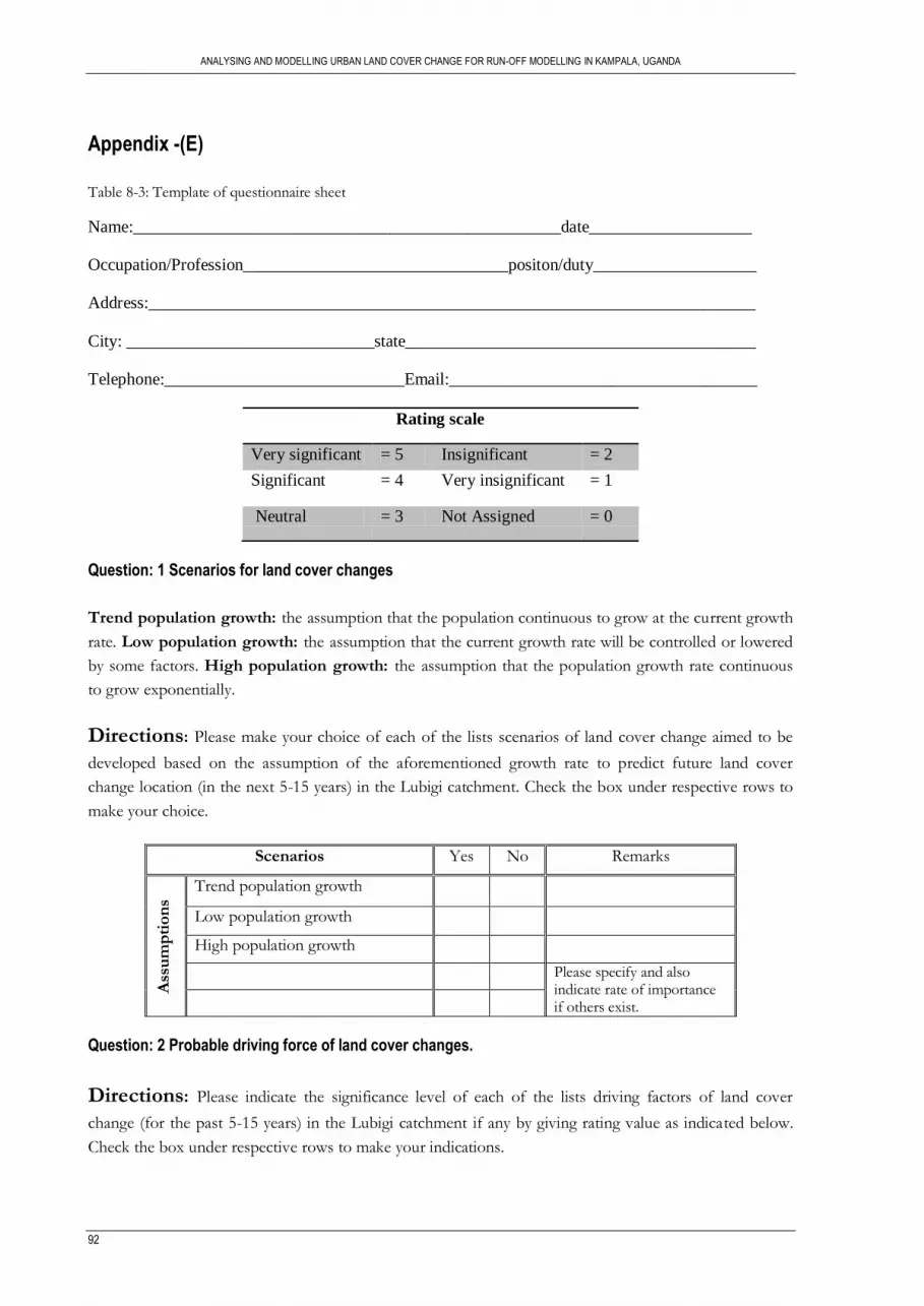
ANALYSING AND MODELLING URBAN LAND COVER CHANGE FOR RUN-OFF MODELLING IN KAMPALA, UGANDA
92
Appendix -(E)
Table 8-3: Template of questionnaire sheet
Name:__________________________________________________date___________________
Occupation/Profession_______________________________positon/duty___________________
Address:_______________________________________________________________________
City: _____________________________state_________________________________________
Telephone:____________________________Email:____________________________________
Rating scale
Very significant = 5 Insignificant = 2
Significant = 4 Very insignificant = 1
Neutral = 3 Not Assigned = 0
Question: 1 Scenarios for land cover changes
Trend population growth: the assumption that the population continuous to grow at the current growth
rate. Low population growth: the assumption that the current growth rate will be controlled or lowered
by some factors. High population growth: the assumption that the population growth rate continuous
to grow exponentially.
Directions: Please make your choice of each of the lists scenarios of land cover change aimed to be
developed based on the assumption of the aforementioned growth rate to predict future land cover
change location (in the next 5-15 years) in the Lubigi catchment. Check the box under respective rows to
make your choice.
Scenarios Yes No Remarks
Ass
um
pti
on
s
Trend population growth
Low population growth
High population growth
Please specify and also indicate rate of importance if others exist.
Question: 2 Probable driving force of land cover changes.
Directions: Please indicate the significance level of each of the lists driving factors of land cover
change (for the past 5-15 years) in the Lubigi catchment if any by giving rating value as indicated below.
Check the box under respective rows to make your indications.

ANALYSING AND MODELLING URBAN LAND COVER CHANGE FOR RUN-OFF MODELLING IN KAMPALA, UGANDA
93
Probable driving force 5 4 3 2 1 0 Remarks Sit
e s
pec
ific
ch
ara
cte
rist
ics
Slope
Zoning status of the land
Master plan
Suitability of the land location for development
Please specify and also indicate rate of contribution if
others exist.
Neig
hb
ou
rho
od
s ch
ara
cte
rist
ics
Proportion of undeveloped land in the surrounding area
Proportion of urban land in the surrounding area
Spatial policies, such as protected area and conserved land
Please specify and also indicate rate of contribution if others exist.
Pro
xim
ity
ch
ara
cte
rist
ics
Distance to major roads
Distance to minor roads
Distance to industrial sites
Distance to minor city centres
Distance to rivers/ streams
Distance to market centre Please specify and also indicate rate of contribution if others exist.
Distance to bus stops
Very significant = 5; Significant = 4; Neutral = 3; Insignificant = 2; Very insignificant= 1; Not Assigned= 0
Question: 3 possible available developable land locations in the parishes of Lubigi catchment.
Directions: Please give significance level of where possible future land for development (in the next 5-
15 years) is available (expected to happen) with in each of the lists of parishes in the Lubigi catchment
given below, if exist by giving rating value in the same way as indicated above. Check the box under
respective rows to make your indications.

ANALYSING AND MODELLING URBAN LAND COVER CHANGE FOR RUN-OFF MODELLING IN KAMPALA, UGANDA
94
Parishes Name 5 4 3 2 1 0 Remarks Q1. In which parishes do you think the growth much will take place in the next 5- 15 years? Why?
________________________________________________________________________________________________________________________________________________________________________________________________________________________________________________________________________________________________________________________________________________________________________________________________________________________________________________________________________________________________
1 BUKOTO I
2 BUKOTO II
3 BWAISE I
4 BWAISE II
5 BWAISE III
6 KAMWOKYA I
7 KAMWOKYA II
8 KANYANYA . Q2. In which parishes do you think much developable land is available for the next 5- 15 years? Why?
________________________________________________________________________________________________________________________________________________________________________________________________________________________________________________________________________________________________________________________________
9 KAWEMPE I
10 KAZO
11 KIKAYA
12 KYEBANDO
13 MAKERERE I
14 MAKERERE II
15 MAKERERE III Q3. In which parishes do you think much protected land is available for the next 5- 15 years? Why?
________________________________________________________________________________________________________________________________________________________________________________________________________________________________________________________________________________________________________________________________________________________________________
16 MAKERERE UNIVERSITY
17 MULAGO I
18 MULAGO II
19 MULAGO III
20 WANDEGEYA
Very significant = 5; Significant = 4; Neutral = 3; Insignificant = 2; Very insignificant = 1; Not Assigned = 0

ANALYSING AND MODELLING URBAN LAND COVER CHANGE FOR RUN-OFF MODELLING IN KAMPALA, UGANDA
95
Appendix-(F)
Table 8-4: Rated responses of the key informants (Probable driving force of land cover changes)
Driving Factors 5 4 3 2 1 Total Respondent
Rating Score
Slope 2 5 1 1 3 12 3.2
Zoning status of the land 2 2 2 3 3 12 2.8
Master plan 1 1 4 3 3 12 2.5
Suitability of the land location 6 2 3 1 - 12 4.1
Proportion of undeveloped land 4 3 - 3 2 12 3.3
Proportion of urban land 5 5 1 - 1 12 4.1
Spatial policies - 1 - 3 8 12 1.5
Distance to major roads 10 2 - - - 12 4.8
Distance to minor roads 3 3 3 3 - 12 3.5
Distance to industrial sites 2 3 1 3 3 12 2.8
Distance to minor city centres 3 5 2 2 12 3.4
Distance to rivers/ streams 2 1 3 1 5 12 2.5
Distance to market centre 5 5 - 1 1 12 4.0
Distance to bus stops 2 2 2 - 6 12 2.5
Table 8-5: Rated responses of the key informants (possible available developable land locations)
Parishes Name 5 4 3 2 1 Total Respondent
Rating Score
Kanyanya 4 6 - 2 - 12 4.0
Kikaya 5 3 2 - 2 12 3.8
Kyebando 1 7 4 - - 12 3.8
kazoo 1 5 5 - 1 12 3.4
Bwaise III 3 2 3 3 1 12 3.3
Mekerere II 1 4 3 4 - 12 3.2
Bwaise II 3 2 2 3 2 12 3.1
Mekerere III 3 3 1 2 3 12 3.1
Mekerere I 1 4 3 2 2 12 3.0
Mulugo III 2 5 1 4 12 3.0
Kawempe I 1 4 3 1 3 12 2.9
Bukoto II 2 1 4 3 2 12 2.8
Kamwokya II 2 2 3 2 3 12 2.8
Kamwokya I - 4 3 3 2 12 2.8
Mulugo I 3 2 1 - 6 12 2.7
Bukoto I 2 1 3 2 4 12 2.6
Bwaise I - 3 3 4 2 12 2.6
Mekerere university 2 1 4 - 5 12 2.6
Wandegeya - 5 2 - 5 12 2.6
Mulugo II 1 3 1 2 5 12 2.4

ANALYSING AND MODELLING URBAN LAND COVER CHANGE FOR RUN-OFF MODELLING IN KAMPALA, UGANDA
96
Table 8-6: Rated responses of the key informants (Expected Scenarios for land cover changes)
Scenario type Yes No Total no of respondents
Trend population growth 7 5 12
Low population growth 1 11 12
High population growth 11 1 12
Appendix-(G)
Table 8-7: Lists of key informants
No Key informant Institution Position
1 Baker Sengendo KCCA PDC/ Bwasie-II
2 Godwin Othieno KCCA Physical Planner
3 John Kisembo KCCA PDC/Bwasie-III
4 Kisembo Teddy Mekerere University Student/Geography department
5 Kuyiga Maximus KCCA Environmentalist/Kwamepe
6 Lutaaga Hassan KCCA PDC/ Bwasie-I
7 Mpanga Musassa KCCA PDC/ Mekerere-III
8 Nakoko Emmanuel Mekerere University Student/Ministry of lands
9 Nalule Harriet Mekerere University Student/Geography department
10 Nambassi Moses Mekerere University Student/Geography department
11 Prince Kanaakulya KCCA PDC/ Mulago-II
12 Shuwab Lwasa (Dr.) Mekerere University Lecturer/Geographer
Appendix-(H)
Figure 8-5: Consideration of neighbourhood effect for proximity characteristics

ANALYSING AND MODELLING URBAN LAND COVER CHANGE FOR RUN-OFF MODELLING IN KAMPALA, UGANDA
97
Appendix-(I)
Figure 8-6: Suitability layer
Figure 8-7: Land cover map for the Trend growth scenario 2020

ANALYSING AND MODELLING URBAN LAND COVER CHANGE FOR RUN-OFF MODELLING IN KAMPALA, UGANDA
98
Figure 8-8: Land cover map for the Low growth scenario 2020
Figure 8-9: Land cover map for the High growth scenario 2020