Finite Elements in Analysis and Design 50 (2012) 21–32

Contents lists available at SciVerse ScienceDirect

Finite Elements in Analysis and Design

0168-87

doi:10.1

n Corr

E-m

antonio

raffaele

URL

journal homepage: www.elsevier.com/locate/finel

An isostatic quadrilateral membrane finite element with drilling rotationsand no spurious modes

A. Madeo n, G. Zagari, R. Casciaro

Dipartimento di Modellistica per l’Ingegneria, Universita della Calabria, 87030 Rende (Cosenza), Italy

a r t i c l e i n f o

Article history:

Received 23 December 2010

Accepted 20 August 2011Available online 11 October 2011

Keywords:

Mixed finite element

Isostatic and equilibrated stress

Drilling rotations

Spurious modes

Analytical integration

Penalty constraints

Geometrically nonlinear analysis

4X/$ - see front matter & 2011 Elsevier B.V.

016/j.finel.2011.08.009

esponding author. Tel.: þ39 0984 496904; fa

ail addresses: antoniomadeo81@gmail.com,

.madeo@unical.it (A. Madeo), gzagari@unical.

.casciaro@unical.it (R. Casciaro).

: http://www.labmec.unical.it (A. Madeo).

a b s t r a c t

A new quadrilateral four node membrane finite element based on a mixed Hellinger–Reissner

variational formulation is proposed. Displacement and stress interpolations are defined by 12

kinematical DOFs (two displacements and one drilling rotation per node) and 9 stress parameters.

The displacement interpolation is obtained as a sum of three contributions. The first two correspond

to compatible modes that assume a linear and quadratic (Allman-like) shape along the sides. The latter

corresponds to a cubic incompatible mode depending on the average nodal rotations of the element.

The stress interpolation is obtained from a complete quadratic polynomial by enforcing the internal

bulk equilibrium and three further ul Pian equilibrium conditions, so obtaining an equilibrated and

non-redundant field. The compliance and compatibility matrices are derived analytically, using an

efficient boundary integration scheme.

Numerical comparisons show that the proposed element performs better and is less sensitive to

mesh distortion than similar elements in the literature. The constant stress states are recovered exactly

and a very accurate recovery, for both stress and rotation fields, is also obtained in bending as well as in

shear contexts. As shown by some numerical tests in buckling problems, the element is suitable for

extension to nonlinear analysis.

& 2011 Elsevier B.V. All rights reserved.

1. Introduction

The general framework based on corotational formulationdiscussed in paper [1] allows the geometrically nonlinear FEManalysis of beam or plate assemblages, either using path-followingor asymptotic numerical strategies, simply starting from finiteelements defined for linear analysis. In the same paper theproposed approach was used for 3D beam assemblages with verygood results. A preliminary implementation for plate assemblages[2] provided quite satisfactory results but also suggested improve-ments by a better tuning of the plate element used, particularlywith reference to its in-plane (membrane) behavior. This led toresearch in this direction the results of which are presented here.

The purpose of the paper is to develop a linear membranefinite element which, when coupled with an appropriate flexuraldescription and a corotational solution strategy, could be suitablefor use in the geometrical nonlinear analysis of slender foldedplates and flat shells. This element has certain requirements.

All rights reserved.

x: þ39 0984 496912.

it (G. Zagari),

A good linear response, free from locking and spurious zero-energy modes, is a basic prerequisite, for reliability and goodperformance also in the nonlinear context. The use of a mixedinterpolation strategy appears to be the most effective approachto obtain this result [3]. It also connects directly with themixed solution format devised in [4,5] to increase the efficiencyand robustness of both path-following and asymptotic solutionprocedures. Moreover, rotational (drilling) degrees of freedom areneeded for an easier handling of the in- and out-of-plane couplingof boundary conditions between elements with different orienta-tion and also for a direct implementation of the corotationalstrategy (see [1]). A quadrilateral format for the element is alsosuggested by the geometry of the plate assemblages underconsideration. Finally, a minimal number of internal DOFs isadvantageous in order to simplify the element matrices andreduce the mesh size, for the same overall number of unknowns,and so improve the accuracy of the corotational treatment.

According to these requirements, our proposal is a four nodeassumed stress quadrilateral element, based on mixed formulationwhich uses the Hellinger–Reissner variational framework [6] byassuming separate interpolations for the displacement and stressfields. The element is defined by 12 external degrees of freedom(two translations and one drilling rotation for each node of theelement) and by nine internal stress parameters controlling thestress interpolation which is obtained starting from a complete

A. Madeo et al. / Finite Elements in Analysis and Design 50 (2012) 21–3222

quadratic expansion for the stress components and enforcing asufficient number of equilibrium conditions to render the elementnon-redundant statically.

Note that, while convenient for an easier coupling withflexural elements, the use of drilling rotations is not a naturalchoice for membrane elements. In fact, it introduces a high-order(cubic) interpolation for the transversal displacements on theelement sides which conflicts with the relative overall poorness ofthe internal kinematics and then tends to generate interpolationlocking, at least when using compatible interpolations.

To overcome this inconvenience the method devised by Allman[7,8] appears to be particularly simple and effective. The originalidea, to interpolate the side displacements by a simpler quadraticfunction governed by the difference in the end edge rotations, isreally elegant. In fact, this simplified shape allows a smoother strainrepresentation to be obtained and the interpolation locking asso-ciated with the use of drilling nodal rotations to be reduced. As acounterpart, the side interpolation becomes insensitive to the nodalrotation average, so the element is rank defective and the overallassemblage has one zero-energy spurious mode corresponding to aconstant rotation in all nodes of the mesh. In principle, this is adisturbing but not necessarily a serious problem in linear analysis. Infact, the spurious mode is generally not directly activated by theexternal load and it can be removed, quite naturally, simply by arotational constraint over all the boundary conditions. In this way itdoes not cause any practical inconvenience and so it is oftenneglected or, at least, considered as a minor problem.

The original Allman proposal is based on a purely compatibleformulation so it is affected by the persistence of a residuallocking which can be avoided, as suggested by MacNeal andHarder in [9], by the use of a reduced integration scheme in theelement matrices construction. However, two additional spuriouszero-energy hourglass modes are introduced which increase therank-defectiveness already due to the Allman interpolation.

Starting from the papers by Aminpour [10,11] it became clearthat the use of a mixed interpolation could be a more effectiveway to eliminate locking and develop high-performance finiteelements. In particular, the element proposed in [11] generallyshows a good behavior in terms of displacements and stresses andlittle sensitivity to mesh distortion, but seems to be little suitedfor the geometrically nonlinear analysis of folded plate assem-blages, because of its poor recovery of nodal rotations caused bythe Allman rank defectiveness (see discussion in Section 3.5).

A different line of research, for introducing drilling rotations in amembrane element, started with the well known paper by Hughesand Brezzi [12]. While accepting the Allman interpolation theseauthors refer to a non standard variational formulation based on aseparate interpolation for the displacement, stress and rotationfields. The stress tensor is assumed to be unsymmetrical, ingeneral, while its symmetry and the correspondence between therotation and the unsymmetrical part of the displacement gradientis assured, in weak form, by the variational condition. The paperintroduced a well stated theoretical framework also allowingdifferent variants, by the introduction of different penalty con-straints, further investigated in successive papers [3,13–17], alsoexploiting the incompatible modes method [18–20]. The elementproposed by Kugler [21], obtained as a discretization of a Cosseratcontinuum, was similar. In general, this formulation is appealing,and potentially could allow a better recovery of the rotation field,which is taken as a primary variable of the problem, but elementsalready developed on these bases generally suffer from meshdistortion sensitivity and have unsatisfactory behavior in the caseof orthotropic materials and dynamics problems, as outlined in thenumerical comparison made by Long in [22].

Distortion sensitivity is a potential drawback in quadrangularAllman-like elements, especially when recovering linear stress

fields. The problem can be related to the use of the internaldimensionless coordinates in defining both displacements andstress interpolations. A formulation in Cartesian coordinates couldbe desirable, but generally this strategy implies some difficultiesin assuring inter-element compatibility and so different strategieshave been proposed in the literature. The element proposed in[23], based on area coordinates, reduces the sensitivity to meshdistortion but implies the violation of compatibility, as outlined in[24] with reference to some interesting benchmarks. Finally, theway proposed in the paper [25] allows mesh distortion sensitivityto be reduced while introducing an unsymmetric formulation.

It also worth mentioning that the convenience of using self-equilibrated stress interpolations in Cartesian coordinates wasalready recognized by Aminpour in [11], and by Cannarozzi in[26] which proposed the use of self-equilibrated stress fieldsbased on Airy solutions in Cartesian coordinates. In the latter casethe kinematics of the element was actually based on a cubicexpansion of the transversal side displacement, in spite of theAllman quadratic interpolation. This choice and that of using Airystress interpolation, which can be considered somewhat toorestrictive, cause the persistence of a residual locking in theelement behavior (see numerical benchmarks in Section 3).Moreover, the choice of referring to relative nodal rotations (i.e.to consider them as additional rotations superimposed on thebilinear deformation due to the nodal displacements) introducessome difficulties in recovering the absolute rotation field.

Some of the previous ideas, such as the Allman kinematics andthe use of a mixed formulation and internal self-equilibratedstress fields appear very effective and have also been followed inour proposal. As shown by the numerical comparisons reported inSection 3, the proposed element outperform in both accuracy androbustness the previous proposals.

The paper is organized as follows. Section 2 describes theproposed membrane element in detail and gives explicit expressionsfor its relevant matrices. Section 3 considers a series of validationbenchmarks, showing the good performance of the element. Furthercomments and concluding remarks are given in Section 4.

2. Formulation of the element

2.1. Main features of the proposed element

The external format of the element being set in advance themain choices in our proposal can be summarized as follows:

1.

A mixed formulation is used with a separate interpolation ofthe stress and displacement fields in order to increase thestress recovery and reduce kinematical locking.

2.

The element kinematics is based on Allman interpolation,enriched by an incompatible cubic mode in order to avoidrank defectiveness.

3.

Its statics is described by an isostatic interpolation for the stresses,obtained exploiting bulk equilibrium and Pian’s ul technique, inorder to increase accuracy and filter the kinematical locking.

4.

The stresses are referred to a local Cartesian frame aligned tothe element in order to express the equilibrium condition easilyand to obtain an objective definition of the element statics.

5.

Element matrices are obtained through analytical contourintegration.

All these choices are important to obtain a good overall behaviorfor the element, according to the following considerations.

The possible advantages of mixed interpolations in comparisonto the compatible ones are well known in literature. A carefulcombination of the displacement and stress interpolations generally

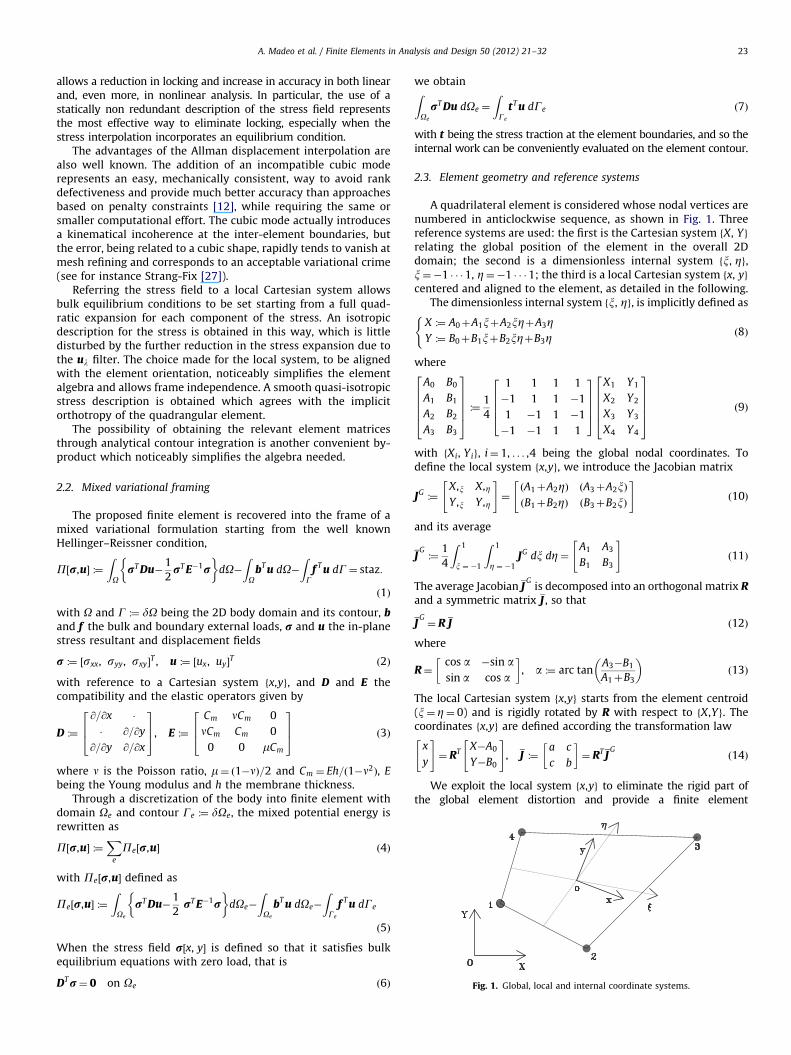
Fig. 1. Global, local and internal coordinate systems.

A. Madeo et al. / Finite Elements in Analysis and Design 50 (2012) 21–32 23

allows a reduction in locking and increase in accuracy in both linearand, even more, in nonlinear analysis. In particular, the use of astatically non redundant description of the stress field representsthe most effective way to eliminate locking, especially when thestress interpolation incorporates an equilibrium condition.

The advantages of the Allman displacement interpolation arealso well known. The addition of an incompatible cubic moderepresents an easy, mechanically consistent, way to avoid rankdefectiveness and provide much better accuracy than approachesbased on penalty constraints [12], while requiring the same orsmaller computational effort. The cubic mode actually introducesa kinematical incoherence at the inter-element boundaries, butthe error, being related to a cubic shape, rapidly tends to vanish atmesh refining and corresponds to an acceptable variational crime(see for instance Strang-Fix [27]).

Referring the stress field to a local Cartesian system allowsbulk equilibrium conditions to be set starting from a full quad-ratic expansion for each component of the stress. An isotropicdescription for the stress is obtained in this way, which is littledisturbed by the further reduction in the stress expansion due tothe ul filter. The choice made for the local system, to be alignedwith the element orientation, noticeably simplifies the elementalgebra and allows frame independence. A smooth quasi-isotropicstress description is obtained which agrees with the implicitorthotropy of the quadrangular element.

The possibility of obtaining the relevant element matricesthrough analytical contour integration is another convenient by-product which noticeably simplifies the algebra needed.

2.2. Mixed variational framing

The proposed finite element is recovered into the frame of amixed variational formulation starting from the well knownHellinger–Reissner condition,

P½r,u� :¼ZO

rT Du�1

2rT E�1r

� �dO�

ZO

bT u dO�ZG

f T u dG¼ staz:

ð1Þ

with O and G :¼ dO being the 2D body domain and its contour, band f the bulk and boundary external loads, r and u the in-planestress resultant and displacement fields

r :¼ ½sxx, syy, sxy�T , u :¼ ½ux, uy�

T ð2Þ

with reference to a Cartesian system fx,yg, and D and E thecompatibility and the elastic operators given by

D :¼

@=@x �

� @=@y

@=@y @=@x

264

375, E :¼

Cm nCm 0

nCm Cm 0

0 0 mCm

264

375 ð3Þ

where n is the Poisson ratio, m¼ ð1�nÞ=2 and Cm ¼ Eh=ð1�n2Þ, E

being the Young modulus and h the membrane thickness.Through a discretization of the body into finite element with

domain Oe and contour Ge :¼ dOe, the mixed potential energy isrewritten as

P½r,u� :¼X

e

Pe½r,u� ð4Þ

with Pe½r,u� defined as

Pe½r,u� :¼ZOe

rT Du�1

2rT E�1r

� �dOe�

ZOe

bT u dOe�

ZGe

f T u dGe

ð5Þ

When the stress field r½x, y� is defined so that it satisfies bulkequilibrium equations with zero load, that is

DTr¼ 0 on Oe ð6Þ

we obtainZOe

rT Du dOe ¼

ZGe

tT u dGe ð7Þ

with t being the stress traction at the element boundaries, and so theinternal work can be conveniently evaluated on the element contour.

2.3. Element geometry and reference systems

A quadrilateral element is considered whose nodal vertices arenumbered in anticlockwise sequence, as shown in Fig. 1. Threereference systems are used: the first is the Cartesian system fX, Yg

relating the global position of the element in the overall 2Ddomain; the second is a dimensionless internal system fx, Zg,x¼�1 � � �1, Z¼�1 � � �1; the third is a local Cartesian system fx, yg

centered and aligned to the element, as detailed in the following.The dimensionless internal system fx, Zg, is implicitly defined as

X :¼ A0þA1xþA2xZþA3ZY :¼ B0þB1xþB2xZþB3Z

(ð8Þ

where

A0 B0

A1 B1

A2 B2

A3 B3

266664

377775 :¼

1

4

1 1 1 1

�1 1 1 �1

1 �1 1 �1

�1 �1 1 1

26664

37775

X1 Y1

X2 Y2

X3 Y3

X4 Y4

266664

377775 ð9Þ

with fXi, Yig, i¼ 1, . . . ,4 being the global nodal coordinates. Todefine the local system fx,yg, we introduce the Jacobian matrix

JG :¼X,x X,Z

Y ,x Y ,Z

" #¼ðA1þA2ZÞ ðA3þA2xÞðB1þB2ZÞ ðB3þB2xÞ

" #ð10Þ

and its average

JG:¼

1

4

Z 1

x ¼ �1

Z 1

Z ¼ �1JG dx dZ¼

A1 A3

B1 B3

" #ð11Þ

The average Jacobian JG

is decomposed into an orthogonal matrix Rand a symmetric matrix J , so that

JG¼ R J ð12Þ

where

R¼cos a �sin asin a cos a

� �, a :¼ arc tan

A3�B1

A1þB3

� �ð13Þ

The local Cartesian system fx,yg starts from the element centroid(x¼ Z¼ 0) and is rigidly rotated by R with respect to fX,Yg. Thecoordinates fx,yg are defined according the transformation law

x

y

" #¼ RT

X�A0

Y�B0

" #, J :¼

a c

c b

� �¼ RT J

Gð14Þ

We exploit the local system fx,yg to eliminate the rigid part ofthe global element distortion and provide a finite element

A. Madeo et al. / Finite Elements in Analysis and Design 50 (2012) 21–3224

description which is objective with respect to a rigid body motion ofthe element, so allowing its reuse in geometrical nonlinear analysis.

Finally, it is convenient to introduce some further helpfuldefinitions. For each side Gi, connecting nodes i and j in antic-lockwise order, we define gi and di and its external normal ni,according to the following expression:

gi :¼gix

giy

" #:¼

xjþxi

yjþyi

" #, di :¼

dix

diy

" #:¼

xj�xi

yj�yi

" #,

ni :¼nx

ny

" #¼

1

Li

yij

�xij

" #ð15Þ

with Li :¼ffiffiffiffiffiffiffiffiffiffiffiffiffiffiffix2

ijþy2ij

qbeing the side length. We will use one-

dimensional abscissa �1rzr1 along Gi such that

x¼1

2ðgixþdix zÞ, y¼

1

2ðgiyþdiy zÞ ð16Þ

2.4. Stress interpolation

The stress interpolation is referred to the local fx, yg system.It is derived starting from a complete quadratic expansion for thestress components and enforcing the internal equilibrium withzero bulk loads

DTr¼ 0 on Oe ð17Þ

We obtain the 12-parameter expansion

sxx :¼ s1þs4xþs7y�2s8x yþs10x2þs12y2

syy :¼ s2þs5x�s6y�2s9x yþs11x2þs10y2

sxy :¼ s3þs6x�s4y�2s10x yþs9x2þs8y2

8><>: ð18Þ

which, exploiting the Pian ul filter technique [6], is furtherreduced to a 9-parameter expansion by enforcing 3 ul additionalequilibrium conditions:ZOe

rT Dulk dO :¼

Z 1

�1

Z 1

�1rT JT Dulk dx dn¼ 0, k¼ 1, . . . ,3 ð19Þ

where

ul1 :¼ l1

x3�x

Z3�Z

" #, ul2 :¼ l2

a3ðZ2 x�x=3Þ

b3ðx2 Z�Z=3Þ

" #,ul3 :¼ l3

bðZ3x2�Z=3Þ

aðx3 Z2�x=3Þ

" #

ð20Þ

have been selected according the general criteria discussed in[28]: (i) obtain an isostatic element; (ii) complement the poly-nomial expansion (24) which defines the displacement interpola-tion u; (iii) be orthogonal to constant and linear stress; (iv) agreewith the element orthotropy.

As devised in [28], even rough approximations for Jacobian Jare acceptable in the integrals (19) (see Section 3 for a comment).Approximating the Jacobian by a diagonalization of its average J ,that is, assuming

J �a �

� b

� �ð21Þ

and performing integration, filter conditions reduce to

s10 ¼ 0, s9 ¼�b2

a2s8, s11 ¼�s12

We can then rearrange the stress expansion in the form

r :¼ Bs½x, y� b, Bs :

¼

1 � � y � x � y2 �2a2xy

� 1 � � x � y �x2 2b2xy

� � 1 � � �y �x � a2y2�b2x2

2664

3775 ð22Þ

b being the [9�1] vector of the element stress free parameters.

It is worth noting that stress interpolation (22) coincides withthe one assumed in [11], apart from a different rearrangement ofquadratic terms in the two high-order modes. This difference,together with the assumed displacement interpolation (24), willbe essential in avoiding Allman defectiveness of the element.Moreover, the choice made for the local Cartesian system,through (12), and the presence of the shape constants a and b

allow the element geometry to be accounted for and perfor-mances in distorted meshes improved.

2.5. Displacement interpolation

The displacement interpolation u :¼ fux, uyg is referred to theinternal system fx, Zg and controlled by the [12�1] externalelement displacement vector

de :¼ ½ux1, uy1, f1,ux2, . . . ,f4�T ð23Þ

collecting displacements ux, uy and additional Allman rotations fof the four nodes of the element.

Recalling that the stress satisfies equilibrium equation (17)internal work can be obtained by integrating on the elementcontour through Eq. (7), its evaluation only needing that thecontour displacements be defined. We define the displacementinterpolation along each side as a sum of three contributions:

u½z� :¼ ul½z�þuq½z�þuc½z� ð24Þ

The first is a linear expansion

ul½z� ¼1

2

ð1�zÞuiþð1þzÞuj

ð1�zÞviþð1þzÞvj

" #ð25Þ

relating to the nodal displacements. The second and third, relat-ing to the drilling rotations, correspond to a quadratic and cubicexpansion for the normal component of the side displacement

uq½z� ¼ 18 Liðz

2�1Þðfi�fjÞni

uc½z� ¼ 14 Liðz�z

3Þani

8<: , i¼ 1, . . . ,4 ð26Þ

a being the average distortional nodal rotation, defined by

a :¼ 1

4

X4

i ¼ 1

fi�fe ð27Þ

where fe is the average rigid rotation of the element

fe :¼ Nade,

Na ¼1

4Oe½�d4y, d4x, � ,�d1y, d1x, � , �d2y, d2x, � , �d3y, d3x, �� ð28Þ

Note that, while the linear ul and the quadratic uq parts of thedisplacement are continuous at the inter-element boundaries bydefinition, the cubic contribution uc corresponds to an incompa-tible mode, needed to avoid rank defectiveness in the element.This introduces a kinematical incongruence at the inter-elementboundaries which is however irrelevant because it rapidlyvanishes with mesh refining.

2.6. Compliance matrix

The element compliance matrix He is defined by the energyequivalence

bTe Hebe :¼

ZOe

rT E�1r dO ð29Þ

Due to Eq. (22), we obtain

He ¼

ZOe

BTsE�1Bs dO ð30Þ

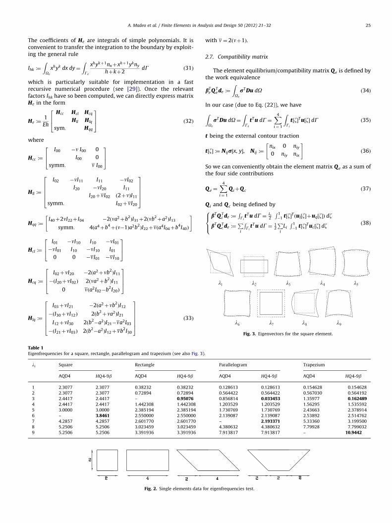
Fig. 3. Eigenvectors for the square element.

A. Madeo et al. / Finite Elements in Analysis and Design 50 (2012) 21–32 25

The coefficients of He are integrals of simple polynomials. It isconvenient to transfer the integration to the boundary by exploit-ing the general rule

Ihk :¼

ZOe

xhyk dx dy¼

ZGe

xhykþ1nxþxhþ1ykny

hþkþ2dG ð31Þ

which is particularly suitable for implementation in a fastrecursive numerical procedure (see [29]). Once the relevantfactors Ihk have so been computed, we can directly express matrixHe in the form

He :¼1

Eh

Hcc Hcl Hcq

Hll Hlq

sym: Hqq

264

375 ð32Þ

where

Hcc :¼

I00 �n I00 0

I00 0

symm: n I00

264

375

Hll :¼

I02 �nI11 I11 �nI02

I20 �nI20 I11

I20þnI02 ð2þnÞI11

symm: I02þnI20

266664

377775

Hqq :¼I40þ2nI22þ I04 �2ðna2þb2

ÞI31þ2ðnb2þa2ÞI13

symm: 4ða4þb4þðn�1Þa2b2

ÞI22þnða4I04þb4I40Þ

" #

Hcl :¼

I01 �nI10 I10 �nI01

�nI01 I10 �nI10 I01

0 0 �nI01 �nI10

264

375

Hcq :¼

I02þnI20 �2ða2þnb2ÞI11

�ðI20þnI02Þ 2ðna2þb2ÞI11

0 nða2I02�b2I20Þ

2664

3775

Hlq :¼

I03þnI21 �2ða2þnb2ÞI12

�ðI30þnI12Þ 2ðb2þna2ÞI21

I12þnI30 2ðb2�a2ÞI21�na2I03

�ðI21þnI03Þ 2ðb2�a2ÞI12þnb2I30

2666664

3777775 ð33Þ

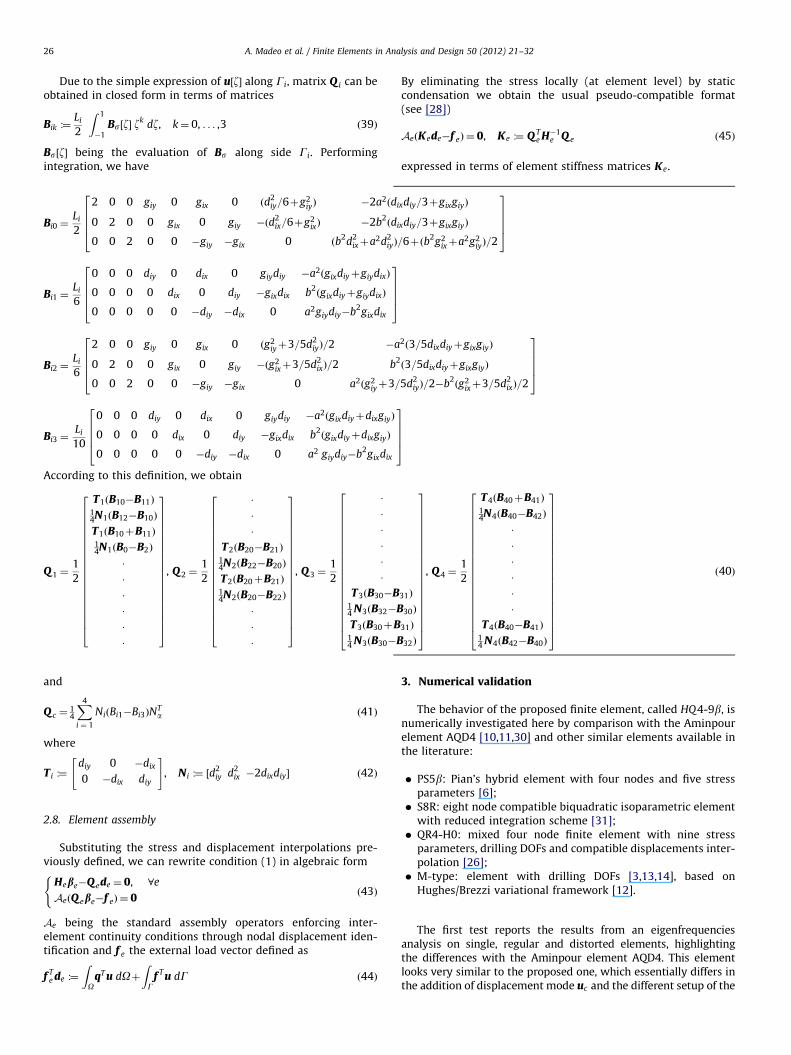
Fig. 2. Single elements data f

Table 1Eigenfrequencies for a square, rectangle, parallelogram and trapezium (see also Fig. 3)

li Square Rectangle

AQD4 HQ4-9b AQD4 HQ4-9b

1 2.3077 2.3077 0.38232 0.38232

2 2.3077 2.3077 0.72894 0.72894

3 2.4417 2.4417 – 0.950764 2.4417 2.4417 1.442308 1.442308

5 3.0000 3.0000 2.385194 2.385194

6 – 3.8461 2.550000 2.550000

7 4.2857 4.2857 2.601770 2.601770

8 5.2506 5.2506 3.023459 3.023459

9 5.2506 5.2506 3.391936 3.391936

with n ¼ 2ðnþ1Þ.

2.7. Compatibility matrix

The element equilibrium/compatibility matrix Q e is defined bythe work equivalence

bTe Q T

e de :¼

ZOe

rT Du dO ð34Þ

In our case (due to Eq. (22)), we have

ZOe

rT Du dO¼ZGe

tT u dG¼X4

i ¼ 1

ZGi

t½z�T u½z� dG ð35Þ

t being the external contour traction

t½z� :¼ N ijr½x, y�, N ij :¼nix 0 niy

0 niy nix

" #ð36Þ

So we can conveniently obtain the element matrix Q e as a sum ofthe four side contributions

Q e ¼X4

i ¼ 1

Q iþQ c ð37Þ

Q i and Q c being defined by

bT Q Ti de :¼

RGi

tT u dG¼ Li2

R 1�1 t½z�T ðul½z�þuq½z�Þ dz

bT Q Tc de :¼

Pi

RGi

tT u dG¼ 12

Pi

Li

R 1�1 t½z�T uc½z� dz

8><>: ð38Þ

or eigenfrequencies test.

.

Parallelogram Trapezium

AQD4 HQ4-9b AQD4 HQ4-9b

0.128613 0.128613 0.154628 0.154628

0.564422 0.564422 0.567030 0.564192

0.856814 0.033453 1.35977 0.1624891.203529 1.203529 1.56295 1.535592

1.730769 1.730769 2.43663 2.378914

2.139087 2.139087 2.53892 2.514762

– 2.193371 5.33360 3.199500

4.380632 4.380632 7.79928 7.799032

7.913817 7.913817 – 10.9442

A. Madeo et al. / Finite Elements in Analysis and Design 50 (2012) 21–3226

Due to the simple expression of u½z� along Gi, matrix Q i can beobtained in closed form in terms of matrices

Bik :¼Li

2

Z 1

�1Bs½z� z

k dz, k¼ 0, . . . ,3 ð39Þ

Bs½z� being the evaluation of Bs along side Gi. Performingintegration, we have

Bi0 ¼Li

2

2 0 0 giy 0 gix 0 ðd2iy=6þg2

iyÞ �2a2ðdixdiy=3þgixgiyÞ

0 2 0 0 gix 0 giy �ðd2ix=6þg2

ixÞ �2b2ðdixdiy=3þgixgiyÞ

0 0 2 0 0 �giy �gix 0 ðb2d2ixþa2d2

iyÞ=6þðb2g2ixþa2g2

iyÞ=2

26664

37775

Bi1 ¼Li

6

0 0 0 diy 0 dix 0 giydiy �a2ðgixdiyþgiydixÞ

0 0 0 0 dix 0 diy �gixdix b2ðgixdiyþgiydixÞ

0 0 0 0 0 �diy �dix 0 a2giydiy�b2gixdix

26664

37775

Bi2 ¼Li

6

2 0 0 giy 0 gix 0 ðg2iyþ3=5d2

iyÞ=2 �a2ð3=5dixdiyþgixgiyÞ

0 2 0 0 gix 0 giy �ðg2ixþ3=5d2

ixÞ=2 b2ð3=5dixdiyþgixgiyÞ

0 0 2 0 0 �giy �gix 0 a2ðg2iyþ3=5d2

iyÞ=2�b2ðg2

ixþ3=5d2ixÞ=2

26664

37775

Bi3 ¼Li

10

0 0 0 diy 0 dix 0 giydiy �a2ðgixdiyþdixgiyÞ

0 0 0 0 dix 0 diy �gixdix b2ðgixdiyþdixgiyÞ

0 0 0 0 0 �diy �dix 0 a2 giydiy�b2gixdix

26664

37775

According to this definition, we obtain

Q 1 ¼1

2

T1ðB10�B11Þ

14N1ðB12�B10Þ

T1ðB10þB11Þ

14N1ðB0�B2Þ

�

�

�

�

�

�

26666666666666666664

37777777777777777775

, Q 2 ¼1

2

�

�

�

T2ðB20�B21Þ

14N2ðB22�B20Þ

T2ðB20þB21Þ

14N2ðB20�B22Þ

�

�

�

26666666666666666664

37777777777777777775

, Q 3 ¼1

2

�

�

�

�

�

�

T3ðB30�B31Þ

14 N3ðB32�B30Þ

T3ðB30þB31Þ

14 N3ðB30�B32Þ

266666666666666666664

377777777777777777775

, Q 4 ¼1

2

T4ðB40þB41Þ

14N4ðB40�B42Þ

�

�

�

�

�

�

T4ðB40�B41Þ

14 N4ðB42�B40Þ

266666666666666666664

377777777777777777775

ð40Þ

and

Q c ¼14

X4

i ¼ 1

Ni Bi1�Bi3ð ÞNTa ð41Þ

where

T i :¼diy 0 �dix

0 �dix diy

" #, N i :¼ ½d

2iy d2

ix �2dixdiy� ð42Þ

2.8. Element assembly

Substituting the stress and displacement interpolations pre-viously defined, we can rewrite condition (1) in algebraic form

Hebe�Q ede ¼ 0, 8e

AeðQ ebe�f eÞ ¼ 0

(ð43Þ

Ae being the standard assembly operators enforcing inter-element continuity conditions through nodal displacement iden-tification and f e the external load vector defined as

f Te de :¼

ZO

qT u dOþZG

f T u dG ð44Þ

By eliminating the stress locally (at element level) by staticcondensation we obtain the usual pseudo-compatible format(see [28])

AeðKede�f eÞ ¼ 0, Ke :¼ Q Te H�1

e Q e ð45Þ

expressed in terms of element stiffness matrices Ke.

3. Numerical validation

The behavior of the proposed finite element, called HQ4-9b, isnumerically investigated here by comparison with the Aminpourelement AQD4 [10,11,30] and other similar elements available inthe literature:

�

PS5b: Pian’s hybrid element with four nodes and five stressparameters [6]; � S8R: eight node compatible biquadratic isoparametric element

with reduced integration scheme [31];

� QR4-H0: mixed four node finite element with nine stress

parameters, drilling DOFs and compatible displacements inter-polation [26];

� M-type: element with drilling DOFs [3,13,14], based on

Hughes/Brezzi variational framework [12].

The first test reports the results from an eigenfrequenciesanalysis on single, regular and distorted elements, highlightingthe differences with the Aminpour element AQD4. This elementlooks very similar to the proposed one, which essentially differs inthe addition of displacement mode uc and the different setup of the

A. Madeo et al. / Finite Elements in Analysis and Design 50 (2012) 21–32 27

quadratic stress fields, both needed for avoiding Allman defective-ness. Apart from this, the two elements show the same behaviorfor regular geometry and slight differences for distorted geometry.

Some simple tests are presented, which show the ability of theelement in recovering the constant and linear stress solutions.More complex benchmarks are then reported, such as the classicCook’s membrane and the ones proposed by Karakose in [32].

Finally further tests are presented which show the ability ofHQ4-9b to recover the rotation field in problems where rotationplays an essential role or where we are interested.

3.1. Comparison with AQD4 element in element eigenfrequencies

HQ4-9b may be considered a variant (actually an improve-ment) of the Aminpour element AQD4 [11]. In fact, apart fromminor details, the main differences are only a slightly differentchoice for the quadratic terms in the stress interpolation and theaddition of the cubic mode used for eliminating rank-defective-ness. This is confirmed by the comparison in terms of eigenfre-quencies recovery shown in Table 1. The analysis is performedassuming a mass density r¼ 1, E¼1 and n¼ 0:3 for differentcases: a square of size 2�2, a rectangle of size 2�4, a parallelo-gram and a trapezium (see Fig. 2).

For regular elements (square and rectangle), HQ4-9b andAQD4 have the same eigenmodes and eigenfrequencies, apartthe cubic shape modes unavailable for AQD4 (see Fig. 3). In thecase of distorted geometry, further differences appear related to a

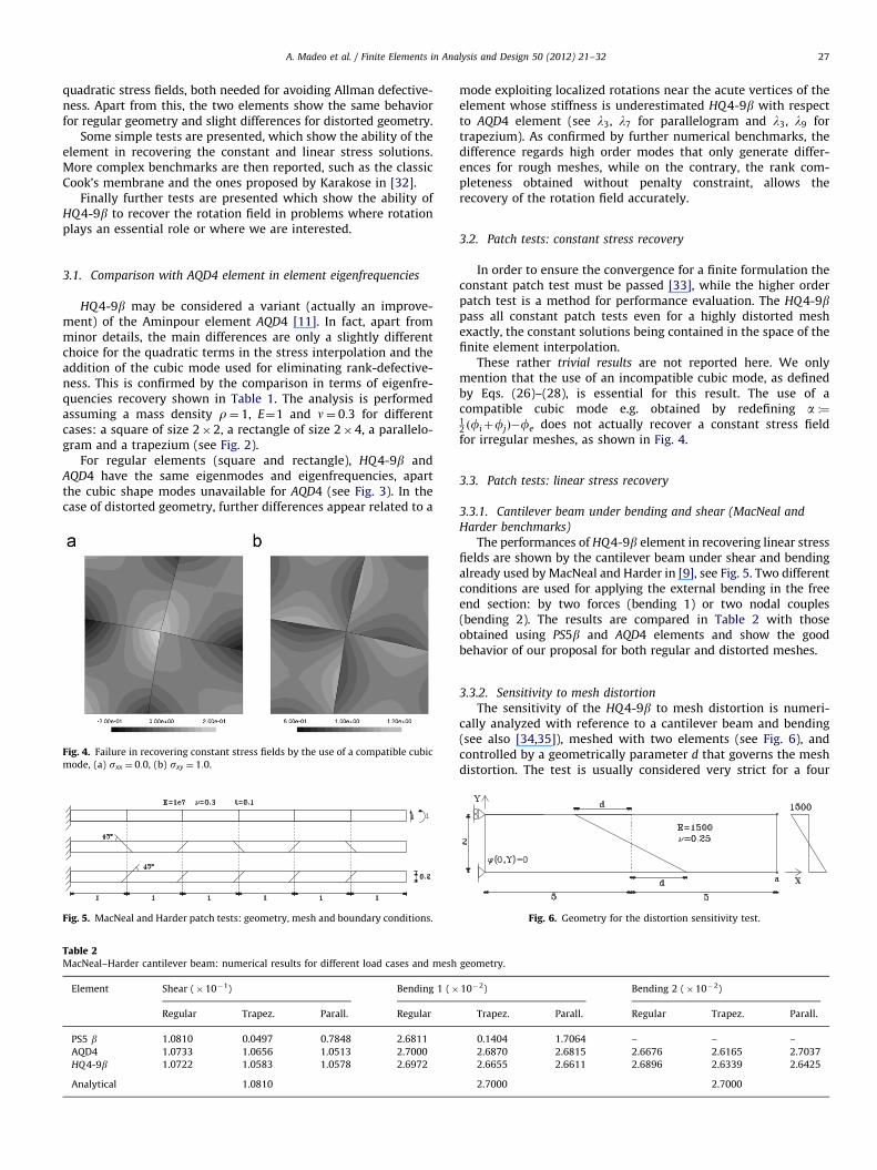
Fig. 4. Failure in recovering constant stress fields by the use of a compatible cubic

mode, (a) sxx ¼ 0:0, (b) sxy ¼ 1:0.

Fig. 5. MacNeal and Harder patch tests: geometry, mesh and boundary conditions.

Table 2MacNeal–Harder cantilever beam: numerical results for different load cases and mesh

Element Shear (�10�1) Bending 1 (�

Regular Trapez. Parall. Regular

PS5 b 1.0810 0.0497 0.7848 2.6811

AQD4 1.0733 1.0656 1.0513 2.7000

HQ4-9b 1.0722 1.0583 1.0578 2.6972

Analytical 1.0810

mode exploiting localized rotations near the acute vertices of theelement whose stiffness is underestimated HQ4-9b with respectto AQD4 element (see l3, l7 for parallelogram and l3, l9 fortrapezium). As confirmed by further numerical benchmarks, thedifference regards high order modes that only generate differ-ences for rough meshes, while on the contrary, the rank com-pleteness obtained without penalty constraint, allows therecovery of the rotation field accurately.

3.2. Patch tests: constant stress recovery

In order to ensure the convergence for a finite formulation theconstant patch test must be passed [33], while the higher orderpatch test is a method for performance evaluation. The HQ4-9bpass all constant patch tests even for a highly distorted meshexactly, the constant solutions being contained in the space of thefinite element interpolation.

These rather trivial results are not reported here. We onlymention that the use of an incompatible cubic mode, as definedby Eqs. (26)–(28), is essential for this result. The use of acompatible cubic mode e.g. obtained by redefining a :¼12 ðfiþfjÞ�fe does not actually recover a constant stress fieldfor irregular meshes, as shown in Fig. 4.

3.3. Patch tests: linear stress recovery

3.3.1. Cantilever beam under bending and shear (MacNeal and

Harder benchmarks)

The performances of HQ4-9b element in recovering linear stressfields are shown by the cantilever beam under shear and bendingalready used by MacNeal and Harder in [9], see Fig. 5. Two differentconditions are used for applying the external bending in the freeend section: by two forces (bending 1) or two nodal couples(bending 2). The results are compared in Table 2 with thoseobtained using PS5b and AQD4 elements and show the goodbehavior of our proposal for both regular and distorted meshes.

3.3.2. Sensitivity to mesh distortion

The sensitivity of the HQ4-9b to mesh distortion is numeri-cally analyzed with reference to a cantilever beam and bending(see also [34,35]), meshed with two elements (see Fig. 6), andcontrolled by a geometrically parameter d that governs the meshdistortion. The test is usually considered very strict for a four

geometry.

10�2) Bending 2 (�10�2)

Trapez. Parall. Regular Trapez. Parall.

0.1404 1.7064 – – –

2.6870 2.6815 2.6676 2.6165 2.7037

2.6655 2.6611 2.6896 2.6339 2.6425

2.7000 2.7000

Fig. 6. Geometry for the distortion sensitivity test.

A. Madeo et al. / Finite Elements in Analysis and Design 50 (2012) 21–3228

node finite element while being generally passed by eight nodeelements (or six node specialized for recovering this kind ofsolution [28]). The results, for different values of distortion d

with those obtained using PS5b, AQD4 and S8R elements arecompared in Fig. 7. Note that, while only S8R is distortioninsensitive (as expected for eight node finite element), bothHQ4-9b and AQD4 are little influenced by moderate distortionsand provide a noticeable improvement with respect to PS5b.

3.3.3. Graded mesh patch test

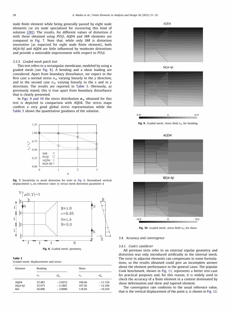
This test refers to a rectangular membrane, modeled by using agraded mesh (see Fig. 8). A bending and a shear loading areconsidered. Apart from boundary disturbance, we expect in thefirst case a normal stress sxx varying linearly in the y direction,and in the second case sxx varying linearly in the x and in y

directions. The results are reported in Table 3. Obviously, aspreviously stated, this is true apart from boundary disturbancethat is clearly presented.

In Figs. 9 and 10 the stress distribution rxx obtained for thistest is depicted in comparison with AQD4. The stress mapsconfirm a very good global stress representation while theTable 3 shows the quantitative goodness of the solution.

Table 3Graded mesh: displacements and stress.

Element Bending Shear

va sbxx

va sbxx

AQD4 35.483 �3.0252 106.66 �11.724

HQ4-9b 35.975 �3.1881 107.56 �12.100

Ref. 36.000 �3.0000 118.94 �10.350

Fig. 9. Graded mesh: stress field sxx for bending.

Fig. 10. Graded mesh: stress field sxx for shear.

0.00

0.25

0.50

0.75

1.00

1.25

0 1 2 3

v a /

v a*

d

S8R PS5βAQD4HQ4-9β

Fig. 7. Sensitivity to mesh distortion for tests in Fig. 6. Normalized vertical

displacement va on reference value vna versus mesh distortion parameter d.

Fig. 8. Graded mesh: geometry.

3.4. Accuracy and convergence

3.4.1. Cook’s cantilever

All previous tests refer to an external regular geometry anddistortion was only introduced artificially in the internal mesh.The error in adjacent elements can compensate in some formula-tions, so the results obtained could give an incomplete answerabout the element performance in the general cases. The popularCook benchmark, shown in Fig. 11, represents a better test-casefor practical purposes and, for this reason, it is widely used tocheck the accuracy of a finite element in a context dominated byshear deformation and skew and tapered element.

The convergence rate conforms to the usual reference value,that is the vertical displacement of the point a, is shown in Fig. 12.

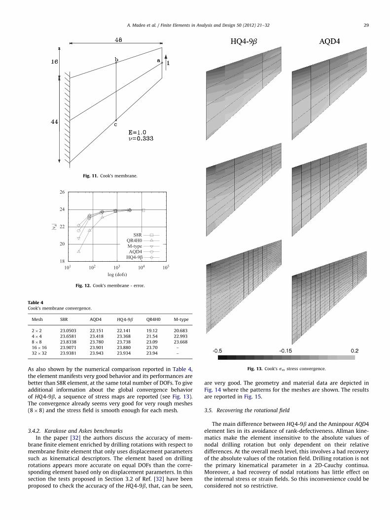
Fig. 13. Cook’s sxx stress convergence.

Fig. 11. Cook’s membrane.

18

20

22

24

26

101 102 103 104 105

|va|

log (dofs)

S8RQR4H0M-typeAQD4

HQ4-9β

Fig. 12. Cook’s membrane - error.

Table 4Cook’s membrane convergence.

Mesh S8R AQD4 HQ4-9b QR4H0 M-type

2�2 23.0503 22.151 22.141 19.12 20.683

4�4 23.6581 23.418 23.368 21.54 22.993

8�8 23.8338 23.780 23.738 23.09 23.668

16�16 23.9071 23.901 23.880 23.70 –

32�32 23.9381 23.943 23.934 23.94 –

A. Madeo et al. / Finite Elements in Analysis and Design 50 (2012) 21–32 29

As also shown by the numerical comparison reported in Table 4,the element manifests very good behavior and its performances arebetter than S8R element, at the same total number of DOFs. To giveadditional information about the global convergence behaviorof HQ4-9b, a sequence of stress maps are reported (see Fig. 13).The convergence already seems very good for very rough meshes(8�8) and the stress field is smooth enough for each mesh.

3.4.2. Karakose and Askes benchmarks

In the paper [32] the authors discuss the accuracy of mem-brane finite element enriched by drilling rotations with respect tomembrane finite element that only uses displacement parameterssuch as kinematical descriptors. The element based on drillingrotations appears more accurate on equal DOFs than the corre-sponding element based only on displacement parameters. In thissection the tests proposed in Section 3.2 of Ref. [32] have beenproposed to check the accuracy of the HQ4-9b, that, can be seen,

are very good. The geometry and material data are depicted inFig. 14 where the patterns for the meshes are shown. The resultsare reported in Fig. 15.

3.5. Recovering the rotational field

The main difference between HQ4-9b and the Aminpour AQD4element lies in its avoidance of rank-defectiveness. Allman kine-matics make the element insensitive to the absolute values ofnodal drilling rotation but only dependent on their relativedifferences. At the overall mesh level, this involves a bad recoveryof the absolute values of the rotation field. Drilling rotation is notthe primary kinematical parameter in a 2D-Cauchy continua.Moreover, a bad recovery of nodal rotations has little effect onthe internal stress or strain fields. So this inconvenience could beconsidered not so restrictive.

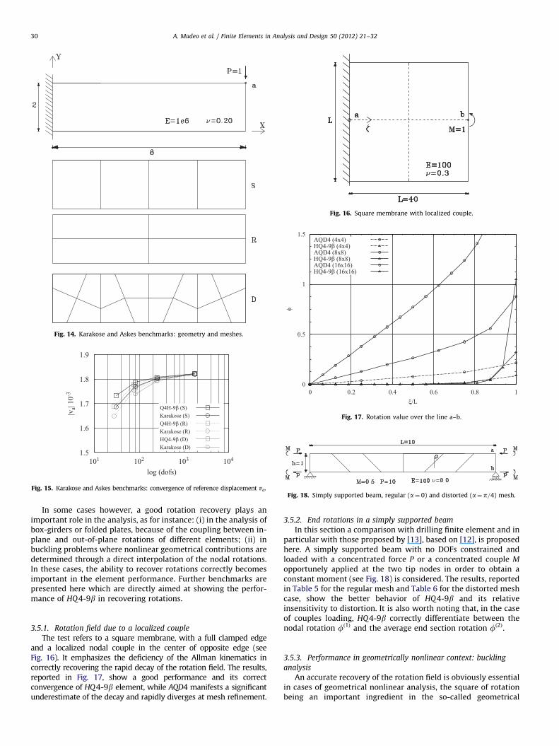
Fig. 14. Karakose and Askes benchmarks: geometry and meshes.

1.5

1.6

1.7

1.8

1.9

101 102 103 104

|va|

10-3

log (dofs)

Q4H-9β (S)Karakose (S)Q4H-9β (R)Karakose (R)HQ4-9β (D)Karakose (D)

Fig. 15. Karakose and Askes benchmarks: convergence of reference displacement va.

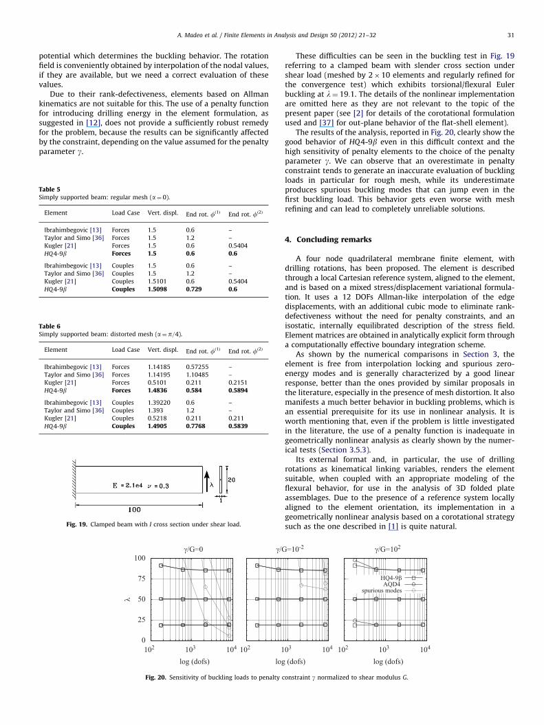
Fig. 16. Square membrane with localized couple.

0

0.5

1

1.5

0 0.2 0.4 0.6 0.8 1

φ

ξ/L

AQD4 (4x4)HQ4-9β (4x4)AQD4 (8x8)HQ4-9β (8x8)AQD4 (16x16)HQ4-9β (16x16)

Fig. 17. Rotation value over the line a–b.

Fig. 18. Simply supported beam, regular (a¼ 0) and distorted (a¼ p=4) mesh.

A. Madeo et al. / Finite Elements in Analysis and Design 50 (2012) 21–3230

In some cases however, a good rotation recovery plays animportant role in the analysis, as for instance: (i) in the analysis ofbox-girders or folded plates, because of the coupling between in-plane and out-of-plane rotations of different elements; (ii) inbuckling problems where nonlinear geometrical contributions aredetermined through a direct interpolation of the nodal rotations.In these cases, the ability to recover rotations correctly becomesimportant in the element performance. Further benchmarks arepresented here which are directly aimed at showing the perfor-mance of HQ4-9b in recovering rotations.

3.5.1. Rotation field due to a localized couple

The test refers to a square membrane, with a full clamped edgeand a localized nodal couple in the center of opposite edge (seeFig. 16). It emphasizes the deficiency of the Allman kinematics incorrectly recovering the rapid decay of the rotation field. The results,reported in Fig. 17, show a good performance and its correctconvergence of HQ4-9b element, while AQD4 manifests a significantunderestimate of the decay and rapidly diverges at mesh refinement.

3.5.2. End rotations in a simply supported beam

In this section a comparison with drilling finite element and inparticular with those proposed by [13], based on [12], is proposedhere. A simply supported beam with no DOFs constrained andloaded with a concentrated force P or a concentrated couple M

opportunely applied at the two tip nodes in order to obtain aconstant moment (see Fig. 18) is considered. The results, reportedin Table 5 for the regular mesh and Table 6 for the distorted meshcase, show the better behavior of HQ4-9b and its relativeinsensitivity to distortion. It is also worth noting that, in the caseof couples loading, HQ4-9b correctly differentiate between thenodal rotation fð1Þ and the average end section rotation fð2Þ.

3.5.3. Performance in geometrically nonlinear context: buckling

analysis

An accurate recovery of the rotation field is obviously essentialin cases of geometrical nonlinear analysis, the square of rotationbeing an important ingredient in the so-called geometrical

A. Madeo et al. / Finite Elements in Analysis and Design 50 (2012) 21–32 31

potential which determines the buckling behavior. The rotationfield is conveniently obtained by interpolation of the nodal values,if they are available, but we need a correct evaluation of thesevalues.

Due to their rank-defectiveness, elements based on Allmankinematics are not suitable for this. The use of a penalty functionfor introducing drilling energy in the element formulation, assuggested in [12], does not provide a sufficiently robust remedyfor the problem, because the results can be significantly affectedby the constraint, depending on the value assumed for the penaltyparameter g.

Table 6Simply supported beam: distorted mesh (a¼ p=4).

Element Load Case Vert. displ. End rot. fð1Þ End rot. fð2Þ

Ibrahimbegovic [13] Forces 1.14185 0.57255 –

Taylor and Simo [36] Forces 1.14195 1.10485 –

Kugler [21] Forces 0.5101 0.211 0.2151

HQ4-9b Forces 1.4836 0.584 0.5894

Ibrahimbegovic [13] Couples 1.39220 0.6 –

Taylor and Simo [36] Couples 1.393 1.2 –

Kugler [21] Couples 0.5218 0.211 0.211

HQ4-9b Couples 1.4905 0.7768 0.5839

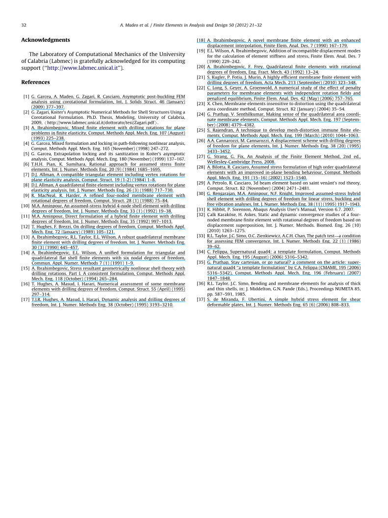
Fig. 19. Clamped beam with I cross section under shear load.

0

25

50

75

100

102 103 104

λ

log (dofs)

γ/G=0

102 1log

γ/G

Fig. 20. Sensitivity of buckling loads to penalty c

Table 5Simply supported beam: regular mesh (a¼ 0).

Element Load Case Vert. displ. End rot. fð1Þ End rot. fð2Þ

Ibrahimbegovic [13] Forces 1.5 0.6 –

Taylor and Simo [36] Forces 1.5 1.2 –

Kugler [21] Forces 1.5 0.6 0.5404

HQ4-9b Forces 1.5 0.6 0.6

Ibrahimbegovic [13] Couples 1.5 0.6 –

Taylor and Simo [36] Couples 1.5 1.2 –

Kugler [21] Couples 1.5101 0.6 0.5404

HQ4-9b Couples 1.5098 0.729 0.6

These difficulties can be seen in the buckling test in Fig. 19referring to a clamped beam with slender cross section undershear load (meshed by 2�10 elements and regularly refined forthe convergence test) which exhibits torsional/flexural Eulerbuckling at l¼ 19:1. The details of the nonlinear implementationare omitted here as they are not relevant to the topic of thepresent paper (see [2] for details of the corotational formulationused and [37] for out-plane behavior of the flat-shell element).

The results of the analysis, reported in Fig. 20, clearly show thegood behavior of HQ4-9b even in this difficult context and thehigh sensitivity of penalty elements to the choice of the penaltyparameter g. We can observe that an overestimate in penaltyconstraint tends to generate an inaccurate evaluation of bucklingloads in particular for rough mesh, while its underestimateproduces spurious buckling modes that can jump even in thefirst buckling load. This behavior gets even worse with meshrefining and can lead to completely unreliable solutions.

4. Concluding remarks

A four node quadrilateral membrane finite element, withdrilling rotations, has been proposed. The element is describedthrough a local Cartesian reference system, aligned to the element,and is based on a mixed stress/displacement variational formula-tion. It uses a 12 DOFs Allman-like interpolation of the edgedisplacements, with an additional cubic mode to eliminate rank-defectiveness without the need for penalty constraints, and anisostatic, internally equilibrated description of the stress field.Element matrices are obtained in analytically explicit form througha computationally effective boundary integration scheme.

As shown by the numerical comparisons in Section 3, theelement is free from interpolation locking and spurious zero-energy modes and is generally characterized by a good linearresponse, better than the ones provided by similar proposals inthe literature, especially in the presence of mesh distortion. It alsomanifests a much better behavior in buckling problems, which isan essential prerequisite for its use in nonlinear analysis. It isworth mentioning that, even if the problem is little investigatedin the literature, the use of a penalty function is inadequate ingeometrically nonlinear analysis as clearly shown by the numer-ical tests (Section 3.5.3).

Its external format and, in particular, the use of drillingrotations as kinematical linking variables, renders the elementsuitable, when coupled with an appropriate modeling of theflexural behavior, for use in the analysis of 3D folded plateassemblages. Due to the presence of a reference system locallyaligned to the element orientation, its implementation in ageometrically nonlinear analysis based on a corotational strategysuch as the one described in [1] is quite natural.

03 104

(dofs)

=10-2

102 103 104

log (dofs)

γ/G=102

HQ4-9βAQD4

spurious modes

onstraint g normalized to shear modulus G.

A. Madeo et al. / Finite Elements in Analysis and Design 50 (2012) 21–3232

Acknowledgments

The Laboratory of Computational Mechanics of the Universityof Calabria (Labmec) is gratefully acknowledged for its computingsupport (‘‘http://www.labmec.unical.it’’).

References

[1] G. Garcea, A. Madeo, G. Zagari, R. Casciaro, Asymptotic post-buckling FEManalysis using corotational formulation, Int. J. Solids Struct. 46 (January)(2009) 377–397.

[2] G. Zagari, Koiter’s Asymptotic Numerical Methods for Shell Structures Using aCorotational Formulation. Ph.D. Thesis, Modeling, University of Calabria,2009, /http://www.labmec.unical.it/dottorato/tesi/Zagari.pdfS.

[3] A. Ibrahimbegovic, Mixed finite element with drilling rotations for planeproblems in finite elasticity, Comput. Methods Appl. Mech. Eng. 107 (August)(1993) 225–238.

[4] G. Garcea, Mixed formulation and locking in path-following nonlinear analysis,Comput. Methods Appl. Mech. Eng. 165 (November) (1998) 247–272.

[5] G. Garcea, Extrapolation locking and its sanitization in Koiter’s asymptoticanalysis, Comput. Methods Appl. Mech. Eng. 180 (November) (1999) 137–167.

[6] T.H.H. Pian, K. Sumihara, Rational approach for assumed stress finiteelements, Int. J. Numer. Methods Eng. 20 (9) (1984) 1685–1695.

[7] D.J. Allman, A compatible triangular element including vertex rotations forplane elasticity analysis, Comput. Struct. 19 (1-2) (1984) 1–8.

[8] D.J. Allman, A quadrilateral finite element including vertex rotations for planeelasticity analysis, Int. J. Numer. Methods Eng. 26 (3) (1988) 717–730.

[9] R. MacNeal, R. Harder, A refined four-noded membrane element withrotational degrees of freedom, Comput. Struct. 28 (1) (1988) 75–84.

[10] M.A. Aminpour, An assumed-stress hybrid 4-node shell element with drillingdegrees of freedom, Int. J. Numer. Methods Eng. 33 (1) (1992) 19–38.

[11] M.A. Aminpour, Direct formulation of a hybrid finite element with drillingdegrees of freedom, Int. J. Numer. Methods Eng. 35 (1992) 997–1013.

[12] T. Hughes, F. Brezzi, On drilling degrees of freedom, Comput. Methods Appl.Mech. Eng. 72 (January) (1989) 105–121.

[13] A. Ibrahimbegovic, R.L. Taylor, E.L. Wilson, A robust quadrilateral membranefinite element with drilling degrees of freedom, Int. J. Numer. Methods Eng.30 (3) (1990) 445–457.

[14] A. Ibrahimbegovic, E.L. Wilson, A unified formulation for triangular andquadrilateral flat shell finite elements with six nodal degrees of freedom,Commun. Appl. Numer. Methods 7 (1) (1991) 1–9.

[15] A. Ibrahimbegovic, Stress resultant geometrically nonlinear shell theory withdrilling rotations. Part I. A consistent formulation, Comput. Methods Appl.Mech. Eng. 118 (October) (1994) 265–284.

[16] T. Hughes, A. Masud, I. Harari, Numerical assessment of some membraneelements with drilling degrees of freedom, Comput. Struct. 55 (April) (1995)297–314.

[17] T.J.R. Hughes, A. Masud, I. Harari, Dynamic analysis and drilling degrees offreedom, Int. J. Numer. Methods Eng. 38 (October) (1995) 3193–3210.

[18] A. Ibrahimbegovic, A novel membrane finite element with an enhanceddisplacement interpolation, Finite Elem. Anal. Des. 7 (1990) 167–179.

[19] E.L. Wilson, A. Ibrahimbegovic, Addition of incompatible displacement modesfor the calculation of element stiffness and stress, Finite Elem. Anal. Des. 7(1990) 229–242.

[20] A. Ibrahimbegovic, F. Frey, Quadrilateral finite elements with rotationaldegrees of freedom, Eng. Fract. Mech. 43 (1992) 13–24.

[21] S. Kugler, P. Fotiu, J. Murin, A highly efficient membrane finite element withdrilling degrees of freedom, Acta Mech. 213 (September) (2010) 323–348.

[22] C. Long, S. Geyer, A. Groenwold, A numerical study of the effect of penaltyparameters for membrane elements with independent rotation fields andpenalized equilibrium, Finite Elem. Anal. Des. 42 (May) (2006) 757–765.

[23] X. Chen, Membrane elements insensitive to distortion using the quadrilateralarea coordinate method, Comput. Struct. 82 (January) (2004) 35–54.

[24] G. Prathap, V. Senthilkumar, Making sense of the quadrilateral area coordi-nate membrane elements, Comput. Methods Appl. Mech. Eng. 197 (Septem-ber) (2008) 4379–4382.

[25] S. Rajendran, A technique to develop mesh-distortion immune finite ele-ments, Comput. Methods Appl. Mech. Eng. 199 (March) (2010) 1044–1063.

[26] A.A. Cannarozzi, M. Cannarozzi, A displacement scheme with drilling degreesof freedom for plane elements, Int. J. Numer. Methods Eng. 38 (20) (1995)3433–3452.

[27] G. Strang, G. Fix, An Analysis of the Finite Element Method, 2nd ed.,Wellesley-Cambridge Press, 2008.

[28] A. Bilotta, R. Casciaro, Assumed stress formulation of high order quadrilateralelements with an improved in-plane bending behaviour, Comput. MethodsAppl. Mech. Eng. 191 (15–16) (2002) 1523–1540.

[29] A. Petrolo, R. Casciaro, 3d beam element based on saint venant’s rod theory,Comput. Struct. 82 (November) (2004) 2471–2481.

[30] G. Rengarajan, M.A. Aminpour, N.F. Knight, Improved assumed-stress hybridshell element with drilling degrees of freedom for linear stress, buckling andfree vibration analyses, Int. J. Numer. Methods Eng. 38 (11) (1995) 1917–1943.

[31] K. Hibbit, P. Sorenson, Abaqus Analysis User’s Manual, Version 6.7. 2007.[32] C- alk Karakose, H. Askes, Static and dynamic convergence studies of a four-

noded membrane finite element with rotational degrees of freedom based ondisplacement superposition, Int. J. Numer. Methods. Biomed. Eng. 26 (10)(2010) 1263–1275.

[33] R.L. Taylor, J.C. Simo, O.C. Zienkiewicz, A.C.H. Chan, The patch test—a conditionfor assessing FEM convergence, Int. J. Numer. Methods Eng. 22 (1) (1986)39–62.

[34] C. Felippa, Supernatural quad4: a template formulation, Comput. MethodsAppl. Mech. Eng. 195 (August) (2006) 5316–5342.

[35] G. Prathap, Stay cartesian, or go natural? a comment on the article: super-natural quad4 ‘‘a template formulation’’ by C.A. Felippa (CMAME, 195 (2006)5316–5342), Comput. Methods Appl. Mech. Eng. 196 (February) (2007)1847–1848.

[36] R.L. Taylor, J.C. Simo, Bending and membrane elements for analysis of thickand thin shells, in: J. Middelton, G.N. Pande (Eds.), Proceedings NUMETA 85,pp. 587–591, 1985.

[37] S. de Miranda, F. Ubertini, A simple hybrid stress element for sheardeformable plates, Int. J. Numer. Methods Eng. 65 (6) (2006) 808–833.