an integrated growing-pruning method for feedforward network training

This article appeared in a journal published by Elsevier. The attachedcopy is furnished to the author for internal non-commercial researchand education use, including for instruction at the authors institution

and sharing with colleagues.

Other uses, including reproduction and distribution, or selling orlicensing copies, or posting to personal, institutional or third party

websites are prohibited.

In most cases authors are permitted to post their version of thearticle (e.g. in Word or Tex form) to their personal website orinstitutional repository. Authors requiring further information

regarding Elsevier’s archiving and manuscript policies areencouraged to visit:

http://www.elsevier.com/copyright

http://www.elsevier.com/copyright

Author's personal copy

Neurocomputing 71 (2008) 2831–2847

An integrated growing-pruning method forfeedforward network training

Pramod L. Narasimhaa,�, Walter H. Delashmitb, Michael T. Manrya,Jiang Lic, Francisco Maldonadod

aDepartment of Electrical Engineering, University of Texas at Arlington, Arlington, TX 76013, USAbLockheed Martin, Missiles and Fire Control Dallas, Grand Prairie, TX 75051, USA

cElectrical and Computer Engineering, Old Dominion University, Norfolk, VA 23529, USAdWilliams Pyro, Inc., 200 Greenleaf Street, Fort Worth, TX 76107, USA

Received 12 March 2007; received in revised form 8 August 2007; accepted 20 August 2007

Communicated by Dr. J. Zhang

Available online 12 October 2007

Abstract

In order to facilitate complexity optimization in feedforward networks, several algorithms are developed that combine growing and

pruning. First, a growing scheme is presented which iteratively adds new hidden units to full-trained networks. Then, a non-heuristic one-

pass pruning technique is presented, which utilizes orthogonal least squares. Based upon pruning, a one-pass approach is developed for

generating the validation error versus network size curve. A combined approach is described in which networks are continually pruned

during the growing process. As a result, the hidden units are ordered according to their usefulness, and the least useful units are

eliminated. Examples show that networks designed using the combined method have less training and validation error than growing or

pruning alone. The combined method exhibits reduced sensitivity to the initial weights and generates an almost monotonic error versus

network size curve. It is shown to perform better than two well-known growing methods—constructive backpropagation and cascade

correlation.

r 2007 Elsevier B.V. All rights reserved.

Keywords: Growing; Pruning; Cascade correlation; Back propagation; Output weight optimization–Hidden weight optimization

1. Introduction

When optimizing the structural complexity of feedfor-ward neural networks, different size networks are designedwhich minimize the mean-square training error. Typically,the machine with the smallest validation error is saved.When different size networks are independently initializedand trained, however, the training error versus networksize curve is not monotonic. Similarly, the resultingvalidation error versus size curve is not smooth, makingit difficult to find a proper minimum. Monotonic trainingcurves and smooth validation curves can be produced bygrowing methods or by pruning methods.

In growing methods [11], new hidden units arecontinually added to a trained network, and furthertraining is performed [7]. In [31], the addition of newunits continues as long as the sum of the accuracies fortraining and crossvalidation samples improves. Thiseliminates the requirement of specifying minimumaccuracy for the growing network. Guan and Li [15] haveused output parallelism to decompose the originalproblem into several subproblems, each of which iscomposed of the whole input vector and a fraction of thedesired output vector. They use constructive backpropaga-tion (CBP) to train modules of the appropriate size.Modules are merged to get a final network. A drawback ofgrowing methods is that some of the intermediate networkscan get trapped in local minima. Also, growing methodsare sensitive to initial conditions. Unfortunately, when asequence of networks is grown, there is no guarantee that

ARTICLE IN PRESS

www.elsevier.com/locate/neucom

0925-2312/$ - see front matter r 2007 Elsevier B.V. All rights reserved.

doi:10.1016/j.neucom.2007.08.026

�Corresponding author.

E-mail addresses: [email protected],

[email protected] (P.L. Narasimha).


all of the added hidden units are properly trained. Somecan be linearly dependent.

In pruning methods, a large network is trained and thenthe least useful nodes or weights are removed [1,16,24,25,27]. Orthogonal least squares or Gram–Schmidt [32]based pruning has been described by Chen et al. [6] andKaminsky and Strumillo [18] for radial basis functions(RBF) and by Maldonado et al. [21] for the multilayerperceptron (MLP). In crosswise propagation [20], linearlydependent hidden units are detected using an orthogonalprojection method, and then removed. The contribution ofthe removed neuron is approximated by the remaininghidden units. In [4], the hidden units are iterativelyremoved and the remaining weights are adjusted tomaintain the original input–output behavior. A weightadjustment is carried out by solving the system of linearequations using the conjugate gradient algorithm in theleast squares sense. Unfortunately, if one large network istrained and pruned, the resulting error versus number ofhidden units ðNhÞ curve is not minimal for smallernetworks. In other words, it is possible, though unlikely,for each hidden unit to be equally useful after training.

A promising alternative to growing or pruning alone isto combine them. Huang et al. [17] have developed anonline training algorithm for RBF-based minimal resourceallocation networks (MRAN), which uses both growingand pruning. However, as MRAN is an online procedure,it does not optimize the network over all past training data.Also, network initialization requires prior knowledge onthe data which may not be available.

In this paper, we describe batch mode methods for trainingand validating sequences of different size neural nets. Eachmethod’s training error versus the network size curve ismonotonic or approximately monotonic. In Section 2, we givebasic notation and briefly describe the output weightoptimization-hidden Weight optimization (OWO-HWO)training algorithm. Section 3 gives brief analyses of weightinitialization methods. In Section 4 a growing method isdescribed. Then a pruning method is presented which requiresonly one pass through the training data. A one-pass validationmethod is presented, which is based upon pruning. Next, twomethods that combine growing and pruning are presented. Itis shown that the combination approaches overcome theshortcomings of growing or pruning alone. Our proposedmethod is benchmarked against well-known growing algo-rithms in Section 5. The conclusions are given in Section 6.

2. Multilayer perceptron

In this section we define some notation and review aneffective, convergent MLP training algorithm.

2.1. Notation

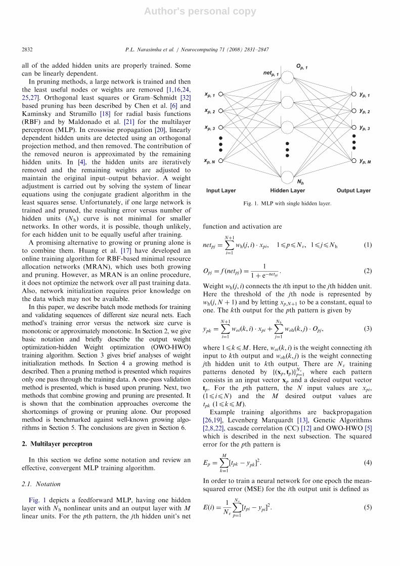
Fig. 1 depicts a feedforward MLP, having one hiddenlayer with Nh nonlinear units and an output layer with M

linear units. For the pth pattern, the jth hidden unit’s net

function and activation are

netpj ¼XNþ1i¼1

whðj; iÞ � xpi; 1pppNv; 1pjpNh (1)

Opj ¼ f ðnetpjÞ ¼1

1þ e�netpj. (2)

Weight whðj; iÞ connects the ith input to the jth hidden unit.Here the threshold of the jth node is represented bywhðj;N þ 1Þ and by letting xp;Nþ1 to be a constant, equal toone. The kth output for the pth pattern is given by

ypk ¼XNþ1i¼1

woiðk; iÞ � xpi þXNh

j¼1

wohðk; jÞ �Opj , (3)

where 1pkpM. Here, woiðk; iÞ is the weight connecting ithinput to kth output and wohðk; jÞ is the weight connectingjth hidden unit to kth output. There are Nv trainingpatterns denoted by fðxp; tpÞg

Nv

p¼1 where each patternconsists in an input vector xp and a desired output vectortp. For the pth pattern, the N input values are xpi,(1pipN) and the M desired output values aretpk ð1pkpMÞ.Example training algorithms are backpropagation

[26,19], Levenberg Marquardt [13], Genetic Algorithms[2,8,22], cascade correlation (CC) [12] and OWO-HWO [5]which is described in the next subsection. The squarederror for the pth pattern is

Ep ¼XMk¼1

½tpk � ypk�2. (4)

In order to train a neural network for one epoch the mean-squared error (MSE) for the ith output unit is defined as

EðiÞ ¼1

Nv

XNv

p¼1

½tpi � ypi�2. (5)

ARTICLE IN PRESS

xp, 1

xp, 2

xp, 3

xp, N

Input Layer

yp, 1

yp, 2

yp, 3

yp, M

Output LayerHidden Layer

netp, 1

Op, 1

Nh

Fig. 1. MLP with single hidden layer.

P.L. Narasimha et al. / Neurocomputing 71 (2008) 2831–28472832


The overall performance of an MLP network, measured asMSE, can be written as

E ¼XMi¼1

EðiÞ ¼1

Nv

XNv

p¼1

Ep. (6)

2.2. OWO-HWO algorithm

In OWO-HWO training [5,34], we alternately updatehidden weights [30] and solve linear equations for outputweights [29]. It is well known that optimizing in thegradient direction, as in steepest descent, is very slow. So,an alternative approach for improving hidden weights(HWO) has been developed.

Let the desired net function netpjd for the pth trainingpattern and jth hidden unit be

netpjd ¼ netpj þ Z � Dnet�pj , (7)

where Dnet�pj written as

Dnet�pj ¼ net�pj � netpj (8)

is the difference between current net function netpj and theoptimal value net�pj . Now the net function approaches theoptimal value net�pj , instead of moving in the negativegradient direction. The current task for constructing theHWO algorithm is to find Dnet�pj .

Using Taylor series expansion in Eq. (2) about netpj ,we get

O�pj ¼ f ðnet�pjÞ ¼ Opj þ f 0pj � Z � Dnet�pj , (9)

where f 0pj is the derivative of the activation function f ðnetpjÞ

with respect to netpj . Now Dnet�pj can be derived based on

qE

qnetpj

��netpj¼net�

pj

¼ 0. (10)

The desired change in net function can be derived as

Dnet�pj ¼dpj

ðf 0pjÞ2PM

i¼1w2ohði; jÞ

. (11)

It can be shown [34] that minimizing E is equivalent tominimizing the weighted hidden error function

EdðkÞ ¼1

Nv

XNv

p¼1

ðf 0pkÞ2 Dnet�pk �

XNþ1n¼1

eðk; nÞxpn

" #2, (12)

where eðk; nÞ is the change in hidden weight. The auto andcrosscorrelation matrices are found as

Rðn;mÞ ¼1

Nv

XNv

p¼1

ðxpn � xpmÞ � ðf0pkÞ

2 (13)

and

Cdðk;mÞ ¼1

Nv

XNv

p¼1

ðDnet�pk � xpmÞ � ðf0pkÞ

2. (14)

We have ðN þ 1Þ equations in ðN þ 1Þ unknowns for thekth hidden unit. After finding the learning factor Z, thehidden weights are updated as

whiðk; nÞ whiðk; nÞ þ Z � eðk; nÞ. (15)

As discussed by Yu et al. [34], this HWO algorithmconverges as the change in the error function E is non-increasing and the algorithm uses backtracking in order tosave the best network without diverging from the solution.It is also shown that the convergence speed of the newalgorithm is higher than those of other competingtechniques.After improving hidden weights using HWO, we

optimize output weights using OWO [23] by solving thefollowing linear equations

W0 � R ¼ C, (16)

where R 2 RðNþNhþ1Þ�ðNþNhþ1Þ and C 2 RM�ðNþNhþ1Þ areauto and crosscorrelation matrices, respectively, as de-scribed in the Appendix. W0 2 RM�ðNþNhþ1Þ is the matrixof weights connecting the inputs and hidden units to theoutput units.

3. Structured initialization

MLP training is inherently very dependent on the initialweights, so proper initialization is critical. In this section,several basic approaches for feedforward network initiali-zation are discussed. To define the problem beingconsidered, assume that a set of MLPs of different sizes(i.e., different numbers of hidden units, Nh) are to bedesigned for a given training data set.Let Ef ðNhÞ denote the final training MSE, E, of an MLP

with Nh hidden units.

Axiom 1. If Ef ðNhÞXEf ðNh � 1Þ, then the network havingNh hidden units is useless since the training resulted in alarger, more complex network with a larger or the sametraining error.

Three distinct types of network initialization areconsidered. We give theorems related to these threemethods, which give a basis for this paper. Delashmit[11] has, in his work, identified problems in MLP trainingand has stated them in the form of these theorems. Detaileddiscussions can be found in his work.

3.1. Randomly initialized networks

When a set of MLPs are randomly initialized (RI), nomembers of the set are constrained to have any initialweights or thresholds in common. Practically, this meansthat the initial random number seeds (IRNS) of thenetworks are different. These networks are useful whenthe goal is to quickly design one or more networks of thesame or different sizes whose weights are statisticallyindependent of each other.

ARTICLE IN PRESSP.L. Narasimha et al. / Neurocomputing 71 (2008) 2831–2847 2833


Theorem 1. If two initial RI networks (1) are the same size,(2) have the same training data set and (3) the training data

set has more than one unique input vector, then the hidden

unit basis functions are different for the two networks.

This means that the commonly used RI networks vary inperformance, even when they are the same size. A problemwith RI networks is that Ef ðNhÞ is non-monotonic. That is,for well-trained MLPs, Ef ðNhÞ does not always decrease asNh increases since the initial hidden unit basis functions aredifferent. Let EiðNhÞ denote the final training error for anRI network having Nh hidden units, which has beeninitialized using the ith random number seed out of a totalof Ns seeds. Let EavðNhÞ denote the average EiðNhÞ, that is

EavðNhÞ ¼1

Ns

XNs

i¼1

EiðNhÞ. (17)

Using the Chebyshev inequality, a bound has beendeveloped on the probability that the average error forNh hidden units, EavðNhÞ is increasing [11] and that thenetwork with Nh þ 1 hidden units is useless.

PðEavðNh þ 1Þ4EavðNhÞÞ

pvarðEiðNh þ 1ÞÞ þ varðEiðNhÞÞ

2 �Ns � ðmavðNhÞ �mavðNh þ 1ÞÞ2, ð18Þ

where varðÞ represents the variance and mavðNhÞ representthe average MSE for the network with Nh hidden units.This result quantifies the probability that RI networks havenon-monotonic error versus Nh curves, for given valuesof Nh.

3.2. Common starting point initialized networks

One way to increase the likelihood of monotonic EðNhÞ

curve is to force the corresponding initial basis functions tobe nested. When a set of MLPs are common starting pointinitialized with structured weight initialization (CSPI-SWI), each one starts with the same IRNS. Also, theinitialization of the weights and thresholds is ordered suchthat every hidden unit of the smaller network has the sameweights as the corresponding hidden unit of the largernetwork. Input to output weights, if present, are alsoidentical. These networks are useful when it is desired tomake performance comparisons of networks that have thesame IRNS for the starting point.

Theorem 2. If two initial CSPI-SWI networks (1) are the

same size and (2) use the same algorithm for processing

random numbers into weights, then they are identical.

As the size of the MLP is increased by adding newhidden units, a consistent technique for initializing thesenew units as well as the previous hidden units is needed forCSPI-SWI networks.

Theorem 3. If two CSPI-SWI networks are designed, the

common subset of the initial hidden unit basis functions are

identical.

The above theorems have been proved by Delashmit[11]. Unfortunately, growing with CSPI-SWI networksalthough better than RI, does not guarantee a monotonicEf ðNhÞ curve. This is true because after training, theresulting networks are not guaranteed to have any hiddenbasis functions in common.

3.3. Dependently initialized networks

Here a series of different size networks are designed witheach subsequent network having one or more hidden unitsthan the previous network. Larger networks are initializedusing the final weights and thresholds that resulted fromtraining a smaller network. Such dependently initialized(DI) networks take advantage of previous training onsmaller networks in a systematic manner.

Properties of DI networks. Let E intðNhÞ denote the initialvalue of error during the training of an MLP with Nh

hidden units and let Nhp denote the number of hidden unitsin the previous network. That is, N� ¼ Nh �Nhp newhidden units are added to a well-trained smaller network,to initialize the larger one. Then:

(i) EintðNhÞoEintðNhpÞ

(ii) Ef ðNhÞpEf ðNhpÞ

(iii) EintðNhÞ ¼ Ef ðNhpÞ.

As seen in property (ii), DI networks have a mono-tonically non-increasing Ef ðNhÞ versus Nh curve. Thisoccurs because all basis functions in a small network arealso present in larger networks. Unfortunately, there is noguarantee that a Ef ðNhÞ sample represents a globalminimum.

3.4. Pruned networks

One of the most popular regularization procedures inneural nets is done by limiting the number of hidden units[3]. Pruning generates series of different size networksstarting from a large network and each subsequent networkhaving one less hidden unit than the previous network. Inother words, the hidden units will be ordered according totheir importance and the pruning will sequentially deletethem one at a time starting with the least important hiddenunit. Hidden units of bigger networks will always besupersets of those of smaller networks.

Axiom 2. Assume that a large network with Nh hiddenunits is pruned, using the approach of [6,8,21]. Then thefinal MSE values satisfy Ef ðkÞpEf ðk � 1Þ for 1pkpNh.

This axiom indicates that pruning produces monotoni-cally non-increasing Ef ðNhÞ versus Nh curves as doDI-based growing approaches.

ARTICLE IN PRESSP.L. Narasimha et al. / Neurocomputing 71 (2008) 2831–28472834


4. Methods of generating networks of different sizes

According to the structural risk minimization (SRM)principle, the best network in an ensemble of MLPsis the one that has minimum guaranteed risk. However,the guaranteed risk is an upper bound for the general-ization error EvalðNhÞ. Hence the best network is the onefor which EvalðNhÞ is the smallest. In this section we presentfour general approaches or design methodologies forgenerating sequences of networks having monotonicEf ðNhÞ curves.

4.1. Growing method or Design Methodology 1

In growing methods, we start by training a smallnetwork (with small Nh) and then successively train largernetworks by adding more hidden units, producing a finaltraining MSE versus Nh curve, Ef ðNhÞ. After training asequence of these different size DI networks, we calculatevalidation MSE versus Nh curve EvalðNhÞ. The validationerror will be the key to decide the network size needed.Growing methods, which are motivated by the propertiesof DI networks, are collectively denoted as DesignMethodology 1 (DM-1).

Given training data fxp; tpgNv

p¼1, our growing algorithm,which is called DM-1 is described as follows. First, we traina linear network (no hidden units, Nh ¼ 0) using the OWOalgorithm and the network obtained is represented byW0

DM1. Then we successively add a few hidden units (N� ¼ 5in our case) and re-train the network. During re-training, forthe first few iterations (say 20% of the total iterations), wetrain only the newly added hidden units using OWO-HWO[5] as described in Section 2.2. Then during the remainingiterations, we train all the weights and thresholds. Thenetwork obtained at the end of training is represented byWNh

DM1. Also at each step of growing, we validate thenetwork obtained at that point with validation data setfxvalp ; tvalp g

Nvalv

p¼1 to help decide upon the final network size. LetEvalðW

Nh

DM1Þ be the validation error for a DM-1 networkwith Nh hidden units. The best network among the sequenceof different size networks can be chosen as

WN

opt

h

DM1 ¼ argmin EvalðWkDM1Þ, (19)

where WN

opt

h

DM1 represents the DM-1 network with optimalnumber of hidden units N

opth and NhFinal represents the

maximum number of hidden units at the end of growing. Thisnumber should be conveniently large so that the best networkfalls within the sequence of grown DM-1 networks. Thevalidation error is the MSE on the validation set, given by

Eval ¼1

Nvalv

XNvalv

p¼1

XMk¼1

ðtvalpk � yvalpk Þ

2. (20)

In order to validate the performance of the method, werepeat the growing procedure several times with different

random numbers initializing the network. Then the averageMSEs are calculated, which gives the expected values of theMSEs for each size network. Also, to obtain a measure forthe confidence interval of the method, we calculate thestandard deviations of the MSEs. The average MSEs aregiven by

MðEvalÞ ¼1

Nr

XNr

i¼1

Eival, (21)

where Eival are the validation MSEs for the ith random

initial network and Nr is the number of randominitial networks. The standard deviations of the MSEsare given by

SDðEvalÞ ¼1

Nr

XNr

i¼1

ðEival �MðEvalÞÞ

2

" #1=2. (22)

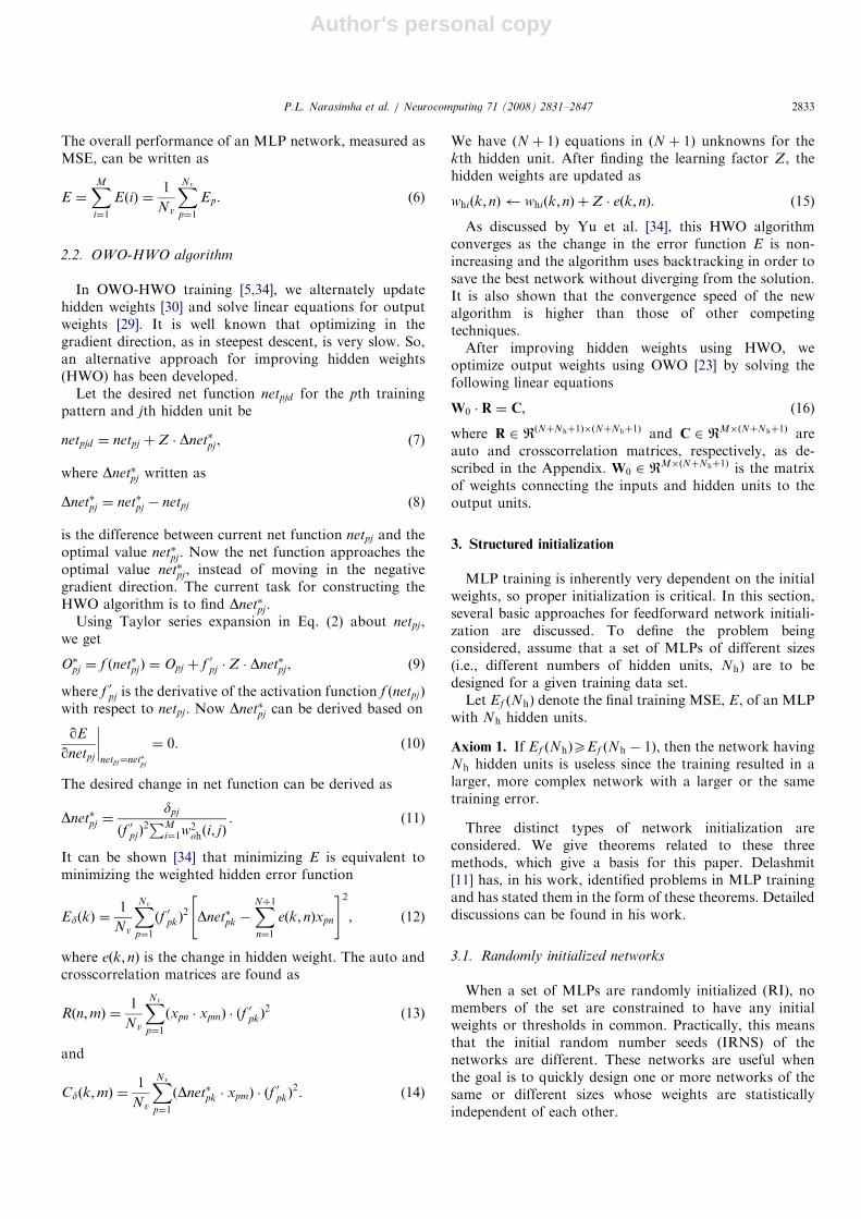
Fig. 2 shows the sample plot of the training andvalidation MSEs as a function of number of hidden units(Nh) for Nr ¼ 10. Note that in this method, there will notbe any intermediate size networks as the step size used togrow the network is equal to five (N� ¼ 5). A more detailedanalysis on the plots of means and standard deviations ofthe design methodologies will be made at the end of thissection and hence at this point we have not shown theseplots.

4.2. Ordered pruning or Design Methodology 2

In Design Methodology 2 (DM-2), we prune a largenetwork in order to produce a monotonic Ef ðNhÞ curve.The pruning procedure is explained in appendix. Duringpruning, the orthonormalization matrix A ¼ famkg for1pmpNu and 1pkpm is saved, where Nu ¼ N þNh þ

1 is the total number of basis functions.

4.2.1. One pass validation

Given the matrix A and the MLP network with orderedhidden units, we wish to generate the validation errorversus Nh curve EvalðNhÞ from the validation data setfxvalp ; tvalp g

Nvalv

p¼1. For each pattern, we augment the inputvector as in the previous sections. So the augmented inputvector is xvalp ½x

valT

p ; 1;OvalT

p �T. Then the augmented

vector is converted into orthonormal basis functions bythe transformation

xval0

p ðmÞ ¼Xm

k¼1

amk � xvalp ðkÞ for 1pmpNu. (23)

In order to get the validation error for all size networks in asingle pass through the data, we use the following strategy:Let yval

pi ðmÞ represent the ith output of the networkhaving m hidden units for the pth pattern, let EvalðmÞ

represent the mean square error of the network forvalidation with m hidden units. First, the linear networkoutput is obtained and the corresponding error is



calculated as follows:

yvalpi ð0Þ ¼

XNþ1k¼1

w00ði; kÞ � xval0

p ðkÞ for 1pipM,

Evalð0Þ Evalð0Þ þXMi¼1

½tvalpi � yvalpi ð0Þ�

2. ð24Þ

Then for 1pmpNh, the following two steps are per-formed:

Step 1: For 1pipM

yvalpi ðmÞ ¼ yval

pi ðm� 1Þ þ w0ohði;mÞ �Oval0

p ðmÞ. (25)

Step 2:

EvalðmÞ EvalðmÞ þXMi¼1

½tvalpi � yvalpi ðmÞ�

2, (26)

where w0ohði;mÞ is the orthonormal weight connecting mthhidden unit to ith output. Apply Eqs. (23)–(26) for1pppNv and get the total validation error over all thepatterns for each size network. Then these error valuesshould be normalized as

EvalðmÞ EvalðmÞ

Nvalv

for 0pmpNh. (27)

Thus we generate the validation error versus the networksize curve in one pass through the validation data set.

4.3. Pruning a grown network or Design Methodology 3

The DI network growing approach (DM-1) generatesmonotonic Ef ðNhÞ curves. However, hidden units addedearlier in the process tend to reduce the MSE more thanthose added later. Unfortunately, there is no guarantee thatan Ef ðNhÞ sample represents a global minimum. There isalso no guarantee that the hidden units are orderedproperly, since useless hidden units can occur at any pointin the growing process. In Design Methodology 3 (DM-3a), we attempt to solve these problems by (1) performing

growing as in DI network (DM-1) and (2) performingordered pruning of the final network (DM-2). This forcesthe grown hidden units to be stepwise optimally ordered.This method works better than pruning a large trainednetwork because the growing by DI network approachwould produce sets of hidden units that are optimallyplaced with respect to the previously trained hidden units.Pruning the grown network (DM-3a) always produces amonotonic Ef ðNhÞ curve. Let us denote the DM-3anetwork for Nh hidden units by WNh

DM3a.An alternative solution (DM-3b) would be to save the

intermediate grown networks and to select the bestperforming network obtained either by DM-1 or DM-3astep. In other words,

WkDM3b ¼ argmin

dm2fDM1;DM3ag

EvalfWkdmg (28)

for 1pkpNhFinal, and the optimal network is obtained bypicking the network with minimum validation MSE.

WN

opt

h

DM3b ¼ argmin EvalfWkDM3bg. (29)

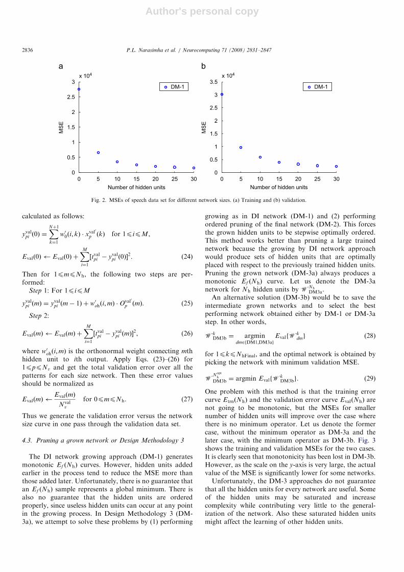
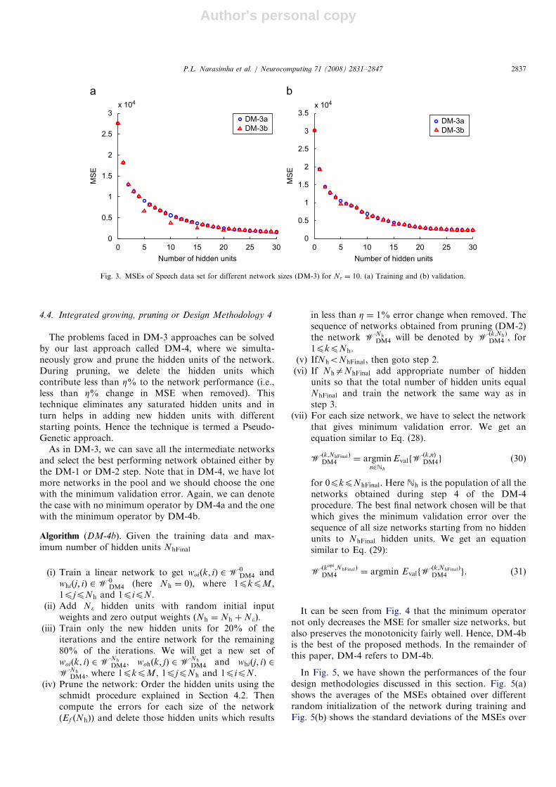
One problem with this method is that the training errorcurve EtrnðNhÞ and the validation error curve EvalðNhÞ arenot going to be monotonic, but the MSEs for smallernumber of hidden units will improve over the case wherethere is no minimum operator. Let us denote the formercase, without the minimum operator as DM-3a and thelater case, with the minimum operator as DM-3b. Fig. 3shows the training and validation MSEs for the two cases.It is clearly seen that monotonicity has been lost in DM-3b.However, as the scale on the y-axis is very large, the actualvalue of the MSE is significantly lower for some networks.Unfortunately, the DM-3 approaches do not guarantee

that all the hidden units for every network are useful. Someof the hidden units may be saturated and increasecomplexity while contributing very little to the general-ization of the network. Also these saturated hidden unitsmight affect the learning of other hidden units.

ARTICLE IN PRESS

0 5 10 15 20 25 300

0.5

1

1.5

2

2.5

3x 104

Number of hidden units

MS

E

DM-1 DM-1

0 5 10 15 20 25 300

0.5

1

1.5

2

2.5

3

3.5x 104


MS

EFig. 2. MSEs of speech data set for different network sizes. (a) Training and (b) validation.



4.4. Integrated growing, pruning or Design Methodology 4

The problems faced in DM-3 approaches can be solvedby our last approach called DM-4, where we simulta-neously grow and prune the hidden units of the network.During pruning, we delete the hidden units whichcontribute less than Z% to the network performance (i.e.,less than Z% change in MSE when removed). Thistechnique eliminates any saturated hidden units and inturn helps in adding new hidden units with differentstarting points. Hence the technique is termed a Pseudo-Genetic approach.

As in DM-3, we can save all the intermediate networksand select the best performing network obtained either bythe DM-1 or DM-2 step. Note that in DM-4, we have lotmore networks in the pool and we should choose the onewith the minimum validation error. Again, we can denotethe case with no minimum operator by DM-4a and the onewith the minimum operator by DM-4b.

Algorithm (DM-4b). Given the training data and max-imum number of hidden units NhFinal

(i) Train a linear network to get woiðk; iÞ 2W0DM4 and

whiðj; iÞ 2W0DM4 (here Nh ¼ 0), where 1pkpM,

1pjpNh and 1pipN.(ii) Add N� hidden units with random initial input

weights and zero output weights (Nh ¼ Nh þN�).(iii) Train only the new hidden units for 20% of the

iterations and the entire network for the remaining80% of the iterations. We will get a new set ofwoiðk; iÞ 2WNh

DM4, wohðk; jÞ 2WNh

DM4 and whiðj; iÞ 2WNh

DM4, where 1pkpM, 1pjpNh and 1pipN.(iv) Prune the network: Order the hidden units using the

schmidt procedure explained in Section 4.2. Thencompute the errors for each size of the network(Ef ðNhÞ) and delete those hidden units which results

in less than Z ¼ 1% error change when removed. Thesequence of networks obtained from pruning (DM-2)the network WNh

DM4 will be denoted by Wðk;NhÞ

DM4 , for1pkpNh.

(v) IfNhoNhFinal, then goto step 2.(vi) If NhaNhFinal add appropriate number of hidden

units so that the total number of hidden units equalNhFinal and train the network the same way as instep 3.

(vii) For each size network, we have to select the networkthat gives minimum validation error. We get anequation similar to Eq. (28).

Wðk;NhFinalÞ

DM4 ¼ argminn2Nh

EvalfWðk;nÞDM4g (30)

for 0pkpNhFinal. Here Nh is the population of all thenetworks obtained during step 4 of the DM-4procedure. The best final network chosen will be thatwhich gives the minimum validation error over thesequence of all size networks starting from no hiddenunits to NhFinal hidden units. We get an equationsimilar to Eq. (29):

Wðkopt;NhFinalÞ

DM4 ¼ argmin EvalfWðk;NhFinalÞ

DM4 g. (31)

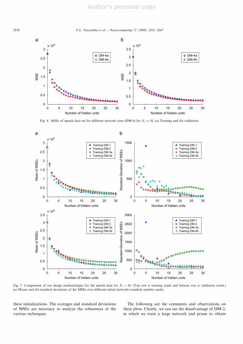
It can be seen from Fig. 4 that the minimum operatornot only decreases the MSE for smaller size networks, butalso preserves the monotonicity fairly well. Hence, DM-4bis the best of the proposed methods. In the remainder ofthis paper, DM-4 refers to DM-4b.

In Fig. 5, we have shown the performances of the fourdesign methodologies discussed in this section. Fig. 5(a)shows the averages of the MSEs obtained over differentrandom initialization of the network during training andFig. 5(b) shows the standard deviations of the MSEs over

ARTICLE IN PRESS

0 5 10 15 20 25 300

0.5

1

1.5

2

2.5

3x 104


MS

E

DM-3a

DM-3bDM-3a

DM-3b

0 5 10 15 20 25 300

0.5

1

1.5

2

2.5

3

3.5x 104


MS

E

Fig. 3. MSEs of Speech data set for different network sizes (DM-3) for Nr ¼ 10. (a) Training and (b) validation.

P.L. Narasimha et al. / Neurocomputing 71 (2008) 2831–2847 2837


these initializations. The averages and standard deviationsof MSEs are necessary to analyze the robustness of thevarious techniques.

The following are the comments and observations onthese plots. Clearly, we can see the disadvantage of DM-2,in which we train a large network and prune to obtain

ARTICLE IN PRESS

0 5 10 15 20 25 300

0.5

1

1.5

2

2.5

3x 104


MS

E

DM-4a

DM-4b

DM-4a

DM-4b

0 5 10 15 20 25 300

0.5

1

1.5

2

2.5

3

3.5x 104


MS

EFig. 4. MSEs of speech data set for different network sizes (DM-4) for Nr ¼ 10. (a) Training and (b) validation.

0 5 10 15 20 25 30

0

0.5

1

1.5

2

2.5

3x 104


Mean o

f M

SE

s

Training DM-1

Training DM-2

Training DM-3a

Training DM-4b

Training DM-1

Training DM-2

Training DM-3a

Training DM-4b

Training DM-1

Training DM-2

Training DM-3a

Training DM-4b

Training DM-1

Training DM-2

Training DM-3a

Training DM-4b

0 5 10 15 20 25 30

0

500

1000

1500


Sta

ndard

Devia

tion o

f M

SE

s

0 5 10 15 20 25 30

0

0.5

1

1.5

2

2.5

3

3.5x 104


Mean o

f M

SE

s

0 5 10 15 20 25 30

0

500

1000

1500

2000

2500

3000


Sta

ndard

Devia

tion o

f M

SE

s

a

Fig. 5. Comparison of our design methodologies for the speech data for Nr ¼ 10. (Top row is training result and bottom row is validation result.)

(a) Means and (b) standard deviations of the MSEs over different initial networks (random number seeds).



different size networks. Both the training and validationerrors are high in this case. Also, the standard deviationincreases for larger networks (i.e., as number of hiddenunits Nh increases) in DM-2, which indicates that the largernetworks in this technique are more sensitive to initialweights. This also demonstrates that the growing methodperforms better than training a RI large network. In DM-1,the average MSE for smaller networks is less than that ofthe other methods, but the standard deviation is very highwhen compared to other methods. This shows that thesmaller networks in DM-1 are very sensitive to initialweights. As our goal is to find a network generationtechnique that is less sensitive to initial conditions and havemonotonic error versus number of hidden units curve, weneed to find a technique that has advantages of both DM-1and DM-2. So, in DM-3, we first grow the MLP and laterprune the final large grown network. From the plots, it canbe seen that both average MSE and standard deviation ofthe MSE for DM-3 are less than for the other methods.Further, if there are saturated hidden units or the hiddenunits that are linearly dependent, those units can beremoved. This is achieved using the DM-4 approach, wherethe hidden units are pruned in every step of growing.Consistent to our analysis, the DM-4 method does give thebest result.

Note that in DM-4, R and C do not need to be calculatedfor pruning in Eqs. (A.5) and A.11since they are alreadyfound during training in the OWO step. This saves an extrapass through the data at each growing step. The number ofmultiples eliminated for calculating the hidden unitactivations, auto and crosscorrelation matrices is

Nm ¼ Nv � ðM þNÞ �Nh þNh � ðNh þ 1Þ

2

� �. (32)

This savings in multiples is significant, though small.

5. Numerical results

In the previous section, we show that DM-4 hasadvantages over other training algorithms we have devel-oped. In this section, we briefly discuss two existing well-known DI approaches for growing a sequence of networksand compare them to DM-4.

5.1. Existing growing methods

5.1.1. Constructive backpropagation (CBP)

In the CBP algorithm of Lehtokangas [19], the back-propagation algorithm is used to train the network. Let theinitial network trained be linear (Nh ¼ 0) and be denotedby W0

cbp. Then add a batch of hidden units(Nh ¼ Nh þN�) and train them to get another networkWNh

cbp. Once the new hidden units are trained,their input and output weights are frozen and furthertraining is continued only on the newly added hiddenunits. There is only one error function to be minimized,which is the squared error between the previous error of the

output unit and the weighted sum of the newly addedhidden units:

Ecbp ¼XNv

p¼1

XMk¼1

tpk � ycbppk

n o2

¼XNv

p¼0

XMk¼1

tpk �XNþ1i¼1

wcbpoi ðk; iÞ � xpi

(

þXNh�N�

j¼1

wcbpoh ðk; jÞ �Opj

!

�XNh

n¼Nh�N�þ1

wcbpoh ðk; nÞ �Opn

)2

¼XNv

p¼1

XMk¼1

ecbppk �

XNh

n¼Nh�N�þ1

wcbpoh ðk; nÞ �Opn

( )2

. ð33Þ

Here ycbppk is the kth output of the pth pattern of the

network WNh

cbp, epk is the error between the desiredoutput and the output of the previous network WNh�N�

cbp .The weights connecting the inputs and hidden units to theoutput units respectively, are represented by w

cbpoi 2WNh

cbp

and wcbpoh 2WNh

cbp.Also it is shown in [19] that adding multiple hidden units

at a time and training together is much more efficient thanadapting many single units trained independently. Hence inthis paper, we have fixed the growing step size to be five.In order to compare the convergence time of the

algorithms, we have to compute the number of multiplesfor CBP training as shown in the following inequality:

McbppNitNv 0:2N� N þNh þ1

2ð1�N�Þ þM

� ��

þ 0:8 ðN þMÞNh þNhðNh þ 1Þ

2

� �

þ NhðN þ 2M þ 3Þ½ �

�. ð34Þ

Here N� is the number of new hidden units added in everygrowing step. Mcbp is proportional to the time taken for theentire training algorithm.

5.1.2. Cascade correlation (CC)

The CC learning procedure [12] is similar to CBP, in thatthe initial network is linear (i.e., Nh ¼ 0). The networkobtained is represented by W0

cc. We have slightly modifiedthe original CC algorithm so that we can add multiplehidden units at each growing step, making it easier tocompare with the other methods. Also, the CC architecturecan be viewed as standard single hidden layer MLP withadditional lateral weights in the hidden layer connectingevery hidden unit to all its previous hidden units. This setof lateral weights can be represented by wcc

hhði; jÞ 2WNhcc for

2pipNh and 1pjoi. Therefore, wcchhði; jÞ is the weight

going from jth hidden unit to ith hidden unit. The cost



function to be maximized is

Ecc ¼XNh

j¼Nh�N�þ1

XMk¼1

XNv

p¼1

ðOpj � OjÞ � ðEpk � EkÞ

��, (35)

where Oj is the mean of the activations of the jth hiddenunit and Ek is the mean of the errors of the kth output unitover all the patterns. Here also, once the hidden unit’sinput and output weights are trained, they will be frozenand the next step in growing will adapt only the weightsconnecting the new hidden units.

The number of multiples for CC training is given in thefollowing inequality:

MccpNit Nv 4MNh þN�ð3Nh þ 5MÞ½ ��

þN�ð2M þ 5Þ�. ð36Þ

5.2. Comparison results

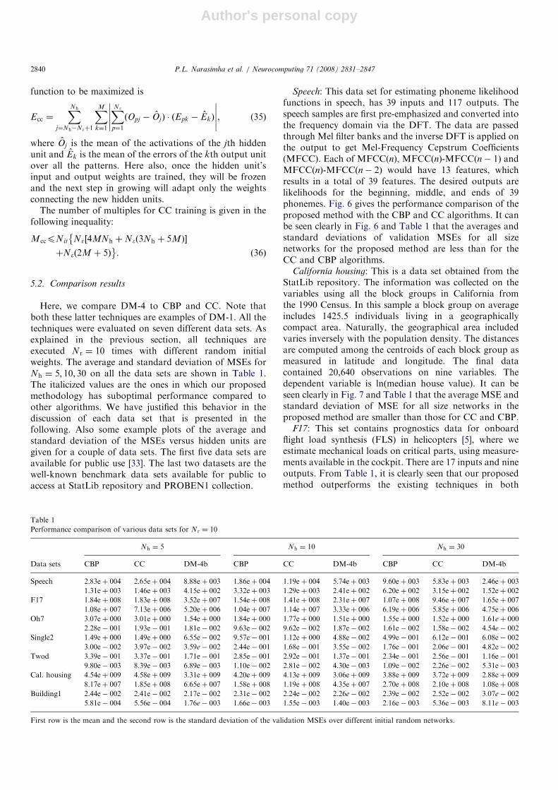
Here, we compare DM-4 to CBP and CC. Note thatboth these latter techniques are examples of DM-1. All thetechniques were evaluated on seven different data sets. Asexplained in the previous section, all techniques areexecuted Nr ¼ 10 times with different random initialweights. The average and standard deviation of MSEs forNh ¼ 5; 10; 30 on all the data sets are shown in Table 1.The italicized values are the ones in which our proposedmethodology has suboptimal performance compared toother algorithms. We have justified this behavior in thediscussion of each data set that is presented in thefollowing. Also some example plots of the average andstandard deviation of the MSEs versus hidden units aregiven for a couple of data sets. The first five data sets areavailable for public use [33]. The last two datasets are thewell-known benchmark data sets available for public toaccess at StatLib repository and PROBEN1 collection.

Speech: This data set for estimating phoneme likelihoodfunctions in speech, has 39 inputs and 117 outputs. Thespeech samples are first pre-emphasized and converted intothe frequency domain via the DFT. The data are passedthrough Mel filter banks and the inverse DFT is applied onthe output to get Mel-Frequency Cepstrum Coefficients(MFCC). Each of MFCC(n), MFCC(n)-MFCCðn� 1Þ andMFCCðnÞ-MFCCðn� 2Þ would have 13 features, whichresults in a total of 39 features. The desired outputs arelikelihoods for the beginning, middle, and ends of 39phonemes. Fig. 6 gives the performance comparison of theproposed method with the CBP and CC algorithms. It canbe seen clearly in Fig. 6 and Table 1 that the averages andstandard deviations of validation MSEs for all sizenetworks for the proposed method are less than for theCC and CBP algorithms.

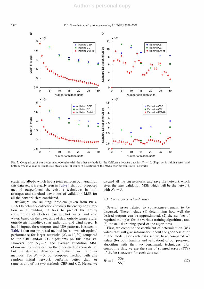
California housing: This is a data set obtained from theStatLib repository. The information was collected on thevariables using all the block groups in California fromthe 1990 Census. In this sample a block group on averageincludes 1425.5 individuals living in a geographicallycompact area. Naturally, the geographical area includedvaries inversely with the population density. The distancesare computed among the centroids of each block group asmeasured in latitude and longitude. The final datacontained 20,640 observations on nine variables. Thedependent variable is ln(median house value). It can beseen clearly in Fig. 7 and Table 1 that the average MSE andstandard deviation of MSE for all size networks in theproposed method are smaller than those for CC and CBP.

F17: This set contains prognostics data for onboardflight load synthesis (FLS) in helicopters [5], where weestimate mechanical loads on critical parts, using measure-ments available in the cockpit. There are 17 inputs and nineoutputs. From Table 1, it is clearly seen that our proposedmethod outperforms the existing techniques in both

ARTICLE IN PRESS

Table 1

Performance comparison of various data sets for Nr ¼ 10

Nh ¼ 5 Nh ¼ 10 Nh ¼ 30

Data sets CBP CC DM-4b CBP CC DM-4b CBP CC DM-4b

Speech 2:83eþ 004 2:65eþ 004 8:88eþ 003 1:86eþ 004 1:19eþ 004 5:74eþ 003 9:60eþ 003 5:83eþ 003 2:46eþ 003

1:31eþ 003 1:46eþ 003 4:15eþ 002 3:32eþ 003 1:29eþ 003 2:41eþ 002 6:20eþ 002 3:15eþ 002 1:52eþ 002

F17 1:84eþ 008 1:83eþ 008 3:52eþ 007 1:54eþ 008 1:41eþ 008 2:31eþ 007 1:07eþ 008 9:46eþ 007 1:65eþ 007


Oh7 3:07eþ 000 3:01eþ 000 1:54eþ 000 1:84eþ 000 1:77eþ 000 1:51eþ 000 1:55eþ 000 1:52eþ 000 1:61eþ 000

2:28e� 001 1:93e� 001 1:81e� 002 9:63e� 002 9:62e� 002 1:87e� 002 1:61e� 002 1:58e� 002 4:54e� 002

Single2 1:49eþ 000 1:49eþ 000 6:55e� 002 9:57e� 001 1:12eþ 000 4:88e� 002 4:99e� 001 6:12e� 001 6:08e� 002

3:00e� 002 3:97e� 002 3:59e� 002 2:44e� 001 1:68e� 001 3:55e� 002 1:76e� 001 2:06e� 001 4:82e� 002

Twod 3:39e� 001 3:37e� 001 1:71e� 001 2:85e� 001 2:92e� 001 1:37e� 001 2:34e� 001 2:56e� 001 1:16e� 001

9:80e� 003 8:39e� 003 6:89e� 003 1:10e� 002 2:81e� 002 4:30e� 003 1:09e� 002 2:26e� 002 5:31e� 003

Cal. housing 4:54eþ 009 4:58eþ 009 3:31eþ 009 4:20eþ 009 4:13eþ 009 3:06eþ 009 3:88eþ 009 3:72eþ 009 2:88eþ 009


Building1 2:44e� 002 2:41e� 002 2:17e� 002 2:31e� 002 2:24e� 002 2:26e� 002 2:39e� 002 2:52e� 002 3:07e� 002

5:81e� 004 5:56e� 004 1:76e� 003 1:66e� 003 1:55e� 003 1:40e� 003 2:16e� 003 5:36e� 003 8:11e� 003

First row is the mean and the second row is the standard deviation of the validation MSEs over different initial random networks.



averages and standard deviations of validation MSE for allthe network sizes considered. The large MSE values for thisdata set are due to the large variances of the desiredoutputs.

Oh7: This data set is for inversion of radar scatteringfrom bare soil surfaces [28]. It has 20 inputs and threeoutputs. The training set contains VV and HH polarizationat L 301, 401, C 101, 301, 401, 501, 601, and X 301, 401, 50�

along with the corresponding unknowns rms surfaceheight, surface correlation length, and volumetric soilmoisture content in g=cm3. In this case, it is observed fromTable 1 that the average and standard deviation ofvalidation MSEs for big networks (Nh ¼ 30) for theproposed method are larger than the existing methods.However, the averages and standard deviations of valida-tion MSE for smaller network (Nh ¼ 5; 10) are lesser.Hence the networks with larger MSEs are discarded.

Single2: This data set is for the inversion of surfacepermittivity [14]. These data have 16 inputs and threeoutputs. The inputs represent the simulated back scatteringcoefficient measured at 101, 301, 501and 701at both verticaland horizontal polarization. The remaining eight arevarious combinations of ratios of the original eight values.

For this data set, all the averages of validation MSEs forthe proposed method are clearly better than for the existingmethods as seen in Table 1, but the standard deviation ofvalidation MSE for Nh ¼ 5 on the proposed method is alittle higher. However, the average MSEs for proposedmethod are so much better than for the existing methods,that the higher standard deviation does not affect actualperformance.

Twod: This training file [9,10] is used in the task ofinverting the surface scattering parameters from aninhomogeneous layer above a homogeneous half space,where both interfaces are randomly rough. The parametersto be inverted are the effective permittivity of the surface,the normalized rms height, the normalized surface correla-tion length, the optical depth, and single scattering albedoof an inhomogeneous irregular layer above a homogeneoushalf space from back scattering measurements. The inputsconsist of eight theoretical values of back scatteringcoefficient parameters at V and H polarization and fourincident angles. The outputs were the corresponding valuesof permittivity, upper surface height, lower surface height,normalized upper surface correlation length, normalizedlower surface correlation length, optical depth and single

ARTICLE IN PRESS

0 5 10 15 20 25 30

0

0.5

1

1.5

2

2.5

3x 104


Mean o

f M

SE

s

Training CBP

Training CC

Training DM-4b

Training CBP

Training CC

Training DM-4b

0 5 10 15 20 25 30

0

500

1000

1500

2000

2500


Sta

ndard

Devia

tion o

f M

SE

s

0 5 10 15 20 25 30

0

0.5

1

1.5

2

2.5

3

3.5x 104


Mean o

f M

SE

s

Validation CBP

Validation CC

Validation DM-4b

Validation CBP

Validation CC

Validation DM-4b

0 5 10 15 20 25 300

500

1000

1500

2000

2500

3000

3500


Sta

ndard

Devia

tion o

f M

SE

s

Fig. 6. Comparison of our design methodologies with the other methods for the speech data for Nr ¼ 10. (Top row is training result and bottom row is

validation result.) (a) Means and (b) standard deviations of the MSEs over different initial networks.



scattering albedo which had a joint uniform pdf. Again onthis data set, it is clearly seen in Table 1 that our proposedmethod outperforms the existing techniques in bothaverages and standard deviations of validation MSE forall the network sizes considered.

Building1: The Building1 problem (taken from PRO-BEN1 benchmark collection) predicts the energy consump-tion in a building. It tries to predict the hourlyconsumption of electrical energy, hot water, and coldwater, based on the date, time of day, outside temperature,outside air humidity, solar radiation, and wind speed. Ithas 14 inputs, three outputs, and 4208 patterns. It is seen inTable 1 that our proposed method has shown sub-optimalperformance for larger networks (Nh ¼ 10; 30) comparedto the CBP and/or CC algorithms on this data set.However, for Nh ¼ 5, the average validation MSEof our method is lesser than the other methods considered,but the standard deviation is higher than the othermethods. For Nh ¼ 5, our proposed method with anyrandom initial network performs better than orsame as any of the two methods CBP and CC. Hence, we

discard all the big networks and save the network whichgives the least validation MSE which will be the networkwith Nh ¼ 5.

5.3. Convergence related issues

Several issues related to convergence remain to bediscussed. These include (1) determining how well thedesired outputs can be approximated, (2) the number ofrequired multiples for the various training algorithms, and(3) the actual training speed of the algorithms.First, we compute the coefficient of determination (R2)

values that will give information about the goodness of fitof the model. For each data set we have compared R2

values (for both training and validation) of our proposedalgorithm with the two benchmark techniques. Forcomputing this, we use the sum of squared errors (SSE)of the best network for each data set.

R2 ¼ 1�SSE

SST, (37)

ARTICLE IN PRESS

0 5 10 15 20 25 302.5

3

3.5

4

4.5

5x 109


Me

an

of

MS

Es

Training CBP

Training CC

Training DM-4b

0 5 10 15 20 25 300

2

4

6

8

10

12x 107


Sta

nd

ard

De

via

tio

n o

f M

SE

s

0 5 10 15 20 25 302.5

3

3.5

4

4.5

5x 109


Me

an

of

MS

Es

Validation CBP

Validation CC

Validation DM-4b

Training CBP

Training CC

Training DM-4b

Validation CBP

Validation CC

Validation DM-4b

0 5 10 15 20 25 300

0.5

1

1.5

2

2.5

3

3.5

4

4.5x 108


Sta

nd

ard

De

via

tio

n o

f M

SE

s

Fig. 7. Comparison of our design methodologies with the other methods for the California housing data for Nr ¼ 10. (Top row is training result and

bottom row is validation result.) (a) Means and (b) standard deviations of the MSEs over different initial networks.



where SSE is the sum of squared error (residual error) andSST is the total sum of squares of the desired outputs.Table 2 shows the coefficient of determination values forboth training and validation. Note that in terms of modelfitting (training R2), our proposed method outperforms theother methods. In terms of generalization, our proposedmethod is better in all of the data sets except for Oh7 wherethe R2 value is insignificantly lower than that of the othermethods.

In order to analyze the complexity of the trainingalgorithms, we compare the total number of multiples foreach training algorithm to train a sequence of networks.Then we give comparison plots of MSE versus time inseconds for the three training algorithms on example datasets. The number of multiples for DM-4 is given below:

MDM4pMcbp þNit

7N2 þ 3N

2þNhNðN þ 1Þ

� �

þNhðNh þ 1Þð7N2 þ 3NÞ

4. ð38Þ

As mentioned before, N� is the number of hidden unitsadded in each growing step (see Step 2 of Algorithm

DM-4b), Mcbp is given in Eq. (34). From the aboveequation, it is clear that the number of multiples for DM-4algorithm is greater than that of CBP. However, it shouldbe noted that the additional term is very small compared tothe Mcbp value as it does not involve the number ofpatterns, Nv, which is usually very large. This smalladditional computation sometimes helps the algorithm toconverge faster as discussed below.Figs. 8(a) and (b) show the plots of the MSE versus time

in seconds for California housing and speech data sets,respectively. Note that the convergence time for DM-4 onCalifornia housing data set is shorter as it reaches the localminima before it executes total number of iterations, Nit.This is because, if the learning factor is very small and theMSE does not decrease for more than five iterations, then alocal minimal is reached and the training is stopped for thatnetwork.

6. Conclusions

In this paper, we explore four design methodologiesfor producing sequences of trained and validated feed-forward networks of different size. In the growing

ARTICLE IN PRESS

Table 2

Coefficient of determination ðR2Þ values for all data sets computed using the sum of squared errors of the best network for each technique

Training Validation

Datasets Constructive Cascade OWO-HWO Constructive Cascade OWO-HWO

backpropagation correlation (DM-4b) backpropagation correlation (DM-4b)

Speech 0.895355 0.927280 0.967146 0.796655 0.876492 0.949425

F17 0.972791 0.975443 0.997999 0.970566 0.973926 0.996710

Oh7 0.841103 0.843756 0.883139 0.838076 0.841178 0.832213

Single2 0.992278 0.989352 0.999960 0.986611 0.983582 0.999400

Twod 0.803962 0.802961 0.923472 0.788988 0.770901 0.902647

Cal. housing 0.714922 0.719687 0.804399 0.705777 0.718300 0.777062

Building1 0.900011 0.892534 0.934435 0.110040 0.132986 0.135555

0 200 400 600 800 1000 1200 1400 1600 1800

2.5

3

3.5

4

4.5

5x 109

Time in seconds

MS

E

CBPCCDM-4b

CBPCCDM-4b

0 1000 2000 3000 4000 5000 60000

0.5

1

1.5

2

2.5

3x 104

Time in seconds

MS

E

Fig. 8. Comparison of convergence time of our design methodologies with the other methods for the (a) California housing, (b) speech data sets. Note that

these plots show MSEs for only one random number seed and hence they are not average MSEs.



approach (DM-1), DI networks result in monotonicallydecreasing Ef ðNhÞ curves. A pruning method (DM-2) isshown that requires one pass through the data. A methodis also described for simultaneously validating manydifferent size networks, using a second data pass. In thethird, combined approach (DM-3), ordered pruning isapplied to grown networks. Lastly, our final combinedapproach (DM-4) successively grows the network by a fewunits, and then prunes. As seen in the simulations, thisapproach usually produces smaller training and validationerrors than the other methodologies. The final MSE versusNh curves are almost monotonic. The DM-4 approach alsoexhibits reduced sensitivity to initial weights.

Our final method was compared with the two other wellknown growing techniques: CBP and CC. On sevendifferent data sets, the results show that our proposedmethod performs significantly better than these othermethods.

Appendix A. Hidden unit pruning using the Schmidt

procedure

For the ease of notation, in this section, we use theaugmented input vector, i.e., xp ½x

Tp ; 1;O

Tp �

T, where 1 is forthe threshold. The new dimension of xp is Nu ¼ N þNh þ 1.Also, for simplicity, the subscript p indicating the patternnumber will not be used unless it is necessary. The output ofthe network in Eq. (3), can be rewritten as

yi ¼XNu

k¼1

w0ði; kÞ � xk, (A.1)

where w0 is the corresponding augmented weight matrixconsisting of woi and woh including the threshold. In Eq. (A.1),the signals xk are the raw basis functions for producing yi.

The normal Gram–Schmidt procedure [32] is a recursiveprocess that requires obtaining scalar products between rawbasis functions and orthonormal basis functions. The dis-advantage in this process is that it requires one pass throughthe training data to obtain each new basis function. In thissection a more useful form of the Schmidt process is reviewed,which will let us express the orthonormal system in terms ofautocorrelation elements.

A.1. Basic algorithm

The mth orthonormal basis function x0m, can beexpressed as

x0m ¼Xm

k¼1

amk � xk. (A.2)

From Eq. (A.2), for m ¼ 1, the first basis function isobtained as

x01 ¼X1k¼1

a1k � xk ¼ a11x1; ðA:3Þ

a11 ¼1

kx1k¼

1

rð1; 1Þ1=2; ðA:4Þ

where elements of the autocorrelation matrix R aredefined as

rði; jÞ ¼ hxi;xji ¼1

Nv

XNv

p¼1

xpi � xpj . (A.5)

For values of m between 2 and Nu, ci is first found for1pipm� 1 as

ci ¼Xi

q¼1

aiq � rðq;mÞ. (A.6)

Then obtain m coefficients bk as

bk ¼�Pm�1i¼k

ci � aik; 1pkpm� 1;

1; k ¼ m:

8><>: ðA:7Þ

Finally, for the mth basis function the new amk coefficients(for 1pkpm) are found as

amk ¼bk

rðm;mÞ �Pm�1

i¼1 c2i

h i1=2 . (A.8)

The output equation (A.1) can be written as

yi ¼XNu

q¼1

w00ði; qÞ � x0q, (A.9)

where the weights in the orthonormal system are

w00ði; qÞ ¼Xq

k¼1

aqk � hxk; tii ¼Xq

k¼1

aqk � cði; kÞ, (A.10)

where elements of the crosscorrelation matrix C are definedas

cði; kÞ ¼1

Nv

XNv

p¼1

tpi � xpk. (A.11)

Using Eq. (A.2), we obtain output weights for the systemas

w0ði; kÞ ¼XNu

q¼k

w00ði; qÞ � aqk. (A.12)

Substituting Eq. (A.9) into Eq. (5), we obtain EðiÞ inorthonormal system as

EðiÞ ¼ ti �XNu

k¼1

w00ði; kÞ � x0k

!; ti �

XNu

q¼1

w00ði; qÞ � x0q

!* +.

(A.13)

If we decide to use the first Nhd hidden units in our originalnetwork, the training error is

EðiÞ ¼ hti; tii �XNþ1þNhd

k¼1

ðw00ði; kÞÞ2. (A.14)



Modifying Eq. (A.12), the output weights would be

w0ði; kÞ ¼XNþ1þNhd

q¼k

w0oði; qÞ � aqk. (A.15)

The purpose of pruning is to eliminate useless inputs andhidden units as well as hidden units that are less useful.Useless units are those which (1) have no informationrelevant for estimating outputs or (2) are linearly depen-dent on inputs or hidden units that have already beenorthonormalized.

We modify the Schmidt procedure so that duringpruning, the hidden units are ordered according to theirusefulness and useless basis functions x0m are eliminated.

Let jðmÞ be an integer valued function that specifies theorder in which raw basis functions xk are processed intoorthonormal basis functions x0k. Then x0m is to be calculatedfrom xjðmÞ; xjðm�1Þ and so on. This function also definesthe structure of the new hidden layer where 1pmpNu

and 1pjðmÞpNu. If jðmÞ ¼ k then the mth unit of thenew structure comes from the kth unit of the originalstructure.

Given the function jðmÞ, and generalizing theSchmidt procedure, the mth orthonormal basis functionis described as

x0m ¼Xm

k¼1

amk � xjðkÞ. (A.16)

Initially, x01 is found as a11 � xjð1Þ where

a11 ¼1

kxjð1Þk¼

1

rðjð1Þ; jð1ÞÞ1=2. (A.17)

For 2pmpNu, we first perform

ci ¼Xi

q¼1

aiq � rðjðqÞ; jðmÞÞ for 1pipm� 1. (A.18)

Second, we set bm ¼ 1 and get

bk ¼ �Xm�1i¼k

ci � aik for 1pkpm� 1. (A.19)

Lastly, we get coefficients amk as

amk ¼bk

rðjðmÞ; jðmÞÞ �Pm�1

i¼1 c2i

h i1=2 for 1pkpm. (A.20)

Then weights in the orthonormal system are found as

w0oði;mÞ ¼Xm

k¼1

amk � cði; jðkÞÞ for 1pipM. (A.21)

The goal of pruning is to find the function jðmÞ whichdefines the structure of the hidden layer. Here it is assumedthat the original basis functions are linearly independenti.e., the denominator of Eq. (A.20) is not zero.

Since we want the effects of inputs and the constant ‘‘1’’to be removed from orthonormal basis functions, the firstN þ 1 basis functions are picked as

jðmÞ ¼ m for 1pmpN þ 1. (A.22)

The selection process will be applied to the hidden units ofthe network. We now define notation that helps us specifythe set of candidate basis function to choose in a giveniteration. First, define SðmÞ as the set of indices of chosenbasis functions where m is the number of units of thecurrent network (i.e., the one that the algorithm isprocessing). Then SðmÞ is given by

SðmÞ ¼ffg for m ¼ 0;

fjð1Þ; jð2Þ; . . . ; jðmÞg for 0ompNu:

((A.23)

Starting with an initial linear network having 0 hiddenunits, where m is equal to N þ 1, the set of candidate basisfunctions is clearly Scfmg ¼ f1; 2; 3; . . . ;Nug � SðmÞ, whichis fN þ 2;N þ 3; . . . ;Nug. For N þ 2pmpNu, we obtainScfm� 1g. For each trial value of jðmÞ 2 Scfm� 1g, weperform operations in Eqs. (A.18)–(A.21). Then PðmÞ is

PðmÞ ¼XMi¼1

½w0oði;mÞ�2. (A.24)

The trial value of jðmÞ that maximizes PðmÞ is found.Assuming that PðmÞ is maximum when validation the ithelement, then jðmÞ ¼ i. SðmÞ is updated as

SðmÞ ¼ Sðm� 1Þ [ fjðmÞg. (A.25)

Then for the general case the candidate basis functions are,Scðm� 1Þ ¼ f1; 2; 3; . . . ;Nug � fjð1Þ; jð2Þ; . . . ; jðm� 1Þg withNu �mþ 1 candidate basis function. By using Eq. (A.24),after validation all the candidate basis function, jðmÞ takesits value and SðmÞ is updated according to Eq. (A.25).Defining Nhd as the desired number of units in the hiddenlayer, the process is repeated until m ¼ N þ 1þNhd . Thenthe orthonormal weights are mapped to normal weightsaccording to Eq. (A.30). Considering the final value offunction jðmÞ row reordering of the original input weightsmatrix is performed for generating the right Opj valueswhen applying Eq. (A.1). After reordering the rows,because only the Nhd units are kept then the remainingunits (Opj with NhdojpNh) are pruned by deleting the lastNh �Nhd rows.

A.2. Linear dependency condition

Unfortunately, ordered pruning by itself is not able tohandle linearly dependent basis functions. A minormodification is necessary. Assume that raw basis functionxjðmÞ is linearly dependent on previously chosen basisfunctions, where jðmÞ denotes an input (1pmpN) and jðmÞ

has taken on a trial value. Then

xjðmÞ ¼Xm�1k¼1

dk � x0k. (A.26)



Now the denominator of amk in (A.20) can be rewritten as

g ¼ hzm; zmi1=2, (A.27)

where

zm ¼ xjðmÞ �Xm�1i¼1

hx0i;xjðmÞi � x0i. (A.28)

Substituting (A.26) into (A.28), however, we get

hx0i;xjðmÞi ¼ di (A.29)

and zm and g are both zero.If jðmÞ denotes an input and g is infinitesimally small,

then we equate jðkÞ to k for 1pkom and jðkÞ ¼ k þ 1 formpkpN. In effect we decrease N by one and let the jðkÞ

function skip over the linearly dependent input. If jðmÞ

denotes a hidden unit, the same procedure is used todetermine whether or not xjðmÞ is useful. If xjðmÞ is found tobe linearly dependent, the current, bad value of jðmÞ isdiscarded before amk is calculated.

Once we get these orthonormal weights, the hidden unitsand their weights are reordered in the descending order oftheir energies. Then the output weights of the originalsystem are obtained using the equation

wDM2o ði; kÞ ¼

XNu

q¼k

w0oði; qÞ � aqk. (A.30)

Here wDM2o 2WNh

DM2 is the output weights obtained usingSchmidt procedure.

References

[1] H. Amin, K.M. Curtis, B.R.H. Gill, Dynamically pruning output

weights in an expanding multilayer perceptron neural network, in:

13th International Conference on DSP, vol. 2, 1997.

[2] P. Arena, R. Caponetto, L. Fortuna, M.G. Xibilia, Genetic

algorithms to select optimal neural network topology, in: Proceedings

of the 35th Midwest Symposium on Circuits and Systems, vol. 2,

1992.

[3] C.M. Bishop, Neural Networks and Machine Learning, vol. 168,

Springer, Berlin, 1998.

[4] G. Castellano, A.M. Fanelli, M. Pelillo, An iterative pruning

algorithm for feedforward neural networks, IEEE Trans. Neural

Networks 8 (3) (1997) 519–531.

[5] H.H. Chen, M.T. Manry, H. Chandrasekaran, A neural network

training algorithm utilizing multiple sets of linear equations,

Neurocomputing 25 (1–3) (1999) 55–72.

[6] S. Chen, C.F.N. Cowan, P.M. Grant, Orthogonal least squares

learning algorithm for radial basis function networks, IEEE Trans.

Neural Networks 2 (2) (1991) 302–309.

[7] F.L. Chung, T. Lee, Network-growth approach to design of

feedforward neural networks, IEE Proce. Control Theory 142 (5)

(1995) 486–492.

[8] J. Davila, Genetic optimization of NN topologies for the task of

natural language processing, in: Proceedings of International Joint

Conference on Neural Networks, vol. 2, 1999.

[9] M.S. Dawson, A.K. Fung, M.T. Manry, Surface parameter retrival

using fast learning neural networks, Remote Sensing Rev 7 (1993).

[10] M.S. Dawson, J. Olvera, A.K. Fung, M.T. Manry, Inversion of

surface parameters using fast learning neural networks, in: Proceed-

ings of IGARSS, vol. 2, 1992.

[11] W.H. Delashmit, Multilayer perceptron structured initialization and

separating mean processing, Dissertation, University of Texas,

Arlington, December 2003.

[12] S.E. Fahlman, C. Lebiere, The cascade-correlation learning archi-

tecture, in: Advances in Neural Information Processing Systems 2,

Morgan Kaufmann, Los Altos, CA, 1990.

[13] M.H. Fun, M.T. Hagan, Levenberg-marquardt training for modular

networks, in: IEEE International Conference on Neural Networks,

vol. 1, 1996.

[14] A.K. Fung, Z. Li, K.S. Chen, Back scattering from a randomly rough

dielectric surface, IEEE Trans. Geosci. Remote Sensing 30 (2) (1992)

356–369.

[15] S.-U. Guan, S. Li, Parallel growing and training of neural networks

using output parallelism, IEEE Trans. Neural Networks 13 (3) (2002)

542–550.

[16] Y. Hirose, K. Yamashita, S. Hijiya, Back-propagation algorithm

that varies the number of hidden units, Neural Networks 4

(1991).

[17] G.B. Huang, P. Saratchandran, N. Sundararajan, A generalized

growing and pruning RBF neural network for function approxima-

tion, IEEE Trans. Neural Networks 16 (1) (2005) 57–67.

[18] W. Kaminski, P. Strumillo, Kernel orthonormalization in radial basis

function neural networks, IEEE Trans. Neural Networks 8 (5) (1997)

1177–1183.

[19] M. Lehtokangas, Modelling with constructive backpropagation,

Neural Networks 12 (1999) 707–716.

[20] X. Liang, L. Ma, A study of removing hidden neurons in cascade

correlation neural networks, in: IEEE International Joint Conference

on Neural Networks, vol. 2, 2004.

[21] F.J. Maldonado, T.H.K.M.T. Manry, Finding optimal neural

network basis function subsets using the schmidt procedure, in:

Proceedings of the International Joint Conference on Neural

Networks, vol. 1, 2003, pp. 20–24.

[22] V. Maniezzo, Genetic evolution of the topology and weight

distribution of neural networks, IEEE Trans. Neural Networks 5

(1) (1994).

[23] M.T. Manry, S.J. Apollo, L.S. Allen, W.D. Lyle, W. Gong, M.S.

Dawson, A.K. Fung, Fast training of neural networks for remote

sensing, Remote Sensing Rev. 9 (1994).

[24] P.V.S. Ponnapalli, K.C. Ho, M. Thomson, A formal selection and

pruning algorithm for feedforward artificial neural network optimi-

zation, IEEE Trans. Neural Networks 10 (4) (1999) 964–968.

[25] R. Reed, Pruning algorithms—a survey, IEEE Trans. Neural

Networks 4 (5) (1993) 740–747.

[26] D.E. Rumelhart, J.L. McClelland, Parallel Distributed Processing:

Explorations in the Microstructure of Cognition, vol. 1, MIT Press,

Cambridge, MA, 1986.

[27] I.I. Sakhnini, M.T. Manry, H. Chandrasekaran, Iterative improve-

ment of trigonometric networks, in: Proceedings of the International

Joint Conference on Neural Networks, vol. 2, 1999.

[28] Y.K. Sarabandi, F.T. Ulaby, An empirical model and an inversion

technique for radar scattering from bare soil surfaces, IEEE Trans.

Geosci. Remote Sensing 30 (2) (1992) 370–381.

[29] M.A. Sartori, P.J. Antsaklis, A simple method to derive bounds on

the size and to train multilayer neural networks, IEEE Trans. Neural

Networks 2 (4) (1991) 467–471.

[30] R.S. Scalero, N. Tepedelenlioglu, A fast new algorithm for training

feedforward neural networks, IEEE Trans. Signal Process. 40 (1992)

202–210.

[31] R. Sentiono, Feedforward neural network construction using cross

validation, Neural Computation 13 (2001) 2865–2877.

[32] G. Strang, Linear Algebra and its Application, Harcourt Brace,

New York, 1988.

[33] University of Texas at Arlington, Training datasets, hhttp://www-ee.uta.

edu/eeweb/IP/training_data_files.htmi.

[34] C. Yu, M.T. Manry, J. Li, P.L. Narasimha, An efficient hidden layer

training method for the multilayer perceptron, Neurocomputing 70

(2006) 525–535.



Pramod Lakshmi Narasimha received his B.E. in

Telecommunications Engineering from Banga-

lore University, India. He joined the Neural

Networks and Image Processing Lab in the

Department of Electrical Engineering at the

University of Texas at Arlington (UTA) as a

Research Assistant in 2002. In 2003, he received

his M.S. degree in EE at UTA. Currently, he is

working on his Ph.D. His research interests focus

on machine learning, neural networks, estimation

theory, pattern recognition and computer vision. He is a member of Tau

Beta Pi and a student member of the IEEE.

Walter H. Delashmit was born in Memphis,

Tennessee, in 1944. He received the B.S. degree

from Christian Brothers University in Electrical

Engineering in 1966 and the M.S. degree from the

University of Tennessee in Electrical Engineering

with a minor in Mathematics in 1968. He

graduated with the Ph.D. degree in Electrical

Engineering at the University of Texas at

Arlington, Spring 2003. Currently, he is em-

ployed at Lockheed Martin Missiles and Fire

Control (formerly Loral Vought Systems and LTV Aerospace and

Defense) in Dallas, Texas, where he is a Senior Staff Research Engineer.

Among his duties, he is Program Manager/Principal Investigator for the

Weapon Seeker Improvement Program and Manager of the Signal and

Image Processing Group. He is a Senior Member of the IEEE, a member

of Tau Beta Pi and a member of Eta Kappa Nu. His research interests are

in the areas of neural networks, two- and three-dimensional image

processing and signal processing techniques. Dr. Delashmit is also an avid

jogger.

Michael T. Manry was born in Houston, Texas,

in 1949. He received the B.S., M.S., and Ph.D. in

Electrical Engineering in 1971, 1973, and 1976,

respectively, from The University of Texas at

Austin. After working there for two years as an

Assistant Professor, he joined Schlumberger

Well Services in Houston where he developed

signal processing algorithms for magnetic reso-

nance well logging and sonic well logging. He

joined the Department of Electrical Engineering

at the University of Texas at Arlington in 1982, and has held the rank of

Professor since 1993. In summer 1989, Dr. Manry developed neural

networks for the Image Processing Laboratory of Texas Instruments in

Dallas. His recent work, sponsored by the Advanced Technology Program

of the state of Texas, E-Systems, Mobil Research, and NASA, has

involved the development of techniques for the analysis and fast design of

neural networks for image processing, parameter estimation, and

pattern classification. Dr. Manry has served as a consultant for the

Office of Missile Electronic Warfare at White Sands Missile

Range, MICOM (Missile Command) at Redstone Arsenal, NSF, Texas

Instruments, Geophysics International, Halliburton Logging Services,

Mobil Research and Verity Instruments. He is a Senior Member of the

IEEE.

Jiang Li received his B.S. degree in Electrical

Engineering from Shanghai Jiaotong University,

China, in 1992, the M.S. degree in automation

from Tsinghua University, China, in 2000, and

the Ph.D. degree in Electrical Engineering from

the University of Texas at Arlington, TX, in

2004. His research interests include machine

learning, computer aided medical diagnosis

systems, medical signal/image processing, neural

network and modeling and simulation. Dr. Li

worked as a postdoctoral fellow at the Department of Radiology,

National Institutes of Health, from 2004 to 2006. He joined ECE

Department at ODU as an Assistant Professor in 2006. He is also affiliated

with Virginia Modeling, Analysis, and Simulation Center (VMASC).

Dr. Li is a member of the IEEE and Sigma Xi.

Francisco Javier Maldonado Diaz has received

the Masters in Electrical Engineering from the

Chihuahua Institute of Technology, and the

Ph.D. in Electrical Engineering from the Uni-

versity of Texas at Arlington (UTA). He was the

recipient of the Fulbright sponsorship for doc-

toral studies at UTA. He has worked on

Intelligent Systems with Dr. Frank Lewis (Ad-

vanced Controls, Sensors and MEMS group) at

the Automation and Robotics Research Institute

of UTA. Dr. Maldonado has also developed advanced learning algorithms

with Dr. Michael Manry in the Image Processing and Neural Networks

Lab at UTA. In 2002, Dr. Maldonado joined Williams-Pyro’s research

and development department and has been involved in several SBIR

projects for the US government. Dr. Maldonado’s research has centered

on using neural networks for (1) failure detection, (2) implementation in

embedded systems, and (3) pseudogenetic algorithms for multi-layer

perceptron design. He is a reviewer for the Neurocomputing International

Journal and has published eight conference papers on neural networks and

intelligent systems. He is a member of the IEEE Control and

Instrumentation Systems societies and has been named a Marquis Who’s

Who in the World, 2006 edition. He has been a member of the Society of

Hispanic Engineers at UTA, being an official of the society during 2000.

He is also a member of HKN and was an International University Scholar

and University Scholar at UTA in 2001.


an integrated growing-pruning method for feedforward network training

Documents