an improved method for calculating flow past flapping and hovering airfoils

Theor. Comput. Fluid Dyn. (2005) 19(6): 417–440DOI 10.1007/s00162-005-0003-9

ORIGINAL ARTICLE

T. K. Sengupta · V. Vikas · A. Johri

An improved method for calculating flow past flappingand hovering airfoils

Received: 15 November 2004 / Accepted: 19 July 2005 / Published online: 7 December 2005C© Springer-Verlag 2005

Abstract A method is reported here for calculating unsteady aerodynamics of hovering and flapping airfoilfor two-dimensional flow via the following improved methodologies: (a) a correct formulation of the problemusing stream function (ψ) and vorticity (ω) as dependent variables; (b) calculating loads and moment by anew method to solve the governing pressure Poisson equation (PPE) in a truncated part of the computationaldomain on a nonstaggered grid; (c) accurate solution using high accuracy compact difference scheme for thevorticity transport equation (VTE) and (d) accelerating the computations by using a high-order filter aftereach time step of integration. These have been used to solve Navier–Stokes equation for flow past flappingand hovering NACA 0014 and 0015 airfoils at typical Reynolds numbers relevant to the study of unsteadyaerodynamics of micro air vehicle (MAV) and insect/bird flight.

Keywords Stream function–vorticity formulation · Pressure poisson equation · Compact schemes ·Navier–Stokes equation · Unsteady aerodynamics · Flapping and hovering flight

1 Introduction

Computing unsteady flows at low to moderate Reynolds numbers continues to be of significant interest due toits application in MAVs and its relevance to insect and bird flights. Flapping and hovering flight of bird andinsect are fine examples of optimum motion of aerodynamic surfaces that simultaneously develop necessarythrust for forward motion and sustained lift to keep it airborne. This is totally different from aircraft motionwhere lift and thrust are created by different subsystems. Also, lift and thrust are created in aircraft by steadyflow devices, while natural fliers use unsteady aerodynamics to create the same by articulating same surfaces.Comprehensive reviews of the subject can be found in [1–4]. While biologists have focused attention on kine-matics of motion for birds and insects (see [5, 6] for example), bio-fluid dynamicists have attempted to explainmechanisms of flights based on simplified models in the limit of quasi-steady and unsteady operation. Recentinterest in engineering community on bird and insect flight is the requirement of flying payload carrying flightvehicles that are very small in dimension and weight for their perceived mission requirements. With restrictionon size of such devices (around 15 cm or less) and speed regimes (of about 10 m/s)—the operating Reynoldsnumbers are in the range of 104–105. Such flows display massive boundary layer separation, flow transition,and large vortical structures that make theoretical and experimental studies a formidable task. At the same

Communicated by P. Sagaut

T. K. Sengupta (B) · A. JohriDepartment of Aerospace Engineering, I.I.T. Kanpur, U.P. 208016, IndiaE-mail: [email protected]

V. VikasDepartment of Aerospace Engineering, I.I.T. Kharagpur, W. Bengal 741302, India

418 T. K. Sengupta et al.

time, birds and insects flying with similar parameters display extraordinary maneuverability, agility and low-speed flying capability and even the ability to hover. To mimic such modes of flight in man-made devices, itis essential to understand and model such dynamics. In general, bird/insect flight is due to complex combina-tions of translational and angular motion of lifting surfaces. It is understood that the flow dynamics is viscousin nature at the relevant moderate Reynolds number. Understanding complex phase relationships betweenwing kinematics and system response is central to design any engineering devices delivering simultaneouslyhigh aerodynamic and propulsive efficiencies. Experimental studies are difficult and the existing state-of-theart is discussed in [1–4]. Of particular interest are the visual signatures of wing kinematics recorded in, e.g.,Tobalske & Dial [7] and Nachtigall [8]. Freymuth [9] has experimentally investigated the motion of an airfoilin combined harmonic plunging and pitching oscillatory motion with phase difference to generate thrust instill air environment. The role of vortex street acting as a jet stream in the wake is discussed in [9] as themechanism for generating lift and thrust. The author identified 3 generic cases of hover modes. Zero baselineangle of attack of the airfoil with 90◦ phase difference between horizontal and pitch oscillation is termedas the first hover or the water-treading mode. In the second hover or degenerate figure-of-eight mode, thebaseline angle of attack is 90◦ and pitching oscillation has a phase lag of 90◦ with respect to translationaloscillation. For the third mode, also called the oblique or dragonfly mode, the lifting surface is at an angle ofattack nominally between zero and 90◦ while the phase difference between horizontal and pitch oscillationsis kept close to 90◦. In the present study, the second hover mode case will be computed and analyzed.

It is now accepted that theoretical studies involving steady-state aerodynamics is of limited value andsome unsteady flow models have been studied. For example, in [10] a flapping wing inviscid flow modelhas been proposed and Spedding [11] provides an extensive review of early aerodynamic models of flappingflight. However, it is essential that any unsteady flow model must include viscous effects involving separationand transition in the presence of large vortices. This has been attempted by using CFD techniques to studyflapping flight, where the airfoil executes heaving oscillations being placed in an uniform flow. In [2], acommercial software, based on finite volume primitive variable formulation is used to solve Navier–Stokesequation in Lagrangian–Eulerian framework. The authors remark that it is essential to satisfy the conservationlaw, otherwise false mass is created leading to large errors. In [3], three-dimensional incompressible Navier–Stokes equation in primitive variables have been solved in strong conservation form using SIMPLEC andPISO methods. Sun & Tang [12] have reported solving three-dimensional Navier–Stokes equation using theartificial compressibility method of [13]. In [12], spatial discretization was performed by third-order upwindflux-difference splitting and time integration by second-order Adams–Bashforth technique. Relatively goodagreement was reported with experimental data. However, this time integration strategy displays spuriouscomputational mode with large error for unsteady flows (see [14] for details).

Ideally, three-dimensional computation around a deforming wing is desirable to understand the fluid dy-namics of flapping and hover modes of motion. The present day situation remains the same as was notedearlier by Wang [15] that from a practical point of view, while it is possible to resolve two-dimensionalflows at Reynolds numbers relevant to insect flight, it remains to be seen whether one can do the same forthree-dimensional flows. This is due to problems of resolving length and time scales involved in solution ofunsteady Navier–Stokes equation while satisfying mass conservation accurately in primitive variable formu-lations. This is avoided in computing two-dimensional flows given by Navier–Stokes equation using streamfunction–vorticity (ψ–ω) formulation. This equation satisfies mass conservation identically and allows takinglarger number of grid points as the number of unknowns reduces from three to two. Gustafson & Leben [16]and Gustafson et al. [17] have used this formulation to compute hovering flight of an elliptic cylinder. Unfor-tunately, the governing VTE written in the moving frame had an important angular acceleration term omittederroneously. This term is essential for hovering flight, with the lifting surface executing pitching oscillations.In [15] same formulation is used, but the considered heaving oscillation in a uniform flow does not requirethis angular acceleration term. For the flapping motion vortex shedding was investigated in [15] and an opti-mal flapping frequency based on time scales associated with shedding of leading and trailing edge vortices isreported. In solving the problem a fourth-order compact finite difference scheme, developed in [18] is used.In [15–17], the Navier–Stokes equation is solved for an elliptic airfoil and results are qualitatively comparedwith the experiments of [9] that was performed with an airfoil with rectangular cross section with roundedoff edges of significantly lower thickness ratio. Choice of elliptic airfoil allows creating orthogonal grid thatis known to yield accurate numerical solution of Navier–Stokes equation. However in [15–17], loads andmoment are calculated by quadrature of the vorticity field—a technique known for its limitation as discussedin [19] and [20] in details. In [19] and [20], instead, the solution of PPE for accurate loads and momentcalculation is suggested—a procedure followed here.

Flow past flapping and hovering airfoils 419

Based on above discussions, a reformulation of the problem is necessary to study general flapping andhover mode of motion in two-dimensions for an actual airfoil. To account for an actual airfoil, one canconstruct orthogonal grids following the method proposed in [21]. Here the PPE is solved using the or-thogonal nonstaggered grid by a new method to calculate loads and moment. This is done by solving the PPEin a subdomain with exact boundary conditions on subdomain boundaries. This is a significant improvementover the method in [22] that was developed for steady flow problems solved in Cartesian grids. Furthermore,a very high spectral accuracy compact scheme is used here along with a high-order filter applied to the so-lution at the end of every time step. Both of these accelerate computations by orders of magnitude (morethan hundred-folds) in solving NS equation for flapping and hovering airfoils at moderate Reynolds numbers.Ideas of [22] for calculating PPE have also been used in [23] and [24] for further development.

In a combined experimental and computational investigation for flapping wing aerodynamics, Jones et al.[25] reported results that included wind tunnel investigation on finite aspect ratio wing to directly measureforces, time-accurate LDV measurements and flow visualization for a NACA 0014 airfoil. Two- and three-dimensional Navier–Stokes and Euler solutions were also obtained computationally and compared with ex-perimental results with limited success. The airfoil in the experiments were made to execute only plungingoscillation given by

y(t) = h cos(kt) (1)

A plunge amplitude of h = 0.4c was considered for a range of reduced frequencies, k for different anglesof attack. In the present work, this geometry and motion is considered to compute the flow field for Re =20,000 when the airfoil is set at zero angle of attack and the reduced frequency is k = 0.4. In addition tothis, the second hover mode case of [9] is computed for oscillating NACA 0015 airfoil in the pitch planewith the rotating center at the mid-chord for Re = 27,000. In [9], the Reynolds number was chosen less thanRe = 600, while the case computed in [17] corresponds to Re = 1700 for a different geometry. Accordingto the definition of this mode of motion, the mean angle of attack is 90◦ with the pitching angle oscillationamplitude was 5◦ in [9]. The airfoil executed horizontal oscillation with an amplitude that is equal to the chordof the airfoil. In addition to these two cases, a combined flapping hover mode of motion is also computed herefor which no definitive results exist but that seems to be closer to the actual case in the natural world.

It is to be noted that the present problem has similarities with the unsteady airfoil aerodynamics oftenstudied for rotary wing devices. Some experimental and numerical contribution in this field are recorded in[26–29] and other references contained therein. However, we note that the Reynolds number ranges are muchhigher for helicopter rotor blades and flow behavior is qualitatively different that is encountered in rotarywings and that in insect and bird flights.

The paper is structured in the following manner. In the next section governing equations are given inboth the inertial and noninertial frames for the kinematics, kinetics, and the governing PPE. In Sect. 3, thenumerical methods used for the various solvers are detailed. In Sect. 4, results for various cases considered forthe individual flapping, hover and a combined flapping hover mode motion are discussed. The paper closeswith few concluding remarks in Sect. 5.

2 Governing equations in inertial and noninertial frames

In the following, the equations are derived for both the inertial and the moving frame of reference withvariables/operators represented with a subscript I indicating the quantities in the inertial frame and a subscriptr indicating the corresponding moving frame quantities. The Navier–Stokes equation written in inertial frameis given by

∂ �VI

∂t+ �VI · ∇ �VI = − 1

ρ∇ p + ν∇2 �VI (2)

The same equation can be written down for the moving frame of reference, whose origin translates with avelocity �VoI and rotates with an angular velocity �� with respect to the inertial frame, given by the followingequation:

∂ �Vr

∂t+ 2( �� × �Vr) + ( �� × �� × �Rr) + ∂ ��

∂t× �Rr + �Vr · ∇ �Vr = − 1

ρ∇ p + ν∇2 �Vr (3)


The local acceleration terms are obtained in the respective reference frames and �Rr represents the positionvector of any field point with respect to the moving frame of reference. The gradient and the Laplacianoperators are the same for both the reference frames. Corresponding vorticity transport equations (VTEs) forthe two-dimensional flows are obtained by taking curl of Eqs. (2) and (3) and are given respectively by

∂ �ωI

∂t+ ( �VI · ∇) �ωI = ν∇2 �ωI (4)

∂ �ωr

∂t+ ( �Vr · ∇) �ωr = ν∇2 �ωr − 2

∂ ��∂t

(5)

where ωI is the out-of-plane component of vorticity defined by ωI = (∇ × VI). k and hence the vortexstretching terms are absent for the considered two-dimensional flow. In [15] and [16] the last term on theright-hand side Eq. (5) was omitted. The velocity is related to the stream function by VI = ∇ × �I, where�I = (0, 0, ψI). Similarly, one can relate the vorticity, velocity, and stream function for the moving frameof reference. The stream function is related to the corresponding vorticity fields by the kinematic definitionsexpressed as the stream function equations (SFEs) given by, ∇2ψI = −ωI and ∇2ψr = −ωr. Also, thevorticity fields in the inertial and moving frame of references are related by ωI = ωr + 2�. The streamfunction for the inertial and moving frame of references are also related as

ψI = ψr − �

2R2

r + f (xr, yr) (6)

with f an unknown function that can be defined in terms of the velocity field. However, one can define a newstream function, ψN, by

ψN = ψr − �

2

(R2

r − R2oI + uoI yI − voIxI

)(7)

such that ψN satisfies the Poisson equation: ∇2ψN = −ωI. The motion of the origin of the moving frame ofreference is defined by the following relationships:

xoI = (xoI)m + ax cos(kx t) (8)

yoI = (yoI)m + aycos(kyt) (9)

and the pitching motion of the airfoil is given by

α = αm + αacos(kαt + φ) (10)

In the above equations, quantities with subscript m signify mean quantities and φ is the phase differencebetween the pitching and heaving/horizontal oscillation executed by the airfoil. It is, in general, possible toprescribe different reduced frequencies for the translational and rotational motion of the airfoil.

The stream function–vorticity formulation avoids the problems of pressure–velocity coupling and satis-faction of mass conservation everywhere in the flow field as opposed to the primitive variable formulation.However, to calculate the load accurately, one needs to solve a pressure Poisson equation (PPE) instead.This can be performed by taking the divergence of Eqs. (2) and (3) and after some simplification yields thefollowing equations:

∇2

(p

ρ+ V 2

I

2

)

= ∇( �VI × �ωI) (11)

and

∇2

(p

ρ+ V 2

r

2

)

= ( �Vr · ∇2 �Vr + ω2r

) + 2 �� · �ωr (12)

The quantity in parenthesis, on the left-hand side of above is the total pressure (pt) and is a good measureof mechanical energy of the flow. To calculate the loads and moment, it would be preferable to solve Eq. (11),as it involves calculating fewer terms. Above equations are solved in appropriate nondimensional forms that


are obtained by introducing relevant length (c) and velocity (Uo) scales. The nondimensional VTE that issolved is given by

∂ �ωr

∂t+ ( �Vr · ∇) �ωr = 1

Re∇2 �ωr − 2

∂ ��∂t

(13)

where the Reynolds number is given by Re = Uocν

with c as the chord of the airfoil. The vorticities, frequencies

and angular rotation rates are nondimensionalized by Uoc . For the flapping motion, the oncoming free-stream

speed is chosen as the velocity scale.The velocity field for a given vorticity distribution is calculated by solving two Poisson equations given

by

∇2ψI = −ωI (14)

∇2ψN = −ωI (15)

Having obtained the velocity and vorticity field, one solves the PPE given by Eq. (11) to obtain the pressurefield. Obtained pressure and vorticity fields are integrated to calculate the pressure and viscous forces actingon the airfoil. Note that the kinematic parameters of the airfoil motion given in Eqs. (8)–(10) retains the sameform when nondimensionalized. For the pure hover mode of motion, when the airfoil oscillates in pitch andin horizontal direction in the absence of mean motion, the velocity scale is taken as kx

2πc.

3 Numerical method

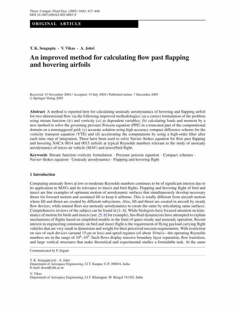
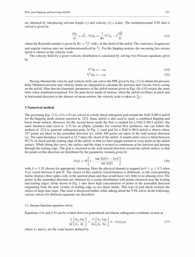
The governing Eqs. (11), (13)–(15) are solved in a body-fitted orthogonal grid around the NACA 0014 airfoilfor the flapping mode motion reported in [25]. Same airfoil is also used to study a combined flapping andhover mode motion. However, for the second hover mode the flow is studied for a NACA 0015 airfoil—thesame thickness ratio used in [17] for an elliptic cylinder. For external flow problems, one can follow themethod of [21] to generate orthogonal grids. In Fig. 1, used grid for a NACA 0014 airfoil is shown where257 points are taken in the azimuthal direction (ξ ), while 300 points are taken in the wall normal direction(η). The outer boundary is located at 22.5 times the chord of the airfoil. A fourth-order curve is fitted between99.7% of chord and the trailing edge of the airfoil, so that we have unique normal at every point on the airfoilsurface. While fitting this curve, the surface and the slope is treated as continuous at the junction and passingthrough the trailing edge. The grid is clustered in the wall normal direction toward the airfoil surface so thatthe points in this direction are distributed by the parametric formula given by

S(η) = H

[1 − tan h[β(1 − 2η)]

tan h[β]]

(16)

with β = 1.55 chosen for appropriate clustering. Here the physical domain is mapped in 0 ≤ η ≤ 0.5 whenS(η) varied between 0 and H . The choice of this analytic transformation is deliberate, as the correspondingmetric displays three spikes only in the spectral plane and thus would have very little or no aliasing error. Thepoints in the azimuthal direction are obtained by a cosine distribution with points clustered near the leadingand trailing edges. Grids shown in Fig. 1 also show high concentration of points in the azimuthal directionoriginating from the near vicinity of trailing edge as two dense bands. This type of grid shock restricts thechoice of large time steps. This issue is discussed further while talking about the VTE solver. In the following,various solvers for different equations are described.

3.1 Stream function equation solver

Equations (14) and (15) can be written down in generalized curvilinear orthogonal coordinate system as

∂

∂ξ

[h2

h1

∂ψI

∂ξ

]+ ∂

∂η

[h1

h2

∂ψI

∂η

]= −h1h2ωI (17)

where h1 and h2 are the scale factors defined by


Fig. 1 Orthogonal (257 × 300) grid generated by the hyperbolic grid generation method of [20]. Only the grids near the aerofoilsurface are shown

h21 =

(∂x

∂ξ

)2

+(

∂y

∂ξ

)2

and

h22 =

(∂x

∂η

)2

+(

∂y

∂η

)2

Similar representation can be written down for Eq. (15). To solve these two Poisson equations, on thesurface of the airfoil no-slip condition is used, while at the far-field the Neumann boundary conditions havebeen used: ∂ψI

∂η= Uo

∂y∂η

and ∂ψN∂η

= Uo∂y∂η

. The Poisson equations for stream functions are solved by thestrongly implicit procedure (SIP) as given in [30]. Instead of using the nine-point representation of [30], afive-point finite difference formula is used here employing second-order central differencing.

3.2 VTE solver

The VTE written in the moving frame of reference in nondimensional form is given by Eq. (13). This iswritten for the generalized curvilinear orthogonal coordinates as

h1h2∂ωr

∂t+ h2u

∂ωr

∂ξ+ h1v

∂ωr

∂η= 1

Re

[∂

∂ξ

(h2

h1

∂ωr

∂ξ

)+ ∂

∂η

(h1

h2

∂ωr

∂η

)]− 2�h1h2 (18)

Diffusion terms of this equation are discretized by standard second-order central differencing as theyappear in self-adjoint form. The associated linear algebraic equations are then in positive definite form thatconverges easily. Despite the linearity of these terms, computing the above equation at lower Reynolds numbersuffers from effects of aliasing error that does not create problems at higher Reynolds number due to thedivision by the higher value of Re. Aliasing problem can be avoided by creating smoothly varying grids thatdoes not show grid-shocks. Discussion about aliasing error of diffusion terms have been provided in detailsfor different grid types in [31]. In solving VTE, we distinguish between two types of problems when Dirichletboundary conditions are prescribed—in the first type, the vorticity and its derivatives are periodic (as in the ξdirection) and for the other type where the vorticity is nonperiodic. In choosing very high spectral accuracycompact schemes to evaluate first derivatives (indicated by primed quantities below), a general recursionrelation of the following form is used

b j−1u′j−1 + b j u

′j + b j+1u′

j+1 = 1

h

2∑

k=−2

a j+ku j+k (19)


In the periodic direction, the discretization error is minimized if one chooses the following coefficients inthe above equation [32]: b j±1 = 0.3793894912; b j = 1; a j±1 = ±0.7877868; a j±2 = ±0.0458012 anda j = 0. One solves the periodic tridiagonal system to evaluate the required first derivatives in this direction.While this scheme is formally second order accurate, the spectral accuracy obtained by this is one of thehighest among all the known compact schemes.

In the nonperiodic direction, one needs stable boundary closure schemes and the ones used here for thefirst and second node are [32, 33],

u′1 = −3u1 + 4u2 − u3

2h(20)

u′2 =

[(2β

3− 1

3

)u1 −

(8β

3+ 1

2

)u2 + (4β + 1)u3 −

(8β

3+ 1

6

)u4 + 2β

3u5

] /h (21)

with β as a parameter chosen to ensure accuracy and stability. Similar set of closure relations are employedfor the other end (at j = N and N − 1) of the nonperiodic direction. For the optimum performance, we haveused β = −0.025 for j = 2 and β = 0.09 for j = N − 1. Here, one solves a tridiagonal system to obtain thederivatives with respect to η for the vorticity employing this method. To numerically stabilize computations,an explicit fourth-order dissipation term is added to the calculated first derivatives.

Four-stage Runge–Kutta scheme is used to time-advance the above equation. For the grids shown in Fig. 1,when the flapping motion case was computed, it was noticed that only a very small time step is allowed forthe solution of Navier–Stokes equation. This stiff time-step restriction can be significantly relaxed by filteringthe vorticity values in the azimuthal direction after each step of time integration of VTE. As this directionis periodic, the eighth-order filter of [34] (given by Eq. (15) of the reference with the coefficients providedin Table IV) with α f = 0.49 is used for filtering the time-integrated vorticity values. The filtering allows toincrease the time-step by two orders of magnitude to 1.0E−05.

To solve the VTE, the required condition at the outer boundary is obtained by taking the vorticity equal to−2�. On the airfoil surface vorticity is continually created due to the requirement of no-slip condition. FromEq. (17), one can calculate the wall vorticity as

ωr|body = − 1

h22

∂2ψr

∂η2

∣∣∣∣∣body

(22)

After obtaining the velocity field by solving Eq. (17), new wall vorticity is calculated from Eq. (22) thatis used as the boundary condition for integrating the VTE given by Eq. (18). At the cut—originating from thetrailing edge of the airfoil—periodic boundary condition is applied for the vorticity.

3.3 Pressure solver

For the orthogonal curvilinear co-ordinate system the governing PPE given by Eq. (11) can be rewritten as

∂

∂ξ

(h2

h1

∂ PI

∂ξ

)+ ∂

∂η

(h1

h2

∂ PI

∂η

)= ∂

∂ξ(h2vIωI) − ∂

∂η(h1uIωI) (23)

where PI = pρ

+ V 2I

2 , uI = 1h2

∂ψI∂η

, and vI = − 1h1

∂ψI∂ξ

.Equation (23) is solved subject to the boundary condition derived from the normal momentum equation

as applied on the airfoil and the outer boundary. These are obtained from the normal (η) momentum equationgiven by

h1

h2

∂ PI

∂η= −h1uIωI + 1

Re

∂ωI

∂ξ− h1

∂vI

∂t(24)

Unlike other boundary conditions used in CFD over truncated domain, this boundary condition is exact.For this reason, it is possible to truncate the domain to obtain the pressure field and also to calculate loadsseparately for multiply connected domains. In doing so the accuracy of the load calculated is not compromisedif a consistent differencing of the equation and boundary conditions are used. This is discussed next, wherewe extend the procedure of [22] to the more general case solved here. In Abdallah [22], only the steady


state boundary condition was considered in a Cartesian frame with uniform non-staggered grid system for adriven cavity problem. Presented formulation for the PPE is one major development reported here. The caseconsidered here, does not require that the Neumann boundary condition to be steady at the far-field boundary.Also the problem solved here is in a curvilinear orthogonal clustered grid system.

Abdallah [22] has shown that the existence of solution for PPE requires the satisfaction of a compatibilitycondition that relates the source terms with the Neumann boundary condition—a consequence of applyingthe Green’s theorem for the PPE. This condition is not satisfied automatically in a non-staggered grid sys-tem and solution drifts without convergence. This is explained for the Poisson equation: ∇2 P = σ in atwo-dimensional plane. Existence of the solution to this with Neumann boundary condition requires uponapplication of divergence theorem

∫ ∫

AreaσdA =

∮∂ P

∂ηdl (25)

It has been shown in [22] that satisfying (25) is equivalent to the following identities:

LHM = RHM = 0 (26)

where the LHM and RHM are the finite difference analog of the left and right-hand side respectively for Eqs.(23) and (24) summed over all the nodes in the computing domain. To ensure that this is indeed true, specificstencils are to be chosen for the discretization. For example, Eq. (23) is discretized as

1

�ξ2

(h2

h1

∣∣∣∣(i+1/2, j)

PI (i+1, j) + h2

h1

∣∣∣∣(i−1/2, j)

PI (i−1, j)

)−

(1

�ξ2

[h2

h1

∣∣∣∣(i+1/2, j)

+ h2

h1

∣∣∣∣(i−1/2, j)

]

+ 1

�η2

[h1

h2

∣∣∣∣(i, j+1/2)

+ h1

h2

∣∣∣∣(i, j−1/2)

])PI (i, j) + 1

�η2

(h1

h2

∣∣∣∣(i, j+1/2)

PI (i, j+1) + h1

h2

∣∣∣∣(i, j−1/2)

PI (i, j−1)

)

= (h2vω)(i+1/2, j) − (h2vω)(i−1/2, j)

�ξ− (h1uω)(i, j+1/2) − (h1uω)(i, j−1/2)

�η(27)

for 2 ≤ i ≤ n and 2 ≤ j ≤ m, where the subscript i denotes constant ξ -lines and the subscript j denotesconstant η-lines. The half-node quantities are taken as the arithmetic average of adjacent cell values. Theright-hand side quantities of Eq. (27) are discretized in the following manner:

(h2vω)(i+1/2, j) = 1

8{h2|(i, j) + h2|(i+1, j)}{v(i, j) + v(i+1, j)}{ω(i, j) + ω(i+1, j)}

(h2vω)(i−1/2, j) = 1

8{h2|(i, j) + h2|(i−1, j)}{v(i, j) + v(i−1, j)}{ω(i, j) + ω(i−1, j)}

(h1uω)(i, j+1/2) = 1

8{h1|(i, j) + h1|(i, j+1)}{ω(i, j) + ω(i, j+1)}{u(i, j) + u(i, j+1)}

(h1uω)(i, j−1/2) = 1

8{h1|(i, j) + h1|(i, j−1)}{ω(i, j) + ω(i, j−1)}{u(i, j) + u(i, j−1)}

Neumann boundary condition (24) on the airfoil surface is discretized as follows:

PI (i,2) − PI (i,1)

�η= 1

Re

(h2

h1

∂ω

∂ξ

)

(i,3/2)

− (h2uω)(i,3/2) −[

h2∂v

∂t

]

(i,3/2)

(28)

To make LHM equal to zero, the above equation has been multiplied by 1�η

[ h1h2

](i,3/2) on both sides.Individual terms are discretized as indicated above. The last term of the right-hand side is represented as

[h1

∂v

∂t

]

(i,3/2)

= − ∂

∂t

(∂ψI

∂ξ

)

(i,3/2)

(29)


The right-hand side quantities are obtained as central averages with individual quantities discretized usingsecond-order central difference scheme. Similarly, the Neumann boundary condition at the outer boundary iswritten as

PI (i,m−1) − PI (i,m)

�η= 1

Re

(h2

h1

∂ω

∂ξ

)

(i,m−1/2)

− (h2uω)(i,m−1/2) −[

h2∂v

∂t

]

(i,m−1/2)

(30)

This equation is multiplied by 1�η

[ h1h2

](i,m−1/2) to make LHM equal to zero. The discretization procedureis similar to that adopted for the Neumann boundary condition applied on the airfoil surface. Discretizedequations are then solved using the conjugate-gradient algorithm of [35]. The above formulation of the PPEwith the boundary condition of (24) is solved following the discretization as indicated above and it can alsobe solved by taking a smaller domain as compared to the domain used for solving SFEs and the VTE. This isdue to the fact that the boundary condition used here are exact up to the accuracy by which the velocity andvorticity fields are numerically calculated.

3.4 Validation studies

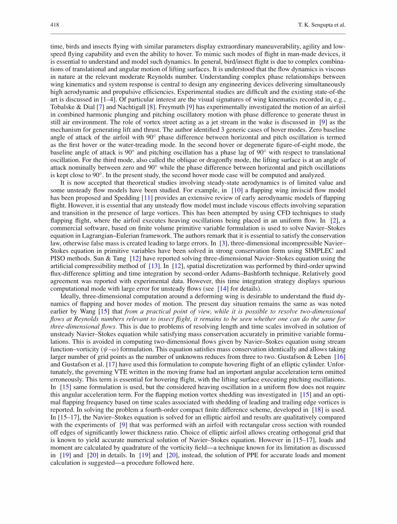
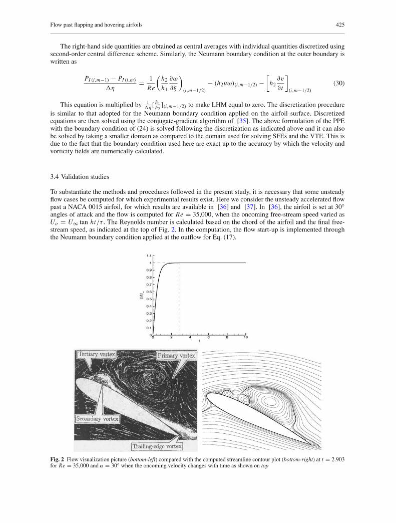
To substantiate the methods and procedures followed in the present study, it is necessary that some unsteadyflow cases be computed for which experimental results exist. Here we consider the unsteady accelerated flowpast a NACA 0015 airfoil, for which results are available in [36] and [37]. In [36], the airfoil is set at 30◦angles of attack and the flow is computed for Re = 35,000, when the oncoming free-stream speed varied asUo = U∞ tan ht/τ . The Reynolds number is calculated based on the chord of the airfoil and the final free-stream speed, as indicated at the top of Fig. 2. In the computation, the flow start-up is implemented throughthe Neumann boundary condition applied at the outflow for Eq. (17).

Fig. 2 Flow visualization picture (bottom-left) compared with the computed streamline contour plot (bottom-right) at t = 2.903for Re = 35,000 and α = 30◦ when the oncoming velocity changes with time as shown on top


In Fig. 2, the computed streamline contours are compared with flow visualization picture of [36]. The finalsteady mean flow velocity is 64 cm/s in dimensional units and τ is the characterstic acceleration time givenby 50 ms—that is equal to 0.60 in the nondimensional unit used in the present formulation. The mean flowcreates a nonuniform acceleration for a time up to 100 ms, beyond which the mean flow remains steady but theunsteady effects persist much longer. The computed and experimental results shown in Fig. 2 corresponds tot = 2.903—a nondimensional time. It is noted that the computed flow field matches with all essential detailsof the experimental visualization data, in terms of size, shape and orientations of the primary, secondary, andtertiary vortices.

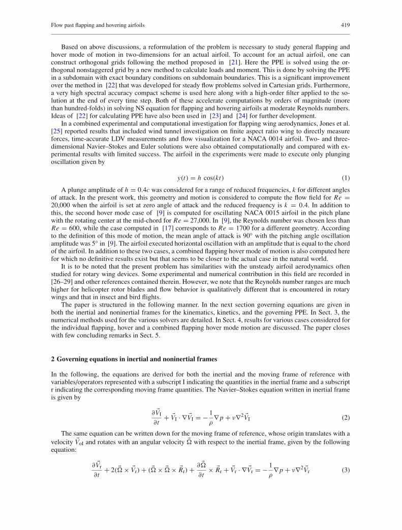
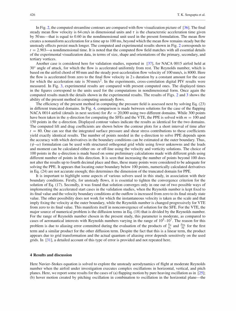
Another case is considered here for validation studies, reported in [37], for NACA 0015 airfoil held at30◦ angle of attack, for which the flow is accelerated uniformly from rest. The Reynolds number, which isbased on the airfoil chord of 80 mm and the steady post-acceleration flow velocity of 100 mm/s, is 8000. Herethe flow is accelerated from zero to the final flow velocity in 2 s duration by a constant amount for the casefor which the acceleration rate is 50 mm/s2. In the experiments, cross-correlation digital PIV results weremeasured. In Fig. 3, experimental results are compared with present computed ones. The displayed timesin the figures correspond to the units used for the computations in nondimensional form. Once again thecomputed results match the details shown in the experimental results. The results of Figs. 2 and 3 shows theability of the present method in computing unsteady flows.

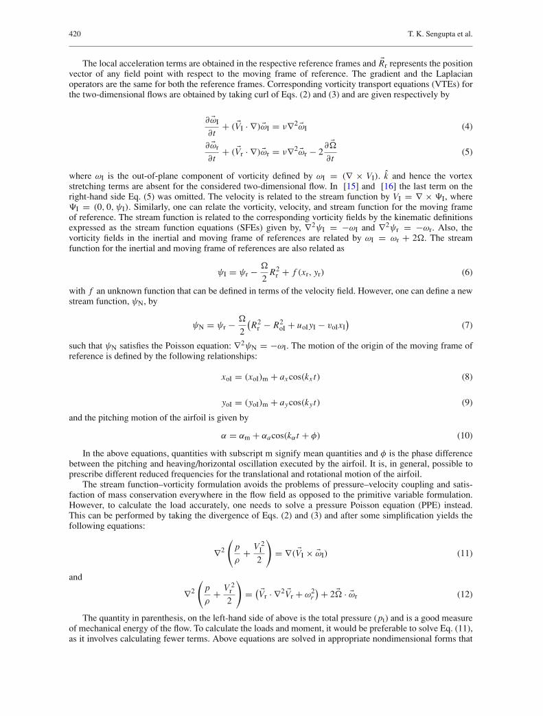
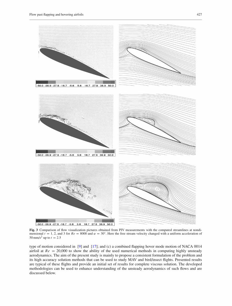
The efficiency of the present method in computing the pressure field is assessed next by solving Eq. (23)in different truncated domains. In Fig. 4, comparison is made between solutions for the case of the flappingNACA 0014 airfoil (details in next section) for Re = 20,000 using two different domains. While 300 pointshave been taken in the η-direction for computing the SFEs and the VTE, the PPE is solved with m = 100 and150 points in the η-direction. Displayed contour values indicate the results as identical for the two domains.The computed lift and drag coefficients are shown below the contour plots for a short interval of time aftert = 80. One can see that the integrated surface pressure and shear stress contributions to these coefficientsyield exactly identical results. The number of points needed in the η-direction to solve PPE depends uponthe accuracy with which derivatives in the boundary conditions can be estimated at the outer boundary. Thus,(ψ–ω) formulation can be used with structured orthogonal grid while using fewer unknowns and the loadsand moment can be calculated either on- or off-line using the velocity and vorticity solutions. The choice of100 points in the η-direction is made based on some preliminary calculations made with different grids usingdifferent number of points in this direction. It is seen that increasing the number of points beyond 100 doesnot alter the results up to fourth decimal place and thus, these many points were considered to be adequate forsolving the PPE. It appears that locating outer boundary below 100 points, numerically calculated derivativesin Eq. (24) are not accurate enough; this determines the dimension of the truncated domain for PPE.

It is important to highlight some aspects of various solvers used in this study, in association with theirboundary conditions. Firstly, for unsteady flows, it is essential to tighten the convergence criterion for thesolution of Eq. (17). Secondly, it was found that solution converges only in one out of two possible ways ofimplementing the accelerated start cases in the validation studies, when the Reynolds number is kept fixed toits final value and the velocity boundary conditions at the outflow is increased from zero to its final steady statevalue. The other possibility does not work for which the instantaneous velocity is taken as the scale and thatimply fixing the velocity at the outer boundary, while the Reynolds number is changed progressively for VTEfrom zero to its final value. This manifests itself in nonconvergence of solution for the SFE. For the VTE, themajor source of numerical problem is the diffusion terms in Eq. (18) that is divided by the Reynolds number.For the range of Reynolds number chosen in the present study, this parameter is moderate, as compared tocases of aeronautical interests with Reynolds numbers varying in the range of 105–107. The reason for thisproblem is due to aliasing error committed during the evaluation of the products of h2

h1and ∂ωr

∂ξfor the first

term and a similar product for the other diffusion term. Despite the fact that this is a linear term, the productappears due to grid transformation and the actual quantum of aliasing error depends sensitively on the usedgrids. In [31], a detailed account of this type of error is provided and not repeated here.

4 Results and discussion

Here Navier–Stokes equation is solved to explore the unsteady aerodynamics of flight at moderate Reynoldsnumber when the airfoil under investigation executes complex oscillations in horizontal, vertical, and pitchplanes. Here, we report some results for the cases of (a) flapping motion by pure heaving oscillation as in [25];(b) hover motion created by pitching oscillation in combination to oscillation in the horizontal plane—the


Fig. 3 Comparison of flow visualization pictures obtained from PIV measurements with the computed streamlines at nondi-mensional t = 1, 2, and 3 for Re = 8000 and α = 30◦. Here the free stream velocity changed with a uniform acceleration of50 mm/s2 up to t = 2.5

type of motion considered in [9] and [17]; and (c) a combined flapping hover mode motion of NACA 0014airfoil at Re = 20,000 to show the ability of the used numerical methods in computing highly unsteadyaerodynamics. The aim of the present study is mainly to propose a consistent formulation of the problem andits high accuracy solution methods that can be used to study MAV and bird/insect flights. Presented resultsare typical of these flights and provide an initial set of results for complete viscous solution. The developedmethodologies can be used to enhance understanding of the unsteady aerodynamics of such flows and arediscussed below.


(a)

t

CL

81.5 82

-5

-4.5

-4

-3.5

-3

(b)

t

CD

81.5 82

0.6

0.65

0.7

0.75

0.8

0.85

0.9

(c)

(d)

t

CL

81.5 82

-5

-4.5

-4

-3.5

-3

(e)

t

CD

81.5 82

0.6

0.65

0.7

0.75

0.8

0.85

0.9

(f)

Fig. 4 Solution of PPE using two different values of m. a to c are for m = 100 and d to f are for m = 150. In a and d thepressure contours are shown; b and e show the lift variation with time and c and f show the variation of drag coefficient withtime

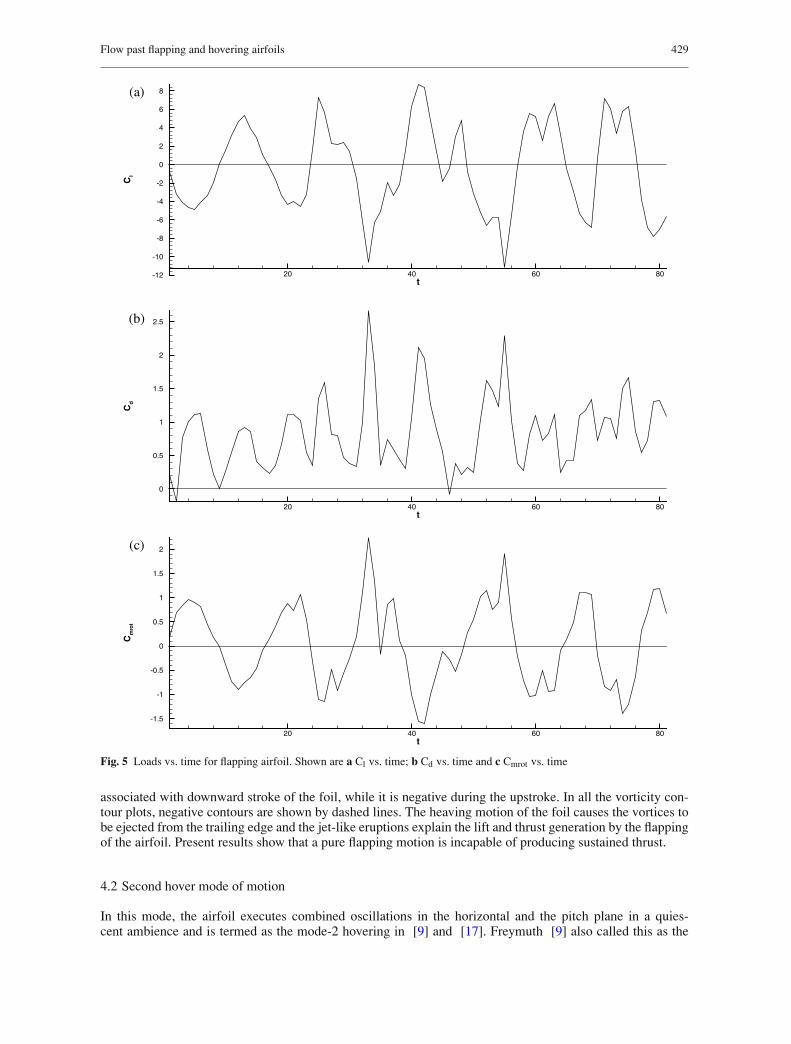
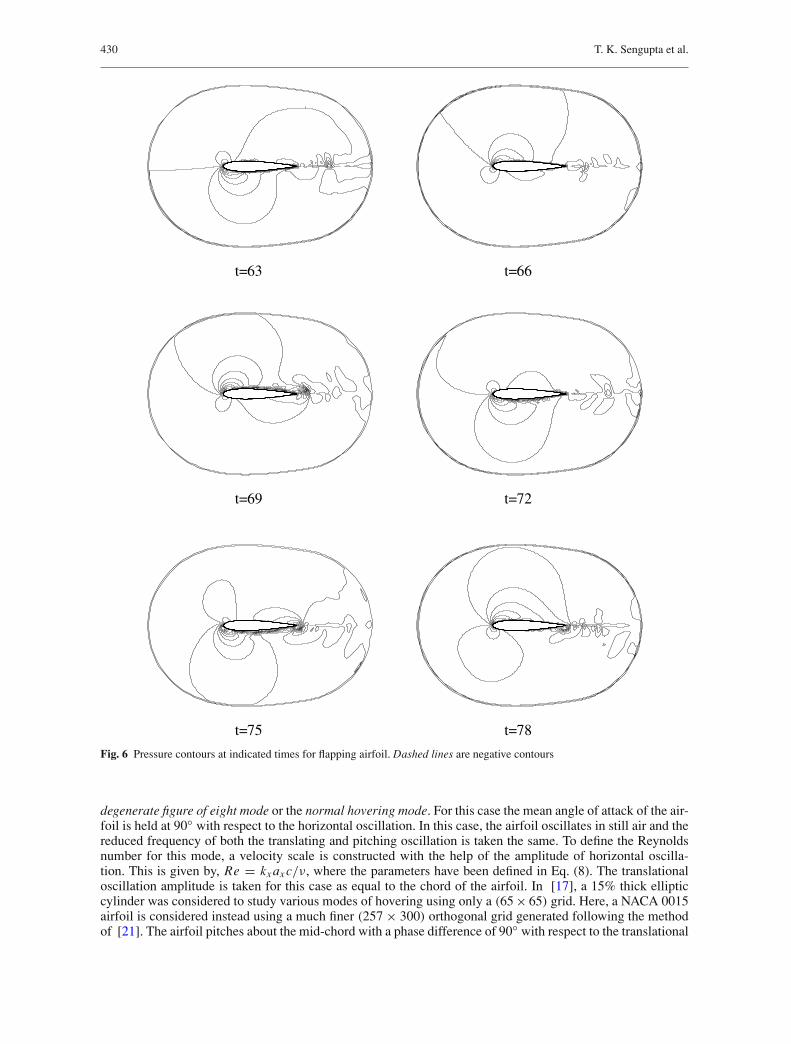
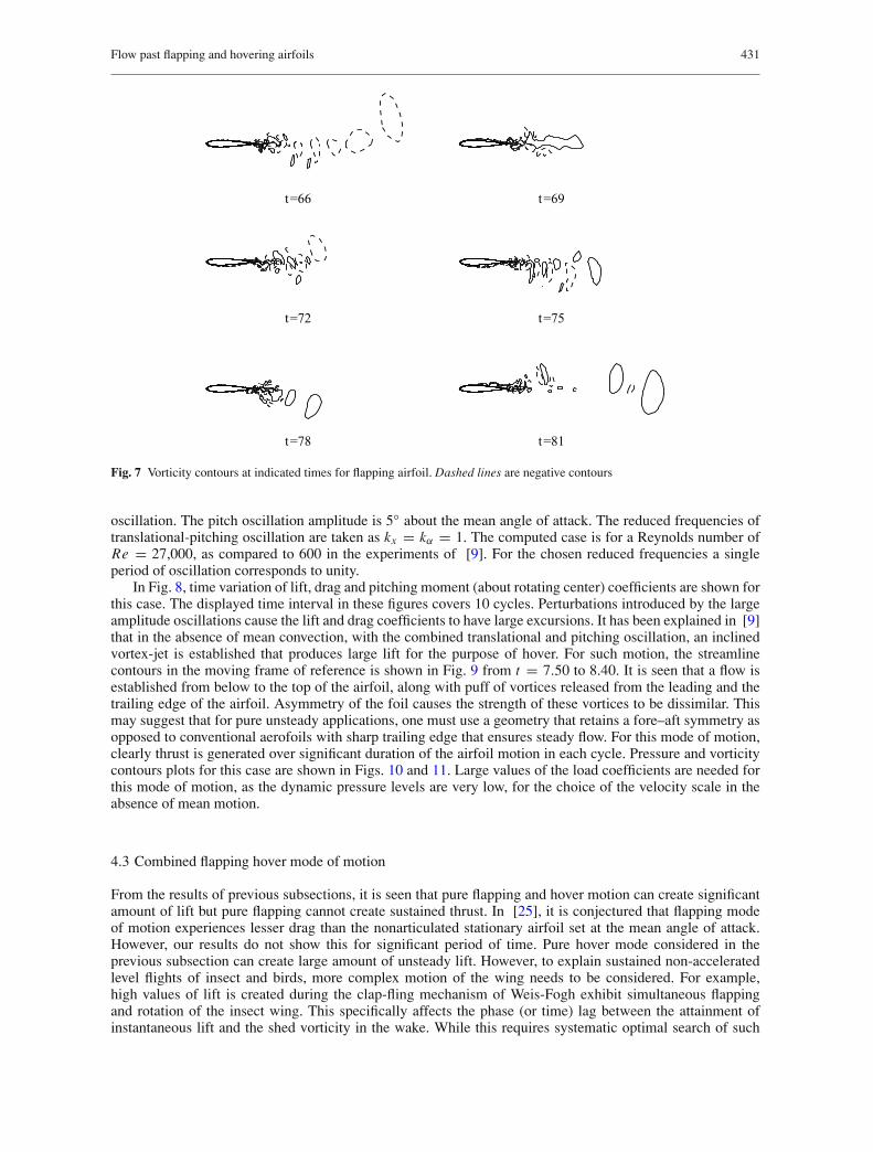
4.1 Flapping motion of an airfoil

In this mode, a case is considered that corresponds to that given in [25] for NACA 0014 airfoil at Re =20, 000. Here, the airfoil executes pure heaving oscillation for zero angle of attack setting. The heaving oscil-lation amplitude is equal to 0.40c producing large perturbations to the oncoming flow. The reduced frequencyof oscillation is given by k = 0.4. In Fig. 5, lift, drag and pitching moment (about mid-chord) coefficients areshown as time series. The period of heaving oscillation is 16 and the presented results are for about five cycles.Corresponding pressure and vorticity contour plots are shown in Figs. 6 and 7, respectively. Pressure is calcu-lated over a truncated domain whose rationale is already discussed with respect to Fig. 4. High values of lift is


t

Cl

20 40 60 80-12

-10

-8

-6

-4

-2

0

2

4

6

8(a)

t

Cd

20 40 60 80

0

0.5

1

1.5

2

2.5(b)

t

Cm

rot

20 40 60 80

-1.5

-1

-0.5

0

0.5

1

1.5

2(c)

Fig. 5 Loads vs. time for flapping airfoil. Shown are a Cl vs. time; b Cd vs. time and c Cmrot vs. time

associated with downward stroke of the foil, while it is negative during the upstroke. In all the vorticity con-tour plots, negative contours are shown by dashed lines. The heaving motion of the foil causes the vortices tobe ejected from the trailing edge and the jet-like eruptions explain the lift and thrust generation by the flappingof the airfoil. Present results show that a pure flapping motion is incapable of producing sustained thrust.

4.2 Second hover mode of motion

In this mode, the airfoil executes combined oscillations in the horizontal and the pitch plane in a quies-cent ambience and is termed as the mode-2 hovering in [9] and [17]. Freymuth [9] also called this as the


t=63 t=66

t=69 t=72

t=75 t=78

Fig. 6 Pressure contours at indicated times for flapping airfoil. Dashed lines are negative contours

degenerate figure of eight mode or the normal hovering mode. For this case the mean angle of attack of the air-foil is held at 90◦ with respect to the horizontal oscillation. In this case, the airfoil oscillates in still air and thereduced frequency of both the translating and pitching oscillation is taken the same. To define the Reynoldsnumber for this mode, a velocity scale is constructed with the help of the amplitude of horizontal oscilla-tion. This is given by, Re = kx ax c/ν, where the parameters have been defined in Eq. (8). The translationaloscillation amplitude is taken for this case as equal to the chord of the airfoil. In [17], a 15% thick ellipticcylinder was considered to study various modes of hovering using only a (65 × 65) grid. Here, a NACA 0015airfoil is considered instead using a much finer (257 × 300) orthogonal grid generated following the methodof [21]. The airfoil pitches about the mid-chord with a phase difference of 90◦ with respect to the translational


t=69

t=72

t=78

t=66

t=75

t=81

Fig. 7 Vorticity contours at indicated times for flapping airfoil. Dashed lines are negative contours

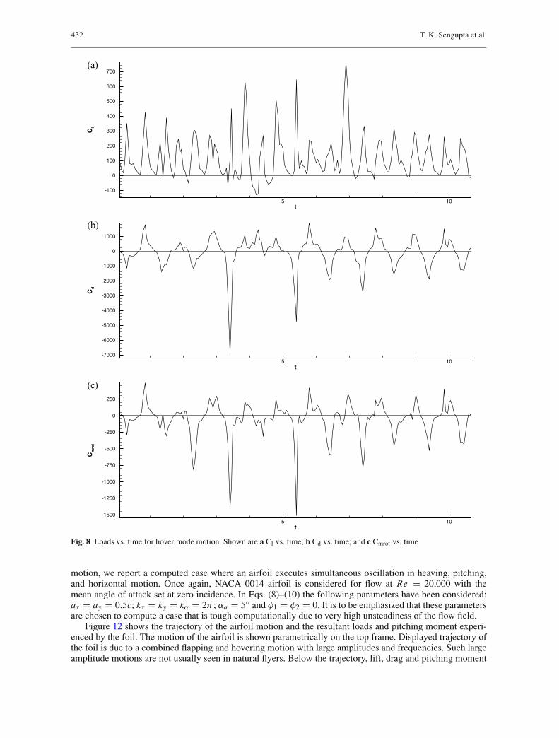
oscillation. The pitch oscillation amplitude is 5◦ about the mean angle of attack. The reduced frequencies oftranslational-pitching oscillation are taken as kx = kα = 1. The computed case is for a Reynolds number ofRe = 27,000, as compared to 600 in the experiments of [9]. For the chosen reduced frequencies a singleperiod of oscillation corresponds to unity.

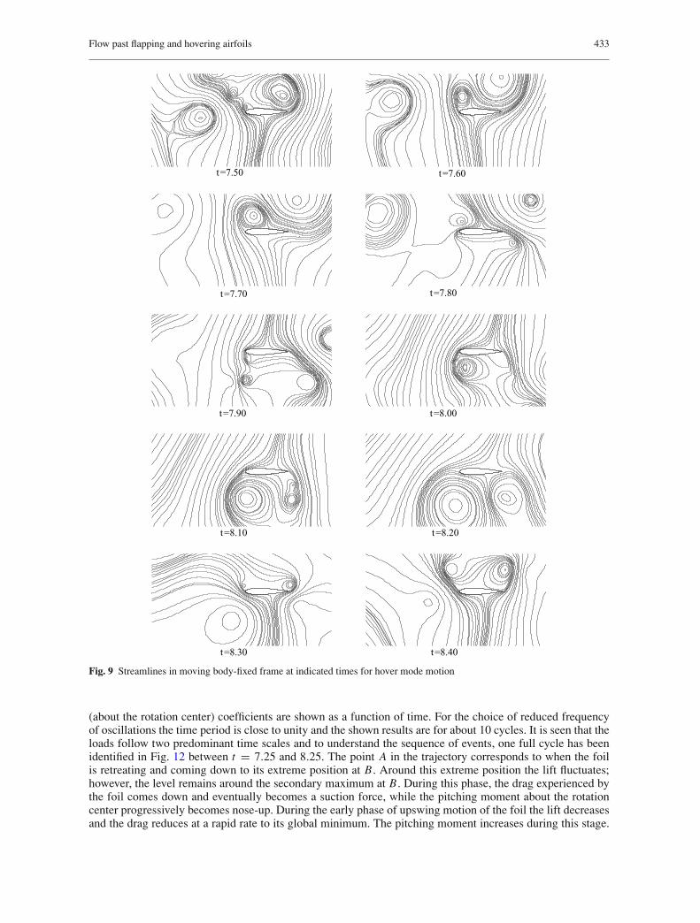
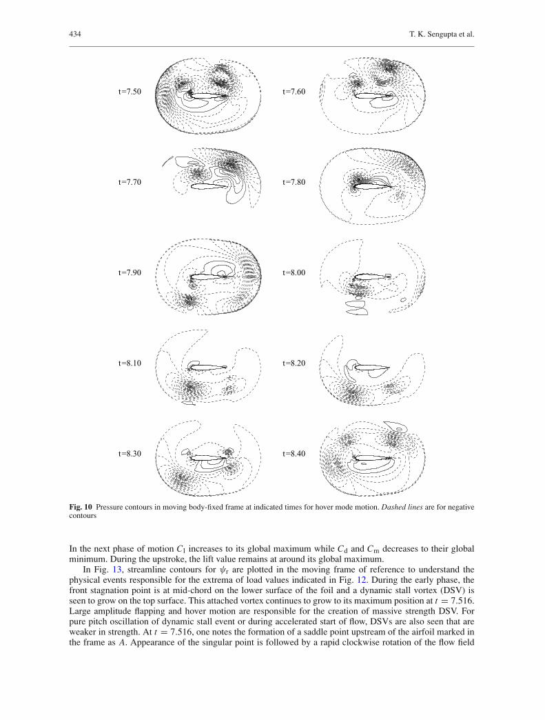
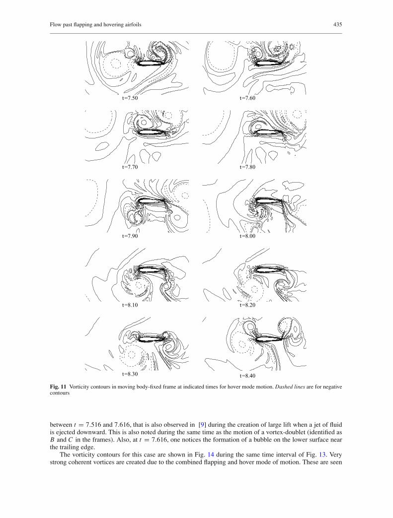
In Fig. 8, time variation of lift, drag and pitching moment (about rotating center) coefficients are shown forthis case. The displayed time interval in these figures covers 10 cycles. Perturbations introduced by the largeamplitude oscillations cause the lift and drag coefficients to have large excursions. It has been explained in [9]that in the absence of mean convection, with the combined translational and pitching oscillation, an inclinedvortex-jet is established that produces large lift for the purpose of hover. For such motion, the streamlinecontours in the moving frame of reference is shown in Fig. 9 from t = 7.50 to 8.40. It is seen that a flow isestablished from below to the top of the airfoil, along with puff of vortices released from the leading and thetrailing edge of the airfoil. Asymmetry of the foil causes the strength of these vortices to be dissimilar. Thismay suggest that for pure unsteady applications, one must use a geometry that retains a fore–aft symmetry asopposed to conventional aerofoils with sharp trailing edge that ensures steady flow. For this mode of motion,clearly thrust is generated over significant duration of the airfoil motion in each cycle. Pressure and vorticitycontours plots for this case are shown in Figs. 10 and 11. Large values of the load coefficients are needed forthis mode of motion, as the dynamic pressure levels are very low, for the choice of the velocity scale in theabsence of mean motion.

4.3 Combined flapping hover mode of motion

From the results of previous subsections, it is seen that pure flapping and hover motion can create significantamount of lift but pure flapping cannot create sustained thrust. In [25], it is conjectured that flapping modeof motion experiences lesser drag than the nonarticulated stationary airfoil set at the mean angle of attack.However, our results do not show this for significant period of time. Pure hover mode considered in theprevious subsection can create large amount of unsteady lift. However, to explain sustained non-acceleratedlevel flights of insect and birds, more complex motion of the wing needs to be considered. For example,high values of lift is created during the clap-fling mechanism of Weis-Fogh exhibit simultaneous flappingand rotation of the insect wing. This specifically affects the phase (or time) lag between the attainment ofinstantaneous lift and the shed vorticity in the wake. While this requires systematic optimal search of such


t

Cl

5 10

-100

0

100

200

300

400

500

600

700(a)

t

Cd

5 10-7000

-6000

-5000

-4000

-3000

-2000

-1000

0

1000

(b)

t

Cm

rot

5 10-1500

-1250

-1000

-750

-500

-250

0

250

(c)

Fig. 8 Loads vs. time for hover mode motion. Shown are a Cl vs. time; b Cd vs. time; and c Cmrot vs. time

motion, we report a computed case where an airfoil executes simultaneous oscillation in heaving, pitching,and horizontal motion. Once again, NACA 0014 airfoil is considered for flow at Re = 20,000 with themean angle of attack set at zero incidence. In Eqs. (8)–(10) the following parameters have been considered:ax = ay = 0.5c; kx = ky = kα = 2π ; αa = 5◦ and φ1 = φ2 = 0. It is to be emphasized that these parametersare chosen to compute a case that is tough computationally due to very high unsteadiness of the flow field.

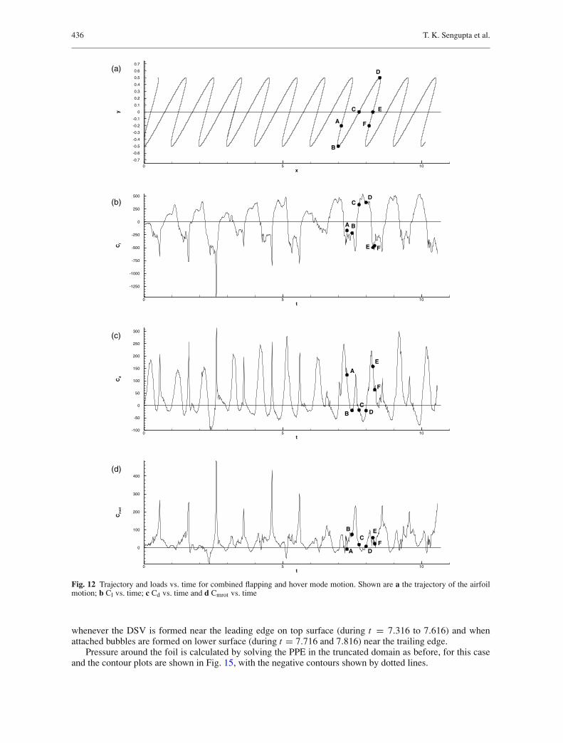
Figure 12 shows the trajectory of the airfoil motion and the resultant loads and pitching moment experi-enced by the foil. The motion of the airfoil is shown parametrically on the top frame. Displayed trajectory ofthe foil is due to a combined flapping and hovering motion with large amplitudes and frequencies. Such largeamplitude motions are not usually seen in natural flyers. Below the trajectory, lift, drag and pitching moment


t=7.50 t=7.60

t=7.70 t=7.80

t=7.90 t=8.00

t=8.10 t=8.20

t=8.30 t=8.40

Fig. 9 Streamlines in moving body-fixed frame at indicated times for hover mode motion

(about the rotation center) coefficients are shown as a function of time. For the choice of reduced frequencyof oscillations the time period is close to unity and the shown results are for about 10 cycles. It is seen that theloads follow two predominant time scales and to understand the sequence of events, one full cycle has beenidentified in Fig. 12 between t = 7.25 and 8.25. The point A in the trajectory corresponds to when the foilis retreating and coming down to its extreme position at B. Around this extreme position the lift fluctuates;however, the level remains around the secondary maximum at B. During this phase, the drag experienced bythe foil comes down and eventually becomes a suction force, while the pitching moment about the rotationcenter progressively becomes nose-up. During the early phase of upswing motion of the foil the lift decreasesand the drag reduces at a rapid rate to its global minimum. The pitching moment increases during this stage.


t=7.50 t=7.60

t=7.70

t=7.90

t=8.10

t=8.30

t=7.80

t=8.20

t=8.40

t=8.00

Fig. 10 Pressure contours in moving body-fixed frame at indicated times for hover mode motion. Dashed lines are for negativecontours

In the next phase of motion Cl increases to its global maximum while Cd and Cm decreases to their globalminimum. During the upstroke, the lift value remains at around its global maximum.

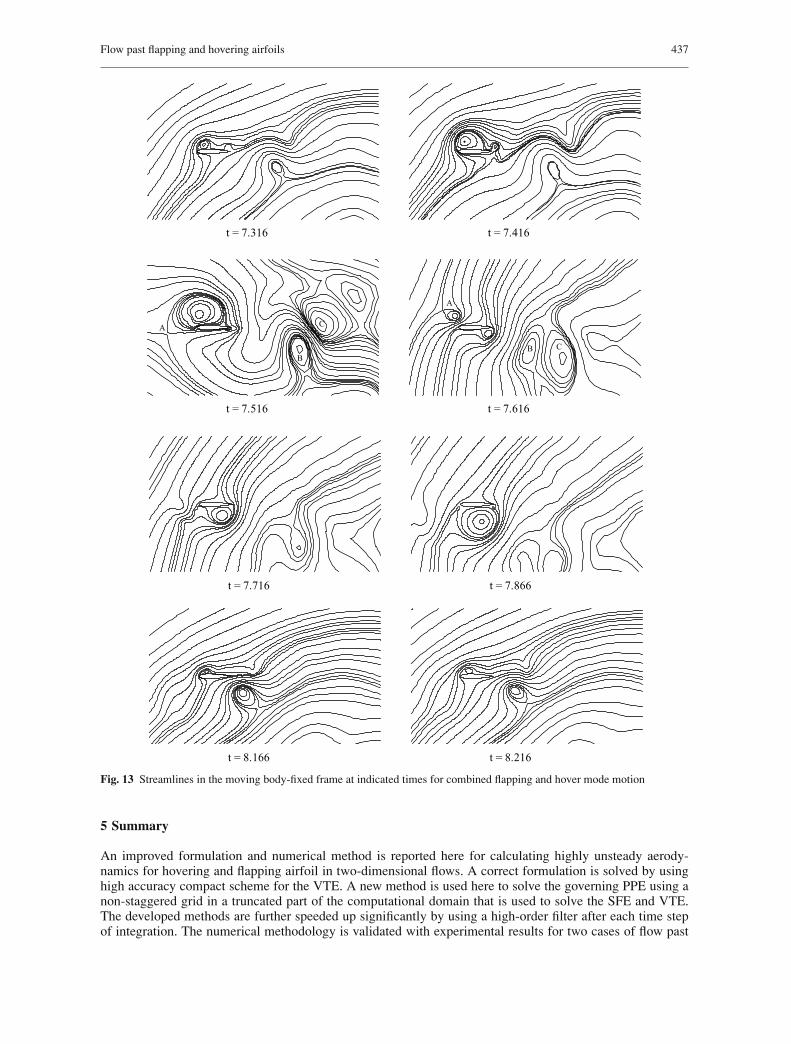
In Fig. 13, streamline contours for ψr are plotted in the moving frame of reference to understand thephysical events responsible for the extrema of load values indicated in Fig. 12. During the early phase, thefront stagnation point is at mid-chord on the lower surface of the foil and a dynamic stall vortex (DSV) isseen to grow on the top surface. This attached vortex continues to grow to its maximum position at t = 7.516.Large amplitude flapping and hover motion are responsible for the creation of massive strength DSV. Forpure pitch oscillation of dynamic stall event or during accelerated start of flow, DSVs are also seen that areweaker in strength. At t = 7.516, one notes the formation of a saddle point upstream of the airfoil marked inthe frame as A. Appearance of the singular point is followed by a rapid clockwise rotation of the flow field


t=7.70

t=7.90

t=8.30

t=8.00

t=8.40

t=7.50

t=7.80

t=7.60

t=8.10 t=8.20

Fig. 11 Vorticity contours in moving body-fixed frame at indicated times for hover mode motion. Dashed lines are for negativecontours

between t = 7.516 and 7.616, that is also observed in [9] during the creation of large lift when a jet of fluidis ejected downward. This is also noted during the same time as the motion of a vortex-doublet (identified asB and C in the frames). Also, at t = 7.616, one notices the formation of a bubble on the lower surface nearthe trailing edge.

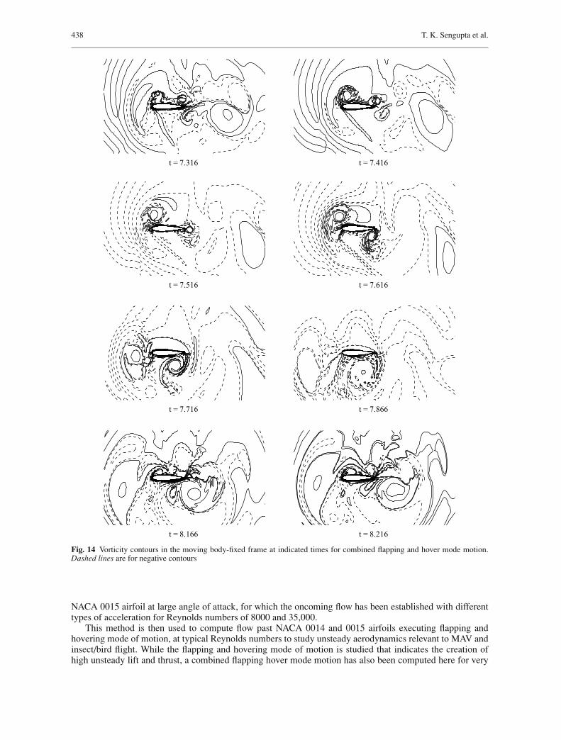
The vorticity contours for this case are shown in Fig. 14 during the same time interval of Fig. 13. Verystrong coherent vortices are created due to the combined flapping and hover mode of motion. These are seen


x

y

0 5 10

-0.7

-0.6

-0.5

-0.4

-0.3

-0.2

-0.1

0

0.1

0.2

0.3

0.4

0.5

0.6

0.7

(a)

A

B

C

D

E

F

t

Cl

0 5 10

-1250

-1000

-750

-500

-250

0

250

500

(b)

A B

CD

E F

t

Cd

0 5 10-100

-50

0

50

100

150

200

250

300(c)

A

BC

D

E

F

t

Cm

rot

0 5 10

0

100

200

300

400(d)

A

BC

D

E

F

Fig. 12 Trajectory and loads vs. time for combined flapping and hover mode motion. Shown are a the trajectory of the airfoilmotion; b Cl vs. time; c Cd vs. time and d Cmrot vs. time

whenever the DSV is formed near the leading edge on top surface (during t = 7.316 to 7.616) and whenattached bubbles are formed on lower surface (during t = 7.716 and 7.816) near the trailing edge.

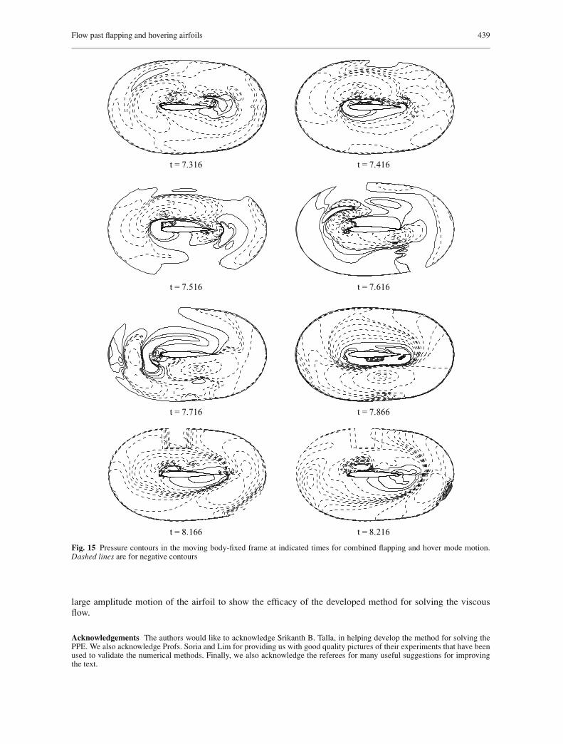
Pressure around the foil is calculated by solving the PPE in the truncated domain as before, for this caseand the contour plots are shown in Fig. 15, with the negative contours shown by dotted lines.


t = 7.316 t = 7.416

t = 7.516

A

B

C

t = 7.616

A

B C

t = 7.716 t = 7.866

t = 8.166 t = 8.216

Fig. 13 Streamlines in the moving body-fixed frame at indicated times for combined flapping and hover mode motion

5 Summary

An improved formulation and numerical method is reported here for calculating highly unsteady aerody-namics for hovering and flapping airfoil in two-dimensional flows. A correct formulation is solved by usinghigh accuracy compact scheme for the VTE. A new method is used here to solve the governing PPE using anon-staggered grid in a truncated part of the computational domain that is used to solve the SFE and VTE.The developed methods are further speeded up significantly by using a high-order filter after each time stepof integration. The numerical methodology is validated with experimental results for two cases of flow past


t = 7.316 t = 7.416

t = 7.516 t = 7.616

t = 7.716 t = 7.866

t = 8.166 t = 8.216

Fig. 14 Vorticity contours in the moving body-fixed frame at indicated times for combined flapping and hover mode motion.Dashed lines are for negative contours

NACA 0015 airfoil at large angle of attack, for which the oncoming flow has been established with differenttypes of acceleration for Reynolds numbers of 8000 and 35,000.

This method is then used to compute flow past NACA 0014 and 0015 airfoils executing flapping andhovering mode of motion, at typical Reynolds numbers to study unsteady aerodynamics relevant to MAV andinsect/bird flight. While the flapping and hovering mode of motion is studied that indicates the creation ofhigh unsteady lift and thrust, a combined flapping hover mode motion has also been computed here for very


t = 7.316 t = 7.416

t = 7.516 t = 7.616

t = 7.716 t = 7.866

t = 8.166 t = 8.216

Fig. 15 Pressure contours in the moving body-fixed frame at indicated times for combined flapping and hover mode motion.Dashed lines are for negative contours

large amplitude motion of the airfoil to show the efficacy of the developed method for solving the viscousflow.

Acknowledgements The authors would like to acknowledge Srikanth B. Talla, in helping develop the method for solving thePPE. We also acknowledge Profs. Soria and Lim for providing us with good quality pictures of their experiments that have beenused to validate the numerical methods. Finally, we also acknowledge the referees for many useful suggestions for improvingthe text.


References

1. Rozhdestvensky, K.V., Ryzhov, V.A.: Aerohydrodynamics of flapping-wing propulsors. Prog. Aerospace Sci. 39, 585–633(2003)

2. Ho, S., Nassef, H., Pornsinsirirak, N., Tai, Y.-C., Ho, C.M.: Unsteady aerodynamics and flow control for flapping wingflyers. Prog. Aerosp. Sci. 39, 635–681 (2003)

3. Lian, Y., Shyy, W., Viieru, D., Zhang, B.: Membrane wing aerodynamics for micro air vehicles. Prog. Aerosp. Sci. 39,425–465 (2003)

4. Sane, S.P.: The aerodynamics of insect flight. J. Exp. Biol. 206, 4191–4208 (2003)5. Norberg, U.M.: Vertebrate flight: mechanics, physiology, morphology, ecology and evolution. Springer, New York (1990)6. Pennycuick, C.J.: Actual and ‘optimum’ flight speeds: field data reassessed. J. Exp. Biol. 200, 2355–2361 (1997)7. Tobalske, B.W., Dial, K.P.: Flight kinematics of black-billed magpies and pigeons over a wide range of speed. J. Exp. Biol.

199, 263–280 (1996)8. Nachtigall, W.: Insects in flight. Mc-Graw Hill, New York (1974)9. Freymuth, P.: Thrust generation by an airfoil in hover modes. Exp. Fluids 9, 17–24 (1990)

10. DeLaurier, J.D.: An aerodynamic model for flapping wing flight. Aeronaut. J. 97, 125–130 (1993)11. Spedding, G.R.: The aerodynamics of flight. Adv. Comp. Env. Physiol. 11, 51–111 (1992)12. Sun, M., Tang, J.: Lift and power requirements of hovering flight in Drosophila virilis. J. Exp. Biol. 205, 2413–2427 (2002)13. Rogers, S.E., Kwak, D.: Upwind differencing scheme for the time-accurate incompressible Navier–Stokes equation. AIAA

J. 28, 253–262 (1990)14. Sengupta, T.K., Dipankar, A.: A comparative study of time advancement methods for solving Navier–Stokes equations. J.

Sci. Comp. 21(2), 225–250 (2004)15. Wang, Z.J.: Vortex shedding and frequency selection in flapping flight. J. Fluid Mech. 410, 323–341 (2000)16. Gustafson, K., Leben, R.: Computation of dragonfly aerodynamics. Comput. Phys. Commun. 65, 121–132 (1991)17. Gustafson, K., Leben, R., McArthur, J.: Lift and thrust generation by an airfoil in hover modes, Comput. Fluid Dyn. J. 1(1),

47–57 (1992)18. Weinan, E., Liu, J.-G.: Essentially compact schemes for unsteady viscous incompressible flows. J. Comput. Phys. 126, 122

(1996)19. Roache, P.J.: Computational fluid dynamics. Hermosa Publishers. New Mexcio, USA (1976)20. Sengupta, T.K., Kasliwal, A., De, S., Nair, M.: Temporal flow instability for Magnus-Robins effect at high rotation rates. J.

Fluids Struct. 17, 941–953 (2003)21. Nair, M.T., Sengupta, T.K.: Orthogonal grid generation for Navier–Stokes computations. Int. J. Num. Meth. Fluids 28,

215–224 (1998)22. Abdallah, S.: Numerical solutions for the pressure Poisson equation with Neumann boundary conditions using a nonstag-

gered grid-I. J. Comput. Phys. 70, 182–192 (1987)23. Grescho, P.M., Sani, R.L.: On pressure boundary conditions for the incompressible Navier–Stokes equation. Int. J. Num.

Meth. Fluids 7, 1111–1145 (1987)24. Clayssen, J.R., Platte, R.B., Bravo, E.: Simulation in primitive variables of incompressible flow with pressure Neumann

condition. Int. J. Num. Meth. Fluids 30, 1009–1026 (1999)25. Jones, K.D., Castro, B.M., Mahmoud, O., Pollard, S.J., Platzer, M.F., Neef, M.F., Gonet, K., Hummel, D.: A collaborative

numerical and experimental investigation of flapping-wing propulsion. AIAA Paper No. AIAA-2002–0706 (2002)26. McCroskey, W.J.: Unsteady airfoils. Ann. Rev. Fluid Mech., 24, 285–311 (1982)27. Carr, L.W.: Progress in analysis and prediction of dynamic stall. J. Aircraft 25(1), 6–17 (1988)28. Bousman, W.G.: Airfoil dynamic stall and rotorcraft maneuverability. NASA TM-2000–209601 (2000)29. Berton, E., Maresca, C., Favier, D.: A new experimental method for determining local airloads on rotor blades in forward

flight. Exp. Fluids 37(3), 455–457 (2004)30. Schneider, G.E., Zedan, M.: A modified strongly implicit procedure for the numerical solution of field problems. J. Numer.

Heat Transf. 4, 1–19 (1981)31. Sengupta, T.K.: Fundamentals of CFD. Universities Press. Hyderabad, India (2004)32. Sengupta, T.K., Guntaka, A., Dey, S.: Navier–Stokes solution by new compact scheme for incompressible flows. J. Sci.

Comput. 21(3), 269–282 (2004)33. Sengupta, T.K., Ganeriwal, G., De, S.: Analysis of central and upwind compact schemes. J. Comput. Phys. 192, 677–694

(2003)34. Visval, M.R., Gaitonde, D.V.: On the use of higher order finite-difference schemes on curvilinear and deforming meshes. J.

Comput. Phys. 181, 155–185 (2002)35. Van Der Vorst, H.A.: Bi-CGSTAB: A fast and smoothly converging variant of Bi-CG for the solution of nonsymmetric

linear systems. SIAM J. Sci. Stat. Comput. 13(2), 631–644 (1992)36. Morikawa, K., Gronig, H.: Formation and structure of vortex systems around a translating and oscillating airfoil. Z. Flug-

wiss. Weltraumforsch. 19, 391–396 (1995)37. Soria, J., New, T.H., Lim, T.T., Parker, K.: Multigrid CCDPIV measurements of accelerated flow past an airfoil at an angle

of attack of 30o. Exp. Therm. Fluid Sci. 27, 667–676 (2003)

an improved method for calculating flow past flapping and hovering airfoils

Documents