an empirical comparison of kriging methods for nonlinear spatial point prediction

P1: FHD/GMF/GIR/GGT P2: GCR/FOM/GCY QC:

Mathematical Geology [mg] pp429-matg-369676 March 26, 2002 11:0 Style file version June 30, 1999

Mathematical Geology, Vol. 34, No. 4, May 2002 (C© 2002)

An Empirical Comparison of Kriging Methodsfor Nonlinear Spatial Point Prediction1

Rana A. Moyeed2 and Andreas Papritz3

Spatial prediction is a problem common to many disciplines. A simple application is the mapping of anattribute recorded at a set of points. Frequently a nonlinear functional of the observed variable is ofinterest, and this calls for nonlinear approaches to prediction. Nonlinear kriging methods, developedin recent years, endeavour to do so and additionally provide estimates of the distribution of the targetquantity conditional on the observations. There are few empirical studies that validate the variousforms of nonlinear kriging. This study compares linear and nonlinear kriging methods with respect toprecision and their success in modelling prediction uncertainty. The methods were applied to a data setgiving measurements of the topsoil concentrations of cobalt and copper at more than 3000 locations inthe Border Region of Scotland. The data stem from a survey undertaken to identify places where thesetrace elements are deficient for livestock. The comparison was carried out by dividing the data setinto calibration and validation sets. No clear differences between the precision of ordinary, lognormal,disjunctive, indicator, and model-based kriging were found, neither for linear nor for nonlinear targetquantities. Linear kriging, supplemented with the assumption of normally distributed prediction errors,failed to model the conditional distribution of the marginally skewed data, whereas the nonlinearmethods modelled the conditional distributions almost equally well. In our study the plug-in methodsdid not fare any worse than model-based kriging, which takes parameter uncertainty into account.

KEY WORDS: nonlinear kriging, parameter uncertainty, precision, validation.

INTRODUCTION

One of the most basic problem in geostatistics is that of spatial prediction. Predic-tions are often required for planning, risk assessment, and decision-making. Typicalexamples include determining the profitability of mining an orebody, managementof soil resources, cost-effective remediation of soil pollutants, designing a networkof environmental monitoring stations, and, last but not least, quantifying the un-certainties inherent in spatial prediction. In these and many other applications the

1Received 21 July 2000; accepted 28 March 2001.2Department of Mathematics and Statistics, University of Plymouth, Drake Circus, Plymouth PL4 8AA,United Kingdom; e-mail: [email protected]

3Institute of Terrestrial Ecology, Swiss Federal Institute of Technology ETHZ, Grabenstrasse 3,CH-8952 Schlieren, Switzerland; e-mail: [email protected]

365

0882-8121/02/0500-0365/1C© 2002 International Association for Mathematical Geology



366 Moyeed and Papritz

target quantity is a nonlinear functional of the recorded attributes, and it can be pre-dicted optimally for any criterion, given an estimate of its probability distributionconditional on the available information.

The need to model the conditional distribution of the rock metal contentin mining gave the impetus for developing the nonlinear prediction methods ofdisjunctive kriging (Armstrong and Matheron, 1986a,b; Matheron, 1976a,b) inthe 1970s and indicator (Journel, 1983), probability (Sullivan, 1984), and multi-Gaussian kriging (Verly, 1983, 1984) a decade later, although a variant of thelatter method, lognormal kriging, was in use before. Recently, Diggle, Tawn, andMoyeed (1998) have developed a fully model-based method by embedding thelinear kriging methodology within a more general distributional framework thatis characteristically similar to the structure of a generalized linear model. Theyadopt a Bayesian approach, implemented via the Markov chain Monte Carlo(MCMC) methodology, to predict arbitrary functionals of an unobserved latentprocess whilst making a proper allowance for the uncertainty in the estimation ofany model parameters. Henceforth, we shall refer to this approach as model-basedkriging.

Nonlinear kriging methods have, at least theoretically, a further advantageover linear kriging: their predictions should be more precise when a Gaussianrandom process is inappropriate to model the observations. The conditional ex-pectation, which minimizes the mean square error of prediction, is in this case nolonger linear in the observations, and nonlinear techniques are expected to performbetter. Departures from the Gaussian model occur frequently in practice where thedata are often positively skewed.

The practitioner does not get much advice from the literature about the methodthat may be the most suitable to use. It appears that the various approaches weredeveloped by different “schools” that had little interest in exploring merits anddisadvantages. Advocates of the respective methods usually base their argumentson theory, and their conclusions seem valid only insofar as the adopted probabilisticmodel is appropriate for the data at hand.

Unlike linear spatial prediction, where there is some evidence about the per-formance of various methods (Laslett, 1994; Zimmerman and others, 1999), thereare very few empirical validation studies that compare nonlinear methods of pre-diction with each other and with linear prediction. Most comparative validationstudies address the rather special problem of recovery estimation in mining andare, therefore, linked with the issue of change of support, that is, the modelling ofthe metal content of larger volumes of rock, given “point” samples. Only a handfulof studies compare the nonlinear methods for the purposes of point predictions. Itis difficult to draw any conclusions from these studies because most of these paperseither failed to investigate both the precision and the modelling of uncertainty, orcompared only a small number of methods at one time (see Papritz and Moyeed,1999, for a list of relevant validation papers).



Empirical Validation of Nonlinear Kriging 367

This lack of empirical evidence prompts further validation studies, although,admittedly, the results of such studies always depend on the analyzed sets ofdata and cannot be generalized readily. But we believe that an increasing num-ber of such investigations will finally shed some light on the performance of thevarious techniques, which will help the practitioners in their choice. Thus, us-ing Matheron’s terminology (Matheron, 1989c, p. 38), we are convinced that the“external objectivity” of a method can be assessed in the long run.

We have recently carried out some investigations along these lines using bothreal and simulated data. In this paper our plan is to compare the different methodsof linear and nonlinear kriging on a data set giving measurements of the topsoilconcentrations of cobalt (Co) and copper (Cu) at 2649 locations in the BorderRegion of Scotland. This data set (referred to as the Border data henceforth) hasbeen the subject of investigation in the past, first by McBratney and others (1982),who give a detailed account of the data. Later, Webster and Oliver (1989) andWebster (1991) analysed the data by disjunctive kriging, and Goovaerts (1994)as well as Goovaerts and Journel (1995) used this data for comparing the perfor-mances of several variants of indicator kriging. The purpose for surveying the traceelement concentrations in the soils of the Border Region was to identify placeswhere the metals are deficient so that corrective action may be taken for bettergrowth of livestock. Hence, by choosing these data for our comparison we facedthe problem of predicting a nonlinear functional of a recorded attribute, and wewere interested in seeing whether the methods differed in effectiveness.

When several methods are compared on real data, the only objective way ofmaking the comparisons is to validate the predictions against actual observationsthat had not been used in obtaining the predictions. Accordingly, we split up theBorder data into two unequal subsets: the smaller set to use for inference andprediction, and the larger set for the purpose of validation. Our objectives weretwofold: first, we wanted to compare the precision of linear and several nonlinearkriging methods in making point predictions, and, secondly, we wished to comparetheir performance in modelling the prediction uncertainty.

The paper is organized as follows. The next section describes the data, fol-lowed by a brief overview of all the methods used in the comparison. We thenintroduce criteria employed for assessing the predictions, present the results, andclose with a discussion of the findings.

DATA

The Border data relate to a survey undertaken over a 3500 km2 area in thesouth-east of Scotland (McBratney and others, 1982). In large parts of the Bordercounties the soils have a poor concentration of Co and Cu and this paucity isknown to cause nutritional deficiencies in livestock, particularly sheep and cattle.This has been a considerable problem in the Border counties and so the Scottish




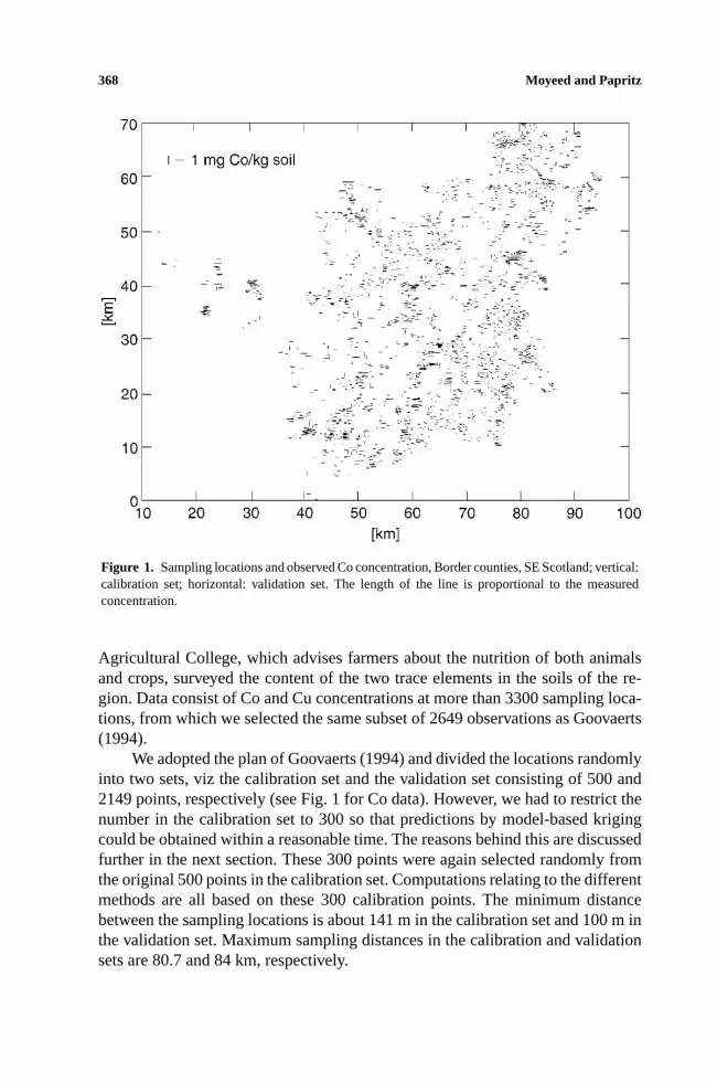
Figure 1. Sampling locations and observed Co concentration, Border counties, SE Scotland; vertical:calibration set; horizontal: validation set. The length of the line is proportional to the measuredconcentration.

Agricultural College, which advises farmers about the nutrition of both animalsand crops, surveyed the content of the two trace elements in the soils of the re-gion. Data consist of Co and Cu concentrations at more than 3300 sampling loca-tions, from which we selected the same subset of 2649 observations as Goovaerts(1994).

We adopted the plan of Goovaerts (1994) and divided the locations randomlyinto two sets, viz the calibration set and the validation set consisting of 500 and2149 points, respectively (see Fig. 1 for Co data). However, we had to restrict thenumber in the calibration set to 300 so that predictions by model-based krigingcould be obtained within a reasonable time. The reasons behind this are discussedfurther in the next section. These 300 points were again selected randomly fromthe original 500 points in the calibration set. Computations relating to the differentmethods are all based on these 300 calibration points. The minimum distancebetween the sampling locations is about 141 m in the calibration set and 100 m inthe validation set. Maximum sampling distances in the calibration and validationsets are 80.7 and 84 km, respectively.




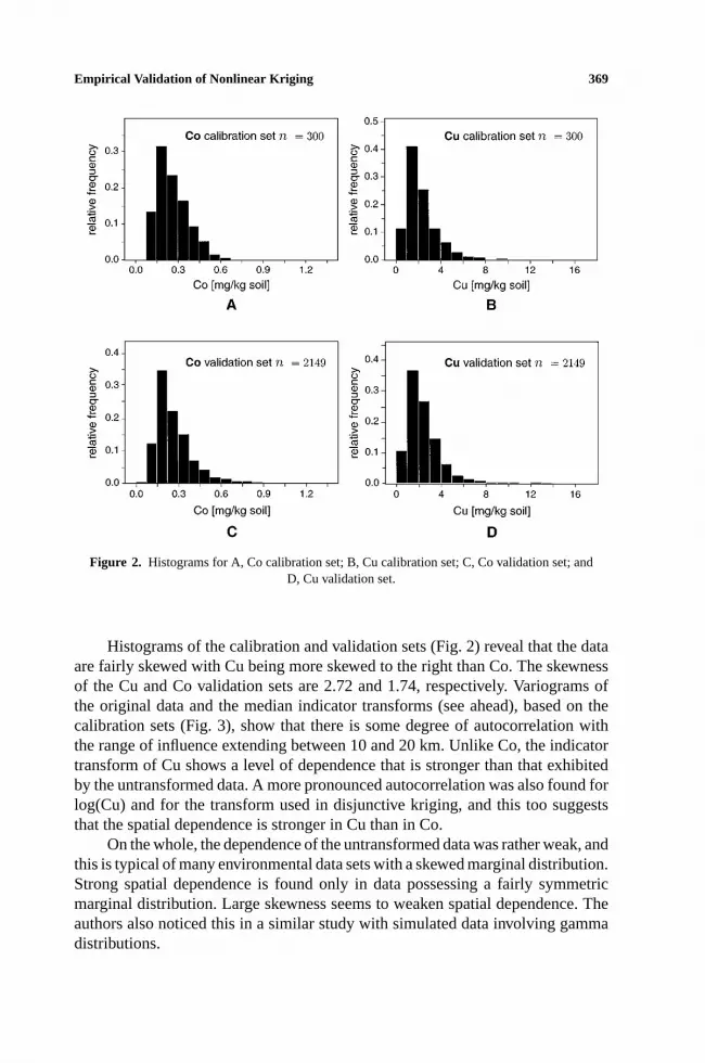
Figure 2. Histograms for A, Co calibration set; B, Cu calibration set; C, Co validation set; andD, Cu validation set.

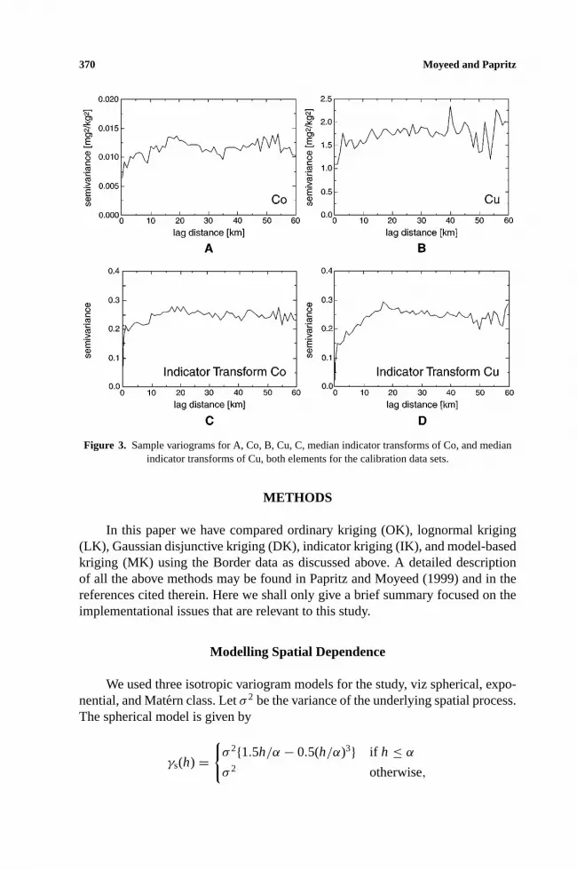
Histograms of the calibration and validation sets (Fig. 2) reveal that the dataare fairly skewed with Cu being more skewed to the right than Co. The skewnessof the Cu and Co validation sets are 2.72 and 1.74, respectively. Variograms ofthe original data and the median indicator transforms (see ahead), based on thecalibration sets (Fig. 3), show that there is some degree of autocorrelation withthe range of influence extending between 10 and 20 km. Unlike Co, the indicatortransform of Cu shows a level of dependence that is stronger than that exhibitedby the untransformed data. A more pronounced autocorrelation was also found forlog(Cu) and for the transform used in disjunctive kriging, and this too suggeststhat the spatial dependence is stronger in Cu than in Co.

On the whole, the dependence of the untransformed data was rather weak, andthis is typical of many environmental data sets with a skewed marginal distribution.Strong spatial dependence is found only in data possessing a fairly symmetricmarginal distribution. Large skewness seems to weaken spatial dependence. Theauthors also noticed this in a similar study with simulated data involving gammadistributions.




Figure 3. Sample variograms for A, Co, B, Cu, C, median indicator transforms of Co, and medianindicator transforms of Cu, both elements for the calibration data sets.

METHODS

In this paper we have compared ordinary kriging (OK), lognormal kriging(LK), Gaussian disjunctive kriging (DK), indicator kriging (IK), and model-basedkriging (MK) using the Border data as discussed above. A detailed descriptionof all the above methods may be found in Papritz and Moyeed (1999) and in thereferences cited therein. Here we shall only give a brief summary focused on theimplementational issues that are relevant to this study.

Modelling Spatial Dependence

We used three isotropic variogram models for the study, viz spherical, expo-nential, and Mat´ern class. Letσ 2 be the variance of the underlying spatial process.The spherical model is given by

γs(h) ={σ 2{1.5h/α − 0.5(h/α)3} if h ≤ ασ 2 otherwise,




whereα > 0 is the range parameter. The exponential model is defined as

γe(h) = σ 2[1− exp{−(h/α)δ}],

for some range parameterα > 0 and smoothness parameter 0< δ < 2. The thirdvariogram is based on the Matérn class of covariance functions having the form,

γb(h) = σ 2

{1− 1

2δ−10(δ)(h/α)δ Kδ(h/α)

},

whereα > 0 controls the range of the spatial correlation,δ > 0 is the smoothnessparameter, andKδ(·) is the modified Bessel function of the second kind of orderδ.For further details, see Matérn (1986) and Handcock and Wallis (1994). Notethat these models also parameterize valid covariance functions because all thevariograms are bounded.

For OK, LK, DK, and IK each of these variograms was combined with a“pure nugget” variogram

γn(h) ={

0 if h = 0

σ 20 otherwise,

to allow for a random process that is not mean square continuous.For all the methods excepting MK the variograms were estimated by the

method-of-moments estimator (Cressie, 1993, p. 69) from the data (OK) or anappropriate transform thereof (LK, DK, IK), and the model functions were fittedby least squares. The use of the iteratively reweighted least squares procedure(Cressie, 1993, p. 96; Müller, 1999) to fit the Bessel function and exponentialvariograms resulted in absurd values for the parameterδ. In the case of the Besselfunction, the values obtained were very large (δ > 30), and in the exponential casea value greater than 2 was returned. Therefore, we used the method of unweightedleast squares to fit these two models, unlike in the case of the spherical model wherethe weighted least squares method was used. One might question the use of thisad hoc approach to inference of the covariance structure, but the simulation studyby Zimmerman and Zimmerman (1991) has shown that for the Gaussian model theleast squares method performs as well as the more sophisticated likelihood basedprocedures such as the maximum likelihood or restricted maximum likelihood andthe minimum variance quadratic unbiased estimation.

For OK, LK, DK, and IK the fitted model parameters were then used forprediction in the customary “plug-in” approach, thus ignoring the additional un-certainty caused by inferring the covariance structure from the data. Model-basedkriging does not suffer from this obvious disadvantage because it incorporatesparameter uncertainty in a natural way into the predictions.




Ordinary Kriging

We used ordinary kriging to predict the data linearly, and we modelled theconditional distribution of the soil metal content by a normal distribution withparameters taken from the OK results. For positively skewed data this is certainlya naive choice, but we wanted to include “blind” application of linear kriging asa reference. Since model-based kriging uses all the data to predict the value at agiven point, we used this “global neighbourhood” for the remaining methods aswell. This is not a common practice in geostatistics, where only a subset of theobservations closest to the target point is used for the purposes of prediction.However, a sensitivity analysis showed that—unless the local neighbourhood wasrestricted to a very small number of points (typically≤10)—the performance ofthe methods was affected very little by the choice of the neighbourhood.

Lognormal Kriging

For LK the variogram of the logarithms of the data was estimated and thetransformed data were predicted linearly by ordinary kriging. The predictions werethen transformed back to the original scale by the commonly used backtransfor-mation (Cressie, 1993, Eq. 3.2.40), which is marginally unbiased. Given the OKpredictions of the transformed data and the corresponding simple kriging variances(Cressie, 1993, p. 110), we modelled Co and Cu concentrations by conditional log-normal distributions with these quantities as parameters. This model is motivatedby the fact that the conditional distribution of the OK prediction error is normalunder the Gaussian model with mean equal to (1−∑i λi )(µ− µ) and varianceequal to the simple kriging variance. Theλi denote here the simple kriging weightsandµ is the stationary expectation of the process with ˆµ as its generalized leastsquares estimate.

Disjunctive Kriging

The DK predictor of some functional,T(x) = t(Y(x)), of the random variable,Y(x), has the form

TDK(x) =n∑

i=1

hi (Y(xi )),

where thehi (·) are measurable functions of the random variablesY(xi ), whichmodel the observationsyi , i = 1, 2, . . . ,n. Functionshi (Y(x)) are assumed tohave finite variance. The optimalhi (·), which minimize the expected squared




prediction error, are implicitly given by the set of equations (Matheron, 1976a)

E[TDK(x) | Y(xi )] = E[T(Y(x)) | Y(xi )] ∀i = 1, 2, . . . ,n, (1)

and they are completely specified if we assume a stationary bivariate distribution.Closed form solutions to Equation (1) are readily obtained for a special class of

random processes with stationary bivariate distributions, the so-called “isofactorialmodels” (Armstrong and Matheron, 1986a,b; Matheron, 1976a, 1989b). Any mea-surable functionalt(·) of such an isofactorial processY(x) can be expanded asa seriest(Y(x)) =∑∞k=0 tk χk(Y(x)), where the “factors,”{χk(·)}, are a familyof functions (usually polynomials), which are orthonormal with respect to themarginal distribution ofY(x). The coefficientstk are equal to E[t(Y(x))χk(Y(x))].We can expand thehi (Y(xi )) in a similar way so that the DK predictor is given by

TDK(x) =∞∑

k=0

tkn∑

i=1

hikχk(Y(xi )), (2)

and the coefficients,hik = E[hi (Y(xi ))χk(Y(xi ))], are determined by the simplekriging systems to predict the factorsχk(Y(x)), k = 0, 1, . . . .

Isofactorial models can be found for various distributions, but in practiceGaussian disjunctive kriging is mostly used. The orthonormal functions arethen normalized Hermite polynomials, that is,χk(y) ≡ (−1)kHek(y)/

√k!

(Abramowitz and Stegun, 1965), and their covariance is given by Cov [χk(Y(xi )),χk(Y(x j ))] = {ρ(xi − x j )}k, whereρ(xi − x j ) is the stationary correlation be-tweenY(xi ) andY(x j ). The functionρ(·) specifies the Gaussian isofactorial modelcompletely. It is clear that the correlation of the factors decays quickly with increas-ingk, and for somek > Kmaxthe best predictor ofχk(Y(x)) can be approximated byE[χk(Y(x))] ≈ 0. Thus the series expansion can in practice be cut off atk = Kmax.

There are two main applications of disjunctive kriging. First, we may wish topredict the indicator transform

I [Y(x) ≤ y] ={

1 if Y(x) ≤ y

0 otherwise,(3)

and take the predicted indicator as an estimate of the conditional distribution ofY(x) given the vector of observationsY. Secondly, DK can be used as a more gen-eral form of trans-Gaussian kriging. To this end let us assume that the observationsare sampled from a measurable one-to-one transform of a processZ with stationaryisofactorial bivariate distributions, that is,Y(x) = 8(Z(x)) =∑∞k=0 8kχk(Z(x)).Since8(·) is one-to-one, the8k = E[Y(x)χk(Z(x))] can be evaluated numerically(Rivoirard, 1994, Ch. 6).




In our study we used Gaussian DK withKmax= 20. We transformed theobservations,yi , to standard normal by solvingyi =

∑20k=08k(−1)kHek(zi )/

√k!

for zi by Brent’s method (Press and others, 1992), and we estimated the variogramof the transformed data. The conditional distributions were estimated by predictingthe indicator transform (3).

Indicator Kriging

Indicator kriging is a nonparametric, discrete approximation to DK(Matheron, 1976a; Papritz and Moyeed, 1999; Rivoirard, 1994) with the fac-tors corresponding to a set of indicator transforms of the data, for example,χk(Y(x)) ≡ I [Y(x) ≤ ck] for a set of “cut-off” values{ck}, k = 1, 2, . . . , K . Ingeneral, the factors are no longer orthogonal, and one must resort to cokriging tofind the optimal predictor (2). However, indicator cokriging is hardly ever used inpractice, and various simplifications such as univariate indicator kriging, medianindicator kriging, or principal component indicator kriging have been suggested(see Deutsch and Journel, 1998, for an overview).

In our study we used median indicator kriging. This method relies on theso-called “mosaic” model (Rivoirard, 1994, Ch. 3) for which all the cross- andautocorrelograms of the indicators are the same. Thus, any indicator can be pre-dicted by univariate kriging, using a common variogram, typically that of themedian indicator transform,I [Y(x) ≤ median (Y)]. Other variants of indicatorkriging usually rely on inconsistent models of the stationary bivariate distribu-tions because it is not in general known what conditions the set indicator (cross-)covariance functions must satisfy to code the stationary bivariate distributionsconsistently (Matheron, 1989a).

In the implementation we followed the procedure suggested by Deutsch andJournel (1998), and we used their code. The empirical distribution of the data wascomputed from the unweighted observations. We predicted nine indicators with theck equal to the deciles of the empirical distribution. To model the conditional distri-bution, we interpolated the probability linearly between any two kriged indicators,and the tails of the distribution were extrapolated using the tails of the empiri-cal marginal distribution (optionsltail = 3, utail = 3 of programpostik,Deutsch and Journel, 1998). The metal content was predicted by the so-called“E-type” estimate of Deutsch and Journel (1998).

Model-Based Kriging

This approach is based on the assumption that (i) the underlying spatial sur-face,S, is a stationary Gaussian process with E[S(x)] = 0 and Cov [S(xi ), S(x j )] =σ 2ρ(xi − x j ); (ii) conditional onS, the random variablesY(xi ), i = 1, 2, . . . ,n




are mutually independent, with distributionsfi (y | S(xi )) = f (y;µi , φ) speci-fied by the values of the conditional expectationsµi = µ(xi ) = E[Y(xi ) | S(xi )]and some parametersφ; and (iii) for some link functiong(·), g(µi ) = S(xi )+ β,whereβ is a parameter and may be interpreted as a nonzero mean for the processS.Under these general assumptions, the kriging predictorS(x) = E[S(x) | Y] or theprediction variance cannot be evaluated analytically. MCMC methods are requiredto obtainS(x) or, for that matter, any functional ofS(x). In fact, in most applica-tions the target quantity will be the conditional expectationµ(x) = E[Y(x) | S(x)],which is some functional ofS(x) as observed from assumption (iii) above.

We implemented the MK method for each of the three spatial dependencemodels: the modified Bessel function, the exponential, and the spherical as de-scribed above. We assumed a normal distribution for the conditional distributionin (ii) above with a log-link function, that is,µi = exp(S(xi )+ β), and varianceparameterφ = τ 2. With this parametrization we cannot identify bothτ 2 and anugget effect in the covariance structure of the signal process. Alternatively, agamma distribution could have been used in place of the normal. However, we hadto abandon the idea of using the gamma distribution as we encountered problemsof identifiability with the gamma shape (or variance) parameter.

Besidesσ 2, β, and τ 2, we had a scale parameter,α, common to all thecovariance models, and an additional smoothness parameterδ for the exponentialand the modified Bessel function models. In our study we assumed improperuniform priors forσ 2, β, and τ 2. A proper uniform prior was assumed forδ.The selection ofδ for the modified Bessel function is discussed in depth in theDiscussion section. The prior chosen forα was

p(α) = 1

α2. (4)

There were several reasons for this choice. First, the algorithm failed to convergewith an improper uniform prior onα. However, the prior in (4) did not cause anyconvergence or numerical problems in the computation. Secondly, the prior in (4)is equivalent to putting an improper uniform prior onα′ = 1/α, which could betaken as another parameterization for the range of the correlation function. Thirdly,this choice has an intuitive appeal: a priori one would put a higher belief in therange of the correlation to be short rather than long.

The parametersσ 2,α, andβwere updated using a random-walk Metropolis al-gorithm with a normal proposal density for log(σ 2), log(α), andβ. For updatingτ 2,a standard normal proposal density was used for sampling

√2∑n

i (yi − µi )2/τ 2 −√2ν − 1, whereν = n− 2. The updating of the correlation parameters within the

MCMC framework requires inversion of the covariance matrix at each iteration.Since inversion is anO(n3) operation, the MK method can be painfully slow.For both Co and Cu data sets, and for all the different models that were used,




the Markov chain was run until convergence was judged to have occurred (ap-proximately 1000 iterations), and then the chain was sampled on every 10th of5000 iterations to give a sample of 500 values ofS(x) at each of the predictionlocations. For each of the 500 values ofS(x) one realization ofY(x) was simulated,and the conditional distribution ofY(x) | Y and its mean was estimated from theset of 500 values ofY(x).

VALIDATION CRITERIA

The performance of the different methods was compared by using severalcriteria. We looked at the precision of the predictions and, more importantly, theability of these methods to model prediction uncertainty. The latter was investigatedin two ways, viz by modelling the conditional distribution of the predictor given thedata and by adopting a decision-theoretic approach that involved the minimizationof the Bayes risk of an associated loss function. These criteria are discussed below.

Precision

We assessed the precision of the methods by computing therelative bias,rBIAS, and therelative mean square error of prediction, rMSEP, which are definedas follows

rBIAS =∑n

j=1(y j − yj )

nyc, (5)

rMSEP=∑n

j=1(y j − yj )2∑nj=1(yc− yj )2

, (6)

wherey j is the value predicted at locationx j , yj is the observed value,yc is thearithmetic mean of the calibration set (naive predictor), andn is the size of thevalidation set.

Prediction Uncertainty

The modelling of the conditional distributions was assessed by looking atthe coverage probabilites. Coverage probabilities are a global accuracy measurefor assessing the modelling of local prediction uncertainty. Fori = 1, . . . ,n, wecomputed the nominal probability

pi = P[Y(xi ) ≤ yi | Y]




and obtained their order statistics,p(i ). The coverage probability,f (p(i )), that is,the proportion of observations,yj , that are smaller than the conditional quantilesfor a nominal probabilityp(i ), is then obtained from

f(p(i )) = 1

n

n∑j=1

I[pj ≤ p(i )

] = RANK(p(i ))/n = i /n. (7)

If, on average, the conditional distributions are modelled correctly,f (p(i )) shouldbe equal top(i ). Hence, the P–P plot off (p(i )) againstp(i ) for all i = 1, . . . ,n wasused to compare the different methods.

Our criterion is closely related to the “symmetric” coverage probability

f (p) = 1

n

n∑j=1

I [q j (0.5− p/2)< yj ≤ q j (0.5+ p/2)],

where q j (·) denotes the quantile of the estimated conditional distribution. Weprefer f (p) to f (p) for two reasons. First, the symmetric coverage probabilitycan be easily read from the P–P plots by evaluating the coverage for the interval(0.5− p/2, 0.5+ p/2]. Secondly,f (pi ) enables us to spot deviations that cannotbe detected byf (p). If, for instance, f (p) is too small both for large and smallvalues ofp, then f (p) will not reveal this deficiency.

Minimization of an Expected Loss

The very purpose for measuring the Co and Cu concentrations in the topsoilis to identify places where these metals are deficient for animals so that correctiveaction may be taken. This usually entails taking financial costs into consideration.Hence, in practice, decisions have to be made by using a specific loss function.

For the Border data, the loss associated by assigning a placex deficient in Coor Cu could be

L1[Y(x)] ={

0 if Y(x) ≤ yc

l otherwise,(8)

whereyc is the critical threshold andl is the cost incurred because of underestimat-ing the metal concentration. Remedial action involves adding the deficient metalto the diet of the stock or fertilizing the pasture land. This cost might be regardedas being independent of the concentration of the metal, and so we assume this tobe a constant value ofl .




On the other hand, if a place is judged to be adequate in the element, then theloss function would be defined as

L2[Y(x)] ={

yc− y(x) if Y(x) ≤ yc

0 otherwise.(9)

This means that if a placex is actually not deficient in the element, then theassignment is correct and no loss is incurred. However, if the place is deficient andno action is taken, then the livestock will suffer from retarded growth. The higherthe deficiency, the poorer will be the livestock quality. We quantify this loss byassuming the cost to be equal to the excess of the threshold over the actual metalconcentration, that is,yc− y(x).

At each prediction point we worked out the actual loss resulting from takingthe optimal decision that minimized the expected loss defined in Equations (8)and (9). The average of these losses over all the prediction points was used tocompare the different methods.

The generally accepted thresholds for Co and Cu are 0.25 and 1.0 mg/kg,respectively (McBratney and others, 1982). We assessed the methods using thesethresholds with different values ofl . We usedl = 0.01, 0.1, 1 for Co andl =0.0001, 0.001, 0.01, 0.1 for Cu. Additionally, we utilized one more thresholdvalue each for Co and Cu data to gauge the sensitivity of the different methodsto the change in the threshold. The value used for Co was 0.125 mg/kg withl = 0.00001, 0.0001, 0.001, 0.01, and for Cu a threshold of 2.0 mg/kg was appliedwith l = 0.1, 1, 10.

RESULTS

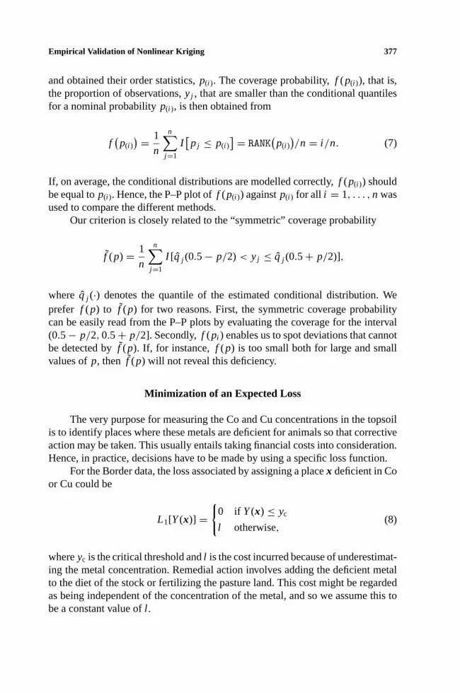
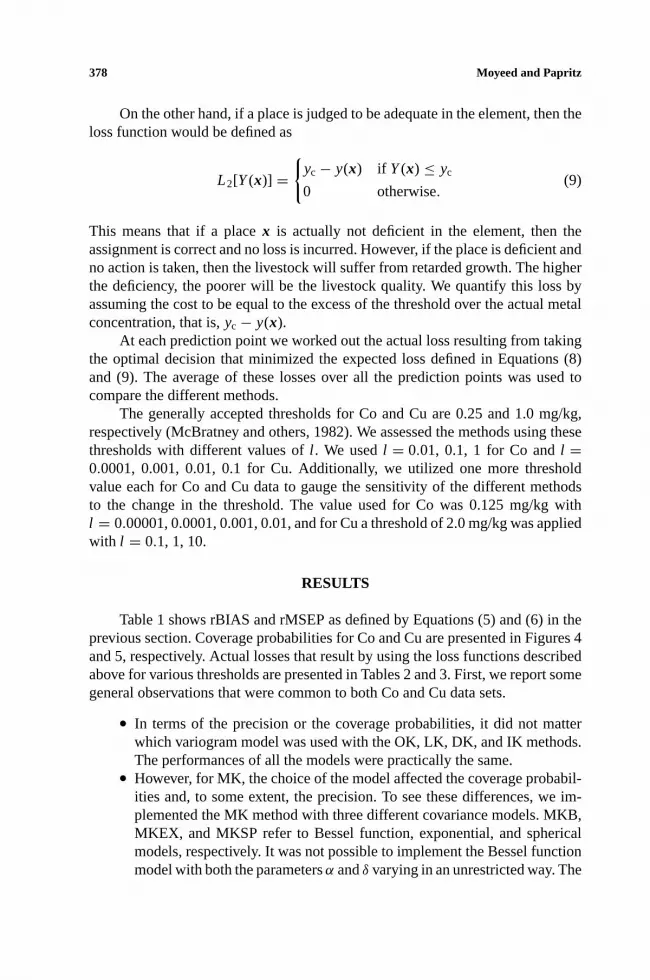
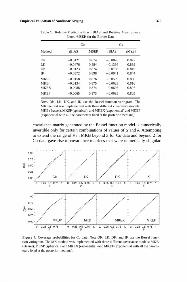
Table 1 shows rBIAS and rMSEP as defined by Equations (5) and (6) in theprevious section. Coverage probabilities for Co and Cu are presented in Figures 4and 5, respectively. Actual losses that result by using the loss functions describedabove for various thresholds are presented in Tables 2 and 3. First, we report somegeneral observations that were common to both Co and Cu data sets.

• In terms of the precision or the coverage probabilities, it did not matterwhich variogram model was used with the OK, LK, DK, and IK methods.The performances of all the models were practically the same.• However, for MK, the choice of the model affected the coverage probabil-

ities and, to some extent, the precision. To see these differences, we im-plemented the MK method with three different covariance models. MKB,MKEX, and MKSP refer to Bessel function, exponential, and sphericalmodels, respectively. It was not possible to implement the Bessel functionmodel with both the parametersα andδ varying in an unrestricted way. The




Table 1. Relative Prediction Bias, rBIAS, and Relative Mean SquareError, rMSEP, for the Border Data

Co Cu

Method rBIAS rMSEP rBIAS rMSEP

OK −0.0121 0.874 −0.0828 0.827LK −0.0476 0.884 −0.1366 0.839DK −0.0123 0.874 −0.0786 0.816IK −0.0372 0.898 −0.0941 0.844

MKSP −0.0158 0.876 −0.0509 0.860MKB −0.0134 0.875 −0.0639 0.816MKEX −0.0088 0.874 −0.0605 0.807

MKEF −0.0065 0.873 −0.0689 0.809

Note. OK, LK, DK, and IK use the Bessel function variogram. TheMK method was implemented with three different covariance models:MKB (Bessel), MKSP (spherical), and MKEX (exponential) and MKEF(exponential with all the parameters fixed at the posterior medians).

covariance matrix generated by the Bessel function model is numericallyinvertible only for certain combinations of values ofα andδ. Attemptingto extend the range ofδ in MKB beyond 3 for Co data and beyond 2 forCu data gave rise to covariance matrices that were numerically singular.

Figure 4. Coverage probabilities for Co data. Note OK, LK, DK, and IK use the Bessel func-tion variogram. The MK method was implemented with three different covariance models: MKB(Bessel), MKSP (spherical), and MKEX (exponential) and MKEF (exponential with all the param-eters fixed at the posterior medians).




Figure 5. Coverage probabilities for Cu data. Note OK, LK, DK, and IK use the Bessel func-tion variogram. The MK method was implemented with three different covariance models: MKB(Bessel), MKSP (spherical), and MKEX (exponential) and MKEF (exponential with all the param-eters fixed at the posterior medians).

Finally, to study the effect of parameter uncertainty, we used an exponen-tial covariance model with fixed values for all the parameters and denotethis model by MKEF. Within the MK framework, MKSP was in generalinferior to both MKB and MKEX.

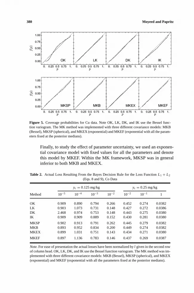
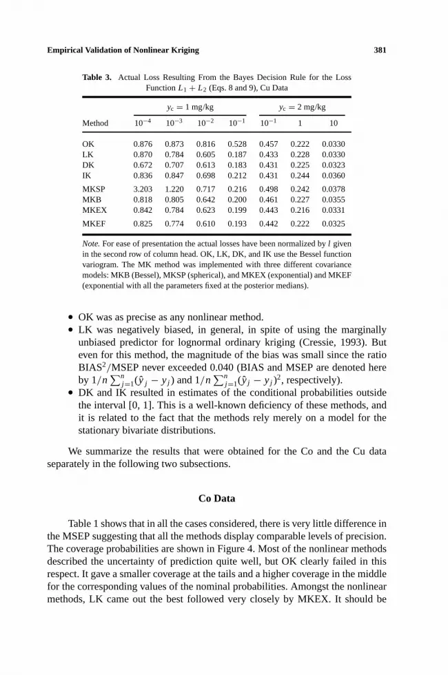
Table 2. Actual Loss Resulting From the Bayes Decision Rule for the Loss FunctionL1 + L2

(Eqs. 8 and 9), Co Data

yc = 0.125 mg/kg yc = 0.25 mg/kg

Method 10−5 10−4 10−3 10−2 10−2 10−1 1

OK 0.909 0.890 0.794 0.266 0.452 0.274 0.0382LK 0.903 1.073 0.731 0.148 0.427 0.272 0.0386DK 2.468 0.974 0.753 0.148 0.443 0.275 0.0380IK 0.909 0.909 0.889 0.152 0.430 0.281 0.0380

MKSP 0.902 0.913 0.791 0.262 0.445 0.279 0.0382MKB 0.893 0.952 0.834 0.200 0.449 0.274 0.0382MKEX 0.899 1.031 0.751 0.143 0.434 0.271 0.0380

MKEF 0.897 1.136 0.783 0.146 0.437 0.269 0.0387

Note.For ease of presentation the actual losses have been normalized byl given in the second rowof column head. OK, LK, DK, and IK use the Bessel function variogram. The MK method was im-plemented with three different covariance models: MKB (Bessel), MKSP (spherical), and MKEX(exponential) and MKEF (exponential with all the parameters fixed at the posterior medians).




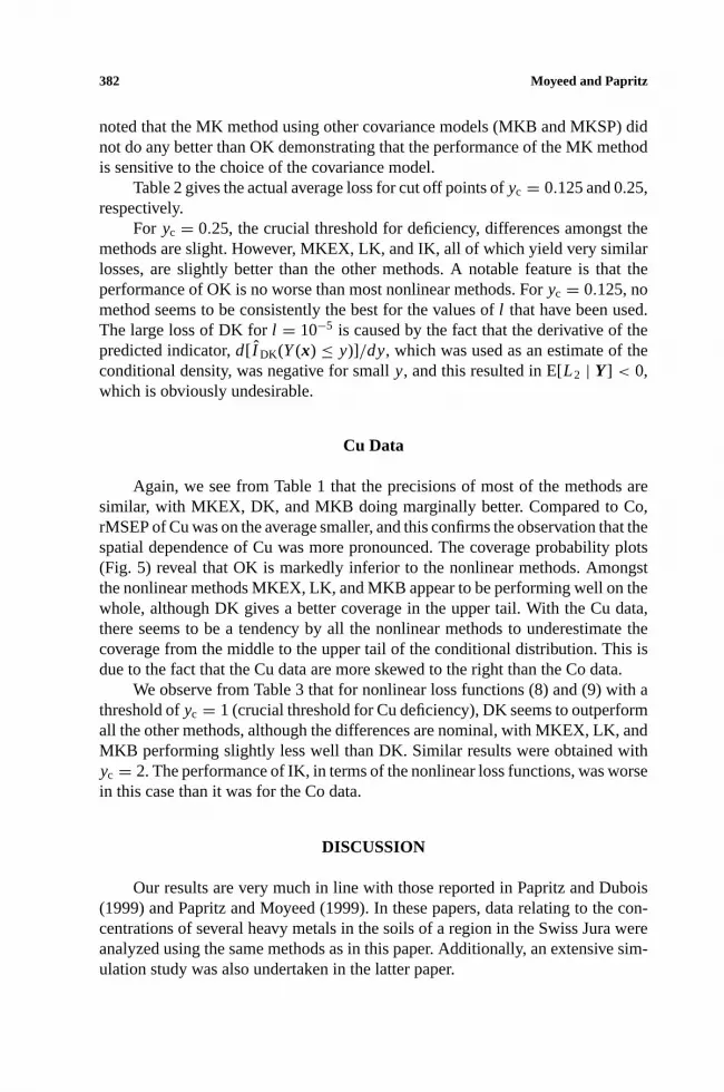
Table 3. Actual Loss Resulting From the Bayes Decision Rule for the LossFunctionL1 + L2 (Eqs. 8 and 9), Cu Data

yc = 1 mg/kg yc = 2 mg/kg

Method 10−4 10−3 10−2 10−1 10−1 1 10

OK 0.876 0.873 0.816 0.528 0.457 0.222 0.0330LK 0.870 0.784 0.605 0.187 0.433 0.228 0.0330DK 0.672 0.707 0.613 0.183 0.431 0.225 0.0323IK 0.836 0.847 0.698 0.212 0.431 0.244 0.0360

MKSP 3.203 1.220 0.717 0.216 0.498 0.242 0.0378MKB 0.818 0.805 0.642 0.200 0.461 0.227 0.0355MKEX 0.842 0.784 0.623 0.199 0.443 0.216 0.0331

MKEF 0.825 0.774 0.610 0.193 0.442 0.222 0.0325

Note.For ease of presentation the actual losses have been normalized byl givenin the second row of column head. OK, LK, DK, and IK use the Bessel functionvariogram. The MK method was implemented with three different covariancemodels: MKB (Bessel), MKSP (spherical), and MKEX (exponential) and MKEF(exponential with all the parameters fixed at the posterior medians).

• OK was as precise as any nonlinear method.• LK was negatively biased, in general, in spite of using the marginally

unbiased predictor for lognormal ordinary kriging (Cressie, 1993). Buteven for this method, the magnitude of the bias was small since the ratioBIAS2/MSEP never exceeded 0.040 (BIAS and MSEP are denoted hereby 1/n

∑nj=1(y j − yj ) and 1/n

∑nj=1(yj − yj )2, respectively).

• DK and IK resulted in estimates of the conditional probabilities outsidethe interval [0, 1]. This is a well-known deficiency of these methods, andit is related to the fact that the methods rely merely on a model for thestationary bivariate distributions.

We summarize the results that were obtained for the Co and the Cu dataseparately in the following two subsections.

Co Data

Table 1 shows that in all the cases considered, there is very little difference inthe MSEP suggesting that all the methods display comparable levels of precision.The coverage probabilities are shown in Figure 4. Most of the nonlinear methodsdescribed the uncertainty of prediction quite well, but OK clearly failed in thisrespect. It gave a smaller coverage at the tails and a higher coverage in the middlefor the corresponding values of the nominal probabilities. Amongst the nonlinearmethods, LK came out the best followed very closely by MKEX. It should be




noted that the MK method using other covariance models (MKB and MKSP) didnot do any better than OK demonstrating that the performance of the MK methodis sensitive to the choice of the covariance model.

Table 2 gives the actual average loss for cut off points ofyc = 0.125 and 0.25,respectively.

For yc = 0.25, the crucial threshold for deficiency, differences amongst themethods are slight. However, MKEX, LK, and IK, all of which yield very similarlosses, are slightly better than the other methods. A notable feature is that theperformance of OK is no worse than most nonlinear methods. Foryc = 0.125, nomethod seems to be consistently the best for the values ofl that have been used.The large loss of DK forl = 10−5 is caused by the fact that the derivative of thepredicted indicator,d[ I DK(Y(x) ≤ y)]/dy, which was used as an estimate of theconditional density, was negative for smally, and this resulted in E[L2 | Y] < 0,which is obviously undesirable.

Cu Data

Again, we see from Table 1 that the precisions of most of the methods aresimilar, with MKEX, DK, and MKB doing marginally better. Compared to Co,rMSEP of Cu was on the average smaller, and this confirms the observation that thespatial dependence of Cu was more pronounced. The coverage probability plots(Fig. 5) reveal that OK is markedly inferior to the nonlinear methods. Amongstthe nonlinear methods MKEX, LK, and MKB appear to be performing well on thewhole, although DK gives a better coverage in the upper tail. With the Cu data,there seems to be a tendency by all the nonlinear methods to underestimate thecoverage from the middle to the upper tail of the conditional distribution. This isdue to the fact that the Cu data are more skewed to the right than the Co data.

We observe from Table 3 that for nonlinear loss functions (8) and (9) with athreshold ofyc = 1 (crucial threshold for Cu deficiency), DK seems to outperformall the other methods, although the differences are nominal, with MKEX, LK, andMKB performing slightly less well than DK. Similar results were obtained withyc = 2. The performance of IK, in terms of the nonlinear loss functions, was worsein this case than it was for the Co data.

DISCUSSION

Our results are very much in line with those reported in Papritz and Dubois(1999) and Papritz and Moyeed (1999). In these papers, data relating to the con-centrations of several heavy metals in the soils of a region in the Swiss Jura wereanalyzed using the same methods as in this paper. Additionally, an extensive sim-ulation study was also undertaken in the latter paper.




The salient features of our findings may be summarized as follows.

1. Ordinary kriging was almost as precise as any nonlinear method for themarginally skewed Border data.

2. The nonlinear methods modelled the conditional distributions with, moreor less, similar success. In this respect, ordinary kriging did not do as wellas the nonlinear methods. In general the performance of linear kriging getsworse as the data become more skewed.

3. For moderately skewed data (Co in this case), LK does particularly well,although MKEX is almost as good. It should, however, be noted thatsince LK is negatively biased, it predicts the large values rather poorly.With this kind of data, the choice of the covariance model does affect theperformance of MK to a great extent.

4. For data that exhibit a substantial degree of positive skewness (like the Cudata), all the nonlinear methods perform almost equally well or, for thatmatter, equally badly. However, DK appears to be slightly better than theother methods. When data are highly (positively) skewed, the choice ofthe covariance model in MK has little impact. Again, the performance ofMKEX seems to be marginally better.

5. Although, for the Border data the performance of IK was slightly inferior tothe other methods, it was more or less equivalent to DK and LK for otherdata sets. However, IK has two major disadvantages: the mathematicalrationale underlying the method is flawed, and its practical implementa-tion is quite cumbersome. Furthermore, the fact that it is free from anyparametric modelling does not yield any apparent advantages over themethods that require a parametric framework.

6. The implementation of the MK method is, in practice, still rather pro-hibitive. The method in its present form cannot be applied to data recordedon a large number of sites as inverting large covariance matrices at eachstep of the MCMC iteration is a very slow process. In addition, ascertainingthe convergence of a chain is by no means straightforward.

We like to point out that the comments made in items 3–5 above cannot begeneralized. There is not enough evidence to suggest that the performance of LKand DK depend on the skewness of the data, or that IK is inferior to either DKor LK in general. We also have very little experience to say anything concreteabout the sensitivity of MK to the choice of the covariance model. However,our results are in general agreement with the few empirical validation studiesundertaken by other authors (see Papritz and Moyeed, 1999, for a more detaileddiscussion), and they partly contradict the commonly held views about the prosand cons of the different methods. As an example, we are unaware of any empiricalevidence to substantiate the worry of the advocates of IK (see e.g., Journel, 1983)that the parametric methods (LK, DK, MK) bear much risk of failure because




model assumptions might be violated. But the evidence is still scanty, and furtherempirical validation studies are required.

In this study, unlike the one carried out in Papritz and Moyeed (1999), weinvestigated two additional aspects. One was the use of the Mat´ern class of covari-ance models, and the other was the effect of parameter uncertainty. First, we havefound that it is difficult to implement to MK method using a Bessel function modelunless the smoothness parameterδ is restricted to a narrow interval. Handcock andWallis (1994) and Kent, Handcock, and Stein in their separate contributions tothe discussion of the paper by Diggle, Tawn, and Moyeed (1998) advocate theuse of this model as it allows for any degree of mean square differentiability forthe spatial process. However, we believe that the issue of differentiability is notcritical. In practice, the sample variograms rarely have a parabolic behaviour nearthe origin; rather they often have a nugget that is attributable not just to mea-surement error but also to small-scale variation. Additionally, with just one setof realized values on a few locations, one can at best say that a process is differ-entiable once, if at all. This suggests thatδ > 1. In fact, the correlation functionfor processes that are once differentiable (1< δ ≤ 2) is almost indistinguishablefrom those that are more than once differentiable (δ > 2). The crucial choice isbetweenδ ≤ 1 and 1< δ ≤ 2. In most applications that we have encountered,the value ofδ obtained using the MK method was less than 2. The posteriormean, median, and mode ofδ for the Co data were 1.303, 0.977, and 0.758,respectively, while for the Cu data they were 0.357, 0.337, and 0.292, respec-tively. Performancewise, MKB fared no better than MKEX in our applications,rather it performed worse in certain circumstances besides being more difficult toimplement.

We now turn to the issue of parameter uncertainty. It is well known that thenon-Bayesian kriging methods, OK, LK, DK, and IK, unlike MK, do not makea proper allowance for the uncertainty in the estimation of thecovariancemodelparameters. Within the framework of the MK method, when we compared MKEX,that is, the model using the exponential correlation function with all the parametersvarying, and MKEF, that is, the model with all the parameters fixed at the posteriormedian, we found that the two models yielded almost identical results in terms ofthe precision statistics, coverage probabilities, and predictions based on nonlinearloss functions (Tables 2 and 3 and Figs. 4 and 5). Moreover, in our applications weencountered no evidence to corroborate the advantage of the MK method over theother nonlinear methods on the grounds that it explicitly incorporates parameteruncertainty into predictive inferences. This is primarily due to the fact that theposteriors of the parameters are all highly concentrated. All the functionals thatwe looked at were, more or less, dominated by values of the parameters thatwere close to the plug-in estimates. In other words, our results demonstrate that ahighly concentrated posterior with a weak prior diminishes the effect of parameteruncertainty greatly.




We end by saying that if the data are marginally skewed and the goal isto predict nonlinear functionals, then LK, DK, and MK would all be suitable.However, the computational burden and the lack of automation are at present themajor obstacles toward the general use of MK. Unless ways are found for analyzinglarge data sets (exceeding, say 300 observations) that do not require a considerablecomputer time, the use of MK will be quite limited.

ACKNOWLEDGMENTS

The authors thank Mr R. B. Speirs, SAC Environmental, SAC, Bush Estate,Penicuick EH26 OHP, UK ([email protected]) for the data. The work wasundertaken while RAM was visiting the Institute of Terrestrial Ecology, ETHZurich. The financial support of ETH Z¨urich is gratefully acknowledged.

REFERENCES

Abramowitz, M., and Stegun, I. A., 1965, Handbook of mathematical functions: Dover, New York,1046 p.

Armstrong, M., and Matheron, G., 1986a, Disjunctive kriging revisited: Part I: Math. Geol., v. 18, no. 8,p. 711–728.

Armstrong, M., and Matheron, G., 1986b, Disjunctive kriging revisited: Part II: Math. Geol., v. 18,no. 8, p. 729–742.

Cressie, N. A. C., 1993, Statistics for spatial data, revised edn.: Wiley, New York, 900 p.Deutsch, C. V., and Journel, A. G., 1998, GSLIB geostatistical software library and user’s guide,

2nd edn.: Oxford University Press, New York, 369 p.Diggle, P. J., Tawn, J. A., and Moyeed, R. A., 1998, Model-based geostatistics: Appl. Stat., v. 47, no. 3,

p. 299–350.Goovaerts, P., 1994, Comparative performance of indicator algorithms for modeling conditional prob-

ability distribution functions: Math. Geol., v. 26, no. 3, p. 389–411.Goovaerts, P., and Journel, A. G., 1995, Integrating soil map information in modelling the spatial

variation of continuous soil properties: Eur. J. Soil Sci., v. 46, p. 397–414.Handcock, M. S., and Wallis, J. R., 1994, An approach to statistical spatial-temporal modeling of

meteorological fields: J. Am. Stat. Assoc., v. 89, p. 369–378.Journel, A. G., 1983, Nonparametric estimation of spatial distributions: Math. Geol., v. 15, no. 3,

p. 445–468.Laslett, G. M., 1994, Kriging and splines: An empirical comparison of their predictive performance in

some applications: J. Am. Stat. Assoc., v. 89, p. 391–400.Matern, B., 1986, Spatial variation, 2nd edn.: Springer, Berlin. Lecture notes in statistics, Vol. 36,

151 p. [1st Edn., Meddelanden fr˚an Statens Skogsforskningsinstitut 49, no. 5, 1960, Uppsala.]Matheron, G., 1976a, A simple substitute for conditional expectation: The disjunctive kriging,in

Guarascio, M., David, M., and Huijbregts, Ch. J., eds., Advanced geostatistics in the miningindustry: Reidel, Dordrecht, p. 221–236.

Matheron, G., 1976b, Forecasting block grade distributions: The transfer functions,in Guarascio,M., David, M., and Huijbregts, Ch. J., eds., Advanced geostatistics in the mining industry: Reidel,Dordrecht, p. 237–251.




Matheron, G., 1989a, The internal consistency of models in geostatistics,in Armstrong, M., ed.,Geostatistics: Kluwer, Dordrecht, Vol. 1, p. 21–38.

Matheron, G., 1989b, Two classes of isofactorial models,in Armstrong, M., ed., Geostatistics: Kluwer,Dordrecht, Vol. 1, p. 309–322.

Matheron, G., 1989c, Estimating and choosing: An essay on probability in practice: Springer, Berlin,141 p.

McBratney, A. B., Webster, R., McLaren, R. G., and Spiers, R. B., 1982, Regional variation of ex-tractable copper and cobalt in the topsoil of south-east Scotland: Agronomie, v. 2, no. 10, p. 969–982.

Muller, W. G., 1999, Least-squares fitting from the variogram cloud: Stat. Probab. Lett., v. 43, p. 93–98.Papritz, A., and Dubois, J.-P., 1999, Mapping heavy metals in soil by (non-)linear kriging: An empirical

validation,in Gomez-Hernández, J., Soares, A., and Froidevaux, R., eds., geoENV II: Geostatisticsfor environmental applications: Kluwer, Dordrecht, p. 429–440.

Papritz, A., and Moyeed, R. A., 1999, Linear and non-linear kriging methods: Tools for monitoring soilpollution, in Barnett, V., Turkman, K., and Stein, A., eds., Statistics for the environment, Vol. 4:Statistical aspects of health and the environment: Wiley, Chichester, p. 303–336.

Press, W. H., Teukolsky, S. A., Vetterling, W. T., and Flannery, B. P., 1992, Numerical recipes inFORTRAN: The art of scientific computing, 2nd edn.: Cambridge University Press, Cambridge,963 p.

Rivoirard, J., 1994, Introduction to disjunctive kriging and non-linear geostatistics: Spatial informationsystems: Clarendon, Oxford, 181 p.

Sullivan, J., 1984, Conditional recovery estimation through probability kriging—Theory and practice,in Verly, G., David, M., Journel, A., and Maréchal, A., eds., Geostatistics for natural resourcescharacterization: Reidel, Dordrecht, Vol. 1, p. 365–384.

Verly, G., 1983, The multigaussian approach and its applications to the estimation of local reserves:Math. Geol., v. 15, no. 2, p. 259–286.

Verly, G., 1984, The block distribution given a point multivariate normal distribution,in Verly, G.,David, M., Journel, A., and Maréchal, A., eds., Geostatistics for natural resources characterization:Reidel, Dordrecht, Vol. 1, p. 495–515.

Webster, R., 1991, Local disjunctive kriging of soil properties with change of support: J. Soil Sci.,v. 42, p. 301–318.

Webster, R., and Oliver, M. A., 1989, Optimal interpolation and isarithmic mapping of soil properties.VI. Disjunctive kriging and mapping the conditional probability: J. Soil Sci., v. 40, p. 497–512.

Zimmerman, D., Pavlik, C., Ruggles, A., and Armstrong, M. P., 1999, An experimental comparison ofordinary and universal kriging and inverse distance weighting: Math. Geol., v. 31, no. 4, p. 375–390.

Zimmerman, D. L., and Zimmerman, M. B., 1991, A comparison of spatial semivariogram estimatorsand corresponding ordinary kriging predictors: Technometrics, v. 33, no. 1, p. 77–91.

an empirical comparison of kriging methods for nonlinear spatial point prediction

Documents