alignment of the cms silicon strip tracker during stand-alone commissioning

arX

iv:0

904.

1220

v1 [

phys

ics.

ins-

det]

7 A

pr 2

009

Preprint typeset in JINST style - HYPER VERSION

Alignment of the CMS Silicon Strip Tracker duringstand-alone Commissioning

W. Adam, T. Bergauer, M. Dragicevic, M. Friedl, R. Frühwirth , S. Hänsel, J. Hrubec,M. Krammer, M.Oberegger, M. Pernicka, S. Schmid, R. Stark, H . Steininger, D. Uhl,W. Waltenberger, E. Widl

Institut für Hochenergiephysik der Österreichischen Akademie der Wissenschaften (HEPHY),Vienna, Austria

P. Van Mechelen, M. Cardaci, W. Beaumont, E. de Langhe, E. A. d e Wolf,E. Delmeire, M. Hashemi

Universiteit Antwerpen, Belgium

O. Bouhali, O. Charaf, B. Clerbaux, J.-P. Dewulf. S. Elgamma l, G. Hammad,G. de Lentdecker, P. Marage, C. Vander Velde, P. Vanlaer, J. W ickens

Université Libre de Bruxelles, ULB, Bruxelles, Belgium

V. Adler, O. Devroede, S. De Weirdt, J. D’Hondt, R. Goorens, J . Heyninck, J. Maes,M. Mozer, S. Tavernier, L. Van Lancker, P. Van Mulders, I. Vil lella, C. Wastiels

Vrije Universiteit Brussel, VUB, Brussel, Belgium

J.-L. Bonnet, G. Bruno, B. De Callatay, B. Florins, A. Giamma nco, G. Gregoire,Th. Keutgen, D. Kcira, V. Lemaitre, D. Michotte, O. Militaru , K. Piotrzkowski,L. Quertermont, V. Roberfroid, X. Rouby, D. Teyssier

Université catholique de Louvain, UCL, Louvain-la-Neuve,Belgium

E. Daubie

Université de Mons-Hainaut, Mons, Belgium

E. Anttila, S. Czellar, P. Engström, J. Härkönen, V. Karimäk i, J. Kostesmaa,A. Kuronen, T. Lampén, T. Lindén, P. -R. Luukka, T. Mäenää, S. Michal,E. Tuominen, J. Tuominiemi

Helsinki Institute of Physics, Helsinki, Finland

M. Ageron, G. Baulieu, A. Bonnevaux, G. Boudoul, E. Chabanat , E. Chabert,R. Chierici, D. Contardo, R. Della Negra, T. Dupasquier, G. G elin, N. Giraud,G. Guillot, N. Estre, R. Haroutunian, N. Lumb, S. Perries, F. Schirra, B. Trocme,S. Vanzetto

Université de Lyon, Université Claude Bernard Lyon 1, CNRS/IN2P3, Institut de PhysiqueNucléaire de Lyon, France

– 1 –

http://arXiv.org/abs/0904.1220v1

J.-L. Agram, R. Blaes, F. Drouhin a, J.-P. Ernenwein, J.-C. Fontaine

Groupe de Recherches en Physique des Hautes Energies, Université de Haute Alsace, Mulhouse,France

J.-D. Berst, J.-M. Brom, F. Didierjean, U. Goerlach, P. Grae hling, L. Gross,J. Hosselet, P. Juillot, A. Lounis, C. Maazouzi, C. Olivetto , R. Strub, P. Van Hove

Institut Pluridisciplinaire Hubert Curien, Université Louis Pasteur Strasbourg, IN2P3-CNRS,France

G. Anagnostou, R. Brauer, H. Esser, L. Feld, W. Karpinski, K. Klein, C. Kukulies,J. Olzem, A. Ostapchuk, D. Pandoulas, G. Pierschel, F. Raupa ch, S. Schael,G. Schwering, D. Sprenger, M. Thomas, M. Weber, B. Wittmer, M . Wlochal

I. Physikalisches Institut, RWTH Aachen University, Germany

F. Beissel, E. Bock, G. Flugge, C. Gillissen, T. Hermanns, D. Heydhausen, D. Jahn,G. Kaussen b, A. Linn, L. Perchalla, M. Poettgens, O. Pooth, A. Stahl, M. H . Zoeller

III. Physikalisches Institut, RWTH Aachen University, Germany

P. Buhmann, E. Butz, G. Flucke ∗, R. Hamdorf, J. Hauk, R. Klanner, U. Pein,P. Schleper, G. Steinbrück

University of Hamburg, Institute for Experimental Physics, Hamburg, Germany

P. Blüm, W. De Boer, A. Dierlamm, G. Dirkes, M. Fahrer, M. Frey , A. Furgeri,F. Hartmann a, S. Heier, K.-H. Hoffmann, J. Kaminski, B. Ledermann, T. Lia msuwan,S. Müller, Th. Müller, F.-P. Schilling, H.-J. Simonis, P. St eck, V. Zhukov

Karlsruhe-IEKP, Germany

P. Cariola, G. De Robertis, R. Ferorelli, L. Fiore, M. Preda c, G. Sala, L. Silvestris,P. Tempesta, G. Zito

INFN Bari, Italy

D. Creanza, N. De Filippis d, M. De Palma, D. Giordano, G. Maggi, N. Manna, S. My,G. Selvaggi

INFN and Dipartimento Interateneo di Fisica, Bari, Italy

S. Albergo, M. Chiorboli, S. Costa, M. Galanti, N. Giudice, N . Guardone, F. Noto,R. Potenza, M. A. Saizu c, V. Sparti, C. Sutera, A. Tricomi, C. Tuvè

INFN and University of Catania, Italy

M. Brianzi, C. Civinini, F. Maletta, F. Manolescu, M. Meschi ni, S. Paoletti,G. Sguazzoni

INFN Firenze, Italy

B. Broccolo, V. Ciulli, R. D’Alessandro. E. Focardi, S. Fros ali, C. Genta, G. Landi,P. Lenzi, A. Macchiolo, N. Magini, G. Parrini, E. Scarlini

INFN and University of Firenze, Italy

G. Cerati

– 2 –

INFN and Università degli Studi di Milano-Bicocca, Italy

P. Azzi, N. Bacchetta a, A. Candelori, T. Dorigo, A. Kaminsky, S. Karaevski,V. Khomenkov b, S. Reznikov, M. Tessaro

INFN Padova, Italy

D. Bisello, M. De Mattia, P. Giubilato, M. Loreti, S. Mattiaz zo, M. Nigro,A. Paccagnella, D. Pantano, N. Pozzobon, M. Tosi

INFN and University of Padova, Italy

G. M. Bilei a, B. Checcucci, L. Fanò, L. Servoli

INFN Perugia, Italy

F. Ambroglini, E. Babucci, D. Benedetti e, M. Biasini, B. Caponeri, R. Covarelli,M. Giorgi, P. Lariccia, G. Mantovani, M. Marcantonini, V. Po stolache, A. Santocchia,D. Spiga

INFN and University of Perugia, Italy

G. Bagliesi , G. Balestri, L. Berretta, S. Bianucci, T. Bocca li, F. Bosi, F. Bracci,R. Castaldi, M. Ceccanti, R. Cecchi, C. Cerri, A .S. Cucoanes , R. Dell’Orso,D .Dobur, S .Dutta, A. Giassi, S. Giusti, D. Kartashov, A. Kra an, T. Lomtadze,G. A. Lungu, G. Magazzù, P. Mammini, F. Mariani, G. Martinell i, A. Moggi, F. Palla,F. Palmonari, G. Petragnani, A. Profeti, F. Raffaelli, D. Ri zzi, G. Sanguinetti,S. Sarkar, D. Sentenac, A. T. Serban, A. Slav, A. Soldani, P. S pagnolo, R. Tenchini,S. Tolaini, A. Venturi, P. G. Verdini a, M. Vos f , L. Zaccarelli

INFN Pisa, Italy

C. Avanzini, A. Basti, L. Benucci g, A. Bocci, U. Cazzola, F. Fiori, S. Linari, M. Massa,A. Messineo, G. Segneri, G. Tonelli

University of Pisa and INFN Pisa, Italy

P. Azzurri, J. Bernardini, L. Borrello, F. Calzolari, L. Foà , S. Gennai, F. Ligabue,G. Petrucciani, A. Rizzi h, Z. Yang i

Scuola Normale Superiore di Pisa and INFN Pisa, Italy

F. Benotto, N. Demaria, F. Dumitrache, R. Farano

INFN Torino, Italy

M.A. Borgia, R. Castello, M. Costa, E. Migliore, A. Romero

INFN and University of Torino, Italy

– 3 –

D. Abbaneo, M. Abbas,I. Ahmed, I. Akhtar, E. Albert, C. Bloch , H. Breuker,S. Butt,O. Buchmuller j , A. Cattai, C. Delaere k, M. Delattre,L. M. Edera, P. Engstrom,M. Eppard, M. Gateau, K. Gill, A.-S. Giolo-Nicollerat, R. Gr abit, A. Honma,M. Huhtinen, K. Kloukinas, J. Kortesmaa, L. J. Kottelat, A. K uronen, N. Leonardo,C. Ljuslin, M. Mannelli, L. Masetti, A. Marchioro, S. Mersi, S. Michal, L. Mirabito,J. Muffat-Joly, A. Onnela, C. Paillard, I. Pal, J. F. Pernot, P. Petagna, P. Petit,C. Piccut, M. Pioppi, H. Postema, R. Ranieri, D. Ricci, G. Rol andi, F. Ronga l ,C. Sigaud, A. Syed, P. Siegrist, P. Tropea, J. Troska, A. Tsir ou, M. Vander Donckt,F. Vasey

European Organization for Nuclear Research (CERN), Geneva, Switzerland

E. Alagoz, C. Amsler, V. Chiochia, C. Regenfus, P. Robmann, J . Rochet,T. Rommerskirchen, A. Schmidt, S. Steiner, L. Wilke

University of Zürich, Switzerland

I. Church, J. Cole n, J. Coughlan, A. Gay, S. Taghavi, I. Tomalin

STFC, Rutherford Appleton Laboratory, Chilton, Didcot, United Kingdom

R. Bainbridge, N. Cripps, J. Fulcher, G. Hall, M. Noy, M. Pesa resi, V. Radicci n,D. M. Raymond, P. Sharp a, M. Stoye, M. Wingham, O. Zorba

Imperial College, London, United Kingdom

I. Goitom, P. R. Hobson, I. Reid, L. Teodorescu

Brunel University, Uxbridge, United Kingdom

G. Hanson, G.-Y. Jeng, H. Liu, G. Pasztor o, A. Satpathy, R. Stringer

University of California, Riverside, California, USA

B. Mangano

University of California, San Diego, California, USA

K. Affolder, T. Affolder p, A. Allen, D. Barge, S. Burke, D. Callahan, C. Campagnari,A. Crook, M. D’Alfonso, J. Dietch, J. Garberson, D. Hale, H. I ncandela, J. Incandela,S. Jaditz q, P. Kalavase, S. Kreyer, S. Kyre, J. Lamb, C. Mc Guinness r, C. Mills s,H. Nguyen, M. Nikolic m, S. Lowette, F. Rebassoo, J. Ribnik, J. Richman,N. Rubinstein, S. Sanhueza, Y. Shah, L. Simms r , D. Staszak t, J. Stoner, D. Stuart,S. Swain, J.-R. Vlimant, D. White

University of California, Santa Barbara, California, USA

K. A. Ulmer, S. R. Wagner

University of Colorado, Boulder, Colorado, USA

L. Bagby, P. C. Bhat, K. Burkett, S. Cihangir, O. Gutsche, H. J ensen, M. Johnson,N. Luzhetskiy, D. Mason, T. Miao, S. Moccia, C. Noeding, A. Ro nzhin, E. Skup,W. J. Spalding, L. Spiegel, S. Tkaczyk, F. Yumiceva, A. Zatse rklyaniy, E. Zerev

– 4 –

Fermi National Accelerator Laboratory (FNAL), Batavia, Illinois, USA

I. Anghel, V. E. Bazterra, C. E. Gerber, S. Khalatian, E. Shab alina

University of Illinois, Chicago, Illinois, USA

P. Baringer, A. Bean, J. Chen, C. Hinchey, C. Martin,T. Mouli k, R. Robinson

University of Kansas, Lawrence, Kansas, USA

A. V. Gritsan †, C. K. Lae, N. V. Tran

Johns Hopkins University, Baltimore, Maryland, USA

P. Everaerts, K. A. Hahn, P. Harris, S. Nahn, M. Rudolph, K. Su ng

Massachusetts Institute of Technology, Cambridge, Massachusetts, USA

B. Betchart, R. Demina, Y. Gotra, S. Korjenevski, D. Miner, D . Orbaker

University of Rochester, New York, USA

L. Christofek, R. Hooper, G. Landsberg, D. Nguyen, M. Narain ,T. Speer, K. V. Tsang

Brown University, Providence, Rhode Island, USA

aAlso at CERN, European Organization for Nuclear Research, Geneva, SwitzerlandbNow at University of Hamburg, Institute for Experimental Physics, Hamburg, GermanycOn leave from IFIN-HH, Bucharest, RomaniadNow at LLR-Ecole Polytechnique, FranceeNow at Northeastern University, Boston, USAf Now at IFIC, Centro mixto U. Valencia/CSIC, Valencia, SpaingNow at Universiteit Antwerpen, Antwerpen, BelgiumhNow at ETH Zurich, Zurich, SwitzerlandiAlso Peking University, ChinajNow at Imperial College, London, UKkNow at Université catholique de Louvain, UCL, Louvain-la-Neuve, Belgiuml Now at Eidgenössische Technische Hochschule, Zürich, SwitzerlandmNow at University of California, Davis, California, USAnNow at Kansas University, USAoAlso at Research Institute for Particle and Nuclear Physics, Budapest, HungarypNow at University of Liverpool, UKqNow at Massachusetts Institute of Technology, Cambridge, Massachusetts, USArNow at Stanford University, Stanford, California, USAsNow at Harvard University, Cambridge, Massachusetts, USAtNow at University of California, Los Angeles, California, USA∗Corresponding author, E-mail:[email protected]†Corresponding author, E-mail:[email protected]

– 5 –

mailto:[email protected]

mailto:[email protected]

ABSTRACT: The results of the CMS tracker alignment analysis are presented using the data fromcosmic tracks, optical survey information, and the laser alignment system at the Tracker IntegrationFacility at CERN. During several months of operation in the spring and summer of 2007, about fivemillion cosmic track events were collected with a partiallyactive CMS Tracker. This allowed us toperform first alignment of the active silicon modules with the cosmic tracks using three differentstatistical approaches; validate the survey and laser alignment system performance; and test thestability of Tracker structures under various stresses andtemperatures ranging from+15◦C to−15◦C. Comparison with simulation shows that the achieved alignment precision in the barrel partof the tracker leads to residual distributions similar to those obtained with a random misalignmentof 50 (80)µm in the outer (inner) part of the barrel.

KEYWORDS: alignment; silicon; detectors.

∗Corresponding author.†Corresponding author.

Contents

1. Introduction 21.1 CMS Tracker Alignment during Commissioning 2

1.2 CMS Tracker Geometry 2

2. Input to Alignment 32.1 Charged Particle Tracks 3

2.2 Survey of the CMS Tracker 6

2.3 Laser Alignment System of the CMS Tracker 7

3. Statistical Methods and Approaches 83.1 HIP algorithm 9

3.2 Kalman filter algorithm 9

3.3 Millepede algorithm 10

3.4 Limitations of alignment algorithms 10

3.5 Application of Alignment Algorithms to the TIF Analysis 11

4. Validation of Alignment of the CMS Tracker at TIF 154.1 Validation Methods 15

4.2 Validation of the Assembly and Survey Precision 15

4.3 Validation of the Track-Based Alignment 17

4.4 Geometry comparisons 19

4.5 Track-Based Alignment with Simulated Data and Estimation of Alignment Precision 21

5. Stability of the Tracker Geometry with Temperature and Time 255.1 Stability of the Tracker Barrels 25

5.2 Stability of the Tracker Endcap 28

6. Laser Alignment System Analysis and Discussion 306.1 Data Taking 30

6.2 Results from Alignment Tubes 30

6.3 Comparison of LAS and Track Based Alignment Results 31

7. Summary and Conclusion 33

8. Acknowledgments 34

– 1 –

1. Introduction

The all-silicon design of the CMS tracker poses new challenges in aligning a system with more than15,000 independent modules. It is necessary to understand the alignment of the silicon modulesto close to a few micron precision. Given the inaccessibility of the interaction region, the mostaccurate way to determine the silicon detector positions isto use the data generated by the silicondetectors themselves when they are traversed in-situ by charged particles. Additional informationabout the module positions is provided by the optical surveyduring construction and by the LaserAlignment System during the detector operation.

1.1 CMS Tracker Alignment during Commissioning

A unique opportunity to gain experience in alignment of the CMS silicon strip tracker [1, 2] aheadof the installation in the underground cavern comes from tests performed at the Tracker IntegrationFacility (TIF). During several months of operation in the spring and summer of 2007, about fivemillion cosmic track events were collected. The tracker wasoperated with different coolant tem-peratures ranging from+15◦C to−15◦C. About 15% of the silicon strip tracker was powered andread-out simultaneously. An external trigger system was used to trigger on cosmic track events.The silicon pixel detector was only trial-inserted at TIF and was not involved in data taking.

This note primarily shows alignment results with the track-based approach, where three statis-tical algorithms have been employed showing consistent results. Assembly precision and structurestability with time are also studied. The experience gainedin analysis of the TIF data will helpevolving alignment strategies with tracks, give input intothe stability of the detector componentswith temperature and assembly progress, and test the reliability of the optical survey informationand the laser alignment system in anticipation of the first LHC beam collisions.

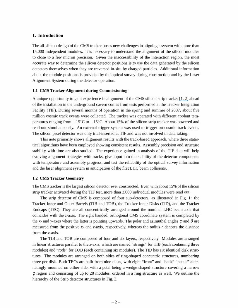
1.2 CMS Tracker Geometry

The CMS tracker is the largest silicon detector ever constructed. Even with about 15% of the siliconstrip tracker activated during the TIF test, more than 2,000individual modules were read out.

The strip detector of CMS is composed of four sub-detectors,as illustrated in Fig. 1: theTracker Inner and Outer Barrels (TIB and TOB), the Tracker Inner Disks (TID), and the TrackerEndcaps (TEC). They are all concentrically arranged aroundthe nominal LHC beam axis thatcoincides with thez-axis. The right handed, orthogonal CMS coordinate system is completed bythex- andy-axes where the latter is pointing upwards. The polar and azimuthal anglesφ andθ aremeasured from the positivex- andz-axis, respectively, whereas the radiusr denotes the distancefrom thez-axis.

The TIB and TOB are composed of four and six layers, respectively. Modules are arrangedin linear structures parallel to thez-axis, which are named “strings” for TIB (each containing threemodules) and “rods” for TOB (each containing six modules). The TID has six identical disk struc-tures. The modules are arranged on both sides of ring-shapedconcentric structures, numberingthree per disk. Both TECs are built from nine disks, with eight “front” and “back” “petals” alter-natingly mounted on either side, with a petal being a wedge-shaped structure covering a narrowφ region and consisting of up to 28 modules, ordered in a ring structure as well. We outline thehierarchy of the Strip detector structures in Fig. 2.

– 2 –

https://www.researchgate.net/publication/230947766_The_CMS_experiment_at_the_CERN_LHC?el=1_x_8&enrichId=rgreq-f1aef4fa82159a5ff4d4b3a530a24a97-XXX&enrichSource=Y292ZXJQYWdlOzUwMjc2OTM3O0FTOjk5Njc2MzM0MzI5ODY2QDE0MDA3NzYwOTkxNTE=

Strips in therφ modules have their direction parallel to the beam axis in thebarrel and radiallyin the endcaps. There are also stereo modules in the first two layers or rings of all four sub-detectors (TIB, TOB, TID, TEC) and also in ring five of the TEC.The stereo modules are mountedback-to-back to therφ modules with a stereo angle of 100 mrad and provide, when combiningmeasurements with therφ modules, a measurement ofz in the barrel orr in the endcap. A pair ofan rφ and a stereo module is also called a double-sided module. Thestrip pitch varies from 80 to205 µm depending on the module, leading to single point resolutions of up to 23−53 µm in thebarrel [2].

2. Input to Alignment

In this section we discuss the input data for the alignment procedure of the CMS Tracker: chargedparticle tracks, optical survey prior to and during installation, and laser alignment system measure-ments.

2.1 Charged Particle Tracks

Track reconstruction and performance specific to the Tracker Integration Facility configuration arediscussed in detail in Refs. [3, 4].

Three different trigger configurations were used in TIF data-taking, called A, B and C andshown in Fig. 3. About 15% of the detector modules, all located at z > 0, were powered andread-out. This includes 444 modules in TIB (16%), 720 modules in TOB (14%), 204 modules inTID (25%), and 800 modules in TEC (13%). Lead plates were included above the lower triggerscintillators, which enforced a minimum energy of the cosmic rays of 200 MeV to be triggered.

The data were collected in trigger configuration A at room temperature (+15◦C), both beforeand after insertion of the TEC atz< 0. All other configurations (B and C) had all strip detectorcomponents integrated. In addition to room temperature, configuration C was operated at +10◦C,-1 ◦C, -10◦C, and -15◦C. Due to cooling limitations, a large number of modules had to be turned

Figure 1. A quarter of the CMS silicon tracker in anrz view. Single module positions are indicated aspurple lines and dark blue lines indicate pairs ofrφ and stereo modules. The path of the laser rays, the beamsplitters (BS) and the alignment tubes (AT) of the Laser Alignment System are shown.

– 3 –

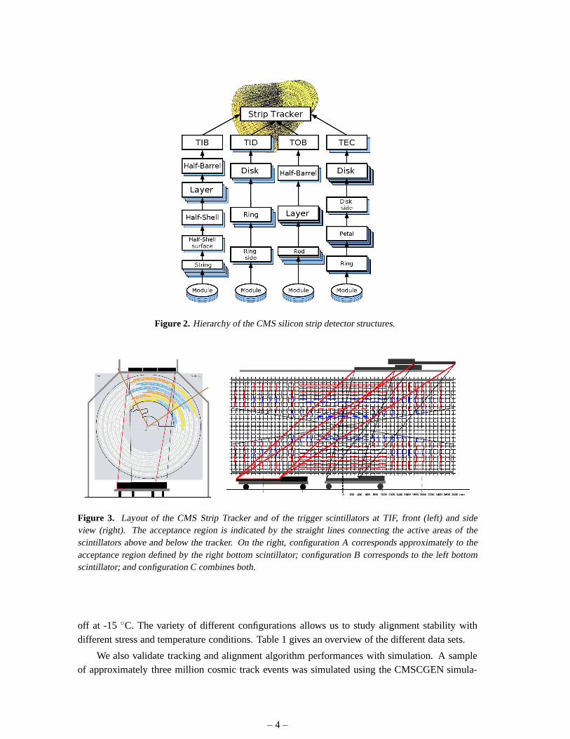
https://www.researchgate.net/publication/230947766_The_CMS_experiment_at_the_CERN_LHC?el=1_x_8&enrichId=rgreq-f1aef4fa82159a5ff4d4b3a530a24a97-XXX&enrichSource=Y292ZXJQYWdlOzUwMjc2OTM3O0FTOjk5Njc2MzM0MzI5ODY2QDE0MDA3NzYwOTkxNTE=

https://www.researchgate.net/publication/258244536_Track_Reconstruction_with_Cosmic_Ray_Data_at_the_Tracker_Integration_Facility?el=1_x_8&enrichId=rgreq-f1aef4fa82159a5ff4d4b3a530a24a97-XXX&enrichSource=Y292ZXJQYWdlOzUwMjc2OTM3O0FTOjk5Njc2MzM0MzI5ODY2QDE0MDA3NzYwOTkxNTE=

Figure 2. Hierarchy of the CMS silicon strip detector structures.

Figure 3. Layout of the CMS Strip Tracker and of the trigger scintillators at TIF, front (left) and sideview (right). The acceptance region is indicated by the straight lines connecting the active areas of thescintillators above and below the tracker. On the right, configuration A corresponds approximately to theacceptance region defined by the right bottom scintillator;configuration B corresponds to the left bottomscintillator; and configuration C combines both.

off at -15 ◦C. The variety of different configurations allows us to studyalignment stability withdifferent stress and temperature conditions. Table 1 givesan overview of the different data sets.

We also validate tracking and alignment algorithm performances with simulation. A sampleof approximately three million cosmic track events was simulated using the CMSCGEN simula-

– 4 –

LabelTriggerPosition

Temperature Ntrig Comments

A1 A 15◦C 665 409 before TEC- insertionA2 A 15◦C 189 925 after TEC- insertion

B B 15◦C 177 768

C15 C 15◦C 129 378

C10 C 10◦C 534 759

C0 C -1◦C 886 801

C−10 C -10◦C 902 881

C−15 C -15◦C 655 301 less modules read out

C14 C 14.5◦C 112 134

MC C – 3 091 306 simulation

Table 1. Overview of different data sets, ordered in time, and their number of triggered eventsNtrig takinginto account only good running conditions.

tor [5]. Only cosmic muon tracks within specific geometricalranges were selected to simulatethe scintillator trigger configuration C. To extend CMSCGEN’s energy range, events at low muonenergy have been re-weighted to adjust the energy spectrum to the CAPRICE data [6].

Charged track reconstruction includes three essential steps: seed finding, pattern recognition,and track fitting. Several pattern recognition algorithms are employed on CMS, such as “Combina-torial Track Finder” (CTF), “Road Search”, and “Cosmic Track Finder”, the latter being specific tothe cosmic track reconstruction. All three algorithms use the Kalman filter algorithm for final trackfitting, but the first two steps are different. The track modelused is a straight line parametrisedby four parameters where the Kalman filter track fit includes multiple scattering effects in eachcrossed layer. We employ the CTF algorithm for alignment studies in this note.

In order to recover tracking efficiency which is otherwise lost in the pattern recognition phasebecause hits are moved outside the standard search window defined by the detector resolution, an“alignment position error” (APE) is introduced. This APE isadded quadratically to the hit resolu-tion, and the combined value is subsequently used as a searchwindow in the pattern recognitionstep. The APE settings used for the TIF data are modelling theassembly tolerances [2].

There are several important aspects of the TIF configurationwhich require special handlingwith respect to normal data-taking. First of all, no magnetic field is present. Therefore, the mo-mentum of the tracks cannot be measured and estimates of the energy loss and multiple scatteringcan be done only approximately. A track momentum of 1 GeV/c is assumed in the estimates, whichis close to the average cosmic track momentum observed in simulated spectra. Other TIF-specificfeatures are due to the fact that the cosmic muons do not originate from the interaction region.Therefore the standard seeding mechanism is extended to usealso hits in the TOB and TEC, andno beam spot constraint is applied. For more details see Ref.[3].

Reconstruction of exactly one cosmic muon track in the eventis required. A number of selec-tion criteria is applied on the hits, tracks, and detector components subject to alignment, to ensuregood quality data. This is done based on trajectory estimates and the fiducial tracking geometry.In addition, hits from noisy clusters or from combinatorialbackground tracks are suppressed by

– 5 –


https://www.researchgate.net/publication/45865260_Parametrization_of_the_Cosmic_Muon_Flux_for_the_Generator_CMSCGEN?el=1_x_8&enrichId=rgreq-f1aef4fa82159a5ff4d4b3a530a24a97-XXX&enrichSource=Y292ZXJQYWdlOzUwMjc2OTM3O0FTOjk5Njc2MzM0MzI5ODY2QDE0MDA3NzYwOTkxNTE=

quality cuts on the clusters. The detailed track selection is as follows:

• The direction of the track trajectory satisfies the requirements: −1.5 < ηtrack < 0.6 and−1.8 < φtrack < −1.2 rad, according to the fiducial scintillator positions.

• Theχ2 value of the track fit, normalised to the number of degrees of freedom, fulfilsχ2track/ndof<

4.

• The track has at least 5 hits associated and among those at least 2 matched hits in double-sided modules.

A hit is kept for the track fit:

• If it is associated to a cluster with a total charge of at least50 ADC counts. If the hit ismatched, both components must satisfy this requirement.

• If it is isolated, i.e. if any other reconstructed hit is found on the same module within 8.0 mm,the whole track is rejected. This cut helps in rejecting fakeclusters generated by noisy stripsand modules.

• If it is not discarded by the outlier rejection step during the refit (see below).

The remaining tracks and their associated hits are refit in every iteration of the alignmentalgorithms. An outlier rejection technique is applied during the refit. Its principle is to iterate thefinal track fit until no outliers are found. An outlier is defined as a hit whose trajectory estimate islarger than a given cut value (ecut = 5). The trajectory estimate of a hit is the quantity:e= rT

·V−1·

r , wherer is the 1- or 2-dimensional local residual vector andV is the associated covariance matrix.If one or more outliers are found in the first track fit, they areremoved from the hit collection andthe fit is repeated. This procedure is iterated until there are no more outliers or the number ofsurviving hits is less than 4.

Unless otherwise specified, these cuts are common to all alignment algorithms used. Thecombined efficiency for all the cuts above is estimated to be 8.3% on TIF data (the C−10 sample isused in this estimate) and 20.5% in the TIF simulation sample.

2.2 Survey of the CMS Tracker

Information about the relative position of modules within detector components and of the larger-level structures within the tracker is available from the optical survey analysis prior to or duringthe tracker integration. This includes Coordinate Measuring Machine (CMM) data and photogram-metry, the former usually used for the active element measurements and the latter for the largerobject alignment. For the inner strip detectors (TIB and TID), survey data at all levels was usedin analysis. For the outer strip detectors (TOB and TEC), module-level survey was used only formounting precision monitoring, while survey of high-levelstructures was used in analysis.

For TIB, survey measurements are available for the module positions with respect to shells,and of cylinders with respect to the tracker support tube. Similarly, for TID, survey measurementswere done for modules with respect to the rings, rings with respect to the disks and disks with

– 6 –

Figure 4. Displacement of modules in global cylindrical coordinatesas measured in survey with respect todesign geometry. A colour coding is used: black for TIB, green for TID, red for TOB, and blue for TEC.

respect to the tracker support tube. For TOB, the wheel was measured with respect to the trackersupport tube. For TEC, measurements are stored at the level of disks with respect to the endcapsand endcaps with respect to the tracker support tube.

Figure 4 illustrates the relative positions of the CMS tracker modules with respect to designgeometry as measured in optical survey: as can be seen, differences from design geometry aslarge as several millimetres are expected. Since hierarchical survey measurements were performedand TOB and TEC have only large-structure information, the corresponding modules appear to becoherently displaced in the plot.

2.3 Laser Alignment System of the CMS Tracker

The Laser Alignment System (LAS, see Fig. 1) [1, 2] uses infrared laser beams with a wavelengthof λ = 1075 nm to monitor the position of selected tracker modules.It operates globally on trackersubstructures (TIB, TOB and TEC disks) and cannot determinethe position of individual mod-ules. The goal of the system is to generate alignment information on a continuous basis, providing

– 7 –

geometry reconstruction of the tracker substructures at the level of 100µm. In addition, possibletracker structure movements can be monitored at the level of10 µm, providing additional input forthe track based alignment.

In each TEC, laser beams cross all nine TEC disks in ring 6 and ring 4 on the back petals,equally distributed inφ . Here, special silicon sensors with a 10 mm hole in the backside metallisa-tion and an anti-reflective coating are mounted. The beams are used for the internal alignment ofthe TEC disks. The other eight beams, distributed inφ , are foreseen to align TIB, TOB, and bothTECs with respect to each other. Finally, there is a link to the muon system, which is establishedby 12 laser beams (six on each side) with precise position andorientation in the tracker coordinatesystem.

The signal induced by the laser beams on the silicon sensors decreases in height as the beamspenetrate through subsequent silicon layers in the TECs andthrough beam splitters in the align-ment tubes that partly deflect the beams onto TIB and TOB sensors. To obtain optimal signals onall sensors, a sequence of laser pulses with increasing intensities, optimised for each position, isgenerated. Several triggers per intensity are taken and thesignals are averaged. In total, a fewhundred triggers are needed to get a full picture of the alignment of the tracker structure. Since thetrigger rate for the alignment system is around 100 Hz, this takes only a few seconds.

3. Statistical Methods and Approaches

Alignment analysis with tracks uses the fact that the hit positions and the measured trajectoryimpact points of a track are systematically displaced if themodule position is not known correctly.The difference in local module coordinates between these two quantities are thetrack-hit residualsr i , which are 1- (2-dimensional) vectors in the case of a single(double) sided module and whichone would like to minimise. More precisely, one can minimisethe χ2 function which includes acovariance matrixV of the measurement uncertainties:

χ2 =hits

∑i

rTi (p,q)V−1

i r i(p,q) (3.1)

whereq represents the track parameters andp represents the alignment parameters of the modules.

A module is assumed to be a rigid body, so three absolute positions and three rotations aresufficient to parametrise its degrees of freedom. These are commonly defined for all methods inthe module coordinates as illustrated in Fig. 5. The local positions are calledu, v andw, where

w ( r)

u ( rφ)v ( z)

αγβ

+

++

Figure 5. Schematic illustration of the local coordinates of a moduleas used for alignment. Global parame-ters (in parentheses) are shown for modules in the barrel detectors (TIB and TOB).

– 8 –

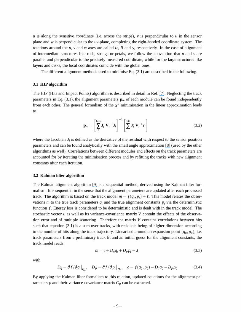
u is along the sensitive coordinate (i.e. across the strips),v is perpendicular tou in the sensorplane andw is perpendicular to theuv-plane, completing the right-handed coordinate system. Therotations around theu, v andw axes are calledα , β andγ , respectively. In the case of alignmentof intermediate structures like rods, strings or petals, wefollow the convention thatu andv areparallel and perpendicular to the precisely measured coordinate, while for the large structures likelayers and disks, the local coordinates coincide with the global ones.

The different alignment methods used to minimise Eq. (3.1) are described in the following.

3.1 HIP algorithm

The HIP (Hits and Impact Points) algorithm is described in detail in Ref. [7]. Neglecting the trackparameters in Eq. (3.1), the alignment parameterspm of each module can be found independentlyfrom each other. The general formalism of theχ2 minimisation in the linear approximation leadsto

pm =

[

hits

∑i

JTi V−1

i Ji

]

−1[

hits

∑i

JTi V−1

i r i

]

(3.2)

where the JacobianJi is defined as the derivative of the residual with respect to the sensor positionparameters and can be found analytically with the small angle approximation [8] (used by the otheralgorithms as well). Correlations between different modules and effects on the track parameters areaccounted for by iterating the minimisation process and by refitting the tracks with new alignmentconstants after each iteration.

3.2 Kalman filter algorithm

The Kalman alignment algorithm [9] is a sequential method, derived using the Kalman filter for-malism. It is sequential in the sense that the alignment parameters are updated after each processedtrack. The algorithm is based on the track modelm= f (qt , pt)+ ε. This model relates the obser-vationsm to the true track parametersqt and the true alignment constantspt via the deterministicfunction f . Energy loss is considered to be deterministic and is dealt with in the track model. Thestochastic vectorε as well as its variance-covariance matrixV contain the effects of the observa-tion error and of multiple scattering. Therefore the matrixV contains correlations between hitssuch that equation (3.1) is a sum over tracks, with residualsbeing of higher dimension accordingto the number of hits along the track trajectory. Linearisedaround an expansion point(q0, p0), i.e.track parameters from a preliminary track fit and an initial guess for the alignment constants, thetrack model reads:

m= c+Dqqt +Dppt + ε, (3.3)

with

Dq = ∂ f /∂qt

∣

∣

q0, Dp = ∂ f /∂ pt

∣

∣

p0, c = f (q0, p0)−Dqq0−Dpp0 (3.4)

By applying the Kalman filter formalism to this relation, updated equations for the alignment pa-rametersp and their variance-covariance matrixCp can be extracted.

– 9 –

https://www.researchgate.net/publication/2169000_Sensor_Alignment_by_Tracks?el=1_x_8&enrichId=rgreq-f1aef4fa82159a5ff4d4b3a530a24a97-XXX&enrichSource=Y292ZXJQYWdlOzUwMjc2OTM3O0FTOjk5Njc2MzM0MzI5ODY2QDE0MDA3NzYwOTkxNTE=

https://www.researchgate.net/publication/267704422_The_HIP_Algorithm_for_Track_Based_Alignment_and_its_Application_to_the_CMS_Pixel_Detector?el=1_x_8&enrichId=rgreq-f1aef4fa82159a5ff4d4b3a530a24a97-XXX&enrichSource=Y292ZXJQYWdlOzUwMjc2OTM3O0FTOjk5Njc2MzM0MzI5ODY2QDE0MDA3NzYwOTkxNTE=

https://www.researchgate.net/publication/266497341_A_Kalman_Filter_for_Track-based_Alignment?el=1_x_8&enrichId=rgreq-f1aef4fa82159a5ff4d4b3a530a24a97-XXX&enrichSource=Y292ZXJQYWdlOzUwMjc2OTM3O0FTOjk5Njc2MzM0MzI5ODY2QDE0MDA3NzYwOTkxNTE=

3.3 Millepede algorithm

Millepede II [11] is an upgraded version of the Millepede program [10]. Its principle is a global fitto minimise theχ2 function, simultaneously taking into account track and alignment parameters.Since angular corrections are small, the linearised problem is a good approximation for alignment.Being interested only in then alignment parameters, the problem is reduced to the solution of amatrix equation of sizen.

The χ2 function, Eq. (3.1), depends on track (local,q) and alignment (global,p) parameters.For uncorrelated hit measurementsy ji of the track j, with uncertaintiesσ ji , it can be rewritten as

χ2(p,q) =tracks

∑j

hits

∑i

(y ji − f ji (p,q j))2

σ2ji

(3.5)

whereq j denotes the parameters of trackj.

Given reasonable start valuesp0 andq j0 as expected in alignment, the track model predictionf ji (p,q j) can be linearised. Applying the least squares method to minimize χ2, results in a largelinear system with one equation for each alignment parameter and all the track parameters of eachtrack. The particular structure of the system of equations allows a reduction of its size, leading tothe matrix equation

Ca = b (3.6)

for the small correctionsa to the alignment parameter start valuesp0.

3.4 Limitations of alignment algorithms

We should note that Eq. (3.1) may be invariant under certain coherent transformations of assumedmodule positions, the so-called “weak” modes. The trivial transformation which isχ2-invariant isa global translation and rotation of the whole tracker. Thistransformation has no effect in internalalignment, and is easily resolved by a suitable convention for defining the global reference frame.Different algorithms employ different approaches and conventions here, so we will discuss this inmore detail as it applies to each algorithm.

The non-trivialχ2-invariant transformations which preserve Eq. (3.1) are oflarger concern.For the full CMS tracker with cylindrical symmetry one coulddefine certain “weak” modes, suchas elliptical distortion, twist, etc., depending on the track sample used. However, since we use onlya partial CMS tracker without the full azimuthal coverage, different “weak” modes may show up.For example, since we have predominantly vertical cosmic tracks (along the globaly axis), a simpleshift of all modules in they direction approximately constitutes a “weak” mode, this transformationpreserving the size of the track residuals for a vertical track. However, since we still have trackswith some angle to vertical axis, some sensitivity to they coordinate remains.

In general, any particular track sample would have its own “weak” modes and the goal of anunbiased alignment procedure is to remove allχ2-invariant transformations with a balanced inputof different kinds of tracks. In this study we are limited to only predominantly vertical singlecosmic tracks and this limits our ability to constrainχ2-invariant transformations, or the “weak”modes. This is discussed more in the validation section.

– 10 –

https://www.researchgate.net/publication/1980776_A_New_Method_for_the_High-Precision_Alignment_of_Track_Detectors?el=1_x_8&enrichId=rgreq-f1aef4fa82159a5ff4d4b3a530a24a97-XXX&enrichSource=Y292ZXJQYWdlOzUwMjc2OTM3O0FTOjk5Njc2MzM0MzI5ODY2QDE0MDA3NzYwOTkxNTE=

3.5 Application of Alignment Algorithms to the TIF Analysis

Accurate studies have been performed with all algorithms inorder to determine the maximal setof detectors that can be aligned and the aligned coordinatesthat are sensitive to the peculiar trackpattern and limited statistics of TIF cosmic track events.

For the tracker barrels (TIB and TOB), the collected statistics is sufficient to align at the levelof single modules if restricting to a geometrical subset corresponding to the positions of the scintil-lators used for triggering. The detectors aligned are thosewhose centres lie inside the geometricalrangesz> 0, x < 75 cm and 0.5< φ < 1.7 rad where all the coordinates are in the global CMSframe.

The local coordinates aligned for each module are

• u, v, γ for TOB double-sided modules,

• u, γ for TOB single-sided modules,

• u, v, w, γ for TIB double-sided modules and

• u, w, γ for TIB single-sided modules.

Due to the rapidly decreasing cosmic track rate∼ cos2ψ (with ψ measured from zenith) onlya small fraction of tracks cross the endcap detector modulesat an angle suitable for alignment.Therefore, thez+-side Tracker endcap (TEC) could only be aligned at the levelof disks. All ninedisks are considered in TEC alignment, and the only aligned coordinate is the angle∆φ around theCMS z-axis. Because there are only data in two sectors of the TEC, the track-based alignment isnot sensitive to thex andy coordinates of the disks.

The Tracker Inner Disks (TID) are not aligned due to lack of statistics. Figure 6 visualises themodules selected for the track-based alignment procedure.

3.5.1 HIP algorithm

Preliminary residual studies show that, in real data, the misalignment of the TIB is larger than inTOB, and TEC alignment is quite independent from that of other structures. For this reason, theoverall alignment result is obtained in three steps:

1. In the first step, the TIB is excluded from the analysis and the tracks are refit using onlyreconstructed hits in the TOB. Alignment parameters are obtained for this subdetector only.No constraints are applied on the global coordinates of the TOB as a whole.

2. In the second step, the tracks are refit using all their hits; the TOB is fixed to the positionsfound after step 1 providing the global reference frame; andalignment parameters are ob-tained for TIB only.

3. The alignment of the TEC is then performed as a final step starting from the aligned barrelgeometry found after steps 1 and 2.

Selection of aligned objects and coordinates is done according to the common criteria de-scribed in Secs. 2.1 and 3.5.

– 11 –

Figure 6. Visualisation of the modules used in the track-based alignment procedure. Selected modules basedon the common geometrical and track-based selection for thealgorithms.

The Alignment Position Error (APE) for the aligned detectors is set at the first iteration to avalue compatible with the expected positioning uncertainties after assembly, then decreased lin-early with the iteration number, reaching zero at iterationn (n varies for different alignment steps).Further iterations are then run using zero APE.

In order to avoid a bias in track refitting from parts of the TIFtracker that are not aligned inthis procedure (e.g. low-φ barrel detectors), an arbitrarily large APE is assigned forall iterations totrajectory measurements whose corresponding hits lie in these detectors, de-weighting them in theχ2 calculation.

For illustrative purposes, we show here the results of HIP alignment on the C−10 TIF datasample after event selection. Figure 7 shows examples of theevolution of the aligned positionsand the alignment parameters calculated by the HIP algorithm after every iteration. We observereasonable convergence for the coordinates that are expected to be most precisely determined (seeSec. 4.3) and a stable result in subsequent iterations usingzero APE.

3.5.2 Kalman filter algorithm

In the barrel, the alignment is carried out starting from themodule survey geometry. The alignmentparameters are calculated for all modules in the TIB and the TOB at once, using the commonalignable selection described in Sec. 3.5. No additional alignable selection criteria, for instance aminimum number of hits per module, is used. Due to the lack of any external aligned referencesystem, some global distortions in the final alignment can show up, e.g. shearing or rotation withrespect to the true geometry.

The tracking is adapted to the needs of the algorithm, especially to include the current estimateof the alignment parameters. Since for every module the position error can be calculated from the

– 12 –

Iteration0 1 2 3 4 5 6 7 8 9 10

m]

µx

[∆

-600-400-200

0200400600

Iteration0 1 2 3 4 5 6 7 8 9 10

m]

µ [ xP

-600-400-200

0200400600

Iteration0 1 2 3 4 5 6 7 8 9 10

m]

µz

[∆

-1500

-1000

-500

0

500

1000

1500

Iteration0 1 2 3 4 5 6 7 8 9 10

m]

µ [ zP

-1500

-1000

-500

0

500

1000

1500

Figure 7. Results of the first HIP alignment step (TOB modules only) on the C−10 TIF data sample. Fromtop to bottom the plots show respectively the quantities∆x for all modules and∆z for double-sided moduleswhere∆ stands for the difference between the aligned local position of a module at a given iteration of thealgorithm and the nominal position of the same module. On theleft column the evolution of the objectposition is plotted vs. the iteration number (different line styles correspond to the 6 TOB layers), while onthe right the parameter increment for each iteration of the corresponding alignment parameters is shown.

up-to-date parameter errors, no additional fixed AlignmentPosition Error (APE) is used. Thematerial effects are crudely taken into account by assuminga momentum of 1.5 GeV/c, which islarger than the one used in standard track reconstruction.

TEC alignment is determined on disk level. Outlying tracks,which would cause unreasonablylarge changes of the alignment parameters if used by the algorithm, are discarded. Due to theexperimental setup, the total number of hits per disk decreases such that the error on the calculatedparameter increases from disk one to disk nine. During the alignment process, disk 1 is used asreference. After that, the alignment parameters are transformed into the coordinate system definedby fixing the mean and slope ofφ(z) to zero. This is done because there is no sensitivity to a lineartorsion, which, in a linear approximation, corresponds to aslope inφ(z), expected for the TEC.Due to differences in the second order approximation between a track inclination and a torsionof the TEC, the algorithm basically has a small sensitivity to a torsion of the endcap. Here, thelinear component is expected to be superimposed into movements of the disks inx andy, whichare converted by the algorithm into rotations because theseare the only free parameters.

The alignment parameters do not seem to depend strongly on the temperature (see section 5.2),so all data except for the runs at -15◦C were merged to increase the statistics.

3.5.3 Millepede algorithm

Millepede alignment is performed at module level in both TIBand TOB, and at disk level in theTEC, in one step only. To fix the six degrees of freedom from global translation and rotation,equality constraints are used on the parameters in the TOB: These inhibit overall shifts and rotations

– 13 –

(#hits)10

log0 1 2 3 4 5 6

#par

amet

ers

0

10

20

30

40

50

60

70

/ndf2χ0 1 2 3 4 5 6 7 8

norm

alis

ed #

trac

ks

-710

-610

-510

-410

before first iteration

after final iteration

Figure 8. Number of hits for the parameters aligned with Millepede (left) and improvement of the nor-malisedχ2 distribution as seen by Millepede (right).

of the TOB, while the TIB parameters are free to adjust to the fixed TOB position. In addition, TECdisk one is kept as fixed.

The requirements to select a track useful for alignment are described in Sec. 2.1. All thesecriteria are applied, except for the hit outlier rejection since outlier down-weighting is appliedwithin the minimisation process. Since Millepede internally refits the tracks, it is additionallyrequired that a track hits at least five of those modules whichare subject to the alignment procedure.Multiple scattering and energy loss effects are treated, asin the Kalman filter alignment algorithm,by increasing and correlating the hit uncertainties, assuming a track momentum of 1.5 GeV/c. Thislimits the accuracy of the assumption of uncorrelated measured hit positions in Eq. (3.5).

The alignment parameters are calculated for all modules using the common alignable selectiondescribed in Sec. 3.5. Due to the fact that barrel and endcap are aligned together in one step, norequest on the minimum number of hits in the subdetector for aselected track is done.

The required minimum number of hits for a module to be alignedis set to 50. Due to themodest number of parameters, the matrix equation (3.6) is solved by inversion with five Millepedeglobal iterations. In each global iteration, the track fits are repeated four times with alignmentparameters updated from the previous global iteration. Except for the first track fit iteration, down-weighting factors are assigned for each hit depending on itsnormalised residuum of the previousfit (details see [11]). About 0.5% of the tracks with an average hit weight below 0.8 are rejectedcompletely.

Fig. 8 shows, on the left, the number of hits per alignment parameter used for the globalminimisation; 58 modules fail the cut of 50 hits. On the right, the normalisedχ2 distributions ofthe Millepede internal track fits before and after minimisation are shown. The distributions do nothave a peak close to one, indicating that the hit uncertainties are overestimated. Nevertheless, theeffect of minimisation can clearly be seen.

– 14 –

4. Validation of Alignment of the CMS Tracker at TIF

In this section we present validation of the alignment results. Despite the limited precision ofalignment that prevents detailed systematic distortion studies, the available results from TIF provideimportant validation of tracker alignment for the set of modules used in this study.

The evolution of the module positions is shown starting fromthe design geometry, moving tosurvey measurements, and finally comparing to the results from the track-based algorithms. Boththe overall track quality and individual hit residuals improve between the three steps. All threetrack-based algorithms produce similar results when the same input and similar approaches aretaken. We show that the residual misalignments are consistent with statistical uncertainties in theprocedure. Therefore, we pick just one alignment geometry from the track-based algorithms forillustration of results when comparison between differentalgorithms is not relevant.

4.1 Validation Methods

We use two methods in validation and illustration of the alignment results. One approach is track-based and the other approach directly compares geometries resulting from different sets of align-ment constants.

In the track-based approach, we refit the tracks with all Alignment Position Errors (APE) setto zero. A loose track selection is applied, requiring at least six hits where more than one of themmust be two-dimensional. Hit residuals will be shown as the difference between the measured hitposition and the track position on the module plane. To avoida bias, the latter is predicted withoutusing the information of the considered hit. In the barrel part of the tracker, the residuals in localx′ andy′ direction, parallel tou andv, will be shown. The sign is chosen such that positive valuesalways point into the samerφ andz directions, irrespective of the orientation of the local coordi-nate system. For the wedge-shaped sensors as in TID and TEC, the residuals have a correlationdepending on the localx- andy-coordinates of the track impact point. The residuals in global rφ -andr-coordinates therefore are used for these modules.

In addition to misalignment, hit residual distributions depend on the intrinsic hit resolutionand the track prediction uncertainty. For low-momentum tracks (as expected to dominate the TIFdata) in the CMS tracker, the latter is large. For a momentum of 1 GeV/c and an extrapolationas between two adjacent TOB layers between two consecutive hits, the mean multiple scatteringdisplacement is about 250µm. So even with perfect alignment one expects a width of the residualdistribution that is significantly larger than the intrinsic hit resolution of up to 23−53 µm in thestrip tracker barrel [2].

Another way of validating alignment results is provided by direct comparison of the obtainedtracker geometries. This is done by showing differences between the same module coordinate intwo geometries (e.g. ideal and aligned) vs. their geometrical position (e.g.r, φ or z) or correlatingthese differences as seen by two different alignment methods. Since not all alignment algorithmsfix the position and orientation of the full tracker, comparison between two geometries is done aftermaking the centre of gravity and the overall orientation of the considered modules coincide.

4.2 Validation of the Assembly and Survey Precision

Improvements of the absolute track fitχ2 are observed when design geometry, survey measure-

– 15 –

2χ0 100 200 300 400 500 600 700 800

# tr

acks

10

210

310

410

2χ0 20 40 60 80 100

# tr

acks

0

2000

4000

6000

8000

10000

12000

14000

16000

18000

20000

22000

Design: mean= 78.4

Survey: mean= 63.7

Aligned: mean= 43.0

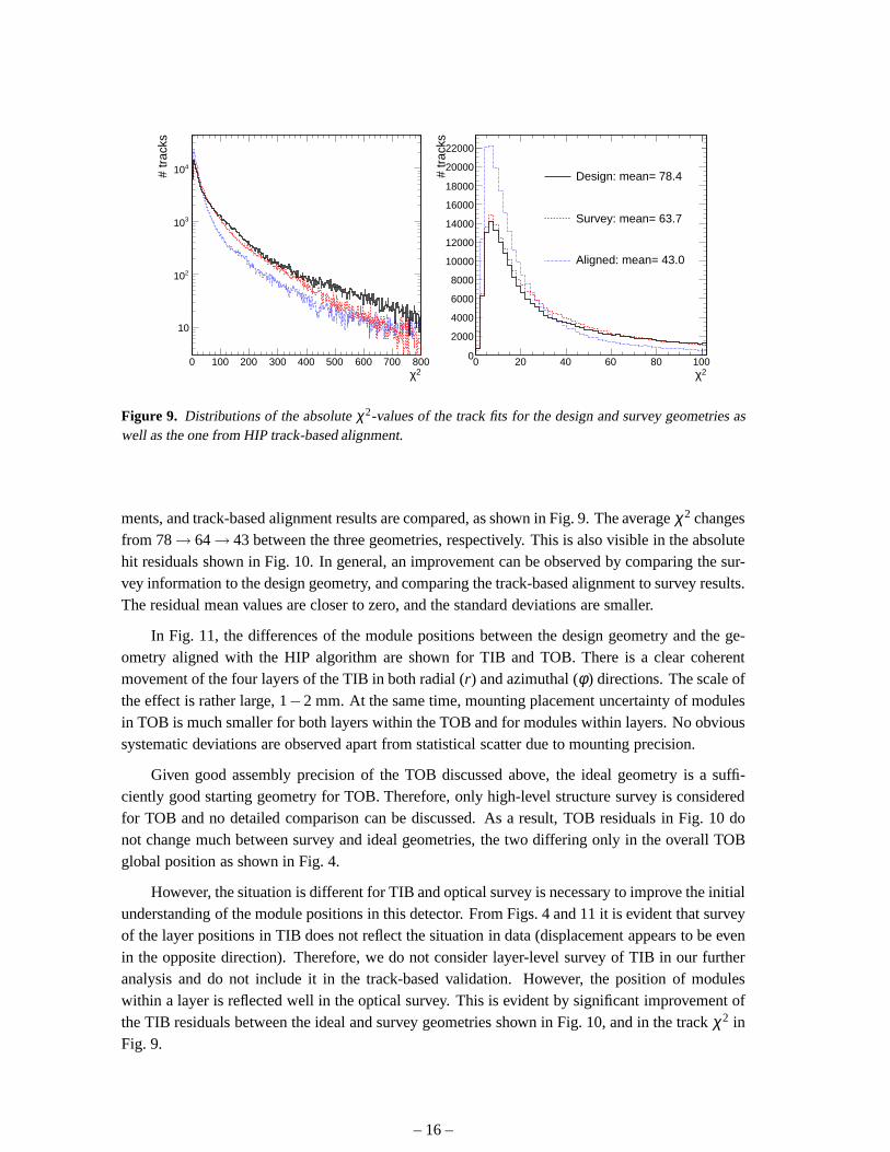
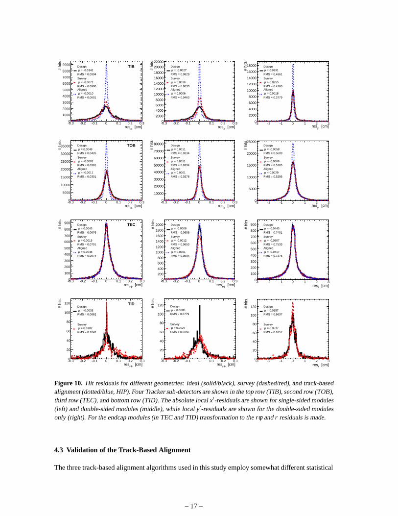
Figure 9. Distributions of the absoluteχ2-values of the track fits for the design and survey geometriesaswell as the one from HIP track-based alignment.

ments, and track-based alignment results are compared, as shown in Fig. 9. The averageχ2 changesfrom 78→ 64→ 43 between the three geometries, respectively. This is alsovisible in the absolutehit residuals shown in Fig. 10. In general, an improvement can be observed by comparing the sur-vey information to the design geometry, and comparing the track-based alignment to survey results.The residual mean values are closer to zero, and the standarddeviations are smaller.

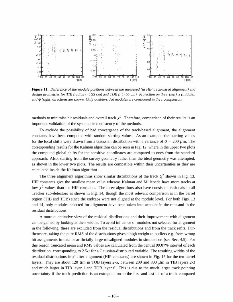
In Fig. 11, the differences of the module positions between the design geometry and the ge-ometry aligned with the HIP algorithm are shown for TIB and TOB. There is a clear coherentmovement of the four layers of the TIB in both radial (r) and azimuthal (φ ) directions. The scale ofthe effect is rather large, 1−2 mm. At the same time, mounting placement uncertainty of modulesin TOB is much smaller for both layers within the TOB and for modules within layers. No obvioussystematic deviations are observed apart from statisticalscatter due to mounting precision.

Given good assembly precision of the TOB discussed above, the ideal geometry is a suffi-ciently good starting geometry for TOB. Therefore, only high-level structure survey is consideredfor TOB and no detailed comparison can be discussed. As a result, TOB residuals in Fig. 10 donot change much between survey and ideal geometries, the twodiffering only in the overall TOBglobal position as shown in Fig. 4.

However, the situation is different for TIB and optical survey is necessary to improve the initialunderstanding of the module positions in this detector. From Figs. 4 and 11 it is evident that surveyof the layer positions in TIB does not reflect the situation indata (displacement appears to be evenin the opposite direction). Therefore, we do not consider layer-level survey of TIB in our furtheranalysis and do not include it in the track-based validation. However, the position of moduleswithin a layer is reflected well in the optical survey. This isevident by significant improvement ofthe TIB residuals between the ideal and survey geometries shown in Fig. 10, and in the trackχ2 inFig. 9.

– 16 –

[cm]x’res-0.3 -0.2 -0.1 0 0.1 0.2 0.3

# hi

ts

0

1000

2000

3000

4000

5000

6000

7000

8000

9000

RMS = 0.0994 = -0.0141µ

Design

RMS = 0.0900 = -0.0071µ

Survey

RMS = 0.0601 = -0.0010µ

Aligned

TIB

[cm]x’res-0.3 -0.2 -0.1 0 0.1 0.2 0.3

# hi

ts

0

2000

4000

6000

8000

10000

12000

14000

16000

18000

20000

22000

RMS = 0.0829 = -0.0027µ

Design

RMS = 0.0633 = 0.0036µ

Survey

RMS = 0.0463 = 0.0006µ

Aligned

[cm]y’res-3 -2 -1 0 1 2 3

# hi

ts

0

2000

4000

6000

8000

10000

12000

14000

16000

18000

RMS = 0.4861 = 0.0331µ

Design

RMS = 0.4760 = 0.0255µ

Survey

RMS = 0.3779 = 0.0018µ

Aligned

[cm]x’

res-0.3 -0.2 -0.1 0 0.1 0.2 0.3

# hi

ts

0

5000

10000

15000

20000

25000

30000

35000

RMS = 0.0426 = 0.0049µ

Design

RMS = 0.0391 = -0.0001µ

Survey

RMS = 0.0301 = -0.0011µ

Aligned

TOB

[cm]x’

res-0.3 -0.2 -0.1 0 0.1 0.2 0.3

# hi

ts

0

10000

20000

30000

40000

50000

60000

70000

80000

RMS = 0.0334 = 0.0011µ

Design

RMS = 0.0334 = 0.0011µ

Survey

RMS = 0.0278 = 0.0001µ

Aligned

[cm]y’

res-3 -2 -1 0 1 2 3

# hi

ts

0

5000

10000

15000

20000

25000

RMS = 0.5609 = -0.0058µ

Design

RMS = 0.5705 = -0.0066µ

Survey

RMS = 0.5285 = 0.0029µ

Aligned

[cm]Φrres-0.3 -0.2 -0.1 0 0.1 0.2 0.3

# hi

ts

0

100

200

300

400

500

600

700

800

900

RMS = 0.0676 = 0.0043µ

Design

RMS = 0.0701 = 0.0015µ

Survey

RMS = 0.0674 = 0.0048µ

Aligned

TEC

[cm]Φrres-0.3 -0.2 -0.1 0 0.1 0.2 0.3

# hi

ts

0

200

400

600

800

1000

1200

1400

1600

1800

2000

RMS = 0.0606 = -0.0006µ

Design

RMS = 0.0653 = -0.0012µ

Survey

RMS = 0.0594 = 0.0001µ

Aligned

[cm]rres-3 -2 -1 0 1 2 3

# hi

ts

0

100

200

300

400

500

600

700

800

900

RMS = 0.7401 = -0.0445µ

Design

RMS = 0.7533 = -0.0507µ

Survey

RMS = 0.7375 = -0.0417µ

Aligned

[cm]Φrres-0.3 -0.2 -0.1 0 0.1 0.2 0.3

# hi

ts

0

20

40

60

80

100

120

RMS = 0.0862 = -0.0033µ

Design

RMS = 0.1042 = 0.0182µ

Survey

TID

[cm]Φrres

-0.3 -0.2 -0.1 0 0.1 0.2 0.3

# hi

ts

0

20

40

60

80

100

120

RMS = 0.0779 = 0.0085µ

Design

RMS = 0.0850 = 0.0027µ

Survey

[cm]rres-3 -2 -1 0 1 2 3

# hi

ts

0

20

40

60

80

100

120

RMS = 0.6637 = 0.0257µ

Design

RMS = 0.6757 = 0.0537µ

Survey

Figure 10. Hit residuals for different geometries: ideal (solid/black), survey (dashed/red), and track-basedalignment (dotted/blue, HIP). Four Tracker sub-detectorsare shown in the top row (TIB), second row (TOB),third row (TEC), and bottom row (TID). The absolute localx′-residuals are shown for single-sided modules(left) and double-sided modules (middle), while localy′-residuals are shown for the double-sided modulesonly (right). For the endcap modules (in TEC and TID) transformation to therφ andr residuals is made.

4.3 Validation of the Track-Based Alignment

The three track-based alignment algorithms used in this study employ somewhat different statistical

– 17 –

r [cm]20 30 40 50 60 70 80 90 100 110

r [c

m]

∆

-0.3

-0.25

-0.2

-0.15

-0.1

-0.05

-0

0.05

0.1

0.15

0.2

r [cm]20 30 40 50 60 70 80 90 100 110

z [c

m]

∆

-0.2

-0.15

-0.1

-0.05

-0

0.05

0.1

0.15

0.2

r [cm]20 30 40 50 60 70 80 90 100 110

[cm

]φ

∆ r

*

-0.3

-0.2

-0.1

0

0.1

0.2

0.3

Figure 11. Difference of the module positions between the measured (inHIP track-based alignment) anddesign geometries for TIB (radiusr < 55 cm) and TOB (r > 55 cm). Projection on ther (left), z (middle),andφ (right) directions are shown. Only double-sided modules are considered in thezcomparison.

methods to minimise hit residuals and overall trackχ2. Therefore, comparison of their results is animportant validation of the systematic consistency of the methods.

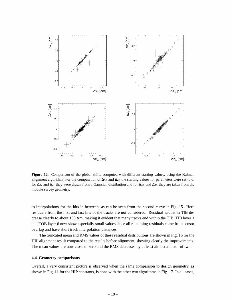
To exclude the possibility of bad convergence of the track-based alignment, the alignmentconstants have been computed with random starting values. As an example, the starting valuesfor the local shifts were drawn from a Gaussian distributionwith a variance ofσ = 200 µm. Thecorresponding results for the Kalman algorithm can be seen in Fig. 12, where in the upper two plotsthe computed global shifts for the sensitive coordinates are compared to ones from the standardapproach. Also, starting from the survey geometry rather than the ideal geometry was attempted,as shown in the lower two plots. The results are compatible within their uncertainties as they arecalculated inside the Kalman algorithm.

The three alignment algorithms show similar distributionsof the trackχ2 shown in Fig. 13.HIP constants give the smallest mean value whereas Kalman and Millepede have more tracks atlow χ2 values than the HIP constants. The three algorithms also have consistent residuals in allTracker sub-detectors as shown in Fig. 14, though the most relevant comparison is in the barrelregion (TIB and TOB) since the endcaps were not aligned at themodule level. For both Figs. 13and 14, only modules selected for alignment have been taken into account in the refit and in theresidual distributions.

A more quantitative view of the residual distributions and their improvement with alignmentcan be gained by looking at their widths. To avoid influence ofmodules not selected for alignmentin the following, these are excluded from the residual distributions and from the track refits. Fur-thermore, taking the pure RMS of the distributions gives a high weight to outliers e.g. from wronghit assignments in data or artificially large misaligned modules in simulations (see Sec. 4.5). Forthis reason truncated mean and RMS values are calculated from the central 99.87% interval of eachdistribution, corresponding to 2.5σ for a Gaussian-distributed variable. The resulting widthsof theresidual distributions inx′ after alignment (HIP constants) are shown in Fig. 15 for the ten barrellayers. They are about 120µm in TOB layers 2-5, between 200 and 300µm in TIB layers 2-3and much larger in TIB layer 1 and TOB layer 6. This is due to themuch larger track pointinguncertainty if the track prediction is an extrapolation to the first and last hit of a track compared

– 18 –

[cm]0x∆-0.2 -0.1 0 0.1 0.2

[cm

]r

x∆

-0.2

-0.1

0

0.1

0.2

[cm]0z∆-0.2 0 0.2

[cm

]r

z∆

-0.2

0

0.2

[cm]0x∆-0.2 -0.1 0 0.1 0.2

[cm

]s

x∆

-0.2

-0.1

0

0.1

0.2

[cm]0z∆-0.2 0 0.2

[cm

]s

z∆

-0.2

0

0.2

Figure 12. Comparison of the global shifts computed with different starting values, using the Kalmanalignment algorithm. For the computation of∆x0 and∆z0 the starting values for parameters were set to 0,for ∆xr and∆zr they were drawn from a Gaussian distribution and for∆xS and∆zS they are taken from themodule survey geometry.

to interpolations for the hits in between, as can be seen fromthe second curve in Fig. 15. Hereresiduals from the first and last hits of the tracks are not considered. Residual widths in TIB de-crease clearly to about 150µm, making it evident that many tracks end within the TIB. TIB layer 1and TOB layer 6 now show especially small values since all remaining residuals come from sensoroverlap and have short track interpolation distances.

The truncated mean and RMS values of these residual distributions are shown in Fig. 16 for theHIP alignment result compared to the results before alignment, showing clearly the improvements.The mean values are now close to zero and the RMS decreases by at least almost a factor of two.

4.4 Geometry comparisons

Overall, a very consistent picture is observed when the samecomparison to design geometry, asshown in Fig. 11 for the HIP constants, is done with the other two algorithms in Fig. 17. In all cases,

– 19 –

2χ0 100 200 300 400 500 600 700 800

# tr

acks

1

10

210

310

410

2χ0 20 40 60 80 100

# tr

acks

0

2000

4000

6000

8000

10000

12000

HIP: mean= 31.0

Millepede: mean= 46.1

Kalman: mean= 35.3

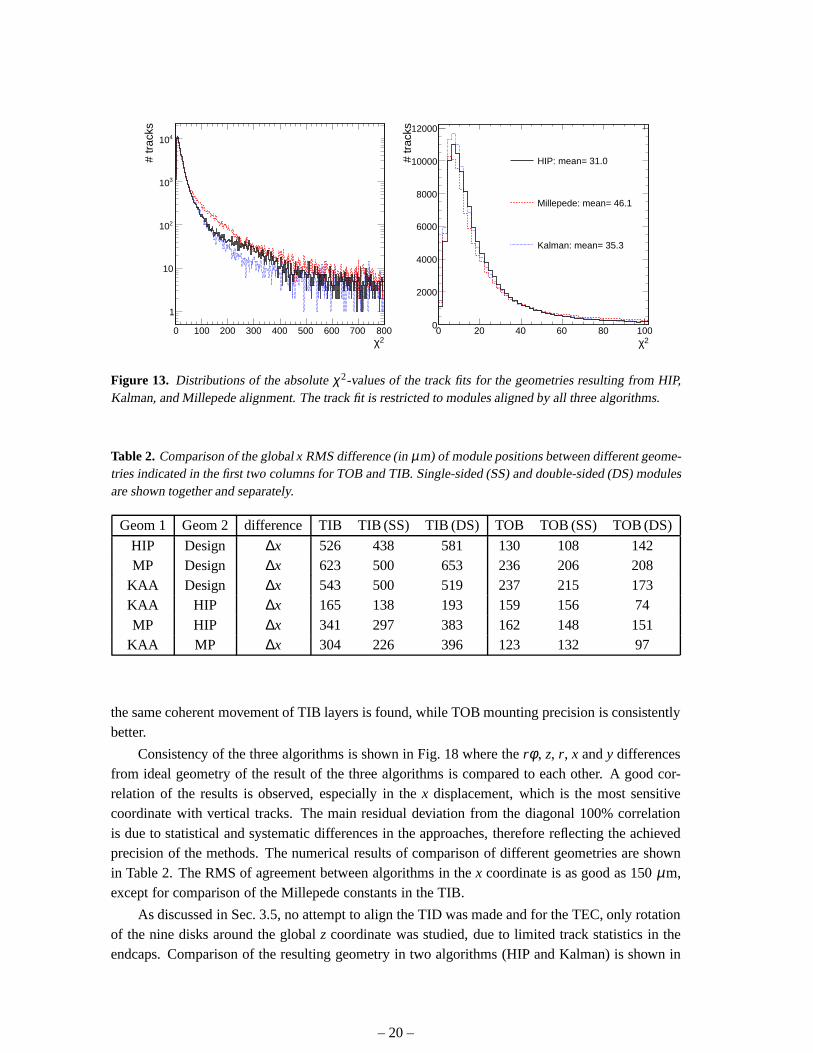
Figure 13. Distributions of the absoluteχ2-values of the track fits for the geometries resulting from HIP,Kalman, and Millepede alignment. The track fit is restrictedto modules aligned by all three algorithms.

Table 2. Comparison of the globalx RMS difference (inµm) of module positions between different geome-tries indicated in the first two columns for TOB and TIB. Single-sided (SS) and double-sided (DS) modulesare shown together and separately.

Geom 1 Geom 2 difference TIB TIB (SS) TIB (DS) TOB TOB (SS) TOB (DS)

HIP Design ∆x 526 438 581 130 108 142MP Design ∆x 623 500 653 236 206 208

KAA Design ∆x 543 500 519 237 215 173KAA HIP ∆x 165 138 193 159 156 74MP HIP ∆x 341 297 383 162 148 151

KAA MP ∆x 304 226 396 123 132 97

the same coherent movement of TIB layers is found, while TOB mounting precision is consistentlybetter.

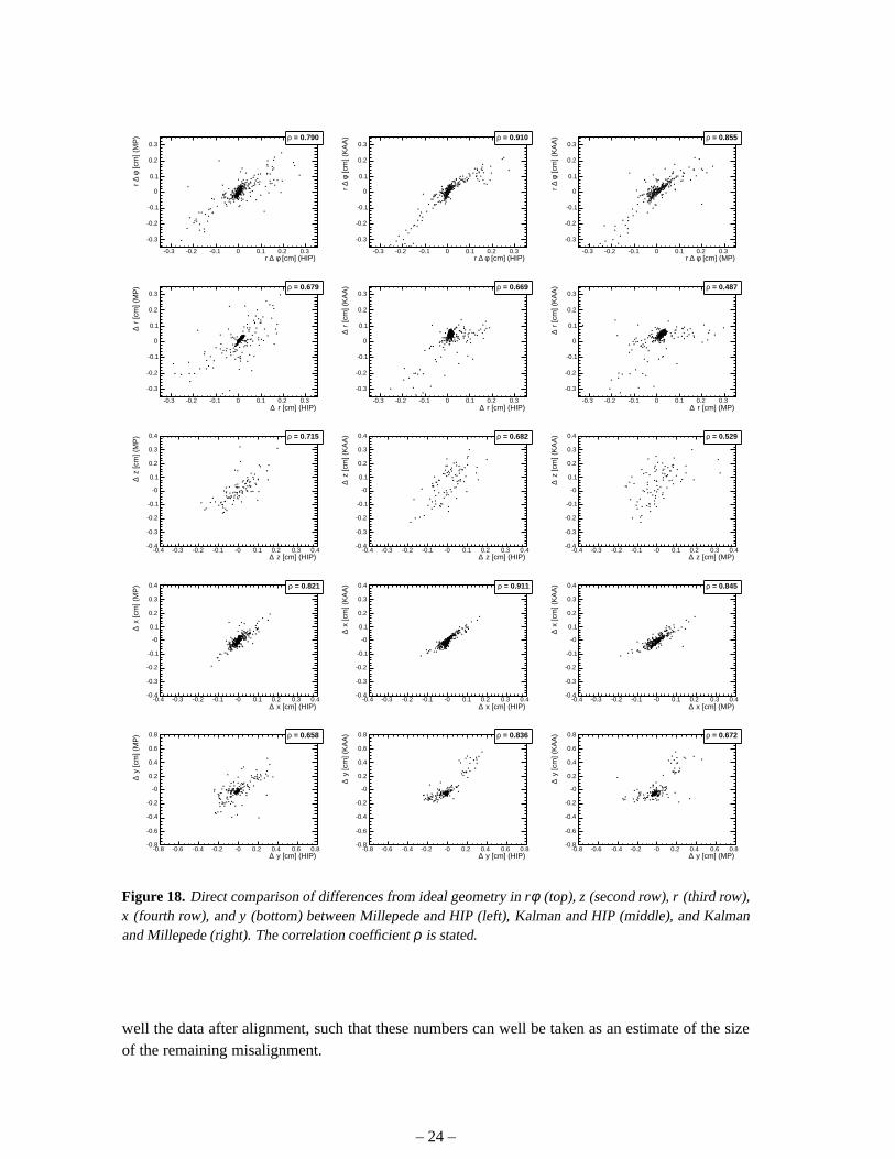
Consistency of the three algorithms is shown in Fig. 18 wheretherφ , z, r, x andy differencesfrom ideal geometry of the result of the three algorithms is compared to each other. A good cor-relation of the results is observed, especially in thex displacement, which is the most sensitivecoordinate with vertical tracks. The main residual deviation from the diagonal 100% correlationis due to statistical and systematic differences in the approaches, therefore reflecting the achievedprecision of the methods. The numerical results of comparison of different geometries are shownin Table 2. The RMS of agreement between algorithms in thex coordinate is as good as 150µm,except for comparison of the Millepede constants in the TIB.

As discussed in Sec. 3.5, no attempt to align the TID was made and for the TEC, only rotationof the nine disks around the globalz coordinate was studied, due to limited track statistics in theendcaps. Comparison of the resulting geometry in two algorithms (HIP and Kalman) is shown in

– 20 –

[cm]x’

res-0.3 -0.2 -0.1 0 0.1 0.2 0.3

# hi

ts

0

1000

2000

3000

4000

5000

6000RMS = 0.0498

= -0.0029µ HIP

RMS = 0.0639 = 0.0029µ

Millepede

RMS = 0.0461 = -0.0033µ

Kalman

TIB

[cm]x’

res-0.3 -0.2 -0.1 0 0.1 0.2 0.3

# hi

ts

0

2000

4000

6000

8000

10000

12000

14000

16000

18000

20000

22000

RMS = 0.0367 = 0.0003µ

HIP

RMS = 0.0408 = -0.0006µ

Millepede

RMS = 0.0314 = 0.0013µ

Kalman

[cm]y’

res-3 -2 -1 0 1 2 3

# hi

ts

0

2000

4000

6000

8000

10000RMS = 0.4655

= 0.0089µ HIP

RMS = 0.4769 = -0.0024µ

Millepede

RMS = 0.4686 = -0.0140µ

Kalman

[cm]x’

res-0.3 -0.2 -0.1 0 0.1 0.2 0.3

# hi

ts

0

5000

10000

15000

20000

25000

RMS = 0.0273 = -0.0009µ

HIP

RMS = 0.0284 = 0.0002µ

Millepede

RMS = 0.0266 = -0.0005µ

Kalman

TOB

[cm]x’

res-0.3 -0.2 -0.1 0 0.1 0.2 0.3

# hi

ts

0

10000

20000

30000

40000

50000RMS = 0.0288

= 0.0002µ HIP

RMS = 0.0279 = 0.0002µ

Millepede

RMS = 0.0278 = -0.0000µ

Kalman

[cm]y’

res-3 -2 -1 0 1 2 3

# hi

ts

0

2000

4000

6000

8000

10000

12000

14000

RMS = 0.4539 = -0.0049µ

HIP

RMS = 0.5118 = -0.0076µ

Millepede

RMS = 0.4581 = -0.0060µ

Kalman

[cm]Φrres-0.3 -0.2 -0.1 0 0.1 0.2 0.3

# hi

ts

0

100

200

300

400

500

600

RMS = 0.0711 = 0.0061µ

HIP

RMS = 0.0719 = 0.0057µ

Millepede

RMS = 0.0723 = 0.0050µ

Kalman

TEC

[cm]Φrres-0.3 -0.2 -0.1 0 0.1 0.2 0.3

# hi

ts

0

200

400

600

800

1000

RMS = 0.0648 = 0.0016µ

HIP

RMS = 0.0661 = 0.0005µ

Millepede

RMS = 0.0676 = 0.0008µ

Kalman

[cm]rres-3 -2 -1 0 1 2 3

# hi

ts

0

100

200

300

400

500

600

700

RMS = 0.6862 = -0.0332µ

HIP

RMS = 0.6963 = -0.0410µ

Millepede

RMS = 0.6937 = -0.0408µ

Kalman

Figure 14. Hit residuals for different geometries from three track-based algorithms: HIP (solid/black),Millepede (dashed/red), and Kalman (dotted/blue) based alignment. Three Tracker sub-detectors are shownin the top row (TIB), second row (TOB), and bottom row (TEC). The absolute localx′-residuals are shownfor single-sided modules (left) and double-sided modules (middle), while localy′-residuals are shown for thedouble-sided modules only (right). For the endcap modules (TEC) transformation to therφ andr residualsis made. The track fit is restricted to modules aligned by all three algorithms.

Fig. 19. The results exhibit slight differences, but they clearly show the same trend.

4.5 Track-Based Alignment with Simulated Data and Estimation of Alignment Precision

Alignment tests on simulated data have been performed with the Kalman algorithm on approxi-mately 40k events from a sample that mimics the situation at the TIF. In order to reproduce ourknowledge of the real tracker geometry after survey measurements only, movements and errors tothe tracker elements are applied according to the expected starting misalignment [12]. The align-ment strategy and track selection discussed above are applied to obtain the results shown in Fig. 20,resulting in a precision of 80µm in globalx position.

– 21 –

https://www.researchgate.net/publication/277129940_Comprehensive_Set_of_Misalignment_Scenarios_for_the_CMS_Tracker?el=1_x_8&enrichId=rgreq-f1aef4fa82159a5ff4d4b3a530a24a97-XXX&enrichSource=Y292ZXJQYWdlOzUwMjc2OTM3O0FTOjk5Njc2MzM0MzI5ODY2QDE0MDA3NzYwOTkxNTE=

Layer 2 4 6 8 10

m)

µR

MS

(

0

100

200

300

400

500

600HIP alignment - all hits

HIP alignment - no first/last

Figure 15. Hit residual RMS in localx′ coordinate in ten layers of the barrel tracker, i.e. four layers of TIBand six layers of TOB, after track-based alignment with HIP.In contrast to the blue squares, the red circlesare obtained including residuals from the first and last hitsof the track. Hits on modules not aligned are notconsidered in the track fit.

Layer 2 4 6 8 10

m)

µM

ean

(

-300

-200

-100

0

100

200

300 Data - no alignment

Data - HIP alignment

MC - ideal geometry

MC - tuned misalignment

m)µm, TOB = 50 µ(TIB = 80

Layer 2 4 6 8 10

m)

µR

MS

(

0

100

200

300

400

500

600 Data - no alignment

Data - HIP alignment

MC - ideal geometry

MC - tuned misalignment

m)µm, TOB = 50 µ(TIB = 80

Figure 16. Hit residual means in localx′ coordinate (left) and RMS (right) in ten layers of the barreltracker,i.e. four layers of TIB and six layers of TOB, shown in data before track-based alignment (red full circles),after track-based alignment (HIP, red full squares), in simulation with ideal geometry (blue open circles) andin simulation after tuning of misalignment according to data (blue open squares).

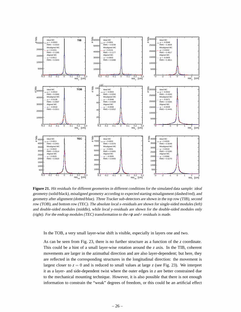
An alignment study on the full MC data set has been performed with the Millepede algorithmwith the same settings as for the data, i.e. alignment of a subset of the barrel part at module leveland of the TEC at disk level. The resulting residual distributions in TIB, TOB and TEC are shownin Fig. 21 and compared with the startup misalignment [12] and the ideal geometry. Comparisonwith the distributions obtained from data using the design geometry (Fig. 14) reveals that in TIB

– 22 –


r [cm]20 30 40 50 60 70 80 90 100 110

r [c

m]

∆

-0.5

-0.4

-0.3

-0.2

-0.1

0

0.1

0.2

r [cm]20 30 40 50 60 70 80 90 100 110

z [c

m]

∆

-0.3

-0.2

-0.1

-0

0.1

0.2

0.3

0.4

r [cm]20 30 40 50 60 70 80 90 100 110

[cm

]φ

∆ r

*

-0.5

-0.4

-0.3

-0.2

-0.1

0

0.1

0.2

0.3

r [cm]20 30 40 50 60 70 80 90 100 110

r [c

m]

∆

-0.5

-0.4

-0.3

-0.2

-0.1

0

0.1

0.2

0.3

0.4

r [cm]20 30 40 50 60 70 80 90 100 110

z [c

m]

∆

-0.2

-0.1

0

0.1

0.2

0.3

0.4

0.5

r [cm]20 30 40 50 60 70 80 90 100 110

[cm

]φ

∆ r

*

-0.4

-0.3

-0.2

-0.1

-0

0.1

0.2

0.3

Figure 17. Difference of the module positions between the measured (intrack-based alignment) and designgeometries shown for Kalman (top) and Millepede (bottom) algorithms for TIB (radiusr < 55cm) and TOB(r > 55 cm). Projection on ther (left), z (middle), andφ (right) directions are shown. Only double-sidedmodules are considered in thezcomparison.

and TOB the starting misalignment is overestimated while inTEC it is slightly underestimated. Theresidual widths after alignment are generally much smallerthan those obtained from the aligneddata, especially in the TIB. This could be due to the larger statistics of the simulation data sample,but also due to effects not properly simulated, e.g. relative misalignment of the two components ofa double-sided module or possible differences in the momentum spectrum of Monte Carlo.

The results of the truncated RMS of the layerwise residual distributions in Fig. 16 are usedto estimate alignment precision in the aligned barrel region via comparison with simulations. Dif-ferent misalignment scenarios have been applied to the ideal (“true”) Tracker geometry used inreconstructing the simulated data until truncated RMS values are found to be similar to the ones indata in all layers. The modules in TIB and TOB have been randomly shifted in three dimensionsby Gaussian distributions. The influence of possibly large misalignments from the tails of theseGaussians is reduced by truncating the distributions as stated above.

Besides the truncated mean and RMS values from data before and after alignment, Fig. 16shows also the results from the simulation reconstructed with the ideal geometry and reconstructedwith a random misalignment according to Gaussian distributions with standard deviations of 50µmand 80µm in the TOB and the TIB, respectively. It can be clearly seen that the simulation with theideal, i.e. true, geometry has smaller widths than the data,especially in the TIB. On the other hand,the geometry with a simulated misalignment of 50µm and 80µm, respectively, resembles rather

– 23 –

[cm] (HIP)φ ∆ r -0.3 -0.2 -0.1 0 0.1 0.2 0.3

[cm

] (M

P)

φ ∆

r

-0.3

-0.2

-0.1

0

0.1

0.2

0.3 = 0.790 ρ

[cm] (HIP)φ ∆ r -0.3 -0.2 -0.1 0 0.1 0.2 0.3

[cm

] (K

AA

)φ

∆ r

-0.3

-0.2

-0.1

0

0.1

0.2

0.3 = 0.910 ρ

[cm] (MP)φ ∆ r -0.3 -0.2 -0.1 0 0.1 0.2 0.3

[cm

] (K

AA

)φ

∆ r

-0.3

-0.2

-0.1

0

0.1

0.2

0.3 = 0.855 ρ

r [cm] (HIP)∆ -0.3 -0.2 -0.1 0 0.1 0.2 0.3

r [c

m] (

MP

)∆

-0.3

-0.2

-0.1

0

0.1

0.2

0.3 = 0.679 ρ

r [cm] (HIP)∆ -0.3 -0.2 -0.1 0 0.1 0.2 0.3

r [c

m] (

KA

A)

∆

-0.3

-0.2

-0.1

0

0.1

0.2

0.3 = 0.669 ρ

r [cm] (MP)∆ -0.3 -0.2 -0.1 0 0.1 0.2 0.3

r [c

m] (

KA

A)

∆

-0.3

-0.2

-0.1

0

0.1

0.2

0.3 = 0.487 ρ

z [cm] (HIP)∆ -0.4 -0.3 -0.2 -0.1 -0 0.1 0.2 0.3 0.4

z [c

m] (

MP

)∆

-0.4

-0.3

-0.2

-0.1

-0

0.1

0.2

0.3

0.4 = 0.715 ρ

z [cm] (HIP)∆ -0.4 -0.3 -0.2 -0.1 -0 0.1 0.2 0.3 0.4

z [c

m] (

KA

A)

∆

-0.4

-0.3

-0.2

-0.1

-0

0.1

0.2

0.3

0.4 = 0.682 ρ

z [cm] (MP)∆ -0.4 -0.3 -0.2 -0.1 -0 0.1 0.2 0.3 0.4

z [c

m] (

KA

A)

∆ -0.4

-0.3

-0.2

-0.1

-0

0.1

0.2

0.3

0.4 = 0.529 ρ

x [cm] (HIP)∆ -0.4 -0.3 -0.2 -0.1 -0 0.1 0.2 0.3 0.4

x [c

m] (

MP

)∆

-0.4

-0.3

-0.2

-0.1

-0

0.1

0.2

0.3

0.4 = 0.821 ρ

x [cm] (HIP)∆ -0.4 -0.3 -0.2 -0.1 -0 0.1 0.2 0.3 0.4

x [c

m] (

KA

A)

∆

-0.4

-0.3

-0.2

-0.1

-0

0.1

0.2

0.3

0.4 = 0.911 ρ

x [cm] (MP)∆ -0.4 -0.3 -0.2 -0.1 -0 0.1 0.2 0.3 0.4

x [c

m] (

KA

A)

∆

-0.4

-0.3

-0.2

-0.1

-0

0.1

0.2

0.3

0.4 = 0.845 ρ

y [cm] (HIP)∆ -0.8 -0.6 -0.4 -0.2 -0 0.2 0.4 0.6 0.8

y [c

m] (

MP

)∆

-0.8

-0.6

-0.4

-0.2

-0

0.2

0.4

0.6

0.8 = 0.658 ρ

y [cm] (HIP)∆ -0.8 -0.6 -0.4 -0.2 -0 0.2 0.4 0.6 0.8

y [c

m] (

KA

A)

∆

-0.8

-0.6

-0.4

-0.2

-0

0.2

0.4

0.6

0.8 = 0.836 ρ

y [cm] (MP)∆ -0.8 -0.6 -0.4 -0.2 -0 0.2 0.4 0.6 0.8

y [c

m] (

KA

A)

∆

-0.8

-0.6

-0.4

-0.2

-0

0.2

0.4

0.6

0.8 = 0.672 ρ

Figure 18. Direct comparison of differences from ideal geometry inrφ (top),z (second row),r (third row),x (fourth row), andy (bottom) between Millepede and HIP (left), Kalman and HIP (middle), and Kalmanand Millepede (right). The correlation coefficientρ is stated.

well the data after alignment, such that these numbers can well be taken as an estimate of the sizeof the remaining misalignment.

– 24 –

z [mm]1400 1600 1800 2000 2200 2400 2600 2800

[mra

d]φ∆

-1

-0.5

0

0.5

1 Algorithm

HIP

Kalman

Figure 19. Rotations of the TEC disks around the globalz in comparison of the measured (in track-basedalignment) and design geometries for TEC. Two track-based results are shown: HIP (triangles) and Kalmanfilter (circles) algorithms.

Mean -0.002515

RMS 0.008347

x [cm]∆-0.05 0 0.050

5

10

15

20

25

30Mean -0.002515

RMS 0.008347

Mean 0.01003

RMS 0.03205

y [cm]∆-0.15 -0.1 -0.05 0 0.05 0.1 0.150

2

4

6

8

10

12Mean 0.01003

RMS 0.03205

Mean 0.002994

RMS 0.05544

z [cm]∆-0.15 -0.1 -0.05 0 0.05 0.1 0.150

2

4

6

8

10

12

14

16

Mean 0.002994

RMS 0.05544

Figure 20. Alignment resolution in global coordinates achieved with the Kalman alignment algorithm onsimulated data.

5. Stability of the Tracker Geometry with Temperature and Time

5.1 Stability of the Tracker Barrels

In order to investigate the stability of the tracker components with respect to the cooling temper-ature and stress due to TEC insertion, full alignment of the Tracker in different periods has beenperformed and the positions of modules in space are compared. The advantage of this approach isthat we can see module movements directly, but the potentialproblem is that we may be misled bya systematic effect or a weakly constrained misalignment. Statistical scatter of up to 100µm limitsthe resolution of the method. These tests have been done withthe HIP algorithm.

1. +15 ◦C (A1, before TEC- insertion) vs. +10◦C (C10, after TEC- insertion).

This test is intended to show the effect of the insertion of a mechanical object between twodata-taking conditions. Fig. 22 shows the shifts between the two sets of aligned positions inglobalx, y andz as a function of the radial coordinate and projected separately for TIB andTOB.

– 25 –

[cm]x’

res-0.3 -0.2 -0.1 0 0.1 0.2 0.3

# hi

ts

0

5000

10000

15000

20000

25000RMS = 0.0310

= -0.0003µ Ideal MC

RMS = 0.1265 = 0.0151µ

Misaligned MC

RMS = 0.0343 = 0.0011µ

Aligned MC

TIB

[cm]x’

res-0.3 -0.2 -0.1 0 0.1 0.2 0.3

# hi

ts

0

10000

20000

30000

40000

50000

60000

RMS = 0.0238 = 0.0001µ

Ideal MC

RMS = 0.1177 = 0.0131µ

Misaligned MC

RMS = 0.0288 = 0.0003µ

Aligned MC

[cm]y’

res-3 -2 -1 0 1 2 3

# hi

ts

0

5000

10000

15000

20000

25000

30000

RMS = 0.3826 = -0.0048µ

Ideal MC

RMS = 0.4617 = 0.0432µ

Misaligned MC

RMS = 0.3811 = -0.0005µ

Aligned MC

[cm]x’

res-0.3 -0.2 -0.1 0 0.1 0.2 0.3

# hi

ts

0

10000

20000

30000

40000

50000

RMS = 0.0300 = -0.0010µ

Ideal MC

RMS = 0.0597 = -0.0138µ

Misaligned MC

RMS = 0.0311 = -0.0018µ

Aligned MC

TOB

[cm]x’

res-0.3 -0.2 -0.1 0 0.1 0.2 0.3

# hi

ts

0

20

40

60

80

100

310×

RMS = 0.0250 = -0.0003µ

Ideal MC

RMS = 0.0339 = -0.0048µ

Misaligned MC

RMS = 0.0252 = -0.0008µ

Aligned MC

[cm]y’

res-3 -2 -1 0 1 2 3

# hi

ts

0

5000

10000

15000

20000

25000

30000

RMS = 0.4320 = -0.0032µ

Ideal MC

RMS = 0.5305 = -0.0071µ

Misaligned MC

RMS = 0.4445 = -0.0039µ

Aligned MC

[cm]Φrres-0.3 -0.2 -0.1 0 0.1 0.2 0.3

# hi

ts

0

500

1000

1500

2000

2500

3000

3500

4000

4500

RMS = 0.0451 = 0.0011µ

Ideal MC

RMS = 0.0514 = 0.0022µ

Misaligned MC

RMS = 0.0520 = 0.0025µ

Aligned MC

TEC

[cm]Φrres-0.3 -0.2 -0.1 0 0.1 0.2 0.3

# hi

ts

0

1000

2000

3000

4000

5000

6000

7000

8000

RMS = 0.0376 = 0.0003µ

Ideal MC

RMS = 0.0405 = 0.0001µ

Misaligned MC

RMS = 0.0405 = -0.0005µ

Aligned MC

[cm]rres-3 -2 -1 0 1 2 3

# hi

ts

0

500

1000

1500

2000

2500

3000

3500

4000

RMS = 0.5049 = 0.0026µ

Ideal MC

RMS = 0.5285 = 0.0019µ

Misaligned MC

RMS = 0.5270 = 0.0066µ

Aligned MC

Figure 21. Hit residuals for different geometries in different conditions for the simulated data sample: idealgeometry (solid/black), misaligned geometry according toexpected starting misalignment (dashed/red), andgeometry after alignment (dotted/blue). Three Tracker sub-detectors are shown in the top row (TIB), secondrow (TOB), and bottom row (TEC). The absolute localx-residuals are shown for single-sided modules (left)and double-sided modules (middle), while localy-residuals are shown for the double-sided modules only(right). For the endcap modules (TEC) transformation to therφ andr residuals is made.

In the TOB, a very small layer-wise shift is visible, especially in layers one and two.

As can be seen from Fig. 23, there is no further structure as a function of thez coordinate.This could be a hint of a small layer-wise rotation around thez axis. In the TIB, coherentmovements are larger in the azimuthal direction and are alsolayer-dependent; but here, theyare reflected in the corresponding structures in the longitudinal direction: the movement islargest closer toz= 0 and is reduced to small values at largez (see Fig. 23). We interpretit as a layer- and side-dependent twist where the outer edgesin z are better constrained dueto the mechanical mounting technique. However, it is also possible that there is not enoughinformation to constrain the “weak” degrees of freedom, or this could be an artificial effect

– 26 –

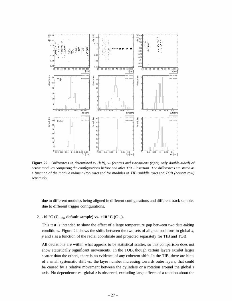
r [cm]20 30 40 50 60 70 80 90 100 110

x [c

m]

∆

-0.03

-0.02

-0.01

0

0.01

0.02

0.03

r [cm]20 30 40 50 60 70 80 90 100 110

y [c

m]

∆

-0.15

-0.1

-0.05

0

0.05

0.1

r [cm]20 30 40 50 60 70 80 90 100 110

z [c

m]

∆

-0.14

-0.12

-0.1

-0.08

-0.06

-0.04

-0.02

0

0.02

0.04

0.06

Mean 0.001396

RMS 0.007528

x [cm]∆-0.03 -0.02 -0.01 0 0.01 0.02 0.03

#mod

ules

0

5

10

15

20

25

30Mean 0.001396

RMS 0.007528TIB

Mean -0.005325

RMS 0.04042

y [cm]∆-0.15 -0.1 -0.05 0 0.05 0.1

#mod

ules

0

2

4

6

8

10

12

14

Mean -0.005325

RMS 0.04042

Mean -0.00642

RMS 0.02617

z [cm]∆-0.1 -0.05 0 0.05 0.1

#mod

ules

0

1

2

3

4

5Mean -0.00642

RMS 0.02617

Mean -0.0003391

RMS 0.004431

x [cm]∆-0.03 -0.02 -0.01 0 0.01 0.02 0.03

#mod

ules

0

5

10

15

20

25

30

35

Mean -0.0003391

RMS 0.004431TOB

Mean 0.003641

RMS 0.002826

y [cm]∆-0.15 -0.1 -0.05 0 0.05 0.1

#mod

ules

0

10

20

30

40

50

60

70

80Mean 0.003641

RMS 0.002826

Mean -0.001143

RMS 0.02727

z [cm]∆-0.1 -0.05 0 0.05 0.1

#mod

ules

0

1

2

3

4

5

6

7

8Mean -0.001143

RMS 0.02727

Figure 22. Differences in determinedx- (left), y- (centre) andz-positions (right, only double-sided) ofactive modules comparing the configurations before and after TEC- insertion. The differences are stated asa function of the module radiusr (top row) and for modules in TIB (middle row) and TOB (bottom row)separately.

due to different modules being aligned in different configurations and different track samplesdue to different trigger configurations.

2. -10 ◦C (C−10, default sample) vs. +10◦C (C10).

This test is intended to show the effect of a large temperature gap between two data-takingconditions. Figure 24 shows the shifts between the two sets of aligned positions in globalx,y andzas a function of the radial coordinate and projected separately for TIB and TOB.

All deviations are within what appears to be statistical scatter, so this comparison does notshow statistically significant movements. In the TOB, though certain layers exhibit largerscatter than the others, there is no evidence of any coherentshift. In the TIB, there are hintsof a small systematic shift vs. the layer number increasing towards outer layers, that couldbe caused by a relative movement between the cylinders or a rotation around the globalzaxis. No dependence vs. globalz is observed, excluding large effects of a rotation about the

– 27 –

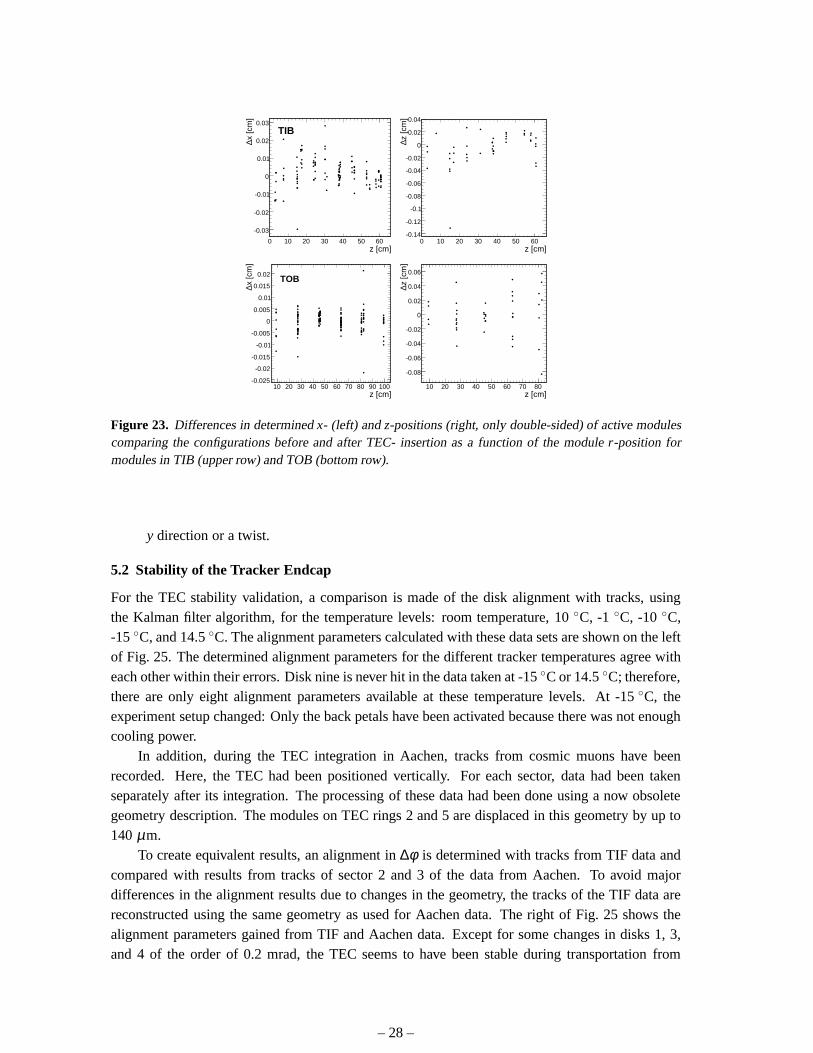
z [cm]0 10 20 30 40 50 60

x [c

m]

∆

-0.03

-0.02

-0.01

0

0.01

0.02

0.03TIB

z [cm]0 10 20 30 40 50 60

z [c

m]

∆

-0.14

-0.12

-0.1

-0.08

-0.06

-0.04

-0.02

0

0.02

0.04

z [cm]10 20 30 40 50 60 70 80 90 100

x [c

m]

∆

-0.025

-0.02

-0.015

-0.01

-0.005

0

0.005

0.01

0.015

0.02 TOB

z [cm]10 20 30 40 50 60 70 80

z [c

m]

∆

-0.08

-0.06

-0.04

-0.02

0

0.02

0.04

0.06

Figure 23. Differences in determinedx- (left) andz-positions (right, only double-sided) of active modulescomparing the configurations before and after TEC- insertion as a function of the moduler-position formodules in TIB (upper row) and TOB (bottom row).

y direction or a twist.

5.2 Stability of the Tracker Endcap

For the TEC stability validation, a comparison is made of thedisk alignment with tracks, usingthe Kalman filter algorithm, for the temperature levels: room temperature, 10◦C, -1 ◦C, -10 ◦C,-15 ◦C, and 14.5◦C. The alignment parameters calculated with these data setsare shown on the leftof Fig. 25. The determined alignment parameters for the different tracker temperatures agree witheach other within their errors. Disk nine is never hit in the data taken at -15◦C or 14.5◦C; therefore,there are only eight alignment parameters available at these temperature levels. At -15◦C, theexperiment setup changed: Only the back petals have been activated because there was not enoughcooling power.

In addition, during the TEC integration in Aachen, tracks from cosmic muons have beenrecorded. Here, the TEC had been positioned vertically. Foreach sector, data had been takenseparately after its integration. The processing of these data had been done using a now obsoletegeometry description. The modules on TEC rings 2 and 5 are displaced in this geometry by up to140µm.

To create equivalent results, an alignment in∆φ is determined with tracks from TIF data andcompared with results from tracks of sector 2 and 3 of the datafrom Aachen. To avoid majordifferences in the alignment results due to changes in the geometry, the tracks of the TIF data arereconstructed using the same geometry as used for Aachen data. The right of Fig. 25 shows thealignment parameters gained from TIF and Aachen data. Except for some changes in disks 1, 3,and 4 of the order of 0.2 mrad, the TEC seems to have been stableduring transportation from

– 28 –

r [cm]20 30 40 50 60 70 80 90 100 110

x [c

m]

∆

-0.04

-0.03

-0.02

-0.01

0

0.01

0.02

0.03

r [cm]20 30 40 50 60 70 80 90 100 110

y [c

m]

∆

-0.1

-0.05

0

0.05

0.1

0.15

0.2

0.25

r [cm]20 30 40 50 60 70 80 90 100 110

z [c

m]

∆

-0.08

-0.06

-0.04

-0.02

0

0.02

0.04

0.06

0.08

0.1

0.12

Mean 2.8e-05

RMS 0.007999

x [cm]∆-0.03 -0.02 -0.01 0 0.01 0.02 0.03

#mod

ules

0

2

4

6

8

10

12

14

16

18

Mean 2.8e-05

RMS 0.007999

TIB

Mean 0.005567

RMS 0.04072

y [cm]∆-0.2 -0.15 -0.1 -0.05 -0 0.05 0.1 0.15 0.2

#mod

ules

0

5

10

15

20

25

30

35Mean 0.005567

RMS 0.04072

Mean 0.001333

RMS 0.03512

z [cm]∆-0.1 -0.05 0 0.05 0.1

#mod

ules

0

1

2

3

4

5

6

7

8Mean 0.001333

RMS 0.03512

Mean 0.0004975

RMS 0.002848

x [cm]∆-0.03 -0.02 -0.01 0 0.01 0.02 0.03

#mod

ules

0

5

10

15

20

25

30

35Mean 0.0004975

RMS 0.002848

TOB

Mean -0.006436

RMS 0.004038

y [cm]∆-0.2 -0.15 -0.1 -0.05 -0 0.05 0.1 0.15 0.2

#mod

ules

0

10

20

30

40

50

60

70

80

90Mean -0.006436

RMS 0.004038

Mean 0.001791

RMS 0.01911

z [cm]∆-0.1 -0.05 0 0.05 0.1

#mod

ules

0

1

2

3

4

5

6

7

8Mean 0.001791

RMS 0.01911

Figure 24.Differences in determinedx- (left), y- (centre) andz-positions (right, only double-sided) of activemodules comparing the +10◦C and -10◦C configurations. The differences are stated as a function ofthemodule radiusr (top row) and for modules in TIB (middle row) and TOB (bottom row) separately.

z [mm]1400 1600 1800 2000 2200 2400 2600 2800

[mra

d]φ∆

-0.6

-0.4

-0.2

0

0.2

0.4

0.6Data set

C°T = 15 C°T = 10 C°T = -1 C°T = -10 C°T = -15 C°T =14.5

z [mm]1400 1600 1800 2000 2200 2400 2600 2800

[mra

d]φ∆

-0.6

-0.4

-0.2

0

0.2

0.4

0.6 Data set

TIF (merged T)

Aachen

Figure 25. Alignment parameter∆φ for TEC disks at six tracker temperature levels (left). Alignmentparameter∆φ for TEC disks, determined with TIF data and Aachen data usingan obsolete, but commongeometry (right).

– 29 –

Aachen to Geneva, tilting from a vertical to a horizontal position, and integration into the tracker.Two petals have been replaced in the active TEC sectors before taking the TIF data: A back petal ofdisk 3 and a front petal of disk 4. Thus, changes in the corrections∆φ of these disks are expected.

6. Laser Alignment System Analysis and Discussion

In this section, we discuss results from the Laser AlignmentSystem. Analysis of the measurementsfrom this system have not been integrated with the track-based statistical methods. Therefore, wediscuss the data analysis and results independently.

6.1 Data Taking

At the TIF, data was taken with the laser alignment system. Onthez+ side of the tracker, the beamsfrom the alignment tubes of sector 1, 2 and 3 were seen by the barrel modules. The endcap sectors2 and 3 were operated with the TEC internal beams and the alignment tubes of those sectors. Datawas taken before cooling the tracker down, during the cooling cycle, and at the end, when thetracker was back at room temperature.

As we mentioned earlier, the Laser Alignment System was designed to measure deformationsand movements of the tracker support structures. To do this properly, the wholeφ -range of thelaser beams needs to be operated. The fact that only a slice ofthe tracker was operated during theTIF tests means that no complete picture of the tracker alignment parameters could be obtained.Nevertheless, the data taking was very useful to verify the proper functioning of the laser beams andthe laser data taking. First of all, the evolution of the measured laser spot positions with temperaturewas studied. Movements could be either due to thermal deformations of the tracker structure, orcaused by small movements of the beamsplitter holders. Then, the data taken in the TEC sectorscan be compared to the data obtained during the TEC integration. Here, observed differences couldalso have been caused by the handling, transport and insertion of the endcaps.

6.2 Results from Alignment Tubes

The alignment tubes were first operated at room temperature.Then, as the tracker was graduallycooled down, they were measured at 10◦C, -1 ◦C, -15◦C and finally again at room temperature,after the tracker had been warmed up again. The measured laser spot positions were all comparedto the first measurements at room temperature. The result is shown in Fig. 26. The largest changesof about 600µm were observed in the TOB. The observed movements could comeeither frommovements of the tracker structure, or from movements of thelaser beams. Nevertheless, twobounds can be given. First, one could assume that all detected movements were due to trackerstructure deformations. In this case, we would have observed movements of 600µm. On the otherhand, one could try to absorb as much as of the observed laser spot changes into movements of thelaser beams. In this case, one calculates the tilt of the laser beams and rotations of the alignmenttubes that fit best to the observed laser spot movements. After subtracting this contribution, theremaining laser spot movements would be due to the tracker support deformation. This is shownin Fig. 27. Now the maximal movements of the tracker would be less than 100µm.

– 30 –

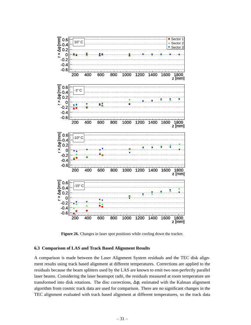
z [mm]200 400 600 800 1000 1200 1400 1600 1800

[mm

]φ∆ ×

r

-0.6-0.4-0.2

00.20.40.6

z [mm]200 400 600 800 1000 1200 1400 1600 1800

[mm

]φ∆ ×

r

-0.6-0.4-0.2

00.20.40.6 Sector 1

Sector 2Sector 3

C°10

z [mm]200 400 600 800 1000 1200 1400 1600 1800

[mm

]φ∆ ×

r

-0.6-0.4-0.2

00.20.40.6

z [mm]200 400 600 800 1000 1200 1400 1600 1800

[mm

]φ∆ ×

r

-0.6-0.4-0.2

00.20.40.6

C°-1

z [mm]200 400 600 800 1000 1200 1400 1600 1800

[mm

]φ∆ ×

r

-0.6-0.4-0.2

00.20.40.6

z [mm]200 400 600 800 1000 1200 1400 1600 1800

[mm

]φ∆ ×

r

-0.6-0.4-0.2

00.20.40.6

C°-10

z [mm]200 400 600 800 1000 1200 1400 1600 1800

[mm

]φ∆ ×

r

-0.6-0.4-0.2

00.20.40.6

z [mm]200 400 600 800 1000 1200 1400 1600 1800

[mm

]φ∆ ×

r

-0.6-0.4-0.2

00.20.40.6

C°-15

Figure 26. Changes in laser spot positions while cooling down the tracker.

6.3 Comparison of LAS and Track Based Alignment Results

A comparison is made between the Laser Alignment System residuals and the TEC disk align-ment results using track based alignment at different temperatures. Corrections are applied to theresiduals because the beam splitters used by the LAS are known to emit two non-perfectly parallellaser beams. Considering the laser beamspot radii, the residuals measured at room temperature aretransformed into disk rotations. The disc corrections,∆φ , estimated with the Kalman alignmentalgorithm from cosmic track data are used for comparison. There are no significant changes in theTEC alignment evaluated with track based alignment at different temperatures, so the track data

– 31 –

z [mm]200 400 600 800 1000 1200 1400 1600 1800

[mm

]φ∆ ×

r

-0.6-0.4-0.2

00.20.40.6

z [mm]200 400 600 800 1000 1200 1400 1600 1800

[mm

]φ∆ ×

r

-0.6-0.4-0.2

00.20.40.6 Sector 1

Sector 2Sector 3

C°10

z [mm]200 400 600 800 1000 1200 1400 1600 1800

[mm

]φ∆ ×

r

-0.6-0.4-0.2

00.20.40.6

z [mm]200 400 600 800 1000 1200 1400 1600 1800

[mm

]φ∆ ×

r

-0.6-0.4-0.2

00.20.40.6

C°-1

z [mm]200 400 600 800 1000 1200 1400 1600 1800

[mm

]φ∆ ×

r

-0.6-0.4-0.2

00.20.40.6

z [mm]200 400 600 800 1000 1200 1400 1600 1800

[mm

]φ∆ ×

r

-0.6-0.4-0.2

00.20.40.6

C°-10

z [mm]200 400 600 800 1000 1200 1400 1600 1800

[mm

]φ∆ ×

r

-0.6-0.4-0.2

00.20.40.6

z [mm]200 400 600 800 1000 1200 1400 1600 1800

[mm

]φ∆ ×

r

-0.6-0.4-0.2

00.20.40.6 C°-15

Figure 27. Changes in laser spot positions while cooling down the tracker, removing the maximum contri-bution that can be due to movements of the alignment tube.

merged from all temperature runs exceptT = −15 ◦C were used to obtain a better precision.

Because the exact direction of the laser beams is unknown, a linear dependence ofφ on zcannot be determined using the LAS residuals. Therefore, mean and slope (as a function ofz) ofthe corrections to the disc rotations are subtracted. The same is done with the results from theKalman alignment algorithm to use a common coordinate system. The remaining corrections aredisplayed in Fig. 28. For LAS, the mean and RMS of the four measurements estimated from thefour active laser beams in the endcap are shown for each disk.There are differences among the LAS

– 32 –

corrections for the same disk of up to 0.7 mrad. These differences are interpreted as misalignmenton module and petal level. Considering the accuracy of the Kalman alignment parameters and thespread of the LAS results, the estimated corrections show a good agreement.

z [mm]1400 1600 1800 2000 2200 2400 2600 2800

[mra

d]φ∆

-1

-0.5

0

0.5

1Data set

Cosmic tracks

LAS

Figure 28. Corrections∆φ for TEC disks determined with track based alignment and LAS residuals.

7. Summary and Conclusion

We have presented results of the CMS tracker alignment analysis at the Integration Facility atCERN by means of cosmic tracks, optical survey information,and the Laser Alignment System.The first alignment of the active silicon modules with three different statistical approaches wasperformed, using cosmic track events collected with the partially active CMS tracker during springand summer of 2007.

Optical survey measurements of the tracker were validated with the track residuals in the activepart of the detector. Clear improvement with respect to the design geometry description was seen.Overall, further significant improvements in trackχ2 and track-hit residuals are achieved aftertrack-based alignment of the tracker at TIF, when compared either to design or survey geometry.

Detailed studies have been performed on the Tracker Inner and Outer Barrel alignment withtracks. The typical achieved precision on module position measurement in the localx coordinate isestimated to be about 50µm and 80µm in the Tracker Outer and Inner Barrels, respectively. How-ever, since no magnetic field was applied in the tracker, no momentum estimate of the cosmic trackswas possible. Therefore, detailed understanding of alignment precision suffers from uncertaintiesin multiple scattering of tracks with unknown momentum, this being the dominant contribution tothe hit resolution. For this reason, the above alignment precision estimates are based on predictionfrom simulations of hit residuals and may overestimate the detector misalignment.

– 33 –

Consistent alignment results have been obtained with threedifferent alignment algorithmsDirect comparison of obtained geometries indicate∼150µm consistency in the precisely measuredcoordinate, consistent with the indirect interpretation of track residuals. However, certainχ2-invariant deformations appear in the alignment procedure when using only cosmic tracks. Theseχ2-invariant deformations do not affect track residuals and therefore are not visible in the alignmentminimisation, thus limiting understanding of relative position of all modules in space from the puregeometrical point of view.

Alignment of the Tracker Endcap was performed at the disk level, both with tracks and byoperating the CMS Laser Alignment System and showed good agreement between the two results.

No significant deformations of the tracker have been observed under stress and with variationof temperature, within the resolution of the alignment methods.

The operation of the Laser Alignment System during the TIF slice test has shown that the laserbeams operate properly. Useful laser signals were detectedby all modules that were illuminatedby the laser beams. In the worst-case scenario, where all observed laser spot shifts are assumed tocome from structure deformations, the movements would be upto 600µm. Assuming that mostof the observed changes were coming from laser beam and alignment tube movements, shifts godown below 100µm. To disentangle the two contributions and get a complete picture of the trackerdeformations, more beams, distributed around all the 2π φ -range, have to be operated.

Finally, experience gained in alignment analysis of the silicon modules at the Tracker Integra-tion Facility is valuable in preparation for the full CMS tracker alignment, which is crucial for highprecision necessary to achieve the design physics goals of the CMS detector.

8. Acknowledgments

We thank the administrative staff at CERN and other Tracker Institutes. This work has beensupported by: the Austrian Federal Ministry of Science and Research; the Belgium Fonds de laRecherche Scientifique and Fonds voor Wetenschappelijk Onderzoek; the Academy of Finland andHelsinki Institute of Physics; the Institut National de Physique Nucléaire et de Physique des Par-ticules / CNRS, France; the Bundesministerium für Bildung und Forschung, Germany; the IstitutoNazionale di Fisica Nucleare, Italy; the Swiss Funding Agencies; the Science and Technology Fa-cilities Council, UK; the US Department of Energy, and National Science Foundation. Individualshave received support from the Marie-Curie IEF program (European Union) and the A. P. SloanFoundation.

———————————————————————–

References

[1] The CMS Tracker System Project TDR, CERN/LHCC 98-6, CMS TDR 5 (1998).The CMS Tracker System Project TDR Addendum, CERN/LHCC 2000-016, CMS TDR 5Addendum 1 (2000).

[2] CMS Collaboration, S. Chatrchyanet al., “The CMS Experiment at the CERN LHC”, JINST3,S08004 (2008).

[3] W. Adamet al., “Track Reconstruction with Cosmic Ray Data at the Tracker Integration Facility”,CMS NOTE 2009/003, submitted to JINST (2009).

– 34 –



[4] W. Adamet al., “Silicon Strip Tracker Detector Performance with Cosmic Ray Data at the TrackerIntegration Facility”, CMS NOTE 2008/032, submitted to JINST (2009).

[5] P. Biallass, T. Hebbeker, “Improved Parameterization of the Cosmic Muon Flux for the GeneratorCMSCGEN”, CMS NOTE 2007/033.

[6] M. Boezioet al., “Energy spectra of atmospheric muons measured with the CAPRICE98 balloonexperiment,” Phys. Rev. D67, 072003 (2003).

[7] V. Karimaki, T. Lampén, F.-P. Schilling, “The HIP Algorithm for Track Based Alignment and itsApplication to the CMS Pixel Detector,” CMS NOTE 2006/018.

[8] V. Karimäki, A. Heikkinen, T. Lampén and T. Lindén, “Sensor Alignment by Tracks”,In theProceedings of 2003 Conference for Computing in High-Energy and Nuclear Physics (CHEP 03), LaJolla, California, 24-28 Mar 2003, pp TULT008[arXiv:physics/0306034].

[9] E. Widl, R. Frühwirth, W. Adam, “A Kalman Filter for Track-based Alignment”, CMS NOTE2006/022.

[10] V. Blobel and C. Kleinwort, “A New Method for High-Precision Alignment of Track Detectors”,contribution to theConference on Advanced Statistical Techniques in ParticlePhysics, Durham,March 18-22 2002,[hep-ex/0208021].

[11] V. Blobel, “Software Alignment for Tracking Detectors,” Nucl. Instrum. Meth. A566(2006) 5.A program description for Millepede II and the code is available via:http://www.desy.de/~blobel

[12] T. Lampén, N. de Filippis, F.-P. Schilling, A. Schmidt,M. Weber “Comprehensive Set ofMisalignment Scenarios for the CMS Tracker”, CMS NOTE 2008/029.

– 35 –















alignment of the cms silicon strip tracker during stand-alone commissioning

Documents