air quality criteria for lead - epa - hero - us environmental
TRANSCRIPT

United States Environmental Protection Agency
Research and Development
Environmental Criteria and Assessment Office Research Triangle Park. NC 2771 1
Air Quality Criteria for Lead
Volume II of IV
EPA-600/8-83/028bF June 1986
EPA-600/8-83/028bF June 1986
Air Quality Criteria for Lead
Vol·ume II of IV
U.S. ENVIRONMENTAL PROTECTION AGENCY Office of Research and Development
Office of Health and Environmental Assessment Environmental Criteria and Assessment Office
Research Triangle Park, NC 27711
DISCLAIMER
This document has been reviewed in accordance with U.S. Environmental Protection Agency policy and approved for publication. Mention of trade names or commercial products does not constitute endorsement or recommendation.
i i
ABSTRACT
The document evaluates and assesses scientific information on the health and welfare effects associated with exposure to various concentrations of lead in ambient air. The literature through 1985 has been reviewed thoroughly for information re 1 evant to air qua 1 i ty criteria, although the document is not intended as a complete and detailed review of all literature pertaining to 1 ead. An attempt has been made to identify the major discrepancies in our
current knowledge and understanding of the effects of these pollutants. A 1 though this document is pri nci pa lly concerned with the he a 1 th and
welfare effects of lead, other scientific data are presented and evaluated in order to provide a better understanding of this pollutant in the environment. To this end, the document includes chapters that discuss the chemistry and physics of the pollutant; analytical techniques; sources, and types of emissions; environmental concentrations and exposure levels; atmospheric
chemistry and dispersion mode 1 i ng; effects on vegetation; and respiratory, physiological, toxicological, clinical, and epidemiological aspects of human
exposure.
i i i
VOLUME I Chapter 1.
VOLUME II Chapter 2. Chapter 3. Chapter 4. Chapter 5. Chapter 6. Chapter 7. Chapter 8.
VOLUME III Chapter 9.
Chapter 10. Chapter 11.
Volume IV Chapter 12. Chapter 13.
CONTENTS
Executive Summary and Conclusions ...................................... .
I nt reduction .......................................................... . Chemica 1 and Phys i ca 1 Properties ...................................... . Sampling and Analytical Methods for Environmental Lead ................ . Sources and Emissions ................................................. . Transport and Transformation .......................................... . Environmental Concentrations and Potential Pathways to Human Exposure .. Effects of Lead on Ecosystems ......................................... .
Quantitative Evaluation of Lead and Biochemical Indices of Lead Exposure in Phys i o 1 ogi ca 1 Media ....................................... . Metabo 1 ism of Lead .................................................... . Assessment of Lead Exposures and Absorption in Human Populations ...... .
Biological Effects of Lead Exposure ................................... . Evaluation of Human Health Risk Associated with Exposure to Lead and Its Compounds ..................................................... .
iv
1-1
2-1 3-1 4-1 5-1 6-1 7-1 8-1
9-1 10-1 11-1
12-1
13-1
TABLE OF CONTENTS
Page
2. INTRODUCTION . . . . . . . . . . . . . . . . . . . . . . . . . . . . . . . . . . . . . . . . . . . . . . . . . . . . . . . . . . . . . . . . . . . 2-1
3. CHEMICAL AND PHYSICAL PROPERTIES . . . . . . . . . . . . . . . . . . . . . . . . . . . . . . . . . . . . . . . . . . . . . . . . 3-1 3.1 INTRODUCTION . . . . . . . . . . . . . . . . . . . . . . . . . . . . . . . . . . . . . . . • . . . . . . . . . . . . . . . . . . . . . . . 3-1 3. 2 ELEMENTAL LEAD . . . . . . . . . . . . . . . . . . . . . . . . . . . . . . . . . . . . . . . . . . . . . . . . . . . . . . . . . . . . . 3-1 3. 3 GENERAL CHEMISTRY OF LEAD . . . . . . . . . . . . . . . . . . . . . . . . . . . . . . . . . . . . . . . . . . . . . . . . . . 3-2 3.4 ORGANOMETALLIC CHEMISTRY OF LEAD........................................... 3-3 3.5 FORMATION OF CHELATES AND OTHER COMPLEXES.................................. 3-4 3. 6 REFERENCES . . . . . . . . . . . . . . . . . . . . . . . . . . . . . . . . . . . . . . . . . . . . . . . . . . . . . . . . . . . . . . . . . 3-8 3.A APPENDIX: PHYSICAL/CHEMICAL DATA FOR LEAD COMPOUNDS....................... 3A-1
3A.1 Data Tables . . . . . . . . . . . . . . . . . . . . . . . . . . . . . . . . . . . . . . . . . . . . . . . . . . . . . . . . . . . 3A-1 3A. 2 The Che 1 ate Effect . . . . . . . . . . . . . . . . . . . . . . . . . . . . . . . . . . . . . . . . . . . . . . . . . . . . 3A- 3 3A. 3 References . . . . . . . . . . . . . . . . . . . . . . . . . . . . . . . . . . . . . . . . . . . . . . . . . . . . . . . . . . . . 3A-4
4. SAMPLING AND ANALYTICAL METHODS FOR ENVIRONMENTAL LEAD.......................... 4-1 4.1 INTRODUCTION . . . . . . . . . . . . . . . . . . . . . . . . . . . . . . . . . . . . . . . . . . . . . . . . . . . . . . . . . . . . . . . 4-1 4. 2 SAMPLING . . . . . . . . . . . . . . . . . . . . . . . . . . . . . . . . . . . . . . . . . . . . . . . . . . . . . . . . . . . . . . . . . . . 4-2
4.2.1 Regulatory Siting Criteria for Ambient Aerosol Samplers............. 4-2 4.2.2 Ambient Sampling for Particulate and Gaseous Lead................... 4-6
4.2.2.1 High Volume Sampler (hi-vol) . . . . . . . . . . . . . . . . . . . . . . . . . . . . . . . 4-6 4.2.2.2 Dichotomous Sampler . . . . . . . . . . . . . . . . . . . . . . . . . . . . . . . . . . . . . . . . 4-8 4.2.2.3 Impactor Samplers . . . . . . . . . . . . . . . . . . . . . . . . . . . . . . . . . . . . . . . . . . 4-9 4.2.2.4 Dry Deposition Sampling . . . . . . . . . . . . . . . . . . . . . . . . . . . . . . . . . . . . 4-10 4.2.2.5 Gas Collection............................................. 4-11
4.2.3 Source Sampling . . . . . . . . . . . . . . . . . . . . . . . . . . . . . . .. . . . . . . . . . . . . . . . . . . . . . 4-11 4.2.3.1 Stationary Sources......................................... 4-12 4.2.3.2 Mobile Sources .............................. ~.............. 4-12
4.2.4 Sampling for Lead in Water, Soil, Plants, and Food.................. 4-13 4. 2. 4.1 Precipitation . . . . . . . . . . . . . . . . . . . . . . . . . . . . . . . . . . . . . . . . . . . . . . 4-13 4.2.4.2 Surface Water . . . . . .. . . . . . . . . . .. . . . . . . . . .. . . . . . . . . . . . .. . . . . . 4-14 4.2.4.3 Soils . . . . . . . . . . . . . . . . . . . . .. . . . . . . . . . . . . . . . .. . . . . . . . . . . . . . . . 4-15 4.2.4.4 Vegetation . . . . . . . . . . . . . . . . . . . . . . .. . . . . . . . .. . . . . . .. . . . . . . . . . 4-15 4.2.4.5 Foodstuffs . . . . . . . . . . . . . . . . . . . . . . . . . . . . . . . . . . . . . . .. . . . . . . . . . 4-16
4.2.5 Filter Selection and Sample Preparation . . . . . . . . . . . . . . . . . . . . . . . . . . . .. 4-16 4. 3 ANALYSIS . . . . . . . . . . . . . . . . . . . . . . . . . . . . . . . . . . . . . . . . . . . . . . . . . . . . . . . . . . . . . . . . . . . 4-17
4.3.1 Atomic Absorption Analysis (AAS) ................ .................... 4-18 4.3.2 Emission Spectroscopy ..... :......................................... 4-19 4. 3. 3 X-Ray Fluorescence (XRF) . . . . . . . . . . . . . . . . . . . . . . . . . . . . . . . . . . . . . . . . . . . . 4-20 4.3.4 Isotope Dilution Mass Spectrometry (IDMS) ........................... 4-22 4.3.5 Colorimetric Analysis . . . . . . . . . . . . . . . . . . . . . . . . . . . . . . . . . . . . . . . . . . . . . . . 4-22 4.3.6 Electrochemical Methods: Anodic Stripping Voltammetry
(ASV), and Differential Pulse Polarography (DPP) .. .................. 4-23 4.3.7 Methods for Compound Analysis....................................... 4-24
4.4 CONCLUSIONS . . . . . . . . . . . . . . . . . . . . . . . . . . . . . . . . . . . . . . . . . . . . . . . . . . . . . . . . . . . . . . . . 4-24 4. 5 REFERENCES . . . . . . . . . . . . . . . . . . . . . . . . . . . . . . . . . . . . . . . . . . . . . . . . . . . . . . . . . . . . . . . . . 4-25
v
TABLE OF CONTENTS (continued).
Page
5. SOURCES AND EMISSIONS . . . . . . . . . . . . . . . . . . . . . . . . . . . . . . . . . . . . . . . . . . . . . . . . . . . . . . . . . . . 5-1 5.1 HISTORICAL PERSPECTIVE . . . . . . . . . . . . . . . . . . . . . . . . . . . . . . . . . . . . . . . . . . . . . . . . . . . . . 5-1 5. 2 NATURAL SOURCES . . . . . . . . . . . . . . . . . . . . . . . . . . . . . . . . . . . . . . . . . . . . . . . . . . . . . . . . . . . . 5-4 5. 3 MANMADE SOURCES . . . . . . . . . . . . . . . . . . . . . . . . . . . . . . . . . . . . . . . . . . . . . . . . . . . . . . . . . . . . 5-5
5.3.1 Production . .. . . . . . . .. . . . . . . . . . . . . . . . .. . . . . . . . . . . . . . . . . . . . . . . . . . .. . .. 5-5 5.3.2 Utilization . .. . . . . . . .. . . . . . . . . . . . . . . . . .. . . . . . . . . . . . . ... . . . . . .. . .. . . . 5-6 5.3.3 Emissions . . . .. . . . . . . .. . .. . . . . .. . . . ... . . . . . . . . . . . . . . . . ... . . . . . . . . . . . . 5-6
5.3.3.1 Mobile Sources............................................. 5-6 5.3.3.2 Stationary Sources . . . . . . . . . . . . . . . . . . . . . . . . . . . . . . . . . . . . . . . . . 5-16
5. 4 SUMMARY . . . . . . . . . . . . . . . . . . . . . . . . . . . . . . . . . . . . . . . . . . . . . . . . . . . . . . . . . . . . . . . . . . . . 5-19 5. 5 REFERENCES . . . . . . . . . . . . . . . . . . . . . . . . . . . . . . . . . . . . . . . . . . . . . . . . . . . . . . . . . . . . . . . . . 5-20
6. TRANSPORT AND TRANSFORMATION.................................................... 6-1 6. 1 INTRODUCTION . . . . . . . . . . . . . . . . . . . . . . . . . . . . . . . . . . . . . . . . . . . . . . . . . . . . . . . . . . . . . . . 6-1 6.2 TRANSPORT OF LEAD IN AIR BY DISPERSION..................................... 6-2
6.2.1 Fluid Mechanics of Dispersion....................................... 6-2 6.2.2 Influence of Dispersion on Ambient Lead Concentrations.............. 6-4
6.2.2.1 Confined and Roadway Situations............................ 6-4 6.2.2.2 Dispersion of Lead on. an Urban Scale....................... 6-6 6.2.2.3 Dispersion from Smelter and Refinery Locations............. 6-8 6.2.2.4 Dispersion to Regional and Remote Locations ................ 6-8
6.3 TRANSFORMATION OF LEAD IN AIR . . . . . . . . . . . . . . . . . . . . . . . . . . . . . . . . . . . . . . . . . . . . . . 6-16 6.3.1 Particle Size Distribution . . . . . . . . . . . . . . . . . . . . . . . . . . . . . . . . . . . . . . . . . . 6-16 6.3.2 Organic (Vapor Phase) Lead in Air................................... 6-18 6.3.3 Chemical Transformations of Inorganic Lead in Air................... 6-19
6.4. REMOVAL OF LEAD FROM THE ATMOSPHERE........................................ 6-21 6.4.1 Dry Deposition . . . . . . . . . . . . . . . . . . . . . . . . . . . . . . . . . . . . . . . . . . . . . . . . . . . . . . 6-21
6.4.1.1 Mechanisms of dry deposition............................... 6-21 6.4.1.2 Dry deposition models...................................... 6-22 6.4.1.3 Calculation of dry deposition.............................. 6-23 6.4.1.4 Field measurements of dry deposition on
surrogate natural surfaces................................. 6-25 6.4.2 Wet Deposition . . . . . . . . . . . . . .. . . . .. . . . . . . .. . . . . . . . . . . . . . . . . . . . . . . . . . . 6-25 6.4.3 Global Budget of Atmospheric Lead................................... 6-27
6.5 TRANSFORMATION AND TRANSPORT IN OTHER ENVIRONMENTAL MEDIA.................. 6-29 6. 5. 1 So i 1 . . . . . . . . . . . . . . . . . . . . . . . . . . . . . . . . . . . . . . . . . . . . . . . . . . . . . . . . . . . . . . . . 6-29 6.5.2 Water . . . . . . . . . . . . . . . . . . .. . . . . . . . . . . . . . . . . . . . . . .. .. . . . . . . . . . . . . . . . . . . 6-34
6. 5. 2.1 Inorganic . . . . . . . . . . . . . . . . . . . . . . . . . . . . . . . . . . . . . . . . . . . . . . . . . . 6-34 6.5.2.2 Organic . . . . . . . . . . . . . . . . . .. . . . . . . . . . . . . . . . . . . . . . . . . . . . . . . . . . 6-35
6. 5. 3 Vegetation Surfaces . . . . . . . . . . . . . . . . . . . . . . . . . . . . . . . . . . . . . . . . . . . . . . . . . 6-38 6. 6 SUMMARY . . . . . . . . . . . . . . . . . . . . . . . . . . . . . . . . . . . . . . . . . . . . . . . . . . . . . . . . . . . . . . . . . . . . 6-39 6. 7 REFERENCES . . . . . . . . . . . . . . . . . . . . . . . . . . . . . . . . . . . . . . . . . . . . . . . . . . . . . . . . . . . . . . . . . 6-41
7. ENVIRONMENTAL CONCENTRATIONS AND POTENTIAL PATHWAYS TO HUMAN EXPOSURE........... 7-1 7. 1 INTRODUCTION . . . . . . . . . . . . . . . . . . . . . . . . . . . . . . . . . . . . . . . . . . . . . . . . . . . . . . . . . . . . . . . 7-1 7. 2 ENVIRONMENTAL CONCENTRATIONS . . . . . . . . . . . . . . . . . . . . . . . . . . . . . . . . . . . . . . . . . . . . . . . 7-1
7.2.1 Ambient Air......................................................... 7-1 7.2.1.1 Total Airborne Lead Concentrations......................... 7-3 7.2.1.2 Compliance with the 1978 Air Quality Standard.............. 7-8 7.2.1.3 Changes in Air Lead Prior to Human Uptake.................. 7-20
vi
TABLE OF CONTENTS (continued).
Page
7.2.2 Lead in Soil . . . . . . . . . . . . . . . . . . . . . . . . . . . . . . . . . . . . . . . . . . . . . . . . . . . . . . . . 7-26 7.2.2.1 Typical Concentrations of Lead in Soil .................. :.. 7-28 7.2.2.2 Pathways of Soil Lead to Human Consumption................. 7-32
7.2.3 Lead in Surface and Ground Water.................................... 7-36 7.2.3.1 Typical Concentrations of Lead in Untreated Water.......... 7-36 7.2.3.2 Human Consumption of Lead in Water......................... 7-37
7.2.4 Summary of Environmental Concentrations of Lead..................... 7-39 7.3 POTENTIAL PATHWAYS TO HUMAN EXPOSURE....................................... 7-40
7.3.1 Baseline Human Exposure............................................. 7-41 7.3.1.1 Lead in Inhaled Air........................................ 7-43 7.3.1.2 Lead in Food . . . . . . . . . . . . . . . . . . . . . . . . . . . . . . . . . . . . .. . . . . . . . . . 7-44 7.3.1.3 Lead in Drinking Water . . . . . . . . . . . . . . . . . . . . . . . . . . . . . . . . . . . . . 7-52 7. 3.1. 4 Lead in Dusts . . . . . . . . . . . . . . . . . . . . . . . . . . . . . . . . . . . . . . . . . . . . . . 7-54 7.3.1.5 Summary of Baseline Human Exposure to Lead................. 7-58
7.3.2 Additive Exposure Factors........................................... 7-58 7.3.2.1 Special Living and Working Environments.................... 7-58 7.3.2.2 Additive Exposures Due to Age, Sex, or Socioeconomic
Status . . . . . . . . . . . . . . . . . . . . . . . . . . . . . . . . . . . . . . . . . . . . . . . . . . . . . 7-68 7.3.2.3 Special Habits or Activities............................... 7-68
7.3.3 Summary of Additive Exposure Factors................................ 7-70 7. 4 SUMMARY . . . . . . . . . . . . . . . . . . . . . . . . . . . . . . . . . . . . . . . . . . . . . . . . . . . . . . . . . . . . . . . . . . . . 7-71 7. 5 REFERENCES . . . . . . . . . . . . . . . . . . . . . . . . . . . . . . . . . . . . . . . . . . . . . . . . . . . . . . . . . . . . . . . . . 7-73
7A. APPENDIX: SUPPLEMENTAL AIR MONITORING INFORMATION.............................. 7A-1 7A.1 Airborne Lead Size Distribution............................................ 7A-1
7B. APPENDIX: SUPPLEMENTAL SOIL AND DUST INFORMATION............................... 78-1 7C. APPENDIX: STUDIES OF SPECIFIC POINT SOURCES OF LEAD............................ 7C-1
7C. i Sme 1 ters and Mines . . . . . . . . . . . . . . . . . . . . . . . . . . . . . . . . . . . . . . . . . . . . . . . . . . . . . . . . . 7C-1 7C. 1. 1 Two Smelter Study . . . . . . . . . . . . . . . . . . . . . . . . . . . . . . . . . . . . . . . . . . . . . . . . . . . 7C-1 7C.1.2 British Columbia, Canada............................................ 7C-2 7C.1. 3 Netherlands . . . . . . . . . . . . . . . . . . . . . . . . . . . . . . . . . . . . . . . . . . . . . . . . . . . . . . . . . 7C-2 7C.1.4 Belgium . . . . . . . . . . . . . . . . . . . . . .. . . . . . . . . . . .. . . . . . . . . . . . . . . . . . . . . . . . . . . 7C-2 7C.1.5 Meza River Valley, Yugoslavia . . . . . . . . . . . . . . . . . . . .. . . . . . . . . . . . . . . . . . . 7C-5 7C.1.6 Kosova Province, Yugoslavia......................................... 7C-6 7C.1. 7 Czechoslovakia . . . . . . . . . . . . . . . . . . . . . . . . . . . . . . . . . . . . . . . . . . . . . . . . . . . . . . 7C-6 7C.1.8 Australia . . . .. . . . . . . . . . . . . . . . . . ... . . . . . . . . . . . . . . . . . . .. . . . . . . . . . . . . . . 7C-6
7C. 2 BATIERY FACTORIES . . . . . . . . . . . . . . . . . . . . . . . . . . . . . . . . . . . . . . . . . . . . . . . . . . . . . . . . . . 7C-6 7C. 2.1 Southern Vermont . . . . . . . . . . . . . . . . . . . . . . . . . . . . . . . . . . . . . . . . . . . . . . . . . . . . 7C-6 7C.2.2 North Carolina . . . . . . . . . . . . . . . .. . . . . . . . . . . . . . . . . . . . .. . . . . . . . . . . . . . . . . 7C-9 7C.2.3 Oklahoma . . . . . . . . . . . . . . . . . . . . . . . . . . .. . . . . . . . . . . . . . . . . . . . . . . . . . . . . . . . . 7C-9 7C.2.4 Oakland, CA . . . . . . . . . . . . . . . . . . . . . . . . .. . . . . . . . . . . . . . . . . . . . . . . . . . . . . . . . 7C-10 7C.2.5 Manchester, England . . . . . . . . . . . . . . . . . . . . . . . . . . . . . . . . . . . . . . . . . . . . . . . . . 7C-10
7D. APPENDIX: SUPPLEMENTAL DIETARY INFORMATION FROM THE U.S. FDA TOTAL DIET STUDY.. 7D-1 7E. REFERENCES . . . . . . . . . . . . . . . . . . . . . . . . . . . . . . . . . . . . . . . . . . . . . . . . . . . . . . . . . . . . . . . . . . . . . . 7E-1
vii
TABLE OF CONTENTS (continued).
Page
8. EFFECTS OF LEAD ON ECOSYSTEMS................................................... 8-1 8.1 INTRODUCTION ..................................................... ~......... 8-1
8.1.1 Scope of Chapter 8 . . . . . . . . . . . . . . . . . . . . . . . . . . . . . . . . . . . . . . . . . . . . . . . . . . 8-1 8.1.1.1 Plants . . . . . ... . . . . ... .. . . .. . .. . . . ... . . .. .. . . . ........ .. . . . . 8-3 8.1.1.2 Animals . . .. . .. . . . . .. ... . . .. .. . . .. . . . . . .. . . . .. . .... .. . .. . . . . 8-3 8.1.1. 3 Microorganisms . . . . . . . . . . . . . . . . . . . . . . . . . . . . . . . . . . . . . . . . . . . . . 8-4 8.1.1. 4 Ecosystems . . . . . . . . . . . . . . . . . . . . . . . . . . . . . . . . . . . . . . . . . . . . . . . . . 8-4
8.1. 2 Ecosystem Functions . . . . . . . . . . . . . . . . . . . . . . . . . . . . . . . . . . . . . . . . . . . . . . . . . 8-4 8. 1. 2.1 Types of Ecosystems . . . . . . . . . . . . . . . . . . . . . . . . . . . . . . . . . . . . . . . . 8-4 8.1.2.2 Energy Flow and Biogeochemical Cycles...................... 8-5 8.1.2.3 Biogeochemistry of lead .. .. .... . .. . . .. .. .. . .... .. .. . . . . . . .. 8-6
8.1.3 Criteria for Evaluating Ecosystem Effects........................... 8-8 8. 2 LEAD IN SOILS AND SEDIMENTS .. .. .. .. .. .. .. .. .. .. .. .. .. .. .. .. . .. . . . . .. . . . .. . . 8-12
8.2.1 Distribution of Lead in Soils....................................... 8-12 8.2.2 Origin and Availability of Lead in Aquatic Sediments................ 8-14
8. 3 EFFECTS OF LEAD ON PLANTS . . . . . . . . . . . . . . . . . . . . .. . . . .. . .. . . .. .. . . . . . . . . . . . . . . 8-15 8.3.1 Effects on Vascular Plants and Algae................................ 8-15
8. 3.1.1 Uptake by Plants . . . . . . . . . . . . . . . . . . . . . . . . . . . . . . . . . . . . . . . . . . . 8-15 8.3.1.2 Physiological Effects on Plants............................ 8-19 8.3.1.3 Lead Tolerance in Vascular Plants.......................... 8-23 8.3.1.4 Effects of Lead on Forage Crops .. . .. . .. .. . . .. .. .. .. .. . . .. .. 8-24 8.3.1.5 Effects on Algae . . . . .. . . . . . . . . . . . . . . . . . . . . . . .. . . . . . . . . . . . . . 8-24 8.3.1.6 Summary of Plant Effects................................... 8-25
8.3.2 Effects on Bacteria and Fungi ...................................... ; 8-25 8.3.2.1 Effects on Decomposers..................................... 8-25 8.3.2.2 Effects on Nitrifying Bacteria............................. 8-28 8.3.2.3 Methylation by Aquatic Microorganisms...................... 8-29 8.3.2.4 Summary of Effects on Microorganisms....................... 8-29
8.4 EFFECTS OF LEAD ON DOMESTIC AND WILD ANIMALS............................... 8-29 8. 4.1 Vertebrates . . . . . . . . . . . . . . . . . . . . . . . . . . . . . . . . . . . . . . . . . . . . . . . . . . . . . . . . . 8-29
8.4.1.1 Terrestrial Vertebrates.................................... 8-29 8.4.1.2 Effects on Aquatic Vertebrates............................. 8-35
8. 4. 2 Invertebrates . . . . . . . . . . . . . . . . . . . . . . . . . . . . . . . . . . . . . . . . . . . . . . . . . . . . . . . 8-36 8.4.3 Summary of Effects on Animals....................................... 8-40
8.5 EFFECTS OF LEAD ON ECOSYSTEMS.............................................. 8-40 8.5.1 Delayed Decomposition .. .. .. .. . .. .. .. .. .. .. .. . . .. .. . . .. .. .. .. .. . . . . . . 8-41 8.5.2 Circumvention of Calcium Biopurification ............................ 8-42 8.5.3 Population Shifts Toward Lead Tolerant Populations.................. 8-44 8.5.4 Biogeochemical Distribution of Lead in Ecosystems................... 8-44
8. 6 SUMMARY . . . . . . . . . . . . . . . . . . . . . . . . . . . . . . . • . . . . . . . . . . . . . . . . . . . . . . . . . . . . . . . . . . . . 8-46 8. 7 REFERENCES . . . . . . . . . . . . . . . . . . . . . . . . . . . . . . . . . . . . . . . . . . . . . . . . . . . . . . . . . . . . . . . . . 8-48
viii
LIST OF FIGURES
Figure
3-1 Meta 1 camp 1 exes of 1 ead ..................................................... . 3-2 Softness parameters of metals ............................................... . 3-3 Structure of chelating agents ............................................... . 4-1 Acceptable zone for siting TSP monitors .............. , ...................... . 5-1 Chronological record of the relative increase of lead in snow strata, pond
and lake sediments, marine sediments, and tree rings ........................ . 5-2 The global lead production has changed historically ......................... . 5-3 Location of major lead operations in the United States ...................... . 5-4 Estimated lead-only emissions distribution per gallon of combusted fuel ..... . 5-5 Trend in lead content of U.S. gasolines, 1975-1984 .......................... . 5-6 Trend in U.S. gasoline sales, 1975-1984 ..................................... . 5-7 Lead consumed in gasoline and ambient lead concentrations, 1975-1984 ........ . 6-1 Horizontal and vertical distributions of lead ............................... . 6-2 Spatial distribution of surface street and freeway traffic in
the Los Angeles Basin (103 VMT/day) for 1979 ................................ . 6-3 Annual average suspended lead concentrations for 1969 in the
Los Angeles Basin, calculated from the model of Cass (1975) ................. . 6-4 Profile of lead concentrations in the northeast Pacific ..................... . 6-5 Lead concentration profiles in the oceans ................................... . 6-6 Lead concentration profile in snow strata of northern Greenland ............. . 6-7 Airborne mass size distributions for ambient and vehicle aerosol lead ....... . 6-8 Predicted relationship between particle size and deposition velocity at
various conditions of atmospheric stability and roughness height ............ . 6-9 Variation of lead saturation capacity with cation exchange
capacity in soil at selected pH values ...................................... . 6-10 Lead distribution between filtrate and suspended solids in
stream water from urban and rural compartments .............................. . 7-1 Principle pathways of lead from the environment to human consumption ........ . 7-2 Percent of urban stations reporting indicated concentration interval ........ . 7-3 Seasonal patterns and trends quarterly average urban lead concentrations .... . 7-4 Comparison of trends in maximum quarterly average lead concentrations at
36 sites, 1975-1984 .................................................. ~ ...... . 7-5 Airborne mass size distributions for lead taken from the literature ......... . 7-6 Decrease with distance in soil lead concentrations adjacent to a highway .... . 7-7 Paint pigments and solder are two additional sources of potential lead
exposure which are not of atmospheric origin ................................ . 7-8 Change in drinking water lead concentration in a house with lead
plumbing for the first use of water in the morning. Flushing rate was 10 1 i ters/mi nute ........................................................ .
7C-1 Concentrations of lead in air, in dust, and on children•s hands, measured during the third population survey. Values obtained less than 1 krn from the smelter, at 2.5 km from the smelters, and in two control areas are shown .... .
7C-2 Schematic plan of lead mine and smelter from Mexa Valley, Yugoslavia study .. . 8-1 The major components of an ecosystem are the primary producers,
grazers, and decomposers .................................................... .
ix
Page
3-6 3-6 3-7 4-5
5-2 5-4 5-9 5-14 5-15 5-17 5-18 6-7
6-9
6-10 6-13 6-13 6-15 6-17
6-24
6-33
6-36 7-2 7-6 7-7
7-9 7-22 7-30
7-42
7-53
7C-4 7C-7
8-7
LIST OF FIGURES (continued).
Figure
8-2 The ecological success of a population depends in part on the availability of all nutrients at some optimum concentration.................. 8-10
8-3 This figure attempts to reconstruct the right portion of a tolerance curve . . . . . . . . . . . . . . . . . . . . . . . . . . . . . . . . . . . . . . . . . . . . . . . . . . . . . . . . . . . . . . 8-11
8-4 Within the decomposer food chain, detritus is progressively broken down in a sequence of steps........................................... 8-28
8-5 The atomic ratios Sr/Ca, Ba/Ca and Pb/Ca (0) normally decrease by several . . . . . . . . . . . . . . . . . . . . . . . . . . . . . . . . . . . . . . . . . . . . . . . . . . . . . . . . . . 8-43
X
Table
3-1 3A-1 3A-2 4-1 4-2 4-3 4-4
5-1 5-2 5-3 5-4 5-5 6-1 6-2 6-3
6-4 6-5
6-6 7-1 7-2 7-3 7-4 7-5 7-6 7-7 7-8 7-9 7-10 7-11 7-12 7-13
7-14 7-15 7-16 7-17 7-18 7-19 7-20
LIST OF TABLES
Properties of elemental lead ................................................ . Physical properties of inorganic lead compounds ............................ · .. Temperature at which selected lead compounds ................................ . Design of national air monitoring stations .................................. . TSP NAMS criteria ........................................................... . Description of spatial scales of representativeness ......................... . Relationship between monitoring objectives and appropriate spatia 1 sea 1 es .................................................. . U.S. utilization of lead by product category ................................ . Estimated atmospheric lead emissions for the U.S., 1981, and the world ...... . Light-duty vehicular particulate emissions .................................. . Heavy-duty vehicular particulate emissions .................................. . Recent and projected consumption of gasoline lead ........................... . Summary of mi crosca 1 e concentrat i.ons ........................................ . Enrichment of atmospheric aerosols over crustal abundance ................... . Distribution of lead in two size fractions at several sites in the United States ........................................................ . Summary of surrogate and vegetation surface deposition of lead .............. . Annual and seasonal deposition of lead at the Walker Branch Watershed, 1976-77 ..................................................................... . Estimated global deposition of atmospheric lead ............................. . Atmospheric lead in urban, rural and remote areas of the world .............. . Air lead concentrations in major metropolitan areas ......................... . Stations with air lead concentrations greater than 1.0 ~g/m3 ................ . Distribution of air lead concentrations by type of site ..................... . Vertical distribution of lead concentrations ................................ . Comparison of indoor and outdoor airborne lead concentrations ............... . Summary of soil lead concentrations ......................................... . Background 1 ead in basic food crops and meats ............................... . Summary of lead in drinking water supplies .................................. . Summary of environmental concentrations of lead ............................. . Summary of inhaled air lead exposure ........................................ . Addition of lead to food products ........................................... . Prehistoric and modern concentrations in human food from a marine food chain ....................................................................... . Recent trends of lead concentrations in food items .......................... . Total consumption, by age and sex, of food and beverages .................... . Total consumption, by age and sex, of lead in food and beverages ............ . Summary by source of lead consumed in food and beverages .................... . Current baseline estimates of potential human exposure to dusts ............. . Summary of baseline human exposures to lead ................................. . Summary of potential additive exposures to lead ............................. .
xi
Page
3-2 3A-1 3A-3 4-3 4-4 4-7
4-7 5-7 5-8 5-11 5-11 5-12 6-5 6-14
6-18 6-26
6-28 6-28 7-4 7-10 7-13 7-21 7-24 7-27 7-32 7-33 7-39 7-39 7-43 7-46
7-47 7-49 7-50 7-51 7-52 7-57 7-59 7-62
Table
7A-1
78-1 78-2 78-3 78-4 7C-1 7C-2 7C-3 7C-4 7C-5 70-1 70-2 8-1 8-2
LIST OF TABLES
Information associated with the airborne lead size distributions of Figure 7-5 ................................................................... . Lead dust on and near heavily traveled roadways ............................. . Lead concentrations in street dust in Lancaster, England .................... . Lead dust in residential areas ............................................. .. Airborne lead concentrations based on personal samplers ..................... . Lead concentrations in indoor and outdoor air ............................... . Airborne concentrations of lead during five population surveys .............. . Atmospheric lead concentrations (24-hour) in the Meza Valley, Yugoslavia .... . Concentrations of total airborne dust ... Czechoslovakia .................... . Lead concentrations in soil at ... Oakland, CA .............................. . Food list and preliminary lead concentrations ............................... . Scheme for condensation of 201 categories ... into 9 categories ............. . Estimated natural levels of lead in ecosystem ............................... . Estimates of the degree of contamination of herbivores, omnivores, and carnivores ................................................... .
xii
7A-2 78-2 78-2 78-3 78-3 7C-3 7C-5 7C-8 7C-8 7C-10 70-2 70-8 8-12
8-33
AAS Ach ACTH ADCC ADP/0 ratio AIDS AIHA All ALA A LA-D ALA-S ALA-U APDC APHA ASTM ASV ATP B-cells Ba BAL BAP BSA BUN BW c. v. CaBP CaEDTA CaNa2EDTA CBD Cd CDC CEC CEH CFR CMP CNS co COHb CP-U c cBah D. F. DA o-ALA DCMU DPP DNA DTH EEC EEG EMC EP
LIST OF ABBREVIATIONS
Atomic absorption spectrometry Acetylcholine Adrenocorticotrophic hormone Antibody-dependent cell-mediated cytotoxicity Adenosine diphosphate/oxygen ratio . Acquired immune deficiency syndrome American Industrial Hygiene Association Angiotensin II Aminolevulinic acid Aminolevulinic acid dehydrase Aminolevulinic acid synthetase Aminolevulinic acid in urine Ammonium pyrrolidine-dithiocarbamate American Public Health Association Amercian Society for Testing and Materials Anodic stripping voltammetry Adenosine triphosphate Bone marrow-derived lymphocytes Barium British anti-Lewisite (AKA dimercaprol) benzo(a)pyrene Bovine serum albumin Blood serum urea nitrogen Body weight Coefficient of variation Calcium binding protein Calcium ethylenediaminetetraacetate Calcium sodium ethylenediaminetetraacetate Central business district Cadmium Centers for Disease Control Cation exchange capacity Center for Environmental Health reference method Cytidine monophosphate Central nervous system Carbon monoxide Carboxyhemoglobin · Urinary coproporphyrin plasma clearance of p-aminohippuric acid Copper Degrees of freedom Dopamine delta-aminolevulinic acid [3-(3,4-dichlorophenyl)-1,1-dimethylurea Differential pulse polarography Deoxyribonucleic acid Delayed-type hypersensitivity European Economic Community Electroencephalogram Encephalomyocarditis Erythrocyte protoporphyrin
xiii
EPA FA FDA Fe FEP FY G.M. G-6-PD GABA GALT GC GFR HA Hg hi-vol HPLC i.m. i. p. i. v. IAA !ARC ICD ICP IDMS IF ILE IRPC K LDH-X LC5o LD5o LH LIPO ln LPS LRT mRNA ME MEPP MES MeV MLC MMD MMAD Mn MND MSV MTD n N/A
LIST OF ABBREVIATIONS (continued).
U.S. Environmental Protection Agency Fulvic acid Food and Drug Administration Iron Free erythrocyte protoporphyrin Fiscal year Grand mean Glucose-6-phosphate dehydrogenase Gamma-aminobutyric acid Gut-associated lymphoid tissue Gas chromatography Glomerular filtration rate Humic acid Mercury High-volume air sampler High-performance liquid chromatography Intramuscular (method of injection) Intraperitoneally (method of injection) Intravenously (method of injection) Indol-3-ylacetic acid International Agency for Research on Cancer International ~lassification of diseases Inductively coupled plasma emission spectroscopy Isotope dilution mass spectrometry Interferon Isotopic Lead Experiment (Italy) International Radiological Protection Commission Potassium Lactate dehydrogenase isoenzyme x Lethyl concentration (50 percent) Lethal dose (50 percent) Luteinizing hormone Laboratory Improvement Program Office Natural logarithm Lipopolysaccharide Long range transport Messenger ribonucleic acid Mercaptoethanol Miniature end-plate potential Maximal electroshock seizure Mega-electron volts Mixed lymphocyte culture Mass median diameter Mass median aerodynamic diameter Manganese Motor neuron disease Moloney sarcoma virus Maximum tolerated dose Number of subjects or observations Not Available
xiv
NA NAAQS NAD NADB NAMS NAS NASN NBS NE NFAN NFR-82 NHANES II Ni NTA OSHA p p PAH Pb PBA Pb(Ac) 2 PbB PbBrCl PBG PFC pH PHA PHZ PIXE PMN PND PNS P.O. ppm PRA PRS PWM Py-5-N RBC RBF RCR redox RES RLV RNA S-HT SA-7 S.C. scm S.D. SDS S.E.M.
LIST OF ABBREVIATIONS (continued).
Not Applicable National ambient air quality standards Nicotinamide Adenine Dinucleotide National Aerometric Data Bank National Air Monitoring Station National Academy of Sciences National Air Surveillance Network National Bureau of Standards Norepinephrine National Filter Analysis Network Nutrition Foundation Report of 1982 National Health Assessment and Nutritional Evaluation Survey II Nickel Nitrilotriacetonitrile Occupational Safety and Health Administration Phosphorus Significance symbol Para-aminohippuric acid Lead Air lead Lead acetate concentration of lead in blood Lead (II) bromochloride Porphobilinogen Plaque-forming cells Measure of acidity Phytohemagglutinin Polyacrylamide-hydrous-zirconia Proton-induced X-ray emissions Polymorphonuclear leukocytes Post-natal day Peripheral nervous system Per os (orally) Parts per million Plasma renin activity Plasma renin substrate Pokeweed mitogen Pyrimide-5'-nucleotidase Red blood cell; erythrocyte Renal blood flow Respiratory control ratios/rates Oxidation-reduction potential Reticuloendothelial system Rauscher leukemia virus Ribonucleic acid Serotonin Simian adenovirus Subcutaneously (method of injection) Standard cubic meter Standard deviation Sodium dodecyl sulfate Standard error of the mean
XV
SES SGOT sig SLAMS SMR Sr SRBC SRMs STEL SW voltage T-cells t-tests TBL TEA TEL TIBC TML TMLC TSH TSP U.K. UMP US PHS VA v V~R WHO X~F X Zn ZPP
dl ft g g/gal g/ha·mo km/hr 1/min mg/km 1Jg/m3 mm 1Jm 1-1mo 1 ng/cm2
nm nM sec t
LIST OF ABBREVIATIONS (continued).
Socioeconomic status Serum glutamic oxaloacetic transaminase Surface immunoglobulin State and local air monitoring stations Standardized mortality ratio Strontium Sheep red blood cells Standard reference materials Short-term exposure limit Slow-wave voltage Thymus-derived lymphocytes Tests of significance Tri-n-butyl lead Tetraethyl-ammonium Tetraethyllead Total iron binding capacity Tetramethyllead Tetramethyllead chloride Thyroid-stimulating hormone Total suspended particulate United Kingdom Uridine monophosphate U.S. Public Health Service Veterans Administration Deposition velocity Visual evoked response World Health Organization X-Ray fluorescence Chi squared Zinc Erythrocyte zinc protoporphyrin
MEASUREMENT ABBREVIATIONS
deciliter feet gram gram/gallon gram/hectare·month kilometer/hour liter/minute milligram/kilometer microgram/cubic meter millimeter micrometer micromole nanograms/square centimeter nanometer nanomole second tons
xvi
GLOSSARY VOLUME II
A horizon of soils- the top layer of soil, immediately below the litter layer; organically rich.
anorexia - loss of appetite.
anthropogenic - generated by the activities of man.
apoplast- extracellular portion of the root cross-section.
Brownian movement - the random movement of microscopic particles.
carnivore - meat-eating organism.
catenation - linkage between atoms of the same chemical element.
cation exchange capacity (CEC) - the ability of a matrix to selectively exchange positively charged ions.
chemical mass balance - the input/output balance of a chemical within a defined system.
coprophilic fungi - fungi which thrive on the biological waste products of other organisms.
detritus - the organic remains of plants and animals.
dictyosome - a portion of the chloroplast structurally similar to a stack of disks.
dry deposition - the transfer of atmospheric particles to surfaces by sedimentation or impaction.
ecosystem- one or more ecological communities linked by a common set of environmental parameters.
electronegativity - a measure of the tendency of an atom to become negatively charged.
enrichment factor - the degree to which the environmental concentration of an element exceeds the expected (natural or crustal) concentration.
galena - natural lead sulfide.
gravimetric - pertaining to a method of chemical analysis in which the concentration of an element in a sample is determined by weight (e.g., a precipitate).
herbivore - plant-eating organism.
humic substances - humic and fulvic acids in soil and surface water.
xvii
hydroponically grown plants - plants which are grown with their roots immersed in a nutrient-containing solution instead of soil.
Law of Tolerance - for every environmental factor there is both a m1n1mum and a maximum that can be tolerated by a population of plants or animals.
leaf area index (LAI) - the effective leaf-surface (upfacing) area of a tree as a function of the plane projected area of the tree canopy.
LC50 - concentration of an agent at which 50 percent of the exposed population dies.
lithosphere - the portion of the earth 1 s crust subject to interaction with the atmosphere and hydrosphere.
mass median aerodynamic diameter (MMAD) - the aerodynamic diameter (in ~m) at which half the mass of particles in an aerosol is associated with values below and half above.
meristematic tissue - growth tissue in plants capable of differentiating into any of several cell types.
microcosm- a small, artificially controlled ecosystem.
mycorrhizal fungi - fungi symbiotic with the root tissue of plants.
NADP - National Atmospheric Deposition Program.
photolysis - decomposition of molecules into simpler units by the application of light.
photosytem I light reaction - the light reaction of photosystem converts light to chemical energy (ATP and reduced NADP). Photosystem I of the light reaction receives excited electrons from photosystem II, increases their energy by the absorption of light, and passes these excited electrons to redox substances that eventually produce reduced NADP.
primary producers - plants and other organisms capable of transforming carbon dioxide and light or chemical energy into organic compounds.
promotional energy - the energy required to move an atom from one valence state to another.
saprotrophs - heterotrophic organisms that feed primarily on dead organic material.
stoichiometry - calculation of the quantities of substances that enter into and are produced by chemical reactions.
xviii
stratospheric transfer - in the context of this document, transfer from the troposphere to the stratosphere.
symplast- intracellular portion of the root cross-section.
troposphere - the lowest portion of the atmosphere, bounded on the upper level by the stratosphere.
wet deposition - the transfer of atmospheric particles to surfaces by precipitation, e.g., rain or snow.
xix
AUTHORS, CONTRIBUTORS, AND REVIEWERS
Chapter 3: Physical and Chemical Properties of Lead
Principal Author
Dr. Derek Hodgson Department of Chemistry University of North Carolina Chapel Hill, NC 27514
The following persons reviewed this chapter at EPA 1 s reguest:
Dr. Clarence A. Hall Air Conservation Division Ethyl Corporation 1600 West 8-Mile Road Ferndale, Ml 48220
Dr. David E. Koeppe Department of Plant and Soil Science Texas Technical University Lubbock, TX 79409
Dr. Samuel Lestz Department of Mechanical Engineering Pennsylvania State University University Park, PA 16802
Dr. Ben Y. H. Liu Department of Mechanical Engineering University of Minnesota Minneapolis, MN 55455
Dr. Michael Oppenheimer Environmental Defense Fund 444 Park Avenue, S. New York, NY 10016
Dr. William R. Pierson Research Staff Ford Motor Company P.O. Box 2053 Dearborn, MI 48121
XX
Dr. Gary Rolfe Department of Forestry University of Illinois Urbana, IL 61801
Dr. Glen Sanderson University of Illinois Illinois Natural History Survey Urbana, IL 61801
Dr. Rodney K. Skogerboe Department of Chemistry Colorado State University Fort Collins, CO 80521
Dr. William H. Smith Greeley Memorial Laboratory
and Environmental Studies Yale University, School of Forestry New Haven, CT 06511
Dr. Gary Ter Haar Toxicology and Industrial Hygiene Ethyl Corporation Baton Rouge, LA 70801
Dr. James Wedding Engineering Research Center Colorado State University Fort Collins, CO 80523
Chapter 4: Sampling and Analytical Methods for Environmental Lead
Principal Authors
Dr. Rodney K. Skogerboe Department of Chemistry Colorado State University Fort Collins, CO 80521
Contributing Author
Dr. Robert Bruce Environmental Criteria and Assessment Office MD-52 U.S. Environmental Protection Agency Research Triangle Park, NC 27711
Dr. James Wedding Engineering Research Center Colorado State University Fort.Collins, CO 80521
The following persons reviewed this chapter at EPA's request:
Dr. John B. Clements Environmental Monitoring Systems Laboratory MD-78 U.S. Environmental Protection Agency Research Triangle Park, NC 27711
Dr. Tom Dzubay Inorganic Pollutant Analysis Branch MD-47 U.S. Environmental Protection Agency Research Triangle Park, NC 27711
Dr. Clarence A. Hall Air Conservation Division Ethyl Corporation 1600 West 8-Mile Road Ferndale, MI 48220
Dr. Derek Hodgson Department of Chemistry University of North Carolina Chapel Hill, NC 27514
Dr. Bi 11 Hunt Monitoring and Data Analysis Division MD-14 U.S. Environmental Protection Agency Research Triangle Park, NC 27711
Dr. David E. Koeppe Department of Plant and Soil Science Texas Technical University Lubbock, TX 79409
xxi
Dr. Samuel Lestz Department of Mechanical
Engineering Pennsylvania State University University Park, PA 16802
Dr. Ben Y. H. Liu Department of Mechanical
Engineering University of Minnesota Minneapolis, MN 55455
Dr. Michael Oppenheimer Environmental Defense Fund 444 Park Avenue, S. New York, NY 10016
Dr. William R. Pierson Research Staff Ford Motor Company P.O. Box 2053 Dearborn, MI 48121
Dr. Gary Rolfe Department of Forestry University of Illinois Urbana, IL 61801
Dr. Glen Sanderson University of Illinois Illinois Natural History Survey Urbana, IL 61801
Mr. Stan Sleva Office of Air Quality Planning and Standards MD-14 U.S. Environmental Protection Agency Research Triangle Park, NC 27711
Dr. William H. Smith Greeley Memorial Laboratory
and Environmental Studies Yale University, School of Forestry New Haven, CT 06511
Chapter 5: Sources and Emissions
Principal Author
Dr. James Braddock Mobile Source Emissions Research Branch MD-46 U.S. Environmental Protection Agency Research Triangle Park, NC 27711
Contributing Author
Dr. Tom McMullen Environmental Criteria and Assessment Office MD-52 U.S. Environmental Protection Agency Research Triangle Park, NC 27711
Dr. Robert Stevens Inorganic Pollutant Analysis Branch . MD-47 U.S. Environmental Protection
Agency Research Triangle Park, NC 27711
Dr. Gary Ter Haar Toxicology and Industrial Hygiene Ethyl Corporation 451 Florida Boulevard Baton Rouge, LA 70801
Dr. Robert Elias Environmental Criteria and
Assessment Office MD-52 U.S. Environmental Protection
Agency Research Triangle Park, NC 27711
The following persons reviewed this chapter at EPA's reguest:
Dr. Clarence A. Hall Air Conservation Division Ethyl Corporation 1600 West 8-Mile Road Ferndale, MI 48220
Dr. Derek Hodgson Department of Chemistry University of North Carolina Chapel Hill, NC 27514
Dr. David E. Koeppe Department of Plant and Soil Science Texas Technical University Lubbock, TX 79409
Dr. Samuel Lestz Department of Mechanical Engineering Pennsylvania State University University Park, PA 16802
xxii
Dr. William R. Pierson Research Staff Ford Motor Company P.O. Box 2053 Dearborn, MI 48121
Dr. Gary Rolfe Department of Forestry University of Illinois Urbana, IL 61801
Dr. Glen Sanderson University of Illinois Illinois Natural History Survey Urbana, IL 61801
Dr. Rodney K. Skogerboe Department of Chemistry Colorado State University Fort Collins, CO 80521
Dr. Ben Y. H. Liu Department of Mechanical Engineering University of Minnesota Minneapolis, MN 55455
Dr. Michael Oppenheimer Environmental Defense Fund 444 Park Avenue, S. New York, NY 10016
Dr. James Wedding Engineering Research Center Colorado State University Fort Collins, CO 80523
Chapter 6: Transport and Transformation
Principal Author
Dr. Ron Bradow Mobile Source Emissions Research Branch MD-46 U.S. Environmental Protection Agency Research Triangle Park, NC 27711
Contributing Authors
Dr. Robert Elias Environmental Criteria and Assessment Office MD-52 U.S. Environmental Protection Agency Research Triangle Park, NC 27711
Dr. William H. Smith Greeley Memorial Laboratory
and Environmental Studies Uale University, School of Forestry New Haven, CT 06511
Dr. Gary Ter Haar Toxicology and Industrial Hygiene Ethyl Corporation 451 Florida Boulevard Baton Rouge, LA 70801
Dr. Rodney Skogerboe Department of Chemistry Colorado State University Fort Collins, CO 80521
The following persons reviewed this chapter at EPA's reguest:
Dr. Clarence A. Hall Air Conservation Division Ethyl Corporation 1600 West 8-Mile Road Ferndale, Ml 48220
Dr. Derek Hodgson Department of Chemistry University of North Carolina Chapel Hill, NC 27514
Dr. David E. Koeppe Department of Plant and Soil Science Texas Technical University Lubbock, TX 79409
xxiii
Dr. William R. Pierson Research Staff Ford Motor Company P.O. Box 2053 Dearborn, Ml 48121
Dr. Gary Rolfe Department of Forestry University of Illinois Urbana, IL 61801
Dr. Glen Sanderson Illinois Natural History Survey University of Illinois Urbana, IL 61801
Dr. Samuel Lestz Department of Mechanical Engineering Pennsylvania State University University Park, PA 16802
Dr. Ben Y. H. Liu Department of Mechanical Engineering University of Minnesota Minneapolis, MN 55455
Dr. Michael Oppenheimer Environmental Defense Fund 444 Park Avenue, S. New York, NY 10016
Dr. William H. Smith Greeley Memorial Laboratory
and Environmental Studies Yale University, School of
Forestry New Haven, CT 06511
Dr. Gary Ter Haar Toxicology and Industrial Hygiene Ethyl Corporation 451 Florida Boulevard Baton Rouge, LA 70801
Dr. James Wedding Engineering Research Center Colorado State University Fort Collins, CO 80523
Chapter 7: Environmental Concentrations and Potential Pathways to Human Exposure
Principal Authors
Dr. Cliff Davidson Department of Civil Engineering Carnegie-Mellon University Schenley Park Pittsburgh, PA 15213
Dr. Robert Elias Environmental Criteria and
Assessment Office MD-52 U.S. Environmental Protection
Agency Research Triangle Park, NC 27711
The following persons reviewed this chapter at EPA 1 s reguest:
Dr. Carol Angle Department of Pediatrics University of Nebraska College of Medicine Omaha, NE 68105
Dr. Lee Annest Division of Health Examin. Statistics National Center for Health Statistics 3700 East-West Highway Hyattsville, MD 20782
Dr. Donald Barltrop Department of Child Health Westminister Children•s Hospital London SWlP 2NS England
xxiv
Dr. A. C. Chamberlain Environmental and Medical
Sciences Division Atomic Energy Research
Establishment Harwell OX11 England
Dr. Neil Chernoff Division of Developmental Biology MD-67 U.S. Environmental Protection
Agency Research Triangle Park, NC 27711
Dr. Julian Chisolm Baltimore City Hospital 4940 Eastern Avenue Baltimore, MD 21224
Dr. I rv B i 11 i c k Gas Research Institute 8600 West Bryn Mawr Avenue Chicago, IL 60631
Dr. Joe Boone Clinical Chemistry and
Toxicology Section Centers for Disease Control Atlanta, GA 30333
Dr. Robert Bornschein University of Cincinnati Kettering Laboratory Cincinnati, OH 45267
Dr. Jack Dean Immunobiology Program and
Immunotoxicology/Cell Biology program CIIT P.O. Box 12137 Research Triangle Park, NC 27709
Dr. Fred deSerres Associate Director for Genetics NIEHS P.O. Box 12233 Research Triangle Park, NC 27709
Dr. Robert Dixon Laboratory of Reproductive and
Developmental Toxicology NIEHS P.O. Box 12233 Research Triangle Park, NC 27709
Dr. Claire Ernhart Department of Psychiatry Cleveland Metropolitan General Hospital Cleveland, OH 44109
Dr. Sergio Fachetti Section Head - Isotope Analysis Chemistry Division Joint Research Center 121020 Ispra Varese, Italy
Dr. Virgil Ferm Department of Anatomy and Cytology Dartmouth Medical School Hanover, NH 03755
XXV
Mr. Jerry Cole International Lead-Zinc Research
Organization 292 Madison Avenue New York, NY 10017
Dr. Max Costa Department of Pharmacology University of Texas Medical
School Houston, TX 77025
Dr. Anita Curran Commissioner of Health Westchester County White Plains, NY 10607
Dr. Warren Galke Department of Biostatistics
and Epidemiology School of Allied Health East Carolina University Greenville, NC 27834
Mr. Eric Goldstein Natural Resources Defense
Council, Inc. 122 E. 42nd Street New York, NY 10168
Dr. Harvey Gonick 1033 Gayley Avenue Suite 116 Los Angeles, CA 90024
Dr. Robert Goyer Deputy Director NIEHS P.O. Box 12233 Research Triangle Park, NC 27709
Dr. Stanley Gross Hazard Evaluation Division Toxicology Branch U.S. Environmental Protection
Agency Washington, DC 20460
Dr. Paul Hammond University of Cincinnati Kettering Laboratory Cincinnati, OH 45267
Dr. Alf Fischbein Environmental Sciences Laboratory Mt. Sinai School of Medicine New York, NY 10029
Dr. Jack Fowle Reproductive Effects Assessment Group U.S. Environmental Protection Agency RD-689 Washington, DC 20460
Dr. Bruce Fowler Laboratory of Pharmacology NIEHS P.O. Box 12233 Research Triangle Park, NC 27709
Dr. Kristal Kostial Institute for Medical Research
and Occupational Health Yu-4100 Zagreb Yugoslavia
Dr. Lawrence Kupper Department of Biostatistics UNC School of Public Health Chapel Hill, NC 27514
Dr. Phillip Landrigan Division of Surveillance,
Hazard Evaluation and Field Studies Taft Laboratories - NIOSH Cincinnati, OH 45226
Dr. David Lawrence Microbiology and Immunology Dept. Albany Medical College of Union University
Albany, NY 12208
Or. Jane Lin-Fu Office of Maternal and Child Health Department of Health and Human Services Rockville, MD 20857
Dr. Don Lynam Air Conservation Ethyl Corporation 451 Florida Boulevard Baton Rouge, LA 70801
xxvi
Dr. Ronald D. Hood Department of Biology The University of Alabama University, AL 35486
Dr. V. Houk Centers for Disease Control 1600 Clifton Road, NE Atlanta, GA 30333
Dr. Loren D. Koller School of Veterinary Medicine University of Idaho Moscow, ID 83843
Dr. Chuck Nauman Exposure Assessment Group U.S. Environmental Protection
Agency Washington, DC 20460
Dr. Herbert L. Needleman Children•s Hospital of Pittsburgh Pittsburgh, PA 15213
Dr. H. Mitchell Perry V.A. Medical Center St. Louis, MO 63131
Dr. Jack Pierrard E.I. duPont de Nemours and
Compancy, Inc. Petroleum Laboratory Wilmington, DE 19898
Dr. Sergio Piomelli Columbia University Medical School Division of Pediatric Hematology
and Oncology New York, NY 10032
Dr. Magnus Piscator Department of Environmental Hygiene The Karolinska Institute 104 01 Stockholm Sweden
Dr. Kathryn Mahaffey Division of Nutrition Food and Drug Administration 1090 Tusculum Avenue Cincinnati, OH 45226
Dr. Ed McCabe Departmen·t of Pediatrics University of Wisconsin Madison, WI 53706
Dr. Paul Mushak Department of Pathology UNC School of Medicine Chapel Hill, NC 27514
Dr. John Rosen Division of Pediatric Metabolism Albert Einstein College of Medicine Montefiore Hospital and Medical Center 111 East 210 Street Bronx, NY 10467
Dr. Stephen R. Schroeder Division for Disorders
of Development and Learning Biological Sciences Research Center University of North Carolina Chapel Hill, NC 27514
Dr. Anna-Maria Seppalainen Institutes of Occupational Health Tyoterveyslaitos Haartmaninkatu 1 00290 Helsinki 29 Finland
Dr. Ellen Silbergeld Environmental Defense Fund 1525 18th Street, NW Washington, DC 20036
Chapter 8: Effects of Lead on Ecosystems
Principal Author
Dr. Robert Elias Environmental Criteria and Assessment Office MD-52 U.S. Environmental Protection Agency Research Triangle Park, NC 27711
xxvii
Dr. Robert Putnam International Lead-Zinc
Research Organization 292 Madison Avenue New York, NY 10017
Dr. Michael Rabinowitz Children•s Hospital Medical
Center 300 Longwood Avenue Boston, MA 02115
Dr. Harry Roels Unite de Toxicologie
Industrielle et Medicale Universite de Louvain Brussels, Belgium
Dr. Ron Snee E.I. duPont Nemours and
Company, Inc. Engineering Department L3167 Wilmington, DE 19898
Mr. Gary Ter Haar Toxicology and Industrial
Hygiene Ethyl Corporation 451 Florida Boulevard Baton Rouge, LA 70801
Mr. Ian von Lindern Department of Chemical
Engineering University of Idaho Moscow, ID 83843
Dr. Richard P. Wedeen V.A. Medical Center Tremont Avenue East Orange, NJ 07019
Contributing Author
Dr. J.H.B Garner Environmental Criteria and Assessment Office MD-52 U.S. Environmental Protection Agency Research Triangle Park, NC 27711
The following persons reviewed this chapter at EPA's reguest:
Dr. Clarence A. Hall Air Conservation Division Ethyl Corporation 1600 West 8-Mile Road Ferndale, MI 48220
Dr. Derek Hodgson Department of Chemistry University of North Carolina Chapel Hill, NC 27514
Dr. David E. Koeppe Department of Plant and Soil Science P.O. Box 4169 Texas Technical University Lubbock, TX 79409
Dr. Samuel Lestz Department of Mechanical Engineering Pennsylvania State University University Park, PA 16802
Dr. Ben Y. H. Liu Department of Mechanical Engineering University of Minnesota Minneapolis, MN 55455
Dr. Michael Oppenheimer Environmental Defense Fund 444 Park Avenue, S. New York, NY 10016
Dr. William R. Pierson Research Staff Ford Motor Company P.O. Box 2053 Dearborn, MI 48121
xxviii
Dr. Keturah Reinbold Illinois Natural History Survey Urbana, IL 61801
Dr. Gary Rolfe Department of Forestry University of Illinois Urbana, IL 61801
Dr. Glen Sanderson Illinois Natural History Survey University of Illinois Urbana, IL 61801
Dr. William H. Schlesinger Department of Botany Duke University Durham, NC 27706
Dr. Rodney K. Skogerboe Department of Chemistry Colorado State University Fort Collins, CO 80521
Or. William H. Smith Greeley Memorial Laboratory
and Environmental Studies Yale University, School of
Forestry New Haven, CT 06511
Dr. Gary Ter Haar Toxicology and Industrial Hygiene Ethyl Corporation 451 Florida Boulevard Baton Rouge, LA 70801
Or. James Wedding Engineering Research Center Colorado State University Fort Collins, CO 80523
2. INTRODUCTION
According to Section 108 of the Clean Air Act of 1970, as amended in June 1974, a criteria document for a specific pollutant or class of pollutants shall
... accurately reflect the latest scientific knowledge useful in indicating the kind and extent of all identifiable effects on public health or welfare which may be expected from the presence of such pollutant in the ambient air, in varying quantities.
Air quality criteria are of necessity based on presently available scientific data, which in turn reflect the sophistication of the technology used in obtaining those data as well as the magnitude of the experimental efforts expended. Thus air quality criteria for atmospheric pollutants are a scientific expression of current knowledge and uncertainties. Specifically, air quality criteria are expressions of the scientific knowledge of the relationships between various concentrations--averaged over a suitable time period--of pollutants in the same atmosphere and their adverse effects upon public health and the environment. Criteria are issued to help make decisions about the need for control of a pollutant and about the development of air quality standards governing the pollutant. Air quality criteria are descriptive; that is, they describe the effects that have been observed to occur as a result of external exposure at specific levels of a pollutant. In contrast, air quality standards are prescriptive; that is, they prescribe what a political jurisdiction has determined to be the maximum permissible
exposure for a given time in a specified geographic area. In the case of criteria for pollutants that appear in the atmosphere only in the gas
phase (and thus remain airborne), the sources, levels, and effects of exposure must be con
side red only as they affect the human population through i nha 1 at ion of or externa 1 contact with that pollutant. Lead, however, is found in the atmosphere primarily as inorganic particulate, with only a small fraction normally occurring as vapor-phase organic lead. Consequently, inhalation and contact are but two of the routes by which human populations may be exposed to lead. Some particulate lead may remain suspended in the air and enter the human body only by inhalation, but other lead-containing particles will be deposited on vegetation, surface waters, dust, soil, pavements, interior and exterior surfaces of housing--in fact, on
any surface in contact with the air. Thus criteria for lead must be developed that will take
into account all principal routes of exposure of the human population. This criteria document is a revision of the previous Air Quality Criteria Document for
Lead (EPA-600/8-77-017) published in December, 1977. This revision is mandated by the Clean
Air Act (Sections 108 and 109), as amended U.S.C. §§7408 and 7409. The criteria document sets
forth what is known about the effects of lead contamination in the environment on human health
2-1
and welfare. This requires that the relationship between levels of exposure to lead, via all routes and averaged over a suitable time period, and the biological responses to those levels be carefully assessed. Assessment of exposure must take into consideration the temporal and spatial distribution of lead and its various forms in the environment.
This document focuses primarily on lead as found in its various forms in the ambient atmosphere; in order to assess its effects on human health, however, the distribution and biological availability of lead in other environmental media have been considered. The rationale for structuring the document was based primarily on the two major questions of exposure and response. The first portion of the document is devoted to lead in the environment--its physical and chemical properties; the monitoring of lead in various media; sources, emissions, and concentrations of lead; and the transport and transfor·mation of lead within environmental media. The later chapters are devoted to discussion of biological responses and effects on ecosystems and human health.
In order to facilitate printing and distribution •:>f the present materials, this Draft Final version of the revised EPA Air Quality Criteria Document for Lead is being released in the form of four volumes. The first volume (Volume I) contains the executive summary and conclusions chapter (Chapter 1) for the entire document. Volume II (the present volume) contains Chapters 2-8, which include: the introduction for the document (Chapter 2); discussions of the above listed topics concerning lead in the environment (Chapters 3-7); and evaluation of lead effects on ecosystems (Chapter 8). The remaining two volumes contain Chapters 9-13, which deal with the extensive available literature relevant to assessment of health effects associated with lead exposure. In addition to the above materials, there is appended to Chapter 1 an addendum specifically addressing: the complex relationship between blood lead
level and blood pressure; and the effects of fetal and pediatric exposures on growth and neurobehavioral development.
An effort has been made to limit the document to a highly critical assessment of the
scientific data base through December, 1985. The references cited do not canst itute an exhaustive bibliography of all available lead-related literature but they are thought to be sufficient to reflect the current state of knowledge c'n those issues most relevant to the review of the air quality standard for lead.
The status of control technology for lead is not discussed in this document. For information on the subject, the reader is referred to appropriate control technology documentation
published by the Office of Air Quality Planning and Standards (OAQPS), EPA. The subject of
adequate margin of safety stipulated in Section 108 of the Clean Air Act also is not explicitly addressed here; this topic will be considered in depth by EPA's Office of Air Quality Planning and Standards in documentation prepared as a part of the process of revising the National
Ambient Air Quality Standard for Lead.
2-2
....... _______________________________________________ j
3. CHEMICAL AND PHYSICAL PROPERTIES
3.1 INTRODUCTION
Lead is a gray-white metal of silvery luster that, because of its easy isolation and low
melting point (327.5°C), was among the first of the metals· to be placed in the service of civilization. The Phoenicians traveled as far as Spain and England to mine lead as early as
2000 B.C. The Egyptians also used lead extensively; the British Museum contains a lead figure
found in an Egyptian temple which possibly dates from 3000 B.C. The most abundant ore is
galena, in which lead is present as the sulfide (PbS); metallic lead is readily smelted from
galena. The metal is soft, malleable, and ductile, a poor electrical conductor, and highly
impervious to corrosion. This unique combination of physical properties has led to its use in
piping and roofing, and in containers for corrosive liquids. By the time of the Roman Empire, it was already in wide use in aqueducts and public water systems, as well as in cooking and
storage utensils. Solder, type metal, and various antifriction materials are manufactured
from alloys of lead. Metallic lead and lead dioxide are used in storage batteries, and
metallic lead is used in cable covering, plumbing and ammunition. Because of its high nuclear
cross section, the 1 ead atom can absorb a broad range of radiation, making this e 1 ement an
effective shield around X-ray equipment and nuclear reactors.
This chapter does not attempt to describe all of the properties of 1 ead for each
environmental medium. Additional discussions of the chemical properties of lead, as they
pertain to specific media such as air and soil, may be found in chapters 6 and 8.
3.2 ELEMENTAL LEAD
In comparison with the most abundant metals in the earth 1 s crust (aluminum and iron),
lead is a rare metal; even copper and zinc are more abundant by factors of five and eight,
respectively. Lead is, however, more abundant than the other toxic heavy metals; its
abundance in the earth 1 s crust has been estimated (Moeller, 1952) to be as high as 160 ~g/g,
although some other authors (Heslop and Jones, 1976) suggest a lower value of 20 ~g/g. Either
of these estimates suggests that the abundance of lead is more than 100 times that of cadmium
or mercury, two other significant systemic metallic poisons. More important, since lead
occurs in highly concentrated ores from which it is readily separated, the availability of
lead is far greater than its natural abundance would suggest. The environmental significance
of lead is the result both of its utility and of its availability to mankind. Lead ranks
fifth among metals in tonnage consumed, after iron, copper, aluminum and zinc; it is,
therefore, produced in far larger quantities than any other toxic heavy metal (Dyrssen, 1972).
The properties of elemental lead are summarized in Table 3-1.
3-1
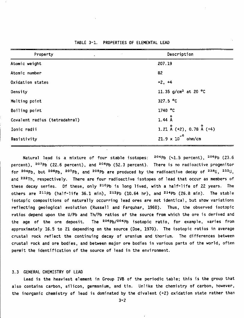
TABLE 3-1. PROPERTIES OF ELEMENTAL LEAD
Property Description
Atomic weight 207.19
Atomic number 82
Oxidation states
Density
Melting point
Boiling point
Covalent radius (tetradehral)
Ionic radii
Resistivity
+2, +4
11.35 g/cm3
327.5 oc
1740 oc 0
1.44 A 0
1.21 A (+2), -6
21.9 X 10
at 20 °C
0
0.78 A (+4)
ohm/em
Natural lead is a mixture of four stable isotopes: 2°4Pb ("-1.5 percent), 206 Pb (23.6 percent), 2° 7 Pb (22.6 percent), and 208 Pb (52.3 percent). There is no radioactive progenitor for 204Pb, but 2°6 Pb, 2° 7 Pb, and 208 Pb are produced by the radioactive decay of 238U, 235 U,
and 232Th, respectively. There are four radioactive isotopes of lead that occur as members of
these decay series. Of these, only 210 Pb is long lived,. with a half-life of 22 years. The
others are 211 Pb (half-life 36.1 min), 2l2pb (10.64 hr), and 214 Pb (26.8 min). The stable isotopic compositions of naturally occurring lead ores are not identical, but show variations reflecting geological evolution (Russell and Farquhar, 1960). Thus, the observed isotopic
ratios depend upon the U/Pb and Th/Pb ratios of the source from which the ore is derived and the age of the ore deposit. The 206 Pbf204 Pb isotopic ratio, for example, varies from
approximately 16.5 to 21 depending on the source (Doe, 1970). The isotopic ratios in average
crusta 1 rock reflect the continuing decay of uranium and thorium. The differences between crustal rock and ore bodies, and between major ore bodies in various parts of the world, often
permit the identification of the source of lead in the environment.
3.3 GENERAL CHEMISTRY OF LEAD Lead is the heaviest element in Group IVB of the periodic table; this is the group that
also contains carbon, silicon, germanium, and tin. Unlike the chemistry of carbon, however,
the inorganic chemistry of lead is dominated by the divalent (+2) oxidation state rather than
3-2
the tetravalent (+4) oxidation state. This important chemical feature is a direct result of the fact that the strengths of single bonds between the Group IV atoms and other atoms generally decrease as the atomic number of the Group IV atom increases (Cotton and Wilkinson,
1980). Thus, the average energy of a C-H bond is 100 kcal/mole, and it is this ~actor that stabilizes CH 4 relative to CH2 ; for lead, the Pb-H energy is only approximately 50 kcal/mole
(Shaw and Allred, 1970), and this is presumably too small to compensate fo-r the Pb(Il) -+
Pb(IV) promotional energy. It is this same feature that explains the marked difference in the
tendencies to catenation shown by these elements. Though C-C bonds are present in literally
mi 11 ions of compounds, 1 ead catenation occurs on 1 y in organa 1 ead compounds. Lead does,
however, form compounds like Na4 Pb9 which contain distinct polyatomic lead clusters (Britton, 1964), and Pb-Pb bonds are found in the cationic cluster [Pb6 0(0H) 6 ]+4 (Olin and Soderquist, 1972).
A listing of the solubilities and physical properties of the more common compounds of lead is given in Appendix 3A (Table 3A-1) (Weast, 1982). As can be discerned from those data,
most inorganic lead salts are sparingly soluble (e.g., PbF2 , PbC12 ) or virtually insoluble
(PbS04 , PbCr04 ) in water; the notable exceptions are lead nitrate, Pb(N03 ) 2 , and lead acetate,
Pb(OCOCH3 ) 2 . Inorganic lead (II) salts are, for the most part, relatively high-melting-point
solids with correspondingly low vapor pressures at room temperatures. The vapor pressures of
the most commonly encountered lead salts are also tabulated in Appendix 3A (Table 3A-2)
(Stull, 1947). The transformation of lead salts in the atmosphere is discussed in Chapter 6.
3.4 ORGANOMETALLIC CHEMISTRY OF LEAD
The properties of organolead compounds (i.e., compounds containing bonds between lead and
carbon) are entirely different from those of the inorganic compounds of lead; although a few
organolead(II) compounds, such as dicyclopentadienyllead, Pb(C5 H5h, are known, the organic
chemistry of lead is dominated by the tetravalent (+4) oxidation state. An important property
of most organolead compounds is that they undergo photolysis when exposed to light (Rufman and
Rotenberg, 1980).
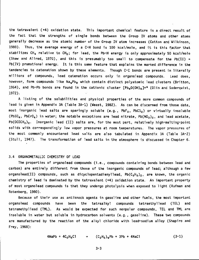
Because of their use as antiknock agents in gasoline and other fuels, the most important
organo 1 ead compounds have been the tetraa 1 kyl compounds tetraethyllead (TE.L) and
tetramethyllead (TML). As would be expected for such nonpolar compounds, TEL and TML are
insoluble in water but soluble in hydrocarbon solvents (e.g., gasoline). These two compounds
are manufactured by the reaction of the alkyl chloride with lead-sodium alloy (Shapiro and
Frey, 1968):
(3-1)
3-3
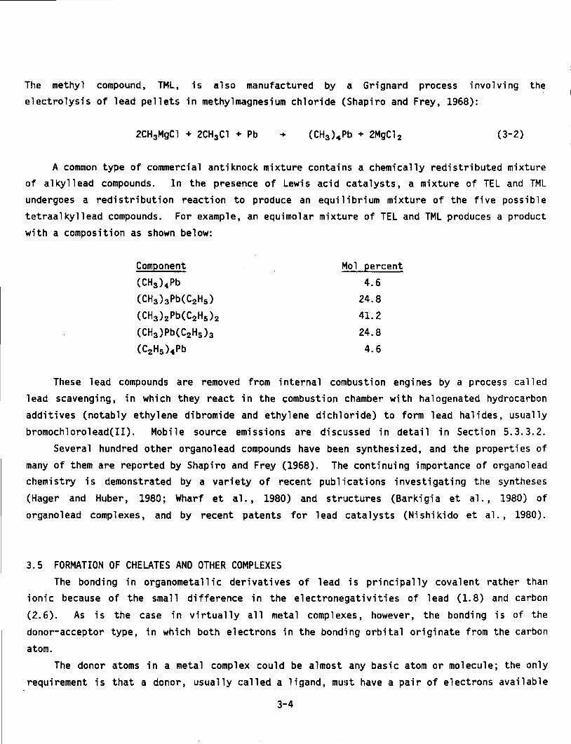
The methyl compound, TML, is also manufactured by a Grignard process involving the electrolysis of lead pellets in methylmagnesium chloride (Shapiro and Frey, 1968):
2CH3 MgCl + 2CH3 Cl + Pb (3-2)
A common type of commercial antiknock mixture contains a chemically redistributed mixture of al kyll ead compounds. In the presence of Lewis acid catalysts, a mixture of TEL and TML
undergoes a redi stri but ion reaction to produce an equi 1 i bri um mixture of the five poss i b 1 e tetraalkyllead compounds. For example, an equimolar mixture of TEL and TML produces a product
with a composition as shown below:
Component Mol percent (CH3 ) 4 Pb 4.6 (CH3 )aPb(C2H5 ) 24.8
(CH3 hPb(C2 H5 ) 2 41.2
(CH3 )Pb(C2 H5 )s 24.8 (C2 H5 ) 4 Pb 4.6
These lead compounds are removed from internal combustion engines by a process called
lead scavenging, in which they react in the combustion chamber with halogenated hydrocarbon
additives (notably ethylene dibromide and ethylene dichloride) to form lead halides, usually
bromochlorolead(II). Mobile source emissions are discussed in detail in Section 5.3.3.2.
Several hundred other organolead compounds have been synthesized, and the properties of
many of them are reported by Shapiro and Frey (1968). The continuing importance of organolead chemistry is demonstrated by a variety of recent pub 1 i cations investigating the syntheses
(Hager and Huber, 1980; Wharf et al., 1980) and structures (Barki gi a et al., 1980) of
organolead complexes, and by recent patents for lead catalysts (Nishikido et al., 1980).
3.5 FORMATION OF CHELATES AND OTHER COMPLEXES
The bonding in organometallic derivatives of lead is principally covalent rather than ionic because of the small difference in the electronegativities of lead (1.8) and carbon
(2. 6). As is the case in virtually all meta 1 comp 1 exes, however, the bonding is of the
donor-acceptor type, in which both e 1 ectrons in the bond·i ng orbi ta 1 originate from the carbon
atom.
The donor atoms in a metal complex could be almost any basic atom or molecule; the only
requirement is that a donor, usually called a ligand, must have a pair of electrons available
3-4
L..___ ___________________ _
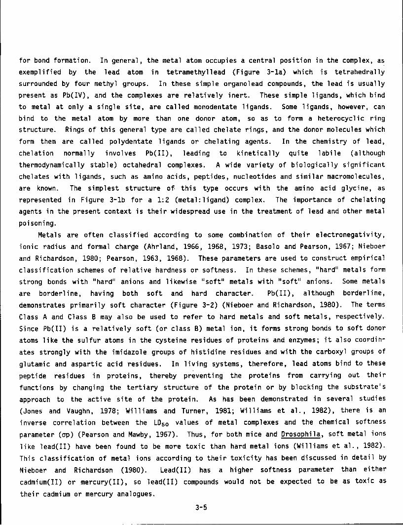
for bond formation. exemplified by the
In general, the metal atom occupies a central position in the complex, as lead atom in tetramethyllead (Figure 3-1a) which is tetrahedrally
surrounded by four methyl groups. In these simple organolead compounds, the lead is usually present as Pb(IV), and the complexes are relatively inert. These simple ligands, which bind to metal at only a single site, are called monodentate ligands. Some ligands, however, can bind to the metal atom by more than one donor atom, so as to form a heterocyclic ring structure. Rings of this general type are called chelate rings, and the donor molecules which
form them are called polydentate ligands or chelating agents. In the chemistry of lead, chelation normally involves Pb(II), leading to kinetically quite labile (although
thermodynamically stable) octahedral complexes. A wide variety of biologically significant chelates with ligands, such as amino acids, peptides, nucleotides and similar macromolecules, are known. The simplest structure of· this type occurs with the amino acid glycine, as represented in Figure 3-1b for a 1:2 (metal:ligand) complex. The importance of chelating agents in the present context is their widespread use in the treatment of lead and other metal
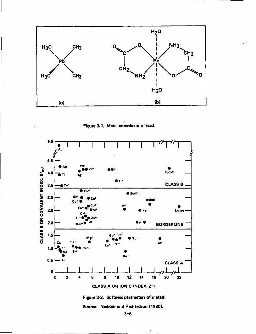
poisoning. Metals are often classified according to some combination of their electronegativity,
ionic radius and formal charge (Ahrland, 1966, 1968, 1973; Basolo and Pearson, 1967; Nieboer and Richardson, 1980; Pearson, 1963, 1968). These parameters are used to construct empirical classification schemes of relative hardness or softness. In these schemes, 11 hard11 metals form strong bonds with 11 hard11 anions and likewise 11 soft11 metals with 11 soft11 anions. Some metals are borderline, having both soft and hard character. Pb(II), although borderline,
demonstrates primarily soft character (Figure 3-2) (Nieboer and Richardson, 1980). The terms Class A and Class 8 may also be used to refer to hard metals and soft metals, respectively.
Since Pb(II) is a relatively soft (or class B) metal ion, it forms strong bonds to soft donor atoms like the sulfur atoms in the cysteine residues of proteins and enzymes; it also coordin
ates strongly with the imidazole groups of histidine residues and with the carboxyl groups of
glutamic and aspartic acid residues. In living systems, therefore, lead atoms bind to these
peptide residues in proteins, thereby preventing the proteins from carrying out their functions by changing the tertiary structure of the protein or by blocking the substrate• s
approach to the active site of the protein. As has been demonstrated in several studies (Jones and Vaughn, 1978; Williams and Turner, 1981; Williams et al., 1982), there is an inverse corre 1 at ion between the LD 50 va 1 ues of meta 1 comp 1 exes and the chemica 1 softness
parameter (crp) (Pearson and Mawby, 1967). Thus, for both mice and Drosophila, soft metal ions
like lead(II) have been found to be more toxic than hard metal ions (Williams et al., 1982).
This classification of metal ions according to their toxicity has been discussed in detail by
Nieboer and Richardson (1980). Lead(II) has a higher softness parameter than either
cadmium( II) or mercury(! I), so lead(! I) compounds would not be expected to be as toxic as
their cadmium or mercury analogues.
3-5
~
E )c )( w Q z -.... z w ~ c > 0 CJ cz: 0 CD Cl) Cl)
c ~ CJ
(a) (b)
Figure 3-1. Metal complexes of lead.
Pd'' e88Pt1
'
Hg''
8Pb''
Sn•·e 8cu•· Cd1'8
•co•· Fe•·• 8Ni1 '
Cr•· Ti'"8~zn•· Mn•·• v•·
Mg•· sa•· • ••eca•· Sr•·
I
8Bi'·
8Ti•·
8 Sblllll
tn•·
•
Gd'' Lu•·
•••• u•· v•·
•
Aslllll
• 8 Fe•·
Ga•·e
• sc•·
Be•·
• PbUVI
CLASS B
• SniiVI
BORDERLINE
• At•·
CLASS A
0~--._------~--~--_.--~--------~. 0 2 4 6 8 10 12 14 16 20 23
CLASS A OR IONIC INDEX. Z'lr
Figure 3-2. Softness parameters of metals.
Source: Nieboer and Richardson (1980).
3-6
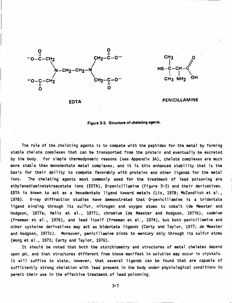
CHJ 0
I I! HS-C-CH-C
I I \ CH3 NH2 OH
EDTA PENICILLAMINE
Figure 3-3. Structure of chelating agents.
The role of the chelating agents is to compete with the peptides for the metal by forming stable chelate complexes that can be transported from the protein and eventually be excreted by the body. For simple thermodynamic reasons (see Appendix 3A), chelate complexes are much more stabie than monodentate metal complexes, and it is this enhanced stability that is the basis for their ability to compete favorably with proteins and other ligands for the metal ions. The che 1 at i ng agents most conunon ly used for the treatment of 1 ead poisoning are
ethylenediaminetetraacetate ions (EDTA), D-penicillamine (Figure 3-3) and their derivatives. EDTA is known to act as a hexadentate 1 i gand toward meta 1 s (Lis, 1978; McCandlish et a 1. ,
1978). X-ray diffraction studies have demonstrated that D-penicillamine is a tridentate ligand binding through its sulfur, nitrogen and oxygen atoms to cobalt (de Meester and Hodgson, 1977a; Helis et al., 1977), chromium (de Meester and Hodgson, 1977b), cadmium (Freeman et al., 1976), and lead itself (Freeman et al., 1974), but both penicillamine and other cysteine derivatives may act as bidentate ligands (Carty and Taylor, 1977; de Meester and Hodgson, 1977c). Moreover, penicillamine binds to mercury only through its sulfur atoms (Wong et al., 1973; Carty and Taylor, 1976).
It should be noted that both the stoichiometry and structures of metal chelates depend
upon pH, and that structures different from those manifest in solution may occur in crystals. It wi 11 suffice to state, however, that sever a 1 1 i gands can be found that are capab 1 e of sufficiently strong chelation with lead present in the body under physiological conditions to
permit their use in the effective treatment of lead poisoning.
3-7
3.6 REFERENCES
Ahrland, S. (1966) Factors contributing to (b)-behaviour in acceptors. Struct. Bonding (Berlin) 1: 207-220.
Ahrland, S. (1968) Thermodynamics of complex formation between hard and soft acceptors and donors. Struct. Bonding (Berlin) 5: 118-149.
Ahrland, S. (1973) Thermodynamics of the stepwise formation of metal-ion complexes in aqueous solution. Struct. Bonding (Berlin) 15: 167-188.
Barkigia, K. M.; Fajer, J.; Adler, A. D.; Williams, G. J. B. (1980) Crystal and molecular structure of (5,10,15,20-tetra-n-propylporphinato)lead(II): a "roof" porphyrin. Inorg. Chern. 19: 2057-2061. -
Basolo, F.; Pearson, R. G. (1967) Mechanisms of inorganic reactions: a study of metal complexes in solution. New York, NY: John Wiley & Sons, Inc.; pp. 23-25, 113-119.
-4 Britton, D. (1964) The structure of the Pb9 ion. Inorg. Chern. 3: 305.
Carty, A. J.; Taylor, N. J. (1976) Binding of inorganic mercury at biological sites: crystal structures of Hg2+ complexes with sulphur amino-acids. J. Chern. Soc. Chern. Commun. (6): 214-216.
Carty, A. J.; Taylor, N. J. (1977) Binding of heavy metals at biologically important sites: synthesis and molecular structure of aquo(bromo)-DL-penicillaminatocadmium(II) dihydrate. Inorg. Chern. 16: 177-181. -
Cotton, F. A.; Wilkinson, G. (1980) Advanced inorganic chemistry: a comprehensive text. 4th ed. New York, NY: John Wiley & Sons, Inc. pp. 374-406.
de Meester, P.; Hodgson, D. J. (1977a) Model for the binding of D-penicillamine to metal ions in living systems: synthesis and structure of L-histidinyl-D-penicillaminatocobalt(III) monohydrate, [Co(L-his)(D-pen)] H20. J. Am. Chern. Soc. 99: 101-104.
de Meester, P.; Hodgson, D. J. (1977b) Synthesis and structural characterization of L-histidinato-D-penicillaminatochromium (III) monohydrate. J. Chern. Soc. Dalton Trans. (17): 1604-1607.
de Meester, P.; Hodgson, D. J. (1977c) Absence of metal interaction with sulfur in two metal complexes of a cysteine derivative: the structural characterization of Bis(S-methyl-Lcysteinato)cadmium(II) and Bis(S-methyl-L-cysteinato)zinc(II). J. Am. Chern. Soc. 99: 6884-6889.
Doe, B. R. (1970) Lead isotopes. New York, NY: Springer-Verlag. (Engelhardt, W.; Hahn, T.; Roy, R.; Winchester, J. W.; Wyllie, P. J., eds. Minerals, rocks and inorganic materials: monograph series of theoretical and experimental studies: v. 3).
Dyrssen, D. (1972) The changing chemistry of the oceans. J\mbio 1: 21-25.
Freeman, H. C.; Stevens, G. N.; Taylor, I. F., Jr. (1974) Metal binding in chelation therapy: the crystal structure of D-penicillaminatolead(II). J. Chern. Soc. Chern. Commun. (10): 366-367.
3-8
Freeman, H. C.; Huq, F.; Stevens, G. N. (1976) Metal binding by D-penicillamine: crystal structure of D-penicillaminatocadmium(II) hydrate. J. Chem. Soc. Chem. Commun. (3): 90-91.
Hager, C.-D.; Huber, F. (1980) Organobleiverbindungen von Mercaptocarbonsauren [Organolead compounds of mercaptocarboxylic acids]. Z. Naturforsch. 35b: 542-547.
Helis, H. M.; de Meester, P.; Hodgson, D. J. (1977) Binding of penicillamine to toxic metal ions: synthesis and structure of potassium(D-penicillaminato) (L-Penicillaminato)cobaltate(III) dihydrate, K[Co(D-pen)(L-pen)]·2H20. J. Am. Chem. Soc. 99: 3309-3312.
Heslop, R. B.; Jones, K. (1976) Inorganic chemistry: a guide to advanced study. New York, NY: Elsevier Science Publishing Co.; pp. 402-403.
Jones, M. M.; Vaughn, W. K. (1978) HSAB theory and acute metal ion toxicity and detoxification processes. J. Inorg. Nucl. Chem. 40: 2081-2088.
Lis, T. (1978) Potassium ethyl enedi ami netetraacetatomanganate( II I) dihydrate. Acta Crysta 1-logr. Sect. B 34: 1342-1344.
McCandlish, E. F. K.; Michael, T. K.; Neal, J. A.; Lingafelter, E. C.; Rose, N. J. (1978) Comparison of the structures and aqueous solutions of [o-phenylenediaminetetraacetato(4-)] cobalt(!!) and [ethylenediaminetetraacetato(4-)] cobalt(!!) ions. Inorg. Chem. 17: 1383-1394.
Moeller, T. (1952) Inorganic chemistry: an advanced textbook. New York, NY: John Wiley & Sons, Inc.
Nieboer, E.; Richardson, D. H. S. (1980) The replacement of the nondescript term heavy metals by a biologically and chemically significant classification of metal ions. Environ. Pollut. Ser. B. 1: 3-26.
Nishikido, J.; Tamura, N.; Fukuoka, Y. (1980) (Asahi Chemical Industry Co. Ltd.) Ger. patent no. 2,936,652.
Olin, A.; Soderquist, R. (1972) The crystal structure of p-[Pb60{0H) 8 ](C104 ) 4 H20. Acta Chem. Scand. 26: 3505-3514.
Pearson, R. G. (1963) Hard and soft acids and bases. J. Am. Chem. Soc. 85: 3533-3539.
Pearson, R. G. (1968) Hard and soft acids and bases, HSAB, part 1: fundamental principles. J. Chem. Educ. 45: 581-587.
Pearson, R. G.; Mawby, R. J. (1967) The nature of metal-halogen bonds. In: Gutmann, V., ed. Halogen chemistry: volume 3. New York, NY: Academic Press, Inc.; pp. 55-84.
Rufman, N. M.; Rotenberg, Z. A. (1980) Special kinetic features of the photodecomposition of organolead compounds at lead electrode surfaces. Sov. Electrochem. Engl. Transl. 16: 309-314.
Russell, R. D.; Farquhar, R. M. (1960) Introduction. In: Lead isotopes in geology. New York, NY: Interscience; pp. 1-12.
3-9
Shapiro, H.; Frey, F. W. (1968) The organic compounds of lead. New York, NY: John Wiley & Sons. (Seyferth, D., ed. The chemistry of organometallic compounds: a series of monographs).
Shaw, C. F., III; Allred, A. L. (1970) Nonbonded interactions in organometallic compounds of Group IV B. Organometallic Chem. Rev. A 5: 95-142.
Wharf, I.; Onyszchuk, M.; Miller, J. M.; Jones, T. R. B. (1980) Synthesis and spectroscopic studies of phenyllead halide and thiocyanate adducts with hexamethylphosphoramide. J. Organomet. Chem. 190: 417-433.
Williams, M. W.; Turner, J. E. (1981) Comments on softness parameters and metal ion toxicity. J. Inorg. Nucl. Chem. 43: 1689-1691.
Williams, M. W.; Hoeschele, J. D.; Turner, J. E.; Jacobson, K. B.; Christie, N. T.; Paton, C. L.; Smith, L. H.; Witschi, H. R.; Lee, E. H. (1982) Chemical softness and acute metal toxicity in mice and Drosophila. Toxicol. Appl. Pharmacal. 63: 461-469.
Wong, Y. S.; Chieh, P. C.; Carty, A. J. (1973) Binding of methylmercury by amino-acids: X-ray structures of DL-penicillaminatomethylmercury(II). J. Chem. Soc. Chem. Commun. (19): 741-742.
3-10
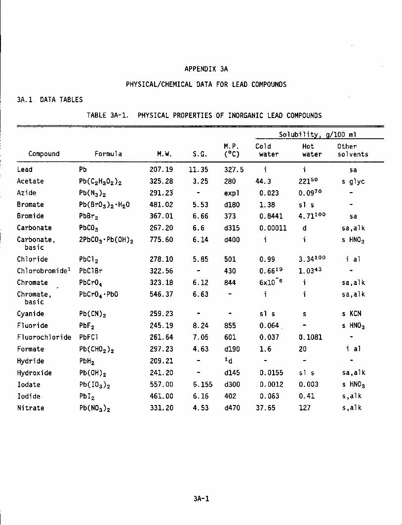
APPENDIX 3A
PHYSICAL/CHEMICAL DATA FOR LEAD COMPOUNDS
3A.1 DATA TABLES
TABLE 3A-1. PHYSICAL PROPERTIES OF INORGANIC LEAD COMPOUNDS
Solubility, g/100 ml
M.P. Cold Hot Other Compound Formula M.W. S.G. (°C) water water solvents
Lead Pb 207.19 11.35 327.5 i i sa Acetate Pb(C2H302h 325.28 3.25 280 44.3 22150 s glyc Azide Pb(N3 h 291.23. expl 0.023 0.0970
Bromate Pb(BrOah • H20 481.02 5.53 d180 1.38 sl s Bromide PbBr2 367.01 6.66 373 0.8441 4.71100 sa Carbonate PbC03 267.20 6.6 d315 0.00011 d sa,alk Carbonate, 2PbC03 ·Pb(OH)2 775.60 6.14 d400 i i s HN0 3
basic Chloride PbCl2 278.10 5.85 501 0.99 3.34100 i a 1
Chlorobromide1 PbClBr 322.56 430 0.6619 1.0343
Chromate PbCr04 323.18 6.12 844 6x10⁻⁶ i sa,alk Chromate, PbCr04 ·PbO 546.37 6.63 i i sa,alk
basic Cyanide Pb(CNh 259.23 sl s s s KCN
Fluoride PbF2 245.19 8.24 855 0.064 s HN03
Fluorochloride PbFCl 261.64 7.05 601 0.037 0.1081 Formate Pb(CH02)2 297.23 4.63 d190 1.6 20 i a 1
Hydride PbH2 209.21 1d
Hydroxide Pb(OHh 241.20 d145 0.0155 s 1 s sa,alk
Iodate Pb(IOah 557.00 6.155 d300 0.0012 0.003 s HN03
Iodide Pbl2 461.00 6.16 402 0.063 0.41 s ,al k
Nitrate Pb(N03 h 331.20 4.53 d470 37.65 127 s,alk
3A-1
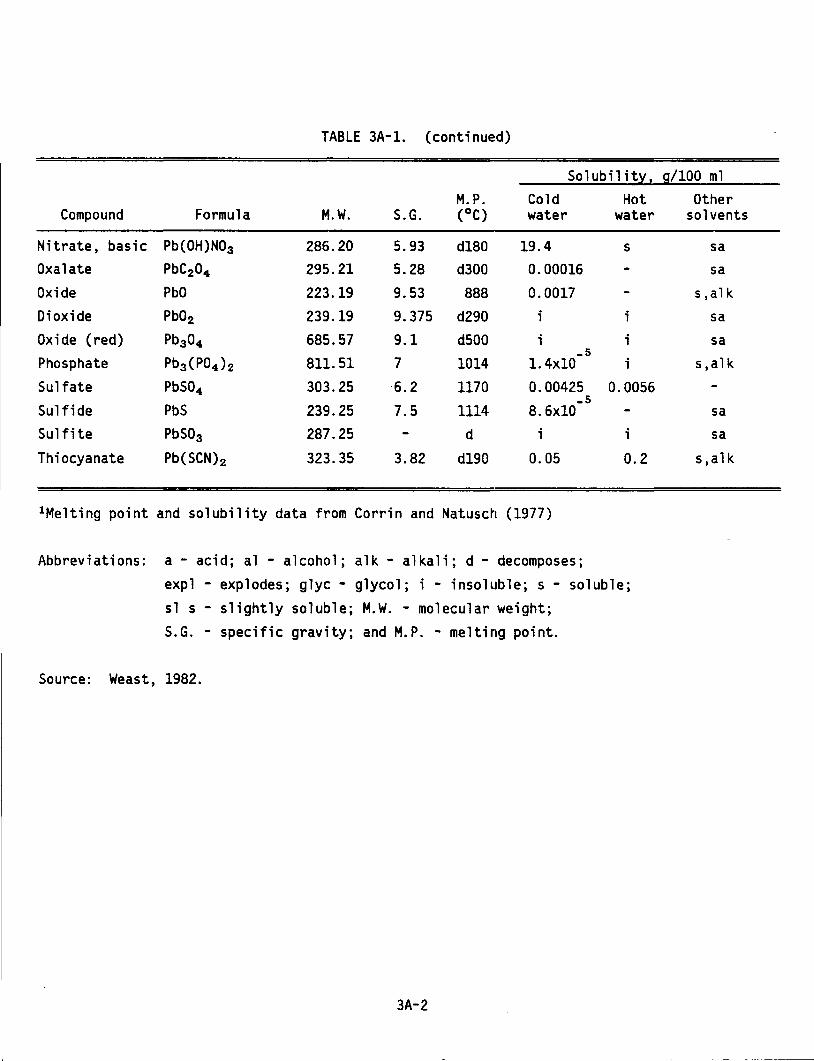
TABLE 3A-1. (continued)
Solubility, g/100 ml M.P. Cold Hot
Compound Formula M.W. S.G. (°C) water water
Nitrate, basic Pb(OH)N03 286.20 5.93 dl80 19.4 s Oxalate PbC204 295.21 5.28 d300 0.00016 Oxide PbO 223.19 9.53 888 0.0017 Dioxide Pb02 239.19 9.375 d290 i i Oxide (red) Pb304 685.57 9.1 d500 i i
-5 Phosphate Pb3 (P04 ) 2 811.51 7 1014 1. 4x10 i Sulfate PbS04 303.25 6.2 1170 0.00425 0.0056
_s Sulfide PbS 239.25 7.5 1114 8.6x10 Sulfite PbS03 287.25 d i i
Thiocyanate Pb(SCNh 323.35 3.82 dl90 0.05 0.2
1 Melting point and solubility data from Corrin and Natusctt (1977)
Abbreviations: a- acid; al -alcohol; alk- alkali; d- decomposes; expl- explodes; glyc- glycol; i- insoluble; s- soluble;
sl s - slightly soluble; M.W. - molecular weight;
S.G. - specific gravity; and M.P. - melting point.
Source: Weast, 1982.
3A-2
Other solvents
sa sa
s,alk sa sa
s,alk
sa sa
s,alk
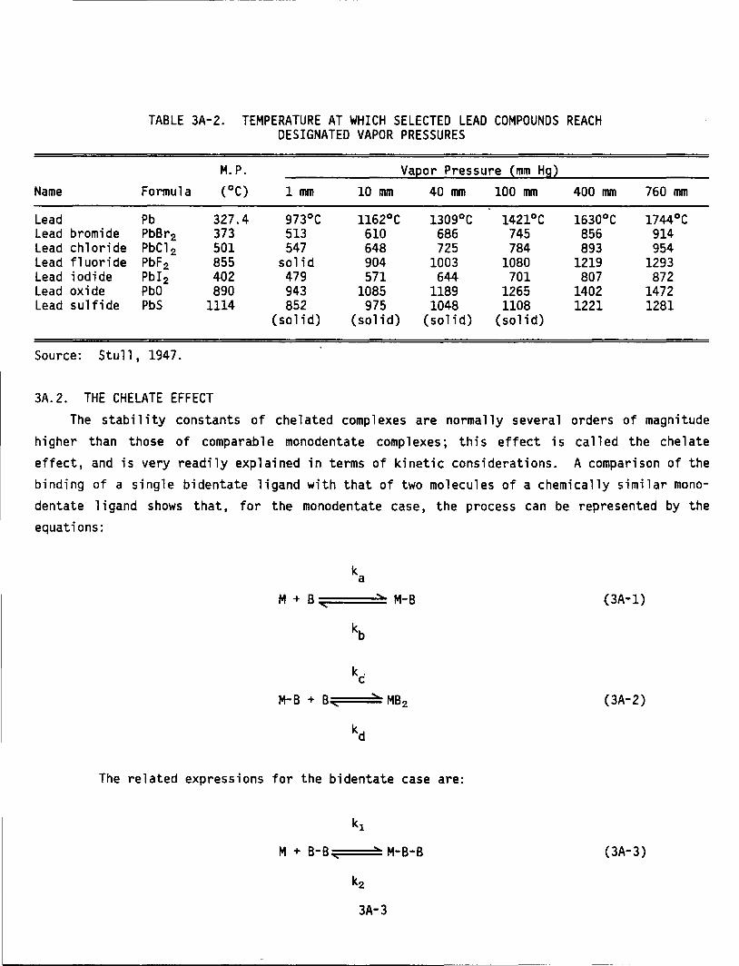
TABLE 3A-2. TEMPERATURE AT WHICH SELECTED LEAD COMPOUNDS REACH DESIGNATED VAPOR PRESSURES
M.P. Vapor Pressure (mm Hg) Name Formula (oC) 1 mm 10 mm 40 mm 100 mm 400 mm
Lead Pb 327.4 973°C 1162°C 1309°C 1421°C 1630°C Lead bromide PbBr2 373 513 610 686 745 856 Lead chloride PbC1 2 501 547 648 725 784 893 Lead fluoride PbF2 855 solid 904 1003 1080 1219 Lead iodide Pbi 2 402 479 571 644 701 807 Lead oxide PbO 890 943 1085 1189 1265 1402 Lead sulfide PbS 1114 852 975 1048 1108 1221
(solid) (solid) (solid) (solid)
Source: Stull, 1947.
3A.2. THE CHELATE EFFECT
760 mm
1744°C 914 954
1293 872
1472 1281
The stabi 1 ity constants of chelated complexes are normally several orders of magnitude higher than those of comparab 1 e monodentate camp 1 exes; this effect is called the che 1 ate
effect, and is very readily explained in terms of kinetic considerations. A comparison of the binding of a single bidentate ligand with that of two molecules of a chemically similar monodentate 1 i gand shows that, for the monodentate case, the process can be represented by the equations:
k a
M-B {3A-1)
kb
k. c MB 2 (3A-2)
The related expressions for the bidentate case are:
(3A-3)
3A-3
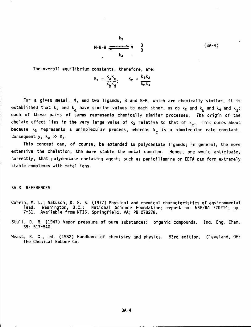
The overall equilibrium constants,
Kl = kakc kbkd;
B B
therefore, are:
K2 = klk3
k2k4
(3A-4)
For a given metal, M, and two ligands, Band B-B, which are chemically similar, it is established that k1 and ka have similar values to each other, as do k2 and kb and k4 and kd; each of these pairs of terms represents chemically similar processes. The origin of the chelate effect lies in the very large value of k3 relative to that of kc. This comes about because k3 represents a unimolecular process, whereas kc is a bimolecular rate constant. Consequently, K2 >> K1 •
This concept can, of course, be extended to polydentate ligands; in general, the more extensive the chelation, the more stable. the metal complex. Hence, one would anticipate, correctly, that polydentate chelating agents such as penicillamine or EDTA can form extremely stable complexes with metal ions.
3A.3 REFERENCES
Corrin, M. L.; Natusch, D. F. S. (1977) Physical and chemical characteristics of environmental lead. Washington, D.C.: National Science Foundation; report no. NSF/RA 770214; pp. 7-31. Available from NTIS, Springfield, VA; PB-278278.
Stull, D. R. (1947) Vapor pressure of pure substances: organic compounds. Ind. Eng. Chem. 39: 517-540.
Weast, R. C., ed. (1982) Handbook of chemistry and physics. 63rd edition. Cleveland, OH: The Chemical Rubber Co.
3A-4
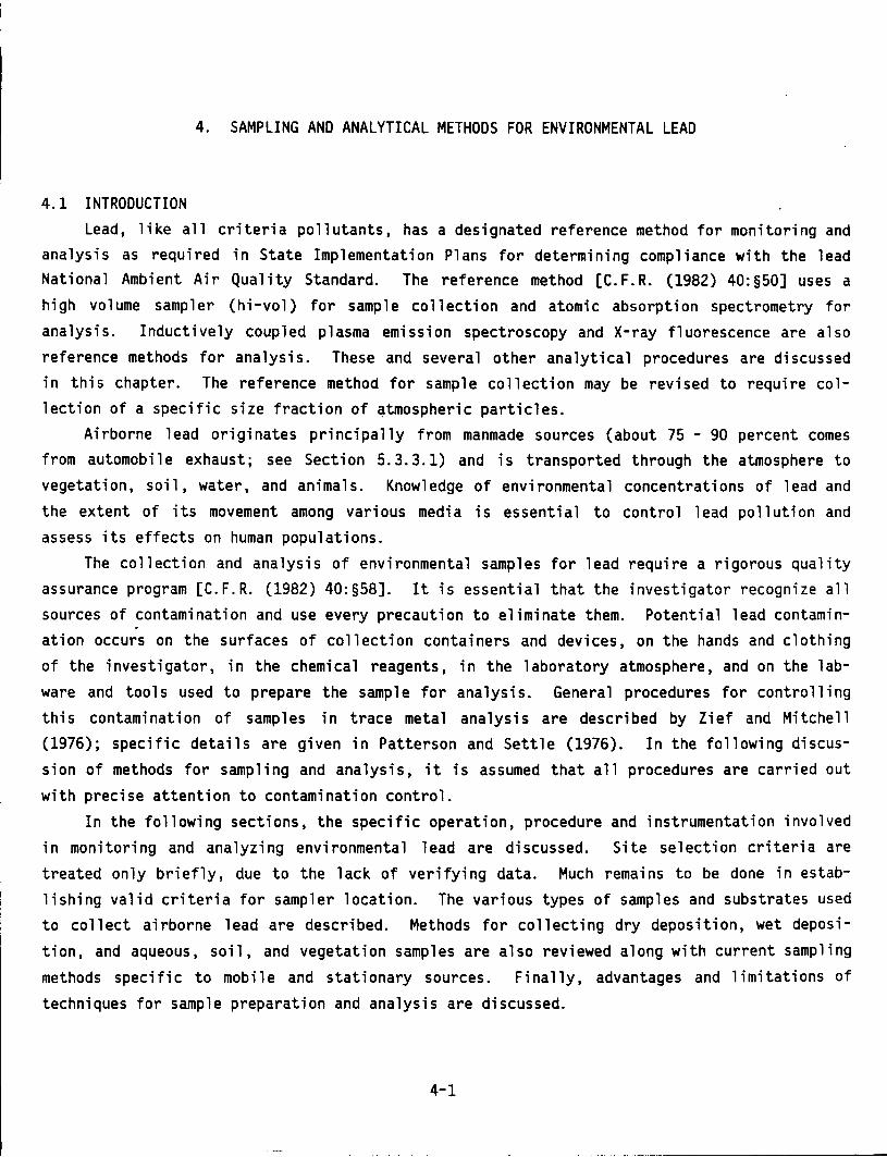
4. SAMPLING AND ANALYTICAL METHODS FOR ENVIRONMENTAL LEAD
4.1 INTRODUCTION
Lead, like all criteria pollutants, has a designated reference method for monitoring and analysis as required in State Implementation Plans for determining compliance with the lead National Ambient Air Quality Standard. The reference method [C.F.R. (1982) 40:§50] uses a high volume sampler (hi-vol) for sample collection and atomic absorption spectrometry for
analysis. Inductively coupled plasma emission spectroscopy and X-ray fluorescence are also reference methods for analysis. These and several other analytical procedures are discussed in this chapter. The reference method for sample collection may be revised to require collection of a specific size fraction of ~tmospheric particles.
Airborne lead originates principally from manmade sources (about 75 - 90 percent comes from automobile exhaust; see Section 5.3.3.1) and is transported through the atmosphere to vegetation, soil, water, and animals. Knowledge of environmental concentrations of lead and
the extent of its movement among various media is es senti a 1 to contra 1 1 ead pollution and assess its effects on human populations.
The collection and analysis of environmental samples for lead require a rigorous quality assurance program [C.F.R. (1982) 40:§58]. It is essential that the investigator recognize all sources of contamination and use every precaution to eliminate them. Potential lead contamination occurs on the surfaces of collection containers and devices, on the hands and clothing of the investigator, in the chemical reagents, in the laboratory atmosphere, and on the labware and tools used to prepare the sample for analysis. General procedures for controlling
this contamination of samples in trace metal analysis are described by Zief and Mitchell (1976); specific details are given in Patterson and Settle (1976). In the following discussion of methods for sampling and analysis, it is assumed that all procedures are carried out
with precise attention to contamination control. In the following sections, the specific operation, procedure and instrumentation involved
in monitoring and analyzing environmental lead are discussed. Site selection criteria are
treated only briefly, due to the lack of verifying data. Much remains to be done in estab
lishing valid criteria for sampler location. The various types of samples and substrates used to collect airborne lead are described. Methods for collecting dry deposition, wet deposi
tion, and aqueous, soil, and vegetation samples are also reviewed along with current sampling
methods specific to mobile and stationary sources. Finally, advantages and limitations of
techniques for sample preparation and analysis are discussed.
4-1
------ -------------~
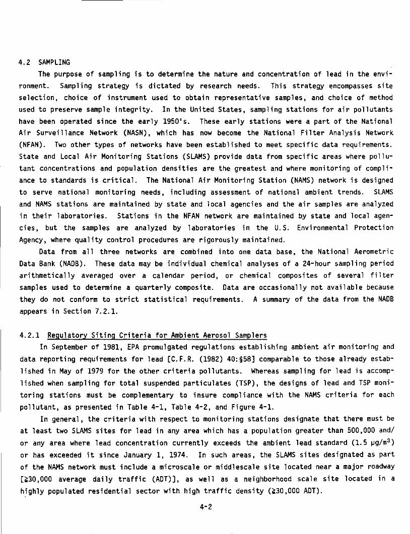
4. 2 SAMPLING The purpose of sampling is to determine the nature and concentration of lead in the envi
ronment. Samp 1 i ng strategy is dictated by research needs. This strategy encompasses site selection, choice of instrument used to obtain representative samples, and choice of method used to preserve sample integrity. In the United States, sampling stations for air pollutants have been operated since the early 1950 1 s. These early stations were a part of the National Air Surveillance Network (NASN), which has now become the National Filter Analysis Network (NFAN). Two other types of networks have been established to meet specific data requirements. State and Local Air Monitoring Stations (SLAMS) provide data from specific areas where pollutant concentrations and population densities are the greatest and where monitoring of compliance to standards is critical. The National Air Monitoring Station (NAMS) network is designed to serve national monitoring needs, including assessment of national ambient trends. SLAMS and NAMS stations are maintained by state and local agencies and the air samples are analyzed in their laboratories. Stations in the NFAN network are maintained by state and local agen
cies, but the samples are analyzed by laboratories in the U.S. Environmental Protection
Agency, where quality control procedures are rigorously maintained. Data from all three networks are combined into one data base, the Nat i ana 1 Aerometri c
Data Bank (NADB). These data may be individual chemical analyses of a 24-hour sampling period arithmetically averaged over a calendar period, or c~1emical composites of several filter samples used to determine a quarterly composite. Data are occasionally not available because they do not conform to strict statistical requirements. A summary of the data from the NADB
appears in Section 7.2.1.
4.2.1 Regulatory Siting Criteria for Ambient Aerosol Samplers In September of 1981, EPA promulgated regulations establishing ambient air monitoring and
data reporting requirements for lead [C.F.R. (1982) 40:§58] comparable to those already established in May of 1979 for the other criteria pollutants. Whereas sampling for lead is accomp
lished when sampling for total suspended particulates (TSP), the designs of lead and TSP moni
toring stations must be camp 1 ementary to insure camp 1 i ance with the NAMS criteria for each
pollutant, as presented in Table 4-1, Table 4-2, and Figure 4-1. In general, the criteria with respect to monitoring stations designate that there must be
at least two SLAMS sites for lead in any area which has a population greater than 500,000 and/
or any area where lead concentration currently exceeds the ambient lead standard (1.5 1Jg/m3)
or has exceeded it since January 1, 1974. In such areas, the SLAMS sites designated as part
of the NAMS network must include a microscale or middlescale site located near a major roadway
[~30,000 average daily traffic (ADT)], as well as a neighborhood scale site located in a
highly populated residential sector with high traffic density (~30,000 ADT).
4-2
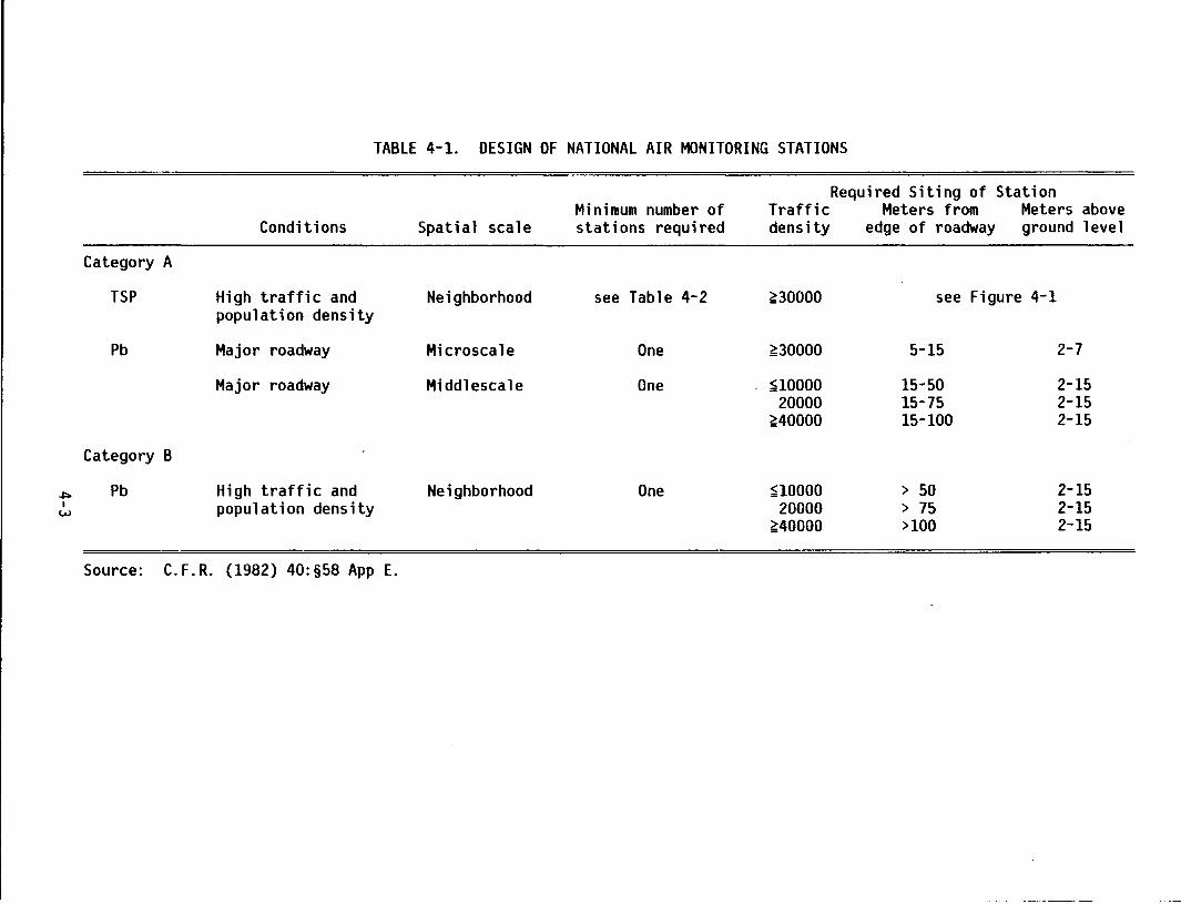
~ I
w
TABLE 4-1. DESIGN OF NATIONAL AIR MONITORING STATIONS
Conditions
Category A
TSP High traffic and population density
Pb Major roadway
Category B
Pb
Major roadway
High traffic and population density
Source: C.F.R. (1982) 40:§58 App E.
Spatial scale
Neighborhood
Microscale
Middlescale
Neighborhood
Minimum number of stations required
see Table 4-2
One
One
One
Required Siting of Station Traffic Meters from Meters above density edge of roadway ground level
~30000
~30000
~10000 20000
~40000
~10000 20000
~40000
see Figure 4-1
5-15
15-50 15-75 15-100
> 50 > 75 >100
2-7
2-15 2-15 2-15
2-15 2-15 2-15
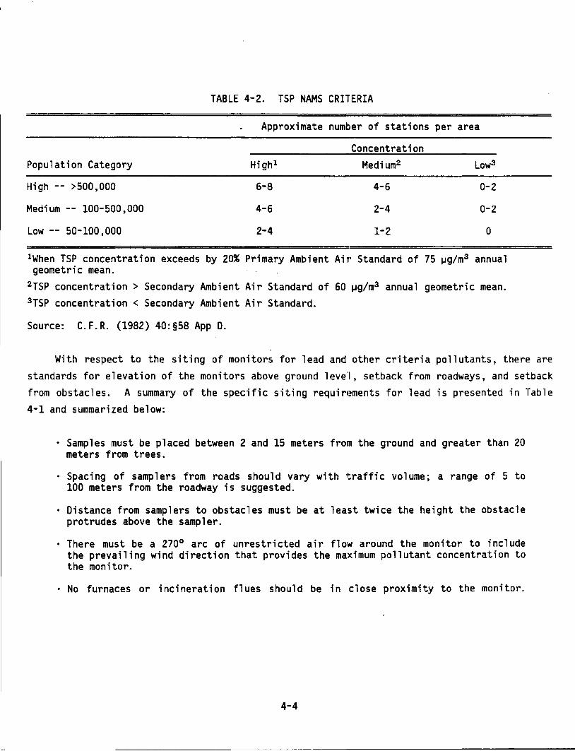
TABLE 4-2. TSP NAMS CRITERIA
Approxim·ate number of stations per area
Population Category
High -- >500,000
Medium -- 100-500,000
Low -- 50-100,000
High 1
6-8
4-6
2-4
Concentration Medium2 Low3
4-6 0-2
2-4 0-2
1-2 0
1When TSP concentration exceeds by 20% Primary Ambient Ait• Standard of 75 ~g/m3 annual geometric mean.
2TSP concentration > Secondary Ambient Air Standard of 60 ~g/m3 annual geometric mean. 3TSP concentration < Secondary Ambient Air Standard.
Source: C.F.R. (1982) 40:§58 App D.
With respect to the siting of monitors for lead and other criteria pollutants, there are standards for elevation of the monitors above ground level, setback from roadways, and setback from obstacles. A summary of the specific siting requir•~ments for lead is presented in Table 4-1 and summarized below:
• Samples must be placed between 2 and 15 meters from the ground and greater than 20 meters from trees.
• Spacing of samplers from roads should vary with traffic volume; a range of 5 to 100 meters from the roadway is suggested.
• Distance from samplers to obstacles must be at least twice the height the obstacle protrudes above the sampler.
There must be a 270° arc of unrestricted air flow around the monitor to include the prevailing wind direction that provides the maximum pollutant concentration to the monitor.
• No furnaces or incineration flues should be in close proximity to the monitor.
4-4
----------------------------------------------
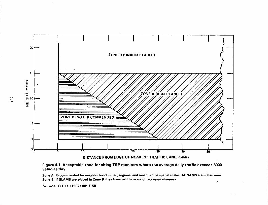
.f::o I
U1
20
ZONE C (UNACCEPTABLE)
15
ZONE 8 (NOT RECOMMENDED)
0~--------~----------~----------L---------~~--------~----------~----------L---------~ 0 10 20 25 30 35
DISTANCE FROM EDGE OF NEAREST TRAFFIC LANE, meten
Figure 4-1. Acceptable zone for siting TSP monitors where the average daily traffic exceeds 3000 vehicles/day_
Zone A: Recommended for neighborhood, urban, regional and most middle spatial scales. All NAMS are in this zone. Zone 8: If SLAMS are placed in Zone B they have middle scale of representativeness.
Source: C.F.R. (1982) 40: §58
To clarify the relationship between monitoring objectives and the actual siting of a monitor, the concept of a spatial scale of representativeness was developed. The spatial scales are described in terms of the physical dimensions of the air space surrounding the monitor throughout which pollutant concentrations are fairly similar. Table 4-3 describes the scales of representativeness while Table 4-4 relates monitoring objectives to the appropriate spatial scale [C.F.R. (1982) 40:§58].
The time scale may also be an important factor. A study by Lynam (1972) illustrates the effect of setback distance on short-term (15-minute) measurements of lead concentrations directly downwind from the source. They found sharp reductions in lead concentration with increasing distance from the roadway. A similar study by PEDCo Environmental, Inc. (1981) did not show the same pronounced reduction when the data were averaged over monthly or quarterly time periods. The apparent reason for this effect is that windspeed and direction are not consistent. Therefore, siting criteria must include sampling times sufficiently long to include average windspeed and direction, or a sufficient number of samples must be collected
over short sampling periods to provide an average value consistent with a 24-hour exposure.
4.2.2 Ambient Sampling for Particulate and Gaseous Lead Airborne lead is primarily inorganic particulate matter (PM) but may occur in the form of
organic gases. Devices used for collecting samples of ambient atmospheric lead include the standard hi-val and a variety of other collectors employiing filters, impactors, impingers, or
scrubbers, either separately or in combination. Some samplers measure total particulate matter gravimetrically; thus the lead data are usually expressed in IJg/g PM or 1Jg/m3 air.
Other samplers do not measure PM gravimetrically; therefore, the lead data can only be
expressed as 1Jg/m3 • Some samplers measure lead deposition expressed in 1Jg/cm2 . Some instruments separate particles by size. As a general rule, particles smaller than 2.5 1-1m are
defined as fine, and those larger than 2.5 1-1m are defined as coarse. In a typical sampler, the ambient air is drawn down into the inlet and deposited on the
collection surface after one or more stages of particle s·ize separation. Inlet effectiveness, internal wall losses, and retention efficiency of the collection surface may bias the
collected sample by selectively excluding particles of certain sizes.
4.2.2.1 High Volume Sampler (hi-vol). The present SLAMS and NAMS employ the standard hi-val sampler (Robson and Foster, 1962; Silverman and Viles, 1948; U.S. Environmental Protection
Agency, 1971) as part of their sampling networks. As a Federal Reference Method Sampler, the
hi-vol operates with a specific flow rate range of 1.13- 1.70 m3 /min, drawing air through a
4-6
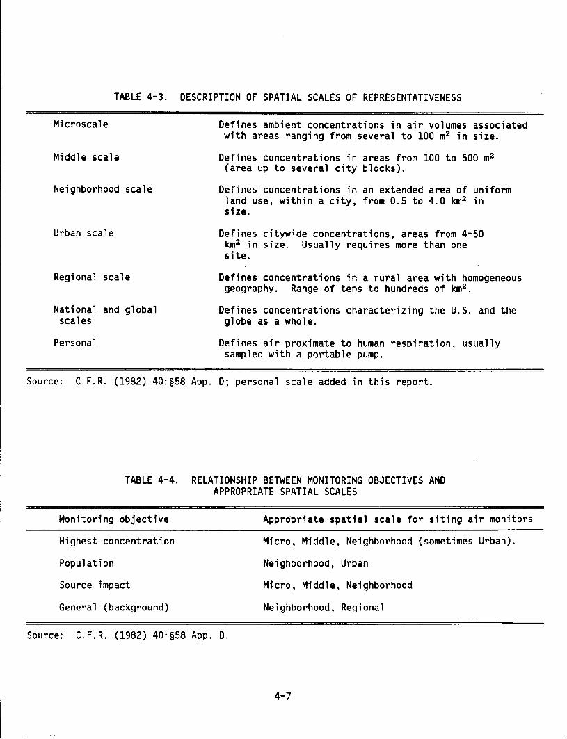
TABLE 4-3.
Microscale
Middle scale
Neighborhood scale
Urban scale
Regional scale
National and global scales
Personal
DESCRIPTION OF SPATIAL SCALES OF REPRESENTATIVENESS
Defines ambient concentrations in air volumes associated with areas ranging from several to 100 m2 in size.
Defines concentrations in areas from 100 to 500 m2
(area up to several city blocks).
Defines concentrations in an extended area of uniform land use, within a city, from 0.5 to 4.0 km2 in size.
Defines citywide concentrations, areas from 4-50 km2 in size. Usually requires more than one site.
Defines concentrations in a rural area with homogeneous geography. Range of tens to hundreds of km2 .
Defines concentrations characterizing the U.S. and the globe as a whole.
Defines air proximate to human respiration, usually sampled with a portable pump.
Source: C.F.R. (1982) 40:§58 App. D; personal scale added in this report.
TABLE 4-4. RELATIONSHIP BETWEEN MONITORING OBJECTIVES AND APPROPRIATE SPATIAL SCALES
Monitoring objective Appropriate spatial scale for siting air monitors
Highest concentration Micro, Middle, Neighborhood (sometimes Urban).
Population Neighborhood, Urban
Source impact Micro, Middle, Neighborhood
General (background) Neighborhood, Regional
Source: C.F.R. (1982) 40:§58 App. D.
4-7
200 x 250 mm glass fiber filter. At these flow rates, 1600 - 2500 m3 of air per day are sampled. Many hi-vol systems are presently equipped with mass flow sensors to control the total flow rate through the filter.
The present hi-vol approach has been shown during performance characterization tests to have a number of deficiencies. Wind tunnel testing by Wedding et al. (1977) has shown that the collection characteristics of hi-vol samples are strongly affected by particle size, wind speed and direction, and inlet size. However, since most lead particles have been shown to have a mass median aerodynamic diameter (MMAD) in the range of 0. 25 - 1. 4 1-1m (Lee and Goranson, 1972), the hi-vol sampler should present reasonably good estimates of ambient lead concentrations. For particles larger than 5 1-1m, the hi-vol system is unlikely to collect representative samples (McFarland et al., 1979; Wedding et al., 1977). 4.2.2.2 Dichotomous Sampler. The dichotomous sampler collects two particle size fractions, typically 0 - 2.5 1-1m and 2.5 1-1m to the upper cutoff of the inlet employed (normally 10 1-1m). The impetus for the dichotomy of collection, which approximately separates the fine and coarse particles, was provided by Whitby et al. (1972) to assist in the identification of particle sources. A 2.5 1-1m cutpoint for the separator was also recommended by Miller et al. (1979) because it satisfied the requirements of health researchers interested in respirable particles, provided adequate separation between two naturally occurring peaks in the size distribution, and was mechanically practical. Because the fine and coarse fractions collected in most locations tend to be acidic and basic, respectively, this separation also minimizes potential particle interaction after collection.
The particle separation principle used by this sampler was described by Hounam and Sherwood (1965) and Conner (1966). The version now in use by EPA was developed by Loo et al. (1979). The separation principle involves acceleration of the particles through a nozzle. Ninety percent of the flowstream is diverted to a small particle collector, while the larger particles continue by inertia toward the large particle c:ollection surface. The inertial virtual impactor design causes 10 percent of the fine particles to be collected with the coarse particle fraction. Therefore, the mass of fine and coarse particles must be adjusted to allow for their cross contamination. This mass correction procedure has been described by Dzubay et al. (1982).
Teflon® membrane filters with pore sizes as large as 2.0 1-1m can be used in the dichotomous sampler (Dzubay et al, 1982; Stevens et al., 1980) and have been shown to have essentially 100 percent collection efficiency for particles 1~ith an aerodynamic diameter as small as 0.03 1-1m (Liu et al., 1976; see Section 4.2.5). Because the sampler operates at a flowrate of 1 m3 /hr (167 1/min) and collects sub-milligram quantities of particles, a microbalance with a 1 1-1g resolution is recommended for filter weighing (Shaw, 1980). Removal of the fine particles via this fractionation technique may result in some of the collected coarse particles
4-8
-- ----- -----------
falling off the filter if care is not taken during filter handling and shipping. However, Dzubay and Barbour (1983) have developed a filter coating procedure which eliminates particle loss during transport. A study by Wedding et al. (1980) has shown that the Sierra® inlet to the dichotomous sampler was sensitive to windspeed. The 50 percent cutpoint (050 ) was. found to vary from 10 to 22 ~m over the windspeed range of 0 to 15 km/hr.
Automated versions of the sampler allow timely and unattended changes of the sampler filters. Depending on atmospheric concentrations, short-term samples of as little as 4 hours
can provide diurnal pattern information. The mass collected during such short sample periods, however, is extremely small and highly variable results may be expected.
4.2.2.3 Impactor Samplers. Impactors provide a means of dividing an ambient particle sample into subtractions of specific particle size for possible use in determining size distribution. A jet of air is directed toward a collection surface, which is often coated with an adhesive or grease to reduce particle bounce. Large, high-inertia particles are unable to turn with the airstream; consequently, they hit the collection surface. Smaller particles follow the
airstream and are directed toward the next impactor stage or to the filter. Use of multiple stages, each with a different particle size cutpoint, provides collection of particles in several size ranges.
For determining particle mass, removable impaction surfaces may be weighed before and after exposure. The particles collected may be removed and analyzed for individual elements. The se 1 ect ion and preparation of these impaction surfaces have s i gni fi cant effects on the impactor performance. Improperly coated or overloaded surfaces can cause particle bounce to lower stages resulting in substantial cutpoint shifts (Dzubay et al., 1976). Additionally, coatings may cause contamination of the sample. Marple and Willeke (1976) showed the effect
of various impactor substrates on the sharpness of the stage cutpoint. Glass fiber substrates can also cause particle bounce or particle interception (Dzubay et al., 1976) and are subject
to the formation of artifacts, due to reactive gases interacting with the glass fiber, similar
to those on hi-vol sampler filters (Stevens et al., 1978).
Cascade impactors typically have 2 to 10 stages, and flowrates for commercial low-volume versions range from about 0.01 to 0.10 m3/min. Lee and Goranson (1972) modified a commer
cially available 0.03 m3/min low-volume impactor and operated it at 0.14 m3/min to obtain larger mass collections on each stage. Cascade impactors have also been designed to mount on a hi-vol sampler and operate at flowrates as high as 0.6- 1.1 m3/min.
Particle size cutpoints for each stage depend primarily on sampler geometry and flowrate.
The smallest particle size cutpoint routinely used is approximately 0.3 ~m, although special
low-pressure impactors such as that described by Hering et al. (1978) are available with cut
points as small as 0.05 ~m. However, due to the low pressure, volatile organics and nitrates
4-9
are lost during sampling. A membrane filter is typically used after the last stage to collect the remaining small particles.
4.2.2.4 Dry Deposition Sampling. Dry deposition may be measured directly with surrogate or natural surfaces, or indirectly using micrometeorological techniques. The earliest surrogate surfaces were dustfall buckets placed upright and exposed for several days. The Health and Safety Laboratory (HASL) wet-dry collector is a modification which permits one of a pair of buckets to remain covered except during rainfall. These buckets do not collect a representative sample of particles in the small size range where lead is found because the rim perturbs the natural turbulent flow of the main airstream (Hicks et al., 1980). They are widely used for other pollutants, especially those found primarily on large particles, in the National Atmospheric Deposition Program.
Other surrogate surface devices with smaller rims or no rims have been developed recently (Elias et al., 1976; Lindberg et al., 1979; Peirson et al., 1973). Peirson et al. (1973) used horizontal sheets of filter paper exposed for several days with protection from rainfall. Elias et al. (1976) used Teflon® disks held rigid with a 1 em Teflon® ring. Lindberg et al.
(1979) used petri dishes suspended in a forest canopy. In all of these studies, the calculated deposition velocity (see Section 6.3.1) was within the range expected for small aerosol particles.
A few studies have measured direct deposition on vegetation surfaces using chemical washing techniques to remove surface particles. These determinations are generally 4- 10 times lower than comparable surrogate surface measurements (Elias et al., 1976; Lindberg et al.,
1979), but the reason for this difference could be that natural surfaces represent net accumu
lation rather than total deposition. Lead removed by rain, dripping dew, or other processes
such as foliar uptake would result in an apparently lower deposition rate. In the Lindberg et al. (1979) study, leaves were collected during rainless periods and could not have been influenced by rain washoff. Removal by dew or intercepted fog dripping from the leaves could
not be ruled out, but the explanation given by a subsequent report (Lindberg and Harriss,
1981) was that some dry deposition was absorbed by the foliage, that is, foliar uptake was
occurring. There are several micrometeorological techniques that have been used to measure particle
deposition. They overcome a deficiency of surrogate surf.~ces, the lack of correlation between the natural and artificial surfaces, but micrometeorological techniques require expensive
equipment and skilled operators. They measure instantaneous or short-term deposition only,
and this deposition is inferred to be to a plane-projected surface area only, not necessarily
to vegetation surfaces. Of the five micrometeorological techniques commonly used to measure particle deposition,
only two have been used to measure lead particle deposition. Everett et al. (1979) used the
4-10
profi 1 e gradient technique by which 1 ead concentrations are measured at two or more 1 eve 1 s within 10 m above the surface. Parallel meteorological data are used to calculate the net flux downward. Droppo (1980) used eddy correlation, which measures fluctuations in the vertical wind component with adjacent measurements of lead concentrations. The calculated differences of each can be used to determine the turbulent flux. These two micrometeorological techniques and the three not yet used for lead, modified Bowen, variance, and eddy accumulation, are described in detail in Hicks et al. (1980).
4.2.2.5 Gas Collection. When sampling ambient lead with systems employing filters, it is likely that vapor-phase organolead compounds will pass through the filter media. The use of
bubblers downstream of the filter containing a suitable reagent or absorber for collection of these compounds has been shown to be effective (Purdue et al., 1973). Organolead may be collected on iodine crystals, adsorbed 011 activated charcoal, or absorbed in an iodine monochloride solution (Skogerboe et al., 1977b).
In one experiment, Purdue et al. (1973) operated two bubblers in series containing iodine
nionoch 1 ori de so 1 uti on. One hundred percent of the 1 ead was recovered in the first bubb 1 er. It should be noted, however, that the analytical detection sensitivity was poor. In general,
use of bubblers limits the sample volume (and consequently the sample collection period) due to losses by evaporation and/or bubble carryover. Birch et al. (1980) addressed this problem
by increasing the volume of iodine monochloride solution and modifying the inlet impinger to reduce foaming. These authors reported a 97-99 percent collection efficiency of 100 to 500 ng Pb in the first of two bubblers in series. Under ambient sample conditions, this procedure can be used to co 11 ect a 24-48 hour samp 1 e, provided precautions are taken to retard the decomposition of iodine monochloride by avoiding exposure to light. The sensitivity was
0.25 ng Pb/m3 for a 48-hour sample. These procedures do not identify the specific organolead compound collected. Blaszkewicz
and Neidhart (1983) have described a technique for the quantitative identification of four
organolead compounds: tetramethyl lead, tetraethyl lead, trimethyl lead, and triethyl lead.
This technique requires a minimum sample size of 70 ng Pb, which is probably higher than
ambient under most collection conditions for a 24- to 48-hour sampling period.
4.2.3 Source Sampling Sources of atmospheric lead include automobiles, smelters, coal-burning facilities, waste
oil combustion, battery manufacturing plants, chemical processing plants, facilities for scrap
processing, and welding and soldering operations (see Section 5.3.3). A potentially important
secondary source is fugitive dust from mining operations and from soils contaminated with
automotive emissions (Olson and Skogerboe, 1975). Chapter 5 contains a complete discussion of
4-11
sources of lead emissions. The following sections discuss the sampling near potential stationary and mobi 1 e sources. Neither indoor nor persona 1 monitoring for 1 ead is performed routinely for ambient situations, although Roy (1977) and Tosteson et al. (1982) discuss the techniques used for personal sampling \.lnder special circumstances (see Section 7.2.1.3.3). 4.2.3.1 Stationary Sources. Sampling of stationary sources for lead requires the use of a
sequence of samplers at the source of the effluent stream. Since lead in stack emissions may be present in a variety of physical and chemical forms, source sampling trains must be designed to trap and retain both gaseous and particulate lead. A sampling probe is inserted directly in the stack or exhaust stream. In the tentative ASTM method for sampling for atmospheric lead, air is pulled through a 0.45 ~m membrane filter and an activated carbon adsorption tube (American Society for Testing and Materials, 1975a).
4.2.3.2 Mobile Sources. Three principal procedures have been used to obtain samples of auto exhaust aerosols for subsequent analysis for lead compounds: a horizontal dilution tunnel, plastic sample collection bags, and a low residence time proportional sampler. In each proce
dure, samples are air-diluted to simulate roadside exposure conditions. In the most commonly
used procedure, a large horizontal air dilution tube segregates fine combustion-derived particles from larger lead particles ablated from.combustion chamber and exhaust deposits. In one example of this procedure (Habibi, 1970), hot exhaust is ducted into a 56-cm diameter, 12-m long, air dilution tunnel and mixed with filtered amb'ient air in a 10-cm diameter mixing baffle in a concurrent flow arrangement. Total exhaust and dilution airflow rate is 28 - 36
m3 /min, which produces a residence time of approximately 5 sec in the tunnel. At the downstream end of the tunnel, samples of the aerosol are obtained by means of isokinetic probes
using filters or cascade impactors.
In recent years, various configurations of the horizontal air dilution tunnel have been developed. Several dilution tunnels have been made of polyvinyl chloride with a diameter of
46 em, but these are subject to wall losses due to charge effects (Gentel et al., 1973; Moran
et al., 1972; Trayser et al., 1975). Such tunnels of varying lengths have been limited by
exhaust temperatures to total flows above approximately 11 m3 /min. Similar tunnels have a
centrifugal fan located upstream, rather than a positive displacement pump located downstream (Trayser et al., 1975). This geometry produces a slight positive pressure in the tunnel and
expedites transfer of the aerosol to holding chambers for studies of aerosol growth. However, turbulence from the fan may affect the sampling efficiency. Since the total exhaust plus
dilution airflow is not held constant in this system, potential errors can be reduced by main
taining a very high dilution air/exhaust flow ratio (Trayser et al., 1975). There have also been a number of studies using total filtration of the exhaust stream to
arrive at materia 1 ba 1 ances for 1 ead with rather 1 ow back-pressure meta 1 filters in an air
4-12
distribution tunnel (Habibi, 1973; Hirschler et al., 1957; Hirschler and Gilbert, 1964; Sampson and Springer, 1973). The cylindrical filtration unit used in these studies is better than 99 percent efficient in retaining lead particles (Habibi, 1973). Supporting data for lead balances generally confirm this conclusion (Kunz et al., 1975).
In the bag technique, auto emissions produced during simulated driving cycles are airdiluted and collected in a large plastic bag. The aerosol sample is passed through a filtration or impaction sampler prior to lead analysis (TerHaar et al., 1972). This technique may result in errors of aerosol size analysis because of condensation of low vapor pressure organic substances onto the lead particles.
To minimize condensation problems, a third technique, a low residence time proportional sampling system, has been used. It is based on proportional sampling of raw exhaust, again diluted with ambient air followed by. filtration or impaction (Ganley and Springer, 1974;
Sampson and Springer, 1973). Since the sample flow must be a constant proportion of the total exhaust flow, this technique may be limited by the response time of the equipment to operating cycle phases that cause relatively small transients in the exhaust flow rate.
4.2.4 Sampling for Lead in Water, Soil, Plants, and Food Other primary environmental media that may contain airborne lead include precipitation,
surface water, soil, vegetation, and foodstuffs. The sampling plans and the sampling methodologies used jn dealing with these media depend on the purpose of the experiments, the types
of measurements to be carried out, and the analytical technique to be used. General approaches are given below in lieu of specific procedures associated with the numerous possi
ble special situations.
4.2.4.1 Precipitation. Methods developed and used at the Oak Ridge National Laboratory for precipitation collection and analysis for lead are described in Lindberg et al. (1979),
Lindberg (1982), and Lindberg and Turner (1983). The investigation should be aware that dry deposition occurs continuously, that lead at the start of a rain event is higher in concentra
tion than at the end, and that rain striking the canopy of a forest may rinse dry deposition particles from the leaf surfaces. Rain collection systems should be designed to collect precipitation on an event basis and to collect sequential samples during the event. They should be tightly sealed from the atmosphere before and after sampling to prevent contamination from dry deposition, falling leaves, and flying insects. Samples for total lead analysis should be
acidified to pH less than 2 with nitric acid and refrigerated immediately after sampling.
Samples to be separated for particulate and dissolved lead analysis should be filtered prior
to acidification. All collection and storage surfaces should be thoroughly cleaned and free
of contamination.
4-13
Two automated rain-collecting systems have been in use for some time. The Sangamo Precipitation Collector, Type A, collects rain in a single bucket exposed at the beginning of the rain event (Samant and Vaidya, 1982). These authors reported no leaching of lead from the bucket into a solution of 0.3N HN03 • A second sampler, described by Cascio et al. (1982), also remains covered between rain events; it can collect a sequence of eight samples during the period of rain and may be fitted with a refrigeration unit for sample cooling. No reports of lead analyses were given. Because neither system is widely used for lead sampling, their monitoring effectiveness has not been thoroughly evaluated. 4.2.4.2 Surface Water. Atmospheric lead may be dissolved in water as hydrated ions, chemical complexes, and soluble compounds, or it may be associated with suspended matter. Because the physicochemical form often influences environmental effects, there is a need to differentiate among the various chemical forms of lead. Complete differentiation among all such forms is a complex task that has not yet been fully accomplished. The most commonly used approach is to distinguish between dissolved and suspended forms of lead. All lead passing through a 0.45 ~m membrane filter is operationally defined as dissolved, while that retained on the filter is
defined as suspended (Kopp and McKee, 1983). Figura and McDuffie (1979, 1980) broadened this scheme to encompass four categories of metal lability that are presumably more representative of uptake by biological systems. These categories ar·e: very labile, moderately labile, slowly labile, and inert. Distinctions between categories are made experimentally by column
ion exchange, batch ion exchange, and anodic stripping voltammetry. The key point is the kinetics of the experimental process. If the metal complex can be made to dissociate within
milliseconds (anodic stripping voltammetry), then it is considered very labile. Assuming that
biological systems take up metals in the free ion state rather than as metal complexes, this scheme can provide important information on the bioavailability of lead in natural waters. Cox et al. (1984) provide evidence that Donnan dialysis, which uses an ion exchange membrane rather than a resin column, may provide a better estimate of lability for lead in natural
waters than Chelex-100. When sampling water bodies, flow dynamics should be considered in the context of the pur
pose for which the sample is collected. Water at the convergence point of two flowing
streams, for example, may not be well mixed for several hundred meters. Similarly, the heavy metal concentrations above and below the thermocline of a lake may be very different. Thus, severa 1 samp 1 es should be se 1 ected in order to define the degree of hori zonta 1 or vert i ca 1
variation. The final sampling plan should be based on the results of pilot studies. In cases
where the average concentration is of primary concern, samp 1 es can be co 11 ected at severa 1
points and then mixed to obtain a composite.
4-14
Containers used for sample collection and storage should be fabricated from essentially lead-free plastic or glass, e.g., conventional polyethylene, Teflon®, or quartz. These containers must be leached with hot acid for several days to ensure minimum lead contamination (Patterson and Settle, 1976). If only the total lead is to be determined, the sample may be collected without filtration in the field. Nitric acid should be added immediately to reduce the pH to less than 2; the acid will normally dissolve the suspend'ed lead. Otherwise, it is recommended that the sample be filtered upon collection to separate the suspended and dissol
ved lead and the latter preserved by acid addition as above (U.S. Environmental Protection Agency, 1978). It is also recommended that water samples be stored at 4°C until analysis to avoid further leaching from the container wall (Fishman and Erdmann, 1973; Kopp and Kroner,
1967; Lovering, 1976; National Academy of Sciences, 1972; U.S. Environmental Protection Agency, 1978).
4.2.4.3 Soils. The distance from emission sources and depth gradients associated with lead in soil must be considered in designing the sampling plan. Vegetation, litter, and large objects such as stones should not be included in the sample, depth samples should be collected
at 2 em intervals to preserve vertical integrity, and the samples should be air dried and stored in sealed containers until analyzed. Brown and Black (1983) have addressed the problem
of quality assurance and quality control in the collection and analysis of soil samples. A twelve-step procedural protocol and a three-step data validation process were recommended to obtain the most accurate results, and some suggestions were made for handling data bias, precision and uncertainty. Eastwood and Jackson (1984) reported the results of an interlaboratory study that showed greater variations between laboratories than within a laboratory, especially when different analytical procedures are followed.
The chemical similarities between lead complexes in natural waters and in· the water associated with soil are not clearly established in the literature. In the more concentrated
medium of soil moisture, the lability of lead may change, favoring higher percentages of inert
or slowly labile lead (see Section 6.5.1). Altho~gh there are many procedures for the analysis of bulk soil samples and for extruding metals from soils in a manner that simulates plant uptake, there are few reports on the collection and analysis of soil moisture at the site of root uptake. The techniques developed by Hinkley and Patterson (1973) for sampling the film
of moisture surrounding soil particles have been used by Elias et al. (1976, 1978, 1982) and Elias and Patterson (1980) for the analysis of lead in small volumes of moisture extracted
from soil particles in the root zone.
4.2.4.4 Vegetation. Because most soil lead is in forms unavailable to plants, and because
lead is not easily transported by plants, roots typically contain very little lead and shoots
even less (Zimdahl, 1976; Zimdahl and Koeppe, 1977). Before analysis, a decision must be made
4-15
as to whether or not the plant material should be washed to remove surface contamination from dry deposition and soil particles. If the plants are sampled for total lead content (e.g., if they represent animal food sources), they cannot be w~shed. If the effect of lead on internal p 1 ant processes is being studied, the pi ant samp 1 es should be washed. In either case, the decision must be made at the time of sampling, as washing cannot be effective after the plant materials have dried. Fresh plant samples cannot be stored for any length of time in a tightly closed container before washing because molds and enzymatic action may affect the distribution of lead on and in the plant tissues. Freshly picked leaves stored in sealed polyethylene bags at room temperature generally begin to decompose in a few days. Storage time may be
increased to approximately 2 weeks by refrigeration. Samples that are to be stored for extended periods of time should be oven dried to arrest enzymatic reactions and render the plant tissue amenable to grinding. Storage in se~led containers is required after grinding. For analysis of surface lead, fresh, intact plant parts are agitated in dilute nitric acid or EDTA solutions for a few seconds.
4.2.4.5 Foodstuffs. Analyses for lead in food have been included in the Food and Drug Admin
istration•s Total Diet Study since 1972. Initially,· this survey involved sampling of foods
representing the average diet of a 15 to 20 ·year-old male, i.e., the individual who on a statistical basis eats the greatest quantity of food (Kolbye et al., 1974). Various food items from the several food classes were purchased in retail stores in various cities across the nation. The foods were cooked or otherwise prepared as they would be in the kitchen, then composited into 12 food classes and analyzed chemically. Other FDA sampling programs are
required for different investigative purposes, e.g., enforcement of regulations. For those
foods where lead may be deposited on the edible portion, typical kitchen washing procedures are used. This survey procedure has been replaced by one involving separate analyses of 234 individual foods and covering 8 age-sex groups (Pennington, 1983). It is this revised sam
pling and analytical format that is the basis for food exposure estimates in Section 7.3.1.2.
4.2.5 Filter Selection and Sample Preparation In sampling for airborne lead, air is drawn through ·filter materials such as glass fiber,
cellulose acetate, or porous plastic (Skogerboe et al., 1977b, Stern, 1976). These materials
often include contaminant lead that can interfere with the subsequent analysis (Gandrud and Lazrus, 1972; Kometani et a 1. 1972; Luke et a 1. , 1972; See 1 ey and Skogerboe, 1974). If a
large mass of particulate matter is collected, then the effects of these trace contaminants
may be negligible (Witz and MacPhee, 1976). Procedures for cleaning filters to reduce the
lead blank rely on washing with acids or complexing agents (Gandrud and Lazrus, 1972). The type of filter and the analytical method to be used often determines the washing technique.
4-16
In some methods, e.g., X-ray fluorescence, analysis can be performed directly on the filter if the filter material is suitable (Ozubay and Stevens, 1975). Skogerboe (1974) provided a general review of filter materials.
The main advantages of glass fiber filters are low pressure drop and high particle collection efficiency at high flow rates. The main disadvantage is variable lead blank, which makes their use inadvisable in many cases (Kometani et al., 1972; Luke at al., 1972). This has p 1 aced a high priority on the standardization of a sui tab 1 e fi 1 ter for hi -vo 1 samp 1 es
(Witz and MacPhee, 1976). Other investigations have indicated, however, that glass fiber
filters are now available that do not present a lead interference problem (Scott et al., 1976b). Teflon® filters have been used since 1975 by Dzubay et al. (1982) and Stevens et al. (1978), who have shown these filters to have very low lead blanks (<2 ng/cm2 ). The collection efficiencies of filters, and also of impactors, have been shown to be dominant factors in the
quality of the derived data (Skogerboe et al., 1977a). Sample preparation usually involves conversion to a solution through wet ashing of solids
with acids or through dry as hi ng in a furnace fo 11 owed by acid treatment. Either approach works effectively if used properly (Kometani et al., 1972; Skogerboe et al., 1977b). In one investigation of porous plastic Nuclepore® filters, some lead blanks were too high to allow
measurements of ambient air lead concentrations (Skogerboe et al., 1977b).
4.3 ANALYSIS .
The choice of analytical method depends on the nature of the data required, the type of
sample being analyzed, the skill of the analyst, and the equipment available. For general determination of elemental lead, atomic absorption spectroscopy is widely used and recommended
[C.F.R. (1982) 40:§50]. Optical emission spectrometry (Scott et al., 1976b) and X-ray fluorescence (Stevens et al., 1978) are rapid and inexpensive methods for multi-elemental analyses.
X-ray fluorescence can measure lead concentrations reliably to 1 ng/m3 using samples col
lected with commercial dichotomous samplers. Other analytical methods have specific advantages appropriate for special studies. Only those analytical techniques receiving widespread
current use in lead analysis are described below. More complete reviews are available in the
literature (American Public Health Association, 1971; Lovering, 1976; Skogerboe et al., 1977b;
National Academy of Sciences, 1980). With respect to measuring lead without sampling or laboratory contamination, several in
vestigators have shown that the magnitude of the problem is quite large (Patterson and Settle,
1976; Patterson et al., 1976; Pierce et al., 1976; Patterson, 1983; Skogerboe, 1982). It ap
pears that the problem may be caused by failure to control the blank or by failure to stan
dardize instrument operation (Patterson, 1983; Skogerboe, 1982). The laboratory atmosphere,
4-17
collecting containers, and the labware used may be primary contributors to the lead blank problem (Murphy, 1976; Patterson, 1983; Skogerboe, 1982). Failure to recognize these and othe~ sources such as reagents and hand contact is very likely to result in the generation of artificially high analytical results. Samples with less than 100 1-1g Pb should be analyzed in a clean laboratory especially designed for the elimination of lead contamination. Moody (1982) has described the construction and application of such a laboratory at the National Bureau of Standards.
For many analytical techniques, a preconcentration step is recommended. Leyden and Wegschneider (1981) have described several procedures and the associated problems with
controlling the analytical blank. There are two steps to preconcentration. The first is the removal of organic matter by dry ashing or wet digestion. The second is the separation of lead from interfering metallic elements by coprecip·itation, co-crystallization, solvent extraction of chelate, electro-deposition or passing through a chelating ion exchange resin column. New separation techniques are continuously being evaluated, many of which have
application to specific analytical problems. Torsi and Palmisano (1984) have described
electrochemica.l deposition directly on a glassy carbon crucible during atomic absorption
spectrometry. Yang and Yeh (1982) have described a polyacrylamide-hydrous-zirconia (PHZ) composite ion exchanger suitable for high phosphate solutions. Corsini et al. (1982) evaluated a macroreticular acrylic ester resin capable of removing free and inorganically bound metal ions directly from aqueous solution without prior chelation.
Occasionally, it is advantageous to automate the sample preparation and preconcentration
process. Tyson (1985) has reviewed the use of flow injec:tion analysis techniques specific for
atomic absorption spectrometry. Another promising technique involves a flow-injection system
in conjunction with an ion-exchange column and flame atomic absorption (Fang et al., 1984a; 1984b). For aqueous samp 1 es, preconcentrat ion factors of 50 to 100-fo 1 d were achieved whi 1 e
maintaining a sample frequency of 60 samples per hour. The application of these and other new techniques can be expected to shed further light
on the chemistry and biological availability of lead in natural systems.
4.3.1 Atomic Absorption Spectroscopy (AAS)
Atomic absorption spectroscopy (AAS) is a widely accepted method for the measurement of lead in environmental sampling (Skogerboe et al., 1977b). A variety of lead studies using AAS
have been reported (Kometani et al., 1972; Zoller et al., 1974; Huntzicker et al., 1975; Scott
et al., 1976b; Lester et al., 1977; Hirao et al., 1979; Compton and Thomas, 1980; Bertenshaw and Gelsthorpe, 1981).
4-18
The lead atoms in the sample must be vaporized either in a precisely controlled flame or in a furnace. Furnace systems in AAS offer high sensitivity as well as the ability to analyze small samples (Lester et al., 1977; Rouseff and Ting, 1980; Stein et al., 1980; Bertenshaw and Gelsthorpe, 1981). These enhanced capabilities are offset in part by greater difficulty in analytical calibration and by loss of analytical precision.
Pachuta and Love (1980) collected particles on cellulose acetate filters. Disks (0.5 cm2 ) were punched from these filters and analyzed by insertion of the nichrome cups containing
the disks into a flame. Another application involves the use of graphite cups as particle filters with the subsequent analysis of the cups directly in the furnace system (Seeley and Skogerboe, 1974; Torsi et al., 1981). These two procedures offer the ability to determine particulate lead directly with minimal sample handling.
In an analysis using AAS and hi-vol samplers, atmospheric concentrations of lead were found to be 0.076 ng/m3 at the South Pole (Maenhaut et al., 1979). Lead analyses of 995 particulate samples from the NASN were accomplished by AAS with an indicated precision of 11 percent (Scott et al., 1976a; see also Section 7.2.1.1). More specialized AAS methods have
been described for the determination of tetraalkyl lead compounds in water and fish tissue (Chau et al., 1979) and in air (Birnie and Noden, 1980; Rohbock et al., 1980).
Atomic absorption requires as much care as other techniques to obtain highly precise data. Background absorption, chemical interference, background light loss, and other factors
can cause errors. A major problem with AAS is that untrained operators use it in many laboratories without adequate quality control.
Techniques for AAS are still evolving. An alternative to the graphite furnace, evaluated
by Jin and Taga (1982), uses a heated quartz tube through which the metal ion in gaseous hydride form flows continuously. Sensitivities were 1 - 3 ng/g for lead. The technique is simi 1 ar to the hydride generators used for mercury, arsenic, and se 1 eni um. Other nonfl ame
atomization systems, electrodeless discharge lamps, and other equipment refinements and tech
nique developments have been reported (Horlick, 1982). A promising technique for the analysis of samples with high salt content has been developed by Olsen et al. (1983) using flow injec
tion analysis. In an automated system, these authors reported a detection limit of 10 ng/g in seawater while analyzing 30 to 60 samples per hour. This sensitivity is not as low as AAS with a graphite furnace, so the technique would not improve the analysis of air samples without further refinement.
4.3.2 Emission Spectroscopy
Optical emission spectroscopy is based on the measurement of the light emitted by ele
ments when they are excited in an appropriate energy medium. The technique has been used to
4-19
determine the lead content of soils, rocks, and minerals .at the 5 - 10 ~g/g level with a relative standard deviation of 5 - 10 percent (Jolly, 1963); this method has also been applied to the analysis of a large number of air samples (Scott et al., 1976b; Sugimae and Skogerboe, 1978). The primary advantage of this method is that it allows simultaneous measurement of a large number of elements in a small sample (Ward and Fishman, 1976).
In a study of environmental contamination by automotive lead, sampling times were shortened by using a sampling technique in which lead-free porous graphite was used both as the filter medium and as the electrode in the spectrometer (Copeland et al., 1973; Seeley and Skogerboe, 1974). Lead concentrations of 1 - 10 ~g/m3 were detected after a half-hour flow at 800 to 1200 ml/min through the filter.
Scott et al. (1976a) analyzed composited particulate samples obtained with hi-vol samplers for 24 elements, including lead., using a direct reading emission spectrometer. Over 1000 samples collected by the NASN in 1970 were analyzed. Careful consideration of accuracy and precision led to the conclusion that optical emission spectroscopy is a rapid and practical technique for particle analysis.
More recent activities have focused attention on the inductively coupled plasma (ICP) system as a valuable means of excitation and analysis (Garbarino and Taylor, 1979; Winge et al., 1977). The ICP system offers a higher degree of sensitivity with less analytical interference than is typical of many of the other emission spectroscopic systems. Optical emission methods are inefficient when used for analysis of a single element, since the equipment is expensive and a high level of operator training is required. This problem is largely offset when analysis for several elements is required, as is often the case for atmospheric aerosols. However, the ICP procedure does not provide the sens·itivity required for determining the levels of lead in foods (Jones and Boyer, 1978; Jones et al., 1982).
4.3.3 X-Ray Fluorescence (XRF) X-ray emissions that characterize the elemental content of a sample also occur when atoms
are irradiated at sufficient energy to excite an inner-shell electron (Hammerle and Pierson, 1975; Jaklevic et al., 1973; Skogerboe et al., 1977b; Stevens et al., 1978). This fluorescence allows simultaneous identification of a range of elements including lead.
X-ray fluorescence may require a high-energy irradiation source. But with the X-ray tubes coupled with fluorescers (Jaklevic et al., 1973; Dzubay and Stevens, 1975; Paciga and Jervis, 1976) very little energy is transmitted to the sample; thus sample degradation is kept to a minimum (Shaw et al., 1980). Electron beams (McKinley et al., 1966) and radioactive isotope sources (Kneip and Laurer 1972) have been used extensively as energy sources for XRF analysis (Birks et al., 1971; Birks, 1972). To reduce background interference, secondary
4-20
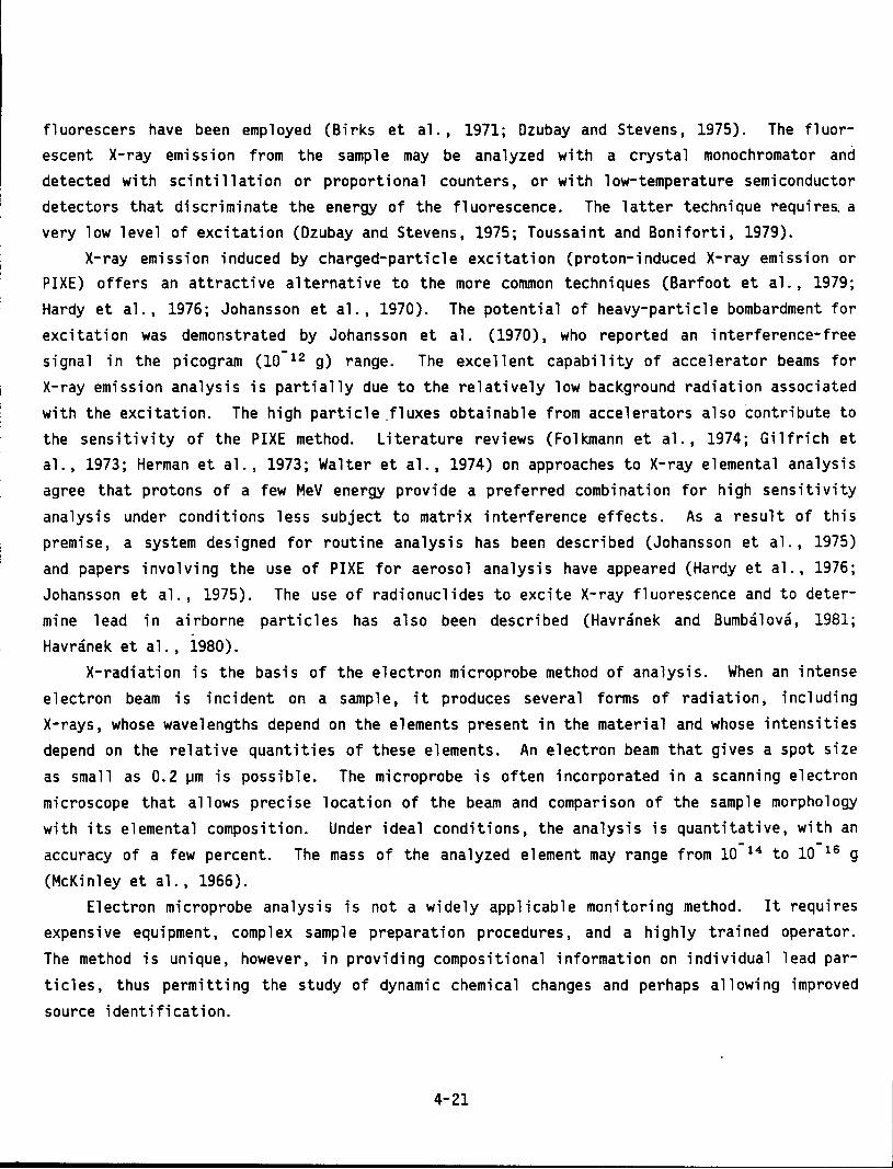
fluorescers have been employed (Birks et al., 1971; Dzubay and Stevens, 1975). The fluorescent X-ray emission from the sample may be analyzed with a crystal monochromator and detected with scintillation or proportional counters, or with low-temperature semiconductor detectors that discriminate the energy of the fluorescence. The latter technique requires. a very low level of excitation (Dzubay and Stevens, 1975; Toussaint and Boniforti, 1979).
X-ray emission induced by charged-particle excitation (proton-induced X-ray emission or PIXE) offers an attractive alternative to the more common techniques (Barfoot et al., 1979; Hardy et al., 1976; Johansson et al., 1970). The potential of heavy-particle bombardment for
excitation was demonstrated by Johansson et al. (1970), who reported an interference-free signal in the picogram (10- 12 g) range. The excellent capability of accelerator beams for X-ray emission analysis is partially due to the relatively low background radiation associated with the excitation. The high particle .fluxes obtainable from accelerators also contribute to the sensitivity of the PIXE method. Literature reviews (Folkmann et al., 1974; Gilfrich et al., 1973; Herman et al., 1973; Walter et al., 1974) on approaches to X-ray elemental analysis agree that protons of a few MeV energy provide a preferred combination for high sensitivity
analysis under conditions less subject to matrix interference effects. As a result of this premise, a system designed for routine analysis has been described (Johansson et al., 1975) and papers involving the use of PIXE for aerosol analysis have appeared (Hardy et al., 1976; Johansson et al., 1975). The use of radionuclides to excite X-ray fluorescence and to determine lead in airborne particles has also been described (Havranek and Bumbalova, 1981;
. Havranek et al., 1980).
X-radiation is the basis of the electron microprobe method of analysis. When an intense electron beam is incident on a sample, it produces several forms of radiation, including X-rays, whose wavelengths depend on the elements present in the material and whose intensities depend on the relative quantities of these elements. An electron beam that gives a spot size
as small as 0.2 ~m is possible. The microprobe is often incorporated in a scanning electron
microscope that allows precise location of the beam and comparison of the sample morphology with its elemental composition. Under ideal conditions, the analysis is quantitative, with an accuracy of a few percent. The mass of the analyzed element may range from 10- 14 to 10- 16 g
(McKinley et al., 1966). Electron microprobe analysis is not a widely applicable monitoring method. It requires
expensive equipment, complex sample preparation procedures, and a highly trained operator.
The method is unique, however, in providing compositional information on individual lead par
ticles, thus permitting the study of dynamic chemical changes and perhaps allowing improved
source identification.
4-21
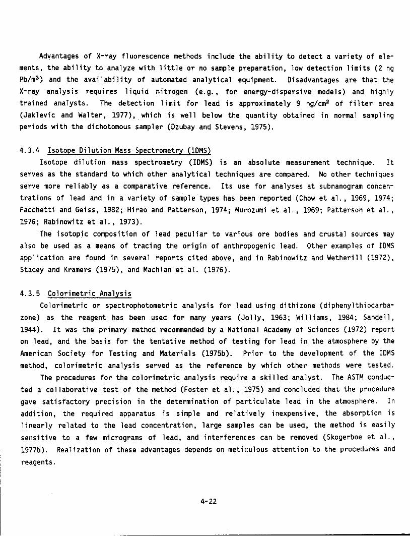
Advantages of X-ray fluorescence methods include the ability to detect a variety of elements, the ability to analyze with little or no sample preparation, low detection limits (2 ng Pb/m3 ) and the availability of automated analytical equipment. Disadvantages are that the X-ray analysis requires liquid nitrogen (e.g., for energy-dispersive models) and highly trained analysts. The detection limit for lead is approximately 9 ng/cm2 of filter area (Jaklevic and Walter, 1977), which is well below the quantity obtained in normal sampling periods with the dichotomous sampler (Dzubay and Stevens, 1975).
4.3.4 Isotope Dilution Mass Spectrometry (IDMS) Isotope dilution mass spectrometry (IDMS) is an absolute measurement technique. It
serves as the standard to which other analytical techniques are compared. No other techniques serve more reliably as a comparative reference. Its use for analyses at subnanogram concentrations of lead and in a variety of sample types has been reported (Chow et al., 1969, 1974; Facchetti and Geiss, 1982; Hirao and Patterson, 1974; Murozumi et al., 1969; Patterson et al., 1976; Rabinowitz et al., 1973).
The isotopic composition of lead peculiar to various ore bodies and crustal sources may also be used as a means of tracing the origin of anthropogenic lead. Other examples of IDMS application are found in several reports cited above, and in Rabinowitz and Wetherill (1972), Stacey and Kramers (1975), and Machlan et al. (1976).
4.3.5 Colorimetric Analysis Colorimetric or spectrophotometric analysis for lead using dithizone (diphenylthiocarba
zone) as the reagent has been used for many years (Jolly, 1963; Wi 11 i ams, 1984; Sande 11, 1944). It was the primary method recommended by a National Academy of Sciences (1972) report on lead, and the basis for the tentative method of testing for lead in the atmosphere by the American Society for Testing and Materials (1975b). Prior to the development of the IDMS method, colorimetric analysis served as the reference by which other methods were tested.
The procedures for the colorimetric analysis require a skilled analyst. The ASTM conducted a collaborative test of the method (Foster et al., 1975) and concluded that the procedure gave satisfactory precision in the determination of par·ticulate lead in the atmosphere. In addition, the required apparatus is simple and relat·ively inexpensive, the absorption is 1 i nearly re 1 a ted to the 1 ead concentration, 1 arge samp 1 es can be used, the method is easily sensitive to a few micrograms of lead, and interferences can be removed (Skogerboe et al., 1977b). Realization of these advantages depends on metic:ulous attention to the procedures and
reagents.
4-22
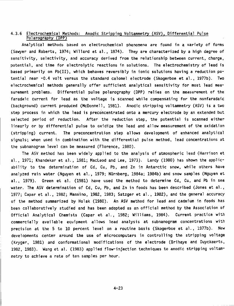
Anodic Stri Voltammetr Differential Pulse
Ana lyt i ca 1 methods based on e 1 ectrochemi ca 1 phenomena are found in a variety of forms (Sawyer and Roberts, 1974; Willard et al., 1974). They are characterized by a high degree of sensitivity, selectivity, and accuracy derived from the relationship between current, charge,
potential, and time for electrolytic reactions in solutions. The electrochemistry of lead is based primarily on Pb(II), which behaves reversibly in ionic solutions having a reduction potential near -0.4 volt versus the standard calomel electrode (Skogerboe et al., 1977b). Two electrochemical methods generally offer sufficient analytical sensitivity for most lead mea
surement problems. Differential pulse polarography (DPP) relies on the measurement of the faradaic current for lead as the voltage is scanned while compensating for the nonfaradaic
(background) current produced (McDonnell, 1981). Anodic stripping voltammetry (ASV) is a two step process in which the lead is preconcentrated onto a mercury electrode by an extended but selected period of reduction. After the reduction step, the potential is scanned either linearly or by differential pulse to oxidize the lead and allow measurement of the oxidation
(stripping) current. The preconcentrati on step allows deve 1 opment of enhanced analytical signals; when used in combination with the differential pulse method, lead concentrations at
the subnanogram level can be measured (Florence, 1980). The ASV method has been widely applied to the analysis of atmospheric lead (Harrison et
al., 1971; Khandekar et al., 1981; Macleod and Lee, 1973). Landy (1980) has shown the applicability to the determination of Cd, Cu, Pb, and Zn in Antarctic snow, while others have
analyzed rain water (Nguyen et al., 1979; Nurnberg, 1984a; 1984b) and snow samples (Nguyen et al., 1979). Green et al. (1981) have used the method to determine Cd, Cu, and Pb in sea
water. The ASV determination of Cd, Cu, Pb, and Zn in foods has been described (Jones et al., 1977; Capar et al., 1982; Mannino, 1982, 1983; Satzger et al., 1982), and the general accuracy of the method summarized by Ho 1 ak (1980). An ASV method for 1 ead and cadmium in foods has
been collaboratively studied and has been adopted as an official method by the Association of Official Analytical Chemists (Capar et al., 1982; Williams, 1984). Current practice with
commercially available equipment allows lead analysis at subnanogram concentrations with
precision at the 5 to 10 percent level on a routine basis (Skogerboe et al., 1977b). New developments center around the use of microcomputers in controlling the stripping voltage (Kryger, 1981) and conformational modifications of the electrode (Brihaye and Duyckaerts, 1982, 1983). Wang et al. (1983) applied flow-injection techniques to anodic stripping voltam
metry to achieve a rate of ten samples per hour.
4-23
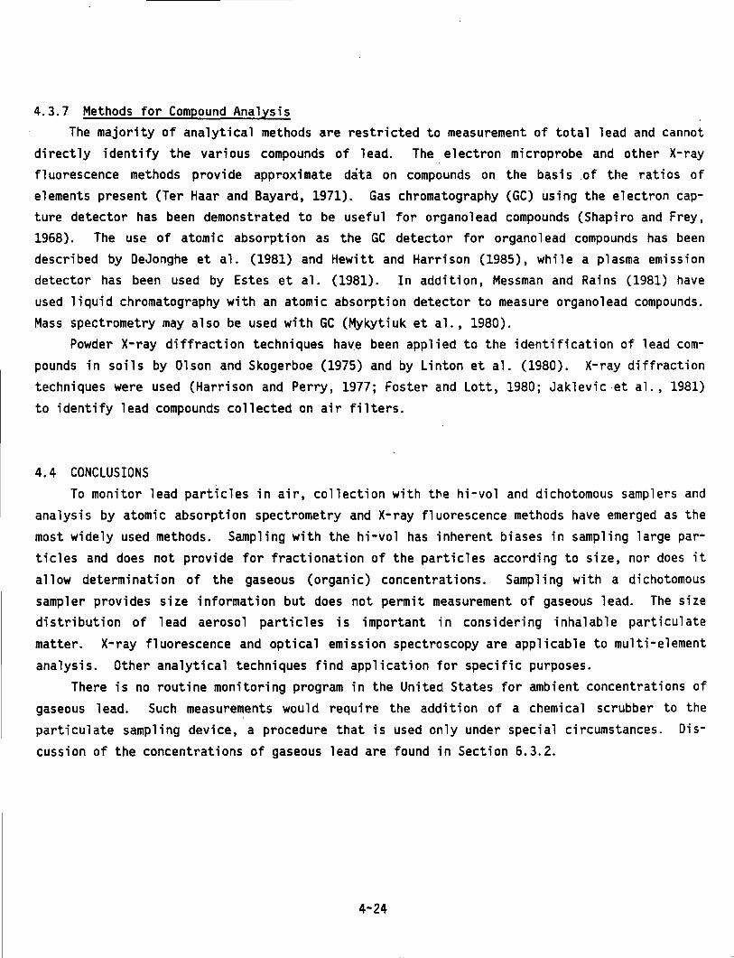
4.3.7 Methods for Compound Analysis The majority of analytical methods are restricted to measurement of total lead and cannot
directly identify the various compounds of lead. The electron microprobe and other X-ray fluorescence methods provide approximate data on compounds on the basis .of the ratios of elements present (Ter Haar and Bayard, 1971). Gas chromatography (GC) using the electron capture detector has been demonstrated to be useful for organolead compounds (Shapiro and Frey, 1968). The use of atomic absorption as the GC detector for organa 1 ead compounds has been described by DeJonghe et al. (1981) and Hewitt and Harrison (1985), while a plasma emission detector has been used by Estes et al. (1981). In addition, Messman and Rains (1981) have used liquid chromatography with an atomic absorption detector to measure organolead compounds. Mass spectrometry may also be used with GC (Mykytiuk et al., 1980).
Powder X-ray diffraction techniques hav.e been applied to the identification of lead compounds in soils by Olson and Skogerboe (1975) and by Linton et al. (1980). X-ray diffraction techniques were used (Harrison and Perry, 1977; Foster and Lott, 1980; Jaklevic et al., 1981) to identify lead compounds collected on air filters.
4.4 CONCLUSIONS To monitor lead particles in air, collection with the hi-vol and dichotomous samplers and
analysis by atomic absorption spectrometry and X-ray fluorescence methods have emerged as the most widely used methods. Sampling with the hi-vol has inherent biases in sampling large particles and does not provide for fractionation of the particles according to size, nor does it
allow determination of the gaseous (organic) concentrations. Sampling with a dichotomous sampler provides size information but does not permit measurement of gaseous lead. The size distribution of lead aerosol particles is important in considering inhalable particulate
matter. X-ray fluorescence and optical emission spectroscopy are applicable to multi-element analysis. Other analytical techniques find application for specific purposes.
There is no routine monitoring program in the United States for ambient concentrations of gaseous lead. Such measurements would require the addition of a chemical scrubber to the particulate sampling device, a procedure that is used only under special circumstances. Discussion of the concentrations of gaseous lead are found in Section 6.3.2.
4-24
4.5 REFERENCES
American Public Health Association. (1971) Standard methods for the examination of water and wastewater; 13th ed. New York, NY: American Public Health Association.
American Society for Testing and Materials. (1975a) Standard method for collection and analysis of dustfall (settleable particulates); D 1739-70. In: 1975 annual book of ASTM standards; part 26. gaseous fuels; coal and coke; atmospheric analysis. Philadelphia, PA: American Society for Testing and Materials; pp. 517-521.
American Society for Testing and Materials. (1975b) Tentative method of test for lead in the atmosphere by colorimetric dithizone procedure; D 3112-72T. In: 1975 annual book of ASTM standards; part 26. gaseous fuels; coal and coke; atmospheric analysis. Philadelphia, PA: American Society for Testing and Materials; pp. 633-641.
Barfoot, K. M.; Mitchell, I. V.; Eschbach, H. L.; Mason, P. I.; Gilboy, W. B. (1979) The analysis of air particulate deposits using 2 MeV protons. J. Radioanal. Chern. 53: 255-271.
Bertenshaw, M. P.; Gelsthorpe, D. (1981) Determination of lead in drinking water by atomicabsorption spectrophotometry with electrothermal atomisation. Analyst (London) 106: 23-31.
Birch, J.; Harrison, R. M.; Laxen, D. P. H. (1980) A specific method for 24-48 hour analysis of tetraalkyl lead in air. Sci. Total Environ. 14: 31-42.
Birks, L. S. (1972) X-ray absorption and emission. Anal. Chern. 44: 557R-562R.
Birks, L. S.; Gilfrich, J. V.; Nagel, D. J. (1971) Large-scale monitoring of automobile exhaust particulates: methods and costs. Washington, DC: Naval Research Laboratory; NRL memorandum report 2350. Available from: NTIS, Springfield, VA; AD-738801.
Birnie, S. E.; Noden, F. G. (1980) Determination of tetramethyl- and tetraethyllead vapours in air following collection on a glass-fibre-iodised carbon filter disc. Analyst (London) 105: 110-118.
Blaszkewicz, M.: Neidhart, B. (1983) A sensitive method for simultaneous determination of airborne organolead compounds; part 1: chromatographic separation and chemical reaction detection. Int. J. Environ. Anal. Chem. 14: 11-21.
Brihaye, C.; Duyckaerts, G. (1982) Determination of traces of metals by anodic stripping voltammetry at a rotating glassy carbon ring-disc electrode: part 1. method and instrumentation with evaluation of some parameters. Anal. Chim. Acta 143: 111-120.
Brihaye, C.; Duyckaerts, G. (1983) Determination of traces of metals by anodic stripping voltammetry at a rotating glassy carbon ring-disc electrode: part 2. Comparison between linear anodic stripping voltammetry with ring collection and various other stripping techniques. Anal. Chim. Acta 146: 37-43.
Brown, K. W.; Black, S. C. (1983) Quality assurance and quality control data validation procedures used for the Love Canal and Dallas lead soil monitoring programs. Environ. Manit. Asses. 3: 113-122.
4-25
Capar, S. G.; Gajan, R. J.; Madzsar, E.; Albert, R. H.; Sanders, M.; Zyren, J. (1982) Determi-. nation of lead and cadmium in foods by anodic stripping volarnmetry: II. Collaborative study. J. Assoc. Off. Anal. Chem. 65: 978-986.
Chau, Y. K.; Wong, P. T. S.; Bengert, G. A.; Kramar, 0. (1979) Determination of tetraalkyllead compounds in water, sediment, and fish samples. Anal. Chem. 51: 186-188.
Chow, T. J.; Earl, J. L.; Bennet, C. F. (1969) Lead aerosols in marine atmosphere. Environ. Sci. Technol. 3: 737-740.
Chow, T. J.; Patterson, C. C.; Settle, D. (1974) Occurrence of lead in tuna [letter]. Nature (London) 251: 159-161.
Code of Federal Regulations. (1982) Ambient air quality surveilance. C. F. R. 40: § 58.
Code of Federal Regulations. (1984) National primary and secondary ambient air quality standards. C. F. R. 40: § 50.
Compton, R. D.; Thomas, L. A. (1980) Analysis of air samples for lead and manganese. Tex. J. Sci. 32: 351-355.
Conner, W. D. (1966) An inertial-type particle separator for collecting large samples. J. Air Pollut. Control Assoc. 16: 35-38.
Copeland, T. R.; Christie, J. H.; Skogerboe, R. K.; Osteryoung, R. A. (1973) Effect of supporting electrolyte concentration in pulsed stripping voltammetry at the thin film mercury electrode. Anal. Chem. 45: 995-996.
Corsini, A.; Chiang, S.; Difruscia, R. (1982) Direct preconcentration of trace elements in aqueous solutions on macroreticular acrylic ester resin [letter]. Anal. Chem. 54: 1433-1435.
Cascio, M. R.; Pratt, G. C.; Krupa, S. V. (1982) An automated, refrigerated, sequential precipitation sampler. Atmos. Environ. 16: 1939-1944.
Cox, J. A. ; Slonawska, K.; Gatchell, D. K.; Hiebert, A. G. (1984) Metal speciation by Donnan dialysis. Anal. Chem. 56: 650-653.
De Jonghe, W. R. A.; Chakraborti, D.; Adams, F. C. (1981) Identification and determination of individual tetraalkyllead species in air. Environ. Sci. Technol. 15: 1217-1222.
Droppo, J. (1980) Micrometeorological profiles of sulfur-containing particles. For presentation at: 73rd Annual Meeting of Air Pollution Control Association; June; Montreal, PQ, Canada. Pittsburgh, PA: Air Pollution Control Association; paper no. 80-40.1.
Dzubay, T. G.; Barbour, R. K. (1983) A method to improve the adhesion of aerosol particles on teflon filters. J. Air Pollut. Control Assoc. 33: 692-695.
Dzubay, T. G.; Stevens, R. K. (1975) Ambient air analysis with dichotomous sampler and X-ray fluorescence spectrometer. Environ. Sci. Technol. 9: 663-668.
Dzubay, T. G.; Hines, L. E.; Stevens, R. K. (1976) Particle bounce errors in cascade impactors. Atmos. Environ. 10: 229-234.
4-26
Dzubay, T. G.; Stevens, R. K.; Lewis, C. W.; Hern, D. H.; Courtney, W. J.; Tesch, J. W.; Mason, M. A. (1982) Visibility and aerosol composition in Houston, Texas. Environ. Sci. Technol. 16: 514-525.
Eastwood, I. W.; Jackson K. W. (1984) Interlaboratory comparison of soil lead determinations. Environ. Pollut. Ser. B 8: 231-243.
Elias, R. W.; Patterson, C. C. (1980) Toxicological implications of biogeochemical studies of atmospheric lead. In: Toribara, T. Y.; Miller, M. W.; Morrow, P. E., eds. Polluted rain. New York, NY: Plenum Press; pp. 391-403.
Elias, R. W.; Hinkley, T. K.; Hirao, Y.; Patterson, C. C. (1976) Improved techniques for studies of mass balances and fractionations among families of metals within terrestrial ecosystems. Geochim. Cosmochim. Acta 40: 583-587.
Elias, R.; Hirao, Y.; Patterson, C. C. (1978) The deposition of lead aerosols on plant surfaces in a remote subalpine ecosystem. In: Adriano, D. C.; Brisbin, I. L., Jr., eds. Environmental chemistry and cycling processes: proceedings of a symposium; April 1976; Augusta, GA. Washington, DC: U. S. Department of Energy, Technical Information Center; pp. 691-699. Available from: NTIS, Springfield, VA; CONF-760429.
Elias, R. W.; Hirao, Y.; Patterson, C. C. (1982) The circumvention of the natural biopurification of calcium along nutrient pathways by atmospheric inputs of industrial lead. Geochim. Cosmochim. Acta 46: 2561-2580.
Estes, S. A.; Uden, P. C.; Barnes, R. M. (1981) High-resolution gas chromatography of trialkyllead chlorides with an inert solvent venting interface for microwave excited helium plasma detection. Anal. Chern. 53: 1336-1340.
Everett, R. G.; Hicks, B. B.; Berg, W. W.; Winchester, J. W. (1979) An analysis of particulate sulfur and lead gradient data collected at Argonne National Laboratory. Atmos. Environ. 13: 931-934.
Facchetti, S.; Geiss, F. (1982) Isotopic lead experiment: status report. Luxembourg: Commission of the European Communities; publication no. EUR 8352 EN.
Fang, Z.; Ruzicka, J.; Hansen, E. H. (1984a) An efficient flow-injection system with on-line ion-exchange preconcentration for the determination of trace amounts of heavy metals by atomic absorption spectrometry. Anal. Chim. Acta 164: 23-39.
Fang, Z.; Xu, S.; Zhang, S. (1984b) The determination of trace amounts of heavy metals in waters by a flow-injection system including ion-exchange preconcentration and flame atomic absorption spectrometric detection. Anal. Chim. Acta 164: 41-50.
Figura, P.; McDuffie, B. (1979) Use of Chelex resin for determination of labile trace metal fractions in aqueous ligand media and comparison of the method with anodic stripping voltammetry. Anal. Chern. 51: 120-125.
Figura, P.; McDuffie, B. (1980) Determination of labilities of soluble trace metal species in aqueous environmental samples by anodic stripping voltammetry and Chelex column and batch methods. Anal Chern. 52: 1433-1439.
Fishman, M. J.; Erdmann, D. E. (1973) Water analysis. Anal. Chern. 45: 361R-403R.
4-27
Florence, T. M. (1980) Comparison of linear scan and differential pulse anodic stripping voltammetry at a thin mercury film glassy carbon electrode. Anal. Chim. Acta 119: 217-223.
Folkmann, F.; Gaarde, C.; Huus, T.; Kemp, K. (1974) Proton induced X-ray emission as a tool for trace element analysis. Nucl. Instrum. Methods 116: 487-499.
Foster, R. L.; Lott, P. F. (1980) X-ray diffractometry examination of air filters for compounds emitted by lead smelting operations. Environ. Sci. Technol. 14: 1240-1244.
Foster, J. F.; Beatty, G. H.; Howes, J. E., Jr. (1975) Interlaboratory cooperative study of the precision and accuracy of the measurement of lead in the atmosphere using the colorimetric dithizone procedure. Philadelphia, PA: American Society for Testing and Materials. (ASTM data ser. OS 55-SS 1975).
Gandrud, B. W.; Lazrus, A. L. (1972) Design of system for removing water-soluble materials from IPC-1478 filter paper. Environ~ Sci. Technol. 6: 455-457.
Ganley, J. T.; Springer, G. S. (1974) Physical and chemical characteristics of particulates in spark ignition engine exhaust. Environ. Sci. Technol. 8: 340-347.
Garbarino, J. R.; Taylor, H. E. (1979) An inductive-coupled plasma atomic-emission spectrometric method for routine water quality testing. Appl.' Spectrosc. 33: 220-226.
Gentel, J. E.; Manary, 0. J.; Valenta, J. C. (1973) Characterization of particulates and other non-regulated emissions from mobile sources and the effects of exhaust emissions control devices on these emissions. Ann Arbor, MI: U. S. Environmental Protection Agency, Office of Air and Water Programs; publication no. APTD-1567. Available from: NTIS, Springfield, VA; PB-224243.
Gilfrich, J. V.; Burkhalter, P. G.; Birks, L. S. (1973) X-ray spectrometry for particulate air pollution--a quantitative comparison of techniques. Anal. Chem. 45: 2002-2009.
Green, D. G.; Green, L. W.; Page, J. A.; Poland, J. S.; van Loon, G. (1981) The determination of copper, cadmium, and lead in sea water by anodic stripping voltammetry with a thin film mercury electrode. Can. J. Chem. 59: 1476-1486.
Habibi, K. (1970) Characterization of particulate lead in vehicle exhaust: experimental techniques. Environ. Sci. Technol. 4: 252-253.
Habibi, K. (1973) Characterization of particulate matter in vehicle exhaust. Environ. Sci. Technol. 7: 223234.
Hammerle, R. H.; Pierson, W. R. (1975) Sources and elemental composition of aerosol in Pasadena, Calif., by energy-dispersive X-ray fluorescence. Environ. Sci. Technol. 9: 1058-1068.
Hardy, K. A.; Akselsson, R.; Nelson, J. W.; Winchester, J. W. (1976) Elemental constituents of Miami aerosol as function of particle size. Environ. Sci. Technol. 10: 176-182.
Harrison, R. M.; Perry, R. (1977) The analysis of tetraalkyl lead compounds and their significance as urban air pollutants. Atmos. Environ. 11: 847-852.
4-28
Harrison, P. R.; Matson, W. R.; Winchester, J. W. (1971) Time variations of lead, copper and cadmium concentrations in aerosols in Ann Arbor, Michigan. Atmos. Environ. 5: 613-619.
Havranek, E.; Bumbalova, A. (1981) Multielement analysis of air samples determination of iron, zinc, lead, and bromine content by the radionuclide X-ray fluorescence analysis. Chem. Zvesti 35: 57-63.
Havranek, E.; Bumbalova, A.; Dejmkova, E. (1980) Nondestructive determination of airborne lead particulates by the radionuclide X-ray fluorescence analysis. Chem. Zvesti. 34: 373-379.
Hering, S. V.; Flagan, R. C.; Friedlander, S. K. (1978) Design and evaluation of new lowpressure impactor. 1. Environ. Sci. Technol. 12: 667-673.
Herman, A. W.; McNelles, L. A.; Campbell, J. L. (1973) Choice of physical parameters in charged particle induced X-ray fluorescence analysis. Int. J. Appl. Radiat. Isotop. 24: 677-688.
Hewitt, C. N.; Harrison, R. M. (1985) A sensitive, specific method for the determination of tetraalklul lead compounds in air by gas chromatography/atomic absorption spectrometry. Anal. Chim. Acta 162: 277-287.
Hicks, B. B.; Wesely, M. L.; Durham, J. L. (1980) Critique of methods to measure dry deposition: workshop summary. Research Triangle Park, NC: U.S. Environmental Protection Agency, Environmental Sciences Research Laboratory; EPA report no. EPA-600/9-80-050. Available from NTIS, Springfield, VA; PB81-126443.
Hinkley, T.; Patterson, C. (1973) Concentrations of metals in a soil moisture film. Nature (london) Phys. Sci. 246: 123-124.
Hirao, Y.; Patterson: C. C. (1974) Lead aerosol pollution in the High Sierra overrides natural mechanisms which exclude lead from a food chain. Science (Washington, DC) 184: 989-992.
Hirao, Y.; Fukumoto, K.; Sugisaki, H.; Kimura, K. (1979) Determination of lead in seawater by furnace atomic absorption spectrometry after concentration with yield tracer. Anal. Chem. 51: 651-653.
Hirschler, D. A.; Gilbert, L. F. (1964) Nature of lead in automobile exhaust gas. Arch. Environ. Health 8: 297-313.
Hirschler, D. A.; Gilbert, L. F.; Lamb, F. W.; Niebylski, L. M. (1957) Particulate lead compounds in automobile exhaust gas. Ind. Eng. Chem. 49: 1131-1142.
Holak, W. (1980) Analysis of foods for lead, cadmium, copper, zinc, arsenic, and selenium, using closed system sample digestion: collaborative study. J. Assoc. Off. Anal. Chem. 63: 485-495.
Horlick, G. (1982) Atomic absorption, atomic fluorescence, and flame spectrometry. Anal. Chem. 54: 276R-293R.
Hounam, R. F.; Sherwood, R. J. (1965) The cascade centripeter: a device for determining the concentration and size distribution of aerosols. Am. Ind. Hyg. Assoc. J. 26: 122-131.
Huntzicker, J. J.; Friedlander, S. K.; Davidson, C. I. (1975) Material balance for automobileemitted lead in Los Angeles basin. Environ. Sci. Technol. 9: 448-457.
4-29
Jaklevic, J. M.; Walter, R. L. (1977) Comparison of m1n1mum detectable limits among X-ray spectrometers. In: Dzubay, T. G., ed. X-ray fluorescence analysis of environmental samples. Ann Arbor, MI: Ann Arbor Science Publishers Inc.; pp. 63-75.
Jaklevic, J. M.; Goulding, F. S.; Jarrett, B. V.; Meng, J. D. (1973) Application of X-ray fluorescence techniques to measure elemental composition of particles in the atmosphere. Presented at: 165th American society meeting on analytical methods applied to air pollution measurements; April; Dallas, TX. Available from: NTIS, Springfield, VA; LBL-1743.
Jaklevic, J. M.; Gatti, R. C.; Goulding, F. S.; Lao, B. W. (1981) A p-gauge method applied to aerosol samples. Environ. Sci. Technol. 15: 680-686.
Jin, K.; Taga, M. (1982) Determination of lead by continuous-flow hydride generation and atomic absorption spectrometry: comparison of malic acid-dichromate, nitric acid-hydrogen peroxide and nitric acid-peroxodisulfate reaction matrices in combination with sodium tetrahydroborate. Anal. Chim. Acta 143: 229-236.
Johansson, T. B.; Akse}sson, R.; Johansson,· S. A. E. (1970) X-ray analysis: elemental trace analysis at the 10 12g level. Nucl. Instrum. Methods 84: 141-143.
Johansson, T. B.; Van Grieken, R. E.; Nelson, J. W.; Winchester, J. W. (1975) Elemental trace analysis of small samples by proton induced X-ray emission. Anal. Chem. 47: 855-860.
Jolly, S. C. (1963) Official, standardised and recommended methods of analysis: compiled and edited for the analytical methods committee of the society for analytical chemistry. Cambridge, MA: W. Heffer and Sons, Ltd.
Jones, J. W.; Boyer, K. W. (1978) Analysis of foods and related materials using inductively coupled plasma spectroscopy. In: Barnes, R. M., ed. Applications of inductively coupled plasmas to emission spectroscopy: 1977 eastern analytical symposium. Philadelphia, PA: The Franklin Institute Press; pp. 83-106.
Jones, J. W.; Gajan, R. J.; Boyer, K. W.; Fiorino, J. A. (1977) Dry ash-voltammetric determination of cadmium, copper, lead, and zinc in foods. J. Anal. Chem. Assoc. 60: 826-832.
Jones, J. W.; Capar, S. G.; O'Haver, T. C. (1982) Cr;itical evaluation of a multi-element scheme using plasma emission and hydride evolution atomic-absorption spectrometry for the analysis of plant and animal tissues. Analyst (London) 107: 353-377.
Khandekar, R. N.; Dhaneshwar, R. G.; Palrecha, M. M.; Zarapkar, L. R. (1981) Simultaneous determination of lead, cadmium and zinc in aerosols by anodic stripping voltammetry. Fresenius Z. Anal. Chem. 307: 365-368.
Kneip, T. J.; Laurer, G. R. (1972) Isotope excited K-ray fluorescence. Anal. Chem. 44: 57A-68A.
Kolbye, A. C., Jr.; Mahaffey, K. R.; Fiorino, J. A.; Corneliussen, P. C.; Jelinek, C. F. (1974) Food exposures to lead. Environ. Health Perspect. 7: 65-74.
Kometani, T. Y.; Bove, J. L.; Nathanson, B.; Siebenberg, S.; Magyar, M. (1972) Dry ashing of airborne particulate matter on paper and glass fiber filters for trace metal analysis by atomic absorption spectrometry. Environ. Sci. Technol. 6: 617-620.
4-30
Kopp, J. F.; Kroner, R. C. (1967) Trace metals in waters of the United States: a five year summary of trace metals in rivers and lakes of the United States (October 1, 1962 -September 30, 1967). Cincinnati, OH: U.S. Department of the Interior, Division of Pollution Surveillance. Available from: NTIS, Springfield, VA; PB-215680.
Kopp, J. F.; McKee, D. (1983) Methods for chemical analysis of water and wastes. Cincinnati, OH: U.S. Environmental Protection Agency, Environmental Monitoring and Support Laboratory; p. 74; EPA report no. EPA-600/4-79-020. Available from: NTIS, Springfield, VA; PB84-128677.
Kryger, L. (1981) Microcomputers in electrochemical trace elemental analysis. Anal. Chim. Acta 133: 591-602.
Kunz, W. G., Jr.; Jacobs, E. S.; Pahnke, A. J. (1975) Design and performance of muffler lead traps for vehicles. [Presented before: Union Intersyndicale de 1' Industrie du Petrole; January; Paris, France]. Wilmington, DE: E. I. duPont de Nemours & Company.
Landy, M. P. (1980) An evaluation of differential pulse anodic stripping voltammetry at a rotating glassy carbon electrode for the determination of cadmium, copper, lead and zinc in Antarctic snow samples. Anal. Chim. Acta 121: 39-49.
Lee, R. E., Jr.; Goranson, S. S. (1972) National air surveillance cascade impactor network. I. Size distribution measurements of suspended particulate matter in air. Environ. Sci. Technol. 6: 1019-1024.
Lester, J. N.; Harrison, R. M.; Perry, R. (1977) Rapid flameless atomic absorption analysis of the metallic content of sewage sludges: I. lead, cadmium and copper. Sci. Total Environ. 8: 153-158.
Leyden, D. E.; Wegscheider, W. (1981) Preconcentration for trace element determination in aqueous samples. Anal. Chem. 53: 1059A-1065A.
Lindberg, S. E. (1982) Factors influencing trace metal sulfate and hydrogen ion concentrations in rain. Atmos. Environ. 16: 1701-1709.
Lindberg, S. E.; Harriss, R. C. (1981) The role of atmospheric deposition in an eastern U.S. deciduous forest. Water Air Soil Pollut. 16: 13-31.
Lindberg, S. E.; Turner, R. R. (1983) Trace metals in rain at forested sites in the eastern United States. In: International conference: heavy.metals in the environment; September; Heidelberg, West Germany. Edinburgh, United Kingdom: CEP Consultants, Ltd.; pp. 107-114.
Lindberg, S. E.; Harriss, R. C.; Turner, R. R.; Shriner, D. S.; Huff, D. D. (1979) Mechanisms and rates of atmospheric deposition of selected trace elements and sulfate to a deciduous forest watershed [dissertation]. Oak Ridge, TN: Oak Ridge National Laboratory, Environmental Sciences Division; publication no. 1299. Available from: NTIS, Springfield, VA; ORNL/TM-6674.
Linton, R. W.; Natusch, D. F. S.; Solomon, R. L.; Evans, C. A., Jr. (1980) Physicochemical characterization of lead in urban dusts. A microanalytical approach to lead tracing. Environ. Sci. Technol. 14: 159-164.
4-31
Liu, M.-K.; Whitney, D. C.; Seinfeld, J. H.; Roth, P. M. (1976) Continued research in meso~ scale air pollution simulation modeling. Vol. 1. Assessment of prior model evaluation studies and analysis of model validity and sensitivity. Research Triangle Park, NC: U. S. Environmental Protection Agency, Environmental Sciences Research Laboratory; EPA report no. EPA- 600/4-76-016A. Available from: NTIS, Springfield, VA; PB-257526.
Loo, B. W.; Adachi, R. S.; Cork, C. P.; Goulding, S. S.; Jaklevic, J. N.; Landis, D. A.; Searles, W. L. (1979) A second generation dichotomous sampler for large-scale monitoring of airborne particulate matter. Lawrence Berkeley Laboratory, report no. 8725. Available from: NTIS, Springfield, VA; LBL-8725.
Lovering, T. G., ed. (1976) Lead in the environment. Washington, DC: U.S. Department of the Interior, Geological Survey; Geological Survey professional paper no. 957. Available from: GPO, Washington, DC; S/N 024-001-02911-1.
Luke, C. L.; Kometani, T. Y.; Kessler, J. E.; Loomis, T. C:.; Bove, J. L.; Nathanson, B. (1972) X-ray spectrometric analysis of air pollution dust. Environ. Sci. Technol. 6: 1105-1109.
Lynam, 0. R. (1972) The atmospheric diffusion of carbon monoxide and lead from an expressway [dissertation]. Cincinnati, OH: University of Cincinnati. Available from: University Microfilms, Ann Arbor, MI; publication no. 73-3827.
Machlan, L. A.; Gramlich, J. W.; Murphy, T. J.; Barnes, I. L. (1976) The accurate determination of lead in biological and environmental samples by isotope dilution mass spectrometry. In: LaFleur, P. 0., ed. Accuracy in trace analysis: sampling, sample handling, analysis- volume 2. Proceedings of the 7th materials research symposium; October 1974; Gaithersburg, MO. Washington, DC: National Bureau of Standards; NBS special publication no. 422; pp. 929-935. Available from: NTIS, Springfield, VA; PB -258092.
Macleod, K. E.; Lee, R. E., Jr. (1973) Selected trace metal determination of spot tape samples by anodic stripping voltammetry. Anal. Chem. 45: 2380-2383.
Maenhaut, W.; Zoller, W. H.; Ouce, R. A.; Hoffman, G. L. (1979) Concentration and size distribution of particulate trace elements in the south polar atmosphere. J. Geophys. Res. 84: 2421-2431.
Mannino, S. (1982) Determination of lead in fruit juices and soft drinks by potentiometric stripping analysis. Analyst (London) 107: 1466-1470.
Mannino, S. (1983) Simultaneous determination of lead and tin in fruit juices and soft drinks by potentiometric stripping analysis. Analyst (London) 108: 1257-1260.
Marple, V. A.; Willeke, K. (1976) Impactor design. Atmos. Environ. 10: 891-896.
McDonnell, 0. B. (1981) Simultaneous determination of ce~pper, lead, cadmium and zinc in nonferrous smelter products by differential-pulse polarography. Analyst (London) 106: 790-793.
McFarland, A. R.; Ortiz, C. A.; Rodes, C. E. (1979) Characteristics of aerosol samplers used in ambient air monitoring. Presented at: 86th national meeting, American Institute of Chemical Engineers; April; Houston, TX. Houston, TX: Texas A & M University.
McKinley, T. 0.; Heinrich, K. F. J.; Wittry, 0. B., eds. (1966) The electron microprobe: proceedings of the symposium; October 1964; Washington, DC. New York, NY; John Wiley & Sons, Inc.
4-32
Messman, J. D.; Rains, T. C. (1981) Determination of tetraalkyllead compounds in gasoline by liquid chromatography-atomic absorption spectrometry. Anal. Chem. 53: 1632-1636.
Miller, F. J.; Gardner, D. E.; Graham, J. A.; Lee, R. E., Jr.; Wilson, W. E.; Bachmann, J. D. (1979) Size considerations for establishing a standard for inhalable particles. J. Air Pollut. Control Assoc. 29: 610-615.
Moody, J. R. (1982) NBS clean laboratories for trace element analysis. Anal. Chem. 54: 1358A-1376A.
Moran, J. B.; Baldwin, M. J.; Manary, 0. J.; Valenta, J. C. (1972) Effect of fuel additives on the chemical and physical characteristics of particulate emissions in automotive exhaust. Final report. Research Triangle Park, NC: U.S. Environmental Protection Agency; EPA report no. EPA-R2-72-066. Available from: NTIS, Springfield, VA; PB-222799.
Murozumi, M.; Chow, T. J.; Patterson, C. (1969) Chemical concentrations of pollutant lead aerosols, terrestrial dusts and sea salts in Greenland and Antarctic snow strata. Geochim. Cosmochim. Acta 33: 1247-1294.
Murphy, T. J. (1976) The role of the analytical blank in accurate trace analysis. In: LaFleur, P. D., ed. Accuracy in trace analysis: sampling, sample handling, analysis - volume 1. Proceedings of the 7th materials research symposium; October 1974; Gaithersburg, MD. Washington, DC: U.S. Department of Commerce, National Bureau of Standards; NBS special publication no. 422; pp. 509-539. Available from: NTIS, Springfield, VA; PB-258092/6.
Mykytiuk, A. P.; Russell, D. S.; Sturgeon, R. E. (1980) Simultaneous determination of iron, cadmium, zinc, copper, nickel, lead, and uranium in seawater by stable isotope dilution spark source mass spectrometry. Anal. Chem. 52: 1281-1283.
National Academy of Sciences. (1972) Lead: airborne lead in perspective. Washington, DC: National Academy of Sciences. (Biologic effects of atmospheric pollutants).
National Academy of Sciences, Committee on Lead in the Human Environment. (1980) Lead in the human environment. Washington, DC: National Academy of Sciences.
Nguyen, V. D.; Valenta, P.; NUrnberg, H. W. (1979) Voltammetry in the analysis of atmospheric pollutants. The determination of toxic trace metals in rain water and snow by differential pulse stripping voltammetry. Sci. Total Environ. 12: 151-167.
NUrnberg, H. W. (1984a) The voltammetric approach in trace metal chemistry of natural waters and atmospheric precipitation. Anal. Chim. Acta 164: 1-21.
NUrnberg, H. W. (1984b) Trace analytical procedures with modern voltammetric determination methods for the investigation and monitoring of ecotoxic heavy metals in natural waters and atmospheric precipitates. Sci. Total Environ. 37: 9-34.
Olsen, S.; Pessenda, L. C. R.; Ruzicka, J.; Hansen, E. H. (1983) Combination of flow injection analysis with flame atomic-absorption spectrophotometry: determination of trace amounts of heavy metals in polluted seawater. Analyst (London) 108: 905-917.
Olson, K. W.; Skogerboe, R. K. (1975) Identification of soil lead compounds from automotive sources. Environ. Sci. Technol. 9: 227-230.
4-33
Pachuta, D. G.; Love, L. J. C. (1980) Determination of lead in urban air particulates by microsampling cup atomic absorption spectrometry. Anal. Chern. 52: 444-448.
Paciga, J. J.; Jervis, R. E. (1976) Multielement size characterization of urban aerosols. Environ. Sci. Technol. 10: 1124-1128.
Patterson, C. C. (1983) Criticism of "Flow of metals into the global atmosphere" [letter]. Geochim. Cosmochim. Acta 47: 1163-1168.
Patterson, C. C.; Settle, D. M. (1976) The reduction of orders of magnitude errors in lead analyses of biological materials and natural waters by evaluating and controlling the extent and sources of industrial lead contamination introduced during sample collecting, handling, and analyses. In: LaFleur, P. D., ed. Accuracy in trace analysis: sampling, sample handling, analysis - volume 1. Proceedings of the 7th materials research symposium; October 1974; Gaithersburg, MD. Washington, DC: U. S. Department of Commerce, National Bureau of Standards; NBS special publication no. 422; pp. 321-352.
Patterson, C.; Settle, D.; Glover, B. (1976) Analysis of lead in polluted coastal seawater. Mar. Chern. 4: 305-319.
PEDCo Environmental, Inc. (1981) Field study to determine spatial variability of lead from roadways. Research Triangle Park, NC: U.S. Environmental Protection Agency, Monitoring and Data Analysis Division; EPA report no. EPA-450/4-83-002. Available from: NTIS, Springfield, VA; PB83-207845.
Peirson, D. H.; Cawse, P. A.; Salmon, L.; Cambray, R. S. (1973) Trace elements in the atmospheric environment. Nature (London) 241: 252-256.
Pennington, J. A. T. (1983) Revision of the total diet study food list and diets. J. Am. Diet. Assoc. 82: 166-173.
Pierce, J. 0.; Koirtyohann, S. R.; Clevenger, T. E.; Lichte, F. E. (1976) The determination of lead in blood: a review and critique of the state of the art, 1975. New York, NY: International Lead Zinc Research Organization, Inc.
Purdue, L. J.; Enrione, R. E.; Thompson, R. J.; Bonfield, B. A. (1973) Determination of organic and total lead in the atmosphere by atomic absorption spectrometry. Anal. Chern. 45: 527-530.
Rabinowitz, M. B.; Wetherill, G. W. (1972) Identifying sources of lead contamination by stable isotope techniques. Environ. Sci. Technol. 6: 705-709.
Rabinowitz, M. B.; Wetherill, G. W.; Kopple, J. D. (1973) Lead metabolism in the normal human: stable isotope studies. Science (Washington, DC) 182: 725727.
Robson, C. D.; Foster, K. E. (1962) Evaluation of air particulate sampling equipment. Am. Ind. Hyg. Assoc. J. 23: 404-410.
Rohbock, E.; Georgii, H.-W.; MUller, J. (1980) Measurements of gaseous lead alkyls in polluted atmospheres. Atmos. Environ. 14: 89-98.
Rouseff, R. L.; Ting, S. V. (1980) Lead uptake of grapefruit juices stored in cans as determined by flameless atomic absorption spectroscopy. J. Food Sci. 45: 965-968.
4-34
Roy, B. R. (1977) Effects of particle sizes and solubilities of lead sulphide dust on mill workers. Am. Ind. Hyg. Assoc. J. 38: 327-332.
Samant, H. S.; Vaidya, 0. C. (1982) Evaluation of the sampling buckets used in the Sangamo collector, type A for heavy metals in precipitation. Atmos. Environ. 16: 2183-2186.
Sampson, R. E.; Springer, G. S. (1973) Effects of exhaust gas temperature and fuel composition on particulate emission from spark ignition engines. Environ. Sci. Technol. 7: 55-60.
Sandell, E. B. (1944) Colorimetric determination of traces of metals. New York, NY: Interscience Publishers, Inc.; pp. 279-300. (Clarke, B. L.; Kalthoff, I. M.; Willard, H. H., eds. Chemical analysis: a series of monographs on analytical chemistry and its applications: v. 3).
Satzger, R. D.; Clow, C. S.; Bonnin, E.; Fricke, F. L. (1982) Determination of background levels of lead and cadmium in raw agricultural crops by using differential pulse anodic stripping voltammetry. J. Assoc. Off. Anal. Chem. 65: 987-991.
Sawyer, D. T.; Roberts, J. L., Jr. (1974) Experimental electrochemistry for chemists. New York, NY: John Wiley & Sons.
Scott, D. R.; Loseke, W. A.; Holboke, L. E.; Thompson, R. J. (1976a) Analysis of atmospheric particulates for trace elements by optical emission spectrometry. Appl. Spectrosc. 30: 392-405.
Scott, D. R.; Hemphill, D. C.; Holboke, L. E.; Long, S. J.; Loseke, W. A.; Pranger, L. J.; Thompson, R. J. (1976b) Atomic absorption and optical emission analysis of NASN atmospheric particulate samples for lead. Environ. Sci. Technol. 10: 877-880.
Seeley, J. L.; Skogerboe, R. K. (1974) Combined sampling-analysis method for the determination of trace elements in atmospheric particulates. Anal. Chem. 46: 415-421.
Shapiro, H.; Frey, F. W. (1968) The organic compounds of lead. New York, NY: John Wiley and Sons, Inc.. (Seyferth, D. , ed. The chemistry of organometallic compounds: a series of monographs).
Shaw, R. W. (1980) Balance corrections for buoyancy. J. Air Pollut. Control Assoc. 30: 908-909.
Shaw, R. W.; Stevens, R. K.; Courtney, W. J. (1980) Exchange of comments on inaccuracies encountered in sulfur determination by particle induced X-ray emission. Anal. Chem. 52: 2217-2218.
Silverman, L.; Viles, F. J., Jr. (1948) A high volume air sampling and filter weighing method for certain aerosols. J. Ind. Hyg. Toxicol. 30: 124-128.
Skogerboe, R. K. (1974) Monitoring trace metal particulates: an evaluation of the sampling and analysis problems; ASTIM STP 555. Philadelphia, PA: American Society for Testing and Materials; pp. 125-136.
Skogerboe, R. K. (1982) The analytical blank: sources and effects on lead analyses. J. Assoc. Off. Anal. Chem. 65: 957-964.
4-35
-- ---- -------------'
Skogerboe, R. K.; Dick, D. L.; Lamothe, P. J. (1977a) Evaluation of filter inefficiencies for particulate collection under low loading conditions. Atmos. Environ. 11: 243-249.
Skogerboe, R. K.; Hartley, A. M.; Vogel, R. S.; Koirtyohann, S. R. (1977b) Monitoring for lead in the environment. In: Boggess, W. R., ed: Lead in the environment. Washington, DC: National Science Foundation; pp. 33-70; NSF report no. NSF/RA-770214 .. Available from: NTIS, Springfield, VA; PB-278278.
Stacey, J. S.; Kramers, J. D. (1975) Approximation of terrestrial lead isotope evolution by a two-stage model. Earth Planet. Sci. Lett. 26: 207-221.
Stein, V. B.; Canelli, E.; Richards, A. H. (1980) Simplified determination of cadmium, lead and chromium in estuarine waters by flameless atomic absorption. Int. J. Environ. Anal. Chern. 8: 99-106.
Stern, A. C., ed. (1976) Air pollution: air pollutants, their transformation and transport. 3rd ed. New York, NY: Academic Press, Inc. (Lee, D. H. K.; Hewson, E. W.; Okun, D., eds. Environmental sciences: an interdisciplinary monograph series: v. 1).
Stevens, R. K.; Dzubay, T. G.; Russwurm, G.; Rickel, D. (1978) Sampling and analysis of atmospheric sulfates and related species. Atmos. Environ. 12: 55-68.
Stevens, R. K.; Dzubay, T. G.; Shaw, R. W., Jr.; McClenny, W. A.; Lewis, C. W.; Wilson, W. E. (1980) Characterization of the aerosol in the .Great Smoky Mountains. Environ. Sci. Technol. 14: 1491-1498.
Sugimae, A.; Skogerboe, R. K. · (1978) Dual approach to the emission spectrographic determination of elements in airborne particulate matter. Anal. Chim. Acta 97: 1-11.
TerHaar, G. L.; Bayard, M. A. (1971) Composition of airborne lead particles. Nature (London) 232: 553-554.
Ter Haar, G. L.; Lenane, D. L.; Hu, J. N.; Brandt, M. (1972) Composition, size and control of automotive exhaust particulates. J. Air Pollut. Control Assoc. 22: 39-46.
Torsi, G.; Palmisano, F. (1983) Electrostatic capture of gaseous tetraalkyllead compounds and their determination by electrothermal atomic-absorption spectrometry. Analyst (London) 108: 1318-1322.
Torsi, G.; Palmisano, F. (1984) Electrochemical preconcentration combined with atomic absorption spectrometry for the determination of heavy metals in water samples. Sci. Total Environ. 37: 35-40.
Torsi, G.; Desimoni, E.; Palmisano, F.; Sabbatini, L. (1981) Determination of lead in air by electrothermal atomic spectrometry with electrostatic accumulation furnace. Anal. Chern. 53: 1035-1038.
Tosteson, T. D.; Spengler, J. D.; Weker, R. A. (1982) Atomic absorption analysis in a personal monitoring study. Boston, MA: Harvard University School of Public Health.
Toussaint, C. J.; Boniforti, R. (1979) Application of X-ray fluorescence spectrometry to the study of the marine environment. Int. J. Environ. Anal. Chern. 6: 217-228.
4-36
Trayser, D. A.; Blosser, E. R.; Creswick, F. A.; Pierson, W. R. (1975) Sulfuric acid and ni.,. trate emissions from oxidation catalysts. Warrendale, PA: Society of Automotive En-gineers; SAE technical paper no. 750091.
Tyson, J. F. (1985) Flow injection analysis techniques for atomic-absorption spectrometry: a review. Analyst (London) 110: 419-429.
U. S. Environmental Protection Agency. (1971) Guidelines: air quality surveillance networks. Research Triangle Park, NC: Office of Air Programs; Office of Air Programs publication no. AP-98. Available from: NTIS, Springfield, VA; PB-200728.
U. S. Environmental Protection Agency. (1978) Ambient water quality criteria: lead. Washington, DC: Criteria and Standards Division. Protection Agency. Available from: NTIS, Springfield, VA; PB-292437.
Walter, R. L.; Willis, R. D.; Gutknecht, W. F.; Joyce, J. M. (1974) Analysis of biological, clinical, and environmental samples using proton-induced X-ray emission. Anal. Chem. 46: 843-855.
Wang, J.; Dewald, H. D.; Greene, B. (1983) Anodic stripping voltammetry of heavy metals with a flow injection system. Anal. Chim. Acta 146: 45-50.
Ward, F. N.; Fishman, M. J. (1976) Analytical methods for determination of lead. In: Lovering, T. G., ed. Lead in the environment. Washington, DC: U. S. Department of the Interior, U. S. Geological Survey; Geological Survey professional paper 957; pp. 81-84.
Wedding, J. B.; McFarland, A. R.; Cermak, J. E. (1977) Large particle collection characteristics of ambient aerosol samplers. Environ. Sci. Technol. 11: 387-390.
Wedding, J. B.; Weigand: M.; John, W.; Wall, S. (1980) Sampling effectiveness of the inlet to the dichotomous sampler. Environ. Sci. Technol. 14: 1367-1370.
Whitby, K. T.; Husar, R. B.; Liu, B. Y. H. (1972) The aerosol size distribution of Los Angeles smog. J. Colloid Interface Sci. 39: 177-204.
Willard, H. H.; Merritt, L. L., Jr.; Dean, J. A. (1974) Instrumental methods of analysis. 5th ed. New York, NY: D. Van Nostrand Co.
Williams, M. K. (1984) Biological tests of lead absorption following a brief massive exposure. J. Occup. Med. 26: 532-533.
Winge, R. K.; Fassel, V. A.; Kniseley, R. N.; DeKalb, E.; Hass, W. J., Jr. (1977) Determination of trace elements in soft, hard, and saline waters by the inductively coupled plasma, multi-element atomic emission spectroscopic (ICP-MAES) technique. Spectrochim. Acta 32B: 327-345.
Witz, S.; MacPhee, R. D. (1976) Effect of different types of glass filters on total suspended particulates and their chemical composition. Los Angles, CA: Southern California Air Pollution Control District Metropolitan Zone.
Yang, C.-Y.; Yeh, Y.-C. (1982) Isolation and determination of trace amounts of calcium, iron, europium, dysrosium and lead in phosphoric acid. Analyst (London) 107: 1492-1495.
4-37
Zief, M.; Mitchell, J. W. (1976) Contamination control iin trace element analysis. New York., NY: John Wiley and Sons.
Zimdahl, R. L. (1976) Entry and movement in vegetation of lead derived from air and soil sources. J. Air Pollut. Control Assoc. 26: 655-660.
Zimdahl, R. L.; Koeppe, D. E. (1977) Uptake by plants. In: Boggess, W. R., ed. Lead in the environment. Washington, DC: National Science Foundation; pp. 99-104; NSF report no. NSF/RA-770214. Available from: NTIS, Springfield, VA; PB-278278.
Zoller, W. H.; Gladney, E. S.; Duce, R. A. (1974) Atmospheric concentrations and sources of trace metals at the South Pole. Science (Washington, DC) 183: 198-200.
4-38
5. SOURCES AND EMISSIONS
5.1 HISTORICAL PERSPECTIVE The history of global lead emissions has been assembled from chronological records of
deposition in polar snow strata, marine and freshwater sediments, coral sk@leton bands, and the annual rings of trees. These records are important for two reasons. They aid in
establishing natural background levels of lead in air, soils, plants, animals, and humans.
They a 1 so p 1 ace current trends in atmospheric 1 ead concentrations in the perspective of hi stori ca 1 changes. Most chrono 1 ogi ca 1 records document the sudden increase in atmospheric lead at the time of the industrial revolution, and a later burst starting in the 1920's when lead-alkyls were first added to gasoline.
Tree ring analyses are not likely to show the detailed year-by-year chronological record of atmospheric lead increases. In situations where ring-porous trees (species that retain the nutrient solution only in the most recent annual rings) grow in heavily polluted areas where
soil lead has increased 100-fold, significant increases in the lead content of tree rings over the last several decades have been documented. Rolfe (1974) found 4-fold increases in both rural and urban tree rings using pooled samples from the period of 1910-20 compared to samples
from the period from 1963-73. Symeonides (1979) found a 2-fold increase during a comparable interval at a high lead site but no increase at a low lead site. Baes and Ragsdale (1981) found significant post-1930 increases in oak (Quercus) and hickory ( Carya) with high lead exposure, but only in hickory with low lead exposure. Dodge and Gilbert (1984) reported a
chronological increase in lead deposited in the annual bands of coral skeletons near St. Croix, U.S. Virgin Islands. The 2-fold increase from 1950 to 1980 in the coral at the relatively unpolluted site appeared to reflect regional or global deposition.
Pond sediment analyses (Shirahata et al., 1980) have shown a 20-fold increase in lead
deposition during the last 150 years in the western United States (Figure 5-l), documenting not only the increasing use of lead since the beginning of the industrial revolution in that
region, but a 1 so the re 1 at i ve fraction of natura 1 vs. anthropogenic 1 ead inputs. Other studies have shown a similar magnitude of increasing deposition in freshwater sediments
(Christensen and Chien, 1981; Galloway and Likens, 1979; Edgington and Robbins, 1976; Dominik et al., 1984; Wong et al., 1984), and marine sediments (Ng and Patterson, 1982). The pond and
marine sediments of Shirahata et al. (1980) and Ng and Patterson (1982) also document the
shift in isotopic composition caused by the recent opening of the New Lead Belt in Missouri
(see Section 5.3.3.2) where the ore body has an isotopic composition substantially different from other ore bodies of the world.
5-1
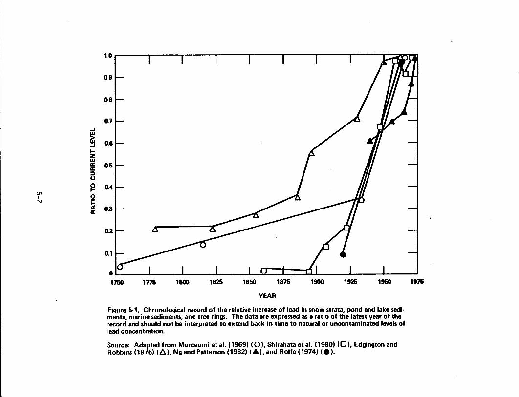
U1 I
N
... w
~ ... z w a: a: :::::) 0 0 ... 0
~ a:
1.0
0.9
0.8
0.7
0.&
0.6
0.4
0.3
0.2
0.1
0 1760 1116 1800 1825 1860 1816 1900 1926 1960
YEAR
Figure 5-1. Chronological record of the relative increase of lead in snow strata, pond and lake sedi· ments, marine sediments, and tree rings. The data are expressed as a ratio of the latest year of the record and should not be interpreted to extend back in time to natural or uncontaminated levels of lead concentration.
Source: Adapted from Murozumi et al. (1969) (0), Shirahata et al. (1980) (0), Edgington and Robbins (1976) (6), Ng and Patterson (1982) (.),and Rolfe (1974) Ce).
1916
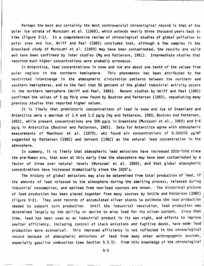
Perhaps the best and certainly the most controversial chronological record is that of the polar ice strata of Murozumi et al. (1969), which extends nearly three thousand years back .i~
time (Figure 5-1). In a comprehensive review of chronological studies of global pollution in polar snow and ice, Wolff and Peel (1985) concluded that, although a few samples in the Greenland study of Murozumi et al. (1969) may have been contaminated, the results are valid and have been confirmed by later studies (Ng and Patterson, 1981). Intermediate studies that reported much higher concentrations were probably erroneous.
In Antarctica, lead concentrations in snow and ice are about one tenth of the values from polar regions in the northern hemisphere. This phenomenon has been attributed to the restricted interchange in the atmospheric ci rcul at ion patterns between the northern and southern hemispheres, and to the fact that 90 percent of the global industrial activity occurs in the northern hemisphere (Wolff and Peel, 1985). Recent studies by Wolff and Peel (1985) confirmed the values of 5 pg Pb/g snow.found by Boutron and Patterson (1983), repudiating many previous studies that reported higher values.
It is likely that prehistoric concentrations of lead in snow and ice of Greenland and Antarctica were a maximum of 1.4 and 1.2 pg/g (Ng and Patterson, 1983; Boutron and Patterson, 1983), while present concentrations are 200 pg/p in Greenland (Murozumi et al., 1969) and 5-6 pg/g in Antarctica (Boutron and Patterson, 1983). Data for Antarctica agree with atmospheric measurements of Maenhaut et al. (1979), who found air concentrations of 0. 000076 1-1g/m3
suggested by Patterson (1980) and Servant (1982) as the natural lead concentration in the atmosphere.
In summary, it is likely that atmospheric lead emissions have increased 2000-fold since 1
the pre-Roman era, that even at this early time the atmosphere may have been contaminated by a factor of three over natural levels (Murozumi et al. 1969), and that global atmospheric concentrations have increased dramatically since the 1920 1 s.
The history of global emissions may also be determined from total production of lead, if the amounts of lead released to the atmosphere during the smelting process, released during industrial consumption, and emitted from non-lead sources are known. The historical picture of lead production has been pieced together from many sources by Settle and Patterson (1980) (Figure 5-2). They used records of accumulated silver stocks to estimate the lead production needed to support coin production. Until the industrial revolution, lead production was determined largely by the ability or desire to mine lead for its silver content. Since that time, lead has been used as an industrial product in its own right, and efforts to improve smelter efficiency, including control of stack emissions and fugitive dusts, have made lead 1
production more economical. This improved efficiency is not reflected in the chronological record because of atmospheric emissions of lead from many other anthropogenic sources, especially gasoline combustion (see Section 5.3.3). From this knowledge of the chronological '
5-3
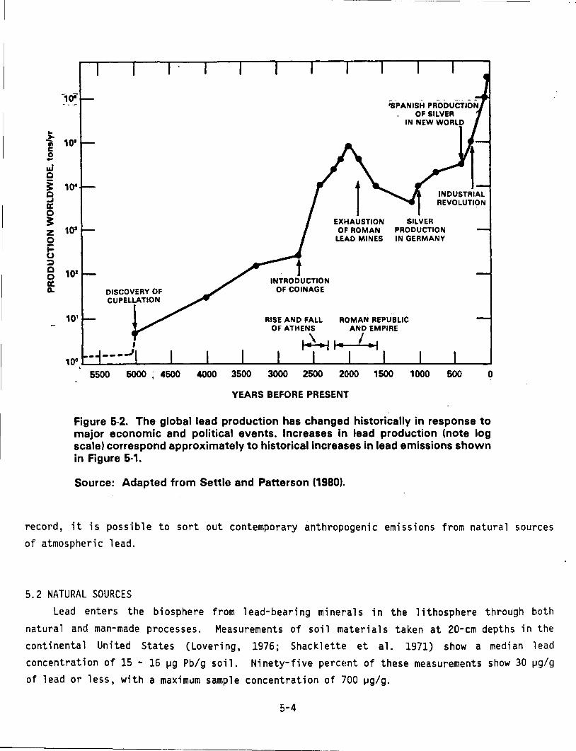
.. ~ ., 10' c s w c i 1~ c ...J a: 0 := z 10' 0
~ :::> Q
f 10'
DISCOVERY OF CUPELLATION
INTRODUCTION OF COINAGE
EXHAUSTION OF ROMAN
LEAD MINES
- . --'SPANISH PRODUCTION
OF SILVER IN NEW WORLD .
SILVER PRODUCTION IN GERMANY
RISE AND FALL ROMAN REPUBLIC OF ATHENS AND EMPIRE
~ .... , .. ~~~-~~ 6500 6000 i 4500 4000 3500 3000 2500 2000 1500 1000 500 0
YEARS BEFORE PRESENT
Figure 5-2. The global lead production has changed historically in response to major economic and political events. Increases in lead production (note log scale) correspond approximately to historical increases in lead emissions shown in Figure 5-1.
Source: Adapted from Settle and Patterson (1980).
record, it is possible to sort out contemporary anthropogenic emissions from natural sources of atmospheric lead.
5.2 NATURAL SOURCES
Lead enters the biosphere from 1 ead-beari ng mi ner·a 1 s in the 1 i thosphere through both natural and man-made processes. Measurements of soil materials taken at 20-cm depths in the continental United States (Lovering, 1976; Shacklette et al. 1971) show a median lead concentration of 15- 16 ~g Pb/g soil. Ninety-five percE!nt of these measurements show 30 ~g/g of lead or less, with a maxim~m sample concentration of 700 ~g/g.
5-4
In natural processes, lead is first incorporated in soil in the active root zone, from which it may be absorbed by p 1 ants, 1 eached into surface waters, or eroded into wi ndborne dusts (National Academy of Sciences, 1980; Chamberlain, 1970; Patterson, 1965; Chow and Patterson, 1962).
Natural emissions of lead from volcanoes have been estimated by Nriagu (1979) to be 6400
metric tons (t)/year based on enrichment over crustal abundance. That is, 10 X·109 kg/year of volcanic dust are produced, with an average lead concentration of 640 ~g/g, or 40 times the
crustal abundance of 16 ~g/g. The enrichment factor is based on Lepel et al. (1978), who
measured lead in the plume of the Augustine volcano in Alaska. Settle and Patterson (1980) _7
have calculated emissions of only 1 t/year, based on a measured Pb/S ratio of 2 X 10
(Buat-Menard and Arnold, 1978), and estimated sulfur emissions of 6 X 10⁶ t/year. The estimate of Settle and Patterson (1980) is more direct, and perhaps more reliable, because it depends on estimates of sulfur emissions rather than total volcanic dust.
Calculations of natural contributions using geochemical information indicate that natural sources contribute a relatively small amount of lead to the atmosphere. For example, if the
typical 25 - 40 ~g/m3 of rural airborne particulate matter consisted solely of wind-entrained soils containing 15 ~g/g (and rarely more than 30 ~g of lead/g), as cited above, then the natural contribution to airborne lead would range from 0.0004 to 0.0012 ~g/m3 . It has been estimated from geochemi ca 1 evidence that the natura 1 particulate 1 ead 1 eve 1 is 1 ess than 0.0005 ~g/m3 (National Academy of Sciences, 1980; United Kingdom Department of the Environment, 1974). In fact, levels as low as 0.000076 ~g/m3 have been measured at the South
Pole in Anarctica (Maenhaut et al., 1979). In contrast, lead concentrations in urban suspended particulate matter may be as high as 6 ~g/m3 (Akland, 1976; U.S. Environmental
Protection Agency, 1979, 1978). Most of this urban particulate lead stems from manmade sources.
5.3 MANMADE SOURCES
5.3.1 Production
Lead occupies an important position in the U.S. economy, ranking fifth among all metals in tonnage used. Approximately 85 percent of the primary lead produced in this country is from native mines; it is often associ a ted with minor amounts of zinc, cadmium, copper,
bismuth, gold, silver, and other minerals (U.S. Bureau of Mines, 1975). Missouri lead ore
deposits account for approximately 80 to 90 percent of the domestic production. Approximately 40 to 50 percent of annual lead production is recovered and eventually recycled.
5-5
5.3.2 Utilization
The 1971-1982 uses of lead are listed by major product category in Table 5-1 (U.S. Bureau
of Mines, 1972-1984). Total utilization averaged approximately 1.29 x 10⁶ t/yr over the
12-year period, with storage batteries and gasoline ·additives accounting for -70 percent of
total use. The gasoline antiknock compounds listed in Table 5-1 include additives for both
domestic and import markets. The additive fraction of total lead utilization has decreased
from greater than 18 percent in 1971-1973 to less than 9.5 percent in 1981. Certain products,
especially batteries, cables, plumbing, weights, and ballast, contain lead that is
ecqnomically recoverable as secondary lead. This reserve of lead in use is estimated at 3.8
mi 11 ion metric tons. Of the one mi 11 ion metric tons c1f 1 ead used in commercia 1 products
annually, 0.5 to 0.8 million tons are recovered. Lead used in pigments, gasoline additives,
ammunition, foil, solder, and steel products is widely dispersed and therefore is largely
unrecoverable.
5.3.3 Emissions
Lead or its compounds may enter the environment at any point during m1 n1 ng, sme 1 t i ng,
processing, use, recycling, or disposal. Estimates of the dispersal of lead emissions into
the environment by principal sources indicate that the atmosphere is the major initial
recipient. Estimated lead emissions to the atmosphere are shown in Table 5-2. Mobile and
stationary sources of 1 ead emissions, a 1 though found throughout the nation, tend to be
concentrated in areas of high population density, with the exception of smelters. Figure 5-3
shows the approximate 1 ocat ions of major 1 ead mines, primary and secondary smelters and
refineries, and alkyl lead plants (International Lead Zinc Research Organization, 1982).
5.3.3.1 Mobile Sources. The majority of lead compounds found in the atmosphere result from
leaded gasoline combustion. Several reports indicate that transportation sources, which
include 1 i ght-duty, heavy-duty, and off-highway vehicles, contribute over 80 percent of the
total atmospheric lead (Nationwide [lead] emissions report, 1980, 1979; U.S. Environmental
Protection Agency, 1977). Other mobile sources, including aviation use of leaded gasoline and
diesel and jet fuel combustion, contribute i nsi gnifi cant 1 ead emissions to the atmosphere.
The detailed emissions inventory in Table 5-2 shows that 89 percent of the lead emissions in
the United States are from gasoline combustion. Cass and McRae (1983) assembled emissions
inventory data on the Los Angeles Basin and determined that 83 percent of the fine particle
emissions originated from highway vehicles. Lead is added to gasoline as an antiknock
additive to enhance engine performance in the form of two tetralkyl lead compounds, tetraethyl
and tetramethyl lead (see Section 3.4). Lead is emitted from vehicles primarily in the form
of inorganic particles, although a very small fraction (<10 percent) of lead emissions are
released as volatile organic compounds, i.e., lead alkyls (see Section 6.3.2)
5-6
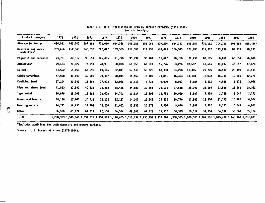
TABLE 5-l. u.s. UTILIZATION OF LEAD BY PRODUCT CATEGORY (1971-1980) (•etric tons/yr)
Product category 1971 1972 1973 1974 1975 1976 1977 1978 1979 1980 1981 1982 1983 1984
Storage batteries 616,581 661,740 697,888 772,656 634,368 746,085 858,099 879,274 814,332 645,357 770,152 704,323 806,999 865, 547
Gasoline anliknock 239,666 252,545 additives
248,890 227,847 189,369 217,508 211,296 178,473 186,945 127,903 111,367 119,234 89,118 78,933
Pig~ents and cera•ics 73,701 80,917 98,651 105,405 71,718 95,792 90,704 91,642 90,790 78,430 80,165 60,866 68,694 76,808
~unit ion 79,423 76,822 73,091 78,991 68,098 66,659 62,043 55,776 53,236 48,662 49,514 44,237 43,697 47,828
Solder 63,502 64,659 65,095 60,116 52,011 57,448 58,320 68,390 54,278 41,366 29,705 28,500 28,490 24,441
Cable coverings 47,998 41,659 39,006 39,387 20,044 14,452 13,705 13,851 16,393 13,408 12,072 15,181 10,505 12,270
Caulking lead 27,204 20,392 18,192 17,903 12,966 11,317 8,725 9,909 8,017 5,684 5,522 4,056 3,572 3,966
Pipe and sheet lead 41,523 37,592 40,529 34,238 35,456 34,680 30,861 23,105 . 27,618 28,393 28,184 23,838 27,261 28,323
Type 11etal 18,876 18,089 19,883 18,608 14,703 13,614 11,395 10,795 10,019 8,997 7,838 2,766 2,540 2,162
Brass and bronze 18,180 17,963 20,621 20,172 12,157 14,207 15,148 16,502 18,748 13,981 13,306 11,352 10,980 6,954
Bearing 11etals 14,771 14,435 14,201 13,250 11,051 11,851 10,873 9,510 9,630 7,808 6,922 6,133 5,844 4,677 <..n I Other 56,958 63,124 61,019 62,106 54,524 68,181 64,328 75,517 68,329 50,314 52,354 54,922 50,887 55,124 .......
TOTAL 1,298,383 1,349,846 1,397,876 1,450,679 1,176,465 1,351,794 1,435,497 1,432,744 1,358,335 1,070,303 1,167,101 1,075,408 1,148,487 1,207,033
alncludes additives for both d011estic and export .arkets.
Source: U.S. Bureau of Mines (1972-1984).
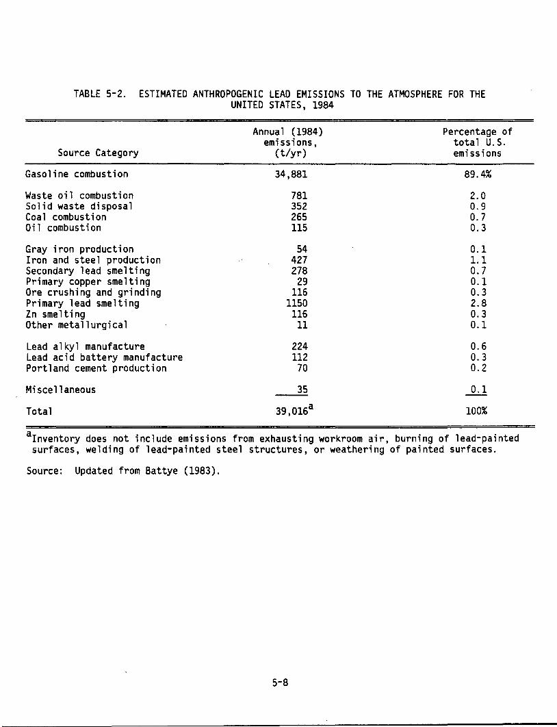
TABLE 5-2. ESTIMATED ANTHROPOGENIC LEAD EMISSIONS TO THE ATMOSPHERE FOR THE UNITED STATES, 1984
Annual (1984) Percentage of emissions, total U.S.
Source Category (t/yr) emissions
Gasoline combustion 34,881 89.4%
Waste oil combustion 781 2.0 Solid waste disposal 352 0.9 Coal combustion 265 0.7 Oil combustion 115 0.3
Gray iron production 54 0.1 Iron and steel production 427 1.1 Secondary lead smelting 278 0.7 Primary copper smelting 29 0.1 Ore crushing and grinding 116 0.3 Primary lead smelting 1150 2.8 Zn smelting 116 0.3 Other metallurgical 11 0.1
Lead alkyl manufacture 224 0.6 Lead acid battery manufacture 112 0.3 Portland cement production 70 0.2
Miscellaneous 35 0.1
Total 39,016a 100%
ainventory does not include emissions from exhausting workroom air, burning of lead-painted surfaces, welding of lead-painted steel structures, or weathering of painted surfaces.
Source: Updated from Battye (1983).
5-8
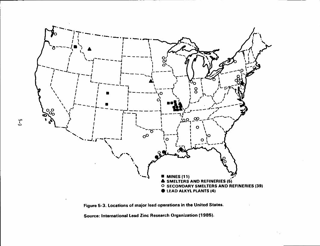
U1 I
w
........ ......... _ I I·-·-
/ I ·- ·~ I \ ·r-·--·-.·
..... I ' I \ o----~ • 'I 6 1 , ' l
1 I f "' I 1
,' \ -J-- _ 1-- ----; ot• - ----1 ' Ol
I ' ' I "' --- I I I I 0 ..... , ,---.~__ I L !..----~ I -~--J I---- I I I I "'-"' ',-1 I L I ._,
I I ---- I _, .) I I ----- \ ' •L --
\ I I I \..-- - - 4 1 \r"f'f \ I / • r-----~,o ', : o \, ,t rl '
' I 1 1 \ '- r -"'" 1
\ I 1 01 " I J \ I \ r- - - I • I I • • 1-_, /V·"' --\ I __ ,__ I . , --- --- - - - J I ', - J-- -,- .-
\ 1 I -r----- - -1 'J ,. --- "' ~ I ,-- -, .----~ ,-- ~
I -, I' -\ I I I 00 .£.-"- --... , I I I /..SJ-0,---\ ', '
I I ' I I \,
·~ I : - .... - ... ~---L / : 0 \ ', • I v I .l 1 \ "-. I 1 0 0 r---- \ 1 \Q
......... -.J J" -r----l I 0 1 I 0 I
• '·, \ ,' I -- --"-----' I ---, I . '~~--
\. I'"' ,. \ \ \ ·-. • MINES (11) ,'
A SMELTERS AND REFINERIES (6.1
'
0 SECONDARY SMELTERS AND REFINERIES (391 e LEAD ALKYL PLANTS (4)
Figure 5-3. locations of major lead operations in the United States.
Source: International lead Zinc Research Organization (1985).
Commercial lead antiknock additives of all types contain halogens designated as scavengers that serve to reduce the accumulation of decomposition products of the lead alkyls in certain critical areas of the engine combustion chamber. The most commonly used additive package contains enough ethylene dibromide to tie up all of the. lead as PbBr2 , and enough ethylene dichloride to tie up 1.5 times the amount of lead as PbC1 2 .
The factors which affect both the rate of particulate lead emissions and the physicochemical properties of the emissions are: lead content of the fuel, other additives, vehicle fuel economy, the driving speed or conditions, and type of vehicle, as well as design parameters, maintenance, and ages of the engine, exhaust, and emission control systems. The major types of vehicles are light-duty (predominantly cars) and heavy-duty (trucks and buses). The important properties of the particulate emissions include the total amount emitted, the size distribution of the particles, and the chemical composition of these particles as a function of particle size. The most commonly used index of particle size is the mass median aerodynamic diameter (MMAD), which is defined as the point in the size distribution of particles such that half the mass lies on either side of the MMAD value (National Air Pollution Control Administration, 1969). Table 5-3 summarizes a recent study estimating the particulate emission rates and particle composition for light-duty vehicles operated on a leaded fuel of 1.8 g Pb/gallon (Hare and Black, 1981). ·Table 5-4 estimates particulate emission rates for heavy-duty vehicles (trucks) operated on a leaded fuel of 1.8 g Pb/gallon (Hare and Black, 1981). The lead content of 1.8 g Pb/~~allon was chosen to approximate the lead concentration of leaded gasoline during 1979 (Table 5-5). Another recent study utilizing similar composite emission factors provides estimates of motor vehicle lead emissions for large areas (Provenzano, 1978).
The fate of emitted lead particles depends upon their particle size (see Section 6.3.1).
Particles initially formed by condensation of lead compounds in the combustion gases are quite small (well under 0.1 !Jm in diameter, see Section 6.3.1) (Pierson and Brachaczek, 1983).
Particles in this size category are subject to growth by coagulation and, when airborne, can remain suspended in the atmosphere for 7 - 30 days and travel thousands of miles from their original source (Chamberlain et al., 1.979). Larger particles are formed as the result of agglomeration of smaller condensation particles and have limited atmospheric lifetimes (Harrison and Laxen, 1981). The largest vehicle-emitted particles, which are greater than 100
!Jm in diameter, may be formed by materia 1 s flaking off from the surfaces of the exhaust system. As indicated in Table 5-3, the estimated mass median equivalent diameter of leaded particles from light-duty vehicles is <0.25 !Jm, suggesting that such particles with relatively long atmospheric lifetimes have the potential for long-distance transport. Similar values for MMAD in automobile exhausts were found in Britain (0. 27 !Jm) (Chamberlain et al. 1979) and
5-10
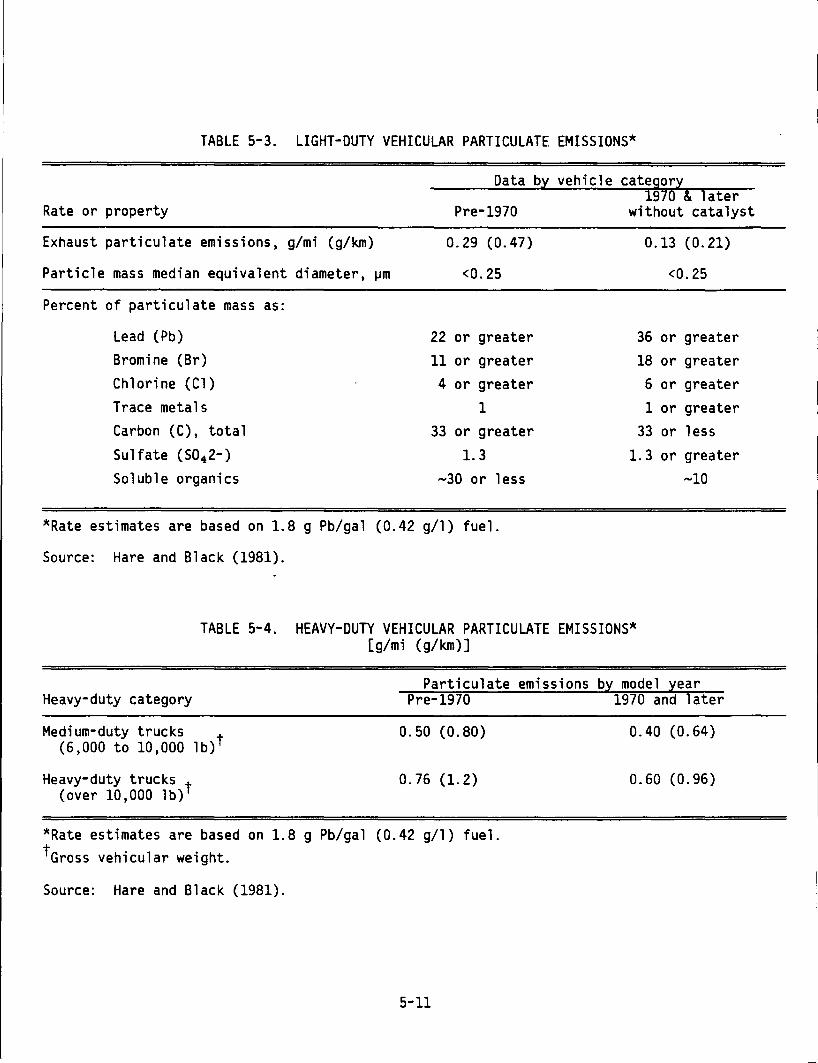
TABLE 5-3. LIGHT-DUTY VEHICULAR PARTICULATE EMISSIONS*
Data by vehicle category 1970 & later
Rate or property Pre-1970 without catalyst
Exhaust particulate emissions, g/mi (g/km)
Particle mass median equivalent diameter, ~m
Percent of particulate mass as:
Lead (Pb) Bromine (Br) Chlorine (Cl) Trace metals Carbon (C), total
Sulfate (S04 2-) Soluble organics
0.29 (0.47)
<0.25
22 or greater 11 or greater 4 or greater
1 33 or greater
1.3
-30 or less
*Rate estimates are based on 1.8 g Pb/gal (0.42 g/1) fuel.
Source: Hare and Black (1981).
0.13 (0.21)
<0.25
36 or greater 18 or greater 6 or greater 1 or greater
33 or less
1. 3 or greater
-10
TABLE 5-4. HEAVY-DUTY VEHICULAR PARTICULATE EMISSIONS* [g/mi (g/km)]
Particulate emissions by model year Heavy-duty category Pre-1970 1970 and later
Medium-duty trucks t (6,000 to 10,000 lb)
Heavy-duty trucks t (over 10,000 lb)
0.50 (0.80)
0.76 (1.2)
*Rate estimates are based on 1.8 g Pb/gal (0.42 g/1) fuel. tGross vehicular weight.
Source: Hare and Black (1981).
5-11
0.40 (0.64)
0.60 (0.96)
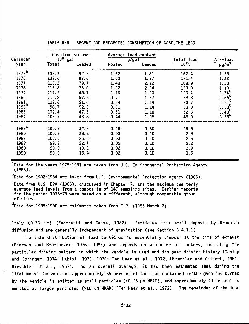
TABLE 5-5. RECENT AND PROJECTED CONSUMPTION OF GASOLINE LEAD
Gasoline volume Average lead content Calendar 109 gal g/gal Total lead Air-lead
year Total Leaded Pooled Leaded 103 t j.Jg/m:J
1975a 102.3 92.5 1.62 1.81 167.4 1. 23 1976 107.0 87.0 1. 60 1. 97 171.4 1. 22 1977 113.2 79.7 1.49 2.12 168.9 1. 20 1978 115.8 75.0 1. 32 2.04 153.0 1.13 1979 111.2 68.1 1.16 1. 90 129.4 0.74c 1980 110.8 57.5 0.71 1. 3.7 78.8 0.66c 1981b 102.6 51.0 0.59 1.19 60.7 0.51c 1982 98.7 52.5 0.61 1.14 59.9 0.53c 1983 102.4 47.5 0.51 1.10 52.3 0.40c 1984 105.7 43.8 . 0.44 1. 05 46.0 0.36c
----------------------------------------------------------·------------------------------------1985d 100.6 32.2 0.26 0.80 25.8 1986 100.3 28.8 0.03 0.10 2.9 1987 100.0 25.6 0.03 0.10 2.6 1988 99.3 22.4 0.02 0.10 2.2 1989 99.0 19.2 0.02 0.10 1.9 1990 99.0 16.4 0.02 0.10 1.6
aData for the years 1975-1981 are taken from U.S. Environmental Protection Agency (1983).
PData for 1982-1984 are taken from U.S. Environmental Protection Agency (1985).
cData from U.S. EPA (1986), discussed in Chapter 7, are the maximum quarterly average lead levels from a composite of 147 sampling sites. Earlier reports for the period 1975-78 were based on a different, although comparable group of sites.
dData for 1985-1990 are estimates taken from F.R. (1985 March 7).
Italy (0.33 iJm) (Facchetti and Geiss, 1982). Particles this small deposit by Brownian
diffusion and are generally independent of gravitation (see Section 6.4.1.1).
The size distribution of lead particles is essent·ially bimodal at the time of exhaust (Pierson and Brachaczek, 1976, 1983) and depends on a number of factors, including the
particular driving pattern in which the vehicle is used and its past driving history (Ganley and Springer, 1974; Habibi, 1973, 1970; TerHaar et al., 1972; Hirschler and Gilbert, 1964;
Hirsch 1 er et a 1. , 1957). As an over a 11 average, it has been estimated that during the lifetime of the vehicle, approximately 35 percent of the lead contained in•the gasoline burned
by the vehicle is emitted as small particles (<0.25 iJm MMAD), and approximately 40 percent is
emitted as larger particles (>10 iJm MMAD) (TerHaar et al., 1972). The remainder of the lead
5-12
increased consumption of unleaded fuel, from 10 percent of the total gasoline pool in 1975 to 59 percent in 1984 (Table 5-5 and Figure 5-6). Since 1975, when the catalytic converter was introduced by automobile manufacturers for automotive exhaust emissions control, virtually all new passenger cars have been certified on unleaded gasoline (with the exception of a few diesels and a very few leaded-gasoline vehicles).
Data describing the lead consumed in gasoline and average ambient lead levels (composite of maximum quarterly values) vs. calendar year are listed in Table 5-5 and plotted in Figure 5-7. The 1975 through 1979 composite quarterly lead averages are based on 105 lead-monitoring sites, primarily urban. The 1980 through 1984 composite average is based on 147 sites with valid annual data. Between 1975 and 1984, the lead consumed in gasoline decreased 73 percent (from 167,400 to 46,000 metric tons) while the corresponding composite maximum quarterly average of ambient air lead decreased 71 percent (from 1.23 to 0.36 ~g/m3 ). This indicates that control of lead in gasoline over the past several years has effected a direct decrease in peak ambient lead concentrations, at least for this group of monitoring sites. 5.3.3.2 Stationary Sources. As shown in Table 5-2 (based on 1984 emission estimates), primary lead smelting, coal combustion, and combustion of waste oil are the principal contributors of lead emissions from stationary sources. Coal-fired electric power stations typically burn 5,000 to 10,000 tons of coal per day. Pulverized coal is mixed with hot air and passed into a burning chamber or boi 1 er, where the mixture is ignited. Some of the unburned residue falls to the bottom of the boiler, where it is removed as 'bottom ash'. The residue that passes through the boiler is called 'fly ash', much of which is removed by electrostatic precipitators and other pollution control devices. In a well-designed system, 99.8 percent of the original inorganic mass of the coal is retained by the system. At 10 g Pb/ton of coal, very little lead would be emitted. However, the remaining 0.2 percent of the coal mass that is emitted from the stack is highly enriched in lead, compared to the original coal. Although data on stack emissions of lead are limited, the concentration of lead in fly ash may provide a reasonable indication of stack lead emissions. Klusek et al. (1983)
reported an enrichment of 6.1 between coal and fly ash. On this basis, a typical power plant consuming 10,000 tons of coal per day would emit 1.2 kg Pb/day (10,000 t/day x 0.002 x 6.1 x 10 g Pb/t coal). Turner and Lowry (1983) reported enrichment factors of 17 to 75 for conventional coal-fired power plants in Pennsylvania and New Hampshire.
The manufacture of consumer products such as 1 ead glass, storage batteries, and 1 ead additives for gasoline also contributes significantly to stationary source lead emissions. Since 1970, the quantity of lead emitted from the metallurgical industry has decreased somewhat because of the application of control equipment and the closing of several plants, particularly in the zinc and pyrometallurgical industries.
5-16
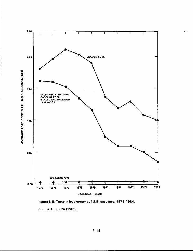
jij Ol g,
Cl) loU z ::i
2.00
~ 1.50 C( (!)
Cl) :; ~
0 .... z loU .... z 0 (J
Q C( loU _, loU (!) C( a: loU
~
1.00
0.50
SALES·WEIGHTED TOTAL GASOLINE POOL (LEADED AND UNLEADED "AVERAGE")
UNLEADED FUEL
1975 1976 1977 1978 1979 1980 1981
CALENDAR YEAR
Figure 5-5. Trend in lead content of U.S. gasolines. 1975-1984.
Source: U.S. EPA (1985).
5-15
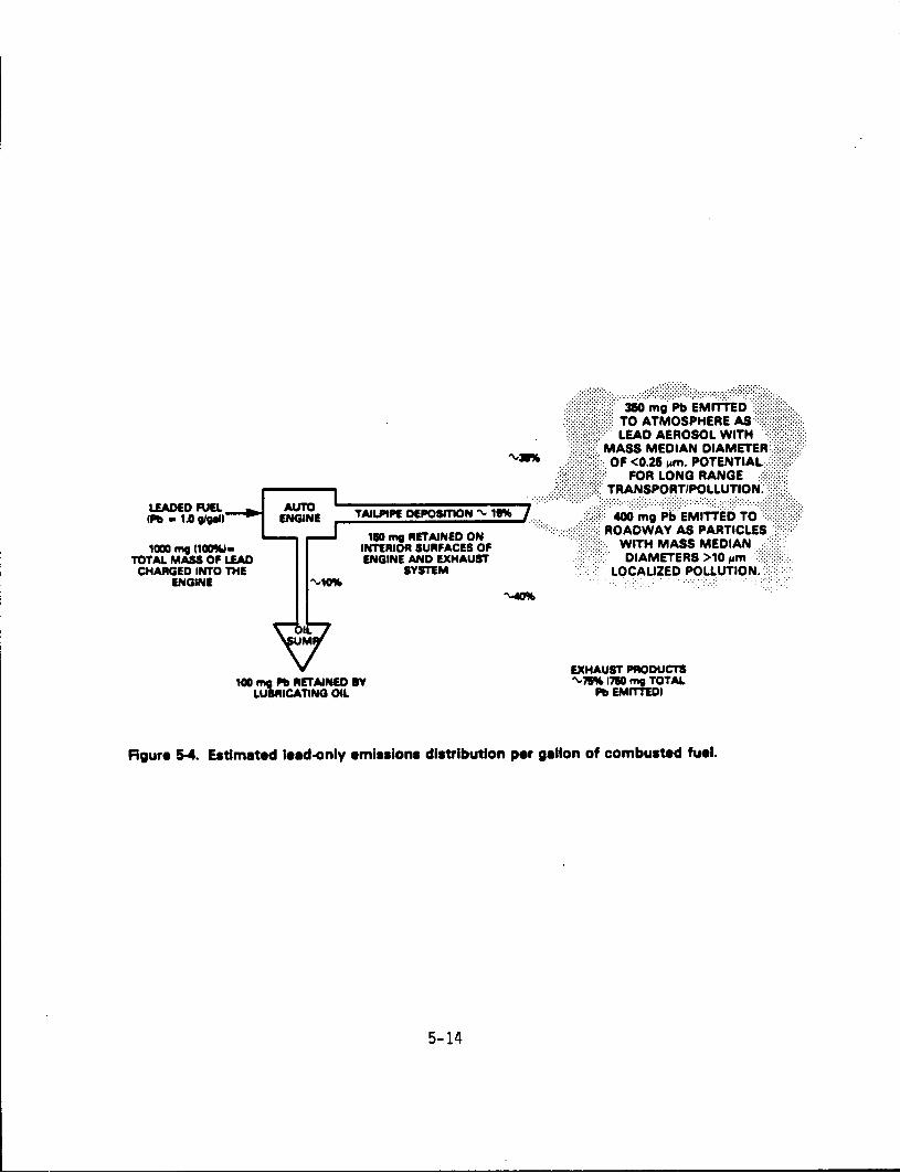
LEADEDRJEL IPb • 1.0 g/pll
1000 mg 11CIO'Mol• TOTAL MASS OF LEAD
CHARGED INTO THE ENGINE
:::::U)\\\:t\e::
-..;T.:;;:AI:.:IJII~PE:..:,:DE::.PO.:.::smo:.:.;::;.:;N:.."'-..;....:;11'Mt:;.::...J ··:-·· .·:-:·:-:··· 400 mg Pb EMITTED TO ·-:-:-:-:·:-:-:-:·::: 110 mg RETAINED ON ::::(}:}{ROADWAY AS PARTICLES·:(:)?
INTERIOR SURFACES OF .·.·.·. WITH MASS MEDIAN .. -:::::::: ENGINE AND EXHAUST ·>> ·:::: :- DIAMETERS >10 11m .}}} :-
SYSTEM .. LOCAUZED POLLUTION.·\:>
100 mg Pb RETAINED IV LUBRICATING OIL
EXHAUST PRODUCTS "'-~ 17'10 mg TOTAL
Pb EMITTEDI
Figure 5-4. &tlmated lead-only emiuiona diatributlon per gallon of combuated fuel.
5-14
consumed in gasoline combustion is deposited in the engine! and exhaust system. Engine deposits
are, in part, gradually transferred to the lubricating oil and removed from the vehicle whe.n
the oil is changed. A flow chart depicting lead-only emissions per gallon of fuel charged
into the engine is shown in Figure 5-4. It is estimated that 10 percent of the 1 ead consumed
during combustion is re 1 eased into the environment vi a di sposa 1 of used 1 ubri cat i ng oil
(Piver, 1977). In addition, some of the lead deposited in the exhaust system gradually flakes
off, is emitted in the exhaust as extremely large particles, and rapidly falls into the
streets and roads where it is incorporated into the dust and washed into sewers or onto
adjacent soil.
Although the majority (>90 percent on a mass basis) of vehicular lead compounds are
emitted as inorganic particles (e.g., PbBrCl), some organolead vapors (e.g., lead alkyls) are
also emitted. The largest volume of organolead vapors arises from the manufacture, transport,
and handling of 1 eaded gaso 1 i ne. Such vapors are photoreact i ve and their presence in 1 oca 1
atmospheres is transitory; i.e., the estimated atmospheric half-lives of lead alkyls, under
typical summertime conditions, are less than half a day (Nielsen, 1984). Organolead vapors
are most likely to occur in occupational settings (e.g., gasoline transport and handling
operations, gas stations, parking garages) and have been found to contribute less than 10 percent of the total lead present in the atmosphere (Gibson and Farmer, 1981; National Academy
of Sciences, 1972).
The use of lead additives in gasoline, which increased in volume for many years, is now
decreasing as automobiles designed to use unleaded fuel constitute the major portion of the
fleet (Table 5-1). The decline in the use of leaded fiJel is the result of two regulations
promulgated by the U.S. Environmental Protection Agency (F.R., 1973, December 6). The first
required the availability of unleaded fuel for use in automobiles designed to meet federal
emission standards with lead-sensitive emission control devices (e.g., catalytic converters);
the second required a reduction or phase-down of the lead content in leaded gasoline. The
phase-down schedule of lead in gasoline was modified in 1982 (F.R., 1982, October 29),
replacing the 0.5 g/gal standard for the average lead content of all gasoline with a standard
of 1.10 g Pb/gal for leaded gasoline alone, and again in 1985 (F.R., 1985, March 7), calling
for a reduction to 0.5 g Pb/gal leaded gas by July 1985 and 0.1 g Pb/gal leaded gas by
January 1986. The trend in lead content for U.S. gasolines is shown in Figure 5-5 and Table 5-5. Of
the total gasoline pool, which includes both leaded and unleaded fuels, the average lead
content has decreased 73 percent, from an average of 1.62 g/gal in 1975 to 0.44 g/gal in 1984 (Table 5-5, Figure 5-5). Accompanying the phase-down of lead in leaded fuel has been the
5-13
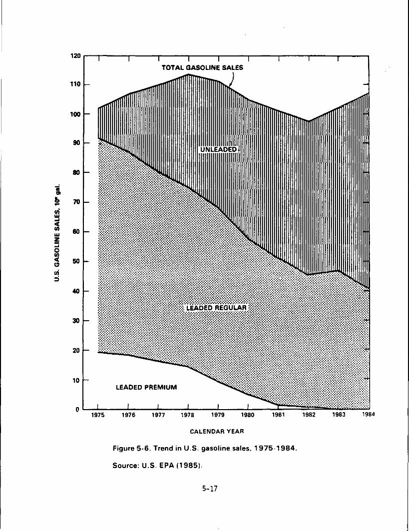
1~r--,.---~,-----.-,--~,-----.-,--~,-----r-,---,,-------.--~
TOTAL GASOLINE SALES
110 ~ -
100 f-
UNLEADED
50-
40-
30-
20 ~
10 I-LEADED PREMIUM
1980 1981 1982 1983 1984
CALENDAR YEAR
Figure 5-6. Trend in U.S. gasoline sales, 1 975 · 1984.
Source: U.S. EPA (1 985).
5-17
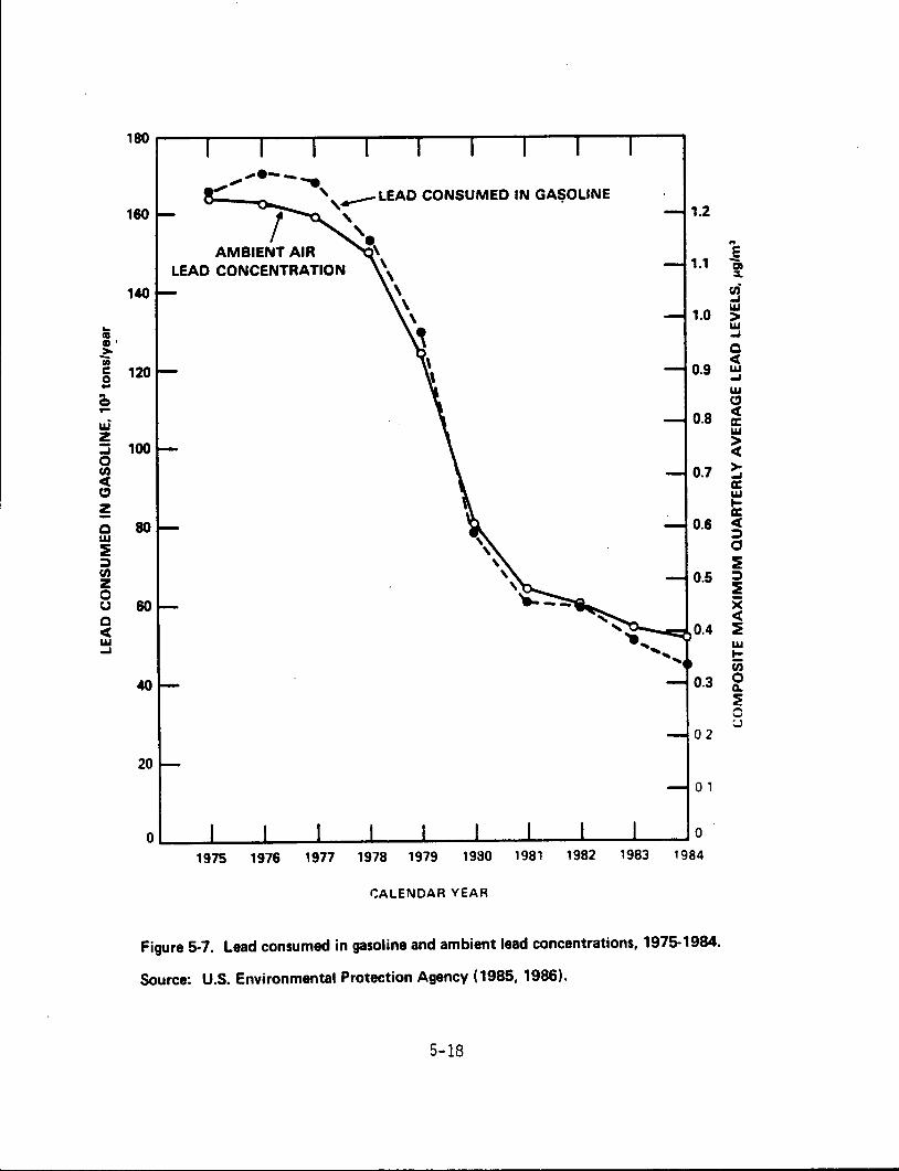
.. as II' > iii c 0 -.. 0 ... w z :J 0 en c( 0 z -Q 1&.1
~ ~ en z 0 CJ Q c( 1&.1 ~
180
,.,-•-- .... ' ,.,..--LEAD CONSUMED IN GA~OLINE
160 1.2
' '• AMBIENT AIR :\
LEAD CONCENTRATION \ 1.1 \
140 \ \ \ 1.0
~ 120 0.9
0.8
100
0.7
80 0.6
0.5
60
0.4
40 0.3
o~--~----._--~----~--~~--~----~--_. ____ ._ __ ~0 1975 1976 1977 1978 1979 1980 1981 1982 1983 1984
CALENDAR YEAR
Figure 5-7. Lead consumed in gasoline and ambient lead concentrations, 1975-1984.
Source: U.S. Environmental Protection Agency ( 1985, 1986).
5-18
..
.e en ::L
u; ~ 1&.1 > 1&.1 ~
Q c( 1&.1 ~
1&.1 0 c( a: 1&.1 > c(
> ~ a: 1&.1 ~ a: c( ~ 0 ~ ~ ~ x c(
~ 1&.1 ~ c;; 0 Q.
~ 0 w
In the United States, a new source for lead emissions emerged in the mid-1960s with the
opening of the 11 Vi burnum Trend 11 or 11 New Lead Be lt11 in southeastern Missouri. The presence of
eight mines and three accompanying lead smelters in this area makes it the largest lead
producing district in the world and has moved the United States into first place among the
world's lead-producing nations.
Although some contamination of soil and water occurs as a result of such mechanisms as
leaching from mine and smelter wastes, quantitative estimates of the extent of this
contamination are not avai 1 ab 1 e. Spill age of ore concentrates from open trucks and rai 1 road
cars, however, is known to contribute significantly to contamination along transportation
routes. For examp 1 e, a 1 ong two routes used by ore trucks in southeastern Missouri, 1 ead
levels in leaf litter ranged from 2000 - 5000 IJg/g at the roadway, declining to a fairly
constant 100- 200 1-1g/g beyond about 400ft from the roadway (Wixson et al., 1977).
Another possible source of land or water contamination is the disposal of particulate
lead collected by air pollution control systems. The potential impact on soil and water
systems from the disposal of dusts collected by these control systems has not been quantified.
5.4 SUMMARY
There is no doubt that atmospheric 1 ead has been a component of the human environment
since the earliest written record of civilization. Atmospheric emissions are recorded in
glacial ice strata and pond and lake sediments. The history of these global emissions seems
closely tied to production of lead by industrially oriented civilizations.
A 1 though there are conflicting reports of the amount of 1 ead emitted from natura 1
sources, even the more liberal estimate (25 X 103 t/year, Nriagu, 1979) is dwarfed by the
global emissions from anthropogenic sources (450 X 103 t/year).
Production of lead in the United States has remained steady at about 1.2 X 10⁶ t/year for
the past decade. The gasoline additive share of this market has dropped from 18 to 6.5
percent during the period 1971- 1984. The contribution of gasoline lead to total atmospheric
emissions has remained high, at 89 percent, as emissions from stationary sources have
decreased at the same pace as from mobile sources. The decrease in stationary source
emissions is due primarily to control of stack emissions, whereas the decrease in mobile
source emissions is a result of switchover to unleaded gasolines. The decreasing use of lead
in gasoline is projected to continue through 1990.
5-19
5.5 REFERENCES
Akland, G. G. (1976) Air quality data for metals, 1970 through 1974, from the National Air Surveillance Networks. Research Triangle Park, NC: U.S. Environmental Protection Agency, Office of Research and Development; EPA report no. EPA 600/ 4-76-041. Available from: NTIS, Springfield, VA; PB-260905.
Baes, C. F., III; Ragsdale, H. L. (1981) Age-specific lead distribution in xylem rings of three tree genera in Atlanta, Georgia. Environ. Pollut. Ser. B 2: 21-35.
Battye, B. (1983) Lead emissions inventory, 1981 [memo to John Haines]. Chapel Hill, NC: GCA Crporation; January 31. Available for inspection at: U.S. Environmental Protection Agency, Environmental Criteria and Assessment Office, Research Triangle Park, NC.
Boutron, C. (1982) Atmospheric trace metals in the snow layers deposited at the South Pole from 1928 to 1977. Atmos. Environ. 16: 2451-2459.
Boutron, C. F.; Patterson, C. C. (1983) The occurrence of lead in Antarctic recent snow, firm deposited over the last two centuries and prehistoric ice. Geochim. Cosmochim. Acta 47: 1355-1368.
Buat-Menard, P.; Arnold, M. (1978) The heavy metal chemistry of atmospheric particulate matter emitted by Mount Etna volcano. Geophys. Res. Lett. 5: 245-248.
Cass, G. R.; McRae, G. J. (1983) Source-receptor reconciliation of routine air monitoring data for trace metals: an emission inventory assisted approach. Environ. Sci. Technol. 17: 129-139.
Chamberlain, A. C. (1970) Interception and retention of radioactive aerosols by vegetation. Atmos. Environ. 4: 57-77.
Chamberlain, A. C.; Heard, M. J.; Little, P.; Wiffen, R. D. (1979) The dispersion of lead from motor exhausts. In: Proceedings of the Royal Society discussion meeting, pathways of pollutants in the atmosphere; 1977; London, United Kingdom. Philos. Trans. R. Soc. London Ser. A 290: 577-589.
Chow, T. J.; Patterson, C. C. (1962) The occurrence and significance of lead isotopes in pelagic sediments. Geochim. Cosmochim. Acta 26: 263-308.
Christensen, E. R.; Chien, N. (1981) Fluxes of arsenic, lead, zinc, and cadmium to Green Bay and Lake Michigan sediments. Environ. Sci. Technol. 15: 553-558.
Dodge, R. E.·; Gil bert, T. R. (1984) Chrono 1 ogy of 1 ead po 11 uti on contained in banded cora 1 skeletons. Mar. Biol. (Berlin) 82: 9-13.
Dominik, J.; Mangini, A.; Prosi, F. (1984) Sedimentation rate variations and anthropogenic metal fluxes into Lake Constance sediments. Environ. Geol. 5: 151-157.
Edgington, D. N.; Robbins, J. A. (1976) Records of lead deposition in Lake Michigan sediments since 1800. Environ. Sci. Technol. 10: 266-274.
Facchetti, S.; Geiss, F. (1982) Isotopic lead experiment: status report. Luxembourg: Commission of the European Communities; publication no. EUR 8352 EN.
5-20
Federal Register. (1973) Regulation of fuels and fuel additives: control of lead additives in gasoline. (December 6) 38: 33734-33741.
Federal Register. (1982) 40 CFR Part 80: regulation of fuels and fuel additives: final rule. (October 29) 47: 49322-49334.
Federal Register. (1985) Regulation of fuels and fuel additives; gasoline lead content. F. R. (March 7) 50: 9386-9408. ·
Galloway, J. N.; Likens, G. E. (1979) Atmospheric enhancement of metal deposition in Adirondack lake sediments. Limnol. Oceanogr. 24: 427-433.
Ganley, J. T.; Springer, G. S. (1974) Physical and chemical characteristics of particulates in spark ignition engine exhaust. Environ. Sci. Technol. 8: 340-347.
Gibson, M. J.; Farmer, J. G. (1981) Tetraalkyl lead in the urban atmosphere of Glasgow. Environ. Technol. Lett. 2: 521-530.
Habibi, K. (1970) Characterization of particulate lead in vehicle exhaust: experimental techniques. Environ. Sci. Technol. 4: 252-253.
Habibi, K. (1973) Characterization of particulate matter in vehicle exhaust. Environ. Sci. Technol. 7: 223234.
Hare, C. T.; Black, F. M. (1981) Motor vehicle particulate emission factors. Presented at: 74th meeting and exposition of the Air Pollution Control Association; June. Philadelphia, PA: Air Pollution Control Association; paper no. 81-56.5.
Harrison, R. M.; Laxen, D. P. H. (1981) Lead pollution: causes and control. New York, NY: Chapman and Hall.
Hirschler, D. A.; Gilbert, L. F. (1964) Nature of lead in automobile exhaust gas. Arch. Environ. Health 8: 297-313.
Hirschler, D. A.; Gilbert, L. F.; Lamb, F. W.; Niebylski, L. M. (1957) Particulate lead compounds in automobile exhaust gas. Ind. Eng. Chem. 49: 1131-1142.
Hunt, W. F., Jr., ed.; Curran, T. C.; Faoro, R. B.; Frank, N. H.; Mann, C.; Neligan, R. E.; Sleva, S.; Berg, N.; Lutz, D.; Manire, G.; Shipman, D. (1985b) National air quality and emissions trends report, 1983. Research Triangle Park, NC: U. S. £nvironmental Protection Agency, Office of Air Quality Planning and Standards; EPA report no. EPA-450/4-84-029.
International Lead Zinc Research Organization (1982) Locations of major lead operations in the United States [map]. New York, NY: International Lead Zinc Research Organization.
Klusek, C. S.; Miller, K. M.; Heit, M. (1983) Trace element and radionuclide mass balances at a coal-fired electric generating station. Environ. Int. 9: 139-144.
Lepel, E. A.; Stefansson, K. M.; Zoller, W. H. (1978) The enrichment of volatile elements in the atmosphere by volcanic activity: Augustine volcano 1976. J. Geophys. Res. 83: 6213-6220.
5-21
Lovering, T. G., ed. (1976) Lead in the environment. Washington, DC: U.S. Department of the Interior, G·eological Survey; Geological Survey professional paper no. 957. Available from: GPO, Washington, DC; S/N 024-001-02911-1.
Maenhaut, W.; Zoller, W. H.; Duce, R. A.; Hoffman, G. L. (1979) Concentration and size distribution of particulate trace elements in the south polar atmosphere. J. Geophys. Res. 84: 2421-2431.
Murozumi, M.; Chow, T. J.; Patterson, C. (1969) Chemical concentrations of pollutant lead aerosols, terrestrial dusts and sea salts in Greenland and Antarctic snow strata. Geochim. Cosmochim. Acta 33: 1247-1294.
National Academy of Sciences. (1972) Lead: airborne lead in perspective. Washington, DC: National Academy of Sciences. (Biologic effects of atmospheric pollutants).
National Academy of Sciences, Committee on Lead in the Human Environment. (1980) Lead in the human environment. Washington, DC: National Academy of Sciences.
National Air Pollution Control Administration. (1969) Control techniques for particulate air pollutants. Washington, DC: U.S. Department of Health, Education and Welfare; publication no. AP-51. Available from: NTIS, Springfield, VA; PB-190253.
Nationwide [lead] emissions report. (1979) From: NEDS, National Emissions Data System [data base]. Research Triangle Park, NC: U.S. Environmental Protec~ion Agency, Office of Air Quality Planning and Standards. Printout. Available for inspection at: U.S. Environmental Protection Agency, Environmental Criteria and Assessment Office, Research Triangle Park, NC. ·
Nationwide [lead] emissions report. (1980) From: NEDS, National Emissions Data System [data base]. Research Triangle Park, NC: U.S. Environmental Protection Agency, Office of Air Quality Planning and Standards. Printout. Available for inspection at: U.S. Environmental Protection Agency, Environmental Criteria and Assessment Office, Research Triangle Park, NC.
Ng, A.; Patterson, C. (1981) Natural concentrations of lead in ancient Arctic and Antarctic ice. Geochim. Cosmochim. Acta 45: 2109-2121.
Ng, A.; Patterson, C. C. (1982) Changes of lead and barium with time in California off-shore basin sediments. Geochim. Cosmochim. Acta 46: 2307-2321.
Nielsen, T. (1984) Atmospheric occurrence of organolead compounds. In: Grandjean, P., ed. Biological effects of organolead compounds. Boca Raton, FL: CRC Press; pp. 44-62.
Nri agu, J. 0. (1979) Gl oba 1 inventory of natura 1 and anthropogenic emissions of trace meta 1 s to the atmosphere. Nature (London) 279: 409-411.
Patterson, C. C. (1965) Contaminated and natural lead environments of man. Arch. Environ. Health 11: 344-360.
Patterson, C. C. (1980) An alternative perspective - lead pollution in the human environment: origin, extent and significance. In: National Academy of Sciences, Committee on Lead in the Human Environment. Lead in the human environment. Washington, DC: National Academy of Sciences; pp. 265-349.
5-22
Pierson, W. R.; Brachaczek, W. W. (1976) Particulate matter associated with vehicles on the road. Warrendale, PA: Society of Automotive Engineers; SAE technical paper no. 760039. SAE transactions 85: 209-227.
Pierson, W. R.; Brachaczek, W. W .. (1983) Emissions of ammonia and amines from vehicles on the road. Environ. Sci. Technol. 17: 757-760.
Piver, W. T. (1977) Environmental transport and transformation of automotive-emitted lead. Environ. Health Perspect. 19: 247-259.
Provenzano, G. (1978) Motor vehicle lead emissions in the United States: an analysis of important determinants, geographic patterns and future trends. J. Air Pollut. Control Assoc. 28: 1193-1199.
Rolfe, G. L. (1974) Lead distribution in tree rings. For. Sci. 20: 283286.
Servant, J. (1982) Atmospheric trace elements from natural and industrial sources. London, United Kingdom: University of London, Monitoring and Assessment Research Centre.
Settle, D. M.; Patterson, C. C. (1980) Lead in albacore: guide to lead pollution in Americans. Science (Washington, DC) 207: 1167-1176.
Shacklette, H. T.; Hamilton, J. C.; Boerngen, J. G.; Bowles, J. M. (1971) Elemental composition of surficial materials in the conterminous United States: an account of the amounts of certain chemical elements in samples of soils and other regoliths. Washington, DC: U.S. Department of the Interior, Geological Survey; Geological Survey professional paper no. 574-D.
Shirahata, H.; Elias, R. W.; Patterson, C. C.; Koide, M. (1980) Chronological variations in concentrations and isotopic compositions of anthropogenic atmospheric lead in sediments of a remote subalpine pond. Geochim. Cosmochim. Acta 44: 149-162.
Symeonides, C. (1979) Tree-ring analysis for tracing the history of pollution: application to a study in northern Sweden. J. Environ. Qual. 8: 482-486.
Ter Haar, G. L.; Lenane, D. L.; Hu, J. N.; Brandt, M. (1972) Composition, size and control of automotive exhaust particulates. J. Air Pollut. Control Assoc. 22: 39-46.
Turner, R. R.; Lowry, P. D. (1983) Comparison of coal gasification and combustion residues. J. Environ. Eng. 109: 305-320.
U. S. Bureau of Mines. (1972-1984) Lead. In: Minerals yearbook; volume I. metals and minerals. Washington, DC: U. S. Department of the Interior.
U. S. Environmental Protection Agency. (1977) Control techniques for lead air emissions: volumes I and II. Durham, NC: Office of Air Quality Planning and Standards; EPA report nos. EPA-450/2-77-012A and EPA-450/2-77-012B. Available from: NTIS, Springfield, VA; PB80-197544 and PB80-197551.
U. S. Envi ronmenta 1 Protection Agency. (1978) Air qua 1 i ty data for meta 1 s 1975, from the Nat i ona 1 Air Survei 11 ance Networks. Research Triangle Park, NC: Office of Research and Development; EPA report no. EPA-600/4-78-059. Available from: NTIS, Springfield, VA; PB-293106.
5-23
U. S. Environmental Protection Agency. (1979) Air quality data for metals 1976, from the. National Air Surveillance Networks. Research Triangle Park, NC: Office of Research and Development; EPA report no. EPA-600/4-79-054. Available from NTIS, Springfield, VA; PBB0-147432.
U. S. Environmental Protection Agency. (1986) National air quality and emission trends report, 1984. Research Triangle Park, NC: Office of Air Quality Planning and Standards; EPA report no. EPA 450/4-86-001.
U. S. Environmental Protection Agency. (1985) Summary of lead additive reports for refineries. Washington, DC: Office of Mobile Source: draft report.
United Kingdom Department of the Environment, Central Unit on Environmental Pollution. (1974) Lead in the environment and its significance to man. London, United Kingdom: Her Majesty•s Stationery Office; pollution paper no. 2.
Wixson, B. G.; Bolter, E.; Gale, N. L.; Hemphill, D. D.; Jennett, J. C.; Koirtyohann, S. R.; Pierce, J. 0.; Lowsley, I. H., Jr.; Tranter, W. H. (1977) The Missouri lead study: an interdisciplinary investigation of environmental pollution by lead and other heavy metals from industrial development in the new lead belt of southeastern Missouri: vols. 1 and 2. Washington, DC: National Science Foundation. Available from: NTIS, Springfield, VA; PB-274242, PB-281859.
Wolff, E. W.; Peel, D. A. (1985) The record of global pollution in polar snow and ice. Nature (London) 313: 535-540.
Wong, H. K. T. ; Nri agu, J. 0. ; Coker, R. D. (1984) Atmospheric input of heavy meta 1 s chronicled in lake sediments of the Algonquin Provincial Park, Ontario, Canada. Chem. Geol. 44: 187-201.
5-24
6. TRANSPORT AND TRANSFORMATION
6.1 INTRODUCTION This chapter describes the transition from the emission of lead particles into the atmos
phere to their ultimate deposition on environmental surfaces, i.e., vegetation, soil, household dust, or water. Lead emissions at the tailpipe are typically around 24,000 ~g/m3 (38 x 104 ~g Pb/Kg gas x 0.0838 Kg gas/m3 air x 0.75 tailpipe efficiency), while in city air, ambient lead values are usually between 0.1 and 10 ~g/m3 (Dzubay et al., 1979; Reiter et al., 1977; also see Section 7.2.1.1.1). These reduced concentrations are the result of dilution of effluent gas with clean air and the removal of particles by wet or dry deposition. Characteristically, lead concentrations are highest in confined areas close to sources and are progressively reduced by dilution or deposition in air masses more removed from sources.
At any particular location and time, the concentration of lead found in the atmosphere depends on the proximity to the source, the amount of lead emitted from sources, and the degree of mixing provided by the motion of the atmosphere. It is possible to describe quantitatively the physics of atmospheric mixing in a variety of ways and, with some limiting assumptions, to develop simulation models that predict atmospheric lead concentrations. These models are not sensitive to short-term variations in air motion over a period of weeks or months because these variations are suppressed by integration over long periods of time.
In highly confined areas such as parking garages or tunnels, atmospheric lead concentrations can be 10-1000 times greater than values measured near roadways or in urban areas. In turn, atmospheric lead concentrations are usually about 2~ times greater in the central city
than in residential suburbs. Rural areas have even lower concentrations. Because lead emissions in the United States have declined dramatically in the past few
years, the older lead concentration data on which recent dispersion studies are based may seem irrelevant to existing conditions. Such studies do in fact illustrate principles of atmospheric dispersion and are valid when applied to existing concentrations of lead with appro
priate corrections (see Section 7.2.1.1). Transformations that may occur during dispersion are physical changes in particle size
distribution, chemical changes from the organic to the inorganic phase, and chemical changes in the inorganic phase of lead particles. Particle size distribution stabilizes within a few
hundred ki 1 ometers of the sources, although atmospheric concentration continues to decrease with distance. Concentrations of organolead compounds are relatively small (1-6 percent of total lead) except in special situations where gasoline is handled or where engines are started cold within confined areas. Ambient organolead concentrations decrease more rapidly
6-1
than inorganic lead, suggesting conversion from the organic to the inorganic phase during transport. Inorganic lead appears to convert from lead halides and oxides to lead sulfates:
Lead is removed from the atmosphere by wet or dry deposition. The mechanisms of dry deposition have been incorporated into models that estimate the flux of atmospheric lead to the earth's surface. Of particular interest is deposition on vegetation surfaces, since this lead may be incorporated into food chains. Between wet and dry deposition, it is possible to calculate an atmospheric lead budget that balances the emission inputs discussed in Section 5.3.3. with deposition outputs.
6.2 TRANSPORT OF LEAD IN AIR BY DISPERSION 6.2.1 Fluid Mechanics of Dispersion
Particles in air streams are subject to the same principles of fluid mechanics as particles in flowing water (Friedlander, 1977). On this basis, the authors of several texts have described the mathematical arguments for the mixing of polluted air with clean air (Benarie, 1980; Dobbins, 1979; Pasquill, 1974). If the airflow is steady and free of turbulence, the
·rate of mixing is constant along a concentration gradient and is a function of particle size (Dobbins, 1979). If the steady flow of air is interrupted by obstacles near the ground, turbulent eddies or vortices may be formed. Diffusivity is no longer constant with particle size and concentration but may be influenced by windspeed,. atmospheric stability, and the nature of the obstacle. By making generalizations of windspeed, stability, and surface roughness, it i_s possible to construct models using a variable transport factor called eddy diffusivity (K), in which K varies in each direction, including vertically. There is a family of K-theory models that describe the dispersion of particulate pollutants.
The simplest K-theory model, which assumes that the surface is uniform and the wind is steady (Pasquill, 1974), produces a Gaussian plume, where the concentration of the pollutant decreases according to a normal or Gaussian distribution in both the vertical and horizontal directions. Although these models are the basis for most of the air quality simulations performed to date (Benarie, 1980), the assumptions of steady windspeed and smooth surface limit their use.
Some theoretical approaches, circumventing the constraints of the Gaussian models, have been adapted for studying 1 ong range transport ( LRT) (more than 100 km) of po 11 utants. Johnson (1981) discusses 35 LRT models developed during the 1970s to describe the dispersion of atmospheric sulfur compounds. One family of mode 1 s is based on the conservative vo 1 ume element approach, where volumes of air are seen as discrete parcels having conservative meteorological properties, such as water vapor mixing ratio, potential temperature, and absolute vorticity (Benarie, 1980). The effect of pollutants on these parcels is expressed as a mixing
6-2
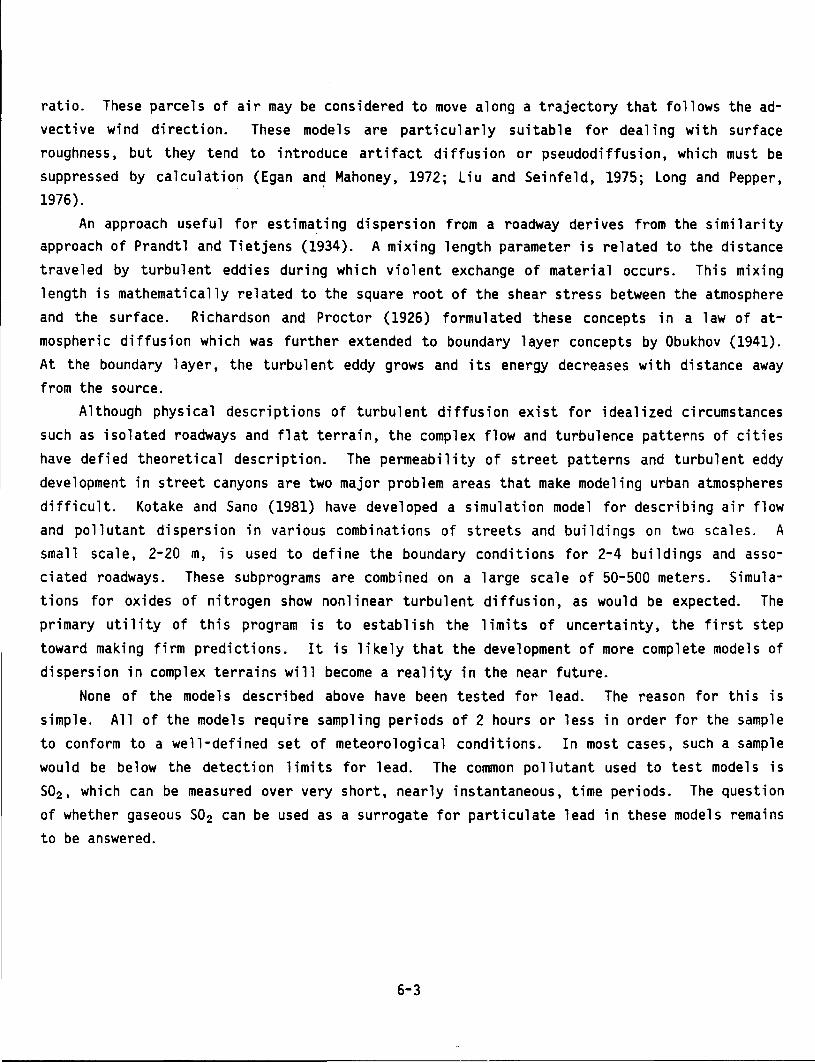
ratio. These parcels of air may be considered to move along a trajectory that follows the advective wind direction. These models are particularly suitable for dealing with surface roughness, but they tend to introduce artifact diffusion or pseudodiffusion, which must be suppressed by calculation (Egan an~ Mahoney, 1972; Liu and Seinfeld, 1975; Long and Pepper, 1976).
An approach useful for estima~ing dispersion from a roadway derives from the similarity approach of Prandtl and Tietjens (1934). A mixing length parameter is related to the distance traveled by turbulent eddies during which violent exchange of material occurs. This mixing length is mathematically related to the square root of the shear stress between the atmosphere and the surface. Richardson and Proctor (1926) formula ted these concepts in a 1 aw of atmospheric diffusion which was further extended to boundary layer concepts by Obukhov (1941).
At the boundary 1 ayer, the turbulent eddy grows and its energy decreases with distance away from the source.
Although physical descriptions of turbulent diffusion exist for idealized circumstances such as isolated roadways and flat terrain, the complex flow and turbulence patterns of cities
have defied theoretical description. The permeability of street patterns and turbulent eddy development in street canyons are two major problem areas that make modeling urban atmospheres
difficult. Kotake and Sano (1981) have developed a simulation model for describing air flow and pollutant dispersion in various combinations of streets and buildings on two scales. A small scale, 2-20 m, is used to define the boundary conditions for 2-4 buildings and associated roadways. These subprograms are combined on a large scale of 50-500 meters. Simulations for oxides of nitrogen show nonlinear turbulent diffusion, as would be expected. The
primary utility of this program is to establish the limits of uncertainty, the first step toward making firm predictions. It is likely that the development of more complete models of dispersion in complex terrains will become a reality in the near future.
None of the models described above have been tested for lead. The reason for this is simple. All of the models require sampling periods of 2 hours or less in order for the sample
to conform to a well-defined set of meteorological conditions. In most cases, such a sample would be below the detection limits for lead. The common pollutant used to test models is
502 , which can be measured over very short, nearly instantaneous, time periods. The question of whether gaseous 502 can be used as a surrogate for particulate lead in these models remains to be answered.
6-3
6.2.2 Influence of Dispersion on Ambient Lead Concentrations Dispersion within confined situations, such as parking garages, residential garages and
tunnels, and away from expressways and other roadways not influenced by complex terrain features depends on emission rates and the volume of clean air available for mixing. These factors are relatively easy to estimate and some effort has been made to describe ambient lead concentrations that can result under selected conditions. On an urban scale, the routes of transport are not clearly defined, but can be inferred from an isopleth diagram, i.e., a plot connecting points of identical ambient concentrations. These plots always show that lead concentrations are maximum where traffic density is highest.
Dispersion beyond cities to regional and remote locations is complicated by the facts that there are no monitoring network data from which to construct isopleth diagrams, that removal by deposition plays a more important role with time and distance, and that emissions from many different sources converge. Some techniques of source reconciliation are described, but these become· less precise with increasing distance from major sources of lead. Dispersion from point sources such as smelters and refineries results in a concentration distribution pattern similar to urban dispersion, although the available data are notably less abundant. 6.2.2.1 Confined and Roadway Situations. Ingalls and Garbe (1982) used a variety of box and Gaussian p 1 ume mode 1 s to ca 1 cul ate typi ca 1 1 eve 1 s of automat i ve air po 11 utants that might be present in microscale (within 100 m of the source) situations with limited ventilation, such as garages, tunnels, and street canyons. Table 6-1 shows a comparison of six exposure situations, recomputed for a flat-average lead emission factor of 6.3 mg/km for roadway situations and 1.0 mg/min for garage situations. The roadway emission factor chosen corresponds roughly to values chosen by Dzubay et al. (1979) and Pierson and Brachaczek (1976) scaled to 1979 lead-use statistics. The parking garage factor was estimated from roadway factors by correction for fuel consumption (Ingalls and Garbe, 1982).
Confined situations, with low air volumes and little ventilation, allow automotive pollutant concentrations to reach one to three orders of magnitude higher than are found in open air. Thus, parking garages and tunnels are likely to have considerably higher ambient lead concentrations than are found in expressways with high traffic density or in city streets. Purdue et al. (1973) found total lead levels of 1.4-2.3 1Jg/m3 in five of six U.S. cities in 1972. In similar samples from an underground parking garage, total lead was 11-12 IJQ/m3 .
Vaitkus et al. (1974) developed a model for the transport of automotive lead that predicted an
exponential decrease in air lead concentrations with distance, up to 100 m downwind from the roadway. Dzubay et al. (1979) found lead concentrations of 4-20 1Jg/m3 in air over Los Angeles freeways in 1976; at nearby sites off the freeways, concentrations of 0.3-4.7 IJQ/m3
were measured.
6-4
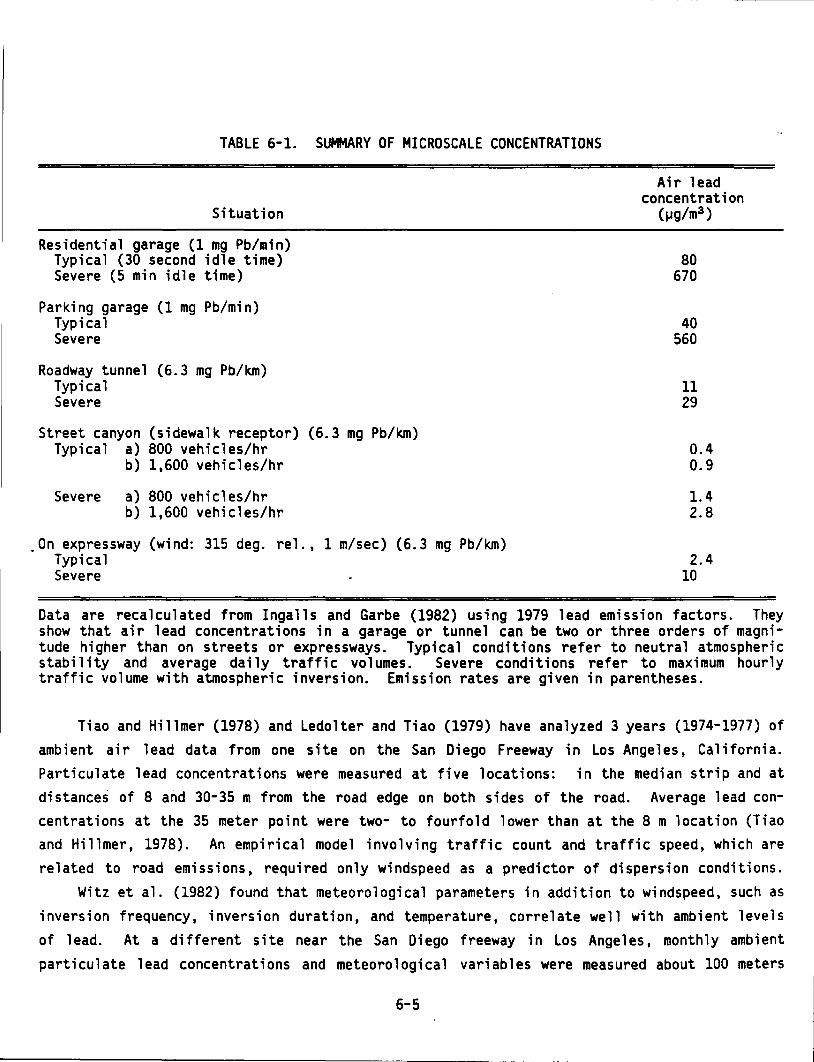
TABLE 6-1. SUMMARY OF MICROSCALE CONCENTRATIONS
Air lead concentration
Situation (~g/m3)
Residential garage (1 mg Pb/min) Typical (30 second idle time) 80 Severe (5 min idle time) 670
Parking garage (1 mg Pb/min) Typical 40 Severe 560
Roadway tunnel (6.3 mg Pb/km) Typical 11 Severe 29
Street canyon (sidewalk receptor) (6.3 mg Pb/km) Typical a) 800 vehicles/hr
b) 1,600 vehicles/hr
Severe a) 800 vehicles/hr b) 1,600 vehicles/hr
.On expressway (wind: 315 deg. rel., 1m/sec) (6.3 mg Pb/km) Typical Severe
0.4 0.9
1.4 2.8
2.4 10
Data are recalculated from Ingalls and Garbe (1982) using 1979 lead emission factors. They show that air lead concentrations in a garage or tunnel can be two or three orders of magnitude higher than on streets or expressways. Typical conditions refer to neutral atmospheric stability and average daily traffic volumes. Severe conditions refer to maximum hourly traffic volume with atmospheric inversion. Emission rates are given in parentheses.
Tiao and Hillmer (1978) and Ledolter and Tiao (1979) have analyzed 3 years (1974-1977) of ambient air lead data from one site on the San Diego Freeway in Los Angeles, California. Particulate lead concentrations were measured at five locations: in the median strip and at distances of 8 and 30-35 m from the road edge on both sides of the road. Average lead concentrations at the 35 meter point were two- to fourfold lower than at the 8 m location (Tiao and Hillmer, 1978). An empirical model involving traffic count and traffic speed, which are related to road emissions, required only windspeed as a predictor of dispersion conditions.
Witz et al. (1982) found that meteorological parameters in addition to windspeed, such as inversion frequency, inversion duration, and temperature, correlate well with ambient levels of lead. At a different site near the San Diego freeway in Los Angeles, monthly ambient particulate lead concentrations and meteorological variables were measured about 100 meters
6-5
~--------------------------------------------------------------------------------------
from the roadway through 1980. Multiple linear regression analysis showed that temperature at 6 AM, windspeed, wind direction, and a surface-based inversion factor were important variables in accurately predicting monthly average lead concentrations. In this data set, lead values for December were about fivefold higher than those measured in the May to September summer season, suggesting that seasonal variations in wind direction and the occurrence of surfacebased inversions favor high winter lead values. Unusually high early morning temperatures and windspeed during the winter increased dispersion and reduced lead concentration.
In a study of a newly constructed freeway near Melbourne, Australia, Clift et al. (1983) found that lead concentrations in the top centimeter of soil one meter from the road edge increased in lead concentration from 60 ~g/g in March 1974 to 1250 ~g/g in November 1980. The traffic density in November 1980 was 37,000 vehicles per day and the typical pattern of lead concentrations decreasing exponentially with distance from the road edge had deve 1 oped. At 4-6 meters from the road edge, 1 ead concentrations decreased to constant va 1 ues, a 1 though these values were significantly higher than the pre-1974 concentrations.
In Philadelphia, a recent study of dispersion away from a major highway showed the zone of influence may extend farther downwind than previously expected (Burton and Suggs, 1984). The Philadelphia Roadway study was designed to measure the vertical (15 m) and horizontal (175m) dispersion of large and small particles (Figure 6-1). Horizontally, air concentrations decreased exponentially at 2m height for fine, coarse, and total Pb according to the
following equations:
Coarse Pb Fine Pb Total Pb
C = 0.187- (0.029 x lnD) C = 0.715- (0.106 X lnD) C = 0.903- (0.135 x lnD)
where C is the concentration of lead in air (~g/m3 ) at the downwind distance, D (m), measured from the edge of the road. The numerical coefficients are specific for this site, and were
found to vary with windspeed and traffic density. Vertical profiles showed decreasing lead concentrations with increasing height for
coarse, fine, and total particulate lead at 5 and 25 m downwind, although the effect was less pronounced at 25m. Bullin et al. (1985) found similar results in Houston, somewhat tempered by greater mixing due to the presence of tall buildings. 6.2.2.2 Dispersion of Lead on an Urban Scale. In cities, air pollutants, including lead,
that are emitted from automobiles tend to be highest in concentration in high traffic areas. Most U.S. cities have a well-defined central business district (CBD) where lead concentrations are highest. To illustrate the dispersion of lead experienced in cities, two cases are
presented below.
6-6
~-~-------
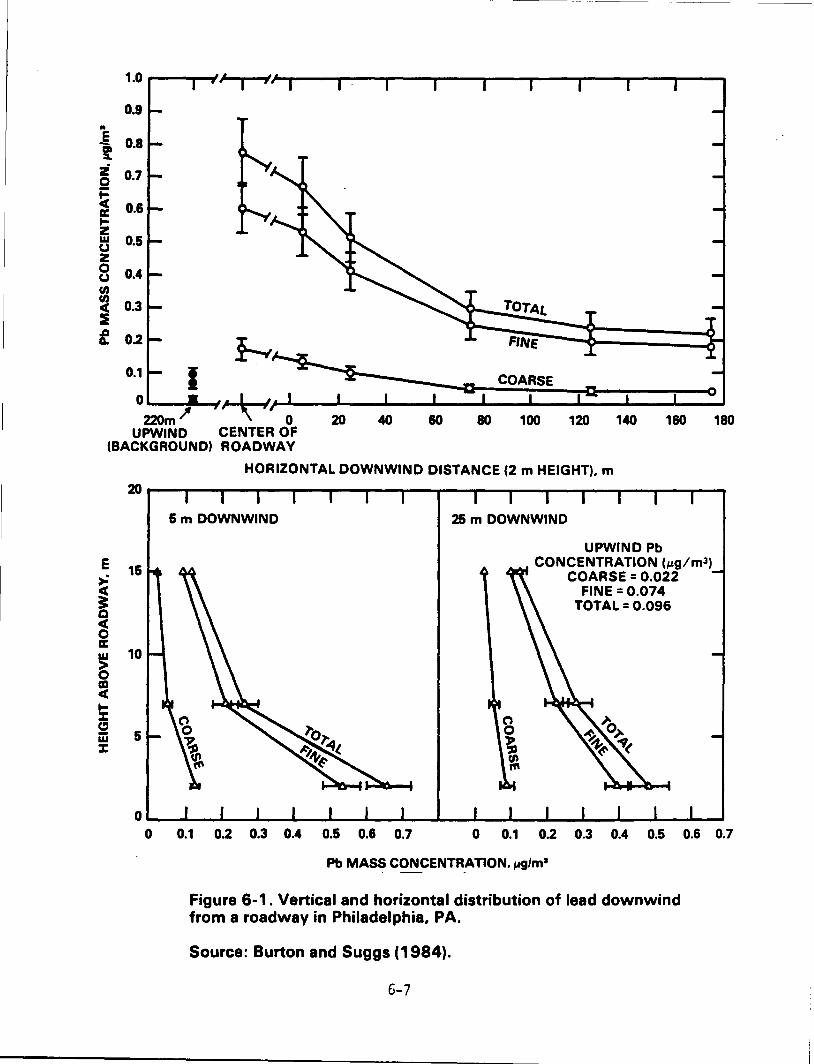
0.9 .. .E ! 0.8
z 0 0.7
~ a: 0.6 ~ z ~ 0.5 z 0 (.) 0.4
~ c 0.3 ::E f. 0.2
0.1
FINE
I 0 0zm __ m __ ?~~~~o~--~~----~-----~*----~*----100~---1~~--1~~~--1~~--~1~
UPWIND CENTER OF (BACKGROUND) ROADWAY
HORIZONTAL DOWNWIND DISTANCE (2m HEIGHT), m
5m DOWNWIND
0 0.1 0.2 0.3 0.4 0.5 0.6 o. 7
25 m DOWNWIND
UPWIND Pb CONCENTRATION (#lg/ml)
COARSE = 0.022 FINE =0.074
TOTAL= 0.096
0 0.1 0.2 0.3 0.4 0.5 0.6 0. 7
Pb MASS CONCENTRATION. ,..glm1
- -
Figure 6-1 . Vertical and horizontal distribution of lead downwind from a roadway in Philadelphia, PA.
Source: Burton and Suggs (1984).
6-7
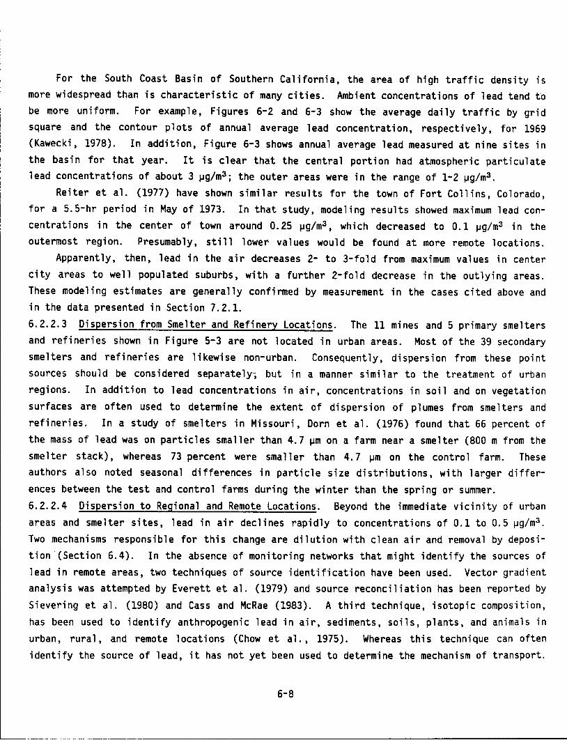
For the South Coast Basin of Southern California, the area of high traffic density is more widespread than is characteristic of many cities. Ambient concentrations of lead tend to be more uniform. For example, Figures 6-2 and 6-3 show the average daily traffic by grid square and the contour p 1 ots of annua 1 average 1 ead concentration, respectively, for 1969 (Kawecki, 1978). In addition, Figure 6-3 shows annual average lead measured at nine sites in the basin for that year. It is clear that the central portion had atmospheric particulate lead concentrations of about 3 ~g/m3 ; the outer areas were in the range of 1-2 ~g/ma.
Reiter et al. (1977) have shown similar results for the town of Fort Collins, Colorado, for a 5.5-hr period in May of 1973. In that study, modeling results showed maximum lead concentrations in the center of town around 0. 25 ~g/m3 , which decreased to 0.1 ~g/m3 in the outermost region. Presumably, still lower values would be found at more remote locations.
Apparently, then, lead in the air decreases 2- to 3-fold from maximum values in center city areas to well populated suburbs, with a further 2-fold decrease in the outlying areas. These modeling estimates are generally confirmed by measurement in the cases cited above and in the data presented in Section 7.2.1.
6.2.2.3 Dispersion from Smelter and Refinery Locations. The 11 mines and 5 primary smelters and refineries shown in Figure 5-3 are not located in urban areas. Most of the 39 secondary sme 1 ters and refineries are 1 i kewi se non-urban. Consequently, dispersion from these point sources should be considered separately-, but in a manner similar to the treatment of urban regions. In addition to lead concentrations in air, concentrations in soil and on vegetation surfaces are often used to determine the extent of dispersion of p 1 umes from sme 1 ters and refineries. In a study of smelters in Missouri, Darn et al. (1976) found that 66 percent of the mass of lead was on particles smaller than 4.7 ~mona farm near a smelter (800 m from the smelter stack), whereas 73 percent were smaller than 4. 7 ~m on the control farm. These authors also noted seasonal differences in particle size distributions, with larger differences between the test and control farms during the winter than the spring or summer. 6.2.2.4 Dispersion to Regional and Remote Locations. Beyond the immediate vicinity of urban areas and smelter sites, lead in air declines rapidly to concentrations of 0.1 to 0.5 ~g/m3 .
Two mechanisms responsible for this change are dilution with clean air and removal by deposition (Section 6.4). In the absence of monitoring networks that might identify the sources of lead in remote areas, two techniques of source identification have been used. Vector gradient analysis was attempted by Everett et al. (1979) and source reconciliation has been reported by
Sievering et al. (1980) and Cass and McRae (1983). A third technique, isotopic composition, has been used to identify anthropogenic lead in air, sediments, soils, plants, and animals in urban, rura 1 , and remote 1 ocat ions (Chow et a 1. , 1975). Whereas this technique can often identify the source of lead, it has not yet been used to determine the mechanism of transport.
6-8
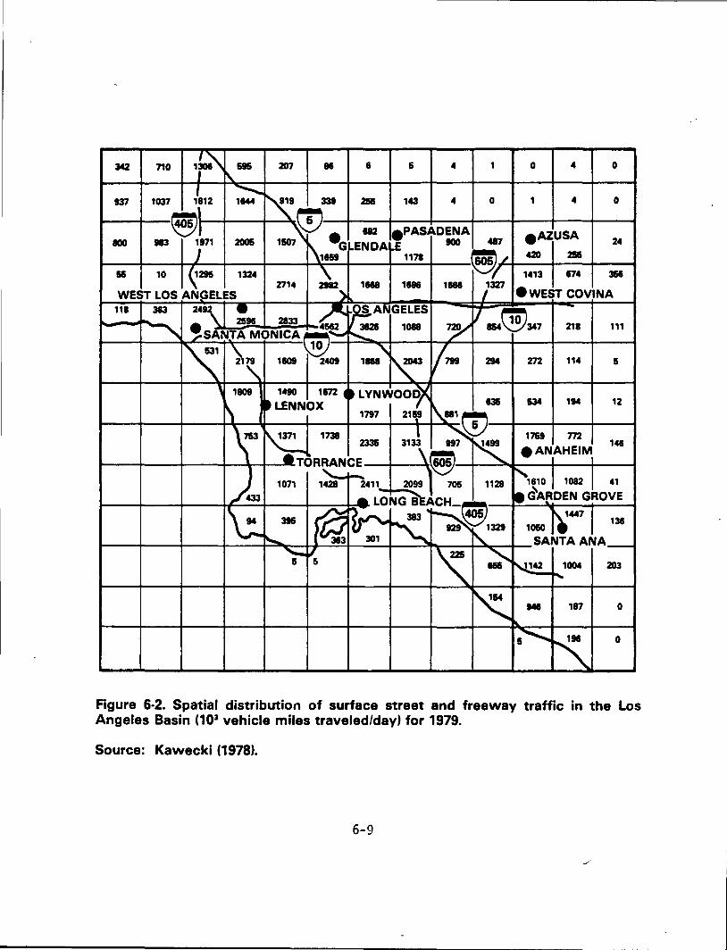
710 fe"',- 207 .. • 5 4 1 0 4 0
137 1037 ,'812 ~I'\: 338 - 143 4
1---1---~A ,\!? 192 .PASADENA SA 100 183 1111 2005 11101\\ •Gr-ENDA E 100 487 eAZU
1 1151 1178 a L 420 -
5I 10 {1215 1324 .\_ '/' 1413 174
1 4 0
24
0
-\ 2714 2182 1518 1118 1518 1327 WEST LOS ANGELES -) / ewEST COVINA
118 383 241~ • A .OS AI\ GELES I ~ • \...
2511. 2833 4562 r:. 1088 720/ 854~347 218 111
' ,sANTA MONICA®"""~ / "" \' ,.. 10_-~1:::11818 .... ,.-+i'!:-2043--+lf-,799~--+--294--f-.-272--+--1-14--4--5--t
' 1809 1490 1172 4. LYNWOOd)( ~ t LENNOX 1797 21~ , [\aa1 f""51131 534 114 12
753 '1371 1738 _! ...........,v:v 1759 772 ~ 2335 3133\ 197 ~99 • ANAHEIM 141
~--~---+------~~~~·aTORRANCE ~ ~ I I
J 1011 1428- 2411 2099 705 1128 r"1110 J 1082 l 41
\;./433 ~~~~N~:.~~@ .G'Af1~~:7GR,OVE
- I u-___ -~-- I ~~ 1329 1050 ~~ 136
"""' 383 301 I "" ' SANTA ANA
15 5 225
- N,142 1004 203 ~~ "~ ·--,
' 141 117 0
0
Figure 6-2. Spatial distribution of surface street and freeway traffic in the Los Angeles Basin (103 vehicle miles traveled/day) for 1979.
Source: Kawecki (1978).
6-9
.. /
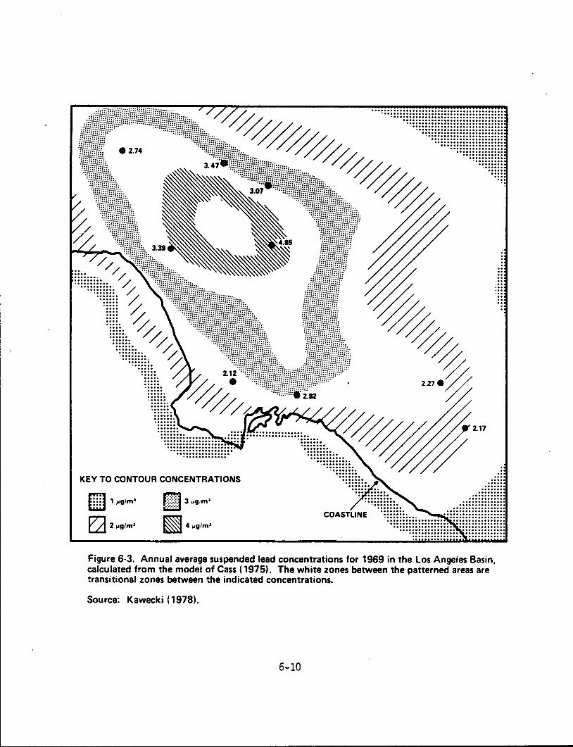
~ 1"gtm• ~
EL)z"gtm•
.............. . .. ········ ..... ... .... .. . .. ..... .. . .. .. ... . . .. .. . .. . .. .. . ..
.. . .. . . .. ... ..
Figure 6-3. Annual average suspended lead concentrations for 1969 in the Los Angeles Basin, calculated from the model of Cass ( 1975). The white zones between the patterned areas are transitional zones between the indicated concentrations.
Source: Kawecki (1978).
6-10
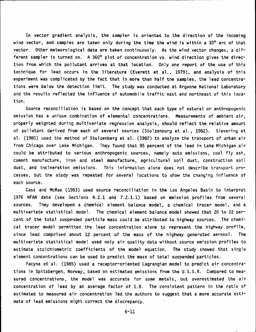
In vector gradient analysis, the sampler is oriented to the direction of the incoming wind vector, and samples are taken only during the time the wind is within a 30° arc of that vector. Other meteorological data are taken continuously. As the wind vector changes, a different sampler is turned on. A 360° plo~ of concentration vs. wind direction gives the direction from which the pollutant arrives at that location. Only one report of the use of this technique for lead occurs in the· literature (Everett et al., 1979), and analysis of this experiment was complicated by the fact that in more than half the samples, the lead concentrations were below the detection limit. The study was conducted at Argonne National Laboratory and the results reflected the influence of automobile traffic east and northeast of this location.
Source reconciliation is based on the concept that each type of natural or anthropogenic emission has a unique combination of elemental concentrations. Measurements of ambient air, properly weighted during multivariate regression analysis, should reflect the relative amount of pollutant derived from each of several sources (Stolzenburg et al., 1982). Sievering et al. (1980) used the method of Stolzenberg et al. (1982) to analyze the transport of urban air from Chicago over Lake Michigan. They found that 95 percent of the lead in Lake Michigan air could be attributed to various anthropogenic sources, namely auto emissions, coal fly ash, cement manufacture, iron and steel manufacture, agricultural soil dust, construction soil dust, and incineration emissions. This information alone does not describe transport processes, but the study was repeated for severa 1 1 ocat ions to show the changing influence of each source.
Cass and McRae (1983) used source reconciliation in the Los Angeles Basin to interpret 1976 NFAN data (see Sections 4.2.1 and 7.2.1.1) based on emission profiles from several sources. They deve 1 oped a chemica 1 e 1 ement ba 1 ance mode 1 , a chemica 1 tracer mode 1 , and a multivariate statistical model. The chemical element balance model showed that 20 to 22 percent of the total suspended particle mass could be attributed to highway sources. The chemical tracer model permitted the lead concentration alone to represent the highway profile, since lead comprised about 12 percent of the mass of the highway generated aerosol. The multivariate statistical model used only air quality data without source emission profiles to estimate stoichiometric coefficients of the model equation. The study showed that single element concentrations can be used to predict the mass of total suspended particles.
Pacyna et al. (1985) used a receptor-oriented Lagrangian model to predict air concentra
tions in Spitsbergen, Norway, based on estimated emissions from the U.S.S.R. Compared to measured concentrations, the model was accurate for some metals, but overestimated the air concentration of lead by an average factor of 1.8. The consistent pattern in the ratio of estimated to measured air concentration led the authors to suggest that a more accurate estimate of lead emissions might correct the discrepancy.
6-11
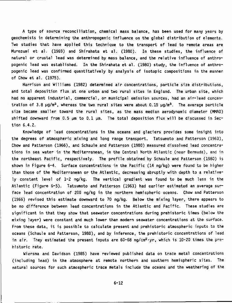
A type of source reconciliation, chemical mass balance, has been used for many years by geochemists in determining the anthropogenic influence on the global distribution of elements. Two studies that have app 1 i ed this technique to the transport of 1 ead to remote areas are Murozumi et al. (1969) and Shirahata et al. (1980). In these studies, the influence of natural or crustal lead was determined by mass balance, and the relative influence of anthropogenic lead was established. In the Shirahata et al. (1980) study, the influence of anthropogenic lead was confirmed quantitatively by analysis of isotopic compositions in the manner of Chow et al. (1975).
Harrison and Williams (1982) determined air concentrations, particle size distributions, and total deposition flux at one urban and two rural sites in England. The urban site, which had no apparent industrial, commercial, or municipal emission sources, had an air-lead concentration of 3.8 ~g/m3 , whereas the two rural sites were about 0.15 ~g/m3 . The average particle size became smaller toward the rural sites, as the mass median aerodynamic diameter (MMAD) shifted downward from 0.5 ~m to 0.1 ~m. The total deposition flux will be discussed in Section 6.4.2.
Knowledge of lead concentrations in the oceans and glaciers provides some insight into the degrees of atmospheric mixing and long range transport. Tatsumoto and Patterson (1963), Chow and Patterson (1966), and Schaule and Patterson (1980) measured dissolved lead concentrations in sea water in the Mediterranean, i~ the Central North Atlantic (near Bermuda), and in the northeast Pacific, respectively. The profile obtained by Schaule and Patterson (1980) is shown in Figure 6-4. Surface concentrations in the Pacific (14 ng/kg) were found to be higher than those of the Mediterranean or the Atlantic, decreasing abruptly with depth to a relatively constant level of 1-2 ng/kg. The vertical gradient was found to be much less in the Atlantic (Figure 6-5). Tatsumoto and Patterson (1963) had earlier estimated an average surface lead concentration of 200 ng/kg in the northern hemispheric oceans. Chow and Patterson (1966) revised this estimate downward to 70 ng/kg. Below the mixing layer, there appears to be no difference between lead concentrations in the Atlantic and Pacific. These studies are significant in that they show that seawater concentrations during prehistoric times (below the mixing layer) were constant and much lower than modern seawater concentrations at the surface. From these data, it is possible to calculate present and prehistoric atmospheric inputs to the oceans (Schaule and Patterson, 1980), and by inference, the prehistoric concentrations of lead in air. They estimated the present inputs are 60-68 ng/cm2 ·yr, which is 10-20 times the prehistoric rate.
Wiersma and Davidson (1985) have reviewed pub 1 i shed data on trace meta 1 concentrations (including lead) in the atmosphere at remote northern and southern hemispheric sites. The natural sources for such atmospheric trace metals include the oceans and the weathering of the
6-12
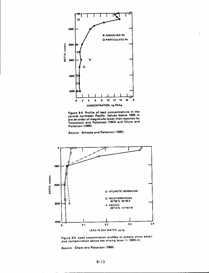
.. a; i E
1000
::i 2000
~ ... 0
3000
.. a; Oi E
::t' 1-ll. ... 0
1000
e DISSOLVED Pb
C PARTICULATE Pb
2000
3000 c
c
4000
0 2 c 6 8 10 12 1C 16 0
CONCENTRATION. ng Pblkg
Figure 6-4. Profile of lead concentrations in the central northeast Pacific. Values below 1000 m are an order of magnitude lower than reported by Tatsumoto and Patterson 11963) and Chow and Patterson 11966).
Source: Schaule and Patterson 11980!.
0 ATLANTIC IBERMUDAI
0 MEDITERR/\1\!EAN C0"39'N. 05°48'E
6 PACIFIC 29°13'N, 117"37'W
·000~4-------~------------~----------L---------~ o.c 0 01 0.2 03
LEAD IN SEA WATER. .,g kg
Figure 6·5. Lead concentration profiles in oceans show exten· sive contamination above the mixing layer (rv 1000 ml
Source: Chow and Patterson 119661.
6-13
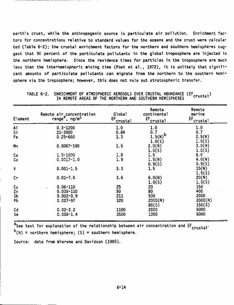
earth 1 s crust, while the anthropogenic source is particulate air pollution. Enrichment factors for concentrations relative to standard values for the oceans and the crust were calculated (Table 6-2); the crustal enrichment factors for the northern and southern hemispheres suggest that 90 percent of the particulate pollutants in the global troposphere are injected in the northern hemisphere. Since the residence times for particles in the troposphere are much less than the interhemispheric mixing time (Poet et al., 1972), it is unlikely that significant amounts of particulate pollutants can migrate from the northern to the southern hemisphere via the troposphere; however, this does not rule out stratospheric transfer.
TABLE 6-2. ENRICHMENT OF ATMOSPHERIC AEROSOLS OVER CRUSTAL ABUNDANCE (EFcrustal) IN REMOTE AREAS OF THE NORTHERN AND SOUTHERN HEMISPHERES
Remote Remote Remote air concentration Global continental marine
Element rangea, ng/m3 EFcrustal EFcrustal EFcrustal
Al 0.3-1200 1.0 1.0 1.0 Si 21-3900 0.84 0.7 b 0.7 Fe 0.25-660 1.3 1. 5(N) 2.5(N)
1.0(5) 1.0(5) Mn 0.0067-190 1.5 2.0(N) 3.0(N)
1.0(5) 1. 0(5) Ca 1.9-1600 1.8 1.5 8.0 Co 0. 0017-1.0 1.9 1. 5(N) 4.0(N)
0.9(5) 0.9(5) v 0.001-1.5 3.3 1.5 15(N)
1. 5(5) Cr 0.01-7.0 3.6 6.0(N) 20(N)
1. O(S) 1. 0(5) Cu 0.06-110 25 20 150 Zn 0.035-110 50 80 400 Sb 0.002-0.9 211 500 2000 Pb 0.027-97 320 2000(N) 2000(N)
80(S) 150(S) Cd 0.02-2.2 1100 2000 5000 Se 0. 006-1.4 3500 1000 6000
aSee text for explanation of the relationship between air concentration and EFcrustal" b(N) = northern hemisphere; (5) = southern hemisphere.
Source: data from Wiersma and Davidson (1985).
6-14
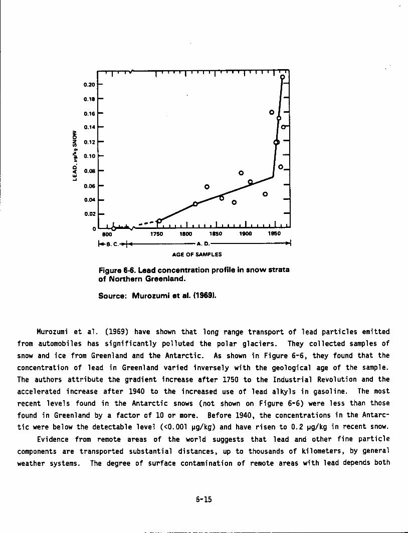
! ~ Cll .. -Cll :a. Q c "' .J
0.20
0.18
0.16
0.14
0.12
0.10
0.08
0.06
0.04
800 1750 1800 1850 1900
~B. c.-...+-------A. o.--------+-~
AGE OF SAMPLES
Figure 6-6. Lead concentration profile in snow strata of Northern Greenland.
Source: Murozumi at al. (1969).
Murozumi et al. (1969) have shown that long range transport of lead particles emitted
from automobiles has significantly polluted the polar glaciers. They collected samples of
snow and ice from Greenland and the Antarctic. As shown in Figure 6-6, they found that the
concentration of lead in Greenland varied inversely with the geological age of the sample.
The authors attribute the gradient increase after 1750 to the Industrial Revolution and the
acce 1 era ted increase after 1940 to the increased use of 1 ead a 1 ky 1s in gaso 1 i ne. The mast
recent levels found in the Antarctic snows (not shown on Figure 6-6) were less than those
found in Greenland by a factor of 10 or more. Before 1940, the concentrations in the Antarc
tic were below the detectable level (<0.001 ~g/kg) and have risen to 0.2 ~g/kg in recent snow.
Evidence from remote areas of the world suggests that lead and other fine particle
components are transported substantia 1 distances, up to thousands of ki 1 ometers, by genera 1
weather systems. The degree of surface contamination of remote areas with lead depends both
6-15
on weather influences and on the degree of air contamination. However, even in remote areas, man•s primitive activities can play an important role in atmospheric lead levels. Davidson et al. (1982) have shown that there are significant levels of fine particle lead, up to 0.5 ~g/m3 , in remote villages in Nepa 1. The apparent source is combustion of dried yak dung, which contains small amounts of naturally occurring lead derived from plant life in those remote valleys.
6.3 TRANSFORMATION OF LEAD IN AIR 6.3.1 Particle Size Distribution
Whitby et al. (1975) placed atmospheric particles into three different size regimes: the nuclei mode (<0.1 ~m), the accumulation mode (0.1-2 ~m) and the large particle mode (>2 ~m). At the source, lead particles are generally in the nuclei and large particle modes. Large particles are removed by deposition close to the source and particles in the nuclei mode diffuse to surfaces or agglomerate while airborne to form larger particles of the accumulation mode. Thus it is in the accumulation mode that parti·cles are dispersed great distances.
Pierson and Brachaczek (1983) reported particle size distributions for ambient air that were skewed farther to the right (more large particles) than in a roadway tunnel, where vehicle exhaust must be dominant (Figure 6-7).- The large particles may have been deposited in the roadway itself and small particles may have agglomer·ated during transport away from the roadway (see Section 5.3.3.1). Since 40 to 1,000 ~m particles are found in gutter debris, deposition of large particles appears confirmed (Pierson ctnd Brachaczek, 1976, 1983).
Particle size distributions reported by Huntzicker et al. (1975) show bimodal distributions for on-roadway samples, with peak mass values at about 0.1 and 10 ~m. For off-roadway Pasadena samples, there is no evidence of bimodality and only a broad maximum in lead mass between 0.1 and 1 ~m.
In cities or in rural areas, there is a remarkable consistency in lead particle size range. For example, Robinson and Ludwig (1964) report cascade impactor MMAD values for lead ranging from 0.23 to 0.3 ~m in six U.S. cities and three rural areas. Stevens et al. (1978) have reported dichotomous sampler data for six U.S. cities, as shown in Table 6-3, and Stevens et al. (1980, 1982) have reported similar results for remc•te locations. Virtually every other study reported in the literature for Europe, South America, and Asia has come to the conclusion that ambient urban and rural air contains predominantly fine particles (Cholak et al., 1968; De Jonghe and Adams, 1980; Durando and Aragon, 1982; Lee et a 1. , 1968; Htun and Ramachandran, 1977). The size distributions of lead-bearing particles in ambient air from several global locations are discussed further in Section 7.2.1.3.1 and shown in Figure 7-5.
6-16
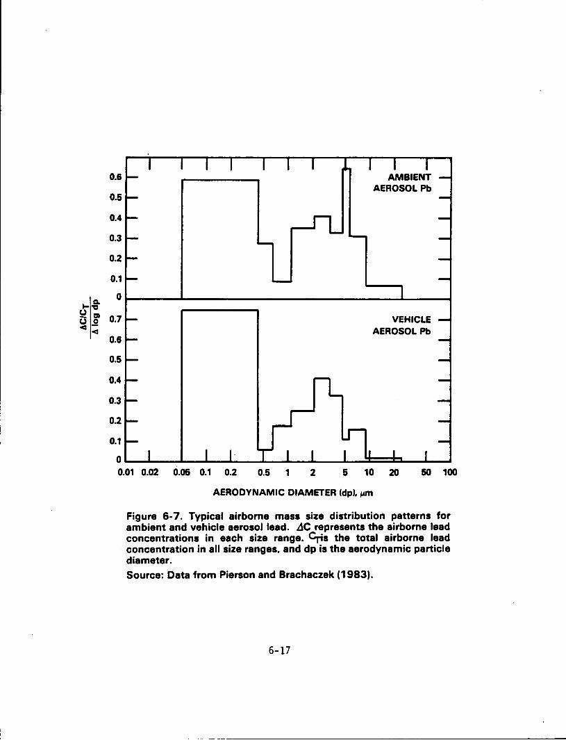
Q.
2 , = u .S! ~ ~
0.6
0.5
0.4
0.3
0.2
0.1
0
0.7
0.6
0.5
0.4
0.3
0.2
0.1
0
VEHICLE AEROSOL Pb
0.01 0.02 0.05 0.1 0.2 0.5 1 2 5 10 20
AERODYNAMIC DIAMETER (dp), ~
50 100
Figure 6-7. Typical airborne mass size distribution patterns for ambient and vehicle aerosol lead. ~C represents the airborne lead concentrations in each size range. Cr;s the total airborne lead concentration in all size ranges. and dp is the aerodynamic particle diameter. Source: Data from Pierson and Brachaczek (1983).
6-17
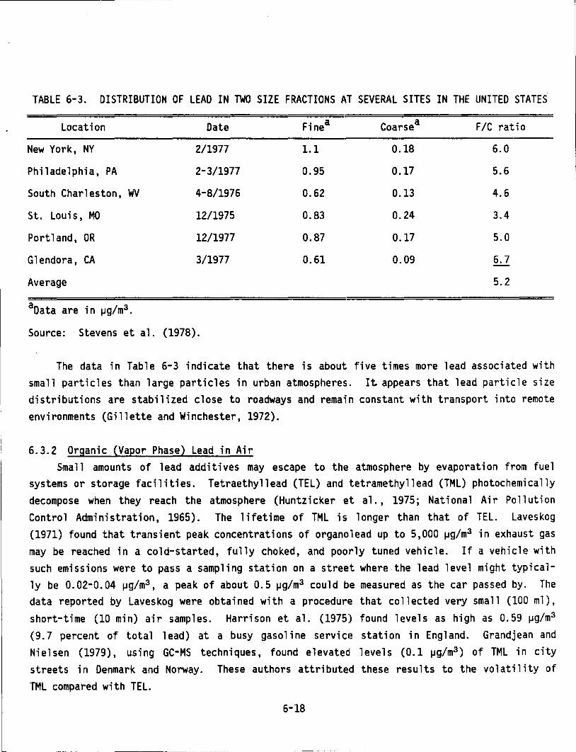
TABLE 6-3. DISTRIBUTION OF LEAD IN TWO SIZE FRACTIONS AT SEVERAL SITES IN THE UNITED STATES
Location Date Fine a Coarse a F/C ratio
New York, NY 2/1977 1.1 0.18 6.0
Philadelphia, PA 2-3/1977 0.95 0.17 5.6
South Charleston, wv 4-8/1976 0.62 0.13 4.6
St. Louis, MO 12/1975 0.83 0.24 3.4
Portland, OR 12/1977 0.87 0.17 5.0
Glendora, CA 3/1977 0.61 0.09 6.7
Average 5.2
aData are in ~g/m3 •
Source: ·Stevens et al. (1978).
The data in Table 6-3 indicate that there is about five times more lead associated with small particles than large particles in urban atmospheres. It appears that lead particle size distributions are stabilized close to roadways and remain constant with transport into remote environments (Gillette and Winchester, 1972).
6.3.2 Organic (Vapor Phase) Lead in Air Small amounts of lead additives may escape to the atmosphere by evaporation from fuel
systems or storage facilities. Tetraethyllead (TEL) and tetramethyllead (TML) photochemically decompose when they reach the atmosphere (Huntzicker et al., 1975; National Air Pollution Control Administration, 1965). The lifetime of TML is longer than that of TEL. Laveskog (1971) found that transient peak concentrations of organolead up to 5,000 ~g/m3 in exhaust gas may be reached in a cold-started, fully choked, and poorly tuned vehicle. If a vehicle with such emissions were to pass a sampling station on a street where the lead level might typically be 0.02-0.04 ~g/m3 , a peak of about 0.5 ~g/m3 could be measured as the car passed by. The data reported by Laveskog were obtained with a procedure that collected very small (100 ml), short-time (10 min) air samples. Harrison et al. (1975) found levels as high as 0.59 ~g/m3
(9.7 percent of total lead) at a busy gasoline servicl! station in England. Grandjean and Nielsen (1979), using GC-MS techniques, found elevated levels (0.1 ~g/m3 ) of TML in city streets in Denmark and Norway. These authors attributed these results to the volatility of TML compared with TEL.
6-18
A number of studies have used gas absorbers behind fi 1 ters to trap vapor-phase 1 ead compounds (see Section 4.2.2.5). Because it is not clear that all the lead captured in the backup traps is, in fact, in the vapor phase in the atmosphere, "organic" or "vapor phase" lead is an operational definition in these studies .. Purdue et al. (1973) measured both particulate and organic lead in atmospheric samples. They found that the vapor phase lead was about 5 percent of the total lead in most samples (see Section 5.3.3.1). The results are consistent with the studies by Huntzicker et al. (1975) who reported an organic component of 6 percent of the total airborne lead in Pasadena for a 3-day period in June, 1974, and by Skogerboe (1976), who measured fractions in the range of 4 to 12 percent at a site in Fort Collins, Colorado. It is noteworthy, however, that in an underground garage, total lead concentrations were approximately five times greater than those in ambient urban atmospheres, and the organic lead increased to approximately 17 percent.
Harrison et al. (1979) report typical organolead percentages in ambient urban air of 1-6 percent. Rohbock et al. (1980) reported higher fractions, up to 20 percent, but the data and interpretations have been questioned by Harrison and Laxen (1981). Rohbock et al. (1980) and De Jonghe and Adams (1980) report one to two orders of magnitude decrease in organolead concentrations from the central urban areas to residential areas. A review by Nielsen (1984) documents the concentrations of organolead in partially enclosed areas such as gas stations, parking garages, car repair shops, and tunnels, and in open urban and rural areas in the U.S. and Europe. Mean concentrations varied from 0.15 to 3.5 ~g organolead/m3 in enclosed areas and 0.014 to 0.47 in open urban areas.
6.3.3 Chemical Transformations of Inorganic Lead in Air Lead is emitted into the air from automobiles as lead halides and as double salts with
ammonium halides (e.g., PbBrCl • 2NH4 Cl). From mines and smelters, PbS04 , PbO·PbS04 , and PbS appear to be the dominant species. In the atmosphere, lead is present mainly as the sulfate with minor amounts of halides. It is not completely clear just how the chemical composition changes in transport.
Biggins and Harrison (1978, 1979) have studied the chemical composition of lead particles in exhaust and in city air in England by X-ray diffractometry. These authors reported that the dominant exhaust forms were PbBrCl, PbBrC1·2NH4Cl, and a-2PbBrCl·NH4Cl, in agreement with the earlier studies of Hirschler and Gilbert (1964) and TerHaar and Bayard (1971).
At sampling sites in Lancaster, England, Biggins and Harrison (1978, 1979) found PbS04 ·(NH4 hS04 , and PbS04 ·(NH4 ) 2 BrCl together with minor amounts of the lead halides and double salts found in auto exhaust. These authors suggested that emitted lead halides react with acidic gases or aerosol components (502 or H2 S04 ) on filters to form substantial levels
6-19
2-of sulfate salts. It is not clear whether reactions with S04 occur in the atmosphere or on the sample filter.
The ratio of Br to Pb is often cited as an indication of automotive emissions. From the mixtures commonly used in gasoline additives, the mass Br/Pb ratio should be 0.4-0.5 (Pierson and Brachaczek, 1976, 1983; Dzubay et al., 1979; Dietzmann et al., 1981; Lang et al., 1981). However, several authors have reported loss of halide, preferentially bromine, from lead salts in atmospheric transport (Dzubay and Stevens, 1973; Pi errard, 1969; Ter Haar and Bayard, 1971). Both photochemical decomposition (Lee et al., 1971; TerHaar and Bayard, 1971) and acidic gas displacement (Robbins and Snitz, 1972) have been postulated as mechanisms. Chang et al. (1977) have reported only very slow decomposition t>f lead bromochloride in natural sunlight; currently the acid displacement of halide seems to be the most likely mechanism. o•connor et al. (1977) have compared roadside and suburban-rural aerosol samples from western Australia and reported no loss in bromine; low levels of 502 and sulfate aerosol could account for that result. Harrison and Sturges (1983) warn of several other factors that can alter the Br/Pb ratio. Bromine may pass through the filter as hydrogen bromide gas, lead may be retained in the exhaust system, or bromine may be added to the atmosphere from other sources, such as marine aerosols. They concluded that Br/Pb ratios are only crude estimates of automobile emissions, and that this ratio would decrease with d'istance from the highway from 0.39 to 0.35 at less proximate sites to 0.25 in suburban residential areas. For an aged aerosol, the Br/Pb mass ratio is usually about 0.22.
Habibi et al. (1970) studied the composition of auto exhaust particles as a function of particle size. Their main conclusions follow:
1. Chemical composition of emitted exhaust particles is related to particle size.
a. Very large particles, greater than 200 ~m, have a composition similar to lead-containing material deposited in the exhaust system, confirming that they have been emitted from the exhaust system. These particles contain approximately 60 to 65 percent lead salts. 30 to 35 percent ferric oxide (Fe203 ), and 2 to 3 percent soot and cat·bonaceous material. The major lead salt is lead bromochloride (PbBrCl), with (15 to 17 percent) lead oxide (PbO) occurring as the 2PbO·PbBrCl double salt. Lead sulfate and 1 ead phosphate account for 5 to 6 percEmt of these deposits. (These compositions resulted from the combustion of low-sulfur and low-phosphorus fuel.)
b. PbBrCl is the major lead salt in particles of 2 to 10 ~m equivalent diameter, with 2PbBrCl•NH4Cl present as a minor constituent.
c. Submicrometer-sized lead salts are primarily 2PbBrCl·NH4Cl.
6-20
2. Lead-halogen molar ratios in particles of less than 10 !Jm MMAD indicate that much more halogen is associated with these solids than the amount expected from the presence of 2PbBrCl·NH4 Cl, as identified by X-ray diffraction. This is particularly true for particles in the 0.5 to 2 j.lm size range.
3. There is considerably more soot and carbonaceous material associated with fine-mode particles than with coarse mode particles re-entrained after having been deposited following emission from the exhaust system. This carbonaceous material accounts for 15 to 20 percent of the fine particles.
4. Particulate matter emitted under typical driving conditions is rich in carbonaceous material. There is substantially less material emitted under continuous hot operation.
5. Only small quantities of 2PbBrCl·NH4 Cl were found in samples collected at the tailpipe from the hot exhaust gas. Its formation therefore takes place primarily during cooling and mixing of exhaust with ambient air.
Foster and Lott (1980) used X-ray diffractometry to study the composition of lead compounds associated with ore handling, sintering, and blast furnace operations around a lead smelter in Missouri. Lead sulfide was the main constituent of those samples associated with ore handling and fugitive dust from open mounds of ore concentrate. The major constituents from sintering and blast furnace operations appeared to be PbS04 and PbO·PbS04 , respectively.
6.4 REMOVAL OF LEAD FROM THE ATMOSPHERE Before atmospheric lead can have any effect on organisms or ecosystems, it must be trans
ferred from the air to a surface by wet or dry deposition.
6.4.1 Dry Deposition 6.4.1.1 Mechanisms of Dry Deposition. The theory and mechanics of particle deposition from the atmosphere to smooth surfaces are fairly well understood (Friedlander, 1977). Transfer by dry deposition requires that the particle move from the main airstream through the boundary layer to a surface. The boundary layer is defined as the region of minimal air flow immediately adjacent to that surface. The thickness of the boundary layer depends mostly on the windspeed and roughness of the surface. Schack et al. (1985) have extended particle deposition theory to include completely rough surfaces, such as terrestrial surfaces.
Airborne particles do not follow a smooth, straight path in the airstream. On the con
trary, the path of a particle may be affected by micro-turbulent air currents, gravitation, or inertia. There are several mechanisms that may alter the particle path enough to cause transfer to a surface. These mechanisms are a function of particle size, windspeed, and surface
characteristics.
6-21
Particles larger than a few micrometers in diameter are influenced primarily by sedimentation, where the particle accelerates downward until aerodynamic drag is exactly balanced by gravitational force. The particle continues at this velocity until it reaches a surface.
· Sedimentation is not influenced by horizontal windspeed or surface characteristics. Particles moving in an airstream may be removed by impaction whenever they are unable to follow the airstream around roughness elements of the surface, such as leaves, branches, or tree trunks. In this case, the particle moves parallel to the airstream and strikes a surface perpendicular to the airstream. A related mechanism, turbulent inertial deposition, occurs when a particle encounters turbulence within the airstream causing the particle to move perpendicular to the airstream. It may then strike a surface parallel to the airstream. In two mechanisms, wind eddy diffusion and interception, the particle remains in the airstream until it is transferred to a surface. With wind eddy diffusion, the particle is transported downward by turbulent eddies. Interception occurs when the particle in the airstream passes within one particle radius of a surface. This mechanism is more a function of particle size than windspeed. The final mechanism, Brownian diffusion, is important for ve~ry small particles at very low windspeeds. Brownian diffusion is motion, caused by random collision with molecules, in the direction of a decreasing concentration gradient.
Transfer from the main airstream to the boundary layer is usually by sedimentation or wind eddy diffusion. From the boundary layer to the su1·face, transfer may be by any of the six mechanisms, although those that are independent of windspeed (sedimentation, interception, Brownian diffusion) are more likely. Determining deposition onto rough surfaces requires information of the height, shape and density of protrusions from the surface into the boundary layer (Schack et al., 1985). If dry deposition is seen as a two-step process, diffusion through the boundary layer and interception by the surfac1~, then for rough surfaces with rapid eddy diffusion, interception by the protrusion surfaces becomes the rate-limiting step. Consequently, surfaces such as water, grass, or bare rod~s can be evaluated using a general correlation with a reference surface (Schack et al., 1985), and a more complete understanding of dry deposition to natural surfaces may be possible with the application of these experimental results. 6.4.1.2 Dry deposition models. A particle influenced on'ly by sedimentation may be considered to be moving downward at a specific velocity usually expressed in em/sec. Similarly, particles transported to a surface by any mechanism are said to have an effective deposition velocity (Vd), which is an expression of the rate of particlt! mass transfer measured by accumulation on a surface as a function of time and air concentration. This relationship is expressed in the equation:
6-22
(6-1)
where J is the flux or accumulation expressed in ng/cm2 ·s and C is the air concentration in ng/cm3 . The units of Vd become em/sec.
Several recent models of dry deposition have evolved from the theoretical discussion of Fuchs (1964) and the wind tunnel experiments of Chamberlain (1966). From those early works, it was obvious that the transfer of particles from the atmosphere to the Earth's surface involved more than rain or snow. The models of Slinn (1982) and Davidson et al. (1982) are particularly useful for lead deposition and were strongly influenced by the theoretical discussions of fluid dynamics by Friedlander (1977). Slinn's model considers a multitude of vegetation parameters to find several approximate solutions for particles in the size range of 0.1-1.0 ~m. In the absence of appropriate field studies, Slinn (1982) estimates deposition velocities of 0.01-0.1 em/sec.
The model of Davidson et al. (1982) is based on detailed vegetation measurements and wind data to predict a Vd of 0.05-1.0 em/sec. Deposition velocities are specific for each vegetation type. This approach has the advantage of using vegetation parameters of the type made for vegetation analysis in ecological studies (density, leaf area index (LAI), height, diameter) and thus may be applicable to a broad range of vegetation types for which data are already available in the ecological literature.
Both models show a decrease in deposition velocity with decreasing particle size down to about 0.1-0.2 ~m, followed by an increase in Vd with decreasing diameter from 0.1 to 0.001 em/sec. On a log plot of Vd versus diameter, this curve is v-shaped (Sehmel, 1980), and the plots of several vegetation types show large changes (lOX) in minimum Vd, although the minima commonly occur at about the same particle diameter (Figure 6-8). Although shown on the diagram, particles larger than 0.1 ~m diameter are not likely to have a density as great as 11.5 g/km3.
In summary, it is not correct to assume that air concentration and particle size alone determine the flux of lead from the atmosphere to terrestrial surfaces. The type of vegetation canopy and the influence of the canopy on windspeed are important predictors of dry deposition. Both of these models predict deposition velocities more than one order of magnitude lower than reported in several earlier studies (e.g., Sehmel and Hodgson, 1976). 6.4.1.3 Calculation of Dry Deposition. The data required for calculating the flux of lead from the atmosphere by dry deposition are leaf area index (LAI), windspeed, deposition velocity, and air concentration by particle size. The LAI should be total surface rather than upfacing surface, as used in photosynthetic productivity measurements. LAI's should also be expressed for the entire community rather than by individual plant, in order to incorporate
6-23
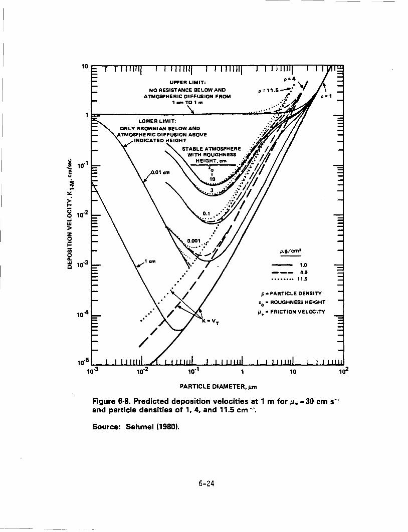
10-4
UPPER LIMIT:
NO RESISTANCE BELOWANO ATMOSPHERIC DIFFUSION FROM
1cmT01m
LOWER LIMIT:
ONLY BROWNIAN BELOW AND ATMOSPHERIC DIFFUSION ABOVE
INDICATED HEIGHT
STABLE ATMOSPHERE
1
PARTICLE DIAMETER, 11-m
p,g/cm3
1.0
--- 4.0 • • • • • • •• 11.5
p • PARTICLE DENSITY
z0
• ROUGHNESS HEIGHT
11-. • FRICTION VELOCITY
10
Figure 6-8. Predicted deposition velocities at 1 m for lA• = 30 em s-' and particle densities of 1, 4, and 11.5 em -J.
Source: Sehmel (1980).
6-24
variations in density. Some models use a more generalized surface roughness parameter, in which case the deposition velocity may also be different.
The value selected for Vd depends on the type of vegetation, usually described as either short (grasses or shrubs) or tall (forests). For particles with an MMAD of about 0.5 1Jm, Hicks (1979) gives values for tall vegetation deposition velocity from 0.1-0.4 em/sec. Lannefors et al. (1983) estimated values of 0.2-0.5 em/sec in the particle size range of 0.06-2.0 IJm in a coniferous forest. For lead, with an MMAD of 0.55 1-1m, they measured a deposition velocity of 0.41 em/sec. In a series of articles (Wiman and Agren, 1985; Wiman and Lannefors, 1985; and Wiman et al., 1985), this research group has described the modeling parameters required to define deposition in coniferous forests. They found a significant depletion of aerosols from the forest edge to the interior, and distinct edge effects, for larger particles, but nearly negligible depletion and edge effects for submicron particles. This suggests that because lead is borne primarily on particles less than 1 IJm, lead deposition within a forest may be comparable to open grasslands and other vegetation types. 6.4.1.4 Field Measurements of Dry Deposition on Surrogate and Natural Surfaces. Several investigators have used surrogate surface devices similar to those described in Section 4.2.2.4. These data are summarized in Table 6-4. The few studies available on deposition to vegetation surfaces show deposition rates comparable to those of surrogate surfaces and deposition velocities in the range predicted by the models discussed above. A study to compare vegetation washing and several types of surrogate surfaces was reported by Oolske and Gatz (1984). Although the study emphasizes sulfate particles, the devices and techniques are similar to those used for lead. One important observation was that surrogate surface devices may be more representative of actua 1 deposition if the device has a very sha 11 ow rim or no rim at a 11.
Therefore, the data of Table 6-4 do not include measurements made with deposition buckets. In Section 6.4.3, these data are used to show that global emissions are in approximate balance with global deposition. It is reasonable to expect that future refinements of field measurements and model calculations will permit more accurate estimates of dry deposition in specific regions or under specific environmental conditions.
6.4.2 Wet Deposition Wet deposition includes removal by rainout and washout. Rainout occurs when particulate
matter is present in the supersaturated environment of a growing cloud. The small particles (0.1 to 0.2 IJm) act as nuclei for the formation of small droplets, which grow into raindrops (Junge, 1963). Droplets also collect particles under 0.11Jm by Brownian motion and by the water-vapor gradient. These processes are referred to as rainout. Washout, on the other hand, occurs when falling raindrops collect particles by diffusion and impaction on the way to
6-25
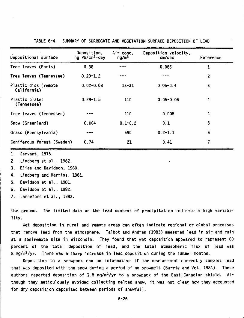
TABLE 6-4. SUMMARY OF SURROGATE AND VEGETATION SURFACE DEPOSITION OF LEAD
. Deposition, Air cone, Deposition velocity, Depositional surface ng Pb/cm2 ·day ng/m3 em/sec Reference
Tree leaves (Paris) 0.38 0.086 1
Tree leaves (Tennessee) 0. 29-1.2 2
Plastic disk (remote 0.02-0.08 13-31 0.05-0.4 3 California)
Plastic plates 0. 29-1.5 110 0.05-0.06 4 (Tennessee)
Tree leaves (Tennessee) 110 0.005 4
Snow (Greenland) 0.004 0.1-0.2 0.1 5
Grass (Pennsylvania) 590 0.2-1.1 6
Coniferous fo.rest (Sweden) 0.74 21 0.41 7
1. Servant, 1975. 2. Lindberg et al., 1982.
3. Elias and Davidson, 1980.
4. Lindberg and Harriss, 1981.
5. Davidson et al., 1981.
6. Davidson et al., 1982.
7. Lannefors et al., 1983.
the ground. The limited data on the lead content of precipitation indicate a high variabi-1 ity.
Wet deposition in rural and remote areas can often indicate regional or global processes that remove lead from the atmosphere. Talbot and Andren (1983) measured lead in air and rain at a semiremote site in Wisconsin. They found that wet deposition appeared to represent 80
percent of the tota 1 deposition of 1 ead, and the tota 1 atmospheric flux of 1 ead was 8 mg/m2/yr. There was a sharp increase in lead deposition during the summer months.
Deposition to a snowpack can be informative if thE! measurement correctly samples lead that was deposited with the snow during a period of no snctwmelt (Barrie and Vet, 1984). These authors reported deposition of 1.8 mg/m2/yr to a snowpack of the East Canadian shield. Although they meticulously avoided collecting melted snow, it was not clear how they accounted for dry deposition deposited between periods of snowfall.
6-26
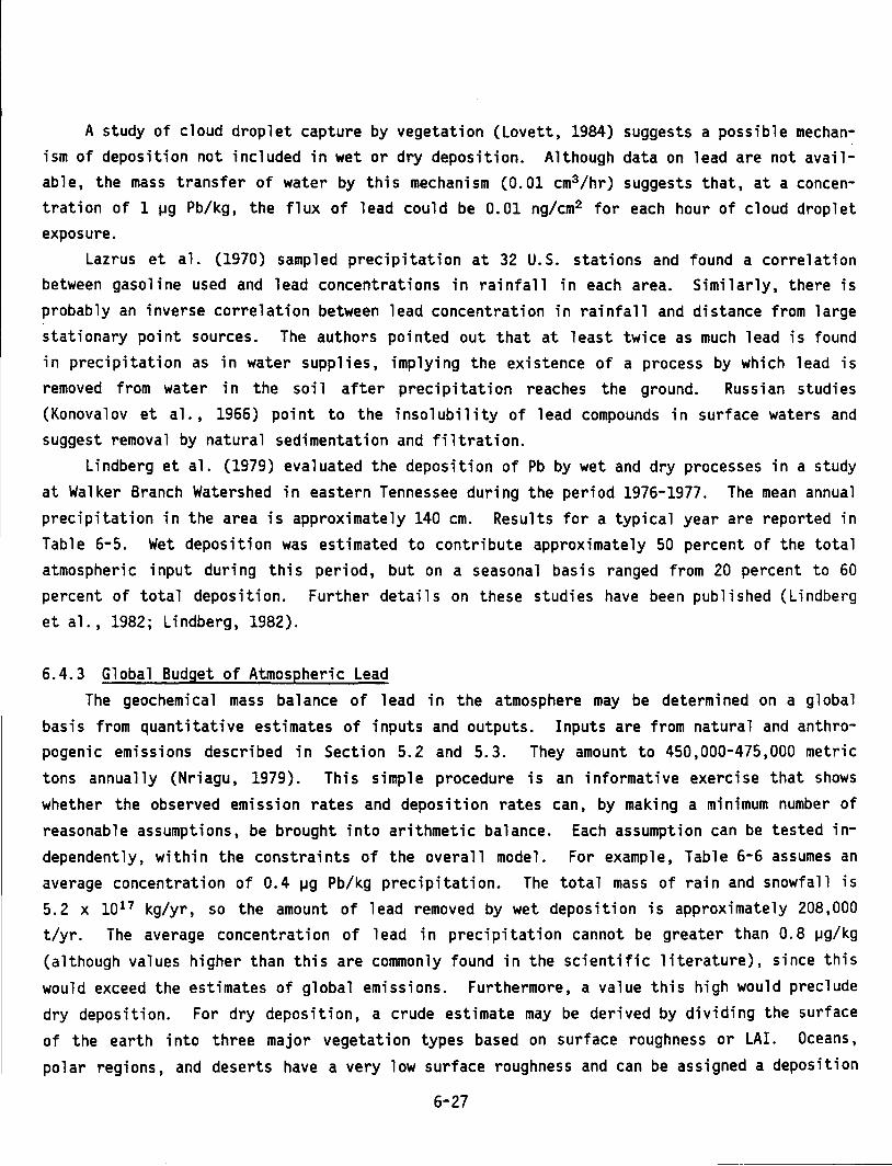
A study of cloud droplet capture by vegetation (Lovett, 1984) suggests a possible mechanism of deposition not included in wet or dry deposition. Although data on lead are not available, the mass transfer of water by this mechanism (0.01 cm3 /hr) suggests that, at a concentration of 1 ~g Pb/kg, the flux of lead could be 0.01 ng/cm2 for each hour of cloud droplet exposure.
Lazrus et al. (1970) sampled precipitation at 32 U.S. stations and found a correlation between gasoline used and lead concentrations in rainfall in each area. Similarly, there is probably an inverse correlation between lead concentration in rainfall and distance from large stationary point sources. The authors pointed out that at least twice as much lead is found in precipitation as in water supplies, implying the existence of a process by which lead is removed from water in the soil after precipitation reaches the ground. Russian studies (Konovalov et al., 1966) point to the insolubility of lead compounds in surface waters and suggest removal by natural sedimentation and filtration.
Lindberg et al. (1979) evaluated the deposition of Pb by wet and dry processes in a study at Walker Branch Watershed in eastern Tennessee during the period 1976-1977. The mean annual precipitation in the area is approximately 140 em. Results for a typical year are reported in Table 6-5. Wet deposition was estimated to contribute approximately 50 percent of the total atmospheric input during this period, but on a seasona 1 basis ranged from 20 percent to 60 percent of total deposition. Further details on these studies have been published (Lindberg et al., 1982; Lindberg, 1982).
6.4.3 Global Budget of Atmospheric Lead The geochemical mass balance of lead in the atmosphere may be determined on a global
basis from quantitative estimates of inputs and outputs. Inputs are from natural and anthropogenic emissions described in Section 5.2 and 5.3. They amount to 450,000-475,000 metric tons annually (Nriagu, 1979). This simple procedure is an informative exercise that shows whether the observed emission rates and deposition rates can, by making a minimum number of reasonable assumptions, be brought into arithmetic balance. Each assumption can be tested independently, within the constraints of the avera 11 mode 1. For examp 1 e, Tab 1 e 6-6 assumes an average concentration of 0.4 ~g Pb/kg precipitation. The total mass of rain and snowfall is 5. 2 x 10¹⁷ kg/yr, so the amount of 1 ead removed by wet deposition is approximately 208,000 t/yr. The average concentration of lead in precipitation cannot be greater than 0.8 ~g/kg
(although values higher than this are commonly found in the scientific literature), since this would exceed the estimates of global emissions. Furthermore, a value this high would preclude dry deposition. For dry deposition, a crude estimate may be derived by dividing the surface of the earth into three major vegetation types based on surface roughness or LA I. Oceans,
polar regions, and deserts have a very low surface roughness and can be assigned a deposition
6-27
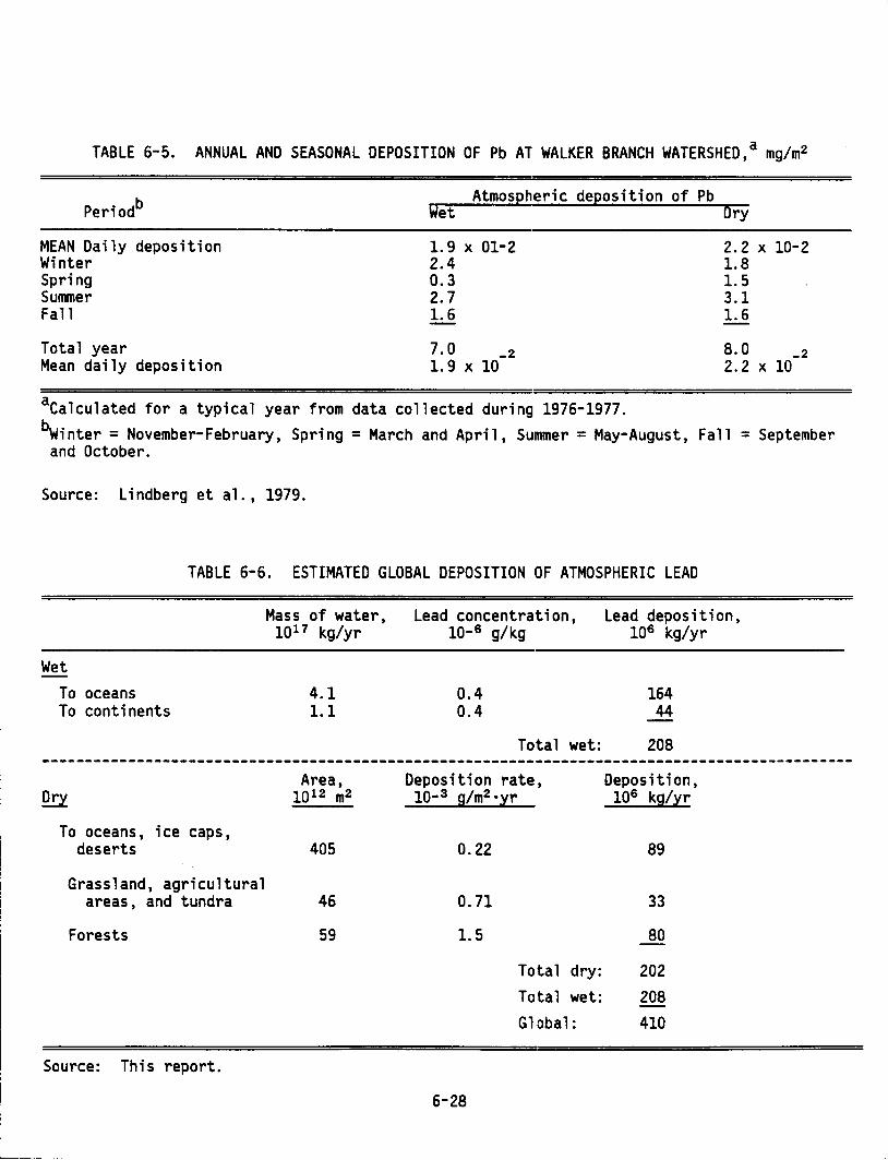
TABLE 6-5. ANNUAL AND SEASONAL DEPOSITION OF Pb AT WALKER BRANCH WATERSHED,a mg/m2
Atmospheric deposition of Pb Periodb Wet Dry
MEAN Daily deposition Winter Spring Summer Fall
Total year Mean daily deposition
1. 9 X 01-2 2.4 0.3 2.7 1.6
7. 0 -2 1. 9 X 10
aCalculated for a typical year from data collected during 1976-1977.
2.2 X 10⁻² 1.8 1.5 3.1 1.6
8.0 -2 2.2 X 10
bwinter =November-February, Spring= March and April, Summer= May-August, Fall= September and October.
Source: Lindberg et al., 1979.
TABLE 6-6. ESTIMATED GLOBAL DEPOSITION OF ATMOSPHERIC LEAD
Wet To oceans To continents
Mass of water, Lead concentration, 1017 kg/yr 10-6 g/kg
4.1 1.1
0.4 0.4
Lead deposition, 106 kg/yr
164 44
Total wet: 208
To oceans, ice caps, deserts
Grassland, agricultural
Area, 1012 m2
405
areas, and tundra 46
Forests 59
Source: This report.
Deposition rate, 10-3 g/m2 ·yr
0.22
0.71
1.5
Total dry: Total wet: Gl·obal:
6-28
Deposition, 106 kg/yr
89
33
80
202 208 410
velocity of 0.01 em/sec, which gives a flux of 0.2 ~g/m2 ·yr, assuming 75 ng Pb/m3 air concentration. Grasslands, tundra, and other areas of low-lying vegetation have a some• what higher deposition velocity; forests would have the highest. Values of 0.3 and 0.65 can be assigned to these two vegetation types, based on the data of Davidson et al. (1982). Whittaker (1975) lists the global surface area of each of the three types as 405, 46, and 59 x 1012 m2 , respectively. In the absence of data on the global distribution of air concentrations of lead, an average of 0.075 ~g/m3 is assumed. Multiplying air concentration by deposition velocity gives the deposition flux for each surface roughness type shown on Table 6-6. The combined wet and dry deposition is 410,000 metric tons, which compares favorably with the estimated 450,000-475,000 metric tons of emissions.
The data used above are not held to be absolutely firm. Certainly, more refined estimates of air concentrations and deposition velocities can be made in the future. On the other hand, the calculations above show some published calculations to be unreasonable. In particular, if the values for lead in rain (36 ~g/kg) reported by Lazrus et al. (1970) were applied to this global model, more than 50 times the total global emissions would be required for mass balance. Likewise, deposition fluxes of 0.95 ~g/cm2 ·yr reported by Jaworowski et al. (1981) would account for 10 times global emissions. Chemical mass balance budgets are an effective aid to evaluating reports of environmental lead data.
6.5 TRANSFORMATION AND TRANSPORT IN OTHER ENVIRONMENTAL MEDIA 6.5.1 Soil
The accumulation of lead in soils is primarily a function of the rate of deposition, since most lead is retained by the soil and.very little passes through into surface or ground water. The wet and dry deposition rates discussed in Section 6.4 would apply provided the surface roughness and location (urban, rural, remote) are considered. A value of 8 mg/m2 yr such as that measured by Talbot and Andren (1983) in a semiremote location in Wisconsin converts to 0."8 ~g/cm2 yr. It is difficult to generalize on the depth of penetration of lead in undisturbed soils, but if it is assumed that most of the lead is retained in the upper 5 em (Reaves and Berrow, 1984; Garcia-Miragaya, 1984), then the accumulation rate of 0.8 ~g/cm2 yr becomes 0.16 ~g/cm3 yr, or 0.16 ~g/g if a density of 1 is assumed for soil. Ewing and Pearson (1974) reported an accumulation of 13 ~g/g soil from the 1920 1 s to the late 196o•s, or an annual rate of about 0.26 ~g/g in a rural setting. It should be noted that the atmospheric concentration of lead increased 20~fold during this period (Shirahata et al., 1980). Page and Ganje (1970) found an accumulation of 0.83 ~g/g during the same time for a site near high
traffic density.
6-29
These accumulation rates are discussed further in Section 7.2.2.1. Understanding the distinction between atmospheric and natural lead in soil can provide some insight into the mechanisms regulating transport in soil. Of particular importance are solubility and the stabi Hty of lead ·complexes with humic substances.
Soils have both a liquid and solid phase, and trace metals are normally distributed between these two phases. In the liquid phase, metals may exist as free ions or as soluble complexes with organic or inorganic ligands. Organic ligands are typically humic substances such as fulvic or humic acid; inorganic ligands may be iron or manganese hydrous oxides. Since lead rarely occurs as a free ion in the liquid phase (Camerlynck and Kiekens, 1982), its mobility in the soil solution depends on the availability of organic or inorganic ligands. The liquid phase of soil often exists as a thin film of mclisture in intimate contact with the solid phase. The availability of metals to plants dept!nds on the equilibrium between the liquid and solid phase.
In the solid phase, metals may be incorporated into crystalline minerals of parent rock material, into secondary clay minerals, or precipitated a!i insoluble organic or inorganic complexes. They may also be adsorbed onto the surfaces of any of these solid forms. Of these categories, the most mobile form is in the film of moisture surrounding soil particles, where 1 ead can move freely into p 1 ant roots or soi 1 microorganisms with di sso 1 ved nutrients. The least mobile is parent rock material, where lead may be bound within crystalline structures over geologic periods of time. Intermediate are the lead complexes and precipitates. Transformation from one form to another depends on the chemical environment of the soil. For example, at pH 6-8, insoluble organic-Pb complexes are favc,red if sufficient organic matter is available; otherwise hydrous oxide complexes may form or the lead may precipitate with the carbonate or phosphate ion. In the pH range of 4-6, the organic7Pb complexes become soluble. Soils outside the pH range of 4-8 are rare. The interconversion between soluble and insoluble organic complexes affects the equilibrium of lead between the liquid and solid phase of soil.
Dong et al. (1985) found that only 0.2 percent of the total lead in soil can be released to solution by physical shaking. Even if 99.99 percent of the total lead in soil is immobilized, 0.01 percent of the total lead in soil can have a significant effect on plants and microorganisms if the soils are heavily contaminated with lead (see Section 8.3.1).
The water soluble and exchangeable (as determined by chemical extraction) forms of metals are the forms generally considered potentially available for plant uptake. It is important not to confuse the term "extractable" with "plant uptake. 11 Lead that can be extracted from soil by chemical treatment may not be taken up by plants, even though the same chemical treatment is known to release other metals to plants. Because little is known of this relationship, lead that is extractable by chemical means normal for other metals is considered only
6-30
potentially available for plant uptake. Camerlynck and Kiekens (1982) demonstrated that in normal soils, only a small fraction of the total lead is in exchangeable form (about 1 ~g/g) and none exists as free lead ions. Of the exchangeable lead, 30 percent existed as stable complexes, 70 percent as labile complexes. The organic content of these soils was low (3.2 percent clay, 8.5 percent silt, 88.3 percent sand). In heavily contaminated soils near a midwestern industrial site, Miller and McFee (1983) found that 77 percent of the lead was in either the exchangeable or organic form, although still none could be found in aqueous solution. Soils had a total lead content from 64 to 360 ~g/g and an organic content of 7-16 percent.
There is evidence that atmospheric lead enters the soil system as PbS04 or is rapidly converted to PbS04 at the soil surface (Olson and Skogerboe, 1975). Lead sulfate is more soluble than PbC03 or Pb3 (P04 ) 2 and thus could remain mobile if not transformed. Lead could be immobilized by precipitation as less soluble compounds [PbC03 , Pb3 (P04 ) 2 ], by ion exchange with hydrous oxides or clays, or by chelation with humic and fulvic acids. Santillan-Medrano and Jurinak (1975) discussed the possibility that the mobility of lead is regulated by the formation of Pb(OHh, Pb3 (P04 h, Pb 5 (P04 )aOH, and PbC03 • This model, however, did not consider the possible influence of organic matter on lead immobilization. Zimdahl and Skogerboe (1977), on the other hand, found lead varied linearly with cation exchange capacity (CEC) of soil at a given pH, and linearly with pH at a given CEC (Figure 6-9). The relationship between CEC and organic carbon is discussed below.
If surface adsorption on clays plays a major role in lead immobilization, then the capacity to immobilize should vary directly with the surface-to-volume ratio of clay. In two separate experiments using the nitrogen BET method for determining surface area and size fractionation techniques to obtain samples with different surface-to-volume ratios, Zimdahl and Skogerboe (1977) demonstrated that this was not the case. They also showed that precipitation as lead phosphate or lead sulfate is not significant, although carbonate precipitation can be important in soils that are carbonaceous in nature or to which lime (CaC03 ) has been added.
Of the two remaining processes, lead immobilization is more strongly correlated with organic chelation than with iron and manganese oxide formation (Zimdahl and Skogerboe, 1977). It is possible, however, that chelation with fulvic and humic acids is catalyzed by the presence of iron and manganese oxides (Saar and Weber, 1982). This would explain the positive correlation for both mechanisms observed by Zimdahl and Skogerboe (1977). The study of Miller and McFee (1983) discussed above indicates that atmospheric lead added to soil is distributed to organic matter (43 percent) and ferro-manganese hydrous oxides (39 percent), with 8 percent found in the exchangeable fraction (determined by chemical extraction) and 10 percent as insoluble precipitates.
6-31
If organic chelation is the correct model of lead immobilization in soil, then several features of this model merit further discussion. First, the total capacity of soil to immobi~ 1 i ze 1 ead can be predicted from the 1 i near re 1 at i onshi p deve 1 oped by Z i mdah 1 and Skogerboe (1977) (Figure 6-9) based on the equation:
N = 2.8 x 10⁻⁶ (A) + 1.1 x 10⁻⁵ (B) - 4.9 x 10⁻⁵ (6-2)
where N is the saturation capacity of the soil expressed in moles/g soil, A is the CEC of the soi 1 in meq/100 g soi 1, and B is the pH. Because the CEC of soil is more difficult to determine than total organic carbon, it is useful to define the relationship between CEC and organic content. Pratt (1957) and Klemmedson and Jenny (1966) found a linear correlation between CEC and organic carbon for soils of similar sand, silt, and clay content. The data of Zimdahl and Skogerboe (1977) also show this relationship when grouped by soil type. They show that sandy clay loam with an organic content of 1.5 percent might be expected to have a CEC of 12 meq/100 g. From the equation, the saturation capacity for lead in soil of pH 5.5 would be 45 ~moles/g soil or 9,300 ~g/g. The same soil at pH 4.0 would have a total capacity of 5,900 ~g/g.
When the soil contains sufficient organic matter, the adsorption of lead and other metals is a function of pH. In reality, it is not the totai organic matter but the number of reactive sites that determines metal absorption (Harter, 1983), and there appears to be a weak relationship between cation exchange capacity and metal r·etention. In competition with other metals, lead would normally be more strongly favored for retention, in accordance with the Irving-Williams series (Irving and Williams, 1953). Gamble et al. (1983) have shown that the Irving-Williams series becomes somewhat distorted when the binding sites are chemically dissimilar.
The soil humus model also facilitates the calculation of lead in soil moisture using values available in the literature for conditional stability constants with fulvic acid (FA). The term conditional is used to specify that the stabili~y constants are specific for the conditions of the reaction. Conditional stability constants for humic acid (HA) and FA are comparab 1 e. The va 1 ues reported for 1 og K are 1 i near in the pH range of 3 to 6 (Buffl e and Greter, 1979; Buffle et al., 1976; Greter et al., 1979), so that interpolations in the critical range of pH 4 to 5.5 are possible. Thus, at pH 4.5, the ratio of complexed lead to ionic lead is expected to be 3.8 x 10³ . For soils of 100 ~n/g, the ionic lead in soil moisture solution would be 0.03 ~g/g. The significance of this ratio is discussed in Section 8.3.1.1.
6-32
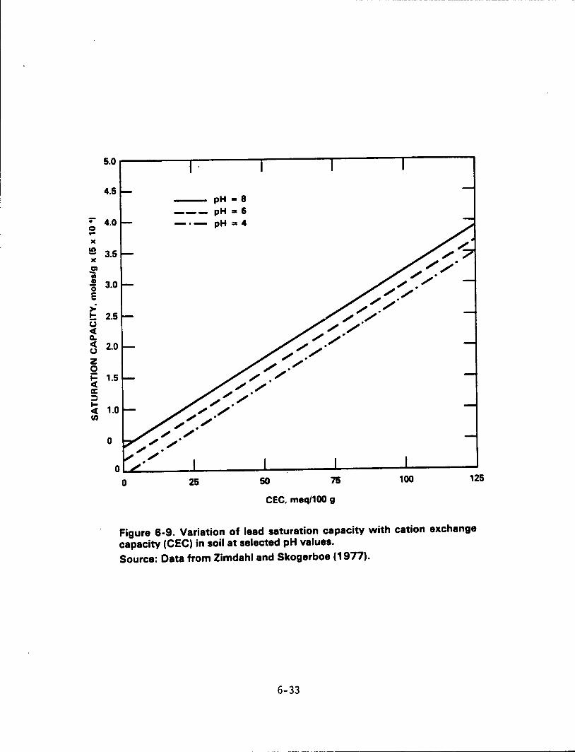
• 0 ~
)(
~ )(
~
"' Gl 0 E > ~ u ct 0. ct u z 0 j: ct a: ;j ~ ct en
5.0
4.5
4.0
3.5
3.0
2.5
2.0
1.5
1.0
0
pH"" 8 ---pH"" 6 -·-pH .,.4
0 0 25 50 75 100 125
CEC. meq/100 g
Figure 6-9. Variation of lead saturation capacity with cation exchange capacity (CEC) in soil at selected pH values. Source: Data from Zimdahl and Skogerboe (1977}.
6-33
It is also important to consider the stability constant of the Pb-FA complex relative to other metals. Schnitzer and Hansen (1970) showed that at pH 3, Fe3 + is the most stable in th~ sequence Fe3+ > Al 3 + > Cu2+ > Ni 2+ >Co2+> Pb2+ > Ca2+ > zn2+ > Mn2+ > Mg2+. At pH 5, this
. . + 2+ + + + + + + . sequence becomes N1 2 = Co > Pb2 > Cu2 > Zn2 = Mn2 > Ca2 > Mg2 . Th1s means that at normal soil pH levels of 4.5-8, lead is bound to FA and liA in preference to many other metals that are known plant nutrients (Zn, Mn, Ca, and Mg). Furthermore, if lead displaces iron in this scheme, an important function of FA may be inhibited at near saturation capacity (above 6000 ~g Pb/g.) Fulvic acid is believed to play a role in the weathering of parent rock material by the removal of iron from the crystalline structure of the minerals, causing the rock to weather more rapidly. In the absence of this process, the weathering ~f parent rock material and the subsequent release of nutrients to soil would proceed more slowly. Bizri et al. (1984) found stability constants for humic substances wert! log K1 = 4.2 and log K2 = 3.7. For humic materials in aquatic systems, Alberts and Giesy (1983) reported conditional stability constants of log K1 = 5.09 and log K2 = 2.00.
6.5.2 Water 6.5.2.1 Inorganic. The chemistry of lead in an aqueous solution is highly complex because the element can be found in a multiplicity of forms. Ht!m and Durum (1973) have reviewed the chemistry of lead in water in detail; the aspects of aqueous lead chemistry that are germane to this document are discussed in Section 3.3.
Lead in ore deposits does not pass easily to ground or surface water. Any lead dissolved from primary lead sulfide ore tends to combine with carbonate or sulfate ions to (1) form inso 1 ub 1 e 1 ead carbonate or 1 ead sulfate, or (2) be absorbed by ferric hydroxide (Lovering, 1976). An outstanding characteristic of lead is its tendency to form compounds of low solubility with the major anions of natural water. Hydroxide,. carbonate, sulfide, and more rarely sulfate may act as solubility controls in precipitating lead from water. The amount of lead that can remain in solution is a function of the pH of the water and the dissolved salt content. Equilibrium calculations show that at pH > 5.4, the total solubility of lead is about 30 ~g/1 in hard water and about 500 ~g/1 in soft water (Davies and Everhart, 1973). Lead sulfate is present in soft water and limits the lead concentration in solution. Above pH 5.4, PbC03 and Pb2(0H)2 C03 limit the concentration. The carbonate concentration is in turn dependent on the partial pressure of C02 as well as the pH. Calculations by Hem and Ourum (1973) show that many river waters in the United States have lead concentrations near the solubility limits imposed by their pH levels and contents of dissolved C02 . Because of the influence of temperature on the solubility of C02 , observed lead concentrations may vary significantly from theoretically calculated ones.
6-34
'-------------------
Concentrations as high as 330 ~g/1 could be stable in water with pH near 6.5 and an alkalinity of about 25 mg bicarbonate ion/1 of water. Water having these properties is common in runoff areas of New York State and New England; hence, the potential for high lead concentrations exists there. In other areas, the average pH and alkalinity are so high that maximum concentrations of lead of about 1 ~g/1 could be retained in solutions at equilibrium (Lovering, 1976).
A significant fraction of the lead carried by river water may be in an undissolved state. This insoluble lead can consist of colloidal particles or larger undissolved particles of lead carbonate, -oxide, -hydroxide, or other 1 ead compounds incorporated in other components of particulate lead from runoff; it may occur either as sorbed ions or surface coatings on sediment mineral particles or be carried as a part of suspended living or nonliving organic matter (Lovering, 1976). A laboratory study by Hem (1976) of sorption of lead by cation exchange indicated that a major part of the lead in stream water may be adsorbed on suspended sediment. Figure 6-10 illustrates the distribution of lead outputs between filtrate and solids in water from both urban and rural streams, as reported by Getz et al. (1977). The majority of lead output is associated with suspended solids in both urban and rural streams, with very little dissolved in the filtrate. The ratio of lead in suspended solids to lead in filtrate varies from 4:1 in rural streams to 27:1 in urban streams.
Soluble lead is operationally defined as that fraction which is separated from the insoluble fraction by filtration. However, most filtration techniques do not remove all colloidal particles. Upon acidification of the filtered sample, which is usually done to preserve it before analysis, the colloidal material that passed through the filter is dissolved and is reported as dissolved lead. Because the lead in rainfall can be mainly particulate, it is necessary to obtain more information on the amounts of insoluble lead (Lovering, 1976) before a valid estimate can be obtained of the effectiveness of runoff in transporting lead away from areas where it has been deposited by wet and dry deposition. 6.5.2.2 Organic. The bulk of organic compounds in surface waters originates from natural sources (Neubecker and Allen, 1983). The humic and fulvic acids that are primary complexing agents in soils are also found in surface waters at concentrations from 1-5 mg/1, occasionally exceeding 10 mg/1 (Steelink, 1977), and have approximately the same chemical characteristics (Reuter and Perdue, 1977). The most common anthropogenic organic compounds are nitrilotriacetonitrile (NTA) and ethylenediaminetetraacetic acid (EDTA) (Neubecker and Allen, 1983). There are many other organic compounds such as oi 1 s, p 1 ast i ci zers, and polymers discharged from manufacturing processes that may complex with lead.
6-35
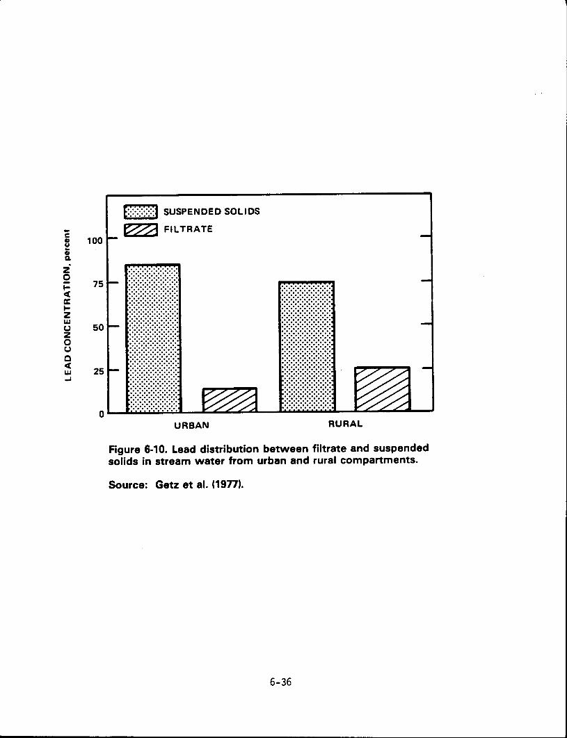
.. c 5 100 .. CD Q.
z 0 let a: 1-z w u z 0 u 0 c:t w ..1
75
50
25
r:~?:~:~j SUSPENDED SOLIDS
~FILTRATE
........... . . . . . . . . . . . . . . . . . . . . . . ........... . . . .. . . . . . . . . . . . . . . . . . ........... ~: ~: ~: ~: ~: ~: ~: ~: ~: ~: ~: :::::::::::::::::::::: : ~: ~: ~: ~: ~: ~: ~: ~: ~: ~: ~ ~: ~: ~: ~: ~: ~: ~: ~: ~: ~: ~: :::::::::::::::::::::: :::::::::::::::::::::: ~: ~: ~: ~: ~: ~: ~: ~: ~: ~: ~: : ~: ~: ~= ~: t ~: ~: ~: ~: ~ :::::::::::::::::::::· :::::::::::::::::::::: ~: ~: ~: ~: ~: ~: ~: ~: ~: ~: ~. : ~: ~: ~: ~: ~: ~=~: ~: ~ =~: ~ .·.·.·.·.·.·.·.·.·.·. ·.·.·.·.·.·.·.·.·.·.·. ::::::::::::::::::::: :::::::::::::::::::::: .·.·.·.·.·.·.·.·.·.·. .·.·.·.·.·.·.·.·.·.·. ::::::::::::::::::::: :::::::::::::::::::::
0 ·······.·.·.·. ··········· r<<<4 ,
URBAN RLIRAL
Figure 6-10. Lead distribution between filtrate and suspended solids in stream water from urban and rural compartments.
Source: Getz et al. (19n).
6-36
The presence of fulvic acid in water has been shown to increase the rate of solution of lead sulfide 10 to 60 times over that of a water solution at the same pH that did not contain fulvic acid (Bondarenko, 1968; Lovering, 1976). At pH values near 7, soluble Pb-FA complexes are present in solution. At initial pH values between 7.4 and about 9, the Pb-FA complexes are partially decomposed, and lead hydroxide and carbonate are precipitated. At initial pH values of about 10, the Pb-FA complexes again increase. This increase is attributed to dissociation of phenolic groups at high pH values, which increases the complexing capacity of the FA. But it also may be due to the formation of soluble lead-hydroxyl complexes.
Beijer and Jernelov (1984) review the evidence for the microbial methylation of lead in aquatic systems. The transformation of inorganic lead, especially in sediment, to tetramethyllead (TML) has been observed and biomethylation has been postulated (Schmidt and Huber, 1976; Wong et al., 1975). Reisinger et al. (1981) have reported extensive studies of the methylation of lead in the presence of numerous bacterial species known to alkylate mercury and other heavy metals. In these experiments no biological methylation of lead was found under any condition. Chemical alkylation from methylcobalamine was found to occur in the presence of sulfide or of aluminum ion; chemical methylation was independent of the presence of bacteria.
Jarvie et al. (1975, 1981) have recently shown that tetraalkyllead compounds are unstable in water. Small amounts of Ca2+ and Fe2+ ions and sunlight have been shown to cause decomposition of TEL over time periods of 5-50 days. The only product detected was triethyllead, which appears to be considerably more stable than the TEL. Tetramethyllead is-decomposed much more rapidly than TEL in water, to form the trimethyl lead ion. Initial concentrations of
-4 10 molar were reduced by one order of magnitude either in the dark or light in one day. Tetramethyllead was virtually undetectable after 21 days. Apparently, chemical methylation of lead to the trialkyllead cation does occur in some water systems, but evolution of TML appears insignificant.
Lead occurs in riverine and estuarial waters and alluvial deposits. Laxen and Harrison (1977) and Harrison and Laxen (1981) found large concentrations of lead (-1 mg/1) in rainwater runoff from a roadway; but only 5-10 percent of this is soluble in water. Concentrations of lead in ground water appear to decrease logarithmically with distance from a roadway. Rainwater runoff has been found to be an important transport mechanism in the removal of lead from a roadway surface in a number of studies (Bryan, 1974; Harrison and Laxon, 1981; Hedley and Lockley, 1975; Laxen and Harrison, 1977). Apparently, only a light rainfall, 2-3 mm, is sufficient to remove 90 percent of the 1 ead from the road surface to surrounding soi 1 and to waterways (Laxen and Harrison, 1977).
6-37
The Applied Geochemistry Research Group (1978) has reported elevated lead concentrations (40 ~g/g and above) in about 30 percent of stream bed sediment samples from England and Wales in a study of 50,000 such samp 1 es. Abdullah and Royle ( 1973) have reported 1 ead 1 eve 1 s in coastal ~reas of th~ Irish sea of 400 ~g/g and higher.
Evidence for the sedimentation of lead in freshwater streams may be found in several reports. Laxen and Harrison (1983) found that lead in the effluent of a lead-acid battery plant near Manchester, England, changed drastically in particle size. In the plant effluent, 53 percent of the lead was on particles smaller than 0.015 ~m and 43 percent on particles greater than 1 ~m. Just downstream of the plant, 91 percent of the lead was on particles greater than 1 ~m and only 1 percent on particles smaller than 0.015 ~m. Under these conditions, lead formed or attached to large particles at a rate exceeding that of Cd, Cu, Fe or Mn.
The lead concentrations in off-shore sediments often show a marked increase corresponding to anthropogenic activity in the region (Section 5.1). Rippey et al. (1982) found such increases recorded in the sediments of Lough Neagh, No1·thern Ireland, beginning during the 1600 1 s and increasing during the late 1800 1 s. Corresponding increases were also observed for Cr, Cu, Zn, Hg, P, ~nd Ni. For lead, the authors found an average anthropogenic flux of 72 mg/m2 ·yr, of ~hich 27 mg/m2 ·yr could be attributed to direct atmospheric deposition. Prior to 1650, the total flux was 12 mg/m2 ·yr, so there has been a 6-fold increase since that time.
Ng and Patterson (1982) found prehistoric fluxes of 1-7 mg Pb/m2 ·yr in three offshore basins in southern California, which have now increased 3 to 9-fold to 11-21 mg/m2 ·yr. Much of this lead is deposited directly from sewage outfalls, although at least 25 percent probably comes from the atmosphere.
6.5.3 Vegetation Surfaces The deposition of lead on the leaf surfaces of plants where the particles are often re
tained for a long time must also be considered (Dedolph et al., 1970; Page et al., 1971; Schuck and Locke, 1970). Many studies have shown that plants near roadways exhibit considerably higher 1 eve 1 s of 1 ead than those further away. In most instances, the higher concentrations were due to lead particle deposition on plant surfaces (Schuck and Locke, 1970). Studies have shown that particles deposited on plant surfaces are difficult to remove by typical kitchen washing techniques. (Arvik and Zimdahl, 1974; Page et al., 1971; Lagerwerff et al., 1973). Leaves with pubescent surfaces seem able to retain particles via an electrostatic mechanism. Other types of leaves are covered with a cuticular wax physically suitable for retaining particles. Rainfall does not remove all of the particles on the leaf surface. It appears that there is a buildup with time of surface deposition on leafy vegetation. Animals consuming the leafy portions of such plants can certainly be exposed to higher than normal levels of lead.
6-38
The uptake of soluble lead by aquatic plants can be an important mechanism for depleting lead concentrations in downstream waterways. Gale and Wixson (1979) have studied the influence of algae, cattails, and other aquatic plants on lead and zinc levels in wastewater in the New Lead Belt of Missouri. These authors report that mineral particles become trapped by roots, stems, and fi 1 aments of aquatic p 1 ants. Numerous anionic sites on and within ce 11 walls participate in cation exchange, replacing metals such as lead with Na+, K+, and H+ ions. Mi nera 1 i zat ion of 1 ead in these Missouri waters may a 1 so be promoted by water a 1 ka 1 i ni ty. However, construction of stream meanders and settling ponds have greatly reduced downstream water concentrations of lead, mainly because of absorption in aquatic plants (Gale and Wixson, 1979).
6.6 SUMMARY From the source of emission to the site of deposition, lead particles are dispersed by
the flow of the airstream, transformed by physical and chemical processes, and removed from the atmosphere by wet or dry deposition. Under the simplest of conditions (smooth, flat terrain), the dispersion of lead particles has been modeled and can be predicted (Benarie, 1980). Dispersion modeling in complex terrains is still under development and these models have not been evaluated (Kotake and Sano, 1981).
Air lead concentrations decrease logarithmically away from roadways (Edwards, 1976) and smelters (Roberts et al., 1974). Within urban regions, air concentrations decrease from the central business district to the outlying residential areas by a factor of 2-3. From urban to rura 1 areas, air concentrations decrease from 1-2 1Jg/m3 down to 0. 1-0. 5 1Jg/m3 (Chapter 7).
This decrease is caused by dilution with clean air and removal by deposition. During dispersion to remote areas, concentrations decrease to 0.01 1Jg/m3 in the United States (Elias and Davidson, 1980), to 0.001 1Jg/m3 in the Atlantic Ocean (Duce et al., 1975), and to 0.000076 1Jg/m3 in Antarctica (Maenhaut et al., 1979).
Physical transformations of lead particles cause a shift in the particle size distribution. The bimodal distribution of large and small particles normally found near the roadway changes with time and distance to a single mode of intermediate sized particles (Huntzicker et al., 1975). This is probably because large particles deposit near roadways and small particles agglomerate to medium sized particles with an MMAD of about 0.2-0.3 !Jm.
Particles transform chemically from lead halides to lead sulfates and oxides. Organolead compounds constitute 1-6 percent of the total airborne lead in ambient urban air (Harrison
et al., 1979).
6-39
On a regional or global basis, wet deposition accounts for about half of the removal of lead particles from the atmosphere. The other half of the atmospheric lead is removed by dry deposition. Mechanisms may be gravitational for large particles or a combination of gravitational and wind-related mechanisms for small particles (Elias and Davidson, 1980). Models of dry deposition predict deposition velocities as a function of particle size, windspeed, and surface roughness. Because of their large surface area/ground area ratio, grasslands, croplands, and forested areas receive the bulk of dry deposited particles over continental areas.
Lead enters soil as a moderately insoluble lead sulfate and is immobilized by complexation with humic and fulvic acids. This immobilization is a function of pH and the concentration of humic substances. At low pH (-4) and low organic content (<5 percent), immobilization of lead in soil may be limited to a few hundred ~g/g (Zimdahl and Skogerboe, 1977), but at 20
percent organic content and pH 6, 10,000 ~g Pb/g soil may be found. In natural waters, lead may precipitate as lead suHate or carbonate, or it may form a
complex with ferric hydroxide (Lovering, 1976). The solubility of lead in water is a function of pH and hardness (a combination of Ca and Mg content). Below pH 5.4, concentrations of dis
so 1 ved 1 ead may vary from 30 ~g/1 in hard water to 500 ~g/1 in soft water at saturation
(Lovering, 1976).
6-40
6.7 REFERENCES
Abdullah, M. I.; Royle, L. G. (1973) The occurrence of lead in natural waters. In: Barth, D.; Berlin, A.; Engel, R.; Recht, P.; Smeets, J., eds. Enviromental health aspects of lead: proceedings, international symposium; October 1972; Amsterdam, The Netherlands. Luxembourg: Commission of the Europ~an Communities; pp. 113-124.
Alberts, J. J.; Giesy, J. P. (1983) Conditional stability constants of trace metals and naturally occurring humic materials: application in equilibrium models and verification with field data. In: Christman, R. F.; Gjessing, E. T. Aquatic and terrestrial humic materials: symposium; November 1981; Chapel Hill, NC. Woburn, MA: Butterworth; pp. 333-348.
Applied Geochemistry Research Group. (1978) The Wolfson geochemical atlas of England and Wales. Oxford, United Kingdom: Clarendon Press.
Arvik, J. H.; Zimdahl, R. L. (1974) Barriers to the foliar uptake of lead. J. Environ. Qual. 3: 369373.
Barrie, L. A.; Vet, R. J. (1984) The concentration and deposition of acidity, major ions and trace metals in the snowpack of the eastern Canadian shield during the winter of 1980-81. Atmos. Environ. 18: 1459-1469.
Beijer, K.; Jernelov, A. (1984) Microbial methylation of lead. In: Grandjean, P., ed. Biological effects of organolead compounds. Boca Raton, FL: CRC Press, Inc.; pp. 13-19.
Benarie, M. M. (1980) Urban air pollution modelling. Cambridge, MA: MIT Press.
Biggins, P. D. E.; Harrison, R. M. (1978) Identification of lead compounds i·n urban air. Nature (London) 272: 531-532.
Biggins, P. D. E.; Harrison, R. M. (1979) Atmospheric chemistry of automotive lead. Environ. Sci. Technol. 13: 558-565.
Bizri, Y.; Cromer, M.; Scharff, J. P.; Guillet, B.; Rouiller, J. (1984) Constantes de stabilite de complexes organo-mineraux. Interactions des ions plombeux avec les composes organiques hydrosolubles des eaux gravitaires de podzol [Stability constants of organamineral complexes. Interactions of lead ions with watersoluble organic compounds from the passage of heavy water through podzol]. Geochim. Cosmochim. Acta 48: 227-234.
Bondarenko, G. P. (1968) An experimental study of the solubility of galena in the presence of fulvic acidsA Geochem. Int. 5: 525-531.
Bryan, E. H. (1974) Concentrations of lead in urban stormwater. J. Water Pollut. Control Fed. 46: 2419-2421.
Buffle, J.; Greter, F.-L. (1979) Voltammetric study of humic and fulvic substances: part II. mechanism of reaction of the Pb-fulvic complexes on the mercury electrode. J. Electroanal. Chern. 101: 231-251.
Buffle, J.; Greter, F.-L.; Nembrini, G.; Paul, J.; Haerdi, W. (1976) Capabilities of voltammetric techniques for water quality control problems. Z. Anal. Chern. 282: 339-350.
6-41
Bull in, J. A.; Bower, S. C.; Hinz, M.; Moe, R. D. (1985) Aerosols near urban street inter:sections. J. Air Pollut. Control Assoc. 35: 355-358.
Burton, R. M.; Suggs,. J. C. (1984) Philadelphia roadway study. Research Triangle Park, NC: U. s: Environmental Protection Agency, Environmental Monitoring Systems Laboratory; EPA report no: 600/4-84-070. Available from: NTIS, Springfield, VA; PB84-226927.
Camerlynck, R.; Kiekens, L. (1982) Speciation of heavy metals in soils based on charge separation. Plant Soil 68: 331-339.
Cass, G. R.; McRae, G. J. (1983) Source-receptor reconciliation of routine air monitoring data for trace metals: an emission inventory assisted approach. Environ. Sci. Technol. 17: 129-139.
Chamberlain, A. C. (1966) Transport of Lycopodium spores and other small particles to rough surfaces. Proc. R. Soc. London Ser. A 296: 45-70.
Chang, S.-G.; Dod, R. L.; Giauque, R. D.; Novakov, T. (1977) Photodecomposition of lead bromochloride. In: Rosen, H., ed. Annual report 1976-77. Berkeley, CA: Lawrence Berkeley Laboratory, Energy and Environment Division; pp. i'4-82. Available from: NTIS, Springfield, VA; LBL-6819.
Cholak, J.; Schafer, L. J.; Yeager, D. (1968) The air transport of lead compounds present in automobile·exhaust gases. J. Am. Ind. Hyg. Assoc. 29: 562-568.
Chow, T. J.; Patterson, C. C. (1966) Concentration profiles of barium and lead in Atlantic waters off Bermuda. Earth Planet. Sci. Lett. 1: 397-400.
Chow, T. J.; Snyder, C. B.; Earl, J. L. (1975) Isotope ratios of lead as pollutant source indicators. Proceedings of the symposium on isotope ratios as pollutant source and behavior indicators; Vienna, Austria. International Atomic Energy Agency paper no. IAEA-SM-191/4.
Clift, D.; Dickson, I. E.; Roos, T.; Collins, P.; Jolly, M.; Klindworth, A. (1983) Accumulation of lead beside the Mulgrave Freeway, Victoria. Search 14: 155-157.
Davidson, C. I.; Chu, L.; Grimm, T. C.; Nasta, M. A.; Qamoos, M. P. (1981) Wet and dry deposition of trace elements onto the Greenland ice sheet. Atmos. Environ. 15: 1429-1437.
Davidson, C. I.; Miller, J. M.; Pleskow, M. A. (1982) The influence of surface structure on predicted particle dry deposition to natural grass canopies. Water Air Soil Pollut. 18: 25-43.
Davies, P. H.; Everhart, W. H. (1973) Effects of chemical variations in aquatic environments: vol. 3 lead toxicity to rainbow trout and testing application factor concept. Washington, DC: U.S. Environmental Protection Agency; EPA repc,rt no. EPAR3730llC. Available from: NTIS, Springfield, VA; PB-221345.
De Jonghe, W. R. A.; Adams, F. C. (1980) Organic and inorganic lead concentrations in environmental air in Antwerp, Belgium. Atmos. Environ. 14: 1177-1180.
Dedolph, R.; Ter Haar, G.; Holtzman, R.; Lucas, H., Jr. (1970) Sources of lead in perennial ryegrass and radishes. In: Symposium on air consel"vation and lead, division of water, air, and waste chemistry, 157th national meeting, ~nerican Chemical Society; April 1969; Minneapolis, MN. Environ. Sci. Technol. 4: 217-223.
6-42
Dietzmann, H. E.; Parness, M. A.; Bradow, R. L. (1981) Emissions from gasoline and diesel delivery trucks by chassis transient cycle. In: Energy-sources technology conference and exhibition; January; Houston, TX. New York, NY: American Society of Mechanical Engineers; ASME paper no. 81-DPG-6.
Dobbins, R. A. (1979) Atmospheric motion and air pollution: an introduction for students of engineering and science. New York, NY: John Wiley and Sons.
Dolske, D. A.; Gatz, D. F. (1984) Field intercomparison of sulfate dry deposition monitoring and measurement methods: preliminary results. Hicks, B. B., ed. Deposition both wet and dry. Boston, MA: Butterworth Publishers; pp. 121-131. (Teasley, J. I., ed. Acid precipitati~n series - v. 4).
Dong, A.; Simsiman, G. V.; Chesters, G. (1985) Release of phosphorus and metals from soils and sediments during dispersion. Soil Sci. 139: 97-99.
Dorn, C. R.; Pierce, J. 0., II; Phillips, P. E.; Chase, G. R. (1976) Airborne Pb, Cd, Zn and Cu concentration by particle size near a Pb smelter. Atmos. Environ. 10: 443-446.
Duce, R. A.; Hoffman, G. L.; Zoller, W. H. (1975) Atmospheric trace metals at remote northern and southern hemisphere sites: pollution or natural? Science (Washington, DC) 187: 59-61.
Durando, M. L.; Aragon, S. R. (1982) Atmospheric lead in downtown Guatemala City. Environ. Sci. Technol. 16: 20-23.
Dzubay, T. G.; Stevens, R. K. (1973) Applications of X-ray fluorescence to particulate measurements. In: Second joint conference on sensing of environmental pollutants; December; Washington, DC. Pittsburgh, PA: Instrument Society of America; pp. 211-216.
Dzubay, T. G.; Stevens, R. K.; Richards, L. W. (1979) Composition of aerosols over Los Angeles freeways. Atmos. Environ. 13: 653-659.
Edwards, H. W., ed. (1976) Environmental contamination caused by lead: final report; National Science Foundation grant no. AEN74-17624 A01. Fort Collins, CO: Colorado State University.
Egan, B. A.; Mahoney, J. R. (1972) Numerical modeling of advection and diffusion of urban area source pollutants. J. Appl. Meteorol. 11: 312-322.
Elias, R. W.; Davidson, C. (1980) Mechanisms of trace element deposition from the free atmosphere to surfaces in a remote High Sierra canyon. Atmos. Environ. 14: 1427-1432.
Everett, R. G.; Hicks, B. B.; Berg, W. W.; Winchester, J. W. (1979) An analysis of particulate sulfur and lead gradient data collected at Argonne National Laboratory. Atmos. Environ. 13: 931-934.
Foster, R. L. ; Lott, P. F. (1980) X-ray diffractometry examination of air fi 1 ters for compounds emitted by lead smelting operations. Environ. Sci. Technol. 14: 1240-1244.
Friedlander, S. K. (1977) Smoke, dust and haze: fundamentals of aerosol behavior. New York, NY: John Wiley & Sons; pp. 1-23.
Fuchs, N. A. (1964) The mechanics of aerosols. Oxford, United Kingdom: Pergamon Press; pp. 21-69, 181-287.
6-43
Gale, N. L.; Wixson, B. G. (1979) Control of heavy metals in lead industry effluents by algae and other aquatic vegetation. In: International conference: management and control of heavy metals in the environment; September; London, United Kingdom. Edinburgh, United Kingdom: CEP Consultants, Ltd.; pp. 580-583.
Gamble, D. S.; Schnitzer, M.; Kerndorff, H. (1983) Multiple metal ion exchange equilibria with humic acid. Geochim. Cosmochim. Acta 47: 1311-1323.
Garcia-Miragaya, J. (1984) Levels, chemical fractionation, and solubility of lead in roadside soils of Caracas, Venezuela. Soil Sci. 138: 147-152.
Getz, L. L.; Haney, A. W.; Larimore, R. W.; McNurney, J. W.; Leland, H. V.; Price, P. W.; Rolfe, G. L.; Wortman, R. L.; Hudson, J. L.; Solomon, R. L.; Reinbold, K. A. (1977) Transport and distribution in a watershed ecosystem. In: Boggess, W. R., ed. Lead in the environment. National Science Foundation; NSF report no. NSF/RA-770214; pp. 105-133. Available from: NTIS, Springfield, VA; PB-278278.
Gillette, D. A.; Winchester, J. W. (1972) A study of aging of lead aerosols - I: observations. Atmos. Environ. 6: 443-450.
Grandjean, P.; Nielsen, T. (1979) Organolead compounds: environmental health aspects. Residue Rev. 72: 98-148.
Greter, F.-L.; Buffle, J.; Haerdi, W. (1979) Voltammetric study of humic and fulvic substances. Part I: study of the factors influencing the measurement of their complexing properties with lead. J. Electroanal. Chem. 101: 211-229.
Habibi, K.; Jacobs, E. S.; Kunz, W. G., Jr.; Pastell, D. L. (1970) Characterization and control of gaseous and particulate exhaust emissions from vehicles. Presented at: 5th technical meeting of the Air Pollution Control Association, West Coast section; October; San Francisco, CA. Available for inspection at: U.S. Environmental Protection Agency, Environmental Criteria and Assessment Office, Research Triangle Park, NC.
Harrison, R. M.; Laxen, D. P. H. (1981) Measurements of gaseous lead alkyls in polluted atmospheres [letter followed by author•s reply]. Atmos. Environ. 15: 422-424.
Harrison, R. M.; Sturges, W. T. (1983) The measurement and interpretation of Br/Pb ratios in airborne particles. Atmos. Environ. 17: 311-328.
Harrison, R. M. ; Wi 11 i ams, C. R. (1982) Airborne cadmium, 1 ead and zinc at rura 1 and urban sites in north-west England. Atmos. Environ. 16: 2669-2681.
Harrison, R. M.; Laxen, D. P. H.; Birch, J. (1979) Tetraalkyllead in air: sources, sinks and concentrations. In: International conference: management and control of heavy metals in the environment; September; London, United Kingdom. Edinburgh, United Kingdom: CEP Consultants, Ltd.; pp. 257-261.
Harrison, R. M.; Perry, R.; Slater, D. H. (1975) The contribution of organic lead compounds to tota 1 1 ead 1 eve 1 s in urban atmospheres. In: Recent advances in the assessment of the health effects of environmental pollution: proceedings, international symposium, vol. 3; June 1974; Paris, France. Luxembourg: Commission of the European Communities; pp. 1783-1788.
6-44
Harter, R. D. (1983) Effect of soil pH on adsorption of lead, copper, zinc, and nickel. Soil Sci. Soc. Am. J. 47: 47-51.
Hedley, G.; Lockley, J. C. (1975) Quality of water discharged from an urban motorway. Water Pollut. Control (Don Mills, Can.) 74: 659-674.
Hem, J. D. (1976) Geochemical controls on lead concentrations in stream water and sediments. Geochim. Cosmochim. Acta 40: 599-609.
Hem, J. D.; Durum, W. H. (1973) Solubility and occurrence of lead in surface water. J. Am. Water Works Assoc. 65: 562568.
Hicks, B. B. (1979) On the dry deposition of acid particles to natural surfaces. In: Toribara, T. Y.; Miller, M. W.; Morrow, P. E., eds. Polluted rain: proceedings of the twelfth Rochester international conference on environmental toxicity: polluted rain; May; Rochester, NY. New York, NY: Plenum Press; pp. 327-339.
Hirschler, D. A.; Gilbert, L. F. (1964) Nature of lead in automobile exhaust gas. Arch. Environ. Health 8: 297-313.
Htun, M. N.; Ramachandran, P. N. (1977) An investigation of blood lead content and atmospheric lead levels in Bangkok. Water Air Soil Pollut. 7: 79-93.
Huntzicker, J. J.; Friedlander, S. K.; Davidson, C. I. (1975) Material balance for automobileemitted lead in Los Angeles basin. Environ. Sci. Technol. 9: 448~457.
Ingalls, M. N.; Garbe, R. J. (1982) Ambient pollutant concentrations from mobile sources in microscale situations. From: Passenger car meeting; June; Troy, MI. Warrendale, PA: Society of Automotive Engineers; SAE Paper No. 820787.
Irving, H. M.; Williams, R. J. P. (1953) Stability of transition-metal complexes. J. Chem. Soc.: 3192-3210.
Jarvie, A. W. P.; Markall, R.N.; Potter, H. R. (1975) Chemical alkylation of lead. Nature (London) 255: 217-218.
Jarvie, A. W. P.; Markall, R. N.; Potter, H. R. (1981) Decomposition of organolead compounds in aqueous systems. Environ. Res. 25: 241-249.
Jaworowski, Z.; Bysiek, M.; Kownacka, L. (1981) Flow of metals into the global atmosphere. Geochim. Cosmochim. Acta 45: 2185-2199.
Johnson, W. B. (1981) Interregional exchanges of air pollution: model types and applications. In: de Wispelaere, C., ed. Air pollution modeling and its application I. New York, NY: Plenum Press; pp. 3-41. (NATO challenges of modern society series: v. 1).
Junge, C. E. (1963) Air chemistry and radioactivity. New York, NY: Academic Press. (Miegham, J., ed. International geophysics series: v. 4).
Kawecki, J. M. (1978) Emission of sulfur-bearing compounds from motor vehicle and aircraft engines: a report to Congress. Research Triangle Park, NC: U.S. Environmental Protection Agency, Environmental Sciences Research Laboratory; EPA report no. EPA-600/9-78-028. Available from: NTIS, Springfield, VA; PB-295485.
6-45
Klemmedson, J. 0.; Jenny, H. (1966} Nitrogen availability in California soils in relation tC? precipitation and parent material. Soil Sci. 102: 215-222.
Konovalov, G. S.; IvanoYa, A. A.; Kolesnikova, T. Kh. (1966} Rare and dispersed elements ·(microelements} in the water and in the suspended substances in rivers of the European territory of U.S.S.R. Gidrokhim. Mater. 42: 94-111. ·
Kotake, S.; Sano, T. (1981} Simulation model of air pollution in complex terrains including streets and buildings. Atmos. Environ. 15: 1001-1009.
Lagerwerff, J. V.; Armiger, W. H.; Specht, A. W. (1973) Uptake of lead by alfalfa and corn from soil and air. Soil Sci. 115: 455-460.
Lang, J. M.; Snow, L.; Carlson, R.; Black, F.; Zweidinger, R.; Tejada, S. (1981) Characterization of particulate emissions from in-use gasoline-fueled motor vehicles. New York, NY: Society of Automotive Engineers; SAE paper no. 811186.
Lannefors, H.; Hansson, H.-C.; Granat, L. (1983} Background aerosol composition in southern Sweden - fourteen micro and macro constituents measured in seven particle size intervals at one site during one year. Atmos. Environ. 17: 87-101.
Laveskog, A. (1971} A method for determining tetramethyl lead (TML} and tetraethyl lead (TEL) in air. In: Englund~ H. M.; Beery, W. T., eds. Prc,ceedings of the second international clean air congress of the International Union of Air Pollution Prevention Associations; December 1970; Washington, DC. New York, NY: Academic Press; pp. 549-557.
Laxen, D. P. H.; Harrison, R. M. (1977} The highway as a source of water pollution: an ap-praisal with the heavy metal lead. Water Res. 11: 1-11. ·
Laxen, D. P. H.; Harrison, R. M. (1983} Physico-chemical speciation of selected metals in the treated effluent of a lead-acid battery manufactur,er and in the receiving river. Water Res. 17: 71-80.
Lazrus, A. L.; Lorange, E.; Lodge, J. P., Jr. (1970} Lead and other metal ions in United States precipitation. Environ. Sci. Technol. 4: 55-58.
Ledolter, J.; Tiao, G. C. (1979} Statistical models for ambient air pollutants, with special reference to the Los Angeles Catalyst Study (LACS} data. Environ. Sci. Technol. 13: 1233-1240.
Lee, R. E., Jr.; Patterson, R. K.; Wagman, J. (1968} Particlesize distribution of metal components in urban air. Environ. Sci. Technol. 2: 288-290.
Lee, R. E., Jr.; Patterson, R. K.; Crider, W. L.; Wagman, J. (1971} Concentration and particle size distribution of particulate emissions in automobile exhaust. Atmos. Environ. 5: 225-237.
Lindberg, S. E. (1982} Factors influencing trace metal sulfate and hydrogen ion concentrations in rain. Atmos. Environ. 16: 1701-1709.
Lindberg, S. E.; Harriss, R. C. (1981} The role of atmospheric deposition in an eastern U.S. deciduous forest. Water Air Soil Pollut. 16: 13-31.
6-46
'------------ - -
Lindberg, S. E.; Harriss, R. C.; Turner, R. R.; Shriner, D. S.; Huff, D. D. (1979) Mechanisms and rates of atmosyheric deposition of selected trace elements and sulfate to a deciduous forest watershed [dissertation]. Oak Ridge, TN: Oak Ridge National Laboratory, Environmental Sciences Division; publication no. 1299. Available from: NTIS, Springfield, VA; ORNL/TM-6674. · .
Lindberg, S. E.; Turner, R. R.; Lovett, G. M. (1982) Processes of atmospheric deposition of metals and acids to forests. For presentation at the 75th annual meeting of the Air Pollution Control Association; June; New Orleans, LA. Pittsburgh, PA: Air Pollution Control Association; paper no. 82-SSM.3.
Liu, M.-K.; Seinfeld, J. H. (1975) On the validity of grid and trajectory models of urban air pollution. Atmos. Environ. 9: 555-574.
Long, P. E.; Pepper, D. W. (1976) A comparison of six numerical schemes for calculating the advection of atmospheric pollution. In: Third symposium on atmospheric turbulence, diffusion, and air quality; October; Raleigh, NC. Boston, MA: American Meteorological Society; pp. 181-187.
Lovering, T. G., ed. (1976) Lead in the environment. Washington, DC: U.S. Department of the Interior, Geological Survey; Geological Survey professional paper no. 957. Available from: GPO, Washington, DC; S/N 024-001-02911-1.
Lovett, G. M. (1984) Rates and mechanisms of cloud water deposition to a subalpine balsam fir forest. Atmos. Environ. 18: 361-371.
Maenhaut, W.; Zoller, W. H.; Ouce, R. A.; Hoffman, G. L. (1979) Concentration and size distribution of particulate trace elements in the south polar atmosphere. J. Geophys. Res. 84: 2421-2431.
Miller, W. P.; McFee, W. W. (1983) Distribution of cadmium, zinc, copper, and lead in soils of industrial northwestern Indiana. J. Environ. Qual. 12: 29-33.
Murozumi, M.; Chow, T. J.; Patterson, C. (1969) Chemical concentrations of pollutant lead aerosols, terrestrial dusts and sea salts in Greenland and Antarctic snow strata. Geochim. Cosmochim. Acta 33: 1247-1294.
National Air Pollution Control Administration. (1965) Survey of lead in the atmosphere of three urban communities. Washington, DC: U.S. Department of Health, Education and Welfare, Public Health Service; PHS publication no. 99-AP-12. Available from: NTIS, Springfield, VA; PB-170739/BE.
Neubecker, T. A.; Allen, H. E. (1983) The measurement of complexation capacity and conditional stability constants for ligands in natural waters. Water Res. 17: 1-14.
Ng, A.; Patterson, C. C. (1982) Changes of lead and barium with time in California off-shore basin sediments. Geochim. Cosmochim. Acta 46: 2307-2321.
Nielsen, T. (1984) Atmospheric occurrence of organolead compounds. In: Grandjean, P., ed. Biological effects of organolead compounds. Boca Raton, FL: CRC Press; pp. 44-62.
Nriagu, J. 0. (1979) Global inventory of natural and anthropogenic emissions of trace metals to the atmosphere. Nature (London) 279: 409-411.
6-47
Obukhov, A. M. (1941) Energy distribution in the spectrum of turbulent flow. Izv. Akad. Nauk; SSSR Geogr. Geofiz. 5: 453-466.
01Connor, B. H.; Kerrigan, G. C.; Thomas, W. W.; Pearce, ~~. T. (1977) Use of bromine levels in airborne particulate samples to infer vehicular lead concentrations in the atmosphere. Atmos. Environ. 11: 635-638.
Olson, K. W.; Skogerboe, R. K. (1975) Identification of soil lead compounds from automotive sources. Environ. Sci. Technol. 9: 227-230.
Pacyna, J. M.; Ottar, B.; Tomza, U.; Maenhaut, W. (9185) Long-range transport of trace elements to Ny Alesund, Spitsbergen. Atmos. Environ. 19: 857-865.
Page, A. L.; Ganje, T. J. (1970) Accumulations of lead in soils for regions of high and low motor vehicle traffic density. Environ. Sci. Technol. 4: 140-142.
Page, A. L.; Ganje, T. J.; Joshi. M. S. (1971) Lead quantities in plants, soil, and air near some major highways in southern California. Hilgardia 41: 1-31.
Pasquill, F. (1974) Atmospheric diffusion. New York, NY: John Wiley & Sons.
Pierrard, J. M. (1969) Photochemical decomposition of lead halides from automobile exhaust. Environ. Sci. Technol. 3: 48-51.
Pierson, W. R.; Brachaczek, W. W. (1976) Particulate matter associated with vehicles on the road. Warrenda 1 e, PA: Society of Automat i ve Engineers; SAE techni ca 1 paper no. 760039. SAE transactions 85: 209-227.
Pierson, W. R.; Brachaczek, W. W. (1983) Emissions of ammonia and amines from vehicles on the road. Environ. Sci. Technol. 17: 757-760.
Poet, S. E.; Moore, H. E.; Martell, E. A. (1972) Lead 210, bismuth 210, and polonium 210 in the atmosphere: accurate ratio measurement and application to aerosol residence time determination. J. Geophys. Res. 77: 65156527.
Prandtl, L.; Tietjens, 0. G. (1934) Applied hydro- andl aeromechanics. New York, NY: Dover Publications, Inc.; pp. 6-13. (Craver, H. W., ed. Engineering societies monographs).
Pratt, P. F. (1957) Effect of fert i 1 i zers and organ·i c materia 1 s on the cation-exchange capacity of an irrigated soil. Soil Sci. 83: 85-89.
Purdue, L. J.; Enrione, R. E.; Thompson, R. J.; Bonfield, B. A. (1973) Determination of organic and total lead in the atmosphere by atomic absorption spectrometry. Anal. Chem. 45: 527-530.
Reaves, G. A.; Berrow, M. L. (1984) Total lead concentrations in Scottish soils. Geoderma 32: 1-8.
Reisinger, K.; Stoeppler, M.; Nurnberg, H. W. (1981) Evidence for the absence of biological methylation of lead in the environment. Nature (London) 291: 228-230.
Reiter, E. R.; Henmi, T.; Katen, P. C. (1977) Modeling atmospheric transport. In: Boggess, W. R., ed. Lead in the environment. Washington, DC: National Science Foundation; pp. 73-92; NSF report no. NSF/RA-770214. Available from: NTIS, Springfield, VA; PB-278278.
6-48
Reuter, J. H.; Perdue, E. M. (1977) Importance of heavy metal-organic matter interactions in natural waters. Geochim. Cosmochim. Acta 41: 325-334.
Richardson, L. F.; Proctor~ D. (1926) Diffusion over distances ranging from 3km. to 86km. Mem. R. Meteorol. Soc. 1(1;: 1-15.
Rippey, B.; Murphy, R. J.; Kyle, S. W. (1982) Anthropogenically derived changes in the sedimentary flux of Mg, Cr, Ni, Cu, Zri, Hg, Pb, and P in Lough Neagh, Northern Ireland. Environ. Sci. Technol. 16: 23-30.
Robbins, J. A.; Snitz, F. L. (1972) Bromine and chlorine loss from lead halide automobile exhaust particulates. Environ. Sci. Technol. 6: 164-169.
Roberts, T. M.; Hutchinson, T. C.; Paciga, J.; Chattopadhyay, A.; Jervis, R. E.; Vanloon, J.; Parkinson, D. K. (1974) Lead contamination around secondary smelters: estimation of dispersal and accumulation by humans. Science (Washington, DC) 186: 1120-1123.
Robinson, E.; Ludwig, F. L. (1964) Size distributions of atmospheric lead aerosols. New York, NY: International Lead Zinc Research Organization; Stanford Research Institute project no. PA-4788.
Rohbock, E.; Georgii, H.-W.; Muller, J. (1980) Measurements of gaseous lead alkyls in polluted atmospheres. Atmos. Environ. 14: 89-98.
Saar, R. A.; Weber, J. H. (1982) Fulvic acid: modifier of metal-ion chemistry. Environ. Sci. Technol. 16: 510A-517A.
Santillan-Medrano, J.; Jurinak, J. J. (1975) The chemistry of lead and cadmium in soil: solid phase formation. Soil Sci. Soc. Am. Proc. 39: 851-856.
Schack, C. J., Jr.; Pratsinis, S. E.; Friedlander, S. K. (1985) A general correlation for deposition of suspended particles from turbulent gases to completely rough surfaces. Atmos. Environ. 19: 953-960.
Schaule, B.; Patterson, C. C. (1980) The occurrence of lead in the northeast Pacific and the effects of anthropogenic inputs. In: Branica, M.; Konrad, Z., eds. Lead in the marine environment. New York, NY: Pergamon Press; pp. 31-43.
Schmidt, U.; Huber, F. (1976) Methylation of organolead and lead(II) compounds to (CH3 ) 4 Pb by microorganisms. Nature (London) 259: 157-158.
Schnitzer, M.; Hansen, E. H. (1970) Organo-metallic interactions in soils: 8. an evaluation of methods for the determination of stability constants of metal-fulvic acid complexes. Soil Sci. 109: 333-340.
Schuck, E. A.; Locke, J. K. (1970) Relationship of automotive lead particulates to certain consumer crops. Environ. Sci. Technol. 4: 324-330.
Sehmel, G. A. (1980) Particle and gas dry deposition: a review. Atmos. Environ. 14: 983-1011.
Sehmel, G. A.; Hodgson, W. H. (1976) Predicted dry deposition velocities. In: Atmospheresurface exchange of particulate and gaseous pollutants (1974): proceedings of a symposium; September 1974; Richland, WA. Oak Rid9e, TN: Energ¥ Research and Development Administration; pp. 399-422. (ERDA Symposium ser1es: 38). Ava1lable from: NTIS, Springfield, VA; CONF-740921.
6-49
Servant, J. (1975) The deposition of lead over France (1972-1973) consideration about the bud~ get importance of the dry deposition. In: International conference on heavy metals in the environment; symposium proceedngs: volume II, part 2; October; Toronto, ON, Canada. Toronto, ON, Canada: University of Toronto, Institute for Environmental Studies; pp. 975-986. .
Shirahata, H.; Elias, R. W.; Patterson, C. C.; Koide, M. (1980) Chronological variations in concentrations and isotopic compositions of anthropogenic atmospheric lead in sediments of a remote subalpine pond. Geochim. Cosmochim. Acta 44: 149-162.
Sievering, H.; Dave, M.; Dolske, D.; McCoy, P. (1980) Trace element concentrations over midlake Michigan as a function of meteorology and source region. Atmos. Environ. 14: 39-53.
Skogerboe, R. K. (1976) Analytical chemistry of lead. In: Edwards, H. W., ed. Environmental contamination caused by lead: final report. Fort Collins, CO: Colorado State University; pp. 131-178.
Slinn, W. G. N. (1982) Predictions for particle deposition to vegetative canopies. Atmos. Environ. 16: 1785-1794.
Steelink, C. (1977) Humates and other natural organic substances in the aquatic environment. J. Chem. Ed. 54: 599-603.
Stevens, R. K.; Dzubay, T. G.; Russwurm, G.; Rickel, D. (1978) Sampling and analysis of atmospheric sulfates ~nd related species. Atmos. Environ. 12: 55-68.
Stevens, R. K.; Dzubay, T. G.; Shaw, R. W., Jr.; McClenny, W. A.; Lewis, C. W.; Wilson, W. E. (1980) Characterization of the aerosol in the Gr·eat Smoky Mountains. Ehviron. Sci. Technol. 14: 1491-1498.
Stevens, R. K.; McClenny, W. A.; Dzubay, T. G.; Mason, M. A.; Courtney, W. J. (1982) Analytical methods to measure the carbonaceous content of aerosols. In: Wolff, G. T.; Klimisch, R. L., eds. Particulate carbon: atmospheric life cycle. New York, NY: Plenum Publishing Corp.; pp. 111-129.
Stolzenburg, T. R.; Andren, A. W.; Stolzenburg, M. R. (1982) Source reconciliation of atmospheric aerosols. Water Air Soil Pollut. 17: 75-85.
Talbot, R. W.; Andren, A. W. (1983) Relationships between Pb and Z1°Pb in aerosol and precipitation at a semiremote site in northern Wisconsin. J. Geophys. Res. 88: 6752-6760.
Tatsumoto, M.; Patterson, C. C. (1963) Concentrations of common lead in some Atlantic and Mediterranean waters and in snow. Nature (London) 19'3: 350-352.
Ter Haar, G. L.; Bayard, M. A. (1971) Composition of airborne lead particles. Nature (London) 232: 553-554.
Tiao, G. C.; Hillmer, S. C. (1978) Statistical models for ambient concentrations of carbon monoxide, lead, and sulfate based on the LACS [Los Angeles Catalyst Study] data. Environ. Sci. Technol. 12: 820-828.
6-50
Vaitkus, D. R.; Edwards, H. W.; Johnson, G. R. (1974) Model for environmental transport o·f automotive lead. In: Hemphill, D. D., ed. Trace substances in environmental health- VII: [proceedings of University of Missouri • s 7th annua 1 conference on trace substances in environmental health]; June 1973; Columbia, MO. Columbia, MO: University of MissouriColumbia; pp. 147-159.
Whitby, K. T.; Clark, W. E.; Marple, V. A.; Sverdrup, G. M.; Sem, G. J.; Willeke, K.; Liu, B. Y. H.; Pui, D. Y. H. (1975) Characterization of California aerosols - I. Size distributions of freeway aerosol. Atmos. Environ. 9: 463-482.
Whittaker, R. H. (1975) Communities and ecosystems. 2nd Ed. New York, NY: The MacMillan Co.
Wiersma, G. B.; Davidson, C. I. (1985) Trace metals in the atmosphere of remote areas. In: Nriagu, J. 0.; Davidson, C. I., eds. Toxic metals in the air. New York, NY: Wiley.
0
Wiman, B. L. B.; Agren, G. I. (1985) Aerosol depletion and deposition in forests - a model analysis. Atmos. Environ. 19: 335-347.
Wiman, B. L. B.; Lannefors, H. 0. (1985) Aerosol characteristics in a mature coniferous forest - methodology, composition, sources and spatial concentration variations. Atmos. Environ. 19: 349-362.
0
Wiman, B. L. B.; Agren, G. I.; Lannefors, H. 0. (1985) Aerosol concentration profiles within a mature coniferous forest - model versus field results. Atmos. Environ. 19: 363-367.
Witz, S.; Larm, A. M.; Elvin, B. M.; Moore, A. B. (1982) The relationship between concentration of traffic-related pollutants and meteorology at a Los Angeles site. J. Air Pollut. Control Assoc. 32: 643-644.
Wong, P. T. S.; Chau, Y. K.; Luxon, P. L. (1975) Methylation of lead in the environment. Nature (London) 253: 263-264.
Zimdahl, R. L.; Skogerboe, R. K. (1977) Behavior of lead in soil. Environ. Sci. Technol. 11: 1202-1207.
6-51
7. ENVIRONMENTAL CONCENTRATIONS AND POTENTIAL PATHWAYS TO HUMAN EXPOSURE
7.1 INTRODUCTION In general, typical levels of human lead exposure may be attributed to four components of
the human environment: food, inhaled air, dusts of various types, and drinking water. This chapter presents information on the ranges and temporal trends of concentrations in ambient air, soil, and natural waters, and discusses the pathways from each source to food, inhaled air, dust, and drinking water. The ultimate goal is to quantify the contribution of anthropogenic lead to each source and the contribution of each source to the total lead consumed by humans. These sources and pathways of human lead exposure are diagrammed in Figure 7-1.
Chapters 5 and 6 ~iscuss the emission, transport, and deposition of lead in ambient air. Some information is also presented in Chapter 6 on the accumulation of lead in soil and on plant surfaces. Because this accumulation is at the beginning of the human food chain, it is critical to understand the relationship between this lead and lead in the human diet. It is
also important where possible to project temporal trends. In this chapter, a baseline level of potential human exposure is determined equivalent to
that for a normal adult eating a typical diet and living in a non-urban community. This baseline exposure is deemed to be unavoidable by any reasonable means: Beyond this level, additive exposure factors can be determined for other environments (e.g., urban, occupational,
smelter communities), for certain habits and activities (e.g., pica, smoking, drinking, and
hobbies), and for variations due to age, sex, or socioeconomic status.
7.2 ENVIRONMENTAL CONCENTRATIONS Quantifying human exposure to 1 ead requires an understanding of ambient 1 ead 1 eve 1 s in
environmental media. Of particular importance are lead concentrations in ambient air, soil, and surface or ground water. The following sections discuss environmental lead concentrations in each of these media in the context of anthropogenic vs. natural origin, and the contribu
tion of each to potential human exposure.
7.2.1 Ambient Air Ambient airborne lead concentrations may influence human exposure through direct inhala
tion of lead-containing particles and through ingestion of lead that has been deposited from
the air onto surfaces. Although a plethora of data on airborne lead is now available, our
7-1
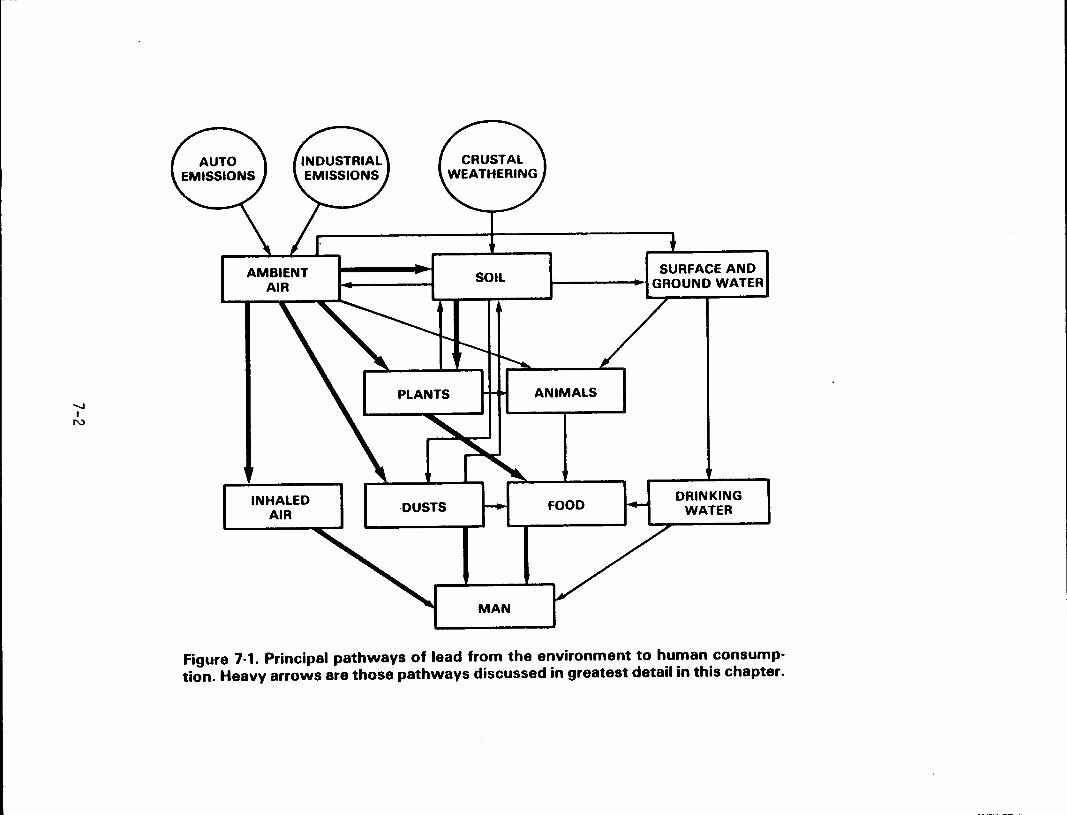
....... I
N
AMBIENT AIR
INHALED AIR
PLANTS
·DUSTS
SOIL
MAN
SURFACE AND 1-----..,.1 GROUND WATER
ANIMALS
DRINKING WATER
Figure 7-1. Principal pathways of lead from the environment to human consumption. Heavy arrows are those pathways discussed in greatest detail in this chapter.
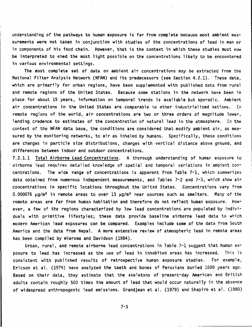
understanding of the pathways to human exposure is far frc•m complete because most ambient measurements were not taken in conjunction with studies of the concentrations of lead in man or in components of his food chain. However, that is the context in which these studies must now be interpreted to ~hed the mo~t light possible on the concentrations likely to be encountered in various environmental settings.
The most complete set of data on ambient air conCE!ntrations may be extracted from the National Filter Analysis Network (NFAN) and its predecessors (see Section 4.2.1). These data, which are primarily for urban regions, have been supplemented with published data from rural and remote regions of the United States. Because some stations in the network have been in place for about 15 years, information on temporal trends is available but sporadic. Ambient air concentrations in the United States are comparable to other industrialized nations. In remote regions of the world, air concentrations are two or three orders of magnitude lower, lending credence to estimates of the concentration of natural lead in the atmosphere. In the context of the NFAN data base, the conditions are considE!red that modify ambient air, as measured by the monitoring networks, to air as inhaled by humans. Specifically, these conditions
are changes in particle size distributions, changes with vertical distance above ground, and
differences between indoor and outdoor concentrations. 7. 2.1.1 Tota 1 Airborne Lead Concentrations. A thorough understanding of human exposure to airborne lead requires detailed knowledge of spatial and temporal variations in ambient concentrations. The wide range of concentrations is apparE!nt from Table 7-1, which summarizes
data obtained from numerous independent measurements, and Tables 7-2 and 7-3, which show air concentrations in specific 1 ocat ions throughout the Unitt!d States. Concentrations vary from
0.000076 ~g/m3 in remote areas to over 13 ~g/m3 near sources such as smelters. Many of the
remote areas are far from human habitation and therefore do not reflect human exposure. However, a few of the regions characterized by low lead concentrations are populated by individuals with primitive lifestyles; these data provide baseline airborne lead data to which
modern American lead exposures can be compared. Examples include some of the data from South
America and the data from Nepal. A more extensive revie'J of atmospheric lead in remote areas
has been compiled by Wiersma and Davidson (1984). Urban, rural, and remote airborne lead concentrations in Table 7-1 suggest that human ex
posure to lead has increased as the use of lead in inhabited areas has increased. This is consistent with published results of retrospective human exposure studies. For example,
Ericson et al. (1979) have analyzed the teeth and bones of Peruvians buried 1600 years ago.
Based on their data, they estimate that the skeletons of present-day American and British
adults contain roughly 500 times the amount of lead that would occur naturally in the absence
of widespread anthropogenic lead emissions. Grandjean et al. (1979) and Shapiro et al. (1980)
7-3
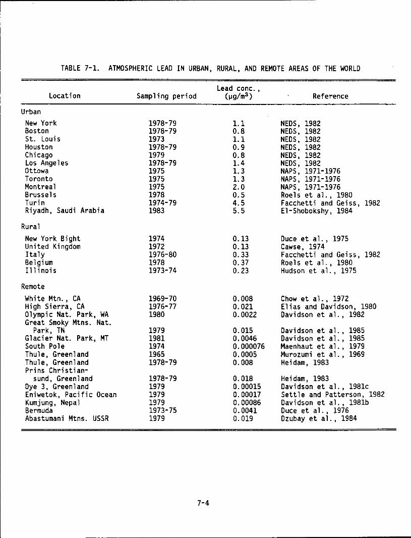
TABLE 7-1. ATMOSPHERIC LEAD IN URBAN, RURAL, AND REMOTE AREAS OF THE WORLD
Location
Urban New York Boston St. Louis Houston Chicago Los Angeles Ottowa Toronto Montreal Brussels Turin Riyadh, Saudi Arabia
Rural New York Bight United Kingdom Italy Belgium Illinois
Remote White Mtn., CA High Sierra, CA Olympic Nat. Park, WA Great Smoky Mtns. Nat.
Park, TN Glacier Nat. Park, MT South Pole Thule, Greenland Thule, Greenland Prins Christian-
sund, Greenland Dye 3, Greenland Eniwetok, Pacific Ocean Kumjung, Nepal Bermuda Abastumani Mtns. USSR
Sampling period
1978-79 1978-79 1973 1978-79 1979 1978-79 1975 1975 1975 1978 1974-79 1983
1974 1972 1976-80 1978 1973-74
1969-70 1976-77 1980
1979 1981 1974 1965 1978-79
1978-79 1979 1979 1979 1973-75 1979
7-4
Lead cone. , (J.Jg/m3)
1.1 0.8 1.1 0.9 0.8 1.4 1.3 1.3 2.0 0.5 4.5 5.5
0.13 0.13 0.33 0.37 0.23
0.008 0.021 0.0022
0.015 0.0046 0.000076 0.0005 0.008
0.018 0.00015 0.00017 0.00086 0.0041 0.019
Reference
NEDS, 1982 NEDS, 1982 NEDS, 1982 NEDS, 1982 NEDS, 1982 NEDS, 1982 NAPS, 1971-1976 NAPS, 1971-1976 NAPS, 1971-1976 Reels et al., 1980 Facchetti and Geiss, 1982 El-Shobokshy, 1984
Duce et al., 1975 Cawse, 1974 Facchetti and Geiss, 1982 Reels et al., 1980 Hudson et al., 1975
Chow et al., 1972 Elias and Davidson, 1980 Davidson et al., 1982
Davidson et al., 1985 Davidson et al., 1985 Maenhaut et al., 1979 Murozumi et al., 1969 Heidam, 1983
Heidam, 1983 Davidson et al., 1981c Settle and Patterson, 1982 Davidson et al., 1981b Duce et al., 1976 Dzubay et al., 1984
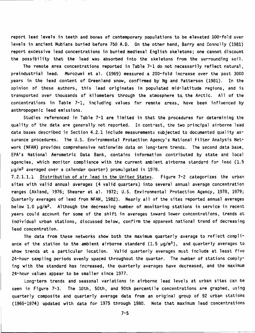
report lead levels in teeth and bones of contemporary populations to be elevated 100-fold over levels in ancient Nubians buried before 750 A.D. On the ,other hand, Barry and Connolly (1981) report excessive lead concentrations in buried medieval English skeletons; one cannot discount the poss i bi 1 i ty that the 1 ead was absorbed into the s ke 1 etons from the surrounding soi 1.
The remote area concentrations reported in Table 7-1 do not necessarily reflect natural, preindustrial lead. Murozumi et al. (1969) measured a .200-fold increase over the past 3000 years in the lead content of Greenland snow, confirmed by Ng and Patterson (1981). In the
opinion of these authors, this lead originates in populated mid-latitude regions, and is transported over thousands of kilometers through the atmosphere to. the Arctic. A 11 of the concentrations in Table 7-1, including values for remote areas, have been influenced by anthropogenic lead emissions.
Studies referenced in Table 7-1 are limited in that the procedures for determining the quality of the data are generally not reported. In cont:rast, the two principal airborne lead data bases described in Section 4.2.1 include measurement:; subjected to documented quality as
surance procedures. The U.S. Environmental Protection A!~ency•s National Filter Analysis Net
work (NFAN) provides comprehensive nationwide data on lon!~-term trends. The second data base, EPA 1 s National Aerometric Data Bank, contains information contributed by state and local agencies, which monitor compliance with the current ambient airborne standard for lead (1.5 ~g/m3 averaged over a calendar quarter) promulgated in 1978. 7.2.1.1.1 Distribution of air lead in the United States. Figure 7-2 categorizes the urban sites with valid annual averages (4 valid quarters) into several annual average concentration
ranges (Akland, 1976; Shearer et al. 1972; U.S. Environmental Protection Agency, 1978, 1979;
Quarterly averages of lead from NFAN, 1982). Nearly all of the sites reported annual averages below 1.0 ~g/m3 • Although the decreasing number of monitoring stations in service in recent years could account for some of the shift in averages toward lower concentrations, trends at
individual urban stations, discussed below, confirm the apparent national trend of decreasing
lead concentration. The data from these networks show both the maximum quarterly average to reflect compli
ance of the station to the ambient airborne standard (1.5 ~g/m3 ), and quarterly averages to show trends at a particular location. Valid quarterly averages must include at least five 24-hour sampling periods evenly spaced throughout the quay·ter. The number of stations complying with the standard has increased, the quarterly averages have decreased, and the maximum
24-hour values appear to be smaller since 1977. Long-term trends and seasonal variations in airborne lead levels at urban sites can be
seen in Figure 7-3. The lOth, 50th, and 90th percenti"le concentrations are graphed, using
quarterly composite and quarterly average data from an original group of 92 urban stations (1965-1974) updated with data for 1975 through 1980. Note that maximum lead concentrations
7-5
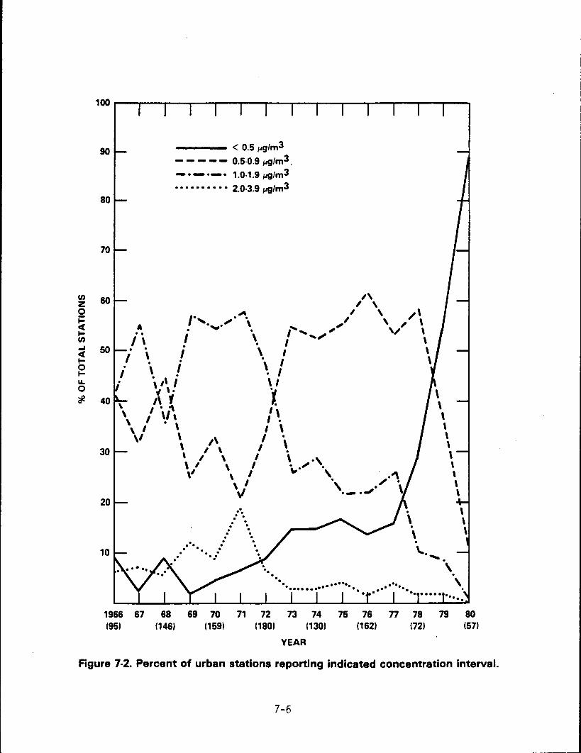
en z 0
~ len ..... < 1-0 I-I&. 0 '#
90
80
70
60
50
---- < 0.5 !-l9/m3 - - - -- 0.5-0.9 lolQ/m3.
-·-·-· 1.0·1.9 lolQ/m3 • • • • • • • • • • 2.0·3.9 lolQ/m3
,, ~ '
/., ~·.;t· ~' \ /\ . .._,.... \ , ' , \ i \ ;-- .... ..._,.' \/
• • I I \ I • \ I
\ I . I ·, '' j \ I ., ' • "<~.
40\ 1\t I. \ I •\/"\\ I\
30
20
10
\ I • \ I •
'vi ', ~~ 1\ I \ I \ •
\ I \ I \ •\ \ I \ I ~-·-" • \' \ I .. \ .• _,
\ I • / • ' . \ \1 ·-·J . .. : . . . . . . . . . . . . . . . . . . . . . . .· .. ·
1966 67 68 69 10 11 72 73 74 75 76 n 78 79 80 1951 11461 (1591 (1801 (1301 (1621 1721 1571
YEAR
Figure 7-2. Percent of urban stations reporting indicated concentration interval.
7-6
typically occur in the winter, while m1mma occur in the sununer. In contrast, automotive emissions of lead would be expected to be greater in the sununer for two reasons: (1) gasoline usage is higher in t~e summer; and (2) lead content is raised in summer gasolines to replace some of the more volatile high-octane components that cannot be used in summertime gasolines. Apparently, the troposphere has a greater capacity to disperse submicron particles in the
summer than in the winter. Figure 7-3 also clearly portrays the significant decrease in airborne lead levels over
the past decade. This trend is attributed to the decreasing lead content of regular and premium gasoline, and to the increasing usage of unleaded gasoline. The close parallel between these two parameters is discussed in detail in Chapter 5. (See Figure 5-7 and Table 5-5.)
Table 7-2 shows lead concentrations in the atmospheres of several major metropolitan areas of epidemiological interest. Some of the data presented do not meet the stringent requirements for quarterly averages and occasionally there have been changes in site location or sampling methodology. Nevertheless, the data are the best available for reporting the history of 1 ead contamination in these specific urban atmosphert!S. Further discussions of these data
appear in Chapter 11.
-.. \ .., 3.0 en z 0
~ ~ w (.) z 0 (.)
~ e& 18 &7 ea • 10 11 n
YEAR
Figure 7·3. Seasonal patterns and trends in quarterly ;iiYerage urban lead concentrations.
7-7
J
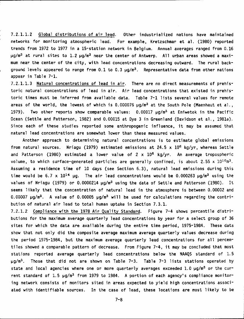
7.2.1.1.2 Global distributions of air lead. Other industrialized nations have maintained networks for monitoring atmospheric lead. For example, Kretzschmar et al. (1980) reported trends from 1972 to 1977 in a 15-station network in Belgium. Annual averages ranged from 0.16 ~g/m3 at rural sites to 1.2 ~g/m3 near the center of Antwerp. All urban areas showed a maximum near the center of the city, with lead concentrations decreasing outward. The rural background levels appeared to range from 0.1 to 0.3 ~g/m3 . Representative data from other nations appear in Table 7-1.
7.2.1.1.3 Natural concentrations of lead in air. There are no direct measurements of prehis
toric natural concentrations of lead in air. Air lead concentrations that existed in prehistoric times must be .inferred from available data. Table 7-1 lists several values for remote areas of the world, the lowest of which is 0.000076 ~g/m3 at the South Pole (Maenhaut et al., 1979). Two other reports show comparable values: 0.00017 ~g/m3 at Eniwetok in the Pacific Ocean (Settle and Patterson, 1982) and 0.00015 at Dye 3 in Greenland (Davidson et al., 1981a). Since each of these studies reported some anthropogenic influence, it may be assumed that natural lead concentrations are somewhat lower than these measured values.
Another approach to determining natura 1 concentrations is to estimate gl oba 1 emissions from natural sources. Nriagu (1979) estimated emissions at 24.5 x 10⁶ kg/yr, whereas Settle
and Patterson (1980) estimated a lower value of 2 x 10⁶ kg/yr. An average tropospheric volume, to which surface-generated particles are generally confined, is about 2.55 x 10¹⁰m3 .
Assuming a residence time of 10 days (see Section 6.3), natural lead emissions during this
time would be 6.7 x 10¹⁴ ~g. The air lead concentrations would be 0.000263 ~g/m3 using the values of Nriagu (1979) or 0.0000214 ~g/m3 using the data of Settle and Patterson (1980). It seems likely that the concentration of natural lead in the atmosphere is between 0.00002 and 0.00007 ~g/m3 • A value of 0.00005 ~g/m3 will be used for calculations regarding the contribution of natural air lead to total human uptake in Section 7.3.1.
7.2.1.2 Compliance with the 1978 Air Quality Standard. Figure 7-4 shows percentile distributions for the maximum average quarterly lead concentrations by year for a select group of 36
sites for which the data are available during the entire time period, 1975-1984. These data
show that not only did the composite average maximum average quarterly values decrease during the period 1975-1984, but the maximum average quarterly lead concentrations for all percen
tiles showed a comparable pattern of decrease. From Figure 7-4, it may be concluded that most stations reported average quarterly lead concentrations below the NAAQS standard of 1.5
~g/m3 . Those that did not are shown on Table 7-3. Table 7-3 lists stations operated by
state and local agencies where one or more quarterly averages exceeded 1.0 ~g/m3 or the cur
rent standard of 1.5 ~g/m3 from 1979 to 1984. A portion of each agency's compliance monitoring network consists of monitors sited in areas expected to yield high concentrations associated with identifiable sources. In the case of lead, these locations are most likely to be
7-8
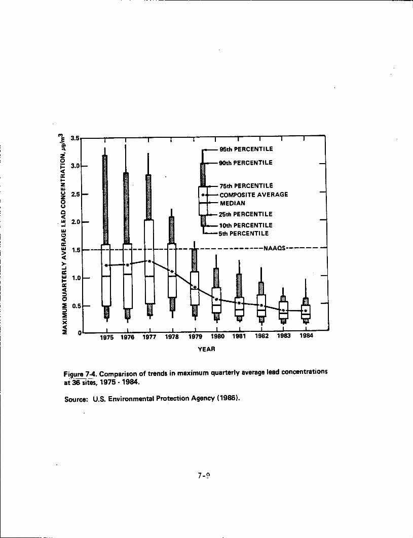
95th PERCENTILE
90th PERCIENTILE
.-.-75th PERCENTILE
COMPOSITE AVERAGE .._.._MEDIAN
25th PERCIENTILE
10th PERCENTILE 5th PERCENTILE
---------·---NAAQS------
1981 1982 1983 1984
YEAR
Figure 7-4. Comparison of trends in maximum quarterly average lead concentrations at"36 siteS, 1975 · 1984.
Source: U.S. Environmental Protection Agency (1986).
7-C)
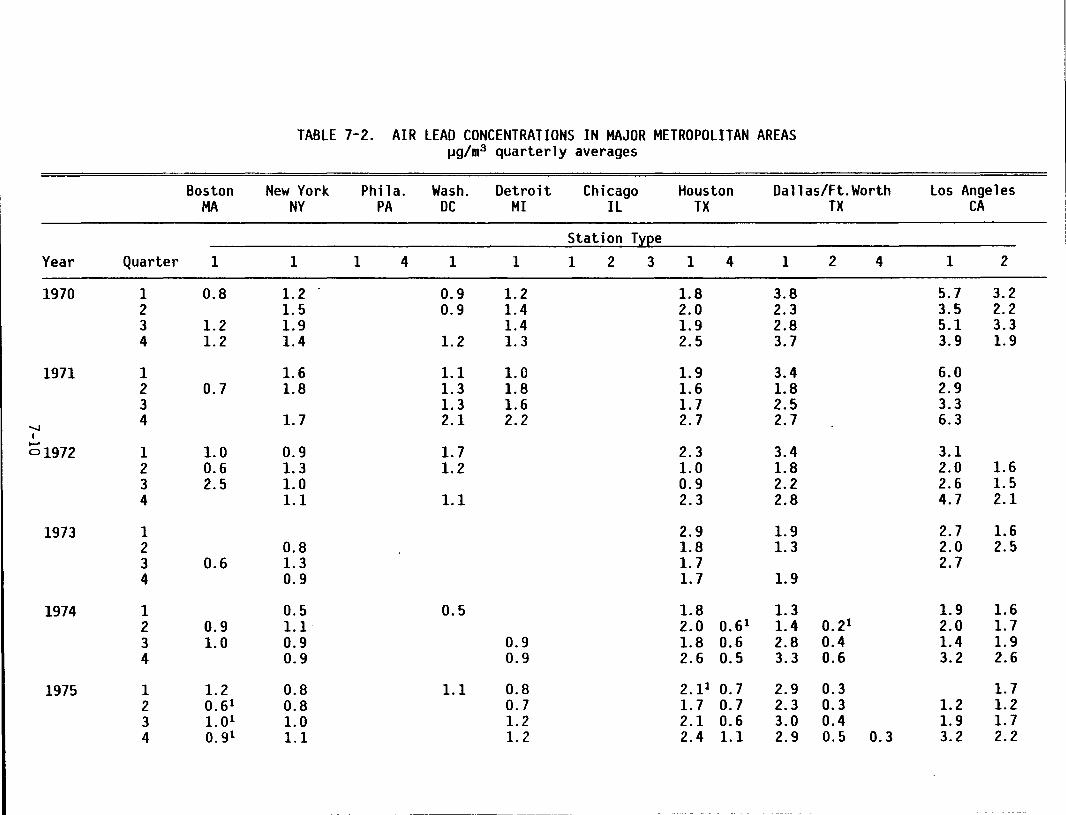
TABLE 7-2. AIR LEAD CONCENTRATIONS IN MAJOR METROPOLITAN AREAS ~g/m3 quarterly averages
Boston New York Phil a. Wash. Detroit Chicago Houston Dallas/Ft. Worth los Angeles MA NY PA DC MI Il TX TX CA
Station T~ee Year Quarter 1 1 1 4 1 1 1 2 3 1 4 1 2 4 1 2
1970 1 0.8 1.2 0.9 1.2 1.8 3.8 5.7 3.2 2 1.5 0.9 1.4 2.0 2.3 3.5 2.2 3 1.2 1.9 1.4 1.9 2.8 5.1 3.3 4 1.2 1.4 1.2 1.3 2.5 3.7 3.9 1.9
1971 1 1.6 1.1 1.0 1.9 3.4 6.0 2 0.7 1.8 1.3 1.8 1.6 1.8 2.9 3 1.3 1.6 1.7 2.5 3.3 4 1.7 2.1 2.2 2.7 2.7 6.3 ......,
I ...... o1972 1 1.0 0.9 1.7 2.3 3.4 3.1
2 0.6 1.3 1.2 1.0 1.8 2.0 1.6 3 2.5 1.0 0.9 2.2 2.6 1.5 4 1.1 1.1 2.3 2.8 4.7 2.1
1973 1 2.9 1.9 2.7 1.6 2 0.8 1.8 1.3 2.0 2.5 3 0.6 1.3 1.7 2.7 4 0.9 1.7 1.9
1974 1 0.5 0.5 1.8 1.3 1.9 1.6 2 0.9 1.1 2.0 0.61 1.4 0.21 2.0 1.7 3 1.0 0.9 0.9 1.8 0.6 2.8 0.4 1.4 1.9 4 0.9 0.9 2.6 0.5 3.3 0.6 3.2 2.6
1975 1 1.2 0.8 1.1 0.8 2.11 0.7 2.9 0.3 1.7 2 0.61 0.8 0.7 1.7 0.7 2.3 0.3 1.2 1.2 3 1. 01 1.0 1.2 2.1 0.6 3.0 0.4 1.9 1.7 4 0.91 1.1 1.2 2.4 1.1 2.9 0.5 0.3 3.2 2.2
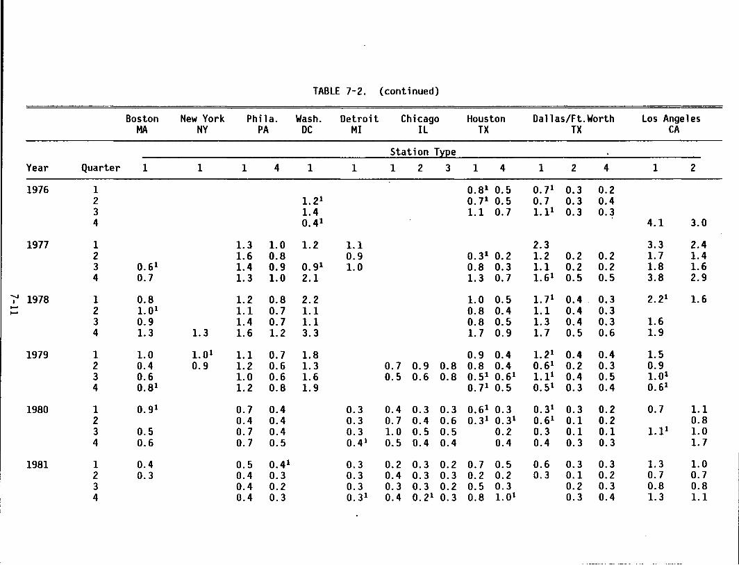
TABLE 7-2. (continued)
Boston New York Phil a. Wash. Detroit Chicago Houston Dallas/Ft. Worth Los Angeles MA NY PA DC MI IL TX TX CA
Station T~~e Year Quarter 1 1 1 4 1 1 1 2 3 1 4 1 2 4 1 2
1976 1 0.81 0.5 0.71 0.3 0.2 2 1. 21 0.71 0.5 0.7 0.3 0.4 3 1.4 1.1 0.7 1.11 0.3 0.3 4 0.41 4.1 3.0
1977 1 1.3 1.0 1.2 1.1 2.3 3.3 2.4 2 1.6 0.8 0.9 0.31 0.2 1.2 0.2 0.2 1.7 1.4 3 0.61 1.4 0.9 0.91 1.0 0.8 0.3 1.1 0.2 0.2 1.8 1.6 4 0.7 1.3 1.0 2.1 1.3 0.7 1.61 0.5 0.5 3.8 2.9
......., 1978 1 0.8 1.2 0.8 2.2 1.0 0.5 1. 71 0.4 . 0.3 2.21 1.6 I
...... 2 1. 01 1.1 0.7 1.1 0.8 0.4 1.1 0.4 0.3 ...... 3 0.9 1.4 0.7 1.1 0.8 0.5 1.3 0.4 0.3 1.6 4 1.3 1.3 1.6 1.2 3.3 1.7 0.9 1.7 0.5 0.6 1.9
1979 1 1.0 1.01 1.1 0.7 1.8 0.9 0.4 1. 21 0.4 0.4 1.5 2 0.4 0.9 1.2 0.6 1.3 0.7 0.9 0.8 0.8 0.4 0.61 0.2 0.3 0.9 3 0.6 1.0 0.6 1.6 0.5 0.6 0.8 0.51 0.61 1.11 0.4 0.5 1.01 4 0.81 1.2 0.8 1.9 0.71 0.5 0.51 0.3 0.4 0.61
1980 1 0.91 0.7 0.4 0.3 0.4 0.3 0.3 0.61 0.3 0.31 0.3 0.2 0.7 1.1 2 0.4 0.4 0.3 0.7 0.4 0.6 0.31 0.3 1 0.61 0.1 0.2 0.8 3 0.5 0.7 0.4 0.3 1.0 0.5 0.5 0.2 0.3 0.1 0.1 l.Il 1.0 4 0.6 0.7 0.5 0.41 0.5 0.4 0.4 0.4 0.4 0.3 0.3 1.7
1981 1 0.4 0.5 0.41 0.3 0.2 0.3 0.2 0.7 0.5 0.6 0.3 0.3 1.3 1.0 2 0.3 0.4 0.3 0.3 0.4 0.3 0.3 0.2 0.2 0.3 0.1 0.2 0.7 0.7 3 0.4 0.2 0.3 0.3 0.3 0.2 0.5 0.3 0.2 0.3 0.8 0.8 4 0.4 0.3 0.31 0.4 0.21 0.3 0.8 1. ot 0.3 0.4 1.3 1.1
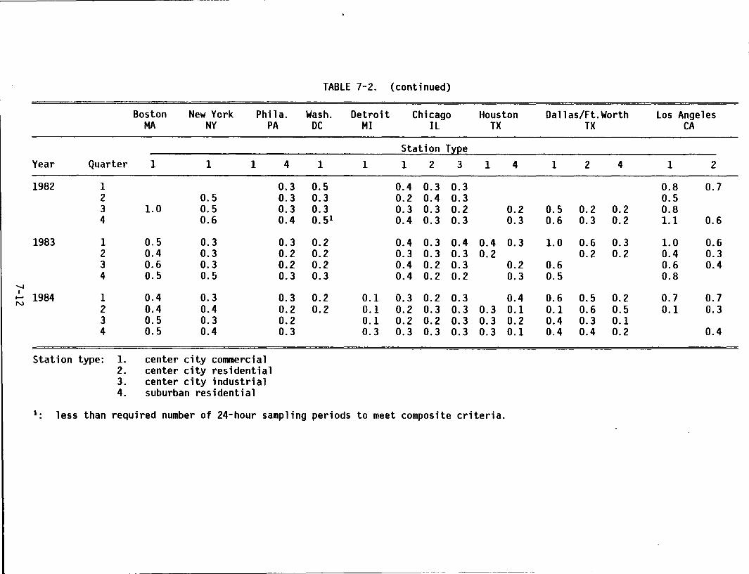
TABLE 7-2. (continued)
Boston New York Phil a. Wash. Detroit Chicago Houston Dallas/Ft. Worth los Angeles MA NY PA DC MI ll TX TX CA
Station T~~e Year Quarter 1 1 1 4 1 1 1 2 3 1 4 1 2 4 1 2
1982 1 0.3 0.5 0.4 0.3 0.3 0.8 0.7 2 0.5 0.3 0.3 0.2 0.4 0.3 0.5 3 1.0 0.5 0.3 0.3 0.3 0.3 0.2 0.2 0.5 0.2 0.2 0.8 4 0.6 0.4 0.51 0.4 0.3 0.3 0.3 0.6 0.3 0.2 1.1 0.6
1983 1 0.5 0.3 0.3 0.2 0.4 0.3 0.4 0.4 0.3 1.0 0.6 0.3 1.0 0.6 2 0.4 0.3 0.2 0.2 0.3 0.3 0.3 0.2 0.2 0.2 0.4 0.3 3 0.6 0.3 0.2 0.2 0.4 0.2 0.3 0.2 0.6 0.6 0.4 4 0.5 0.5 0.3 0.3 0.4 0.2 0.2 0.3 0.5 0.8
'-J I
1984 1 0.4 0.3 0.3 0.2 ...... 0.1 0.3 0.2 0.3 0.4 0.6 0.5 0.2 0.7 0.7 N
2 0.4 0.4 0.2 0.2 0.2 0.3 0.3 0.1 0.1 0.6 0.5 0.1 0.3 0.1 0.3 3 0.5 0.3 0.2 0.1 0.2 0.2 0.3 0.3 0.2 0.4 0.3 0.1 4 0.5 0.4 0.3 0.3 0.3 0.3 0.3 0.3 0.1 0.4 0.4 0.2 0.4
Station type: 1. center city commercial 2. center city residential 3. center city industrial 4. suburban residential
t. less than required number of 24-hour sampling periods to meet composite criteria.
L_ ____________________________________________________________________ -----
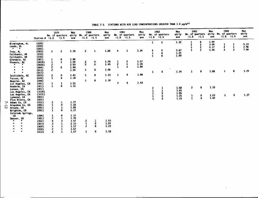
TABlE 7-3. STATIONS WITH AIR lEAD CONCENTRATIONS GREATER THAN 1.0 ~g/•3*
1979 Max 1980 Max 1981 Max 1982 Max 1983 Max 1984 Max No. of quarters qtrly No. of quarters qtrly No. of quarters qtrly No. of quarters qtrly No. of quarters qtrly No. of quarters qtrly
Station I >1.0 >1. 5 ave >1.0 >1. 5 ave >1.0 >1.5 ave >1.0 >1.5 ave >1.0 >1. 5 ave >1.0 >1. 5 ave
Bil'llingha., Al (028) 1 0 1.32 1 0 1.04
leeds, Al (004) 2 2 3.04 1 1 5.33 .. u (005) 3 2 4.17 2 1 2.96
Troy, Al (003) 2 2 2.78 2 1 1.89 4 3 3.34 4 4 3.67 3 2 5.44 4 3 7.08
Fairbanks, AK (010) 1 0 1.01 Fairbanks, AK (016) 1 0 1.09 Glendale, AZ (001) 1 0 1.06 Phoenix, AZ (002A) 1 1 1.54 2 0 1.29 1 0 1.17
N .. (002G) 2 2.59 2 0 1.49 2 0 1.39
" M (004) 2 0 1.48 1 0 1.04 H H (013) 2 1.55 1 0 1.06 " N (017) 1 0 1.24 1 0 1.08 1 0 1.29
Scottsdale, Al. (003) 2 0 1.41 1 0 1.13 1 0 1.08 Tucson, AZ (009) 1 0 1.18 Nogales, AZ (004) 1 0 1.10 los Angeles, CA (001) 1 1 1.51 2 0 1.43 Anahei•, CA (001) 1 0 1.11 lennox, CA (001) 2 1 1.68 2 0 1.10
los Angeles, CA (lOlA) 1 1 1.65 los Angeles, CA (1031) 1 0 1.05 lynwood, CA (001) 1 0 1.25 1 0 1.03 1 0 1.27
Pico Rivera, CA (001) 1 0 1.15 1 0 1.02 OOooooJ Adas Co, CO (001) 2 1 1.77 I
...... Arapahoe Co, CO (001) 1 0 1.10 w Arvada, CO (001) 1 1 1.60
Brighton, CO (001) 1 0 1.17 Colorado Springs,
co (004) 1 0 1.37 Denver, co (001) 2 1 1. 70 .. M (002) 4 3 3.47 2 1 1. 53
" " (003) 3 1 2.13 1 0 1.03 .. • (009) 1 1 1.57 2 0 1.23 " • (010) 2 1 1.67 .. .. (012) 2 1 1. 67 1 0 1.10
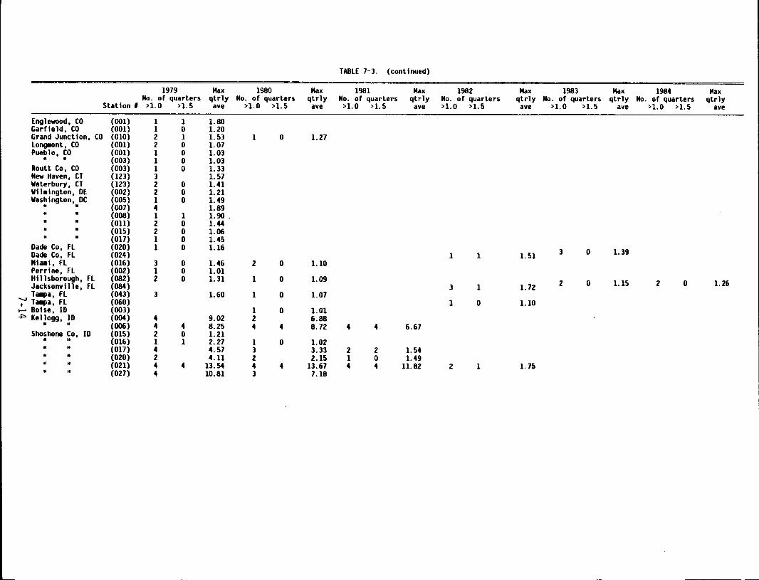
TABLE 7-3. (continued)
1979 Max 1980 Max 1981 Max 1982 Max 1983 Max 1984 Max No. of quarters qtrly No. of quarters qtrly No. of quarters qtrly No. of quarters qtrly No. of quarters qtrly No. of quarters qtrly
Station I >1. 0 >1.5 ave >1.0 >1. 5 ave >1.0 >1. 5 ave >1.0 >1. 5 ave >1.0 >1. 5 ave >1.0 >1. 5 ave
Englewood, CO (001) 1 1 1.80 Garfield, CO (001) 1 0 1.20 Grand Junction, CO (010) 2 1 1. 53 1 0 1.27 Long110nt, CO (001) 2 0 1.07 Pueblo, CO (001) 1 0 1.03
• II (003) 1 0 1.03 Routt Co, CO (003) 1 0 1.33 New Haven, CT (123) 3 1.57 Waterbury, CT (123) 2 0 1.41 Wil•ington, DE (002) 2 0 1.21 Washington, DC (005) 1 0 1.49
II II (007) 4 1.89 II u (008) 1 1 1.90 . • II (011) 2 0 1.44 II II (015) 2 0 1.06 II II (017) 1 0 1.45
Dade Co, Fl (020) 1 0 1.16 3 0 1. 39 Dade Co, Fl (024) 1 1 1.51 MIMi, Fl (016) 3 0 1.46 2 0 1.10 Perrine, Fl (002) 1 0 1.01 Hillsborough, Fl (082) 2 0 1.31 1 0 1.09 2 0 1.15 2 0 1.26 Jacksonville, Fl (084) 3 1 1. 72 Ta~~~~a, Fl (043) 3 1.60 1 0 1.07
~ T a~~pa, Fl (060) 1 0 1.10 ...... Boise, ID (003) 1 0 1.01 +>- Kellogg, ID (004) 4 9.02 2 6.88
II H (006) 4 4 8.25 4 4 8. 72 4 4 6.67 Shoshone Co, ID (015) 2 0 1.21
II .. (016) 1 1 2.27 1 0 1.02 II II (017) 4 4.57 3 3.33 2 2 1.54 II II (020) 2 4.11 2 2.15 1 0 1.49 II II (021) 4 4 13.54 4 4 13.67 4 4 11.82 2 1 1. 75 II .. (027) 4 10.81 3 7.18
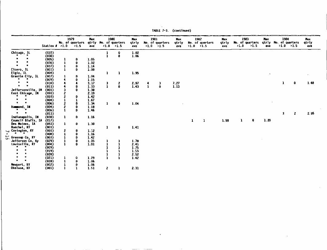
TABLE 7-3. (continued)
1979 Max 1980 Max 1981 Max 1982 Max 1983 Max 1984 Max No. of quarters qtrly No. of quarters qtrly No. of quarters qtrly No. of quarters qtrly No. of quarters qtrly No. of quarters qtrly
Station I >1.0 >1. 5 ave >1.0 >1. 5 ave >1.0 >1. 5 ave >1.0 >1.5 ave >1.0 >1.5 ave >1.0 >1.5 ave
Chicago, IL (022) 1 0 1.02 II M (030) 1 0 1.06 .. .. (005) 1 0 1.05 " u (036) 1 0 1.02 " u (037) 1 0 1.14
Cicero, ll (001) 1 0 1.00 Elgin, ll (004) 1 1 1.95 Granite City, ll (007) 1 0 1.04
II H (009} 4 0 1.15 H II (010} 4 4 3.17 3 2 2.97 4 3 7.27 1 0 1.48 .. u (011} 4 0 1.33 1 0 1.43 1 0 1.13
Jeffersonville, IN (001) 3 0 1.38 East Chicago, IN (001} 2 2.19 .. .. (003) 2 0 1.42
" .. (004} 1 1 1.67 .. M (006} 2 0 1.34 1 0 1.04 Ha.ond, IN (004) 2 0 1.18 .. " (006) 1 0 1.46
II .. (011) 3 2 2.95 Indianapolis, IN (030) 1 0 1.16 Council Bluffs, lA (017) 1 1 1.59 1 0 1.20 Des Moines, lA (051) 1 0 1. 30 Buechel, KY (001) 1 0 1.41
-.....J Covington, KY (001) 2 0 1.12 I .. .. (008) 1 0 1.16 t;. Greenup Co, KY (003} 1 0 1.42
Jefferson Co, Ky (029) 1 0 1.05 1 1 1.78 Louisville, KY (004) 1 0 1.01 1 1 2.41 .. .. (009) 1 1 1.75 .. .. tn1a\ ' ' 1.!,9 , ......... , .. ..
" .. (020) 1 1 2.52 .. " (021) 1 0 1. 29 1 1 1.42 .. .. (028) 1 0 1.06 Newport, KY (002) 1 0 1.06 Okolona, KY (001) 1 1 1.51 2 1 2.31
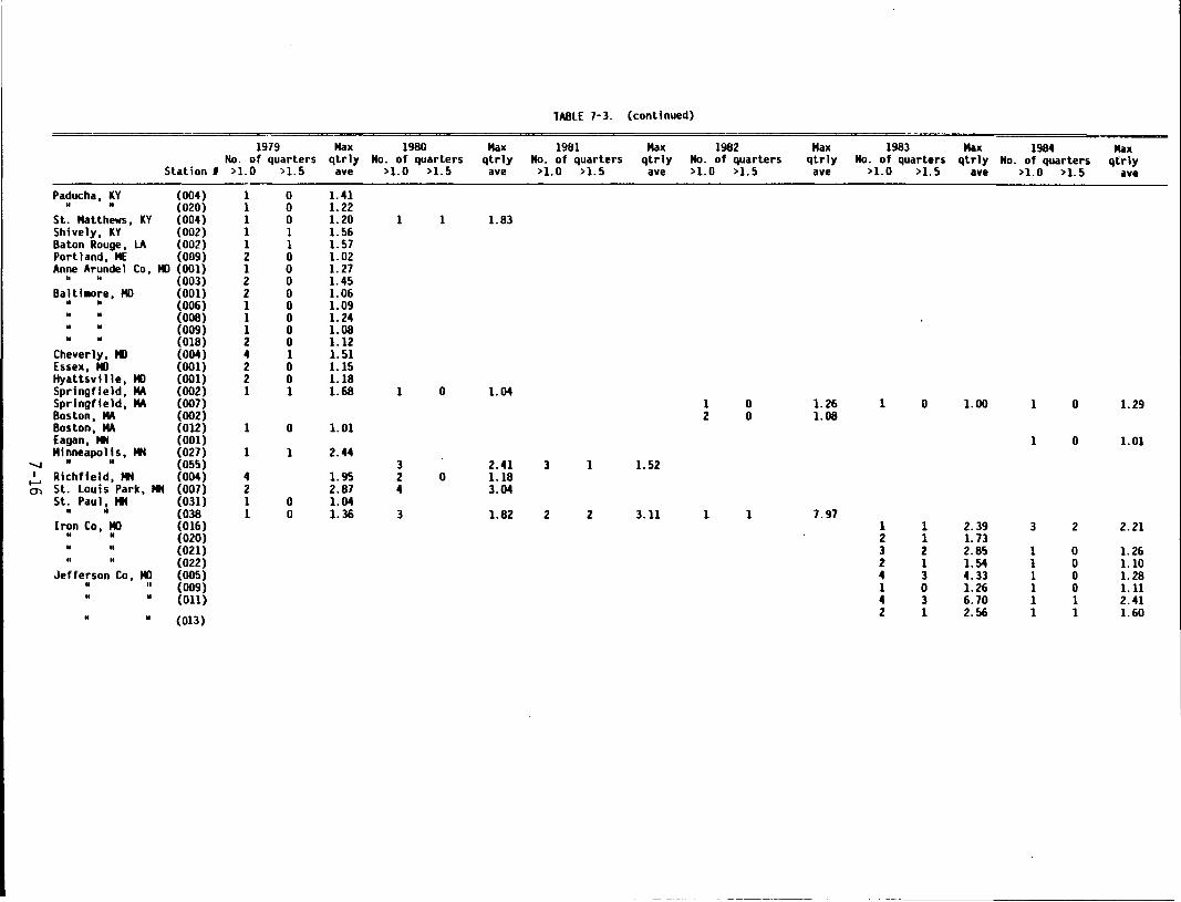
TABLE 7-3. (continued)
1979 Max 1980 Max 1981 Max 1982 Max 1983 Max 1984 Max No. of quarters qtrl1 No. of quarters qtrly No. of quarters qtrly No. of quarters qtrly No. of quarters qtrly No. of quarters qtrly
Station I >1.0 >l.S ave >1.0 >1. s ave >1.0 >1. s ave >1.0 >1. s ave >1. 0 >1. s ave >1.0 >1. s ave
Paducha, KY (004) 1 0 1.41 M • (020) 1 0 1. 22
St. Matthews, KY (004) 1 0 1. 20 1 1 1.83 Shively, KY (002) 1 1 1. 56 Baton Rouge, LA (002) 1 1 1. 57 Portland, ME (009) 2 0 1. 02 Anne Arundel Co, MD (001) 1 0 1. 27
II II (003) 2 0 1.45 Ba 1 ti110re, MD (001) 2 0 1.06
• • (006) 1 0 1.09 II • (008) 1 0 1. 24 u • (009) 1 0 1.08 u II (018) 2 0 1.12
Cheverly, MD (004) 4 1 1.51 Essex, MD (001) 2 0 1.15 Hyattsv i 11 e, MD (001) 2 0 1.18 Springfield, MA (002) 1 1 1.68 1 0 1.04 Springfield, MA (007) 1 0 1. 26 1 0 1.00 1 0 1.29 Boston, MA (002) 2 0 1.08 Boston, MA (012) 1 0 1.01 Eagan, til (001) 1 0 1.01 Mi nneapo 11 s, til (027) 1 1 2.44
-...J • u (OSS) 3 2.41 3 1 1. 52 I Richfield, til (004) 4 1.95 2 0 1.18 ~ St. Louis Park, til (007) 2 2.87 4 3.04
St. Paul, til (031) 1 0 1.04 " u (038 1 0 1.36 3 1.82 2 2 3.11 1 1 7.97
Iron Co, MD (016) 1 1 2.39 3 2 2.21 h • (020) 2 1 1.73 M II (021) 3 2 2.85 1 0 1. 26 II II (022) 2 1 1.54 1 0 1.10
Jefferson Co, MD (DOS) 4 3 4.33 1 0 1. 28 h H (009) 1 0 1. 26 1 0 1.11 II " (011) 4 3 6. 70 1 1 2.41 • • (013)
2 1 2.56 1 1 1.60
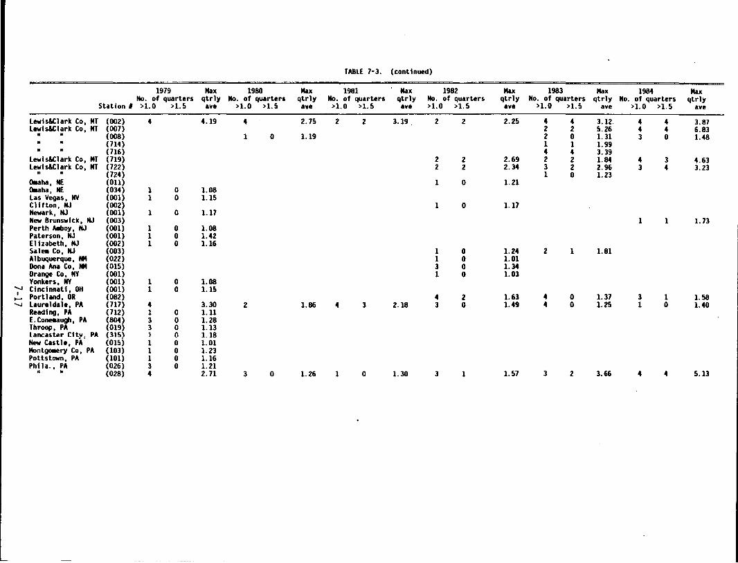
TABLE 7-3. (continued)
1979 Max 1980 Max 1981 Max 1982 Max 1983 Max 1984 Max No. of quarters qtrly No. of quarters qtrly No. of quarters qtrly No. of quarters qtrly No. of quarters qtrly No. of quarters qtrly
Station I >1.0 >1.5 ave >1.0 >1.5 ave >1.0 >1.5 ave >1.0 >1.5 ave >1.0 >1. 5 ave >1.0 >1.5 ave
lewis&Clark Co, MT (002) 4 4.19 4 2.75 2 2 3.19 2 2 2.25 4 4 3.12. 4 4 3.87 lewis&Clark Co, MT (007) 2 2 5.26 4 4 6.83 • II (008) 1 0 1.19 2 0 1.31 3 0 1.48
u • (714) 1 1 1.99 • • (716) 4 4 3.39
lewis&clark Co, MT (719) 2 2 2.69 2 2 1.84 4 3 4.63 lewis&Clark Co, MT (722) 2 2 2.34 3 2 2.96 3 4 3.23
II • (724) 1 0 1.23 Dllaha, HE (011) 1 0 1.21 Dllaha, HE (034) 1 0 1.08 las Vegas , NV (001) 1 0 1.15 Clifton, HJ (002) 1 0 1.17 Newark, HJ (001) 1 0 1.17 New Brunswick, HJ (003) 1 1 1. 73 Perth Allboy, HJ (001) 1 0 1.08 Paterson, HJ (001) 1 0 1.42 Elizabeth, NJ (002) 1 0 1.16 Salet1 Co, NJ (003) 1 0 1.24 2 1 1.81 Albuquerque, HM (022) 1 0 1.01 Dona Ana Co, HM (015) 3 0 1.34 Orange Co, NY (001) 1 0 1.03 Yonkers, NY (001) 1 0 1.08
........ Cincinnati, ott (001) 1 0 1.15 I Portland, OR (082) 4 2 1.63 4 0 1.37 3 1 1.58 ~
........ laureldale, PA (717) 4 3.30 2 1.86 4 3 2.18 3 0 1.49 4 0 1.25 1 0 1.40 Reading, PA (712) 1 0 1.11 E.Cone~~augh, PA (804) 3 0 1.28 Throop, PA (019} 3 0 1.13 lancaster Cttv. PA {3l5) l 0 1.18 Hew Castle, PA. (015) 1 0 1.01 MontgoMry Co, PA (103) 1 0 1.23 Pottstown, PA (101) 1 0 1.16 Phil a., PA (026) 3 0 1. 21
II II (028) 4 2.71 3 0 1.26 1 0 1.30 3 1 1.57 3 2 3.66 4 4 5.13
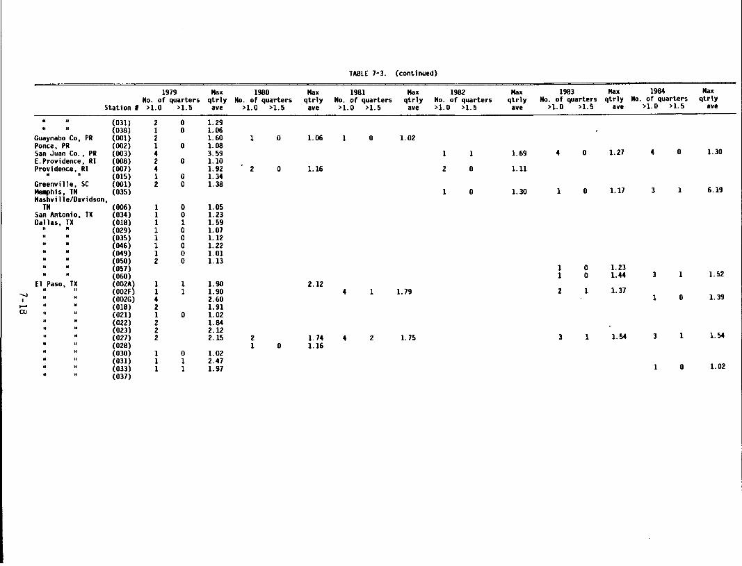
TABLE 7-3. (continued)
1979 Hax 1980 Hax 1981 Hax 1982 Max 1983 Max 1984 Hax No. of quarters qtrly No. of quarters qtrly No. of quarters qtrly No. of quarters qtrly No. of quarters qtrly No. of quarters qtrly
Station I >1.0 >1. 5 ave >1.0 >1.5 ave >1.0 >1. 5 ave >1.0 >1.5 ave >1.0 >1. 5 ave >1.0 >1. 5 ave
• .. (031) 2 0 1.29 " II (038) 1 0 1.06
Guaynabo Co, PR (001) 2 1.60 1 0 1.06 1 0 1.02 Ponce, PR (002) 1 0 1.08 San Juan Co. , PR (003) 4 3.59 1 1 1.69 4 0 1.27 4 0 1. 30 [.Providence, RI (008) 2 0 1.10 Providence, RI (007) 4 1. 92 2 0 1.16 2 0 1.11
• II (015) 1 0 1.34 Greenville, SC (001) 2 0 1.38 MeiiPhi s, TN (035) 1 0 1.30 1 0 1.17 3 1 6.19 Nashville/Davidson,
TN (006) 1 0 1.05 San Antonio, TX (034) 1 0 1.23 Dallas, TX (018) 1 1 1.59
" II (029) 1 0 1.07 " II (035) 1 0 1.12 " II (046) 1 0 1. 22 " " (049) 1 0 1.01 " N (050) 2 0 1.13 II N (057) 1 0 1.23 " " (060) 1 0 1.44 3 1 1.52
El Paso, TX (002A) 1 1 1.90 2.12 -...,J
(002F) 1 1 1.90 4 1 1.79 2 1 1.37 I (002G) 4 2.60 1 0 1. 39
...... (018) 2 1.91 (XJ (021) 1 0 1.02
(022) 2 1.84 (023) 2 2.12 (027) 2 2.15 2 1. 74 4 2 1. 75 3 1 1.54 3 1 1.54 (028) 1 0 1.16 (030) 1 0 1.02 (031) 1 1 2.47 (033) 1 1 1.97 1 0 1.02 (037)
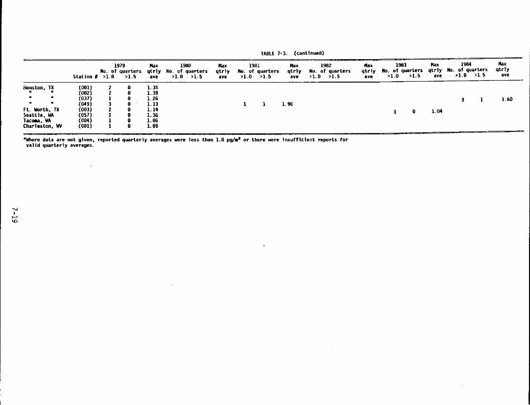
1979 No. of quarters
Station I >1.0 >1.5
Houston, TX (001) 2 0 H II (002) 2 0 II II (037) 1 0 II II (049) 3 0
Ft. Worth, TX (003) 2 0 Seattle, WA (057) 1 0 T ac011c1, WA (004) 1 0 Charleston, WV (001) 1 0
Max 1980 qtrly No. of quarters ave >1.0 >1.5
1.35 1.39 1.26 1.13 1.14 1.36 1.06 1.09
Max qtrly ave
TABLE 7-3. (continued)
1981 No. of quarters >1.0 >1.5
1 1
Max qtrly ave
1.96
1982 No. of quarters >1.0 >1.5
•Where data are not given, reported quarterly averages were less than 1.0 pg/•3 or there were insufficient reports for valid quarterly averages.
Max qtrly ave
1983 Max 1984 No. of quarters qtrly No. of quarters
>1.0 >1.5 ave >1.0 >1.5
3 1
1 0 1.04
Max qtrly
ave
1.60
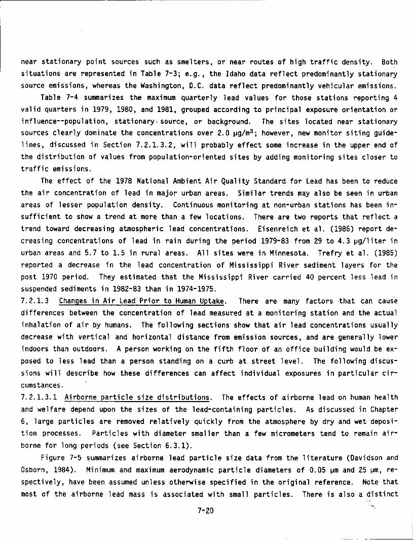
near stationary point sources such as smelters, or near routes of high traffic density. Both situations are represented in Table 7-3; e.g., the Idaho data reflect predominantly stationary source emissions, whereas the Washington, D.C. data reflect predominantly vehicular emissions.
Table 7-4 summarizes the maximum quarterly lead values for those stations reporting 4 valid quarters in 1979, 1980, and 1981, grouped according to principal exposure orientation or influence--population, stationary. source, or background. The sites located near stationary sources clearly dominate the concentrations over 2.0 ~g/m3 ; however, new monitor siting guidelines, discussed in Section 7.2.1.3.2, will probably effect some increase in the upper end of the distribution of values from population-oriented sites by adding monitoring sites closer to traffic emissions.
The effect of the 1978 National Ambient Air Quality Standard for Lead has been to reduce the air concentration of lead in major urban areas. Similar trends may also be seen in urban areas of lesser population density. Continuous monitoring at non-urban stations has been insufficient to show a trend at more than a few locations. There are two reports that reflect a trend toward decreasing atmospheric lead concentrations. Eisenreich et al. (1986) report decreasing concentrations of lead in rain during the period 1979-83 from 29 to 4.3 ~g/liter in urban areas and 5.7 to 1.5 in rural areas. All sites were in Minnesota. Trefry et al. (1985) reported a decrease in the lead concentration of Mississippi River sediment layers for the post 1970 period. They estimated that the Mississippi River carried 40 percent less lead in suspended sediments in 1982-83 than in 1974-1975. 7. 2.1. 3 Changes in Air Lead Prior to Human Uptake. There are many factors that can cause differences between the concentration of lead measured at a monitoring station and the actual inhalation of air by humans. The following sections show that air lead concentrations usually decrease with vertical and horizontal distance f~om emission sources, and are generally lower indoors than outdoors. A person working on the fifth floor of an office building would be exposed to less lead than a person standing on a curb at street level. The following discussions will describe how these differences can affect individual exposures in particular circumstances. 7.2.1.3.1 Airborne particle size distributions. The effects of airborne lead on human health and welfare depend upon the sizes of the lead-containing particles. As discussed in Chapter 6, large particles are removed relatively quickly from the atmosphere by dry and wet deposition processes. Particles with diameter smaller than a few micrometers tend to remain airborne for long periods (see Section 6.3.1).
Figure 7-5 summarizes airborne lead particle size data from the literature (Davidson and Osborn, 1984). Minimum and maximum aerodynamic particle diameters of 0.05 ~m and 25 ~m, respectively, have been assumed unless otherwise specified in the original reference. Note that most of the airborne lead mass is associated with small particles. There is also a distinct
... 7-20
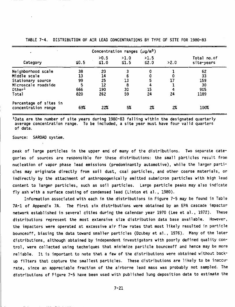
TABLE 7-4. DISTRIBUTION OF AIR LEAD CONCENTRATIONS BY TYPE OF SITE FOR 1980-83
Concentration ranges (~Jg/m3)
>0.5 >1. 0 >1. 5 Total no.of Category ~0.5 ~1.0 Sl. 5 ~2.0 >2.0 site-years
Neighborhood scale 38 20 3 0 1 62 Middle scale 13 14 6 0 0 33 Stationary source 99 25 13 5 17 159 Microscale roadside 5 12 8 4 1 30 Other1 666 190 30 15 4 905 Total 820 262 59 24 24 1189
Percentage of sites in concentration range 69% 22% 5% 2% 2% 100%
1 Data are the number of site years during 1980-83 falling within the designated quarterly average concentration range. To be included, a site year must have four valid quarters of data.
Source: SAROAD system.
peak of large particles in the upper end of many of the distributions. Two separate categories of sources are responsible for these distributions: the small particles result from nucleation of vapor phase lead emissions (predominantly automotive), while the larger particles may originate directly from soil dust, coal particles, and other coarse materials, or indirectly by the attachment of anthropogenically emitted submicron particles with high lead
content to larger particles, such as soil particles. L:~rge particle peaks may also indicate fly ash with a surface coating of condensed lead (Linton et al., 1980).
Information associated with each in the distributions in Figure 7-5 may be found in Table 7A-1 of Appendix 7A. The first six distributions were obtained by an EPA cascade impactor network established in several cities during the calendar· year 1970 (Lee et al., 1972). These distributions represent the most extensive size distribution data base available. However, the impactors were operated at excessive air flow rates that most likely resulted in particle bounceoff, biasing the data toward smaller particles (DZLibay et al., 1976). Many of the later distributions, although obtained by independent investigattors with poorly defined quality control, were collected using techniques that minimize particle bounceoff and hence may be more
reliable. It is important to note that a few of the distributions were obtained without backup filters that capture the smallest particles. These distributions are likely to be inaccurate, since an appreciable fraction of the airborne lead mass was probably not sampled. The distributions of Figure 7-5 have been used with published lung deposition data to estimate the
7-21
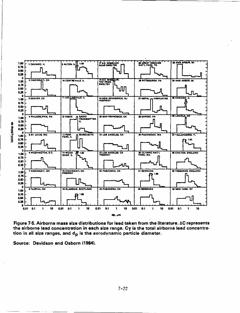
1.00 0.71 0.110 0.21
0 1.00 0.71 0.110 0.2&
0 1.00 0.71 0.110 0.2&
0 1.00
i 0.71 0.110
I 0.21
... 0 u 1.00 u 0.71 ~
0.110 0.21
0 1.00 0.71 0.110 0.21
0 1.00 0.71 0.110 0.21
0 1.00 0.71 0.110 0.21
0 0.01 0.1 10 0.01 0.1 10 0.01 0.1 10 0.01 0.1 1 10 0.01 0.1 1 10
dp.""' Figure 7-5. Airborne mass size distributions for lead taken from the literature. AC represents the airborne lead concentration in each size range. CT is the total airborne lead concentration in all size ranges, and dp is the aerodynamic particle diameter.
Source: Davidson and Osborn (1984).
7-22
fraction of inhaled airborne lead deposited in the human respiratory system (see Section 10.2.1).
7.2.1.3.2 Vertical gradients and siting guidelines. New guidelines for placing ambient air lead monitors went into effect in July, 1981 (C.F.R. (1984) 40: §58, see Section 4.2.1). 11 Mi crosca 1 e11 sites, p 1 aced between 5 and 15 meters from thoroughfares and 2 to 7 m above the ground, are prescribed, but until now few monitors have been located close to heavily traveled roadways. Many of these microscale sites might be expected to show higher lead concentrations than that measured at nearby middlescale urban sites, due to vertical gradients in lead concentrations near the source. One study (PEDCo, 1981) gives limited insight into the relationship between a microscale location and locations further from a roadway. The data in the lower half of Table 7-5 summarize total suspended particulates and particulate lead concentrations in samples collected in Cincinnati, Ohio, on 21 consecutive days in April and May, 1980, adjacent to a 58,500 average daily traffic (ADT) expressway connector. Simple interpolation indicates that a microscale monitor as close as 5 meters from the roadway and 2 m above
the ground would record concentrations some 20 percent higher than those at a 11 middle scale 11
site 21. 4 m from the roadway. On the other hand, these data a 1 so indicate that a 1 though 1 ead concentrations very close to the roadway (2.8 m setback) are quite dependent on the height of the sampler, the averages at the three selected heights converge rapidly with increasing distance from the roadway. In fact, the average lead concentration (1.07 ~g/m3 ) for the one mon
itor (6.3 m height, 7.1 m setback) that satisfies the microscale site definition does not prove to be s i gni fi cant ly different from the averages for its two companions at other heights but the same 7. 1 m setback, or from the averages for any of the three monitors at the 21. 4 m setback. It also appears that distance from the source, whether vertical or horizontal, can be the primary determining factor for changes in air lead concentrations. At 7.1 m setback distance, the samplers at heights of 1.1 and 6.3 m would be about 7 and 11m, respectively,
from the road surface. The values at these vertical distances are only slightly lower than the corresponding values for comparable horizontal distances.
Other urban locations around the country with their own characteristic wind flow patterns
and complex settings, such as multiple roadways, may prCiduce situations where the microscale site does not record the highest concentrations. Collectively, however, the addition of these microscale sites to the nation•s networks can be expected to shift the distribution of reported quarterly averages toward higher values. This shift will result from the change in com
position of the networks and is a separate phenomenon from downward trend at long-established
sites described above, reflecting the decrease in lead additives used in gasoline. Two other studies show that lead concentrations decrease with vertical distance from the
source (PEDCo Environmental, 1977; Sinn, 1980). PEDCo Environmental (1977) measured lead concentrations at heights of 1.5 and 6.1 mat sites in Ka11sas City, MO and Cincinnati, OH (top
7-23
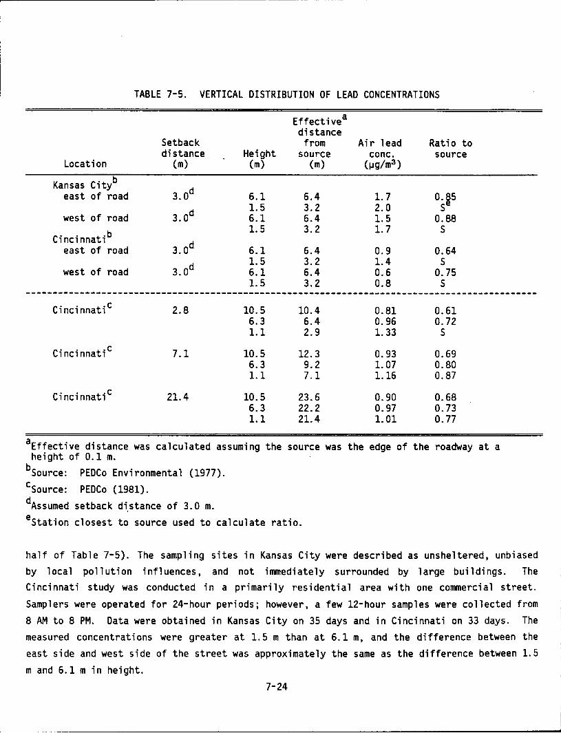
TABLE 7-5. VERTICAL DISTRIBUTION OF LEAD CONCENTRATIONS
Effective a distance
Setback from Air lead Ratio to distance Height source cone. source
Location (m) (m) (m) (1Jg/m3)
Kansas Cityb 3.0d east of road 6.1 6.4 1.7 0.~5
3.0d 1.5 3.2 2.0 s
west of road 6.1 6.4 1.5 0.88
Cincinnatib 1.5 3.2 1.7 s
3.0d east of road 6.1 6.4 0.9 0.64
3.0d 1.5 3.2 1.4 s
west of road 6.1 6.4 0.6 0.75 1.5 3.2 0.8 s
----------------------------------------------------------------------------------------------Cincinnatic 2.8 10.5
6.3 1.1
Cincinnatic 7.1 10.5 6.3 1.1
Cincinnatic 21.4 10.5 6.3 1.1
aEffective distance was calculated assuming height of 0.1 m.
bsource: PEDCo Environmental (1977).
cSource: PEDCo (1981).
dAssumed setback distance of 3.0 m.
10.4 6.4 2.9
12.3 9.2 7.1
23.6 22.2 21.4
the source was
eStation closest to source used to calculate ratio.
0.81 0.61 0.96 0.72 1. 33 s
0.93 0.69 1. 07 0.80 1.16 0.87
0.90 0.68 0.97 0.73 1. 01 0.77
the edge of the roadway at a
half of Table 7-5). The sampling sites in Kansas City were described as unsheltered, unbiased by local pollution influences, and not immediately surrounded by large buildings. The Cincinnati study was conducted in a primarily residential area with one commercial street.
Samplers were operated for 24-hour periods; however, a few 12-hour samples were collected from
8 AM to 8 PM. Data were obtained in Kansas City on 35 days and in Cincinnati on 33 days. The measured concentrations were greater at 1.5 m than at 6.1 m, and the difference between the
east side and west side of the street was approximately the same as the difference between 1.5
m and 6.1 min height.
7-24
Sinn (1980) investigated airborne lead concentrations at heights of 3 and 20 m above a road in Frankfurt, Germany. Measurements conducted in December 1975, December 1976, and January 1978 gave monthly mean values of 3.18, 1.04, and 0.66 ~g/m3 , respectively, at 3m height. The corresponding values at 20m height were 0.59, 0.38, and 0.31 ~g/m3 , showing a substantial reduction at this height. The decrease in concentration over the 2-year period was attributed to a decrease in the permissible lead content of gasoline from 0.4 to 0.15 g/liter beginning in January, 1976.
Two reports show no relationship between air c:oncentration and vertical distance (Barltrop and Strehlow, 1976; Ter Haar, 1979). From August, 1975 to July, 1976, Barltrop and Strehlow (1976) conducted an air sampling program in London at a proposed nursery site under an elevated motorway. The height of the motorway was 9. 3 m. Air samplers were operated at five to seven sites during the period from Monday to Friday, 8 AM to 6 PM, for one year. The maximum individual value observed was 18 ~g/m3 . The 12-month mean ranged from 1.35 to 1.51 ~g/m3 , with standard deviations of 0.91 and 0.66, respectively. The authors reported that the airborne concentrations were independent of height from ground level up to 7 m.
Ter Haar (1979) measured airborne lead at several heights above the ground, using samplers positioned 6 m from a heavily traveled road in Detroit. A total of nine 8-hour daytime samp 1 es were co 11 ected. The avera 11 average airborne 1 ead concentrations at heights of 0. 3, 0.9, 1.5, and 3.0 m were 4.2, 4.8, 4.7, and 4.6 ~g/m3 , respectively, indicat~ng a uniform concentration over this range of heights at the measurement site. It should be noted that at any one height, the concentration varied by as much as a fa.ctor of 10 from one day to the next; the importance of simultaneous sampling when attempting to measure gradients is clearly demonstrated.
Data that show variations with vertical distance reflect the strong influence of the geometry of the boundary layer, wind, and atmospheric stability conditions on the vertical gradient of lead resulting from automobile emissions. The var·iability of concentration with height is further complicated by the higher emission elevation of smokestacks. Concentrations measured from sampling stations on the roofs of buildings several stories high may not reflect actual human exposure conditions, but neither would ct single sampling station located at ground level among several buildings. The height variation in concentration resulting from vertical diffusion of automobile emissions is likely to be small compared to temporal and spatial variations resulting from surface geometry, wind, and atmospheric conditions. Our understanding of the complex factors affecting the vertical distribution of airborne lead is extremely limited, but the data of Table 7-5 indicate that air lead concentrations are primarily a function of distance from the source, whether VE!rtical or horizontal.
7-25
7.2.1.3.3 Indoor/outdoor relationships and personal monitoring. Because people spend much of their time indoors, ambient air samp 1 ed outdoors may not accurate 1 y represent actua 1 i nha 1 a·tion exposure to airborne lead. Table 7-6 summarizes the results of several indoor/outdoor airborne lead studies. In nearly all cases, the indoor concentration is substantially lower than the corresponding value outdoors; the only indoor/outdoor ratio exceeding unity is for a high-rise apartment building, where air taken in near street level is rapidly distributed through the building air circulation system. Some of the studies in Table 7-6 show smaller indoor/outdoor ratios during the winter, when windows and doors are tightly closed. Overall, the data suggest indoor/outdoor ratios of 0.6-0.8 are typical for airborne lead in houses without air conditioning. Ratios in air conditioned houses are expected to be in the range of 0.3-0.5 (Yocom, 1982). The available data imply that virtually all airborne lead found indoors is associated with material transported from the outside. Because of the complexity of factors affecting infiltration of air into buildings, however, it is difficult to predict accurately indoor lead concentrations based on outdoor levels. Rabinowitz et al. (1984) found a correlation between indoor air lead in Boston homes and the amount of lead sold in gasoline in Massachusetts.
Even detailed knowledge of indoor and outdoor airborne lead concentrations at fixed locations may still be insufficient to assess human exposure to airborne lead. The study of Tosteson et al. (1982) in Table 7-6 included measurement of airborne lead concentrations using personal exposure monitors carried by individuals going about their day-to-day activities. In contrast to the lead concentrations of 0.092 and 0.12 ~g/m3 at fixed locations, the average personal exposure was 0.16 ~g/m3 • The authors suggest this indicates an inadequacy of using fixed monitors at either indoor or outdoor locations to assess exposure.
Rohbock (1981) reported that, whereas a parked car may ex hi bit properties similar to buildings in reducing internal air concentrations, a moving car quickly reaches the same air lead concentration inside as outside, suggesting a rapid exchange of air in a moving vehicle.
7.2.2 Lead in Soil Much of the lead in the atmosphere is transferred to terrestrial surfaces where it is
eventually passed to the upper layer of the soil surface. The mechanisms that determine the transfer rate of lead to soil are described in Section 6.4.1 and the transformation of lead in soil in Section 6.5.1. The uptake of lead by plants and its subsequent effect on animals may be found in Sections 8.3 and 8.4, respectively. The purpose of this section is to discuss the distribution of lead in U.S. soils and the impact of this lead on potential human exposures.
7-26
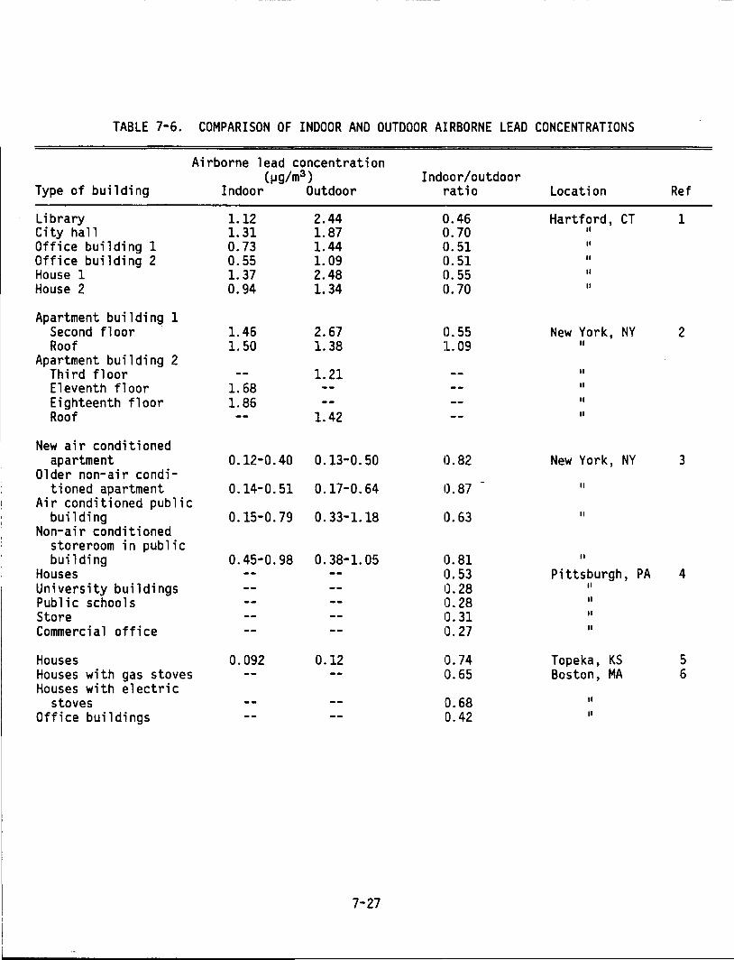
TABLE 7-6. COMPARISON OF INDOOR AND OUTDOOR AIRBORNE LEAD CONCENTRATIONS
Airborne lead concentration (1Jg/m3) Indc1or/outdoor
Type of building Indoor Outdoor r·ati o Location Ref
Library 1.12 2.44 0.46 Hartford, CT 1 City hall 1. 31 1.87 0.70 II
Office building 1 0.73 1.44 0.51 II
Office building 2 0.55 1. 09 0.51 II
House 1 1. 37 2.48 0.55 II
House 2 0.94 1.34 0.70 II
Apartment building 1 Second floor 1.46 2.67 0.55 New York, NY 2 Roof 1. so 1. 38 1. 09 II
Apartment building 2 Third floor 1.21 II
Eleventh floor 1. 68 II
Eighteenth floor 1. 86 II
Roof 1.42 II
New air conditioned apartment 0.12-0.40 0.13-0.50 0.82 New York, NY 3
Older non-air condi-tioned apartment 0.14-0.S1 0.17-0.64 0.87 II
Air conditioned public building 0.15-0.79 0. 33-1.18 0.63 II
Non-air conditioned storeroom in public building 0.4S-0.98 0. 38-1. OS 0.81 II
Houses O.S3 Pittsburgh, PA 4 University buildings 0.28 II
Public schools 0.28 II
Store 0.31 II
Commercial office 0.27 II
Houses 0.092 0.12 0.74 Topeka, KS 5 Houses with gas stoves 0.65 Boston, MA 6 Houses with electric
stoves 0.68 II
Office buildings 0.42 II
7-27
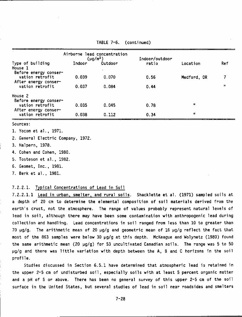
TABLE 7-6. (continued)
Airborne lead concentration (~g/m3 ) Indoor/outdoor
Type of building Indoor Outdoor ratio Location Ref House 1 Before energy conser-
vation retrofit 0.039 0.070 0.56 Medford, OR 7 After energy conser-
vation retrofit 0.037 0.084 0.44 II
House 2 Before energy conser-
vation retrofit 0.035 0.045 0.78 II
After energy conser-vation retrofit 0.038 0.112 0.34 II
Sources: 1. Yocom et al., 1971.
2. General Electric Company, 1972.
3. Halpern, 1978.
4. Cohen and Cohen, 1980. 5. Tosteson et al., 1982. 6. Geomet, Inc. , 1981. 7. Berk et al., 1981.
7.2.2.1. Typical Concentrations of Lead in Soil
7.2.2.1.1 Lead in urban, smelter, and rural soils. Shacklette et al. (1971) sampled soils at a depth of 20 em to determine the elemental composition of soil materials derived from the earth•s crust, not the atmosphere. The range of values probably represent natural levels of lead in soil, although there may have been some contamination with anthropogenic lead during
collection and handli·ng. Lead concentrations in soil ranged from less than 10 to greater than
70 ~g/g. The arithmetic mean of 20 ~g/g and geometric mean of 16 ~g/g reflect the fact that most of the 863 samples were below 30 ~g/g at this depth. McKeague and Wolynetz (1980) found
the same arithmetic mean (20 ~g/g) for 53 uncultivated Canadian soils. The range was 5 to 50 ~g/g and there was little variation with depth between the A, B and C horizons in the soil profile.
Studies discussed in Section 6.5.1 have determined that atmospheric lead is retained in the upper 2-5 em of undisturbed soil, especially soils with at least 5 percent organic matter
and a pH of 5 or above. There has been no general survey of this upper 2-5 em of the soil
surface in the United States, but several studies of lead in soil near roadsides and smelters
7-28
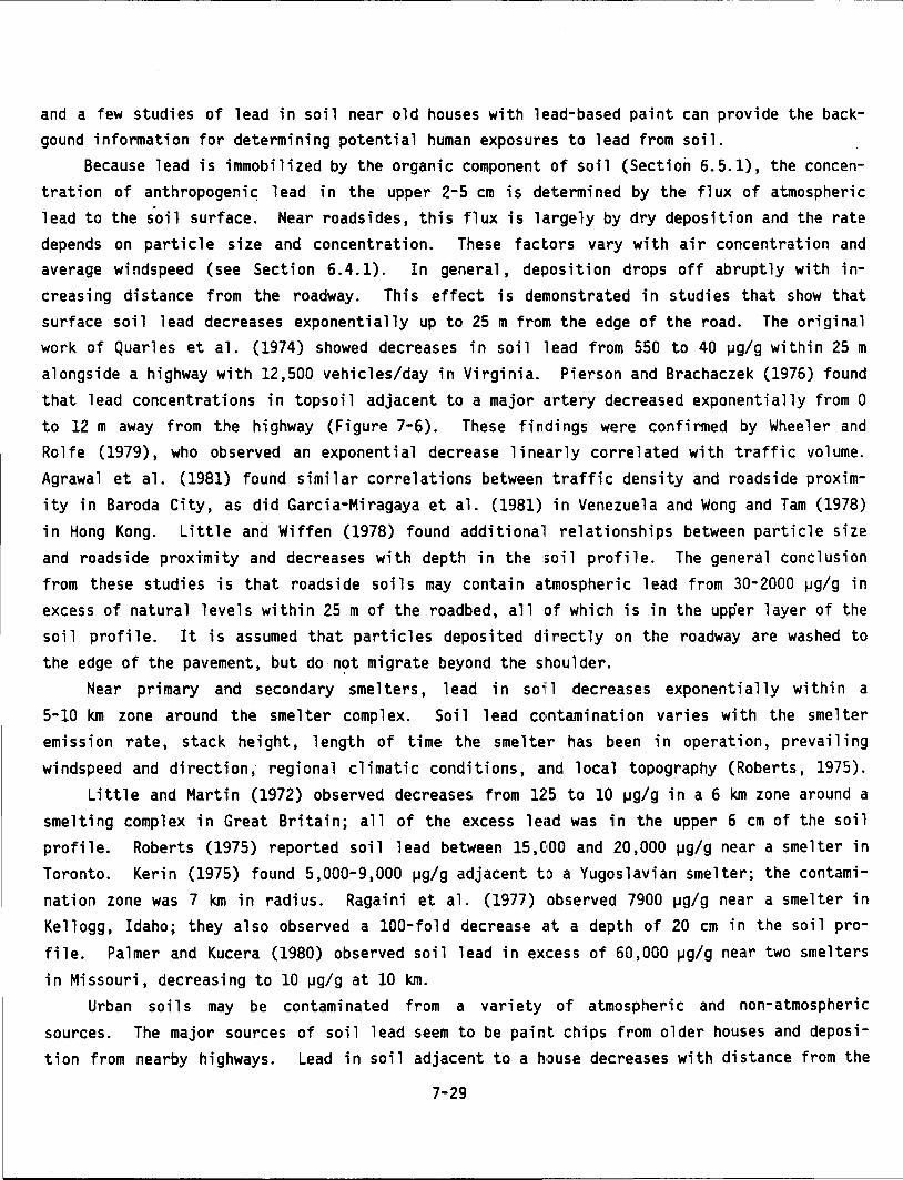
and a few studies of lead in soil near old houses with lead-based paint can provide the backgound information for determining potential human exposures to lead from soil.
Because lead is immobilized by the organic component of soil (Section 6.5.1), the concentration of anthropogeni ~ 1 ead in the upper 2-5 em is determined by the flux of atmospheric lead to the soil surface. Near roadsides, this flux is largely by dry deposition and the rate depends on particle size and concentration. These factors vary with air concentration and average windspeed (see Section 6.4.1). In general, deposition drops off abruptly with increasing distance from the roadway. This effect is demonstrated in studies that show that surface soil lead decreases exponentially up to 25 m from the edge of the road. The original work of Quarles et al. (1974) showed decreases in soil lead from 550 to 40 ~g/g within 25m alongside a highway with 12,500 vehicles/day in Virginia. Pierson and Brachaczek (1976) found that lead concentrations in topsoil adjacent to a major artery decreased exponentially from 0 to 12 m away from the highway (Figure 7-6). These findings were confirmed by Wheeler and Rolfe (1979), who observed an exponential decrease linearly correlated with traffic volume. Agrawal et al. (1981) found similar correlations between traffic density and roadside proximity in Baroda City, as did Garcia-Miragaya et al. (1981) in Venezuela and Wong and Tam (1978) in Hong Kong. Little an~ Wiffen (1978) found additional relationships between particle size and roadside proxi"mity and decreases with depth in the :;oil profile. The general conclusion from these studies is that roadside soils may contain atmospheric lead from 30-2000 ~g/g in excess of natural levels within 25 m of the roadbed, all of which is in the upper layer of the soil profile. It is assumed that particles deposited directly on the roadway are washed to the edge of the pavement, but do n~t migrate beyond the shoulder.
Near primary and secondary smelters, lead in soiil decreases exponentially within a 5-10 km zone around the sme 1 ter camp 1 ex. Soi 1 1 ead cc,ntami nation varies with the smelter emission rate, stack height, length of time the smelter has been in operation, prevailing windspeed and direction, regional climatic conditions, and local topography (Roberts, 1975).
Li tt 1 e and Martin (1972) observed decreases from 12:5 to 10 ~g/g in a 6 km zone around a smelting profile. Toronto.
complex in Great Britain; all of the excess lead was in the upper 6 em of the soil Roberts (1975) reported soil lead between 15,000 and 20,000 ~g/g near a smelter in Kerin (1975) found 5,000-9,000 ~g/g adjacent to a Yugoslavian smelter; the contami-
nation zone was 7 km in radius. Ragai ni et a 1. (1977) observed 7900 ~g/g near a sme 1 ter in Kellogg, Idaho; they also observed a 100-fold decrease at a depth of 20 em in the soil profile. Palmer and Kucera (1980) observed soil lead in ex,cess of 60,000 ~g/g near two smelters
in Missouri, decreasing to 10 ~g/g at 10 km.
Urban soils may be contaminated from a variety of atmospheric and non-atmospheric sources. The major sources of soil lead seem to be paint chips from older houses and deposition from nearby highways. Lead in soil adjacent to a h1:>use decreases with distance from the
7-29
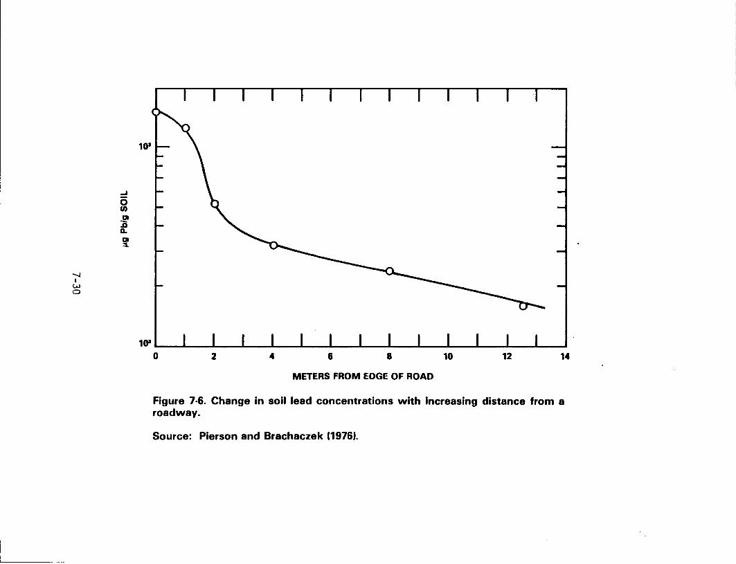
-....J I
w 0
0 2 4 6 8 10 12 14
METERS FROM EDGE OF ROAD
Figure 7-6. Change in soil lead concentrations with Increasing distance from a roadway.
Source: Pierson and Brachaczek (1976).
house; this may be due to paint chips or to dust of atmospheric origin washing from the rooftop (Wheeler and Rolfe, 1979).
Andresen et al. (1980) reported lead in the litter layer of 51 forest soils in the northeastern United States. They found values from 20-700 ~g/g, which can be compared only qualitatively to the soil lead concentration cited above. This study clearly shows that the major pathway of lead to the soil is by the decomposition of plant material containing high concentrations of atmospheric lead on or within their tissues. Because this organic matter is a part of the decomposer food chain, and because the organic matter is in dynamic equilibrium with soil moisture, it is reasonable to assume that lead associated with organic matter is biologically more mobile than lead tightly bound within the crystalline structure of inorganic rock fragments.
Finally, a definitive study that describes the source of soil lead was reported by Gulson et al. (1981) for soils in the vicinity of Adelaide, South Australia. In an urban to rural transect, stable lead isotopes were measured in the top 10 em of soils over a 50 km distance. By their isotopic compositions, three sources of lead were identified: natural, non-automotive industrial lead from Australia, and tetraethyl lead manufactured in the United States. The results indicated that most of the soil surface lt!ad originated from leaded gasoline. Similar studies have not been conducted in the United States. 7.2.2.1.2 Natural and anthropogenic sources of soil lea~. Although no study has clearly identified the relative concentrations of natural and anthropogenic lead in soil, a few clarifying statements can be made with some certainty. Lea:d may be found in inorganic primary minerals, on humic substances, complexed with Fe-Mn oxide films, on secondary minerals or in soil moisture. All of the lead in primary minerals is natural and is bound tightly within the crystalline structure of the minerals. Most of this lead can be released only by harsh treatment with acids. The lead on the surface of these minerals is leached slowly into the soil moisture. Atmospheric lead forms complexes with humic substances or on oxide films that are in equilibrium with soil moisture, although the equilibrium strongly favors the complexing agents. Consequently, the ratio of anthropogenic to natural lead in soil moisture depends mostly on the amounts of each type of lead in the complexing agents and very little on the concentration of natural lead in the inorganic minerals.
Except near roadsides and smelters, only a few micrograms of atmospheric lead have been added to each square centimeter of soil surface. Several studies indicate that this lead is available to plants (Section 8.3.1.1). Even with small amounts of atmospheric lead, as much as 75 percent of the lead in soil moisture is of atmospheric origin (Elias et al., 1982). A conservative estimate of 50 percent is used in the discussions in Section 7.3.1.2. A breakdown of the types of lead in soil may be found in Table 7-7.
7-31
------------
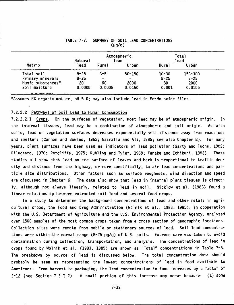
TABLE 7-7. SUMMARY OF SOIL LEAD CONCENTRATIONS (J,Jg/g)
Atmospheric Total Natural lead lead
Matrix lead Rur~l Urban Rural Urban
Total soil 8-25 3-5 50-150 10-30 150-300 Primary minerals 8-25 8-25 8-25 Humic substances* 20 60 2000 80 2000 Soil moisture 0.0005 0.0005 0.0150 0.001 0.0155
*Assumes 5% organic matter, pH 5.0; may also include lead in Fe-Mn oxide films.
7.2.2.2 Pathways of Soil Lead to Human Consumption 7.2.2.2.1 Crops. On the surfaces of vegetation, most lead may be of atmospheric origin. In the internal tissues, lead may be a combination of atmospheric and soil origin. As with soils, lead on vegetation surfaces decreases exponentially with distance away from roadsides and smelters (Cannon and Bowles, 1962; Nasralla and Ali, 1985; see also Chapter 8). For many years, plant surfaces have been used as indicators of lead pollution (Garty and Fuchs, 1982; Pilegaard, 1978; Ratcliffe, 1975; Ruhling and Tyler, 1969; Tanaka and Ichikuni, 1982). These studies all show that lead on the surface of leaves and bark is proportional to traffic density and distance from the highway, or more specifically, to air lead concentrations and particle size distributions. Other factors such as surface roughness, wind direction and speed are discussed in Chapter 6. The data also show that lead in internal plant tissues is directly, although not always linearly, related to lead in soil. Nicklow et al. (1983) found a linear relationship between extracted soil lead and several food crops.
In a study to determine the background concentrations of lead and other metals in agricultural crops, the Food and Drug Administration (Wolnik et al., 1983, 1985), in cooperation with the U.S. Department of Agriculture and the U.S. Environmental Protection Agency, analyzed over 1500 samples of the most common crops taken from a cross section of geographic locations. Collection sites were remote from mobile or stationary sources of lead. Soil lead concentrations were within the normal range (8-25 J.Jg/g) of U.S. soils. Extreme care was taken to avoid contamination during collection, transportation, and analysis. The concentrations of lead in crops found by Wolnik et al. (1983, 1985) are shown as 11 Total 11 concentrations in Table 7-8. The breakdown by source of lead is discussed below. The total concentration data should probably be seen as representing the lowest concentrations of lead in food available to Americans. From harvest to packaging, the lead concentration in food increases by a factor of
2-12 (see Section 7.3.1.2). A small portion of this increase may occur because: (1) some
7-32
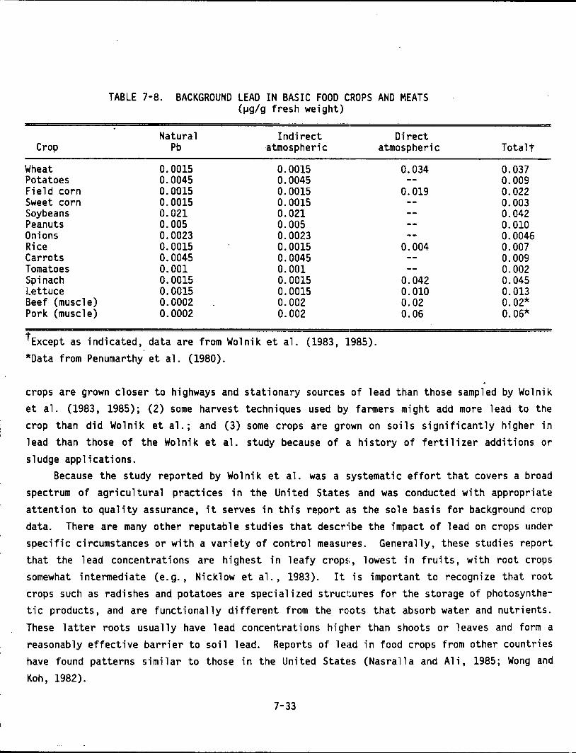
Crop
Wheat Potatoes Field corn Sweet corn Soybeans Peanuts Onions Rice Carrots Tomatoes Spinach Lettuce Beef (muscle) Pork (muscle)
TABLE 7-8. BACKGROUND LEAD IN BASIC FOOD CROPS AND MEATS (~g/g fresh weight)
Natural Indirect Direct Pb atmospheric atmospheric
0.0015 0.0015 0.034 0.0045 0.0045 0.0015 0.0015 0.019 0.0015 0.0015 0.021 0.021 0.005 0.005 0.0023 0.0023 0.0015 0.0015 0.004 0.0045 0.0045 0.001 0.001 0.0015 0.0015 0.042 0.0015 0.0015 0.010 0.0002 0.002 0.02 0.0002 0.002 0.06
tExcept as indicated, data are from Wolnik et al. (1983, 1985). *Data from Penumarthy et al. (1980).
Totalt
0.037 0.009 0.022 0.003 0.042 0.010 0.0046 0.007 0.009 0.002 0.045 0.013 0.02* 0.06*
crops are grown closer to highways and stationary sources of lead than those sampled by Wolnik et al. (1983, 1985); (2) some harvest techniques used by farmers might add more lead to the crop than did Wolnik et al.; and (3) some crops are grc1wn on soils significantly higher in lead than those of the Wolnik et al. study because of a history of fertilizer additions or sludge applications.
Because the study reported by Wo 1 ni k et a 1. was a systematic effort that covers a broad spectrum of agri cul tura 1 practices in the United States. and was conducted with appropriate attention to quality assurance, it serves in this report as the sole basis for background crop data. There are many other reputab 1 e studies that descr;i be the impact of 1 ead on crops under specific circumstances or with a variety of control measu1·es. Generally, these studies report that the lead concentrations are highest in leafy crops;, lowest in fruits, with root crops somewhat intermediate (e.g., Nicklow et al., 1983). It is important to recognize that root crops such as radishes and potatoes are specialized structures for the storage of photosynthetic products, and are functionally different from the roots that absorb water and nutrients. These latter roots usually have lead concentrations higher than shoots or leaves and form a reasonably effective barrier to soil lead. Reports of lead in food crops from other countries have found patterns similar to those in the United States (Nasralla and Ali, 1985; Wong and Koh, 1982).
7-33
Studies that specifically apply to roadside or stationary source conditions can be evaluated in the context of these recent background findings by Wo 1 ni k et a 1. (1983, 1985 )'.
Studies of the lead associated with crops near highways have shown that both lead taken up from soil and aerosol lead delivered by deposition are found associated with the edible portions of common vegetable crops. However, there is enormous variability in the total amount of lead associated with such crops and in the relative amounts of lead in the plants versus on the plants. The variability depends upon several factors, the most prominent of which are the plant species, the traffic density, the meteorological conditions, and the local soil conditions (Welch and Dick, 1975; Rabinowitz, 1974; Dedolph et al., 1970; Motto et al., 1970;
Schuck and Locke, 1970; Ter Haar, 1970). These factors, coupled with the fact that many studies have not differentiated between lead on plants versus lead in plants, make it difficult to generalize on the relationship between lead in crops and lead in soil or air. Data of Schuck and Locke (1970) suggest that in some cases (e.g., tomatoes and oranges) much of the surface lead is readily removed by washing. But as noted in Section 6.4.3, this is not universally true; in some cases, much more vigorous washing procedures would be necessary to remove all or most of the surface lead.
Ter Haar (1970) found that inedible portions of several plants (bean leaves, corn husks, soybean husks, and chaff from oats, wheat, and rice) had two to three times the lead concentration when grown near a busy highway compared with similar plants grown 160 m from the highway or in a greenhouse supplied with filtered air. The edible portions of these and other plants showed little or no difference in lead content between those grown in ambient air and those grown in the filtered air. However, the lead concentrations found by Ter Haar (1970)
for edible portions of crops grown in filtered air in the greenhouse were generally one to two orders of magnitude higher than those of the same types of crops taken from actual agricultural situations by Wolnik et al. (1983, 1985). Dedolph et al. (1970) found that while ryegrass and radish leaves grown near a busy highway contained deposited airborne lead, the edible portion of the radish was unaffected by variations in either soil lead or air lead.
The accumulation of lead by edible portions of crops was measured by TerHaar (1970), who showed that edible plant parts not exposed to air (potatoes, corn, carrots, etc.) do not accumulate atmospheric lead, while leafy vegetables do. These results were confirmed by Mclean and Shields (1977), who found that most of the lead associated with food crops is on leaves and husks. The general conclusion from these studies is that lead associated with food crops varies according to exposure to the atmosphere and in proportion to the effort taken to separate husks, chaff, and hulls from edible parts during processing for human or animal con
sumption. To estimate the distribution of natural and atmospheric lead in food crops (Table 7-8),
it is necessary to recognize that some crops of the Wolnik et al. study have no lead from
7-34
direct atmospheric deposition, but rather that all lead found in these crops comes through soil moisture. The lowest concentrations of lead are found in those crops where the edibl~ portion grows above ground and it does not accumulate lead from atmospheric deposition (sweet corn and tomatoes). Belowground crops are protected from atmospheric deposition but have slightly higher concentrations of lead, partly because lead accumulates in the roots of plants (potatoes, onions, carrots). Leafy aboveground plants (lettuce, spinach, wheat) have even higher lead concentrations presumably because of increased exposure to atmospheric lead. The assumption that can be made here is that, in the absence of atmospheric deposition, exposed aboveground plant parts would have lead concentrations similar to sweet corn and tomatoes.
The data on these ten crops suggest that root vegetables have lead concentrations between 0.0046 and 0.009 ~g/g. This is all lead of soil origin, of which presumably half is natural and half anthropogenic (called indirect atmospheric lead here). Aboveground parts not exposed to significant amounts of atmospheric deposition (sweet corn and tomatoes) have less lead internally, also equally divided between natural and indirect atmospheric lead. If it is assumed that this same concentration is the internal concentration for aboveground parts for other plants, it is apparent that five crops (wheat, field corn, rice, spinach, and lettuce) have direct atmospheric deposition in proportion to surface area and estimated duration of exposure. The deposition rate of only 0.04 ng/cm2 ·day, which is much smaller than would normally be expected in rural environments (see Section 6.4.1) could account for these amounts of direct atmospheric lead. In this scheme, soybeans are anomalously high. Soybeans grow inside a sheath and should have an internal lead concentr·ation similar to sweet corn.
These discussions lead to the conclusion that root parts and protected aboveground parts of edible crops contain natural lead and indirect atmospheric lead, both derived from the soi 1. For exposed aboveground parts, any 1 ead in exce~ss of the average found on unexposed aboveground parts is considered to be the result of direct atmospheric deposition.
Near smelters, Merry et al. (1981) found a pattern different from roadside studies cited above. They observed that wheat crops contained lead in proportion to the amount of soil lead, not vegetation surface contamination. A similar E~ffect was reported by Harris (1981).
7.2.2.2.2 Livestock. Lead in forage was found to exceed 950 ~g/g within 25 m of roadsides with 15,000 or more vehicles per day (Graham and Kalman!, 1974). At lesser traffic densities, 200 ~g/g were found. Other reports have observed 20-660 ~g/g with the same relationship to traffic density and distance from the road (see review by Graham and Kalman, 1974). A more recent study by Crump and Barlow (1982) showed that the accumulation of lead in forage is directly related to the deposition rate, which varied seasonally according to traffic density. The deposition rate was measured using the moss bag technique, in which bags of moss are exposed and analyzed as relative indicators of deposition flux. Rain was not effective in removing lead from the surface of the moss. The ratio of atmospheric lead to total lead in
7-35
meat products is partly a function of the same ratio in forage. The fact that most lead in cattle is stored in bones and not eaten by man does not alter the ratio of atmospheric to
total lead in meat. Factors that might add non-atmospheric lead would be soil ingestion by cattle, processed
food given to catt 1 e in feedlots, and 1 ead added during processing. Thornton and Abrahams (1983) estimated that 1 to 18 percent of the dry matter ingested by cattle is soil, based the titanium content of feces. Soil ingestion increases when overgrazing is permitted because of
dry weather, seasonal changes or other farm management practices. Most of the ingested soil would be from the upper 1-5 em. In a normal pasture this soil layer would contain a signifi
cant fraction of atmospheric lead.
7.2.3 Lead in Surface and Ground Water Lead occurs in untreated water in either dissolved or particulate form. Dissolved lead is
operationally defined as that which passes through a 0.45 ~m membrane filter. Because atmos
pheric lead in rain or snow is retained by soil, there is little correlation between lead in
precipitation and lead in streams which drain terrestrial watersheds. Rather, the important factors seem to be the chemistry of the stream (pH and hardness) and the volume of the stream
flow. For groundwater, chemistry is also important, as is the geochemical composition of the
water-bearing bedrock. Of the year-round housing units in the United States, 84 percent receive their drinking
water from a municipal or private supply of chemically treated surface or ground water. The
second largest source is privately owned wells (U.S. Bureau of the Census, 1982). In some
communities, the purchase of untreated bottled drinking water is a common practice. The initial concentration of lead in this water depends largely on the source of the untreated water.
7.2.3.1. Typical Concentrations of Lead in Untreated Water
7.2.3.1.1 Surface water. Durum et al. (1971) reported lead concentrations in the range of
1-55 ~g/1 in 749 surface water samples in the United States. Very few samples were above 50 ~g/1, and the average was 3.9 ~g/1. Chow (1978) reviewed other reports with mean values
between 3 and 4 ~g/1. The National Academy of Sciences (1980) reported a mean of 4 ~g/1, with a range from below detection to 890 ~g/1. Concentrations of 100 ~g/1 were found near sites of
sewage treatment, urban runoff, and industrial waste disposal. Because 1 ~g lead/1 was at or below the detection limit of most investigators during the
1970's, it is likely that the mean of 3-4 ~g/1 was unduly influenced by a large number of
erroneously high values at the lower range of detection. On the other hand, Patterson (1980)
reports values of 0.006-0.05 ~g/1 for samples taken from remote streams. Extreme care was
taken to avoid contamination and analytical techniques sensitive to less than 0.001 ~g/1 were
used.
7-36
Streams and 1 akes are influenced by their water chemistry and the 1 ead content of their sediments. At neutral pH, lead moves from the dissolved to the particulate form and the part~ icles eventually pass to sediments. At low pH, the reverse pathway generally takes place. Hardness, which is a combination of the Ca and Mg concentration, also can influence lead concentrations. At higher concentrations of Ca and Mg, the solubility of lead decreases. Further discussion of the chemistry of lead in water may be found in Sections 6.5.2.1 and 8.2.2. 7.2.3.1.2 Ground water. Municipal and private wells account for a large percentage of the drinking water supply. This water typically has a neutral pH and somewhat higher hardness than surface water. Lead concentrations are not influenced by acid rain, surface runoff, or atmospheric deposition. Rather, the primary determinant of lead concentration is the geochemical makeup of the bedrock that is the source of the water supply. Ground water typically ranges from 1 to 100 ~g lead/1 (National Academy of Sciences, 1980). Again, the lower part of the range may be erroneously high due to difficulties of analysis. It is also possible that the careless application of fertilizers or sewage sludge to agricultural lands can cause contamination of ground water supplies. 7.2.3.1.3 Natural vs. anthropogenic lead in water. Although Chow (1978) reports that the natural lead concentration of surface water is 0.5 ~g/1, this value may be excessively high. In a discussion of mass balance considerations (National Academy of Sciences, 1980), natural lead was suggested to range from 0. 005 to 10 ~g/1. Patterson (1980) used further arguments to establish an upper limit of 0.02 ~g/1 for natural lead in surface water. This upper limit will be used in further discussions of natural lead in drinking water.
Because ground water is free of atmospheric lead, lecld in ground water should probably be considered natural in origin as it occurs at the well head, unless there is evidence of sur
face contamination. 7.2.3.2 Human Consumption of Lead in Water. Whether from surface or ground water supplies, municipal waters undergo extensive chemical treatment prior to release to the distribution system. There is no direct effort to remove lead from th1! water supply. However, some treatments, such as flocculation and sedimentation, may inadv1!rtently remove lead along with other undesirable substances. On the other hand, chemical treatment to soften water increases the solubility of lead and enhances the possibility that lead will be added to water as it passes
through the distribution system. 7.2.3.2.1 Contributions to drinking water. For samples taken at the household tap, lead concentrations are usually higher in the initial volume (first daily flush) than after the tap has been running for some time. Water standing in the pipes for several hours is intermediate between these two concentrations (Sharrett et al., 1982; 1Worth et al., 1981). Common plumbing materials are galvanized and copper pipe; lead solder is usually used to seal the joints of
7-37
--- ------------------
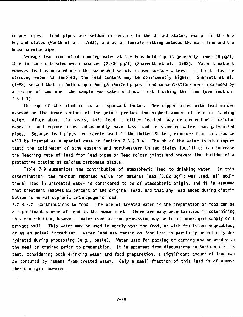
copper pipes. Lead pipes are seldom in service in the United States, except in the New England states (Worth et al., 1981), and as a flexible fitting between the main line and the house service pipe.
Average lead content of running water at the household tap is generally lower (8 ~g/1) than in some untreated water sources (25-30 ~g/1) (Sharrett et al., 1982). Water treatment removes lead associated with the suspended solids in raw surface waters. If first flush or standing water is samp 1 ed, the 1 ead content may be considerably higher. Sharrett et a 1. (1982) showed that in both copper and galvanized pipes, lead concentrations were increased by a factor of two when the sample was taken without first flushing the line (see Section 7.3.1.3).
The age of the plumbing is an important factor. New copper pipes with lead solder exposed on the inner surface of the joints produce the highest amount of 1 ead in standing water. After about six years, this Jead is either leached away or covered with calcium deposits, and copper pipes subsequently have less lead in standing water than galvanized pipes. Because lead pipes are rarely used in the United States, exposure from this source will be treated as a special case in Section 7.3.2.1.4. The pH of the water is also important; the acid water of some eastern and northwestern United States localities can increase the leaching rate of lead from lead pipes or lead solder joints and prevent the buildup of a protective coating of calcium carbonate plaque.
Table 7-9 summarizes the contribution of atmospheric lead to drinking water. In this determination, the maximum reported value for natural lead (0. 02 ~g/1) was used, all additional lead in untreated water is considered to be of atmospheric origin, and it is assumed that treatment removes 85 percent of the original lead, and that any lead added during distribution is non-atmospheric anthropogenic lead. 7.2.3.2.2 Contributions to food. The use of treated water in the preparation of food can be a significant source of lead in the human diet. There are many uncertainties in determining this contribution, however. Water used in food processing may be from a municipal supply or a private well. This water may be used to merely wash the food, as with fruits and vegetables, or as an actual ingredient. Water lead may remain on food that is partially or entirely dehydrated during processing (e.g., pasta). Water used for packing or canning may be used with the meal or drained prior to preparation. It is apparent from discussions in Section 7.3.1.3 that, considering both drinking water and food preparation, a significant amount of lead can be consumed by humans from treated water. Only a small fraction of this lead is of atmospheric origin, however.
7-38
TABLE 7-9. SUMMARY OF LEAD CONCENTRATIONS IN DRINKING WATER SUPPLIES (j.Jg/1)
Indirect Direct Non-atmospheric Natural atmospheric atmospheric anthropogenic Total
Source lead lead lead lead lead
Untreated Lakes 0.02 15 10 0 25 Rivers 0.02 15 15 0 30 Streams 0.02 2.5 2.5 0 5 Groundwater 3 0 0 0 3
Treated Surface 0.003 2.5 1.5 4 8 Ground 0.45 0 0 7.5 8
Source: Text
7.2.4 Summary of Environmental Concentrations of Lead Lead concentrations in environmental media that are in the pathway to human consumption
are summarized in Table 7-10. These values are estimates derived from the preceding discussions. A single value has been used, rather than a riinge, in order to facilitate further estimates of actual human consumption. This use of a single value is not meant to imply a high degree of certainty in its determination or homogene·ity within the human population. The units for water are converted from j.Jg/1 as in Table 7-9 to j.Jg/g to facilitate the discussions of dietary consumption of water and beverages.
TABLE 7-10. SUMMARY OF ENVIRONMENTAL CONCENTRATIONS OF LEAD
Natural Atmospheric Total Medium lead 1 ead lead
Urban air (J.Jg/m3 ) 0.00005 0.3-1.1 0. 3-1.1 Rural air (j.Jg/m3 ) 0.00005 0.15-0.3 0.15-0.3
Total soil (j.Jg/g) 8-25 3-5 10-30
Food crops (j.Jg/g) 0.0025 0.00-0.042 0.002-0.045
Surface water (J.Jg/g)* 0.00002 0.005-0.030 0.005-0.030
Ground water (j.Jg/g)* 0.003 0.00 0.001-0.1
*Note change in units from Table 7-9.
7-39
Because concentrations of natura 1 1 ead are generally three to four orders of magnitude lower than anthropogenic lead in ambient rural or urban air, all atmospheric contributions 6f
lead are considered to be of anthropogenic origin. Natural soil lead typically ranges from 10 to 30 ~g/g, but much of this is tightly bound within the crystalline matrix of soil minerals at normal soil pHs of 4-8. lead in the organic fraction of soil is part natural and part atmospheric. The fraction derived from fertilizer is considered to be minimal. In undisturbed rural and remote soils, the ratio of natural to atmospheric lead is about 1:1, perhaps as high as 1:3. This ratio persists in soil moisture and in internal plant tissues. Thus, some of the internal lead in crops is of anthropogenic origin, and some is natural. Information on the effect of fertilizer on this ratio is not available. lead in untreated surface water is 99 percent anthropogenic. Except near municipal waste outfalls, this anthropogenic lead is mostly atmospheric. It is possible that 75 percent of this lead is removed during treatment. lead in untreated ground water is presumed to be natura 1 in the absence of evidence of groundwater contamination.
In tracking air lead through pathways to human exposure, it is necessary to distinguish between 1 ead of atmospheric origin that has passed through the soil (indirect atmospheric lead), and atmospheric lead that has deposited directly on crops or water. Because indirect atmospheric lead will remain in the soil for many decades, this source is insensitive to projected changes in atmospheric lead concentrations. Regulation of ambient air lead concentrations will not affect indirect atmospheric lead concentrations over the next several decades.
The method used in this document for calculating the relative contribution of atmospheric lead to total potential human exposure relies partially on the relationship between air concentration and deposition flux described on Section 6.4. Estimates of contributions from other sources are usually based on the observed value for total lead concentration from which the estimated contribution of atmospheric lead is subtracted. The forms of lead subject to the greatest human exposure are atmospheric lead, lead in food cans, and lead in paint pigments. There is little evidence for the substantial contribution of other forms of anthropogenic lead to the total lead consumption by the general U.S. population.
7.3 POTENTIAL PATHWAYS TO HUMAN EXPOSURE The preceding section discussed ambient concentrations of lead in the environment, focus
ing on levels in the air, soil, food crops, and water. In this section, environmental lead concentrations are examined from the perspective of pathways to human exposure (Figure 7-1). Exposure is a measure of the amount of pollutant available at the interface between the human
7-40
and the human environment. The estimation of exposure requires a knowledge of pollutant concentrations of each environmental component, the amounts of each environmental component con~ sumed, and the time budgets or other specific activitiies normal for humans (Moschandreas, 1981). For this analysis, a curr·ent baseline exposure scenario is described for an individual with a minimum amount of daily lead consumption. It is assumed that this person lives and works in a nonurban environment, eats a norma 1 diet of food taken from a typi ca 1 grocery shelf, and has no habits or activities that tend to increase lead exposure. Without drastic changes in lifestyle, lead exposure at the baseline level is considered unavoidable without further reductions of lead in the atmosphere or in canned foods. Most of the baseline lead is of anthropogenic origin, although a portion is natural, as discussed in Section 7.3.1.5.
7.3.1 Baseline Human Exposure To arrive at a minimum or baseline exposure for humans, it is necessary to begin with the
environmental components (air, soil, food crops, and water) that are the major sources of lead consumed by humans (Tab 1 e 7-10). These components are measured frequently, even monitored routinely in the case of air, so. that many data are available on their concentrations. But there are several factors .that modify these components prior to actual human exposure. We do not breathe air as monitored at an atmospheric sampling station. We may be closer to or farther from the source of lead than is the monitor. We may be inside a building, with or without filtered air; the water we drink does not come dire,:tly from a stream or river. It has passed through a chemical treatment plant and a distribution system. A similar type of processing has modified the lead levels present in our food.
It is inappropriate to assess human exposure to lead from a single source or through a single medium without a simultaneous assessment from other sources (Laxon et al., 1985). Our ability to monitor the environment depends on the available technology. But our knowledge of human exposure depends on the correct understanding of the transfer of a pollutant from the environmental component to the human body. In the past, exposure to air pollutants have been interpreted strictly in the context of inhalation, with little consideration given to other routes of exposure. This document attempts to assess the total human exposure to lead from all sources and through all pathways.
Besides the atmospheric lead in environmental components, there are two other anthropogenic sources that contribute to this baseline of human exposure: paint pigments and lead solder (Figure 7-7). Solder contributes directly to the human diet through canned food and copper water distribution systems. Chips of paint pigments are discussed later under special environments. But paint and solder are also a source of lead-bearing dusts. The most common dusts in the baseline human environment are street dusts and household dusts. They originate as emissions from mobile or stationary sources, as the ox·idation products of surface exposure,
7-41
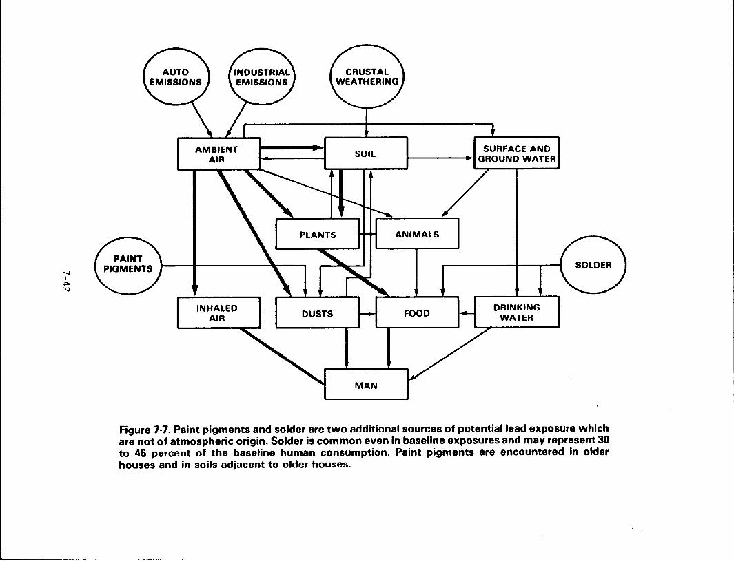
AMBIENT AIR
INHALED AIR
PLANTS
DUSTS
SOIL
MAN
SURFACE AND J------. GROUND WATER
ANIMALS
DRINKING WATER
Figure 7-7. Paint pigments and solder are two additional sources of potential lead exposure which are not of atmospheric origin. Solder is common even in baseline exposures and may represent 30 to 45 percent of the baseline human consumption. Paint pigments are encountered in older houses and in soils adjacent to older houses.
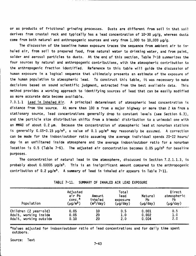
or as products of frictional grinding processes. Dusts are different from soil in that soil derives from crustal rock and typically has a lead concentration of 10-30 1-1g/g, whereas dusts come from both natural and anthropogenic sources and vary from 1,000 to 10,000 1-1g/g.
The discussion of the baseline human exposure traces the sequence from ambient air to inhaled air, from soil to prepared food, from natural water to drinking water, and from paint, solder and aerosol particles to dusts. At the end of this section, Table 7-18 summarizes the four sources by natural and anthropogenic contributions, with the atmospheric contribution to the anthropogenic fraction identified. Reference to this table will guide the discussion of human exposure in a logical sequence that ultimately presents an estimate of the exposure of the human population to atmospheric lead. To construct this table, it was necessary to make decisions based on sound scientific judgment, extracted from the best available data. This method provides a working approach to identifying sources of lead that can be easily modified as more accurate data become available. 7.3.1.1 Lead in Inhaled Air. A principal determinant of atmospheric lead concentration is distance from the source. At more than 100 m from a major highway or more than 2 km from a stationary source, lead concentrations generally drop to constant levels (see Section 6.3),
and the particle size distribution shifts from a bimodal distribution to a unimodal one with an MMAD of about 0. 2 !Jm. Because the concentration of ;:t.tmospheric lead at nonurban stations is generally 0.05-0.15 1-1g/m3, a value of 0.1 1-1g/m3 may reasonably be assumed. A correction can be made for the indoor/outdoor ratio assuming the average individual spends 20-22 hours/ day in an unfi 1 tered inside atmosphere and the average indoor/outdoor ratio for a nonurban location is 0.5 (Table 7-6). The adjusted air concentration becomes 0.05 1Jg/m3 for baseline purposes.
The concentration of natural lead in the atmospherE!, discussed in Section 7.2.1.1.3, is probably about 0.00005 j.lg/m3 . This is an insignificant amount compared to the anthropogenic contribution of 0.2 j.lg/m3. A summary of lead in inhaled air appears in Table 7-11.
TABLE 7-11. SUMMARY OF INHALED AIR LEAD EXPOSURE
Adjusted Total Direct air Pb Amount lead Natural atmospheric cone.* inhaled exposure Pb Pb
Population (1Jg/m3) (m3/day) (!Jg/day) (!Jg/day) (1Jg/day)
Children (2 year-old) 0.05 10 0.5 0.001 0.5 Adult, working inside 0.05 20 1.0 0.002 1.0 Adult, working outside 0.10 20 2.0 0.004 2.0
*Values adjusted for indoor/outdoor ratio of lead concentrations and for daily time spent outdoors.
Source: Text 7-43
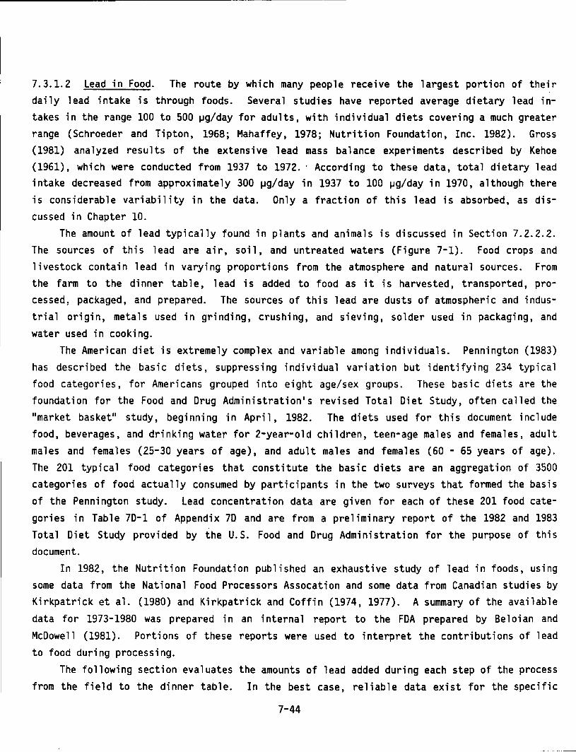
7.3.1.2 Lead in Food. The route by which many people receive the largest portion of their daily lead intake is through foods. Several studies have reported average dietary lead intakes in the range 100 to 500 ~g/day for adults, with individual diets covering a much greater range (Schroeder and Tipton, 1968; Mahaffey, 1978; Nutrition Foundation, Inc. 1982). Gross (1981) analyzed results of the extensive lead mass balance experiments described by Kehoe (1961), which were conducted from 1937 to 1972. · According to these data, total dietary lead intake decreased from approximately 300 ~g/day in 1937 to 100 ~g/day in 1970, although there is considerable variability in the data. Only a fraction of this lead is absorbed, as discussed in Chapter 10.
The amount of lead typically found in plants and animals is discussed in Section 7.2.2.2. The sources of this lead are air, soil, and untreated waters (Figure 7-1). Food crops and livestock contain lead in varying proportions from the atmosphere and natural sources. From the farm to the dinner table, lead is added to food as it is harvested, transported, processed, packaged, and prepared. The sources of this lead are dusts of atmospheric and industrial origin, metals used in grinding, crushing, and sieving, solder used in packaging, and
water used in cooking.
The American diet is extremely complex and variable among individuals. Pennington (1983) has described the basic diets, suppressing individual variation but identifying 234 typical food categories, for Americans grouped into eight age/sex groups. These basic diets are the foundation for the Food and Drug Administration•s revised Total Diet Study, often called the 11 market basket11 study, beginning in April, 1982. The diets used for this document include food, beverages, and drinking water for 2-year-old children, teen-age males and females, adult
males and females (25-30 years of age), and adult males and females (60 - 65 years of age). The 201 typical food categories that constitute the basic diet.s are an aggregation of 3500 categories of food actually consumed by participants in the two surveys that formed the basis
of the Pennington study. Lead concentration data are given for each of these 201 food cate
gories in Table 7D-1 of Appendix 7D and are from a preliminary report of the 1982 and 1983 Total Diet Study provided by the U.S. Food and Drug Administration for the purpose of this document.
In 1982, the Nutrition Foundation published an exhaustive study of lead in foods, using some data from the National Food Processors Assocation and some data from Canadian studies by Kirkpatrick et al. (1980) and Kirkpatrick and Coffin (1974, 1977). A summary of the available
data for 1973-1980 was prepared in an i nterna 1 report to the FDA prepared by Be 1 oi an and
McDowell (1981). Portions of these reports were used to interpret the contributions of lead to food during processing.
The following section evaluates the amounts of lead added during each step of the process
from the field to the dinner table. In the best case, reliable data exist for the specific
7-44
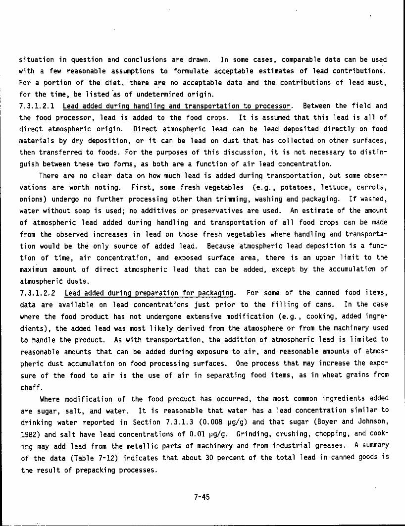
situation in question and conclusions are drawn. In some cases, comparable data can be used with a few reasonable assumptions to formulate acceptable estimates of lead contributions. For a portion of the diet, there a~e no acceptable data and the contributions of lead must, for the time, be listed ~s of undetermined origin. 7.3.1.2.1 Lead added during handling and transportation to processor. Between the field and the food processor, lead is added to the food crops. It is assumed that this lead is all of direct atmospheric origin. Direct atmospheric lead can be lead deposited directly on food materials by dry deposition, or it can be lead on dust that has collected on other surfaces, then transferred to foods. For the purposes of this discussion, it is not necessary to distinguish between these two forms, as both are a function of Clir lead concentration.
There are no clear data on how much lead is added during transportation, but some observations are worth noting. First, some fresh vegetables (e.g., potatoes, lettuce, carrots, onions) undergo no further processing other than trimmin~J, washing and packaging. If washed, water without soap is used; no additives or preservatives are used. An estimate of the amount of atmospheric 1 ead added during handling and transportation of a 11 food crops can be made from the observed i.ncreases in lead on those fresh vegetables where handling and transportation would be the only source of added lead. Because atmospheric lead deposition is a function of time, air concentration, and exposed surface area, there is an upper limit to the maximum amount of direct atmospheric 1 ead that can be added, except by the accumulation of atmospheric dusts. 7. 3.1. 2. 2 Lead added during preparation for packaging. For some of the canned food items, data are avail ab 1 e on 1 ead concentrations just prior t'o the fi 11 i ng of cans. In the case where the food product has not undergone extensive modification (e.g., cooking, added ingredients), the added lead was most likely derived from the i!tmosphere or from the machinery used to handle the product. As with transportation, the addit·ion of atmospheric lead is limited to reasonab 1 e amounts that can be added during exposure to i! i r, and reasonab 1 e amounts of atmospheric dust accumulation on food processing surfaces. Ont~ process that may increase the exposure of the food to air is the use of air in separating food items, as in wheat grains from
chaff. Where modification of the food product has occurred, the most common ingredients added
are sugar, salt, and water. It is reasonable that water has a lead concentration similar to drinking water reported in Section 7.3.1.3 (0.008 tJg/g) and that sugar (Boyer and Johnson, 1982) and salt have lead concentrations of 0.01 tJg/g. Grinding, crushing, chopping, and cooking may add lead from the metallic parts of machinery and from industrial greases. A summary of the data (Table 7-12) indicates that about 30 percent of the total lead in canned goods is
the result of prepacking processes.
7-45
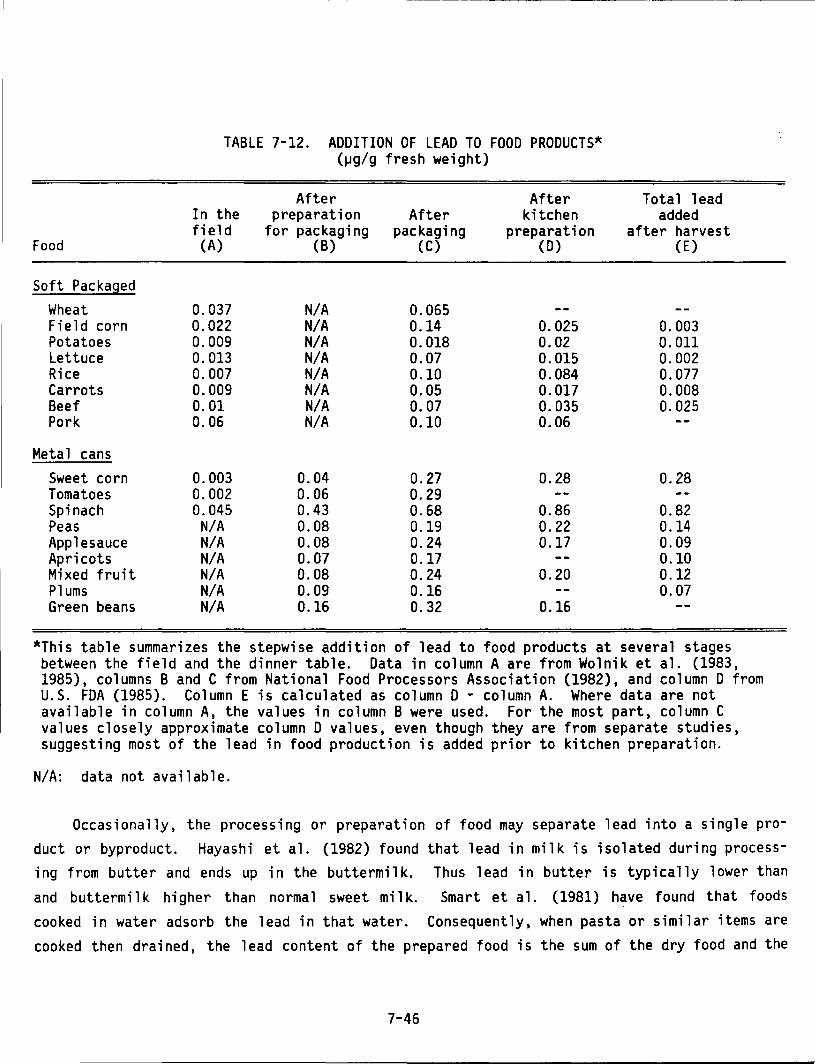
Food
Soft Packaged Wheat Field corn Potatoes Lettuce Rice Carrots Beef Pork
Metal cans Sweet corn Tomatoes Spinach Peas Applesauce Apricots Mixed fruit Plums Green beans
TABLE 7-12. ADDITION OF LEAD TO FOOD PRODUCTS* (~g/g fresh weight)
In the field
(A)
0.037 0.022 0.009 0.013 0.007 0.009 0.01 0.06
0.003 0.002 0.045
N/A N/A N/A N/A N/A N/A
After preparation
for packaging (B)
N/A N/A N/A N/A N/A N/A N/A N/A
0.04 0.06 0.43 0.08 0.08 0.07 0.08 0.09 0.16
After packaging
(C)
0.065 0.14 0.018 0.07 0.10 0.05 0.07 0.10
0.27 0.29 0.68 0.19 0.24 0.17 0.24 0.16 0.32
After kitchen
preparation (D)
0.025 0.02 0.015 0.084 0.017 0.035 0.06
0.28
0.86 0.22 0.17
0.20
0.16
Total lead added
after harvest (E)
0.003 0.011 0.002 0.077 0.008 0.025
0.28
0.82 0.14 0.09 0.10 0.12 0.07
*This table summarizes the stepwise addition of lead to food products at several stages between the field and the dinner table. Data in column A are from Wolnik et al. (1983, 1985), columns B and C from National Food Processors Association (1982), and column D from U.S. FDA (1985). Column E is calculated as column D - column A. Where data are not available in column A, the values in column B were used. For the most part, column C values closely approximate column D values, even though they are from separate studies, suggesting most of the lead in food production is added prior to kitchen preparation.
N/A: data not available.
Occasionally, the processing or preparation of food may separate lead into a single product or byproduct. Hayashi et a 1. (1982) found that 1 ead in milk is i so 1 a ted during processing from butter and ends up in the buttermilk. Thus lead in butter is typically lower than
and buttermilk higher than norma 1 sweet mi 1 k. Smart et a 1. (1981) have found that foods cooked in water adsorb the lead in that water. Consequently, when pasta or similar items are
cooked then drained, the lead content of the prepared food is the sum of the dry food and the
7-46
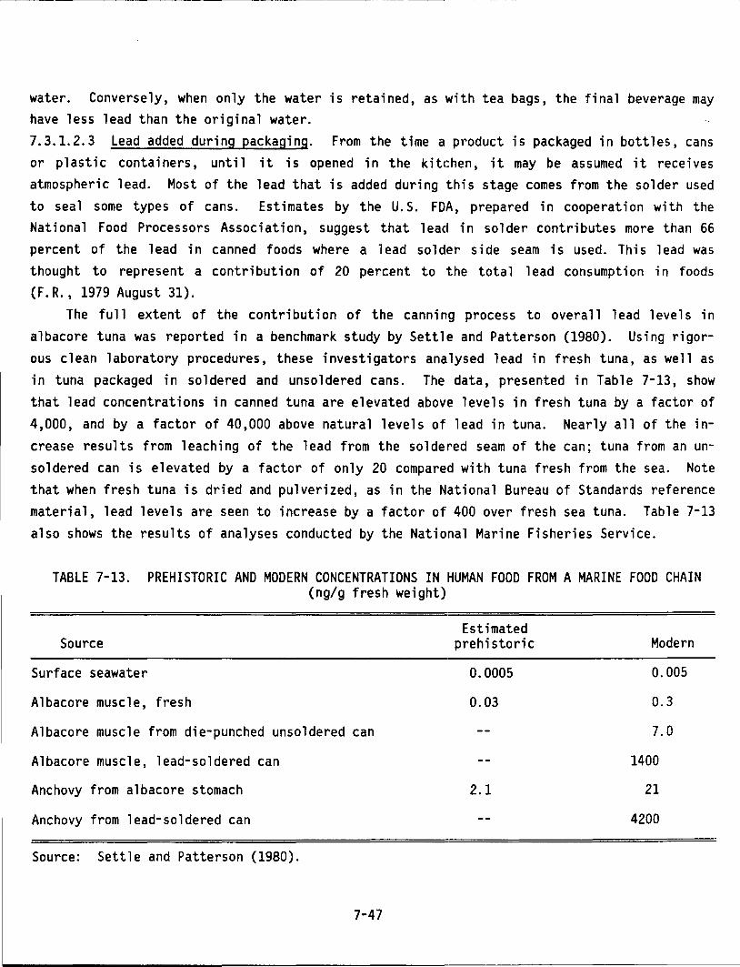
water. Conversely, when only the water is retained, as with tea bags, the final beverage may have less lead than the original water. 7.3.1.2.3 Lead added during packaging. From the time a product is packaged in bottles, cans or plastic containers, until it is opened in the kitchen, it may be assumed it receives atmospheric lead. Most of the lead that is added during this stage comes from the solder used to seal some types of cans. Estimates by the U.S. FDA, prepared in cooperation with the National Food Processors Association, suggest that lead in solder contributes more than 66 percent of the 1 ead in canned foods where a 1 ead so 1 der side seam is used. This 1 ead was thought to represent a contribution of 20 percent to the tota 1 1 ead consumption in foods (F.R., 1979 August 31).
The full extent of the contribution of the canning process to overall 1 ead 1 eve 1 s in albacore tuna was reported in a benchmark study by Settle and Patterson (1980). Using rigorous clean laboratory procedures, these investigators analysed lead in fresh tuna, as well as in tuna packaged in soldered and unsoldered cans. The data, presented in Table 7-13, show that lead concentrations in canned tuna are elevated above levels in fresh tuna by a factor of 4,000, and by a factor of 40,000 above natural levels of lead in tuna. Nearly all of the increase results from leaching of the lead from the soldered seam of the can; tuna from an unsoldered can is elevated by a factor of only 20 compared with tuna fresh from the sea. Note that when fresh tuna is dried and pulverized, as in the National Bureau of Standards reference material, lead levels are seen to increase by a factor of 400 over fresh sea tuna. Table 7-13
also shows the results of analyses conducted by the National Marine Fisheries Service.
TABLE 7-13. PREHISTORIC AND MODERN CONCENTRATIONS IN HUMAN FOOD FROM A MARINE FOOD CHAIN (ng/g fresh weight)
Source
Surface seawater
Albacore muscle, fresh
Albacore muscle from die-punched unsoldered can
Albacore muscle, lead-soldered can
Anchovy from albacore stomach
Anchovy from lead-soldered can
Source: Settle and Patterson (1980).
7-47
Estimated prehistoric
0.0005
0.03
2.1
Modern
0.005
0.3
7.0
1400
21
4200
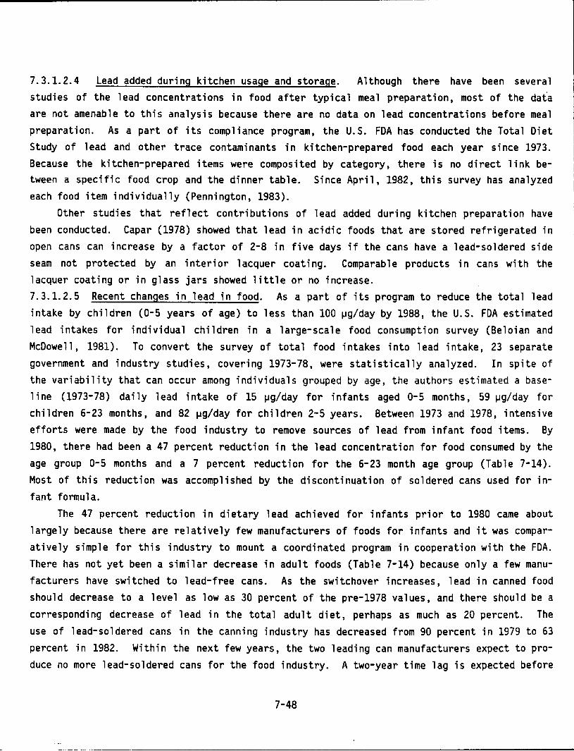
7.3.1.2.4 Lead added during kitchen usage and storage. Although there have been several studies of the lead concentrations in food after typical meal preparation, most of the data are not amenable to this analysis because there are no data on lead concentrations before meal preparation. As a part of its compliance program, the U.S. FDA has conducted the Total Diet Study of lead and other trace contaminants in kitchen-prepared food each year since 1973. Because the kitchen-prepared items were composited by category, there is no direct link between a specific food crop and the dinner table. Since April, 1982, this survey has analyzed each food item individually (Pennington, 1983).
Other studies that reflect contributions of 1 ead added during kitchen preparation have been conducted. Capar (1978) showed that lead in acidic foods that are stored refrigerated in open cans can increase by a factor of 2-8 in five days if the cans have a lead-soldered side seam not protected by an interior lacquer coating. Comparable products in cans with the lacquer coating or in glass jars showed little or no increase. 7.3.1.2.5 Recent changes in lead in food. As a part of its program to reduce the total lead intake by children (0-5 years of age) to less than 100 ~g/day by 1988, the U.S. FDA estimated lead intakes for individual children in a large-scale food consumption survey (Beloian and McDowell, 1981). To convert the survey of total food intakes into lead intake, 23 separate government and industry studies, covering 1973-78, were statistically analyzed. In spite of the variability that can occur among individuals grouped by age, the authors estimated a baseline (1973-78) daily lead intake of 15 ~g/day for infants aged 0-5 months, 59 ~g/day for children 6-23 months, and 82 ~g/day for children 2-5 years. Between 1973 and 1978, intensive efforts were made by the food industry to remove sources of lead from infant food items. By 1980, there had been a 47 percent reduction in the lead concentration for food consumed by the age group 0-5 months and a 7 percent reduction for the 6-23 month age group (Table 7-14). Most of this reduction was accomplished by the discontinuation of soldered cans used for infant formula.
The 47 percent reduction in dietary lead achieved for infants prior to 1980 came about largely because there are relatively few manufacturers of foods for infants and it was comparatively simple for this industry to mount a coordinated program in cooperation with the FDA. There has not yet been a similar decrease in adult foods (Table 7-14) because only a few manufacturers have switched to lead-free cans. As the switchover increases, lead in canned food should decrease to a level as low as 30 percent of the pre-1978 values, and there should be a corresponding decrease of lead in the total adult diet, perhaps as much as 20 percent. The use of lead-soldered cans in the canning industry has decreased from 90 percent in 1979 to 63 percent in 1982. Within the next few years, the two leading can manufacturers expect to produce no more lead-soldered cans for the food industry. A two-year time lag is expected before
7-48
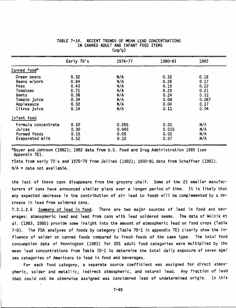
Canned food* Green beans Beans w/pork Peas Tomatoes Beets Tomato juice Applesauce Citrus juice
Infant food
TABLE 7-14. RECENT TRENDS OF MEAN LEAD CONCENTRATIONS IN CANNED ADULT AND INFANT FOOD ITEMS
(jJg/g)
Early 7o•s 1976-77 1980-81
0.32 N/A 0.32 0.64 N/A 0.26 0.43 N/A 0.19 0.71 N/A 0.29 0.38 N/A 0.24 0.34 N/A 0.08 0.32 N/A 0.04 0.14 N/A 0.11
Formula concentrate 0.10 0.055 0.01 Juices 0.30 0.045 0.015 Pureed foods 0.15 0.05 0.02 Evaporated milk 0.52 0.10 0.07
*Boyer and Johnson (1982); 1982 data from U.S. Food and Drug Administration Appendix 7D).
1982
0.16 0.17 0.22 0.21 0.12 0.067 0.17 0.04
N/A N/A N/A N/A
1985 (see
tData from early 70 1 5 and 1976-79 from Jelinek (1982); 1980-81 data from Schaffner (1981). N/A = data not available.
the 1 ast of these cans disappears from the grocery she H. Some of the 23 sma 11 er manufacturers of cans have announced similar plans over a longer period of time. It is likely that any expected decrease in the contribution of air 1 ead to foods wi 11 be comp 1 emented by a decrease in lead from soldered cans. 7. 3.1. 2. 6 Summary of 1 ead in food. There are two major sources of 1 ead in food and beverages: atmospheric 1 ead and 1 ead from cans with 1 ead 51) 1 de red seams. The data of Wo 1 ni k et al. (1983, 1985) provide some insight into the amount of atmospheric lead on food crops (Table 7-8). The FDA analyses of foods by category (Table 70-1 in appendix 70) clearly show the influence of so 1 der on canned foods compared to fresh foods of the same type. The tota 1 food consumption data of Pennington (1983) for 201 adult food categories were multiplied by the mean lead concentrations from Table 70-1 to determine the total daily exposure of seven age/
sex categories of Americans to lead in food and beverages. For each food category, a separate source coefficient was assigned for direct atmos
pheric, so 1 der and meta 11 i c, indirect atmospheric, and natura 1 1 ead. Any fraction of 1 ead that could not be otherwise assigned was considered le!ad of undetermined origin. In this
7-49
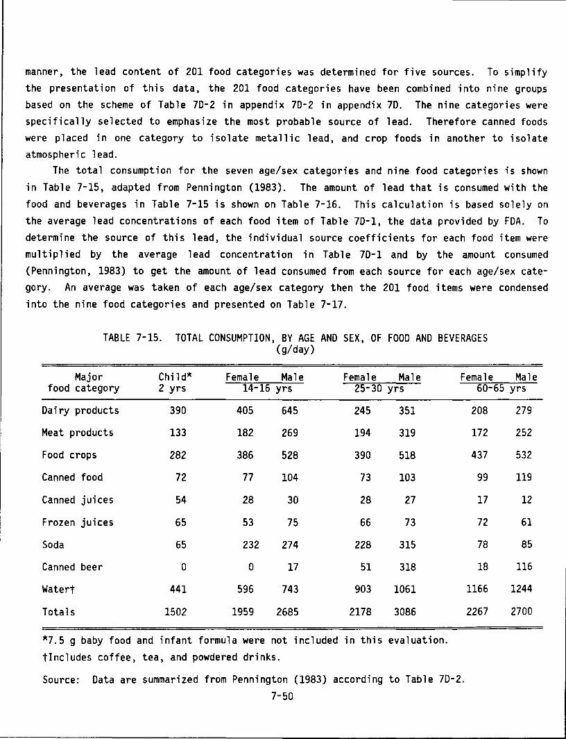
manner, the lead content of 201 food categories was determined for five sources. To simplify the presentation of this data, the 201 food categories have been combined into nine groups based on the scheme of Table 7D-2 in appendix 7D-2 in appendix 7D. The nine categories were specifically selected to emphasize the most probable source of lead. Therefore canned foods were p 1 aced in one category to i so 1 ate meta 11 i c 1 ead, and crop foods in another to i so 1 ate atmospheric lead.
The total consumption for the seven age/sex categories and nine food categories is shown
in Table 7-15, adapted from Pennington (1983). The amount of lead that is consumed with the food and beverages in Table 7-15 is shown on Table 7-16. This calculation is based solely on
the average lead concentrations of each food item of Table 7D-1, the data provided by FDA. To determine the source of this lead, the individual source coefficients for each food item were
multiplied by the average lead concentration in Table 7D-1 and by the amount consumed (Pennington, 1983) to get the amount of lead consumed from each source for each age/sex category. An average was taken of each age/sex category then the 201 food items were condensed
into the nine food categories and presented on Table 7-17.
TABLE 7-15. TOTAL CONSUMPTION, BY AGE AND SEX, OF FOOD AND BEVERAGES (g/day)
Major food category
Child* 2 yrs
Female Male Female Male Female Male
Dairy products
Meat products
Food crops
Canned food
Canned juices
Frozen juices
Soda
Canned beer
Watert
Totals
390
133
282
72
54
65
65
0
441
1502
14-16 yrs
405 645
182 269
386 528
77 104
28 30
53 75
232 274
0 17
596 743
1959 2685
25-30 yrs
245
194
390
73
28
66
228
51
903
2178
351
319
518
103
27
73
315
318
1061
3086
*7.5 g baby food and infant formula were not included in this evaluation.
tlncludes coffee, tea, and powdered drinks.
Source: Data are summarized from Pennington (1983) according to Table 7D-2.
7-50
60-65 yrs
208
172
437
99
17
72
78
18
1166
2267
279
252
532
119
12
61
85
116
1244
2700
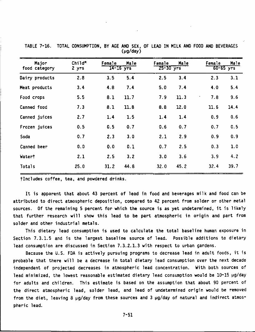
TABLE 7-16. TOTAL CONSUMPTION, BY AGE AND SEX, OF LEAD IN MILK AND FOOD AND BEVERAGES (~g/day)
Major Child* Female Male Female Male Female Male food category 2 yrs 14-!6 yrs 2~-30 yrs 60-65 yrs
Dairy products 2.8 3.5 5.4 2.5 3.4 2.3 3.1
Meat products 3.4 4.8 7.4 5.0 7.4 4.0 5.4
Food crops 5.5 8.1 11.7 7.9 11.3 7.8 9.6
Canned food 7.3 8.1 11.8 8.8 12.0 11.6 14.4
Canned juices 2.7 1.4 1.5 1.4 1.4 0.9 0.6
Frozen juices 0.5 0.5 0.7 0.6 0.7 0.7 0.5
Soda 0.7 2.3 3.0 2.1 2.9 0.9 0.9
Canned beer 0.0 0.0 0.1 0.7 2.5 0.3 1.0
Watert 2.1 2.5 3.2 3.0 3.6 3.9 4.2
Totals 25.0 31.2 44.8 32.0 45.2 32.4 39.7
tincludes coffee, tea, and powdered drinks.
It is apparent that about 43 percent of lead in food and beverages milk and food can be attributed to direct atmospheric deposition, compared to 42 percent from solder or other metal sources. Of the remaining 5 percent for which the source is as yet undetermined, it is likely that further research wi 11 show this 1 ead to be part atmospheric in origin and part from solder and other industrial metals.
This dietary lead consumption is used to calculate the total baseline human exposure in Section 7.3.1.5 and is the largest baseline source of lead. Possible additions to dietary lead consumption are discussed in Section 7.3.2.1.3 with respect to urban gardens.
Because the U.S. FDA is actively pursuing programs to decrease lead in adult foods, it is probable that there will be a decrease in total dietary lead consumption over the next decade independent of projected decreases in atmospheric lead concentration. With both sources of lead minimized, the lowest reasonable estimated dietary lead consumption would be 10-15 ~g/day for adults and children. This estimate is based on the assumption that about 90 percent of the direct atmospheric lead, solder lead, and lead of undetermined origin would be removed from the diet, leaving 8 ~g/day from these sources and 3 ~g/day of natural and indirect atmospheric lead.
7-51
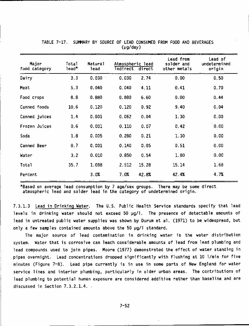
TABLE 7-17. SUMMARY BY SOURCE OF LEAD CONSUMED FROM FOOD AND BEVERAGES (IJg/day)
Lead from Lead of Major Total Natural AtmosEheric lead solder and undetermined
food category lead* lead indirect direct other metals origin
Dairy 3.3 0.030 0.030 2.74 0.00 0.50
Meat 5.3 0.040 0.040 4.11 0.41 0.70
Food crops 8.8 0.880 0.880 6.60 0.00 0.44
Canned foods 10.6 0.120 0.120 0.92 9.40 0.04
Canned juices 1.4 0.001 0.062 0.04 1. 30 0.00
Frozen Juices 0.6 0.001 0.110 0.07 0.42 0.00
Soda 1.8 0.005 0.280 0.21 1. 30 0.00
Canned Beer 0.7 0.001 0.140 0.05 0.51 0.00
Water 3.2 0.010 0.850 0.54 1. 80 0.00
Total 35.7 1.088 2.512 15.28 15.14 1. 68
Percent 3.0% 7.0% 42.8% 42.4% 4.7%
*Based on average lead consumption by 7 age/sex groups. There may be some direct atmospheric lead and solder lead in the category of undetermined origin.
7.3.1.3 Lead in Drinking Water. The U.S. Public Health Service standards specify that lead 1 eve 1 s in drinking water should not exceed 50 j.Jg/1. The presence of detectab 1 e amounts of lead in untreated public water supplies was shown by Durum et al. (1971) to be widespread, but only a few samples contained amounts above the 50 j.Jg/1 standard.
The major source of lead contamination in drinking water is the water distribution system. Water that is corrosive can leach considerable amounts of lead from lead plumbing and lead compounds used to join pipes. Moore (1977) demonstrated the effect of water standing in pipes overnight. Lead concentrations dropped significantly with flushing at 10 1/min for five minutes (Figure 7-8). Lead pipe currently is in use in some parts of New England for water service lines and interior plumbing, particularly in older urban areas. The contributions of lead plumbing to potential human exposure are considered additive rather than baseline and are discussed in Section 7.3.2.1.4 ..
7-52
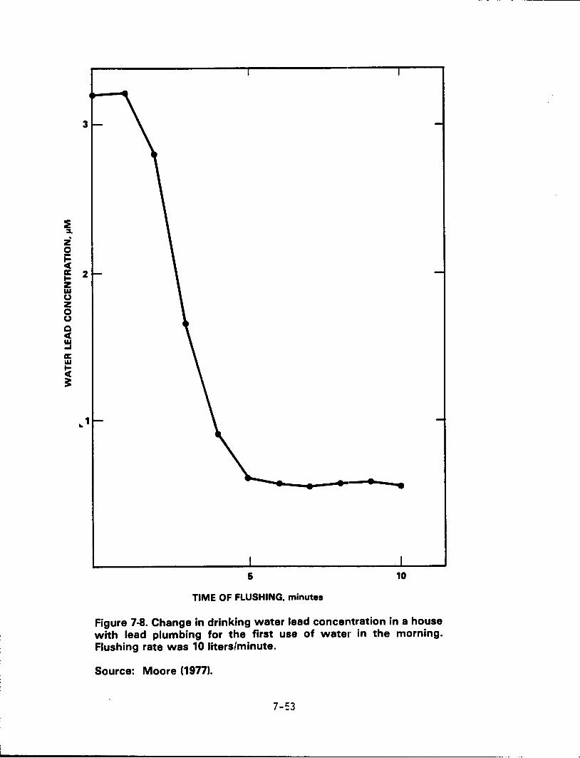
~ :s. z 0
~
3
a: 2 ~ z w (.) z 0 (.)
Q c(
~ a: w
~ 3:
.,1
6 10
TIME OF FLUSHING, minutes
Figure 7-8. Change in drinking water lead concentration in a house with lead plumbing for the first use of watel' in the morning. Flushing rate was 10 liters/minute.
Source: Moore (19n).
7-53
~------------------------------------------------------------------------------~~-~----
There have been severa 1 studies in North America and Europe of the sources of 1 ead in drinking water. A recent study in Seattle, WA by Sharrett et al. (1982) showed that the age of the house and the type of plumbing determined the lead concentration in tap water. Standing water in copper pipes from houses newer than five years averaged 31 ~g/1; those less than 18 months average about 70 ~g/1. Houses older than five years and houses with galvanized pipe averaged less than 6 ~g/1. The source of the water supply, the length of the pipe, and the use of plastic pipes in the service line had little or no effect on the lead concentrations.
It appears certain that the source of lead in new homes with copper pipes is the solder used to join these pipes, and that this lead is either leached away with age or isolated by accumulated deposits within the pipes. A study of copper pipes in cottages using local lakes for a water source revealed a similar pattern of lead with increased standing time in the pipes (Meranger et al., 1983). The lead concentration in the first liter drawn continued to increase with standing time, even up to ten days.
The Sharrett et al. (1982) study of the Seattle population also provided data on water and beverage consumption which extended the scope of the Pennington (1983) study of ali Americans. While the total amount of liquids consumed was slightly higher in Seattle (2200 g/day vs. 1800 g/day for all Americans), the breakdown between water consumed inside and outside the home can prove useful. Men, women, and children consume 53, 87, and 87 percent, respectively, of their water and beverages within the home.
Bai 1 ey and Russe 11 (1981) have deve 1 oped a mode 1 for population exposure to 1 ead in home drinking water. The model incorporates data for lead concentration as a function of stagnation time in the pipes, as well as probability distributions for times of water use throughout the day. Population surveys conducted as part of the United Kingdom Region a 1 Heart Survey provided these water-use distributions.
Other studies have been conducted in Canada and Belgium. Lead levels in water boiled in electric kettles were measured in 574 households in Ottawa (Wigle and Charlebois, 1978). Concentrations greater than 50 ~g/1 were observed in 42.5 percent of the households, and excessive lead levels were associated with kettles more than five years old. 7.3.1.4 Lead in Dusts. By technical definition, dusts are solid particles produced by the disintegration of materials (Friedlander, 1977) and appear to have no size limitations. Although dusts are of complex origin, they may be placed conveniently into a few categories relating to human exposure. Generally, the most convenient categories are household dusts, soil
dust, street dusts, and occupational dusts. In each case, the lead in dust arises from a complex mixture of fine particles of soil, flaked paint, and airborne particles of industrial or automotive origin. It is a characteristic of dust particles that they accumulate on exposed surfaces and are trapped in the fibers of clothing and carpets. Ingestion of dust particles,
7-54
rather than inhalation, appears to be the greater problem in the baseline environment, especially ingestion during meals and playtime activity by small children.
Two other features of dust are important. First, they must be described in both concentration and amount. The concentration of lead in street dust may be the same in a rural and urban environment, but the amount of dust may differ by a wide margin. Secondly, each category represents a different combination of sources. Household dusts contain some atmospheric lead, some paint lead, and some soil lead. Street dusts contain atmospheric, soil, and occasionally paint lead. This apparent paradox does not prevent the evaluation of exposures to dust, but it does confound efforts to identify the amounts of atmospheric lead contributed to dusts. For the baseline human exposure, it is assumed that workers are not exposed to occupational dusts, nor do they live in houses with interior leaded paints. Street dust, soil dust, and some househo 1 d dust are the primary dust sources for· base 1 i ne potentia 1 human 1 ead exposure.
In considering the impact of street dust on the human environment, the obvious question arises as to whether lead in street dust varies with trnffic density. In a transect through Minneapolis/St. Paul, Mielke et al. (1984) found soil lead concentrations 10 to 1000-fold higher near major interstate highways. Nriagu (1978) l'"eviewed several studies of lead in street dust. Warren et al. (1971) reported 20,000 ~g Pb/!~ street dust in a heavily trafficked area. In the review by Nri agu (1978), street dust 1 ead concentrations ranged from 300 to 18,000 ~g/g in several cities in the United States. Mt)re recent studies have attempted to characterize lead in street dust in greater detail. Franz and Hadley (1981) separated street dust by particle size and found that smaller particles co1ntain greater concentrations of lead. One-third of the mass was less than 150 ~m and contained 37 percent of the total lead. The average concentration in the Albuquerque street dust was 5000 ~g/g, 20 percent of which was attributed to curb paint. Dong et al. (1984) separated street dusts by mechanical sieve and found, with one exception, 50 percent or more of the lead on clay-sized particles, the smallest fraction both in particle size and in total mass (S-6 percent). There was, however, considerable variation in the absolute concentrations of lead in the samples from the same location taken four days apart.
There are several reports of street dusts outside the United States that show similar relationships. Fergusson and Ryan (1984) found concentrations in small urban cities in Canada, New Zealand and Jamaica ranged from 700 to 2000 ~g/g, while in New York and London the range was from 2000 to 4000 ~g/g. Sequential extractions showed much of the lead (44 percent) was on the Fe-Mn oxide fraction, but that 36 percent ~,as on the exchangeable and carbonate fractions that are more readily available. Gibson and Farmer (1984) also found 41 percent of the street dust lead in Glascow, Scotland to be on the exchangeable and carbonate fractions.
7-55
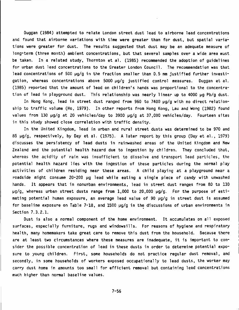
Duggan (1984) attempted to relate London street dust lead to airborne lead concentrations and found that airborne variations with time were greater than for dust, but spatial varia~
tions were greater for dust. The results suggested that dust may be an adequate measure of long-term (three month) ambient concentrations, but that several samples over a wide area must be taken. In a related study, Thornton et al. (1985) recommended the adoption of guidelines for urban dust lead concentrations to the Greater London Council. The recommendation was that lead concentrations of 500 ~g/g in the fraction smaller than 0.5 mm justified further investi
gation, whereas concentrations above 5000 ~g/g justified control measures. Duggan et al. (1985) reported that the amount of lead on children•s hands was proportional to the concentration of lead in playground dust. This relationship was nearly linear up to 4000 ~g Pb/g dust.
In Hong Kong, lead in street dust ranged from 960 to 7400 ~gig with no direct relationship to traffic volume (Ho, 1979). In other reports from Hong Kong, Lau and Wong (1982) found values from 130 ~g/g at 20 vehicles/day to 3900 ~gig at 37,000 vehicles/day. Fourteen sites in this study showed close correlation with traffic density.
In the United Kingdom, lead in urban and rural street dusts was determined to be 970 and 85 ~g/g, respectively, by Day et al. (1975). A later report by this group (Day et al., 1979)
discusses the persistency of 1 ead dusts in rai nwashed areas of the United Kingdom and New Zealand and the potential health hazard due to ingestion by children. They concluded that, whereas the acidity of rain was insufficient to dissolve and transport lead particles, the
potentia 1 he a 1 th hazard 1 i es with the ingestion of these part i c 1 es during the norma 1 p 1 ay activities of children residing near these areas. A child playing at a playground near a roadside might consume 20-200 ~g lead while eating a single piece of candy with unwashed hands. It appears that in nonurban environments, lead in street dust ranges from 80 to 130
~g/g, whereas urban street dusts range from 1,000 to 20,000 ~g/g. For the purpose of estimating potential human exposure, an average lead value of 90 ~g/g in street dust is assumed
for baseline exposure on Table 7-18, and 1500 ~g/g in th~ discussions of urban environments in Section 7.3.2.1.
Dust is also a normal component of the home environment. It accumulates on all exposed surfaces, especially furniture, rugs and windowsills. For reasons of hygiene and respiratory health, many homemakers take great care to remove this dust from the household. Because there are at least two circumstances where these measures are inadequate, it is important to consider the possible concentration of lead in these dusts in order to determine potential exposure to young children. First, some households do not practice regular dust removal, and
secondly, in some households of workers exposed occupationally to lead dusts, the worker may
carry dust home in amounts too small for efficient removal but containing lead concentrations
much higher than normal baseline values.
7-56
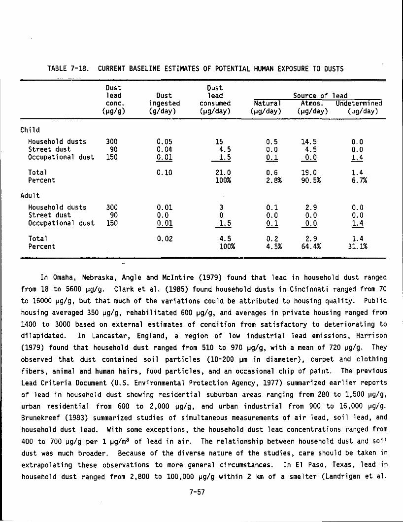
TABLE 7-18. CURRENT BASELINE ESTIMATES OF POTENTIJ~L HUMAN EXPOSURE TO DUSTS
Dust Dust lead Dust lead Source of lead cone. ingested consumed Natural Atmos. Undeterm1ned (~g/g) (g/day) (~g/day) (~g/day) (~g/day) (~g/day)
Child Household dusts 300 0.05 15 0.5 14.5 0.0 Street dust 90 0.04 4.5 0.0 4.5 0.0 Occupational dust 150 0.01 1.5 0.1 0.0 1.4
Total 0.10 21.0 0.6 19.0 1.4 Percent 100% 2.8% 90.5% 6.7%
Adult Household dusts 300 0.01 3 0.1 2.9 0.0 Street dust 90 0.0 0 0.0 0.0 0.0 Occupational dust 150 0.01 1.5 0.1 0.0 1.4
Total 0.02 4.5 0.2 2.9 1.4 Percent 100% 4.5% 64.4% 31.1.%
In Omaha, Nebraska, Angle and Mcintire (1979) found that lead in household dust ranged
from 18 to 5600 ~g/g. Clark et al. (1985) found household dusts in Cincinnati ranged from 70
to 16000 ~g/g, but that much of the variations could be attributed to housing quality. Public housing averaged 350 ~g/g, rehabilitated 600 ~g/g, and averages in private housing ranged from 1400 to 3000 based on external estimates of condition from satisfactory to deteriorating to dilapidated. In Lancaster, England, a region of low industrial lead emissions, Harrison
(1979) found that household dust ranged from 510 to 970 ~g/g, with a mean of 720 ~g/g. They
observed that dust contained soil particles (10-200 ~m in diameter), carpet and clothing fibers, animal and human hairs, food particles, and an occasional chip of paint. The previous
Lead Criteria Document (U.S. Environmental Protection Agency, 1977) summarized earlier reports of lead in household dust showing residential suburban areas ranging from 280 to 1,500 ~g/g,
urban residential from 600 to 2,000 ~g/g, and urban industrial from 900 to 16,000 ~g/g.
Brunekreef (1983) summarized studies of simultaneous measurements of air lead, soil lead, and
household dust lead. With some exceptions, the household dust lead concentrations ranged from
400 to 700 ~g/g per 1 ~g/m3 of lead in air. The relationship between household dust and soil dust was much broader. Because of the diverse nature of the studies, care should be taken in
extrapolating these observations to more general circumstances. In El Paso, Texas, lead in household dust ranged from 2,800 to 100,000 ~g/g within 2 km of a smelter (Landrigan et al.
7-57
-- ---------------------
1975). Davies et al. (1985) found a correlation between soil dust and household dust in an old lead mining area of North Wales, Great Britain, where a tenfold increase in soil lead was associated with a twofold increase in household dust lead.
It appears that most of the values for lead in dust in nonurban household environments fall in the range of 50-500 ~g/g. A mean value of 300 ~g/g is assumed. The only natural lead in dust would be some fraction of that derived from soil ·lead. A value of 10 ~g/g seems reasonable, since some of the soil lead is of atmospheric origin. Since very little paint lead is included in the baseline estimate, most of the remaining dust lead would be from the atmosphere. Table 7-18 summarizes these estimates of human exposure to dusts for children and adults. It assumes that children ingest about five times as much dust as adults, most of the excess being street dusts from sidewalks and playgrounds. Exposure of children to occupational lead would be through contaminated clothing brought home by parents. Most of this lead is of undetermined origin because no data exist on whether the source is dust simi 1 ar to household dust or unusual dust from the grinding and milling activities of factories. 7.3.1.5 Summary of Baseline Human Exposure to Lead. The values derived or assumed in the preceeding sections are summarized in Table 7-19. These values represent only consumption, not absorption, of lead by the human body. The key question of what are the risks to human health from these baseline exposures is addressed in Chapter 13. The approach used here to evaluate potential human exposure is similar to that used by the National Academy of Sciences (1980) and the Nutrition Foundation (1982) in their assessments of the impact of lead in the human environment.
7.3.2 Additive Exposure Factors There are many conditions, even in nonurban environments, where an individual may in
crease his lead exposure by choice, habit, or unavoidable circumstance. The following sections describe these conditions as separate exposures to be added as appropriate to the baseline of human exposure described above. Most of these additive exposures clearly derive from air or dust, while a few derive from water or food. 7.3.2.1 Living and Working Environments With Increased Lead Exposure. Ambient air lead concentrations are typically higher in an urban than a rural environment. This factor alone can contribute significantly to the potential lead exposure of Americans, through increases in i nha 1 ed air and consumed dust. Produce from urban gardens may a 1 so increase the daily consumption of lead. Some environmental exposures may not be related only to urban living, such as houses with interior lead paint or lead plumbing, residences near smelters or refineries, or family gardens grown on high-lead soils. Occupational exposures may also occur in an urban or rural setting. These exposures, whether primarily in the occupational environment or
7-58
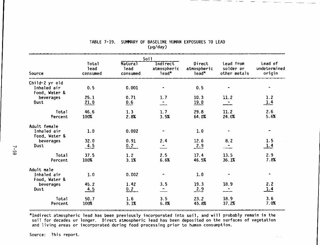
TABLE 7-19. SUMMARY OF BASELINE HUMAN EXPOSURES TO LEAD (IJg/day)
Soil Total Natural Indirect Direct Lead from Lead of lead lead atmospheric atmospheric solder or undetermined
Source consumed consumed lead* lead* other metals origin
Child-2 yr old Inhaled air 0.5 0.001 0.5 Food, Water &
beverages 25.1 0.71 1.7 10.3 11.2 1.2 Oust 21.0 0.6 19.0 1.4
Total 46.6 1.3 1.7 29.8 11.2 2.6 Percent 100% 2.8% 3.5% 64.0% 24.0% 5.6%
Adult female Inhaled air 1.0 0.002 1.0 Food, Water &
beverages 32.0 0.91 2.4 12.6 8.2 1.5 ........ Oust 4.5 n ? 2.9 1.4 u .... I
U'1 1.0 Total 37.5 1.2 2.5 17.4 13.5 2.9
Percent 100% 3.1.% 6.6% 46.5% 36.1.% 7.8%
Adult male Inhaled air 1.0 0.002 1.0 Food, Water &
beverages 45.2 1.42 3.5 19.3 18.9 2.2 Oust 4.5 0.2 2.9 1.4 --
Total 50.7 1.6 3.5 23.2 18.9 3.6 Percent 100% 3.1.% 6.8% 45.8% 37.2% 7.0%
*Indirect atmospheric lead has been previously incorporated into soi 1 , and wi 11 probably remain in the soil for decades or longer. Direct atmospheric lead has been deposited on the surfaces of vegetation and living areas or incorporated during food processing prior to human consumption.
Source: This report.
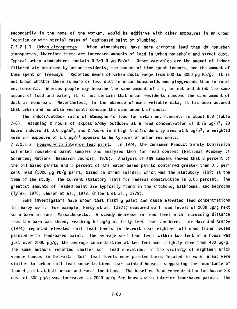
secondarily in the home of the worker, would be additive with other exposures in an urban location or with special cases of lead-based paint or plumbing. 7. 3. 2.1.1 Urban atmospheres. Urban atmospheres have more airborne lead than do non urban atmospheres, therefore there are increased amounts of lead in urban household and street dust. Typical urban atmospheres contain 0.5-1.0 ~g Pb/m3 . Other variables are the amount of indoor filtered air breathed by urban residents, the amount of time spent indoors, and the amount of time spent on freeways. Reported means of urban dusts range from 500 to 3000 ~g Pb/g. It is not known whether there is more or less dust in urban households and playgrounds than in rural environments. Whereas people may breathe the same amount of air, or eat and drink the same amount of food and water, it is not certain that urban residents consume the same amount of dust as nonurban. Nevertheless, in the absence of more reliable data, it has been assumed that urban and nonurban residents consume the same amount of dusts.
The indoor/outdoor ratio of atmospheric lead for urban environments is about 0.8 (Table 7-6). Assuming 2 hours of exposure/day outdoors at a lead concentration of 0. 75 ~g/m3 , 20 hours indoors at 0.6 ~g/m3 , and 2 hours in a high traffic density area at 5 ~g/m3 , a weighted mean air exposure of 1.0 ~g/m3 appears to be typical of urban residents. 7.3.2.1.2 Houses with interior lead paint. In 1974, the Consumer Product Safety Commission collected household paint samples and analyzed them for lead content (National Academy of Sciences; National Research Council, 1976). Analysis of 489 samples showed that 8 percent of the oil-based paints and 1 percent of the water-based paints contained greater than 0.5 percent lead (5000 ~g Pb/g paint, based on dried solids), which was the statutory limit at the time of the study. The current statutory limit for Federal construction is 0.06 percent. The greatest amounts of leaded paint are typically found in the kitchens, bathrooms, and bedrooms (Tyler, 1970; Laurer et al., 1973; Gilbert et al., 1979).
Some investigators have shown that flaking paint can cause elevated lead concentrations in nearby soil. For example, Hardy et al. (1971) measured soil lead levels of 2000 ~g/g next to a barn in rural Massachusetts. A steady decrease in lead level with increasing distance from the barn was shown, reaching 60 ~g/g at fifty feet from the barn. Ter Haar and Aronow (1974) reported elevated soil lead levels in Detroit near eighteen old wood frame houses painted with lead-based paint. The average soil lead level within two feet of a house was just over 2000 ~g/g; the average concentration at ten feet was slightly more than 400 ~g/g.
The same authors reported smaller soil lead elevations in the vicinity of eighteen brick
veneer houses in Detroit. Soil lead levels near painted barns located in rural areas were similar to urban soil lead concentrations near painted houses, suggesting the importance of leaded paint at both urban and rural locations. The baseline lead concentration for household dust of 300 ~g/g was increased to 2000 ~g/g for houses with interior lead-based paints. The
7-60
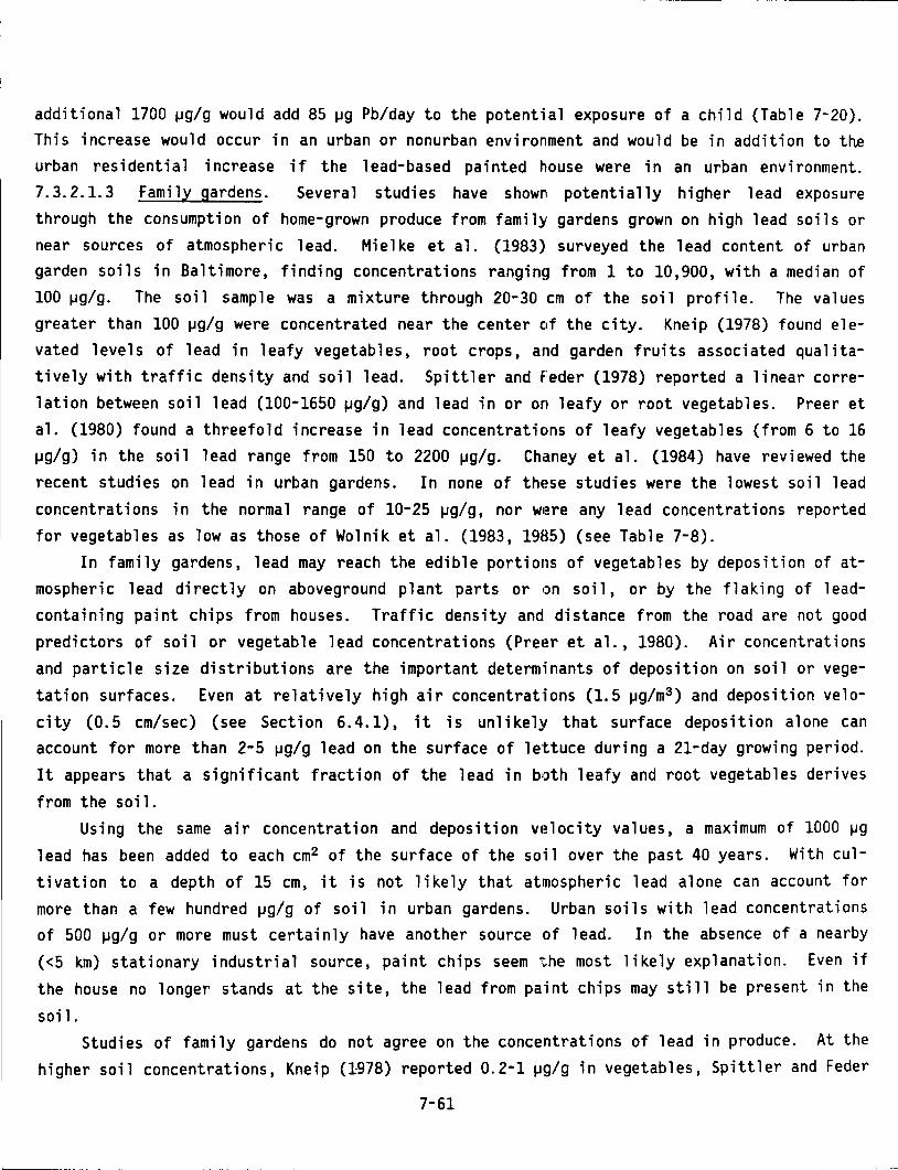
additional 1700 ~g/g would add 85 ~g Pb/day to the potential exposure of a child (Table 7-20). This increase would occur in an urban or nonurban environment and would be in addition to the urban resident i a 1 increase if the 1 ead-based painted house were in an urban environment. 7.3.2.1.3 Family gardens. Several studies have shown potentially higher lead exposure through the consumption of home-grown produce from family gardens grown on high lead soils or near sources of atmospheric lead. Mielke et al. (1983) surveyed the lead content of urban garden soils in Baltimore, finding concentrations ranging from 1 to 10,900, with a median of 100 ~g/g. The soil sample was a mixture through 20-30 em of the soil profile. The values greater than 100 ~g/g were concentrated near the center of the city. Kneip (1978) found elevated 1 eve 1 s of 1 ead in 1 eafy vegetab 1 es, root crops, and garden fruits associ a ted qua 1i tatively with traffic density and soil lead. Spittler and Feder (1978) reported a linear correlation between soil lead (100-1650 ~g/g) and lead in or on leafy or root vegetables. Preer et al. (1980) found a threefold increase in lead concentratic1ns of leafy vegetables (from 6 to 16 ~g/ g) in the soil 1 ead range from 150 to 2200 ~g/ g. Chaney et a 1. (1984) have reviewed the recent studies on lead in urban gardens. In none of these studies were the lowest soil lead concentrations in the normal range of 10-25 ~g/g, nor Wl:!re any lead concentrations reported for vegetables as low as those of Wolnik et al. (1983, 1985) (see Table 7-8).
In family gardens, lead may reach the edible portions of vegetables by deposition of atmospheric lead directly on aboveground plant parts or t::>n soil, or by the flaking of leadcontaining paint chips from houses. Traffic density and distance from the road are not good predictors of soil or vegetable lead concentrations (Preer et al., 1980). Air concentrations and particle size distributions are the important determinants of deposition on soil or vegetation surfaces. Even at relatively high air concentrations (1.5 ~g/m3 ) and deposition velocity (0.5 em/sec) (see Section 6.4.1), it is unlikely that surface deposition alone can account for more than 2-5 ~g/g lead on the surface of lettuce during a 21-day growing period. It appears that a s i gni fi cant fraction of the 1 ead in both 1 eafy and root vegetab 1 es derives from the soi 1.
Using the same air concentration and deposition v1~locity values, a maximum of 1000 ~g
lead has been added to each cm2 of the surface of the soil over the past 40 years. With cultivation to a depth of 15 em, it is not 1 ike ly that atmospheric 1 ead a 1 one can account for more than a few hundred ~g/g of soil in urban gardens. Urban soils with lead concentrations of 500 ~g/g or more must certainly have another source of lead. In the absence of a nearby (<5 km) stationary industrial source, paint chips seem the most likely explanation. Even if the house no longer stands at the site, the lead from paint chips may still be present in the
soil. Studies of family gardens do not agree on the concentrations of lead in produce. At the
higher soil concentrations, Kneip (1978) reported 0.2-1 ~g/g in vegetables, Spittler and Feder
7-61
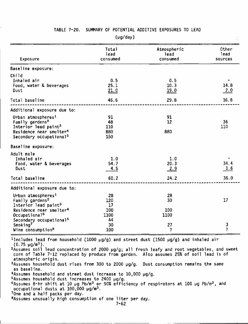
TABLE 7-20. SUMMARY OF POTENTIAL ADDITIVE EXPOSURES TO LEAD (tJg/day)
Exposure
Baseline exposure: Child Inhaled air Food, water & beverages Dust
Total baseline
Additional exposure due to: Urban atmospheresl Family gardens2
Interior lead paint3
Residence near smelter4
Secondary occupational 5
Baseline exposure: Adult male
Inhaled air Food, water & beverages Dust
Total baseline
Additional exposure due to: Urban atmospheresl Family gardens 2
Interior lead paint3
Residence near smelter4
Occupationals Secondary occupational 5
Smoking7
Wine consumption8
Total lead
consumed
0.5 25.1 21.0
46.6
91 48
110 880 150
1.0 54.7 4.5
60.2
28 120
17 100
1100 44 30
100
Atmospheric lead
consumed
0.5 10.3 19.0
29.8
91 12
880
1.0 20.3 2.9
24.2
28 30
100 1100
27 ?
Other lead
sources
14.8 2.0
16.8
36 110
34.4 1.6
36.0
17
3 ?
1 Includes lead from household (1000 tJg/g) and street dust (1500 tJg/g) and inhaled air (0. 75 tJg/m3 ).
2Assumes soil lead concentration of 2000 tJg/g; all fresh leafy and root vegetables, and sweet corn of Table 7-12 replaced by produce from garden. Also assumes 25% of soil lead is of atmospheric origin.
3 Assumes household dust rises from 300 to 2000 tJg/g. Dust consumption remains the same as baseline.
4Assumes household and street dust increase to 10,000 tJg/g. 5 Assumes household dust increases to 2400 tJg/g. 6 Assumes 8-hr shift at 10 tJg Pb/m3 or 90% efficiency of respirators at 100 tJg Pb/m3 , and occupational dusts at 100,000 tJg/m3 •
70ne and a half packs per day. 8Assumes unusually high consumption of one liter per day.
7-62
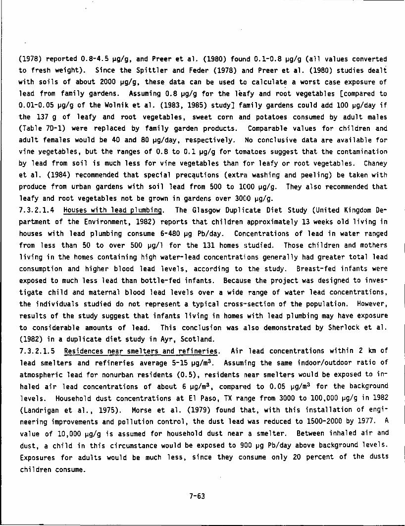
(1978) reported 0.8-4.5 ~g/g, and Preer et al. (1980) found 0.1-0.8 ~g/g (all values converted to fresh weight). Since the Spittler and Feder (1978) and Preer et al. (1980) studies dealt with soils of about 2000 ~g/g, these data can be used to calculate a worst case exposure of lead from family gardens. Assuming 0.8 ~g/g for the leafy and root vegetables [compared to 0.01-0.05 ~g/g of the Wolnik et al. (1983, 1985) study] family gardens could add 100 ~g/day if the 137 g of leafy and root vegetables, sweet corn and potatoes consumed by adult males (Table 7D-1) were replaced by family garden products. Comparable values for children and adult females would be 40 and 80 ~g/day, respectively. No conclusive data are available for vine yegetables, but the ranges of 0.8 to 0.1 ~g/g for tomatoes suggest that the contamination by lead from soil is much less for vine vegetables than for leafy or root vegetables. Chaney et al. (1984) recommended that special prec~utions (extra washing and peeling) be taken with produce from urban gardens with soi 1 lead from 500 to 1000 ~g/g. They also recommended that leafy and root vegetables not be grown in gardens over 3000 ~g/g. 7.3.2.1.4 Houses with lead plumbing. The Glasgow Duplicate Diet Study (United Kingdom Department of the Environment, 1982) reports that children approximately 13 weeks old living in houses with 1 ead p 1 umbi ng consume 6-480 IJg Pb/day. Con cent rations of 1 ead in water ranged from 1 ess than 50 to over 500 IJg/1 for the 131 homes ~;tud-i ed. Those chi 1 dren and mothers living in the homes containing high water-lead concentrati:ons generally had greater total lead consumption and higher blood lead levels, according to the study. Breast-fed infants were exposed to much less lead than bottle-fed infants. Because the project was designed to investigate child and maternal blood lead levels over a wide range of water lead concentrations, the individuals studied do not represent a typical cross··section of the population. However, results of the study suggest that infants living in homes with lead plumbing may have exposure to considerable amounts of lead. This conclusion was i:tlso demonstrated by Sherlock et al. (1982) in a duplicate diet study in Ayr, Scotland. 7.3.2.1.5 Residences near smelters and refineries. Air lead concentrations within 2 km of lead smelters and refineries average 5-15 1Jg/m3 • Assuming the same indoor/outdoor ratio of atmospheric lead for nonurban residents (0.5), residents near smelters would be exposed to inhaled air lead concentrations of about 6 ~g/m3 , compared to 0.05 1Jg/m3 for the background levels. Household dust concentrations at El Paso, TX range from 3000 to 100,000 ~g/g in 1982 (Landrigan et al., 1975). Morse et al. (1979) found that, with this installation of engineering improvements and pollution control, the dust lead was reduced to 1500-2000 by 1977. A value of 10,000 ~g/g is assumed for household dust near a smelter. Between inhaled air and dust, a child in this circumstance would be exposed to 900 IJQ Pb/day above background levels. Exposures for adults would be much less, since they CIJnsume only 20 percent of the dusts
children consume.
7-63
7.3.2.1.6 Occupational exposures. The highest and most prolonged exposures to lead are found among workers in the lead smelting, refining, and manufacturing industries (World Health Organization, 1977). In all work areas, the major route of lead exposure is by inhalation and ingestion of lead-bearing dusts and fumes. Airborne dusts settle out of the air onto food, water, the workers• clothing, and other objects, and may be transferred subsequently to the mouth. Therefore, good housekeeping and good ventilation have a major impact on exposure. It has been found that concentrations might be quite high in one factory and low in another solely because of differences in ventilation, or differences in custodial practices and worker education. The estimate of additional exposure in Table 7-20 is for an 8-hour shift at 100 ~g Pb/m3 • Occupational exposure under these conditions is primarily determined by occupational dust consumed. Even tiny amounts (e.g., 10 mg) of dust containing 100,000 ~g Pb/g dust can account for 1,000 ~g/day exposure.
7.3.2.1.6.1 Lead mining, smelting, and refining. Roy (1977) studied exposures during mining and grinding of lead sulfide at a mill in the Missouri lead belt. Primary smelting operations were 4 km from the mi 11 , hence the influence of the sme 1 ter was be 1 i eved to be negligible. The total airborne lead levels were much greater than the concentrations of respirable lead, indicating a predominance of coarse material.
The greatest potential for high-level exposure exists in the process of lead smelting and refining (World Health Organization, 1977). The most hazardous operations are those in which molten lead and lead alloys are brought to high temperatures, resulting in the vaporization of lead. This is because condensed lead vapor or fume has, to a substantial degree, a small (respirable) particle size range. Although the total air lead concentration may be greater in the vicinity of ore-proportioning bins than it is in the vicinity of a blast furnace in a smelter, the amount of particle mass in the respirable size range may be much greater near the furnace.
A measure of the potential lead exposure in smelters was obtained in a study of three typical installations in Utah (World Health Organization, 1977). Air lead concentrations near all major operations, as determined using personal monitors worn by workers, were found to vary from about 100 to more than 4000 ~g/m3 . Obviously, the hazard to these workers would be extremely serious if it were not ~or the fact that the use of respirators is mandatory in these particular smelters. Maximum airborne lead concentrations of about 300 ~g/m3 were measured in a primary lead-zinc smelter in the United Kingdom (King et al., 1979). These authors found poor correlations between airborne lead and blood lead in the smelter workers, and concluded that a program designed to protect these workers should focus on monitoring of biological parameters rather than environmental concentrations.
Spivey et al. (1979) studied a secondary smelter in southern California that recovers lead mainly from automotive storage batteries. Airborne lead concentrations of 10-4800 ~g/m3
7-64
were measured. The project also involved measurement of biological parameters as well as a survey of symptoms commonly associated with lead exposure; a poor correlation was found between indices of 1 ead absorption and symptom report ii ng. The authors suggested that such factors as educational level, knowledge of possible symptoms, and biological susceptibility may be important factors in influencing symptom reporting. In a second article covering this same study, Brown et al. (1980) reported that smokers working at a smelter had greater blood 1 ead concentrations than nonsmokers. Furthermore, smokers who brought their cigarettes into the workplace had greater blood lead concentrations than those who left their cigarettes elsewhere. It was concluded that direct environmental contamination of the cigarettes by leadcontaining dust may be a major exposure pathway for thes•~ individuals (See Section 7.3.2.3.1).
Secondary lead smelters in Memphis, Tennessee and Salt Lake City, Utah were studied by Baker et al. (1979). The Memphis plant extracted lead principally from automotive batteries, producing 11,500 metric tons of 1 ead in the e 1 even months preceding the measurements. The Salt Lake City plant used scrap to recover 258 metric to1is of lead in the six months preceding the measurements. Airborne concentrations of lead in the Tennessee study exceeded 200 ~g/m3
in some instances, with personal air sampler data ranging from 120 ~g/m3 for a battery wrecker to 350 ~g/m3 for two yard workers. At the Utah plant,, airborne lead levels in the office, lunchroom, and furnace room (furnace not operating) were 60, 90, and 100 ~g/m3 , respectively. When charging the furnace, this value increased to 2650 pg/m3 . Personal samplers yielded concentrations of 17 ~g/m3 for an office worker, 700 ~g/m3 for two welders, and 2660 ~g/m3 for two furnace workers. Some workers in both plants showed clinical manifestations of lead poisoning; a s i gni fi cant corre 1 at ion was found between b 1 ood 1 ead concentrations and symptom reporting.
High levels of atmospheric lead are also reported in foundries in which molten lead is alloyed with other metals. Berg and Zenz (1967) found in one such operation that average concentrations of lead in various work areas were 280 to 600 ~g/m3 . These levels were subsequently reduced to 30 to 40 ~g/m3 with the installation of forced ventilation systems to exhaust the work area atmosphere to the outside.
7.3.2.1.6.2 Welding and cutting of metals containing lead. When metals that contain lead or are protected with a lead-containing coating are heated in the process of welding or cutting, copious quantities of lead in the respirable si:~e range may be emitted. Under conditions of poor ventilation, electric arc welding of zinc silicate-coated steel (containing 4.5
mg Pb/cm2 of coating) produced breathing-zone concentrations of lead reaching 15,000 ~g/m3 ,
far in excess of 450 ~g/m3 , which is the current occupational short-term exposure limit (STEL) in the United States (Pegues, 1960). Under good ventilation conditions, a concentration of 140 ~g/m3 was measured (Tabershaw et al., 1943).
7-65
monitoring, rather than airborne lead monitoring, is a more reliable indicator of potential
exposure problems.
7.3.2.1.6.6 Other occupations. In the rubber products industry and the plastics
industry there are potentially high exposures to lead. The potential hazard of the use of
lead stearate as a stabilizer in the manufacture of polyvinyl chloride was noted in the 1971
Annual Report of the British Chief Inspector of Factories (United Kingdom Department of
Employment, Chief Inspector of Factories 1972). The inspector stated that the number of
reported cases of lead poisoning in the plastics industry was second only to that in the lead
smelting industry. Scarlata et al. (1969) reported other individual cases of exposure. The
source of this prob 1 em is the dust that is generated when the 1 ead stearate is mi 11 ed and
mixed with the polyvinyl chloride and the plasticizer. An encapsulated stabilizer which
greatly reduces the occupational hazard is reported by Fischbein et al. (1982).
Sakurai et al. (1974), in a study of bioindicators of lead exposure, found ambient air
concentrations averaging 58 ~g/m3 in the lead-covering department of a rubber hose manufactu
ring plant. Unfortunately, no ambient air measurements were taken for other departments or
the control group.
The manufacture of cans with leaded seams may expose workers to elevated ambient lead
levels. Bishop (1980) reports airborne lead concentrations of 25-800 ~g/m3 in several can
manufacturing plants in the United Kingdom. Between 23 and 54 percent of the airborne lead
was associated with respirable particles, based on cyclone sampler data.
Firing ranges may be characterized by high airborne lead concentrations, hence instruc
tors who spend considerable amounts of time in such areas may be exposed to lead. For exam
ple, Smith (1976) reports airborne lead concentrations of 30-160 ~g/m3 at a firing range in
the United Kingdom. Anderson et al. (1977) discuss lead poisoning in a 17 year old male
employee of a New York City firing range, where airborne lead concentrations as great as 1000
~g/m3 were measured during sweeping operations. Another report from the same research group
presents time-weighted average exposures of instructors of 45-900 ~g/m3 in three New York City
firing ranges (Fischbein et al., 1979).
Removal of leaded paint from walls and other surfaces in old houses may pose a health
hazard. Feldman (1978) reports an airborne lead concentration of 510 ~g/m3 , after 22 minutes
of sanding an outdoor post coated with paint containing 2.5 mg Pb/cm2 . After only five min
utes of sanding an indoor window sill containing 0.8-0.9 mg Pb/cm2 , the air contained 550
~g/m3 . Homeowners who attempt to remove leaded paint themselves may be at risk of excessive
lead exposure. Garage mechanics may be exposed to excessive lead concentrations. Clausen and
Rastogi (1977) report airborne lead levels of 0.2-35.5 ~g/m3 in ten garages in Denmark; the
greatest concentration was measured in a paint workshop. Used motor oils were found to
contain 1500-3500 ~g Pb/g, whi 1 e one brand of unused gear oi 1 contained 9280 ~g Pb/g. The
7-67
In a study of salvage workers using oxyacetylene cutting torches on lead-painted struc-:tural steel under conditions of good ventilation, breathing-zone concentrations of lead averaged 1200 ~g/m3 and ranged as high as 2400 ~g/m3 (Rieke, 1969). Lead poisoning in workers dismantling a painted bridge has been reported by Graben et al. (1978). Fischbein et al. (1978) discuss the exposure of workers dismantling an elevated subway line in New York City, where the lead content of the paint was as great as 40 percent .. The authors report that one m3 of air can contain 0.05 g lead at the source of emission. Similarly, Grandjean and Kon (1981) report elevated lead exposures of welders and other employees in a Baltimore, Maryland shipyard.
7.3.2.1.6.3 Storage battery industry. At all stages in battery manufacture except for final assembly and finishing, workers are exposed to high air lead concentrations, particularly lead oxide dust. For example, Boscolo et al. (1978) report air lead concentrations of 16-100 ~g/m3 in a battery factory in Italy, while values up to 1315 ~g/m3 have been measured by Richter et al. (1979) in an Israeli battery factory. !Excessive concentrations, as great as 5400 ~g/m3 , have been reported by the World Health Organization (1977).
7.3.2.1.6.4 Printing industry. The use of lead in typesetting machines has declined in recent years (see Table 5-1). Air concentrations of 10 to 30 ~g/m3 have been reported where this technique is used (Parikh et al., 1979). Lead is also a component of inks and dyes used in the printing industry, and consequently can present a hazard to workers handling these products.
7.3.2.1.6.5 Alkyl lead manufacture. Workers involved in the manufacture of alkyl lead compounds are exposed to both inorganic and alkyl lead. Some exposure also occurs at the petroleum refineries where the two compounds are blended into gasoline, but no data are available on these blenders.
The major potential hazard in the manufacture of te:traethyl lead and tetramethyl lead is from skin absorption, which is minimized by the use of protective clothing. Linch et al. (1970) found a correlation between a~ index of organic plus inorganic lead concentrations in a
I
plant and the rate of lead excrettbn in the urine of workers. Significant concentrations of I
organic lead in the urine were found in workers involved with both tetramethyl lead and tetra-ethyl lead; lead levels in the tetramethyl lead workers were slightly higher because the reaction between the organic reagent and 1 ead a 11 oy takes p 1 ace at a somewhat higher temperature and pressure than that employed in tetraethyl lead production.
Cope et al. (1979) used personal air samplers to assess exposures of five alkyl lead workers exposed primarily to tetraethyl lead. Blood c:md urine levels were measured over a six-week period. Alkyl lead levels in air ranged from 1.3 to 1249 ~g/m3 , while inorganic lead varied from 1.3 to 62.6 ~g/m3 . There was no significant correlation between airborne lead (either alkyl or inorganic) and blood or urine levels. The authors concluded that biological
7-66
authors state that absorption through damaged skin could be an important exposure pathway: Other occupations involving risk of lead exposure include stained glass manufacturing and repair, arts and crafts, and soldering and splicing. 7.3.2.1.7 Secondary occupational exposure. Winegar et al. (1977) examined environmental concentrations as well as biological indicators and symptom reporting in workers in a secondary lead smelter near St. Paul, Minnesota. The smelter recovers approximately 9000 metric tons of lead per year from automotive batteries. The lead concentrations in cuff dust from trousers worn by two workers were 60,000 and 600,000 ~g/g. The amount of lead contained in pieces of cloth 1 cm2 cut from the bottoms of trousers worn by the workers ranged from 110 to 3000 ~g, with a median of 410 ~g. In all cases, the trousers were worn under coveralls. Dust samples from 25 households of smelter workers ranged from 120 to 26,000 ~g/g, with a median of 2400 ~g/g. No significant correlations were found between dust lead concentrations and biological indicators, or between symptom reporting and biological indicators. However, there was an increased frequency of certain objective physical signs, possibly due to lead toxicity, with increased b 1 ood 1 ead 1 eve 1. The authors a 1 so concluded that the high dust 1 ead 1 eve 1 s in the workers• homes are most likely due to lead originating in the smelter. 7.3.2.2 Additive Exposure Due to Age, Sex, or Socio-Economic Status 7.3.2.2.1 Quality and quantity of food. The quantity of food consumed per body weight varies greatly with age and somewhat with sex. A 14 kg, 2-year-old child eats and drinks 1.5 kg food and water per day. This is 110 g/kg, or 3 times the consumption of an 80 kg adult male, who ·eats 39 g/kg. Teenage girls consume less than boys and elderly women eat more than men, on a body weight basis.
It is 1 ike ly that poor peop 1 e eat more canned foods and 1 ess frozen and pre-prepared foods. Rural populations probably eat more home-grown foods and meats packed locally. 7.3.2.2.2 Mouthing behavior of children. Children place their mouths on dust-collecting surfaces and lick non-food items with their tongues. This fingersucking and mouthing activity are natural forms of behavior for young children that expose them to some of the highest concentrations of lead in their environment. A single gram of dust may contain ten times more lead than the total diet of the child. 7.3.2.3 Special Habits or Activities. Rabinowitz and Needleman (1984) found a positive correlation between cord blood lead and such maternal exposure factors as use of tobacco, hard alcohol, coffee, and amount of lead in dust. Factors unrelated to cord blood lead levels were amount of dust, tap water lead, air lead, and lead paint. One or more of the above exposure factors may be correlated with other factors, such as race, marital status, schooling, or maternal age. Of these, race and marital status demonstrated a relationship to blood lead. Whereas this study did not attempt to quantify actual exposure, it does identify several activities that are likely to increase human exposure to lead.
7-68
7.3.2.3.1 Smoking. Lead is also present in tobacco. The World Health Organization (1977) estimates a lead content of 2.5-12.2 ~g per cigarette; roughly two to six percent of this lead may be inhaled by the smoker. The National Academy of Sciences (1980) has used these data to conclude that a typical urban resident who smokes 30 cigarettes per day may inhale roughly equal amounts of lead from smoking and from breathing urban air. 7.3.2.3.2 A.lcoholic beverages. Reports of lead in European wines (Olsen et al., 1981; Boudene et al., 1975; Zurlo and Griffini, 1973) show concentrations averaging 100-200 ~g/1 and ranging as high as 300 ~g/1. Measurements of lead in domestic wines were in the range of 100-300 ~g/1 for California wines with and without lead foil caps. The U.S. Food and Drug Administration (1983) found 30 ~g/1 in the 1982 Market Basket Survey. The average daily consumption of table wine by a 25- to 30-year-old adult in the U.S. is about 12 g. Even with a lead content of 0.1 ~g/g, which is ten times higher than drinking water, wine does not appear to represent a significant potential exposure to lead. At one liter per day, however, lead consumption in wine would be greater than the total baseline consumption.
McDonald (1981) points out that older wines with lE!ad foil caps may represent a hazard, especially if they have been damaged or corroded. Wai et al. (1979) found that the lead content of wine rose from 200 to 1200 ~g/1 when the wine was allowed to pass over the thin ring of residue left by the corroded lead foil cap. Newer wines (1971 and later) use other means of sealing. If a lead foil is u~ed, the foil is tin-plated and coated with an acid-resistant substance. Lead concentrations in beer are generally lower than those in wine; Thalacker (1980) reports a maximum concentration of 80 ~g/1 in several brands of German beer. The U.S. Food and Drug Administration (1983) found 13 ~g/1 in beer consumed by Americans (Table 70-1). 7.3.2.3.3 Pica. Pica is the compulsive, habitual consumption of non-food items, such as paint chips and soil. This habit can present a significant lead exposure to the afflicted person, especially to children, who are more apt to have pica. There are very little data on the amounts of paint or soi 1 eaten by chi 1 dren with varying degrees of pi ca. Exposure can only be expressed on a unit basis. Billick and Gray (1978) report lead concentrations of 1000 to 5000 ~g/cm2 surface area in lead-based paint pigments. To a child with pica, a single chip of paint can represent greater exposure than any other source of lead. A gram of urban soil
may have 150 to 2000 ~g lead. 7.3.2.3.4 Glazed earthenware vessels. Another potential source of dietary lead poisoning is the use of inadequately glazed earthenware vessels for food storage and cooking. An example of this danger involved the severe poisoning of a family in Idaho that resulted from drinking orange juice that had been stored in an earthenware piitcher (Block, 1969). Similar cases,
sometimes including fatalities, have involved other relatively acidic beverages such as fruit juices and soft drinks, and have been documented by other workers (Klein et al., 1970; Harris and Elsen, 1967). Because of these incidents, the U.S. Food and Drug Administration (1980)
7-69
has established a maximum permissible concentration of 2.5-7 ~g Pb/ml in solution after leaching with 4 percent acetic acid in the kitchenware for 24 hours, depending on the shape and volume of the vessel.
Inadequately glazed pottery manufactured in other countries continues to pose a significant health hazard. For example, Spielholtz and Kaplan (1980) report 24-hour acetic acid-1 eached 1 ead concentrations as great as 4400 ~gig in Mexican pottery. The 1 eached 1 ead decreased with exposure time, and after several days appears to asymptotically approach a value which may be as high as 600 ~g/g. These investigators have also measured excessive lead concentrations leached into acidic foods cooked for two hours in the same pottery. Similarly, Acra et al. (1981) report that 85 percent of 275 earthenware vessels produced in primitive Lebanese potteries had lead concentrations above the 7 ~g/g 1 imit set by the U .. s. FDA. However, only 9 percent of 75 vessels produced in a modern Beirut pottery exceeded the limit. Cubbon et al. (1981) have examined properly glazed ceramic plates in the United Kingdom, and have found a decrease in leached lead with exposure time down to very low levels. The authors state that earthenware satisfying the 7 ~gig limit can contribute about 3 ~g/day to the dietary intake of the average consumer. 7.3.2.3.5 Hobbies. There are a few hobbies where the ~se of metallic lead or solder may present a hazard to the user. Examples are electronics projects, stained glass window construction, and firing range ammunition recovery. There are no reports in which the exposure to lead has been quantified during these activities.
7.3.3 Summary of Additive Exposure Factors Beyond the baseline level of human exposure, additional amounts of lead consumption are
largely a matter of individual choice or circumstance. Many of these additional exposures arise from the ingestion of atmospheric lead in dust. In one or more ways probably 90 percent of the American population are exposed to lead at greater than baseline levels. A summary of the most common additive exposure factors appears in Table 7-20. In some cases, the additive exposure can be fully quantified and the amount of lead consumed can be added to the baseline consumption. These may be continuous (urban residence), or seasonal (family gardening) exposures. Some factors can be quantified only on a unit basis because of wide ranges in exposure duration or concentration. For example, factors affecting occupational exposure are air lead concentrations (10-4000 ~g/m3 ), use and efficiency of respirators, length of time of exposure, dust control techniques, and worker training in occupational hygiene.
7-70
7.4 SUMMARY Ambient airborne lead concentrations have shown no marked trend from 1965 to 1977. Over
the past five years, however, distinct decreases have occurred. The mean air concentration has dropped from 1.3 ~g/m3 in 1977 to 0.40 ~g/m3 in 1984. This decrease reflects the lower lead emissions from mobile sources in recent years. Airborne size distribution data indicate that most of the airborne lead mass is found in submicron particles.
Atmospheric lead is deposited on vegetation and soil surfaces, entering the human food chain through contamination of grains and 1 eafy vegetab 1 es, of pasture 1 ands, and of soi 1
moisture taken up by all crops. Lead contamination of' drinking water supplies appears to originate mostly from within the distribution system.
Most people receive the largest portion of their lead intake through foods. Unprocessed foods such as fresh fruits and vegetables receive lead by atmospheric deposition as well as uptake from soil; crops grown near heavily traveled roads generally have greater lead levels than those grown at greater distances from traffic. For many crops the edible internal portions of the plant (e.g., kernels of corn and wheat) have considerably less lead than the outer, more exposed parts, such as stems, leaves, and husks. Atmospheric lead accounts for about 45 percent of the tota 1 adult 1 ead exposure, and 65 percent of the exposure for chi 1 dren. Processed foods have greater 1 ead concentrations than unprocessed foods, due to lead inadvertently added during processing. Foods-packa~1ed in soldered cans have much greater lead levels than foods packaged in other types of containers. About 35 percent of the b~seline adult exposure to lead results from the use of solder lead in packaging food and distributing drinking water.
Significant amounts of lead in drinking water can r·esult from contamination at the water source and from the use of lead solder in the water distribution system. Atmospheric deposition has been shown to increase lead in rivers, reservoirs, and other sources of drinking water; in some areas, however, lead pipes pose a more SE!rious problem. Soft, acidic water in homes with lead plumbing may have excessive lead concentrations. Besides direct consumption of the water, exposure may occur when vegetables and other foods are cooked in water containing lead.
All of the categories of potential lead exposure discussed above may influence or be influenced by dust and soil. For example, lead in street dust is derived primarily from vehicular emissions, while in house dust may originate from nearby stationary or mobile sources. Food and water may include lead adsorbed from soil as WE!ll as deposited atmospheric material. Flaking lead-based paint has been shown to increase soil lead levels. Natural concentrations of lead in soil average approximately 15 ~g/g; this natu1·al lead, in addition to anthropogenic lead emissions, influences human exposure.
7-71
"------------ ---
Americans living in rural areas away from sources of atmospheric lead consume 35-55 ~g Pb/day from all sources. Circumstances that can increase this exposure are urban residence (25-100 ~g/day), family garden on high-lead soil (40-100 ~g/day), houses with interior leadbased paint (20-85 ~g/day), and residence near a smelter (400-900 ~g/day). Occupational settings, smoking, and wine consumption also can increase consumption of lead according to the degree of exposure.
A number of manmade materials are known to contain lead, the most important being paint and plastics. Lead-based interior paints, although no longer used, are a major problem in older homes. Small children who ingest paint flakes can receive excessive lead exposure. Incineration of plastics may emit large amounts of lead into the atmosphere. Because of the increasing use of plastics, this source is likely to become more important. Other manmade materials containing lead include colored dyes, cosmetic products, candle wicks, and products made of pewter and silver.
The greatest occupational exposures are found in the lead smelting and refining industries. Excessive airborne lead concentrations and dust lead levels are occasionally found in primary and secondary smelters; smaller exposures are associated with mining and processing of the lead ores. Welding and cutting of metal surfaces coated with lead-based paint may also result in excessive exposure. Other occupations with potentially high exposures to lead include the manufacture of lead storage batteries, printing equipment, alkyl lead, rubber products, plastics, and cans; individuals removing lead paint from walls and those who work in indoor firing ranges may also be exposed to lead.
Environmental contamination by lead should be measured in terms of the total amount of lead emitted to the biosphere. American industry contributes several hundred thousand tons of lead to the environment each year: 55,000 tons from petroleum additives, 50,000 tons from ammunition, 45,000 tons in glass and ceramic products, 16,000 tons in paint pigments, 8,000 tons
in food can solder, and untold thousands of tons of captured wastes during smelting, refining, and coal combustion. These are uses of lead that are generally not recoverable, thus they represent a permanent contamination of the human or natura 1 environment. A 1 though much of this lead is confined to municipal and industrial waste dumps, a large amount is emitted to the atmosphere, waterways, and soil, to become a part of the biosphere.
Potential human exposure can be expressed as the concentrations of lead in these environmental components (air, dust, food, and water) that interface with man. It appears that, with the exception of extraordinary cases of exposure, about 80 to 100 ~g of 1 ead are consumed
daily by each American, including additional exposure above baseline.
7-72
7.5 REFERENCES
Acra, A.; Dajani, R.; Raffoul, Z.; Karahagopian, Y. (1981) Lead-glazed pottery: a potential health hazard in the Middle East. Lancet 1(8217): 433-434.
Agrawal, Y. K.; Patel, M. P.; Merh, S. S. (1981) Lead in soils and plants: its relationship to traffic volume and proximity to highway (Lalbag, Baroda City). Int. J. Environ. Stud. 16: 222-224.
Akland, G. G. (1976) Air quality data for metals, 1970 through 1974, from the National Air Surveillance Networks. Research Triangle Park, NC: ll. S. Environmental Protection Agency, Office of Research and Development; EPA report no. EPA 600/ 4-76-041. Available from: NTIS, Springfield, VA; PB-260905.
Anderson, K. E.; Fishbein, A.; Kestenbaum, D.; Sassa, S.; Alvares, A. P.; Kappas, A. (1977) Plumbism from airborne lead in a firing range: an unusual exposure to a toxic heavy metal. Am. J. Med. 63: 306-312.
Andresen, A. M.; Johnson, A. H.; Siccama, T. G. (1980) LE!Vels of lead, copper, and zinc in the forest floor in the northeastern United States. J. Environ. Qual. 9: 293-296.
Angle, C. R.; Mcintire, M. S. (1979) Environmental leild and children: the Omaha study. J. Toxicol. Environ. Health 5: 855-870.
Bailey, R. J.; Russell, P. F. (1981) Predicting drinkin~1 water lead levels. Environ. Technol. Lett. 2: 57-66.
Baker, E. L., Jr.; Landrigan, P. J.; Barbour, A. G.; Co>:, D. H.; Folland, D. S.; Ligo, R. N.; Throckmorton, J. (1979) Occupational lead poisoning in the United States: clinical and biochemical findings related to blood lead levels. E1r. J. Ind. Med. 36: 314-322.
Barltrop, D.; Strehlow, C. D. (1976) Westway nursery testing project: report to Greater London Council. London, United Kingdom: St. Mary• s Hospital Medical School, Pediatric unit. Available for inspection at: U. S. Environmental Protection Agency, Environmental Criteria and Assessment Office, Research Triangle Park, NC.
Barry, P. S. 1.; Connolly, R. (1981) Lead concentrations in mediaeval bones. Int. Arch. Occup. Environ. Health 48: 173-177.
Beloian, A.; McDowell, M. (1981) Estimates of lead intakes among children up to 5 years of age, 1973-1978 and 1980. Washington, DC: U. S. Food and Drug Administration, Bureau of Foods; Division of Nutrition final internal report. Available from: U. S. Food and Drug Administration, Bureau of Foods, Washington, DC.
Berg, B. A.; Zenz, C. (1967) Environmental and clinical control of lead exposure in a nonferrous foundry. J. Am. Ind. Hyg. Assoc. 28: 175-179;.
Berk, J. V.; Young, R. A.; Brown, S. R.; Hollowell, C. D. (1981) Impact of energy-conserving retrofits on indoor air quality in residential housing. Presented at: 74th annual meeting of the Air Pollution Control Association; June; Philadelphia, PA. Pittsburgh, PA: Air Pollution Control Association; paper no. 81-22.1.
7-73
Billick, I. H.; Gray, V. E. (1978) Lead based paint poisoning research: review and evaluation 1971-1977. Washington, DC: U. S. Department of Housing and Urban Development, Office of Policy Development and Research; HUD report no. HUD 0000809. Available from: NTIS, Springfield, VA; PB80-136849.
Bishop, J. R. (1980) Atmospheric lead and the related blood-levels of workers in high-speed can-making. Am. Ind. Hyg. Assoc. J. 41: 61-63.
Block, J. L. (1969) The accident that saved five lives. Good Housekeeping 169: 60-70.
Boscolo, P.; Porcelli, G.; Cecchetti, G.; Salimei, E.; Iannaccone, A. (1978) Urinary kallikrein activity of workers exposed to lead. Br. J. Ind. Med. 35: 226-229.
Boudene, C.; Arsac, F.; Meininger, J. (1975) Etude des taux de plomb dans l'air et dans la population en France [Study of the lead levels in the air and in the population of France]. In: International symposium on environmental lead research; May; Dubrovnik, Yugoslavia. Arh. Hig. Rada Toksikol. Suppl. 26: 179-189.
Boyer, K. W.; Johnson, R. D. (1982) Levels of lead, cadmium, and zinc in selected canned foods (1980/1981). J. Food Saf. 4: 207-222.
Brown, C. P.; Spivey, G. H.; Valentine, J. L.; Browdy, B. L. (1980) Cigarette smoking and lead levels in occupationally exposed lead workers. J. Toxicol. Environ. Health 6: 877-883.
Brunekreef, B. (1983) The relationship between air lead and blood lead in children: a critical review. Wegeningen, The Netherlands: Gezondsheidsleer. (Gezondsheidsleer verslagen, rapporten, scripties en nota's: 167).
Cannon, H. L.; Bowles, J. M. (1962) Contamination of vegetation by tetraethyl lead. Science (Washington, DC) 137: 765-766.
Capar, S. G. (1978) Changes in lead concentration of foods stored in their opened cans. J. Food Saf. 1: 241-245.
Cawse, P. A. (1974) A survey of atmospheric trace elements in the U.K. (1972-73). Harwell, United Kingdom: Atomic Energy Research Establishment, Environmental & Medical Sciences Division. Available from: NTIS, Sp.ringfield, VA; PB81-126443.
Chaney, R. L.; Sterrett, S. B.; Mielke, H. W. (1984) The potential for heavy metal exposure from urban gardens and soils. In: Preer, J. R., ed. Proceedings, symposium on heavy metals in urban gardens. Washington, DC: District of Columbia Extension Service, pp. 37-84.
Chow, T. J. (1978) Lead in natural waters. In: Nriagu, J. 0., ed. The biogeochemistry of lead in the environment; part A. ecological cycles. New York, NY: Elsevier/North-Holland Biomedical Press; pp. 185-218. (Topics in environmental health: v. lA).
Chow, T. J.; Earl, J. L.; Snyder, C. B. (1972) Lead aerosol baseline: concentration at White Mountain and Laguna Mountain, California. Science (Washington, DC) 178: 401-402.
Clark, C. S.; Bornschein, R. L.; Succop, P.; Que Hee, S. S.; Hammond, P. B.; Peace, B. (1985) Condition and type of housing as an indicator of potential environmental lead exposure and pediatric blood lead levels. Environ. Res. 38: 46-53.
7-74
Clausen, J.; Rastogi, S. C. (1977) Heavy metal pollution among autoworkers: I. lead. Br. J .. Ind. Med. 34: 208-215 .
. Code of Federal Regulations. (1984) National primary and secondary ambient air quality standards. C. F. R. 40: § 50. ·
Cohen, A. F.; Cohen, B. L. (1980) Protection from being indoors against inhalation of suspended particulate matter of outdoor origin. Atmos. Environ. 14: 183-184.
Cope, R. F.; Pancamo, B. P.; Rinehart, W. E.; Ter Haar, G. L. (1979) Personnel monitoring for tetraalkyl lead in the workplace. Am. Ind. Hyg. Asso,c. J. 40: 372-379.
Crump, D. R.; Barlow, P. J. (1982) Factors controlling the lead content of a pasture grass. Environ. Pollut. Ser. B 3: 181-192.
Cubbon, R. C. P.; Roberts, W.; Marshall, K. (1981) The extraction of lead from ceramic tableware by foodstuffs. Trans. J. Br. Ceram. Soc. 80: 12:5-127.
Davidson, C. I.; Osborn, J. F. (1985) The sizes of airborne trace metal-containing particles. In: Nriagu, J. 0.; Davidson, C. I., eds. Toxic metals in the air. New York, NY: Wiley. _
·Davidson, C. I.; Goold, W. D.; Nasta, M. A.; Reilly, M. T. (1981a) Airborne size distributions of trace elements in an industrial section of P·ittsburgh. Presented at: 74th annual meeting of the Air Pollution Control Association; June; Philadelphia, PA. Pittsburgh, PA: Air Pollution Control Association; paper no. 81-28.6.
Davidson, C. I.; Grimm, T. C.; Nasta, M. A. (1981b)" Airborne lead and other elements derived from local fires in the Himalayas. Science (Washington, DC) 214: 1344-1346. .
Davidson, C. I.; Chu, L.; Grimm, T. C.; Nasta, M. A.; Qamoos, M. P. (1981c) Wet and dry deposition of trace elements onto the Greenland ice sheet. Atmos. Environ. 15: 1429-1437.
Davidson, C. I.; Miller, J. M.; Pleskow, M. A. (1982) The influence of surface structure on predicted particle dry deposition to natural grass canopies. Water Air Soil Pollut. 18: 25-43.
Davies, B. E.; Elwood, P. C.; Gallacher, J.; Ginnerver, R. C. (1985) The relationships between heavy metals in garden soils and house dusts in an old lead mining area of North Wales, Great Britain. Environ. Pollut. Ser. B 9: 255-266.
Day, J. P.; Hart, M.; Robinson, M. S. (1975) Lead in urban street dust. Nature (London) 253: 343-345.
Day, J. P.; Fergusson, J. E.; Chee, T. M. (1979) Solubility and potential toxicity of lead in urban street dust. Bull. Environ. Contam. Toxicol. 23: 497-502.
Dedolph, R.; Ter Haar, G.; Holtzman, R.; Lucas, H., Jr. (1970) Sources of lead in perennial ryegrass and radishes. In: Symposium on air conse~rvation and lead, division of water, air, and waste chemistry, 157th national meeting, American Chemical Society; April 1969; Minneapolis, MN. Environ. Sci. Technol. 4: 217-223.
Dong, A.; Chesters, G.; Simsiman, G. V. (1984) Metal composition of soil, sediments, and urban dust and dirt samples from the Menomonee River watershed, Wisconsin, U. S.A. Water Air Soil Pollut. 22: 257-275.
7-75
Duce, R. A.; Hoffman, G. L.; Zoller, W. H. (1975) Atmospheric trace metals at remote northern and southern hemisphere sites: pollution or natural? Science (Washington, DC) 187: 59-61.
Duce, R. A.; Ray, B. J.; Hoffman, G. L.; Walsh, P. R. (1976) Trace metal concentration as a function of particle size in marine aerosols from Bermuda. Geophys. Res. Lett. 3: 339-346.
Duggan, M. J.; Inskip, M. J.; Rundle, S. A.; Moorcroft, J. S. (1985) Lead in playground dust and on the hands of schoolchildren. Sci. Total Environ. 44: 65-79.
Durum, W. H.; Hem, J. D.; Heidel, S. G. (1971) Reconnaissance of selected minor elements in surface waters of the United States, October 1970. Washington, DC: U. S. Department of Interior, Geological Survey; USGS circular no. 643.
Dzubay, T. G.; Hines, L. E.; Stevens, R. K. (1976) Particle bounce errors in cascade impactors. Atmos. Environ. 10: 229-234.
Dzubay, T. G.; Stevens, R. K.; Haagenson, P. L. (1984) Composition and origins of aerosol at a forested mountain in Soviet Georgia. Environ. Sci. Technol. 18: 873-883.
Eisenreich, S. J.; Metzer, N. A.; Urban, N. R.; Robbins, J. A. (1986) Response of atmospheric lead to decreased use of lead in gasoline. Environ. Sci. Technol. 20: 171-174.
El-Shobokshy, M. S. (1984) A preliminary analysis of the inhalable particulate lead in the ambient atmosphere of the city of Riyadh, Saudi Arabia. Atmos. Environ. 18: 2125-2130.
Elias, R. W.; Davidson, C. (1980) Mechanisms of trace element deposition from the free atmosphere to surfaces in a remote High Sierra canyon. Atmos. Environ. 14: 1427-1432.
Eliasl R. W.; Hirao, Y.; Patterson, C. C. (1982) The circumvention of the natural biopurificat ion of ca 1 ci um a 1 ong nutrient pathways by atmospheric inputs of industria 1 1 ead. Geochim. Cosmochim. Acta 46: 2561-2580.
Ericson, J. E.; Shirahata, H.; Patterson, C. C. (1979) Skeletal concentrations of lead in ancient Peruvians. N. Engl. J. Med. 300: 946-951.
Facchetti, S.; Geiss, F. (1982) Isotopic lead experiment: status report. Luxembourg: Commission of the European Communities; publication no. EUR 8352 EN.
Federal Register. (1979). Lead in food: advance notice of proposed rulemaking: request for data. (August 31) 44: 51233-51242.
Feldman, R. G. (1978) Urban lead mining: lead intoxication among deleaders. N. Engl. J. Med. 298: 1143-1145.
Fergusson, J. E.; Ryan, D. E. (1984) The elemental composition of street dust from large and small urban areas related to city type, source and particle size. Sci. Total Environ. 34: 101-116.
Fischbein, A.; Daum, S. M.; Davidow, B.; Slavin, G.; Alvares, A. P.; Sassa, S.; Anderson, K. E.; Kappas, A.; Eisinger, J.; Blumberg, W. E.; Winicow, E. H.; Selikoff, I. J. (1978) Lead hazard among ironworkers dismantling lead-painted elevated subway line in New York City. N. Y. State J. Med. 78: 1250-1259.
7-76
Fischbein, A.; Rice, C.; Sarkozi, L.; Kon, S. H.; Petr·occi, M.; Selikoff, I. J. (1979) Ex-:posure to lead in firing ranges. J. Am. Med. Assoc. 241: 1141-1144.
Fischbein, A.; Thornton, J. C.; Berube, L.; Villa, F.; Selikoff, I. J. (1982) Lead exposure reduction in workers using stabilizers in PVC manufacturing: the effect of a new encapsulated stabilizer. Am. Ind. Hyg. Assoc. J. 43: 652-6~i5.
Franz, D. A.; Hadley, W. M. (1981) Lead in Albuquerque street dirt and the effect of curb paint. Bull. Environ. Contam. Toxicol. 27: 353-358.
Frefry, J. H.; Metz, S.; Trocine, R. P. (1985) A decline in lead transport by the Mississippi River. Science (Washington, DC) 230: 439-441.
Friedlander, S. K. (1977) Smoke, dust and haze: fundamEmtals of aerosol behavior. New York, NY: John Wiley & Sons; pp. 1-23.
Garcia-Miragaya, J.; Castro, S.; Paolini, J. (1981) Lead and zinc levels and chemical fractionation in road-side soils of Caracas, Venezuela. Water Air Soil Pollut. 15: 285-297.
Garty, J.; Fuchs, C. (1982) Heavy metals in the lichen Ramal ina duriaei transplanted in biomonitoring stations. Water Air Soil Pollut. 17: 175-183.
General Electric Company. (1972) Indoor-outdoor carbor1 monoxide pollution study. Research Triangle Park, NC: U. S. Environmental Protection Agency, National Environmental Research Center, Quality Assurance and Environmental Monitoring Laboratory; EPA report no. EPA-R4-73-020. Available from: NTIS, Springfield, VA.; PB-220428.
-Geomet, Inc. (1981) Comparison of indoor and outdoor ctir quality. Palo Alto, CA: Electric
Power Research Institute; EPRI report no. EA-1733. A.vailable from: NTIS, Springfield, VA; EPRI-EA-1733.
Gibson, M. J.; Farmer, J. G. (1984) Chemical partitioning of trace metal contaminants in urban street dirt. Sci. Total Environ. 33: 49-57.
Gilbert, C.; Tuthill, R. W.; Calabrese, E. J.; Peters, H. A. (1979) A comparison of lead hazards in the housing environment of lead poisoned children versus nonpoisoned controls. J. Environ. Sci. Health Part #A 14: 145-168.
Graben, N.; Wilhelms, W.; Kloppel, H. A.; Tiepermann, R. V.; Doss, M. (1978) Acute heavy lead poisoning in welders. J. Clin. Chem. Clin. Biochem. 16: 63.
Graham, D. L.; Kalman, S. M. (1974) Lead in forage gr.ass from a suburban area in northern California. Environ. Pollut. 7: 209-215.
Grandjean, P.; Kon, S. H. (1981) Lead exposure of welders and bystanders in a ship repair yard. Am. J. Ind. Med. 2: 65-70.
Grandjean, P.; Nielsen, 0. V.; Shapiro, I. M. (1979) Lead retention in ancient Nubian and contemporary populations. J. Environ. Pathol. Toxicol. 2: 781-787.
Gross, S. B. (1981) Human oral and inhalation exposures to lead: summary of Kehoe balance experiments. J. Toxicol. Environ. Health 8: 333-377.
7-77
Gulson, B. L.; Tiller, K. G.; Mizen, K. J.; Merry, R. M. (1981) Use of lead isotopes in soils to identify the source of lead contamination near Adelaide, South Australia. Environ~ Sci. Technol. 15: 691-696.
Halpern, M. (1978) Indoor/outdoor air pollution exposure continuity relationships. J. Air Pollut. Control Assoc. 28: 689-691.
Hardy, H. L.; Chamberlin, R. I.; Maloof, C. C.; Boylen, G. W., Jr.; Howell, M. C. (1971) Lead as an environmental poison. Clin. Pharmacal. Ther. 12: 982-1002.
Harris, M. R. (1981) Distribution of lead in winter wheat plants grown in the vicinity of a lead smelter. Environ. Technol. Lett. 2: 243-252.
Harris, R. W.; Elsen, W. R. (1967) Ceramic glaze as a source of lead poisoning. J. Am. Med. Assoc. 202: 208-210.
Harrison, R. M. (1979) Toxic metals in street and household dusts. Sci. Total Environ. 11: 89-97.
Hayashi, M.; Ito, 0.; Ohira, S.; Akuzawa, Y. (1982) Transfer of lead and cadmium from cow milk to butter. Bull. Environ. Contam. Toxicol. 29: 658-664.
Heidam, N. Z. (1983) Studies of the aerosol in the Greenland atmosphere; SAGA I: results 1979-1980. Roskilde, Denmark: Riso National Laboratory; National Agency of Environmental Protection report no. MST-LUFT-A--73. ~vailable from: NTIS, Springfield, VA; DE84-751004.
Ho, Y. B. (1979) Lead contamination in street dust in Hong Kong. Bull. Environ. Contam. Toxicol. 21: 639-642.
Hudson, J. L~; Stukel, J. J.; Solomon, R. L. (1975) Measurement of the ambient lead concentration in the vicinity of Urbana-Champaign, Illinois. Atmos. Environ. 9: 1000-1006.
Jelinek, C. F. (1982) Levels of lead in the United States food supply. J. Assoc. Off. Anal. Chern. 65: 942-946.
Kehoe, R. A. (1961) The metabolism of lead in man in health and disease: the normal metabolism of lead. (The Harben lectures, 1960). J. R. Inst. Public Health Hyg. 24: 81-97.
Kerin, Z. (1975) Relationship between lead content in the soil and in the plants contaminated by industrial emissions of lead aerosols. In: Hutchinson, T. C.; Epstein, S.; Page, A. L.; Van Loon, J.; Davey, T., eds. International conference on heavy metals in the environment: symposium proceedings, volume II, part 2; October; Toronto, ON, Canada. Toronto, ON, Canada: University of Toronto, Institute for Environmental Studies; pp. 487-502.
King, E.; Conchie, A.; Hiett, D.; Milligan, B. (1979) Industrial lead absorption. Ann. Occup. Hyg. 22: 213-239.
Kirkpatrick, D. C.; Coffin, D. E. (1974) The trace metal content of representative Canadian diets in 1970 and 1971. J. Inst. Can. Sci. Technol. Aliment. 7: 56-58.
Kirkpatrick, D. C.; Coffin, D. E. (1977) The trace metal content of a representative Canadian diet in 1972. Can. J. Public Health 68: 162-164.
7-78
Kirkpatrick, D. C.; Conacher, H. B. S.; Meranger, J. C.; llabeka, R.; Collins, B.; McKenzie, A. D.; Lacroix, G. M. A.; Savary, G. (1980) The trace e'lement content of Canadian baby foods and estimation of trace element intake by infants. Can. Inst. Food Sci. Technol. J. 13: 154-161.
Klein, M.; Namer, R.; Harpur, E.; Corbin, R. (1970) Earthenware containers as a source of fatal lead poisoning: case study and public-health considerations. N. Engl. J. Med. 283: 669-672.
Kneip, T. J. (1978) Concentrations of lead and cadmium in garden vegetables grown in New York City. Presented at: Toxic-element studies: food Cl"ops and urban vegetable gardens. A symposium sponsored by the New York City Gardening Program; June; The Bronx, NY. Ithaca, NY: Cornell University Cooperative Extension; pp. 1-:22.
Kretzschmar, J. G.; Delespaul, I.; De Rijck, T. (1980) Heavy metal levels in Belgium: a five year survey. Sci. Total Environ. 14: 85-97.
Landrigan, P. J.; Gehlbach, S. H.; Rosenblum, B. F.; Shoults, J. M.; Candelaria, R. M.; Barthel, W. F.; Liddle, J. A.; Smrek, A. L.; Staehling, N. W.; Sanders, J. F. (1975) Epidemic lead absorption near an ore smelter: the r·ole of particulate lead. N. Engl. J. Med. 292: 123-129.
Lau, W. M.; Wong, H. M. (1982) An ecological survey of lead contents in roadside dusts and soils in Hong Kong. Environ. Res. 28: 39-54.
Laurer, G. R.; Albert, R. E.; Kneip, T. J.; Pasternack, B .. ; Strehlow, C.; Nelson, N.; Kent, F. S. (1973) The distribution of lead paint in New .York City tenement buildings. Am. J. Public Health 63: 163-168.
Laxen, D. P. H.; Lindsay, F.; Fulton, M.; Raab, G. (1985) The importance of lead-in-air as an exposure source - an assessment for children in Edinburgh. Environ. Technol. Lett. 6: 107-114.
Lee, R. E., Jr.; Goranson, S. S.; Enrione, R. E.; Morgan, G. B. (1972) National air surveillance cascade impactor network. II. Size distribut·ion measurements of trace metal components. Environ. Sci. Technol. 6: 1025-1030.
Linch, A. L.; Wiest, E. G.; Carter, M. D. (1970) Evaluiltion of tetraalkyl lead exposure by personnel monitor surveys. J. Am. Ind. Hyg. Assoc. 3"1: 170-179.
Linton, R. W.; Natusch, D. F. S.; Solomon, R. L.; Evans, C. A., Jr. (1980) Physicochemical characterization of lead in urban dusts. A microanalytical approach to lead tracing. Environ. Sci. Technol. 14: 159-164.
Little, P.; Martin, M. H. (1972) A survey of zinc, lead and cadmium in soil and natural vegetation around a smelting complex. Environ. Pollut. 3: 241-254.
Little, P.; Wiffen, R. D. (1978) Emission and depositi1ln of lead from motor exhausts--II. airborne concentration, particle size and deposit1ion of lead near motorways. Atmos. Environ. 12: 1331-1341.
Maenhaut, W.; Zoller, W. H.; Duce, R. A.; Hoffman, G. L. (1979) Concentration and size distribution of particulate trace elements in the south polrar atmosphere. J. Geophys. Res. 84: 2421-2431.
7-79
Mahaffey, K. R. (1978) Environmental exposure to lead. In: Nriagu, J. 0., ed. The biogeo.chemistry of lead in the environment; part B. biological effects. Amsterdam, The Netherlands: Elsevier/North-Holland Biomedical Press; pp. 1-36. (Topics in environmental health: v. 1B).
Masralla, M. M.; Ali, E. A. (1985) Lead accumulation in edible portions of crops gown near Egyptian traffic roads. Agric. Ecosys. Environ. 13: 73-82.
McDonald, J. (1981) The lead contamination problem with emphasis on the lead content of wine. Am. J. Enol. Vitic. 32: 219-222.
McKeague, J. A.; Wolynetz, M. S. (1980) Background levels of minor elements in some Canadian soils. Geoderma 24: 299-307.
Mclean, R. 0.; Shields, B. (1977) A study of factors causing changes in the lead levels of crops growing beside roadways. Environ. Pollut. 14: 267-273.
Meranger, J. C.; Khan, T. R.; Vairo, C.; Jackson, R.; Li, W. C. (1983) Lake water acidity and the quality of pumped cottage water in selected areas of Northern Ontario. Int. J. Environ. Anal. Chem. 15: 185-212.
Merry, R. H.; Tiller, K. G.; De Vries, M. P. C.; Cartwright, B. (1981) Contamination of wheat crops around a lead-zinc smelter. Environ. Pollut. 2: 37-48.
Mielke, H.; Blake, B.; Burroughs, S.; Hassinger, N. (1984) Urban lead levels in Minneapolis: the case of the Hmong children. Environ. Res. 34: 64-76.
Moore, M. R. (1977) Lead in drinking water in soft water areas--health hazards. Sci. Total Environ. 7: 109-115.
Moschandreas, D. J. (1981) Exposure to pollutants and daily time budgets of people. Bull. N. Y. Acad. Med. 57: 845-859.
Motto, H. L.; Daines, R. H.; Chilko, D. M.; Motto, C. K. (1970) Lead in soils and plants: its relationship to traffic volume and proximity to highways. Environ. Sci. Technol. 4: 231-238.
Murozumi, M.; Chow, T. J.; Patterson, C. (1969) Chemical concentrations of pollutant lead aerosols, terrestrial dusts and sea salts in Greenland and Antarctic snow strata. Geochim. Cosmochim. Acta 33: 1247-1294.
Nasralla, M. M.; Ali, E. A. (1985) Lead accumulation in edible portions of crops grown near Egyptian traffic roads. Agric. Ecosys. Environ. 13: 73-82.
National Academy of Sciences; National Research Council. (1976) Recommendations for the prevention of lead poisoning in children. Washington, DC: National Academy of Sciences. Available from: NTIS, Springfield, VA; PB-257645.
National Academy of Sciences, Committee on Lead in the Human Environment. (1980) Lead in the human environment. Washington, DC: National Academy of Sciences.
National Air Pollution Surveillance Reports (NAPS). (1971-1976) Air Pollution Control Directorate, Ottawa, Canada, report series EPS-5-AP.
7-80
·----
National Food Processors Association; Can Manufacturers Institute, Inc. (1982) Comprehensive supplementary report covering further research, February 1980 through May 1982, on foodborne lead in the diet of children. Available from: U. S. Department of Health and Human Services, Washington, DC; FDA docket no. 79N-0200.
NEDS, National Emissions Data System [data base]. (1982) Nationwide [lead] emissions reports [for] 1979 and 1980 - United States. Research Tr·iangle Park, NC: U. S. Environmental Protection Agency, Office of Air Quality Planning and Standards. Printout. Available for inspection at: U. S. Environmental Protection Agenc:y, Environmental Criteria and Assessment Office, Research Triangle Park, NC.
NFAN, National Filter Analysis Network [data base]. (19:32) Annual averages of lead from NFAN as of September 1982. Research Triangle Park, NC: U. S. Environmental Protection Agency, Environmental Monitoring Systems Laboratory. Printout. Available for inspection at: U. S. Envi ronmenta 1 Protection Agency, Envi ronmenta 1 Cri 1~eri a and Assessment Office, Research Triangle Park, NC.
Ng, A.; Patterson, C. (1981) Natural concentrations of lead in ancient Arctic and Antarctic ice. Geochim. Cosmochim. Acta 45: 2109-2121.
Nicklow, C. W.; Comas-Haezebrouck, P. H.; Feder, W. A. (1983) Influence of varying soil lead levels on lead uptake of leafy and root vegetables. J. Am. Soc. Hortic. Sci. 108: 193-195.
Nriagu, J. 0. (1978) Lead in the atmosphere. In: Nriagu, J. 0., ed. The biogeochemistry of lead in the environment; part A. ecological cycles. Amsterdam, The Netherlands: Elsevier/ North-Holland Biomedical Press; pp. -137-184. (Topics in environmental health: v. lA).
Nriagu, J. 0. (1979) Global inventory of natural and anthropogenic emissions of trace metals to the atmosphere. Nature (London) 279: 409-411.
Nutrition Foundation, Inc. (1982) Assessment of the saft!ty of lead and lead salts in food: a report of the Nutrition Foundation• s Expert Advisory Committee. Washington, DC: The Nutrition Foundation.
Olsen, N. B.; Hollnagel, H.; Grandjean, P. (1981) Indicators of lead exposure in an adult Danish suburban population. Dan. Med. Bull. 28: 168-176.
Palmer, K. T.; Kucera, C. L. (1980) Lead contamination of sycamore and soil from lead mining and smelting operations in eastern Missouri. J. Environ. Qual. 9: 106-111.
Parikh, D. J.; Pandya, C. B.; Ghodasara, N. B.; Ramanathan, N. L. (1979) Exposure of workers to inorganic lead in some small and medium industr·ies. Indian J. Med. Res. 70: 116-124.
Patterson, C. C. (1980) An alternative perspective - lead pollution in the human environment: origin, extent and significance. In: National Acade!my of Sciences, Committee on Lead in the Human Environment. Lead in the human environment. Washington, DC: National Academy of Sciences; pp. 265-349.
PEDCo Environmental, Inc. (1977) Lead analysis for Kansas City and Cincinnati. Draft report no. PN3264E; EPA contract no. 68-02-2515. Available for inspection at: Environmental Criteria and Assessment Office, Research Triangle Park, NC.
7-81
PEDCo Environmental, Inc. (1981) Field study to determine spatial variability of lead from roadways. Research Triangle Park, NC: U. S. Environmental Protection Agency, Monitoring and Data Analysis Division; EPA report no. EPA-450/4-83-002. Available from: NTIS, Springfield, VA; PB83-207845.
Pegues, W. l. (1960) lead fume from welding on galvanized and zinc-silicate coated steels. J. Am. Ind. Hyg. Assoc. 21: 252-255 ..
Pennington, J. A. T. (1983) Revision of the total diet study food list and diets. J. Am. Diet. Assoc. 82: 166-173.
Penumarthy, l.; Oehme, F. W.; Hayes, R. H. (1980) lead, cadmium, and mercury tissue residues in healthy swine, cattle, dogs, and horses from the midwestern United States. Arch. Environ. Contam. Toxicol. 9: 193-206.
Pierson, W. R.; Brachaczek, W. W. (1976) Particulate matter associated with vehicles on the road. Warrendale, PA: Society of Automotive Engineers; SAE technical paper no. 760039. SAE transactions 85: 209-227.
Pilegaard, K. (1978) Airborne metals and S02 monitored by epiphytic lichens in an industrial area. Environ. Pollut. 17: 81-92.
Preer, J. R.; Sekhon, H. S.; Stephens, B. R.; Collins, M. S. (1980) Factors affecting heavy metal content of garden vegetables. Environ. Pollut. Ser. B 1: 95-104.
Quarles, H. D., III; Hanawalt, R. B.; Odum, W. E. (1974) lead in small mammals, plants, and soil at varying distances from a highway. J. Appl. Ecol. 11: 937-949.
Rabinowitz, M. B. (1974) Lead contamination of the biosphere by human activity: a stable isotope study .[dissertation]. Los Angeles, CA: University of California, Los Angeles. Available from: University Microfilms, Ann Arbor, MI: publication no. 74-21,115.
Rabinowitz, M. B.; Needleman, H. L. (1984) Environmental, demographic, and medical factors related to cord blood lead levels. Biol. Trace Elem. Res. 6: 57-67.
Ragaini, R. C.; Ralston, H. R.; Roberts, N. (1977) Environmental trace metal contamination in Kellogg, Idaho, near a lead smelting co~plex. Environ. Sci. Technol. 11: 773-781.
Ratcliffe, J. M. (1975) An evaluation of the use of biological indicators in an atmospheric lead survey. Atmos. Environ. 9: 623-629.
Richter, E. D.; Yaffe, Y.; Gruener, N. (1979) Air and blood lead levels in a battery factory. Environ. Res. 20: 87-98.
Rieke, F. E. (1969) Lead intoxication in shipbuilding and shipscrapping 1941 to 1968. Arch. Environ. Health 19: 521-539.
Roberts, T. M. (1975) A review of some biological effects of lead emissions from primary and secondary smelters. In: Hutchinson, T. C.; Epstein, S.; Page, A. L.; Van Loon, J.; Davey, T., eds. International conference on heavy metals in the environment: symposium .proceedings, volume II., part 2; October; Toronto, ON, Canada. Toronto, ON, Canada: Unlversity of Toronto, Institute for Environmental Studies; pp. 503-532.
7-82
Reels, H. A.; Buchet, J.-P.; Lauwerys, R. R.; Bruaux, P.; Claeys-Thoreau, F.; Lafontaine, A.; Verduyn, G. (1980) Exposure to lead by the oral and the pulmonary routes of children living in the vincinity of a primary lead smelter. Environ. Res. 22: 81-94.
Rohbock, E. (1981) The effect of airborne heavy metals on automobile passengers in Germany. Environ. Int. 5: 133-139.
Roy, B. R. (1977) Effects of particle sizes and solubi'lities of lead sulphide dust on mill workers. Am. Ind. Hyg. Assoc. J. 38: 327-332.
0
Ruhling, A.; Tyler, G. (1969) Ecology of heavy metals--a regional and historical study. Bot. Notis. 122: 248-259.
Sakurai, H.; Sugita, M.; Tsuchiya, K. (1974) Biological response and subjective symptoms in low level lead exposure. Arch. Environ. Health 29: 157-163.
Scarlata, G.; Smirne, S.; Poloni, A. E. (1969) L'encefalopatia saturnina acuta dell'adulto [Acute saturnine encephalopathy in the adult]. Acta Neural. 24: 578-580.
Schaffner, R. M. (1981) Lead in canned foods. Food Technol. (Chicago) 35: 60-64.
Schroeder, H. A.; Tipton, I. H. (1968) The human body burden of lead. Arch. Environ. Health "17: 965-978.
Schuck, E. A.; Locke, J. K. (1970) Relationship of automotive lead particulates to certain consumer crops. Environ. Sci. Technol. 4: 324-330.
Settle, D. M.; Patterson, C. C. (1980) Lead in albacore: g~ide to lead pollution in Americans. Science (Washington, DC) 207: 1167-1176.
Settle, D. M.; Patterson, C. C. (1982) Magnitude and sources of precipitation and dry deposition fluxes of industrial and natural leads to the North Pac1fic at Enewetak. J. Geophys. Res. 87: 8857-8869.
Shacklette, H. T.; Hamilton, J. C.; Boerngen, J. G.; Bowles, J. M. (1971) Elemental composition of surficial materials in the conterminous United States: an account of the amounts of certain chemical elements in samples of S1Jils and other regoliths. WashinQton, DC: U. S. Department of the Interior, Geological Survey; Geological Survey profess1onal paper no. 574-D.
Shapiro, I. M.; Grandjean, P.; Nielsen, 0. V. (1980) Lead levels in bones and teeth of children in ancient Nubia: evidence of both minimal lead exposure and lead poisoning. In: Needleman, H. L., ed. Low level lead exposure: the clinical implications of current research. New York, NY: Raven Press; pp. 35-41.
Sharrett, A. R.; Carter, A. P.; Orheim, R. M.; Feinleib, M. (1982) Daily intake of lead, cadmium, copper, and zinc from drinking water: the S•~attle study of trace metal exposure. Environ. Res. 28: 456-475.
Shearer, S. D.; Akland, G. G.; Fair, D. H.; McMullen, T. B.; Tabor, E. C. (1972) Concentrations of particulate lead in the ambient air of the United States. Statement presented at Public Hearing on Gasoline Lead Additives Regulations; May; Los Angeles, CA. Research Triangle Park, NC: U. S. Environmental Protection Agt~ncy, National Environmental Research Center.
7-83
Sherlock, J.; Smart, G.; Forbes, G. I.; Moore, M. R.; Patterson, W. J.; Richards, W. N.; Wilson, T. S. (1982) Assessment of lead intakes and dose-response for a population in Ayr exposed to a plumbsolvent water supply. Hum. Toxicol. 1: 115-122 . ..
Sinn, W. (1980) Uber den Zusammenhang von Luftbleikonzentration und Bleigehalt des Blutes von Anwohnern und Berufstatigen im Kerngebiet einer Grossstadt (Blutbleistudie Frankfurt): I. Versuchsanlage und DifferenzprUfung [Relationship between lead concentration in the air and blood levels of people living and working in the centre of a city (Frankfurt blood lead study): I. experimental method and examination of differences]. Int. Arch. Occup. Environ. Health 47: 93-118.
Smith, D. L. (1976) Lead absorption in police small-arms instructors. J. Soc. Occup. Med. 26: 139-140.
Spielholtz, G. I.; Kaplan, F. S. (1980) The problem of lead in Mexican pottery. Talanta 27: 997-1000.
Spittler, T. M.; Feder, W. A. (1978) A study of soil contamination and plant lead uptake in Boston urban gardens. Presented at: Toxic element studies: food crops and urban vegetable gardens. A symposium sponsored by the New York City Gardening Pro~ram; June; The Bronx, NY. Ithaca, NY: Cornell University Cooperative Extension. Also 1n: Commun. Soil Sci. Plant Anal. 10: 1195-1210 (1979).
Spivey, G. H.; Brown, C. P.; Baloh, R. W.; Campion, D. S.; Valentine, J. L.; Massey, F. J., Jr.; Browdy, B. L.; Culver, B. D. (1979) Subclinical effects of chronic increased lead absorption - a prospective study. I. Study design and analysis of symptoms. J. Occup. Med. 21: 423-429.
Tabershaw, I. R.; Ruotolo, B. P. W.; Gleason. R. P. (1943) Plumbism resulting from oxyacetylene c~tting of painted structural steel. J. Ind. Hyg. Toxicol. 25: 189-191.
Tanaka, J.; Ichikuni, M. (1982) Monitoring of heavy metals in airborne particles by using bark samples of Japanese cedar collected from the metropolitan region of Japan. Atmos. Environ. 16: 2015-2018.
Ter Haar, G. (1970) Air as a source of lead in edible crops. Environ. Sci. Technol. 4: 226-229.
Ter Haar, G. (1979) Sources of lead in children. In: International conference: management and control of heavy metals in the environment; September; London, United Kingdom. Edinburgh, United Kingdom: CEP Consultants, Ltd.; pp. 70-76.
Ter Haar, G.; Aronow, R. (1974) New information on lead in dirt and dust as related to the childhood lead problem. Environ. Health Perspect. 7: 83-89.
Thalacker, V. R. (1980) Untersuchungen an hessischen Bieren. VII: Mitteilung: Ermittlung des Gehalts einiger Spurenelemente in untergarigen Vollbieren [Analysis of Hessian beers. VII: determination of the content of certain trace elements in lager beers]. Monatsschr. Brau. 33: 401-405.
Thornton, I. ; Abrahams, P. ( 1983) Soi 1 ingestion - a major pathway of heavy meta 1 s into livestock grazing contaminated land. Sci. Total Environ. 28: 287-294.
7-84
Thornton, I.; Culbard, E.; Moorcroft, S.; Watt, J.; Wheatley, M.; Thompson, M. (1985) Metals in urban dusts and soils. Environ. Technol. Lett. 6: 137-144.
Tosteson, T. D.; Spengler, J. D.; Weker, R. A. (1982) Aluminum, iron, and lead content of respirable particulate samples from a personal 11nonitoring study. In: Spengler, J.; Hollowell, C.; Moschandreas, D.; Fanger, 0., eds. Indoor air pollution: proceedings of the international symposium on indoor air pollut·ion, health and energy conservation; October, 1981. Environ. Int. 8: 265-268.
Trefry, J. H.; Metz, S.; Trocine, R. P. (1985) A decline in lead transport by the Mississippi River. Science (Washington, DC) 230: 439-441.
Tyler, R. L. (1970) Philadelphia combats 11 silent epidemic11 in the 11 ghetto11: lead poisoning
control. J. Environ. Health 33: 64-71.
U. S. Bureau of the Census. (1982) 1980 census of pc1pulation and housing: supplementary report: provisional estimates of social, economic, and housing characteristics: states and selected standard metropolitan statistical areas. Washington, DC: U. S. Department of Commerce; Bureau of the Census report no. PHC 80-Sl-1. Available from: U. S. Department of Commerce, Bureau of the Census, Washington, DC.
U. S. Environmental Protection Agency. (1977) Air quality criteria for lead. Research Triangle Park, NC: Health Effects Research Lab, Criteria and Special Studies Office; EPA report no. EPA-600/8-77-017. Available from: NTIS, Springfield, VA; PB-280411.
U.S. Environmental Protection Agency. (1978) Air quality data for metals 1975, from the National Air Surveillance Networks. Research Triangle Park, NC: Office of Research and Development; EPA report no. EPA-600/4-78-059. Available from: NTIS, Springfield, VA; PB-293106.
U. S. Environmental Protection Agency. (1979) Air quality data for metals 1976, from the National Air Surveillance Networks. Research Triangle Park, NC: Office of Research and Development; EPA report no. EPA-600/4-79-054. Avi:tilable from NTIS, Springfield, VA; PB80-147432.
U. S. Environmental Protection Agency. (1986) National air quality and emission trends report, 1984. Research Triangle Park, NC: Office of Air Quality Planning and Standards; EPA report no. EPA 450/4-86-001.
U. S. Food and Drug Administration. (1980) Compliance program report of findings: FY 77 total diet studies--adult (7320.73). Washington, DC: U. S. Department of Health, Education and Welfare. Available from: NTIS, Springfield, VA; PB82-260639.
U. S. Food and Drug Administration. (1985) Market basket survey: preliminary results for lead analysis. Available for inspection at: U. S. Environmental Protection Agency, Environmental Criteria and Assessment Office, Research Triangle Park, NC.
United Kingdom Department of Employment, Chief Inspector of Factories. (1972) Annual Report, 1971. London, United Kingdom: Her Majesty•s Stationery Office; pp. 60, 95.
United Kingdom Department of the Environment/Welsh Offi,ce. (1982) Lead in the environment. London, United Kingdom: Her Majesty•s Stationery Office; circular no. 22/82.
7-85
Wai, C. M.; Knowles, C. R.; Keely, J. F. (1979) Lead caps on wine bottles and their potential problems. Bull. Environ. Contam. Toxicol. 21: 4-6. ·
Warren, H. V.; Delavault, R. E.; Fletcher, K.; Wilks, E. (1971) Variations in the copper, zinc, lead, and molybdenum content of some British Columbia vegetables. In: Hemphill, D. D., ed. Trace substances in environmental health - IV: [proceedings of University of Missouri • s 4th annua 1 conference on trace substances in envi ronmenta 1 hea 1 th]; June; Columbia, MO. Columbia, MO: University of Missouri-Columbia; pp. 94-103.
Welch, W. R.; Dick, D. L. (1975) Lead concentrations in tissues of roadside mice. Environ. Po 11 ut. 8: 15-21.
Wheeler, G. L.; Rolfe, G. L. (1979) The relationship between daily traffic volume and the distribution of lead in roadside soil and vegetation. Environ. Pollut. 18: 265-274.
Wigle, D. T.; Charlebois, E. J. (1978) Electric kettles as a source of human lead exposure. Arch. Environ. Health 33: 72-78.
Winegar, D. A.; Levy, B. S.; Andrews, J. S., Jr.; Landrigan, P. J.; Scruton, W. H.; Krause, M. J. (1977) Chronic occupational exposure to lead: an evaluation of the health of smelter workers. J. Occup. Med. 19: 603-606.
Wolnik, K. A.,; Fricke, F. L.; Capar, S. G.; Braude, G. L.; Meyt;!r, M. W.; Satzger, R. D.; Bonnin, E. (1983) Elements in major raw agricultural crops in the United States: 1. Cadmi urn and 1 ead in 1 ettuce, peanuts, potatotes, soybeans, sweet corn, and wheat. J. Agric. Food Chern. 31: 1240-1244.
Wong, M. H.; Tam, F. Y. (1978) Lead contamination of soil and vegetables grown near motorways in Hong Kong. J. Environ. Sci. Health A13: 13-22.
World Health Organization, United Nations Environmental Programme. (1977) Lead. Geneva, Switzerland: World Health Organization. (Environmental health criteria 3).
Worth, D.; Matranga, A.; Lieberman, M.; DeVos, E.; Karelekas, P.; Ryan, C.; Craun, G. (1981) Lead in drinking water: the contribution of household tap water to blood lead levels. In: Lynam, D. R.; Piantanida, L. G.; Cole, J. F., eds. Environmental lead: proceedings of the second international symposium on environmental lead research; December 1978; Cincinnati, OH. New York, NY: Academic Press; pp. 199-225. (Coulston, F.; Korte, F., eds. Ecotoxicology and environmental qualities series).
Yocom, J. E. (1982) Indoor-outdoor air quality relationships: a critical review. J. Air Pollut. Control Assoc. 32: 500-520.
Yocom, J. E.; Clink, W. L.; Cote, W. A. (1971) Indoor/outdoor air quality relationships. J. Air Pollut. Control Assoc. 21: 251-259.
Zurlo, N.; Griffini, A. M. (1973) Le plomb dans les aliments et dans les boissons consommes a Milan [Lead contents in foods and beverages consumed in Milan]. In: Barth, D.; Berlin, A.; Engel, R.; Recht, P.; Smelt, J., eds. Environmental health aspects of lead: proceedings, international symposium; October 1972; Amsterdam, The Netherlands. Luxembourg: Commission of the European Communities; pp. 93-98.
7-8&
APPENDIX 7A SUPPLEMENTAL AIR MONITORING INFORMATION
7A.l AIRBORNE LEAD SIZE DISTRIBUTION In Section 7.2.1.3.1, several studies of the particle size distributions for atmospheric
lead were discussed. The distributions at forty locations were given in Figure 7-5. Supplementary information from each of these studies is given in Table 7A-l.
7A-l
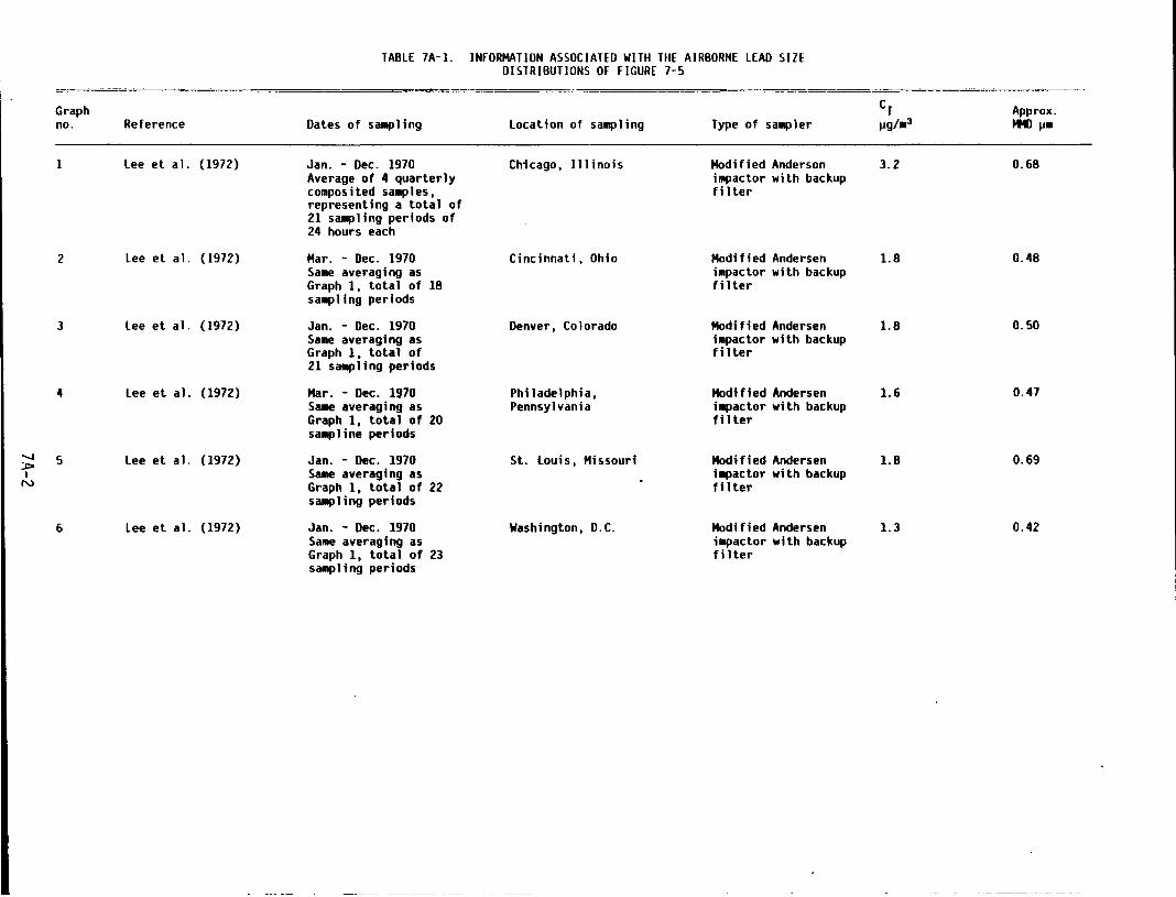
TABLE 7A-l. INFORMATION ASSOCIATED WITH THE AIRBORNE LEAD SIZE DISTRIBUTIONS OF FIGURE 7-5
Graph CT Approx. no. Reference Oates of sa~ling location of sampling Type of sa111pler j.lg/•3 MHO IJ•
1 lee et al. (1972) Jan. - Dec. 1970 Chicago, Illinois Modified Anderson 3.2 0.68 Average of 4 quarterly i~npactor with backup composited sa~les, filter representing a total of 21 sa~ling periods of 24 hours each
2 lee et al. ( 1972) Mar. - Dec. 1970 Cincinnati, Ohio Modified Andersen 1.8 0.48 Sa.e averaging as i~actor with backup Graph 1, total of 18 filter sa11pling periods
3 lee et al. (1972) Jan. - Dec. 1970 Denver, Colorado Modified Andersen 1.8 0.50 Same averaging as i~npactor with backup Graph 1, total of filter 21 sa~ling periods
4 lee et al. (1972) Mar. - Dec. 1970 Philadelphia, Modified Andersen 1.6 0.47 Sa~ averaging as Pennsylvania i~npactor with backup Graph 1, total of 20 filter sa~line periods
........ 5 lee et al. (1972) Jan. - Dec. 1970 St. louis, Missouri Modified Andersen 1.8 0.69 :.t» I Sa~ averaging as i~actor with backup
N Graph 1, total of 22 filter sa~ling periods
6 lee et al. (1972) Jan. - Dec. 1970 Washington, D.C. Modified Andersen 1.3 0.42 Sa•e averaging as i~npactor with backup Graph 1, total of 23 filter sa111p ling periods
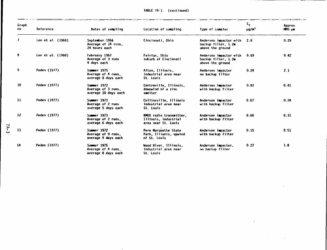
TABLE 7A-l. (continued)
Graph CT Approx. no Reference Dates of sampling location of sampling Type of sampler j.lg/113 ..,0 IJIII
7 lee et al. {1968) Septetllber 1966 Cincinnati, Ohio Andersen impactor with 2.8 0.29 Average of 14 runs, backup filter, 1.2m 24 hours each above the ground
8 lee et al. (1968) February 1967 Fairfax, Ohio Andersen i~actor with 0.69 0.42 Average of 3 runs suburb of Cincinnati backup filter, 1.211 4 days each above the ground
9 Peden (1977) S...-er 1975 Alton, Illinois, Andersen impactor 0.24 2.1 Average of 4 runs, industrial area near no backup filter average 8 days each St. louis
10 Peden (1977) Su.er 1972 Centreville, Illinois, Andersen i~actor 0.62 0.41 Average of 3 runs, downwind of a zinc with backup filter average 10 days each s~~elter
11 Peden (1977) Su.er 1973 Collinsville, Illinois Andersen i~~pactor 0.67 0.24 Average of 2 runs industrial area near with backup filter average 5 days each St. louis
12 Peden (1977) SUMer 1973 KMOX radio trans•itter, Andersen i~~pactor 0.60 0.31 Average of 2 runs, Illinois, industrial with backup filter
........ average 6 days each area near St . louis ::c:> I
0.15 0.51 I 13 Peden (1977) SUMer 1972 Pere Marquette State Andersen i~~pactor w Average of 9 runs, Park, lllionis, upwind with backup filter average 9 days each of St. louis
14 Peden (1977) SUMer 1975 Wood River, Illinois, Andersen i~~pactor, 0.27 1.8 Average of 4 runs, industrial area near nn h;orkun filtPr ··- ---··-r ... --. average 8 days each St. louis
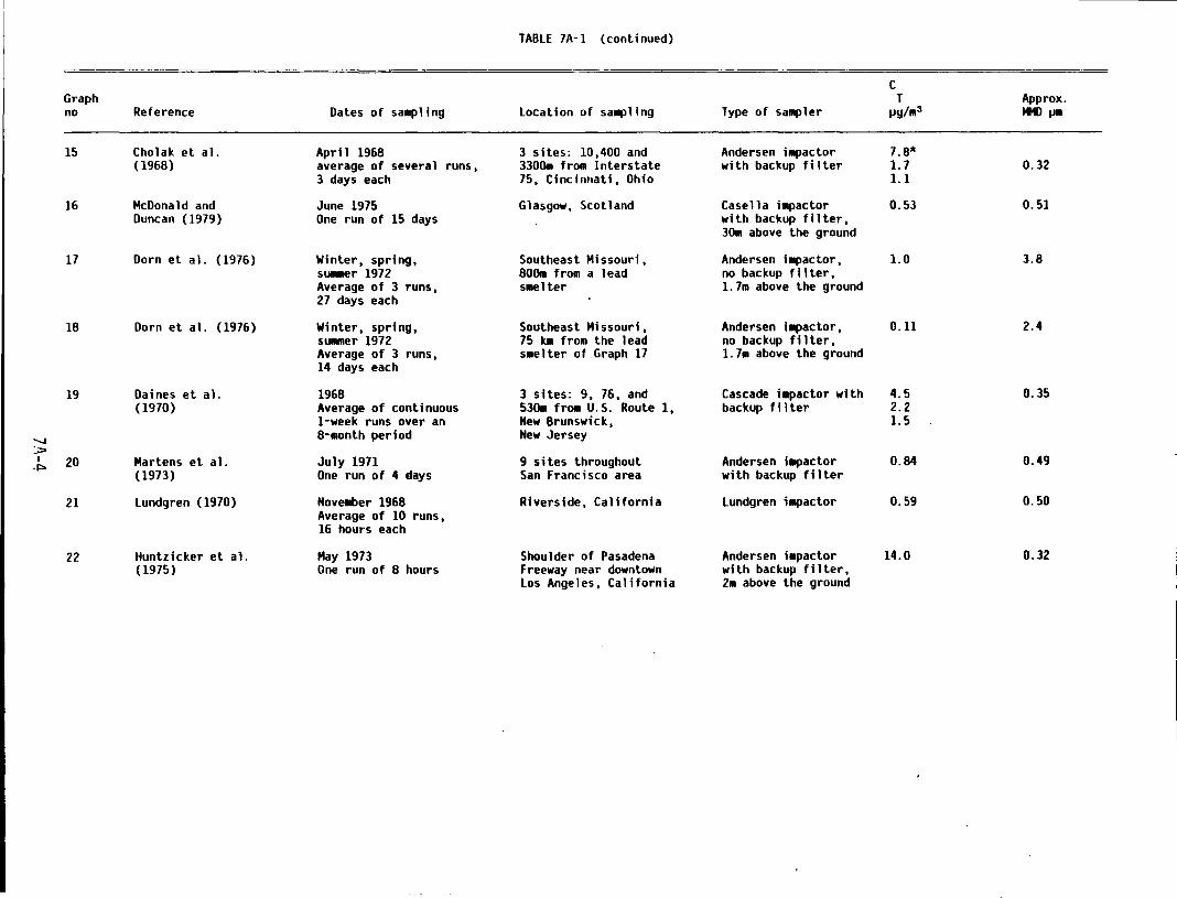
TABLE 7A-1 (continued)
c Graph T Approx. no Reference Oates of sa~ling location of sa11pling Type of sampler IJg/1113 MHO IJII
15 Cholak et al. April 1968 3 sites: 10,400 and Andersen i~actor 7.8* (1968) average of several runs, 3300. from Interstate with backup filter 1.7 0.32
3 days each 75, Cincinnati, Ohio 1.1
16 McDonald and June 1975 Glasgow, Scotland Casella i~~pactor 0.53 0.51 Duncan (1979) One run of 15 days with backup filter,
30.. above the ground
17 Dorn et al. (1976) Winter, spring, Southeast Missouri, Andersen impactor, 1.0 3.8 su.er 1972 800. from a lead no backup filter, Average of 3 runs, s•elter 1.7m above the ground 27 days each
18 Dorn et al. (1976) Winter, spring, Southeast Missouri, Andersen i~~pactor, 0.11 2.4 sumer 1972 75 kll from the lead no backup filter, Average of 3 runs, s•elter of Graph 17 1.7111 above the ground 14 days each
19 Daines et al. 1968 3 sites: 9, 76, and Cascade i~actor with 4.5 0.35 (1970) Average of continuous 530. fro. U.S. Route 1, backup filter 2.2
1-week runs over an New Brunswick, 1.5 ..........
8-~~anth period New Jersey :.;:. I 20 Martens et a 1. July 1971 9 sites throughout Andersen i~~pactor 0.84 0.49 .J::o
(1973) One run of 4 days San Francisco area with backup filter
21 Lundgren (1970) NoveMber 1968 Riverside, California Lundgren i~~pactor 0.59 0.50 Average of 10 runs, 16 hours each
22 Huntzicker et al. May 1973 Shoulder of Pasadena Andersen i•pactor 14.0 0.32 (1975) One run of 8 hours Freeway near downtown with backup filter,
los Angeles, California 2111 above the ground
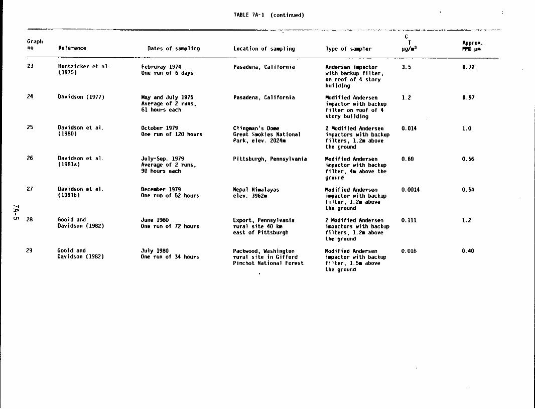
TABLE 7A-1 (continued)
c Graph T Approx. no Reference Oates of sampling Location of sa111p 1 i ng Type of sa111pler IJg/113 lf4D IJII
23 Huntzicker et al. Februray 1974 Pasadena, California Andersen impactor 3.5 0. 72 (1975) One run of 6 days with backup filter,
on roof of 4 story building
24 Davidson (1977) May and July 1975 Pasadena, California Modified Andersen 1.2 0.97 Average of 2 runs, i~actor with backup 61 hours each filter on roof of 4
story building
25 Davidson et al. October 1979 Cling~~an' s 0011e 2 Modified Andersen 0.014 1.0 (1980) One run of 120 hours Great Smokies National impactors with backup
Park, elev. 202411 filters, 1.211 above the ground
26 Davidson et al. July-Sep. 1979 Pittsburgh, Pennsylvania Modified Andersen 0.60 0.56 (1981a) Average of 2 runs, impactor with backup
90 hours each filter, 411 above the ground
27 Oav i dson et a 1. Oecellber 1979 Nepal Hi..alayas Modified Andersen 0.0014 0.54 (1981b) One run of 52 hours elev. 396211 i~~pactor with backup
filter, 1.211 above ....... the ground :t:a I
U1 28 Goold and June 1980 Export, Pennsylvania 2 Modified Andersen 0.111 1.2 Davidson (1982) One run of 72 hours rural site 40 kM i.pactors with backup
east of Pittsburgh filters, 1.211 above the ground
29 Goold and July 1980 Packwood, Washington Modified Andersen 0.016 0.40 Davidson (1982) One run of 34 hours rural site in Gifford i~~pactor with backup
Pinchot National Forest filter, 1.511 above the ground
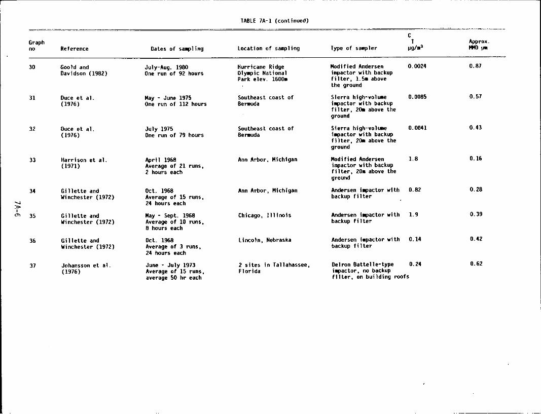
Graph no
30
31
32
33
34
36
37
Reference
Goold and Davidson (1982)
Duce et al. (1976)
Duce et al. (1976)
Harrison et al. (1971)
G i 11 ette and Winchester (1972)
Gillette and Winchester (1972)
Gillette and Winchester (1972)
Johansson et al. (1976)
Dates of sa~ling
July-Aug. 1980 One run of 92 hours
May - June 1975 One run of 112 hours
July 1975 One run of 79 hours
April 1968 Average of 21 runs, 2 hours each
Oct. 1968 Average of 15 runs, 24 hours each
May - Sept. 1968 Average of 10 runs, 8 hours each
Oct. 1968 Average of 3 runs, 24 hours each
June - July 1973 Average of 15 runs, average 50 hr each
TABLE 7A-1 (continued)
location of sampling
Hurricane Ridge Olympic National Park elev. 1600m
Southeast coast of Bermuda
Southeast coast of Bermuda
Ann Arbor, Michigan
Ann Arbor, Michigan
Chicago, Illinois
lincoln, Nebraska
2 sites in Tallahassee, Florida
Type of sampler
Modified Andersen impactor with backup filter, 1.5m above the ground
Sierra high-volu.e impactor with backup filter, 20. above the ground
Sierra high-volume impactor with backup filter, 20. above the ground
Modified Andersen impactor with backup filter, 20• above the ground
0.0024
0.0085
0.0041
1.8
Andersen impactor with 0.82 backup filter
Andersen impactor with 1.9 backup filter
Andersen i•pactor with 0.14 backup f i1 ter
Delron Battelle-type 0.24 i~actor, no backup filter, on building roofs
Approx. tf4l) !Jm
0.87
0.57
0.43
0.16
0.28
0.39
0.42
0.62
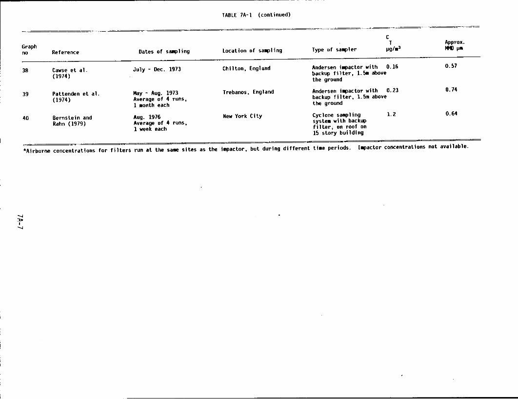
Graph no
38
39
40
Reference
Cawse et al. (1974)
Pattenden et a 1. (1974)
Bernstein and Rahn (1979)
Oates of sa~ling
July - Dec. 1973
Hay - Aug. 1973 Average of 4 runs, 1 •onth each
Aug. 1976 Average of 4 runs, 1 week each
TABLE 7A-l (continued)
Location of sampling
Chilton, England
Trebanos, England
New York City
c T
Type of saMpler ~g/•3
Andersen i.pactor with 0.16 backup filter, 1.~ above the ground
Andersen impactor with 0.23 backup filter, 1.5m above the ground
Cyclone sampling syst~ with backup filter, on roof on 15 story building
1.2
Approx. tM) ~·
0.57
0.74
0.64
*Airborne concentrations for filters run at the sa.e sites as the impactor, but during different ti.e periods. Impactor concentrations not available.
APPENDIX 78 SUPPLEMENTAL SOIL AND DUST INFORMATION
Lead in soi 1, and dust of soil or1 g1 n, is discussed in Section 7. 2. 2. The data show average soil concentrations are 8-25 ~g/g, and·dust from this soil rarely exceeds 80-100 ~g/g. Street dust, househo 1 d dust, and occupation a 1 dusts often exceed this 1 eve 1 by one to two orders of magnitude. Tables 78-1 and 78-2 summarize several studies of street dust. Table 78-3 shows data on household and residential soil dust. These data support the estimates of mean lead concentrations in dust discussed in Section 7.3.1.4. Table 78-4 gives airborne lead concentrations for an occupational setting, which are only qualitatively related to dust lead concentrations.
78-1
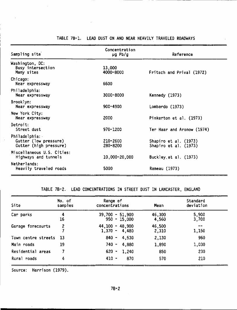
TABLE 7B-1. LEAD DUST ON AND NEAR HEAVILY TRAVELED ROADWAYS
Samp 1 i ng s i te ·
Washington, DC: Busy intersection Many sites
Chicago: Near expressway
Philadelphia: Near expressway
Brooklyn: Near expressway
New York City: Near expressway
Detroit: Street dust
Philadelphia:· Gutter (low pressure) Gutter (high pressure)
Miscellaneous U;S. Cities: Highways and tunnels
Netherlands: Heavily traveled roads
Concentration !Jg Pb/g
13,000 4000-8000
6600
3000-8000
900-4900
2000
970-1200
210-2600 280-8200
10,000-20,000
5000
Reference
Fritsch and Prival (1972)
Kennedy (1973)
Lombardo (1973)
Pinkerton et al. (1973)
Ter Haar and Aronow (1974)
Shapiro et al. (1973) Shapiro et al. (1973)
Buckley.et al. (1973)
Rameau (1973)
TABLE 7B-2. LEAD CONCENTRATIONS IN STREET DUST IN LANCASTER, ENGLAND
No. of Site samples
Car parks 4 16
Garage forecourts 2 7
Town centre streets 13
Main roads 19 Residential areas 7 Rural roads 4
Source: Harrison (1979).
Range of concentrations
39,700- 51,900 950 - 15,000
44,100 - 48,900 1,370 - 4,480
840 - 4,530 740 - 4,880 620 - 1,240 410 - 870
7B-2
Mean
46,300 4,560
46,500 2,310 2,130 1,890
850 570
Standard deviation
5,900 3,700
1,150 960
1,030 230 210
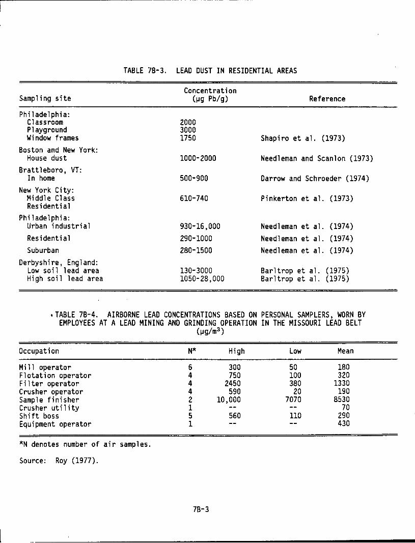
Sampling site
Philadelphia: Classroom Playground Window frames
Boston and New York: House dust
Brattleboro, VT: In home
New York City: Middle Class Residential
Philadelphia: Urban industrial Residential Suburban
Derbyshire, England: Low soil lead area High soil lead area
TABLE 7B-3. LEAD DUST IN RESIDENTIAL AREAS
Concentration (!Jg Pb/g) Reference
2000 3000 1750 Shapiro et al. (1973)
1000-2000 Needleman and Scanlon (1973)
500-900 Darrow and Schroeder (1974)
610-740 Pinkerton et al. (1973)
930-16,000 Needleman et al. (1974) 290-1000 Needleman et al. (1974) 280-1500 Needleman et a 1. (1974)
130-3000 Barltrop et al. (1975) 1050-28,000 Barltrop et al. (1975)
·TABLE 7B-4. AIRBORNE LEAD CONCENTRATIONS BASED ON PERSONAL SAMPLERS, WORN BY EMPLOYEES AT A LEAD MINING AND GRINDING OPERATION IN THE MISSOURI LEAD BELT
(1Jg/m3)
Occupation N* High Low Mean
Mill operator 6 300 50 180 Flotation operator 4 750 100 320 Filter operator 4 2450 380 1330 Crusher operator 4 590 20 190 Sample finisher 2 10,000 7070 8530 Crusher utility 1 70 Shift boss 5 560 110 290 Equipment operator 1 430
*N denotes number of air samples.
Source: Roy (1977).
7B-3
APPENDIX 7C STUDIES OF SPECIFIC POINT SOURCES
OF LEAD
This collection of studies is intended to extend and detail the general picture of lead concentrations in proximity to identified major point sources as portrayed in Chapter 7. Because emissions and control technology vary between point sources, each point source is unique in the degree of environmental contamination. Tl1e list is by no means all-inclusive, but is intended to be representative and to supplement the data cited in Chapter 7. In many of the studies, b 1 ood samp 1 es of workers and their families were taken. These studies are also discussed in Chapter 11.
7C.1 SMELTERS AND MINES
7C.1.1 Two Smelter Study The homes of workers of two unidentified secondary lead smelters in different geograph
ical areas of the United States were studied by Rice et al. (1978). Paper towels were used to collect dust from surfaces in each house, following th•e method of Vostal et al. (1974). A total of 33 homes of smelter workers and 19 control homes located in the same or similar neighborhoods were investigated. The geometric mean lead levels on the towels were 79.3 ~g
(smelter workers) versus 28.8 ~g (controls) in the first area, while in the second area mean va 1 ues were 112 ~g versus 9. 7 ~g. A 1 so in the second ctrea, sett 1 ed dust above doorways was collected by brushing the dust into glassine envelopes for subsequent analysis. The geometric mean lead content of this dust in 15 workers• homes was 3300 ~g/g, compared with 1200 ~g/g
in eight control homes. Curbside dust collected near each home in the second area had a geometric mean lead content of 1500 ~g/g, with no significant difference between worker and centro 1 homes. No significant difference was reported in the paint 1 ead content between worker and contra 1 homes. The authors cone 1 uded that 1 ead in dust carried home by these workers contributed to the lead content of dust in their homes, despite showering and changing clothes at the plant, and despite work clothes being laundered by the company. Storage of employee street clothes in dusty lockers, walking across lead-contaminated areas on the way home, and particulate settling on workers• cars in the parking lot may have been important factors. Based on measurement of zinc protoporphyrin levels in the blood of children in these homes, the authors also concluded that the greater lead levels in housedust contributed to increased child absorption of lead.
7C-1
7C.1.2 British Columbia, Canada Neri et al. (1978) and Schmitt et al. (1979) examined environmental lead levels in the
vicinity of a lead-zinc smelter at Trail, British Columbia. Total emissions from the smelter averaged about 135 kg Pb/day. Measurements were conducted in Trail (population 12,000), in Nelson, a control city 41 km north of Trail (population 10,000), and in Vancouver. The annual mean airborne lead concentrations in Trail and in· Nelson were 2.0 and 0.5 ~g/m3, respectively. Mean lead levels in surface soil were 1320 ~g/g in Trail (153 samples), 192 ~g/g in Nelson (55 samples), and 1545 ~g/g in Vancouver (37 samples).
Blood lead measurements show a positive correlation with soil lead levels for children aged 1-3 years and for first graders, but no significant correlation for ninth graders. The authors concluded that small children are most likely to ingest soil dust, and hence deposited smelter-emitted lead may pose a potential hazard for the youngest age group.
7C.1.3 Netherlands
Environmental lead concentrations were measured in 1978 near a secondary lead smelter in
Arnhem, Netherlands (Diemel et al., 1981). Air and dust were sampled in over 100 houses at distances of 450-1000 meters from the smelter, with outdoor samples of air, dust, and soil co 11 ected for comparison. Results are presented in Tab 1 e 7C-l. Note that the mean indoor concentration of total suspended particulates (TSP) is greater than the mean outdoor concentration, yet the mean indoor lead level is smaller than the corresponding outdoor level. The authors reasoned that indoor sources such as tobacco smoke, consumer products, and decay of furnishings are likely to be important in affecting indoor TSP; however, much of the indoor
1 ead was probably carried in from the outside by the occupants, e. g. , as dust adhering to shoes. The importance of resuspension of indoor particles by activity around the house was also discussed.
7C.l.4 Belgium Reels et al. (1978, 1980) measured lead levels in the air, in dust, and on childrens'
hands at varying distances from a lead smelter in Belgium (annual production 100,000 metric tons). Blood data from children living near the smelter were also obtained. Air samples were
collected nearly continuously beginning in September 1973. Table 7C-2 lists the airborne concentrations recorded during five di st i net population surveys between 1974 and 1978, while
Figure 7C-1 presents air, dust, and hand data for Survey #3 in 1976. Statistical tests showed
that blood lead levels were better correlated with lead on childrens' hands than with air lead. The authors suggested that ingestion of contaminated dust by hand-to-mouth activities
7C-2
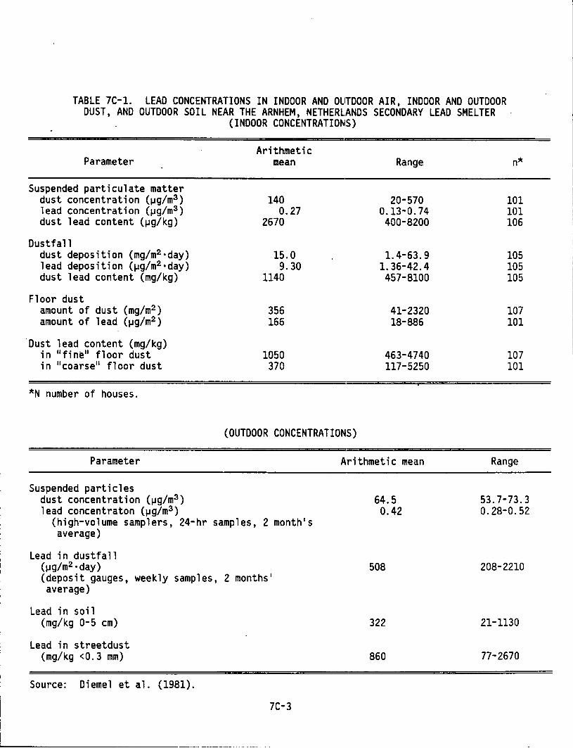
TABLE 7C-1. LEAD CONCENTRATIONS IN INDOOR AND OUTDOOR AIR, INDOOR AND OUTDOOR OUST, AND OUTDOOR SOIL NEAR THE ARNHEM, NETHERLANDS SECONDARY LEAD SMELTER
(INDOOR CONCENTRATIONS)
Parameter
Suspended particulate matter dust concentration (~g/m3 ) lead concentration (~g/m3 ) dust lead content (~g/kg)
Oustfall dust deposition (mg/m2·day) lead deposition (~g/m2 ·day) dust lead content (mg/kg)
Floor dust amount of dust (mg/m2) amount of lead (~gfm2)
Oust lead content (mg/kg) in 11 fine 11 floor dust in 11 coarse11 floor dust
*N number of houses.
Arithmetic mean
140 0.27
2670
15.0 9.30
1140
356 166
1050 370
Range
20-570 0.13-0.74 400-8200
1. 4-63.9 1. 36-42.4 457-8100
41-2320 18-886
463-4740 117-5250
(OUTDOOR CONCENTRATIONS)
Parameter
Suspended particles dust concentration (~g/m3 ) lead concentraton (~g/m3 )
(high-volume samplers, 24-hr samples, 2 month's average)
Lead in dustfall (~g/m2 ·day) (deposit gauges, weekly samples, 2 months' average)
Lead in soil (mg/kg 0-5 em)
Lead in streetdust (mg/kg <0.3 mm)
Source: Diemel et al. (1981).
7C-3
Arithmetic mean
64.5 0.42
508
322
860
n*
101 101 106
105 105 105
107 101
107 101
Range
53.7-73.3 0.28-0.52
208-2210
21-1130
77-2670
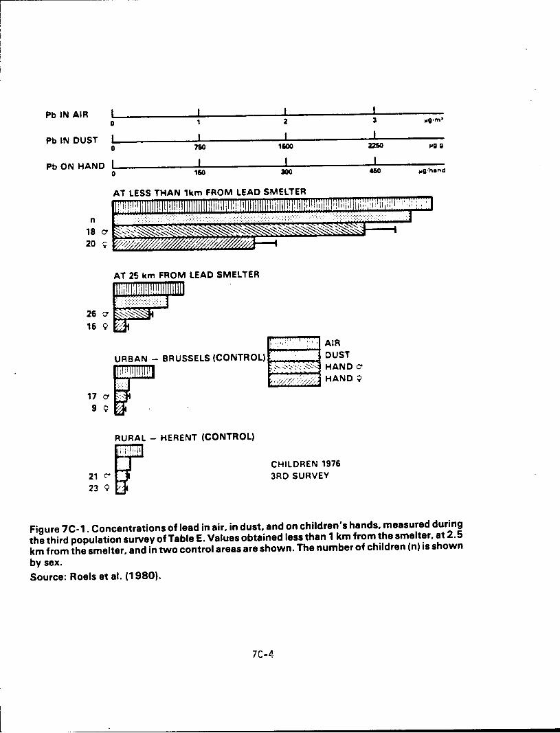
Pb IN AIR 0 2 3
Pb IN DUST 0 11i00 2250
Pb ON HAND 0 110
AT LESS THAN 1km FROM LEAD SMELTER
n
18 C1 ~~~~~~~~~~~~~~~~~---4 20 ~ ~~~~~~~~~ij-'""'i
! · ,. ,,, · AIR
URBAN - BRUSSELS (CONTROL) ~--....1 DUST
r' 0::.,...:.._~--:-·;~~.:.,_; HAND C1
1 ~ ~ '; ' .;, //:;.;;; HAND 9
RURAL- HERENT (CONTROL)
~! ~ ~iiU CHILDREN 1976 3RD SURVEY
Figure 7C-1. Concentrations of lead in air, in dust, and on children's hands, measured during the third population survey of Table E. Values obtained less than 1 km from the smelter, at 2.5 km from the smelter, and in two control areas are shown. The number of children (n) is shown by sex. Source: Roels et al. (1980).
7C-4-
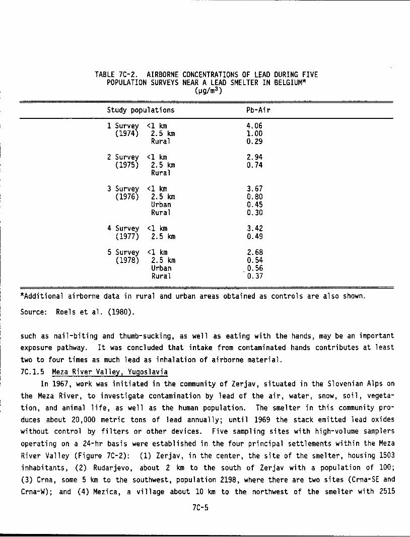
TABLE 7C-2. AIRBORNE CONCENTRATIONS OF LEAD DURING FIVE POPULATION SURVEYS NEAR A LEAD SMELTER IN BELGIUM*
(1Jg/m3)
Study populations Pb-Air
1 Survey <1 km 4.06 (1974) 2.5 km 1. 00
Rural 0.29
2 Survey <1 km 2.94 (1975) 2.5 km 0.74
Rural
3 Survey <1 km 3.67 (1976) 2. 5 km 0.80
Urban 0.45 Rural 0.30
4 Survey <1 km 3.42 (1977) 2.5 km 0.49
5 Survey <1 km 2.68 (1978) 2.5 km 0.54
Urban 0.56 Rural 0.37
*Additional airborne data in rural and urban areas obtained as controls are also shown.
Source: Roels et al. (1980).
such as nail-biting and thumb-sucking, as well as eatinu with the hands, may be an important exposure pathway. It was concluded that intake from contaminated hands contributes at 1 east two to four times as much lead as inhalation of airborne material. 7C.1.5 Meza River Valley, Yugoslavia
In 1967, work was initiated in the community of Zerjav, situated in the Slovenian Alps on the Meza River, to investigate contamination by lead of the air, water, snow, soil, vegetation, and animal life, as well as the human population. The smelter in this community produces about 20,000 metric tons of lead annually; until 1969 the stack emitted lead oxides without control by filters or other devices. Five sampling sites with high-volume samplers operating on a 24-hr basis were established in the four principal settlements within the Meza River Valley (Figure 7C-2): (1) Zerjav, in the center, the site of the smelter, housing 1503 inhabitants, (2) Rudarjevo, about 2 km to the south C>f Zerjav with a population of 100; (3) Crna, some 5 km to the southwest, population 2198, where there are two sites (Crna-SE and Crna-W); and (4) Mezica, a village about 10 km to the northwest of the smelter with 2515
7C-5
inhabitants. The data in Table 7C-3 are sufficient to depict general environmental contamination of striking proportions.
7C.1.6 Kosova Province, Yugoslavia Popovac et al. (1982) discuss lead exposure in an industrialized region near the town of
Kosova Mitrovica, Yugoslavia, containing a lead smelter and refinery, and a battery factory. In 1979, 5800 kg of lead were emitted daily from the lead smelter alone. Ambient air concentrations in the town were in the range 21.2-29.2 1Jg/m3 in 1980, with levels occasionally reaching 70 1-1g/m3 . The authors report e 1 eva ted b 1 ood 1 ead 1 eve 1 s in most of the children tested; some extremely high values were found, suggesting the presence of congenital lead poisoning.
7C.1.7 Czechoslovakia Wagner et al. (1981) measured total suspended particulate and airborne lead concentra
tions in the vicinity of a waste lead processing plant in Czechoslovakia. Data are shown in Table 7C-4. Blood lead levels in 90 children living near the plant were significantly greater than in 61 control children.
7C.1.8 Australia Heyworth et al. (1981) examined child response to lead in the vicinity of a lead sulfide
mine in Northhampton, Western Austra 1 i a. Two samp 1 es of mine tai 1 i ngs measured in 1969 contained 12,000 IJg/g and 28,000 IJg/g lead; several additional samples analyzed in 1978 contained 22,000-157,000 IJg/g lead. Surface soil from the town boundary contained 300 IJg/g, while a playground and a recreational area had soil containing 11,000 IJg/g and 12,000 IJg/g lead, respectively.
Blood lead levels measured in Northhampton children, near the mine, were slightly greater than levels measured in children living a short distance away. The Northhampton blood lead levels were also slightly greater than those reported for children in Victoria, Australia (DeSilva and Donnan, 1980). Heyworth et al. (1981) concluded that the mine tailings could have increased the lead exposure of children living in the area.
7C.2 BATTERY FACTORIES
7C.2.1 Southern Vermont Watson et al. (1978) investigated homes of employees of a lead storage battery plant in
southern Vermont in August and September, 1976. Lead levels in household dust, drinking
7C-6
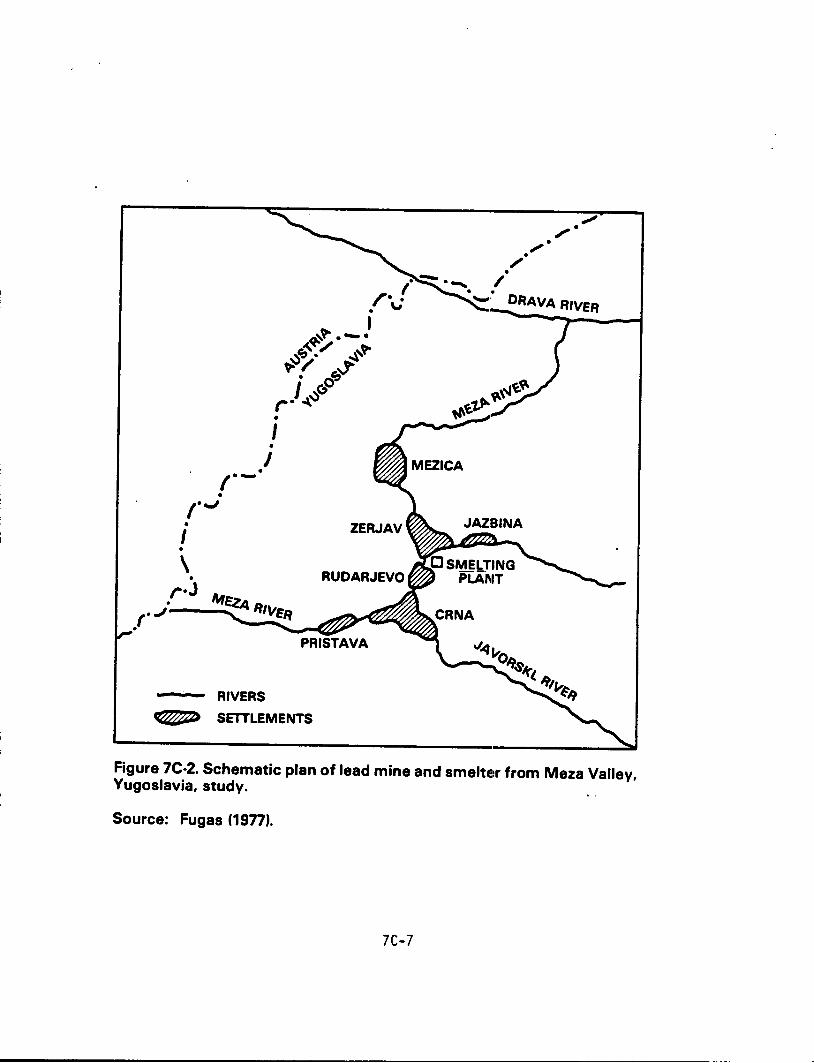
,·..J . I . \
RIVERS
~ SETTLEMENTS
RUDARJEVO
....... /.
,. ,. • ._.· DRAVA RIVER
Figure 7C-2. Schematic plan of lead mine and smelte'r from Meza Valley, Yugoslavia, study.
Source: Fugas (19n).
7C-7
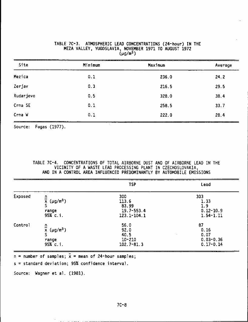
Site
Mezica
Zerjav
TABLE 7C-3. ATMOSPHERIC LEAD CONCENTRATIONS (24-hour) IN THE MEZA VALLEY, YUGOSLAVIA, NOVEMBER 1971 TO AUGUST 1972
(1Jg/m3)
Minimum Maximum
0.1 236.0
0.3 216.5
Average
24.2
29.5
Rudarjevo 0.5 328.0 38.4
Crna SE 0.1 258.5 33.7
Crna W 0.1 222.0 28.4
Source: Fugas (1977).
TABLE 7C-4. CONCENTRATIONS OF TOTAL AIRBORNE DUST AND OF AIRBORNE LEAD IN THE VICINITY OF A WASTE LEAD PROCESSING PLANT IN CZECHOSLOVAKIA,
AND IN A CONTROL AREA INFLUENCED PREDOMINANTLY BY AUTOMOBILE EMISSIONS
TSP
Exposed n 300 x (1Jg/m3) 113.6 s 83.99 range 19.7-553.4 95% c. i. 123.1-104.1
Control n 56.0 x (1Jg/m3) 92.0 s 40.5 range 10-210 95% c. i. 102.7-81.3
n = number of samples; x = mean of 24-hour samples; s =standard deviation; 95% confidence interval.
Source: Wagner et al. (1981).
7C-8
Lead
303 1. 33 1.9 0.12-10.9 1. 54-1.11
87 0.16 0.07 0.03-0.36 0.17-0.14
water, and paint were determined for 22 workers' homes and 22 control homes. The mean lead concentration in dust in the workers' homes was 2,200 IJg/g, compared with 720 !Jg/g in the control homes. Blood lead levels in the workers' children were greater than levels in the control children, and were significantly correlated with dust lead concentrations. No significant correlations were found between drinking water lead and blood lead, or between paint lead and blood lead. It is noteworthy that although 90 percent of the employees showered and changed clothes at the plant, 87 percent brought their work clothes home for laundering. The authors concluded that dust carried home by the workers contributed to increased lead absorption in their children.
7C.2.2 North Carolina Several cases of elevated environmental lead levels near point sources in North Carolina
have been reported by Do 1 court et a 1. (1978, 1981). In the first instance, dust 1 ead was measured in the homes of mothers employed in a battery factory in Raleigh; blood lead levels in the mothers and their chldren were also measured. Carpet dust was found to contain 1,700-48,000 !Jg/g lead in six homes where the children had elevated blood lead levels (>40 IJg/dl). The authors concluded that lead carried home on the mothers' clothing resulted in increased exposure to their children (Dolcourt et al., 1978). In this particular plant, no uniforms or garment covers were provided by the factory; work clothing was worn home.
In a second case, discarded automobile battery casi·ngs from a small-scale lead recovery operation in rural North Carolina were brought home by a worker and used in the f-amily's wood-burning stove (Dolcourt et al., 1981). Two sampl,es of indoor dust yielded 13,000 and 41,000 1-1g/g lead. A three-year-old girl living in the house developed encephalopathy resulting in permanent brain damage.
In a third case, also in rural North Carolina, a worker employed in an automobile battery reclamation plant was found to be operating an illicit battery recycling operation in his home. Reclaimed lead was melted on the kitchen stove. Soil samples obtained near the house measured as high as 49 percent 1 ead by weight; the driveway was covered with fragments of battery casings. Although no family member had evidence of lead poisoning, there were unexplained deaths among chickens who fed where the lead waste products were discarded (Dolcourt et al., 1981).
7C.2.3 Oklahoma Morton et a 1. (1982) studied 1 ead exposure in children of emp 1 oyees at a battery manu
facturing plant in Oklahoma. A total of 34 lead-exposed children and 34 control children were examined during February and March, 1978; 18 children in the lead-exposed group had elevated blood lead levels (>30 IJg/dl), while none of the controls were in this category.
7C-9
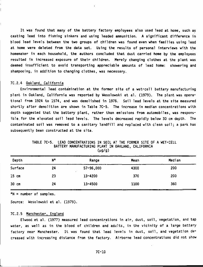
It was found that many of the battery factory employees also used lead at home, such a~
casting lead into fishing sinkers and using leaded ammunition. A significant difference in blood lead levels between the two groups of children was found even when families using lead at home were deleted from the data set. Using the results of personal interviews with the homemaker in each household, the authors concluded that dust carried home by the employees resulted in increased exposure of their children. Merely changing clothes at the plant was deemed insufficient to avoid transporting appreciable amounts of lead home: showering and shampooing, in addition to changing clothes, was necessary.
7C.2.4 Oakland, California Environmental lead contamination at the former site of a wet-cell battery manufacturing
plant in Oakland, California was reported by Wesolowski et al. (1979). The plant was operational from 1924 to 1974, and was demolished in 1976. Soil lead levels at the site measured shortly after demolition are shown in Table 7C-5. The increase in median concentrations with depth suggested that the battery plant, rather than emissions from automobiles, was responsible. for the elevated soil lead levels. The levels decreased rapidly below 30 em depth. The contaminated soil was removed to a sanitary landfill and replaced with clean soil; a park has subsequently been constructed at the site.
TABLE 7C-5. LEAD CONCENTRATIONS IN SOIL AT THE FORMER SITE OF A WET-CELL BATTERY MANUFACTURING PLANT IN OAKLAND, CALIFORNIA
(~g/g)
Depth N* Range Mean Median
Surface 24 57-96,000 4300 200
15 em 23 13-4200 370 200
30 em 24 13-4500 1100 360
*N = number of samples.
Source: Wesolowski et al. (1979).
7C.2.5 Manchester, England Elwood et al. (1977) measured lead concentrations in air, dust, soil, vegetation, and tap
water, as well as in the blood of children and adults, in the vicinity of a large battery factory near Manchester. It was found that lead levels in dust, soil, and vegetation decreased with increasing distance from the factory. Airborne lead concentrations did not show
7C-10
a consistent effect with downwind distance, although higher concentrations were found downwind compared with upwind of the factory. Blood lead levels were greatest in the households of battery factory employees: other factors such as distance from the factory, car ownership,
age of house, and presence of lead water pipes were outweighed by the presence of a leadworker in the household. These results strongly suggest that lead dust carried home by the factory
employees is a dominant exposure pathway for their families. The authors also discussed the work of Burrows (1976), who demonstrated experimentally that the most important means of lead
transport from the factory into the home is via the workers' shoes.
7C-11
APPENDIX 7D SUPPLEMENTAL DIETARY INFORMATION FROM THE
U.S. FDA TOTAL DIET STUDY
The U.S. Food and Drug Administration published a new Total Diet Food List (Pennington, '
1983) based on over 100,000 daily diets from 50,000 participants. Thirty five hundred categories of foods were condensed to 201 adult food categories for 8 age/sex groups. Summaries of these data were used in Section 7.3.1.2 to arrive at lead exposures through food, water, and beverages. For brevity and continuity with the crop data of Section 7.2.2.2.1, it was necessary to condense the 201 categories of the Pennington study to 25 categories in this report.
The preliminary lead concentrations for all 201 items of the food list were provided by U.S. Food and Drug Admi ni strati on (1985). These data represent four Market Basket Surveys, each from a different geographic location. Means of these values have been calculated by
EPA, using one-half the detection limit for values reported below detection limit. These data appear in Table 7D-1.
In condensing the 201 categories of Table 7D-1 to the 9 categories of Table 7-17, combinations and fract i ona 1 combinations of categories were made according to the scheme of Table 7D-2. In this way, specific categories of food more closely identified with farm products were summarized. The assumptions made concerning the ingredients in the final product, (mainly water, flour, eggs, and milk) had little influence on the outcome of the summarization.
7D-1
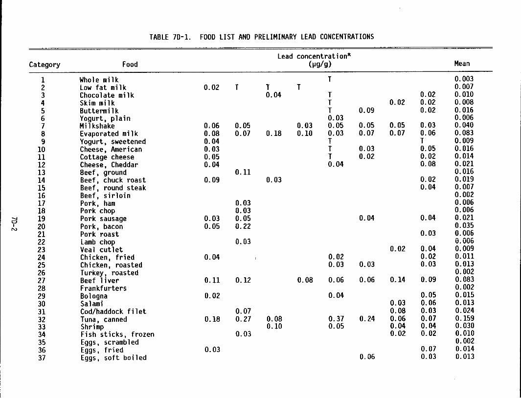
TABLE 7D-l. FOOD LIST AND PRELIMINARY LEAD CONCENTRATIONS
lead concentration* Category Food (~g/g) Mean
1 Whole milk T 0.003 2 low fat milk 0.02 T T T 0.007 3 Chocolate milk 0.04 T 0.02 0.010 4 Skim milk T 0.02 0.02 0.008 5 Buttermilk T 0.09 0.02 0.016 6 Yogurt, plain 0.03 0.006 7 Milkshake 0.06 0.05 0.03 0.05 0.05 0.05 0.03 0.040 8 Evaporated milk 0.08 0.07 0.18 0.10 0.03 0.07 0.07 0.06 0.083 9 Yogurt, sweetened 0.04 T T 0.009
10 Cheese, American 0.03 T 0.03 0.05 0.016 11 Cottage cheese 0.05 T 0.02 0.02 0.014 12 Cheese, Cheddar 0.04 0.04 0.08 0.021 13 Beef, ground 0.11 0.016 14 Beef, chuck roast 0.09 0.03 0.02 0.019 15 Beef, round steak 0.04 0.007 16 Beef, sirloin 0.002 17 Pork, ham 0.03 0.006 18 Pork chop 0.03 0.006
......, 19 Pork sausage 0.03 0.05 0.04 0.04 0.021 0 I 20 Pork, bacon 0.05 0.22 0.035
N
21 Pork roast 0.03 0.006 22 Lamb chop 0.03 0.006 23 Veal cutlet 0.02 0.04 0.009 24 Chicken, fried 0.04 0.02 0.02 0.011 25 Chicken, roasted 0.03 0.03 0.03 0.013 26 Turkey, roasted 0.002 27 Beef liver 0.11 0.12 0.08 0.06 0.06 0.14 0.09 0.083 28 Frankfurters 0.002 29 Bologna 0.02 0.04 0.05 0.015 30 Salami 0.03 0.06 0.013 31 Cod/haddock filet 0.07 0.08 0.03 0.024 32 Tuna, canned 0.18 0.27 0.08 0.37 0.24 0.06 0.07 0.159 33 Shrimp 0.10 0.05 0.04 0.04 0.030 34 Fish sticks, frozen 0.03 0.02 0.02 0.010 35 Eggs, scrambled 0.002 36 Eggs, fried 0.03 0.07 0.014 37 Eggs, soft boiled 0.06 0.03 0.013
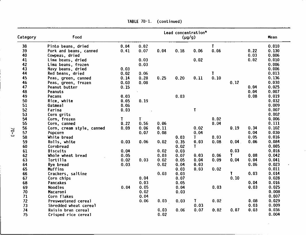
TABLE 70-1. (continued)
Lead concentration* Category Food (~g/g) Mean
38 Pinto beans, dried 0.04 0.02 T 0.010 39 Pork and beans, canned 0.41 0.07 0.04 0.18 0.06 0.06 0.22 0.130 40 Cowpeas, dried 0.03 0.006 41 Lima beans, dried 0.03 0.02 0.02 0.010 42 Lima beans, frozen 0.03 0.006 43 Navy beans, dried 0.03 0.006 44 Red beans, dried 0.02 0.06 T 0.013 45 Peas, green, canned 0.14 0.28 0.25 0.20 0.11 0.10 0.136 46 Peas, green, frozen 0.03 0.08 0.12 0.030 47 Peanut butter 0.15 0.04 0.025 48 Peanuts 0.04 0.007 49 Pecans 0.03 0.03 0.08 0.019 50 Rice, white 0.05 0.19 0.032 51 Oatmeal 0.06 0.009 52 Farina 0.03 T 0.007 53 Corn grits 0.002 54 Corn, frozen T T 0.02 0.006 55 Corn, canned 0.22 0.56 0.06 0.04 0.111
"'-.J 56 Corn, cream style, canned 0.09 0.06 0.11 0.02 0.19 0.34 0.102 a 57 Popcorn 0.07 0.08 0.04 0.04 0.030 I w 58 White bread 0.03 T 0.03 0.05 0.016
59 Ro 11 s , wh i te 0.03 0.06 0.02 0.35 0.03 0.08 0.04. 0.06 0.084 60 Cornbread 0.02 T 0.005 61 Biscuits 0.04 0.02 0.03 0.03 0.016 62 Whole wheat bread 0.05 0.03 0.07 0.03 0.06 T 0.08 0.042 63 Tortilla 0.02 0.03 0.02 0.05 0.04 0.09 0.04 0.04 0.041 64 Rye bread 0.03 0.02 0.04 0.03 0.06 0.023 65 Muffins 0.03 0.03 0.02 0.011 66 Crackers, saltine 0.03 0.03 T 0.03 0.014 67 Corn chips 0.04 0.07 0.10 0.028 68 Pancakes 0.03 0.05 0.04 0.016 69 Noodles 0.04 0.05 0.04 0.03 0.03 0.025 70 Macaroni 0.02 0.03 0.008 71 Corn flakes 0.04 0.007 72 Presweetened cereal 0.06 0.03 0.03 T 0.02 0.08 0.029 73 Shredded wheat cereal 0.03 0.03 0.009 74 Raisin bran cereal 0.03 0.06 0.07 0.02 0.07 0.03 0.036 75 Crisped rice cereal 0.02 0.004
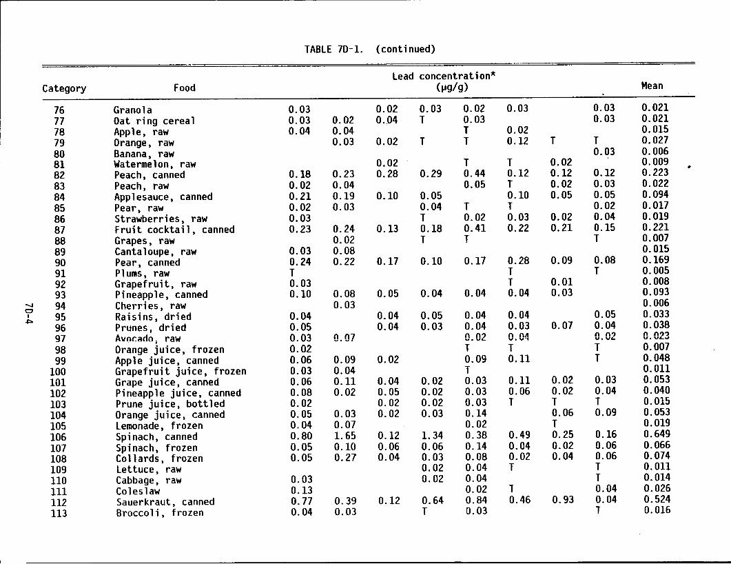
TABLE 70-1. (continued)
Lead concentration* Category Food (f.Jg/g) Mean
76 Granola 0.03 0.02 0.03 0.02 0.03 0.03 0.021 77 Oat ring cereal 0.03 0.02 0 .. 04 T 0.03 0.03 0.021 78 Apple, raw 0.04 0.04 T 0.02 0.015 79 Orange, raw 0.03 0.02 T T 0.12 T T 0.027 80 Banana, raw 0.03 0.006 81 Watermelon, raw 0.02 T T 0.02 0.009 82 Peach, canned 0.18 0.23 0.28 0.29 0.44 0.12 0.12 0.12 0.223 •
83 Peach, raw 0.02 0.04 0.05 T 0.02 0.03 0.022 84 Applesauce, canned 0.21 0.19 0.10 0.05 0.10 0.05 0.05 0.094 85 Pear, raw 0.02 0.03 0.04 T T 0.02 0.017 86 Strawberries, raw 0.03 T 0.02 0.03 0.02 0.04 0.019 87 Fruit cocktail, canned 0.23 0.24 0.13 0.18 0.41 0.22 0.21 0.15 0.221 88 Grapes, raw 0.02 T T T 0.007 89 Cantaloupe, raw 0.03 0.08 0.015 90 Pear, canned 0.24 0.22 0.17 0.10 0.17 0.28 0.09 0.08 0.169 91 Plums, raw T T T 0.005 92 Grapefruit, raw 0.03 T 0.01 0.008 93 Pineapple, canned 0.10 0.08 0.05 0.04 0.04 0.04 0.03 0.093
....... 94 Cherries, raw 0.03 0.006 0 I 95 Raisins, dried 0.04 0.04 0.05 0.04 0.04 0.05 0.033 ~
96 Prunes, dried 0.05 0.04 0.03 0.04 0.03 0.07 0.04 0.038 97 Avocado; raw 0.03 0.07 n n? n nJI 0.02 n n?'l
v. "''- v.u..,- u.ve-J
98 Orange juice, frozen 0.02 T T T 0.007 99 Apple juice, canned 0.06 0.09 0.02 0.09 0.11 T 0.048
100 Grapefruit juice, frozen 0.03 0.04 T 0.011 101 Grape juice, canned 0.06 0.11 0.04 0.02 0.03 0.11 0.02 0.03 0.053 102 Pineapple juice, canned 0.08 0.02 0.05 0.02 0.03 0.06 0.02 0.04 0.040 103 Prune juice, bottled 0.02 0.02 0.02 0.03 T T T 0.015 104 Orange juice, canned 0.05 0.03 0.02 0.03 0.14 0.06 0.09 0.053 105 Lemonade, frozen 0.04 0.07 0.02 T 0.019 106 Spinach, canned 0.80 1. 65 0.12 1. 34 0.38 0.49 0.25 0.16 0.649 107 Spinach, frozen 0.05 0.10 0.06 0.06 0.14 0.04 0.02 0.06 0.066 108 Collards, frozen 0.05 0.27 0.04 0.03 0.08 0.02 0.04 0.06 0.074 109 Lettuce, raw 0.02 0.04 T T 0.011 110 Cabbage, raw 0.03 0.02 0.04 T 0.014 111 Coleslaw 0.13 0.02 T 0.04 0.026 112 Sauerkraut, canned 0.77 0.39 0.12 0.64 0.84 0.46 0.93 0.04 0.524 113 Broccoli, frozen 0.04 0.03 T 0.03 T 0.016
l __________________________________________________________________ _
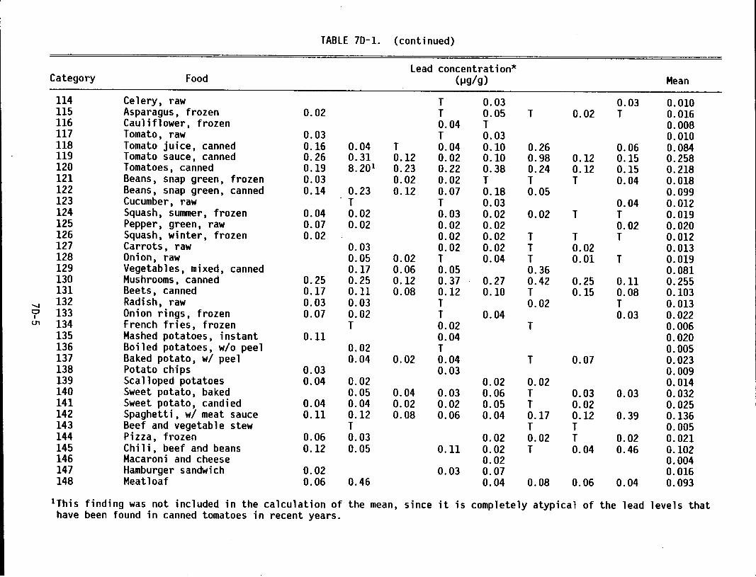
TABLE 70-1. (continued)
Lead concentration* Category Food (jjg/g) Mean
114 Celery, raw T 0.03 0.03 0.010 115 Asparagus, frozen 0.02 T 0.05 T 0.02 T 0.016 116 Cauliflower, frozen 0.04 T 0.008 117 Tomato, raw 0.03 T 0.03 0.010 118 Tomato juice, canned 0.16 0.04 T 0.04 0.10 0.26 0.06 0.084 119 Tomato sauce, canned 0.26 0.31 0.12 0.02 0.10 0.98 0.12 0.15 0.258 120 Tomatoes, canned 0.19 8.201 0.23 0.22 0.38 0.24 0.12 0.15 0.218 121 Beans, snap green, frozen 0.03 0.02 0.02 T T T 0.04 0.018 122 Beans, snap green, canned 0.14 0.23 0.12 0.07 0.18 0.05 0.099 123 Cucumber, raw T T 0.03 0.04 0.012 124 Squash, summer, frozen 0.04 0.02 0.03 0.02 0.02 T T 0.019 125 Pepper, green, raw 0.07 0.02 0.02 0.02 0.02 0.020 126 Squash, winter, frozen 0.02 0.02 0.02 T T T 0.012 127 Carrots, raw 0.03 0.02 0.02 T 0.02 0.013 128 Onion, raw 0.05 0.02 T 0.04 T 0.01 T 0.019 129 Vegetables, mixed, canned 0.17 0.06 0.05 0.36 0.081 130 Mushrooms, canned 0.25 0.25 0.12 0.37 0.27 0.42 0.25 0.11 0.255 131 Beets, canned 0.17 0.11 0.08 0.12 0.10 T 0.15 0.08 0.103
...... 132 Radish, raw 0.03 0.03 T 0.02 T 0.013 a 133 Onion rings, frozen 0.07 0.02 T 0.04 0.03 0.022 I U1 134 French fries, frozen T 0.02 T 0.006
135 Mashed potatoes, instant 0.11 0.04 0.020 136 Boiled potatoes, w/o peel 0.02 T 0.005 137 Baked potato, w/ peel 0.04 0.02 0.04 T 0.07 0.023 138 Potato chips 0.03 0.03 0.009 139 Scalloped potatoes 0.04 0.02 0.02 0.02 0.014 140 Sweet potato, baked 0.05 0.04 0.03 0.06 T 0.03 0.03 0.032 141 Sweet potato, candied 0.04 0.04 0.02 0.02 0.05 T 0.02 0.025 142 Spaghetti, w/ meat sauce 0.11 0.12 0.08 0.06 0.04 0.17 0.12 0.39 0.136 143 Beef and vegetable stew T T T 0.005 144 Pizza, frozen 0.06 0.03 0.02 0.02 T 0.02 0.021 145 Chili, beef and beans 0.12 0.05 0.11 0.02 T 0.04 0.46 0.102 146 Macaroni and cheese 0.02 0.004 147 Hamburger sandwich 0.02 0.03 0.07 0.016 148 Meatloaf 0.06 0.46 0.04 0.08 0.06 0.04 0.093
1 This finding was not included in the calculation of the mean, have been found in canned tomatoes in recent years.
since it is completely atypical of the lead levels that
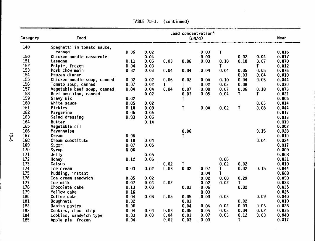
TABLE 7D-l. (continued)
lead concentration* Category Food (JJg/g) Mean
149 Spaghetti in tomato sauce, canned 0.06 0.02 0.03 T 0.016
150 Chicken noodle casserole 0.04 0.03 0.02 0.04 0.017 151 lasagne 0.11 0.06 0.03 0.06 0.03 0.10 0.10 0.07 0.070 152 Potpie, frozen 0.04 0.03 T T 0.012 153 Pork chow mein 0.32 0.03 0.04 0.04 0.04 0.04 0.05 0.05 0.076 154 Frozen dinner 0.03 0.04 0.010 155 Chicken noodle soup, canned 0.02 0.02 0.06 0.02 0.04 0.10 0.04 0.05 0.044 156 Tomato soup, canned 0.07 0.02 T T 0.02 0.03 0.08 0.030 157 Vegetable beef soup, canned 0.04 0.04 0.04 0.07 0.08 0.07 0.06 0.18 0.073 158 Beef bouillon, canned 0.02 0.03 0.05 0.04 T T 0.021 159 Gravy mix 0.02 T 0.005 160 White sauce 0.05 0.02 0.03 0.014 161 Pickles 0.10 0.09 T 0.04 0.02 T 0.08 0.044 162 Margarine 0.06 0.06 0.017 163 Salad dressing 0.03 0.06 0.013 164 Butter 0.14 0.019 165 Vegetab 1 e oil 0.002 166 Mayonnaise 0.06 0.15 0.028
......... 167 Cream 0.06 T 0.010 CJ
I 168 Cream substitute 0.10 0.04 0.04 0.024 m 169 Sugar n n-, 0.05 0.017 u.u1 170 Syrup 0.06 0.009 171 Jelly 0.05 0.008 172 Honey 0.12 0.06 0.06 0.031 173 Catsup 0.02 T 0.02 0.02 0.010 174 Ice cream 0.03 0.02 0.03 0.02 0.07 T 0.02 0.15 0.044 175 Pudding, instant 0.04 T 0.008 176 Ice cream sandwich 0.05 0.02 0.02 0.08 0.29 0.058 177 Ice milk 0.07 0.04 0.02 0.02 0.02 T 0.023 178 Chocolate cake 0.13 0.03 0.03 0.06 0.02 0.035 179 Yellow cake 0.16 0.03 0.025 180 Coffee cake 0.04 0.03 0.05 0.05 0.03 0.03 0.09 0.040 181 Doughnuts 0.02 0.03 0.02 0.010 182 Danish pastry 0.06 0.04 0.04 0.02 0.03 0.03 0.028 183 Cookies, choc. chip 0.04 0.03 0.03 0.05 0.04 0.03 0.04 0.02 0.035 184 Cookies, sandwich type 0.03 0.03 0.04 0.03 0.07 0.03 0.12 0.03 0.048 185 Apple pie, frozen 0.04 0.02 0.03 0.03 T 0.017
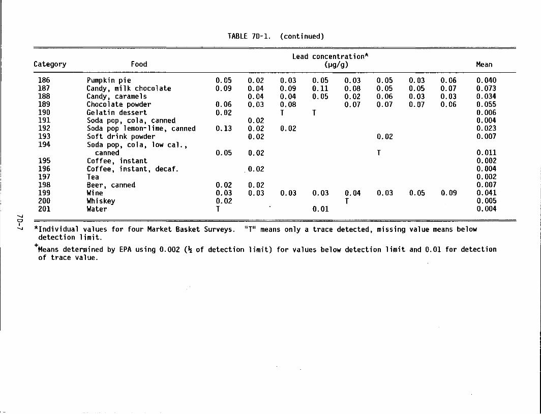
TABLE 70-1. (continued}
Lead concentration* Category Food (j.Jg/g} Mean
186 Pumpkin pie 0.05 0.02 0.03 0.05 0.03 0.05 0.03 0.06 0.040 187 Candy, milk chocolate 0.09 0.04 0.09 0.11 0.08 0.05 0.05 0.07 0.073 188 Candy, caramels 0.04 0.04 0.05 0.02 0.06 0.03 0.03 0.034 189 Chocolate powder 0.06 0.03 0.08 0.07 0.07 0.07 0.06 0.055 190 Gelatin dessert 0.02 T T 0.006 191 Soda pop, cola, canned 0.02 0.004 192 Soda pop lemon-lime, canned 0.13 0.02 0.02 0.023 193 Soft drink powder 0.02 0.02 0.007 194 Soda pop, cola, low cal.,
canned 0.05 0.02 T 0.011 195 Coffee, instant 0.002 196 Coffee, instant, decaf. 0.02 0.004 197 Tea 0.002 198 Beer, canned 0.02 0.02 0.007 199 Wine 0.03 0.03 0.03 0.03 0.04 0.03 0.05 0.09 0.041 200 Whiskey 0.02 T 0.005 201 Water T 0.01 0.004
"' a I
*Individual values "' for four Market Basket Surveys. 11 T11 means only a trace detected, missing value means below detection limit.
+Means determined by EPA using 0.002 (~of detection limit} for values below detection limit and 0. 01 for detection of trace value.
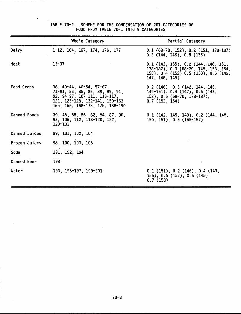
Dairy
Meat
Food Crops
Canned Foods
Canned Juices
Frozen Juices
Soda
Canned Beer
Water
TABLE 7D-2. SCHEME FOR THE CONDENSATION OF 201 CATEGORIES OF FOOD FROM TABLE 7D-1 INTO 9 CATEGORIES
Whole Category
1-12, 164, 167, 174, 176, 177
13-37
38, 40-44, 46-54, 57-67, 71-81, 83, 85, 86, 88, 89, 91, 92, 94-97, 107-111, 113-117, 121, 123-128, 132-141, 159-163 165, 166, 168-173, 175, 188-190
39, 45, 55, 56, 82, 84, 87, 90, 93, 106, 112, 118-120, 122, 129-131
99, 101, 102, 104
98, 100, 103, 105
191, 192, 194
198
193, 195-197, 199-201
7D-8
Partial Category
0.1 (68-70, 152), 0.2 (151, 178-187) 0.3 (144, 146), 0.5 (156)
0.1 (143, 155), 0.2 (144, 146, 151, 178-187), 0.3 (68-70, 145, 153, 154, 158), 0.4 (152) 0.5 (150), 0.6 (142, 147, 148, 149)
0.2 (148), 0.3 (142, 144, 146, 149-151), 0.4 (147), 0.5 (143, 152), 0.6 (68-70, 178-187), 0.7 (153, 154)
0.1 (142, 145, 149), 0.2 (144, 148, 150, 151), 0.5 (155-157)
0.1 (151), 0.2 (146), 0.4 (143, 155), 0.5 (157), 0.6 (145), 0.7 (158)
7E REFERENCES
Akland, G. G. (1976) Air quality data for •etals, 1970 through 1974, from the National Air Surveillance Network. Research Triangle Park, NC: U.S. Environmental Protection Agency, Office of Research and Development; EPA report no. EPA 600/ 4-76-041. Available from: NTIS, Springfield, VA; PB 260905.
Annual averages of lead from NFAN as of September 1982. (1982) From: NFAN, National Filter Analysis Network [Data base]. Research Triangle Park, NC: U.S. Environmental Protection Agency, Environmental Monitoring Systems Laboratory. Printout. Available for inspection at: U.S. Environ•ental Protection Agency, Environmental Criteria and Assessment Office, Research Triangle Park, NC.
Barltrop, D.; Strehlow, C. D.; Thornton, I.; Webb, J. S. (1975) Absorption of lead from dust and soil. Postgrad. Med. J. 51: 801-804.
Bernstein, D. M.; Rahn, K. A. (1979) New York summer aerosol study: trace element concentrations as a function of particle size. Ann. N.Y. Acad. Sci. 322: 87-97.
Buckley et al. (1973) - See U.S. Environmental Protection Agency. (1972).
Burrows, G. E. (1976) Lead: from the factory to the home. Liverpool, United Kingdom: University of Liverpool. M.D. thesis.
Cawse, P. A. (1974) A survey of atmospheric trace elements in the U.K. (1972-73). Harwell, United Kingdom: Atomic Energy Research Establishment, Environmental & Medical Sciences Division. Available from: NTIS, Springfield, VA; AERE-R7669.
Cholak, J.; Schafer, L. J.; Yeager, D. (1968) The air transport of lead compounds present in automobile exhaust gases. J. Am. Ind. Hyg. Assoc. 29: 562-568.
Daines, R. H.; Motto, H.; Chilko, D. M. (1970). Atmospheric lead: its relationship to traffic volume and proximity to highways. Environ. Sci. Technol. 4: 318-322.
Darrow, D. K.; Schroeder, H. A. (1974) Childhood exposure to lead. Adv. Exp. Med. Bfol. 48: 425-445.
Davidson, C. 1.; Nasta, M. A.; Reilly, M. T.; Suuberg, E. M. (1980) Dry deposition of trace elements in Great Smoky Mountains National Park. Part I: Airborn concentrations and size distributions Carnegie-Mellon University report.
Davidson, C. I. (1977) The deposition of trace metal-containing particles in the Los Angeles area. Powder Technol. 18: 117-126.
Davidson, C. I.; Goold, W. D.; Nasta, M. A.; Reilly, M. T. (198la) Airborne size distributions of trace elements in an industrialized section of Pittsburgh. In: Proceedings, 74th Air Pollution Control Administration annual meeting; June; Philadelphia, PA. Pittsburgh, PA: Air Pollution Control Association; paper no. 81-28.6.
Davidson, C. I.; Grimm, T. C.; Nasta, M. A. (1981b) Airborne lead and other elements derived from local fires in the Himalayas. Science (Washington D.C.) 214: 1344-1346.
7E-1
DeSilva, P. E.; Donnan, M. B. (1980) Blood lead levels in Victorian children. Med. J. Au$t. 2: 315-318.
Diemel, J. A. L.; Brunekreef, B.; Boleij, J. S. M.; Biersteker, K.; Veenstra, S. J. (1981) The Arnhem lead study. II: Indoor pollution, and indoor/outdoor relationships. Environ. Res. 25: 449-456.
Dol court, J. L.; Hamrick, H. J.; O'Tuama, L. A.; Wooten, J.; Barker, E. L., Jr. (1978) Increased lead burden fn children of battery workers: asymptomatic exposure resulting from contaminated work clothing. Pediatrics 62: 563-566.
Dolcourt, J. L.; Finch, C.; Coleman, G. D.; Klimas, A. J.; Milar, C. R. (1981) Hazard of lead exposure in the home from recycled automobile stor·age batteries. Pediatrics 68: 225-230.
Dorn, C. R.; Pierce, J. 0., II; Phillips, P. E.; Chase-, G. R. (1976) Airborne Pb, Cd, Zn and Cu concentration by particle size near a Pb smelter·. Atmos. Environ. 10: 443-446.
Duce, R. A.; Ray, B. J.; Hoffman, G. L.; Walsh, P. R. (1976) Trace metal concentration as a function of particle sfze in marine aerosols from Bermuda. Geophys. Res. Lett. 3: 339-342.
Elwood, W. J.; Clayton, B. E.; Cox, R. A.; Delves, H. T.; King, E.; Malcolm, D.; Ratcliffe, J. M.; Taylor, J. F. {1977) Lead in human blood •snd in the environment near a battery factory. Br. J. Prev. Soc. Med. 31: 154-163.
Fritsch, A.; Prival, M. (1972) Response to the Unned States Environmental Protection Agency's notice for additional health effects inf~ormation concerning the use of leaded gasoline. Washington, DC: Center for Science in t;he Public Interest; pp. 11.
Fugas, M. (1977) Biological significance of some metatls as air pollutants. Part I: Lead. Research Triangle Park, NC: U.S. Environmental Protection Agency, Health Effects Research Laboratory; EPA report no. EPA-600/1-77-041. Avai'lable from: NTIS, Springfield, VA; PB 274055.
Gillette, D. A.; Winchester, J. W. (1972) A study of ag·ing of lead aerosols. I: Observations. Atmos. Environ. 6: 443-450.
Goold, W. D.; Davidson, C. I. (1982) Sources and sinks of airborne trace elements in Olympic National Park biosphere reserve, Carnegie-Mellon Uniiversity report.
Harrison, P. R.; Matson, W. R.; Winchester, J. W. (1971.) Time variations of lead, copper and cadmium concentrations in aerosols in Ann Arbor, Michigan. Atmos. Environ. 5: 613-619.
Harrison, R. M. (1979) Toxic aetals in street and houuhold dusts. Sci. Total Environ. 11: 89-97.
Heyworth, F.; Spickett, J.; Dick, M.; Margetts, B.; Armstrong, B. (1981) Tailings from a lead mine and lead levels in school children: a preliminary report. Med. J. Aust. 2: 232-234.
Huntzicker, J. J.; Friedlander, S. K.; Davidson, C. I. (1975) Material balance for automobileemitted lead in Los Angeles basin. Environ. Sci. Technol. 9: 448-457.
7E-2
Johansson, T. B.; Van Grieken, R. E.; Winchester, J. W. (1976) Elemental abundance variation with particle size in north Florida aerosols. J. Geophys. Res. 81: 1039-1046. ·
Kennedy, G. L., Jr. (1973) Blood and tissue lead content study following exposure of 111ale albino rats to lead-containing expressway dirt, neighborhood street dirt, lead acetate, or lead oxide. Northbrook, Il: Industrial Bio-Test laboratories; Research report IBT no. n733C.
lee, R. E., Jr.; Patterson, R. K.; Wagman, J. (1968) Particlesize distribution of metal compounds in urban air. Environ. Sci. Technol. 2: 288-290.
Lee, R. E., Jr.; Goranson, S. S.; Enrione, R. E.; Morgan, G. B. (1972) National air surveillance cascade impactor network. Part II: Size distribution measurements of trace metal ~omponents. Environ. Sci. Technol. 6: 1025-1030.
Lombardo, L. V. (1973) [Letter to Mr. William D. Ruckelhaus]. March 9. Available ...
Lundgren, D. A. (1970) Atmospheric aerosol composition and concentration as a function of particle size and of time. J. Air Pollut. Control Assoc. 20: 603-608.
Martens, C. S.; Wesolowski, J. J.; Kaifer, R.; John, W. (1973) Lead and bromine particle size distributions in the San Francisco Bay area. Atmos. Environ. 7: 905-914.
McDonald, C.; Duncan, H. J. (1979) Particle size distribution of metals in the atmosphere of Glasgow. Atmos. Environ. 13: 977-980.
Morton, D. E.; Saah, A. J.; Silberg, S. L.; Owens, W. L.; Roberts, M. A.; Saah, M. D. (1982) Lead absorption in children of employees ;n a lead-related industry. Am. J. Epidemiol. 115: 549-555.
Needleman, H. l.; Scanlon, J. (1973) Getting the lead out. N. Engl. J. Med. 288: 466-467.
Needleman, H. L.; Davidson, I.; Sewell, E. M.; Shapiro, I. M. (1974) Subclinical lead exposure in Philadelphia school children: identification by dentine lead analysis. N. Engl. J. Med. 290: 245-248.
Heri, L. C.; Johansen, H. L.; Schmitt, N.; Pagan, R. T.; Hewitt, D. (1978) Blood lead levels in children in two British Columbia co111111unities. In: Hemphill, D. D., ed. Trace substances in environmental health-XII: [proceedings of University of Missouri's 12th annual conference on trace substances in environmental health]; June; Columbia, MO. Columbia, MO: University of Missouri-Columbia; pp. 403-410.
Pattenden, N. J. (1974) Atmospheric concentrations and deposition rates of some trace elements aeasured in the Swansea/Neath/Port Talbot area. Harwell, United Kingdom: Atomic Energy Research Establishment, Environment and Medical Sciences Division. Available from: NTIS, Springfield, VA; AERE-R7729.
Peden, M. E. (1977) Flameless atomic absorption determinations of cadmium, lead, and manganese in particle size fractionated aerosols. In: Kirchhoff, W. H., ed. Methods and standards for environmental measurement: proceedings of the 8th materials research symposium; September 1976; Gaithersburg, MD. Washington, DC: U.S. Department of Commerce, National Bureau of Standards; special publication no. 464; pp. 367-378.
7E-3
Pennington, J. A. T. (1983) Revision of the total diet :study food list and diets. J. Am. Diet. Assoc. 82: 166-173.
Pinkerton, C.; Creason, J. P.; Hammer, D. I.; Colucci·, A. V. (1973) Multi-media indices of environmental trace-metal exposure in humans. ln: Hoekstra, W. G.; Suttie, J. W.; Ganther, H. E.; Mertz, W., eds. Trace element .atabolism in animals-2: proceedings of the 2nd international symposium on trace element Mtabolism in animals; Madison, WI. Baltimore, MD: University Park Press; pp. 465-469.
Popovac, D.; Graziano, J.; Seaman, C.; Kaul, 8.; Colakovic, B.; Popovac, R.; Osmani, I.; Haxhiu, M.; Begraca, M.; Bozovic, Z.; Mikic, M. (1982) Elevated blood lead in a population near a lead smelter in Kosovo, Yugoslavia. Arc:h. Environ. Health 37: 19-23.
Quarterly averages of lead from NFAN as of September 1982. (1982) From: NFAN, National Filter Analysis Network [Data base]. Research Triangle Park, NC: U.S. Environmental Protection Agency, Environmental Monitoring Systems laborator~. Printout. Available for inspection at: U.S. Environmental Protection Agency, Environmental Criteria and Assessment Office, Research Triangle Park, NC.
Rameau, J. T. L. B. (1973) Lead as an environmental pollutant. In: Proceedings, international symposium: environmental health aspects of lead. Amsterdam, The Netherlands; October 1972. Luxembourg: Commission of the European Communities; pp. 189-200.
Rice, C.; Fischbein, A.; lil{s, R.; Sarkozi, L.; Kon, S.; Selikoff, I. J. (1978) lead contamination in the ho~es of employees of secondary lead smelters. Environ. Res. 15: 375-380.
Roels, H. A.; Buchet, J-P.; lauwerys, R. R.; Bruaux, P .. ; Claeys-Thoreau, F.; Lafontaine, A.; Verduyn, G. (1980) Exposure to lead by the oral and the pulmonary routes of children living in the vicinity of a primary lead smelter. E1wiron. Res. 22: 81-94.
Roels, H. A.; Buchet, J-P.; lauwerys, R.; Bruaux, P.; Claeys-Thoreau, F.; Lafontaine, A.; van Overschelde, J.; Verduyn, G. (1978) Lead and cadmium absorption among children near a nonferrous metal plant: a follow-up study of a t1est case. Environ. Res. 15: 290-308.
Roy, B. R. (1977) Effects of particle sizes and solubilities of lead sulphide dust on mill workers. Am. Ind. Hyg. Assoc. J. 38: 327-332.
Schmitt, N.; Philion, J. J.; Larsen, A. A.; Harnadek, M.; Lynch, A. J. (1979) Surface soil as a potential source of lead exposure for young children. Can. Med. Assoc. J. 121: 1474-1478.
Shapiro, I. M.; Dobkin, B.; Tuncay, 0. C.; Needleman, H. L. (1973) Lead levels in dentine and circumpulpal dentine of deciduous teeth of normal and lead poisoned children. Clin. Chim. Acta 46: 119-123.
Shearer, S. D.; Akland, G. G.; Fair, D. H.; McMullen, 1'. B.; Tabor, E. C. (1972) Concentrations of particulate lead in the ambient air of the United States. Statement presented at Public Hearing on Gasoline Lead Additives Regulat'ions; May; Los Angeles, CA. Research Triangle Park, NC: U.S. Environmental Protection Agency, National Environmental Research Center.
Ter Haar, G.; Aronow, R. (1974) New information on lead in dirt and dust as related to the childhood lead problem. Environ. Health Perspect. 7: 83-89.
7E-4
U.S. Environmental Protection Agency. (1972) EPA's position on the health effects of airborne lead. Washington, DC: U.S. Environmental Protection Agency, Processes and Effects Division. Available from: NTIS, Springfield, VA; PB 228594.
U.S. Environmental Protection Agency. (1978) Air quality data for •etals 1975 from the National Air Surveillance Networks. Research Triangle Park, NC: U.S. Environmental Protection Agency; Office of Research and Development; EPA report no. EPA-600/4-78-059. Available from: NTIS, Springfield, VA; PB 293106.
U.S. Environmental Protection Agency. (1979) Air quality data for metals 1976 from the National Air Surveillance Networks. Research Triangle Park, NC: U.S. Environmental Protection Agency, Office of Research and Development; EPA report no. EPA-600/4-79-054. Available from NTIS, Springfield, VA; PB80-147432.
Vostal, J. J.; Taves, E.; Sayre, J. W.; Charney, E. (1974) Lead analysis of the house dust: a inner city children. Environ. Health Perspect. 7: 91-97.
Wagner, V.; Wagnerova, M.; Wokounova, D.; Kriz, J.; Madlo, Z.; Mohyla, 0. (1981) Correlations between blood lead concentrations and some blood protein levels in children residing in lead-polluted and control areas. J. Hyg. Epidemiol. Microbial. Immunol. 25: 97-112.
Watson, W. N.; Witherell, L. E.; Giguere, G. C. (1978) Increased lead absorption in children of workers in a lead storage battery plant. J. Occup. Med. 20: 759-761.
Wesolowski, J. J.; Flessel, C. P.; Twiss, S.; Stanley, R. L.; Knight, N. W.; Coleman, G. C.; DeGarmo, T. E. (1979) The identification and elimination of a potential lead hazard in an urban park. Arch. Environ. Health 34: 413-418.
7E-5
8. EFFECTS OF LEAD ON ECOSYSTEMS
8.1 INTRODUCTION
8.1.1 Scope of Chapter 8 This chapter describes the potential effects of atmospheric lead inputs on several types
of ecosystems. An effect is any condition attributable to lead that causes an abnormal
phys i o 1 ogi ca 1 response in i ndi vi dua 1 organisms or that perturbs the norma 1 processes of an
ecosystem. A distinction is made among natural, cultivated, and urban ecosystems, and extend
ed discussions are included on the mobility and bioavailability of lead in ecosystems.
There are many reports on the effects of lead on individual populations of plants and
animals and a few studies on the effects of lead in simulated ecosystems or microcosms.
However, the most rea 1 i st i c studies are those that exumi ne the effects of 1 ead on entire
ecosystems, as they incorporate a 11 of the eco 1 ogi ca 1 interactions among the various popu
lations and all of the chemical and biochemical processE!S relating to lead (National Academy
of Sciences, 1981). Unfortunately, these studies have a 1 so had to cope with the inherent
variability of natural systems and the confounding frustrations of large-scale projects.
Consequently, there are only a handful of ecosystem studies on which to base this report.
Effects at the ecosystem level are usually seen as a form of stress. In nearly every
case of stress caused by pollutants, the initial effect is to cause cytological or biochemical
changes in specific cells of individual organisms. Mclaughlin (1985) has summarized some of
the effects on forest ecosystems that have been caused by air pollutants. Examp 1 es of cyto
logical or biochemical changes are reduction in enzyme ctctivity, a change in membrane perme
ability or osmotic potential, or a loss of organelle int~egrity. These cellular changes cause
some disruption of physiological function, such as photosynthesis, respiration, transpiration,
root uptake, the opening and closing of stomata, or a disruption of resource allocation, such
as growth, reproduction, or defense mechanisms. In turn, the growth of the individual may be
directly or indirectly affected, either in amount, timing, or quality. These effects on the
individual can cause a change in the productivity of the ~~ntire community. Some of the expec
ted effects on the community as a whole or populations 1r1ithin the community might be reduced
growth, increased mortality, unbalanced competition, delayed succession, or reduced rate of
reproduction.
Because of the complexity of processes that can affect an ecosystem, it is difficult to
predict the mechanism by which a specific air pollutant might influence an ecosystem. General
categories of effects are those that predispose an ecosystem to stress, those that incite
stress, and those that contribute directly to stress (from Manion, 1981, as modified by
Mclaughlin, 1985). Examples of predisposition are chr1)nic weakening caused by changes in
8-1
climate, soil moisture, soil nutrients, or competition. Inciting factors are triggering episodes, such as insect defoliation, frost, drought, mechanical injury or increased salinity: Those factors that directly contribute to effects generally do so by accelerating the processes already taking place, such as infections of bark beetles, canker fungi, viruses, root decay fungi, or increased competition. As a general rule, air pollutants are either predisposing or inciting types of agents and are noticed only when a change is triggered by the effect of the pollutant. The effects of air pollutants may go unnoticed for decades, causing only a chronic weakening that cannot be detected by normal methods of evaluating ecosystem stability.
The pri nci p 1 e sources of 1 ead entering an ecosystem inc 1 ude the fo 11 owing: the atmosphere (largely from automotive emissions), paint chips, spent ammunition, the application of fertilizers and pesticides, and the careless disposal of lead-acid batteries or other industria 1 products. Atmospheric 1 ead is deposited on the surfaces of vegetation as we 11 as on ground and water surfaces. In terrestrial ecosystems, this lead is transferred to the upper layers of the soil surface, where it may be retained for a period of several years. The movement of lead within ecosystems is influenced by the chemical and physical properties of lead and by the bi ogeochemi ca 1 processes within the ecosystem. Lead is persistent, but in the appropriate chemical environment, may undergo transformations that affect its solubility (e.g., formation of lead sulfate in soils), its bioavailability (e.g., chelation with humic substances), or its toxicity (e.g., chemical methyla~ion).
Because the effects of 1 ead on ecosystems begin with some i nit i a 1 effect on specific cells of individuals within the ecosystem, there are a number of mechanisms or strategies whereby individuals or populations may have developed a resistance to lead toxicity. Wood (1984) has described six potential strategies for resistance to toxic metals: 1) the cell may pump the metal out through the cell membrane, a process that requires energy; 2) the metal may be enzymatically oxidized or reduced to a less toxic form; 3) the cell may synthesize a polymer to trap and remove the metal; 4) the metal may be bound to the cell surface; 5) the metal may be precipitated as an insoluble metal complex; 6) the metal may be biomethylated and transported through the cell membrane by diffusion a process that requires less energy than actively pumping. The evidence for the biomethylation of lead is circumstantial at best and clearly not conclusive (Craig and Wood, 1981, Reisinger et al., 1981, Chau, 1986).
The previous Air Quality Criteria for Lead (U.S. Environmental Protection Agency, 1977) recognized the problems of atmospheric lead exposure incurred by all organisms including man. Emphasis in the chapter on ecosystem effects was given to reports of toxic effects on specific groups of organisms, e.g. domestic animals, wildlife, aquatic organisms, and vascular and nonvascular plants. Forage containing lead at 80 j.lg/g dry weight was reported to be lethal to horses, whereas 300 !Jg/g dry weight caused lethal clinical symptoms in cattle. This report
8-2
will attempt to place the data in the context of sublethctl effects of lead exposure, to extend the conclusions to a greater variety of domestic animals, and to describe the types and ranges of exposures in ecosystems likely to present a problem fc,r domestic animals.
Research on lea~ in wildlife has traditionally fallen into the following somewhat artificial categories: waterfowl; birds and small mammals; fish; and invertebrates. In all these categories, no correlation could be made in the 1977 repo,rt between toxic effects and environmental concentrations. Some recent toxicity studies have been completed on fish and invertebrates and the data are reported below, but there is still little information on the levels of lead that can cause toxic effects in small mammals or bir·ds.
Information on the re 1 at i onship between soi 1 1 ead and p 1 ants can be expanded somewhat beyond the 1977 report, primarily due to a better understanding of the role of humic substances in binding lead. Although the situation is extremely complex, it is reasonable to state that most plants cannot survive in soil containinq 10,000 IJg/g dry weight if the pH is bel ow 4. 5 and the organic content is be 1 ow 5 percent. The specifics of this statement are discussed more extensively in Section 8.3.1.2.
Before 1977, natura 1 1 eve 1 s of 1 ead in en vi ronmenta l media other than soil were not we 11 known. Reports of sublethal effects of lead were spars~~ and there were few studies of total ecosystem effects. Although several ecosystem studies have been completed since 1977 and many problems have been overcome, it is still difficult to translate observed effects under. specific conditions directly to predicted effects in ecosystems. Some of the known effects, which are documented in detail in the appropriate sections, are summarized here. 8.1.1.1 Plants. The basic effect of lead on plants is to stunt growth. This may be through a reduction of photosynthetic rate, inhibition of respiration, cell elongation, or root development, or premature senescence. Lead tolerance in ecotypes suggests some effects on population genetics. All of these effects have been observed in isolated cells or in hydroponicallygrown plants in solutions comparable to 1 to 2 IJg/g soil moisture. These concentrations are well above those normally found in any ecosystem except near smelters or roadsides. Terrestrial plants take up lead from the soil moisture and rnost of this lead is retained by the roots. There is some evidence for foliar uptake of lead and little evidence that lead can be translocated freely to the upper portions of the plant. Soil applications of calcium and phosphorus may reduce the uptake of lead by roots. 8.1.1.2 Animals. Lead affects the central nervous system of animals and their ability to synthesize red blood cells. Blood concentrations above 0.4 ppm (40 IJg/dl) can cause observable clinical symptoms in domestic animals. Calcium and phosphorus can reduce the intestinal absorption of lead. The physiological effects of lead exposures in laboratory animals are discussed in extensive detail in Chapters 10 and 12 of this document.
8-3
8.1.1.3 Microorganisms. There is evidence that lead at environmental concentrations occa-:sionally found near roadsides and smelters [10,000- 40,000 ~g/g dw (dry weight)] can eliminate populations of bacteria and fungi on leaf surfaces and in soil. Many of those microorganisms play key roles in the decomposition food chain. It is likely that the affected microbial populations are replaced by others of the same or different species, perhaps less efficient at decomposing organic matter. There is also evidence that microorganisms can mobilize lead by making it more soluble and more readily taken up by plants. This process occurs when bacteria exude organic acids that lower the pH in the immediate vicinity of the plant root.
8.1.1.4 Ecosystems. There are three known conditions under which lead may perturb ecosystem processes. At soil concentrations of 1,000 ~g/g or higher, delayed decomposition may result from the elimination of a single population of decomposer microorganisms. Secondly, at concentrations of 500 - 1,000 ~g/g, populations of plants, microorganisms, and invertebrates may shift toward lead-tolerant populations of the same or different species. Finally, the normal biogeochemical process that purifies and repurifies the calcium pool in grazing and decomposer food chains may be circumvented by the addition of lead to vegetation and animal surfaces. This third effect can be measured at all ambient atmospheric concentrations of lead.
Some additional effects may occur due to the uneven distribution of lead in ecosystems. It is known that lead accumulates in soil, especially soil with high organic content. Although no firm documentation exists, it is reasonable to assume the following from the known chemistry of 1 ead in soi 1: 1) other meta 1 s may be di sp 1 aced from the binding sites on the organic matter; 2) the chemical breakdown of inorganic soil fragments may be retarded by the interference of lead with the action of fulvic acid on iron-bearing crystals; and 3) lead in soil may be in equilibrium with moisture films surrounding soil particles and thus be available for uptake by plants.
To aid the reader in understanding the effects of lead on ecosystems, sections have been included that discuss such important matters as how ecosystems are organized, what processes regulate metal cycles, what criteria are valid in interpreting ecosystem effects, and how soil systems function to regulate the contra 11 ed re 1 ease of nutrients to p 1 ants. The informed reader may wish to turn directly to Section 8.3, where the discussion of the effects of lead on organisms begins.
I
8.1.2 Ecosystem Functions 8.1.2.1 Types of Ecosystems. Based on ambient concentrations of atmospheric lead and the distribution of lead in the soil profile, it is useful to distinguish among three types of ecosystems: natural, cultivated, and urban. Natural ecosystems include aquatic and terrestrial
8-4
ecosystems that are otherwise unperturbed by man, and those managed ecosystems, such as com
mercial forests, grazing areas, and abandoned fields, where the soil profile has remained un~
disturbed for several decades. Cultivated ecosystems include those where the soil profile is
frequently disturbed and those where chemical fertili:zers, weed killers, and pest-control
agents may be added. In urban ecosystems, a significant part of the exposed surface includes
rooftops, roadways, and parking lots from which runoff, if not channeled into municipal waste
processing plants, is spread over relatively small areas of soil surface. The ambient air
concentration of lead in urban ecosystems is 5 - 10 times. higher than in natural or cultivated
ecosystems (See Chapter 7). Urban ecosystems may also be exposed to lead from other than
atmospheric sources, such as paint, discarded batteries~, and used motor oil. The effects of
atmospheric 1 ead depend on the type of ecosystems exami ne!d.
8.1.2.2 Energy Flow and Biogeochemical Cycles. To func:tion properly, ecosystems require an
adequate supply of energy, which continually flows through the system, and an adequate supply
of nutrients, which for the most part, cycle within the ecosystem. There is evidence that
lead can interfere with both of these processes. Energy usually enters the ecosystem in the
form of sunlight and leaves as heat of respiration. Stored chemical energy may be transported
into or out of an ecosystem (e.g., leaf detritus in a stream) or be retained by the ecosystem
for long periods of time (e.g., tree trunks). Energy flow through an ecosystem may give
structure to the ecosystem by establishing food webs that efficiently regulate the transfer
of energy. Segments of these food webs are called food chains. Energy that flows a 1 ong a
grazing food chain is diverted at each step to the detrital food chain.
Unlike energy, nutrient and non-nutrient elements are recycled by the ecosystem and
transferred from reservoir to reservoir in a pattern usually referred to as a biogeochemical
cycle (Brewer, 1979, p. 139). The reservoirs correspond approximately to the food webs of
energy flow. A 1 though e 1 ements may enter (e.g. , weathering of so i1) or 1 eave the ecosystem
(e.g., stream runoff), the greater fraction of the available mass of the element is usually
cycled within the ecosystem.
Two important characteristics of a reservoir are the amount of the e 1 ement that may be
stored in the reservoir and the rate at which the e 1 ement enters or 1 eaves the reservoir.
Some reservoirs may contain a disproportionately large ctmount of a given element. For exam
ple, most of the carbon in a forest is bound in the trunks and roots of trees, whereas most of
the calcium may be found in the soil (Smith, 1980, p. 316). Some large storage reservoirs,
such as soil, are not actively involved in the rapid exchange of the nutrient element, but
serve as a reserve source of the element through the slow exchange with a more active reser
voir, such as soil moisture. When inputs exceed outputs, the size of the reservoir increases.
Increases of a single element may reflect instability of the ecosystem. If several elements
increase simultaneously, this expansion may reflect stable growth of the community.
8-5
Reservoirs are connected by pathways that represent rea 1 ecosystem processes. Figure 8-1 depicts the biogeochemical reservoirs and pathways of a typical terrestrial ecosystem; Most elements, especially those with no gaseous phase, do not undergo changes in oxidation state and are equally available for exchange between any two reservoirs, provided a pathway exists between the two reservoirs. The chemica 1 environment of the reservoir may, however, regulate the availability of an element by controlling solubility or·binding strengths. This condition is especially true for soils.
Ecosystems have boundaries. These boundaries may be as distinct as the border of a pond or as arbitrary as an imaginary circle drawn on a map. Many trace metal studies are conducted in watersheds where some of the boundaries are determined by topography. For atmospheric inputs to terrestrial ecosystems, the boundary is usually defined as the surface of vegetation, exposed rock, or soil. The water surface suffices for aquatic ecosystems.
Non-nutrient elements differ little from nutrient elements in their biogeochemical cycles. Quite often, the cycling patterns are similar to those of a major nutrient. In the case of lead, the reservoirs and pathways are very similar to those of calcium.
There are three important questions concerning the effect of lead on ecosystems: Does atmospheric 1 ead interfere with the norma 1 mechanisms of nutrient eye 1 es? How does atmospheric lead influence the normal lead cycle in an ecosystem? Can atmospheric lead interfere with the normal flow of energy through an ecosystem? 8.1.2.3 Biogeochemistry of Lead. Naturally occurring lead from the earth's crust is common1y found in soi 1 s and the atmosphere. Lead may enter an ecosystem by weathering of parent rock or by deposition of atmospheric particles. This lead becomes a part of the nutrient medium of plants and the diet of animals. All ecosystems receive lead from the atmosphere. More than 99 percent of the current atmospheric lead deposition is now due to human activities (National Academy of Sciences, 1980). In addition, lead shot from ammunition may be found in many waterways and popular hunting regions, leaded paint chips often occur in older urban regions, and lead in fertilizer may contaminate the soil in agricultural regions.
In prehistoric times, the contribution of lead from weathering of soil was probably about 4 g Pb/ha·yr and from atmospheric deposition about 0.02 g Pb/ha•yr, based on estimates of natural and anthropogenic emissions in Chapter 5 and deposition rates discussed in Chapter 6. Weathering rates are presumed to have remained the same, but atmospheric inputs are believed to have increased to 180 g/ha·yr in natural and some cultivated ecosystems, and 3,000 g/ha·yr in urban ecosystems and along roadways (see Chapter 6). In every terrestrial ecosystem of the Northern Hemisphere, atmospheric 1 ead deposition now exceeds weathering by a factor of at least 10, sometimes by as much as 1,000.
8-6
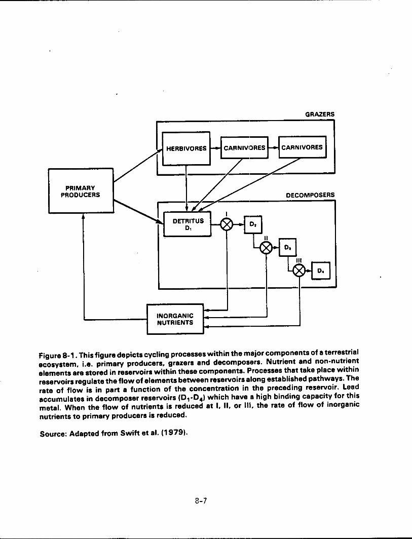
PRIMARY PRODUCERS
INORGANIC NUTRIENTS
GRAZERS
DECOMPOSERS
Figure 8-1. This figure depicts cycling processes within the major components of a terrestrial ecosystem. i.e. primary producers. grazers and decomposers. Nutrient and non-nutrient elements are stored in reservoirs within these components. Processes that take place within reservoirs regulate the flow of elements between reservoirs along established pathways. The rate of flow is in part a function of the concentration in the preceding reservoir. Lead accumulates in decomposer reservoirs (01-04 ) which have a high binding capacity for this metal. When the flow of nutrients is reduced at I. II. or m. the rate of flow of inorganic nutrients to primary producers is reduced.
Source: Adapted from Swift at al. (1979).
8-7
Many of the effects of lead on plants, microorganisms, and ecosystems arise from the fact that 1 ead from atmospheric and weathering inputs is retained by soi 1. Geochemi ca 1 studies show that less than 3 percent of the inputs to a watershed leave by stream runoff (Siccama and Smith, 1978; Shirahata et al., 1980). In prehistoric times, stream output nearly equalled weathering inputs and the lead content of soil probably remained stable, accumulating at an annual rate of less than 0.1 percent of the original natural lead (reviewed by Nriagu, 1978). Due to human activity, lead in natural soils now accumulates on the surface at an annual rate
of 5 - 10 percent of the natural lead. One effect of cultivation is that atmospheric lead is
mixed to a greater depth than the 0 - 3 em of natural soils. Most of the effects on grazing vertebrates stem from the deposition of atmospheric parti
cles on vegetation surfaces. Atmospheric deposition may occur by either of two mechanisms. Wet deposition (precipitation scavenging through rainout or washout) generally transfers lead
directly to the soil. Dry deposition transfers particles to all exposed surfaces. Large particles (>4 ~m) are transferred by gravitational mechanisms; small particles (<0.5 ~m) are
also deposited by wind-related mechanisms. About half of the foliar dry deposition remains on leaf surfaces following normal rain
fall (Elias et al., 1976; Peterson, 1978), but heavy rainfall may transfer the lead to other portions of the plant (Elias and Croxdale, 1980). Koeppe (1981) has reviewed the literature and concluded that less than 1 percent of the surface lead can pass directly into the internal
leaf tissues of higher plants. The cuticular layer of the leaves may be an effective barrier to aerosol particles and even to metals i~ solution on the leaf surface (Arvik and Zimdahl, 1974), and passage through the stomata does not appear to account for a significant fraction
of the lead inside leaves (Carlson et al., 1976; 1977). When particles attach to vegetation surfaces, transfer to soil is delayed from a few
months to several years. Due to this delay, large amounts of lead are diverted to grazing food chains, bypassing the soil moisture and plant root reservoirs (Elias et al., 1982).
8.1.3 Criteria for Evaluating Ecosystem Effects As it is the purpose of this chapter to describe the levels of atmospheric lead that may
produce adverse effects in plants, animals, and ecosystems, it is necessary to establish the
criteria for evaluating these effects. The first step is to determine the connection between air concentration and ecosystem exposure. If the air concentration is known, ecosystem inputs
from the atmosphere can be predicted over time and under normal conditions. These inputs and those from the weathering of soil determine the concentration of lead in the nutrient media of
plants, animals, and microorganisms. It follows that the concentration of lead in the nutri
ent medium determines the concentration of lead in the organism and this in turn determines
the effects of lead on the organism.
8-8
The fundamental nutrient medium of a terrestrial ecosystem is the soil moisture film
that surrounds organic and inorganic soil particles. This film of water is in equilibrium
with other soil components and provides dissolved inorganic nutrients to plants. It is chemi
cally different than ground water or rain water and there is little reliable information on
the relationship between lead in soil and lead in soil moisture. Thus, it appears impossible
to quantify. all the steps by which atmospheric lead is transferred to plants. Unti 1 more
information is available on lead in soil moisture, another approach may be more productive.
This involves determining the degree of contamination of organisms by comparing the present
known concentrations with calculated prehistoric concentrations.
Prehistoric concentrations of lead have been calculated for only a few types of organ
isms. However, the results are so low that any normal variation, even of an order of magni
tude, would not seriously influence the calculation of the degree of contamination. The link
between lead in the prehistoric atmosphere and in prehi!itoric organisms may allow us to pre
dict concentrations of lead in organisms based on present or future concentrations of
atmospheric lead.
It is reasonable to infer a relationship between degree of contamination and physio-
1 ogi ca 1 effect. It seems appropriate to assume that Mtura 1 1 eve 1 s of 1 ead that were safe
for organisms in prehistoric times would also be safe today. It is also reasonable that some
additional atmospheric lead can be tolerated by all populations of organisms with no ill
effects, that some populations are more tolerant than others, and that some individuals within
populations are more tolerant of lead effects than others.
For nutrient e 1 ements, the concept of to 1 erance is not new. The Law of To 1 erance
( i 11 ustrated in Figure 8-2) states that any nutrient may be present at concentrations either
too low or too high for a given population and that the ecological success of a population is
greatest at some optimum concentration of the nutrient (Smith, 1980, p. 35). In a similar
manner, the principle applies to non-nutrient elements. Although there is no minimum concen
tration below which the population cannot survive, therE! is a concentration above which the
success of the population will decline (point of initial response) and a concentration at
which the entire population will die (point of absolute toxicity). In this respect, both
nutrients and non-nutrients behave in a similar manner at concentrations above some optimum.
Certain variables make the points of initial response and absolute toxicity somewhat
imprecise. The point of initial response depends on the type of response investigated. This
response may be at the molecular, tissue, or organismic level, with the molecular response
occurring at the lowest concentration. Similarly, at the point of absolute toxicity, death
may occur instantly at high concentrations or over a prolonged period of time at somewhat
8-9
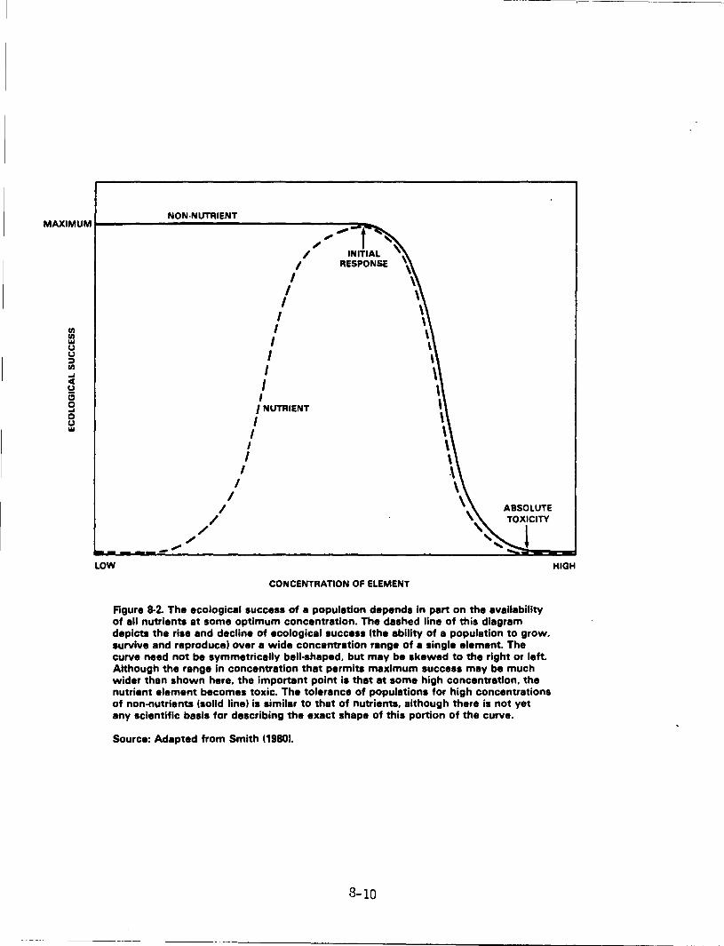
NON-NUTRIENT MAXIMUM~----------------------------------~~~ ," ..... -f
C/1 C/1 161 (,) (,) ::) C/1 ... ~ § 0 (,) 161
/ / _,.
LOW
I /
I I
I
I I
I I I I I I I I
/ INITIAL 1 RESPONSE
I NUTRIENT
I I I I
CONCENTRATION OF ELEMENT
ABSOLUTE TOXICITY
l
Figure 8-2. The ecological success of a population depends in part on the availability of all nutrients at some optimum concentration. The dashed line of this diagram depicts the rise and decline of ecological success (the ability of a population to grow. survive and reproduce! over a wide concentration range of a single element. The curve need not be symmetrically bell-shaped. but may be skewed to the right or left. Although the range in concentration that permits maximum success may be much wider than shown here. the important point is that at some high concentration. the nutrient element becomes toxic. The tolerance of populations for high concentrations of non-nutrients (solid linel is similar to that of nutrients, although there is not yet any scientific basis for describing the exact shape of this portion of the curve.
Source: Adapted from Smith 119801.
8-10
HIGH
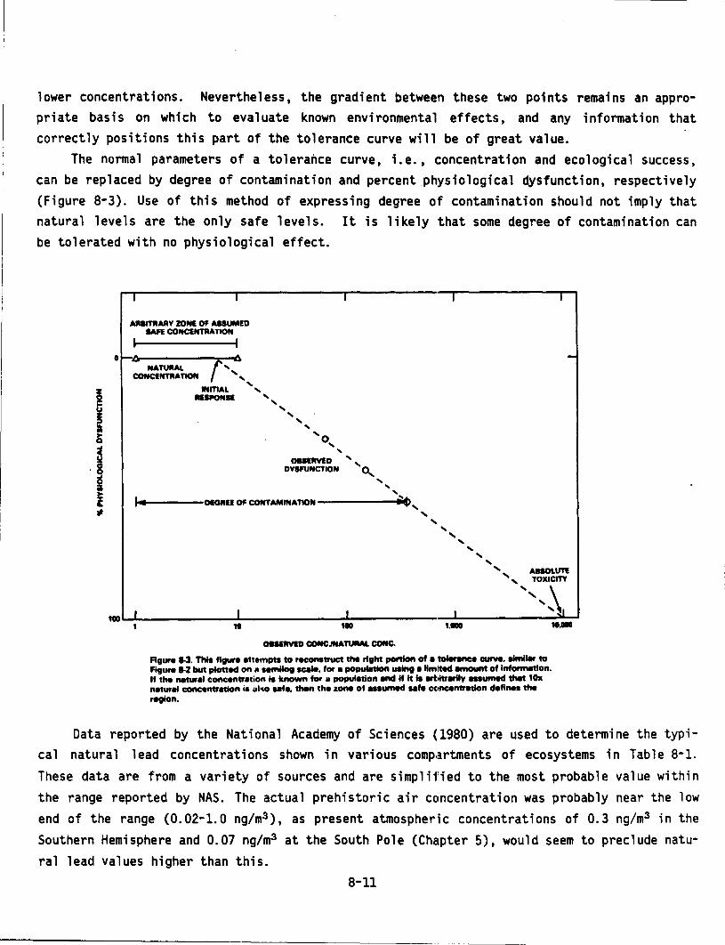
lower concentrations. Nevertheless, the gradient between these two points remains an appropriate basis on which to evaluate known environmental effects, and any information that correctly positions this part of the tolerance curve will be of great value.
The norma 1 parameters of a to 1 erance curve, i.e. , c:oncentrat ion and eco 1 ogi ca 1 success, can be replaced by degree of contamination and percent physiological dysfunction, respectively (Figure 8-3). Use of this method of expressing degree of contamination should not imply that natural levels are the only safe levels. It is likely that some degree of contamination can be tolerated with no physiological effect.
I I
Alt8'"'ARY ZONE OF ASSUMED SAFE CONCENTRATION
I
o :0 A NATURAL ('
CONCENTRATION ',
INmAL ', IIESPONSE ', ... ... ...
' 'o ' '
I
OBSERVED ' DYSFUNCTION '0..,
' ' ' 1-~------ ----------~~ 1·• DIGRU OF CONTAMINAnDN -,
' '
I
' ' ... ...
I
-
... ' ' AIISOLUTE
', TOXIC1TY
tOO j_ I I I
',,\ ,. tOO t.OOO
088lftYED CONCJNATURAL CONC.
Figure 1-3. Thlt flgure ettempta to reconstruct the right ponlon of • tolerence curve. limller to Figure 1-2 but plotted on 11 semllog scele. for • populetlon uaint • Hmlted emount of inform~~tion. If the neturel concentretion is known for a populetlon end H It Ia .ttitrerlly naumed thM 10x n•turel concentretlon ia al~ Mf•. then the zone of ... umed Nf• CCIRCentr•tlon deflnn the region.
,. ...
Data reported by the National Academy of Sciences (1980) are used to determine the typica 1 natura 1 1 ead concentrations shown in various comp.:.rtrnents of ecosystems in Tab 1 e 8-1.
These data are from a variety of sources and are simplified to the most probable value within the range reported by NAS. The actual prehistoric air concentration was probably near the low end of the range (0.02-1.0 ng/m3 ), as present atmospheric concentrations of 0.3 ng/m3 in the Southern Hemisphere and 0.07 ng/m3 at the South Pole (Chc1pter 5), would seem to preclude natural lead values higher than this.
8-11
---------------------------~----- -----
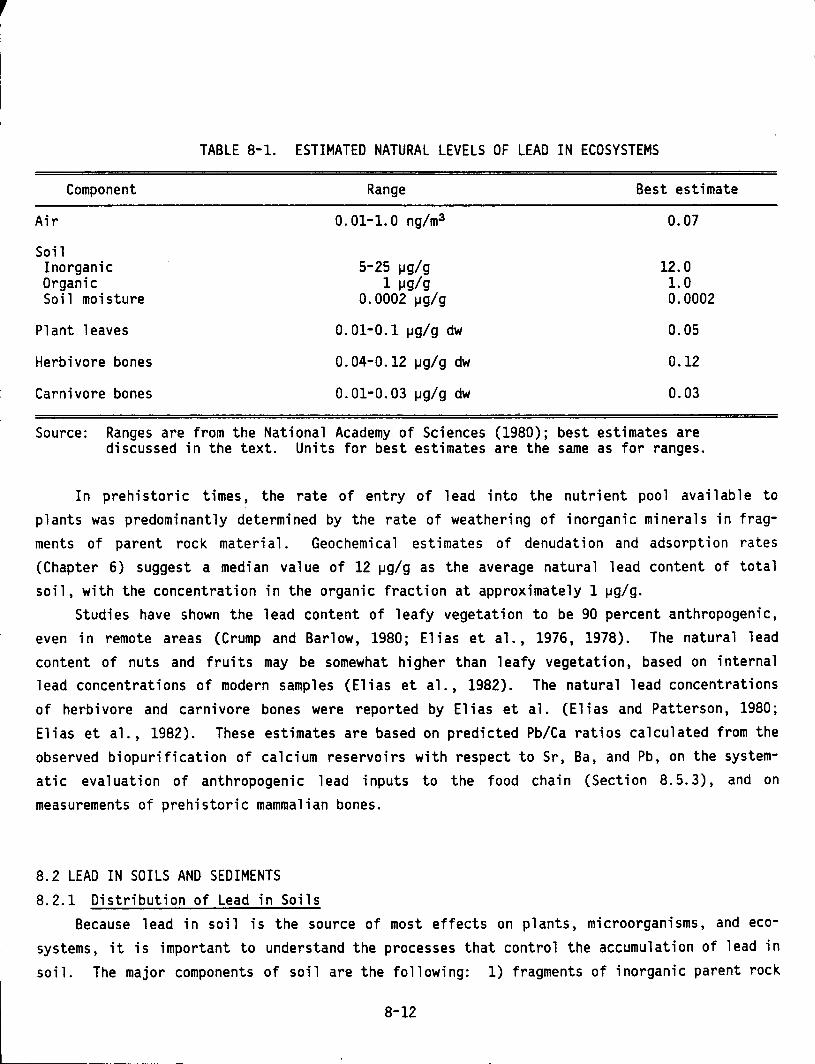
TABLE 8-1. ESTIMATED NATURAL LEVELS OF LEAD IN ECOSYSTEMS
Component
Air
Soil Inorganic Organic Soil moisture
Plant leaves
Herbivore bones
Carnivore bones
Range
0.01-1.0 ng/m3
5-25 tJg/g 1 tJg/g
0.0002 tJg/g
0.01-0.1 tJg/g dw
0.04-0.12 tJg/g dw
0.01-0.03 tJg/g dw
Best estimate
0.07
12.0 1.0 0.0002
0.05
0.12
0.03
Source: Ranges are from the National Academy of Sciences (1980); best estimates are discussed in the text. Units for best estimates are the same as for ranges.
In prehistoric times, the rate of entry of lead into the nutrient pool available to plants was predominantly determined by the rate of weathering of inorganic minerals in fragments of parent rock material. Geochemical estimates of denudation and adsorption rates (Chapter 6) suggest a median value of 12 tJg/g as the average natural lead content of total soil, with the concentration in the organic fraction at approximately 1 tJg/g.
Studies have shown the lead content of leafy vegetation to be 90 percent anthropogenic, even in remote areas (Crump and Barlow, 1980; Elias et al., 1976, 1978). The natural lead content of nuts and fruits may be somewhat higher than 1 eafy vegetation, based on i nterna 1
lead concentrations of modern samples (Elias et al., 1982). The natural lead concentrations of herbivore and carnivore bones were reported by Elias et al. (Elias and Patterson, 1980; Elias et al., 1982). These estimates are based on predicted Pb/Ca ratios calculated from the observed biopurification of calcium reservoirs with respect to Sr, Ba, and Pb, on the systematic evaluation of anthropogenic lead inputs to the food chain (Section 8.5.3), and on measurements of prehistoric mammalian bones.
8.2 LEAD IN SOILS AND SEDIMENTS 8.2.1 Distribution of Lead in Soils
Because 1 ead in soil is the source of most effects on p 1 ants, microorganisms, and ecosystems, it is important to understand the processes that control the accumulation of lead in soil. The major components of soil are the following: 1) fragments of inorganic parent rock
8-12
material; 2) secondary inorganic minerals; 3) organic constituents, primarily humic sub
stances, which are residues of decomposition or products of decomposer organisms; 4) Fe-Mn
oxide films, which coat the surfaces of all soil particles and appear to have a high binding
capacity for meta 1 s; 5) soi 1 microorganisms, most commonly bacteria and fungi , a 1 though
protozoa and soil algae may also be found; and 6) soil moisture, the thin film of water sur
rounding soil particles that is the nutrient medium of plants. Some watershed studies con
sider that fragments of inorganic parent rock materia·! lie outside the forest ecosystem,
because transfer from this compartment is so slow that much of the material remains inert for
centuries.
The concentration of natural lead ranges from 5 to 30 ~g/g in the top 5 em of most soils
not adjacent to ore bodies, where natural lead may reach BOO ~g/g. Aside from surface deposi
tion of atmospheric particles, plants in North Amer·ica average about 0.5- 1 ~g/g dw
(Peterson, 1978) and animals roughly 2 ~g/g (Forbes and Siinderson, 1978). Thus, soils contain
the greater part of total ecosystem lead. In soils, lead in parent rock fragments is tightly
bound within the crystalline structures of the inorganic !ioil minerals. It is released to the
ecosystem only by surface contact with soil moisture films.
The evidence for atmospheric inputs of lead to soil ,~ests mainly with the accumulation of
lead in the soil profile. There are several reports that lead accumulates in the upper
layers, usually about 2-5 em, of the soil, just below the litter layer. This is the soil
layer that is usually highest in organic content. Many soils develop by podzolization, char
acterized by di st i net soi 1 horizons caused by the separation and segretat ion of organic and
inorganic compounds, including metal salts and metal-,:>rganic complexes. Siccama et al.,
(1980), and Friedland et al. (1984a, 1984b), found that 'lead in the forest floors (the litter
1 ayer above the mi nera 1 soil) of New England have i ncrea!;ed during the 1960-1980 at about the
same rate that atmospheric concentrations of lead increased. Friedland et al. (1984a, 1984b)
found that copper, zinc, and nickel also increased over the same time period, as did the total
organic content. They concluded that lead and perhaps other metals may have inhibited
decomposition.
Soils adjacent to smelters may be contaminated at a. distance of several kilometers away
from the source and to a depth of ten or more centimeters. Hogan and Wotton (1984) found
elevated concentrations of lead at a distance of 38 kilometers from a Cu-Zn smelter on the
surface of the soil, and up to six kilometers at a depth of fifteen centimeters. McNeilly
et al. (1984) reported an exponential decrease in lead concentrations of surface soil from 0
to 75 meters for mine spoils. Effects of the spoils we·re detectab 1 e even at a depth of 20
centimeters.
8-13
Hutchinson (1980) has reviewed the effects of acid precipitation on the ability of soils to retain cations. Excess calcium and other metals are leached from the A horizon of soils by rain with a pH more acidic than 4.5. Most soils in the eastern United States are normally acidic (pH 3.5 to 5.2) and the leaching process is a part of the complex equilibrium maintained in the soil system. By increasing the leaching rate, acid rain can reduce the availability of nutrient metals to organisms dependent on the top layer of soil. Tyler (1978) reports the effect of acid rain on the leaching rate (reported as residence time) for lead and other metals. Simulated rain of pH 4.2 to 2.8 showed the leaching rate for lead increases with decreasing pH, but not nearly as much as that of other metals, especially Cu, Mn, and Zn. This would be as expected from the high stability constant of lead relative to other metals in humic acids (see Section 6.5.1). It appears from this limited information that acidification of soil may increase the rate of removal of lead from the soil, but not before several major nutrients are removed first. The effect of acid rain on the retention of lead by soil moisture is not known.
8.2.2 Origin and Availability of Lead in Aquatic Sediments Atmospheric lead may enter aquatic ecosystems by wet or dry deposition (Dolske and
Sievering, 1979) or by the erosional transport of soil particles (Baier and Healy, 1977). In waters not polluted by industrial, agricultural, or municipai effluents, the lead concentration is usually less than 1 ~g/1. Of this amount, approximately 0.02 ~g/1 is natural lead and the rest is anthropogenic lead, probably of atmospheric origin (Patterson, 1980). Surface waters mixed with urban effluents may frequently reach lead concentrations of 50 ~g/1, and occasionally higher (Bradford, 1977).
In aqueous solution, virtually all lead is divalent, as tetravalent lead can exist only under extremely oxidizing conditions (reviewed by Rickard and Nriagu, 1978; Chapter 3). At pH
. + higher than 5, divalent lead can form a number of hydroxyl complexes, most commonly PbOH , Pb(OHh, and Pb(OH)a-. At pH lower than 5, lead exists in solution as hydrated Pb. In still water, lead is removed from the water column by the settling of lead-containing particulate matter, by the formation of insoluble complexes, or by the adsorption of lead onto suspended organic particles. The rate of sedimentation is determined by temperature, pH, oxidationreduction potential, ionic competition, the chemical form of lead in water, and certain biological activities (Jenne and Luoma, 1977). McNurney et al. (1977) found 14 ~g Pb/g in stream sediments draining cultivated areas and 400 ~g/g in sediments associated with urban ecosystems. Small sediment grain size and high organic content contributed to increased reten
tion in sediments.
8-14
8.3 EFFECTS OF LEAD ON PLANTS
8.3.1 Effects on Vascular Plants and Algae
Some physiological and biochemical effects of lead on vascular plants have been detected
under laboratory conditions at·concentrations higher tha.n normally found in the environment.
The commonly reported effects are the inhibition of photosynthesis, respiration, or cell elon
gation, all of which reduce the growth of the plant (Koeppe, 1981). Lead may also induce
premature senescence, which may affect the long-term sur·vival of the plant or the ecological
success of the plant population. To provide a meaningful evaluation of these effects, it is
necessary to examine the correlation between laboratory conditions and typical conditions in
nature with respect to form, concentration, and availability of lead. First, the reader must
understand what is known of the movement of lead from soil to the root to the stem and finally
to the 1 eaf or flower. Most notably, there are specif-ic barriers to 1 ead at the soil: soi 1
moisture interface and at the root:shoot interface that retard the movement of lead and reduce
the impact of lead on photosynthetic and meristematic (gr1Jwth and reproduction) tissue.
8.3.1.1 Uptake by Plants. Most of the lead in or on a plant occurs on the surfaces of leaves
and the trunk or stem. The surface concentration of 1 ead in trees, shrubs, and grasses
exceeds the internal concentration by a factor of at lea!it five (Elias et al., 1978). Foliar
uptake was be 1 i eved to account for 1 ess than 1 percent of the uptake by roots (Arvi k and
Zimdahl, 1974; reviewed by Koeppe, 1981; Zimdahl, 1976). Krause and Kaiser (1977) were able
to show fo 1 i ar uptake and trans 1 ocat ion of 1 ead mixed with cadmium, copper, and manganese
oxides when applied in extremely large amounts (122 mg/m2 ) directly to leaves. This would be
comparable to 100,000 days accumulation at a remote site (0.12 ng/cm2 ·d) (Elias et al., 1978). However, recent isotopic evidence by Facchetti and Geiss (1982) and Patterson (1982) and mass
balance interpretations from watershed data (lindberg and Harriss, 1981) suggest that lead can
be absorbed across the leaf surface into internal plant tissues. Nevertheless, the major
effect of surface lead at ambient concentrations seems to be on subsequent components of the
grazing food chain (Section 8.4.1) and on the decomposer food chain following litterfall
(Elias et al., 1982). (See also Section 8.4.2.) In the soil, the availability of metals to plants i~; generally controlled by the concen
tration and form of the meta 1 , which are in turn i nfl uenc:ed by such soi 1 fermi ng processes as
gleying, leaching, podzolization, and the accumulation of organic matter at the surface.
Other factors such as pH and the presence of other cations may a 1 so be important. The amount
of lead that enters plants by this route is determined by the availability of lead in soil,
with apparent variations according to plant species. son cation exchange capacity, a major
factor, is determined by the relative size of the clay and organic fractions, soil pH, and the
amount of Fe-Mn oxide films present (Nriagu, 1978). Of these, organic humus and high soil pH
8-15
are the dominant factors in immobilizing lead (see Section 6.5.1). Under natural conditions, most of the total lead in soil would be tightly bound within the crystalline structure of inorganic soil fragments, unavailable to soil moisture. Available lead, bound on clays, organic colloids, and Fe-Mn films, would be controlled by the slow release of bound lead from inorganic rock sources. Since before 3000 B.C., atmospheric lead inputs through litter decomposition have increased the pool of available lead bound on organic matter within the soil reservoir (see Section 5.1).
Because lead is strongly immobilized by humic substances, only a small fraction (perhaps 0.01 percent in soils with 20 percent organic matter, pH 5.5) is released to soil moisture (see Section 6.5.1). In soil moisture, lead may pass along the pathway of water and nutrient uptake on either a cellular route through the cell membranes of root hairs (symplastic route) or an extracellular route between epidermal cells into the intercellular spaces of the root cortex (apoplastic route) (Foy et al., 1978). Lead probably passes into the symplast by membrane transport mechanisms similar to the uptake of calcium or other bivalent cations.
In soils with lead concentrations within the range of natural lead (15-30 tJg/g), only trace amounts of lead are absorbed by plants. The amount absorbed increases when the concentration of lead in soil increases or when the binding capacity of soil for lead decreases. Uptake by root systems does not necessarily mean the lead reaches the stems, leaves or fruits. Rather, the process should be seen as a soil-plant continuum that strongly favors retention of lead by the soil and the root system.
When viewed from the perspective of the uptake of nutrients such as calcium, there are at least three mechanisms whereby lead can be taken up by roots: transpirational mass flow, diffusion, and active transport (Jenny, 1980). Probably the most significant is transpiration a 1 mass flow. In the process of absorbing and transporting water from the soi 1 to the leaves, the plant absorbs relatively large amounts of ions in solution. Since plants take up about 100 times their weight in water each growing season, this process could account for twice the normal amounts of lead found in vegetation, assuming equilibrium between the soil and the soil solution. For example, a lettuce plant transpired 100 liters of water during the season, which contained 5000 f.lg of lead (Rabinowitz, 1972). But the plant itself contained
only 2500 f.lg, most of which was in the roots. Diffusion can occur along a concentration gradient whenever the transpiration stream is
idle, e.g., during the night or during periods of high humidity. Because the concentration of lead in the soil solution is usually higher than in the plant, and because lead bound on the cellulose matrix of the cell wall would not effect the concentration gradient, the flow of lead would probably be toward the root. Although the third mechanism, active transport, is an important process for nutrient elements, there is no evidence that such a process occurs for
8-16
lead or any other non-nutrient. This process requires energy, and it is unreasonable that a plant would expend energy to take up non-nutrient elements.
The soil-root continuum is a complex structure that consists of the soil particles, the soil solution, the mutigel or other remnants of root exudates, the epidermal cells with elongated root hairs, and the root cortial cells. The walls of the epidermal cells are a loose matrix of cellulose and hemicellulose fibers. Much of this continuum is of biological origin and contains compounds active in ion exchange, such as hemicelluloses and pectic substances that are heavily endowed with -COOH groups, and proteins that also have charged groups. As a cation moves from the soil particle to the root cortex, whether by mass flow or diffusion, it is continually proximate to root structures with a high binding capacity. Lead is more tightly bound at these sites than .other cations, even calc·ium. Consequently, relatively little 1 ead passes through the roots into the shoot. It appears that most of the soi 1 1 ead is retained within the root. However, some plants may allow more lead to translocate than others. Rabinowitz (1972) found that for lettuce and wild oats growing in soils with increasing lead concentrations, the lettuce translocated very little soil lead but the wild oats translocated proportionately greater amounts. The author was able to distinguish isotopically between sot 1 and atmospheric 1 ead, and found a 1 so that more than half the 1 ead in p 1 ants, after water washing, was of atmospheric origin when the plants were grown at 30 meters from a freeway.
At 500 ~g Pb/g nutrient solution, lead has been shown to accumulate in the cell walls of germinating Raphinus sativus roots (Lane and Martin, 1982). This concentration is much higher than that found by Wong and Bradshaw (1982) to cause inhibition of germinating root elongation (less than 2.5 ~g/g), absence of root growth (5 ~g/g), or 55 percent inhibition of seed germination (20-40 ~g/g) in the rye grass, Colium perenne. Lane and Martin (1982) also observed lead in cytoplasmic organelles that because of their osmiophillic properties, appeared to have a storage function. It was suggested that the organelles eventually emptied their contents into the tonoplast.
The accumulation of lead in cell walls and cytoplasmic bodies has also been observed in blue-green algae by Jensen et al. (1982), who used X-ra,y energy dispersive analysis in conjunction with scanning electron microscopy to observe high concentrations of lead and other metals in these single-celled procaryotic organisms. They found the lead concentrated in the third of the four-layered cell wall and in polyphosphate bodies (not organelles, since they are not membrane-bound) which appeared to be a storage site for essential metals. The nutrient solution contained 100 ~g Pb/g. The same graup (Rachlin et al., 1982) reported morphological changes in the same blue-green alga (Plectonema boryanum). There was a significant increase in cell size caused by the lead, which indicated that the cell was able to detoxify its cytoplasm by excreting lead with innocuous cell wall material.
8-17
----·------ ---- -----------------
It appears that two defensive mechanisms may exist in the roots of plants for removing lead from the stream of nutrients flowing to the above-ground portions of plants: lead may be deposited with cell wall material exterior to the individual root cells, or may be sequestered in organelles within the root cells. Any lead not captured by these mechanisms would likely move with nutrient meta 1 s ce 11-to-ce 11 through the symp 1 ast and into the v~scul ar system.
Uptake of lead by plants may be enhanced by symbiotic associations between plant roots and mycorrhizal fungi. The three primary factors that control the uptake of nutrients by plants are the surface area of the roots, the ability of the root to absorb particular ions, and the transfer of ions through the soil. The symbiotic relationship between mycorrhizal fungi and the roots of higher p 1 ants can increase the uptake of nutrients by enhancing a 11
three of these factors (Voigt, 1969). The typical ectomycorrhiza consists of a mantle or sheath of mycelia that completely surrounds the root. The physical extension of the sheath may increase the volume of the root two to three times (Voigt, 1969). Mycorrhizal roots often show greater affinities for nutrients than do uninfected roots of the same species grown in the same conditions. In many soil systems, where the bulk of the nutrients are bound up in parent rock material, efficient uptake of these nutrients by plants depends on the ability of organisms in the rhizosphere (plant roots, soil fungi, and bacteria) to increase the rates of weathering. Mycorrhizal fungi are known to produce and secrete into their environment many different acidic compounds (e. g. , malic and oxalic acids). In add it ion, mycorrhi za 1 roots have been shown to release more carbon dioxide into the rhizosphere than do non-mycorrhizal roots as a result of their increased rates of respirat1on. Carbon dioxide readily combines with soil moisture to produce carbonic acid. All of these acids are capable of increasing the weathering rates of soil particles such as clays, and altering the binding capacity of organic material, thereby increasing the amount of nutrients and other cations in the soil solution. Mycorrhizae are known to enhance the uptake of zinc by pine roots (Bowen et al., 1974), and it is likely that lead uptake is similarly increased, by inference to the ability of mycorrhizae to enhance the uptake of calcium by pine roots (Melin and Nilsson, 1955; Melin et al., 1958).
The translocation of lead to aboveground portions of the plant is not clearly understood. Lead may follow the same pathway and be subject to the same controls as a nutrient metal such as calcium. This assumption implies that the plant root has no means of discriminating against 1 ead during the uptake process, and it is not known that any such di scri mi nation mechanism exists. There may be several mechanisms, however, that excrete lead back out of the root or that prevent its translocation to other plant parts. The primary mechanisms may be storage in cell organelles or adsorption on cell walls. The apoplast contains an important supply of plant nutrients, including water. Lead in the apoplast remains external to the cells and cannot pass to vascular tissue without at least passing through the cell membranes
8-18
of the endodermis. Because this extracellular region is bounded on all sides by cell walls, the surface of which is composed of 1 ayers of ce 11 ul ose strands, the surface area of the apoplast is comparable to a sponge. It is likely that much of the lead in roots is adsorbed to the apoplast surface. Oictyosomes (cytoplasmic c•rganelles that contain cell wall material) may carry lead from inside the cell through the membrane to become a part of the external cell wall (Malone et al., 1974), possibly replacing calcium in calcium pectate. Lead may also be stored and excreted as lead phosphate in dictyosome vesicles (Malone et al., 1974). Nevertheless, some lead does pass into the vas.cular tissue, along with water and dissolved nutrients, and is carried to physiologically active tissue of the plant.
Evidence that lead in contaminated soils can enter the vascular system of plants and be transported to above-ground parts may be found in the analysis of tree rings. Rolfe (1974) found fourfold increases in both rural and urban trees, cc,mparing 10-year increments of annual rings for the period 1910-20 to annual rings of the period 1963-73. Symeonides (1979) found a twofold increase from 1907-17 to 1967-77 in trees at a high-lead site, with no increase in trees from a low-lead site. Baes and Ragsdale (1981), using only ring porous species, found significant post-1930 increases in Quercus and Carya with high lead exposure, but only in Carya with low-lead exposure. These chronological records confirm that lead can be translocated from roots to the upper portions of the plant and that the amounts translocated are in proportion to the concentrations of lead in soil. 8.3.1.2 Physiological Effects on Plants. Because most of the physiologically active tissue of plants is involved in growth, maintenance, and photosynthesis, it is expected that lead might interfere with one or more of these processes. Indeed, such interferences have been observed under optimal growth conditions in laboratory experiments at lead concentrations greater than those normally found in the field, except near smelters or mines (Koeppe, 1981). It is likely that because these are the physiological processes studied more vigorously than others, more is known of these effects. Studies of lead effects on other plant processes, especially maintenance, flowering, and hormone development, have not been conducted and no conclusion can be reached concerning these processes.
Inhibition of photosynthesis by lead may be by dire•:t interference with the light reaction or the indirect interference with carbohydrate synthesis. With 21 ~g Pb/g reaction solution, Miles et al. (1972) demonstrated substantial inhibition of photosystem II near the site of water splitting, a biochemical process believed to require manganese. Homer et al. (1979)
found a second effect on photosystem II at slightly h;igher concentrations of lead. This effect was similar to that of OCMU [3-(3,4-dichloropheny·1.)-1,1-dimethylurea], a reagent commonly used to uncoup 1 e the photosynthetic e 1 ectron transport system. Bazzaz and Go vi ndjee (1974) suggested that the mechanism of lead inhibition was a change in the conformation of the
8-19
thylakoid membranes, separating and isolating pigment systems I and II. Wong and Govindje~
(1976) found that lead also interferes with P700 photooxidation and re-reduction, a part of the photosystem I light reaction. Homer et al. (1981) found a lead tolerant population of the grass Phalaris arundinacea had lowered the ratio of chlorophyll a/chlorophyll b, believed to be a compensation for photosystem II inhibition. There was no change in the total amount of chlorophyll, but the mechanism of inhibition was considered different from that of Miles et al. (1972). Hampp and Lendzian (1974) found that lead chloride inhibits the synthesis of chlorophyll b more than that of chlorophyll a at concentrations up to 100 mg Pb/g. Devi Prasad and Devi Prasad (1982) found 10 percent inhibition of pigment production in three species of green algae at 1 ~g/g, increasing to 50 percent inhibition at 3 ~g/g. Bazzaz et al. (1974, 1975) observed reduced net photosynthesis which may have been caused indirectly by
inhibition of carbohydrate synthesis. Without carbohydrates, stomatal guard cells remain flaccid, transpiration ceases, carbon dioxide fixation decreases, and further carbohydrate synthesis is inhibited.
In the quantification of growth inhibition, one can measure either the concentration of lead in the nutrient medium or in the tissue that is growth inhibited. Lead concentrations in the nutrient medium relate directly to the degree of environmental contamination, but the more precise measurement is in the tissue, since there would be a more direct correlation between the lead concentration and the physiological processes inhibited. Burton et al. (1983) deter
mined that when tissue concentrations in the shoots of Sitka-spruce seedlings exceeded about 20 ~g Pb/g dw, growth inhibition became significant,·and lethal at about 40 ~g/g. This narrow range between the onset of inhibition and lethality was attributed to the sequestering of lead in the roots and shoots up to 19 ~g/g, above which any additional lead would be more available and extremely toxic. The stunting of plant growth may be by the inhibition of the growth hormone IAA (indole-3-ylacetic acid). Lane· et al. (1978) found a 25 percent reduction in elongation at 10 ~g/g lead as lead nitrate in the nutrient medium of wheat coleoptiles. This
effect could be reversed with the addition of calcium at 18 ~g/g. Lead may also interfere with plant growth by reducing respiration or inhibiting cell division. Miller and Koeppe
(1971) and Miller et al. (1975) showed succinate oxidation inhibition in isolated mitochondria as well as stimulation of exogenous NADH oxidation with related mitochondrial swelling. Hassett et al. (1976), Koeppe (1977), and Malone et al. (1978) described significant inhibition of lateral root initiation in corn. Inhibition increased with the simultaneous addition
of cadmium. Sung and Yang (1979) found that lead at 1 ~g/g can complex with and inactivate ATPase to
reduce the production and utilization of ATP in kidney bean (Phaseolus vulgaris) and buckwheat
1 eaves (Fagopyrum escul entum). The lead was added hydroponically at concentrations up to
8-20
1,000 ~g/g. Kidney bean ATPase showed a continued response from 1 to 1,000 ~g/g, but buckwheat leaves showed little further reduction after 10 ~g/g. Neither extracted ATP nor chemically added ATP could be used by the treated plants. Lee et al. (1976) found a 50 percent increase in the activity of severa 1 enzymes re 1 a ted to the onset of senescence in soybean leaves when lead was added hydroponically at 20 ~g/g. These enzymes were acid phosphatase, peroxidase, and alpha.-amylase. A build-up of ammonia was observed along with a reduction in nitrate, calcium, and phosphorus. Glutamine synthetase activity was also reduced by 65 percent. Continued increases in effects were observed up to 100 ~g/g, including a build-up of soluble protein. Paivoke (1979) also observed a 60 percent increase in acid phosphatase activity during the first 6 days of pea seedling germination (Pisum sativum) at 2 ~g/g, under low nutrient conditions. The accumulation of soluble protein was observed and the effect could be reversed with the addition of nutrients, including calcium.
Scarponi and Perucci (1984) reported that lead can interfere with the synthesis of ALAdehydratase in corn, but does not appear to affect the activity of this enzyme. This enzyme catalyzes the conversion of c5-aminolevulinic acid to porphobilinogen, an intermediate in chlorophyll synthesis. The concentration of lead was above 10,000 ~g/1 in the nutrient solution.
The interaction of lead with calcium has been shown by several authors, most recently by Garland and Wilkins (1981), who demonstrated that calcium could partially overcome the effects of lead on growth in barley seedlings (Hordeum vulgare). Seedlings that were growth-inhibited at 2 ~g Pb/g sol. with no added calcium, grew at about half the control rate with 17 ~g Ca/g sol. This relation persisted up to 25 ~g Pb/g sol. and 500 ~g Ca/g sol.
Chaney and Strickland (1984) measured the effects of lead on the germination on red pine pollen. Following exposure in an aqueous nutrient medium, two parameters were measured: pollen germination and germ tube elongation. Pollen germination was inhibited by greater than 10 percent only at relatively high concentrations of l-ead, about 1,000 ~g/1, but the most significant effect was shown for germ tube elongation, which showed 10 percent inhibition at
about 150 ~g/1. These studies of the physiological effects of lead on plants all show some effect at
concentrations from 2 to 10 ~g/g in the nutrient medium of hydroponically-grown agricultural plants. It is probable that no effects would have been observed at these concentrations had the lead solutions been added to normal soil, where the lead would have been bound by humic
substances. There is no firm relationship between soil lead and soil moisture lead, because each soil type has a unique capacity to retain lead and to release that lead to the soil moisture film surrounding the soil particle. Once in soi'l moisture, lead seems to pass freely to the plant root according to the capacity of the plant root to absorb water and dissolved substances (Koeppe, 1981).
8-21
Chapter 6 discusses the many parameters controlling the release of lead from soil to soil moisture, but so few data are available on observed lead concentrations in soil moisture that no mode 1 can be formed. It seems reasonab 1 e that there may be a direct corre 1 at ion between lead in hydroponic media and lead in soil moisture. Hydroponic media typically have an excess of essential nutrients, including calcium and phosphorus, so that movement of lead from hydroponic media to plant root would be equal to or slower than movement from soil. moisture to plant root. Hughes (1981) adopted the general conclusion that extractable soil lead is typically 10 percent of total soil lead. However, this lead was extracted chemically under laboratory conditions more rigorous than the natural equilibrium between soil and soil moisture. Ten percent should therefore be considered the upper limit, where the ability of soil to retain lead is at a minimum. A lower limit of 0.01 percent is based on the only known report of lead in both soil and soil moisture (16 ~g/g soil, 1.4 ng/g soil moisture; Elias et al., 1982). This single value shows neither trends with different soil concentrations nor the soil component (organic or inorganic) that provides the lead to the soil moisture. But the number (0.01 percent) is a conservative estimate of the ability of soil to retain lead, since the conditions (pH, organic content) were optimum for retaining lead. A further complication is that atmospheric 1 ead is retained at the surface (0-2 em) of the soil profile (Martin and Coughtrey, 1981), whereas most reports of lead in soil pertain to samples from 0 to 10 em as the 11 Upper 11 layer of soil. Any plant that absorbs solely from the top few centimeters of soil obviously is exposed to more lead than one with roots penetrating to a depth of 25 em or more. Agricultural practices that cultivate soil to a depth of 25 em blend in the upper layers with lower to create a soil with average lead content somewhat above background.
These observations lead to the general conclusion that even under the best of conditions where soil has the highest capacity to retain lead, most plants would experience reduced growth rate (inhibition of photosynthesis, respiration, or cell elongation) in soils of 10,000
1.1g Pb/g or greater. Khan and Frankland (1983) observed stunted growth in radish plants at 1000 1.1g Pb/g soil when the lead was added as chloride, with complete growth inhibition at 5000 1.1g/g. The effects were 1 ess severe when 1 ead oxide was added to the soi 1. Concentrations approaching these values typically occur around smelters (Martin and Coughtrey, 1981)
and near major highways (Wheeler and Rolfe, 1979). These conclusions pertain to soil with the ideal composition and pH to retain the maximum amount of lead. Acid soils or soils lacking organic matter would inhibit plants at much lower lead concentrations.
The rate at which atmospheric lead accumulates in soil varies from 1.1 mg/m2 ·yr average global deposition (Table 6-6) to 3,000 mg/m2 ·yr near a smelter (Patterson et al., 1975).
Assuming an average density of 1.5 g/cm3 , undisturbed soil to a depth of 2 em (20,000 cm3 /m2 )
would incur an increase in lead concentration at a rate of 0.04 to 100 1.1g/g soil·yr. This
8-22
means remote or rural area soils may never reach the 10,000 IJg/g threshold but that undisturbed soils closer to major sources may be within range in the next 50 years. 8.3.1.3 Lead Tolerance in Vascular Plants. Some plant species have developed populations tolerant to high-lead soils (Antonovics et al. ·, 1971). In addition to Homer et al. (1981) cited above, Jowett (1964) found populations of Agrostis tenuis -in pure stands on acidic spoil banks near an abandoned mine. The exclusion of other species was attributed to root inhibition. Populations of ~· tenuis from low-lead soils had no tolerance for the high-lead soils. Several other studies suggest that similar responses may occur in populations growing in lead-rich soils (reviewed in Peterson, 1978). A few have suggested that crops may be cultivated for their resistance to high-lead soils (Gerakis et al., 1980; John, 1977).
Using populations taken from mine waste and uncontaminated control areas, some authors have quantified the degree of tolerance of Agrostis tEmuis (Karataglis, 1982) and Festuca rubra (Wong, 1982) under controlled laboratory conditions. Root elongation was used as the index of tolerance. At 36 1-1g Pb/g nutrient solution, all populations of ~· tenuis were completely inhibited. At 12 !Jg Pb/g, the control populations from low-lead soils were completely inhibited, but the populations from mine soils· achieved 30 percent of their normal growth (growth at no lead in nutrient solution) .. At 6 IJg/g, the control populations achieved 10 percent of their normal growth; tolerant populations achieved 42 percent. There were no measurements below 6 !Jg/g. Wong (1982) measured the index of tolerance at one concentration only, 2.5 !Jg Pb/g nutrient solution, and found that non-adapted populations of Festuca rubra that had grown on soils with 47 IJQ/g total lead content were completely inhibited, populations from soils with 350 - 650 !Jg/g achieved 3-7 percent of normal growth, and populations from 5,000 !Jg/g soil achieved nearly 40 percent of normal growth. Tolerance indices should be used with caution because they depend on two measurements th.~t may be genetically independent. Humphreys and Nicholls (1984) suggested that different genes regula ted root e 1 ongat ion in a control solution and in the heavy-metal solution.
These studies support the conclusion that inhibition of plant growth begins at a lead concentration of less than 1 IJg/g soil moisture and bec1:>mes completely inhibitory at a level between 3 and 10 1-1g/g. Plant populations that are genetically adapted to high-lead soils may achieve 50 percent of their normal root growth at lead concentrations above 3 1-1g/g. These experiments did not show the effect of reduced root growth on total productivity, but they did show that exposure to high-lead soils is a requirement for genetic adaptation and that, at least in the case of f. rubra, plant lead concentration::; increase with increasing concentra
tions in the soil. There are a few plants known to be hyperaccumulators of metals (Reeves and Brooks, 1983).
These p 1 ants appear to show no adverse effects even when their tissue concentrations reach
8-23
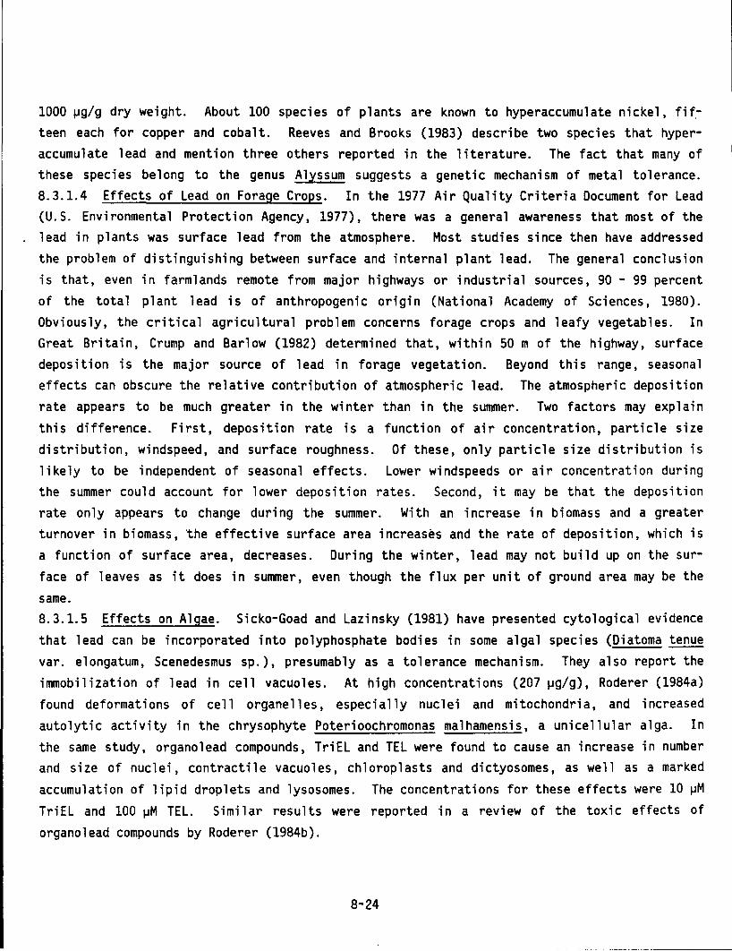
1000 J.Jg/g dry weight. About 100 species of plants are known to hyperaccumulate nickel, fif.teen each for copper and cobalt. Reeves and Brooks (1983) describe two species that hyperaccumulate lead and mention three others reported in the literature. The fact that many of these species belong to the genus Alyssum suggests a genetic mechanism of metal tolerance. 8.3.1.4 Effects of Lead on Forage Crops. In the 1977 Air Quality Criteria Document for Lead (U.S. Environmental Protection Agency, 1977), there was a general awareness that most of the lead in plants was surface lead from the atmosphere. Most studies since then have addressed the problem of distinguishing between surface and internal plant lead. The general conclusion is that, even in farmlands remote from major highways or industrial sources, 90 - 99 percent of the total plant lead is of anthropogenic origin (National Academy of Sciences, 1980). Obviously, the critical agricultural problem concerns forage crops and leafy vegetables. In Great Britain, Crump and Barlow (1982) determined that, within 50 m of the highway, surface deposition is the major source of lead in forage vegetation. Beyond this range, seasonal effects can obscure the relative contribution of atmospheric lead. The atmospheric deposition rate appears to be much greater in the winter than in the summer. Two factors may explain
this difference. First, deposition rate is a function of air concentration, particle size distribution, windspeed, and surface roughness. Of these, only particle size distribution is likely to be independent of seasonal effects. Lower windspeeds or air concentration during the summer could account for 1 ower deposition rates. Second, it may be that the deposition rate only appears to change during the summer. With an increase in biomass and a greater turnover in biomass, ·the effective surface area increases and the rate of deposition, which is a function of surface area, decreases. During the winter, lead may not build up on the surface of leaves as it does in summer, even though the flux per unit of ground area may be the
same. 8.3.1.5 Effects on Algae. Sicko-Goad and Lazinsky (1981) have presented cytological evidence that lead can be incorporated into polyphosphate bodies in some algal species (Diatoma tenue var. elongatum, Scenedesmus sp.), presumably as a tolerance mechanism. They also report the immobilization of lead in cell vacuoles. At high concentrations (207 J.Jg/g), Roderer (1984a) found deformations of cell organelles, especially nuclei and mitochondria, and increased autolytic activity in the chrysophyte Poterioochromonas malhamensis, a unicellular alga. In the same study, organolead compounds, TriEL and TEL were found to cause an increase in number and size of nuclei, contractile vacuoles, chloroplasts and dictyosomes, as well as a marked
accumulation of lipid droplets and lysosomes. The concentrations for these effects were 10 JJM TriEL and 100 J..IM TEL. Similar results were reported in a review of the toxic effects of
organolead compounds by Roderer (1984b).
8-24
-----------------~
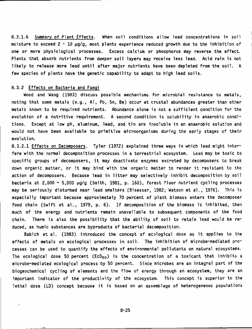
8.3.1.6 Summary of Plant Effects. When soil condition!; allow lead concentrations in soil
moisture to exceed 2 - 10 ~g/g, most plants experience reduced growth due to the inhibition of
one or more physiological processes. Excess calcium or· phosphorus may reverse the effect.
Plants that absorb nutrients from deeper soil layers may receive less lead. Acid rain is not
likely to release more lead until after major nutrients have been depleted from the soil. A
few species of plants have the genetic capability to adapt to high lead soils.
8.3.2 Effects on Bacteria and Fungi
Wood and Wang ( 1983) discuss poss i b 1 e mechanisms for microbia 1 resistance to meta 1 s,
noting that some metals (e.g., Al, Pb, Sn, Be) occur at c:rustal abundances greater than other
metals known to be required nutrients. Abundance alone is not a sufficient condition for the
evolution of a nutritive requirement. A second conditic•n is solubility in anaerobic condi
tions. Except at low pH, aluminum, lead, and tin are insoluble in an anaerobic solution and
would not have been available to primitive microorganisms during the early stages of their
evolution.
8.3.2.1 Effects on Decomposers. Tyler (1972) explained three ways in which lead might inter
fere with the normal decomposition processes in a terrestT'ial ecosystem. Lead may be toxic to
specific groups of decomposers, it may deactivate enzymes excreted by decomposers to break
down organic matter, or it may bind with the organic matter to render it resistant to the
action of decomposers. Because lead in litter may selectively inhibit decomposition by soil
bacteria at 2,000 - 5,000 ~g/g (Smith, 1981, p. 160), for·est floor nutrient cycling processes
may be seriously disturbed near lead smelters (Bisessar, 1982; Watson et al., 1976). This is
especially important because approximately 70 percent of plant biomass enters the decomposer
food chain (Swift et al., 1979, p. 6). If decomposition of the biomass is inhibited, then
much of the energy and nutrients remain unavailable to· subsequent components of the food
chain. There is also the possibility that the ability ,of soil to retain lead would be re
duced, as humic substances are byproducts of bacterial decomposition.
Babich et al. (1983) introduced the concept of ec,::>logical dose as it applies to the
effects of metals on ecological processes in soil. The inhibition of microbe-mediated pro
cesses can be used to quantify the effects of environmental pollutants on natural ecosystems.
The ecological dose 50 percent (Ec050 ) is the concentration of a toxicant that inhibits a
microbe-mediated ecological process by 50 percent. Since microbes are an integral part of the
biogeochemical cycling of elements and the flow of energy through an ecosystem, they are an
important i ndi cater of the productivity of the ecosystem. This concept is superior to the
lethal dose (LD) concept because it is based on an ass•!mblage of heterogeneous populations
8-25
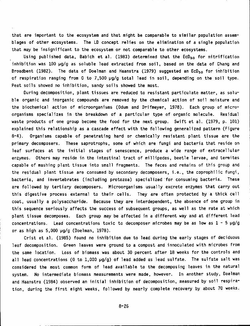
that are important to the ecosystem and that might be comparable to similar population assemblages of other ecosystems. The LD concept relies on the elimination of a single population that may be insignificant to the ecosystem or not comparable to other ecosystems.
Using published data, Babich et al. (1983) determined that the Ec050 for nitrification inhibition was 100 ~/gas soluble lead extracted from soil, based on the data of Chang and Broadbent (1982). The data of Doelman and Haanstra (1979) suggested an Ec050 for inhibition of respiration ranging from 0 to 7,500 ~g/g total lead in soil, depending on the soil type. Peat soils showed no inhibition, sandy soils showed the most.
During decomposition, plant tissues are reduced to resistant particulate matter, as soluble organic and inorganic compounds are removed by the chemical action of soil moisture and the biochemical action of microorganisms (Odum and Drifmeyer, 1978). Each group of microorganisms specializes in the breakdown of a particular type of organic molecule. Residual waste products of one group become the food for the next group. Swift et al. (1979, p. 101) explained this relationship as a cascade effect with the following generalized pattern (Figure 8-4). Organisms capable of penetrating hard or chemically resistant plant tissue are the primary decomposers. These saprotrophs, some of which are fungi and bacteria that reside on leaf surfaces at the initial stages of senescence, produce a wide range of extracellular enzymes. Others may reside in the intestinal tract of millipedes, beetle larvae, and termites capable of mashing plant tissue into small fragments. The feces and remains of this group and the residual plant tissue are consumed by secondary decomposers, i.e., the coprophilic fungi, bacteria, and invertebrates ( i ncl udi ng protozoa) speci a 1 i zed ·for consuming bacteria. These are followed by tertiary decomposers. Microorganisms usually excrete enzymes that carry out this digestive process external to their cells. They are often protected by a thick cell coat, usually a polysaccharide. Because they are interdependent, the absence of one group in this sequence seriously affects the success of subsequent groups, as well as the rate at which plant tissue decomposes. Each group may be affected in a different way and at different lead concentrations. Lead concentrations toxic to decomposer microbes may be as low as 1 - 5 ~g/g
or as high as 5,000 ~g/g (Doelman, 1978). Crist et al. (1985) found no inhibition due to lead during the early stages of deciduous
leaf decomposition. Green leaves were ground to a compost and innoculated with microbes from the same location. Loss of biomass was about 30 percent after 18 weeks for the controls and all lead concentrations (0 to 1,000 ~g/g) of lead added as lead sulfate. The sulfate salt was
considered the most common form of lead available to the decomposing leaves in the natural system. No intermediate biomass measurements were made, however. In another study, Doelman and Haanstra (1984) observed an initial inhibition of decomposition, measured by soil respiration, during the first eight weeks, followed by nearly complete recovery by about 70 weeks.
8-26
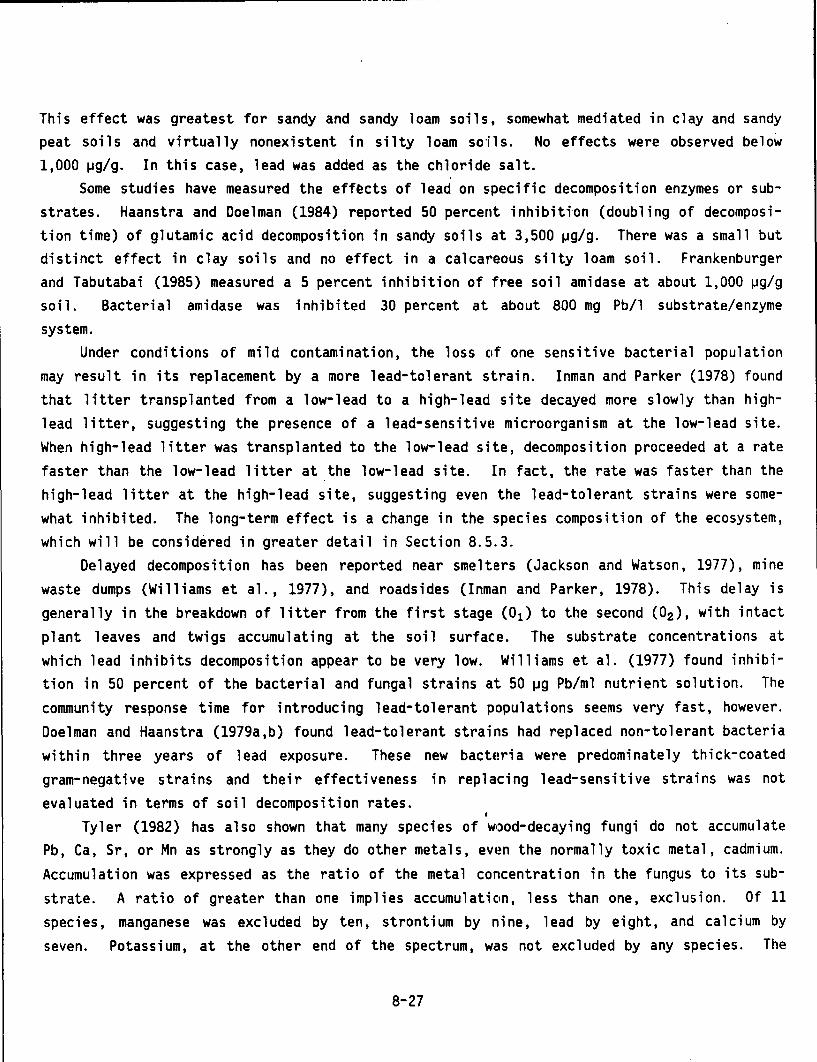
This effect was greatest for sandy and sandy loam soils, somewhat mediated in clay and sandy peat soils and virtually nonexistent in silty loam so"ils. No effects were observed below 1,000 ~g/g. In this case, lead was added as the chloride salt.
Some studies have measured the eff~cts of lead on specific decomposition enzymes or substrates. Haanstra and Doelman (1984) reported 50 percent inhibitton (doubling of decomposition time) of glutamic acid decomposition in sandy soils at 3,500 ~g/g. There was a small but distinct effect in clay soils and no effect in a calcat·eous silty loam soil. Frankenburger and Tabutabai (1985) measured a 5 percent inhibition of free soil amidase at about 1,000 ~g/g soil. Bacterial amidase was inhibited 30 percent at about 800 mg Pb/1 substrate/enzyme system.
Under conditions of mild contamination, the loss ctf one sensitive bacterial population may result in its replacement by a more lead-tolerant strain. Inman and Parker (1978) found that litter transplanted from a low-lead to a high-lead site decayed more slowly than highlead litter, suggesting the presence of a lead-sensitivE! microorganism at the low-lead site. When high-lead litter was transplanted to the low-lead site, decomposition proceeded at a rate faster than the low-lead litter at the low-lead site. In fact, the rate was faster than the high-lead litter at the high-lead site, suggesting even the lead-tolerant strains were somewhat inhibited. The long-term effect is a change in the species composition of the ecosystem, which will be considered in greater detail in Section 8.5.3.
Delayed decomposition has been reported near smelters (Jackson and Watson, 1977), mine waste dumps (Williams et al., 1977), and roadsides (Inman and Parker, 1978). This delay is generally in the breakdown of litter from the first stage (01 ) to the second (02 ), with intact p 1 ant 1 eaves and twigs accumulating at the soi 1 surface. The substrate concentrations at which lead inhibits decomposition appear to be very low. Williams et al. (1977) found inhibition in 50 percent of the bacterial and fungal strains at 50 ~g Pb/ml nutrient solution. The community response time for introducing lead-tolerant populations seems very fast, however. Doelman and Haanstra (1979a,b) found lead-tolerant strains had replaced non-tolerant bacteria within three years of lead exposure. These new bactE!ria were predominately thick-coated gram-negative strains and their effectiveness in replacing lead-sensitive strains was not evaluated in terms of soil decomposition rates.
I
Tyler (1982) has a 1 so shown that many species of w~:>od-decayi ng fungi do not accumulate Pb, Ca, Sr, or Mn as strongly as they do other metals, eVE!n the normally toxic metal, cadmium.
Accumulation was expressed as the ratio of the metal concentration in the fungus to its substrate. A ratio of greater than one implies accumulatiCin, less than one, exclusion. Of 11 species, manganese was excluded by ten, strontium by nine, lead by eight, and calcium by seven. Potassium, at the other end of the spectrum, wa1s not excluded by any species. The
8-27
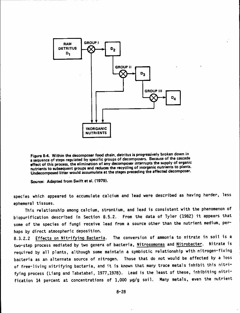
RAW GROUP.I DETRITUS
o,
INORGANIC NUTRIENTS
GROUP II
GROUP Ill
Figure 8-4. Within the decomposer food chain, detritus is progressively broken down in a sequence of steps regulated by specific groups of decomposers. Because of the cascade effect of this process, the elimination of any decomposer interrupts the supply of organic nutrients to subsequent groups and reduces the recycling of inorganic nutrients to plants. Undecomposed litter. would accumulate at the stages preceding the affected decomposer.
Source: Adapted from Swift at al. (1979).
species which appeared to accumulate calcium and lead were described as having harder, less
ephemeral tissues. This relationship among calcium, strontium, and lead is consistent with the phenomenon of
biopurification described in Section 8.5.2. From the data of Tyler (1982) it appears that some of the species of fungi receive lead from a source other than the nutrient medium, per
haps by direct atmospheric deposition. 8.3.2.2 Effects on Nitrifying Bacteria. The conversion of ammonia to nitrate in soil is a two-step process mediated by two genera of bacteria, Nitrosomonas and Nitrobacter. Nitrate is required by all plants, although some maintain a symbiotic relationship with nitrogen-fixing bacteria as an alternate source of nitrogen. Those that do not would be affected by a loss of free-living nitrifying bacteria, and it is known that many trace metals inhibit this nitrifying process (Liang and Tabatabai, 1977,1978). Lead is the least of these, inhibiting nitrification 14 percent at concentrations of 1,000 IJg/g soil. Many metals, even the nutrient
8-28
metals, manganese and iron, show greater inhibition at comparable molar concentrations.
Nevertheless, soils with environmental concentrations above 1,000 IJg Pb/g are frequently
found. Even a 14 percent inhibition of nitrification can reduce the potential success of a
plant population, as nitrate is usually the limiting nutrient in terrestrial ecosystems. In
cultivated ecosystems, nitrification inhibition is not a problem if nitrate fertilizer is
added to soil, but could reduce the effectiveness of amm·onia fertilizer if the crops rely on
nitrifying bacteria for conversion to nitrates. Rother et al. (1983) found that lead concen
trations as high as 30,000 !Jg/g soil did not affect symbiotic nitrogen fixation in white
clover (Trifolium repens).
8.3.2.3 Methylation by Aguatic Microorganisms. While m•athyllead is not a primary form of
environmental lead, methylation greatly increases the toxicity of lead to aquatic organisms
(Wong and Chau, 1979; Thayer and Brinckrnan, 1982). There is some uncertainty about whether
the mechanism of methylation is bi at i c or abi at i c. Some reports (Wong and Chau, 1979;
Thompson and Crerar, 1980) conclude that lead in sedimE!nts can be methylated by bacteria.
Reisinger et al. (1981) report that biomethylation of le.:td under aerobic or anaerobic condi
tions does not occur and such reports are probably due to sulfide-induced chemical conversion
of organic lead salts. These authors generally agree that tetramethyl lead can be formed
under environmental conditions when another tetravalent organolead compound is available, but
methylation of divalent lead salts such as Pb(N03)2 does not appear to be significant. Jarvie
et al. (1983) also report that they were unable to produce any definite evidence for bio
methylation of lead.
8.3.2.4 Summary of Effects on Microorganisms. It appear·s that microorganisms are more sen
sitive than p 1 ants to soil 1 ead po 11 uti on and that changes in the composition of bacteria 1
populations may be an early indication of lead effects. Delayed decomposition may occur at
750 !Jg Pb/g soil and nitrification inhibition at 1,000 IJQ/g. Many of the environmental vari
ables that can raise or lower these estimates are not yet known. In certain chemical en
vironments, the highly toxic tetramethyllead can be formed, but this process does not appear
to be mediated by aquatic microorganisms.
8.4 EFFECTS OF LEAD ON DOMESTIC AND WILD ANIMALS
8.4. 1 Vertebrates
8. 4.1.1 Terrestri a 1 Vertebrates. Forbes and Sanderson (1978) have reviewed reports of 1 ead
toxicity in domestic and wild animals. Lethal toxicity can usually be traced to consumption
of lead battery casings, lead-based paints, oil wastes, putty, linoleum, pesticides, lead
shot, or forage near smelters. Except for lead shot ingestion, these problems can be solved
8-29
by proper management of domestic animals. However, the 3,000 tons of lead shot falling annually along waterways and other hunting grounds continues to be a problem.
A single pellet of lead shot weighs about 110 mg, and 70 percent of this may be eroded in ringed turtle dove gizzards over a period of 14 days (Kendall et al., 1982). Their data showed an immediate elevation of blood lead and reduction of aminolevulinic acid dehydrogenase (ALA-D) activity within one day of swallowing two pellets. Feierabend (1983) revie\tfed 97 reports on the effects of lead shot on waterfowl. Of the estimated 80 to 125 million waterfowl in North America, 1. 5 to 38 mi 11 ion die each year from 1 ead poisoning. Many more are greatly impaired by chronic sublethal exposure. Reichell et al. (1984) reported that 17 of 293 ba 1 d eagles samp 1 ed had 1 ead concentrations in their 1 i ver high enough to suspect 1 ead poisoning. The 293 specimens were found dead or nearly dead during 1978 to 1983. The most common causes of death were trauma from being hit by a motor vehicle (20 percent) and shooting (19 percent). Bjorn et al., (1982) also reported the uptake of lead shot by grazing cattle near a trapshooting site.
Bull et al. (1983) and Osborn et al. (1983) reported extensive bird mortality that could be attributed to alkyl lead pollution of the Mersey Estuary in the United Kingdom. Bull et al. (1983) found 3-18 ~g/g alkyl lead in dead birds, 1-14 ~g/g in sick birds, and 0.3-1.2 ~g/g in apparently healthy birds. Osborn et al. (1983), in laboratory studies, found that 2000 ~g/day alkyl lead in the diet caused heavy mortality and 200 ~g/day caused tremors, impaired balance, and feeding irregularities, although no mortality was observed. Tissue concentrations of alkyl lead at the lower dose were in the range of 0.2 to 5.4 ~g/g. The authors concluded that many of the apparently healthy wild birds were experiencing symptoms likely to impair their chances for survival.
Awareness of the routes of uptake is important in interpreting the exposure and accumulation in vertebrates. Inhalation rarely accounts for more than 10 - 15 percent of the daily intake of lead (National Academy of Sciences, 1980). Much of the inhaled lead is trapped on the wa 11 s of the bronchi a 1 tubes and passes to the stomach embedded in swa 11 owed mucus. Because lead concentrations in lakes or running stream water are quite low, intake from drinking water may also be insignificant unless the animal drinks from a stagnant or otherwise contaminated source.
Food is the largest contributor of lead to animals. The type of food an herbivore eats determines the rate of lead ingestion. More than 90 percent of the total lead in leaves and bark may be due to surface deposition, but relatively little surface deposition may be found on some fruits, berries, and seeds that have short exposure times. no surface deposition. Similarly, ingestion of lead by a carnivore tion on herbivore fur and somewhat less on lead in herbivore tissue.
8-30
Roots intrinsically have depends mostly on deposiHarrison and Oyer (1984)
estimated that mule deer grazing in the Rocky Mountain National Park would exceed acceptable lead exposure by grazing on roadside vegetation for just 1 to 2 percent of the time. This estimate was based on the assumption that the upper limit of exposure should be 3,000 IJg Pb/day. Mule deer grazing on non-roadside forage would cc1nsume about 1,500 j.lg/day.
The type of food eaten is a major determinant of lead body burdens in small mammals. Goldsmith and Scanlon (1977) and Scanlon (1979) measured higher lead concentrations in insectivorous species than in herbivorous species, confirming the earlier work of Quarles et al. (1974), which showed body burdens of granivores < herbivores < insectivores, and Jeffries and French (1972) that granivores < herbivores. Animals in these studies were analyzed whole minus the digestive tract. It is likely that observed diet-related differences were somewhat diluted by including fur in the analysis, because fur lead might be similar for small mammals from the same habitats with different feeding habits.
Since 1977, there has been a trend away from whole body analyses toward analyses of isolated tissues, especially bones and blood. Bone concentrations of lead are better than blood as indicators of long-term exposure. Because natural levels of blood lead are not well known for animals and blood is not a good indicator of chronic E!Xposure, blood lead is poorly suited for estimating total body burdens. One experiment with sheep shows the rapid response of blood to changes in lead ingestion and the relative contr·ibution of food and air to the total blood level. Ward et ~1. (1978) analyzed the blood in sheep grazing near a highway (0.9 j.lg/g ml) and in an uncontaminated area (0.2 j.lg/ml). When sheep from the uncontaminated area were allowed to graze near the roadway, their blood levels roSE! rapidly (within 1 day) to about 3.0 j.lg/ml, then decreased to 2.0 j.lg/ml during the next 2 days, remaining constant for the remainder of the 14-day period. Sheep from the contaminated a: rea were moved to the uncontaminated area, where upon their blood dropped to 0.5 j.lg/ml in 10 days and decreased to 0.3 j.lg/ml during the next 180 days. Sheep in the uncontaminated area tha:t were fed forage from the roadside experienced an increase in blood lead from 0.2 to 1.1 j.lg/ml in 9 days. Conversely, sheep from the uncontaminated area moved to the roadside but fed forage only from the uncontaminated site experienced an increase from 0.2 to 0.5 j.lg/ml in 4 days. These data show that both air and food contribute to lead in blood and that blood lead conCE!ntrations are a function of both the recent history of lead exposure and the long-term storage of lead in bone tissue.
Beyer et al. (1985) reported a decrease in red blCiod cell ALA-D activity for 14 small mammals and 15 songbirds in a habitat near a smelter. There were no changes in packed cell
volume or hemoglobin concentrations and little evidence of gross or microscopic lesions that could be attributed to metal poisoning. Intranuclear inclusion bodies were found in a kidney of one shrew. The soil concentrations at the surface were 1,200-2,700 j.lg/g. Foliage concentrations were 21 !Jg/g and the fruits and berries averagE!d 4 j.lg/g, a typical pattern for the
8-31
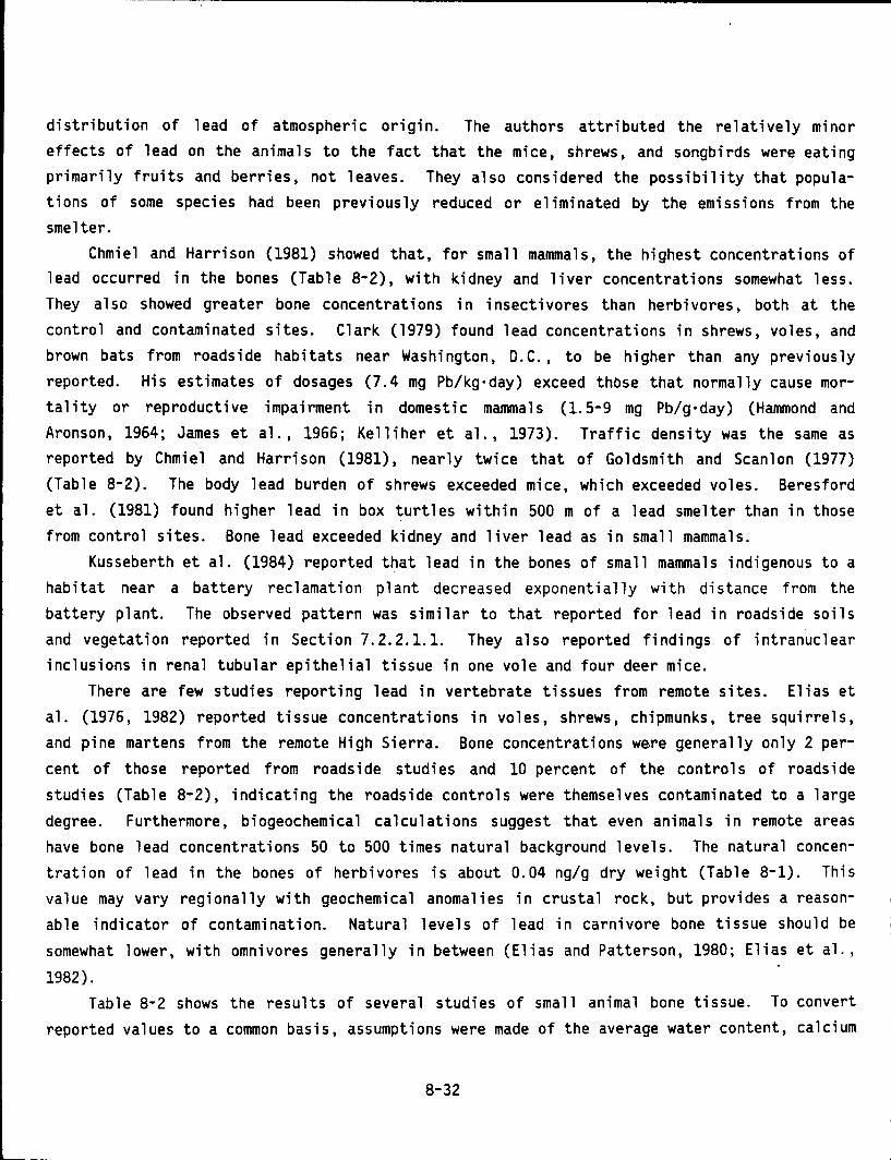
distribution of lead of atmospheric origin. The authors attributed the relatively minor effects of lead on the animals to the fact that the mice, shrews, and songbirds were eating primarily fruits and berries, not leaves. They also considered the possibility that populations of some species had been previously reduced or e 1 imi nated by the emissions from the smelter.
Chmiel and Harrison (1981) showed that, for small mammals, the highest concentrations of lead occurred in the bones (Table 8-2), with kidney and liver concentrations somewhat less. They a 1 so showed greater bone concentrations in insectivores than herbivores, both at the control and contaminated sites. Clark (1979) found lead concentrations in shrews, voles, and brown bats from roadside habitats near Washington, D.C., to be higher than any previously reported. His estimates of dosages (7.4 mg Pb/kg·day) exceed those that normally cause mortality or reproductive impairment in domestic mammals (1.5-9 mg Pb/g·day) (Hammond and Aronson, 1964; James et al., 1966; Kelliher et al., 1973). Traffic density was the same as reported by Chmiel and Harrison (1981), nearly twice that of Goldsmith and Scanlon (1977)
(Table 8-2). The body lead burden of shrews exceeded mice, which exceeded voles. Beresford et a l. (1981) found higher 1 ead in box ~urt 1 es within 500 m of a 1 ead sme 1 ter than in those from control sites. Bone lead exceeded kidney and liver lead as in small mammals.
Kusseberth et al. (1984) reported that lead in the bones of small mammals indigenous to a habitat near a battery reclamation plant decreased exponentially with distance from the battery plant. The observed pattern was similar to that reported for lead in roadside soils and vegetation reported in Section 7.2.2.1.1. They also reported findings of intranuclear inclusions in renal tubular epithelial tissue in one vole and four deer mice.
There are few studies reporting lead in vertebrate tissues from remote sites. Elias et al. (1976, 1982) reported tissue concentrations in voles, shrews, chipmunks, tree squirrels, and pine martens from the remote High Sierra. Bone concentrations we.re generally only 2 percent of those reported from roadside studies and 10 percent of the contra 1 s of roadside studies (Table 8-2), indicating the roadside controls were themselves contaminated to a large degree. Furthermore, biogeochemical calculations suggest that even animals in remote areas have bone lead concentrations 50 to 500 times natural background levels. The natural concentration of lead in the bones of herbivores is about 0.04 ng/g dry weight (Table 8-1). This value may vary regionally with geochemical anomalies in crustal rock, but provides a reasonable indicator of contamination. Natural levels of lead in carnivore bone tissue should be somewhat lower, with omnivores generally in between (Elias and Patterson, 1980; Elias et al.,
1982). Table 8-2 shows the results of several studies of small animal bone tissue. To convert
reported values to a common basis, assumptions were made of the average water content, calcium
8-32
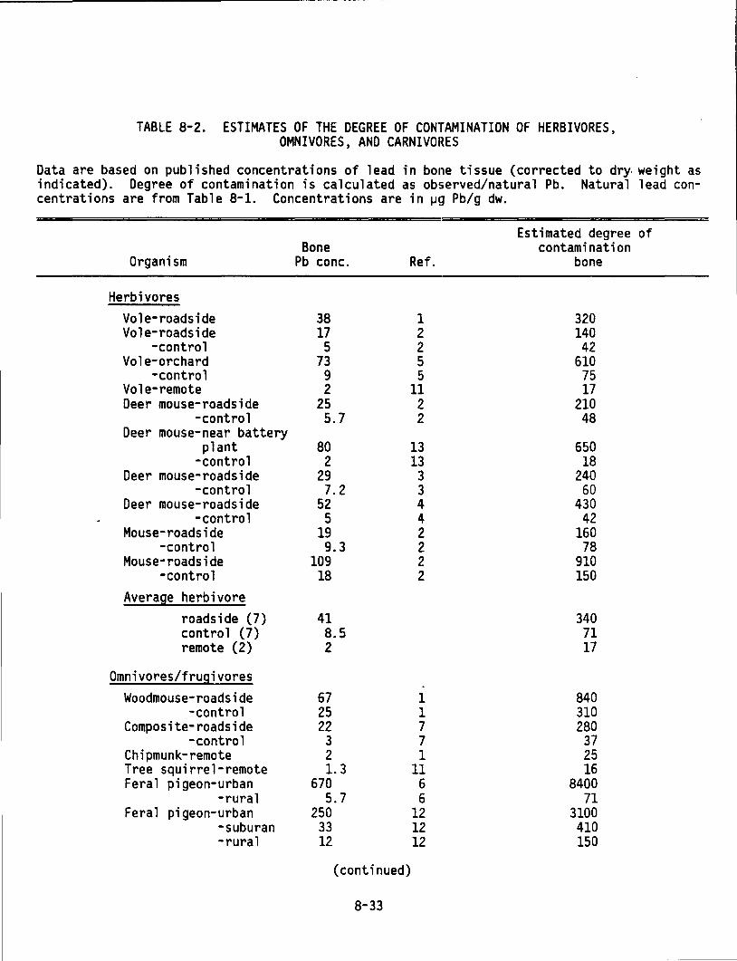
TABLE 8-2. ESTIMATES OF THE DEGREE OF CONTAMINATION OF HERBIVORES, OMNIVORES, AND CARNIVOI~ES
Data are based on published concentrations of lead in bone tissue (corrected to dry. weight as indicated). Degree of contamination is calculated as observed/natural Pb. Natural lead concentrations are from Table 8-1. Concentrations are in ~~J Pb/g dw.
Estimated degree of Bone contamination
Organism Pb cone. Ref. bone
Herbivores Vole-roadside 38 1 320 Vole-roadside 17 2 140
-control 5 2 42 Vole-orchard 73 5 610
-control 9 5 75 Vole-remote 2 11 17 Deer mouse-roadside 25 2 210
-control 5.7 2 48 Deer mouse-near battery
plant 80 13 650 -control 2 13 18
Deer mouse-roadside 29 3 240 -control 7.2 3 60
Deer mouse-roadside 52 4 430 -control 5 4 42
Mouse-roadside 19 2 160 -control 9.3 2 78
Mouse-roadside 109 2 910 -control 18 2 150
Average herbivore roadside (7) 41 340 control (7) 8.5 71 remote (2) 2 17
Omnivores/frugivores Woodmouse-roadside 67 1 840
-control 25 1 310 Composite-roadside 22 7 280
-control 3 7 37 Chipmunk-remote 2 1 25 Tree squirrel-remote 1.3 11 16 Feral pigeon-urban 670 6 8400
-rural 5.7 6 71 Feral pigeon-urban 250 12 3100
-suburan 33 12 410 -rural 12 12 150
(continued)
8-33
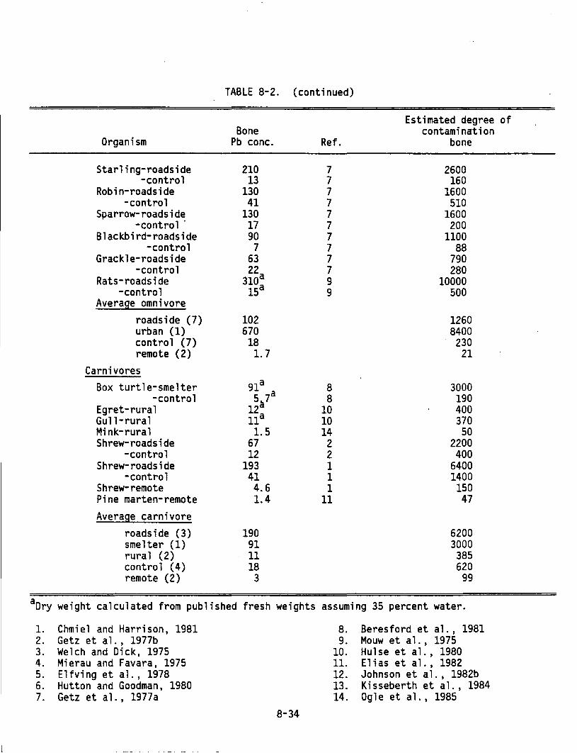
Organism
Starling-roadside -control
Robin-roadside -control
Sparrow-roadside -control ·
Blackbird-roadside -control
Grackle-roadside -control
Rats-roadside -control
Average omnivore roadside (7) urban (1) control (7) remote (2)
Carnivores Box turtle-smelter
-control Egret-rural Gull-rural Mi nk-rura 1 Shrew-roadside
-control Shrew-roadside
-control Shrew-remote Pine marten-remote Average carnivore
roadside (3) smelter (1) rural (2) control (4) remote (2)
TABLE 8-2. (continued)
Bone Pb cone.
210 13
130 41
130 17 90 7
63 22
310a 15a
102 670 18 1.7
91a 5 7a
12~ 11a 1.5
67 12
193 41 4.6 1.4
190 91 11 18 3
Ref.
7 7 7 7 7 7 7 7 7 7 9 9
8 8
10 10 14 2 2 1 1 1
11
Estimated degree of contamination
bone
2600 160
1600 510
1600 200
1100 88
790 280
10000 500
1260 8400
230 21
3000 190 400 370
50 2200 400
6400 1400 150
47
6200 3000
385 620
99
aDry weight calculated from published fresh weights assuming 35 percent water.
1. Chmiel and Harrison, 1981 8. Beresford et al., 1981 2. Getz et al., 1977b 9. Mouw et al., 1975 3. Welch and Dick, 1975 10. Hulse et al., 1980 4. Mierau and Favara, 1975 11. Elias et al., 1982 5. Elfving et al., 1978 12. Johnson et al., 1982b 6. Hutton and Goodman, 1980 13. Kisseberth et al., 1984 7. Getz et al., 1977a 14. Ogle et al., 1985
8-34
concentration, and average crustal concentration. Because! ranges of natural concentrations of lead in bones, plants, soils, and air are known with reatsonable certainty (Table 8-1), it is possible to estimate the degree of contamination of vertebrates from a wide range of habitats. It is important to recognize that these are merely estimates that do not allow for possible errors in analysis or anomalies in regional crustal abundances of lead. 8.4.1.2 Effects on Aquatic Vertebrates. Lowe et al. (1985) reported the results of a nationwide survey of metal concentrations in freshwater fish dur·ing the period 1979 to 1981. At 112 monitoring stations they found an average (geometric mean) of 0.19 ~g Pb/g wet weight for the period 1978-79 and 0.17 ~g/g for 1980-81. Several laboratories have reported experiments that measure the effects of lead on freshwater fish. Two requirements limit the evaluation of literature reports of lead effects on aquatic organisms. First, any laboratory study should incorporate the entire life cycle of the organism studied. It is clear that certain stages of a life cycle are more vulnerable than others (Hodson, 1979, Hodson et al., 1979). For fish, the egg or fry is usually most sensitive. Secondly, the same index must be used to compare results. Christensen et a 1. (1977) proposed three i ndi CE!S useful for i dent ifyi ng the effects of lead on organisms. A molecular index reports the maximum concentration of lead causing no significant biochemical change; residue index is the maximum concentration showing no continuing increase of deposition in tissue; and a bioassay index is the maximum concentration causing no mortality, growth change, or physical deformity. These indices are comparable to those of physiological dysfunction (molecular, tissue, and organismic) discussed in Section 8.1. 3.
From the standpoint of environmental protection, thE! most useful index is the molecular index. This index is comparable to the point of initial response discussed previously and is equivalent to the 11 safe concentration11 originally described by the U.S. Environmental Protection Agency (Battelle, 1971) as being the concentration that permits normal reproduction, growth, and all other life-processes of all organisms. It is unfortunate that very few of the toxicity studies in the aquatic literature report safe concentrations as defined above. Nearly all report levels at which some or all of the organisms die.
Hematological and neurological responses are the mc•st commonly reported effects of extended lead exposures in aquatic vertebrates. Hematologic:al effects include the disabling and destruction of mature red blood cells and the inhibition of the enzyme ALA-D required for hemoglobin synthesis. At low exposures, fish compensate by forming additional red blood ce 11 s. These red b 1 ood cells often do not reach maturity. At higher exposures, the fish become anemic. Symptoms of neuro 1 ogi ca 1 responses are eli ffi cult to detect at 1 ow exposure, but higher exposure can induce neuromuscular distortion, ctnorexia, and muscle tremors. Spinal curvature eventually occurs with time or increased concentration (Hodson 1979; Hodson et al.,
8-35
~~~~--~--------------
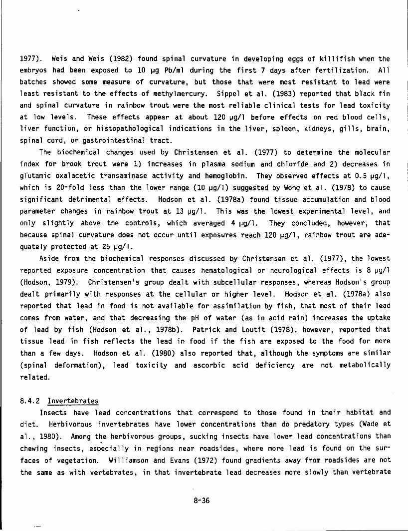
1977). Weis and Weis (1982) found spinal curvature in developing eggs of killifish when the embryos had been exposed to 10 J.lg Pb/ml during the first 7 days after fertilization. All batches showed some measure of curvature, but those that were most resistant to 1 ead were least resistant to the effects of methylmercury. Sippel et al. (1983) reported that black fin and spinal curvature in rainbow trout were the most reliable clinical tests for lead toxicity at 1 ow 1 eve 1 s. These effects appear at about 120 J.lg/1 before effects on red b 1 ood ce 11 s, liver function, or histopathological indications in the liver, spleen, kidneys, gills, brain, spinal cord, or gastrointestinal tract.
The biochemical changes used by Christensen et al. (1977) to determine the molecular index for brook trout were 1) increases in plasma sodium and chloride and 2) decreases in gTutamic oxalacetic transaminase activity and hemoglobin. They observed effects at 0.5 J.lg/1, which is 20-fold less than the lower range (10 J.lg/1) suggested by Wong et al. (1978) to cause significant detrimental effects. Hodson et al. (1978a) found tissue accumulation and blood parameter changes in rainbow trout at 13 J.lg/1. This was the lowest experimental level, and only slightly above the controls, which averaged 4 !Jg/1. They concluded, however, that because spinal curvature does not occur until exposures reach 120 J.lg/1, rainbow trout are adequately protected at 25 J.lg/1.
Aside from the biochemical responses discussed by Christensen et al. (1977), the lowest reported exposure concentration that causes hemato 1 ogi ca 1 or neuro 1 ogi ca 1 effects is 8 !Jg/1 (Hodson, 1979). Christensen•s group dealt with subcellular responses, whereas Hodson•s group dealt primarily with responses at the cellular or higher level. Hodson et al. (1978a) also reported that lead in food is not available for assimilation by fish, that most of their lead comes from water, and that decreasing the pH of water (as in acid rain) increases the uptake of lead by fish (Hodson et al., 1978b). Patrick and Loutit (1978), however, reported that tissue lead in fish reflects the lead in food if the fish are exposed to the food for more than a few days. Hodson et al. (1980) also reported that, although the symptoms are similar (spinal deformation), lead toxicity and ascorbic acid deficiency are not metabolically
related.
8.4.2 Invertebrates Insects have lead concentrations that correspond to those found in their habitat and
diet. Herbivorous invertebrates have 1 ower concentrations than do predatory types (Wade et
al., 1980). Among the herbivorous groups, sucking insects have lower lead concentrations than chewing insects, especially in regions near roadsides, where more lead is found on the surfaces of vegetation. Williamson and Evans (1972) found gradients away from roadsides are not the same as with vertebrates, in that invertebrate lead decreases more slowly than vertebrate
8-36
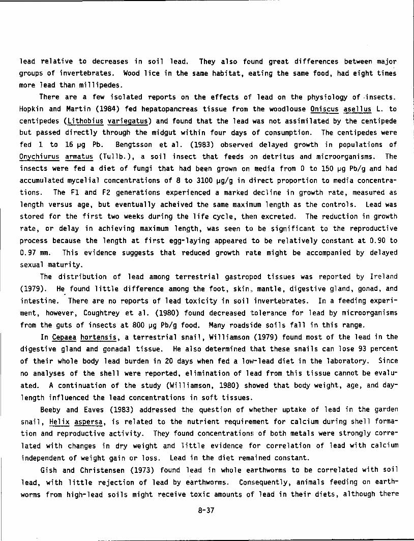
lead relative to decreases in soil lead. They also fc,und great differences between major
groups of invertebrates. Wood lice in the same habitat, t!ating the same food, had eight times
more lead than millipedes.
There are a few i so 1 a ted reports on the effects of 1 ead on the phys i o 1 ogy of . insects.
Hopkin and Martin (1984) fed hepatopancreas tissue from the woodlouse Oniscus asellus L. to
centipedes (Lithobius variegatus) and found that the lead was not assimilated by the centipede
but passed directly through the midgut within four days of consumption. The centipedes were
fed 1 to 16 jJg Pb. Bengtsson et al. (1983) observed delayed growth in populations of
Onychiurus armatus (Tullb.), a soil insect that feeds •:ln detritus and microorganisms. The
insects were fed a diet of fungi that had been grown on media from 0 to 150 jJg Pb/g and had
accumulated mycelial concentrations of 8 to 3100 jJg/g in direct proportion to media concentra
tions. The F1 and F2 generations experienced a marked decline in growth rate, measured as
length versus age, but eventually acheived the same maximum length as the controls. Lead was
stored for the first two weeks during the life cycle, thtm excreted. The reduction in growth
rate, or delay in achieving maximum length, was seen to be significant to the reproductive
process because the length at first egg-laying appeared to be relatively constant at 0.90 to
0. 97 mm. This evidence suggests that reduced growth rate might be accompanied by delayed
sexual maturity.
The distribution of lead among terrestrial gastropod tissues was reported by Ireland
(1979). He found little difference among the foot, skin,, mantle, digestive gland, gonad, and
intestine. There are no reports of lead toxicity in soil invertebrates. In a feeding experi
ment, however, Coughtrey et al. (1980) found decreased tolerance for lead by microorganisms
from the guts of insects at 800 jJg Pb/g food. Many roads4ide soils fall in this range.
In Cepaea hortensis, a terrestrial snail, Williamson (1979) found most of the lead in the
digestive gland and gonadal tissue. He also determined that these snails can lose 93 percent
of their who 1 e body 1 ead burden in 20 days when fed a 1 0\11-l ead diet in the 1 aboratory. Si nee
no analyses of the shell were reported, elimination of lead from this tissue cannot be evalu
ated. A continuation of the study (Williamson, 1980) showed that body weight, age, and day
length influenced the lead concentrations in soft tissues.
Beeby and Eaves (1983) addressed the question of whether uptake of lead in the garden
snail, Helix aspersa, is related to the nutrient requirement for calcium during shell forma
tion and reproductive activity. They found concentrations of both metals were strongly corre
lated with changes in dry weight and little evidence for correlation of lead with calcium
independent of weight gain or loss. Lead in the diet remctined constant.
Gish and Christensen (1973) found lead in whole ectrthworms to be correlated with soil
lead, with little rejection of lead by earthworms. Consequently, animals feeding on earth
worms from high-lead soils might receive toxic amounts o1' lead in their diets, although there
8-37
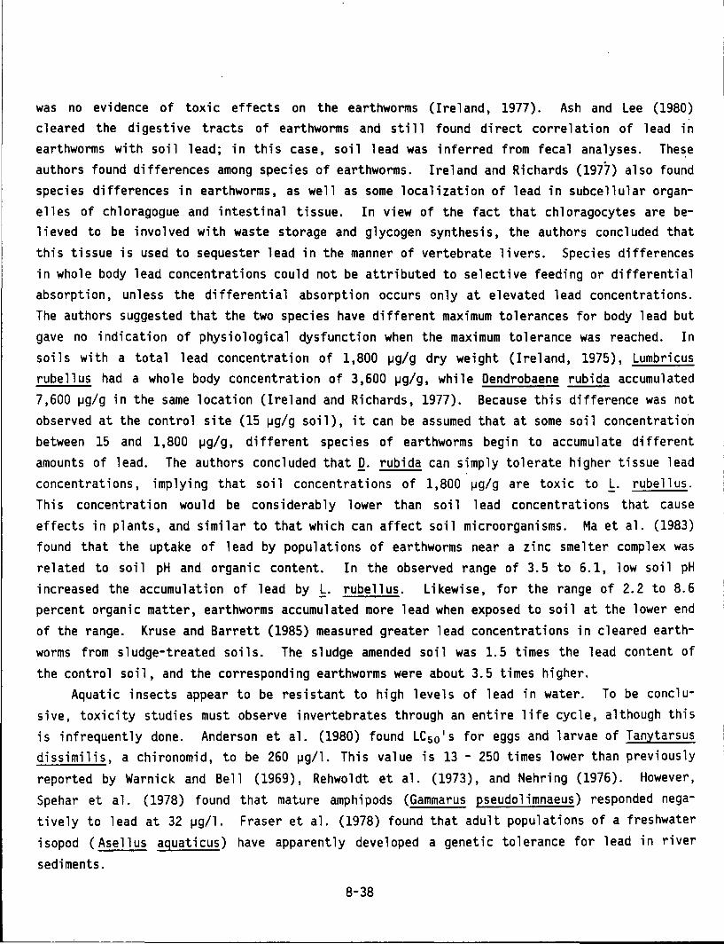
was no evidence of toxic effects on the earthworms (Ireland, 1977). Ash and Lee (1980)
cleared the digestive tracts of earthworms and still found direct correlation of lead in earthworms with soil lead; in this case, soil lead was inferred from fecal analyses. The~e
authors found differences among species of earthworms. Ireland and Richards (1977) also found species differences in earthworms, as well as some localization of lead in subcellular organelles of chloragogue and intestinal tissue. In view of the fact that chloragocytes are believed to be involved with waste storage and glycogen synthesis, the authors concluded that this tissue is used to sequester lead in the manner of vertebrate livers. Species differences in whole body lead concentrations could not be attributed to selective feeding or differential absorption, unless the differential absorption occurs only at elevated lead concentrations. The authors suggested that the two species have different maximum tolerances for body lead but gave no indication of physiological dysfunction when the maximum tolerance was reached. In soils with a total lead concentration of 1,800 1-1g/g dry weight (Ireland, 1975), Lumbricus rubellus had a whole body concentration of 3,600 IJg/g, while Dendrobaene rubida accumulated 7,600 IJg/g in the same location (Ireland and Richards, 1977). Because this difference was not observed at the control site (15 IJg/g soil), it can be assumed that at some soil concentratioh between 15 and 1,800 1-1g/g, different species of earthworms begin to accumulate different amounts of lead. The authors concluded that Q. rubida can simply tolerate higher tissue lead concentrations, implying that soil concentrations of 1,800 IJg/g are toxic to .!:· rubellus. This concentration would be considerably 1 ower than sci 1 1 ead concentrati ens that cause effects in plants, and similar to that which can affect soil microorganisms. Ma et al. (1983)
found that the uptake of lead by populations of earthworms near a zinc smelter complex was related to soil pH and organic content. In the observed range of 3.5 to 6.1, low soil pH increased the accumulation of lead by.!:· rubellus. Likewise, for the range of 2.2 to 8.6
percent organic matter, earthworms accumulated more lead when exposed to soil at the lower end of the range. Kruse and Barrett (1985) measured greater lead concentrations in cleared earthworms from sludge-treated soils. The sludge amended soil was 1.5 times the lead content of the control soil, and the corresponding earthworms were about 3.5 times higher.
Aquatic insects appear to be resistant to high levels of lead in water. To be conclusive, toxicity studies must observe invertebrates through an entire life cycle, although this is infrequently done. Anderson et al. (1980) found LC 50
1 s for eggs and larvae of Tanytarsus dissimilis, a chironomid, to be 260 IJg/1. This value is 13 - 250 times lower than previously reported by Warnick and Bell (1969), Rehwoldt et al. (1973), and Nehring (1976). However, Spehar et al. (1978) found that mature amphipods (Gammarus pseudol imnaeus) responded negatively to lead at 32 IJg/1. Fraser et al. (1978) found that adult populations of a freshwater isopod ( Asellus aguaticus) have apparently developed a genetic tolerance for lead in river
sediments.
8-38
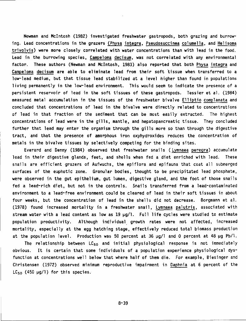
Newman and Mcintosh (1982) investigated freshwater gastropods, both grazing and burrowing. Lead concentrations in the grazers (Physa integra, !'seudosuccinea columella, and Helisoma trivolvis) were more closely correlated with water concEmtrations than with lead in the food. Lead in the burrowing species, Campe 1 oma deci sum, was not corre 1 a ted with any en vi ronmenta 1 factor. These authors (Newman and Mcintosh, 1983) also reported that both Physa integra and Campeloma decisum are able to eliminate lead from the·ir soft 'tissue when transferred to a low-lead medium, but that tissue lead stabilized at a level higher than found in populations living permanently in the low-lead environment. This would seem to indicate the presence of a persistent reservoir of lead in the soft tissues of these gastropods. Tessier et al. (1984) measured metal accumulation in the tissues of the fresh,~ater bivalve Elliptic complanata and concluded that concentrations of lead in the bivalve were directly related to concentrations of lead in that fraction of the sediment that can be most easily extracted. The highest concentrations of lead were in the gills, mantle, and hepatopancreatic tissue. They concluded further that lead may enter the organism through the gills more so than through the digestive tract, and that the presence of amorphous iron oxyhyd1·oxi des reduces the concentration of metals in the bivalve tissues by selectively competing for the binding sites.
Everard and Denny (1984) observed that freshwater snails (Lymnaea peregra) accumulate lead in their digestive glands, feet, and shells when fed a diet enriched with lead. These snails are efficient grazers of Aufwuchs, the epiflora and epifauna that coat all submerged surfaces of the euphotic zone. Granular bodies, thought to be precipitated lead phosphate, were observed in the gut epithelium, gut lumen, digestive gland, and the foot of those snails fed a lead-rich diet, but not in the controls. Snails transferred from a lead-contaminated environment to a lead-free environment could be cleared of lead in their soft tissues in about four weeks, but the concentration of 1 ead in the she 11:; did not decrease. Borgmann et a 1. (1978) found increased mortality in a freshwater snail, Lymnaea palutris, associated with stream water with a lead content as low as 19 ~g/1. Full life cycles were studied to estimate population productivity. Although individual. growth rates were not affected, increased mortality, especially at the egg hatching stage, effectively reduced total biomass production at the population level. Production was 50 percent at 36 ~g/1 and 0 percent at 48 ~g Pb/1.
The relationship between LC 50 and initial physiological response is not immediately obvious. It is certain that some individuals of a population experience physiological dysfunction at concentrations well below that where half of them die. For example, Biesinger and Christensen (1972) observed minimum reproductive impairment in Daphnia at 6 percent of the LC 50 (450 ~g/1) for this species.
8-39
8.4.3 Summary of Effects on Animals While it is impossible to establish a safe limit of daily lead consumption, it is reason
able to generalize that a regular diet of 2-8 mg Pb/kg·day body weight over an extended period of time (Botts, 1977) will cause death in most animals. Animals of the grazing food chain are affected most directly by the accumulation of aerosol particles on vegetation surfaces and somewhat indirectly by the uptake of lead through plant roots. Many of these animals consume more than 1 mg Pb/kg·day in habitats near smelters and roadsides, but no toxic effects have been documented. Animals of the decomposer food chain are affected indirectly by lead in soil which can eliminate populations of microorganisms preceding animals in the food chain or occupying the digestive tract of animals and aiding in the breakdown of organic matter. Invertebrates may also accumultate lead at levels toxic to their predators.
Aquatic animals are affected by lead at water concentrations lower than previously considered safe (50 ~g Pb/1) for wildlife. These concentrations occur commonly, but the contribution of atmospheric lead to specific sites of high aquatic lead is not clear.
8.5 EFFECTS OF LEAD ON ECOSYSTEMS There is wide variation in the mass transfer of lead from the atmosphere to terrestrial
ecosystems. Even within the somewhat artificial classification of undisturbed, cultivated, and urban ecosystems, reported fluxes in undisturbed ecosystems vary by nearly 20-fold. Smith and Siccama (1981) report 270 g/ha·yr in the Hubbard Brook forest of New Hampshire; Lindberg and Harriss (1981) found 150 g/ha·yr in the Walker Branch watershed of Tennessee; and Elias et al. (1976) found 15 g/ha·yr in a remote subalpine ecosystem of California. Jackson and Watson (1977) found 1,000,000 g/ha·yr near a smelter in southeastern Missouri. Getz et al. (1977c) estimated 240 g/ha·yr by wet precipitation alone in a rural ecosystem largely cultivated and 770 g/ha·yr in an urban ecosystem.
One factor causing great variation is remoteness from source, which translates to lower air concentrations, smaller particles, and greater dependence on wind as a mechanism of deposition (Elias and Davidson, 1980). Another factor is type of vegetation cover. Deciduous leaves may, by the nature of their surface and orientation in the wind stream, be more suitable deposition surfaces than conifer needles. Davidson et al. (1982) discussed the influence of leaf surface on deposition rates to grasses.
The history of lead contamination in roadside ecosystems has been reviewed by Smith (1976). Recent studies have shown three areas of concern where the effects of 1 ead on ecosystems may be extremely sensitive (Martin and Coughtrey, 1981; Smith, 1981). First, decomposition is delayed by lead, as some decomposer microorganisms and invertebrates are inhibited
8-40
by soil lead. Secondly, the natural processes of calcium biopurification are circumvented by the accumulation of lead on the surfaces of vegetation and in the soil reservoir. Thirdly~
some ecosystems experience subtle shifts toward lead tolerant plant populations. These problems all arise because lead in ecosystems is deposited on vegetation surfaces, accumulates in the soil reservoir, and is not removed with the surface and ground water passing out of the ecosystem. Other potentia 1 effects are discussed that may occur because of the 1 ong-term build-up of lead in soil.
8.5.1 Delayed Decomposition The flow of energy through an ecosystem is regulated largely by the ability of organisms
to trap energy in the form of sunlight and to convert this energy from one chemical form to another (photosynthesis). Through photosynthesis, p 1 ant:s convert 1 i ght to stored chemica 1
energy. Starch is only a minor product of this energy conversion. The most abundant substance produced by net primary production is cellulose, cl structural carbohydrate of plants. Terrestrial ecosystems, especially forests, accumulate a tremendous amount of cellulose as woody tissue of trees. Few animals can digest cellulose and most of these require symbiotic associations with specialized bacteria. It is no surprise then, that most of this cellulose must eventually pass through the decomposer food chain. Litter fall is the major route for this pathway. Because 80 percent or more of net primary production passes through the decomposing food chain (Swift et al., 1979), the energy of this litter is vital to the rest of the plant community and the inorganic nutrients·are vital to plants.
The amount of lead that causes litter to be resistant to decomposition is not known. Although laboratory studies show that 50 1-1g Pb/ml nutrit:mt medium definitely inhibits soil bacterial populations, field studies indicate little or no effect at 600 !Jg/g litter (Doelman and Haanstra, 1979b). One explanation is that the lead in the laboratory nutrient medium was readily available, while the lead in the litter was chemically bound to soil organic matter. Indeed, Doelman and Haanstra (1979a) demonstrated the effects of soil lead content on delayed decomposition: sandy soils lacking organic complexing compounds showed a 30 percent inhibition of decomposition at 750 !Jg/g, including the complete loss of major bacterial species, whereas the effect was reduced in clay soils and non-existent in peat soils. Organic matter maintains the cation exchange capacity of soils. A reduction in decomposition rate was observed by Doelman and Haanstra (1979a) even at the lowest experimental concentration of lead, leading to the conclusion that some effect might have occurred at even lower concentrations.
When decomposition is delayed, nutrients may be limiting to plants. In tropical regions or areas with sandy soils, rapid turnover of nutrients is essential for the success of the forest community. Even in a mixed deciduous forest, a significant portion of the nutrients,
8-41
especially nitrogen and sulfur, may be found in the litter reservoir (Likens et al. 1977).
Annual litter inputs of calcium and nitrogen to the soil account for about 60 percent of root uptake. With delayed decomposition, plants must rely on precipitation and soil weathering for the bulk of their nutrients. Furthermore, the organic content of soil may decrease, reducing the cation exchange capacity of soil.
8.5.2 Circumvention of Calcium Biopurification B i opurifi cation is a process that regulates the re 1 at i ve concentrations of nutrient to
non-nutrient elements in biological components of a food chain. In the absence of absolute knowledge of natural lead concentrations, biopurification can be a convenient method for estimating the degree of contamination. Following the suggestion by Comar (1965) that carnivorous animals show reduced Sr/Ca ratios compared to herbivorous animals which, in turn show less than plants, Elias et al. (1976, 1982) developed a theory of biopurification, which hypothesizes that calcium reservoirs are progressively purified of Sr, Ba, and Pb in successive stages of a food chain. In other words, if the Sr/Ca and Ba/Ca ratios are known, the natural Pb/Ca ratio can be predicted and the observed Pb/Ca to natural Pb/Ca ratio is an expression of the degree of contamination. Elias et al. (1976, 1982) and Elias and Patterson (1980)
observed continuous biopurification of calcium in grazing and detrital food chains by the progressive exclusion of Sr, Ba, and Pb (Figure 8-5). It is now believed that members of grazing and decomposer food chains are contaminated by factors of 30- 500, i.e., that 97- 99.9 percent of the lead in organisms is of anthropogenic origin. Burnett and Patterson (1980) have shown a similar pattern for a marine food chain.
The mechanism of biopurification relies heavily on the selective transport of calcium across membranes, the selective retention of non-nutrients at physiologically inactive binding sites, and the reduced solubility of non-nutrient elements in the nutrient medium of plants and animals. For example, lead is bound more vigorously to soil organic complexes and is less soluble in soil moisture (Section 6.5.1). Lead is also adsorbed to cell walls in the root apoplast, is excluded by the cortical cell membrane, and is isolated as a precipitate in subcellular vesicles of cortical cells (Koeppe, 1981). Further selectivity at the endodermis results in a nutrient solution of calcium in the vascular tissue that is greatly purified of lead. Similar mechanisms occur in the stems and leaves of plants, in the digestive and circulatory systems of herbivores and carnivores, and in the nutrient processing mechanisms of
insects. Atmospheric lead circumvents the natural biopurification of calcium. Deposition on plant
surfaces, which accounts for 90 percent of the total plant lead, increases the ratio of Pb/Ca in the diet of herbivores. Deposition on herbivore fur increases the Pb/Ca ratio in the diet
8-42
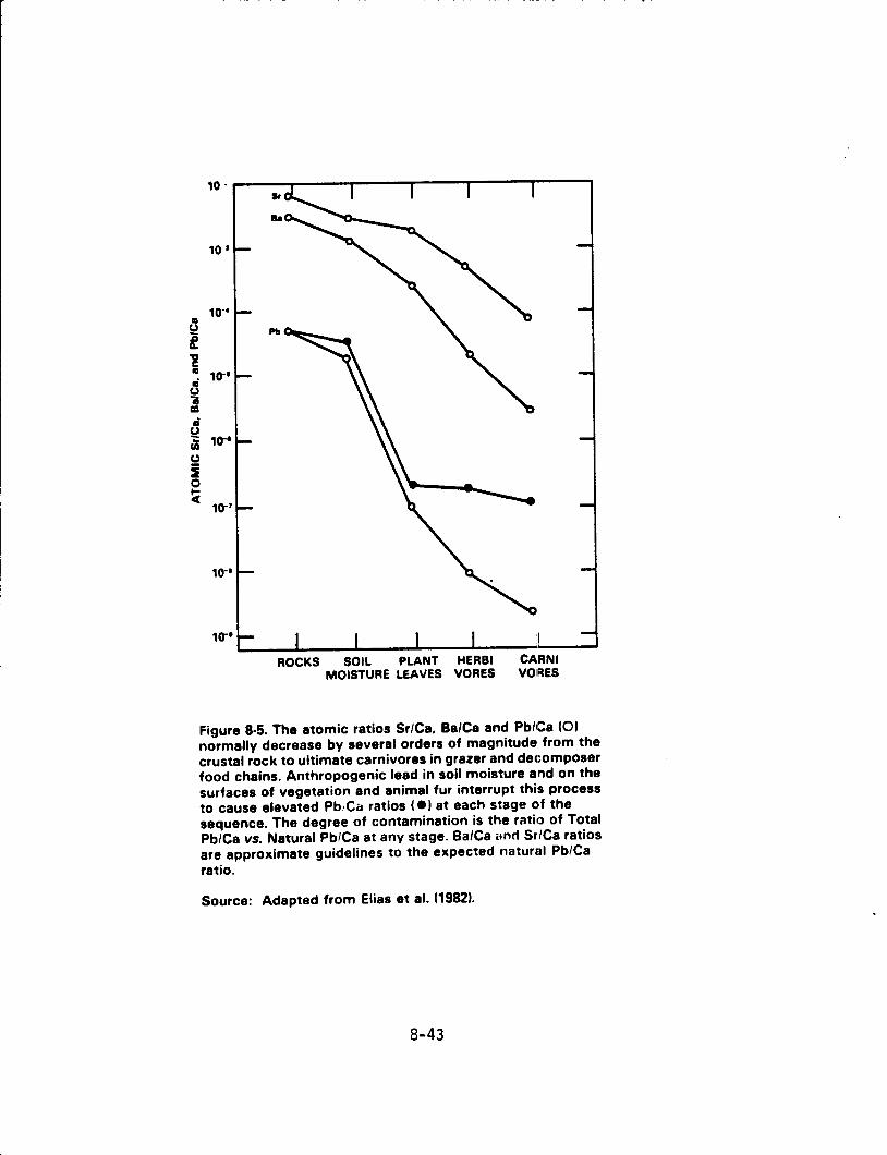
1o-•
1o-" ROCKS SOIL PLANT HERBI CARNI
MOISTURE LEAVES VORES VOIFIES
Figure 8-5. The atomic ratios Sr/Ca. Ba/Ca and Pb/Ca (01 normally decrease by several orders of magnitude from the crustal rock to ultimate carnivores in grazer and dec:omposer food chains. Anthropogenic lead in soil moisture and on the surfaces of vegetation and animal fur interrupt this process to cause elevated Pb, Ca ratios ( •1 at each stage of the sequence. The degree of contamination is the rati1J of Total Pb/Ca vs. Natural Pb/Ca at any stage. Ba/Ca <tnd Sr/Ca ratios are approximate guidelines to the expected natuml Pb/Ca ratio.
Source: Adapted from Elias et al. (19821.
8-43
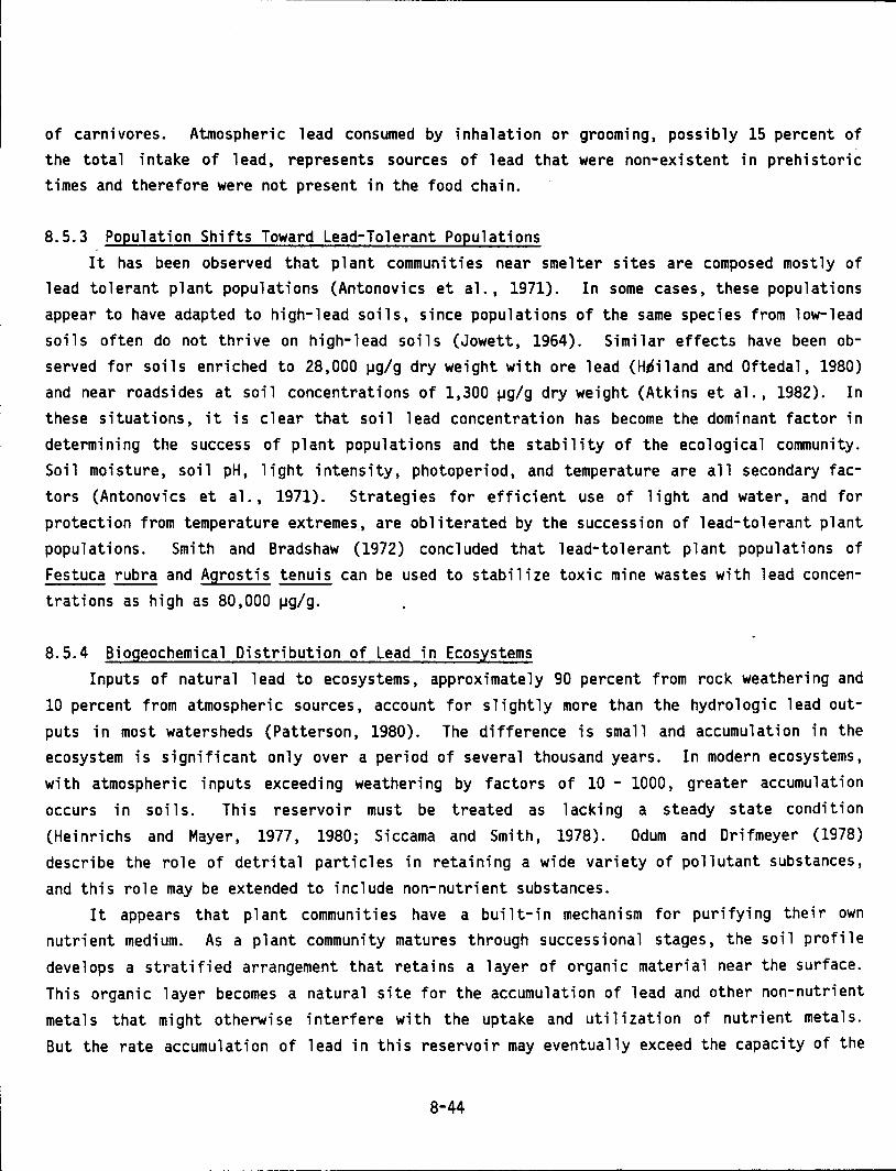
of carnivores. Atmospheric lead consumed by inhalation or grooming, possibly 15 percent of the total intake of lead, represents sources of lead that were non-existent in prehistoric times and therefore were not present in the food chain.
8.5.3 Population Shifts Toward Lead-Tolerant Populations It has been observed that plant communities near smelter sites are composed mostly of
lead tolerant plant populations (Antonovics et al., 1971). In some cases, these populations appear to have adapted to high-lead soils, since populations of the same species from low-lead soils often do not thrive on high-lead soils (Jowett, 1964). Similar effects have been observed for soils enriched to 28,000 ~g/g dry weight with ore lead (H~iland and Oftedal, 1980) and near roadsides at soil concentrations of 1,300 ~g/g dry weight (Atkins et al., 1982). In these situations, it is clear that soil lead concentration has become the dominant factor in determining the success of plant populations and the stability of the ecological community. Soil moisture, soil pH, light intensity, photoperiod, and temperature are all secondary factors (Antonovi cs et a 1. , 1971). Strategies for efficient use of 1 i ght and water, and for protection from temperature extremes, are obliterated by the succession of lead-tolerant plant populations. Smith and Bradshaw (1972) concluded that lead-tolerant plant populations of Festuca rubra and Agrostis tenuis can be used to stabilize toxic mine wastes with lead concentrations as high as 80,000 ~g/g.
8.5.4 Biogeochemical Distribution of Lead in Ecosystems Inputs of natural lead to ecosystems, approximately 90 percent from rock weathering and
10 percent from atmospheric sources, account for slightly more than the hydrologic lead outputs in most watersheds (Patterson, 1980). The difference is small and accumulation in the ecosystem is significant only over a period of several thousand years. In modern ecosystems, with atmospheric inputs exceeding weathering by factors of 10 - 1000, greater accumulation occurs in soils. This reservoir must be treated as lacking a steady state condition (Heinrichs and Mayer, 1977, 1980; Siccama and Smith, 1978). Odum and Drifmeyer (1978) describe the role of detrital particles in retaining a wide variety of pollutant substances, and this role may be extended to include non-nutrient substances.
It appears that plant communities have a built-in mechanism for purifying their own nutrient medium. As a plant community matures through successional stages, the soil profile develops a stratified arrangement that retains a layer of organic material near the surface. This organic layer becomes a natural site for the accumulation of lead and other non-nutrient meta 1 s that might otherwise interfere with the uptake and uti 1 i zat ion of nutrient meta 1 s. But the rate accumulation of lead in this reservoir may eventually exceed the capacity of the
8-44
---- ----------------------------------------------
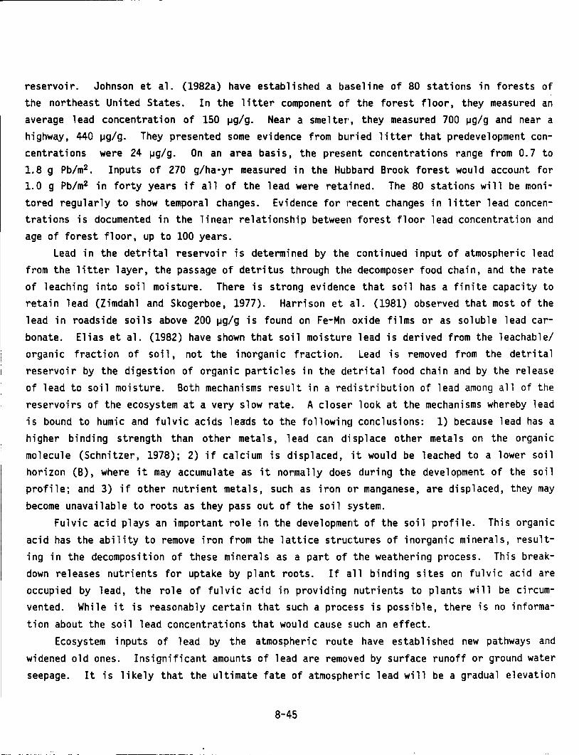
reservoir. Johnson et a 1. (1982a) have estab 1 i shed a buse 1 i ne of 80 stations in forests of the northeast United States. In the litter component of the forest floor, they measured an average lead concentration of 150 ~g/g. Near a smelter, they measured 700 ~g/g and near a highway, 440 ~g/g. They presented some evidence from bL1ri ed 1 i tter that predeve 1 opment concentrations were 24 ~g/g. On an area basis, the pres1:!nt concentrations range from 0. 7 to 1.8 g Pb/m2 • Inputs of 270 g/ha·yr measured in the Hubbard Brook forest would account for 1.0 g Pb/m2 in forty years if all of the lead were retained. The 80 stations will be monitored regularly to show temporal changes. Evidence for r·ecent changes in litter lead concentrations is documented in the linear relationship between forest floor lead concentration and age of forest floor, up to 100 years.
Lead in the detrital reservoir is determined by the continued input of atmospheric lead from the litter layer, the passage of detritus through th•! decomposer food chain, and the rate of leaching into soil moisture. There is strong evidence that soil has a finite capacity to retain lead (Zimdahl and Skogerboe, 1977). Harrison et al. (1981) observed that most of the lead in roadside soils above 200 ~g/g is found on Fe-Mn oxide films or as soluble lead carbonate. Elias et al. (1982) have shown that soil moisturE! lead is derived from the leachable/ organic fraction of soi 1 , not the inorganic fraction. Lead is removed from the detrita 1
reservoir by the digestion of organic particles in the dE!trital food chain and by the release of lead to soil moisture. Both mechanisms result in a redistribution of lead among all of the reservoirs of the ecosystem at a very slow rate. A closer· look at the mechanisms whereby lead is bound to humic and fulvic acids leads to the followin~l conclusions: 1) because lead has a higher binding strength than other metals, lead can displace other metals on the organic molecule (Schnitzer, 1978); 2) if calcium is displaced, it would be leached to a lower soil horizon (B), where it may accumulate as it normally does during the development of the soil profile; and 3) if other nutrient metals, such as iron or manganese, are displaced, they may become unavailable to roots as they pass out of the soil system.
Fulvic acid plays an important role in the development of the soil profile. This organic acid has the ability to remove iron from the lattice struc:tures of inorganic minerals, resulting in the decomposition of these minerals as a part of the weathering process. This breakdown releases nutrients for uptake by plant roots. If all binding sites on fulvic acid are occupied by lead, the role of fulvic acid in providing nutrients to plants will be circumvented. While it is reasonably certain that such a process is possible, there is no information about the soil lead concentrations that would cause such an effect.
Ecosystem inputs of 1 ead by the atmospheric route~ have estab 1 i shed new pathways and widened old ones. Insignificant amounts of lead are removed by surface runoff or ground water seepage. It is likely that the ultimate fate of atmosphe·ric lead will be a gradual elevation
8-45
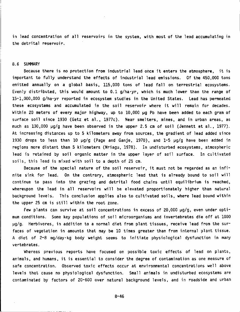
in lead concentration of all reservoirs in the system, with most of the lead accumulating in the detrital reservoir.
8.6 SUMMARY Because there is no protection from industrial lead once it enters the atmosphere, it is
important to fully understand the effects of industrial lead emissions. Of the 450,000 tons emitted annually on a global basis, 115,000 tons of lead fall on terrestrial ecosystems. Evenly distributed, this would amount to 0.1 g/ha·yr, which is much lower than the range of 15-1,000,000 g/ha·yr reported in ecosystem studies in the United States. Lead has permeated these ecosystems and accumulated in the soi 1 reservoir where it will remain for decades. Within 20 meters of every major highway, up to 10,000 ~g Pb have been added to each gram of surface soil since 1930 (Getz et al., 1977c). Near smelters, mines, and in urban areas, as much as 130,000 ~g/g have been observed in the upper 2.5 em of soil (Jennett et al., 1977). At increasing distances up to 5 kilometers away from sources, the gradient of lead added since 1930 drops to less than 10 ~g/g (Page and Ganje, 1970), and 1-5 ~g/g have been added in regions more distant than 5 kilometers (Nriagu, 1978). In undisturbed ecosystems, atmospheric lead is retained by soil organic matter in the upper layer of soil surface. In cultivated soils, this lead is mixed with soil to a depth of 25 em.
Because of the special nature of the soil reservoir, it must not be regarded as an infinite sink for 1 ead. On the contrary, atmospheric 1 ead that is a 1 ready bound to soil will continue to pass into the grazing and detrital food chains until equilibrium is reached, whereupon the 1 ead in a 11 reservoirs wi 11 be e 1 eva ted proportion ate ly higher than natura 1
background levels. This conclusion applies also to cultivated soils, where lead bound within the upper 25 em is still within the root zone.
Few plants can survive at soil concentrations in excess of 20,000 ~g/g, even under optimum conditions. Some key populations of .soil microorganisms and invertebrates die off at 1000 ~g/g. Herbivores, in addition to a normal diet from plant tissues, receive lead from the surfaces of vegetation in amounts that may be 10 times greater than from internal plant tissue. A diet of 2-8 mg/day·kg body weight seems to initiate physiological dysfunction in many vertebrates.
Whereas previous reports have focused on poss i b 1 e taxi c effects of 1 ead on p 1 ants, animals, and humans, it is essential to consider the degree of contamination as one measure of safe concentration. Observed toxic effects occur at environmental concentrations well above levels that cause no physiological dysfunction. Small animals in undisturbed ecosystems are contaminated by factors of 20-600 over natural background levels, and in roadside and urban
8-46
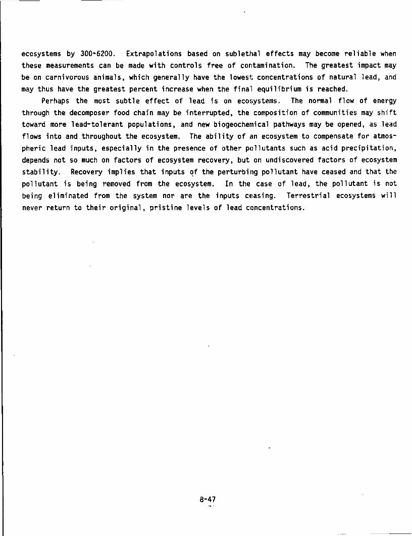
ecosystems by 300-6200. Extrapo 1 at ions based on sub 1 etha 1 effects may become re 1 i ab 1 e when these measurements can be made with controls free of contamination. The greatest impact may be on carnivorous animals, which generally have the lowest concentrations of natural lead, and may thus have the greatest percent increase when the fina·l equilibrium is reached.
Perhaps the most subtle effect of lead is on ecosystems. The normal flow of energy through the decomposer food chain may be interrupted, the composition of communities may shift toward more lead-tolerant populations, and new biogeochemical pathways may be opened, as lead flows into and throughout the ecosystem. The ability of an ecosystem to compensate for atmospheric lead inputs, especially in the presence of other pollutants such as acid precipitation, depends not so much on factors of ecosystem recovery, but on undiscovered factors of ecosystem stability. Recovery implies that inputs qf the perturbing pollutant have ceased and that the pollutant is being removed from the ecosystem. In the case of lead, the pollutant is not being eliminated from the system nor are the inputs CE!asing. Terrestrial ecosystems will never return to their original, pristine levels of lead concentrations.
8-47
8.7 REFERENCES
Anderson, R. L.; Walbridge, C. T.; Fiandt, J. T. (1980) Survival and growth of Tanytarsus dissimilis (chironomidae) exposed to copper, cadmium, zinc, and lead. Arch. Environ. Contam. Toxicol. 9: 329-335.
Antonovics, J.; Bradshaw, A. D.; Turner, R. G. (1971) Heavy metal tolerance in plants. Adv. Ecol. Res. (London) 7: 185.
Arvik, J. H.; Zimdahl, R. L. (1974) Barriers to the foliar uptake of lead. J. Environ. Qual. 3: 369-373.
Ash, C. P. J.; Lee, D. L. (1980) Lead, cadmium, copper and iron in earthworms from roadside sites. Environ. Pollut. Ser. A 22: 59-67.
Atkins, D. P.; Trueman, I. C.; Clarke, C. B.; Bradshaw, A. D. (1982) The evolution of lead tolerance by Festuca rubra on a motorway verge. Environ. Pollut. Ser. A 27: 233-241.
Babich, H.; Bewley, R. J. F.; Stotzky, G. (1983) Application of the 11 ecological dose11 concept to the impact of heavy metals on some microbe-mediated ecologic processes in soil. Arch. Environ. Contam. Toxicol. 12: 421-426.
Baes, C. F., III; Ragsdale, H. L. (1981) Age-specific lead distribution in xylem rings of three tree genera in Atlanta, Georgia. Environ. Pollut. Ser. B 2: 21-35.
Baier, R. W.; Healy, M. L. (1977) Partitioning and transport of lead in Lake Washington. J. Environ. Qual. 6: 291-296.
Battelle's Columbus Laboratories. (1971) Water quality criteria data book -val. 3: effects of chemicals on aquatic life: selected data from the literature through 1968. Washington, DC: U. S. Environmental Protection Agency; EPA report nos. EPA-18050-GWV-05/71 and W73-01976. (Water pollution control research series). Available from: NTIS, Springfield, VA; PB-213210/8BE.
Bazzaz, M. B.; Govindjee (1974) Effects of lead chloride on chloroplast reactions. Environ. Lett. 6: 175-191.
Bazzaz, F. A.; Carlson, R. W.; Rolfe, G. L. (1974) The effect of heavy metals on plants: part I. inhibition of gas exchange in sunflower by Pb, Cd, Ni and Tl. Environ. Pollut. 7: 241-246.
Bazzaz, F. A.; Carlson, R. W.; Rolfe, G. L. (1975) Inhibition of corn and sunflower photosynthesis by lead. Physiol. Plant 34: 326-329.
Beeby, A.; Eaves, S. L. (1983) Short-term changes in Ca, Pb, Zn and Cd concentrations of the garden snail Helix aspersa MUller from a central London car park. Environ. Pollut. Ser. A 30: 233-244.
Bengtsson, G.; Nordstrom, S.; Rundgren, S. (1983) Population density and tissue metal concentration of lumbricids in forest soils near a brass mill. Environ. Pollut. Ser. A 30: 87-108.
8-48
Beresford, W. A.; Donovan, M. P.; Henninger, J. M.; Waalkes, M. P. (1981) Lead in the bone and soft tissues of box turtles caught near smelters. Bull. Environ. Contam. Toxicol. 27: 349-352.
Beyer, W. N.; Pattee, 0. H.; Sileo, L.; Hoffman, D. J.; Mulhern, B. M. (1985) Metal contamination in wildlife living near two zinc smelters. Environ. Pollut. Ser. A 38: 63-86.
Biesinger, K. E.; Christensen, G. M. (1972) Effects of various metals on survival, growth, reproduction, and metabolism of Daphnia magna. J. Fish. Res. Board Can. 29: 1691-1700.
Bisessar, S. (1982) Effect of heavy metals on microorganisms in soils near a secondary lead smelter. Water Air Soil Pollut. 17: 305-308.
Bj~rn, H.; Gyrd-Hansen, N.; Kraul, I. (1982) Birdshooting, lead pellets, and grazing cattle. Bull. Environ. Contam. Toxicol. 29: 174-175.
Borgmann, U.; Kramar, 0.; Loveridge, C. (1978) Rates of mortality, growth, and biomass production of Lymnaea palustris during chronic exposur·e to lead. J. Fish. Res. Board Can. 35: 1109-1115.
Botts, R. P. (1977) The short-term effects of lead on domestic and wild animals. Corvallis, OR: Corvallis Environmental Research Laboratory; EP1~ report no. EPA-600/3-77-009. Available from: NTIS, Springfield, VA; PB-272099.
Bowen, G. D.; Skinner, M. F.; Bevege, D. I. (1974) Zinc uptake by mycorrhizal and uninfected roots of Pinus radiata and Araucaria cunninghamii. Sclil Biol. Biochem. 6: 141-144.
Bradford, W. L. (1977) Urban stormwater pollutant loadings: a statistical summary through 1972. J. Water Pollut. Control Fed. 49: 613-622.
Brewer, R. (1979) Principles of ecology. Philadelphia, PA:: W. B. Saunders Company.
Bull, K. R.; Every, W. J.; Freestone, P.; Hall, J. R.; Osborn, D. (1983) Alkyl lead pollution and bird mortalities on the Mersey Estuary, UK, 19:79-1981. Environ. Pollut. Ser. A 31: 239-259.
Burnett, M. W.; Patterson, C. C. (1980) Perturbation o1F natural lead transport in nutrient calcium pathways of marine ecosystems by industrial lead. In: Goldberg, E. D.; Horibe, Y.; Saruhashi, K., eds. Isotope marine chemistry. Tokyo, Japan: Uchida Rokakuho Publishing Co., Ltd.; pp. 413-438.
Burton, K. W.; Morgan, E.; Roig, A. (1981) The influence of heavy metals upon the growth of sitka-spruce in South Wales forests; I. upper critical and foliar concentrations. Plant Soil 73: 327-336.
Carlson, R. W.; Bazzaz, F. A.; Stukel, J. J.; Wedding, J. B. (1976) Physiological effects, wind reentrainment, and rainwash of Pb aerosol par·ticulate deposited on plant leaves. Environ. Sci. Technol. 10: 1139-1142.
Carlson, R. W.; Stukel, J. J.; Bazzaz, F. A. (1977) Aerosol studies. In: Rolfe, G. L.; Reinbold, K. A., eds. Environmental contamination of lead and other heavy metals. Urbana, IL: Institute for Environmental Studies; pp. 51-66.
8-49
- - ~~~~~-------------
Chaney, W. R.; Strickland, R. C. (1984) Relative toxicity of heavy metals to red pine pollen germination and germ tube elongation. J. Environ. Qual. 13: 391-394.
Chang, F.-H.; Broadbent, F. E. (1982) Influence of trace metals on some soil nitrogen transformations. J. Environ. Qual. 11: 1.
Chau, Y. K. (1986) Speciation of organolead in the environm~nt and mehtylation of lead. Presented at: Workshop on pathways, cycling, and transformation of lead in the environment; October 1985; Edmonton, Canada. Ottowa, Canada: Royal Society of Canada.
Chmiel, K. M.; Harrison, R. M. (1981) Lead content of small mammals at a roadside site in relation to the pathways of exposure. Sci. Total Environ. 17: 145-154.
Christensen, G.; Hunt, E.; Fiandt, J. (1977) The effect of methylmercuric chloride, cadmium chloride, and lead nitrate on six biochemical factors of the brook trout (Salvelinus fontinalis). Toxicol. Appl. Pharmacal. 42: 523-530.
Clark, D. R., Jr. (1979) Lead concentrations: bats vs. terrestrial small mammals collected near a major highway. Environ. Sci. Technol. 13: 338-341.
Comar, C. L. (1965) Movement of fallout radionuclides through the biosphere and man. Annu. Rev. Nucl. Sci. 15: 175-206.
Coughtrey, P. J.; Martin, M. H.; Chard, J.; Shales, S. W. (1980) Micro-organisms and metal retention in the woodlouse Oniscus asellus. Soil Biol. Biochem. 12: 23-27.
Craig, P. J.; Wood, J. M. (1981) The biological methylation of lead: an assessment of the present position. In: Lynam, D. R.; Piantanida, L. G.; Cole, J. F., eds. Environmental lead: proceedings of the second international symposium on environmental lead research; December 1978; Cincinnati, OH. New York, NY: Academic Press; pp. 333-349. (Coulston, F; Korte, F., eds. Ecotoxicology and environmental series).
Crist, T. 0.; Williams, N. R.; Amthor, J. S.; Siccama, T. G. (1985) The lack of an effect of lead and acidity on leaf decomposition in laboratory micrososms. Environ. Pollut. Ser. A 38: 295-303. .
Crump, D. R.; Barlow, P. J. (1980) A field method of assessing lead uptake by plants. Sci. Total Environ. 15: 269-274.
Crump, D. R.; Barlow, P. J. (1982) Factors controlling the lead content of a pasture grass. Environ. Pollut. Ser. B 3: 181-192.
Davidson, C. I.; Miller, J. M.; Pleskow, M. A. (1982) The influence of surface structure on predicted particle dry deposition to natural grass canopies. Water Air Soil Pollut. 18: 25-43.
Devi Prasad, P. V.; Devi Prasad, P. S. (1982) Effect of cadmium, lead and nickel on three freshwater green algae. Water Air Soil Pollut. 17: 263-268.
Doelman, P. (1978) Lead and terrestrial microbiota. In: Nriagu, J. 0., ed. The biogeochemistry of lead in the environment; part B. biological effects. Amsterdam, The Netherlands: Elsevier/North-Holland Biomedical Press; pp. 343-353. (Topics in environmental health: v. 1B).
8-50
Doelman, P.; Haanstra, L. (1979a) Effects of lead on the decomposition of organic matter. Soil Biol. Biochem. 11: 481-485.
Doelman, P.; Haanstra, L. (1979b) Effects of lead on the soil bacterial microflora. Soil Biol. Biochem. 11: 487-491.
Dolske, D. A.; Sievering, H. (1979) Trace element loading of southern Lake Michigan by dry deposition of atmospheric aerosol. Water Air Soil Pollut. 12: 485-502.
Elfving, D. C.; Haschek, W. M.; Stehn, R. A.; Bache, C .. A.; Lisk, D. J. (1978) Heavy metal residues in plants cultivated on and in small mammals indigenous to old orchard soils. Arch. Environ. Health 33: 95-99.
Elias, R. W.; Croxdale, J. (1980) Investigations of the deposition of lead-bearing aerosols on the surfaces of vegetation. Sci. Total Environ. 14: 265-278.
Elias, R. W.; Davidson, C. (1980) Mechanisms of trace element deposition from the free atmosphere to surfaces in a remote High Sierra canyon. Atmos. Environ. 14: 1427-1432.
Elias, R. W.; Patterson, C. C. (1980) Toxicological implications of biogeochemical studies of atmospheric lead. In: Toribara, T. Y.; Miller, M. W.; Morrow, P. E., eds. Polluted rain. New York, NY: Plenum Press; pp. 391-403.
Elias, R. W.; Hinkley, T. K.; Hirao, Y.; Patterson, C. C. (1976) Improved techniques for studies of mass balances and fractionations among families of metals within terrestrial ecosystems. Geochim. Cosmochim. Acta 40: 583-587.
Elias, R.; Hirao, Y.; Patterson, C. C. (1978) The deposition of lead aerosols on plant surfaces in a remote subalpine ecosystem. In: AdriaM, D. C.; Brisbin, I. L., Jr., eds. Environmental chemistry and cycling processes: proceedings of a symposium; April 1976; Augusta, GA. Washington, DC: U. S. Department of E:nergy, Technical Information Center; pp. 691-699. Available from: NTIS, Springfield, VA; CONF-760429.
Elias, R. W.; Hirao, Y.; Patterson, C. C. (1982) The circumvention of the natural biopurification of calcium along nutrient pathways by atmc1spheric inputs of industrial lead. Geochim. Cosmochim. Acta 46: 2561-2580.
Everard, M.; Denny, P. (1984) The transfer of lead by freshwater snails in Ullswater, Cumbria, Environ. Pollut. Ser. A 35: 299-314.
Facchetti, S.; Geiss, F. (1982) Isotopic lead experiment: status report. Luxembourg: Commission of the European Communities; Publication no. EUR 8352 EN.
Feierabend, J. S. (1983) Steel shot and lead poisoning in waterfowl. Washington, DC: National Wildlife Federation. (Scientific and technical series: 8).
Forbes, R. M.; Sanderson, G. C. (1978) Lead toxicity in domestic animals and wildlife. In: Nriagu, J. 0. ed. The biogeochemistry of lead in the environment; part B. biological effects. Amsterdam, The Netherlands: Elsevier/North-Holland Biomedical Press; pp. 225-277. (Topics in environmental health: v. 1B).
Foy, C. D.; Chaney, R. L.; White, M. C. (1978) The physiology of metal toxicity in plants. Annu. Rev. Plant Physiol. 29: 511-566.
8-51
Frankenburger, W. T., Jr.; Tabatabai, M. A (1985) Characteristics of an amidase isolated from a soil bacterium. Soil Biol. Biochem. 17: 303-308. ·
Fraser, J.; Parkin, D. T.; Verspoor, E. (1978) Tolerance to lead in the freshwater isopod Asellus aguaticus. Water Res. 12: 637-641. ·
Friedland, A. J.; Johnson, A. H.; Siccama, T. G. (1984a) Trace metal content of the forest floor in the green mountains of Vermont: spatial and temporal patterns. Water Air Soil Pollut. 21: 161-170.
Friedland, A. J.; Johnson, A. H.; Siccama, T. G.; Mader, D. L. (1984b) Trace metal profiles in the forest floor of New England. Soil Sci. Soc. Am. J. 48: 422-425.
Garland, C. J.; Wilkins, D. A. (1981) Effect of calcium on the uptake and toxicity of lead in Hordeum vulgare L. and Festuca ovina L. New Phytol. 87: 581-593.
Gerakis, P. A.; Veresoglou, D. S.; Sakellariadis, S. D. (1980) Differential response of sugar beet Beta vulgaris L. cultivars to lead. Environ. Pollut. 21: 77-83.
Getz, L. L.; Best, L. B.; Prather, M. (1977a) Lead in urban and rural song birds. Environ. Pollut. 12: 235-238.
Getz, L. L.; Verner, L.; Prather, M. (1977b) Lead concentrations in small mammals living near highways. Environ. Pollut. 13: 151-157.
Getz, L. L.; Haney, A. W.; Larimore, R. W.; McNurney, J. W.; Leland, H. V.; Price, P. W.; Rolfe, G. L.; Wortman, R. L.; Hudson, J. L.; Solomon, R. L.; Reinbold, K. A. (1977c) Transport and distribution in a watershed ecosystem. In: Boggess, W. R., ed. Lead in the envir.onment. Washington, DC: National Science Foundation; pp. 105-133; NSF report no. NSF/RA-770214. Available from: NTIS, Springfield, VA; PB-278278.
Gish, C. D.; Christensen, R. E. (1973) Cadmium, nickel, lead, and zinc in earthworms from roadside soil. Environ. Sci. Technol. 7: 1060-1062.
Goldsmith, C. D., Jr.; Scanlon, P. F. (1977) Lead levels in small mammals and selected invertebrates associated with highways of different traffic densities. Bull. Environ. Contam. Toxicol. 17: 311-316.
Haanstra, L.; Doelman, P. (1984) Glutamic acid decomposition as a senstive measure of heavy metal pollution in soil. Soil Biol. Biochem. 16: 595-600.
Hammond, P. B.; Aronson, A. L. (1964) Lead poisoning in cattle and horses in the vicinity of a smelter. Ann. N. Y. Acad. Sci. 111: 595-611.
Hampp, R.; Lendzian, K. (1974) Effect of lead ions on chlorophyll synthesis. Naturwissen-s chaften 61: 218-219.
Harrison, P. D.; Dyer, M. L. (1984) Lead in mule deer forage in Rocky Mountain National Park, Colorado. J. Wildl. Manage. 48: 510-517.
Harrison, R. M.; Laxen, D. P. H.; Wilson, S. J. (1981) Chemical associations of lead, cadmium, copper, and zinc in street dusts and roadside soils. Environ. Sci. Technol. 15: 1378-1383.
8-52
Hassett, J. J.; Miller, J. E.; Koeppe, D. E. (1976) Interaction of lead and cadmium on maize root growth and uptake of lead and cadmium by roots. Environ. Pollut. 11: 297-302.
Heinrichs, H.; Mayer, R. (1977) Distribution and cycling of major and trace elements in two central European forest ecosystems. J. Environ. Qual. 6: 402-407.
Heinrichs, H.; Mayer, R. (1980) The role of forest veget;!ltion in the biogeochemical cycle of heavy metals. J. Environ. Qual. 9: 111-118.
Hodson, P. V. (1979) Factors affecting the sublethal toxicity of lead to fish. In: International conference: management and control of heavy metals in the environment; September; London, United Kingdom. Edinburgh, United Kingdom: CEP Consultants, Ltd.; pp. 135-138.
Hodson, P. V.; Blunt, B. R.; Spry, D. J. (1978a) Chronic toxicity of water-borne and dietary lead to rainbow trout (Salmo gairdneri) in Lake Ontario water. Water Res. 12: 869-878.
Hodson, P. V.; Blunt, B. R.; Spry, D. J. (1978b) pH-induced changes in blood lead of leadexposed rainbow trout (Salmo gairdneri). J. Fish. Res. Board Can. 35: 437-445.
Hodson, P. V.; Blunt, B. R.; Spry, D. J.; Austen, K. (1977) Evaluation of erythrocyte d-amino levulinic acid dehydratase activity as a short-term indicator in fish of a harmful exposure to lead. J. Fish. Res. Board Can. 34: 501-508.
Hodson, P. V.; Blunt, B. R.; Jensen, D.; Morgan, S. (1979) Effect of fish age on predicted and observed chronic toxicity of lead to rainbow trout in Lake Ontario water. J. Great Lakes Res. 5: 84-89.
Hodson, P. V.; Hilton, J. W.; Blunt, B. R.; Slinger, S. ~1. (1980) Effects of dietary ascorbic acid on chronic lead toxicity to young rainbow tr·out Salmo gairdneri. Can. J. Fish. Aquat. Sci. 37: 170-176.
Hogan, G. D.; Wotton, D. L. (1984) Pollutant distribution and effects in forests adjacent to smelters. J. Environ. Qual. 13: 377-382.
H~iland, K.; Oftedal, P. (1980) Lead-tolerance in Deschampsia flexuosa from a naturally lead polluted area in S Norway. Oikos 34: 168-172.
Homer, J. R.; Cotton, R.; Evans, E. H. (1979) The effects of lead on whole-leaf photosynthesis determined by fluorescence measurements. Biochem. Soc:. Trans. 7: 1259-1260.
Homer, J. R.; Cotton, R.; Evans, E. H. (1981) Changes in photosystem 2 activity associated with plant tolerance to lead. Plant Sci. Lett. 21: 269-274.
Hopkin, S. P.; Martin, M. H. (1984) Assimilation of zinc, cadmium, lead and copper by the centipede Lithobius variegatus (Chilopoda). J. Appl. Ecol. 21: 535-546.
Hughes, M. K. (1981) Cycling of trace metals in ecosystems. In: Lepp, N. W., ed. Effect of heavy metal pollution on plants. Vol. 1: effects of trace metals on plant function. Barking, United Kingdom: Applied Science Publishers, Ltd.; pp. 95-118. (Mellanby, K., ed. Pollution monitoring series).
Hulse, M.; Mahoney, J. S.; Schroder, G. D.; Hacker, C. S.; Pier, S. M. (1980) Environmentally acquired lead, cadmium, and manganese in the cattle egret, Bubulcus ibis, and the laughing gull, Larus atricilla. Arch. Environ. Contam. Toxicol. 9: 65-78.
----- 8-53
Humphreys, M. 0.; Nicholls, M. K. (1984) Relationships between tolerance to heavy metals in Agrostis capillaris L. (~. tenuis sibth.). New Phytol. 98: 177-190.
Hutchinson, T. C. (1980) Effects of acid leaching on cation loss from soils. In: Hutchinson, T. C.; Havas, M., eds. Effects of acid precipitation on terrestrial ecosystems: North Atlantic Treaty Organization conference on effects of acid precipitation on vegetation and soils; May 1978; Toronto, ON, Canada. New York, NY: Ple~um Press; pp. 481-497.
Hutton, M.; Goodman, G. T. (1980) Metal contamination of feral pigeons Columba livia from the London area: part 1-tissue accumulation of lead, cadmium and zinc. Environ~lut. Ser. A 22: 207-217.
Inman, J. C.; Parker, G. R. (1978) Decomposition and heavy metal dynamics of forest litter in northwestern Indiana. Environ. Pollut. 17: 39-51.
Ireland, M. P. (1975) The effect of the earthworm Dendrobaena rubida on the solubility of lead, zinc, and calcium in heavy metal contaminated soil in Wales. J. Soil Sci. 26: 313-318.
Ireland, M. P. (1977) Lead retention in toads Xeno~us laevis fed increasing levels of leadcontaminated earthworms. Environ. Pollut. 12: 8 -92.
Ireland, M. P. (1979) Distribution of essential and toxic metals in the terrestrial gastropod Arion ater. Environ. Pollut. 20: 271-278.
Ireland, M. P.; Richards, K. S. (1977) The occurrence and localisation of heavy metals and glycogen in the earthworms Lumbricus rubellus and Dendrobaena rubida from a heavy metal site. Histochemistry 51: 153-166.
Jackson, D. R.; Watson, A. P. (1977) Disruption of nutrient pools and transport of heavy metals in a forested watershed near a lead smelter. J. Environ. Qual. 6: 331-338.
James, L. F.; Lazar, V. A.; Binns, W. (1966) Effects of sublethal doses of certain minerals on pregnant ewes and fetal development. Am. J. Vet. Res. 27: 132-135.
Jarvie, A. W. P.; Whitmore, A. P.; Markall, R. N.; Potter, H. R. (1983) Lead biomethylation, an elusive goal. Environ. Pollut. Ser. B 6: 81-94.
Jeffries, D. J.; French, M. C. (1972) Lead concentrations in small mammals trapped on roadside verges and field sites. Environ. Pollut. 3: 147-156.
Jenne, E. A.; Luoma, S. N. (1977) Forms of trace elements in soils, sediments, and associated waters: an overview of their determination and biological availability. In: Drucker, H.; Wildung, R. E., eds. Biological implications of metals in the environment. Proceedings of the fifteenth annual Hanford life sciences symposium; September-October 1975; Richland, WA. Washington, DC: Energy Research and Development Administration; pp. 110-143. Available from: NTIS, Springfield, VA; CONF-750929.
Jennett, J. C.; Wixson, B. G.; Lowsley, I. H.; Purushothaman, K.; Bolter, E.; Hemphill, D. D.; Gale, N. L.; Tranter, W. H. (1977) Transport and distribution from mining, milling, and smelting operations in a forest ecosystem. In: Boggess, W. R., ed. Lead in the environment. Washington, DC: National Science Foundation; pp. 135-178; NSF report no. NSF/RA-770214. Available from: NTIS, Springfield, VA; PB-278278.
8-54
Jenny, H. (1980) The soil resource: or1g1n and behavior. New York, NY: Springer-Verlag; pp. 1-146. (Billings, W. D.; Galley, F.; Lange, 0. L.;; Olson, J. S.; Remmert, K., eds. Ecological studies: analysis and synthesis: v. 37).
Jensen, T. E.; Baxter, M.; Rachlin, J. W.; Jani, V. (1982) Uptake of heavy metals by Plectonema boryanum (Cyanophyceae) into cellular components, especially polyphosphate bodies: an X-ray energy dispersive study. Environ. Pollut. Ser. A 27: 119-127.
John, M. K. (1977) Varietal response to lead by lettuce. Water Air Soil Pollut. 8: 133-144.
Johnson, A. H.; Siccama, T. G.; Friedland, A. J. (1982a) Spatial and temporal patterns of lead accumulation in the forest floor in the northeastern United States. J. Environ. Qual. 11: 577-580.
Johnson, M. S.; Pluck, H.; Hutton, M.; Moore,·G. (1982b) Accumulation and renal effects of lead in urban populations of feral pigeons, Columba livia. Arch. Environ. Contam. Toxicol. 11: 761-767. -----
Jowett, D. (1964) Population studies on lead-tolerant Agrostis tenuis. Evolution (Lawrence, KS) 18: 70-81.
Karataglis, S. S. (1982) Combined tolerance to copper, zinc and lead by populations of Agrostis tenuis. Oikos 38: 234-241.
Kendall, R. J.; Scanlon, P. F.; Di Giulio, R. T. (1982) Toxicology of ingested lead shot in ringed turtle doves. Arch. Environ. Contam. To:<icol. 11: 259-263.
Khan, D. H.; Frankland, B. (1983) Effects of cadmium and lead on radish plants with particular reference to movement of metals through soil profile and plant. Plant Soil 70: 335-345.
Kisseberth, W. C.; Sundberg, J. P.; Nyboer, R. W.; Reyno'lds, J. D.; Kasten, S. C.; Beasley, V. R. (1984) Industrial lead, contamination llf an Illinois wildlife refuge and indigenous small mammals. J. Am. Vet. Med. Ass1lc. 185: 1309-1313.
Koeppe, D. E. (1977) The uptake, distribution, and effec:t of cadmium and lead in plants. Sci. Total Environ. 7: 197-206.
Koeppe, D. E. (1981) Lead: understanding the minimal toJdcity of lead in plants. In: Lepp, N. W., ed. Effect of heavy metal pollution on plants; ''· 1. effects of trace metals on plant function. Barking, United Kingdom: Applied Science Publishers, Ltd.; pp. 55-76. (Mellanby, K., ed. Pollution monitoring series).
Krause, G. H. M.; Kaiser, H. (1977) Plant response to heavy metals and sulfur dioxide. Environ. Pollut. 12: 63-71.
Kruse, E. A.; Barrett, G. W. (1985) Effects of municipal sludges and fertilizer on heavy metal accumulation in earthworms. Environ. Pollut. Ser. A 38: 235-244.
Lane, S. D.; Martin, E. S. (1982) An ultrastructural examinatien of lead localisation in germinating seeds of Raphanus sativus. Z. Pflanzenphysiol. 107: 33-40.
Lane, S. D.; Martin, E. S.; Garrod, J. F. (1978) Lead toxicity effects on indole-3-ylacetic acid-induced cell elongation. Planta 144: 79-84.
8-55
Lee, K. C.; Cunningham, B. A.; Chung, K. H.; Paulsen, G. M.; Liang, G. H. (1976) Lead effects on several enzymes and nitrogenous compounds in soybean leaf. J. Environ. Qual. 5: 357-359.
Liang, C. N.; Tabatabai, M. A. (1977) Effects of trace elements on nitrogen mineralisation in soils. Environ. Pollut. 12: 141-147.
Liang, C. N.; Tabatabai, M. A. (1978) Effects of trace elements on nitrification in soils. J. Environ. Qual. 7: 291-293.
Likens, G. E.; Bormann, F. H.; Pierce, S.; Eaton, J. S.; Johnson, N. M. (1977) Biogeochemistry of a forested ecosystem. New York, NY: Springer-Verlag.
Lindberg, S. E.; Harriss, R. C. (1981) The role of atmospheric deposition in an eastern U.S. deciduous forest. Water Air Soil Pollut. 16: 13-31.
Lowe, T. P.; May, T. W.; Brumbaugh, W. G.; Kane, D. A. (1985) National contaminant biomonitoring program: concentrations of seven elements in freshwater fish, 1978-1981. Arch. Environ. Contam. Toxicol. 14: 363-388.
Ma, W.; Edelman, T.; van Beersum, I.; Jans, T. (1983) Uptake of cadmium, zinc, lead, and copper by earthworms near a zinc-smelting complex: influence of soil pH and organic matter. Bull. Environ. Contam. Toxicol. 30: 424-427.
Malone, C.; Koeppe, D. E.; Miller, R. J. (1974) Localization of lead accumulated by corn plants. Plant Physiol. 53: 388-394.
Malone, C. P.; Miller, R. J.; Koeppe, D. E. (1978) Root growth in corn and soybeans: effects of cadmium and lead on lateral root initiation. Can. J. Bot. 56: 277-281.
Manion, P. D. (1981) Tree disease concepts. Englewood Cliffs, NJ: Prentice Hall, Inc.
Martin, M. H. ; Coughtrey, P. J. (1981) Impact of meta 1 s on ecosystem function and productivity. In: Lepp, N. W., ed. Effect of heavy metal pollution on plants; v. 2. metals in the environment. Barking, United Kingdom: Applied Science Publishers, Ltd.; pp. 119-158. (Mellanby, K., ed. Pollution monitoring series).
Mclaughlin, S. B. (1985) Effects of air pollution on forests: a critical review. J. Air Pollut. Control Assoc. 35: 512-534.
McNeilly, T.; Williams, S. T.; Christian, P. J. (1984) Lead and zinc in a contaminated pasture at Minerva, North Wales, and their impact on productivity and organic matter breakdown. Sci. Total Environ. 38: 183-198.
McNurney, J. M.; Larimore, R. W.; Wetzel, M. J. (1977) Distribution of lead in the sediments and fauna of a small midwestern stream. In: Drucker, H.; Wildung, R. E., eds. Biological implications of metals in the environment. Proceedings of the fifteenth annual Hanford life sciences symposium; September-October 1975; Richland, WA. Energy Research and Development Administration, Technical Information Center. Available from: NTIS, Springfield, VA; CONF-750929.
Melin, E.; Nilsson, H. (1955) Ca4 & used as indicator of transport of cations to pine seedlings by means of mycorrhizal mycelium. Sven. Bot. Tidskr. 49: 119-122.
8-56
Melin, E.; Nilsson, H.; Hacskaylo, E. (1958) Translocati'on of cations to seedlings of Pinus virginiana through mycorrhizal mycelium. Bot. Gaz. (Chicago) 119: 243-246. --
Mierau, G. W.; Favara, B. E. (1975) Lead poisoning in roadside populations of deer mice. Environ. Pollut. 8: 55-64.
Miles, C. D.; Brandle, J. R.; Daniel, D. J.; Chu-Der, 0.:; Schnare, P. D.; Uhlik, D. J. (1972) Inhibition of photosystem II in isolated chloroplasts by lead. Plant Physiol. 49: 820-825.
Miller, J. E.; Hassett, J. J.; Koeppe, D. E. (1975) The t!ffect of soil lead sorption capacity on the uptake of lead by corn. Commun. Soil Sci. Plant Anal. 6: 349-358 ..
Miller, R. J.; Koeppe, D. E. (1971) Accumulation and physiological effects of lead in corn. In: Hemphill, D. D., ed. Trace substances in environmental health- IV: [proceedings of University of Missouri•s 4th annual conference on trace substances in environmental health]; June 1970; Columbia, MO. Columbia, MO: Un;iversity of Missouri - Columbia; pp. 186-193.
Mouw, D.; Kalitis, K.; Anver, M.; Schwartz, J.; Constan, A.; Hartung, R.; Cohen, B.; Ringler, D. (1975) Lead: possible toxicity in urban vs. rU1ral rats. Arch. Environ. Health 30: 276-280.
National Academy of Sciences; National Research Council. (1981) Testing for the effects of chemicals on ecosystems: a report by the committee to review methods for ecotoxicology. Washington, DC: National Academy Press.
National Academy of Sciences, Committee on Lead in the Human Environment. (1980) Lead in the human environment. Washington, DC: National Academy c1f Sciences.
Nehring, R. B. (1976) Aquatic insects as biological monitors of heavy metal pollution. Bull. Environ. Contam. Toxicol. 15: 147-154.
Newman, M. C.; Mcintosh, A. W. (1982) The influence of lead in components of a freshwater ecosystem on molluscan tissue lead concentrations. Ac1uat. Toxicol. 2: 1-19.
Newman, M. C.; Mcintosh, A. W. (1983) Lead elimination ancl size effects on accumulation by two freshwater gastropods. Arch. Environ. Contam. Toxicol. 12: 25-29.
Nriagu, J. 0. (1978) Lead in soils, sediments and major rc,ck types. In: Nriagu, J. 0., ed. The biogeochemistry of lead in the environment; part A. ecological cycles. Amsterdam, The Netherlands: Elsevier/North-Holland Biomedical Press; pp. 15-72. (Topics in environmental health: v. lA).
Odum, W. E.; Drifmeyer, J. E. (1978) Sorption of pollutants by plant detritus: a review. Environ. Health Perspect. 27: 133-137.
Ogle, M. C.; Scanlon, P. F.; Kirkpatrick, R. L.; Gwynn, J. V. (1985) Heavy metal concentratons in tissues of mink in Virginia. Bull. Environ. Contam. Toxicol. 35: 29-37.
Osborn, D.; Every, W. J.; Bull, K. R. (1983) The toxicity of trialkyl lead compounds to birds. Environ. Pollut. Ser. A 31: 261-275.
8-57
Page, A. L.; Ganje, T. J. (1970) Accumulations of lead in soils for regions of high and low motor vehicle traffic density. Environ. Sci. Technol. 4: 140-142.
Pai voke, A. (1979) The effects of 1 ead and arsenate on the growth and acid phosphatase activity of pea seedlings. Ann. Bot. Fenn. 16: 18-27.
Patrick, F. M.; Loutit, M. W. (1978) Passage of metals to freshw~ter fish from their food. Water Res. 12: 395-398.
Patterson, C. C. (1980) An alternative perspective - lead pollution in the human environment: origin, extent and significance. In: National Academy of Sciences, Committee on Lead in the Human Environment. Lead in the human environment. Washington, DC: National Academy of Sciences; pp. 265-349.
Patterson, C. C. (1982) Natural levels of lead in humans. Chapel Hill, NC: University of North Carolina, Institute for Environmental Studies. (Carolina environmental essay series: v. 3).
Patterson, M. R.; Munro, J. K.; Luxmoore, R. J. (1975) Simulation of lead transport on the Crooked Creek watershed. In: Hemphill, D. D., ed. Trace substances in environmental health - IX: [proceedings of University of Missouri • s 9th annual conference on trace substances in environmental health]; June; Columbia, MO. Columbia, MO: University of Missouri-Columbia; pp. 217-225.
Peterson, P. J. (1978) Lead and vegetation. In: Nriagu, J. 0., ed. The biogeochemistry of lead in the environment; part B. biological effects. Amsterdam, The Netherlands: Elsevier/ North-Holland Biomedical Press; pp. 355-384. (Topics in environmental health: volume 1B).
Quarles, H. D., III; Hanawalt, R. B.; Odum, W. E. (1974) Lead in small mammals, plants, and soil at varying distances from a highway. J. Appl. Ecol. 11: 937-949.
Rabinowitz, M. (1972) Plant uptake of soil and atmospheric lead in southern California. Chemosphere (4): 175-180.
Rachlin, J. W.; Jensen, T. E.; Baxter, M.; Jani, V. (1982) Utilization of morphometric analysis in evaluating response of Plectonema borpnum (Cyanophyceae) to exposure to eight heavy metals. Arch. Environ. Contam. Toxicol. 1: 323-333.
Reeves, R. D.; Brooks, R. R. (1983) Hyperaccumulation of lead and zinc by two metallophytes from mining areas of central Europe. Environ: Pollut. Ser. A 31: 277-285.
Rehwoldt, R.; Lasko, L.; Shaw, C.; Wirhowski, E. (1973) The acute toxicity of some heavy metal ions toward benthic organisms. Bull. Environ. Contam. Toxicol. 10: 291-294.
Reichel, W. L.; Schmeling, S. K.; Cromartie, E.; Kaiser, T. F.; Krynitsky, A. J.; Lamont, T. G.; Mulhern, B. M.; Pronty, P. M.; Stafford, C. R.; Swineford, D. M. (1984) Pesticide, PCB, and 1 ead residues and necropsy data for ba 1 d eagles from 32 states - 1978-81. Environ. Manit. Assess. 4: 395-403.
Reisinger, K.; Stoeppler, M.; Nurnberg, H. W. (1981) Evidence for the absence of biological methylation of lead in the environment. Nature (London) 291: 228-230.
8-58
Rickard, D. T.; Nriagu, J. 0. (1978) Aqueous environment.al chemistry of lead. In: Nriagu, J .. 0., ed. The biogeochemistry of lead in the environment; part A. ecological cycles. Amsterdam, The Netherlands: Elsevier/North-Holland Biomedical Press; pp. 219-284. (Topics in environmental health: v. lA).
Roderer, G. (1984a) On the toxic effects of tetraethyl lead and its derivatives on the chrysophyte Poterioochromonas malhamensis; V. electron microscopical studies. Environ. Exp. Bot. 24: 17-30.
Roderer, G. (1984b) Toxic effects in plant organisms. In: Grandjean, P., ed. Biological effects of organolead compounds. Boca Raton, FL: CRC Pr·ess, Inc.; pp. 63-95.
Rolfe, G. L. (1974) Lead distribution in tree rings. For. Sci. 20: 283-286.
Rother, J. A.; Millbank., J. W.; Thornton, I. {1983) Nitrogen fixation by white clover (Tri fo 1i um repens) in grass 1 ands on soi 1 s contaminated with cadmium, 1 ead and zinc. J. Soil Sci. 34: 127-136.
Scanlon P. F. (1979) Lead contamination of mammals and invertebrates near highways with different traffic volumes. In: Nielsen, S. W.; Migaki, G.; Scarpelli, D. G., eds. Animals as monitors of environmental pollutants: proceedings of a symposium; 1977; Storrs, CT. Washington, DC: National Academy of Sciences; pp. 200-208.
Scarponi, L.; Perucci, P. (1984) Effect of some metals and related metal-organic compounds on ALA-dehydratase activity of corn. Plant Soil 79: 69-i'5.
Schnitzer, M. (1978) Humic substances: chemistry and re!actions: ch. 1. In: Schnitzer, M.; Khan, S. U., eds. Soil organic matter. New York, NY: Elsevier Scientific Publishing Co.; pp. 1-64. (Developments in soil science: v. 8).
Shirahata, H.; Elias, R. W.; Patterson, C. C.; Koide, M. (1980) Chronological variations in concentrations and isotopic compositions of anthropogenic atmospheric lead in sediments of a remote subalpine pond. Geochim. Cosmochim. Acta 44: 149-162.
Siccama, T. G.; Smith, W. H. (1978) Lead accumulation in a northern hardwood forest. Environ. Sci. Technol. 12: 593-594.
Siccama, T. G.; Smith, W. H.; Mader, D. L. (1980) Changes in lead, zinc, copper, dry weight, and organic matter content of the forest floor of white pine stands in central Massachusetts over 16 years. Environ. Sci. Techno 1. 14: 54-5Ei.
Sicko-Goad, L.; Lazinsky, D. (1981) Accumulation and c:ellular effects of heavy metals in benthic and planktonic algae. Micron 22: 289-290.
Sippel, A. J. A.; Geraci, J. R.; Hodson, P. V. (1983) Histopathological and physiological responses of rainbow trout (Salmo gairdneri Richat•dson) to sublethal levels of lead. Water Res. 17: 1115-1118.
Smart, G. A.; Warrington, M.; Evans, W. H.· (1981) The contribution of had in water to dietary lead intakes. J. Sci. Food Agric. 32: 129-133.
Smith, W. H. (1976) Lead contamination of the roadsidt! ecosystem. J. Air Pollut. Control Assoc. 26: 753-766.
8-59
Smith, R. L. (1980) Ecology and field biology. Third ed. New York, NY: Harper and Row.
Smith, W. H. (1981) Air pollution and forests: interactions between air contaminants and forest ecosystems. New York, NY: Springer-Verlag.
Smith, R. A. H.; Bradshaw, A. D. (1972) Stabilization of toxic mine wastes by the use of tolerant plant populations. Trans. Inst. Min. Metall. Sec. B 81: A230-A237.
Smith, W. H.; Siccama, T. G. (1981) The Hubbard Brook ecosystem study: biogeochemistry of lead in the northern hardwood forest. J. Environ. Qual. 10: 323-333.
Spehar, R. L.; Anderson, R. L.; Fiandt, J. T. (1978) Toxicity and bioaccumulation of cadmium and lead in aquatic invertebrates. Environ. Pollut. 15: 195-208.
Sung, M. W.; Yang, W. J. (1979) Effects of some heavy metals (Al, Cd, Hg, and Pb) on ATP content in plant leaves. Korean J. Bot. 22: 107-113.
Swift, M. J.; Heal, 0. W.; Anderson, J. M. (1979) Decomposition in terrestrial ecosystems. Los Angeles, CA: University of California Press. (Anderson, D. J.; Greig-Smith, P.; Pitelka, F. A., eds. Studies in ecology: v. 5).
Symeonides, C. (1979) Tree-ring analysis for tracing the history of pollution: application to a study in northern Sweden. J. Environ. Qual. 8: 482-486.
Tessier, A.; Campbell, P. G. C.; Auclair, J. C.; Bisson, M. (1984) Relationships between the partitioning of trace metals in sediments and their accumulation in the tissues of the freshwater mollusc Elliptic complanata in a mining area. Can. J. Fish. Aquat. Sci. 41: 1463-1472.
Thayer, J. S.; Brinckman, F. E. (1982) The biological methylation of metals and metalloids. In: Stone, F. G. A.; West, R., eds. Advances in organometallic chemistry: v. 20. New York, NY: Academic Press; pp. 314-356.
Thompson, J. A. J.; Crerar, J. A. (1980) Methylation of lead in marine sediments. Mar. Pollut. Bull. 11: 251-253.
Tyler, G. (1972) Heavy metals pollute nature, may reduce productivity. Ambio 1: 52-59.
Tyler, G. (1978) Leaching rates of heavy metal ions in forest soil. Water Air Soil Pollut. 9: 137-148.
Tyler, G. (1982) Metal accumulation by wood-decaying fungi. Chemosphere 11: 1141-1146.
U. S. Environmental Protection Agency. (1977) Air quality criteria for lead. Research Triangle Park, NC: Health Effects Research Lab, Criteria and Special Studies Office; EPA report no. EPA-600/8-77-017. Available from: NTIS, Springfield, VA; PB-280411.
Voigt, G. K. (1969) Mycorrhizae and nutrient mobilization. In: Hacskaylo, E., ed. Proceedings of the first North American conference on mycorrhizae; April; Washington, DC. Washington, DC: U.S. Department of Agriculture miscellaneous publication no. 1189; pp. 122-131.
Wade, K. J.; Flanagan, J. T.; Currie, A.; Curtis, D. J. (1980) Roadside gradients of lead and zinc concentrations in surface-dwelling invertebrates. Environ. Pollut. Ser. B 1: 87-93.
8-60
Ward, N. I.; Brooks, R. R.; Roberts, E. (1978) Blood lead levels in sheep exposed to auto-:motive emissions. Bull. Environ. Contam. Toxicol. 20: 44-51.
Warnick, S. L.; Bell, H. L. (1969) The acute toxicity of some heavy metals to different species of aquatic insects. J. Water Pollut. Control Fed. 41: 280-284.
Watson, A. P.; Van Hook, R. I.; Jackson, D. R.; Reichle, D. E. (1976) Impact of a lead mining smelting complex on the forest-floor litter arthropod fauna in the new lead belt region of southeast Missouri. Oak Ridge, TN: Oak Ridge National Laboratory, Environmental Sciences Division; Environmental Sciences Division publication no. 881. Available from: NTIS, Springfield, VA; ORNL/NSF/EATC-30.
Weis, P.; Weis, J. S. (1982) Toxicity of methylmercury, mercuric chloride, and lead in killifish (Fundulus heteroclitus) from Southampton, New York. Environ. Res. 28: 364-374.
Welch, W. R.; Dick, 0. L. (1975) Lead concentrations in tissues of roadside mice. Environ. Pollut. 8: 15-21.
Wheeler, G. L.; Rolfe, G. L. (1979) The relationship between daily traffic volume and the distribution of lead in roadside soil and vegeta.tion. Environ. Pollut. 18: 265-274.
Williams, S. T.; McNeilly, T.; Wellington, E. M. H. (1977) The decomposition of vegetation growing on metal mine waste. Soil Biol. Biochem. 9: 271-275.
Williamson, P. (1979) Comparison of metal levels in invertebrate detritivores and their natural diets: concentration factors reassessed. Oecologia 44: 75-79.
Williamson, P. (1980) Variables affecting body burdens of lead, zinc and cadmium in a roadside population of the snail Cepaea hortensis MUller. Oecologia 44: 213-220.
Williamson, P.; Evans, P. R. (1972) Lead: levels in roadside invertebrates and small mammals. Bull. Environ. Contam. Toxicol. 8: 280-288.
Wong, D.; Govindjee. (1976) Effects of lead ions on photosystem I in isolated chloroplasts: studies on the reaction center P700. Photosynthetica 10: 241-254.
Wong, M. H. (1982) Metal cotolerance to copper, lead, and zinc in Festuca rubra. Environ. Res. 29: 42-47.
Wong, M. H.; Bradshaw, A. D. (1982) A comparison of the toxicity of heavy metals, using root elongation of rye grass, Lolium perenne. New Phytol. 91: 255-261.
Wong, P. T. S.; Chau, Y. K. (1979) Methylation and toxit:ity of lead in the aquatic environment. In: International conference: management and control of heavy metals in the environment; September; London, United Kingdom. Edinbul~gh, United Kingdom: CEP Consultants, Ltd.; pp. 131-134.
Wong, P. T. S.; Silverberg, B. A.; Chau, Y. K.; Hodson, P. V. (1978) Lead and the aquatic biota. In: Nriagu, J. 0., ed. The biogeochemistry of lead in the environment; part B. biological effects. Amsterdam, The Netherlands: Elst!vier/North-Holland Biomedical Press; pp. 279-342. (Topics in environmental health: v. 1B).
Wood, J. M. (1984) Alkylation of metals and the activity of metalalkyls. Toxicol. Environ. Chem. 7: 229-240.
8-61
Wood, J. M.; Wang, H.-K. (1983) Microbial resistance to heavy metals. Environ. Sci. Technol. 17: 582A-590A.
Zimdahl, R. L. (1976) Entry and movement in vegetation of lead derived from air and soil sources. J. Air Pollut. Control Assoc. 26: 655-660.
Zimdahl, R. L.; Skogerboe, R. K. (1977) Behavior of lead in soil. Environ. Sci. Technol. 11: 1202-1207.
8-62