Vol. 11(3), pp. 171-183, 21 January, 2016

DOI: 10.5897/AJAR2015.9541

Article Number: 95A3C4256745

ISSN 1991-637X

Copyright ©2016

Author(s) retain the copyright of this article

http://www.academicjournals.org/AJAR

African Journal of Agricultural Research

Full Length Research Paper

Agricultural extension for enhancing productivity and poverty alleviation in small scale irrigation agriculture

for sustainable development in Ethiopia

Aklilu Nigussie*, Abiy Adisu, Kidane Desalegn and Arkebe Gebreegziabher

Ethiopian Institutes of Agricultural Research, Werer Agricultural Research Center, Department of Agricultural Economics, Extension and Gender Research, P. O. Box 2003, Addis Ababa Ethiopia.

Received 23 January, 2015; Accepted 15 October, 2015

The combination of agricultural extension system with small scale irrigation development helps to reduce poverty, and now utmost attention is given to it. Extension system development can increases the production and income of the households and helps to improve their overall economic welfare. This study was conducted to assess the strengths and constraints of the public extension system and to provide suggestions on “best fit” solutions and their scale-up opportunities in the small scale irrigation user; furthermore it examines the impact of agricultural extension system on small-scale irrigation on total income, and the probability of being poor or not at household level. Survey was carried out involving 900 extension users’ households and 875 non-extension users in Afar, Oromia and Somali regional states of Ethiopia which was a total of 1775 households. The result of the study by taking indicators of family size extension service users had more families 6.3 to 5.6 in non-user. The total crop income for one season was 41,282 Ethiopian birr while it was 16,276 for non-users. At the time of the data collection the exchange rate for a dollar was 19.67 Ethiopian Birr. Using a Tobit model to determine the total income parameters of education, extension service access, total land holding had a significant level of increment, while with marginal analysis (dy/dx) factors like household leaders’ age, access to credit and dependency ratios were negatively related with total income. In general, the average annual income of extension users with application of small scale irrigation households was significantly greater than non-extension users. This shows that extension users in small-scale irrigation significantly promote total income of a household. The poverty incidence in non-extension user households is by far greater than user households. Thus, for the agrarian country, Ethiopia, extension system development in small-scale irrigation districts has significant impact on poverty reduction, so agricultural extension development should be given emphasis in development planning. Key words: Income, poverty, small-scale irrigation, extension service, Logit, Tobit, marginal effect.

INTRODUCTION The quality of agricultural extension services is an especially important issue in Ethiopia, where agriculture dominates the economy, accounting for 85% of employment, 50% of exports, and 43% of gross domestic

product (GDP). Over 80% of the country’s 91 million people live in rural areas (FAO, 2010; CIA, 2011), and most are extremely poor, with a daily per capita income of less than $0.50, and access to one hectare or less of

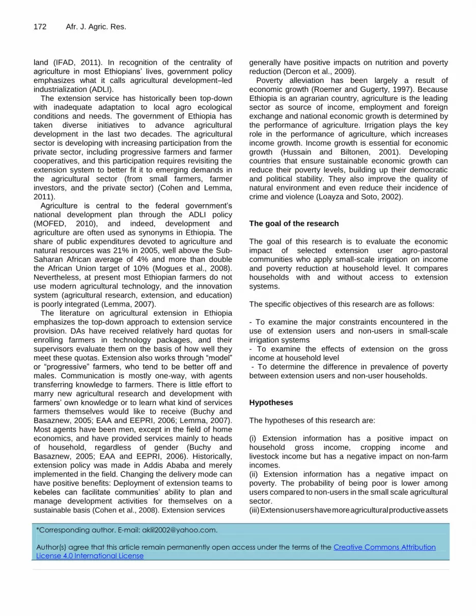
172 Afr. J. Agric. Res. land (IFAD, 2011). In recognition of the centrality of agriculture in most Ethiopians’ lives, government policy emphasizes what it calls agricultural development–led industrialization (ADLI).

The extension service has historically been top-down with inadequate adaptation to local agro ecological conditions and needs. The government of Ethiopia has taken diverse initiatives to advance agricultural development in the last two decades. The agricultural sector is developing with increasing participation from the private sector, including progressive farmers and farmer cooperatives, and this participation requires revisiting the extension system to better fit it to emerging demands in the agricultural sector (from small farmers, farmer investors, and the private sector) (Cohen and Lemma, 2011). Agriculture is central to the federal government’s

national development plan through the ADLI policy (MOFED, 2010), and indeed, development and agriculture are often used as synonyms in Ethiopia. The share of public expenditures devoted to agriculture and natural resources was 21% in 2005, well above the Sub-Saharan African average of 4% and more than double the African Union target of 10% (Mogues et al., 2008). Nevertheless, at present most Ethiopian farmers do not use modern agricultural technology, and the innovation system (agricultural research, extension, and education) is poorly integrated (Lemma, 2007).

The literature on agricultural extension in Ethiopia emphasizes the top-down approach to extension service provision. DAs have received relatively hard quotas for enrolling farmers in technology packages, and their supervisors evaluate them on the basis of how well they meet these quotas. Extension also works through “model” or “progressive” farmers, who tend to be better off and males. Communication is mostly one-way, with agents transferring knowledge to farmers. There is little effort to marry new agricultural research and development with farmers’ own knowledge or to learn what kind of services farmers themselves would like to receive (Buchy and Basaznew, 2005; EAA and EEPRI, 2006; Lemma, 2007). Most agents have been men, except in the field of home economics, and have provided services mainly to heads of household, regardless of gender (Buchy and Basaznew, 2005; EAA and EEPRI, 2006). Historically, extension policy was made in Addis Ababa and merely implemented in the field. Changing the delivery mode can have positive benefits: Deployment of extension teams to kebeles can facilitate communities’ ability to plan and manage development activities for themselves on a sustainable basis (Cohen et al., 2008). Extension services

generally have positive impacts on nutrition and poverty reduction (Dercon et al., 2009).

Poverty alleviation has been largely a result of economic growth (Roemer and Gugerty, 1997). Because Ethiopia is an agrarian country, agriculture is the leading sector as source of income, employment and foreign exchange and national economic growth is determined by the performance of agriculture. Irrigation plays the key role in the performance of agriculture, which increases income growth. Income growth is essential for economic growth (Hussain and Biltonen, 2001). Developing countries that ensure sustainable economic growth can reduce their poverty levels, building up their democratic and political stability. They also improve the quality of natural environment and even reduce their incidence of crime and violence (Loayza and Soto, 2002). The goal of the research The goal of this research is to evaluate the economic impact of selected extension user agro-pastoral communities who apply small-scale irrigation on income and poverty reduction at household level. It compares households with and without access to extension systems. The specific objectives of this research are as follows: - To examine the major constraints encountered in the use of extension users and non-users in small-scale irrigation systems - To examine the effects of extension on the gross income at household level - To determine the difference in prevalence of poverty between extension users and non-user households. Hypotheses The hypotheses of this research are: (i) Extension information has a positive impact on household gross income, cropping income and livestock income but has a negative impact on non-farm incomes. (ii) Extension information has a negative impact on poverty. The probability of being poor is lower among users compared to non-users in the small scale agricultural sector. (iii) Extension users have more agricultural productive assets

*Corresponding author. E-mail: aklil2002@yahoo.com.

Author(s) agree that this article remain permanently open access under the terms of the Creative Commons Attribution

License 4.0 International License

Nigussie et al. 173

Table 1. Summary of variables.

Variable Variables definition and measurements Expected sign

IHh Annual household gross income in ETB Dependent

EXs Extension service (1=extension service user 0= non users) +

TLh Total cultivated land in hectares +

FSh Family size of the household in adult equivalent +

EDu Education level of the household head (1= read and write 0= does not) +

AGe Age of a household head in years -

AIp Access to input1 ( 1=access to inputs 0 = no access) +

LIv Livestock number owned in TLU +

DRh Dependency ratio of the household -

ACs Access to credit service ( 1 = access to credit and 0 =no access) +

AOh Asset owned by household in ETB +

SHh Sex of the household head ( 1= male and 0 = female) +

N.B. 1Access to input means the application of agricultural inputs like improved seed, fertilizer, pesticide etc.

and non-agricultural asset holdings than non-extension users. METHODOLOGY

Approach for data collection, entry and checking

Household data collection was undertaken in six woredas from each woredas three PAs were selected that have access to extension services and non-extension users. Data collection methods included a survey, semi-structured interviews and focus group discussions. Data were collected at household and community level with the assistance of development agents. Each PA has three developmental agents who live and work with the agro pastorals. Using development agents as assistance for data collection is important for the reliability of the data because the communities are more likely to report accurate information to development agents, especially on income, land size and other assets.

The sample households were selected by utilizing the following three-stage stratified sampling procedure. The first stage involved consultation with District Agricultural offices, and eighteen PAs were selected purposively on the basis of their similarity in agricultural practices, potential for irrigation, and the type of small-scale irrigation they used.

In the second stage, household lists in the selected PAs were obtained from village administration and Development agents’ office. Extension service users and non-users households were selected from this list.

In the final stage, households were listed by each small-scale irrigation category with extension service users and non-users then the random sampling technique was used to select sample households from each household type using a random number table. The aim is to carefully examine and compare the income and poverty level of small-scale irrigation users with extension service users and non-users.

Based on these multi-stages sampling processes the total sample households were selected on a random sampling basis from eighteen villages in the six district of Afar (Amibara, Chifira), Oromia (Meiso and Fentale) and Somalia (Kebribeyah, Aware and Lagahida).

Data analysis To control for other factors that influence household incomes this study uses an econometric modeling approach. As stated by Zhou et al. (2009), household gross income is a function of many determinants including household characteristics, asset holding, village location characteristics, and the prices of goods and services. Mathematically, this can be written as (Table 1):

IHh = f (EXs, TLh, FSh, EDu, AGe,AIp, LIv,DRh, ACs,AOh,SHh) (1) Following previous studies, the determinants of household gross income were analyzed by multiple regression models. The model is of this form:- Y = α + hx + gx+ …+ (2) Where:- α = intercept, h and g are parameter estimates Some households may not derive income from livestock, off-farm and other activities; therefore in this study, the impacts of extension service on income were estimated using a Tobit model. This approach was developed by Nobel laureate economist James Tobin in 1958 for analyzing situations whenever dependent variable can take zero values. There are many previous studies with similar works (Zhou et al., 2009; Aschalew, 2009; Barket et al., 2002). The specific form of the Tobit model is described as follows:

Yi* = βx i + (3) We define a new random variable Y transformed from the original one, y*, by Y* = 0, if y≤0 Y* = y, if y ≥0

Where:- Yi is the observed dependent variable measuring combined livestock income, off-farm income, cropping income and household total income, y* is a latent variable, x is a vector of explanatory variables that influence incomes , β is a vector of parameters to be estimated, and ԑ is a random disturbance term with mean 0 and variance σ2. On the basis of the Tobit model specification, the unknown parameters of the explanatory variables can be estimated

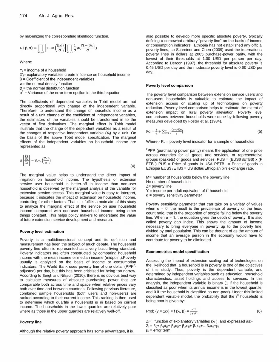
174 Afr. J. Agric. Res. by maximizing the corresponding likelihood function.

Where:

Yi = income of a household X'i= explanatory variables create influence on household income β = Coefficient of the independent variables = the normal density function = the normal distribution function σ2 = Variance of the error term epsilon in the third equation The coefficients of dependent variables in Tobit model are not directly proportional with change of the independent variable. Therefore, to understand the change of household income as a result of a unit change of the coefficient of independent variables, the estimators of the variables should be transformed in to the vector of first derivatives. The marginal effect in Tobit model illustrate that the change of the dependent variables as a result of the changes of respective independent variable (Xi) by a unit. On the basis of the above Tobit model specification. The marginal effects of the independent variables on household income are represented as:

(4) The marginal value helps to understand the direct impact of irrigation on household income. The hypothesis of extension service user household is better-off in income than non-user household is observed by the marginal analysis of the variable for extension service access. This marginal value is easy to interpret, because it indicates the impact of extension on household income, controlling for other factors. That is, it fulfills a main aim of this study to analyze the marginal effect of the service on user household income compared with non-user household income being other things constant. This helps policy makers to understand the value of future extension service development and research.

Poverty level estimation

Poverty is a multidimensional concept and its definition and measurement has been the subject of much debate. The household poverty line often is represented as a very basic living standard. Poverty indicators are often constructed by comparing household income with the mean income or median income (midpoint).Poverty usually is analyzed on the basis of income or consumption indicators. The World Bank uses poverty line of one dollar (PPP2-adjusted) per day, but this has been criticized for being too narrow. According to Bergh and Nilsson (2010), there is no obvious best way to calculate measures of absolute purchasing power that are comparable both across time and space when relative prices vary both over time and between countries. Following pervious literature, combined sample households (both users and non-users) are ranked according to their current income. This ranking is then used to determine which quartile a household is in based on current income. The households in the lower quartiles are relatively poor where as those in the upper quartiles are relatively well-off.

Poverty line

Although the relative poverty approach has some advantages, it is

also possible to develop more specific absolute poverty, typically defining a somewhat arbitrary “poverty line” on the basis of income or consumption indicators. Ethiopia has not established any official poverty lines, so Schreiner and Chen (2009) used the international poverty lines in dollars at 2005 purchase-power parity, with the lowest of their thresholds at 1.00 USD per person per day. According to Dercon (1997), the threshold for absolute poverty is 0.45 USD per day and the moderate poverty level is 0.60 USD per day. Poverty level comparison The poverty level comparison between extension service users and non-users households is valuable to estimate the impact of extension access or scaling up of technologies on poverty reduction. Poverty level comparison helps to estimate the extent of extension impact on rural poverty alleviation. Poverty level comparisons between households were done by following poverty measures developed by Foster et al. (1984).

α

∑ *

( )α

+ (5)

Where:- Pα = poverty level indicator for a sample of households 2PPP (purchasing power parity) means the application of one price across countries for all goods and services, or representative groups (baskets) of goods and services. PUS = (EUS$ /ETB$) x (P ETB ) PUS = Price of goods in USA PETB = Price of goods in Ethiopia EUS$ /ETB$ = US dollar/Ethiopian birr exchange rate. M= number of households below the poverty line N= number of households Z= poverty line Yi = income per adult equivalent of ith household α = poverty sensitivity parameter Poverty sensitivity parameter that can take on a variety of values when α = 0, the result is the prevalence of poverty or the head count ratio, that is the proportion of people falling below the poverty line. When α = 1, the equation gives the depth of poverty. It is also called poverty gap index. This shows the amount of income necessary to bring everyone in poverty up to the poverty line, divided by total population. This can be thought of as the amount of income that an average person in the economy would have to contribute for poverty to be eliminated.

Econometrics model specification Assessing the impact of extension scaling out of technologies on the likelihood that; a household is in poverty is one of the objectives of this study. Thus, poverty is the dependent variable, and determined by independent variables such as education, household characteristics, asset holdings and access to services. In this analysis, the independent variable is binary (1 if the household is classified as poor when its annual income is in the lowest quartile, and 0 if the household is classified as non-poor). Under this limited dependent variable model, the probability that the ith household is being poor is given by:

Prob (y = 1/x) = f (xi, β) =

(6)

Zi= function of explanatory variables (xki), and expressed as:- Zi = β0+ β1x1i+ β2x2i+ β3x3i+ β4x4i+…βkxni+µi µi = error term

L ( β,σ) = 1− βxi

σ

Yi=0

1

σ (

Yi − βx′i

σYi>1

)

𝐸

𝑌𝑖𝑋𝑖𝑋𝑖

= 𝛽. 𝛽𝑥𝑖

𝜎

Nigussie et al. 175

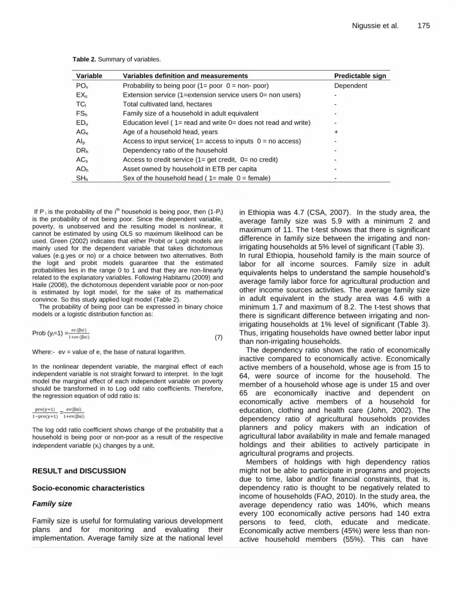
Table 2. Summary of variables.

Variable Variables definition and measurements Predictable sign

POv Probability to being poor (1= poor 0 = non- poor) Dependent

EXs Extension service (1=extension service users 0= non users) -

TCl Total cultivated land, hectares -

FSh Family size of a household in adult equivalent -

EDu Education level ( 1= read and write 0= does not read and write) -

AGe Age of a household head, years +

AIp Access to input service( 1= access to inputs 0 = no access) -

DRh Dependency ratio of the household -

ACs Access to credit service (1= get credit, 0= no credit) -

AOh Asset owned by household in ETB per capita -

SHh Sex of the household head ( 1= male 0 = female) -

If P i is the probability of the ith household is being poor, then (1-Pi) is the probability of not being poor. Since the dependent variable, poverty, is unobserved and the resulting model is nonlinear, it cannot be estimated by using OLS so maximum likelihood can be used. Green (2002) indicates that either Probit or Logit models are mainly used for the dependent variable that takes dichotomous values (e.g.yes or no) or a choice between two alternatives. Both the logit and probit models guarantee that the estimated probabilities lies in the range 0 to 1 and that they are non-linearly related to the explanatory variables. Following Habitamu (2009) and Haile (2008), the dichotomous dependent variable poor or non-poor is estimated by logit model, for the sake of its mathematical convince. So this study applied logit model (Table 2).

The probability of being poor can be expressed in binary choice models or a logistic distribution function as:

(7) Where:- ev = value of e, the base of natural logarithm. In the nonlinear dependent variable, the marginal effect of each independent variable is not straight forward to interpret. In the logit model the marginal effect of each independent variable on poverty should be transformed in to Log odd ratio coefficients. Therefore, the regression equation of odd ratio is: ( )

( ) =

(β )

(β )

The log odd ratio coefficient shows change of the probability that a household is being poor or non-poor as a result of the respective

independent variable (xi) changes by a unit. RESULT and DISCUSSION Socio-economic characteristics

Family size Family size is useful for formulating various development plans and for monitoring and evaluating their implementation. Average family size at the national level

in Ethiopia was 4.7 (CSA, 2007). In the study area, the average family size was 5.9 with a minimum 2 and maximum of 11. The t-test shows that there is significant difference in family size between the irrigating and non-irrigating households at 5% level of significant (Table 3). In rural Ethiopia, household family is the main source of labor for all income sources. Family size in adult equivalents helps to understand the sample household’s average family labor force for agricultural production and other income sources activities. The average family size in adult equivalent in the study area was 4.6 with a minimum 1.7 and maximum of 8.2. The t-test shows that there is significant difference between irrigating and non-irrigating households at 1% level of significant (Table 3). Thus, irrigating households have owned better labor input than non-irrigating households.

The dependency ratio shows the ratio of economically inactive compared to economically active. Economically active members of a household, whose age is from 15 to 64, were source of income for the household. The member of a household whose age is under 15 and over 65 are economically inactive and dependent on economically active members of a household for education, clothing and health care (John, 2002). The dependency ratio of agricultural households provides planners and policy makers with an indication of agricultural labor availability in male and female managed holdings and their abilities to actively participate in agricultural programs and projects.

Members of holdings with high dependency ratios might not be able to participate in programs and projects due to time, labor and/or financial constraints, that is, dependency ratio is thought to be negatively related to income of households (FAO, 2010). In the study area, the average dependency ratio was 140%, which means every 100 economically active persons had 140 extra persons to feed, cloth, educate and medicate. Economically active members (45%) were less than non-active household members (55%). This can have

Prob (yi=1) =ev (βxi)

1+ev (βxi)

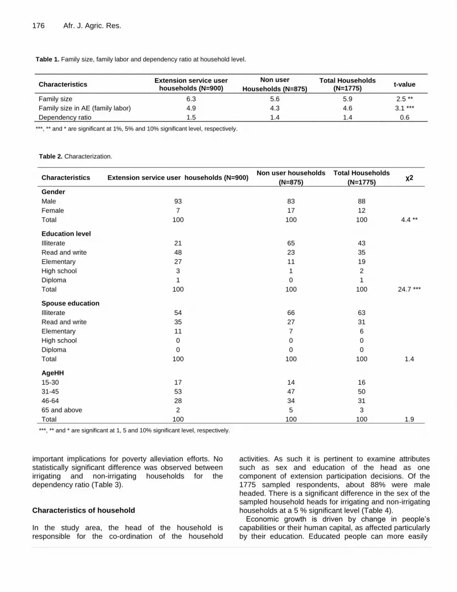
176 Afr. J. Agric. Res. Table 1. Family size, family labor and dependency ratio at household level.

Characteristics Extension service user

households (N=900)

Non user

Households (N=875)

Total Households (N=1775)

t-value

Family size 6.3 5.6 5.9 2.5 **

Family size in AE (family labor) 4.9 4.3 4.6 3.1 ***

Dependency ratio 1.5 1.4 1.4 0.6

***, ** and * are significant at 1%, 5% and 10% significant level, respectively.

Table 2. Characterization.

Characteristics Extension service user households (N=900) Non user households

(N=875)

Total Households

(N=1775) χ2

Gender

Male 93 83 88

Female 7 17 12

Total 100 100 100 4.4 **

Education level

Illiterate 21 65 43

Read and write 48 23 35

Elementary 27 11 19

High school 3 1 2

Diploma 1 0 1

Total 100 100 100 24.7 ***

Spouse education

Illiterate 54 66 63

Read and write 35 27 31

Elementary 11 7 6

High school 0 0 0

Diploma 0 0 0

Total 100 100 100 1.4

AgeHH

15-30 17 14 16

31-45 53 47 50

46-64 28 34 31

65 and above 2 5 3

Total 100 100 100 1.9

***, ** and * are significant at 1, 5 and 10% significant level, respectively.

important implications for poverty alleviation efforts. No statistically significant difference was observed between irrigating and non-irrigating households for the dependency ratio (Table 3). Characteristics of household In the study area, the head of the household is responsible for the co-ordination of the household

activities. As such it is pertinent to examine attributes such as sex and education of the head as one component of extension participation decisions. Of the 1775 sampled respondents, about 88% were male headed. There is a significant difference in the sex of the sampled household heads for irrigating and non-irrigating households at a 5 % significant level (Table 4). Economic growth is driven by change in people’s

capabilities or their human capital, as affected particularly by their education. Educated people can more easily

Nigussie et al. 177

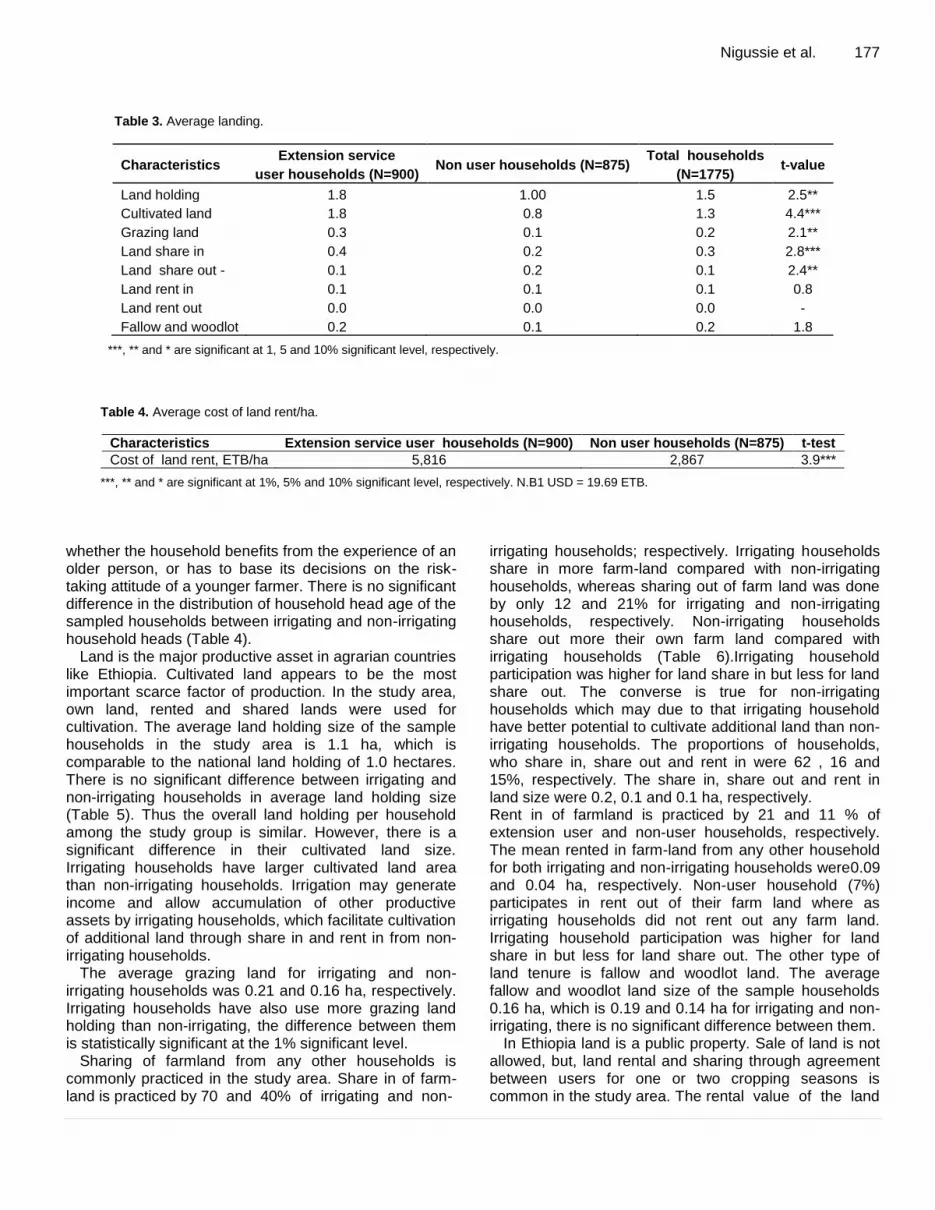
Table 3. Average landing.

Characteristics Extension service

user households (N=900) Non user households (N=875)

Total households

(N=1775) t-value

Land holding 1.8 1.00 1.5 2.5**

Cultivated land 1.8 0.8 1.3 4.4***

Grazing land 0.3 0.1 0.2 2.1**

Land share in 0.4 0.2 0.3 2.8***

Land share out - 0.1 0.2 0.1 2.4**

Land rent in 0.1 0.1 0.1 0.8

Land rent out 0.0 0.0 0.0 -

Fallow and woodlot 0.2 0.1 0.2 1.8

***, ** and * are significant at 1, 5 and 10% significant level, respectively.

Table 4. Average cost of land rent/ha.

Characteristics Extension service user households (N=900) Non user households (N=875) t-test

Cost of land rent, ETB/ha 5,816 2,867 3.9***

***, ** and * are significant at 1%, 5% and 10% significant level, respectively. N.B1 USD = 19.69 ETB.

whether the household benefits from the experience of an older person, or has to base its decisions on the risk-taking attitude of a younger farmer. There is no significant difference in the distribution of household head age of the sampled households between irrigating and non-irrigating household heads (Table 4).

Land is the major productive asset in agrarian countries like Ethiopia. Cultivated land appears to be the most important scarce factor of production. In the study area, own land, rented and shared lands were used for cultivation. The average land holding size of the sample households in the study area is 1.1 ha, which is comparable to the national land holding of 1.0 hectares. There is no significant difference between irrigating and non-irrigating households in average land holding size (Table 5). Thus the overall land holding per household among the study group is similar. However, there is a significant difference in their cultivated land size. Irrigating households have larger cultivated land area than non-irrigating households. Irrigation may generate income and allow accumulation of other productive assets by irrigating households, which facilitate cultivation of additional land through share in and rent in from non-irrigating households.

The average grazing land for irrigating and non-irrigating households was 0.21 and 0.16 ha, respectively. Irrigating households have also use more grazing land holding than non-irrigating, the difference between them is statistically significant at the 1% significant level.

Sharing of farmland from any other households is commonly practiced in the study area. Share in of farm- land is practiced by 70 and 40% of irrigating and non-

irrigating households; respectively. Irrigating households share in more farm-land compared with non-irrigating households, whereas sharing out of farm land was done by only 12 and 21% for irrigating and non-irrigating households, respectively. Non-irrigating households share out more their own farm land compared with irrigating households (Table 6).Irrigating household participation was higher for land share in but less for land share out. The converse is true for non-irrigating households which may due to that irrigating household have better potential to cultivate additional land than non-irrigating households. The proportions of households, who share in, share out and rent in were 62 , 16 and 15%, respectively. The share in, share out and rent in land size were 0.2, 0.1 and 0.1 ha, respectively. Rent in of farmland is practiced by 21 and 11 % of extension user and non-user households, respectively. The mean rented in farm-land from any other household for both irrigating and non-irrigating households were0.09 and 0.04 ha, respectively. Non-user household (7%) participates in rent out of their farm land where as irrigating households did not rent out any farm land. Irrigating household participation was higher for land share in but less for land share out. The other type of land tenure is fallow and woodlot land. The average fallow and woodlot land size of the sample households 0.16 ha, which is 0.19 and 0.14 ha for irrigating and non- irrigating, there is no significant difference between them.

In Ethiopia land is a public property. Sale of land is not allowed, but, land rental and sharing through agreement between users for one or two cropping seasons is common in the study area. The rental value of the land

178 Afr. J. Agric. Res.

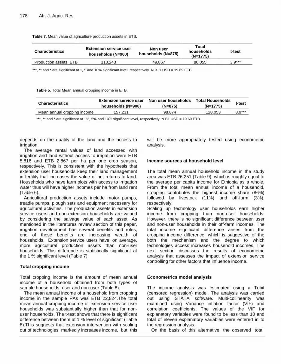
Table 7. Mean value of agriculture production assets in ETB.

Characteristics Extension service user

households (N=900)

Non user households (N=875)

Total households

(N=1775) t-test

Production assets, ETB 110,243 49,867 80,055 3.9***

***, ** and * are significant at 1, 5 and 10% significant level, respectively. N.B. 1 USD = 19.69 ETB.

Table 5. Total Mean annual cropping income in ETB.

Characteristics Extension service user

households (N=900)

Non user households

(N=875)

Total Households

(N=1775) t-test

Mean annual cropping income 157,231 98,874 128,053 8.9***

***, ** and * are significant at 1%, 5% and 10% significant level, respectively. N.B1 USD = 19.69 ETB.

depends on the quality of the land and the access to irrigation.

The average rental values of land accessed with irrigation and land without access to irrigation were ETB 5,816 and ETB 2,867 per ha per one crop season, respectively. This is consistent with the hypothesis that extension user households keep their land management in fertility that increases the value of net returns to land. Households who have farm plots with access to irrigation water thus will have higher incomes per ha from land rent (Table 6).

Agricultural production assets include motor pumps, treadle pumps, plough sets and equipment necessary for agricultural activities. The production assets in extension service users and non-extension households are valued by considering the salvage value of each asset. As mentioned in the literatures review section of this paper, irrigation development has several benefits and roles, one of these benefits are increasing wealth of households. Extension service users have, on average, more agricultural production assets than non-user households. This difference is statistically significant at the 1 % significant level (Table 7). Total cropping income Total cropping income is the amount of mean annual income of a household obtained from both types of sample households, user and non-user (Table 8).

The mean annual income of a household from cropping income in the sample PAs was ETB 22,824.The total mean annual cropping income of extension service user households was substantially higher than that for non-user households. The t-test shows that there is significant difference between them at 1 % level of significant (Table 8).This suggests that extension intervention with scaling out of technologies markedly increases income, but this

will be more appropriately tested using econometric analysis. Income sources at household level The total mean annual household income in the study area was ETB 26,251 (Table 9), which is roughly equal to the average per capita income for Ethiopia as a whole. From the total mean annual income of a household, cropping contributes the highest income share (86%) followed by livestock (11%) and off-farm (3%), respectively. Scaling up technology user households earn higher income from cropping than non-user households. However, there is no significant difference between user and non-user households in their off-farm incomes. The total income significant difference arises from the cropping income difference, which is suggestive of the both the mechanism and the degree to which technologies access increases household incomes. The next section discusses the results of econometric analysis that assesses the impact of extension service controlling for other factors that influence income. Econometrics model analysis The income analysis was estimated using a Tobit (censored regression) model. The analysis was carried out using STATA software. Multi-collinearity was examined using Variance inflation factor (VIF) and correlation coefficients. The values of the VIF for explanatory variables were found to be less than 10 and total of eleven explanatory variables were entered in to the regression analysis.

On the basis of this alternative, the observed total

Nigussie et al. 179

Table 9. Total Mean annual cropping income in ETB.

Characteristics Extension service user households

(N=900)

Non user households (N=875)

Total households

(N=1775) % t-test

Crop income 32,282 13,366 22,824 8.9***

Livestock income 3,132 2,433 2,783 11 1.4

Off-farm income 622 667 645 3 - 0.3

Total income 36,036 16,466 26,251 100 7.6 ***

***, ** and * are significant at 1, 5 and 10% significant level, respectively. N.B1 USD = 19.69 ETB.

Table 10. Tobit estimates of the determinants for total income.

Variable Coef. Std. Err. P>|t|

AGe -16.54 50.7 0.74

EDu 4915.29 *** 1487.4 0.0

EXs 3359.46*** 1222.01 0.01

TLh 10291.91*** 1607.31 0.00

FSh 1554.59 *** 505.83 0.00

AIp 4688.55*** 1738.96 0.01

LIv 2285.07 *** 374.29 0.00

DRh -1031.12 692.57 0.14

ACs -894.16 1052.57 0.39

AOh 2.81*** .34 0.00

SHh 98.65 1755.29 0.96

Constant -1696.12 3561.15 0.00

Sigma 6778.27 358.72

Number of obs. 1775

Prob > chi2 0.00

***, ** and * are significant at 1, 5 and 10% significant level, respectively.

minimum income at household level is ETB 1,256; it is non-zero value. By considering the above revised approaches Tobit regression model was used with 1255 as lower limit. The estimates of coefficients by the Tobit regression model as tool of parameter estimation are depicted in Table 10.

The Tobit analysis suggests that several variables have a statistically significant impact on the total income of the household, many of which are consistent with the hypothesized relationships. The analysis indicates which determinants are more important for the improvement of total household income. Some variables appear to be insignificant; this may be due to the relatively small sample size involved.

Education (EDu) has significant positive impact on income. This seems rational; educated human capital can more easily adopt technologies and make more informed production decision. This can increase the marginal productivity of labor. The increase in productivity of labor is one of the important factors to increase income of a

household (Table 10). Household family size in adult equivalent (FSh) and

livestock holding in TLU (LIv) are positively associated with household total income; both of them are significant. Household family size in adult equivalent means a larger amount of labor available to the household. Labor increases productivity per ha of land, and in turn, household total income increases for a given land base. The positive association between labor and household total income seems reasonable. Livestock holding in have high contribution on total household income by directly sale of livestock and their products, and by used as source of draught power for ploughing in crop production activities.

Access to extension service (EXs) influences the household total income significantly with a positive sign as expected. As Norton et al (1970) suggest, access of technology shifts the production function and offsets the diminishing marginal return by doing so increases income and used as a source of economic growth. According to Makombe and Dawit, (2007), the production function analysis of irrigated and non-irrigated farm plots, the result shows that irrigation shifts the agricultural production frontier to a higher level. The marginal productivities of land and labor for the irrigated farms are almost four, and five times more, respectively. Thus, access to irrigation is one among many factors that increase household incomes.

Household production asset value (AOh) influences the household total income significantly with a positive sign. This tells us households with high production assets can produce more and increase their total income. This is consistent with the economics of transformation and growth principles (Norton et al, 1970) as people accumulate physical capital allows the people to expand production by changing the marginal productivity of inputs like land and labor.

Education (EDu) is also the important factor that influences the annual total income of a household. The analysis shows that access to education significantly increases the household’s total income by ETB 4,903.3 (1USD = 19.67 ETB at the time the study) (Table 11).

The previous discussion indicated the sign and statistical significance of the coefficients from the Tobit

180 Afr. J. Agric. Res.

Table 11. Marginal effects of determinants on household total income.

Determinant dy/dx Std. Err. P>|z|

AGe -12.1 50.4 0.7

EDu 4203.7 11.1 0.0

EXs 3843.9 2.5 0.0

TLh 12744.9 6.4 0.0

FSh 1457.0 5.9 0.0

AIp 4359.4 2.1 0.0

LIv 2811.9 3.7 0.0

DRh -102.3 91.43 0.2

ACs -992.6 87.5 0.9

AOh 2111.8 0.4 0.0

SHh 8.8 72.0 0.8

model. However, in that model the coefficients do not directly represent the marginal-effect, that is, the impact on household income from a one-unit change in the independent variables. The marginal effect estimates reveal that the land size (TLh) has the largest impact. That is, a one ha land change has an impact on income for 10,274.9 ETB per year (Table 11). Thus, land holding size is very important input in rural poor households to increase their annual income. Since, the agrarian nature of the country; agriculture is the main source of income and livelihood for more than 85% of the country’s population. Thus, land is critical and sensitive political issue in contemporary history of Ethiopia (Helland, 1999). In the study area, land is very scarce resource. Land share in/out and rent in/out is common. Even though the cost in cash of land is not far from the estimated marginal impact of land, the additional costs such as transaction cost and monitoring cost are high. Therefore, it is not easy to increase a land as required.

Extension service (EXs) has a significant impact on the total income of a household, ETB 3843.9 per year. This supports the initial hypothesis that extension service use increases households’ income. Households who have access to agricultural extension service can cultivate their irrigated land two or more times a year. Although the econometric analysis cannot indicate directly why the increase in income occurs, extension allows the farmers to practice crop intensification

2 and diversification, which

increases crop yields and revenues from crop sales. Irrigation likely also increases the marginal land and labor productivity, increases the crop production and then promotes household income.

Livestock holding (LIv) also affects annual total income of a household. An increase of household’s livestock holding by one TLU is estimated to increase the total income of a household by ETB 2811.9 per annum. As expected, the value of productive assets owned by the household (AOh) also increases total income of a

household. The increase in asset holding of a household by ETB1000 significantly increases the household total income by ETB 2800. This suggests that households should invest in more productive assets. There should be credit or surplus income to invest on these production assets. The source of credit in the study area is ACSI, the interest rate is high (18%) compared to the Commercial bank of Ethiopia (5%). Thus, both surplus income and credit are unaffordable by subsistent farmers. Household size in adult equivalent (FSh) also increases the annual income of a household. A one-unit increase family size in adult equivalent increases the total income of a household by about ETB 1,600.

Multivariate logit regression The estimated coefficient for dummy variable access to extension service with the odd of being poor over non-poor was negatively correlated and significant. This suggests that the probability to being poor decreases if one has access to extension services, other factors being constant. This probably is due to the influence that extension service on agricultural intensity and diversification. Agricultural intensity is higher in extension service user household as compared to non-user households. Because the definition of the poverty threshold in this study is based on current income, and previous results suggest that access to extension services increases income, it is not particularly surprising that the likelihood of poverty is lowered by extension service implementers.

However, other factors also influence the likelihood that a household is in poverty. As expected, the coefficient of household education is negatively correlated with poverty and significant. The result suggests that household head who is literate had a lower probability of being poor compared with those who are illiterate. Education is assumed to increase productivity and thereby lead to higher levels of welfare for the household (Table 12).

The estimated coefficient for dummy variable access to extension service with the odd of being poor over non-poor was negatively correlated and significant. This suggests that the probability to being poor decreases if one has access to extension service technologies, other factors being constant. This probably is due to the influence that extension on agricultural production intensity and diversification. Production intensity is higher in extension user household as compared to non-user households (Table 12).

The coefficient of land holding per capita was negatively correlated with the probability of a person being poor and statistically significant. The odds ratio illustrates that a one-ha increase in land holding per capita, the odds of being poor decrease markedly(although this is not surprising given that it would result in a doubling of average farm size).

Nigussie et al. 181

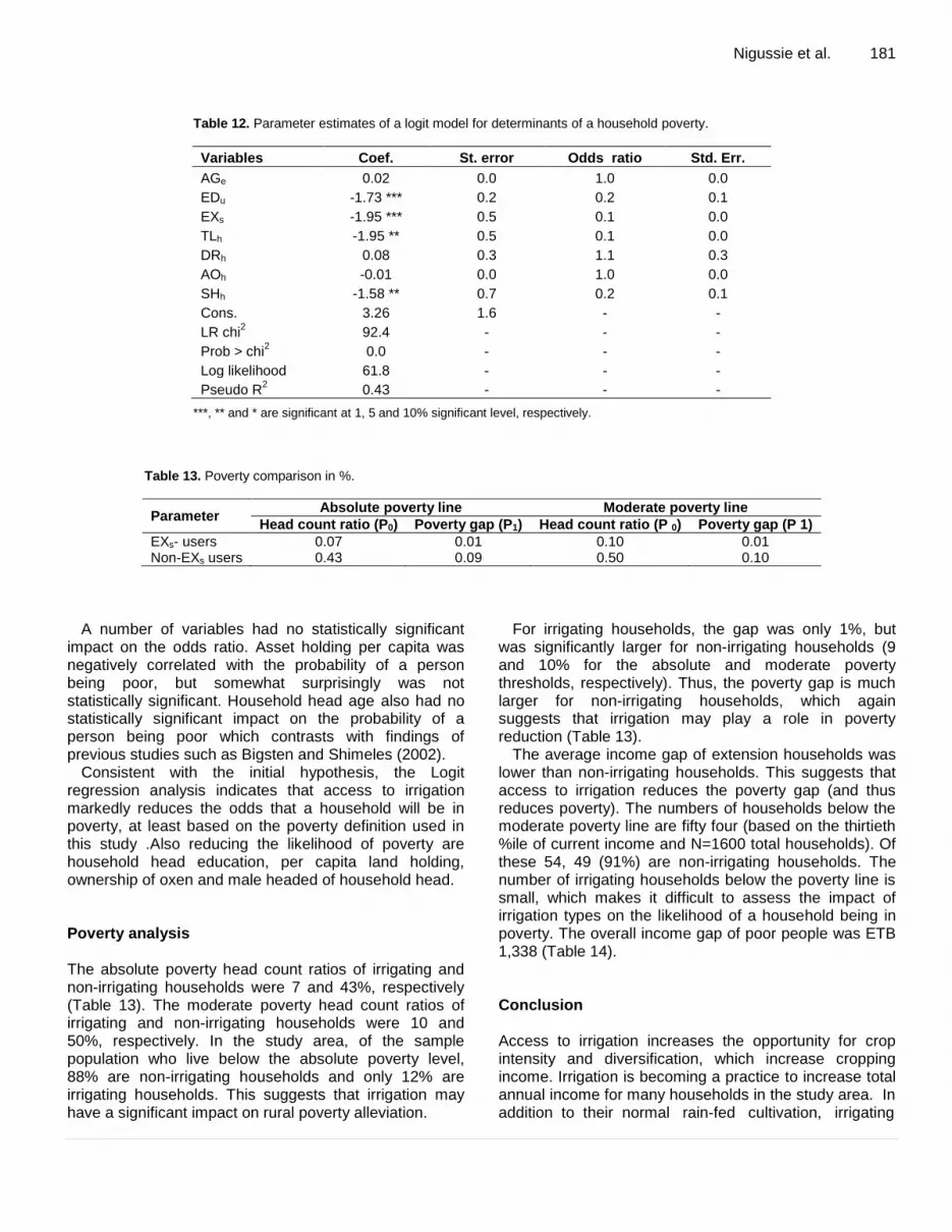
Table 12. Parameter estimates of a logit model for determinants of a household poverty.

Variables Coef. St. error Odds ratio Std. Err.

AGe 0.02 0.0 1.0 0.0

EDu -1.73 *** 0.2 0.2 0.1

EXs -1.95 *** 0.5 0.1 0.0

TLh -1.95 ** 0.5 0.1 0.0

DRh 0.08 0.3 1.1 0.3

AOh -0.01 0.0 1.0 0.0

SHh -1.58 ** 0.7 0.2 0.1

Cons. 3.26 1.6 - -

LR chi2 92.4 - - -

Prob > chi2 0.0 - - -

Log likelihood 61.8 - - -

Pseudo R2 0.43 - - -

***, ** and * are significant at 1, 5 and 10% significant level, respectively.

Table 13. Poverty comparison in %.

Parameter Absolute poverty line Moderate poverty line

Head count ratio (P0) Poverty gap (P1) Head count ratio (P 0) Poverty gap (P 1)

EXs- users 0.07 0.01 0.10 0.01 Non-EXs users 0.43 0.09 0.50 0.10

A number of variables had no statistically significant impact on the odds ratio. Asset holding per capita was negatively correlated with the probability of a person being poor, but somewhat surprisingly was not statistically significant. Household head age also had no statistically significant impact on the probability of a person being poor which contrasts with findings of previous studies such as Bigsten and Shimeles (2002).

Consistent with the initial hypothesis, the Logit regression analysis indicates that access to irrigation markedly reduces the odds that a household will be in poverty, at least based on the poverty definition used in this study .Also reducing the likelihood of poverty are household head education, per capita land holding, ownership of oxen and male headed of household head. Poverty analysis The absolute poverty head count ratios of irrigating and non-irrigating households were 7 and 43%, respectively (Table 13). The moderate poverty head count ratios of irrigating and non-irrigating households were 10 and 50%, respectively. In the study area, of the sample population who live below the absolute poverty level, 88% are non-irrigating households and only 12% are irrigating households. This suggests that irrigation may have a significant impact on rural poverty alleviation.

For irrigating households, the gap was only 1%, but was significantly larger for non-irrigating households (9 and 10% for the absolute and moderate poverty thresholds, respectively). Thus, the poverty gap is much larger for non-irrigating households, which again suggests that irrigation may play a role in poverty reduction (Table 13).

The average income gap of extension households was lower than non-irrigating households. This suggests that access to irrigation reduces the poverty gap (and thus reduces poverty). The numbers of households below the moderate poverty line are fifty four (based on the thirtieth %ile of current income and N=1600 total households). Of these 54, 49 (91%) are non-irrigating households. The number of irrigating households below the poverty line is small, which makes it difficult to assess the impact of irrigation types on the likelihood of a household being in poverty. The overall income gap of poor people was ETB 1,338 (Table 14). Conclusion Access to irrigation increases the opportunity for crop intensity and diversification, which increase cropping income. Irrigation is becoming a practice to increase total annual income for many households in the study area. In addition to their normal rain-fed cultivation, irrigating

182 Afr. J. Agric. Res. Table 6. The average income poverty gap.

Parameter Mean income per adult equivalent of the poor in ETB Mean of income poverty Gap in ETB

Extension service users 2282 943

Non-user 1826 1399

Total 1887 1338

households cultivate cash crops using small-scale irrigation. The main irrigated crops were onion, tomato, potato, maize, oat and vetch. Irrigated crops were selected due to good production potential, economic returns and ease of cultivation, respectively. Onion and rice were the major income source crops for irrigating and non-irrigating households, respectively.

Econometric analyses that control for other factors that influence household income indicate that accesses to small–scale irrigation increases mean household income significantly (about ETB 3,353 per year, or a 27% increase over non-irrigating household),which is hypothesized to occur primarily through crop intensification and crop diversification. It is important to note that other factors (such as input access) also had large effects on household income, and this study did not explore in detail the complementarities between irrigation access and other input use.

The other objective of this study is to assess the impact of irrigation on the likelihood that a household was in poverty. The results indicate that irrigation development has a profound impact in alleviating poverty. The poverty analysis indicates that a much higher proportion of those who are poor are non-irrigating rather than irrigating households. Thus, the poverty prevalence in non-irrigating households is by far greater than irrigating households. This suggests that irrigation has an important influence on rural poverty alleviation. Additional econometric analyses indicate that use of irrigation reduces the probability of a household being poor.

RECOMMENDATIONS AND POLICY IMPLICATION

This study has found that extension service development helps to increase household income and reduces the incidence of poverty at the household level. Based on these findings as well as the outcomes of focus group discussions and key informant interviews, further development and refinement of small-scale irrigation systems appears merited. This, of course, raises the question about this might best is undertaken. Although a formal analysis of strategies for future scaling out development is beyond the scope of this research, following actions are suggested to facilitate future extension service development. 1. Equip the research wing with: materials, human resource and other facilities because the generation

technologies lie on the research institutes. Research institutes are the power house and key for development (thoughts, economical, technologies…) sustainability, Economic growth, poverty eradication, invention and innovation incubating different ideas that can upgrade the extension system. 2. Ensure extension services development፡ extension

needs to address vulnerability as well as productivity and to offer new options from which poor households can choose according to their circumstances. The design of extension strategies must take account of differing degrees of market integration, which determine the degree to which the poor can take advantage of market opportunities. 3. Access to quality service of extension out of political influences in a manner of professional dimension and service access Extension strategies need to differentiate between highly and weakly integrated areas and acknowledge the need to take difficult decisions between supporting production strategies, on the one hand, and broader based livelihood extension, on the other. 4. Renewed and improved the existed irrigation canal development for small irrigation 5. Supply access to technologies: Extension should offer a wider range of services, some focused on support to production and others focused on wider livelihood support, targeted according to an analysis of a particular area’s market integration, degree of vulnerability, and production prospects. 6. Strengthen education and training (adult training and farmers training).

Future studies questions This study focuses on the impact of extension service access on gross income and poverty reduction at household level. However, there are limitations which need further and depth analysis in net income of technologies using cost-benefit.

Choice of scaling out technology types for small-scale, medium scale or large scale irrigation and their impact on income and poverty. The impact of extension scaling out technologies on actual livelihood change on the community like feeding habit, nutritional contribution and urbanization.

Scaling out technologies were cultivated and harvested by all farmers at the same time which cause the problems

of marketing and post-harvest handling in the study area. Conflict of Interests The authors have not declared any conflict of interests. REFERENCES Aschalew D (2009). Soil and water. Articles of Cornell University. In

Partial Fulfillment of the Requirements for the Degree of. Master of Professional Studies.

Barket A, Khan S, Rahman M, Zeman S (2002). Economic and social impact evaluation study on the rural electrification program in Bangladesh, HDRC, Dhaka.

Bergh A, Nilsson T (2010). The globalization and absolute poverty-a panel data study Version to be presented at Nationell konferens nationalekonomi, October 1-2, 2010, Lund University.

Bigsten A, Shimeles A (2002). Growth and Poverty Reduction in Ethiopia: Evidence from Household Panel Surveys, Working Papers in Economics no 65, January 2002, Department of Economics; Göteborg University.

Buchy M, Basaznew F (2005). Gender-Blind Organisations Deliver Gender-Biased Services: The Case of Awasa Bureau of Agriculture in Southern Ethiopia. Gend. Technol. Dev. 9(2):235-251.

CIA (US Central Intelligence Agency). (2011). World Factbook: Ethiopia. Available at: www.cia.gov/library/publications/the-world-factbook/geos/et.html.

Cohen MJ, Lemma M (2011). Agricultural Extension Services and Gender Equality an Institutional Analysis of Four Districts in Ethiopia. Ethiopia Strategy Support Program II (ESSP II) ESSP II Working Paper 28 August 2011. Available at: http://www.ifpri.org/sites/default/files/publications/esspwp28.pdf

Cohen MJ, Roc chigiani M, Garrett JL (2008). Empowering Communities through Food Based Programs: Ethiopia Case Study. World Food Program Discussion Paper. Rome: World Food Programme. Available at: www.wfp.org/sites/default/files/WFP_Discussion_Paper-Empowering_communities Ethiopia_0.pdf.

CSA (Central statistics agency) (2007). Central statistics agency of Ethiopia.

Dercon S (1997). Poverty and deprivation in Ethiopia, Center for the study of African economies, department of economics and Jesus College, Oxford University. FAO (Food and Agricultural Organization) (1997) Irrigation technology transfer in support of food security proceeding of a sub-regional workshop, Harare, Zimbabwe, 14-17 April, water report 14.

Dercon S, Gilligan DO, Hoddinott J, Woldehanna T( 2009). The Impact of Agricultural Extension and Roads on Poverty and Consumption Growth in Fifteen Ethiopian Villages. Am. J. Agric. Econ. 91(4):1007-1021.

EEA (Ethiopian Economic Association) and EEPRI (Ethiopian Economic Policy Research Institute). 2006. Evaluation of the Ethiopian Agricultural Extension with Particular Emphasis on the Participatory Demonstration and Training Extension System (PADETES). Addis Ababa, Ethiopia: EEA and EEPRI.

FAO (2010), Agricultural populations and households. Available at: www.fao.org/fileadmin/templetes/gender/agrigender_docs/t1.pdf

Foster J, Greer J, Thorbecke E (1984). A Class of Decomposable Poverty 113 Measures. Econometrical 52(3):761-766.

Greene W (2002). Econometric analysis, fifth edition, William, New York University, Upper Saddle River, New Jersey 07458.

Habitamu T (2009). Payment for environmental service to enhance resource use efficiency and labor force participation in managing and maintain irrigation infrastructure, the case of Upper Blue Nile basin, Cornell University MPS Thesis.

Haile T (2008). Impact of irrigation development on poverty reduction in Northern Ethiopia.

Nigussie et al. 183 Helland J (1999). Land alienation in Borena: Some land tenure issues

in a pastoral context of Ethiopia. East. Afr. Soc. Sci. Res. Rev. 15(2):1-15.

Hussain I, Biltonen E (2001). Irrigation against Rural Poverty: An Overview of Issues and Pro-Poor Intervention Strategies in Irrigated Agriculture in Asia, Proceedings of National Workshops on Pro-Poor Intervention Strategies in Irrigated Agriculture in Asia Bangladesh, China, India, Indonesia, Pakistan, and Vietnam, IWMI, August, 2001.

IFAD (2011). Rural Poverty in Ethiopia. Available at: www.ruralpovertyportal.org/web/guest/country/home/tags/ethiopia.

John M (2002). Dependency ratio. Available at: http://www.scalloway.org.uk/popu13.htm.

Lemma M (2007). The Agricultural Knowledge System in Tigray, Ethiopia: Recent History and Actual Effectiveness. Weikersheim, Germany: Margraff Publishers.

Loayza N, Soto R (2002). Economic Growth: Sources, Trends, and Cycles, Santiago, Chile, 2002 Central Bank of Chile.

Makombe G, Dawit D (2007). A comparative analysis of rainfed and irrigated agricultural production in Ethiopia. J. Article Irrigat. Drainage Syst. Springer, Netherlands. 21(1):35-44.

MOFED (2010). The Federal Democratic Republic of Ethiopia, Growth and Transformation Plan (GTP), 2010/11-2014/15 Draft, September 2010, Addis Ababa.

Mogues T, Ayele G, Paulos Z (2008). The Bang for the Birr: Public Expenditures and Rural Welfare in Ethiopia. Research Report 160. Washington, DC: International Food Policy Research Institute.

orton W, Jeffrey A, William A 19 0). Economic progress and olicy in Developing countries, ew York orton W, Jeffrey A, William A. P 34.

Roemer M, Gugerty M (1997). Does economic growth reduce poverty? Technical Paper, Harvard Institute for International Development, March 1997.

Schreiner M, Chen M (2009). A Simple Poverty Scorecard for Ethiopia. Available at: http://www.microfinance.com/#Ethiopia.

Zhou Y, Zhang Y, Abbaspour CK, Yang H, Mosler JH (2009). Economic Impacts on farm households due to water reallocation in China’s Chaobai Watershed.