aeration performance and flow resistance in ... - unsworks
TRANSCRIPT
Aeration Performance and Flow Resistance in High-Velocity Flows
over Moderately Sloped Spillways with micro-rough bed
Armaghan Severi
A thesis in fulfilment of the requirements of the degree of
Doctor of Philosophy
School of Civil and Environmental Engineering
Faculty of Engineering
UNSW Sydney
November 2018
ii
THE UNIVERSITY OF NEW SOUTH WALES
Thesis/ Dissertation Sheet
Surname: SEVERI
First name: ARMAGHAN Other names: -
Abbreviation for degree’s given in the University calendar: PhD
School: School of Civil and Environmental Engineering Faculty: Faculty of Engineering
Title: Aeration Performance and Flow Resistance in High-Velocity Flows over Moderately Sloped Spillways with micro-rough bed
Abstract 350 words maximum
Spillways are important flow conveyance structures that safely discharge flood waters to lower elevations. Spillways can be designed with
various invert roughnesses ranging from smooth to macro-rough inverts and various slopes. While spillways with macro-roughness such as
stepped spillways are associated with air entrainment, spillways with smooth inverts may not be naturally aerated for moderate slopes.
Numerous studies have provided insights into the flow aeration and energy dissipation on spillways with macro-roughness, while there is
little information on flow aeration and energy dissipation on spillways with micro-rough beds.
The present study investigated air-water flow properties, energy dissipation and air-water mass transfer on an uncontrolled moderately
sloped spillway (θ = 11˚) with bed micro-roughness comprising a very smooth bed and three configurations with uniformly distributed
micro-roughness. The laboratory testing was conducted at the UNSW Sydney’s Water Research Laboratory on a large-scale spillway model.
Visual observations of flow patterns on the smooth spillway showed no free-surface aeration along the spillway. Instead, free-surface
roughness and entrapped air were observed. With increasing bed micro-roughness, the free-surface roughness increased leading to free-
surface aeration further downstream. The rougher bed configurations were also characterised by an earlier onset of free-surface roughness, a
faster growth rate of the turbulent boundary layer, and larger bed shear stresses indicating an increase in flow resistance.
Detailed measurements of the air-water flow properties highlighted strong interactions of air and water entities downstream of the
inception point of free-surface roughness. With increasing bed roughness, air-water interactions increased yielding enhanced void fraction,
air-water interface count rate, turbulence intensity as well as auto- and cross-correlation timescales. With increasing bed roughness, both air-
water mass transfer and energy dissipation performance rates increased, and the residual head at the toe of the spillway decreased. Empirical
equations were proposed to estimate the re-aeration rate, the air-water mass transfer and the residual head at the toe of the spillway. The
present study revealed strong interactions between bed micro-roughness and flow properties providing a more efficient hydraulic design of
small dam spillways.
Declaration relating to disposition of project thesis/ dissertation
I hereby grant to the University of New South Wales or its agents the right to achieve and to make available my thesis or dissertation in
whole or in part in the University Libraries in all forms of media, now or here after known, subject to the provision of the Copyright Act
1968. I retain all property rights, such as patent rights. I also retain the right to use in future works (such as articles or books) all or part of
this thesis or dissertation.
I also authorise University Microfilms to use the 2350 word abstract of my thesis in Dissertation Abstracts International (this applies to
doctoral theses only).
Signature Witness Date
The University recognises that there may be exceptional circumstances requiring restrictions on copying or conditions of use. Requests for
restriction for a period of up to 2 years must be made in writing. Requests for a longer period of restriction may be considered in exceptional
circumstances and require the approval of the Dean of the Graduate Research.
FOR OFFICIAL USE ONLY Date of completion of requirements for Award
21th
November 2018

iii
ORIGINALITY STATEMENT
‘I hereby declare that this submission is my own work and to the best of my knowledge it contains no
materials previously published or written by another person, or substantial proportions of material
which have been accepted for the award of any other degree or diploma at UNSW or any other
educational institution, except where due acknowledgment is made in the thesis. Any contribution
made to the research by others, with whom I have worked at UNSW or elsewhere, is explicitly
acknowledged in the thesis. I also declare that the intellectual content of this thesis is the product of
my own work, except to the extent that assistance from others in the project’s design and conception
or style, presentation and linguistic expression is acknowledged.’
Signed ………………………….
Date …………………………. 21
th November 2018

iv
INCLUSION OF PUBLICATIONS STATEMENT
UNSW is supportive of candidates publishing their research results during their candidature as
detailed in the UNSW Thesis Examination Procedure.
Publications can be used in their thesis in lieu of a Chapter if:
The student contributed greater than 50% of the content in the publication and is the “primary
author”, i.e. the student was responsible primarily for the planning, execution and preparation of
the work for publication
The student has approval to include the publication in their thesis in lieu of a Chapter from their
supervisor and Postgraduate Coordinator.
The publication is not subject to any obligations or contractual agreements with a third party that
would constrain its inclusion in the thesis
Please indicate whether this thesis contains published material or not.
☒ This thesis contains no publications, either published or submitted for publication (if this
box is checked, you may delete all the material on page 2)
☐Some of the work described in this thesis has been published and it has been documented
in the relevant Chapters with acknowledgement (if this box is checked, you may delete all
the material on page 2)
☐ This thesis has publications (either published or submitted for publication) incorporated
into it in lieu of a chapter and the details are presented below
CANDIDATE’S DECLARATION
I declare that:
I have complied with the Thesis Examination Procedure
where I have used a publication in lieu of a Chapter, the listed publication(s) below meet(s) the
requirements to be included in the thesis.
Name
Armaghan Severi
Signature Date (dd/mm/yy)
21th November 2018
Postgraduate Coordinator’s Declaration (to be filled in where publications are used in lieu of
Chapters)
I declare that:
the information below is accurate
where listed publication(s) have been used in lieu of Chapter(s), their use complies with the
Thesis Examination Procedure
the minimum requirements for the format of the thesis have been met.
PGC’s Name PGC’s Signature Date (dd/mm/yy)
v
COPYRIGHT STATEMENT
‘I hereby grant to the University of New South Wales or its agents the right to archive and to make
available my thesis or dissertation in whole or part in the University libraries in all forms of media,
now or hereafter known, subject to the provisions of the Copyright Act 1968. I retain all proprietary
rights, such as patent rights. I also retain the right to use in future works (such as articles or books) all
or part of this thesis or dissertation. I also authorise University Microfilms to use the abstract of my
thesis in Dissertations Abstract International (this applies to doctoral theses only). I have either used
no substantial portions of copyright material in my thesis or I have obtained permission to use
copyright material; where permission has not been granted I have applied/will apply for a partial
restriction of the digital copy of my thesis or dissertation.’
Signed ………………………….
Date ………………………….
AUTHENTICITY STATEMENT
‘I certify that the Library deposit digital copy is a direct equivalent of the final officially approved
version of my thesis. No emendation of content has occurred, and if there are any minor variations in
formatting, they are the result of the conversion to digital format.’
Signed ………………………….
Date …………………………. 21
th November 2018
21th November 2018
vi
ACKNOWLEDGEMENT
I would like to express my sincere gratitude to my supervisors Dr. Stefan Felder and Associate
Professor William Peirson and my co-supervisor Professor Ian Turner for their support and generosity
of knowledge which provide me the possibility to conduct my PhD. I would like to offer my special
thanks to my supervisor Dr. Stefan Felder for his guidance, academic support and useful critiques of
this research in the course of my PhD. Also, I would like to thank Stefan for always being available to
offer his advice and guidance despite his busy schedules. I would like to express my very great
appreciation to my joint supervisor Associate Professor William Peirson for his valuable and
constructive suggestions in the course of the development of this thesis. I truly appreciate his
enthusiasm, support and generosity of knowledge. My special thanks are extended to my co-supervisor
Professor Ian Turner for his enthusiasm and encouragement throughout all highs and lows of this
journey.
I would like to acknowledge the School of Civil and Environmental Engineering, UNSW Sydney
for funding this PhD project. I extend my appreciation to the entire UNSW Sydney’s Water Research
Laboratory (WRL) including the academic, administration and project teams, for providing such a
supportive, experienced and collaborative environment. I would like to gratefully acknowledge Larry
Paice and Rob Jenkins for their technical assistance and expertise at the service of my project. The
extensive experimental plan of the present study would not have come to a successful completion,
without the help I received from Larry and Rob. Furthermore, I extend my appreciation to UNSW
Sydney library staff for their services which without the Library no research is possible.
Heartfelt thanks go to my friends in the WRL student rooms for their friendship, support and
creating a cordial working environment. My special thanks are also extended to Joshua Simmons and
Kilian Vos for sharing their expertise in MATLAB programming willingly to facilitate the image
processing conducted within this project.
Last but not the least, I would like to express my greatest gratitude to my parents for their
continuous and unparalleled love, encouragement, emotional support and all their sacrifices
throughout my entire life. I extend my thanks to my sister for all her love, affection and good wishes.
vii
ABSTRACT
Spillways are important flow conveyance structures that safely discharge flood waters to lower
elevations. Spillways can be designed with various invert roughnesses ranging from smooth to macro-
rough inverts and various slopes. While spillways with macro-roughness such as stepped spillways are
associated with air entrainment, spillways with smooth inverts may not be naturally aerated for
moderate slopes. Numerous studies have provided insights into the flow aeration and energy
dissipation on spillways with macro-roughness, while there is little information on flow aeration and
energy dissipation on spillways with micro-rough beds.
The present study investigated air-water flow properties, energy dissipation and air-water mass
transfer on an uncontrolled moderately sloped spillway (θ = 11˚) with bed micro-roughness
comprising a very smooth bed and three configurations with uniformly distributed micro-roughness.
The laboratory testing was conducted at the UNSW Sydney’s Water Research Laboratory on a large-
scale spillway model.
Visual observations of flow patterns on the smooth spillway showed no free-surface aeration
along the spillway. Instead, free-surface roughness and entrapped air were observed. With increasing
bed micro-roughness, the free-surface roughness increased leading to free-surface aeration further
downstream. The rougher bed configurations were also characterised by an earlier onset of free-
surface roughness, a faster growth rate of the turbulent boundary layer, and larger bed shear stresses
indicating an increase in flow resistance.
Detailed measurements of the air-water flow properties highlighted strong interactions of air and
water entities downstream of the inception point of free-surface roughness. With increasing bed
roughness, air-water interactions increased yielding enhanced void fraction, air-water interface count
rate, turbulence intensity as well as auto- and cross-correlation timescales. With increasing bed
roughness, both air-water mass transfer and energy dissipation performance rates increased, and the
residual head at the toe of the spillway decreased. Empirical equations were proposed to estimate the
re-aeration rate, the air-water mass transfer and the residual head at the toe of the spillway. The
present study revealed strong interactions between bed micro-roughness and flow properties providing
a more efficient hydraulic design of small dam spillways.
viii
TABLE OF CONTENTS
ORIGINALITY STATEMENT ............................................................................................................. iii
INCLUSION OF PUBLICATIONS STATEMENT ............................................................................... iv
COPYRIGHT STATEMENT .................................................................................................................. v
AUTHENTICITY STATEMENT ............................................................................................................ v
ACKNOWLEDGEMENT ...................................................................................................................... vi
ABSTRACT .......................................................................................................................................... vii
TABLE OF CONTENTS ..................................................................................................................... viii
LIST OF FIGURES ............................................................................................................................... xii
LIST OF TABLES ................................................................................................................................ xxi
LIST OF SYMBOLS ......................................................................................................................... xxiii
LIST OF ABBREVIATIONS ............................................................................................................. xxvi
1 INTRODUCTION .................................................................................................................... 1
Overview and motivation ................................................................................................. 1 1.1
Objectives of the present study ........................................................................................ 8 1.2
Thesis outline ................................................................................................................... 9 1.3
2 LITERATURE REVIEW ....................................................................................................... 12
Flow regions on spillways .............................................................................................. 12 2.1
2.1.1 Non-aerated gradually varied flow region ...................................................................... 13
2.1.2 The rapidly varied flow region ....................................................................................... 17
2.1.3 The gradually varied flow region featured with intense air and water interactions ....... 18
2.1.4 Uniform equilibrium flow region ................................................................................... 20
Flow resistance ............................................................................................................... 27 2.2
2.2.1 Flow resistance of non-aerated turbulent flows ............................................................. 28
2.2.2 Flow resistance of aerated turbulent flows ..................................................................... 31
Air-water mass transfer .................................................................................................. 36 2.3
2.3.1 Air-water mass transfer in aerated flows ........................................................................ 36
2.3.2 Air-water mass transfer in non-aerated flows ................................................................ 37
Summary ........................................................................................................................ 40 2.4
3 EXPERIMENTAL FACILITY AND INSTRUMENTATION ............................................. 42
Physical modelling of high-velocity flow over spillways .............................................. 42 3.1
Experimental facilities .................................................................................................... 44 3.2
Spillway bed roughness configurations .......................................................................... 48 3.3
Instrumentation ............................................................................................................... 52 3.4
3.4.1 Pointer gauge .................................................................................................................. 52
ix
3.4.2 Prandtl-Pitot tube ............................................................................................................ 52
3.4.3 Double-tip conductivity probe........................................................................................ 53
3.4.4 High-speed video recording system ............................................................................... 56
3.4.5 Acoustic displacement meter.......................................................................................... 57
Data Analysis ................................................................................................................. 58 3.5
3.5.1 Free-surface profile ........................................................................................................ 58
3.5.2 Time-averaged velocity and boundary layer data analysis ............................................. 58
3.5.3 Calculation of boundary shear stress and friction factor ................................................ 59
3.5.4 Air-water flow properties ............................................................................................... 61
3.5.5 Air-water mass transfer .................................................................................................. 65
Experimental program .................................................................................................... 66 3.6
4 FREE-SURFACE PATTERNS IN HIGH-VELOCITY FLOWS ON THE SPILLWAY
WITH MICRO-ROUGHNESS .............................................................................................................. 69
Observation of flow patterns .......................................................................................... 69 4.1
4.1.1 Inception point of free-surface roughness ...................................................................... 70
4.1.2 Inception point of free-surface aeration ......................................................................... 72
4.1.3 Flow patterns downstream of the inception point of free-surface roughness ................. 75
Free-surface profile ........................................................................................................ 81 4.2
Discussion ...................................................................................................................... 82 4.3
Summary ........................................................................................................................ 85 4.4
5 BOUNDARY LAYER PROPERTIES AND SHEAR STRESSES IN THE DEVELOPING
FLOW REGION .................................................................................................................................... 86
Velocity distributions ..................................................................................................... 86 5.1
Development of turbulent boundary layer ...................................................................... 88 5.2
5.2.1 Turbulent boundary layer properties .............................................................................. 92
5.2.2 Comparison of present study data with the power law................................................... 95
Boundary shear stress ..................................................................................................... 98 5.3
5.3.1 The logarithmic law within the inner flow region .......................................................... 98
5.3.2 The velocity defect law in the outer flow region .......................................................... 101
5.3.3 Momentum integral method ......................................................................................... 104
5.3.4 Gradually varied and uniform flow theories ................................................................ 106
Discussion .................................................................................................................... 109 5.4
Summary ...................................................................................................................... 110 5.5
6 AIR-WATER FLOW PROPERTIES IN THE FULLY DEVELOPED FLOW REGION .. 112
Void fraction ................................................................................................................ 112 6.1
6.1.1 Selection of integration limit ........................................................................................ 112
x
6.1.2 Void fraction distributions ........................................................................................... 115
6.1.3 Gradient of void fraction distributions ......................................................................... 119
6.1.4 Discussion on void fraction .......................................................................................... 120
Air-water interface count rate....................................................................................... 122 6.2
6.2.1 Air-water interface count rate distributions .................................................................. 122
6.2.2 Maximum air-water interface count rate ...................................................................... 124
6.2.3 Effect of air-water interface count rate on void fraction .............................................. 125
6.2.4 Discussion on air-water interface count rate ................................................................ 127
Interfacial velocity ........................................................................................................ 129 6.3
6.3.1 Interfacial velocity distributions ................................................................................... 129
6.3.2 Discussion on velocity data .......................................................................................... 131
Turbulence intensity ..................................................................................................... 133 6.4
6.4.1 Turbulence intensity distributions ................................................................................ 133
6.4.2 Maximum turbulence intensity ..................................................................................... 135
6.4.3 Discussion on the turbulence intensity ......................................................................... 136
Auto- and cross-correlation timescales ........................................................................ 137 6.5
6.5.1 Auto- and cross-correlation timescales distributions ................................................... 137
6.5.2 Maximum auto- and cross-correlation timescales ........................................................ 140
6.5.3 Discussion on auto- and cross-correlation timescales .................................................. 142
Chord length ................................................................................................................. 144 6.6
6.6.1 Chord length distributions ............................................................................................ 144
6.6.2 Discussion on average air chord length ........................................................................ 146
Discussion .................................................................................................................... 148 6.7
6.7.1 Flow depth in high-velocity flow characterised by free-surface roughness ................. 148
6.7.2 Free-surface of flow characterised by free-surface roughness ..................................... 151
6.7.3 Characteristic air-water flow parameters change along the spillway ........................... 152
6.7.4 Air and water chord times ............................................................................................ 155
6.7.5 Flow resistance ............................................................................................................. 159
Summary ...................................................................................................................... 160 6.8
7 DISCUSSION ...................................................................................................................... 162
Flow resistance ............................................................................................................. 162 7.1
Energy dissipation and residual energy ........................................................................ 169 7.2
Re-aeration performance .............................................................................................. 174 7.3
Air-water mass transfer ................................................................................................ 178 7.4
Design implications ...................................................................................................... 181 7.5
8 CONCLUSION .................................................................................................................... 184
xi
Key findings of the present experimental study ........................................................... 184 8.1
Future work .................................................................................................................. 187 8.2
9 BIBLIOGRAPHY ................................................................................................................ 189
APPENDIX …………………………………………………………………………………………. 200
A FREE-SURFACE ROUGHNESS AND FREE-SURFACE PROFILES ...……………… 201
A.1. High-speed video observations .................................................................................... 201
A.2. Free-surface profile ...................................................................................................... 207
B VELOCITY DISTRIBUTION AND BOUNDARY LAYER …………………………… 211
B.1. Velocity distributions and boundary layer development .............................................. 211
B.2. Logarithmic law within inner flow region ................................................................... 223
B.3. Velocity defect law in outer flow region ...................................................................... 226
B.4. Boundary shear stress based on momentum integral method ...................................... 228
C AIR-WATER FLOW PROPERTIES ……………………………………………….…… 230
C.1. Void fraction distributions ........................................................................................... 230
C.2. Air-water interface count rate distributions .................................................................. 243
C.3. Turbulence intensity distributions ................................................................................ 255
C.4. Auto- and cross-correlation time scales distributions .................................................. 268
C.5. Average chord length distributions .............................................................................. 294
C.6. Characteristic air-water flow parameters changes along the spillway ......................... 307
D APPLICATION OF DESIGN GUIDLINES …………………………………………….. 317
xii
LIST OF FIGURES
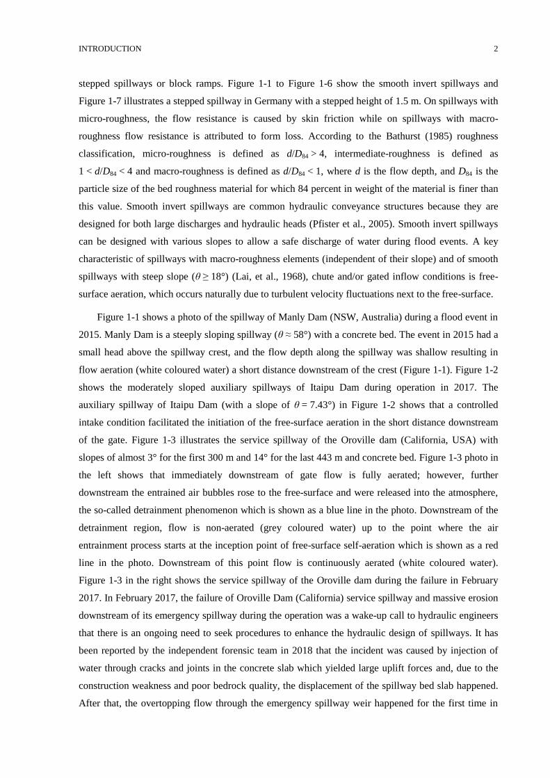
Figure 1-1: Smooth invert spillway of Manly Dam with a slope of θ ≈ 58° (NSW, Australia) during
2015 flood event (courtesy of Dr. Felder). .............................................................................................. 5
Figure 1-2: Smooth invert spillway of Itaipu Dam on the Paraná River between Brazil and Paraguay
with a slope of θ ≈ 7.43°(courtesy of Associate Professor Ron Cox). .................................................... 5
Figure 1-3: The service spillway of the Oroville dam with slopes of almost 3° for the first 300 m and
14° for the last 443 m and concrete bed (California, USA) during the failure in February 2017 (left
photo modified version of the satellite photo from Google Earth (2018) and right photo from
Independent forensic team report, 2018). ................................................................................................ 6
Figure 1-4: The gated spillway of the Clyde dam with a slope of 50° and the aerator device on
spillway bed (New Zealand) (captured by the author, September 2015). ............................................... 6
Figure 1-5: Smooth invert auxiliary spillway of Warragamba Dam (NSW, Australia) (satellite photo
from Google Earth, 2018). ...................................................................................................................... 7
Figure 1-6: Concrete invert spillway in Blue Mountains stormwater with a mild slope (NSW,
Australia) (courtesy of Dr. Felder). ......................................................................................................... 7
Figure 1-7: Stepped spillway of the Urft dam with steps height of h = 1.5 m (Germany) (courtesy of
Dr. Felder). .............................................................................................................................................. 8
Figure 2-1: Scheme of the fully aerated high-velocity supercritical flow regions over an ungated
spillway. ................................................................................................................................................ 13
Figure 2-2: Graph from Wood (1984): Depth-average void fraction Cmean in fully aerated flow region
plotted as a function of slope, and the empirical constant γ×cosθ......................................................... 21
Figure 2-3: Friction factor versus mean void fraction on fully aerated flow over smooth invert spillway
with braod range of chute slope between 7.5° and 75° based on Staub and Anderson (1958) data
(Wood, 1983). ....................................................................................................................................... 33
Figure 3-1: Large-scale spillway model and header tank No. A with chute section of L = 8 m,
W = 0.8 m and θ = 11˚ with transparent Perspex boundaries (ks = 0.01 mm). ...................................... 45
Figure 3-2: Side view of the experimental recirculation system and header tank No. B: Smooth bed
configuration, qw = 0.375 m2/s, dc = 0.243 m, Re = 1.2×10
6. ................................................................ 47
Figure 3-3: Front view of the T-shape diffuser pipe with a length of 1.8 m, Dd = 0.45 m, Dh = 0.05 m,
ds = 0.075 m. ......................................................................................................................................... 47
xiii
Figure 3-4: View of the convergent sidewalls, broad-crested weir and T-shape disused pipe inside the
new header tank. .................................................................................................................................... 48
Figure 3-5: Samples of natural grains for the three investigated micro-roughness configurations in the
present study with D50 = 1.56, 4.41 and 9.49 mm. ................................................................................ 49
Figure 3-6: Summary of sieving analysis of the three rough bed configurations in the present study. 50
Figure 3-7: Top view of the bed roughness configurations in the present study. ................................. 51
Figure 3-8: Side view of the bed roughness configurations in the present study .................................. 51
Figure 3-9: Pointer gauge positioned in the centre line of the spillway. ............................................... 52
Figure 3-10: Prandtl-Pitot tube with a diameter of 3 mm positioned in spillway centre line. .............. 53
Figure 3-11: A double-tip conductivity probe and its positioning aligned with the flow direction and a
photomicrograph with 0.7 mm sensor size captured with Leica M205 C microscope. ........................ 55
Figure 3-12: Sketch of the positioning of the double-tip conductivity probe. ...................................... 55
Figure 3-13: The ISEL® robotic arm and its specially designed trolley............................................... 55
Figure 3-14: Mikrotron MC4082 high-speed camera equipped with AF Nikkor 50 mm f/1.4D lens
mounted on a tripod. ............................................................................................................................. 56
Figure 3-15: A CanonTM EOS 1000D Digital SLR camera with Canon Zoom Lenz EF-S 18-55 mm
1:3.5-5.6 IS. ........................................................................................................................................... 57
Figure 3-16: Acoustic displacement meter Microsonic™ with Mic+35/IU/TC sensor. ....................... 57
Figure 3-17: Definition sketch of the auto- and cross-correlation functions for a double-tip
conductivity probe signal corresponding to the flow over rough configuration with D50 = 1.56 mm,
qw = 0.188 m2/s, x/dc = 44.09 m and C = 0.509. .................................................................................... 65
Figure 4-1: Observations of free-surface roughness in the present study: qw = 0.05 m2/s, dc = 0.063 m
(Flow direction from top to bottom), dashed line illustrates the visually identified inception point of
free-surface roughness........................................................................................................................... 72
Figure 4-2: Comparison of locations of inception point of free-surface roughness and free-surface
aeration in the present study with previous experimental data; (solid symbols = LFR; hollow
symbols = LI); and comparison with an equations developed by Wood et al. (1983) and Ferrando and
Rico (2002) (Table 2-1)......................................................................................................................... 75
Figure 4-3: Observations of free-surface roughness downstream of the inception point of free-surface
roughness and downstream of the inception point of free-surface aeration: qw = 0.100 m2/s,
dc = 0.101 m (Flow direction from top to bottom). ............................................................................... 76
xiv
Figure 4-4: Free-surface roughness in fully developed flow region at 41.16 ≤ x/dc ≤ 44.43:
qw = 0.188 m2/s, (Flow from left to right). ............................................................................................ 78
Figure 4-5: Free-surface roughness downstream of LFR at 64.6 ≤ x/dc ≤ 66.6: qw = 0.1 m2/s, dc = 0.101
m, Re = 3.68×10⁵, LFR = 3.5 m; Photo order from top left to bottom right with time step of 10 ms
between photos; Flow direction from left to right. ................................................................................ 79
Figure 4-6: Free-surface roughness downstream of LFR on rough bed configuration II D50 = 4.41 mm;
64.6 ≤ x/dc ≤ 66.6, ks/d = 0.163, qw = 0.1 m2/s, dc = 0.101 m, Re = 4.0×10
5, LFR = 1.5 m; Photo order
from top left to bottom with time step of 5 ms between photos; Flow direction from left to right. ...... 80
Figure 4-7: Water column ejection from the free-surface in fully developed flows on a rough bed
configuration II D50 = 4.41 mm; 64.6 ≤ x/dc ≤ 66.6, ks/d = 0.163, qw = 0.1 m2/s, dc = 0.101 m,
Re = 4.0×10⁵, LFR = 1.5 m; Photo order from top left to bottom with time step of 10 ms between
photos; Flow direction from left to right. .............................................................................................. 81
Figure 4-8: Dimensionless free-surface profile along the spillway and comparison with gradually
varied flow theory (GVF) for qw = 0.250 m2/s, 9.0×10
5 ≤ Re ≤ 9.5×10
5. ............................................. 82
Figure 5-1: Comparison of dimensionless velocity distributions in the developing flow region for
various flow conditions and the four roughness configurations. ........................................................... 88
Figure 5-2: Dimensional velocity distributions and turbulent boundary layer development along the
spillway; Pitot tube data: qw = 0.250 m2/s, Re ≈ 9.3×10
5, dc = 0.185 m (hollow symbols: velocities at
cross-sections upstream of LFR; black solid symbols: velocities at cross-sections between LFR and LI;
black solid stars : velocities at cross-sections between LI and LBL; colored solid symbols: velocities
at cross-sections downstream of the LBL). ............................................................................................. 91
Figure 5-3: Boundary layer thickness along the spillway up to the point of its intersection with the
free-surface for four tested roughness configurations. .......................................................................... 92
Figure 5-4: Boundary layer properties for all investigated flow conditions and comparison with best-fit
equations (equation 5-1 to 5-6). ............................................................................................................ 93
Figure 5-5: Dimensionless velocity distributions on the smooth and rough bed configurations for all
flow conditions in developing and fully developed boundary layer regions; Comparison with power-
law (equation (5-13)). ............................................................................................................................ 97
Figure 5-6: Comparison of velocity distributions along the spillway with the logarithmic law in inner
flow region equations (3-12) and (3-13). .............................................................................................. 99
Figure 5-7: Summary of dimensionless shear stress using log-law within the inner flow region. ...... 101
xv
Figure 5-8: Comparison of velocity distributions with the velocity defect law in outer flow region
equation (3-19). ................................................................................................................................... 102
Figure 5-9: Summary of dimensionless shear stress using velocity defect law in the outer flow region.
............................................................................................................................................................. 104
Figure 5-10: Summary of dimensionless shear stress using the momentum integral method. ........... 106
Figure 5-11: Comparison of the dimensionless shear stress estimated using the logarithmic law within
the inner flow region, velocity defect law within the outer flow region and the momentum integral
method. ................................................................................................................................................ 110
Figure 6-1: Void fraction distributions downstream of the onset of free-surface roughness; Comparison
of experimental data with the empirical equation of Wood (1984) (equation 2-6) and the advective
diffusion equation of Toombes and Chanson (2007) (equation 6-1). ................................................. 117
Figure 6-2: Void fraction distributions at the downstream end of the spillway (for x = 6.76 m) for
various discharges. .............................................................................................................................. 118
Figure 6-3: Gradient of void fraction distributions downstream of the inception point of free-surface
roughness............................................................................................................................................. 120
Figure 6-4: Comparison of void fraction distributions for various bed roughness configurations. .... 121
Figure 6-5: Air-water interface count rate distributions on the smooth bed spillway downstream of LFR.
............................................................................................................................................................. 122
Figure 6-6: Air-water interface count rate distributions on the rough spillways downstream of the LI.
............................................................................................................................................................. 123
Figure 6-7: Relationship between dimensionless air-water interface count rate and void fraction
downstream of the inception point of free-surface roughness for all flow conditions; Comparison with
parabolic relationships (equations 6-4 and 6-5) .................................................................................. 127
Figure 6-8: Air-water interface count rate distributions on various bed roughness configurations. ... 129
Figure 6-9: Dimensionless velocity distributions on the smooth and rough bed configurations
downstream of the inception point of free-surface roughness; Comparison with power-law equation (2-
23). ...................................................................................................................................................... 131
Figure 6-10: Comparison of dimensionless velocity distributions measured by Prandtl Pitot tube (PT:
solid symbols) and double-tip conductivity probe (CP: hollow symbols) at several cross-sections along
the spillway downstream of the inception point of free-surface roughness. ....................................... 132
Figure 6-11: Turbulence intensity distributions on the smooth bed. ................................................... 133
xvi
Figure 6-12: Typical turbulence intensity distributions on rough bed configurations (Hollow symbols:
downstream of LFR; Solid symbols: downstream of LI)....................................................................... 134
Figure 6-13: Turbulence intensity distributions for all tested bed configurations. ............................. 137
Figure 6-14: Dimensionless distributions of auto- and cross-correlation time scales. ........................ 139
Figure 6-15: Auto- and cross-correlation time scales on all tested bed configurations. ..................... 143
Figure 6-16: Average chord length distributions on smooth bed configuration downstream of the LFR.
............................................................................................................................................................. 144
Figure 6-17: Typical average air chord length distributions on rough bed configurations (Hollow
symbols: downstream of LFR; Solid symbols: downstream of LI). ...................................................... 145
Figure 6-18: Average air chord length distributions for all bed configurations. ................................. 147
Figure 6-19: Distribution of void fraction, interface count rate, characteristic flow depth Y98 and flow
depth d based upon pointer gauge data for qw = 0.100 m2/s at an almost constant distance from the
inception point of free-surface roughness for the four-bed roughness configurations. ....................... 152
Figure 6-20: Comparison of characteristic air-water flow parameters along the spillways. ............... 155
Figure 6-21: Probability distribution function of air and water chord times with equal void fractions
C ≈ 0.50. .............................................................................................................................................. 157
Figure 6-22: Probability distribution function of air and water chord times with equal void fractions
C ≈ 0.50 for various tested bed roughness configurations. ................................................................. 159
Figure 7-1: Friction factor for all tested spillway bed configurations (R (1998): Rice et al. (1998), P
(2008): Pagliara et al. (2008), P (2010): Pagliara et al. (2010)). ......................................................... 164
Figure 7-2: Comparison of present study friction factor for smooth bed spillway with data of Wood
(1983). ................................................................................................................................................. 166
Figure 7-3: Energy dissipation rate for all tested configurations in the present study. ....................... 172
Figure 7-4: Dimensionless residual energy at the toe of the spillway for all tested configurations in the
present study and comparison with previous studies (C (1993a): Chanson (1993a), O (2004): Ohtsu et
al. (2004), FC (2016): Felder and Chanson (2016)). ........................................................................... 174
Figure 7-5: Depth-averaged void fraction for all tested configurations in the present study and
comparison with previous studies (*: Present study data, A (1965): Anderson (1965), A (1986):
Aivazyan (1986), CC (1996): Chanson and Cummings (1996), P (2011a): Pagliara et al. (2011a), F
(2013): Felder (2013), H (1991): Hager (1991), C (1993c): Chanson (1993c), WG (2005): Wilhelms
xvii
and Gullivers (2005), M (2012): Meireles et al. (2012), VB (2016), Valero and Bung (2016)); **:
using previous equations based upon present study flow condition. ................................................... 178
Figure 7-6: Aeration efficiency as a function of qw for all tested bed configurations. ........................ 179
Figure 7-7: Aeration efficiency per meter drop in invert elevation at the downstream end of the
spillway for all tested configurations and comparison with previous studies (RG (1991): Rindels and
Gulliver (1991), C (1995c): Chanson (1995c), FC (2015): Felder and Chanson (2015)). .................. 181
Figure A-1: Free-surface roughness in fully developed flow region at 191.07 ≤ x/dc ≤ 206.25:
qw = 0.019 m2/s, dc = 0.033 m, (Flow from left to right). .................................................................... 201
Figure A-2: Free-surface roughness in fully developed flow region at 135.92 ≤ x/dc ≤ 146.72:
qw = 0.031 m2/s, dc = 0.046 m, (Flow from left to right). .................................................................... 201
Figure A-3: Free-surface roughness in fully developed flow region at 99.36 ≤ x/dc ≤ 107.25:
qw = 0.050 m2/s, dc = 0.063 m, (Flow from left to right). .................................................................... 202
Figure A-4: Free-surface roughness in fully developed flow region at 75.82 ≤ x/dc ≤ 81.85:
qw = 0.075 m2/s, dc = 0.083 m, (Flow from left to right). .................................................................... 202
Figure A-5: Free-surface roughness in fully developed flow region at 62.59 ≤ x/dc ≤ 67.57:
qw = 0.100 m2/s, dc = 0.101 m, (Flow from left to right). .................................................................... 203
Figure A-6: Free-surface roughness in fully developed flow region at 53.94 ≤ x/dc ≤ 58.23:
qw = 0.125 m2/s, dc = 0.117 m, (Flow from left to right). .................................................................... 204
Figure A-7: Free-surface roughness in fully developed flow region at 41.16 ≤ x/dc ≤ 44.43:
qw = 0.188 m2/s, dc = 0.153 m, (Flow from left to right). .................................................................... 204
Figure A-8: Free-surface roughness in fully developed flow region at 33.98 ≤ x/dc ≤ 36.68:
qw = 0.250 m2/s, dc = 0.185 m, (Flow from left to right). .................................................................... 205
Figure A-9: Free-surface roughness in fully developed flow region at 29.28 ≤ x/dc ≤ 31.61:
qw = 0.313 m2/s, dc = 0.215 m, (Flow from left to right). .................................................................... 206
Figure A-10: Free-surface roughness in fully developed flow region at 25.93 ≤ x/dc ≤ 27.99:
qw = 0.375 m2/s, dc = 0.243 m, (Flow from left to right). .................................................................... 207
Figure A-11: Dimensionless free-surface profile along the spillway and comparison with gradually
varied flow theory (GVF) for qw = 0.019 m2/s. ................................................................................... 210
Figure B-1: Velocity distributions and turbulent boundary layer development along the spillway; Pitot
tube data: qw = 0.031 m2/s, dc = 0.046 m (Hollow symbols: velocities upstream of LFR; Bold symbols:
velocities downstream of LFR). ............................................................................................................ 212

xviii
Figure B-2: Velocity distributions and turbulent boundary layer development along the spillway; Pitot
tube data: qw = 0.075 m2/s, dc = 0.083 m (Hollow symbols: velocities upstream of LFR; Bold symbols:
velocities downstream of LFR). ............................................................................................................ 214
Figure B-3: Velocity distributions and turbulent boundary layer development along the spillway; Pitot
tube data: qw = 0.125 m2/s, dc = 0.117 m (Hollow symbols: velocities upstream of LFR; Bold symbols:
velocities downstream of LFR). ............................................................................................................ 216
Figure B-4: Velocity distributions and turbulent boundary layer development along the spillway; Pitot
tube data: qw = 0.375 m2/s, dc = 0.243 m (hollow symbols: velocities at cross-sections upstream of LFR;
black solid symbols: velocities at cross-sections between LFR and LI; black solid stars : velocities at
cross-sections between LI and LBL; colored solid symbols: velocities at cross-sections downstream of
the LBL). ............................................................................................................................................... 218
Figure B-5: Comparison of velocity distributions with logarithmic law. ........................................... 224
Figure B-6: Summary of wall shear stress using log-law within inner flow region. ........................... 224
Figure B-7: Summary of wall shear stress using log-law within inner flow region. ........................... 225
Figure B-8: Comparison of velocity distributions with velocity defect law. ...................................... 226
Figure B-9: Summary of wall shear stress using velocity defect law in outer flow region. ................ 227
Figure B-10: Summary of wall shear stress using velocity defect law in outer flow region. .............. 228
Figure B-11: Summary of wall shear stress using momentum integral method. ................................ 228
Figure B-12: Summary of wall shear stress using momentum integral method. ................................ 229
Figure C-1: Void fraction distributions along spillway downstream of the inception point of free-
surface roughness on smooth bed configuration. ................................................................................ 232
Figure C-2: Void fraction distributions along spillway on rough bed configuration with D50= 1.56 mm
(hollow symbols: downstream of LFR, solid symbols: downstream of the LI). .................................... 234
Figure C-3: Void fraction distributions along spillway on rough bed configuration with D50= 4.41 mm
(hollow symbols: downstream of LFR, solid symbols: downstream of the LI). .................................... 236
Figure C-4: Void fraction distributions along spillway on rough bed configuration with D50= 9.49 mm
(hollow symbols: downstream of LFR, solid symbols: downstream of the LI). .................................... 239
Figure C-5: Void fraction distributions downstream of the inception point of free-surface roughness at
x = 6.76 m. ........................................................................................................................................... 240
Figure C-6: Void fraction distributions of various bed roughness configurations. ............................. 242
xix
Figure C-7: Air-water interface count rate distributions along spillway downstream of the inception
point of free-surface roughness on smooth bed configuration. ........................................................... 245
Figure C-8: Air-water interface count rate distributions along spillway on rough bed configuration
with D50= 1.56 mm (hollow symbols: downstream of LFR, solid symbols: downstream of the LI). .... 247
Figure C-9: Air-water interface count rate distributions along spillway on rough bed configuration
with D50= 4.41 mm (hollow symbols: downstream of LFR, solid symbols: downstream of the LI). .... 249
Figure C-10: Air-water interface count rate distributions along spillway on rough bed configuration
with D50= 9.49 mm (hollow symbols: downstream of LFR, solid symbols: downstream of the LI). .... 251
Figure C-11: Air-water interface count rate distributions downstream of the inception point of free-
surface roughness at x = 5.76 m. ......................................................................................................... 252
Figure C-12: Air-water interface count rate distributions of various bed roughness configurations. . 254
Figure C-13: Turbulence intensity distributions along spillway downstream of the inception point of
free-surface roughness on smooth bed configuration. ......................................................................... 257
Figure C-14: Turbulence intensity distributions along spillway on rough bed configuration with
D50= 1.56 mm (hollow symbols: downstream of LFR, solid symbols: downstream of the LI). ............ 259
Figure C-15: Turbulence intensity distributions along spillway on rough bed configuration with
D50= 4.41 mm (hollow symbols: downstream of LFR, solid symbols: downstream of the LI). ............ 261
Figure C-16: Turbulence intensity distributions along spillway on rough bed configuration with
D50= 9.49 mm (hollow symbols: downstream of LFR, solid symbols: downstream of the LI). ............ 264
Figure C-17: Turbulence intensity distributions downstream of the inception point of free-surface
roughness at x = 5.76 m. ...................................................................................................................... 265
Figure C-18: Turbulence intensity distributions of various bed roughness configurations. ............... 267
Figure C-19: Auto-correlation distributions along spillway downstream of the inception point of free-
surface roughness on smooth bed configuration. ................................................................................ 270
Figure C-20: Auto-correlation distributions along spillway on rough bed configuration with
D50= 1.56 mm (hollow symbols: downstream of LFR, solid symbols: downstream of the LI). ............ 272
Figure C-21: Auto-correlation distributions along spillway on rough bed configuration with
D50= 4.41 mm (hollow symbols: downstream of LFR, solid symbols: downstream of the LI). ............ 274
Figure C-22: Auto-correlation distributions along spillway on rough bed configuration with
D50= 9.49 mm (hollow symbols: downstream of LFR, solid symbols: downstream of the LI). ............ 277
xx
Figure C-23: Auto-correlation distributions downstream of the inception point of free-surface
roughness at x = 5.76 m. ...................................................................................................................... 278
Figure C-24: Auto-correlation distributions of various bed roughness configurations. ...................... 280
Figure C-25: Cross-correlation distributions along spillway downstream of the inception point of free-
surface roughness on smooth bed configuration. ................................................................................ 283
Figure C-26: Cross-correlation distributions along spillway on rough bed configuration with
D50= 1.56 mm (hollow symbols: downstream of LFR, solid symbols: downstream of the LI). ............ 285
Figure C-27: Cross-correlation distributions along spillway on rough bed configuration with
D50= 4.41 mm (hollow symbols: downstream of LFR, solid symbols: downstream of the LI). ............ 287
Figure C-28: Cross-correlation distributions along spillway on rough bed configuration with
D50= 9.49 mm (hollow symbols: downstream of LFR, solid symbols: downstream of the LI). ............ 290
Figure C-29: Cross-correlation distributions downstream of the inception point of free-surface
roughness at x = 5.76 m. ...................................................................................................................... 291
Figure C-30: Cross-correlation distributions of various bed roughness configurations. ..................... 293
Figure C-31: Turbulence intensity distributions along spillway downstream of the inception point of
free-surface roughness on smooth bed configuration. ......................................................................... 296
Figure C-32: Turbulence intensity distributions along spillway on rough bed configuration with
D50= 1.56 mm (hollow symbols: downstream of LFR, solid symbols: downstream of the LI). ............ 298
Figure C-33: Turbulence intensity distributions along spillway on rough bed configuration with
D50= 4.41 mm (hollow symbols: downstream of LFR, solid symbols: downstream of the LI). ............ 300
Figure C-34: Turbulence intensity distributions along spillway on rough bed configuration with
D50= 9.49 mm (hollow symbols: downstream of LFR, solid symbols: downstream of the LI). ............ 303
Figure C-35: Turbulence intensity distributions downstream of the inception point of free-surface
roughness at x = 5.76 m. ...................................................................................................................... 304
Figure C-36: Turbulence intensity distributions of various bed roughness configurations. ............... 306
Figure C-37: Comparison of the characteristic air-water flow parameters along the spillways. ........ 308
xxi
LIST OF TABLES
Table 1-1: Thesis outline. ........................................................................................................................ 9
Table 1-2: Appendix outline. ................................................................................................................ 11
Table 2-1: Empirical equations proposed to estimate the location of the inception point of free-surface
air entrainment (LI) and its corresponding flow depth (dI) on smooth and rough spillways. ................ 15
Table 2-2: Summary of prototype and model studies on various flow regions over spillways with
θ < 15°. .................................................................................................................................................. 24
Table 2-3: Summary of prototype and model studies on flow resistance over block ramps featured with
non-aerated flow condition with a moderated slope (θ < 15°). ............................................................. 30
Table 2-4: Selected prototype and model studies on flow resistance over spillways with the air-water
flow with a moderate slope (θ < 15°). ................................................................................................... 35
Table 2-5: Summary of air-water mass transfer studies over moderately sloped stepped spillways and
various range of smooth spillways slope. .............................................................................................. 39
Table 3-1: Summary of the natural grains characteristics obtained from sieve analysis. ..................... 49
Table 3-2: Summary of the air-water flow properties and corresponding signal processing techniques.
............................................................................................................................................................... 62
Table 3-3: Summary of experimental flow conditions comprising flow discharge, critical flow depth,
averaged Froude, Reynolds and Weber numbers for all investigated bed roughness configurations. .. 67
Table 3-4: Experimental program of the present study. ........................................................................ 68
Table 4-1: Summary of flow condition in the uniform region at the downstream of the spillway. ...... 70
Table 4-2: Summary of experimental flow conditions in the present study and basic observations of
the characteristic distance of inception point of free-surface roughness LFR from the upstream crest and
distance of inception point of free-surface aeration LI from the crest. .................................................. 72
Table 4-3: Summary of flow depths in the present study at x = 6.76 m. ............................................... 84
Table 5-1: Summary of experimental flow conditions in the present study and observations of
characteristic distances LFR, LBL and LI from the upstream crest. .......................................................... 91
Table 5-2: Summary of shear stress and friction factor in the uniform region at the downstream of the
spillway. .............................................................................................................................................. 108
Table 6-1: Summary of sensitivity analysis results: Variation of the normalised standard deviation of
the depth-averaged void fraction Cmean for various integration limits on the investigated bed
xxii
configurations (green boxes indicate the smallest values of the normalised standard deviation of the
Cmean). .................................................................................................................................................. 114
Table 6-2: Characteristic parameters of air-water interface count rate for qw = 0.125 m2/s. ............... 125
Table 6-3: Characteristic parameters of turbulence intensity-water interface count rate for
qw = 0.125 m2/s. ................................................................................................................................... 135
Table 6-4: Characteristic parameters of auto-correlation timescale for qw = 0.125 m2/s. ................... 140
Table 6-5: Characteristic parameters of cross-correlation timescale for qw = 0.125 m2/s. .................. 141
Table 6-6: Summary of flow depths in the present study at x = 6.76 m. ............................................. 150
Table 7-1: Comparison of present data with previous studies on flow resistance over moderately
sloped spillways. ................................................................................................................................. 167
Table 7-2: Summary of present study design guideline. ..................................................................... 183
Table B-1: Summary of boundary layer properties in the developing flow region. ............................ 219
Table C-1: Characteristic parameters of air-water flow properties for all investigated flow conditions
over smooth bed configuration. ........................................................................................................... 309
Table C-2: Characteristic parameters of air-water flow properties for all investigated flow conditions
over rough bed configuration D50 = 1.56 mm. .................................................................................... 310
Table C-3: Characteristic parameters of air-water flow properties for all investigated flow conditions
over rough bed configuration D50 = 4.41 mm. .................................................................................... 312
Table C-4: Characteristic parameters of air-water flow properties for all investigated flow conditions
over rough bed configuration D50 = 9.49 mm. .................................................................................... 314
Table D-1: Calculated Cmean at several locations downstream of the inception point of free-surface
roughness on moderately sloped spillway (θ = 11°). .......................................................................... 318
xxiii
LIST OF SYMBOLS
a Specific area (m2)
b Characteristic value of the maximum variation of β(C) (-)
C Void fraction (-)
(Cgas)d/s Downstream dissolved gas concentration (mg/l)
(Cgas)u/s Upstream dissolved gas concentration (mg/l)
C((Txx)max) Characteristic void fraction where (Txx)max (-)
C((Txz)max) Characteristic void fraction where (Txz)max (-)
C(Tumax) Characteristic void fraction where Tumax (-)
CFmax Characteristic void fraction where Fmax (-)
Cgas Dissolved gas concentration in the volume of water (mg/l)
ch Chord length (m)
Cmean Depth-averaged void fraction (-)
Csat Concentration of dissolved gas in water at equilibrium (mg/l)
d Flow depth (m)
D’ Dimensionless diffusivity (-)
d25 25% percentile of the flow depth (m)
d75 75% percentile of the flow depth (m)
dc Critical flow depth (m)
de Equivalent clear water flow depth (m)
Dgas Molecular diffusivity of oxygen calculated for 20°C (m2/s)
DH Hydraulic diameter (m)
dmean-A Mean flow depth measured with acoustic displacement meter (m)
dmean-C Mean flow depth extracted from high-speed camera videos (m)
dUniform Uniform flow depth (m)
E Aeration efficiency
E(O2) Aeration efficiency in terms of dissolved Oxygen
F Air-water interface count rate (Hz)
fD Darcy friction factor calculated using gradually varied flow theory based on pointer
gauge data (-)
fe Friction factor calculated using gradually varied flow theory based on double-tip
conductivity probe data (-)
fInner Friction factor obtained based on logarithmic law within inner flow region (-)
Fmax Maximum air-water interface count rate in given cross-section (Hz)
xxiv
fMI Friction factor calculated using momentum integral method (-)
fOuter Friction factor obtained based on velocity defect law within outer flow region (-)
Fr Froude number (-)
Fr* Froude number defined in term of roughness height (-)
fUniform Friction factor calculated using uniform flow theory (-)
g Gravity acceleration, g = 9.81 (m/s2)
h Vertical step height (m)
H Total head (m)
Hdam Dam height (m)
Hmax Maximum upstream head above chute toe (m)
Hres Residual energy (m)
HStatic Static head (m)
K’ Dimensionless integration constant (-)
KL Liquid film coefficient (-)
ks Equivalent sand roughness height (m)
L Length of spillway (m)
LBL Length from upstream crest to the intersection of the turbulent boundary layer with the
free-surface (m)
LFR Length from upstream crest to the inception point of free-surface roughness (m)
LI Length from upstream crest to the inception point of free-surface self-aeration (m)
LUniform Length from upstream crest to the point where flow depth reached uniform flow depth
(m)
Mo Morton number (-)
N Power law exponent
Qw Water discharge (m3/s)
qw Water discharge per unit width (m2/s)
Re Reynolds number (-)
Rxz Normalised cross-correlation function between two probe output signals separated in a
streamwise direction (-)
(Rxz)max Maximum cross-correlation between two probe output signals separated in a streamwise
direction (-)
Sf Friction slope (-)
T Average travel time between conductivity probe tips (s)
tch Air-water phase chord time (s)
Tu Turbulence intensity (-)
xxv
Tumax Maximum turbulence intensity (-)
Txx Auto-correlation time scale (s)
Txz Cross-correlation time scale (s)
(Txx)max Maximum auto-correlation (s)
(Txz)max Maximum cross-correlation (s)
Uw Mean flow velocity calculated based on double-tip conductivity probe (m/s)
Vc Critical flow velocity (m/s)
VCP Interfacial velocity measured with double tip conductivity probe (m/s)
Vo Freestream velocity (m/s)
VP Velocity measured with Prandtl Pitot tube (m/s)
W Width of spillway (m)
We Weber number (-)
x Distance along the spillway (m)
y Distance measured normal to the invert (m)
Y((Txx)max) Characteristic depth where (Txx)max (m)
Y((Txz)max) Characteristic depth where (Txz)max (m)
Y(Tumax) Characteristic depth where Tumax (m)
YFmax Characteristic depth where Fmax (m)
Yxx Characteristic depth where the void fraction is xx% (m)
zo Zero velocity level from chute bed (m)
ΔH Total head loss (m)
ΔZo Drop in elevation between the broad-crested weir and the last measured cross-section at
the toe of the spillway (m)
a(C) Parameter for adjustment of different average chord sizes of air and water phase (-)
β(C) Parameter for variation of bubble and droplet chord sizes with a void fraction (-)
δw Boundary layer thickness (m)
δ1 Displacement thickness (m)
δ2 Momentum thickness (m)
θ Channel slope (°)
λa Air particle size (m)
λw Water particle size (m)
μ Dynamic viscosity (Pa×s)
ρ Density (kg/m3)
Ø Probe tip diameter (m)
∀ Volume of air and water (m3)
xxvi
LIST OF ABBREVIATIONS
BL Boundary layer
DO Dissolved Oxygen
FR Free-surface roughness
GVF Gradually varied flow
MI Momentum integral
NA Not available
PDF Probability distribution function
STD Standard deviation

Chapter 1
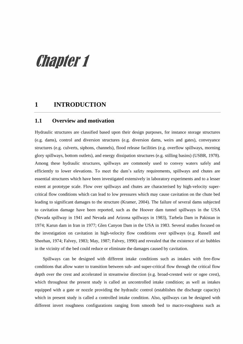
1 INTRODUCTION
Overview and motivation 1.1
Hydraulic structures are classified based upon their design purposes, for instance storage structures
(e.g. dams), control and diversion structures (e.g. diversion dams, weirs and gates), conveyance
structures (e.g. culverts, siphons, channels), flood release facilities (e.g. overflow spillways, morning
glory spillways, bottom outlets), and energy dissipation structures (e.g. stilling basins) (USBR, 1978).
Among these hydraulic structures, spillways are commonly used to convey waters safely and
efficiently to lower elevations. To meet the dam’s safety requirements, spillways and chutes are
essential structures which have been investigated extensively in laboratory experiments and to a lesser
extent at prototype scale. Flow over spillways and chutes are characterised by high-velocity super-
critical flow conditions which can lead to low pressures which may cause cavitation on the chute bed
leading to significant damages to the structure (Kramer, 2004). The failure of several dams subjected
to cavitation damage have been reported, such as the Hoover dam tunnel spillways in the USA
(Nevada spillway in 1941 and Nevada and Arizona spillways in 1983), Tarbela Dam in Pakistan in
1974; Karun dam in Iran in 1977; Glen Canyon Dam in the USA in 1983. Several studies focused on
the investigation on cavitation in high-velocity flow conditions over spillways (e.g. Russell and
Sheehan, 1974; Falvey, 1983; May, 1987; Falvey, 1990) and revealed that the existence of air bubbles
in the vicinity of the bed could reduce or eliminate the damages caused by cavitation.
Spillways can be designed with different intake conditions such as intakes with free-flow
conditions that allow water to transition between sub- and super-critical flow through the critical flow
depth over the crest and accelerated in streamwise direction (e.g. broad-crested weir or ogee crest),
which throughout the present study is called an uncontrolled intake condition; as well as intakes
equipped with a gate or nozzle providing the hydraulic control (establishes the discharge capacity)
which in present study is called a controlled intake condition. Also, spillways can be designed with
different invert roughness configurations ranging from smooth bed to macro-roughness such as
INTRODUCTION 2
stepped spillways or block ramps. Figure 1-1 to Figure 1-6 show the smooth invert spillways and
Figure 1-7 illustrates a stepped spillway in Germany with a stepped height of 1.5 m. On spillways with
micro-roughness, the flow resistance is caused by skin friction while on spillways with macro-
roughness flow resistance is attributed to form loss. According to the Bathurst (1985) roughness
classification, micro-roughness is defined as d/D84 > 4, intermediate-roughness is defined as
1 < d/D84 < 4 and macro-roughness is defined as d/D84 < 1, where d is the flow depth, and D84 is the
particle size of the bed roughness material for which 84 percent in weight of the material is finer than
this value. Smooth invert spillways are common hydraulic conveyance structures because they are
designed for both large discharges and hydraulic heads (Pfister et al., 2005). Smooth invert spillways
can be designed with various slopes to allow a safe discharge of water during flood events. A key
characteristic of spillways with macro-roughness elements (independent of their slope) and of smooth
spillways with steep slope (θ ≥ 18°) (Lai, et al., 1968), chute and/or gated inflow conditions is free-
surface aeration, which occurs naturally due to turbulent velocity fluctuations next to the free-surface.
Figure 1-1 shows a photo of the spillway of Manly Dam (NSW, Australia) during a flood event in
2015. Manly Dam is a steeply sloping spillway (θ ≈ 58°) with a concrete bed. The event in 2015 had a
small head above the spillway crest, and the flow depth along the spillway was shallow resulting in
flow aeration (white coloured water) a short distance downstream of the crest (Figure 1-1). Figure 1-2
shows the moderately sloped auxiliary spillways of Itaipu Dam during operation in 2017. The
auxiliary spillway of Itaipu Dam (with a slope of θ = 7.43°) in Figure 1-2 shows that a controlled
intake condition facilitated the initiation of the free-surface aeration in the short distance downstream
of the gate. Figure 1-3 illustrates the service spillway of the Oroville dam (California, USA) with
slopes of almost 3° for the first 300 m and 14° for the last 443 m and concrete bed. Figure 1-3 photo in
the left shows that immediately downstream of gate flow is fully aerated; however, further
downstream the entrained air bubbles rose to the free-surface and were released into the atmosphere,
the so-called detrainment phenomenon which is shown as a blue line in the photo. Downstream of the
detrainment region, flow is non-aerated (grey coloured water) up to the point where the air
entrainment process starts at the inception point of free-surface self-aeration which is shown as a red
line in the photo. Downstream of this point flow is continuously aerated (white coloured water).
Figure 1-3 in the right shows the service spillway of the Oroville dam during the failure in February
2017. In February 2017, the failure of Oroville Dam (California) service spillway and massive erosion
downstream of its emergency spillway during the operation was a wake-up call to hydraulic engineers
that there is an ongoing need to seek procedures to enhance the hydraulic design of spillways. It has
been reported by the independent forensic team in 2018 that the incident was caused by injection of
water through cracks and joints in the concrete slab which yielded large uplift forces and, due to the
construction weakness and poor bedrock quality, the displacement of the spillway bed slab happened.
After that, the overtopping flow through the emergency spillway weir happened for the first time in
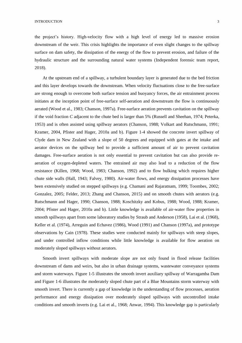
INTRODUCTION 3
the project’s history. High-velocity flow with a high level of energy led to massive erosion
downstream of the weir. This crisis highlights the importance of even slight changes to the spillway
surface on dam safety, the dissipation of the energy of the flow to prevent erosion, and failure of the
hydraulic structure and the surrounding natural water systems (Independent forensic team report,
2018).
At the upstream end of a spillway, a turbulent boundary layer is generated due to the bed friction
and this layer develops towards the downstream. When velocity fluctuations close to the free-surface
are strong enough to overcome both surface tension and buoyancy forces, the air entrainment process
initiates at the inception point of free-surface self-aeration and downstream the flow is continuously
aerated (Wood et al., 1983; Chanson, 1997a). Free-surface aeration prevents cavitation on the spillway
if the void fraction C adjacent to the chute bed is larger than 5% (Russell and Sheehan, 1974; Peterka,
1953) and is often assisted using spillway aerators (Chanson, 1988; Volkart and Rutschmann, 1991;
Kramer, 2004, Pfister and Hager, 2010a and b). Figure 1-4 showed the concrete invert spillway of
Clyde dam in New Zealand with a slope of 50 degrees and equipped with gates at the intake and
aerator devices on the spillway bed to provide a sufficient amount of air to prevent cavitation
damages. Free-surface aeration is not only essential to prevent cavitation but can also provide re-
aeration of oxygen-depleted waters. The entrained air may also lead to a reduction of the flow
resistance (Killen, 1968; Wood, 1983; Chanson, 1992) and to flow bulking which requires higher
chute side walls (Hall, 1943; Falvey, 1980). Air-water flows, and energy dissipation processes have
been extensively studied on stepped spillways (e.g. Chamani and Rajaratnam, 1999; Toombes, 2002;
Gonzalez, 2005; Felder, 2013; Zhang and Chanson, 2015) and on smooth chutes with aerators (e.g.
Rutschmann and Hager, 1990; Chanson, 1988; Koschitzky and Kobus, 1988; Wood, 1988; Kramer,
2004; Pfister and Hager, 2010a and b). Little knowledge is available of air-water flow properties in
smooth spillways apart from some laboratory studies by Straub and Anderson (1958), Lai et al. (1968),
Keller et al. (1974), Arreguin and Echavez (1986), Wood (1991) and Chanson (1997a), and prototype
observations by Cain (1978). These studies were conducted mainly for spillways with steep slopes,
and under controlled inflow conditions while little knowledge is available for flow aeration on
moderately sloped spillways without aerators.
Smooth invert spillways with moderate slope are not only found in flood release facilities
downstream of dams and weirs, but also in urban drainage systems, wastewater conveyance systems
and storm waterways. Figure 1-5 illustrates the smooth invert auxiliary spillway of Warragamba Dam
and Figure 1-6 illustrates the moderately sloped chute part of a Blue Mountains storm waterway with
smooth invert. There is currently a gap of knowledge in the understanding of flow processes, aeration
performance and energy dissipation over moderately sloped spillways with uncontrolled intake
conditions and smooth inverts (e.g. Lai et al., 1968; Anwar, 1994). This knowledge gap is particularly
INTRODUCTION 4
apparent in chutes which are not steep or equipped with macro-rough elements to observe free-surface
self-aeration. In these cases free-surface might be characterised by free-surface roughness which to the
leaser extend has been addressed in the literature. Several researchers have addressed free-surface
agitations and deformations qualitatively (Straub and Anderson, 1958; Killen, 1968; Lai et al., 1968;
Aivazyan, 1986; Anwar, 1994). Wilhelms and Gulliver (2005) used Killen (1968) data on a smooth
invert spillway with θ = 30° and 52.5° to introduce the concepts of entrapped and entrained air.
According to Wilhelms and Gulliver (2005), total conveyed air within high-velocity flow comprised
air transported with free-surface roughness (so-called entrapped air) and air transported in the form of
the air bubbles in the flow (so-called entrained air). Later, Toombes and Chanson (2007) and Valero
and Bung (2016) focused on the impacts of surface waves and free-surface roughness in high-velocity
flows over smooth invert chutes.
While previous studies have investigated air-water flows and energy dissipation processes on
stepped spillways and to some extent on smooth spillways, little research has been conducted on
spillways with micro-roughness inverts. Several laboratory studies have been conducted on spillway
models equipped with smooth bed configurations such as smooth painted steel, planed board with
subsequent painting, galvanized tin, painted timber and Perspex with various equivalent sand
roughnesses ranging between 0.01 < ks <1 mm (e.g. Anderson, 1965; Lai et al., 1968; Aivazyan, 1986;
Arreguin and Echavez, 1986; Chanson, 1995a; Valero and Bung, 2016; Wei at al., 2017). However,
prototype studies on spillways with smooth bed configurations were conducted on smooth concrete
with ks = 1 mm (Cain, 1978). Comparison of void fraction distribution profiles from the model data
reported by Keller et al. (1974) on Perspex bed for slopes of 18 and 24 degrees with model data of
Anderson (1965) on smooth painted steel with θ ≤ 15° revealed that Anderson’s (1965) profiles laid
consistently above the curves of the Keller et al. (1974) model data. This discrepancy might be due to
the impact of bed configuration and the conflicting definition of smooth bed. Therefore, the
understanding of the effects of micro-roughness is essential to better understanding different results in
previous studies of smooth spillway conditions. In particular, the present study aims to investigate the
effect that small changes in bed roughness can have on the overall flow behaviour, the air-water flow
processes and the energy dissipation performances. Herein, the present study conducted experiments
on a model at near prototype scale using an uncontrolled spillway with various micro-roughness bed
configurations and with a moderate slope of θ = 11º. A slope of θ = 11º is considered as a moderate
slope where no flow aeration occurs naturally for smooth flow conditions (Anwar, 1994). This slope
is, therefore, best suited to study the effect of the bed roughness on the re-aeration and energy
dissipation performances.
INTRODUCTION 5
Figure 1-1: Smooth invert spillway of Manly Dam with a slope of θ ≈ 58° (NSW, Australia) during 2015 flood
event (courtesy of Dr. Felder).
Figure 1-2: Smooth invert spillway of Itaipu Dam on the Paraná River between Brazil and Paraguay with a slope
of θ ≈ 7.43°(courtesy of Associate Professor Ron Cox).
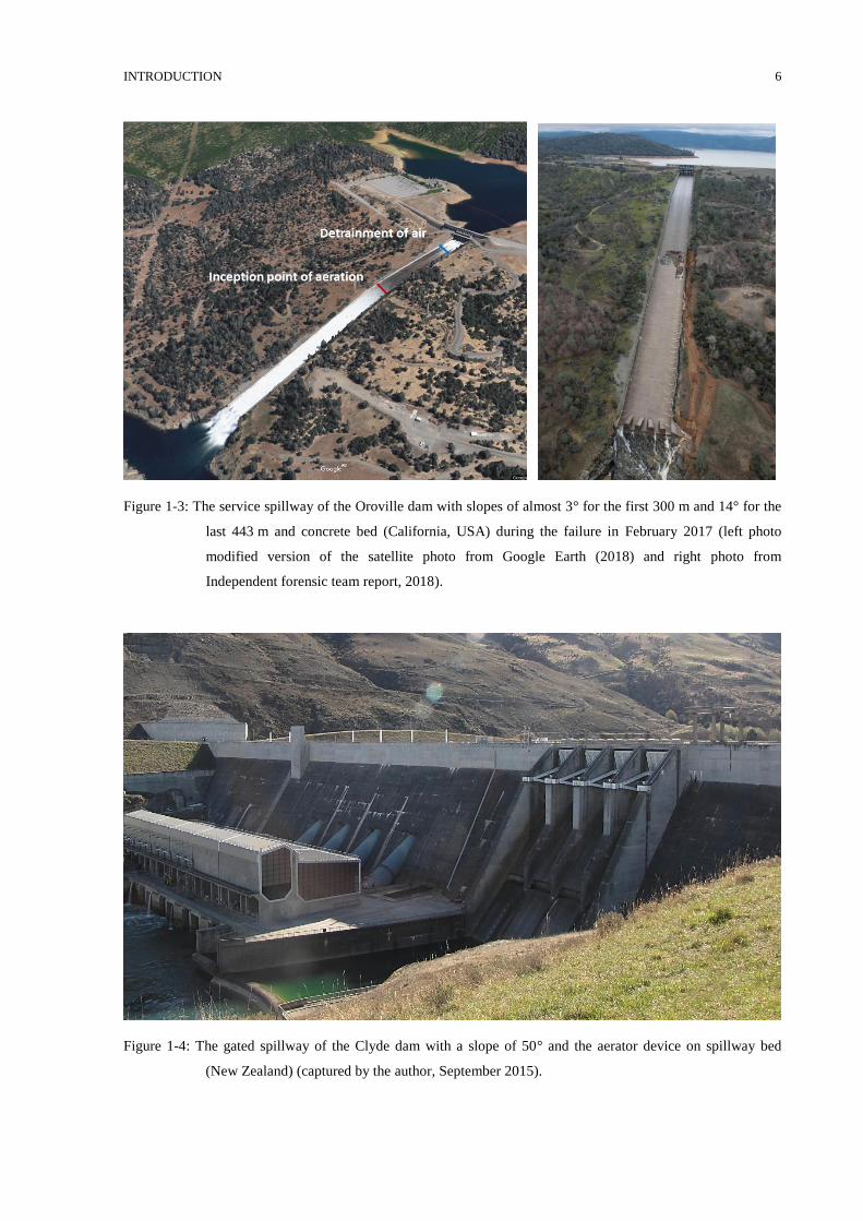
INTRODUCTION 6
Figure 1-3: The service spillway of the Oroville dam with slopes of almost 3° for the first 300 m and 14° for the
last 443 m and concrete bed (California, USA) during the failure in February 2017 (left photo
modified version of the satellite photo from Google Earth (2018) and right photo from
Independent forensic team report, 2018).
Figure 1-4: The gated spillway of the Clyde dam with a slope of 50° and the aerator device on spillway bed
(New Zealand) (captured by the author, September 2015).
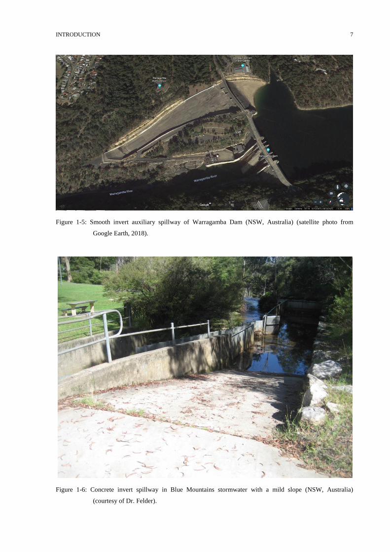
INTRODUCTION 7
Figure 1-5: Smooth invert auxiliary spillway of Warragamba Dam (NSW, Australia) (satellite photo from
Google Earth, 2018).
Figure 1-6: Concrete invert spillway in Blue Mountains stormwater with a mild slope (NSW, Australia)
(courtesy of Dr. Felder).
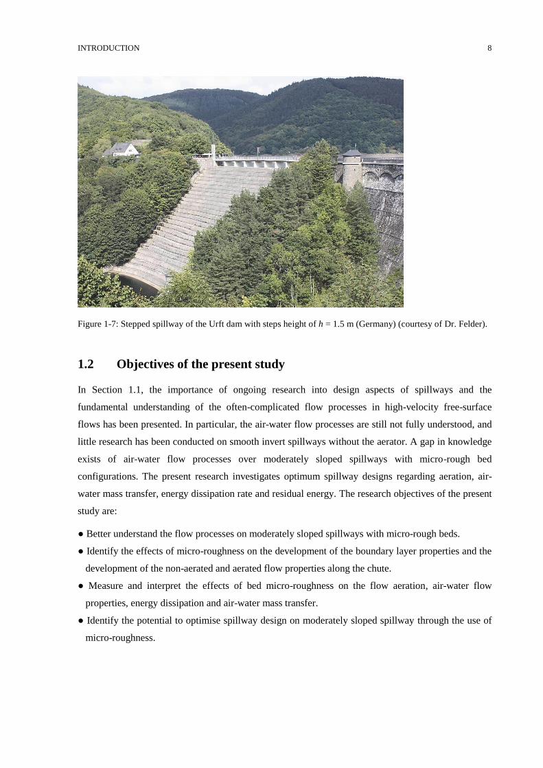
INTRODUCTION 8
Figure 1-7: Stepped spillway of the Urft dam with steps height of h = 1.5 m (Germany) (courtesy of Dr. Felder).
Objectives of the present study 1.2
In Section 1.1, the importance of ongoing research into design aspects of spillways and the
fundamental understanding of the often-complicated flow processes in high-velocity free-surface
flows has been presented. In particular, the air-water flow processes are still not fully understood, and
little research has been conducted on smooth invert spillways without the aerator. A gap in knowledge
exists of air-water flow processes over moderately sloped spillways with micro-rough bed
configurations. The present research investigates optimum spillway designs regarding aeration, air-
water mass transfer, energy dissipation rate and residual energy. The research objectives of the present
study are:
● Better understand the flow processes on moderately sloped spillways with micro-rough beds.
● Identify the effects of micro-roughness on the development of the boundary layer properties and the
development of the non-aerated and aerated flow properties along the chute.
● Measure and interpret the effects of bed micro-roughness on the flow aeration, air-water flow
properties, energy dissipation and air-water mass transfer.
● Identify the potential to optimise spillway design on moderately sloped spillway through the use of
micro-roughness.

INTRODUCTION 9
Thesis outline 1.3
The thesis presents the results of an experimental investigation at the UNSW Sydney’s Water
Research Laboratory in a large scale spillway facility. Table 1-1 shows the outline of the thesis and
lists briefly the contents of the chapters. Table 1-2 provides an overview of the Appendixes.
Table 1-1: Thesis outline.
Chapter Description
1. Introduction
Presentation of relevant background on spillways and the importance of studying high-
velocity flows over spillways with a micro-rough bed.
2. Literature review
Review of literature with a focus on existing spillway research, including the flow regions on
smooth invert spillways, as well as flow resistance and air-water mass transfer processes.
3. Experimental facility and instrumentation
Details of the experimental facility, the spillway configurations as well as instrumentation
and data post-processing.
4. Free-surface patterns in high-velocity flows on the spillway with micro-roughness
Visual observations of high-velocity flow patterns and free-surface profiles over the
moderately sloped spillway (θ = 11˚) in the present study for four different bed roughness
configurations. The visual observations highlighted free-surface roughness which increased
with increasing bed roughness. While the region close to the free-surface was characterised
by entrapped air for the smooth bed, the air was entrained with increasing bed roughness.
5. Boundary layer properties and shear stresses in the developing flow region
Investigation of the turbulent boundary later properties and boundary growth rate were
conducted using a Prandtl-Pitot tube. With increasing bed roughness, the turbulent boundary
layer growth rate increased. Presentation of new empirical equations to estimate the boundary
layer growth rate on moderately sloped spillways with uncontrolled inflow conditions and
bed micro-roughness.
6. Air-water flow properties in the fully developed flow region
Measurement of air-water flow properties with a double-tip conductivity probe resulting in
distributions of void fraction, air-water interface count rate, interfacial velocity, turbulence
levels, air and water chord times and lengths and auto- and cross-correlations timescales
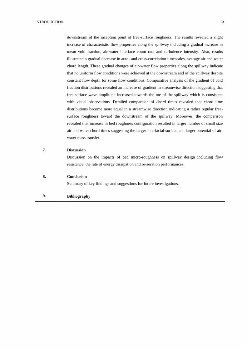
INTRODUCTION 10
downstream of the inception point of free-surface roughness. The results revealed a slight
increase of characteristic flow properties along the spillway including a gradual increase in
mean void fraction, air-water interface count rate and turbulence intensity. Also, results
illustrated a gradual decrease in auto- and cross-correlation timescales, average air and water
chord length. These gradual changes of air-water flow properties along the spillway indicate
that no uniform flow conditions were achieved at the downstream end of the spillway despite
constant flow depth for some flow conditions. Comparative analysis of the gradient of void
fraction distributions revealed an increase of gradient in streamwise direction suggesting that
free-surface wave amplitude increased towards the toe of the spillway which is consistent
with visual observations. Detailed comparison of chord times revealed that chord time
distributions become more equal in a streamwise direction indicating a rather regular free-
surface roughness toward the downstream of the spillway. Moreover, the comparison
revealed that increase in bed roughness configuration resulted in larger number of small size
air and water chord times suggesting the larger interfacial surface and larger potential of air-
water mass transfer.
7. Discussion
Discussion on the impacts of bed micro-roughness on spillway design including flow
resistance, the rate of energy dissipation and re-aeration performances.
8. Conclusion
Summary of key findings and suggestions for future investigations.
9. Bibliography
INTRODUCTION 11
Table 1-2: Appendix outline.
Appendix Description
A. Free-surface roughness and free-surface profiles
This appendix presents the further data and photos of free-surface patterns and profiles
complementing the presented data in the thesis Chapter 4.
B. Velocity distributions and boundary layer development
This appendix presents the further data and figures of velocity distributions along the
spillway, turbulent boundary layer development and properties complementing the presented
data in the thesis Chapter 5.
C. Air-water flow properties
This appendix presents the further data and figures of air-water flow properties
complementing the presented data in the thesis Chapter 6.
Chapter 2
2 LITERATURE REVIEW
Flow regions on spillways 2.1
Spillways are hydraulic structures to convey water safely and efficiently to lower elevations. An
overflow spillway typically includes three sections: a crest, a chute and an energy dissipater at the
downstream end of the structure. The crest is designed to maximise the discharge capacity of the
spillway. The chute is designed to carry the flowing water safely to the lower elevation. The design
purpose of energy dissipater structure is to dissipate the kinetic energy of the flowing water at the
downstream end of the chute to avoid erosion and any damages to the structure and surrounding
natural water system (Novak et al., 2007). Spillways are commonly classified based on geometrical
features such as slope, length, intake condition and invert roughness ranging from smooth invert to
macro-roughness elements such as steps or block ramps. Spillways are often associated with air
entrainment which has been of interest to hydraulic engineers because it can prevent cavitation
(Peterka, 1953; Chanson, 1997a), affect the energy dissipation performances (Wood, 1983; Chanson,
1993b), lead to flow bulking (Hall, 1943; Falvey, 1980) and increase air-water mass transfer (Gulliver
and Rindels, 1993; Felder and Chanson, 2015a). Therefore, it is crucial to take into account the flow
aeration to design of the spillway and the energy dissipater at the downstream end. According to the
literature, flow over spillways can be divided into a number of regions comprising, non-aerated clear
water flow region upstream of the inception point of free-surface aeration, aerated gradually varied
flow region downstream of the inception point of free-surface aeration and fully aerated uniform
equilibrium flow region further downstream of the inception point of free-surface aeration (Wood,
1991; Chanson, 1996)Figure 2-1. However, high-velocity supercritical flow over moderately sloped
spillway of present study revealed some differences with the identified flow regions over steep slope
spillways as presented in Figure 2-1.
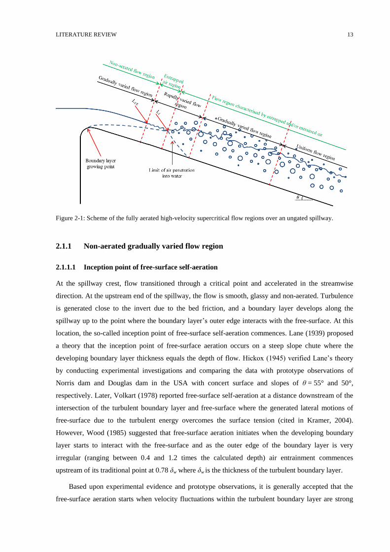
LITERATURE REVIEW 13
Figure 2-1: Scheme of the fully aerated high-velocity supercritical flow regions over an ungated spillway.
2.1.1 Non-aerated gradually varied flow region
2.1.1.1 Inception point of free-surface self-aeration
At the spillway crest, flow transitioned through a critical point and accelerated in the streamwise
direction. At the upstream end of the spillway, the flow is smooth, glassy and non-aerated. Turbulence
is generated close to the invert due to the bed friction, and a boundary layer develops along the
spillway up to the point where the boundary layer’s outer edge interacts with the free-surface. At this
location, the so-called inception point of free-surface self-aeration commences. Lane (1939) proposed
a theory that the inception point of free-surface aeration occurs on a steep slope chute where the
developing boundary layer thickness equals the depth of flow. Hickox (1945) verified Lane’s theory
by conducting experimental investigations and comparing the data with prototype observations of
Norris dam and Douglas dam in the USA with concert surface and slopes of θ = 55° and 50°,
respectively. Later, Volkart (1978) reported free-surface self-aeration at a distance downstream of the
intersection of the turbulent boundary layer and free-surface where the generated lateral motions of
free-surface due to the turbulent energy overcomes the surface tension (cited in Kramer, 2004).
However, Wood (1985) suggested that free-surface aeration initiates when the developing boundary
layer starts to interact with the free-surface and as the outer edge of the boundary layer is very
irregular (ranging between 0.4 and 1.2 times the calculated depth) air entrainment commences
upstream of its traditional point at 0.78 δw where δw is the thickness of the turbulent boundary layer.
Based upon experimental evidence and prototype observations, it is generally accepted that the
free-surface aeration starts when velocity fluctuations within the turbulent boundary layer are strong
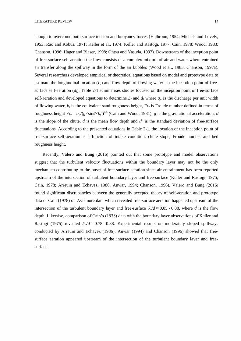
LITERATURE REVIEW 14
enough to overcome both surface tension and buoyancy forces (Halbronn, 1954; Michels and Lovely,
1953; Rao and Kobus, 1971; Keller et al., 1974; Keller and Rastogi, 1977; Cain, 1978; Wood, 1983;
Chanson, 1996; Hager and Blaser, 1998; Ohtsu and Yasuda, 1997). Downstream of the inception point
of free-surface self-aeration the flow consists of a complex mixture of air and water where entrained
air transfer along the spillway in the form of the air bubbles (Wood et al., 1983; Chanson, 1997a).
Several researchers developed empirical or theoretical equations based on model and prototype data to
estimate the longitudinal location (LI) and flow depth of flowing water at the inception point of free-
surface self-aeration (dI). Table 2-1 summarises studies focused on the inception point of free-surface
self-aeration and developed equations to determine LI and dI where qw is the discharge per unit width
of flowing water, ks is the equivalent sand roughness height, Fr* is Froude number defined in terms of
roughness height Fr* = qw/(g×sinθ×ks3)
0.5 (Cain and Wood, 1981), g is the gravitational acceleration, θ
is the slope of the chute, d is the mean flow depth and d’ is the standard deviation of free-surface
fluctuations. According to the presented equations in Table 2-1, the location of the inception point of
free-surface self-aeration is a function of intake condition, chute slope, Froude number and bed
roughness height.
Recently, Valero and Bung (2016) pointed out that some prototype and model observations
suggest that the turbulent velocity fluctuations within the boundary layer may not be the only
mechanism contributing to the onset of free-surface aeration since air entrainment has been reported
upstream of the intersection of turbulent boundary layer and free-surface (Keller and Rastogi, 1975;
Cain, 1978; Arreuin and Echavez, 1986; Anwar, 1994; Chanson, 1996). Valero and Bung (2016)
found significant discrepancies between the generally accepted theory of self-aeration and prototype
data of Cain (1978) on Aviemore dam which revealed free-surface aeration happened upstream of the
intersection of the turbulent boundary layer and free-surface δw/d ≈ 0.85 - 0.88, where d is the flow
depth. Likewise, comparison of Cain’s (1978) data with the boundary layer observations of Keller and
Rastogi (1975) revealed δw/d ≈ 0.78 - 0.88. Experimental results on moderately sloped spillways
conducted by Arreuin and Echavez (1986), Anwar (1994) and Chanson (1996) showed that free-
surface aeration appeared upstream of the intersection of the turbulent boundary layer and free-
surface.
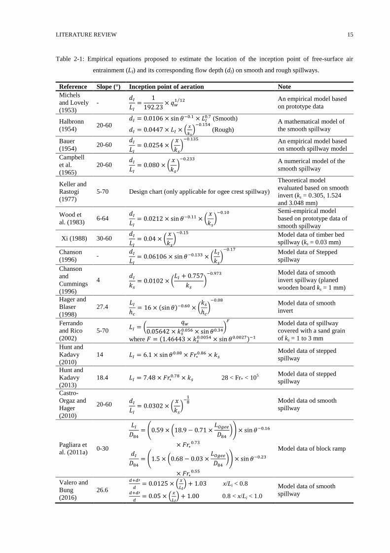
LITERATURE REVIEW 15
Table 2-1: Empirical equations proposed to estimate the location of the inception point of free-surface air
entrainment (LI) and its corresponding flow depth (dI) on smooth and rough spillways.
Reference Slope (°) Inception point of aeration Note
Michels
and Lovely
(1953)
- 𝑑𝐼
𝐿𝐼
=1
192.23× 𝑞𝑤
1 12⁄
An empirical model based
on prototype data
Halbronn
(1954) 20-60
𝑑𝐼 = 0.0106 × sin 𝜃−0.1 × 𝐿𝐼0.7 (Smooth)
𝑑𝐼 = 0.0447 × 𝐿𝐼 × (𝑥
𝑘𝑠)
−0.154
(Rough)
A mathematical model of
the smooth spillway
Bauer
(1954) 20-60
𝑑𝐼
𝐿𝐼
= 0.0254 × (𝑥
𝑘𝑠
)−0.135
An empirical model based
on smooth spillway model
Campbell
et al.
(1965)
20-60 𝑑𝐼
𝐿𝐼
= 0.080 × (𝑥
𝑘𝑠
)−0.233
A numerical model of the
smooth spillway
Keller and
Rastogi
(1977)
5-70 Design chart (only applicable for ogee crest spillway)
Theoretical model
evaluated based on smooth
invert (ks = 0.305, 1.524
and 3.048 mm)
Wood et
al. (1983) 6-64
𝑑𝐼
𝐿𝐼
= 0.0212 × sin 𝜃−0.11 × (𝑥
𝑘𝑠
)−0.10
Semi-empirical model
based on prototype data of
smooth spillway
Xi (1988) 30-60 𝑑𝐼
𝐿𝐼
= 0.04 × (𝑥
𝑘𝑠
)−0.15
Model data of timber bed
spillway (ks = 0.03 mm)
Chanson
(1996) -
𝑑𝐼
𝐿𝐼
= 0.06106 × sin 𝜃−0.133 × (𝐿𝐼
𝑘𝑠
)−0.17
Model data of Stepped
spillway
Chanson
and
Cummings
(1996)
4 𝑑𝐼
𝑘𝑠
= 0.0102 × (𝐿𝐼 + 0.757
𝑘𝑠
)−0.973
Model data of smooth
invert spillway (planed
wooden board ks = 1 mm)
Hager and
Blaser
(1998)
27.4 𝐿𝐼
ℎ𝑐
= 16 × (sin 𝜃)−0.60 × (𝑘𝑠
ℎ𝑐
)−0.08
Model data of smooth
invert
Ferrando
and Rico
(2002)
5-70 𝐿𝐼 = (
𝑞𝑤
0.05642 × 𝑘𝑠0.056 × sin 𝜃0.34
)𝐹
where 𝐹 = (1.46443 × 𝑘𝑠0.0054 × sin 𝜃0.0027)−1
Model data of spillway
covered with a sand grain
of ks = 1 to 3 mm
Hunt and
Kadavy
(2010)
14 𝐿𝐼 = 6.1 × sin 𝜃0.08 × 𝐹𝑟∗0.86 × 𝑘𝑠
Model data of stepped
spillway
Hunt and
Kadavy
(2013)
18.4 𝐿𝐼 = 7.48 × 𝐹𝑟∗0.78 × 𝑘𝑠 28 < Fr* < 10
5
Model data of stepped
spillway
Castro-
Orgaz and
Hager
(2010)
20-60 𝑑𝐼
𝐿𝐼
= 0.0302 × (𝑥
𝑘𝑠
)−
18
Model data od smooth
spillway
Pagliara et
al. (2011a) 0-30
𝐿𝐼
𝐷84
= (0.59 × (18.9 − 0.71 ×𝐿𝑂𝑔𝑒𝑒
𝐷84
)) × sin 𝜃−0.16
× 𝐹𝑟∗0.73
𝑑𝐼
𝐷84
= (1.5 × (0.68 − 0.03 ×𝐿𝑂𝑔𝑒𝑒
𝐷84
)) × sin 𝜃−0.23
× 𝐹𝑟∗0.55
Model data of block ramp
Valero and
Bung
(2016)
26.6
𝑑+𝑑′
𝑑= 0.0125 × (
𝑥
𝐿𝐼) + 1.03 x/Li < 0.8
𝑑+𝑑′
𝑑= 0.05 × (
𝑥
𝐿𝐼) + 1.00 0.8 < x/Li < 1.0
Model data of smooth
spillway
LITERATURE REVIEW 16
2.1.1.2 Inception point of free-surface roughness
Several researchers reported a very contoured, fluctuating and rough free-surface upstream of the
inception point of air entrainment (Straub and Anderson, 1958; Killen, 1968; Lai et al., 1968;
Aivazyan, 1986; Anwar, 1994). Lai et al. (1968) observed initiation of free-surface roughness
upstream of the inception point of free-surface aeration on uncontrolled smooth invert spillway with a
slope of θ = 18° and 24°. Killen (1968) presented very contoured free-surface with a small quantity of
ejected water droplets over the free-surface on smooth invert spillway equipped with roughness
elements (mean particle size of 0.7 mm) and slopes of θ = 30° and 52.5°. Based on Killen’s (1968)
data, Wilhelms and Gulliver (2005) introduced the concepts of entrapped air between free-surface
waves and entrained air transported along the spillway with the flow in the form of the air bubbles.
Falvey and Ervine (1988) and Wei et al. (2017) presented that free-surface deformation caused by
turbulence was a possible mechanism by which self-aeration occurs in open-channel flows. Valero and
Bung (2016) highlighted that free-surface roughness was generated by interfacial shear at the air-water
interface due to velocity differences between the high-velocity water flow and the air layer above the
flow. Most of these studies were reported free-surface agitation on spillways with θ > 15˚, but there is
no detailed information about the location of the inception point of free-surface roughness and flow
properties within the region on moderately sloped spillway θ < 15˚. On smooth invert spillways with
moderate slope flow may not reach fully aerated condition and be characterised by free-surface
roughness and air trapped between these free-surface roughness; therefore, it is essential to know the
flow properties and behaviour within this region.
Several studies of high-velocity flows were conducted on model (Straub and Anderson, 1958;
Killen, 1968) and prototype spillways (Cain, 1978) with a steep slope (θ ≥ 26˚) or chutes with an
upstream sluice gate or nozzle controlling the inflow conditions (Straub and Anderson, 1958,
Chanson, 1995a). Under these conditions, the free-surface self-aeration is a major feature of the flow
(Ehrenberger and Wilsey, 1926; Straub and Anderson, 1958; Killen, 1968; Wood, 1991; Chanson
1995a). While on smooth invert spillway with uncontrolled intake condition and moderate slope
(θ < 15˚) free-surface self-aeration might not happen. According to the sketch presented in Anwar
(1994), a slope of θ = 11º is considered as a moderate slope where no flow aeration occurs naturally
for smooth flow condition and uncontrolled intake. It appeared that there is little information on flow
behaviour on moderately sloped spillways with uncontrolled inflow conditions (Anwar, 1994; Felder
and Severi, 2016). Therefore, studying the flow behaviour over moderately sloped spillway θ = 11º
with the uncontrolled intake is in the scope of the present research.
Several laboratory studies have been conducted on spillway models equipped with smooth bed
configuration such as smooth painted steel, planed board with subsequent painting, Galvanized tin,
painted timber and Perspex with various equivalent sand roughness ranging between 0.01 < ks <1 mm
LITERATURE REVIEW 17
(e.g. Anderson, 1965; Lai et al., 1968; Aivazyan, 1986; Arreguin and Echavez, 1986; Chanson, 1995a;
Valero and Bung, 2016; Wei at al., 2017). However, prototype studies on spillways with smooth bed
configuration were conducted on smooth concrete with ks = 1 mm (Cain, 1978). Hence, the
understanding of the effects of micro-roughness on initiation of free-surface roughness and free-
surface aeration is essential to better understand different results in previous studies of smooth
spillway conditions. A better understanding of the non-aerated flows is essential for the hydraulic
design of spillways, particularly on small dams and moderately sloped water conveyance structures
where the chute may not be long enough to observe free-surface self-aeration and uniform flow region.
Herein, the present study conducted experiments at large scale model using an uncontrolled spillway
with various micro-roughness bed configurations and with a moderate slope of θ = 11º.
2.1.2 The rapidly varied flow region
Experimental investigations revealed a region with rapid changes in flow properties, i.e. flow depth,
void fraction distribution, immediately downstream of the inception point of free-surface air
entrainment over macro-rough bed spillways (such as stepped spillways) recognized as rapidly varied
flow region (Ohtsu and Yasuda, 1997; Chamani and Rajaratnam, 1999; Gonzalez, 2005; Pfister and
Hager, 2011; Felder, 2013, Matos and Meireles, 2014). Matos and Meireles (2014) pointed out the
existence of the rapidly varied flow region downstream of the inception point of free-surface self-
aeration due to the turbulence induced by macro-roughness elements and the contrast with the classical
concept of gradually varied flow region downstream of the inception point of free-surface aeration
over smooth invert spillways. They presented a gradually varied flow region downstream of the short
distance of a rapid change of the air-water flow properties. The key characteristics of rapidly varied
flow region downstream of the inception point of free-surface aeration comprised of a substantial
number of air bubbles within the flow, strong mixing and momentum losses, high rate of splashing and
bulking up the flow. Felder and Sever (2016) reported rapid changes of air-water flow properties
within flow region characterised by free-surface roughness on moderately sloped smooth spillway.
Since rapidly varied flow region has been recognised downstream of the inception point of free-
surface aeration due to the turbulence induced by macro-roughness elements still there no information
of appearance of this flow region downstream of the inception point of free-surface roughness over
spillway with micro-roughness which is within the scope of this study to investigate the flow regions
over micro-rough spillways.
LITERATURE REVIEW 18
2.1.3 The gradually varied flow region featured with intense air and water
interactions
Downstream of the rapidly varied flow region, flow is characterised by a gradual decrease of flow
depth, increase of velocity and the quantity of air entrapped in free-surface roughness and entrained air
bubbles into the water body recognised as gradually varied flow region. The quantity of air entities in
the form of the entrapped air between free-surface waves and in the form of air bubbles conveyed with
stream has been estimated by a void fraction which is the ratio of the volume of air per unit volume of
air-water. Void fraction presents the average value of the concentration of air in the region measured
by the probes. The amount of air concentration conveyed within the flow is defined regarding the
depth-averaged void fraction so-called mean void fraction (Chanson, 1996). Several studies revealed
that in gradually varied flow region characterised by air entrainment, the void fraction and velocity
distributions change gradually with the distance downstream of the inception point of free-surface
self-aeration and approaching the constant value of the uniform flow region (Keller et al. 1974; Cain,
1978; Arreguin and Echaves, 1986; Xi, 1988; Chanson, 1996; Wilhelms, 1997). These studies reported
that in aerated flow region the mean void fraction increased gradually along the spillway. However,
Wilhelms and Gulliver (2005) reported that in gradually varied flow region characterised by entrapped
air between free-surface waves and entrained air the mean void fraction of the total conveyed air
gradually increased and entrained air concentration followed the similar trend, while the entrapped air
concentration remained constant (about 23 percent) along the spillway.
Keller et al. (1974) developed a chart to determine velocity and void fraction distribution in
gradually varied flow region on fully aerated flow over smooth invert spillway and slopes of θ = 18
and 24°. Xi (1988) suggested that mean void fraction in a gradually varied flow region featured with
entrained air over steep slope smooth spillway with timber bed of ks = 0.03 mm can be estimated as
𝐶𝑚𝑒𝑎𝑛 = 4.745 × (𝑥
𝑑𝑐)
0.581× 𝑆𝑜
0.671 (2-1)
which Cmean is the depth-averaged void fraction, So is the gradient of the chute calculated in radiant.
The depth-averaged void fraction is calculated as
𝐶𝑚𝑒𝑎𝑛 =1
𝑌𝑥𝑥∫ (1 − 𝐶)
𝑦=𝑌𝑥𝑥
𝑦=0× 𝑑𝑦 (2-2)
where the integration limit Yxx is the characteristic depth corresponding to void fraction of C = xx
percent. Xi (1988) used Y95 as the characteristic depth to determine the depth-averaged void fraction in
his study. Chanson (1996) developed analytical solutions to determine mean void fraction and flow
depth as a function of the distance in gradually varied flow region of fully aerated flow over spillways
with θ > 30°through applying the continuity and energy equations, respectively. He assumed that the
entrainment and rise velocities are the same in gradually varied flow as in the uniform flows and
LITERATURE REVIEW 19
proposed the following equation To determine mean void fraction in gradually varied flow region
independent of the velocity, roughness and flow depth.
𝑑
𝑑𝑥′𝐶𝑚𝑒𝑎𝑛 = (1 − 𝐶𝑚𝑒𝑎𝑛) × (
𝑢𝑟×𝑑∗×cos 𝜃
𝑞𝑤× (𝐶𝑒 − 𝐶𝑚𝑒𝑎𝑛) × (1 − 𝐶𝑚𝑒𝑎𝑛) +
𝐶𝑚𝑒𝑎𝑛
𝑊′×
𝑑𝑊′
𝑑𝑥′) (2-3)
Herein, Ce is the depth-averaged void fraction in the uniform equilibrium flow region, x’ is defined as
x’ = x/d*, W’ is defined as W’ = W/d*’, W is the width of the channel, ur is the local bubble rise velocity
and d* is the flow depth at x = 0 m. Chanson (1996) observed that over chute with a slope of θ = 4°
and gated intake condition, flow characterised by fully aerated flow condition in a short distance
downstream of the intake, and the mean void fraction increased in a streamwise direction downstream
of the inception point of free-surface self-aeration approaching a maximum value of
(𝐶𝑚𝑒𝑎𝑛)𝑚𝑎𝑥 = 0.0738 × 𝑉𝐼0.316 (2-4)
which VI is the intake flow velocity. Chanson (1996) presented that under gated intake condition and
moderately sloped chute, downstream of the position where mean void fraction reached the maximum
value, the mean void fraction decreased gradually. Also, Pagliara et al. (2011a) conducted experiments
on block ramps with a slope of 9.9 ≤ θ ≤ 24.7° characterised by fully aerated flow region. Pagliara et
al. (2011a) reported that in the gradually varied flow region downstream of the inception point of free-
surface aeration, the void fraction increased in a streamwise direction up to the point
𝐿(𝐶𝑚𝑒𝑎𝑛)𝑚𝑎𝑥− 𝐿𝐼 = 12 × 𝐷84 × 𝐹𝑟∗
0.66 (2-5)
where the mean void fraction reached a maximum value and followed by air detrainment. Detail
information regarding provided references has been addressed in Table 2-2 including flow conditions,
model or prototype data and flow region where investigations and measurements were carried out.
Table 2-2, presents that several studies carried out on gradually varied flow region over steep slope
spillways including Keller et al. (1974), Cain (1978), Cain and Wood (1981) and Xi (1988) while few
researches focused on gradually varied flow region over moderately sloped spillway (e.g. Arreguin
and Echavez, 1986; Chanson, 1996; Pagliara et al., 2011a). Most of the studies on gradually varied
flow region were conducted under gated inflow condition which facilitated free-surface air
entrainment while focused on total conveyed air contained in the bubbles and waves. Despite some
data available in gradually varied flow region, still, there is a gap in knowledge of flow behaviour and
properties within a region characterised by free-surface waves and entrapped air. A deeper
understanding of gradually varied flow region characterised by free-surface roughness over moderate
slope chutes and uncontrolled intake condition is crucial because, in high discharges, uniform flow
condition may not occur along the structure as well as no aeration may occur and flow in gradually
varied flow region may determine the inflow into the downstream energy dissipater structure.
LITERATURE REVIEW 20
2.1.4 Uniform equilibrium flow region
A uniform flow region is defined as a flow region in which mean flow properties such as mean
velocity, mean flow depth and specific energy become independent of the longitudinal distance along
the spillway (Chow, 1959). Over a long spillway, downstream of the gradually varied flow region,
flow approaches the so-called uniform equilibrium condition in which mean flow properties such as
the mean void fraction, mean velocity and flow depth will not vary along the spillway (Staub and
Anderson, 1958; Keller, 1972; Wood, 1983; Chanson, 1996; Bung, 2011). Studying behaviour and
properties of flow in uniform equilibrium region is also essential because over long spillways or under
lower flow discharges flow may reach uniform equilibrium condition; therefore, the uniform
equilibrium region has an essential role in determining the input flow condition into the energy
dissipation structures downstream of the spillways.
Several researchers reported that in uniform equilibrium flow region, the quantity of air reaches
constant value and the mean void fraction is only a function of channel slope (e.g. Wood, 1983; Hager,
1991; Chanson, 1993c - Table 2-2). Wood (1983) revealed that for a constant slope, mean void
fraction decreased with increasing discharge. He reported that the mean void fraction is a function of
the slope. Later, Wood (1984) proposed an empirical equation as
𝐶 =𝛽
𝛽+𝑒−𝛾 cos 𝜃(𝑦 𝑌90⁄ )2 (2-6)
to estimate void fraction distribution in the uniform equilibrium flow region. Wood (1984) developed
this empirical equation using prototype data of Aviemore's dam with concrete surface, gated inflow
condition and slope of θ = 45°(Cain, 1978) as well as model data of Straub and Anderson (1958) with
gated intake condition and slope ranging between θ = 7.5° and θ = 75°. Note that γ and β are constant
values obtained through Figure 2-2 and following equation
0.9 =𝛽
𝛽+𝑒−𝛾 cos 𝜃 (2-7)
The constant value of γ is related to the mean void fraction Cmean defined with an upper integration
limit of Y90 (equation 2-2). Figure 2-2 revealed a jump in slope curve which might be due to the
different behaviour of the mean void fraction for moderately sloped chutes (θ ≤ 15°) compared to the
steep slopes (θ ≥ 30°).
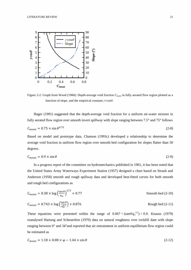
LITERATURE REVIEW 21
Figure 2-2: Graph from Wood (1984): Depth-average void fraction Cmean in fully aerated flow region plotted as a
function of slope, and the empirical constant γ×cosθ.
Hager (1991) suggested that the depth-average void fraction for a uniform air-water mixture in
fully aerated flow region over smooth invert spillway with slope ranging between 7.5° and 75° follows
𝐶𝑚𝑒𝑎𝑛 = 0.75 × sin 𝜃0.75 (2-8)
Based on model and prototype data, Chanson (1993c) developed a relationship to determine the
average void fraction in uniform flow region over smooth bed configuration for slopes flatter than 50
degrees.
𝐶𝑚𝑒𝑎𝑛 = 0.9 × sin 𝜃 (2-9)
In a progress report of the committee on hydromechanics published in 1961, it has been noted that
the United States Army Waterways Experiment Station (1957) designed a chart based on Straub and
Anderson (1958) smooth and rough spillway data and developed best-fitted curves for both smooth
and rough bed configurations as
𝐶𝑚𝑒𝑎𝑛 = 0.38 × log (tan 𝜃
𝑞𝑤)
2 3⁄
+ 0.77 Smooth bed (2-10)
𝐶𝑚𝑒𝑎𝑛 = 0.743 × log (tan 𝜃
𝑞𝑤0.2 ) + 0.876 Rough bed (2-11)
These equations were presented within the range of 0.067 < (tanθ/qw0.2
) < 0.9. Knauss (1979)
reanalysed Hartung and Scheuerlein (1970) data on natural roughness over rockfill dam with slope
ranging between 6° and 34°and reported that air entrainment in uniform equilibrium flow region could
be estimated as
𝐶𝑚𝑒𝑎𝑛 = 1.18 + 0.08 × φ − 1.44 × sin 𝜃 (2-12)
Cmean
cos
Slo
pe ()
0 0.2 0.4 0.6 0.8
0 0
1 10
2 20
3 30
4 40
5 50
6 60
7 70
8 80
9 90
cosSlope
LITERATURE REVIEW 22
where φ is the packing parameter defined as the ratio of mean geometric roughness height to the width
of the average stone. It suggests that the entrained air is a function of bed roughness and channel slope.
Aivazyan (1986) established a relationship to determine the aeration coefficient in uniform
equilibrium flow region over steep chutes as a function of the energy dissipation gradient and
independent of bed roughness as follows
𝐶𝑚𝑒𝑎𝑛 = 0.17 + 0.73 × 𝑆𝑓 (2-13)
which Sf is the energy gradient defined as
𝑆𝑓 = −𝜕𝐻
𝜕𝑥 (2-14)
moreover, H is the total energy at each cross-section and x is the longitudinal position in the
streamwise direction.
Later, Wood (1991) stated the mean void fraction and depth of the flow in the uniform
equilibrium flow region could be the function of the spillway discharge, slope, bed roughness and the
fluid properties. All these equations were developed to estimate the mean void fraction of total
conveyed air within a fully aerated flow condition in uniform equilibrium flow region at the
downstream end of the spillways. Wilhelms and Gulliver (2005) reanalysed data of Killien (1968) and
Straub and Anderson (1958) and developed equations
𝐶𝑒 = 0.656 × (1 − 𝑒−0.0356(𝜃−10.9)) (2-15)
𝐶𝑚𝑒𝑎𝑛 = 𝐶𝑒 × (1 − 𝑒−0.010(𝑥−𝐿𝐼)/𝑑𝐼) (2-16)
to estimate the uniform equilibrium air concentration (2-15) and entrained air concentration (2-16)
applicable for slopes between 11 and 75 degrees. Where 𝐶𝑒 is the entrained air equilibrium value.
Pagliara et al. (2010) developed an empirical equation corresponding to their void fraction
measurements in the uniform flow region on block ramps with bed simulated with pebbles
(D50 = 43.41 mm) and slope of θ = 5.2 to 24.7° as
𝐶𝑚𝑒𝑎𝑛 = 0.12 + (1.69 × tan 𝜃2.27) × (𝑑𝑒
𝐷84)
−0.9 (2-17)
to determine the mean void fraction as a function of slope, equivalent clear water flow depth de and
bed roughness defined as D84 which is the characteristic diameter of the bed material for which 84
percent of the material is finer than this value. Felder and Severi (2016) reported that void fraction
distributions changed gradually in streamwise direction over smooth invert spillway with θ = 11°
suggesting that flow not attain a uniform condition regarding the mean void fraction despite the
constant flow depth at the toe of the spillway. This observation was consistence with findings of
Chanson and Toombes (2001) and Chanson (2006) on stepped spillways who argued that no
LITERATURE REVIEW 23
equilibrium flow condition existed. Also, the experimental investigation of Felder and Chanson (2009)
confirmed those findings and indicated that the air-water interface count rate did not reach an
equilibrium value and the number of entrained air bubbles increased with increasing distance
downstream of the inception point. Hence, still, there is a gap in knowledge of the air-water flow
properties in uniform equilibrium flow region on smooth invert spillways and the impacts of micro-
roughness elements on air-water flow properties such as mean void fraction.
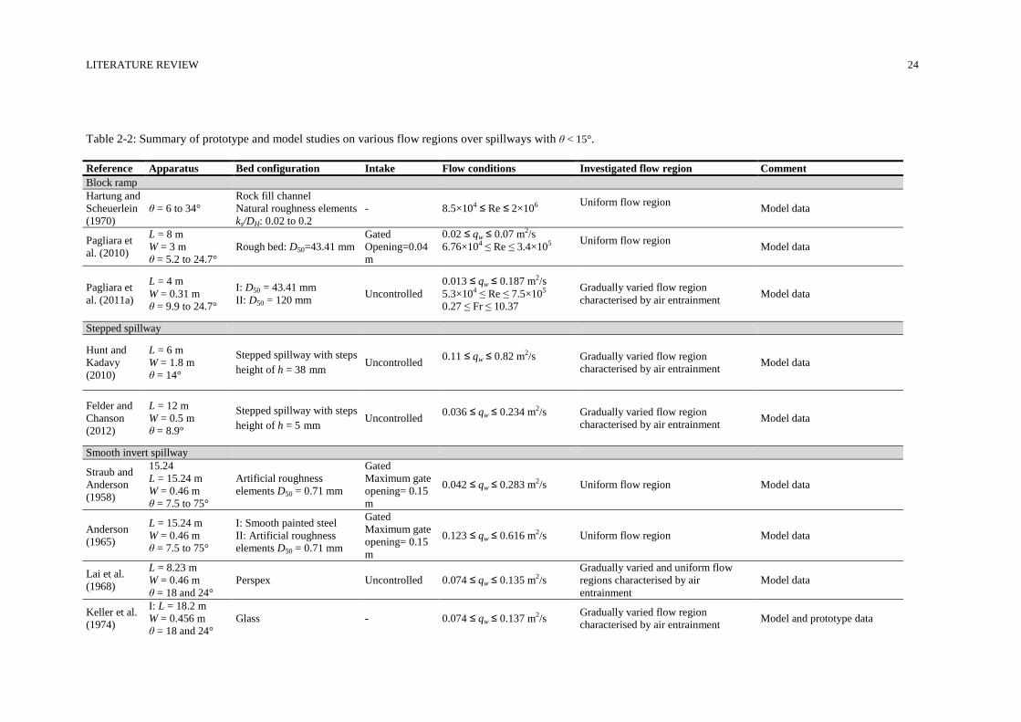
LITERATURE REVIEW 24
Table 2-2: Summary of prototype and model studies on various flow regions over spillways with θ < 15°.
Reference Apparatus Bed configuration Intake Flow conditions Investigated flow region Comment
Block ramp
Hartung and
Scheuerlein
(1970)
θ = 6 to 34°
Rock fill channel
Natural roughness elements
ks/DH: 0.02 to 0.2
- 8.5×10⁴ ≤ Re ≤ 2×10⁶ Uniform flow region
Model data
Pagliara et
al. (2010)
L = 8 m
W = 3 m
θ = 5.2 to 24.7°
Rough bed: D50=43.41 mm
Gated
Opening=0.04
m
0.02 ≤ qw ≤ 0.07 m2/s
6.76×10⁴ ≤ Re ≤ 3.4×10⁵
Uniform flow region
Model data
Pagliara et
al. (2011a)
L = 4 m
W = 0.31 m
θ = 9.9 to 24.7°
I: D50 = 43.41 mm
II: D50 = 120 mm Uncontrolled
0.013 ≤ qw ≤ 0.187 m2/s
5.3×10⁴ ≤ Re ≤ 7.5×10⁵
0.27 ≤ Fr ≤ 10.37
Gradually varied flow region
characterised by air entrainment Model data
Stepped spillway
Hunt and
Kadavy
(2010)
L = 6 m
W = 1.8 m
θ = 14°
Stepped spillway with steps
height of h = 38 mm Uncontrolled
0.11 ≤ qw ≤ 0.82 m2/s
Gradually varied flow region
characterised by air entrainment Model data
Felder and
Chanson
(2012)
L = 12 m
W = 0.5 m
θ = 8.9°
Stepped spillway with steps
height of h = 5 mm Uncontrolled
0.036 ≤ qw ≤ 0.234 m2/s
Gradually varied flow region
characterised by air entrainment Model data
Smooth invert spillway
Straub and
Anderson
(1958)
15.24
L = 15.24 m
W = 0.46 m
θ = 7.5 to 75°
Artificial roughness
elements D50 = 0.71 mm
Gated
Maximum gate
opening= 0.15
m
0.042 ≤ qw ≤ 0.283 m2/s Uniform flow region Model data
Anderson
(1965)
L = 15.24 m
W = 0.46 m
θ = 7.5 to 75°
I: Smooth painted steel
II: Artificial roughness
elements D50 = 0.71 mm
Gated
Maximum gate
opening= 0.15
m
0.123 ≤ qw ≤ 0.616 m2/s Uniform flow region Model data
Lai et al.
(1968)
L = 8.23 m
W = 0.46 m
θ = 18 and 24°
Perspex Uncontrolled 0.074 ≤ qw ≤ 0.135 m2/s
Gradually varied and uniform flow
regions characterised by air
entrainment
Model data
Keller et al.
(1974)
I: L = 18.2 m
W = 0.456 m
θ = 18 and 24°
Glass - 0.074 ≤ qw ≤ 0.137 m2/s Gradually varied flow region
characterised by air entrainment Model and prototype data
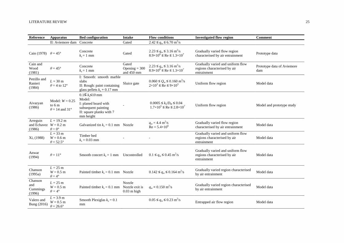
LITERATURE REVIEW 25
Reference Apparatus Bed configuration Intake Flow conditions Investigated flow region Comment
II: Aviemore dam Concrete Gated 2.42 ≤ qw ≤ 6.70 m2/s
Cain (1978) θ = 45° Concrete
ks = 1 mm Gated
2.23 ≤ qw ≤ 3.16 m2/s
8.9×10⁶ ≤ Re ≤ 1.3×10⁷
Gradually varied flow region
characterised by air entrainment
Prototype data
Cain and
Wood
(1981)
θ = 45° Concrete
ks = 1 mm
Gated
Opening = 300
and 450 mm
2.23 ≤ qw ≤ 3.16 m2/s
8.9×10⁶ ≤ Re ≤ 1.3×10⁷
Gradually varied and uniform flow
regions characterised by air
entrainment
Prototype data of Aviemore
dam
Petrillo and
Ranieri
(1984)
L = 30 m
θ = 4 to 12°
I: Smooth: smooth marble
slabs
II: Rough: paint containing
glass pellets ks = 0.17 mm
Sluice gate 0.060 ≤ Qw ≤ 0.160 m3/s
2×10³ ≤ Re ≤ 9×10³ Uniform flow region Model data
Aivazyan
(1986)
Model: W = 0.25
to 6 m
θ = 14 and 31°
0.1≤ ks≤10 mm Model:
I: planed board with
subsequent painting
II: square planks with 7
mm height
- 0.0005 ≤ ks/DH ≤ 0.04
1.7×10⁵ ≤ Re ≤ 2.8×10⁷ Uniform flow region Model and prototype study
Arreguin
and Echavez
(1986)
L = 19.2 m
W = 0.2 m
θ = 0°
Galvanized tin ks = 0.1 mm Nozzle qw = 4.4 m2/s
Re = 5.4×10⁶
Gradually varied flow region
characterised by air entrainment Model data
Xi, (1988)
L = 33 m
W = 0.6 m
θ = 52.5°
Timber bed
ks = 0.03 mm - -
Gradually varied and uniform flow
regions characterised by air
entrainment
Model data
Anwar
(1994) θ = 11° Smooth concert ks = 1 mm Uncontrolled 0.1 ≤ qw ≤ 0.45 m2/s
Gradually varied and uniform flow
regions characterised by air
entrainment
Model data
Chanson
(1995a)
L = 25 m
W = 0.5 m
θ = 4°
Painted timber ks = 0.1 mm Nozzle 0.142 ≤ qw ≤ 0.164 m2/s Gradually varied region characterised
by air entrainment Model data
Chanson
and
Cummings
(1996)
L = 25 m
W = 0.5 m
θ = 4°
Painted timber ks = 0.1 mm
Nozzle
Nozzle exit is
0.03 m high
qw = 0.150 m2/s Gradually varied region characterised
by air entrainment Model data
Valero and
Bung (2016)
L = 3.9 m
W = 0.5 m
θ = 26.6°
Smooth Plexiglas ks = 0.1
mm
0.05 ≤ qw ≤ 0.23 m2/s
Entrapped air flow region Model data
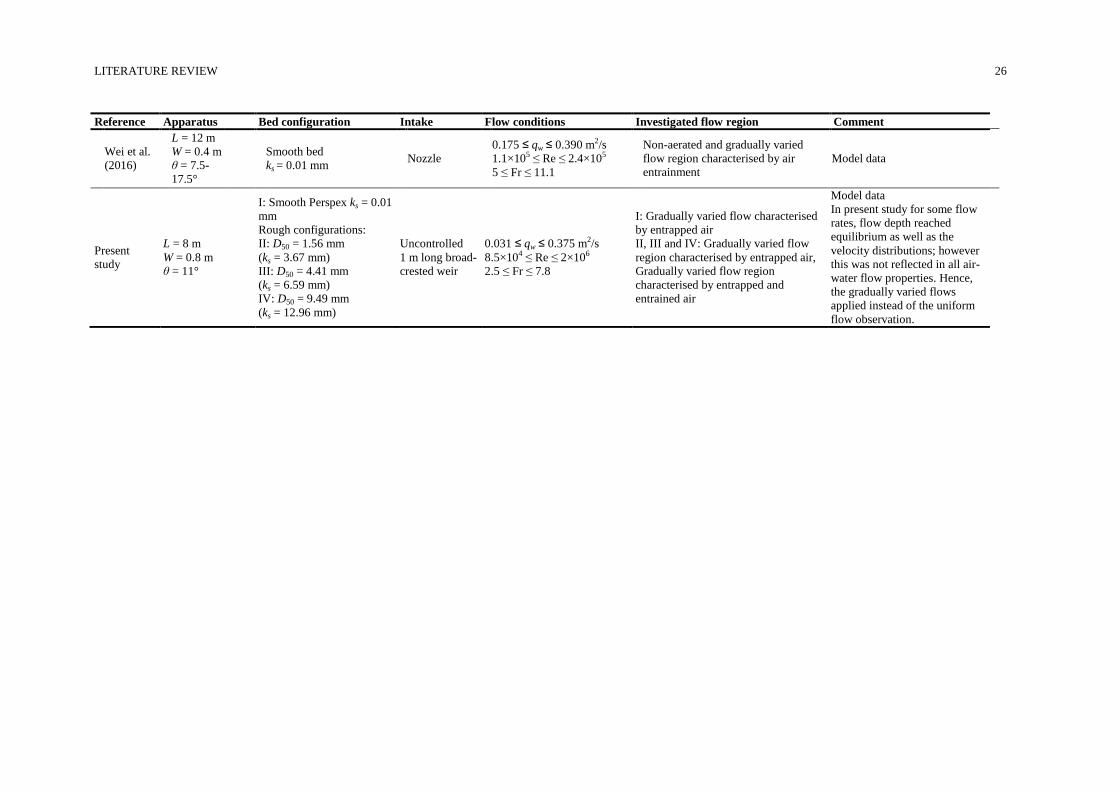
LITERATURE REVIEW 26
Reference Apparatus Bed configuration Intake Flow conditions Investigated flow region Comment
Wei et al.
(2016)
L = 12 m
W = 0.4 m
θ = 7.5-
17.5°
Smooth bed
ks = 0.01 mm Nozzle
0.175 ≤ qw ≤ 0.390 m2/s
1.1×10⁵ ≤ Re ≤ 2.4×10⁵
5 ≤ Fr ≤ 11.1
Non-aerated and gradually varied
flow region characterised by air
entrainment
Model data
Present
study
L = 8 m
W = 0.8 m
θ = 11°
I: Smooth Perspex ks = 0.01
mm
Rough configurations:
II: D50 = 1.56 mm
(ks = 3.67 mm)
III: D50 = 4.41 mm
(ks = 6.59 mm)
IV: D50 = 9.49 mm
(ks = 12.96 mm)
Uncontrolled
1 m long broad-
crested weir
0.031 ≤ qw ≤ 0.375 m2/s
8.5×10⁴ ≤ Re ≤ 2×10⁶
2.5 ≤ Fr ≤ 7.8
I: Gradually varied flow characterised
by entrapped air
II, III and IV: Gradually varied flow
region characterised by entrapped air,
Gradually varied flow region
characterised by entrapped and
entrained air
Model data
In present study for some flow
rates, flow depth reached
equilibrium as well as the
velocity distributions; however
this was not reflected in all air-
water flow properties. Hence,
the gradually varied flows
applied instead of the uniform
flow observation.
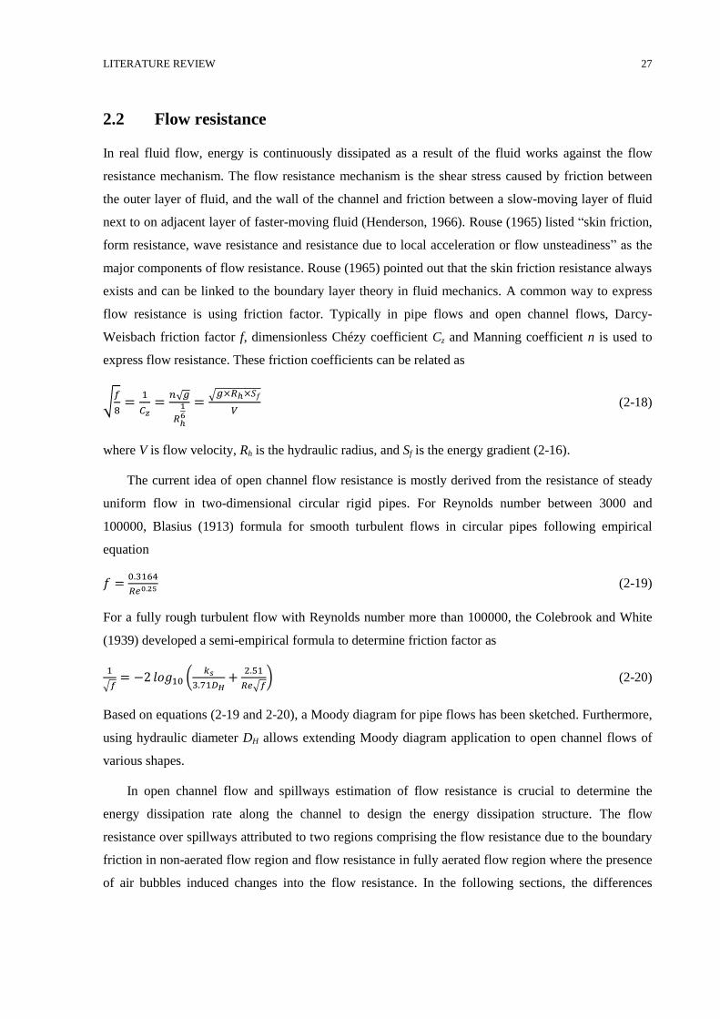
LITERATURE REVIEW 27
Flow resistance 2.2
In real fluid flow, energy is continuously dissipated as a result of the fluid works against the flow
resistance mechanism. The flow resistance mechanism is the shear stress caused by friction between
the outer layer of fluid, and the wall of the channel and friction between a slow-moving layer of fluid
next to on adjacent layer of faster-moving fluid (Henderson, 1966). Rouse (1965) listed “skin friction,
form resistance, wave resistance and resistance due to local acceleration or flow unsteadiness” as the
major components of flow resistance. Rouse (1965) pointed out that the skin friction resistance always
exists and can be linked to the boundary layer theory in fluid mechanics. A common way to express
flow resistance is using friction factor. Typically in pipe flows and open channel flows, Darcy-
Weisbach friction factor f, dimensionless Chézy coefficient Cz and Manning coefficient n is used to
express flow resistance. These friction coefficients can be related as
√𝑓
8=
1
𝐶𝑧=
𝑛√𝑔
𝑅ℎ
16
=√𝑔×𝑅ℎ×𝑆𝑓
𝑉 (2-18)
where V is flow velocity, Rh is the hydraulic radius, and Sf is the energy gradient (2-16).
The current idea of open channel flow resistance is mostly derived from the resistance of steady
uniform flow in two-dimensional circular rigid pipes. For Reynolds number between 3000 and
100000, Blasius (1913) formula for smooth turbulent flows in circular pipes following empirical
equation
𝑓 =0.3164
𝑅𝑒0.25 (2-19)
For a fully rough turbulent flow with Reynolds number more than 100000, the Colebrook and White
(1939) developed a semi-empirical formula to determine friction factor as
1
√𝑓= −2 𝑙𝑜𝑔10 (
𝑘𝑠
3.71𝐷𝐻+
2.51
𝑅𝑒√𝑓) (2-20)
Based on equations (2-19 and 2-20), a Moody diagram for pipe flows has been sketched. Furthermore,
using hydraulic diameter DH allows extending Moody diagram application to open channel flows of
various shapes.
In open channel flow and spillways estimation of flow resistance is crucial to determine the
energy dissipation rate along the channel to design the energy dissipation structure. The flow
resistance over spillways attributed to two regions comprising the flow resistance due to the boundary
friction in non-aerated flow region and flow resistance in fully aerated flow region where the presence
of air bubbles induced changes into the flow resistance. In the following sections, the differences
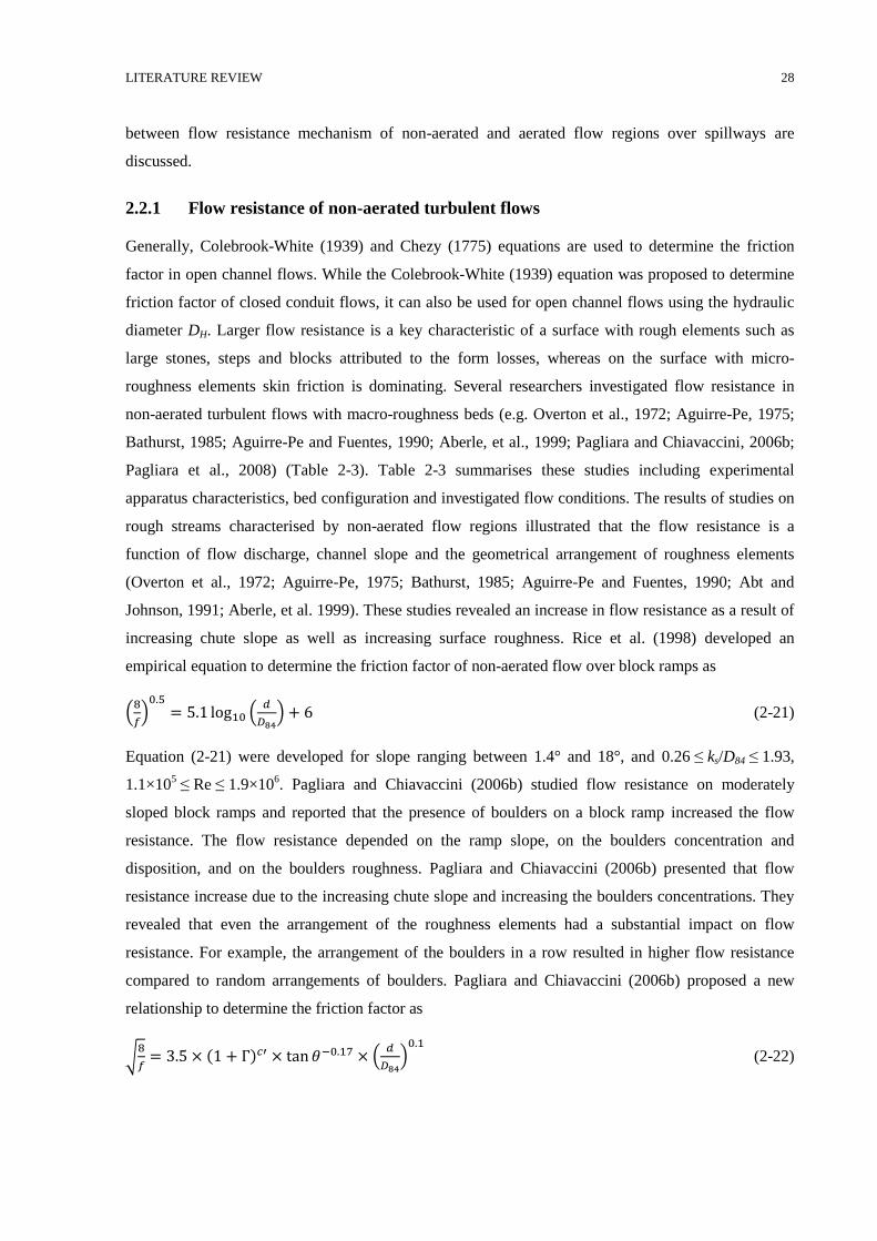
LITERATURE REVIEW 28
between flow resistance mechanism of non-aerated and aerated flow regions over spillways are
discussed.
2.2.1 Flow resistance of non-aerated turbulent flows
Generally, Colebrook-White (1939) and Chezy (1775) equations are used to determine the friction
factor in open channel flows. While the Colebrook-White (1939) equation was proposed to determine
friction factor of closed conduit flows, it can also be used for open channel flows using the hydraulic
diameter DH. Larger flow resistance is a key characteristic of a surface with rough elements such as
large stones, steps and blocks attributed to the form losses, whereas on the surface with micro-
roughness elements skin friction is dominating. Several researchers investigated flow resistance in
non-aerated turbulent flows with macro-roughness beds (e.g. Overton et al., 1972; Aguirre-Pe, 1975;
Bathurst, 1985; Aguirre-Pe and Fuentes, 1990; Aberle, et al., 1999; Pagliara and Chiavaccini, 2006b;
Pagliara et al., 2008) (Table 2-3). Table 2-3 summarises these studies including experimental
apparatus characteristics, bed configuration and investigated flow conditions. The results of studies on
rough streams characterised by non-aerated flow regions illustrated that the flow resistance is a
function of flow discharge, channel slope and the geometrical arrangement of roughness elements
(Overton et al., 1972; Aguirre-Pe, 1975; Bathurst, 1985; Aguirre-Pe and Fuentes, 1990; Abt and
Johnson, 1991; Aberle, et al. 1999). These studies revealed an increase in flow resistance as a result of
increasing chute slope as well as increasing surface roughness. Rice et al. (1998) developed an
empirical equation to determine the friction factor of non-aerated flow over block ramps as
(8
𝑓)
0.5= 5.1 log10 (
𝑑
𝐷84) + 6 (2-21)
Equation (2-21) were developed for slope ranging between 1.4° and 18°, and 0.26 ≤ ks/D84 ≤ 1.93,
1.1×10⁵ ≤ Re ≤ 1.9×10
6. Pagliara and Chiavaccini (2006b) studied flow resistance on moderately
sloped block ramps and reported that the presence of boulders on a block ramp increased the flow
resistance. The flow resistance depended on the ramp slope, on the boulders concentration and
disposition, and on the boulders roughness. Pagliara and Chiavaccini (2006b) presented that flow
resistance increase due to the increasing chute slope and increasing the boulders concentrations. They
revealed that even the arrangement of the roughness elements had a substantial impact on flow
resistance. For example, the arrangement of the boulders in a row resulted in higher flow resistance
compared to random arrangements of boulders. Pagliara and Chiavaccini (2006b) proposed a new
relationship to determine the friction factor as
√8
𝑓= 3.5 × (1 + Г)𝑐′ × tan 𝜃−0.17 × (
𝑑
𝐷84)
0.1 (2-22)
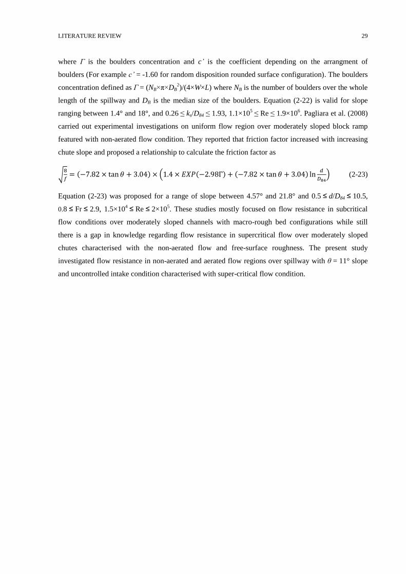
LITERATURE REVIEW 29
where Г is the boulders concentration and c’ is the coefficient depending on the arrangment of
boulders (For example c’ = -1.60 for random disposition rounded surface configuration). The boulders
concentration defined as Г = (NB×π×DB2)/(4×W×L) where NB is the number of boulders over the whole
length of the spillway and DB is the median size of the boulders. Equation (2-22) is valid for slope
ranging between 1.4° and 18°, and 0.26 ≤ ks/D84 ≤ 1.93, 1.1×10⁵ ≤ Re ≤ 1.9×10
6. Pagliara et al. (2008)
carried out experimental investigations on uniform flow region over moderately sloped block ramp
featured with non-aerated flow condition. They reported that friction factor increased with increasing
chute slope and proposed a relationship to calculate the friction factor as
√8
𝑓= (−7.82 × tan 𝜃 + 3.04) × (1.4 × 𝐸𝑋𝑃(−2.98Г) + (−7.82 × tan 𝜃 + 3.04) ln
𝑑
𝐷84) (2-23)
Equation (2-23) was proposed for a range of slope between 4.57° and 21.8° and 0.5 ≤ d/D84 ≤ 10.5,
0.8 ≤ Fr ≤ 2.9, 1.5×10⁴ ≤ Re ≤ 2×10
5. These studies mostly focused on flow resistance in subcritical
flow conditions over moderately sloped channels with macro-rough bed configurations while still
there is a gap in knowledge regarding flow resistance in supercritical flow over moderately sloped
chutes characterised with the non-aerated flow and free-surface roughness. The present study
investigated flow resistance in non-aerated and aerated flow regions over spillway with θ = 11° slope
and uncontrolled intake condition characterised with super-critical flow condition.
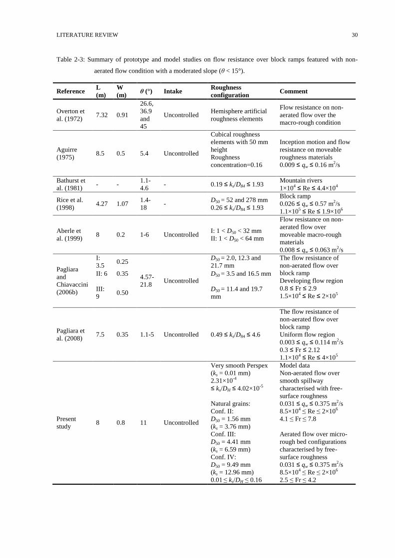
LITERATURE REVIEW 30
Table 2-3: Summary of prototype and model studies on flow resistance over block ramps featured with non-
aerated flow condition with a moderated slope (θ < 15°).
Reference L
(m)
W
(m) θ (°) Intake
Roughness
configuration Comment
Overton et
al. (1972) 7.32 0.91
26.6,
36.9
and
45
Uncontrolled Hemisphere artificial
roughness elements
Flow resistance on non-
aerated flow over the
macro-rough condition
Aguirre
(1975) 8.5 0.5 5.4 Uncontrolled
Cubical roughness
elements with 50 mm
height
Roughness
concentration=0.16
Inception motion and flow
resistance on moveable
roughness materials
0.009 ≤ qw ≤ 0.16 m2/s
Bathurst et
al. (1981) - -
1.1-
4.6 - 0.19 ≤ ks/D84 ≤ 1.93
Mountain rivers
1×10⁴ ≤ Re ≤ 4.4×10
4
Rice et al.
(1998) 4.27 1.07
1.4-
18 -
D50 = 52 and 278 mm
0.26 ≤ ks/D84 ≤ 1.93
Block ramp
0.026 ≤ qw ≤ 0.57 m2/s
1.1×10⁵ ≤ Re ≤ 1.9×10
6
Aberle et
al. (1999) 8 0.2 1-6 Uncontrolled
I: 1 < D50 < 32 mm
II: 1 < D50 < 64 mm
Flow resistance on non-
aerated flow over
moveable macro-rough
materials
0.008 ≤ qw ≤ 0.063 m2/s
Pagliara
and
Chiavaccini
(2006b)
I:
3.5 0.25
4.57-
21.8 Uncontrolled
D50 = 2.0, 12.3 and
21.7 mm
The flow resistance of
non-aerated flow over
block ramp
Developing flow region
0.8 ≤ Fr ≤ 2.9
1.5×10⁴ ≤ Re ≤ 2×10
5
II: 6 0.35 D50 = 3.5 and 16.5 mm
III:
9 0.50
D50 = 11.4 and 19.7
mm
Pagliara et
al. (2008) 7.5 0.35 1.1-5 Uncontrolled 0.49 ≤ ks/D84 ≤ 4.6
The flow resistance of
non-aerated flow over
block ramp
Uniform flow region
0.003 ≤ qw ≤ 0.114 m2/s
0.3 ≤ Fr ≤ 2.12
1.1×10⁴ ≤ Re ≤ 4×10
5
Present
study 8 0.8 11 Uncontrolled
Very smooth Perspex
(ks = 0.01 mm)
2.31×10⁻⁴
≤ ks/DH ≤ 4.02×10⁻⁵
Natural grains:
Conf. II:
D50 = 1.56 mm
(ks = 3.76 mm)
Conf. III:
D50 = 4.41 mm
(ks = 6.59 mm)
Conf. IV:
D50 = 9.49 mm
(ks = 12.96 mm)
0.01 ≤ ks/DH ≤ 0.16
Model data
Non-aerated flow over
smooth spillway
characterised with free-
surface roughness
0.031 ≤ qw ≤ 0.375 m2/s
8.5×10⁴ ≤ Re ≤ 2×10
6
4.1 ≤ Fr ≤ 7.8
Aerated flow over micro-
rough bed configurations
characterised by free-
surface roughness
0.031 ≤ qw ≤ 0.375 m2/s
8.5×10⁴ ≤ Re ≤ 2×10
6
2.5 ≤ Fr ≤ 4.2
LITERATURE REVIEW 31
2.2.2 Flow resistance of aerated turbulent flows
Several studies revealed that the presence of air bubbles within high-velocity supercritical flow over
spillways causes reduction of flow resistance (Killen, 1968; Wood, 1983; Chanson, 1992). Table 2-4
summarises studies on flow resistance and friction factor of fully aerated flows of supercritical flow
over spillways with a range of bed roughness configurations and moderately sloped chutes. Several
researches focused on the flow resistance and friction losses due to air entrainment on steep slope
spillways as well as spillways equipped with macro-roughness elements which are susceptible to
substantial aeration. Flow resistance on spillways with macro-rough elements is mainly attributed to
the form losses. Under macro-roughness condition such as stepped spillways cavity vortices beneath
the mainstream, momentum exchange and the mixing layer formed downstream of each step edge are
exist in addition to the skin friction. These mechanisms cause significant form resistance on stepped
spillways (Gonzalez, 2005; Felder and Chanson, 2009). Such a large friction factor observed on
stepped chute will reduce the flow velocity, increase the flow depth and enhance the energy
dissipation and decrease the residual energy at the downstream end of the spillways (Felder, 2013).
Chanson et al. (2002) reanalysed prototype and model data of stepped spillways with the various
invert slopes. The outcomes yielded
1
√𝑓𝑒= −1.224 − 1.245 × ln (
ℎ×cos 𝜃
𝐷𝐻) Prototype data (2-24)
1
√𝑓𝑒= 2.43 − 0.2676 × ln (
ℎ×cos 𝜃
𝐷𝐻) Model data (2-25)
to determine friction factor on θ < 20° where h is the height of the step. In equations (2-24) and (2-25),
fe is the friction factor of the aerated flow. Chanson et al. (2002) reported no clear correlation of
friction factor data for chutes with θ > 20°, but data were distributed around the fe = 0.17 to 0.3.
Gonzalez (2005) reported average friction factor of fe = 0.12 and 0.19 on a stepped spillway with a
mild slope and suggested that flow resistance increases with channel slope. Gonzalez and Chanson
(2007) reported a formula to determine the drag reduction on fully aerated flow over the stepped
spillway as
𝑓𝑒
𝑓= 0.5 (1 + tanh (2.5
0.5−𝐶𝑚𝑒𝑎𝑛
𝐶𝑚𝑒𝑎𝑛(1−𝐶𝑚𝑒𝑎𝑛))) (2-26)
Furthermore, Felder and Chanson (2016) summarised the friction factor on fully aerated gradually
varied flow over stepped spillways with slope ranging from 3.4° to 26.6°. They revealed that stepped
with slope of 21.8° might be the optimum design in terms of energy dissipation performance and
Darcy friction factors were reasonably close for all stepped spillways ranging between 0.1 ≤ fe ≤ 0.4
suggested that for stepped spillways flow resistance is independent of channel slopes and discharges.
LITERATURE REVIEW 32
Besides studies focused on flow resistance on stepped spillways, some researchers investigated
flow resistance over block ramps with extreme roughness elements (Hartung and Scheuerlein, 1970;
Pagliara et al., 2010). Hartung and Scheuerlein (1970) studied flow resistance over rockfill dams with
natural macro-roughness elements on chutes with slope ranging between 6° and 34°. Hartung and
Scheuerlein (1970) results on a fully aerated flow over rockfill dams indicated a drag reduction due to
the presence of air bubbles within flow which might be determined as
𝑓𝑒
𝑓=
1
(1−3.2×√𝑓×log(1−𝐶𝑚𝑒𝑎𝑛))2 (2-27)
Pagliara et al. (2010) presented an empirical equation to predict the friction factor for fully aerated
flows over block ramps as
√8
𝑓𝑒= (−17 × tan 𝜃2 + 2.36 × tan 𝜃 + 4.26) + (2.07 × 𝐸𝑋𝑃(2.33 × tan 𝜃)) × (
𝑑𝑒
𝐷84) (2-28)
Equation (2-28) was developed for a range of slope between 5.2° and 24.7° and 0.52 ≤ ks/D84 ≤ 1.35
and 6.76×10⁴ ≤ Re ≤ 34.2×10
4. Flow resistance in a smooth spillway is primarily friction loss and
presence of air bubbles within flow causes reduction of the shear stress between flow layers and hence
reduction of friction factor. Bung (2010) conducted a comparison between friction factor of fully
aerated flow over stepped spillway with steps height of 30 mm and smooth invert spillway with
roughness height of 8 mm for a constant slope of 26.6°. He presented a friction factor of 0.1, 0.06 and
0.02 for stepped spillway, smooth invert spillway with micro-roughness elements and almost non-
aerated flow on the smooth spillway, respectively. He revealed that the friction factor of the stepped
spillway is more significant than the values observed on a smooth invert spillway (Bung, 2010).
In fully aerated flow condition, the presence of the air bubbles next to the invert may increase the
effective dynamic viscosity, resulting in a thickening of the viscose sublayer reducing the shear stress
between the flow layers (Killen, 1968; Wood, 1983; Chanson, 1992). Self-aeration over spillways
induces drag reduction which increases with mean void fraction leading to less energy dissipation
efficiency. Wood (1983) reanalysed Straub and Anderson’s (1958) model data and reported that in
aerated flow conditions, the friction factor decreases when the average void fraction increases (Table
2-4). Also Wood (1983) developed a graph of friction factor for aerated flow as a function of a mean
void fraction based on Straub and Anderson (1958) data on smooth invert spillway (Figure 2-3).
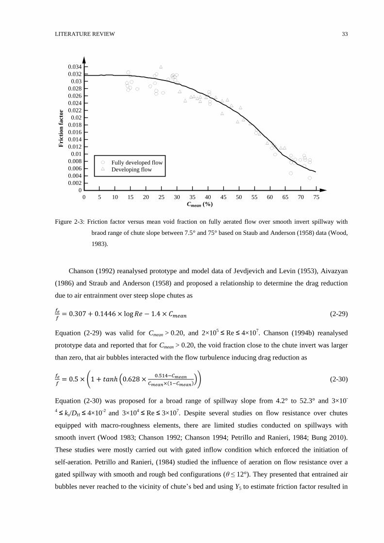
LITERATURE REVIEW 33
Figure 2-3: Friction factor versus mean void fraction on fully aerated flow over smooth invert spillway with
braod range of chute slope between 7.5° and 75° based on Staub and Anderson (1958) data (Wood,
1983).
Chanson (1992) reanalysed prototype and model data of Jevdjevich and Levin (1953), Aivazyan
(1986) and Straub and Anderson (1958) and proposed a relationship to determine the drag reduction
due to air entrainment over steep slope chutes as
𝑓𝑒
𝑓= 0.307 + 0.1446 × log 𝑅𝑒 − 1.4 × 𝐶𝑚𝑒𝑎𝑛 (2-29)
Equation (2-29) was valid for Cmean > 0.20, and 2×10⁵ ≤ Re ≤ 4×10
7. Chanson (1994b) reanalysed
prototype data and reported that for Cmean > 0.20, the void fraction close to the chute invert was larger
than zero, that air bubbles interacted with the flow turbulence inducing drag reduction as
𝑓𝑒
𝑓= 0.5 × (1 + 𝑡𝑎𝑛ℎ (0.628 ×
0.514−𝐶𝑚𝑒𝑎𝑛
𝐶𝑚𝑒𝑎𝑛×(1−𝐶𝑚𝑒𝑎𝑛))) (2-30)
Equation (2-30) was proposed for a broad range of spillway slope from 4.2° to 52.3° and 3×10-
4 ≤ ks/DH ≤ 4×10
-2 and 3×10
4 ≤ Re ≤ 3×10
7. Despite several studies on flow resistance over chutes
equipped with macro-roughness elements, there are limited studies conducted on spillways with
smooth invert (Wood 1983; Chanson 1992; Chanson 1994; Petrillo and Ranieri, 1984; Bung 2010).
These studies were mostly carried out with gated inflow condition which enforced the initiation of
self-aeration. Petrillo and Ranieri, (1984) studied the influence of aeration on flow resistance over a
gated spillway with smooth and rough bed configurations (θ ≤ 12°). They presented that entrained air
bubbles never reached to the vicinity of chute’s bed and using Y5 to estimate friction factor resulted in
Cmean (%)
Fri
cti
on
fact
or
0 5 10 15 20 25 30 35 40 45 50 55 60 65 70 75
0
0.002
0.004
0.006
0.008
0.01
0.012
0.014
0.016
0.018
0.02
0.022
0.024
0.026
0.028
0.03
0.032
0.034
Fully developed flow
Developing flow
LITERATURE REVIEW 34
good agreement with laws applicable to pipes. Still, there is a lack of a mature understanding of the
action of micro-roughness on flow resistance over supercritical flow condition on moderately-sloped
spillway (θ < 15°) with uncontrolled intake condition under non-aerated and partially aerated flow
conditions. An enhanced understanding of the flow resistance will be used towards the design of
spillways, in particular on small dams and water conveyance structures.
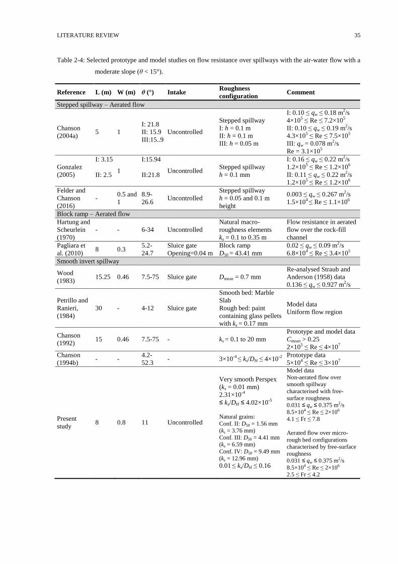
LITERATURE REVIEW 35
Table 2-4: Selected prototype and model studies on flow resistance over spillways with the air-water flow with a
moderate slope (θ < 15°).
Reference L (m) W (m) θ (°) Intake Roughness
configuration Comment
Stepped spillway – Aerated flow
Chanson
(2004a) 5 1
I: 21.8
II: 15.9
III:15..9
Uncontrolled
Stepped spillway
I: h = 0.1 m
II: h = 0.1 m
III: h = 0.05 m
I: 0.10 ≤ qw ≤ 0.18 m2/s
4×10⁵ ≤ Re ≤ 7.2×10
5
II: 0.10 ≤ qw ≤ 0.19 m2/s
4.3×10⁵ ≤ Re ≤ 7.5×10
5
III: qw = 0.078 m2/s
Re = 3.1×10⁵
Gonzalez
(2005)
I: 3.15
1
I:15.94
Uncontrolled Stepped spillway
h = 0.1 mm
I: 0.16 ≤ qw ≤ 0.22 m2/s
1.2×10⁵ ≤ Re ≤ 1.2×10
6
II: 0.11 ≤ qw ≤ 0.22 m2/s
1.2×10⁵ ≤ Re ≤ 1.2×10
6
II: 2.5 II:21.8
Felder and
Chanson
(2016)
- 0.5 and
1
8.9-
26.6 Uncontrolled
Stepped spillway
h = 0.05 and 0.1 m
height
0.003 ≤ qw ≤ 0.267 m2/s
1.5×10⁴ ≤ Re ≤ 1.1×10
6
Block ramp – Aerated flow
Hartung and
Scheurlein
(1970)
- - 6-34 Uncontrolled
Natural macro-
roughness elements
ks = 0.1 to 0.35 m
Flow resistance in aerated
flow over the rock-fill
channel
Pagliara et
al. (2010) 8 0.3
5.2-
24.7
Sluice gate
Opening=0.04 m
Block ramp
D50 = 43.41 mm
0.02 ≤ qw ≤ 0.09 m2/s
6.8×10⁴ ≤ Re ≤ 3.4×10
5
Smooth invert spillway
Wood
(1983) 15.25 0.46 7.5-75 Sluice gate Dmean = 0.7 mm
Re-analysed Straub and
Anderson (1958) data
0.136 ≤ qw ≤ 0.927 m2/s
Petrillo and
Ranieri,
(1984)
30 - 4-12 Sluice gate
Smooth bed: Marble
Slab
Rough bed: paint
containing glass pellets
with ks = 0.17 mm
Model data
Uniform flow region
Chanson
(1992) 15 0.46 7.5-75 - ks = 0.1 to 20 mm
Prototype and model data
Cmean > 0.25
2×10⁵ ≤ Re ≤ 4×10
7
Chanson
(1994b) - -
4.2-
52.3 - 3×10
-4 ≤ ks/DH ≤ 4×10
-2 Prototype data
5×10⁴ ≤ Re ≤ 3×10
7
Present
study 8 0.8 11 Uncontrolled
Very smooth Perspex
(ks = 0.01 mm)
2.31×10⁻⁴
≤ ks/DH ≤ 4.02×10⁻⁵
Natural grains:
Conf. II: D50 = 1.56 mm
(ks = 3.76 mm)
Conf. III: D50 = 4.41 mm
(ks = 6.59 mm)
Conf. IV: D50 = 9.49 mm
(ks = 12.96 mm) 0.01
≤ ks/DH ≤ 0.16
Model data
Non-aerated flow over
smooth spillway
characterised with free-
surface roughness
0.031 ≤ qw ≤ 0.375 m2/s
8.5×10⁴ ≤ Re ≤ 2×10⁶
4.1 ≤ Fr ≤ 7.8
Aerated flow over micro-
rough bed configurations
characterised by free-surface
roughness
0.031 ≤ qw ≤ 0.375 m2/s
8.5×10⁴ ≤ Re ≤ 2×10⁶
2.5 ≤ Fr ≤ 4.2
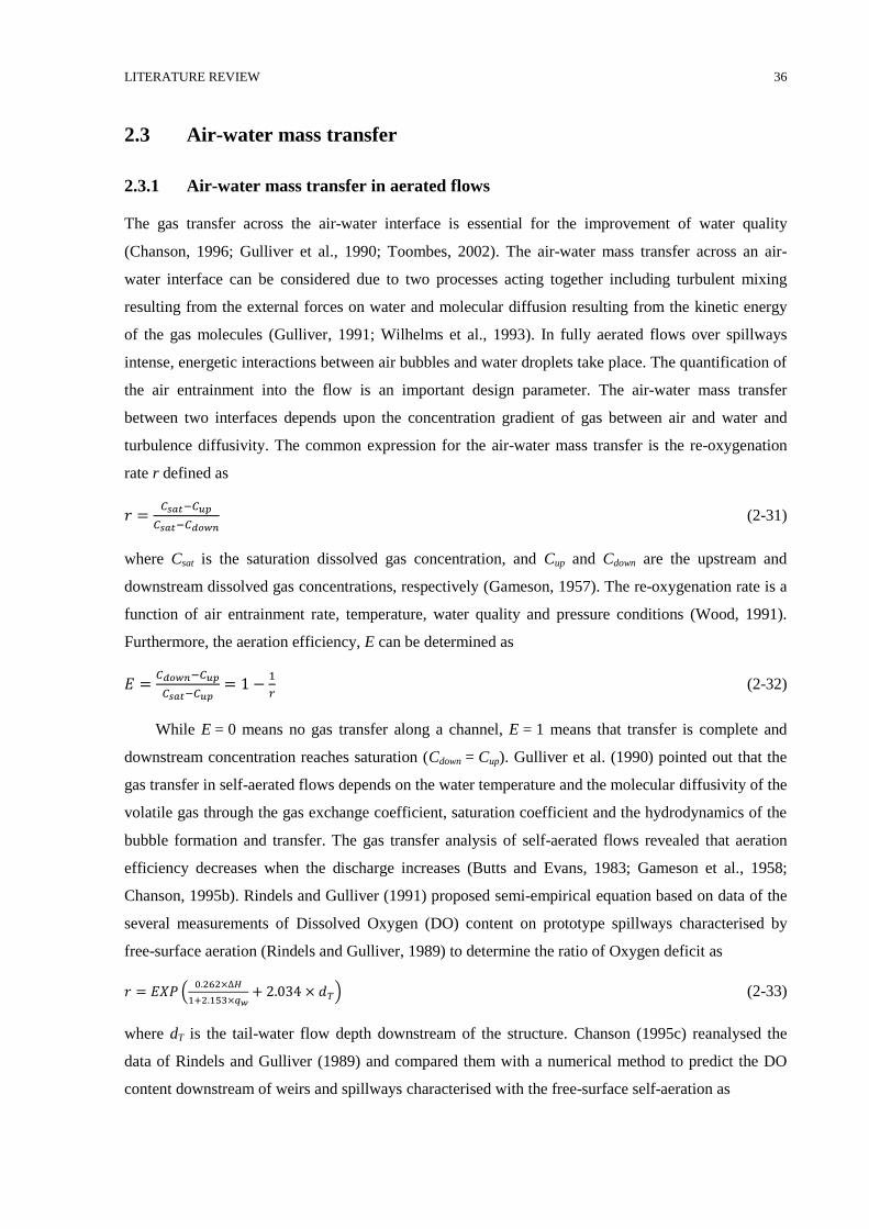
LITERATURE REVIEW 36
Air-water mass transfer 2.3
2.3.1 Air-water mass transfer in aerated flows
The gas transfer across the air-water interface is essential for the improvement of water quality
(Chanson, 1996; Gulliver et al., 1990; Toombes, 2002). The air-water mass transfer across an air-
water interface can be considered due to two processes acting together including turbulent mixing
resulting from the external forces on water and molecular diffusion resulting from the kinetic energy
of the gas molecules (Gulliver, 1991; Wilhelms et al., 1993). In fully aerated flows over spillways
intense, energetic interactions between air bubbles and water droplets take place. The quantification of
the air entrainment into the flow is an important design parameter. The air-water mass transfer
between two interfaces depends upon the concentration gradient of gas between air and water and
turbulence diffusivity. The common expression for the air-water mass transfer is the re-oxygenation
rate r defined as
𝑟 =𝐶𝑠𝑎𝑡−𝐶𝑢𝑝
𝐶𝑠𝑎𝑡−𝐶𝑑𝑜𝑤𝑛 (2-31)
where Csat is the saturation dissolved gas concentration, and Cup and Cdown are the upstream and
downstream dissolved gas concentrations, respectively (Gameson, 1957). The re-oxygenation rate is a
function of air entrainment rate, temperature, water quality and pressure conditions (Wood, 1991).
Furthermore, the aeration efficiency, E can be determined as
𝐸 =𝐶𝑑𝑜𝑤𝑛−𝐶𝑢𝑝
𝐶𝑠𝑎𝑡−𝐶𝑢𝑝= 1 −
1
𝑟 (2-32)
While E = 0 means no gas transfer along a channel, E = 1 means that transfer is complete and
downstream concentration reaches saturation (Cdown = Cup). Gulliver et al. (1990) pointed out that the
gas transfer in self-aerated flows depends on the water temperature and the molecular diffusivity of the
volatile gas through the gas exchange coefficient, saturation coefficient and the hydrodynamics of the
bubble formation and transfer. The gas transfer analysis of self-aerated flows revealed that aeration
efficiency decreases when the discharge increases (Butts and Evans, 1983; Gameson et al., 1958;
Chanson, 1995b). Rindels and Gulliver (1991) proposed semi-empirical equation based on data of the
several measurements of Dissolved Oxygen (DO) content on prototype spillways characterised by
free-surface aeration (Rindels and Gulliver, 1989) to determine the ratio of Oxygen deficit as
𝑟 = 𝐸𝑋𝑃 (0.262×∆𝐻
1+2.153×𝑞𝑤+ 2.034 × 𝑑𝑇) (2-33)
where dT is the tail-water flow depth downstream of the structure. Chanson (1995c) reanalysed the
data of Rindels and Gulliver (1989) and compared them with a numerical method to predict the DO
content downstream of weirs and spillways characterised with the free-surface self-aeration as
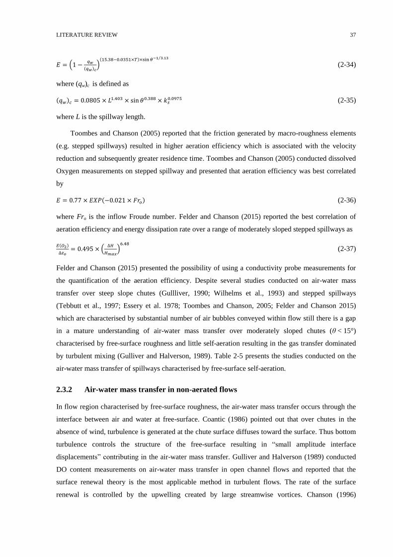
LITERATURE REVIEW 37
𝐸 = (1 −𝑞𝑤
(𝑞𝑤)𝑐)
(15.38−0.0351×𝑇)×sin 𝜃−1 3.13⁄
(2-34)
where (qw)c is defined as
(𝑞𝑤)𝑐 = 0.0805 × 𝐿1.403 × sin 𝜃0.388 × 𝑘𝑠0.0975 (2-35)
where L is the spillway length.
Toombes and Chanson (2005) reported that the friction generated by macro-roughness elements
(e.g. stepped spillways) resulted in higher aeration efficiency which is associated with the velocity
reduction and subsequently greater residence time. Toombes and Chanson (2005) conducted dissolved
Oxygen measurements on stepped spillway and presented that aeration efficiency was best correlated
by
𝐸 = 0.77 × 𝐸𝑋𝑃(−0.021 × 𝐹𝑟𝑜) (2-36)
where Fro is the inflow Froude number. Felder and Chanson (2015) reported the best correlation of
aeration efficiency and energy dissipation rate over a range of moderately sloped stepped spillways as
𝐸(𝑂2)
∆𝑧𝑜= 0.495 × (
∆𝐻
𝐻𝑚𝑎𝑥)
6.48
(2-37)
Felder and Chanson (2015) presented the possibility of using a conductivity probe measurements for
the quantification of the aeration efficiency. Despite several studies conducted on air-water mass
transfer over steep slope chutes (Gullliver, 1990; Wilhelms et al., 1993) and stepped spillways
(Tebbutt et al., 1997; Essery et al. 1978; Toombes and Chanson, 2005; Felder and Chanson 2015)
which are characterised by substantial number of air bubbles conveyed within flow still there is a gap
in a mature understanding of air-water mass transfer over moderately sloped chutes (θ < 15°)
characterised by free-surface roughness and little self-aeration resulting in the gas transfer dominated
by turbulent mixing (Gulliver and Halverson, 1989). Table 2-5 presents the studies conducted on the
air-water mass transfer of spillways characterised by free-surface self-aeration.
2.3.2 Air-water mass transfer in non-aerated flows
In flow region characterised by free-surface roughness, the air-water mass transfer occurs through the
interface between air and water at free-surface. Coantic (1986) pointed out that over chutes in the
absence of wind, turbulence is generated at the chute surface diffuses toward the surface. Thus bottom
turbulence controls the structure of the free-surface resulting in “small amplitude interface
displacements” contributing in the air-water mass transfer. Gulliver and Halverson (1989) conducted
DO content measurements on air-water mass transfer in open channel flows and reported that the
surface renewal theory is the most applicable method in turbulent flows. The rate of the surface
renewal is controlled by the upwelling created by large streamwise vortices. Chanson (1996)
LITERATURE REVIEW 38
suggested that for moderately sloped spillways, the intake geometry affects the flow condition at the
upstream of the spillway and the self-aeration process resulting in the domination of turbulent mixing
in the air-water transfer process. Since on moderately sloped spillway with uncontrolled intake
condition, little self-aeration may occur along the spillway the air-water transfer process will be
dominated by free-surface roughness and waves. The present study is aiming to investigate the air-
water mas transfer over moderately sloped spillway with uncontrolled intake condition characterised
by free-surface roughness and small amplitude waves.
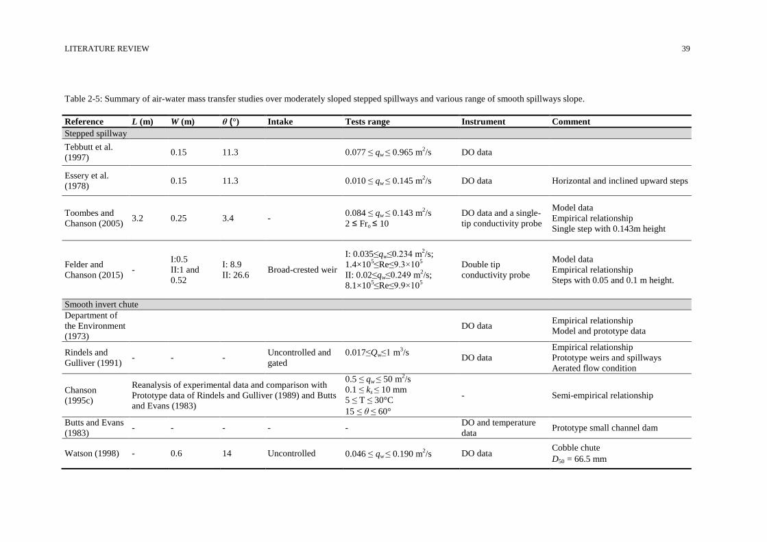
LITERATURE REVIEW 39
Table 2-5: Summary of air-water mass transfer studies over moderately sloped stepped spillways and various range of smooth spillways slope.
Reference L (m) W (m) θ (°) Intake Tests range Instrument Comment
Stepped spillway
Tebbutt et al.
(1997) 0.15 11.3 0.077 ≤ qw ≤ 0.965 m
2/s DO data
Essery et al.
(1978) 0.15 11.3 0.010 ≤ qw ≤ 0.145 m
2/s DO data Horizontal and inclined upward steps
Toombes and
Chanson (2005) 3.2 0.25 3.4 -
0.084 ≤ qw ≤ 0.143 m2/s
2 ≤ Fro ≤ 10
DO data and a single-
tip conductivity probe
Model data
Empirical relationship
Single step with 0.143m height
Felder and
Chanson (2015) -
I:0.5
II:1 and
0.52
I: 8.9
II: 26.6 Broad-crested weir
I: 0.035≤qw≤0.234 m2/s;
1.4×10⁵≤Re≤9.3×10
5
II: 0.02≤qw≤0.249 m2/s;
8.1×10⁵≤Re≤9.9×10
5
Double tip
conductivity probe
Model data
Empirical relationship
Steps with 0.05 and 0.1 m height.
Smooth invert chute
Department of
the Environment
(1973)
DO data Empirical relationship
Model and prototype data
Rindels and
Gulliver (1991) - - -
Uncontrolled and
gated
0.017≤Qw≤1 m3/s
DO data
Empirical relationship
Prototype weirs and spillways
Aerated flow condition
Chanson
(1995c)
Reanalysis of experimental data and comparison with
Prototype data of Rindels and Gulliver (1989) and Butts
and Evans (1983)
0.5 ≤ qw ≤ 50 m2/s
0.1 ≤ ks ≤ 10 mm
5 ≤ T ≤ 30°C
15 ≤ θ ≤ 60°
- Semi-empirical relationship
Butts and Evans
(1983) - - - - -
DO and temperature
data Prototype small channel dam
Watson (1998) - 0.6 14 Uncontrolled 0.046 ≤ qw ≤ 0.190 m2/s DO data
Cobble chute
D50 = 66.5 mm
LITERATURE REVIEW 40
Summary 2.4
In the past decade's several studies conducted on model and prototype data of smooth invert spillways
mostly with a steep slope and gated inflow conditions which are susceptible to substantial self-
aeration. Although few studies reported the free-surface roughness upstream of the inception point of
free-surface aeration, there is limited information about the flow properties within this region which is
characterised by free-surface roughness and entrapped air. A deeper understanding of gradually varied
flow region over moderate slope chutes and uncontrolled intake condition is crucial because, in high
discharges, uniform flow condition may not occur along the structure and flow in gradually varied
flow region may determine the inflow into the downstream energy dissipater. However, several studies
conducted on flow properties in uniform equilibrium flow region on smooth and macro-rough bed
spillways; there is a gap in knowledge of the broad range of air-water flow properties such as mean
void fraction, air-water interface count rate, turbulence intensity, auto- and cross-correlation
timescales, and air and water chord sizes over the moderately sloped spillway with micro-roughness
configurations. The present research aims to investigate design aspects of aeration, air-water mass
transfer, energy dissipation rate and residual energy by a small increase of bed roughness. While
existing knowledge is more focused on the air-water flows and energy dissipation processes on
stepped spillways and to some extent on smooth spillways, little research has been conducted on
spillways with micro-roughness invert. Several laboratory studies have been conducted on spillway
models equipped with smooth bed configuration with a range of equivalent sand roughness
0.1< ks < 1 mm resulting in discrepancies which might be due to the impact of bed configuration and
the conflicting definition of smooth bed. Therefore, the understanding of the effects of micro-
roughness is essential to better understand different results in previous studies of smooth spillway
conditions. In particular, the present study aims to investigate the effect of small changes in bed
roughness can have on the overall flow behaviour, and design aspects such as the re-aeration and the
energy dissipation performances. Herein, the present study conducted experiments at near prototype
scale model using an uncontrolled spillway with various micro-roughness bed configurations and with
a moderate slope of θ = 11º. A slope of θ = 11º is considered as a moderate slope where no flow
aeration occurs naturally for smooth flow conditions (Anwar, 1994). Therefore, in present study
θ = 11º has been selected to study the effect of the bed roughness on the re-aeration and energy
dissipation performances. The research goals have been identified as:
● Better understand the flow processes on moderately sloped spillways with micro-rough beds.
● Identify the effects of micro-roughness on the development of the boundary layer properties and the
development of the non-aerated and aerated flow properties along the chute.
● Measure and interpret the effects of bed micro-roughness on the flow aeration, air-water flow
properties, energy dissipation and air-water mass transfer.

LITERATURE REVIEW 41
● Identify the potential to optimise spillway design on moderately sloped spillway through the use of
micro-roughness.
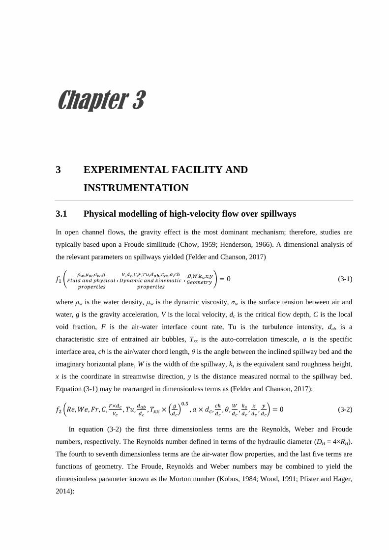
Chapter 3
3 EXPERIMENTAL FACILITY AND
INSTRUMENTATION
Physical modelling of high-velocity flow over spillways 3.1
In open channel flows, the gravity effect is the most dominant mechanism; therefore, studies are
typically based upon a Froude similitude (Chow, 1959; Henderson, 1966). A dimensional analysis of
the relevant parameters on spillways yielded (Felder and Chanson, 2017)
𝑓1 (𝜌𝑤,𝜇𝑤,𝜎𝑤,𝑔
𝐹𝑙𝑢𝑖𝑑 𝑎𝑛𝑑 𝑝ℎ𝑦𝑠𝑖𝑐𝑎𝑙 𝑝𝑟𝑜𝑝𝑒𝑟𝑡𝑖𝑒𝑠
,𝑉,𝑑𝑐,𝐶,𝐹,𝑇𝑢,𝑑𝑎𝑏,𝑇𝑥𝑥,𝑎,𝑐ℎ
𝐷𝑦𝑛𝑎𝑚𝑖𝑐 𝑎𝑛𝑑 𝑘𝑖𝑛𝑒𝑚𝑎𝑡𝑖𝑐 𝑝𝑟𝑜𝑝𝑒𝑟𝑡𝑖𝑒𝑠
, ,𝜃,𝑊,𝑘𝑠,𝑥,𝑦𝐺𝑒𝑜𝑚𝑒𝑡𝑟𝑦
) = 0 (3-1)
where ρw is the water density, μw is the dynamic viscosity, σw is the surface tension between air and
water, g is the gravity acceleration, V is the local velocity, dc is the critical flow depth, C is the local
void fraction, F is the air-water interface count rate, Tu is the turbulence intensity, dab is a
characteristic size of entrained air bubbles, Txx is the auto-correlation timescale, a is the specific
interface area, ch is the air/water chord length, θ is the angle between the inclined spillway bed and the
imaginary horizontal plane, W is the width of the spillway, ks is the equivalent sand roughness height,
x is the coordinate in streamwise direction, y is the distance measured normal to the spillway bed.
Equation (3-1) may be rearranged in dimensionless terms as (Felder and Chanson, 2017):
𝑓2 (𝑅𝑒, 𝑊𝑒, 𝐹𝑟, 𝐶,𝐹×𝑑𝑐
𝑉𝑐, 𝑇𝑢,
𝑑𝑎𝑏
𝑑𝑐, 𝑇𝑥𝑥 × (
𝑔
𝑑𝑐)
0.5, 𝑎 × 𝑑𝑐 ,
𝑐ℎ
𝑑𝑐, 𝜃,
𝑊
𝑑𝑐,
𝑘𝑠
𝑑𝑐,
𝑥
𝑑𝑐,
𝑦
𝑑𝑐) = 0 (3-2)
In equation (3-2) the first three dimensionless terms are the Reynolds, Weber and Froude
numbers, respectively. The Reynolds number defined in terms of the hydraulic diameter (DH = 4×RH).
The fourth to seventh dimensionless terms are the air-water flow properties, and the last five terms are
functions of geometry. The Froude, Reynolds and Weber numbers may be combined to yield the
dimensionless parameter known as the Morton number (Kobus, 1984; Wood, 1991; Pfister and Hager,
2014):
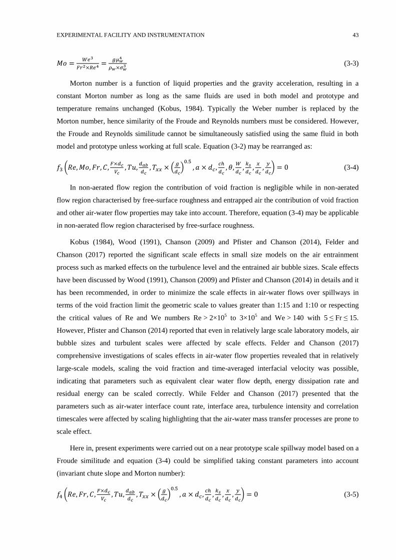
EXPERIMENTAL FACILITY AND INSTRUMENTATION 43
𝑀𝑜 =𝑊𝑒3
𝐹𝑟2×𝑅𝑒4 =𝑔𝜇𝑤
4
𝜌𝑤×𝜎𝑤3 (3-3)
Morton number is a function of liquid properties and the gravity acceleration, resulting in a
constant Morton number as long as the same fluids are used in both model and prototype and
temperature remains unchanged (Kobus, 1984). Typically the Weber number is replaced by the
Morton number, hence similarity of the Froude and Reynolds numbers must be considered. However,
the Froude and Reynolds similitude cannot be simultaneously satisfied using the same fluid in both
model and prototype unless working at full scale. Equation (3-2) may be rearranged as:
𝑓3 (𝑅𝑒, 𝑀𝑜, 𝐹𝑟, 𝐶,𝐹×𝑑𝑐
𝑉𝑐, 𝑇𝑢,
𝑑𝑎𝑏
𝑑𝑐, 𝑇𝑥𝑥 × (
𝑔
𝑑𝑐)
0.5, 𝑎 × 𝑑𝑐 ,
𝑐ℎ
𝑑𝑐, 𝜃,
𝑊
𝑑𝑐,
𝑘𝑠
𝑑𝑐,
𝑥
𝑑𝑐,
𝑦
𝑑𝑐) = 0 (3-4)
In non-aerated flow region the contribution of void fraction is negligible while in non-aerated
flow region characterised by free-surface roughness and entrapped air the contribution of void fraction
and other air-water flow properties may take into account. Therefore, equation (3-4) may be applicable
in non-aerated flow region characterised by free-surface roughness.
Kobus (1984), Wood (1991), Chanson (2009) and Pfister and Chanson (2014), Felder and
Chanson (2017) reported the significant scale effects in small size models on the air entrainment
process such as marked effects on the turbulence level and the entrained air bubble sizes. Scale effects
have been discussed by Wood (1991), Chanson (2009) and Pfister and Chanson (2014) in details and it
has been recommended, in order to minimize the scale effects in air-water flows over spillways in
terms of the void fraction limit the geometric scale to values greater than 1:15 and 1:10 or respecting
the critical values of Re and We numbers Re > 2×10⁵ to 3×10
5 and We > 140 with 5 ≤ Fr ≤ 15.
However, Pfister and Chanson (2014) reported that even in relatively large scale laboratory models, air
bubble sizes and turbulent scales were affected by scale effects. Felder and Chanson (2017)
comprehensive investigations of scales effects in air-water flow properties revealed that in relatively
large-scale models, scaling the void fraction and time-averaged interfacial velocity was possible,
indicating that parameters such as equivalent clear water flow depth, energy dissipation rate and
residual energy can be scaled correctly. While Felder and Chanson (2017) presented that the
parameters such as air-water interface count rate, interface area, turbulence intensity and correlation
timescales were affected by scaling highlighting that the air-water mass transfer processes are prone to
scale effect.
Here in, present experiments were carried out on a near prototype scale spillway model based on a
Froude similitude and equation (3-4) could be simplified taking constant parameters into account
(invariant chute slope and Morton number):
𝑓4 (𝑅𝑒, 𝐹𝑟, 𝐶,𝐹×𝑑𝑐
𝑉𝑐, 𝑇𝑢,
𝑑𝑎𝑏
𝑑𝑐, 𝑇𝑥𝑥 × (
𝑔
𝑑𝑐)
0.5, 𝑎 × 𝑑𝑐 ,
𝑐ℎ
𝑑𝑐,
𝑘𝑠
𝑑𝑐,
𝑥
𝑑𝑐,
𝑦
𝑑𝑐) = 0 (3-5)
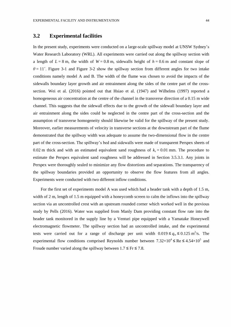
EXPERIMENTAL FACILITY AND INSTRUMENTATION 44
Experimental facilities 3.2
In the present study, experiments were conducted on a large-scale spillway model at UNSW Sydney’s
Water Research Laboratory (WRL). All experiments were carried out along the spillway section with
a length of L = 8 m, the width of W = 0.8 m, sidewalls height of h = 0.6 m and constant slope of
θ = 11˚. Figure 3-1 and Figure 3-2 show the spillway section from different angles for two intake
conditions namely model A and B. The width of the flume was chosen to avoid the impacts of the
sidewalls boundary layer growth and air entrainment along the sides of the centre part of the cross-
section. Wei et al. (2016) pointed out that Hsiao et al. (1947) and Wilhelms (1997) reported a
homogeneous air concentration at the centre of the channel in the transverse direction of a 0.15 m wide
channel. This suggests that the sidewall effects due to the growth of the sidewall boundary layer and
air entrainment along the sides could be neglected in the centre part of the cross-section and the
assumption of transverse homogeneity should likewise be valid for the spillway of the present study.
Moreover, earlier measurements of velocity in transverse sections at the downstream part of the flume
demonstrated that the spillway width was adequate to assume the two-dimensional flow in the centre
part of the cross-section. The spillway’s bed and sidewalls were made of transparent Perspex sheets of
0.02 m thick and with an estimated equivalent sand roughness of ks = 0.01 mm. The procedure to
estimate the Perspex equivalent sand roughness will be addressed in Section 3.5.3.1. Any joints in
Perspex were thoroughly sealed to minimize any flow distortions and separations. The transparency of
the spillway boundaries provided an opportunity to observe the flow features from all angles.
Experiments were conducted with two different inflow conditions.
For the first set of experiments model A was used which had a header tank with a depth of 1.5 m,
width of 2 m, length of 1.5 m equipped with a honeycomb screen to calm the inflows into the spillway
section via an uncontrolled crest with an upstream rounded corner which worked well in the previous
study by Pells (2016). Water was supplied from Manly Dam providing constant flow rate into the
header tank monitored in the supply line by a Venturi pipe equipped with a Yamatake Honeywell
electromagnetic flowmeter. The spillway section had an uncontrolled intake, and the experimental
tests were carried out for a range of discharge per unit width 0.019 ≤ qw ≤ 0.125 m2/s. The
experimental flow conditions comprised Reynolds number between 7.32×10⁴ ≤ Re ≤ 4.54×10
5 and
Froude number varied along the spillway between 1.7 ≤ Fr ≤ 7.8.
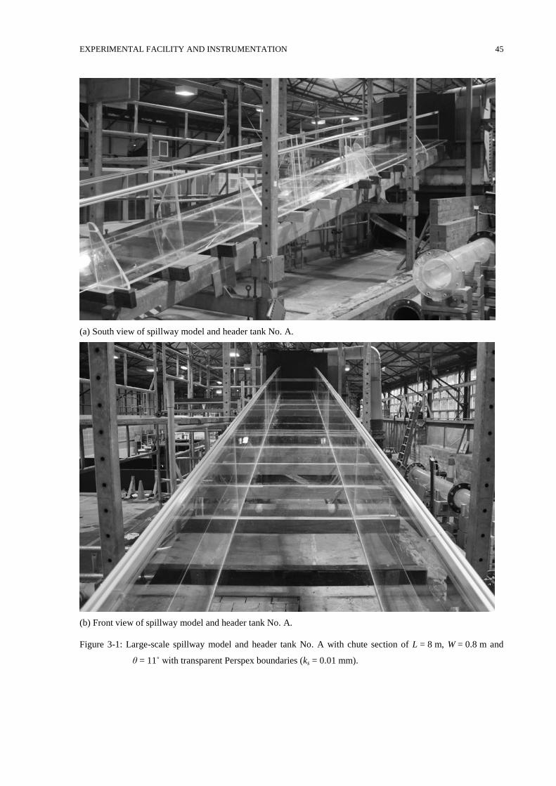
EXPERIMENTAL FACILITY AND INSTRUMENTATION 45
(a) South view of spillway model and header tank No. A.
(b) Front view of spillway model and header tank No. A.
Figure 3-1: Large-scale spillway model and header tank No. A with chute section of L = 8 m, W = 0.8 m and
θ = 11˚ with transparent Perspex boundaries (ks = 0.01 mm).
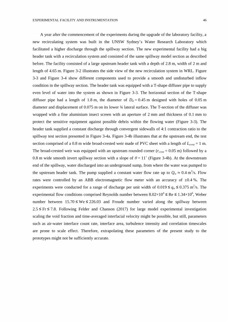
EXPERIMENTAL FACILITY AND INSTRUMENTATION 46
A year after the commencement of the experiments during the upgrade of the laboratory facility, a
new recirculating system was built in the UNSW Sydney’s Water Research Laboratory which
facilitated a higher discharge through the spillway section. The new experimental facility had a big
header tank with a recirculation system and consisted of the same spillway model section as described
before. The facility consisted of a large upstream header tank with a depth of 2.8 m, width of 2 m and
length of 4.65 m. Figure 3-2 illustrates the side view of the new recirculation system in WRL. Figure
3-3 and Figure 3-4 show different components used to provide a smooth and undisturbed inflow
condition in the spillway section. The header tank was equipped with a T-shape diffuser pipe to supply
even level of water into the system as shown in Figure 3-3. The horizontal section of the T-shape
diffuser pipe had a length of 1.8 m, the diameter of Dd = 0.45 m designed with holes of 0.05 m
diameter and displacement of 0.075 m on its lower ¾ lateral surface. The T-section of the diffuser was
wrapped with a fine aluminium insect screen with an aperture of 2 mm and thickness of 0.1 mm to
protect the sensitive equipment against possible debris within the flowing water (Figure 3-3). The
header tank supplied a constant discharge through convergent sidewalls of 4:1 contraction ratio to the
spillway test section presented in Figure 3-4a. Figure 3-4b illustrates that at the upstream end, the test
section comprised of a 0.8 m wide broad-crested weir made of PVC sheet with a length of Lcrest = 1 m.
The broad-crested weir was equipped with an upstream rounded corner (rcrest = 0.05 m) followed by a
0.8 m wide smooth invert spillway section with a slope of θ = 11˚ (Figure 3-4b). At the downstream
end of the spillway, water discharged into an underground sump, from where the water was pumped to
the upstream header tank. The pump supplied a constant water flow rate up to Qw ≃ 0.4 m3/s. Flow
rates were controlled by an ABB electromagnetic flow meter with an accuracy of ±0.4 %. The
experiments were conducted for a range of discharge per unit width of 0.019 ≤ qw ≤ 0.375 m2/s. The
experimental flow conditions comprised Reynolds number between 8.02×10⁴ ≤ Re ≤ 1.34×10
6, Weber
number between 15.70 ≤ We ≤ 226.03 and Froude number varied along the spillway between
2.5 ≤ Fr ≤ 7.8. Following Felder and Chanson (2017) for large model experimental investigation
scaling the void fraction and time-averaged interfacial velocity might be possible, but still, parameters
such as air-water interface count rate, interface area, turbulence intensity and correlation timescales
are prone to scale effect. Therefore, extrapolating these parameters of the present study to the
prototypes might not be sufficiently accurate.
EXPERIMENTAL FACILITY AND INSTRUMENTATION 47
Figure 3-2: Side view of the experimental recirculation system and header tank No. B: Smooth bed
configuration, qw = 0.375 m2/s, dc = 0.243 m, Re = 1.2×10
6.
Figure 3-3: Front view of the T-shape diffuser pipe with a length of 1.8 m, Dd = 0.45 m, Dh = 0.05 m,
ds = 0.075 m.
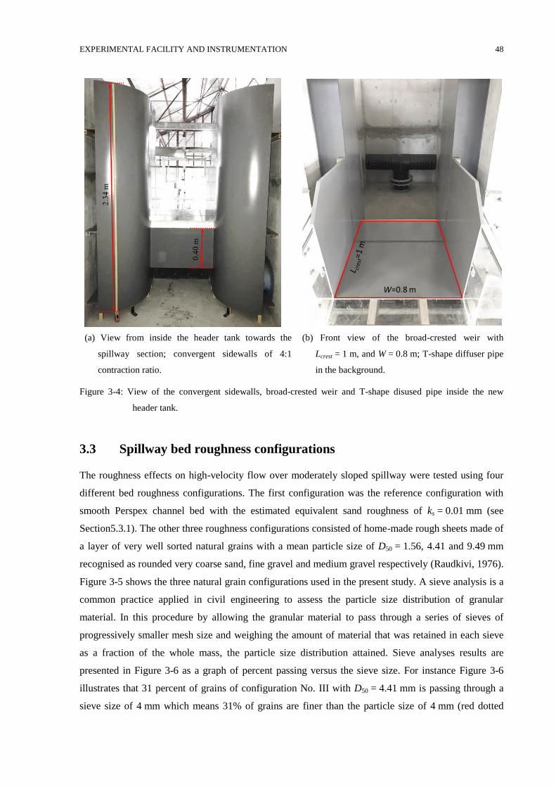
EXPERIMENTAL FACILITY AND INSTRUMENTATION 48
(a) View from inside the header tank towards the
spillway section; convergent sidewalls of 4:1
contraction ratio.
(b) Front view of the broad-crested weir with
Lcrest = 1 m, and W = 0.8 m; T-shape diffuser pipe
in the background.
Figure 3-4: View of the convergent sidewalls, broad-crested weir and T-shape disused pipe inside the new
header tank.
Spillway bed roughness configurations 3.3
The roughness effects on high-velocity flow over moderately sloped spillway were tested using four
different bed roughness configurations. The first configuration was the reference configuration with
smooth Perspex channel bed with the estimated equivalent sand roughness of ks = 0.01 mm (see
Section5.3.1). The other three roughness configurations consisted of home-made rough sheets made of
a layer of very well sorted natural grains with a mean particle size of D50 = 1.56, 4.41 and 9.49 mm
recognised as rounded very coarse sand, fine gravel and medium gravel respectively (Raudkivi, 1976).
Figure 3-5 shows the three natural grain configurations used in the present study. A sieve analysis is a
common practice applied in civil engineering to assess the particle size distribution of granular
material. In this procedure by allowing the granular material to pass through a series of sieves of
progressively smaller mesh size and weighing the amount of material that was retained in each sieve
as a fraction of the whole mass, the particle size distribution attained. Sieve analyses results are
presented in Figure 3-6 as a graph of percent passing versus the sieve size. For instance Figure 3-6
illustrates that 31 percent of grains of configuration No. III with D50 = 4.41 mm is passing through a
sieve size of 4 mm which means 31% of grains are finer than the particle size of 4 mm (red dotted
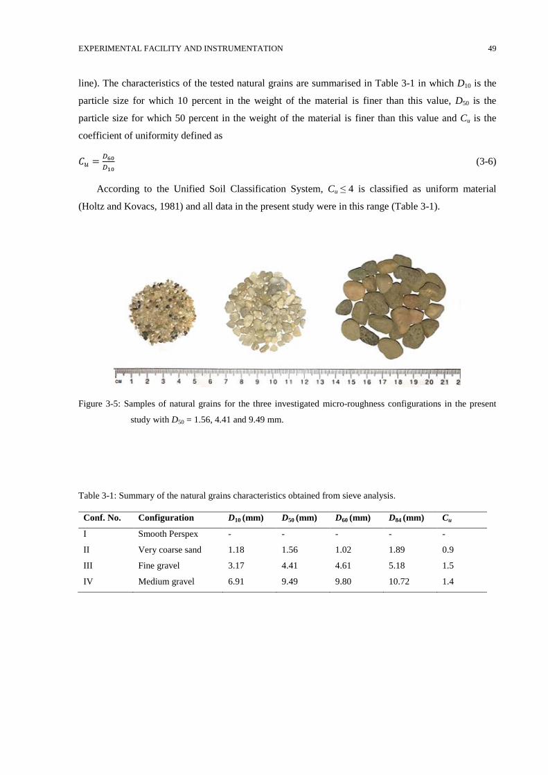
EXPERIMENTAL FACILITY AND INSTRUMENTATION 49
line). The characteristics of the tested natural grains are summarised in Table 3-1 in which D10 is the
particle size for which 10 percent in the weight of the material is finer than this value, D50 is the
particle size for which 50 percent in the weight of the material is finer than this value and Cu is the
coefficient of uniformity defined as
𝐶𝑢 =𝐷60
𝐷10 (3-6)
According to the Unified Soil Classification System, Cu ≤ 4 is classified as uniform material
(Holtz and Kovacs, 1981) and all data in the present study were in this range (Table 3-1).
Figure 3-5: Samples of natural grains for the three investigated micro-roughness configurations in the present
study with D50 = 1.56, 4.41 and 9.49 mm.
Table 3-1: Summary of the natural grains characteristics obtained from sieve analysis.
Conf. No. Configuration D10 (mm) D50 (mm) D60 (mm) D84 (mm) Cu
I Smooth Perspex - - - - -
II Very coarse sand 1.18 1.56 1.02 1.89 0.9
III Fine gravel 3.17 4.41 4.61 5.18 1.5
IV Medium gravel 6.91 9.49 9.80 10.72 1.4
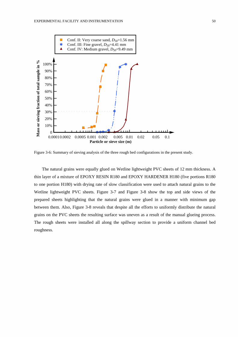
EXPERIMENTAL FACILITY AND INSTRUMENTATION 50
Figure 3-6: Summary of sieving analysis of the three rough bed configurations in the present study.
The natural grains were equally glued on Wetline lightweight PVC sheets of 12 mm thickness. A
thin layer of a mixture of EPOXY RESIN R180 and EPOXY HARDENER H180 (five portions R180
to one portion H180) with drying rate of slow classification were used to attach natural grains to the
Wetline lightweight PVC sheets. Figure 3-7 and Figure 3-8 show the top and side views of the
prepared sheets highlighting that the natural grains were glued in a manner with minimum gap
between them. Also, Figure 3-8 reveals that despite all the efforts to uniformly distribute the natural
grains on the PVC sheets the resulting surface was uneven as a result of the manual glueing process.
The rough sheets were installed all along the spillway section to provide a uniform channel bed
roughness.
Particle or sieve size (m)
Mass
or
sievin
g f
ract
ion
of
tota
l sa
mp
le i
n %
0.00010.0002 0.0005 0.001 0.002 0.005 0.01 0.02 0.05 0.1
0
10%
20%
30%
40%
50%
60%
70%
80%
90%
100%
Conf. II: Very coarse sand, D50=1.56 mm
Conf. III: Fine gravel, D50=4.41 mm
Conf. IV: Medium gravel, D50=9.49 mm
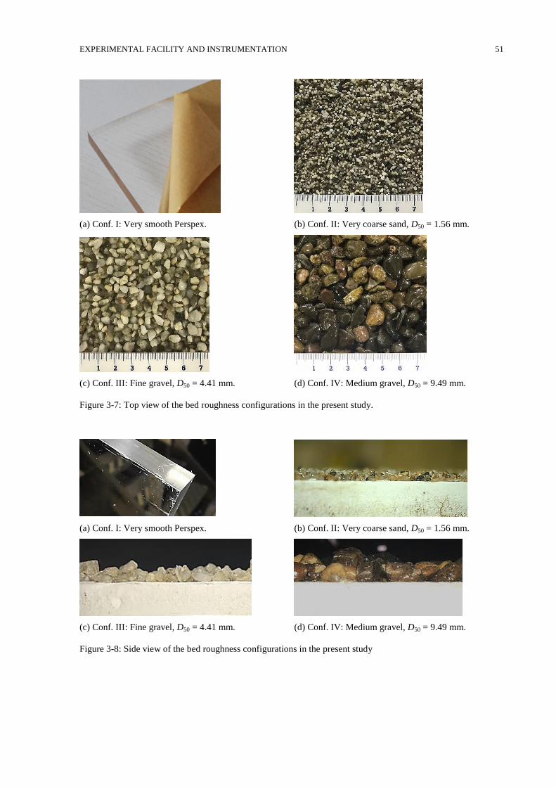
EXPERIMENTAL FACILITY AND INSTRUMENTATION 51
(a) Conf. I: Very smooth Perspex. (b) Conf. II: Very coarse sand, D50 = 1.56 mm.
(c) Conf. III: Fine gravel, D50 = 4.41 mm. (d) Conf. IV: Medium gravel, D50 = 9.49 mm.
Figure 3-7: Top view of the bed roughness configurations in the present study.
(a) Conf. I: Very smooth Perspex. (b) Conf. II: Very coarse sand, D50 = 1.56 mm.
(c) Conf. III: Fine gravel, D50 = 4.41 mm. (d) Conf. IV: Medium gravel, D50 = 9.49 mm.
Figure 3-8: Side view of the bed roughness configurations in the present study
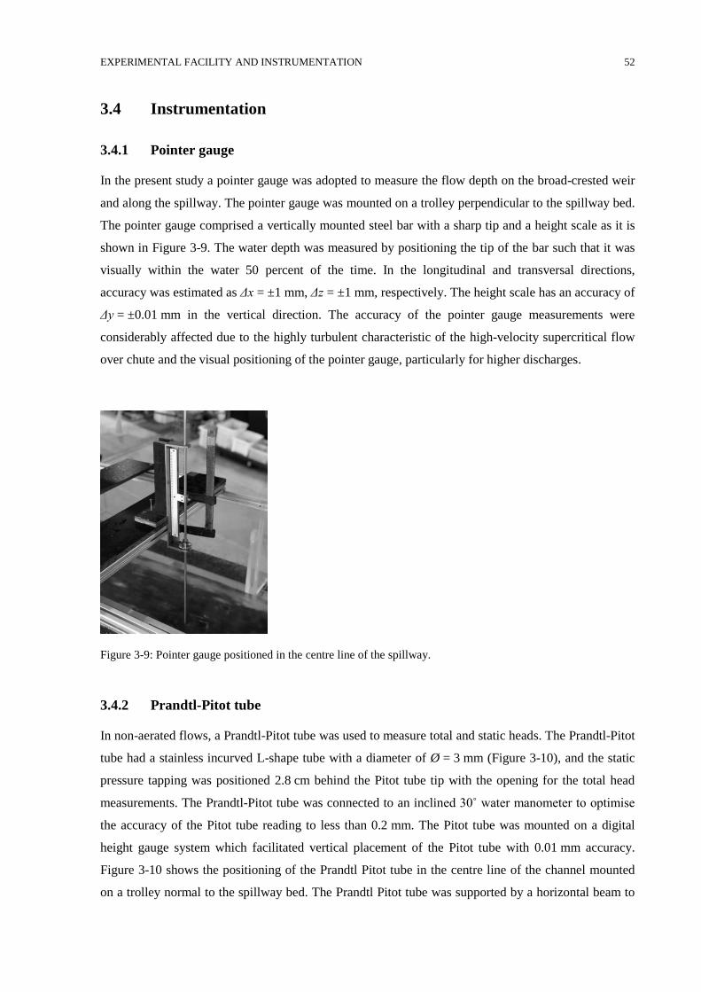
EXPERIMENTAL FACILITY AND INSTRUMENTATION 52
Instrumentation 3.4
3.4.1 Pointer gauge
In the present study a pointer gauge was adopted to measure the flow depth on the broad-crested weir
and along the spillway. The pointer gauge was mounted on a trolley perpendicular to the spillway bed.
The pointer gauge comprised a vertically mounted steel bar with a sharp tip and a height scale as it is
shown in Figure 3-9. The water depth was measured by positioning the tip of the bar such that it was
visually within the water 50 percent of the time. In the longitudinal and transversal directions,
accuracy was estimated as Δx = ±1 mm, Δz = ±1 mm, respectively. The height scale has an accuracy of
Δy = ±0.01 mm in the vertical direction. The accuracy of the pointer gauge measurements were
considerably affected due to the highly turbulent characteristic of the high-velocity supercritical flow
over chute and the visual positioning of the pointer gauge, particularly for higher discharges.
Figure 3-9: Pointer gauge positioned in the centre line of the spillway.
3.4.2 Prandtl-Pitot tube
In non-aerated flows, a Prandtl-Pitot tube was used to measure total and static heads. The Prandtl-Pitot
tube had a stainless incurved L-shape tube with a diameter of Ø = 3 mm (Figure 3-10), and the static
pressure tapping was positioned 2.8 cm behind the Pitot tube tip with the opening for the total head
measurements. The Prandtl-Pitot tube was connected to an inclined 30˚ water manometer to optimise
the accuracy of the Pitot tube reading to less than 0.2 mm. The Pitot tube was mounted on a digital
height gauge system which facilitated vertical placement of the Pitot tube with 0.01 mm accuracy.
Figure 3-10 shows the positioning of the Prandtl Pitot tube in the centre line of the channel mounted
on a trolley normal to the spillway bed. The Prandtl Pitot tube was supported by a horizontal beam to
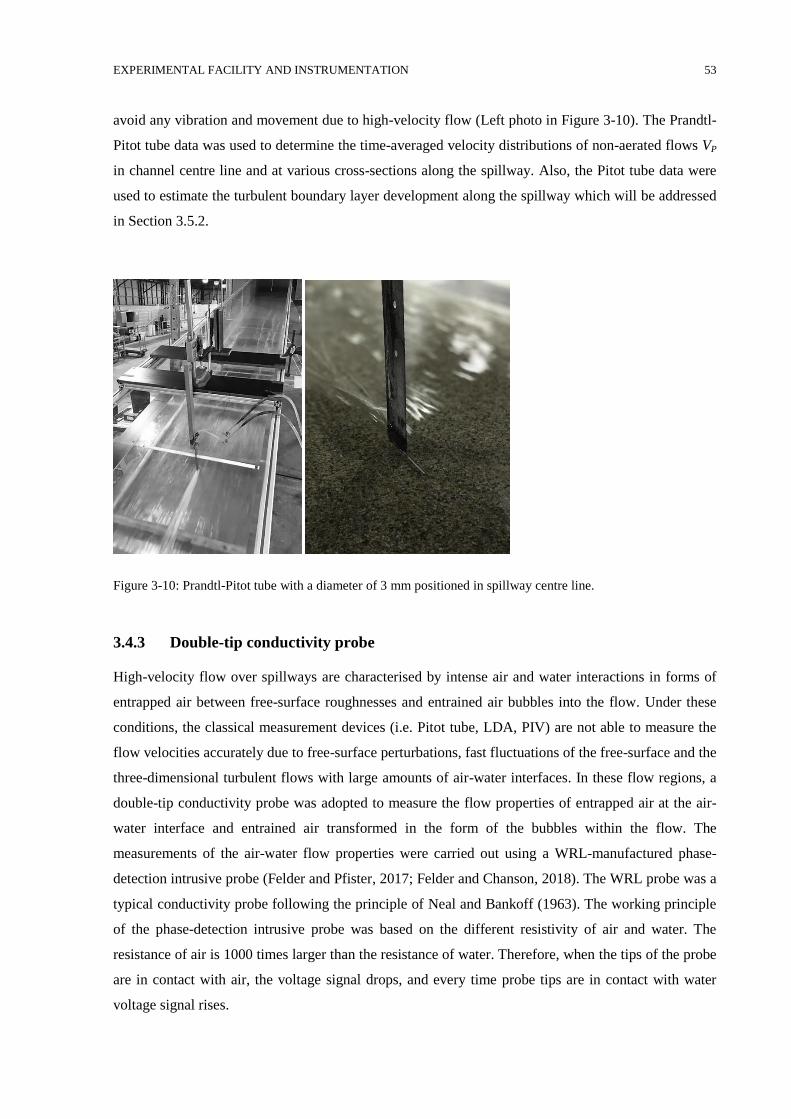
EXPERIMENTAL FACILITY AND INSTRUMENTATION 53
avoid any vibration and movement due to high-velocity flow (Left photo in Figure 3-10). The Prandtl-
Pitot tube data was used to determine the time-averaged velocity distributions of non-aerated flows VP
in channel centre line and at various cross-sections along the spillway. Also, the Pitot tube data were
used to estimate the turbulent boundary layer development along the spillway which will be addressed
in Section 3.5.2.
Figure 3-10: Prandtl-Pitot tube with a diameter of 3 mm positioned in spillway centre line.
3.4.3 Double-tip conductivity probe
High-velocity flow over spillways are characterised by intense air and water interactions in forms of
entrapped air between free-surface roughnesses and entrained air bubbles into the flow. Under these
conditions, the classical measurement devices (i.e. Pitot tube, LDA, PIV) are not able to measure the
flow velocities accurately due to free-surface perturbations, fast fluctuations of the free-surface and the
three-dimensional turbulent flows with large amounts of air-water interfaces. In these flow regions, a
double-tip conductivity probe was adopted to measure the flow properties of entrapped air at the air-
water interface and entrained air transformed in the form of the bubbles within the flow. The
measurements of the air-water flow properties were carried out using a WRL-manufactured phase-
detection intrusive probe (Felder and Pfister, 2017; Felder and Chanson, 2018). The WRL probe was a
typical conductivity probe following the principle of Neal and Bankoff (1963). The working principle
of the phase-detection intrusive probe was based on the different resistivity of air and water. The
resistance of air is 1000 times larger than the resistance of water. Therefore, when the tips of the probe
are in contact with air, the voltage signal drops, and every time probe tips are in contact with water
voltage signal rises.
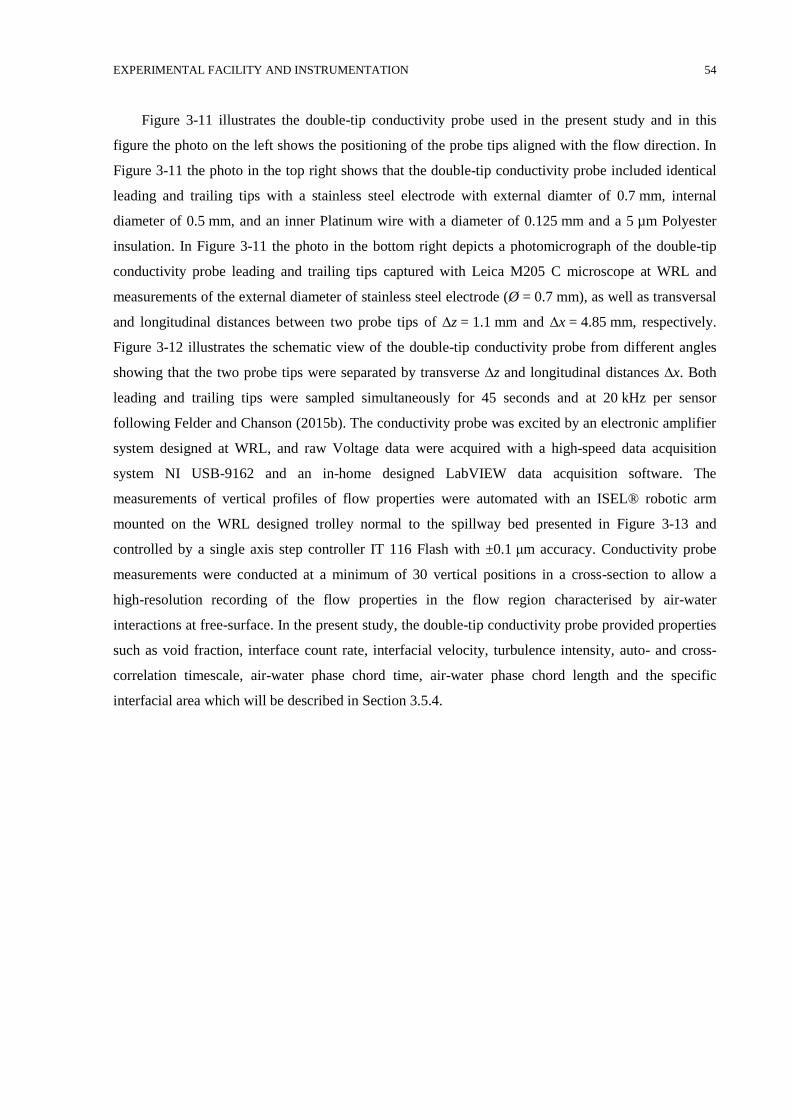
EXPERIMENTAL FACILITY AND INSTRUMENTATION 54
Figure 3-11 illustrates the double-tip conductivity probe used in the present study and in this
figure the photo on the left shows the positioning of the probe tips aligned with the flow direction. In
Figure 3-11 the photo in the top right shows that the double-tip conductivity probe included identical
leading and trailing tips with a stainless steel electrode with external diamter of 0.7 mm, internal
diameter of 0.5 mm, and an inner Platinum wire with a diameter of 0.125 mm and a 5 µm Polyester
insulation. In Figure 3-11 the photo in the bottom right depicts a photomicrograph of the double-tip
conductivity probe leading and trailing tips captured with Leica M205 C microscope at WRL and
measurements of the external diameter of stainless steel electrode (Ø = 0.7 mm), as well as transversal
and longitudinal distances between two probe tips of ∆z = 1.1 mm and ∆x = 4.85 mm, respectively.
Figure 3-12 illustrates the schematic view of the double-tip conductivity probe from different angles
showing that the two probe tips were separated by transverse ∆z and longitudinal distances ∆x. Both
leading and trailing tips were sampled simultaneously for 45 seconds and at 20 kHz per sensor
following Felder and Chanson (2015b). The conductivity probe was excited by an electronic amplifier
system designed at WRL, and raw Voltage data were acquired with a high-speed data acquisition
system NI USB-9162 and an in-home designed LabVIEW data acquisition software. The
measurements of vertical profiles of flow properties were automated with an ISEL® robotic arm
mounted on the WRL designed trolley normal to the spillway bed presented in Figure 3-13 and
controlled by a single axis step controller IT 116 Flash with ±0.1 μm accuracy. Conductivity probe
measurements were conducted at a minimum of 30 vertical positions in a cross-section to allow a
high-resolution recording of the flow properties in the flow region characterised by air-water
interactions at free-surface. In the present study, the double-tip conductivity probe provided properties
such as void fraction, interface count rate, interfacial velocity, turbulence intensity, auto- and cross-
correlation timescale, air-water phase chord time, air-water phase chord length and the specific
interfacial area which will be described in Section 3.5.4.
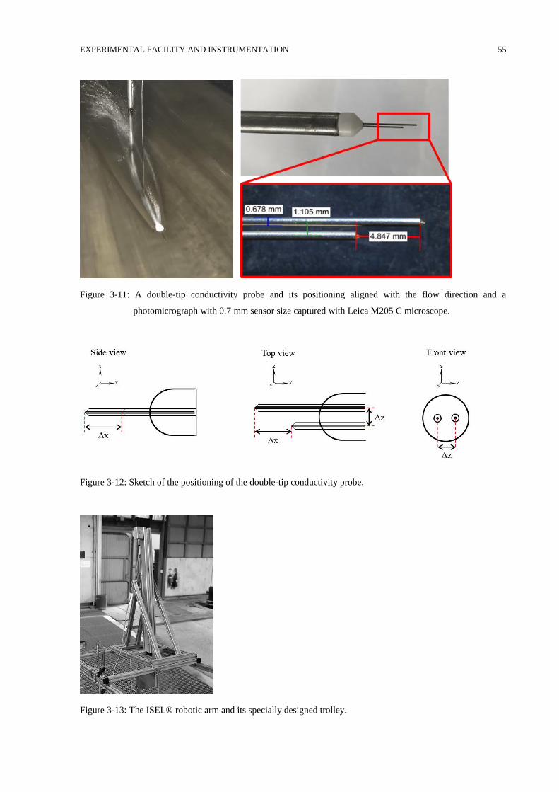
EXPERIMENTAL FACILITY AND INSTRUMENTATION 55
Figure 3-11: A double-tip conductivity probe and its positioning aligned with the flow direction and a
photomicrograph with 0.7 mm sensor size captured with Leica M205 C microscope.
Figure 3-12: Sketch of the positioning of the double-tip conductivity probe.
Figure 3-13: The ISEL® robotic arm and its specially designed trolley.
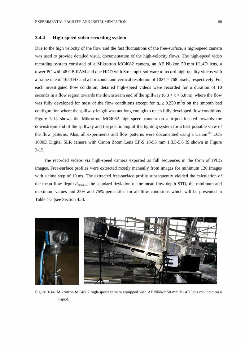
EXPERIMENTAL FACILITY AND INSTRUMENTATION 56
3.4.4 High-speed video recording system
Due to the high velocity of the flow and the fast fluctuations of the free-surface, a high-speed camera
was used to provide detailed visual documentation of the high-velocity flows. The high-speed video
recording system consisted of a Mikrotron MC4082 camera, an AF Nikkon 50 mm f/1.4D lens, a
tower PC with 48 GB RAM and one HDD with Streampix software to record high-quality videos with
a frame rate of 1054 Hz and a horizontal and vertical resolution of 1024 × 768 pixels, respectively. For
each investigated flow condition, detailed high-speed videos were recorded for a duration of 10
seconds in a flow region towards the downstream end of the spillway (6.3 ≤ x ≤ 6.8 m), where the flow
was fully developed for most of the flow conditions except for qw ≥ 0.250 m2/s on the smooth bed
configuration where the spillway length was not long enough to reach fully developed flow conditions.
Figure 3-14 shows the Mikrotron MC4082 high-speed camera on a tripod located towards the
downstream end of the spillway and the positioning of the lighting system for a best possible view of
the flow patterns. Also, all experiments and flow patterns were documented using a CanonTM
EOS
1000D Digital SLR camera with Canon Zoom Lenz EF-S 18-55 mm 1:3.5-5.6 IS shown in Figure
3-15.
The recorded videos via high-speed camera exported as full sequences in the form of JPEG
images. Free-surface profiles were extracted mostly manually from images for minimum 120 images
with a time step of 10 ms. The extracted free-surface profile subsequently yielded the calculation of
the mean flow depth dmean-C, the standard deviation of the mean flow depth STD, the minimum and
maximum values and 25% and 75% percentiles for all flow conditions which will be presented in
Table 4-3 (see Section 4.3).
Figure 3-14: Mikrotron MC4082 high-speed camera equipped with AF Nikkor 50 mm f/1.4D lens mounted on a
tripod.
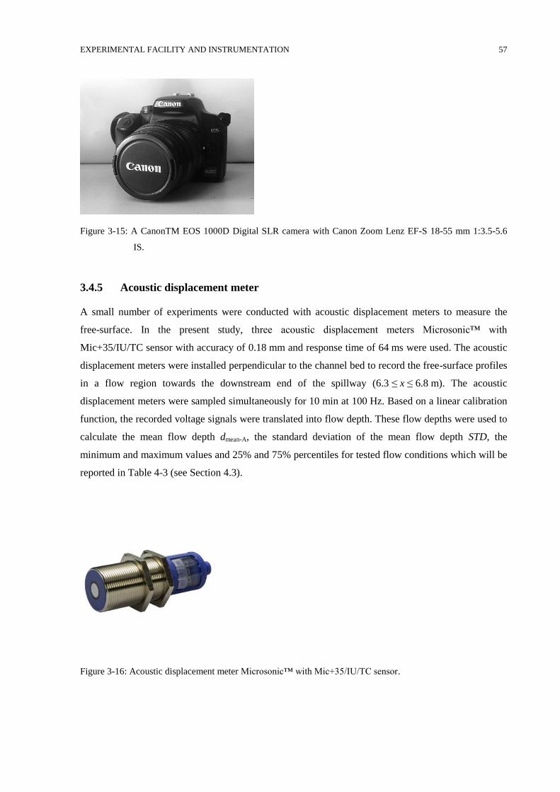
EXPERIMENTAL FACILITY AND INSTRUMENTATION 57
Figure 3-15: A CanonTM EOS 1000D Digital SLR camera with Canon Zoom Lenz EF-S 18-55 mm 1:3.5-5.6
IS.
3.4.5 Acoustic displacement meter
A small number of experiments were conducted with acoustic displacement meters to measure the
free-surface. In the present study, three acoustic displacement meters Microsonic™ with
Mic+35/IU/TC sensor with accuracy of 0.18 mm and response time of 64 ms were used. The acoustic
displacement meters were installed perpendicular to the channel bed to record the free-surface profiles
in a flow region towards the downstream end of the spillway (6.3 ≤ x ≤ 6.8 m). The acoustic
displacement meters were sampled simultaneously for 10 min at 100 Hz. Based on a linear calibration
function, the recorded voltage signals were translated into flow depth. These flow depths were used to
calculate the mean flow depth dmean-A, the standard deviation of the mean flow depth STD, the
minimum and maximum values and 25% and 75% percentiles for tested flow conditions which will be
reported in Table 4-3 (see Section 4.3).
Figure 3-16: Acoustic displacement meter Microsonic™ with Mic+35/IU/TC sensor.
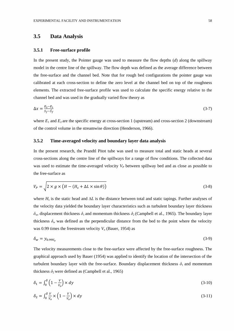
EXPERIMENTAL FACILITY AND INSTRUMENTATION 58
Data Analysis 3.5
3.5.1 Free-surface profile
In the present study, the Pointer gauge was used to measure the flow depths (d) along the spillway
model in the centre line of the spillway. The flow depth was defined as the average difference between
the free-surface and the channel bed. Note that for rough bed configurations the pointer gauge was
calibrated at each cross-section to define the zero level at the channel bed on top of the roughness
elements. The extracted free-surface profile was used to calculate the specific energy relative to the
channel bed and was used in the gradually varied flow theory as
∆𝑥 =𝐸2−𝐸1
𝑆𝑓−�̅�𝑓 (3-7)
where E1 and E2 are the specific energy at cross-section 1 (upstream) and cross-section 2 (downstream)
of the control volume in the streamwise direction (Henderson, 1966).
3.5.2 Time-averaged velocity and boundary layer data analysis
In the present research, the Prandtl Pitot tube was used to measure total and static heads at several
cross-sections along the centre line of the spillways for a range of flow conditions. The collected data
was used to estimate the time-averaged velocity VP between spillway bed and as close as possible to
the free-surface as
𝑉𝑃 = √2 × 𝑔 × (𝐻 − (𝐻𝑠 + ∆𝐿 × sin 𝜃)) (3-8)
where Hs is the static head and ∆L is the distance between total and static tapings. Further analyses of
the velocity data yielded the boundary layer characteristics such as turbulent boundary layer thickness
δw, displacement thickness δ1 and momentum thickness δ2 (Campbell et al., 1965). The boundary layer
thickness δw was defined as the perpendicular distance from the bed to the point where the velocity
was 0.99 times the freestream velocity Vo (Bauer, 1954) as
𝛿𝑤 = 𝑦0.99𝑉𝑜 (3-9)
The velocity measurements close to the free-surface were affected by the free-surface roughness. The
graphical approach used by Bauer (1954) was applied to identify the location of the intersection of the
turbulent boundary layer with the free-surface. Boundary displacement thickness δ1 and momentum
thickness δ2 were defined as (Campbell et al., 1965)
𝛿1 = ∫ (1 −𝑉
𝑉𝑜) × 𝑑𝑦
𝛿
0 (3-10)
𝛿2 = ∫𝑉
𝑉𝑜× (1 −
𝑉
𝑉𝑜) × 𝑑𝑦
𝛿
0 (3-11)
EXPERIMENTAL FACILITY AND INSTRUMENTATION 59
These values were used for further analysis of turbulent boundary layer characteristics including the
boundary shear stress and friction factor.
3.5.3 Calculation of boundary shear stress and friction factor
Shear stress is a parameter to define flow resistance. In the present study, boundary shear stress was
calculated by applying various methods and data sets collected using different instruments. These
boundary shear stress calculation approaches include the logarithmic law within the inner flow region,
the velocity defect law in the outer flow region, the momentum integral method which in these three
methods Prandtl-pitot tube data were used, as well as shear stress based on gradually varied flow
theory using two sets of data comprising the flow depth d measurements conducted by pointer gauge
and the equivalent clear flow depth de estimated through the double-tip conductivity probe records. In
the first three methods, boundary layer properties presented in Section 3.5.2 were used to estimate the
boundary shear stress which will be addressed in Sections 3.5.3.1, 3.5.3.2 and 3.5.3.3 and boundary
shear stress based on gradually varied flow theory will be presented in Section 3.5.3.4.
3.5.3.1 The logarithmic law within the inner flow region
In open channel flow, the boundary layer comprises two self-similar regions defined as the inner flow
region with the domination of viscous forces for y/δw < 0.15 to 0.2 and outer flow region dominated by
inertial forces (Rouse, 1965). The flow in the inner region follows the logarithmic law (Schlichting,
1960) defined as
𝑉
𝑉∗=
1
𝜅× ln (
𝑉∗×𝑦
𝜈) + 𝐴 − ∆𝑉+ (3-12)
Where 𝑉∗ = √𝜏0 𝜌⁄ is a kinematic shear measure usually called shear velocity, μ is the dynamic
viscosity of the fluid, V is the velocity in the x direction, κ is the Von Karman constant and A is
integration constant. Auel (2014) pointed out that several researches verified Von-Karman constant of
κ = 0.41±5% for steady, fully developed closed and open channel flows over smooth and rough beds
regardless of the Froude and Reynolds numbers. For smooth boundary layers, Schlichting (1979)
reported A = 5.5, Nezu and Rodi (1986) presented A = 5.29 while Liggett (1994) and Montes (1998)
recommended A = 5.0. For the rough bed configurations, the log-law velocity distributions were
shifted downward by the roughness function ΔV+ (Hama, 1954). Following the approach used by
Schlichting (1960) who applied Nikuradse’s equivalent sand roughness height ks instead of the
roughness shift ∆V+, the log-law follows
𝑉
𝑉∗=
1
𝜅× ln (
𝑦
𝑘𝑠) + 𝐵 (3-13)
where B is an integral constant. For a fully rough bed configurations, Nikuradse (1933) reported
B = 8.49 and Chanson (2009) presented B = 8.5. The measured velocity data were fitted to equation
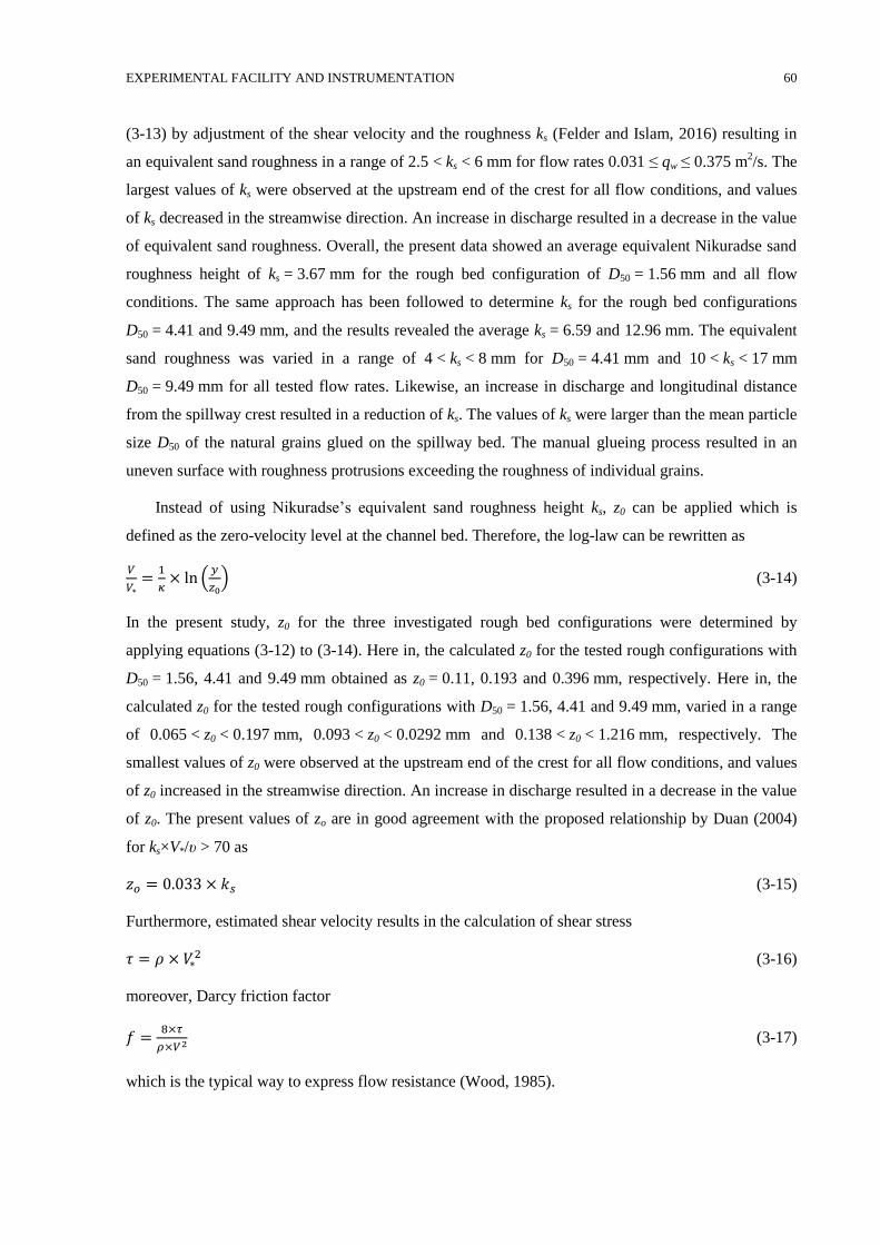
EXPERIMENTAL FACILITY AND INSTRUMENTATION 60
(3-13) by adjustment of the shear velocity and the roughness ks (Felder and Islam, 2016) resulting in
an equivalent sand roughness in a range of 2.5 < ks < 6 mm for flow rates 0.031 ≤ qw ≤ 0.375 m2/s. The
largest values of ks were observed at the upstream end of the crest for all flow conditions, and values
of ks decreased in the streamwise direction. An increase in discharge resulted in a decrease in the value
of equivalent sand roughness. Overall, the present data showed an average equivalent Nikuradse sand
roughness height of ks = 3.67 mm for the rough bed configuration of D50 = 1.56 mm and all flow
conditions. The same approach has been followed to determine ks for the rough bed configurations
D50 = 4.41 and 9.49 mm, and the results revealed the average ks = 6.59 and 12.96 mm. The equivalent
sand roughness was varied in a range of 4 < ks < 8 mm for D50 = 4.41 mm and 10 < ks < 17 mm
D50 = 9.49 mm for all tested flow rates. Likewise, an increase in discharge and longitudinal distance
from the spillway crest resulted in a reduction of ks. The values of ks were larger than the mean particle
size D50 of the natural grains glued on the spillway bed. The manual glueing process resulted in an
uneven surface with roughness protrusions exceeding the roughness of individual grains.
Instead of using Nikuradse’s equivalent sand roughness height ks, z0 can be applied which is
defined as the zero-velocity level at the channel bed. Therefore, the log-law can be rewritten as
𝑉
𝑉∗=
1
𝜅× ln (
𝑦
𝑧0) (3-14)
In the present study, z0 for the three investigated rough bed configurations were determined by
applying equations (3-12) to (3-14). Here in, the calculated z0 for the tested rough configurations with
D50 = 1.56, 4.41 and 9.49 mm obtained as z0 = 0.11, 0.193 and 0.396 mm, respectively. Here in, the
calculated z0 for the tested rough configurations with D50 = 1.56, 4.41 and 9.49 mm, varied in a range
of 0.065 < z0 < 0.197 mm, 0.093 < z0 < 0.0292 mm and 0.138 < z0 < 1.216 mm, respectively. The
smallest values of z0 were observed at the upstream end of the crest for all flow conditions, and values
of z0 increased in the streamwise direction. An increase in discharge resulted in a decrease in the value
of z0. The present values of zo are in good agreement with the proposed relationship by Duan (2004)
for ks×V*/υ > 70 as
𝑧𝑜 = 0.033 × 𝑘𝑠 (3-15)
Furthermore, estimated shear velocity results in the calculation of shear stress
𝜏 = 𝜌 × 𝑉∗2 (3-16)
moreover, Darcy friction factor
𝑓 =8×𝜏
𝜌×𝑉2 (3-17)
which is the typical way to express flow resistance (Wood, 1985).
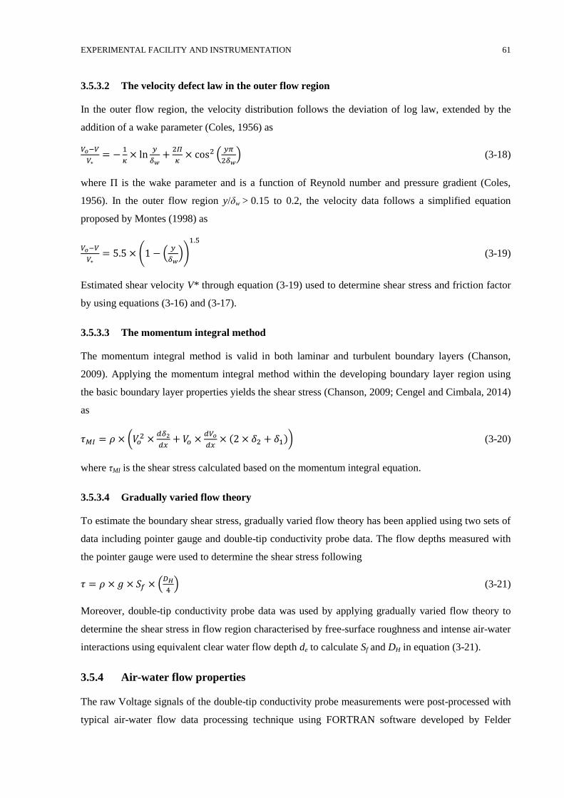
EXPERIMENTAL FACILITY AND INSTRUMENTATION 61
3.5.3.2 The velocity defect law in the outer flow region
In the outer flow region, the velocity distribution follows the deviation of log law, extended by the
addition of a wake parameter (Coles, 1956) as
𝑉𝑜−𝑉
𝑉∗= −
1
𝜅× ln
𝑦
𝛿𝑤+
2𝛱
𝜅× cos2 (
𝑦𝜋
2𝛿𝑤) (3-18)
where Π is the wake parameter and is a function of Reynold number and pressure gradient (Coles,
1956). In the outer flow region y/δw > 0.15 to 0.2, the velocity data follows a simplified equation
proposed by Montes (1998) as
𝑉𝑜−𝑉
𝑉∗= 5.5 × (1 − (
𝑦
𝛿𝑤))
1.5
(3-19)
Estimated shear velocity V* through equation (3-19) used to determine shear stress and friction factor
by using equations (3-16) and (3-17).
3.5.3.3 The momentum integral method
The momentum integral method is valid in both laminar and turbulent boundary layers (Chanson,
2009). Applying the momentum integral method within the developing boundary layer region using
the basic boundary layer properties yields the shear stress (Chanson, 2009; Cengel and Cimbala, 2014)
as
𝜏𝑀𝐼 = 𝜌 × (𝑉𝑜2 ×
𝑑𝛿2
𝑑𝑥+ 𝑉𝑜 ×
𝑑𝑉𝑜
𝑑𝑥× (2 × 𝛿2 + 𝛿1)) (3-20)
where τMI is the shear stress calculated based on the momentum integral equation.
3.5.3.4 Gradually varied flow theory
To estimate the boundary shear stress, gradually varied flow theory has been applied using two sets of
data including pointer gauge and double-tip conductivity probe data. The flow depths measured with
the pointer gauge were used to determine the shear stress following
𝜏 = 𝜌 × 𝑔 × 𝑆𝑓 × (𝐷𝐻
4) (3-21)
Moreover, double-tip conductivity probe data was used by applying gradually varied flow theory to
determine the shear stress in flow region characterised by free-surface roughness and intense air-water
interactions using equivalent clear water flow depth de to calculate Sf and DH in equation (3-21).
3.5.4 Air-water flow properties
The raw Voltage signals of the double-tip conductivity probe measurements were post-processed with
typical air-water flow data processing technique using FORTRAN software developed by Felder
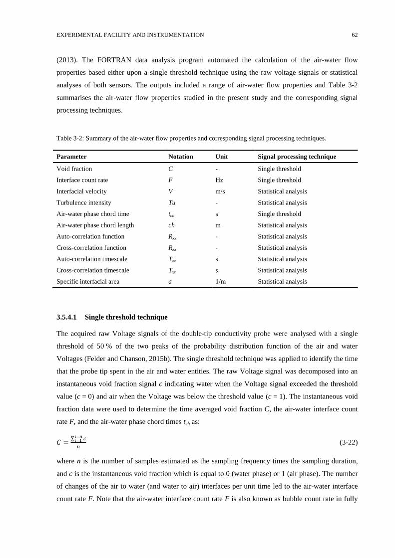
EXPERIMENTAL FACILITY AND INSTRUMENTATION 62
(2013). The FORTRAN data analysis program automated the calculation of the air-water flow
properties based either upon a single threshold technique using the raw voltage signals or statistical
analyses of both sensors. The outputs included a range of air-water flow properties and Table 3-2
summarises the air-water flow properties studied in the present study and the corresponding signal
processing techniques.
Table 3-2: Summary of the air-water flow properties and corresponding signal processing techniques.
Parameter Notation Unit Signal processing technique
Void fraction C - Single threshold
Interface count rate F Hz Single threshold
Interfacial velocity V m/s Statistical analysis
Turbulence intensity Tu - Statistical analysis
Air-water phase chord time tch s Single threshold
Air-water phase chord length ch m Statistical analysis
Auto-correlation function Rxx - Statistical analysis
Cross-correlation function Rxz - Statistical analysis
Auto-correlation timescale Txx s Statistical analysis
Cross-correlation timescale Txz s Statistical analysis
Specific interfacial area a 1/m Statistical analysis
3.5.4.1 Single threshold technique
The acquired raw Voltage signals of the double-tip conductivity probe were analysed with a single
threshold of 50 % of the two peaks of the probability distribution function of the air and water
Voltages (Felder and Chanson, 2015b). The single threshold technique was applied to identify the time
that the probe tip spent in the air and water entities. The raw Voltage signal was decomposed into an
instantaneous void fraction signal c indicating water when the Voltage signal exceeded the threshold
value (c = 0) and air when the Voltage was below the threshold value (c = 1). The instantaneous void
fraction data were used to determine the time averaged void fraction C, the air-water interface count
rate F, and the air-water phase chord times tch as:
𝐶 =∑ 𝑐𝑖=𝑛
𝑖=1
𝑛 (3-22)
where n is the number of samples estimated as the sampling frequency times the sampling duration,
and c is the instantaneous void fraction which is equal to 0 (water phase) or 1 (air phase). The number
of changes of the air to water (and water to air) interfaces per unit time led to the air-water interface
count rate F. Note that the air-water interface count rate F is also known as bubble count rate in fully
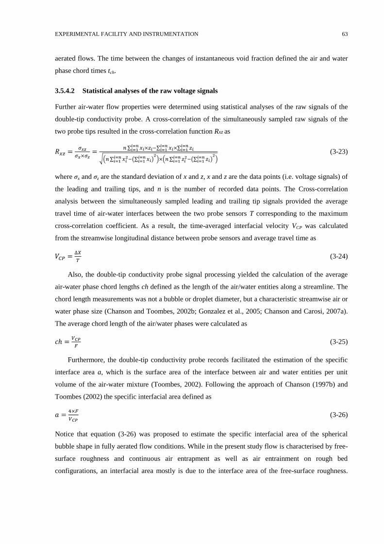
EXPERIMENTAL FACILITY AND INSTRUMENTATION 63
aerated flows. The time between the changes of instantaneous void fraction defined the air and water
phase chord times tch.
3.5.4.2 Statistical analyses of the raw voltage signals
Further air-water flow properties were determined using statistical analyses of the raw signals of the
double-tip conductivity probe. A cross-correlation of the simultaneously sampled raw signals of the
two probe tips resulted in the cross-correlation function Rxz as
𝑅𝑥𝑧 =𝜎𝑥𝑧
𝜎𝑥×𝜎𝑧=
𝑛 ∑ 𝑥𝑖×𝑧𝑖𝑖=𝑛𝑖=1 −∑ 𝑥𝑖
𝑖=𝑛𝑖=1 ×∑ 𝑧𝑖
𝑖=𝑛𝑖=1
√(𝑛 ∑ 𝑥𝑖2𝑖=𝑛
𝑖=1 −(∑ 𝑥𝑖𝑖=𝑛𝑖=1 )
2)×(𝑛 ∑ 𝑧𝑖
2𝑖=𝑛𝑖=1 −(∑ 𝑧𝑖
𝑖=𝑛𝑖=1 )
2)
(3-23)
where σx and σz are the standard deviation of x and z, x and z are the data points (i.e. voltage signals) of
the leading and trailing tips, and n is the number of recorded data points. The Cross-correlation
analysis between the simultaneously sampled leading and trailing tip signals provided the average
travel time of air-water interfaces between the two probe sensors T corresponding to the maximum
cross-correlation coefficient. As a result, the time-averaged interfacial velocity VCP was calculated
from the streamwise longitudinal distance between probe sensors and average travel time as
𝑉𝐶𝑃 =∆𝑋
𝑇 (3-24)
Also, the double-tip conductivity probe signal processing yielded the calculation of the average
air-water phase chord lengths ch defined as the length of the air/water entities along a streamline. The
chord length measurements was not a bubble or droplet diameter, but a characteristic streamwise air or
water phase size (Chanson and Toombes, 2002b; Gonzalez et al., 2005; Chanson and Carosi, 2007a).
The average chord length of the air/water phases were calculated as
𝑐ℎ =𝑉𝐶𝑃
𝐹 (3-25)
Furthermore, the double-tip conductivity probe records facilitated the estimation of the specific
interface area a, which is the surface area of the interface between air and water entities per unit
volume of the air-water mixture (Toombes, 2002). Following the approach of Chanson (1997b) and
Toombes (2002) the specific interfacial area defined as
𝑎 =4×𝐹
𝑉𝐶𝑃 (3-26)
Notice that equation (3-26) was proposed to estimate the specific interfacial area of the spherical
bubble shape in fully aerated flow conditions. While in the present study flow is characterised by free-
surface roughness and continuous air entrapment as well as air entrainment on rough bed
configurations, an interfacial area mostly is due to the interface area of the free-surface roughness.
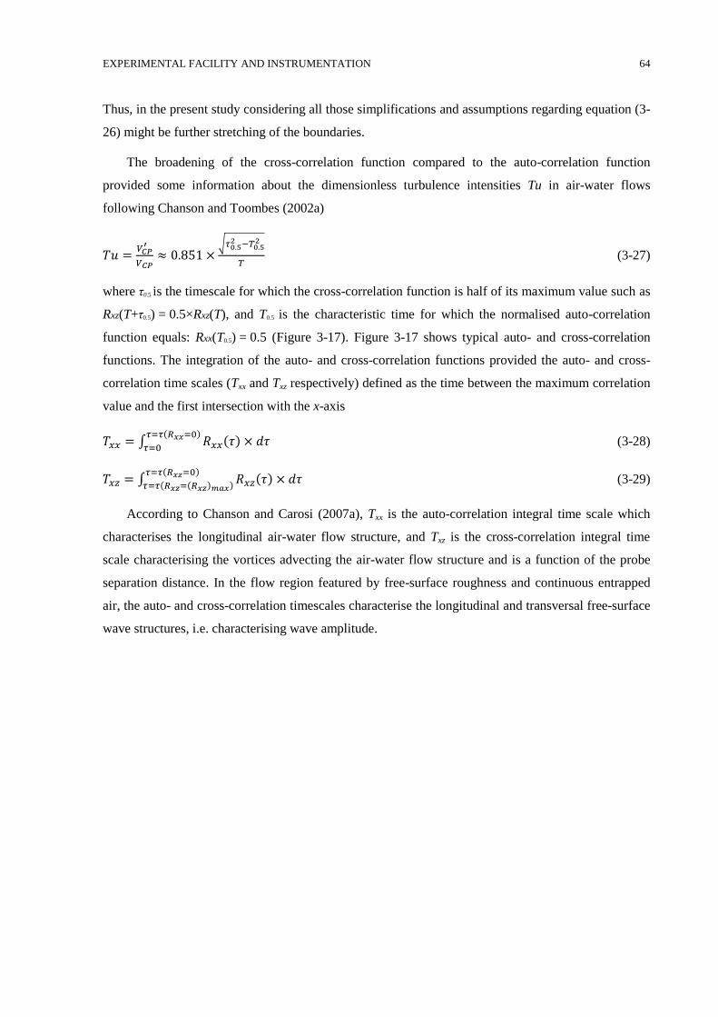
EXPERIMENTAL FACILITY AND INSTRUMENTATION 64
Thus, in the present study considering all those simplifications and assumptions regarding equation (3-
26) might be further stretching of the boundaries.
The broadening of the cross-correlation function compared to the auto-correlation function
provided some information about the dimensionless turbulence intensities Tu in air-water flows
following Chanson and Toombes (2002a)
𝑇𝑢 =𝑉𝐶𝑃
′
𝑉𝐶𝑃≈ 0.851 ×
√𝜏0.52 −𝑇0.5
2
𝑇 (3-27)
where τ0.5 is the timescale for which the cross-correlation function is half of its maximum value such as
Rxz(T+τ0.5) = 0.5×Rxz(T), and T0.5 is the characteristic time for which the normalised auto-correlation
function equals: Rxx(T0.5) = 0.5 (Figure 3-17). Figure 3-17 shows typical auto- and cross-correlation
functions. The integration of the auto- and cross-correlation functions provided the auto- and cross-
correlation time scales (Txx and Txz respectively) defined as the time between the maximum correlation
value and the first intersection with the x-axis
𝑇𝑥𝑥 = ∫ 𝑅𝑥𝑥(𝜏) × 𝑑𝜏𝜏=𝜏(𝑅𝑥𝑥=0)
𝜏=0 (3-28)
𝑇𝑥𝑧 = ∫ 𝑅𝑥𝑧(𝜏) × 𝑑𝜏𝜏=𝜏(𝑅𝑥𝑧=0)
𝜏=𝜏(𝑅𝑥𝑧=(𝑅𝑥𝑧)𝑚𝑎𝑥) (3-29)
According to Chanson and Carosi (2007a), Txx is the auto-correlation integral time scale which
characterises the longitudinal air-water flow structure, and Txz is the cross-correlation integral time
scale characterising the vortices advecting the air-water flow structure and is a function of the probe
separation distance. In the flow region featured by free-surface roughness and continuous entrapped
air, the auto- and cross-correlation timescales characterise the longitudinal and transversal free-surface
wave structures, i.e. characterising wave amplitude.
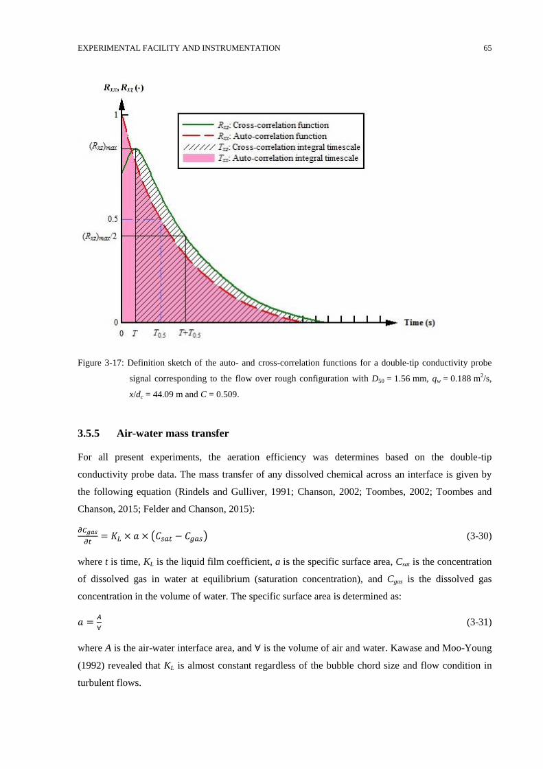
EXPERIMENTAL FACILITY AND INSTRUMENTATION 65
Figure 3-17: Definition sketch of the auto- and cross-correlation functions for a double-tip conductivity probe
signal corresponding to the flow over rough configuration with D50 = 1.56 mm, qw = 0.188 m2/s,
x/dc = 44.09 m and C = 0.509.
3.5.5 Air-water mass transfer
For all present experiments, the aeration efficiency was determines based on the double-tip
conductivity probe data. The mass transfer of any dissolved chemical across an interface is given by
the following equation (Rindels and Gulliver, 1991; Chanson, 2002; Toombes, 2002; Toombes and
Chanson, 2015; Felder and Chanson, 2015):
𝜕𝐶𝑔𝑎𝑠
𝜕𝑡= 𝐾𝐿 × 𝑎 × (𝐶𝑠𝑎𝑡 − 𝐶𝑔𝑎𝑠) (3-30)
where t is time, KL is the liquid film coefficient, a is the specific surface area, Csat is the concentration
of dissolved gas in water at equilibrium (saturation concentration), and Cgas is the dissolved gas
concentration in the volume of water. The specific surface area is determined as:
𝑎 =𝐴
∀ (3-31)
where A is the air-water interface area, and ∀ is the volume of air and water. Kawase and Moo-Young
(1992) revealed that KL is almost constant regardless of the bubble chord size and flow condition in
turbulent flows.
EXPERIMENTAL FACILITY AND INSTRUMENTATION 66
𝐾𝐿 = 0.47 × √𝑔3 × √𝐷𝑔𝑎𝑠 × 𝜈𝑤−1 6⁄
(3-32)
where Dgas is the molecular diffusivity of oxygen calculated for 20°C. Molecular diffusivity for
oxygen is calculated as (Felder and Chanson, 2014):
𝐷𝑔𝑎𝑠 = 1.16793 × 10⁻²⁷ × (𝑇 + 273)7.3892 (3-33)
Equation (3-30) was rewritten by Toombes and Chanson (2005) as follows:
𝑑𝐶𝑔𝑎𝑠
𝑑𝑡= 𝐾𝐿 × 𝑈𝑤 × 𝑎𝑚𝑒𝑎𝑛 × (𝐶𝑠𝑎𝑡 − 𝐶𝑔𝑎𝑠) (3-34)
where amean is cross-section average specific interface area; and Uw is average velocity defined as:
𝑎𝑚𝑒𝑎𝑛 =1
𝑌98× ∫ 𝑎 × 𝑑𝑦
𝑌98
0 (3-35)
𝑈𝑤 =𝑞𝑤
𝑑𝑌98
(3-36)
The aeration potential of the structure may be defined regarding the re-oxygenation rate as
𝑟 =𝐶𝑠𝑎𝑡−𝐶𝑢𝑠
𝐶𝑠𝑎𝑡−𝐶𝑑𝑠 (3-37)
where Csat is the saturation dissolved gas concentration, and Cus and Cds are the upstream and
downstream dissolved gas concentrations, respectively. Furthermore, the aeration efficiency, E can be
calculated as:
𝐸 =𝐶𝑑𝑠−𝐶𝑢𝑠
𝐶𝑠𝑎𝑡−𝐶𝑢𝑠= 1 −
1
𝑟 (3-38)
The results of the aeration efficiency of present study according to the assumptions above will be
presented in Section 7.4.
Experimental program 3.6
In the present study, large numbers of experiments were conducted in a WRL’s large-scale
recirculation spillway facility to investigate the effects of micro-roughness on design aspects of re-
aeration, air-water mass transfer, energy dissipation rate and residual energy. Furthermore, an
optimum and a novel spillways design was provided by considering the energy dissipation rate,
residual energy and air-water mass transfer processes. The present experiments were carried out for a
range of flow conditions summarised in Table 3-3. Table 3-4 reported the experimental plan carried
out in present study such as information of using various instrumentations on investigated discharges.
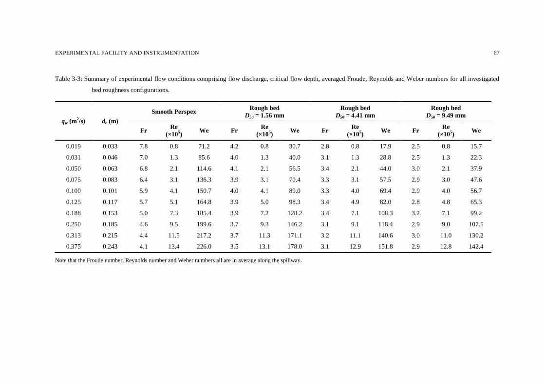
EXPERIMENTAL FACILITY AND INSTRUMENTATION 67
Table 3-3: Summary of experimental flow conditions comprising flow discharge, critical flow depth, averaged Froude, Reynolds and Weber numbers for all investigated
bed roughness configurations.
qw (m2/s) dc (m)
Smooth Perspex Rough bed
D50 = 1.56 mm
Rough bed
D50 = 4.41 mm
Rough bed
D50 = 9.49 mm
Fr Re
(×105)
We Fr Re
(×105)
We Fr Re
(×105)
We Fr Re
(×105)
We
0.019 0.033 7.8 0.8 71.2 4.2 0.8 30.7 2.8 0.8 17.9 2.5 0.8 15.7
0.031 0.046 7.0 1.3 85.6 4.0 1.3 40.0 3.1 1.3 28.8 2.5 1.3 22.3
0.050 0.063 6.8 2.1 114.6 4.1 2.1 56.5 3.4 2.1 44.0 3.0 2.1 37.9
0.075 0.083 6.4 3.1 136.3 3.9 3.1 70.4 3.3 3.1 57.5 2.9 3.0 47.6
0.100 0.101 5.9 4.1 150.7 4.0 4.1 89.0 3.3 4.0 69.4 2.9 4.0 56.7
0.125 0.117 5.7 5.1 164.8 3.9 5.0 98.3 3.4 4.9 82.0 2.8 4.8 65.3
0.188 0.153 5.0 7.3 185.4 3.9 7.2 128.2 3.4 7.1 108.3 3.2 7.1 99.2
0.250 0.185 4.6 9.5 199.6 3.7 9.3 146.2 3.1 9.1 118.4 2.9 9.0 107.5
0.313 0.215 4.4 11.5 217.2 3.7 11.3 171.1 3.2 11.1 140.6 3.0 11.0 130.2
0.375 0.243 4.1 13.4 226.0 3.5 13.1 178.0 3.1 12.9 151.8 2.9 12.8 142.4
Note that the Froude number, Reynolds number and Weber numbers all are in average along the spillway.
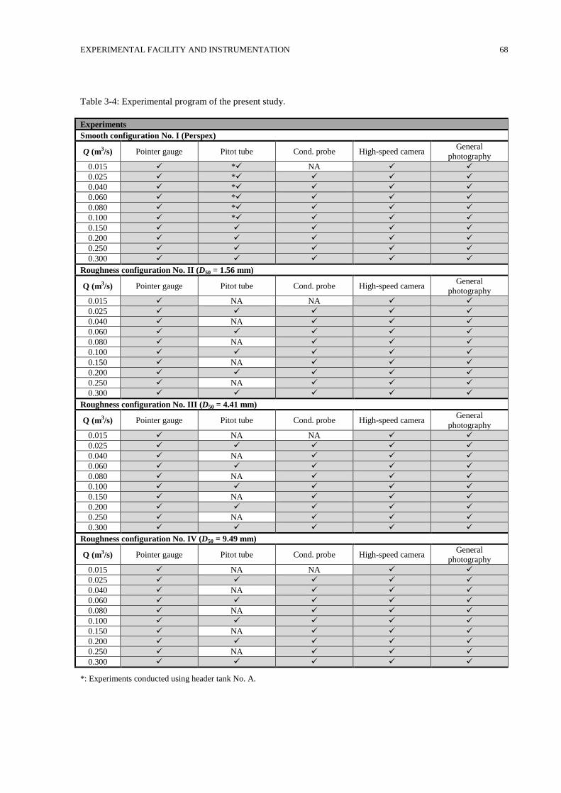
EXPERIMENTAL FACILITY AND INSTRUMENTATION 68
Table 3-4: Experimental program of the present study.
Experiments
Smooth configuration No. I (Perspex)
Q (m3/s) Pointer gauge Pitot tube Cond. probe High-speed camera General
photography
0.015 * NA
0.025 *
0.040 *
0.060 *
0.080 *
0.100 *
0.150
0.200
0.250
0.300
Roughness configuration No. II (D50 = 1.56 mm)
Q (m3/s) Pointer gauge Pitot tube Cond. probe High-speed camera General
photography
0.015 NA NA
0.025
0.040 NA
0.060
0.080 NA
0.100
0.150 NA
0.200
0.250 NA
0.300
Roughness configuration No. III (D50 = 4.41 mm)
Q (m3/s) Pointer gauge Pitot tube Cond. probe High-speed camera General
photography
0.015 NA NA
0.025
0.040 NA
0.060
0.080 NA
0.100
0.150 NA
0.200
0.250 NA
0.300
Roughness configuration No. IV (D50 = 9.49 mm)
Q (m3/s) Pointer gauge Pitot tube Cond. probe High-speed camera General
photography
0.015 NA NA
0.025
0.040 NA
0.060
0.080 NA
0.100
0.150 NA
0.200
0.250 NA
0.300
*: Experiments conducted using header tank No. A.
Chapter 4
4 FREE-SURFACE PATTERNS IN HIGH-VELOCITY
FLOWS ON THE SPILLWAY WITH MICRO-
ROUGHNESS
The present chapter reports the results of the detailed experimental investigations conducted to
describe qualitatively and quantitatively the characteristics of the high-velocity flows on the
moderately sloped spillway with uncontrolled intake condition for the four tested bed micro-roughness
configurations. The performances and flow patterns for the bed roughness configurations are discussed
and compared including the onset of the free-surface roughness, the patterns of the free-surface air
entrainment, as well as the free-surface profiles along the spillway.
Observation of flow patterns 4.1
Detailed visual observations were conducted for all tested flow conditions (0.019 ≤ qw ≤ 0.375 m2/s).
For all spillway bed configurations, at the upstream end of the spillway, the flows were calm and
steady over the broad-crested weir and water transitioned through critical flow depth over the crest.
Flow accelerated in streamwise direction, and the flow depth decreased gradually approaching
uniform condition in terms of the flow depth towards the downstream end of the spillway for the listed
flow conditions in Table 4-1. Table 4-1 summarises the basic flow features for the cases where
uniform flows were achieved including the longitudinal distance from the spillway crest to the point
where the flow reached constant depth LUniform, the dimensionless distance along the spillway LUniform/dc
the corresponding uniform flow depth dUniform, as well as Froude number and Reynolds numbers for the
uniform conditions. LUniform have been estimated using flow depth data measured by pointer gauge and
applying the gradually varied flow theory along the spillway up to the point where flow depth reached
a constant value which considered as a uniform condition. Note that, in Table 4-1, “NA” presented
flow conditions with insufficient length of the spillway to allow uniform flow depth along the
spillway. Table 4-1 highlights that for a specific roughness flow reached uniform condition while for
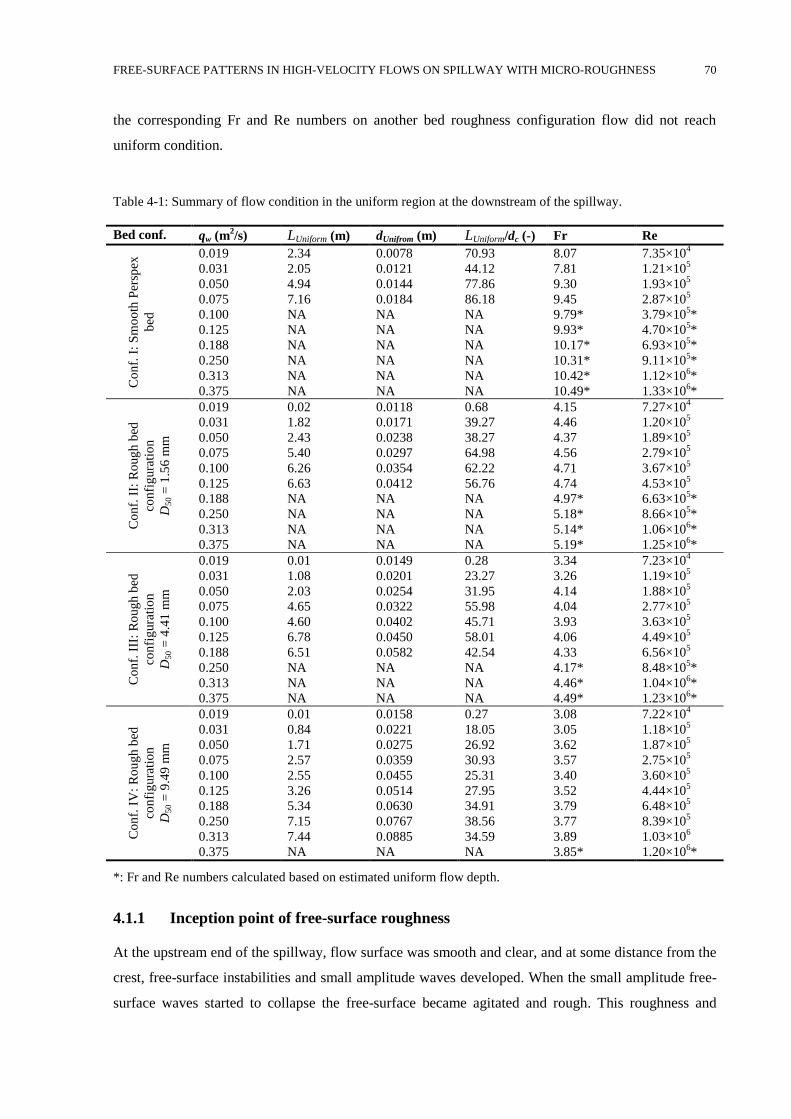
FREE-SURFACE PATTERNS IN HIGH-VELOCITY FLOWS ON SPILLWAY WITH MICRO-ROUGHNESS 70
the corresponding Fr and Re numbers on another bed roughness configuration flow did not reach
uniform condition.
Table 4-1: Summary of flow condition in the uniform region at the downstream of the spillway.
Bed conf. qw (m2/s) LUniform (m) dUnifrom (m) LUniform/dc (-) Fr Re
Co
nf.
I:
Sm
oo
th P
ersp
ex
bed
0.019 2.34 0.0078 70.93 8.07 7.35×10⁴
0.031 2.05 0.0121 44.12 7.81 1.21×10⁵
0.050 4.94 0.0144 77.86 9.30 1.93×10⁵
0.075 7.16 0.0184 86.18 9.45 2.87×10⁵
0.100 NA NA NA 9.79* 3.79×105*
0.125 NA NA NA 9.93* 4.70×105*
0.188 NA NA NA 10.17* 6.93×105*
0.250 NA NA NA 10.31* 9.11×105*
0.313 NA NA NA 10.42* 1.12×106*
0.375 NA NA NA 10.49* 1.33×106*
Co
nf.
II:
Ro
ug
h b
ed
con
fig
ura
tio
n
D50 =
1.5
6 m
m
0.019 0.02 0.0118 0.68 4.15 7.27×10⁴
0.031 1.82 0.0171 39.27 4.46 1.20×10⁵
0.050 2.43 0.0238 38.27 4.37 1.89×10⁵
0.075 5.40 0.0297 64.98 4.56 2.79×10⁵
0.100 6.26 0.0354 62.22 4.71 3.67×10⁵
0.125 6.63 0.0412 56.76 4.74 4.53×10⁵
0.188 NA NA NA 4.97* 6.63×105*
0.250 NA NA NA 5.18* 8.66×105*
0.313 NA NA NA 5.14* 1.06×106*
0.375 NA NA NA 5.19* 1.25×106*
Co
nf.
III
: R
oug
h b
ed
con
fig
ura
tio
n
D50 =
4.4
1 m
m
0.019 0.01 0.0149 0.28 3.34 7.23×10⁴
0.031 1.08 0.0201 23.27 3.26 1.19×10⁵
0.050 2.03 0.0254 31.95 4.14 1.88×10⁵
0.075 4.65 0.0322 55.98 4.04 2.77×10⁵
0.100 4.60 0.0402 45.71 3.93 3.63×10⁵
0.125 6.78 0.0450 58.01 4.06 4.49×10⁵
0.188 6.51 0.0582 42.54 4.33 6.56×10⁵
0.250 NA NA NA 4.17* 8.48×105*
0.313 NA NA NA 4.46* 1.04×106*
0.375 NA NA NA 4.49* 1.23×106*
Co
nf.
IV
: R
ou
gh b
ed
con
fig
ura
tio
n
D5
0 =
9.4
9 m
m
0.019 0.01 0.0158 0.27 3.08 7.22×10⁴
0.031 0.84 0.0221 18.05 3.05 1.18×10⁵
0.050 1.71 0.0275 26.92 3.62 1.87×10⁵
0.075 2.57 0.0359 30.93 3.57 2.75×10⁵
0.100 2.55 0.0455 25.31 3.40 3.60×10⁵
0.125 3.26 0.0514 27.95 3.52 4.44×10⁵
0.188 5.34 0.0630 34.91 3.79 6.48×10⁵
0.250 7.15 0.0767 38.56 3.77 8.39×10⁵
0.313 7.44 0.0885 34.59 3.89 1.03×10⁶
0.375 NA NA NA 3.85* 1.20×106*
*: Fr and Re numbers calculated based on estimated uniform flow depth.
4.1.1 Inception point of free-surface roughness
At the upstream end of the spillway, flow surface was smooth and clear, and at some distance from the
crest, free-surface instabilities and small amplitude waves developed. When the small amplitude free-
surface waves started to collapse the free-surface became agitated and rough. This roughness and
FREE-SURFACE PATTERNS IN HIGH-VELOCITY FLOWS ON SPILLWAY WITH MICRO-ROUGHNESS 71
agitations developed very fast across the width of the flow and when these instabilities present in the
whole width of the spillway, this position considered as inception point of free-surface roughness. This
phenomenon was observed for all tested bed configurations. This observation is consistent with
observations of Anwar (1994) who reported “surface deformations” upstream of the inception point of
air entrainment over smooth invert spillway with a slope of θ = 11°. The distance from the spillway
crest to the inception point of free-surface roughness defined as LFR. Visual observations revealed that
downstream of the inception point of free-surface roughness, free-surface is continuously rough and
some air was entrapped between these roughnesses and transported along the spillway. The present
observations were consistent with the observation by Lai et al. (1968) who reported continuous free-
surface fluctuation over a smooth invert spillway with slopes of 18 and 24 degrees (Figure 4-2). Figure
4-1 illustrates details of the rough free-surface from top view for the four investigated spillway bed
roughness configurations highlighting the fragmentation of the flow and a change from a smooth and
clear water surface upstream of the inception point of free-surface roughness to a rough and wavy
free-surface downstream of LFR. In Figure 4-1, the red dashed line shows the cross-section considered
as inception point of free-surface roughness on each investigated spillway bed configurations where
free-surface roughness developed across the whole width of the channel. Table 4-2 summarises the
positions of LFR for all flow conditions highlighting that an increase in flow rates led to a downward
shift of the onset of free-surface roughness and more significant wave amplitude of free-surface
waves. For rough bed configurations, downstream of the inception point of free-surface roughness, the
air was continuously entrapped in the air-water interface as well as some air was transported in the
form of air bubbles within the flow.
Table 4-2 shows that increase in bed roughness yielded the upward shift of the inception point of
free-surface roughness for comparable flow conditions which is consistent with observations of Anwar
(1994) who reported that by decreasing the bed roughness, the appearance of free-surface
deformations shifted downstream. Figure 4-3 illustrates the free-surface roughness downstream of the
inception point of free-surface roughness for the present configurations indicating that an increase in
bed roughness led to more pronounced free-surface roughness and stronger air-water interactions at
the air-water interface. Visual observations of free-surface roughness over smooth and rough beds
depicted that increase in bed roughness yielded to more considerable free-surface wave amplitude
which is consistent with high-speed recorded videos and free-surface data analysis with larger
standard deviation values for rough beds which will be addressed in Table 4-3 in Section 4.3.
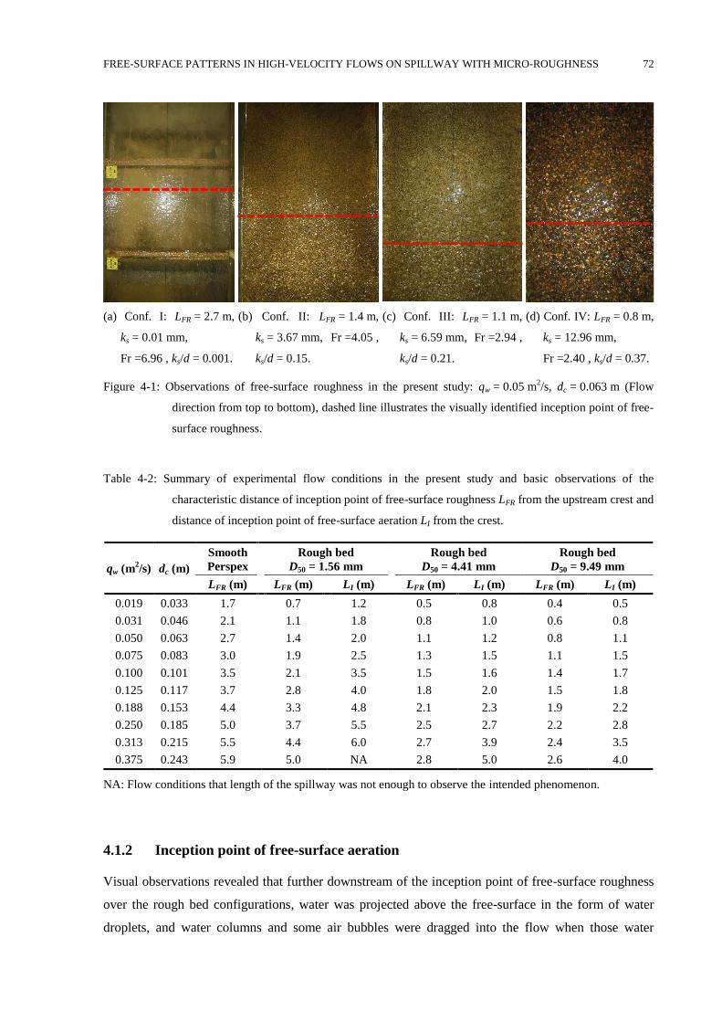
FREE-SURFACE PATTERNS IN HIGH-VELOCITY FLOWS ON SPILLWAY WITH MICRO-ROUGHNESS 72
(a) Conf. I: LFR = 2.7 m,
ks = 0.01 mm,
Fr =6.96 , ks/d = 0.001.
(b) Conf. II: LFR = 1.4 m,
ks = 3.67 mm, Fr =4.05 ,
ks/d = 0.15.
(c) Conf. III: LFR = 1.1 m,
ks = 6.59 mm, Fr =2.94 ,
ks/d = 0.21.
(d) Conf. IV: LFR = 0.8 m,
ks = 12.96 mm,
Fr =2.40 , ks/d = 0.37.
Figure 4-1: Observations of free-surface roughness in the present study: qw = 0.05 m2/s, dc = 0.063 m (Flow
direction from top to bottom), dashed line illustrates the visually identified inception point of free-
surface roughness.
Table 4-2: Summary of experimental flow conditions in the present study and basic observations of the
characteristic distance of inception point of free-surface roughness LFR from the upstream crest and
distance of inception point of free-surface aeration LI from the crest.
qw (m2/s) dc (m)
Smooth
Perspex
Rough bed
D50 = 1.56 mm
Rough bed
D50 = 4.41 mm
Rough bed
D50 = 9.49 mm
LFR (m) LFR (m) LI (m) LFR (m) LI (m) LFR (m) LI (m)
0.019 0.033 1.7 0.7 1.2 0.5 0.8 0.4 0.5
0.031 0.046 2.1 1.1 1.8 0.8 1.0 0.6 0.8
0.050 0.063 2.7 1.4 2.0 1.1 1.2 0.8 1.1
0.075 0.083 3.0 1.9 2.5 1.3 1.5 1.1 1.5
0.100 0.101 3.5 2.1 3.5 1.5 1.6 1.4 1.7
0.125 0.117 3.7 2.8 4.0 1.8 2.0 1.5 1.8
0.188 0.153 4.4 3.3 4.8 2.1 2.3 1.9 2.2
0.250 0.185 5.0 3.7 5.5 2.5 2.7 2.2 2.8
0.313 0.215 5.5 4.4 6.0 2.7 3.9 2.4 3.5
0.375 0.243 5.9 5.0 NA 2.8 5.0 2.6 4.0
NA: Flow conditions that length of the spillway was not enough to observe the intended phenomenon.
4.1.2 Inception point of free-surface aeration
Visual observations revealed that further downstream of the inception point of free-surface roughness
over the rough bed configurations, water was projected above the free-surface in the form of water
droplets, and water columns and some air bubbles were dragged into the flow when those water
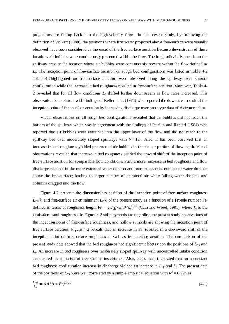
FREE-SURFACE PATTERNS IN HIGH-VELOCITY FLOWS ON SPILLWAY WITH MICRO-ROUGHNESS 73
projections are falling back into the high-velocity flows. In the present study, by following the
definition of Volkart (1980), the positions where first water projected above free-surface were visually
observed have been considered as the onset of the free-surface aeration because downstream of these
locations air bubbles were continuously presented within the flow. The longitudinal distance from the
spillway crest to the location where air bubbles were continuously present within the flow defined as
LI. The inception point of free-surface aeration on rough bed configurations was listed in Table 4-2
Table 4-2highlighted no free-surface aeration were observed along the spillway over smooth
configuration while the increase in bed roughness resulted in free-surface aeration. Moreover, Table 4-
2 revealed that for all flow conditions LI shifted further downstream as flow rates increased. This
observation is consistent with findings of Keller et al. (1974) who reported the downstream shift of the
inception point of free-surface aeration by increasing discharge over prototype data of Aviemore dam.
Visual observations on all rough bed configurations revealed that air bubbles did not reach the
bottom of the spillway which was in agreement with the findings of Petrillo and Ranieri (1984) who
reported that air bubbles were entrained into the upper layer of the flow and did not reach to the
spillway bed over moderately sloped spillways with θ = 12°. Also, it has been observed that an
increase in bed roughness yielded presence of air bubbles in the deeper portion of flow depth. Visual
observations revealed that increase in bed roughness yielded the upward shift of the inception point of
free-surface aeration for comparable flow conditions. Furthermore, increase in bed roughness and flow
discharge resulted in the more extended water column and more substantial number of water droplets
above the free-surface; leading to larger number of entrained air while falling water droplets and
columns dragged into the flow.
Figure 4-2 presents the dimensionless position of the inception point of free-surface roughness
LFR/ks and free-surface air entrainment LI/ks of the present study as a function of a Froude number Fr*
defined in terms of roughness height Fr* = qw/(g×sinθ×ks3)
0.5 (Cain and Wood, 1981), where ks is the
equivalent sand roughness. In Figure 4-2 solid symbols are regarding the present study observations of
the inception point of free-surface roughness, and hollow symbols are showing the inception point of
free-surface aeration. Figure 4-2 reveals that an increase in Fr* resulted in a downward shift of the
inception point of free-surface roughness as well as free-surface aeration. The comparison of the
present study data showed that the bed roughness had significant effects upon the positions of LFR and
LI. An increase in bed roughness over moderately sloped spillway with uncontrolled intake condition
accelerated the initiation of free-surface instabilities. Also, it has been illustrated that for a constant
bed roughness configuration increase in discharge yielded an increase in LFR and LI. The present data
of the positions of LFR were well correlated by a simple empirical equation with R2 = 0.994 as
𝐿𝐹𝑅
𝑘𝑠= 6.438 × 𝐹𝑟∗
0.739 (4-1)
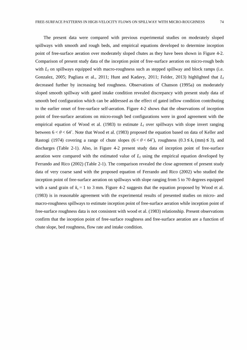
FREE-SURFACE PATTERNS IN HIGH-VELOCITY FLOWS ON SPILLWAY WITH MICRO-ROUGHNESS 74
The present data were compared with previous experimental studies on moderately sloped
spillways with smooth and rough beds, and empirical equations developed to determine inception
point of free-surface aeration over moderately sloped chutes as they have been shown in Figure 4-2.
Comparison of present study data of the inception point of free-surface aeration on micro-rough beds
with LI on spillways equipped with macro-roughness such as stepped spillway and block ramps (i.e.
Gonzalez, 2005; Pagliara et al., 2011; Hunt and Kadavy, 2011; Felder, 2013) highlighted that LI
decreased further by increasing bed roughness. Observations of Chanson (1995a) on moderately
sloped smooth spillway with gated intake condition revealed discrepancy with present study data of
smooth bed configuration which can be addressed as the effect of gated inflow condition contributing
to the earlier onset of free-surface self-aeration. Figure 4-2 shows that the observations of inception
point of free-surface aerations on micro-rough bed configurations were in good agreement with the
empirical equation of Wood et al. (1983) to estimate LI over spillways with slope invert ranging
between 6 < θ < 64˚. Note that Wood et al. (1983) proposed the equation based on data of Keller and
Rastogi (1974) covering a range of chute slopes (6 < θ < 64˚), roughness (0.3 ≤ ks (mm) ≤ 3), and
discharges (Table 2-1). Also, in Figure 4-2 present study data of inception point of free-surface
aeration were compared with the estimated value of LI using the empirical equation developed by
Ferrando and Rico (2002) (Table 2-1). The comparison revealed the close agreement of present study
data of very coarse sand with the proposed equation of Ferrando and Rico (2002) who studied the
inception point of free-surface aeration on spillways with slope ranging from 5 to 70 degrees equipped
with a sand grain of ks = 1 to 3 mm. Figure 4-2 suggests that the equation proposed by Wood et al.
(1983) is in reasonable agreement with the experimental results of presented studies on micro- and
macro-roughness spillways to estimate inception point of free-surface aeration while inception point of
free-surface roughness data is not consistent with wood et al. (1983) relationship. Present observations
confirm that the inception point of free-surface roughness and free-surface aeration are a function of
chute slope, bed roughness, flow rate and intake condition.
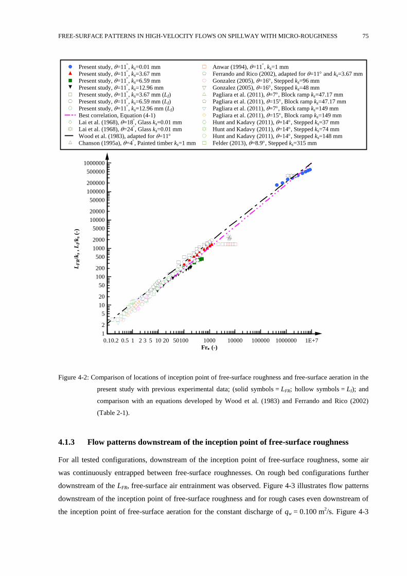
FREE-SURFACE PATTERNS IN HIGH-VELOCITY FLOWS ON SPILLWAY WITH MICRO-ROUGHNESS 75
Figure 4-2: Comparison of locations of inception point of free-surface roughness and free-surface aeration in the
present study with previous experimental data; (solid symbols = LFR; hollow symbols = LI); and
comparison with an equations developed by Wood et al. (1983) and Ferrando and Rico (2002)
(Table 2-1).
4.1.3 Flow patterns downstream of the inception point of free-surface roughness
For all tested configurations, downstream of the inception point of free-surface roughness, some air
was continuously entrapped between free-surface roughnesses. On rough bed configurations further
downstream of the LFR, free-surface air entrainment was observed. Figure 4-3 illustrates flow patterns
downstream of the inception point of free-surface roughness and for rough cases even downstream of
the inception point of free-surface aeration for the constant discharge of qw = 0.100 m2/s. Figure 4-3
Fr (-)
LF
R/k
s , L
I/k
s (-
)
0.10.2 0.5 1 2 3 5 10 20 50100 1000 10000 100000 1000000 1E+7
1
2
5
10
20
50
100
200
500
1000
2000
5000
10000
20000
50000
100000
200000
500000
1000000
Present study, =11, ks=0.01 mm
Present study, =11, ks=3.67 mm
Present study, =11, ks=6.59 mm
Present study, =11, ks=12.96 mm
Present study, =11, ks=3.67 mm (LI)
Present study, =11, ks=6.59 mm (LI)
Present study, =11, ks=12.96 mm (LI)
Best correlation, Equation (4-1)
Lai et al. (1968), =18, Glass ks=0.01 mm
Lai et al. (1968), =24, Glass ks=0.01 mm
Wood et al. (1983), adapted for =11
Chanson (1995a), =4, Painted timber ks=1 mm
Anwar (1994), =11, ks=1 mm
Ferrando and Rico (2002), adapted for =11 and ks=3.67 mm
Gonzalez (2005), =16, Stepped ks=96 mm
Gonzalez (2005), =16, Stepped ks=48 mm
Pagliara et al. (2011), =7, Block ramp ks=47.17 mm
Pagliara et al. (2011), =15, Block ramp ks=47.17 mm
Pagliara et al. (2011), =7, Block ramp ks=149 mm
Pagliara et al. (2011), =15, Block ramp ks=149 mm
Hunt and Kadavy (2011), =14, Stepped ks=37 mm
Hunt and Kadavy (2011), =14, Stepped ks=74 mm
Hunt and Kadavy (2011), =14, Stepped ks=148 mm
Felder (2013), =8.9, Stepped ks=315 mm
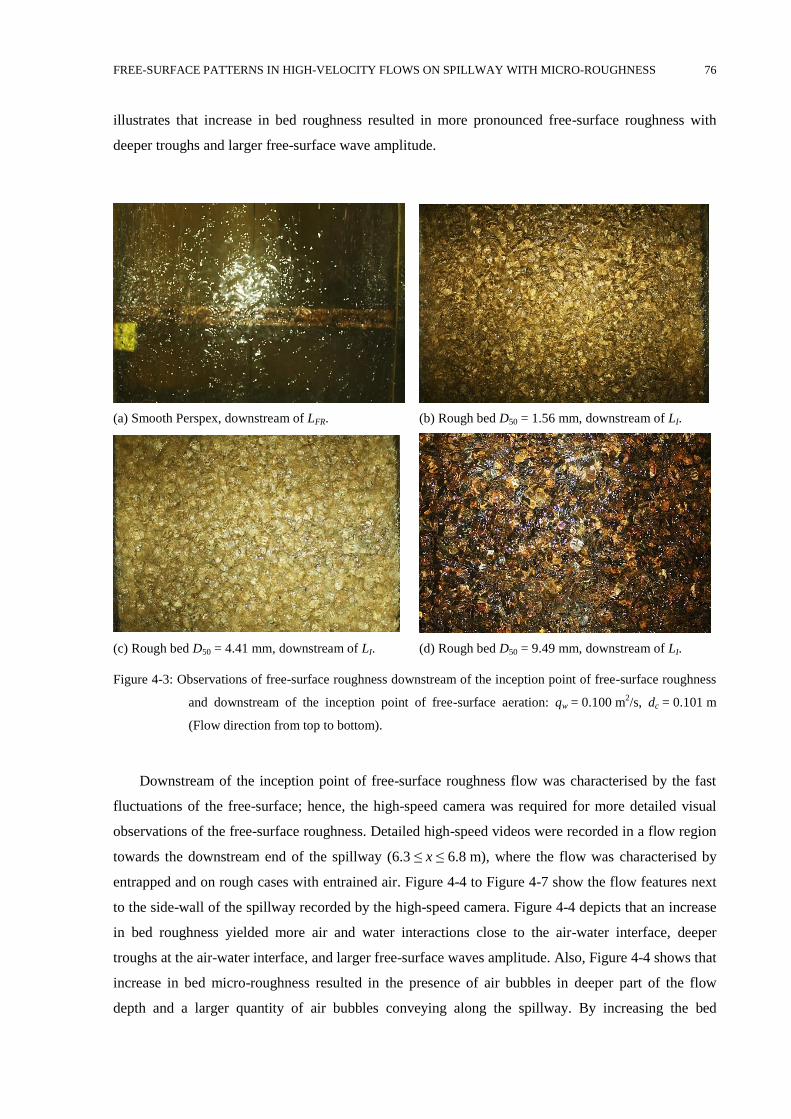
FREE-SURFACE PATTERNS IN HIGH-VELOCITY FLOWS ON SPILLWAY WITH MICRO-ROUGHNESS 76
illustrates that increase in bed roughness resulted in more pronounced free-surface roughness with
deeper troughs and larger free-surface wave amplitude.
(a) Smooth Perspex, downstream of LFR. (b) Rough bed D50 = 1.56 mm, downstream of LI.
(c) Rough bed D50 = 4.41 mm, downstream of LI. (d) Rough bed D50 = 9.49 mm, downstream of LI.
Figure 4-3: Observations of free-surface roughness downstream of the inception point of free-surface roughness
and downstream of the inception point of free-surface aeration: qw = 0.100 m2/s, dc = 0.101 m
(Flow direction from top to bottom).
Downstream of the inception point of free-surface roughness flow was characterised by the fast
fluctuations of the free-surface; hence, the high-speed camera was required for more detailed visual
observations of the free-surface roughness. Detailed high-speed videos were recorded in a flow region
towards the downstream end of the spillway (6.3 ≤ x ≤ 6.8 m), where the flow was characterised by
entrapped and on rough cases with entrained air. Figure 4-4 to Figure 4-7 show the flow features next
to the side-wall of the spillway recorded by the high-speed camera. Figure 4-4 depicts that an increase
in bed roughness yielded more air and water interactions close to the air-water interface, deeper
troughs at the air-water interface, and larger free-surface waves amplitude. Also, Figure 4-4 shows that
increase in bed micro-roughness resulted in the presence of air bubbles in deeper part of the flow
depth and a larger quantity of air bubbles conveying along the spillway. By increasing the bed
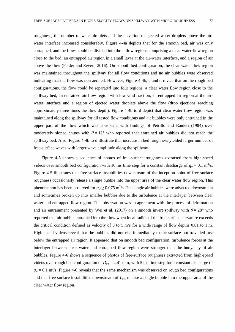
FREE-SURFACE PATTERNS IN HIGH-VELOCITY FLOWS ON SPILLWAY WITH MICRO-ROUGHNESS 77
roughness, the number of water droplets and the elevation of ejected water droplets above the air-
water interface increased considerably. Figure 4-4a depicts that for the smooth bed, air was only
entrapped, and the flows could be divided into three flow regions comprising a clear water flow region
close to the bed, an entrapped air region in a small layer at the air-water interface, and a region of air
above the flow (Felder and Severi, 2016). On smooth bed configuration, the clear water flow region
was maintained throughout the spillway for all flow conditions and no air bubbles were observed
indicating that the flow was non-aerated. However, Figure 4-4b, c and d reveal that on the rough bed
configurations, the flow could be separated into four regions: a clear water flow region close to the
spillway bed, an entrained air flow region with low void fraction, an entrapped air region at the air-
water interface and a region of ejected water droplets above the flow (drop ejections reaching
approximately three times the flow depth). Figure 4-4b to d depict that clear water flow region was
maintained along the spillway for all tested flow conditions and air bubbles were only entrained in the
upper part of the flow which was consistent with findings of Petrillo and Ranieri (1984) over
moderately sloped chutes with θ = 12° who reported that entrained air bubbles did not reach the
spillway bed. Also, Figure 4-4b to d illustrate that increase in bed roughness yielded larger number of
free-surface waves with larger wave amplitude along the spillway.
Figure 4-5 shows a sequence of photos of free-surface roughness extracted from high-speed
videos over smooth bed configuration with 10 ms time step for a constant discharge of qw = 0.1 m2/s.
Figure 4-5 illustrates that free-surface instabilities downstream of the inception point of free-surface
roughness occasionally release a single bubble into the upper area of the clear water flow region. This
phenomenon has been observed for qw ≥ 0.075 m2/s. The single air bubbles were advected downstream
and sometimes broken up into smaller bubbles due to the turbulence at the interlayer between clear
water and entrapped flow region. This observation was in agreement with the process of deformation
and air entrainment presented by Wei et al. (2017) on a smooth invert spillway with θ = 28° who
reported that air bubble entrained into the flow when local radius of the free-surface curvature exceeds
the critical condition defined as velocity of 3 to 5 m/s for a wide range of flow depths 0.01 to 1 m.
High-speed videos reveal that the bubbles did not rise immediately to the surface but travelled just
below the entrapped air region. It appeared that on smooth bed configuration, turbulence forces at the
interlayer between clear water and entrapped flow region were stronger than the buoyancy of air
bubbles. Figure 4-6 shows a sequence of photos of free-surface roughness extracted from high-speed
videos over rough bed configuration of D50 = 4.41 mm, with 5 ms time step for a constant discharge of
qw = 0.1 m2/s. Figure 4-6 reveals that the same mechanism was observed on rough bed configurations
and that free-surface instabilities downstream of LFR release a single bubble into the upper area of the
clear water flow region.
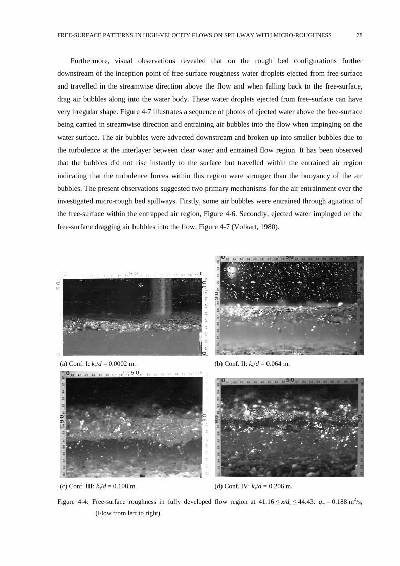
FREE-SURFACE PATTERNS IN HIGH-VELOCITY FLOWS ON SPILLWAY WITH MICRO-ROUGHNESS 78
Furthermore, visual observations revealed that on the rough bed configurations further
downstream of the inception point of free-surface roughness water droplets ejected from free-surface
and travelled in the streamwise direction above the flow and when falling back to the free-surface,
drag air bubbles along into the water body. These water droplets ejected from free-surface can have
very irregular shape. Figure 4-7 illustrates a sequence of photos of ejected water above the free-surface
being carried in streamwise direction and entraining air bubbles into the flow when impinging on the
water surface. The air bubbles were advected downstream and broken up into smaller bubbles due to
the turbulence at the interlayer between clear water and entrained flow region. It has been observed
that the bubbles did not rise instantly to the surface but travelled within the entrained air region
indicating that the turbulence forces within this region were stronger than the buoyancy of the air
bubbles. The present observations suggested two primary mechanisms for the air entrainment over the
investigated micro-rough bed spillways. Firstly, some air bubbles were entrained through agitation of
the free-surface within the entrapped air region, Figure 4-6. Secondly, ejected water impinged on the
free-surface dragging air bubbles into the flow, Figure 4-7 (Volkart, 1980).
(a) Conf. I: ks/d = 0.0002 m. (b) Conf. II: ks/d = 0.064 m.
(c) Conf. III: ks/d = 0.108 m. (d) Conf. IV: ks/d = 0.206 m.
Figure 4-4: Free-surface roughness in fully developed flow region at 41.16 ≤ x/dc ≤ 44.43: qw = 0.188 m2/s,
(Flow from left to right).
FREE-SURFACE PATTERNS IN HIGH-VELOCITY FLOWS ON SPILLWAY WITH MICRO-ROUGHNESS 79
Figure 4-5: Free-surface roughness downstream of LFR at 64.6 ≤ x/dc ≤ 66.6: qw = 0.1 m2/s, dc = 0.101 m,
Re = 3.68×10⁵, LFR = 3.5 m; Photo order from top left to bottom right with time step of 10 ms
between photos; Flow direction from left to right.
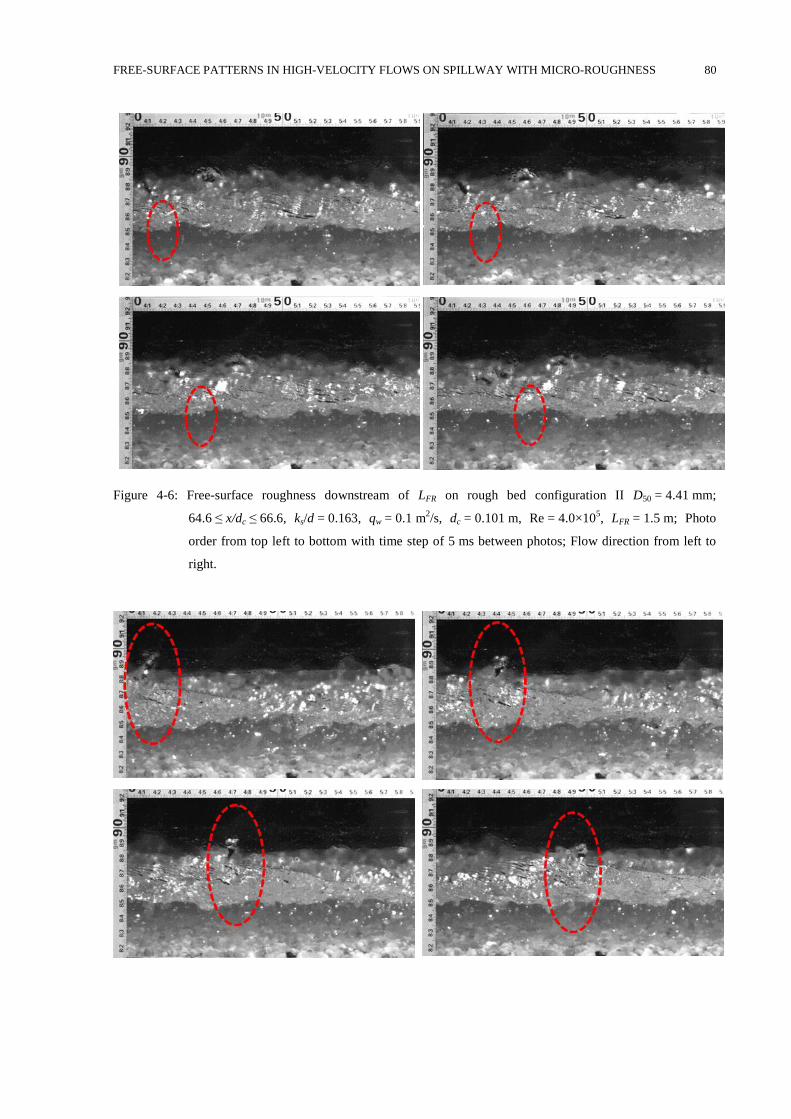
FREE-SURFACE PATTERNS IN HIGH-VELOCITY FLOWS ON SPILLWAY WITH MICRO-ROUGHNESS 80
Figure 4-6: Free-surface roughness downstream of LFR on rough bed configuration II D50 = 4.41 mm;
64.6 ≤ x/dc ≤ 66.6, ks/d = 0.163, qw = 0.1 m2/s, dc = 0.101 m, Re = 4.0×10
5, LFR = 1.5 m; Photo
order from top left to bottom with time step of 5 ms between photos; Flow direction from left to
right.
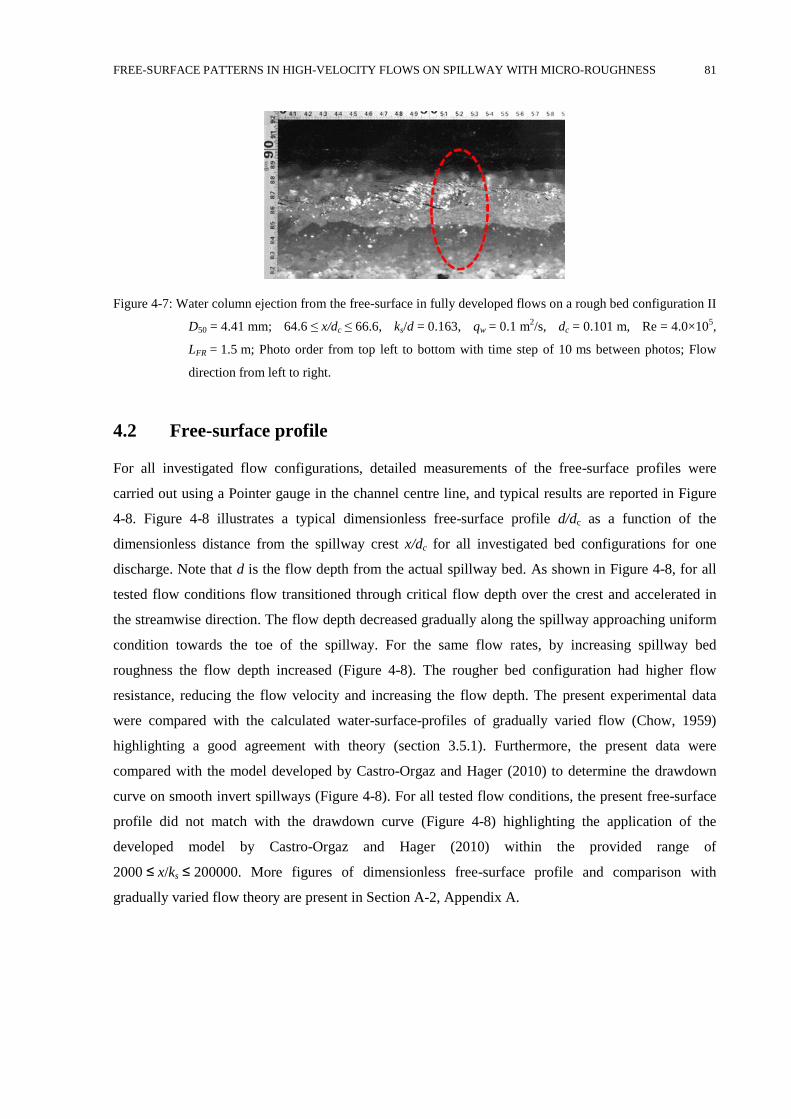
FREE-SURFACE PATTERNS IN HIGH-VELOCITY FLOWS ON SPILLWAY WITH MICRO-ROUGHNESS 81
Figure 4-7: Water column ejection from the free-surface in fully developed flows on a rough bed configuration II
D50 = 4.41 mm; 64.6 ≤ x/dc ≤ 66.6, ks/d = 0.163, qw = 0.1 m2/s, dc = 0.101 m, Re = 4.0×10
5,
LFR = 1.5 m; Photo order from top left to bottom with time step of 10 ms between photos; Flow
direction from left to right.
Free-surface profile 4.2
For all investigated flow configurations, detailed measurements of the free-surface profiles were
carried out using a Pointer gauge in the channel centre line, and typical results are reported in Figure
4-8. Figure 4-8 illustrates a typical dimensionless free-surface profile d/dc as a function of the
dimensionless distance from the spillway crest x/dc for all investigated bed configurations for one
discharge. Note that d is the flow depth from the actual spillway bed. As shown in Figure 4-8, for all
tested flow conditions flow transitioned through critical flow depth over the crest and accelerated in
the streamwise direction. The flow depth decreased gradually along the spillway approaching uniform
condition towards the toe of the spillway. For the same flow rates, by increasing spillway bed
roughness the flow depth increased (Figure 4-8). The rougher bed configuration had higher flow
resistance, reducing the flow velocity and increasing the flow depth. The present experimental data
were compared with the calculated water-surface-profiles of gradually varied flow (Chow, 1959)
highlighting a good agreement with theory (section 3.5.1). Furthermore, the present data were
compared with the model developed by Castro-Orgaz and Hager (2010) to determine the drawdown
curve on smooth invert spillways (Figure 4-8). For all tested flow conditions, the present free-surface
profile did not match with the drawdown curve (Figure 4-8) highlighting the application of the
developed model by Castro-Orgaz and Hager (2010) within the provided range of
2000 ≤ x/ks ≤ 200000. More figures of dimensionless free-surface profile and comparison with
gradually varied flow theory are present in Section A-2, Appendix A.
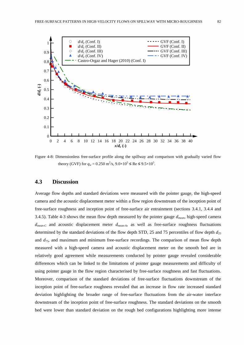
FREE-SURFACE PATTERNS IN HIGH-VELOCITY FLOWS ON SPILLWAY WITH MICRO-ROUGHNESS 82
Figure 4-8: Dimensionless free-surface profile along the spillway and comparison with gradually varied flow
theory (GVF) for qw = 0.250 m2/s, 9.0×10
5 ≤ Re ≤ 9.5×10
5.
Discussion 4.3
Average flow depths and standard deviations were measured with the pointer gauge, the high-speed
camera and the acoustic displacement meter within a flow region downstream of the inception point of
free-surface roughness and inception point of free-surface air entrainment (sections 3.4.1, 3.4.4 and
3.4.5). Table 4-3 shows the mean flow depth measured by the pointer gauge dmean, high-speed camera
dmean-C and acoustic displacement meter dmean-A, as well as free-surface roughness fluctuations
determined by the standard deviations of the flow depth STD, 25 and 75 percentiles of flow depth d25
and d75, and maximum and minimum free-surface recordings. The comparison of mean flow depth
measured with a high-speed camera and acoustic displacement meter on the smooth bed are in
relatively good agreement while measurements conducted by pointer gauge revealed considerable
differences which can be linked to the limitations of pointer gauge measurements and difficulty of
using pointer gauge in the flow region characterised by free-surface roughness and fast fluctuations.
Moreover, comparison of the standard deviations of free-surface fluctuations downstream of the
inception point of free-surface roughness revealed that an increase in flow rate increased standard
deviation highlighting the broader range of free-surface fluctuations from the air-water interface
downstream of the inception point of free-surface roughness. The standard deviations on the smooth
bed were lower than standard deviation on the rough bed configurations highlighting more intense
x/dc (-)
d/d
c (-
)
0 2 4 6 8 10 12 14 16 18 20 22 24 26 28 30 32 34 36 38 40
0
0.1
0.2
0.3
0.4
0.5
0.6
0.7
0.8
0.9
1 d/dc (Conf. I)
d/dc (Conf. II)
d/dc (Conf. III)
d/dc (Conf. IV)
Castro-Orgaz and Hager (2010) (Conf. I)
GVF (Conf. I)
GVF (Conf. II)
GVF (Conf. III)
GVF (Conf. IV)
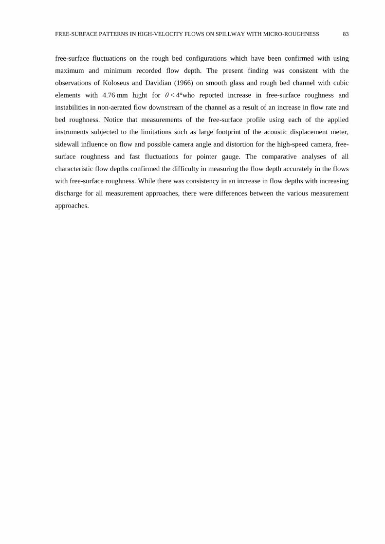
FREE-SURFACE PATTERNS IN HIGH-VELOCITY FLOWS ON SPILLWAY WITH MICRO-ROUGHNESS 83
free-surface fluctuations on the rough bed configurations which have been confirmed with using
maximum and minimum recorded flow depth. The present finding was consistent with the
observations of Koloseus and Davidian (1966) on smooth glass and rough bed channel with cubic
elements with 4.76 mm hight for θ < 4°who reported increase in free-surface roughness and
instabilities in non-aerated flow downstream of the channel as a result of an increase in flow rate and
bed roughness. Notice that measurements of the free-surface profile using each of the applied
instruments subjected to the limitations such as large footprint of the acoustic displacement meter,
sidewall influence on flow and possible camera angle and distortion for the high-speed camera, free-
surface roughness and fast fluctuations for pointer gauge. The comparative analyses of all
characteristic flow depths confirmed the difficulty in measuring the flow depth accurately in the flows
with free-surface roughness. While there was consistency in an increase in flow depths with increasing
discharge for all measurement approaches, there were differences between the various measurement
approaches.
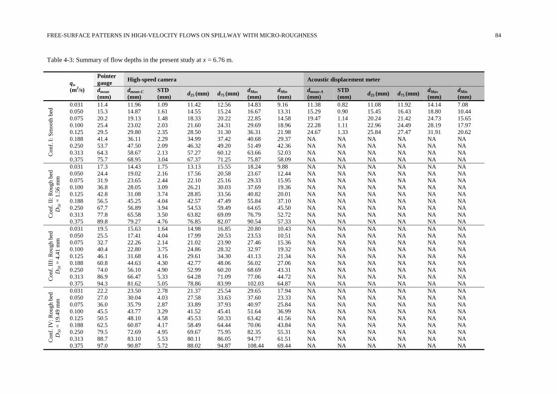
FREE-SURFACE PATTERNS IN HIGH-VELOCITY FLOWS ON SPILLWAY WITH MICRO-ROUGHNESS 84
Table 4-3: Summary of flow depths in the present study at x = 6.76 m.
qw
(m2/s)
Pointer
gauge High-speed camera Acoustic displacement meter
dmean
(mm)
dmean-C
(mm)
STD
(mm) d25 (mm) d75 (mm)
dMax
(mm)
dMin
(mm)
dmean-A
(mm)
STD
(mm) d25 (mm) d75 (mm)
dMax
(mm)
dMin
(mm)
Co
nf.
I:
Sm
oo
th b
ed 0.031 11.4 11.96 1.09 11.42 12.56 14.83 9.16 11.38 0.82 11.08 11.92 14.14 7.08
0.050 15.3 14.87 1.61 14.55 15.24 16.67 13.31 15.29 0.90 15.45 16.43 18.80 10.44
0.075 20.2 19.13 1.48 18.33 20.22 22.85 14.58 19.47 1.14 20.24 21.42 24.73 15.65
0.100 25.4 23.02 2.03 21.60 24.31 29.69 18.96 22.28 1.11 22.96 24.49 28.19 17.97
0.125 29.5 29.80 2.35 28.50 31.30 36.31 21.98 24.67 1.33 25.84 27.47 31.91 20.62
0.188 41.4 36.11 2.29 34.99 37.42 40.68 29.37 NA NA NA NA NA NA
0.250 53.7 47.50 2.09 46.32 49.20 51.49 42.36 NA NA NA NA NA NA
0.313 64.3 58.67 2.13 57.27 60.12 63.66 52.03 NA NA NA NA NA NA
0.375 75.7 68.95 3.04 67.37 71.25 75.87 58.09 NA NA NA NA NA NA
Co
nf.
II:
Rou
gh
bed
D50 =
1.5
6 m
m
0.031 17.3 14.43 1.75 13.13 15.55 18.24 9.88 NA NA NA NA NA NA
0.050 24.4 19.02 2.16 17.56 20.58 23.67 12.44 NA NA NA NA NA NA
0.075 31.9 23.65 2.44 22.10 25.16 29.33 15.95 NA NA NA NA NA NA
0.100 36.8 28.05 3.09 26.21 30.03 37.69 19.36 NA NA NA NA NA NA
0.125 42.8 31.08 3.74 28.85 33.56 40.82 20.01 NA NA NA NA NA NA
0.188 56.5 45.25 4.04 42.57 47.49 55.84 37.10 NA NA NA NA NA NA
0.250 67.7 56.89 3.94 54.53 59.49 64.65 45.50 NA NA NA NA NA NA
0.313 77.8 65.58 3.50 63.82 69.09 76.79 52.72 NA NA NA NA NA NA
0.375 89.8 79.27 4.76 76.85 82.07 90.54 57.33 NA NA NA NA NA NA
Co
nf.
III
: R
ou
gh
bed
D50 =
4.4
1 m
m
0.031 19.5 15.63 1.64 14.98 16.85 20.80 10.43 NA NA NA NA NA NA
0.050 25.5 17.41 4.04 17.99 20.53 23.53 10.51 NA NA NA NA NA NA
0.075 32.7 22.26 2.14 21.02 23.90 27.46 15.36 NA NA NA NA NA NA
0.100 40.4 22.80 3.75 24.86 28.32 32.97 19.32 NA NA NA NA NA NA
0.125 46.1 31.68 4.16 29.61 34.30 41.13 21.34 NA NA NA NA NA NA
0.188 60.8 44.63 4.30 42.77 48.06 56.02 27.06 NA NA NA NA NA NA
0.250 74.0 56.10 4.90 52.99 60.20 68.69 43.31 NA NA NA NA NA NA
0.313 86.9 66.47 5.33 64.28 71.09 77.06 44.72 NA NA NA NA NA NA
0.375 94.3 81.62 5.05 78.86 83.99 102.03 64.87 NA NA NA NA NA NA
Co
nf.
IV
: R
ou
gh
bed
D50 =
19
.49 m
m
0.031 22.2 23.50 2.78 21.37 25.54 29.65 17.94 NA NA NA NA NA NA
0.050 27.0 30.04 4.03 27.58 33.63 37.60 23.33 NA NA NA NA NA NA
0.075 36.0 35.79 2.87 33.89 37.93 40.97 25.84 NA NA NA NA NA NA
0.100 45.5 43.77 3.29 41.52 45.41 51.64 36.99 NA NA NA NA NA NA
0.125 50.5 48.10 4.58 45.53 50.33 63.42 41.56 NA NA NA NA NA NA
0.188 62.5 60.87 4.17 58.49 64.44 70.06 43.84 NA NA NA NA NA NA
0.250 79.5 72.69 4.95 69.67 75.95 82.35 55.31 NA NA NA NA NA NA
0.313 88.7 83.10 5.53 80.11 86.05 94.77 61.51 NA NA NA NA NA NA
0.375 97.0 90.87 5.72 88.02 94.87 108.44 69.44 NA NA NA NA NA NA
FREE-SURFACE PATTERNS IN HIGH-VELOCITY FLOWS ON SPILLWAY WITH MICRO-ROUGHNESS 85
Summary 4.4
Detailed observations of flow patterns and free-surface profile were carried out on a spillway with a
slope of θ = 11° for four-bed configurations and discharge per unit width of 0.019 ≤ qw ≤ 0.375 m2/s.
Visual observations revealed that no air was entrained into the flow over the smooth bed
configuration. Instead, free-surface became agitated, and some air was continuously entrapped within
a small layer next to the free-surface known as free-surface roughness. Recorded videos and photos
illustrate that with increasing the spillway bed micro-roughness, the air-water interactions at the air-
water interface increased; free-surface roughness increased leading to free-surface aeration further
downstream. The present observations suggested two main mechanisms for the air entrainment over
the tested micro-rough bed spillways comprising entrainment of some air bubbles into the flow
through agitation of the free-surface within the entrapped air region, as well as entrainment of air
bubbles while the ejected water is impinging on the free-surface dragging air bubbles into the flow.
Visual observations of flow patterns highlighted the downward shift of the inception point of free-
surface roughness by increasing flow rate and upward shift of the free-surface roughness by increasing
bed roughness. Also, increase in bed rough lead to the earlier appearance of free-surface aeration.
Visual observations revealed that flow on a smooth bed could be separated into three regions: clear
water flow region close to the bed, entrapped air region at air-water interface and air region above the
flow; while flow over micro-rough bed configurations can be divided into four regions: clear water
flow region close to the bed, entrained region, entrapped air region at air-water interface and region of
flying water droplets above the flow. Furthermore, visual observations and photos revealed a different
type of free-surface roughness and waves on smooth bed configuration. It suggests that increase in bed
roughness yielded larger number of free-surface waves with larger wave amplitude along the spillway.
Comparison of the free-surface profile obtained through various methods depicted inconsistency of the
mean flow depth downstream of the inception point of free-surface roughness confirmed the difficulty
in measuring the flow depth accurately in the flows characterised by free-surface roughness. Further
comparison conducted between measured flow depth along the spillway and applying gradually varied
flow theory revealed that for some flow conditions flow depth approached uniform value towards the
end of the spillway while for the other flow conditions the length of the spillway model was no
sufficient to allow the flowing water achieve uniform condition.
Chapter 5
5 BOUNDARY LAYER PROPERTIES AND SHEAR
STRESSES IN THE DEVELOPING FLOW REGION
In this chapter, time-averaged velocity distributions are compared for the different configurations of
bed roughness. The analysis of velocity distributions provided further data on the boundary layer
thickness δw, displacement thickness δ1, momentum thickness δ2 and the growth rate of the turbulent
boundary layer along the spillway model. Furthermore, the boundary shear stress and corresponding
friction factor have been calculated by applying different approaches.
Velocity distributions 5.1
Velocity measurements were performed with the Prandtl-Pitot tube in channel centre line at 16 cross-
sections between 0.08 ≤ x ≤ 7.76 m for all investigated flow conditions. At each cross-section, time-
averaged velocities VP were computed between spillway bed and as close as possible to the free-
surface. For all flow conditions, the velocities increased along the spillway approaching uniform
velocities towards the downstream end of the spillway (see Section 5.2). Figure 5-1, shows typical
dimensionless velocity distributions VP/Vc as a function of dimensionless elevation y/dc for all tested
roughness configurations. Figure 5-1a to d show an upward shift of the time-averaged local velocity
distributions close to the channel bed with increasing bed roughness at a constant distance from the
crest. This observation is consistent with observations of Krogstad and Antonio (1999) for
experiments conducted in the wind tunnel over smooth and two rough bed configurations of ks = 4.96
and 9.7 mm, who reported the upward shift of velocity distributions from the smooth configuration.
Moreover, Figure 5-1a to d illustrates the difference in velocity distributions due to increasing flow
discharge. For instance, Figure 5-1a shows that for qw = 0.075 m2/s the upward shift of velocity
distribution due to increase in bed roughness is more considerable compared to the corresponding
upward shift in Figure 5-1d for qw = 0.375 m2/s. It suggests that as flow discharge increases, the effect
of bed roughness on the velocity distribution is decreased due to the reduction of the relative
roughness ks/DH. Further comparisons were conducted for constant Fr numbers shown in Figure 5-1e
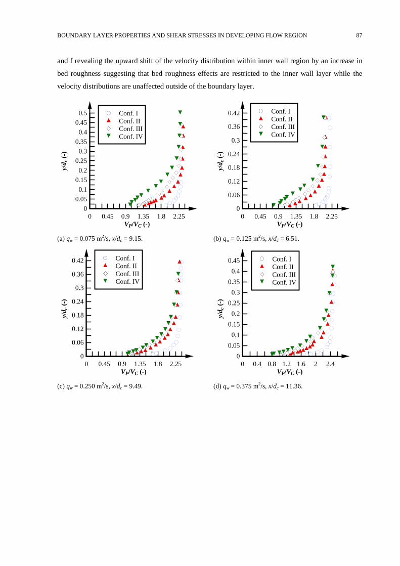
BOUNDARY LAYER PROPERTIES AND SHEAR STRESSES IN DEVELOPING FLOW REGION 87
and f revealing the upward shift of the velocity distribution within inner wall region by an increase in
bed roughness suggesting that bed roughness effects are restricted to the inner wall layer while the
velocity distributions are unaffected outside of the boundary layer.
(a) qw = 0.075 m2/s, x/dc = 9.15. (b) qw = 0.125 m
2/s, x/dc = 6.51.
(c) qw = 0.250 m2/s, x/dc = 9.49. (d) qw = 0.375 m
2/s, x/dc = 11.36.
VP/VC (-)
y/d
c (-
)
0 0.45 0.9 1.35 1.8 2.25
0
0.05
0.1
0.15
0.2
0.25
0.3
0.35
0.4
0.45
0.5 Conf. I
Conf. II
Conf. III
Conf. IV
VP/VC (-)y/
dc
(-)
0 0.45 0.9 1.35 1.8 2.25
0
0.06
0.12
0.18
0.24
0.3
0.36
0.42 Conf. I
Conf. II
Conf. III
Conf. IV
VP/VC (-)
y/d
c (-
)
0 0.45 0.9 1.35 1.8 2.25
0
0.06
0.12
0.18
0.24
0.3
0.36
0.42 Conf. I
Conf. II
Conf. III
Conf. IV
VP/VC (-)
y/d
c (-
)
0 0.4 0.8 1.2 1.6 2 2.4
0
0.05
0.1
0.15
0.2
0.25
0.3
0.35
0.4
0.45 Conf. I
Conf. II
Conf. III
Conf. IV
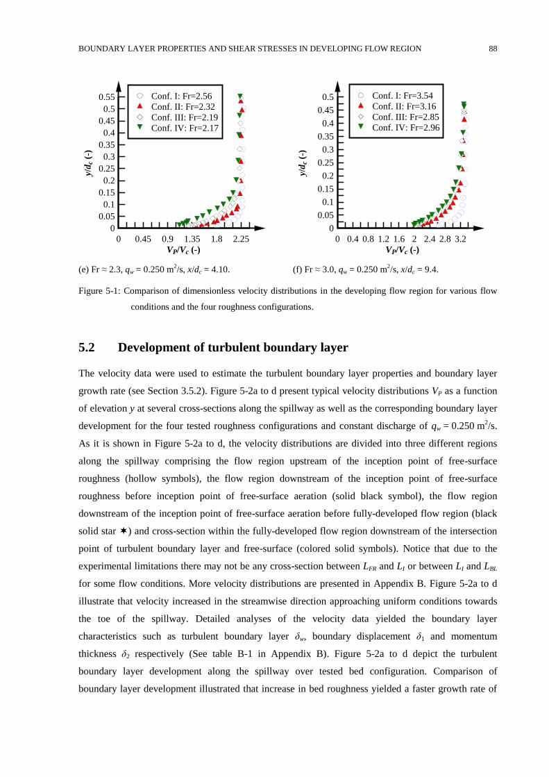
BOUNDARY LAYER PROPERTIES AND SHEAR STRESSES IN DEVELOPING FLOW REGION 88
(e) Fr ≈ 2.3, qw = 0.250 m2/s, x/dc = 4.10. (f) Fr ≈ 3.0, qw = 0.250 m
2/s, x/dc = 9.4.
Figure 5-1: Comparison of dimensionless velocity distributions in the developing flow region for various flow
conditions and the four roughness configurations.
Development of turbulent boundary layer 5.2
The velocity data were used to estimate the turbulent boundary layer properties and boundary layer
growth rate (see Section 3.5.2). Figure 5-2a to d present typical velocity distributions VP as a function
of elevation y at several cross-sections along the spillway as well as the corresponding boundary layer
development for the four tested roughness configurations and constant discharge of qw = 0.250 m2/s.
As it is shown in Figure 5-2a to d, the velocity distributions are divided into three different regions
along the spillway comprising the flow region upstream of the inception point of free-surface
roughness (hollow symbols), the flow region downstream of the inception point of free-surface
roughness before inception point of free-surface aeration (solid black symbol), the flow region
downstream of the inception point of free-surface aeration before fully-developed flow region (black
solid star ) and cross-section within the fully-developed flow region downstream of the intersection
point of turbulent boundary layer and free-surface (colored solid symbols). Notice that due to the
experimental limitations there may not be any cross-section between LFR and LI or between LI and LBL
for some flow conditions. More velocity distributions are presented in Appendix B. Figure 5-2a to d
illustrate that velocity increased in the streamwise direction approaching uniform conditions towards
the toe of the spillway. Detailed analyses of the velocity data yielded the boundary layer
characteristics such as turbulent boundary layer δw, boundary displacement δ1 and momentum
thickness δ2 respectively (See table B-1 in Appendix B). Figure 5-2a to d depict the turbulent
boundary layer development along the spillway over tested bed configuration. Comparison of
boundary layer development illustrated that increase in bed roughness yielded a faster growth rate of
VP/Vc (-)
y/d
c (-
)
0 0.45 0.9 1.35 1.8 2.25
0
0.05
0.1
0.15
0.2
0.25
0.3
0.35
0.4
0.45
0.5
0.55 Conf. I: Fr=2.56
Conf. II: Fr=2.32
Conf. III: Fr=2.19
Conf. IV: Fr=2.17
VP/Vc (-)
y/d
c (-
)
0 0.4 0.8 1.2 1.6 2 2.4 2.8 3.2
0
0.05
0.1
0.15
0.2
0.25
0.3
0.35
0.4
0.45
0.5 Conf. I: Fr=3.54
Conf. II: Fr=3.16
Conf. III: Fr=2.85
Conf. IV: Fr=2.96
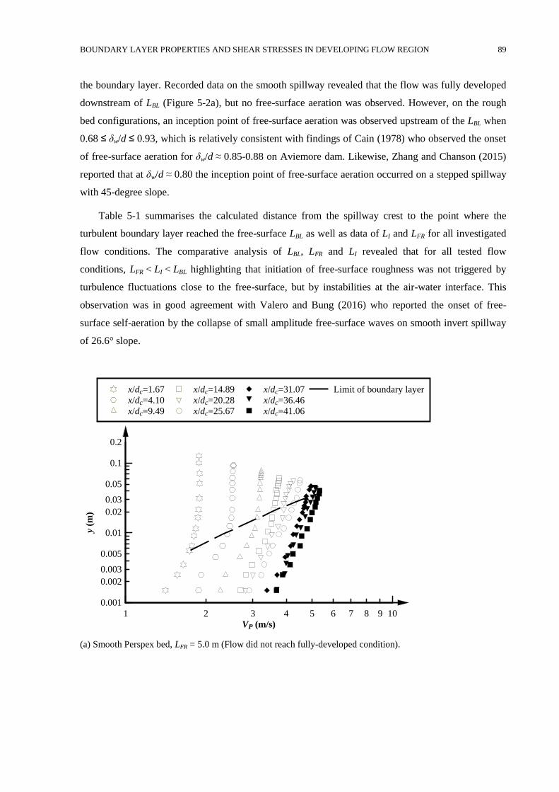
BOUNDARY LAYER PROPERTIES AND SHEAR STRESSES IN DEVELOPING FLOW REGION 89
the boundary layer. Recorded data on the smooth spillway revealed that the flow was fully developed
downstream of LBL (Figure 5-2a), but no free-surface aeration was observed. However, on the rough
bed configurations, an inception point of free-surface aeration was observed upstream of the LBL when
0.68 ≤ δw/d ≤ 0.93, which is relatively consistent with findings of Cain (1978) who observed the onset
of free-surface aeration for δw/d ≈ 0.85-0.88 on Aviemore dam. Likewise, Zhang and Chanson (2015)
reported that at δw/d ≈ 0.80 the inception point of free-surface aeration occurred on a stepped spillway
with 45-degree slope.
Table 5-1 summarises the calculated distance from the spillway crest to the point where the
turbulent boundary layer reached the free-surface LBL as well as data of LI and LFR for all investigated
flow conditions. The comparative analysis of LBL, LFR and LI revealed that for all tested flow
conditions, LFR < LI < LBL highlighting that initiation of free-surface roughness was not triggered by
turbulence fluctuations close to the free-surface, but by instabilities at the air-water interface. This
observation was in good agreement with Valero and Bung (2016) who reported the onset of free-
surface self-aeration by the collapse of small amplitude free-surface waves on smooth invert spillway
of 26.6° slope.
(a) Smooth Perspex bed, LFR = 5.0 m (Flow did not reach fully-developed condition).
VP (m/s)
y (m
)
1 2 3 4 5 6 7 8 9 10
0.001
0.002
0.003
0.005
0.01
0.02
0.03
0.05
0.1
0.2
x/dc=1.67
x/dc=4.10
x/dc=9.49
x/dc=14.89
x/dc=20.28
x/dc=25.67
x/dc=31.07
x/dc=36.46
x/dc=41.06
Limit of boundary layer
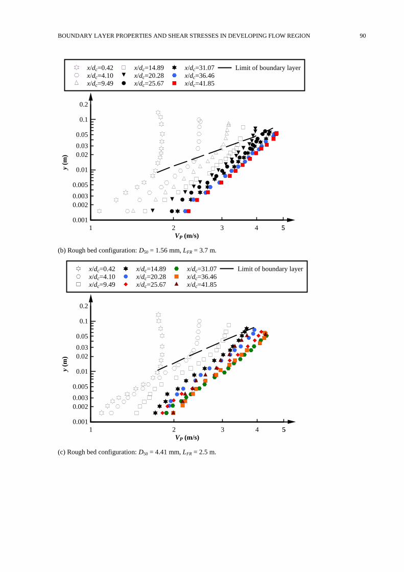
BOUNDARY LAYER PROPERTIES AND SHEAR STRESSES IN DEVELOPING FLOW REGION 90
(b) Rough bed configuration: D50 = 1.56 mm, LFR = 3.7 m.
(c) Rough bed configuration: D50 = 4.41 mm, LFR = 2.5 m.
VP (m/s)
y (m
)
1 2 3 4 55
0.001
0.002
0.003
0.005
0.01
0.02
0.03
0.05
0.1
0.2
x/dc=0.42
x/dc=4.10
x/dc=9.49
x/dc=14.89
x/dc=20.28
x/dc=25.67
x/dc=31.07
x/dc=36.46
x/dc=41.85
Limit of boundary layer
VP (m/s)
y (m
)
1 2 3 4 55
0.001
0.002
0.003
0.005
0.01
0.02
0.03
0.05
0.1
0.2
x/dc=0.42
x/dc=4.10
x/dc=9.49
x/dc=14.89
x/dc=20.28
x/dc=25.67
x/dc=31.07
x/dc=36.46
x/dc=41.85
Limit of boundary layer
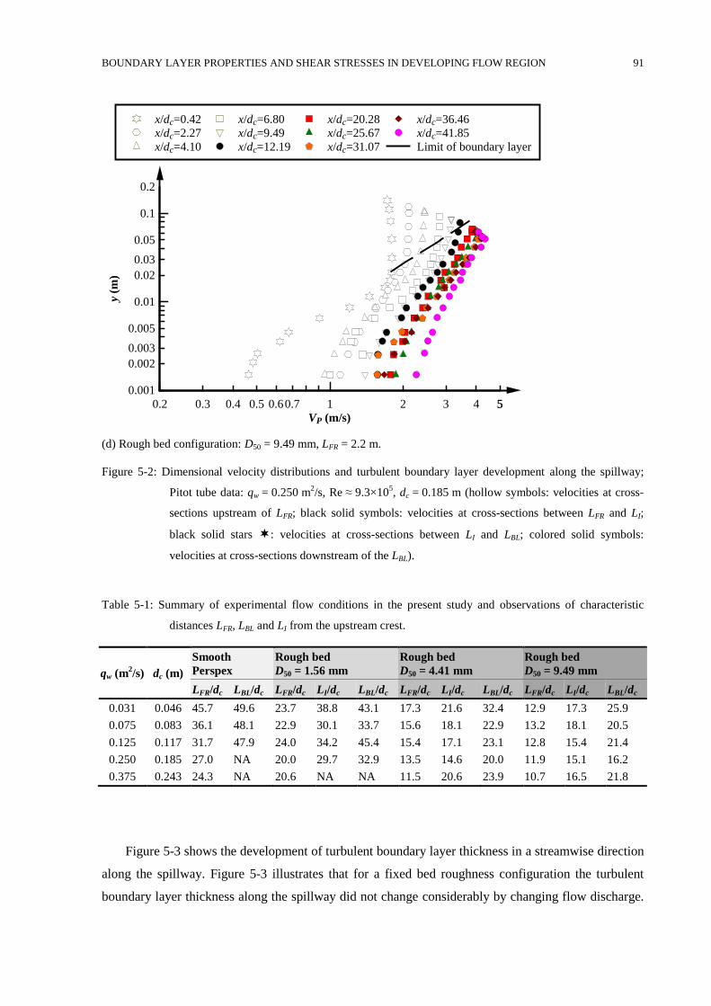
BOUNDARY LAYER PROPERTIES AND SHEAR STRESSES IN DEVELOPING FLOW REGION 91
(d) Rough bed configuration: D50 = 9.49 mm, LFR = 2.2 m.
Figure 5-2: Dimensional velocity distributions and turbulent boundary layer development along the spillway;
Pitot tube data: qw = 0.250 m2/s, Re ≈ 9.3×10
5, dc = 0.185 m (hollow symbols: velocities at cross-
sections upstream of LFR; black solid symbols: velocities at cross-sections between LFR and LI;
black solid stars : velocities at cross-sections between LI and LBL; colored solid symbols:
velocities at cross-sections downstream of the LBL).
Table 5-1: Summary of experimental flow conditions in the present study and observations of characteristic
distances LFR, LBL and LI from the upstream crest.
qw (m2/s) dc (m)
Smooth
Perspex
Rough bed
D50 = 1.56 mm
Rough bed
D50 = 4.41 mm
Rough bed
D50 = 9.49 mm
LFR/dc LBL/dc LFR/dc LI/dc LBL/dc LFR/dc LI/dc LBL/dc LFR/dc LI/dc LBL/dc
0.031 0.046 45.7 49.6 23.7 38.8 43.1 17.3 21.6 32.4 12.9 17.3 25.9
0.075 0.083 36.1 48.1 22.9 30.1 33.7 15.6 18.1 22.9 13.2 18.1 20.5
0.125 0.117 31.7 47.9 24.0 34.2 45.4 15.4 17.1 23.1 12.8 15.4 21.4
0.250 0.185 27.0 NA 20.0 29.7 32.9 13.5 14.6 20.0 11.9 15.1 16.2
0.375 0.243 24.3 NA 20.6 NA NA 11.5 20.6 23.9 10.7 16.5 21.8
Figure 5-3 shows the development of turbulent boundary layer thickness in a streamwise direction
along the spillway. Figure 5-3 illustrates that for a fixed bed roughness configuration the turbulent
boundary layer thickness along the spillway did not change considerably by changing flow discharge.
VP (m/s)
y (m
)
0.2 0.3 0.4 0.5 0.60.7 1 2 3 4 55
0.001
0.002
0.003
0.005
0.01
0.02
0.03
0.05
0.1
0.2
x/dc=0.42
x/dc=2.27
x/dc=4.10
x/dc=6.80
x/dc=9.49
x/dc=12.19
x/dc=20.28
x/dc=25.67
x/dc=31.07
x/dc=36.46
x/dc=41.85
Limit of boundary layer
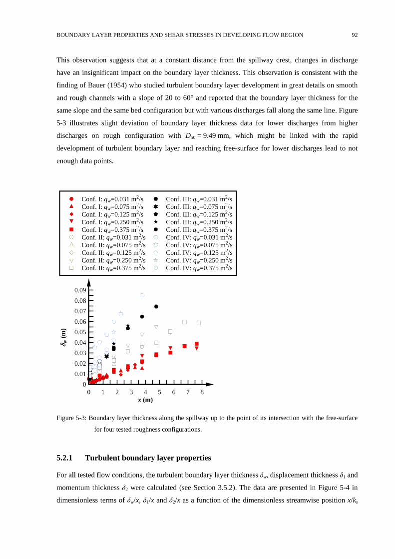
BOUNDARY LAYER PROPERTIES AND SHEAR STRESSES IN DEVELOPING FLOW REGION 92
This observation suggests that at a constant distance from the spillway crest, changes in discharge
have an insignificant impact on the boundary layer thickness. This observation is consistent with the
finding of Bauer (1954) who studied turbulent boundary layer development in great details on smooth
and rough channels with a slope of 20 to 60° and reported that the boundary layer thickness for the
same slope and the same bed configuration but with various discharges fall along the same line. Figure
5-3 illustrates slight deviation of boundary layer thickness data for lower discharges from higher
discharges on rough configuration with D50 = 9.49 mm, which might be linked with the rapid
development of turbulent boundary layer and reaching free-surface for lower discharges lead to not
enough data points.
Figure 5-3: Boundary layer thickness along the spillway up to the point of its intersection with the free-surface
for four tested roughness configurations.
5.2.1 Turbulent boundary layer properties
For all tested flow conditions, the turbulent boundary layer thickness δw, displacement thickness δ1 and
momentum thickness δ2 were calculated (see Section 3.5.2). The data are presented in Figure 5-4 in
dimensionless terms of δw/x, δ1/x and δ2/x as a function of the dimensionless streamwise position x/ks
x (m)
w (
m)
0 1 2 3 4 5 6 7 8
0
0.01
0.02
0.03
0.04
0.05
0.06
0.07
0.08
0.09
Conf. I: qw=0.031 m2/s
Conf. I: qw=0.075 m2/s
Conf. I: qw=0.125 m2/s
Conf. I: qw=0.250 m2/s
Conf. I: qw=0.375 m2/s
Conf. II: qw=0.031 m2/s
Conf. II: qw=0.075 m2/s
Conf. II: qw=0.125 m2/s
Conf. II: qw=0.250 m2/s
Conf. II: qw=0.375 m2/s
Conf. III: qw=0.031 m2/s
Conf. III: qw=0.075 m2/s
Conf. III: qw=0.125 m2/s
Conf. III: qw=0.250 m2/s
Conf. III: qw=0.375 m2/s
Conf. IV: qw=0.031 m2/s
Conf. IV: qw=0.075 m2/s
Conf. IV: qw=0.125 m2/s
Conf. IV: qw=0.250 m2/s
Conf. IV: qw=0.375 m2/s
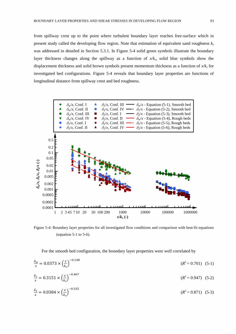
BOUNDARY LAYER PROPERTIES AND SHEAR STRESSES IN DEVELOPING FLOW REGION 93
from spillway crest up to the point where turbulent boundary layer reaches free-surface which in
present study called the developing flow region. Note that estimation of equivalent sand roughness ks
was addressed in detailed in Section 5.3.1. In Figure 5-4 solid green symbols illustrate the boundary
layer thickness changes along the spillway as a function of x/ks, solid blue symbols show the
displacement thickness and solid brown symbols present momentum thickness as a function of x/ks for
investigated bed configurations. Figure 5-4 reveals that boundary layer properties are functions of
longitudinal distance from spillway crest and bed roughness.
Figure 5-4: Boundary layer properties for all investigated flow conditions and comparison with best-fit equations
(equation 5-1 to 5-6).
For the smooth bed configuration, the boundary layer properties were well correlated by
𝛿𝑤
𝑥= 0.0373 × (
𝑥
𝑘𝑠)
−0.148 (R
2 = 0.701) (5-1)
𝛿1
𝑥= 0.3151 × (
𝑥
𝑘𝑠)
−0.467 (R
2 = 0.947) (5-2)
𝛿2
𝑥= 0.0384 × (
𝑥
𝑘𝑠)
−0.335 (R
2 = 0.871) (5-3)
x/ks (-)
w/x
,
1/x
,
2/x
(-)
1 2 3 45 7 10 20 50 100 200 1000 10000 100000 1000000
0.0001
0.0002
0.0005
0.001
0.002
0.005
0.01
0.02
0.05
0.1
0.2
0.5
w/x, Conf. I
w/x, Conf. II
w/x, Conf. III
w/x, Conf. IV
1/x, Conf. I
1/x, Conf. II
1/x, Conf. III
1/x, Conf. IV
2/x, Conf. I
2/x, Conf. II
2/x, Conf. III
2/x, Conf. IV
w/x - Equation (5-1), Smooth bed
1/x - Equation (5-2), Smooth bed
2/x - Equation (5-3), Smooth bed
w/x - Equation (5-4), Rough beds
1/x - Equation (5-5), Rough beds
2/x - Equation (5-6), Rough beds
BOUNDARY LAYER PROPERTIES AND SHEAR STRESSES IN DEVELOPING FLOW REGION 94
The boundary layer growth rate (equation 5-1) compared well with previous studies on smooth
invert spillways including with the empirical equations proposed by Bauer (1954) and Wood et al.
(1983) who reported boundary layer growth rate as x0.8
to x1.0
on smooth invert spillways with slopes
between 7.5˚ ≤ θ ≤ 75˚. The present boundary layer growth rate was in close agreement with a
numerical solution by Castro-Orgaz and Hager (2010) who reported the boundary layer growth rate as
x0.875
on smooth invert spillways for 2000 ≤ x/ks ≤ 20000, highlighting that the numerical solution by
Castro-Orgaz and Hager (2010) is applicable for 30000 < x/ks < 1000000 on smooth bed spillways.
The present results on the smooth bed were also similar to the turbulent boundary layer growth rate on
smooth flat plates δw ~ x0.8
(Schlichting, 1979). Moreover, the present boundary layer growth rate
showed agreement with results of the numerical model developed by Halbronn (1954) on the smooth
glass with slope ranging between 20 and 60 degrees who reported boundary layer growth rate as x0.7
(see Table 2-1).
Rough bed data were best correlated by the following empirical equation:
𝛿𝑤
𝑥= 0.3748 × (
𝑥
𝑘𝑠)
−0.532 (R
2 = 0.889) (5-4)
𝛿1
𝑥= 0.1146 × (
𝑥
𝑘𝑠)
−0.609 (R
2 = 0.915) (5-5)
𝛿2
𝑥= 0.0534 × (
𝑥
𝑘𝑠)
−0.559 (R
2 = 0.911) (5-6)
For rough bed configurations, the present boundary layer (equation 5-4) developed slower
compared to the computed growth rate using the numerical model developed by Halbronn’s (1954) on
rough bed (such as concrete and screen with diameter of 0.254 mm) with slope ranging between 20
and 60 degrees who reported boundary layer growth rate as x0.8
(see Table 2-1). Further comparison of
the present study’s boundary layer growth rate was conducted with Campbell et al. (1965) who
proposed an equation to estimate boundary layer development using model data of Bauer (1951), and
prototype data of Norris Dam, Arkabutla dam data collected by Michels and Lovely (1953) and
Glenmaggie dam for a range of bed slope between 18 and 60 degrees. Present study boundary layer
growth rate on tested rough configurations revealed δw ~ x0.5
, while Campbell et al. (1965) reported the
boundary layer growth rate as x0.8
(see Table 2-1). This deviation might be linked with the impacts of
slope on boundary layer developments over rough bed configurations where steep slope spillway
yielded faster boundary layer growth rate.
Schlichting (1979) presented that the turbulent boundary layer thickness is a function of distance
and the Reynolds number defined as Rex = ρ×Vo×x/μ. For smooth bed configuration, the boundary
layer properties were well correlated by
BOUNDARY LAYER PROPERTIES AND SHEAR STRESSES IN DEVELOPING FLOW REGION 95
𝛿𝑤
𝑥= 0.0361 × (
𝜌×𝑉𝑜×𝑥
𝜇)
−0.111 (R
2 = 0.572) (5-7)
𝛿1
𝑥= 0.1713 × (
𝜌×𝑉𝑜×𝑥
𝜇)
−0.327 (R
2 = 0.936) (5-8)
𝛿2
𝑥= 0.0244 × (
𝜌×𝑉𝑜×𝑥
𝜇)
−0.233 (R
2 = 0.854) (5-9)
The low values of R2, might be due to the limited data sets and some influence of the flow rate.
The comparison of the boundary layer and momentum thickness ratio on tested smooth bed
configuration was in reasonable agreement with the data on smooth flat plates with zero pressure
gradient by Schlichting (1979), i.e. δw/x and δ2/x ~ Re-0.2
. The ratio of boundary displacement thickness
was slightly lower than the reported value by Schlichting (1979) (δ1/x ~ Re-0.2
). Also, Liu et al. (1966)
reported δw/x and δ1/x and δ2/x ~ Re-0.2
on the smooth bed. Also, Liu et al. (1966) investigated
boundary layer properties over the smooth and rough bed with flat slope and zero pressure gradients
and presented that boundary layer growth rate on the smooth bed can be represented by powers of
Re-0.2
.
Rough bed data were best correlated by the following empirical equation:
𝛿𝑤
𝑥= 16.728 × (
𝜌×𝑉𝑜×𝑥
𝜇)
−0.434 (R
2 = 0.749) (5-10)
𝛿1
𝑥= 10.309 × (
𝜌×𝑉𝑜×𝑥
𝜇)
−0.507 (R
2 = 0.803) (5-11)
𝛿2
𝑥= 3.157 × (
𝜌×𝑉𝑜×𝑥
𝜇)
−0.462 (R
2 = 0.788) (5-12)
Herein, comparison between smooth and rough datasets revealed that the present study data was
in relatively good agreement with Liu et al. (1966) who reported δw/x and δ1/x and δ2/x ~ Re-0.33
on the
rough bed with roughness element of transverse square roughness with height of 6.35 mm and
Reynolds number ranging from 5×10⁵ to 10
7. Overall, comparison conducted among turbulent
boundary layer properties and growth rate on smooth and tested rough bed configurations highlighted
that on both smooth and rough beds, boundary growth rate could be represented by the distance from
spillway crest and bed roughness as well as Reynolds number. Also, increase in bed roughness
resulted in the faster growth rate of boundary layer properties.
5.2.2 Comparison of present study data with the power law
The power law is one of the most appropriate formulations for the mean velocity distribution. In
Figure 5-5, all dimensionless velocity distributions VP/Vo are presented as a function of the
dimensionless depth y/δw, where Vo is the freestream velocity. Figure 5-5a to d show velocity
distributions and compared them with best-fitted power law for all tested bed configurations ranging
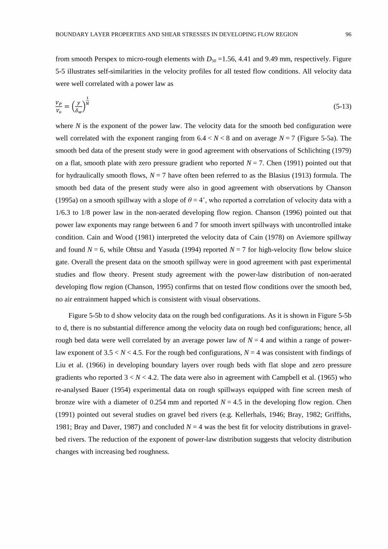
BOUNDARY LAYER PROPERTIES AND SHEAR STRESSES IN DEVELOPING FLOW REGION 96
from smooth Perspex to micro-rough elements with D50 =1.56, 4.41 and 9.49 mm, respectively. Figure
5-5 illustrates self-similarities in the velocity profiles for all tested flow conditions. All velocity data
were well correlated with a power law as
𝑉𝑃
𝑉𝑜= (
𝑦
𝛿𝑤)
1
𝑁 (5-13)
where N is the exponent of the power law. The velocity data for the smooth bed configuration were
well correlated with the exponent ranging from 6.4 < N < 8 and on average N = 7 (Figure 5-5a). The
smooth bed data of the present study were in good agreement with observations of Schlichting (1979)
on a flat, smooth plate with zero pressure gradient who reported N = 7. Chen (1991) pointed out that
for hydraulically smooth flows, N = 7 have often been referred to as the Blasius (1913) formula. The
smooth bed data of the present study were also in good agreement with observations by Chanson
(1995a) on a smooth spillway with a slope of θ = 4˚, who reported a correlation of velocity data with a
1/6.3 to 1/8 power law in the non-aerated developing flow region. Chanson (1996) pointed out that
power law exponents may range between 6 and 7 for smooth invert spillways with uncontrolled intake
condition. Cain and Wood (1981) interpreted the velocity data of Cain (1978) on Aviemore spillway
and found N = 6, while Ohtsu and Yasuda (1994) reported N = 7 for high-velocity flow below sluice
gate. Overall the present data on the smooth spillway were in good agreement with past experimental
studies and flow theory. Present study agreement with the power-law distribution of non-aerated
developing flow region (Chanson, 1995) confirms that on tested flow conditions over the smooth bed,
no air entrainment happed which is consistent with visual observations.
Figure 5-5b to d show velocity data on the rough bed configurations. As it is shown in Figure 5-5b
to d, there is no substantial difference among the velocity data on rough bed configurations; hence, all
rough bed data were well correlated by an average power law of N = 4 and within a range of power-
law exponent of 3.5 < N < 4.5. For the rough bed configurations, N = 4 was consistent with findings of
Liu et al. (1966) in developing boundary layers over rough beds with flat slope and zero pressure
gradients who reported 3 < N < 4.2. The data were also in agreement with Campbell et al. (1965) who
re-analysed Bauer (1954) experimental data on rough spillways equipped with fine screen mesh of
bronze wire with a diameter of 0.254 mm and reported N = 4.5 in the developing flow region. Chen
(1991) pointed out several studies on gravel bed rivers (e.g. Kellerhals, 1946; Bray, 1982; Griffiths,
1981; Bray and Daver, 1987) and concluded N = 4 was the best fit for velocity distributions in gravel-
bed rivers. The reduction of the exponent of power-law distribution suggests that velocity distribution
changes with increasing bed roughness.
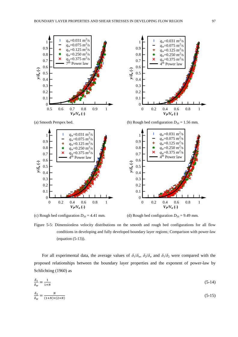
BOUNDARY LAYER PROPERTIES AND SHEAR STRESSES IN DEVELOPING FLOW REGION 97
(a) Smooth Perspex bed. (b) Rough bed configuration D50 = 1.56 mm.
(c) Rough bed configuration D50 = 4.41 mm. (d) Rough bed configuration D50 = 9.49 mm.
Figure 5-5: Dimensionless velocity distributions on the smooth and rough bed configurations for all flow
conditions in developing and fully developed boundary layer regions; Comparison with power-law
(equation (5-13)).
For all experimental data, the average values of δ1/δw, δ2/δw and δ1/δ2 were compared with the
proposed relationships between the boundary layer properties and the exponent of power-law by
Schlichting (1960) as
𝛿1
𝛿𝑤=
1
1+𝑁 (5-14)
𝛿2
𝛿𝑤=
𝑁
(1+𝑁)×(2+𝑁) (5-15)
VP/Vo (-)
y/
w (
-)
0.5 0.6 0.7 0.8 0.9 1
0
0.1
0.2
0.3
0.4
0.5
0.6
0.7
0.8
0.9
1 qw=0.031 m2/s
qw=0.075 m2/s
qw=0.125 m2/s
qw=0.250 m2/s
qw=0.375 m2/s
7th Power law
VP/Vo (-)
y/
w (
-)
0 0.2 0.4 0.6 0.8 1
0
0.1
0.2
0.3
0.4
0.5
0.6
0.7
0.8
0.9
1 qw=0.031 m2/s
qw=0.075 m2/s
qw=0.125 m2/s
qw=0.250 m2/s
qw=0.375 m2/s
4th Power law
VP/Vo (-)
y/
w (
-)
0 0.2 0.4 0.6 0.8 1
0
0.1
0.2
0.3
0.4
0.5
0.6
0.7
0.8
0.9
1 qw=0.031 m2/s
qw=0.075 m2/s
qw=0.125 m2/s
qw=0.250 m2/s
qw=0.375 m2/s
4th Power law
VP/Vo (-)
y/
w (
-)
0 0.2 0.4 0.6 0.8 1
0
0.1
0.2
0.3
0.4
0.5
0.6
0.7
0.8
0.9
1 qw=0.031 m2/s
qw=0.075 m2/s
qw=0.125 m2/s
qw=0.250 m2/s
qw=0.375 m2/s
4th Power law
BOUNDARY LAYER PROPERTIES AND SHEAR STRESSES IN DEVELOPING FLOW REGION 98
𝛿1
𝛿2=
𝑁+2
𝑁 (5-16)
In the present study, the boundary layer properties obtained from measurements on the smooth
bed yielded 0.10 ≤ δ1/δw ≤ 0.37, 0.10 ≤ δ2/δw ≤ 0.18, 1.32 ≤ δ1/δ2 ≤ 2 and with average ratios of
δ1/δw = 0.14, δ2/δw = 0.10 and δ1/δ2 = 1.54. These values compared well with the results of applying
equation (5-14) to (5-16) using N = 7 which resulted in δ1/δw = 0.13, δ2/δw = 0.10 and δ1/δ2 = 1.29.
Comparison of the values obtained from boundary layer data with the calculated results of equation (5-
14) to (5-16) using N = 7 was in close consistency highlighting that the velocity distributions in
developing boundary layer followed the 7th power law. The average ratios obtained from boundary
layer data on smooth invert spillway were in reasonable agreement with the findings of Liu et al.
(1966) who reported ratios of δ2/δw = 0.11 and δ1/δ2 = 1.4 in the boundary layer developing flow
region over a smooth bed.
The boundary layer properties obtained from velocity measurements on the rough bed
configurations yielded 0.13 ≤ δ1/δw ≤ 0.38, 0.10 ≤ δ2/δw ≤ 0.18, 1.26 ≤ δ1/δ2 ≤ 2.39 and with average
ratios of δ1/δw = 0.21, δ2/δw = 0.13 and δ1/δ2 = 1.63. These values compared well with the results of
applying equation (5-14) to (5-16) using N = 4 yielding δ1/δw = 0.20, δ2/δw = 0.13 and δ1/δ2 = 1.50.
These values on rough bed configurations were close to observations of Liu et al. (1966) who reported
ratios δ2/δw = 0.14 and δ1/δ2 = 1.6 on developing boundary layers over the rough bed. Also, Campbell
et al. (1965) used Bauer (1951) data, and prototype data collected by Michels and Lovely (1953) and
Glenmaggie dam for a range of bed slope between 18 and 60 degrees with roughness height of
ks = 0.61 mm. They presented δ1/δw = 0.18 in developing boundary layer flow region over smooth
invert spillway with ks = 0.61 mm.
Boundary shear stress 5.3
The boundary shear stress on spillway is an essential design consideration to evaluate the energy
dissipation along the spillway. Therefore, in this section, various approaches to estimate shear stress
are examined. In following the estimated boundary layer properties used to determine boundary shear
stress based on four different approaches comprising the logarithmic law within the inner flow region,
the velocity defect law in the outer flow region, the momentum integral method as well as the
gradually varied and uniform flow theories.
5.3.1 The logarithmic law within the inner flow region
In Figure 5-6, a comparison of typical velocity distributions VP/V* with the logarithmic law (equations
3-12 and 3-13) is shown as a function of the dimensionless elevation V*×y/ν. The measured velocity
data on the smooth and rough bed configurations were fitted with the logarithmic law by adjustment of
the shear velocity and the equivalent sand roughness height ks (Felder and Islam, 2016). The data on
BOUNDARY LAYER PROPERTIES AND SHEAR STRESSES IN DEVELOPING FLOW REGION 99
the smooth bed yielded shear velocities in the range 0.10 ≤ V* ≤ 0.20 m/s. For the rough bed
configurations with mean grain sizes of D50 = 1.56, 4.41 and 9.49 mm, the velocity distributions were
shifted downward by ΔV+ = 13.5, 15 and 17, respectively (Figure 5-6). The rough bed configurations
resulted in 0.20 ≤ V* ≤ 0.40 m/s, and an average ks = 3.67, 6.59 and 12.96 mm, respectively. For all
tested flow conditions, shear velocity increased in streamwise direction and by increasing flow rate.
Similar results were observed for all velocity data which are present in Appendix B-2.
(a) qw = 0.075 m2/s, dc = 0.083 m. (b) qw = 0.250 m
2/s, dc = 0.185 m.
Figure 5-6: Comparison of velocity distributions along the spillway with the logarithmic law in inner flow region
equations (3-12) and (3-13).
The shear stress was calculated using the equation (3-16). In Figure 5-7a and b, the experimental
results of the computed shear stress are plotted as a non-dimensional shear stress τo/(ρ×g×dc) as a
function of the dimensionless distance along the spillway x/dc for smooth and an exemplary rough bed
configuration (D50 = 1.56 mm), respectively. Figure 5-7a and b illustrate that in the developing flow
region, the shear stress increased while it increased gradually approaching pseudo-uniform conditions
in the fully developed flow region. Figure 5-7a depicts that the shear stress for flow conditions with
qw = 0.031 and 0.075 m2/s reached uniform condition while for the larger discharges the length of the
spillway model was not sufficient to allow flow approaches uniform condition which is consistent with
pointer gauge data (Table 4-1). Figure 5-7a and b also show a decrease in shear stress with increasing
flow rate. Likewise, on presented rough bed configuration, the shear stress for flow conditions with
qw ≤ 0.125 m2/s reached uniform condition while for the larger discharges the length of the spillway
model was not sufficient to allow flow approaches uniform condition which is consistent with pointer
Vy/ (-)
V/V
(
-)
100 200 300 500 700 1000 2000
0
4
8
12
16
20
24
Conf. I
Conf. II
Conf. III
Conf. IV
Conf. I, Eq (3-12)
Conf. II, Eq (3-13)
Conf. III, Eq (3-13)
Conf. IV, Eq (3-13)
Vy/ (-)
V/V
(
-)
100 200 300 500 7001000 20003000
0
2
4
6
8
10
12
14
16
18
20
22
24
Conf. I
Conf. II
Conf. III
Conf. IV
Conf. I, Eq (3-12)
Conf. II, Eq (3-13)
Conf. III, Eq (3-13)
Conf. IV, Eq (3-13)
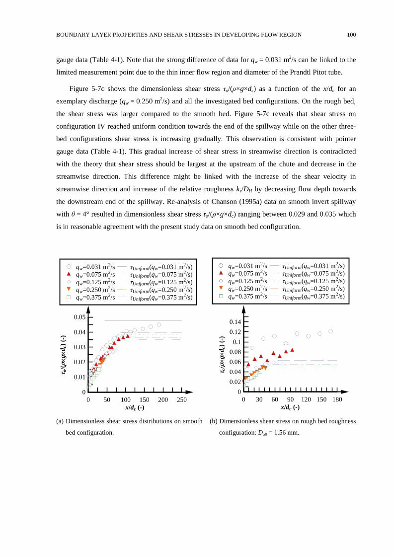
BOUNDARY LAYER PROPERTIES AND SHEAR STRESSES IN DEVELOPING FLOW REGION 100
gauge data (Table 4-1). Note that the strong difference of data for qw = 0.031 m2/s can be linked to the
limited measurement point due to the thin inner flow region and diameter of the Prandtl Pitot tube.
Figure 5-7c shows the dimensionless shear stress τo/(ρ×g×dc) as a function of the x/dc for an
exemplary discharge (qw = 0.250 m2/s) and all the investigated bed configurations. On the rough bed,
the shear stress was larger compared to the smooth bed. Figure 5-7c reveals that shear stress on
configuration IV reached uniform condition towards the end of the spillway while on the other three-
bed configurations shear stress is increasing gradually. This observation is consistent with pointer
gauge data (Table 4-1). This gradual increase of shear stress in streamwise direction is contradicted
with the theory that shear stress should be largest at the upstream of the chute and decrease in the
streamwise direction. This difference might be linked with the increase of the shear velocity in
streamwise direction and increase of the relative roughness ks/DH by decreasing flow depth towards
the downstream end of the spillway. Re-analysis of Chanson (1995a) data on smooth invert spillway
with θ = 4° resulted in dimensionless shear stress τo/(ρ×g×dc) ranging between 0.029 and 0.035 which
is in reasonable agreement with the present study data on smooth bed configuration.
(a) Dimensionless shear stress distributions on smooth
bed configuration.
(b) Dimensionless shear stress on rough bed roughness
configuration: D50 = 1.56 mm.
x/dc (-)
o/(
g
dc)
(-)
0 50 100 150 200 250
0
0.01
0.02
0.03
0.04
0.05
qw=0.031 m2/s
qw=0.075 m2/s
qw=0.125 m2/s
qw=0.250 m2/s
qw=0.375 m2/s
Uniform(qw=0.031 m2/s)
Uniform(qw=0.075 m2/s)
Uniform(qw=0.125 m2/s)
Uniform(qw=0.250 m2/s)
Uniform(qw=0.375 m2/s)
x/dc (-)
o/
g
dc)
(-)
0 30 60 90 120 150 180
0
0.02
0.04
0.06
0.08
0.1
0.12
0.14
qw=0.031 m2/s
qw=0.075 m2/s
qw=0.125 m2/s
qw=0.250 m2/s
qw=0.375 m2/s
Uniform(qw=0.031 m2/s)
Uniform(qw=0.075 m2/s)
Uniform(qw=0.125 m2/s)
Uniform(qw=0.250 m2/s)
Uniform(qw=0.375 m2/s)
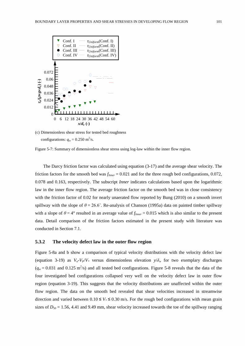
BOUNDARY LAYER PROPERTIES AND SHEAR STRESSES IN DEVELOPING FLOW REGION 101
(c) Dimensionless shear stress for tested bed roughness
configurations: qw = 0.250 m2/s.
Figure 5-7: Summary of dimensionless shear stress using log-law within the inner flow region.
The Darcy friction factor was calculated using equation (3-17) and the average shear velocity. The
friction factors for the smooth bed was fInner = 0.021 and for the three rough bed configurations, 0.072,
0.078 and 0.163, respectively. The subscript Inner indicates calculations based upon the logarithmic
law in the inner flow region. The average friction factor on the smooth bed was in close consistency
with the friction factor of 0.02 for nearly unaerated flow reported by Bung (2010) on a smooth invert
spillway with the slope of θ = 26.6˚. Re-analysis of Chanson (1995a) data on painted timber spillway
with a slope of θ = 4° resulted in an average value of fInner = 0.015 which is also similar to the present
data. Detail comparison of the friction factors estimated in the present study with literature was
conducted in Section 7.1.
5.3.2 The velocity defect law in the outer flow region
Figure 5-8a and b show a comparison of typical velocity distributions with the velocity defect law
(equation 3-19) as Vo-VP/V* versus dimensionless elevation y/δw for two exemplary discharges
(qw = 0.031 and 0.125 m2/s) and all tested bed configurations. Figure 5-8 reveals that the data of the
four investigated bed configurations collapsed very well on the velocity defect law in outer flow
region (equation 3-19). This suggests that the velocity distributions are unaffected within the outer
flow region. The data on the smooth bed revealed that shear velocities increased in streamwise
direction and varied between 0.10 ≤ V* ≤ 0.30 m/s. For the rough bed configurations with mean grain
sizes of D50 = 1.56, 4.41 and 9.49 mm, shear velocity increased towards the toe of the spillway ranging
x/dc (-)
o/(
g
dc)
(-)
0 6 12 18 24 30 36 42 48 54 60
0
0.012
0.024
0.036
0.048
0.06
0.072
Conf. I
Conf. II
Conf. III
Conf. IV
Uniform(Conf. I)
Uniform(Conf. II)
Uniform(Conf. III)
Uniform(Conf. IV)
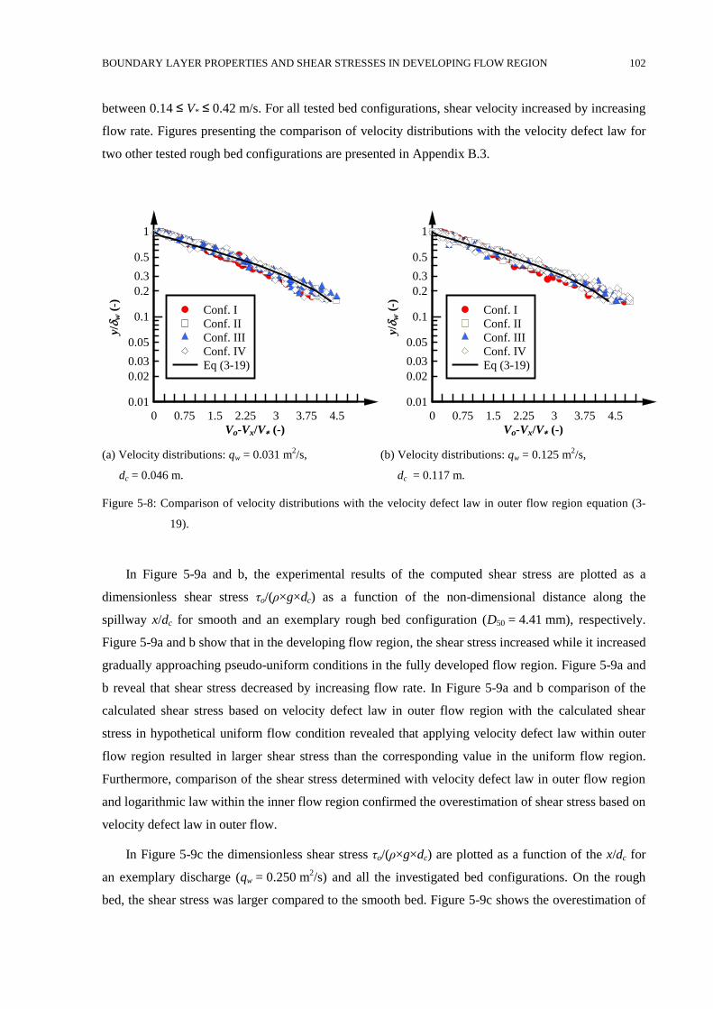
BOUNDARY LAYER PROPERTIES AND SHEAR STRESSES IN DEVELOPING FLOW REGION 102
between 0.14 ≤ V* ≤ 0.42 m/s. For all tested bed configurations, shear velocity increased by increasing
flow rate. Figures presenting the comparison of velocity distributions with the velocity defect law for
two other tested rough bed configurations are presented in Appendix B.3.
(a) Velocity distributions: qw = 0.031 m2/s,
dc = 0.046 m.
(b) Velocity distributions: qw = 0.125 m2/s,
dc = 0.117 m.
Figure 5-8: Comparison of velocity distributions with the velocity defect law in outer flow region equation (3-
19).
In Figure 5-9a and b, the experimental results of the computed shear stress are plotted as a
dimensionless shear stress τo/(ρ×g×dc) as a function of the non-dimensional distance along the
spillway x/dc for smooth and an exemplary rough bed configuration (D50 = 4.41 mm), respectively.
Figure 5-9a and b show that in the developing flow region, the shear stress increased while it increased
gradually approaching pseudo-uniform conditions in the fully developed flow region. Figure 5-9a and
b reveal that shear stress decreased by increasing flow rate. In Figure 5-9a and b comparison of the
calculated shear stress based on velocity defect law in outer flow region with the calculated shear
stress in hypothetical uniform flow condition revealed that applying velocity defect law within outer
flow region resulted in larger shear stress than the corresponding value in the uniform flow region.
Furthermore, comparison of the shear stress determined with velocity defect law in outer flow region
and logarithmic law within the inner flow region confirmed the overestimation of shear stress based on
velocity defect law in outer flow.
In Figure 5-9c the dimensionless shear stress τo/(ρ×g×dc) are plotted as a function of the x/dc for
an exemplary discharge (qw = 0.250 m2/s) and all the investigated bed configurations. On the rough
bed, the shear stress was larger compared to the smooth bed. Figure 5-9c shows the overestimation of
Vo-Vx/V (-)
y/
w (
-)
0 0.75 1.5 2.25 3 3.75 4.5
0.01
0.02
0.03
0.05
0.1
0.2
0.3
0.5
1
Conf. I
Conf. II
Conf. III
Conf. IV
Eq (3-19)
Vo-Vx/V (-)
y/
w (
-)
0 0.75 1.5 2.25 3 3.75 4.5
0.01
0.02
0.03
0.05
0.1
0.2
0.3
0.5
1
Conf. I
Conf. II
Conf. III
Conf. IV
Eq (3-19)
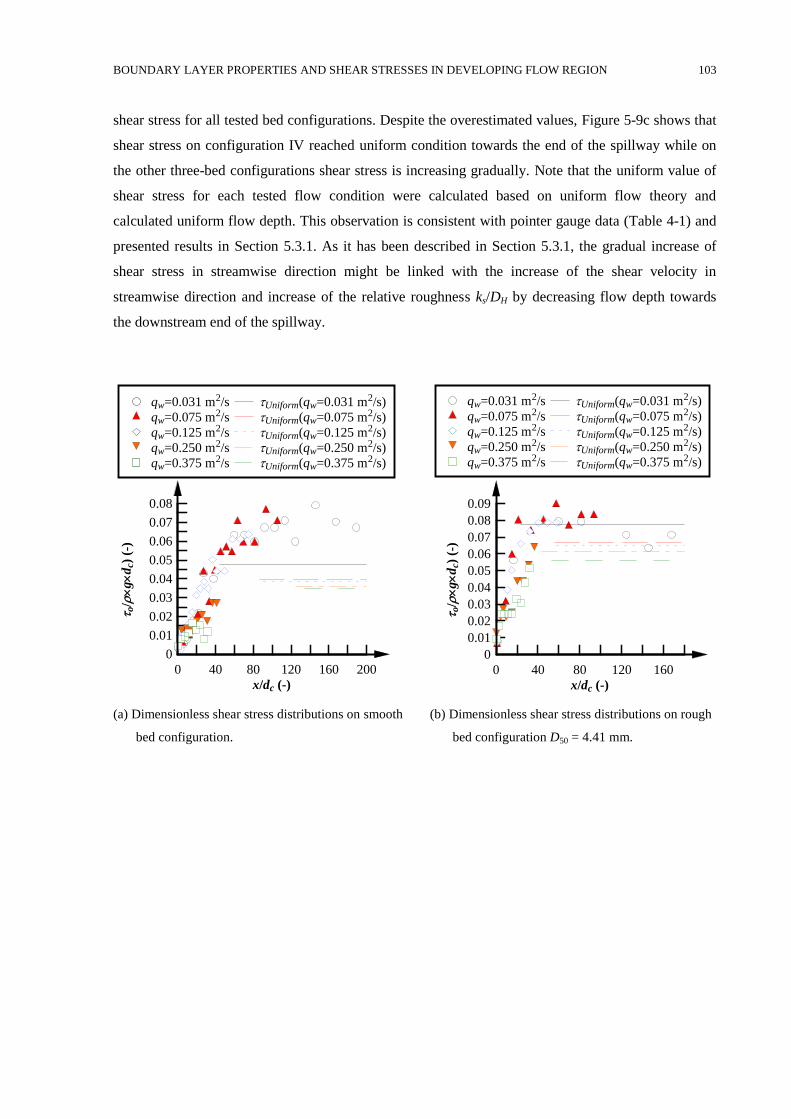
BOUNDARY LAYER PROPERTIES AND SHEAR STRESSES IN DEVELOPING FLOW REGION 103
shear stress for all tested bed configurations. Despite the overestimated values, Figure 5-9c shows that
shear stress on configuration IV reached uniform condition towards the end of the spillway while on
the other three-bed configurations shear stress is increasing gradually. Note that the uniform value of
shear stress for each tested flow condition were calculated based on uniform flow theory and
calculated uniform flow depth. This observation is consistent with pointer gauge data (Table 4-1) and
presented results in Section 5.3.1. As it has been described in Section 5.3.1, the gradual increase of
shear stress in streamwise direction might be linked with the increase of the shear velocity in
streamwise direction and increase of the relative roughness ks/DH by decreasing flow depth towards
the downstream end of the spillway.
(a) Dimensionless shear stress distributions on smooth
bed configuration.
(b) Dimensionless shear stress distributions on rough
bed configuration D50 = 4.41 mm.
x/dc (-)
o/
g
dc)
(-)
0 40 80 120 160 200
0
0.01
0.02
0.03
0.04
0.05
0.06
0.07
0.08
qw=0.031 m2/s
qw=0.075 m2/s
qw=0.125 m2/s
qw=0.250 m2/s
qw=0.375 m2/s
Uniform(qw=0.031 m2/s)
Uniform(qw=0.075 m2/s)
Uniform(qw=0.125 m2/s)
Uniform(qw=0.250 m2/s)
Uniform(qw=0.375 m2/s)
x/dc (-)
o/
g
dc)
(-)
0 40 80 120 160
0
0.01
0.02
0.03
0.04
0.05
0.06
0.07
0.08
0.09
qw=0.031 m2/s
qw=0.075 m2/s
qw=0.125 m2/s
qw=0.250 m2/s
qw=0.375 m2/s
Uniform(qw=0.031 m2/s)
Uniform(qw=0.075 m2/s)
Uniform(qw=0.125 m2/s)
Uniform(qw=0.250 m2/s)
Uniform(qw=0.375 m2/s)
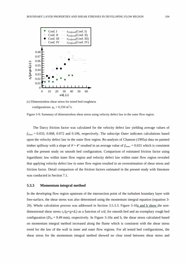
BOUNDARY LAYER PROPERTIES AND SHEAR STRESSES IN DEVELOPING FLOW REGION 104
(c) Dimensionless shear stress for tested bed roughness
configurations: qw = 0.250 m2/s.
Figure 5-9: Summary of dimensionless shear stress using velocity defect law in the outer flow region.
The Darcy friction factor was calculated for the velocity defect law yielding average values of
fOuter = 0.033, 0.068, 0.072 and 0.106, respectively. The subscript Outer indicates calculations based
upon the velocity defect law in the outer flow region. Re-analysis of Chanson (1995a) data on painted
timber spillway with a slope of θ = 4° resulted in an average value of fOuter = 0.031 which is consistent
with the present study on smooth bed configuration. Comparison of estimated friction factor using
logarithmic law within inner flow region and velocity defect law within outer flow region revealed
that applying velocity defect law in outer flow region resulted in an overestimation of shear stress and
friction factor. Detail comparison of the friction factors estimated in the present study with literature
was conducted in Section 7.1.
5.3.3 Momentum integral method
In the developing flow region upstream of the intersection point of the turbulent boundary layer with
free-surface, the shear stress was also determined using the momentum integral equation (equation 3-
20). Whole calculation process was addressed in Section 3.5.3.3. Figure 5-10a and b show the non-
dimensional shear stress τo/(ρ×g×dc) as a function of x/dc for smooth bed and an exemplary rough bed
configuration (D50 = 9.49 mm), respectively. In Figure 5-10a and b, the shear stress calculated based
on momentum integral method increased along the flume which is consistent with the shear stress
trend for the law of the wall in inner and outer flow regions. For all tested bed configurations, the
shear stress for the momentum integral method showed no clear trend between shear stress and
x/dc (-)
o/(
g
dc)
(-)
0 10 20 30 40 50 60
0
0.01
0.02
0.03
0.04
0.05
0.06
0.07
0.08
Conf. I
Conf. II
Conf. III
Conf. IV
Uniform(Conf. I)
Uniform(Conf. II)
Uniform(Conf. III)
Uniform(Conf. IV)
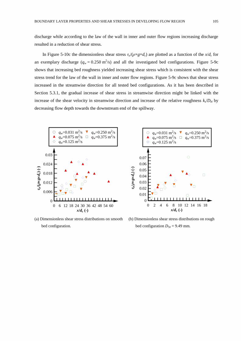
BOUNDARY LAYER PROPERTIES AND SHEAR STRESSES IN DEVELOPING FLOW REGION 105
discharge while according to the law of the wall in inner and outer flow regions increasing discharge
resulted in a reduction of shear stress.
In Figure 5-10c the dimensionless shear stress τo/(ρ×g×dc) are plotted as a function of the x/dc for
an exemplary discharge (qw = 0.250 m2/s) and all the investigated bed configurations. Figure 5-9c
shows that increasing bed roughness yielded increasing shear stress which is consistent with the shear
stress trend for the law of the wall in inner and outer flow regions. Figure 5-9c shows that shear stress
increased in the streamwise direction for all tested bed configurations. As it has been described in
Section 5.3.1, the gradual increase of shear stress in streamwise direction might be linked with the
increase of the shear velocity in streamwise direction and increase of the relative roughness ks/DH by
decreasing flow depth towards the downstream end of the spillway.
(a) Dimensionless shear stress distributions on smooth
bed configuration.
(b) Dimensionless shear stress distributions on rough
bed configuration D50 = 9.49 mm.
x/dc (-)
o/(
g
dc)
(-)
0 6 12 18 24 30 36 42 48 54 60
0
0.006
0.012
0.018
0.024
0.03
qw=0.031 m2/s
qw=0.075 m2/s
qw=0.125 m2/s
qw=0.250 m2/s
qw=0.375 m2/s
x/dc (-)
o/
g
dc)
(-)
0 2 4 6 8 10 12 14 16 18
0
0.01
0.02
0.03
0.04
0.05
0.06
0.07
qw=0.031 m2/s
qw=0.075 m2/s
qw=0.125 m2/s
qw=0.250 m2/s
qw=0.375 m2/s
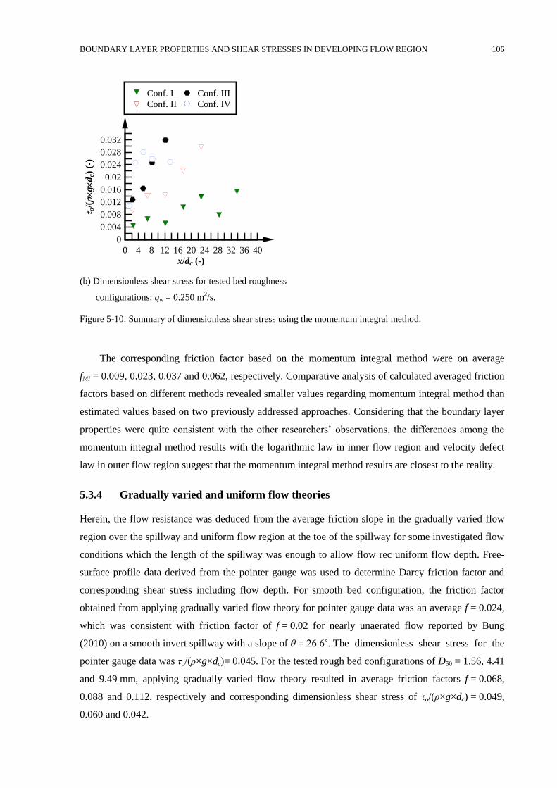
BOUNDARY LAYER PROPERTIES AND SHEAR STRESSES IN DEVELOPING FLOW REGION 106
(b) Dimensionless shear stress for tested bed roughness
configurations: qw = 0.250 m2/s.
Figure 5-10: Summary of dimensionless shear stress using the momentum integral method.
The corresponding friction factor based on the momentum integral method were on average
fMI = 0.009, 0.023, 0.037 and 0.062, respectively. Comparative analysis of calculated averaged friction
factors based on different methods revealed smaller values regarding momentum integral method than
estimated values based on two previously addressed approaches. Considering that the boundary layer
properties were quite consistent with the other researchers’ observations, the differences among the
momentum integral method results with the logarithmic law in inner flow region and velocity defect
law in outer flow region suggest that the momentum integral method results are closest to the reality.
5.3.4 Gradually varied and uniform flow theories
Herein, the flow resistance was deduced from the average friction slope in the gradually varied flow
region over the spillway and uniform flow region at the toe of the spillway for some investigated flow
conditions which the length of the spillway was enough to allow flow rec uniform flow depth. Free-
surface profile data derived from the pointer gauge was used to determine Darcy friction factor and
corresponding shear stress including flow depth. For smooth bed configuration, the friction factor
obtained from applying gradually varied flow theory for pointer gauge data was an average f = 0.024,
which was consistent with friction factor of f = 0.02 for nearly unaerated flow reported by Bung
(2010) on a smooth invert spillway with a slope of θ = 26.6˚. The dimensionless shear stress for the
pointer gauge data was τo/(ρ×g×dc)= 0.045. For the tested rough bed configurations of D50 = 1.56, 4.41
and 9.49 mm, applying gradually varied flow theory resulted in average friction factors f = 0.068,
0.088 and 0.112, respectively and corresponding dimensionless shear stress of τo/(ρ×g×dc) = 0.049,
0.060 and 0.042.
x/dc (-)
o/(
g
dc)
(-)
0 4 8 12 16 20 24 28 32 36 40
0
0.004
0.008
0.012
0.016
0.02
0.024
0.028
0.032
Conf. I
Conf. II
Conf. III
Conf. IV
BOUNDARY LAYER PROPERTIES AND SHEAR STRESSES IN DEVELOPING FLOW REGION 107
Further analysis was conducted to estimate the shear stress in the uniform flow region. Table 5-2
summarises the uniform flow region characteristics such as flow depth, friction factor and
dimensionless shear stress. For smooth bed configuration, shear stress varied between
0.035 ≤ τUniform ≤ 0.048 and for rough bed configuration of D50 = 1.56, 4.41 and 9.49 mm, shear
stresses varied ranging between 0.052 ≤ τUniform ≤ 0.066, 0.056 ≤ τUniform ≤ 0.082 and
0.061 ≤ τUniform ≤ 0.086, respectively. Subsequently, the friction factor in uniform flow region was
estimated. The results revealed that an increase in flow rate yielded a decrease in friction factor. For
smooth bed configuration, friction factor varied between 0.012 ≤ fUniform ≤ 0.026 with an average value
of fUniform = 0.016. For rough bed configuration of D50 = 1.56, 4.41 and 9.49 mm, friction factors varied
as 0.045 ≤ fUniform ≤ 0.074, 0.060 ≤ fUniform ≤ 0.133 and 0.079 ≤ fUniform ≤ 0.158, respectively. Also, the
average friction faction of rough bed configurations II, III and IV, are fUniform = 0.059, 0.085 and 0.112,
respectively.
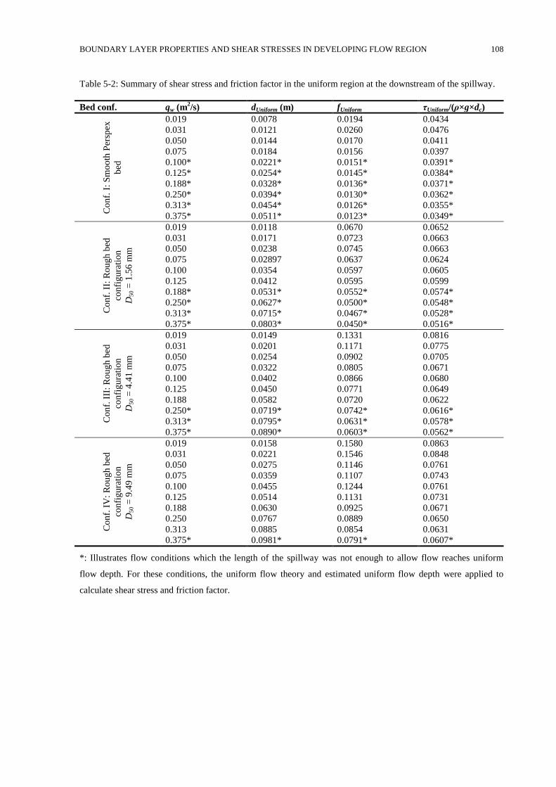
BOUNDARY LAYER PROPERTIES AND SHEAR STRESSES IN DEVELOPING FLOW REGION 108
Table 5-2: Summary of shear stress and friction factor in the uniform region at the downstream of the spillway.
Bed conf. qw (m2/s) dUniform (m) fUniform τUniform/(ρ×g×dc)
Co
nf.
I:
Sm
oo
th P
ersp
ex
bed
0.019 0.0078 0.0194 0.0434
0.031 0.0121 0.0260 0.0476
0.050 0.0144 0.0170 0.0411
0.075 0.0184 0.0156 0.0397
0.100* 0.0221* 0.0151* 0.0391*
0.125* 0.0254* 0.0145* 0.0384*
0.188* 0.0328* 0.0136* 0.0371*
0.250* 0.0394* 0.0130* 0.0362*
0.313* 0.0454* 0.0126* 0.0355*
0.375* 0.0511* 0.0123* 0.0349*
Co
nf.
II:
Ro
ug
h b
ed
con
fig
ura
tio
n
D50 =
1.5
6 m
m
0.019 0.0118 0.0670 0.0652
0.031 0.0171 0.0723 0.0663
0.050 0.0238 0.0745 0.0663
0.075 0.02897 0.0637 0.0624
0.100 0.0354 0.0597 0.0605
0.125 0.0412 0.0595 0.0599
0.188* 0.0531* 0.0552* 0.0574*
0.250* 0.0627* 0.0500* 0.0548*
0.313* 0.0715* 0.0467* 0.0528*
0.375* 0.0803* 0.0450* 0.0516*
Co
nf.
III
: R
oug
h b
ed
con
fig
ura
tio
n
D50 =
4.4
1 m
m
0.019 0.0149 0.1331 0.0816
0.031 0.0201 0.1171 0.0775
0.050 0.0254 0.0902 0.0705
0.075 0.0322 0.0805 0.0671
0.100 0.0402 0.0866 0.0680
0.125 0.0450 0.0771 0.0649
0.188 0.0582 0.0720 0.0622
0.250* 0.0719* 0.0742* 0.0616*
0.313* 0.0795* 0.0631* 0.0578*
0.375* 0.0890* 0.0603* 0.0562*
Co
nf.
IV
: R
ou
gh b
ed
con
fig
ura
tio
n
D50 =
9.4
9 m
m
0.019 0.0158 0.1580 0.0863
0.031 0.0221 0.1546 0.0848
0.050 0.0275 0.1146 0.0761
0.075 0.0359 0.1107 0.0743
0.100 0.0455 0.1244 0.0761
0.125 0.0514 0.1131 0.0731
0.188 0.0630 0.0925 0.0671
0.250 0.0767 0.0889 0.0650
0.313 0.0885 0.0854 0.0631
0.375* 0.0981* 0.0791* 0.0607*
*: Illustrates flow conditions which the length of the spillway was not enough to allow flow reaches uniform
flow depth. For these conditions, the uniform flow theory and estimated uniform flow depth were applied to
calculate shear stress and friction factor.
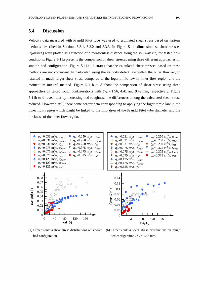
BOUNDARY LAYER PROPERTIES AND SHEAR STRESSES IN DEVELOPING FLOW REGION 109
Discussion 5.4
Velocity data measured with Prandtl Pitot tube was used to estimated shear stress based on various
methods described in Sections 5.3.1, 5.3.2 and 5.3.3. In Figure 5-11, dimensionless shear stresses
τ/(ρ×g×dc) were plotted as a function of dimensionless distance along the spillway x/dc for tested flow
conditions. Figure 5-11a presents the comparison of shear stresses using three different approaches on
smooth bed configuration. Figure 5-11a illustrates that the calculated shear stresses based on these
methods are not consistent. In particular, using the velocity defect law within the outer flow region
resulted in much larger shear stress compared to the logarithmic law in inner flow region and the
momentum integral method. Figure 5-11b to d show the comparison of shear stress using three
approaches on tested rough configurations with D50 = 1.56, 4.41 and 9.49 mm, respectively. Figure
5-11b to d reveal that by increasing bed roughness the differences among the calculated shear stress
reduced. However, still, there some scatter data corresponding to applying the logarithmic law in the
inner flow region which might be linked to the limitation of the Prandtl Pitot tube diameter and the
thickness of the inner flow region.
(a) Dimensionless shear stress distributions on smooth
bed configuration.
(b) Dimensionless shear stress distributions on rough
bed configuration D50 = 1.56 mm.
x/dc (-)
/
g
dc)
(-)
0 40 80 120 160
0
0.01
0.02
0.03
0.04
0.05
0.06
0.07
0.08
qw=0.031 m2/s, Inner
qw=0.031 m2/s, Outer
qw=0.031 m2/s, MI
qw=0.075 m2/s, Inner
qw=0.075 m2/s, Outer
qw=0.075 m2/s, MI
qw=0.125 m2/s, Inner
qw=0.125 m2/s, Outer
qw=0.125 m2/s, MI
qw=0.250 m2/s, Inner
qw=0.250 m2/s, Outer
qw=0.250 m2/s, MI
qw=0.375 m2/s, Inner
qw=0.375 m2/s, Outer
qw=0.375 m2/s, MI
x/dc (-)
/
g
dc)
(-)
0 40 80 120 160
0
0.02
0.04
0.06
0.08
0.1
0.12
0.14
qw=0.031 m2/s, Inner
qw=0.031 m2/s, Outer
qw=0.031 m2/s, MI
qw=0.075 m2/s, Inner
qw=0.075 m2/s, Outer
qw=0.075 m2/s, MI
qw=0.125 m2/s, Inner
qw=0.125 m2/s, Outer
qw=0.125 m2/s, MI
qw=0.250 m2/s, Inner
qw=0.250 m2/s, Outer
qw=0.250 m2/s, MI
qw=0.375 m2/s, Inner
qw=0.375 m2/s, Outer
qw=0.375 m2/s, MI
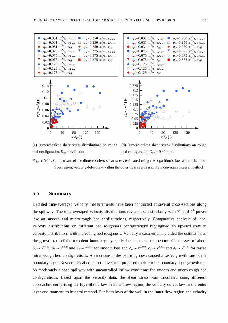
BOUNDARY LAYER PROPERTIES AND SHEAR STRESSES IN DEVELOPING FLOW REGION 110
(c) Dimensionless shear stress distributions on rough
bed configuration D50 = 4.41 mm.
(d) Dimensionless shear stress distributions on rough
bed configuration D50 = 9.49 mm.
Figure 5-11: Comparison of the dimensionless shear stress estimated using the logarithmic law within the inner
flow region, velocity defect law within the outer flow region and the momentum integral method.
Summary 5.5
Detailed time-averaged velocity measurements have been conducted at several cross-sections along
the spillway. The time-averaged velocity distributions revealed self-similarity with 7th and 4
th power
law on smooth and micro-rough bed configurations, respectively. Comparative analysis of local
velocity distributions on different bed roughness configurations highlighted an upward shift of
velocity distributions with increasing bed roughness. Velocity measurements yielded the estimation of
the growth rate of the turbulent boundary layer, displacement and momentum thicknesses of about
δw ∼ x0.838, δ1 ∼ x
0.533 and δ2 ∼ x
0.665 for smooth bed and δw ∼ x0.468
, δ1 ∼ x0.391
and δ2 ∼ x0.441
for tested
micro-rough bed configurations. An increase in the bed roughness caused a faster growth rate of the
boundary layer. New empirical equations have been proposed to determine boundary layer growth rate
on moderately sloped spillway with uncontrolled inflow conditions for smooth and micro-rough bed
configurations. Based upon the velocity data, the shear stress was calculated using different
approaches comprising the logarithmic law in inner flow region, the velocity defect law in the outer
layer and momentum integral method. For both laws of the wall in the inner flow region and velocity
x/dc (-)
/
g
dc)
(-)
0 40 80 120 160
0
0.02
0.04
0.06
0.08
0.1
0.12
0.14
qw=0.031 m2/s, Inner
qw=0.031 m2/s, Outer
qw=0.031 m2/s, MI
qw=0.075 m2/s, Inner
qw=0.075 m2/s, Outer
qw=0.075 m2/s, MI
qw=0.125 m2/s, Inner
qw=0.125 m2/s, Outer
qw=0.175 m2/s, MI
qw=0.250 m2/s, Inner
qw=0.250 m2/s, Outer
qw=0.250 m2/s, MI
qw=0.375 m2/s, Inner
qw=0.375 m2/s, Outer
qw=0.375 m2/s, MI
x/dc (-)
/
g
dc)
(-)
0 40 80 120 160
0
0.025
0.05
0.075
0.1
0.125
0.15
0.175
0.2
0.225
qw=0.031 m2/s, Inner
qw=0.031 m2/s, Outer
qw=0.031 m2/s, MI
qw=0.075 m2/s, Inner
qw=0.075 m2/s, Outer
qw=0.075 m2/s, MI
qw=0.125 m2/s, Inner
qw=0.125 m2/s, Outer
qw=0.125 m2/s, MI
qw=0.250 m2/s, Inner
qw=0.250 m2/s, Outer
qw=0.250 m2/s, MI
qw=0.375 m2/s, Inner
qw=0.375 m2/s, Outer
qw=0.375 m2/s, MI
BOUNDARY LAYER PROPERTIES AND SHEAR STRESSES IN DEVELOPING FLOW REGION 111
defect law in the outer region, the shear stress increased in gradually varied flow region approaching
pseudo-uniform value towards the toe of the spillway. The dimensionless shear stress calculated using
logarithmic law in the inner flow region revealed that shear stress approached uniform value at the end
of the spillway for some of the flow conditions. Comparative analysis of dimensionless shear stress
revealed that an increase in bed roughness resulted in an increase of shear stress and the corresponding
friction factor.
Chapter 6
6 AIR-WATER FLOW PROPERTIES IN THE FULLY
DEVELOPED FLOW REGION
Detailed measurements of the entrapped and entrained air properties were performed with a double-tip
conductivity probe downstream of the inception point of free-surface roughness at the same cross-
sections as the Pitot tube and pointer gauge measurements. The air-water flow properties included the
distributions of void fraction C, interface count rate F, interfacial time-averaged velocity VCP,
turbulence intensity Tu, auto- and cross-correlation time scales Txx and Txz, averaged chord length ch,
and air and water phase chord sizes. The calculation procedures of these properties were presented in
Section 3.5.4.
Void fraction 6.1
6.1.1 Selection of integration limit
Defining the free-surface in high-velocity flows over spillway is difficult due to free-surface
roughness, perturbations and fluctuations, as well as an undefined free-surface in air-water flows.
There is no final agreement on the most suitable flow depth defining the free-surface. Straub and
Anderson (1958) suggested characteristic depths between 0.95 < C < 0.99. Wood (1985) adopted an
integration limit of Y90 which is a widely used flow depth in air-water flows studies (Chanson, 1988).
Wood (1985) suggested Y90 as a characteristic depth in highly aerated flows because he observed that
for y < Y90, the air-water flow behaved as a homogeneous mixture and velocities of air and water
phases were assumed to be equal. In the last decades, following Wood (1985) Y90 is widely accepted as
the characteristic flow depth in any form of air-water flows including hydraulic jumps and various
types of spillways. Aivazyan (1986) considered flow depths Y98 and Y99 corresponding to void
fractions of C = 0.98 and 0.99 as an upper boundary of the free-surface in air-water flow over rough
bed spillways. Wilhelms and Gulliver (1994) reported that by increasing the integration limit, the
entrapped void fractions on air-water flow over smooth invert spillway showed less variability;
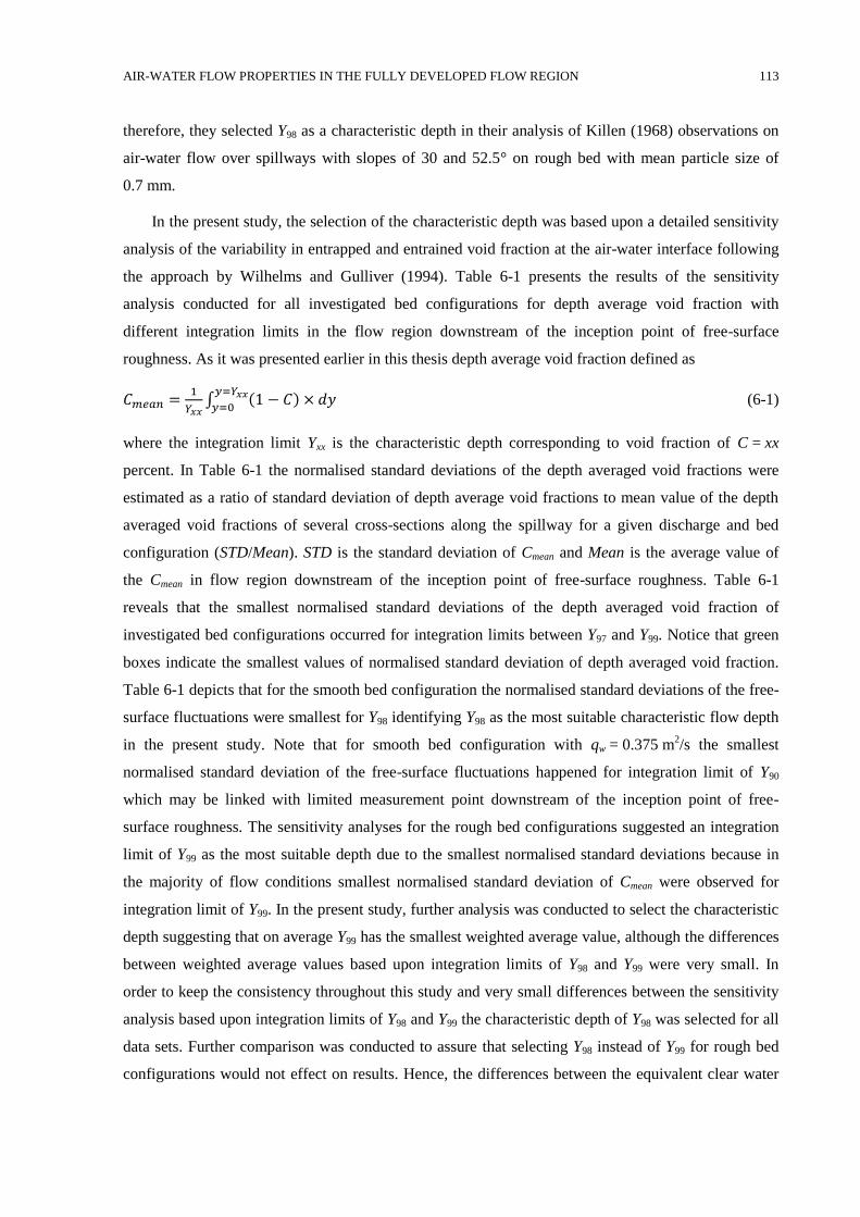
AIR-WATER FLOW PROPERTIES IN THE FULLY DEVELOPED FLOW REGION 113
therefore, they selected Y98 as a characteristic depth in their analysis of Killen (1968) observations on
air-water flow over spillways with slopes of 30 and 52.5° on rough bed with mean particle size of
0.7 mm.
In the present study, the selection of the characteristic depth was based upon a detailed sensitivity
analysis of the variability in entrapped and entrained void fraction at the air-water interface following
the approach by Wilhelms and Gulliver (1994). Table 6-1 presents the results of the sensitivity
analysis conducted for all investigated bed configurations for depth average void fraction with
different integration limits in the flow region downstream of the inception point of free-surface
roughness. As it was presented earlier in this thesis depth average void fraction defined as
𝐶𝑚𝑒𝑎𝑛 =1
𝑌𝑥𝑥∫ (1 − 𝐶)
𝑦=𝑌𝑥𝑥
𝑦=0× 𝑑𝑦 (6-1)
where the integration limit Yxx is the characteristic depth corresponding to void fraction of C = xx
percent. In Table 6-1 the normalised standard deviations of the depth averaged void fractions were
estimated as a ratio of standard deviation of depth average void fractions to mean value of the depth
averaged void fractions of several cross-sections along the spillway for a given discharge and bed
configuration (STD/Mean). STD is the standard deviation of Cmean and Mean is the average value of
the Cmean in flow region downstream of the inception point of free-surface roughness. Table 6-1
reveals that the smallest normalised standard deviations of the depth averaged void fraction of
investigated bed configurations occurred for integration limits between Y97 and Y99. Notice that green
boxes indicate the smallest values of normalised standard deviation of depth averaged void fraction.
Table 6-1 depicts that for the smooth bed configuration the normalised standard deviations of the free-
surface fluctuations were smallest for Y98 identifying Y98 as the most suitable characteristic flow depth
in the present study. Note that for smooth bed configuration with qw = 0.375 m2/s the smallest
normalised standard deviation of the free-surface fluctuations happened for integration limit of Y90
which may be linked with limited measurement point downstream of the inception point of free-
surface roughness. The sensitivity analyses for the rough bed configurations suggested an integration
limit of Y99 as the most suitable depth due to the smallest normalised standard deviations because in
the majority of flow conditions smallest normalised standard deviation of Cmean were observed for
integration limit of Y99. In the present study, further analysis was conducted to select the characteristic
depth suggesting that on average Y99 has the smallest weighted average value, although the differences
between weighted average values based upon integration limits of Y98 and Y99 were very small. In
order to keep the consistency throughout this study and very small differences between the sensitivity
analysis based upon integration limits of Y98 and Y99 the characteristic depth of Y98 was selected for all
data sets. Further comparison was conducted to assure that selecting Y98 instead of Y99 for rough bed
configurations would not effect on results. Hence, the differences between the equivalent clear water
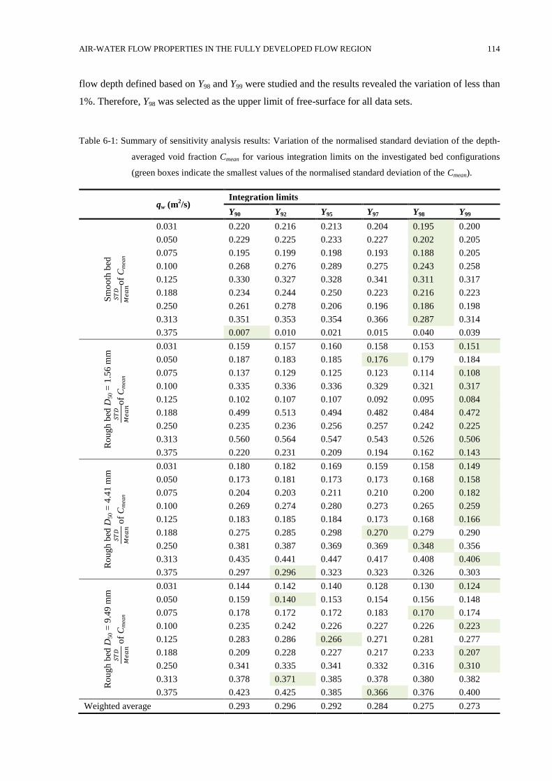
AIR-WATER FLOW PROPERTIES IN THE FULLY DEVELOPED FLOW REGION 114
flow depth defined based on Y98 and Y99 were studied and the results revealed the variation of less than
1%. Therefore, Y98 was selected as the upper limit of free-surface for all data sets.
Table 6-1: Summary of sensitivity analysis results: Variation of the normalised standard deviation of the depth-
averaged void fraction Cmean for various integration limits on the investigated bed configurations
(green boxes indicate the smallest values of the normalised standard deviation of the Cmean).
qw (m2/s)
Integration limits
Y90 Y92 Y95 Y97 Y98 Y99
Sm
oo
th b
ed
𝑆𝑇
𝐷
𝑀𝑒
𝑎𝑛o
f C
mea
n
0.031 0.220 0.216 0.213 0.204 0.195 0.200
0.050 0.229 0.225 0.233 0.227 0.202 0.205
0.075 0.195 0.199 0.198 0.193 0.188 0.205
0.100 0.268 0.276 0.289 0.275 0.243 0.258
0.125 0.330 0.327 0.328 0.341 0.311 0.317
0.188 0.234 0.244 0.250 0.223 0.216 0.223
0.250 0.261 0.278 0.206 0.196 0.186 0.198
0.313 0.351 0.353 0.354 0.366 0.287 0.314
0.375 0.007 0.010 0.021 0.015 0.040 0.039
Ro
ug
h b
ed D
50 =
1.5
6 m
m
𝑆𝑇
𝐷
𝑀𝑒
𝑎𝑛o
f C
mea
n
0.031 0.159 0.157 0.160 0.158 0.153 0.151
0.050 0.187 0.183 0.185 0.176 0.179 0.184
0.075 0.137 0.129 0.125 0.123 0.114 0.108
0.100 0.335 0.336 0.336 0.329 0.321 0.317
0.125 0.102 0.107 0.107 0.092 0.095 0.084
0.188 0.499 0.513 0.494 0.482 0.484 0.472
0.250 0.235 0.236 0.256 0.257 0.242 0.225
0.313 0.560 0.564 0.547 0.543 0.526 0.506
0.375 0.220 0.231 0.209 0.194 0.162 0.143
Ro
ug
h b
ed D
50 =
4.4
1 m
m
𝑆𝑇
𝐷
𝑀𝑒
𝑎𝑛 o
f C
mea
n
0.031 0.180 0.182 0.169 0.159 0.158 0.149
0.050 0.173 0.181 0.173 0.173 0.168 0.158
0.075 0.204 0.203 0.211 0.210 0.200 0.182
0.100 0.269 0.274 0.280 0.273 0.265 0.259
0.125 0.183 0.185 0.184 0.173 0.168 0.166
0.188 0.275 0.285 0.298 0.270 0.279 0.290
0.250 0.381 0.387 0.369 0.369 0.348 0.356
0.313 0.435 0.441 0.447 0.417 0.408 0.406
0.375 0.297 0.296 0.323 0.323 0.326 0.303
Ro
ug
h b
ed D
50 =
9.4
9 m
m
𝑆𝑇
𝐷
𝑀𝑒
𝑎𝑛 o
f C
mea
n
0.031 0.144 0.142 0.140 0.128 0.130 0.124
0.050 0.159 0.140 0.153 0.154 0.156 0.148
0.075 0.178 0.172 0.172 0.183 0.170 0.174
0.100 0.235 0.242 0.226 0.227 0.226 0.223
0.125 0.283 0.286 0.266 0.271 0.281 0.277
0.188 0.209 0.228 0.227 0.217 0.233 0.207
0.250 0.341 0.335 0.341 0.332 0.316 0.310
0.313 0.378 0.371 0.385 0.378 0.380 0.382
0.375 0.423 0.425 0.385 0.366 0.376 0.400
Weighted average 0.293 0.296 0.292 0.284 0.275 0.273
AIR-WATER FLOW PROPERTIES IN THE FULLY DEVELOPED FLOW REGION 115
6.1.2 Void fraction distributions
Typical void fraction distributions are presented in Figure 6-1. The void fraction distributions are
illustrated as a function of the dimensionless vertical elevation y/Y98. For all flow conditions, the void
fraction distributions had typical S-shape profiles. Figure 6-1a illustrates the void fraction distributions
on the smooth bed configuration, indicating that in the clear water flow region underneath the
entrapped air region (y/Y98 < 0.6), no void fraction was observed (C ≈ 0) which was consistent with the
visual observations reported in Section 4.1.3. In the air flow region above the entrapped air region
(y/Y98 > 1.05), the void fraction was close to unity (C ≈ 1) highlighting that no water droplets and
water projections were observed within this region (see Section 4.1.3). Figure 6-1a shows that in the
flow region characterised by entrapped air (0.6 < y/Y98 < 1.05), the void fraction increased steeply over
a small section of the flow depth. For the same flow rate, a downward shift of void fraction
distributions in the streamwise direction has been observed indicating an increase in the thickness of
the entrapped air region and the depth-averaged void fraction towards the toe of the spillway. The
results suggested that the void fraction distributions did not reach uniform conditions at the
downstream end of the smooth spillway. This suggested that while the flow depth approached a
constant value at the toe of the spillway for some flow conditions (See Table 4-1), the void fraction
still increased gradually.
Figure 6-1b presents typical void fraction distributions at several cross-sections downstream of
the inception point of free-surface roughness (hollow symbols) and downstream of the inception point
of free-surface aeration (solid coloured symbols) on a spillway with rough bed configuration. Note
that for rough bed configurations to calculate dimensionless flow depth y/Y98, zero velocity level zo has
been taken into account. The details about the approach to estimate zo were presented in Section
3.5.3.1. The void fraction distributions on rough bed had typical S-shape profiles. More figures of void
fraction distribution were provided in Appendix C. For the rough bed configurations, no void fraction
(C ≈ 0) was observed in the clear water flow region (y/Y98 < 0.4) highlighting that no air bubbles
reached the region close to the bed. This finding was consistent with visual observations (section
4.1.3). According to the visual observations flow on rough bed configurations were characterised by
entrapped air between free-surface roughness and entrained air into the flow. Hence, the double-tip
conductivity probe measured both void fractions due to the free-surface roughness within entrapped
flow region and air bubbles within entrained air region; so-called total conveyed (Wilhelms and
Gulliver, 2005) void fraction. In the flow region of total conveyed air (0.4 < y/Y98 < 1.05), the void
fraction increased gradually over a section of the flow depth containing free-surface roughness and
entrained air. Similar to the smooth bed data, a downward shift of the void fraction distributions in
streamwise direction was observed indicating an increase in the thickness of the total conveyed air
region and the depth-average void fraction. This gradual increase of Cmean highlighted that the void
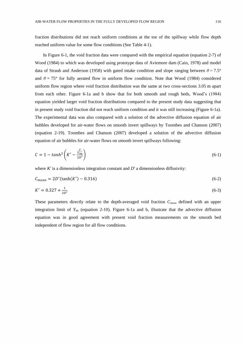
AIR-WATER FLOW PROPERTIES IN THE FULLY DEVELOPED FLOW REGION 116
fraction distributions did not reach uniform conditions at the toe of the spillway while flow depth
reached uniform value for some flow conditions (See Table 4-1).
In Figure 6-1, the void fraction data were compared with the empirical equation (equation 2-7) of
Wood (1984) to which was developed using prototype data of Aviemore dam (Cain, 1978) and model
data of Straub and Anderson (1958) with gated intake condition and slope ranging between θ = 7.5°
and θ = 75° for fully aerated flow in uniform flow condition. Note that Wood (1984) considered
uniform flow region where void fraction distribution was the same at two cross-sections 3.05 m apart
from each other. Figure 6-1a and b show that for both smooth and rough beds, Wood’s (1984)
equation yielded larger void fraction distributions compared to the present study data suggesting that
in present study void fraction did not reach uniform condition and it was still increasing (Figure 6-1a).
The experimental data was also compared with a solution of the advective diffusion equation of air
bubbles developed for air-water flows on smooth invert spillways by Toombes and Chanson (2007)
(equation 2-19). Toombes and Chanson (2007) developed a solution of the advective diffusion
equation of air bubbles for air-water flows on smooth invert spillways following:
𝐶 = 1 − 𝑡𝑎𝑛ℎ2 (𝐾′ −
𝑦
𝑌90
2𝐷′ ) (6-1)
where K' is a dimensionless integration constant and D' a dimensionless diffusivity:
𝐶𝑚𝑒𝑎𝑛 = 2𝐷′(tanh(𝐾′) − 0.316) (6-2)
𝐾′ = 0.327 +1
2𝐷′ (6-3)
These parameters directly relate to the depth-averaged void fraction Cmean defined with an upper
integration limit of Y90 (equation 2-10). Figure 6-1a and b, illustrate that the advective diffusion
equation was in good agreement with present void fraction measurements on the smooth bed
independent of flow region for all flow conditions.
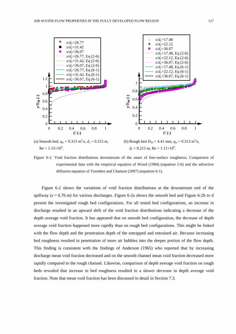
AIR-WATER FLOW PROPERTIES IN THE FULLY DEVELOPED FLOW REGION 117
(a) Smooth bed, qw = 0.313 m2/s, dc = 0.215 m,
Re = 1.15×10⁶.
(b) Rough bed D50 = 4.41 mm, qw = 0.313 m2/s,
dc = 0.215 m, Re = 1.11×10⁶.
Figure 6-1: Void fraction distributions downstream of the onset of free-surface roughness; Comparison of
experimental data with the empirical equation of Wood (1984) (equation 2-6) and the advective
diffusion equation of Toombes and Chanson (2007) (equation 6-1).
Figure 6-2 shows the variations of void fraction distributions at the downstream end of the
spillway (x = 6.76 m) for various discharges. Figure 6-2a shows the smooth bed and Figure 6-2b to d
present the investigated rough bed configurations. For all tested bed configurations, an increase in
discharge resulted in an upward shift of the void fraction distributions indicating a decrease of the
depth average void fraction. It has appeared that on smooth bed configuration, the decrease of depth
average void fraction happened more rapidly than on rough bed configurations. This might be linked
with the flow depth and the penetration depth of the entrapped and entrained air. Because increasing
bed roughness resulted in penetration of more air bubbles into the deeper portion of the flow depth.
This finding is consistent with the findings of Anderson (1965) who reported that by increasing
discharge mean void fraction decreased and on the smooth channel mean void fraction decreased more
rapidly compared to the rough channel. Likewise, comparison of depth average void fraction on rough
beds revealed that increase in bed roughness resulted in a slower decrease in depth average void
fraction. Note that mean void fraction has been discussed in detail in Section 7.3.
C (-)
y/Y
98 (
-)
0 0.2 0.4 0.6 0.8 1
0
0.2
0.4
0.6
0.8
1
1.2
x/dc=26.77
x/dc=31.42
x/dc=36.07
x/dc=26.77, Eq (2-6)
x/dc=31.42, Eq (2-6)
x/dc=36.07, Eq (2-6)
x/dc=26.77, Eq (6-1)
x/dc=31.42, Eq (6-1)
x/dc=36.07, Eq (6-1)
C (-)
y/Y
98 (
-)0 0.2 0.4 0.6 0.8 1
0
0.2
0.4
0.6
0.8
1
x/dc=17.48
x/dc=22.12
x/dc=36.07
x/dc=17.48, Eq (2-6)
x/dc=22.12, Eq (2-6)
x/dc=36.07, Eq (2-6)
x/dc=17.48, Eq (6-1)
x/dc=22.12, Eq (6-1)
x/dc=36.07, Eq (6-1)
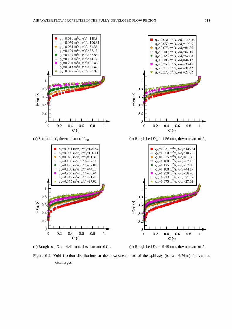
AIR-WATER FLOW PROPERTIES IN THE FULLY DEVELOPED FLOW REGION 118
(a) Smooth bed, downstream of LFR. (b) Rough bed D50 = 1.56 mm, downstream of LI.
(c) Rough bed D50 = 4.41 mm, downstream of LI.. (d) Rough bed D50 = 9.49 mm, downstream of LI.
Figure 6-2: Void fraction distributions at the downstream end of the spillway (for x = 6.76 m) for various
discharges.
C (-)
y/Y
98 (
-)
0 0.2 0.4 0.6 0.8 1
0
0.2
0.4
0.6
0.8
1
qw=0.031 m2/s, x/dc=145.84
qw=0.050 m2/s, x/dc=106.61
qw=0.075 m2/s, x/dc=81.36
qw=0.100 m2/s, x/dc=67.16
qw=0.125 m2/s, x/dc=57.88
qw=0.188 m2/s, x/dc=44.17
qw=0.250 m2/s, x/dc=36.46
qw=0.313 m2/s, x/dc=31.42
qw=0.375 m2/s, x/dc=27.82
C (-)y/
Y9
8 (
-)
0 0.2 0.4 0.6 0.8 1
0
0.2
0.4
0.6
0.8
1
qw=0.031 m2/s, x/dc=145.84
qw=0.050 m2/s, x/dc=106.61
qw=0.075 m2/s, x/dc=81.36
qw=0.100 m2/s, x/dc=67.16
qw=0.125 m2/s, x/dc=57.88
qw=0.188 m2/s, x/dc=44.17
qw=0.250 m2/s, x/dc=36.46
qw=0.313 m2/s, x/dc=31.42
qw=0.375 m2/s, x/dc=27.82
C (-)
y/Y
98 (
-)
0 0.2 0.4 0.6 0.8 1
0
0.2
0.4
0.6
0.8
1
qw=0.031 m2/s, x/dc=145.84
qw=0.050 m2/s, x/dc=106.61
qw=0.075 m2/s, x/dc=81.36
qw=0.100 m2/s, x/dc=67.16
qw=0.125 m2/s, x/dc=57.88
qw=0.188 m2/s, x/dc=44.17
qw=0.250 m2/s, x/dc=36.46
qw=0.313 m2/s, x/dc=31.42
qw=0.375 m2/s, x/dc=27.82
C (-)
y/Y
98 (
-)
0 0.2 0.4 0.6 0.8 1
0
0.2
0.4
0.6
0.8
1
qw=0.031 m2/s, x/dc=145.84
qw=0.050 m2/s, x/dc=106.61
qw=0.075 m2/s, x/dc=81.36
qw=0.100 m2/s, x/dc=67.16
qw=0.125 m2/s, x/dc=57.88
qw=0.188 m2/s, x/dc=44.17
qw=0.250 m2/s, x/dc=36.46
qw=0.313 m2/s, x/dc=31.42
qw=0.375 m2/s, x/dc=27.82
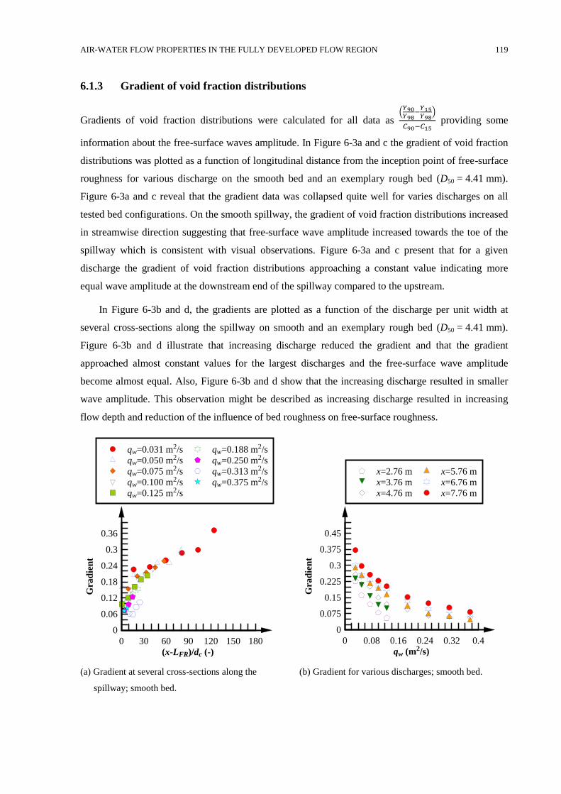
AIR-WATER FLOW PROPERTIES IN THE FULLY DEVELOPED FLOW REGION 119
6.1.3 Gradient of void fraction distributions
Gradients of void fraction distributions were calculated for all data as (
𝑌90𝑌98
−𝑌15𝑌98
)
𝐶90−𝐶15 providing some
information about the free-surface waves amplitude. In Figure 6-3a and c the gradient of void fraction
distributions was plotted as a function of longitudinal distance from the inception point of free-surface
roughness for various discharge on the smooth bed and an exemplary rough bed (D50 = 4.41 mm).
Figure 6-3a and c reveal that the gradient data was collapsed quite well for varies discharges on all
tested bed configurations. On the smooth spillway, the gradient of void fraction distributions increased
in streamwise direction suggesting that free-surface wave amplitude increased towards the toe of the
spillway which is consistent with visual observations. Figure 6-3a and c present that for a given
discharge the gradient of void fraction distributions approaching a constant value indicating more
equal wave amplitude at the downstream end of the spillway compared to the upstream.
In Figure 6-3b and d, the gradients are plotted as a function of the discharge per unit width at
several cross-sections along the spillway on smooth and an exemplary rough bed (D50 = 4.41 mm).
Figure 6-3b and d illustrate that increasing discharge reduced the gradient and that the gradient
approached almost constant values for the largest discharges and the free-surface wave amplitude
become almost equal. Also, Figure 6-3b and d show that the increasing discharge resulted in smaller
wave amplitude. This observation might be described as increasing discharge resulted in increasing
flow depth and reduction of the influence of bed roughness on free-surface roughness.
(a) Gradient at several cross-sections along the
spillway; smooth bed.
(b) Gradient for various discharges; smooth bed.
(x-LFR)/dc (-)
Gra
die
nt
0 30 60 90 120 150 180
0
0.06
0.12
0.18
0.24
0.3
0.36
qw=0.031 m2/s
qw=0.050 m2/s
qw=0.075 m2/s
qw=0.100 m2/s
qw=0.125 m2/s
qw=0.188 m2/s
qw=0.250 m2/s
qw=0.313 m2/s
qw=0.375 m2/s
qw (m2/s)
Gra
die
nt
0 0.08 0.16 0.24 0.32 0.4
0
0.075
0.15
0.225
0.3
0.375
0.45
x=2.76 m
x=3.76 m
x=4.76 m
x=5.76 m
x=6.76 m
x=7.76 m
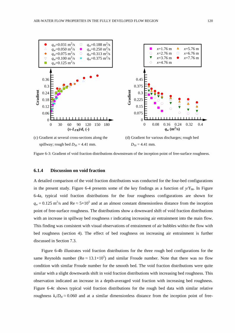
AIR-WATER FLOW PROPERTIES IN THE FULLY DEVELOPED FLOW REGION 120
(c) Gradient at several cross-sections along the
spillway; rough bed D50 = 4.41 mm.
(d) Gradient for various discharges; rough bed
D50 = 4.41 mm.
Figure 6-3: Gradient of void fraction distributions downstream of the inception point of free-surface roughness.
6.1.4 Discussion on void fraction
A detailed comparison of the void fraction distributions was conducted for the four-bed configurations
in the present study. Figure 6-4 presents some of the key findings as a function of y/Y98. In Figure
6-4a, typical void fraction distributions for the four roughness configurations are shown for
qw = 0.125 m2/s and Re ≈ 5×10
5 and at an almost constant dimensionless distance from the inception
point of free-surface roughness. The distributions show a downward shift of void fraction distributions
with an increase in spillway bed roughness r indicating increasing air entrainment into the main flow.
This finding was consistent with visual observations of entrainment of air bubbles within the flow with
bed roughness (section 4). The effect of bed roughness on increasing air entrainment is further
discussed in Section 7.3.
Figure 6-4b illustrates void fraction distributions for the three rough bed configurations for the
same Reynolds number (Re ≈ 13.1×10⁵) and similar Froude number. Note that there was no flow
condition with similar Froude number for the smooth bed. The void fraction distributions were quite
similar with a slight downwards shift in void fraction distributions with increasing bed roughness. This
observation indicated an increase in a depth-averaged void fraction with increasing bed roughness.
Figure 6-4c shows typical void fraction distributions for the rough bed data with similar relative
roughness ks/DH ≈ 0.060 and at a similar dimensionless distance from the inception point of free-
(x-LFR)/dc (-)
Gra
die
nt
0 30 60 90 120 150 180
0
0.06
0.12
0.18
0.24
0.3
0.36
qw=0.031 m2/s
qw=0.050 m2/s
qw=0.075 m2/s
qw=0.100 m2/s
qw=0.125 m2/s
qw=0.188 m2/s
qw=0.250 m2/s
qw=0.313 m2/s
qw=0.375 m2/s
qw (m2/s)G
rad
ien
t
0 0.08 0.16 0.24 0.32 0.4
0
0.075
0.15
0.225
0.3
0.375
0.45
x=1.76 m
x=2.76 m
x=3.76 m
x=4.76 m
x=5.76 m
x=6.76 m
x=7.76 m
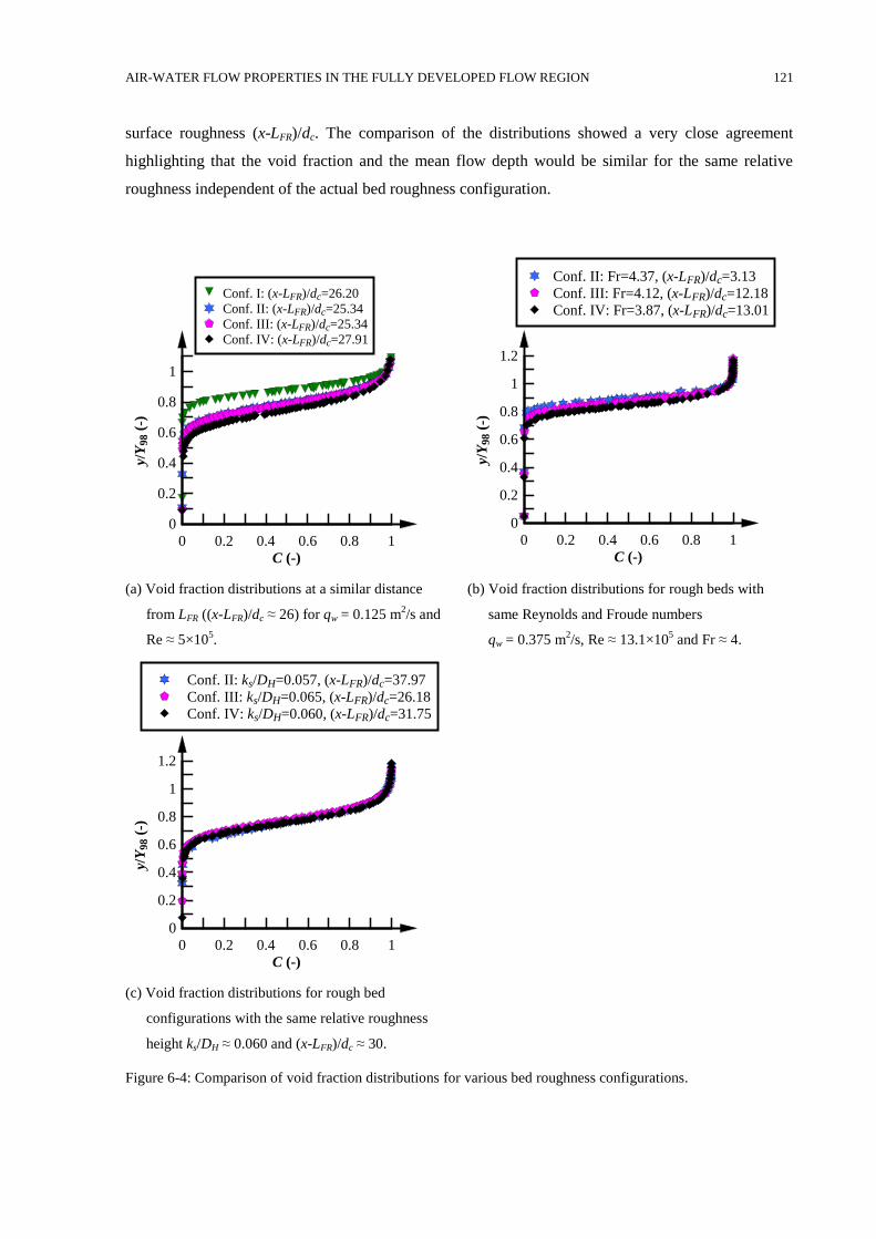
AIR-WATER FLOW PROPERTIES IN THE FULLY DEVELOPED FLOW REGION 121
surface roughness (x-LFR)/dc. The comparison of the distributions showed a very close agreement
highlighting that the void fraction and the mean flow depth would be similar for the same relative
roughness independent of the actual bed roughness configuration.
(a) Void fraction distributions at a similar distance
from LFR ((x-LFR)/dc ≈ 26) for qw = 0.125 m2/s and
Re ≈ 5×10⁵.
(b) Void fraction distributions for rough beds with
same Reynolds and Froude numbers
qw = 0.375 m2/s, Re ≈ 13.1×10
5 and Fr ≈ 4.
(c) Void fraction distributions for rough bed
configurations with the same relative roughness
height ks/DH ≈ 0.060 and (x-LFR)/dc ≈ 30.
Figure 6-4: Comparison of void fraction distributions for various bed roughness configurations.
C (-)
y/Y
98 (
-)
0 0.2 0.4 0.6 0.8 1
0
0.2
0.4
0.6
0.8
1
Conf. I: (x-LFR)/dc=26.20
Conf. II: (x-LFR)/dc=25.34
Conf. III: (x-LFR)/dc=25.34
Conf. IV: (x-LFR)/dc=27.91
C (-)
y/Y
98 (
-)
0 0.2 0.4 0.6 0.8 1
0
0.2
0.4
0.6
0.8
1
1.2
Conf. II: Fr=4.37, (x-LFR)/dc=3.13
Conf. III: Fr=4.12, (x-LFR)/dc=12.18
Conf. IV: Fr=3.87, (x-LFR)/dc=13.01
C (-)
y/Y
98 (
-)
0 0.2 0.4 0.6 0.8 1
0
0.2
0.4
0.6
0.8
1
1.2
Conf. II: ks/DH=0.057, (x-LFR)/dc=37.97
Conf. III: ks/DH=0.065, (x-LFR)/dc=26.18
Conf. IV: ks/DH=0.060, (x-LFR)/dc=31.75
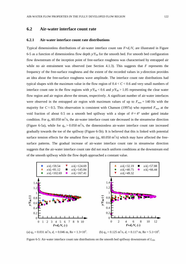
AIR-WATER FLOW PROPERTIES IN THE FULLY DEVELOPED FLOW REGION 122
Air-water interface count rate 6.2
6.2.1 Air-water interface count rate distributions
Typical dimensionless distributions of air-water interface count rate F×dc/Vc are illustrated in Figure
6-5 as a function of dimensionless flow depth y/Y98 for the smooth bed. For smooth bed configuration
flow downstream of the inception point of free-surface roughness was characterised by entrapped air
while no air entrainment was observed (see Section 4.1.3). This suggests that F represents the
frequency of the free-surface roughness and the extent of the recorded values in y-direction provides
an idea about the free-surface roughness wave amplitude. The interface count rate distributions had
typical shapes with the maximum value in the flow region of 0.4 < C < 0.6 and very small numbers of
interface count rate in the flow regions with y/Y98 < 0.6 and y/Y98 > 1.05 representing the clear water
flow region and air region above the stream, respectively. A significant number of air-water interfaces
were observed in the entrapped air region with maximum values of up to Fmax = 140 Hz with the
majority for C ≈ 0.5. This observation is consistent with Chanson (1997a) who reported Fmax at the
void fraction of about 0.5 on a smooth bed spillway with a slope of θ = 4° under gated intake
condition. For qw ≤0.050 m2/s, the air-water interface count rate decreased in the streamwise direction
(Figure 6-5a), while for qw > 0.050 m2/s, the dimensionless air-water interface count rate increased
gradually towards the toe of the spillway (Figure 6-5b). It is believed that this is linked with potential
surface tension effects for the smallest flow rate (qw ≤0.050 m2/s) which may have affected the free-
surface patterns. The gradual increase of air-water interface count rate in streamwise direction
suggests that the air-water interface count rate did not reach uniform conditions at the downstream end
of the smooth spillway while the flow depth approached a constant value.
(a) qw = 0.031 m2/s, dc = 0.046 m, Re = 1.3×10
5. (b) qw = 0.125 m
2/s, dc = 0.117 m, Re = 5.1×10
5.
Figure 6-5: Air-water interface count rate distributions on the smooth bed spillway downstream of LFR.
Fdc/Vc (-)
y/Y
98 (
-)
0 1 2 3 4 5 6 7 8 9 10
0
0.2
0.4
0.6
0.8
1
1.2
1.4
x/dc=59.54
x/dc=81.12
x/dc=102.69
x/dc=124.69
x/dc=145.84
x/dc=167.41
Fdc/Vc (-)
y/Y
98 (
-)
0 2 4 6 8 10 12
0
0.2
0.4
0.6
0.8
1
1.2
1.4
x/dc=32.19
x/dc=40.75
x/dc=49.32
x/dc=57.88
x/dc=66.44
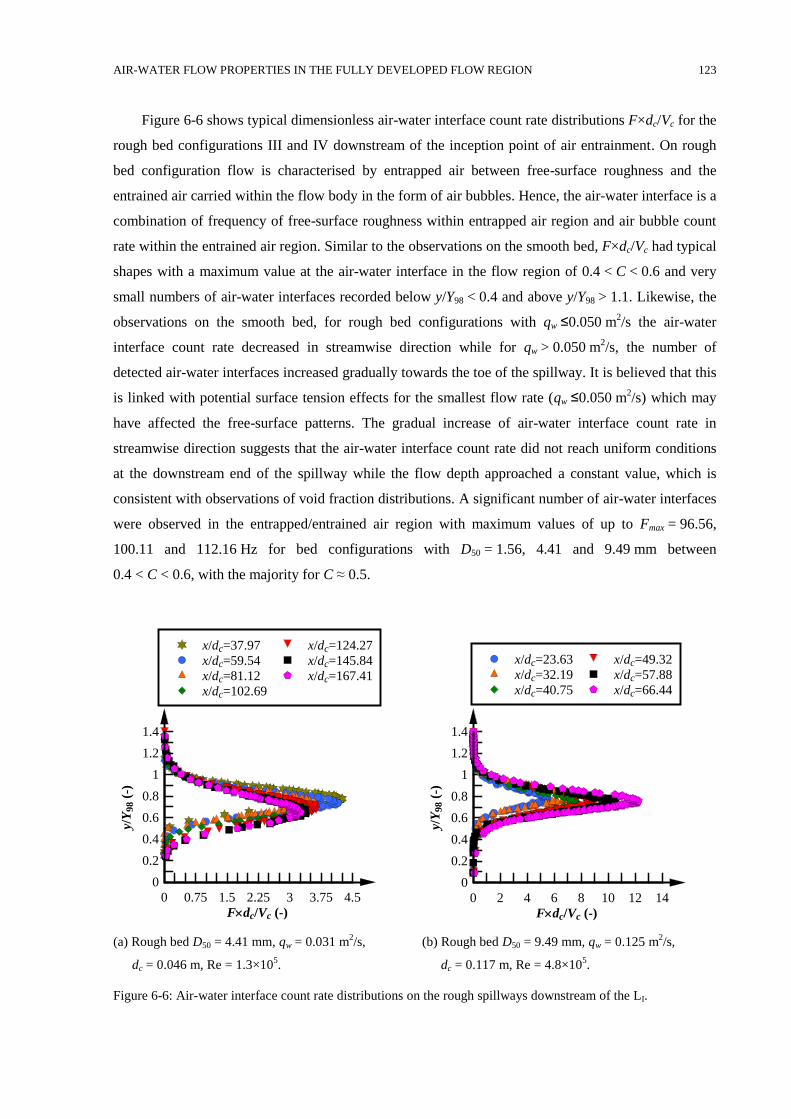
AIR-WATER FLOW PROPERTIES IN THE FULLY DEVELOPED FLOW REGION 123
Figure 6-6 shows typical dimensionless air-water interface count rate distributions F×dc/Vc for the
rough bed configurations III and IV downstream of the inception point of air entrainment. On rough
bed configuration flow is characterised by entrapped air between free-surface roughness and the
entrained air carried within the flow body in the form of air bubbles. Hence, the air-water interface is a
combination of frequency of free-surface roughness within entrapped air region and air bubble count
rate within the entrained air region. Similar to the observations on the smooth bed, F×dc/Vc had typical
shapes with a maximum value at the air-water interface in the flow region of 0.4 < C < 0.6 and very
small numbers of air-water interfaces recorded below y/Y98 < 0.4 and above y/Y98 > 1.1. Likewise, the
observations on the smooth bed, for rough bed configurations with qw ≤0.050 m2/s the air-water
interface count rate decreased in streamwise direction while for qw > 0.050 m2/s, the number of
detected air-water interfaces increased gradually towards the toe of the spillway. It is believed that this
is linked with potential surface tension effects for the smallest flow rate (qw ≤0.050 m2/s) which may
have affected the free-surface patterns. The gradual increase of air-water interface count rate in
streamwise direction suggests that the air-water interface count rate did not reach uniform conditions
at the downstream end of the spillway while the flow depth approached a constant value, which is
consistent with observations of void fraction distributions. A significant number of air-water interfaces
were observed in the entrapped/entrained air region with maximum values of up to Fmax = 96.56,
100.11 and 112.16 Hz for bed configurations with D50 = 1.56, 4.41 and 9.49 mm between
0.4 < C < 0.6, with the majority for C ≈ 0.5.
(a) Rough bed D50 = 4.41 mm, qw = 0.031 m2/s,
dc = 0.046 m, Re = 1.3×10⁵.
(b) Rough bed D50 = 9.49 mm, qw = 0.125 m2/s,
dc = 0.117 m, Re = 4.8×10⁵.
Figure 6-6: Air-water interface count rate distributions on the rough spillways downstream of the LI.
Fdc/Vc (-)
y/Y
98 (
-)
0 0.75 1.5 2.25 3 3.75 4.5
0
0.2
0.4
0.6
0.8
1
1.2
1.4
x/dc=37.97
x/dc=59.54
x/dc=81.12
x/dc=102.69
x/dc=124.27
x/dc=145.84
x/dc=167.41
Fdc/Vc (-)
y/Y
98 (
-)
0 2 4 6 8 10 12 14
0
0.2
0.4
0.6
0.8
1
1.2
1.4
x/dc=23.63
x/dc=32.19
x/dc=40.75
x/dc=49.32
x/dc=57.88
x/dc=66.44
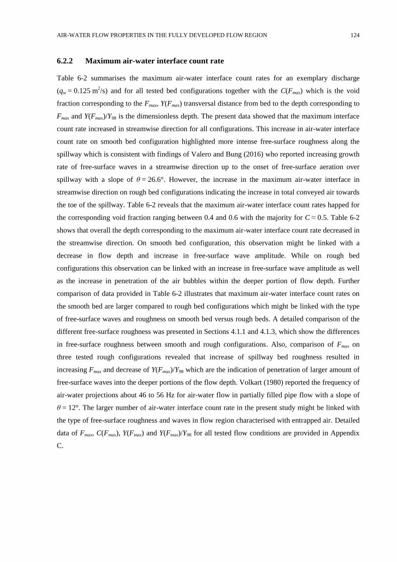
AIR-WATER FLOW PROPERTIES IN THE FULLY DEVELOPED FLOW REGION 124
6.2.2 Maximum air-water interface count rate
Table 6-2 summarises the maximum air-water interface count rates for an exemplary discharge
(qw = 0.125 m2/s) and for all tested bed configurations together with the C(Fmax) which is the void
fraction corresponding to the Fmax, Y(Fmax) transversal distance from bed to the depth corresponding to
Fmax and Y(Fmax)/Y98 is the dimensionless depth. The present data showed that the maximum interface
count rate increased in streamwise direction for all configurations. This increase in air-water interface
count rate on smooth bed configuration highlighted more intense free-surface roughness along the
spillway which is consistent with findings of Valero and Bung (2016) who reported increasing growth
rate of free-surface waves in a streamwise direction up to the onset of free-surface aeration over
spillway with a slope of θ = 26.6°. However, the increase in the maximum air-water interface in
streamwise direction on rough bed configurations indicating the increase in total conveyed air towards
the toe of the spillway. Table 6-2 reveals that the maximum air-water interface count rates happed for
the corresponding void fraction ranging between 0.4 and 0.6 with the majority for C ≈ 0.5. Table 6-2
shows that overall the depth corresponding to the maximum air-water interface count rate decreased in
the streamwise direction. On smooth bed configuration, this observation might be linked with a
decrease in flow depth and increase in free-surface wave amplitude. While on rough bed
configurations this observation can be linked with an increase in free-surface wave amplitude as well
as the increase in penetration of the air bubbles within the deeper portion of flow depth. Further
comparison of data provided in Table 6-2 illustrates that maximum air-water interface count rates on
the smooth bed are larger compared to rough bed configurations which might be linked with the type
of free-surface waves and roughness on smooth bed versus rough beds. A detailed comparison of the
different free-surface roughness was presented in Sections 4.1.1 and 4.1.3, which show the differences
in free-surface roughness between smooth and rough configurations. Also, comparison of Fmax on
three tested rough configurations revealed that increase of spillway bed roughness resulted in
increasing Fmax and decrease of Y(Fmax)/Y98 which are the indication of penetration of larger amount of
free-surface waves into the deeper portions of the flow depth. Volkart (1980) reported the frequency of
air-water projections about 46 to 56 Hz for air-water flow in partially filled pipe flow with a slope of
θ = 12°. The larger number of air-water interface count rate in the present study might be linked with
the type of free-surface roughness and waves in flow region characterised with entrapped air. Detailed
data of Fmax, C(Fmax), Y(Fmax) and Y(Fmax)/Y98 for all tested flow conditions are provided in Appendix
C.
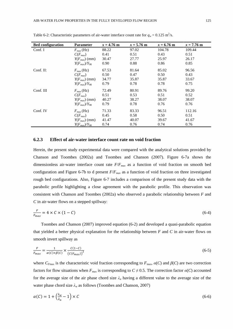
AIR-WATER FLOW PROPERTIES IN THE FULLY DEVELOPED FLOW REGION 125
Table 6-2: Characteristic parameters of air-water interface count rate for qw = 0.125 m2/s.
Bed configuration Parameter x = 4.76 m x = 5.76 m x = 6.76 m x = 7.76 m
Conf. I Fmax (Hz) 88.22 97.02 104.78 109.44
C(Fmax) 0.41 0.51 0.43 0.51
Y(Fmax) (mm) 30.47 27.77 25.97 26.17
Y(Fmax)/Y98 0.90 0.88 0.86 0.85
Conf. II: Fmax (Hz) 67.53 81.64 85.02 96.56
C(Fmax) 0.50 0.47 0.50 0.43
Y(Fmax) (mm) 34.77 35.87 35.87 33.67
Y(Fmax)/Y98 0.79 0.78 0.78 0.75
Conf. III Fmax (Hz) 72.49 80.91 89.76 99.20
C(Fmax) 0.51 0.53 0.51 0.52
Y(Fmax) (mm) 40.27 38.27 38.07 38.07
Y(Fmax)/Y98 0.79 0.78 0.76 0.76
Conf. IV Fmax (Hz) 71.33 83.33 96.51 112.16
C(Fmax) 0.45 0.58 0.50 0.51
Y(Fmax) (mm) 41.47 40.07 39.67 41.67
Y(Fmax)/Y98 0.74 0.76 0.74 0.76
6.2.3 Effect of air-water interface count rate on void fraction
Herein, the present study experimental data were compared with the analytical solutions provided by
Chanson and Toombes (2002a) and Toombes and Chanson (2007). Figure 6-7a shows the
dimensionless air-water interface count rate F/Fmax as a function of void fraction on smooth bed
configuration and Figure 6-7b to d present F/Fmax as a function of void fraction on three investigated
rough bed configurations. Also, Figure 6-7 includes a comparison of the present study data with the
parabolic profile highlighting a close agreement with the parabolic profile. This observation was
consistent with Chanson and Toombes (2002a) who observed a parabolic relationship between F and
C in air-water flows on a stepped spillway:
𝐹
𝐹𝑚𝑎𝑥= 4 × 𝐶 × (1 − 𝐶) (6-4)
Toombes and Chanson (2007) improved equation (6-2) and developed a quasi-parabolic equation
that yielded a better physical explanation for the relationship between F and C in air-water flows on
smooth invert spillway as
𝐹
𝐹𝑚𝑎𝑥=
1
𝛼(𝐶)×𝛽(𝐶)×
𝐶(1−𝐶)
(𝐶(𝐹𝑚𝑎𝑥))2 (6-5)
where CFmax is the characteristic void fraction corresponding to Fmax, α(C) and β(C) are two correction
factors for flow situations when Fmax is corresponding to C ≠ 0.5. The correction factor α(C) accounted
for the average size of the air phase chord size λa having a different value to the average size of the
water phase chord size λw as follows (Toombes and Chanson, 2007)
𝛼(𝐶) = 1 + (𝜆𝑤
𝜆𝑎− 1) × 𝐶 (6-6)
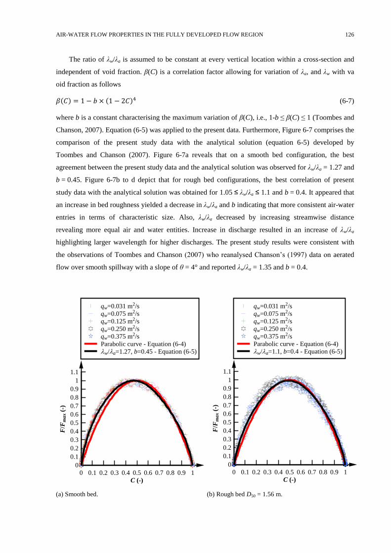
AIR-WATER FLOW PROPERTIES IN THE FULLY DEVELOPED FLOW REGION 126
The ratio of λw/λa is assumed to be constant at every vertical location within a cross-section and
independent of void fraction. β(C) is a correlation factor allowing for variation of λa, and λw with va
oid fraction as follows
𝛽(𝐶) = 1 − 𝑏 × (1 − 2𝐶)4 (6-7)
where b is a constant characterising the maximum variation of β(C), i.e., 1-b ≤ β(C) ≤ 1 (Toombes and
Chanson, 2007). Equation (6-5) was applied to the present data. Furthermore, Figure 6-7 comprises the
comparison of the present study data with the analytical solution (equation 6-5) developed by
Toombes and Chanson (2007). Figure 6-7a reveals that on a smooth bed configuration, the best
agreement between the present study data and the analytical solution was observed for λw/λa = 1.27 and
b = 0.45. Figure 6-7b to d depict that for rough bed configurations, the best correlation of present
study data with the analytical solution was obtained for 1.05 ≤ λw/λa ≤ 1.1 and b = 0.4. It appeared that
an increase in bed roughness yielded a decrease in λw/λa and b indicating that more consistent air-water
entries in terms of characteristic size. Also, λw/λa decreased by increasing streamwise distance
revealing more equal air and water entities. Increase in discharge resulted in an increase of λw/λa
highlighting larger wavelength for higher discharges. The present study results were consistent with
the observations of Toombes and Chanson (2007) who reanalysed Chanson’s (1997) data on aerated
flow over smooth spillway with a slope of θ = 4° and reported λw/λa = 1.35 and b = 0.4.
(a) Smooth bed. (b) Rough bed D50 = 1.56 m.
C (-)
F/F
max (
-)
0 0.1 0.2 0.3 0.4 0.5 0.6 0.7 0.8 0.9 1
0
0.1
0.2
0.3
0.4
0.5
0.6
0.7
0.8
0.9
1
1.1
qw=0.031 m2/s
qw=0.075 m2/s
qw=0.125 m2/s
qw=0.250 m2/s
qw=0.375 m2/s
Parabolic curve - Equation (6-4)
w/a=1.27, b=0.45 - Equation (6-5)
C (-)
F/F
ma
x (
-)
0 0.1 0.2 0.3 0.4 0.5 0.6 0.7 0.8 0.9 1
0
0.1
0.2
0.3
0.4
0.5
0.6
0.7
0.8
0.9
1
1.1
qw=0.031 m2/s
qw=0.075 m2/s
qw=0.125 m2/s
qw=0.250 m2/s
qw=0.375 m2/s
Parabolic curve - Equation (6-4)
w/a=1.1, b=0.4 - Equation (6-5)
AIR-WATER FLOW PROPERTIES IN THE FULLY DEVELOPED FLOW REGION 127
(c) Rough bed D50 = 4.41 m. (d) Rough bed D50 = 9.49 m.
Figure 6-7: Relationship between dimensionless air-water interface count rate and void fraction downstream of
the inception point of free-surface roughness for all flow conditions; Comparison with parabolic
relationships (equations 6-4 and 6-5)
6.2.4 Discussion on air-water interface count rate
A detailed comparison of the air-water interface count rate distributions was conducted for the four-
bed configurations in the present study. Figure 6-8a shows some of the key findings as a function of
y/Y98. In Figure 6-8a, typical air-water interface count rate distributions for the four roughness
configurations are shown for an exemplary discharge qw = 0.125 m2/s and Re ≈ 5×10
5 and at an almost
constant dimensionless distance from the inception point of free-surface roughness. The distributions
show that by increasing bed roughness the maximum air-water interface count rate declined. This can
be explained as the maximum interface count rate over smooth bed configuration were recorded very
close to the free-surface roughness, highlighting that the double-tip conductivity probe recorded the
small free-surface waves. While maximum interface count rate over rough bed configurations had
been recorded in the flow region at the transition area between the region of entrapped air and region
of entrained air. The type of the free-surface roughness and waves on smooth bed yielded the larger
number of interfaces impinging the probe tips in comparison with rough bed configurations.
C (-)
F/F
max (
-)
0 0.1 0.2 0.3 0.4 0.5 0.6 0.7 0.8 0.9 1
0
0.1
0.2
0.3
0.4
0.5
0.6
0.7
0.8
0.9
1
1.1
qw=0.031 m2/s
qw=0.075 m2/s
qw=0.125 m2/s
qw=0.250 m2/s
qw=0.375 m2/s
Parabolic curve - Equation (6-4)
w/a=1.05, b=0.4 - Equation (6-5)
C (-)
F/F
ma
x (
-)
0 0.1 0.2 0.3 0.4 0.5 0.6 0.7 0.8 0.9 1
0
0.1
0.2
0.3
0.4
0.5
0.6
0.7
0.8
0.9
1
1.1
qw=0.031 m2/s
qw=0.075 m2/s
qw=0.125 m2/s
qw=0.250 m2/s
qw=0.375 m2/s
Parabolic curve - Equation (6-4)
w/a=1.05, b=0.4 - Equation (6-5)
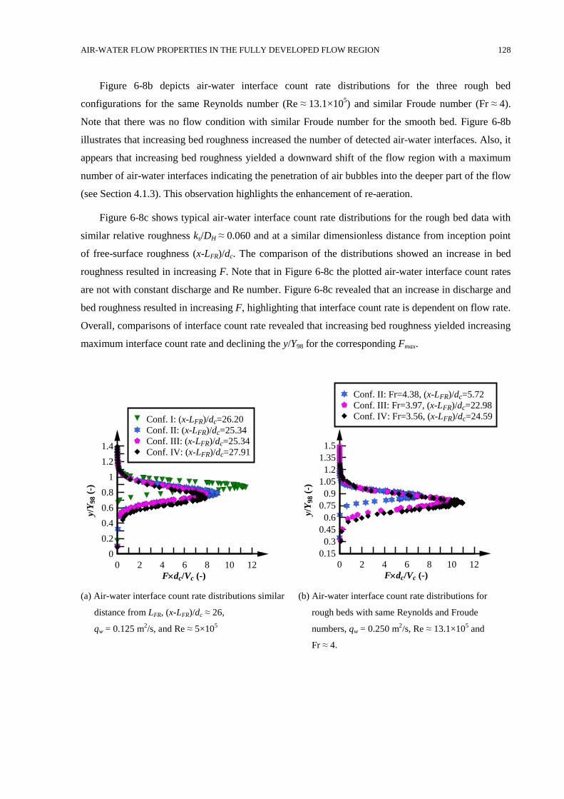
AIR-WATER FLOW PROPERTIES IN THE FULLY DEVELOPED FLOW REGION 128
Figure 6-8b depicts air-water interface count rate distributions for the three rough bed
configurations for the same Reynolds number (Re ≈ 13.1×10⁵) and similar Froude number (Fr ≈ 4).
Note that there was no flow condition with similar Froude number for the smooth bed. Figure 6-8b
illustrates that increasing bed roughness increased the number of detected air-water interfaces. Also, it
appears that increasing bed roughness yielded a downward shift of the flow region with a maximum
number of air-water interfaces indicating the penetration of air bubbles into the deeper part of the flow
(see Section 4.1.3). This observation highlights the enhancement of re-aeration.
Figure 6-8c shows typical air-water interface count rate distributions for the rough bed data with
similar relative roughness ks/DH ≈ 0.060 and at a similar dimensionless distance from inception point
of free-surface roughness (x-LFR)/dc. The comparison of the distributions showed an increase in bed
roughness resulted in increasing F. Note that in Figure 6-8c the plotted air-water interface count rates
are not with constant discharge and Re number. Figure 6-8c revealed that an increase in discharge and
bed roughness resulted in increasing F, highlighting that interface count rate is dependent on flow rate.
Overall, comparisons of interface count rate revealed that increasing bed roughness yielded increasing
maximum interface count rate and declining the y/Y98 for the corresponding Fmax.
(a) Air-water interface count rate distributions similar
distance from LFR, (x-LFR)/dc ≈ 26,
qw = 0.125 m2/s, and Re ≈ 5×10
5
(b) Air-water interface count rate distributions for
rough beds with same Reynolds and Froude
numbers, qw = 0.250 m2/s, Re ≈ 13.1×10
5 and
Fr ≈ 4.
Fdc/Vc (-)
y/Y
98 (
-)
0 2 4 6 8 10 12
0
0.2
0.4
0.6
0.8
1
1.2
1.4
Conf. I: (x-LFR)/dc=26.20
Conf. II: (x-LFR)/dc=25.34
Conf. III: (x-LFR)/dc=25.34
Conf. IV: (x-LFR)/dc=27.91
Fdc/Vc (-)
y/Y
98 (
-)
0 2 4 6 8 10 12
0.15
0.3
0.45
0.6
0.75
0.9
1.05
1.2
1.35
1.5
Conf. II: Fr=4.38, (x-LFR)/dc=5.72
Conf. III: Fr=3.97, (x-LFR)/dc=22.98
Conf. IV: Fr=3.56, (x-LFR)/dc=24.59
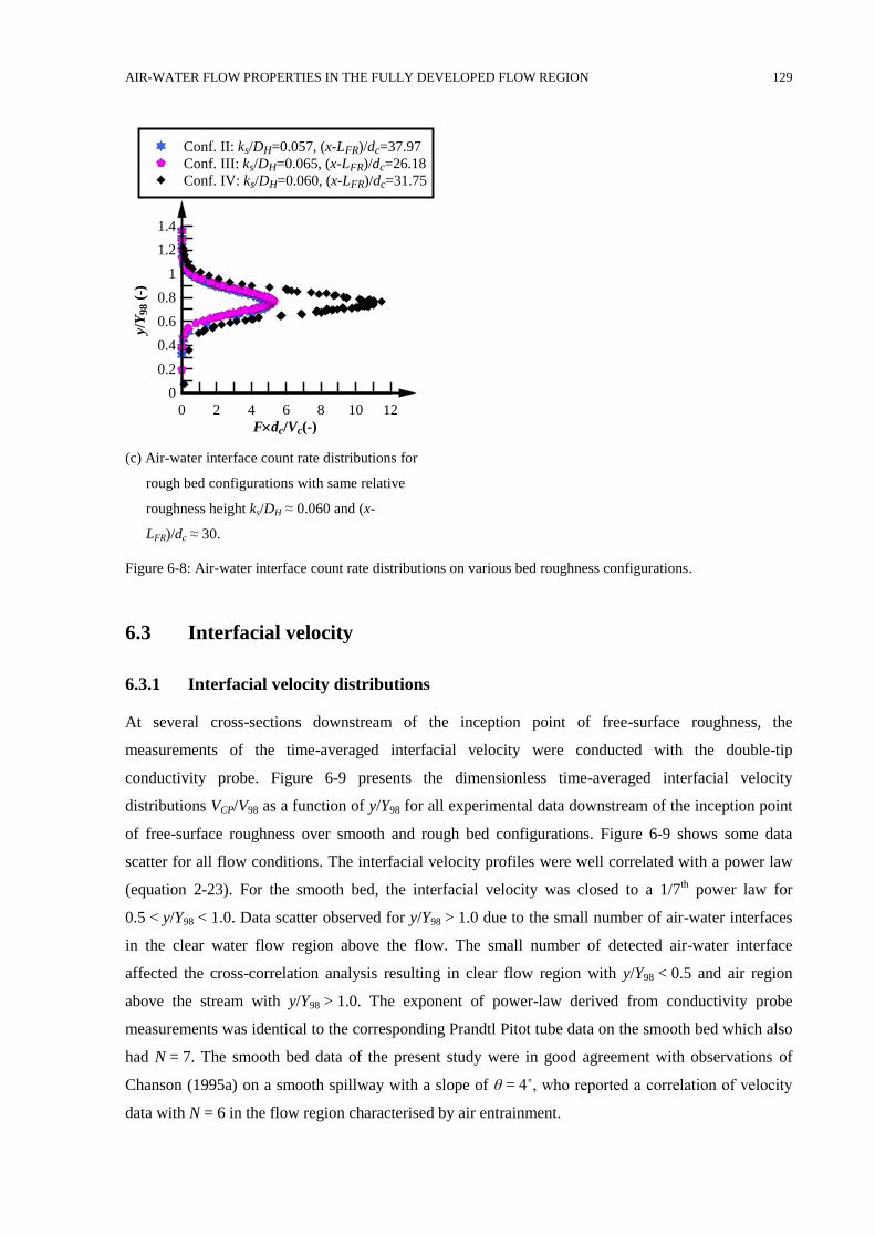
AIR-WATER FLOW PROPERTIES IN THE FULLY DEVELOPED FLOW REGION 129
(c) Air-water interface count rate distributions for
rough bed configurations with same relative
roughness height ks/DH ≈ 0.060 and (x-
LFR)/dc ≈ 30.
Figure 6-8: Air-water interface count rate distributions on various bed roughness configurations.
Interfacial velocity 6.3
6.3.1 Interfacial velocity distributions
At several cross-sections downstream of the inception point of free-surface roughness, the
measurements of the time-averaged interfacial velocity were conducted with the double-tip
conductivity probe. Figure 6-9 presents the dimensionless time-averaged interfacial velocity
distributions VCP/V98 as a function of y/Y98 for all experimental data downstream of the inception point
of free-surface roughness over smooth and rough bed configurations. Figure 6-9 shows some data
scatter for all flow conditions. The interfacial velocity profiles were well correlated with a power law
(equation 2-23). For the smooth bed, the interfacial velocity was closed to a 1/7th power law for
0.5 < y/Y98 < 1.0. Data scatter observed for y/Y98 > 1.0 due to the small number of air-water interfaces
in the clear water flow region above the flow. The small number of detected air-water interface
affected the cross-correlation analysis resulting in clear flow region with y/Y98 < 0.5 and air region
above the stream with y/Y98 > 1.0. The exponent of power-law derived from conductivity probe
measurements was identical to the corresponding Prandtl Pitot tube data on the smooth bed which also
had N = 7. The smooth bed data of the present study were in good agreement with observations of
Chanson (1995a) on a smooth spillway with a slope of θ = 4˚, who reported a correlation of velocity
data with N = 6 in the flow region characterised by air entrainment.
Fdc/Vc(-)
y/Y
98 (
-)
0 2 4 6 8 10 12
0
0.2
0.4
0.6
0.8
1
1.2
1.4
Conf. II: ks/DH=0.057, (x-LFR)/dc=37.97
Conf. III: ks/DH=0.065, (x-LFR)/dc=26.18
Conf. IV: ks/DH=0.060, (x-LFR)/dc=31.75
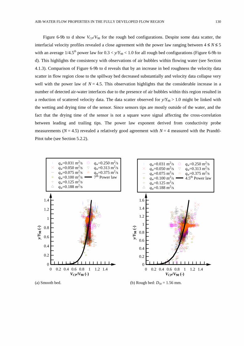
AIR-WATER FLOW PROPERTIES IN THE FULLY DEVELOPED FLOW REGION 130
Figure 6-9b to d show VCP/V98 for the rough bed configurations. Despite some data scatter, the
interfacial velocity profiles revealed a close agreement with the power law ranging between 4 ≤ N ≤ 5
with an average 1/4.5th power law for 0.3 < y/Y98 < 1.0 for all rough bed configurations (Figure 6-9b to
d). This highlights the consistency with observations of air bubbles within flowing water (see Section
4.1.3). Comparison of Figure 6-9b to d reveals that by an increase in bed roughness the velocity data
scatter in flow region close to the spillway bed decreased substantially and velocity data collapse very
well with the power law of N = 4.5. This observation highlights that the considerable increase in a
number of detected air-water interfaces due to the presence of air bubbles within this region resulted in
a reduction of scattered velocity data. The data scatter observed for y/Y98 > 1.0 might be linked with
the wetting and drying time of the sensor. Since sensors tips are mostly outside of the water, and the
fact that the drying time of the sensor is not a square wave signal affecting the cross-correlation
between leading and trailing tips. The power law exponent derived from conductivity probe
measurements (N = 4.5) revealed a relatively good agreement with N = 4 measured with the Prandtl-
Pitot tube (see Section 5.2.2).
(a) Smooth bed. (b) Rough bed: D50 = 1.56 mm.
VCP/V98 (-)
y/Y
98 (
-)
0 0.2 0.4 0.6 0.8 1 1.2 1.4
0
0.2
0.4
0.6
0.8
1
1.2
1.4
qw=0.031 m2/s
qw=0.050 m2/s
qw=0.075 m2/s
qw=0.100 m2/s
qw=0.125 m2/s
qw=0.188 m2/s
qw=0.250 m2/s
qw=0.313 m2/s
qw=0.375 m2/s
7th Power law
VCP/V98 (-)
y/Y
98 (
-)
0 0.2 0.4 0.6 0.8 1 1.2 1.4
0
0.2
0.4
0.6
0.8
1
1.2
1.4
1.6
qw=0.031 m2/s
qw=0.050 m2/s
qw=0.075 m2/s
qw=0.100 m2/s
qw=0.125 m2/s
qw=0.188 m2/s
qw=0.250 m2/s
qw=0.313 m2/s
qw=0.375 m2/s
4.5th Power law
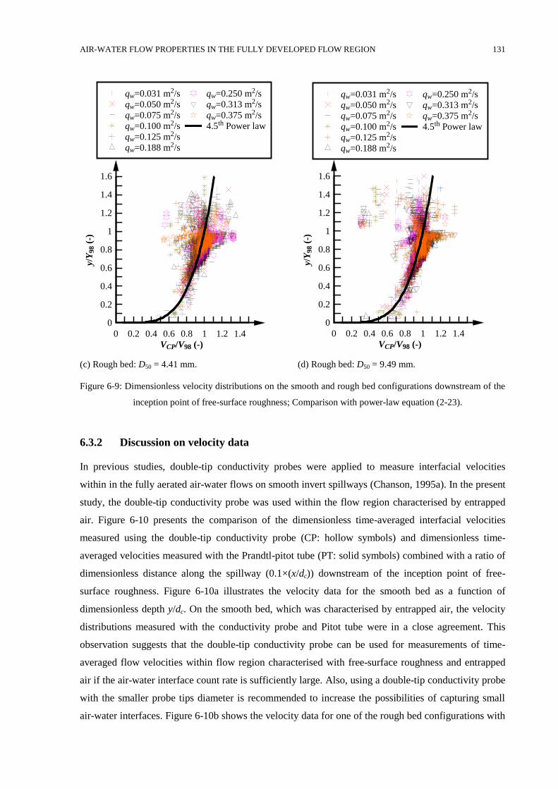
AIR-WATER FLOW PROPERTIES IN THE FULLY DEVELOPED FLOW REGION 131
(c) Rough bed: D50 = 4.41 mm. (d) Rough bed: D50 = 9.49 mm.
Figure 6-9: Dimensionless velocity distributions on the smooth and rough bed configurations downstream of the
inception point of free-surface roughness; Comparison with power-law equation (2-23).
6.3.2 Discussion on velocity data
In previous studies, double-tip conductivity probes were applied to measure interfacial velocities
within in the fully aerated air-water flows on smooth invert spillways (Chanson, 1995a). In the present
study, the double-tip conductivity probe was used within the flow region characterised by entrapped
air. Figure 6-10 presents the comparison of the dimensionless time-averaged interfacial velocities
measured using the double-tip conductivity probe (CP: hollow symbols) and dimensionless time-
averaged velocities measured with the Prandtl-pitot tube (PT: solid symbols) combined with a ratio of
dimensionless distance along the spillway (0.1×(x/dc)) downstream of the inception point of free-
surface roughness. Figure 6-10a illustrates the velocity data for the smooth bed as a function of
dimensionless depth y/dc. On the smooth bed, which was characterised by entrapped air, the velocity
distributions measured with the conductivity probe and Pitot tube were in a close agreement. This
observation suggests that the double-tip conductivity probe can be used for measurements of time-
averaged flow velocities within flow region characterised with free-surface roughness and entrapped
air if the air-water interface count rate is sufficiently large. Also, using a double-tip conductivity probe
with the smaller probe tips diameter is recommended to increase the possibilities of capturing small
air-water interfaces. Figure 6-10b shows the velocity data for one of the rough bed configurations with
VCP/V98 (-)
y/Y
98 (
-)
0 0.2 0.4 0.6 0.8 1 1.2 1.4
0
0.2
0.4
0.6
0.8
1
1.2
1.4
1.6
qw=0.031 m2/s
qw=0.050 m2/s
qw=0.075 m2/s
qw=0.100 m2/s
qw=0.125 m2/s
qw=0.188 m2/s
qw=0.250 m2/s
qw=0.313 m2/s
qw=0.375 m2/s
4.5th Power law
VCP/V98 (-)
y/Y
98 (
-)
0 0.2 0.4 0.6 0.8 1 1.2 1.4
0
0.2
0.4
0.6
0.8
1
1.2
1.4
1.6
qw=0.031 m2/s
qw=0.050 m2/s
qw=0.075 m2/s
qw=0.100 m2/s
qw=0.125 m2/s
qw=0.188 m2/s
qw=0.250 m2/s
qw=0.313 m2/s
qw=0.375 m2/s
4.5th Power law
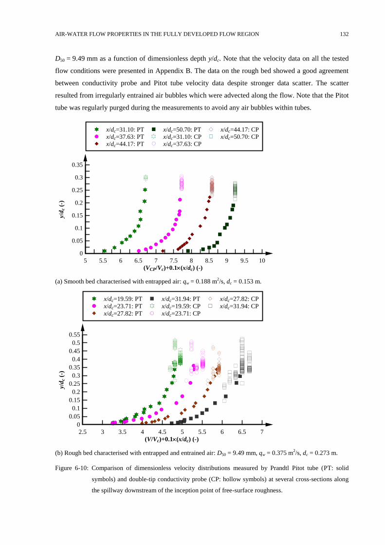
AIR-WATER FLOW PROPERTIES IN THE FULLY DEVELOPED FLOW REGION 132
D50 = 9.49 mm as a function of dimensionless depth y/dc. Note that the velocity data on all the tested
flow conditions were presented in Appendix B. The data on the rough bed showed a good agreement
between conductivity probe and Pitot tube velocity data despite stronger data scatter. The scatter
resulted from irregularly entrained air bubbles which were advected along the flow. Note that the Pitot
tube was regularly purged during the measurements to avoid any air bubbles within tubes.
(a) Smooth bed characterised with entrapped air: qw = 0.188 m2/s, dc = 0.153 m.
(b) Rough bed characterised with entrapped and entrained air: D50 = 9.49 mm, qw = 0.375 m2/s, dc = 0.273 m.
Figure 6-10: Comparison of dimensionless velocity distributions measured by Prandtl Pitot tube (PT: solid
symbols) and double-tip conductivity probe (CP: hollow symbols) at several cross-sections along
the spillway downstream of the inception point of free-surface roughness.
(VCP/Vc)+0.1(x/dc) (-)
y/d
c (-
)
5 5.5 6 6.5 7 7.5 8 8.5 9 9.5 10
0
0.05
0.1
0.15
0.2
0.25
0.3
0.35
x/dc=31.10: PT
x/dc=37.63: PT
x/dc=44.17: PT
x/dc=50.70: PT
x/dc=31.10: CP
x/dc=37.63: CP
x/dc=44.17: CP
x/dc=50.70: CP
(V/Vc)+0.1(x/dc) (-)
y/d
c (-
)
2.5 3 3.5 4 4.5 5 5.5 6 6.5 7
0
0.05
0.1
0.15
0.2
0.25
0.3
0.35
0.4
0.45
0.5
0.55
x/dc=19.59: PT
x/dc=23.71: PT
x/dc=27.82: PT
x/dc=31.94: PT
x/dc=19.59: CP
x/dc=23.71: CP
x/dc=27.82: CP
x/dc=31.94: CP
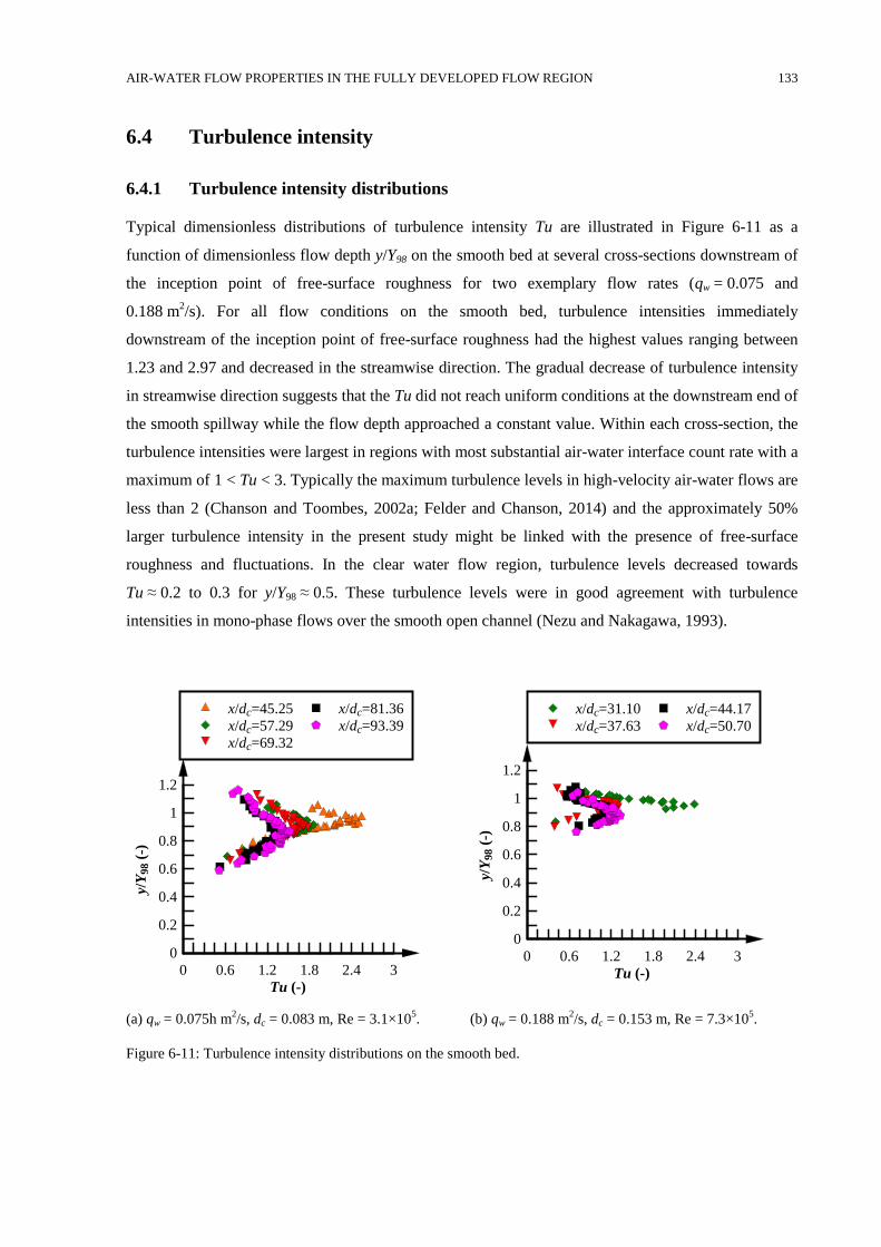
AIR-WATER FLOW PROPERTIES IN THE FULLY DEVELOPED FLOW REGION 133
Turbulence intensity 6.4
6.4.1 Turbulence intensity distributions
Typical dimensionless distributions of turbulence intensity Tu are illustrated in Figure 6-11 as a
function of dimensionless flow depth y/Y98 on the smooth bed at several cross-sections downstream of
the inception point of free-surface roughness for two exemplary flow rates (qw = 0.075 and
0.188 m2/s). For all flow conditions on the smooth bed, turbulence intensities immediately
downstream of the inception point of free-surface roughness had the highest values ranging between
1.23 and 2.97 and decreased in the streamwise direction. The gradual decrease of turbulence intensity
in streamwise direction suggests that the Tu did not reach uniform conditions at the downstream end of
the smooth spillway while the flow depth approached a constant value. Within each cross-section, the
turbulence intensities were largest in regions with most substantial air-water interface count rate with a
maximum of 1 < Tu < 3. Typically the maximum turbulence levels in high-velocity air-water flows are
less than 2 (Chanson and Toombes, 2002a; Felder and Chanson, 2014) and the approximately 50%
larger turbulence intensity in the present study might be linked with the presence of free-surface
roughness and fluctuations. In the clear water flow region, turbulence levels decreased towards
Tu ≈ 0.2 to 0.3 for y/Y98 ≈ 0.5. These turbulence levels were in good agreement with turbulence
intensities in mono-phase flows over the smooth open channel (Nezu and Nakagawa, 1993).
(a) qw = 0.075h m2/s, dc = 0.083 m, Re = 3.1×10
5. (b) qw = 0.188 m
2/s, dc = 0.153 m, Re = 7.3×10
5.
Figure 6-11: Turbulence intensity distributions on the smooth bed.
Tu (-)
y/Y
98 (
-)
0 0.6 1.2 1.8 2.4 3
0
0.2
0.4
0.6
0.8
1
1.2
x/dc=45.25
x/dc=57.29
x/dc=69.32
x/dc=81.36
x/dc=93.39
Tu (-)
y/Y
98 (
-)
0 0.6 1.2 1.8 2.4 3
0
0.2
0.4
0.6
0.8
1
1.2
x/dc=31.10
x/dc=37.63
x/dc=44.17
x/dc=50.70
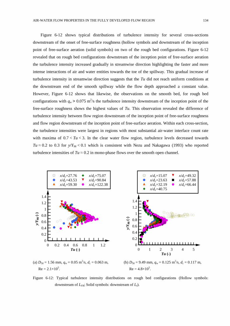
AIR-WATER FLOW PROPERTIES IN THE FULLY DEVELOPED FLOW REGION 134
Figure 6-12 shows typical distributions of turbulence intensity for several cross-sections
downstream of the onset of free-surface roughness (hollow symbols and downstream of the inception
point of free-surface aeration (solid symbols) on two of the rough bed configurations. Figure 6-12
revealed that on rough bed configurations downstream of the inception point of free-surface aeration
the turbulence intensity increased gradually in streamwise direction highlighting the faster and more
intense interactions of air and water entities towards the toe of the spillway. This gradual increase of
turbulence intensity in streamwise direction suggests that the Tu did not reach uniform conditions at
the downstream end of the smooth spillway while the flow depth approached a constant value.
However, Figure 6-12 shows that likewise, the observations on the smooth bed, for rough bed
configurations with qw > 0.075 m2/s the turbulence intensity downstream of the inception point of the
free-surface roughness shows the highest values of Tu. This observation revealed the difference of
turbulence intensity between flow region downstream of the inception point of free-surface roughness
and flow region downstream of the inception point of free-surface aeration. Within each cross-section,
the turbulence intensities were largest in regions with most substantial air-water interface count rate
with maxima of 0.7 < Tu < 3. In the clear water flow region, turbulence levels decreased towards
Tu ≈ 0.2 to 0.3 for y/Y98 < 0.1 which is consistent with Nezu and Nakagawa (1993) who reported
turbulence intensities of Tu ≈ 0.2 in mono-phase flows over the smooth open channel.
(a) D50 = 1.56 mm, qw = 0.05 m2/s, dc = 0.063 m,
Re = 2.1×10⁵.
(b) D50 = 9.49 mm, qw = 0.125 m2/s, dc = 0.117 m,
Re = 4.8×10⁵.
Figure 6-12: Typical turbulence intensity distributions on rough bed configurations (Hollow symbols:
downstream of LFR; Solid symbols: downstream of LI).
Tu (-)
y/Y
98 (
-)
0 0.2 0.4 0.6 0.8 1 1.2
0
0.2
0.4
0.6
0.8
1
1.2
1.4
x/dc=27.76
x/dc=43.53
x/dc=59.30
x/dc=75.07
x/dc=90.84
x/dc=122.38
Tu (-)
y/Y
98 (
-)
0 1 2 3 4 5
0
0.2
0.4
0.6
0.8
1
1.2
1.4
x/dc=15.07
x/dc=23.63
x/dc=32.19
x/dc=40.75
x/dc=49.32
x/dc=57.88
x/dc=66.44
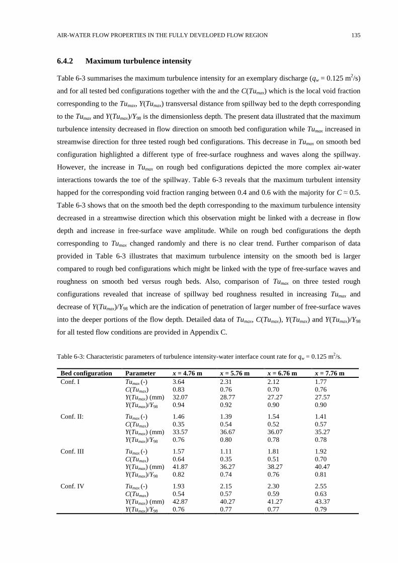
AIR-WATER FLOW PROPERTIES IN THE FULLY DEVELOPED FLOW REGION 135
6.4.2 Maximum turbulence intensity
Table 6-3 summarises the maximum turbulence intensity for an exemplary discharge (qw = 0.125 m2/s)
and for all tested bed configurations together with the and the C(Tumax) which is the local void fraction
corresponding to the Tumax, Y(Tumax) transversal distance from spillway bed to the depth corresponding
to the Tumax and Y(Tumax)/Y98 is the dimensionless depth. The present data illustrated that the maximum
turbulence intensity decreased in flow direction on smooth bed configuration while Tumax increased in
streamwise direction for three tested rough bed configurations. This decrease in Tumax on smooth bed
configuration highlighted a different type of free-surface roughness and waves along the spillway.
However, the increase in Tumax on rough bed configurations depicted the more complex air-water
interactions towards the toe of the spillway. Table 6-3 reveals that the maximum turbulent intensity
happed for the corresponding void fraction ranging between 0.4 and 0.6 with the majority for C ≈ 0.5.
Table 6-3 shows that on the smooth bed the depth corresponding to the maximum turbulence intensity
decreased in a streamwise direction which this observation might be linked with a decrease in flow
depth and increase in free-surface wave amplitude. While on rough bed configurations the depth
corresponding to Tumax changed randomly and there is no clear trend. Further comparison of data
provided in Table 6-3 illustrates that maximum turbulence intensity on the smooth bed is larger
compared to rough bed configurations which might be linked with the type of free-surface waves and
roughness on smooth bed versus rough beds. Also, comparison of Tumax on three tested rough
configurations revealed that increase of spillway bed roughness resulted in increasing Tumax and
decrease of Y(Tumax)/Y98 which are the indication of penetration of larger number of free-surface waves
into the deeper portions of the flow depth. Detailed data of Tumax, C(Tumax), Y(Tumax) and Y(Tumax)/Y98
for all tested flow conditions are provided in Appendix C.
Table 6-3: Characteristic parameters of turbulence intensity-water interface count rate for qw = 0.125 m2/s.
Bed configuration Parameter x = 4.76 m x = 5.76 m x = 6.76 m x = 7.76 m
Conf. I Tumax (-) 3.64 2.31 2.12 1.77
C(Tumax) 0.83 0.76 0.70 0.76
Y(Tumax) (mm) 32.07 28.77 27.27 27.57
Y(Tumax)/Y98 0.94 0.92 0.90 0.90
Conf. II: Tumax (-) 1.46 1.39 1.54 1.41
C(Tumax) 0.35 0.54 0.52 0.57
Y(Tumax) (mm) 33.57 36.67 36.07 35.27
Y(Tumax)/Y98 0.76 0.80 0.78 0.78
Conf. III Tumax (-) 1.57 1.11 1.81 1.92
C(Tumax) 0.64 0.35 0.51 0.70
Y(Tumax) (mm) 41.87 36.27 38.27 40.47
Y(Tumax)/Y98 0.82 0.74 0.76 0.81
Conf. IV Tumax (-) 1.93 2.15 2.30 2.55
C(Tumax) 0.54 0.57 0.59 0.63
Y(Tumax) (mm) 42.87 40.27 41.27 43.37
Y(Tumax)/Y98 0.76 0.77 0.77 0.79
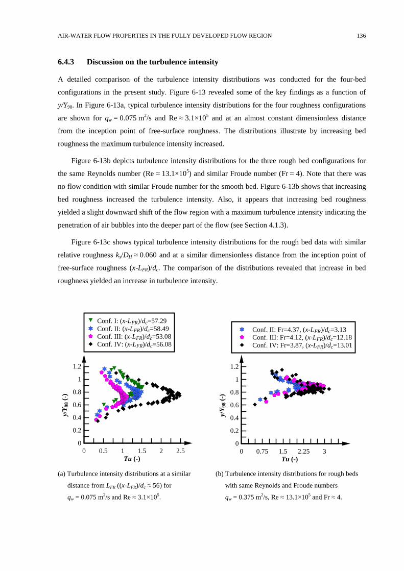
AIR-WATER FLOW PROPERTIES IN THE FULLY DEVELOPED FLOW REGION 136
6.4.3 Discussion on the turbulence intensity
A detailed comparison of the turbulence intensity distributions was conducted for the four-bed
configurations in the present study. Figure 6-13 revealed some of the key findings as a function of
y/Y98. In Figure 6-13a, typical turbulence intensity distributions for the four roughness configurations
are shown for qw = 0.075 m2/s and Re ≈ 3.1×10
5 and at an almost constant dimensionless distance
from the inception point of free-surface roughness. The distributions illustrate by increasing bed
roughness the maximum turbulence intensity increased.
Figure 6-13b depicts turbulence intensity distributions for the three rough bed configurations for
the same Reynolds number (Re ≈ 13.1×10⁵) and similar Froude number (Fr ≈ 4). Note that there was
no flow condition with similar Froude number for the smooth bed. Figure 6-13b shows that increasing
bed roughness increased the turbulence intensity. Also, it appears that increasing bed roughness
yielded a slight downward shift of the flow region with a maximum turbulence intensity indicating the
penetration of air bubbles into the deeper part of the flow (see Section 4.1.3).
Figure 6-13c shows typical turbulence intensity distributions for the rough bed data with similar
relative roughness ks/DH ≈ 0.060 and at a similar dimensionless distance from the inception point of
free-surface roughness (x-LFR)/dc. The comparison of the distributions revealed that increase in bed
roughness yielded an increase in turbulence intensity.
(a) Turbulence intensity distributions at a similar
distance from LFR ((x-LFR)/dc ≈ 56) for
qw = 0.075 m2/s and Re ≈ 3.1×10
5.
(b) Turbulence intensity distributions for rough beds
with same Reynolds and Froude numbers
qw = 0.375 m2/s, Re ≈ 13.1×10
5 and Fr ≈ 4.
Tu (-)
y/Y
98 (
-)
0 0.5 1 1.5 2 2.5
0
0.2
0.4
0.6
0.8
1
1.2
Conf. I: (x-LFR)/dc=57.29
Conf. II: (x-LFR)/dc=58.49
Conf. III: (x-LFR)/dc=53.08
Conf. IV: (x-LFR)/dc=56.08
Tu (-)
y/Y
98 (
-)
0 0.75 1.5 2.25 3
0
0.2
0.4
0.6
0.8
1
1.2
Conf. II: Fr=4.37, (x-LFR)/dc=3.13
Conf. III: Fr=4.12, (x-LFR)/dc=12.18
Conf. IV: Fr=3.87, (x-LFR)/dc=13.01
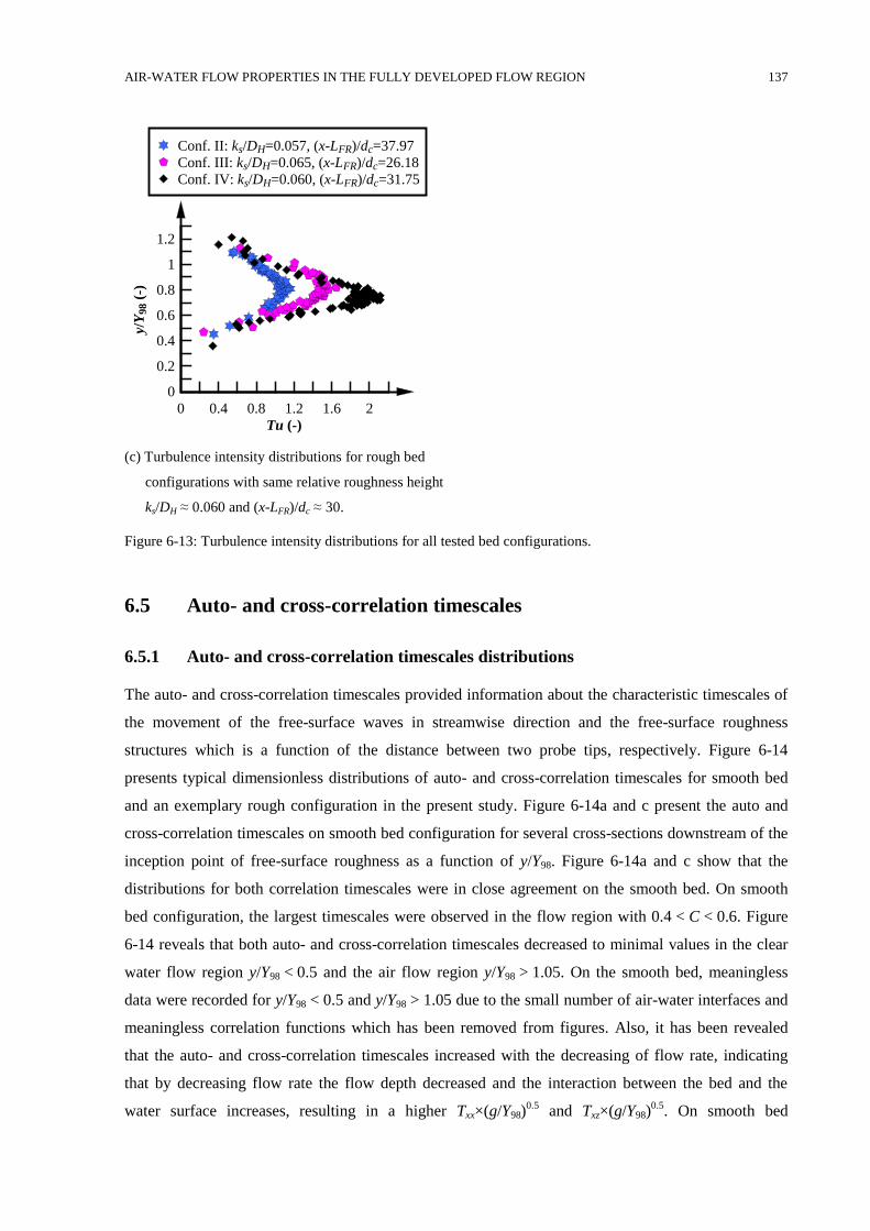
AIR-WATER FLOW PROPERTIES IN THE FULLY DEVELOPED FLOW REGION 137
(c) Turbulence intensity distributions for rough bed
configurations with same relative roughness height
ks/DH ≈ 0.060 and (x-LFR)/dc ≈ 30.
Figure 6-13: Turbulence intensity distributions for all tested bed configurations.
Auto- and cross-correlation timescales 6.5
6.5.1 Auto- and cross-correlation timescales distributions
The auto- and cross-correlation timescales provided information about the characteristic timescales of
the movement of the free-surface waves in streamwise direction and the free-surface roughness
structures which is a function of the distance between two probe tips, respectively. Figure 6-14
presents typical dimensionless distributions of auto- and cross-correlation timescales for smooth bed
and an exemplary rough configuration in the present study. Figure 6-14a and c present the auto and
cross-correlation timescales on smooth bed configuration for several cross-sections downstream of the
inception point of free-surface roughness as a function of y/Y98. Figure 6-14a and c show that the
distributions for both correlation timescales were in close agreement on the smooth bed. On smooth
bed configuration, the largest timescales were observed in the flow region with 0.4 < C < 0.6. Figure
6-14 reveals that both auto- and cross-correlation timescales decreased to minimal values in the clear
water flow region y/Y98 < 0.5 and the air flow region y/Y98 > 1.05. On the smooth bed, meaningless
data were recorded for y/Y98 < 0.5 and y/Y98 > 1.05 due to the small number of air-water interfaces and
meaningless correlation functions which has been removed from figures. Also, it has been revealed
that the auto- and cross-correlation timescales increased with the decreasing of flow rate, indicating
that by decreasing flow rate the flow depth decreased and the interaction between the bed and the
water surface increases, resulting in a higher Txx×(g/Y98)0.5
and Txz×(g/Y98)0.5
. On smooth bed
Tu (-)
y/Y
98 (
-)
0 0.4 0.8 1.2 1.6 2
0
0.2
0.4
0.6
0.8
1
1.2
Conf. II: ks/DH=0.057, (x-LFR)/dc=37.97
Conf. III: ks/DH=0.065, (x-LFR)/dc=26.18
Conf. IV: ks/DH=0.060, (x-LFR)/dc=31.75
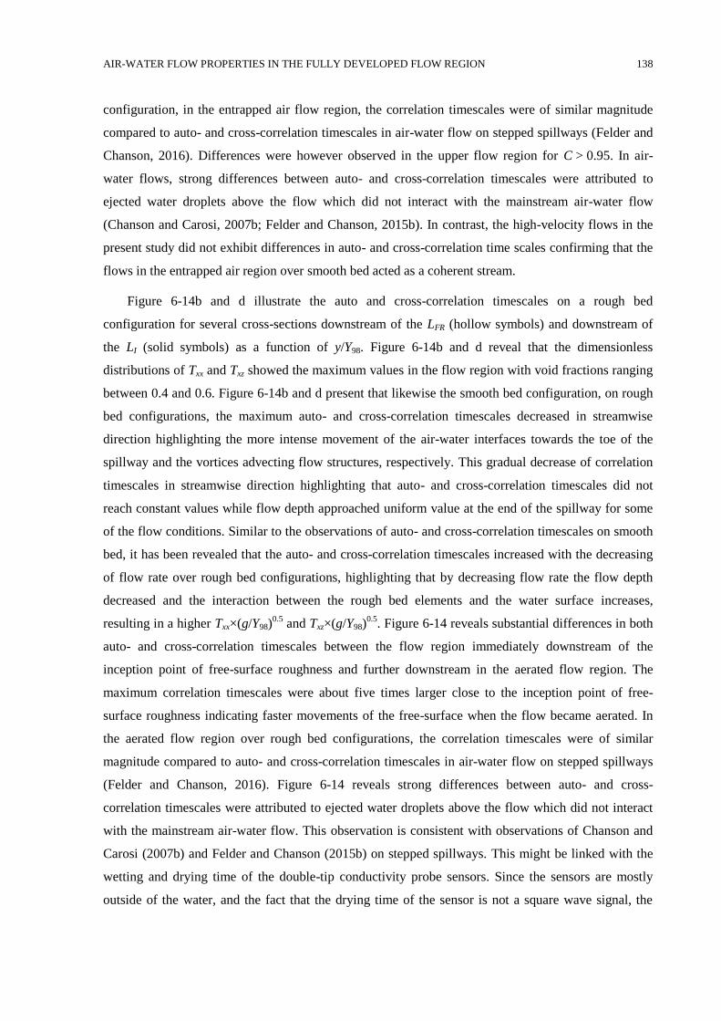
AIR-WATER FLOW PROPERTIES IN THE FULLY DEVELOPED FLOW REGION 138
configuration, in the entrapped air flow region, the correlation timescales were of similar magnitude
compared to auto- and cross-correlation timescales in air-water flow on stepped spillways (Felder and
Chanson, 2016). Differences were however observed in the upper flow region for C > 0.95. In air-
water flows, strong differences between auto- and cross-correlation timescales were attributed to
ejected water droplets above the flow which did not interact with the mainstream air-water flow
(Chanson and Carosi, 2007b; Felder and Chanson, 2015b). In contrast, the high-velocity flows in the
present study did not exhibit differences in auto- and cross-correlation time scales confirming that the
flows in the entrapped air region over smooth bed acted as a coherent stream.
Figure 6-14b and d illustrate the auto and cross-correlation timescales on a rough bed
configuration for several cross-sections downstream of the LFR (hollow symbols) and downstream of
the LI (solid symbols) as a function of y/Y98. Figure 6-14b and d reveal that the dimensionless
distributions of Txx and Txz showed the maximum values in the flow region with void fractions ranging
between 0.4 and 0.6. Figure 6-14b and d present that likewise the smooth bed configuration, on rough
bed configurations, the maximum auto- and cross-correlation timescales decreased in streamwise
direction highlighting the more intense movement of the air-water interfaces towards the toe of the
spillway and the vortices advecting flow structures, respectively. This gradual decrease of correlation
timescales in streamwise direction highlighting that auto- and cross-correlation timescales did not
reach constant values while flow depth approached uniform value at the end of the spillway for some
of the flow conditions. Similar to the observations of auto- and cross-correlation timescales on smooth
bed, it has been revealed that the auto- and cross-correlation timescales increased with the decreasing
of flow rate over rough bed configurations, highlighting that by decreasing flow rate the flow depth
decreased and the interaction between the rough bed elements and the water surface increases,
resulting in a higher Txx×(g/Y98)0.5
and Txz×(g/Y98)0.5
. Figure 6-14 reveals substantial differences in both
auto- and cross-correlation timescales between the flow region immediately downstream of the
inception point of free-surface roughness and further downstream in the aerated flow region. The
maximum correlation timescales were about five times larger close to the inception point of free-
surface roughness indicating faster movements of the free-surface when the flow became aerated. In
the aerated flow region over rough bed configurations, the correlation timescales were of similar
magnitude compared to auto- and cross-correlation timescales in air-water flow on stepped spillways
(Felder and Chanson, 2016). Figure 6-14 reveals strong differences between auto- and cross-
correlation timescales were attributed to ejected water droplets above the flow which did not interact
with the mainstream air-water flow. This observation is consistent with observations of Chanson and
Carosi (2007b) and Felder and Chanson (2015b) on stepped spillways. This might be linked with the
wetting and drying time of the double-tip conductivity probe sensors. Since the sensors are mostly
outside of the water, and the fact that the drying time of the sensor is not a square wave signal, the
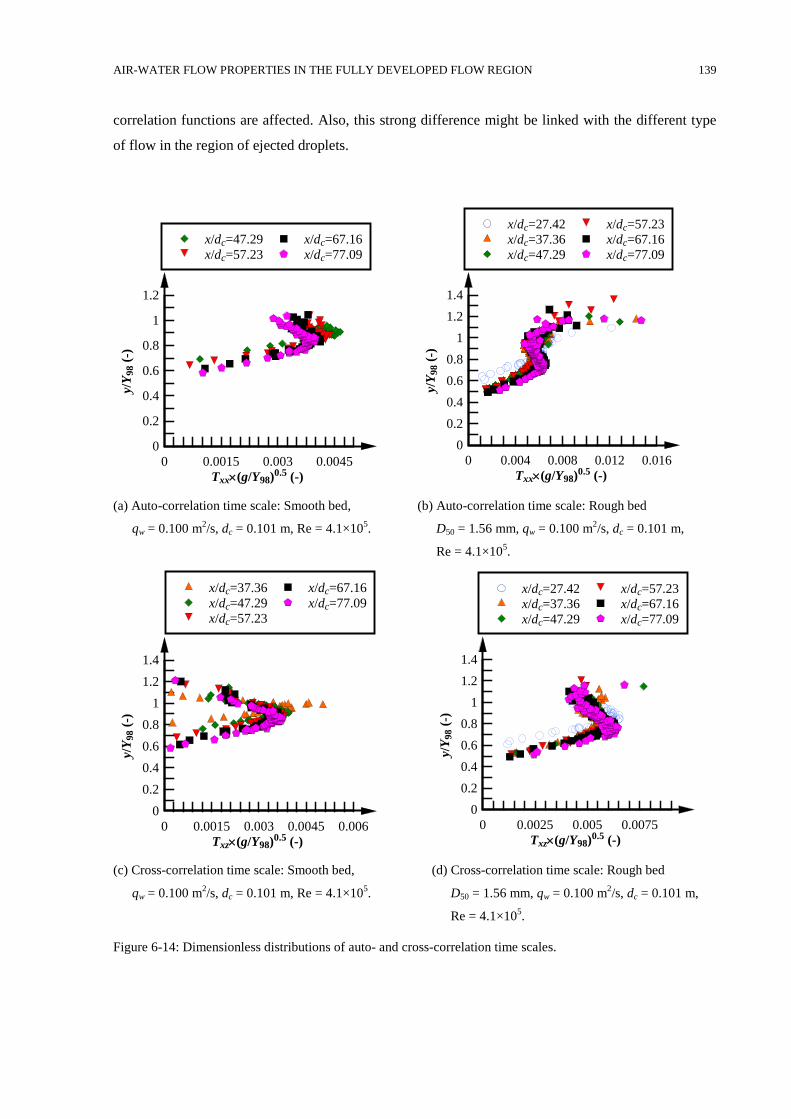
AIR-WATER FLOW PROPERTIES IN THE FULLY DEVELOPED FLOW REGION 139
correlation functions are affected. Also, this strong difference might be linked with the different type
of flow in the region of ejected droplets.
(a) Auto-correlation time scale: Smooth bed,
qw = 0.100 m2/s, dc = 0.101 m, Re = 4.1×10
5.
(b) Auto-correlation time scale: Rough bed
D50 = 1.56 mm, qw = 0.100 m2/s, dc = 0.101 m,
Re = 4.1×10⁵.
(c) Cross-correlation time scale: Smooth bed,
qw = 0.100 m2/s, dc = 0.101 m, Re = 4.1×10
5.
(d) Cross-correlation time scale: Rough bed
D50 = 1.56 mm, qw = 0.100 m2/s, dc = 0.101 m,
Re = 4.1×10⁵.
Figure 6-14: Dimensionless distributions of auto- and cross-correlation time scales.
Txx(g/Y98)0.5 (-)
y/Y
98 (
-)
0 0.0015 0.003 0.0045
0
0.2
0.4
0.6
0.8
1
1.2
x/dc=47.29
x/dc=57.23
x/dc=67.16
x/dc=77.09
Txx(g/Y98)0.5 (-)
y/Y
98 (
-)
0 0.004 0.008 0.012 0.016
0
0.2
0.4
0.6
0.8
1
1.2
1.4
x/dc=27.42
x/dc=37.36
x/dc=47.29
x/dc=57.23
x/dc=67.16
x/dc=77.09
Txz(g/Y98)0.5 (-)
y/Y
98 (
-)
0 0.0015 0.003 0.0045 0.006
0
0.2
0.4
0.6
0.8
1
1.2
1.4
x/dc=37.36
x/dc=47.29
x/dc=57.23
x/dc=67.16
x/dc=77.09
Txz(g/Y98)0.5 (-)
y/Y
98 (
-)
0 0.0025 0.005 0.0075
0
0.2
0.4
0.6
0.8
1
1.2
1.4
x/dc=27.42
x/dc=37.36
x/dc=47.29
x/dc=57.23
x/dc=67.16
x/dc=77.09
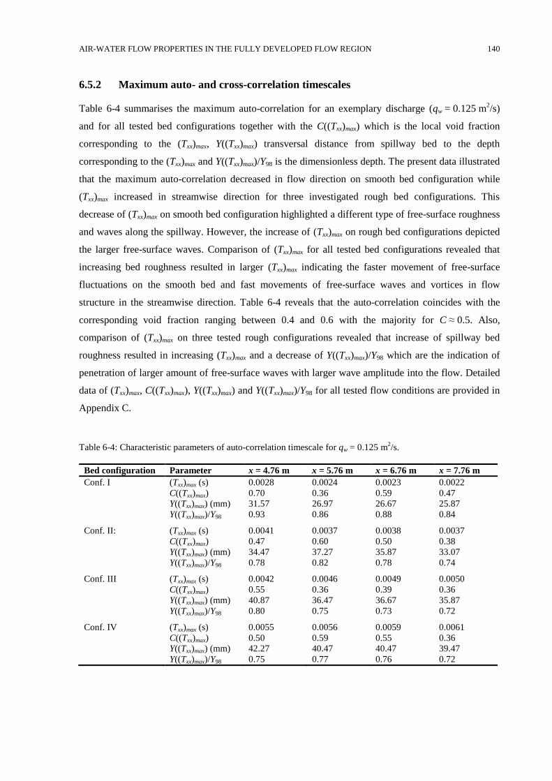
AIR-WATER FLOW PROPERTIES IN THE FULLY DEVELOPED FLOW REGION 140
6.5.2 Maximum auto- and cross-correlation timescales
Table 6-4 summarises the maximum auto-correlation for an exemplary discharge (qw = 0.125 m2/s)
and for all tested bed configurations together with the C((Txx)max) which is the local void fraction
corresponding to the (Txx)max, Y((Txx)max) transversal distance from spillway bed to the depth
corresponding to the (Txx)max and Y((Txx)max)/Y98 is the dimensionless depth. The present data illustrated
that the maximum auto-correlation decreased in flow direction on smooth bed configuration while
(Txx)max increased in streamwise direction for three investigated rough bed configurations. This
decrease of (Txx)max on smooth bed configuration highlighted a different type of free-surface roughness
and waves along the spillway. However, the increase of (Txx)max on rough bed configurations depicted
the larger free-surface waves. Comparison of (Txx)max for all tested bed configurations revealed that
increasing bed roughness resulted in larger (Txx)max indicating the faster movement of free-surface
fluctuations on the smooth bed and fast movements of free-surface waves and vortices in flow
structure in the streamwise direction. Table 6-4 reveals that the auto-correlation coincides with the
corresponding void fraction ranging between 0.4 and 0.6 with the majority for C ≈ 0.5. Also,
comparison of (Txx)max on three tested rough configurations revealed that increase of spillway bed
roughness resulted in increasing (Txx)max and a decrease of Y((Txx)max)/Y98 which are the indication of
penetration of larger amount of free-surface waves with larger wave amplitude into the flow. Detailed
data of (Txx)max, C((Txx)max), Y((Txx)max) and Y((Txx)max)/Y98 for all tested flow conditions are provided in
Appendix C.
Table 6-4: Characteristic parameters of auto-correlation timescale for qw = 0.125 m2/s.
Bed configuration Parameter x = 4.76 m x = 5.76 m x = 6.76 m x = 7.76 m
Conf. I (Txx)max (s) 0.0028 0.0024 0.0023 0.0022
C((Txx)max) 0.70 0.36 0.59 0.47
Y((Txx)max) (mm) 31.57 26.97 26.67 25.87
Y((Txx)max)/Y98 0.93 0.86 0.88 0.84
Conf. II: (Txx)max (s) 0.0041 0.0037 0.0038 0.0037
C((Txx)max) 0.47 0.60 0.50 0.38
Y((Txx)max) (mm) 34.47 37.27 35.87 33.07
Y((Txx)max)/Y98 0.78 0.82 0.78 0.74
Conf. III (Txx)max (s) 0.0042 0.0046 0.0049 0.0050
C((Txx)max) 0.55 0.36 0.39 0.36
Y((Txx)max) (mm) 40.87 36.47 36.67 35.87
Y((Txx)max)/Y98 0.80 0.75 0.73 0.72
Conf. IV (Txx)max (s) 0.0055 0.0056 0.0059 0.0061
C((Txx)max) 0.50 0.59 0.55 0.36
Y((Txx)max) (mm) 42.27 40.47 40.47 39.47
Y((Txx)max)/Y98 0.75 0.77 0.76 0.72
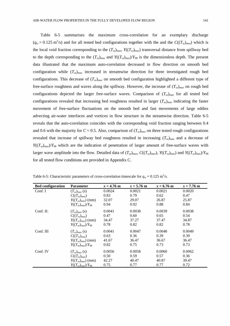
AIR-WATER FLOW PROPERTIES IN THE FULLY DEVELOPED FLOW REGION 141
Table 6-5 summarises the maximum cross-correlation for an exemplary discharge
(qw = 0.125 m2/s) and for all tested bed configurations together with the and the C((Txz)max) which is
the local void fraction corresponding to the (Txz)max, Y((Txz)max) transversal distance from spillway bed
to the depth corresponding to the (Txz)max and Y((Txz)max)/Y98 is the dimensionless depth. The present
data illustrated that the maximum auto-correlation decreased in flow direction on smooth bed
configuration while (Txz)max increased in streamwise direction for three investigated rough bed
configurations. This decrease of (Txz)max on smooth bed configuration highlighted a different type of
free-surface roughness and waves along the spillway. However, the increase of (Txz)max on rough bed
configurations depicted the larger free-surface waves. Comparison of (Txz)max for all tested bed
configurations revealed that increasing bed roughness resulted in larger (Txz)max indicating the faster
movement of free-surface fluctuations on the smooth bed and fast movements of large eddies
advecting air-water interfaces and vortices in flow structure in the streamwise direction. Table 6-5
reveals that the auto-correlation coincides with the corresponding void fraction ranging between 0.4
and 0.6 with the majority for C ≈ 0.5. Also, comparison of (Txz)max on three tested rough configurations
revealed that increase of spillway bed roughness resulted in increasing (Txz)max and a decrease of
Y((Txz)max)/Y98 which are the indication of penetration of larger amount of free-surface waves with
larger wave amplitude into the flow. Detailed data of (Txz)max, C((Txz)max), Y((Txz)max) and Y((Txz)max)/Y98
for all tested flow conditions are provided in Appendix C.
Table 6-5: Characteristic parameters of cross-correlation timescale for qw = 0.125 m2/s.
Bed configuration Parameter x = 4.76 m x = 5.76 m x = 6.76 m x = 7.76 m
Conf. I (Txz)max (s) 0.0024 0.0021 0.0021 0.0020
C((Txz)max) 0.83 0.79 0.62 0.47
Y((Txz)max) (mm) 32.07 29.07 26.87 25.87
Y((Txz)max)/Y98 0.94 0.92 0.88 0.84
Conf. II: (Txz)max (s) 0.0041 0.0038 0.0039 0.0038
C((Txz)max) 0.47 0.60 0.65 0.54
Y((Txz)max) (mm) 34.47 37.27 37.47 34.87
Y((Txz)max)/Y98 0.78 0.82 0.82 0.78
Conf. III (Txz)max (s) 0.0041 0.0047 0.0048 0.0049
C((Txz)max) 0.63 0.36 0.39 0.39
Y((Txz)max) (mm) 41.67 36.47 36.67 36.47
Y((Txz)max)/Y98 0.82 0.75 0.73 0.73
Conf. IV (Txz)max (s) 0.0056 0.0058 0.0060 0.0062
C((Txz)max) 0.50 0.59 0.57 0.36
Y((Txz)max) (mm) 42.27 40.47 40.87 39.47
Y((Txz)max)/Y98 0.75 0.77 0.77 0.72
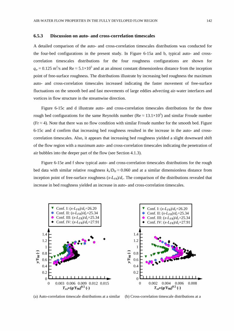
AIR-WATER FLOW PROPERTIES IN THE FULLY DEVELOPED FLOW REGION 142
6.5.3 Discussion on auto- and cross-correlation timescales
A detailed comparison of the auto- and cross-correlation timescales distributions was conducted for
the four-bed configurations in the present study. In Figure 6-15a and b, typical auto- and cross-
correlation timescales distributions for the four roughness configurations are shown for
qw = 0.125 m2/s and Re ≈ 5.1×10
5 and at an almost constant dimensionless distance from the inception
point of free-surface roughness. The distributions illustrate by increasing bed roughness the maximum
auto- and cross-correlation timescales increased indicating the faster movement of free-surface
fluctuations on the smooth bed and fast movements of large eddies advecting air-water interfaces and
vortices in flow structure in the streamwise direction.
Figure 6-15c and d illustrate auto- and cross-correlation timescales distributions for the three
rough bed configurations for the same Reynolds number (Re ≈ 13.1×10⁵) and similar Froude number
(Fr ≈ 4). Note that there was no flow condition with similar Froude number for the smooth bed. Figure
6-15c and d confirm that increasing bed roughness resulted in the increase in the auto- and cross-
correlation timescales. Also, it appears that increasing bed roughness yielded a slight downward shift
of the flow region with a maximum auto- and cross-correlation timescales indicating the penetration of
air bubbles into the deeper part of the flow (see Section 4.1.3).
Figure 6-15e and f show typical auto- and cross-correlation timescales distributions for the rough
bed data with similar relative roughness ks/DH ≈ 0.060 and at a similar dimensionless distance from
inception point of free-surface roughness (x-LFR)/dc. The comparison of the distributions revealed that
increase in bed roughness yielded an increase in auto- and cross-correlation timescales.
(a) Auto-correlation timescale distributions at a similar (b) Cross-correlation timescale distributions at a
Txx(g/Y98)0.5 (-)
y/Y
98 (
-)
0 0.003 0.006 0.009 0.012 0.015
0
0.2
0.4
0.6
0.8
1
1.2
1.4
Conf. I: (x-LFR)/dc=26.20
Conf. II: (x-LFR)/dc=25.34
Conf. III: (x-LFR)/dc=25.34
Conf. IV: (x-LFR)/dc=27.91
Txz(g/Y98)0.5 (-)
y/Y
98 (
-)
0 0.002 0.004 0.006 0.008
0
0.2
0.4
0.6
0.8
1
1.2
1.4
Conf. I: (x-LFR)/dc=26.20
Conf. II: (x-LFR)/dc=25.34
Conf. III: (x-LFR)/dc=25.34
Conf. IV: (x-LFR)/dc=27.91
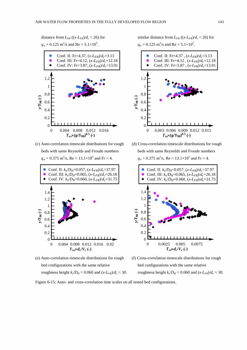
AIR-WATER FLOW PROPERTIES IN THE FULLY DEVELOPED FLOW REGION 143
distance from LFR ((x-LFR)/dc ≈ 26) for
qw = 0.125 m2/s and Re ≈ 5.1×10
5.
similar distance from LFR ((x-LFR)/dc ≈ 26) for
qw = 0.125 m2/s and Re ≈ 5.1×10
5.
(c) Auto-correlation timescale distributions for rough
beds with same Reynolds and Froude numbers
qw = 0.375 m2/s, Re ≈ 13.1×10
5 and Fr ≈ 4.
(d) Cross-correlation timescale distributions for rough
beds with same Reynolds and Froude numbers
qw = 0.375 m2/s, Re ≈ 13.1×10
5 and Fr ≈ 4.
(e) Auto-correlation timescale distributions for rough
bed configurations with the same relative
roughness height ks/DH ≈ 0.060 and (x-LFR)/dc ≈ 30.
(f) Cross-correlation timescale distributions for rough
bed configurations with the same relative
roughness height ks/DH ≈ 0.060 and (x-LFR)/dc ≈ 30.
Figure 6-15: Auto- and cross-correlation time scales on all tested bed configurations.
Txx(g/Y98)0.5 (-)
y/Y
98 (
-)
0 0.004 0.008 0.012 0.016
0
0.2
0.4
0.6
0.8
1
1.2
Conf. II: Fr=4.37, (x-LFR)/dc=3.13
Conf. III: Fr=4.12, (x-LFR)/dc=12.18
Conf. IV: Fr=3.87, (x-LFR)/dc=13.01
Txz(g/Y98)0.5 (-)y/
Y98 (
-)
0 0.003 0.006 0.009 0.012 0.015
0
0.2
0.4
0.6
0.8
1
1.2
Conf. II: Fr=4.37 , (x-LFR)/dc=3.13
Conf. III: Fr=4.12 , (x-LFR)/dc=12.18
Conf. IV: Fr=3.87 , (x-LFR)/dc=13.01
Txxdc/Vc (-)
y/Y
98 (
-)
0 0.004 0.008 0.012 0.016 0.02
0
0.2
0.4
0.6
0.8
1
1.2
1.4
Conf. II: ks/DH=0.057, (x-LFR)/dc=37.97
Conf. III: ks/DH=0.065, (x-LFR)/dc=26.18
Conf. IV: ks/DH=0.060, (x-LFR)/dc=31.75
Txzdc/Vc (-)
y/Y
98 (
-)
0 0.0025 0.005 0.0075
0
0.2
0.4
0.6
0.8
1
1.2
1.4
Conf. II: ks/DH=0.057, (x-LFR)/dc=37.97
Conf. III: ks/DH=0.065, (x-LFR)/dc=26.18
Conf. IV: ks/DH=0.060, (x-LFR)/dc=31.75
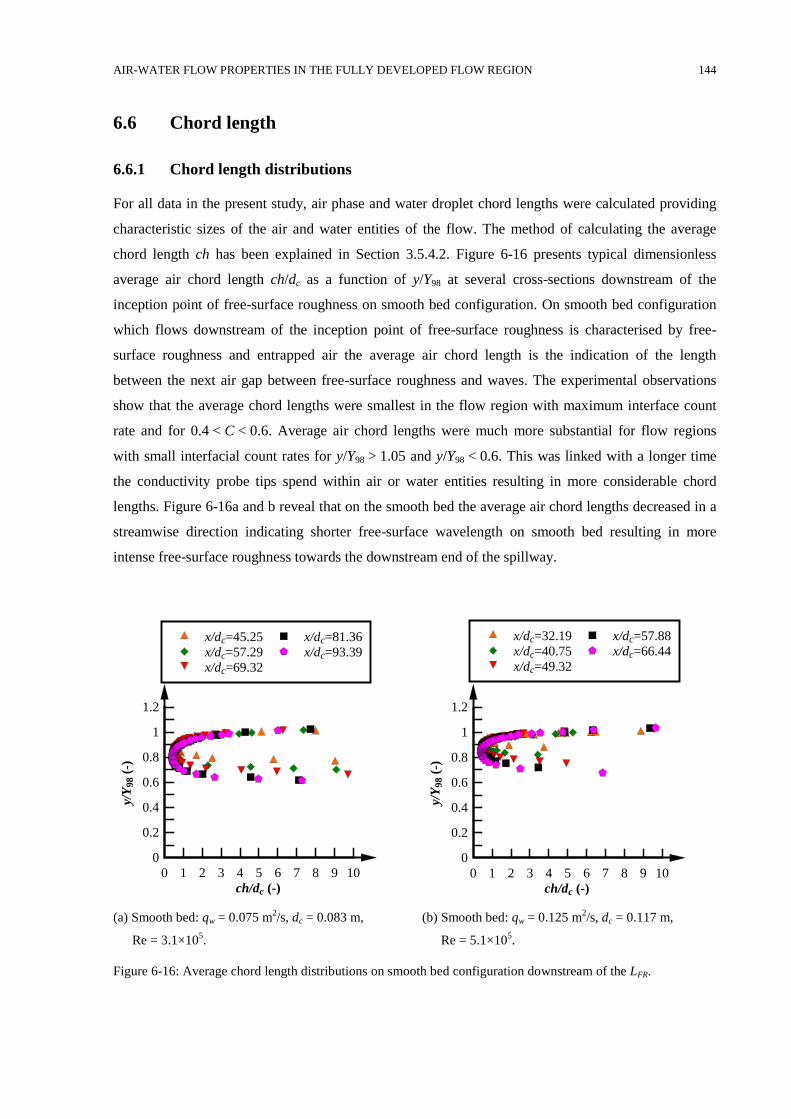
AIR-WATER FLOW PROPERTIES IN THE FULLY DEVELOPED FLOW REGION 144
Chord length 6.6
6.6.1 Chord length distributions
For all data in the present study, air phase and water droplet chord lengths were calculated providing
characteristic sizes of the air and water entities of the flow. The method of calculating the average
chord length ch has been explained in Section 3.5.4.2. Figure 6-16 presents typical dimensionless
average air chord length ch/dc as a function of y/Y98 at several cross-sections downstream of the
inception point of free-surface roughness on smooth bed configuration. On smooth bed configuration
which flows downstream of the inception point of free-surface roughness is characterised by free-
surface roughness and entrapped air the average air chord length is the indication of the length
between the next air gap between free-surface roughness and waves. The experimental observations
show that the average chord lengths were smallest in the flow region with maximum interface count
rate and for 0.4 < C < 0.6. Average air chord lengths were much more substantial for flow regions
with small interfacial count rates for y/Y98 > 1.05 and y/Y98 < 0.6. This was linked with a longer time
the conductivity probe tips spend within air or water entities resulting in more considerable chord
lengths. Figure 6-16a and b reveal that on the smooth bed the average air chord lengths decreased in a
streamwise direction indicating shorter free-surface wavelength on smooth bed resulting in more
intense free-surface roughness towards the downstream end of the spillway.
(a) Smooth bed: qw = 0.075 m2/s, dc = 0.083 m,
Re = 3.1×10⁵.
(b) Smooth bed: qw = 0.125 m2/s, dc = 0.117 m,
Re = 5.1×10⁵.
Figure 6-16: Average chord length distributions on smooth bed configuration downstream of the LFR.
ch/dc (-)
y/Y
98 (
-)
0 1 2 3 4 5 6 7 8 9 10
0
0.2
0.4
0.6
0.8
1
1.2
x/dc=45.25
x/dc=57.29
x/dc=69.32
x/dc=81.36
x/dc=93.39
ch/dc (-)
y/Y
98 (
-)
0 1 2 3 4 5 6 7 8 9 10
0
0.2
0.4
0.6
0.8
1
1.2
x/dc=32.19
x/dc=40.75
x/dc=49.32
x/dc=57.88
x/dc=66.44
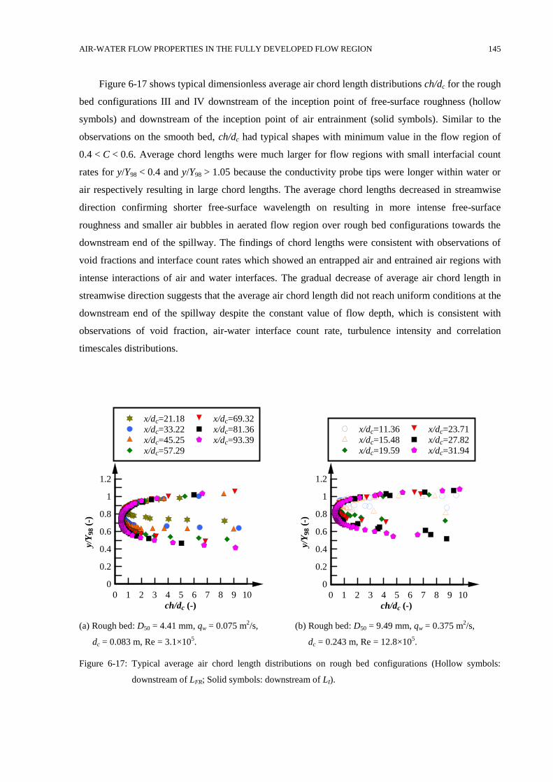
AIR-WATER FLOW PROPERTIES IN THE FULLY DEVELOPED FLOW REGION 145
Figure 6-17 shows typical dimensionless average air chord length distributions ch/dc for the rough
bed configurations III and IV downstream of the inception point of free-surface roughness (hollow
symbols) and downstream of the inception point of air entrainment (solid symbols). Similar to the
observations on the smooth bed, ch/dc had typical shapes with minimum value in the flow region of
0.4 < C < 0.6. Average chord lengths were much larger for flow regions with small interfacial count
rates for y/Y98 < 0.4 and y/Y98 > 1.05 because the conductivity probe tips were longer within water or
air respectively resulting in large chord lengths. The average chord lengths decreased in streamwise
direction confirming shorter free-surface wavelength on resulting in more intense free-surface
roughness and smaller air bubbles in aerated flow region over rough bed configurations towards the
downstream end of the spillway. The findings of chord lengths were consistent with observations of
void fractions and interface count rates which showed an entrapped air and entrained air regions with
intense interactions of air and water interfaces. The gradual decrease of average air chord length in
streamwise direction suggests that the average air chord length did not reach uniform conditions at the
downstream end of the spillway despite the constant value of flow depth, which is consistent with
observations of void fraction, air-water interface count rate, turbulence intensity and correlation
timescales distributions.
(a) Rough bed: D50 = 4.41 mm, qw = 0.075 m2/s,
dc = 0.083 m, Re = 3.1×10⁵.
(b) Rough bed: D50 = 9.49 mm, qw = 0.375 m2/s,
dc = 0.243 m, Re = 12.8×10⁵.
Figure 6-17: Typical average air chord length distributions on rough bed configurations (Hollow symbols:
downstream of LFR; Solid symbols: downstream of LI).
ch/dc (-)
y/Y
98 (
-)
0 1 2 3 4 5 6 7 8 9 10
0
0.2
0.4
0.6
0.8
1
1.2
x/dc=21.18
x/dc=33.22
x/dc=45.25
x/dc=57.29
x/dc=69.32
x/dc=81.36
x/dc=93.39
ch/dc (-)
y/Y
98 (
-)
0 1 2 3 4 5 6 7 8 9 10
0
0.2
0.4
0.6
0.8
1
1.2
x/dc=11.36
x/dc=15.48
x/dc=19.59
x/dc=23.71
x/dc=27.82
x/dc=31.94
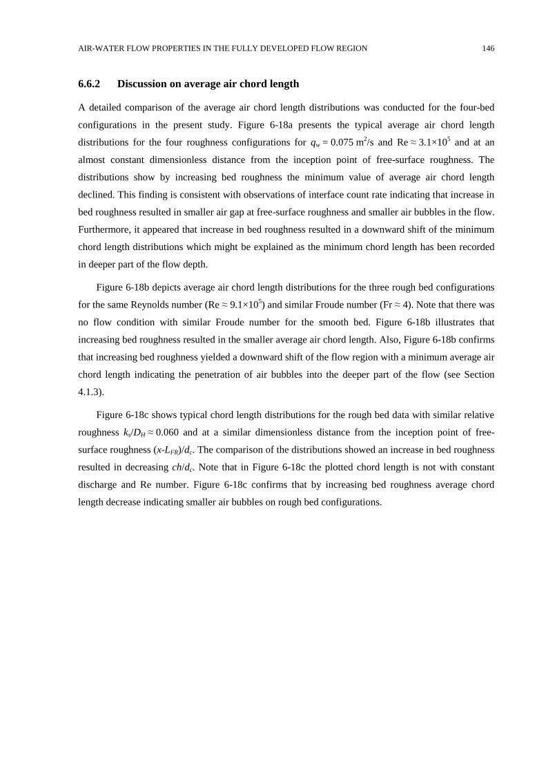
AIR-WATER FLOW PROPERTIES IN THE FULLY DEVELOPED FLOW REGION 146
6.6.2 Discussion on average air chord length
A detailed comparison of the average air chord length distributions was conducted for the four-bed
configurations in the present study. Figure 6-18a presents the typical average air chord length
distributions for the four roughness configurations for qw = 0.075 m2/s and Re ≈ 3.1×10
5 and at an
almost constant dimensionless distance from the inception point of free-surface roughness. The
distributions show by increasing bed roughness the minimum value of average air chord length
declined. This finding is consistent with observations of interface count rate indicating that increase in
bed roughness resulted in smaller air gap at free-surface roughness and smaller air bubbles in the flow.
Furthermore, it appeared that increase in bed roughness resulted in a downward shift of the minimum
chord length distributions which might be explained as the minimum chord length has been recorded
in deeper part of the flow depth.
Figure 6-18b depicts average air chord length distributions for the three rough bed configurations
for the same Reynolds number (Re ≈ 9.1×10⁵) and similar Froude number (Fr ≈ 4). Note that there was
no flow condition with similar Froude number for the smooth bed. Figure 6-18b illustrates that
increasing bed roughness resulted in the smaller average air chord length. Also, Figure 6-18b confirms
that increasing bed roughness yielded a downward shift of the flow region with a minimum average air
chord length indicating the penetration of air bubbles into the deeper part of the flow (see Section
4.1.3).
Figure 6-18c shows typical chord length distributions for the rough bed data with similar relative
roughness ks/DH ≈ 0.060 and at a similar dimensionless distance from the inception point of free-
surface roughness (x-LFR)/dc. The comparison of the distributions showed an increase in bed roughness
resulted in decreasing ch/dc. Note that in Figure 6-18c the plotted chord length is not with constant
discharge and Re number. Figure 6-18c confirms that by increasing bed roughness average chord
length decrease indicating smaller air bubbles on rough bed configurations.
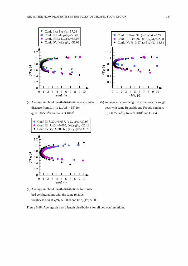
AIR-WATER FLOW PROPERTIES IN THE FULLY DEVELOPED FLOW REGION 147
(a) Average air chord length distributions at a similar
distance from LFR ((x-LFR)/dc ≈ 55) for
qw = 0.075 m2/s and Re ≈ 3.1×10
5.
(b) Average air chord length distributions for rough
beds with same Reynolds and Froude numbers
qw = 0.250 m2/s, Re ≈ 9.1×10
5 and Fr ≈ 4.
(c) Average air chord length distributions for rough
bed configurations with the same relative
roughness height ks/DH ≈ 0.060 and (x-LFR)/dc ≈ 30.
Figure 6-18: Average air chord length distributions for all bed configurations.
ch/dc (-)
y/Y
98 (
-)
0 1 2 3 4 5 6 7 8 9 10
0
0.2
0.4
0.6
0.8
1
1.2
Conf. I: (x-LFR)/dc=57.29
Conf. II: (x-LFR)/dc=58.49
Conf. III: (x-LFR)/dc=53.08
Conf. IV: (x-LFR)/dc=56.08
ch/dc (-)
y/Y
98 (
-)
0 1 2 3 4 5 6 7 8 9 10
0
0.2
0.4
0.6
0.8
1
1.2
Conf. II: Fr=4.38, (x-LFR)/dc=5.72
Conf. III: Fr=3.97, (x-LFR)/dc=22.98
Conf. IV: Fr=3.97, (x-LFR)/dc=13.81
ch/dc (-)
y/Y
98 (
-)
0 1 2 3 4 5 6 7 8 9 10
0
0.2
0.4
0.6
0.8
1
1.2
Conf. II: ks/DH=0.057, (x-LFR)/dc=37.97
Conf. III: ks/DH=0.065, (x-LFR)/dc=26.18
Conf. IV: ks/DH=0.060, (x-LFR)/dc=31.75
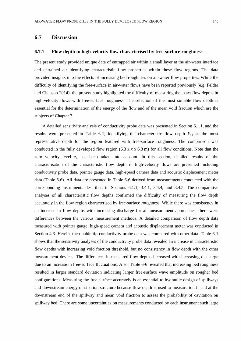
AIR-WATER FLOW PROPERTIES IN THE FULLY DEVELOPED FLOW REGION 148
Discussion 6.7
6.7.1 Flow depth in high-velocity flow characterised by free-surface roughness
The present study provided unique data of entrapped air within a small layer at the air-water interface
and entrained air identifying characteristic flow properties within these flow regions. The data
provided insights into the effects of increasing bed roughness on air-water flow properties. While the
difficulty of identifying the free-surface in air-water flows have been reported previously (e.g. Felder
and Chanson 2014), the present study highlighted the difficulty of measuring the exact flow depths in
high-velocity flows with free-surface roughness. The selection of the most suitable flow depth is
essential for the determination of the energy of the flow and of the mean void fraction which are the
subjects of Chapter 7.
A detailed sensitivity analysis of conductivity probe data was presented in Section 6.1.1, and the
results were presented in Table 6-1, identifying the characteristic flow depth Y98 as the most
representative depth for the region featured with free-surface roughness. The comparison was
conducted in the fully developed flow region (6.3 ≤ x ≤ 6.8 m) for all flow conditions. Note that the
zero velocity level zo has been taken into account. In this section, detailed results of the
characterisation of the characteristic flow depth in high-velocity flows are presented including
conductivity probe data, pointer gauge data, high-speed camera data and acoustic displacement meter
data (Table 6-6). All data are presented in Table 6-6 derived from measurements conducted with the
corresponding instruments described in Sections 6.1.1, 3.4.1, 3.4.4, and 3.4.5. The comparative
analyses of all characteristic flow depths confirmed the difficulty of measuring the flow depth
accurately in the flow region characterised by free-surface roughness. While there was consistency in
an increase in flow depths with increasing discharge for all measurement approaches, there were
differences between the various measurement methods. A detailed comparison of flow depth data
measured with pointer gauge, high-speed camera and acoustic displacement meter was conducted in
Section 4.3. Herein, the double-tip conductivity probe data was compared with other data. Table 6-1
shows that the sensitivity analyses of the conductivity probe data revealed an increase in characteristic
flow depths with increasing void fraction threshold, but no consistency in flow depth with the other
measurement devices. The differences in measured flow depths increased with increasing discharge
due to an increase in free-surface fluctuations. Also, Table 6-6 revealed that increasing bed roughness
resulted in larger standard deviation indicating larger free-surface wave amplitude on rougher bed
configurations. Measuring the free-surface accurately is an essential to hydraulic design of spillways
and downstream energy dissipation structure because flow depth is used to measure total head at the
downstream end of the spillway and mean void fraction to assess the probability of cavitation on
spillway bed. There are some uncertainties on measurements conducted by each instrument such large

AIR-WATER FLOW PROPERTIES IN THE FULLY DEVELOPED FLOW REGION 149
footprint, very few data to compare for acoustic displacement meter, sidewall and potential camera
angle and distortion for high-speed camera application, fluctuations of free-surface and subjectivity of
observer and double-tip conductivity probe regarding the signal is not entirely rectangular because of
the small size of the probe tips, the wetting and drying time of the tips and the response time of the
instrument and the data acquisition system (Felder, 2013). It appears that flow depth measurements
with a double-tip conductivity probe are a viable alternative.
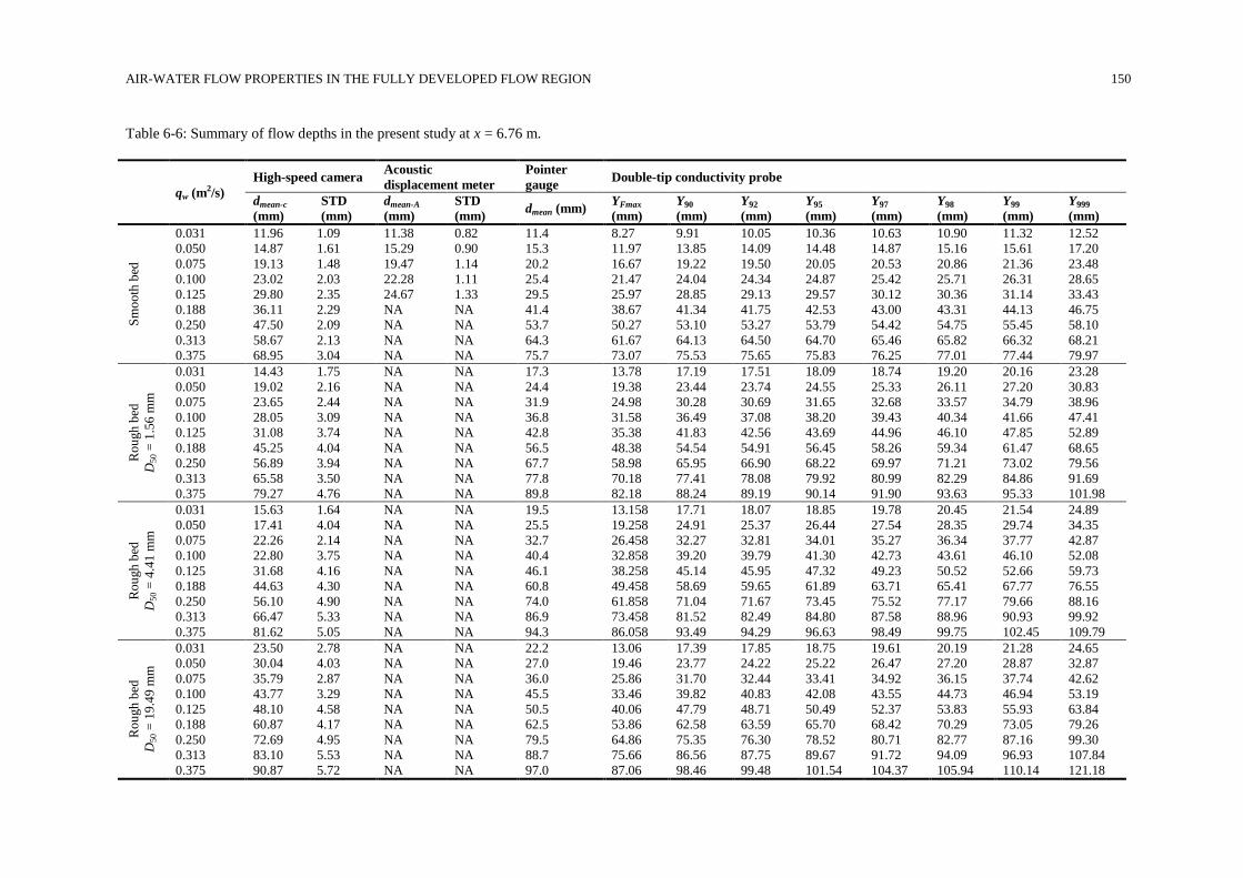
AIR-WATER FLOW PROPERTIES IN THE FULLY DEVELOPED FLOW REGION 150
Table 6-6: Summary of flow depths in the present study at x = 6.76 m.
qw (m2/s)
High-speed camera Acoustic
displacement meter
Pointer
gauge Double-tip conductivity probe
dmean-c
(mm)
STD
(mm)
dmean-A
(mm)
STD
(mm) dmean (mm)
YFmax
(mm)
Y90
(mm)
Y92
(mm)
Y95
(mm)
Y97
(mm)
Y98
(mm)
Y99
(mm)
Y999
(mm)
Sm
oo
th b
ed
0.031 11.96 1.09 11.38 0.82 11.4 8.27 9.91 10.05 10.36 10.63 10.90 11.32 12.52
0.050 14.87 1.61 15.29 0.90 15.3 11.97 13.85 14.09 14.48 14.87 15.16 15.61 17.20
0.075 19.13 1.48 19.47 1.14 20.2 16.67 19.22 19.50 20.05 20.53 20.86 21.36 23.48
0.100 23.02 2.03 22.28 1.11 25.4 21.47 24.04 24.34 24.87 25.42 25.71 26.31 28.65
0.125 29.80 2.35 24.67 1.33 29.5 25.97 28.85 29.13 29.57 30.12 30.36 31.14 33.43
0.188 36.11 2.29 NA NA 41.4 38.67 41.34 41.75 42.53 43.00 43.31 44.13 46.75
0.250 47.50 2.09 NA NA 53.7 50.27 53.10 53.27 53.79 54.42 54.75 55.45 58.10
0.313 58.67 2.13 NA NA 64.3 61.67 64.13 64.50 64.70 65.46 65.82 66.32 68.21
0.375 68.95 3.04 NA NA 75.7 73.07 75.53 75.65 75.83 76.25 77.01 77.44 79.97
Ro
ugh
bed
D50 =
1.5
6 m
m
0.031 14.43 1.75 NA NA 17.3 13.78 17.19 17.51 18.09 18.74 19.20 20.16 23.28
0.050 19.02 2.16 NA NA 24.4 19.38 23.44 23.74 24.55 25.33 26.11 27.20 30.83
0.075 23.65 2.44 NA NA 31.9 24.98 30.28 30.69 31.65 32.68 33.57 34.79 38.96
0.100 28.05 3.09 NA NA 36.8 31.58 36.49 37.08 38.20 39.43 40.34 41.66 47.41
0.125 31.08 3.74 NA NA 42.8 35.38 41.83 42.56 43.69 44.96 46.10 47.85 52.89
0.188 45.25 4.04 NA NA 56.5 48.38 54.54 54.91 56.45 58.26 59.34 61.47 68.65
0.250 56.89 3.94 NA NA 67.7 58.98 65.95 66.90 68.22 69.97 71.21 73.02 79.56
0.313 65.58 3.50 NA NA 77.8 70.18 77.41 78.08 79.92 80.99 82.29 84.86 91.69
0.375 79.27 4.76 NA NA 89.8 82.18 88.24 89.19 90.14 91.90 93.63 95.33 101.98
Ro
ugh
bed
D50 =
4.4
1 m
m
0.031 15.63 1.64 NA NA 19.5 13.158 17.71 18.07 18.85 19.78 20.45 21.54 24.89
0.050 17.41 4.04 NA NA 25.5 19.258 24.91 25.37 26.44 27.54 28.35 29.74 34.35
0.075 22.26 2.14 NA NA 32.7 26.458 32.27 32.81 34.01 35.27 36.34 37.77 42.87
0.100 22.80 3.75 NA NA 40.4 32.858 39.20 39.79 41.30 42.73 43.61 46.10 52.08
0.125 31.68 4.16 NA NA 46.1 38.258 45.14 45.95 47.32 49.23 50.52 52.66 59.73
0.188 44.63 4.30 NA NA 60.8 49.458 58.69 59.65 61.89 63.71 65.41 67.77 76.55
0.250 56.10 4.90 NA NA 74.0 61.858 71.04 71.67 73.45 75.52 77.17 79.66 88.16
0.313 66.47 5.33 NA NA 86.9 73.458 81.52 82.49 84.80 87.58 88.96 90.93 99.92
0.375 81.62 5.05 NA NA 94.3 86.058 93.49 94.29 96.63 98.49 99.75 102.45 109.79
Ro
ugh
bed
D50 =
19
.49 m
m
0.031 23.50 2.78 NA NA 22.2 13.06 17.39 17.85 18.75 19.61 20.19 21.28 24.65
0.050 30.04 4.03 NA NA 27.0 19.46 23.77 24.22 25.22 26.47 27.20 28.87 32.87
0.075 35.79 2.87 NA NA 36.0 25.86 31.70 32.44 33.41 34.92 36.15 37.74 42.62
0.100 43.77 3.29 NA NA 45.5 33.46 39.82 40.83 42.08 43.55 44.73 46.94 53.19
0.125 48.10 4.58 NA NA 50.5 40.06 47.79 48.71 50.49 52.37 53.83 55.93 63.84
0.188 60.87 4.17 NA NA 62.5 53.86 62.58 63.59 65.70 68.42 70.29 73.05 79.26
0.250 72.69 4.95 NA NA 79.5 64.86 75.35 76.30 78.52 80.71 82.77 87.16 99.30
0.313 83.10 5.53 NA NA 88.7 75.66 86.56 87.75 89.67 91.72 94.09 96.93 107.84
0.375 90.87 5.72 NA NA 97.0 87.06 98.46 99.48 101.54 104.37 105.94 110.14 121.18
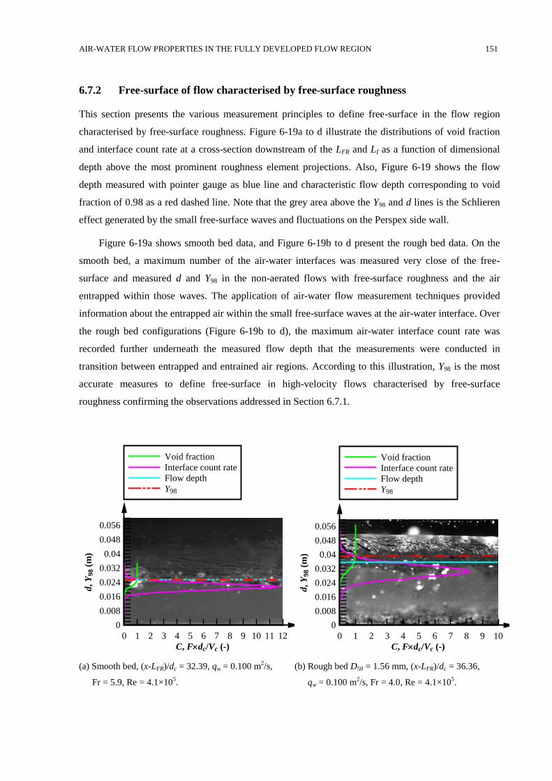
AIR-WATER FLOW PROPERTIES IN THE FULLY DEVELOPED FLOW REGION 151
6.7.2 Free-surface of flow characterised by free-surface roughness
This section presents the various measurement principles to define free-surface in the flow region
characterised by free-surface roughness. Figure 6-19a to d illustrate the distributions of void fraction
and interface count rate at a cross-section downstream of the LFR and LI as a function of dimensional
depth above the most prominent roughness element projections. Also, Figure 6-19 shows the flow
depth measured with pointer gauge as blue line and characteristic flow depth corresponding to void
fraction of 0.98 as a red dashed line. Note that the grey area above the Y98 and d lines is the Schlieren
effect generated by the small free-surface waves and fluctuations on the Perspex side wall.
Figure 6-19a shows smooth bed data, and Figure 6-19b to d present the rough bed data. On the
smooth bed, a maximum number of the air-water interfaces was measured very close of the free-
surface and measured d and Y98 in the non-aerated flows with free-surface roughness and the air
entrapped within those waves. The application of air-water flow measurement techniques provided
information about the entrapped air within the small free-surface waves at the air-water interface. Over
the rough bed configurations (Figure 6-19b to d), the maximum air-water interface count rate was
recorded further underneath the measured flow depth that the measurements were conducted in
transition between entrapped and entrained air regions. According to this illustration, Y98 is the most
accurate measures to define free-surface in high-velocity flows characterised by free-surface
roughness confirming the observations addressed in Section 6.7.1.
(a) Smooth bed, (x-LFR)/dc = 32.39, qw = 0.100 m2/s,
Fr = 5.9, Re = 4.1×10⁵.
(b) Rough bed D50 = 1.56 mm, (x-LFR)/dc = 36.36,
qw = 0.100 m2/s, Fr = 4.0, Re = 4.1×10
5.
C, Fdc/Vc (-)
d, Y
98 (
m)
0 1 2 3 4 5 6 7 8 9 10 11 12
0
0.008
0.016
0.024
0.032
0.04
0.048
0.056
Void fraction
Interface count rate
Flow depth
Y98
C, Fdc/Vc (-)
d, Y
98 (
m)
0 1 2 3 4 5 6 7 8 9 10
0
0.008
0.016
0.024
0.032
0.04
0.048
0.056
Void fraction
Interface count rate
Flow depth
Y98
AIR-WATER FLOW PROPERTIES IN THE FULLY DEVELOPED FLOW REGION 152
(c) Rough bed D50 = 4.41 mm, (x-LFR)/dc = 32.39,
qw = 0.100 m2/s, Fr = 3.3, Re = 4.0×10
5.
(d) Rough bed D50 = 9.49 mm, (x-LFR)/dc = 33.38,
qw = 0.100 m2/s, Fr = 2.9, Re = 4.0×10
5.
Figure 6-19: Distribution of void fraction, interface count rate, characteristic flow depth Y98 and flow depth d
based upon pointer gauge data for qw = 0.100 m2/s at an almost constant distance from the
inception point of free-surface roughness for the four-bed roughness configurations.
6.7.3 Characteristic air-water flow parameters change along the spillway
In the present study, at the air-water interface, void fractions were between 0.4 < C < 0.6 with the
majority of maximum values of Fmax, Tumax, (Txx)max and (Txz)max observed for C ≈ 0.5. In this section,
further comparison of changes in Fmax, Tumax, (Txx)max and (Txz)max along the spillway were studied for
all tested bed configurations.
Figure 6-20a and b show the dimensionless maximum air-water interface count rate as a function
of dimensionless longitudinal distance along the spillway from inception point of free-surface
roughness on the smooth bed and an exemplary rough bed configuration (D50 = 4.41 mm),
respectively. Figure 6-20a and b present that for all tested flow conditions at the same distance from
the inception point of free-surface roughness the maximum air-water interface count rate increases by
increasing discharge. Figure 6-20b shows that for qw ≤ 0.050 m2/s on rough bed configuration the air-
water interface count rate tending to reach almost constant values while for qw > 0.050 m2/s interface
count rate increased sharply in the streamwise direction. However, the uniform flow depth observed
on the rough bed configurations (see Section 4.1) were not reflected in Figure 6-20b. This observation
is consistent with findings of Felder (2013) who reported that bubble count rate F did not reach an
equilibrium value on fully aerated flow condition on stepped spillways. Figures for two other tested
micro-rough bed configurations were presented in Appendix C Section C.6.
C, Fdc/Vc (-)
d, Y
98 (
m)
0 1 2 3 4 5 6 7 8 9 10
0
0.008
0.016
0.024
0.032
0.04
0.048
0.056
Void fraction
Interface count rate
Flow depth
Y98
C, Fdc/Vc (-)
d, Y
98 (
m)
0 1 2 3 4 5 6 7 8 9 10
0
0.008
0.016
0.024
0.032
0.04
0.048
0.056
Void fraction
Interface count rate
Flow depth
Y98
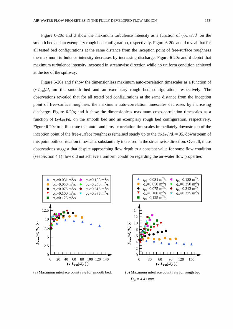
AIR-WATER FLOW PROPERTIES IN THE FULLY DEVELOPED FLOW REGION 153
Figure 6-20c and d show the maximum turbulence intensity as a function of (x-LFR)/dc on the
smooth bed and an exemplary rough bed configuration, respectively. Figure 6-20c and d reveal that for
all tested bed configurations at the same distance from the inception point of free-surface roughness
the maximum turbulence intensity decreases by increasing discharge. Figure 6-20c and d depict that
maximum turbulence intensity increased in streamwise direction while no uniform condition achieved
at the toe of the spillway.
Figure 6-20e and f show the dimensionless maximum auto-correlation timescales as a function of
(x-LFR)/dc on the smooth bed and an exemplary rough bed configuration, respectively. The
observations revealed that for all tested bed configurations at the same distance from the inception
point of free-surface roughness the maximum auto-correlation timescales decreases by increasing
discharge. Figure 6-20g and h show the dimensionless maximum cross-correlation timescales as a
function of (x-LFR)/dc on the smooth bed and an exemplary rough bed configuration, respectively.
Figure 6-20e to h illustrate that auto- and cross-correlation timescales immediately downstream of the
inception point of the free-surface roughness remained steady up to the (x-LFR)/dc ≈ 35, downstream of
this point both correlation timescales substantially increased in the streamwise direction. Overall, these
observations suggest that despite approaching flow depth to a constant value for some flow condition
(see Section 4.1) flow did not achieve a uniform condition regarding the air-water flow properties.
(a) Maximum interface count rate for smooth bed. (b) Maximum interface count rate for rough bed
D50 = 4.41 mm.
(x-LFR)/dc (-)
Fm
ax
dc/
Vc
(-)
0 20 40 60 80 100 120 140
0
2.5
5
7.5
10
12.5
qw=0.031 m2/s
qw=0.050 m2/s
qw=0.075 m2/s
qw=0.100 m2/s
qw=0.125 m2/s
qw=0.188 m2/s
qw=0.250 m2/s
qw=0.313 m2/s
qw=0.375 m2/s
(x-LFR)/dc (-)
Fm
ax
dc/
Vc
(-)
0 30 60 90 120 150
0
2
4
6
8
10
12
14
qw=0.031 m2/s
qw=0.050 m2/s
qw=0.075 m2/s
qw=0.100 m2/s
qw=0.125 m2/s
qw=0.188 m2/s
qw=0.250 m2/s
qw=0.313 m2/s
qw=0.375 m2/s
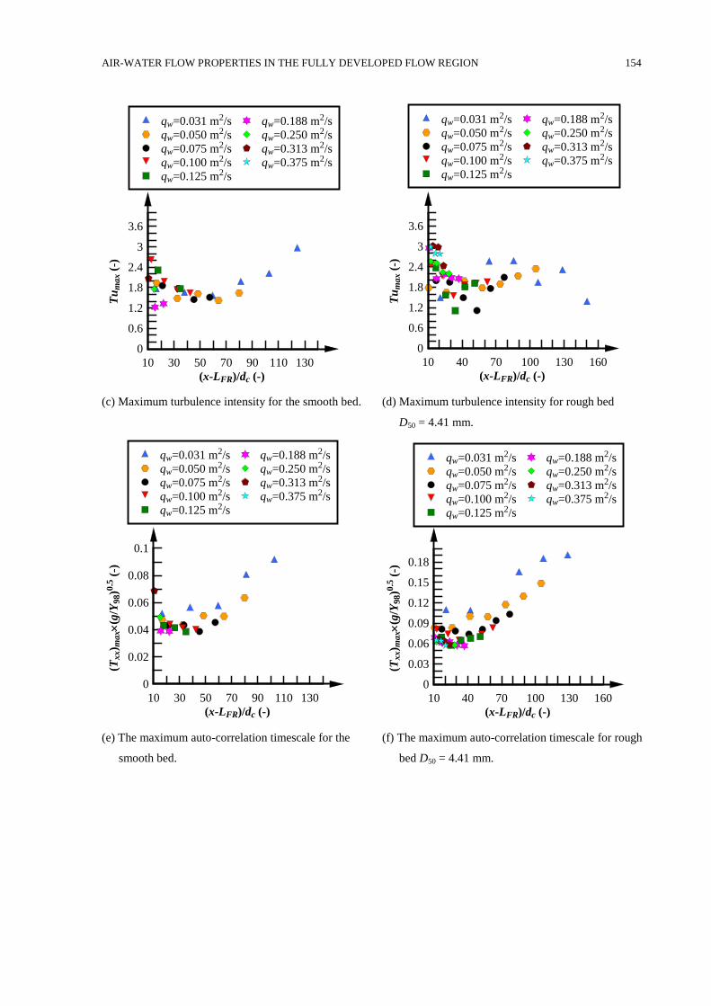
AIR-WATER FLOW PROPERTIES IN THE FULLY DEVELOPED FLOW REGION 154
(c) Maximum turbulence intensity for the smooth bed. (d) Maximum turbulence intensity for rough bed
D50 = 4.41 mm.
(e) The maximum auto-correlation timescale for the
smooth bed.
(f) The maximum auto-correlation timescale for rough
bed D50 = 4.41 mm.
(x-LFR)/dc (-)
Tu
max (
-)
10 30 50 70 90 110 130
0
0.6
1.2
1.8
2.4
3
3.6
qw=0.031 m2/s
qw=0.050 m2/s
qw=0.075 m2/s
qw=0.100 m2/s
qw=0.125 m2/s
qw=0.188 m2/s
qw=0.250 m2/s
qw=0.313 m2/s
qw=0.375 m2/s
(x-LFR)/dc (-)
Tu
ma
x (
-)
10 40 70 100 130 160
0
0.6
1.2
1.8
2.4
3
3.6
qw=0.031 m2/s
qw=0.050 m2/s
qw=0.075 m2/s
qw=0.100 m2/s
qw=0.125 m2/s
qw=0.188 m2/s
qw=0.250 m2/s
qw=0.313 m2/s
qw=0.375 m2/s
(x-LFR)/dc (-)
(Tx
x) m
ax
(g/Y
98)0
.5 (
-)
10 30 50 70 90 110 130
0
0.02
0.04
0.06
0.08
0.1
qw=0.031 m2/s
qw=0.050 m2/s
qw=0.075 m2/s
qw=0.100 m2/s
qw=0.125 m2/s
qw=0.188 m2/s
qw=0.250 m2/s
qw=0.313 m2/s
qw=0.375 m2/s
(x-LFR)/dc (-)
(Tx
x) m
ax
(g/Y
98)0
.5 (
-)
10 40 70 100 130 160
0
0.03
0.06
0.09
0.12
0.15
0.18
qw=0.031 m2/s
qw=0.050 m2/s
qw=0.075 m2/s
qw=0.100 m2/s
qw=0.125 m2/s
qw=0.188 m2/s
qw=0.250 m2/s
qw=0.313 m2/s
qw=0.375 m2/s
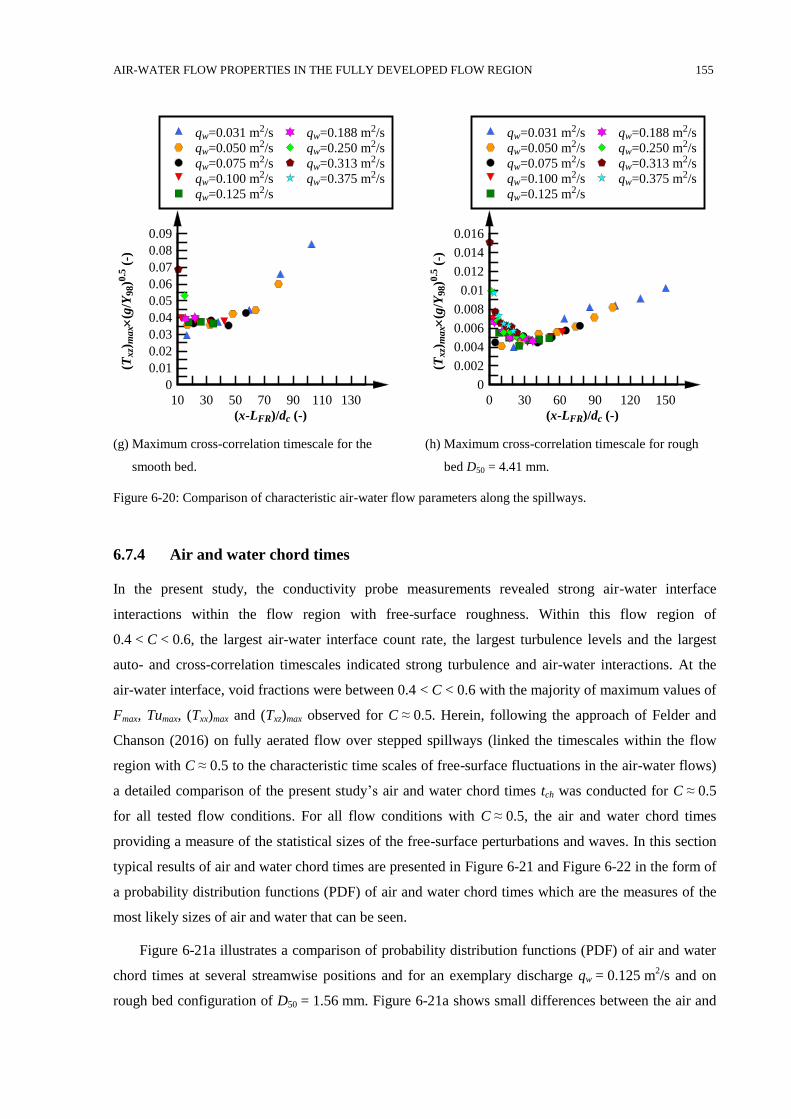
AIR-WATER FLOW PROPERTIES IN THE FULLY DEVELOPED FLOW REGION 155
(g) Maximum cross-correlation timescale for the
smooth bed.
(h) Maximum cross-correlation timescale for rough
bed D50 = 4.41 mm.
Figure 6-20: Comparison of characteristic air-water flow parameters along the spillways.
6.7.4 Air and water chord times
In the present study, the conductivity probe measurements revealed strong air-water interface
interactions within the flow region with free-surface roughness. Within this flow region of
0.4 < C < 0.6, the largest air-water interface count rate, the largest turbulence levels and the largest
auto- and cross-correlation timescales indicated strong turbulence and air-water interactions. At the
air-water interface, void fractions were between 0.4 < C < 0.6 with the majority of maximum values of
Fmax, Tumax, (Txx)max and (Txz)max observed for C ≈ 0.5. Herein, following the approach of Felder and
Chanson (2016) on fully aerated flow over stepped spillways (linked the timescales within the flow
region with C ≈ 0.5 to the characteristic time scales of free-surface fluctuations in the air-water flows)
a detailed comparison of the present study’s air and water chord times tch was conducted for C ≈ 0.5
for all tested flow conditions. For all flow conditions with C ≈ 0.5, the air and water chord times
providing a measure of the statistical sizes of the free-surface perturbations and waves. In this section
typical results of air and water chord times are presented in Figure 6-21 and Figure 6-22 in the form of
a probability distribution functions (PDF) of air and water chord times which are the measures of the
most likely sizes of air and water that can be seen.
Figure 6-21a illustrates a comparison of probability distribution functions (PDF) of air and water
chord times at several streamwise positions and for an exemplary discharge qw = 0.125 m2/s and on
rough bed configuration of D50 = 1.56 mm. Figure 6-21a shows small differences between the air and
(x-LFR)/dc (-)
(Txz)
max
(g/Y
98)0
.5 (
-)
10 30 50 70 90 110 130
0
0.01
0.02
0.03
0.04
0.05
0.06
0.07
0.08
0.09
qw=0.031 m2/s
qw=0.050 m2/s
qw=0.075 m2/s
qw=0.100 m2/s
qw=0.125 m2/s
qw=0.188 m2/s
qw=0.250 m2/s
qw=0.313 m2/s
qw=0.375 m2/s
(x-LFR)/dc (-)
(Txz)
max
(g/Y
98)0
.5 (
-)
0 30 60 90 120 150
0
0.002
0.004
0.006
0.008
0.01
0.012
0.014
0.016
qw=0.031 m2/s
qw=0.050 m2/s
qw=0.075 m2/s
qw=0.100 m2/s
qw=0.125 m2/s
qw=0.188 m2/s
qw=0.250 m2/s
qw=0.313 m2/s
qw=0.375 m2/s
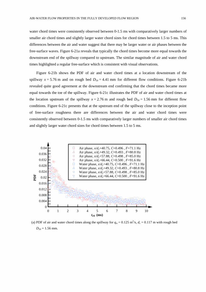
AIR-WATER FLOW PROPERTIES IN THE FULLY DEVELOPED FLOW REGION 156
water chord times were consistently observed between 0-1.5 ms with comparatively larger numbers of
smaller air chord times and slightly larger water chord sizes for chord times between 1.5 to 5 ms. This
differences between the air and water suggest that there may be larger water or air phases between the
free-surface waves. Figure 6-21a reveals that typically the chord times become more equal towards the
downstream end of the spillway compared to upstream. The similar magnitude of air and water chord
times highlighted a regular free-surface which is consistent with visual observations.
Figure 6-21b shows the PDF of air and water chord times at a location downstream of the
spillway x = 5.76 m and on rough bed D50 = 4.41 mm for different flow conditions. Figure 6-21b
revealed quite good agreement at the downstream end confirming that the chord times became more
equal towards the toe of the spillway. Figure 6-21c illustrates the PDF of air and water chord times at
the location upstream of the spillway x = 2.76 m and rough bed D50 = 1.56 mm for different flow
conditions. Figure 6-21c presents that at the upstream end of the spillway close to the inception point
of free-surface roughness there are differences between the air and water chord times were
consistently observed between 0-1.5 ms with comparatively larger numbers of smaller air chord times
and slightly larger water chord sizes for chord times between 1.5 to 5 ms.
(a) PDF of air and water chord times along the spillway for qw = 0.125 m2/s, dc = 0.117 m with rough bed
D50 = 1.56 mm.
tch (ms)
PD
F
0 1 2 3 4 5 6 7 8 9 10
0
0.004
0.008
0.012
0.016
0.02
0.024
0.028
0.032
0.036
0.04 Air phase, x/dc=40.75, C=0.496 , F=71.1 Hz
Air phase, x/dc=49.32, C=0.493 , F=80.8 Hz
Air phase, x/dc=57.88, C=0.498 , F=85.0 Hz
Air phase, x/dc=66.44, C=0.500 , F=91.6 Hz
Water phase, x/dc=40.75, C=0.496 , F=71.1 Hz
Water phase, x/dc=49.32, C=0.493 , F=80.8 Hz
Water phase, x/dc=57.88, C=0.498 , F=85.0 Hz
Water phase, x/dc=66.44, C=0.500 , F=91.6 Hz
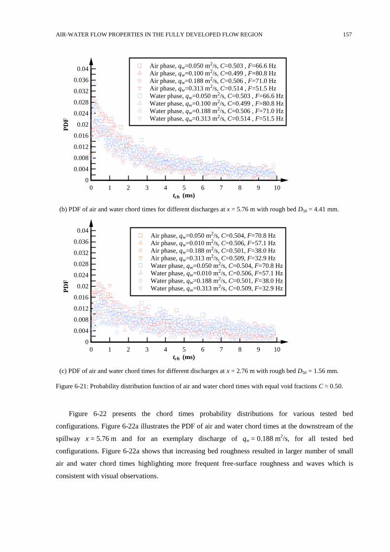
AIR-WATER FLOW PROPERTIES IN THE FULLY DEVELOPED FLOW REGION 157
(b) PDF of air and water chord times for different discharges at x = 5.76 m with rough bed D50 = 4.41 mm.
(c) PDF of air and water chord times for different discharges at x = 2.76 m with rough bed D50 = 1.56 mm.
Figure 6-21: Probability distribution function of air and water chord times with equal void fractions C ≈ 0.50.
Figure 6-22 presents the chord times probability distributions for various tested bed
configurations. Figure 6-22a illustrates the PDF of air and water chord times at the downstream of the
spillway x = 5.76 m and for an exemplary discharge of qw = 0.188 m2/s, for all tested bed
configurations. Figure 6-22a shows that increasing bed roughness resulted in larger number of small
air and water chord times highlighting more frequent free-surface roughness and waves which is
consistent with visual observations.
tch (ms)
PD
F
0 1 2 3 4 5 6 7 8 9 10
0
0.004
0.008
0.012
0.016
0.02
0.024
0.028
0.032
0.036
0.04Air phase, qw=0.050 m2/s, C=0.503 , F=66.6 Hz
Air phase, qw=0.100 m2/s, C=0.499 , F=80.8 Hz
Air phase, qw=0.188 m2/s, C=0.506 , F=71.0 Hz
Air phase, qw=0.313 m2/s, C=0.514 , F=51.5 Hz
Water phase, qw=0.050 m2/s, C=0.503 , F=66.6 Hz
Water phase, qw=0.100 m2/s, C=0.499 , F=80.8 Hz
Water phase, qw=0.188 m2/s, C=0.506 , F=71.0 Hz
Water phase, qw=0.313 m2/s, C=0.514 , F=51.5 Hz
tch (ms)
PD
F
0 1 2 3 4 5 6 7 8 9 10
0
0.004
0.008
0.012
0.016
0.02
0.024
0.028
0.032
0.036
0.04Air phase, qw=0.050 m2/s, C=0.504, F=70.8 Hz
Air phase, qw=0.010 m2/s, C=0.506, F=57.1 Hz
Air phase, qw=0.188 m2/s, C=0.501, F=38.0 Hz
Air phase, qw=0.313 m2/s, C=0.509, F=32.9 Hz
Water phase, qw=0.050 m2/s, C=0.504, F=70.8 Hz
Water phase, qw=0.010 m2/s, C=0.506, F=57.1 Hz
Water phase, qw=0.188 m2/s, C=0.501, F=38.0 Hz
Water phase, qw=0.313 m2/s, C=0.509, F=32.9 Hz
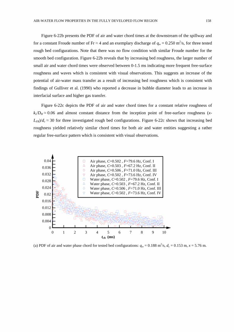
AIR-WATER FLOW PROPERTIES IN THE FULLY DEVELOPED FLOW REGION 158
Figure 6-22b presents the PDF of air and water chord times at the downstream of the spillway and
for a constant Froude number of Fr ≈ 4 and an exemplary discharge of qw = 0.250 m2/s, for three tested
rough bed configurations. Note that there was no flow condition with similar Froude number for the
smooth bed configuration. Figure 6-22b reveals that by increasing bed roughness, the larger number of
small air and water chord times were observed between 0-1.5 ms indicating more frequent free-surface
roughness and waves which is consistent with visual observations. This suggests an increase of the
potential of air-water mass transfer as a result of increasing bed roughness which is consistent with
findings of Gulliver et al. (1990) who reported a decrease in bubble diameter leads to an increase in
interfacial surface and higher gas transfer.
Figure 6-22c depicts the PDF of air and water chord times for a constant relative roughness of
ks/DH ≈ 0.06 and almost constant distance from the inception point of free-surface roughness (x-
LFR)/dc ≈ 30 for three investigated rough bed configurations. Figure 6-22c shows that increasing bed
roughness yielded relatively similar chord times for both air and water entities suggesting a rather
regular free-surface pattern which is consistent with visual observations.
(a) PDF of air and water phase chord for tested bed configurations: qw = 0.188 m2/s, dc = 0.153 m, x = 5.76 m.
tch (ms)
PD
F
0 1 2 3 4 5 6 7 8 9 10
0
0.004
0.008
0.012
0.016
0.02
0.024
0.028
0.032
0.036
0.04 Air phase, C=0.502 , F=79.6 Hz, Conf. I
Air phase, C=0.503 , F=67.2 Hz, Conf. II
Air phase, C=0.506 , F=71.0 Hz, Conf. III
Air phase, C=0.502 , F=73.6 Hz, Conf. IV
Water phase, C=0.502 , F=79.6 Hz, Conf. I
Water phase, C=0.503 , F=67.2 Hz, Conf. II
Water phase, C=0.506 , F=71.0 Hz, Conf. III
Water phase, C=0.502 , F=73.6 Hz, Conf. IV
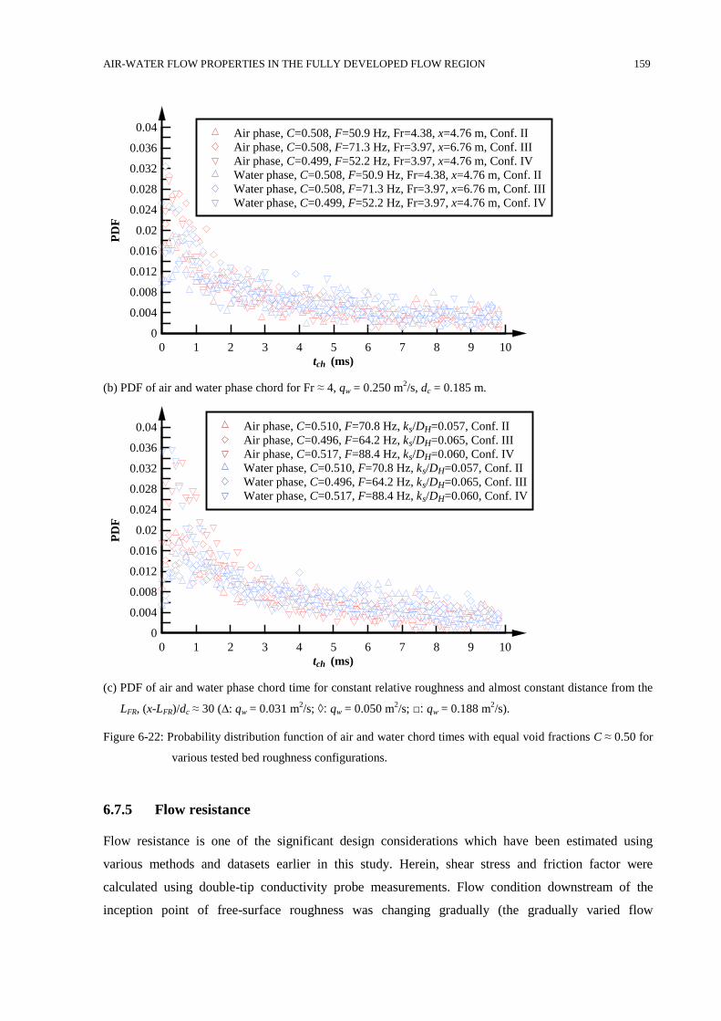
AIR-WATER FLOW PROPERTIES IN THE FULLY DEVELOPED FLOW REGION 159
(b) PDF of air and water phase chord for Fr ≈ 4, qw = 0.250 m2/s, dc = 0.185 m.
(c) PDF of air and water phase chord time for constant relative roughness and almost constant distance from the
LFR, (x-LFR)/dc ≈ 30 (∆: qw = 0.031 m2/s; ◊: qw = 0.050 m
2/s; □: qw = 0.188 m
2/s).
Figure 6-22: Probability distribution function of air and water chord times with equal void fractions C ≈ 0.50 for
various tested bed roughness configurations.
6.7.5 Flow resistance
Flow resistance is one of the significant design considerations which have been estimated using
various methods and datasets earlier in this study. Herein, shear stress and friction factor were
calculated using double-tip conductivity probe measurements. Flow condition downstream of the
inception point of free-surface roughness was changing gradually (the gradually varied flow
tch (ms)
PD
F
0 1 2 3 4 5 6 7 8 9 10
0
0.004
0.008
0.012
0.016
0.02
0.024
0.028
0.032
0.036
0.04Air phase, C=0.508, F=50.9 Hz, Fr=4.38, x=4.76 m, Conf. II
Air phase, C=0.508, F=71.3 Hz, Fr=3.97, x=6.76 m, Conf. III
Air phase, C=0.499, F=52.2 Hz, Fr=3.97, x=4.76 m, Conf. IV
Water phase, C=0.508, F=50.9 Hz, Fr=4.38, x=4.76 m, Conf. II
Water phase, C=0.508, F=71.3 Hz, Fr=3.97, x=6.76 m, Conf. III
Water phase, C=0.499, F=52.2 Hz, Fr=3.97, x=4.76 m, Conf. IV
tch (ms)
PD
F
0 1 2 3 4 5 6 7 8 9 10
0
0.004
0.008
0.012
0.016
0.02
0.024
0.028
0.032
0.036
0.04 Air phase, C=0.510, F=70.8 Hz, ks/DH=0.057, Conf. II
Air phase, C=0.496, F=64.2 Hz, ks/DH=0.065, Conf. III
Air phase, C=0.517, F=88.4 Hz, ks/DH=0.060, Conf. IV
Water phase, C=0.510, F=70.8 Hz, ks/DH=0.057, Conf. II
Water phase, C=0.496, F=64.2 Hz, ks/DH=0.065, Conf. III
Water phase, C=0.517, F=88.4 Hz, ks/DH=0.060, Conf. IV
AIR-WATER FLOW PROPERTIES IN THE FULLY DEVELOPED FLOW REGION 160
condition); therefore, the flow resistance was deduced from the average friction slope applying
gradually varied flow theory. In the flow region characterised by free-surface roughness, the
equivalent Darcy friction factors for air-water flows fe were applied as
𝑓𝑒 =8𝑔
𝑞2 × (𝑧0 + ∫ (1 − 𝐶)𝑑𝑦𝑦=𝑌90
𝑦=0)
2× (
𝐷𝐻
4) × 𝑆𝑓 (6-8)
For smooth bed configuration, the friction factor obtained from applying gradually varied flow theory
for double-tip conductivity probe data was fe = 0.024. The dimensionless shear stress for the double-tip
conductivity probe data was τo/(ρ×g×dc)= 0.045. For the tested rough bed configurations of D50 = 1.56,
4.41 and 9.49 mm, applying gradually varied flow theory resulted in friction factor of 0.031, 0.045 and
0.055 based on the double-tip conductivity probe, and corresponding dimensionless shear stress of
τo/(ρ×g×dc)= 0.039, 0.049 and 0.057. Details comparison of estimated friction factor based on various
approaches studied in this thesis will be addressed in Section 7.1.
Summary 6.8
Air-water flow measurements technique was applied in the flow region characterised by free-surface
roughness and entrapped air. Detailed air-water flow measurements were performed using a double-tip
conductivity probe for all tested flow conditions. The present data provided information about the
entrapped flow region downstream of the inception point of free-surface roughness and entrained flow
region downstream of the inception point of free-surface aeration. It has been observed that flow over
smooth bed configuration was characterised by free-surface roughness and continuous entrapped air
within a small layer at the air-water interface towards the toe of the spillway. While flow over tested
micro-rough bed configurations was characterised by free-surface roughness and continuous entrapped
air as well as free-surface aeration towards the downstream end of the spillway.
Experimental results revealed that the air-water flow measurements technique applies to measure
flow properties within the flow region characterised by entrapped air. A detail sensitivity analysis
revealed that Y98 is the most appropriate characteristic depth to define flow depth in flow characterised
by free-surface roughness and entrapped air. The observations of all air-water flow properties on
smooth bed showed strong interactions of air and water phases within the flow region of
0.6 < y/Y98 < 1.05 with void fraction ranging between 0.4 < C < 0.6. The results highlighted that the
flow region with equal amounts of air and water phases (C ≈ 0.5) was the most representative location
for flows with free-surface roughness. Also, on tested rough bed configurations the strong interactions
of air and water phases were observed within the flow region of 0.4 < y/Y98 < 1.05 with void fraction
ranging between 0.4 < C < 0.6. The flow properties in the flow region characterised by entrapped air
showed shapes similar to fully aerated air-water flows. In the present study, within flow region
characterised by free-surface roughness, the maximum value of air-water interface count rate,
AIR-WATER FLOW PROPERTIES IN THE FULLY DEVELOPED FLOW REGION 161
turbulence levels and auto- and cross-correlation timescales observed for C ≈ 0.5 indicating the strong
turbulence and air-water interactions within this region. The comparative analysis of air-water flow
properties for investigated bed configurations illustrated that an increase in bed roughness increased
mean void fraction and air-water interface count rate, turbulence intensity, and auto- and cross-
correlation timescales. Also, a monotonic decrease of average chord length and chord time with
increasing air-water interface count rate was observed.
Furthermore, a slight increase of characteristic flow properties along the spillway including a
gradual increase in mean void fraction, air-water interface count rate, turbulence intensity and gradual
decrease in auto- and cross-correlation timescale, average air and water chord length indicating that no
uniform flow conditions were achieved at the downstream end of the spillway despite constant flow
depth for some flow conditions. Also, analysis of air-water flow properties revealed that increasing
bed roughness resulted in increasing Fmax, Tumax ̧ (Txz)max, (Txx)max and a decrease of Y(Fmax)/Y98,
Y(Tumax)/Y98, Y((Txz)max)/Y98, Y((Txx)max)/Y98 which are the indication of penetration of larger amount of
free-surface waves with larger wave amplitude into the flow. Comparative analysis of the gradient of
void fraction distributions revealed the increase of gradient in streamwise direction suggesting that
free-surface wave amplitude increased towards the toe of the spillway which is consistent with visual
observations. Also, for a given discharge the gradient of void fraction distributions approaching a
constant value indicating more equal wave amplitude at the downstream end of the spillway compared
to the upstream. Detail comparison of chord times revealed that chord time distributions become more
equal in a streamwise direction indicating a rather regular free-surface roughness toward the
downstream of the spillway. Moreover, the comparison revealed that increase in bed roughness
configuration resulted in larger number of small size air and water chord times suggesting the larger
interfacial surface and larger potential of air-water mass transfer.
Chapter 7
7 DISCUSSION
Flow resistance 7.1
On smooth invert channels, energy dissipation occurs predominantly through boundary friction.
Experimental results regarding flow resistance obtained for smooth invert spillways equipped with
different micro-rough configurations are presented in this section. The results are compared using
Darcy-Weisbach friction factors f. Figure 7-1 presents Darcy-Weisbach friction factor data resulting
from different approaches including applying logarithmic law within the inner flow region (fInner:
Section 5.3.1), velocity defect law within the outer flow region (fOuter: Section 5.3.2), momentum
integral method (fMI: Section 5.3.3), using gradually varied flow approach based on two sets of data
including pointer gauge data (fDarcy: Section 5.3.4) and the double-tip conductivity data (fe: Section
6.7.5). Figure 7-1 shows the estimated friction factors corresponding to the aforementioned
approaches as a function of dimensionless relative roughness ks/DH for tested flow conditions. Figure
7-1 presents scatter and differences between data using different approaches. For example on rough
bed configuration, friction factor data calculated based on logarithmic law within inner flow region,
velocity defect law within outer flow region and gradually varied flow theory using pointer gauge data
show close agreement. While friction factors calculated based on momentum integral method and
gradually varied flow theory using the double-tip conductivity probe data constantly showing smaller
values. Figure 7-1 reveals a close agreement between friction factors calculated based on momentum
integral method in boundary layer developing flow region and gradually varied flow theory using the
double-tip conductivity probe data downstream of the inception point of free-surface roughness
independent of discharge. It has been observed that an increase in flow rate resulted in the closer
agreement of estimated friction factors based on different approaches. For example, under the flow
condition of qw = 0.031 m2/s friction factor determined based on the logarithmic law in inner flow
region shows the largest discrepancy indicating the thin layer of inner flow region close to the bottom
and few numbers of measurement points within this region due to the limitation of Pitot-tube diameter.
DISCUSSION 163
Figure 7-1a illustrates that according to the momentum integral method and gradually varied flow
theory based on conductivity probe datasets, friction factor ranging between 0.008 and 0.015. Also,
friction factor estimated based on law of the wall in the inner flow region and gradually varied flow
theory based on pointer gauge data varied from 0.015 to 0.026. However, friction factor obtained
based on the law of the wall in outer flow region shows strong scatter. Hence in order to calculate
average value the data derived from using law of the wall within outer flow region has been excluded.
Overall, the average friction factor of all methods for smooth bed configuration found as
0.012 ≤ fave ≤ 0.017 for 0.031 ≤ qw ≤ 0.375 m2/s. Figure 7-1b depicts that according to the momentum
integral method and gradually varied flow theory based on conductivity probe datasets, friction factor
ranging between 0.022 and 0.034. Also, friction factor estimated based on the both laws of the wall in
the inner and outer flow regions and gradually varied flow theory based upon pointer gauge data
varied from 0.043 to 0.094. The average friction factor of all methods for micro-rough bed
configuration with D50 = 1.56 mm was estimated 0.037 ≤ fave ≤ 0.069. Figure 7-1c depicts that
according to the momentum integral method and gradually varied flow theory based on conductivity
probe datasets, friction factor ranging between 0.035 and 0.050. Also, friction factor estimated based
on the both laws of the wall in the inner and outer flow regions and gradually varied flow theory based
on pointer gauge data varied from 0.044 to 0.135. The average friction factor of all methods for micro-
rough bed configuration with D50 = 4.41 mm estimated 0.046 ≤ fave ≤ 0.086. Figure 7-1d depicts that
according to the momentum integral method and gradually varied flow theory based on conductivity
probe datasets, friction factor ranging between 0.040 and 0.084. Also, friction factor estimated based
on the both laws of the wall in the inner and outer flow regions and gradually varied flow theory based
on pointer gauge data varied from 0.060 to 0.168. The average friction factor of all methods for micro-
rough bed configuration with D50 = 9.49 mm estimated 0.060 ≤ fave ≤ 0.113. Note that to define the
range of variation of friction factor those data points with extreme values due to the small number of
measurement points within the inner flow region were excluded.
Furthermore, Figure 7-1b to d present calculated friction factor using uniform flow properties
illustrated as hollow stars. These figures reveal that friction factor in flow region with uniform flow
depth and velocity distribution can be estimated using uniform flow theory. Figure 7-1b to d illustrates
comparison of equation (2-21) developed by Rice et al. (1998) for non-aerated flow over block ramps
indicating reasonable agreement with average value of friction factor of present study. However,
comparison of the present study data with Pagliara et al. (2008) for non-aerated flow condition over
block ramp revealed that friction factors were overestimated about 30 to 70 percent by applying
Pagliara et al. (2008) equation. This strong differences highlighted the limitation of Pagliara et al.
(2008) proposed equation within the experimental limits of their study (see Section 2.2.1). Also,
Figure 7-1a to d comprises the calculated friction factor using Colebrook-White equation highlighting
that average value of the present study data compare well with the Moody diagram. This suggests that
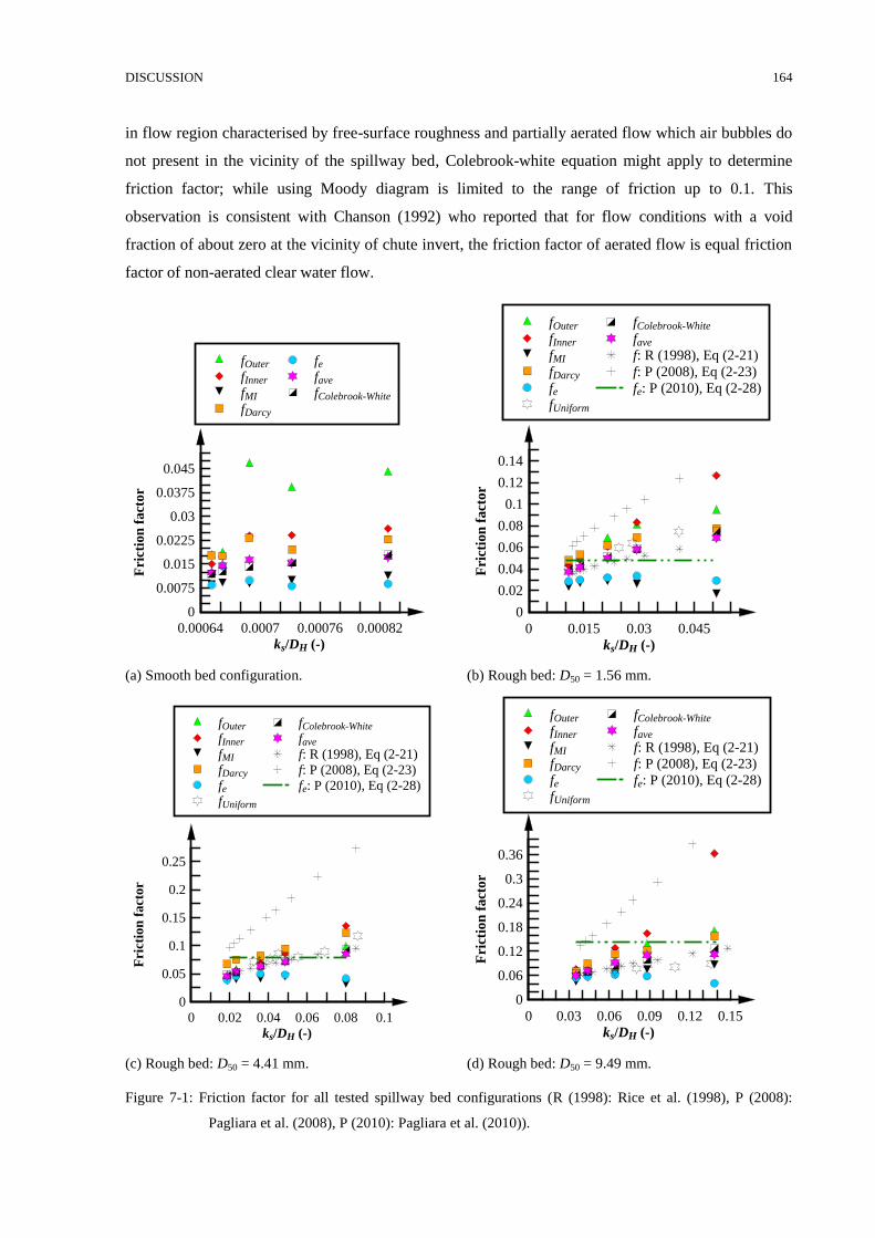
DISCUSSION 164
in flow region characterised by free-surface roughness and partially aerated flow which air bubbles do
not present in the vicinity of the spillway bed, Colebrook-white equation might apply to determine
friction factor; while using Moody diagram is limited to the range of friction up to 0.1. This
observation is consistent with Chanson (1992) who reported that for flow conditions with a void
fraction of about zero at the vicinity of chute invert, the friction factor of aerated flow is equal friction
factor of non-aerated clear water flow.
(a) Smooth bed configuration. (b) Rough bed: D50 = 1.56 mm.
(c) Rough bed: D50 = 4.41 mm. (d) Rough bed: D50 = 9.49 mm.
Figure 7-1: Friction factor for all tested spillway bed configurations (R (1998): Rice et al. (1998), P (2008):
Pagliara et al. (2008), P (2010): Pagliara et al. (2010)).
ks/DH (-)
Fri
ctio
n f
act
or
0.00064 0.0007 0.00076 0.00082
0
0.0075
0.015
0.0225
0.03
0.0375
0.045
fOuter
fInner
fMI
fDarcy
fefave
fColebrook-White
ks/DH (-)
Fri
ctio
n f
act
or
0 0.015 0.03 0.045
0
0.02
0.04
0.06
0.08
0.1
0.12
0.14
fOuter
fInner
fMI
fDarcy
fefUniform
fColebrook-White
fave
f: R (1998), Eq (2-21)
f: P (2008), Eq (2-23)
fe: P (2010), Eq (2-28)
ks/DH (-)
Fri
ctio
n f
act
or
0 0.02 0.04 0.06 0.08 0.1
0
0.05
0.1
0.15
0.2
0.25
fOuter
fInner
fMI
fDarcy
fefUniform
fColebrook-White
fave
f: R (1998), Eq (2-21)
f: P (2008), Eq (2-23)
fe: P (2010), Eq (2-28)
ks/DH (-)
Fri
ctio
n f
act
or
0 0.03 0.06 0.09 0.12 0.15
0
0.06
0.12
0.18
0.24
0.3
0.36
fOuter
fInner
fMI
fDarcy
fefUniform
fColebrook-White
fave
f: R (1998), Eq (2-21)
f: P (2008), Eq (2-23)
fe: P (2010), Eq (2-28)
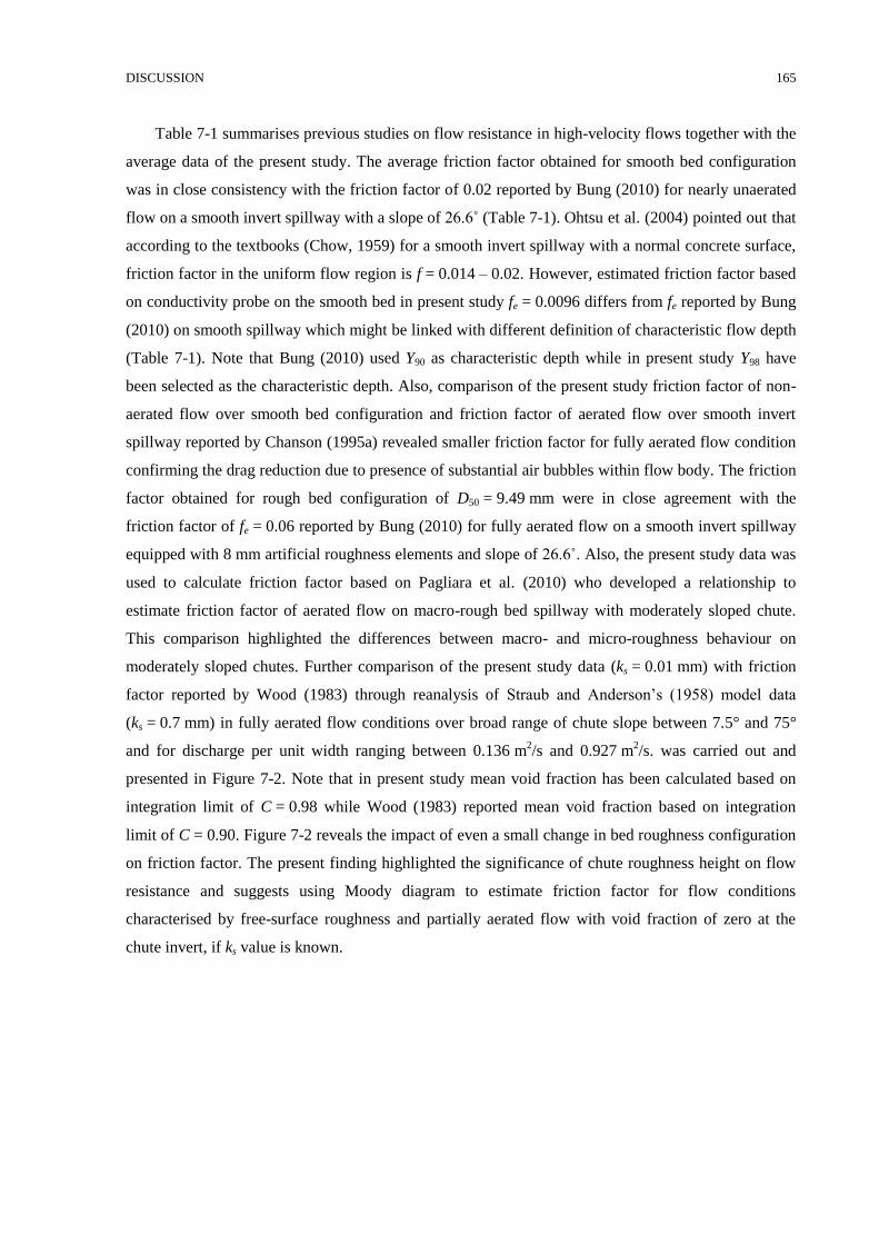
DISCUSSION 165
Table 7-1 summarises previous studies on flow resistance in high-velocity flows together with the
average data of the present study. The average friction factor obtained for smooth bed configuration
was in close consistency with the friction factor of 0.02 reported by Bung (2010) for nearly unaerated
flow on a smooth invert spillway with a slope of 26.6˚ (Table 7-1). Ohtsu et al. (2004) pointed out that
according to the textbooks (Chow, 1959) for a smooth invert spillway with a normal concrete surface,
friction factor in the uniform flow region is f = 0.014 – 0.02. However, estimated friction factor based
on conductivity probe on the smooth bed in present study fe = 0.0096 differs from fe reported by Bung
(2010) on smooth spillway which might be linked with different definition of characteristic flow depth
(Table 7-1). Note that Bung (2010) used Y90 as characteristic depth while in present study Y98 have
been selected as the characteristic depth. Also, comparison of the present study friction factor of non-
aerated flow over smooth bed configuration and friction factor of aerated flow over smooth invert
spillway reported by Chanson (1995a) revealed smaller friction factor for fully aerated flow condition
confirming the drag reduction due to presence of substantial air bubbles within flow body. The friction
factor obtained for rough bed configuration of D50 = 9.49 mm were in close agreement with the
friction factor of fe = 0.06 reported by Bung (2010) for fully aerated flow on a smooth invert spillway
equipped with 8 mm artificial roughness elements and slope of 26.6˚. Also, the present study data was
used to calculate friction factor based on Pagliara et al. (2010) who developed a relationship to
estimate friction factor of aerated flow on macro-rough bed spillway with moderately sloped chute.
This comparison highlighted the differences between macro- and micro-roughness behaviour on
moderately sloped chutes. Further comparison of the present study data (ks = 0.01 mm) with friction
factor reported by Wood (1983) through reanalysis of Straub and Anderson’s (1958) model data
(ks = 0.7 mm) in fully aerated flow conditions over broad range of chute slope between 7.5° and 75°
and for discharge per unit width ranging between 0.136 m2/s and 0.927 m
2/s. was carried out and
presented in Figure 7-2. Note that in present study mean void fraction has been calculated based on
integration limit of C = 0.98 while Wood (1983) reported mean void fraction based on integration
limit of C = 0.90. Figure 7-2 reveals the impact of even a small change in bed roughness configuration
on friction factor. The present finding highlighted the significance of chute roughness height on flow
resistance and suggests using Moody diagram to estimate friction factor for flow conditions
characterised by free-surface roughness and partially aerated flow with void fraction of zero at the
chute invert, if ks value is known.
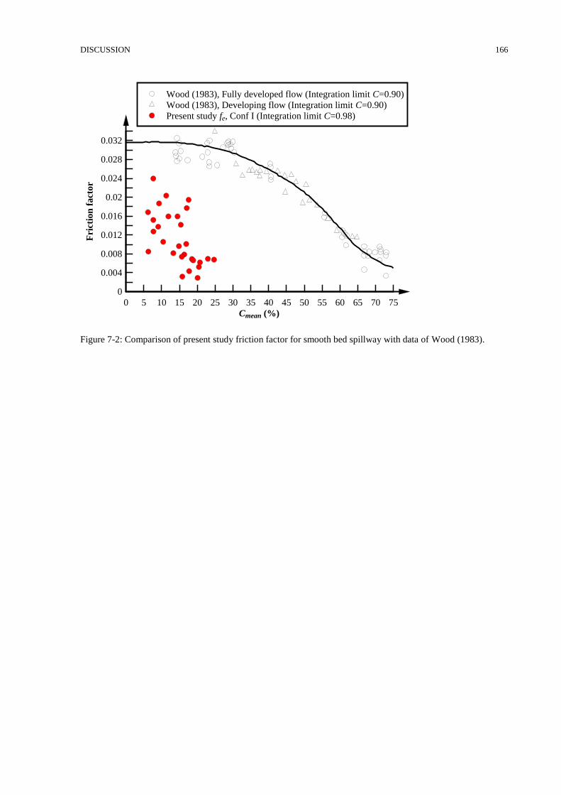
DISCUSSION 166
Figure 7-2: Comparison of present study friction factor for smooth bed spillway with data of Wood (1983).
Cmean (%)
Fri
ctio
n f
act
or
0 5 10 15 20 25 30 35 40 45 50 55 60 65 70 75
0
0.004
0.008
0.012
0.016
0.02
0.024
0.028
0.032
Wood (1983), Fully developed flow (Integration limit C=0.90)
Wood (1983), Developing flow (Integration limit C=0.90)
Present study fe, Conf I (Integration limit C=0.98)
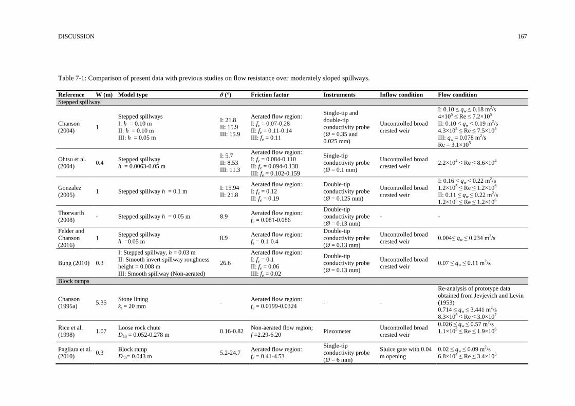
DISCUSSION 167
Table 7-1: Comparison of present data with previous studies on flow resistance over moderately sloped spillways.
Reference W (m) Model type θ (°) Friction factor Instruments Inflow condition Flow condition
Stepped spillway
Chanson
(2004) 1
Stepped spillways
I: h = 0.10 m
II: h = 0.10 m
III: h = 0.05 m
I: 21.8
II: 15.9
III: 15.9
Aerated flow region:
I: fe = 0.07-0.28
II: fe = 0.11-0.14
III: fe = 0.11
Single-tip and
double-tip
conductivity probe
(Ø = 0.35 and
0.025 mm)
Uncontrolled broad
crested weir
I: 0.10 ≤ qw ≤ 0.18 m2/s
4×10⁵ ≤ Re ≤ 7.2×10⁵
II: 0.10 ≤ qw ≤ 0.19 m2/s
4.3×10⁵ ≤ Re ≤ 7.5×10⁵
III: qw = 0.078 m2/s
Re = 3.1×10⁵
Ohtsu et al.
(2004) 0.4
Stepped spillway
h = 0.0063-0.05 m
I: 5.7
II: 8.53
III: 11.3
Aerated flow region:
I: fe = 0.084-0.110
II: fe = 0.094-0.138
III: fe = 0.102-0.159
Single-tip
conductivity probe
(Ø = 0.1 mm)
Uncontrolled broad
crested weir 2.2×10⁴ ≤ Re ≤ 8.6×10⁴
Gonzalez
(2005) 1 Stepped spillway h = 0.1 m
I: 15.94
II: 21.8
Aerated flow region:
I: fe = 0.12
II: fe = 0.19
Double-tip
conductivity probe
(Ø = 0.125 mm)
Uncontrolled broad
crested weir
I: 0.16 ≤ qw ≤ 0.22 m2/s
1.2×10⁵ ≤ Re ≤ 1.2×10⁶
II: 0.11 ≤ qw ≤ 0.22 m2/s
1.2×10⁵ ≤ Re ≤ 1.2×10⁶
Thorwarth
(2008) - Stepped spillway h = 0.05 m 8.9
Aerated flow region:
fe = 0.081-0.086
Double-tip
conductivity probe
(Ø = 0.13 mm)
- -
Felder and
Chanson
(2016)
1 Stepped spillway
h =0.05 m 8.9
Aerated flow region:
fe = 0.1-0.4
Double-tip
conductivity probe
(Ø = 0.13 mm)
Uncontrolled broad
crested weir 0.004≤ qw ≤ 0.234 m2/s
Bung (2010) 0.3
I: Stepped spillway, h = 0.03 m
II: Smooth invert spillway roughness
height = 0.008 m
III: Smooth spillway (Non-aerated)
26.6
Aerated flow region:
I: fe = 0.1
II: fe = 0.06
III: fe = 0.02
Double-tip
conductivity probe
(Ø = 0.13 mm)
Uncontrolled broad
crested weir 0.07 ≤ qw ≤ 0.11 m2/s
Block ramps
Chanson
(1995a) 5.35
Stone lining
ks = 20 mm -
Aerated flow region:
fe = 0.0199-0.0324 - -
Re-analysis of prototype data
obtained from Jevjevich and Levin
(1953)
0.714 ≤ qw ≤ 3.441 m2/s
8.3×10⁵ ≤ Re ≤ 3.0×10⁷
Rice et al.
(1998) 1.07
Loose rock chute
D50 = 0.052-0.278 m 0.16-0.82
Non-aerated flow region;
f =2.29-6.20 Piezometer
Uncontrolled broad
crested weir
0.026 ≤ qw ≤ 0.57 m2/s
1.1×10⁵ ≤ Re ≤ 1.9×10⁶
Pagliara et al.
(2010) 0.3
Block ramp
D50= 0.043 m 5.2-24.7
Aerated flow region:
fe = 0.41-4.53
Single-tip
conductivity probe
(Ø = 6 mm)
Sluice gate with 0.04
m opening
0.02 ≤ qw ≤ 0.09 m2/s
6.8×10⁴ ≤ Re ≤ 3.4×10⁵
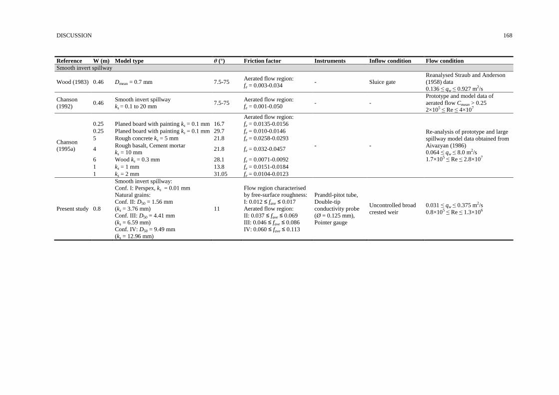
DISCUSSION 168
Reference W (m) Model type θ (°) Friction factor Instruments Inflow condition Flow condition
Smooth invert spillway
Wood (1983) 0.46 Dmean = 0.7 mm 7.5-75 Aerated flow region:
fe = 0.003-0.034 - Sluice gate
Reanalysed Straub and Anderson
(1958) data
0.136 ≤ qw ≤ 0.927 m2/s
Chanson
(1992) 0.46
Smooth invert spillway
ks = 0.1 to 20 mm 7.5-75
Aerated flow region:
fe = 0.001-0.050 - -
Prototype and model data of
aerated flow Cmean > 0.25
2×10⁵ ≤ Re ≤ 4×10⁷
Chanson
(1995a)
0.25
Planed board with painting ks = 0.1 mm
16.7
Aerated flow region:
fe = 0.0135-0.0156
- -
Re-analysis of prototype and large
spillway model data obtained from
Aivazyan (1986)
0.064 ≤ qw ≤ 8.0 m2/s
1.7×10⁵ ≤ Re ≤ 2.8×10⁷
0.25 Planed board with painting ks = 0.1 mm 29.7 fe = 0.010-0.0146
5 Rough concrete ks = 5 mm 21.8 fe = 0.0258-0.0293
4 Rough basalt, Cement mortar
ks = 10 mm 21.8 fe = 0.032-0.0457
6 Wood ks = 0.3 mm 28.1 fe = 0.0071-0.0092
1 ks = 1 mm 13.8 fe = 0.0151-0.0184
1 ks = 2 mm 31.05 fe = 0.0104-0.0123
Present study 0.8
Smooth invert spillway:
Conf. I: Perspex, ks = 0.01 mm
Natural grains:
Conf. II: D50 = 1.56 mm
(ks = 3.76 mm)
Conf. III: D50 = 4.41 mm
(ks = 6.59 mm)
Conf. IV: D50 = 9.49 mm
(ks = 12.96 mm)
11
Flow region characterised
by free-surface roughness:
I: 0.012 ≤ fave ≤ 0.017
Aerated flow region:
II: 0.037 ≤ fave ≤ 0.069
III: 0.046 ≤ fave ≤ 0.086
IV: 0.060 ≤ fave ≤ 0.113
Prandtl-pitot tube,
Double-tip
conductivity probe
(Ø = 0.125 mm),
Pointer gauge
Uncontrolled broad
crested weir
0.031 ≤ qw ≤ 0.375 m2/s
0.8×10⁵ ≤ Re ≤ 1.3×10⁶
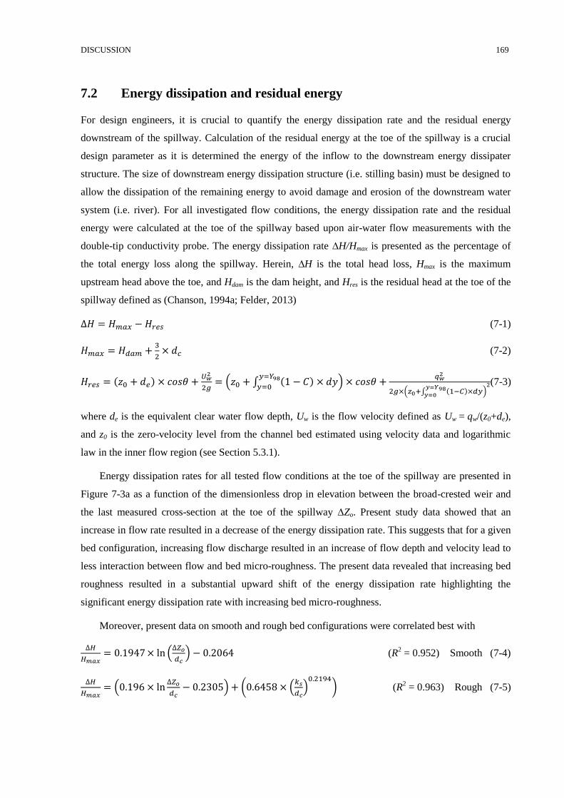
DISCUSSION 169
Energy dissipation and residual energy 7.2
For design engineers, it is crucial to quantify the energy dissipation rate and the residual energy
downstream of the spillway. Calculation of the residual energy at the toe of the spillway is a crucial
design parameter as it is determined the energy of the inflow to the downstream energy dissipater
structure. The size of downstream energy dissipation structure (i.e. stilling basin) must be designed to
allow the dissipation of the remaining energy to avoid damage and erosion of the downstream water
system (i.e. river). For all investigated flow conditions, the energy dissipation rate and the residual
energy were calculated at the toe of the spillway based upon air-water flow measurements with the
double-tip conductivity probe. The energy dissipation rate ∆H/Hmax is presented as the percentage of
the total energy loss along the spillway. Herein, ∆H is the total head loss, Hmax is the maximum
upstream head above the toe, and Hdam is the dam height, and Hres is the residual head at the toe of the
spillway defined as (Chanson, 1994a; Felder, 2013)
∆𝐻 = 𝐻𝑚𝑎𝑥 − 𝐻𝑟𝑒𝑠 (7-1)
𝐻𝑚𝑎𝑥 = 𝐻𝑑𝑎𝑚 +3
2× 𝑑𝑐 (7-2)
𝐻𝑟𝑒𝑠 = (𝑧0 + 𝑑𝑒) × 𝑐𝑜𝑠𝜃 +𝑈𝑤
2
2𝑔= (𝑧0 + ∫ (1 − 𝐶) × 𝑑𝑦
𝑦=𝑌98
𝑦=0) × 𝑐𝑜𝑠𝜃 +
𝑞𝑤2
2𝑔×(𝑧0+∫ (1−𝐶)×𝑑𝑦𝑦=𝑌98
𝑦=0)
2(7-3)
where de is the equivalent clear water flow depth, Uw is the flow velocity defined as Uw = qw/(z0+de),
and z0 is the zero-velocity level from the channel bed estimated using velocity data and logarithmic
law in the inner flow region (see Section 5.3.1).
Energy dissipation rates for all tested flow conditions at the toe of the spillway are presented in
Figure 7-3a as a function of the dimensionless drop in elevation between the broad-crested weir and
the last measured cross-section at the toe of the spillway ∆Zo. Present study data showed that an
increase in flow rate resulted in a decrease of the energy dissipation rate. This suggests that for a given
bed configuration, increasing flow discharge resulted in an increase of flow depth and velocity lead to
less interaction between flow and bed micro-roughness. The present data revealed that increasing bed
roughness resulted in a substantial upward shift of the energy dissipation rate highlighting the
significant energy dissipation rate with increasing bed micro-roughness.
Moreover, present data on smooth and rough bed configurations were correlated best with
∆𝐻
𝐻𝑚𝑎𝑥= 0.1947 × ln (
∆𝑍𝑜
𝑑𝑐) − 0.2064 (R
2 = 0.952) Smooth (7-4)
∆𝐻
𝐻𝑚𝑎𝑥= (0.196 × ln
∆𝑍𝑜
𝑑𝑐− 0.2305) + (0.6458 × (
𝑘𝑠
𝑑𝑐)
0.2194) (R
2 = 0.963) Rough (7-5)
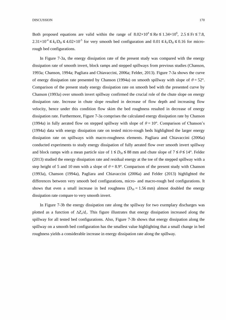
DISCUSSION 170
Both proposed equations are valid within the range of 8.02×10⁴ ≤ Re ≤ 1.34×10
6, 2.5 ≤ Fr ≤ 7.8,
2.31×10⁻⁴
≤ ks/DH ≤ 4.02×10⁻⁵
for very smooth bed configuration and 0.01 ≤ ks/DH ≤ 0.16 for micro-
rough bed configurations.
In Figure 7-3a, the energy dissipation rate of the present study was compared with the energy
dissipation rate of smooth invert, block ramps and stepped spillways from previous studies (Chanson,
1993a; Chanson, 1994a; Pagliara and Chiavaccini, 2006a; Felder, 2013). Figure 7-3a shows the curve
of energy dissipation rate presented by Chanson (1994a) on smooth spillway with slope of θ = 52°.
Comparison of the present study energy dissipation rate on smooth bed with the presented curve by
Chanson (1993a) over smooth invert spillway confirmed the crucial role of the chute slope on energy
dissipation rate. Increase in chute slope resulted in decrease of flow depth and increasing flow
velocity, hence under this condition flow skim the bed roughness resulted in decrease of energy
dissipation rate. Furthermore, Figure 7-3a comprises the calculated energy dissipation rate by Chanson
(1994a) in fully aerated flow on stepped spillway with slope of θ = 10°. Comparison of Chanson’s
(1994a) data with energy dissipation rate on tested micro-rough beds highlighted the larger energy
dissipation rate on spillways with macro-roughness elements. Pagliara and Chiavaccini (2006a)
conducted experiments to study energy dissipation of fully aerated flow over smooth invert spillway
and block ramps with a mean particle size of 1 ≤ D50 ≤ 88 mm and chute slope of 7 ≤ θ ≤ 14°. Felder
(2013) studied the energy dissipation rate and residual energy at the toe of the stepped spillway with a
step height of 5 and 10 mm with a slope of θ = 8.9°. Comparison of the present study with Chanson
(1993a), Chanson (1994a), Pagliara and Chiavaccini (2006a) and Felder (2013) highlighted the
differences between very smooth bed configurations, micro- and macro-rough bed configurations. It
shows that even a small increase in bed roughness (D50 = 1.56 mm) almost doubled the energy
dissipation rate compare to very smooth invert.
In Figure 7-3b the energy dissipation rate along the spillway for two exemplary discharges was
plotted as a function of ∆Zo/dc. This figure illustrates that energy dissipation increased along the
spillway for all tested bed configurations. Also, Figure 7-3b shows that energy dissipation along the
spillway on a smooth bed configuration has the smallest value highlighting that a small change in bed
roughness yields a considerable increase in energy dissipation rate along the spillway.
DISCUSSION 171
(a) Energy dissipation rate at the downstream end of the spillway for all tested configurations in the present
study and comparison with previous studies (*: Present study data, C (1993a): Chanson (1993a), C (1994a):
Chanson (1994a), PC (2006a): Pagliara and Chiavaccini (2006a), F (2013): Felder (2013)).
Zo/dc (-)
H
/Hm
ax (
-)
0 3 6 9 12 15 18 21 24 27 30 33 36 39 42 45 48 51 54 57 60
0
0.1
0.2
0.3
0.4
0.5
0.6
0.7
0.8
0.9
1
Conf. I: ks=0.01 mmConf. II: ks=3.67 mm, D50=1.56 mmConf. III: ks=6.59 mm, D50=4.41 mmConf. IV: ks=12.96 mm, D50=9.49 mm
PC (2006a): Metal plane ks=1 mm, =9.46
PC (2006a): 6.6<d/D50<42, =9.46
PC (2006a): 2.5<d/D50<6.6, =9.46
PC (2006a): d/D50<2.5, =9.46
PC (2006a): Metal plane ks=1 mm, =14
PC (2006a): 6.6<d/D50<42, =14
PC (2006a): 2.5<d/D50<6.6, =14
PC (2006a): d/D50<2.5, =14
F (2013): Stepped h=0.05 m, ks=49.40 mm, =8.9Conf. I: ks=0.01 mm, Eq (7-4)Conf. II: ks=3.67 mm, Eq (7-5)Conf. III: ks=6.59 mm, Eq (7-5)Conf. IV: ks=12.96 mm, Eq (7-5)
C (1993a): Non-aerated smooth spillway, U, =52
C (1994a): Stepped spillway, U, =10
DISCUSSION 172
(b) Energy dissipation rate along the spillway for two examplary discharges on investigated bed configurations
in the present study.
Figure 7-3: Energy dissipation rate for all tested configurations in the present study.
In practical applications, the residual head is more appropriate compare to the energy dissipation
rate (Chanson, 2001). Hence, Figure 7-4 presents the dimensionless residual head Hres/dc measured at
the last cross-section close to the toe of the spillway as a function of ∆Zo/dc for all tested discharges
and bed configurations. Figure 7-4 shows that flow over smooth bed has the largest residual head and
a small increase in bed roughness resulted in a decrease of the residual head which was consistent with
the observations of the energy dissipation performance. As shown in Figure 7-4, the dimensionless
residual head varied slightly by changing discharges on the rough bed configurations. However, for
smooth bed configuration, the dimensionless residual head increased with increasing discharge. Figure
7-4 depicts that for smooth bed configuration residual head at the toe of the spillway increased
gradually approaching equilibrium condition. For the tested flow conditions on micro-rough bed
configurations, the residual head was determined on average Hres/dc = 6 for configuration II
(ks = 3.67 mm), Hres/dc = 5 for configuration III (ks = 6.59 mm), and the lowest residual head was
Zo/dc (-)
H
/Hm
ax (
-)
0 3 6 9 12 15 18 21 24
0
0.05
0.1
0.15
0.2
0.25
0.3
0.35
0.4
0.45
0.5
0.55
0.6
0.65
0.7
0.75
0.8
0.85
Conf. I: ks=0.01 mm, qw=0.05 m2/s
Conf. II: ks=3.67 mm, qw=0.05 m2/s
Conf. III: ks=6.59 mm, qw=0.05 m2/s
Conf. IV: ks=12.96 mm, qw=0.05 m2/s
Conf. I: ks=0.01 mm, qw=0.075 m2/s
Conf. II: ks=3.67 mm, qw=0.075 m2/s
Conf. III: ks=6.59 mm, qw=0.075 m2/s
Conf. IV: ks=12.59 mm, qw=0.075 m2/s
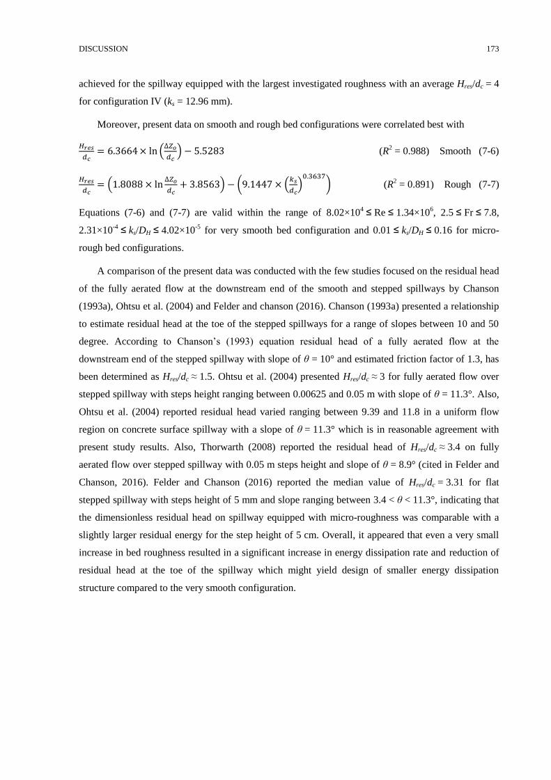
DISCUSSION 173
achieved for the spillway equipped with the largest investigated roughness with an average Hres/dc = 4
for configuration IV (ks = 12.96 mm).
Moreover, present data on smooth and rough bed configurations were correlated best with
𝐻𝑟𝑒𝑠
𝑑𝑐= 6.3664 × ln (
∆𝑍𝑜
𝑑𝑐) − 5.5283 (R
2 = 0.988) Smooth (7-6)
𝐻𝑟𝑒𝑠
𝑑𝑐= (1.8088 × ln
∆𝑍𝑜
𝑑𝑐+ 3.8563) − (9.1447 × (
𝑘𝑠
𝑑𝑐)
0.3637) (R
2 = 0.891) Rough (7-7)
Equations (7-6) and (7-7) are valid within the range of 8.02×10⁴ ≤ Re ≤ 1.34×10
6, 2.5 ≤ Fr ≤ 7.8,
2.31×10⁻⁴
≤ ks/DH ≤ 4.02×10⁻⁵
for very smooth bed configuration and 0.01 ≤ ks/DH ≤ 0.16 for micro-
rough bed configurations.
A comparison of the present data was conducted with the few studies focused on the residual head
of the fully aerated flow at the downstream end of the smooth and stepped spillways by Chanson
(1993a), Ohtsu et al. (2004) and Felder and chanson (2016). Chanson (1993a) presented a relationship
to estimate residual head at the toe of the stepped spillways for a range of slopes between 10 and 50
degree. According to Chanson’s (1993) equation residual head of a fully aerated flow at the
downstream end of the stepped spillway with slope of θ = 10° and estimated friction factor of 1.3, has
been determined as Hres/dc ≈ 1.5. Ohtsu et al. (2004) presented Hres/dc ≈ 3 for fully aerated flow over
stepped spillway with steps height ranging between 0.00625 and 0.05 m with slope of θ = 11.3°. Also,
Ohtsu et al. (2004) reported residual head varied ranging between 9.39 and 11.8 in a uniform flow
region on concrete surface spillway with a slope of θ = 11.3° which is in reasonable agreement with
present study results. Also, Thorwarth (2008) reported the residual head of Hres/dc ≈ 3.4 on fully
aerated flow over stepped spillway with 0.05 m steps height and slope of θ = 8.9° (cited in Felder and
Chanson, 2016). Felder and Chanson (2016) reported the median value of Hres/dc = 3.31 for flat
stepped spillway with steps height of 5 mm and slope ranging between 3.4 < θ < 11.3°, indicating that
the dimensionless residual head on spillway equipped with micro-roughness was comparable with a
slightly larger residual energy for the step height of 5 cm. Overall, it appeared that even a very small
increase in bed roughness resulted in a significant increase in energy dissipation rate and reduction of
residual head at the toe of the spillway which might yield design of smaller energy dissipation
structure compared to the very smooth configuration.
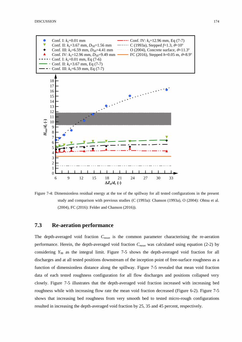
DISCUSSION 174
Figure 7-4: Dimensionless residual energy at the toe of the spillway for all tested configurations in the present
study and comparison with previous studies (C (1993a): Chanson (1993a), O (2004): Ohtsu et al.
(2004), FC (2016): Felder and Chanson (2016)).
Re-aeration performance 7.3
The depth-averaged void fraction Cmean is the common parameter characterising the re-aeration
performance. Herein, the depth-averaged void fraction Cmean was calculated using equation (2-2) by
considering Y98 as the integral limit. Figure 7-5 shows the depth-averaged void fraction for all
discharges and at all tested positions downstream of the inception point of free-surface roughness as a
function of dimensionless distance along the spillway. Figure 7-5 revealed that mean void fraction
data of each tested roughness configuration for all flow discharges and positions collapsed very
closely. Figure 7-5 illustrates that the depth-averaged void fraction increased with increasing bed
roughness while with increasing flow rate the mean void fraction decreased (Figure 6-2). Figure 7-5
shows that increasing bed roughness from very smooth bed to tested micro-rough configurations
resulted in increasing the depth-averaged void fraction by 25, 35 and 45 percent, respectively.
Zo/dc (-)
Hre
s/d
c (-
)
6 9 12 15 18 21 24 27 30 33
0
1
2
3
4
5
6
7
8
9
10
11
12
13
14
15
16
17
18
Conf. I: ks=0.01 mm
Conf. II: ks=3.67 mm, D50=1.56 mm
Conf. III: ks=6.59 mm, D50=4.41 mm
Conf. IV: ks=12.96 mm, D50=9.49 mm
Conf. I: ks=0.01 mm, Eq (7-6)
Conf. II: ks=3.67 mm, Eq (7-7)
Conf. III: ks=6.59 mm, Eq (7-7)
Conf. IV: ks=12.96 mm, Eq (7-7)
C (1993a), Stepped f=1.3, =10
O (2004), Concrete surface, =11.3
FC (2016), Stepped h=0.05 m, =8.9
DISCUSSION 175
For the smooth bed, and flow rates 0.031 ≤ qw ≤ 0.375 m2/s, Cmean increased from Cmean = 0.04
downstream of the inception point of free-surface roughness to Cmean = 0.25 at the downstream end of
the spillway. This gradual increase was best correlated by
𝐶𝑚𝑒𝑎𝑛 = 0.1084 ln (𝑥
𝑑𝑐) − 0.3068 (R
2 = 0.98) (7-8)
within the investigated flow conditions of 25 < x/dc < 200, 2.31×10⁻⁴
≤ ks/DH ≤ 4.02×10⁻⁵
and 4.12×10-
5 ≤ ks/dc ≤ 2.17×10
-4 .
For the rough bed configurations, depth-averaged void fraction increased from Cmean = 0.07
downstream of the inception point of free-surface roughness to Cmean = 0.37 at the toe of the spillway.
The gradual increase of mean void fraction was best correlated by
𝐶𝑚𝑒𝑎𝑛 = 0.0892 × ln (𝑥
𝑑𝑐) + 0.4248 ×
𝑘𝑠
𝑑𝑐
1.5001− 0.1441 (R
2 = 0.90) (7-9)
within the tested flow conditions of 9 < x/dc < 200, 0.01 ≤ ks/DH ≤ 0.16 and 0.015 ≤ ks/dc ≤ 0.281. Both
equations (7-8) and (7-9) are valid within the range of 8.02×10⁴ ≤ Re ≤ 1.34×10
6, and 2.5 ≤ Fr ≤ 7.8,
In Figure 7-5a, the present data were compared with other studies conducted by Wilhelms and
Gulliver (2005), Meireles et al. (2012) and Valero and Bung (2016) as well as empirical equations of
mean void fractions on smooth and stepped spillways within the non-aerated flow region characterised
by entrapped air. Wilhelms and Gulliver (2005) reanalysed the experimental data of Killen (1968) in
uniform flow region observing constant entrapped air concentrations of Cmean = 0.073, 0.142 and 0.23
for different integration limits of Y90, Y95 and Y98, respectively. Whilhelms and Gulliver (2005)
reported an entrapped air concentration of 0.23 in uniform flow region by considering the integration
limit of Y98. However, due to the insufficient length of the present study spillway model, flow did not
reach a uniform condition regarding the air-water flow properties. Meireles et al. (2012) observed
Cmean ≈ 0.14 corresponding to the conductivity probe measurements with integration limit of Y99 in the
non-aerated flow region upstream of the inception point of free-surface self-aeration which was
characterised by entrapped air on a stepped spillway with a slope of θ = 53.1˚. Using an integration
limit of Y99 and an analytical solution, Valero and Bung (2016) calculated mean void fraction of
Cmean ≈ 0.09 in the flow region characterised by free-surface roughness upstream of the inception point
of free-surface aeration on a smooth invert spillway with slope of θ = 26.6˚. Meireles et al. (2012) and
Valero and Bung (2016) reported a slight increase in a mean void fraction in a downstream direction
towards the inception point of free-surface aeration. The comparison of the observations in the present
study with mean void fractions of entrapped air conducted by Meireles et al. (2012) and Valero and
Bung (2016) showed some substantial differences which might be linked with the type of the free-
surface roughness and by the possible influence of bed roughness on free-surface and entrapped air.
DISCUSSION 176
In Figure 7-5b, the mean void fractions of the present study were compared with data on smooth
and stepped spillways characterised by fully aerated flow conditions. Chanson (1995a) re-analysed
Aivazyan (1986) data and reported 0.21 ≤ Cmean ≤ 0.54 on the prototype and large spillway model with
a range of bed roughness height from 0.1 to 10 mm and slope ranging between 14° ≤ θ ≤ 31° within
uniform flow region. Bung (2010) reported 0.30 ≤ Cmean ≤ 0.35 on stepped and smooth invert spillway
equipped with roughness elements of 8 mm height with a slope of θ = 26.6° in the uniform flow
region. Note that Chanson (1995a) and Bung (2010) estimated Cmean based on integration limit of Y90.
This comparison revealed that in the present study the mean void fraction on rough bed configurations
did not reach uniform flow condition. Further comparison has been conducted with using proposed
equations by United States Army Waterways Experiments Station (1957) on smooth bed (2-10) and
rough bed (2-11). According to these equations mean void faction within uniform flow region varied
between 0.70 and 0.97 over smooth bed and for rough bed configurations ranging from 0.41 to 0.57
for varies tested discharges. This highlights that in the present study, mean void fraction did not
approach uniform condition. Using equations (2-8), (2-9) and (2-13) developed for fully aerated flows
on steep slope spillways (θ > 15°) by Hager (1991), Chanson (1993c) and Aivazyan (1986),
respectively, resulted in mean void fraction of 0.22, 0.17 and 0.31 in uniform flow region confirming
that for tested flow conditions in present study despite reaching the flow to constant depth and velocity
towards the toe of the spillway, mean void fraction did not approach a uniform value and it is
increasing gradually. Comparison of the results of equations (2-8), (2-9), (2-10) ans (2-13) on smooth
invert spillway reveales strong diffrernces in mean void fraction which might be link with the
conflicing definition of smooth bed. This highlighted that mean void fraction is a function of not only
spillway slope but also bed roughness and flow discharge. This result is consistent with changes of
interface count rate discussed in Section 6.7.3 (Figure 6-20a and b) suggesting the insufficient length
of the spillway to allows void fraction and interface count rate reach uniform condition.
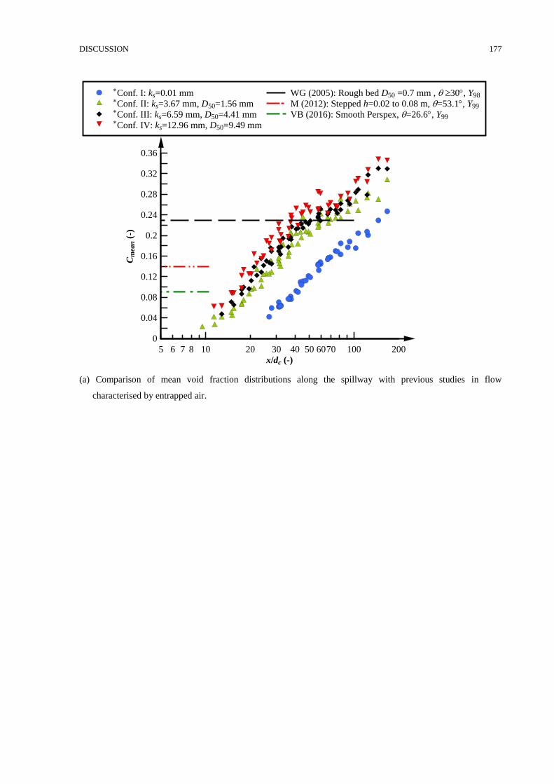
DISCUSSION 177
(a) Comparison of mean void fraction distributions along the spillway with previous studies in flow
characterised by entrapped air.
x/dc (-)
Cm
ean (
-)
5 6 7 8 10 20 30 40 50 6070 100 200
0
0.04
0.08
0.12
0.16
0.2
0.24
0.28
0.32
0.36
Conf. I: ks=0.01 mmConf. II: ks=3.67 mm, D50=1.56 mmConf. III: ks=6.59 mm, D50=4.41 mmConf. IV: ks=12.96 mm, D50=9.49 mm
WG (2005): Rough bed D50 =0.7 mm , 30, Y98
M (2012): Stepped h=0.02 to 0.08 m, =53.1, Y99
VB (2016): Smooth Perspex, =26.6, Y99
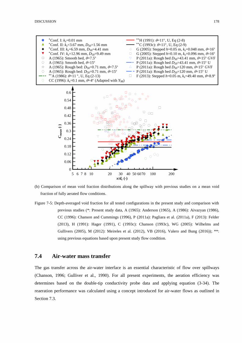
DISCUSSION 178
(b) Comparison of mean void fraction distributions along the spillway with previous studies on a mean void
fraction of fully aerated flow conditions.
Figure 7-5: Depth-averaged void fraction for all tested configurations in the present study and comparison with
previous studies (*: Present study data, A (1965): Anderson (1965), A (1986): Aivazyan (1986),
CC (1996): Chanson and Cummings (1996), P (2011a): Pagliara et al. (2011a), F (2013): Felder
(2013), H (1991): Hager (1991), C (1993c): Chanson (1993c), WG (2005): Wilhelms and
Gullivers (2005), M (2012): Meireles et al. (2012), VB (2016), Valero and Bung (2016)); **:
using previous equations based upon present study flow condition.
Air-water mass transfer 7.4
The gas transfer across the air-water interface is an essential characteristic of flow over spillways
(Chanson, 1996; Gulliver et al., 1990). For all present experiments, the aeration efficiency was
determines based on the double-tip conductivity probe data and applying equation (3-34). The
reaeration performance was calculated using a concept introduced for air-water flows as outlined in
Section 7.3.
x/dc (-)
Cm
ean (
-)
5 6 7 8 10 20 30 40 50 6070 100 200
0
0.06
0.12
0.18
0.24
0.3
0.36
0.42
0.48
0.54
0.6
Conf. I: ks=0.01 mmConf. II: ks=3.67 mm, D50=1.56 mmConf. III: ks=6.59 mm, D50=4.41 mmConf. IV: ks=12.96 mm, D50=9.49 mm
A (1965): Smooth bed, =7.5
A (1965): Smooth bed, =15
A (1965): Rough bed: D50=0.71 mm, =7.5
A (1965): Rough bed: D50=0.71 mm, =15A (1986): =11 , U, Eq (2-13)
CC (1996): ks=0.1 mm, =4 (Adapted with Y98)
H (1991): =11, U, Eq (2-8)C (1993c): =11, U, Eq (2-9)
G (2005): Stepped h=0.05 m, ks=0.048 mm, =16
G (2005): Stepped h=0.10 m, ks=0.096 mm, =16
P (2011a): Rough bed D50=43.41 mm, =15 GVF
P (2011a): Rough bed D50=43.41 mm, =15 U
P (2011a): Rough bed D50=120 mm, =15 GVF
P (2011a): Rough bed D50=120 mm, =15 U
F (2013): Stepped h=0.05 m, ks=49.40 mm, =8.9
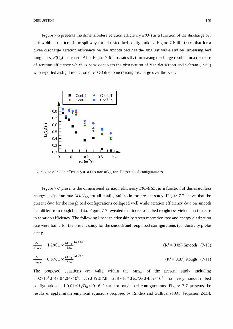
DISCUSSION 179
Figure 7-6 presents the dimensionless aeration efficiency E(O2) as a function of the discharge per
unit width at the toe of the spillway for all tested bed configurations. Figure 7-6 illustrates that for a
given discharge aeration efficiency on the smooth bed has the smallest value and by increasing bed
roughness, E(O2) increased. Also, Figure 7-6 illustrates that increasing discharge resulted in a decrease
of aeration efficiency which is consistent with the observation of Van der Kroon and Schram (1969)
who reported a slight reduction of E(O2) due to increasing discharge over the weir.
Figure 7-6: Aeration efficiency as a function of qw for all tested bed configurations.
Figure 7-7 presents the dimensional aeration efficiency E(O2)/∆Zo as a function of dimensionless
energy dissipation rate ∆H/Hmax for all configurations in the present study. Figure 7-7 shows that the
present data for the rough bed configurations collapsed well while aeration efficiency data on smooth
bed differ from rough bed data. Figure 7-7 revealed that increase in bed roughness yielded an increase
in aeration efficiency. The following linear relationship between reaeration rate and energy dissipation
rate were found for the present study for the smooth and rough bed configurations (conductivity probe
data):
∆𝐻
𝐻𝑚𝑎𝑥= 1.2981 ×
𝐸(𝑂2)
∆𝑍𝑜
1.0898 (R
2 = 0.89) Smooth (7-10)
∆𝐻
𝐻𝑚𝑎𝑥= 0.6761 ×
𝐸(𝑂2)
∆𝑍𝑜
0.8087 (R
2 = 0.87) Rough (7-11)
The proposed equations are valid within the range of the present study including
8.02×10⁴ ≤ Re ≤ 1.34×10
6, 2.5 ≤ Fr ≤ 7.8, 2.31×10
-4 ≤ ks/DH ≤ 4.02×10
-5 for very smooth bed
configuration and 0.01 ≤ ks/DH ≤ 0.16 for micro-rough bed configurations. Figure 7-7 presents the
results of applying the empirical equations proposed by Rindels and Gulliver (1991) [equation 2-33],
qw (m2/s)
E(O
2)
(-)
0 0.1 0.2 0.3 0.4
0.2
0.3
0.4
0.5
0.6
0.7
0.8
Conf. I
Conf. II
Conf. III
Conf. IV
DISCUSSION 180
Chanson (1995c) [equation 2-34] using the two exemplary tested bed configurations. Also, Figure 7-7
includes the empirical correlation reported by Felder (2013) [equation 2-37] on fully aerated flow over
stepped spillways. Rindels and Gulliver (1991) developed an equation based on dissolved Oxygen
content of the flow in fully aerated flow condition on model and prototype data of spillways. All data
illustrates an increase in aeration efficiency by increasing the energy dissipation rate. Comparison of
the present study data with Rindels and Gulliver (1991) and Chanson (1995c) results show strong
discrepancy which might be linked with a scale effect and different type of flow and subsequently the
assumptions applied in the present study. The enormous difference between present study data and
estimated aeration efficiency based on Chanson (1995c) semi-empirical equation can be linked with
the limitation of the spherical bubble shape in fully aerated flow and calculation of specific interfacial
area. Notice that specific interfacial area was proposed to estimate the specific interfacial area of the
spherical bubble shape in fully aerated flow conditions. Since, in the present study, flow is
characterised by free-surface roughness and continuous air entrapment as well as air entrainment on
rough bed configurations; an interfacial area mostly is due to the interface area of the free-surface
roughness. Thus, in the present study, all those simplifications and assumptions regarding specific
interfacial area were used resulting in an extremely crude estimation of air-water mass transfer. Felder
(2013) presented that aeration efficiency is subjected to the size of the conductivity probe tip. Hence,
he pointed out the more enhanced aeration efficiency for experiments conducted with smaller
conductivity probe tips which increased the number of detected bubbles and subsequently increase the
interface area.
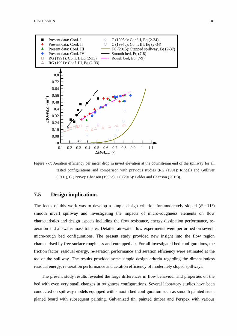
DISCUSSION 181
Figure 7-7: Aeration efficiency per meter drop in invert elevation at the downstream end of the spillway for all
tested configurations and comparison with previous studies (RG (1991): Rindels and Gulliver
(1991), C (1995c): Chanson (1995c), FC (2015): Felder and Chanson (2015)).
Design implications 7.5
The focus of this work was to develop a simple design criterion for moderately sloped (θ = 11°)
smooth invert spillway and investigating the impacts of micro-roughness elements on flow
characteristics and design aspects including the flow resistance, energy dissipation performance, re-
aeration and air-water mass transfer. Detailed air-water flow experiments were performed on several
micro-rough bed configurations. The present study provided new insight into the flow region
characterised by free-surface roughness and entrapped air. For all investigated bed configurations, the
friction factor, residual energy, re-aeration performance and aeration efficiency were estimated at the
toe of the spillway. The results provided some simple design criteria regarding the dimensionless
residual energy, re-aeration performance and aeration efficiency of moderately sloped spillways.
The present study results revealed the large differences in flow behaviour and properties on the
bed with even very small changes in roughness configurations. Several laboratory studies have been
conducted on spillway models equipped with smooth bed configuration such as smooth painted steel,
planed board with subsequent painting, Galvanized tin, painted timber and Perspex with various
H/Hmax (-)
E(O
2)/
Zo (
m-1
)
0.1 0.2 0.3 0.4 0.5 0.6 0.7 0.8 0.9 1 1.1
0
0.08
0.16
0.24
0.32
0.4
0.48
0.56
0.64
0.72
0.8
Present data: Conf. I
Present data: Conf. II
Present data: Conf. III
Present data: Conf. IV
RG (1991): Conf. I, Eq (2-33)
RG (1991): Conf. III, Eq (2-33)
C (1995c): Conf. I, Eq (2-34)
C (1995c): Conf. III, Eq (2-34)
FC (2015): Stepped spillway, Eq (2-37)
Smooth bed, Eq (7-8)
Rough bed, Eq (7-9)
DISCUSSION 182
equivalent sand roughness ranging between 0.01 < ks <1 mm. Comparison of results revealed some
discrepancies which can be linked with the impact of bed configuration and the conflicting definition
of smooth bed. Therefore, the understanding of the effects of micro-roughness is essential to better
understand different results in previous studies of smooth spillway conditions.
Table 7-2 summarised the guidelines valid for a range of flow conditions independently of the
height of the spillway for gradually varied non-aerated and partially aerated flows over smooth and
micro-rough bed configurations. In flow region characterised by entrapped air and partially aerated
flow condition while void fraction in vicinity of the bed is zero friction factor can be estimated by
using Moody diagram if the value of equivalent sand roughness is known. Equations (7-4) and (7-5)
were developed to determine energy dissipation rate for the tested flow conditions. The residual head
at the downstream end of the spillway was determined using equations (7-6) and (7-7) on smooth and
micro-rough bed configuration resulted in inflow information into the downstream energy dissipater.
Also, re-aeration performance can be estimated using equations (7-8) and (7-9) on smooth and micro-
rough bed configurations, respectively. Aeration efficiency can be calculated using equations (7-10)
and (7-11) on smooth and micro-rough bed configuration, respectively. The simple use of the
presented equations in Table 7-2 is demonstrated by an example in Appendix D.
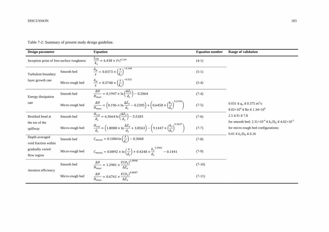
DISCUSSION 183
Table 7-2: Summary of present study design guideline.
Design parameter Equation Equation number Range of validation
Inception point of free-surface roughness 𝐿𝐹𝑅
𝑘𝑠= 6.438 × 𝐹𝑟∗
0.739 (4-1)
0.031 ≤ qw ≤ 0.375 m2/s
8.02×10⁴ ≤ Re ≤ 1.34×10⁶
2.5 ≤ Fr ≤ 7.8
for smooth bed: 2.31×10⁻⁴ ≤ ks/DH ≤ 4.02×10⁻⁵
for micro-rough bed configurations:
0.01 ≤ ks/DH ≤ 0.16
Turbulent boundary
layer growth rate
Smooth bed 𝛿𝑤
𝑥= 0.0373 × (
𝑥
𝑘𝑠)
−0.148
(5-1)
Micro-rough bed 𝛿𝑤
𝑥= 0.3748 × (
𝑥
𝑘𝑠)
−0.532
(5-4)
Energy dissipation
rate
Smooth bed ∆𝐻
𝐻𝑚𝑎𝑥= 0.1947 × ln (
∆𝑍𝑜
𝑑𝑐) − 0.2064 (7-4)
Micro-rough bed ∆𝐻
𝐻𝑚𝑎𝑥= (0.196 × ln
∆𝑍𝑜
𝑑𝑐− 0.2305) + (0.6458 × (
𝑘𝑠
𝑑𝑐)
0.2194
) (7-5)
Residual head at
the toe of the
spillway
Smooth bed 𝐻𝑟𝑒𝑠
𝑑𝑐= 6.3664 ln (
∆𝑍𝑜
𝑑𝑐) − 5.5283 (7-6)
Micro-rough bed 𝐻𝑟𝑒𝑠
𝑑𝑐= (1.8088 × ln
∆𝑍𝑜
𝑑𝑐+ 3.8563) − (9.1447 × (
𝑘𝑠
𝑑𝑐)
0.3637
) (7-7)
Depth-averaged
void fraction within
gradually varied
flow region
Smooth bed 𝐶𝑚𝑒𝑎𝑛 = 0.1084 ln (𝑥
𝑑𝑐) − 0.3068 (7-8)
Micro-rough bed 𝐶𝑚𝑒𝑎𝑛 = 0.0892 × ln (𝑥
𝑑𝑐) + 0.4248 ×
𝑘𝑠
𝑑𝑐
1.5001
− 0.1441 (7-9)
Aeration efficiency
Smooth bed ∆𝐻
𝐻𝑚𝑎𝑥= 1.2981 ×
𝐸(𝑂2)
∆𝑍𝑜
1.0898
(7-10)
Micro-rough bed ∆𝐻
𝐻𝑚𝑎𝑥= 0.6761 ×
𝐸(𝑂2)
∆𝑍𝑜
0.8087
(7-11)
Chapter 8
8 CONCLUSION
Key findings of the present experimental study 8.1
Macro-roughness elements are recognised for strong energy dissipation and aeration. During the past
few decades, they have been studied extensively. However, there is limited information available on
the characteristics of high-velocity supercritical flows, energy dissipation and re-aeration
performances of spillways with the micro-rough beds. There is also little information on smooth invert
spillways with moderate slope (θ < 15°) and the uncontrolled intake, for which flow is not naturally
aerated. Herein, a comprehensive experimental study was conducted in a large scale spillway model
with θ = 11° and an uncontrolled broad-crested weir at the upstream end. New insights were provided
into the non-aerated flow region characterised by entrapped air and partially aerated flow region along
the spillway. Furthermore, flow resistance, energy dissipation performance and re-aeration
performance of flow over spillways equipped with micro-roughness elements was studied. The key
findings of present study are addressed below.
In the present study, detailed observations of flow patterns and flow structure were conducted
using detailed photography and high-speed recorded videos. For the smooth bed configuration, visual
observations of flow patterns and free-surface profiles revealed that no air bubbles were entrained into
the flow. However, the free-surface became agitated, and some air was continuously entrapped
between small amplitude free-surface waves known as free-surface roughness. Recorded videos and
photos illustrated that on micro-rough bed configurations in addition to continuous free-surface
roughness, some air bubbles entrained into the flow body. It has been observed that bubbles did not
present in the vicinity of chute’s bed and flow is partially aerated. The present observations suggested
entrainment of air into the flow body due to the agitation of the free-surface as well as dragging air
into the water through ejected water droplets. Visual observations of flow patterns revealed that
increasing chute’s bed roughness yielded earlier appearance of free-surface roughness. An empirical
relationship was developed to estimate inception point of free-surface roughness along the moderately
CONCLUSION 185
sloped spillway. Also, the inception point of free-surface air entrainment on tested micro-rough bed
configurations was consistent with previous studies of fully aerated flows reporting the downward
shift of the inception point of free-surface roughness with increasing flow rate. Moreover, visual
observations revealed a different type of free-surface roughness and waves on a smooth Perspex bed
compared to micro-rough beds. It has been illustrated that an increase in bed roughness resulted in
free-surface waves with larger wave amplitude. Furthermore, visual observations suggest that wave
amplitude became more equal in the streamwise direction resulting in a regular free-surface pattern
towards the downstream end of the spillway.
In the present study, detailed time-averaged velocity measurements have been conducted at
several cross-sections along the spillway using a Prandtl Pitot tube. The time-averaged velocity
distributions revealed self-similarities with 7th and 4
th power law on smooth and micro-rough bed
configurations, respectively. Comparative analysis of local velocity distributions on different bed
roughness configurations highlighted an upward shift of velocity distribution within boundary layer
region by increasing bed roughness while velocity distributions were unaffected outside of the
boundary layer. Velocity measurements yielded the estimation of the growth rate of the turbulent
boundary layer, displacement and momentum thicknesses of about δw ∼ x0.838, δ1 ∼ x
0.533 and δ2 ∼ x
0.665
for smooth bed and δw ∼ x0.468, δ1 ∼ x
0.391 and δ2 ∼ x
0.441 for micro-rough bed configurations. An
increase in the bed roughness caused a faster growth rate of the boundary layer. New empirical
equations have been proposed to determine boundary layer growth rate on moderately sloped spillway
with uncontrolled inflow conditions for smooth and rough bed configurations. Also, for all tested flow
conditions, LFR < LI < LBL highlighting that initiation of free-surface roughness was not triggered by
turbulence fluctuations close to the free-surface, but by instabilities at the air-water interface.
Furthermore, based upon the velocity data, the shear stress was calculated using different approaches
comprising the logarithmic law in inner flow region, the velocity defect law in the outer layer and the
momentum integral method. For both laws of the wall in the inner flow region and velocity defect law
in the outer region, the shear stress increased gradually in a streamwise direction approaching pseudo-
uniform value toward the toe of the spillway. Shear stress increased due to the increase of shear
velocity. Comparative analysis of dimensionless shear stress revealed that an increase in bed
roughness resulted in an increase of shear stress and the corresponding friction factor highlighting the
increase of flow resistance.
Due to the fast fluctuation of free-surface, entrapped air between free-surface waves and entrained
air bubbles into the flow, a double-tip conductivity probe was used to provide insight into the air-water
flow properties of the present study. Detailed air-water flow measurements were performed using a
double-tip conductivity probe for all tested flow conditions. The present study data provided
information about the entrapped flow region over the very smooth spillway as well as total conveyed
CONCLUSION 186
air flow (entrapped air + entrained air) region on three micro-rough bed configurations. A detail
sensitivity analysis revealed that Y98 is the most appropriate characteristic depth to define flow depth in
flow characterised by free-surface roughness and entrapped air. Experimental results revealed that the
air-water flow measurements technique applies to measure flow properties within the flow region
characterised by entrapped air. In the present study, within flows region characterised by free-surface
roughness, the maximum value of air-water interface count rate, turbulence levels and auto- and cross-
correlation timescales observed for C ≈ 0.5 indicating the strong turbulence and air-water interactions
within this region. The comparative analysis of air-water flow properties for investigated bed
configurations illustrated that an increase in bed roughness increased mean void fraction and air-water
interface count rate, turbulence intensity, and auto- and cross-correlation timescales highlighting the
increase of air-water interactions by increasing bed roughness. Also, a monotonic decrease of average
chord length and chord time with increasing air-water interface count rate was observed suggesting the
increase of interfacial area and subcequentaly enhancement of air-water mass transfer.
Further analysis of air-water flow properties revealed that increasing bed roughness resulted in an
increase of Fmax, Tumax¸ (Txz)max, (Txx)max and a decrease of Y(Fmax)/Y98, Y(Tumax)/Y98, Y((Txz)max)/Y98,
Y((Txx)max)/Y98 which are the indication of penetration of larger amount of free-surface waves with
larger wave amplitude into the flow. Results revealed a gradual increase of characteristic flow
properties along the spillway including mean void fraction, air-water interface count rate, turbulence
intensity. Also, results depicted a gradual decrease in auto- and cross-correlation timescale, average air
and water chord length along the spillway. These gradual changes of air-water flow properties indicate
that no uniform flow conditions were achieved at the downstream end of the spillway in terms of air-
water flow properties despite reaching the flow to a constant flow depth and velocity for some flow
conditions. Comparative analysis of the gradient of void fraction distributions revealed the increase of
gradient in the streamwise direction suggesting that free-surface wave amplitude increased towards the
toe of the spillway which is consistent with visual observations. Also, for a given discharge the
gradient of void fraction distributions approached a constant value, indicating equal wave amplitude at
the downstream end of the spillway compared to the upstream end. Detailed comparison of chord
times revealed that chord time distributions become more equal in a streamwise direction indicating a
rather regular free-surface roughness toward the downstream end of the spillway. Moreover, the
comparison revealed that increase in bed roughness configuration resulted in larger number of small
size air and water chord times suggesting the larger interfacial area and larger potential of air-water
mass transfer.
Overall, the present study experimental investigations revealed that small increases in bed
roughness resulted in an increase of the energy dissipation rate, reduction of the residual head at the
toe of the spillway, enhancement of re-aeration and air-water mass transfer which can be influential
CONCLUSION 187
for surrounding water system. Moreover, comparative analysis of friction factor based on various
methods revealed that on chute flows characterised by entrapped air and partially aerated conditions in
which air bubbles did not reach spillway surface, friction factor can be estimated using Moody
diagram and Colebrook-White equation. Also, the guidelines were developed to estimate the energy
dissipation rate using equations (7-4) and (7-5) and estimating the residual head at the downstream end
of the spillway using equations (7-6) and (7-7) on smooth and micro-rough bed configuration.
Equations (7-8) and (7-9) can be adopted to estimate re-aeration performance on smooth and micro-
rough bed configurations, respectively. Aeration efficiency can be determined using equations (7-10)
and (7-11) on smooth and micro-rough bed configuration, respectively. The present study revealed
strong interactions between bed micro-roughness and flow properties providing a more efficient
hydraulic design of small dam spillways.
Future work 8.2
In the present study, detailed investigations were conducted on a moderately sloped spillway with
different bed roughness configuration ranging between very smooth Perspex and micro-rough
configurations with mean particle sizes of D50 = 1.56, 4.41 and 9.49 mm. The current study revealed
the effectiveness of using micro-roughness on moderately sloped spillways to improve energy
dissipation and re-aeration performances. Also, it validated the application of a double-tip conductivity
probe to measure entrapped air in free-surface roughness. A limitation of the present experimental
investigations was the limited length of the spillway which might not allow uniform equilibrium flow
conditions in terms of the air-water flow properties at the downstream end of the spillway, despite
reaching the flow depth and velocity to a uniform condition for some flow conditions (see Section
4.1).
The present study results revealed the essential role of the bed roughness even in micro-rough
sizes on design aspects of a spillway comprising flow resistance, energy dissipation performance, re-
aeration and air-water mass transfer. While most of the conducted experiments in laboratories have
been done on Perspex, glass, painted wood, it is worth considering smooth concrete which is the main
material on prototype spillways. Also, further experiments are required to get information about the
flow structure and design aspects of high-velocity supercritical flows over spillways with meso-
roughness configurations. Also, continuous flows of water and growth of micro-organisms such as
algae and fungus are the parameters which can have an influence on bed roughness and boundary
development.
Moreover, in the present study, the air-water mass transfer has been calculated following the
approach of Toombes (2002) by using the specific area and velocity data measured by the double-tip

CONCLUSION 188
conductivity probe and considering all his assumptions in fully aerated flow regions. Further
investigation of air-water mass transfer can be done by applying dissolved Oxygen measurements.
BIBLIOGRAPHY
Aberle, J., Dittrich, A. and Nestmann, F. (1999). “Description of steep stream roughness with the
standard deviation S.” In Proceedings of the 28th Congress of the IAHR, Graz,.
Abt, S.R. and Johnson, T.L. (1991), “Riprap design for overtopping flow.” Journal of Hydraulic
Engineering, Vol. 117, No. 8, Pp. 959–72.
Aguirre-Pe, J. (1975). “Incipient erosion in high gradient open channel flow with artificial roughness
elements.” Proc. 16th Congr. Int. Assoc. Hydraul. Res. San Paulo Brazil, Vol. 2, Pp: 137–80.
Aguirre-Pe, J. and Fuentes, R. (1990). “Resistance to flow in steep rough streams.” Journal of
Hydraulic Engineering, Vol. 116, No. 11, Pp: 1374–87.
Aivazyan, O.M. (1986). “Stabilized aeration on chutes.” Power Technology and Engineering
(formerly Hydrotechnical Construction), Vol. 20, No. 12, Pp: 713-722.
Anderson, A.G. (1965). “Influence of channel roughness on the aeration of high-velocity, open-
channel flow.” IAHR. Eleventh Congr., Leningrad, 1(1.37).
Anwar, H.O. (1994). “Discussion of ‘Self-aerated flows on chutes and spillways’ by H. Chanson
(February, 1993, Vol. 119, No. 2).” Journal of Hydraulic Engineering, .
Arreguin, F. and Echavez, G. (1986). “Natural air entrainment in high velocity flows.” In
Advancements in aerodynamics, fluid mechanics and hydraulics (pp. 186-192). ASCE.
Auel, C. (2014). “Flow characteristics, particle motion and invert abrasion in sediment bypass
tunnels.” A PhD thesis, ETH Zurich.
Bathurst, J.C. (1985). “Flow resistance estimation in mountain rivers.” Journal of Hydraulic
Engineering, Vol. 111, No. 4, Pp: 625-643.
Bathurst, J.C., Li, R.M. and Simons, D.B. (1981). “Resistance equation for large-scale roughness.”
Journal of the Hydraulics Division, ASCE, Proc. Paper 16743, Dec, Vol. 107, No. HY12, Pp:
1593-1613.
Bauer, W.J. (1951). “The development of the turbulent boundary on steep slopes.” PhD thesis of the
University of Iowa.
Bauer, W.J. (1954). “Turbulent boundary layer on steep slopes.” Transactions of the American Society
of Civil Engineers, Vol. 119, No. 1, Pp: 1212–33.
Bergstrom, D., Tachie, M., Balachandar, R. (2001). “Application of power laws to low Reynolds
number boundary layers on smooth and rough surfaces.” Physics of Fluids, Vol. 13, No. 11, Pp:
3277–3284.
Blasius, H. (1913). “Das ähnlichkeitsgesetz bei reibungsvorgängen in flüssigkeiten.” In Mitteilungen
über Forschungsarbeiten auf dem Gebiete des Ingenieurwesens (Pp. 1-41). Springer, Berlin,
Heidelberg.
Bray, D.I. (1982). “Flow resistance in gravel-bed rivers.” Gravel-bed rivers, R. D. Hey, J. C. Bathurst,
and C. R. Thome, eds., John Wiley and Sons, Ltd., New York, N.Y., Pp: 109-137.
BIBLIOGRAPHY 190
Bray, D.I. and Davar, K.S. (1987). “Resistance to flow in gravel-bed rivers.” Canadian Journal of
Civil Engineering, Vol. 13, No. 1, Pp: 77-86.
Bung, D.B. (2010). “A comparative study of self-aerated stepped spillway and smooth invert chute
flow: The effect of step-induced macro-roughness.” In Chinese-German joint symposium on
hydraulic and ocean engineering (CG JOINT 2010), Pp: 451-456.
Bung, D.B. (2011). “Developing flow in skimming flow regime on embankment stepped spillways.”
Journal of Hydraulic Research, Vol. 49, No. 5, Pp: 639–48.
Bung, D.B. and Schlenkhoff, A. (2010), “Self-aerated skimming flow on embankment stepped
spillways-the effect of additional micro-roughness on energy dissipation and oxygen transfer.”
IAHR European Congress, Pp. 6.
Butts, T.A. and Evans, R.L. (1983). “Small stream channel dam aeration characteristics.” Journal of
Environmental Engineering, Vol. 109, No. 3, Pp: 555–73.
Cain, P. (1978). “Measurements within self-aerated flow on a large spillway.”
Cain, P. and Wood, I.R. (1981). “Measurements of self-aerated flow on a spillway.” Journal of the
Hydraulics Division, Vol. 107, No. 11, Pp: 1425–44.
Campbell, F.B., Cox, R.C. and Boyd, M.B. (1965). “Boundary layer development and spillway energy
losses.” Journal of the Hydraulics Division, Vol. 91, No. 3, Pp: 149–63.
Castro-Orgaz, O. and Hager, W.H. (2010). “Drawdown curve and turbulent boundary layer
development for chute flow.” Journal of hydraulic research, Vol. 48, No. 5, Pp: 591-602.
Chamani, M.R. and Rajaratnam, N. (1999). “Characteristics of skimming flow over stepped
spillways.” Journal of Hydraulic Engineering, Vol. 125, No. 4, Pp: 361–68.
Chanson, H. (1988). “A study of air entrainment and aeration devices on a spillway model.”
Chanson, H. (1992). “Air entrainment in chutes and spillways.”
Chanson, H. (1993a). “Stepped spillway flows and air entrainment.” Canadian Journal of Civil
Engineering, Vo. 20, No. 3, Pp: 422-435.
Chanson, H. (1993b). “Flow resistance in high velocity supercritical flows.” Australian Civil
Engineering Transactions, No. 2, Pp: 141–49.
Chanson, H. (1993c). “Self‐aerated flows on chutes and spillways.” Journal of Hydraulic Engineering,
Vol. 119, No. 2, Pp: 220–43.
Chanson, H. (1994a). “Comparison of energy dissipation between nappe and skimming flow regimes
on stepped chutes.” Journal of hydraulic research, Vol. 32, No. 2, Pp: 213-218.
Chanson, H. (1994b). “Drag reduction in open channel flow by aeration and suspended load.” Journal
of Hydraulic Research, Vol. 32, No. 1, Pp: 87–101.
Chanson, H. (1995a). “Air bubble entrainment in free-surface turbulent flows: Experimental
investigations.” (No. CH46/95).
Chanson, H. (1995b). “Hydraulic design of stepped cascades, channels, weirs and spillways.”
BIBLIOGRAPHY 191
Chanson, H. (1995c). “Predicting oxygen content downstream of weirs, spillways and waterways.” In
Proceedings of the Institution of Civil Engineers, Water and Maritime Engineering, Vol. 112,
No. 1, Pp: 20-30.
Chanson, H. (1996). “Air bubble entrainment in free-surface turbulent shear flows.” Academic Press.
Chanson, H. (1997a). “Air bubble entrainment in open channels: flow structure and bubble size
distributions.” International Journal of Multiphase Flow, Vol. 23, No. 1, Pp: 193-203.
Chanson, H. (1997b). “Measuring air-water interface area in supercritical open channel flow.” Water
research, Vol. 31, No. 6, Pp: 1414-1420.
Chanson, H. (2001). “The Hydraulics of Stepped Chutes and Spillways.” CRC Press.
Chanson, H. (2002). “Air–water flow measurements with intrusive phase-detection probes. Can we
improve their interpretation?” Journal of Hydraulic Engineering, ASCE, Vol. 128, No. 3, Pp:
252–255.
Chanson, H. (2006). “Hydraulics of Skimming Flows on Stepped Chutes: The Effects of Inflow
Conditions?” Journal of Hydraulic Research, Vol. 44, No. 1, Pp: 51–60.
Chanson, H. (2009). “Turbulent air-water flows in hydraulic structures: dynamic similarity and scale
effects.” Environmental Fluid Mechanics, Vol. 9, No. 2, Pp: 125-142.
Chanson, H. and Carosi, G. (2007a). “Advanced post-processing and correlation analyses in the high-
velocity air-water flows.” Environmental Fluid Mechanics, Vol. 7, No. 6, Pp: 495-508.
Chanson, H. and Carosi, G. (2007b). “Turbulent time and length scale measurements in high-velocity
open channel flows.” Experiments in Fluids, Vol. 42, No. 3, Pp: 385-401.
Chanson, H. and Cummings, P.D. (1996). “Air-water interface area in supercritical flows down small-
slope chutes.”
Chanson, H. and Qiao, G. L. (1994). “Air bubble entrainment and gas transfer at hydraulic jumps (No.
CE149).”
Chanson, H. and Toombes, L. (2001). “experimental investigations of air entrainment in transition and
skimming flows down a stepped chute: application to embankment overflow stepped spillways.”
Department of Civil Engineering, University of Queensland.
Chanson, H. and Toombes, L. (2002a). “Energy dissipation and air entrainment in stepped storm
waterway: experimental study.” Journal of Irrigation and Drainage Engineering.
Chanson, H., and Toombes, L. (2002b). “Air-water flows down stepped chutes: Turbulence and flow
structure observations.” International Journal of Multiphase Flow, Vol. 28, No. 11, Pp. 1737-
1761.
Chanson, H., Yasuda, Y. and Ohtsu, I. (2002). “Flow resistance in skimming flows in stepped
spillways and its modelling.” Canadian Journal of Civil Engineering, Vol. 29, No. 6, Pp: 809-
819.
Chen, C.L. (1991). “Unified theory on power laws for flow resistance.” Journal of Hydraulic
Engineering, Vol. 117, No. 3, Pp: 371-389.
BIBLIOGRAPHY 192
Chow, V. (1959), “Open channel hydraulics.” McGraw-Hill Book Company, Inc; New York.
Coantic, M. (1986). “A model of gas transfer across air‐water interfaces with capillary waves.” Journal
of Geophysical Research: Oceans, Vol. 91, No. C3, Pp: 3925-3943.
Colebrook, C.F. (1939). “Turbulent flow in pipes, with particular reference to the transition region
between the smooth and rough pipe laws.” Journal of the ICE. Vol. 11, No. 4, Pp: 133–156.
Coles, D. (1956). “The law of the wake in the turbulent boundary layer.” Guggenheim Aeronautical
Laboratory, California Institute of Technology, Pasadena, USA, Pp: 191–226.
Committee on Hydromechanics (1961). “Aerated flow in open channels.” Progress report, Task
Committee on Air Entrainment in Open Channels, Journal of the Hydraulics Division,
Proceedings of the American Society of Civil Engineers, Vol. 87, No. HY3, Pp: 73-86.
Department of Environment (1973). “Aeration at weirs.” Notes on Water Pollution, No. 61, Water
Research Laboratory, Elder Way, Stevenage, Herts, England.
Duan J.G. (2004). “Simulation of flow and mass dispersion in meandering channels.” Journal of
Hydraulic Engineering, Vol. 130, No. 10, Pp: 964–976.
Ehrenberger, R, and Wilsey, E.F. (1926). “Flow of water in steep chutes with special reference to self-
aeration.” US Department of the Interior, Bureau of Reclamation.
Essery, I.T.S., Tebbutt, T.H.Y. and Rasaratnam, S.K. (1978). “Design of spillways for re-aeration of
polluted waters.” Construction Industry Research and Information Association.
Falvey, H.R. and Ervine, D.A. (1988). “Aeration in jets and high velocity flows.” ASCE.
Falvey, H.T. (1980). “Air-water flow in hydraulic structures.” Unknown, No. 41.
Falvey, H.T. (1983). “Prevention of cavitation on chutes and spillways.” Frontiers in hydraulic
engineering 432-431, H.T. Shen, ed. Massachusetts Institute of Technology, Cambridge.
Falvey, H.T. (1990). “Cavitation in chutes and spillways.” US Department of the Interior, Bureau of
Reclamation.
Felder, S. (2013). “Air-water flow properties on stepped spillways for embankment dams: Aeration,
energy dissipation and turbulence on uniform, non-uniform and pooled stepped chutes.” PhD
thesis, School of Civil Engineering, The University of Queensland.
Felder, S. and Chanson, H. (2009). “Energy dissipation, flow resistance and gas-liquid interfacial area
in skimming flows on moderate-slope stepped spillways.” Environmental fluid mechanics, Vol.
9, No. 4, Pp: 427–41.
Felder, S. and Chanson, H. (2015a). “Aeration and air–water mass transfer on stepped chutes with
embankment dam slopes.” Environmental Fluid Mechanics, Vol. 15, No. 4, Pp: 695-710.
Felder, S. and Chanson, H. (2015b). “Phase-detection probe measurements in high-velocity free-
surface flows including a discussion of key sampling parameters.” Experimental Thermal and
Fluid Science, Vol. 61, Pp: 66-78.
Felder, S. and Chanson, H. (2017). “Scale effects in microscopic air-water flow properties in high-
velocity free-surface flows.” Experimental Thermal and Fluid Science, Vol. 83, Pp: 19-36.
BIBLIOGRAPHY 193
Felder, S. and Islam, N. (2016). “Hydraulic performance of an embankment weir with rough crest.”
Journal of Hydraulic Engineering, Vol. 143, No. 3, Pp: 04016086.1-11.
Felder, S. and Severi, A. (2016).” Entrapped air in high-velocity free-surface flows on a flat-sloped
spillway.” In Proceedings of 20th Australasian Fluid Mechanics Conference.
Felder, S., and Chanson, H. (2012). “Air-water flow measurements in instationary free-surface flows:
A triple decomposition technique.” (No. CH85/12, pp. 1-161). School of Civil Engineering. The
University of Queensland.
Ferrando, A.M. and Rico, J.R. (2002). “On the incipient aerated flow in chutes and spillways.” Journal
of Hydraulic Research, Vol. 40, No. 1, Pp: 95–97.
Gameson, A.L.H. (1957). “Weirs and the aeration of rivers.” J. Inst. Water Eng., 11, 477–490.
Gameson, A.L.H., Vandyke, K.G., and Ogden, C.G. (1958). “The effect of temperature on aeration at
weirs.” Water and Water Engineering (British), Vol. 753, No. 62, P: 489.
Gonzalez, C.A. (2005). “An experimental study of free-surface aeration on embankment stepped
chutes.” The University of Queensland.
Gonzalez, C.A. and Chanson, H. (2007). “Hydraulic design of stepped spillways and downstream
energy dissipaters for embankment dams.” Dam Engineering, 17(4), 223-244.
Gonzalez, C.A., Takahashi, M., and Chanson, H. (2005). “Effects of step roughness in skimming
flows: an experimental study.” Research Report No. CE160, Dept. of Civil Engineering, The
University of Queensland, Brisbane, Australia, July, 149 pages.
Google Earth. (2018). Warragamba dam. Retrieved from
https://earth.google.com/web/search/Warragamba+Dam.
Griffiths, G.A. (1981). “Flow resistance in coarse gravel bed rivers.” Journal Hydraulic Division,
ASCE, Vol. 107, No. 7, Pp: 899-918.
Gulliver, J.S. (1991). “Introduction to air-water mass transfer.” In 2nd International Symposium on
Gas Transfer at Water Surfaces. Publ by ASCE.
Gulliver, J.S. and Halverson, M.J. (1989). “Air‐water gas transfer in open channels.” Water Resources
Research, 25(8), 1783-1793.
Gulliver, J.S. and Rindels, A.J. (1993). “Measurement of air‐water oxygen transfer at hydraulic
structures.” Journal of Hydraulic Engineering, Vol. 119, No. 3, Pp: 327–49.
Gulliver, J.S., Thene, J.R. and Rindels, A.J. (1990). “Indexing gas transfer in self-aerated flows.”
Journal of Environmental Engineering, Vol. 116, No. 3, Pp: 503-523.
Hager, W.H. (1991). “Uniform aerated chute flow.” Journal of Hydraulic Engineering, Vol. 117, No.
4, Pp: 528-533.
Hager, W.H. and Blaser, F. (1998). “Drawdown curve and incipient aeration for chute flow.”
Canadian Journal of Civil Engineering, Vol. 25, No. 3, Pp: 467-473.
Halbronn, G. (1954) “Discussion of ‘Turbulent boundary layer on steep slopes.’” Transactions of the
American Society of Civil Engineers, Vol. 119, No. 1, Pp: 1234–39.
BIBLIOGRAPHY 194
Hall, L.S. (1943). “Entrainment of air in flowing water: A symposium: Open channel flow at high
velocities.” In Proceedings of the American Society of Civil Engineers, Vol. 68, No. 7, Pp: 1100-
1140. ASCE.
Hama, F.R. (1954). “Boundary layer characteristics for smooth and rough surfaces.” Trans. Soc. Nav.
Arch. Marine Engrs., Vol. 62, Pp: 333-358.
Hartung, F. and Scheuerlein, H. (1970). “Design of overflow rockfill dams.”
Henderson, F.M. (1966). “Open channel flow.” (No. 532 H4).
Hickox, G.H. (1945). “Air entrainment on spillway faces.” Civil Engineering, Vol. 15, No. 12, Pp:
562–63.
Hinze, J.O. (1959). “Turbulence: an introduction to its mechanism and theory.” McGraw-Hill Book
Company, Inc., New York, N.Y.
Hinze, J.O. (1975). “Turbulence.” McGraw-Hill. New York, 218.
Holtz, R. and Kovacs, W. (1981). “An introduction to geotechnical engineering.” Prentice-Hall, Inc.
ISBN 0-13-484394-0.
Hsiao, F., Lamb, O.P., and Pilch, M. (1947). “Report on the high-velocity flow of water in a small
rectangular channel.” The University of Minnesota, Minneapolis.
Hunt, S.L. and Kadavy, K.C. (2011). “Inception point relationship for flat-sloped stepped spillways.”
Journal of Hydraulic Engineering, Vol. 137, No. 2, Pp: 262-266.
Hunt, Sherry L, and Kem C Kadavy. (2013) “Inception point for embankment dam stepped spillways.”
Journal of Hydraulic Engineering, Vol. 139, No. 1, Pp: 60–64.
Independent forensic team report Oroville dam spillway incident (2018).
Jevdjevich, V. and Levin, L. (1953). “Entrainment of air in flowing water and technical problems
connected with it.” In Proceedings: Minnesota International Hydraulic Convention (pp. 439-
454). ASCE.
Kawase, Y. and Moo‐Young, M. (1992). “Correlations for liquid‐phase mass transfer coefficients in
bubble column reactors with Newtonian and non‐Newtonian fluids.” The Canadian Journal of
Chemical Engineering, Vol. 70, No. 1, Pp: 48-54.
Keller, R.J. (1972) “Field measurement of self-aerated high-speed open channel flow.” The University
of Canterbury.
Keller, R.J. and Rastogi, A.K. (1975). “Prediction of flow development on spillways.” Journal of the
Hydraulics Division, Vol. 101, No. 9, Pp: 1171–84.
Keller, R.J. and Rastogi, A.K. (1977). “Design chart for predicting critical point on spillways.” Journal
of the Hydraulics Division, Vol. 103, No. 12, Pp: 1417–29.
Keller, R.J., Lai, K.K. and Wood, I.R. (1974). “Developing region in self-aerated flows.” Journal of
the Hydraulics Division, 100(hy4).
Kellerhals, R. (1967). “Stable channels with gravel-paved beds.” Journal of the Waterways and
Harbors Division, Vol. 93, No. 1, Pp: 63-84.
BIBLIOGRAPHY 195
Killen, J.M. (1968). “The surface characteristics of self-aerated flow in steep channels.” PhD thesis,
University of Minnesota.
Knauss, J. (1979). “Computation of maximum discharge at overflow rockfill dams.” In Proceedings,
Pp: 143-160.
Kobus, H. (1984). Local air entrainment and detrainment. Symp. scale effects in modelling hydraulic
structures)(M). Esslingen: Technische Akademie, Pp: 1-10.
Koloseus, H.J. and Davidian, J. (1966). “Free-surface instability correlations, and Roughness-
concentration effects on flow over hydrodynamically rough surfaces (No. 1592-C, D).”
Geological Survey (US).
Koschitzky, H.P. and Kobus, H. (1988). “Hydraulics and design of spillway aerators for cavitation
prevention in high speed flows.” The International Symposium on Hydraulics for High Dams,
Beijing, China, Pp: 724-733.
Kramer, K. (2004). “Development of aerated chute flow.” Doctoral dissertation, ETH Zurich.
Krogstadt, P.A. and Antonia, R.A. (1999). “Surface roughness effects in turbulent boundary layers.”
Experiments in fluids, Vol. 27, No. 5, Pp: 450-460.
Lai, K.K., and BE, M. (1968). “A study of air entrainment in steep open channels.” In Proceedings:
Conference on Hydraulics and Fluid Mechanics.
Lane, E.W. (1939). “Entrainment of air in swiftly flowing water.” Civil Engineering, Vol. 9, No. 2,
Pp: 88–91.
Liggett, J.A. (1994). “Fluid Mechanics.” McGraw-Hill, New York, USA.
Liu, C.K., Klein, S.J. and Johnston, J.P. (1966). “An experimental study of turbulent boundary layer
on rough walls (No. MD-15).” Stanford University, California, Thermosciences Division.
Matos, J. and Meireles, I. (2014). “Hydraulics of stepped weirs and dam spillways: Engineering
challenges, labyrinths of research.” In ISHS 2014-Hydraulic Structures and Society-Engineering
Challenges and Extremes: Proceedings of the 5th IAHR International Symposium on Hydraulic
Structures (Pp: 1-30). The University of Queensland.
Meireles, I., Renna, F., Matos, J. and Bombardelli, F. (2012). “Skimming, non-aerated flow on stepped
spillways over roller compacted concrete dams.” Journal of Hydraulic Engineering, Vol. 138,
No. 10, Pp: 870- 877.
Michels, V, and Lovely, M. (1953). “Some prototype observations of air entrained flow.” In
Proceedings Minnesota International Hydraulic Convention, ASCE, Pp: 403–414.
Montes, J.S. (1998). “Hydraulics of open channel flow,” ASCE Press, New York, USA, 697 pages.
Neal, L.G. and Bankoff, S.G. (1963). “A high resolution resistivity probe for determination of local
void properties in gas‐liquid flow.” AIChE Journal, Vol. 9, No. 4, Pp: 490-494.
Netherlands, 418 pages.
Nezu, I. and Nakagawa, H. (1993). “Turbulence in open channel flows.” IAHR Monograph, Balkema,
Rotter-dam, The Netherlands.
BIBLIOGRAPHY 196
Nezu, I. and Rodi, W. (1986). “Open channel flow measurements with a laser Doppler anemometer.”
Journal of Hydraulic Engineering, Vol. 112, No. 5, Pp: 335–355.
Nikuradse, J. (1933). “Strömungsgesetze in rauhen Rohren (Flow laws in rough ducts).” For-
schungsheft 361, VDI-Verlag GmbH, Berlin, Germany.
Novak, P., Moffat, A.I.B., Nalluri, C., and Narayanan, R. (2007). “Hydraulic structures.” Fourth
edition, CRC Press.
Ohtsu, I, and Yasuda, Y. (1997). “Characteristics of flow conditions on stepped channels.” In Energy
and Water@ sSustainable Development, ASCE, 583–88.
Ohtsu, I. and Yasuda, Y. (1994). “Characteristics of supercritical flow below sluice gate.” Journal of
Hydraulic Engineering, ASCE, Vol. 120, No. 3, Pp: 332-346.
Ohtsu, I., Yasuda, Y. and Takahashi, M. (2004). “Flow characteristics of skimming flows in stepped
channels.” Journal of hydraulic Engineering, Vol. 130, No. 9, Pp: 860-869.
Overton, D.E., Judd, H.E. and Johnson, C.W. (1972). “Optimizing resistance coefficients for large bed
element streams.”
Pagliara, S. and Chiavaccini, P. (2006a). “Energy dissipation on block ramps.” Journal of Hydraulic
Engineering, Vol. 132, No. 1, Pp: 41–48.
Pagliara, S., and Chiavaccini, P. (2006b). “Flow resistance of rock chutes with protruding boulders.”
Journal of Hydraulic Engineering, Vol. 132, No. 6, Pp: 545-552.
Pagliara, S., Carnacina, I. and Roshni, T. (2010). “Self-aeration and friction over rock chutes in
uniform flow conditions.” Journal of Hydraulic Engineering, Vol. 136, No. 11, Pp: 959-964.
Pagliara, S., Carnacina, I., and Roshni, T. (2011a). “Inception point and air entrainment on flows
under macro-roughness condition.” Journal of Environmental Engineering, Vol. 137, No. 7, Pp:
629-638.
Pagliara, S., Das, R., and Carnacina, I. (2008). “Flow resistance in large-scale roughness condition.”
Canadian Journal of Civil Engineering, Vol. 35, No. 11, Pp: 1285-1293.
Pagliara, S., Roshni, T. and Carnacina, I. (2011b). “Turbulence, aeration and bubble Features of Air-
water flows in macro-and intermediate roughness conditions.” Water Science and Engineering,
Vol. 4, No. 2, Pp: 170–84.
Pells, S. (2016). “Erosion of rock in spillways.” PhD thesis. School of Civil and Environmental
Engineering, UNSW Sydney.
Peterka, A.J. (1953). “The effect of entrained air on cavitation pitting.” In Proceedings@ sMinnesota
International Hydraulic Convention, ASCE, Pp: 507–18.
Petrillo, A. and Ranieri, M. (1984). “The Influence of self-aeration on resistance in smooth and rough
steep channels.” Meccanica, Vol. 19, No. 2, Pp: 116–26.
Pfister, M. and Hager, W. H. (2010a). “Chute aerators. II: Hydraulic design.” Journal of Hydraulic
Engineering, Vol. 136, No. 6, Pp: 360-367.
Pfister, M. and Hager, W.H. (2010b). “Chute aerators. I: Air transport characteristics.” Journal of
BIBLIOGRAPHY 197
Hydraulic Engineering, Vol. 136, No. 6, Pp: 352-359.
Pfister, M. and Hager, W.H. (2011). “Self-entrainment of air on stepped spillways.” International
Journal of Multiphase Flow, Vol. 37, No. 2, Pp: 99–107.
Pfister, M. and Hager, W.H. (2014). “History and significance of the Morton number in hydraulic
engineering.” Journal of hydraulic engineering, Vol. 140, No. 5, Pp: 02514001.
Pfister, M., and Chanson, H. (2014). “Two-phase air-water flows: Scale effects in physical
modelling”. Journal of Hydrodynamics, Ser. B, Vol. 26, No. 2, Pp: 291-298.
Pfister, M., Hager, W.H. and Minor H.E. (2005). “Stepped chutes: Pre-aertion and spray redtion.”
Internaional Journal of Muli-phase Flow, Vol. 32, Pp: 269-284.
Rao, N.S.L., and Kobus, H.E. (1971). "Characteristics of self-aerated free-surface flows." Water and
Waste Water: Current Research and Practice, 10, Eric Schmidt Veflag, Berlin, Germany.
Raudkivi, A.J. (1976). “Loose boundary hydraulics.” Second edition, CRC Press.
Rice, C E, Kadavy, K.C. and Robinson, K.M. (1998), “Roughness of loose rock riprap on steep
slopes.” Journal of Hydraulic Engineering, Vol. 124, No. 2, Pp: 179–85.
Rindels, A.J. and Gulliver, J.S. (1989). “Measurements of oxygen transfer at spillways and overfalls.”
Project report No. 266, University of Minnesota.
Rindels, A.J. and Gulliver, J.S. (1991). “Oxygen transfer at spillways.” In Second International
Symposium on Gas Transfer at Water Surfaces. Publ by ASCE.
Rouse, H. (1965). “Critical analysis of open-channel resistance.” Journal of the Hydraulics Division,
Vol. 91, No. 4, Pp: 1-23.
Russell, S.O. and Sheehan, G.J. (1974). “Effect of entrained air on cavitation damage.” Canadian
Journal of Civil Engineering, Vol. 1, No. 1, Pp: 97-107.
Rutschmann, P. and Hager, W.H. (1990). “Air entrainment by spillway aerators.” Journal of Hydraulic
Engineering, Vol. 116, No. 6, Pp: 765-782.
Schlichting, H. (1960). “Boundary layer theory.” 4th Ed., McGraw-Hill, New York.
Schlichting, H. (1979). “Boundary layer theory.” 7th Ed., McGraw-Hill, New York.
Straub, L.G. and Anderson, A.G. (1958). “Experiments on Self-Aerated Flow in Open Channels.”
Journal of the Hydraulics Division, Vol. 84, No. 7, Pp: 1–35.
Te Chow, V. (1959). “Open channel hydraulics.” McGraw-Hill Book Company, Inc; New York.
Tebbutt, T.H.Y., Essery, L.T.S. and Rasaratnam, S.K. (1977). “Reaeration performance of stepped
cascades.” Journal of the Institution of Water Engineers and Scientists, Vol. 31, No. 4, Pp: 285–
297.
Thorwarth, J. (2008). “Hydraulics of pooled stepped spillways—Self-induced unsteady flow and
energy dissipation.” PhD thesis, University of Aachen, Germany (in German).
Toombes, L. (2002). “Experimental study of air-water flow properties on low-gradient stepped
cascades.” PhD thesis, University of Queensland.
BIBLIOGRAPHY 198
Toombes, L. and Chanson, H. (2005). “Air–water mass transfer on a stepped waterway.” Journal of
Environmental Engineering, Vol. 131, No.10, Pp: 1377-1386.
Toombes, L. and Chanson, H. (2007). “Surface waves and roughness in self-aerated supercritical
flow.” Environmental Fluid Mechanics, Vol. 7, No. 3, Pp: 259-270.
United States. Bureau of Reclamation, Aisenbrey, A. J., Hayes, R. and Warren, H. (1978). “Design of
small canal structures”.
Valero, D., and Bung, D.B. (2016). “Development of the interfacial air layer in the non-aerated region
of high-velocity spillway flows. Instabilities growth, entrapped air and influence on the self-
aeration onset.” International Journal of Multiphase Flow, Vol. 84, Pp: 66-74.
Van der Kroon, G.T. and Schram, A.H. (1969). “Weir aeration—Part I: Single free fall.” Water, Vol.
2, No. 22, Pp: 528-537.
Volkart, P. (1978). “Hydraulische bemessung steiler kanalisationsleitungen unter berücksichtigung der
luftaufnahme.” Mitteilung 30. Versuchsanstalt für Wasserbau, Hydrologie und Glaziologie. ETH,
Zürich.
Volkart, P. (1980). “The mechanism of air bubble entrainment in self-aerated flow.” International
Journal of Multiphase Flow, Vol. 6, No. 5, Pp: 411-423.
Volkart, P. and Rutschmann, P. (1991). “Aerators on spillways.” IAHR Hydraulic Structures Design
Manual 4, Air entrainment in free-surface flows 85-113, I.R. Wood, ed. Balkema, Rotterdam.
Watson, C.C., Walters, R.W. and Hogan, S.A. (1998). “Aeration performance of low drop weirs.”
Journal of Hydraulic Engineering, Vol. 124, No. 1, Pp: 65-71.
Wei, W., Deng, J. and Zhang, F. (2016). “Development of self-aeration process for supercritical chute
flows.” International Journal of Multiphase Flow, Vol. 79, Pp: 172-180.
Wei, W., Deng, J., and Zhang, F. (2016). “Development of self-aeration process for supercritical chute
flows.” International Journal of Multiphase Flow, Vol. 79, Pp: 172-180.
Wei, W., Xu, W., Deng, J., Tian, Z. and Zhang, F. (2017). “Free-surface air entrainment in open-
channel flows.” Science China Technological Sciences, Vol. 60, No. 6, Pp: 893-901.
Wei, W., Xu, W., Deng, J., Tian, Z., and Zhang, F. (2017). “Free-surface air entrainment in open-
channel flows.” Science China Technological Sciences, Vol. 60, No. 6, Pp: 893-901.
Wilhelms, S.C. (1997). “Self-aerated spillway flow.” PhD thesis, University of Minnesota.
Wilhelms, S.C. and Gulliver, J.S. (1994). “Self-aerated flow on corps of engineers spillways.”
Technical report W-94-2.
Wilhelms, S.C. and Gulliver, J.S. (2005). “Bubbles and waves description of self-aerated spillway
flow.” Journal of hydraulic research, Vol. 43, No. 5, Pp: 522-531.
Wilhelms, Steven C., John S. Gulliver, and Kenneth Parkhill. (1993) “Reaeration at Low-Head
Hydraulic Structures.”
Williams, G.S., and Hazen, A. (1933). “Hydraulic tables.” 3rd Ed., John Wiley and Sons, Inc., New
York, N.Y.
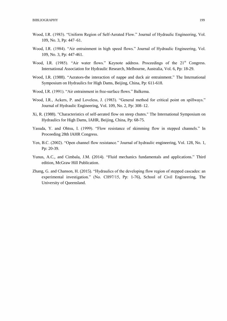
BIBLIOGRAPHY 199
Wood, I.R. (1983). “Uniform Region of Self-Aerated Flow.” Journal of Hydraulic Engineering, Vol.
109, No. 3, Pp: 447–61.
Wood, I.R. (1984). “Air entrainment in high speed flows.” Journal of Hydraulic Engineering, Vol.
109, No. 3, Pp: 447-461.
Wood, I.R. (1985). “Air water flows.” Keynote address. Proceedings of the 21st Congress.
International Association for Hydraulic Research, Melbourne, Australia, Vol. 6, Pp: 18-29.
Wood, I.R. (1988). “Aerators-the interaction of nappe and duck air entrainment.” The International
Symposium on Hydraulics for High Dams, Beijing, China, Pp: 611-618.
Wood, I.R. (1991). “Air entrainment in free-surface flows.” Balkema.
Wood, I.R., Ackers, P. and Loveless, J. (1983). “General method for critical point on spillways.”
Journal of Hydraulic Engineering, Vol. 109, No. 2, Pp: 308–12.
Xi, R. (1988). "Characteristics of self-aerated flow on steep chutes." The International Symposium on
Hydraulics for High Dams, IAHR, Beijing, China, Pp: 68-75.
Yasuda, Y. and Ohtsu, I. (1999). “Flow resistance of skimming flow in stepped channels.” In
Proceeding 28th IAHR Congress.
Yen, B.C. (2002). “Open channel flow resistance.” Journal of hydraulic engineering, Vol. 128, No. 1,
Pp: 20-39.
Yunus, A.C., and Cimbala, J.M. (2014). “Fluid mechanics fundamentals and applications.” Third
edition, McGraw Hill Publication.
Zhang, G. and Chanson, H. (2015). “Hydraulics of the developing flow region of stepped cascades: an
experimental investigation.” (No. CH97/15, Pp: 1-76), School of Civil Engineering, The
University of Queensland.

Appendix
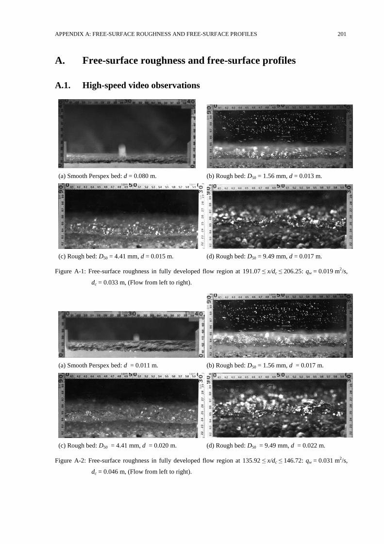
APPENDIX A: FREE-SURFACE ROUGHNESS AND FREE-SURFACE PROFILES 201
A. Free-surface roughness and free-surface profiles
A.1. High-speed video observations
(a) Smooth Perspex bed: d = 0.080 m. (b) Rough bed: D50 = 1.56 mm, d = 0.013 m.
(c) Rough bed: D50 = 4.41 mm, d = 0.015 m. (d) Rough bed: D50 = 9.49 mm, d = 0.017 m.
Figure A-1: Free-surface roughness in fully developed flow region at 191.07 ≤ x/dc ≤ 206.25: qw = 0.019 m2/s,
dc = 0.033 m, (Flow from left to right).
(a) Smooth Perspex bed: d = 0.011 m. (b) Rough bed: D50 = 1.56 mm, d = 0.017 m.
(c) Rough bed: D50 = 4.41 mm, d = 0.020 m. (d) Rough bed: D50 = 9.49 mm, d = 0.022 m.
Figure A-2: Free-surface roughness in fully developed flow region at 135.92 ≤ x/dc ≤ 146.72: qw = 0.031 m2/s,
dc = 0.046 m, (Flow from left to right).
APPENDIX A: FREE-SURFACE ROUGHNESS AND FREE-SURFACE PROFILES 202
(a) Smooth Perspex bed: d = 0.015 m. (b) Rough bed: D50 = 1.56 mm, d = 0.024 m.
(c) Rough bed: D50 = 4.41 mm, d = 0.026 m. (d) Rough bed: D50 = 9.49 mm, d = 0.027 m.
Figure A-3: Free-surface roughness in fully developed flow region at 99.36 ≤ x/dc ≤ 107.25: qw = 0.050 m2/s,
dc = 0.063 m, (Flow from left to right).
(a) Smooth Perspex bed: d = 0.020 m. (b) Rough bed: D50 = 1.56 mm, d = 0.032 m.
(c) Rough bed: D50 = 4.41 mm, d = 0.033 m. (d) Rough bed: D50 = 9.49 mm, d = 0.036 m.
Figure A-4: Free-surface roughness in fully developed flow region at 75.82 ≤ x/dc ≤ 81.85: qw = 0.075 m2/s,
dc = 0.083 m, (Flow from left to right).
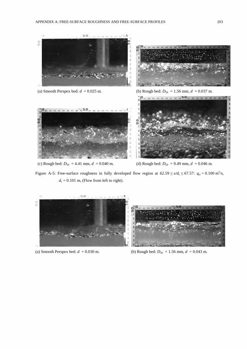
APPENDIX A: FREE-SURFACE ROUGHNESS AND FREE-SURFACE PROFILES 203
(a) Smooth Perspex bed: d = 0.025 m. (b) Rough bed: D50 = 1.56 mm, d = 0.037 m.
(c) Rough bed: D50 = 4.41 mm, d = 0.040 m. (d) Rough bed: D50 = 9.49 mm, d = 0.046 m.
Figure A-5: Free-surface roughness in fully developed flow region at 62.59 ≤ x/dc ≤ 67.57: qw = 0.100 m2/s,
dc = 0.101 m, (Flow from left to right).
(a) Smooth Perspex bed: d = 0.030 m. (b) Rough bed: D50 = 1.56 mm, d = 0.043 m.
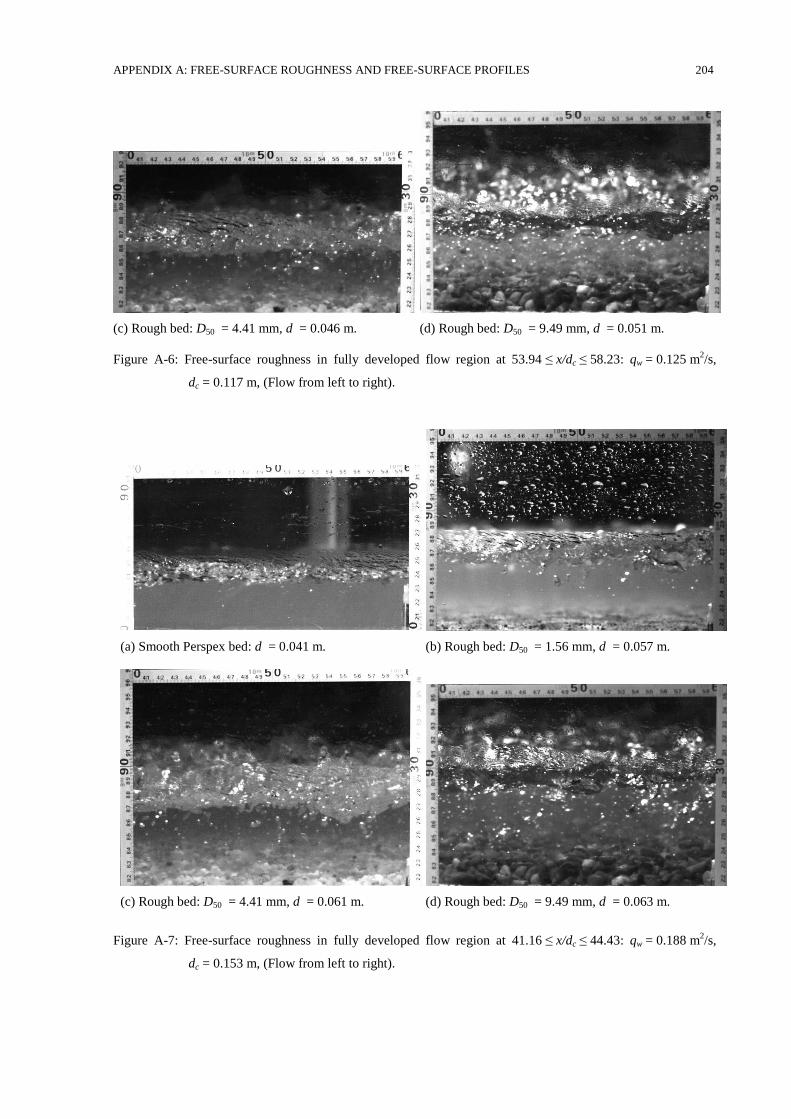
APPENDIX A: FREE-SURFACE ROUGHNESS AND FREE-SURFACE PROFILES 204
(c) Rough bed: D50 = 4.41 mm, d = 0.046 m. (d) Rough bed: D50 = 9.49 mm, d = 0.051 m.
Figure A-6: Free-surface roughness in fully developed flow region at 53.94 ≤ x/dc ≤ 58.23: qw = 0.125 m2/s,
dc = 0.117 m, (Flow from left to right).
(a) Smooth Perspex bed: d = 0.041 m. (b) Rough bed: D50 = 1.56 mm, d = 0.057 m.
(c) Rough bed: D50 = 4.41 mm, d = 0.061 m. (d) Rough bed: D50 = 9.49 mm, d = 0.063 m.
Figure A-7: Free-surface roughness in fully developed flow region at 41.16 ≤ x/dc ≤ 44.43: qw = 0.188 m2/s,
dc = 0.153 m, (Flow from left to right).
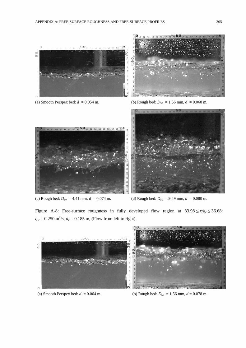
APPENDIX A: FREE-SURFACE ROUGHNESS AND FREE-SURFACE PROFILES 205
(a) Smooth Perspex bed: d = 0.054 m. (b) Rough bed: D50 = 1.56 mm, d = 0.068 m.
(c) Rough bed: D50 = 4.41 mm, d = 0.074 m. (d) Rough bed: D50 = 9.49 mm, d = 0.080 m.
Figure A-8: Free-surface roughness in fully developed flow region at 33.98 ≤ x/dc ≤ 36.68:
qw = 0.250 m2/s, dc = 0.185 m, (Flow from left to right).
(a) Smooth Perspex bed: d = 0.064 m. (b) Rough bed: D50 = 1.56 mm, d = 0.078 m.
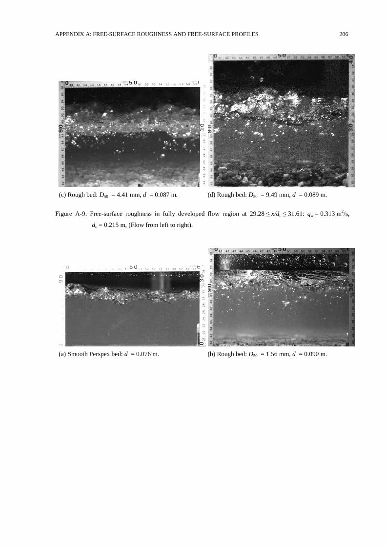
APPENDIX A: FREE-SURFACE ROUGHNESS AND FREE-SURFACE PROFILES 206
(c) Rough bed: D50 = 4.41 mm, d = 0.087 m. (d) Rough bed: D50 = 9.49 mm, d = 0.089 m.
Figure A-9: Free-surface roughness in fully developed flow region at 29.28 ≤ x/dc ≤ 31.61: qw = 0.313 m2/s,
dc = 0.215 m, (Flow from left to right).
(a) Smooth Perspex bed: d = 0.076 m. (b) Rough bed: D50 = 1.56 mm, d = 0.090 m.
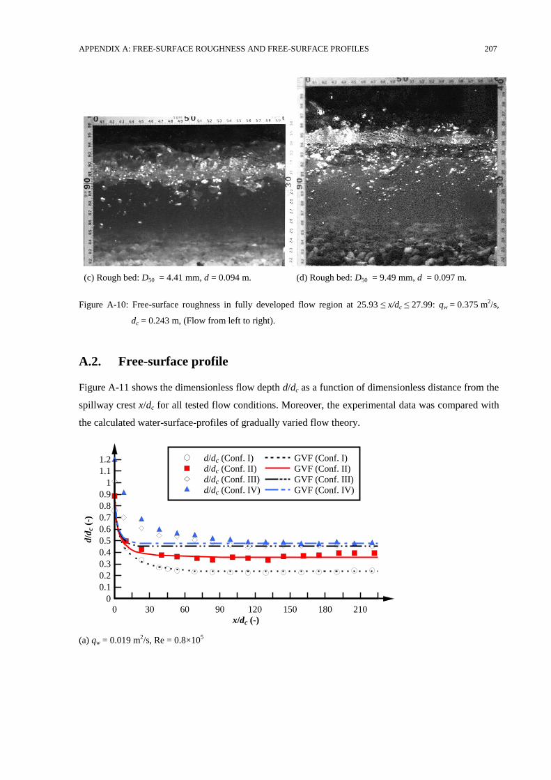
APPENDIX A: FREE-SURFACE ROUGHNESS AND FREE-SURFACE PROFILES 207
(c) Rough bed: D50 = 4.41 mm, d = 0.094 m. (d) Rough bed: D50 = 9.49 mm, d = 0.097 m.
Figure A-10: Free-surface roughness in fully developed flow region at 25.93 ≤ x/dc ≤ 27.99: qw = 0.375 m2/s,
dc = 0.243 m, (Flow from left to right).
A.2. Free-surface profile
Figure A-11 shows the dimensionless flow depth d/dc as a function of dimensionless distance from the
spillway crest x/dc for all tested flow conditions. Moreover, the experimental data was compared with
the calculated water-surface-profiles of gradually varied flow theory.
(a) qw = 0.019 m2/s, Re = 0.8×10
5
x/dc (-)
d/d
c (-
)
0 30 60 90 120 150 180 210
0
0.1
0.2
0.3
0.4
0.5
0.6
0.7
0.8
0.9
1
1.1
1.2 d/dc (Conf. I)
d/dc (Conf. II)
d/dc (Conf. III)
d/dc (Conf. IV)
GVF (Conf. I)
GVF (Conf. II)
GVF (Conf. III)
GVF (Conf. IV)
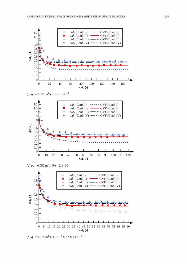
APPENDIX A: FREE-SURFACE ROUGHNESS AND FREE-SURFACE PROFILES 208
(b) qw = 0.031 m2/s, Re = 1.3×10
5
(c) qw = 0.050 m2/s, Re = 2.1×10
5
(d) qw = 0.075 m2/s, 3.0×10
5 ≤ Re ≤ 3.1×10
5
x/dc (-)
d/d
c (-
)
0 20 40 60 80 100 120 140 160
0
0.1
0.2
0.3
0.4
0.5
0.6
0.7
0.8
0.9
1
1.1
1.2 d/dc (Conf. I)
d/dc (Conf. II)
d/dc (Conf. III)
d/dc (Conf. IV)
GVF (Conf. I)
GVF (Conf. II)
GVF (Conf. III)
GVF (Conf. IV)
x/dc (-)
d/d
c (-
)
0 10 20 30 40 50 60 70 80 90 100 110 120
0
0.1
0.2
0.3
0.4
0.5
0.6
0.7
0.8
0.9
1
1.1
1.2 d/dc (Conf. I)
d/dc (Conf. II)
d/dc (Conf. III)
d/dc (Conf. IV)
GVF (Conf. I)
GVF (Conf. II)
GVF (Conf. III)
GVF (Conf. IV)
x/dc (-)
d/d
c (-
)
0 5 10 15 20 25 30 35 40 45 50 55 60 65 70 75 80 85 90
0
0.1
0.2
0.3
0.4
0.5
0.6
0.7
0.8
0.9
1 d/dc (Conf. I)
d/dc (Conf. II)
d/dc (Conf. III)
d/dc (Conf. IV)
GVF (Conf. I)
GVF (Conf. II)
GVF (Conf. III)
GVF (Conf. IV)
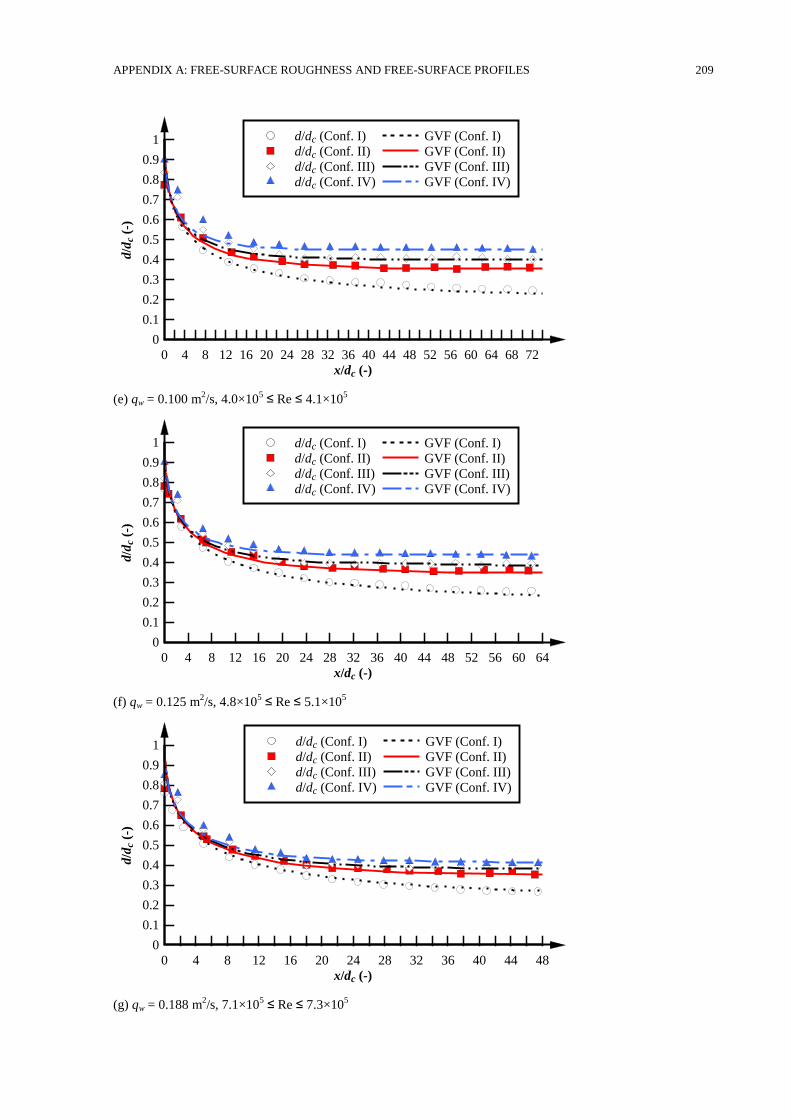
APPENDIX A: FREE-SURFACE ROUGHNESS AND FREE-SURFACE PROFILES 209
(e) qw = 0.100 m2/s, 4.0×10
5 ≤ Re ≤ 4.1×10
5
(f) qw = 0.125 m2/s, 4.8×10
5 ≤ Re ≤ 5.1×10
5
(g) qw = 0.188 m2/s, 7.1×10
5 ≤ Re ≤ 7.3×10
5
x/dc (-)
d/d
c (-
)
0 4 8 12 16 20 24 28 32 36 40 44 48 52 56 60 64 68 72
0
0.1
0.2
0.3
0.4
0.5
0.6
0.7
0.8
0.9
1 d/dc (Conf. I)
d/dc (Conf. II)
d/dc (Conf. III)
d/dc (Conf. IV)
GVF (Conf. I)
GVF (Conf. II)
GVF (Conf. III)
GVF (Conf. IV)
x/dc (-)
d/d
c (-
)
0 4 8 12 16 20 24 28 32 36 40 44 48 52 56 60 64
0
0.1
0.2
0.3
0.4
0.5
0.6
0.7
0.8
0.9
1 d/dc (Conf. I)
d/dc (Conf. II)
d/dc (Conf. III)
d/dc (Conf. IV)
GVF (Conf. I)
GVF (Conf. II)
GVF (Conf. III)
GVF (Conf. IV)
x/dc (-)
d/d
c (-
)
0 4 8 12 16 20 24 28 32 36 40 44 48
0
0.1
0.2
0.3
0.4
0.5
0.6
0.7
0.8
0.9
1 d/dc (Conf. I)
d/dc (Conf. II)
d/dc (Conf. III)
d/dc (Conf. IV)
GVF (Conf. I)
GVF (Conf. II)
GVF (Conf. III)
GVF (Conf. IV)
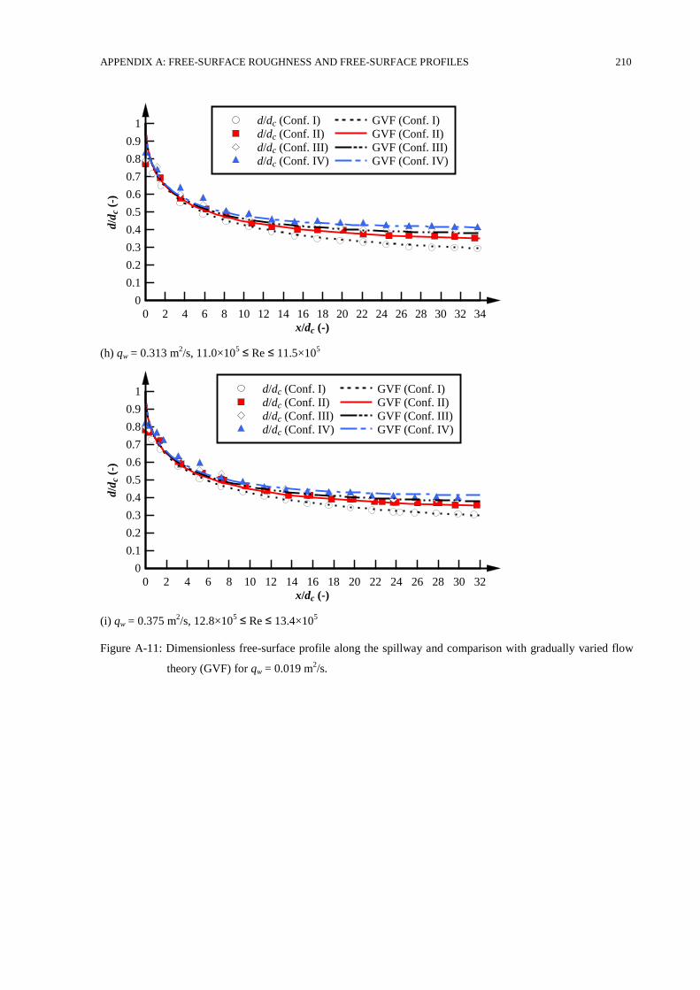
APPENDIX A: FREE-SURFACE ROUGHNESS AND FREE-SURFACE PROFILES 210
(h) qw = 0.313 m2/s, 11.0×10
5 ≤ Re ≤ 11.5×10
5
(i) qw = 0.375 m2/s, 12.8×10
5 ≤ Re ≤ 13.4×10
5
Figure A-11: Dimensionless free-surface profile along the spillway and comparison with gradually varied flow
theory (GVF) for qw = 0.019 m2/s.
x/dc (-)
d/d
c (-
)
0 2 4 6 8 10 12 14 16 18 20 22 24 26 28 30 32 34
0
0.1
0.2
0.3
0.4
0.5
0.6
0.7
0.8
0.9
1 d/dc (Conf. I)
d/dc (Conf. II)
d/dc (Conf. III)
d/dc (Conf. IV)
GVF (Conf. I)
GVF (Conf. II)
GVF (Conf. III)
GVF (Conf. IV)
x/dc (-)
d/d
c (-
)
0 2 4 6 8 10 12 14 16 18 20 22 24 26 28 30 32
0
0.1
0.2
0.3
0.4
0.5
0.6
0.7
0.8
0.9
1 d/dc (Conf. I)
d/dc (Conf. II)
d/dc (Conf. III)
d/dc (Conf. IV)
GVF (Conf. I)
GVF (Conf. II)
GVF (Conf. III)
GVF (Conf. IV)
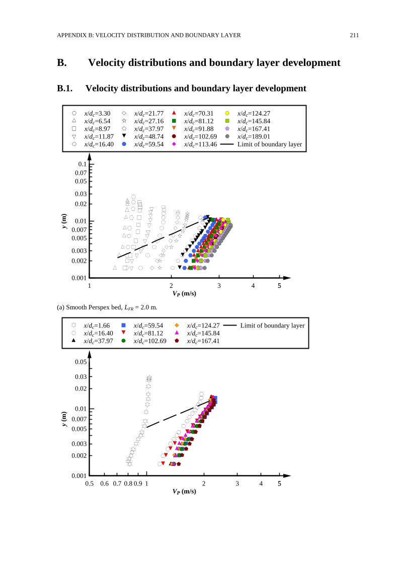
APPENDIX B: VELOCITY DISTRIBUTION AND BOUNDARY LAYER 211
B. Velocity distributions and boundary layer development
B.1. Velocity distributions and boundary layer development
(a) Smooth Perspex bed, LFR = 2.0 m.
VP (m/s)
y (m
)
1 2 3 4 55
0.001
0.002
0.003
0.005
0.007
0.01
0.02
0.03
0.05
0.07
0.1
x/dc=3.30
x/dc=6.54
x/dc=8.97
x/dc=11.87
x/dc=16.40
x/dc=21.77
x/dc=27.16
x/dc=37.97
x/dc=48.74
x/dc=59.54
x/dc=70.31
x/dc=81.12
x/dc=91.88
x/dc=102.69
x/dc=113.46
x/dc=124.27
x/dc=145.84
x/dc=167.41
x/dc=189.01
Limit of boundary layer
VP (m/s)
y (m
)
0.5 0.6 0.7 0.8 0.9 1 2 3 4 55
0.001
0.002
0.003
0.005
0.007
0.01
0.02
0.03
0.05
x/dc=1.66
x/dc=16.40
x/dc=37.97
x/dc=59.54
x/dc=81.12
x/dc=102.69
x/dc=124.27
x/dc=145.84
x/dc=167.41
Limit of boundary layer
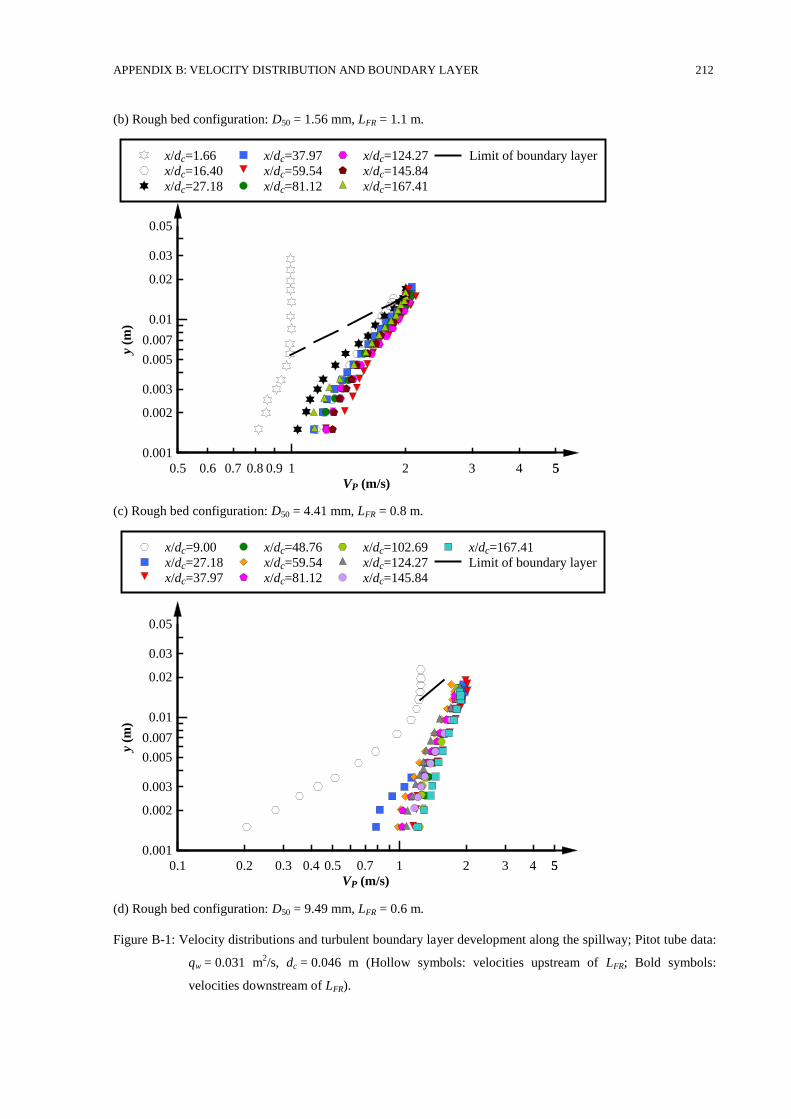
APPENDIX B: VELOCITY DISTRIBUTION AND BOUNDARY LAYER 212
(b) Rough bed configuration: D50 = 1.56 mm, LFR = 1.1 m.
(c) Rough bed configuration: D50 = 4.41 mm, LFR = 0.8 m.
(d) Rough bed configuration: D50 = 9.49 mm, LFR = 0.6 m.
Figure B-1: Velocity distributions and turbulent boundary layer development along the spillway; Pitot tube data:
qw = 0.031 m2/s, dc = 0.046 m (Hollow symbols: velocities upstream of LFR; Bold symbols:
velocities downstream of LFR).
VP (m/s)
y (m
)
0.5 0.6 0.7 0.8 0.9 1 2 3 4 55
0.001
0.002
0.003
0.005
0.007
0.01
0.02
0.03
0.05
x/dc=1.66
x/dc=16.40
x/dc=27.18
x/dc=37.97
x/dc=59.54
x/dc=81.12
x/dc=124.27
x/dc=145.84
x/dc=167.41
Limit of boundary layer
VP (m/s)
y (m
)
0.1 0.2 0.3 0.4 0.5 0.7 1 2 3 4 55
0.001
0.002
0.003
0.005
0.007
0.01
0.02
0.03
0.05
x/dc=9.00
x/dc=27.18
x/dc=37.97
x/dc=48.76
x/dc=59.54
x/dc=81.12
x/dc=102.69
x/dc=124.27
x/dc=145.84
x/dc=167.41
Limit of boundary layer
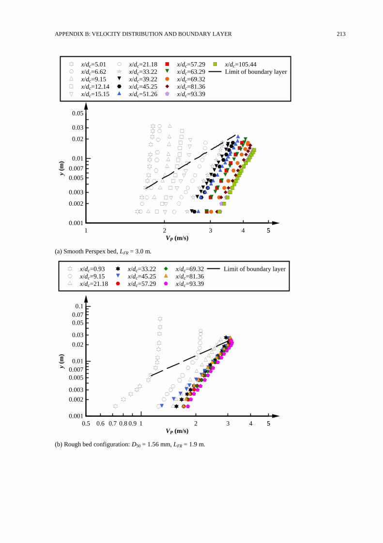
APPENDIX B: VELOCITY DISTRIBUTION AND BOUNDARY LAYER 213
(a) Smooth Perspex bed, LFR = 3.0 m.
(b) Rough bed configuration: D50 = 1.56 mm, LFR = 1.9 m.
VP (m/s)
y (m
)
1 2 3 4 55
0.001
0.002
0.003
0.005
0.007
0.01
0.02
0.03
0.05
x/dc=5.01
x/dc=6.62
x/dc=9.15
x/dc=12.14
x/dc=15.15
x/dc=21.18
x/dc=33.22
x/dc=39.22
x/dc=45.25
x/dc=51.26
x/dc=57.29
x/dc=63.29
x/dc=69.32
x/dc=81.36
x/dc=93.39
x/dc=105.44
Limit of boundary layer
VP (m/s)
y (m
)
0.5 0.6 0.7 0.8 0.9 1 2 3 4 55
0.001
0.002
0.003
0.005
0.007
0.01
0.02
0.03
0.05
0.07
0.1
x/dc=0.93
x/dc=9.15
x/dc=21.18
x/dc=33.22
x/dc=45.25
x/dc=57.29
x/dc=69.32
x/dc=81.36
x/dc=93.39
Limit of boundary layer
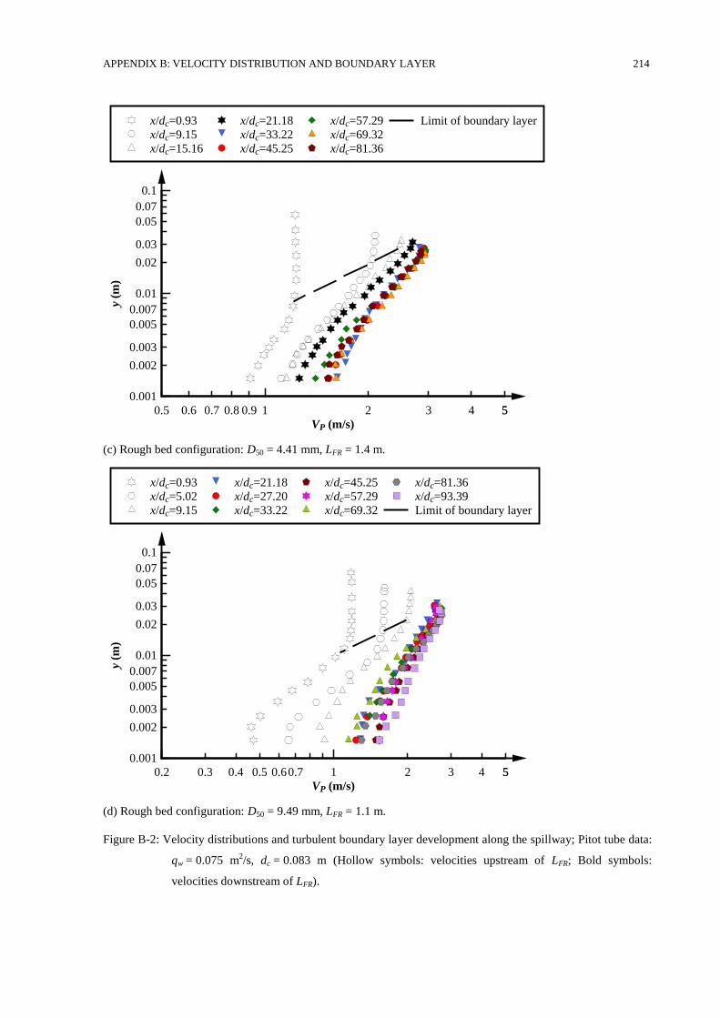
APPENDIX B: VELOCITY DISTRIBUTION AND BOUNDARY LAYER 214
(c) Rough bed configuration: D50 = 4.41 mm, LFR = 1.4 m.
(d) Rough bed configuration: D50 = 9.49 mm, LFR = 1.1 m.
Figure B-2: Velocity distributions and turbulent boundary layer development along the spillway; Pitot tube data:
qw = 0.075 m2/s, dc = 0.083 m (Hollow symbols: velocities upstream of LFR; Bold symbols:
velocities downstream of LFR).
VP (m/s)
y (m
)
0.5 0.6 0.7 0.8 0.9 1 2 3 4 55
0.001
0.002
0.003
0.005
0.007
0.01
0.02
0.03
0.05
0.07
0.1
x/dc=0.93
x/dc=9.15
x/dc=15.16
x/dc=21.18
x/dc=33.22
x/dc=45.25
x/dc=57.29
x/dc=69.32
x/dc=81.36
Limit of boundary layer
VP (m/s)
y (m
)
0.2 0.3 0.4 0.5 0.60.7 1 2 3 4 55
0.001
0.002
0.003
0.005
0.007
0.01
0.02
0.03
0.05
0.07
0.1
x/dc=0.93
x/dc=5.02
x/dc=9.15
x/dc=21.18
x/dc=27.20
x/dc=33.22
x/dc=45.25
x/dc=57.29
x/dc=69.32
x/dc=81.36
x/dc=93.39
Limit of boundary layer
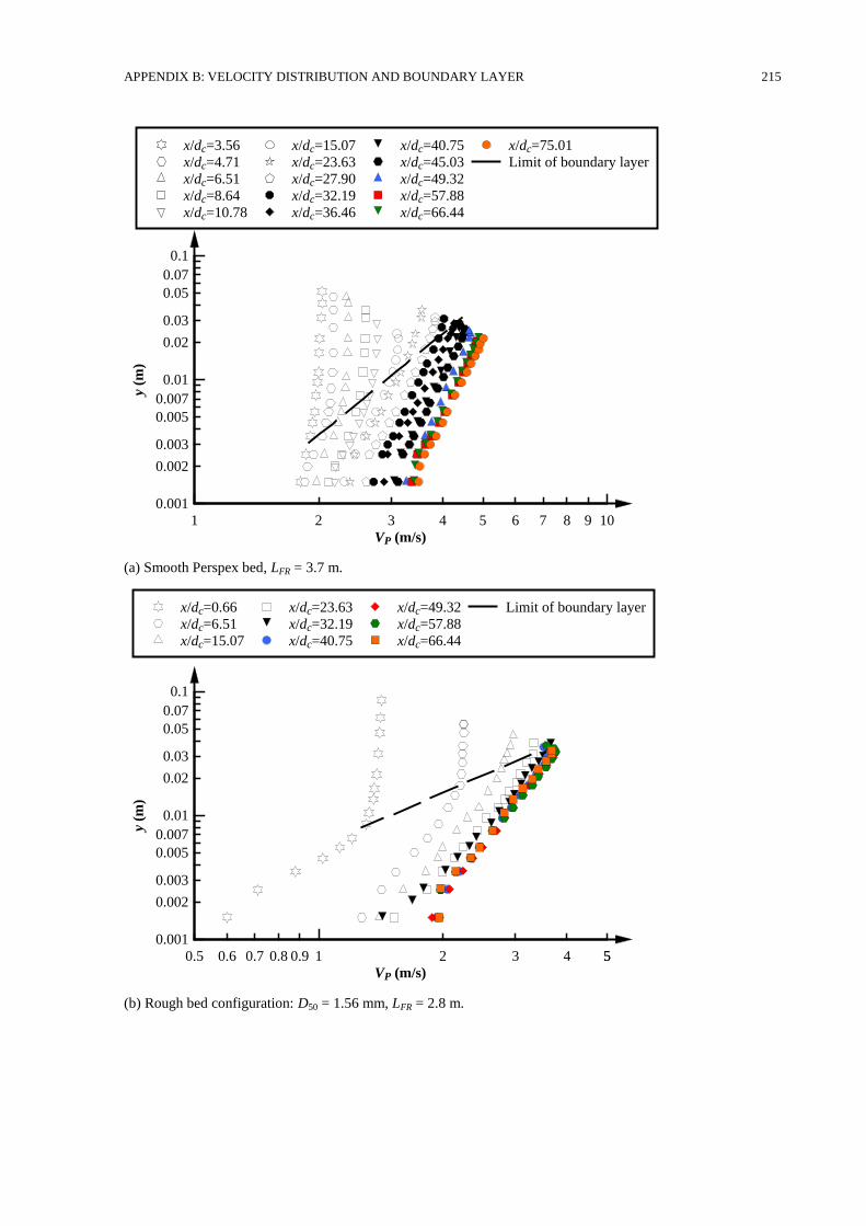
APPENDIX B: VELOCITY DISTRIBUTION AND BOUNDARY LAYER 215
(a) Smooth Perspex bed, LFR = 3.7 m.
(b) Rough bed configuration: D50 = 1.56 mm, LFR = 2.8 m.
VP (m/s)
y (m
)
1 2 3 4 5 6 7 8 9 10
0.001
0.002
0.003
0.005
0.007
0.01
0.02
0.03
0.05
0.07
0.1
x/dc=3.56
x/dc=4.71
x/dc=6.51
x/dc=8.64
x/dc=10.78
x/dc=15.07
x/dc=23.63
x/dc=27.90
x/dc=32.19
x/dc=36.46
x/dc=40.75
x/dc=45.03
x/dc=49.32
x/dc=57.88
x/dc=66.44
x/dc=75.01
Limit of boundary layer
VP (m/s)
y (m
)
0.5 0.6 0.7 0.8 0.9 1 2 3 4 55
0.001
0.002
0.003
0.005
0.007
0.01
0.02
0.03
0.05
0.07
0.1
x/dc=0.66
x/dc=6.51
x/dc=15.07
x/dc=23.63
x/dc=32.19
x/dc=40.75
x/dc=49.32
x/dc=57.88
x/dc=66.44
Limit of boundary layer
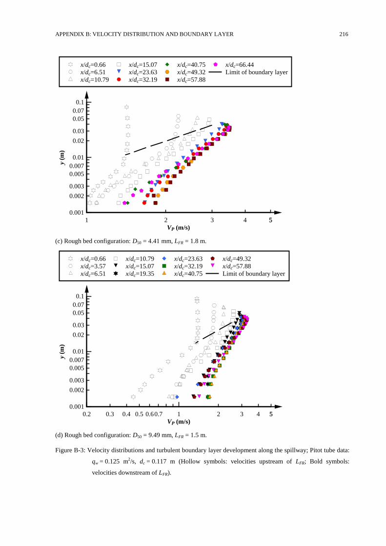
APPENDIX B: VELOCITY DISTRIBUTION AND BOUNDARY LAYER 216
(c) Rough bed configuration: D50 = 4.41 mm, LFR = 1.8 m.
(d) Rough bed configuration: D50 = 9.49 mm, LFR = 1.5 m.
Figure B-3: Velocity distributions and turbulent boundary layer development along the spillway; Pitot tube data:
qw = 0.125 m2/s, dc = 0.117 m (Hollow symbols: velocities upstream of LFR; Bold symbols:
velocities downstream of LFR).
VP (m/s)
y (m
)
1 2 3 4 55
0.001
0.002
0.003
0.005
0.007
0.01
0.02
0.03
0.05
0.07
0.1
x/dc=0.66
x/dc=6.51
x/dc=10.79
x/dc=15.07
x/dc=23.63
x/dc=32.19
x/dc=40.75
x/dc=49.32
x/dc=57.88
x/dc=66.44
Limit of boundary layer
VP (m/s)
y (m
)
0.2 0.3 0.4 0.5 0.60.7 1 2 3 4 55
0.001
0.002
0.003
0.005
0.007
0.01
0.02
0.03
0.05
0.07
0.1
x/dc=0.66
x/dc=3.57
x/dc=6.51
x/dc=10.79
x/dc=15.07
x/dc=19.35
x/dc=23.63
x/dc=32.19
x/dc=40.75
x/dc=49.32
x/dc=57.88
Limit of boundary layer
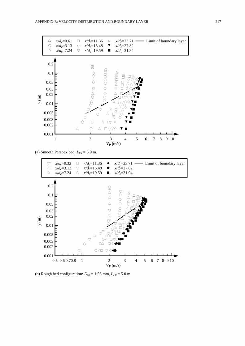
APPENDIX B: VELOCITY DISTRIBUTION AND BOUNDARY LAYER 217
(a) Smooth Perspex bed, LFR = 5.9 m.
(b) Rough bed configuration: D50 = 1.56 mm, LFR = 5.0 m.
VP (m/s)
y (m
)
1 2 3 4 5 6 7 8 9 10
0.001
0.002
0.003
0.005
0.01
0.02
0.03
0.05
0.1
0.2
x/dc=0.61
x/dc=3.13
x/dc=7.24
x/dc=11.36
x/dc=15.48
x/dc=19.59
x/dc=23.71
x/dc=27.82
x/dc=31.34
Limit of boundary layer
VP (m/s)
y (m
)
0.5 0.6 0.70.8 1 2 3 4 5 6 7 8 9 10
0.001
0.002
0.003
0.005
0.01
0.02
0.03
0.05
0.1
0.2
x/dc=0.32
x/dc=3.13
x/dc=7.24
x/dc=11.36
x/dc=15.48
x/dc=19.59
x/dc=23.71
x/dc=27.82
x/dc=31.94
Limit of boundary layer
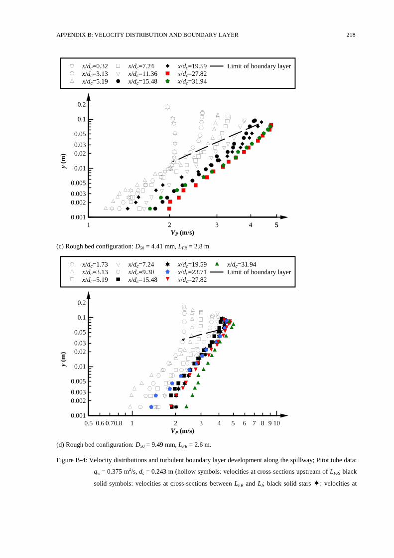
APPENDIX B: VELOCITY DISTRIBUTION AND BOUNDARY LAYER 218
(c) Rough bed configuration: D50 = 4.41 mm, LFR = 2.8 m.
(d) Rough bed configuration: D50 = 9.49 mm, LFR = 2.6 m.
Figure B-4: Velocity distributions and turbulent boundary layer development along the spillway; Pitot tube data:
qw = 0.375 m2/s, dc = 0.243 m (hollow symbols: velocities at cross-sections upstream of LFR; black
solid symbols: velocities at cross-sections between LFR and LI; black solid stars : velocities at
VP (m/s)
y (m
)
1 2 3 4 55
0.001
0.002
0.003
0.005
0.01
0.02
0.03
0.05
0.1
0.2
x/dc=0.32
x/dc=3.13
x/dc=5.19
x/dc=7.24
x/dc=11.36
x/dc=15.48
x/dc=19.59
x/dc=27.82
x/dc=31.94
Limit of boundary layer
VP (m/s)
y (m
)
0.5 0.6 0.70.8 1 2 3 4 5 6 7 8 9 10
0.001
0.002
0.003
0.005
0.01
0.02
0.03
0.05
0.1
0.2
x/dc=1.73
x/dc=3.13
x/dc=5.19
x/dc=7.24
x/dc=9.30
x/dc=15.48
x/dc=19.59
x/dc=23.71
x/dc=27.82
x/dc=31.94
Limit of boundary layer
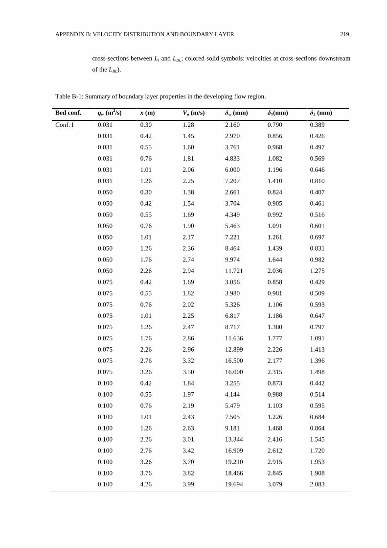
APPENDIX B: VELOCITY DISTRIBUTION AND BOUNDARY LAYER 219
cross-sections between LI and LBL; colored solid symbols: velocities at cross-sections downstream
of the LBL).
Table B-1: Summary of boundary layer properties in the developing flow region.
Bed conf. qw (m2/s) x (m) Vo (m/s) δw (mm) δ1(mm) δ2 (mm)
Conf. I 0.031 0.30 1.28 2.160 0.790 0.389
0.031 0.42 1.45 2.970 0.856 0.426
0.031 0.55 1.60 3.761 0.968 0.497
0.031 0.76 1.81 4.833 1.082 0.569
0.031 1.01 2.06 6.000 1.196 0.646
0.031 1.26 2.25 7.207 1.410 0.810
0.050 0.30 1.38 2.661 0.824 0.407
0.050 0.42 1.54 3.704 0.905 0.461
0.050 0.55 1.69 4.349 0.992 0.516
0.050 0.76 1.90 5.463 1.091 0.601
0.050 1.01 2.17 7.221 1.261 0.697
0.050 1.26 2.36 8.464 1.439 0.831
0.050 1.76 2.74 9.974 1.644 0.982
0.050 2.26 2.94 11.721 2.036 1.275
0.075 0.42 1.69 3.056 0.858 0.429
0.075 0.55 1.82 3.980 0.981 0.509
0.075 0.76 2.02 5.326 1.106 0.593
0.075 1.01 2.25 6.817 1.186 0.647
0.075 1.26 2.47 8.717 1.380 0.797
0.075 1.76 2.86 11.636 1.777 1.091
0.075 2.26 2.96 12.899 2.226 1.413
0.075 2.76 3.32 16.500 2.177 1.396
0.075 3.26 3.50 16.000 2.315 1.498
0.100 0.42 1.84 3.255 0.873 0.442
0.100 0.55 1.97 4.144 0.988 0.514
0.100 0.76 2.19 5.479 1.103 0.595
0.100 1.01 2.43 7.505 1.226 0.684
0.100 1.26 2.63 9.181 1.468 0.864
0.100 2.26 3.01 13.344 2.416 1.545
0.100 2.76 3.42 16.909 2.612 1.720
0.100 3.26 3.70 19.210 2.915 1.953
0.100 3.76 3.82 18.466 2.845 1.908
0.100 4.26 3.99 19.694 3.079 2.083
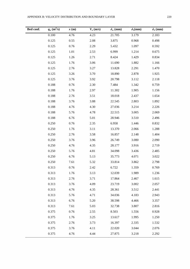
APPENDIX B: VELOCITY DISTRIBUTION AND BOUNDARY LAYER 220
Bed conf. qw (m2/s) x (m) Vo (m/s) δw (mm) δ1(mm) δ2 (mm)
0.100 4.76 4.23 21.705 3.179 2.183
0.125 0.55 2.08 3.875 0.968 0.498
0.125 0.76 2.29 5.432 1.097 0.592
0.125 1.01 2.53 6.999 1.214 0.675
0.125 1.26 2.71 8.424 1.429 0.834
0.125 1.76 3.06 11.690 1.882 1.166
0.125 2.76 3.27 13.828 2.291 1.470
0.125 3.26 3.70 18.890 2.878 1.925
0.125 3.76 3.92 20.798 3.112 2.118
0.188 0.76 2.30 7.484 1.342 0.759
0.188 1.76 2.97 11.302 1.905 1.156
0.188 2.76 3.51 18.018 2.437 1.654
0.188 3.76 3.88 22.545 2.803 1.892
0.188 4.76 4.30 27.036 3.214 2.226
0.188 5.76 4.78 22.515 3.005 2.069
0.188 6.76 5.01 28.946 3.510 2.496
0.250 0.76 2.35 6.958 1.446 0.832
0.250 1.76 3.11 13.370 2.066 1.288
0.250 2.76 3.58 16.857 2.148 1.404
0.250 3.76 3.96 26.749 3.080 2.090
0.250 4.76 4.35 28.177 3.916 2.719
0.250 5.76 4.81 34.098 3.436 2.485
0.250 6.76 5.13 35.773 4.071 3.022
0.250 7.61 5.32 33.814 3.862 2.798
0.313 0.76 2.42 6.722 1.359 0.769
0.313 1.76 3.13 12.039 1.989 1.236
0.313 2.76 3.71 17.864 2.467 1.615
0.313 3.76 4.09 23.719 3.002 2.057
0.313 4.76 4.35 28.361 3.512 2.441
0.313 5.76 4.71 34.036 4.183 2.943
0.313 6.76 5.20 38.598 4.466 3.357
0.313 7.61 5.03 32.738 3.807 2.816
0.375 0.76 2.55 8.503 1.556 0.928
0.375 1.76 3.25 13.617 1.995 1.250
0.375 2.76 3.73 16.397 2.335 1.532
0.375 3.76 4.11 22.020 3.044 2.076
0.375 4.76 4.44 27.875 3.218 2.292
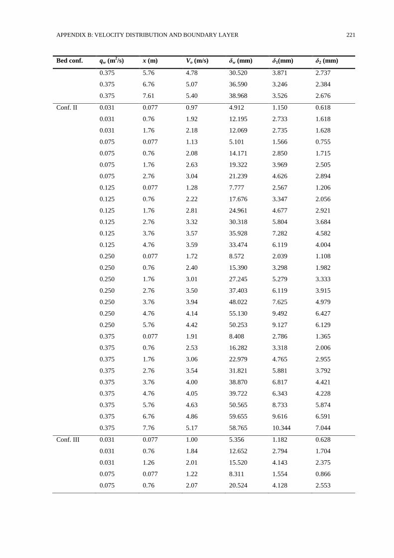
APPENDIX B: VELOCITY DISTRIBUTION AND BOUNDARY LAYER 221
Bed conf. qw (m2/s) x (m) Vo (m/s) δw (mm) δ1(mm) δ2 (mm)
0.375 5.76 4.78 30.520 3.871 2.737
0.375 6.76 5.07 36.590 3.246 2.384
0.375 7.61 5.40 38.968 3.526 2.676
Conf. II 0.031 0.077 0.97 4.912 1.150 0.618
0.031 0.76 1.92 12.195 2.733 1.618
0.031 1.76 2.18 12.069 2.735 1.628
0.075 0.077 1.13 5.101 1.566 0.755
0.075 0.76 2.08 14.171 2.850 1.715
0.075 1.76 2.63 19.322 3.969 2.505
0.075 2.76 3.04 21.239 4.626 2.894
0.125 0.077 1.28 7.777 2.567 1.206
0.125 0.76 2.22 17.676 3.347 2.056
0.125 1.76 2.81 24.961 4.677 2.921
0.125 2.76 3.32 30.318 5.804 3.684
0.125 3.76 3.57 35.928 7.282 4.582
0.125 4.76 3.59 33.474 6.119 4.004
0.250 0.077 1.72 8.572 2.039 1.108
0.250 0.76 2.40 15.390 3.298 1.982
0.250 1.76 3.01 27.245 5.279 3.333
0.250 2.76 3.50 37.403 6.119 3.915
0.250 3.76 3.94 48.022 7.625 4.979
0.250 4.76 4.14 55.130 9.492 6.427
0.250 5.76 4.42 50.253 9.127 6.129
0.375 0.077 1.91 8.408 2.786 1.365
0.375 0.76 2.53 16.282 3.318 2.006
0.375 1.76 3.06 22.979 4.765 2.955
0.375 2.76 3.54 31.821 5.881 3.792
0.375 3.76 4.00 38.870 6.817 4.421
0.375 4.76 4.05 39.722 6.343 4.228
0.375 5.76 4.63 50.565 8.733 5.874
0.375 6.76 4.86 59.655 9.616 6.591
0.375 7.76 5.17 58.765 10.344 7.044
Conf. III 0.031 0.077 1.00 5.356 1.182 0.628
0.031 0.76 1.84 12.652 2.794 1.704
0.031 1.26 2.01 15.520 4.143 2.375
0.075 0.077 1.22 8.311 1.554 0.866
0.075 0.76 2.07 20.524 4.128 2.553
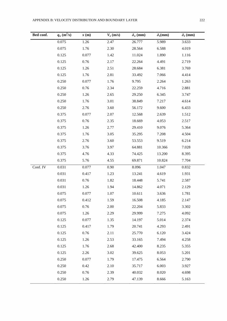
APPENDIX B: VELOCITY DISTRIBUTION AND BOUNDARY LAYER 222
Bed conf. qw (m2/s) x (m) Vo (m/s) δw (mm) δ1(mm) δ2 (mm)
0.075 1.26 2.47 26.777 5.989 3.633
0.075 1.76 2.30 28.564 6.588 4.019
0.125 0.077 1.42 11.024 1.890 1.116
0.125 0.76 2.17 22.264 4.491 2.719
0.125 1.26 2.51 28.684 6.381 3.769
0.125 1.76 2.81 33.492 7.066 4.414
0.250 0.077 1.76 9.795 2.264 1.263
0.250 0.76 2.34 22.259 4.716 2.881
0.250 1.26 2.65 29.250 6.345 3.747
0.250 1.76 3.01 38.849 7.217 4.614
0.250 2.76 3.60 56.172 9.600 6.433
0.375 0.077 2.07 12.568 2.639 1.512
0.375 0.76 2.35 18.669 4.053 2.517
0.375 1.26 2.77 29.410 9.076 5.364
0.375 1.76 3.05 35.295 7.208 4.504
0.375 2.76 3.60 53.553 9.519 6.214
0.375 3.76 3.97 64.881 10.366 7.028
0.375 4.76 4.33 74.425 13.200 8.395
0.375 5.76 4.55 69.871 10.824 7.704
Conf. IV 0.031 0.077 0.90 8.096 1.047 0.832
0.031 0.417 1.23 13.241 4.619 1.931
0.031 0.76 1.82 18.448 5.741 2.587
0.031 1.26 1.94 14.862 4.071 2.129
0.075 0.077 1.07 10.611 3.636 1.781
0.075 0.412 1.59 16.508 4.185 2.147
0.075 0.76 2.00 22.204 5.833 3.302
0.075 1.26 2.29 29.999 7.275 4.092
0.125 0.077 1.35 14.197 5.014 2.374
0.125 0.417 1.79 20.741 4.293 2.491
0.125 0.76 2.11 25.770 6.120 3.424
0.125 1.26 2.53 33.165 7.494 4.258
0.125 1.76 2.68 42.400 8.235 5.355
0.125 2.26 3.02 39.625 8.053 5.201
0.250 0.077 1.79 17.475 6.564 2.790
0.250 0.42 2.10 35.717 6.003 3.927
0.250 0.76 2.39 40.032 8.020 4.698
0.250 1.26 2.79 47.139 8.666 5.163
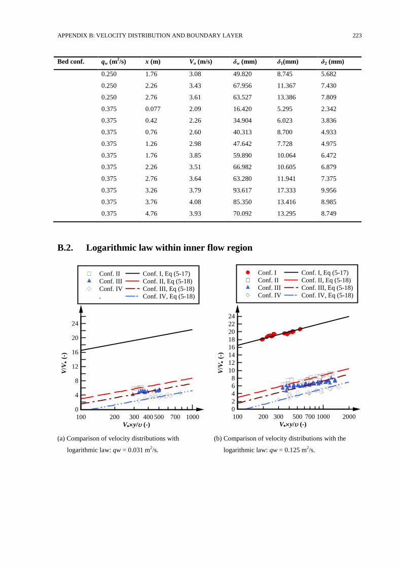
APPENDIX B: VELOCITY DISTRIBUTION AND BOUNDARY LAYER 223
Bed conf. qw (m2/s) x (m) Vo (m/s) δw (mm) δ1(mm) δ2 (mm)
0.250 1.76 3.08 49.820 8.745 5.682
0.250 2.26 3.43 67.956 11.367 7.430
0.250 2.76 3.61 63.527 13.386 7.809
0.375 0.077 2.09 16.420 5.295 2.342
0.375 0.42 2.26 34.904 6.023 3.836
0.375 0.76 2.60 40.313 8.700 4.933
0.375 1.26 2.98 47.642 7.728 4.975
0.375 1.76 3.85 59.890 10.064 6.472
0.375 2.26 3.51 66.982 10.605 6.879
0.375 2.76 3.64 63.280 11.941 7.375
0.375 3.26 3.79 93.617 17.333 9.956
0.375 3.76 4.08 85.350 13.416 8.985
0.375 4.76 3.93 70.092 13.295 8.749
B.2. Logarithmic law within inner flow region
(a) Comparison of velocity distributions with
logarithmic law: qw = 0.031 m2/s.
(b) Comparison of velocity distributions with the
logarithmic law: qw = 0.125 m2/s.
Vy/ (-)
V/V
(
-)
100 200 300 400 500 700 1000
0
4
8
12
16
20
24
Conf. II
Conf. III
Conf. IV
.
Conf. I, Eq (5-17)
Conf. II, Eq (5-18)
Conf. III, Eq (5-18)
Conf. IV, Eq (5-18)
Vy/ (-)
V/V
(
-)
100 200 300 500 700 1000 2000
0
2
4
6
8
10
12
14
16
18
20
22
24
Conf. I
Conf. II
Conf. III
Conf. IV
Conf. I, Eq (5-17)
Conf. II, Eq (5-18)
Conf. III, Eq (5-18)
Conf. IV, Eq (5-18)
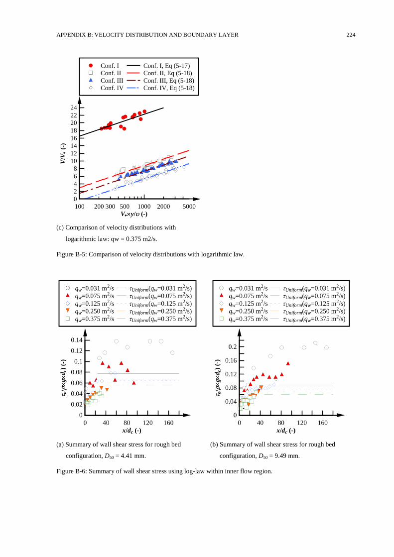
APPENDIX B: VELOCITY DISTRIBUTION AND BOUNDARY LAYER 224
(c) Comparison of velocity distributions with
logarithmic law: qw = 0.375 m2/s.
Figure B-5: Comparison of velocity distributions with logarithmic law.
(a) Summary of wall shear stress for rough bed
configuration, D50 = 4.41 mm.
(b) Summary of wall shear stress for rough bed
configuration, D50 = 9.49 mm.
Figure B-6: Summary of wall shear stress using log-law within inner flow region.
Vy/ (-)
V/V
(
-)
100 200 300 500 1000 2000 5000
0
2
4
6
8
10
12
14
16
18
20
22
24
Conf. I
Conf. II
Conf. III
Conf. IV
Conf. I, Eq (5-17)
Conf. II, Eq (5-18)
Conf. III, Eq (5-18)
Conf. IV, Eq (5-18)
x/dc (-)
o/
g
dc)
(-)
0 40 80 120 160
0
0.02
0.04
0.06
0.08
0.1
0.12
0.14
qw=0.031 m2/s
qw=0.075 m2/s
qw=0.125 m2/s
qw=0.250 m2/s
qw=0.375 m2/s
Uniform(qw=0.031 m2/s)
Uniform(qw=0.075 m2/s)
Uniform(qw=0.125 m2/s)
Uniform(qw=0.250 m2/s)
Uniform(qw=0.375 m2/s)
x/dc (-)
o/
g
dc)
(-)
0 40 80 120 160
0
0.04
0.08
0.12
0.16
0.2
qw=0.031 m2/s
qw=0.075 m2/s
qw=0.125 m2/s
qw=0.250 m2/s
qw=0.375 m2/s
Uniform(qw=0.031 m2/s)
Uniform(qw=0.075 m2/s)
Uniform(qw=0.125 m2/s)
Uniform(qw=0.250 m2/s)
Uniform(qw=0.375 m2/s)
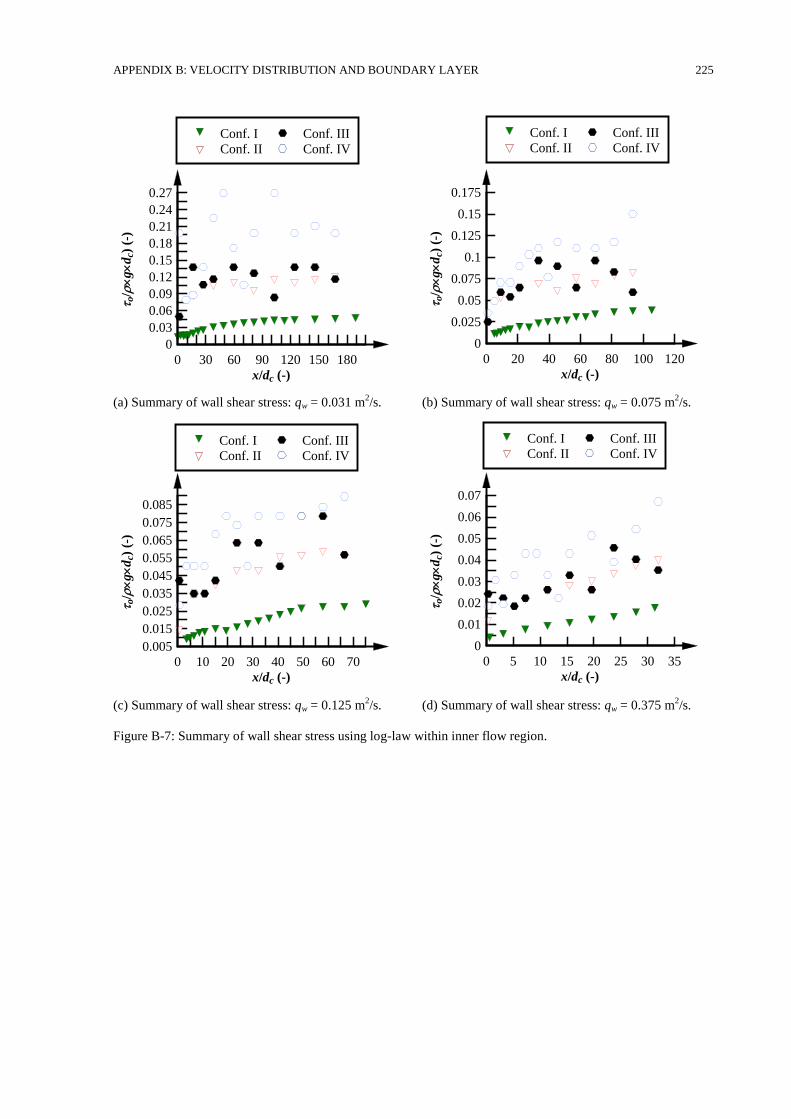
APPENDIX B: VELOCITY DISTRIBUTION AND BOUNDARY LAYER 225
(a) Summary of wall shear stress: qw = 0.031 m2/s. (b) Summary of wall shear stress: qw = 0.075 m
2/s.
(c) Summary of wall shear stress: qw = 0.125 m2/s. (d) Summary of wall shear stress: qw = 0.375 m
2/s.
Figure B-7: Summary of wall shear stress using log-law within inner flow region.
x/dc (-)
o/
g
dc)
(-)
0 30 60 90 120 150 180
0
0.03
0.06
0.09
0.12
0.15
0.18
0.21
0.24
0.27
Conf. I
Conf. II
Conf. III
Conf. IV
x/dc (-)
o/
g
dc)
(-)
0 20 40 60 80 100 120
0
0.025
0.05
0.075
0.1
0.125
0.15
0.175
Conf. I
Conf. II
Conf. III
Conf. IV
x/dc (-)
o/
g
dc)
(-)
0 10 20 30 40 50 60 70
0.005
0.015
0.025
0.035
0.045
0.055
0.065
0.075
0.085
Conf. I
Conf. II
Conf. III
Conf. IV
x/dc (-)
o/
g
dc)
(-)
0 5 10 15 20 25 30 35
0
0.01
0.02
0.03
0.04
0.05
0.06
0.07
Conf. I
Conf. II
Conf. III
Conf. IV
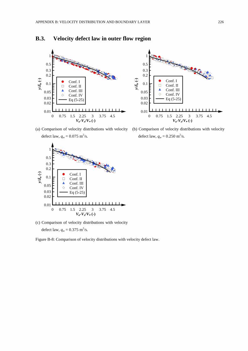
APPENDIX B: VELOCITY DISTRIBUTION AND BOUNDARY LAYER 226
B.3. Velocity defect law in outer flow region
(a) Comparison of velocity distributions with velocity
defect law, qw = 0.075 m2/s.
(b) Comparison of velocity distributions with velocity
defect law, qw = 0.250 m2/s.
(c) Comparison of velocity distributions with velocity
defect law, qw = 0.375 m2/s.
Figure B-8: Comparison of velocity distributions with velocity defect law.
Vo-Vx/V (-)
y/
w (
-)
0 0.75 1.5 2.25 3 3.75 4.5
0.01
0.02
0.03
0.05
0.1
0.2
0.3
0.5
1
Conf. I
Conf. II
Conf. III
Conf. IV
Eq (5-25)
Vo-Vx/V (-)
y/
w (
-)
0 0.75 1.5 2.25 3 3.75 4.5
0.01
0.02
0.03
0.05
0.1
0.2
0.3
0.5
1
Conf. I
Conf. II
Conf. III
Conf. IV
Eq (5-25)
Vo-Vx/V (-)
y/
w (
-)
0 0.75 1.5 2.25 3 3.75 4.5
0.01
0.02
0.03
0.05
0.1
0.2
0.3
0.5
1
Conf. I
Conf. II
Conf. III
Conf. IV
Eq (5-25)
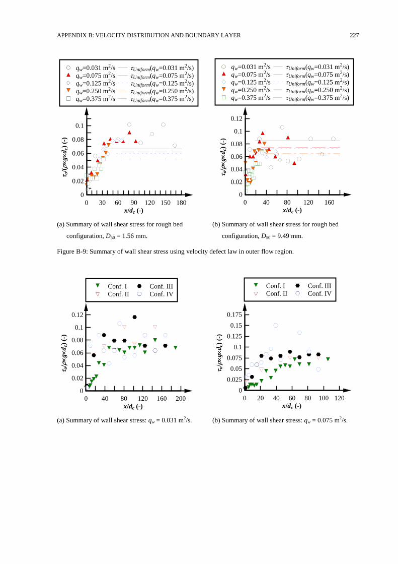
APPENDIX B: VELOCITY DISTRIBUTION AND BOUNDARY LAYER 227
(a) Summary of wall shear stress for rough bed
configuration, D50 = 1.56 mm.
(b) Summary of wall shear stress for rough bed
configuration, D50 = 9.49 mm.
Figure B-9: Summary of wall shear stress using velocity defect law in outer flow region.
(a) Summary of wall shear stress: qw = 0.031 m2/s. (b) Summary of wall shear stress: qw = 0.075 m
2/s.
x/dc (-)
o/(
g
dc)
(-)
0 30 60 90 120 150 180
0
0.02
0.04
0.06
0.08
0.1
qw=0.031 m2/s
qw=0.075 m2/s
qw=0.125 m2/s
qw=0.250 m2/s
qw=0.375 m2/s
Uniform(qw=0.031 m2/s)
Uniform(qw=0.075 m2/s)
Uniform(qw=0.125 m2/s)
Uniform(qw=0.250 m2/s)
Uniform(qw=0.375 m2/s)
x/dc (-)
o/
g
dc)
(-)
0 40 80 120 160
0
0.02
0.04
0.06
0.08
0.1
0.12
qw=0.031 m2/s
qw=0.075 m2/s
qw=0.125 m2/s
qw=0.250 m2/s
qw=0.375 m2/s
Uniform(qw=0.031 m2/s)
Uniform(qw=0.075 m2/s)
Uniform(qw=0.125 m2/s)
Uniform(qw=0.250 m2/s)
Uniform(qw=0.375 m2/s)
x/dc (-)
o/
g
dc)
(-)
0 40 80 120 160 200
0
0.02
0.04
0.06
0.08
0.1
0.12
Conf. I
Conf. II
Conf. III
Conf. IV
x/dc (-)
o/
g
dc)
(-)
0 20 40 60 80 100 120
0
0.025
0.05
0.075
0.1
0.125
0.15
0.175
Conf. I
Conf. II
Conf. III
Conf. IV
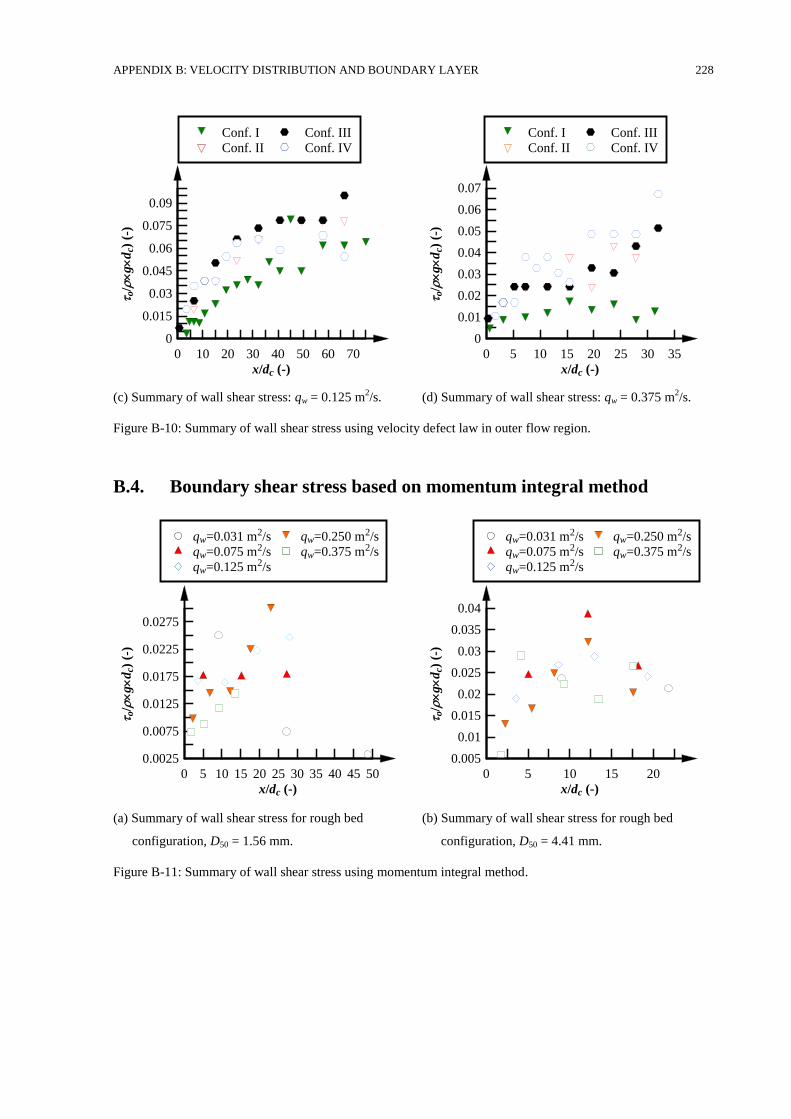
APPENDIX B: VELOCITY DISTRIBUTION AND BOUNDARY LAYER 228
(c) Summary of wall shear stress: qw = 0.125 m2/s. (d) Summary of wall shear stress: qw = 0.375 m
2/s.
Figure B-10: Summary of wall shear stress using velocity defect law in outer flow region.
B.4. Boundary shear stress based on momentum integral method
(a) Summary of wall shear stress for rough bed
configuration, D50 = 1.56 mm.
(b) Summary of wall shear stress for rough bed
configuration, D50 = 4.41 mm.
Figure B-11: Summary of wall shear stress using momentum integral method.
x/dc (-)
o/
g
dc)
(-)
0 10 20 30 40 50 60 70
0
0.015
0.03
0.045
0.06
0.075
0.09
Conf. I
Conf. II
Conf. III
Conf. IV
x/dc (-)
o/
g
dc)
(-)
0 5 10 15 20 25 30 35
0
0.01
0.02
0.03
0.04
0.05
0.06
0.07
Conf. I
Conf. II
Conf. III
Conf. IV
x/dc (-)
o/
g
dc)
(-)
0 5 10 15 20 25 30 35 40 45 50
0.0025
0.0075
0.0125
0.0175
0.0225
0.0275
qw=0.031 m2/s
qw=0.075 m2/s
qw=0.125 m2/s
qw=0.250 m2/s
qw=0.375 m2/s
x/dc (-)
o/
g
dc)
(-)
0 5 10 15 20
0.005
0.01
0.015
0.02
0.025
0.03
0.035
0.04
qw=0.031 m2/s
qw=0.075 m2/s
qw=0.125 m2/s
qw=0.250 m2/s
qw=0.375 m2/s
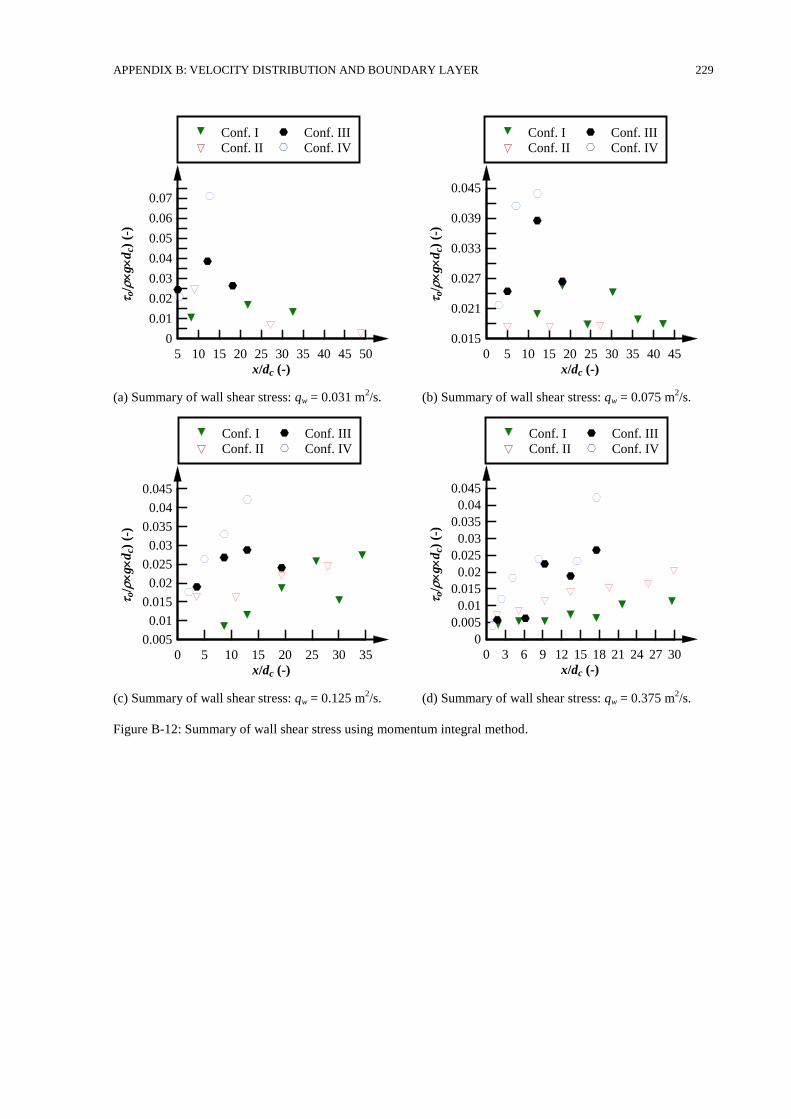
APPENDIX B: VELOCITY DISTRIBUTION AND BOUNDARY LAYER 229
(a) Summary of wall shear stress: qw = 0.031 m2/s. (b) Summary of wall shear stress: qw = 0.075 m
2/s.
(c) Summary of wall shear stress: qw = 0.125 m2/s. (d) Summary of wall shear stress: qw = 0.375 m
2/s.
Figure B-12: Summary of wall shear stress using momentum integral method.
x/dc (-)
o/
g
dc)
(-)
5 10 15 20 25 30 35 40 45 50
0
0.01
0.02
0.03
0.04
0.05
0.06
0.07
Conf. I
Conf. II
Conf. III
Conf. IV
x/dc (-)
o/
g
dc)
(-)
0 5 10 15 20 25 30 35 40 45
0.015
0.021
0.027
0.033
0.039
0.045
Conf. I
Conf. II
Conf. III
Conf. IV
x/dc (-)
o/
g
dc)
(-)
0 5 10 15 20 25 30 35
0.005
0.01
0.015
0.02
0.025
0.03
0.035
0.04
0.045
Conf. I
Conf. II
Conf. III
Conf. IV
x/dc (-)
o/
g
dc)
(-)
0 3 6 9 12 15 18 21 24 27 30
0
0.005
0.01
0.015
0.02
0.025
0.03
0.035
0.04
0.045
Conf. I
Conf. II
Conf. III
Conf. IV
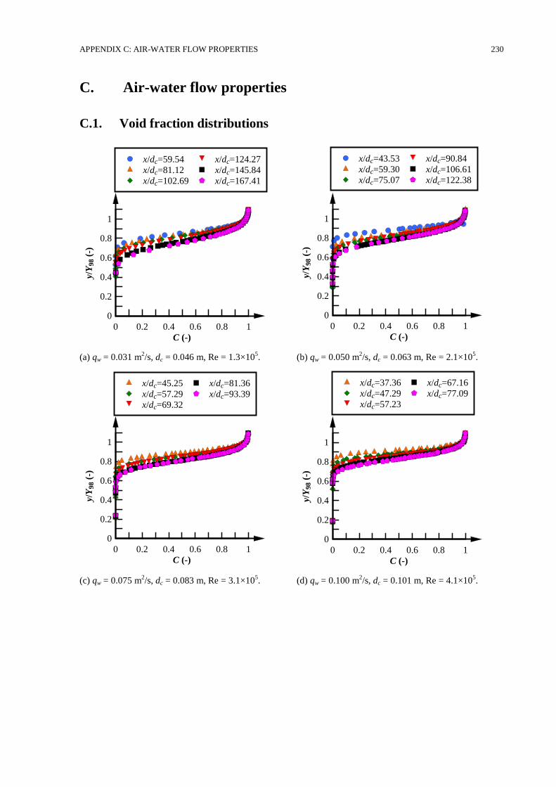
APPENDIX C: AIR-WATER FLOW PROPERTIES 230
C. Air-water flow properties
C.1. Void fraction distributions
(a) qw = 0.031 m2/s, dc = 0.046 m, Re = 1.3×10
5. (b) qw = 0.050 m
2/s, dc = 0.063 m, Re = 2.1×10
5.
(c) qw = 0.075 m2/s, dc = 0.083 m, Re = 3.1×10
5. (d) qw = 0.100 m
2/s, dc = 0.101 m, Re = 4.1×10
5.
C (-)
y/Y
98 (
-)
0 0.2 0.4 0.6 0.8 1
0
0.2
0.4
0.6
0.8
1
x/dc=59.54
x/dc=81.12
x/dc=102.69
x/dc=124.27
x/dc=145.84
x/dc=167.41
C (-)
y/Y
98 (
-)
0 0.2 0.4 0.6 0.8 1
0
0.2
0.4
0.6
0.8
1
x/dc=43.53
x/dc=59.30
x/dc=75.07
x/dc=90.84
x/dc=106.61
x/dc=122.38
C (-)
y/Y
98 (
-)
0 0.2 0.4 0.6 0.8 1
0
0.2
0.4
0.6
0.8
1
x/dc=45.25
x/dc=57.29
x/dc=69.32
x/dc=81.36
x/dc=93.39
C (-)
y/Y
98 (
-)
0 0.2 0.4 0.6 0.8 1
0
0.2
0.4
0.6
0.8
1
x/dc=37.36
x/dc=47.29
x/dc=57.23
x/dc=67.16
x/dc=77.09
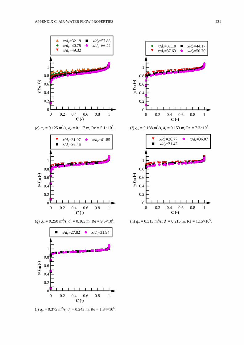
APPENDIX C: AIR-WATER FLOW PROPERTIES 231
(e) qw = 0.125 m2/s, dc = 0.117 m, Re = 5.1×10
5. (f) qw = 0.188 m
2/s, dc = 0.153 m, Re = 7.3×10
5.
(g) qw = 0.250 m2/s, dc = 0.185 m, Re = 9.5×10
5. (h) qw = 0.313 m
2/s, dc = 0.215 m, Re = 1.15×10
6.
(i) qw = 0.375 m2/s, dc = 0.243 m, Re = 1.34×10
6.
C (-)
y/Y
98 (
-)
0 0.2 0.4 0.6 0.8 1
0
0.2
0.4
0.6
0.8
1
x/dc=32.19
x/dc=40.75
x/dc=49.32
x/dc=57.88
x/dc=66.44
C (-)
y/Y
98 (
-)
0 0.2 0.4 0.6 0.8 1
0
0.2
0.4
0.6
0.8
1
x/dc=31.10
x/dc=37.63
x/dc=44.17
x/dc=50.70
C (-)
y/Y
98 (
-)
0 0.2 0.4 0.6 0.8 1
0
0.2
0.4
0.6
0.8
1
x/dc=31.07
x/dc=36.46
x/dc=41.85
C (-)
y/Y
98 (
-)
0 0.2 0.4 0.6 0.8 1
0
0.2
0.4
0.6
0.8
1
x/dc=26.77
x/dc=31.42
x/dc=36.07
C (-)
y/Y
98 (
-)
0 0.2 0.4 0.6 0.8 1
0
0.2
0.4
0.6
0.8
1
x/dc=27.82 x/dc=31.94
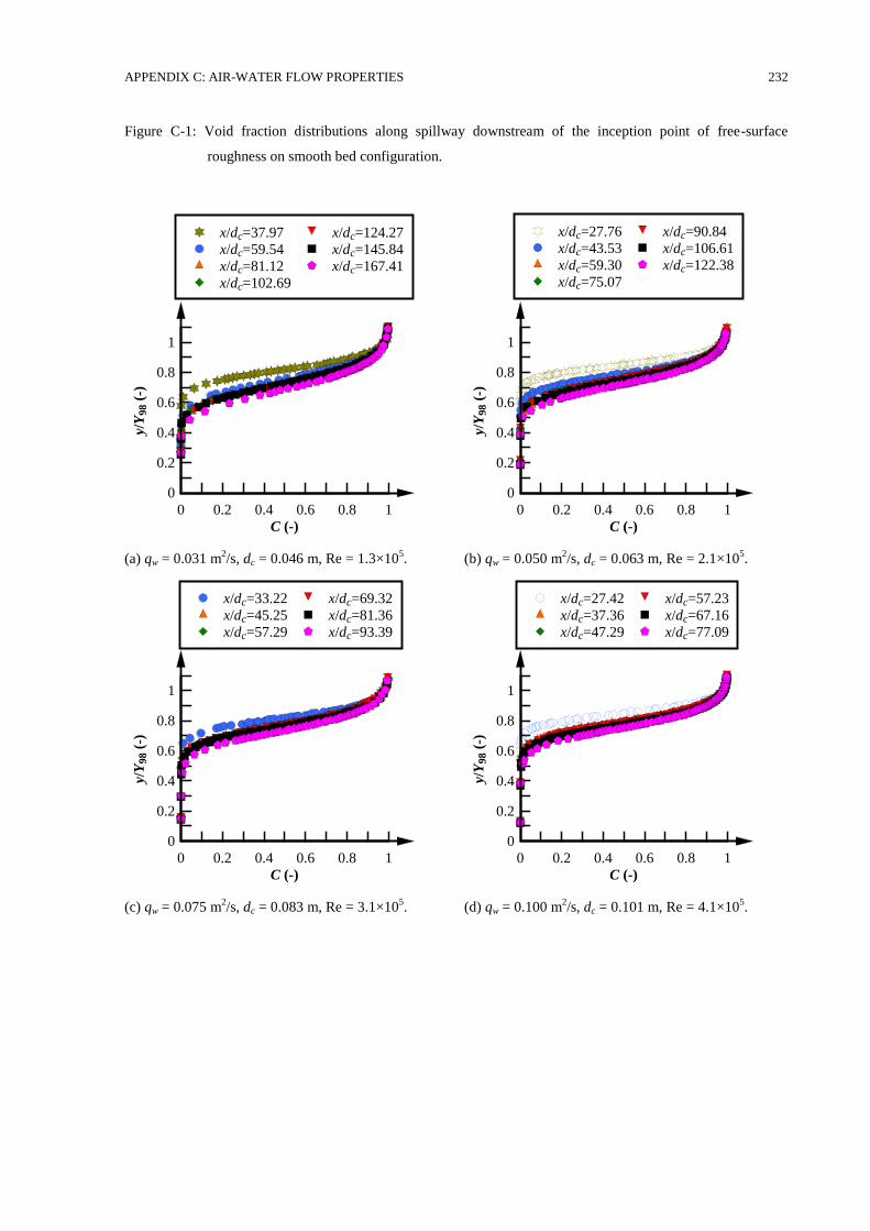
APPENDIX C: AIR-WATER FLOW PROPERTIES 232
Figure C-1: Void fraction distributions along spillway downstream of the inception point of free-surface
roughness on smooth bed configuration.
(a) qw = 0.031 m2/s, dc = 0.046 m, Re = 1.3×10
5. (b) qw = 0.050 m
2/s, dc = 0.063 m, Re = 2.1×10
5.
(c) qw = 0.075 m2/s, dc = 0.083 m, Re = 3.1×10
5. (d) qw = 0.100 m
2/s, dc = 0.101 m, Re = 4.1×10
5.
C (-)
y/Y
98 (
-)
0 0.2 0.4 0.6 0.8 1
0
0.2
0.4
0.6
0.8
1
x/dc=37.97
x/dc=59.54
x/dc=81.12
x/dc=102.69
x/dc=124.27
x/dc=145.84
x/dc=167.41
C (-)
y/Y
98 (
-)
0 0.2 0.4 0.6 0.8 1
0
0.2
0.4
0.6
0.8
1
x/dc=27.76
x/dc=43.53
x/dc=59.30
x/dc=75.07
x/dc=90.84
x/dc=106.61
x/dc=122.38
C (-)
y/Y
98 (
-)
0 0.2 0.4 0.6 0.8 1
0
0.2
0.4
0.6
0.8
1
x/dc=33.22
x/dc=45.25
x/dc=57.29
x/dc=69.32
x/dc=81.36
x/dc=93.39
C (-)
y/Y
98 (
-)
0 0.2 0.4 0.6 0.8 1
0
0.2
0.4
0.6
0.8
1
x/dc=27.42
x/dc=37.36
x/dc=47.29
x/dc=57.23
x/dc=67.16
x/dc=77.09
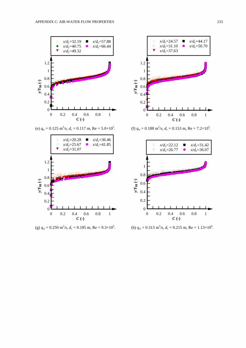
APPENDIX C: AIR-WATER FLOW PROPERTIES 233
(e) qw = 0.125 m2/s, dc = 0.117 m, Re = 5.0×10
5. (f) qw = 0.188 m
2/s, dc = 0.153 m, Re = 7.2×10
5.
(g) qw = 0.250 m2/s, dc = 0.185 m, Re = 9.3×10
5. (h) qw = 0.313 m
2/s, dc = 0.215 m, Re = 1.13×10
6.
C (-)
y/Y
98 (
-)
0 0.2 0.4 0.6 0.8 1
0
0.2
0.4
0.6
0.8
1
1.2
x/dc=32.19
x/dc=40.75
x/dc=49.32
x/dc=57.88
x/dc=66.44
C (-)
y/Y
98 (
-)
0 0.2 0.4 0.6 0.8 1
0
0.2
0.4
0.6
0.8
1
1.2
x/dc=24.57
x/dc=31.10
x/dc=37.63
x/dc=44.17
x/dc=50.70
C (-)
y/Y
98 (
-)
0 0.2 0.4 0.6 0.8 1
0
0.2
0.4
0.6
0.8
1
1.2
x/dc=20.28
x/dc=25.67
x/dc=31.07
x/dc=36.46
x/dc=41.85
C (-)
y/Y
98 (
-)
0 0.2 0.4 0.6 0.8 1
0
0.2
0.4
0.6
0.8
1
x/dc=22.12
x/dc=26.77
x/dc=31.42
x/dc=36.07
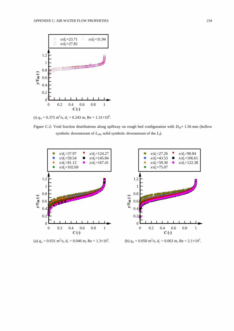
APPENDIX C: AIR-WATER FLOW PROPERTIES 234
(i) qw = 0.375 m2/s, dc = 0.243 m, Re = 1.31×10
6.
Figure C-2: Void fraction distributions along spillway on rough bed configuration with D50= 1.56 mm (hollow
symbols: downstream of LFR, solid symbols: downstream of the LI).
(a) qw = 0.031 m2/s, dc = 0.046 m, Re = 1.3×10
5. (b) qw = 0.050 m
2/s, dc = 0.063 m, Re = 2.1×10
5.
C (-)
y/Y
98 (
-)
0 0.2 0.4 0.6 0.8 1
0
0.2
0.4
0.6
0.8
1
1.2
x/dc=23.71
x/dc=27.82
x/dc=31.94
C (-)
y/Y
98 (
-)
0 0.2 0.4 0.6 0.8 1
0
0.2
0.4
0.6
0.8
1
1.2
x/dc=37.97
x/dc=59.54
x/dc=81.12
x/dc=102.69
x/dc=124.27
x/dc=145.84
x/dc=167.41
C (-)
y/Y
98 (
-)
0 0.2 0.4 0.6 0.8 1
0
0.2
0.4
0.6
0.8
1
1.2
x/dc=27.26
x/dc=43.53
x/dc=59.30
x/dc=75.07
x/dc=90.84
x/dc=106.61
x/dc=122.38
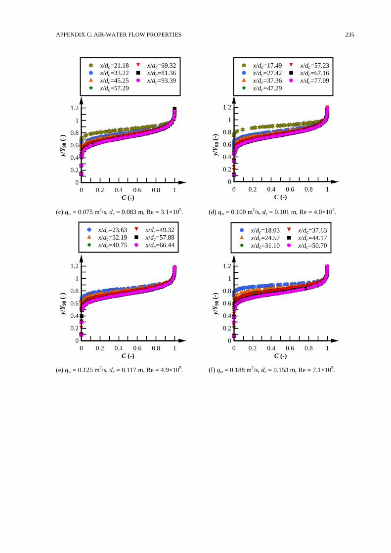
APPENDIX C: AIR-WATER FLOW PROPERTIES 235
(c) qw = 0.075 m2/s, dc = 0.083 m, Re = 3.1×10
5. (d) qw = 0.100 m
2/s, dc = 0.101 m, Re = 4.0×10
5.
(e) qw = 0.125 m2/s, dc = 0.117 m, Re = 4.9×10
5. (f) qw = 0.188 m
2/s, dc = 0.153 m, Re = 7.1×10
5.
C (-)
y/Y
98 (
-)
0 0.2 0.4 0.6 0.8 1
0
0.2
0.4
0.6
0.8
1
1.2
x/dc=21.18
x/dc=33.22
x/dc=45.25
x/dc=57.29
x/dc=69.32
x/dc=81.36
x/dc=93.39
C (-)
y/Y
98 (
-)
0 0.2 0.4 0.6 0.8 1
0
0.2
0.4
0.6
0.8
1
1.2
x/dc=17.49
x/dc=27.42
x/dc=37.36
x/dc=47.29
x/dc=57.23
x/dc=67.16
x/dc=77.09
C (-)
y/Y
98 (
-)
0 0.2 0.4 0.6 0.8 1
0
0.2
0.4
0.6
0.8
1
1.2
x/dc=23.63
x/dc=32.19
x/dc=40.75
x/dc=49.32
x/dc=57.88
x/dc=66.44
C (-)
y/Y
98 (
-)
0 0.2 0.4 0.6 0.8 1
0
0.2
0.4
0.6
0.8
1
1.2
x/dc=18.03
x/dc=24.57
x/dc=31.10
x/dc=37.63
x/dc=44.17
x/dc=50.70
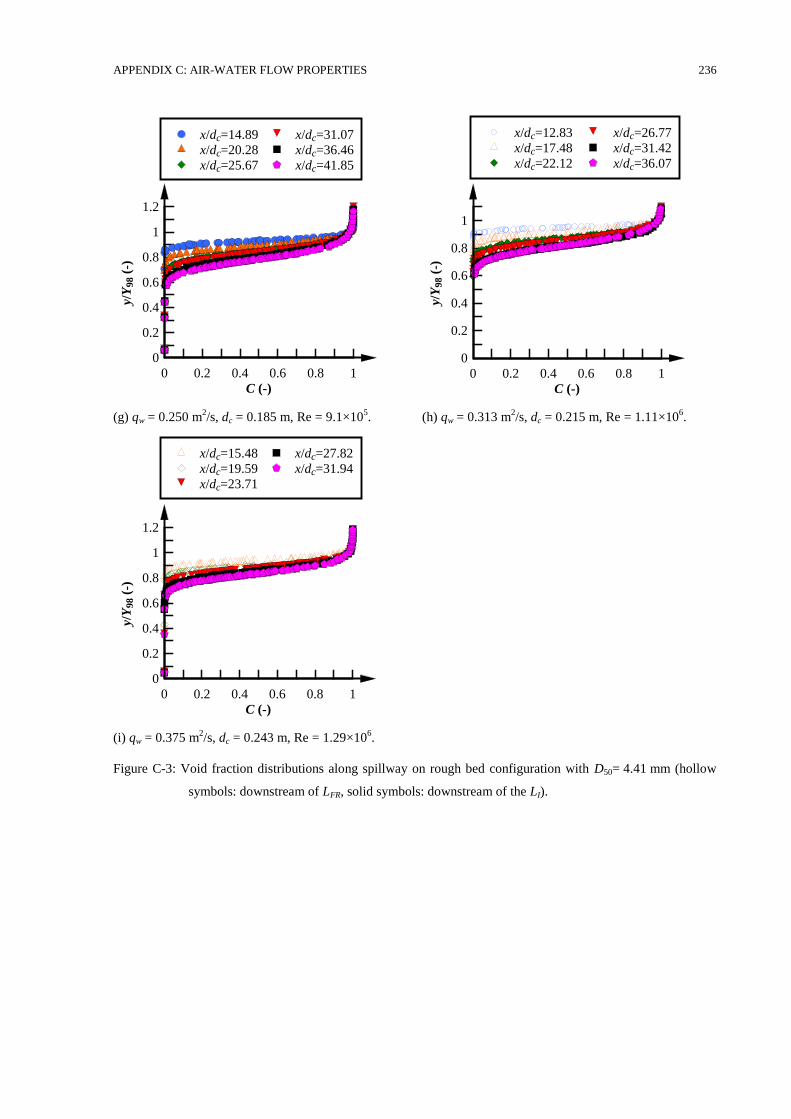
APPENDIX C: AIR-WATER FLOW PROPERTIES 236
(g) qw = 0.250 m2/s, dc = 0.185 m, Re = 9.1×10
5. (h) qw = 0.313 m
2/s, dc = 0.215 m, Re = 1.11×10
6.
(i) qw = 0.375 m2/s, dc = 0.243 m, Re = 1.29×10
6.
Figure C-3: Void fraction distributions along spillway on rough bed configuration with D50= 4.41 mm (hollow
symbols: downstream of LFR, solid symbols: downstream of the LI).
C (-)
y/Y
98 (
-)
0 0.2 0.4 0.6 0.8 1
0
0.2
0.4
0.6
0.8
1
1.2
x/dc=14.89
x/dc=20.28
x/dc=25.67
x/dc=31.07
x/dc=36.46
x/dc=41.85
C (-)
y/Y
98 (
-)
0 0.2 0.4 0.6 0.8 1
0
0.2
0.4
0.6
0.8
1
x/dc=12.83
x/dc=17.48
x/dc=22.12
x/dc=26.77
x/dc=31.42
x/dc=36.07
C (-)
y/Y
98 (
-)
0 0.2 0.4 0.6 0.8 1
0
0.2
0.4
0.6
0.8
1
1.2
x/dc=15.48
x/dc=19.59
x/dc=23.71
x/dc=27.82
x/dc=31.94
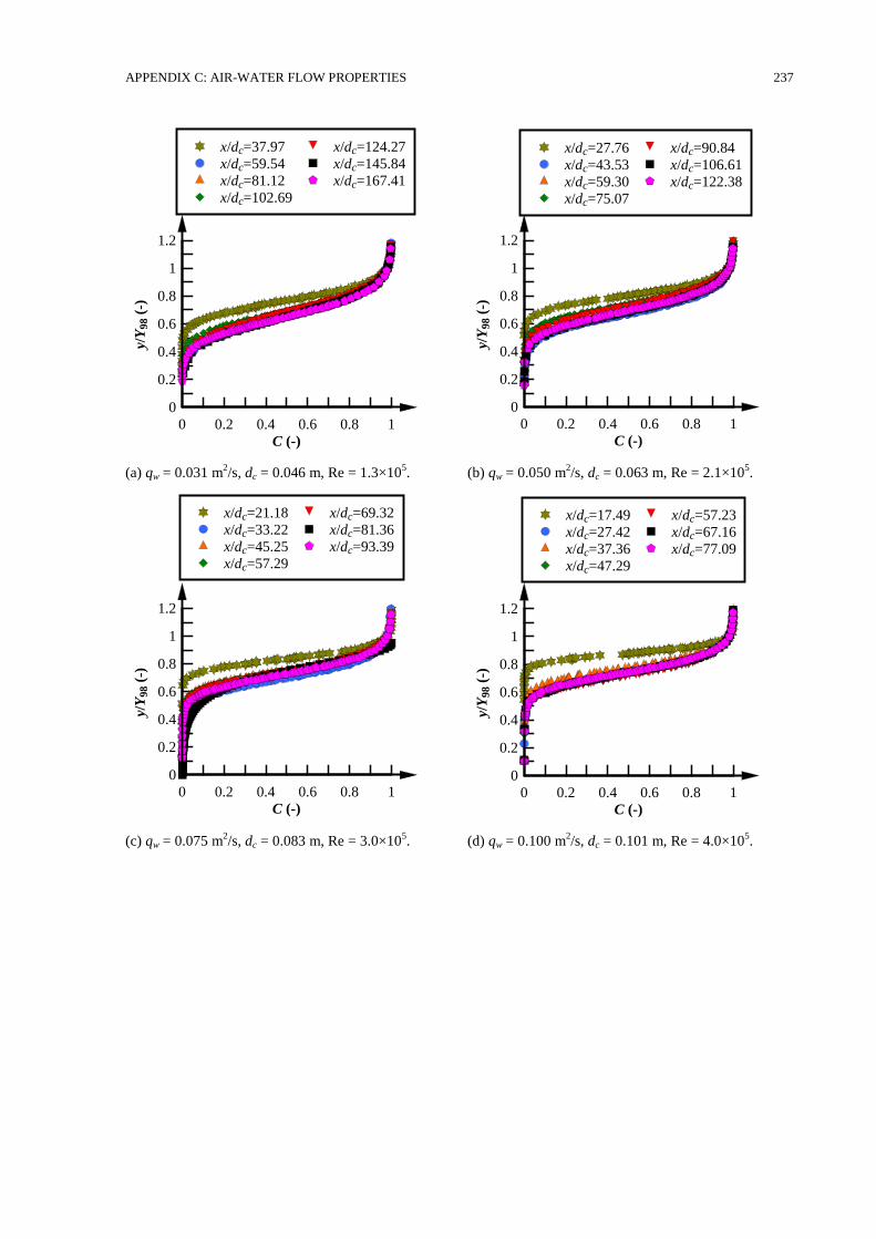
APPENDIX C: AIR-WATER FLOW PROPERTIES 237
(a) qw = 0.031 m2/s, dc = 0.046 m, Re = 1.3×10
5. (b) qw = 0.050 m
2/s, dc = 0.063 m, Re = 2.1×10
5.
(c) qw = 0.075 m2/s, dc = 0.083 m, Re = 3.0×10
5. (d) qw = 0.100 m
2/s, dc = 0.101 m, Re = 4.0×10
5.
C (-)
y/Y
98 (
-)
0 0.2 0.4 0.6 0.8 1
0
0.2
0.4
0.6
0.8
1
1.2
x/dc=37.97
x/dc=59.54
x/dc=81.12
x/dc=102.69
x/dc=124.27
x/dc=145.84
x/dc=167.41
C (-)
y/Y
98 (
-)
0 0.2 0.4 0.6 0.8 1
0
0.2
0.4
0.6
0.8
1
1.2
x/dc=27.76
x/dc=43.53
x/dc=59.30
x/dc=75.07
x/dc=90.84
x/dc=106.61
x/dc=122.38
C (-)
y/Y
98 (
-)
0 0.2 0.4 0.6 0.8 1
0
0.2
0.4
0.6
0.8
1
1.2
x/dc=21.18
x/dc=33.22
x/dc=45.25
x/dc=57.29
x/dc=69.32
x/dc=81.36
x/dc=93.39
C (-)
y/Y
98 (
-)
0 0.2 0.4 0.6 0.8 1
0
0.2
0.4
0.6
0.8
1
1.2
x/dc=17.49
x/dc=27.42
x/dc=37.36
x/dc=47.29
x/dc=57.23
x/dc=67.16
x/dc=77.09
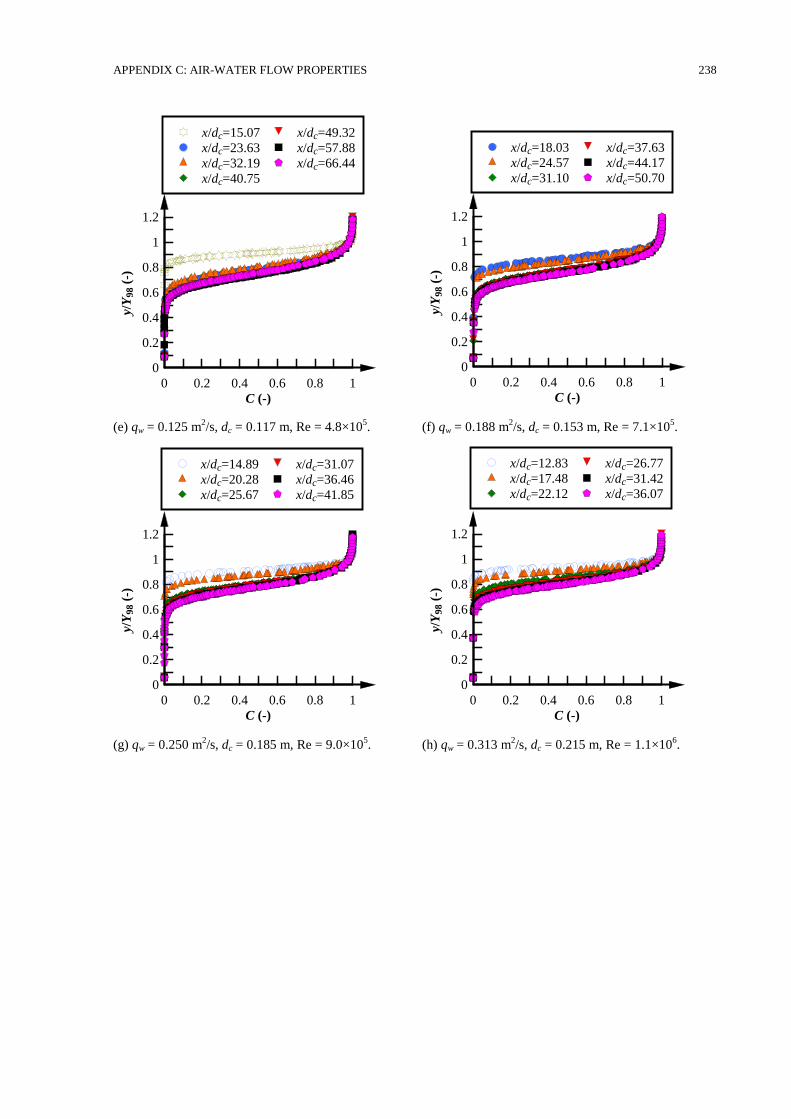
APPENDIX C: AIR-WATER FLOW PROPERTIES 238
(e) qw = 0.125 m2/s, dc = 0.117 m, Re = 4.8×10
5. (f) qw = 0.188 m
2/s, dc = 0.153 m, Re = 7.1×10
5.
(g) qw = 0.250 m2/s, dc = 0.185 m, Re = 9.0×10
5. (h) qw = 0.313 m
2/s, dc = 0.215 m, Re = 1.1×10
6.
C (-)
y/Y
98 (
-)
0 0.2 0.4 0.6 0.8 1
0
0.2
0.4
0.6
0.8
1
1.2
x/dc=15.07
x/dc=23.63
x/dc=32.19
x/dc=40.75
x/dc=49.32
x/dc=57.88
x/dc=66.44
C (-)
y/Y
98 (
-)
0 0.2 0.4 0.6 0.8 1
0
0.2
0.4
0.6
0.8
1
1.2
x/dc=18.03
x/dc=24.57
x/dc=31.10
x/dc=37.63
x/dc=44.17
x/dc=50.70
C (-)
y/Y
98 (
-)
0 0.2 0.4 0.6 0.8 1
0
0.2
0.4
0.6
0.8
1
1.2
x/dc=14.89
x/dc=20.28
x/dc=25.67
x/dc=31.07
x/dc=36.46
x/dc=41.85
C (-)
y/Y
98 (
-)
0 0.2 0.4 0.6 0.8 1
0
0.2
0.4
0.6
0.8
1
1.2
x/dc=12.83
x/dc=17.48
x/dc=22.12
x/dc=26.77
x/dc=31.42
x/dc=36.07
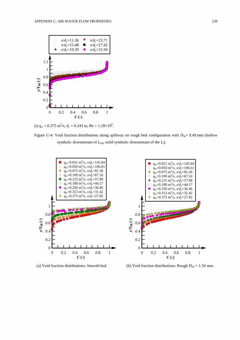
APPENDIX C: AIR-WATER FLOW PROPERTIES 239
(i) qw = 0.375 m2/s, dc = 0.243 m, Re = 1.28×10
6.
Figure C-4: Void fraction distributions along spillway on rough bed configuration with D50= 9.49 mm (hollow
symbols: downstream of LFR, solid symbols: downstream of the LI).
(a) Void fraction distributions: Smooth bed. (b) Void fraction distributions: Rough D50 = 1.56 mm.
C (-)
y/Y
98 (
-)
0 0.2 0.4 0.6 0.8 1
0
0.2
0.4
0.6
0.8
1
1.2
x/dc=11.36
x/dc=15.48
x/dc=19.29
x/dc=23.71
x/dc=27.82
x/dc=31.94
C (-)
y/Y
98 (
-)
0 0.2 0.4 0.6 0.8 1
0
0.2
0.4
0.6
0.8
1
qw=0.031 m2/s, x/dc=145.84
qw=0.050 m2/s, x/dc=106.61
qw=0.075 m2/s, x/dc=81.36
qw=0.100 m2/s, x/dc=67.16
qw=0.125 m2/s, x/dc=57.88
qw=0.188 m2/s, x/dc=44.17
qw=0.250 m2/s, x/dc=36.46
qw=0.313 m2/s, x/dc=31.42
qw=0.375 m2/s, x/dc=27.82
C (-)
y/Y
98 (
-)
0 0.2 0.4 0.6 0.8 1
0
0.2
0.4
0.6
0.8
1
qw=0.031 m2/s, x/dc=145.84
qw=0.050 m2/s, x/dc=106.61
qw=0.075 m2/s, x/dc=81.36
qw=0.100 m2/s, x/dc=67.16
qw=0.125 m2/s, x/dc=57.88
qw=0.188 m2/s, x/dc=44.17
qw=0.250 m2/s, x/dc=36.46
qw=0.313 m2/s, x/dc=31.42
qw=0.375 m2/s, x/dc=27.82
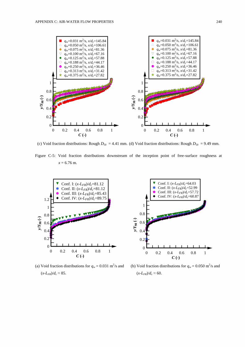
APPENDIX C: AIR-WATER FLOW PROPERTIES 240
(c) Void fraction distributions: Rough D50 = 4.41 mm. (d) Void fraction distributions: Rough D50 = 9.49 mm.
Figure C-5: Void fraction distributions downstream of the inception point of free-surface roughness at
x = 6.76 m.
(a) Void fraction distributions for qw = 0.031 m2/s and
(x-LFR)/dc ≈ 85.
(b) Void fraction distributions for qw = 0.050 m2/s and
(x-LFR)/dc ≈ 60.
C (-)
y/Y
98 (
-)
0 0.2 0.4 0.6 0.8 1
0
0.2
0.4
0.6
0.8
1
qw=0.031 m2/s, x/dc=145.84
qw=0.050 m2/s, x/dc=106.61
qw=0.075 m2/s, x/dc=81.36
qw=0.100 m2/s, x/dc=67.16
qw=0.125 m2/s, x/dc=57.88
qw=0.188 m2/s, x/dc=44.17
qw=0.250 m2/s, x/dc=36.46
qw=0.313 m2/s, x/dc=31.42
qw=0.375 m2/s, x/dc=27.82
C (-)y/
Y98 (
-)0 0.2 0.4 0.6 0.8 1
0
0.2
0.4
0.6
0.8
1
qw=0.031 m2/s, x/dc=145.84
qw=0.050 m2/s, x/dc=106.61
qw=0.075 m2/s, x/dc=81.36
qw=0.100 m2/s, x/dc=67.16
qw=0.125 m2/s, x/dc=57.88
qw=0.188 m2/s, x/dc=44.17
qw=0.250 m2/s, x/dc=36.46
qw=0.313 m2/s, x/dc=31.42
qw=0.375 m2/s, x/dc=27.82
C (-)
y/Y
98 (
-)
0 0.2 0.4 0.6 0.8 1
0
0.2
0.4
0.6
0.8
1
1.2
Conf. I: (x-LFR)/dc=81.12
Conf. II: (x-LFR)/dc=81.12
Conf. III: (x-LFR)/dc=85.43
Conf. IV: (x-LFR)/dc=89.75
C (-)
y/Y
98 (
-)
0 0.2 0.4 0.6 0.8 1
0
0.2
0.4
0.6
0.8
1
Conf. I: (x-LFR)/dc=64.03
Conf. II: (x-LFR)/dc=52.99
Conf. III: (x-LFR)/dc=57.72
Conf. IV: (x-LFR)/dc=60.87
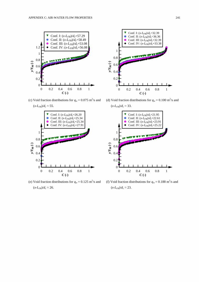
APPENDIX C: AIR-WATER FLOW PROPERTIES 241
(c) Void fraction distributions for qw = 0.075 m2/s and
(x-LFR)/dc ≈ 55.
(d) Void fraction distributions for qw = 0.100 m2/s and
(x-LFR)/dc ≈ 33.
(e) Void fraction distributions for qw = 0.125 m2/s and
(x-LFR)/dc ≈ 26.
(f) Void fraction distributions for qw = 0.188 m2/s and
(x-LFR)/dc ≈ 23.
C (-)
y/Y
98 (
-)
0 0.2 0.4 0.6 0.8 1
0
0.2
0.4
0.6
0.8
1
1.2
Conf. I: (x-LFR)/dc=57.29
Conf. II: (x-LFR)/dc=58.49
Conf. III: (x-LFR)/dc=53.08
Conf. IV: (x-LFR)/dc=56.08
C (-)
y/Y
98 (
-)
0 0.2 0.4 0.6 0.8 1
0
0.2
0.4
0.6
0.8
1
Conf. I: (x-LFR)/dc=32.39
Conf. II: (x-LFR)/dc=36.36
Conf. III: (x-LFR)/dc=32.39
Conf. IV: (x-LFR)/dc=33.38
C (-)
y/Y
98 (
-)
0 0.2 0.4 0.6 0.8 1
0
0.2
0.4
0.6
0.8
1
Conf. I: (x-LFR)/dc=26.20
Conf. II: (x-LFR)/dc=25.34
Conf. III: (x-LFR)/dc=25.34
Conf. IV: (x-LFR)/dc=27.91
C (-)
y/Y
98 (
-)
0 0.2 0.4 0.6 0.8 1
0
0.2
0.4
0.6
0.8
1
Conf. I: (x-LFR)/dc=21.95
Conf. II: (x-LFR)/dc=22.61
Conf. III: (x-LFR)/dc=23.91
Conf. IV: (x-LFR)/dc=25.22
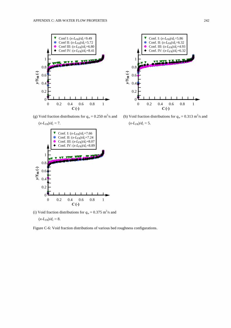
APPENDIX C: AIR-WATER FLOW PROPERTIES 242
(g) Void fraction distributions for qw = 0.250 m2/s and
(x-LFR)/dc ≈ 7.
(h) Void fraction distributions for qw = 0.313 m2/s and
(x-LFR)/dc ≈ 5.
(i) Void fraction distributions for qw = 0.375 m2/s and
(x-LFR)/dc ≈ 8.
Figure C-6: Void fraction distributions of various bed roughness configurations.
C (-)
y/Y
98 (
-)
0 0.2 0.4 0.6 0.8 1
0
0.2
0.4
0.6
0.8
1
Conf I: (x-LFR)/dc=9.49
Conf II: (x-LFR)/dc=5.72
Conf III: (x-LFR)/dc=6.80
Conf IV: (x-LFR)/dc=8.41
C (-)
y/Y
98 (
-)
0 0.2 0.4 0.6 0.8 1
0
0.2
0.4
0.6
0.8
1
Conf. I: (x-LFR)/dc=5.86
Conf. II: (x-LFR)/dc=6.32
Conf. III: (x-LFR)/dc=4.93
Conf. IV: (x-LFR)/dc=6.32
C (-)
y/Y
98 (
-)
0 0.2 0.4 0.6 0.8 1
0
0.2
0.4
0.6
0.8
1
Conf. I: (x-LFR)/dc=7.66
Conf. II: (x-LFR)/dc=7.24
Conf. III: (x-LFR)/dc=8.07
Conf. IV: (x-LFR)/dc=8.89
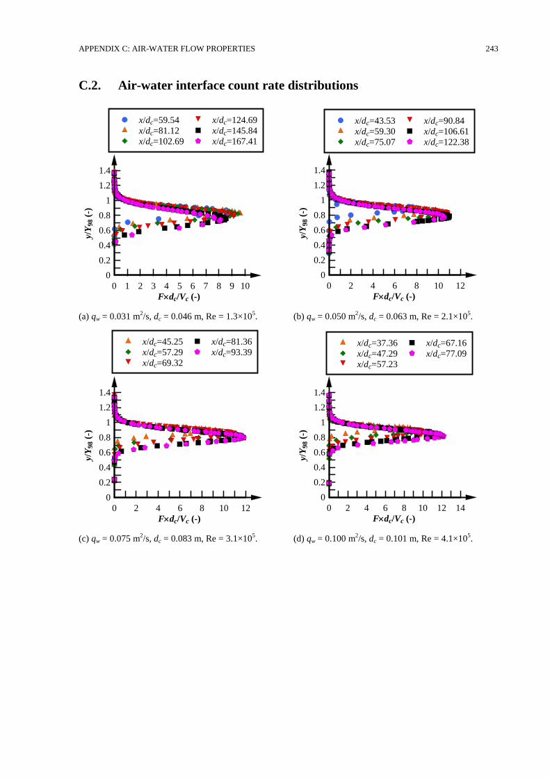
APPENDIX C: AIR-WATER FLOW PROPERTIES 243
C.2. Air-water interface count rate distributions
(a) qw = 0.031 m2/s, dc = 0.046 m, Re = 1.3×10
5. (b) qw = 0.050 m
2/s, dc = 0.063 m, Re = 2.1×10
5.
(c) qw = 0.075 m2/s, dc = 0.083 m, Re = 3.1×10
5. (d) qw = 0.100 m
2/s, dc = 0.101 m, Re = 4.1×10
5.
Fdc/Vc (-)
y/Y
98 (
-)
0 1 2 3 4 5 6 7 8 9 10
0
0.2
0.4
0.6
0.8
1
1.2
1.4
x/dc=59.54
x/dc=81.12
x/dc=102.69
x/dc=124.69
x/dc=145.84
x/dc=167.41
Fdc/Vc (-)y/
Y98 (
-)
0 2 4 6 8 10 12
0
0.2
0.4
0.6
0.8
1
1.2
1.4
x/dc=43.53
x/dc=59.30
x/dc=75.07
x/dc=90.84
x/dc=106.61
x/dc=122.38
Fdc/Vc (-)
y/Y
98 (
-)
0 2 4 6 8 10 12
0
0.2
0.4
0.6
0.8
1
1.2
1.4
x/dc=45.25
x/dc=57.29
x/dc=69.32
x/dc=81.36
x/dc=93.39
Fdc/Vc (-)
y/Y
98 (
-)
0 2 4 6 8 10 12 14
0
0.2
0.4
0.6
0.8
1
1.2
1.4
x/dc=37.36
x/dc=47.29
x/dc=57.23
x/dc=67.16
x/dc=77.09
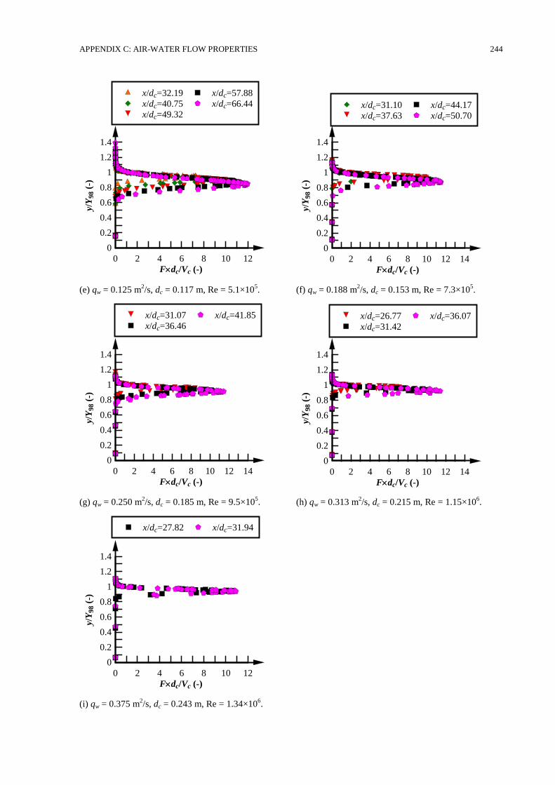
APPENDIX C: AIR-WATER FLOW PROPERTIES 244
(e) qw = 0.125 m2/s, dc = 0.117 m, Re = 5.1×10
5. (f) qw = 0.188 m
2/s, dc = 0.153 m, Re = 7.3×10
5.
(g) qw = 0.250 m2/s, dc = 0.185 m, Re = 9.5×10
5. (h) qw = 0.313 m
2/s, dc = 0.215 m, Re = 1.15×10
6.
(i) qw = 0.375 m2/s, dc = 0.243 m, Re = 1.34×10
6.
Fdc/Vc (-)
y/Y
98 (
-)
0 2 4 6 8 10 12
0
0.2
0.4
0.6
0.8
1
1.2
1.4
x/dc=32.19
x/dc=40.75
x/dc=49.32
x/dc=57.88
x/dc=66.44
Fdc/Vc (-)
y/Y
98 (
-)
0 2 4 6 8 10 12 14
0
0.2
0.4
0.6
0.8
1
1.2
1.4
x/dc=31.10
x/dc=37.63
x/dc=44.17
x/dc=50.70
Fdc/Vc (-)
y/Y
98 (
-)
0 2 4 6 8 10 12 14
0
0.2
0.4
0.6
0.8
1
1.2
1.4
x/dc=31.07
x/dc=36.46
x/dc=41.85
Fdc/Vc (-)
y/Y
98 (
-)
0 2 4 6 8 10 12 14
0
0.2
0.4
0.6
0.8
1
1.2
1.4
x/dc=26.77
x/dc=31.42
x/dc=36.07
Fdc/Vc (-)
y/Y
98 (
-)
0 2 4 6 8 10 12
0
0.2
0.4
0.6
0.8
1
1.2
1.4
x/dc=27.82 x/dc=31.94
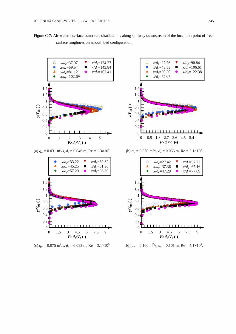
APPENDIX C: AIR-WATER FLOW PROPERTIES 245
Figure C-7: Air-water interface count rate distributions along spillway downstream of the inception point of free-
surface roughness on smooth bed configuration.
(a) qw = 0.031 m2/s, dc = 0.046 m, Re = 1.3×10
5. (b) qw = 0.050 m
2/s, dc = 0.063 m, Re = 2.1×10
5.
(c) qw = 0.075 m2/s, dc = 0.083 m, Re = 3.1×10
5. (d) qw = 0.100 m
2/s, dc = 0.101 m, Re = 4.1×10
5.
Fdc/Vc (-)
y/Y
98 (
-)
0 1 2 3 4 5
0
0.2
0.4
0.6
0.8
1
1.2
1.4
x/dc=37.97
x/dc=59.54
x/dc=81.12
x/dc=102.69
x/dc=124.27
x/dc=145.84
x/dc=167.41
Fdc/Vc (-)
y/Y
98 (
-)
0 0.9 1.8 2.7 3.6 4.5 5.4
0
0.2
0.4
0.6
0.8
1
1.2
1.4
x/dc=27.76
x/dc=43.53
x/dc=59.30
x/dc=75.07
x/dc=90.84
x/dc=106.61
x/dc=122.38
Fdc/Vc (-)
y/Y
98 (
-)
0 1.5 3 4.5 6 7.5 9
0
0.2
0.4
0.6
0.8
1
1.2
1.4
x/dc=33.22
x/dc=45.25
x/dc=57.29
x/dc=69.32
x/dc=81.36
x/dc=93.39
Fdc/Vc (-)
y/Y
98 (
-)
0 1.5 3 4.5 6 7.5 9
0
0.2
0.4
0.6
0.8
1
1.2
1.4
x/dc=27.42
x/dc=37.36
x/dc=47.29
x/dc=57.23
x/dc=67.16
x/dc=77.09
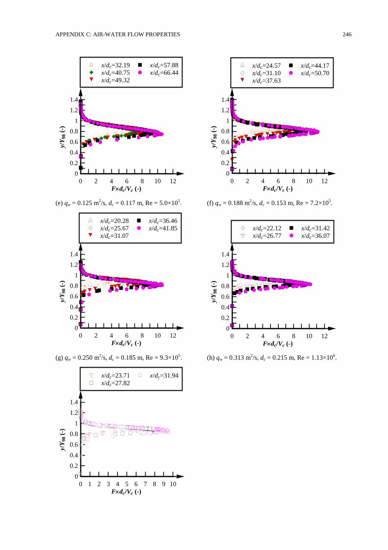
APPENDIX C: AIR-WATER FLOW PROPERTIES 246
(e) qw = 0.125 m2/s, dc = 0.117 m, Re = 5.0×10
5. (f) qw = 0.188 m
2/s, dc = 0.153 m, Re = 7.2×10
5.
(g) qw = 0.250 m2/s, dc = 0.185 m, Re = 9.3×10
5. (h) qw = 0.313 m
2/s, dc = 0.215 m, Re = 1.13×10
6.
Fdc/Vc (-)
y/Y
98 (
-)
0 2 4 6 8 10 12
0
0.2
0.4
0.6
0.8
1
1.2
1.4
x/dc=32.19
x/dc=40.75
x/dc=49.32
x/dc=57.88
x/dc=66.44
Fdc/Vc (-)
y/Y
98 (
-)
0 2 4 6 8 10 12
0
0.2
0.4
0.6
0.8
1
1.2
1.4
x/dc=24.57
x/dc=31.10
x/dc=37.63
x/dc=44.17
x/dc=50.70
Fdc/Vc (-)
y/Y
98 (
-)
0 2 4 6 8 10 12
0
0.2
0.4
0.6
0.8
1
1.2
1.4
x/dc=20.28
x/dc=25.67
x/dc=31.07
x/dc=36.46
x/dc=41.85
Fdc/Vc (-)
y/Y
98 (
-)
0 2 4 6 8 10 12
0
0.2
0.4
0.6
0.8
1
1.2
1.4
x/dc=22.12
x/dc=26.77
x/dc=31.42
x/dc=36.07
Fdc/Vc (-)
y/Y
98 (
-)
0 1 2 3 4 5 6 7 8 9 10
0
0.2
0.4
0.6
0.8
1
1.2
1.4
x/dc=23.71
x/dc=27.82
x/dc=31.94
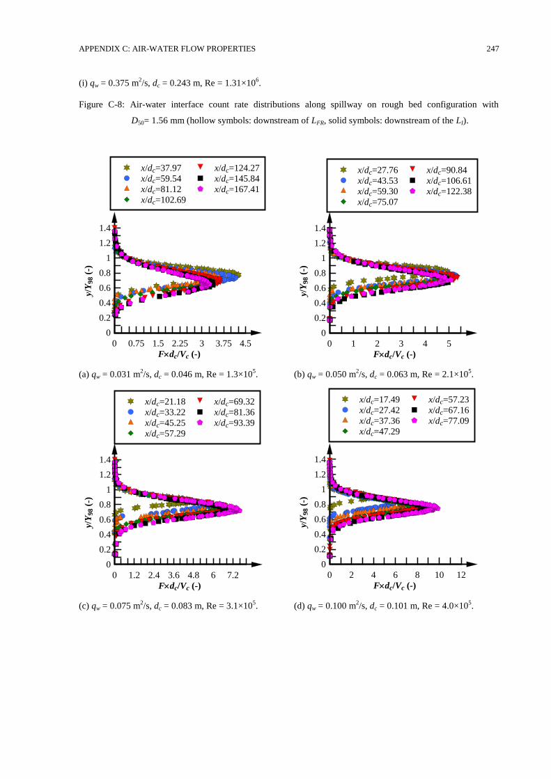
APPENDIX C: AIR-WATER FLOW PROPERTIES 247
(i) qw = 0.375 m2/s, dc = 0.243 m, Re = 1.31×10
6.
Figure C-8: Air-water interface count rate distributions along spillway on rough bed configuration with
D50= 1.56 mm (hollow symbols: downstream of LFR, solid symbols: downstream of the LI).
(a) qw = 0.031 m2/s, dc = 0.046 m, Re = 1.3×10
5. (b) qw = 0.050 m
2/s, dc = 0.063 m, Re = 2.1×10
5.
(c) qw = 0.075 m2/s, dc = 0.083 m, Re = 3.1×10
5. (d) qw = 0.100 m
2/s, dc = 0.101 m, Re = 4.0×10
5.
Fdc/Vc (-)
y/Y
98 (
-)
0 0.75 1.5 2.25 3 3.75 4.5
0
0.2
0.4
0.6
0.8
1
1.2
1.4
x/dc=37.97
x/dc=59.54
x/dc=81.12
x/dc=102.69
x/dc=124.27
x/dc=145.84
x/dc=167.41
Fdc/Vc (-)
y/Y
98 (
-)
0 1 2 3 4 5
0
0.2
0.4
0.6
0.8
1
1.2
1.4
x/dc=27.76
x/dc=43.53
x/dc=59.30
x/dc=75.07
x/dc=90.84
x/dc=106.61
x/dc=122.38
Fdc/Vc (-)
y/Y
98 (
-)
0 1.2 2.4 3.6 4.8 6 7.2
0
0.2
0.4
0.6
0.8
1
1.2
1.4
x/dc=21.18
x/dc=33.22
x/dc=45.25
x/dc=57.29
x/dc=69.32
x/dc=81.36
x/dc=93.39
Fdc/Vc (-)
y/Y
98 (
-)
0 2 4 6 8 10 12
0
0.2
0.4
0.6
0.8
1
1.2
1.4
x/dc=17.49
x/dc=27.42
x/dc=37.36
x/dc=47.29
x/dc=57.23
x/dc=67.16
x/dc=77.09
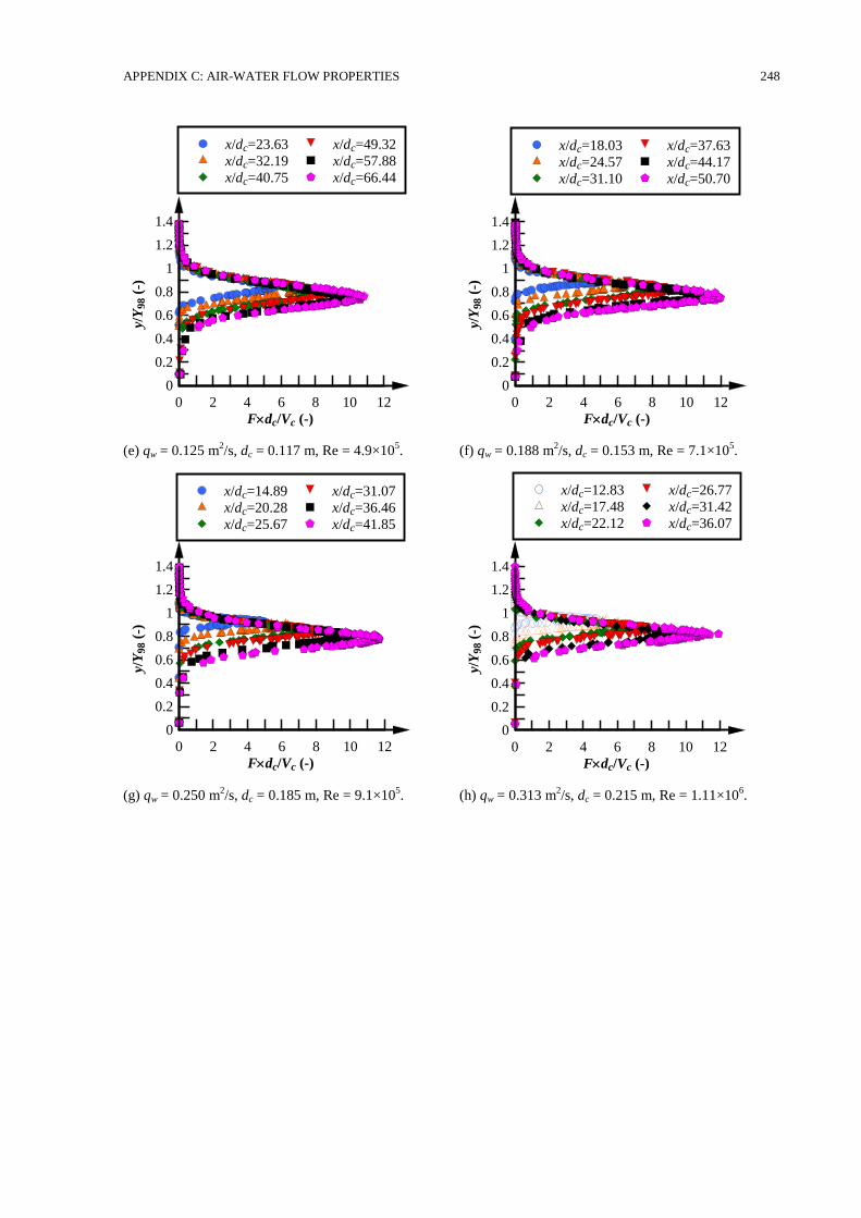
APPENDIX C: AIR-WATER FLOW PROPERTIES 248
(e) qw = 0.125 m2/s, dc = 0.117 m, Re = 4.9×10
5. (f) qw = 0.188 m
2/s, dc = 0.153 m, Re = 7.1×10
5.
(g) qw = 0.250 m2/s, dc = 0.185 m, Re = 9.1×10
5. (h) qw = 0.313 m
2/s, dc = 0.215 m, Re = 1.11×10
6.
Fdc/Vc (-)
y/Y
98 (
-)
0 2 4 6 8 10 12
0
0.2
0.4
0.6
0.8
1
1.2
1.4
x/dc=23.63
x/dc=32.19
x/dc=40.75
x/dc=49.32
x/dc=57.88
x/dc=66.44
Fdc/Vc (-)
y/Y
98 (
-)
0 2 4 6 8 10 12
0
0.2
0.4
0.6
0.8
1
1.2
1.4
x/dc=18.03
x/dc=24.57
x/dc=31.10
x/dc=37.63
x/dc=44.17
x/dc=50.70
Fdc/Vc (-)
y/Y
98 (
-)
0 2 4 6 8 10 12
0
0.2
0.4
0.6
0.8
1
1.2
1.4
x/dc=14.89
x/dc=20.28
x/dc=25.67
x/dc=31.07
x/dc=36.46
x/dc=41.85
Fdc/Vc (-)
y/Y
98 (
-)
0 2 4 6 8 10 12
0
0.2
0.4
0.6
0.8
1
1.2
1.4
x/dc=12.83
x/dc=17.48
x/dc=22.12
x/dc=26.77
x/dc=31.42
x/dc=36.07
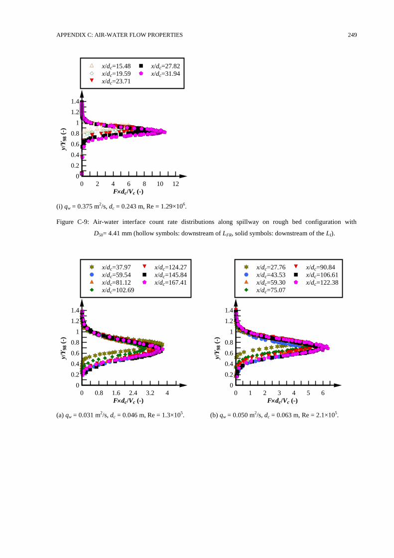
APPENDIX C: AIR-WATER FLOW PROPERTIES 249
(i) qw = 0.375 m2/s, dc = 0.243 m, Re = 1.29×10
6.
Figure C-9: Air-water interface count rate distributions along spillway on rough bed configuration with
D50= 4.41 mm (hollow symbols: downstream of LFR, solid symbols: downstream of the LI).
(a) qw = 0.031 m2/s, dc = 0.046 m, Re = 1.3×10
5. (b) qw = 0.050 m
2/s, dc = 0.063 m, Re = 2.1×10
5.
Fdc/Vc (-)
y/Y
98 (
-)
0 2 4 6 8 10 12
0
0.2
0.4
0.6
0.8
1
1.2
1.4
x/dc=15.48
x/dc=19.59
x/dc=23.71
x/dc=27.82
x/dc=31.94
Fdc/Vc (-)
y/Y
98 (
-)
0 0.8 1.6 2.4 3.2 4
0
0.2
0.4
0.6
0.8
1
1.2
1.4
x/dc=37.97
x/dc=59.54
x/dc=81.12
x/dc=102.69
x/dc=124.27
x/dc=145.84
x/dc=167.41
Fdc/Vc (-)
y/Y
98 (
-)
0 1 2 3 4 5 6
0
0.2
0.4
0.6
0.8
1
1.2
1.4
x/dc=27.76
x/dc=43.53
x/dc=59.30
x/dc=75.07
x/dc=90.84
x/dc=106.61
x/dc=122.38
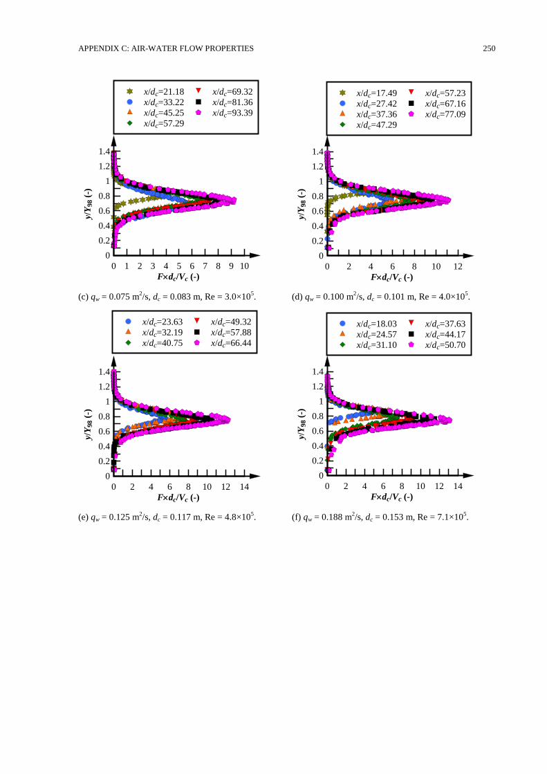
APPENDIX C: AIR-WATER FLOW PROPERTIES 250
(c) qw = 0.075 m2/s, dc = 0.083 m, Re = 3.0×10
5. (d) qw = 0.100 m
2/s, dc = 0.101 m, Re = 4.0×10
5.
(e) qw = 0.125 m2/s, dc = 0.117 m, Re = 4.8×10
5. (f) qw = 0.188 m
2/s, dc = 0.153 m, Re = 7.1×10
5.
Fdc/Vc (-)
y/Y
98 (
-)
0 1 2 3 4 5 6 7 8 9 10
0
0.2
0.4
0.6
0.8
1
1.2
1.4
x/dc=21.18
x/dc=33.22
x/dc=45.25
x/dc=57.29
x/dc=69.32
x/dc=81.36
x/dc=93.39
Fdc/Vc (-)
y/Y
98 (
-)
0 2 4 6 8 10 12
0
0.2
0.4
0.6
0.8
1
1.2
1.4
x/dc=17.49
x/dc=27.42
x/dc=37.36
x/dc=47.29
x/dc=57.23
x/dc=67.16
x/dc=77.09
Fdc/Vc (-)
y/Y
98 (
-)
0 2 4 6 8 10 12 14
0
0.2
0.4
0.6
0.8
1
1.2
1.4
x/dc=23.63
x/dc=32.19
x/dc=40.75
x/dc=49.32
x/dc=57.88
x/dc=66.44
Fdc/Vc (-)
y/Y
98 (
-)
0 2 4 6 8 10 12 14
0
0.2
0.4
0.6
0.8
1
1.2
1.4
x/dc=18.03
x/dc=24.57
x/dc=31.10
x/dc=37.63
x/dc=44.17
x/dc=50.70
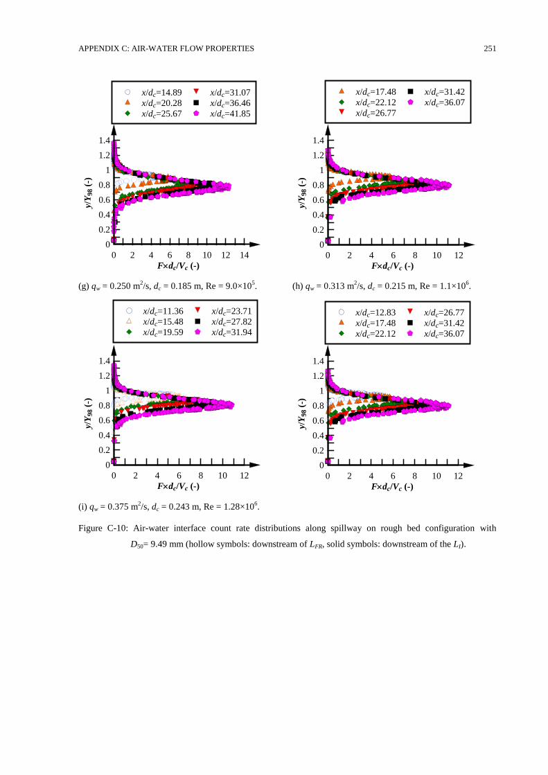
APPENDIX C: AIR-WATER FLOW PROPERTIES 251
(g) qw = 0.250 m2/s, dc = 0.185 m, Re = 9.0×10
5. (h) qw = 0.313 m
2/s, dc = 0.215 m, Re = 1.1×10
6.
(i) qw = 0.375 m2/s, dc = 0.243 m, Re = 1.28×10
6.
Figure C-10: Air-water interface count rate distributions along spillway on rough bed configuration with
D50= 9.49 mm (hollow symbols: downstream of LFR, solid symbols: downstream of the LI).
Fdc/Vc (-)
y/Y
98 (
-)
0 2 4 6 8 10 12 14
0
0.2
0.4
0.6
0.8
1
1.2
1.4
x/dc=14.89
x/dc=20.28
x/dc=25.67
x/dc=31.07
x/dc=36.46
x/dc=41.85
Fdc/Vc (-)
y/Y
98 (
-)
0 2 4 6 8 10 12
0
0.2
0.4
0.6
0.8
1
1.2
1.4
x/dc=17.48
x/dc=22.12
x/dc=26.77
x/dc=31.42
x/dc=36.07
Fdc/Vc (-)
y/Y
98 (
-)
0 2 4 6 8 10 12
0
0.2
0.4
0.6
0.8
1
1.2
1.4
x/dc=11.36
x/dc=15.48
x/dc=19.59
x/dc=23.71
x/dc=27.82
x/dc=31.94
Fdc/Vc (-)
y/Y
98 (
-)
0 2 4 6 8 10 12
0
0.2
0.4
0.6
0.8
1
1.2
1.4
x/dc=12.83
x/dc=17.48
x/dc=22.12
x/dc=26.77
x/dc=31.42
x/dc=36.07
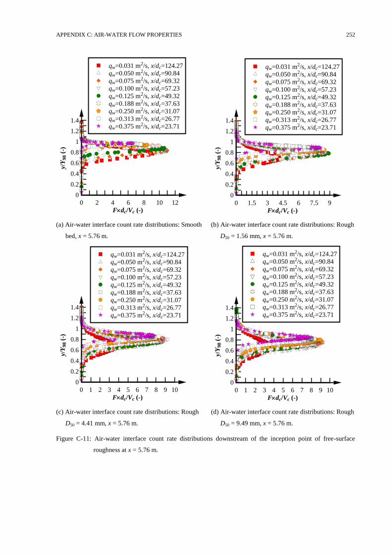
APPENDIX C: AIR-WATER FLOW PROPERTIES 252
(a) Air-water interface count rate distributions: Smooth
bed, x = 5.76 m.
(b) Air-water interface count rate distributions: Rough
D50 = 1.56 mm, x = 5.76 m.
(c) Air-water interface count rate distributions: Rough
D50 = 4.41 mm, x = 5.76 m.
(d) Air-water interface count rate distributions: Rough
D50 = 9.49 mm, x = 5.76 m.
Figure C-11: Air-water interface count rate distributions downstream of the inception point of free-surface
roughness at x = 5.76 m.
Fdc/Vc (-)
y/Y
98 (
-)
0 2 4 6 8 10 12
0
0.2
0.4
0.6
0.8
1
1.2
1.4
qw=0.031 m2/s, x/dc=124.27
qw=0.050 m2/s, x/dc=90.84
qw=0.075 m2/s, x/dc=69.32
qw=0.100 m2/s, x/dc=57.23
qw=0.125 m2/s, x/dc=49.32
qw=0.188 m2/s, x/dc=37.63
qw=0.250 m2/s, x/dc=31.07
qw=0.313 m2/s, x/dc=26.77
qw=0.375 m2/s, x/dc=23.71
Fdc/Vc (-)y/
Y98 (
-)
0 1.5 3 4.5 6 7.5 9
0
0.2
0.4
0.6
0.8
1
1.2
1.4
qw=0.031 m2/s, x/dc=124.27
qw=0.050 m2/s, x/dc=90.84
qw=0.075 m2/s, x/dc=69.32
qw=0.100 m2/s, x/dc=57.23
qw=0.125 m2/s, x/dc=49.32
qw=0.188 m2/s, x/dc=37.63
qw=0.250 m2/s, x/dc=31.07
qw=0.313 m2/s, x/dc=26.77
qw=0.375 m2/s, x/dc=23.71
Fdc/Vc (-)
y/Y
98 (
-)
0 1 2 3 4 5 6 7 8 9 10
0
0.2
0.4
0.6
0.8
1
1.2
1.4
qw=0.031 m2/s, x/dc=124.27
qw=0.050 m2/s, x/dc=90.84
qw=0.075 m2/s, x/dc=69.32
qw=0.100 m2/s, x/dc=57.23
qw=0.125 m2/s, x/dc=49.32
qw=0.188 m2/s, x/dc=37.63
qw=0.250 m2/s, x/dc=31.07
qw=0.313 m2/s, x/dc=26.77
qw=0.375 m2/s, x/dc=23.71
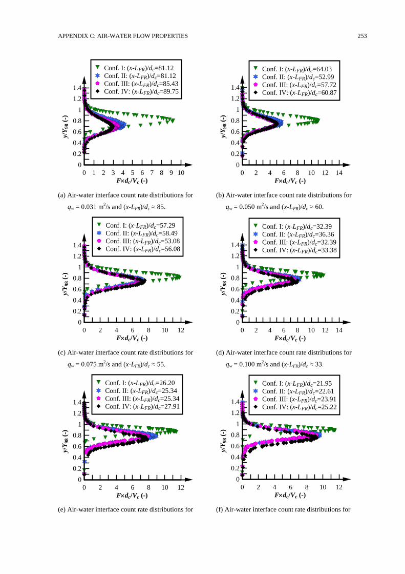
APPENDIX C: AIR-WATER FLOW PROPERTIES 253
(a) Air-water interface count rate distributions for
qw = 0.031 m2/s and (x-LFR)/dc ≈ 85.
(b) Air-water interface count rate distributions for
qw = 0.050 m2/s and (x-LFR)/dc ≈ 60.
(c) Air-water interface count rate distributions for
qw = 0.075 m2/s and (x-LFR)/dc ≈ 55.
(d) Air-water interface count rate distributions for
qw = 0.100 m2/s and (x-LFR)/dc ≈ 33.
(e) Air-water interface count rate distributions for (f) Air-water interface count rate distributions for
Fdc/Vc (-)
y/Y
98 (
-)
0 1 2 3 4 5 6 7 8 9 10
0
0.2
0.4
0.6
0.8
1
1.2
1.4
Conf. I: (x-LFR)/dc=81.12
Conf. II: (x-LFR)/dc=81.12
Conf. III: (x-LFR)/dc=85.43
Conf. IV: (x-LFR)/dc=89.75
Fdc/Vc (-)
y/Y
98 (
-)
0 2 4 6 8 10 12 14
0
0.2
0.4
0.6
0.8
1
1.2
1.4
Conf. I: (x-LFR)/dc=64.03
Conf. II: (x-LFR)/dc=52.99
Conf. III: (x-LFR)/dc=57.72
Conf. IV: (x-LFR)/dc=60.87
Fdc/Vc (-)
y/Y
98 (
-)
0 2 4 6 8 10 12
0
0.2
0.4
0.6
0.8
1
1.2
1.4
Conf. I: (x-LFR)/dc=57.29
Conf. II: (x-LFR)/dc=58.49
Conf. III: (x-LFR)/dc=53.08
Conf. IV: (x-LFR)/dc=56.08
Fdc/Vc (-)
y/Y
98 (
-)
0 2 4 6 8 10 12 14
0
0.2
0.4
0.6
0.8
1
1.2
1.4
Conf. I: (x-LFR)/dc=32.39
Conf. II: (x-LFR)/dc=36.36
Conf. III: (x-LFR)/dc=32.39
Conf. IV: (x-LFR)/dc=33.38
Fdc/Vc (-)
y/Y
98 (
-)
0 2 4 6 8 10 12
0
0.2
0.4
0.6
0.8
1
1.2
1.4
Conf. I: (x-LFR)/dc=26.20
Conf. II: (x-LFR)/dc=25.34
Conf. III: (x-LFR)/dc=25.34
Conf. IV: (x-LFR)/dc=27.91
Fdc/Vc (-)
y/Y
98 (
-)
0 2 4 6 8 10 12
0
0.2
0.4
0.6
0.8
1
1.2
1.4
Conf. I: (x-LFR)/dc=21.95
Conf. II: (x-LFR)/dc=22.61
Conf. III: (x-LFR)/dc=23.91
Conf. IV: (x-LFR)/dc=25.22
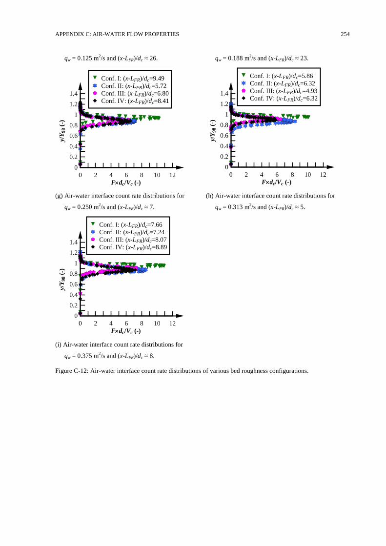
APPENDIX C: AIR-WATER FLOW PROPERTIES 254
qw = 0.125 m2/s and (x-LFR)/dc ≈ 26. qw = 0.188 m
2/s and (x-LFR)/dc ≈ 23.
(g) Air-water interface count rate distributions for
qw = 0.250 m2/s and (x-LFR)/dc ≈ 7.
(h) Air-water interface count rate distributions for
qw = 0.313 m2/s and (x-LFR)/dc ≈ 5.
(i) Air-water interface count rate distributions for
qw = 0.375 m2/s and (x-LFR)/dc ≈ 8.
Figure C-12: Air-water interface count rate distributions of various bed roughness configurations.
Fdc/Vc (-)
y/Y
98 (
-)
0 2 4 6 8 10 12
0
0.2
0.4
0.6
0.8
1
1.2
1.4
Conf. I: (x-LFR)/dc=9.49
Conf. II: (x-LFR)/dc=5.72
Conf. III: (x-LFR)/dc=6.80
Conf. IV: (x-LFR)/dc=8.41
Fdc/Vc (-)
y/Y
98 (
-)
0 2 4 6 8 10 12
0
0.2
0.4
0.6
0.8
1
1.2
1.4
Conf. I: (x-LFR)/dc=5.86
Conf. II: (x-LFR)/dc=6.32
Conf. III: (x-LFR)/dc=4.93
Conf. IV: (x-LFR)/dc=6.32
Fdc/Vc (-)
y/Y
98 (
-)
0 2 4 6 8 10 12
0
0.2
0.4
0.6
0.8
1
1.2
1.4
Conf. I: (x-LFR)/dc=7.66
Conf. II: (x-LFR)/dc=7.24
Conf. III: (x-LFR)/dc=8.07
Conf. IV: (x-LFR)/dc=8.89
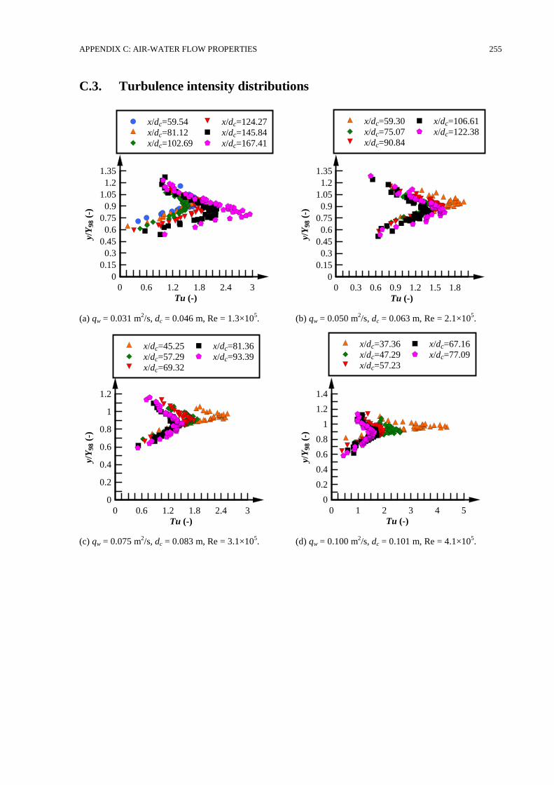
APPENDIX C: AIR-WATER FLOW PROPERTIES 255
C.3. Turbulence intensity distributions
(a) qw = 0.031 m2/s, dc = 0.046 m, Re = 1.3×10
5. (b) qw = 0.050 m
2/s, dc = 0.063 m, Re = 2.1×10
5.
(c) qw = 0.075 m2/s, dc = 0.083 m, Re = 3.1×10
5. (d) qw = 0.100 m
2/s, dc = 0.101 m, Re = 4.1×10
5.
Tu (-)
y/Y
98 (
-)
0 0.6 1.2 1.8 2.4 3
0
0.15
0.3
0.45
0.6
0.75
0.9
1.05
1.2
1.35
x/dc=59.54
x/dc=81.12
x/dc=102.69
x/dc=124.27
x/dc=145.84
x/dc=167.41
Tu (-)y/
Y98 (
-)
0 0.3 0.6 0.9 1.2 1.5 1.8
0
0.15
0.3
0.45
0.6
0.75
0.9
1.05
1.2
1.35
x/dc=59.30
x/dc=75.07
x/dc=90.84
x/dc=106.61
x/dc=122.38
Tu (-)
y/Y
98 (
-)
0 0.6 1.2 1.8 2.4 3
0
0.2
0.4
0.6
0.8
1
1.2
x/dc=45.25
x/dc=57.29
x/dc=69.32
x/dc=81.36
x/dc=93.39
Tu (-)
y/Y
98 (
-)
0 1 2 3 4 5
0
0.2
0.4
0.6
0.8
1
1.2
1.4
x/dc=37.36
x/dc=47.29
x/dc=57.23
x/dc=67.16
x/dc=77.09
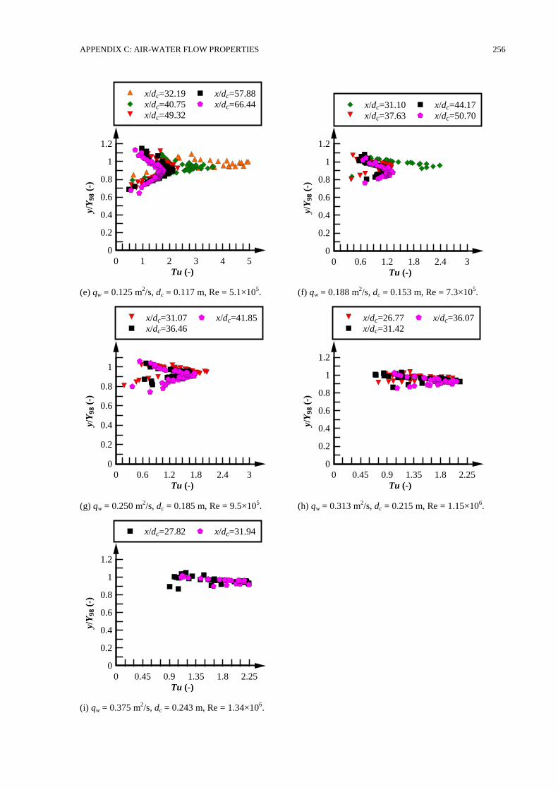
APPENDIX C: AIR-WATER FLOW PROPERTIES 256
(e) qw = 0.125 m2/s, dc = 0.117 m, Re = 5.1×10
5. (f) qw = 0.188 m
2/s, dc = 0.153 m, Re = 7.3×10
5.
(g) qw = 0.250 m2/s, dc = 0.185 m, Re = 9.5×10
5. (h) qw = 0.313 m
2/s, dc = 0.215 m, Re = 1.15×10
6.
(i) qw = 0.375 m2/s, dc = 0.243 m, Re = 1.34×10
6.
Tu (-)
y/Y
98 (
-)
0 1 2 3 4 5
0
0.2
0.4
0.6
0.8
1
1.2
x/dc=32.19
x/dc=40.75
x/dc=49.32
x/dc=57.88
x/dc=66.44
Tu (-)
y/Y
98 (
-)
0 0.6 1.2 1.8 2.4 3
0
0.2
0.4
0.6
0.8
1
1.2
x/dc=31.10
x/dc=37.63
x/dc=44.17
x/dc=50.70
Tu (-)
y/Y
98 (
-)
0 0.6 1.2 1.8 2.4 3
0
0.2
0.4
0.6
0.8
1
x/dc=31.07
x/dc=36.46
x/dc=41.85
Tu (-)
y/Y
98 (
-)
0 0.45 0.9 1.35 1.8 2.25
0
0.2
0.4
0.6
0.8
1
1.2
x/dc=26.77
x/dc=31.42
x/dc=36.07
Tu (-)
y/Y
98 (
-)
0 0.45 0.9 1.35 1.8 2.25
0
0.2
0.4
0.6
0.8
1
1.2
x/dc=27.82 x/dc=31.94
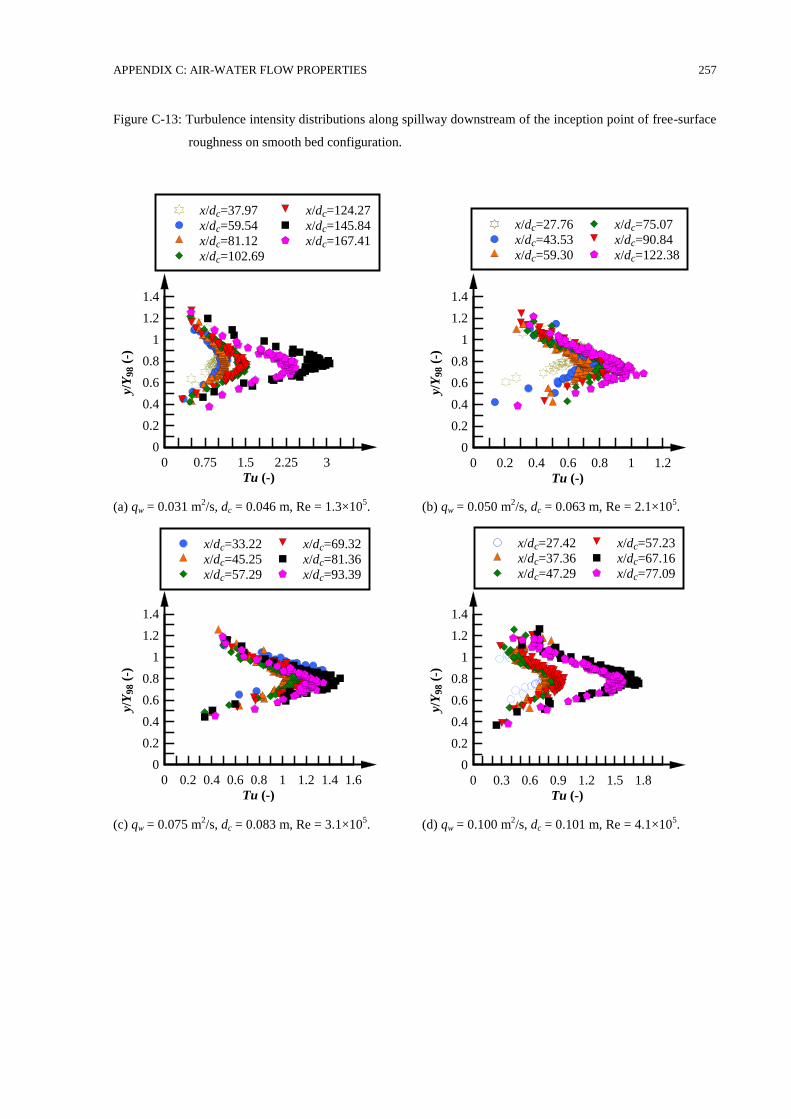
APPENDIX C: AIR-WATER FLOW PROPERTIES 257
Figure C-13: Turbulence intensity distributions along spillway downstream of the inception point of free-surface
roughness on smooth bed configuration.
(a) qw = 0.031 m2/s, dc = 0.046 m, Re = 1.3×10
5. (b) qw = 0.050 m
2/s, dc = 0.063 m, Re = 2.1×10
5.
(c) qw = 0.075 m2/s, dc = 0.083 m, Re = 3.1×10
5. (d) qw = 0.100 m
2/s, dc = 0.101 m, Re = 4.1×10
5.
Tu (-)
y/Y
98 (
-)
0 0.75 1.5 2.25 3
0
0.2
0.4
0.6
0.8
1
1.2
1.4
x/dc=37.97
x/dc=59.54
x/dc=81.12
x/dc=102.69
x/dc=124.27
x/dc=145.84
x/dc=167.41
Tu (-)
y/Y
98 (
-)
0 0.2 0.4 0.6 0.8 1 1.2
0
0.2
0.4
0.6
0.8
1
1.2
1.4
x/dc=27.76
x/dc=43.53
x/dc=59.30
x/dc=75.07
x/dc=90.84
x/dc=122.38
Tu (-)
y/Y
98 (
-)
0 0.2 0.4 0.6 0.8 1 1.2 1.4 1.6
0
0.2
0.4
0.6
0.8
1
1.2
1.4
x/dc=33.22
x/dc=45.25
x/dc=57.29
x/dc=69.32
x/dc=81.36
x/dc=93.39
Tu (-)
y/Y
98 (
-)
0 0.3 0.6 0.9 1.2 1.5 1.8
0
0.2
0.4
0.6
0.8
1
1.2
1.4
x/dc=27.42
x/dc=37.36
x/dc=47.29
x/dc=57.23
x/dc=67.16
x/dc=77.09
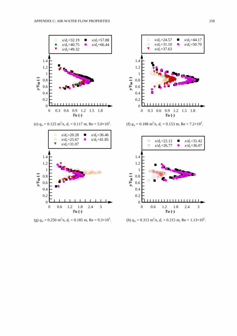
APPENDIX C: AIR-WATER FLOW PROPERTIES 258
(e) qw = 0.125 m2/s, dc = 0.117 m, Re = 5.0×10
5. (f) qw = 0.188 m
2/s, dc = 0.153 m, Re = 7.2×10
5.
(g) qw = 0.250 m2/s, dc = 0.185 m, Re = 9.3×10
5. (h) qw = 0.313 m
2/s, dc = 0.215 m, Re = 1.13×10
6.
Tu (-)
y/Y
98 (
-)
0 0.3 0.6 0.9 1.2 1.5 1.8
0
0.2
0.4
0.6
0.8
1
1.2
1.4
x/dc=32.19
x/dc=40.75
x/dc=49.32
x/dc=57.88
x/dc=66.44
Tu (-)
y/Y
98 (
-)
0 0.3 0.6 0.9 1.2 1.5 1.8
0
0.2
0.4
0.6
0.8
1
1.2
1.4
x/dc=24.57
x/dc=31.10
x/dc=37.63
x/dc=44.17
x/dc=50.70
Tu (-)
y/Y
98 (
-)
0 0.6 1.2 1.8 2.4 3
0
0.2
0.4
0.6
0.8
1
1.2
1.4
x/dc=20.28
x/dc=25.67
x/dc=31.07
x/dc=36.46
x/dc=41.85
Tu (-)
y/Y
98 (
-)
0 0.6 1.2 1.8 2.4 3
0
0.2
0.4
0.6
0.8
1
1.2
1.4
x/dc=22.12
x/dc=26.77
x/dc=31.42
x/dc=36.07
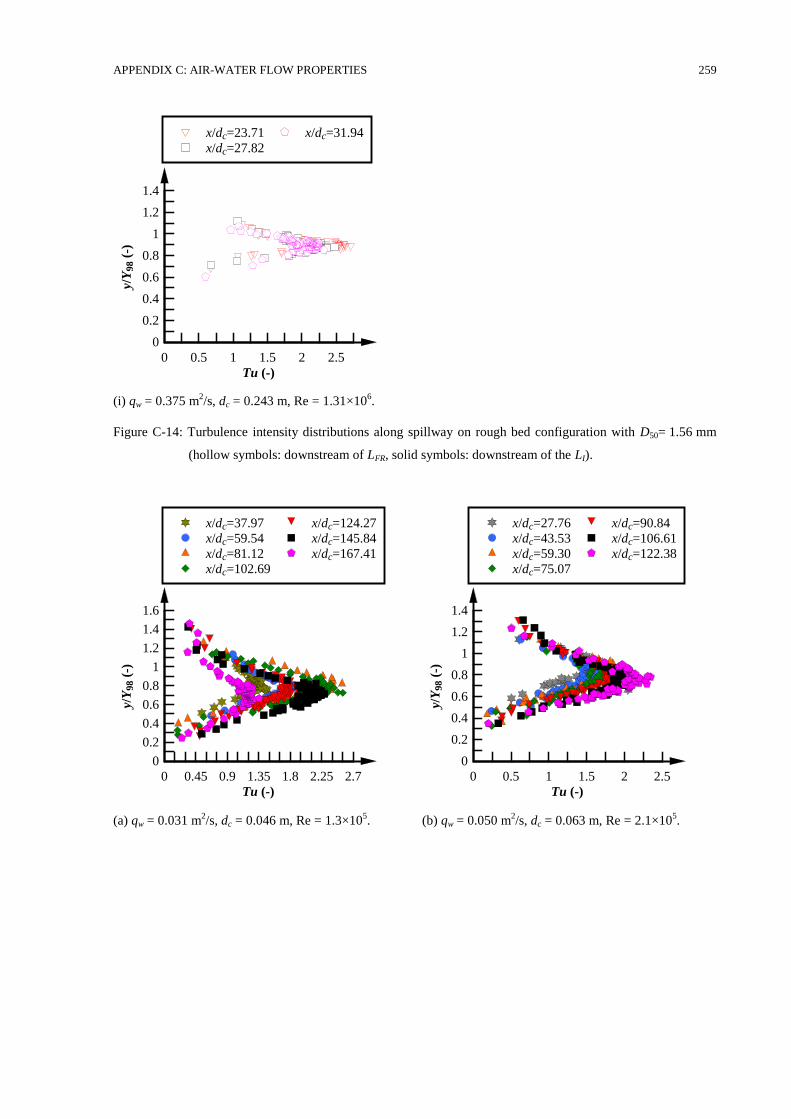
APPENDIX C: AIR-WATER FLOW PROPERTIES 259
(i) qw = 0.375 m2/s, dc = 0.243 m, Re = 1.31×10
6.
Figure C-14: Turbulence intensity distributions along spillway on rough bed configuration with D50= 1.56 mm
(hollow symbols: downstream of LFR, solid symbols: downstream of the LI).
(a) qw = 0.031 m2/s, dc = 0.046 m, Re = 1.3×10
5. (b) qw = 0.050 m
2/s, dc = 0.063 m, Re = 2.1×10
5.
Tu (-)
y/Y
98 (
-)
0 0.5 1 1.5 2 2.5
0
0.2
0.4
0.6
0.8
1
1.2
1.4
x/dc=23.71
x/dc=27.82
x/dc=31.94
Tu (-)
y/Y
98 (
-)
0 0.45 0.9 1.35 1.8 2.25 2.7
0
0.2
0.4
0.6
0.8
1
1.2
1.4
1.6
x/dc=37.97
x/dc=59.54
x/dc=81.12
x/dc=102.69
x/dc=124.27
x/dc=145.84
x/dc=167.41
Tu (-)
y/Y
98 (
-)
0 0.5 1 1.5 2 2.5
0
0.2
0.4
0.6
0.8
1
1.2
1.4
x/dc=27.76
x/dc=43.53
x/dc=59.30
x/dc=75.07
x/dc=90.84
x/dc=106.61
x/dc=122.38
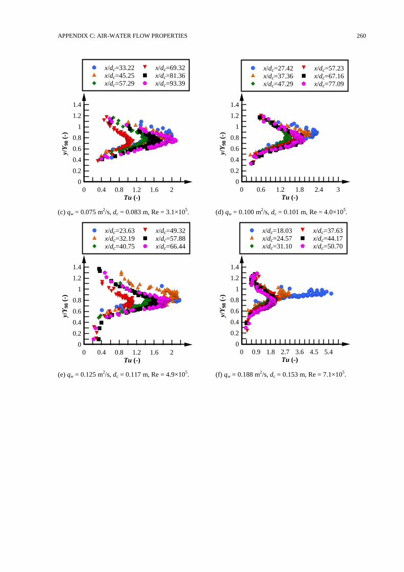
APPENDIX C: AIR-WATER FLOW PROPERTIES 260
(c) qw = 0.075 m2/s, dc = 0.083 m, Re = 3.1×10
5. (d) qw = 0.100 m
2/s, dc = 0.101 m, Re = 4.0×10
5.
(e) qw = 0.125 m2/s, dc = 0.117 m, Re = 4.9×10
5. (f) qw = 0.188 m
2/s, dc = 0.153 m, Re = 7.1×10
5.
Tu (-)
y/Y
98 (
-)
0 0.4 0.8 1.2 1.6 2
0
0.2
0.4
0.6
0.8
1
1.2
1.4
x/dc=33.22
x/dc=45.25
x/dc=57.29
x/dc=69.32
x/dc=81.36
x/dc=93.39
Tu (-)
y/Y
98 (
-)
0 0.6 1.2 1.8 2.4 3
0
0.2
0.4
0.6
0.8
1
1.2
1.4
x/dc=27.42
x/dc=37.36
x/dc=47.29
x/dc=57.23
x/dc=67.16
x/dc=77.09
Tu (-)
y/Y
98 (
-)
0 0.4 0.8 1.2 1.6 2
0
0.2
0.4
0.6
0.8
1
1.2
1.4
x/dc=23.63
x/dc=32.19
x/dc=40.75
x/dc=49.32
x/dc=57.88
x/dc=66.44
Tu (-)
y/Y
98 (
-)
0 0.9 1.8 2.7 3.6 4.5 5.4
0
0.2
0.4
0.6
0.8
1
1.2
1.4
x/dc=18.03
x/dc=24.57
x/dc=31.10
x/dc=37.63
x/dc=44.17
x/dc=50.70
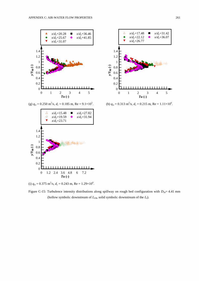
APPENDIX C: AIR-WATER FLOW PROPERTIES 261
(g) qw = 0.250 m2/s, dc = 0.185 m, Re = 9.1×10
5. (h) qw = 0.313 m
2/s, dc = 0.215 m, Re = 1.11×10
6.
(i) qw = 0.375 m2/s, dc = 0.243 m, Re = 1.29×10
6.
Figure C-15: Turbulence intensity distributions along spillway on rough bed configuration with D50= 4.41 mm
(hollow symbols: downstream of LFR, solid symbols: downstream of the LI).
Tu (-)
y/Y
98 (
-)
0 1 2 3 4 5
0
0.2
0.4
0.6
0.8
1
1.2
1.4
x/dc=20.28
x/dc=25.67
x/dc=31.07
x/dc=36.46
x/dc=41.85
Tu (-)
y/Y
98 (
-)
0 1 2 3 4 5
0
0.2
0.4
0.6
0.8
1
1.2
1.4
x/dc=17.48
x/dc=22.12
x/dc=26.77
x/dc=31.42
x/dc=36.07
Tu (-)
y/Y
98 (
-)
0 1.2 2.4 3.6 4.8 6 7.2
0
0.2
0.4
0.6
0.8
1
1.2
1.4
x/dc=15.48
x/dc=19.59
x/dc=23.71
x/dc=27.82
x/dc=31.94
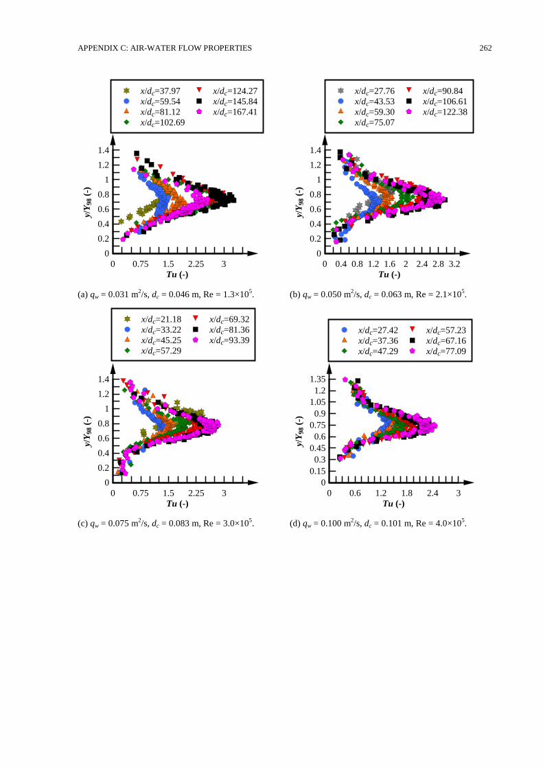
APPENDIX C: AIR-WATER FLOW PROPERTIES 262
(a) qw = 0.031 m2/s, dc = 0.046 m, Re = 1.3×10
5. (b) qw = 0.050 m
2/s, dc = 0.063 m, Re = 2.1×10
5.
(c) qw = 0.075 m2/s, dc = 0.083 m, Re = 3.0×10
5. (d) qw = 0.100 m
2/s, dc = 0.101 m, Re = 4.0×10
5.
Tu (-)
y/Y
98 (
-)
0 0.75 1.5 2.25 3
0
0.2
0.4
0.6
0.8
1
1.2
1.4
x/dc=37.97
x/dc=59.54
x/dc=81.12
x/dc=102.69
x/dc=124.27
x/dc=145.84
x/dc=167.41
Tu (-)
y/Y
98 (
-)
0 0.4 0.8 1.2 1.6 2 2.4 2.8 3.2
0
0.2
0.4
0.6
0.8
1
1.2
1.4
x/dc=27.76
x/dc=43.53
x/dc=59.30
x/dc=75.07
x/dc=90.84
x/dc=106.61
x/dc=122.38
Tu (-)
y/Y
98 (
-)
0 0.75 1.5 2.25 3
0
0.2
0.4
0.6
0.8
1
1.2
1.4
x/dc=21.18
x/dc=33.22
x/dc=45.25
x/dc=57.29
x/dc=69.32
x/dc=81.36
x/dc=93.39
Tu (-)
y/Y
98 (
-)
0 0.6 1.2 1.8 2.4 3
0
0.15
0.3
0.45
0.6
0.75
0.9
1.05
1.2
1.35
x/dc=27.42
x/dc=37.36
x/dc=47.29
x/dc=57.23
x/dc=67.16
x/dc=77.09
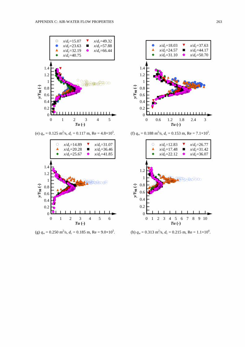
APPENDIX C: AIR-WATER FLOW PROPERTIES 263
(e) qw = 0.125 m2/s, dc = 0.117 m, Re = 4.8×10
5. (f) qw = 0.188 m
2/s, dc = 0.153 m, Re = 7.1×10
5.
(g) qw = 0.250 m2/s, dc = 0.185 m, Re = 9.0×10
5. (h) qw = 0.313 m
2/s, dc = 0.215 m, Re = 1.1×10
6.
Tu (-)
y/Y
98 (
-)
0 1 2 3 4 5
0
0.2
0.4
0.6
0.8
1
1.2
1.4
x/dc=15.07
x/dc=23.63
x/dc=32.19
x/dc=40.75
x/dc=49.32
x/dc=57.88
x/dc=66.44
Tu (-)
y/Y
98 (
-)
0 0.6 1.2 1.8 2.4 3
0
0.2
0.4
0.6
0.8
1
1.2
1.4
x/dc=18.03
x/dc=24.57
x/dc=31.10
x/dc=37.63
x/dc=44.17
x/dc=50.70
Tu (-)
y/Y
98 (
-)
0 1 2 3 4 5 6
0
0.2
0.4
0.6
0.8
1
1.2
1.4
x/dc=14.89
x/dc=20.28
x/dc=25.67
x/dc=31.07
x/dc=36.46
x/dc=41.85
Tu (-)
y/Y
98 (
-)
0 1 2 3 4 5 6 7 8 9 10
0
0.2
0.4
0.6
0.8
1
1.2
x/dc=12.83
x/dc=17.48
x/dc=22.12
x/dc=26.77
x/dc=31.42
x/dc=36.07
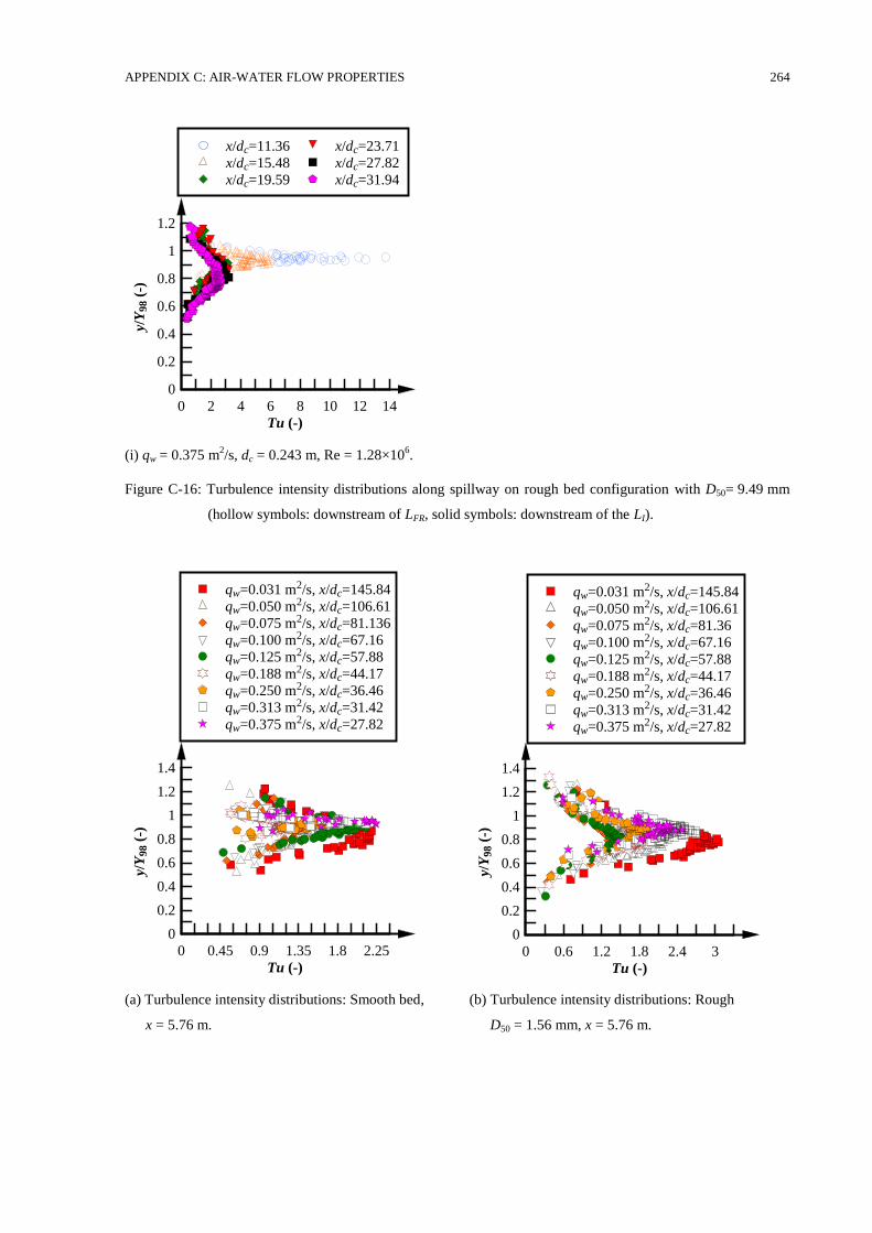
APPENDIX C: AIR-WATER FLOW PROPERTIES 264
(i) qw = 0.375 m2/s, dc = 0.243 m, Re = 1.28×10
6.
Figure C-16: Turbulence intensity distributions along spillway on rough bed configuration with D50= 9.49 mm
(hollow symbols: downstream of LFR, solid symbols: downstream of the LI).
(a) Turbulence intensity distributions: Smooth bed,
x = 5.76 m.
(b) Turbulence intensity distributions: Rough
D50 = 1.56 mm, x = 5.76 m.
Tu (-)
y/Y
98 (
-)
0 2 4 6 8 10 12 14
0
0.2
0.4
0.6
0.8
1
1.2
x/dc=11.36
x/dc=15.48
x/dc=19.59
x/dc=23.71
x/dc=27.82
x/dc=31.94
Tu (-)
y/Y
98 (
-)
0 0.45 0.9 1.35 1.8 2.25
0
0.2
0.4
0.6
0.8
1
1.2
1.4
qw=0.031 m2/s, x/dc=145.84
qw=0.050 m2/s, x/dc=106.61
qw=0.075 m2/s, x/dc=81.136
qw=0.100 m2/s, x/dc=67.16
qw=0.125 m2/s, x/dc=57.88
qw=0.188 m2/s, x/dc=44.17
qw=0.250 m2/s, x/dc=36.46
qw=0.313 m2/s, x/dc=31.42
qw=0.375 m2/s, x/dc=27.82
Tu (-)
y/Y
98 (
-)
0 0.6 1.2 1.8 2.4 3
0
0.2
0.4
0.6
0.8
1
1.2
1.4
qw=0.031 m2/s, x/dc=145.84
qw=0.050 m2/s, x/dc=106.61
qw=0.075 m2/s, x/dc=81.36
qw=0.100 m2/s, x/dc=67.16
qw=0.125 m2/s, x/dc=57.88
qw=0.188 m2/s, x/dc=44.17
qw=0.250 m2/s, x/dc=36.46
qw=0.313 m2/s, x/dc=31.42
qw=0.375 m2/s, x/dc=27.82
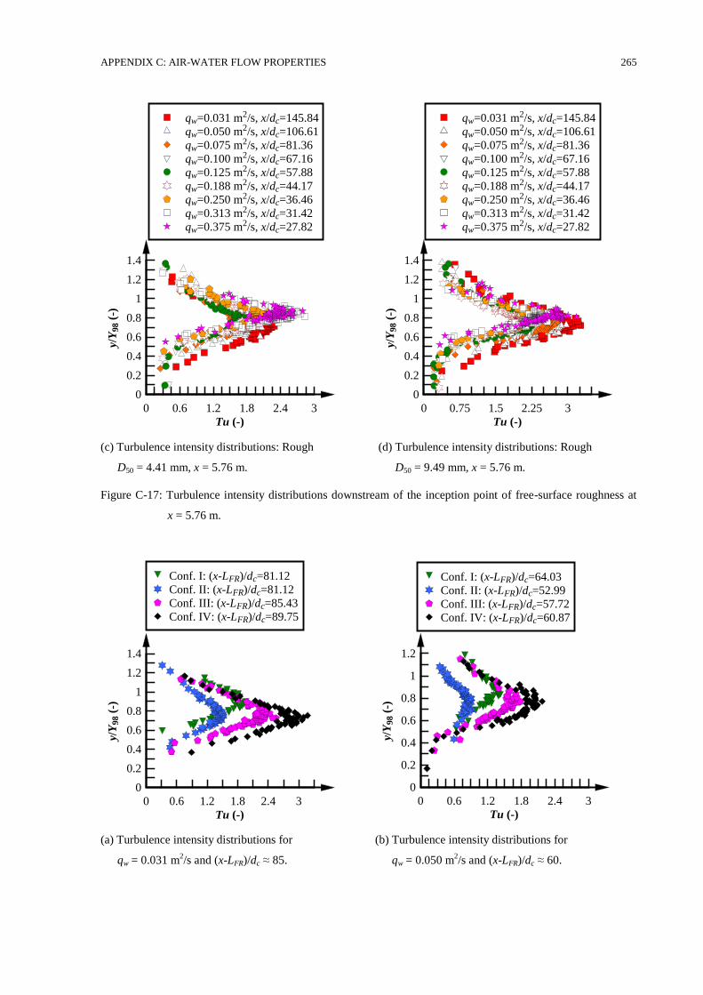
APPENDIX C: AIR-WATER FLOW PROPERTIES 265
(c) Turbulence intensity distributions: Rough
D50 = 4.41 mm, x = 5.76 m.
(d) Turbulence intensity distributions: Rough
D50 = 9.49 mm, x = 5.76 m.
Figure C-17: Turbulence intensity distributions downstream of the inception point of free-surface roughness at
x = 5.76 m.
(a) Turbulence intensity distributions for
qw = 0.031 m2/s and (x-LFR)/dc ≈ 85.
(b) Turbulence intensity distributions for
qw = 0.050 m2/s and (x-LFR)/dc ≈ 60.
Tu (-)
y/Y
98 (
-)
0 0.6 1.2 1.8 2.4 3
0
0.2
0.4
0.6
0.8
1
1.2
1.4
qw=0.031 m2/s, x/dc=145.84
qw=0.050 m2/s, x/dc=106.61
qw=0.075 m2/s, x/dc=81.36
qw=0.100 m2/s, x/dc=67.16
qw=0.125 m2/s, x/dc=57.88
qw=0.188 m2/s, x/dc=44.17
qw=0.250 m2/s, x/dc=36.46
qw=0.313 m2/s, x/dc=31.42
qw=0.375 m2/s, x/dc=27.82
Tu (-)
y/Y
98 (
-)
0 0.75 1.5 2.25 3
0
0.2
0.4
0.6
0.8
1
1.2
1.4
qw=0.031 m2/s, x/dc=145.84
qw=0.050 m2/s, x/dc=106.61
qw=0.075 m2/s, x/dc=81.36
qw=0.100 m2/s, x/dc=67.16
qw=0.125 m2/s, x/dc=57.88
qw=0.188 m2/s, x/dc=44.17
qw=0.250 m2/s, x/dc=36.46
qw=0.313 m2/s, x/dc=31.42
qw=0.375 m2/s, x/dc=27.82
Tu (-)
y/Y
98 (
-)
0 0.6 1.2 1.8 2.4 3
0
0.2
0.4
0.6
0.8
1
1.2
1.4
Conf. I: (x-LFR)/dc=81.12
Conf. II: (x-LFR)/dc=81.12
Conf. III: (x-LFR)/dc=85.43
Conf. IV: (x-LFR)/dc=89.75
Tu (-)
y/Y
98 (
-)
0 0.6 1.2 1.8 2.4 3
0
0.2
0.4
0.6
0.8
1
1.2
Conf. I: (x-LFR)/dc=64.03
Conf. II: (x-LFR)/dc=52.99
Conf. III: (x-LFR)/dc=57.72
Conf. IV: (x-LFR)/dc=60.87
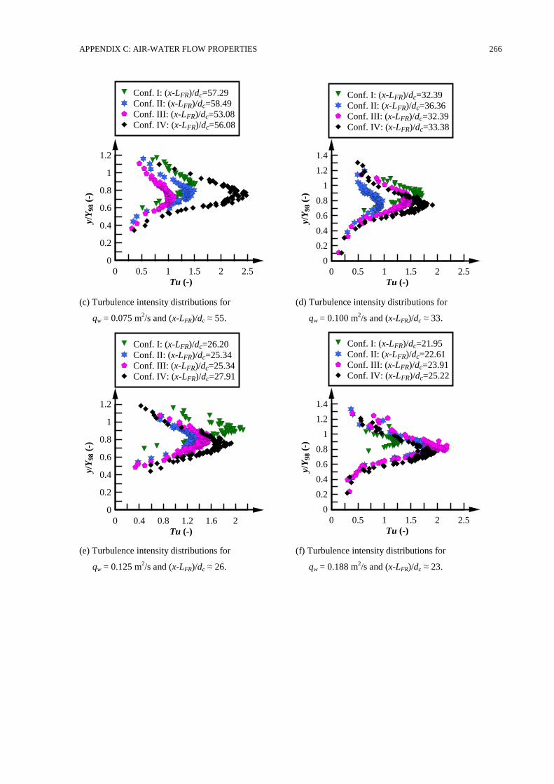
APPENDIX C: AIR-WATER FLOW PROPERTIES 266
(c) Turbulence intensity distributions for
qw = 0.075 m2/s and (x-LFR)/dc ≈ 55.
(d) Turbulence intensity distributions for
qw = 0.100 m2/s and (x-LFR)/dc ≈ 33.
(e) Turbulence intensity distributions for
qw = 0.125 m2/s and (x-LFR)/dc ≈ 26.
(f) Turbulence intensity distributions for
qw = 0.188 m2/s and (x-LFR)/dc ≈ 23.
Tu (-)
y/Y
98 (
-)
0 0.5 1 1.5 2 2.5
0
0.2
0.4
0.6
0.8
1
1.2
Conf. I: (x-LFR)/dc=57.29
Conf. II: (x-LFR)/dc=58.49
Conf. III: (x-LFR)/dc=53.08
Conf. IV: (x-LFR)/dc=56.08
Tu (-)
y/Y
98 (
-)
0 0.5 1 1.5 2 2.5
0
0.2
0.4
0.6
0.8
1
1.2
1.4
Conf. I: (x-LFR)/dc=32.39
Conf. II: (x-LFR)/dc=36.36
Conf. III: (x-LFR)/dc=32.39
Conf. IV: (x-LFR)/dc=33.38
Tu (-)
y/Y
98 (
-)
0 0.4 0.8 1.2 1.6 2
0
0.2
0.4
0.6
0.8
1
1.2
Conf. I: (x-LFR)/dc=26.20
Conf. II: (x-LFR)/dc=25.34
Conf. III: (x-LFR)/dc=25.34
Conf. IV: (x-LFR)/dc=27.91
Tu (-)
y/Y
98 (
-)
0 0.5 1 1.5 2 2.5
0
0.2
0.4
0.6
0.8
1
1.2
1.4
Conf. I: (x-LFR)/dc=21.95
Conf. II: (x-LFR)/dc=22.61
Conf. III: (x-LFR)/dc=23.91
Conf. IV: (x-LFR)/dc=25.22
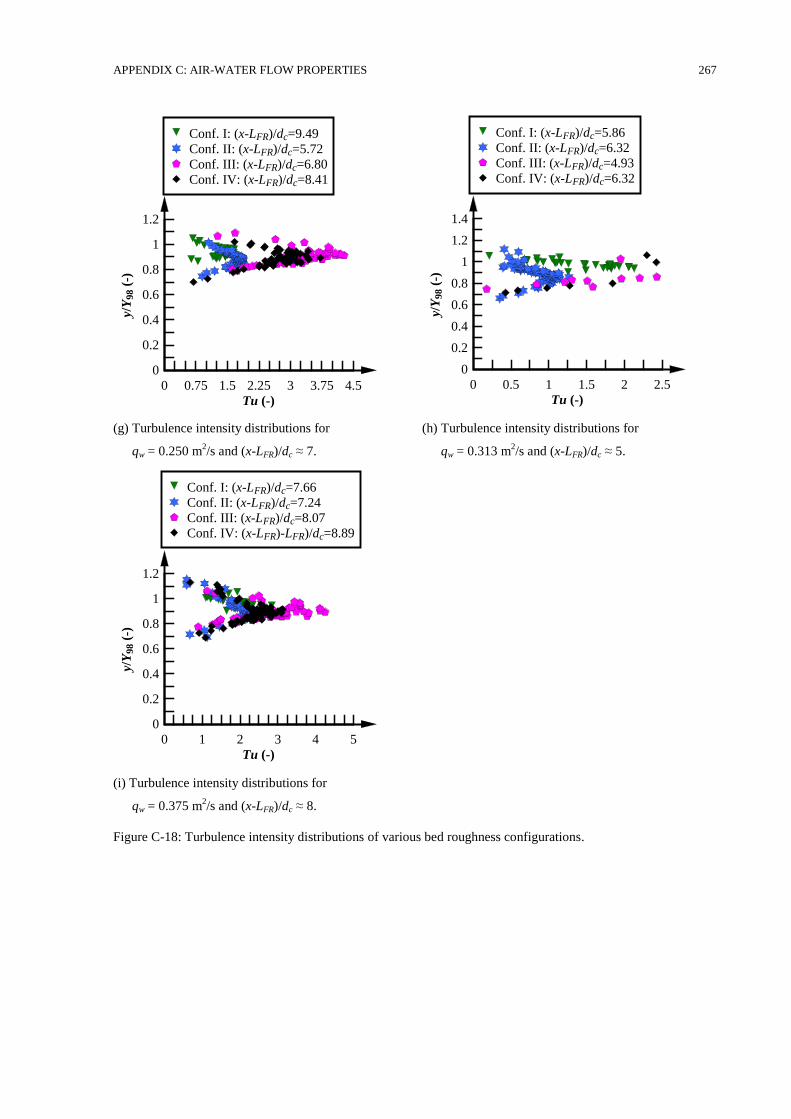
APPENDIX C: AIR-WATER FLOW PROPERTIES 267
(g) Turbulence intensity distributions for
qw = 0.250 m2/s and (x-LFR)/dc ≈ 7.
(h) Turbulence intensity distributions for
qw = 0.313 m2/s and (x-LFR)/dc ≈ 5.
(i) Turbulence intensity distributions for
qw = 0.375 m2/s and (x-LFR)/dc ≈ 8.
Figure C-18: Turbulence intensity distributions of various bed roughness configurations.
Tu (-)
y/Y
98 (
-)
0 0.75 1.5 2.25 3 3.75 4.5
0
0.2
0.4
0.6
0.8
1
1.2
Conf. I: (x-LFR)/dc=9.49
Conf. II: (x-LFR)/dc=5.72
Conf. III: (x-LFR)/dc=6.80
Conf. IV: (x-LFR)/dc=8.41
Tu (-)
y/Y
98 (
-)
0 0.5 1 1.5 2 2.5
0
0.2
0.4
0.6
0.8
1
1.2
1.4
Conf. I: (x-LFR)/dc=5.86
Conf. II: (x-LFR)/dc=6.32
Conf. III: (x-LFR)/dc=4.93
Conf. IV: (x-LFR)/dc=6.32
Tu (-)
y/Y
98 (
-)
0 1 2 3 4 5
0
0.2
0.4
0.6
0.8
1
1.2
Conf. I: (x-LFR)/dc=7.66
Conf. II: (x-LFR)/dc=7.24
Conf. III: (x-LFR)/dc=8.07
Conf. IV: (x-LFR)-LFR)/dc=8.89
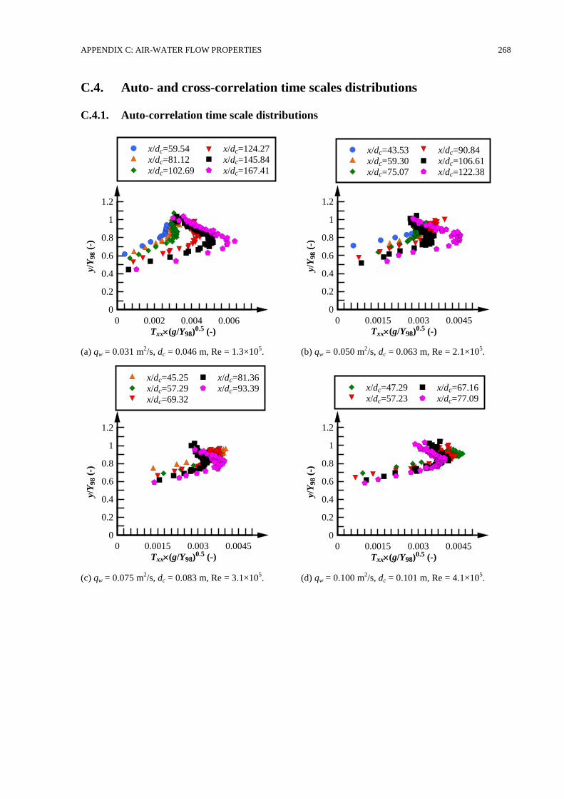
APPENDIX C: AIR-WATER FLOW PROPERTIES 268
C.4. Auto- and cross-correlation time scales distributions
C.4.1. Auto-correlation time scale distributions
(a) qw = 0.031 m2/s, dc = 0.046 m, Re = 1.3×10
5. (b) qw = 0.050 m
2/s, dc = 0.063 m, Re = 2.1×10
5.
(c) qw = 0.075 m2/s, dc = 0.083 m, Re = 3.1×10
5. (d) qw = 0.100 m
2/s, dc = 0.101 m, Re = 4.1×10
5.
Txx(g/Y98)0.5 (-)
y/Y
98 (
-)
0 0.002 0.004 0.006
0
0.2
0.4
0.6
0.8
1
1.2
x/dc=59.54
x/dc=81.12
x/dc=102.69
x/dc=124.27
x/dc=145.84
x/dc=167.41
Txx(g/Y98)0.5 (-)
y/Y
98 (
-)
0 0.0015 0.003 0.0045
0
0.2
0.4
0.6
0.8
1
1.2
x/dc=43.53
x/dc=59.30
x/dc=75.07
x/dc=90.84
x/dc=106.61
x/dc=122.38
Txx(g/Y98)0.5 (-)
y/Y
98 (
-)
0 0.0015 0.003 0.0045
0
0.2
0.4
0.6
0.8
1
1.2
x/dc=45.25
x/dc=57.29
x/dc=69.32
x/dc=81.36
x/dc=93.39
Txx(g/Y98)0.5 (-)
y/Y
98 (
-)
0 0.0015 0.003 0.0045
0
0.2
0.4
0.6
0.8
1
1.2
x/dc=47.29
x/dc=57.23
x/dc=67.16
x/dc=77.09
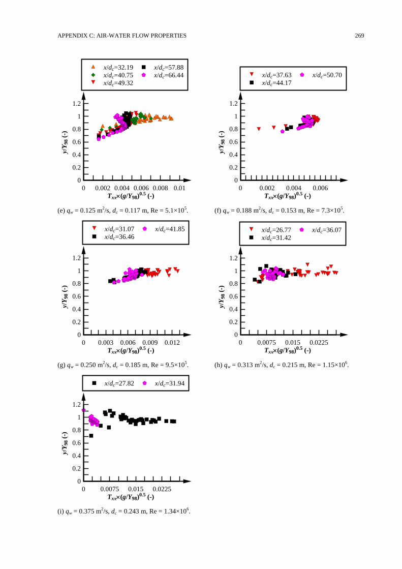
APPENDIX C: AIR-WATER FLOW PROPERTIES 269
(e) qw = 0.125 m2/s, dc = 0.117 m, Re = 5.1×10
5. (f) qw = 0.188 m
2/s, dc = 0.153 m, Re = 7.3×10
5.
(g) qw = 0.250 m2/s, dc = 0.185 m, Re = 9.5×10
5. (h) qw = 0.313 m
2/s, dc = 0.215 m, Re = 1.15×10
6.
(i) qw = 0.375 m2/s, dc = 0.243 m, Re = 1.34×10
6.
Txx(g/Y98)0.5 (-)
y/Y
98 (
-)
0 0.002 0.004 0.006 0.008 0.01
0
0.2
0.4
0.6
0.8
1
1.2
x/dc=32.19
x/dc=40.75
x/dc=49.32
x/dc=57.88
x/dc=66.44
Txx(g/Y98)0.5 (-)
y/Y
98 (
-)
0 0.002 0.004 0.006
0
0.2
0.4
0.6
0.8
1
1.2
x/dc=37.63
x/dc=44.17
x/dc=50.70
Txx(g/Y98)0.5 (-)
y/Y
98 (
-)
0 0.003 0.006 0.009 0.012
0
0.2
0.4
0.6
0.8
1
1.2
x/dc=31.07
x/dc=36.46
x/dc=41.85
Txx(g/Y98)0.5 (-)
y/Y
98 (
-)
0 0.0075 0.015 0.0225
0
0.2
0.4
0.6
0.8
1
1.2
x/dc=26.77
x/dc=31.42
x/dc=36.07
Txx(g/Y98)0.5 (-)
y/Y
98 (
-)
0 0.0075 0.015 0.0225
0
0.2
0.4
0.6
0.8
1
1.2
x/dc=27.82 x/dc=31.94
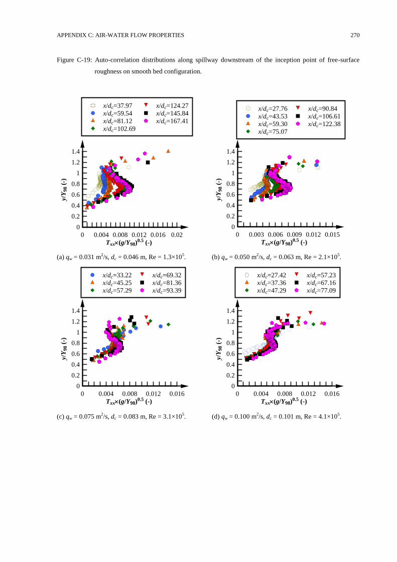
APPENDIX C: AIR-WATER FLOW PROPERTIES 270
Figure C-19: Auto-correlation distributions along spillway downstream of the inception point of free-surface
roughness on smooth bed configuration.
(a) qw = 0.031 m2/s, dc = 0.046 m, Re = 1.3×10
5. (b) qw = 0.050 m
2/s, dc = 0.063 m, Re = 2.1×10
5.
(c) qw = 0.075 m2/s, dc = 0.083 m, Re = 3.1×10
5. (d) qw = 0.100 m
2/s, dc = 0.101 m, Re = 4.1×10
5.
Txx(g/Y98)0.5 (-)
y/Y
98 (
-)
0 0.004 0.008 0.012 0.016 0.02
0
0.2
0.4
0.6
0.8
1
1.2
1.4
x/dc=37.97
x/dc=59.54
x/dc=81.12
x/dc=102.69
x/dc=124.27
x/dc=145.84
x/dc=167.41
Txx(g/Y98)0.5 (-)
y/Y
98 (
-)
0 0.003 0.006 0.009 0.012 0.015
0
0.2
0.4
0.6
0.8
1
1.2
1.4
x/dc=27.76
x/dc=43.53
x/dc=59.30
x/dc=75.07
x/dc=90.84
x/dc=106.61
x/dc=122.38
Txx(g/Y98)0.5 (-)
y/Y
98 (
-)
0 0.004 0.008 0.012 0.016
0
0.2
0.4
0.6
0.8
1
1.2
1.4
x/dc=33.22
x/dc=45.25
x/dc=57.29
x/dc=69.32
x/dc=81.36
x/dc=93.39
Txx(g/Y98)0.5 (-)
y/Y
98 (
-)
0 0.004 0.008 0.012 0.016
0
0.2
0.4
0.6
0.8
1
1.2
1.4
x/dc=27.42
x/dc=37.36
x/dc=47.29
x/dc=57.23
x/dc=67.16
x/dc=77.09
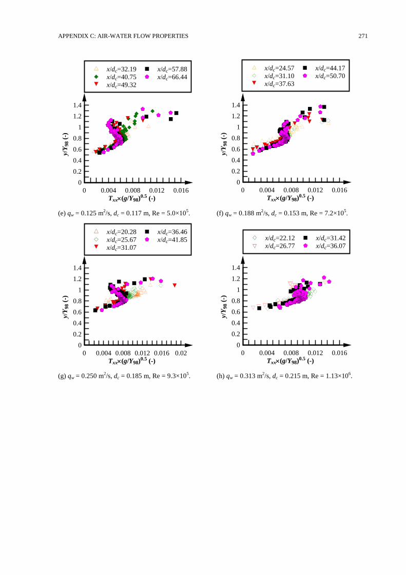
APPENDIX C: AIR-WATER FLOW PROPERTIES 271
(e) qw = 0.125 m2/s, dc = 0.117 m, Re = 5.0×10
5. (f) qw = 0.188 m
2/s, dc = 0.153 m, Re = 7.2×10
5.
(g) qw = 0.250 m2/s, dc = 0.185 m, Re = 9.3×10
5. (h) qw = 0.313 m
2/s, dc = 0.215 m, Re = 1.13×10
6.
Txx(g/Y98)0.5 (-)
y/Y
98 (
-)
0 0.004 0.008 0.012 0.016
0
0.2
0.4
0.6
0.8
1
1.2
1.4
x/dc=32.19
x/dc=40.75
x/dc=49.32
x/dc=57.88
x/dc=66.44
Txx(g/Y98)0.5 (-)
y/Y
98 (
-)
0 0.004 0.008 0.012 0.016
0
0.2
0.4
0.6
0.8
1
1.2
1.4
x/dc=24.57
x/dc=31.10
x/dc=37.63
x/dc=44.17
x/dc=50.70
Txx(g/Y98)0.5 (-)
y/Y
98 (
-)
0 0.004 0.008 0.012 0.016 0.02
0
0.2
0.4
0.6
0.8
1
1.2
1.4
x/dc=20.28
x/dc=25.67
x/dc=31.07
x/dc=36.46
x/dc=41.85
Txx(g/Y98)0.5 (-)
y/Y
98 (
-)
0 0.004 0.008 0.012 0.016
0
0.2
0.4
0.6
0.8
1
1.2
1.4
x/dc=22.12
x/dc=26.77
x/dc=31.42
x/dc=36.07
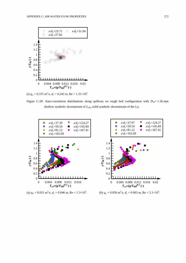
APPENDIX C: AIR-WATER FLOW PROPERTIES 272
(i) qw = 0.375 m2/s, dc = 0.243 m, Re = 1.31×10
6.
Figure C-20: Auto-correlation distributions along spillway on rough bed configuration with D50= 1.56 mm
(hollow symbols: downstream of LFR, solid symbols: downstream of the LI).
(a) qw = 0.031 m2/s, dc = 0.046 m, Re = 1.3×10
5. (b) qw = 0.050 m
2/s, dc = 0.063 m, Re = 2.1×10
5.
Txx(g/Y98)0.5 (-)
y/Y
98 (
-)
0 0.004 0.008 0.012 0.016 0.02
0
0.2
0.4
0.6
0.8
1
1.2
1.4
x/dc=23.71
x/dc=27.82
x/dc=31.94
Txx(g/Y98)0.5 (-)
y/Y
98 (
-)
0 0.004 0.008 0.012 0.016
0
0.2
0.4
0.6
0.8
1
1.2
1.4
x/dc=37.39
x/dc=59.54
x/dc=81.12
x/dc=102.69
x/dc=124.27
x/dc=145.84
x/dc=167.41
Txx(g/Y98)0.5 (-)
y/Y
98 (
-)
0 0.004 0.008 0.012 0.016 0.02
0
0.2
0.4
0.6
0.8
1
1.2
1.4
x/dc=37.97
x/dc=59.54
x/dc=81.12
x/dc=102.69
x/dc=124.27
x/dc=145.84
x/dc=167.41
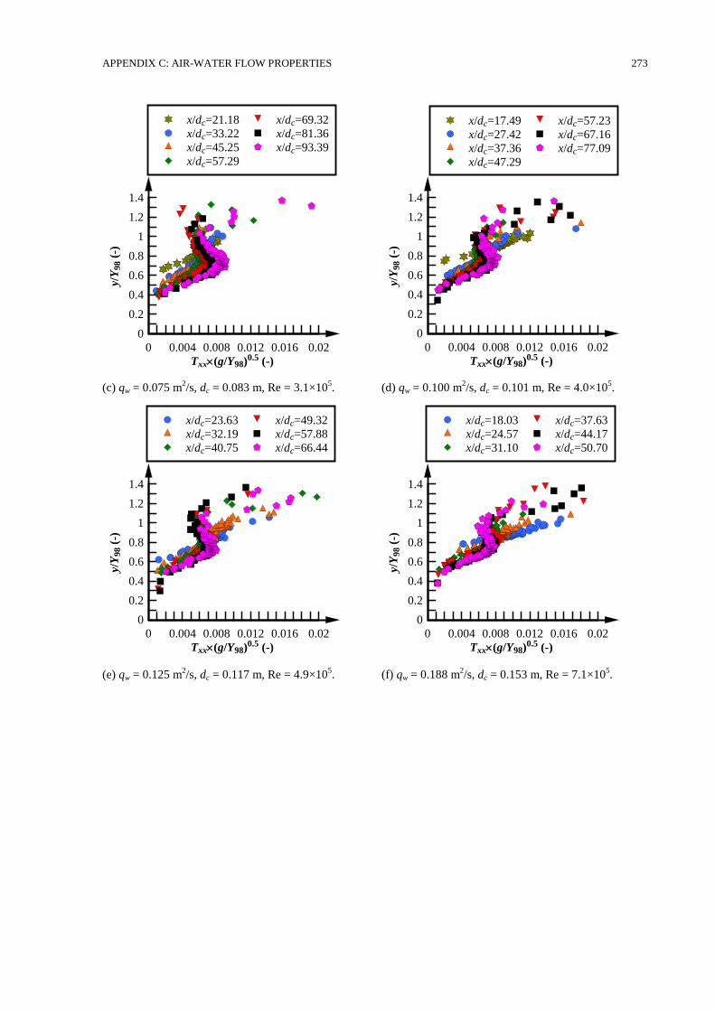
APPENDIX C: AIR-WATER FLOW PROPERTIES 273
(c) qw = 0.075 m2/s, dc = 0.083 m, Re = 3.1×10
5. (d) qw = 0.100 m
2/s, dc = 0.101 m, Re = 4.0×10
5.
(e) qw = 0.125 m2/s, dc = 0.117 m, Re = 4.9×10
5. (f) qw = 0.188 m
2/s, dc = 0.153 m, Re = 7.1×10
5.
Txx(g/Y98)0.5 (-)
y/Y
98 (
-)
0 0.004 0.008 0.012 0.016 0.02
0
0.2
0.4
0.6
0.8
1
1.2
1.4
x/dc=21.18
x/dc=33.22
x/dc=45.25
x/dc=57.29
x/dc=69.32
x/dc=81.36
x/dc=93.39
Txx(g/Y98)0.5 (-)
y/Y
98 (
-)
0 0.004 0.008 0.012 0.016 0.02
0
0.2
0.4
0.6
0.8
1
1.2
1.4
x/dc=17.49
x/dc=27.42
x/dc=37.36
x/dc=47.29
x/dc=57.23
x/dc=67.16
x/dc=77.09
Txx(g/Y98)0.5 (-)
y/Y
98 (
-)
0 0.004 0.008 0.012 0.016 0.02
0
0.2
0.4
0.6
0.8
1
1.2
1.4
x/dc=23.63
x/dc=32.19
x/dc=40.75
x/dc=49.32
x/dc=57.88
x/dc=66.44
Txx(g/Y98)0.5 (-)
y/Y
98 (
-)
0 0.004 0.008 0.012 0.016 0.02
0
0.2
0.4
0.6
0.8
1
1.2
1.4
x/dc=18.03
x/dc=24.57
x/dc=31.10
x/dc=37.63
x/dc=44.17
x/dc=50.70
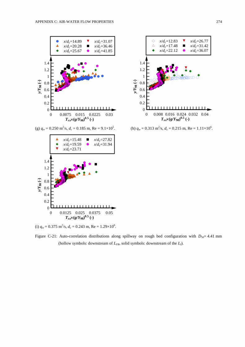
APPENDIX C: AIR-WATER FLOW PROPERTIES 274
(g) qw = 0.250 m2/s, dc = 0.185 m, Re = 9.1×10
5. (h) qw = 0.313 m
2/s, dc = 0.215 m, Re = 1.11×10
6.
(i) qw = 0.375 m2/s, dc = 0.243 m, Re = 1.29×10
6.
Figure C-21: Auto-correlation distributions along spillway on rough bed configuration with D50= 4.41 mm
(hollow symbols: downstream of LFR, solid symbols: downstream of the LI).
Txx(g/Y98)0.5 (-)
y/Y
98 (
-)
0 0.0075 0.015 0.0225 0.03
0
0.2
0.4
0.6
0.8
1
1.2
1.4
x/dc=14.89
x/dc=20.28
x/dc=25.67
x/dc=31.07
x/dc=36.46
x/dc=41.85
Txx(g/Y98)0.5 (-)
y/Y
98 (
-)
0 0.008 0.016 0.024 0.032 0.04
0
0.2
0.4
0.6
0.8
1
1.2
1.4
x/dc=12.83
x/dc=17.48
x/dc=22.12
x/dc=26.77
x/dc=31.42
x/dc=36.07
Txx(g/Y98)0.5 (-)
y/Y
98 (
-)
0 0.0125 0.025 0.0375 0.05
0
0.2
0.4
0.6
0.8
1
1.2
1.4
x/dc=15.48
x/dc=19.59
x/dc=23.71
x/dc=27.82
x/dc=31.94

APPENDIX C: AIR-WATER FLOW PROPERTIES 275
(a) qw = 0.031 m2/s, dc = 0.046 m, Re = 1.3×10
5. (b) qw = 0.050 m
2/s, dc = 0.063 m, Re = 2.1×10
5.
(c) qw = 0.075 m2/s, dc = 0.083 m, Re = 3.0×10
5. (d) qw = 0.100 m
2/s, dc = 0.101 m, Re = 4.0×10
5.
Txx(g/Y98)0.5 (-)
y/Y
98 (
-)
0 0.0075 0.015 0.0225
0
0.3
0.6
0.9
1.2
1.5
1.8
x/dc=37.97
x/dc=59.54
x/dc=81.12
x/dc=102.69
x/dc=124.27
x/dc=145.84
x/dc=167.41
Txx(g/Y98)0.5 (-)
y/Y
98 (
-)
0 0.004 0.008 0.012
0
0.2
0.4
0.6
0.8
1
1.2
1.4
1.6
x/dc=27.76
x/dc=43.53
x/dc=59.30
x/dc=75.07
x/dc=90.84
x/dc=106.61
x/dc=122.38
Txx(g/Y98)0.5 (-)
y/Y
98 (
-)
0 0.0075 0.015 0.0225
0
0.2
0.4
0.6
0.8
1
1.2
1.4
1.6
x/dc=21.18
x/dc=33.22
x/dc=45.25
x/dc=57.29
x/dc=69.32
x/dc=81.36
x/dc=93.39
Txx(g/Y98)0.5 (-)
y/Y
98 (
-)
0 0.0045 0.009 0.0135
0
0.2
0.4
0.6
0.8
1
1.2
1.4
1.6
x/dc=17.49
x/dc=27.42
x/dc=37.36
x/dc=47.29
x/dc=57.23
x/dc=67.16
x/dc=77.09
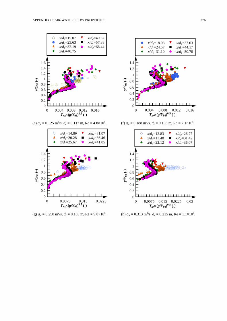
APPENDIX C: AIR-WATER FLOW PROPERTIES 276
(e) qw = 0.125 m2/s, dc = 0.117 m, Re = 4.8×10
5. (f) qw = 0.188 m
2/s, dc = 0.153 m, Re = 7.1×10
5.
(g) qw = 0.250 m2/s, dc = 0.185 m, Re = 9.0×10
5. (h) qw = 0.313 m
2/s, dc = 0.215 m, Re = 1.1×10
6.
Txx(g/Y98)0.5 (-)
y/Y
98 (
-)
0 0.004 0.008 0.012 0.016
0
0.2
0.4
0.6
0.8
1
1.2
1.4
1.6
x/dc=15.07
x/dc=23.63
x/dc=32.19
x/dc=40.75
x/dc=49.32
x/dc=57.88
x/dc=66.44
Txx(g/Y98)0.5 (-)
y/Y
98 (
-)
0 0.004 0.008 0.012 0.016
0
0.2
0.4
0.6
0.8
1
1.2
1.4
x/dc=18.03
x/dc=24.57
x/dc=31.10
x/dc=37.63
x/dc=44.17
x/dc=50.70
Txx(g/Y98)0.5 (-)
y/Y
98 (
-)
0 0.0075 0.015 0.0225
0
0.2
0.4
0.6
0.8
1
1.2
1.4
x/dc=14.89
x/dc=20.28
x/dc=25.67
x/dc=31.07
x/dc=36.46
x/dc=41.85
Txx(g/Y98)0.5 (-)
y/Y
98 (
-)
0 0.0075 0.015 0.0225 0.03
0
0.2
0.4
0.6
0.8
1
1.2
1.4
x/dc=12.83
x/dc=17.48
x/dc=22.12
x/dc=26.77
x/dc=31.42
x/dc=36.07
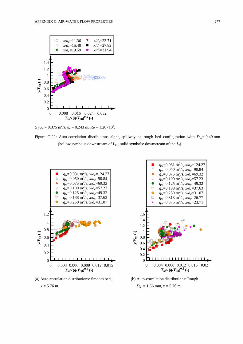
APPENDIX C: AIR-WATER FLOW PROPERTIES 277
(i) qw = 0.375 m2/s, dc = 0.243 m, Re = 1.28×10
6.
Figure C-22: Auto-correlation distributions along spillway on rough bed configuration with D50= 9.49 mm
(hollow symbols: downstream of LFR, solid symbols: downstream of the LI).
(a) Auto-correlation distributions: Smooth bed,
x = 5.76 m.
(b) Auto-correlation distributions: Rough
D50 = 1.56 mm, x = 5.76 m.
Txx(g/Y98)0.5 (-)
y/Y
98 (
-)
0 0.008 0.016 0.024 0.032
0
0.2
0.4
0.6
0.8
1
1.2
1.4
x/dc=11.36
x/dc=15.48
x/dc=19.59
x/dc=23.71
x/dc=27.82
x/dc=31.94
Txx(g/Y98)0.5 (-)
y/Y
98 (
-)
0 0.003 0.006 0.009 0.012 0.015
0
0.2
0.4
0.6
0.8
1
1.2
qw=0.031 m2/s, x/dc=124.27
qw=0.050 m2/s, x/dc=90.84
qw=0.075 m2/s, x/dc=69.32
qw=0.100 m2/s, x/dc=57.23
qw=0.125 m2/s, x/dc=49.32
qw=0.188 m2/s, x/dc=37.63
qw=0.250 m2/s, x/dc=31.07
Txx(g/Y98)0.5 (-)
y/Y
98 (
-)
0 0.004 0.008 0.012 0.016 0.02
0
0.2
0.4
0.6
0.8
1
1.2
1.4
1.6
qw=0.031 m2/s, x/dc=124.27
qw=0.050 m2/s, x/dc=90.84
qw=0.075 m2/s, x/dc=69.32
qw=0.100 m2/s, x/dc=57.23
qw=0.125 m2/s, x/dc=49.32
qw=0.188 m2/s, x/dc=37.63
qw=0.250 m2/s, x/dc=31.07
qw=0.313 m2/s, x/dc=26.77
qw=0.375 m2/s, x/dc=23.71
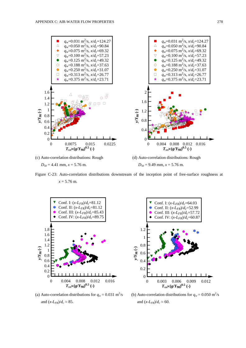
APPENDIX C: AIR-WATER FLOW PROPERTIES 278
(c) Auto-correlation distributions: Rough
D50 = 4.41 mm, x = 5.76 m.
(d) Auto-correlation distributions: Rough
D50 = 9.49 mm, x = 5.76 m.
Figure C-23: Auto-correlation distributions downstream of the inception point of free-surface roughness at
x = 5.76 m.
(a) Auto-correlation distributions for qw = 0.031 m2/s
and (x-LFR)/dc ≈ 85.
(b) Auto-correlation distributions for qw = 0.050 m2/s
and (x-LFR)/dc ≈ 60.
Txx(g/Y98)0.5 (-)
y/Y
98 (
-)
0 0.0075 0.015 0.0225
0
0.2
0.4
0.6
0.8
1
1.2
1.4
1.6
qw=0.031 m2/s, x/dc=124.27
qw=0.050 m2/s, x/dc=90.84
qw=0.075 m2/s, x/dc=69.32
qw=0.100 m2/s, x/dc=57.23
qw=0.125 m2/s, x/dc=49.32
qw=0.188 m2/s, x/dc=37.63
qw=0.250 m2/s, x/dc=31.07
qw=0.313 m2/s, x/dc=26.77
qw=0.375 m2/s, x/dc=23.71
Txx(g/Y98)0.5 (-)
y/Y
98 (
-)
0 0.004 0.008 0.012 0.016
0
0.4
0.8
1.2
1.6
2
qw=0.031 m2/s, x/dc=124.27
qw=0.050 m2/s, x/dc=90.84
qw=0.075 m2/s, x/dc=69.32
qw=0.100 m2/s, x/dc=57.23
qw=0.125 m2/s, x/dc=49.32
qw=0.188 m2/s, x/dc=37.63
qw=0.250 m2/s, x/dc=31.07
qw=0.313 m2/s, x/dc=26.77
qw=0.375 m2/s, x/dc=23.71
Txx(g/Y98)0.5 (-)
y/Y
98 (
-)
0 0.004 0.008 0.012 0.016
0
0.2
0.4
0.6
0.8
1
1.2
1.4
1.6
1.8
Conf. I: (x-LFR)/dc=81.12
Conf. II: (x-LFR)/dc=81.12
Conf. III: (x-LFR)/dc=85.43
Conf. IV: (x-LFR)/dc=89.75
Txx(g/Y98)0.5 (-)
y/Y
98 (
-)
0 0.003 0.006 0.009 0.012
0
0.2
0.4
0.6
0.8
1
1.2
Conf. I: (x-LFR)/dc=64.03
Conf. II: (x-LFR)/dc=52.99
Conf. III: (x-LFR)/dc=57.72
Conf. IV: (x-LFR)/dc=60.87
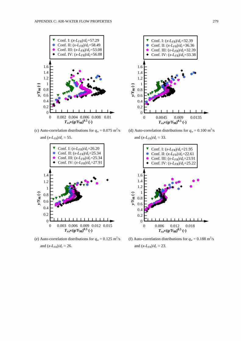
APPENDIX C: AIR-WATER FLOW PROPERTIES 279
(c) Auto-correlation distributions for qw = 0.075 m2/s
and (x-LFR)/dc ≈ 55.
(d) Auto-correlation distributions for qw = 0.100 m2/s
and (x-LFR)/dc ≈ 33.
(e) Auto-correlation distributions for qw = 0.125 m2/s
and (x-LFR)/dc ≈ 26.
(f) Auto-correlation distributions for qw = 0.188 m2/s
and (x-LFR)/dc ≈ 23.
Txx(g/Y98)0.5 (-)
y/Y
98 (
-)
0 0.002 0.004 0.006 0.008 0.01
0
0.2
0.4
0.6
0.8
1
1.2
1.4
1.6
Conf. I: (x-LFR)/dc=57.29
Conf. II: (x-LFR)/dc=58.49
Conf. III: (x-LFR)/dc=53.08
Conf. IV: (x-LFR)/dc=56.08
Txx(g/Y98)0.5 (-)
y/Y
98 (
-)
0 0.0045 0.009 0.0135
0
0.2
0.4
0.6
0.8
1
1.2
1.4
1.6
Conf. I: (x-LFR)/dc=32.39
Conf. II: (x-LFR)/dc=36.36
Conf. III: (x-LFR)/dc=32.39
Conf. IV: (x-LFR)/dc=33.38
Txx(g/Y98)0.5 (-)
y/Y
98 (
-)
0 0.003 0.006 0.009 0.012 0.015
0
0.2
0.4
0.6
0.8
1
1.2
1.4
Conf. I: (x-LFR)/dc=26.20
Conf. II: (x-LFR)/dc=25.34
Conf. III: (x-LFR)/dc=25.34
Conf. IV: (x-LFR)/dc=27.91
Txx(g/Y98)0.5 (-)
y/Y
98 (
-)
0 0.006 0.012 0.018
0
0.2
0.4
0.6
0.8
1
1.2
1.4
1.6
Conf. I: (x-LFR)/dc=21.95
Conf. II: (x-LFR)/dc=22.61
Conf. III: (x-LFR)/dc=23.91
Conf. IV: (x-LFR)/dc=25.22
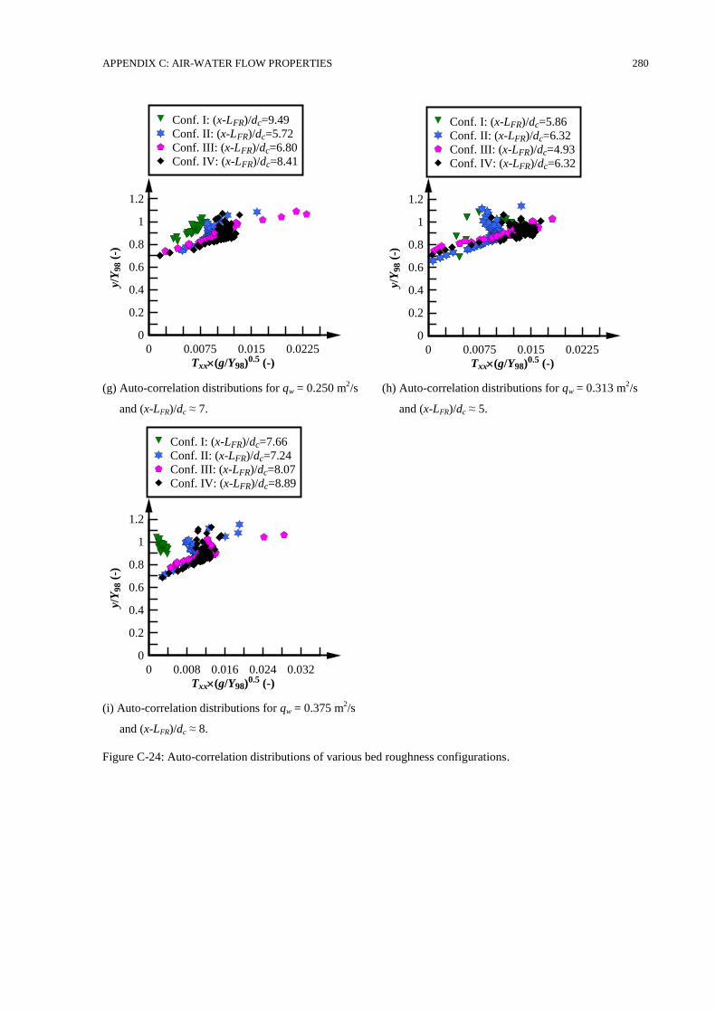
APPENDIX C: AIR-WATER FLOW PROPERTIES 280
(g) Auto-correlation distributions for qw = 0.250 m2/s
and (x-LFR)/dc ≈ 7.
(h) Auto-correlation distributions for qw = 0.313 m2/s
and (x-LFR)/dc ≈ 5.
(i) Auto-correlation distributions for qw = 0.375 m2/s
and (x-LFR)/dc ≈ 8.
Figure C-24: Auto-correlation distributions of various bed roughness configurations.
Txx(g/Y98)0.5 (-)
y/Y
98 (
-)
0 0.0075 0.015 0.0225
0
0.2
0.4
0.6
0.8
1
1.2
Conf. I: (x-LFR)/dc=9.49
Conf. II: (x-LFR)/dc=5.72
Conf. III: (x-LFR)/dc=6.80
Conf. IV: (x-LFR)/dc=8.41
Txx(g/Y98)0.5 (-)
y/Y
98 (
-)
0 0.0075 0.015 0.0225
0
0.2
0.4
0.6
0.8
1
1.2
Conf. I: (x-LFR)/dc=5.86
Conf. II: (x-LFR)/dc=6.32
Conf. III: (x-LFR)/dc=4.93
Conf. IV: (x-LFR)/dc=6.32
Txx(g/Y98)0.5 (-)
y/Y
98 (
-)
0 0.008 0.016 0.024 0.032
0
0.2
0.4
0.6
0.8
1
1.2
Conf. I: (x-LFR)/dc=7.66
Conf. II: (x-LFR)/dc=7.24
Conf. III: (x-LFR)/dc=8.07
Conf. IV: (x-LFR)/dc=8.89
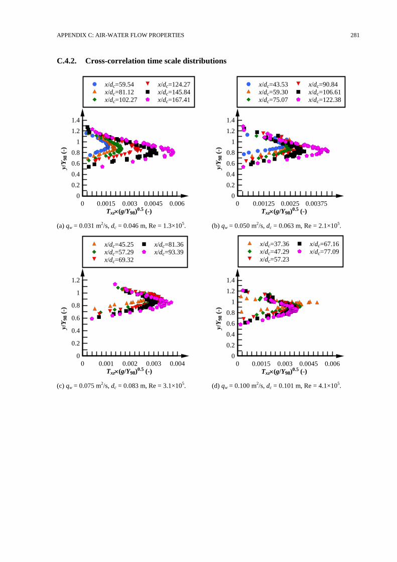
APPENDIX C: AIR-WATER FLOW PROPERTIES 281
C.4.2. Cross-correlation time scale distributions
(a) qw = 0.031 m2/s, dc = 0.046 m, Re = 1.3×10
5. (b) qw = 0.050 m
2/s, dc = 0.063 m, Re = 2.1×10
5.
(c) qw = 0.075 m2/s, dc = 0.083 m, Re = 3.1×10
5. (d) qw = 0.100 m
2/s, dc = 0.101 m, Re = 4.1×10
5.
Txz(g/Y98)0.5 (-)
y/Y
98 (
-)
0 0.0015 0.003 0.0045 0.006
0
0.2
0.4
0.6
0.8
1
1.2
1.4
x/dc=59.54
x/dc=81.12
x/dc=102.27
x/dc=124.27
x/dc=145.84
x/dc=167.41
Txz(g/Y98)0.5 (-)y/
Y98 (
-)
0 0.00125 0.0025 0.00375
0
0.2
0.4
0.6
0.8
1
1.2
1.4
x/dc=43.53
x/dc=59.30
x/dc=75.07
x/dc=90.84
x/dc=106.61
x/dc=122.38
Txz(g/Y98)0.5 (-)
y/Y
98 (
-)
0 0.001 0.002 0.003 0.004
0
0.2
0.4
0.6
0.8
1
1.2
x/dc=45.25
x/dc=57.29
x/dc=69.32
x/dc=81.36
x/dc=93.39
Txz(g/Y98)0.5 (-)
y/Y
98 (
-)
0 0.0015 0.003 0.0045 0.006
0
0.2
0.4
0.6
0.8
1
1.2
1.4
x/dc=37.36
x/dc=47.29
x/dc=57.23
x/dc=67.16
x/dc=77.09
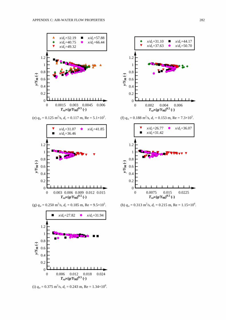
APPENDIX C: AIR-WATER FLOW PROPERTIES 282
(e) qw = 0.125 m2/s, dc = 0.117 m, Re = 5.1×10
5. (f) qw = 0.188 m
2/s, dc = 0.153 m, Re = 7.3×10
5.
(g) qw = 0.250 m2/s, dc = 0.185 m, Re = 9.5×10
5. (h) qw = 0.313 m
2/s, dc = 0.215 m, Re = 1.15×10
6.
(i) qw = 0.375 m2/s, dc = 0.243 m, Re = 1.34×10
6.
Txz(g/Y98)0.5 (-)
y/Y
98 (
-)
0 0.0015 0.003 0.0045 0.006
0
0.2
0.4
0.6
0.8
1
1.2
x/dc=32.19
x/dc=40.75
x/dc=49.32
x/dc=57.88
x/dc=66.44
Txz(g/Y98)0.5 (-)
y/Y
98 (
-)
0 0.002 0.004 0.006
0
0.2
0.4
0.6
0.8
1
1.2
x/dc=31.10
x/dc=37.63
x/dc=44.17
x/dc=50.70
Txz(g/Y98)0.5 (-)
y/Y
98 (
-)
0 0.003 0.006 0.009 0.012 0.015
0
0.2
0.4
0.6
0.8
1
1.2
x/dc=31.07
x/dc=36.46
x/dc=41.85
Txz(g/Y98)0.5 (-)
y/Y
98 (
-)
0 0.0075 0.015 0.0225
0
0.2
0.4
0.6
0.8
1
1.2
x/dc=26.77
x/dc=31.42
x/dc=36.07
Txz(g/Y98)0.5 (-)
y/Y
98 (
-)
0 0.006 0.012 0.018 0.024
0
0.2
0.4
0.6
0.8
1
1.2
x/dc=27.82 x/dc=31.94
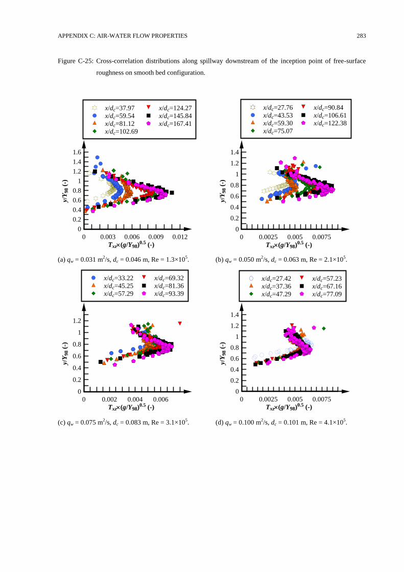
APPENDIX C: AIR-WATER FLOW PROPERTIES 283
Figure C-25: Cross-correlation distributions along spillway downstream of the inception point of free-surface
roughness on smooth bed configuration.
(a) qw = 0.031 m2/s, dc = 0.046 m, Re = 1.3×10
5. (b) qw = 0.050 m
2/s, dc = 0.063 m, Re = 2.1×10
5.
(c) qw = 0.075 m2/s, dc = 0.083 m, Re = 3.1×10
5. (d) qw = 0.100 m
2/s, dc = 0.101 m, Re = 4.1×10
5.
Txz(g/Y98)0.5 (-)
y/Y
98 (
-)
0 0.003 0.006 0.009 0.012
0
0.2
0.4
0.6
0.8
1
1.2
1.4
1.6
x/dc=37.97
x/dc=59.54
x/dc=81.12
x/dc=102.69
x/dc=124.27
x/dc=145.84
x/dc=167.41
Txz(g/Y98)0.5 (-)
y/Y
98 (
-)
0 0.0025 0.005 0.0075
0
0.2
0.4
0.6
0.8
1
1.2
1.4
x/dc=27.76
x/dc=43.53
x/dc=59.30
x/dc=75.07
x/dc=90.84
x/dc=106.61
x/dc=122.38
Txz(g/Y98)0.5 (-)
y/Y
98 (
-)
0 0.002 0.004 0.006
0
0.2
0.4
0.6
0.8
1
1.2
x/dc=33.22
x/dc=45.25
x/dc=57.29
x/dc=69.32
x/dc=81.36
x/dc=93.39
Txz(g/Y98)0.5 (-)
y/Y
98 (
-)
0 0.0025 0.005 0.0075
0
0.2
0.4
0.6
0.8
1
1.2
1.4
x/dc=27.42
x/dc=37.36
x/dc=47.29
x/dc=57.23
x/dc=67.16
x/dc=77.09
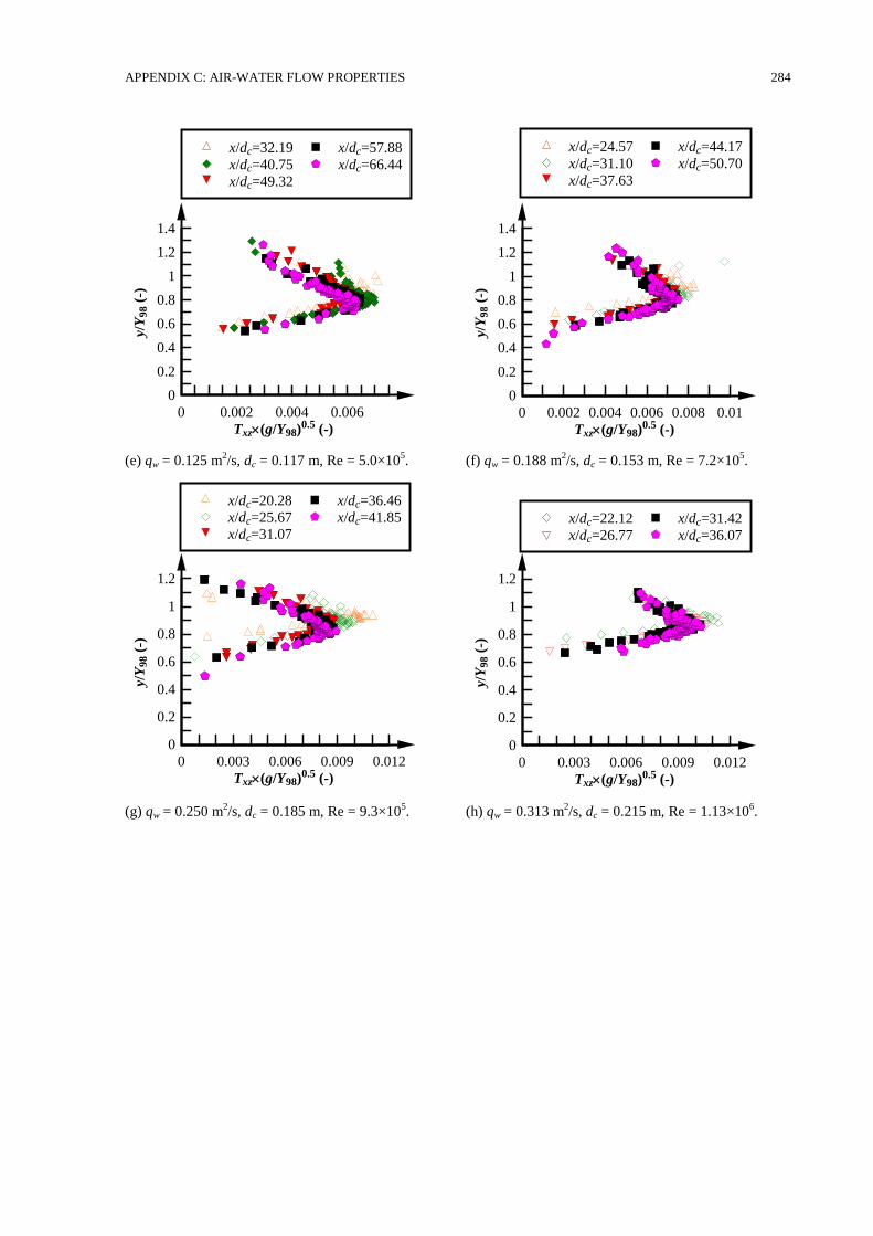
APPENDIX C: AIR-WATER FLOW PROPERTIES 284
(e) qw = 0.125 m2/s, dc = 0.117 m, Re = 5.0×10
5. (f) qw = 0.188 m
2/s, dc = 0.153 m, Re = 7.2×10
5.
(g) qw = 0.250 m2/s, dc = 0.185 m, Re = 9.3×10
5. (h) qw = 0.313 m
2/s, dc = 0.215 m, Re = 1.13×10
6.
Txz(g/Y98)0.5 (-)
y/Y
98 (
-)
0 0.002 0.004 0.006
0
0.2
0.4
0.6
0.8
1
1.2
1.4
x/dc=32.19
x/dc=40.75
x/dc=49.32
x/dc=57.88
x/dc=66.44
Txz(g/Y98)0.5 (-)
y/Y
98 (
-)
0 0.002 0.004 0.006 0.008 0.01
0
0.2
0.4
0.6
0.8
1
1.2
1.4
x/dc=24.57
x/dc=31.10
x/dc=37.63
x/dc=44.17
x/dc=50.70
Txz(g/Y98)0.5 (-)
y/Y
98 (
-)
0 0.003 0.006 0.009 0.012
0
0.2
0.4
0.6
0.8
1
1.2
x/dc=20.28
x/dc=25.67
x/dc=31.07
x/dc=36.46
x/dc=41.85
Txz(g/Y98)0.5 (-)
y/Y
98 (
-)
0 0.003 0.006 0.009 0.012
0
0.2
0.4
0.6
0.8
1
1.2
x/dc=22.12
x/dc=26.77
x/dc=31.42
x/dc=36.07
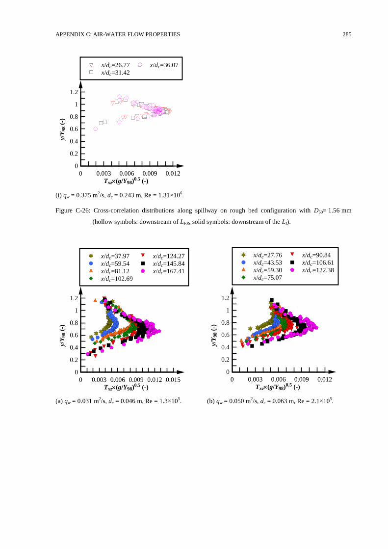
APPENDIX C: AIR-WATER FLOW PROPERTIES 285
(i) qw = 0.375 m2/s, dc = 0.243 m, Re = 1.31×10
6.
Figure C-26: Cross-correlation distributions along spillway on rough bed configuration with D50= 1.56 mm
(hollow symbols: downstream of LFR, solid symbols: downstream of the LI).
(a) qw = 0.031 m2/s, dc = 0.046 m, Re = 1.3×10
5. (b) qw = 0.050 m
2/s, dc = 0.063 m, Re = 2.1×10
5.
Txz(g/Y98)0.5 (-)
y/Y
98 (
-)
0 0.003 0.006 0.009 0.012
0
0.2
0.4
0.6
0.8
1
1.2
x/dc=26.77
x/dc=31.42
x/dc=36.07
Txz(g/Y98)0.5 (-)
y/Y
98 (
-)
0 0.003 0.006 0.009 0.012 0.015
0
0.2
0.4
0.6
0.8
1
1.2
x/dc=37.97
x/dc=59.54
x/dc=81.12
x/dc=102.69
x/dc=124.27
x/dc=145.84
x/dc=167.41
Txz(g/Y98)0.5 (-)
y/Y
98 (
-)
0 0.003 0.006 0.009 0.012
0
0.2
0.4
0.6
0.8
1
1.2
x/dc=27.76
x/dc=43.53
x/dc=59.30
x/dc=75.07
x/dc=90.84
x/dc=106.61
x/dc=122.38
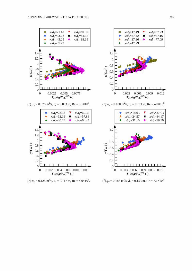
APPENDIX C: AIR-WATER FLOW PROPERTIES 286
(c) qw = 0.075 m2/s, dc = 0.083 m, Re = 3.1×10
5. (d) qw = 0.100 m
2/s, dc = 0.101 m, Re = 4.0×10
5.
(e) qw = 0.125 m2/s, dc = 0.117 m, Re = 4.9×10
5. (f) qw = 0.188 m
2/s, dc = 0.153 m, Re = 7.1×10
5.
Txz(g/Y98)0.5 (-)
y/Y
98 (
-)
0 0.0025 0.005 0.0075
0
0.2
0.4
0.6
0.8
1
1.2
1.4
x/dc=21.18
x/dc=33.22
x/dc=45.25
x/dc=57.29
x/dc=69.32
x/dc=81.36
x/dc=93.39
Txz(g/Y98)0.5 (-)
y/Y
98 (
-)
0 0.003 0.006 0.009 0.012
0
0.2
0.4
0.6
0.8
1
1.2
x/dc=17.49
x/dc=27.42
x/dc=37.36
x/dc=47.29
x/dc=57.23
x/dc=67.16
x/dc=77.09
Txz(g/Y98)0.5 (-)
y/Y
98 (
-)
0 0.002 0.004 0.006 0.008 0.01
0
0.2
0.4
0.6
0.8
1
1.2
1.4
x/dc=23.63
x/dc=32.19
x/dc=40.75
x/dc=49.32
x/dc=57.88
x/dc=66.44
Txz(g/Y98)0.5 (-)
y/Y
98 (
-)
0 0.003 0.006 0.009 0.012 0.015
0
0.2
0.4
0.6
0.8
1
1.2
x/dc=18.03
x/dc=24.57
x/dc=31.10
x/dc=37.63
x/dc=44.17
x/dc=50.70
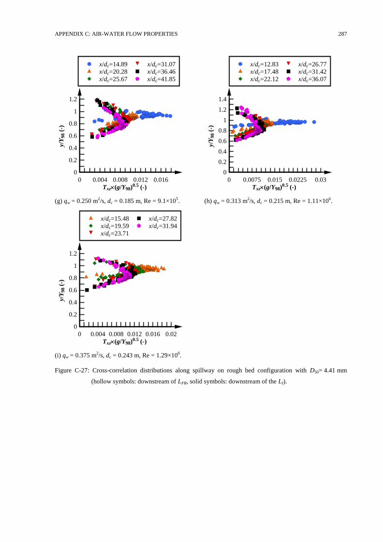
APPENDIX C: AIR-WATER FLOW PROPERTIES 287
(g) qw = 0.250 m2/s, dc = 0.185 m, Re = 9.1×10
5. (h) qw = 0.313 m
2/s, dc = 0.215 m, Re = 1.11×10
6.
(i) qw = 0.375 m2/s, dc = 0.243 m, Re = 1.29×10
6.
Figure C-27: Cross-correlation distributions along spillway on rough bed configuration with D50= 4.41 mm
(hollow symbols: downstream of LFR, solid symbols: downstream of the LI).
Txz(g/Y98)0.5 (-)
y/Y
98 (
-)
0 0.004 0.008 0.012 0.016
0
0.2
0.4
0.6
0.8
1
1.2
x/dc=14.89
x/dc=20.28
x/dc=25.67
x/dc=31.07
x/dc=36.46
x/dc=41.85
Txz(g/Y98)0.5 (-)
y/Y
98 (
-)
0 0.0075 0.015 0.0225 0.03
0
0.2
0.4
0.6
0.8
1
1.2
1.4
x/dc=12.83
x/dc=17.48
x/dc=22.12
x/dc=26.77
x/dc=31.42
x/dc=36.07
Txz(g/Y98)0.5 (-)
y/Y
98 (
-)
0 0.004 0.008 0.012 0.016 0.02
0
0.2
0.4
0.6
0.8
1
1.2
x/dc=15.48
x/dc=19.59
x/dc=23.71
x/dc=27.82
x/dc=31.94
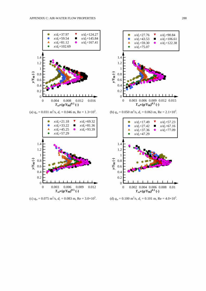
APPENDIX C: AIR-WATER FLOW PROPERTIES 288
(a) qw = 0.031 m2/s, dc = 0.046 m, Re = 1.3×10
5. (b) qw = 0.050 m
2/s, dc = 0.063 m, Re = 2.1×10
5.
(c) qw = 0.075 m2/s, dc = 0.083 m, Re = 3.0×10
5. (d) qw = 0.100 m
2/s, dc = 0.101 m, Re = 4.0×10
5.
Txz(g/Y98)0.5 (-)
y/Y
98 (
-)
0 0.004 0.008 0.012 0.016
0
0.2
0.4
0.6
0.8
1
1.2
1.4
x/dc=37.97
x/dc=59.54
x/dc=81.12
x/dc=102.69
x/dc=124.27
x/dc=145.84
x/dc=167.41
Txz(g/Y98)0.5 (-)
y/Y
98 (
-)
0 0.003 0.006 0.009 0.012 0.015
0
0.2
0.4
0.6
0.8
1
1.2
1.4
x/dc=27.76
x/dc=43.53
x/dc=59.30
x/dc=75.07
x/dc=90.84
x/dc=106.61
x/dc=122.38
Txz(g/Y98)0.5 (-)
y/Y
98 (
-)
0 0.003 0.006 0.009 0.012
0
0.2
0.4
0.6
0.8
1
1.2
1.4
x/dc=21.18
x/dc=33.22
x/dc=45.25
x/dc=57.29
x/dc=69.32
x/dc=81.36
x/dc=93.39
Txz(g/Y98)0.5 (-)
y/Y
98 (
-)
0 0.002 0.004 0.006 0.008 0.01
0
0.2
0.4
0.6
0.8
1
1.2
1.4
x/dc=17.49
x/dc=27.42
x/dc=37.36
x/dc=47.29
x/dc=57.23
x/dc=67.16
x/dc=77.09
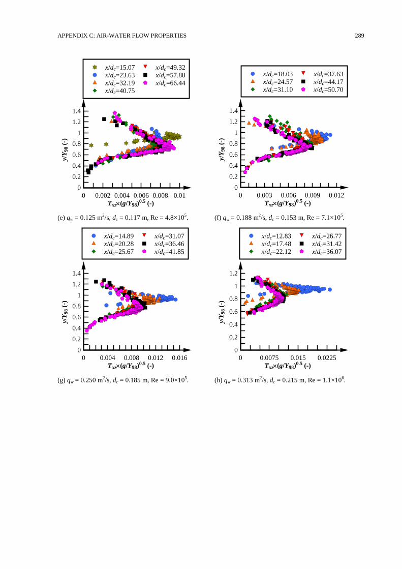
APPENDIX C: AIR-WATER FLOW PROPERTIES 289
(e) qw = 0.125 m2/s, dc = 0.117 m, Re = 4.8×10
5. (f) qw = 0.188 m
2/s, dc = 0.153 m, Re = 7.1×10
5.
(g) qw = 0.250 m2/s, dc = 0.185 m, Re = 9.0×10
5. (h) qw = 0.313 m
2/s, dc = 0.215 m, Re = 1.1×10
6.
Txz(g/Y98)0.5 (-)
y/Y
98 (
-)
0 0.002 0.004 0.006 0.008 0.01
0
0.2
0.4
0.6
0.8
1
1.2
1.4
x/dc=15.07
x/dc=23.63
x/dc=32.19
x/dc=40.75
x/dc=49.32
x/dc=57.88
x/dc=66.44
Txz(g/Y98)0.5 (-)
y/Y
98 (
-)
0 0.003 0.006 0.009 0.012
0
0.2
0.4
0.6
0.8
1
1.2
1.4
x/dc=18.03
x/dc=24.57
x/dc=31.10
x/dc=37.63
x/dc=44.17
x/dc=50.70
Txz(g/Y98)0.5 (-)
y/Y
98 (
-)
0 0.004 0.008 0.012 0.016
0
0.2
0.4
0.6
0.8
1
1.2
1.4
x/dc=14.89
x/dc=20.28
x/dc=25.67
x/dc=31.07
x/dc=36.46
x/dc=41.85
Txz(g/Y98)0.5 (-)
y/Y
98 (
-)
0 0.0075 0.015 0.0225
0
0.2
0.4
0.6
0.8
1
1.2
x/dc=12.83
x/dc=17.48
x/dc=22.12
x/dc=26.77
x/dc=31.42
x/dc=36.07
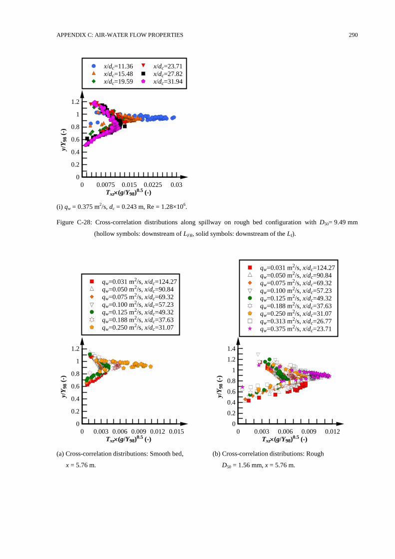
APPENDIX C: AIR-WATER FLOW PROPERTIES 290
(i) qw = 0.375 m2/s, dc = 0.243 m, Re = 1.28×10
6.
Figure C-28: Cross-correlation distributions along spillway on rough bed configuration with D50= 9.49 mm
(hollow symbols: downstream of LFR, solid symbols: downstream of the LI).
(a) Cross-correlation distributions: Smooth bed,
x = 5.76 m.
(b) Cross-correlation distributions: Rough
D50 = 1.56 mm, x = 5.76 m.
Txz(g/Y98)0.5 (-)
y/Y
98 (
-)
0 0.0075 0.015 0.0225 0.03
0
0.2
0.4
0.6
0.8
1
1.2
x/dc=11.36
x/dc=15.48
x/dc=19.59
x/dc=23.71
x/dc=27.82
x/dc=31.94
Txz(g/Y98)0.5 (-)
y/Y
98 (
-)
0 0.003 0.006 0.009 0.012 0.015
0
0.2
0.4
0.6
0.8
1
1.2
qw=0.031 m2/s, x/dc=124.27
qw=0.050 m2/s, x/dc=90.84
qw=0.075 m2/s, x/dc=69.32
qw=0.100 m2/s, x/dc=57.23
qw=0.125 m2/s, x/dc=49.32
qw=0.188 m2/s, x/dc=37.63
qw=0.250 m2/s, x/dc=31.07
Txz(g/Y98)0.5 (-)
y/Y
98 (
-)
0 0.003 0.006 0.009 0.012
0
0.2
0.4
0.6
0.8
1
1.2
1.4
qw=0.031 m2/s, x/dc=124.27
qw=0.050 m2/s, x/dc=90.84
qw=0.075 m2/s, x/dc=69.32
qw=0.100 m2/s, x/dc=57.23
qw=0.125 m2/s, x/dc=49.32
qw=0.188 m2/s, x/dc=37.63
qw=0.250 m2/s, x/dc=31.07
qw=0.313 m2/s, x/dc=26.77
qw=0.375 m2/s, x/dc=23.71
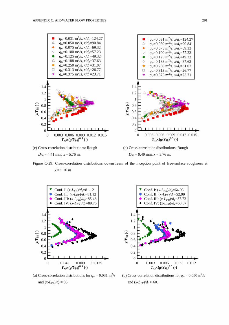
APPENDIX C: AIR-WATER FLOW PROPERTIES 291
(c) Cross-correlation distributions: Rough
D50 = 4.41 mm, x = 5.76 m.
(d) Cross-correlation distributions: Rough
D50 = 9.49 mm, x = 5.76 m.
Figure C-29: Cross-correlation distributions downstream of the inception point of free-surface roughness at
x = 5.76 m.
(a) Cross-correlation distributions for qw = 0.031 m2/s
and (x-LFR)/dc ≈ 85.
(b) Cross-correlation distributions for qw = 0.050 m2/s
and (x-LFR)/dc ≈ 60.
Txz(g/Y98)0.5 (-)
y/Y
98 (
-)
0 0.003 0.006 0.009 0.012 0.015
0
0.2
0.4
0.6
0.8
1
1.2
1.4
qw=0.031 m2/s, x/dc=124.27
qw=0.050 m2/s, x/dc=90.84
qw=0.075 m2/s, x/dc=69.32
qw=0.100 m2/s, x/dc=57.23
qw=0.125 m2/s, x/dc=49.32
qw=0.188 m2/s, x/dc=37.63
qw=0.250 m2/s, x/dc=31.07
qw=0.313 m2/s, x/dc=26.77
qw=0.375 m2/s, x/dc=23.71
Txz(g/Y98)0.5 (-)
y/Y
98 (
-)
0 0.0045 0.009 0.0135
0
0.2
0.4
0.6
0.8
1
1.2
1.4
Conf. I: (x-LFR)/dc=81.12
Conf. II: (x-LFR)/dc=81.12
Conf. III: (x-LFR)/dc=85.43
Conf. IV: (x-LFR)/dc=89.75
Txz(g/Y98)0.5 (-)
y/Y
98 (
-)
0 0.003 0.006 0.009 0.012
0
0.2
0.4
0.6
0.8
1
1.2
1.4
Conf. I: (x-LFR)/dc=64.03
Conf. II: (x-LFR)/dc=52.99
Conf. III: (x-LFR)/dc=57.72
Conf. IV: (x-LFR)/dc=60.87
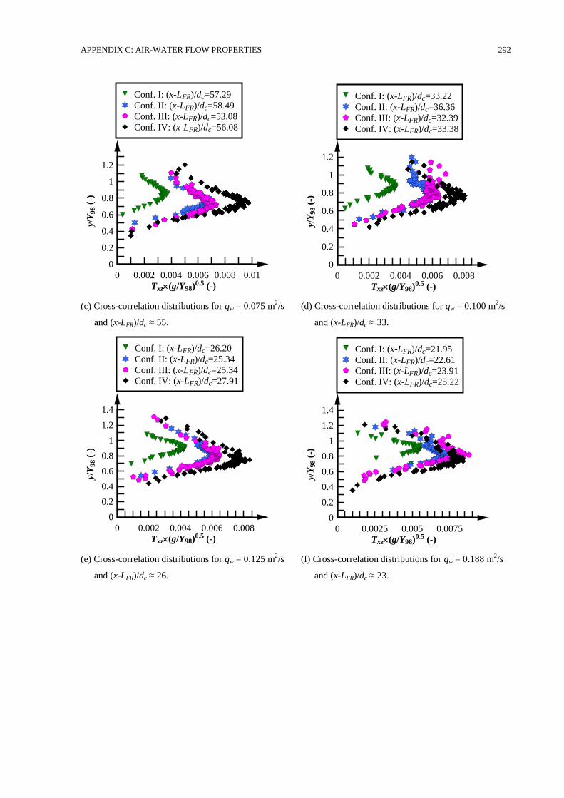
APPENDIX C: AIR-WATER FLOW PROPERTIES 292
(c) Cross-correlation distributions for qw = 0.075 m2/s
and (x-LFR)/dc ≈ 55.
(d) Cross-correlation distributions for qw = 0.100 m2/s
and (x-LFR)/dc ≈ 33.
(e) Cross-correlation distributions for qw = 0.125 m2/s
and (x-LFR)/dc ≈ 26.
(f) Cross-correlation distributions for qw = 0.188 m2/s
and (x-LFR)/dc ≈ 23.
Txz(g/Y98)0.5 (-)
y/Y
98 (
-)
0 0.002 0.004 0.006 0.008 0.01
0
0.2
0.4
0.6
0.8
1
1.2
Conf. I: (x-LFR)/dc=57.29
Conf. II: (x-LFR)/dc=58.49
Conf. III: (x-LFR)/dc=53.08
Conf. IV: (x-LFR)/dc=56.08
Txz(g/Y98)0.5 (-)
y/Y
98 (
-)
0 0.002 0.004 0.006 0.008
0
0.2
0.4
0.6
0.8
1
1.2
Conf. I: (x-LFR)/dc=33.22
Conf. II: (x-LFR)/dc=36.36
Conf. III: (x-LFR)/dc=32.39
Conf. IV: (x-LFR)/dc=33.38
Txz(g/Y98)0.5 (-)
y/Y
98 (
-)
0 0.002 0.004 0.006 0.008
0
0.2
0.4
0.6
0.8
1
1.2
1.4
Conf. I: (x-LFR)/dc=26.20
Conf. II: (x-LFR)/dc=25.34
Conf. III: (x-LFR)/dc=25.34
Conf. IV: (x-LFR)/dc=27.91
Txz(g/Y98)0.5 (-)
y/Y
98 (
-)
0 0.0025 0.005 0.0075
0
0.2
0.4
0.6
0.8
1
1.2
1.4
Conf. I: (x-LFR)/dc=21.95
Conf. II: (x-LFR)/dc=22.61
Conf. III: (x-LFR)/dc=23.91
Conf. IV: (x-LFR)/dc=25.22
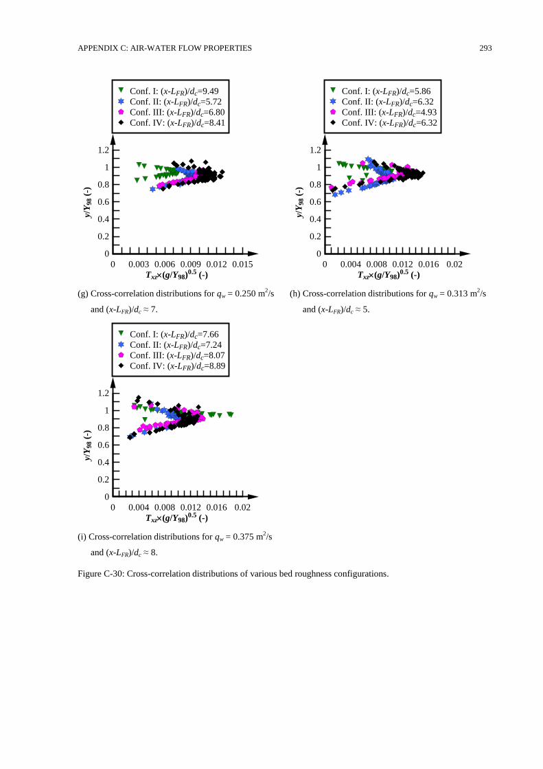
APPENDIX C: AIR-WATER FLOW PROPERTIES 293
(g) Cross-correlation distributions for qw = 0.250 m2/s
and (x-LFR)/dc ≈ 7.
(h) Cross-correlation distributions for qw = 0.313 m2/s
and (x-LFR)/dc ≈ 5.
(i) Cross-correlation distributions for qw = 0.375 m2/s
and (x-LFR)/dc ≈ 8.
Figure C-30: Cross-correlation distributions of various bed roughness configurations.
Txz(g/Y98)0.5 (-)
y/Y
98 (
-)
0 0.003 0.006 0.009 0.012 0.015
0
0.2
0.4
0.6
0.8
1
1.2
Conf. I: (x-LFR)/dc=9.49
Conf. II: (x-LFR)/dc=5.72
Conf. III: (x-LFR)/dc=6.80
Conf. IV: (x-LFR)/dc=8.41
Txz(g/Y98)0.5 (-)
y/Y
98 (
-)
0 0.004 0.008 0.012 0.016 0.02
0
0.2
0.4
0.6
0.8
1
1.2
Conf. I: (x-LFR)/dc=5.86
Conf. II: (x-LFR)/dc=6.32
Conf. III: (x-LFR)/dc=4.93
Conf. IV: (x-LFR)/dc=6.32
Txz(g/Y98)0.5 (-)
y/Y
98 (
-)
0 0.004 0.008 0.012 0.016 0.02
0
0.2
0.4
0.6
0.8
1
1.2
Conf. I: (x-LFR)/dc=7.66
Conf. II: (x-LFR)/dc=7.24
Conf. III: (x-LFR)/dc=8.07
Conf. IV: (x-LFR)/dc=8.89
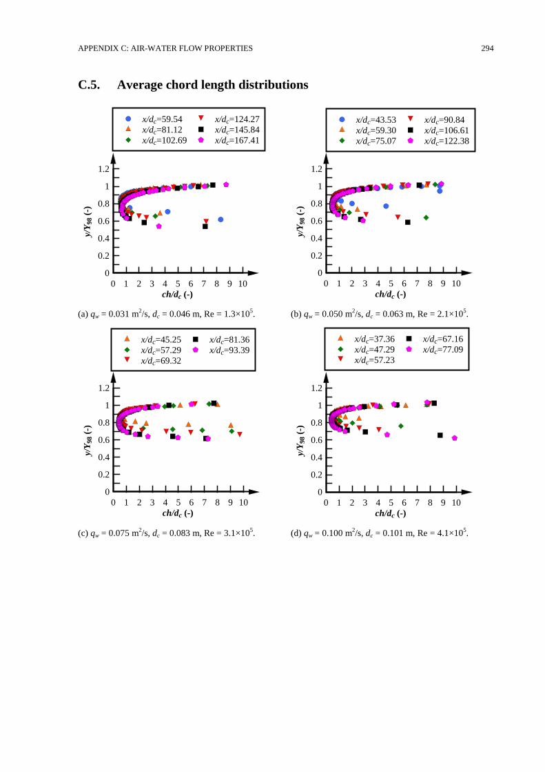
APPENDIX C: AIR-WATER FLOW PROPERTIES 294
C.5. Average chord length distributions
(a) qw = 0.031 m2/s, dc = 0.046 m, Re = 1.3×10
5. (b) qw = 0.050 m
2/s, dc = 0.063 m, Re = 2.1×10
5.
(c) qw = 0.075 m2/s, dc = 0.083 m, Re = 3.1×10
5. (d) qw = 0.100 m
2/s, dc = 0.101 m, Re = 4.1×10
5.
ch/dc (-)
y/Y
98 (
-)
0 1 2 3 4 5 6 7 8 9 10
0
0.2
0.4
0.6
0.8
1
1.2
x/dc=59.54
x/dc=81.12
x/dc=102.69
x/dc=124.27
x/dc=145.84
x/dc=167.41
ch/dc (-)y/
Y98 (
-)
0 1 2 3 4 5 6 7 8 9 10
0
0.2
0.4
0.6
0.8
1
1.2
x/dc=43.53
x/dc=59.30
x/dc=75.07
x/dc=90.84
x/dc=106.61
x/dc=122.38
ch/dc (-)
y/Y
98 (
-)
0 1 2 3 4 5 6 7 8 9 10
0
0.2
0.4
0.6
0.8
1
1.2
x/dc=45.25
x/dc=57.29
x/dc=69.32
x/dc=81.36
x/dc=93.39
ch/dc (-)
y/Y
98 (
-)
0 1 2 3 4 5 6 7 8 9 10
0
0.2
0.4
0.6
0.8
1
1.2
x/dc=37.36
x/dc=47.29
x/dc=57.23
x/dc=67.16
x/dc=77.09
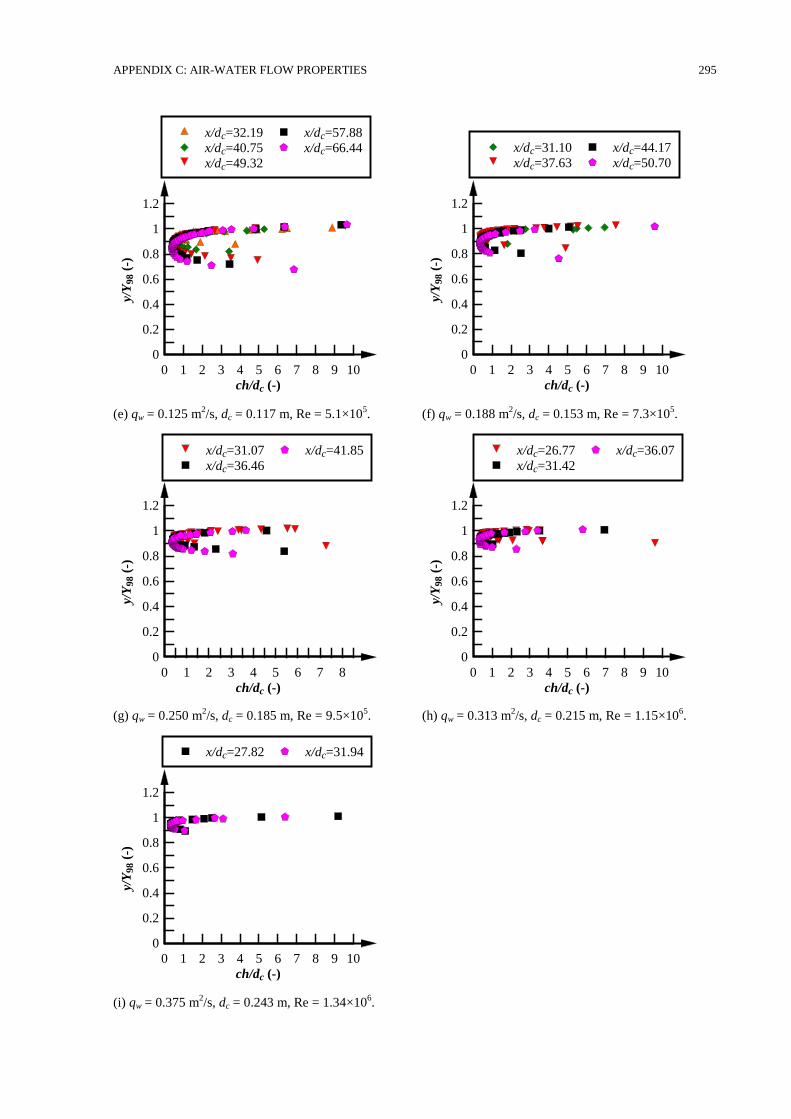
APPENDIX C: AIR-WATER FLOW PROPERTIES 295
(e) qw = 0.125 m2/s, dc = 0.117 m, Re = 5.1×10
5. (f) qw = 0.188 m
2/s, dc = 0.153 m, Re = 7.3×10
5.
(g) qw = 0.250 m2/s, dc = 0.185 m, Re = 9.5×10
5. (h) qw = 0.313 m
2/s, dc = 0.215 m, Re = 1.15×10
6.
(i) qw = 0.375 m2/s, dc = 0.243 m, Re = 1.34×10
6.
ch/dc (-)
y/Y
98 (
-)
0 1 2 3 4 5 6 7 8 9 10
0
0.2
0.4
0.6
0.8
1
1.2
x/dc=32.19
x/dc=40.75
x/dc=49.32
x/dc=57.88
x/dc=66.44
ch/dc (-)
y/Y
98 (
-)
0 1 2 3 4 5 6 7 8 9 10
0
0.2
0.4
0.6
0.8
1
1.2
x/dc=31.10
x/dc=37.63
x/dc=44.17
x/dc=50.70
ch/dc (-)
y/Y
98 (
-)
0 1 2 3 4 5 6 7 8
0
0.2
0.4
0.6
0.8
1
1.2
x/dc=31.07
x/dc=36.46
x/dc=41.85
ch/dc (-)
y/Y
98 (
-)
0 1 2 3 4 5 6 7 8 9 10
0
0.2
0.4
0.6
0.8
1
1.2
x/dc=26.77
x/dc=31.42
x/dc=36.07
ch/dc (-)
y/Y
98 (
-)
0 1 2 3 4 5 6 7 8 9 10
0
0.2
0.4
0.6
0.8
1
1.2
x/dc=27.82 x/dc=31.94
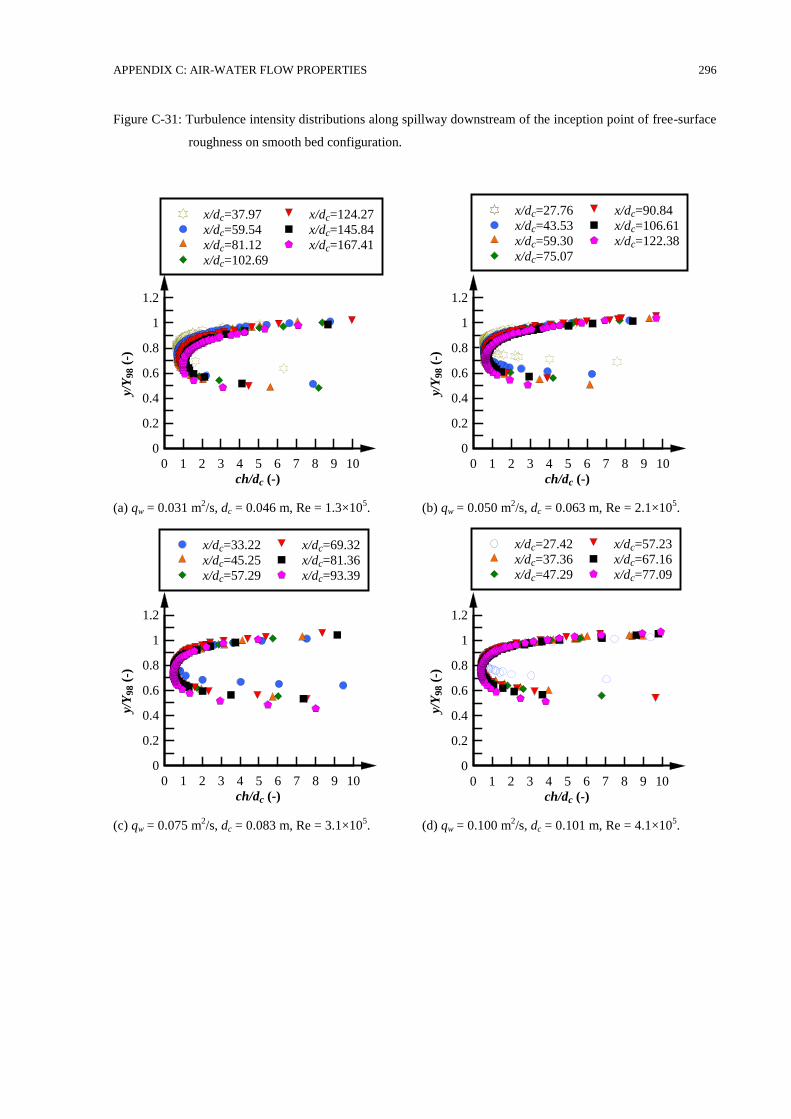
APPENDIX C: AIR-WATER FLOW PROPERTIES 296
Figure C-31: Turbulence intensity distributions along spillway downstream of the inception point of free-surface
roughness on smooth bed configuration.
(a) qw = 0.031 m2/s, dc = 0.046 m, Re = 1.3×10
5. (b) qw = 0.050 m
2/s, dc = 0.063 m, Re = 2.1×10
5.
(c) qw = 0.075 m2/s, dc = 0.083 m, Re = 3.1×10
5. (d) qw = 0.100 m
2/s, dc = 0.101 m, Re = 4.1×10
5.
ch/dc (-)
y/Y
98 (
-)
0 1 2 3 4 5 6 7 8 9 10
0
0.2
0.4
0.6
0.8
1
1.2
x/dc=37.97
x/dc=59.54
x/dc=81.12
x/dc=102.69
x/dc=124.27
x/dc=145.84
x/dc=167.41
ch/dc (-)
y/Y
98 (
-)
0 1 2 3 4 5 6 7 8 9 10
0
0.2
0.4
0.6
0.8
1
1.2
x/dc=27.76
x/dc=43.53
x/dc=59.30
x/dc=75.07
x/dc=90.84
x/dc=106.61
x/dc=122.38
ch/dc (-)
y/Y
98 (
-)
0 1 2 3 4 5 6 7 8 9 10
0
0.2
0.4
0.6
0.8
1
1.2
x/dc=33.22
x/dc=45.25
x/dc=57.29
x/dc=69.32
x/dc=81.36
x/dc=93.39
ch/dc (-)
y/Y
98 (
-)
0 1 2 3 4 5 6 7 8 9 10
0
0.2
0.4
0.6
0.8
1
1.2
x/dc=27.42
x/dc=37.36
x/dc=47.29
x/dc=57.23
x/dc=67.16
x/dc=77.09
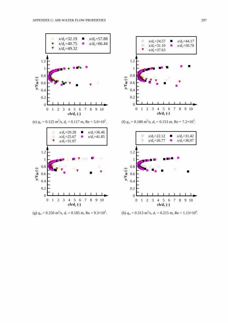
APPENDIX C: AIR-WATER FLOW PROPERTIES 297
(e) qw = 0.125 m2/s, dc = 0.117 m, Re = 5.0×10
5. (f) qw = 0.188 m
2/s, dc = 0.153 m, Re = 7.2×10
5.
(g) qw = 0.250 m2/s, dc = 0.185 m, Re = 9.3×10
5. (h) qw = 0.313 m
2/s, dc = 0.215 m, Re = 1.13×10
6.
ch/dc (-)
y/Y
98 (
-)
0 1 2 3 4 5 6 7 8 9 10
0
0.2
0.4
0.6
0.8
1
1.2
x/dc=32.19
x/dc=40.75
x/dc=49.32
x/dc=57.88
x/dc=66.44
ch/dc (-)
y/Y
98 (
-)
0 1 2 3 4 5 6 7 8 9 10
0
0.2
0.4
0.6
0.8
1
1.2
x/dc=24.57
x/dc=31.10
x/dc=37.63
x/dc=44.17
x/dc=50.70
ch/dc (-)
y/Y
98 (
-)
0 1 2 3 4 5 6 7 8 9 10
0
0.2
0.4
0.6
0.8
1
1.2
x/dc=20.28
x/dc=25.67
x/dc=31.07
x/dc=36.46
x/dc=41.85
ch/dc (-)
y/Y
98 (
-)
0 1 2 3 4 5 6 7 8 9 10
0
0.2
0.4
0.6
0.8
1
1.2
x/dc=22.12
x/dc=26.77
x/dc=31.42
x/dc=36.07
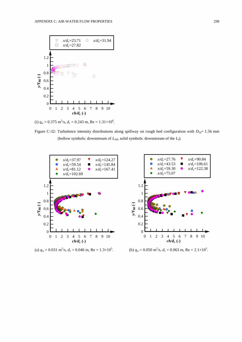
APPENDIX C: AIR-WATER FLOW PROPERTIES 298
(i) qw = 0.375 m2/s, dc = 0.243 m, Re = 1.31×10
6.
Figure C-32: Turbulence intensity distributions along spillway on rough bed configuration with D50= 1.56 mm
(hollow symbols: downstream of LFR, solid symbols: downstream of the LI).
(a) qw = 0.031 m2/s, dc = 0.046 m, Re = 1.3×10
5. (b) qw = 0.050 m
2/s, dc = 0.063 m, Re = 2.1×10
5.
ch/dc (-)
y/Y
98 (
-)
0 1 2 3 4 5 6 7 8 9 10
0
0.2
0.4
0.6
0.8
1
1.2
x/dc=23.71
x/dc=27.82
x/dc=31.94
ch/dc (-)
y/Y
98 (
-)
0 1 2 3 4 5 6 7 8 9 10
0
0.2
0.4
0.6
0.8
1
1.2
x/dc=37.97
x/dc=59.54
x/dc=81.12
x/dc=102.69
x/dc=124.27
x/dc=145.84
x/dc=167.41
ch/dc (-)
y/Y
98 (
-)
0 1 2 3 4 5 6 7 8 9 10
0
0.2
0.4
0.6
0.8
1
1.2
x/dc=27.76
x/dc=43.53
x/dc=59.30
x/dc=75.07
x/dc=90.84
x/dc=106.61
x/dc=122.38
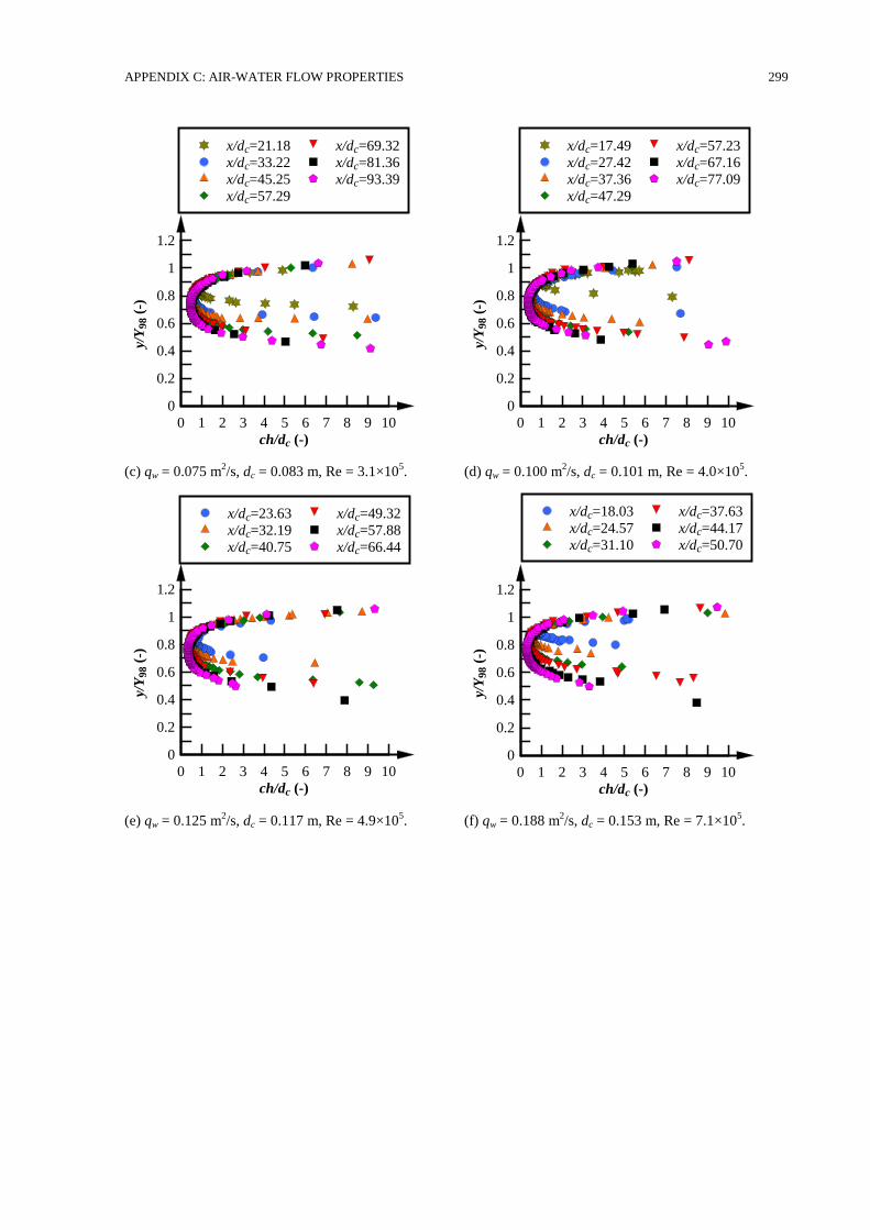
APPENDIX C: AIR-WATER FLOW PROPERTIES 299
(c) qw = 0.075 m2/s, dc = 0.083 m, Re = 3.1×10
5. (d) qw = 0.100 m
2/s, dc = 0.101 m, Re = 4.0×10
5.
(e) qw = 0.125 m2/s, dc = 0.117 m, Re = 4.9×10
5. (f) qw = 0.188 m
2/s, dc = 0.153 m, Re = 7.1×10
5.
ch/dc (-)
y/Y
98 (
-)
0 1 2 3 4 5 6 7 8 9 10
0
0.2
0.4
0.6
0.8
1
1.2
x/dc=21.18
x/dc=33.22
x/dc=45.25
x/dc=57.29
x/dc=69.32
x/dc=81.36
x/dc=93.39
ch/dc (-)
y/Y
98 (
-)
0 1 2 3 4 5 6 7 8 9 10
0
0.2
0.4
0.6
0.8
1
1.2
x/dc=17.49
x/dc=27.42
x/dc=37.36
x/dc=47.29
x/dc=57.23
x/dc=67.16
x/dc=77.09
ch/dc (-)
y/Y
98 (
-)
0 1 2 3 4 5 6 7 8 9 10
0
0.2
0.4
0.6
0.8
1
1.2
x/dc=23.63
x/dc=32.19
x/dc=40.75
x/dc=49.32
x/dc=57.88
x/dc=66.44
ch/dc (-)
y/Y
98 (
-)
0 1 2 3 4 5 6 7 8 9 10
0
0.2
0.4
0.6
0.8
1
1.2
x/dc=18.03
x/dc=24.57
x/dc=31.10
x/dc=37.63
x/dc=44.17
x/dc=50.70
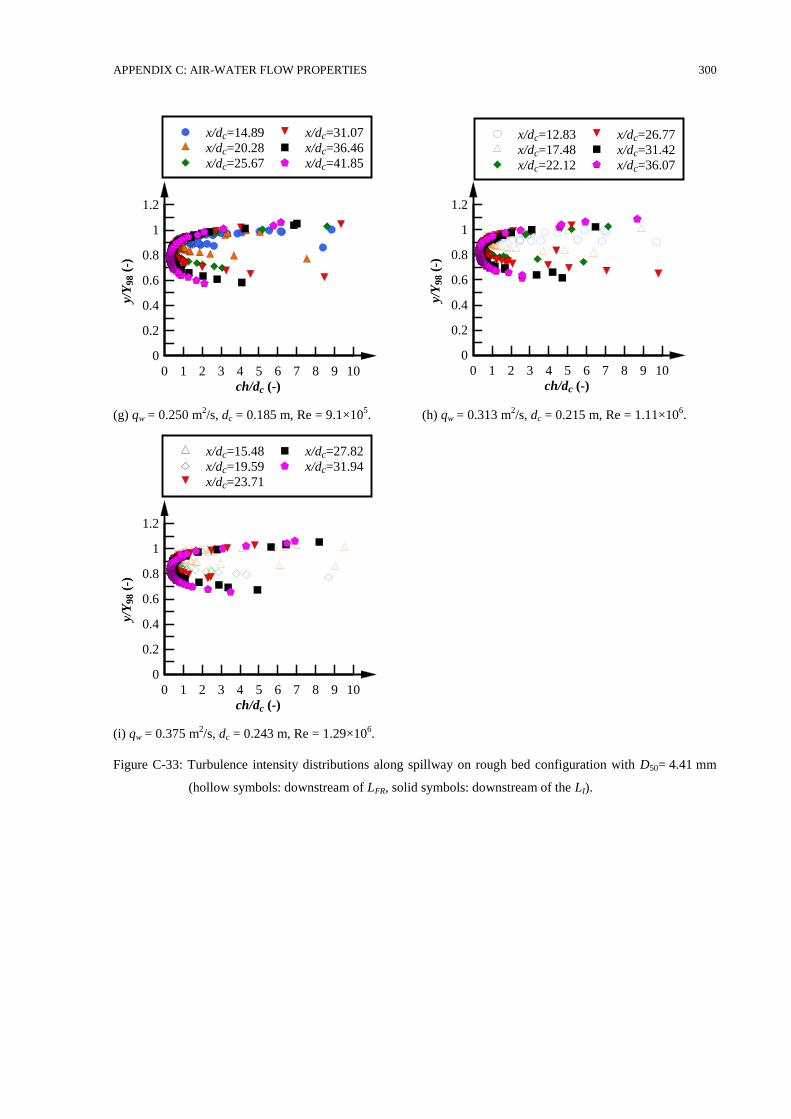
APPENDIX C: AIR-WATER FLOW PROPERTIES 300
(g) qw = 0.250 m2/s, dc = 0.185 m, Re = 9.1×10
5. (h) qw = 0.313 m
2/s, dc = 0.215 m, Re = 1.11×10
6.
(i) qw = 0.375 m2/s, dc = 0.243 m, Re = 1.29×10
6.
Figure C-33: Turbulence intensity distributions along spillway on rough bed configuration with D50= 4.41 mm
(hollow symbols: downstream of LFR, solid symbols: downstream of the LI).
ch/dc (-)
y/Y
98 (
-)
0 1 2 3 4 5 6 7 8 9 10
0
0.2
0.4
0.6
0.8
1
1.2
x/dc=14.89
x/dc=20.28
x/dc=25.67
x/dc=31.07
x/dc=36.46
x/dc=41.85
ch/dc (-)
y/Y
98 (
-)
0 1 2 3 4 5 6 7 8 9 10
0
0.2
0.4
0.6
0.8
1
1.2
x/dc=12.83
x/dc=17.48
x/dc=22.12
x/dc=26.77
x/dc=31.42
x/dc=36.07
ch/dc (-)
y/Y
98 (
-)
0 1 2 3 4 5 6 7 8 9 10
0
0.2
0.4
0.6
0.8
1
1.2
x/dc=15.48
x/dc=19.59
x/dc=23.71
x/dc=27.82
x/dc=31.94
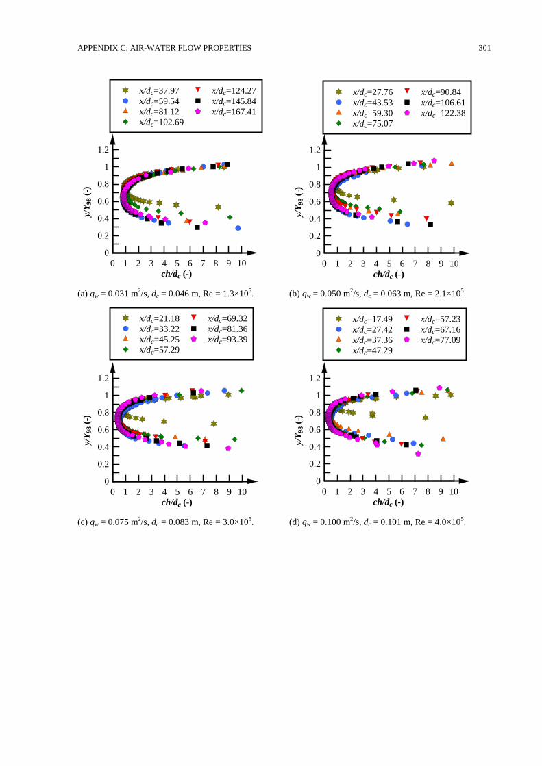
APPENDIX C: AIR-WATER FLOW PROPERTIES 301
(a) qw = 0.031 m2/s, dc = 0.046 m, Re = 1.3×10
5. (b) qw = 0.050 m
2/s, dc = 0.063 m, Re = 2.1×10
5.
(c) qw = 0.075 m2/s, dc = 0.083 m, Re = 3.0×10
5. (d) qw = 0.100 m
2/s, dc = 0.101 m, Re = 4.0×10
5.
ch/dc (-)
y/Y
98 (
-)
0 1 2 3 4 5 6 7 8 9 10
0
0.2
0.4
0.6
0.8
1
1.2
x/dc=37.97
x/dc=59.54
x/dc=81.12
x/dc=102.69
x/dc=124.27
x/dc=145.84
x/dc=167.41
ch/dc (-)
y/Y
98 (
-)
0 1 2 3 4 5 6 7 8 9 10
0
0.2
0.4
0.6
0.8
1
1.2
x/dc=27.76
x/dc=43.53
x/dc=59.30
x/dc=75.07
x/dc=90.84
x/dc=106.61
x/dc=122.38
ch/dc (-)
y/Y
98 (
-)
0 1 2 3 4 5 6 7 8 9 10
0
0.2
0.4
0.6
0.8
1
1.2
x/dc=21.18
x/dc=33.22
x/dc=45.25
x/dc=57.29
x/dc=69.32
x/dc=81.36
x/dc=93.39
ch/dc (-)
y/Y
98 (
-)
0 1 2 3 4 5 6 7 8 9 10
0
0.2
0.4
0.6
0.8
1
1.2
x/dc=17.49
x/dc=27.42
x/dc=37.36
x/dc=47.29
x/dc=57.23
x/dc=67.16
x/dc=77.09
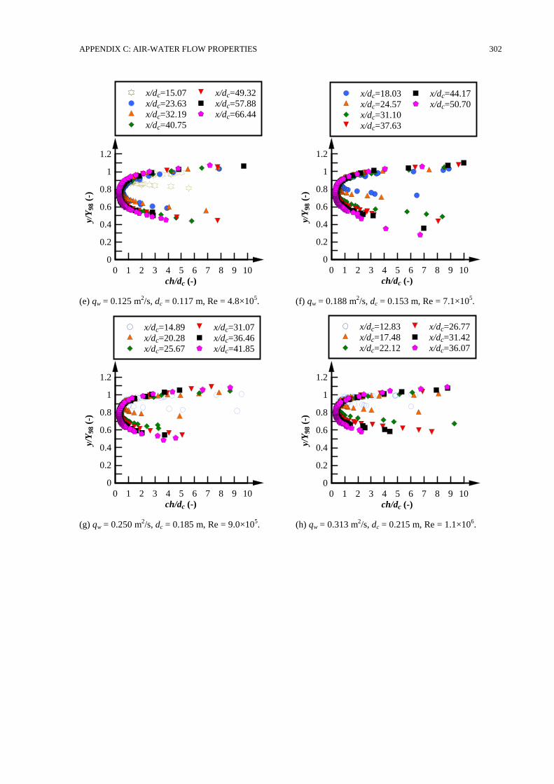
APPENDIX C: AIR-WATER FLOW PROPERTIES 302
(e) qw = 0.125 m2/s, dc = 0.117 m, Re = 4.8×10
5. (f) qw = 0.188 m
2/s, dc = 0.153 m, Re = 7.1×10
5.
(g) qw = 0.250 m2/s, dc = 0.185 m, Re = 9.0×10
5. (h) qw = 0.313 m
2/s, dc = 0.215 m, Re = 1.1×10
6.
ch/dc (-)
y/Y
98 (
-)
0 1 2 3 4 5 6 7 8 9 10
0
0.2
0.4
0.6
0.8
1
1.2
x/dc=15.07
x/dc=23.63
x/dc=32.19
x/dc=40.75
x/dc=49.32
x/dc=57.88
x/dc=66.44
ch/dc (-)
y/Y
98 (
-)
0 1 2 3 4 5 6 7 8 9 10
0
0.2
0.4
0.6
0.8
1
1.2
x/dc=18.03
x/dc=24.57
x/dc=31.10
x/dc=37.63
x/dc=44.17
x/dc=50.70
ch/dc (-)
y/Y
98 (
-)
0 1 2 3 4 5 6 7 8 9 10
0
0.2
0.4
0.6
0.8
1
1.2
x/dc=14.89
x/dc=20.28
x/dc=25.67
x/dc=31.07
x/dc=36.46
x/dc=41.85
ch/dc (-)
y/Y
98 (
-)
0 1 2 3 4 5 6 7 8 9 10
0
0.2
0.4
0.6
0.8
1
1.2
x/dc=12.83
x/dc=17.48
x/dc=22.12
x/dc=26.77
x/dc=31.42
x/dc=36.07
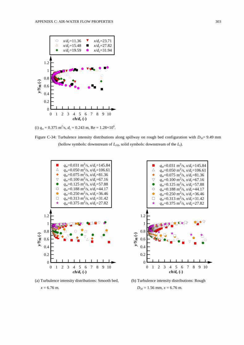
APPENDIX C: AIR-WATER FLOW PROPERTIES 303
(i) qw = 0.375 m2/s, dc = 0.243 m, Re = 1.28×10
6.
Figure C-34: Turbulence intensity distributions along spillway on rough bed configuration with D50= 9.49 mm
(hollow symbols: downstream of LFR, solid symbols: downstream of the LI).
(a) Turbulence intensity distributions: Smooth bed,
x = 6.76 m.
(b) Turbulence intensity distributions: Rough
D50 = 1.56 mm, x = 6.76 m.
ch/dc (-)
y/Y
98 (
-)
0 1 2 3 4 5 6 7 8 9 10
0
0.2
0.4
0.6
0.8
1
1.2
x/dc=11.36
x/dc=15.48
x/dc=19.59
x/dc=23.71
x/dc=27.82
x/dc=31.94
ch/dc (-)
y/Y
98 (
-)
0 1 2 3 4 5 6 7 8 9 10
0
0.2
0.4
0.6
0.8
1
1.2
qw=0.031 m2/s, x/dc=145.84
qw=0.050 m2/s, x/dc=106.61
qw=0.075 m2/s, x/dc=81.36
qw=0.100 m2/s, x/dc=67.16
qw=0.125 m2/s, x/dc=57.88
qw=0.188 m2/s, x/dc=44.17
qw=0.250 m2/s, x/dc=36.46
qw=0.313 m2/s, x/dc=31.42
qw=0.375 m2/s, x/dc=27.82
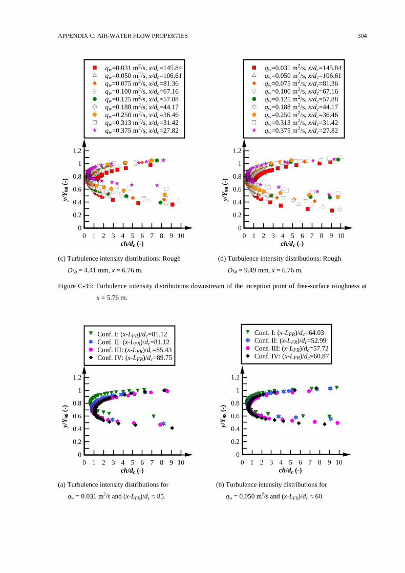
APPENDIX C: AIR-WATER FLOW PROPERTIES 304
(c) Turbulence intensity distributions: Rough
D50 = 4.41 mm, x = 6.76 m.
(d) Turbulence intensity distributions: Rough
D50 = 9.49 mm, x = 6.76 m.
Figure C-35: Turbulence intensity distributions downstream of the inception point of free-surface roughness at
x = 5.76 m.
(a) Turbulence intensity distributions for
qw = 0.031 m2/s and (x-LFR)/dc ≈ 85.
(b) Turbulence intensity distributions for
qw = 0.050 m2/s and (x-LFR)/dc ≈ 60.
ch/dc (-)
y/Y
98 (
-)
0 1 2 3 4 5 6 7 8 9 10
0
0.2
0.4
0.6
0.8
1
1.2
qw=0.031 m2/s, x/dc=145.84
qw=0.050 m2/s, x/dc=106.61
qw=0.075 m2/s, x/dc=81.36
qw=0.100 m2/s, x/dc=67.16
qw=0.125 m2/s, x/dc=57.88
qw=0.188 m2/s, x/dc=44.17
qw=0.250 m2/s, x/dc=36.46
qw=0.313 m2/s, x/dc=31.42
qw=0.375 m2/s, x/dc=27.82
ch/dc (-)
y/Y
98 (
-)
0 1 2 3 4 5 6 7 8 9 10
0
0.2
0.4
0.6
0.8
1
1.2
Conf. I: (x-LFR)/dc=81.12
Conf. II: (x-LFR)/dc=81.12
Conf. III: (x-LFR)/dc=85.43
Conf. IV: (x-LFR)/dc=89.75
ch/dc (-)
y/Y
98 (
-)
0 1 2 3 4 5 6 7 8 9 10
0
0.2
0.4
0.6
0.8
1
1.2
Conf. I: (x-LFR)/dc=64.03
Conf. II: (x-LFR)/dc=52.99
Conf. III: (x-LFR)/dc=57.72
Conf. IV: (x-LFR)/dc=60.87
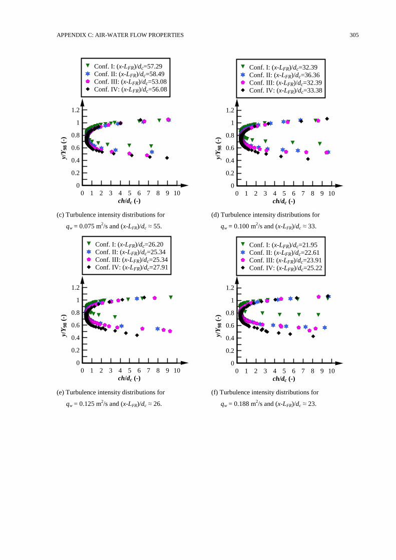
APPENDIX C: AIR-WATER FLOW PROPERTIES 305
(c) Turbulence intensity distributions for
qw = 0.075 m2/s and (x-LFR)/dc ≈ 55.
(d) Turbulence intensity distributions for
qw = 0.100 m2/s and (x-LFR)/dc ≈ 33.
(e) Turbulence intensity distributions for
qw = 0.125 m2/s and (x-LFR)/dc ≈ 26.
(f) Turbulence intensity distributions for
qw = 0.188 m2/s and (x-LFR)/dc ≈ 23.
ch/dc (-)
y/Y
98 (
-)
0 1 2 3 4 5 6 7 8 9 10
0
0.2
0.4
0.6
0.8
1
1.2
Conf. I: (x-LFR)/dc=57.29
Conf. II: (x-LFR)/dc=58.49
Conf. III: (x-LFR)/dc=53.08
Conf. IV: (x-LFR)/dc=56.08
ch/dc (-)
y/Y
98 (
-)
0 1 2 3 4 5 6 7 8 9 10
0
0.2
0.4
0.6
0.8
1
1.2
Conf. I: (x-LFR)/dc=32.39
Conf. II: (x-LFR)/dc=36.36
Conf. III: (x-LFR)/dc=32.39
Conf. IV: (x-LFR)/dc=33.38
ch/dc (-)
y/Y
98 (
-)
0 1 2 3 4 5 6 7 8 9 10
0
0.2
0.4
0.6
0.8
1
1.2
Conf. I: (x-LFR)/dc=26.20
Conf. II: (x-LFR)/dc=25.34
Conf. III: (x-LFR)/dc=25.34
Conf. IV: (x-LFR)/dc=27.91
ch/dc (-)
y/Y
98 (
-)
0 1 2 3 4 5 6 7 8 9 10
0
0.2
0.4
0.6
0.8
1
1.2
Conf. I: (x-LFR)/dc=21.95
Conf. II: (x-LFR)/dc=22.61
Conf. III: (x-LFR)/dc=23.91
Conf. IV: (x-LFR)/dc=25.22
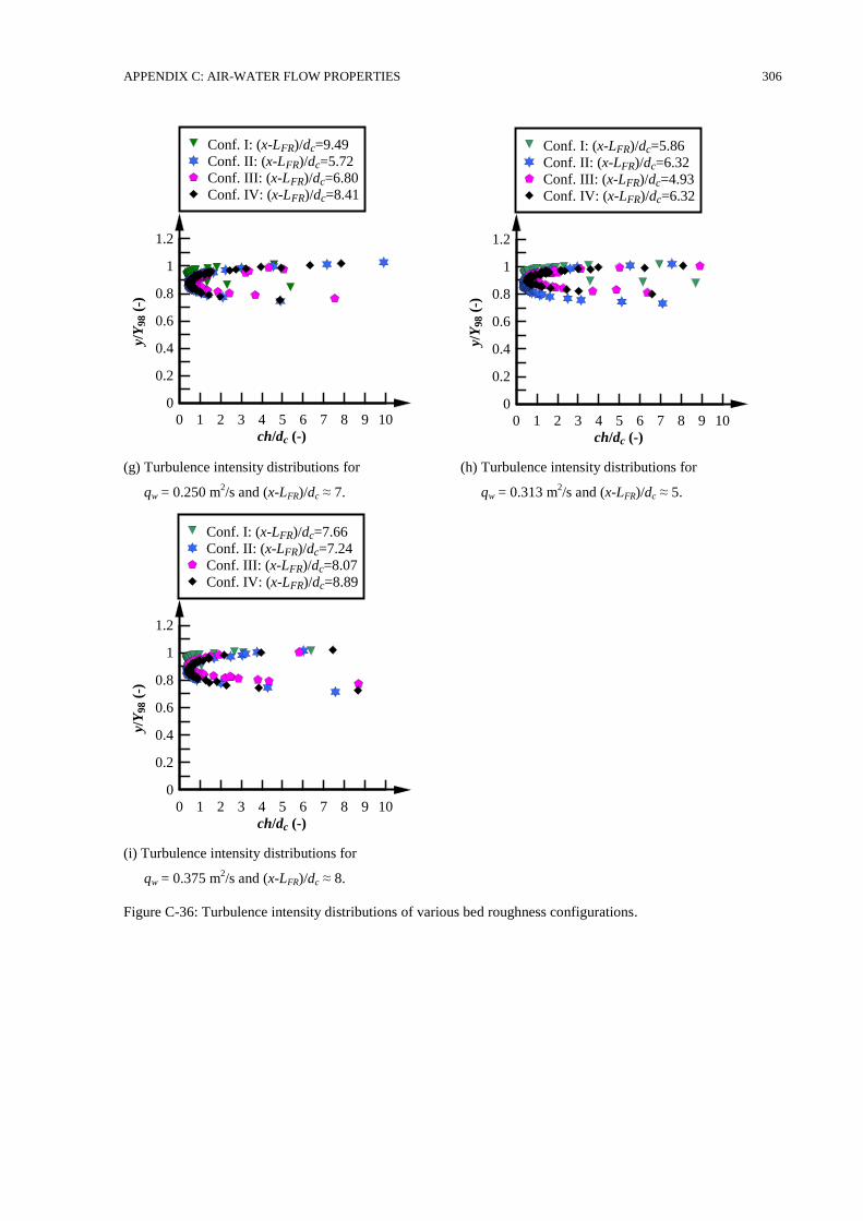
APPENDIX C: AIR-WATER FLOW PROPERTIES 306
(g) Turbulence intensity distributions for
qw = 0.250 m2/s and (x-LFR)/dc ≈ 7.
(h) Turbulence intensity distributions for
qw = 0.313 m2/s and (x-LFR)/dc ≈ 5.
(i) Turbulence intensity distributions for
qw = 0.375 m2/s and (x-LFR)/dc ≈ 8.
Figure C-36: Turbulence intensity distributions of various bed roughness configurations.
ch/dc (-)
y/Y
98 (
-)
0 1 2 3 4 5 6 7 8 9 10
0
0.2
0.4
0.6
0.8
1
1.2
Conf. I: (x-LFR)/dc=9.49
Conf. II: (x-LFR)/dc=5.72
Conf. III: (x-LFR)/dc=6.80
Conf. IV: (x-LFR)/dc=8.41
ch/dc (-)
y/Y
98 (
-)
0 1 2 3 4 5 6 7 8 9 10
0
0.2
0.4
0.6
0.8
1
1.2
Conf. I: (x-LFR)/dc=5.86
Conf. II: (x-LFR)/dc=6.32
Conf. III: (x-LFR)/dc=4.93
Conf. IV: (x-LFR)/dc=6.32
ch/dc (-)
y/Y
98 (
-)
0 1 2 3 4 5 6 7 8 9 10
0
0.2
0.4
0.6
0.8
1
1.2
Conf. I: (x-LFR)/dc=7.66
Conf. II: (x-LFR)/dc=7.24
Conf. III: (x-LFR)/dc=8.07
Conf. IV: (x-LFR)/dc=8.89
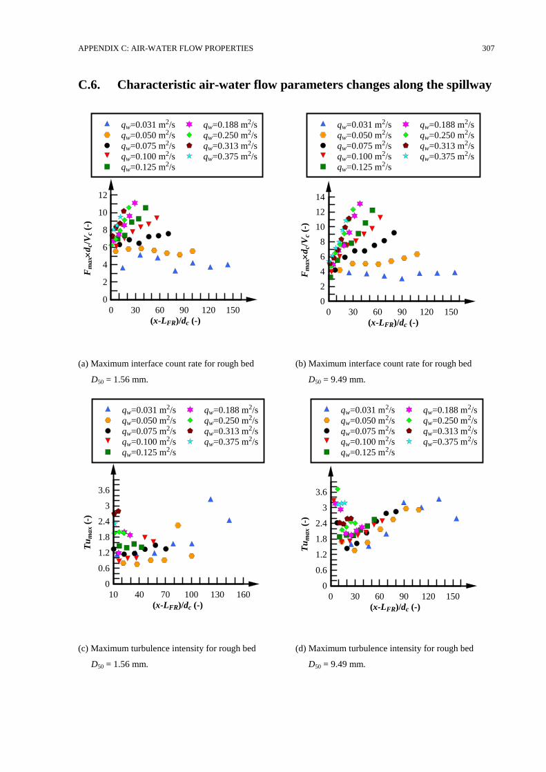
APPENDIX C: AIR-WATER FLOW PROPERTIES 307
C.6. Characteristic air-water flow parameters changes along the spillway
(a) Maximum interface count rate for rough bed
D50 = 1.56 mm.
(b) Maximum interface count rate for rough bed
D50 = 9.49 mm.
(c) Maximum turbulence intensity for rough bed
D50 = 1.56 mm.
(d) Maximum turbulence intensity for rough bed
D50 = 9.49 mm.
(x-LFR)/dc (-)
Fm
ax
dc/
Vc
(-)
0 30 60 90 120 150
0
2
4
6
8
10
12
qw=0.031 m2/s
qw=0.050 m2/s
qw=0.075 m2/s
qw=0.100 m2/s
qw=0.125 m2/s
qw=0.188 m2/s
qw=0.250 m2/s
qw=0.313 m2/s
qw=0.375 m2/s
(x-LFR)/dc (-)
Fm
ax
dc/
Vc
(-)
0 30 60 90 120 150
0
2
4
6
8
10
12
14
qw=0.031 m2/s
qw=0.050 m2/s
qw=0.075 m2/s
qw=0.100 m2/s
qw=0.125 m2/s
qw=0.188 m2/s
qw=0.250 m2/s
qw=0.313 m2/s
qw=0.375 m2/s
(x-LFR)/dc (-)
Tu
ma
x (
-)
10 40 70 100 130 160
0
0.6
1.2
1.8
2.4
3
3.6
qw=0.031 m2/s
qw=0.050 m2/s
qw=0.075 m2/s
qw=0.100 m2/s
qw=0.125 m2/s
qw=0.188 m2/s
qw=0.250 m2/s
qw=0.313 m2/s
qw=0.375 m2/s
(x-LFR)/dc (-)
Tu
ma
x (
-)
0 30 60 90 120 150
0
0.6
1.2
1.8
2.4
3
3.6
qw=0.031 m2/s
qw=0.050 m2/s
qw=0.075 m2/s
qw=0.100 m2/s
qw=0.125 m2/s
qw=0.188 m2/s
qw=0.250 m2/s
qw=0.313 m2/s
qw=0.375 m2/s
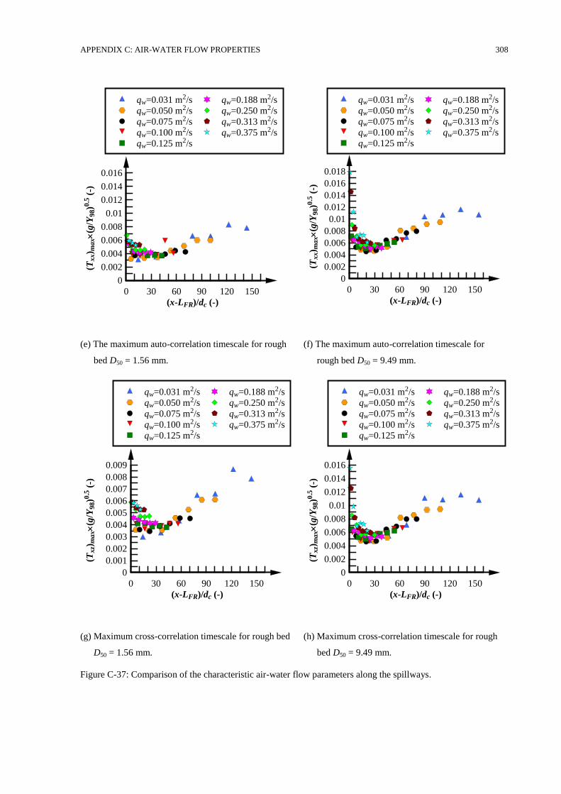
APPENDIX C: AIR-WATER FLOW PROPERTIES 308
(e) The maximum auto-correlation timescale for rough
bed D50 = 1.56 mm.
(f) The maximum auto-correlation timescale for
rough bed D50 = 9.49 mm.
(g) Maximum cross-correlation timescale for rough bed
D50 = 1.56 mm.
(h) Maximum cross-correlation timescale for rough
bed D50 = 9.49 mm.
Figure C-37: Comparison of the characteristic air-water flow parameters along the spillways.
(x-LFR)/dc (-)
(Txx) m
ax
(g/Y
98)0
.5 (
-)
0 30 60 90 120 150
0
0.002
0.004
0.006
0.008
0.01
0.012
0.014
0.016
qw=0.031 m2/s
qw=0.050 m2/s
qw=0.075 m2/s
qw=0.100 m2/s
qw=0.125 m2/s
qw=0.188 m2/s
qw=0.250 m2/s
qw=0.313 m2/s
qw=0.375 m2/s
(x-LFR)/dc (-)
(Txx) m
ax
(g/Y
98)0
.5 (
-)
0 30 60 90 120 150
0
0.002
0.004
0.006
0.008
0.01
0.012
0.014
0.016
0.018
qw=0.031 m2/s
qw=0.050 m2/s
qw=0.075 m2/s
qw=0.100 m2/s
qw=0.125 m2/s
qw=0.188 m2/s
qw=0.250 m2/s
qw=0.313 m2/s
qw=0.375 m2/s
(x-LFR)/dc (-)
(Txz)
max
(g/Y
98)0
.5 (
-)
0 30 60 90 120 150
0
0.001
0.002
0.003
0.004
0.005
0.006
0.007
0.008
0.009
qw=0.031 m2/s
qw=0.050 m2/s
qw=0.075 m2/s
qw=0.100 m2/s
qw=0.125 m2/s
qw=0.188 m2/s
qw=0.250 m2/s
qw=0.313 m2/s
qw=0.375 m2/s
(x-LFR)/dc (-)
(Txz)
max
(g/Y
98)0
.5 (
-)
0 30 60 90 120 150
0
0.002
0.004
0.006
0.008
0.01
0.012
0.014
0.016
qw=0.031 m2/s
qw=0.050 m2/s
qw=0.075 m2/s
qw=0.100 m2/s
qw=0.125 m2/s
qw=0.188 m2/s
qw=0.250 m2/s
qw=0.313 m2/s
qw=0.375 m2/s
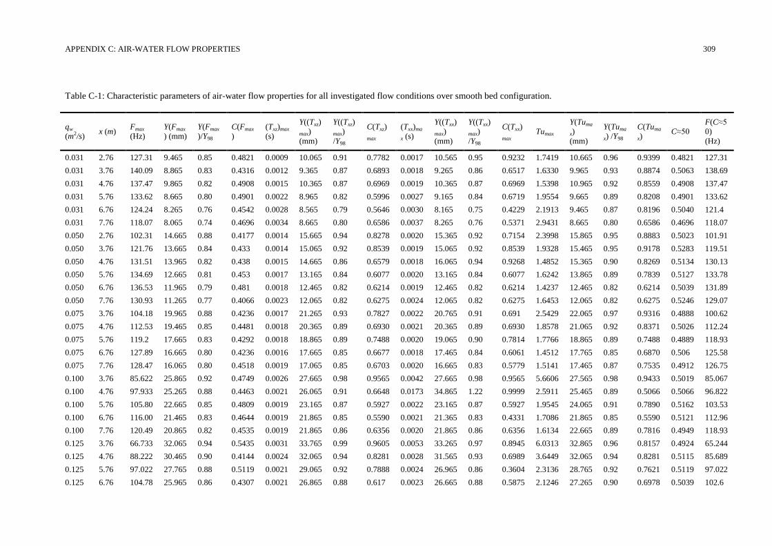
APPENDIX C: AIR-WATER FLOW PROPERTIES 309
Table C-1: Characteristic parameters of air-water flow properties for all investigated flow conditions over smooth bed configuration.
qw
(m2/s) x (m)
Fmax
(Hz)
Y(Fmax
) (mm)
Y(Fmax
)/Y98
C(Fmax
)
(Txz)max
(s)
Y((Txz)
max)
(mm)
Y((Txz)
max)
/Y98
C(Txz)
max
(Txx)ma
x (s)
Y((Txx)
max)
(mm)
Y((Txx)
max)
/Y98
C(Txx)
max Tumax
Y(Tuma
x)
(mm)
Y(Tuma
x) /Y98
C(Tuma
x) C≈50
F(C≈5
0)
(Hz)
0.031 2.76 127.31 9.465 0.85 0.4821 0.0009 10.065 0.91 0.7782 0.0017 10.565 0.95 0.9232 1.7419 10.665 0.96 0.9399 0.4821 127.31
0.031 3.76 140.09 8.865 0.83 0.4316 0.0012 9.365 0.87 0.6893 0.0018 9.265 0.86 0.6517 1.6330 9.965 0.93 0.8874 0.5063 138.69
0.031 4.76 137.47 9.865 0.82 0.4908 0.0015 10.365 0.87 0.6969 0.0019 10.365 0.87 0.6969 1.5398 10.965 0.92 0.8559 0.4908 137.47
0.031 5.76 133.62 8.665 0.80 0.4901 0.0022 8.965 0.82 0.5996 0.0027 9.165 0.84 0.6719 1.9554 9.665 0.89 0.8208 0.4901 133.62
0.031 6.76 124.24 8.265 0.76 0.4542 0.0028 8.565 0.79 0.5646 0.0030 8.165 0.75 0.4229 2.1913 9.465 0.87 0.8196 0.5040 121.4
0.031 7.76 118.07 8.065 0.74 0.4696 0.0034 8.665 0.80 0.6586 0.0037 8.265 0.76 0.5371 2.9431 8.665 0.80 0.6586 0.4696 118.07
0.050 2.76 102.31 14.665 0.88 0.4177 0.0014 15.665 0.94 0.8278 0.0020 15.365 0.92 0.7154 2.3998 15.865 0.95 0.8883 0.5023 101.91
0.050 3.76 121.76 13.665 0.84 0.433 0.0014 15.065 0.92 0.8539 0.0019 15.065 0.92 0.8539 1.9328 15.465 0.95 0.9178 0.5283 119.51
0.050 4.76 131.51 13.965 0.82 0.438 0.0015 14.665 0.86 0.6579 0.0018 16.065 0.94 0.9268 1.4852 15.365 0.90 0.8269 0.5134 130.13
0.050 5.76 134.69 12.665 0.81 0.453 0.0017 13.165 0.84 0.6077 0.0020 13.165 0.84 0.6077 1.6242 13.865 0.89 0.7839 0.5127 133.78
0.050 6.76 136.53 11.965 0.79 0.481 0.0018 12.465 0.82 0.6214 0.0019 12.465 0.82 0.6214 1.4237 12.465 0.82 0.6214 0.5039 131.89
0.050 7.76 130.93 11.265 0.77 0.4066 0.0023 12.065 0.82 0.6275 0.0024 12.065 0.82 0.6275 1.6453 12.065 0.82 0.6275 0.5246 129.07
0.075 3.76 104.18 19.965 0.88 0.4236 0.0017 21.265 0.93 0.7827 0.0022 20.765 0.91 0.691 2.5429 22.065 0.97 0.9316 0.4888 100.62
0.075 4.76 112.53 19.465 0.85 0.4481 0.0018 20.365 0.89 0.6930 0.0021 20.365 0.89 0.6930 1.8578 21.065 0.92 0.8371 0.5026 112.24
0.075 5.76 119.2 17.665 0.83 0.4292 0.0018 18.865 0.89 0.7488 0.0020 19.065 0.90 0.7814 1.7766 18.865 0.89 0.7488 0.4889 118.93
0.075 6.76 127.89 16.665 0.80 0.4236 0.0016 17.665 0.85 0.6677 0.0018 17.465 0.84 0.6061 1.4512 17.765 0.85 0.6870 0.506 125.58
0.075 7.76 128.47 16.065 0.80 0.4518 0.0019 17.065 0.85 0.6703 0.0020 16.665 0.83 0.5779 1.5141 17.465 0.87 0.7535 0.4912 126.75
0.100 3.76 85.622 25.865 0.92 0.4749 0.0026 27.665 0.98 0.9565 0.0042 27.665 0.98 0.9565 5.6606 27.565 0.98 0.9433 0.5019 85.067
0.100 4.76 97.933 25.265 0.88 0.4463 0.0021 26.065 0.91 0.6648 0.0173 34.865 1.22 0.9999 2.5911 25.465 0.89 0.5066 0.5066 96.822
0.100 5.76 105.80 22.665 0.85 0.4809 0.0019 23.165 0.87 0.5927 0.0022 23.165 0.87 0.5927 1.9545 24.065 0.91 0.7890 0.5162 103.53
0.100 6.76 116.00 21.465 0.83 0.4644 0.0019 21.865 0.85 0.5590 0.0021 21.365 0.83 0.4331 1.7086 21.865 0.85 0.5590 0.5121 112.96
0.100 7.76 120.49 20.865 0.82 0.4535 0.0019 21.865 0.86 0.6356 0.0020 21.865 0.86 0.6356 1.6134 22.665 0.89 0.7816 0.4949 118.93
0.125 3.76 66.733 32.065 0.94 0.5435 0.0031 33.765 0.99 0.9605 0.0053 33.265 0.97 0.8945 6.0313 32.865 0.96 0.8157 0.4924 65.244
0.125 4.76 88.222 30.465 0.90 0.4144 0.0024 32.065 0.94 0.8281 0.0028 31.565 0.93 0.6989 3.6449 32.065 0.94 0.8281 0.5115 85.689
0.125 5.76 97.022 27.765 0.88 0.5119 0.0021 29.065 0.92 0.7888 0.0024 26.965 0.86 0.3604 2.3136 28.765 0.92 0.7621 0.5119 97.022
0.125 6.76 104.78 25.965 0.86 0.4307 0.0021 26.865 0.88 0.617 0.0023 26.665 0.88 0.5875 2.1246 27.265 0.90 0.6978 0.5039 102.6
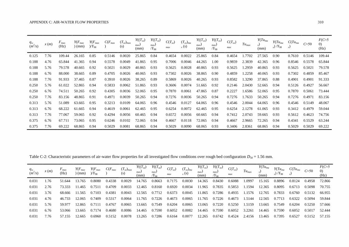
APPENDIX C: AIR-WATER FLOW PROPERTIES 310
qw
(m2/s) x (m)
Fmax
(Hz)
Y(Fmax
) (mm)
Y(Fmax
)/Y98
C(Fmax
)
(Txz)max
(s)
Y((Txz)
max)
(mm)
Y((Txz)
max)
/Y98
C(Txz)
max
(Txx)ma
x (s)
Y((Txx)
max)
(mm)
Y((Txx)
max)
/Y98
C(Txx)
max Tumax
Y(Tuma
x)
(mm)
Y(Tuma
x) /Y98
C(Tuma
x) C≈50
F(C≈5
0)
(Hz)
0.125 7.76 109.44 26.165 0.85 0.5146 0.0020 25.865 0.84 0.4654 0.0022 25.865 0.84 0.4654 1.7702 27.565 0.90 0.7610 0.5146 109.44
0.188 4.76 65.844 41.365 0.94 0.5578 0.0049 41.865 0.95 0.7006 0.0046 44.265 1.00 0.9859 2.3839 42.365 0.96 0.8546 0.5578 65.844
0.188 5.76 79.578 40.665 0.92 0.5021 0.0029 40.865 0.93 0.5625 0.0028 40.865 0.93 0.5625 1.2959 40.865 0.93 0.5625 0.5021 79.578
0.188 6.76 88.000 38.665 0.89 0.4705 0.0026 40.065 0.93 0.7302 0.0026 38.865 0.90 0.4859 1.2258 40.065 0.93 0.7302 0.4859 85.467
0.188 7.76 91.933 37.465 0.87 0.3910 0.0026 38.265 0.89 0.5869 0.0026 40.265 0.93 0.8582 1.3290 37.865 0.88 0.4901 0.4901 91.333
0.250 5.76 61.022 52.865 0.94 0.5833 0.0062 51.865 0.93 0.3606 0.0074 51.665 0.92 0.2146 2.0430 52.665 0.94 0.5126 0.4927 56.667
0.250 6.76 74.511 50.265 0.92 0.4305 0.0036 52.065 0.95 0.7870 0.0061 47.865 0.87 0.2227 1.6586 52.065 0.95 0.7870 0.5061 73.444
0.250 7.76 83.156 48.865 0.91 0.4971 0.0039 50.265 0.94 0.7276 0.0036 50.265 0.94 0.7276 1.7633 50.265 0.94 0.7276 0.4971 83.156
0.313 5.76 51.089 63.665 0.95 0.3213 0.0109 64.065 0.96 0.4546 0.0127 64.065 0.96 0.4546 2.0044 64.065 0.96 0.4546 0.5149 48.067
0.313 6.76 68.222 61.665 0.94 0.4619 0.0061 62.465 0.95 0.6254 0.0072 62.465 0.95 0.6254 2.1278 61.065 0.93 0.3412 0.4979 59.044
0.313 7.76 77.067 59.065 0.92 0.4294 0.0056 60.465 0.94 0.6572 0.0056 60.665 0.94 0.7412 2.0743 59.665 0.93 0.5612 0.4623 74.756
0.375 6.76 67.711 73.065 0.95 0.6246 0.0102 72.065 0.94 0.4667 0.0118 72.065 0.94 0.4667 2.9665 72.265 0.94 0.4341 0.5529 63.244
0.375 7.76 69.222 68.865 0.94 0.5029 0.0081 68.865 0.94 0.5029 0.0090 68.065 0.93 0.3406 2.8361 68.865 0.94 0.5029 0.5029 69.222
Table C-2: Characteristic parameters of air-water flow properties for all investigated flow conditions over rough bed configuration D50 = 1.56 mm.
qw
(m2/s) x (m)
Fmax
(Hz)
Y(Fmax
) (mm)
Y(Fmax
)/Y98
C(Fmax
)
(Txz)max
(s)
Y((Txz)
max)
(mm)
Y((Txz)
max)
/Y98
C(Txz)
max
(Txx)ma
x (s)
Y((Txx)
max)
(mm)
Y((Txx)
max)
/Y98
C(Txx)
max Tumax
Y(Tuma
x)
(mm)
Y(Tuma
x) /Y98
C(Tuma
x) C≈50
F(C≈5
0)
(Hz)
0.031 1.76 51.644 13.765 0.8080 0.4338 0.0029 14.765 0.8663 0.7175 0.0030 14.365 0.8430 0.6088 1.0997 15.165 0.8896 0.8124 0.4958 72.866
0.031 2.76 73.333 11.465 0.7511 0.4709 0.0033 12.465 0.8160 0.6920 0.0034 11.965 0.7835 0.5853 1.1594 12.365 0.8095 0.6713 0.5098 70.755
0.031 3.76 68.666 11.565 0.7103 0.4381 0.0043 12.565 0.7712 0.6373 0.0045 11.865 0.7286 0.4935 1.1576 12.765 0.7833 0.6760 0.5132 66.955
0.031 4.76 46.733 12.065 0.7409 0.5317 0.0064 11.765 0.7226 0.4673 0.0065 11.765 0.7226 0.4673 1.5144 12.565 0.7713 0.6322 0.5094 59.844
0.031 5.76 59.977 12.865 0.7111 0.4767 0.0065 13.665 0.7549 0.6204 0.0065 13.065 0.7220 0.5250 1.5159 13.665 0.7549 0.6204 0.5250 57.666
0.031 6.76 53.066 13.665 0.7174 0.4680 0.0086 14.465 0.7590 0.6052 0.0082 14.465 0.7590 0.6052 3.2261 14.465 0.7590 0.6052 0.5017 52.444
0.031 7.76 57.155 12.665 0.6960 0.5152 0.0078 13.265 0.7286 0.6164 0.0077 12.265 0.6742 0.4524 2.4156 13.465 0.7395 0.6527 0.5152 57.155

APPENDIX C: AIR-WATER FLOW PROPERTIES 311
qw
(m2/s) x (m)
Fmax
(Hz)
Y(Fmax
) (mm)
Y(Fmax
)/Y98
C(Fmax
)
(Txz)max
(s)
Y((Txz)
max)
(mm)
Y((Txz)
max)
/Y98
C(Txz)
max
(Txx)ma
x (s)
Y((Txx)
max)
(mm)
Y((Txx)
max)
/Y98
C(Txx)
max Tumax
Y(Tuma
x)
(mm)
Y(Tuma
x) /Y98
C(Tuma
x) C≈50
F(C≈5
0)
(Hz)
0.050 1.76 68.933 20.665 0.8461 0.4866 0.0036 22.465 0.9195 0.8451 0.0032 22.465 0.9195 0.8451 0.7585 21.665 0.8869 0.7107 0.5017 66.711
0.050 2.76 72.177 18.365 0.7859 0.4739 0.0035 18.865 0.8072 0.5688 0.0034 18.065 0.7732 0.4036 0.7979 17.865 0.7646 0.3766 0.5039 70.800
0.050 3.76 73.000 17.865 0.7543 0.5179 0.0036 18.165 0.7669 0.5776 0.0035 18.165 0.7669 0.5776 0.7606 16.865 0.7123 0.3660 0.4961 72.444
0.050 4.76 70.177 17.865 0.7800 0.5578 0.0046 17.665 0.7713 0.5174 0.0044 17.265 0.7539 0.4505 0.9123 15.865 0.6932 0.2262 0.5174 69.911
0.050 5.76 66.288 17.265 0.7390 0.4467 0.0053 17.065 0.7305 0.4152 0.0051 17.065 0.7305 0.4152 0.9166 17.065 0.7305 0.4152 0.5093 65.133
0.050 6.76 63.933 19.265 0.7422 0.4624 0.0061 20.465 0.7881 0.6456 0.0060 19.465 0.7498 0.5033 2.2483 20.465 0.7881 0.6456 0.5033 63.533
0.050 7.76 69.177 18.865 0.7439 0.5581 0.0061 18.265 0.7203 0.4900 0.0060 18.265 0.7203 0.4900 1.0782 17.465 0.6890 0.3702 0.4900 65.066
0.075 2.76 68.666 25.065 0.8223 0.5218 0.0036 25.365 0.8321 0.5648 0.0037 26.865 0.8811 0.8026 1.3376 26.865 0.8811 0.8026 0.5023 67.488
0.075 3.76 74.644 23.665 0.7594 0.4926 0.0035 23.265 0.7466 0.4277 0.0157 26.065 0.8360 0.7642 1.1440 24.165 0.7753 0.5609 0.5135 69.688
0.075 4.76 70.200 22.965 0.7554 0.4216 0.0039 25.065 0.8241 0.6970 0.0039 25.065 0.8241 0.6970 1.1714 22.665 0.7455 0.3657 0.5131 75.511
0.075 5.76 78.511 24.265 0.7520 0.4518 0.0041 24.665 0.7643 0.4865 0.0039 24.665 0.7643 0.4865 1.3320 24.465 0.7582 0.4605 0.5189 78.311
0.075 6.76 79.622 24.865 0.7439 0.4192 0.0046 26.865 0.8035 0.6384 0.0044 23.665 0.7082 0.2723 1.4875 26.865 0.8035 0.6384 0.5140 77.644
0.075 7.76 82.177 23.265 0.7131 0.4121 0.0045 24.865 0.7619 0.5866 0.0043 23.865 0.7314 0.4771 1.3450 24.865 0.7619 0.5866 0.5071 81.333
0.100 2.76 59.511 32.265 0.8629 0.5348 0.0040 31.665 0.8469 0.4941 0.0039 31.665 0.8469 0.4941 0.8810 31.665 0.8469 0.4941 0.5064 57.088
0.100 3.76 68.311 29.865 0.7793 0.4598 0.0036 30.865 0.8053 0.5524 0.0035 32.265 0.8417 0.7126 0.8385 30.065 0.7845 0.4448 0.5004 68.000
0.100 4.76 75.777 29.065 0.7802 0.4446 0.0039 30.065 0.8069 0.5530 0.0037 30.065 0.8069 0.5530 0.9486 29.665 0.7962 0.5133 0.4919 74.711
0.100 5.76 81.177 30.065 0.7683 0.4313 0.0039 30.265 0.7734 0.4588 0.0037 30.265 0.7734 0.4588 0.9615 31.265 0.7989 0.5756 0.5032 79.111
0.100 6.76 84.466 31.465 0.7827 0.5375 0.0040 30.665 0.7629 0.4511 0.0058 44.865 1.1149 0.9982 1.7508 30.465 0.7579 0.4304 0.5144 83.111
0.100 7.76 91.400 29.265 0.7560 0.5031 0.0040 29.665 0.7663 0.5438 0.0040 28.865 0.7457 0.4651 1.5827 30.065 0.7765 0.5855 0.5031 91.400
0.125 3.76 63.888 35.865 0.8140 0.4921 0.0041 36.865 0.8366 0.6099 0.0044 36.865 0.8366 0.6099 1.4922 36.865 0.8366 0.6099 0.5128 60.800
0.125 4.76 67.533 34.765 0.7912 0.4957 0.0041 34.465 0.7844 0.4671 0.0041 34.465 0.7844 0.4671 1.4587 33.565 0.7640 0.3501 0.4957 71.111
0.125 5.76 81.644 35.865 0.7846 0.4698 0.0038 37.265 0.8151 0.6011 0.0037 37.265 0.8151 0.6011 1.3913 36.665 0.8020 0.5405 0.5117 78.355
0.125 6.76 85.022 35.865 0.7803 0.4977 0.0039 37.465 0.8151 0.6472 0.0038 35.865 0.7803 0.4977 1.5352 36.065 0.7847 0.5191 0.4977 85.022
0.125 7.76 96.555 33.665 0.7487 0.4273 0.0038 34.865 0.7753 0.5426 0.0037 33.065 0.7354 0.3772 1.4077 35.265 0.7842 0.5746 0.4999 91.555
0.188 3.76 54.022 50.265 0.8679 0.4496 0.0046 52.065 0.8989 0.6771 0.0055 57.865 0.9988 0.9794 0.9923 52.065 0.8989 0.6771 0.5036 52.844
0.188 4.76 60.000 48.865 0.8453 0.5219 0.0044 47.865 0.8280 0.4249 0.0043 49.265 0.8522 0.5687 1.1127 48.065 0.8315 0.4226 0.5169 59.733
0.188 5.76 68.377 48.065 0.8082 0.4313 0.0042 47.465 0.7981 0.4038 0.0041 55.865 0.9390 0.9289 1.1890 47.265 0.7947 0.3739 0.5026 67.200
0.188 6.76 76.866 48.265 0.8153 0.5591 0.0041 49.465 0.8355 0.6505 0.0042 48.465 0.8187 0.5664 1.9873 48.665 0.8220 0.5874 0.5094 76.288
0.188 7.76 88.866 45.065 0.7850 0.4416 0.0042 46.265 0.8058 0.5408 0.0042 46.265 0.8058 0.5408 1.8770 46.665 0.8128 0.5626 0.4973 88.844
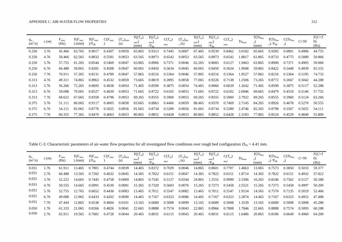
APPENDIX C: AIR-WATER FLOW PROPERTIES 312
qw
(m2/s) x (m)
Fmax
(Hz)
Y(Fmax
) (mm)
Y(Fmax
)/Y98
C(Fmax
)
(Txz)max
(s)
Y((Txz)
max)
(mm)
Y((Txz)
max)
/Y98
C(Txz)
max
(Txx)ma
x (s)
Y((Txx)
max)
(mm)
Y((Txx)
max)
/Y98
C(Txx)
max Tumax
Y(Tuma
x)
(mm)
Y(Tuma
x) /Y98
C(Tuma
x) C≈50
F(C≈5
0)
(Hz)
0.250 3.76 45.466 63.765 0.9017 0.4307 0.0059 65.865 0.9313 0.7445 0.0067 67.465 0.9539 0.8462 3.0182 65.665 0.9285 0.6801 0.4906 44.755
0.250 4.76 50.466 62.565 0.8832 0.5581 0.0053 63.565 0.8973 0.6542 0.0053 63.565 0.8973 0.6542 1.8817 61.865 0.8733 0.4775 0.5080 50.866
0.250 5.76 57.755 61.265 0.8544 0.5469 0.0047 63.865 0.8906 0.7371 0.0046 62.265 0.8683 0.6127 1.9463 63.865 0.8906 0.7371 0.4905 59.066
0.250 6.76 66.488 58.865 0.8281 0.4508 0.0047 60.065 0.8450 0.5634 0.0045 60.065 0.8450 0.5634 1.9948 59.865 0.8422 0.5448 0.4939 65.555
0.250 7.76 76.911 57.265 0.8131 0.4789 0.0047 57.865 0.8216 0.5364 0.0046 57.865 0.8216 0.5364 1.9527 57.865 0.8216 0.5364 0.5195 74.733
0.313 4.76 49.311 74.865 0.8963 0.4532 0.0059 73.665 0.8819 0.2895 0.0058 77.065 0.9226 0.7138 1.2506 73.265 0.8772 0.2667 0.5042 44.288
0.313 5.76 56.266 72.265 0.8695 0.4658 0.0054 71.465 0.8599 0.3875 0.0054 74.465 0.8960 0.6629 1.2642 71.465 0.8599 0.3875 0.5117 52.288
0.313 6.76 59.088 70.065 0.8527 0.4639 0.0053 71.665 0.8722 0.6102 0.0053 71.665 0.8722 0.6102 2.6946 69.665 0.8479 0.4519 0.5146 57.755
0.313 7.76 68.622 67.665 0.8358 0.4796 0.0053 69.265 0.8555 0.5960 0.0053 69.265 0.8555 0.5960 2.7922 69.265 0.8555 0.5960 0.5124 63.266
0.375 5.76 51.111 86.065 0.9117 0.4005 0.0058 83.665 0.8863 0.4460 0.0059 88.465 0.9370 0.7469 2.7145 84.265 0.8926 0.4678 0.5270 50.555
0.375 6.76 54.111 82.065 0.8776 0.5025 0.0056 81.665 0.8734 0.5289 0.0056 81.665 0.8734 0.5289 2.4746 82.265 0.8798 0.5567 0.5025 54.111
0.375 7.76 60.355 77.365 0.8470 0.4063 0.0053 80.865 0.8852 0.6428 0.0053 80.865 0.8852 0.6428 2.3183 77.865 0.8524 0.4529 0.4840 55.800
Table C-3: Characteristic parameters of air-water flow properties for all investigated flow conditions over rough bed configuration D50 = 4.41 mm.
qw
(m2/s) x (m)
Fmax
(Hz)
Y(Fmax
) (mm)
Y(Fmax
)/Y98
C(Fmax
)
(Txz)max
(s)
Y((Txz)
max)
(mm)
Y((Txz)
max)
/Y98
C(Txz)
max
(Txx)ma
x (s)
Y((Txx)
max)
(mm)
Y((Txx)
max)
/Y98
C(Txx)
max Tumax
Y(Tuma
x)
(mm)
Y(Tuma
x) /Y98
C(Tuma
x) C≈50
F(C≈5
0)
(Hz)
0.031 1.76 61.911 13.465 0.7801 0.4744 0.0039 14.465 0.8372 0.7029 0.0046 14.865 0.8601 0.7707 1.4663 13.065 0.7573 0.3850 0.5033 59.377
0.031 2.76 60.488 13.565 0.7392 0.4632 0.0045 14.365 0.7822 0.6151 0.0047 14.365 0.7822 0.6151 1.8714 14.365 0.7822 0.6151 0.4932 57.822
0.031 3.76 52.222 14.665 0.7445 0.4758 0.0069 14.865 0.7545 0.5127 0.0244 24.865 1.2555 0.9999 2.5396 16.265 0.8246 0.7562 0.5127 50.288
0.031 4.76 50.555 14.665 0.6991 0.4530 0.0081 15.365 0.7320 0.5603 0.0076 15.265 0.7273 0.5458 2.5521 15.265 0.7273 0.5458 0.4997 50.200
0.031 5.76 52.755 12.765 0.6652 0.4436 0.0083 13.465 0.7011 0.5547 0.0082 13.465 0.7011 0.5547 1.9154 14.565 0.7576 0.7135 0.5019 52.466
0.031 6.76 49.088 12.965 0.6433 0.4262 0.0090 14.465 0.7167 0.6323 0.0086 14.465 0.7167 0.6323 2.2874 14.465 0.7167 0.6323 0.4952 47.488
0.031 7.76 47.444 12.865 0.6538 0.4604 0.0101 13.165 0.6689 0.5008 0.0099 13.165 0.6689 0.5008 1.3539 13.165 0.6689 0.5008 0.5008 45.288
0.050 1.76 61.333 21.065 0.8266 0.4826 0.0041 22.665 0.8888 0.7574 0.0043 22.865 0.8966 0.7808 1.7846 22.665 0.8888 0.7574 0.5093 60.288
0.050 2.76 65.911 19.565 0.7681 0.4728 0.0044 20.465 0.8031 0.6115 0.0043 20.465 0.8031 0.6115 1.6486 20.865 0.8186 0.6649 0.4960 64.200
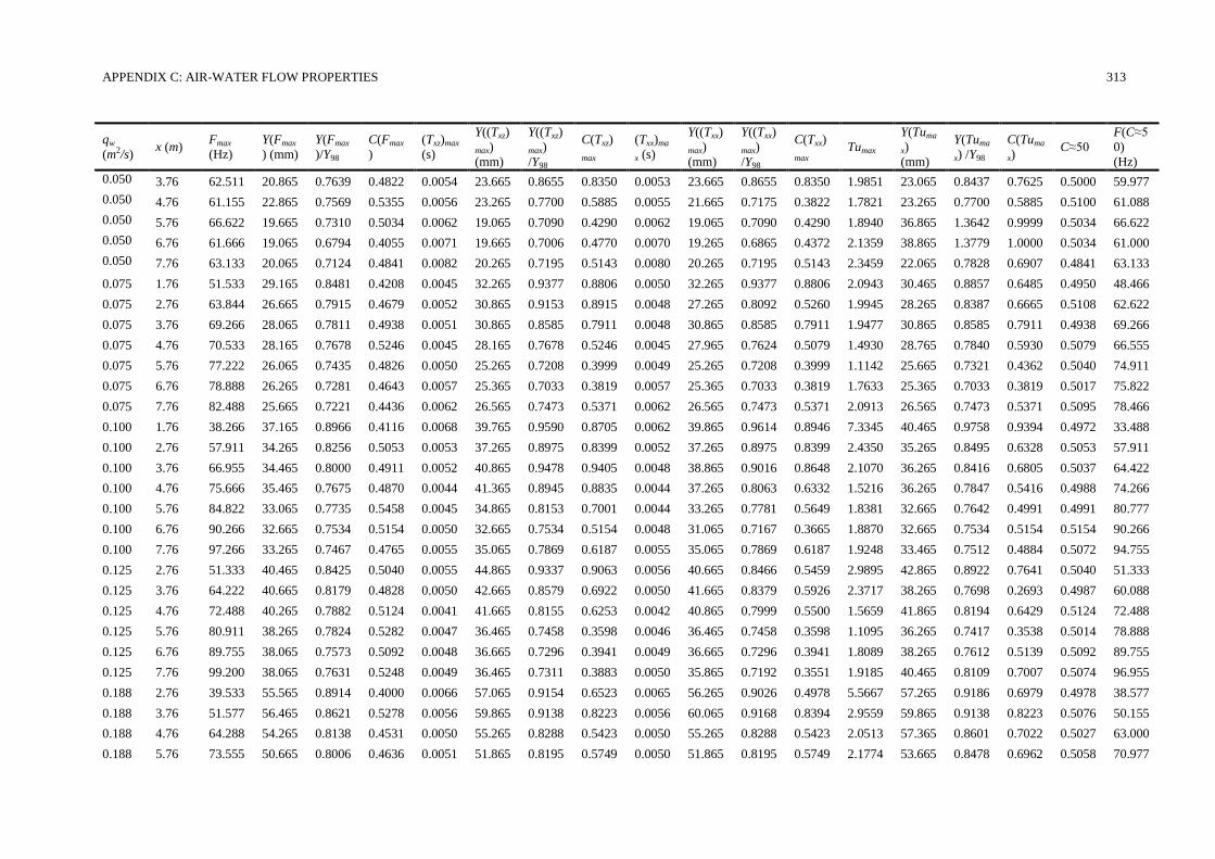
APPENDIX C: AIR-WATER FLOW PROPERTIES 313
qw
(m2/s) x (m)
Fmax
(Hz)
Y(Fmax
) (mm)
Y(Fmax
)/Y98
C(Fmax
)
(Txz)max
(s)
Y((Txz)
max)
(mm)
Y((Txz)
max)
/Y98
C(Txz)
max
(Txx)ma
x (s)
Y((Txx)
max)
(mm)
Y((Txx)
max)
/Y98
C(Txx)
max Tumax
Y(Tuma
x)
(mm)
Y(Tuma
x) /Y98
C(Tuma
x) C≈50
F(C≈5
0)
(Hz)
0.050 3.76 62.511 20.865 0.7639 0.4822 0.0054 23.665 0.8655 0.8350 0.0053 23.665 0.8655 0.8350 1.9851 23.065 0.8437 0.7625 0.5000 59.977
0.050 4.76 61.155 22.865 0.7569 0.5355 0.0056 23.265 0.7700 0.5885 0.0055 21.665 0.7175 0.3822 1.7821 23.265 0.7700 0.5885 0.5100 61.088
0.050 5.76 66.622 19.665 0.7310 0.5034 0.0062 19.065 0.7090 0.4290 0.0062 19.065 0.7090 0.4290 1.8940 36.865 1.3642 0.9999 0.5034 66.622
0.050 6.76 61.666 19.065 0.6794 0.4055 0.0071 19.665 0.7006 0.4770 0.0070 19.265 0.6865 0.4372 2.1359 38.865 1.3779 1.0000 0.5034 61.000
0.050 7.76 63.133 20.065 0.7124 0.4841 0.0082 20.265 0.7195 0.5143 0.0080 20.265 0.7195 0.5143 2.3459 22.065 0.7828 0.6907 0.4841 63.133
0.075 1.76 51.533 29.165 0.8481 0.4208 0.0045 32.265 0.9377 0.8806 0.0050 32.265 0.9377 0.8806 2.0943 30.465 0.8857 0.6485 0.4950 48.466
0.075 2.76 63.844 26.665 0.7915 0.4679 0.0052 30.865 0.9153 0.8915 0.0048 27.265 0.8092 0.5260 1.9945 28.265 0.8387 0.6665 0.5108 62.622
0.075 3.76 69.266 28.065 0.7811 0.4938 0.0051 30.865 0.8585 0.7911 0.0048 30.865 0.8585 0.7911 1.9477 30.865 0.8585 0.7911 0.4938 69.266
0.075 4.76 70.533 28.165 0.7678 0.5246 0.0045 28.165 0.7678 0.5246 0.0045 27.965 0.7624 0.5079 1.4930 28.765 0.7840 0.5930 0.5079 66.555
0.075 5.76 77.222 26.065 0.7435 0.4826 0.0050 25.265 0.7208 0.3999 0.0049 25.265 0.7208 0.3999 1.1142 25.665 0.7321 0.4362 0.5040 74.911
0.075 6.76 78.888 26.265 0.7281 0.4643 0.0057 25.365 0.7033 0.3819 0.0057 25.365 0.7033 0.3819 1.7633 25.365 0.7033 0.3819 0.5017 75.822
0.075 7.76 82.488 25.665 0.7221 0.4436 0.0062 26.565 0.7473 0.5371 0.0062 26.565 0.7473 0.5371 2.0913 26.565 0.7473 0.5371 0.5095 78.466
0.100 1.76 38.266 37.165 0.8966 0.4116 0.0068 39.765 0.9590 0.8705 0.0062 39.865 0.9614 0.8946 7.3345 40.465 0.9758 0.9394 0.4972 33.488
0.100 2.76 57.911 34.265 0.8256 0.5053 0.0053 37.265 0.8975 0.8399 0.0052 37.265 0.8975 0.8399 2.4350 35.265 0.8495 0.6328 0.5053 57.911
0.100 3.76 66.955 34.465 0.8000 0.4911 0.0052 40.865 0.9478 0.9405 0.0048 38.865 0.9016 0.8648 2.1070 36.265 0.8416 0.6805 0.5037 64.422
0.100 4.76 75.666 35.465 0.7675 0.4870 0.0044 41.365 0.8945 0.8835 0.0044 37.265 0.8063 0.6332 1.5216 36.265 0.7847 0.5416 0.4988 74.266
0.100 5.76 84.822 33.065 0.7735 0.5458 0.0045 34.865 0.8153 0.7001 0.0044 33.265 0.7781 0.5649 1.8381 32.665 0.7642 0.4991 0.4991 80.777
0.100 6.76 90.266 32.665 0.7534 0.5154 0.0050 32.665 0.7534 0.5154 0.0048 31.065 0.7167 0.3665 1.8870 32.665 0.7534 0.5154 0.5154 90.266
0.100 7.76 97.266 33.265 0.7467 0.4765 0.0055 35.065 0.7869 0.6187 0.0055 35.065 0.7869 0.6187 1.9248 33.465 0.7512 0.4884 0.5072 94.755
0.125 2.76 51.333 40.465 0.8425 0.5040 0.0055 44.865 0.9337 0.9063 0.0056 40.665 0.8466 0.5459 2.9895 42.865 0.8922 0.7641 0.5040 51.333
0.125 3.76 64.222 40.665 0.8179 0.4828 0.0050 42.665 0.8579 0.6922 0.0050 41.665 0.8379 0.5926 2.3717 38.265 0.7698 0.2693 0.4987 60.088
0.125 4.76 72.488 40.265 0.7882 0.5124 0.0041 41.665 0.8155 0.6253 0.0042 40.865 0.7999 0.5500 1.5659 41.865 0.8194 0.6429 0.5124 72.488
0.125 5.76 80.911 38.265 0.7824 0.5282 0.0047 36.465 0.7458 0.3598 0.0046 36.465 0.7458 0.3598 1.1095 36.265 0.7417 0.3538 0.5014 78.888
0.125 6.76 89.755 38.065 0.7573 0.5092 0.0048 36.665 0.7296 0.3941 0.0049 36.665 0.7296 0.3941 1.8089 38.265 0.7612 0.5139 0.5092 89.755
0.125 7.76 99.200 38.065 0.7631 0.5248 0.0049 36.465 0.7311 0.3883 0.0050 35.865 0.7192 0.3551 1.9185 40.465 0.8109 0.7007 0.5074 96.955
0.188 2.76 39.533 55.565 0.8914 0.4000 0.0066 57.065 0.9154 0.6523 0.0065 56.265 0.9026 0.4978 5.5667 57.265 0.9186 0.6979 0.4978 38.577
0.188 3.76 51.577 56.465 0.8621 0.5278 0.0056 59.865 0.9138 0.8223 0.0056 60.065 0.9168 0.8394 2.9559 59.865 0.9138 0.8223 0.5076 50.155
0.188 4.76 64.288 54.265 0.8138 0.4531 0.0050 55.265 0.8288 0.5423 0.0050 55.265 0.8288 0.5423 2.0513 57.365 0.8601 0.7022 0.5027 63.000
0.188 5.76 73.555 50.665 0.8006 0.4636 0.0051 51.865 0.8195 0.5749 0.0050 51.865 0.8195 0.5749 2.1774 53.665 0.8478 0.6962 0.5058 70.977
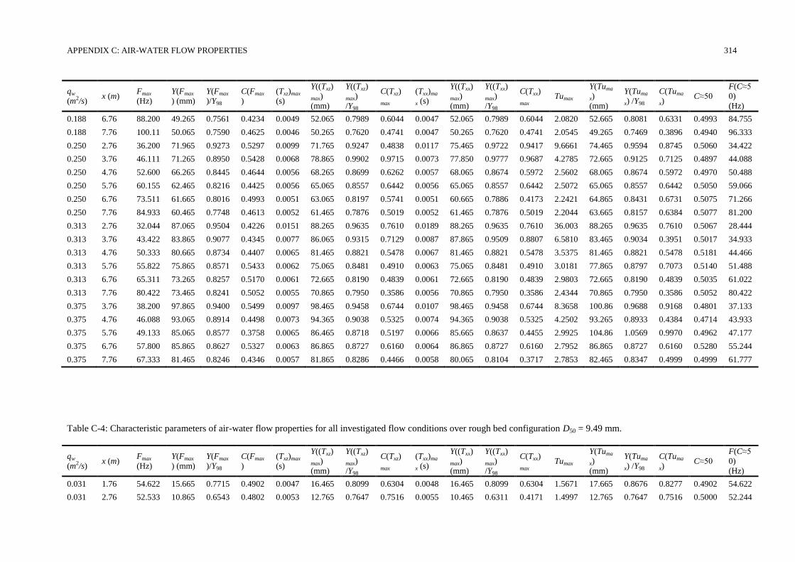
APPENDIX C: AIR-WATER FLOW PROPERTIES 314
qw
(m2/s) x (m)
Fmax
(Hz)
Y(Fmax
) (mm)
Y(Fmax
)/Y98
C(Fmax
)
(Txz)max
(s)
Y((Txz)
max)
(mm)
Y((Txz)
max)
/Y98
C(Txz)
max
(Txx)ma
x (s)
Y((Txx)
max)
(mm)
Y((Txx)
max)
/Y98
C(Txx)
max Tumax
Y(Tuma
x)
(mm)
Y(Tuma
x) /Y98
C(Tuma
x) C≈50
F(C≈5
0)
(Hz)
0.188 6.76 88.200 49.265 0.7561 0.4234 0.0049 52.065 0.7989 0.6044 0.0047 52.065 0.7989 0.6044 2.0820 52.665 0.8081 0.6331 0.4993 84.755
0.188 7.76 100.11 50.065 0.7590 0.4625 0.0046 50.265 0.7620 0.4741 0.0047 50.265 0.7620 0.4741 2.0545 49.265 0.7469 0.3896 0.4940 96.333
0.250 2.76 36.200 71.965 0.9273 0.5297 0.0099 71.765 0.9247 0.4838 0.0117 75.465 0.9722 0.9417 9.6661 74.465 0.9594 0.8745 0.5060 34.422
0.250 3.76 46.111 71.265 0.8950 0.5428 0.0068 78.865 0.9902 0.9715 0.0073 77.850 0.9777 0.9687 4.2785 72.665 0.9125 0.7125 0.4897 44.088
0.250 4.76 52.600 66.265 0.8445 0.4644 0.0056 68.265 0.8699 0.6262 0.0057 68.065 0.8674 0.5972 2.5602 68.065 0.8674 0.5972 0.4970 50.488
0.250 5.76 60.155 62.465 0.8216 0.4425 0.0056 65.065 0.8557 0.6442 0.0056 65.065 0.8557 0.6442 2.5072 65.065 0.8557 0.6442 0.5050 59.066
0.250 6.76 73.511 61.665 0.8016 0.4993 0.0051 63.065 0.8197 0.5741 0.0051 60.665 0.7886 0.4173 2.2421 64.865 0.8431 0.6731 0.5075 71.266
0.250 7.76 84.933 60.465 0.7748 0.4613 0.0052 61.465 0.7876 0.5019 0.0052 61.465 0.7876 0.5019 2.2044 63.665 0.8157 0.6384 0.5077 81.200
0.313 2.76 32.044 87.065 0.9504 0.4226 0.0151 88.265 0.9635 0.7610 0.0189 88.265 0.9635 0.7610 36.003 88.265 0.9635 0.7610 0.5067 28.444
0.313 3.76 43.422 83.865 0.9077 0.4345 0.0077 86.065 0.9315 0.7129 0.0087 87.865 0.9509 0.8807 6.5810 83.465 0.9034 0.3951 0.5017 34.933
0.313 4.76 50.333 80.665 0.8734 0.4407 0.0065 81.465 0.8821 0.5478 0.0067 81.465 0.8821 0.5478 3.5375 81.465 0.8821 0.5478 0.5181 44.466
0.313 5.76 55.822 75.865 0.8571 0.5433 0.0062 75.065 0.8481 0.4910 0.0063 75.065 0.8481 0.4910 3.0181 77.865 0.8797 0.7073 0.5140 51.488
0.313 6.76 65.311 73.265 0.8257 0.5170 0.0061 72.665 0.8190 0.4839 0.0061 72.665 0.8190 0.4839 2.9803 72.665 0.8190 0.4839 0.5035 61.022
0.313 7.76 80.422 73.465 0.8241 0.5052 0.0055 70.865 0.7950 0.3586 0.0056 70.865 0.7950 0.3586 2.4344 70.865 0.7950 0.3586 0.5052 80.422
0.375 3.76 38.200 97.865 0.9400 0.5499 0.0097 98.465 0.9458 0.6744 0.0107 98.465 0.9458 0.6744 8.3658 100.86 0.9688 0.9168 0.4801 37.133
0.375 4.76 46.088 93.065 0.8914 0.4498 0.0073 94.365 0.9038 0.5325 0.0074 94.365 0.9038 0.5325 4.2502 93.265 0.8933 0.4384 0.4714 43.933
0.375 5.76 49.133 85.065 0.8577 0.3758 0.0065 86.465 0.8718 0.5197 0.0066 85.665 0.8637 0.4455 2.9925 104.86 1.0569 0.9970 0.4962 47.177
0.375 6.76 57.800 85.865 0.8627 0.5327 0.0063 86.865 0.8727 0.6160 0.0064 86.865 0.8727 0.6160 2.7952 86.865 0.8727 0.6160 0.5280 55.244
0.375 7.76 67.333 81.465 0.8246 0.4346 0.0057 81.865 0.8286 0.4466 0.0058 80.065 0.8104 0.3717 2.7853 82.465 0.8347 0.4999 0.4999 61.777
Table C-4: Characteristic parameters of air-water flow properties for all investigated flow conditions over rough bed configuration D50 = 9.49 mm.
qw
(m2/s) x (m)
Fmax
(Hz)
Y(Fmax
) (mm)
Y(Fmax
)/Y98
C(Fmax
)
(Txz)max
(s)
Y((Txz)
max)
(mm)
Y((Txz)
max)
/Y98
C(Txz)
max
(Txx)ma
x (s)
Y((Txx)
max)
(mm)
Y((Txx)
max)
/Y98
C(Txx)
max Tumax
Y(Tuma
x)
(mm)
Y(Tuma
x) /Y98
C(Tuma
x) C≈50
F(C≈5
0)
(Hz)
0.031 1.76 54.622 15.665 0.7715 0.4902 0.0047 16.465 0.8099 0.6304 0.0048 16.465 0.8099 0.6304 1.5671 17.665 0.8676 0.8277 0.4902 54.622
0.031 2.76 52.533 10.865 0.6543 0.4802 0.0053 12.765 0.7647 0.7516 0.0055 10.465 0.6311 0.4171 1.4997 12.765 0.7647 0.7516 0.5000 52.244
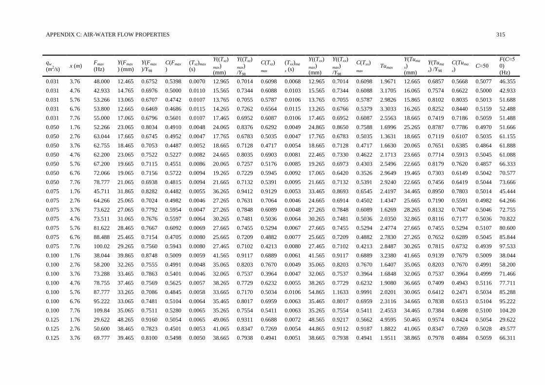
APPENDIX C: AIR-WATER FLOW PROPERTIES 315
qw
(m2/s) x (m)
Fmax
(Hz)
Y(Fmax
) (mm)
Y(Fmax
)/Y98
C(Fmax
)
(Txz)max
(s)
Y((Txz)
max)
(mm)
Y((Txz)
max)
/Y98
C(Txz)
max
(Txx)ma
x (s)
Y((Txx)
max)
(mm)
Y((Txx)
max)
/Y98
C(Txx)
max Tumax
Y(Tuma
x)
(mm)
Y(Tuma
x) /Y98
C(Tuma
x) C≈50
F(C≈5
0)
(Hz)
0.031 3.76 48.000 12.465 0.6752 0.5398 0.0070 12.965 0.7014 0.6098 0.0068 12.965 0.7014 0.6098 1.9671 12.665 0.6857 0.5668 0.5077 46.355
0.031 4.76 42.933 14.765 0.6976 0.5000 0.0110 15.565 0.7344 0.6088 0.0103 15.565 0.7344 0.6088 3.1705 16.065 0.7574 0.6622 0.5000 42.933
0.031 5.76 53.266 13.065 0.6707 0.4742 0.0107 13.765 0.7055 0.5787 0.0106 13.765 0.7055 0.5787 2.9826 15.865 0.8102 0.8035 0.5013 51.688
0.031 6.76 53.800 12.665 0.6469 0.4686 0.0115 14.265 0.7262 0.6564 0.0115 13.265 0.6766 0.5379 3.3033 16.265 0.8252 0.8440 0.5159 52.488
0.031 7.76 55.000 17.065 0.6796 0.5601 0.0107 17.465 0.6952 0.6087 0.0106 17.465 0.6952 0.6087 2.5563 18.665 0.7419 0.7186 0.5059 51.488
0.050 1.76 52.266 23.065 0.8034 0.4910 0.0048 24.065 0.8376 0.6292 0.0049 24.865 0.8650 0.7588 1.6996 25.265 0.8787 0.7786 0.4970 51.666
0.050 2.76 63.044 17.665 0.6745 0.4952 0.0047 17.765 0.6783 0.5035 0.0047 17.765 0.6783 0.5035 1.3631 18.665 0.7119 0.6107 0.5035 61.155
0.050 3.76 62.755 18.465 0.7053 0.4487 0.0052 18.665 0.7128 0.4717 0.0054 18.665 0.7128 0.4717 1.6630 20.065 0.7651 0.6385 0.4864 61.888
0.050 4.76 62.200 23.065 0.7522 0.5227 0.0082 24.665 0.8035 0.6903 0.0081 22.465 0.7330 0.4622 2.1713 23.665 0.7714 0.5913 0.5045 61.088
0.050 5.76 67.200 19.665 0.7115 0.4551 0.0086 20.065 0.7257 0.5176 0.0085 19.265 0.6973 0.4303 2.5496 22.665 0.8179 0.7620 0.4857 66.333
0.050 6.76 72.066 19.065 0.7156 0.5722 0.0094 19.265 0.7229 0.5945 0.0092 17.065 0.6420 0.3526 2.9649 19.465 0.7303 0.6149 0.5042 70.577
0.050 7.76 78.777 21.065 0.6938 0.4815 0.0094 21.665 0.7132 0.5391 0.0095 21.665 0.7132 0.5391 2.9240 22.665 0.7456 0.6419 0.5044 73.666
0.075 1.76 45.711 31.865 0.8282 0.4482 0.0055 36.265 0.9412 0.9129 0.0053 33.465 0.8693 0.6545 2.4197 34.465 0.8950 0.7803 0.5014 45.444
0.075 2.76 64.266 25.065 0.7024 0.4982 0.0046 27.265 0.7631 0.7064 0.0046 24.665 0.6914 0.4502 1.4347 25.665 0.7190 0.5591 0.4982 64.266
0.075 3.76 73.622 27.065 0.7792 0.5954 0.0047 27.265 0.7848 0.6089 0.0048 27.265 0.7848 0.6089 1.6269 28.265 0.8132 0.7047 0.5046 72.755
0.075 4.76 73.511 31.065 0.7676 0.5597 0.0064 30.265 0.7481 0.5036 0.0064 30.265 0.7481 0.5036 2.0350 32.865 0.8116 0.7177 0.5036 70.822
0.075 5.76 81.622 28.465 0.7667 0.6092 0.0069 27.665 0.7455 0.5294 0.0067 27.665 0.7455 0.5294 2.4774 27.665 0.7455 0.5294 0.5107 80.600
0.075 6.76 88.488 25.465 0.7154 0.4705 0.0080 25.665 0.7209 0.4882 0.0077 25.665 0.7209 0.4882 2.7830 27.265 0.7652 0.6289 0.5045 85.844
0.075 7.76 100.02 29.265 0.7560 0.5943 0.0080 27.465 0.7102 0.4213 0.0080 27.465 0.7102 0.4213 2.8487 30.265 0.7815 0.6732 0.4939 97.533
0.100 1.76 38.044 39.865 0.8748 0.5009 0.0059 41.565 0.9117 0.6889 0.0061 41.565 0.9117 0.6889 3.2380 41.665 0.9139 0.7679 0.5009 38.044
0.100 2.76 58.200 32.265 0.7555 0.4991 0.0048 35.065 0.8203 0.7670 0.0049 35.065 0.8203 0.7670 1.6407 35.065 0.8203 0.7670 0.4991 58.200
0.100 3.76 73.288 33.465 0.7863 0.5401 0.0046 32.065 0.7537 0.3964 0.0047 32.065 0.7537 0.3964 1.6848 32.065 0.7537 0.3964 0.4999 71.466
0.100 4.76 78.755 37.465 0.7569 0.5625 0.0057 38.265 0.7729 0.6232 0.0055 38.265 0.7729 0.6232 1.9080 36.665 0.7409 0.4943 0.5116 77.711
0.100 5.76 87.777 33.265 0.7086 0.4845 0.0058 33.665 0.7170 0.5034 0.0106 54.865 1.1633 0.9991 2.0201 30.065 0.6412 0.2471 0.5034 85.288
0.100 6.76 95.222 33.065 0.7481 0.5104 0.0064 35.465 0.8017 0.6959 0.0063 35.465 0.8017 0.6959 2.3116 34.665 0.7838 0.6513 0.5104 95.222
0.100 7.76 109.84 35.065 0.7511 0.5280 0.0065 35.265 0.7554 0.5411 0.0063 35.265 0.7554 0.5411 2.4553 34.465 0.7384 0.4698 0.5100 104.20
0.125 1.76 29.622 48.265 0.9160 0.5054 0.0065 49.065 0.9311 0.6688 0.0072 48.565 0.9217 0.5662 4.9595 50.465 0.9574 0.8424 0.5054 29.622
0.125 2.76 50.600 38.465 0.7823 0.4501 0.0053 41.065 0.8347 0.7269 0.0054 44.865 0.9112 0.9187 1.8822 41.065 0.8347 0.7269 0.5028 49.577
0.125 3.76 69.777 39.465 0.8100 0.5498 0.0050 38.665 0.7938 0.4941 0.0051 38.665 0.7938 0.4941 1.9511 38.865 0.7978 0.4884 0.5059 66.311
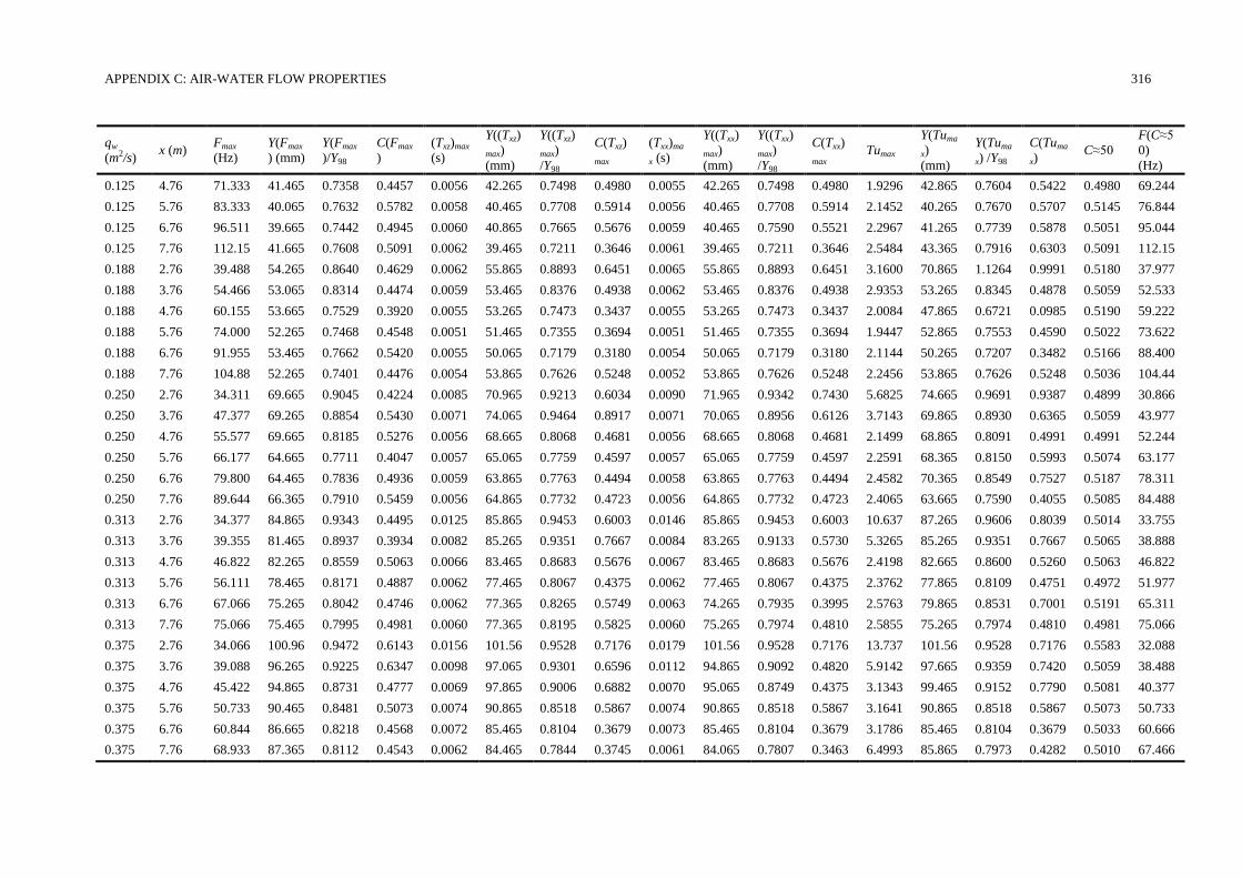
APPENDIX C: AIR-WATER FLOW PROPERTIES 316
qw
(m2/s) x (m)
Fmax
(Hz)
Y(Fmax
) (mm)
Y(Fmax
)/Y98
C(Fmax
)
(Txz)max
(s)
Y((Txz)
max)
(mm)
Y((Txz)
max)
/Y98
C(Txz)
max
(Txx)ma
x (s)
Y((Txx)
max)
(mm)
Y((Txx)
max)
/Y98
C(Txx)
max Tumax
Y(Tuma
x)
(mm)
Y(Tuma
x) /Y98
C(Tuma
x) C≈50
F(C≈5
0)
(Hz)
0.125 4.76 71.333 41.465 0.7358 0.4457 0.0056 42.265 0.7498 0.4980 0.0055 42.265 0.7498 0.4980 1.9296 42.865 0.7604 0.5422 0.4980 69.244
0.125 5.76 83.333 40.065 0.7632 0.5782 0.0058 40.465 0.7708 0.5914 0.0056 40.465 0.7708 0.5914 2.1452 40.265 0.7670 0.5707 0.5145 76.844
0.125 6.76 96.511 39.665 0.7442 0.4945 0.0060 40.865 0.7665 0.5676 0.0059 40.465 0.7590 0.5521 2.2967 41.265 0.7739 0.5878 0.5051 95.044
0.125 7.76 112.15 41.665 0.7608 0.5091 0.0062 39.465 0.7211 0.3646 0.0061 39.465 0.7211 0.3646 2.5484 43.365 0.7916 0.6303 0.5091 112.15
0.188 2.76 39.488 54.265 0.8640 0.4629 0.0062 55.865 0.8893 0.6451 0.0065 55.865 0.8893 0.6451 3.1600 70.865 1.1264 0.9991 0.5180 37.977
0.188 3.76 54.466 53.065 0.8314 0.4474 0.0059 53.465 0.8376 0.4938 0.0062 53.465 0.8376 0.4938 2.9353 53.265 0.8345 0.4878 0.5059 52.533
0.188 4.76 60.155 53.665 0.7529 0.3920 0.0055 53.265 0.7473 0.3437 0.0055 53.265 0.7473 0.3437 2.0084 47.865 0.6721 0.0985 0.5190 59.222
0.188 5.76 74.000 52.265 0.7468 0.4548 0.0051 51.465 0.7355 0.3694 0.0051 51.465 0.7355 0.3694 1.9447 52.865 0.7553 0.4590 0.5022 73.622
0.188 6.76 91.955 53.465 0.7662 0.5420 0.0055 50.065 0.7179 0.3180 0.0054 50.065 0.7179 0.3180 2.1144 50.265 0.7207 0.3482 0.5166 88.400
0.188 7.76 104.88 52.265 0.7401 0.4476 0.0054 53.865 0.7626 0.5248 0.0052 53.865 0.7626 0.5248 2.2456 53.865 0.7626 0.5248 0.5036 104.44
0.250 2.76 34.311 69.665 0.9045 0.4224 0.0085 70.965 0.9213 0.6034 0.0090 71.965 0.9342 0.7430 5.6825 74.665 0.9691 0.9387 0.4899 30.866
0.250 3.76 47.377 69.265 0.8854 0.5430 0.0071 74.065 0.9464 0.8917 0.0071 70.065 0.8956 0.6126 3.7143 69.865 0.8930 0.6365 0.5059 43.977
0.250 4.76 55.577 69.665 0.8185 0.5276 0.0056 68.665 0.8068 0.4681 0.0056 68.665 0.8068 0.4681 2.1499 68.865 0.8091 0.4991 0.4991 52.244
0.250 5.76 66.177 64.665 0.7711 0.4047 0.0057 65.065 0.7759 0.4597 0.0057 65.065 0.7759 0.4597 2.2591 68.365 0.8150 0.5993 0.5074 63.177
0.250 6.76 79.800 64.465 0.7836 0.4936 0.0059 63.865 0.7763 0.4494 0.0058 63.865 0.7763 0.4494 2.4582 70.365 0.8549 0.7527 0.5187 78.311
0.250 7.76 89.644 66.365 0.7910 0.5459 0.0056 64.865 0.7732 0.4723 0.0056 64.865 0.7732 0.4723 2.4065 63.665 0.7590 0.4055 0.5085 84.488
0.313 2.76 34.377 84.865 0.9343 0.4495 0.0125 85.865 0.9453 0.6003 0.0146 85.865 0.9453 0.6003 10.637 87.265 0.9606 0.8039 0.5014 33.755
0.313 3.76 39.355 81.465 0.8937 0.3934 0.0082 85.265 0.9351 0.7667 0.0084 83.265 0.9133 0.5730 5.3265 85.265 0.9351 0.7667 0.5065 38.888
0.313 4.76 46.822 82.265 0.8559 0.5063 0.0066 83.465 0.8683 0.5676 0.0067 83.465 0.8683 0.5676 2.4198 82.665 0.8600 0.5260 0.5063 46.822
0.313 5.76 56.111 78.465 0.8171 0.4887 0.0062 77.465 0.8067 0.4375 0.0062 77.465 0.8067 0.4375 2.3762 77.865 0.8109 0.4751 0.4972 51.977
0.313 6.76 67.066 75.265 0.8042 0.4746 0.0062 77.365 0.8265 0.5749 0.0063 74.265 0.7935 0.3995 2.5763 79.865 0.8531 0.7001 0.5191 65.311
0.313 7.76 75.066 75.465 0.7995 0.4981 0.0060 77.365 0.8195 0.5825 0.0060 75.265 0.7974 0.4810 2.5855 75.265 0.7974 0.4810 0.4981 75.066
0.375 2.76 34.066 100.96 0.9472 0.6143 0.0156 101.56 0.9528 0.7176 0.0179 101.56 0.9528 0.7176 13.737 101.56 0.9528 0.7176 0.5583 32.088
0.375 3.76 39.088 96.265 0.9225 0.6347 0.0098 97.065 0.9301 0.6596 0.0112 94.865 0.9092 0.4820 5.9142 97.665 0.9359 0.7420 0.5059 38.488
0.375 4.76 45.422 94.865 0.8731 0.4777 0.0069 97.865 0.9006 0.6882 0.0070 95.065 0.8749 0.4375 3.1343 99.465 0.9152 0.7790 0.5081 40.377
0.375 5.76 50.733 90.465 0.8481 0.5073 0.0074 90.865 0.8518 0.5867 0.0074 90.865 0.8518 0.5867 3.1641 90.865 0.8518 0.5867 0.5073 50.733
0.375 6.76 60.844 86.665 0.8218 0.4568 0.0072 85.465 0.8104 0.3679 0.0073 85.465 0.8104 0.3679 3.1786 85.465 0.8104 0.3679 0.5033 60.666
0.375 7.76 68.933 87.365 0.8112 0.4543 0.0062 84.465 0.7844 0.3745 0.0061 84.065 0.7807 0.3463 6.4993 85.865 0.7973 0.4282 0.5010 67.466
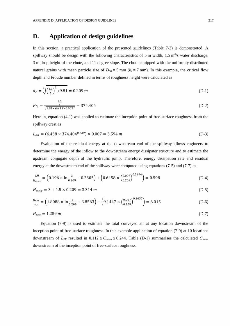
APPENDIX D: APPLICATION OF DESIGN GUIDLINES 317
D. Application of design guidelines
In this section, a practical application of the presented guidelines (Table 7-2) is demonstrated. A
spillway should be design with the following characteristics of 5 m width, 1.5 m3/s water discharge,
3 m drop height of the chute, and 11 degree slope. The chute equipped with the uniformly distributed
natural grains with mean particle size of D50 = 5 mm (ks = 7 mm). In this example, the critical flow
depth and Froude number defined in terms of roughness height were calculated as
𝑑𝑐 = √(1.3
5)
2/9.81
3
= 0.209 𝑚 (D-1)
𝐹𝑟∗ =1.5
5
√9.81×sin 11×0.0073= 374.404 (D-2)
Here in, equation (4-1) was applied to estimate the inception point of free-surface roughness from the
spillway crest as
𝐿𝐹𝑅 = (6.438 × 374.4040.739) × 0.007 = 3.594 𝑚 (D-3)
Evaluation of the residual energy at the downstream end of the spillway allows engineers to
determine the energy of the inflow to the downstream energy dissipater structure and to estimate the
upstream conjugate depth of the hydraulic jump. Therefore, energy dissipation rate and residual
energy at the downstream end of the spillway were computed using equations (7-5) and (7-7) as
∆𝐻
𝐻𝑚𝑎𝑥= (0.196 × ln
3
0.209− 0.2305) + (0.6458 × (
0.007
0.209)
0.2194) = 0.598 (D-4)
𝐻𝑚𝑎𝑥 = 3 + 1.5 × 0.209 = 3.314 𝑚 (D-5)
𝐻𝑟𝑒𝑠
𝑑𝑐= (1.8088 × ln
3
0.209+ 3.8563) − (9.1447 × (
0.007
0.209)
0.3637) = 6.015 (D-6)
𝐻𝑟𝑒𝑠 = 1.259 𝑚 (D-7)
Equation (7-9) is used to estimate the total conveyed air at any location downstream of the
inception point of free-surface roughness. In this example application of equation (7-9) at 10 locations
downstream of LFR resulted in 0.112 ≤ Cmean ≤ 0.244. Table (D-1) summarises the calculated Cmean
downstream of the inception point of free-surface roughness.
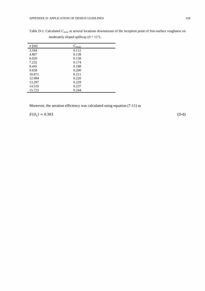
APPENDIX D: APPLICATION OF DESIGN GUIDLINES 318
Table D-1: Calculated Cmean at several locations downstream of the inception point of free-surface roughness on
moderately sloped spillway (θ = 11°).
x (m) Cmean
3.594 0.112
4.807 0.138
6.020 0.158
7.232 0.174
8.445 0.188
9.658 0.200
10.871 0.211
12.084 0.220
13.297 0.229
14.510 0.237
15.723 0.244
Moreover, the aeration efficiency was calculated using equation (7-11) as
𝐸(𝑂2) = 0.383 (D-8)