advances in science, technology & engineering systems
TRANSCRIPT

Advances in Science, Technology &Engineering Systems Journal
V O L U M E 2 - I S S U E 5 | S E P T - O C T 2 0 1 7
www.astesj.comISSN: 2415-6698

EDITORIAL BOARD Editor-in-Chief
Prof. Passerini Kazmerski University of Chicago, USA
Editorial Board Members
Prof. Rehan Ullah Khan Qassim University, Saudi Arabia
Prof. María Jesús Espinosa Universidad Tecnológica Metropolitana, Mexico
Dr. Hongbo Du Prairie View A&M University, USA
Dr. Nguyen Tung Linh Electric Power University, Vietnam
Tariq Kamal University of Nottingham, UK
Sakarya University, Turkey
Dr. Mohmaed Abdel Fattah Ashabrawy Prince Sattam bin Abdulaziz University, Saudi Arabia
Mohamed Mohamed Abdel-Daim Suez Canal University, Egypt
Dr. Omeje Maxwell Covenant University, Nigeria
Prof. Majida Ali Abed Meshari Tikrit University Campus, Iraq
Dr. Heba Afify MTI university, Cairo, Egypt
Regional Editors
Dr. Hung-Wei Wu Kun Shan University, Taiwan
Dr. Maryam Asghari Shahid Ashrafi Esfahani, Iran
Dr. Shakir Ali Aligarh Muslim University, India
Dr. Ahmet Kayabasi Karamanoglu Mehmetbey University, Turkey
Dr. Ebubekir Altuntas Gaziosmanpasa University, Turkey
Dr. Sabry Ali Abdallah El-Naggar Tanta University, Egypt
Dr. Shagufta Haneef Aalborg University, Denmark
Dr. Gomathi Periasamy Mekelle University, Ethiopia
Dr. Walid Wafik Mohamed Badawy National Organization for Drug Control and Research, Egypt
Aamir Nawaz Gomal University, Pakistan
Abdullah El-Bayoumi Cairo University, Egypt
Ayham Hassan Abazid Jordan university of science and technology, Jordan
Dr. Abhishek Shukla R.D. Engineering College, India

Editorial
dvances in Science, Technology and Engineering Systems Journal (ASTESJ) is an online-only journal
dedicated to publishing significant advances covering all aspects of technology relevant to the physical science and engineering communities. The journal regularly publishes articles covering specific topics of interest.
Current Issue features key papers
related to multidisciplinary domains involving complex system stemming from numerous disciplines; this is exactly how this journal differs from other interdisciplinary and multidisciplinary engineering journals. This issue contains 26 accepted papers in Mathematics domain.
Editor-in-chief
Prof. Passerini Kazmersk
A

ADVANCES IN SCIENCE, TECHNOLOGY AND ENGINEERING SYSTEMS JOURNAL
Volume 2 Issue 5 September-October 2017
CONTENTS Three-Pass Protocol Implementation in Vigenere Cipher Classic Cryptography Algorithm with Keystream Generator Modification Amin Subandi, Rini Meiyanti, Cut Lika Mestika Sandy, Rahmat Widia Sembiring
01
Modification of Symmetric Cryptography with Combining Affine Chiper and Caesar Chiper which Dynamic Nature in Matrix of Chiper Transposition by Applying Flow Pattern in the Planting Rice Dewi Sartika Ginting, Kristin Sitompul, Jasael Simanulang, Rahmat Widia Sembiring, Muhammad Zarlis
06
Collaborative Encryption Algorithm Between Vigenere Cipher, Rotation of Matrix (ROM), and One Time Pad (OTP) Algoritma Elwinus H. A. Mendrofa, Elwin Yunith Purba, Boy Yako Siahaan, Rahmad W Sembiring
13
Combination of Caesar Cipher Modification with Transposition Cipher Fahrul Ikhsan Lubis, Hasanal Fachri Satia Simbolon, Toras Pangidoan Batubara, Rahmat Widia Sembiring
22
Analysis of Learning Development With Sugeno Fuzzy Logic And Clustering Maulana Erwin Saputra, Safrizal
26
A Theoretical and Experimental Comparison of One Time Pad Cryptography using Key and Plaintext Insertion and Transposition (KPIT) and Key Coloumnar Transposition (KCT) Method Pryo Utomo, Nadia Widari Nasution, Arisman, Rahmat Widia Sembiring
31
System Control Device Electronics Smart Home Using Neural Networks Safarul Ilham, Abdul Muin, Dedi Candro
35
Comparison of K-Means and Fuzzy C-Means Algorithms on Simplification of 3D Point Cloud Based on Entropy Estimation Abdelaaziz Mahdaoui, Aziz Bouazi, Abdallah Marhraoui Hsaini, El Hassan Sbai
38
Degenerate p(x)-elliptic equation with second membre in L1 Adil Abbassi, Elhoussine Azroul, Abdelkrim Barbara
45
Steel heat treating: mathematical modelling and numerical simulation of a problem arising in the automotive industry Jose Manuel Diaz Moreno, Concepcion Garcia Vazquez, Maria Teresa Gonzalez Montesinos, Francisco Ortegon Gallego, Giuseppe Viglialoro
55

Petrov-Galerkin formulation for compressible Euler and Navier-Stokes equations Nacer E. El Kadri E, Abdelhakim Chillali
63
Simulation of flows in heterogeneous porous media of variable saturation Nacer E. El Kadri E, Abdelhakim Chillali
70
Models accounting for the thermal degradation of combustible materials under controlled temperature ramps Alain Brillard, Patrick Gilot, Jean-Francois Brilhac
78
Threshold Multi Split-Row algorithm for decoding irregular LDPC codes Chakir Aqil, Rachid El Alami, Ismail Akharraz, Abdelaziz Ahaitouf
88
A new color image encryption algorithm based on iterative mixing of color channels and chaos Mohamed Essaid, Ismail Akharraz, Abderrahim Saaidi and Ali Mouhib
94
Cyclical contractive conditions in probabilistic metric spaces Abderrahim Mbarki, Rachid Oubrahim
100
Group law and the Security of elliptic curves on F_p[e1,...,en] Abdelalim Seddik, Chaichaa Abdelhak, Souhail Mohamed
104
Nonlinear parabolic problem with lower order terms in Musielak-Orlicz spaces Mhamed Elmassoudi, Ahmed Aberqi, Jaouad Bennouna
109
S-asymptotically w-periodic solutions in the p-th mean for a Stochastic Evolution Equation driven by Q-Brownian motion Solym Mawaki Manou-Abi, William Dimbour
124
On the Spectrum of problems involving both p(x)-Laplacian and P(x)-Biharmonic Abdelouahed El Khalil, My Driss Morchid Alaoui, Abdelfattah Touzani
134
Existence and Boundedness of Solutions for Elliptic Equations in General Domains Elhoussine Azroul, Moussa Khouakhi, Chihab Yazough
141
Nonresonance between the first two Eigencurves of Laplacian for a Nonautonomous Neumann Problem Ahmed Sanhaji, Ahmed Dakkak
152
Existence Results for Nonlinear Anisotropic Elliptic Equation Youssef Akdim, Mostafa El moumni, Abdelhafid Salmani
160
Boundary gradient exact enlarged controllability of semilinear parabolic problems Touria Karite, Ali Boutoulout
167

L∞ -Estimates for Nonlinear Degenerate Elliptic Problems with p-growth in the Gradient Youssef Akdim, Mohammed Belayachi
173
Doubly Nonlinear Parabolic Systems In Inhomogeneous Musielak- Orlicz-Sobolev Spcaes Ahmed Aberqi, Mhamed Elmassoudi, Jaouad Bennouna, Mohamed Hammoumi
180

www.astesj.com 1
Three-Pass Protocol Implementation in Vigenere Cipher Classic Cryptography Algorithm with Keystream Generator Modification
Amin Subandi*,1, Rini Meiyanti1, Cut Lika Mestika Sandy1, Rahmat Widia Sembiring2
1Faculty of Computer and Information Technology, “ Universitas Sumatera Utara”, Medan, 20155, Indonesia,
2Politeknik Negeri Medan, Medan, 20155, Indonesia,
Emails: [email protected], [email protected], [email protected], [email protected]
A R T I C L E I N F O A B S T R A C T
Article history: Received: 15 March, 2017 Accepted: 20 April, 2017 Online: 12 June, 2017
Vigenere Cipher is one of the classic cryptographic algorithms and included into symmetric
key cryptography algorithm, where to encryption and decryption process use the same key.
Vigenere Cipher has the disadvantage that if key length is not equal to the length of the
plaintext, then the key will be repeated until equal to the plaintext length, it course allows
cryptanalysts to make the process of cryptanalysis. And weaknesses of the symmetric key
cryptographic algorithm is the safety of key distribution factor, if the key is known by others,
then the function of cryptography itself become useless. Based on two such weaknesses, in
this study, we modify the key on Vigenere Cipher, so when the key length smaller than the
length of plaintext entered, the key will be generated by a process, so the next key character
will be different from the previous key character. In This study also applied the technique
of Three-pass protocol, a technique which message sender does not need to send the key,
because each using its own key for the message encryption and decryption process, so the
security of a message would be more difficult to solved.
Keywords: Three-Pass Protocol Classic Cryptography Algorithm, Vigenere Cipher
1. Introduction
A security issue is one of the most important aspects of an information system. A message that contains important information can be misused by irresponsible people, therefore a message contains important information, in order to secure an important message it is necessary a technique to secure it, cryptography is the science and art to maintain the security of a message [11].
The development of cryptography itself has already begun a long time ago, there are two types of cryptography, classical and modern cryptography, classical cryptography works based on character mode, and modern cryptography works based on bit mode. And if viewed from the key, cryptographic algorithm using symmetric and asymmetric key do not revise any of the current designations.
Vigenere Cipher is a classic cryptographic algorithm, classical cryptography is generally included into the symmetric key algorithm, where to do the encryption and decryption process use the same key. In this case, key security and key distribution become the main factor, when the key and the ciphertext is known, then, of course, plaintext will be known also. This is one of the drawbacks of symmetric key algorithms.
Plaintext PlaintextCiphertext
Key Key
Encryption Decryption
< - Same Key ->
Figure 1: Symmetric key algorithm scheme
ASTESJ
ISSN: 2415-6698
*Corresponding Author: Amin Subandi, Faculty of Computer and Information Technology, Universitas Sumatera Utara, Medan, 20155, Indonesia Email: [email protected]
Advances in Science, Technology and Engineering Systems Journal Vol. 2, No. 5, 1-5 (2017)
www.astesj.com
2nd International Conference of Computer, Environment, Social Science, Health Science, Agriculture & Technology (ICEST) 2017 5-7 May 2017, Medan, Indonesia
https://dx.doi.org/10.25046/aj020501

A. Subandi et al. / Advances in Science, Technology and Engineering Systems Journal Vol. 2, No. 5, 1-5 (2017)
www.astesj.com 2
Plaintext PlaintextCiphertext
Key Key
Encryption Decryption
Different Keys
Figure 2: Asymmetric key algorithm scheme
Vigenere Cipher itself also has drawbacks which have been
solved by a kasiski method, The drawback is if the key length is
not the equal to the length of plaintext, then the key will be
repeated continuously until the same as the plaintext length, it can
cause the occurrence of what is called the histogram, which is the
same ciphertext or repetitive content, kasiski method collect all
the repeated histogram to calculated the distance between the
histogram to find the length of the initial key.
With the existence of these flaws, we interested to try and
examine how to minimize weaknesses. And we try to modify
Vigenere Cipher algorithm with the Key Stream Generator
method, which if key length is not the same length of the plaintext,
then the next key will be generated by a process, this will cause
key to getting the same length as the plaintext length becomes
unrepetitive and it is expected to thus it would be more difficult
to solve by kasiski method.
Furthermore, this paper also will apply what the so-called
Three-Pass protocol, a method for securing messages without
having to distribute keys, because neither the sender nor the
recipient can use owned key each to encryption and decryption
process. It is expected also that by applying the layered method
(Vigenere Cipher key modification and use Three-Pass protocol
methods), can increase the security level of classical cryptography
algorithms Vigenere Cipher.
2. Theories
2.1. Three-Pass Protocol
The Three-Pass protocol is a framework that allows a party
may send a message encrypted securely to the other party without
having provided the key [2], this is possible because between the
sender and receiver using a key belonging to the respective to
perform the encryption and decryption process. Called the
Three-pass protocol as do three exchange time before a message
decrypted into meaningful messages. Three-Pass protocol
invented by Adi Shamer about 1980 [2]. in applying Three-Pass
protocol does not always have to use a cryptographic algorithm,
because basically, this technique has its own function, namely to
use the function exclusive-OR (XOR) [1], but in practice, to
improve the reliability of this technique combined with
cryptographic algorithms.
The implementation of this technique is still less attention [1],
In the previous study, This technique can be a solution to the
classic problem of the symmetric key algorithm which should
send a key to the recipient. A message sender only needs to send
a message to the recipient, and the important one (the key) does
not need to distribute.
Here is a schematic representation Three-Pass protocol:
Sender Receiver
Plaintext Ciphertext
Ciphertext
Ciphertext
PlaintextCiphertext
Ciphertext
Ciphertext
1
2
3
Encryption With Key(a)
Encryption With Key(b)
Decryption With Key(a)
Decryption With Key(b)
Figure 3: Three-Pass Protocol Process Scheme
2.2. Vigenere Cipher
Vigenere Cipher is one of the classic cryptographic algorithms
that included into the category of polyalphabetic substitution [3]
and a symmetric key cryptographic algorithm, whereby for
encryption and decryption process used same keys. In the process
of encryption and decryption, Vigenere Cipher using a table called
tabula recta [11], it is a 26 x 26 matrix containing alphabet letters.
This Algorithm was discovered by Blaise de Vigenere of France
in the century to sixteen, in 1586 and this algorithm cannot be
solved until 1917 [3] [11] Friedman and Kasiski solved it [3].
- - PLAINTEXT - -A B C D E F G H I J K L M N O P Q R S T U V W X Y Z
A A B C D E F G H I J K L M N O P Q R S T U V W X Y Z
B B C D E F G H I J K L M N O P Q R S T U V W X Y Z A
C C D E F G H I J K L M N O P Q R S T U V W X Y Z A B
D D E F G H I J K L M N O P Q R S T U V W X Y Z A B C
E E F G H I J K L M N O P Q R S T U V W X Y Z A B C D
F F G H I J K L M N O P Q R S T U V W X Y Z A B C D E
G G H I J K L M N O P Q R S T U V W X Y Z A B C D E F
H H I J K L M N O P Q R S T U V W X Y Z A B C D E F G
I I J K L M N O P Q R S T U V W X Y Z A B C D E F G H
J J K L M N O P Q R S T U V W X Y Z A B C D E F G H I
K K L M N O P Q R S T U V W X Y Z A B C D E F G H I J
L L M N O P Q R S T U V W X Y Z A B C D E F G H I J K
M M N O P Q R S T U V W X Y Z A B C D E F G H I J K L
N N O P Q R S T U V W X Y Z A B C D E F G H I J K L M
O O P Q R S T U V W X Y Z A B C D E F G H I J K L M N
P P Q R S T U V W X Y Z A B C D E F G H I J K L M N O
Q Q R S T U V W X Y Z A B C D E F G H I J K L M N O P
R R S T U V W X Y Z A B C D E F G H I J K L M N O P Q
S S T U V W X Y Z A B C D E F G H I J K L M N O P Q R
T T U V W X Y Z A B C D E F G H I J K L M N O P Q R S
U U V W X Y Z A B C D E F G H I J K L M N O P Q R S T
V V W X Y Z A B C D E F G H I J K L M N O P Q R S T U
W W X Y Z A B C D E F G H I J K L M N O P Q R S T U V
K
E
Y
Figure 4: Vigenere Cipher table

A. Subandi et al. / Advances in Science, Technology and Engineering Systems Journal Vol. 2, No. 5, 1-5 (2017)
www.astesj.com 3
Mathematically, the process of encryption and decryption Vigenere Cipher can be seen in the following equation:
Ci = E ( Pi + Ki ) mod 26 (1) Pi = D ( Ci – Ki ) mod 26 (2)
Which C is the ciphertext, P is the plaintext, K is the Key, E is
Encryption than D is Decryption. For the encryption process,
every plaintext alphabet combined with the alphabet keys, the
alphabet which intersected (by table) between the plaintext and
ciphertext is the alphabet ciphertext. If the key alphabet is smaller
than the plaintext, then the key will be repeated until equal to the
length of the plaintext.
For example, supposing that the plaintext "THIS IS MY
PAPER" with the keyword "UP", then, based on the table square
vigenere, illustrations encryption can be seen as follows:
Plaintext : THIS IS MY PAPER Keyword : UPUP UP UP UPUPU Ciphertext : NWCH CH GN JPJTL
For the decryption process, with vigenere cipher table and
used the same key, then the resulting plaintext from the ciphertext
comparison with the keys, the alphabet corresponding to the key
and the ciphertext, then the alphabet is the plaintexts.
Ciphertext : NWCH CH GN JPJTL Keyword : UPUP UP UP UPUPU Plaintext : THIS IS MY PAPER
The drawback of Algorithm Vigenere Cipher is if the key
length is smaller than the plaintext length, then the key will be
repeated, because it most likely will produce the same ciphertext
as long as the same plaintext, in the example above, the character
"IS" in the encryption into ciphertext the same as "CH" , this can
be exploited by cryptanalysts to break off the ciphertext. Kasiski
method is a method of cryptanalysis that broke Vigenere Cipher
algorithms, methods kasiski collect the same characters of
ciphertext to calculate the distance to ultimately find a number of
the key length. After a long key is found, the next step is
determining what the keywords to use exhaustive key search [11].
2.3. Keystream Generator
KeyStream Generator is a process for generating the key by
using a function, so that be randomly generated the key. With the
random key, it will further increase the reliability of a
cryptographic algorithm because it would be difficult to solve.
The function used may be any function by use of bait as an
input that is not the same for each process, so it will produce
different output depending on that input.
Process keystream generator receives the initial fill of U (as a
user key), and then processed to generate keys Ki, the next insert
is from the previous process, and so on until the process reached
Kn.
Internal State
Output Function
Next-State Function U
Keystream Ki
Figure 5: Key Stream Generator Process
3. Methodology
In this paper, it will be implemented how to implement cryptographic algorithms classic Vigenere Cipher by the key modification and how it is applied in the Three-pass protocol that the sender and the receiver do not have to exchange keys.
Start
Plaintext
Encryption1
Ciphertext1
Encryption2
Ciphertext2
A
Stop
Plaintext
Decryption2
Ciphertext3
Decryption1
A
Figure 6: Flowchart of Three-Pass Protocol scheme
The key modification of Vigenere Cipher in this study, we use the key stream generator, the key will be generated when the key length is not equal to the length of the plaintext, when the key length equal to the length of the plaintext, the key generating process is not necessary.
In generating the keys, we use the following equation:
Ki = (Ki-1 + n) mod 26 (3)
where Ki is a character key that will be generated, Ki-1 is the index of the previous key character and n is the length of the keys to the Ki-1.
Alphabet in the alphabet A to Z can be described as an index of a row of numbers from 0 to 25 with 0 = A and 25 = Z, an illustration of the process of generating the key is illustrated as follows: suppose the length of plaintext is 10, and the length of the is key 6, suppose the key text "MYCODE", when the standard

A. Subandi et al. / Advances in Science, Technology and Engineering Systems Journal Vol. 2, No. 5, 1-5 (2017)
www.astesj.com 4
key Vigenere Cipher, key will be "MYCODEMYCO", then by using the above functions, the whole key generate to "MYCODEKRZI", where "K" is generated from the summation of index "E"= 4 plus the length of the key of "M" to "E"= 6 equals 10 then in modulo with 26 generating a character to 10 ="K", and so on.
For encryption and decryption is then performed as usual. Flowchart for encryption and decryption process vigenere cipher can be seen as follows:
Start
Plaintext P
Key K
len (K) = len (P) ?
N
YEncryption
Ciphertext
Stop
Generate Key K
i
Figure 7: Vigenere Cipher Encryption Process
Start
Ciphertext C
Key K
len (K) = len (C) ?
N
YDecryption
Plaintext
Stop
Generate Key K
i
Figure 8: Vigenere Cipher Decryption processed
In this paper, to prove each process, we use python, we made it to both encryption and decryption process in plaintext manual input or plaintext taken from a file with .txt extension.
4. Testings And Implementations
As a test, we will do the encryption and decryption of a message with a cryptographic algorithm classic Vigenere Cipher that reads "THE FAMILY AND THE FAV" uses two keys are
assumed as a key owned by the sender "KEY" and keys owned by the recipient "BUNG".
First, the sender will encrypt the plaintext with his own key and produce the first ciphertext, then the first ciphertext sent to the recipient, the recipient encrypts back the first ciphertext with his own key and produce the second ciphertext, and then the second ciphertext is sent back by the recipient to the sender, then sender decrypt the second ciphertext and generates the third ciphertext, the third ciphertext is sent back to the recipient to decrypt into plaintext.
For the illustrations can be seen as follows:
First Encryption by Sender: Plaintext : THE FAMILY AND THE FAV Sender Key : KEY BFKQXF OYJ VIW LBS First Ciphertext : DLC GFWYID OLM OPA QBN
Second Encryption by Recipient: First Ciphertext : DLC GFWYID OLM OPA QBN Recipient Key : BUN GKPVCK TDO ANB QGX Second Ciphertext : EFP MPLTKN HOA OCB GHK
First Decryption by Sender: Second Ciphertext : EFP MPLTKN HOA OCB GHK Sender Key : KEY BFKQXF OYJ VIW LBS Third Ciphertext : UBR LKBDNI TQR TUF VGS
Second Decryption by Recipient: Third Ciphertext : UBR LKBDNI TQR TUF VGS Recipient Key : BUN GKPVCK TDO ANB QGX Plaintext : THE FAMILY AND THE FAV
In the above process, we can see that there have been three exchanges between the sender and the recipient, the first exchange is the sender sends the first ciphertext, the second exchange is the recipient sends back the second ciphertext to the sender, the last exchange is the sender sends the third ciphertext, and finally the recipient decrypts the message to be plaintext.
For comparison, let's see how if the message decrypted by standard Vigenere cipher algorithm method. Where the sender sends the key to the recipient for decrypt the ciphertext simultaneously through different paths and assuming that the key delivered safely.
Encryption by Sender: Plaintext : THE FAMILY AND THE FAV Key : KEY KEYKEY KEY KEY KEY Ciphertext : DLC PEKSPW KRB DLC PET
Decryption by Recipient: Ciphertext : DLC PEKSPW KRB DLC PET Key : KEY KEYKEY KEY KEY KEY Plaintext : THE FAMILY AND THE FAV
For encryption process using the key that has been modified, it appears that the ciphertext generated more random, the word "THE" produce different cipher word, it will be different if we decrypt without key modification, the word "THE" will be decrypted the same word "DLC", then "FA" equal to "PE", this will be loopholes for cryptanalyst to make the cryptanalysis process using kasiski methods. By modifying the key, kasiski method will be more difficult to do, moreover, the key also has to

A. Subandi et al. / Advances in Science, Technology and Engineering Systems Journal Vol. 2, No. 5, 1-5 (2017)
www.astesj.com 5
distributed, this, of course, requires us to ensure that the distribution of the key should be completely safe. But when we applying the method of Three-Pass protocol, the key does not need to be distributed.
5. Conclusions
From the research, it seemed that by modifying keys, classical algorithm Vigenere Cipher actually has better reliability compared with standard Vigenere Cipher, this is due to the modification of the keys that are generated from a process that is done, so that when the key length is not equal to the length of the plaintext, then the key will not be repeated, but will be generated by a function, this has resulted in a more random keys rather than having to repeat the key as in the standard Vigenere Cipher algorithm.
And Vigenere Cipher can also be applied to the method of Three-Pass protocol, so although Vigenere Cipher included into the algorithm symmetric key, the sender of the message does not have to send the key used to encrypt the message, because each can use its own key both to encrypt and decrypt, of course, this is very useful when the key distribution security more vulnerable to tapping, and moreover, if the distribution of key is secure, the message sent does not have to be encrypted, isn’t it ?.
In this study, we simply apply safeguards messages using the standard alphabet consists of 26 characters, for further research, may be applied to a more complex character.
References
[1] Robbi Rahim, Ali Ikhwan, “Study of Three Pass Protocol on data Security” International Journal of Science and Research (IJRS) 5 (11), November 2016.
[2] Boni Oktaviana, Andysah Putera Utama Siahaan, “Three-Pass Protocol Implementation in Caesar Cipher Classic Cryptography” IOSR Journal of Computer Engineering (IOSR-JCE) 18(4) III (Jul-Aug, 2016): 26-29.
[3] Al-Amin Mohammed Aliyu, Abdulrahman Olaniyan “Vigenere Cipher: Trends, Review and Possible Modifications” International Journal of Computer Applications (0975-8887) 135(11), February 2016.
[4] Saloni Garg, Sonam Khera, Archana Aggarwal, “Extended Vigenere Cipher with Stream Cipher” International Journal of Engineering Science and Computing (IJESC) 6 (5), May 2016.
[5] Nimai Agarwal, Poonam Choudhari, Manivannan S S, “A Cryptosystem based on Vigenere Cipher with Enhanced Key Mechanism for data Security a Crypto System Based on Vigenere Cipher to Enhance Data Security”, International Journal of Pharmacy & Technology 8 (4), Dec 2016.
[6] Andysah Putera Utama Siahaan “Three-Pass Protocol Concept in Hill Cipher Encryption Technique”, Seminar Nasional Aplikasi Teknologi Informasi (SNATi), Yogyakarta, 6 Agustus 2016.
[7] Hendro Eko Prabowo, Arimaz, “Hangga Method of Vigenere Cipher Double Columnar Transposition as Modified Cryptographic Technique in Key Establishment ", National Seminar of the 6th SNST of 2015.
[8] Syaiful Anwar, Indra Nugroho, Asep Ahmadi "Cryptography Implementation With Shift Vigenere Cipher Encryption And Checksum Using CRC32 on Text", Journal of Information Systems 2, 2015.
[9] Benni Purnama, "Securing a Secret Message Through Vigenere Cipher Cryptography with a Layered Key", Journal of Media Processor 9 (3), October 2014.
[10] Imam Saputra, Mesran, Nelly Astuti Hasibuan, Robbi Rahim, “Vigenere Cipher Algorithm with Grayscale Image Key Generator for Secure Text File” International Journal of Engineering Research & Technology (IJERT) 6 (01), January 2017.
[11] Dony Ariyus "Introduction to Cryptography, Theory, Analysis and Implementation", Andi Publisher, Yogyakarta, 2008.
[12] Saifuldun Mostafa, Hayder Saad, Mustafa Musa Jaber, Mohammed Hasan Ali, Karam Dhafer: The Design Trends of Keystream Generator For Stream Cipher For High Immunity Attacks”, Researchgate, January 2016.

www.astesj.com 6
Modification of Symmetric Cryptography with Combining Affine Chiper and Caesar Chiper which Dynamic Nature in Matrix of Chiper Transposition by Applying Flow Pattern in the Planting Rice
Dewi Sartika Ginting*,1, Kristin Sitompul1, Jasael Simanulang1, Rahmat Widia Sembiring2, Muhammad Zarlis3 1Faculty of Computer and Information Technology, Universitas Sumatera Utara, Medan, 20155, Indonesia 2Politeknik Negeri Medan, Medan, 20155, Indonesia 3University of North Sumatera, Medan, 20155, Indonesia
Email: [email protected], [email protected], [email protected], [email protected]
A R T I C L E I N F O A B S T R A C T Article history: Received: 14 March, 2017 Accepted: 20 April, 2017 Online: 13 June, 2017
Classical cryptography is a way of disguising the news done by the people when there was no computer. The goal is to protect information by way of encoding. This paper describes a modification of classical algorithms to make cryptanalis difficult to steal undisclosed messages. There are three types of classical algorithms that are combined affine chiper, Caesar chiper and chiper transposition. Where for chiperteks affine chiper and Caesar chiper can be looped as much as the initial key, because the result can be varied as much as key value, then affine chiper and Caesar chiper in this case is dynamic. Then the results of the affine and Caesar will be combined in the transposition chiper matrix by applying the pattern of rice cultivation path and for chipertext retrieval by finally applying the pattern of rice planting path. And the final digit of the digit shown in the form of binary digits so that 5 characters can be changed to 80 digit bits are scrambled. Thus the cryptanalyst will be more difficult and takes a very long time to hack information that has been kept secret.
Keywords: Chiper affine Caesar chiper Dynamic nature
1. Introduction
A security issue is one of the most important aspects of an Advancements in the field of computer technology allows thousands of people and computers around the world connected in a virtual world known as cyberspace or Internet. But unfortunately, technological advances are always followed by a downside to the technology itself. One is the susceptibility of data security, giving rise to the challenges and demands the availability of a data security system is as sophisticated as the technology advances of the computer itself. This is the background of the development of a data security system to protect data transmitted through a communications network [1]. There are several ways to do security data through one channel, one of which is
cryptography. In cryptography, data transmitted via the network will be disguised in a way that even if the data can be read then it cannot be understood by unauthorized parties. Data to be transmitted and not experienced isitilah encoding known as plaintext, and after camouflaged with a way of encoding, then this will turn plaintext into ciphertext. The functions that are fundamental in cryptography is encryption and decryption [2].
Many cryptographic techniques are implemented to safeguard information, but the present condition is much too way or the work done by cryptanalysis to break it. Though an important thing in the delivery of the message is to maintain the security of the information that are not easily known or manipulated by other parties. One solution that can be done is to modify the cryptography solved or create a new cryptography so that it can be an alternative for securing messages [3].
ASTESJ
ISSN: 2415-6698
*Corresponding Author: Dewi Sartika Ginting, Faculty of Computer and Information Technology, Universitas Sumatera Utara, Medan, 20155, Indonesia Email: [email protected]
Advances in Science, Technology and Engineering Systems Journal Vol. 2, No. 5, 6-12 (2017)
www.astesj.com
2nd International Conference of Computer, Environment, Social Science, Health Science, Agriculture & Technology (ICEST) 2017 5-7 May 2017, Medan, Indonesia
https://dx.doi.org/10.25046/aj020502

D. S. Ginting et al. / Advances in Science, Technology and Engineering Systems Journal Vol. 2, No. 5, 6-12 (2017)
www.astesj.com 7
This study design a symmetric key cryptography by using 3 classical cryptographic algorithm, of which two are affine and Caesar chiperteksnya results will be dynamic (changing). And the matrix transposition cipher is a medium to combine chiperteks affine and Caesar on the technique of laying of the bits in the matrix using the rice planting furrow pattern and sampling technique of bits to be chiperteks end using the groove pattern-making transplanting rice. And in this study chiperteks be displayed in the form of binary numbers are 1 and 0. This research could be useful as a modification that serve as an alternative cryptographic security of information, so that the cryptanalyst would have difficulty or even require a very long time in the hacking of information [4-10].
2. Theoretical Basic
Encryption is the process of converting a plain text to be a message in the ciphertext.
C = E (M)
Where: M = original message E = encryption process C = message in code (for brevity called the password), while
Decryption is the process of changing the password message in one language into the original message back.
M = D (C)
Where: D = the decryption process
Generally, apart from using certain functions in the encryption and decryption, it is often a function was given an additional parameter called the key terms. For example, the original text: "experience is the best teacher". Once encrypted password algorithm with key xyz and PQR into cipher text: V583ehao8 @ $%.
2.1. Algorithm of Affine Chiper
Affine cipher on the method of affine is an extension of the method Caesar Cipher, which divert the plaintext with a value and add it with a shift of P produce ciphertext C is expressed by the function of congruent:
C ≡ m P + b (mod n)
In which n is alphabet size, m is an integer which must be relatively prime to n (if not relatively prime, then the decryption can not be done) and b is the number of shifts (Caesar cipher is the specialty of affine cipher with m = 1). To carry out the description, equation (4) herus solved to obtain a solution P. congruence exists only if inver m (mod n), expressed in m -1.Jikam -1 exists then decryption is done by the following equation:
P ≡ m -1(C - b) (mod n)
2.2. Algorithm of Caesar Chiper
Cryptographic one of the oldest and simplest is Caesar cryptography. Historically, this is how Julius Caesar send important letters to the governors. Caesar cryptographic formula, generally can be written as follows:
C = E (P) = (P + k) mod 26 P = D (C) = (C k) mod26, where P is the plaintext, C is the ciphertext, K is shifting letter corresponding to the desired key. 2.3. Algorithm of Chiper Transposition
Cryptographic in column (column cipher), plaintext letters are arranged in groups consisting of several letters. Then the letters in this group write a column by column, the order of columns can be fickle. Cryptography column is one example of cryptographic methods of transposition. Example Cryptography Column:
The phrase 'FATHER HAS ARRIVED YESTERDAY AFTERNOON', if arranged in columns 7 letter, it will be the following columns:
Figure 1. Structure of Character Chiper Transposition
To complete the last column that contains 7 letters, then the rest is filled with the letters' A 'can be any letter or as a complementary letter. Tesebut sentence after 7 columns encrypted with a key sequence of letters and 6,725,431, the result of the encryption:
Figure 2. Column Encryption of Chiper Transposition
3. Research Methods
3.1. Research Design
In the development of classical cryptography is included 3 classic algorithm that is affine cipher, Caesar cipher and a transposition cipher. Wherein the plaintext to be executed by using affine cipher and the Caesar cipher in advance separately, and in the encryption process is dynamic, ie chiperteks generated by affine and caesarean may change according to the wishes, of which a maximum of change as the keys that are used at the beginning of the process affine and Caesar.
Changes that occur chiperteks generated by looping the same

D. S. Ginting et al. / Advances in Science, Technology and Engineering Systems Journal Vol. 2, No. 5, 6-12 (2017)
www.astesj.com 8
process. Below we can see the design of stages of research:
And to process returns to the plaintext message from chiperteks called process descriptions, can be seen in the design below:
3.2. 3.2. Limitations of Problem
To not extend the scope of the discussion of the given limitations in this study, namely;
1. The process of encryption and decryption is done on the text.
2. Key b at the same affine with key k at Caesar specified by the author of the message and should be a number, whereas m in the affine key is a prime number.
3. Affine cipher algorithm and a Caesar cipher generates a dynamic chiperteks, where the results are changed just as much as the initial key specified by the author of the message.
4. Recurrence happened not more than the limit, and the limit on the initial key = used affine key (b) and Caesar (key k).
5. Laying chiperteks affine and Caesar on Marik transposition cipher using rice cropping patterns and making the character to chiperteksnya is to use pattern-making transplanting rice.
4. Results and Discussions
This study to design the development of classical cryptography involving three classic algorithms are affine cipher, Caesar cipher and a transposition cipher, where the encryption result of the affine cipher and the Caesar cipher is dynamic. And matrices on transposition cipher contain binary blend chiperteks of affine cipher and the Caesar cipher.
4.1. Rice Planting Pattern Flow
Method rice planting is usually done in a long horizontal continuous with mapped fields. This study used the same way as the planting of rice, using a matrix transposition ciphe
4.2. Flow Pattern Making Rice Planting
Rice planting take groove pattern is used as a pattern for the process description, which is to get back the encrypted plaintext before the rice planting groove pattern on the matrix transposition cipher.
Figure 6. Flow Patterns Rice Planting Decision
4.3. Flowchart of Encryption
In cryptography this modification, first in plaintext encryption process we execute with affine cipher and the Caesar cipher separately. Where the results of the affine cipher encryption and later Caesar cipher is a dynamic, namely chiperteks generated by each algorithm can be fickle. It is very helpful to add to the confusion of the cryptanalyst. And to create dynamic results, the authors do looping on the affine cipher or Caesar cipher formula denagn respectively. But in this study, we limit the repetition can be done, namely a maximum of keys are initialized at the beginning. For example, key in the beginning is 15, then looping may occur up to 15 times.
Figure 3. Research Design Process Encryption
Figure 4. Process Research Design Description
Figure 5. Pattern of Rice Planting

D. S. Ginting et al. / Advances in Science, Technology and Engineering Systems Journal Vol. 2, No. 5, 6-12 (2017)
www.astesj.com 9
a.Affine Chipper Encryption
Figure 7. Flowchart of Affine Chiper
b. Caesar Chiper Encryption
Figure 8. Flowchart of Caesar Chiper
c. Encryption of Chiper Transposition
Figure 9. Flowchart encryption of Chiper Trasnposition
In transposition ciphers will be included chiperteks of affine cipher and the Caesar cipher to the matrix. Chiperteks of affine and Caesar in the form of binary digits, and the digits of the binary is placed into the matrix to follow the pattern of grooves cropping with the provisions of the first line starts from the affine cipher followed by a Caesar cipher and so on so forth until all the binary digits chiperteks on affine and Caesar composed both in the matrix transposition cipher.
4.4. Flowchart of Description
For the description of the process of restoring the messages that have been encrypted, or in other words to restore the plaintext of chiperteks, starting from a transposition cipher.
a. Description of Transposition Chiper
Figure 10. Flowchart Description of Chiper Trasnposisi
After receiving the plaintext of a transposition cipher, the plaintext is chiperteks results affine and Caesar cipher encryption. It is still necessary for the next stage of the description that the message be the same again. And the next process is mendeksripsikan the description of a transposition cipher using a formula descriptions affine cipher and the Caesar cipher.

D. S. Ginting et al. / Advances in Science, Technology and Engineering Systems Journal Vol. 2, No. 5, 6-12 (2017)
www.astesj.com 10
b. Affine Chiper Description
Figure 11. Flowchart of Affine Chiper
c. Chipper Description
Figure 12. Flowchart of Caesar Chiper
4.5. Discussion of combined Affine chiper and Caesar chiper in the matrix of Chiper Transposition
For processes in detail, if we presuppose the plaintext is Y and chiperteks is C were converted into bits, then:
Y = Y1, Y2, Y3, Y4, Y5, ..., Yn
Y1 = C1, C2, C3, ..., C8 Y2 = C9, C10, C11, ..., C16 Y3 = C17, C18, C19, ..., C24… and so on up to Yn.
To process the cipher transposition, then we take chiperteks on affine cipher and the Caesar cipher and place in the matrix with the provisions of the algorithm is:
The first line is the first character or that has been converted into 8-digit bit chiperteks of affine, which started with a pattern of grooves rice planting ie from left to right on the first row (odd) and so on.
Then for the second row, followed by the first character of the Caesar cipher chiperteks or 8-digit bit after conversion is done according to the rules also cropping the groove pattern from left to right of the second row (even) and so on. So can we symbolize results occur:
Description : A symbol is Affine Chiper, and
B Symbol is Caesar Chiper. Figure 13. Matrix Encryption of Chiper Transposition (Put plaintext)
See matrix above, the number of bits is 8 x 10 = 80 bits, which consists of 40 bits and 40 bits affine Caesar. And the last step in the process of encryption to obtain chiperteks the above matrix is to apply the rice cropping making workflow, from left column top to bottom and so on.
The matrix can be seen in the figure below:
Figure 14. Matrix Encryption of Chiper Transposition (Decision Chiperteks)

D. S. Ginting et al. / Advances in Science, Technology and Engineering Systems Journal Vol. 2, No. 5, 6-12 (2017)
www.astesj.com 11
From the matrix above, we can take chiperteks by following the rice planting groove pattern as above, then chipertek is:
C =C1A, C8B, C9A, C16B, C17A, C24B, C25A, C32B, C33A, C40B, C39B, C34A, C31B, C26A, C23B, C18A, C15B, C10A , C7B, C2A, ... ... ..., C33B, C40A, C25B, C32A, C27B, C24A, C9B, C16A, C1B, C8A
Chiperteks that have been obtained in the above then we descriptions to get the plaintext back. This is what will be done recipient messages or information. The algorithm description on transposition cipher chiperteks above is:
1. Put chiperteks transposition cipher encryption on the results into the matrix, where the matrix is a comprehensive description width x length (number of characters x number of bits per character) or the inverse of the encryption process. Peletakannya same way with encryption that is by adopting a rice planting furrow.
Figure 15. Matrix Description of Chiper Transposition (Put Chiperteks)
2. After putting chiperteks into the matrix, then the next step is to take the initial plaintext or chiperteks of affine and Caesar by following the flow of the rice-planting decision.
Figure 16. Matrix Description of Chiper Transposition (Plaintext Intake /
Chiperteks1)
3. And can be seen in the matrix with the pattern of grooves taking over the rice planting, that plaintext or chiperteks 1 which means chiperteks of affine and Caesar already apparent. If we write the tracks arrow then these bits are arranged well and return to the previous message. And it seems clear also that the symbol is a bit affine cipher A and B are Caesar cipher. The results of the description if written is:
P = P1A, P2A, P3A, P4A, P5A, P6A, P7A, P8A, C1B, C2B, C3B, C4b, C5b, C6b, C7B, C8B, C9A, C10A, C11A, C12A, C13A, C14A, C15A, C16A ... ... ..., C33A, C34A, C35A, C36A, C37A, C38A, C39A, C40A, C33B, C34B, C35B, C36B, C37B, C38B, C39B, C40B
4.6. Test Result
There are some that can can of this algorithm, the invention includes some strengths and weaknesses in this algorithm. Namely:
a. Advantages :
1. The results of the dynamic at chiperteks early stage in the process of the affine cipher and the Caesar cipher, becomes a strength because the results can vary and this will make the cryptanalyst becomes more difficult to hack.
2. Chiperteks end that is sent to the message recipient is the number of binary digits, so if 5 characters or one word shall we send, will generate 80 digit bit. And even this 80-digit randomly arranged by rice cropping pattern groove, so that in testing it becomes an advantage in this algorithm.
b. Weaknesses :
However, there are things that still looks weak in the algorithm, namely a recurrence that may be performed in affine and Caesar does not exceed the value of the key early, it can be said that the larger the key will be the better, but if the keys are initialized at the beginning of the small, then the less recurrence happens that a hacker does not require a long time to try to hijack the message.
5. Conclusions
a. Chiperteks dynamic process and Caesar affine cipher is also an important point on the modification of this algorithm, as plaintext consists of one message alone can generate an arbitrary chiperteks. And this technique can also trickthe cryptanalyst.
b. The use of algorithms rice planting groove pattern on the matrix transposition cipher can prove that this technique generates a symmetric cryptographic methodology stronger.
c. The combination of several methods on classical cryptography such as affine cipher, Caesar cipher and a transposition cipher increase the level of difficulty of this cryptography. The encryption process is layered with berebeda method will make hackers need at a very long time to steal the information or message.
d. Chiperteks display in the form of binary digits that doubled the number of bits in each character, will help add to the confusion cryptanalyst for one word alone can produce tens or hundreds of binary bits consist of 1 and 0.
References [1] Widodo Achmad, "Block Cipher Cryptography Design Based on Planting
Paddy and Rice Field Techniques". Bandung, April 2015. [2] Dunkom. Binary Numbers, (Binary), http: //www.dunovtek. Wordpress.
Com / 2011/08/05 / number-binary-binary, 2011. [3] Ridwan, "Designing The Key Symmetry Cryptography Algorithm By
Expanding the Vigenere Algorithm and Analysis of Kasiski's Methods

D. S. Ginting et al. / Advances in Science, Technology and Engineering Systems Journal Vol. 2, No. 5, 6-12 (2017)
www.astesj.com 12
Against the Algorithm", http: //informatika.stei.itb.ac.id/~inalinal.munir Cryptography. 2006-2007 / Makalah1 / Makalah1-040.pdf.
[4] Munir, R., 2006, Cryptography, Informatics Publishers, Bandung. [5] Hadiwibowo.Pengamanan Information and Cryptography - Adding
khasanah reading cryptology and information security for the people of Indonesia. Http://hadiwibowo.wordpress.com., December 23, 2006.
[6] http://download.portalgaruda.org/article.php?article=423826&val=7596&title=Implementasi%20Combination%20Algorithms%20Encryption%20Aes%20128 [12]% 20And% 20Algorithm% 20Compression% 20Shannon-Fano.
[7] Piper, Fred and Sean Murphy.Cryptography A Very Short Introduction Oxford; 2002.
[8] Munir, Rinaldi. 2004. Diktat Lecture IF2153 Discrete Mathematics - Fourth Edition. Bandung: Tenik Informatika Study Program, STEI ITB. 2004. Classic Chiper System. http: //kur2003.if.itb.ac.id/file/System%20Chiper%20Klasik.doc.
[9] Ardiansyah Rifky, "Development of Viginere Chiper Algorithm Using Binary-Based Lock Method", http://digilib.unmuhjember.ac.id/files/disk1/37/umj-1x-rifkyardia-1813-1-jurnal.pdf.
[10] Mischanz. 2009. Character and Table ASCII, http://mischanz.wordpress.com/2009/12/12/character-and-table-ascii.

www.astesj.com 13
Collaborative Encryption Algorithm Between Vigenere Cipher, Rotation of Matrix (ROM), and One Time Pad (OTP) Algoritma
Elwinus H. A. Mendrofa*1, Elwin Yunith Purba1, Boy Yako Siahaan1, Rahmad W Sembiring2 1Department of Informatics Engineering, University of North Sumatera, Medan, 20155, Indonesia 2Politeknik Negeri Medan, Medan-Indonesia,
Email: [email protected], [email protected], [email protected]
A R T I C L E I N F O A B S T R A C T Article history: Received: 14 March, 2017 Accepted: 20 April, 2017 Online: 13 June, 2017
Cryptography is still developing today. Classical cryptography is still in great demand for research and development. Some of them are Vigenere Cipher and One Time Pad (OTP) Algorithm. Vigenere Cipher is known as the alphabet table used to encrypt messages. While OTP is often used because it is still difficult to solve. Currently there are many ways to solve the Vigenere Cipher algorithm. OTP itself has constraints with the distribution of keys that are too long. The key length in the OTP algorithm is the same as the plaintext length. Key random creation also increases the intensity of key distribution. This requires a secure network at a high cost. The key repeater also lowers the message security level. EM2B Key algorithm is able to overcome key problem in OTP. EM2B and Increment of Key (Lk) collaborations produce key lengths equal to plaintext. The Rotation of Matrix (ROM) algorithm contributes to manipulating the length of plaintext characters. ROM works with Square Matrix tables that also scramble the contents of plaintext. The addition of Vigenere Cipher further enhances plaintext security. The algorithm was developed with the EnC1 function, Subrange (Si), and Length of Plaintext (Lp). This research produces a very strong ciphertext. Because plaintext undergoes four stages of encryption to become cipherteks. Then the length of the plaintext changes with the number of cells in the matrix. The value of Si and Lp is added to the plaintext to be a flag for the decryption process.
Keywords: Cryptography Vigenere Cipher Rotation of Matrixs
1. Introduction
In this increasingly sophisticated era almost all the good circles of government, industry, business to personal companies do the work using computer. The capabilities possessed by computer devices is no doubt, this is proved by the level of accuracy to a high speed in completing a job. Besides the bias advantage obtained from the use of computer, the most important thing to be considered is part of its security which if the information/data stored in the computer suffered damage or loss then it could lead to huge losses. The condition of a computer that is not secured properly, will be a great opportunity to the hackers
to enter the computer access and steal all the data he wants. Some examples of hacking cases in 2016, among others “Ransomware emerges as a top cyber threat to business, UK second only to US in DDoS attacks, 412 million user accounts exposed in Friend Finder Networks hack, Financial Conduct Authority concerned about cyber security of banks, and other cases caused by the weakness of the security system. For that we need a computer security system. Security of data in a computer is very important to protect the data from other parties that do not have the authority to determine the content of the data [1]. Security concerns relate to risk areas such as external data storage, dependency on the public internet, lack of control, multi-tenancy and integration with internal security [2].
ASTESJ
ISSN: 2415-6698
*Corresponding Author: Elwinus H. A. Mendrofa, Department of Informatics Engineering, University of North Sumatera, Medan, 20155, Indonesia Email: [email protected]
Advances in Science, Technology and Engineering Systems Journal Vol. 2, No. 5, 13-21 (2017)
www.astesj.com
2nd International Conference of Computer, Environment, Social Science, Health Science, Agriculture & Technology (ICEST) 2017 5-7 May 2017, Medan, Indonesia
https://dx.doi.org/10.25046/aj020503

E. H. A. Mendrofa et al. / Advances in Science, Technology and Engineering Systems Journal Vol. 2, No. 5, 13-21 (2017)
www.astesj.com 14
2. Literature Review
The NIST Computer Security Handbook [NIST95] defines the term computer security as follows: The protection afforded to an automated information system in order to attain the applicable objectives of preserving the integrity, availability, and confidentiality of information system resources (includes hardware, software, firmware, information/data, and telecommunications) [3]. Cryptography is one of the areas of science that studies about information security / data to avoid adverse effects due to misuse of information by irresponsible parties. Cryptography has an important role in maintaining the confidentiality of information both in the computer and at the time of transaction data.
So a more hardheaded goal of cryptography is to make it too work intensive for attacker [11]. The basic terms used in cryptography are discussed bellow:
Plaintext
In crytography, plaintext is a simple readable text before being encrypted into ciphertext [12]. The data can be read and understood without any special measure is called plaintext [13].
Ciphertext
In Cryptography, the transformation of original message into non-readable message before the transmission is known as cipher text [16]. It is amessage obtained by some kind of encryption operation on plain text.
Encryption
Encryption is a process of converting plain text into cipher text. Encryption process requires encryption algorithm and key to convert the plain text into cipher [17]. In cryptography encryption performed at sender end.
Decryption
Decryption is the reverse process of encryption. It converts the cipher text into plain text. In cryptography decryption performed at receiver end [11].
Key
The key is the numeric or alphanumeric text used for the encryption of plain text and decryption of cipher text [16]
Currently the scientists in the field of cryptography has been a lot of research about the science of cryptography by creating a variety of new algorithms developed from previous algorithms. The level of security offered varies, there is a security priority by applying the stages of a very complex algorithm, and by offering the speed of the execution process of the algorithm they created.
Vigenere Cipher is one of the classic cryptographic algorithms that until now is still widely developed by researchers. In the cryptography, it contains different methods among them the cryptography with the Vigenère matrix. Cipher was proposed by BLAISEDE VIGENÈRE in 1583 and has reigned about 03centuries.
Another classic cryptographic algorithm is Vernam Cipher, known as the One Time Pad algorithm. In its development One
Time Pad algorithm is still much in demand by researchers, because the key length generated randomly equal to the length of the message. But the length of the key to be distributed becomes an interesting thing to develop, because when sending a key must require a secure network where the secure network is expensive. The key looping is also a weak point in the algorithm, which means that if the message is encrypted and decrypted then to encrypt the same message must use a new key, it means that network security is a top priority due to frequent distribution of keys.
The key looping is also a weak point in the algorithm, which means that if the message is encrypted and decrypted then to encrypt the same message must use a new key, it means that network security is a top priority due to frequent distribution of keys. This is the case with Vigenere ciphers though considered safe for centuries but then its weaknesses have been identified. Friedrich Kasiki invented a method to identify the period and therefore the key and plaintext [11]
This research provides a solution to the length of keys to be distributed that have lengths to be equal to the message. Doubts over repetition of key biases that result in cryptanalysis can easily know the contents of the message can be overcome by the collaboration with the algorithm Vigenere Cipher and Rotation of Matrix (ROM). These three algorithms support each other to ensure the security level of the message and make it difficult for the irresponsible party to guess the contents of the original message.
The message will be sent encryption process four stages where each stage will produce 1st ciphertext, 2nd ciphertext, 3rd ciphertext, and final ciphertext [10]. The first stage, the message is encrypted using the Vigenere Cipher algorithm by first determining the index of each message character and key. Both indexes are summed and modulated to the specified character length of the index table. The result of this stage is called 1st ciphertext. . The next step is to determine the value of subrange and Length of plaintext. The subrange value is derived from the sum of each message index and the Length of Plaintext is determined by the number of characters of the message itself. After the subrange and length of plaintext values are obtained then the index value for each key character multiplied by the subrange value and modulated by length of plaintext, this result is called Encryption 1st ciphertext (EnC1). 2nd ciphertext is obtained from multiplication between 1st ciphertext and EnC1 value. The third stage is using the Rotation of Matrix (ROM) algorithm where in this stage the message that has been converted into 2nd ciphertext is inserted into a matrix table. This algorithm aims to scramble messages that have been entered into the matrix table using the rotation method and manipulate the number of characters from the message.
The workings of this algorithm is very easy but requires precision because the rotation value obtained from a key algorithm called E2mbs Key Algorithm and the length of the key characters will determine the number of matrix tables to rotate. After all the process at this stage is done then obtained 3rd
ciphertext, and the final stage is using One Time Pad algorithm, where as we know this algorithm is run by converting all characters of the message and key into binary numbers which then

E. H. A. Mendrofa et al. / Advances in Science, Technology and Engineering Systems Journal Vol. 2, No. 5, 13-21 (2017)
www.astesj.com 15
operated by exclusive or (XOR) method. The One Time Pad algorithm in this research has been modified in the key generation section. Previous research has always used a random machine to generate a key. The need for modifications to the key generation process aims to avoid making such long keys when restoring the original message from ciperthext. The key used to encrypt messages on the One Time Pad algorithm is the primary key that has been altered using the E2mbs Key algorithm, then to increase the length of the key so that it is the same as the message display, the increment key method is used. The encryption results in this final stage produce Final Ciphertext which will be sent to the recipient of the message along with the main key where the length of the character does not have to be the same length of the message. In this classic algorithm has been found a way to find out the contents of the original message without having to know the key, This research is explained that the decryption process will be faster if the recipient of the message to obtain the main key and follow the correct procedure. However, if decrypted by guessing the key then kriptanalis must go through a long route and the weight of the possibility to find out the original message content.
3. Materials and Methods
According to (William, 2010) Cryptography is a technique applied for encryption and decryption. In the field of cryptography there are several techniques available for encryption/decryption. These techniques can be generally classified into two major groups, i.e. Conventional and public key Cryptography [4].
To understand the workings of cryptographic algorithms in this research, the following will be presented a block diagram explaining the flow of the encryption process.
Figure 1. Block Diagram of Cryptography Algorithm Encryption and
Decryption. From the picture above can be known in general the process of
encryption of a plaintext into ciphertext and the decryption of ciphertext to plaintext.
In this cryptographic algorithm used two tables as parameter to determine character index among others, Plaintext Index Table (0, 1, 2, …, 36) of 37 characters to identify characters (A, B, ..., Z, spaces, 0, 1 , ..., 9) and ASCII tables as character parameters changed into ASCII characters.
Figure 2. Plaintext Index Table
P l a i n t e x t
C i p h e r t e x t
Vigenere Cipher
Rotation of Matrix
One Time Pad
Key
Vigenere Cipher
Rotation of Matrix
One Time Pad
Key
Algoritma Kriptografi

E. H. A. Mendrofa et al. / Advances in Science, Technology and Engineering Systems Journal Vol. 2, No. 5, 13-21 (2017)
www.astesj.com 16
Figure 3. Three-Pass Protocol Process Scheme based on ASCII table
Source: http://www.asciitable.com
The Vigenere cipher is a method of encrypting alphabetic text by using a series of different Caesar ciphers based on the letters of a keyword. It is a simple form of polyalphabetic substitution in which each alphabet can replace with several cipher alphabets [5]. The encoding by the Vigenère matrix is the type by substitution. It consists to employ a key composed by a word or by an expression. It utilizes a square composed by the alphabet 25 times in such way it signifies a square matrix where each cell contains a letter of the alphabet (it exists several variants of the matrix) [6]. Message is divided in blocks. Length’s block is equal length’s key K. Maximal Length of key is 208 bits (26*8=208). Key length then could be 128,192,256... for one matrix. To perform the encryption using Vigenere Cipher algorithm development required the following functions:
𝐶𝐶𝑖𝑖 = 𝑃𝑃𝑖𝑖 + 𝐾𝐾𝑖𝑖 𝑚𝑚𝑚𝑚𝑚𝑚 37 (1)
This function is then developed by multiplying each index to the value of 1st ciphertext (Ci1) with Encryption 1st ciphertext. Encryption 1st ciphertext (EnC1) is the sum of subrange with length of plaintext.
3.1. Cryptography
The word Cryptography is derived from the Greek, namely from word Cryptos meaning of the word hidden and graphein means writing. Cryptography can be interpreted as an art or a science which researched how the data is converted into a certain shape that is difficult to understand [1]. Cryptography aims to maintain the confidentiality of information or data that can not be known by unauthorized parties (unauthorized person)
Cryptography components
Basically, the cryptographic component consists of several components, such as:
1. Encryption: is very important in cryptography, is a way of securing the transmitted data that are kept confidential. The original message is called plaintext, which is converted into code that is not understood. Encryption can be interpreted with a cypher or code. Similarly, do not understand a word then we will see it in a dictionary or glossary. Unlike the case with encryption, to convert plain text into text-code we use algorithms to encode the data that we want.
2. Decryption: is the opposite of encryption. The encrypted message is returned to the original form (original text), called the message encryption algorithm used for encryption is different from the algorithm used for encryption.
3. Keywords: that means here is the key used for encryption and description.
Security of cryptographic algorithms depending on how the algorithm works, therefore this kind of algorithm is called finite algorithm. Limited algorithm is an algorithm used a group of people to keep the messages they send.
3.2. Vigenere Chiper
The Vigenère cipher is a method of encrypting alphabetic text by using a series of different Caesar ciphers based on the letters of a keyword. It is a simple form of polyalphabetic substitution. [2]. The characters used in the Cipher Vigenere that is A, B, C, ..., Z and united with the numbers 0, 1, 2, ..., 25. The encryption process is done by writing the key repeatedly. Writing the key repeatedly performed until each character in messages have a couple of key characters. Furthermore, the characters in the message is encrypted using the Caesar Cipher key values that have been paired with numbers. The Confederacy's messages were far from secret and the Union regularly cracked their messages. Throughout the war, the Confederate leadership primarily relied upon three key phrases, "Manchester Bluff", "Complete Victory" and, as the war came to a close, "Come Retribution".[3] The table below show the example of encription using Vigenere Chiper consist of Plaintext, Key and Chipertextin Figure 4.
Figure 4. Examples Using Encryption Vigenere Cipher (Bruen, 2005)
Examples of encryption in Figure 1, the message character "E" is encrypted with a key "M" and generate cipher text "R". The results obtained from the code encrypting the message "E" is worth 5 and a key character "M" which is worth 13. Each character value added 5 + 13 = 18. Because 18 is less than the 26 which is the number of characters used, then 18 divided by 26. The rest of the division is 18 which is a character "R". The encryption process can be calculated by the following equation (Stalling, 2011):
𝐸𝐸𝐸𝐸=(𝑃𝑃𝐸𝐸+𝐾𝐾𝐸𝐸) 𝑚𝑚𝑚𝑚𝑚𝑚 26 (2.0)
where 𝐸𝐸𝐸𝐸, 𝑃𝑃𝐸𝐸 and 𝐾𝐾𝐸𝐸 an encrypted character, the character of the message and the character key. While the decryption process can use the following equation:
𝐷𝐷𝐸𝐸=(𝐶𝐶𝐸𝐸−𝐾𝐾𝐸𝐸) 𝑚𝑚𝑚𝑚𝑚𝑚 26 (2.1)

E. H. A. Mendrofa et al. / Advances in Science, Technology and Engineering Systems Journal Vol. 2, No. 5, 13-21 (2017)
www.astesj.com 17
with 𝐷𝐷𝐸𝐸 is the result of the decryption code, 𝐶𝐶𝐸𝐸 is character cipher text or cipher, 𝐾𝐾𝐸𝐸 is a key character. While other methods to perform the encryption process with Vigenere Cipher method that uses tabula recta (also called Vigenere square; Figure 5).
Figure 5. Tabula recta Vigenere algorithm.
The leftmost column of squares states key letters, while the top line states plaintext letters. Each line in the rectangle states the letters ciphertext obtained by Caesar Cipher, in which the number of shifts letter plaintext specified numerical values of letters that key (ie, a = 0, b = 1, c = 2, ..., z = 25) , Vigenère square is used to obtain the ciphertext by using a key that has been determined. If the key length is shorter than the length of the plaintext, then the key are repeated it’s use (the periodic system). When the key length is m, then the period is said to be m.
3.3. Vernam Chiper
Cryptography for most people is something that is very difficult and we as beginners tend to be lazy to learn it. However there is a cryptographic method that is rather easy to learn and the experts have stated that this method is a cryptographic method that is safe enough to use. The method is commonly known by the name of One Time Pad (OTP) or better known as the Vernam Cipher [4]. Vernam Cipher invented by Major J. Maugborne and G. Vernam in 1917. Algorithms One Time Pad (OTP) is a diversified symetric key algorithm, which means that the key used to encrypt and decrypt the same key. In the process of encryption, algorithm it uses the stream cipher derived from the XOR between bits of plaintext and key bits. In this method, the plain text is converted into ASCII code and then subjected to an XOR operation on the key that has been converted into ASCII code.
3.4. One Time Pad
One-time pad (OTP) is a stream cipher to encrypt and decrypt one character each time [5]. This algorithm was found in 1917 by Major Joseph Mauborgne as improvement of Vernam Cipher to produce a perfect security. Mauborgne proposes the use of One-
Time Pad containing a row of characters randomly generated key. One pad is used only once (one-time) only to encrypt a message, after the pad has been used demolished so as not be reused for other encrypting messages. Encryption can be expressed as the sum modulo 26 of the plaintext character with one key character one-time pad [6]. This is the equation of one-time pad encryption 26 characters shown in Equation 2.2 below:
Ci= (Pi+Ki) mod 26 (2.2) If the character that is used is a member of the set of 256 characters (such as characters with ASCII encoding), then the encryption equation shown in equation 2.3 below.
Pi= (Ci–Ki) mod 26 (2.3)
After the sender encrypts the message with the key, he destroyed the key. Recipient of the message using the same pad to decrypt the ciphertext characters into characters plaintext with equation 2.4 below.
Pi= (Ci–Ki) mod 26 (2.4)
for the 26-letter alphabet, or for the 256-character alphabet with equation 2.5 below.
Pi= (Ci–Ki) mod 256 (2.5)
The ways of working one time pad method:
C = P XOR K (2.6) P = C XOR K (2.7)
Note that the key length should be equal to the length of the plaintext, so there is no need to repeat the use of the key during the encryption process (as in vernam cipher).
3.5. Rotation Matrix
Rotation matrix is shifting ciphertext character that has been incorporated into the matrix column clockwise, along the defined distance of the key. How to determine the length of shifts and the number of shifts can be seen in the following Table 1 below:
Table 1. Calculation of Long Shifts in Matrix
Ki M A N O R S A A = Dec(Ki) 77 65 78 79 82 83 65 (2.8) B = A+Cn-1 76 90 91 79 83 87 70 (2.9) C = A mod 26 25 13 0 1 4 5 13 (2.10) D = B+C mod 26 23 25 13 2 9 14 5 (2.11) Char W Y M B I N E G = Dec(Char) 87 89 77 66 73 78 69 (2.12) Rg = G mod 26 9 11 25 14 21 0 17 (2.13)
Explanation: Ki : Key A : Decimal ASCII value of the key characters B : Results Summation with a decimal value key with the previous result (C). C : The decimal value of a key character mod 26 D : Number of B + C mod 26

E. H. A. Mendrofa et al. / Advances in Science, Technology and Engineering Systems Journal Vol. 2, No. 5, 13-21 (2017)
www.astesj.com 18
Char : The result of the shift in the index table alphabetic characters as much as the value of D G : Decimal ASCII value of the key characters Rg : Long shifts in the character matrix table
Whereas for the amount of shift is determined by the character key.
Forms of research conducted by the authors in this paper is a review of literature. The literature review is a framework, concepts, or orientation to perform the analysis and classification of facts collected in a study. Referral sources from books and journals, which are referred to in this paper are directly related to the object under researched, that is the plaintext encryption. The method of research that used in this paper is a flowchart. This method includes determining a model of encryption, the completion of the encryption algorithm, encryption simulation manufacture and analysis of simulation results encryption. Flowchart design simulations on complete this research can be seen in Figure 6.
Figure 6. Table Testing of Encryption Vigenere Cipher
Rotation Key Algorithm
Rotation key generation algorithm aims to improve the security of the plaintext by changing the keys into a new character. Furthermore, the new character is converted to decimal and then look for the value of the modulation to determine the length of a shift towards the characters in the matrix table. Consider the following Figure 7.
Figure 7. Process Key Algorithm determining Long Shifts on Matrix rotation
Rotation algorithm
In this process, all the characters ciphertext that has been generated on Vigenere Cipher algorithm written into the matrix table where condition matrix which must consist of a matrix of squares, where the number of rows equals the number of columns (Figure 8). To run this algorithm, first consider the following steps.
1. Write down all of the ciphertext into the matrix
2. The matrix will be formed must consist of the same number of rows and columns.
3. To define a matrix of rows and columns calculate the amount of n ciphertext; n = length of ciphertext.
4. If 0 < n <= 9, it will form a 3 x 3 matrix.
If 9 < n <= 16, it will form a matrix of 4 x 4
If 16 < n <= 25, it will form a matrix of 5 x 5, etc.
5. If the matrix column empty, fill it with the alphabet from A until the empty column full of character.
6. Copy the first column then make a new ending column
7. After that copy the first line and then make a new ending line.
8. Make the first shift in which the shift length is determined by the rotation of key algorithms. Rotation matrix will end after reaching n MAX of keys.
Figure 8. Process of Rotation Matrix
Retrieved end Cipertext: BRFXKMPDCFRRPEFBQBSFHSHPRAAPSPFXKMS
Vernam Cipher
Encryption can be expressed as the result of the Exclusive OR (XOR) of the plaintext character with an OTP key characters. This algorithm acts to encrypt the plaintext where the key is generated randomly. This key is valid only disposable where if you want to decrypt the same message then the generated key will be changed.
One Time Pad
In this method, there are two things that need to be encrypted is the key and the ciphertext obtained from vigenere chipper. This method works in advance is change the main key with One Time Pad methode to produce the Ciphertext of the key then this key will be the second key or a new key (Figure 9).
Ei : Pi XOR Ki The main key : MANORSA Random key : Key Ciphertext : "€ +« "n%
Plain Text E L W I N P U R B A M A N O R S AIndex Plaintext 5 12 23 9 14 0 16 21 18 2 1 0 13 1 14 15 18 19 1Index Key 13 1 14 15 18 19 1 13 1 14 15 18 19 1 13 1 14 15 18P + K mod 26 18 13 11 24 6 19 17 8 19 16 16 18 6 2 1 16 6 8 19Cipertext_1 R M K X F S Q H S P P R F B A P F H S
Key M A N O R S AA = ASCII Code 77 65 78 79 82 83 65B = A + C(n-1) 76 90 91 79 83 87 70C = Mod(ASCII Code) 25 13 0 1 4 5 13D = Mod (B + C) 23 25 13 2 9 14 5Chiper_Key W Y M B I N EX = ASCII Code 87 89 77 66 73 78 69Y = Mod(X) 9 11 25 14 21 0 17
RT 9 RT11 RT25 RT14 RT21 RT0 RT17
Matrix 5 X 5 RT = 9 RT = 11 RT = 25R M K X F R 1 X K M R B P 2 K X F R S P 3 P S R M K XS Q H S P S F D C F R P M S P A A P P Q H S P FP R F B A P R E H F Q S R H B S F B B R B S A RP F H S A P B F S B H R S Q F H E R R F F H A SB C D E F B P A A P S M P R F C D F M C D E F PR M K X F R P S R F X K P B R M K X K X F R B P
RT = 14 RT = 21 RT = 0 RT = 174 R S P P B R 5 R S P P B R 4 R S P P B R 5 B R F X K M
F A F E D F F A F E D F F A F E D F P D C F R RX A H F C X X A H F C X X A H F C X P E F B Q BK P S B F K K P S B F K K P S B F K S F H S H PM S H Q R M M S H Q R M M S H Q R M R A A P S PR S P P B R R S P P B R R S P P B R F X K M R S

E. H. A. Mendrofa et al. / Advances in Science, Technology and Engineering Systems Journal Vol. 2, No. 5, 13-21 (2017)
www.astesj.com 19
Plaintext Binary Bit
Random Bit
XOR Key
M 01001101 11100101 10101000 “ A 01000001 11000001 10000000 € N 01001110 01100101 00101011 + O 01001111 11100100 10101011 « R 01010010 11111010 10101000 “ S 01010011 00111101 01101110 n A 01000001 01100100 00100101 %
Figure 9. Encryption Results of Main Key
The next new key that has been generated is used to encrypt the ciphertext that has been obtained from vigenere cipher.
From the results of the main key encryption in the previous process we obtain a new key and then the key is repeated until the key length equal to the length of the plaintext. The result of the encryption of the plaintext and the key will be the end of the process to produce a strong ciphertext.
Plaintext : BRFXKMPDCFRRPEFBQBSFHSHPRAAPSPFXKMRS Key : “€+«“n%“€+«“n%“€+«“n%“€+«“n%“€+«“n%“ Ciphertext :
ÛÊm¾Ò#uým¨·>`¯zÚ¹(m¹¨Ú/u¹ðm¾Ò#w¹ The encryption process is represented in binary form : Pi : 01000010 01010010 01000110
01011000 01001011 01001101
Ki : 10101000 10000000 00101011 10101011 10101000 01101110
Ci : 11101010 11010010 01101101 11110011 11100011 00100011
Pi : 01010000 01000100 01000011
01000110 01010010 01010010
Ki : 00100101 10101000 10000000 00101011 10101011 10101000
Ci : 01110101 11101100 11000011 01101101 11111001 11111010
Pi : 01010000 01000101 01000110
01000010 01010001 01000010
Ki : 01101110 00100101 10101000 10000000 00101011 10101011
Ci : 00111110 01100000 11101110 11000010 01111010 11101001
Pi : 01010011 01000110 01001000 01010011 01001000 01010000
Ki : 10101000 01101110 00100101 10101000 10000000 00101011
Ci : 11111011 00101000 01101101 11111011 11001000 01111011
Pi : 01010010 01000001 01000001
01010000 01010011 01010000
Ki : 10101011 10101000 01101110 00100101 10101000 10000000
Ci : 11111001 11101001 00101111 01110101 11111011 11010000
Pi : 01000110 01011000 01001011
01001101 01010010 01010011
Ki : 00101011 10101011 10101000 01101110 00100101 10101000
Ci : 01101101 11110011 11100011 00100011 01110111 11111011
Fig. 8 The encryption process with the one-time pad method
4. Results and Discussions
The results of encryption on this method obtain ciphertext to be sent to the recipient where there are two keys that are sent, among others, the key to decrypt the plaintext and the key to decrypt the key. 4.1. Description
One Time Pad
To know the plaintext from the ciphertext received by the rightful recipient of the message, that is by first using the one-time pad method. The message recipients require a new key as a reference to recover the plaintext. Ciphertext : ÛÊm¾Ò#uým¨·>`¯zÚ¹(m¹¨Ú/u¹ðm¾Ò#w¹ New Key : “€+«“n% Ciphertext and the key then is XOR ed using the formula:
Di : Ci XOR Ki
The process of the message recipient to get a new message that is still in the form of Ciphertext are:
BRFXKMPDCFRRPEFBQBSFHSHPRAAPSPFXKMRS.

E. H. A. Mendrofa et al. / Advances in Science, Technology and Engineering Systems Journal Vol. 2, No. 5, 13-21 (2017)
www.astesj.com 20
After successful decryption of the message recipient to decrypt back to find out the main key is still the one-time pad method.
Ciperteks key : “€+«“n%
Key : åÁeäú=d
Main Key = Ci XOR Ki “ : 10101000 XOR å : 11100101 = 01001101 : M € : 10000000 XOR Á : 11000001 =01000001 : A + : 00101011 XOR e : 01100101 =01001110 : N « : 10101011 XOR ä : 11100100 =01001111 : O “ : 10101000 XOR ú : 11111010 =01010010 : R N : 01101110 XOR = : 00111101 =01010011 : S % : 00100101 XOR d : 01100100 =01000001 : A
Main Key : MANORSA
Rotation algorithm
The next decryption algorithm is an algorithm in which the rotation that has been encrypted ciphertext of the previous methods to be put into a matrix table. See the Figure 10 below.
Ciphertext: BRFXKMPDCFRRPEFBQBSFHSHPRAAPSPFXKMRS
Figure 10. Matrix Ciphertext
In the previous encryption process, ciphertext character that is in the column of the matrix are moved forward along key value, but on the decryption algorithm ciphertext character that is in the matrix table is sliding backwards or revers along key value and repeated as much as the key length. The key value is obtained from the following process in the Figure 11 and Figure 12.
Figure 11. The process of determining the value of the key.
After a successful key value is determined next process is to do a rotation matrix algorithm.
Figure 12. Process Description ciphertext with Matrix Ciphertext Algorithm
The results of the first rotation indicated at number one in the previous figure 10 wherein R is on the line five-column one. If we look at previous matrix characters that are in row one column one is B, then calculated spin clockwise as key values obtained from the previous process. The key value is taken values that are at the end of the index is 17, the next process is the value at the previous index up until the beginning of the index, this is certainly the opposite of encryption algorithms. Having calculated the characters are on the order of 17 is R then R is placed on row one column one on the following matrix and is followed by the next character, then repeated continuously until the last process (Figure 13). In the process of this algorithm obtained the final matrix below:
Figure 13. The Results of Algorithm Rotation Matrix
B R F X K MP D C F R RP E F B Q BS F H S H PR A A P S PF X K M R S
Key M A N O R S AA = ASCII Code 77 65 78 79 82 83 65B = A + C(n-1) 76 90 91 79 83 87 70C = Mod(ASCII Code) 25 13 0 1 4 5 13D = Mod (B + C) 23 25 13 2 9 14 5Chiper_Key W Y M B I N EX = ASCII Code 87 89 77 66 73 78 69Y = Mod(X) 9 11 25 14 21 0 17
RT 9 RT11 RT25 RT14 RT21 RT0 RT17
RV = 17 RV = 0 RV = 21B R F X K M 1 R S P P B R 2 R S P P B R 3 R S P P B RP D C F R R F A F E D F F A F E D F F A F E D FP E F B Q B X A H F C X X A H F C X X A H F C XS F H S H P K P S B F K K P S B F K K P S B F KR A A P S P M S H Q R M M S H Q R M M S H Q R MF X K M R S R S P P B R R S P P B R R S P P B R
RV = 14 RV = 25 RV = 11 RV = 94 P S R M K X A 5 K X F R S P 6 X K M R B P 7 R M K X F R
P Q H S P F M S P A A P F D C F R P S Q H S P SB R B S A R R H B S F B R E H F Q S P R F B A PR F F H A S S Q F H E R B F S B H R P F H S A PM C D E F P P R F C D F P A A P S M B C D E F BK X F R B P P B R M K X P S R F X K R M K X F R
R M K X F RS Q H S P SP R F B A PP F H S A PB C D E F BR M K X F R

E. H. A. Mendrofa et al. / Advances in Science, Technology and Engineering Systems Journal Vol. 2, No. 5, 13-21 (2017)
www.astesj.com 21
The next stage removes the last row and the last column of the matrix.
The Ciphertext become:
Algoritma Vigenere
Last decryption algorithm using the algorithm vigenere cipher by using the key with formula:
Di = (Ci – Ki) mod 26
So the result we can see below:
Ciphertext : RMKXFSQHSPPRFBAPFHS Key : MANORSAMANORSAMANOR Plaintext : ELWIN PURBA MANORSA
5. Conclusions
The encryption mechanism used in the present research is still modest or simple, but is expected to be useful as a first step to enter into the world of cryptography, particularly in the implementation of message security algorithms using other combinations. To the future, this research is expected to be developed, used and applied in the areas of life that is more complex.
References [1] Zaeniah, Bambang Eka Purnama, “An Analysis of Encryption and
Decryption Application by using One Time Pad Algorithm”, (IJACSA) International Journal of Advanced Computer Science and Applications, 6(9), 2015.
[2] K Hashizume , “An analysis of security issues for cloud computing”, Journal of Internet Services and Applications, a Springer open Journal: 1-13, 2013.
[3] Michael Nieles, Kelley Dempsey, Victoria Yan Pillitteri, “An Introduction to Information Security”, National Institute of Standards and Technology Special Publication 800-12 Revision 1, 2017.
[4] William Stallings, “Cryptography and Network Security: Principles & Practices”, Fifth edition, Prentice Hall, ISBN-13: 978-0136097044, 2010.
[5] C. Bhardwaj, "Modification of Vigenère Cipher by Random Numbers, Punctuations & Mathematical Symbols," Journal of Computer Engineering (IOSRJCE) ISSN No: 2278-0661, 2012.
[6] Anuja Priyam, “Extended Vigenère using double Transposition Cipher with One Time Pad Cipher”, Intl J Engg Sci Adv Research; 1(2):62-65, ISSN No: 2395-0730, 2015.
[7] Sundram Prabhadevi, Rahul De, Pratik Shah, “Cost Effective Poly Vernam Cipher With Cache Optimization”, Journal of Theoretical and Applied Information Technology, ISSN: 1992-8645, 2013.
[8] Shukla, R. and Prakash, H.O., “Sampurna Suraksha: Unconditionally Secure and Authenticated One Time Pad Cryptosystem”, IEEE Conference: International Conference on Machine Intelligence and Research Advancement 174-178, DOI: 10.1109/ICMIRA.2013.40, 2013.
[9] Borowski, M., Lesniewicz, M.,“Modern usage of old one-time pad”, IEEE Conference :Communications and Information Systems: 1-5, ISBN:978-1-4673-1422-0, 2012
[10] Elwinus Mendrofa, Elwin Yunith Purba, Boy Yako Siahaan, Rahmad W Sembiring, “Manipulation Vigenere Cipher Algorithm With Vernam Cipher Trough Matrix Table Rotation”, 2nd International Conference of Computer, Environment, Social Science, Health Science, Agriculture & Technology (ICEST), ISBN: 979-458-964-0, 2017.
[11] Aized Amin Soofi, Irfan Riaz, Umair Rasheed, “An Enhanced Vigenere Cipher For Data Security”, International Journal Of Scientific & Technology Research 5(03), March 2016, ISSN:22778616.
[12] M. Rouse. (2007, Plain text. Available: http://searchsecurity.techtarget.com/definition/plaintext, 2017.
[13] T. Gunasundari and K. Elangovan, "A Comparative Survey on Symmetric Key Encryption Algorithms," International Journal of Computer Science and Mobile Applications, ISSN no.2321-8363, 2014.
[14] Digital Economy Promotion Agency, under the Administrative Supervision of the Minister of Digital Economy and Society, 2016.
[15] Avialable at: ―http://www.sipa.or.th”, 2017. [16] M. Agrawal and P. Mishra, "A comparative survey on symmetric key
encryption techniques," International Journal on Computer Science and Engineering (IJCSE), vol. 4, pp. 877-882, 2012.
[17] V. Beal. (2009, Encryption. Available: http://www.webopedia.com/TERM/E/encryption.html, 2017.
R M K X F S Q H S P P R F B A P F H S
R M K X F S Q H S P P R F B A P F H S18 13 11 24 6 19 17 8 19 16 16 18 6 2 1 16 6 8 19M A N O R S A M A N O R S A M A N O R13 1 14 15 18 19 1 13 1 14 15 18 19 1 13 1 14 15 185 12 23 9 14 0 16 21 18 2 1 0 13 1 14 15 18 19 1E L W I N P U R B A M A N O R S A

www.astesj.com 22
Combination of Caesar Cipher Modification with Transposition Cipher
Fahrul Ikhsan Lubis*1, Hasanal Fachri Satia Simbolon1, Toras Pangidoan Batubara1, Rahmat Widia Sembiring2 1Magister Informatics, Universitas Sumatera Utara, Medan, 20155, Indonesia 2Department of Informatic, Politeknik Negeri Medan, 20155, Indonesia
Email: [email protected], [email protected], [email protected], [email protected]
A R T I C L E I N F O A B S T R A C T Article history: Received: 17 March, 2017 Accepted: 20 April, 2017 Online: 13 June, 2017
The caesar cipher modification will be combine with the transposition cipher, it would be three times encryption on this experiment that is caesar modification at first then the generated ciphertext will be encrypted with transposition, and last, the result from transposition will be encrypted again with the second caesar modification, similarly at the decryption but the process is reversed. In the modification of caesar cipher, what would be done is the shift of letters are not based on the alphabet but based on ASCII table, plaintext will get the addition of characters before encryption and then the new plaintext with the addition of characters will be divided into two, they are plaintext to be encrypted and plaintext are left constantly (no encryption), The third modification is the key that is used dynamically follows the ASCII plaintext value.
Keywords: Modification Caesar Cipher Transposition Cipher
1. Introduction
Cryptography is one way to conceal a message so that it is not easy to read or understood by people who are no right to access it. Cryptographic algorithm is divided into two that is classic and modern cryptographic algorithm. Classical cryptographic algorithm is an algorithm that used in antiquity that generally this algorithm only uses substitution and permutation method. Along with the development of algorithm technology it is considered less secure so then the new algorithms were created, then the modern cryptographic algorithm was born that use various method and in the process it used binary, hexadecimal, etc.
Classical cryptographic algorithm is starting to be abandoned by some people because it is considered less secure or considered it has expired, therefore it is possible to make modifications to the one of the classical cryptographic algorithm that is caesar cipher and combine it to another classical algorithm that is transposition cipher, so the results of ciphertext will be more complex and difficult to solve.
Modifications of caesar cipher have been done by other research, manipulating ciphertext by making readable ciphertext, so cryptanalis or unauthorized parties will not be suspicious if the
message they are reading is a ciphertext [1]. In another research, caesar cipher was manipulated by changing the order of plaintext characters then performed substitution according to the key [2].
The modification of Caesar cipher will be executed by shifting the character based on ASCII table, plaintext will get the addition of characters before encryption and then the new plaintext with the addition of characters will be divided into two, plaintext that will be in encryption and plaintext which is left fixed (without encryption), and the last modification is to use a dynamic key following the value of plaintext ASCII. 2. Materials and Methods
In secure communication field, there are many studies which involves cryptography. Cryptography would be a well-known method for secure communication from the present of intruder. It is the algorithm method in which security goals are preferred. There are the processes to transcribe information into different form so that only authorized parties can access it. [3]
A cryptographic algorithm would be quite efficient when there is a guarantee for the data security. However, time of execution is more important, since it does not have to spend a lot of time to execute. [4]
There are two techniques of encryption: Substitution Technique and Transposition Technique. In substitution
ASTESJ
ISSN: 2415-6698
*Corresponding Author: Fahrul Ikhsan Lubis, Magister Informatics, Universitas Sumatera Utara, Medan, 20155, Indonesia | Email: [email protected]
Advances in Science, Technology and Engineering Systems Journal Vol. 2, No. 5, 22-25 (2017)
www.astesj.com
2nd International Conference of Computer, Environment, Social Science, Health Science, Agriculture & Technology (ICEST) 2017 5-7 May 2017, Medan, Indonesia
https://dx.doi.org/10.25046/aj020504

F. I. Lubis et al. / Advances in Science, Technology and Engineering Systems Journal Vol. 2, No. 5, 22-25 (2017)
www.astesj.com 23
technique, the letters of plaintext are replaced by other letters or any number or by symbols. Example Caesarcipher, hill cipher, monoalphabetic cipher etc. In transposition technique, some sort of permutation is performed on plaintext. Example: rail fence method, columnar method etc[5].
Cryptography is divided into two types, Symmetric key and Asymmetric key cryptography. In Symmetric key cryptography a single key is shared between sender and receiver. The sender uses the shared key and encryption algorithm to encrypt the message. The receiver uses the shared key and decryption algorithm to decrypt the message.
Figure 1. The encryption and decryption process of symmetric keys
In Asymmetric key cryptography each user is assigned a pairof keys, a public key and a private key. The public key isannounced to all members while the private key is kept secretby the user. The sender uses the public key which was announced by the receiver to encrypt the message. Thereceiver uses his own private key to decrypt the message[6].
Figure 2. The encryption and decryption process of asymmetric keys.
2.1. Caesar Cipher
At the encryption of caesar cipher, each letter in the plaintext replaced with another letter with a fixed position apart by a numerical value, it is used as a secret key. [3]
Caesar cipher would be the simplest method of encryption because it is very easy to calculate but rarely used because of lack of robustness. The novelty of the introduced encryption technique is Simple in implementation but difficult in intercepting. And with caesar cipher data transmission can be successfully delivered using LASER. [7]
In cryptography, Caesar cipher is one of the simplest and most famous encryption techniques. The password includes a substitution password in which each letter in the plaintext is replaced by another letter that has a certain position difference in the alphabet. For example, if using shear 3, B will be E, U becomes X, and K becomes N so the plaintext of "buku" will become "EXNX" in encoded text. Caesar's name was taken from Julius Caesar a Roman general, consul, and dictator who used this password to communicate with his commander.
The encoding process (encryption) can mathematically use modulus operation by converting the letters into numbers, A = 0, B = 1, ..., Z = 25. The password (En) of "letter" x with shear n is mathematically written with:
En (x) = (x + n) mod 26 While in the process of solving the code (decryption), the decryption (Dn) is:
Dn (x) = (x - n) mod 26 [8]
Caesar Cipher can be combined with the vigenere cipher [9]. But, it would be possible to combined Caesar cipher with transposition cipher for secure encryption. Because the combination of this two techniques provides more secure and strong cipher. The final cipher text is so strong that is very difficult to solve. The transposition method only change position of characters and substitution method only replaces the letter with any other letter. The above described method provides much more secure cipher with combination of both the transposition and substitution method. [10]
2.2. Transposition Cipher
Ciphertext is obtained by changing the position of the letters inside the plaintext. In other words, this algorithm transfers the sequence of letters in plaintext. Another name for this method is the permutation, because transpose each character in the text is the same as permutating the characters [11].
Examples of transposition cipher are as follows:
Plaintext: "ABCDEFGHI”
A B C D E F G H I
The result of transposition cipher is: ADGBEHCFI
Transposition is often combined with other techniques. With the power of computers, substitution and transposition encryption can be easily performed. The combination of these two classic techniques provides a more secure and strong cipher. The key is like a password for cipher text which is so strong that no one can break it. Transposition method only provides the rearrangement of characters of the plaintext. The attacker may attack on the cipher text to known plaintext. Above described method contain transposition as well as substitution method which makes secure and strong ciphertext. [12]
3. Results and Discussions
Encryption and decryption process through 3 processes. In the encryption process, the plaintext will be encrypted twice with the modified caesar cipher and once with the transposition cipher algorithm. Modifying the caesar cipher algorithm which the caesar not only uses the alphabet letters but also uses the characters in the ASCII table (32-126 characters), Key is used dynamically because the key is one of the ASCII value of one plaintext character. So, different plaintext, different key. Mathematically the process of encryption and decryption are as follows:
Ex= ((A-32)+K) mod 127)
Dx= ((A-32)-K) mod 127

F. I. Lubis et al. / Advances in Science, Technology and Engineering Systems Journal Vol. 2, No. 5, 22-25 (2017)
www.astesj.com 24
3.1. Description
A=ASCII character inthe plaintext K= Key(one of the ASCII characters from plaintext mod 32).
The last modification is by adding certain words to the plaintext, in the encryption process the system will add a certain word on the back of the plaintext then plaintext divided into 2 parts: the unencrypted part, and the encrypted part. Conversely in the process of decryption, system will automatically delete the additional words so plaintext will be back to normal. The process of encryption and decryption is as follows:
Figure 3. The process of encryption and decryption system
The explanation of the first caesar modification is as follows: The plaintext used is the NIK Number of KTP (identity Card) consisting of 16 characters, So the plaintext is 1277020401930003, then added with the word 'TAMBAH', so the plaintext on the system become 22 characters, they are 127702040193TAMBAH. Furthermore, the plaintext is divided into two, they are the unencrypted characters and the character that will be encrypted. The unencrypted charactersare the the four characters at the beginning of the plaintext, they are '1277'and the character that will be encrypted is '02040193TAMBAH'. The key in this encryption is the ASCII value of the second character ('2') which is 50. Then put into the formula where the conversion is executedat every character on the plaintext that will be encrypted.
Ex= ((A-32)+K) mod 127)
The ASCII Value of character ‘0’, which is 48.
Ex = ((48-32)+50) mod 127)
= ((16+50) mod 127)
= 66 mod 127
= 66
The ASCII value of 66 is character 'B'. And so on until the last character. So from the above data '127702040193TAMBAH' become '1277BDBFBCKEBBBEfS_TSZ'
Since the encryption/decryption key depend on the ASCII value of the message so if the key character changed then all of ciphertext will be changed. As in the picture below:
Figure 4. The process of encryption system
Then, the result of the first Caesar modification is encrypted with columnar transposition with 5 as key, since the result of the first encryption just 22 characters then the plaintext will be added 3 characters of ‘!’. There is not any modification at this encryption step, so it will execute as usual.
Plaintext is ‘1277BDBFBCKEBBBEfS_TSZ’
1 2 7 7 B D B F B C K E B B B E F S _ T S Z X X X
So, the ciphertext is :
“1DKES2BEfZ7FBS!7BB_!BCBT!”
Furthermore, the result of columner transposition will be encrypted again with the second Caesar modification. The second modification is similar to the first modification. The difference is the number of unencrypted characters is 5. The word added into this step is “KRIPTOGRAFI” and the key used is the first ASCII value.
The plaintext for the second Caesar modification is ‘1DKES2BEfZ7FBS!7BB_!BCBT!KRIPTOGRAFI”. The unencrypted characters is ‘1DKES’. And the character that will be encrypted is ‘2BEfZ7FBS!7BB_!BCBT!KRIPTOGRAFI’ with The key in from the ASCII value of the first character ('1') which is 49. After all of the part has been known, then put it into the formula.
Ex= ((A-32)+K) mod 127)
The ASCII Value of character ‘2’, which is 50
Ex = ((50-32)+49) mod 127) = ((18+49) mod 127)
= 67 mod 127
= 67
The ASCII value of 67 is character 'C'. And so on until the last character. So from the above data ‘1DKES2BEfZ7FBS!7BB_!BCBT!KRIPTOGRAFI’ become ‘1DKESCSVwkHWSd2HSSp2STSe2\cZae`XcRWZ’.

F. I. Lubis et al. / Advances in Science, Technology and Engineering Systems Journal Vol. 2, No. 5, 22-25 (2017)
www.astesj.com 25
Decryption is the inversion of the encryption process, if there is character addition at the encryption process then there is character reduction at the decryption process. The decryption process is refer to the following Figure 5:
Figure 5. The process of encryption and decryption system
4. Conclusions
From the above explanation, it is known that the original plaintext and final ciphertext have different number of characters and in the process occurs 3 times encryption where each process occurs characters addition. So, the result of ciphertext is very complex and to solve it there are so many possibilities that should be tried cryptanalis such as: must find the sequence of algorithms used, determine the added character part, determine the unencrypted character part and search for the key used, this is not simple, because different plaintext, different keys will be used.
References
[1] Purnama, B. and Rohayati, H, A New Modified Caesar Chiper Cryptography Method With Legible Ciphertext From A Message To Be Encrypted, Procedia Computer Science 59: 195 – 204, 2015.
[2] Abraham, O. and Shefiu, G.,O, An Improved Caesar Cipher (Icc) Algorithm, [IJESAT], International Journal of Engineering Science & Advanced Technology 2(5):1198-1202, 2012.
[3] Han, L. C. and Mahyuddin, N. M, An Implementation of Caesar Cipher and XOR Encryption Technique in a Secure Wireless Communication, International Conference on Electronic Design (ICED):111 –116, 2014.
[4] Gowda, S, N, Innovative Enhancement Of The Caesar Cipher Algorithm For Cryptography, IEEE, 2016.
[5] Mishra, A, Enhancing Security Of Caesar Cipher Using Different, IJRET, International Journal of Research in Engineering and Technology 2(9): 327-332, 2013
[6] Jain, A., Dedhia, R., & Patil, A, Enhancing the Security of Caesar Cipher Substitution Method using a Randomized Approach for More Secure Communication. International Journal of Aplications 129(13): 6-11, 2015.
[7] Abedin, S., Tasbin, T. and Hira, A. Optical Wireless Data Transmission with Enhanced Substitution Caesar Cipher Wheel Encryption, International Conference on Electrical, Computer and Communication Engineering (ECCE): 552-556, 2017.
[8] Pradipta, A, Implementation Caesar Chiper Alphabet Plural Method in Criptografi for Information Security. Indonesian Journal on Networking and Security 5(3):16-19, 2016.
[9] Senthil, K., Prasanthi, K, and Rajaram, R. IEEE, 2013. [10] Shrivastava, G., Sharma, R, and Chouhan, M, International Journal of
Engineering Sciences & Research Technology 2(6): 1475-1478, 2013. [11] Sasongko, J, Protction of Information Data Using Clasic Criptografi, Jurnal
Teknologi Informasi DINAMIK 10(3):160-167, 2005. [12] Padiya, S, D, and Dakhane, D, N, Plaintext Based Transposition Method,
International Journal of Advance Research in Computer Science and Software Engineering. 2(7): 234-236, 2012.
.

www.astesj.com 26
Analysis of Learning Development With Sugeno Fuzzy Logic And Clustering
Maulana Erwin Saputra*,1, Safrizal2 1Technique Informatics, Universitas Sumatera Utara, Medan, 20155, Indonesia 2Technique Informatics, STMIK KAPUTAMA, Medan, Indonesia
Email: [email protected], [email protected]
A R T I C L E I N F O A B S T R A C T Article history: Received: 17 March, 2017 Accepted: 20 April, 2017 Online: 13 June, 2017
In the first journal, I made this attempt to analyze things that affect the achievement of students in each school of course vary. Because students are one of the goals of achieving the goals of successful educational organizations. The mental influence of students' emotions and behaviors themselves in relation to learning performance. Fuzzy logic can be used in various fields as well as Clustering for grouping, as in Learning Development analyzes. The process will be performed on students based on the symptoms that exist. In this research will use fuzzy logic and clustering. Fuzzy is an uncertain logic but its excess is capable in the process of language reasoning so that in its design is not required complicated mathematical equations. However Clustering method is K-Means method is method where data analysis is broken down by group k (k = 1,2,3, .. k). To know the optimal number of Performance group. The results of the research is with a questionnaire entered into matlab will produce a value that means in generating the graph. And simplify the school in seeing Student performance in the learning process by using certain criteria. So from the system that obtained the results for a decision-making required by the school.
Keywords: Fuzzy Logic Clustering Developmental Learning
1. Introduction
The quality of education is largely determined by the ability of schools to manage the learning process and more specifically the learning process that takes place in the classroom. In particular students who are still in junior high school who have adolescence, adolescence is a critical period in the development cycle of a person, where at this time there are many changes, both biological changes, psychological and social changes. This phase of change often leads to conflict between adolescents with themselves and conflicts with the surrounding environment. If the conflict cannot be resolved properly then in its development can bring negative impact, especially on adolescent character maturation and not infrequently trigger the occurrence of mental disorders.
Mentally and emotional disorders such as depression, behavior problems and substance abuse among children and adolescents cause a heavy burden for families, nations and
themselves. For that required an expert to diagnose developmental learning disorders in children by knowing the graph of learning disorders of the learners themselves. By knowing the graph of the level of learning disorders of students, teachers and parents can find out how to educate and more to control the level of patience in educating children.
The data used for the diagnosis of developmental learning disorders categorized mental emotional problems and learning behavior is from the problem below:
1. Behavior 2. Feelings 3. Relationships 4. Individuals who never mature
From the above variables, the authors analyze by applying the
fuzzy logic method, because it is very flexible and has a tolerance to data that is not appropriate and based on natural language.
And also the author tries to add the processing in the analysis of Student Learning Performing Grouping by applying Clustering method by assessing:
ASTESJ
ISSN: 2415-6698
*Corresponding Author: Maulana Erwin Saputra, Technique Informatics, Universitas Sumatera Utara, Medan, 20155, Indonesia Email: [email protected]
Advances in Science, Technology and Engineering Systems Journal Vol. 2, No. 5, 26-30 (2017)
www.astesj.com
2nd International Conference of Computer, Environment, Social Science, Health Science, Agriculture & Technology (ICEST) 2017 5-7 May 2017, Medan, Indonesia
https://dx.doi.org/10.25046/aj020505

M. E. Saputra et al. / Advances in Science, Technology and Engineering Systems Journal Vol. 2, No. 5, 26-30 (2017)
www.astesj.com 27
1. Material 2. Discipline 3. Attitude
2. Research Methods
In order to obtain the data that can be in this study, then held the factors that affect student learning disorders is a factor in everyday life. Learning disorder factors are acceptable in a variable that is:
Table 1. Types of Bounce Emotions and Behavior Problems in Learning
Information: Here the author previously explained in the table above that categorized: 1. Borderline learning problems describe the behavior and
disorders of children who are changing. 2. And if abnormal learning problems are excessive child's
behavior and disorder.
3. Discussion Illustrations to clarify the notion of a fuzzy rule system.
Suppose we want to build a system to control the storage tool, then the process is needed:
3.1. Fuzzification
The input of truth value is certain (crisp input) is converted to fuzzy input form, which is linguistic value whose semantic is determined based on membership function.
3.2. Inference To distinguish from Firs-Order logic, syntax, a fuzzy rule is
written as IF antecendent THEN consequent.
3.3. Defuzzification
At this stage of defuzification we calculate the average (Weight Average / WA) of each predicate on each variable using the following equation:
𝑦𝑦∗ =∑𝑦𝑦𝜇𝜇𝑅𝑅(𝑦𝑦)∑𝜇𝜇𝑅𝑅(𝑦𝑦)
Information:
αn = the value of the predicate rules to-n
Zn = index to the output value -n
4. General Needs
Emotional and mentality problems that are not resolved properly, it will have a negative impact on the development of adolescents in the future, especially on the maturation of his character and not infrequently trigger the occurrence of emotional and behavioral mental disorders that can be high-risk behavior. This shows that 80% of adolescents aged 11-15 years are said to have exhibited risk behaviors such as misbehavior in school, substance abuse, and anti-social behavior (stealing, fighting, pulling, or ditching) and 50% of them also show behavior Other high risk factors such as drunk driving, sexual intercourse without contraception, and minor criminal behavior.
Motivation of teachers to work will encourage to achieve the success of teaching and learning activities. One measure of the success of teaching and learning can be seen from the value obtained from students didikannya.
From the results of questioning based on the questionnaire can be retrieved important data available to be re-managed into information that will be used as source based on the criteria or variables contained in the questionnaire.
Start the fuzzy logic toolbox on matlab by typing fuzzy on the commad window. Next will appear FIS Editor window view with sugeno type. To start the FIS with the usual sugeno type start by adding and adjusting the input and output.
Figure 1. FIS Editor
The next step is to add the desired number of parameters of behavior, feelings, relationships, individuals who never mature.

M. E. Saputra et al. / Advances in Science, Technology and Engineering Systems Journal Vol. 2, No. 5, 26-30 (2017)
www.astesj.com 28
igure 2. FIS Editor Tipe Sugeno
Description, picture above is Variable in Sugeno type. Each input parameter has a certain value, each being a membership function (MF) that has a different type.
For category I using type zmf, category II using type zmf, category III using type zmf and category IV using type zmf. The output variables in the form of results have two categories of MF, namely Borderline (changing nature) and Abnormal (hard and excessive bars). Both categories use tippet zmf.
Figure 3. Membership Function Behavior
4. Rule Editor
The above picture is the Membership Function (MF) of each variable inputted in the Sugeno type. The use of four input
variables with each variable has three MF, then made the rule as much as 16 pieces with the algorithm as follows:
In full, the entire algorithm is created in the Rule Editor by using operand and in determining the result value. As seen in the picture.4 Rule Editor.
Description, the picture above is Rule-rule that will determine the final result in Sugeno type.
The algorithm created in Rule Editor can be visualized by using Rule Viewer, which by using the input parameter values will get the output value.
5. Rule Viewer TipeSugeno
Description, picture above is Rule Viewer in sugeno type. The result of algorithm created in rule editor can be shown in graphical form by using surface viewer. That is shown below.
Figure 6. Surface Viewer Tipe Sugeno
The conclusion of the results at the input is:

M. E. Saputra et al. / Advances in Science, Technology and Engineering Systems Journal Vol. 2, No. 5, 26-30 (2017)
www.astesj.com 29
Table 2. Diagnosis of rule input into Matlab
Here is a flow chart drawing of K-Means algorithm :
7. Flow chart of K-Means
Information:
1. First select the number of clusters k. The initialization of this cluster center k can be done in various ways. The random
way is often used, the cluster centers are scored with random numbers and used as the starting cluster center.
2. Calculate the distance of each data that exists on each cluster center.
3. Determine the cluster with the closest distance to each data. 4. Reassemble each object using the new cluster center. If the
cluster center has not changed again, then the clustering process is complete. When changed, then go back to step no.3 until the cluster center does not change anymore.
To form a group of objects, the first thing to do is to measure the euclidean distance between two points or objects or items X and Y defined as follows:
Table.3 Distance Determination
Student Material Discipline Attitude
X Y Z A 3,15 3,83 3,75 B 3,63 3,88 3,95 C 2,98 3,88 3,75 D 3,63 3,95 3,90 E 3,35 3,88 3,93 F 3,33 3,88 3,95 G 3,83 3,95 3,93 H 3,30 3,95 3,85
From the results of the above data then grouping group can
be seen in the table below: Table.4 Group Determination
Group Search / Determination:
1. If the shortest distance is in C1 then Will be entered into group 1
2. If the shortest distance is in C2 then Will be entered into group 2
3. If the shortest distance is in C3 then Will be entered into group 3
From the results of the above table, the centroid for the second iteration is determined as follows:
Deuclidean (X,Y) = ∑ (𝑿𝑿𝟏𝟏 − 𝒀𝒀𝟏𝟏)𝟐𝟐𝒊𝒊

M. E. Saputra et al. / Advances in Science, Technology and Engineering Systems Journal Vol. 2, No. 5, 26-30 (2017)
www.astesj.com 30
Centroid 1 X=(3,15+3,63)/2 = 3,39 Y=(3,83+3,88 )/2 = 3,86 Z=(3,75+3,95 )/2 = 3,85
Centroid 2
X=(2,98+3,30)/2= 3,14 Y=(3,88+2,95)/2= 3,42 Z=(3,75+3,85)/2= 3,80
Centroid 3 X=(3,63+ 3,35+ 3,33+ 3,83)/4= 3,54 Y=(3,95+3,88+ 3,88 + 3,95)/4= 3,92 Z=(3,90+3,93+ 3,95 + 3,93)/4= 3,93
From the results of the above analysis, the results obtained as
shown in Figure 8 below:
Figure 8 Display Clustering Results
5. Conclusions
From the results of testing the system has been done, it can be taken several conclusions including the following:
1. The system is expected to help users to analyze developmental learning disorders in children.
2. By using the method of data mining will be easy in doing grouping ability or student performance.
3. Data processing is done with the help of matlab program (matrix laboratory) which can calculate the calculation with decludean formula.
4. Utilization of this technology as auxiliary tool to diagnose developmental learning disorders enough to assist the task of a teacher expert (guidance and counseling) and other teachers.
6. References
[1] Yusuf Munawir dkk , Pendidikan Bagi Anak Dengan Problem Belajar, Surakarta : Tiga Serangkai Pustaka Mandiri, 2003.
[2] Prof. Dr. Martini Jamaris, M.Sc.Ed, Kesulitan Belajar, Jakarta : Ghalia Indonesia, 2013.
[3] Prof. Dr. H. Prayitno, M.Sc.Ed.dkk, Dasar-dasar Bimbingan dan Konseling, Jakarta : Rineka Cipta, 1994.
[4] H. Mohammad Asrori, .Pd, Penelitian Tindakan Kelas, Bandung : CV Wacana Prima, 2008.
[5] Jogiyanto HM, Analisis & Desain Sistem Informasi : Pendekatan Terstruktur Teori dan Praktik Aplikasi Bisnis, Yogyakarta : Andi, 2005.
[6] Kusrini dan Luthfi Emha Taufiq, Algoritma Data Mining, Yogakarta: Andi, 2009
[7] Berry dan Linoff, Data Mining Tecnicque for marketing Sales and Customer Support, Yogyakarta:Andi Publisher, 2008
[8] Kusuma Dewi Sri, Artificial Intelligence (Teknik dan Aplikasinya), Yogyakarta: GRAHA ILMU, 2003.
[9] Naba Eng Agus, Belajar Cepat Fuzzy Logic Menggunakan MATLAB, Yogyakarta: Andi, 2009.

www.astesj.com 31
A Theoretical and Experimental Comparison of One Time Pad Cryptography using Key and Plaintext Insertion and Transposition (KPIT) and Key Coloumnar Transposition (KCT) Method
Pryo Utomo*,1, Nadia Widari Nasution1, Arisman1, Rahmat Widia Sembiring2
1School of Informatics Engineering, Univesritas Sumatera Utara, Medan, 20155, Indonesia 2Department of Informatics Engineering, Univesritas Sumatera Utara, Medan, 20155, Indonesia
Email; [email protected], [email protected], [email protected], [email protected]
A R T I C L E I N F O A B S T R A C T Article history: Received: 17 March, 2017 Accepted: 20 April, 2017 Online: 13 June, 2017
One Time Pad (OTP) is a cryptographic algorithm that is quite easy to be implemented. This algorithm works by converting plaintext and key into decimal then converting into binary number and calculating Exclusive-OR logic. In this paper, the authors try to make the comparison of OTP cryptography using KPI and KCT so that the ciphertext will be generated more difficult to be known. In the Key and Plaintext Insertion (KPI) Method, we modify the OTP algorithm by adding the key insertion in the plaintext that has been splitted. Meanwhile in the Key Coloumnar Transposition (KCT) Method, we modify the OTP algorithm by dividing the key into some parts in matrix of rows and coloumns. Implementation of the algorithms using PHP programming language.
Keywords: cryptography Key insertion Exclusive-OR
1. Introduction
In terms about security especially Information Technology (IT), security is very important to be applied. There are many methods that used for this security. But there is no security method that guaranteed reliability. All of them must have weakness. So, for decreasing every weakness we need to make experiment about security method. One of this method is enhancement of cryptography algorithm.
In cryptography are known some algorithms, one of them is One Time Pad (OTP) Algorithm. OTP includes flow ciphers. Discovered by Major J Maugborne and G Vernam in 1971. Each key is only used for a single message.
The encryption process with One Time Pad (OTP) Algorithm or One Time Pad Cryptography is essentially an Exclusive-OR algorithm that is consistent with a less complicated implementation [4].
In transposition cipher, plaintext is similar, but its order was changed. On the other words, the algorithm do transposition of the character set in the text. The other name for this method is
permutation because of doing the transposition each character in the text is similar with make permutation the characters.
In this paper, modified the One Time Pad (OTP) algorithm by splitting each binary plaintext into 4 sections and then inserting a key between separate plaintexts.
In transposition process, there is a key in which is mostly used in order to make the cryptanalist be difficult to guess the ciphertext. Transposition would be solution before doing insertion process. Transposition method in this process using matrix [4x2].
After that, Exclusive-OR process will be done so that the ciphertext will be more difficult to be known.
2. Materials and Methods
The underlying mathematical basis of the process of encryption and decryption is the relation between two sets, plaintext and ciphertext. Encryption and decryption are functions of transformation between the sets.
In principle, cryptography has 4 main components:
1.Plaintext : Readable messages 2.Ciphertext : Random messages that can not be read 3. Key : The key that’s doing cryptographic 4. Technique Algorithm: Methods for encryption and decryption
ASTESJ
ISSN: 2415-6698
*Corresponding Author: Pryo Utomo, School of Informatics Engineering, Univesritas Sumatera Utara, Medan, 20155, Indonesia Email: [email protected]
Advances in Science, Technology and Engineering Systems Journal Vol. 2, No. 5, 31-34 (2017)
www.astesj.com
2nd International Conference of Computer, Environment, Social Science, Health Science, Agriculture & Technology (ICEST) 2017 5-7 May 2017, Medan, Indonesia
https://dx.doi.org/10.25046/aj020506

P. Utomo et al. / Advances in Science, Technology and Engineering Systems Journal Vol. 2, No. 5, 31-34 (2017)
www.astesj.com 32
Figure 1. Flowchart of Encrypt Process
In cryptography, the main process used is encryption and decryption. Encryption is formed based on an algorithm that will randomize an information into a form that cannot be read or cannot be seen. Decryption is a process with the same algorithm to return random information to its original form. The algorithm used should consist of carefully planned arrangement of procedures that must effectively produce an encrypted form that cannot be returned by someone, even if they have the same algorithm.
Encryption is the process used to encode plaintext by converting plaintext into ciphertext. While decryption is the reverse process, which is to change the ciphertext to plaintext [2].
Formula of the encrypt and decrypt process as follows:
ciphertextkeyextplaEncrypt
=⊕int:
extplakeyciphertextDecrypt
int:
=⊕
Here the flowcharts of encrypt and decrypt process:
Figure 2. Flowchart of Decrypt Process
Table 1. Encryption Proces
a PLAINTEXT=K 01001011 FLOW 8 bit binary
b =(a1/4) 01 00 10 11 Split 8 bit binary@2bit c KEY=T= 01010100 8 bit of key d TRANSPOSE Key 00001110 Transpose Key using 4x2 Matrix e MIX(d) to (b) 0100001110 0000001110 1000001110 11 Insert key to splitedplaintextupto 32 bit f MERGER(e) 01000011100000001110100000111011 unallocated merger result
g =(f/4) 01000011 10000000 11101000 00111011 Splitedunallocated merger result @ 8 bitbinary
h XOR KEY(d) with(g) 01001101 10001110 11100110 00110101 XOR result from d1 with f1 i DEC( h) 77 142 230 53 Change to dec j ASCII(i) M Ä µ 5 Cipher

P. Utomo et al. / Advances in Science, Technology and Engineering Systems Journal Vol. 2, No. 5, 31-34 (2017)
www.astesj.com 33
Tabel 2. Decryption Process
a CIPHER K= Mĵ5 FLOW Enkripsi of “K”
b DEC(a) 77 142 230 53 Change to dec
c BINARY CIPHER(a) 01001101 10001110 11100110 00110101 XOR key and plain before it
d KEY T 00001110 00001110 00001110 00001110 Key Transpose
e XOR KEY(d) to CIPHER(c) 01000011 10000000 11101000 00111011 Xor result
f MERGER(e) 01000011100000001110100000111011 Unallocated 32 bit binary
g =TRIM(e) 01 00 10 11 Trim key result
h =CONC(g) 01001011 Mix Trim key result
i =DEC(h) 75 Change to dec e ASCII (i) K Plaintext
3. Results and Discussions
One Time Pad (OTP) in the encryption and decryption process will perform XOR logic on plaintext-key and chipertex-key. The ciphertextthat is generated by OTP has the exact character length of plaintext and key so it opens up opportunities for cryptanalysis to guess key and plaintext.
But in this case, the authors perform the XOR process after the insertion of key into individual plaintext characters. So the ciphertext will be generated more difficult to be guessed. For more details here is a description of how the KPI algorithm works:
3.1. Encryption Process
We must determine the plain text to be encrypted.
According both of the tables, ciphertext was obtained from plaintext “K” with key “T” is “ Mĵ5” and plaintext from cipher“ Mĵ5” with key “T” is “K”.
4. Implementation of The Algorithm
To find out the success of this algorithm, we will try to implementation this algorithm at PHP Language. This application is a program that do encryption and decryption process from the text. On this application User will be requested for entering a plain text, algorithm will processing it and make a result of chiper text up to four times from plain text.
For the fruitfulness test of this algorithm, we will encryption a text as follows:
“PLAINTEXT” The Following is view of encryption process result using the key "KEY".
5. Conclusions
According the Implementation, we have concluded that the modification of One Time Pad (OTP). Algorithm using insertion key On the splitting plain that the authors develop In this paper can working properly as an alternative cryptographic algorithm, so this algorithm able to improve the capability One Time Pad (OTP) algorithm for today and future. Based using this algorithm
we can see the Compare result from the encryption process with a text as follows: “K” and the key "T".
Figure 2. Encryption Interface
The view result of decryption process using the key "KEY" as follows:
Figure 3. Decryption Interface
Table 3.0 Cipher Comparation, OTP with OTP Enhancementt
CHAR OTP OTP with KPI OTP with KCT Plaintext K K K Key T T T Ciphertext Mĵ5 Q.”

P. Utomo et al. / Advances in Science, Technology and Engineering Systems Journal Vol. 2, No. 5, 31-34 (2017)
www.astesj.com 34
References
[1] Chen, Z and Xu, J, One-Time-Pads Encryption in the Tile Assembly Model, IEEE Explorer and Conference Proceeding, 2008.
[2] Kurniawan, Y, Criptography: Internet Security and Comunnication System, Informatika Bandung, 2004.
[3] Mezaal, Y. S, OTP Encryption Enhancement Based on Logical Operations, IEEE Explorer and Conference Proceeding, 2016.
[4] Saragih, F. R, Using Chrtography One Time Pad (AlgoritmaVernam) in Information Security,2008.
[5] Pryo Utomo, Enhancement of OTP Cryptography Using Key and Plaintext Insertion, KPI Journal, 2017.

www.astesj.com 35
System Control Device Electronics Smart Home Using Neural Networks
Safarul Ilham*, Abdul Muin, Dedi Candro
Technique Informatics, Universitas Sumatera Utara, Medan, 20155, Indonesia
Email: [email protected], [email protected], [email protected]
A R T I C L E I N F O A B S T R A C T Article history: Received: 15 March, 2017 Accepted: 20 April, 2017 Online: 13 June, 2017
The use of information technology is very useful for today's life and the next, where the human facilitated in doing a variety of activities in the life day to day. By the development of the existing allows people no longer do a job with difficulty. For that, it takes a system safety home using system technology Web-based and complete video streaming CCTV (video streaming) a person can see the condition of his home whenever and wherever by using handphone, laptops and other tools are connected to the Internet network. This tool can facilitate someone in the monitor at home and control equipment the House as open and close and the lock the gate, turning on and off the lights so homeowners are no longer have to visit their home and fear the state of the House because fully security and control in the House was handled by the system. based on the above problems Writer try to design work system a tool that can control the simulation tools home using two Microcontroller is Attiny 2313 and Atmega16.
Keywords: Control System Smart Home On-Licryptography
1. Introduction Using of information technology is very useful for today's life
and the next, where the human facilitated in doing a variety of activities in the life day to day. With the development of the existing allows people no longer do a job with difficult.
For it takes a system safety home using system technology Web-based and complete video streaming CCTV (video streaming) a person can see the condition of his home whenever and wherever with handphone, laptops and other tools are connected to the Internet network.
This tool can facilitate someone in the monitor the home and control equipment the House as open and close and the lock the gate, turning on and off the lights so homeowners are no longer have to visit his home and fear the state of the House because fully security and control in the House was handled by the system.
Based on the above problems Writer try to design work system a tool that can control the simulation tools home using two microcontroller is ATtiny 2313 and Atmega16.
2. Research Methodology
The previous was conducted testing the use of the ability of NN to receive the input of the sensor Web so that NN, can be decided to do something like that desired. The first test done is
using NN as a control the position of a sensor security on an object. Here NN must understand distance sensor door on certain distance with object recipient of the sensor hitch. At the beginning, sensor used is infrared. Testing this fails, because NN can't be receiving put in the form of binary (on/off or detection/not detected). This is because NN only can learn from comparing the mistake of other errors, but with the value should not be too extreme. Testing followed by using the proximity sensor, so that NN can measure the distance sensor with the Wall. in this test, NN can do a good job.
Testing both performed by trying to use the number of entries for information error that is not the same as the number of the output of NN . Generally NN use the information error with the same amount of the output and reference to NN. From this trial obtained, as long as it can be made a formula that can be used to change the amount of information error that there is a certain number same with the output NN, then it can be used. Of the two experiments this simple tried to design control system motion control home using NN can learn own based on information from some of the sensor to drive the two Motor in order to control the door to move forward and can avoid the theft of people who have not been known by the database.
In general the configuration of the desired is such as in figure 2.1. and figure 2.2. Method used in this study in general use the system is common, that NN with learning Backpropagation. Two or sub-system added the counter error and braking, therefore, in
ASTESJ
ISSN: 2415-6698
*Corresponding Author: Safarul Ilham, Technique Informatics, Universitas Sumatera Utara, Medan, 20155, Indonesia | [email protected]
Advances in Science, Technology and Engineering Systems Journal Vol. 2, No. 5, 35-37 (2017)
www.astesj.com
2nd International Conference of Computer, Environment, Social Science, Health Science, Agriculture & Technology (ICEST) 2017 5-7 May 2017, Medan, Indonesia
https://dx.doi.org/10.25046/aj020507

S. Ilham et al. / Advances in Science, Technology and Engineering Systems Journal Vol. 2, No. 5, 35-37 (2017)
www.astesj.com 36
the discussion next will not shown formulaformula, except for the counter error and braking, as well as an explanation system configuration made. rest (for example of NN) has been much discussed in the book text as in the Freeman (1992) or other reference. For sensor, pre-process, drivers, Motor, mechanical will not discussed here, because it depends on the type used or depending needs. That will be discussed here just a mechanism to a control home appliance can have the ability to move to close and open the door by itself through the process of learning themselves without guide from outside or learning process previous off-line.
Configuration mechanical equipment Figure 1. explain the form of mechanical equipment and Figure 2. shows configuration control system using NN and the process of learning on-line.
Figure 2. System Configuration
2.1. Architecture NN to controller
In this experiment used NN configuration 10 neurons in the input layer to read 8 sensor collision and two speed sensor, some (10 to 20) neurons in the hidden layer and 2 neurons in the output layer to run the Motor the left and Motor right.
Sensor collision is proximity sensor used to measure the distance objects that exist in front of the sensor. This sensor planned have a range of 0 to 25 centimeters. While the speed sensor is used to determine the amount of Motor speed at that time including forward or backward. Pre-process is used only for the condition the output of the sensor collision and speed sensor to fit the input of NN the value of 0 to 1.
The key of this system is a model or formulas that exist in the counter error. In the model NN, the number of error entered or will be used in the process of learning is the same as the number of neurons output. Where error mean error output of NN to reference value. but in this system, not at all used or no data or
reference value given. of course this will make it difficult for learning process NN. The only information that can be used for the learning process is input a number of 10 that point, the actual input is not suitable for error from both sides of the relationship or number of input. Counter error is considered as a major determinant because he should be able to change or calculate than 10 input into 2 data errors can then be used for the learning process NN. Given no relationship direct mathematical between input and error, then made approach functional (operational), that if a sensor has a particular value or detect certain conditions, then are to blame is the Motor next to where. Approach simple this can be made formula a very simple of counter error and even the form of formulas can also be created, as long as it meets the approaches that have been used.
Figure 3. Architecture NN to control system
eL = (-S1 - S2 + S7 + S6 + S5 + sML)
eR = (-S1 - S8 + S3 + S4 + S5 + sMR) (1)
or
eL = (-S1-S2+S7+S6+S5+sML) + (Rnd * 0.5 - 0.25)
eR = (-S1-S8+S3+S4+S5+sMR) + (Rnd * 0.5 - 0.25) (2)
where: • eL and eR is error output counter error for learning process
NN • S1 to S8 is output proximity sensor after through the pre-
process • sML and sMR is output speed sensor after through the pre-
process
Formula (1) is the simplest form to determine the error motion of the Motor, while the formula (2) added functionality random to get the possibility of movement vary. Or can be used other forms.
3. Results and Discussions
After all the design of hardware and software is completed, the next step is testing Circuit has been designed. This test function to show the error writers do when connecting the program is made with a series of which has been designed for each design designed controlled by the system program previously have been made to run the system digital.

S. Ilham et al. / Advances in Science, Technology and Engineering Systems Journal Vol. 2, No. 5, 35-37 (2017)
www.astesj.com 37
3.1. Test Series USB4REL
Serves as a communication between Computers with Devices, and continue execution to atmega16.
Testing in a series of USB4REL this can be done by connecting a series of minimum attinny2313 with adapter power supply as a source voltage. Feet 20th connected by voltage source DC 5 V, while the foot of 10th connected to the ground.
Figure 3 Series USB4REL
Testing program
#include <delay.h>
void main(void)
while (1)
// Place your code here
if (PIND==0xf0)
PORTB=0xff;
4. Conclusions and Suggestions
4.1. Conclusions
The observations made during the study author can draw conclusions:
1. Home security systems can monitor through Video Systems Live Streaming and controlled in a Web interface using simulation.
2. Using the Web systems, users do not need to install the application in the device controller, the user can also access system using laptop or smartphone connected with the Internet network.
4.2. Suggestions
From observations the authors did, there are some things that can be developed back namely:
1. From the results of the design, manufacture and trial security systems this, it would be a maximum if this system developed back to be able to activate the home appliance other such as water pump, shutters, and air conditioning.
2. Video facilities that exist in the system only limited to live streaming, so the camera Web Cam not record and can not be replay, it would be a maximum if the Web Cam available can also record.
5. References
[1] Adhi Prasetio, Web Design Beginners, PT Mediakita, Jakarta, 2010, [2] Andi, Build-Based Applications PHP and MySQL, 2nd Edition, Andi offset,
Yogyakarta, 2012, [3] Anhar, PHP & SQL in Self-Taught, PT Mediakita, Jakarta, 2010, [4] Heri andrianto, Programming AVR Micro controller Atmega16, PT
Informatika, Bandung, 2013, [5] Harmein, Bolton, W, Irzam Harmein, Programable Logic Controller (PLC),
Edition 3, Irzam Harmein, PT Gelora Aksara Pratama, Jakarta, 2011. [6] Muchlas, Digital Circuits, PT Gaya Media, Yogyakarta2013. [7] Prawiroredjo Kiki, Robot Delivery Auto-Based AVR Microcontroller
Atmega16., Journal of electronics. Lecturer Department of Electrical Engineering-FTI, Trisakti University, 2010.
[8] Taufik DWI Septian Suyadhian, The Microcontroller As a Computer System or Microcomputers Single Chip, Edition-1, 406, Gramedia, Jakarta, 2010.
[9] Toni Kun, Website Advanced Design With JQuery, PT Mediakita, Jakarta, 2010.
[10] Rides computers, My SQL Database Server, PT Mediakita, Jakarta, 2010. [11] Widodo Budiharto, S.Si., Digital Electronics + Microprocessors, Publisher
Andi, Yogyakarta, 2010. [12] Zul Bahrum C, Applications Microcontroller System For Parking, Journal
Gradient 3 (1): 200-203, January 2013.

Advances in Science, Technology and Engineering Systems JournalVol. 2, No. 5, 38-44 (2017)
www.astesj.comProceedings of International Conference on Applied Mathematics
(ICAM’2017), Taza, Morocco
ASTES Journal ISSN: 2415-6698
Comparison of K-Means and Fuzzy C-Means Algorithms onSimplification of 3D Point Cloud Based on Entropy Estima-tion
Abdelaaziz Mahdaoui∗1, Aziz Bouazi2, Abdallah Marhraoui Hsaini2, El Hassan Sbai2
1Physics Department, Faculty of sciences, Moulay Ismail University, Mekns, Morocco2 Ecole Suprieure de Technologie,Moulay Ismail University, Mekns, Morocco
A R T I C L E I N F O A B S T R A C TArticle history:Received: 13 June, 2017Accepted: 15 July, 2017Online: 10 December, 2017
In this article we will present a method simplifying 3D point clouds. This method is based on the Shannon entropy. This technique of simplification is a hybrid technique where we use the notion of clustering and iterative computation. In this paper, our main objective is to apply our method on different clouds of 3D points. In the clustering phase we will use two different algorithms; K-means and Fuzzy C-means. Then we will make a comparison between the results obtained.
Keywords:Simplification3DClustering
1 Introduction
The modern 3D scanners are 3D acquisition toolswhich are developed in terms of resolution and acqui-sition speed. The clouds of points obtained from thedigitization of the real objects can be very dense. Thisleads to an important data redundancy. This prob-lem must be solved and optimal point cloud must befound. This optimization of the number of points re-sults in reducing the reconstruction calculation.
The problem of simplifying point cloud can be for-malized as follows: given a set of points X sampling asurface S, find a sample points X
′with |X | ≤ |X |, Such
that X′
sampling a surface S′
is close to S. |X | is thecardinality of set X. This objective requires defining ameasure of geometric error between the original andsimplified surface for which the method will resortto the estimation of the global or local properties ofthe original surface. There are two main categoriesof algorithms to sampling points: sub-sampling algo-rithms and resampling algorithms. The subsamplingalgorithms produce simplified sample points whichare a subset of the original point cloud, while the re-sampling algorithms rely on estimating the proper-ties of the sampled surface to compute new relevantpoints.
In the literature, the categories of simplification al-gorithms have been applied according to three mainsimplification schemes. The first method is simplifi-cation by selection or calculation of points represent-ing subsets of the initial sample. This method consistsof decomposing the initial set into small areas, each ofwhich is represented by a single point in the simpli-fied sample [1-4]. The methods of this category aredistinguished by the criteria defining the areas andtheir construction.
The second method is iterative simplification.The principle of iterative simplification is to removepoints of the initial sample incrementally per geomet-ric or topologic criteria locally measuring the redun-dancy of the data [5-10].
The third method is simplification by incremen-tal sampling. Unlike iterative simplification, the sim-plified sample points can be constructed by progres-sively enriching an initial subset of points or samplingan implicit surface [11-18].
This paper will present a hybrid simplificationtechnique based on the entropy estimation [19] andclustering algorithm [20].
It is organized as follows: In section 2, we will re-call some density function estimators. In section 3,we will present clustering algorithm. Then in section
1∗Corresponding Author: Abddelaaziz Mahdaoui, Email: [email protected]
www.astesj.com 38https://dx.doi.org/10.25046/aj020508

A. Mahdaoui et al. / Advances in Science, Technology and Engineering Systems Journal Vol. 2, No. 5, 38-44 (2017)
4, we will present our 3D point cloud simplificationalgorithm based on Shannon entropy [21]. Section 5will show the results and validation. Finally, we willpresent the conclusion.
2 Defining the Estimation of Den-sity Function and Entropy
There are several methods for density estimation:parametric and nonparametric methods. We willfcus on nonparametric methods which include thekernel density estimator, also known as the Parzen-Rosenblatt method [22,23] and the K nearest neigh-bors (K-NN) method [24]. We will only use in this ar-ticle K-NN estimator.
2.1 The K Nearest Neighbors Estimator
The algorithm of the k nearest neighbors (K-NN) [24]is a method of estimating the nonparametric probabil-ity of the density function. The degree of estimationis defined by an integer k which is the number of thenearest neighbors, generally proportional to the sizeof the sample N. For each x we define the estimationof the density. The distances between points of thesample and x are as follows:
r1(x) < ... < rk−1(x) < rk(x) < ... < rN (x)
ri with (i = 1...k...N ) are distances sorted by ascendingorder.The estimator k-NN in dimension d can be defined asfollows:
pknn(x) =kN
Vk(x)=
kN
Cdrk(x)(1)
where rk(x) is the distance from x to the kth near-est point and Vk(x) is the volume of a sphere of radius.rk(x) and Cd is the volume of the unit sphere in d di-mension.The number k must be adjusted as a function of thesize N of the available sample in order to respect theconstraints that ensure the convergence of the estima-tor. For N observations, the k can be calculated asfollows:
k = k0√N
By respecting these rules of adjustment, it is cer-tain that the estimator converges when the number Nincreases indefinitely whatever is the value of k0.
2.2 Defining Entropy
Claude Shannon introduced the concept of the en-tropy which is associated with a discrete random vari-able X as a basic concept in information theory [21].The distribution of probabilities p = p1,p2, ...,pN as-sociated with the realizations of X. The Shannon en-tropy is calculated by using the following formula:
H(p) = −N∑i=1
p(xi) log(p(xi)) (2)
Entropy measures the uncertainty associated witha random variable. Therefore, the realization of therare event provides more information about the phe-nomenon than the realization of the frequent event.
3 Clustering Algorithms Defini-tion
X = xi ∈ Rd, i = 1, ,N is a set of observations de-scribed by d attributes; the objective of clusteringis the structuring of data into homogeneous classes.Clustering is unsupervised classification. The objec-tive is to try to group clustered points or classes sothat the data in a cluster is as similar as possible.Two types of approaches are possible; hierarchicaland non-hierarchical approaches[25].
In this article, we will concentrate on the non-hierarchical approach which is encapsulated in boththe Fuzzy C-Means Clustering (FCM) algorithm[26,20] and K-means algorithm (KM)[27].
3.1 Fuzzy C-Means Clustering Algorithm
Fuzzy c-means is a data clustering technique whereineach data point belongs to a cluster to some degreethat is specified by a membership grade. This tech-nique was originally introduced by J.C. Dunn[20], andimproved by J.C. Bezdek[26] as an improvement onearlier clustering methods. It provides a method thatshows how to group data points that populate somemultidimensional space into a specific number of dif-ferent clusters.
X = x1,x2, ...,xn is a given data set to be analysed,and V = v1,v2, ...,vc is the set of centers of clustersin X data set in p dimensional space Rp. Where Nis the number of objects, p is the number of featuresand c is the number of partitions or clusters. FCM is aclustering method allowing each data point to belongto multiple clusters with varying degrees of member-ship.
FCM is based on the minimization of the followingobjective function
Jm =c∑
i=1
N∑j=1
umijD
2ijA (3)
Where, D2ijA is the distances between ith features
vector and the centroid of jth cluster. They are com-puted as a squared inner-product distance norm inEquation (4):
DijA =‖ xj − vi ‖= (xj − vi)TA(xj − vi) (4)
In the objective function in Equation (3), U is a fuzzypartition matrix that is computed from data set X:
U = uij (5)
m is fuzzy partition matrix exponent for control-ling the degree of fuzzy overlap, with m > 1. Fuzzy
www.astesj.com 39

A. Mahdaoui et al. / Advances in Science, Technology and Engineering Systems Journal Vol. 2, No. 5, 38-44 (2017)
overlap refers to how fuzzy the boundaries betweenclusters are. That is the number of data points thathave significant membership in more than one clus-ter.
The objective function is minimized with the con-straints as follows: uij ∈ [0,1]; 1 ≤ i ≤ c; 1 ≤ j ≤N ;
∑ci=1uij = 1; 0 <
∑Ni=1uij < N ;
FCM performs the following steps during cluster-ing:
1. Randomly initialize the cluster membershipvalues, uij .
2. Calculate the cluster centres:∑Ni=1u
mij xj∑N
i=1umij
.
3. Update uij according to the following:
1∑Nk=1(DijA/DkjA)2/(m−1)
4. Calculate the objective function, Jm
5. Compare U (t+1) with U (t), where t is the itera-tion number.
6. If ‖ U (t+1) −U (t) ‖< ε then it stop, or else returnsto the step 2. (ε is a specified minimum thresh-old, in this case it uses ε = 10−5).
3.2 K-Means Clustering Algorithm
The K-Means algorithm (KM) iteratively computes thecluster centroids for each distance measurement in or-der to minimize the sum with respect to the specifiedmeasure. The objective of the K-Means algorithm isto minimize an objective function named by squarederror function given in equation (6) as follows:
Jkm(X;V ) =c∑
i=1
N∑j=1
D2ij (6)
D2ij is the chosen distance measure which is in Eu-
clidean norm: ‖ xij − vi ‖2, 1 ≤ i ≤ c,1 ≤ j ≤ Ni . WhereNi represents the number of data points in ith cluster.For c clusters, the K-Means algorithm is based on aniterative algorithm that minimizes the sum of the dis-tances of each object at its cluster center. The goal isto have a minimum value of the sum of the distanceby moving the objects between the clusters. The stepsof K-means are as follows:
1. Centroids of c clusters are chosen from X ran-domly.
2. Distances between data points and cluster cen-troids are calculated.
3. Each data point is assigned to the cluster whosecentroid is close to it.
4. Cluster centroids are updated by using the for-mula in Equation (7):
vi =Ni∑i=1
xijNi
(7)
5. Distances from the updated cluster centroidsare recalculated.
6. If no data point is assigned to a new cluster, theexecution of algorithm is stopped, otherwise thesteps from 3 to 5 are repeated taking into con-sideration probable movements of data pointsbetween the clusters.
4 Evaulation of the SimplifiedMeshes
In order to give a theoretical evaluation for the simpli-fication method, we have based on a metric of meanerrors, max error and RMS(root mean square error)used by Cignoni et al.[28]. Where he measured theHausdorff distance between the approximation andthe original model. Hausdorff distance is defined asfollow:Let X and Y be two non-empty subsets of a metricspace (M,d). We define their Hausdorff distance
dH = maxsupx∈X
infy∈Y
(d(x,y), supy∈Y
infx∈X
(d(x,y)) (8)
In our experiments we will use the symmetricHausdorff distance calculated with the Metro soft-ware tool[28].In order to calculate the approximate error, we will re-construct the models from the point clouds. We findin the literature several reconstruction techniques[29] to create a 3D model from a set of points.
In the next section, we will present our simplifi-cation approach based on the estimation of Shannonentropy and algorithm clustering. Where we will firstuse the FCM algorithm and then replace it with theKM algorithm and compare the results obtained fromthe use of the two algorithms in our simplificationmethod. We have previously two types of nonpara-metric estimators, the K-NN estimator and the Parzenestimator. Each type has advantages and disadvan-tages. For Parzen estimator, the bandwidth choice hasstrong impact on the quality of estimated density [30].For this reason, we will use K-NN estimator to esti-mate the density function.
www.astesj.com 40

A. Mahdaoui et al. / Advances in Science, Technology and Engineering Systems Journal Vol. 2, No. 5, 38-44 (2017)
5 Proposed Approach
Now, we will propose an algorithm to simplify dense3D point cloud. First, this algorithm is based on theentropy estimation algorithm. It allows the estima-tion of the entropy for each 3D point of X as well asmaking the decision to eliminate or to keep the point.In this pproach we will use the K-NN estimator to es-timate the entropy. Moreover, it is based on clusteringalgorithm (KM or FCM) to subdivide point cloud Xinto clusters in order to minimize the computationtime. The procedures are:
SIMPLIFICATION ALGORITHM
• Input
– X = x1,x2, ,xN : The data simple (pointcloud)
– S: threshold
– c: the number of clusters
• Begin
• Decomposing the initial set of points X into csmall areas denoting Rj (j = 1,2, ..., c), and usingclustering algorithm (FCM or KMA).
• For j = 1 to c
– Calculate global entropy of a cluster j byusing all data samples in Rj = y1, y2, , ymaccording to the equation (2), Note this en-tropy H(Rj ).
– Calculate the entropy H(Rj − yi) of pointcloud Rj less point yi(i = 1,2, ,m)
– Calculate 4Hi =| H(Rj ) − H(Rj − yi)| withi = 1,2, ,m
– If 4Hi ≤ S ThenRj = Rj − yi .
– End-if
• End for End.
6 Results and Discussion
To validate the efficiency of the use of the two clus-tering algorithms FCM and KM in our simplifica-tion method, we use three 3D models that representreal objects such as Max Planck (fig. 1,b) and Atene(fig. 1,a). Fig. (2,a), (2,b) show simplification re-sults on various point cloud using FCM algorithm.Fig. (3,a), (3,b) show simplification results on variouspoint cloud using KM algorithm.
(a) (b)
Figure 1: original point cloud, a) Atene, b) Max Planck
(a) (b)
Figure 2: Simplified point cloud using FCM algorithm, a) Atene,b) Max Planck
(a) (b)
Figure 3: Simplified point cloud using KM algorithm, a) Atene,b) Max Planck
(a)
(b)
(c)
Figure 4: Comparison of Max Planck mesh quality, a) Origi-nal point cloud, b) simplified point cloud using FCM, c) simplifiedpoint cloud using KM
www.astesj.com 41

A. Mahdaoui et al. / Advances in Science, Technology and Engineering Systems Journal Vol. 2, No. 5, 38-44 (2017)
(a)
(b)
(c)
Figure 5: Comparison of Atene mesh quality, a) Original pointcloud, b) simplified point cloud using FCM, c) simplified pointcloud using KM
In this section, we will validate the effectiveness ofour proposed method. Actually, we have conducted acomparison between the original and simplified pointcloud. Accordingly, we will use a comparison betweenthe original and simplified mesh.
Thereafter, we make a comparison between theoriginal mesh and the one created from the simpli-fied point cloud. To reconstruct the mesh, we use ballPivoting method [31,29] or A.M Hsaini et al. method[32]. Then, to measure the quality of the obtainedmeshes, we compute the quality of the triangles usingthe compactness formula proposed by Guziec [33]:
c =4√
3a
l21 + l22 + l23(9)
Where li are the lengths of the edges of the triangle.And a is the area of the triangle. We note that thismeasure is equal to 1 for an equilateral triangle and 0for a triangle whose vertices are collinear. Accordingto [34], a triangle is an acceptable quality if c ≥ 0.6.
In figures 4, 5, we have presented the trian-gles compactness histogram of the two meshes. Ineach figure, the first line presents the reconstructedmesh from the original point cloud. The second linepresents the simplified point cloud using FCM algo-rithm. The third line presents the simplified pointcloud using KM algorithm. Note that, the evaluationof the mesh quality is achieved by the compactness ofthe triangles.
Depending on [34] meshes are compact if the per-centage of the number of triangles, which composesmesh with compactness c ≥ 0.6 is greater than or equalto 50%. Also, according to the histograms in figures4 and 5, it is observed that the surfaces obtained fromthe simplified point cloud are compact surfaces.
The table 1 also shows that the use of the KM and
FCM algorithms retains the compactness of the sur-faces. However, the compactness obtained by the FCMalgorithm is greater than that obtained by KM for thetwo surfaces.
Concerning the number of vertices obtained aftersimplification, we note that this number is higher inthe case of FCM for the two models.
It is interesting to note that in the case where FCMis used better results are produced in terms of speed.In contrast, in the other case where KM is used thespeed is slow.
Table 3 and table 4 shows the numerical results ob-tained by the implementation of the two algorithmsFCM and KM in the simplification method. Themain results are average error, maximal error and rootmean square error (RMS).
Figure 6 and 7 present differences between origi-nal and simplified meshes using Hausdorff distance.Note that it is a red-green-blue map, so red is min-imal and blue is maximal, so in our case red meanszero error and blue high error.
a) b)
Figure 6: difference between original and simplified MaxPlanckmesh
a) b)
Figure 7: difference between original and simplified Atene mesh
Table 3 presents the results relative to the eval-uation of the approximation error concerning Max-Planck model. Table 4 Also presents the same errorrelated to Atene model.
using FCM particularly in simplification does notreach a high level of simplification. Moreover, itrecords in general the worst result in terms of error
www.astesj.com 42

A. Mahdaoui et al. / Advances in Science, Technology and Engineering Systems Journal Vol. 2, No. 5, 38-44 (2017)
Table 1: simplification results with s=0.001 using KM algorithm
Object
Number of points Numberofcluster
KM com-putationtime (s)
Percentage of trian-gles with a compact-ness ≥ 0.6 (%)
Original Simplified using KM Simplified using KM OriginalAtene 6942 6289 18 1118.98 57.85 59.84
max planck 49089 44765 123 7752.49 58.54 59.45
Table 2: simplification results with s=0.001 using FCM algorithm
Object
Number of points Numberofcluster
FCMcompu-tationtime (s)
Percentage of trian-gles with a compact-ness ≥ 0.6 (%)
Original Simplified using FCM Simplified using FCM OriginalAtene 6942 6289 18 775.75 60.19 59.84
max planck 49089 44812 123 7356.52 58.55 59.45
Table 3: Comparison of FCM and KM algorithm used in simplification method: MaxPlanck mesh (errors are measured as percentagesof the datasets bounding box diagonal (699.092499))
Methods Number of vertex Number of faces (triangles) Average Error Max Error RMS ErrorEntropy-KM 44765 89355 0.000010 0.001799 0.000054
Entropy-FCM 44567 88960 0.000010 0.002241 0.000055
Table 4: Comparison of FCM and KM algorithm used in simplification method: Atene mesh (errors are measured as percentages of thedatasets bounding box diagonal (6437.052937))
Methods Number of vertex Number of faces (triangles) Average Error Max Error RMS ErrorEntropy-KM 6289 11746 0.000153 0.016014 0.000697
Entropy-FCM 6446 9543 0.000331 0.016022 0.000930
shown figures 6.a et figure 7.a. By contrast, it is in-teresting to note that this method produces the bestresults when speed is needed (look at table 2).
As expected, KM algorithm in table 1 yields goodresults in terms of average error, max error and RMSerror. Moreover, she recorded in general the worst re-sult in terms of calculation speed.
We have implemented our simplification methodunder MATLAB. The calculations are performed on amachine with an i3 CPU, 3.4 Ghz, with 2GB of RAM.
7 Conclusion
This work presents a brief overview of two cluster-ing algorithms, K-means and C-means. The resultsof an empirical comparison are presented to make acomparison between the use of the clustering algo-rithms. These clustering algorithms are integrated inour method of simplifying 3D point clouds. We havecompared the computation time and the precision ofthe simplified meshes.
From the point of view of accuracy, the resultsshow that K-means gives the best results in terms oferror. As for claculation time, the use of Fuzzy C-means algorithm makes simplification faster.
8 Acknowledgment
The Max Planck and Atene models used in this paperare the courtesy of AIM@SHAPE shape repository.
References1. M. Pauly, M. Gross, and L. P. Kobbelt, Efficient simplification
of point-sampled surfaces, in IEEE Visualization, 2002. VIS2002., pp. 163170.
2. J. Wu and L. Kobbelt, Optimized Sub-Sampling of Point Setsfor Surface Splatting, Comput. Graph. Forum, vol. 23, no.3, pp. 643652, Sep. 2004.
3. Y. Ohtake, A. Belyaev, and H.-P. Seidel, An integrating ap-proach to meshing scattered point data, in Proceedings ofthe 2005 ACM symposium on Solid and physical modeling -SPM 05, 2005, pp. 6169.
4. B.-Q. Shi, J. Liang, and Q. Liu, Adaptive simplification ofpoint cloud using K-means clustering, Comput. Des., vol.43, no. 8, pp. 910922, Aug. 2011.
5. L. Linsen, Point cloud representation, Univ. Karlsruhe, Ger.Tech. Report, Fac. Informatics, pp. 118, 2001.
6. T. K. Dey, T. K. Dey, J. Giesen, and J. Hudson, DecimatingSamples for Mesh Simplification, in PROC. 13TH CANA-DIAN CONF. COMPUT. GEOM, 2001, pp. 85–88.
7. N. Amenta, S. Choi, T. K. Dey, and N. Leekha, A simple algo-rithm for homeomorphic surface reconstruction, in Proceed-ings of the sixteenth annual symposium on Computationalgeometry - SCG 00, 2000, pp. 213222.
8. M. Alexa, J. Behr, D. Cohen-Or, S. Fleishman, D. Levin, andC. T. Silva, Point set surfaces, in Proceedings Visualization,2001. VIS 01., 2001, pp. 2128.
9. M. Garland and P. S. Heckbert, Surface simplification us-ing quadric error metrics, in Proceedings of the 24th an-nual conference on Computer graphics and interactive tech-niques - SIGGRAPH 97, 1997, pp. 209216.
10. R. Allegre, R. Chaine, and S. Akkouche, Convection-drivendynamic surface reconstruction, in International Conferenceon Shape Modeling and Applications 2005 (SMI 05), pp.3342.
11. J. Boissonnat and S. Oudot, An Effective Condition for Sam-pling Surfaces with Guarantees, Symp. A Q. J. Mod. ForeignLit., pp. 101112, 2004.
www.astesj.com 43

A. Mahdaoui et al. / Advances in Science, Technology and Engineering Systems Journal Vol. 2, No. 5, 38-44 (2017)
12. Boissonnat J. D. and S. Oudot, Provably good surface sam-pling and approximation, in Proceedings of the 2003 Eu-rographics/ACM SIGGRAPH symposium on Geometry pro-cessing, 2003, pp. 918.
13. J.-D. Boissonnat and S. Oudot, An effective condition forsampling surfaces with guarantees, in Proceedings of theninth ACM symposium on Solid modeling and applications,2004, pp. 101112.
14. J.-D. Boissonnat and S. Oudot, Provably good sampling andmeshing of surfaces, Graph. Models, vol. 67, no. 5, pp.405451, Sep. 2005.
15. L. P. Chew and L. Paul, Guaranteed-quality mesh genera-tion for curved surfaces, in Proceedings of the ninth annualsymposium on Computational geometry - SCG 93, 1993, pp.274280.
16. A. Adamson and M. Alexa, Approximating and IntersectingSurfaces from Points, in In Proc. Symposium on GeometryProcessing, 2003, pp. 230239.
17. M. Pauly and M. Gross, Spectral processing of point-sampledgeometry, in Proceedings of the 28th annual conference onComputer graphics and interactive techniques - SIGGRAPH01, 2001, pp. 379386.
18. A. P. Witkin and P. S. Heckbert, Using particles to sampleand control implicit surfaces, in Proceedings of the 21st an-nual conference on Computer graphics and interactive tech-niques - SIGGRAPH 94, 1994, pp. 269277.
19. Jing Wang, Xiaoling Li, and Jianhong Ni, Probability densityfunction estimation based on representative data samples,in IET International Conference on Communication Tech-nology and Application (ICCTA 2011), 2011, pp. 694698.
20. J. C. Dunn, A Fuzzy Relative of the ISODATA Process andIts Use in Detecting Compact Well-Separated Clusters, J. Cy-bern., vol. 3, no. 3, pp. 3257, Jan. 1973.
21. C. E. Shannon, A mathematical theory of communication,ACM SIGMOBILE Mob. Comput. Commun. Rev., vol. 5, no.1, p. 3, Jan. 2001.
22. E. Parzen, On Estimation of a Probability Density Functionand Mode, Ann. Math. Stat., vol. 33, pp. 10651076.
23. M. Rosenblatt, Remarks On Some Nonparametric Estimatesof a Density Function, Ann. Math. Stat., vol. 27, no. 3, pp.832837, Sep. 1956.
24. B. W. Silverman, Density estimation for statistics and dataanalysis. Chapman and Hall, 1986.
25. A. K. Jain, Data clustering: 50 years beyond K-means, Pat-tern Recognit. Lett., vol. 31, no. 8, pp. 651666, Jun. 2010.
26. J. C. Bezdek, Pattern Recognition with Fuzzy ObjectiveFunction Algorithms. Boston, MA: Springer US, 1981.
27. G. Gan and M. K.-P. Ng, k -means clustering with outlier re-moval, Pattern Recognit. Lett., vol. 90, pp. 814, Apr. 2017.
28. P. Cignoni, C. Rocchini, and R. Scopigno, Metro: MeasuringError on Simplified Surfaces, Comput. Graph. Forum, vol.17, no. 2, pp. 167174, Jun. 1998.
29. A. Mahdaoui, A. Marhraoui Hsaini, A. Bouazi, and E. H.Sbai, Comparative Study of Combinatorial 3D Reconstruc-tion Algorithms, Int. J. Eng. Trends Technol., vol. 48, no. 5,pp. 247251, 2017.
30. H.-G. Mller and A. Petersen, Density Estimation IncludingExamples, in Wiley StatsRef: Statistics Reference Online,Chichester, UK: John Wiley and Sons, Ltd, 2016, pp. 112.
31. F. Bernardini, J. Mittleman, H. Rushmeier, C. Silva, and G.Taubin, The ball-pivoting algorithm for surface reconstruc-tion, IEEE Trans. Vis. Comput. Graph., vol. 5, no. 4, pp.349359, Oct. 1999.
32. A. M. Hsaini, A. Bouazi, A. Mahdaoui, E. H. Sbai, and A. R.Bernstein-bezier, Reconstruction and adjustment of surfacesfrom a 3-D point cloud, nternational J. Comput. TrendsTechnol., vol. 37, no. 2, pp. 105109, 2016.
33. A. Gueziec and Andr, Locally toleranced surface simplifica-tion, IEEE Trans. Vis. Comput. Graph., vol. 5, no. 2, pp.168189, 1999.
34. R. E. Bank, PLTMG: A Software Package for Solving Ellip-tic Partial Differential Equations. Society for Industrial andApplied Mathematics, 1998.
www.astesj.com 44

Advances in Science, Technology and Engineering Systems JournalVol. 2, No. 5, 45-54 (2017)
www.astesj.comProceedings of International Conference on Applied Mathematics
(ICAM2017), Taza, Morocco
ASTES JournalISSN: 2415-6698
Degenerate p(x)-elliptic equation with second membre in L1
Adil Abbassi*,1, Elhoussine Azroul2, Abdelkrim Barbara2
1 Sultan Moulay Slimane University, Mathematics, LMACS Laboratory, FST, Beni-Mellal, Morocco2 Sidi Mohamed Ben Abdellah University, Mathematics, LAMA Laboratory, FSDM, Fez, Morocco
A R T I C L E I N F O A B S T R A C TArticle history:Received: 12 April, 2017Accepted: 04 May, 2017Online: 10 December, 2017
In this paper, we prove the existence of a solution of the stronglynonlinear degenerate p(x)-elliptic equation of type:
(P )−div a(x,u,∇u) + g(x,u,∇u) = f in Ω,
u = 0 on ∂Ω,
where Ω is a bounded open subset of IRN , N ≥ 2, a is a Caratheodoryfunction from Ω× IR× IRN into IRN , who satisfies assumptions ofgrowth, ellipticity and strict monotonicity. The nonlinear term g:Ω× IR× IRN −→ IR checks assumptions of growth, sign condition andcoercivity condition, while the right hand side f belongs to L1(Ω) .
Keywords :Sobolev spaces with weightand to variable exponentsTruncations
1 Introduction
Let Ω be a bounded open subset of IRN , N ≥ 2, let ∂Ωits boundary and p(x) ∈ C(Ω) with p(x) > 1.Let ν be a weight function in Ω, ie: ν measurable andstrictly positive a.e. in Ω. We suppose furthermore,that the weight function satisfies also the integrabilityconditions defined in section 2.Let us consider the following degenerate p(x)-ellipticproblem with boundary condition
(P )Au + g(x,u,∇u) = f in Ω,
u = 0 on ∂Ω,
where A is a Leray-Lions operator defined from
W1,p(x)0 (Ω,ν) to its dual W −1,p′(x)(Ω,ν∗) , with ν∗ =
ν1−p′ (x), by :
Au = −div a(x,u,∇u) .
where a is a Caratheodory function from Ω × IR ×IRN −→ IRN who satisfies assumptions of growth, el-lipticity and strict monotonicity, while the nonlinearterm g: Ω× IR× IRN −→ IR checks assumptions of signand growth. We suppose moreover that g checks thefollowing condition of coercivity:
∃ ρ1 > 0,∃ ρ2 > 0 such that :for |s| ≥ ρ1, |g(x,s,ξ)| ≥ ρ2ν(x)|ξ |p(x)
We suppose also that the second member f be-longs to L1(Ω) .
Let consider the following degenerate p(x)-ellipticproblem of Dirichlet:
Au + g(x,u,∇u) = f in D′ (Ω),
u ∈ W 1,p(x)0 (Ω,ν), g(x,u,∇u) ∈ L1(Ω).
(1)
In the case where p is constant and without weight,there is a wide literature in which one can find exis-tence results for problem (1) . When the second mem-ber f belongs to W −1,p′ (Ω), A. Bensoussan, L. Boc-cardo and F. Murat [6] studied the problem and givean existence result. While if f ∈ L1(Ω) the initiatedbasic works were given by H. Brezis and Strauss [9], L.Boccardo and T. Gallouet [7] also proved an existenceresult for (1) , which was extended to the a unilateralcase studied by A. Benkirane and A. Elmahi [5]. Wheng is not necessarily the null function, T. Del Vecchio[10] proved first existence result for problem (1) inthe case where g does not depend on the gradient andthen in V. M Monetti and L. Randazzo [16] using, inboth works, the rearrangement techniques.Whoever in [1], Y. Akdim, E. Azroul and A. Benki-rane treated the problem (1) within the frameworkof Sobolev spaces with weight W 1,p
0 (Ω,ω), but whilekeeping p constant.E. Azroul, A. Barbara and H. Hjiej [2] studied (1) ,in the nonclassical case by considering nonstandard
Sobolev spaces without weight W 1,p(x)0 (Ω). See as well
[3] where existence and regularity of entropy solu-tions was obtained for equation (1) with degenerated
*Adil Abbassi , FST , Beni-Mellal, Morocco & [email protected]
www.astesj.com 45
https://dx.doi.org/10.25046/aj020509

A. Abbassi et al. / Advances in Science, Technology and Engineering Systems Journal Vol. 2, No. 5, 45-54 (2017)
second member.Our objectif, in this paper, is to study equation (1)by adopting Sobolev spaces with weight ν(x), and
to variable exponents p(x), W1,p(x)0 (Ω,ν). We prove
that the problem (1) admits at least a solution u ∈W
1,p(x)0 (Ω,ν).
2 Functional frame
Throughout this section, we suppose that the variableexponent p(·) : Ω→ [1,+∞[ is log-Holder continuouson Ω, that is there is a real constant c > 0 such that∀x,y ∈Ω, x , y with |x − y| < 1/2 one has:
|p(x)− p(y)| ≤ c−log |x − y|
and satisfying
p− ≤ p(x) ≤ p+ < +∞
where
p− := ess infx∈Ω
p(x); p+ := esssupx∈Ω
p(x).
We define
C+(Ω) = h log-Holder continous on Ω,h(x) > 1.
Definition 1 Let ν be a function defined in Ω; we callν a weight function in Ω if it is measurable and strictlypositive a.e. in Ω.
2.1 Lebesgue spaces with weight and tovariable exponents
Let p ∈ C+(Ω) and ν be a weighted function in Ω.We define the Lebesgue space with weight and to vari-able exponents Lp(x)(Ω,ν), byLp(x)(Ω,ν) = u : Ω → IR, measurable :∫Ω
ν(x)|u|p(x)dx < ∞, equipped with the Luxemburg
norm:
‖u‖p(x),ν = infµ > 0 :
∫Ω
ν(x)|uµ|p(x)dx ≤ 1
Proposition 1 The space(Lp(x)(Ω,ν),‖.‖p(x),ν
)is of Ba-
nach.
Proof:Considering the operator
Mν
1p(x)
: Lp(x)(Ω,ν) −→ Lp(x)(Ω), f →Mν
1p(x)
(f ) = f ν1p(x)
It’s clear that Mν
1p(x)
is isomorphism from Lp(x)(Ω,ν)
into Lp(x)(Ω), then Mν
1p(x)
is a continuous biuniformly
application. Seeing that Lp(x)(Ω) is a Banach space,
then(Lp(x)(Ω,ν),‖.‖p(x),ν
)is of Banach.
Let’s note ρν(u) =∫Ω
ν(x)|u|p(x)dx.
Remark 1 In simple case ν(x) = 1, we find again theLebesgue space with variable exponents Lp(x)(Ω); and
ρν(u) = ρ1(u) := ρ(u) =∫Ω
|u|p(x)dx, (see [12],[13] and
[17])
Lemma 1 For all function u ∈ Lp(x)(Ω,ν). There are thefollowing assertions:(i) ρν(u) > 1 (= 1;< 1) ⇔ ‖u‖p(x),ν > 1 (= 1;<1), respectively.
(ii) If ‖u‖p(x),ν > 1 then ‖u‖p−p(x),ν ≤ ρν(u) ≤ ‖u‖p+
p(x),ν .
(iii) If ‖u‖p(x),ν < 1 then ‖u‖p+
p(x),ν ≤ ρν(u) ≤ ‖u‖p−p(x),ν .
Proof:Seeing that ρν(u) = ρ(ν
1p(x)u) and ‖ν
1p(x)u‖p(x) =
‖u‖p(x),ν , and using [17], we prove the lemma 2.1above.Let ν be a weight function such that the following con-dition:
(w1) ν ∈ L1loc(Ω); ν
−1p(x)−1 ∈ L1
loc(Ω).
Proposition 2 Let Ω be a bounded open subset of IRN ,and ν be a weight function on Ω,If (w1) is verified then Lp(x)(Ω,ν) → L1
loc(Ω).
Proof:Let K be a included compact on Ω. Using Holder
inequality we have∫K|u|dx =
∫K|u|ν
1p(x) ν
−1p(x) dx
≤ 2‖|u|ν1p(x) ‖Lp(x)(K)‖ν
−1p(x) ‖
Lp′ (x)(K)
,
≤ 2‖u‖p(x),ν
(∫Kν−p′(x)
p(x) dx+ 1) 1p′−,
≤ 2‖u‖p(x),ν
(∫Kν
−1p(x)−1 dx+ 1
) 1p′−.
Thanks to the assumption (w1) we deduce that∫K|u|dx ≤ C‖u‖p(x),ν .
2.2 Spaces of Sobolev with weight and tovariable exponents
Let p ∈ C+(Ω) and ν be a weight function in Ω.We define the space of Sobolev with weight and tovariable exponents denoted W 1,p(x)(Ω, −→ν ), by
W 1,p(x)(Ω,ν) =u ∈ Lp(x)(Ω) :
∂u∂xi∈ Lp(x)(Ω,ν), i = 1, ...,N
,
equipped with the norm
‖u‖1,p(x),ν = ‖u‖p(x) +N∑i=1
‖ ∂u∂xi‖p(x),ν
www.astesj.com 46https://dx.doi.org/10.25046/aj020509

A. Abbassi et al. / Advances in Science, Technology and Engineering Systems Journal Vol. 2, No. 5, 45-54 (2017)
which is equivalent to the Luxemburg norm
|||u||| = inf
µ > 0 :∫Ω
(|uµ|p(x)+ν(x)
N∑i=1
|∂u∂xi
µ|p(x)
)dx ≤ 1
.Proposition 3 Let ν be a weight function in Ω whochecks the condition (w1).Then the space
(W 1,p(x)(Ω,ν),‖.‖1,p(x),ν
)is of Banach.
Proof:Let us consider (un)n a Cauchy sequence of(
W 1,p(x)(Ω,ν),‖.‖1,p(x),ν
).
Then (un)n is a Cauchy sequence of Lp(x)(Ω) and thesequence (∂un∂xi
)n is also a Cauchy belong Lp(x)(Ω,ν), i =1, ...,N .According the proposition 2.1, there exists u ∈Lp(x)(Ω) such that un → u in Lp(x)(Ω), andthere exists vi ∈ Lp(x)(Ω,ν) such that ∂un
∂xi→
vi in Lp(x)(Ω,ν), i = 1, ...,N .Seeing that proposition 2.2, we have Lp(x)(Ω,ν) ⊂L1loc(Ω) and L1
loc(Ω) ⊂D ′ (Ω).Thus, we obtain ∀ϕ ∈D(Ω),
〈Tvi ,ϕ〉 = limn→∞〈T ∂un∂xi
,ϕ〉,
= − limn→∞〈Tun ,∂ϕ∂xi〉,
= −〈Tu ,∂ϕ∂xi〉,
= 〈T ∂u∂xi
,ϕ〉.
Hence Tvi = T ∂u∂xi
, i.e. vi = ∂u∂xi.
Consequentlyu ∈W 1,p(x)(Ω,ν),
andun→ u in W 1,p(x)(Ω,ν),
We deduce then thatW 1,p(x)(Ω,ν) is a complete space.• On another side, seeing that ν satisfies the con-
dition (w1), we prove that C∞0 (Ω) is included inW 1,p(x)(Ω,ν); that enables us to define the followingspace
W1,p(x)0 (Ω,ν) = C∞0 (Ω)
‖.‖1,p(x),ν ,
who is closed in complete space, then it’s complete.
Proposition 4 (Characterization of the dual space(W 1,p(x)
0 (Ω,ν))∗)Let p(.) ∈ C+(Ω) and ν a vector of weight whosatisfies the condition (w1). Then for all G ∈(W 1,p(x)
0 (Ω,ν))∗, there exist a unique system of functions
(g0, g1, ..., gN ) ∈ Lp′(x)(Ω)×(Lp
′(x)(Ω,ν1−p′ (x)))N such that
∀f ∈W 1,p(x)0 (Ω,ν) :
G(f ) =∫Ω
f (x)g0(x)dx+N∑i=1
∫Ω
∂f
∂xigi(x)dx.
ProofThe proof of this proposition is similar to that of [14](theorem3.16).Besides the (w1) assumption, we suppose that thefunction weight satisfied
(w2) ν−s(x) ∈ L1loc(Ω)
where s is a positive function to specify afterwards.Let us introduce the function ps defined by
ps(x) =p(x)s(x)s(x) + 1
,
we haveps(x) < p(x) a.e. in Ω.
and p∗s(x) = Nps(x)N−ps(x) = Np(x)s(x)
N (s(x)+1)−p(x)s(x) if p(x)s(x) < N (s(x) + 1),p∗s(x) arbitrary, else if,
Proposition 5 Let p,s ∈ C+(Ω) and ν a function weightwhich satisfies (w1) and (w2). Then W 1,p(x)(Ω,ν) →W 1,ps(x)(Ω).
ProofAccording to the Holder inequality, we have∫
Ω
|v(x)|ps(x)dx =∫Ω
|v(x)|ps(x)νps (x)p(x) ν
−ps (x)p(x) dx
≤(
1( pps )−
+ 1(s+1)−
)‖|v(x)|ps(x)ν
ps (x)p(x) ‖ p(x)
ps (x)‖ν−ps (x)p(x) ‖s(x)+1
≤ C0
(∫Ω
|v(x)|p(x)ν(x)dx) 1γ1
(∫Ω
ν(x)−s(x)dx
) 1γ2
≤ C0
(∫Ω
|v(x)|p(x)ν(x)dx) 1γ1
(∫Ω
ν(x)−s(x)dx
) 1γ2
≤ C0C1
(∫Ω
|v(x)|p(x)ν(x)dx) 1γ1, according to (w2).
If we take v = ∂u∂xi
, we will obtain then
∫Ω
| ∂u∂xi|ps(x)dx ≤ C0C1
(∫Ω
| ∂u∂xi|p(x)ν(x)dx
) 1γ1
where
γ1 =
( pps )− if ‖|v(x)|ps(x)ν
ps (x)p(x) ‖ p(x)
ps (x)≥ 1,
( pps )+ if ‖|v(x)|ps(x)ν
ps (x)p(x) ‖ p(x)
ps (x)< 1,
consequently
‖ ∂u∂xi (x)‖γ2ps(x) ≤ C0C1
(∫Ω
| ∂u∂xi|p(x)ν(x)dx
) 1γ1
≤ C0C1‖ ∂u∂xi (x)‖γ3γ1p(x),ν
where
γ2 =
(ps)− if ‖ ∂u∂xi (x)‖ps(x) ≥ 1,
(ps)+ if ‖ ∂u∂xi (x)‖ps(x) < 1,
www.astesj.com 47

A. Abbassi et al. / Advances in Science, Technology and Engineering Systems Journal Vol. 2, No. 5, 45-54 (2017)
and
γ3 =
p+ if ‖ ∂u∂xi (x)‖p(x),ν ≥ 1,
p− if ‖ ∂u∂xi (x)‖p(x),ν < 1.
thus
‖ ∂u∂xi‖ps(x) ≤ C0C1‖
∂u∂xi‖
γ3γ1γ2p(x),ν , i = 1,2, ...,N . (2)
Seeing thatps(x) < p(x) a.e. in Ω.
then, there is a constant
C > 0 such that ‖u‖Lps (x)(Ω) ≤ C‖u‖Lp(x)(Ω),
we conclude then that
W 1,p(x)(Ω,ν) →W 1,ps(x)(Ω).
Corollaire 1 Let p,s ∈ C+(Ω) and ν a fuction weightwhich satisfies (w1) and (w2). Then W 1,p(x)(Ω,ν) →→Lr(x)(Ω), for 1 ≤ r(x) < p∗s(x)
3 Basic assumption
Let Ω be a bounded open subset of IRN , N ≥ 2, letp(.) ∈ C+(Ω), and ν a function weight in Ω such that:
ν ∈ L1loc(Ω) (3)
ν−1
p(x)−1 ∈ L1loc(Ω) (4)
and
ν−s(x) ∈ L1loc(Ω) where s(x) ∈
]Np(x)
,∞[∩
[1
p(x)− 1,∞
[(5)
Let A Leray-Lions operator defined from W1,p(x)0 (Ω,ν)
to its dual W −1,p′(x)(Ω,ν∗) by
Au = −div a(x,u,∇u),
where a is a Caratheodory function satisfying the fol-lowing assumptions:
|ai(x,r,ζ)| ≤ βν1p(x)
[b(x)+|r |
p(x)
p′ (x) +ν
1p′ (x) |ζ|p(x)−1
], i = 1, ..,N .
(6)[a(x,r,ζ)− a(x,r,ζ)](ζ − ζ) > 0, ∀ ζ , ζ ∈ IRN . (7)
a(x,s,ζ)ζ ≥ αν|ζ|p(x). (8)
with b(x) be a positive function in Lp′(x)(Ω), and α, β
are two strictly positive constants. On another side,let g: Ω× IR× IRN −→ IR a Caratheodory function whosatisfied a.e. for x ∈ Ω and for all r ∈ IR, ζ ∈ IRN thefollowing conditions:
g(x,r,ζ)r ≥ 0. (9)
|g(x,r,ζ)| ≤ d(|r |)(ν(x)|ζ|p(x) + c(x)). (10)
with d : IR+ −→ IR+ a continuous, nondecreasing andpositive function; whereas c(x) be a positive functionin L1(Ω).Moreover, we suppose that g checks:
∃ ρ1 > 0,∃ ρ2 > 0 such that :for |s| ≥ ρ1, |g(x,s,ξ)| ≥ ρ2ν(x)|ξ |p(x) (11)
andf ∈ L1(Ω). (12)
We have the following theorem
Theorem 1 Assume that (3)− (12) holds, then the prob-lem (1) admits at least one solution u ∈W 1,p(x)
0 (Ω,ν)
Remark 2 If f ∈ W −1,p′(x)(Ω,ν∗) then we have
ug(x,u,∇u) ∈ L1(Ω).But if f ∈ L1(Ω), we necessarily do not haveug(x,u,∇u) ∈ L1(Ω).
Counter example:Let us consider Ω = x ∈ IR2 : |x| < 1, the ball openunit of IR2, let λ ∈ [ 1
4 ,13 [, we then have u(x) = lnλ( 1
|x| ) ∈H1
0 (Ω) and −∆u ∈ L1(Ω), such that −∆u ≥ 0,u|∇u|2 ∈L1(Ω) and |u|2|∇u|2 does not belong to L1(Ω) see [7].
Remark 3 The result of theorem 1 is not true wheng(x,r,ζ) = 0, seeing that in the non-degenerate case withp(x) = p constant, p ≤ N, and when f ∈ L1(Ω), a solu-tion of Au = f does not belong to W 1,p
0 (Ω) but belongs to⋂1<q<N (p−1)
N−1
W1,q0 (Ω), see[8].
Definition 2 Let X a Banach space. An operator A fromX to its dual X∗ is called as type (M) if for all sequence(un)n ⊂ X satisfying:
(i) unu weakly in X(ii) Aunχ weakly in X∗
(iii) limsupn→∞〈Aun,un〉 ≤ 〈χ,u〉,
then χ = Au.
Remark 4 The theorem 2.1 (p.171 [15]) remains valid ifwe replace A monotonous by: A of type (M).
4 Approximate problem
Let (fn)n a sequence of regularly functions such thatfn→ f in L1(Ω) and ‖fn‖ ≤ ‖f ‖ = C1.Let us consider the following approximate problem:
(Pn)
Aun + gn(x,un,∇un) = fn in Ω,
un ∈W1,p(x)0 (Ω,ν),
where gn(x,r,ζ) = g(x,r,ζ)1+ 1
n g(x,r,ζ)χΩn
, with χΩnis the char-
acteristic function of Ωn where Ωn is a sequence ofcompact subsets which is increasing towards Ω.
www.astesj.com 48

A. Abbassi et al. / Advances in Science, Technology and Engineering Systems Journal Vol. 2, No. 5, 45-54 (2017)
We have gn(x,r,ζ)r ≥ 0; |gn(x,r,ζ)| ≤ |g(x,r,ζ)| and|gn(x,r,ζ)| ≤ n.Let us consider Gn :W 1,p(x)
0 (Ω,ν) −→W −1,p′(Ω,ν∗) de-
fined by
〈Gnu,v〉 =∫Ω
gn(x,u,∇u)∇vdx,u,v ∈W 1,p(x)0 (Ω,ν).
Proposition 6 The operator Gn is bounded.
Proof:Let u and v in W 1,p(x)
0 (Ω,ν), according to the Holderinequality, we have:
〈Gnu,v〉 =∫Ω
gn(x,u,∇u)∇vdx,
≤∫Ω
|gn(x,u,∇u)|ν(x)−1p(x)∇vν(x)
1p(x) dx
≤ ( 1p−
+ 1p′−
)‖|gn(x,u,∇u)|ν(x)−1p(x) ‖p′ (x)‖∇vν(x)
1p(x) ‖p(x),
≤ C(∫
Ω
|gn(x,u,∇u)|p′(x)ν(x)∗dx
) 1γ1‖v‖
W1,p(x)0 (Ω,ν)
≤ C(∫
Ω
np′(x)ν(x)∗dx
) 1γ1‖v‖
W1,p(x)0 (Ω,ν)
≤ Cnp′+
(∫Ω
ν(x)∗dx) 1γ1‖v‖
W1,p(x)0 (Ω,ν)
≤ C ′‖v‖W
1,p(x)0 (Ω,ν)
Proposition 7 The operator A +Gn : W 1,p(x)0 (Ω,ν) −→
W −1,p′(x)(Ω,ν∗) defined by ∀u,v ∈W 1,p(x)
0 (Ω,ν),
〈(A+Gn)u,v〉 =∫Ω
a(x,u,∇u)∇vdx+∫Ω
gn(x,u,∇u)∇vdx,
is bounded, coercif, hemicontinous and of type (M).
Thanks to [15], the approximate problem admits atleast a solution.Proof of the proposition 7Using (6) and Holder inequality, we conclude that Ais bounded, by taking account of the proposition 6,we will obtain that A+Gn is bounded. The coercivityrise from (8) and from (9). It remains to be shown thatA+Gn is hemicontinous, i.e. that:
∀u,v,w ∈W 1,p(x)0 (Ω,ν),
〈(A+Gn)(u+tv),w〉 −→ 〈(A+Gn)(u+t0v),w〉,whent→ t0.
seeing that for a.e. x ∈Ω, we have:
ai(x,u+tv,∇(u+tv)) −→ ai(x,u+t0v,∇(u+t0v)), t→ t0,
then (6) combined to the lemma 2, impliesthat ai(x,u + tv,∇(u + tv)) ai(x,u + t0v,∇(u +
t0v)), weakly in (Lp′(x)(Ω,ν∗))N , when t → t0. Finally,
∀w ∈W 1,p(x)0 (Ω,ν), ∀u,v,w ∈W 1,p(x)
0 (Ω,ν)
〈A(u + tv),w〉 −→ 〈A(u + t0v),w〉, when t→ t0.
On another side gn(x,u + tv,∇(u + tv)) → gn(x,u +t0v,∇(u + t0v)), when t→ t0 a.e. x ∈Ω, moreover∫
Ω
|gn(x,u + tv,∇(u + tv))|p′(x)dx ≤ (
1n
)p′+ |Ω| <∞,
while using, still the lemma 2, we obtain:
gn(x,u + tv,∇(u + tv))gn(x,u + t0v,∇(u + t0v))
weakly in Lp′(x)(Ω), when t→ t0.
Seeing that w ∈ Lp′(x)(Ω), we will have:
〈Gn(u + tv),w〉 −→ 〈Gn(u + t0v),w〉, when t→ t0.
Now, we will show that A + Gn satisfies the prop-erty of type (M), a.e. that, for all sequence (uj )j ⊂W
1,p(x)0 (Ω,ν) checking:
(i) uj u in W 1,p(x)0 (Ω,ν)
(ii) (A+Gn)uj χ weakly in W −1,p′(x)(Ω,ν∗)
(iii) limsupj→∞〈(A+Gn)uj ,uj −u〉 ≤ 0,
then χ = (A+Gn)u.Indeed:∫
Ω
gn(x,uj ,∇uj )(uj −u)dx ≤ ‖gn(x,uj ,∇uj )‖p′ (x)‖uj −u‖p(x)
≤ C(∫
Ω
|gn(x,uj ,∇uj )|p′(x)dx
) 1υ
‖uj −u‖p(x),ν
≤ C( 1n )p
′+ |Ω|‖uj −u‖p(x),ν −→ 0 when j→∞.
Thus
limj→∞〈Gnuj ,uj −u〉 = 0.
consequently, according to (iii), we obtain
limsupj→∞
〈Auj ,uj −u〉 ≤ 0,
and seeing that A is pseudo-monotonous [11], we de-duce that
Auj Au weakly in W −1,p′(x)(Ω,ν∗)
and limj→∞〈Auj ,uj −u〉 = 0.On another side
0 = limj→∞
∫Ω
a(x,uj ,∇uj )∇(uj −u)dx
= limj→∞
(∫Ω
(a(x,uj ,∇uj )− a(x,uj ,∇u)
)∇(uj −u)dx
+∫Ω
a(x,uj ,∇u)∇(uj −u)dx).
Moreover we have a(x,uj ,∇u) −→ a(x,u,∇u) strongly
in (Lp′(x)(Ω,ν∗))N , then
limj→∞
∫Ω
a(x,uj ,∇u)∇(uj −u)dx = 0.
Thus
limj→∞
∫Ω
(a(x,uj ,∇uj )− a(x,uj ,∇u)
)∇(uj −u)dx = 0.
www.astesj.com 49

A. Abbassi et al. / Advances in Science, Technology and Engineering Systems Journal Vol. 2, No. 5, 45-54 (2017)
Using the lemma 3, see blow, we conclude that
∇uj −→∇u a.e. in Ω, when j→∞.
Consequently
gn(x,uj ,∇uj ) −→ gn(x,u,∇u) a.e. in Ω, when j→∞.
Seeing that |gn(x,uj ,∇uj )| ≤ n ∈ Lp′(x)(Ω), then ac-
cording to the dominated convergence theorem ofLebesgue, we obtain:
gn(x,uj ,∇uj ) −→ gn(x,u,∇u) in Lp′(x)(Ω).
and seeing that v ∈ Lp(x)(Ω), then we have:∫Ω
gn(x,uj ,∇uj )vdx −→∫Ω
gn(x,u,∇u)vdx when j→
∞, that means
Gnuj Gnu in W −1,p′(x)(Ω,ν∗) when j→∞.
Finally
Auj+Gnuj Au+Gnu = χ in W −1,p′(x)(Ω,ν∗) when j→
∞.
5 Technical lemmas
Lemma 2 Let γ a function weight in Ω, r(.) ∈ C+(Ω),g ∈ Lr(x)(Ω,γ) and (gn)n ⊂ Lr(x)(Ω,γ) such that‖gn‖r(x),γ ≤ C.If gn→ g a.e. in Ω then gng weakly in Lr(x)(Ω,γ).
Proof:Let n0 ≥ 1, let us pose
E(n0) =x ∈Ω : |gn(x)− g(x)| ≤ 1,∀n ≥ n0
.
We have
mes(E(n0))→mes(Ω), when n0→∞.
Let
F =ϕn0∈ Lr
′(x)(Ω,γ∗) : ϕn0
= 0 a.e. in Ω \E(n0).
Let us show that F is dense in Lr′(x)(Ω,γ∗) :
let f ∈ Lr′(x)(Ω,γ∗), let us pose:
fn0(x) =
f (x) if x ∈ E(n0),
0 if x ∈Ω \E(n0).
We have
ρr ′ (x),γ∗(fn0(x)− f (x)) =
∫Ω
|fn0(x)− f (x)|r
′(x)γ∗dx
=∫E(n0)|fn0
(x)− f (x)|r′(x)γ∗dx
+∫Ω\E(n0)
|fn0(x)− f (x)|r
′(x)γ∗dx,
=∫Ω\E(n0)
|fn0(x)− f (x)|r
′(x)γ∗dx,
=∫Ω
|f (x)|r′(x)γ∗χΩ\E(n0)(x)dx.
Let us pose ψn0= |f (x)|r
′(x)γ∗χΩ\E(n0)(x). we have
ψn0→ 0 a.e.in Ω,and
|ψn0| ≤ |f (x)|r
′(x)γ∗,
according to the dominate convergence theorem, wewill have
ρr ′ (x),γ∗(fn0(x)− f (x))→ 0, when n0→∞,
what implies that F is dense in Lr′(x)(Ω,γ∗).
let us show, now, that
limn→∞
∫Ω
ϕ(x)(gn(x)− g(x))dx = 0, ∀ϕ ∈ F.
Seeing that ϕ = 0 on Ω\En0, it is thus enough to prove
that
limn→∞
∫En0
ϕ(x)(gn(x)− g(x))dx = 0.
Let us pose φn = ϕ(gn − g), we have|ϕ(x)||(gn(x)− g(x))| ≤ |ϕ(x)| in En0
,and
φn −→ 0, a.e. in Ω
According to the dominate convergence theorem, wehave
φn −→ 0 a.e. in L1(Ω),
what implies that
limn→∞
∫Ω
ϕ(x)(gn(x)− g(x))dx = 0, ∀ϕ ∈ F,
and by density of F in Lr′(x)(Ω,γ∗), we conclude that:
limn→∞
∫Ω
ϕ(x)gn(x)dx =∫Ω
ϕ(x)g(x)dx, ∀ϕ ∈ Lr′(x)(Ω,γ∗),
that means
gng weakly in Lr(x)(Ω,γ).
Lemma 3 Assume that (3.1), (3.3), (3.5) hold, let (un)na sequence in W 1,p(x)
0 (Ω,ν) and u ∈W 1,p(x)0 (Ω,ν).
If
unu weakly inW 1,p(x)
0 (Ω,ν),
and
∫Ω
(a(x,un,∇un)− a(x,un,∇u)
)(∇un −∇u)dx→ 0
then un −→ u strongly in W 1,p(x)0 (Ω,ν).
www.astesj.com 50

A. Abbassi et al. / Advances in Science, Technology and Engineering Systems Journal Vol. 2, No. 5, 45-54 (2017)
Proof:Let us pose
Dn =(a(x,un,∇un)− a(x,un,∇u)
)(∇un −∇u),
according the (3.5), we have Dn is a positive function.We have also Dn→ 0 in L1(Ω).Seeing that
unu weakly inW 1,p(x)0 (Ω,ν),
we have then
un −→ u strongly in Lq(x)(Ω,σ ),
and consequently
un −→ u a.e. in Ω.
Thanks to Dn→ 0 a.e. in Ω,there is then B ⊂ Ω such that mes(B) = 0 and forx ∈Ω \B, we have
|u(x)| <∞, |∇u(x)| <∞, un(x) −→ u(x) and Dn(x)→ 0.
Let us pose
ξn = ∇un(x), ξ = ∇u(x),
we have
Dn(x) ≥ αN∑i=1
ωi |ξ in|p(x) +αN∑i=1
ωi |ξ i |p(x)
−N∑i=1
ω1p(x)i [k(x) + σ
1p′ (x) |un|
q(x)
p′ (x)
+N∑j=1
ω1
p′ (x)j |ξjn|p(x)−1]|ξ i |
−N∑i=1
ω1p(x)i [k(x) + σ
1p′ (x) |un|
q(x)
p′ (x)
+N∑j=1
ω1
p′ (x)j |ξj |p(x)−1]|ξ in|,
≥ αN∑i=1
ωi |ξ in|p(x) −C(x)[1 +N∑j=1
ω1
p′ (x)j |ξjn|p(x)−1
+N∑i=1
ω1
p′ (x)i |ξ in|]
(13)where C(x) is a function depending on x and not on n.seeing that un(x) −→ u(x), we have |un(x)| ≤Mx, whereMx is positive. Then by a standard argument, we willhave |ξn| is uniformly bounded compared to n; indeed:(4.4) becomes
Dn(x) ≥N∑i=1
ωi |ξ in|p(x)(αωi −C(x)
N |ξ i |p(x)−C(x)ω
1p′ (x)i
|ξ in|−
C(x)ω1p(x)i
|ξ in|p(x)−1).
If |ξn| →∞, there is at least i0 such that|ξ i0n | →∞,whatwill give us Dn(x)→∞; what is absurd.Let ξ∗ an adherent point of ξn, we have |ξ∗| < ∞ andby continuity of the operator a compared to two lastvariables, we will have:(
a(x,u,ξ∗)− a(x,u,ξ))(ξ∗ − ξ) = 0,
and according to (3.2), we obtain ξ∗ = ξ.the unicity of the adherent point implies ∇un(x) →∇u(x) a.e. in Ω.Seeing that the sequence (a(x,un,∇un))n is bounded in(Lp(x)(Ω,ν))N , and a(x,un,∇un) −→ a(x,u,∇u) a.e. inΩ, then according the lemma 2 we obtain
a(x,un,∇un)a(x,u,∇u) weakly in (Lp(x)(Ω,ν))N .
let us pose yn = a(x,un,∇un)∇un and y = a(x,u,∇u)∇u,in the same way that in [4], we can writeyn = a(x,un,∇un)∇un −→ y = a(x,u,∇u)∇u strongly in L1(Ω).According to (3.3), we have
αN∑i=1
ν|∂un∂xi|p(x) ≤ yn.
let
zn =N∑i=1
ν|∂un∂xi|p(x), z =
N∑i=1
ν| ∂u∂xi|p(x), yn =
ynα, y =
y
α.
Thanks to Fatou lemma, we obtain∫Ω
2ydx ≤ liminfn→∞
∫Ω
y + yn − |zn − z|dx,
ie
0 ≤ − limsupn→∞
∫Ω
|zn − z|dx,
then
0 ≤ liminfn→∞
∫Ω
|zn − z|dx ≤ limsup∫Ω
|zn − z|dx ≤ 0,
what implies
∇un −→∇u in (Lp(x)(Ω,ν))N ,
consequently
un −→ u in W1,p(x)0 (Ω,ν).
Definition 3 for any k > 0 and s ∈ IR , the truncaturefunction Tk(.) is defined as:
Tk(s) =
s if |s| ≤ k,ks|s|
if |s| > k.
Lemma 4 Let (un)n a sequence from W1,p(x)0 (Ω,ν) such
that un u weakly in W1,p(x)0 (Ω,ν). Then Tk(un)
Tk(u) weakly in W 1,p(x)0 (Ω,ν).
www.astesj.com 51

A. Abbassi et al. / Advances in Science, Technology and Engineering Systems Journal Vol. 2, No. 5, 45-54 (2017)
ProofWe have un u weakly in W
1,p(x)0 (Ω,ν), and
W1,p(x)0 (Ω,ν) →→ Lp(x)(Ω), we will have un → u
strongly in Lp(x)(Ω) and a.e. in Ω, consequentlyTk(un)→ T
k(un) a.e. in Ω.
On another side
‖Tk(un)‖θ1
p(x),ν ≤∫Ω
|∇Tk(un)|p(x)ν(x)dx,
≤∫Ω
|∇T′k (un)||∇un|p(x)ν(x)dx,
≤∫Ω
|∇un|p(x)ν(x)dx,
≤ ‖un‖θ2p(x),ν ,
where
θ1 =p+ if ‖T
k(un)‖p(x),ν ≤ 1,
p− if ‖Tk(un)‖p(x),ν > 1,
and
θ1 =p+ si ‖un‖p(x),ν ≥ 1,p− si ‖un‖p(x),ν < 1.
Thus (Tk(un))n is bounded in W
1,p(x)0 (Ω,ν), conse-
quently Tk(un)Tk(u) weakly in W 1,p(x)0 (Ω,ν).
6 Proof of theorem 1
Step1: a priori estimateThe problem (Pn) admits at least a solution
un belonging to W 1,p(x)0 (Ω,ν). Choosing Tk(un)
as test function in (Pn), and seeing that∫Ω
gn(x,un,∇un)Tk(un)dx ≥ 0, we obtain:∫Ω
a(x,un,∇Tk(un))∇Tk(un)dx ≤∫Ω
fnTk(un)dx.
Using (5), we deduce that
α
∫Ω
ν(x)|∇Tk(un)|p(x)dx ≤ kC1,
that means ∫Ω
ν(x)|∇Tk(un)|p(x)dx ≤ kαC1.
Consequently
‖∇Tk(un)‖γp(x),ν ≤ C2,
where
γ =
p+ if ‖∇Tk(un)‖p(x),ν ≥ 1,p− if ‖∇Tk(un)‖p(x),ν < 1.
Onthe other hand, we have∫Ω
a(x,un,∇Tk(un))∇Tk(un)dx
+∫Ω
gn(x,un,∇un)Tk(un)dx =∫Ω
fnTk(un)dx.
What implies∫Ω
gn(x,un,∇un)Tk(un)dx ≤∫Ω
|fn|kdx.
Thus ∫|un |>k
kun|un|
gn(x,un,∇un)dx
+∫|un |≤k
gn(x,un,∇un)undx ≤∫Ω
|fn|kdx.
Consequently
k
∫|un |>k
gn(x,un,∇un)dx ≤ kC1
However∫Ω
ν(x)|∇un|p(x)dx =∫|un |>k
ν(x)|∇un|p(x)dx
+∫Ω
ν(x)|∇un|p(x)dx.
Then for k > ρ1, we will have:∫Ω
ν(x)|∇un|p(x)dx ≤ 1ρ2
∫|un |>k
gn(x,un,∇un)dx+C2 ≤ C4
What implies that a sequence (un)n is bounded in
W1,p(x)0 (Ω,ν).
Step2: Strong convergence of truncationsSeeing that (un)n is bounded in W 1,p(x)
0 (Ω,ν), and
W1,p(x)0 (Ω,ν) →→ Lp(x)(Ω), we can extract a subse-
quence of (un)n, still noted (un)n, and there is u ∈W
1,p(x)0 (Ω,ν) such that
unu in W1,p(x)0 (Ω,ν),
un→ u a.e. in Ω,
We want to show that Tk(un) → Tk(u) strongly in
W1,p(x)0 (Ω,ν).
Let zn = Tk(un) − Tk(u), let us pose vn = ϕλ(zn),where ϕλ(s) = seλs
2.
Choosing vn as test function in (Pn).
We are (vn)n is bounded in W 1,p(x)0 (Ω,ν), and vn → 0
a.e. in Ω, then according to lemma 4, we obtain
vn 0 weakly in W 1,p(x)0 (Ω,ν),.
thus 〈fn,vn〉 → 0, because vn 0 weakly in L∞(Ω),and fn→ f strongly in L1(Ω).Consequently
η1n = 〈Aun,vn〉+ 〈Gnun,vn〉 −→ 0.
Seeing that gn(x,un,∇un) ≥ 0 on x ∈Ω : |un| ≥ k, thenwe have:
〈Aun,vn〉+∫x∈Ω:|un |≤k
gn(x,un,∇un)vndx ≤ η1n.
Thus
〈Aun,vn〉− |∫x∈Ω:|un |≤k
gn(x,un,∇un)vndx| ≤ η1n. (14)
www.astesj.com 52

A. Abbassi et al. / Advances in Science, Technology and Engineering Systems Journal Vol. 2, No. 5, 45-54 (2017)
however
〈Aun,vn〉 =∫Ω
a(x,un,∇un)∇(Tk(un)− Tk(u))ϕ′λ(zn)dx
=∫Ω
a(x,Tk(un),∇Tk(un))∇(Tk(un)− Tk(u))ϕ′λ(zn)dx
−∫|un |>k
a(x,un,∇un)∇Tk(u)ϕ′λ(zn)dx
(15)
=∫Ω
[a(x,Tk(un),∇Tk(un))−a(x,Tk(un),∇Tk(u))
]∇(Tk(un)−
Tk(u))ϕ′λ(zn)dx+ η2n,
where
η2n =∫Ω
a(x,Tk(un),∇Tk(u))∇(Tk(un)−Tk(u))ϕ′λ(zn)dx−∫
|un |>ka(x,un,∇un)∇Tk(u)ϕ
′λ(zn)dx.
We have∇Tk(u)χ|un>k|→ 0 strongly in (Lp(x)(Ω,ν))N ,
(a(x,un,∇un))n is bounded in (Lp′(x)(Ω,ν∗))N ,
⇒ η2n −→ 0 whenn→∞.On another side
|∫|un |≤k
gn(x,un,∇un)vndx|
≤∫|un |≤k
|gn(x,un,∇un)||vn|dx
≤∫|un |≤k
d(k)(c(x) + ν(x)|∇un|p(x)|vn|dx
≤ d(k)∫|un |≤k
c(x)|ϕλ(zn)|dx
+d(k)α
∫|un |≤k
a(x,un,∇un)∇un|ϕλ(zn)|dx
(16)
≤ η3n + d(k)α
∫Ω
a(x,Tk(un),∇Tk(un))∇Tk(un)|ϕλ(zn)|dx
≤ d(k)α
∫Ω
(a(x,Tk(un),∇Tk(un))− a(x,Tk(un),∇Tk(un))
)×[∇Tk(un)−∇Tk(u)
]|ϕλ(zn)|dx+ η4n,
where
η3n = d(k)∫|un |≤k
c(x)|ϕλ(zn)|dx→ 0 whenn→∞,
and η4n = d(k)α
∫Ω
a(x,Tk(un),∇Tk(un))∇Tk(u)|ϕλ(zn)|dx
+d(k)α
∫Ω
a(x,Tk(un),∇Tk(u))(∇Tk(un)−∇Tk(u))|ϕλ(zn)|dx
+ η3n → 0 whenn→∞,If λ ≥ (d(k)
α )2 then, by a simple calculation, we have
ϕ′λ(s)− d(k)
α|ϕλ(s)| ≥ 1
2.
By combining this last inequality with (14), (15) and(16), we obtain∫Ω
(a(x,Tk(un),∇Tk(un))− a(x,Tk(un),∇Tk(un))
)
×[∇Tk(un)−∇Tk(u)
]≤ 2(η1n − η2n + η4n),−→ 0; whenn→∞.Thanks to lemma 3, we deduce that
Tk(un) −→ Tk(u) strongly in W 1,p(x)0 (Ω,ν). (17)
step3: Equi-integrability of the nonlinearitie(gn(x,un,∇un))nWe will show that gn(x,un,∇un)→ g(x,u,∇u) stronglyin L1(Ω). Seeing (17), we deduce that
∇un→∇u a.e. in Ω, when n→∞. (18)
Let E a measurable part of Ω, and let m > 0, let uspose
Xnm = x ∈Ω : |un| ≤m et (Xnm)c = x ∈Ω : |un| > m.
We have∫E|gn(x,un,∇un)|dx =
∫E∩Xnm
|gn(x,un,∇un)|dx
+∫E∩(Xnm)c
|gn(x,un,∇un)|dx,
≤ d(m)∫E
(ν(x)|∇Tm(un)|p(x)
+c(x))dx+∫
(Xnm)c|gn(x,un,∇un)|dx.
(19)Thanks to (17) and seeing c(x) ∈ L1(Ω), there is δ > 0such that for all E: |E| < δ, then
d(m)∫E
(ν(x)|∇Tm(un)|p(x) + c(x))dx ≤η
2. (20)
Let ψm a function defined by:
ψm(x) =
0 if |s| ≤m− 1,1 if s ≥m,1 if s ≤ −m,
ψ′m(x) = 1 ifm− 1 ≤ |s| ≤m,
we have ψm(un) ∈ W 1,p(x)0 (Ω,ν), choosing ψm(un) as
test function in (Pn), we obtain:∫Ω
a(x,un,∇un)∇unψ′m(un)dx+
∫Ω
gn(x,un,∇un)ψm(un)dx
=∫Ω
fnψm(un)dx.
According (9) and (10), we deduce that∫|un |>m−1
|gn(x,un,∇un)|dx ≤∫|un |>m−1
|fn|dx.
what implies∫|un |>m
|gn(x,un,∇un)|dx ≤∫|un |>m−1
|fn|dx.
however fn→ f in L1(Ω) and ||un| > m−1| → 0 whenm → ∞, uniformly in n, then for m big enough wehave; ∫
|un |>m−1|fn|dx ≤
η
2, ∀n ∈ IN .
www.astesj.com 53

A. Abbassi et al. / Advances in Science, Technology and Engineering Systems Journal Vol. 2, No. 5, 45-54 (2017)
Thus ∫|un |>m
|gn(x,un,∇un)|dx ≤η
2, ∀n ∈ IN . (21)
Combining (19), (20) and (21), we deduce that∫E|gn(x,un,∇un)|dx ≤ η, for alln ∈ IN .
That means that the sequence (gn(x,un,∇un))n is equi-integrable, but gn(x,un,∇un) → g(x,u,∇u) a.e. in Ω,then thanks to Vitali theorem, we deduce that
gn(x,un,∇un)→ g(x,u,∇u) strongly in L1(Ω).
step4: passing to the limitSeeing that (un)n is bounded in W
1,p(x)0 (Ω,ν), and
thanks to (6), we conclude that (a(x,un,∇un))nis bounded in (Lp
′(x)(Ω,ν∗))N , and seeing that
a(x,un,∇un)→ a(x,u,∇u) a.e. in Ω, then according tothe lemma 2, we obtain that
a(x,un,∇un)a(x,u,∇u) weakly in (Lp′(x)(Ω,ν∗))N ,
while making n→∞, we obtain ∀v ∈ W 1,p(x)0 (Ω,ν)∩
L∞(Ω),
〈Au,v〉+∫Ω
g(x,u,∇u)vdx =∫Ω
f vdx.
7 Example of application
Let Ω be a bounded open subset of IRN , N ≥ 2, andlet p(x),q(x) ∈ C+(Ω).Let us pose:
ai(x,r,ζ) = ν(x)|ζi |p(x)−1sgn(ζi), i = 1, ...,N ,andg(x,r,ζ) = ρr |r |q(x)ν(x)|ζ|p(x),ρ > 0,
were ν(x) a function weight in Ω. The function ai ,i = 1, ...,N , which satisfies the assumptions of theo-rem (6), (7) and (8); and well as the function g satis-fies (9), (10) and (11), with |s| ≥ ρ1 = 1 and ρ2 = ρ > 0,consequently the assumptions of theorem 1 are satis-fied; thus for f ∈ L1(Ω), the following theorem, withν(x) = dλ(x):
(E)
N∑i=1
∂∂xi
(dλ(x)| ∂u
∂xi|p(x)−1sgn(
∂u∂xi
))
+ρu|u|q(x) ∑Ni=1
∂∂xidλ(x)| ∂u∂xi |
p(x) = f inD′(Ω),
u ∈W 1,p(x)0 (Ω,dλ(x)) and
ρu|u|q(x) ∑Ni=1
∂∂xidλ(x)| ∂u∂xi |
p(x) ∈ L1(Ω),
admits at least one solution u ∈W 1,p(x)0 (Ω,dλ(x)).
References
1. Y. Akdim, E. Azroul and A. Benkirane, “Existence of solutionfor quasilinear degenerated elliptic equation.”, Electronic J.Equ. 71, 1-19, 2001.
2. E. Azroul, A. Barbara and H. Hjiej, “Strongly nonlinear p(x)-elliptic problems with second member L1-dual.”, AfricanDiaspora Journal of Mathematics. 16, Number 2, 11722,2014.
3. E. Azroul, H. Hjiej and A. Touzani, “Existence and regular-ity of entropy solutions for strongly nonlinear p(x)-ellipticequations.”, Electronic journal of differential equations. 68,1-27, 2013.
4. M. B. Benboubker, E. Azroul, A. Barbara, “Quasilinear El-liptic Problems with non standard growth.”, EJDE, 62, 1-16,2011.
5. A. Benkirane and A. Elmahi, “Strongly nonlinear ellipticunilateral problems having natural growth terms and L1
data.”, Rendiconti di matematica, Serie VII, 18, 28917303,1998.
6. A. Bensoussan, L. Boccardo and F. Murat, “On a nonlinearpartial differential equation having natural growth termsand unbounded solution.”, Ann. Inst. Henri Poincare, 4,347-364, 1988.
7. L. Boccardo and T. Gallouet, “Strongly nonlinear ellipticequations having natural growth terms and L1.”, NonlinearAnalysis Theory methods and applications, 19(6), 573-579,1992.
8. L. Boccardo and T. Gallouet, “Nonlinear elliptic equationswith right hand side measures.”, Comm. P.D.E., 17, 641-655,1992 .
9. H. Brezis and W. Strauss, “Semilinear second-order ellipticequations in L1.”, J. Math. Soc. Japan, 25(4), 565-590, 1973.
10. T. Del Vecchio, “Nonlinear elliptic equations with measuredata.”, Potential Analysis, 4, 185-203, 1995.
11. P. Drabek, A. Kufner and V. Mustonen, “Pseudo-monotonicity and degenerated or singular elliptic opera-tors.”, Bull. Austral. Math. Soc., 58, 213-221, 1998.
12. X. L. Fan and Q. H. Zhang, “Existence for p(x)-Laplacien Di-rechlet problem.”, Nonlinear Analysis, 52, 1843-1852, 2003.
13. X. L. Fan and D. Zhao, “On the generalized Orlicz-SobolevSpaceW k,p(x)(Ω).”, J. Gansu Educ. College, 12(1), 1-6, 1998.
14. O. Kovacik and J. Rakosnik, “On Spaces Lp(x) and W k,p(x).”,Czechoslovak Math. J. , 41, 592-618, 1991.
15. J. L. Lions, “Quelques methodes de resolution des problemesaux limites non lineaires.”, Dunod, 1969.
16. V. M. Monetti and L. Randazzo, “Existence results for non-linear elliptic equations with p-growth in the gradient.”,Riceeche di Matimaica, XLIX(1), 163-181, 2000.
17. D. Zhao, X. J. Qiang and X. L. Fan, “On generalized OrliczSpaces Lp(x)(Ω).”, J. Gansu Sci., 9(2), 1-7, 1997.
www.astesj.com 54

Advances in Science, Technology and Engineering Systems JournalVol. 2, No. 5, 55-62 (2017)
www.astesj.comProceedings of International Conference on Applied Mathematics
(ICAM’2017), Taza, Morocco
ASTES JournalISSN: 2415-6698
Steel heat treating: mathematical modelling and numericalsimulation of a problem arising in the automotive industryJose Manuel Dıaz Moreno1, Concepcion Garcıa Vazquez1, Marıa Teresa Gonzalez Montesinos2,Francisco Ortegon Gallego*,1, Giuseppe Viglialoro3
1Departamento de Matematicas, Facultad de Ciencias, Universidad de Cadiz, 11510 Puerto Real, SPAIN,[email protected], [email protected], [email protected].
2Departamento de Matematica Aplicada I, ETS de Ingenierıa Informatica, Universidad de Sevilla, 41012 Sevilla,SPAIN, [email protected].
3Dipartimento di Matematica ed Informatica, Universita degli Studi di Cagliari, viale Merello 92 – 09123Cagliari, ITALY, [email protected].
A R T I C L E I N F O A B S T R A C TArticle history:Received: 10 June, 2017Accepted: 15 July, 2017Online: 10 December, 2017
We describe a mathematical model for the industrial heating and cooling processes of a steel workpiece representing the steering rack of an automobile. The goal of steel heat treating is to provide a hardened surface on critical parts of the workpiece while keeping the rest soft and ductile in order to reduce fatigue. The high hardness is due to the phase transformation of steel accompanying the rapid cooling. This work takes into account both heating-cooling stage and viscoplastic model. Once the general mathematical formulation is derived, we can perform some numerical simulations.
Keywords :Steel hardeningPhase transitionsPotential Maxwell equationsNumerical SimulationsFinite Element Methods
1 Introduction
In the automative industry, many workpieces suchgears, bearings, racks and pinions, are made of steel.Steel is an alloy of iron and carbon. Generally, indus-trial steel has a carbon content up to about 2 wt%.Other alloying elements may be present, such as Crand V in tools steels, or Si, Mn, Ni and Cr in stain-less steels. Most structural components in mechanicalengineering are made of steel. Certain of these com-ponents, such as toothed wheels, bevel gears, pinionsand so on, engaged each others in order to transmitsome kind of (rotational or longitudinal) movement.In this situation, the contact surfaces of these compo-nents are particularly stressed. The goal of heat treat-ing of steel is to attain a satisfactory hardness. Priorto heat treating, steel is a soft and ductile material.Without a hardening treatment, and due to the sur-face stresses, the gear teeth will soon get damaged andthey will no longer engage correctly.
In this work we are interested in the mathematicaldescription of the hardening procedure of a car steer-ing rack (see Figure 1). This particular situation is oneof the major concerns in the automotive industry. In
this case, the goal is to increase the hardness of thesteel along the tooth line and at the same time keep-ing the rest of the workpiece soft and ductile in orderto reduce fatigue. This problem is governed by a non-linear system of partial differential equations coupledwith a certain system of ordinary differential equa-tions. Once the full system is set we perform somenumerical simulations.
Figure 1: Car steering rack.
Solid steel may be present at different phases,namely austenite, martensite, bainite, pearlite and fer-rite. The phase diagram of steel is shown in Fig-ure 2. For a given wt% of carbon content up to 2.11,
*Corresponding author. Departamento de Matematicas, Facultad de Ciencias, Universidad de Cadiz, 11510 Puerto Real, SPAIN,[email protected]
www.astesj.com 55https://dx.doi.org/10.25046/aj020510

J. M. Dıaz et al. / Advances in Science, Technology and Engineering Systems Journal Vol. 2, No. 5, 55-62 (2017)
all steel phases are transformed into austenite pro-vided the temperature has been raised up to a cer-tain range. The minimum austenization temperature(727) is attained for a carbon content of 0.77 wt%(eutectoid steel). Upon cooling, the austenite is trans-formed back into the other phases (see Figure 3), butits distribution depends strongly on the cooling strat-egy ([4, 12]).
Martensite is the hardest constituent in steel, butat the same time is the most brittle, whereas pearliteis the softest and more ductile phase. Martensite de-rives from austenite and can be obtained only if thecooling rate is high enough. Otherwise, the rest of thesteel phases will appear.
The hardness of the martensite phase is due to astrong supersaturation of carbon atoms in the iron lat-tice and to a high density of crystal defects. Fromthe industrial standpoint, heat treating of steel hasa collateral problem: hardening is usually accom-panied by distortions of the workpiece. The mainreasons of these distortions are due to (1) thermalstrains, since steel phases undergo different volumet-ric changes during the heating and cooling processes,and (2) experiments with steel workpieces under ap-plied loading show an irreversible deformation evenwhen the equivalent stress corresponding to the loadis in the elastic range. This effect is called transforma-tion induced plasticity.
The heating stage is accomplished by aninduction-conduction procedure. This technique hasbeen successfully used in industry since the last cen-tury. During a time interval, a high frequency cur-rent passes through a coil generating an alternatingmagnetic field which induces eddy currents in theworkpiece, which is placed close to the coil. The eddycurrents dissipate energy in the workpiece producingthe necessary heating.
2 Mathematical modeling
We consider the setting corresponding to Figure 4.The domain Ωc represents the inductor (made of cop-per) whereas Ωs stands for the steel workpiece to behardened. Here, the coil is the domain Ω = Ωs ∪Ωc ∪S0. In this way, the workpiece itself takes part of thecoil.
In order to describe the heating-cooling process,we will distinguish two subintervals forming a parti-tion of [0,T ], namely [0,T ] = [0,Th)∪ [Th,Tc], Tc > Th >0. The first one [0,Th) corresponds to the heating pro-cess. All along this time interval, a high frequencyelectric current is supplied through the conductorwhich in its turn induces a magnetic field. The com-bined effect of both conduction and induction givesrise to a production term in the energy balance equa-tion (14), namely b(θ)|At+∇φ|2. This is Joule’s heatingwhich is the principal term in heat production. In ourmodel, we will only consider three steel phase frac-tions, namely austenite (a), martensite (m), and therest of phases (r). In this way, we have a +m + r = 1
and 0 ≤ a,m,r ≤ 1 in Ωs × [0,T ]. At the initial time wehave r(0) = 1 in Ωs. Upon heating only austenite canbe obtained. In particular m = 0 in Ωs× [0,Th] and thetransformation to austenite is derived at the expenseof the other phase fractions (r).
At the instant t = Th, the current is switched offand during the time interval [Th,Tc] the workpiece isseverely cooled down by means of aqua-quenching.
The heating model
The current passing through the set of conductorsΩ = Ωc ∪Ωs ∪ S0 is modeled by the electric poten-tial difference, ϕ0, applied on the surface Γ2 ⊂Ωc (seeFigure 4). Notice that the applied potential on Γ1 iszero. In the sequel, we put Γ = Γ1 ∪ Γ2.
The heating model involves the following un-knowns: the electric potential, φ; the magnetic vec-tor potential, A = (A1,A2,A3); the stress tensor,σ = (σij )1≤i,j≤3, σij = σji for all 1 ≤ i, j ≤ 3; the dis-placement field u = (u1,u2,u3); the austenite phasefraction, a; and the temperature, θ. Among them, onlyA is defined in the domain D containing the set ofconductors Ω. On the other hand, since the inductorand the workpiece are in close contact, both φ and θare defined in Ω. Since phase transitions only occurin the workpiece, we may neglect deformations in Ωc.This implies that σ , u and a are only defined in theworkpiece Ωs.
Since electromagnetic fields generated by high fre-quency currents are sinusoidal in time, both the elec-tric potential, φ, and the magnetic potential field,A,take the form ([1, 2, 14, 15]) M(x, t) = Re
[eiωtM(x)
],
where M is a complex-valued function or vector field,and ω = 2πf is the angular frequency, f being theelectric current frequency. In general,M also dependson t, but at a time scale much greater than 1/ω. Inthis way, we may introduce the complex-valued fieldsϕ and A as
φ = Re[eiωtϕ(x, t)], A = Re[eiωtA(x, t)]. (1)
As a far as the numerical simulation of a systemlike (2)-(15) is concerned, the introduction of the newvariables ϕ and A is quite convenient since the timescale describing the evolution of bothϕ andA is muchsmaller than that of the temperature θ. In the case ofsteel heat treating, f is about 80 KHz.
The heating model reads as follows ([3, 9, 10, 7]):
∇ · (b(θ)∇ϕ) = 0 in ΩTh= Ω× (0,Th), (2)
∂ϕ
∂n= 0 on (∂Ω \ Γ )× (0,Th), (3)
ϕ = 0 on Γ1 × (0,Th), ϕ = ϕ0 on Γ2 × (0,Th), (4)
b0(θ)iωA+∇×(
1µ∇×A
)− δ∇(∇ ·A)
= −b0(θ)∇ϕ in D × (0,Th), (5)
A = 0 on ∂D × (0,Th), (6)
www.astesj.com 56

J. M. Dıaz et al. / Advances in Science, Technology and Engineering Systems Journal Vol. 2, No. 5, 55-62 (2017)
Tem
per
atu
re C
400
600
800
1000
1200
1400
1600
0 1 2 3 4 5 6 7
Fe % C Fe3C (C)
Hypoeutectoide
Hypereutectoide
α(Fe)
Ferrite + Cementite
727 C
1148 C
912 C
1394 C
0.77%
(Eutectoid)
2.11% 4.30%
Austenite + Cementite
Liquid
γ + Liquid
γAustenite
Figure 2: Iron-carbide phase diagram.
Ferrite
Pearlite
Bainite
Martensite
Austenite
Ferrite
Pearlite
Bainite
Martensite
Heating Cooling
Figure 3: Microconstituents of steel. Upon heating, all phases are transformed into austenite, which is transformed back to the otherphases during the cooling process. The distribution of the new phases depends strongly on the cooling strategy. A high cooling ratetransforms austenite into martensite. A slow cooling rate transforms austenite into pearlite.
www.astesj.com 57

J. M. Dıaz et al. / Advances in Science, Technology and Engineering Systems Journal Vol. 2, No. 5, 55-62 (2017)
Ωs (steel)
Ωc (copper) Ωc
Γ1 Γ2
S0S0
D
Figure 4: Domains D, Ω = Ωs∪Ωc∪S0 and the faces Γ1,Γ2 ⊂Ωc. The inductor Ωc is made of copper. The workpiece contains a toothedpart to be hardened by means of the heating-cooling process described below. It is made of a hypoeutectoid steel. The domain is taken asa big enough rectangle containing both the inductor and the rack
−∇ ·σ = F in Ωs × (0,Th), (7)
σ =K(ε(u)−A1(a,m,θ)I
−∫ t
0γ(a,m,at ,mt ,θ)S dτ
), (8)
u = 0 on Γ0 × (0,Th), (9)
σ ·n = 0 on (∂Ωs \ Γ0)× (0,Th), (10)
at =1
τa(θ)(aeq(θ)− a)H(θ −As) in Ωs × (0,Th), (11)
a(0) = 0 in Ωs, (12)
α(θ,a,m,σ )θt −∇ · (κ(θ)∇θ)
+3κq(a,m)θ (∇ ·ut − 3A2(at ,mt ,θ))
= b(θ)|At +∇φ|2 − ρLaat+A2(at ,mt ,θ) trσ
+γ(a,m,at ,mt ,θ)|S|2 in ΩTh, (13)
∂θ∂n
= 0 on ∂Ω× (0,Th), (14)
θ(0) = θ0 in Ω. (15)
Here, b(θ) is the electrical conductivity (by b(θ)we mean the function (x, t) 7→ b(x,θ(x, t)), and also forκ(θ), etc.); ϕ0 represents the potential external source.The domain D containing the set of conductors istaken big enough so that the magnetic vector poten-tial A vanishes on its boundary ∂D (in our model, istaken to be a 2D rectangle or a 3D cube). Since bothσ and a are only defined in Ωs, when they appear ina term referred in Ω, we mean that this term vanishesoutside Ωs (for instance, −ρLaat appearing in (13));b0(x,s) = b(x,s) if x ∈Ω, b0(x,s) = 0 elsewhere; µ = µ(x)is the magnetic permeability; δ > 0 is a small constant;F is a given external force (usually F = 0); K = Kijkl ,1 ≤ i, j,k, l ≤ 3 is the stiffness tensor. Steel can be con-sidered as an isotropic and homogenous material sothat
Kijkl = λδijδkl+µ(δikδjl+δilδjk), for all i, j,k, l ∈ 1,2,3
where λ ≥ 0 and µ > 0 are the Lame coefficientsof steel; ε(u) = 1
2 (∇u + ∇uT ) is the strain tensor;A1(a,m,θ)I models the thermal strain, I being the 3×3
unity matrix, whereas A1(a,m,θ) is defined as
A1(a,m,θ) = qaa(θ −θa) + qmm(θ −θm)
+qr (1− a−m)(θ −θr ),
and in its turn qa, qm and qr are the thermal expan-sion coefficients of the phase fractions a, m and r, re-spectively, and θa, θm and θr are reference tempera-tures (notice that during the heating stage is m = 0);∫ t
0 γ(a,m,at ,mt ,θ)S dτ gives the model, through thefunction γ , of the transformation induced plasticitystrain tensor, where S = σ − 1
3 trσI is the deviator of σ ,that is, the trace free part of the stress tensor; Γ0 is acertain smooth enough part of ∂Ωs; n is the unit outernormal vector to the referred boundary; the functionsτa(θ), aeq(θ) are given from experimental data (seeFigure 5), and H is the Heaviside function; κ(θ) is thethermal conductivity; the functions appearing in (13)are given as follows
α(θ,a,m,σ ) = ρcε − 9κq(a,m)2θ − q(a,m) trσ ,
where ρ and cε are the steel density and the spe-cific heat capacity at constant strain, respectively, κ =13 (3λ+ 2µ) is the bulk modulus, and q(a,m) is definedas
q(a,m) = qaa+ qmm+ (1− a−m)qr ;
A2(at ,mt ,θ) = qaat(θ −θa) + qmmt(θ −θm)
− qr (at +mt)(θ −θr ).
Finally, La > 0 is the latent heat related to the austen-ite phase fraction. Notice that, in a more general situ-ation ρ, cε and La may also depend on a, m and/or θ.
www.astesj.com 58

J. M. Dıaz et al. / Advances in Science, Technology and Engineering Systems Journal Vol. 2, No. 5, 55-62 (2017)
As Af θ
τa(θ)
aeq(θ)
Figure 5: Functions aeq and τa.Equations (2) and (5) derive from Maxwell’s equa-
tions. In [9], it is assumed the Coulomb gauge condi-tion for the magnetic vector potential, namely, ∇ ·A =0. Here, we do not impose this condition since thismakes appear an undesired pressure gradient in theequation for A. In its turn, we include a penalty termin this equation of the form −δ∇(∇ ·A). In doing so,both the theoretical analysis and the numerical simu-lations are simplified.
Equation (7) is a quasistatic balance law of mo-mentum and (8) is Hooke’s law. The transformationto austenite from the initial phase r(0) = 1 is describedin (11).
Finally, equation (13) derives from the balance lawof internal energy. As it has been pointed out above,Joule’s heating is the main responsible in heat pro-duction. Since γ(a,m,at ,mt ,θ)|S|2 ≥ 0, the contribu-tion of the transformation induced plasticity to theenergy balance is also a production term. On the otherhand, during the heating stage we have at ≥ 0 so that−ρLaat ≤ 0. This means that the transformation toaustenite absorbs energy, which is released during thecooling stage.
The cooling model
The heating process ends, the high frequency currentpassing through the coil is switched-off and aqua-quenching begins. The quenching is just modeled viathe Robin boundary condition given in (25).
We put aTh= a(Th), that is, aTh
is the austenitephase fraction distribution at the final heating instantTh obtained from (11). In the same way, we defineθTh
= θ(Th). Obviously, these functions will be takenas the initial phase fraction distribution and temper-ature, respectively, in the cooling model. Here weuse the Koistinen-Marburger model ([11, 13]) for thedescription of the transformation to martensite fromaustenite.
The cooling model reads as follows
−∇ ·σ = F in Ωs × (Th,Tc), (16)
σ =K(ε(u)−A1(a,m,θ)I
−∫ t
0γ(a,m,at ,mt ,θ)S dτ
), (17)
u = 0 on Γ0 × (Th,Tc), (18)
σ ·n = 0 on (∂Ωs \ Γ0)× (Th,Tc), (19)
at =1
τa(θ)(aeq(θ)− a)H(θ −As) in Ωs × (Th,Tc), (20)
a(Th) = aThin Ωs, (21)
mt = cm(1−m)H(−θt)H(Ms −θ) in Ωs × (Th,Tc), (22)
m(Th) = 0 in Ωs, (23)
α(θ,a,m,σ )θt −∇ · (κ(θ)∇θ)
+ 3κq(a,m)θ (∇ ·ut − 3A2(at ,mt ,θ))
= −ρLaat + ρLmmt +A2(at ,mt ,θ) trσ
+γ(a,m,at ,mt ,θ)|S|2 in Ω× (Th,Tc), (24)
∂θθn
= β(x, t)(θ −θe) on ∂Ω× (Th,Tc), (25)
θ(Th) = θThin Ω. (26)
In (22) cm > 0 is a constant value. Also, in (24),Lm > 0 is the latent heat related to the martensitephase fraction. The function β(x, t) in (25) is a heattransfer coefficient and is given by
β(x, t) =
0 on ∂Ω∩∂Ωc,β0(t) on ∂Ω∩∂Ωs.
where β0(t) > 0 (usually taken to be constant). Finally,θe is the temperature of the quenchant.
The mathematical analysis of a system similarto (16)-(26) can be seen in [3]. In this reference, anexistence result is shown assuming that the data aresmooth enough and Tc − Th is sufficiently small.
Dh
Figure 6: Domain triangulation. The mesh contains 61790 trian-gles and 30946 vertices.
www.astesj.com 59

J. M. Dıaz et al. / Advances in Science, Technology and Engineering Systems Journal Vol. 2, No. 5, 55-62 (2017)
3 Numerical simulation
Using the Freefem++ package ([8]), we have per-formed some numerical simulations for the approxi-mation of the solution to the systems (2)-(15) and (16)-(26). We want to describe the hardening treatment ofa car steering rack during the heating-cooling process.The goal is to produce martensite along the tooth linetogether with a thin layer in its neighborhood insidethe steel workpiece ([5, 6]).
Dh
Figure 7: Domain triangulation. Element density near threeteeth.
Figure 4 shows the open sets D, Ω = Ωs ∪Ωc ∪ Sand the faces Γ1 and Γ2 (they appear stick togetherin this figure) which intervene in the setting of theproblem. The workpiece contains a toothed part tobe hardened by means of the heating-cooling processdescribed above. It is made of a hypoeutectoid steel.The open set D \Ω is air. The magnetic permeability µin (5) is then given by
µ(x) =
µ0 if x ∈D \ Ω,0.99995µ0 if x ∈Ωc,2.24× 103µ0 if x ∈Ωs,
where µ0 = 4π × 10−7 (N/A2) is the magnetic constant(vacuum permeability).
The martensite phase can only derive from theaustenite phase. Thus we need to transform firstthe critical part to be hardened (the tooth line) intoaustenite. For our hypoeutectoid steel, austeniteonly exists in a temperature range close to the in-terval [1050,1670] (in K). During the first stage, theworkpiece is heated up by conduction and induction(Joule’s heating) which renders the tooth line up tothe desired temperature. In order to transform theaustenite into martensite, we must cool it down at avery high rate. This second stage is accomplished byaquaquenching.
In this simulation, the final time of the heatingprocess is Th = 5.5 seconds and the cooling processextends also for 5.5 seconds, that is Tc = 11.
We have used the finite elements method for thespace approximation and a Crank-Nicolson schemefor the time discretization. Figures 6 and 7 show thetriangulation of D in our numerical simulations. Wehave used P2-Lagrange approximation for ϕ, A and θand P1 for a and m.
In Figure 8 we can see the temperature distribu-tion of the rack along the tooth line at different in-stants of the the heating-cooling process. The initialtemperature is θ0 = 300K. At t = 5.5 the heating pro-cess ends and the computed temperature shows thatthe temperature along the rack tooth line lies in theinterval [1050,1670] (K).
t = 1s
t = 3s
t = 5.5s
t = 6s
t = 7sFigure 8: Temperature evolution at instants t = 1, t = 3, t = 5.5(end of the heating stage, aqua-quenching begins), t = 6 and t = 7seconds, respectively. At t = 5.5s the temperature along the toothpart has reached the austenization level in this part of the rack. Thetemperature is measured in Kelvin.
t = 5.5s (left), t = 6.5s (right),
t = 7s (left), t = 8s (right)
t = 9s (left) and t = 11s (right).
Figure 9: Transformation of the austenite phase fraction duringthe aquaquenching at time instants t=5.5, 6.5, 7, 8, 9, and 11 sec-onds, respectively.
www.astesj.com 60

J. M. Dıaz et al. / Advances in Science, Technology and Engineering Systems Journal Vol. 2, No. 5, 55-62 (2017)
Figure 9 shows the austenite evolution from thebeginning of the cooling stage. Blue corresponds to0% while red is 100%. We observe that martensitestarts to appear, approximatively, one second after thebeginning of the cooling stage. At the final instant,all the amount of austenite has been transformed intomartensite as it is shown in Figure 10 .
t = 5.5s (left), t = 6.5s (right),
t = 7s (left), t = 8s (right)
t = 9s (left) and t = 11s (right).
Figure 10: Transformation of the martensite phase fraction fromaustenite during the aquaquenching at time instants t=5.5, 6.5, 7,8, 9, and 11 seconds, respectively.
Figure 11 shows the austenization along the toothline at the end of the heating process T = 5.5 seconds.
Figure 12 shows the final distribution of marten-site from austenite along the rack tooth line throughthe cooling stage t = 11 seconds. We have good agree-ment versus the experimental results obtained in theindustrial process.
During the heating-cooling process, the work-piece is deformed so that an industrial rectification isneeded (or otherwise the rack would be useless). Fig-ures 13 and 14 shows the different deformations un-dergone by the workpiece.
Figure 11: Heating process. Austenite at t = 5.5 along the racktooth line.
Figure 12: Cooling process. Martensite transformation at the fi-nal stage of the cooling process t = 11 seconds.
Figure 13: Distorted mesh (with a scale factor of 10) after theheating stage. The austenite transformation along the tooth linechanges the original profile.
Figure 14: Distorted mesh (with a scale factor of 10) after thecooling stage. The original configuration is partially recovered. Dueto the plasticity effect and the lack of the upper supports, the rackbends down.
www.astesj.com 61

J. M. Dıaz et al. / Advances in Science, Technology and Engineering Systems Journal Vol. 2, No. 5, 55-62 (2017)
Conflict of Interest The authors declare no conflictof interest.
Acknowledgments This research was partially sup-ported by Ministerio de Educacion y Ciencia undergrants MTM2010-16401 and TEC2014-54357-C2-2-R with the participation of FEDER, and Consejerıade Educacion y Ciencia de la Junta de Andalucıa, re-search group FQM–315.
References[1] A. Bermudez, J. Bullon, F. Pena and P. Salgado, “A numer-
ical method for transient simulation of metallurgical com-pound electrodes”, Finite Elem. Anal. Des., 39, 283–299, 2003.https://doi.org/10.1016/S0168-874X(02)00069-0
[2] A. Bermudez, D. Gomez, M. C. Muniz and P. Salgado, “Tran-sient numerical simulation of a thermoelectrical problem incylindrical induction heating furnaces”, Adv. Comput. Math.,26, 39–62, 2007. https://doi.org/10.1007/s10444-005-7470-9
[3] K. Chełminski, D. Homberg and D. Kern, “On a ther-momechanical model of phase transitions in steel”,Adv. Math. Sci. Appl., 18, 119–140, 2008.
[4] J. R. Davis et al. “ASM Handbook: Heat Treating”, vol. 4, ASMInternational, USA, 2007.
[5] J. M. Dıaz Moreno, C. Garcıa Vazquez, M. T. Gonzalez Mon-tesinos and F. Ortegon Gallego, “Numerical simulation ofa Induction-Conduction Model Arising in Steel Hardeningmodel arising in steel hardening”, Lecture Notes in Engineer-ing and Computer Science, World Congress on Engineering2009, Volume II, July 2009, 1251–1255.
[6] J. M. Dıaz Moreno, C. Garcıa Vazquez, M. T. Gonzalez Mon-tesinos, F. Ortegon Gallego and G. Viglialoro, “Mathematical
modeling of heat treatment for a steering rack including me-chanical effects”, J. Numer. Math. 20, no. 3-4, 215–231, 2012.https://doi.org/10.1515/jnum-2012-0011
[7] J. Fuhrmann, D. Homberg and M. Uhle, “Numerical simula-tion of induction hardening of steel”, COMPEL, 18, No. 3,482–493, 1999.https://doi.org/10.1108/03321649910275161
[8] F. Hecht, “New development in freeFem++”, J. Numer. Math.20, no. 3-4, 251–265, 2012. https://doi.org/10.1515/jnum-2012-0013
[9] D. Homberg, “A mathematical model for induction hard-ening including mechanical effects”, Nonlinear Anal.-RealWorld Appl., 5, 55–90, 2004. https://doi.org/10.1016/S1468-1218(03)00017-8
[10] D. Homberg and W. Weiss, “PID control of laser surface hard-ening of steel”, IEEE Trans. Control Syst. Technol., 14, No. 5,896–904, 2006. https://doi.org/10.1109/TCST.2006.879978
[11] D. P. Koistinen, R. E. Marburger, “A general equation pre-scribing the extent of the austenite-martensite transforma-tion in pure iron-carbon alloys and plain carbon steels”,Acta Metall., 7, 59–60, 1959. https://doi.org/10.1016/0001-6160(59)90170-1
[12] G. Krauss, “Steels: Heat Treatment and Processing Princi-ples”, ASM International, USA, 2000.
[13] J. B. Leblond and J. Devaux, “A new kinetic model foranisothermal metallurgical transformations in steels includ-ing effect of austenite grain size”, Acta Metall., 32, No. 1, 137–146, 1984. https://doi.org/10.1016/0001-6160(84)90211-6
[14] F. J. Pena Brage, “Contribucion al modelado matematico de al-gunos problemas en la metalurgia del silicio”, Ph. thesis, Uni-versidade de Santiago de Compostela, 2003.
[15] H. M. Yin, “Regularity of weak solution to Maxwell’s equa-tions and applications to microwave heating”, J. Differ. Equ.,200, 137-161, 2004.https://doi.org/10.1016/j.jde.2004.01.010
www.astesj.com 62

www.astesj.com 63
Petrov-Galerkin formulation for compressible Euler and Navier-Stokes equations
Nacer E. El Kadri E., Abdelhakim Chillali*
Sidi Mohamed Ben Abdellah University, Department of Mathematics Physics and Informatics, Polydisciplinary Faculty, Laboratory-LSI, P.O. Box 1223 Taza, Morocco
A R T I C L E I N F O A B S T R A C T Article history: Received: 12 June, 2017 Accepted: 15 July, 2017 Online: 10 December, 2017
The resolution of the Navier-Stokes and Euler equations by the finite element method is the focus of this paper. These equations are solved in conservative form using, as unknown variables, the so-called conservative variables (density, momentum per unit volume and total energy per unit volume). The variational formulation developed is a variant of the Petrov-Galerkin method. The nonlinear system is solved by the iterative GMRES algorithm with diagonal pre-conditioning. Several simulations were carried out, in order to validate the proposed methods and the software developed.
Keywords: Modelling Fnite elements Convection Diffusion Petrov-Galerkin
1. Introduction The mathematical formulation of the conservation laws of
mass, momentum and energy is the first step in the modelling of fluid flow problems by the finite element method. Thus, we obtain the Navier-Stokes equations, convection-diffusion transport equations, and the Euler equations, convection transport equations. In this first step of resolution, it is advisable to make a judicious choice of the form and the independent variables. Indeed, there are several possible choices [1], mainly: the non-conservative form, the conservative form in entropic variables and the conservative form. Physically, the conservative formulation is best suited to the fact that equations fluid dynamics are solved by perfectly respecting the laws of physics; in addition the boundary conditions are directly imposed on the physical variables.
The finite element method is one of the most powerful numerical methods conceived to date. The characteristics that have led to its popularity include: ease of modelling complex shape geometries, natural processing of differential-type boundary conditions, and the possibility of being programmed in the form of software adaptable to the processing of a wide range of problems. The classical formulation of the finite element method is based on the Galerkin weighted residual method. Galerkin's formulation has proved to be extremely effective in applying structural mechanics problems and in other situations such as problems governed by diffusion equations. The reason for this success is that in application to problems governed by elliptic or parabolic partial differential equations, Galerkin's finite element method leads to symmetric stiffness matrices. The advantages of the Galerkin's finite element method in solving the problems of structural mechanics and diffusion transport are not directly exploitable for
the modelling of fluid flow problems, particularly in the simulation of transport phenomena dominated by convection. A major difficulty arose because of the presence of convective terms in the mathematical formulation when using a kinematic description other than the Lagrangian description as this is practically always the case in fluid mechanics. In practice, Galerkin's numerical solutions for dominant convective problems are frequently polluted by non-physical oscillations which can only be eliminated by considerably refining the mesh, or in the case of transient greatly reducing the time step. This, of course, compromises the very usefulness of the Galerkin method and has motivated the development of alternative methods that exclude the presence of non-physical oscillations independently of any mesh refinement or time step [2-6].
This article proposes elements of answer to these points. The objective analysis of the choice of form and variables independent of convection-diffusion transport equations; justifies our choice of the conservative form using conservative variables to solve the Navier-Stokes and Euler equations. The variational form used is based on Galerkin's weighted residual method. For the flow problems of dominant convection or pure convection fluids, the variational form used is based on a Petrov-Galerkin type formulation. Emphasis is placed on the development and implementation of these two types of variational formulations.
2. Mathematical formulation
We recall in this section the equations of the dynamics of compressible and viscous fluids. These equations express conservation laws of mass, momentum and energy. By identifying conservative variables, namely the density ρ, the momentum per unit volume U, and the total energy per unit volume E , as the
ASTESJ
ISSN: 2415-6698
*Correponding Author: [email protected]
Advances in Science, Technology and Engineering Systems Journal Vol. 2, No. 5, 63-69 (2017)
www.astesj.com
Proceedings of International Conference on Applied Mathematics (ICAM'2017), Taza, Morocco
https://dx.doi.org/10.25046/aj020511

N. Kadri et al. / Advances in Science, Technology and Engineering Systems Journal Vol. 2, No. 5, 63-69 (2017)
www.astesj.com 64
independent variables, the Navier-Stokes equations, in conservative form and dimensionless, are written:
𝜕𝜕𝜕𝜕𝜕𝜕𝜕𝜕
+ 𝛻𝛻 ∙ (𝑈𝑈) = 0 = 0 (1𝑎𝑎)
𝜕𝜕𝑈𝑈𝜕𝜕𝜕𝜕
+ 𝛻𝛻 ∙ (𝑢𝑢 ⊗ 𝑈𝑈) + 𝛻𝛻𝛻𝛻 = 𝛻𝛻 ∙ 𝜎𝜎 + 𝑓𝑓 (1𝑏𝑏)
𝜕𝜕𝜕𝜕𝜕𝜕𝜕𝜕
+ 𝛻𝛻 ∙ [(𝜕𝜕 + 𝛻𝛻)𝑢𝑢] = 𝛻𝛻 ∙ 𝜎𝜎 ∙ 𝑢𝑢 − 𝛻𝛻 ∙ 𝑞𝑞 + 𝑟𝑟 + 𝑓𝑓 ∙ 𝑈𝑈 (1𝑐𝑐)
where u , p , q , r , f and σ represent respectively: velocity, pressure, heat flux, energy source, external force and tensor of viscous stresses. The heat flux and the pressure are expressed, in non-dimensional form, as a function of the temperature and of the density by the Fourier law and the equation of a perfect gas, respectively:
𝑞𝑞 = −𝛾𝛾
𝑅𝑅𝑅𝑅 𝑃𝑃𝑟𝑟𝛻𝛻𝛻𝛻 (2)
and
p = (γ − 1)ρT (3)
where Re , Pe , γ and T represent respectively: Reynolds number, Prandlt number, specific heat ratio and temperature. On the other hand, the tensor of viscous stresses σ is given by the relation:
𝜎𝜎(𝐮𝐮) =1𝑅𝑅𝑅𝑅
∇𝐮𝐮 + (∇𝐮𝐮)𝑡𝑡 −23𝜇𝜇(∇ ∙ 𝐮𝐮)𝐼𝐼 (4)
where I is the identity matrix. Temperature and velocity are related to conservative variables by the following relationships:
𝜕𝜕 = 𝜕𝜕 𝛻𝛻 + 12
|𝐮𝐮|2 (5)
𝐮𝐮 =𝐔𝐔𝜕𝜕
(6)
The substitution of equation (6) in equation (4) decomposes the viscous stress tensor in the following form:
𝜎𝜎(𝐮𝐮) =1𝜕𝜕𝜎𝜎(𝐔𝐔) + 𝜎𝜎‡ (7)
where
𝜎𝜎‡ = −𝜇𝜇
𝑅𝑅𝑅𝑅 𝜕𝜕2𝐔𝐔 ∙ (∇𝜕𝜕)𝑡𝑡 + (∇𝜕𝜕) ∙ 𝐔𝐔𝑡𝑡 −
23
(𝐔𝐔𝑡𝑡 ∙ ∇𝜕𝜕)𝐼𝐼
On the other hand, the substitution of equations (5) and (6) in equations (2) and (3) makes it possible to express the heat flux and the pressure, as a function of conservative variables (ρ, U and E), respectively by the following relationships:
𝐪𝐪 = −𝛾𝛾
𝑅𝑅𝑅𝑅 𝑃𝑃𝑟𝑟∇ 𝜕𝜕𝜕𝜕−
|𝐔𝐔|2
2𝜕𝜕2 (8)
and
𝛻𝛻 = (𝛾𝛾 − 1) 𝜕𝜕 −|𝐔𝐔|2
2𝜕𝜕 (9)
Equations (1) are strongly nonlinear, their mathematical study is a great challenge and their numerical resolution is not easy. The variational formulation as well as the finite element approximation must respect, inter alia, the implicit condition that temperature, pressure and density must be positive.
Let V be the vector of conservative variables:
𝐕𝐕 = (𝜕𝜕,𝐔𝐔,𝜕𝜕)𝑡𝑡
the system of equations (1) can be written in the vector form:
𝐕𝐕,𝑡𝑡 + 𝐅𝐅i,iconv(𝐕𝐕) = 𝐅𝐅i,idiff(𝐕𝐕) + 𝓕𝓕 (10)
where Ficonv(V) and Fidiff(V) are respectively the convection and diffusion fluxes in the i direction, and ℱ is the source vector. It is also interesting to write the system (1) in the quasi-linear form:
𝐕𝐕,t + 𝐀𝐀i𝐕𝐕,i = 𝐊𝐊ij𝐕𝐕,j,i+ 𝓕𝓕 (11)
with Ai the Jacobian matrices of the convection fluxes such that Ai = Fi,Vconv and Kij the diffusion matrices such as
KijV,j = Fi,idiff.
The flow problems of non-viscous fluids, governed by the Euler equations, are a special case of the flow of viscous fluids. To find the Euler equations, we suppress the viscous terms in the Navier-Stokes equations.
Fi,idiff(V) or KijV,j,i
The Euler equations can be written respectively in the vector form and the quasi-linear form, as follows:
V,t + Fi,iconv(V) = ℱ and V,t + AiV,i = ℱ
2.1. Boundary and Initial Conditions
We consider external and internal flows, the domain of calculation is denoted Ω of boundary Γ.
Inlet boundary condition Γ∞−
The flow is considered uniform:
ρ = ρ∞ = 1, U∞ = cos βsinβ , E∞ =
12
+1
γ(γ − 1)1
M∞2
where β is the angle of attack and M∞ is the Mach number at infinity.
Wall boundary condition Γ𝐵𝐵
The condition of adhesion (U = 0) is imposed in the case of viscous fluid flow problems and a sliding condition (U ∙ n = 0) in the case of flow problems of non-viscous fluids. In addition, one imposes either a natural condition of Neumann type on the temperature (adiabatic wall): q ∙ n = 0, or a uniform distribution of the temperature TB in order to represent a thermal equilibrium condition to the wall; which amounts to imposing the Dirichlet condition: E = ρTB . In the case of a uniform temperature distribution, for Mach numbers less than 3, we take TB equal to the stagnation temperature:
TB = T∞ 1 +γ − 1
21
M∞2

N. Kadri et al. / Advances in Science, Technology and Engineering Systems Journal Vol. 2, No. 5, 63-69 (2017)
www.astesj.com 65
Since ρ is unknown, the boundary condition E = ρTB is non-linear. During the resolution, the value of the energy at the wall must therefore be continuously updated as a function of the density.
Outlet boundary condition Γ∞+
Two cases must be distinguished. If the local Mach number is less than unity, subsonic regime, then at least one condition at the Dirichlet boundary (on density or on pressure or on total energy) is required. If the local Mach number is greater than unity, supersonic regime, then no boundary condition is necessary.
The initial conditions are:
ρ(x, 0) = ρ0(x), U(x, 0) = U0(x), E(x, 0) = E0(x)
3. Galerkin formulation
Let Ω be a bounded one of the Euclidean space ℝn , of boundary Γ . In order to determine a solution numerically, we cancel the projection of the system of equations (1) onto a set of weighting functions according to the Galerkin method. The weighting functions of the conservative variables (ρ, U, E) are denoted by ψρ , ψU and ψE , respectively. By multiplying the equations (1) in turn by weighting functions, we have:
ψρ,∂ρ∂t + ψρ,∇ ∙ (U) = 0 (12a)
ψU,∂U∂t + ψU,∇ ∙ (u ⊗ U) + (ψU,∇p) + (ψU, U, ρ)
= (ψU, f) + ⟨ψU,σ⟩ (12b)
ψE,∂E∂t + (ψE,∇ ∙ [(E + p)u]) + ∇ψE, σ ∙ u − (∇ψE, q)
= (ψE, r + f ∙ U) − ⟨ψE, q⟩+ ⟨ψE, σ ∙ u⟩ (12c)
where (, ) denotes the scalar product in L2(Ω), and:
(ψU, U, ρ) = ∇ψU:σ dΩ
Ω
⟨ψU,σ⟩ = ψUσ ∙ n dΓ
Γ
⟨ψE, q⟩ = ψE(q ∙ n) dΓ
Γ
The integration by parts of the terms of diffusion makes it possible to reduce the derivation order from two to one. The appearance of contour integrals can be used to impose natural boundary conditions such as adiabatic wall conditions and sliding conditions. Using vector notation (10), the variational formulation (12) is written as follows:
W ∙ V,t + Fi,iconv(V) − ℱ + W,iFidiff dΩ
Ω
− W ∙ Fidiffni dΓ
Γ= 0 (13)
with W = (ψρ,ψU,ψE)t the vector of the weighting functions. Also, using the quasi-linear form (11), we establish the following variational formulation:
W ∙ V,t + AiV,i − ℱ + W,iKijV,j,i dΩ
Ω
− W ∙ Fidiffni dΓ
Γ= 0
4. Petrov-Galerkin formulation
4.1. Artificial Viscosity
The method of artificial viscosity used consists in replacing the dynamic viscosity μ by:
μ∗ = μ + μart
where μart is defined in a similar way as artificial diffusion widely used in finite difference schemes:
μart =‖u‖h
2ζ(Rh)Ca
where h is the size of the element, Ca is the weighting coefficient of the viscosity and Rh is the local Reynolds number:
Rh =‖u‖h
2μ
The function ζ(Rh) is particularly sensitive to zones with dominant convection; it is defined as follows:
ζ(Rh) = min Rh
3, 1
Thus, the modified system of equations includes an artificial viscosity term whose importance depends on the function ζ(Rh) and the weighting coefficient Ca. By experience, it is necessary to increase the viscosity in the zones with dominant convection (ie local Reynolds number is large). The effect of this artificial viscosity is to create additional energy dissipation, thus guaranteeing the positivity of temperature, density and pressure. This method has the advantage of being easy to implement and does not require any additional calculations, however it has the disadvantage of containing an arbitrary coefficient Ca whose value influences the quality of the solution. We essentially use this method to quickly obtain a solution, although diffusive, converges towards the final solution. This solution subsequently serves to initialize the stabilized formulation by Petrov-Galerkin finite element method which we describe in the following section.
4.2. SUPG Method
The Petrov-Galerkin formulation that we use is a variant of the Streamline Upwind Petrov-Galerkin (SUPG) method [2-6]. The SUPG method is based on a Petrov-Galerkin formulation, this method is widely used for the resolution of convection-diffusion transport equations. As already mentioned in the introduction, when convection dominates, the use of the Galerkin method generates non-physical oscillations which can only be eliminated by considerably refining the mesh, or by greatly reducing the time step in the transient case. The SUPG method consists in adding an additional perturbation term to the Galerkin standard formulation. On the other hand, the use of the Petrov-Galerkin formulation amounts to modifying the weighting functions of the Galerkin type by weighting functions having more weight upstream; thus

N. Kadri et al. / Advances in Science, Technology and Engineering Systems Journal Vol. 2, No. 5, 63-69 (2017)
www.astesj.com 66
introducing artificial diffusion in the direction of the flow. The variational formulation (13) is modified as follows:
W ∙ V,t + Fi,iconv(V) − ℱ + W,iFidiff dΩ
Ω
− W ∙ Fidiffni dΓ
Γ= 0
+ Ait ∙ W,iτ V,t + Fi,iconv − KijV,j,i
− ℱ dΩ
Ωee
where Ωe is an element of the triangulation of the computational domain Ω. The matrix τ, for the conservative form using the conservative variables, is written in the following form:
τ = cijAji
−1
ζ(Pe) (14)
In equation (14), the coefficients cij represent the elements of the Jacobian matrix of the geometric transformation of the real element to the reference element. The operator | | applied to a matrix B defines its absolute value B by: B = S|⋀|S, where S and ⋀ are respectively the matrices of the eigenvectors and the eigenvalues of B. In order to compute τ from equation (14) we must obtain the absolute values of matices Bi = cijAj . The definition of the matrix τ therefore requires the solving of a problem with eigenvalues. It should also be recalled that the Jacobian matrices Ai and Ai of the convection flux in direction i with respect to the conservative and non-conservative variables respectively are connected by the following relation:
Ai = MAiM−1
with
M =∂V∂V
In two dimensions, the vectors of conservative and non-conservative variables are written respectively:
V =
ρρu1ρu2
E V =
ρu1u2p
Analytically, the matrices M and M−1 can be obtained in the two-dimensional case
M =
1 0u1 ρ
00
00
u2 0 ρ 0u2/2 ρu1 ρu2 1/(γ − 1)
and
M−1 =
⎝
⎜⎛
1 0−u1/ρ 1/ρ
00
00
−u2/ρ 0 1/ρ 0(γ − 1)
2u2 (1 − γ)u1 (1 − γ)u2 (γ − 1)
⎠
⎟⎞
with u2 = u12 + u22. The expressions of A1 and A2 are given in the two-dimensional case by:
A1 =
u1 ρ 0 00 u1 0 1/ρ00
0ρc2
u10
0u1
and
A2 =
u2 0 ρ 00 u2 0 000
00
u2ρc2
1/ρu2
with c = γp/ρ the velocity of sound.
5. Resolution algorithm
The spatial-temporal discretization of the variational problem leads to the solution of a system of algebraic equations of the form:
[M] V,t + [K(V)] V = ℱ
This system of equations has several types of non-linearities. Some are due to convective terms, others are related to the compressibility of the fluid. In addition, the use of the Petrov-Galerkin method introduces strong non-linearities. Given the set of nonlinear equations, stability of the solution and convergence, the use of a robust algorithm is therefore crucial. Given its convergence properties, the Newton-Raphson algorithm coupled to the chosen implicit time scheme can be effective in solving this problem. However, in the present situation, the implementation of the Newton-Raphson method requires the calculation of the first variations of all the functional ones present in the formulation. These exact analytical expressions are difficult to obtain, especially in the presence of a stabilization method. To solve the problem, we use a variant of the GMRES algorithm [7]. To accelerate the convergence of the GMRES algorithm, pre-conditioning techniques are used.
6. Numerical results
A first series of numerical tests concerning external flows of viscous and non-viscous fluids around a NACA0012 profile was carried out to validate the methods described above. The mesh used comprises 8150 elements. This mesh is illustrated in figure 1, with an enlargement around the profile NACA0012 in figure 2.
Figure 1: Mesh over the entire domain

N. Kadri et al. / Advances in Science, Technology and Engineering Systems Journal Vol. 2, No. 5, 63-69 (2017)
www.astesj.com 67
Figure 2: Mesh around profile NAC0012
Viscous flow
The first problem presented is a viscous flow at M = 0.85 and Re = 2000 with a zero angle of attack. The initial solution used is a uniform field except at the wall. The resolution strategy consists in fixing the Reynolds and Mach numbers to their maximum values and to solve the problem over 200 time steps (∆t = 0.1) with an artificial viscosity (Ca = 1). The resulting solution serves as the initial field for the computation sequence in which the artificial viscosity is canceled by imposing (Ca = 0 ), and the SUPG method is applied until converges of the temporal scheme. The iso-Mach and iso-density curves are shown in figures. 3a and 3b. The pressure coefficients Cp = 2(p − p∞)/(ρu2) on the profile are compared in figure 3c with those obtained by a finite element method using non-conservative variables [8].
Figure 3a: Iso-Mach lines
Figure 3b: Iso-density lines
Figure 3c: Pressure coefficient
Non-viscous flow
The Euler equations are now solved for M = 0.80 and for an angle of attack of β = 1.25 degrees; these conditions are similar to those defined in the [6, 9]. The initial solution used is a uniform field except at the wall where we impose the normal component of the velocity at zero. The resolution strategy consists in using the SUPG method from the beginning of the resolution to the convergence in time. The mesh is identical to that shown above. The iso-Mach and iso-pressure curves are shown in FIGS. 4a and 4b. The presence of two zones of low pressure followed by normal shocks is noted, as can be expected conventionally in transonic flow. FIG. 4c shows the evolution of the pressure coefficient along the profile, these results are compared with those obtained by [6, 10] with Roe schemes in finite volumes. We note that for our results the shocks are well defined on the intrados as on the extrados. Obviously, the resolution of shocks can be further improved by using mesh adaptation methods.
Figure 4a: Iso-Mach lines
Figure 4b: Iso-pressure lines

N. Kadri et al. / Advances in Science, Technology and Engineering Systems Journal Vol. 2, No. 5, 63-69 (2017)
www.astesj.com 68
Figure 4c: pressure coefficient
The same problem is then dealt with for an angle of attack of β = 8.34 degrees. The iso-Mach, iso-pressure curves and the distribution of the pressure coefficient for this test case are presented in figures 4d, 4e and 4f. The presence of a strong shock on the extrados is noted.
Figure 4d: iso-Mach lines
Figure 4e: iso-pressure lines
Figure 4f: pressure coefficient
Flow around a half cylinder
The simulation of this flow is aimed at validating the methods described above in the case of supersonic flows. The test consists of simulating the flow around a half cylinder at a Mach number of M = 3.0 without angle of incidence. The calculation domain and the boundary conditions used are illustrated in figure 5a. The resolution strategy is identical to that used in the previous example. In addition, the mesh has been refined during the resolution. The final mesh consists of 15 148 elements. The iso-pressure is shown in figure 5b, this figure is very similar to that presented by [11]. A section of the iso-Machs at the line of symmetry is shown in figure 5c.
Figure 5a: Meshing around a half cylinder
Figure 5b: Iso-pressure lines
Figure 5c: iso-Mach section at the line of symmetry
7. Conclusion
We have presented a finite element method for solving the Navier-Stokes and Euler equations using conservative variables and a Petrov-Galerkin variational formulation. Particular emphasis

N. Kadri et al. / Advances in Science, Technology and Engineering Systems Journal Vol. 2, No. 5, 63-69 (2017)
www.astesj.com 69
was placed on the effective definition and implementation of the Stabilization Matrix. The use of the pre-conditioned GMRES algorithm with an adequate resolution strategy allows a relatively fast convergence. The numerical results obtained show that the present finite element method gives results at least as good as those obtained with other methods. However, it seems imperative for shock problems to use a conservative method; the use of conservative variables is indeed an essential ingredient. The condition of the conservation of the mass at the level of each element is also respected.
References
[1] T.J.R. Hughes, G. Scovazzi and T.E. Tezduyar. ''Stabilized methods for compressible flows.'' Journal of Scientific Computing, 43, 343-368, 2010.
[2] de Frutos J., B. Garcia-Archilla, V. John and J. Novo, ''An adaptive SUPG method for evolutionary convection–diffusion equations.'' Computer Methods in Applied Mechanics and Engineering, 273, 219-237, 2014.
[3] Ganesan S. ''An operator-splitting Galerkin/SUPG finite element method for population balance equations: Stability and convergence.'' ESAIM: Mathematical Modeling and Numerical Analysis (M2AN), 46, 1447-1465, 2012.
[4] John V. and Novo J., ""Error analysis of the SUPG finite element discretization of evolutionary convection-diffusion-reaction equations.'' SIAM Journal on Numerical Analysis, 49, (3), 1149-1176, 2011.
[5] L. Wang, W. K. Anderson, J. T. Erwin, and S. Kapadia, ''Discontinuous Galerkin and Petrov Galerkin methods for compressible viscous flows.'' Computers & Fluids, (100), 13-29, 2014.
[6] W. K. Anderson, B. R. Ahrabi, and J. C. Newman. ''Finite Element Solutions for Turbulent Flow over the NACA 0012 Airfoil.'' AIAA Journal, 54, (9), 2688-2704, 2016.
[7] Y. Saad and M. H. Schultz, ''GMRES: a generalized minimal residual algorithm for solving nonsymmetric linear systems.'' SIAM J. Sci. Stat. Comp., 7, 856-869, 1986.
[8] M. Fortin, H. Manouzi and A. Soulaimani. ''On finite element approximations and stabilization methods for compressible viscous flows.'' International Journal of Numerical Methods in fluids, 17, (6), 477-499, 1993.
[9] A. Rizzi and H. Viviand editors, ''Numerical methods for the computation of inviscid transonic flows with shock waves, a GAMM-Workshop.'' Volume 3 of notes on numerical fluid mechanics, Vieweg Verlag, 1981.
[10] T. J. Barth. ''Computational fluid dynamics, on unstructured grids and solvers.'' von Karman Institute for fluid dynamics, NASA Ames Research Center, USA, Lecture Series 1990-03, March 5-9, 1990.
[11] Z. Johan, T.J.R. Hughes and F. Shakib, ''A globally convergent matrix-free algorithm for implicit time-marching schemes arising in finite element analysis in fluids.'' Computer Methods in Applied Mechanics and Engineering, 87, 281-304, 1991.

www.astesj.com 70
Simulation of flows in heterogeneous porous media of variable saturation
Nacer E. El Kadri E., Abdelhakim Chillali*
Sidi Mohamed Ben Abdellah University, Department of Mathematics Physics and Informatics, Polydisciplinary Faculty, Laboratory-LSI, P.O. Box 1223 Taza, Morocco
A R T I C L E I N F O A B S T R A C T Article History: Received: 12 June, 2017 Accepted: 15 July, 2017 Online: 26 December, 2017
We develop a resolution of the Richards equation for the porous media of variable saturation by a finite element method. A formulation of interstitial pressure head and volumetric water content is used. A good conservation of the global and local mass is obtained. Some applications in the case of heterogeneous media are presented. These are examples which make it possible to demonstrate the capillary barrier effect. Keywords:
Heterogeneous porous media Variable saturation Finite elements Capillary barrier
1. Introduction
The study of the flow of fluids in porous media of variable saturations is of practical interest in many fields, in agriculture, civil engineering as well as environment. Control of the movement of fluids in industrial waste, tailings and municipal waste sites requires a thorough knowledge of the dynamics of these fluids; either to assess the extent of the damage, or to design retention or containment structures or to implement a rehabilitation strategy.
It is not always technically easy to represent the physical reality of these problems in the laboratory or to design models at a reasonable cost. The mathematical and numerical modeling of the flow of fluids in porous media has for some decades made considerable progress in the wake of the rapid development of the means of calculation. The flow is modeled by nonlinear partial differential equations. These equations rarely have analytical solutions, or at the cost of simplifications which make the model without practical interest. It is rather by the various numerical approximation methods that these equations are solved. The nonlinear character of the properties of the porous media of variable saturation, the high heterogeneity of these media and the mixed nature of certain boundary conditions such as those prevailing on the soil-atmosphere interface, make the problem singularly difficult and require the implementation of robust and efficient approximation methods.
In this study, we propose a mixed formulation in volumetric water content and in interstitial pressure head. The time
discretization is performed with an implicit Euler scheme with variable time step. In space, a finite element method is used. The nonlinear problem is solved by the method of successive iterations. Although the method is of the first order, taking into account the variations of the volumetric water content in the iterative scheme makes it possible to obtain the convergence with a good conservation of the mass.
As applications, we first propose the study of the classic problem of infiltrations of water in a very dry environment. It is a question of testing the convergence and the robustness of the proposed method in comparison with the results of the literature. Subsequently, the case of flow in a heterogeneous medium is examined. We study more precisely the flow of water in a medium formed of several layers of materials of different textures. The flow conditions through these layers are often complex due mainly to the non-linear behavior of the various hydraulic variables of the medium and their discontinuity in the passage from one layer to the other. Due to the contrast of the saturation state between the layers, a capillary barrier effect occurs at their interface. This can greatly reduce the movement of fluids (water and air) between layers. This mechanical phenomenon has been extensively exploited in the design of recovery systems for storage sites of various types of waste (industrial, mining, domestic, etc.). These systems contribute to the isolation of these releases from their immediate environment by restricting the movement of water and oxygen. The general characteristics of multi-layer barriers have been dealt with extensively in the mining and geotechnical literature see [1-4].
ASTESJ
ISSN: 2415-6698
*Correponding Author: [email protected]
Advances in Science, Technology and Engineering Systems Journal Vol. 2, No. 5, 70-77 (2017)
www.astesj.com
Proceedings of International Conference on Applied Mathematics (ICAM'2017), Taza, Morocco
https://dx.doi.org/10.25046/aj020512

N. E. EL KADRI et al. / Advances in Science, Technology and Engineering Systems Journal Vol. 2, No. 5, 70-77 (2017)
www.astesj.com 71
2. Equations of flow Unsaturated subsurface media are triphase: the medium
skeleton is the solid phase, water and air form the liquid and gaseous phases, respectively. When the skeleton is assumed to be rigid and immobile, and air is at atmospheric pressure, the flow of water is governed by Richards' equation [5] . It is a simple (seemingly) equation model describing the evolution of volumetric water content in unsaturated soils. The Richards equation is obtained from the law of conservation of the mass of water and a law of behavior, the law of Darcy [6]. The Richards equation in a mixed formulation, volumetric water content and interstitial pressure head, is:
∂θ∂t
+ ∇ ∙ u = f
in Ω (2.1)u = −K(∇h + ∇z)
Where Ω is a domain of the plane ℝ2 (or the space ℝ3 ) representing (geometrically) the porous medium, θ is the volumetric water content ([L3 L−3] dimensionless), u is the Darcy velocity [L T−1], h is the interstitial pressure head [L], f is a source function [T−1] and z is the elevation [L] . K is the hydraulic conductivity tensor [L T−1] of the medium that is written in the form:
K = KA K = KA ks kr
Where KA is the anisotropy tensor, K is the hydraulic conductivity, ks is the hydraulic conductivity of the medium at water saturation and kr is the relative conductivity.
To the equation (2.1) are associated constitutive relationships between the volumetric water content and the interstitial pressure head on the one hand, and between the hydraulic conductivity and the interstitial pressure head on the other hand. These are empirical relationships such as those proposed by [7], Van Genuchten at 1980:
θ(h) =
⎩⎨
⎧θr +θs − θr
[1 + |αh|n]m h < 0
(2.2)θs h ≥ 0
and
K(h) = ks kr h < 0
(2.3)ks h ≥ 0
with:
kr = Sc1 2⁄ 1 − 1 − Sc1 m⁄ m2
, m = 1 −1n
for n
> 1, and Sc =θ − θrθs − θr
Where: 𝜃𝜃𝑟𝑟 is the residual water content and 𝜃𝜃𝑠𝑠 is the water content at saturation.
Note 1:
In the literature, the Richards equation is also written and studied in a so-called interstitial pressure formulation. To obtain this formulation, we put: C(h) = ∂θ
∂h, thus equation (2.1) becomes:
C(h)
∂θ∂t
+ ∇ ∙ u = f
in Ωu = −K(∇h + ∇z)
where: C(h) is the hydraulic capacity function of the medium. In order to solve mathematically the partial differential equation (2.1), it is associated with initial and boundary conditions.
Initial conditions
We suppose that:
h(x, z, 0) = h0(x, z) in Ω
where: h0 is a given function on Ω.
Boundary conditions
We can associate to the equation (2.1) several types of boundary conditions according to the physical model studied:
Dirichlet boundary conditions
ℎ(𝑥𝑥, 𝑧𝑧, 𝑡𝑡) = ℎ𝐷𝐷(𝑥𝑥, 𝑧𝑧, 𝑡𝑡) on Γ𝐷𝐷 × R+
Neumann boundary conditions
−[K(∇h + ∇z)] ∙ n = σn(x, z, t) on ΓN × R+
Gradient boundary conditions
−[K ∇h)] ∙ n = σG(x, z, t) on ΓG × R+
where: ΓD, ΓN and ΓG are respectively parts of the boundary of the domain Ω and hD, σn and σG are given functions and n is the normal external to ΓN and ΓG . In flow models across soils of varying saturation, boundary conditions are not reduced to the previous types. Non-standard conditions are imposed as seepage boundary conditions, atmospheric boundary conditions, and free drainage boundary conditions.
The seepage boundary conditions consist in imposing the interstitial pressure head at atmospheric pressure on parts ΓS , a priori unknown, of a surface, subject to a potential seepage.
h = 0 on ΓS × R+
The atmospheric boundary conditions are applied to the surface of the soil to take into account the physical phenomena of precipitation and evaporation on the surface Γ𝐴𝐴. These conditions must respect the constraints of the state of saturation or not of the soil in the vicinity of the surface in the form of the two inequalities:
|K(∇h + ∇z) ∙ n| ≤ ES on ΓA × R+
and
hA ≤ h ≤ 0 on ΓA × R+
where: ES is the maximum potential flux on the surface and hA is the minimum pressure head under current soil conditions.
The boundary conditions of free drainage consist in imposing the Neumann condition with: σG(x, z, t) = 0.
3. Discretization
There is a vast literature on the numerical study of the Richards equation, both with the finite difference method and with finite element method see [8-15].

N. E. EL KADRI et al. / Advances in Science, Technology and Engineering Systems Journal Vol. 2, No. 5, 70-77 (2017)
www.astesj.com 72
The finite element method has the advantage of taking into account general boundary conditions and allows to study the equation of the flow in complex geometries. In addition, the finite element method is flexible and practical.
The main difficulty of the numerical resolution of the Richards equation is its nonlinearity in h by the volumetric water content θ(h) and the hydraulic conductivity K(h) on the one hand, and the discontinuities due to heterogeneity of the environment on the other hand. Numerical methods present convergence difficulties as soon as these functions undergo sudden transitions in the vicinity of certain values of the interstitial pressure head. This is the case, for example, during the propagation of the wetting front in dry soil. The solutions exhibit instabilities with bad mass conservation see [9, 16, 17].
In the literature, the Richards equation is written and discretized under three types of formulations: in h, in θ and in h and θ. These formulations are formally identical, but sometimes produce different numerical results [18-20]. The formulation in h does not ensure a good conservation of the mass unless we consider a fine mesh and a small time step. The formulation in θ gives a very good conservation of the mass [9], but it does not make it possible to treat correctly the flow in the saturated zones, because the equation degenerates. The so-called mixed form in h and θ, for its part, ensures a good approximation of the solution and a better conservation of the mass. A discussion of this subject in the one-dimensional case is found in [9], [18]. The choice of iterative methods, such as Newton-Raphson or the method of successive approximations (Picard) as well as their various variants, also depends on the considerations of the cost in computation time.
In this section, we study the approximation of the solutions of the Richards equation. We use a finite difference scheme for time discretization with a variable time step. On each time step, we obtain a nonlinear stationary problem, which is solved after linearization by an iterative method. At each iteration, a linear problem is solved by a standard finite element method.
3.1. Time discretization
In the following, we present the time discretization of the Richards equation in the so-called mixed form h and θ:
∂θ∂t− ∇ ∙ [K(h)(∇h + ∇z)] = f (3.1)
We denote by ∆t the time step and by t0, t1, … , tn, tn+1, … the points of the discretization, with tn+1 = tn + ∆t. We also denote by hn, θn and fn respectively the values of h, θ and f at time tn, ie hn = h(∙, tn) , θn = θ(h(∙, tn)) and fn = f(∙, tn) . The discretization of (3.1) by the implicit Euler scheme leads us to solve the nonlinear problem, finding hn+1 satisfying:
⎩⎪⎨
⎪⎧θ
n+1 − θn
∆t − ∇ ∙ Khn+1 ∇hn+1 + ∇z = fn+1 in Ω
hn+1(x, z) = hD(x, z, tn+1) on ΓD (3.2)−Khn+1 ∇hn+1 + ∇z ∙ n = σN(x, z, tn+1) on ΓN
To be able to write an iterative scheme of successive approximations of this problem, we must first linearize the function θ(h). If we denote by hn+1,ϑ, hn+1,ϑ+1 the ϑ + 1 th and
ϑ th approximation of hn+1 , we then write using the Taylor formula :
θn+1,ϑ+1 − θn+1,ϑ = θhn+1,ϑ+1 − θhn+1,ϑ
≈dθdh
hn+1,ϑ hn+1,ϑ+1 − hn+1,ϑ (3.3)
or
θn+1,ϑ+1 − θn+1,ϑ = θhn+1,ϑ+1 − θhn+1,ϑ≈ Chn+1,ϑ hn+1,ϑ+1 − hn+1,ϑ (3.4)
The linearization of (3.2) is written in the form
⎩⎨
⎧ 𝐂𝐂(𝐡𝐡𝐧𝐧+𝟏𝟏,𝛝𝛝)𝐡𝐡𝐧𝐧+𝟏𝟏,𝛝𝛝+𝟏𝟏 − 𝐡𝐡𝐧𝐧+𝟏𝟏,𝛝𝛝
∆𝐭𝐭 − 𝛁𝛁 ∙ [𝐊𝐊(𝐡𝐡𝐧𝐧+𝟏𝟏,𝛝𝛝) (𝛁𝛁𝐡𝐡𝐧𝐧+𝟏𝟏,𝛝𝛝+𝟏𝟏 + 𝛁𝛁𝛁𝛁)] = 𝐟𝐟𝐧𝐧+𝟏𝟏 −𝛉𝛉𝐧𝐧+𝟏𝟏,𝛝𝛝 − 𝛉𝛉𝐧𝐧
∆𝐭𝐭 𝐢𝐢𝐧𝐧 𝛀𝛀
𝐡𝐡𝐧𝐧+𝟏𝟏,𝛝𝛝+𝟏𝟏(𝐱𝐱, 𝛁𝛁) = 𝐡𝐡𝐃𝐃(𝐱𝐱, 𝛁𝛁, 𝐭𝐭𝐧𝐧+𝟏𝟏) 𝐨𝐨𝐧𝐧 𝚪𝚪𝐃𝐃 (𝟑𝟑.𝟓𝟓)−𝐊𝐊(𝐡𝐡𝐧𝐧+𝟏𝟏,𝛝𝛝) (𝛁𝛁𝐡𝐡𝐧𝐧+𝟏𝟏,𝛝𝛝+𝟏𝟏 + 𝛁𝛁𝛁𝛁) ∙ 𝐧𝐧 = 𝛔𝛔𝐍𝐍(𝐱𝐱, 𝛁𝛁, 𝐭𝐭𝐧𝐧+𝟏𝟏) 𝐨𝐨𝐧𝐧 𝚪𝚪𝐍𝐍
The iterative process (3.5) is called by some authors a method of modified Picard iterations [9, 18].
Note 2:
In the equation (3.2) we could have linearized the function K(hn+1), as we did for θ(hn+1), by writing its Taylor expansion to the order 1 in the neighborhood of a given approximation hn+1,ϑ, which will naturally involve the derived from dK/dh. This would lead to an iterative second order scheme of the Newton type. From this point of view, scheme (3.5) appears in fact as an approximation of Newton's method. The use of the Newton method is advantageous in the case of very dry soils where it converges faster, but with a higher cost [18].
3.2. Finite element discretization
We decompose the domain of the flow Ω into a finite number of elements. The approximate resolution of (3.5) by the finite element method in a standard Galerkin type formulation consists in determining the solution hn+1,ϑ+1 in the form:
hn+1,ϑ+1 = φj hjn+1,ϑ+1
nn
j=1
Where: nn denotes the number of interpolation nodes, φ1, … ,φnn are the basic functions of the Lagrange interpolation space, and hj
n+1,ϑ+1 is the degree of freedom of hin+1,ϑ+1 at the jth
node. Galerkin's method amounts to writing that hin+1,ϑ+1 verifies
(3.5) in the weak sense, that is, the integral identity:
Chn+1,ϑhn+1,ϑ+1 − hn+1,ϑ
∆tφi + Khn+1,ϑ ∇hn+1,ϑ+1 ∙ ∇φi
Ω
+ Khn+1,ϑ ∇z ∙ ∇φi +θn+1,ϑ − θn
∆tφi − fn+1φi dΩ
= σN φi dΓ
ΓN (3.6)
for any basic function φi.
By introducing the explicit form of the terms of identity (3.6), we obtain the linear systems.
[Mn+1]Δt
+ [An+1] hn+1,ϑ+1 = Qn+1

N. E. EL KADRI et al. / Advances in Science, Technology and Engineering Systems Journal Vol. 2, No. 5, 70-77 (2017)
www.astesj.com 73
where: [Mn+1] is the mass matrix given by:
Mijn+1 = Chn+1,ϑ φi φj dΩ
Ω
[An+1] is the stiffness matrix
Aijn+1 = Khn+1,ϑ ∇φi ∙ ∇φj dΩ
Ω
end the vector Qn+1 is given by
Qijn+1 = fn+1φi − Khn+1,ϑ ∇z ∙ ∇φi dΩ
Ω
+ 1∆tChn+1,ϑhn+1,ϑ − θn+1,ϑ
Ω
+ θn φi dΩ + σN φi dΓ
ΓN
for : i, j = 1, nn.
We have thus reduced the approximation of the problem (2.1) to the resolution of a linear system of type (3.7) on each time step.
Resolution algorithm
1. Given tmax the maximum time of the simulation, and ∆tmin ≤ ∆t ≤ ∆tmax the interval of the time steps
2. Given N the maximum number of non-linear iterations
3. Given ε and δ respectively the tolerances on the interstitial pressure head and the volumetric water content
4. Loop on the time steps: t = t n+1 , tn+2 , … , tmax
5. Loop on non-linear iterations: ϑ = 0, 1, … , N
For ϑ = 0, put hn+1,0 = hn
6. Calculate hn+1,ϑ+1 solution of the linear system [Mn+1]Δt
+
[An+1] hn+1,ϑ+1 = Qn+1
7. If hn+1,ϑ+1 − hn+1,ϑ ≤ ε and θn+1,ϑ+1 − θn+1,ϑ ≤ δ
Convergence achieved on non-linear iterations
To pose : hn+1 = hn+1,ϑ+1
Return to step 3 with t = tn+2
8. If the maximum number of iterations on N is reached
Convergence not achieved in N iterations
Reduce time step
Return to step 3 with t = tn+1
Note:
The test on θ (step (7)) allows a better control of the volumetric water content and ensures a better convergence and conservation of the mass.
3.3. Linear system resolution The linear system obtained in (3.7) is of the form: Ax = b,
where A is a symmetric and definite positive sparse matrix N × N,
and b is a vector of ℝN given, x is the unknown vector of ℝN . When Matrix A is small, the system can be solved by a direct method such as the Gauss or Choleski elimination method. If, on the other hand, A is large, it is more advantageous to use iterative methods such as the conjugate gradient method or the preconditioned conjugate gradient method. In our case, we use the conjugate gradient method preconditioned by incomplete LU factorization [21].
4. Numerical simulations
In this section, some examples of flow tests in porous media are presented. The main aim is to demonstrate the effectiveness of the formulation used and the robustness of the finite element method. This is particularly illustrated in the case of water infiltration in very dry porous media as well as in the case of drainage in heterogeneous media.
4.1. Infiltration in a homogeneous column
The classical problem of infiltration of water into a homogeneous porous column is considered. This example has been widely used by several authors to validate their numerical methods for solving flow problems in porous media of variable saturation. See [9, 18, 20, 22, 23, 24]. The hydraulic properties of the medium are:
θr θs α ks (cm/s)
0,102 0,368 0,0335 0,00922
Figures 1 and 2 show the characteristics of the medium, θ(h) and K(h).
Figure 1: Hydraulic conductivity
Figure 2: Volumetric water content
In this first test, the height of the column is L = 30 cm. The initial condition is h(. ,0) = − 1 000 cm , while the boundary conditions are h(L, t) = − 75 cm at the surface of the column and h(. ,0) = − 1 000 cm on its base. The simulation time is 6 hours. A regular mesh has been produced with the height of the elements

N. E. EL KADRI et al. / Advances in Science, Technology and Engineering Systems Journal Vol. 2, No. 5, 70-77 (2017)
www.astesj.com 74
∆z = 0,25 cm. It has been used with several time steps, from the finest ∆t = 0,1 s to the widest 50 s ≤ ∆t ≤ 500 s. The solutions obtained are quite comparable to those of Lehmann in [18], and to the semi-analytical solution of Philip [25] as well as those obtained by [9]. We also considered a fine mesh with elements of size ∆z =0,1 cm and a time step ∆t = 0,1 s. This mesh was used to calculate the comparison solution. In the case of the fine mesh and the small time step, the same results are obtained with a good conservation of the mass. In figures 3 and 4, the curves of the interstitial pressure head and the curves of the volumetric water content as a function of the elevation for a regular mesh, whereas in figures 5 and 6 the same representations in the case of fine mesh.
Figure 3: Interstitial pressure head
(regular mesh ∆z = 0,25 cm)
Figure 4: Interstitial pressure head
(regular mesh ∆z = 0,25 cm)
Figure 5: Interstitial pressure head
(fine mesh ∆z = 0,1 cm)
Figure 6: Volumetric water content
(fine mesh ∆z = 0,1 cm)
Figure 7 shows the curve of the interstitial pressure head as a function of the calculated elevation and the curve of the semi-analytical solution of Philip [25].
Figure 7: Interstitial pressure head (regular mesh, fine mesh and Philip [25])
4.2. Infiltration in a heterogeneous (multilayer) column
An example given by Lehman in [18]. It is a heterogeneous column of height L = 180 cm. In this example, it is sought to test the hydraulic behavior of a heterogeneous medium with boundary conditions relating to a wetting and drainage cycle. The porous medium consists of three layers each 60 cm thick. The hydraulic parameters of the first and the third layer (Berino loamy fine sand) and those of the second layer (Glendale clay loam) are given by:
Table 1: Hydraulic parameters of the first and the third layer
Berino loamy fine sand Glendale clay loam
θr 0,0286 0,1060
θs 0,3658 0,4686
α cm−1 0,0280 0,0104
n 2,239 1,3954
ks (cm/j) 541 13,1
The characteristics of the medium, θ(h) and K(h) are shown in figures 8 and 9.

N. E. EL KADRI et al. / Advances in Science, Technology and Engineering Systems Journal Vol. 2, No. 5, 70-77 (2017)
www.astesj.com 75
Figure 8: Hydraulic conductivity
Figure 9: Volumetric water content
At the top of the column, atmospheric boundary conditions are predicted with precipitation and evaporation, figure 10.
Figure 10: Precipitation and Evaporation
Free drainage conditions are imposed at the bottom of the column. Two types of tests were carried out: a first test with the initially wet medium and a second initially dry test.
Figure 11: Interstitial pressure head
(fine mesh h(∙ ,0) = −100 cm)
I) Initially wet medium
The initial interstitial pressure head is taken as h(. ,0) =−100 cm. We first considered a regular mesh, with the height of elements ∆z = 5,0 cm. For the time steps, 0,01 ≤ ∆t ≤ 1,0 was
used. Thereafter, a mesh with element height ∆z = 1,0 cm was used. In both cases, we find the same results as Lehman and al. [18], figures 11 and 12. In figure 12, it is noted that the middle layer has been saturated rapidly, while the top and bottom layers desaturate. Thus we are in the presence of an effect of capillary barrier between layers.
Figure 12: Volumetric water content
(fine mesh h(∙ ,0) = −100 cm)
II) Initially dry medium
For this test, it is assumed that the three media are initially very dry. The initial interstitial pressure head is taken as h(. ,0) =−10 000 cm and as a time step, successively ∆t = 0,1 days and ∆t = 1,0 days. To obtain good convergence, we have considered the fine mesh (∆z = 1,0 cm) associated with a rather small time step (∆t = 0,0001 days). Figures 13 and 14 shows the interstitial pressure head and the volumetric water content. As in the previous case, a capillary barrier effect is highlighted. Although the medium was initially dry h = −10 000 cm, the layer of fine material in the middle of the column saturates quite rapidly, while that of the top remains slightly saturated and that of the bottom always dry, figure 14.
Figure 13: Interstitial pressure head
(fine mesh h(∙ ,0) = −10 000 cm)
Figure 14: Volumetric water content
(fine mesh h(∙ ,0) = −10 000 cm)

N. E. EL KADRI et al. / Advances in Science, Technology and Engineering Systems Journal Vol. 2, No. 5, 70-77 (2017)
www.astesj.com 76
4.3. Drainage in a heterogeneous column (dry barriers)
This is an example of covers with capillary barrier effects from the authors' work in [26]. An initially saturated multilayer medium is drained. The layers are of materials with highly contrasted hydraulic properties. The values of the parameters characterizing the covering materials are:
Sand Unreactive mining rejection
θr 0,0490 0,0456
θs 0,39 0,41
α cm−1 0,0290 0,0017
n 10,2100 2,1366
ks (cm/j) 2,10x10⁻² 6,58x10⁻⁵
The geometry is a vertical column of height 𝑛𝑛 = 110 cm containing a layer of unreactive mining rejection (fine silty material) 60 cm thick confined between two layers of sand (coarse material) 30 cm thick for the bottom layer and of 20 cm thick for the top layer. The medium was initially saturated (the interstitial pressure head was zero everywhere), thereafter a free drainage condition was imposed at the base of the column. The simulation is 60 days. Both layers of sand drain very quickly, figure 15. On the second day, the water content and pressure curves stabilized. The volumetric water content of the fine layer remains substantially at its saturation value, figure 16.
Figure 15. Interstitial pressure head
Figure 16. Volumetric water content
5. Conclusion
A finite element method has been developed for calculating the distribution of the interstitial pressure head and the volumetric water content in a water flow through a heterogeneous porous medium such as soil with variable saturation and initially dry. In the resolution, boundary conditions close to the actual conditions
are taken into account. In particular, mixed-type conditions corresponding to atmospheric conditions on the soil surface. Conventional flow tests in the columns have proved the robustness and stability of the method with good conservation of the mass.
References
[1] B. Bussière, M. Idrissi, N.E. Elkadri, M. Aubertin, “Simulation des écoulements dans les milieux poreux de saturation variable à l'aide de la formation mixte de l'équation de Richard” Proceedings 1st joint IAH-CNC-CGS groundwater speciality conference, 335-342, 2000.
[2] H. J. Morel-Seytoux, “Capillary Barrier at the Interface of Two Layers” Water Flow and Solute Transport in Soils, 20, 136-151, 1993.
[3] T. Pabst, M. Aubertin, B. Bussière, J. Molson, “Experimental and numerical evaluation of single-layer covers placed on acid-generating tailings” Geotechnical and Geological Engineering. 35(4), 1421-1438, 2017.
[4] B. Ross, “The diversion capacity of capillary barriers”, Water Resources research, 26(10), 2625-2629,1990.
[5] L. A. Richards, “Capillary conduction of liquids through porous medium. Physics”, 1, 318-333, 1931.
[6] J. Bear, “Dynamics of porous media”, Dover Publications, New York. 1988.
[7] Y. Mualem, “A new model for predicting the hydraulic conductivity of unsaturated porous media”, Water Resources research, 12(3), 573-522, 1976.
[8] B. Belfort, F. Lehmann, “Comparison of equivalent conductivities for numerical simulation of onedimensional unsaturated flow”, Vadose Zone Journal, 4, 1191-1200, 2005.
[9] M. A. Celia, E.T. Bouloutas, R.L. Zarba, “A general mass-conservative numerical solution for the unsaturated flow equation”, Water resources research, 26(7), 1483-1496, 1990.
[10] R. Haverkamp, M. Vauclin, J. Touma, P.J. Wierenga, G. Vachaud, “A comparison of numerical simulation models for one-dimensional infiltration”, Soil Science Society of America Journal, 47, 285-294, 1977.
[11] M. W. Farthing, C. E. Kees, C. T. Miller, “Mixed finite element methods and higher order temporal approximations for variably saturated groundwater flow”, Advances in Water Resources, 26(4), 373-394, 2003.
[12] M. Mousavi Nezhad, A. A. Javadi, F. Abbasi,“Stochastic finite element modelling of water flow in variably saturated heterogeneous soils”, International journal for numerical and analytical methods in geomechanics, 35, 1389-1408, 2011.
[13] I. Rees, I. Masters, A.G. Malan, R.W. Lewis, “An edge-based finite volume scheme for saturated unsaturated groundwater flow”, Computer Methods in Applied Mechanics and Engineering, 193, 4741-4759, 2004.
[14] S. E. Serrano “Modeling infiltration with approximate solutions to Richard's equation”, Journal of Hydrologic Engineering, 9(5), 421-432, 2004.
[15] J. Vanderborght, R. Kasteel, M. Herbst, M. Javaux, D. Thiery, M. Vanclooster, C. Mouvet , H. Vereecken, “A set of analytical benchmarks to test numerical models of flow and transport in soils”, Vadose Zone Journal, 4(1), 206-221, 2005.
[16] X. Hao, R. Zhang, A. Kravchenko, “A mass-conservative switching method for simulating saturated-unsaturated flow”, Journal of Hydrology, 311( 1-4), 254-265, 2005.
[17] K. Kosugi, “Comparison of three methods for discretizing the storage term of the Richards equation”, Vadose Zone Journal, 7(3), 957-965, 2008.
[18] F. Lehmann, PH. Ackerer, “Comparison of iterative methods for improved solutions of fluid flow equation in partially saturated porous media”, Transport in Porous Media, 31, 275-292, 1998.
[19] C. Paniconi, M. Putti, “A comparison of Picard and Newton iteration in the numerical solution of multidimensional variably saturated flow”, Water Resources research, 30 (12), 3357-3374, 1994.
[20] K. Rathfelder, L. M. Abriola “Mass conservative numerical solutions of the head based Richards equation”, Water Resources research, 39(9), 2579-2586, 1994.

N. E. EL KADRI et al. / Advances in Science, Technology and Engineering Systems Journal Vol. 2, No. 5, 70-77 (2017)
www.astesj.com 77
[21] P. G. Ciarlet, “Introduction à l'analyse numérique matricielle et à l'optimisation. Masson”, 1985.
[22] R. Haverkamp, M. Vauclin, J. Touma, P. J. Wierenga, G. Vachaud, “A comparison of numerical simulation models for one-dimensional infiltration”, Soil Science Society of America Journal, 47, 285-294, 1977.
[23] J. Touma, M. Vauclin, “Experimental and numerical analysis of two-phase infiltration in a partially saturated soil”, Transport in Porous Media, 1, 22-55, 1986.
[24] M. Vauclin, “Flow of water and air in soils: Theoretical and experimental aspects, in unsaturated flow in hydrologic modeling, Theory and Practice”, edited by H. Morel-Seytoux, 53-91, Kluwer Academic, Dordrecht, Netherlands, 1989.
[25] I. R. Philip, “The theory of infiltration: 1. The infiltration equation and its solution”, Soil Sci., 83, 435-448, 1957.
[26] M. Aachib, M. Aubertin, R. P. Chapuis, “Essais en colonne sur des couvertures avec effets de barrière capillaire”, 51ème conférence canadienne de géotechnique, 2, Edmonton, 1998.

Advances in Science, Technology and Engineering Systems JournalVol. 2, No. 5, 78-87 (2017)
www.astesj.comProceedings of International Conference on Applied Mathematics
(ICAM’2017), Taza, Morocco
ASTES JournalISSN: 2415-6698
Models accounting for the thermal degradation of com-bustible materials under controlled temperature ramps
Alain Brillard1, Patrick Gilot, Jean-Francois Brilhac
Universite de Haute-Alsace, Laboratoire de Gestion des Risques et Environnement (EA2334), Institut J.B.Donnet, 68093 MULHOUSE Cedex, France
A R T I C L E I N F O A B S T R A C TArticle history:Received: 09 June, 2017Accepted: 15 July, 2017Online: 26 December, 2017
The purpose of this conference is to present and analyze differentmodels accounting for the thermal degradation of combustiblematerials (biomass, coals, mixtures...), when submitted to acontrolled temperature ramp and under non-oxidative or oxidativeatmospheres. Because of the possible rarefaction of fossil fuels, theanalysis of different combustible materials which could be used as(renewable) energy sources is important. In industrial conditions,the use of such materials in energy production is performed undervery high temperature ramps (up to 105 K/min in industrial pulverized boilers). But the analysis of the thermal degradation ofthese materials usually first starts under much lower temperatureramps (less than 100 K/min), in order to avoid diffusionallimitations which modify the thermal degradation.
Keywords:CombustionPyrolysisThermal degradationRenewable combustibleModeling
1 Introduction
Before their use as combustible in industrial furnacesfor energy production, materials have to be tested ata laboratory scale. Their physical and chemical prop-erties have to be determined, together with their en-ergy power. Very small amounts of such materials (fewmilligrams) are tested in a thermobalance where thesurrounding gas is injected and for which the evolutionof the temperature, from ambient temperature to 900C generally under a low heating ramp, is controlledwith high accuracy. This thermobalance measures theremaining mass with a high precision along the experi-ment. During a thermogravimetric analysis, the chem-ical products which are emitted may also be analyzed.Figure 1 presents an example of mass loss and massloss rate curves during the combustion process of aCameroonian woody biomass in a thermobalance.
Two peaks appear on the mass loss rate curve (red),with shoulders on both sides of the main peak, alloccurring in successive temperature ranges and cor-responding to more intensive emissions of chemical
species. The thermal degradation is indeed obtainedthrough a progressive destruction of the material struc-ture under the influence of the gas (here syntheticair) which is injected and of course of the increasingtemperature. While different molecules are released,the carbon structure is progressively destroyed. Undernon-oxidative atmospheres, the mass associated to thiscarbon structure is almost preserved, while under air,this carbon structure is totally destroyed and removed.Only ash containing minerals remain at the end of theexperiment. It is important to notice that even under(synthetic) air, such experiments do not lead, up tovery rare and limited occurrences, to the presence offlames inside the thermobalance.
When modeling the thermal degradation of com-bustible materials in a thermobalance, as the diame-ter of the pan is few millimeters long, the space vari-ables may be omitted and one can reasonably considerthe evolution of the mass with respect to only thetime parameter. All biomass are composed of threeconstituents: hemicellulose, cellulose and lignin, plusthe carbon structure (and ash, moisture...) which are
1Corresponding Author: Alain Brillard Email: [email protected]
www.astesj.com 78
https://dx.doi.org/10.25046/aj020513

A. Brillard et al. / Advances in Science, Technology and Engineering Systems Journal Vol. 2, No. 5, 78-87(2017)
known to degrade in different but superimposing tem-perature ranges. The relative fractions of these con-stituents depend on the material and the bonds be-tween them influence the thermal degradation of thematerial.
Figure 1: Mass and mass loss rate curves for aCameroonian wood residue, temperature ramp of 5C/min, under synthetic air.
Based on this assumption and observation, differentmodels have already been proposed for a representa-tion of the thermal degradation in a thermobalance ofa material considered either as global or as the sum ofdifferent constituents which are being degraded in analmost independent way, as their chains are intricatewith the carbon structure.
More complex models are now being proposedwhich are based on balances which are written: massesof the different chemical species which are emitted dur-ing the experiments, momentum, energy. Of course,such complex models involve many equations and oneusually needs a dedicated software for their numericalresolution.
In the different available models, constants have tobe determined from the experimental results. They arecalled kinetic parameters and they are characteristicsof the material and of the experimental conditions. Theresolution of a model has thus to be coupled with anoptimization procedure which determines the optimalset of kinetic parameters.
The purpose of this talk is to present a review ofsuch models, from the simplest ones to the more com-plicated ones.
2 Kinetic modeling througha differential isoconversionalmethod
The differential isoconversional method determines thevalues of the kinetic parameters associated to the ther-
mal degradation of a material performed in a ther-mobalance, considering the material as global. It startswith the ordinary differential equation
dα
dt(t) = k(T (t))f(α(t)), (1)
see [1], which expresses the variations versus time ofthe extent of conversion α taken as
α(t) =mini −m(t)
mini −mfin, (2)
where mini (resp. m(t), mfin) is the initial (resp.remaining at time t, final) mass of the sample. In(1), k(T ) is given an Arrhenius expression k(T ) =Aexp(−Ea/RT ), T being the temperature expressed inKelvin (K) and which evolves with respect to the timeparameter t from the ambient temperature T0 with aconstant rate a: T (t) = at + T0. Here A is the fre-quency factor and Ea is the activation energy associ-ated to the thermal degradation process of the materialunder consideration. Many functions f(α) have beenproposed, starting from Mampel’s first-order functionf1 (α) = 1−α. Another one is the 3D diffusion functionf3 (α) = 1.5(1−α)2/3/(1− (1−α)1/3). The unique or-dinary differential equation (1) is supposed to simulatethe overall thermal degradation process.
It is impossible to solve the equation (1) in an ex-plicit way. Many researchers already proposed differentapproximations of the right-hand side of (1) in orderto obtain approximate solutions to this simple ordinarydifferential equation.
Instead of solving this equation, the differential iso-conversional method consists to find the values of thekinetic parameters A and Ea, dividing (1) by f(α(t))and taking the logarithm of the two members of (1).This leads to
ln
(1
f(α(t)
dα
dt(t)
)= ln(k(T (t))) = ln(A)− Ea
RT (t).
(3)
The values of the left-hand side of the precedingequality (3) are plotted for successive values of theextent of conversion α and for different temperatureramps (at least three), in terms of 1/T . The ICTACrecommendations suggest to take values of the extentof conversion α with steps not larger than 0.05, see [1].The parameters of the straight lines which are plottedfor different values of the extent of conversion usinga linear regression lead to the determination of ln(A)(hence of A) and of Ea. Figure 2 presents such anexample
www.astesj.com 79

A. Brillard et al. / Advances in Science, Technology and Engineering Systems Journal Vol. 2, No. 5, 78-87(2017)
Figure 2: Straight lines for successive values of the ex-tent of conversion and for four temperature ramps.
One obtains values of the kinetic parameters A andEa which are global for the material but which dependon the extent of conversion α.
Mampel’s functionα A (1/s) Ea (kJ/mol)
0.05 2.2 23.00.10 3.5× 10¹¹ 134.70.15 1.2× 10⁹ 110.00.20 7.0× 10⁷ 97.80.25 1.7× 10⁷ 92.6... ... ...
3D diffusion functionα A (1/s) Ea (kJ/mol)
0.05 3.2 23.00.10 5.4× 10¹¹ 134.70.15 1.3× 10⁹ 110.00.20 1.3× 10⁸ 97.70.25 3.3× 10⁷ 92.5... ... ...
What can be done with such lists of values of the ki-netic parameters? First, take mean values and standarddeviations in order to obtain a unique couple of kineticparameters valid for the material. But large variationsof the kinetic parameters may be observed through thedifferent lines. For small or large values of α, the pre-cision of the experimental measurements is not reallyensured, as very low amounts of the material are beingdegraded. But even when removing these lines, largevariations may still be observed. A second tool con-sists to propose a reconstruction process which solves(1) stepwise, according to the time intervals associatedto the stepwise changes of the extent of conversion.On two examples proposed in the GRE lab, this recon-struction process led to poor simulations. Probablybecause the isoconversional method uses logarithms.
This differential isoconversional method givesglobal values of the kinetic parameters for the material,
but which change according to the extent of conversion,hence of the time (or temperature) parameter.
3 Kinetic modeling through theEIPR model
3.1 Description of the model
The EIPR model superimposes the thermal degra-dations of three or four constituents of the material(in the case of a biomass: the H,C,L constituents ofthe sample, plus its char under an oxidative atmo-sphere), whose masses are supposed to evolve in analmost independent way. It leads to a unique set ofkinetic parameters for each constituent of the sample.The initial mass mini of the sample is decomposed asmini = m(0) +mash+mhum, where m(0) (resp. mash,mhum) is the mass of volatiles which will be emittedand of char which will be produced (resp. ashes, mois-ture) in the sample. At time t, the remaining massm(t) of the sample which can produce volatiles andchar is given by
m(t) =∑i=H,C,Lmi(t)
=∑i=H,C,L
(mi(0)−me
vol,i(t)−mpchar,i(t)
),
(4)
where mi(t) is the mass of volatiles and of char con-tained in the constituent i (i = H,C,L) of the sam-ple at time t, mi(0) is the initial mass of the con-stituent i, which may be computed as a fraction ofthe overall mass of the sample: mi(0) = cim(0) (withcH+cC+cL = 1), me
vol,i(t) is the mass of volatiles emit-ted by the constituent i of the sample (i = H,C,L), attime t and mp
char,i(t) is the mass of char produced fromthe constituent i of the sample (i = H,C,L), at timet. The fraction coefficients ci (i = H,C,L) for hemi-cellulose, cellulose and lignin have to be determined,which is not always an easy task. Chemical protocolshave been defined for the determination of these frac-tion coefficients, but they currently lead to quite largeuncertainties.
Under a non-oxidative atmosphere, only thevolatiles are emitted during the thermal degradationof the material. Assuming first-order reactions for eachconstituent, the mass of volatiles emitted from the con-stituent i (i = H,C,L) evolves with respect to the timeparameter according to
dme
vol,i
dt(t) = ki(T (t))
(mi(0)−me
vol,i(t)),
mevol,i(0) = 0,
(5)
where T (t) is the temperature at time t in the sam-ple (expressed in K) and which evolves with respect tothe time parameter t from the ambient temperature T0
www.astesj.com 80

A. Brillard et al. / Advances in Science, Technology and Engineering Systems Journal Vol. 2, No. 5, 78-87(2017)
with a constant rate a: T (t) = at + T0. This leads toa non-coupled system of three equations, which can becompared to (1), in the case of Mampel’s function.
In (5), the kinetic constant ki(T (t)) obeys an Arrhe-nius law: ki(T ) = Ai exp(−Eai/RT ), where Ai (resp.Eai) is the frequency factor (resp. the activation en-ergy) for the constituent i.
Under an oxidative atmosphere, the material loosesits volatiles and its char is also consumed. For eachconstituent, the mass of volatiles emitted is supposedto be proportional to the mass of char produced, thatis
mevol,i (t)
mpchar,i (t)
=τvol,iτchar,i
,
with τvol,i + τchar,i = 1, τvol,i (resp. τchar,i) being thefraction of volatiles (resp. char) contained in the con-stituent i at time t. The fractions τvol,i of volatilesin H,C,L are specific to each material. The mass ofvolatiles emitted from the constituent i (i = H,C,L)here evolves with respect to the time parameter accord-ing to
dme
vol,i
dt(t) = ki(T (t))
(mi(0)−
mevol,i(t)
τvol,i
)mevol,i(0) = 0,
(6)
Under an oxidative atmosphere, the mass of char re-maining at time t in the constituent i of the sample attime t can be decomposed as mchar,i(t) = mp
char,i(t)−mcchar,i(t), where mc
char,i(t) represents the mass of char
consumed at time t among that (mpchar,i(t)) which is
produced from the constituent i of the sample (i =H,C,L). The mass of char is supposed to evolve withrespect to the time parameter t according to a first-order equation, as for the volatiles, but written as
dmcchar,i
dt(t)
= kcomb (T (t))mchar,i (t)PO2,
= kcomb (T (t))
×(mpchar,i (t)−mc
char,i (t))PO2
,
= kcomb (T (t))
×(τchar,iτvol,i
mevol,i (t)−mc
char,i (t)
)PO2
,
(7)for i = H,C,L, where the kinetic constant kcomb (T )also obeys an Arrhenius law:
kcomb (T ) = Acomb exp
(−Eacomb
RT
)and where PO2
is the oxygen pressure which is constantduring the experiment (PO2
= 2.026× 10⁴ Pa).Under an oxidative atmosphere, the coupled system
of six ordinary differential equations has to be solved,with zero initial conditions
dmevol,i
dt(t) = ki (T (t))
×(mi (0)− 1
τvol,imevol,i (t)
),
mevol,i (0) = 0,
dmcchar,i
dt(t) = kcomb (T (t))
×
τchar,iτvol,i
mevol,i (t)
−mcchar,i (t)
PO2 ,
mcchar,i (0) = 0.
(8)The problems (5) or (8) are solved using a numer-
ical software (for example Scilab version 6.0.0) withgiven initial guesses of the kinetic parameters. An erroris built which has to be minimized in order to deter-mine the optimal set of kinetic parameters (Ai,Eai),i = H,C,L, (plus (Acomb,Eacomb) under an oxida-tive atmosphere). This error involves the differencesbetween the experimental and the simulated mass lossrates taken at experimental measure times (tj)j=1,...,J
regularly distributed along the time interval (0, tmax)of the experiment, for example according to
error =∑j=1
((dm
dt
)exp
(tj)−(dm
dt
)sim
(tj)
)2
,
(9)where the simulated mass loss rate taken at time tj isgiven under a non-oxidative atmosphere as(
dm
dt
)sim
(tj) =∑
i=H,C,L
dmevol,i
dt(tj) (10)
and under an oxidative atmosphere as
dm
dt(t)
=∑i=H,C,L
ki (T (t))
×(mi (0)− 1
τvol,imevol,i (t)
)+kcomb (T (t))
×
τchar,iτvol,i
mevol,i (t)
−mcchar,i (t)
PO2
,
(11)(dmdt
)exp
(tj) being the experimental mass loss rate at
time tj . Instead of taking all the experimental measuretimes, only around 150 of them are indeed selected,regularly distributed along the overall experiment du-ration tmax. This reduces in a significant way the com-puting times.
Figure 3 presents an example of the simulated massloss rate curves obtained through the EIPR methodapplied to a product derived from wood (hydrolysislignin, after a torrefaction process at 275 C), where
www.astesj.com 81

A. Brillard et al. / Advances in Science, Technology and Engineering Systems Journal Vol. 2, No. 5, 78-87(2017)
four (H,C,L+char) constituents are considered, be-cause of the presence of two successive but ”connected”peaks. The mass loss rate curve associated to each con-stituent has been represented together with the sum (inblue) of these four partial curves. This blue curve issupposed to represent the experimental mass loss ratecurve of the material (not represented on the figure).
Figure 3: Simulation of the thermal degradation of hy-drolysis lignin torrefied at 275 C under air.
For this material, the optimal values of the kineticparameters (A in 1/s) and Ea in J/mol) are obtainedthrough the EIPR model as:
A1 9000000 A3 1.3Ea1 110000 Ea3 47000A2 110000 Acomb 10000000Ea2 105000 Eacomb 135000
with the following values of the fractions of the threeconstituents and of the volatile fractions
c1 0.3 τvol,1 0.5c2 0.3 τvol,2 0.9c3 0.4 τvol,3 0.5
The maximal difference between the experimentaland simulated mass loss rate curves is equal to 0.008%/s, which has to be compared to the maximal massloss rate curve, round 0.032 %/s.
3.2 Choice of the reaction function
In the above-indicated presentation of the EIPR model,a first-order reaction function has been used. Differentfunctions may also be introduced, like in the differen-tial isoconversional method, especially when the first-order one does not lead to very good simulations of thethermal degradation of the material. For example, inthe case of cotton residue, a unique peak is observed,as cotton is mainly composed of cellulose (more than92%). But this peak is very narrow, as shown in Figure4.
Figure 4: Simulations through the EIPR model withdifferent functions of the thermal degradation underair of cotton residue.
Different functions have been tested for the simula-tion of the thermal degradation of this cotton sample:
• the classical first-order function: f (α) = 1− α;
• an Avrami-Erofeev reaction function: f (α) =
4 (1− α) (− ln (1− α))3/4
;
• the Prout-Tompkins reaction function: f (α) =α (1− α);
• a chain scission function f (α) = 2(α0.5 − α
).
The different functions which have been tested donot simulate in an appropriate way the very narrowdevolatilization peak, see [7] for more details. Otherreaction functions are available which should be tested.
In the EIPR model, the kinetic parameters areglobal but for each constituent of the material andthey do not depend on the time parameter. The EIPRmodel has been tested at GRE lab for different ma-terials, see [2] and [3] for example. Reference articlesfor the simulation of the thermal degradation of ligno-cellulosic materials with independent reactions are [4]and [5], among others. The independent decomposi-tion of the three constituents of a lignocellulosic mate-rial is questionable. The interactions between the threeconstituents of a lignocellulosic material have recentlybeen analyzed in [6].
3.3 Influence of the temperature ramp
It has been observed by several authors and for a longtime that the temperature ramp influences the ther-mal degradation of a material. Shifts to higher tem-peratures indeed appear in the mass loss rate curves,which increase with the temperature ramp, see Figure5 again in the case of the cotton residue.
www.astesj.com 82

A. Brillard et al. / Advances in Science, Technology and Engineering Systems Journal Vol. 2, No. 5, 78-87(2017)
Figure 5: Influence of the temperature ramp on thethermal degradation of cotton residue under nitrogenand on the simulation through the EIPR model.
The simulations through the EIPR model whichlead to a quite perfect superimposition of the massloss rate curves at 5 C/min fail at higher temperatureramps. This may be the consequence of diffusional lim-itations which occur in the material and which increasewith the temperature ramp. In Figure 5, the mass lossrate curves have been transformed (multiplication bya fixed coefficient) in order to reach almost the samemaximal value.
In [7], a heat transfer model has been proposedwhich brings corrections to the temperature really act-ing in the material. The temperature is supposed toevolve in the sample according to the classical heattransfer equation
∂T
∂t(z, t)− a∂
2T
∂z2(z, t) = 0, in [0, e]× [0,∞] , (12)
where e is the thickness of the cotton sample put inthe crucible of the thermobalance and the thermal dif-fusibility coefficient a is given through a = λ
ρc with:
• λ thermal conductivity of cotton, approximatelyequal to 0.038 W/mK,
• ρ density of cotton, approximately equal to40 kg/m3,
• c specific heat coefficient of cotton, approxi-mately equal to 1.725 kJ/kg.
Because of the structure of the TA Q600 thermobal-ance, the boundary condition
∂T
∂z(0, t)
= − 1
λ
(h (Tg (t)− T (0, t))
+εσ(
(Tg (t))4 − (T (0, t))
4) )
is considered at z = 0 (upper surface of the sample incontact with the surrounding heated atmosphere). Inthis boundary condition, h (resp. ε, σ) is taken equalto 5 W/m2K (resp. 0.9, 5.67 × 10⁻⁸ W/m2K4) andTg (t) means the temperature of the heated gas sur-rounding the cotton sample. The temperature Tg (t)is measured in the thermobalance by a thermocouplelocated just under the crucible.
The boundary condition
∂T
∂z
(e2, t)
= 0
is imposed on the mid-thickness (z = e/2, with e =0.001 m) surface of the sample, thus considering asymmetry of the sample layer with respect to its mid-thickness
The temperature T starts at t = 0 from the roomtemperature: T (z, 0) = 20 C= 293.15 K.
The above heat transfer problem is solved throughan implicit finite difference method with dt =8950/896 = 9.99 s and dz = (e/2) /100 = 5.0 × 10⁻⁶
m, using the numerical software Scilab.When solving this heat transfer model, typical
curves representing the difference diff (t) between themeasured temperature Tg (t) of the surrounding gasand the mean value (T (0, t) + T (e/2, t)) /2 of the com-puted temperatures at the upper surface (z = 0) andat the mid-thickness (z = e/2) of the bed are given inFigure 6 for temperature ramps of 5, 20 and 50 C/min.
Figure 6: Differences between the temperatureTg of the surrounding gas and the mean value(T (0, t) + T (e/2, t)) /2 inside the sample, for temper-ature ramps of, 5, 20 and 50 C/min.
The difference diff (t) first increases and reachesits maximal value at 22 C (resp. 10 C) for a tem-perature ramp of 50 C/min (resp. 20 C/min). Thedifferences between the gas temperature and the solidtemperature are really significant and, consequently,have to be taken into account in the determinationof the kinetic parameters. In the model (5), T (t),which was initially taken as the measured gas temper-ature Tg (t), is replaced by the computed mean value
www.astesj.com 83

A. Brillard et al. / Advances in Science, Technology and Engineering Systems Journal Vol. 2, No. 5, 78-87(2017)
(T (0, t) + T (e/2, t)) /2. For example, considering atemperature ramp of 50 C/min, a quite perfect su-perimposition of the devolatilization peaks may be ob-served between the experimental and the simulatedmass loss rate curves using the above computed val-ues of the kinetic parameters for a temperature rampof 5 C/min and considering the above-indicated meanvalue temperature in the sample instead of Tg (t), seeFigure 7.
Figure 7: Comparison between the experimental massloss rate curve (blue) under nitrogen and under tem-perature ramp equal to 50 C/min, and the simulationwith the values of the kinetic parameters obtained fora temperature ramp of 5 C/min without correction(red) or with the correction given by the mean valueof the temperatures (green).
4 A simplified model accountingfor the combustion of coal charparticles in a drop tube fur-nace
4.1 Description of the experiment
Coal char particles are produced from coal particlesthrough a pyrolysis process in a drop tube furnace.Volatiles are emitted from the coal particles and aswelling phenomenon occurs.
In a drop tube furnace, the temperature ramp ismuch higher than in a thermobalance: around 1500K/s, against 10 K/min in a thermobalance. The droptube furnace is 140 cm long and with an internal diam-eter of 5 cm. It is heated by resistances placed betweenits outer and inner envelopes. The reactor temperatureis held fixed, here 1100, 1200 or 1300 C. This devicesimulates the behavior of industrial pulverized boilers.
For each combustion experiment, 2 mg of coal charparticles are injected with an oxidative gas flow (88%N2, 12% O2, 40 l/hr) through a water cooled injectorand entrained by a secondary nitrogen flow (360 l/hr)preheated at 900 C. During the fall in the drop tube
furnace, the temperature of the coal char particle wascontinuously measured by a pyrometer placed at thebottom of the reactor and pointing vertically to theinjection probe of the reactor.
The fall time of the coal char particle is very short:around 1s.
4.2 Description of the model
As a simplifying hypothesis, the structure of the coalchar particles may be considered as uniform at eachtime of the experiment. The temperature of the parti-cle may also be supposed uniform inside the particle.Based on these hypotheses, a simplified model has beenelaborated which intends to predict the temperature ofthe particle during its fall in the drop tube furnace.
The energy balance during the heating up of aspherical char particle of fixed radius Rp is written as
(m0C (1−XC) (Cp)C (Tp)
+m0pτ
0ash (Cp)ash (Tp)
)∂Tp∂t
(t)
= 4πR2pεpσ
(T 4R − T 4
p (t))
+4πR2ph (Tg − Tp (t))
+
(τ∣∣∆RH
0CO (Tp (t))
∣∣+∣∣∆RH
0CO2
(Tp (t))∣∣ ) ΦO2
(t)
1 + τ/2.
(13)
The equation for oxygen transport within the par-ticle is written as
1
r2∂
∂r
(r2De
O2(Tp)
∂CO2
∂r
)(r, t)
=ks (t)AC (t) ρC (t)
Λ (t)CO2
(r, t) ,(14)
with the boundary conditionsDeO2
(Tp)∂CO2
∂r(Rp, t)
= kd (t) ((CO2)∞ − CO2 (Rp, t)) ,∂CO2
∂r(0, t) = 0.
(15)
The evolution of the conversion ratio XC defined asXC (t) = 1−mC (t) /m0
C is described through
dXC
dt(t) =
ΦO2(t)MCΛ (t)
m0C
, (16)
the oxygen flux ΦO2entering the particle being defined
through the expression
(CO2)∞ΦO2 (t)
=3Λ (t)
ηpksρ0p4πR3pA0 (1−XC (t))
√1−Ψ ln (1−XC (t))
+1
kd (t) 4πR2p
.
The different coefficients which appear in equations(13)-(16) are known or are given known expressions.The coefficient ks (t) which appears in (14) is given an
www.astesj.com 84

A. Brillard et al. / Advances in Science, Technology and Engineering Systems Journal Vol. 2, No. 5, 78-87(2017)
Arrhenius expression whose frequency factor and acti-vation energy are deduced from experiments performedon the coal char particles in a thermobalance under anoxidative atmosphere and under a temperature rampof 5 C/min, through the EIPR method described inthe preceding section.
For the resolution of (13) and (16), an explicitEuler method has been applied (progression with re-spect to the time parameter). For the resolution of(14), a second-order finite difference method has beenbuilt, see [9] for the details of this method, which isslightly better than the classical finite element methodbut which does not require the introduction of com-plementary basis functions. Further, observe that theequation (14) is written in spherical coordinates. Theequation may thus look as singular. But the bound-ary condition (15)2 prevents from real singularity. Thewhole problem has been solved using a Fortran code.
The experimental and simulated temperaturecurves are gathered in Figure 8.
Figure 8: Experimental and simulated temperaturecurves of a coal char particle injected in a drop tubefurnace, with a regulation temperature of 1200 C.
The maximal difference between the experimentaland simulated temperature particle is equal to 43 C inthe interesting time range (0.2-0.8 s). This may seemhigh. But first the uncertainties of the temperaturemeasurements in a drop tube furnace through a py-rometer are usually taken equal to 50 C, because ofthe important radiations from the reactor wall. Sec-ond, the accuracy of the pyrometer itself is given at 6C. Finally, the relative difference is equal to 3%, whichis largely acceptable.
Of course, this simplified model does not simulatethe mass loss of the particle during its fall in the droptube furnace, as it does not involve the evolutions ofthe chemical species during the combustion process.
A more sophisticated model is currently being de-veloped in Mulhouse, which takes into account localvariations of the structure of the particle during itsfall in the drop tube furnace (pore opening, progres-sive destruction of the structure from the exterior ofthe particle).
5 More complex models ac-counting for the thermaldegradation of materials
For the construction of such models, the chemicalspecies which are emitted during the thermal degra-dation process have to be determined first. In [10], theauthors give a long list of possible chemical reactionswhich may occur during biomass pyrolysis, togetherwith the corresponding kinetic parameters which aregiven Arrhenius expressions. Then the balance equa-tions are written, see [11], in the case of 3 (main) chem-ical reactions and 5 gas species, which lead to a coupledsystem of 8+7 equations (inside the particle and in aboundary layer around the particle).
5.1 Inside the spherical particle
• Conservation of each of the gaseous species (k =1, . . . , 5)
∂ (ερg,smk,s)
∂t+
1
r2∂
∂r
(r2Ntg,sMavmk,s
)=Dke,sρg,s
r2∂
∂r
(r2∂mk,s
∂r
)+∑l εRlγklMk,
with l = 3.
• Total molar balance of gas mixture
∂ (εct,s)
∂t+
1
r2∂
∂r
(r2Ntg,s
)=∑l
∑k
εRlγkl.
• Energy balance equation
∂ (CpsρsTs)
∂t
+1
r2∂
∂r
(r2Ntg,sMav,sCpg,sTs
)=λer2
∂
∂r
(r2∂Ts∂r
)+∑l εRl (−∆Hl) .
• Carbon mass balance
∂WC
∂t= −
(2η + 1
η + 2R1 +R2
)MC .
5.2 In a gas boundary layer
• Conservation of each of the gaseous species (k =1, . . . , 5)
∂ (ρgmk)
∂t
+1
r2∂
∂r
(r2NtgMavmk
)=Dkeρgr2
∂
∂r
(r2∂mk
∂r
)+R3γk3Mk.
www.astesj.com 85

A. Brillard et al. / Advances in Science, Technology and Engineering Systems Journal Vol. 2, No. 5, 78-87(2017)
• Total molar balance of gas mixture
∂ct∂t
+1
r2∂
∂r
(r2Ntg
)=∑k
R3γk3.
• Energy balance equation
∂ (CpgρgTg)
∂t
+1
r2∂
∂r
(r2NtgMavCpgTg
)=λgr2
∂
∂r
(r2∂Tg∂r
)+R3 (−∆H3) .
Initial and boundary conditions are added to thisproblem.
5.3 Other complex models
In [12], the authors introduce a simpler model, startingwith the conservation law
ε∂ρg∂t
+1
r2∂
∂r
(r2ρgvg
)= Smass,
in the case of a spherical particle, where ε is the poros-ity of the particle (which may evolve along the com-bustion process), ρg is the gas density, v its velocityand Smass represent the mass sources due to a transferto the gas phase. The balance of linear momentum iswritten using Darcy’s law as
ε∂ρgvg∂t
= −∂p∂r− µ
k− vg − Cρgvg |vg| ,
where p is the pressure, µ the viscosity, k the perme-ability and C is a constant. The convection+diffusetransport of the gaseous species inside the particle iswritten as
∂ρi,g∂t
+1
r2∂
∂r
(r2ρi,gvg
)=
1
r2∂
∂r
(r2Di,eff
Mi
∂ρi,g∂r
)+∑k wk,i,gas,
where wk,i,gas is a reaction term. Finally the energyconservation is written as
∂∑i ρiCp,iT
∂t=
1
r2∂
∂r
(r2λeff
∂T
∂r
)+∑k
wkHk.
Appropriate boundary and initial conditions arealso added.
In [13], the authors introduce quite similar balanceequations but in a steady regime.
Of course, for the resolution of such coupled andcomplex systems of evolution equations, numericalcodes have to be built or dedicated software have tobe used. In their paper [11], the authors indicate that
they used Comsol multiphysics software for the resolu-tion of this problem.
Such complex models have not been solved in theGRE lab. Interested readers are referred to the indi-cated references and to the further references these lim-ited references contain.
To our knowledge, existence and uniqueness resultshave never been proved for such coupled systems ofevolution equations, although first they are based onbalance equations and second they are certainly not”singular” systems. A theoretical numerical resolutionof such systems should be developed.
6 Conclusion
Throughout this presentation, different methods andmodels accounting for the thermal degradation of com-bustible materials under controlled temperature rampsand non-oxidative or oxidative atmospheres have beenpresented. Each method or model is based on hypothe-ses and presents limits, although the obtained simula-tion of the thermal degradation process is roughly ac-ceptable. Mathematical analyses of the models shouldbe done in order to also improve these simulations. Thereferences listed below will help the interested read-ers for deeper understandings of these concrete exper-iments.
References
[1] S. Vyazovkin, AK. Burnham, JM. Criado, LA. Perez-Maqueda, C. Popescu and N. Sbirrazuoli, ”ICTAC KineticsCommittee recommendations for performing kinetic com-putations on thermal analysis data,” Therm. Acta 520, 1–19, 2011. http://doi.org/10.1016/j.tca.2011.03.034.
[2] M. Valente, A. Brillard, C. Schonnenbeck and JF.Brilhac, ”Investigation of grape marc combustionusing thermogravimetric analysis. Kinetic model-ing using an extended independent parallel reaction(EIPR),” Fuel Proces. Technol. 131, 297–303, 2015.http://dx.doi.org/10.1016/j.fuproc.2014.10.034.
[3] A. Brillard, JF. Brilhac and M. Valente, ”Modelization ofthe grape marc pyrolysis and combustion based on an ex-tended independent parallel reaction and determination ofthe optimal kinetic constants,” Comp. Appl. Math. 36(1),89-109, 2017. DOI 10.1007/s40314-015-0216-5.
[4] JJM. Orfao, FJA. Antunes and JL. Figueiredo, ”Pyrol-ysis kinetics of lignocellulosic materials - three indepen-dent reactions model,” Fuel 78, 349-358, 1999. PII: S0016-2361(98)00156-2.
[5] T. Damartzis, D. Vamvuka, S. Sfakiotakis and A. Zaban-iotou, ”Thermal degradation studies and kinetic model-ing of cardoon (Cynara cardunculus) pyrolysis using ther-mogravimetric analysis (TGA),” Bioresour Technol. 102,6230–6238, 2011. doi:10.1016/j.biortech.2011.02.060.
[6] J. Yu, N. Paterson, J. Blamey and M. Millan, ”Cel-lulose, xylan and lignin interactions during pyrolysisof lignocellulosic biomass,” Fuel 191, 140–149, 2017.doi:10.1016/j.fuel.2016.11.057.
www.astesj.com 86

A. Brillard et al. / Advances in Science, Technology and Engineering Systems Journal Vol. 2, No. 5, 78-87(2017)
[7] A. Brillard, D. Habermacher and JF. Brilhac, ”Thermaldegradations of used cotton fabrics and of cellulose: kineticand heat transfer modeling,” Cellulose 24(3), 1579-1595,2017. DOI 10.1007/s10570-017-1200-6.
[8] P. Gilot, A. Brillard, C. Schonnenbeck and JF. Bril-hac, ”A simplified model accounting for the combus-tion of pulverized coal char particles in a drop tube fur-nace,” Energy Fuels, 31(10), 11391–11403, 2017. DOI:10.1021/acs.energyfuels.7b01756.
[9] A. Brillard, JF. Brilhac and P. Gilot, ”A second-order fi-nite difference method for the resolution of a boundaryvalue problem associated to a modified Poisson equationin spherical coordinates,” Appl. Math. Model. 49, 182–198,2017. http://dx.doi.org/10.1016/j.apm.2017.04.034.
[10] A. Anca-Couce and R. Scharler, ”Modellingheat of reaction in biomass pyrolysis with de-tailed reaction schemes,” Fuel 206, 572–579, 2017.http://dx.doi.org/10.1016/j.fuel.2017.06.011.
[11] AK. Sadhukhan, P. Gupta and RK. Saha, ”Modeling andexperimental studies on single particle coal devolatilizationand residual char combustion in fluidized bed,” Fuel 90,2132-2141, 2011. doi:10.1016/j.fuel.2011.02.009.
[12] B. Peters, A. Dziugys and R. Navakas, ”A shrinking modelfor combustion/gasification of char based on transport andreaction time scales,” Mechanika 18(2), 177-185, 2012.
[13] K. Annamalai and IK. Puri, ”Combustion science and en-gineering,” CRC Series in Computational Mechanics andApplied Analysis. CRC Press, Boca Raton, 2007.
www.astesj.com 87

Advances in Science, Technology and Engineering Systems JournalVol. 2, No. 5, 88-93 (2017)
www.astesj.comProceedings of International Conference on Applied Mathematics
(ICAM’2017), Taza, Morocco
ASTES JournalISSN: 2415-6698
Threshold Multi Split-Row algorithm for decoding irregularLDPC codesChakir Aqil*,1 , Rachid El Alami2, Ismail Akharraz1 , Abdelaziz Ahaitouf1
1Sidi Mohamed Ben Abdellah University, Mathematics Physics and Computer Science, LSI, FP, Taza, Morocco2Sidi Mohamed Ben Abdellah University, LESSI Laboratory, FSDM, Fez, Morocco
A R T I C L E I N F O A B S T R A C TArticle history:Received: 10 June, 2017Accepted: 15 July, 2017Online: 26 December, 2017
In this work, we propose a new threshold multi split-row algorithm in order to improve the multi split-row algorithm for LDPC irregular codes decoding. We give a complete description of our algorithm as well as its advantages for the LDPC codes. The simulation results over an additive white gaussian channel show that an improvement in code error performance between 0.4 dB and 0.6 dB compared to the multi split-row algorithm.
Keywords:LDPC codesThreshold Multi Split-RowalgorithmMulti Split-Row algorithm
1 Introduction
Low-density parity check (LDPC) codes are a class oflinear block codes, which were first, introduced bygallager in 1963 [1]. As soon as they were re-inventedin 1996 by mackay [2], LDPC codes have received a lotof attention because their error performance is veryclose to the shannon limit when decoded using itera-tive methods [3]. They have emerged as a viable op-tion for forward error correction (FEC) systems andhave been adopted by many advanced standards, suchas 10 gigabit ethernet (10GBASET) [4], [5] and digi-tal video broadcasting (DVB-S2) [6], [7]. In addition,the generations of WiFi and WiMAX are consideringLDPC codes as part of their error correction systems[8], [9].
In the present paper, we propose the thresholdmulti split-row method for decoding irregular low-density parity-check (LDPC) codes [10], to have betterperformance in terms of bit error rate. We will applythe thresholding algorithm in [11] for multi split rowof irregular LDPC codes[10].
The proposed split-row decoder [10],[11] splits therow processing into two or multiple nearly indepen-dent partitions. Each block is simultaneously pro-cessed using minimal information from an adjacentpartition. The key idea of split-row is to reducecommunication between row and column processorswhich has a major role in the interconnect complex-
ity of existing LDPC decoding algorithms such as sumproduct (SPA) [3] and minsum (MS) [12].
This paper introduces threshold multi split-rowdecoding which significantly reduces wire intercon-nect complexity and considerably improves the er-ror performance compared to non-threshold multi-split decoding [10]. The paper is organized as fol-lows: Section II reviews the sum product and min-sum, split-row and split-row threshold decoding al-gorithms. Threshold multi-split-row and its error per-formance result is presented in section III. Finally, theconclusion is in section IV.
2 Previous algorithms
2.1 Sum Product Decoding(SPD)
The SPD assumes a binary code word (x1,x2, ...,xN )transmitted using a binary phase-shift keying (BPSK)modulation. The sequence is transmitted over an ad-ditive white gaussian noise (AWGN) channel and thereceived symbol is (y1, y2, ..., yN ).We define:V(i) = j : Hij = 1 as the set of variable nodes whichparticipate in the check equation i.C(j) = i : Hij = 1 as the set of check nodes which par-ticipate in the variable node j update.AlsoV(i) \ j denote all variable nodes in V(i) except node j.
*Corresponding Author: Chakir Aqil , FP , Taza, Morocco & aqil [email protected]
www.astesj.com 88
https://dx.doi.org/10.25046/aj020514

C. Aqil et al. / Advances in Science, Technology and Engineering Systems Journal Vol. 2, No. 5, 88-93 (2017)
C(j) \ i denote all check nodes in C(j) except node i.Moreover, we define the following variables used inthis paper.
λj : is defined as the information derived from thelog-likelihood ratio of received symbol yj .
λj = log(P (xi = 0|yj )/P (xi = 1|yj )) = (2yj )/σ2 (1)
where σ2 is the noise variance. αij is the messagefrom check node i to variable node j. This is the rowprocessing output. βij is the message from variablenode j to check node i. This is the column processingoutput.
The sum product algorithm decoding as describedby mohsenin and Baas [13], can be summarized in thefollowing four steps:
2.1.1 Initialization
For each i and j, initialize βij to the value of the log-likelihood ratio of the received symbol yj , which isλj . During each iteration, αβ messages are computedand exchanged between variables and check nodesthrough the graph edges according to the followingsteps numbered 2-4.
2. Row processing or check node updateCompute αij messages using β messages coming fromall other variable nodes connected to check node Ci ,excluding the β information from Vj :
αij =∏
j ′∈V (i)\j
sign(βij ′ )×φ(Σj ′∈V (i)\jφ(|βij ′ |)) (2)
where the non-linear function
φ(x) = −log(tanh(|x|/2)) (3)
The first product term in the equation that updatethe parameter, is called the parity (sign) update andthe second product term is the reliability (magnitude)update.
3. Column processing or variable node updateCompute βij messages using channel information λjand incoming, messages α; from all other check nodesconnected to variable node Vj , excluding check nodeCi .
βij = λj +Σi′∈C(j)\iα(i′ j) (4)
4. Syndrome check and early terminationWhen the column processing is finished, every bitin column j is updated by adding the channel infor-mation λj and α, messages from neighboring checknodes.
zj = λj +Σi′∈C(j)α(i′ j) (5)
From the updated vector, an estimated code vectorX = x1, x2, ..., xN is calculated by:
xi =
1 if zi ≤ 00 if zi > 0 (6)
If H × xt = 0 then X is a valid codeword and there-fore the iterative process has converged and decodingstops. Otherwise, the decoding repeats from step 2until a valid codeword is obtained or the number ofiterations reaches a maximum number, which termi-nates the decoding process.
2.2 MinSum Decoding
The check node or row processing stage of SP decod-ing can be simplified by approximating the magni-tude computation in Eq. 2 with a minimum function.The algorithm using this approximation is called min-sum (MS):
αij =∏
j ′∈V (i)\j
sign(βij ′ )×Minj ′∈V (i)\j (|βij ′ |) (7)
In MS decoding, the column operation is the sameas in SP decoding. The error performance loss of MSdecoding can be improved by scaling the check (α)values in Eq. 7 with a scale factor S ≤ 1 which nor-malizes the approximations [14], [15].
αij = S ×∏
j ′∈V (i)\j
sign(βij ′ )×Minj ′∈V (i)\j (|βij ′ |) (8)
2.3 Split Row and Split Row ThresholdDecoding
Recall that a standard message passing two-phase al-gorithm consists of a check node update followed bya variable node update as shown in Fig. 1 (a). The ba-sic idea in split-row [10], [16] and split-row threshold[11], is to divide the check node processing into two ormultiple nearly-independent partitions. Each checknode processor, simultaneously, computes a new mes-sage while using minimal information from its ad-jacent partitions. Split-row is illustrated in Fig. 1 (b)showing how the check node processing is partitionedinto two blocks. A single bit of information (Sign) foreach check node processor must be sent between par-titions to improve the error performance.
Figure 1. Block diagram of (a) standard two-phase decoding (b)
split-row (c) split-row threshold block diagram.
www.astesj.com 89

C. Aqil et al. / Advances in Science, Technology and Engineering Systems Journal Vol. 2, No. 5, 88-93 (2017)
The loss error performance is 0.5-0.7 dB of split-rowthat is the major drawback, when compared to min-sum normalized and SPA decoders. This performancedegradation is dependent on the number of checknode partitions. For minsum split-row each partitionhas no information of the minimum value of the otherpartition, and a Sign signal is sent to minimize the er-ror due to incorrect sign information of the true checknode output α.
The split-row threshold algorithm mitigates the er-ror caused by incorrect magnitude by providing a sig-nal, threshold en, which indicates whether a partitionhas a minimum less than a given threshold (T).Thiscauses all check nodes to take the min of their own lo-cal minimum or T. Thus, any large deviations fromthe true minimum because of the partitioning arereduced, which then makes multi-split implementa-tions feasible.
Figure 1 (c) shows the additional single bit sig-nal (threshold en ) added to the original split-row ar-chitecture by the split-row threshold algorithm. Thissignal allows the split-row to remain essentially un-changed while adding some extra logic and minimalwiring to improve error significantly [11].
Therefore, the split-row architectures reduce thecommunication between check node and variablenode processors, which is the major cause of the inter-connect complexity found in existing LDPC decoderimplementations.In addition, the area of each checknode processor will be reduced. However, note thatthe variable node operation in the SPA, minsum, split-row and split-row threshold algorithms are all identi-cal. Thus, the logic of the variable node processor isleft unchanged.
3 Threshold Mutli Split Row De-coding
3.1 Threshold Mutli Split Row Algorithm
In order to increase the parallelism and reducethe complexity of the decoder, the multi-split-row
method divides the lines of the systematic submatrixHs into Spn blocks called split-Spn. This approxi-mation requires of the wire to correctly process thesign bits between the blocks. For the threshold multisplit-row method, Each partition sends the status ofits local minimum against a threshold to the next par-tition with a single wire, called T hreshold ensp.
The block diagram of threshold multi split-rowdecoding with Spn partitions, highlighting the signand T hreshold ensp passing signals, is shown in Fig.2. These are the only wires passing between the par-titions [17]. In each partition, local minimums aregenerated and compared with a threshold T simulta-neously. If the local minimum is smaller than T thenthe T hreshold ensp signal is asserted high. The mag-nitudes of the check node outputs are finally com-puted using local minimums and the T hreshold enspsignal from neighboring partitions.If a local partition
′s minimums are larger than T , and
at least one of the T hreshold ensp signals is high, thenT is used to update its check node outputs. Other-wise, local minimums are used to update check nodeoutputs.
in the threshold multi split-row algorithm, asshown in Eq. (10) and (11), the first and secondMins are compared with a predefined threshold, and asingle-bit threshold-enable (T hreshold en out) globalsignal is sent to indicate the presence of a potentialglobal minimum to other partitions.
3.1.1 Initialization
The first and second minimums are determined foreach partition according to the following relation-ships:
Minj ′∈V (i)\j (|βij ′ |) =Min1i ; if ; j , argmin(Min1i)Min2i ; if ; j = argmin(Min1i)
(9)
Figure 2. Block diagram of threshold multi split row decoding with Spn partitions.
www.astesj.com 90

C. Aqil et al. / Advances in Science, Technology and Engineering Systems Journal Vol. 2, No. 5, 88-93 (2017)
Min1i =minj∈V (i)(|βij ′ |) (10)
Min2i =minj ′′∈V (i)\argmin(min1i )(|βij ′′ |) (11)
to execute the algorithm one needs the numberof partitions and the threshold value T. FindsT hreshold ensp(i) out(i∓1) for the ith partition of aspn-decoder.
Algorithm 1 Threshold Multi Split-Row Algorithm
1-if Min1i ≤ T and Min2i ≤ T thenT hreshold ensp(i) out(i ∓ 1) = 1
Minj′ ∈V (i)\j (|βij′ |) =Min1i if j , argmin(Min1i )Min2i if j = argmin(Min1i )
(12)
2- if Min1i ≤ T and Min2i ≥ T thenT hreshold ensp(i) out(i ∓ 1) = 1T hreshold ensp(i + 1) == 1 orT hreshold ensp(i − 1) == 1 then
Minj′ ∈V (i)\j (|βij′ |) =Min1i if j , argmin(Min1i )T if j = argmin(Min1i )
(13)
else
Minj′ ∈V (i)\j (|βij′ |) =Min1i if j , argmin(Min1i )Min2i if j = argmin(Min1i )
end if3- else if Min1i ≥ T and (T hreshold ensp(i + 1) == 1 orT hreshold ensp(i − 1) == 1) thenT hreshold ensp(i) out(i ∓ 1) = 0
Minj′ ∈V (i)\j (|βij′ |) = T (14)
4- elseT hreshold ensp(i) ou(i ∓ 1) = 0
Minj′ ∈V (i)\j (|βij′ |) =Min1i if j , argmin(Min1i )Min2i if j = argmin(Min1i )
(15)
end if.
The kernel of the threshold multi split-row algo-rithm is given in Algorithm 1. As shown, four condi-tions will occur:Condition 1: both Min1 and Min2 are less thanthreshold T. In this case these 2 parameters are usedto calculate α messages according to Eq.(12). In ad-dition, T hreshold ensp(i) out(i∓1), which representsthe general threshold-enable signal of a partition withtwo neighbors, is asserted high indicating that theleast minimum (Min1) in this partition is smaller thanT.Condition 2: only Min1 is less than T. As Condi-tion 1 T hreshold ensp(i) out(i∓1)= 1. If at least oneT hreshold ensp(i ∓ 1) signal from the nearest neigh-boring partitions is high, indicating that the localminimum in the other partition is less than T, thenwe use Min1 and T to calculate α messages accordingto Eq.(13). Otherwise, we use Eq.(12).Condition 3: when the local Min1 is larger than T andat least one T hreshold ensp(i∓1) signal from the near-est neighboring partitions is high; thus, we only useT to compute all α messages for the partition usingEq.(14).
Condition 4: when the local Min1 is larger than T andif the T hreshold ensp(i∓1) signals are all low; thus, weagain use Eq.(12).The variable node operation in minsum thresholdmulti split-row algorithm is identical to the minsumnormalized and minsum multi split-row algorithms.
3.2 BER Simulation Results
The error performance simulations presented here as-sume an additive white gaussian noise (AWGN) chan-nel with binary phase-shift keying (BPSK) modula-tion. The maximum number of iterations is set toImax = 7 or earlier when the decoder converged [11].We fix the threshold Imax to satisfy a tradeoff betweenthe performance correction and the speed of the de-coder.
The following labelings are used for the figures:“MS Standard” for normalized minsum, “MS MultiSplit-Row” for the method minsum multi split-row al-gorithm, and “S” for the scaling factor. The perfor-mances of irregular LDPC codes are illustrated in thefigure given below.
The error performance depends strongly on thechoice of threshold T values and the scaling factor S.The optimum values for T and S are obtained by em-pirical simulations as illustrated in the following fig-ures.
The figure 3 shows the simulation to determineexperimentally the threshold for minsum thresholdmulti split-row of the LDPC code (6,18) (1536,1152).with:Code length N= 1536.Information length K=1152.Column weight Wc = 6 which is the number of onesper column.Row weight Wr =18 which is the number of ones perrow.The threshold optimum value for an SNR rangingfrom 2.7 dB to 4.2 dB, with the value of the normal-ization factor S = 0.25 obtained in figure 6, is 1.5.
Figure 3. BER (Bit error rate) performance in function of thethreshold for different SNR (Signal to noise ratio) values.
Figures 4 and 5 show the simulation to determineexperimentally the scaling factor for normalized min-sum and minsum multi split-row, respectively, of theLDPC code (6,18) (1536,1152) . Optimal scale factor,
www.astesj.com 91

C. Aqil et al. / Advances in Science, Technology and Engineering Systems Journal Vol. 2, No. 5, 88-93 (2017)
for normalized minsum, is 0.6. And optimal scale fac-tor, for minsum multi split-row, is 0.2.
Figure 4. BER (Bit error rate) performance in function of the scalefactor using normalized minsum for different SNR (Signal to NoiseRatio) values.
Figure 5. BER (Bit error rate) performance in function of the Scalefactor using minsum multi split-row for different SNR (Signal tonoise ratio) values.
Figure 6 shows the simulation to determine exper-imentally the scaling factor for minsum thresholdmulti split-row of the LDPC code (6,18)(1536,1152).Optimal scale factor is 0.25 with the threshold T=1.5.
Figure 6. BER (Bit error rate) performance in function of the scalefactor using minsum threshold multi split-row for different SNR(Signal to noise ratio) values.
Figure 7 shows the error performance results for a(6,18) (1536,1152) LDPC code for different decodingalgorithms (minsum normalized, minsum multi split-row and minsum threshold multi split-row). The coderate is R=0.75 and the maximum number of iterationis set to Imax = 7, with threshold values obtained inFig.3 and scale factors obtained in Fig.4, Fig.5 andFig.6.
Figure 7. BER performance of (6,18) (1536,1152) irregular codeusing various decoding algorithms.
As shown in the figure, minsum threshold multi split-row with optimal threshold T = 1.5 performs about0.6 dB better than minsum multi split-row and isonly 0.7 dB away from MinSum normalized at BER =6.10−7.
The minsum threshold multi split-row algorithmutilizes a threshold-enable signal to compensate forthe loss of min() interpretation information in multi-split-row algorithm. It provides at least 0.6 dB errorperformance over the multi-split-row algorithm withSpn = 4. Partitioning the parity matrix in Spn blocsallows us to increase the decoder’s parallelism. There-fore, the partitions are performed simultaneously andwe obtained a parallel decoder. That means,the com-plexity decreases and the decoding becomes faster.
As shown in Figure 7, the better performance gapindicated between the minsum threshold multi split-row and minsum multi split-row algorithm revert tothe information passed from one partition to another(Threshold ensp) in algorithm threshold multi split-row, which reduces difference between the local mini-mum in each partition and the first and second globalminimums.
4 Conclusion
In this paper we have extended threshold multi split-row decoding method used for regular LDPC code tothe irregular LDPC code. The aims was to improve theerrors performances of the decoder. Simulation re-sults show that the threshold multi split-row outper-forms the multi split-row algorithm for 0.6 dB whilemaintaining the same level of complexity (only thecomparison between the threshold and the first andsecond minimums is added). Our simulation resultsshow that for a given LDPC code keeping threshold Tconstant at any SNR does not cause any error perfor-mance degradation.
References1. R. G. Gallager, “Low-Density-Parity-Check,”,IRE
Trans. Information Theory, vol. II, no. 8, pp. 21-28,Jan 1962.
2. D. MacKay et R. M. Neal, “Near Shanon Limit Perfor-mance of Low-Density-Parity-Check Codes,” ,Elec-tron. Lett., vol. 32, pp. 1645-1946, Aug. 1996
www.astesj.com 92

C. Aqil et al. / Advances in Science, Technology and Engineering Systems Journal Vol. 2, No. 5, 88-93 (2017)
3. D. J. C. MacKay, “Good error-correcting codes basedon very sparse matrices,”,IEEE Trans. Inform. Theory,vol. 45, p. 399-432, Mar. 1999.
4. “IEEE 802.3an, standard for information technology-telecommunications and information exchange be-tween systems”.
5. Cohen, A.E., Parhi and K.K,“A Low-Complexity Hy-brid LDPC Code Encoder for IEEE 802.3an (10GBase-T) Ethernet,”,IEEE Transactions on Signal Processing,vol. 57, no. 10, pp. 4085-4094, 2009.
6. “T.T.S.I. digital video broadcasting (DVB) second gen-eration framing structure for broadband satellite ap-plications,”[Online].
7. S.-M. Kim, C.-S. Park and S.-Y. Hwang,“A NovelPartially Parallel Architecture for High-ThroughputLDPC Decoder for DVB-S2,”,IEEE Transactions onCon-sumer Electronics, vol. 56, no. 2, pp. 820-825,May 2010.
8. Y.-L. Wang, Y.-L. Ueng, C.-L. Peng and C.-J. Yang,“A Low-Complexity LDPC Decoder Architecture forWiMAX Applications,”,in Proc. of the Int. Symp onVLSI Design, Automation and Test, Hsinchu, April2011.
9. K.-W. Shin and H.-J. Kim,“A Multi-Mode LDPC De-coder for IEEE 802.16e Mobile WiMAX,”, Journal ofSemiconductor Technology and Science, vol. 12, no.1, pp. 24-33, Mar. 2012.
10. R. ElAlami and M. Mrabti,“Reduced Complexity ofDecoding Algorithm for Irregular LDPC Codes Usinga Multiple Split Row Method,”, International Journalof Research and Reviews in Mechatronic Design andSimulation, vol. 1, no. 1, pp. 12-17, March 2011.
11. R. ElAlami, H. Qjidaa, Y. Mehdaoui and M. Mrabti,“AThresholding Algorithm for Improved Split-Row De-coding Method of Irregular LDPC Codes,”,in Proc. ofthe The IEEE International Conference on IntelligentSystems and Computer Vision 2015, Fez, Morocco,March 2015.
12. M. Fossorier, M. Mihaljevic and H. Imai,“ReducedComplexity Iterative Decoding of Low-DensityParity-Check Codes Based on Belief Propagation,”,IEEE Transactions on Communications, vol. 47, no.5, pp. 673-680, May 1999.
13. Mohsenin T, Baas B.“Split-row: a reduced com-plexity, high throughput LDPCdecoder architec-ture,”,Proceedings of the ICCD, October. 2006.
14. J. Chen and M. Fossorier,“Near optimum universalbelief propagation based decoding of low-density par-ity check codes,”, IEEE Transaction Communications,vol. 50, pp. 406-414, Mar. 2002.
15. J. Chen, A. Dholakia, E. Eleftheriou, and M.Fossorier,“Reduced complexity decoding of LDPCcodes,”,IEEE Transaction Communications, vol. 53,pp. 1288-1299, Aug. 2005.
16. R. ElAlami, M. Mrabti and C. B. Gueye,“ReducedComplexity of Decoding Algorithm for IrregularLDPC Codes Using a Split Row Method,”,Journal ofWireless Networking and Communications, vol. 4,no. 2, pp. 29-34, 2012.
17. T. Mohsenin, D. Truong, and B. Baas, “Multi-split-row threshold decoding implementations for LDPCcodes,” in Proc. ISCAS, May 2009,pp. 2449-2452.
www.astesj.com 93

Advances in Science, Technology and Engineering Systems JournalVol. 2, No. 5, 94-99 (2017)
www.astesj.comProceedings of International Conference on Applied Mathematics
(ICAM2017), Taza, Morocco
ASTES JournalISSN: 2415-6698
A new color image encryption algorithm based on iterativemixing of color channels and chaosMohamed Essaid*,1, Ismail Akharraz1, Abderrahim Saaidi1,2 and Ali Mouhib1
1Sidi Mohamed Ben Abdellah University, Mathematics Physics and Computer Science, LSI, FP, Taza, Morocco2LIIAN, Sidi Mohamed Ben Abdellah University, Department of Mathematics and Computer Science, Faculty ofScience, Dhar El Mahraz Fez, Morocco.
A R T I C L E I N F O A B S T R A C T
Article history:Received: 12 April, 2017Accepted: 04 May, 2017Online: 28 December, 2017
Keywords:Image encryptionLogistic Map1D Sin mapSkew tent mapConfusion and Diffusion
In this paper, we present a novel secure cryptosystem for direct encryp-tion of color images, based on an iterative mixing spread over threerounds of the R, G and B color channels and three enhanced chaoticmaps. Each round includes an affine transformation that uses three in-vertible matrices of order 2× 2, whose parameters are chosen randomlyfrom a chaotic map. The proposed algorithm has a large secret key spaceand strong secret key sensitivity, which protects our approach from abrutal attack. The simulation results show that our algorithm is bet-ter for color images in terms of Peak Signal to Noise Ratio (PSNR),entropy, Unified Average Changing Intensity (UACI) and Number ofPixels Change Rate (NPCR).
1 IntroductionThe proliferation of access to information terminals,as well as the implementation of digital personal datatransfers, requires the availability of means that en-sure a reliable, fast and genuine exchange. In fact, theuse of a communications network exposes the trans-fer of data to certain risks, which require adequateand appropriate security measures. For example, Pi-rated images can subsequently be the subject of dataexchange and illegal digital storage. Data encryptionis often the only effective way to meet these require-ments. According to Shannon, the basic techniques[1] for an encryption system can be classified into twomain categories: permutation of positions (diffusion)and transformation of values (confusion). And thecombination between the two classes is also possible.In the literature, several algorithms based on confu-sion and diffusion have been developed [2-3]. Cur-rently, the use of chaos in cryptosystems, has caughtthe attention of researchers. This is due to the char-acteristics of the chaotic signals. To quote, unpre-dictability, ergodicity, and sensitivity to parametersand initial values. Recently, several chaos-based ar-ticles have been proffered [4-5]. Unfortunately, theone-dimensional logistic map has been widely usedin several cryptosystems based on chaos [6-7]. Nev-
ertheless, this map has some disadvantages when it isused in cryptography such as not uniform distribu-tion, small space key, chaotic discontinuous ranges,and periodicity in chaotic ranges [8]. Its very im-portant to produce a new chaotic system with betterchaotic performance. In this work, we proposed amethod based on an improvement of the three chaoticmaps, namely the Pseudorandomly Enhanced Logis-tics Map (PELM) [9], the Pseudorandomly EnhancedSine Map (PESM) and the Pseudorandomly EnhancedSkew Tent Map (PESTM). Thus, the red channel ofthe original image is mixed with the ELM, the greenchannel with the ESM, and the blue channel with theESTM. Then, a strong avalanche effect will be appliedon the three mixed channels, so that a small perturba-tion on a pixel of the original image will be reflectedon the entire image.
The paper is organized as follows. Section 2 makesa new chaotic maps by using the above mentionedthree 1D chaotic maps. Section 3 gives a detailed ex-planation of the proposed image encryption scheme.Section 4 present experimental results demonstratingperformance of the proposed method against statisti-cal and sensitivity cryptanalysis. section 5 shows con-clusion.
*Corresponding Author: Mohamed Essaid , FP , Taza, Morocco, m.essaid [email protected], [email protected]
www.astesj.com 94https://dx.doi.org/10.25046/aj020515

M. Essaid et al. / Advances in Science, Technology and Engineering Systems Journal Vol. 2, No. 5, 94-99 (2017)
2 The pseudorandomnumber gen-erator
The proposed image encryption scheme relies onthree improved chaotic maps PELM, PESME and thePESTM, for the generation of pseudo-random numbersequences. In this section we show the improvementof the three chaotic maps in terms of chaotic behavior,Lyapunov exponent, bifurcation and distribution.
2.1 Pseudorandomly Enhanced LogisticsMap
The logistic map is a simple dynamic nonlinear equa-tion with a complex chaotic behavior, is one of the fa-mous chaotic maps, expressed by the following equa-tion:
Xn+1 = µ×Xn × (1−Xn) (1)
Where µ ∈ [0,4] is a control parameter of the lo-gistic map, the variable Xn ∈ [0,1] with n is the iter-ations number used to generate the iterative values.The one-dimensional logistics map is characterized byits simple structure and its ease of implementation.Its usually used to encrypt large data in real time [11].On the other hand, it has several weaknesses [10], in-cluding discontinuity, non-uniformity, short periodic-ity, numerical degradation and weak key space.
We have thus improved the pseudo-randomnessof the sequences generated by the logistic map, by asimple multiplication by 106 and an application ofthe modular arithmetic (mod 1). This new pseudo-random generator is indicated in equation (2) [9]:
Xn+1 =mod(((µ×Xn × (1−Xn))(106)) (2)
where mod is the operation of module 1. the pro-posed generator has a Lyapunov exponent higher thanthat of the logistic map (Fig. 1), and a good distribu-tion (Fig. 2).
2.2 Pseudorandomly Enhanced Sine Map
The sine map is also one of the one-dimensionalchaotic maps whose chaotic behavior is similar to thatof the logistic map described by the following equa-tion:
Yn+1 = r × sin(π ×Yn) (3)
Where r ∈]0,1] is a control parameter of the sinemap, the variable Yn ∈ [0,1] with n is the iterationsnumber used to generate the iterative values.We have also improved the pseudo-randomness of thesequences generated by the Sine map, by a simplemultiplication by 106 and an application of the modu-lar arithmetic (mod 1). This new pseudo-random gen-erator is indicated in equation (4):
Yn+1 =mod(((r × sin(π ×Yn))(106)) (4)
To test the property of the PESM in terms of theLyapunov exponent and distribution, several simula-tions and analysis were performed (see Fig. 1 and Fig.2).
2.3 Pseudorandomly Enhanced SkewTentMap
The skew tent map is a one-dimensional simplechaotic system which can be described by [12]:
Zn+1 =
Znb if Zn < b
Zn ∈ [0,1]1−Zn1−b if Zn > b
(5)
Where Zn ∈ [0,1] is the state of the chaotic system,and b ∈ [0,0.5]∪ [0.5,1] is the control parameter. Wehave also improved the pseudo-randomness of the se-quences generated by the skew tent map. This newpseudo-random generator is indicated in equation (6):
Zn+1 =
mod(((Znb )(106)),1) if Zn < b
Zn ∈ [0,1]mod((( 1−Zn
1−b )(106)),1) if Zn > b(6)
The figure below shows the Lyapunov exponentsof the logistic map, the sin map, the skew tent map,and of the pseudo-random generators proposed.
Fig. 1 : Lyapunov exponent of: (a) Logistic Map and PELM; (b) Sine
Map and PESM; (c) Skew Tent Map and PESTM.
Fig. 2: Distribution of: (a) Logistic Map; (b) Sine Map; (c) Skew
Tent Map; (d) PELM; (e) PESM; (f) PESTM.
www.astesj.com 95

M. Essaid et al. / Advances in Science, Technology and Engineering Systems Journal Vol. 2, No. 5, 94-99 (2017)
We can see in the fig. 1 that the Lyapunov expo-nent is large for the proposed pseudo-random gen-erator. Therefore, this generator presents a higherand faster divergence between two chaotic trajectorieshaving very similar initial conditions. From a cryp-tographic point of view, a good pseudo-random gen-erator must produce chaotic sequences with uniformdistribution. The figure below shows the distributiondensities of the logistic map, the sin map, the skewtent map, and of the pseudo-random generators pro-posed.
It is clear from the fig. 2 that the pseudo-randomgenerators proposed has a uniform distribution den-sity. Therefore, has excellent statistical properties,and is more recommended to use for a robust encryp-tion system.
3 Description of the proposedscheme
Our algorithm is based on three stages of confu-sion and a diffusion step. Let us consider an H ×W color image P to be encrypted. With H is theheight and W the width. The process of our pro-posed algorithm will be summarized in Fig. 3 :
Fig. 3: Flowchart of the proposed algorithm
3.1 Confusion process
The confusion step is described as follows :Step 1: Load the plain image P of size W × H , anddivide it into 3 images with R, G and B channels re-spectively.Step 2: Choose six values X0,Y0,Z0,µ, r and b whichrepresent the initial conditions and the control pa-rameters of the pseudo-random generators proposed.Step 3 : Iterate the PELM, PESM and PESTM re-spectively for W × H times to get the state X =X0,X1, ...,XW×H−1, Y = X0,Y1, ...,YW×H−1 and Z =Z0,Z1, ...,ZW×H−1.Step 4 : Generate three keys K (1), K (2) andK (3). With K (1) = mod(f loor(X(i) × 1014),256),K (2) = mod(f loor(Y (i) × 1014),256), and K (3) =mod(f loor(Z(i)×1014),256), With i = 0, 1 ... W ×H−1.Then convert each key into a matrix of dimensions
with the size of W ×H.Step 5: Create three invertible matrices M(1), M(2)
and M(3) used for iterative mixing. With
M(1) =(
1 p1q1 1 + p1q1
), M(2) =
(1 p2q2 1 + p2q2
),
and M(3) =(
1 p3q3 1 + p3q3
)Where p1 and q1 are from K (1) , p2 and q2 are fromK (2), p3 and q3 are from K (3).Step 6 : Mix each color channel with to another orwith a key according to the following formulas :(
R(1)
G(1)
)=M(1) ×
(RG
)(mod 256) (7)
(B(1)
Tmp(1)
)=M(1) ×
(BK (1)
)(mod 256) (8)
(R(2)
G(2)
)=M(2) ×
(RG
)(mod 256) (9)
(G(2)
Tmp(2)
)=M(2) ×
(G(1)
K (2)
)(mod 256) (10)
(B(3)
G(3)
)=M(3) ×
(B(2)
G(2)
)(mod 256) (11)
(R(3)
Tmp(3)
)=M(3) ×
(R(2)
K (3)
)(mod 256) (12)
Tmp(1), Tmp(2) and Tmp(3) are variables not takeninto consideration in the encryption process.
3.2 Diffusion process
The diffusion step is described as follows :Step 1: Convert R(3), G(3) and B(3) toa vectors of size W × H , and concate-nate them into a single vector V (RGB) =r0, r1, ..., rW×H−1, g0, g1, ..., gW×H−1,b0,b1, ...,bW×H−1.Where r0, r1, ..., rW×H−1, g0, g1, ..., gW×H−1 andb0,b1, ...,bW×H−1 are respectively the components ofR(3), G(3) and B(3).Step 2 : Concatenate the three sequencesX, Y and Z into a single vector V (K) =X0,X1, ...,XW×H−1,Y0,Y1, ...,YW×H−1,Z0,Z1, ...,ZW×H−1.Then by sorting the order of the vector V (K), thechaotic sequence is changed into a sorted order. Thissequence is called V (p).Step 3 : Obtain the permuted image pixel vectorP′
= p0,p1, ...,pW×H−1, by using the permutation po-sition vector V (p) according to the following formula:
P (i) = V (RGB)(V (p)(i)) (13)
Step 4 : Obtain the diffusion vector D =
www.astesj.com 96

M. Essaid et al. / Advances in Science, Technology and Engineering Systems Journal Vol. 2, No. 5, 94-99 (2017)
d0,d1, ...,d3×W×H−1, by the following algorithm :
Algorithm 1: Diffusion mechanismS←− 0 //InitialisationFor i←− 0 T o 3×W ×H − 1
S←−mod(S + P′(i),256)
EndForD(0)←− SFor i←− 1 T o 3×W ×H − 1
S←−D(i − 1)⊕ P ′ (i)D(i)←− S ⊕V (p)(i)
EndFor
Step 5 : Convert the diffusion vector D into the R, Gand B color image with the size of W ⊗H.
3.3 Decryption algorithm
The decryption process is similar to that of encryptionprocedure in the reversed order.
4 Experimental results and analy-sis
In this section, we will validate our encryption systemin terms of key space, histogram, entropy, correlationcoefficient, NPCR, and UACI. All simulations are per-formed on a personal computer. Table 1 shows thehardware, the software environment and the imagesource.Table. 1: Specification table
Processor Intel CoreTM i5-2430M CPU 2.4GHZRAM 4GBOperating system Windows 8 professionalProgramming language JAVAImage source USC-SIPI image data base [13]
4.1 Space of key
The exhaustive attack is to try all possible combina-tions of keys until obtaining a clear text. Therefore, ina good image cryptosystem, the space of key shouldbe large enough to make brute-force attack infeasible.The secret key of the proposed cryptosystem containssix real numbers (µ, r, b , X0, Y0, Z0). If the precisionis 10−14, the key space size can reach to 2252. From acryptographic point of view, the size of the key spaceshould not be less than 2100 to ensure a high level ofSecurity [14]. This means that our algorithm can with-stand the brute force attack.
4.2 Statistical Analysis
4.2.1 Histogram analysis
An image histogram is a graphical representation ofthe number of pixels with the same gray level. Thus,the abscissa axis represents the color level, whichstarts from zero (color channel off) to 255 (maximumcolor channel). Fig. 4(a)-(b) show the plain and cipherimage. Fig. 4(c)-(d) show the histogram of plain and
cipher components’ R, G, and B.
Fig. 4: (a) Lena 512× 512; (b)encrypted image; (c) Histogram of
plain-image; (d) Histogram of encrypted image
Comparing the two histograms of plain and cipherimage, we can see that histogram of encrypted im-age is fairly uniform and is significantly different fromthat of the original image, and that the encrypted im-ages obtained do not provide any information to theattacker, which can strongly resist statistical attacks.
4.2.2 Information Entropy
Information entropy is designed to evaluate the uncer-tainty in a random variable as shown in the followingequation [1]:
H(m) = −M∑i=0
P (mi)log(P (mi)) (14)
Where, M is the total number of symbols and rep-resents the probability of occurrence of the symbol,for a grayscale image with a data range of, its maxi-mum Information entropy is 8. The results are shownin Table 2.
Table. 2: Entropy of the original image and the encrypted im-
age
mages Original EncryptedHouse 256× 256 7.068625 7.999159Lena 512× 512 7.750197 7.999779Peppers 512× 512 7.669825 7.999776
It is clear from Table 2 that the values of the en-tropy of the encrypted images are very close to thetheoretical value (which is equal to 8).
4.2.3 Correlation analysis
The obvious characteristics of visually meaningfulimages is redundancy and strong correlation among
www.astesj.com 97

M. Essaid et al. / Advances in Science, Technology and Engineering Systems Journal Vol. 2, No. 5, 94-99 (2017)
adjacent pixels, and it can be used by attackers. Inorder to test the correlation, we randomly select 1000pairs of adjacent pixels in three dimension (vertical,horizontal and diagonal). The results are shown inTable 3 and Fig 5.The correlation coefficient for a sequence of adjacentpixels is given by the following formula:
ruv =cov(u,v)√D(u)
√D(v)
, (15)
Where u and v represent two vectors formed re-spectively by the values of the pixels of the chosen se-quence of the image and the values of their adjacentpixels. The terms cov(u,v), D(u) and D(v) are calcu-lated by the following formulas:
E(u) =1N
N∑i=1
ui , (16)
D(u) =1N
N∑i=1
[ui −E(u)]2 , (17)
Cov(u,v) =1N
N∑i=1
[ui −E(u)] ∗ [vi −E(v)] (18)
Where N is a large number of adjacent pixel pairsrandomly selected in the image (In our case N =1000), ui and vi are respectively the color levels of thecollected pixels.
Table. 3: Correlation coefficient of the two adjacentpixels for the original and encrypted image
We can see in the Table 3, the correlation coefficientvalues are nearing to zero and negative values whichprove that there is no correlation between the plainand cipher image.
4.3 Differential analysis
The Number of Pixels Change Rate (NPCR) [15] andUnified Average Changing Intensity (UACI) [16] areused to analyze the effect of slight change (one bit ofsingle pixel) in the plain image on the cipher image[21]. The formulas used to calculate NPCR and UACIare defined by the following two equations:
NPCR =
∑i,j g(i, j)
W ×H× 100
UACI =100W ×H
∑i,j
|C1(i, j)−C2(i, j)|255
× 100
Where, C1(i, j) is the encrypted image and C2(i, j)is the encrypted image after changing a pixel of the
clear image. For the pixels at the position (i, j) , ifC1(i, j) , C2(i, j) , then g(i, j) = 1 , otherwise it’s equalto zero.A value of UACI > 33.4635% and NPCR > 99.6094%ensures that an image encryption scheme is immuneto a differential attack. Table 4 below shows the re-sults of the UACI and NPCR simulations.
Table. 4: NPCR and UACI values after changing thevalue of a pixel.
It is clear from Table 4 that the value of NPCRis greater than 99.6094% and that of UACI is greaterthan 33.4635%. That is to say a modification of a sin-gle pixel of the original image results in a radicalchange of all the pixels of the encrypted image.
Fig. 5: Correlation distribution of adjacent pixels of the Lena
512 × 512 in directions, (a) Horizontal, (c) Vertical, (e) diagonal.
Correlation distribution of adjacent pixels of the Lena 512 × 512
encrypted in the directions, (b) Horizontal, (d) Vertical, (f) diago-
nal.
5 Conclusion
In this work, firstly, we proposed a technique of mak-ing an effective pseudorandom number generator byusing a difference of the output states of three fa-mous one-dimension chaotic maps namely logisticmap, sine map and skew tent map. Simulations eval-uations in terms of the Lyapunov exponent and the
www.astesj.com 98

M. Essaid et al. / Advances in Science, Technology and Engineering Systems Journal Vol. 2, No. 5, 94-99 (2017)
distribution density showed that the proposed gen-erator is able to generate a one-dimension chaoticsystem with excellent statistical properties and goodchaotic behavior. Secondly, we proposed a novel algo-rithm based on an iterative mixing of the three com-ponents R, G and B with the three chaotic sequencesgenerated from the proposed pseudo-random genera-tor, followed by a strong diffusion. The values of theperformance metrics in terms of key space, histogram,entropy, correlation coefficient, NPCR, and UACI, sat-isfy that the proposed algorithm is extremely difficultto break and withstands on various kinds of securityattacks.
References1. Shannon, C. E. (1949). Communication theory of secrecy
systems. Bell Labs Technical Journal, 28(4), 656-715.
2. Chen, G., Mao, Y., and Chui, C. K. (2004). A symmetricimage encryption scheme based on 3D chaotic cat maps.Chaos, Solitons and Fractals, 21(3), 749-761.
3. Kanso, A., and Ghebleh, M. (2012). A novel image encryp-tion algorithm based on a 3D chaotic map. Communica-tions in Nonlinear Science and Numerical Simulation, 17(7),2943-2959.
4. Liu, L., Zhang, Q., and Wei, X. (2012). A RGB image en-cryption algorithm based on DNA encoding and chaos map.Computers and Electrical Engineering, 38(5), 1240-1248.
5. Hua, Z., and Zhou, Y. (2016). Image encryption using2D Logistic-Adjusted-Sine map. Information Sciences, 339,237-253.
6. Wong, K. W., Kwok, B. S. H., and Law, W. S. (2008). A fastimage encryption scheme based on chaotic standard map.Physics Letters A, 372(15), 2645-2652.
7. Hanchinamani, G., and Kulakarni, L. (2014). A New Ap-proach for Image Encryption Based on Cyclic Rotations andMultiple Blockwise Diffusions Using Pomeau-Mannevilleand Sin Maps. JCSE, 8(4), 187-198.
8. Arroyo, D., Alvarez, G., and Fernandez, V. (2008). On the in-adequacy of the logistic map for cryptographic applications.arXiv preprint arXiv:0805.4355.
9. Murillo-Escobar, M. A., Cruz-Hernndez, C., Cardoza-Avendao, L., and Mndez-Ramrez, R. (2017). A novel pseu-dorandom number generator based on pseudorandomly en-hanced logistic map. Nonlinear Dynamics, 87(1), 407-425.
10. Arroyo, D., Alvarez, G., and Fernandez, V. (2008). On the in-adequacy of the logistic map for cryptographic applications.arXiv preprint arXiv:0805.4355.
11. Mazloom, S., and Eftekhari-Moghadam, A. M. (2009). Colorimage encryption based on coupled nonlinear chaotic map.Chaos, Solitons and Fractals, 42(3), 1745-1754.
12. Lai, D., Chen, G., and Hasler, M. (1999). Distribution of theLyapunov exponent of the chaotic skew tent map. Interna-tional Journal of Bifurcation and Chaos, 9(10), 2059-2067.
13. http://sipi.usc.edu/database/database.php?
14. Alvarez, G., and Li, S. (2006). Some basic cryptographicrequirements for chaos-based cryptosystems. InternationalJournal of Bifurcation and Chaos, 16(08), 2129-2151.
15. Akhshani, A., Behnia, S., Akhavan, A., Hassan, H. A., andHassan, Z. (2010). A novel scheme for image encryptionbased on 2D piecewise chaotic maps. Optics Communica-tions, 283(17), 3259-3266.
16. Kwok, H. S., and Tang, W. K. (2007). A fast image encryptionsystem based on chaotic maps with finite precision represen-tation. Chaos, solitons and fractals, 32(4), 1518-1529
www.astesj.com 99

Advances in Science, Technology and Engineering Systems JournalVol. 2, No. 5, 100-103 (2017)
www.astesj.comProceedings of International Conference on Applied Mathematics
(ICAM2017), Taza, Morocco
ASTES JournalISSN: 2415-6698
Cyclical contractive conditions in probabilistic metric spacesAbderrahim Mbarki*,1, Rachid Oubrahim2
1ANO Laboratory, National School of applied sciences, Oujda university, P.O. BOX 669, Morocco2ANO Laboratory, Faculty of sciences, Oujda university, 60000, Morocco
A R T I C L E I N F O A B S T R A C T
Article history:Received: 10 June, 2017Accepted: 15 July, 2017Online: 28 December, 2017
Keywords:Probabilistic metric spacesCyclic contractionsFixed pointProbabilistic k-contractions
The purpose of this paper is to prove a fixed point theorem for a proba-bilistic k-contraction restricted to two nonempty closed sets of a proba-bilistic metric spaces, then we prove that these results can be extendedto a collection of finite closed sets.
1 IntroductionFixed points theory plays a basic role in applicationsof many branches of mathematics. Finding a fixedpoint of contractive mappings becomes the center ofstrong research activity. After that, based on thisfinding, a large number of fixed point results haveappeared in recent years. Generally speaking, thereusually are two generalizations on them, one is fromspaces, the other is from mappings.
Concretely, for one thing, from spaces, for exam-ple, the concept of a probabilistic metric spaces wasintroduced in 1942 by Karl Menger [1], indeed, heproposed replacing the distance d(p,q) by a real func-tion Fpq whose valueFpq(x) for any real number x is in-terpreted as the probability that the distance betweenp and q is less than x.
For another thing, from mappings, for instance, letA and B be nonempty subsets of a metric space (M,d)and let f : A∪B→ A∪B be a mapping such that:(1) f (A) ⊆ B and f (B) ⊆ A.(2) d(f x,f y) ≤ kd(x,y), ∀x ∈ A, ∀y ∈ B,where k ∈ [0,1).If (1) holds we say that f is a cyclic map and if (1) and(2) hold we say that f is a cyclic contraction [2].
In this work, we show the existence and unique-ness of the fixed point for the cyclic probabilis-tic k−contraction mapping in a probabilistic metricspaces.
2 Preliminaries
Throughout this work, we adopt the usual terminol-ogy, notation and conventions of the theory of proba-bilistic metric spaces, as in [3].
Definition 2.1. A distance distribution function (briefly,a d.d.f.) is a nondecreasing function F defined on R
+∪∞that satisfies f (0) = 0 and f (∞) = 1, and is left contin-uous on (0,∞). The set of all d.d.f’s will be noted by ∆+;and the set of all F in ∆+ for which lim
t→∞f (t) = 1 by D+.
For any a in R+ ∪ ∞, εa, the unit step at a, is the
function given by:for 0 ≤ a <∞
εa(x) =
0 if 0 ≤ x ≤ a1 if a < x ≤∞
and
ε∞(x) =
0 if 0 ≤ x ≤∞1 if x =∞
Note that εa ≤ εb if and only if b ≤ a; that εa is in D+ if0 ≤ a <∞; and that ε0 is the maximal element, and ε∞the minimal element, of ∆+.
Definition 2.2. Consider f and g be in ∆+, h ∈ (0,1],and let (f ,g;h) denotes the condition
0 ≤ g(x) ≤ f (x+ h) + h,
for all x in (0, 1h ).
The modified Levy distance is the function dL defined on*Corresponding Author: Abderrahim Mbarki, NATIONAL SCHOOL OF APPLIED SCIENCES, P.O. BOX 669, OUJDA UNIVERSITY.
Email: [email protected]
www.astesj.com 100
https://dx.doi.org/10.25046/aj020516

A. Mbarki et al. / Advances in Science, Technology and Engineering Systems Journal Vol. 2, No. 5, 100-103 (2017)
∆+ ×∆+ bydL(f ,g) = inf h : both conditions (f ,g;h) and (g,f ;h)hold.Note that for any f and g in ∆+, both (f ,g;1) and (g,f ;1)hold, hence dL is well-defined and dL(f ,g) ≤ 1.
Lemma 2.1. The function dL is a metric on ∆+.
Definition 2.3. A sequence Fn of d.d.f’s is said to con-verge weakly to a d.d.f. F if and only if the sequenceFn(x) converges to F(x) at each continuity point x of F.
Lemma 2.2. Let Fn be a sequence of functions in ∆+,and let F be in ∆+. Then Fn converges weakly to F ifand only if dL(Fn,F)→ 0.
Lemma 2.3. The metric spaces (∆+,dL) is compact, andhence complete.
Lemma 2.4. For any F in ∆+ and t > 0,
F(t) > 1− t if f dL(F,ε0 < t).
Lemma 2.5. If F and G are in ∆+ and F ≤ G thendL(G,ε0) ≤ dL(F,ε0).
Definition 2.4. A triangular norm (briefly, a t-norm) isa binary operation T on [0,1] such that:
T (x,y) = T (y,x), (commutativity)
T (x,y) ≤ T (z,w), whenever x ≤ z, y ≤ w,T (x,1) = x, (1 is an identity element)
T (T (x,y), z) = T (x,T (y,z)), (associativity).
Example 2.1. The following t-norms are continuous:(i) The t-norm minimum M(x,y) =Min(x,y).(ii) The t-norm product
∏(x,y) = xy.
(iii) The t-norm W , W (x,y) =Max(x+ y − 1,0).
Definition 2.5. A triangle function is a binary opera-tion τ on ∆+ that is commutative, associative, and non-decreasing in each place, and has ε0 as identity.
Example 2.2. If T is left continuous, then the binary op-eration τT on ∆+ defined by:
τT (F,G)(x) = supT (F(u),G(v)) : u + v = x,
is a triangle function.
Lemma 2.6. If T is continuous, then τT is continuous .
Definition 2.6. A probabilistic metric space (briefly abms ) is a triple (M,F,τ) where M is a nonempty set, F isa function from M ×M into ∆+, τ is a triangle function,and the following conditions are satisfiedfor all p,r;q ∈ S(i) Fpp = ε0,(ii) Fpr = ε0 ⇒ p = r,(iii) Fpr = Frp(iv) Fpr ≥ τ(Fpq,Fqr ) .If τ = τT for some t-norm T , then (M,F,τT ) is called aMenger space.
It should be noted that if T is a continuous t-norm,then (M,F) satisfies (iv) under τT if and only if it sat-isfies
(v) Fpr (x+ y) ≥ T (Fpq(x),Fqr (y)),
for all p,r;q ∈M and for all x,y > 0, under T .
Definition 2.7. Let (M,F) be a probabilistic semimetricspace (i.e., (i), (ii) and (iii) of Definition 2.6 are satis-fied). For p in M and t > 0, the strong t-neighborhood ofp is the set
Np(t) = q ∈M : Fpq(t) > 1− t.
The strong neighborhood system at p is the collection℘p = Np(t) : t > 0, and the strong neighborhood sys-tem for M is the union ℘ =
⋃p∈M ℘p.
An immediate consequence of Lemma 2.4 is
Np(t) = q ∈M : dL(Fpq, ε0) < t.
In probabilistic semimetric space, the convergence ofsequence is defined in the way
Definition 2.8. Let xn be a sequence in a probabilisticsemimetric space (M,F). Then(1) The sequence xn is said to be convergent to x ∈M, iffor every ε > 0, there exists a positive integer N (ε) suchthat Fxnx(ε) > 1− ε whenever n ≥N (ε).(2) The sequence xn is called a Cauchy sequence, if forevery ε > 0 there exists a positive integer N (ε) such thatn, m ≥N (ε)⇒ Fxnxm(ε) > 1− ε .(3) (M,F) is said to be complete if every Cauchy sequencehas a limit.
The proof of the following result is easy to repro-duce.
Proposition 2.1. Let xn be a sequence in a probabilisticsemimetric space (M,F) and x ∈M.1− xn is convergent to x, if either- limn→∞
Fxnx(t) = 1 for all t > 0, or
- for every ε > 0 and δ ∈ (0,1), there exists a posi-tive integer N (ε,δ) such that Fxnx(ε) > 1 − δ, whenevern ≥N (ε,δ).2− xn is Cauchy sequence, if either- limn,m→∞
Fxnxm(t) = 1 for all t > 0, or
- for every ε > 0 and δ ∈ (0,1), there exists a posi-tive integer N (ε,δ) such that Fxnxm(ε) > 1 − δ, whenevern, m ≥N (ε,δ).
Scheizer and Sklar [3] proved that if (M,F,τ) is aprobabilistic metric space with τ is continuous, thenthe family I consisting of ∅ and all unions of elementsof this strong neighborhood system for M determinesa Hausdorff topology for M.Consequently, in such space we have the following as-sertions(a) (M,F,τ) is endowed with the topology I is a Haus-droff topological space.(b) There exists a topologyΛ on S such that the strongneighborhood system ℘ is a basis for Λ.
www.astesj.com 101

A. Mbarki et al. / Advances in Science, Technology and Engineering Systems Journal Vol. 2, No. 5, 100-103 (2017)
Let f a self map on M. Power of f at p ∈ M aredefined by f 0p = p and f n+1p = f (f np), n ≥ 0. Wewill use the notation pn = f np, in particular p0 = p,p1 = f p.The letter Ψ denotes the set of all function ϕ :[0,∞)→ [0,∞) such that
0 < ϕ(t) < t and limn→∞ϕn(t) = 0 f or each t > 0
Definition 2.9. [4] We say that a t-norm T is of H-typeif the family T n(t) is equicontinuous at t = 1, that is,∀ε ∈ (0,1),∃λ ∈ (0,1) : t > 1 − λ ⇒ T n(t) > 1 −
ε, ∀n ≥ 1Where T 1(x) = T (x,x), T n(x) = T (x,T n−1(x)), for ev-
ery n ≥ 2.
The t-norm TM is a trivial example of t-norm of H-type.
Definition 2.10. [5] Let ϕ : [0,∞)→ [0,∞) be a func-tion such that ϕ(t) < t for t > 0, and f be a selfmap ofa probabilistic metric space (M,F,τ). We say that f isϕ-probabilistic contraction if
Ff pf q(ϕ(t)) ≥ Fpq(t).
for all p,q ∈M and t > 0,
Theorem 2.1. [6] Let (M,F,τT ) be a complete proba-bilistic metric space under a continuous t-norm T of H-type such that RanF ⊂ D+. Let f : M → M be a ϕ-probabilistic contraction where ϕ ∈ Ψ . Then f has aunique fixed point x, and, for any x ∈M, lim
n→∞f n(x) = x.
3 Cyclical contractive conditionsin probabilistic metric spaces
Theorem 3.1. Let (M,F,τT , ) be a complete probabilis-tic metric space under a continuous t-norm T of H-typesuch that RanF ⊂ D+. Let f : M → M be a continuousmapping and satisfies
Ff pf 2p(kt) ≥ Fpf p(t).
f or all p ∈M and t > 0 where k ∈ (0,1).Then f has a fixed point in M.
Proof. Let p0 ∈M. Put pn = f (pn−1) = f n(p0) for eachn ∈ 0,1,2, .... We prove that pn is a Cauchy se-quence in M. We need to show that for each δ > 0 and0 < ε < 1 there exists a positive integer n1 = n1(δ,ε)such that:
Fpnpm(δ) > 1− ε f or all m > n > n1(δ,ε)
For each δ > 0, for m > n we have
Fpnpm(δ) ≥ T (Fpnpn+1(δ − kδ),Fpn+1pm(kδ))
≥ T (Fpn−1pn((δ − kδ)k−1),Fpn+1pm(kδ))
≥ T (Fpn−2pn−1((δ − kδ)k−2),Fpn+1pm(kδ))
≥ T (Fpn−3pn−2((δ − kδ)k−3),Fpn+1pm(kδ))
...
≥ T (Fp0p1((δ − kδ)k−n),Fpn+1pm(kδ))
It follows thatFpnpm(δ) ≥ T (Fp0p1
((δ − kδ)k−n),T (Fpn+1pn+2(kδ −
k2δ),Fpn+2pm(k2δ)))ThenFpnpm(δ) ≥ T (Fp0p1
((δ − kδ)k−n),T (Fpnpn+1(δ −
kδ),Fpn+2pm(k2δ)))ThenFpnpm(δ) ≥ T (Fp0p1
((δ − kδ)k−n),T (Fpn−1pn((δ −kδ)k−1),Fpn+2pm(k2δ)))ThenFpnpm(δ) ≥ T (Fp0p1
((δ − kδ)k−n),T (Fp0p1((δ −
kδ)k−n),Fpn+2pm(k2δ)))Using the same argument repeatedly and by defini-tion of the operator T (n), we obtain
Fpnpm(δ) ≥ Tm−n(Fp0p1((δ − kδ)k−n)) (3.1)
Since T is a t-norm of H-type, for given λ ∈ (0,1),there exists λ = λ(ε) ∈ (0,1) such that if we havet > 1−λ then T n(t) > 1− ε for all n ≥ 1.Since
(δ − kδ)k−n→ 0 as n→∞
ThenFp0p1
((δ − kδ)k−n)→ 1 as n→∞
because Fp0p1∈D+.
Then there exists N ∈N such that
Fp0p1((δ − kδ)k−n) > 1−λ f or all n > N (λ(ε))
Hence and by (3.1) we conclude that
Fpnpm(δ) > 1− ε f or all m > n > N
Thus we proved that the pn is a Cauchy sequence inM.Since M is complete there is some q ∈M such that
pn→ q
The continuity of mapping f and the uniqueness ofthe limit implies that
f (q) = q
We now state the main fixed point theorem forcyclical contractive conditions.
www.astesj.com 102

A. Mbarki et al. / Advances in Science, Technology and Engineering Systems Journal Vol. 2, No. 5, 100-103 (2017)
Theorem 3.2. Let (M,F,τT , ) be a complete probabilisticmetric space under a continuous t-norm T ofH-type suchthat RanF ⊂D+. Let A and B be nonempty closed subsetsofM and let f : A∪B→ A∪B be a mapping and satisfies:(1) F(A) ⊂ B and F(B) ⊂ A.(2) Ff pf q(kt) ≥ Fpq(t), ∀p ∈ A and ∀q ∈ B, where k ∈(0,1).Then f has a unique fixed point in A∩B.
Proof. For p ∈ A∪B we have
Ff pf 2p(kt) ≥ Fpf p(t)
By theorem 3.1 pn is a Cauchy sequence. Conse-quently pn converges to some point q ∈M. Howeverin view of (2) an infinite number of terms of the se-quence pn lie in A and an infinite number of termslie in B, so A∩B , ∅. (1) implies f : A∩B→ A∩B and(2) implies that f restrected to A∩B is a probabilisticcontraction mapping. By theorem 2.1 with ϕ(t) = kt,f has a unique fixed point in A∩B.
Corollary 3.1. LetA and B be two non-empty closed sub-sets of a complete probabilistic metric space (M,F,τT ).Let f : A→ B and g : B→ A be two functions such that
Ff pgq(kt) ≥ Fpq(t) ∀p ∈ A and ∀q ∈ B (3.2)
where k ∈ (0,1). Then there exists a unique r ∈ A ∩ Bsuch that
f (r) = g(r) = r.
Proof. Apply theorem 3.1 to the mapping h : A∪B→A∪B defined by
h(p) =f (p) if p ∈ A;g(p) if p ∈ B.
Observ that the mapping h is well define because ifp ∈ A∩B, (3.2) implies
Ff pgp(t) ≥ Fpp(tk
) f or all t > 0
Then Ff pgp = ε0, so f (p) = g(p)
The reasoning of Theorem 3.2 can be extended toa colletion of finite sets.
Theorem 3.3. Let Aimi=1 be nonempty closed subsetsof a complete probabilistic metric space, and supposef :
⋃mi=1Ai →
⋃mi=1Ai satisfies the following conditions
(where Ap+1 = A1):(1) F(Ai) ⊂ Ai+1 for 1 ≤ i ≤ p;(2) ∃k ∈ (0,1) such that Ff pf q(kt) ≥ Fpq(t) ∀p ∈ Ai ,∀q ∈ Ai+1 for 1 ≤ i ≤ p.Then f has a unique fixed point in
⋂mi=1Ai .
Proof. Let p0 ∈⋃mi=1Ai , we observe that, infinitely
terms of the Cauchy sequence pn lie in each Ai . Thus⋂mi=1Ai , ∅, and the restriction of f to this intersection
is a probabilistic contraction mapping. By theorem2.1 f has a unique fixed point in
⋂mi=1Ai .
Conflict of Interest The authors declare that theydo not have any competing interests.
References[1] K. Menger, Statistical metrics, Proc. Natl. Acad. Sci. 28 (1942),
535-537.
[2] W. A. Kirk, P. S. Srinivasan, P. Veeramani, Fixed pointsfor mappings satisfying cyclical contractive conditions. FixedPoint Theory, volume 4, No. 1, 2003, 79-89.
[3] Schweizer B. and A.Sklar, Probabilistic Metric Spaces, North-Holland Series in Probability and Applied Mathimatics, 5,(1983).
[4] O. Hadzic, A fixed point theorem in Menger spaces,Publ. Inst. Math. (Beograd) T 20 (1979) 107–112.http://eudml.org/doc/257517
[5] A. Mbarki, A. Benbrik, A. Ouahab, W. Ahid and T. Ismail,Comments on ”Fixed Point Theorems for ϕ-Contraction inProbabilistic Metric Space”, Int. J. Math. Anal. 7, 2013, no.13, 625 - 635. doi 10.12988/ijma.2013.13060
[6] L. Ciric, Solving the Banach fixed point principle for nonlinearcontractions in probabilistic metric spaces, Nonlinear Analy-sis 72 (2010) 2009-2018. doi 10.1016/j.na.2009.10.001
www.astesj.com 103

Advances in Science, Technology and Engineering Systems JournalVol. 2, No. 5, 104-108 (2017)
www.astesj.comProceedings of International Conference on Applied Mathematics
(ICAM2017), Taza, Morocco
ASTES JournalISSN: 2415-6698
Group law and the Security of elliptic curves on Fp[e1, ..., en]Abdelalim Seddik*, Chaichaa Abdelhak, Souhail Mohamed
Laboratory of Topology, Algebra, Geometry and Discrete Mathematics, Department of Mathematical and computersciences, Faculty of sciences Ain Chock Hassan II University of Casablanca.
Emails: [email protected], [email protected], [email protected]
A R T I C L E I N F O A B S T R A C T
Article history:Received: 12 April, 2017Accepted: 04 May, 2017Online: 28 December, 2017
Keywords:The Discrete LogarithmProblemGroup LowThe Localization of the RingThe maximal idealComplexity
In this paper, we study the elliptic curve Ea,b(AP ), with AP the lo-calization of the ring A = Fp[e1, ..., en] where eiei = ei and eiej = 0if i , j, in the maximal ideal P = (e1, ..., en). Finally we show thatCard(Ea,b(AP )) > (Card(Ea,b(Fp))−3)n+Card(Ea,b(Fp)) and the execu-tion time to solve the problem of discrete logarithm in Ea,b(AP ) is Ω(N ),sch that the execution time to solve the problem of discrete logarithm inEa,b(Fp) is O(
√N ). The motivation for this work came from search for
new groups with intractable (DLP) discrete logarithm problem is there-fore of great importance.
1 Introduction
The elliptic curves are a very fashionable subject inmathematics. They are the basis of the demonstra-tion of Fermat’s great theorem by Andrew Wiles, itwas proposed for cryptographic use independently byNeal Koblitz[1] and Victor Miller in 1985, claim that el-liptic curve cryptography requires much smaller keysthan those used in conventional public key cryptosys-tems, while maintaining an equal level of security. In2008, Virat introduced the elliptic curves over local ringFp[ε] = Fp[X]/(X2)[2], and a proposed a new public keycryptosystem which is a variant of the ElGamal cryp-tosystem on an elliptic curve, in 2013 Chillali general-ized the Virat result for the ring Fp[ε] = Fp[X]/(Xn) [3].Chillali and Abdelalim constructed a ring Fp[e1, e2, e3],defined an elliptic curve over Ea,b(Fp[e1, e2, e3]) and theyshowed that Card(Ea,b(Fp[e1, e2, e3])) ≥ (Card(Ea,b(Fp))−3)n +Card(Ea,b(Fp)) [4].
In this work we will generalize the constructionof Fp[e1, e2, e3] to Fp[e1, .., en], but not a local ring todefine a group law in Fp[e1, .., en],we localized thering Fp[e1, .., en] in a maximal ideal, and we give ita group law and show that Card(Ea,b(Fp[e1, .., en])) ≥(Card(Ea,b(Fp)) − 3)n + Card(Ea,b(Fp)), then shows thediscrete logarithmic complexity is Ω(N ) Such that
N = Ea,b(Fp) by using the attacks baby step/giant stepand ρ−Pollard.
Let p be an odd prime number and n be an integersuch that n ≥ 1. we consider the ring An = Fp[e1, ..., en] =a0 +a1e1 + ...+anen/a0, a1, ..., an ∈ Fp, eiei = ei and eiej = 0if i , j. Fp[e1, ..., en, ] is vector space over Fp with basis(1, e1, ..., en). We haveX +Y = (x0 + y0) + (x1 + x1)e1 + ...+ (xn + yn)en and X.Y =t0 + t1e1 + ...+ tnen with:
t0 = x0y0 if i = 0ti = xiy0 + x0yi + xiyi if i , 0
Proposition 1. Let X = x0 +x1e1 + ...+xnen ∈ Fp[e1, ..., en]then X is invertible if and only if x0 , 0 and xi , −x0 forall i ∈ 1, ...,n.Proof. Let X = x0 +x1e1 + ...+xnen ∈ Fp[e1, ..., en] a invert-ible element, there Y = y0 +y1e1 + ...+ynen ∈ Fp[e1, ..., en]such that X.Y = 1, this implies that
x0y0 = 1 if i = 0xiy0 + x0yi + xiyi = 0 if i , 0
therefore, x0 , 0 and xi , −x0 for all i ∈ 1, ...,n.In this case:
y0 = x−10 if i = 0
yi = −(x0 + xi)−1xix−10 if i , 0
*Corresponding Author: Abdelalim Seddik , UH2C , CASABLANCA, Morocco. Email:[email protected]
www.astesj.com 104https://dx.doi.org/10.25046/aj020517

A. Seddik et al. / Advances in Science, Technology and Engineering Systems Journal Vol. 2, No. 5, 104-108 (2017)
The other since is evident.
Proposition 2. The ideal P = (e1, ..., en) is a maximal(prime) of a ring Fp[e1, ..., en].
Proof. We have Fp[e1, ..., en]/P ' Fp is a field, there P ismaximal.
Proposition 3. Let S = Fp[e1, ..., en]− P = s0 + s1e1 + ...+snen/s0 ∈ Fp, s0 , 0. Then the localized of Fp[e1, ..., en] inP is:AP = x0+x1e1+...+xnen
s0+s1e1+...+snen/x0,x1, ...,xn, s0, s1, ..., sn ∈ Fp, s0 , 0
= x0 + x1e1 + ...+ xnen1 + s1e1 + ...+ snen
/x0,x1, ...,xn, s1, ..., sn ∈ Fp
AP is a local ring its maximal ideal isM = x1e1+...+xnen
1+s1e1+...+snen/x1, ...,xn, s1, ..., sn ∈ Fp and the residual
field is K ' Fp.
Proposition 4. The homomorphism :
π : AP −→ Fpx0+x1e1+...+xnen1+s1e1+...+snen
−→ x0
is a surjective homomorphism of rings.
2 The Elliptic Curve over the ringAP
Let n ∈ N∗, A = Fp[e1, ..., en], p a prime number p ≥ 5,
P = (e1, ..., en) and AP the localized of A in P .
Definition 1. An elliptic curve over ring AP is curve thatis given by such Weierstrass equation:
Y 2Z = X3 + aXZ2 + bZ3
with a,b ∈ AP and 4a3 + 27b2 is invertible on AP , and thereduction over Fp is
Y 2Z = X3 +π(a)XZ2 +π(b)Z3
Ea,b(Fp) = [X : Y : Z] ∈ P2(Fp)/Y 2Z = X3 + aXZ2 + bZ3
Ea,b(A) = [X : Y : Z] ∈ P2(A)/Y 2Z = X3 + aXZ2 + bZ3
Ea,b(AP ) = [X : Y : Z] ∈ P2(AP )/Y 2Z = X3 + aXZ2 +bZ3
Theorem 1. The mapping
φ : Ea,b(A) −→ Ea,b(AP )[x : y : z] −→ [ x1 : y1 : z1 ]
is injective.
Proof. Let [x : y : z], [x′ : y′ : z′] ∈ Ea,b(A)Suppose that [x : y : z] = [x′ : y′ : z′]⇒ ∃λ ∈ A such that (x′ , y′ , z′) = λ(x,y,z)⇒ (x′ , y′ , z′) = (λx,λy,λz)⇒ x′ = λx, y′ = λy and z′ = λz
⇒ x′1 = λ x1 , y
′
1 = λ y1 and z′1 = λ z1
Then [ x′
1 : x′
1 : x′
1 ] = [λ x1 : λ x1 : λ x1 ] = [ x1 : x1 : x1 ]we deduce that φ([x : y : z]) = φ([x′ : y′ : z′])
Then φ is well defined.
Note that mappingf : A −→ APx −→ x
1is injective.
We deduce φ is injective.
Theorem 2. Let a,b ∈ Fp, the mapping
ϕ : Ea,b(AP ) −→ Ea,b(A)[ xs1 : y
s2: zs3
] −→ [xs2s3 : ys1s3 : zs1s2]
is surjective.
Proof. Let [ xs1 : ys2
: zs3
], [ x′
s′1: y′
s′2: z′
s′3] ∈ Ea,b(AP )
Suppose that [ xs1 : ys2
: zs3
] = [ x′
s′1: y′
s′2: z′
s′3]
Then ∃λ ∈ A∗P such that ( x′
s′1, y′
s′2, z′
s′3) = λ( xs1 ,
ys2, zs3 )
⇒ x′
s′1= λ x
s1; y′
s′2= λ y
s2; z′
s′3= λ z
s3
⇒ s1s2s3x′
s′1= λs2s3x; s1s2s3
y′
s′2= λs1s3y; s1s2s3
z′
s′3= λs1s2z
Then ϕ[ x′
s′1: y′
s′2: y′
s′2] = ϕ[s1s2s3
x′
s′1: s1s2s3
y′
s′2: s1s2s3
z′
s′3]
= ϕ[λs2s3x : λs1s3y : λs1s2z]= ϕ[s2s3x : s1s3y : s1s2z]= ϕ[ xs1 : y
s2: zs3
]Then ϕ is well defined.Let [x : y : z] ∈ Ea,b(A), we have ϕ[ x1 : y1 : z1 ] = [x : y : z].Finally the mapping ϕ is surjective.
Corollary 1. Let a,b ∈ Fp, then
Card(Ea,b(AP )) = Card(Ea,b(A))
Proposition 5. A Weierstrass equation is defined a ellip-tic curve over AP if and only if the reduction ever Fp is aelliptic curve.
Proposition 6. Let a,b ∈ AP such that 4a3+27b2 is invert-ible on AP .The set Ea,b(AP ) together with a special pointO = [0 : 1 : 0], a commutative binary operation denotedby +. It is well known that the binary operation + endowsthe set Ea,b(AP ) with an abelian group with O as identityelement.
Proof. The proof in M.Virat theses[2] page 56, based on[5] page 117 corollary 6.6 and [6] page 63.
Proposition 7. Let P = [x : y : z] and P ′ = [x′ : y′ : z′] inEa,b(AP ), we have
1. if πEa,b(AP )(P ) , πEa,b(AP )(P ′) then P + P ′ = [p1 : q1 :r1] withp1 = y2x′z′ − zxy′2 − a(zx′ + xz′)(zx′ − xz′) + (2yy′ −3bzz′)(zx′ − xz′)q1 = yy′(z′y − zy′) − a(xyz′2 − z2x′y′) + (−2azz′ −3xx′)(x′y − xy′)− 3bzz′(z′y − zy′)r1 = (zy′ + z′y)(z′y − zy′) + (3xx′ + azz′)(zx′ − xz′)
2. if πEa,b(R)(P ) = πEa,b(R)(P ′) then P + P ′ = [p2 : q2 : r2]withp2 = (yy′ − bzz′)(x′y + xy′) + (a2zz′ − 2axx′)(zy′ +z′y)− 3b(xyz′2 + z2x′y′)− a(yzx′2 + x2y′z′)
www.astesj.com 105

A. Seddik et al. / Advances in Science, Technology and Engineering Systems Journal Vol. 2, No. 5, 104-108 (2017)
q2 = y2y′2 + 3ax2x′2 + (−a3 − 9b2)z2z′2 − a2(zx′ +xz′)2 − 2a2zxz′x′ + (9bxx′ − 3abzz′)(zx′ + xz′)r2 = (yy′ + 3bzz′)(zy′ + z′y) + (3xx′ + 2azz′)(x′y +xy′) + a(xyz′2 + z2x′y′)
Proof. The proof in M.Virat theses[2] page 57 Proposi-tion 2.1.2. based on formulas I, II and III in the articleof H.Lange and W.Ruppert[7].
Corollary 2. The mapping
πE(AP ) : E(AP ) −→ E(Fp)[x : y : z] −→ [π(x) : π(y) : π(z)]
is a
homomorphism of groups.
Theorem 3. Let a,b ∈ Fp. Then
Card(Ea,b(A)) > (Card(Ea,b(Fp))− 3)n +Card(Ea,b(Fp))
Proof. The proof for n = 3 exist in article of A.Chilali,S.Abdelalim[4].For n ∈N∗ We consider the set:
T = [x : y : z]/y2z = x3 + axz2 + bz3= [x : 0 : z]/0 = x3 + axz2 + bz3= [x : 0 : 1]/0 = x3 + ax+ b
then Card(T ) is exactly the number of the solution ofthe equation x3 + ax+ b = 0therefore Card(T ) ≤ 3.Let
G = Ea,n(Fp)− T= [x : y : z] ∈ P2(Fp)/y2z = x3 + axz2 + bz3 avec y , 0= [x : 1 : z] ∈ P2(Fp)/z = x3 + axz2 + bz3= [x : 1 : z] ∈ P2(Fp)/[x : 1 : z] ∈ Ea,n(Fp)
therefore Card(G) ≥ Card(Ea,n(Fp))− 3We consider the mapping:
α : Gn −→ Ea,b(A)([xi : yi : zi])
i=ni=1 −→ [
∑ni=0 xiei : 1 :
∑ni=0 ziei]
We have:
(n∑i=0
xiei)3 =
n∑i=0
(xiei)3
(n∑i=0
ziei)2 =
n∑i=0
(ziei)2
a(n∑i=0
xiei)(n∑i=0
ziei)2 = a
n∑i=1
(xiei)(ziei)2
Since [xi : 1 : zi] ∈ Ea,n(Fp) then zi = x3i + axiz
2i + bz3
i . It isclear that :
ziei = (xiei)2 + a(xiei)(ziei)
2 + b(ziei)3, ∀i ∈ 1, ..,n
n∑i=0
ziei =n∑i=0
(xiei)3 + a
n∑i=0
(xiei)(ziei)2 + b
n∑i=0
(ziei)3
n∑i=0
ziei = (n∑i=0
xiei)3 + a(
n∑i=0
xiei)(n∑i=0
ziei)2 + b(
n∑i=0
ziei)3
we deduce that:
[n∑i=0
xiei : 1 :n∑i=0
ziei] ∈ Ea,b(A)
α is injective. Then
Ea,n(Fp) ⊆ Ea,b(A)
α(Gn) ⊆ Ea,b(A)
and Ea,n(Fp)∩α(Gn) = [0 : 1 : 0]We result that
Card(Ea,b(A)) ≥ Card(α(Gn)) +Card(Ea,n(Fp))− 1
Since α is injective, then
Card(Gn) = Card(G)n ≥ Card(Ea,n(Fp)− 3)n
we deduce that:
Card(Ea,b(A)) ≥ Card(Ea,n(Fp)− 1)n +Card(Ea,n(Fp))
Corollary 3. Let a and b two elements of Fp. Then
Card(Ea,b(AP )) > (Card(Ea,b(Fp))− 3)n +Card(Ea,b(Fp))
Proof. In Corollary 1 Card(Ea,b(AP )) = Card(Ea,b(A)),and in Theorem 3
Card(Ea,b(A)) > (Card(Ea,b(Fp))− 3)n +Card(Ea,b(Fp))
we deduce that:
Card(Ea,b(AP )) > (Card(Ea,b(Fp))− 3)n +Card(Ea,b(Fp))
3 The discrete logarithm problem:complexity and security
The discrete logarithm problem for G may be stated as:Given g ∈ G and h ∈< g >, find an integer x such thath = gx and ord(g) = q a prime number.
Baby-Step/Giant-Step Method: The idea behindthe Baby-Step/Giant-Step method is a standard divide-and-conquer approach found in many areas of com-puter science. We write
x = x0 + x1dqc
Now, since 0 ≤ x ≤ q, we have that 0 ≤ x0,x1 ≤ dqc Wefirst compute the Baby-Steps
gi ←− g i , f or0 ≤ i ≤ dqc
The pairs (gi , i) are stored in a table so that one can eas-ily search for items indexed by the first entry in the pair.This can be accomplished by sorting the table on thefirst entry, or more efficiently by the use of hash tables.To compute and store the Baby-Steps clearly requiresO(dqc) time and a similar amount of storage.We now compute the Giant-Steps hj ←− h.g−jdqc for
www.astesj.com 106

A. Seddik et al. / Advances in Science, Technology and Engineering Systems Journal Vol. 2, No. 5, 104-108 (2017)
0 ≤ j ≤ dqc , and try to find a match in the table of Baby-Steps, i.e. we try to find a value gi such that gi = hj . Ifsuch a match occurs we have x0 = i and x1 = j.since, if gi = hj , we have g i = h.g−jdqc
i.e g i+jdqc = hNotice that the time to compute the Giant-Steps is atmost O(
√q).
Hence, the overall time and space complexity of theBaby-Step/Giant-Step method is O(
√q)[8].
Pollard-Type Methods: We define a partition G = S0 ∪S1 ∪ S2 and the function
f (y,a,b) =
(hy,a,a+ b mod(q)) if y ∈ S0(y2,2a mod(q),2b mod(q)) if y ∈ S1(gy,a+ 1 mod(q),b) if y ∈ S2
Note that if y = gahb, Then, taking (z,k, l) = (y,a,b),z = gkhl .Then, it is possible to iterate f until finding two identi-cal results: (y,a,b) = (z,k, l) and
gahb = y = z = gkhl ⇒ g l−k = hl−b
As gx = h, we have
ga−k = gx(l−b)⇒ x(l − b) = (a− k) mod(q)
if l − b Is invertible modulo q, We find the solution
x = (a− k)(l − b)−1 mod(q)
The time and space complexity of the method isO(√q).
Let Card(Ea,b(AP )) = M and Card(Ea,b)(Fp) = Nn ≥ 3, and N ≥ 7[8].
Theorem 4. The time for solving DLP in Ea,b(AP ) is Ω(N ),and O(
√N ) for solving DLP in Ea,b(Fp).
Proof. Its clear that for solving DLP in Ea,b(Fp) isO(√N ). We have the time for solving DLP in Ea,b(AP ) is
O(√M). And: M ≥ (N − 3)n +N
⇒M ≥ (N − 3)3 +N ≥N2 because n ≥ 3 and N ≥ 7⇒√M ≥N
⇒√M = Ω(N )
Then the time complexity for solving DLP in Ea,b(AP ) isΩ(N ) Instead of O(
√N ) for Ea,b(Fp).
Example:Let n = 3, p = 5, a = 1 and b = 1.E1,1(F5) = [0 : 1 : 0], [0 : 1 : 1], [0 : 4 : 1], [2 : 1 : 1], [2 : 4 :1], [3 : 1 : 1], [3 : 4 : 1], [4 : 2 : 1], [4 : 3 : 1]We have Card(E1,1(F5)) = 9. ThenCard(E1,1(AP )) ≥ (E1,1(F5) − 3)3 + Card(E1,1(F5)) = 225The following table gives the difficulty of calculating inA = F5[e1, e2, e3], and in E1,1(A) as a function of the F5addition and the multiplication.
Operations + in F5 × in F5+ in F5[e1, e2, e3] 3 0× in F5[e1, e2, e3] 6 10+ in E1,1(F5[e1, e2, e3]) 582 870+ in E1,1(F5) 6 4
Note that the computational difficulty inE1,1(F5[e1, e2, e3]) is much more difficult than in E1,1(F5).
4 The fundamental algorithms
4.1 Algorithms in A
Algorithm 1 sum_1(p)Input:(X = (x0,x1, ...,xn),Y = (y0, y1, ..., yn));Output:(Z = X +Y );for i = 0 to n do:zi = xi + yi ;end for;return Z = (z0, z1, ..., zn);end;
Algorithm 2 prod_1(p)Input:(X = (x0,x1, ...,xn),Y = (y0, y1, ..., yn));Output:(Z = X.Y );z0 = x0.y0;for i = 1 to n do:zi = x0yi + xiyi + xiy0;en for;return Z = (z0, z1, ..., zn);end;
Algorithm 3 if _invertible_1(p)Input:(X = (x0,x1, ...,xn))Output:(true,false)for i = 1 to n do
if (x0 + xi == 0 mod(p) or x0 = 0)return false;end if
end for;return true;end;
Algorithm 4 invertible_1(p)Input:(X = (x0,x1, ...,xn));Output:(Z = X−1);if (if _invertible_1(X) == f alse);print("X is not invertible);return null;end if;z0 = x−1
0 ;for i = 1 to n dozi = −(x0 + xi)−1xix
−10 ;
end for;return Z = (z0, z1, ..., zn);end;
Algorithm 5 projection_1(p)Input:(X = (x0,x1, ...,xn));Output: x0;return x0;end;
www.astesj.com 107
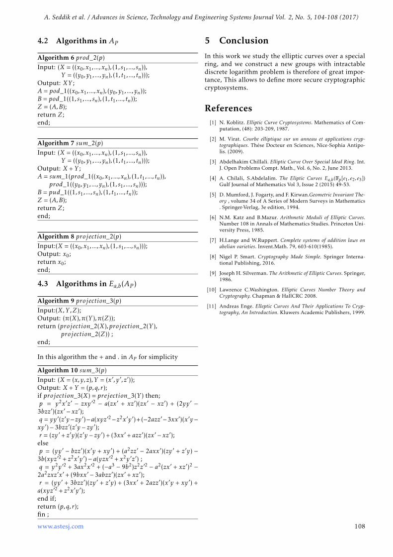
A. Seddik et al. / Advances in Science, Technology and Engineering Systems Journal Vol. 2, No. 5, 104-108 (2017)
4.2 Algorithms in AP
Algorithm 6 prod_2(p)Input: (X = ((x0,x1, ...,xn), (1, s1, ..., sn)),
Y = ((y0, y1, ..., yn), (1, t1, ..., tn)));Output: XY ;A = pod_1((x0,x1, ...,xn), (y0, y1, ..., yn));B = pod_1((1, s1, ..., sn), (1, t1, ..., tn));Z = (A,B);return Z;end;
Algorithm 7 sum_2(p)Input: (X = ((x0,x1, ...,xn), (1, s1, ..., sn)),
Y = ((y0, y1, ..., yn), (1, t1, ..., tn)));Output: X +Y ;A = sum_1(prod_1((x0,x1, ...,xn), (1, t1, ..., tn)),
prod_1((y0, y1, ..., yn), (1, s1, ..., sn)));B = pud_1((1, s1, ..., sn), (1, t1, ..., tn));Z = (A,B);return Z;end;
Algorithm 8 projection_2(p)Input:(X = ((x0,x1, ...,xn), (1, s1, ..., sn)));Output: x0;return x0;end;
4.3 Algorithms in Ea,b(AP )
Algorithm 9 projection_3(p)Input:(X,Y ,Z);Output: (π(X),π(Y ),π(Z));return (projection_2(X),projection_2(Y ),
projection_2(Z)) ;end;
In this algorithm the + and . in AP for simplicity
Algorithm 10 sum_3(p)Input: (X = (x,y,z),Y = (x′ , y′ , z′));Output: X +Y = (p,q, r);if projection_3(X) = prejection_3(Y ) then;p = y2x′z′ − zxy′2 − a(zx′ + xz′)(zx′ − xz′) + (2yy′ −3bzz′)(zx′ − xz′);q = yy′(z′y−zy′)−a(xyz′2−z2x′y′)+(−2azz′−3xx′)(x′y−xy′)− 3bzz′(z′y − zy′);r = (zy′ + z′y)(z′y − zy′) + (3xx′ + azz′)(zx′ − xz′);
elsep = (yy′ − bzz′)(x′y + xy′) + (a2zz′ − 2axx′)(zy′ + z′y) −
3b(xyz′2 + z2x′y′)− a(yzx′2 + x2y′z′) ;q = y2y′2 + 3ax2x′2 + (−a3 − 9b2)z2z′2 − a2(zx′ + xz′)2 −
2a2zxz′x′ + (9bxx′ − 3abzz′)(zx′ + xz′);r = (yy′ + 3bzz′)(zy′ + z′y) + (3xx′ + 2azz′)(x′y + xy′) +a(xyz′2 + z2x′y′);end if;return (p,q, r);fin ;
5 Conclusion
In this work we study the elliptic curves over a specialring, and we construct a new groups with intractablediscrete logarithm problem is therefore of great impor-tance, This allows to define more secure cryptographiccryptosystems.
References[1] N. Koblitz. Elliptic Curve Cryptosystems. Mathematics of Com-
putation, (48): 203-209, 1987.
[2] M. Virat. Courbe elliptique sur un anneau et applications cryp-tographiques. Thése Docteur en Sciences, Nice-Sophia Antipo-lis. (2009).
[3] Abdelhakim Chillali. Elliptic Curve Over Special Ideal Ring. Int.J. Open Problems Compt. Math., Vol. 6, No. 2, June 2013.
[4] A. Chilali, S.Abdelalim. The Eliptic Curves Ea,b(Fp[e1, e2, e3])Gulf Journal of Mathematics Vol 3, Issue 2 (2015) 49-53.
[5] D. Mumford, J. Fogarty, and F. Kirwan.Geometric Invariant The-ory , volume 34 of A Series of Modern Surveys in Mathematics. Springer-Verlag, 3e edition, 1994.
[6] N.M. Katz and B.Mazur. Arithmetic Moduli of Elliptic Curves.Number 108 in Annals of Mathematics Studies. Princeton Uni-versity Press, 1985.
[7] H.Lange and W.Ruppert. Complete systems of addition laws onabelian varieties. Invent.Math. 79, 603-610(1985).
[8] Nigel P. Smart. Cryptography Made Simple. Springer Interna-tional Publishing, 2016.
[9] Joseph H. Silverman. The Arithmetic of Elliptic Curves. Springer,1986.
[10] Lawrence C.Washington. Elliptic Curves Number Theory andCryptography. Chapman & HallCRC 2008.
[11] Andreas Enge. Elleptic Curves And Their Applications To Cryp-tography, An Introduction. Kluwers Academic Publishers, 1999.
www.astesj.com 108

Advances in Science, Technology and Engineering Systems JournalVol. 2, No. 5, 109-123 (2017)
www.astesj.comProceedings of International Conference on Applied Mathematics
(ICAM2017), Taza, Morocco
ASTES JournalISSN: 2415-6698
Nonlinear parabolic problem with lower order terms in Musielak-Orlicz spacesMhamed Elmassoudi*,1, Ahmed Aberqi 2, Jaouad Bennouna 1
1University of Fez, Faculty of Sciences Dhar El Mahraz, Department of Mathematics, B.P 1796 Atlas Fez, Morocco.2University of Fez, National School of Applied Sciences Fez,Morocco.
A R T I C L E I N F O A B S T R A C T
Article history:Received: 05 May, 2017Accepted: 15 July, 2017Online: 28 December, 2017
Keywords:Musielak-Orlicz space Non-linear Parabolic ProblemsEntropy solutionCondition signLower order term
We prove an existence result of entropy solutions for the nonlinearparabolic problems: ∂b(x,u)
∂t +A(u)−div(Φ(x, t,u))+H(x, t,u,∇u) = f , andA(u) = −div(a(x, t,u,∇u)) is a Leary-Lions operator defined on the inho-mogeneous Musielak-Orlicz space, the term Φ(x, t,u) is a Cratheodoryfunction assumed to be continuous on u and satisfy only the growth con-dition Φ(x, t,u) ≤ c(x, t)M−1
M(x,α0u), prescribed by Musielak-Orliczfunctions M and M which inhomogeneous and not satisfy ∆2-condition,H(x, t,u,∇u) is a Cratheodory function not satisfies neither the signcondition or coercivity and f ∈ L1(QT ).
1 Introduction
Let Ω be a bounded open set of IRN (N ≥ 2), T is apositive real number, and QT = Ω × (0,T ). Considerthe following nonlinear Dirichlet equation:
∂b(x,u)∂t +A(u)− div(Φ(x, t,u)) +H(x, t,u,∇u) = f ,
u(x, t) = 0 on ∂Ω× (0,T ),b(x,u)(t = 0) = b(x,u0) in Ω.
(1)where A(u) = −div(a(x, t,u,∇u)) is a Leary-Lions oper-ator defined on the inhomogeneous Musielak-Orlicz-Sobolev space W 1,x
0 LM(QT ), M is a Musielak-Orlicz-function related to the growths of the Caratheodoryfunctions a(x, t,u,∇u), Φ(x, t,u) and H(x, t,u,∇u) (seeassumptions (12), (15) and (16). b : Ω × IR→ IR is aCaratheodory function such that for every x ∈Ω, b(x, .)is a strictly increasing C1(IR)-function, the data f andb(.,u0) in L1(QT ) and L1(Ω) respectively.Starting with the prototype equation:
∂u∂t−4p(u) + div(c(., t)|u|γ−1u) + b|∇u|δ = f , inQT .
In the Classical Sobolev-spaces, the authors in [1] haveproved the existence of weak solutions, with c(., .) ≡ 0.For c(., .) ∈ L2(QT ) and p = 2, in [2] have proved theexistence of entropy solutions, recently in [3] haveproved an existence results of renormalized solutions
in the case where p ≥ 2 and c(., .) ∈ Lr (QT ) with r > N+pp−1 ,
and by in [4] for more general parabolic term. For theelliptic version of the problem (1), more results areobtained see e.g. [5-7].
In the degenerate Sobolev-spaces an existenceresults is shown in [8] without sign condition inH(x, t,u,∇u).
In the Orlicz-Sobolev spaces, the existence of en-tropy solutions of the problem (1) in [9] is provedwhere H(x, t,u,∇u) ≡ 0 and the growth of the firstlower order Φ prescribed by an isotropic N-functionP with (P ≺≺M). To our knowledge, differential equa-tions in general MusielakSobolev spaces have beenstudied rarely see [10-14], then our aim in this paperis to overcome some difficulties encountered in thesespaces and to generalize the result of [4, 9, 15, 16], andwe prove an existence result of entropy solution forthe obstacle parabolic problem (1), with less restrictivegrowth, and no coercivity condition in the first lowerorder term Φ , and without sign condition in the secondlower order H, in the framework of inhomogeneousOrlicz-Sobolev spaces W 1,x
0 LM (QT ), and N-function M,defining space does not satisfy the 42-condition.
This paper is organized as follows. In section 2,we recall some definitions, properties and technicallemmas about Musielak Orlicz Sobolev , In section 3is devoted to specify the assumptions on b,Φ , f , u0,
*Corresponding Author: Mhamed Elmassoudi, Laboratoire LAMA , Fez, Morocco & [email protected]
www.astesj.com 109https://dx.doi.org/10.25046/aj020518

M. Elmassoudi et al. / Advances in Science, Technology and Engineering Systems Journal Vol. 2, No. 5, 109-123(2017)
giving the definition of a entropy solution of (1) andwe establish the existence of such a solution Theorem4. In section 4, we give the proof of Theorem 4.
2 Musielak-Orlicz space and atechnical lemma
In this part we will define the musielak-Orlicz functionwhich control the growth of our operator.
2.1 Musielak-Orlicz function
Let Ω be an open subset of IRN (N ≥ 2), and let M be areal-valued function defined in Ω× IR+ and satisfyingconditions:(Φ1):M(x, .) is an N-function for all x ∈Ω (i.e. convex,non-decreasing, continuous, M(x,0) = 0 ,M(x,0) > 0 for t > 0, limt→0 supx∈Ω
M(x,t)t = 0 and
limt→∞ infx∈ΩM(x,t)t =∞).
(Φ2):M(., t) is a measurable function for all t ≥ 0.A function M which satisfies the conditions Φ1 and
Φ2 is called a Musielak-Orlicz function. For a Musielak-Orlicz function M we put Mx(t) = M(x, t) and we as-sociate its non-negative reciprocal function M−1
x , withrespect to t, that is M−1
x (M(x, t)) = M(x,M−1x (t)) = t.
Let M and P be two Musielak-Orlicz functions, wesay that P grows essentially less rapidly than M at0(resp. near infinity, and we write P ≺≺M, for everypositive constant c, we have limt→0
(supx∈Ω
P (x,ct)M(x,t)
)= 0
(resp.limt→∞(supx∈Ω
P (x,ct)M(x,t)
)= 0
).
Remark 1 [12] If P ≺≺ M near infinity, then ∀ε > 0there exist k(ε) > 0 such that for almost all x ∈Ω we haveP (x, t) ≤ k(ε)M(x,εt) ∀t ≥ 0.
2.2 Musielak-Orlicz space
For a Musielak-Orlicz function M and a mesurablefunction u : Ω→ IR, we define the functionnal
%M,Ω(u) =∫Ω
M(x, |u(x)|)dx.
The set KM(Ω) = u : Ω → IR mesurable :%M,Ω(u) <∞ is called the Musielak-Orlicz class. TheMusielak-Orlicz space LM(Ω) is the vector space gen-erated by KM(Ω); that is, LM(Ω) is the smallest linearspace containing the set KM (Ω). Equivalently
LM (Ω) = u : Ω→ IR mesurable : %M,Ω(uλ
) <∞,
for some λ > 0.
For any Musielak-Orlicz function M, we put M(x,s) =supt≥0(st −M(x,s)). M is called the Musielak-Orliczfunction complementary to M (or conjugate of M) inthe sense of Young with respect to s. We say that a se-quence of function un ∈ LM (Ω) is modular convergentto u ∈ LM(Ω) if there exists a constant λ > 0 such thatlimn→∞ %M,Ω(un−uλ ) = 0.
This implies convergence for σ (ΠLM ,ΠLM )(see [17]).In the space LM (Ω), we define the following two norms
‖u‖M = infλ > 0 :
∫ΩM(x, |u(x)|
λ )dx ≤ 1,
which is called the Luxemburg norm, and the so-calledOrlicz norm by
‖|u|‖M,Ω = sup‖v‖M≤1
∫Ω|u(x)v(x)|dx,
where M is the Musielak-Orlicz function complemen-tary toM. These two norms are equivalent [17]. KM (Ω)is a convex subset of LM(Ω). The closure in LM(Ω) ofthe set of bounded measurable functions with com-pact support in Ω is by denoted EM(Ω). It is a sepa-rable space and (EM(Ω))∗ = LM(Ω). We have EM(Ω) =KM (Ω), if and only if M satisfies the ∆2−condition forlarge values of t or for all values of t, according towhether Ω has finite measure or not.We define
W 1LM (Ω) = u ∈ LM (Ω) :Dαu ∈ LM (Ω), ∀α ≤ 1,W 1EM (Ω) = u ∈ EM (Ω) :Dαu ∈ EM (Ω), ∀α ≤ 1,
where α = (α1, ...,αN ),|α| = |α1| + ... + |αN | and Dαudenote the distributional derivatives. The spaceW 1LM (Ω) is called the Musielak-Orlicz-Sobolev space.Let %M,Ω(u) =
∑|α|≤1 %M,Ω(Dαu) and ‖u‖1M,Ω = infλ >
0 : %M,Ω(uλ ) ≤ 1 for u ∈W 1LM (Ω).These functionals are convex modular and a norm onW 1LM (Ω), respectively. Then pair (W 1LM (Ω),‖u‖1M,Ω)is a Banach space if M satisfies the following condition(see [10]),
There exists a constant c > 0 such that infx∈Ω
M(x,1) > c.
The space W 1LM (Ω) is identified to a subspace of theproduct Πα≤1LM(Ω) = ΠLM . We denote by D(Ω) theSchwartz space of infinitely smooth functions withcompact support in Ω and by D(Ω) the restriction ofD(IR) on Ω. The space W 1
0 LM(Ω) is defined as theσ (ΠLM ,ΠEM ) closure of D(Ω) in W 1LM(Ω) and thespace W 1
0 EM (Ω) as the(norm) closure of the Schwartzspace D(Ω) in W 1LM (Ω).For two complementary Musielak-Orlicz functions Mand M, we have [17].
• The Young inequality:
st ≤M(x,s) +M(x, t) for all s, t ≥ 0 , x ∈Ω.
• The Holder inequality∣∣∣ ∫Ωu(x)v(x)dx
∣∣∣ ≤ ‖u‖M,Ω‖|v|‖M,Ω for allu ∈ LM (Ω),v ∈ LM (Ω).
We say that a sequence of functions un converges tou for the modular convergence in W 1LM(Ω) (respec-tively in W 1
0 LM (Ω)) if, for some λ > 0.
limn→∞
%M,Ω(un −u
λ
)= 0.
The following spaces of distributions will also be used
W −1LM (Ω) =f ∈ D
′(Ω) : f =
∑α≤1
(−1)αDαfα
www.astesj.com 110

M. Elmassoudi et al. / Advances in Science, Technology and Engineering Systems Journal Vol. 2, No. 5, 109-123(2017)
where fα ∈ LM (Ω),
and
W −1EM (Ω) =f ∈ D
′(Ω) : f =
∑α≤1
(−1)αDαfα
where fα ∈ EM (Ω).
Lemma 1 [17] Let Ω be a bounded Lipschitz domain inIRN and let M and M be two complementary Musielak-Orlicz functions which satisfy the following conditions:
• There exists a constant c > 0 such thatinfx∈ΩM(x,1) > c,
• There exists a constant A > 0 such that for allx,y ∈Ω with |x − y| ≤ 1
2 , we have
M(x, t)M(y, t)
≤ t
(A
log( 1|x−y| )
)for all t ≥ 1,
• For all y ∈Ω,∫ΩM(y,1)dx <∞,
• There exists a constant C > 0 such that
M(y, t) ≤ C a.e. in Ω.
Under this assumptions D(Ω) is dense in LM(Ω) withrespect to the modular topology, D(Ω) is dense inW 1
0 LM(Ω) for the modular convergence and D(Ω) isdense in W 1
0 LM (Ω) for the modular convergence.Consequently, the action of a distribution S in inW −1LM(Ω) on an element u of W 1
0 LM(Ω) is well de-fined. It will be denoted by < S,u >.
2.3 Truncation Operator
Tk , k > 0, denotes the truncation function at level kdefined on IR by Tk(r) = max(−k,min(k, r)). The follow-ing abstract lemmas will be applied to the truncationoperators.
Lemma 2 [12] Let F : IR→ IR be uniformly lipschitzian,with F(0) = 0. Let M be an Musielak-Orlicz func-tion and let u ∈ W 1
0 LM(Ω)(resp.u ∈ W 1EM(Ω)). ThenF(u) ∈W 1LM(Ω)(resp.u ∈W 1
0 EM(Ω)). Moreover, if theset of discontinuity points D of F′ is finite, then
∂∂xi
F(u) =F′(x) ∂u∂xi a.e. in x ∈Ω; u(x) <D0 a.e. in x ∈Ω; u(x) ∈D
Lemma 3 Suppose that Ω satisfies the segement prop-erty and let u ∈W 1
0 LM (Ω). Then, there exists a sequenceun ∈ D(Ω) such that un→ u for modular convergence inW 1
0 LM (Ω). Furthermore, if u ∈W 10 LM (Ω)∩L∞(Ω) then
‖un‖∞ ≤ (N + 1)‖u‖∞.
Let Ω be an open subset of IRN and letM be a Musielak-Orlicz function satisfying∫ 1
0
M−1x (t)
tN+1N
dt =∞ a.e. x ∈Ω, (2)
and the conditions of Lemma (1). We may assumewithout loss of generality that∫ 1
0
M−1x (t)
tN+1N
dt <∞ a.e. x ∈Ω. (3)
Define a function M∗ : Ω × [0,∞) by M∗(x,s) =∫ s0M−1x (t)
tN+1N
dt x ∈Ω and s ∈ [0,∞).
M∗ its called the Sobolev conjugate function of M (see[18] for the case of Orlicz function).
Theorem 1 Let Ω be a bounded Lipschitz domain andlet M be a Musielak-Orlicz function satisfying (2),(3) andthe conditions of lemma (1). Then W 1
0 LM (Ω) → LM∗(Ω),where M∗ is the Sobolev conjugate function of M. More-over, if Φ is any Musielak-Orlicz function increasing essen-tially more slowly than M∗ near infinity, then the imbed-ding W 1
0 LM (Ω) → Lφ(Ω), is compact.
Corollaire 1 Under the same assumptions of theorem (1),we have W 1
0 LM (Ω) →→ LM (Ω).
Lemma 4 If a sequence un ∈ LM(Ω) converges a.e. to uand if un remains bounded in LM(Ω), then u ∈ LM(Ω)and unu for σ (LM (Ω),EM (Ω)).
Lemma 5 Let un,u ∈ LM(Ω). If un → u with re-spect to the modular convergence, then un u forσ (LM (Ω),LM (Ω)).
Demonstration: Let λ > 0 such that∫ΩM(x, un−uλ )dx→
0. Thus, for a subsequence, un → u a.e. in Ω. Takev ∈ LM(Ω). Multiplying v by a suitable constant, wecan assume λv ∈ LM (Ω). By Young’s inequality,
|(un −u)v| ≤M(x,un −uλ
) +M(x,λv)
which implies, by Vitali’s theorem, that∫Ω|(un −
u)v|dx→ 0.
2.4 Inhomogeneous Musielak-Orlicz-Sobolev spaces
Let Ω an bounded open subset IRN and let QT =Ω×]0,T [ with some given T > 0. Let M be an Musielak-Orlicz function, for each α ∈ INN , denote by ∇αx thedistributional derivative onQT of order α with respectto the variable x ∈ INN . The inhomogeneous Musielak-Orlicz-Sobolev spaces are defined as follows,
W 1,xLM (QT ) = u ∈ LM (QT ) : ∇αx u ∈ LM (QT ),
∀α ∈ INN , |α| ≤ 1,
W 1,xEM (QT ) = u ∈ EM (QT ) : ∇αx u ∈ EM (QT ),
∀α ∈ INN , |α| ≤ 1.
www.astesj.com 111

M. Elmassoudi et al. / Advances in Science, Technology and Engineering Systems Journal Vol. 2, No. 5, 109-123(2017)
The last space is a subspace of the first one, andboth are Banach spaces under the norm ‖u‖ =∑|α|≤m ‖∇αx u‖M,QT . We can easily show that they form
a complementary system when Ω satisfies the Lips-chitz domain [17]. These spaces are considered as sub-spaces of the product space ΠLM(QT ) which have asmany copies as there is α-order derivatives,|α| ≤ 1. Weshall also consider the weak topologies σ (ΠLM ,ΠEM )and σ (ΠLM ,ΠLM ). If u ∈W 1,xLM(QT ) then the func-tion : t 7→ u(t) = u(t, .) is defined on (0,T ) with val-ues W 1LM(Ω). If, further, u ∈ W 1,xEM(QT ) thenthe concerned function is a W 1,xEM(Ω)-valued andis strongly measurable. Furthermore the followingimbedding holds W 1,xEM(Ω) ⊂ L1(0,T ,W 1,xEM(Ω)).The space W 1,xLM(QT ) is not in general separa-ble, if W 1,xLM(QT ) , we can not conclude that thefunction u(t) is measurable on (0,T ). However,thescalar function t 7→ ‖u(t)‖M,Ω , is in L1(0,T ) .Thespace W 1,x
0 EM(QT ) is defined as the (norm) closureW 1,xEM(QT ) of D(QT ). We can easily show as in[8],that when Ω has the segment property, theneach element u of the closure of D(QT ) with respectof the weak* topology σ (ΠLM ,ΠEM ) is a limit, inW 1,x
0 EM(QT ), of some subsequence (ui) ⊂ D(QT ) forthe modular convergence; i.e. there exists λ > 0 suchthat for all |α| ≤ 1∫
QT
M(x,∇αx ui −∇αx u
λ)dxdt→ 0 asi→∞. (4)
This implies that (ui) converge to u inW 1,xLM (QT ) forthe weak topology σ (ΠLM ,ΠLM ) .Consequently,
D(QT )σ (ΠLM ,ΠEM )
=D(QT )σ (ΠLM ,ΠLM )
. (5)
This space will be denoted byW 1,x0 LM (QT ) . Furthermore,
W 1,x0 EM (QT ) =W 1,x
0 LM (QT )∩ΠEM .We have the following complementary system(W 1,x
0 LM (QT ) FW 1,x
0 EM (QT ) F0
)F being the dual space of
W 1,x0 EM (QT ). It is also, except for an isomorphism, the
quotient of ΠLM by the polar set W 1,x0 EM(QT )⊥, and
will be denoted by F = W −1,xLM(QT ) and it is showthat,
W −1,xLM (QT ) =f =
∑|α|≤1
∇αx fα : fα ∈ LM (QT ).
This space will be equipped with the usual quo-tient norm ‖f ‖ = inf
∑|α|≤1 ‖fα‖M,QT where the infi-
mum is taken on all possible decompositions f =∑|α|≤1∇αx fα , fα ∈ LM (QT ).
The space F0 is then given by, F0 =f =
∑|α|≤1∇αx fα :
fα ∈ EM (QT )
and is denoted by F0 =W −1,xEM (QT ).
Theorem 2 [14] Let Ω be a bounded Lipchitz domainand let M be a Musielak-Orlicz function satisfying the
same conditions of Theorem (1). Then there existsa constant λ > 0 such that ‖u‖M ≤ λ‖∇u‖M , ∀ ∈W 1
0 LM (QT ).
Definition 1 We say that un → u in W −1,xLM(QT ) +L1(QT ) for the modular convergence if we can writeun =
∑|α|≤1D
αx u
αn +u0
n and u =∑|α|≤1D
αx u
α +u0
with uαn → uα in LM (QT ) for modular convergence for all|α| ≤ 1 and u0
n→ u0 strongly in L1(QT )
Lemma 6 Let un be a bounded sequence inW 1,xLM(QT ) such that ∂un
∂t = αn + βn in D′(QT ), un u, weakly in W 1,xLM (QT ), for σ (ΠLM ,ΠEM )
with αn and βn two bounded sequences respectivelyin W −1,xLM (QT ) and inM(QT ). Thenun → u in L1
loc(QT ). Furthermore, if un ∈ W1,x0 LM(QT ),
then un→ u strongly in L1(QT ).
Theorem 3 if u ∈ W 1,xLM(QT ) ∩ L1(QT ) (resp.W 1,x
0 LM (QT )∩L1(QT )) and ∂u∂t ∈W
−1,xLM (QT )+L1(QT )then there exists a sequence (vj ) in D(QT ) (resp.D(I,D(QT ))) such that vj → u in W 1,xLM(QT ) and∂vj∂t →
∂u∂t in W −1,xLM(QT ) + L1(QT ) for the modular
convergence.
Demonstration: Let u ∈ W 1,xLM(QT ) ∩ L1(QT ) and∂u∂t ∈W
−1,xLM(QT ) +L1(QT ) , then for any ε > 0. Writ-ing ∂u
∂t =∑|α|≤1D
αx u
α + u0, where uα ∈ LM(QT ) for all|α| ≤ 1 and u0 ∈ L1(QT ), we will show that there exitsλ > 0 (depending Only on u and N ) and there existsv ∈ D(QT ) for which we can write ∂u
∂t =∑|α|≤1D
αx v
α+v0
with vα ,v0 ∈ D(QT ) such that∫QT
M(x,Dαx v −Dαx u
λ)dxdt ≤ ε,∀|α| ≤ 1, (6)
‖v −u‖L1(QT ) ≤ ε, (7)
‖v0 −u0‖L1(QT ) ≤ ε, (8)∫QT
M(x,vα −uα
λ)dxdt ≤ ε,∀|α| ≤ 1 (9)
The equation (6) flows from a slight adaptationof the arguments [17],The equations (7),(8) flows alsofrom classical approximation results. For The equa-tion (9) we know that D(QT ) is dense in LM(QT )for the modular convergence. The case where u ∈W 1,x
0 LM (QT )∩L1(QT )) can be handled similarly with-out essential difficulty as it mentioned [17].
Remark 2 The assumption u ∈ L1(QT ) in theorem (3) isneeded only when QT has infinite measure, since else, wehave LM (QT )) ⊂ L1(QT ) and so W 1,xLM (QT )∩L1(QT ) =W 1,xLM (QT ).
Remark 3 If in the statement of theorem (3) above, onetakes I = IR, we have that D(Ω × IR) is dense in u ∈W 1,x
0 LM(Ω × IR) ∩ L1Ω × IR) : ∂u∂t ∈ W−1,xLM(Ω × IR) +
L1(Ω × IR) for the modular convergence. This triviallyfollows from the fact that D(IR,D(Ω)) =D(Ω× IR).
www.astesj.com 112

M. Elmassoudi et al. / Advances in Science, Technology and Engineering Systems Journal Vol. 2, No. 5, 109-123(2017)
Remark 4 Let a < b ∈ IR and Ω be a bounded open subsetof IRN with the segment property, then u ∈W 1,x
0 LM (Ω×(a,b))∩L1Ω× (a,b)) : ∂u∂t ∈W
−1,xLM (Ω× (a,b)) +L1(Ω×(a,b)) ⊂ C([a,b],L1(Ω)).
Demonstration: Let u ∈ W 1,x0 LM(Ω × (a,b)) and ∂u
∂t ∈W −1,xLM (Ω× (a,b)) +L1(Ω× (a,b)).After two consecutive reflections first with respectto t = b and then with respect to t = a, u(x, t) =u(x, t)χ(a,b) +u(x,2b−t)χ(b,2b−a) in Ω×(b,2b−a) andu(x, t) = u(x, t)χ(a,2b−a) + u(x,2a− t)χ(3a−2b,a) in Ω×(3a− 2b,2b − a). We get function u ∈W 1,x
0 LM (Ω× (3a−2b,2b − a)) with ∂u
∂t ∈ W−1,xLM(Ω × (3a − 2b,2b − a)) +
L1(Ω× (3a− 2b,2b − a)). Now by letting a function η ∈D(IR) with η = 1 on [a,b] and suppη ⊂ (3a−2b,2b − a),we set u = ηu, therefore,by standard arguments (see[19]), we have u = u on (Ω × (a,b)), u ∈ W 1,x
0 LM(Ω ×IR)∩L1(Ω× IR) and ∂u
∂t ∈W−1,x0 LM (Ω× IR) +L1(Ω× IR).
Let now vj the sequence given by theorem (3) corre-sponding to u, that is,
vj → u in W 1,x0 LM (Ω× IR)
and
∂vj∂t→ ∂u
∂tin W −1,x
0 LM (Ω× IR) +L1(Ω× IR)
for the modular convergence.If we denote Sk(s) =
∫ s0 Tk(t)dt the primitive of Tk .
We have,∫ΩS1(vi − vj )(τ)dx =
∫Ω
∫ r−∞T1(vi − vj )(
∂vi∂t −
∂vj∂t )dxdt → 0 as i, j → 0, from which, one de-
duces that vj is a Cauchy sequence in C(IR;L1(Ω))and hence u ∈ C(IR,L1(Ω)). Consequently, u ∈C([a;b];L1(Ω)).
3 Formulation of the problem andmain results
Let Ω be an open subset of IRN (N ≥ 2) satisfying thesegment property,and let M and P be two Musielak-Orlicz functions such that M and its complementaryM satisfies conditions of Lemma 1, M is decreasing inx and P ≺≺M.b : Ω × IR→ IR is a Caratheodory function such thatfor every, x ∈ Ω, b(x, .) is a strictly increasing C1(IR)-function and
b ∈ L∞(Ω× IR) with b(x,0) = 0, (10)
There exists a constant λ > 0 and functions A ∈ L∞(Ω)and B ∈ LM (Ω) such that
λ ≤ ∂b(x,s)∂s
≤ A(x) and∣∣∣∣∇x(∂b(x,s)
∂s
)∣∣∣∣ ≤ B(x) (11)
a.e. x ∈Ω and ∀ |s| ∈ IR.A : D(A) ⊂ W 1
0 LM(QT ) → W −1LM(QT ) defined byA(u) = −div a(x, t,u,∇u), where a :QT × IR× IRN → IRN
is caratheodory function such that for a.e. x ∈Ω andfor all s ∈ IR,ξ,ξ∗ ∈ IRN ,ξ , ξ∗
|a(x, t, s,ξ)| ≤ ν(a0(x, t) +M−1x P (x, |s|)), (12)
with a0(., .) ∈ EM (QT ),
(a(x, t, s,ξ)− a(x, t, s,ξ∗))(ξ − ξ∗) > 0, (13)
a(x, t, s,ξ).ξ ≥ αM(x, |ξ |) +M(x, |s|). (14)
Φ(x,s,ξ) :QT × IR× IRN → IRN is a Caratheodory func-tion such that
|Φ(x, t, s)| ≤ c(x, t)M−1x M(x,α0|s|), (15)
where c(., .) ∈ L∞(QT ), ‖c(., .)‖L∞(QT ) ≤ α, and0 < α0 <min(1, 1
α ).H(x, t, s,ξ) :QT × IR× IRN → IR is a Caratheodory func-tion such that
|H(x, t, s,ξ)| ≤ h(x, t) + ρ(s)M(x, |ξ |), (16)
ρ : IR→ IR+ is continuous positive function which be-long L1(IR) and h(., .) belong L1(QT ).
f ∈ L1(Ω), (17)
and
u0 ∈ L1(Ω) such that b(x,u0) ∈ L1(Ω). (18)
Note that <,> means for either the pairing betweenW 1,x
0 LM (QT )∩L∞(QT )) and W −1,xLM (QT ) +L1(QT ) orbetween W 1,x
0 LM (QT ) and W −1,xLM (QT ).Weak entropy solution: The definition of a entropysolution of Problem (1) can be stated as follows,
Definition 2 A measurable function u defined onQT is aentropy solution of Problem (1), if it satisfies the followingconditions:
b(x,u) ∈ L∞(0,T ;L1(Ω)),b(x,u)(t = 0) = b(x,u0) in Ω,
Tk(u) ∈W 1,x0 LM (QT ), ∀k > 0, ∀t ∈]0,T ],
∫ T0
⟨∂v∂s ;
∫ u0∂b(x,z)∂s T ′k (z − v)dz
⟩ds
+∫Ω
∫ u0
0∂b(x,s)∂s Tk(s − v(0))dsdx
+∫QTa(u,∇u)∇Tk(u − v)dxds+
∫QT
Φ(u)∇Tk(u − v)dxds
+∫QTH(u,∇u)Tk(u − v)dxds ≤
∫QTf Tk(u − v)dxds
∀k > 0, and ∀v ∈W 1,xLM (QT )∩L∞(QT ) withv(T ) = 0, such that ∂v
∂t ∈W−1,xLM (QT ) +L1(QT )
(19)
Theorem 4 Assume that (11) − (18) hold true . Thenthere exists at least one solution u of the following problem(19).
www.astesj.com 113

M. Elmassoudi et al. / Advances in Science, Technology and Engineering Systems Journal Vol. 2, No. 5, 109-123(2017)
4 Proof of theorem 4
Truncated problem.For each n > 0, we define the following approximations
bn(x,s) = b(x,Tn(s)) +1ns ∀ r ∈ IR, (20)
an(x, t, s,ξ) = a(x, t,Tn(s),ξ) a.e. (x, t) ∈QT , (21)
∀ s ∈ IR, ∀ ξ ∈ IRN ,
Φn(x, t, s) = Φ(x, t,Tn(s)) a.e. (x, t) ∈QT , ∀ s ∈ IR,(22)
Hn(x, t, s,ξ) =H(x, t, s,ξ)
1 + 1n |H(x, t, s,ξ)|
, (23)
fn ∈ L1(QT ) such that fn→ f strongly in L1(QT ), (24)
and ‖fn‖L1(QT ) ≤ ‖f ‖L1(QT ),and
u0n ∈ C∞0 (Ω)such that bn(x,u0n)→ b(x,u0) (25)
strongly in L1(Ω).Let us now consider the approximate problem :
∂bn(x,un)∂t
− div(an(x, t,un,∇un))− div(Φn(x, t,un))
+Hn(x,un,∇un) = fn in QT ,un(x, t) = 0 on ∂Ω× (0,T ),bn(x,un)(t = 0) = bn(x,u0n) in Ω.
(26)Since Hn is bounded for any fixed n > 0, there exists atlast one solution un ∈W
1,x0 LM (QT ) of (26)(see [20]).
Remark 5 the explicit dependence in x and t of the func-tions a, Φ and H will be omitted so that a(x, t,u,∇u) =a(u,∇u), Φ(x, t,u) = Φ(u) and H(x, t,u,∇u) =H(u,∇u).
Proposition 1 let un be a solution of approximate equa-tion (26)such that
Tk(un)→ Tk(u) weakly in W 1,xLM (QT ),un→ u a.e. in QT ,bn(x,un)→ b(x,u) a.e. in QT and b(x,u) ∈ L∞(QT ),a(Tk(un),∇Tk(un))∇Tk(un)a(Tk(u),∇Tk(u))∇Tk(u)
weakly in L1(QT ),∇un→∇u a.e. in QT ,Hn(un,∇un)→H(u,∇u) strongly in L1(QT ).
(27)then u be a solution of problem (19).
Demonstration: Let v ∈W 10 LM (QT )∩L∞(QT ) such that
∂v∂t ∈W
−1,xLM (QT ) +L1(QT ) with v(T ) = 0, then by the-orem 3 we can take v = v on QT , v ∈W 1,xLM(Ω ×IR)∩L1(Ω×IR)∩L∞(Ω×IR), ∂v∂t ∈W
−1,xLM (QT )+L1(QT ),and there exists vj ∈ D(Ω × IR) such that vj(T ) = 0,
vj → v in W 1,x0 LM (Ω× IR) and
∂vj∂t→ ∂v
∂t∈W −1,xLM (QT ) +L1(QT ), (28)
for the modular convergence in W 10 LM(QT ) , with
‖vj‖L∞(QT ) ≤ (N + 2)‖v‖L∞(QT ).
Pointwise multiplication of the approximate equation(26) by Tk(un − vj ), we get
∫ T
0<∂bn(x,un)
∂s;Tk(un − vj ) > ds
+∫QTan(un,∇un)∇Tk(un − vj )dxds
+∫QT
Φn(un)∇Tk(un − vj )dxds
+∫QTHn(un,∇un)∇Tk(un − vj )dxds
=∫QTfnTk(un − vj )dxds
(29)
We pass to the limit as in (29), n tend to +∞ and jtend to +∞:Limit of the first term of (29):The first term can be written∫ T
0<∂bn(x,un)
∂s;Tk(un − vj ) > ds
=∫ T
0<∂v∂s
;∫ un
0
∂bn(x,z)∂s
T ′k (z − vj ) > ds
+∫Ω
∫ un(T )
0
∂bn(x,s)∂s
Tk(s − vj (T ))dsdx
−∫Ω
∫ u0n
0
∂bn(x,s)∂s
Tk(s − vj (0))dsdx,
the fact that ∂bn(x,s)∂s ≥ 0 and vj (T ) = 0 , we get∫
Ω
∫ u(T )
0
∂b(x,s)∂s
Tk(s − vj (T ))dsdx =
∫Ω
∫ u(T )
0
∂b(x,s)∂s
Tk(s)dsdx ≥ 0
On the other hand, we have u0n converge to u0 stronglyin L1(Ω), thenlimn→+∞
∫Ω
∫ u0n
0∂bn(x,s)∂s Tk(s − vj (0))dsdx
=∫Ω
∫ u0
0
∂b(x,s)∂s
Tk(s − vj (0))dsdx,
withM = k+(N+2)‖v‖∞ and TM (un) converges to TM (u)strongly in EM (QT ), we obtain
limn→+∞
∫ T
0<∂vj∂t
;∫ un
0
∂bn(x,z)∂s
T ′k (z − vj )dz > ds
= limn→+∞
∫ T
0<∂vj∂s
;∫ TM (un)
0
∂bn(x,z)∂s
T ′k (z − vj )dz > ds
=∫ T
0<∂vj∂s
;∫ TM (u)
0
∂b(x,z)∂s
T ′k (z − vj )dz > ds,
then∫ T
0<∂vj∂s
;∫ TM (u)
0
∂b(x,z)∂s
T ′k (z − vj )dz > ds
≤ limn→+∞
∫ T
0<∂b(x,un)∂s
Tk(un − vj ) > ds
+∫Ω
∫ u0
0<∂b(x,s)∂s
Tk(s − vj (0)) > dsdx,
www.astesj.com 114

M. Elmassoudi et al. / Advances in Science, Technology and Engineering Systems Journal Vol. 2, No. 5, 109-123(2017)
using (28), the definition of Tk and pass to limit asj→ +∞, we deduce∫ T
0<∂v∂s
;∫ TM (u)
0
∂b(x,z)∂s
T ′k (z − v)dz > ds
≤ limj→+∞
limn→+∞
∫ T
0<∂b(x,un)∂s
Tk(un − vj ) > ds
+∫Ω
∫ u0
0<∂b(x, t)∂s
Tk(s − v(0)) > dsdx.
• We can follow same way in [21]to prove that
liminfj→∞
liminfn→∞
∫QT
a(un,∇un)∇Tk(un − vj )dxds
≥∫QT
a(u,∇u)∇Tk(u − v)dxds.
• For n ≥ k + (N + 2)‖v‖L∞(QT ) Φn(un)∇Tk(un −vj ) =Φ(Tk+(N+2)‖v‖L∞(QT )
(un))∇Tk(un − vj ). The point-wise convergence of un to u as n tends to +∞ and(15), then Φ(Tk+(N+2)‖v‖L∞(QT )
(un))∇Tk(un − vj )Φ(Tk+(N+2)‖v‖L∞(QT )
(u))∇Tk(u − vj ) weakly forσ (ΠLM ,ΠLM ).In a similar way, we obtain
limj→∞
∫QT
Φ(Tk+(N+2)‖v‖L∞(QT )(u))∇Tk(u − vj )dxds
=∫QT
Φ(Tk+(N+2)‖v‖L∞(QT )(u))∇Tk(u − v)dxds
=∫QT
Φ(u)∇Tk(u − v)dxds.
• Limit of Hn(un,∇un)Tk(un − vj ):Since Hn(un,∇un) converge strongly toH(x,s,u,∇u) in L1(QT ) and the pointwiseconvergence of un to u as n → +∞, it ispossible to prove that Hn(un,∇un)Tk(un − vj )converge to H(u,∇u)Tk(u − vj ) in L1(QT )and limj→∞
∫QTH(u,∇u)Tk(u − vj )dxds =∫
QTH(u,∇u)Tk(u − v)dxds.
• Since fn converge strongly to f in L1(QT ) , andTk(un − vj )→ Tk(un − vj ) weakly* in L∞(QT ), we
have∫QT
fnTk(un−vj )dxds→∫QT
f Tk(u−vj )dxds
as n→∞ and also we have∫QT
f Tk(u − vj )dxds →∫QT
f Tk(u − v)dxds as
j→∞Finally, the above convergence result, we are ina position to pass to the limit as n tends to +∞in equation (29) and to conclude that u satisfies(19).
It remains to show that b(x,u) satisfies the ini-tial condition. In fact, remark that, BM(x,un) =∫ un
0
∂b(x,s)∂s
TM(s − v)ds is bounded in L∞(QT ). Sec-
ondly, by (69) we show that∂BM (x,un)
∂tis bounded in
W −1,xLM(QT )) + L1(QT ). As a consequence, a Lemma4 implies that BM(x,un) lies in a compact set ofC0([0,T ];L1(Ω)) . It follows that, BM(x,un)(t = 0)converges to BM(x,u)(t = 0) strongly in L1(Ω). Onthe order hand, the smoothness of BM imply thatBM (x,un)(t = 0) converges to BM (x,u)(t = 0) strongly inL1(Ω), we conclude that BM(x,un)(t = 0) = BM(x,u0n)converges to BM(x,u)(t = 0) strongly in L1(Ω), weobtain BM(x,u)(t = 0) = BM(x,u0) a.e. in Ω and forall M > 0, now letting M to +∞, we conclude thatb(x,u)(t = 0) = b(x,u0) a.e. in Ω.
Remark 6 We focus our work to show the conditions ofthe proposition 27, then for this we go through 4 steps toarrive at our result.
Step 1: In this step let us begin by showing
Lemma 7Let unn be a solution of the approximate problem (26),then for all k > 0, there exists a constants C1 and C2 suchthat ∫
QT
a(Tk(un),∇Tk(un))∇Tk(un)dxdt ≤ kC1, (30)
and ∫QT
M(x, |∇Tk(un)|)dxdt ≤ kC2, (31)
where C1 and C2 does not depend on the n and k.
Demonstration: Fixed k > 0,Let τ ∈ (0,T ) and using exp(G(un))Tk(un)+χ(0,τ) as atest function in problem (26), where
G(s) =∫ s
0
ρ(r)α′
dr and α′ > 0 is a parameter to be speci-
fied later, we get:∫Qτ
∂bn(x,un)∂s
exp(G(un))Tk(un)+χ(0,t)dxdt (32)
+∫Qτ
a(un,∇un)ρ(un)α′
exp(G(un))∇unTk(un)+dxdt
(33)
+∫0≤un≤k
a(un,∇un)exp(G(un))∇Tk(un)dxdt (34)
+∫Qτ
Φn(un)∇(exp(G(un))Tk(un)+
)dxdt (35)
+∫Qτ
H(un,∇un)exp(G(un))Tk(un)+dxdt (36)
≤ k exp(‖ρ‖L1
α′)‖fn‖L1(QT ). (37)
For the (32), we have∫Qτ
∂bn(x,un)∂s
exp(G(un))Tk(un)+χ(0,τ)dxdt
=∫Ω
Bn,k(x,un(τ))dx −∫Ω
Bn,k(x,un(0))dx,
www.astesj.com 115

M. Elmassoudi et al. / Advances in Science, Technology and Engineering Systems Journal Vol. 2, No. 5, 109-123(2017)
where
Bn,k(x,r) =∫ r
0
∂bn(x,s)∂s
exp(G(Tk(s)))Tk(s)+ds.
By (11), we have∫ΩBn,k(x,un(τ))dx ≥ 0 and∫
Qτ
Bn,k(x,un(0))dx ≤ k exp(‖ρ‖L1
α′)‖b(x,u0‖L1(Ω).
For the (35), if we use (15) and Young inequality , weget∫Qτ
Φn(un))∇(exp(G(un))Tk(un)+)dxdt ≤
‖c(., .)‖L∞(QT )
α′[α0
∫Qτ
M(x,un)ρ(un)exp(G(un))Tk(un)+dxdt
+∫Qτ
M(x,∇un)ρ(un)exp(G(un))Tk(un)+dxdt]
+‖c(., .)‖L∞(QT )α0
∫Qτ
M(x,un)exp(G(un))dxdt
+‖c(., .)‖L∞(QT )
∫Qτ
M(x, |∇Tk(un)+|)exp(G(un))dxdt.
For the (36), we have,∫Qτ
Hn(un,∇un)exp(G(un))Tk(un)+dxdt
≤ k exp(‖ρ‖L1
α′)∫QT
|h(x, t)|dxdt
+∫Qτ
ρ(un)exp(G(un))M(x,∇Tk(un))Tk(un)+dxdt.
finally using the previous inequalities and (14), weobtain
1α′
∫Qτ
M(x,un)ρ(un)exp(G(un))Tk(un)+dxdt
+ αα′
∫QτM(x,∇un)ρ(un)exp(G(un))Tk(un)+dxdt
+∫Qτ
a(un,∇un)exp(G(un))∇Tk(un)+dxdt
≤ ‖c(.,.)‖L∞(QT )α′ [α0
∫QτM(x,un)ρ(un)exp(G(un))Tk(un)+dxdt
+∫Qτ
M(x,∇un)ρ(un)exp(G(un))Tk(un)+dxdt]
+α0‖c(., .)‖L∞(QT )
∫0≤un≤k
M(x,un)exp(G(un))dxdt
+‖c(., .)‖L∞(QT )
∫Qτ
M(x,∇Tk(un)+)exp(G(un))dxdt
+∫Qτ
M(x,∇un)ρ(un)exp(G(un))Tk(un)+dxdt
+k[exp(‖ρ‖L1
α′(‖f ‖L1(QT ) + ‖b(x,u0‖L1(Ω)
+∫QT|h(x, t)|dxdt],
(38)
which becomes after simplification,
[1−α0‖c(., .)‖L∞(QT )
α′]∫Qτ
M(x,un)ρ(un)exp(G(un))Tk(un)+dxdt
+[α−‖c(.,.)‖L∞(QT )−α′
α′ ]∫QτM(x,∇un)ρ(un)exp(G(un))Tk(un)+dxdt
+∫Qτ
a(un,∇un)exp(G(un))∇Tk(un)+dxdt
≤‖c(., .)‖L∞(QT )
α[α0α
∫0≤un≤k
M(x,un)exp(G(un))dxdt
+αM(x,∇Tk(un)+)exp(G(un))dxdt] + kC.(39)
If we choose α′ such that α′ < α − ‖c(., .)‖L∞(QT ) andusing again (14) in (39) we get
[1−‖c(., .)‖L∞(QT )
α]∫Qτ
a(un,∇un)exp(G(un))∇Tk(un)+dxdt ≤ kC.
(40)we deduce,∫
0≤un≤ka(un,∇un)exp(G(un))∇Tk(un)dxdt ≤ kc1.
one has exp(G(un)) ≥ 1 for in (x, t) ∈ QT : 0 ≤ un ≤ kthen ∫
0≤un≤ka(un,∇un)∇Tk(un)dxdt ≤ kc1. (41)
and by (14) another again∫Qt
M(x, |∇Tk(un)+|)dxdt ≤ kc2. (42)
Similarly, taking exp(−G(un)Tk(un)−χ(0,τ) as a testfunction in problem (26), we get∫
Qτ
∂bn(x,un)∂t
exp(−G(un))Tk(un)−dxdt (43)
+∫Qτ
an(un,∇un)∇(exp(−G(un))∇Tk(un)−)dxdt (44)
+∫Qτ
Φn(un)∇(exp(−G(un))∇Tk(un)−)dxdt (45)
+∫Qτ
H(un,∇un)exp(−G(un))Tk(un)−dxdt (46)
≥∫Qτ
fn exp(−G(un))Tk(un)−dxdt. (47)
and using same techniques above, we obtain∫−k≤un≤0
a(un,∇un)∇Tk(un)dxdt ≤ kc1. (48)
since exp(−G(un)) ≥ 1 in (x, t) ∈QT : −k ≤ un ≤ 0and ∫
Qτ
M(x, |∇Tk(un)−|)dxdt ≤ kc2. (49)
Combining now (41) and (48) we get,∫Qτ
a(un,∇un)∇Tk(un)dxdt ≤ kC1, (50)
in the same with (42) and (49) we get,∫Qτ
M(x, |∇Tk(un)|)dxdt ≤ kC2. (51)
www.astesj.com 116

M. Elmassoudi et al. / Advances in Science, Technology and Engineering Systems Journal Vol. 2, No. 5, 109-123(2017)
we conclude that Tk(un) is bounded in W 1,x0 LM (QT )
independently of n, and for any k > 0, so there exists asubsequence still denoted by un such that
Tk(un)ξk weakly in W 1,x0 LM (QT ). (52)
On the other hand, using (51), we have
M(x,kδ
)meas|un| > k ≤∫|un |>k
M(x,|Tk(un)|δ
)dxdt
≤∫QT
M(x, |∇Tk(un)|)dxdt ≤ kC2,
then
meas|un| > k ≤kC2
M(x, kδ ),
for all n and for all k.Assuming that there exists a positive function M suchthat limt→∞
M(t)t = +∞ and M(t) ≤ ess infx∈ΩM(x, t),
∀t ≥ 0. thus, we get
limk→∞
meas|un| > k = 0.
Now we turn to prove the almost every convergenceof u
n, bn(x,un) and an(x, t,Tk(un),∇Tk(un)).
Proposition 2 Let un be a solution of the approximateproblem, then
un→ u a.e in QT , (53)
bn(x,un)→ b(x,u) a.e in QT and
b(x,u) ∈ L∞(0,T ,L1(Ω)), (54)
an(Tk(un),∇Tk(un))$k in (LM (QT ))N , (55)
for σ (ΠLM ,ΠEM ),
for some $k ∈ (LM (QT ))N .
Demonstration: :Proof of (53) and (54):Proceeding as in [22], we have for any S ∈ W 2,∞(IR),such that S ′ , has a compact support(suppS ′ ⊂ [−K,K]).
BnS (x,un) is bounded in W 1,x0 LM (QT ), (56)
and
∂BnS (x,un)∂t
is bounded in L1(QT ) +W −1,xLM (QT ),
(57)independently of n.Indeed, we have first
|∇BnS (x,un)| ≤ ‖AK‖L∞(Ω)|DTk(un)|‖S ′‖L∞(Ω)+K‖S ′‖L∞(Ω)BK (x),(58)
a.e. in QT .As a consequence of (58) and (51) we then obtain (56).To show that (57) holds true, we multiply the equation(26) by S ′(un), to obtain
∂BnS (x,un)∂t
= div(S ′(un)an(un,∇un))−S ′′(un)an(un,∇un)∇un(59)
+div(S ′(un)Φn(un))− S ′′(un)Φn(un)∇un
+Hn(un,∇un)S ′(un) + fnS′(un) in D(QT ).
where BnS(x,r) =∫ r
0 S′(s)∂bn(x,s)
∂s ds. Since suppS ′ andsuppS ′′ are both included in [−K,K], un may be re-placed by Tk(un) in each of these terms. As a conse-quence, each term in the right hand side of (59) isbounded either in W −1,xLM(QT ) or in L1(QT ) whichshows that (57) holds true.Arguing again as in [22] estimates (56), (57) and thefollowing remark (1), we can show (53) and (54).Proof of (55) :The same way in [15], we deduce thatan(Tk(un),∇Tk(un)) is a bounded sequence in(LM (QT ))N , and we obtain (55).Step 2: This technical lemma will help us in the step3 of the demonstration,
Lemma 8 If the subsequence un satisfies (26), then
limm→+∞
limsupn→+∞
∫m≤|un |≤m+1
a(un,∇un)∇undxdt = 0.
(60)
Demonstration: Taking the function Zm(un) = T1(un −Tm(un))− and multiplying the approximating equation(26) by the test function exp(−G(un))Zm(un) we get
∫QTBn,m(x,un(T ))dx
+∫QTan(un,∇un)∇(exp(−G(un))Zm(un))dxdt
+∫QT
Φn(un)∇(exp(−G(un))Zm(un))dxdt
+∫QTHn(un,∇un)exp(−G(un))Zm(un)dxdt
=∫QTfn exp(−G(un))Zm(un)dxdt +
∫QTBn,m(x,u0n)dx
(61)
where Bn,m(x,r) =∫ r
0
∂bn(x,s)∂s
exp(−G(s))Zm(s)ds.
Using the same argument in step 2, we obtain∫QT
M(x, |∇Zm(un)|)dxdt ≤ C(∫QT
|h(x, t)|Zm(un)dxdt
+∫QT
fnZm(un)dxdt +∫|u0n |>m
|bn(x,u0n)|dx).
where
C = exp(‖ρ‖L1
α′)(
αα − ‖c(., .)‖L∞(QT )
).
Passing to limit as n→ +∞, since the pointwise conver-gence of un and strongly convergence in L1(QT ) of fnand bn(x,u0n) we get
limn→+∞
∫QT
M(x, |∇Zm(un)|)dxdt ≤ C(∫QT
f Zm(u)dxdt
+∫QT
|h(x, t)|Zm(u)dxdt +∫|u0 |>m
|b(x,u0)|dx).
www.astesj.com 117

M. Elmassoudi et al. / Advances in Science, Technology and Engineering Systems Journal Vol. 2, No. 5, 109-123(2017)
By using Lebesgue’s theorem and passing to limitas m→ +∞, in the all term of the right-hand side, weget
limm→+∞
limn→+∞
∫QT
M(x, |∇Zm(un)|)dxdt = 0, (62)
On the other hand, by (15) and Young inequality,forn > m+ 1 we obtain∫QT|Φn(x, t,un)exp(−G(un))∇Zm(un)|dxdt
≤ exp(‖ρ‖L1
α′)[∫−(m+1)≤un≤−m
M(x,α0|Tm+1(un)|)dxdt
+∫QT
M(x, |∇Zm(un)|)dxdt].
Using the pointwise convergence of un and byLebesgues theorem, it follows,limn→+∞
∫QT|Φn(un)exp(−G(un))∇Zm(un)|dxdt
≤ exp(‖ρ‖L1
α′)[∫−(m+1)≤u≤−m
M(x,α0|Tm+1(u)|)dxdt
+ limn→+∞
∫QT
M(x, |∇Zm(un)|)dxdt]
passing to the limit in as m→ +∞, we get
limm→+∞
limn→+∞
∫QT
Φn(un)exp(−G(un))∇Zm(un)dxdt = 0.
Finally passing to the limit in (61), we get
limm→+∞
limn→+∞
∫−(m+1)≤un≤−m
an(un,∇un)∇undxdt = 0,
In the same way we take Zm(un) = T1(un−Tm(un))+ andmultiplying the approximating equation (26) by thetest function exp(G(un))Zm(un) and we also obtain
limm→+∞
limn→+∞
∫m≤un≤m+1
an(un,∇un)∇undxdt = 0,
on the above we get (60).Step 3: Almost everywhere convergence of the gra-dients.
This step is devoted to introduce a time regulariza-tion of the Tk(u) for k > 0 in order to perform themonotonicity method.
Lemma 9 (See [23]) Under assumptions (11)-(18), andlet (zn) be a sequence in W 1,x
0 LM (QT ) such that:
zn z for σ (ΠLM (QT ),ΠEM (QT )), (63)
(a(x, t,zn,∇zn)) is bounded in (LM (QT ))N , (64)∫QT
[a(x, t,zn,∇zn)−a(x, t,zn,∇zχs)][∇zn−∇zχs]dxdt→ 0,
(65)as n and s tend to +∞, and where χs is the characteristicfunction of Qs = (x, t) ∈QT ; |∇z| ≤ s then,
∇zn→∇z a.e. in QT , (66)
limn→+∞
∫QT
a(x, t,zn,∇zn)∇zndxdt =∫QT
a(x, t,z,∇z)∇zdxdt,
(67)
M(x, |∇zn|)→M(x, |∇z|) in L1(QT ). (68)
Let υj ∈ D(QT ) be a sequence such that υj → u in
W 1,x0 LM (QT ) for the modular convergence.
This specific time regularization of Tk(υj ) (for fixedk ≥ 0) is defined as follows.Let (α
µ0 )µ be a sequence of functions defined on Ω such
that
αµ0 ∈ L
∞(Ω)∩W 10 LM (Ω) for all µ > 0, (69)
‖αµ0‖L∞(Ω) ≤ k, for all µ > 0,
and αµ0 converges to Tk(u0) a.e. in Ω and 1
µ‖αµ0‖M,Ω
converges to 0 as µ→ +∞.For k ≥ 0 and µ > 0, let us consider the unique solu-tion (Tk(υj ))µ ∈ L∞(QT )∩W 1,x
0 LM (QT ) of the monotoneproblem:
∂(Tk(υj ))µ∂t
+µ((Tk(υj ))µ − Tk(υj )) = 0 in D ′(Ω),
(Tk(υj ))µ(t = 0) = αµ0 in Ω.
Remark that due to
∂(Tk(υj ))µ∂t
∈W 1,x0 LM (QT ).
We just recall that, (Tk(υj ))µ → Tk(u) a.e. in QT ,weakly-∗ in L∞(QT ),
(Tk(υj ))µ → (Tk(u))µ in W 1,x0 LM(QT ) for the
modular convergence as j→ +∞ and(Tk(u))µ → Tk(u) in W 1,x
0 LM(QT ), for the modularconvergence as µ→ +∞.
||(Tk(υj ))µ||L∞(QT ) ≤max(||(Tk(u))||L∞(QT ), ||αµ0 ||L∞(Ω)) ≤ k,
∀ µ > 0 ,∀ k > 0.We introduce a sequence of increasing C1(IR)-functionsSm such that Sm(r) = 1 for |r | ≤m, Sm(r) =m+ 1−|r |, for m ≤ |r | ≤m+ 1, Sm(r) = 0 for |r | ≥m+ 1for anym ≥ 1 and we denote by ε(n,µ,η, j,m) the quan-tities such that
limm→+∞
limj→+∞
limη→+∞
limµ→+∞
limn→+∞
ε(n,µ,η, j,m) = 0,
the main estimate isFor fixed k ≥ 0, let W n,j
µ,η = Tη(Tk(un)− Tk(υj )µ)+ and
Wjµ,η = Tη(Tk(u)− Tk(υj )µ)+.
Multiplying the approximating equation byexp(G(un)))W n,j
µ,ηSm(un) and using the same techniquein step 2 we obtain:
www.astesj.com 118

M. Elmassoudi et al. / Advances in Science, Technology and Engineering Systems Journal Vol. 2, No. 5, 109-123(2017)
∫QT
<∂bn(x,un)
∂texp(G(un))W n,j
µ,ηSm(un)dxdt
+∫QT
an(un,∇un)exp(G(un))∇(W n,jµ,η )Sm(un)dxdt
+∫QT
an(un,∇un)∇un exp(G(un))W n,jµ,ηS
′m(un)dxdt
−∫QT
Φn(un)exp(G(un))∇(W n,jµ,η )Sm(un)dxdt
−∫QT
Φn(un)∇un exp(G(un))W n,jµ,ηS
′m(un)dxdt
≤∫QTfn exp(G(un))W n,j
µ,ηSm(un)dxdt
+∫QTh(x, t)exp(G(un))W n,j
µ,ηSm(un)dxdt.(70)
Now we pass to the limit in (70) for k real numberfixed.In order to perform this task we prove below the fol-lowing results for any fixed k ≥ 0:∫QT
∂bn(x,un)∂t
exp(G(un))W n,jµ,ηSm(un)dxdt ≥ ε(n,µ,η, j)
(71)for any m ≥ 1,∫
QT
Φn(un)Sm(un)exp(G(un))∇(W n,jµ,η )dxdt = ε(n,j,µ)
(72)for any m ≥ 1,∫QT
Φn(un)∇unS ′m(un)exp(G(un))W n,jµ,η dxdt = ε(n,j,µ)
(73)for any m ≥ 1,∫
QT
an(un,∇un)∇unS ′m(un)exp(G(un))W n,jµ,η dxdt (74)
≤ ε(n,m),∫QT
an(un,∇un)Sm(un)exp(G(un))∇(W n,jµ,η )dxdt (75)
≤ Cη + ε(n,j,µ,m),∫QT
fnSm(un)exp(G(un))W n,jµ,η dxdt
+∫QT
h(x, t)exp(G(un))W n,jµ,ηSm(un)dxdt (76)
≤ Cη + ε(n,η),∫QT
[a(Tk(un),∇Tk(un))− a(x, t,Tk(un),∇Tk(u))] (77)
×[∇Tk(un)−∇Tk(u)]dxdt→ 0.
Proof of (71):
Lemma 10∫QT
∂bn(x,un)∂t
exp(G(un))W n,jµ,ηSm(un)dxdt ≥ ε(n,µ,η,η, j)
(78)m ≥ 1.
Demonstration: We adopt the same technics in theproof in [8].Proof of (72): If we take n > m + 1, we getΦn(un)exp(G(un))Sm(un) =
Φ(Tm+1(un))exp(G(Tm+1(un)))Sm(Tm+1(un)),
then Φn(un)exp(G(un))Sm(un) is bounded in LM(Q),thus, by using the pointwise convergence of un andLebesgue’s theorem we obtain
Φn(un)exp(G(un))Sm(un)→ Φ(u)exp(G(u))Sm(u),
with the modular convergence as n → +∞, thenΦn(un)exp(G(un))Sm(un) → Φ(u)exp(G(u))Sm(u) forσ (ΠLM ,ΠLM ).
On the other hand ∇W n,jµ,η = ∇Tk(un) −
∇(Tk(υj ))µ for |Tk(un) − (Tk(υj ))µ| ≤ η convergeto ∇Tk(u) − ∇(Tk(υj ))µ weakly in (LM(QT ))N ,
then∫QT
Φn(un)exp(G(un))Sm(un)∇W n,jµ,η dxdt →∫
QTΦ(u)Sm(u)exp(G(u))∇W j
µ,η dxdt, as n→ +∞.
using the modular convergence ofW jµ,η as j→ +∞ and
letting µ tends to infinity, we get (72).Proof of (73): For n > m + 1 > k ,
we have ∇unS ′m(un) = ∇Tm+1(un) a.e. inQT . By the almost every where conver-gence of un we have exp(G(un))W n,j
µ,η →exp(G(u))W j
µ,η in L∞(QT ) weak-* and since thesequence (Φn(Tm+1(un)))n converge strongly inEM(QT ) then Φn(Tm+1(un))exp(G(un)) W
n,jµ,η →
Φ(x, t,Tm+1(u)) exp(G(u))W jµ,η , converge strongly in
EM(QT ) as n → +∞. By virtue of ∇Tm+1(un) →∇Tm+1(u) weakly in (LM (QT ))N as n→ +∞ we have∫m≤|un |≤m+1
Φn(Tm+1(un))∇unS ′m(un)exp(G(un))W n,jµ,η dxdt
→∫m≤|u|≤m+1
Φ(u)∇u exp(G(u))W jµ,η dxdt
as n→ +∞.with the modular convergence of W j
µ,η as j→ +∞ andletting µ→ +∞ we get (73).Proof of (74): we have∫QT
an(un,∇un)S ′m(un)∇un
×exp(G(un))exp(G(un))W n,jµ,η dxdt
=∫m≤|un |≤m+1
an(un,∇un)S ′m(un)∇un
×exp(G(un))W n,jµ,η dxdt
≤ ηC∫m≤|un |≤m+1
an(un,∇un)∇un dxdt.
Using (60), we get∫QT
an(un,∇un)S ′m(un)∇un exp(G(un))W n,jµ,η dxds
≤ ε(n,µ,m).
www.astesj.com 119

M. Elmassoudi et al. / Advances in Science, Technology and Engineering Systems Journal Vol. 2, No. 5, 109-123(2017)
Proof of (76): Since Sm(r) ≤ 1 and W n,jµ,η ≤ η we get∫
QT
fnSm(un)exp(G(un))W n,jµ,η dxdt ≤ ε(n,η),
∫QT
h(x, t)exp(G(un))W n,jµ,ηSm(un)dxdt ≤ Cη.
Proof of (75):∫QT
an(un,∇un)Sm(un)exp(G(un))∇W n,jµ,η dxdt
=∫|un |≤k∩0≤Tk(un)−Tk(υj )µ)≤η
an(Tk(un),∇Tk(un))
×Sm(un)exp(G(un))(∇Tk(un)−∇Tk(υj )µ)dxdt
−∫|un |>k∩0≤Tk(un)−Tk(υj )µ)≤η
an(un,∇un)
× Sm(un)exp(G(un))∇Tk(υj )µ dxdt (79)
Since an(Tk+η(un),∇Tk+η(un)) is bounded in(LM(QT ))N there exist some $k+η ∈ (LM(QT ))N
such that an(Tk+η(un),∇Tk+η(un)) → $k+η weakly in(LM (QT ))N .Consequently,∫|un |>k∩0≤Tk(un)−Tk(υj )µ)≤η
an(un,∇un)Sm(un)
exp(G(un))∇Tk(υj )µ dxdt
=∫|u|>k∩0≤Tk(u)−Tk(υj )µ)≤η
$k+η
× Sm(u)exp(G(u))∇Tk(υj )µ dxdt + ε(n), (80)
where we have used the fact thatSm(un)exp(G(un))∇Tk(υj )µ)χ|un |>k∩0≤Tk(un)−Tk(υj )µ)≤η
→ Sm(u)exp(G(u))∇Tk(υj )µ)χ|u|>k∩0≤Tk(u)−Tk(υj )µ)≤η
strongly in (EM (QT ))N .Letting j→ +∞, we obtain∫|u|>k∩0≤Tk(u)−Tk(υj )µ)≤η
$k+η
Sm(u)exp(G(u))∇Tk(υj )µ dxdt
=∫|u|>k∩0≤Tk(u)−Tk(u)µ)≤η
$k+η
Sm(u)exp(G(u))∇Tk(u)µ dxdt + ε(n,j),
One easily has,∫|u|>k∩0≤Tk(u)−Tk(u)µ)≤ηSm(u)exp(G(u))∇Tk(u)µ$k+η dxdt
= ε(n,j,µ).
By (70)-(76), (79) and (80) we obtain∫|un |≤k∩0≤Tk(un)−Tk(υj )µ)≤η
an(Tk(un),∇Tk(un))Sm(un)
exp(G(un))(∇Tk(un)−∇Tk(υj )µ)dxdt
≤ Cη + ε(n,j,µ,m),
we know that exp(G(un)) ≥ 1 and Sm(un) = 1 for |un| ≤ kthen∫
|un |≤k∩0≤Tk(un)−Tk(υj )µ)≤ηan(x, t,Tk(un),∇Tk(un))
× (∇Tk(un)−∇Tk(υj )µ)dxdt ≤ Cη + ε(n,j,µ,m). (81)
Proof of (77): Setting for s > 0, Qs = (x, t) ∈ Q :|∇Tk(u)| ≤ s and Qsj = (x, t) ∈Q : |∇Tk(υj )| ≤ s and de-noting by χs and χsj the characteristic functions of Qs
and Qsj respectively, we deduce that letting 0 < δ < 1,define
Θn,k = (a(Tk(un),∇Tk(un))− a(Tk(un),∇Tk(u)))
×(∇Tk(un)−∇Tk(u))
For s > 0, we have0 ≤
∫Qs
Θδn,k dxdt =
∫Qs
Θδn,kχ0≤Tk(un)−Tk(υj )µ≤η dxdt
+∫Qs
Θδn,kχTk(un)−Tk(υj )µ>η dxdt
The first term of the right-side hand, with the Holderinequality,∫Qs
Θδn,kχ0≤Tk(un)−Tk(υj )µ≤η dxdt ≤
(∫Qs
Θn,kχ0≤Tk(un)−Tk(υj )µ≤η dxdt)δ(∫Qsdxdt)1−δ
≤ C1(∫Qs
Θn,kχ0≤Tk(un)−Tk(υj )µ≤η dxdt)δ
Also using the Holder inequality, the second term ofthe right-side hand is∫
QsΘδn,kχTk(un)−Tk(υj )µη dxdt ≤ (
∫Qs
Θn,k dxdt)δ
×(∫Tk(un)−Tk(υj )µ>η
dxdt)1−δ
since a(x, t,Tk(un),∇Tk(un)) is bounded in (LM(QT ))N ,while ∇Tk(un) is bounded in (LM(QT ))N then∫Qs
Θδn,kχTk(un)−Tk(υj )µη dxdt ≤ C2meas(x, t) ∈ QT :
|Tk(un)− Tk(υj )µ| > η1−δWe obtain,∫Qs
Θδn,k dxdt ≤ C1(
∫Qs
Θn,kχ0≤Tk(un)−Tk(υj )µ≤η dxdt)δ
+C2meas(x, t) ∈QT : Tk(un)− Tk(υj )µ > η1−δ
On the other hand,∫Qs
Θn,kχ0≤Tk(un)−Tk(υj )µ≤η dxdt
≤∫
0≤Tk(un)−Tk(υj )µ≤η(a(Tk(un),∇Tk(un))
−a(Tk(un),∇Tk(u)χs))(∇Tk(un)−∇Tk(u)χs)dxdt
www.astesj.com 120

M. Elmassoudi et al. / Advances in Science, Technology and Engineering Systems Journal Vol. 2, No. 5, 109-123(2017)
For each s > r, r > 0, one has0 ≤
∫Qr∩0≤Tk(un)−Tk(υj )µ≤η
(a(Tk(un),∇Tk(un))
−a(Tk(un),∇Tk(u)))(∇Tk(un)−∇Tk(u))dxdt
≤∫Qs∩0≤Tk(un)−Tk(υj )µ≤η
(a(Tk(un),∇Tk(un))
−a(Tk(un),∇Tk(u)))(∇Tk(un)−∇Tk(u))dxdt
=∫Qs∩0≤Tk(un)−Tk(υj )µ≤η
(a(Tk(un),∇Tk(un))
−a(Tk(un),∇Tk(u)χs))(∇Tk(un)−∇Tk(u)χs)dxdt
≤∫Q∩0≤Tk(un)−Tk(υj )µ≤η
(a(Tk(un),∇Tk(un))
−a(Tk(un),∇Tk(u)χs))(∇Tk(un)−∇Tk(u)χs)dxdt
=∫0≤Tk(un)−Tk(υj )µ≤η
(a(Tk(un),∇Tk(un))
−a(Tk(un),∇Tk(υj )χsj ))(∇Tk(un)−∇Tk(υj )χsj )dxdt
+∫0≤Tk(un)−Tk(υj )µ≤η
a(Tk(un),∇Tk(un))
×(∇Tk(υj )χsj −∇Tk(u)χs)dxdt
+∫0≤Tk(un)−Tk(υj )µ≤η
(a(Tk(un),∇Tk(υj )χsj )
−a(Tk(un),∇Tk(u)χs))∇Tk(un)dxdt
−∫0≤Tk(un)−Tk(υj )µ≤η
a(Tk(un),∇Tk(υj )χsj )
×∇Tk(υj )χsj )dxdt
+∫0≤Tk(un)−Tk(υj )µ≤η
a(Tk(un),∇Tk(u)χs)∇Tk(u)χs)dxdt
= I1(n,j, s) + I2(n,j) + I3(n,j) + I4(n,j,µ) + I5(n,µ)
we will go to the limit as n, j, µ, and s → +∞ I1 =∫0≤Tk(un)−Tk(υj )µ≤η
a(Tk(un),∇Tk(un))
×(∇Tk(un)−∇Tk(υj )µ)dxdt
−∫0≤Tk(un)−Tk(υj )µ≤η
a(Tk(un),∇Tk(un))
×(∇Tk(υj )χsj −∇Tk(υj )µ)dxdt
−∫0≤Tk(un)−Tk(υj )µ≤η
a(Tk(un),∇Tk(υj )χsj ))
×(∇Tk(un)−∇Tk(υj )χsj ))dxdt
Using (81), the first term of the right-hand side,we get
∫0≤Tk(un)−Tk(υj )µ≤η
a(Tk(un),∇Tk(un))(∇Tk(un) −∇Tk(υj )µ)dxdt
≤ Cη + ε(n,m,j, s)
−∫|u|>k∩|Tk(u)−Tk(υj )µ |≤η
a(Tk(u),0)∇Tk(υj )µ dxdt
≤ Cη + ε(n,m,j,µ)
The second term of the right-hand side tends to∫|Tk(u)−Tk(υj )µ |≤η
$k(∇Tk(υj )χsj −∇Tk(υj )µ)dxdt
since a(Tk(un),∇Tk(un)) is bounded in (LM (QT ))N , thereexist some $k ∈ (LM(QT ))N such that (for a subse-quence still denoted by un
a(Tk(un),∇Tk(un))→$k in (LM (QT ))N
for σ (ΠLM ,ΠEM )
In view of the fact that(∇Tk(υj )χsj − ∇Tk(υj )µ)χ0≤Tk(un)−Tk(υj )µ≤η →(∇Tk(υj )χsj − ∇Tk(υj )µ)χ0≤Tk(u)−Tk(υj )µ≤η Strongly in
(EM (QT ))N as n→ +∞.the third term of the right-hand side tends to∫0≤Tk(u)−Tk(υj )µ≤η
a(Tk(u),∇Tk(υj )χsj ))
(∇Tk(u)−∇Tk(υj )χsj ))dxdt
Since a(Tk(un),∇Tk(υj )χsj ))χ0≤Tk(un)−Tk(υj )µ≤η →a(Tk(u),∇Tk(υj )χsj ))χ|Tk(u)−Tk(υj )µ |≤η in (EM(QT ))N
while
(∇Tk(un)−∇Tk(υj )χsj ))→ (∇Tk(u)−∇Tk(υj )χsj ))
in (LM(QT ))N for σ (ΠLM ,ΠEM ) Passing to limit asj→ +∞ and µ→ +∞ and using Lebesgue’s theorem,we have
I1 ≤ Cη + ε(n,j, s,µ)
For what concerns I2, by letting n→ +∞, we have
I2→∫0≤Tk(u)−Tk(υj )µ≤η
$k(∇Tk(υj )χsj −∇Tk(u)χs)dxdt
Since a(Tk(un),∇Tk(un)) $k in (LM(QT ))N , forσ (ΠLM ,ΠEM ), while (∇Tk(υj )χ
sj−∇Tk(u)χs)χ0≤Tk(un)−Tk(υj )µ≤η
→ (∇Tk(υj )χsj −∇Tk(u)χs)χ0≤Tk(u)−Tk(υj )µ |≤η
strongly in (EM (QT ))N .Passing to limit j → +∞, and using Lebesgue’s theo-rem, we have
I2 = ε(n,j)
Similar ways as above give
I3 = ε(n,j)
I4 =∫0≤Tk(u)−Tk(u)µ≤η
a(Tk(u),∇Tk(u))∇Tk(u)dxdt
+ε(n,j,µ, s,m)
www.astesj.com 121

M. Elmassoudi et al. / Advances in Science, Technology and Engineering Systems Journal Vol. 2, No. 5, 109-123(2017)
I5 =∫0≤Tk(u)−Tk(u)µ≤η
a(Tk(u),∇Tk(u))∇Tk(u)dxdt
+ε(n,j,µ, s,m)
Finally, we obtain,∫Qs
Θn,k dxdt ≤ C1(Cη + ε(n,µ,η,m))δ +C2(ε(n,µ, ))1−δ
Which yields,by passing to the limit sup over n,j,µ ,sand η∫Qr∩0≤Tη (Tk(u)−Tk(u)µ)
[(a(Tk(un),∇Tk(un))−a(Tk(un),∇Tk(u)))
(∇Tk(un)−∇Tk(u))]δ dxdt = ε(n) (82)
Taking on the hand the function Wn,jη,µ = Tη(Tk(un) −
(Tk(υj ))µ)− and W jη,µ = Tη(Tk(u)− (Tk(υj ))µ)−.
Multiplying the approximating equation byexp(G(un)))W n,j
η,µSm(un), we obtain∫Qr∩Tη (Tk(un)−(Tk(υj ))µ)≤0
[(a(x,Tk(un),∇Tk(un))
− a(x,Tk(un),∇Tk(u)))(∇Tk(un)−∇Tk(u))]δ dxdt = ε(n)(83)
by (82) and (83) we get∫Qr
[(a(x,Tk(un),∇Tk(un))− a(x,Tk(un),∇Tk(u)))
×(∇Tk(un)−∇Tk(u))]δ dxdt = ε(n)
Thus, passing to a subsequence if necessary,∇un→∇u a.e. in Qr , and since r is arbitrary,
∇un→∇u a.e. in QT
Step 4: Equi-integrability of the nonlinearity se-quenceWe shall prove that Hn(un,∇un)→ H(u,∇u) stronglyin L1(QT ).
Consider g0(un) =∫ un
0ρ(s)χs>hds and multiply (26)
by exp(G(un))g0(un) , we get[∫QT
Bnh(x,un)dx]T0
+∫QT
a(,un,∇un)∇(exp(G(un))g0(un))dxdt
+∫QT
Φn(un,∇un)∇(exp(G(un))g0(un))dxdt
+∫QT
Hn(un,∇un)exp(G(un))g0(un))dxdt
≤ (∫ +∞
hρ(s)dx)exp
(‖ρ‖L1(IR)
α′)[‖fn‖L1(Q) + ‖h(x, t‖L1(QT )]
where Bnh(x,r) =∫ r
0∂b(x,s)∂s g0(s)exp(G(Tk(s)))ds ≥ 0
then using same technique in step 2 we can have∫un>h
ρ(un)M(x,∇un)dxdt ≤ C(∫ +∞
hρ(s)dx)
Since ρ ∈ L1(IR), we get
limh→0
supn∈IN
∫un>h
ρ(un)M(x,∇un)dxdt = 0
Similarly, let g0(un) =∫ 0
un
ρ(s)χs<−hdx in (26), we have
also
limh→0
supn∈IN
∫un<−h
ρ(un)M(x,∇un)dxdt = 0
We conclude that
limh→0
supn∈IN
∫|un |>h
ρ(un)M(x,∇un)dxdt = 0 (84)
Let D ⊂QT then∫Dρ(un)M(x,∇un)dxdt ≤ max
|un |≤hρ(y)
∫D∩|un |≤h
M(x,∇un)dxdt
+∫D∩|un |>h
ρ(un)M(x,∇un)dxdt
Consequently ρ(un)M(x,∇un) is equi-integrable. Thenρ(un)M(x,∇un) converge to ρ(u)M(x,∇u) strongly inL1(IR). By (16), we get our result.
As a conclusion, the proof of Theorem (4) is com-plete.
References1. M. M. Porzio, “ Existence of solutions for some noncoercive
parabolic equations.”, Discrete and Continuous DynamicalSystems. 5.3, 553-568, 1999.
2. L. Boccardo, L. Orsina, A. Porretta, “ Some noncoerciveparabolic equations with a lower order terms in divergenceform.”, Journal of Evolution Equations 3.3 Dedicated tophilippe Benilan, 407-418,2003.
3. R. Di Nardo, F. Feo, O. Guibe, “ Existence result for nonlinearparabolic equations with lower order terms.”, Analysis andApplications, Vol. 9, No. 2, 161186, 2011.
4. A. Aberqi, J. Bennouna, M. Mekkour, H. Redwane, “ Nonlin-ear parabolic inequality with lower order terms.”, ApplicableAnalysis 2016.
5. L. Boccardo, “ Dirichlet problems with singular convectionterms and applications.”, Journal of Differential Equations258 , 2290-2314,2015.
6. L. Boccardo, G. R. Cirmi, “ W 1,10 solutions of some unilateral
problems.”, Nonlinear Analysis Series A: Theorie, Methodsand Applications, 121 , 447-457, 2015.
7. G. Zecca, “Existence and uniqueness for nonlinear ellipticequations with lower order terms.”, Nonlinear Analysis SerieA: Theorie, Methos and Applications, 75, 899-912, 2012.
8. Y. Akdim, J. Bennouna, M. Mekkour, H. Redwane, “ Stronglynonlinear parabolic inequality in Orlicz spaces via a sequenceof penalized equations.”, African Mathematical Union 2014.
9. M. Mabdaoui, H. Moussa, M. Rhoudaf, “ Entropy solutionsfor a nonlinear parabolic problems with lower order termin Orlicz spaces.”,Analysis and Mathematical Physics DOI10.1007/s13324-016-0129-5, 2016.
www.astesj.com 122

M. Elmassoudi et al. / Advances in Science, Technology and Engineering Systems Journal Vol. 2, No. 5, 109-123(2017)
10. J. Musielak, “ Modular spaces and Orlicz spaces.”, LectureNotes in Math, 1983.
11. A. Ahmed, A. Benkirane, M.S.B.Elemine Vall, A. Touzani, “Existence of entropy solutions for nonlinear elliptic equationsin Musielak framework with L1 data.”, Boletim da SociedadeParanaense de Matematica (3s.) v. 36 1 : 125150, 2018.
12. A. Benkirane, M. Sidi El Vally, “ Some approximation prop-erties in Musielak-Orlicz-Sobolev spaces.” , Thai Journal ofMathematics, pp. 371-381, 2012.
13. A. Benkirane, M. Sidi El Vally, “ Variational inequalities inMusielak-Orlicz-Sobolev spaces.” , Bulletin of the BelgianMathematical Society, pp. 787-811, 2014.
14. M.L. Ahmed Oubeid , A. Benkirane, M. Sidi El Vally, “Strongly nonlinear parabolic problems in Musiealak-Orlicz-Sobolev spaces.”, Boletim da Sociedade Paranaense de Matem-atica, v. (33) 1 , 193-225,2015.
15. M. Ait Kellou, A. Benkirane, S.M. Douiri, “ An inequality oftype Poincare in Musielak spaces and applications to somenonlinear elliptic problems with L1-data.” ,Complex Vari-ables and Elliptic Equations 60, pp. 1217-1242, 2015.
16. H. Redwane, “ Existence of a solution for a class of nonlinearparabolic systems. ”, Electronic Journal of Qualitative Theoryof Differential Equations 24, 18pp., 2007.
17. A. Benkirane, J. Bennouna, “ Existence of entropy solutionsfor some nonlinear problems in orlicz spaces.”, NonlinearAnalysis 54, 85-102, 2001.
18. R. Adams, “ Sobolev spaces.”,New York (NY):Academic Press,1975.
19. H. Brezis, “ Analyse fonctionnelle.”, Masson, 1987.
20. R. Landes, “ On the existence of weak solutions for quasilin-ear parabolic initial-boundary value problems.”, Proceedingsof the Royal Society of Edinburgh Section A 89, 217-237,1981.
21. Y. Akdim, N. El gorch, M. Mekkour, “ Existence of renor-malized solutions for p(x)-parabolic equations with three un-bounded non- linearities.”, Boletim da Sociedade Paranaensede Matematica, v (3) 34 , no. 1, 225-252, 2016.
22. D. Blanchard, H. Redwane, “ Renormalized solutions for classof nonlinear evolution problems.”, Journal de MathmatiquesPures et Appliques. 77, pp. 117-151, 1998.
23. M.S.B. Elemine Vall, A. Ahmed, A. Touzani, A. Benkirane, “Existence of entropy solutions for nonlinear elliptic equationsin Musielak framework with L1 data.”, Boletim da SociedadeParanaense de Matematica, v (3s.) v. 36 1, 125150, 2018.
www.astesj.com 123

Advances in Science, Technology and Engineering Systems JournalVol. 2, No. 5, 124-133 (2017)
www.astesj.comProceedings of International Conference on Applied Mathematics
(ICAM2017), Taza, Morocco
ASTES JournalISSN: 2415-6698
S-asymptotically ω-periodic solutions in the p-th mean for aStochastic Evolution Equation driven by Q-Brownian motion
Solym Mawaki Manou-Abi*,1, William Dimbour 2
1 CUFR Mayotte, IMAG-Montpellier, Departement Sciences et Technologies, 97660 Dembeni, France2 UMR Espace-Dev, Universite de Guyane, Campus de Troubiran 97300,Cayenne, France
A R T I C L E I N F O A B S T R A C T
Article history:Received: 10 June, 2017Accepted: 14 July, 2017Online: 28 December, 2017
Keywords:Asymptotically periodic solu-tionComposition theoremEvolutionary processStochastic evolution equation
In this paper, we study the existence (uniqueness) and asymptotic stabil-ity of the p-th mean S-asymptoticallyω-periodic solutions for some non-autonomous Stochastic Evolution Equations driven by a Q-Brownianmotion. This is done using the Banach fixed point Theorem and a Gron-wall inequality.
1 Introduction
Let (Ω,F ,P) be a complete probability space and(H, ||.||) a real separable Hilbert space. We are con-cerned in this paper with the existence and asymp-totic stability of p-th mean S-asymptotically ω-periodic solution of the following stochastic evolutionequation
dX(t) = A(t)X(t)dt + f (t,X(t))dt
+g(t,X(t))dW (t), t ≥ 0X(0) = c0,
(1)
where (A(t))t≥0 is a family of densely defined closedlinears operators which generates an exponentiallystable ω-periodic two-parameter evolutionary fam-ily. The functions f : R+ × Lp(Ω,H) → L
p(Ω,H),g : R+ × Lp(Ω,H) → L
p(Ω,L02) are continuous satis-
fying some additional conditions and (W (t))t≥0 is a Q-Brownian motion. The spaces L
p(Ω,H), L02 and the
Q-Brownian motion are defined in the next section.The concept of periodicity is important in proba-
bility especially for investigations on stochastic pro-cesses. The interest in such a notion lies in its signif-icance and applications arising in engineering, statis-tics, etc. In recent years, there has been an increasinginterest in periodic solutions (pseudo-almost periodic,almost periodic, almost automorphic, asymptotically
almost periodic, etc) for stochastic evolution equa-tions. For instance among others, let us mentioned theexistence, uniqueness and asymptotic stability resultsof almost periodic solutions, almost automorphic so-lutions, pseudo almost periodic solutions studied bymany authors, see, e.g. ([1]-[11]). The concept of S-asymptotically ω-periodic stochastic processes, whichis the central question to be treated in this paper, wasfirst introduced in the literature by Henriquez, Pierriet al in ([12, 13]). This notion has been developed bymany authors.
In the literature, there has been a significant atten-tion devoted this concept in the deterministic case;we refer the reader to ([14]-[20]) and the referencestherein. However, in the random case, there arefew works related to the notion of S-asymptoticallyω-periodicity with regard to the existence, unique-ness and asymptotic stability for stochastic pro-cesses. To our knowledge, the first work dedicatedto S-asymptotically ω-periodicity for stochastic pro-cesses is due to S. Zhao and M. Song ([21, 22]) wherethey show existence of square-mean S-asymptoticallyω-periodic solutions for a class of stochastic frac-tional functional differential equations and for a cer-tain class of stochastic fractional evolution equationdriven by Levy noise. But until now and to the bestour knowledge,there is no investigations for the exis-
*Corresponding Author: CUFR-Mayotte, IMAG-Montpellier, France,& [email protected]
www.astesj.com 124https://dx.doi.org/10.25046/aj020519

S. M. Manou-Abi et al. / Advances in Science, Technology and Engineering Systems Journal Vol. 2, No. 5, 124-133(2017)
tence (uniqueness), asymptotic stability of p-th meanS-asymptotically ω-periodic solutions when p > 2.
This paper is organized as follows. Section 2 dealswith some preliminaries intended to clarify the pre-sentation of concepts and norms used latter. Wealso give a composition result, see Theorem 1. Insection 3 we present theoretical results on the exis-tence and uniqueness of S-asymptotically ω-periodicsolution of equation (1), see Theorem 2. We alsopresent results on asymptotic stability of the uniqueS-asymptotically ω-periodic solution of equation(1),see Theorem 3.
2 Preliminaries
This section is concerned with some notations, defini-tions, lemmas and preliminary facts which are used inwhat follows.
2.1 p-th mean S asymptotically omega pe-riodic process
Assume that the probability space (Ω,F ,P) isequipped with some filtration (Ft)t≥0 satisfying theusual conditions. Let p ≥ 2. Denote by L
p(Ω,H) thecollection of all strongly measurable p-th integrableH-valued random variables such that
E||X || =∫Ω
||X(ω)||pdP(ω) <∞.
Definition 1 A stochastic process X : R+→ Lp(Ω,H) is
said to be continuous whenever
limt→s
E||X(t)−X(s)||p = 0.
Definition 2 A stochastic process X : R+→ Lp(Ω,H) is
said to be bounded if there exists a constant C > 0 suchthat
E||X(t)||p ≤ C ∀t ≥ 0
Definition 3 A continous and bounded stochastic pro-cess X : R+ → L
p(Ω,H) is said to be p-mean S-asymptotically ω periodic if there exists ω > 0 such that
limt→+∞
E||X(t +ω)−X(t)||p = 0, ∀t ≥ 0.
The collection of p-mean S-asymptotically ω-periodic stochastic process with values in H is thendenoted by SAPω
(Lp(Ω,H)
).
A continuous bounded stochastic processX, whichis 2-mean S-asymptotically ω-periodic is also calledsquare-mean S-asymptotically ω-periodic.
Remark 1 Since any p-mean S-asymptotically ω-periodic process X is Lp(Ω,H) bounded and continuous,the space SAPω
(Lp(Ω,H)
)is a Banach space equipped
with the sup norm :
||X ||∞ = supt≥0
(E||X(t)||p
)1/p
Definition 4 A function F : R+×Lp(Ω,H)→ Lp(Ω,H)
which is jointly continuous, is said to be p-mean S-asymptotically ω periodic in t ∈ R+ uniformly in X ∈ Kwhere K ⊆ L
p(Ω,K) is bounded if for any ε > 0 thereexists Lε > 0 such that
E||F(t +ω,X)−F(t,X)||p]≤ ε
for all t ≥ Lε and all process X : R+→ K
Definition 5 A function F : R+×Lp(Ω,H)→ Lp(Ω,H)
which is jointly continuous, is said to be p-mean asymp-totically uniformly continuous on bounded sets K ′ ⊆Lp(Ω,H), if for all ε > 0 there exists δε > 0 such that
E||F(t,X)−F(t,Y )||p ≤ ε
for all t ≥ δε and every X,Y ∈ K ′ with E||X −Y ||p ≤ δε.
Theorem 1 Let F : R+ ×Lp(Ω,H)→ Lp(Ω,H) be a p-
mean S-asymptotically ω periodic in t ∈ R+ uniformlyin X ∈ K where K ⊆ L
p(Ω,H) is bounded and p-meanasymptotically uniformly continuous on bounded sets.Assume that X : R+ → L
p(Ω,H) is a p-mean S asymp-totically ω-periodic process. Then the stochastic process(F(t,X(t)))t≥0 is p-mean S-asymptotically ω periodic.
Proof 1 Since X : R+ → Lp(Ω,H) is a p-mean S-
asymptotically ω-periodic process, for all ε > 0, there ex-ists Tε > 0 such that for all t ≥ Tε:
E||X(t +ω)−X(t)||p ≤ ε (2)
In addition X is bounded that is
supt≥0
E||X(t)||p <∞
Let K ⊂ Lp(Ω,H) be a bounded set such that X(t) ∈ K for
all t ≥ 0.We have :E ||F(t +ω,X(t +ω))−F(t,X(t))||p
≤ 2p−1E ||F(t +ω,X(t +ω))−F(t +ω,X(t))||p
+ 2p−1E ||F(t +ω,X(t))−F(t,X(t))||p
Taking into account (2) and using the fact that F is p-mean asymptotically uniformly continuous on boundedsets, there exists δε = ε and Lε = Tε such that for all t ≥ Tε:
E ||F(t +ω,X(t +ω))−F(t +ω,X(t))||p ≤ε2p
(3)
Similarly, using the p-mean S-asymptoticallyω periodic-ity in t ≥ 0 uniformly on bounded sets of F it follows thatfor all t ≥ Tε :
E ||F(t +ω,X(t))−F(t,X(t))||p ≤ε2p
(4)
Bringing together the inequalities (3) and (4), we thusobtain that for all t ≥ Tε > 0
E ||F(t +ω,X(t +ω))−F(t,X(t))||p ≤ ε
so that the stochastic process t→ F(t,X(t)) is p-mean S-asymptotically ω- periodic.
www.astesj.com 125

S. M. Manou-Abi et al. / Advances in Science, Technology and Engineering Systems Journal Vol. 2, No. 5, 124-133(2017)
Lemma 1 Assume that F : R+ ×Lp(Ω,H)→ Lp(Ω,H)
is p-mean uniformly S-asymptotically ω-periodic in t ∈R+ uniformly on bounded sets and satisfies the Lipschitzcondition, that is, there exists constant L(F) > 0 such that
E||F(t,X)−F(t,Y )||p ≤ L(F)E||X −Y ||p ∀t ≥ 0,
∀X,Y ∈ Lp(Ω,K). Let X be an p-mean S asymptoticallyω-periodic proces, then the process (F(t,X(t)))t≥0 is p-mean S-asymptotically ω-periodic.
For the proof, the reader can refer to [22] wheneverp = 2. The case p > 2 is similar.
Now let us recall the notion of evolutionary familyof operators.
Definition 6 A two-parameter family of bounded linearoperators U (t, s) : t ≥ s with t, s ≥ 0 from L
p(Ω,H))into itself associate with A(t) is called an evolutionaryfamily of operators whenever the following conditionshold:
(a)
U (t, s)U (s, r) =U (t, r) for every r ≤ s ≤ t;
(b)
U (t, t) = I, where I is the identity operator ;
(c) For all X ∈ Lp(Ω,H)), the function (t, s) →
U (t, s)X is continuous for s < t ;
(d) The function t→U (t, s) is differentiable and
∂∂t
(U (t, s)) = A(t)U (t, s) for every r ≤ s ≤ t;
For additional details on evolution families, we referthe reader to the book by Lunardi [23].
2.2 Q-Brownian motion and Stochasticintegrals
Let (Bn(t))n≥1, t ≥ 0 be a sequence of real valued stan-dard Brownian motion mutulally independent on thefiltered space (Ω,F ,P,Ft). Set
W (t) =∑n≥1
√λnBn(t)en, t ≥ 0,
where λn ≥ 0, n ≥ 1, are non negative real num-bers and (en)n≥1 the complete orthonormal basis in theHilbert space (H, ||.||). Let Q be a symmetric nonnega-tive operator with finite trace defined by
Qen = λnen such that T r(Q) =∑n≥1
λn <∞
It is well known that E[Wt] = 0 and for all t ≥ s ≥ 0,the distribution of W (t)−W (s) is a Gaussian distribu-tion (N (0, (t − s)Q)). The above-mentioned H-valuedstochastic process (W (t))t≥0 is called an Q-Brownian
motion.Let (K, ||.||K ) be a real separable Hilbert space.Let also L(K,H) be the space of all bounded linearoperators from K into H. If K = H, we denote it byL(H).
Set H0 = Q1/2H. The space H0 is a Hilbert space
equipped with the norm ||u||H0
= ||Q1/2u||.Define
L02 = Φ ∈ L(H0,H) : T r
[(ΦQΦ∗)
]<∞
the space of all Hilbert-Schmidt operators from H0 toH equipped with the norm
||Φ ||L02
= T r[(ΦQΦ∗)
]= E||ΦQ1/2||2
In the sequel, to prove Lemma 4 and Theorem 2we need the following Lemma that is a particular caseof Lemma 2.2 in [24] (see also [25]).
Assume T > 0.
Lemma 2 Let G : [0,T ] → L(Lp(Ω,H)) be anFt-adapted measurable stochastic process satisfying∫ T
0 E||G(t)||2dt <∞ almost surely. Then,
(i) the stochastic integral∫ t
0 G(s)dW (s) is a continu-ous, square integrable martingale with values in(H, ||.||) such that
E
∣∣∣∣∣∣∣∣∣∣∣∣∫ t
0G(s)dW (s)
∣∣∣∣∣∣∣∣∣∣∣∣2 ≤ E
∫ t
0||G(s)||2ds
(ii) There exists some constant Cp > 0 such that the fol-lowing particular case of Burkholder-Davis-Gundyinequality holds :
E sup0≤t≤T
∣∣∣∣∣∣∣∣∣∣∣∣∫ t
0G(s)dW (s)
∣∣∣∣∣∣∣∣∣∣∣∣p ≤ CpE
(∫ T
0||G(s)||2ds
)p/2In the sequel, we’ll frequently make use of the fol-
lowing inequalities :
|a+b|p ≤ 2p−1(|a|p+|b|p) for all p ≥ 1 and any real numbers a, b.
∫ t
t0
e−2a(t−s)ds ≤∫ t
t0
e−a(t−s)ds ≤ 1a∀t ≥ t0, where a > 0.
3 Main results
In this section, we investigate the existence andthe asymptotically stability of the p-th mean S-asymptotically ω-periodic solution to the already de-fined stochastic differential equation :
dX(t) = A(t)X(t)dt + f (t,X(t))dt + g(t,X(t))dW (t), t ≥ 0X(0) = c0,
(5)
www.astesj.com 126

S. M. Manou-Abi et al. / Advances in Science, Technology and Engineering Systems Journal Vol. 2, No. 5, 124-133(2017)
where A(t), t ≥ 0 is a family of densely defined closedlinear operators and
f : R+ ×Lp(Ω,H)→ Lp(Ω,H),
g : R+ ×Lp(Ω,H)→ Lp(Ω,L0
2)
are jointly continuous satisfying some additional con-ditions and (W (t))t≥0 is a Q-Brownian motion withvalues in H and Ft-adapted.
Throughout the rest of this section, we require thefollowing assumption on U (t, s) :
(H1): A(t) generates an exponentially ω-periodicstable evolutionnary process (U (t, s))t≥s in L
p(Ω,H),that is, a two-parameter family of bounded linear op-erators with the following additional conditions :
1. U (t + ω,s + ω) = U (t, s) for all t ≥ s (ω-periodicity).
2. There existsM > 0 and a > 0 such that ||U (t, s)|| ≤Me−a(t−s) for t ≥ s.
Now, note that if A(t) generates an evolutionaryfamily (U (t, s))t≥s on L
p(Ω,H)) then the function gdefined by g(s) = U (t, s)X(s) where X is a solution ofequation (1), satisfies the following relation
dg(s) = −A(s)U (t, s)X(s) +U (t, s)dX(s)
= −A(s)U (t, s)X(s) +A(s)U (t, s)X(s)ds
+U (t, s)f (s,X(s))ds+U (t, s)g(s,X(s))dW (s).
Thus
dg(s) =U (t, s)f (s,X(s))ds+U (t, s)g(s,X(s))dW (s). (6)
Integrating (6) on [0, t] we obtain that
X(t)−U (t,0)c0 =∫ t
0U (t, s)f (s,X(s))ds
+∫ t
0U (t, s)g(s,X(s))dW (s).
Therefore, we define
Definition 7 An (Ft)-adapted stochastic process(X(t))t≥0 is called a mild solution of (1) if it satisfiesthe following stochastic integral equation :
X(t) =U (t,0)c0 +∫ t
0U (t, s)f (s,X(s))ds
+∫ t
0U (t, s)g(s,X(s))dW (s).
3.1 The existence of p-th mean S-asymptotically ω-periodic solution
We require the following additional assumptions:
(H.2) The function f : R+ ×Lp(Ω,H)→ Lp(Ω,H)
is p-mean S-asymptotically ω periodic in t ∈ R+ uni-formly in X ∈ K where K ⊆ L
p(Ω,H) is a bounded set.Moreover the function f satisfies the Lipschitz condi-tion, that is, there exists constant L(f ) > 0 such that
E||f (t,X)− f (t,Y )||p ≤ L(f )E||X −Y ||p ∀t ≥ 0
∀X,Y ∈ Lp(Ω,H).(H.3) The function g : R+ ×Lp(Ω,L0
2)→ Lp(Ω,L0
2)is p-mean S-asymptotically ω periodic in t ∈ R+ uni-formly in X ∈ K where K ⊆ L
p(Ω,L02) is a bounded set.
Moreover the function g satisfies the Lipschitz condi-tion, that is, there exists constant L(g) > 0 such that
E||g(t,X)− g(t,Y )||pL0
2≤ L(g)E||X −Y ||p ∀t ≥ 0,
∀X,Y ∈ Lp(Ω,H).
Lemma 3 We assume that hypothesis (H.1) and (H.2)are satisfied. We define the nonlinear operator ∧1 by: foreach φ ∈ SAPω(Lp(Ω,H))
(∧1φ)(t) =∫ t
0U (t, s)f (s,φ(s))ds
Then the operator ∧1 maps SAPω(Lp(Ω,H)) into itself.
Proof 2 We define h(s) = f (s,φ(s)). Since the hypothe-sis (H.2) is satisfied, using Lemma 1, we deduce that thefunction h is p-mean S-asymptotically ω-periodic.Define F(t) =
∫ t0 U (t, s)h(s)ds. It is easy to check that F is
bounded and continuous. Now we have :F(t +ω)−F(t)
=∫ ω
0U (t +ω,s)h(s)ds+
∫ t
0U (t, s)
(h(s+ω)− h(s)
)ds
=U (t +ω,ω)∫ ω
0U (ω,s)h(s)ds
+∫ t
0U (t, s)
(h(s+ω)− h(s)
)ds
E||F(t +ω)−F(t)||p
≤ 2p−1M2pe−aptE(∫ ω
0e−a(ω−s)||h(s)||ds
)p+ 2p−1Mp
E
(∫ t
0e−a(t−s) ||h(s+ω)− h(s)||ds
)pLet p and q be conjugate exponents. Using Holder in-
equality, we obtain that E||F(t +ω)−F(t)||p
≤ 2p−1M2pe−apt(∫ ω
0e−aq(ω−s)ds
)p/q∫ ω
0E||h(s)||pds
+ 2p−1MpE
(∫ t
0e−a(t−s) ||h(s+ω)− h(s)||ds
)p= I(t) + J(t)
where
I(t) = 2p−1M2pe−apt(∫ ω
0e−aq(ω−s)ds
)p/q∫ ω
0E||h(s)||pds
www.astesj.com 127

S. M. Manou-Abi et al. / Advances in Science, Technology and Engineering Systems Journal Vol. 2, No. 5, 124-133(2017)
J(t) = 2p−1MpE
(∫ t
0e−a(t−s) ||h(s+ω)− h(s)||ds
)p= 2p−1Mp
E
(∫ t
0e−
aq (t−s)×e−
aq (t−s) ||h(s+ω)− h(s)||ds
)pIt is obvious that
limt→+∞
I(t) = 0.
Using Holder inequality, we obtain that J(t)
≤ 2p−1Mp(∫ t
0e−a(t−s)ds
)p/q∫ t
0e−a(t−s)E ||h(s+ω)− h(s)||p ds
(7)
≤ 2p−1Mp(1a
)p/q∫ t
0e−a(t−s)E ||h(s+ω)− h(s)||p ds (8)
(9)
Let ε > 0. Since limu→+∞
E||h(u +ω)− h(u)||p = 0 :
∃Tε > 0, u > Tε⇒ E||h(u+ω)−h(u)||p ≤ εap
2p−1Mp. (10)
We haveJ(t)
≤ 2p−1Mp(1a
)p/q∫ Tε
0e−a(t−s)E ||h(s+ω)− h(s)||p ds
+ 2p−1Mp(1a
)p/q∫ t
Tε
e−a(t−s)E ||h(s+ω)− h(s)||p ds
= J1(t) + J2(t),
where
J1(t) = 2p−1Mp(1a
)p/q∫ Tε
0e−a(t−s)E ||h(s+ω)− h(s)||p ds
J2(t) = 2p−1Mp(1a
)p/q∫ t
Tε
e−a(t−s)E ||h(s+ω)− h(s)||p ds
Estimation of J1(t).
J1(t)
≤ 2p−1Mp(1a
)p/q∫ Tε
0e−a(t−s)E ||h(s+ω)− h(s)||p ds
≤ 2p−1Mp(1a
)p/q2p sup
t≥0E||h(t)||pe−at
∫ Tε
0eaqsds.
It is clear that limt→+∞
J1(t) = 0.
Estimation of J2(t).
Unsing the Inequality in (10) we haveJ2(t)
= 2p−1Mp(1a
)p/q∫ t
Tε
e−a(t−s)E ||h(s+ω)− h(s)||p ds
≤ 2p−1Mp(1a
)p/q(1a
) εap
2p−1Mp
= 2p−1Mpa−pεap
2p−1Mp
≤ ε.
Lemma 4 We assume that hypothesis (H.1) and (H.3)are satisfied. We define the nonlinear operator ∧2 by: foreach φ ∈ SAPω(Lp(Ω,L0
2))
(∧2φ)(t) =∫ t
0U (t, s)g(s,φ(s))dW (s)
Then the operator ∧2 maps SAPω(Lp(Ω,L02)) into itself.
Proof 3 We define h(s) = g(s,φ(s)). Since the hypothesis(H.3) is satisfied, using Lemma 1, we deduce that thefunction h is p- mean S asymptotically ω periodic.Define F(t) =
∫ t0 U (t, s)h(s)dW (s)ds. It is easy to check
that F is bounded and continuous. We have :
F(t +ω)−F(t)
=∫ ω
0U (t +ω,s)h(s)dW (s) +
∫ t
0U (t, s)
(h(s+ω)− h(s)
)dW (s)
=U (t +ω,ω)∫ ω
0U (ω,s)h(s)dW (s)+∫ t
0U (t, s)(h(s+ω)− h(s))dW (s)
=U (t +ω,ω)F(ω) +∫ t
0U (t, s)
(h(s+ω)− h(s)
)ds
E||F(t +ω)−F(t)||p
≤ 2p−1Mpe−aptE
∣∣∣∣∣∣∣∣∣∣∫ ω
0U (ω,s)h(s)dW (s)
∣∣∣∣∣∣∣∣∣∣p+ 2p−1
E
∣∣∣∣∣∣∣∣∣∣∣∣∫ t
0U (t, s)
(h(s+ω)− h(s)
)dW (s)
∣∣∣∣∣∣∣∣∣∣∣∣p
:= I(t) + J(t)
where
I(t) = 2p−1Mpe−patE
∣∣∣∣∣∣∣∣∣∣∫ ω
0U (ω,s)h(s)dW (s)
∣∣∣∣∣∣∣∣∣∣p
J(t) = 2p−1E
∣∣∣∣∣∣∣∣∣∣∣∣∫ t
0U (t, s)
(h(s+ω)− h(s)
)dW (s)
∣∣∣∣∣∣∣∣∣∣∣∣p
It is clear that
limt→+∞
EI(t) = 0.
Let ε > 0. Since limt→+∞
E||h(t +ω)− h(t)||p = 0
∃Tε > 0, t > Tε⇒ E||h(s+ω)− h(s)||pL2
0≤ ε (2a)p/2
4p−1MpCp,
(11)
www.astesj.com 128

S. M. Manou-Abi et al. / Advances in Science, Technology and Engineering Systems Journal Vol. 2, No. 5, 124-133(2017)
where the constant Cp will be precised in the next lines.We haveEJ(t)
= 2p−1E
∣∣∣∣∣∣∣∣∣∣∣∣∫ t
0U (t, s)
(h(s+ω)− h(s)
)dW (s)
∣∣∣∣∣∣∣∣∣∣∣∣p
≤ 4p−1E
∣∣∣∣∣∣∣∣∣∣∣∣∫ Tε
0U (t, s)
(h(s+ω)− h(s)
)dW (s)
∣∣∣∣∣∣∣∣∣∣∣∣p
+ 4p−1E
∣∣∣∣∣∣∣∣∣∣∣∣∫ t
Tε
U (t, s)(h(s+ω)− h(s)
)dW (s)
∣∣∣∣∣∣∣∣∣∣∣∣p
:= EJ1(t) +EJ2(t),
where
J1(t) = 4p−1
∣∣∣∣∣∣∣∣∣∣∣∣∫ Tε
0U (t, s)
(h(s+ω)− h(s)
)dW (s)
∣∣∣∣∣∣∣∣∣∣∣∣p
J2(t) = 4p−1
∣∣∣∣∣∣∣∣∣∣∣∣∫ t
Tε
U (t, s)(h(s+ω)− h(s)
)dW (s)
∣∣∣∣∣∣∣∣∣∣∣∣p
Note that for all t ≥ 0,
h(t +ω)− h(t) ∈ Lp(Ω,L02) ⊆ L
2(Ω,L02)
and ∫ t
0E||U (t, s)(h(s+ω)− h(s))||2ds
≤M2∫ t
0e−2a(t−s)
E||h(s+ω)− h(s)||2L0
2ds
≤ 4M2 supt≥0
E||h(t)||2L0
2
∫ t
0e−2a(t−s)ds
≤ 4M2a−2 supt≥0
E||h(t)||2L0
2
<∞.
Estimation of EJ1(t).
Assume that p > 2. Using Holder inequality betweenconjugate exponents p
p−2 and p2 together with Lemma 2,
part (ii), there exists constant Cp such that :EJ1(t)
≤ Cp4p−1MpE
[∫ Tε
0e−2a(t−s)||h(s+ω)− h(s)||2
L02ds
]p/2≤ Cp4p−1Mp
(∫ Tε
0e−
2ap(t−s)p−2 ds
) p−22
∫ Tε
0E||h(s+ω)− h(s)||p
L02ds
≤ Cp4p−1Mp e−apt(∫ Tε
0e
2apsp−2 ds
) p−22Tε2p sup
s≥0E||h(s)||p
L02
Thereforelimt→+∞
EJ1(t) = 0.
Assume that p = 2. By Lemma 2, part (i) we get :EJ1(t)
≤ 4M2E
[∫ Tε
0e−a(t−s)||h(s+ω)− h(s)||L0
2dB(s)
]2
≤ 4M2E
[∫ Tε
0e−2a(t−s)||h(s+ω)− h(s)||2
L02ds
]≤ 16M2e−2at sup
s≥0E||h(s)||2
L02
∫ Tε
0e2asds
≤ 16M2e−2at sups≥0
E||h(s)||2L0
2
∫ Tε
0e2asds
Thuslimt→+∞
EJ1(t) = 0.
Estimation of EJ2(t).
Assume that p > 2. Using again Lemma 2, part (ii),Holder inequality between conjugate exponents p
p−2 andp2 and the inequality in (11) we haveEJ2(t)
= 4p−1E
∣∣∣∣∣∣∣∣∣∣∣∣∫ t
Tε
U (t, s)(h(s+ω)− h(s)
)dW (s)
∣∣∣∣∣∣∣∣∣∣∣∣p
≤ 4p−1MpCpE
[∫ t
Tε
e−2a(t−s)||h(s+ω)− h(s)||2L0
2ds
]p/2= 4p−1MpCpE
[∫ t
Tε
e−2a(t−s) p−2p × e−2a(t−s) 2
p ||h(s+ω)− h(s)||2L0
2ds
]p/2≤ Cp4p−1Mp
(∫ t
Tε
e−2a(t−s)ds) p−2
2∫ t
Tε
e−2a(t−s)E||h(s+ω)− h(s)||p
L02ds
≤Cp4p−1Mpε(2a)p/2
Cp4p−1Mp
(∫ t
Tε
e−2a(t−s)ds) p
2
≤ ε.
We conclude that
limt→+∞
EJ2(t) = 0.
Assume that p = 2. By Lemma 2, part (i) and Cauchy-Schwarz inequality we haveEJ2(t)
= 4E
∣∣∣∣∣∣∣∣∣∣∣∣∫ t
Tε
U (t, s)(h(s+ω)− h(s)
)dW (s)
∣∣∣∣∣∣∣∣∣∣∣∣2
≤ 4M2E
[∫ t
Tε
e−2a(t−s)||h(s+ω)− h(s)||2L0
2ds
]= 4M2
[∫ t
Tε
e−a(t−s) × e−a(t−s)E||h(s+ω)− h(s)||2L0
2ds
]≤ 4M2
(∫ t
Tε
e−2a(t−s)ds)1/2
(∫ t
Tε
e−2a(t−s)(E||h(s+ω)− h(s)||2
L02
)2ds
)1/2
Note also that for t ≥ Tε :
E||h(s+ω)− h(s)||2L
02≤ εa
2M2
www.astesj.com 129

S. M. Manou-Abi et al. / Advances in Science, Technology and Engineering Systems Journal Vol. 2, No. 5, 124-133(2017)
so that
EJ2(t) ≤ 4M2εa
2M2
(∫ t
Tε
e−2a(t−s)ds)
≤ ε.
This implies that
limt→+∞
EJ2(t) = 0
Finally, we conclude that
limt→+∞
E||F(t +ω)−F(t)||p = 0
Theorem 2 We assume that hypothesis (H.1), (H.2) and(H.3) are satisfied and
(i)
Θ = 2p−1Mp(L(f )a−p+CpL(g)a
−p2)< 1 if p > 2
(12)
(ii)
Ξ = 2M2(L(f )
1a2 +L(g)
1a
)< 1 if p = 2 (13)
Then the stochastic evolution equation (1) has a uniquep-mean S-asymptoticaly ω-periodic solution.
Proof 4 We define the nonlinear operator Γ by the ex-pression
(Γ Φ)(t) =U (t,0)c0+
∫ t
0U (t, s)f (s,Φ(s))ds+
∫ t
0U (t, s)g(s,Φ(s))dW (s)
Note that
(Γ Φ)(t) =U (t,0)c0 + (∧1Φ)(t) + (∧2Φ)(t)
According to the hypothesis (H1) we have :E||U (t +ω,0)−U (t,0)||p
≤ 2p−1(E||U (t +ω,0||p +E||U (t,0)||p
)≤ 2p−1Mpe−ap(t+ω) +Mpe−apt
= 2p−1Mpe−apt(e−apω + 1
)Therefore
limt→+∞
E||U (t +ω,0)−U (t,0)||p = 0
According to Lemma 3 and Lemma 4, the operators ∧1and ∧2 maps the space of p-mean S-asymptotically ω-periodic solutions into itself. Thus Γ maps the space ofp-mean S-asymptotically ω periodic solutions into itself.We haveE||Γ Φ(t)− Γ Ψ (t)||p
≤ 2p−1E
(∫ t
0||U (t, s)|| ||f (s,Φ(s))− f (s,Ψ (s))||ds
)p+ 2p−1
E
(∫ t
0||U (t, s)|| ||g(s,Φ(s))− g(s,Ψ (s))||dW (s)
)p≤ 2p−1Mp
E
(∫ t
0e−a(t−s) ||f (s,Φ(s))− f (s,Ψ (s))||ds
)p+ 2p−1Mp
E
(∫ t
0e−a(t−s) ||g(s,Φ(s))− g(s,Ψ (s))||dW (s)
)pCase p > 2 : By Lemma 2, part (ii) and Holder in-
equality we haveE||Γ Φ(t)− Γ Ψ (t)||p
≤ 2p−1MpL(f )(∫ t
0e−a(t−s)ds
)p−1∫ t
0e−a(t−s)E||Φ(s)−Ψ (s)||pds
+ 2p−1MpCpE(∫ t
0e−2a(t−s) ||g(s,Φ(s))− g(s,Ψ (s))||2
L02ds
)p/2≤ 2p−1MpL(f )sup
s≥0E||Φ(s)−Ψ (s)||p
(∫ t
0e−a(t−s)ds
)p+ 2p−1MpCpE
(∫ t
0e−a(t−s) ||g(s,Φ(s))− g(s,Ψ (s))||2
L02ds
)p/2≤ 2p−1Mpa−pL(f )||Φ −Ψ ||p∞+
2p−1MpCpE(∫ t
0e−
ap(t−s)p−2 e−
a(t−s)p ||g(s,Φ(s))− g(s,Ψ (s))||2
L02ds
)p/2≤ 2p−1Mpa−pL(f )||Φ −Ψ ||p∞
+ 2p−1MpCp
(∫ t
0e−a(t−s)ds
) p−22×∫ t
0e−a(t−s)E||g(s,Φ(s))− g(s,Ψ (s))||p
L02ds
≤ 2p−1Mp(L(f )a−p +CpL(g)a−
p2)||Φ −Ψ ||p∞
This implies that
||Γ Φ − Γ Ψ ||p∞ ≤ 2p−1Mp(L(f )a−p +CpL(g)a−
p2)||Φ −Ψ ||p∞
Consequently, if Θ < 1, then Γ is a contraction mapping.One completes the proof by the Banach fixed-point prin-ciple.
Case p = 2 : using Cauchy-Schwarz inequality andLemma 2, part (i), we obtainE||Γ Φ(t)− Γ Ψ (t)||2
≤ 2M2(∫ t
0e−a(t−s)ds
)E
∫ t
0e−a(t−s)||f (s,Φ(s))− f (s,Ψ (s))||2ds
+ 2M2E
∫ t
0e−2a(t−s) ||g(s,Φ(s))− g(s,Ψ (s))||2
L02ds
≤ 2M2L(f )sups≥0
E||Φ(s)−Ψ (s)||2(∫ t
0e−a(t−s)ds
)2
+ 2M2L(g)sups≥0
E||Φ(s)−Ψ (s)||2∫ t
0e−2a(t−s)ds
≤ 2M2(L(f )
1a2 +L(g)
1a
)sups≥0
E||Φ(s)−Ψ (s)||2
www.astesj.com 130

S. M. Manou-Abi et al. / Advances in Science, Technology and Engineering Systems Journal Vol. 2, No. 5, 124-133(2017)
This implies that
||Γ Φ − Γ Ψ ||2∞ ≤ 2M2(L(f )
1a2 +L(g)
1a
)||Φ −Ψ ||2∞
Consequently, if Ξ < 1, then Γ is a contraction map-ping. One completes the proof by the Banach fixed-pointprinciple.
3.2 Stability of p-mean S asymptoticallyω periodic solution
In the previous section, for the non linear SDE, we ob-tain that it has a unique p-mean S-asymptotically ω-periodic solution under some conditions. In this sec-tion, we will show that the unique p mean S asymp-totically ω periodic solution is asymptotically stablein the p mean sense.Recall that
Definition 8 The unique p-mean S asymptoticallyω pe-riodic solution X∗(t) of (1) is said to be stable in p-meansense if for any ε > 0, there exists δ > 0 such that
E||X(t)−X∗(t)||p < ε, t ≥ 0,
whenever E||X(0) −X∗(0)||p < δ, where X(t) stands for asolution of (1) with initial value X(0).
Definition 9 The unique p-mean S asymptoticallyω pe-riodic solution X∗(t) is said to be asymptotically stable inp-mean sense if it is stable in p-mean sense and
limt→∞
E||X(t)−X∗(t)||p = 0
The following Gronwall inequality is proved to beuseful in our asymptotical stability analysis.
Lemma 5 Let u(t) be a non negative continuous func-tions for t ≥ 0, and α,γ be some positive constants. If
u(t) ≤ αe−βt +γ∫ t
0e−β(t−s)u(s)ds, t ≥ 0,
thenu(t) ≤ α exp (−β +γ)t
Theorem 3 Suppose that hypothesis (H.1), (H.2) and(H.3) are satisfied and assume that
(i)3p−1Mp
(L(f )a1−p +L(g)Cp a
2−p2
)< a (14)
whenever p > 2.
(ii)3M2
(L(f )a−1 +L(g)
)< a (15)
whenever p = 2.
Then the p-mean S-asymptotically solution X∗t of (1) isasymptotically stable in the p-mean sense.
Remark 2 Note that the above conditions (14) respec-tively (15) implies conditions (12) respectively (13) ofTheorem 2.
Proof 5 E||X(t)−X∗(t)||p
= E
∣∣∣∣∣∣∣∣U (t,0)(X(0)−X∗(0))
+∫ t
0U (t, s)
(f (s,X(s))− f (s,X∗(s))
)ds
+∫ t
0U (t, s)
(g(s,X(s))− g(s,X∗(s))
)dW (s)
∣∣∣∣∣∣∣∣pAssume that p > 2. Using Holder inequality we have
E||X(t)−X∗(t)||p
≤ 3p−1Mpe−aptE||X(0)−X∗(0)||p
+ 3p−1E
(∫ t
0||U (t, s)|| ||f (s,X(s))− f (s,X∗(s))||ds
)p+ 3p−1
E
(∫ t
0||U (t, s)|| ||g(s,X(s))− g(s,X∗(s))||dW (s)
)p≤ 3p−1Mpe−aptE||X(0)−X∗(0)||p
+ 3p−1MpE
(∫ t
0e−a(t−s) ||f (s,X(s))− f (s,X∗(s))||ds
)p+ 3p−1Mp
E
(∫ t
0e−a(t−s) ||g(s,X(s))− g(s,X∗(s))||dW (s)
)p= 3p−1Mpe−aptE||X(0)−X∗(0)||p + 3p−1Mp ×
(E
(∫ t
0e−
a(p−1)(t−s)p e−
a(t−s)p ||f (s,X(s))− f (s,X∗(s))||ds
)p)+ 3p−1MpCp ×
((∫ t
0e−
2a(p−2)(t−s)p e−
4a(t−s)p
E||g(s,X(s))− g(s,X∗(s))||2L0
2ds
)p/2)≤ 3p−1Mpe−aptE||X(0)−X∗(0)||p
+ 3p−1MpL(f )(∫ t
0e−a(t−s)ds
)p−1×(
∫ t
0e−a(t−s)E||X(s)−X∗(s)||pds
)+ 3p−1MpCp
(∫ t
0e−2a(t−s)
) p−22×(
∫ t
0e−2a(t−s)
E ||g(s,X(s))− g(s,X∗(s))||pL0
2ds
)so thatE||X(t)−X∗(t)||p
≤ 3p−1Mpe−aptE||X(0)−X∗(0)||p
+ 3p−1MpL(f )(1a
)p−1∫ t
0e−a(t−s)E||X(s)−X∗(s)||pds
+ 3p−1MpCpL(g)(1a
)p−2
2
∫ t
0e−a(t−s)E ||X(s)−X∗(s)||pds
Using Lemma 5, we obtain :E||X(t)−X∗(t)||p
≤ 3p−1Mp ×E||X(0)−X∗(0)||p×
exp(− a+ 3p−1Mp
(L(f )a1−p +L(g)Cp a
2−p2
))t
www.astesj.com 131

S. M. Manou-Abi et al. / Advances in Science, Technology and Engineering Systems Journal Vol. 2, No. 5, 124-133(2017)
Straightforwardly, we obtain that X(t) converges to 0exponentially fast if
−a+ 3p−1Mp(L(f )(
1a
)p−1 +L(g)Cp a2−p
2)< 0,
which is equivalent to our condition (14). Therefore X∗
is asymptotically stable in the p-mean sense.
Assume that p = 2. We haveE||X(t)−X∗(t)||2
≤ 3M2e−atE||X(0)−X∗(0)||2
+ 3E(∫ t
0||U (t, s)|| ||f (s,X(s))− f (s,X∗(s))||ds
)2
+ 3E(∫ t
0||U (t, s)|| ||g(s,X(s))− g(s,X∗(s))||dW (s)
)2
≤ 3M2e−atE||X(0)−X∗(0)||2
+ 3M2E
(∫ t
0e−a(t−s) ||f (s,X(s))− f (s,X∗(s))||ds
)2
+ 3M2E
(∫ t
0e−a(t−s) ||g(s,X(s))− g(s,X∗(s))||dW (s)
)2
Then using Cauchy-Schwartz inequality and Lemma 2.3part (i), we haveE||X(t)−X∗(t)||2
≤ 3M2e−atE||X(0)−X∗(0)||2
+ 3M2∫ t
0e−a(t−s)ds
∫ t
0e−a(t−s)E||f (s,X(s))− f (s,X∗(s))||2ds
+ 3M2∫ t
0e−2a(t−s)
E||g(s,X(s))− g(s,X∗(s))||2L0
2ds,
≤ 3M2e−atE||X(0)−X∗(0)||2
+ 3M2L(f )a−1∫ t
0e−a(t−s)E||X(s)−X∗(s)||2ds
+ 3M2L(g)∫ t
0e−a(t−s)E||X(s)−X∗(s)||2ds
ThusE||X(t)−X∗(t)||2
≤ 3M2e−atE||X(0)−X∗(0)||2
+(3M2L(f )
a+ 3M2L(g)
)∫ t
0e−a(t−s)E||X(s)−X∗(s)||2ds
By Lemma 5 we have
E||X(t)−X∗(t)||2
≤ 3M2E||X(0)−X∗(0)||2 exp
(− a+ 3M2(
L(f )a
+L(g)))t
Therefore E||X(t) − X∗(t)||2 converges to 0 exponen-
tially fast whenever condition (15) holds. In particu-lar the unique S-asymptotically ω-periodic solution isasymptotically stable in square mean sense.
Acknowledgement
The first author thanks the Centre Universitaire de May-otte for the financial support. The authors declares thatthere is no conflict of interest regarding the publication ofthis paper.
References[1] P. Bezandry and T. Diagana, Existence of Almost Periodic Solu-
tions to Some Stochastic Differential Equations. Applicable Anal-ysis, 86 (7), 819-827.
[2] P. Bezandry and T. Diagana, Square-Mean Almost Periodic So-lutions Nonautonomous Stochastic Differential Equations. Elec-tron. J. Differential Equations (2007), no. 117, 1-10.
[3] P. Bezandry and T. Diagana, Existence of Quadratic- Mean Al-most Periodic Solutions to Some Stochastic Hyperbolic Differen-tial Equations. Electron. J. Differential Equations, 2009, vol.2009, no. 111, 1-14.
[4] P. Bezandry and T. Diagana, Square-Mean Almost Periodicsolutions to Some Stochastic Hyperbolic Differential Equationswith Infinite Delay. Commun. Math. Anal. 8 (2010), no.2, 1-22
[5] P. Bezandry and T. Diagana, p-th Mean Pseudo Almost Auto-morphic Mild solutions to Some Nonautonomous Stochastic Dif-ferential Equations. Afr. Diaspora. J. Math. Vol. 12 (2011), no.1,60-79
[6] J. Cao, Q.Yang, Z.Huang and Q. Liu Asymptotically almostperiodic solutions of stochastic functional differential equations.Applied Mathematics and Computation 218 (2011) 1499-1511
[7] Y-K. Chang, Z-H. Zhao and G.M. N’Gurkata Square mean al-most automorphic mild solutions to non-autonomous stochasticdifferential equations in Hilbert spaces. Computers and Mathe-matics with Applications 61 (2011),384-391.
[8] M.A. Diop, K.Ezzinbi and M.M. Mbaye. Existence and globalattractiveness of a pseudo almost periodic solution in p-th meansense for stochastic evolution equation driven by a fractionalBrownian motion. Stochastics An International Journal of Prob-ability and Stochastic Processes 87(6):1-33, 2015.
[9] Xie Liang, Square-Mean Almost Periodic solutions to SomeStochastic Evolutions Equations. Acta Mathematica Sinica. En-glish Series. (2014) Vol. 30, no.5, 881-898
[10] ZhenXin Liu and Kai Sun. Almost automorphic solutions toSDE driven by Levy noise. Journal of Functional Analysis 266(2014), 1115-1149
[11] M. Zhang and G. Zong. Almost Periodic Solutions for stochasticDifferential Equations driven by G-Brownian motion. Commu-nications in Statistics. Theory and Methods. 44(11),2371-2384(2015)
[12] H. R. Henrıquez, M. Pierri and P. Taboas. On S-asymptoticallyω-periodic function on Banach spaces and applications. J. Math.Anal Appl. 343, 1119-1130, 2008.
[13] H. R. Henrıquez, M. Pierri and P. Taboas. Existence of S-asymptotically ω-periodic solutions for abstract neutral equa-tions. Bull. Aust. Math.Soc. 78, 365-382, 2008.
[14] J. Blot, P. Cieutat and G. M. N’Guerekata S-asymptoticallyω-periodic functions and applications to evolution equations.African Diaspora J. Math. 12, 113-121, 2011.
[15] C. Cuevas and J.C. de Souza. S-asymptotically ω-periodicsolutions of semilinear fractional integro-differential equations.Appl. Math. Lett, 22, 865-870, 2009.
[16] C. Cuevas and C. Lizanna. S-asymptotically ω-periodic solu-tions of semilinear Volterra equations. Math. Meth. Appl. Sci,33, 1628-1636, 2010.
www.astesj.com 132

S. M. Manou-Abi et al. / Advances in Science, Technology and Engineering Systems Journal Vol. 2, No. 5, 124-133(2017)
[17] C. Cuevas and C. Lizanna. Existence of S-asymptoticallyω-periodic solutions for two-times fractional order differentialequations. Southeast.Asian Bull.Math. 37, 683-690, 2013.
[18] G. Da Prato and J. Zabczyk. Stochastic Equations in InfiniteDimensions. Encyclopedia of Mathematics and Its Applications,44, Cambridge University Press, Cambridge, 1992.
[19] W. Dimbour J-C. Mado. S-asymptotically ω-periodic solutionfor a nonlinear differential equation with piecewise constant ar-gument in a Banach space. CUBO A Mathematical Journal16(13), 55-65, 2014.
[20] W. Dimbour, G.Mophou and G.M. N’Guerekata. S-asymptotically ω-periodic solution for partial differential equa-tions with finite delay. Electron.J.Differ.Equa. 2011, 1-12, 2011.
[21] Shufen Zhao and Minghui Song. S-asymptotically ω-periodicsolutions in distribution for a class of Stochastic fractional func-
tional differential equations. arXiv : 1609.01453v1 [math.DS].6 Sep 2016.
[22] Shufen Zhao and Minghui Song. Square-mean S-asymptotically ω-periodic solutions for a Stochastic fractionalevolution equation driven by Levy noise with piecewise constantargument. arXiv : 1609.01444v1 [math.DS]. 6 Sep 2016.
[23] A. Lunardi. Analytic Semigroups and Optimal Regularity inParabolic Problems. PNLDE Vol. 16, Birkhaauser Verlag,Basel,1995.
[24] J.Seidler. Da Prato-Zzabczyk’s maximal inequality revisited. I.Math. Bohem 118(1), 67-106, 1993
[25] J.Seidler and T. Sobukawa. Exponential Integrability ofStochastic Convolutions. J. London Math. Soc. (2) 67 (2003),245-258
www.astesj.com 133

Advances in Science, Technology and Engineering Systems JournalVol. 2, No. 5, 134-140 (2017)
www.astesj.comProceedings of International Conference on Applied Mathematics
(ICAM2017), Taza, Morocco
ASTES JournalISSN: 2415-6698
On the Spectrum of problems involving both p(x)-Laplacianand P(x)-Biharmonic
Abdelouahed El Khalil1, My Driss Morchid Alaoui*,2, Abdelfattah Touzani2
1 Department of Mathematics and Statistics, College of Science, Al-Imam Mohammad Ibn Saud Islamic University(IMSIU), P.O. Box 90950, 11623 Riyadh, KSA
2 Laboratory LAMA, Department of Mathematics, Faculty of Sciences Dhar El Mahraz, University Sidi MohamedBen Abdellah, P.O. Box 1796 Atlas Fez, Morocco
A R T I C L E I N F O A B S T R A C T
Article history:Received: 31 May, 2017Accepted: 14 July, 2017Online: 29 December, 2017
Keywords:Nonlinear Eigenvalue Prob-lemsVariational MethodsLjusternik-Schnirelman
We prove the existence of at least one non-decreasing sequence of positiveeigenvalues for the problem ∆2
p(x)u −4p(x)u = λ|u|p(x)−2u, in Ω
u ∈W 2,p(x)(Ω)∩W 1,p(x)0 (Ω),
Our analysis mainly relies on variational arguments involvingLjusternik-Schnirelmann theory.
1 Introduction
Consider the following nonlinear eigenvalue problem ∆2p(x)u −∆p(x)u = λ|u|p(x)−2u, in Ω
u ∈W 2,p(x)0 (Ω)∩W 1,p(x)
0 (Ω),(1.1)
where Ω is a bounded domain in RN (N ≥ 4).
The real λ is a parameter which plays the role of eigen-value. For a function p(.) ∈ C(Ω), we assume the fol-lowing hypothesis
1 < p− = minx∈Ω
p(x) ≤ p+ = maxx∈Ω
p(x) < +∞. (1.2)
∆2p(x)u := ∆(|∆u|p(x)−2∆u), is the p(x)-biharmonic op-
erator which is a natural generalization of the p-biharmonic (where the exponent p is constant) and∆p(x)u := div(|∇u|p(x)−2∇u) is the p(x)-harmonic oper-ator.
It is well known that elliptic equations involv-ing the non-standard growth are not trivial general-izations of similar problems studied in the constantcase since the non-standard growth operator is nothomogeneous and, thus, some techniques which canbe applied in the case of the constant growth oper-ators will fail in this new situation, such as the La-grange multiplier theorem, see, e.g [1, 2]. Problerms
with p(x)-growth conditions are an interesting topic,which arises from nonlinear electrorheological fluidsand elastic mechanics.
Recently for the case p(x) ≡ p constant Giri,Choudhuri and Pradhan [3] proved the existenceand concentration phenomena of solutions on the setV −10 for the following p-biharmonic elliptic equa-tion:∆2pu−∆pu+λV (x)|u|p−2u = f (x,u) x ∈RN, as λ→∞
unther some assumptions on the nonlinear functionf . By variational methods, Lihua Liu and CaishengChen [4] establish the existence of infinitely manyhigh-energy solutions to the equation
∆2pu −∆pu +V (x)|u|p−2u = f (x,u), x ∈RN,
with a concave-convex nonlinearity,i.e.,f (x,u) = λh1(x)|u|m−2u + h2(x)|u|q−2u, 1 < m < p < q <
p∗ = pNN−2p .
In our case by using the Ljusternik-Schnirelmann the-ory we obtain the existence of infinitely many solu-tions for the problem (1.1).
The outline of the rest of the paper is as follows. InSection 2 we present some definitions and basic resulsthat are necessary. In Section 3 we give the proof ofour main result about existence of solutions for prob-lem (1.1).
*Corresponding Author: My Driss Morchid Alaoui, FSDM , Fez, Morocco& morchid [email protected]
www.astesj.com 134
https://dx.doi.org/10.25046/aj020520

M.D.M. Alaoui et al. / Advances in Science, Technology and Engineering Systems Journal Vol. 2, No. 5, 134-140(2017)
2 Preliminaries and Useful re-sults
We state some basic properties of the variable expo-nent Lebesgue-Sobolev spaces Lp(.)(Ω) andWm,p(.)(Ω).We refer the reader to the monograph by [5] and to thereferences therein. Define the generalized Lebesguespace by
Lp(.)(Ω) =u : Ω→R measurable and
∫Ω
|u(x)|p(x)dx <∞,
endowed with the Luxemburg norm
|u|p(.) = infµ > 0 :
∫Ω
∣∣∣uµ
∣∣∣p(x)dx ≤ 1
To manipulate this spaces better, we use the modularmapping
ρ : Lp(.)(Ω)→R
defined by
ρ(u) =∫Ω
|u|p(x) dx
Proposition 2.1 (6) Under the hypothesis (1.2), thespace (Lp(x)(Ω), | · |p(x)) is separable, uniformly convex, re-flexive and its conjugate dual space is Lp
′(.)(Ω) where p′(.)is the conjugate function of p(.), related by
p′(x) =p(x)
p(x)− 1, ∀x ∈Ω.
For u ∈ Lp(.)(Ω) and v ∈ Lp′(.)(Ω) we have∣∣∣∣∫Ω
u(x)v(x)dx∣∣∣∣ ≤ ( 1
p−+
1p′−
)|u|p(.)|v|p′(.) ≤ 2|u|p(.)|v|p′(.).
Sobolev space with variable exponent Wm,p(.)(Ω) aredefined as
Wm,p(.)(Ω) =u ∈ Lp(.)(Ω) :Dαu ∈ Lp(.)(Ω), |α| ≤m
,
where Dαu = ∂|α|
∂xα11 ∂x
α22 ...∂x
αNN
u, (the derivation in dis-
tributions sense) with α = (α1, . . . ,αN ) is a multi-index
and |α| =N∑i=1
αi . The space Wm,p(.)(Ω), equipped with
the norm‖u‖m,p(x) =
∑|α|≤m
|Dαu|p(x),
is a Banach, separable and reflexive space. For moredetails, we refer the reader to [6, 7, 8] and [ 9].We denote by W
m,p(x)0 (Ω) the closure of C∞0 (Ω) in
Wm,p(x)(Ω).Note that the weak solutions of the problem (1.1) are
considered in the Sobolev space
W 2,p(x)(Ω)∩W 1,p(x)0 (Ω) is equiped with the norm
‖u‖p(x) = |4u|p(x) + |∇u|p(x)
In the sequel, we Set
X =W 2,p(x)0 (Ω)∩W 1,p(x)
0 (Ω)
Then, endowed with the norm ‖u‖p(x), X is a separa-ble and reflexive Banach space. Moreover, ‖.‖p(x) and|4u|p(x) are two equivalent norms of X by [10, Theo-rem4.4].Let
‖u‖ = infµ > 0;∫Ω
(∣∣∣∣∆uµ ∣∣∣∣p(x)+∣∣∣∣∇uµ ∣∣∣∣p(x))
dx ≤ 1,
Then, ‖u‖ is equivalent to the norms ‖.‖p(x) and |4u|p(x)in X.
Lemma 2.2 (6) For all p,r ∈ C+(Ω) such that r(x) ≤p∗m(x) for all x ∈Ω, then there is a continuous and com-pact embedding Wm,p(x)(Ω) → Lr(x)(Ω), where
p∗m(x) =
Np(x)N−mp(x) , if mp(x) < N ;
+∞, if mp(x) ≥N.
Proposition 2.3 Let I(u) =∫Ω
(|∆uµ |p(x) + |∇uµ |
p(x))dx, for
u ∈ Lp(.), we have
(1) ‖u‖ < (=;> 1)⇔ I(u) < (=;> 1)
(2) ‖u‖ ≤ 1⇒ ‖u‖p+ ≤ I(u) ≤ ‖u‖p−
(3) ‖u‖ ≥ 1⇒ ‖u‖p− ≤ I(u) ≤ ‖u‖p+
(4) ‖u‖ → 0(resp→ +∞)⇔ I(u)→ 0, (resp→ +∞)
The proof of this proposition is similar to the proof of[6, Theorem 1.3] .
Recall that our main result of this work is to showthat problem (1.1) has at least one non-decreasingsequence of nonnegative eigenvalues (λk)k≥1. To at-tain this objective we will use a variational tech-nique based on Ljusternick-Schnirelmann theory onC1-manifolds [11]. In fact, we give a direct characteri-zation of λk involving a mini-max argument over setsof genus greater than k.
We set
λ1 = inf∫
Ω
1p(x)
(|∆u|p(x) + |∇u|p(x))dx,u ∈ X,∫Ω
1p(x)|u|p(x) dx = 1
(2.1)
The value defined in (2.1) can be written as theRayleigh quotient
λ1 = inf
∫Ω
1p(x)
(|∆u|p(x) + |∇u|p(x))dx,∫Ω
1p(x)|u|p(x)dx
, (2.2)
where the infimum is taken over X \ 0.
www.astesj.com 135

M.D.M. Alaoui et al. / Advances in Science, Technology and Engineering Systems Journal Vol. 2, No. 5, 134-140(2017)
Definition 2.4 Let X be a real reflexive Banach spaceand let X∗ stand for its dual with respect to the pairing〈., .〉. We shall deal with mappings T acting from X intoX∗. The strong convergence in X (and in X∗) is denotedby→ and the weak convergence by. T is said to belongto the class (S+), if for any sequence un in X convergingweakly to u ∈ X and limsup
n→+∞〈T ,un − u〉 ≤ 0, it follows
that un converges strongly to u in X. We write T ∈ (S+).
Consider the following two functionals defined on X:
Φ(u) =∫Ω
1p(x)
(|∆u|p(x) + |∇u|p(x))dx and ϕ(u)
=∫Ω
1p(x)|u|p(x) dx,
and setM = u ∈ X;ϕ(u) = 1.
Lemma 2.5 We have the following statements
(i) Φ and ϕ are even, and of class C1 on X.
(ii) M is a closed C1-manifold.
Proof. It is clear that ϕ and Φ are even and of classC1 on X andM = ϕ−11. ThereforeM is closed. Thederivative operator ϕ′ satisfies ϕ′(u) , 0 ∀u ∈ M (i.e.,ϕ′(u) is onto for all u ∈M). Hence ϕ is a submersion,which proves thatM is a C1-manifold. Let as split Φon two functionals.
Φ(u) = Φ1(u) +Φ2(u),
where
Φ1 =∫Ω
1p(x)|∆u|p(x) dx; Φ2 =
∫Ω
1p(x)|∇u|p(x) dx.
Now we consider the operator
T1 := Φ ′1 :W 2,p(.)0 (Ω)→W −2,p′(.)(Ω) is defined as
〈T1(u),v〉 =∫Ω
|∆u|p(x)−2∆u∆v dx, for any u,v ∈W 2,p(.)0 (Ω),
and the p(x)-laplace operator
−4p(x) := T 2 := Φ ′2 :W 1,p(.)0 (Ω)→W −1,p′(.)(Ω) as
〈−4p(x)(u),v〉 = 〈T2(u),v〉
=∫Ω
|∇u|p(x)−2∇u∇v dx, for u,v ∈W 1,p(.)0 (Ω),
Lemma 2.6 The following statements hold
(i) T1 is continuous, bounded and strictly monotone.
(ii) T1 is of (S+) type.
(iii) T2 is a homeomorphism.
Proof.
(i) We recall the following well-known inequalities,which hold for any three real a, b and p(
a|a|p−2 − b|b|p−2)(a− b)
≥ c(p)
|a− b|p, if p ≥ 2|a− b|2
(|a|+ |b|)2−p , if 1 < p < 2,
(2.3)
where c(p) = 22−p when p ≥ 2 and c(p) = p − 1when 1 < p < 2.
Let (un)n ⊂ W2,p(.)0 (Ω) and un u (weakly) in
W2,p(.)0 (Ω). Therefore we have for p(·) ≥ 2.
22−p+∫x∈Ω:p(x)≥2
|∆un −∆u|p(x) dx
≤∫x∈Ω:p(x)≥2
(|∆un|p(x)−2∆un − |∆u|p(x)−2∆u
)(∆un −∆u
)dx
≤∫Ω
(|∆un|p(x)−2∆un − |∆u|p(x)−2∆u
)(∆un −∆u
)dx
:= ε( 1n ).
(2.4)
On the set where 1 < p(·) < 2, we employ (2.3) asfollows:∫
x∈Ω:1<p(x)<2|∆un −∆u|p(x) dx
≤∫x∈Ω:1<p(x)<2
|∆un −∆u|p(x)
(|∆un|+ |∆u|)p(x)(2−p(x))
2
(|∆un|+ |∆u|)p(x)(2−p(x))
2 dx
≤ 2∣∣∣∣∣∣∣∣ |∆un−∆u|p(x)
(|∆un |+|∆u|)p(x)(2−p(x))
2
∣∣∣∣∣∣∣∣L2/p(x)(Ω)
×∣∣∣∣∣∣∣∣ (|∆un|+ |∆u|) p(x)(2−p(x))
2
∣∣∣∣∣∣∣∣L
22−p(x) (Ω)
≤ 2max
(∫Ω
|∆un −∆u|2
(|∆un|+ |∆u|)2−p(x)dx
) p−2,
(∫Ω
|∆un −∆u|2
(|∆un|+ |∆u|)2−p(x)dx
) p+2
×max
(∫Ω
(|∆un|+ |∆u|)p(x) dx) 2−p−
2;
(∫Ω
(|∆un|+ |∆u|)p(x) dx) 2−p+
2
≤ 2max
(p− − 1) −p−
2(ε(
1n
)) p−
2;(p− − 1
) −p+2
(ε(
1n
)) p+
2
×max
(∫Ω
(|∆un|+ |∆u|)p(x) dx) 2−p−
2;
(∫Ω
(|∆un|+ |∆u|)p(x) dx) 2−p+
2
.(2.5)
Since un is bounded in X, implies that ε( 1n )→ 0
as n → ∞. Hence, sending n to ∞ in (2.4) and(2.5), we obtain
limn→∞
∫Ω
|∆un −∆u|p(x) dx = 0.
Since T1 is the Frechet derivative of Φ1, it fol-lows that T1 is continuous and bounded so thatwe deduce that for all u,v ∈W 2,p(.)
0 (Ω) such thatu , v,
〈T1(u)− T1(v),u − v〉 > 0.
This means that T1 is strictly monotone.
www.astesj.com 136

M.D.M. Alaoui et al. / Advances in Science, Technology and Engineering Systems Journal Vol. 2, No. 5, 134-140(2017)
(ii) Let (un)n be a sequence of X such that
un u weakly in W2,p(.)0 (Ω) and
limsupn→+∞〈T1(un),un − u〉 ≤ 0. From (2.3), wehave
〈T1(un)− T1(u),un −u〉 ≥ 0, (2.6)
and since unu weakly inW 2,p(.)0 (Ω), it follows
that
limsupn→+∞
〈T1(un)− T1(u),un −u〉 = 0. (2.7)
Thus again from (2.3), we have
∫x∈Ω:p(x)≥2
|∆un −∆u|p(x) dx
≤ 2(p−−2)∫Ω
A(un,u)dx,∫x∈Ω:1<p(x)<2 |∆un −∆u|
p(x)dx
≤ (p+ − 1)∫Ω
(A(un,u))p(x)
2 (B(un,u))(2−p(x)) p(x)2 dx,
whereA(un,u) =(|∆un|p(x)−2∆un − |∆u|p(x)−2∆u)(∆un −∆u),
B(un,u) = (|∆un|+ |∆u|)2−p(x).
On the other hand, by (2.6) and since∫Ω
A(un,u)dx = 〈T1(un)− T1(u),un −u〉,
we can consider 0 ≤∫Ω
A(un,u)dx < 1.
We distinguish two cases:
First, If∫Ω
A(un,u)dx = 0, then A(un,u) = 0,
since A(un,u) ≥ 0 a.e. in Ω.
Second, If 0 <∫Ω
A(un,u)dx < 1. Thus
tp(x) :=(∫x∈Ω:1<p(x)<2
A(un,u)dx)−1
is positive
and by applying Young’s inequality we deducethat∫x∈Ω:1<p(x)<2
[t(A(un,u))
p(x)2
](B(un,u))(2−p(x)) p(x)
2 dx
≤∫x∈Ω:1<p(x)<2
(A(un,u)(t)
2p(x) + (B(un,u))p(x)
)dx
The fact that 2p(x) < 2, we have∫
x∈Ω:1<p(x)<2
(A(un,u)(t)
2p(x) + (B(un,u))p(x)
)dx
≤∫x∈Ω:1<p(x)<2
(A(un,u)t2 + (B(un,u))p(x)
)dx
≤ 1 +∫x∈Ω:1<p(x)<2
(B(un,u))p(x) dx.
Hence.∫x∈Ω:1<p(x)<2
|∆un −∆u|p(x)dx
≤(∫x∈Ω:1<p(x)<2
A(un,u)dx) 1
2(1 +
∫Ω
(B(un,u))p(x) dx
).
Since∫Ω
(B(un,u))p(x) dx is bounded, then∫x∈Ω:1<p(x)<2
|∆un −∆u|p(x)dx→ 0 as n→∞
(iii) Note that the strict monotonicity of T1 impliesthat T1 is into operator.
Moreover, T1 is a coercive operator. Indeed,from Proposition 2.3 and since p− − 1 > 0, for
each u ∈W 2,p(x)0 (Ω) such that ‖u‖ ≥ 1, we have
〈T1(u),u〉‖u‖
=Φ ′(u)‖u‖
≥ ‖u‖p−−1→∞, as ‖u‖ →∞.
Finally, thanks to Minty-Browder Theorem [12],the operator T1 is an surjection and admits aninverse mapping.To complete the proof of (iii), it suffices thento show the continuity of T −1
1 . Indeed, let (fn)nbe a sequence of W −2,p′(.)(Ω) such that fn → f
in W −2,p′(.)(Ω). Let un and u in W 2,p(.)0 (Ω) such
that Since∫Ω
(B(un,u))p(x) dx is bounded, then∫x∈Ω:1<p(x)<2
|∆un −∆u|p(x)dx→ 0 as n→∞
(iii) Note that the strict monotonicity of T1 impliesthat T1 is into operator.Moreover, T1 is a coercive operator. Indeed,from Proposition 2.3 and since p− − 1 > 0, for
each u ∈ W 2,p(x)0 (Ω) such that ‖u‖ ≥ 1, we have
〈T1(u),u〉‖u‖ = Φ ′(u)
‖u‖ ≥ ‖u‖p−−1→∞, as ‖u‖ →∞.
T −11 (fn) = un and T −1
1 (f ) = u.
By the coercivity of T1, we deduce that the se-quence (un)n is bounded in the reflexive space
W2,p(.)0 (Ω). For a subsequence if necessary, we
have un u in W 2,p(.)0 (Ω), for a some u. Then
limn→+∞
〈T1(un)−T1(u),un−u〉 = limn→+∞
〈fn−f ,un−u〉 = 0.
It follows by the second assertion and the conti-nuity of T1 that
un→ u in W 2,p(x)0 (Ω) strongly and
T1(un)→ T1(u) = T1(u) in W −2,p′(x)(Ω)
Further , since T1 is an into operator, we con-clude that u ≡ u.
This completes the proof.
www.astesj.com 137

M.D.M. Alaoui et al. / Advances in Science, Technology and Engineering Systems Journal Vol. 2, No. 5, 134-140(2017)
Lemma 2.7 [13] The following statements hold
(i) −4p(x) := T2 is continuous, bounded and strictlymonotone.
(ii) −4p(x) := T2 is of (S+) type.
(iii) −4p(x) := T2 is a homeomorphism.
The following lemma plays a central key to prove ourmain result related to the existence.
Lemma 2.8 We have the following statements
(i) ϕ′ is completely continuous.
(ii) The functional Φ satisfies the Palais-Smale condi-tion onM, i.e., forun ⊂M, if Φ(un)n is bounded and
Φ ′(un)→ 0 as n→∞. (2.8)
un has a convergent subsequence in X.
Proof (i) First let us prove that ϕ′ is well defined. Letu,v ∈ X. We have
〈ϕ′(u),v〉 =∫Ω
|u|p(x)−1v dx.
By applying Holder’s inequality, we obtain
〈ϕ′(u),v〉 ≤ |u|p(x)−1p(x) |v|p(x)
Then|〈ϕ′(u),v〉| ≤ C‖u‖p(x)−1‖v‖,
where C is the constant given by the embedding of
W2,p(.)0 (Ω) in Lp(.)(Ω). Hence
‖ϕ′(u)‖∗ ≤ C‖u‖p(x)−1,
where ‖.‖∗ is the dual norm associated with ‖.‖.For the complete continuity of ϕ′ , we argue as fol-low. Let (un)n ⊂ X be a bounded sequence andun u (weakly) in X. Due the fact that the embed-
ding W2,p(.)0 (Ω) → Lp(.)(Ω) is compact un converges
strongly to u in Lp(.)(Ω), and there exists a positivefunction g ∈ Lp(.)(Ω) such that
| u |≤ g a.e. in Ω.
Since g ∈ Lp(.)−1(Ω), it follows from the DominatedConvergence Theorem that
| un |p(x)−2 un→| u |p(x)−2 u in Lp′(.)(Ω)
That is,ϕ′(un)→ ϕ′(u) in Lp
′(.)(Ω).
Recall that the embedding
Lp′(.)(Ω) →W −2,p′(.)(Ω)
is compact. Thus
ϕ′(un)→ ϕ′(u) in X∗
This proves the assertion (i).(ii) by the definition of Φ we have
Φ(u) ≥ 1p+ ‖u‖
p− ,
then un is bounded in X. So we deduce that there ex-ists a subsequence, again denoted un, and u ∈ X suchthat un converges weakly to u in X. On the otherhend, by (2.8) we get
limn→∞〈Φ ′(un), (un −u)〉 = 0. (2.9)
Then, by (ii) of lemma 2.6 and (ii) of lemma 2.7, weconclude that un converges strongly to u ∈ X. Thisachieves the proof the lemma.
3 Existence results
Set
Γj = K ⊂M : K symmetric, compact and γ(K) ≥ j ,
where γ(K) = j being the Krasnoselskii’s genus of setK , i.e., the smallest integer j, such that there exists anodd continuous map from K to R
j \ 0.Now, let us establish some useful properties of
Krasnoselskii genus proved by Szulkin [12].
Lemma 3.1 Let X be a real Banach space and A, B besymmetric subsets of E \ 0 which are closed in X. Then
(a) If there exists an odd continuous mappingf : A→ B, then γ(A) ≤ γ(B)
(b) If A ⊂ B then γ(A) ≤ γ(B).
(c) γ(A∪B) ≤ γ(A) +γ(B).
(d) If γ(B) < +∞ then γ(A−B ≥ γ(A)−γ(B).
(e) If A is compact then γ(A) < +∞ and there exists aneighborhood N of A, N is a symmetric subset ofX \ 0, closed in X such that γ(N ) = γ(A).
(f) If N is a symmetric and bounded neighborhood ofthe origin in R
k and if A is homeomorphic to theboundary of N by an odd homeomorphism thenγ(A) = k.
(g) If X0 is a subspace of X of codimension k and ifγ(A) > k then A∩X0 , φ.
Let us now state the first our main result of thispaper using Ljusternick-Schnirelmann theory:
Theorem 3.2 For any integer j ∈N∗,
λj = infK∈Γj
maxu∈K
Φ(u),
is a critical value of Φ restricted on M. More precisely,there exist uj ∈ K , such that
λj = Φ(uj ) = supu∈K
Φ(u),
and uj is a solution of (1.1) associated to positive eigen-value λj . Moreover,
λj →∞, as j→∞
www.astesj.com 138

M.D.M. Alaoui et al. / Advances in Science, Technology and Engineering Systems Journal Vol. 2, No. 5, 134-140(2017)
Proof We only need to prove that for any j ∈N∗, Γj , ∅and the last assertion. Indeed, since W 2,p(.)
0 (Ω) is sep-
arable, there exists (ei)i≥1 linearly dense in W 2,p(.)0 (Ω)
such thatsuppei ∩ suppen = ∅ if i , n. We may assume thatei ∈M (if not, we take e′i ≡
ei
[p(x)ϕ(ei )]1p(x)
).
Let now j ∈N∗ and denote
Fj = spane1, e2, . . . , ej
Clearly, Fj is a vector subspace with dim Fj = j. Ifv ∈ Fj , then there exist α1, . . .αj in R, such that
v =j∑i=1
αiei .
Thus
ϕ(v) =j∑i=1
|αi |p(.)ϕ(ei) =j∑i=1
|αi |p(.).
It follows that the map
v 7→ (ϕ(v))1p(.) = |||v|||
defines a norm on Fj . Consequently, there is a con-stant c > 0 such that
c ‖v‖ ≤ |||v||| ≤ 1c‖v‖.
This implies that the set
Vj = Fj ∩v ∈W 2,p(.)
0 (Ω) : ϕ(v) ≤ 1,
is bounded because Vk ⊂ B(0, 1c ), where
B(0,
1c
)=
u ∈W 2,p(.)
0 (Ω), such that‖u‖ ≤ 1c
.
Thus, Vj is a symmetric bounded neighborhood of0 ∈ Fj . Moreover, Fj ∩M is a compact set. By (f ) ofLemma 2.7, we conclude that γ(Fj ∩M) = j and thenwe obtain finally that Γj , ∅. This completes the proofof first part of the theorem.Now, we claim that
λj →∞, as j→∞
Let (ek , e∗n)k,n be a bi-orthogonal system such that ek ∈W
2,p(.)0 (Ω) and e∗n ∈ W −2,p′(.)(Ω), the (ek)k are linearly
dense in W 2,p(.)0 (Ω) and the (e∗n)n are total for the dual
W −2,p′(.)(Ω)). For k ∈N∗, set
Fk = spane1, . . . , ek
and F⊥k = span
ek+1, ek+2, . . .
.
By (g) of Lemma 2.7, we have for any K ∈ Γk , K∩F⊥k−1 ,∅. Thus
tk = infK∈Γk
supu∈K∩F⊥k−1
Φ(u)→∞, as k→∞
Indeed, if not, for k is large, there exists uk ∈ F⊥k−1 with|uk |p(.) = 1 such that
tk ≤ Φ(uk) ≤M,
for some M > 0 independent of k. Thus ‖uk‖p(.) ≤M.This implies that (uk)k is bounded in X. For a sub-sequence of uk if necessary, we can assume that ukconverges weakly in X and strongly in Lp(.)(Ω). By ourchoice of F⊥k−1, we have uk 0 weakly in X, because〈e∗n, ek〉 = 0, for any k > n. This contradicts the fact that|uk |p(.) = 1 for all k. Since λk ≥ tk the claim is proved.
Corrolary 3.3 we have the following statements:
(i) λ1 =inf
∫Ω
1p(x) (|∆u|p(x) + |∇u|p(x))dx,u ∈ X,
∫Ω
1p(x) |u|
p(x) dx = 1.,
(ii) 0 < λ1 ≤ λ2 ≤ · · · ≤ λn→ +∞,
(iii) λ1 = InfΛ ( i.e., λ1 is the smallest eigenvalue inthe spectrum of (1.1)).
Proof
(i) For u ∈ M, set K1 = u,−u. It is clear thatγ(K1) = 1, Φ is even and that
Φ(u) = maxK1
Φ ≥ infK∈Γ1
maxu∈K
Φ(u).
Thus
infu∈M
Φ(u) ≥ infK∈Γ1
maxu∈K
Φ(u) = λ1.
On the other hand, ∀K ∈ Γ1, ∀u ∈ K , we have
supu∈K
Φ ≥ Φ(u) ≥ infu∈M
Φ(u).
It follows that
infK∈Γ1
maxK
Φ = λ1 ≥ infu∈M
Φ(u).
Thenλ1 = inf
∫Ω
1p(x) (|∆u|p(x) + |∇u|p(x))
dx,u ∈ X,∫Ω
1p(x) |u|
p(x) dx = 1.
(ii) For all i ≥ j, we have Γi ⊂ Γj and in view of defi-nition of λi , i ∈N∗, we get λi ≥ λj . As regards toλn→∞, it is proved before in Theorem 3.2.
(iii) Let λ ∈Λ. Thus there exists uλ an eigenfunctionof λ such that∫
Ω
1p(x)|uλ|p(x) dx = 1.
Therefore
∆2p(x)uλ −4p(x)uλ = λ|uλ|p(x)−2uλ in Ω.
Then∫Ω
1p(x)
(|∆uλ|p(x) + |∇uλ|p(x))dx = λ∫Ω
1p(x)|uλ|p(x) dx.
In view of the characterization of λ1 in (2.1), weconclude that
λ =
∫Ω
1p(x)
(|∆uλ|p(x) + |∇uλ|p(x))dx∫Ω
1p(x)|uλ|p(x) dx
=∫Ω
1p(x)
(|∆uλ|p(x) + |∇uλ|p(x))dx ≥ λ1.
This implies that λ1 = infΛ.
www.astesj.com 139
M.D.M. Alaoui et al. / Advances in Science, Technology and Engineering Systems Journal Vol. 2, No. 5, 134-140(2017)
References1. A. Ferrero and G. Warnaut, On a solution of second and
fourth order elliptic with power type nonlinearities, Non-linear Analysis TMA, (70), 2889–2902, 2009.
2. T.G. Myers, Thin films with high surface tension, SIAM Re-view, 40 (3), 441–462, 1998.
3. R. K. Giri, D. Choudhuri and Sh. Pradhan, Existenceand Concentration of solutions for a class of elliptic PDEsinvolving p-biharmonic operator, [math.AP] 8 Jun 2016.http://arxiv.org/abs/ 1606.02512.
4. L. Lieu and C.Chen
5. L. Diening, P. Harjulehto, P. Hasto and M. Ruzicka, Lec-ture Notes in Mathematics, issue 2017, Springer Science andbusiness Media, 2011.
6. X. L. Fan and D. Zhao, On the spaces Lp(x)(Ω) andWm,p(x)(Ω), J. Math. Anal. Appl., (263), 424–446, 2001.
7. X. L. Fan and X. Fan, A Knobloch-type result for p(t) Lapla-cian systems, J. Math. Anal. Appl., (282), 453–464, 2003.
8. M. Mihailescu, Existence and multiplicity of solutions fora Neumann problem involving the p(x)-Laplace operator,Nonlinear Anal. T. M. A., (67), 1419–1425, 2007.
9. J. H. Yao, Solution for Neumann boundary problems involv-ing the p(x)-Laplace operators, Nonlinear Anal. T.M.A., (68),1271–1283, 2008.
10. A. Zang, Y. Fu, Interpolation inequalities for derivativesin variable exponent Lebesgue-Sobolev spaces, NonlinearAnal. (69), 3629-3636, 2008.
11. A. Szulkin, Ljusternick-Schnirelmann theory on C1-manifolds, Ann. Inst. Henri Poincare Anal. Non. (5), 119–39, 1988.
12. E. Zeidler, Nonlinear functional analysis and its applica-tions, II/B, Springer-Verlag, New York, 1990.
13. X.L. Fan and Q.H. Zhang, Existence of solutions forp(x)-laplacian Dirichlet problem, Nonlinear Anal. (52),18431852, 2003.
www.astesj.com 140

Advances in Science, Technology and Engineering Systems JournalVol. 2, No. 5, 141-151 (2017)
www.astesj.comProceedings of International Conference on Applied Mathematics
(ICAM2017), Taza, Morocco
ASTES JournalISSN: 2415-6698
Existence and Boundedness of Solutions for Elliptic Equa-tions in General Domains
Elhoussine Azroul*,1, Moussa Khouakhi1, Chihab Yazough2
1 Sidi Mohamed Ben Abdellah University, LAMA, FSDM, Fes, Morocco2 Sidi Mohamed Ben Abdellah University, Mathematics Physics and Computer Science, LSI, FP, Taza, Morocco
Emails: azroul [email protected], [email protected], [email protected]
A R T I C L E I N F O A B S T R A C T
Article history:Received: 12 April, 2017Accepted: 04 May, 2017Online: 29 December, 2017
Keywords:Unbounded DomainsSobolev Spaces With VariableExponentsBoundedness Of SolutionsStrongly Nonlinear EllipticEquationsExistence Results
This article is devoted to study the existence of solutions for the stronglynonlinear p(x)-elliptic problem:
−∆p(x)(u) +α0|u|p(x)−2u = d(x)|∇u|p(x)
|u|p(x) + 1+ f −divg(x) in Ω,
u ∈W 1,p(x)0 (Ω),
where Ω is an open set of RN , possibly of infinite measure, also we willgive some regularity results for these solutions.
1 Introduction
In recent years, there has been an increasing interest inthe study of various mathematical problems with vari-able exponents. These problems are interesting in ap-plications (see [[1], [2]]). For the usual problems whenp is constant, there are many results for existence ofsolutions when the domain is bounded or unbounded.For p variable, when the domain is bounded, on the re-sults of existence of solutions, we refer to [[3], [4], [5]],when the domain is unbounded, results of existence ofsolutions are rare we can cite for example [[6], [7]].
In the case where Ω is a bounded, and for1 < p < N , In [8] authors studied the problem:
−diva(x,u,∇u) =H(x,u,∇u) + f −divg in D ′(Ω),
u ∈W 1,p0 (Ω),
where the right hand side is assumed to satisfy:
f ∈ LN/p(Ω), g ∈ (LN/(p−1)(Ω))N .
Under suitable smallness assumptions on f and g theyprove the existence of a solution u which satisfies afurther regularity.
In [9] in the case of unbounded domains GuoweiDai By variational approach and the theory of the vari-able exponent Sobolev spaces establish the existence ofinfinitely many distinct homoclinic radially symmetricsolutions whose W 1,p(x)(RN )-norms tend to zero (toinfinity, respectively) under weaker hypotheses aboutnonlinearity at zero (at infinity, respectively).
The principal objective of this paper is to provethe existence and some regularity of solutions of thefollowing p(x)-Laplacian equation in open set Ω of RN
(possibly of infinite measure):
−∆p(x)(u) +α0|u|p(x)−2u = d(x)|∇u|p(x)
|u|p(x) + 1+ f −divg(x) in Ω,
u ∈W 1,p(x)0 (Ω),
(1)where p is log-Holder continuous function such that1 < p− ≤ p+ < N , ∆p(x)(u) = div(|∇u|p(x)−2∇u) is thep(x)-Laplace operator, α0 is a positive constant, d is afunction in L∞(Ω). We assume the following hypothe-ses on the source terms f and g :f : Ω → R, g : Ω → R
N are a measurable function* Corresponding Author: E. Azroul & azroul [email protected]
www.astesj.com 141
https://dx.doi.org/10.25046/aj020521

E. Azroul et al. / Advances in Science, Technology and Engineering Systems Journal Vol. 2, No. 5, 141-151 (2017)
satisfying:
f ∈ LN/p(x)(x ∈Ω : 1 < |f (x)|),
f ∈ Lp′(x)(x ∈Ω : |f (x)| ≤ 1)
g ∈ LN/(p(x)−1)(Ω;RN )∩Lp′(x)(Ω;RN )
(2)
We will proceed by solving the problem on a se-quence Ωn of bounded sets after that we pass to thelimit in the approximating problems by using the a pri-ori estimate (this a priori estimates provide the neces-sary compactness properties for solutions) from whichthe desired results are easily inferred. To this aim,we can neither use any embedding theorem betweenLp(.)(Ω) nor any argument involving the measure of Ωn,and under suitable assumptions on f and g we provesome regularity of a solutions u of (1). A similar resulthas been proved in [7] where p is constant such that1 < p < N but in the present setting such an approachcannot be used directly, because of the variability of p.
The plan of the paper is the following: In Section2 we recall some important defnitions and results ofvariable exponent Lebesgue and Sobolev spaces. InSection 3 we will give the precise assumptions andstate the main results. In Section 4 we will define theapproximate problems, state the a priori estimates thatwe want to obtain. In the Sections which follow wewill prove strong convergence of un and their gradients∇un. Section 5 is devoted to conclude the proof of themain existence results. Finally, in Section 6, we provethat, if f and g have higher integrability, then everysolution u of (1) is bounded. More precisely, we willassume that (2) are replaced by:
f ∈ Lq(x)(x ∈Ω : 1 < |f (x)|) for some q(x) > N/p(x),
f ∈ Lp′(x)(x ∈Ω : |f (x)| ≤ 1)
g ∈ Lr(x)(Ω;RN )∩Lp′(x)(Ω;RN )
for some r(x) > N/(p(x)− 1)(3)
2 Preliminaries
In order to discuss the problem (1), we need to recallsome definitions and basic properties of Lebesgue andSobolev spaces with variable exponents.
Let Ω an open bounded set of RN with N ≥ 2. Wesay that a real-valued continuous function p(.) is log-Holder continuous in Ω if:
|p(x)− p(y)| ≤ C| log |x − y||
∀x,y ∈Ω
such that |x − y| < 12,
We denote:
C+(Ω) = log-Holder continuous function
p : Ω→R with 1 < p− ≤ p+ < N ,
where:
p− = essminx∈Ω
p(x) p+ = ess supx∈Ω
p(x).
We define the variable exponent Lebesgue space forp ∈ C+(Ω) by:
Lp(x)(Ω) = u : Ω→R measurable :∫Ω
|u(x)|p(x)dx <∞,
the space Lp(x)(Ω) under the norm:
‖u‖Lp(x)(Ω) = infλ > 0 :
∫Ω
|u(x)λ|p(x)dx ≤ 1
is a uniformly convex Banach space, and therefore re-flexive.
We denote by Lp′(x)(Ω) the conjugate space of
Lp(x)(Ω) where 1p(x) + 1
p′(x) = 1 (see [10, 11]).
Proposition 1 (Generalized Holder inequality [10, 11])(i) For any functions u ∈ Lp(x)(Ω) and v ∈ Lp′(x)(Ω), wehave
|∫Ω
uvdx| ≤( 1p−
+1p′−
)‖u‖Lp(x)(Ω)‖v‖Lp′ (x)(Ω).
(ii) For all p1,p2 ∈ C+(Ω) such that: p1(x) ≤ p2(x) a.e. inΩ, we have: Lp2(x)(Ω) → Lp1(x)(Ω) and the embedding iscontinuous.
Proposition 2 ([10, 11]) If we denote
ρ(u) =∫Ω
|u|p(x)dx ∀u ∈ Lp(x)(Ω),
then, the following assertions hold
(i) ‖u‖Lp(x)(Ω) < 1 (resp, = 1, > 1) if and only if ρ(u) < 1(resp, = 1, > 1);
(ii) ‖u‖Lp(x)(Ω) > 1 implies ‖u‖p−Lp(x)(Ω)
≤ ρ(u) ≤
‖u‖p+
Lp(x)(Ω), and ‖u‖Lp(x)(Ω) < 1 implies ‖u‖p+
Lp(x)(Ω)≤
ρ(u) ≤ ‖u‖p−Lp(x)(Ω)
;
(iii) ‖u‖Lp(x)(Ω)→ 0 if and only if ρ(u)→ 0, and‖u‖Lp(x)(Ω)→∞ if and only if ρ(u)→∞.
Now, we define the variable exponent Sobolev spaceby:
W 1,p(x)(Ω) = u ∈ Lp(x)(Ω) and |∇u| ∈ Lp(x)(Ω),
with the norm:
‖u‖W 1,p(x)(Ω) = ‖u‖Lp(x)(Ω)+‖∇u‖Lp(x)(Ω) ∀u ∈W1,p(x)(Ω).
We denote by W1,p(x)0 (Ω) the closure of C∞0 (Ω) in
W 1,p(x)(Ω), and we define the Sobolev exponent byp∗(x) = Np(x)
N−p(x) for p(x) < N .
Proposition 3 ([10, 12]) (i) If 1 < p− ≤ p+ <∞, thenthe spaces W 1,p(x)(Ω) and W 1,p(x)
0 (Ω) are separableand reflexive Banach spaces.
www.astesj.com 142

E. Azroul et al. / Advances in Science, Technology and Engineering Systems Journal Vol. 2, No. 5, 141-151 (2017)
(ii) If q ∈ C+(Ω) and q(x) < p∗(x) for any x ∈ Ω, then
the embedding W 1,p(x)0 (Ω) →→ Lq(x)(Ω) is contin-
uous and compact.
(iii) Poincare inequality: There exists a constant C > 0,such that:
‖u‖Lp(x)(Ω) ≤ C‖∇u‖Lp(x)(Ω) ∀u ∈W1,p(x)0 (Ω).
(vi) Sobolev-Poincare inequality : there exists an otherconstant C > 0, such that:
‖u‖Lp∗(x)(Ω) ≤ C‖∇u‖Lp(x)(Ω) ∀u ∈W1,p(x)0 (Ω).
The symbol will denote the weak convergence,and the constants Ci , i = 1,2, . . . used in each step ofproof are independent.
3 Approximate problems and Apriori estimates
In this section we will prove the existence result to theapproximate problems. Also we will give a uniformestimate for this solutions un.
Approximate problems
For k > 0 and s ∈ R, the truncation function Tk(.) isdefined by:
Tk(s) =
s if |s| ≤ k,k s|s| if |s| > k.
(4)
Let Ωn = Ω ∩ Bn(0) where Bn(0) is the Ball withcenter 0 and radius n, we consider the approximateproblem:
−∆p(.)(un) + c(x,un) =Hn(x,un,∇un) + fn −divgn in Ωn,
un ∈W1,p(.)0 (Ωn)∩L∞(Ωn),
(5)with c(x,u) = α0|u|p(x)−2u, Hn(x,s,ξ) = Tn(H(x,s,ξ)),
H(x,s,ξ) = d(x) |ξ |p(x)
|s|p(x)+1, fn(x) = Tn(f (x)) and
gn(x) = g(x)1+ 1
n |g(x)|. Let us remark that |Hn| ≤ |H |,
|Hn| ≤ n,|fn| ≤ |f |and |gn| ≤ |g |.
Lemma 1 ([13]) Let p be a measurable function ands > 0 such that sp− > 1 then ‖|f |s‖Lp(x)(Ω) = ‖f ‖s
Lp(x)(Ω)
for every f in Lp(x)(Ω).
Lemma 2 ([3]) Let a : Ω × R × RN → R
N be aCaratheodory function (measurable with respect to x inΩ for every (s,ξ) in R×RN , and continuous with respectto (s,ξ) in R ×RN for almost every x in Ω) and let usAssume that:
|a(x,s,ξ)| ≤ β(K(x) + |s|p(x)−1 + |ξ |p(x)−1), (6)
a(x,s,ξ)ξ ≥ α|ξ |p(x), (7)
[a(x,s,ξ)− a(x,s,ξ)](ξ − ξ) > 0 for all ξ , ξ in RN ,
(8)
hold, and let (un)n be a sequence in W 1,p(x)0 (Ω) such that
unu in W 1,p(x)0 (Ω) and∫
Ω
[a(x,un,∇un)− a(x,un,∇u)]∇(un −u)dx→ 0, (9)
then un→ u in W1,p(x)0 (Ω) for a subsequence.
We define the operator:
Rn :W 1,p(x)0 (Ωn)→W −1,,p′(x)(Ωn), by:
〈Rnu,v〉 =∫Ωn
c(x,u)v−Hn(x,u,∇u)vdx ∀v ∈W 1,p(x)0 (Ωn).
by the Holder inequality we have that:
for all u,v ∈W 1,p(x)0 (Ωn),
∣∣∣∫Ωn
c(x,u)v −Hn(x,u,∇u)vdx∣∣∣
≤( 1p−
+1p′−
)[‖c(x,u)‖Lp′ (x)(Ωn)‖v‖Lp(x)(Ωn)
+ ‖Hn(x,u,∇u)‖Lp′ (x)(Ωn)‖v‖Lp(x)(Ωn)
]≤
( 1p−
+1p′−
)[(∫Ωn
(|c(x,u)|p
′(x)dx+ 1) 1p′−
+(∫
Ωn
(|Hn(x,u,∇u)|p
′(x)dx+ 1) 1p′−
]‖v‖W 1,p(x)(Ωn)
Then:
∣∣∣∫Ωn
c(x,u)v +Hn(x,u,∇u)vdx∣∣∣
≤( 1p−
+1p′−
)[(∫Ωn
|u|p(x))dx+ 1
) 1p′−
+(∫
Ωn
np′(x)dx+ 1
) 1p′−
]‖v‖W 1,p(x)(Ωn)
≤( 1p−
+1p′−
)[(∫Ωn
|u|p(x))dx+ 1
) 1p′−
+(np′+ .meas(Ωn) + 1
) 1p′− ]‖v‖W 1,p(x)(Ωn)
≤ C1‖v‖W 1,p(x)(Ωn),
(10)
Lemma 3 The operator Bn = A+Rn is pseudo-monotonefrom W
1,p(x)0 (Ωn) into W −1,p′(x)(Ωn). Moreover, Bn is co-
ercive in the following sense
〈Bnv,v〉‖v‖W 1,p(x)(Ωn)
→ +∞ as ‖v‖W 1,p(x)(Ωn)→ +∞
for v ∈W 1,p(x)0 (Ωn).
where Au = −∆p(x)(u)
www.astesj.com 143

E. Azroul et al. / Advances in Science, Technology and Engineering Systems Journal Vol. 2, No. 5, 141-151 (2017)
Proof: Using Holder’s inequality we can show that theoperator A is bounded, and by using (10) we concludethat Bn is bounded. For the coercivity, we have for any
u ∈W 1,p(x)0 (Ωn),
〈Bnu,u〉 = 〈Au,u〉+ 〈Rnu,u〉
=∫Ωn
|∇u|p(x)dx+∫Ωn
c(x,u)u −Hn(x,u,∇u)udx
≥∫Ω
|∇u|p(x)dx −C1.‖u‖W 1,p(x)(Ωn) (using(10))
≥ ‖∇u‖δ′
Lp(x)(Ωn)−C1.‖u‖W 1,p(x)(Ωn)
≥ α′‖u‖δ′
W 1,p(x)(Ωn)−C1.‖u‖W 1,p(x)(Ωn)
(using Poincare’s inequality)
With
δ′ =
p− if ‖∇u‖Lp(x)(Ωn) > 1,
p+ if ‖∇u‖Lp(x)(Ωn) ≤ 1,
Then, we obtain:
〈Bnu,u〉‖u‖W 1,p(x)(Ωn)
→ +∞ as ‖u‖W 1,p(x)(Ωn)→ +∞.
It remains now to show that Bn is pseudo-
monotone. Let (uk)k a sequence in W1,p(x)0 (Ωn) such
that:uk u in W 1,p(x)
0 (Ωn),
Bnuk χ in W −1,p′(x)(Ωn),
limsupk→∞
〈Bnuk ,uk〉 ≤ 〈χ,u〉.(11)
We will prove that:
χ = Bnu and 〈Bnuk ,uk〉 → 〈χ,u〉 as k→ +∞.
Firstly, since W1,p(x)0 (Ωn) →→ Lp(x)(Ωn), then
uk → u in Lp(x)(Ωn) for a subsequence still denotedby (uk)k .
We have (uk)k is a bounded sequence in W 1,p(x)0 (Ωn),
then (|∇uk |p(x)−2∇uk)k is bounded in (Lp′(x)(Ωn))N ,
therefore, there exists a functionϕ ∈ (Lp
′(x)(Ωn))N such that:
|∇uk |p(x)−2∇uk ϕ in (Lp′(x)(Ωn))N as k→∞. (12)
Similarly, since (c(x,uk)−Hn(x,uk ,∇uk))k is bounded inLp′(x)(Ωn), then there exists a function ψn ∈ Lp
′(x)(Ωn)such that:
c(x,uk)−Hn(x,uk ,∇uk)ψn in Lp′(x)(Ωn) as k→∞,
(13)
For all v ∈W 1,p(x)0 (Ωn), we have:
〈χ,v〉 = limk→∞〈Bnuk ,v〉
= limk→∞
∫Ωn
|∇uk |p(x)−2∇uk∇vdx
+ limk→∞
∫Ωn
(c(x,uk)−Hn(x,uk ,∇uk))vdx
=∫Ωn
ϕ∇vdx+∫Ωn
ψnvdx.
(14)
Using (11) and (14), we obtain:
limsupk→∞
〈Bn(uk),uk〉
= limsupk→∞
∫Ωn
|∇uk |p(x)dx+∫Ωn
(c(x,uk)−Hn(x,uk ,∇uk))ukdx
≤∫Ω
ϕ∇udx+∫Ω
ψnudx,
(15)Thanks to (13), we have:∫
Ωn
(c(x,uk)−Hn(x,uk ,∇uk))ukdx→∫Ωn
ψnudx; (16)
Therefore,
limsupk→∞
∫Ωn
|∇uk |p(x)dx ≤∫Ωn
ϕ∇udx. (17)
On the other hand, we have:∫Ωn
(|∇uk |p(x)−2∇uk − |∇u|p(x)−2∇u)(∇uk −∇u)dx ≥ 0,
(18)Then∫Ωn
|∇uk |p(x)dx ≥ −∫Ωn
|∇u|p(x)dx+∫Ωn
|∇uk |p(x)−2∇uk∇udx
+∫Ωn
|∇u|p(x)−2∇u∇ukdx,
and by (12), we get:
liminfk→∞
∫Ωn
|∇uk |p(x)dx ≥∫Ωn
ϕ∇udx,
this implies, thanks to (17), that:
limk→∞
∫Ωn
|∇uk |p(x)dx =∫Ωn
ϕ∇udx. (19)
By combining (14), (16) and (19), we deduce that:
〈Bnuk ,uk〉 → 〈χ,u〉 as k→ +∞.
Now, by (19) we can obtain:
limk→+∞
∫Ωn
(|∇uk |p(x)−2∇uk−|∇u|p(x)−2∇u))(∇uk−∇u)dx = 0,
In view of the Lemma 2, we obtain:
uk → u, W1,p(x)0 (Ωn), ∇uk →∇u a.e. in Ωn,
then
|∇uk |p(x)−2∇uk |∇u|p(x)−2∇u in (Lp′(x)(Ωn))N ,
and
c(x,uk)−Hn(x,uk ,∇uk) c(x,u)−Hn(x,u,∇u) in Lp′(x)(Ωn),
we deduce that χ = Bnu, which completes the proof.By Lemma 3, we deduce that there exists at least
one weak solution un ∈W1,p(x)0 (Ωn) of the problem (5),
(cf. [14]).
www.astesj.com 144

E. Azroul et al. / Advances in Science, Technology and Engineering Systems Journal Vol. 2, No. 5, 141-151 (2017)
A priori estimates
Proposition 4 Assuming that p(.) ∈ C+(Ω) holds, and letun be any solution of (5). Then for every λ > 0 there existsa positive constant C = C(N,p,α0,d, f ,g,λ) such that:
‖eλ|un | − 1‖W
1,p(x)0 (Ωn)
≤ C. (20)
Remark 1 The previous estimate yields an estimate for
the functions eλ|un | in Lr(x)loc (Ω) for every r ∈ [1,+∞), every
λ > 0 and every set Ω0 ⊂⊂Ω, one has
‖e|un |‖Lr(x)(Ω0) ≤ C(r∓,λ,Ω0)
Proof:For simplicity of notation we will always omit the
index n of the sequence. We take ϕ(Gk(u)) as test func-tion in (5), where
Gk(s) = s − Tk(s) =
s − k if s > k,0 if |s| ≤ k,s+ k if s < −k.
and ϕ(s) =(eλ|s| − 1
)sign(s).
(21)
we have:∫Ω
|∇Gk(u)|p(x)ϕ′(Gk(u)) +α0
∫Ω
|u|p(x)−1|ϕ(Gk(u))|,
≤ d∫Ω
|∇Gk(u)|p(x)|ϕ(Gk(u))|+∫Ω
|f ||ϕ(Gk(u))
+∫Ω
|g ||∇Gk(u)|ϕ′(Gk(u))
= I + J +K,(22)
For every s in R and if λ satisfies:
λ ≥ 8d (23)
we have:
d|ϕ(s)| ≤ 18ϕ′(s) (24)
then
I ≤ 18
∫Ω
|∇Gk(u)|p(x)ϕ′(Gk(u)) (25)
Before estimating J , we remark that:∫Ω
|∇Gk(u)|p(x)ϕ′(Gk(u)) =∫Ω
|∇Ψ (Gk(u))|p(x) (26)
where
Ψ (s) =∫ |s|
0(ϕ′(t))
1p(x) dt =
p(x)
λ1
p′ (x)
(eλ|s|p(x) − 1) (27)
Moreover, we observe that there exists a positive con-stant c2 = c2(p,λ) such that
|ϕ(s)| ≤ c2(Ψ (s))p(x)for every s such that|s| ≥ 1 (28)
Now let us observe that p is a continuous variableexponent on Ω then there exists a constant δ > 0 suchthat:
maxy∈B(x,δ)∩Ω
N − p(y)Np(y)
≤ miny∈B(x,δ)∩Ω
p(y)(N − p(y))Np(y)
for all x ∈Ω.
(29)while Ω is compact then we can cover it with a finitenumber of balls Bi for i = 1, ...,m from (29) we candeduce the pointwise estimate:
1 < p−,i ≤ p+,i ≤p2−,iN
N − p−,i + p2−,i< N. (30)
is satisfy for all i = 1, ...,m.p−,i ,p+,i denote the local minimum and the local maxi-mum of p on Bi ∩Ω respectively
Estimation of the integral J :
Let H ≥ 1 be a constant that we will chose later. Wecan estimate J by splitting it as follows:
J =m∑i=0
[∫Bi∩|f |>H,|Gk(u)|≥1
|f ||ϕ(Gk(u))|]
+∫|f |>H,|Gk(u)|<1
|f ||ϕ(Gk(u))|+∫|f |≤H
|f ||ϕ(Gk(u))|
= J1 + J2 + J3
By (28) J1, can be estimated as follows
J1 ≤c2
m∑i=0
[∫Bi∩|f |>H,|Gk(u)|≥1
|f |Ψ (Gk(u))p(x)]
Let ε a positive constant to be chosen later. UsingYoung, Sobolev’s embedding and Lemma 1 we have:
J1 ≤ C∫|f |>H
|f |εN
εN+p(x)−N +18
m∑i=0
‖∇Ψ (Gk(u))‖εp∗+,iLp(x)(Bi )
≤ C∫|f |>H
|f |εN
εN+p(x)−N +18
m∑i=0
[∫Bi
|∇Ψ (Gk(u))|p(x)] εp∗+,ip−,i
where p∗(x) = Np(x)N−p(x) and p∗+,i = Np+,i
N−p+,isince (30) we can
choose ε such that:
N − p−,iNp−,i
≤ ε ≤p−,ip∗+,i
(31)
Then using (31) and (26) we obtain that :
J1 ≤ C∫|f |>H
|f |Np(x) +
18
∫Ω
|∇Gk(u)|p(x)ϕ′(Gk(u) (32)
Remark 2 The cases where ‖Ψ (Gk(u))‖Lp∗(x)(Ω) ≤ 1 or‖∇Ψ (Gk(u))‖Lp(x)(Ω) ≤ 1 are easy to see that J1 ≤ C (Cdepend on the data of the problem)
www.astesj.com 145

E. Azroul et al. / Advances in Science, Technology and Engineering Systems Journal Vol. 2, No. 5, 141-151 (2017)
On the other hand
J2 ≤ ϕ(1)∫|f |>H
|f | ≤ϕ(1)
HN−p+p+
∫|f |>H
|f |Np(x) (33)
Finally, if we choose k sufficiently large such that:
α0kp−−1 ≥ 4H (34)
We obtain:
J3 ≤α0
4
∫Ω
kp(x)−1|ϕ(Gk(u))|
≤ α0
4
∫Ω
|u|p(x)−1|ϕ(Gk(u))|(35)
Estimation of the integral K :
Thanks to Young’s inequality, we have:
K ≤18
∫Ω
|∇Gk(u)|p(x)ϕ′(Gk(u))
+C4
∫Ω
|g |p′(x)ϕ′(Gk(u)),
= K1 +K2
(36)
The integral K2 can be estimated as follows:
K2 ≤ C4
∫Ω
|g |p′(x)ϕ′(Gk(u)),
≤ C4λeλ∫|Gk(u)|<1
|g |p′(x)
+C4
m∑i=0
[∫Bi∩|g |>1,|Gk(u)|>1
|g |p′(x)ϕ′(Gk(u))
]+C4
∫|g |≤1,|Gk(u)|>1
ϕ′(Gk(u))
= K2,1 +K2,2 +K2,3
(37)
Since ϕ′(s) ≤ C5(Ψ (s))p(x) for every s such that |s| ≥ 1,we have:
K2,2 ≤ C6
m∑i=0
[∫Bi∩|g |>1,|Gk(u)|>1
|g |p′(x)Ψ (Gk(u))p(x)
]Let ε be a positive constant such that (31). UsingYoung, Sobolev’s embedding and Lemma 1 we have:
K2,2 ≤ C7
∫|g |>1
|g |εNp′ (x)
εN+p(x)−N +18
m∑i=0
‖∇Ψ (Gk(u))‖εp∗+,iLp(x)(Bi )
≤ C7
∫|g |>1
|g |εNp′ (x)
εN+p(x)−N +18
m∑i=0
[∫Bi
|∇Ψ (Gk(u))|p(x)] εp∗+,ip−,i
Then using (31) and (26) we obtain that:
K2,2 ≤ C7
∫|g |>1
|g |N
p(x)−1 +18
∫Ω
|∇Gk(u)|p(x)ϕ′(Gk(u)
(38)The same as before in the cases where‖Ψ (Gk(u))‖Lp∗(x)(Ω) ≤ 1 or ‖∇Ψ (Gk(u))‖Lp(x)(Ω) ≤ 1 it
is easy to check that K2,2 ≤ CFinally, using inequality
ϕ′(s) ≤ C8|ϕ(s)|, for every s such that|s| ≥ 1 (39)
and choosing k = k(p−,α0,λ) sufficiently large suchthat:
α0kp−−1 ≥ 4C4 (40)
we obtain:
K2,3 ≤α0
4
∫Ω
kp(x)−1|ϕ(Gk(u))|
≤ α0
4
∫Ω
|u|p(x)−1|ϕ(Gk(u))|(41)
Putting all the inequalities (22), (25), (32), (33), (35),(38), (41), (37) and (36) together, we get an estimate in
W1,p(x)0 (Ω) for Gk(u),when k is large enough:
12
∫Ω
|∇Gk(u)|p(x)ϕ′(Gk(u)) +α0
2
∫Ω
|u|p(x)−1|ϕ(Gk(u))|
≤ C∫|f |>H
|f |Np(x) +
ϕ(1)
HN−p+p+
∫|f |>H
|f |Np(x)
+C4λeλ∫Ω
|g |p′(x) +C7
∫Ω
|g |N
p(x)−1
= C9(N,p−,p+,α0, f ,g,λ)(42)
For every λ,k satisfying (23), (34), (40) and for ev-ery H ≥ 1. We fix now λ and k such that (42) holds.As before, If we take ϕ(Tk(u)) as a test function in (5)we obtain:∫
Ω
|∇Tk(u)|p(x)ϕ′(Tk(u)) +α0
∫Ω
|u|p(x)−1|ϕ(Tk(u))|,
≤ d∫Ω
|∇Tk(u)|p(x)|ϕ(Tk(u))|+ dϕ(k)∫Ω
|∇Gk(u)|p(x)|
+∫Ω
|f ||ϕ(Tk(u))|+∫Ω
|g ||∇Tk(u)|ϕ′(Tk(u))
= L1 +L2 +L3 +L4,(43)
Using (24), we have:
L1 ≤14
∫Ω
|∇Tk(u)|p(x)ϕ′(Tk(u) (44)
By (42),L2 ≤ C10(N,p−,p+,α0, f ,g,λ) (45)
Remark 3 if meas(Ω) is finite or if f ∈ L1(Ω) it is easyto estimate the integral L3
In general case, let ε be a positive constant to bechosen later, we write
L3 ≤ ϕ(k)∫|f |>1
|f |+∫|f |≤1
|f ||ϕ(Tk(u))|
≤ ϕ(k)∫|f |>1
|f |+ ε∫Ω
|ϕ(Tk(u))|p(x)
+ c(ε,p′−)∫|f |≤1
|f |p′(x)
www.astesj.com 146

E. Azroul et al. / Advances in Science, Technology and Engineering Systems Journal Vol. 2, No. 5, 141-151 (2017)
Since
|ϕ(Tk(u))|p(x) ≤ C11(λ,p+,p−, k)|ϕ(Tk(u))||u|p(x)−1,
choosing ε such that εC11 ≤α02 ,we have:
L3 ≤α0
2
∫Ω
|u|p(x)−1|ϕ(Tk(u))|+C12(α0, f ,λ,p+,p−, k)
(46)Finally, one has
L4 ≤14
∫Ω
|∇Tk(u)|p(x)ϕ′(Tk(u) +C13(α0,λ,p′−, g,p−, k)
(47)In conclusion, putting all the estimations ((43) - (47))together, we get:
12
∫Ω
|∇Tk(u)|p(x)ϕ′(Tk(u)) +α0
2
∫Ω
|u|p(x)−1|ϕ(Tk(u))|
≤ C14(N,p−,p+,α0, f ,g,λ)(48)
In view of (42) and (48), we have:∫|u|≤k
|∇u|p(x)eλ|u| ≤ C15,
∫|u|>k
|∇u|p(x)eλ(|u|−k) ≤ C15
For every λ, k large enough (see (23), (34) and (40)),where C15 depends on λ, k and the data. Since∫
Ω
|∇u|p(x)eλ|u| =∫|u|≤k
|∇u|p(x)eλ|u|
+ eλk∫|u|>k
|∇u|p(x)eλ(|u|−k)
≤ C16
If we fix the value of k (depending on λ), we obtainan estimate of |∇(eλ|u| − 1)| in Lp(x)(Ω) (depending onλ). This implies, by Sobolev’s embedding, that:∫
Ω
(eλ|u| − 1)p∗(x) ≤ C17 (49)
For every λ such that (23) , where C17 depends on λand on the data of the problem. Note that (49) does notimply an estimate in Lp(x)(Ω) for eλ|u|−1, sincemeas(Ω)may be infinite. To obtain such an estimate, we have tocombine (48) and (49) , since, for every k > 0, one hasthe inequalities∫
|u|≤k(eλ|u| − 1)p(x) ≤ C19
∫Ω
|u|p(x)−1|ϕ(Tk(u)|,
∫|u|>k
(eλ|u| − 1)p(x) ≤ C20
∫Ω
(eλ|u| − 1)p∗(x),
Therefore, if k = k(λ) is such that (48) holds, we canwrite∫
Ω
(eλ|u| − 1)p(x)
=∫|u|≤k
(eλ|u| − 1)p(x) +∫|u|>k
(eλ|u| − 1)p(x) ≤ C21
(50)where C21 depends on λ and the data of the problem.
4 Main results
In this section we will prove the main result of this pa-per. Let un be any sequence of solutions of problem(5), we extend them to zero in Ω \Ωn. By (20), thereexist a subsequence (still denoted by un) and a function
u ∈W 1,p(x)0 (Ω) such that unu weakly in W 1,p(x)
0 (Ω).
Theorem 1 There exists at least one solution u of (1);which is such that∫Ω
|∇u|p(x)−2∇u∇ψdx+∫Ω
c(x,u)ψdx+∫Ω
H(x,u,∇u)ψdx
=∫Ω
f ψdx −∫Ω
g∇ψdx.
(51)
for every function ψ ∈W 1,p(x)0 (Ω)∩ L∞(Ω). Moreover u
satisfies
eλ|u| − 1 ∈W 1,p(x)0 (Ω) (52)
for every λ ≥ 0.
The proof will be made in three steps.
Step 1: An estimate for∫Ω|∇Gk(un)|p(x)
In view of (42) we have:∫Ω
|∇Gk(un)|p(x)
≤ 2Cλ
∫|f |>H
|f |Np(x) +
2ϕ(1)
λHN−p+p+
∫|f |>H
|f |Np(x) +
2C4λeλ
λ
∫Ω
|g |p′(x)
+2C7
λ
∫Ω
|g |N
p(x)−1
(53)If η is an arbitrary positive number, let us choose Hsuch that the right-hand side of (53) is smaller than η.It follows that, for every k satisfying (34), (40) , everyλ satisfying (23), and every n ∈N∫
Ω
|∇Gk(un)|p(x) ≤ η
which proves:
supn
∫Ω
|∇Gk(un)|p(x)→ 0 as k→∞ (54)
Step 2: Strong convergence of ∇Tk(un)
In this step, we will fix k > 0 and prove that ∇Tk(un)→∇Tk(u) strongly in Lp(x)(Ω0;RN ) as n→∞; for k fixed.In order to prove this result we define:
zn(x) = Tk(un)− Tk(u)
and we choose ψ a cut-off function such that
ψ ∈ C∞0 (Ω), 0 ≤ ψ ≤ 1, ψ = 0 in Ω0
www.astesj.com 147

E. Azroul et al. / Advances in Science, Technology and Engineering Systems Journal Vol. 2, No. 5, 141-151 (2017)
Let us take:v = ϕ(zn)eδ|un |ψ (55)
as a test function in (5), where λ and δ are a positiveconstant to be chosen later, we obtain:
An +Bn =∫Ω
|∇un|p(x)−2∇un∇znϕ′(zn)eδ|un |ψ
+∫Ω
c(un)ϕ(zn)eδ|un |ψ
≤ d∫Ω
|∇un|p(x)|ϕ(zn)|eδ|un |ψ +∫Ω
|f ||ϕ(zn)|eδ|un |ψ
− δ∫Ω
|∇un|p(x)ϕ(zn)eδ|un |sign(un)ψ
+∫Ω
|∇un|p(x)−1|∇ψ||ϕ(zn)|eδ|un |
+∫Ω
|g ||∇zn|ϕ′(zn)eδ|un |ψ
+ δ∫Ω
|g ||∇un||ϕ(zn)|eδ|un |ψ +∫Ω
|g ||∇ψ||ϕ(zn)|eδ|un |
= Cn +Dn +En +Fn +Gn +Hn +Ln(56)
Splitting Ω into Ω = |un| ≤ k ∪ |un| > k we can write:
An =∫|un |≤k
|∇Tk(un)|p(x)−2∇Tk(un)∇znϕ′(zn)eδ|Tk(un)|ψ
+∫|un |>k
|∇un|p(x)−2∇un∇znϕ′(zn)eδ|un |ψ
=∫|un |≤k
[|∇Tk(un)|p(x)−2∇Tk(un)− |∇Tk(u)|p(x)−2∇Tk(u)]
∗ ∇znϕ′(zn)eδ|Tk(un)|ψ
+∫|un |≤k
|∇Tk(u)|p(x)−2∇Tk(u)∇znϕ′(zn)eδ|Tk(un)|ψ
+∫|un |>k
|∇un|p(x)−2∇un∇znϕ′(zn)eδ|un |ψ
= A1,n +A2,n +A3,n
since
|∇Tk(u)|p(x)−2∇Tk(u)ϕ′(zn)eδ|Tk(un)|ψχ|un |≤k
→ |∇Tk(u)|p(x)−2∇Tk(u)ϕ′(0)eδ|Tk(u)|ψχ|u|≤k
almost everywhere in Ω (on the set where |u(x)| = k wehave |∇Tk(u)|p(x)−2∇Tk(u) = 0)and
||∇Tk(u)|p(x)−2∇Tk(u)ϕ′(zn)eδ|Tk(un)|ψχ|un |≤k|
≤ |∇u|p(x)−1ϕ′(2k)eδkψ
which is a fixed function in Lp′(x)(Ω). Therefore by
Lebesgue’s theorem we have
|∇Tk(u)|p(x)−2∇Tk(u)ϕ′(zn)eδ|Tk(un)|ψχ|un |≤k
→ |∇Tk(u)|p(x)−2∇Tk(u)ϕ′(0)eδ|Tk(u)|ψχ|u|≤k
strongly in Lp′(x)(Ω). Indeed, ∇zn 0 weakly
in Lp(x)(Ω;RN ) then A2,n → 0. Similarly, since∇znχ|un |>k = −∇Tk(u)χ|un |>k → 0 strongly in
Lp′(x)(Ω;RN ), while |∇un|p(x)−2∇unϕ′(zn)eδ|un |ψ is
bounded in Lp′(x)(Ω;RN ), by (6), (20) and Remark
1 we obtain A3,n→ 0. Therefore, we have proved that:
An = A1,n + o(1) (57)
For the integral Bn while ϕ(zn) has the same signas c(un) on the set |un| > k we have
Bn =∫|un |≤k
c(Tk(un))ϕ(zn)eδ|Tk(un)|ψ
+∫|un |>k
c(un)ϕ(zn)eδ|un |ψ
≥∫|un |≤k
c(Tk(un))ϕ(zn)eδ|Tk(un)|ψ
the last integrand converges pointwise and it isbounded then
∫|un |≤k
c(Tk(un))ϕ(zn)eδ|Tk(un)|ψ goes tozero. Therefore, we obtain that:
Bn ≥ o(1) (58)
Let us examine Cn and Dn together. We first fix δsuch that
δ > d
Since ϕ(zn)sign(un) = |ϕ(zn)| on the set |un| > k wehave
Cn +En ≤ d∫Ω
|∇un|p(x)|ϕ(zn)|eδ|un |ψ
− δ∫Ω
|∇un|p(x)ϕ(zn)eδ|un |sign(un)ψ
≤ (d + δ)∫|un |≤k
|∇Tk(un)|p(x)|ϕ(zn)|eδ|Tk(un)|ψ
+ (d − δ)∫|un |>k
|∇un|p(x)ϕ(zn)eδ|un |ψ
≤ (d + δ)∫|un |≤k
|∇Tk(un)|p(x)|ϕ(zn)|eδ|Tk(un)|ψ
= (d + δ)∫|un |≤k
[|∇Tk(un)|p(x)−2∇Tk(un)
− |∇Tk(u)|p(x)−2∇Tk(u)]∇zn|ϕ(zn)|eδ|Tk(un)|ψ
+ (d + δ)∫|un |≤k
|∇Tk(un)|p(x)−2∇Tk(un)∇Tk(u)|
ϕ(zn)|eδ|Tk(un)|ψ
+ (d + δ)∫|un |≤k
|∇Tk(u)|p(x)−2∇Tk(u)∇zn|ϕ(zn)|eδ|Tk(un)|ψ
The last two integrals converge to zero.If we choose λsuch that:
λ ≥ 2(d + δ)
we have:
(d + δ)|ϕ(s)| ≤ϕ′(s)
2for every s in R
then we can obtain:
Cn +En ≤12A1,n + o(1) (59)
www.astesj.com 148

E. Azroul et al. / Advances in Science, Technology and Engineering Systems Journal Vol. 2, No. 5, 141-151 (2017)
Using Remark 1 we can observe that:
Dn→ 0 (60)
For the term Fn we can see that |∇ψ||ϕzn| convergestrongly to zero in Lr(x)(Ω) for every r(x) > 1. by (20)
the term |∇un|p(x)−2∇uneδ|un | is bounded in Lp′(x)loc (Ω)
then we have that:Fn→ 0 (61)
For the term Gn like before we have:
Gn =∫|u|≤k
|g ||∇zn|ϕ′(zn)eδ|un |ψ
+∫|u|>k
|g ||∇zn|ϕ′(zn)eδ|un |ψ
= G1,n +G2,n
since
|g |ϕ′(zn)eδ|un |ψχ|un |≤k→ |g |ϕ′(0)eδ|Tku|ψχ|u|≤k
almost everywhere in Ω and
|g |ϕ′(zn)eδ|un |ψχ|un |≤k ≤ |g |ϕ′(2k)eδkψ
Therefore by Lebesgue’s theorem we have:
|g |ϕ′(zn)eδ|un |ψχ|un |≤k→ |g |ϕ′(0)eδ|Tku|ψχ|u|≤k
strongly in Lp′(x)(Ω). Indeed, ∇zn 0 weakly
in Lp(x)(Ω;RN ) then G1,n → 0. Similarly, since|∇zn|χ|un |>k = |∇Tk(u)|χ|un |>k → 0 strongly inLp′(x)(Ω;RN ), while |g |ϕ′(zn)eδ|un |ψ is bounded in
Lp′(x)(Ω;RN ), by (20) and remark 1 we obtain G2,n→ 0.
Therefore, we have proved that:
Gn→ 0 (62)
Moreover
|g ||ϕ(zn)|ψ→ 0
almost everywhere in Ω and
|g ||ϕ(zn)|ψ ≤ |g ||ϕ(2k)|ψ
Therefore by Lebesgue’s theorem we have:
|g ||ϕ(zn)|ψ→ 0
strongly in Lp′(x)(Ω). Indeed, ∇uneδ|un | ∇ueδ|u|
weakly in Lp(x)(Ω;RN), then:
Hn→ 0 (63)
Finally, |∇ψ||ϕzn| converge strongly to zero inLr(x)(Ω) for every r(x) > 1. by (20) the term |g |eδ|un |
is bounded in Lp′(x)loc (Ω) then we have that:
Ln→ 0 (64)
Putting all inequalities (56), (57), (58), (59), (60), (61),(62), (63) and (64) we can conclude:
A1,n→ 0 (65)
On the other hand we have∫|un |>k
[|∇Tk(un)|p(x)−2∇Tk(un)− |∇Tk(u)|p(x)−2∇Tk(u)]∇zn
ϕ′(zn)eδ|Tk(un)|ψ =∫|un |>k
|∇Tk(u)|p(x)ϕ′(k − Tk(u))eδkψ→ 0
(66)From (65) and (66) we can conclude that:∫
Ω0
[|∇Tk(un)|p(x)−2∇Tk(un)− |∇Tk(u)|p(x)−2∇Tk(u)]
(∇Tk(un)−∇Tk(u))→ 0(67)
Finally, using the Lemma 2 we have:
∇Tk(un)→∇Tk(u) strongly in Lp(x)(Ω0;RN) (68)
Step 3: End of the proof
Observing that:
∇un −∇u = ∇Tkun −∇Tku +∇Gkun −∇Gku
Let Ω0 be an open set compactly contained in Ω, using(54) and (68) we have:
∇un→∇u strongly in Lp(x)(Ω0;RN) (69)
To obtain (51) we have to pass to the limit in thedistributional formulation of problem (5) using (69).Finally, statement (52) follows easily from Proposition4 and (69), using Fatou’s Lemma.
5 Boundedness of solutions
In this section we will gave some regularity on thesolution of the problem (1) using an adaptation of aclassical technique due to Stampacchia. To do this weneed the following lemma (see [15]):
Lemma 4 Let φ be a non-negative, non-increasing func-tion defined on the halfline [k0,∞). Suppose that thereexist positive constants A, µ,β, with β > 1, such that
φ(h) ≤ A(h− k)µ
φ(k)β
for every h > k ≥ k0. Then φ(k) = 0 for every k ≥ k1, where
k1 = k0 +A1/µ2β/(β−1)φ(k0)(β−1)/µ
The result that we are going to prove is the follow-ing:
Theorem 2 Suppose that (3) holds. Then every solutionu of (1); which is specified in (4) is essentially bounded,and
‖un‖L∞(Ω) ≤ C (70)
The proof relies on the combined use of the well-known technique by Stampacchia (see [15]) and suit-able exponential test functions, as in [16].
www.astesj.com 149

E. Azroul et al. / Advances in Science, Technology and Engineering Systems Journal Vol. 2, No. 5, 141-151 (2017)
Proof: Since (42) we can obtain an estimate for∫Ω|u|p(x)−1ϕ(Gk(u)) then for some constant k0 = k(λ)
sufficiently large we have
meas(Ak0) < 1 (71)
where
Ak = x ∈Ω : |u| > k
as before we can take the test function ϕ(Gk(u)) thenwe have:∫Ak
|∇Gk(u)|p(x)ϕ′(Gk(u)) +α0
∫Ak
|u|p(x)−1|ϕ(Gk(u))|,
≤ d∫Ak
|∇Gk(u)|p(x)|ϕ(Gk(u))|+∫Ak∩|f |>1
|f ||ϕ(Gk(u))|
+∫Ak∩|f |≤1
|ϕ(Gk(u))|+∫Ak
|g ||∇Gk(u)|ϕ′(Gk(u))
(72)As in the proof of Proposition 4 one has:∫Ak
|g ||∇Gk(u)|ϕ′(Gk(u))
≤ 14
∫Ak
|∇Gk(u)|p(x)ϕ′(Gk(u)) +C22
∫Ak
|g |p′(x)ϕ′(Gk(u))
and if λ ≥ 4d and k ≥ k0(λ)(large enough) where
α0kp−−10 ≥ 4 (73)
then
12
∫Ak
|∇Gk(u)|p(x)ϕ′(Gk(u)) +3α0
4
∫Ak
|u|p(x)−1|ϕ(Gk(u))|,
≤∫
(Ak\Ak+1)∩|f |>1|f ||ϕ(Gk(u))|
+∫Ak+1∩|f |>1
|f ||ϕ(Gk(u))|+C22ϕ′(1)
∫Ak\Ak+1
|g |p′(x)
+C22
∫Ak+1
|g |p′(x)ϕ′(Gk(u))
(74)using Holder inequality we have:∫
(Ak\Ak+1)∩|f |>1|f ||ϕ(Gk(u))|
≤ ϕ(1)(1q−
+1q′−
)‖f ‖Lq(x)(|f |>1)(meas(Ak))1q′+
by Holder’s inequality and interpolation we obtain:∫Ak+1∩|f |>1
|f ||ϕ(Gk(u))|
≤ ‖f ‖Lq− (Ak+1∩|f |>1)‖ϕ(Gk(u))‖N
p−q−Lp∗−/p− (Ak+1)
‖ϕ(Gk(u))‖1− N
p−q−L1(Ak+1)
while (28), (71) and using Young’s and sobolev’s in-
equalities we can deduce that:∫Ak+1∩|f |>1
|f ||ϕ(Gk(u))|
≤ 18‖∇ψ(Gk(u))‖p−
Lp(x)(Ak )
+C23‖f ‖p−q−
p−q−−NLq− (|f |>1)‖ϕ(Gk(u))‖L1(Ak )
≤ 18
∫Ak
|∇ψ(Gk(u))|p(x) + 1dx
+C23‖f ‖p−q−
p−q−−NLq− (|f |>1)‖ϕ(Gk(u))‖L1(Ak )
≤ 18
∫Ak
|∇(Gk(u))|p(x)ϕ′(Gk(u))dx+18meas(Ak)
+C23‖f ‖p−q−
p−q−−NLq− (|f |>1)‖ϕ(Gk(u))‖L1(Ak )
Therfore, choosing k0 such that:
C23‖f ‖p−q−
p−q−−NLq− (|f |>1) ≤
α0kp−−104
(75)
the second integral in the right-hand side of (74) canbe absorbed by the left-hand side.In view of Holder’s inequality and (71) and (3) we have:
C22ϕ′(1)
∫Ak\Ak+1
|g |p′(x)
≤ C23(∫Ak
|g |p′(x))η(meas(Ak))
1− p′+r−
≤ C24(‖g‖Lr(x)(Ak ))δ”(meas(Ak))
1− p′+r−
where
η =
p′−r+
if∫Ak|g |p′(x) ≤ 1,
p′+r−
if∫Ak|g |p′(x) > 1.
δ” =
ηr−
if ‖g‖Lr(x)(Ak ) ≥ 1,ηr+
if ‖g‖Lr(x)(Ak ) < 1.
Finally, with similar calculations, using (39) we have:
C22
∫Ak+1
|g |p′(x)ϕ′(Gk(u))
≤ C24
∫Ak+1∩|g |>1
|g |p′(x)|ϕ(Gk(u))|
+C24
∫Ak+1∩|g |≤1
|ϕ(Gk(u))|
If we choose k0 such that:
α0kp−−10 > 4C24 (76)
then
C22
∫Ak+1
|g |p′(x)ϕ′(Gk(u))
≤ C24
∫Ak+1∩|g |>1
|g |p′+ |ϕ(Gk(u))|
+α0
4
∫Ak
|u|p(x)−1|ϕ(Gk(u))|
www.astesj.com 150

E. Azroul et al. / Advances in Science, Technology and Engineering Systems Journal Vol. 2, No. 5, 141-151 (2017)
by Holder’s inequality and interpolation we obtain:
C22
∫Ak+1
|g |p′(x)ϕ′(Gk(u))
≤ C24‖g‖p′+Lr− (Ω,RN )‖ϕ(Gk(u))‖
p′+Np−r−Lp∗−/p− (Ak )
‖ϕ(Gk(u))‖1− p
′+Np−r−
L1(Ak )
+α0
4
∫Ak
|u|p(x)−1|ϕ(Gk(u))|
as before while (28), (71) and using Young’s andsobolev’s inequalities we can deduce that:
C22
∫Ak+1
|g |p′(x)ϕ′(Gk(u))
≤ 18
∫Ak
|∇(Gk(u))|p(x)ϕ′(Gk(u))dx+18meas(Ak)
+C25‖g‖p′+p−r−
p−r−−p′+NLr− (Ω,RN )‖ϕ(Gk(u))‖L1(Ak )
+α0
4
∫Ak
|u|p(x)−1|ϕ(Gk(u))|
Therefore, by taking k0 satistying (71), (73), (75), (76)and the further condition:
C25‖g‖p′+p−r−
p−r−−p′+NLr− (Ω,RN ) ≤
α0kp−−104
(77)
one obtains, for every k ≥ k0:
14
∫Ak
|∇Gk(u)|p(x)ϕ′(Gk(u))
≤ ϕ(1)(1q−
+1q′−
)‖f ‖Lq(x)(|f |>1)(meas(Ak))1q′+ +
14meas(Ak)
+C24(‖g‖Lr(x)(Ak ))δ”(meas(Ak))
1− p′+r−
≤ C26(meas(Ak))m
where m = min( 1q′+,1− p
′+r−
) in view of (26) and Sobolev’sinequality we can obtain:
(∫Ak
|ψ(Gk(u))|p∗(x))β ≤ ‖ψ(Gk(u))‖Lp∗(x)(Ak )
≤ C27(meas(Ak))mα
Where:
α =
p+ if ‖∇ψ(Gk(u))‖Lp(x)(Ak ) ≤ 1,
p− if ‖∇ψ(Gk(u))‖Lp(x)(Ak ) > 1.
β =
N−p−Np−
if ‖ψ(Gk(u))‖Lp∗(x)(Ak ) ≤ 1,N−p+Np+
if ‖ψ(Gk(u))‖Lp∗(x)(Ak ) > 1.
We now take h − k > 1 and recall that there existsC28(λ,p+,p−)such that |ψ(s)| ≥ C28|s| for every s ∈ R
so that
[C28(h− k)]p∗−meas(Ah) ≤∫Ah
|ψ(Gk(u))|p∗(x)
≤∫Ak
|ψ(Gk(u))|p∗(x)
≤ C29(meas(Ak))mαβ
Then it follows for every h and k (such that h > k ≥ k0)that
meas(Ah) ≤ C30
[h− k]p∗−(meas(Ak))
mαβ
Since by (3), mαβ > 1 Lemma 4 applied to the function
φ(h) =meas(Ah) gives:
‖un‖L∞(Ω) ≤ C
References1. Y. Chen, S. Levine, M. Rao,, Variable exponent, linear growth
functionals in image restoration., SIAM J. Appl. Math., 66,1383-1406 (2006).
2. V. V. Zhikov, Averaging of functionals of the calculus of varia-tions and elasticity theory., Math. USSR Izvestiya, 29(1), 33-66(1987).
3. E. Azroul, H. Hjiaj, A. Touzani, Existence and regularity ofentropy solutions for strongly nonlinear p(x)− elliptic equations,Electronic Journal of Differential Equations, Vol. (2013), No.68, pp. 1-27.
4. M. B. Benboubker,H. Chrayteh, M. El Moumni, H. Hjiaj; En-tropy and Renormalized Solutions for Nonlinear Elliptic ProblemInvolving Variable Exponent and Measure Data, Acta Mathe-matica Sinica, English Series Jan., 2015, Vol. 31, No. 1, pp.151-169.
5. C. Yazough, E. Azroul, H. Redwane; Existence of solutionsfor some nonlinear elliptic unilateral problems with measuredata, Electronic Journal of Qualitative Theory of DiferentialEquations 2013, No. 43, 1-21;
6. Q. Zhang; Existence of radial solutions for p(x)-Laplacian equa-tions in R
N , J. Math. Anal. Appl. 315 (2006) 506-516.
7. A. Dall’Aglio D. Giachetti J.-P. Puel, Nonlinear elliptic equa-tions with natural growth in general domains, Annali di Matem-atica 181, 407-426 (2002).
8. V. Ferone, F. Murat; Nonlinear problems having natural growthin the gradient: an existence result when the source terms aresmall, Nonlinear Analysis 42 (2000) 1309-1326.
9. Guowei Dai; Infinitely many solutions for a p(x)-Laplacian equa-tion in R
N , Nonlinear Analysis 71 (2009) 1133-1139;
10. X. L. Fan, D. Zhao; On the generalised Orlicz-Sobolev SpaceW k,p(x)(Ω), J. Gansu Educ. College 12(1) (1998), 1-6.
11. D. Zhao, W. J. Qiang, X. L. Fan; On generalized Orlicz spacesLp(x)(Ω), J. Gansu Sci. 9(2), 1997, 1-7.
12. P. Harjulehto, P. Hasto; Sobolev Inequalities for Variable Expo-nents Attaining the Values 1 and n, Publ. Mat. 52 (2008), no.2, 347-363.
13. L. Diening, P. Harjulehto, P. Hasto, M. Rzicka; Lebesgue andSobolev Spaces with Variable Exponents, vol. 2017 of LectureNotes in Mathematics, Springer, Heidelberg, Germany, 2011.
14. J. L. Lions; Quelques methodes de resolution des problemes auxlimites non lineaires, Dunod et Gauthiers-Villars, Paris 1969.
15. G. Stampacchia; Equations elliptiques du second ordre a coeffi-cients discontinus, Seminaire de Mathematiques Suprieures.No. 16, Montreal, Que.: Les Presses de l´Universite deMontreal (1966)
16. L. Boccardo, F. Murat, J.-P. Puel,; L∞ estimate for some non-linear elliptic partial differential equations and application to anexistence result,SIAM J. Math. Anal. (2) 23, 326-333 (1992)
www.astesj.com 151

Advances in Science, Technology and Engineering Systems JournalVol. 2, No. 5, 152-159 (2017)
www.astesj.comProceedings of International Conference on Applied Mathematics
(ICAM2017), Taza, Morocco
ASTES JournalISSN: 2415-6698
Nonresonance between the first two Eigencurves of Laplacianfor a Nonautonomous Neumann Problem
Ahmed Sanhaji*, Ahmed Dakkak
Sidi Mohamed Ben Abdellah University, Mathematics Physics and Computer Science, LSI, FP, Taza, Morocco
A R T I C L E I N F O A B S T R A C TArticle history:Received: 25 May, 2017Accepted: 13 July, 2017Online: 29 December, 2017
We consider the following Neumann elliptic problem−∆u = αm1(x)u +m2(x)g(u) + h(x) inΩ,
∂u∂ν = 0 on∂Ω.
By means of Leray-Schauder degree and under some assumptions onthe asymptotic behavior of the potential of the nonlinearity g, we provean existence result for our equation for every given h ∈ L∞(Ω).
Keywords:LaplacianNonresonanceNeumann problem
1 IntroductionLet Ω be a bounded domain of IRN (N ≥ 1), with C1,1
boundary and let ν be the outward unit normal vectoron ∂Ω.D. Del Santo and P. Omari, have studied in [1] theDirichlet problem
−∆u = g(u) + h(x) in Ω
u = 0 on ∂Ω,
They have proved the existence of nontrivial weak so-lutions for this problem for every given h ∈ Lp(Ω) un-der some assumptions on the function g. In the case ofNeumann elliptic problem J.-P. Gossez and P. Omari,have considered in [2] the following problem
−∆u = g(u) + h(x) in Ω
∂u∂ν = 0 on ∂Ω,
They have shown the existence of weak solutions forthis problem for every given h ∈ L∞(Ω) under someconditions on function g. A.Dakkak and A. Ananestudied in [3] the existence of weak solutions for theproblem
−∆u = λ2m(x)u + g(u) + h(x) in Ω
∂u∂ν = 0 on ∂Ω,
where λ2 = λ2(m) is the second eigenvalueof −∆ with weight m, with m ∈ M+(Ω) =
m ∈ L∞(Ω) : meas(x ∈Ω :m(x) > 0) , 0.
We investigate in the present work the followingNeumann elliptic problem
(P )
−∆u = αm1(x)u +m2(x)g(u) + h(x) in Ω,
∂u∂ν = 0 on ∂Ω.
where −∆ is the Laplacian operator. The functionsm1,m2 ∈ M+(Ω), h ∈ L∞(Ω), g : IR → IR is a con-tinuous function and α is a real parameter such thatα ≥ λ2(m1) or α ≤ λ−2(m1), with λ−2(m1) = −λ2(−m1).By a solution of (P ) we mean a function u ∈ H1(Ω)∩L∞(Ω), such that
∫Ω
∇u∇w =∫Ω
(αm1u +m2g(u) + h)w
for every w ∈H1(Ω).
This paper is organized as follows. In section 2, werecall some results that we will use later. Section 3 isconcerned with the existence of principal eigencurveof the Laplacian operator with Neumann boundaryconditions. In section 4, we show a theorem of nonres-onance between the first and second eigenvalue (seetheorem 2). In section 5, we prove the nonresonancebetween the first two eigencurves for problem (P ).
*Corresponding Author: Ahmed Sanhaji, Laboratory-LSI- sidi Mohamed ben Abdellah University, polydisciplinary, Faculty of TAZA,MOROCCO, & [email protected]
www.astesj.com 152
https://dx.doi.org/10.25046/aj020522

A. Sanhaji et al. / Advances in Science, Technology and Engineering Systems Journal Vol. 2, No. 5, 152-159 (2017)
2 Preliminary
Let us briefly recall some properties of the spectrumof −∆ with weight and with Neumann boundary con-dition to be used later. Let be Ω a smooth boundeddomain in IRN (N ≥ 1) and let m ∈M+(Ω). the eigen-value problem is
−∆u = λm(x)u in Ω
∂u∂ν = 0 on ∂Ω,
(1)
this spectrum contains a sequence of nonnegativeeigenvalues (λn)n>0 given by
1λn
=1
λn(m)= supK∈Γn
minu∈K
∫Ωmu2∫
Ω|∇u|2
, (2)
where Γn = K ⊂ S : K is symetric, compact andγ(K) ≥ n,S is the unit sphere of H1(Ω) and γ is the genus func-tion. This formulation can be found in [4], the se-quence (λn)n>0 verify:i) λn→ +∞ as n→ +∞ii) If m change its sign in Ω and
∫Ωmdx < 0, then the
first eigenvalue defined by
λ1(m) = inf∫
Ω
|∇u|2,u ∈H1(Ω)/∫Ω
mu2dx = 1
(3)
it is known that λ1(m) is > 0, simple and the associatedeigenfunction ϕ1 can be chosen such that ϕ1 > 0 in Ω
and ‖ϕ1‖H1 = 1 hold. Moreover λ1(m) is isolated in thespectrum, which allows to define the second positiveeigenvalue λ2(m) as
λ2(m) = min λ ∈ IR : λ is eigenvalue and λ > λ1(m)(4)
it is also known that any eigenfunction associated to apositive eigenvalue different from λ1(m) changes signin Ω.iii) λ1(m) is strictly monotone decreasing with respectto m (i.e. m m′ implies λ1(m) > λ1(m′)).Throughout this work, the functions m1 and m2 satis-fies the following assumptions:
(A) m1, m2 ∈M+(Ω) and ess infΩm2 > 0.
Proposition 1 ([3]). Let m,m′ ∈M+(Ω).
1. If m ≤m′ , then λ2(m) ≥ λ2(m′).
2. λ2 :m→ λ2(m) is continuous in (M+(Ω),‖.‖∞).
Proposition 2 ([3]). Let (mk)k be a sequence in M+(Ω)such that mk → m in L∞(Ω). then lim
k→∞λ2(mk) = +∞ if
and only if m ≤ 0 almost everywhere in Ω.
3 Existence of the second eigen-curve of the −∆ with weighs inthe Neumann case
The second eigencurve of the −∆ with weighs is de-fined as a set C2 of those (α,β) ∈ IR2 such that the fol-
lowing Neumann problem−∆u = αm1(x)u + βm2(x)u in Ω
∂u∂ν = 0 on ∂Ω,
has a nontrivial solution u ∈ H1(Ω) (i.e. C2 =(α,β) ∈ IR2;λ2(αm1 + βm2) = 1
), where m1 and m2
satisfies the condition (A). For more details see [5, 6].The purpose in this section is to study the followingproblem: For β < 0, we prove the existence and theuniqueness of reel α+
2 (β) such that (α+2 (β),β) ∈ C2).
Given m ∈ M+(Ω), we denote by Ω+m =
x ∈Ω;m(x) > 0 and Ω−m = x ∈Ω;m(x) < 0.
Remark 1 Let (α,β) ∈ C2.1. If α > λ2(m1), then we have β < 0.2. If meas(Ω−m) > 0 and α < λ−2(m1), we have β < 0.
Indeed, assume by contradiction if α > λ2(m1) andβ ≥ 0, then
αm1 ≤ αm1 + βm2,
using the monotony property of λ2, we obtain
λ2(αm1 + βm2) ≤ λ2(αm1) =λ2(m1)α
< 1,
since, (α,β) ∈ C2, we have λ2(αm1 +βm2) = 1, thus nec-essarily β < 0. The proof of the second assertion is similar.
Theorem 1 Let m1, m2 satisfy (A), then we have:
i) For all β < 0, there exists α+2 (β) > λ2(m1) such that
(α+2 (β),β) ∈ C2.
ii) If meas(Ω−m1) > 0, then for all β < 0, there exists
α−2 (β) < λ−2(m1) such that (α−2 (β),β) ∈ C2.
Proof To prove i), we consider β < 0 and we defineα+
2 (β) as follows
1α+
2 (β)= supK∈Γ2
infu∈K
∫Ωm1u
2∫Ω|∇u|2 − β
∫Ωm1u2
(5)
by definition of α+2 (β) and, using the fact that for any
eigenfunction associated to λ2(m1) changes sign inΩ, we obtain that there exists eigenfunction u whichchange sign in Ω such that∫
Ω
∇u.∇v − β∫Ω
m2u v =∫Ω
α+2 (β)m1 v, (6)
for all v ∈H1(Ω), we deduce also that, if w ∈H1(Ω) iseigenfunction of operator −∆(.)−βm2(.) which changesinge in Ω with the corresponding eigenvalue λ > 0,then λ ≥ α+
2 (β). In view of the (6), we have∫Ω
∇u.∇v =∫Ω
(α+2 (β)m1 +βm2u )v for allv ∈H1(Ω)
www.astesj.com 153

A. Sanhaji et al. / Advances in Science, Technology and Engineering Systems Journal Vol. 2, No. 5, 152-159 (2017)
it follows that the real 1 is eigenvalue of −∆ withweight (α+
2 (β) + βm2), since the corresponding eigen-function u change singe in Ω, we conclude that
λ2(α+2 (β)m1 + βm2) ≤ 1. (7)
On the other hand, using (5) for all K ∈ Γ2, there existsuK ∈ K such that
minu∈K
∫Ωm1u
2∫Ω|∇u|2 − β
∫Ωm1u2
=
∫Ωm1u
2K∫
Ω|∇uK |2 − β
∫Ωm2u
2K
≤ 1α+
2 (β),
it follows that∫Ω
(α+2 (β)m1 + βm2)u2
K∫Ω|∇uK |2
≤ 1.
So that
minu∈K
∫Ω
(α+2 (β)m1 + βm2)u2∫
Ω|∇u|2
≤
∫Ω
(α+2 (β)m1 + βm2)u2
K∫Ω|∇uK |2
≤ 1 for allK ∈ Γ2,
this implies
supK∈Γ2
minu∈K
∫Ω
(α+2 (β)m1 + βm2)u2∫
Ω|∇u|2
≤ 1.
Since
1λ2(α+
2 (β)m1 + βm2)= supK∈Γ2
minu∈K
∫Ω
(α+2 (β)m1 + βm2)u2∫
Ω|∇u|2
we deduce that
λ2(α+2 (β)m1 + βm2) ≥ 1. (8)
By combining (7) and (8), we obtain
λ2(α+2 (β)m1 + βm2) = 1.
Let γ > 0 such that λ2(γm1 + βm2) = 1, there existseigenfunction ω change singe in Ω and∫
Ω
∇u.∇ω =∫Ω
(γm1 + βm2u )ω ∀ω ∈H1(Ω)
hence∫Ω
∇u.∇ω −∫Ω
βm2uω = γ∫Ω
m1ω ∀ω ∈H1(Ω)
(9)from (9), we obtain that γ is eigenvalue of the operator−∆(.)−βm2(.) with weightm1, since the eigenfunctionω change singe, we conclude that
γ ≥ α+2 (β).
Assume by contradiction that γ > α+2 (β), then
1γ<
1α+
2 (β)= supK∈Γ2
minu∈K
∫Ωm1u
2∫Ω|∇u|2 − β
∫Ωm2u2
,
by the inequality above we deduce that there existsK0 ∈ Γ2 such that
1γ< minu∈K0
∫Ωm1u
2∫Ω|∇u|2 − β
∫Ωm2u2
,
since K0 is compact, we conclude that, there existsu0 ∈ K0
1γ<
∫Ωm1u
20∫
Ω|∇u0|2 − β
∫Ωm2u
20
,
hence
1 < minu∈K0
∫Ω
(γm1 + βm2)u20∫
Ω|∇u0|2
it follows that
1 < supK∈Γ2
minu∈K0
∫Ω
(γm1 + βm2)u20∫
Ω|∇u0|2
=1
λ2(γm1 + βm2)= 1,
which gives a contradiction, thus we have γ = α+2 (β).
4 Nonresonance between the firstand second eigenvalue
In this section we are interesting to the study of theexistence results for the following Neumann problem
(P2)
−∆u = λ2m1(x)u +m2(x)g(u) + h(x) in Ω
∂u∂ν = 0 on ∂Ω,
where λ2 = λ2(m1) is the second eigenvalue of −∆ withweight m1 under the Neumann boundary condition.
Lemma 1 Let m1, m2 ∈M+(Ω). Assume that (A) is ver-ified, then there exists a unique real c > 0 such that
λ1(λ2m1 − cm2) = 1 (10)
Proof Put a =ess infΩλ2m1
ess infΩm2and b =
ess supΩλ2m1
ess infΩm2since m is a nonconstant function, then we have a < b.So for t ∈ [a,b[ we consider the weight mt = λ2m1 −tm2 and the corresponding increasing and continuousfunction:
f : [a,b[→ IRt 7→ λ1(λ2m1 − tm2) (11)
which satisfy f (a) = 0 and limt→b
f (t) = +∞. According
to be strict monotony property of λ1 with weights weobserve that f is strictly increasing on [a′ ,b[ wherea′ = max t : f (t) = 0.Therefore, f (a′) = 0 ≤ f (0) = λ1(λ2m1) < λ2(λ2m1) =1, so the conclusion follows from the intermediate val-ues theorem.
www.astesj.com 154

A. Sanhaji et al. / Advances in Science, Technology and Engineering Systems Journal Vol. 2, No. 5, 152-159 (2017)
Theorem 2 Let m1, m2 ∈ M+(Ω). Assume that theweights m1 and m2 satisfy (A) and the function g satisfythe following hypotheses
− c ≤ liminfs→±∞
g(s)s≤ limsup
s→±∞
g(s)s≤ 0 (12)
− c < limsup|s|→∞
2G(s)s2
; liminfs→+∞or−∞
2G(s)s2
< 0 (13)
where c is given in (10), then problem (P2) admits at leastone solution for any h ∈ L∞(Ω).
For the proof of theorem 2, we observe that the maintrick introduce in [7] can be adapted in our situation.Furthermore the proof needs some technical lemmas,the two next lemmas concern an a-priori estimateson the possible solutions of the following homotopicproblem.−∆u = ((1−µ)θ +µλ2)m1u +µm2g(u) +µh inΩ
∂u∂ν = 0 on∂Ω,
(14)where µ ∈ [0,1] and θ ∈]λ1,λ2[ to be variable andλ1 = λ1(m1).
Lemma 2 Suppose that (A) and (12) hold and assumethat for some θ ∈]λ1,λ2[ there exists µn,θ ∈ [0,1] andun,θ be a solution of (14), for all n. Then we have
1) (un,θ)n is a sequence of L∞(Ω) and if ‖un,θ‖∞ →+∞ when n→ +∞, then
vn,θ =un,θ‖un,θ‖∞
→ vθ stongly in C1(Ω), (15)
for some subsequence.2) Assume that the following hypothesis holds
(H) ∃θ ∈]λ1,λ2[/ limsupn→∞
µn,θ = 1
then one of the following assertions i) or ii) holds, where
i) vθ = ψ, ψ is a normed (‖ψ‖∞ = 1) eigenfunctionassociated to λ2(m1) and∫
Ω
|g(un,θ)|‖(un,θ‖
dx −→ 0 whenn→ +∞. (16)
Furthermore, there exists η1 > 0, η2 > 0 such that
η1 <max(un,θ)−min(un,θ)
< η2 for n large enough. (17)
ii) vθ = ±ϕ, ϕ is a normed (‖ϕ‖∞ = 1) eigenfunctionassociated to λ1(λ2m1 − cm2) = 1 and∫
Ω
|g(un,θ) + cun,θ |‖(un,θ‖
dx −→ 0 whenn→ +∞. (18)
Furthermore, un,θ not changes sign for n large enough.
3) If (H) is false, then there exists a sequence (θk)k ⊂]λ1,λ2[ and a strictly increasing sequence (nk)k ⊂ INsuch that
a) limk→+∞
θk = λ2, limk→∞
µnk ,θk = 1 and limk→∞‖wk‖ = +∞
where wk = unk ,θk .
b) wk‖wk‖−→ ±ϕ strongly in C1(Ω) and∫
Ω
|g(wk) + cwk |‖wk‖
dx −→ 0 whenn→ +∞.
Proof: 1) From the Anane’s L∞-estimation [8] andthe Tolksdorf’s-regularity [9] we can see that (un,θ)n ⊂C1,α(Ω), since the embedding C1,α(Ω) → L∞(Ω) iscontinuous for some α ∈]0,1[ independent on n, fur-thermore vn,θ = un,θ
‖un,θ‖∞remains a bounded sequence
in C1,α(Ω).By using the following compact embeddingC1,α(Ω) →→ C1(Ω), then there exists a subsequencestill denoted (vn,θ)n such that
vn,θ→ vθ stongly in C1(Ω) and ‖vθ‖∞ = 1. (19)
2) According to the function g satisfy the hypothesis(12), we deduce that for all s ∈ IR, we can write
g(s) = q(s)s+ r(s) (20)
where −c ≤ q(s) ≤ 0 and r(s)s −→ 0 uniformly, when
|s| → +∞. Since un,θ is a solution of (P2,θ,µn ), we get
∫Ω∇un,θ∇wdx =
∫Ω
[(1−µn)θ +µnλ2)m1un,θ
+µnm2g(un,θ) +µnh]wdx(21)
for all w ∈H1(Ω).On the other hand, since (un,θ)n ⊂ L∞(Ω) and q is acontinuous function, it follows that q(un) is bonded inL∞(Ω), then for a subsequence we get
q(un,θ)qθ in L∞(Ω) weak− ∗,
and|r(un,θ)|‖un,θ‖∞
→ 0 strongly in L∞(Ω)
where −c ≤ qθ(x) ≤ 0 a.e. in Ω.Dividing by ‖un,θ‖∞ and passing to the limit as n→∞in (20), we get∫
Ω
∇vθ∇wdx =∫Ω
(λ2m1 + qθm2)vθwdx ∀w ∈H1(Ω).
(22)Since vθ , 0, then 1 is an eigenvalue of Laplacain withweight mqθ = λ2m1 + qθm2.By using the monotony property of λ2 with respect tothe weight, we obtain
λ2(mqθ ) ≥ λ2(λ2m1) = 1
hence λ2(mqθ ) = 1 or λ2(mqθ ) > 1.First case: λ2(mqθ ) = 1.So, we have
qθ = 0 and vθ = ψ.
www.astesj.com 155

A. Sanhaji et al. / Advances in Science, Technology and Engineering Systems Journal Vol. 2, No. 5, 152-159 (2017)
Moreover, let us denotes by Fλ2be the eigenspace as-
sociated to λ2 = λ2(m1), since Fλ2is a vector space of
finite dimension then, we can take
η1 < minv∈Fλ2∩S
max(v)−min(v)
and η2 > maxv∈Fλ2∩S
max(v)−min(v)
where S =v ∈ Fλ2
/ ‖v‖∞ = 1.
It is clear to see that max(vn,θ)−min(vn,θ) →
max(ψ)−min(ψ) when
n→ +∞.It follows that for n large enough
η1 <max(vn,θ)−min(vn,θ)
< η2.
According to (20), we get∫Ω
|m2(x)g(un,θ)|‖un,θ‖∞
dx ≤ ‖m2‖∞∫Ω−q(un,θ)|vn,θ |
+‖m2‖∞∫Ω
|r(unθ)|‖unθ‖∞
dx
by passage to the limit in the above inequality, we find(16).Second case: λ2(mqθ ) > 1.So, we get λ1(mqθ ) = 1 and by using the strictmonotony property of λ1, we can see that
qθ = −c and vθ = ϕ.
The rest of the proof follows directly as in first case.3) We take (θk)k ⊂]λ1,λ2[ such that lim
k→+∞θk = λ2. Let
us denotes by µk = limn→+∞
µk,θk , as in 2) it is clear to see
that−∆u = [((1−µk)θk +µkλ2)m1 +µkqθkm2]vθk in Ω
∂vθk∂ν = 0 on∂Ω,
we recall that 0 ≤ µk < 1, −c ≤ qθk ≤ 0 and q(un,θk ) −→∗
qθk in L∞(Ω) when n→ +∞, where g(s) = q(s)s + r(s),
−c ≤ q(s) ≤ 0 and r(s)r → 0 when |s| → +∞.
Let us consider the following weight
Mk(x) = ((1−µk)θk +µkλ2)m1(x) +µkqθkm2(x)
we have
Mk(x) ≤ ((1−µk)θk +µkλ2)m1(x)
because qθk ≤ 0.Then
λ2(Mk(x)) ≥ λ2(((1−µk)θk +µkλ2)m1(x))
≥ λ2
(1−µk)θk +µkλ2> 1.
Thus it is clear to see that
λ2(Mk(x)) = 1. (23)
Let µk → µ and q(un,θk ) −→∗ q0 in L∞(Ω) when k →
+∞, where −c ≤ q0 ≤ 0. Then by letting k tends toinfinity in (23), it follows that
λ1(λ2m1 +µq0m2) = 1. (24)
In view of lemma 1, we get
µ = 1, q0 = −c anduθk →±ϕ strongly inC1(Ω)when k→ +∞.
On the other hand, using (20), we have∫Ω
|g(wk) + cwk |‖wk‖∞
dx =∫Ω
|q(wk)wk + cwk + r(wk)|‖wk‖∞
dx
≤∫Ω
|q(wk) + c| wk |‖wk‖∞
dx
+∫Ω
|r(wk)|‖wk‖∞
.
Since r(s)s → 0 when |s| → ∞, then for all ε > 0 there
exists nε,k such that for all n ≥ nε,k∫Ω
|g(wk) + cwk |‖wk‖∞
dx ≤∫Ω
|qθk + c||vθk |dx+ ε.
If we take ε = 1k ,n = nk = nε,k and we replace in the
last formula, then we can see that the second memberof this last inequality goes to 0 whenm goes to +∞. Fi-nally, we conclude by the fact that nk will be adjustedsuch that ‖unk ,θk ‖∞ > k and ‖vnk ,θk − vθk ‖C1(Ω) ≤
1k .
Lemma 3 Let us consider the assumptions and nota-tions of lemma 2. We take a ∈ Ω and η > 0 such thatB(a,η) ⊂Ω.
1) Assume that the hypothesis (H) holds, so, if‖un,θ‖∞→ +∞ when n→ +∞ then limsup
n→+∞µn,θ = 1 and
i) If vθ = ψ then
limn→∞
∫ 1
0
|g(un,θ(σx(t)))||∇un,θ(σx(t))||x − a|‖un,θ‖∞
dt = 0
a.e. x ∈ ∂B(a,η)(25)
where σx(t) = a+ t(x − a).ii) If vθ = ±ϕ then
limn→∞
∫ 1
0
|g(un,θ(σx(t))) + cun,θ(σx(t)||∇un,θ(σx(t))||x − a|‖un,θ‖∞
dt = 0
a.e. x ∈ ∂B(a,η).(26)
2) Assume that (H) is false then we have
limn→∞
∫ 1
0
|g(wk(σx(t))) + cwk(σx(t)||∇wk(σx(t))||x − a|‖wk‖∞
dt = 0
a.e. x ∈ ∂B(a,η).(27)
Proof: We only show the relation (25) since the proofof the (26) and (27) one proceeds in the same way.Firstly we have∫
B(a,η)
|g(un,θ)|‖un,θ‖∞
dx ≤∫Ω
|g(un,θ)|‖un,θ‖∞
dx.
According to (16), we obtain
limn→∞
∫B(a,η)
|g(un,θ)|‖un,θ‖∞
dx = 0.
www.astesj.com 156

A. Sanhaji et al. / Advances in Science, Technology and Engineering Systems Journal Vol. 2, No. 5, 152-159 (2017)
Which gives by passing in spherical coordinates
limn→∞
∫[0,π]n
∫ 2π
0
∫ η
0tN−1 |g(un,θ(a+ tω))|
‖ un,θ ‖∞∏N−2j=1 (sinθj )N−1−jdθjdθN−1dt = 0
(28)where, ω = x−a
η ∈ ∂B(0,1).The above equality imply
|g(un,θ(σx(τ)))|‖un,θ‖∞
→ 0 when n→∞
a.e. x ∈ ∂B(a,η) and a.e. τ ∈ [0,1].
By using (12) we can see that g satisfy the followinggrowth condition:
|g(s)| ≤ a|s|+ b, for some positive reals a,b and∀s ∈ IR
hence(|g(un,θ(σx(.)))|‖un,θ‖∞
)n
and(|∇(un,θ(σx(.)))|‖un,θ‖∞
)n
are bounded
in L∞([0,1]).By using the Lebesgue dominated convergence theo-rem, we conclude this proof.
Lemma 4 1) If G satisfy −c < limsups→+∞
2G(s)s2
≤ 0. then
for all r ∈]0,1[, there exists ρr > −c(1−r2) and a sequenceof positive real numbers (Sn) such that
limn→+∞
Sn = +∞ and limn→+∞
2G(Sn)− 2G(rSn)
S2n
= ρr .
2) If G satisfy −c < limsups→+∞
2G(s)s2≤ 0 and
−c < liminfs→+∞
2G(s)s2
< 0, then for all r ∈]0,1[, there exists
ρr > −c(1 − r2) and a sequence of positive real numbers(S′n) such that
limn→+∞S′n = +∞, limn→+∞
2G(S′n)
S′2n
= ρ
and limn→+∞2G(S
′n)−2G(rS
′n)
S′2n
= ρr .
The same conclusion is obtained when we replace +∞par−∞, in this case we should note ρ
′and ρ
′r in place
of ρ and ρr respectively.
Proof: We pose L1 = liminfs→+∞
2G(s)s2
and L2 =
limsups→+∞
2G(s)s2
.
We distinguish the following two cases:Case1: If L1 = L2, it is enough to take ρ = L2 andρr = (1− r2)L2.Case2: If L1 < L2, then we choose ρ ∈]L1,L2[ neighborof L2 in such a way that:
ρ − r2L2 > −c(1− r2).
According to the definition of L1 and L2, we con-clude that, there existence a sequence (Sn) such thatlimn→+∞
Sn = +∞ and 2G(Sn)−2G(rSn)S2n
= ρ. We put
liminfn→+∞
2G(Sn)− 2G(rSn)
S2n
= ρ − r2 limsupn→+∞
2G(rSn)
rS2n
.
Since limsupn→+∞
2G(rSn)(rSn)2 ≤ L2, then we have:
ρr ≥ ρ − r2L2 > −c(1− r2).
5 Proof of Theorem 2
Our purpose now, consists in building in C(Ω) anopen bounded set O such that, there exist θ ∈]λ1,λ2[such that, no solution of (14) with µ ∈ [0,1[ occurs onthe boundary ∂O. Homotopy invariance of the degreethen yields the conclusion. The set O will have thefollowing form
O = OS,T = u ∈ C(Ω); T < u < S,
where, S and T satisfy T < 0 < S.Firstly, according to, (13) we will assume the follow-ing hypothesis holds
−c < limsup|s|→∞
2G(s)s2
and liminfs→+∞
2G(s)s2
< 0 (13+).
An analogous proof will be adapted to the hypothesis(13−) where (13) represents (13+) or (13−). Assumeby contradiction, that for all θ ∈]λ1,λ2[ and for allS, T (T < 0 < S), there exists µ = µθ,S,T ∈ [0,1[ andu = uθ,S,T ∈ ∂O such that u is a solution of (14) whichgives
max(u) = S or min(u) = T . (29)
According to (13+), then owing to lemma 4, there ex-ists two sequence (Tn) and (Sn) such that
limn→+∞
Tn = −∞, limn→+∞
2G(Tn)− 2G(rTn)
T 2n
= ρ′r (30)
limn→+∞
Sn = +∞, limn→+∞
2G(Sn)
S2n
, limn→+∞
2G(Sn)− 2G(rSn)
S2n
= ρr
(31)
where r =minϕmaxϕ
and ρ, ρr and ρ′r provides from
lemma 4.So, we remark that, without loss of generality we canassume that
Sn−Tn≤ η1. (32)
We use the following notations:
T = Tn, S = Sn, µn,θ = µθ,T ,S and un,θ = uθ,T ,S .
According to (29) and (31), we obtain
‖un,θ‖∞→ +∞when n→ +∞.
We will distinguish two cases.First case: We assume that the hypothesis (H) is sat-isfied (c.f. lemma 2).According to lemma 2 we get
vn,θ =un,θ‖un,θ‖∞
→ vθ where vθ = ψ or vθ = ±ϕ.
www.astesj.com 157

A. Sanhaji et al. / Advances in Science, Technology and Engineering Systems Journal Vol. 2, No. 5, 152-159 (2017)
i) If vθ = ψ, we assert that for every n large enough wehave
max(un,θ) = Sn.
Indeed, if not we have
max(un,θ) < Sn and min(un,θ) = Tn
thus,max(un,θ)−min(un,θ)
<Sn−Sn≤ η1.
which gives a contradiction from the definition of η1given in lemma 2. On the other hand, we have un,θchanges sign on Ω, so there exists xn ∈Ω, yn ∈Ω suchthat
un,θ(xn) = Sn and un,θ(yn) = 0,
we write
2G(Sn)
S2n
=2G(un,θ(xn))− 2G(un,θ(xn))‖un,θ‖2∞max(vn,θ)2
=2
max(vn,θ)2
∫Cn
d(G un,θ)‖un,θ‖2∞
where
d(G un,θ)(Cn) = g(un,θ(Cn))∇un,θ(Cn).C′n, a.e.
and Cn is a C1 with morsels line which connects ex-tremity xn and yn.According to lemma 3, we have
limn→+∞
∫Cn
d(G un,θ)‖un,θ‖2∞
.
Since max(vn,θ)→ max(ψ) when n→ +∞, we deducethat
ρ = limn→+∞
2G(Sn)
S2n
= 0,
which is a contradiction since ρ ∈]− c,0[.ii) If vθ = ±ϕ: then, for n large enough un,θ notchanges sign on Ω.so,
max(un,θ) = Sn or min(un,θ) = Tn.
Assume that max(un,θ) = Sn (the same gait will beused for the case min(un,θ) = Tn), so it is clear to seethat vn,θ = +ϕ and min(un,θ) > 0 for n large enough.We put
g(s) = g(s) + cs, G(s) =∫ s
0g(s)ds.
Let xn, yn ∈ Ω such that un,θ(xn) = Sn and un,θ(yn) =min(un,θ).We write
G(Sn)−G(rnSn)
S2n
=2G(un,θ(xn))− 2G(un,θ(xn))
‖un,θ‖2∞
=∫Cn
d(G un,θ)‖un,θ‖2∞
where rn = min(un,θ)max(un,θ) → r = min(ϕ)
max(ϕ) .
Using the Lemma 3, we deduce that
limn→+∞
∫Cn
d(G un,θ)‖un,θ‖2∞
= 0. (33)
On the other hand, it is easy to verify that
0 = limn→+∞
G(Sn)−G(rnSn)
S2n
=ρr + c(1− r2)
2> 0
which gives a contradiction.Second case: Assume that the hypothesis (H) is notverified, so for all θ ∈]λ1,λ2[ such thatlimsupn→+∞
µn,θ < 1.
We take a sequence (θk) such that
limk→+∞
θk = λ2,
and we consider the subsequences
(Tnk )k , (Snk )k and wk = unk ,θk .
Similarly, as in the second point of the previous casewe obtain a contradiction. This completes the proofof theorem 2.
6 Nonresonance between the firsttwo Eigencurves
In this section we will prove an existence result forproblem (P ). We need more restrictive hypotheses onthe nonlinearities g and G.
(Ag ) β1 ≤ liminfs→±∞
g(s)s≤ limsup
s→±∞
g(s)s≤ β2
(A±G) β1 < limsup|s|→∞
2G(s)s2
; liminfs→+∞or−∞
2G(s)s2
< β2
where (β1,β2) ∈ IR2 with β2 − β1 = c and c is given in(10).
Theorem 3 Letm1, m2 ∈M+(Ω). Assume that (A), (Ag )and (A±G) holds. Moreover, if (α,β1) ∈ C1 and (α,β2) ∈ C2,where α ≥ λ2(m1) or α ≤ λ−2(m1). Then the problem (P )has at least one nontrivial weak solution u ∈ H1(Ω) forany given h ∈ L∞(Ω).
Proof: The problem (P ) can be written in the follow-ing equivalent form
(Pe)
−∆u = m|u|p−2u +m2g(u) + h in Ω
∂u∂ν = 0 on ∂Ω,
whereg(s) = g(s)− β2 s,
andm = αm1 + β2m2.
Since (α,β2) ∈ C2, then 1 is the second eigenvalueof laplacian operator with weight m relating to Neu-mann boundary conditions. In view of theorem 2,there exists at least one weak solution u ∈ H1(Ω) of
www.astesj.com 158

A. Sanhaji et al. / Advances in Science, Technology and Engineering Systems Journal Vol. 2, No. 5, 152-159 (2017)
the problem (Pe) for all h ∈ L∞(Ω) if the function gand his potential G satisfy the two conditions (12) and(13). Indeed, in view of (Ag )
β1 − β2 ≤ lim inf|s|→∞
(g(s)s− β2
)≤ 0
thus
−c ≤ lim inf|s|→∞
(g(s)s
)≤ 0.
Consequently, g satisfy (12).On the other hand, using (A±G), we have
β1−β2 < limsup|s|→∞
(2G(s)s2− β2
); liminfs→+∞or−∞
(2G(s)s2− β2
)< 0
hence
−c < limsup|s|→∞
(2G(s)s2
); liminfs→+∞or−∞
(2G(s)s2
)< 0
which means that G satisfy (13).Finally, since the problem (Pe) is a equivalent to theproblem (P ). Then the problem (P ) has at least onenontrivial weak solution u ∈ H1(Ω) for any givenh ∈ L∞(Ω).
References1. D. Del Santo et P. Omari, Nonresonance conditions on the
potential for a semilinear elliptic problem. J. Diff. Equ. pp.
120-138, (1994).
2. J.-P. Gossez and P. Omari, A necessary and sufficient con-dition of nonresonance for a semilinear Neumann problem,Proc. Amer. Math. Soc. Vol. 114, No. 2 (Feb., 1992), pp.433-442.
3. A. Dakkak, A. Anane, Nonresonance Conditions on the Po-tential for a Neumann Problem, proceedings of the interna-tional conference held in Fez, partial differential equationspp. 85-102.
4. A. Dakkak, Etude sur le spectre et la resonance pour desproblemes elliptiques de Neumann, These de 3eme cycle,Faculte des sciences, Oujda, Maroc, (1995).
5. A. Dakkak , M. Hadda, Eigencurves of the p-Laplacianwith weights and their asymptotic behavior EJDE, Vol2007(2007), No. 35, pp. 1–7.
6. A. Dakkak and M. Moussaoui On the second eigencurve forthe p-laplacian operator with weight, Bol. Soc. Paran. Mat.,(3s.) v. 35 1 (2017): 281289.
7. J.-P. Gossez and P. Omari, On a semilinear elliptic Neumannproblem with asymmetric nonlinearities. Transactions ofAmer. Math. Soc. Volume 347, Number 7, pp. 2553-2562,July 1995.
8. A. Anane, Etude des valeurs propres et de la resonance pourl’operateur p-Laplacien , these de Doctorat, Universite Librede Bruxelles, (1988).
9. P.Tolksdorf, Regularity for more general class of quasilinearelliptic equation J.Diff. Eq. 8, (1983), pp. 773–817.
www.astesj.com 159

Advances in Science, Technology and Engineering Systems JournalVol. 2, No. 5, 160-166 (2017)
www.astesj.comProceedings of International Conference on Applied Mathematics
(ICAM2017), Taza, Morocco
ASTES JournalISSN: 2415-6698
Existence Results for Nonlinear Anisotropic Elliptic Equation
Youssef Akdim*,1, Mostafa El moumni 2, Abdelhafid Salmani1
1 Sidi Mohamed Ben Abdellah University, Mathematics Physics and Computer Science, LSI, FP, Taza, Morocco2 Chouaib Doukkali University, Department of Mathematics, Faculty of Sciences El jadida, Morocco
A R T I C L E I N F O A B S T R A C T
Article history:Received: 20 May, 2017Accepted: 15 July, 2017Online: 29 December, 2017
Keywords:Anisotropic elliptic equationsWeak solutionsNonlinear operators
In this work, we shall be concerned with the existence of weak solutionsof anisotropic elliptic operators Au+
∑Ni=1 gi(x,u,∇u)+
∑Ni=1Hi(x,∇u) =
f −∑Ni=1
∂∂xiki , where the right hand side f belongs to Lp
′∞(Ω) and
ki belongs to Lp′i (Ω) for i = 1, ...,N and A is a Leray-Lions operator.
The critical growth condition on gi is the respect to ∇u and no growthcondition with respect to u, while the function Hi grows as|∇u|pi−1.
1 Introduction
In this paper we study the existence of weak solutionsto anisotropic elliptic equations with homogeneousDirichlet boundary conditions of the type
Au +
∑Ni=1 gi(x,u,∇u) +
∑Ni=1Hi(x,∇u)
= f −∑Ni=1
∂∂xiki in Ω,
u = 0 on ∂Ω,
where Ω is a bounded open subset of RN (N ≥ 2) withLipschitz continuous boundary. The operator Au =−∑Ni=1
∂∂xiai(x,u,∇u) is a Leray-Lions operator such
that the functions ai , gi and Hi are the Carathodoryfunctions satisfying the following conditions for alls ∈R, ξ ∈RN ,ξ ′ ∈RN and a.e. in Ω :
N∑i=1
ai(x,s,ξ)ξi ≥ λN∑i=1
|ξi |pi ,
|ai(x,s,ξ)| ≤ γ[|s|p∞p′i + |ξi |pi−1],
(ai(x,s,ξ)− ai(x,s,ξ′))(ξi − ξ
′i ) > 0 for ξi , ξ
′i ,
gi(x,s,ξ)s ≥ 0,
|gi(x,s,ξ)| ≤ L(|s|)|ξi |pi ∀i = 1, ....,N ,
|Hi(x,ξ)| ≤ bi |ξi |pi−1,
where λ,γ,bi are some positive constants, for i =1, ...,N and L : R+ → R
+is a continuous and non de-creasing function. The right hand side f and ki for i =1, ...,N are functions belonging to Lp
′∞(Ω) and Lp
′i (Ω)
where p′i = pipi−1 ,p
′∞ = p∞
p∞−1 with p∞ = maxp∗,p+where p+ = maxp1, ...,pN , p = 1
1N
∑Ni=1
1pi
and p∗ = NpN−p .
Since the growth and the coercivity conditions ofeach ai for all i = 1, ...,N depend on pi , we have need touse the anisotropic Sobolev space. We mention somepapers on anisotropic Sobolev spaces (see e.g.[1]-[5]).
If pi = p for all i = 1, ...,N , we refer some workssuch as by Guibe in [6], by Monetti and Randazzo in[7] and by Y. Akdim, A. Benkirane and M. El Moumniin [8].
In [3], L.Boccardo, T. Gallouet and P. Marcellinihave studied the problem (1) when ai(x,u,∇u) =∣∣∣∣ ∂u∂xi ∣∣∣∣pi−1
∂u∂xi
, gi = 0, Hi = 0, ki = 0 and f = µ is Radon’s
measure. In [5], F. Li has proved the existence andregularity of weak solutions of the problem (1) withgi = 0, Hi = 0, ki = 0 for all i = 1, ...,N and f belongs toLm(Ω) with m > 1. In [9], R. Di Nardo and F. Feo haveproved the existence of weak solution of the problem(1) when gi = 0 for all i = 1, ...,N . In [10], we haveproved the existence and uniqueness of weak solutionof the problem (1) but when Au = −
∑Ni=1
∂∂xiai(x,∇u)
(ai depending only on x and ∇u).In this work, we prove the existence of weak solu-
*Corresponding Author: Youssef Akdim, FP , Taza, Morocco & [email protected]
www.astesj.com 160
https://dx.doi.org/10.25046/aj020523

Y. Akdim et al. / Advances in Science, Technology and Engineering Systems Journal Vol. 2, No. 5, 160-166 (2017)
tions of the problem (1), based on techniques relatedto that of Di castro in [11] and to the recent work’s DiNardo and F. Feo in [9].
2 Preliminaries
Let Ω be a bounded open subset of RN (N ≥ 2) withLipschitz continuous boundary and let 1 < p1, ...,pN <∞ be N real numbers, p+ = maxp1, ...,pN ,p− =minp1, ...,pN and −→p = (p1, ...,pN ). The anisotropicSobolev space (see [12])
W 1,−→p (Ω) =u ∈W 1,1(Ω) :
∂u∂xi∈ Lpi (Ω), i = 1,2, ...,N
is a Banach space with respect to norm
‖u‖W 1,−→p (Ω) = ‖u‖L1(Ω) +N∑i=1
‖ ∂u∂xi‖Lpi (Ω).
The space W 1,−→p0 (Ω) is the closure of C∞0 (Ω) with re-
spect to this norm. We recall a Poincarr-type inequality.
Let u ∈W 1,−→p0 (Ω) then there exists a constant Cp such
that (see[13])
‖u‖Lpi (Ω) ≤ Cp‖∂u∂xi‖Lpi (Ω) for i = 1, ...,N . (1)
Moreover a Sobolev-type inequality holds. Let us de-note by p the harmonic mean of these numbers, i.e.1p = 1
N
∑Ni=1
1pi
. Let u ∈W 1,−→p0 (Ω), then there exists (see
[12]) a constant Cs such that
‖u‖Lq(Ω) ≤ CsN∏i=1
‖ ∂u∂xi‖
1NLpi (Ω). (2)
Where q = p∗ = NpN−p if p < N or q ∈ [1,+∞[ if
p ≥ N . We recall the arithmetic mean: Let a1, ..., aNbe positive numbers, it holds
N∏i=1
a1Ni ≤
1N
N∑i=1
ai . (3)
Which implies by (2)
‖u‖Lq(Ω) ≤CsN
N∑i=1
‖ ∂u∂xi‖Lpi (Ω). (4)
When p < N hold, inequality (4) implies the continu-
ous embedding of the space W 1,−→p0 (Ω) into Lq(Ω) for
every q ∈ [1,p∗]. On the other hand the continuity of
the embedding W 1,−→p0 (Ω) → Lp
+(Ω) relies on inequal-
ity (1). Let us put p∞ := maxp∗,p+
Proposition 1 For q ∈ [1,p∞] there is a continuous em-
bedding W 1,−→p0 (Ω) → Lq(Ω). If q < p∞ the embedding is
compact.
3 Assumptions and Definition
We consider the following class of nonlinearanisotropic elliptic homogenous Dirichlet problems
−N∑i=1
∂∂xi
ai(x,u,∇u) +N∑i=1
gi(x,u,∇u)+
N∑i=1
Hi(x,∇u) = f −N∑i=1
∂∂xi
ki in Ω,
u = 0 on ∂Ω,
where Ω is a bounded open subset of RN (N ≥ 2) withLipschitz continuous boundary ∂Ω, 1 < p1, ...,pN <∞.We assume that ai : Ω×R×RN →R, gi : Ω×R×RN →R
and Hi : Ω×RN →R are Carathodory functions suchthat for all s ∈R, ξ ∈RN ,ξ ′ ∈RN and a. e. in Ω :
N∑i=1
ai(x,s,ξ)ξi ≥ λN∑i=1
|ξi |pi , (5)
|ai(x,s,ξ)| ≤ γ[|s|p∞p′i + |ξi |pi−1], (6)
(ai(x,s,ξ)− ai(x,s,ξ′))(ξi − ξ
′i ) > 0 for ξi , ξ
′i , (7)
gi(x,s,ξ)s ≥ 0, (8)
|gi(x,s,ξ)| ≤ L(|s|)|ξi |pi ∀i = 1, ....,N , (9)
|Hi(x,ξ)| ≤ bi |ξi |pi−1, (10)
where λ,γ,bi are some positive constants, for i =1, ...,N and L : R+ → R
+is a continuous and non de-creasing function. Moreover, we suppose that
f ∈ Lp′∞(Ω), (11)
ki ∈ Lp′i (Ω) for i = 1, ...,N . (12)
Definition 1 A function u ∈ W 1,−→p0 (Ω) is a weak solu-
tion of the problem (1) ifN∑i=1
gi(x,u,∇u) ∈ L1(Ω) and u
satisfies
N∑i=1
∫Ω
[ai(x,u,∇u)
∂ϕ
∂xi+ gi(x,u,∇u)ϕ +Hi(x,∇u)ϕ
]
=∫Ω
[f ϕ +
N∑i=1
ki∂ϕ
∂xi
]∀ ϕ ∈W 1,−→p
0 (Ω)∩L∞(Ω).
www.astesj.com 161

Y. Akdim et al. / Advances in Science, Technology and Engineering Systems Journal Vol. 2, No. 5, 160-166 (2017)
4 Main results
In this section we prove the existence of at least a weaksolution of the problem (1). We consider the approxi-mate problems.
4.1 Approximate problems and a prioriestimates
Let
gni (x,u,∇u) =gi(x,u,∇u)
1 + 1n |gi(x,u,∇u)|
and
Hni (x,∇u) =
Hi(x,∇u)
1 + 1n |Hi(x,∇u)|
.
By Leray-Lions (see e.g. [14]), there exists at least a
weak solution un ∈W1,−→p0 (Ω) of the following approxi-
mate problem
−N∑i=1
∂∂xi
ai(x,un,∇un) +N∑i=1
gni (x,un,∇un)
+N∑i=1
Hni (x,∇un) = f −
N∑i=1
∂∂xi
ki in Ω
un = 0 on ∂Ω.
(13)
Lemma 1 See ([9], lemma 4.2) Let A ∈ R+and u ∈
W1,−→p0 (Ω), then there exists t measurable subsets Ω1, ...,Ωt
of Ω and t functions u1, ...,ut such that Ωi ∩Ωj = ∅ fori , j, |Ωt | ≤ A and |Ωs | = A for s ∈ 1, ..., t−1, x ∈Ω :|∂us∂xi| , 0 for i = 1, ...,N ⊂ Ωs, ∂u
∂xi= ∂us
∂xia. e. in Ωs,
∂(u1+...+us)∂xi
us = ( ∂u∂xi )us, u1 + ... + us = u in Ω andsign(u) = sign(us) if us , 0 for s ∈ 1, ..., t and i ∈1, ...,N .
Proposition 2 Assume that p < N , (5)-(12) hold and let
un ∈W1,−→p0 (Ω) be a solution to problem (13) then, we have
N∑i=1
∫Ω
|∂un∂xi|pi ≤ C, (14)
for some positive constant C depending on N, Ω, λ, γ , pi ,bi , ‖f ‖Lp′∞ (Ω)
, ‖gi‖Lp′i (Ω)
for i = 1, ...,N .
Proof: Let A be a positive real number, that will be cho-sen later, Referring to lemma 1. Let us fix s ∈ 1, ..., tand let us use Tk(us) as test function in problem 13,using (5), (8), Young’s and Holder’s inequalities andproposition 1 we obtain
N∑i=1
∫us≤k
|∂us∂xi|pi (15)
≤ C1
(‖f ‖
Lp′∞ (Ω)
d1Ns +
N∑i=1
∫Ω
|Hi(x,∇u)||us |+N∑i=1
‖ki‖p′i
Lp′i (Ω)
).
The dominated convergence theorem implies that
N∑i=1
∫Ω
|∂us∂xi|pi ≤ C1
(‖f ‖
Lp′∞ (Ω)
d1Ns +
N∑i=1
∫Ω
|Hi(x,∇u)||us |+N∑i=1
‖ki‖p′i
Lp′i (Ω)
),
for some constant C1 > 0, where ds =N∏i=1
(∫Ω
|∂us∂xi|pi
) 1pi
here and in what follows the constants depend on thedata but not on the function u.Using condition (10), Holder’s and Young’s inequali-ties, lemma 1 and proposition 1 we get
N∑i=1
∫Ω
|Hi(x,∇u)||us | ≤N∑i=1
∫Ω
bi |∂u∂xi|pi−1|us |
≤ C2
N∑i=1
[ s∑σ=1
∫Ωσ
|∂uσ∂xi|pi−1|us |
+∫Ω\∪sσ=1Ωσ
| ∂u∂xi|pi−1|us |
]≤ C2
N∑i=1
[ s∑σ=1
∫Ωσ
|∂uσ∂xi|pi−1|us |
]≤ C2
N∑i=1
s∑σ=1
(∫Ωσ
|∂uσ∂xi|pi
) 1p′i
(∫Ω
|us |p∞) 1p∞ |Ωσ |
1pi− 1p∞
≤ C2
N∑i=1
s∑σ=1
[ 1
p′i
∫Ωσ
|∂uσ∂xi|pi
+1pi
(∫Ω
|us |p∞) pip∞
]|Ωσ |
1pi− 1p∞
since(‖us‖Lp∗ (Ω) ≤ Cs
N∏j=1
‖∂us∂xj‖
1N
Lpj (Ω)
and |Ωσ | ≤ A),
henceN∑i=1
∫Ω
|Hi(x,∇u)||us | (16)
≤ C2
N∑i=1
A1pi− 1p∞
s∑σ=1
[ 1
p′i
∫Ωσ
|∂uσ∂xi|pi
+CCspi
N∏j=1
‖∂us∂xj‖piN
Lpj (Ω)
]≤ C3
N∑i=1
A1pi− 1p∞
[∫Ωs
|∂us∂xi|pi +
s−1∑σ=1
∫Ωσ
|∂uσ∂xi|pi + d
piNs
]for some constant C3 > 0. Putting (16) in (15) weobtainN∑i=1
∫Ω
|∂us∂xi|pi ≤ C1
‖f ‖
Lp′∞ (Ω)
d1Ns +
N∑i=1
‖ki‖p′i
Lp′i (Ω)
+
C3
N∑i=1
A1pi− 1p∞
[∫Ωs
|∂us∂xi|pi +
s−1∑σ=1
∫Ωσ
|∂uσ∂xi|pi + d
piNs
]. (17)
If A is such that
1−C1C3
N∑i=1
A1pi− 1p∞ > 0, (18)
www.astesj.com 162

Y. Akdim et al. / Advances in Science, Technology and Engineering Systems Journal Vol. 2, No. 5, 160-166 (2017)
inequality (17) becomesN∑i=1
∫Ω
|∂us∂xi|pi ≤ C4
‖f ‖
Lp′∞ (Ω)
d1Ns +
N∑i=1
‖ki‖p′i
Lp′i (Ω)
+
s−1∑σ=1
N∑i=1
A1pi− 1p∞
( N∑j=1
∫Ωs
|∂us∂xj|pj
)+
N∑i=1
A1pi− 1p∞ d
piNs
(19)
for some constant C4 > 0 and for s = 1, we get∫Ω
|∂u1
∂xi|pi ≤
N∑i=1
∫Ω
|∂u1
∂xi|pi
≤ C4
‖f ‖
Lp′∞ (Ω)
d1N1 +
N∑i=1
‖ki‖p′i
Lp′i (Ω)
+N∑i=1
A1pi− 1p∞ d
piN
1
. (20)
Let us choose A such that (18) and
1−C4∑Ni=1A
Npi
( 1pi− 1p∞ )
> 0 hold, (see [9]).For example, we can take
A <min1, ( 1
2C3)
1mini=1...N
1pi− 1p∞ ; ( 1
2C3)
1mini=1...N
Npi
( 1pi− 1p∞ )
.
By this choice, we obtain
d1 =N∏i=1
(∫Ω
|∂u1
∂xi|pi
) 1pi
≤ C5
[(‖f ‖
Np
Lp′∞ (Ω)
+ ‖ν2‖Np
Lp′∞ (Ω)
)d
1p
1 +N∑i=1
‖ki‖p′i
Lp′i (Ω)
]. Then
there exists a constant C6 > 0 such that d1 ≤ C6 and by(20), we obtain
N∑i=1
∫Ω
|∂u1
∂xi|pi ≤ C7, (21)
for some constant C7 > 0. Moreover using (21) in (19)and iterating on s, we haveN∑i=1
∫Ω
|∂us∂xi|pi
≤ C8
[‖f ‖
Lp′∞ (Ω)
d1Ns +
N∑i=1
‖ki‖p′i
Lp′i (Ω)
+ 1 +N∑i=1
A1pi− 1p∞ d
piNs
]then arguing as before, we obtain
∑Ni=1
∫Ω|∂us∂xi|pi ≤ C9,
for some constant C9 > 0, then
‖u‖W
1,−→p0 (Ω)
≤ k∑Ni=1
(∑ts=1
∫Ω|∂us∂xi|pi
) 1pi ≤ C10, for some
positive k > 0.
Since un is bounded in W1,−→p0 (Ω) and the embed-
ding W 1,−→p0 (Ω) → Lp−(Ω) is compact, we obtain the
following results.
Corollaire 1 If un is a weak solution of problem (13),then there exists a subsequence (un)n such that un u
weakly in W 1,−→p0 (Ω), strongly in Lp−(Ω) and a. e. in Ω.
4.2 Strong convergence of Tk(un)
Lemma 2 Assume that unu weakly in W 1,−→p0 (Ω) and
a. e. in Ω and∑Ni=1
∫Ω
[ai(x,un,∇un)−ai(x,un,∇u)](∂un∂xi− ∂u∂xi )→ 0 then,
un→ u strongly in W 1,−→p0 (Ω).
Proof: The proof follows as in Lemma 5 of [15] takinginto account the anisotropy of operator.
Proposition 3 Let un be a solution to the approximateproblem (13), then
Tk(un)→ Tk(u) strongly in W 1,−→p0 (Ω)
.
Proof: Let us fix k and let δ be a real number suchthat δ ≥ (L(k)
2λ )2. Let us define zn = Tk(un) − Tk(u) and
ϕ(s) = seδs2, it is easy to check that for all s ∈R one has
ϕ′(s)− L(k)
λ|ϕ(s)| ≥ 1
2. (22)
Using ϕ(zn) as test function in (13), we getN∑i=1
∫Ω
ai(x,un,∇un)∂ϕ(zn)∂xi
+N∑i=1
∫Ω
gni (x,un,∇un)ϕ(zn) +N∑i=1
∫Ω
Hni (x,∇un)ϕ(zn) =
∫Ω
f ϕ(zn) +N∑i=1
∫Ω
ki(x)∂ϕ(zn)∂xi
. (23)
Since ϕ(zn) 0 weakly in W1,−→p0 (Ω) → Lp∞(Ω) and
f ∈ Lp′∞(Ω) then
∫Ω
f ϕ(zn)→ 0 as n → +∞. Since
Tk(un) Tk(u) weakly in W1,−→p0 (Ω), ki ∈ Lp
′i (Ω) and
(ϕ′(zn))n is bounded then
N∑i=1
∫Ω
ki(x)∂ϕ(zn)∂xi
→ 0 as
n→ +∞. On the other hand, we have
|N∑i=1
∫Ω
Hni (x,∇un)ϕ(zn)|
≤N∑i=1
∫Ω
|∂un∂xi|pi−1|biϕ(zn)|
≤N∑i=1
(∫Ω
|biϕ(zn)|pi) 1pi(∫
Ω
|∂un∂xi|pi
) 1p′i
≤ CN∑i=1
(∫Ω
|biϕ(zn)|pi) 1pi .
Since biϕ(zn) → 0 a.e. in Ω and |biϕ(zn)| ≤|bi | × 2ke4k2δ ∈ Lpi (Ω), then by dominated conver-gence theorem biϕ(zn) → 0 strongly in Lpi (Ω), then∣∣∣∣ N∑i=1
∫Ω
Hni (x,∇un)ϕ(zn)dx
∣∣∣∣→ 0 as n→ +∞. Denote by
ε1(n), ε2(n), ..... various sequences of real numberswhich converge to zero when n tends to +∞. Using(8), we obtain that gni (x,un,∇un)ϕ(zn) ≥ 0 on the set|un| > k. Then we haveN∑i=1
∫Ω
ai(x,un,∇un)∂ϕ(zn)∂xi
+
N∑i=1
∫|un |≤k
gni (x,un,∇un)ϕ(zn)dx ≤ ε1(n) (24)
www.astesj.com 163

Y. Akdim et al. / Advances in Science, Technology and Engineering Systems Journal Vol. 2, No. 5, 160-166 (2017)
On the other hand, we haveN∑i=1
∫Ω
ai(x,un,∇un)∂ϕ(zn)∂xi
=N∑i=1
∫Ω
ai(x,un,∇un)(∂Tk(un)
∂xi− ∂Tk(u)
∂xi
)ϕ′(zn)
=N∑i=1
∫Ω
ai(x,Tk(un),∇Tk(un))(∂Tk(un)
∂xi− ∂Tk(u)
∂xi
)ϕ′(zn)
−N∑i=1
∫un>k
ai(x,un,∇un)∂Tk(u)∂xi
ϕ′(zn).
The sequence(ai(x,un,∇un)ϕ
′(zn)
)n
is bounded in
Lp′i (Ω), then since ∂Tk(u)
∂xiχ|un |>k→ 0 strongly in Lpi (Ω),
one hasN∑i=1
∫Ω
ai(x,un,∇un)∂ϕ(zn)∂xi
dx
=N∑i=1
∫Ω
ai(x,Tk(un),∇Tk(un))(∂Tk(un)
∂xi− ∂Tk(u)
∂xi
)ϕ′(zn)
+ε2(n)which we can writeN∑i=1
∫Ω
ai(x,un,∇un)∂ϕ(zn)∂xi
dx
=N∑i=1
∫Ω
(ai(x,Tk(un),∇Tk(un))− ai(x,Tk(un),∇Tk(u))
)(∂Tk(un)
∂xi− ∂Tk(u)
∂xi
)ϕ′(zn)dx
+N∑i=1
∫Ω
ai(x,Tk(un),∇Tk(u))(∂Tk(un)
∂xi− ∂Tk(u)
∂xi
)ϕ′(zn)dx
+ε2(n).Since un→ u a.e. in Ω, we haveai(x,Tk(un),∇Tk(u))ϕ
′(zn) converges to
ai(x,Tk(u),∇Tk(u)) a. e. in Ω. Let E be measurable sub-set of Ω, by the growth condition (6), we get∫E|ai(x,Tk(un),∇Tk(u))ϕ
′(zn)|p
′i dx
≤ 2p′i−1(1 + 8δk2)p
′i e4δk2p
′i
(kp∞ |E|+
∫E|∂Tk(u)∂xi
|pi).
Then the sequence(ai(x,Tk(un),∇Tk(u))ϕ
′(zn)
)n
is equi-integrable and by Vitali’s theoremone has ai(x,Tk(un),∇Tk(u))ϕ
′(zn) converges to
ai(x,Tk(u),∇Tk(u)) strongly in Lp′i (Ω). Since
∂Tk(un)∂xi
∂Tk(u)∂xi
weakly in Lpi (Ω), then
limn→+∞
N∑i=1
∫Ω
ai(x,Tk(un),∇Tk(u))(∂Tk(un)∂xi
− ∂Tk(u)∂xi
)ϕ′(zn) = 0. It follows that
N∑i=1
∫Ω
ai(x,un,∇un)∂ϕ(zn)∂xi
=N∑i=1
∫Ω
(ai(x,Tk(un),∇Tk(un))− ai(x,Tk(un),∇Tk(u))
)
(∂Tk(un)∂xi
− ∂Tk(u)∂xi
)ϕ′(zn) + ε3(n). (25)
On the other hand, by virtue of (5) and (9)
|N∑i=1
∫|un |≤k
gni (x,un,∇un)ϕ(zn)dx|
≤ L(k)N∑i=1
∫|un |≤k
|∂un∂xi|pi |ϕ(zn)|dx
≤ L(k)N∑i=1
∫Ω
|∂Tkun∂xi
|pi |ϕ(zn)|dx
≤ L(k)λ
N∑i=1
∫Ω
ai(x,Tk(un),∇Tk(un)).∂Tk(un)∂xi
|ϕ(zn)|dx
≤ L(k)λ
N∑i=1
∫Ω
(ai(x,Tk(un),∇Tk(un))−
ai(x,Tk(un),∇Tk(u)))(∂Tk(un)
∂xi− ∂Tk(u)
∂xi
)|ϕ(zn)|dx+
L(k)λ
N∑i=1
∫Ω
ai(x,Tk(un),∇Tk(un)).∂Tk(u)∂xi
|ϕ(zn)|dx+
L(k)λ
N∑i=1
∫Ω
ai(x,Tk(un),∇Tk(u))
.(∂Tk(un)
∂xi− ∂Tk(u)
∂xi
)|ϕ(zn)|dx.
Similarly as above, it’s easy to see that by (6), corollary1 and Vitali’s theorem one hasai(x,Tk(un),∇Tk(u)) → ai(x,Tk(u),∇Tk(u)) strongly in
Lp′i (Ω). Writing∣∣∣∣ N∑i=1
∫Ω
ai(x,Tk(un),∇Tk(u)).(∂Tk(un)
∂xi− ∂Tk(u)
∂xi
)ϕ(zn)dx
∣∣∣∣≤ ϕ(2k)
N∑i=1
∫Ω
|ai(x,Tk(un),∇Tk(u))|.∣∣∣∣∂Tk(un)∂xi
− ∂Tk(u)∂xi
∣∣∣∣and taking into account that ∂Tk(un)
∂xi ∂Tk(u)
∂xiweakly in
Lpi (Ω), we obtain
N∑i=1
∫Ω
ai(x,Tk(un),∇Tk(u)).(∂Tk(un)
∂xi− ∂Tk(u)
∂xi
)ϕ(zn)dx
tends to zero as n → +∞. Thanks to (6) and (14),
the sequence(ai(x,Tk(un),∇Tk(un))
)n
is bounded in
Lp′i (Ω), so that there exists lik ∈ L
p′i (Ω) such that
ai(x,Tk(un),∇Tk(un)) lik weakly in Lp′i (Ω). We have
N∑i=1
∫Ω
ai(x,Tk(un),∇Tk(un))∂Tk(u)∂xi
ϕ(zn)dx =
N∑i=1
∫Ω
(ai(x,Tk(un),∇Tk(un))− lik
)∂Tk(u)∂xi
ϕ(zn)dx
+N∑i=1
∫Ω
lik∂Tk(u)∂xi
ϕ(zn)dx.
Since ϕ(zn) → 0 weak* in L∞(Ω), we conclude thatN∑i=1
∫Ω
ai(x,Tk(un),∇Tk(un))∂Tk(u)∂xi
ϕ(zn)dx→ 0 as n→
+∞. Hence, we get
www.astesj.com 164

Y. Akdim et al. / Advances in Science, Technology and Engineering Systems Journal Vol. 2, No. 5, 160-166 (2017)
|n∑i=1
∫|un |≤k
gni (x,un,∇un)ϕ(zn)dx|
≤ L(k)λ
N∑i=1
∫Ω
(ai(x,Tk(un),∇Tk(un)) (26)
−ai(x,Tk(un),∇Tk(u)))(∂Tk(un)∂xi
− ∂Tk(u)∂xi
)|ϕ(zn)|dx
+ε5(n).Combining (24), (25) and (26), we obtain
N∑i=1
∫Ω
(ai(x,Tk(un),∇Tk(un))− ai(x,Tk(un),∇Tk(u))
)(∂Tk(un)∂xi
− ∂Tk(u)∂xi
)(ϕ′(zn)− L(k)
λ|ϕ(zn)|
)dx ≤ ε6(n).
Which gives by using (22)
0 ≤N∑i=1
∫Ω
(ai(x,Tk(un),∇Tk(un))− ai(x,Tk(un),∇Tk(u))
)(∂Tk(un)
∂xi− ∂Tk(u)
∂xi
)≤ 2ε6(n),
then lemma 2 gives
Tk(un)→ Tk(u) strongly in W 1,−→p0 (Ω). (27)
4.3 Existence results
Theorem 1 Assume that p < N and (5)-(12) hold. Thenthere exists at least a weak solution of the problem (1).
Proof: By (4.2) the sequence (∂un∂xi)n is bounded in
Lpi (Ω), so we have that ∂un∂xi
∂u∂xi
weakly in Lpi (Ω) fori = 1, ...,N and un → u strongly in Lp−(Ω). By (27)there exists a subsequence, which we still denote byun such that ∂un∂xi
→ ∂u∂xi
a. e. in Ω for i = 1, ...,N , thenfor i = 1, ...,N , we have
ai(x,un,∇un)→ ai(x,u,∇u) a. e. in Ω,gni (x,un,∇un)→ gi(x,u,∇u) a. e. in Ω,Hni (x,∇un)→Hi(x,∇u) a. e. in Ω.
Moreover by (6) and (10), we have∫Ω
|ai(x,un,∇un)|p′i ≤ C
[∫Ω
|un|p∞ +∫Ω
|∂un∂xi|pi
]and∫
Ω
|Hni (x,∇un)|p
′i ≤ C
∫Ω
|∂un∂xi|pi
by (14),(ai(x,un,∇un)
)n
and(Hi(x,∇un)
)n
are bounded
in Lp′i (Ω) then ai(x,un,∇un) ai(x,u,∇u) weakly in
Lp′i (Ω) and Hi(x,∇un) Hi(x,∇u) weakly in Lp
′i (Ω).
Now we prove that gni (x,un,∇un) is uniformly equi-integrable for i = 1, ...,N . For any measurable E of Ωand for any k ∈R+, we have∫E|gni (x,un,∇un)|
=∫E∩|un |≤k
|gni (x,un,∇un)|+∫E∩|un |>k
|gni (x,un,∇un)|
≤∫E∩|un |≤k
L(k)|∂Tk(un)∂xi
|pi +∫E∩|un |>k
|gni (x,un,∇un)|,
for fixed k and for i = 1, ...,N . For the first term we
recall ∂Tk(un)∂xi
strongly converges to ∂Tk(u)∂xi
in Lpi (Ω) fori = 1, ...,N . Taking Tk(un) as test function in (4.1), thenN∑i=1
∫Ω
ai(x,un,∇un)∂Tk(un)∂xi
+N∑i=1
∫Ω
gni (x,un,∇un)Tk(un)+
N∑i=1
∫Ω
Hni (x,∇un)Tk(un) =
∫Ω
f Tk(un) +N∑i=1
∫Ω
ki∂Tk(un)∂xi
,
which implies thatN∑i=1
∫Ω
gni (x,un,∇un)Tk(un) ≤(∫
Ω
|f |p′∞) 1p′∞(∫
Ω
|un|p∞) 1p∞
+
N∑i=1
(∫Ω
|ki |p′i
) 1p′i
(∫Ω
|∂un∂xi|pi
) 1pi +
N∑i=1
∫Ω
bi |∂un∂xi|pi−1|Tk(un)|
≤(∫
Ω
|f |p′∞) 1p′∞(∫
Ω
|un|p∞) 1p∞
+
N∑i=1
(∫Ω
|ki |p′i
) 1p′i
(∫Ω
|∂un∂xi|pi
) 1pi +
N∑i=1
(∫Ω
brii
) 1ri(∫
Ω
|∂un∂xi|pi
) 1p′i
(∫Ω
|un|p∞) 1p∞
≤ C1,where ri is such that 1
ri= 1pi− 1p∞
. Let E a measurablesubset of Ω and for any m ∈R+, we have∫E|gni (x,un,∇un)|dx
=∫E∩|un |≤k
|gni (x,un,∇un)|dx+∫E∩|un |>k
|gni (x,un,∇un)|dx
≤∫E∩|un |≤k
L(k)∣∣∣∣∂un∂xi
∣∣∣∣pidx+∫E∩|un |>k
|gni (x,un,∇un)|dx
≤∫E∩|un |≤k
L(k)∣∣∣∣∂Tk(un)∂xi
∣∣∣∣pidx+
1k
∫|un |>k
Tk(un)gni (x,un,∇un)dx
we have ∂Tk(un)∂xi
→ ∂Tk(u)∂xi
strongly in Lpi (Ω) and∫|un |>k
Tk(un)gni (x,un,∇un)dx ≤ C1
then gni is uniformly equi-integrable for any i,since gni (x,un,∇un) → gi(x,u,∇u) a. e. in Ω, we getgni (x,un,∇un)→ gi(x,u,∇u) in L1(Ω). That allow us topass to the limit in the approximate problem.
Remark 1 The condition (6) can be substituted by
|ai(x,s,ξ)| ≤ γ[ji + |s|
p∞p′i + |ξi |pi−1
], where ji is a positive
function in Lp′i (Ω) for i = 1, ...,N , and the condition (9)
can be substituted by |gi(x,s,ξ)| ≤ L(|s|)(Ci + |ξi |pi
)where
Ci is a positive function in L1(Ω) for i = 1, ...,N .
www.astesj.com 165

Y. Akdim et al. / Advances in Science, Technology and Engineering Systems Journal Vol. 2, No. 5, 160-166 (2017)
References1. A. Alvino, M.F. Betta, A. Mercaldo, “Comparison
principle for some classes of nonlinear elliptic equa-tions.“, J. Differential Equations., 12, 3279–3290, 2010.http://dx.doi.org/10.1016/j.jde.2010.07.030
2. S. Antontsev, M. Chipot, “Anisotropic equa-tions: uniqueness and existence results.“, Differen-tial Integral Equations 21 ( 5), 401–419, 2008.https://projecteuclid.org/euclid.die/1356038624
3. L. Boccardo, T. Gallouet, P. Marcellini,“ Anisotropic equa-tions in L1.“, Differential Integral Equations., 9(1), 209-212,1996.
4. G, Bottaro, M. Marina,“ Problema di Dirichlet per equazioniellittiche di tipo variazionale su insiemi non limitati.“, Boll.Un. Mat. Ital, 8, 46-56, 1973.
5. F. Li, “Anisotropic elliptic equations in Lm.“, J. Convex Anal,8 (2), 417-422, 2001.
6. O. Guibe, A. Mercaldo,“ Uniqueness results for non coercivenonlinear elliptic equations with two lower order terms.“,Commun. Pure Appl. Anal. 7 (1), 163-192, 2008.
7. V. Monetti, L. Randazzo,“ Existence results for nonlinear el-liptic equations with p-growyh in the gradient.“, Ricerche diMatematica 1,. 163-181, 2000.
8. Y. Akdim, A. Benkirane, M. El Moumni, “ Existence resultsfor nonlinear elliptic problems with lower order terms.“, In-ternational Journal of Evolution Equations (IJEE)., 4, 1–20,2014.
9. R. Di Nardo, F. Feo, “Existence and uniqueness For nonlin-ear anisotropic elliptic equations.“, Arch. Math.102 141-153,2014.
10. Y. Akdim, A. Salmani, “ Existence And Uniqueness Resultsfor nonlinear Anisotropic Elliptic Equations.“, Journal ofNonlinear Evolution Equations and Applications (JNEEA).,6, 95–111, 2016.
11. A. Di Castro,“Existence and regularity results for anisotropicelliptic problems.“, Adv. Nonlinear Stud, 9, 367-393, 2009.
12. M.Troisi,“ Teoremi di inclusione per spazi di Sobolev nonisotropi.“, recerche Mat.18, 3-24, 1969.
13. I. Fragala, F. Gazzola, B. Kawohl,“ Existence and nonexistenceresults for anisotropic quasi- linear elliptic equations.“, Ann.Inst. H. Poincar Anal. Non Lineaire, 21(5), 715-734, 2004.
14. J. Leray, J. L. Lions,“ Quelques rsultats de Visik sur lesproblemes elliptiques nonlineaires par les methodes deMinty-Browder.“, Bull. Soc. Math. France 93 97-107, 1965.
15. L. Boccardo, F. Murat, J. P. Puel,“ Existence of bounded solu-tion for non linear elliptic unilateral problems.“, Ann. Mat.pura appl., 152, 183-196, 1988.
www.astesj.com 166

Advances in Science, Technology and Engineering Systems JournalVol. 2, No. 5, 167-172 (2017)
www.astesj.comProceedings of International Conference on Applied Mathematics
(ICAM’2017), Taza, Morocco
ASTES JournalISSN: 2415-6698
Boundary gradient exact enlarged controllability of semilin-ear parabolic problems
Touria Karite, Ali Boutoulout*
TSI Team, MACS Laboratory, Department of Mathematics & Computer Science, Institute of Sciences, MoulayIsmail University, Meknes. Morocco
A R T I C L E I N F O A B S T R A C T
Article history:Received: 12 April, 2017Accepted: 04 May, 2017Online: 29 December, 2017
Keywords:Distributed systemsParabolic systemsBoundary regional controlla-bility SubdifferentialLagrangian multiplier Semi-linear systems GradientMinimum energy
The aim of this paper is to study the boundary enlarged gradient control-lability problem governed by parabolic evolution equations. The purposeis to find and compute the control u which steers the gradient state froman initial gradient one ∇y
0to a gradient vector supposed to be unknown
between two defined bounds b1 and b2, only on a subregion Γ of theboundary ∂Ω of the system evolution domain Ω. The obtained resultshave been proved via two approaches, The subdifferential and Lagrangianmultiplier approach.
1 Introduction
The concept of controllability has been widely devel-oped since the sixties [1,2]. Later, the notion of regionalcontrollability was introduced by El Jai [3,4], and in-teresting results have been obtained, in particular, thepossibility to control a state only on a subregionω of Ω.These results have been extended to the case where ωis a part of the boundary ∂Ω of the evolution domainΩ [5,6]. Then the concept of regional gradient con-trollability and regional enlarged controllability wereintroduced and developed for linear and semilinearsystems [7–11]. Here instead of steering the systemto a desired gradient, we are interested in steering itsgradient between two prescribed functions given onlyon a boundary subregion Γ ⊂ ∂Ω of system evolutiondomain .
Many reasons are motivating this problem: first,the mathematical models are obtained from measure-ments or from approximation techniques and they arevery often affected by perturbations. And the solutionof such system is approximately known. Second, inmany real problems the target required to be betweentwo bounds. Moreover, there are many applicationsof gradient modeling. For example, controlling theconcentration regulation of a substrate at the upper
bottom of a bioreactor between two levels (see Figure1).
Figure 1: Regulation of the concentration flux of thesubstratum at the upper bottom of the bio-reactor
Motivated by the arguments above, in this paper,our goal is to study the regional boundary enlargedcontrollability of the gradient. For that we considera semilinear system of parabolic equations where thecontrol is exerted in an intern subregion ω of the sys-tem evolution domain Ω.
*Corresponding Author: Ali Boutoulout , FSM , Meknes, Morocco & [email protected]
www.astesj.com 167
https://dx.doi.org/10.25046/aj020524

T. Karite et al./ Advances in Science, Technology and Engineering Systems Journal Vol. 2, No. 5, 167-172 (2017)
Thus, let Ω be an open bounded set of Rn(n ≥ 1)with regular boundary ∂Ω. We consider the Banachspaces L2(Ω) and H1
0 (Ω) with their correspondingnorms. For a given T > 0, we denote Q
T= Ω×]0,T [,
ΣT
= ∂Ω×]0,T [ and we consider the following problem:
Minimize J(u) =12‖u‖
2
U(1)
subject to:
∂y(x, t)∂t
−Ay(x, t)−N y(x, t) = Bu(t) inQT
y(x,0) = y0(x) in Ω
∂y(ξ, t)∂νA
= 0 on ΣT
(2)where:
• χΓ
the restriction operator defined by:
χΓ
:(H1/2(∂Ω)
)n−→
(H1/2(Γ )
)ny 7−→ χ
Γy = y|
Γ,
while Γ ∈ ∂Ω is of Lebesgue positive measureand χ∗
Γdenotes its adjoint.
• ∇ is nabla operator given by the formula:
∇ :H10 (Ω)∩H2(Ω) −→
(L2(Ω)
)ny 7−→ ∇y =
(∂y
∂x1, . . . ,
∂y
∂xn
),
• γ :(L2(Ω)
)n→
(H1/2(∂Ω)
)nis the extension of
trace operator of order zero which is linear, con-tinuous and surjective,
• yu(T ) is the mild solution of (2) at the time T
(yu(T ) ∈H1
0 (Ω) [12]), and u is a the control func-tion in the control space U = L2(0,T ;Rm) (wherem is the number of actuators),
• A is linear, second order operator with dense do-main such that the coefficients do not dependon t and generates a C0-semigroup (S(t))
t≥0on
L2(Ω) which we consider compact,
• N : L2(0,T ;L2(Ω)) → L2(Ω) is a non linear k-Lipschitz operator [13],
• B ∈ L(Rm,L2(Ω)
)and y
0is the initial datum in
L2(Ω).
The problem (1-2) is well-posed and has a unique solu-tion.
The remainder contents of this paper are structuredas follows. Some preliminary results are introduced inthe next section. In section 3 we give the definitions ofthe gradient enlarged controllability on the boundary.Two approaches steering the system (2) from the initialgradient vector to a target gradient function betweentwo bounds with minimum energy control is presentedin section 4.
2 Preliminary results
In this section, we introduce some preliminary resultsto be used there after.
Let D be an open subset of L2(Ω), we consider thesystem in (2), where y
0∈D and y : [0,T ]→D.
A continuous function u : [0,T ]→D is said to be a clas-sical solution of (2) if u(0) = y
0(x), u is differentiable
on [0,T ]. and u(t) ∈ D for t ∈ [0,T ] and y satisfies (2)on [0,T ].It is well known that if y is a classical solution of (2),then it satisfies the following:
yu(t) = S(t)y0
+∫ t
0S(t− s)N y(s)ds+
∫ t
0S(t− s)Bu(s)ds·
(3)Definition 1 (14) A continuous function y from [0,T ]into D is called a mild solution of (2) if y satisfies theintegral equation (3) on [0,T ].
Let Γ ⊆ ∂Ω a part of the boundary with y(x, t) satisfies(3), then the regional enlarged controllability on theboundary problem is concerned whether there existsa control u to steer the system (2) from the initialgradient vector ∇y
0to a gradient vector between two
functions in(H1/2(Γ )
)n.
By [15], the adjoint of the gradient operator on aconnected, open bounded subset Ω with a Lipschitzcontinuous boundary ∂Ω is the minus of the diver-gence operator. Then ∇∗ : (L2(Ω))n→H−1(Ω) is givenby
ξ→∇∗ξ := v, (4)
and v solves the following Dirichlet problemv = −div(ξ) in Ω
v = 0 on ∂Ω·(5)
We recall the following definitions
Definition 2 (16) The system (2) is exactly (resp.weakly) gradient controllable on Γ if for every desiredgradient gd ∈
(H1/2(Γ )
)n(resp. for every ε > 0), there
exists a control u ∈ U such that χΓγ∇yu(T ) = gd (resp.
‖χΓγ∇yu(T )− gd‖ ≤ ε)
We recall that an actuator is conventionally defined bya couple (D,f ), where D is a nonempty closed part ofΩ, and it represents the geometric support of the ac-tuator. And f ∈ L2(D) defines the spatial distributionof the action on the support D. For more details aboutthe notion of actuators we refer the readers to [3,17].
We need also to recall this important result:
Theorem 1 Let (X, (·, ·)X,‖ · ‖
X), (Y , (·, ·)
Y,‖ · ‖
Y) be two
Hilbert spaces and let A ⊆ X, B ⊆ Y be non-empty,closed, convex subsets. Assume that a real functionalL : A×B→R satisfies the following conditions
∀µ ∈ B, v→ L(v,µ) is convex and lower semicontinuous;
∀v ∈ A, µ→ L(v,µ), is concave and upper semicontinuous.
www.astesj.com 168

T. Karite et al./ Advances in Science, Technology and Engineering Systems Journal Vol. 2, No. 5, 167-172 (2017)
Moreover,
A is bounded or lim‖v‖
X→∞
v ∈ A
L(v,µ0) = +∞∀µ
0∈ B
B is bounded or lim‖µ‖
Y→∞
µ ∈ B
infv∈A
L(v,µ) = −∞
Then, the functional L has at least one saddle point.
Demonstration: For the proof of this theorem see [18].
3 Gradient enlarged controllabil-ity on the boundary
In this section, we give the definition of the concept ofthe gradient enlarged controllability on the boundary.To do so, we need to introduce the closed sub-vectorialspace G of H1
0 (Ω). Hence, we have the following defi-nition:
Definition 3 Given T > 0. We say that there is gradientenlarged controllability on Γ , if, for every y
0(in a suitable
functional space), we can find a control u such that
χΓγ∇y
u(T ) ∈ G
Remark 1 • This notion depends of course on thechoice of the functional space G.
• If G = 0, we retrieve the classical notion of theexact controllability.
• if G is the space skimmed by yu(T ), the notion is
empty.
For the particular case, we will study the bound-ary gradient enlarged controllability in [ai(·),bi(·)] ∀i ∈1, . . . ,n. For that let’s consider (a(·))i and (b(·))i be twogiven functions in
(H1/2(Γ )
)nsuch that (a(·))i ≤ (b(·))i
for i = 1, . . . ,n a.e on Γ , and we set:
Θ = [ai(·),bi(·)] =(y1, . . . , yn) ∈
(H1/2(Γ )
)n| ai(·) ≤ yi(·) ≤ bi(·) a.e on Γ
for all i ∈ 1, . . . ,n
So the definition of the boundary gradient enlargedcontrollability in Θ is the following:
Definition 4 We say that (2) is Θ-gradient controllableon Γ at time T if there exist a command u ∈U such that:
χΓγ∇y
u(T ) ∈Θ·
Let us define the following operators:
• The Duhamel operator H from U to H10 (Ω)∩H2(Ω)
such that for u ∈U :
Hu =∫ T
0S(T − s)Bu(s)ds,
• and the operator GΘ
given by:
GΘ
: L2(0,T ;H10 (Ω)) −→H1
0 (Ω)∩H2(Ω)
y(·) 7−→∫ T
0S(T − τ)N y(τ)dτ ·
(6)Finally, the solution of the system (2) at the time Tcould be written as follow:
yu(T ) = S(T )y
0+G
Θy +Hu·
And we have the following proposition:
Proposition 1 We say that system (2) is Θ-gradient con-trollable on Γ at time T if and only if:(
ImχΓγ∇G
Θ+ Imχ
Γγ∇H
)∩Θ , ∅·
Demonstration: We suppose that the system (2) is Θ-gradient controllable on Γ at time T which is equiva-lent to write: χ
Γγ∇y
u(T ) ∈Θ.
Hence we can write:
χΓγ∇y
u(T ) = χ
Γγ∇
(S(T )y
0+GΘy +Hu
)= χ
Γγ∇S(T )y
0+χ
Γγ∇GΘy +χ
Γγ∇Hu.
And we have ∇S(T )y0
= 0, furthermore, let’s de-note by: z1 = χ
Γγ∇GΘy, z2 = χ
Γγ∇Hu and z =
χΓγ∇y
u(T ). Which leads to: z1 ∈ Im
(χ
Γγ∇GΘ
)and z2 ∈ Im
(χ
Γγ∇H
). Thus, z ∈ Im
(χ
Γγ∇GΘ
)+
Im(χ
Γγ∇H
)and z ∈Θ which gives:(
ImχΓγ∇GΘ + Imχ
Γγ∇H
)∩Θ , ∅·
Conversely, we suppose that the following expressionis verified:(
ImχΓγ∇GΘ + Imχ
Γγ∇H
)∩Θ , ∅,
then, there exists z ∈ Θ such that z ∈(Imχ
Γγ∇GΘ + Imχ
Γγ∇H
). So z = z1 + z2 where z1 =
χΓγ∇GΘy with y ∈ L2(0,T ;H1
0 (Ω)) and ∃u ∈ U suchthat z2 = χ
Γγ∇Hu. Then z = χ
Γγ∇GΘy +χ
Γγ∇Hu.
While χΓγ∇S(T )y
0= 0, one can write:
z = χΓγ∇S(T )y
0+χ
Γγ∇GΘy +χ
Γγ∇Hu
= χΓγ∇
(S(T )y
0+GΘy +Hu
)= χ
Γγ∇y
u(T ).
Hence, z = χΓγ∇y
u(T ) ∈ Θ, and we prove the equiva-
lence.
Remark 2 1. The above definition means that we areinterested in the transfer of the system (2) to anunknown state just in Θ.
2. If Θ = 0 or ai(·) = bi(·) ∀i ∈ 0,1 we retrieve theregional exact controllability. So, for ai(·) , bi(·)the Θ-gradient controllability on Γ constitutes anextension of the regional controllability.
We can also characterize the enlarged controllabilityby using the notion of strategic actuators. And we cansay:
Definition 5 The actuator (D,f ) is said to be Θ-strategicon Γ if the excited system is Θ-gradient controllable on Γ .
www.astesj.com 169

T. Karite et al./ Advances in Science, Technology and Engineering Systems Journal Vol. 2, No. 5, 167-172 (2017)
4 Computation of the control
In order to compute the control subject to our problem(1-2), we will use two approaches. The first one relieson the subdifferential techniques and convex analy-sis and the second one on the Lagrangian multiplierapproach.
4.1 Subdifferential approach
In this sub-section we are using the subdifferentialtechniques to compute the control steering the systemfrom an initial gradient state to a final one betweentwo functions on the boundary [19,20]. For that, weconsider the optimization problem in (1).inf J(u) =
12‖u‖
2
u ∈Uad ,(7)
where Uad =u ∈U |χ
Γγ∇yu(T ) ∈Θ
.
• Let f be a nontrivial, lower semi-continuous,proper and convex function from a Hilbert spaceW to R =]−∞,+∞[. We denote F (W ) the set ofthe functions f and ‖ · ‖ is the Hilbert norm of W .
• For f ∈ F (W ), the polar function f ∗ of f is givenby
f ∗(v∗) = supv∈dom(f )
〈v∗,v〉 − f (v) ∀v∗ ∈W
where dom(f ) = v ∈W | f (v) < +∞.
• For v0∈ dom(f ), the set:
∂f (v0) =
v∗ ∈W |f (v) ≥ f (v
0) + 〈v∗,v − v
0〉 ∀v ∈W
denotes the subdifferential of f at v
0, then we
have v1∈ ∂f (v∗) if and only if
f (v∗) + f ∗(v1) = 〈v∗,v
1〉
With all these notations, the problem (7) is equivalentto: inf
(σ +Ψ
Uad
)(u)
u ∈Uad,
(8)
where:
• ΨUad
(u) =
0 ifu ∈Uad+∞ otherwise
denotes the indica-
tor functional of Uad (Uad a non empty subset ofU ).
• σ (u) =12‖u‖
2.
Hence the solution of (8) is characterized by the follow-ing result.
Theorem 2 u∗ is a solution of (7) if and only of if thesystem (2) is Θ-gradient controllable on Γ and:
u∗ ∈Uad and Ψ ∗Uad
(−u∗) = −‖u∗‖2· (9)
Demonstration: The system (2) is Θ-gradient con-trollable on Γ , then Uad , ∅. Using Fermat’s rule,we have u∗ is a minimum of (7) if and only if 0 ∈∂(σ +Ψ
Uad
)(u∗).
We prove that Uad is convex, for that we consider uand v two elements of Uad . So χ
Γγ∇y
u(T ) ∈ Θ and
χΓγ∇y
tu+(1−t)v (T ) ∈Θ for t ∈ [0,1] which prove the con-vexity.And we have σ ∈ F (U ) and since Uad is closed, convexand non empty, then Ψ
Uad∈ F (U )
Moreover, domσ ∩ domΨUad, ∅ because the system (2)
is Θ-gradient controllable on Γ .Furthermore, ∂
(σ +Ψ
Uad
)(u∗) = ∂σ (u∗) + ∂Ψ
Uad(u∗) (σ
is continuous). It follows that u∗ is a solution of (7) ifand only if
0 ∈ ∂σ (u∗) +∂ΨUad
(u∗).
Besides we have σ is Frechet-Differentiable, hence∂σ (u∗) = u∗. Furthermore, u∗ is the solution of (7)if and only if −u∗ ∈ ∂Ψ
Uad(u∗) which is equivalent
to ΨUad
(u∗) + Ψ ∗Uad
(−u∗) = −‖u∗‖2 . And which gives
u∗ ∈Uad and Ψ ∗Uad
(−u∗) = −‖u∗‖2 .
4.2 Lagrangian approach
We consider the problem (1) when the system (2) isexcited by one actuator (D,f ). The following resultgives a useful characterization of the solution of theproblem.
Theorem 3 If the system (2) is Θ-gradient controllableon Γ then the solution of (1-2) is given by:
u∗ = −(χ
Γγ∇H
)∗λ∗, (10)
where λ∗ ∈(H1/2(Γ )
)nsatisfies:z∗ = PΘ (ρλ∗ + z∗)
RΘλ∗ + z∗ = χ
Γγ∇
[S(T )y
0+G
Θy],
(11)
while PΘ :(H1/2(Γ )
)n→ Θ denotes the projection opera-
tor, ρ > 0 and RΘ
=(χ
Γγ∇H
)(χ
Γγ∇H
)∗.
Demonstration: If the system (2) is Θ-gradient control-lable on Γ then Uad , ∅ and the problem (1-2) has aunique solution.The minimization problem (1) is equivalent to the fol-lowing saddle point problem:inf
12‖u‖
2
(u,z) ∈ Z,(12)
where Z =(u,z) ∈Uad ×Θ | χΓ
γ∇yu(T )− z = 0
.
To study this constraints, we will use a Lagrangianfunctional and steer the problem (12) to a saddle pointproblem.
www.astesj.com 170

T. Karite et al./ Advances in Science, Technology and Engineering Systems Journal Vol. 2, No. 5, 167-172 (2017)
We associate to the problem (12) the Lagrangian func-tional defined by:
∀(u,z,λ) ∈Uad ×Θ ×(H1/2(Γ )
)nL(u,z,λ) =
12‖u‖
2+⟨λ,χ
Γγ∇y
u(T )− z
⟩·
(13)
. We prove that L admits a saddle point:
The set Uad × Θ is non empty, closed and convex.The functional L satisfies these conditions:
• (u,z) 7→ L(u,z,λ) is convex and lower semi-continuous for all λ ∈
(H1/2(Γ )
)n.
• λ 7→ L(u,z,λ) is concave and upper semi-continuousfor all (u,z) ∈Uad ×Θ.Moreover, there exists λ
0∈(H1/2(Γ )
)nsuch that:
lim‖(u,z)‖→+∞
L(u,z,λ0) = +∞, (14)
and there exists (u0, z
0) ∈Uad ×Θ such that
lim‖λ‖→+∞
L(u0, z
0,λ) = −∞· (15)
Then, the functional L admits a saddle point. For moredetails we refer to [21].
. We prove then that u∗ is a solution of (1) and itis the minimum one:
Let (u∗, z∗,λ∗) be a saddle point of L. Hence, we have:
L(u∗, z∗,λ) ≤ L(u∗, z∗,λ∗) ≤ L(u,z,λ∗)∀ (u,z,λ) ∈Uad ×Θ ×
(H1/2(Γ )
)n (16)
From the first inequality of (16) we have:⟨λ,χ
Γγ∇y
u∗ (T )− z∗⟩≤
⟨λ∗,χ
Γγ∇y
u∗ (T )− z∗⟩
∀λ ∈(H1/2(Γ )
)n,
which implies χΓγ∇y
u∗ (T ) = z∗ and henceχ
Γγ∇y
u∗ (T ) ∈Θ.The second inequality of (16) means that for all u ∈Uadand z ∈Θ, we have:
12‖u∗‖
2+⟨λ∗,χ
Γγ∇y
u∗ (T )− z∗⟩≤ 1
2‖u‖
2
+⟨λ∗,χ
Γγ∇y
u(T )− z
⟩∀ (u,z) ∈Uad ×Θ·
Since χΓγ∇y
u∗ (T ) = z∗, it follows that:
12‖u∗‖
2≤ 1
2‖u‖
2+⟨λ∗,χ
Γγ∇y
u(T )− z
⟩∀ (u,z) ∈Uad×Θ.
Taking z = χΓγ∇y
u(T ) ∈Θ, we obtain:
12‖u∗‖
2≤ 1
2‖u‖
2,
which implies that u∗ is of minimum energy.
. (u∗, z∗) is an optimal solution of (12), then thereexists a Lagrange multiplier λ∗ ∈
(H1/2(Γ )
)nsuch that
the following optimality conditions hold:
〈u∗,u −u∗〉+⟨λ∗,χ
Γγ∇H(u −u∗)
⟩= 0 ∀ u ∈Uad ,
(17)− 〈λ∗, z − z∗〉 ≥ 0 ∀ z ∈Θ, (18)⟨
λ−λ∗,χΓγ∇y
u∗ (T )− z∗⟩
= 0 ∀ λ ∈(H1/2(Γ )
)n·
(19)For more details about the saddle point and its theory,we refer to [22–24].From (17) we deduce (10).The equation (19) is equivalent to:
χΓγ∇y
u∗ (T ) = z∗
And since yu∗ (T ) = S(T )y
0+GΘy(·) +Hu∗, we have:
χΓγ∇
[S(T )y
0+GΘy(·) +Hu∗
]− z∗ = 0·
Then χΓγ∇
[S(T )y
0+GΘy(·)
]+ χ
Γγ∇Hu∗ = z∗. And
with (10), we have:
χΓγ∇
[S(T )y
0+GΘy(·)
]−(χ
Γγ∇H
)(χ
Γγ∇H
)∗λ∗ = z∗,
with RΘ
=(χ
Γγ∇H
)(χ
Γγ∇H
)∗, we obtain the first
equation of (11).And from inequality (18), we obtain:⟨
(ρλ∗ + z∗)− z∗, z − z∗⟩(H1/2(Γ ))n
≤ 0 ∀ z ∈Θ , ρ > 0,
which is equivalent to the second equation of (11).
5 Conclusion
This paper is concerned with the regional gradientcontrollability, which is motivated by many real appli-cations where the objective is to explore the minimumenergy control to steer the system under considera-tion from the initial gradient vector ∇y
0to any gra-
dient vector in an interested subregion of the wholedomain. The presented results here can provide someinsight into the control theory analysis of such systems.They can also be extended to complex fractional or-der distributed parameter systems and various openquestions are still under consideration.
6 Funds
The work has been carried out with a grant from Has-san II Academy of Sciences and Technology.
References1. R. F. Curtain, H. Zwart, An Introduction to Infinite Dimen-
sional Linear Systems Theory, Texts in Applied Mathematics,21, Springer-Verlag, New York, 1995.
2. R. F. Curtain, A. J. Pritchard, Infinite Dimensional LinearSystems Theory, Springer Lecture Notes in Control and Infor-mations, Springer-Verlag, Berlin Heidelberg, 1978.
3. A. El Jai, A. J. Pritchard, Sensors and Actuators in the Analy-sis of Distributed Systems, Wiley, New York, 1988.
www.astesj.com 171
T. Karite et al./ Advances in Science, Technology and Engineering Systems Journal Vol. 2, No. 5, 167-172 (2017)
4. A. El Jai, M. C. Simon, E. Zerrik, A. J. Pritchard, ”Regionalcontrollability of distributed parameter systems.”, Interna-tional Journal of Control, 62(6), 1351-1365, 1995.
5. E. Zerrik, R. Larhrissi, ”Regional target control of the waveequation.”, Int. J. Syst. Sci., 32, 105-110, 2001.
6. E. Zerrik, R. Larhrissi, ”Regional Boundary Controllabilityof Hyperbolic Systems. Numerical Approach.”, Journal ofDynamical and Control Systems, 8, 293-311, 2002.
7. E. Zerrik, F. Ghafrani, ”Minimum energy control subject tooutput constraints numerical approach.”, IEE Proc.-ControlTheory Appl., 149(1), 105-110, 2002.
8. A. Boutoulout, H. Bourray, F. Z. El Alaoui, L. Ezzahri, ”Con-strained Controllability for Distributed Hyperbolic Systems.”,Math. Sci. Lett., 3(3), 207-214, 2014.
9. T. Karite, A. Boutoulout, ”Regional constrained controllabil-ity for parabolic semilinear systems.”, International Journalof Pure and Applied Mathematics, 113(1), 113-129, 2017.
10. T. Karite, A. Boutoulout, F. Z. El Alaoui, ”Regional GradientExact Enlarge Controllability of the Semilinear Heat Equa-tion.”, General Letters in Mathematics, 2(2), 84-93, 2017.
11. T. Karite, A. Boutoulout, ”Regional boundary controllabil-ity of semi-linear parabolic systems with state constraints.”,Int. J. Dynamical Systems and Differential Equations, 8(1/2),150-159 , 2018
12. J. L. Lions, E. Magenes, Problemes aux limites non homogeneset applications, Dunod, Paris, 1, 1968.
13. E. Zeidler, Applied functional analysis : Applications tomathematical physics, Springer-Verlag, New York, 1995.
14. S. B. Agase, V. Rchavendre, ”Existence of mild solutions ofsemilinear differential equations in Banach spaces.”, Indian J.pure appl. Math., 21(9), 813-821, 1990.
15. M. Kurula, H. Zwart, ”The Duality Between the Gradientand Divergence Operators on Bounded Lipschitz Domains.”,Department of Applied Mathematics, University of Twente,October 2012.
16. A. Kamal, A. Boutoulout, S. A. Ould Beinane, ”Regional Gra-dient Controllability of Semi-Linear Parabolic Systems.”, In-ternational Review of Automatic Control, 6(5), 2013.
17. E. Zerrik, A. El Jai, A. Boutoulout, ”Actuators and regionalboundary controllability of parabolic system.”, Int. J. Syst.Sci. 31(1), 73-82, 2000.
18. I. Ekeland, R. Temam, Convex analysis and variational prob-lems, (Studies in mathematics and its applications; 1), North-Holland Publ. Comp., 1976.
19. J. P. Aubin, S. Wilson, Optima and Equilibria: An Introduc-tion to Nonlinear Analysis, Springer-Verlag, Berlin Heidel-berg, 2002.
20. A. G. Kusraev, S. S. Kutateladze, Subdifferentials: Theory andApplications, Springer-Verlag, Netherlands, 1995.
21. A. Matei, ”Weak solvability via Lagrange multipliers fortwo frictional contact models.”, Annals of the university ofBucharest (mathematical series), 4, (LXII), 179-191, 2013.
22. F. Brezzi, M. Fortin, Mixed and Hybrid Finite Element Meth-ods, Springer-Verlag, New York, 1991.
23. M. Fortin, R. Glowinski, Augmented Lagrangian Methods:Applications to the numerical solution of boundary-valueproblems, North-Holland, Amsterdam, 15, 1983.
24. R. T. Rockafellar, ”Lagrange multipliers and optimality”,SIAM Review, 35(2), 183-238, 1993.
www.astesj.com 172

Advances in Science, Technology and Engineering Systems JournalVol. 2, No. 5, 173-179 (2017)
www.astesj.comProceedings of International Conference on Applied Mathematics
(ICAM’2017), Taza, Morocco
ASTES JournalISSN: 2415-6698
L∞-Estimates for Nonlinear Degenerate Elliptic Problems withp-growth in the Gradient
Youssef Akdim, Mohammed Belayachi1Laboratory of Engineering Sciences (L.S.I), Department of Mathematics, Physics and Informatics, Polydisci-
plinary Faculty of Taza, University Sidi Mohamed Ben Abdellah, P.O. Box 1223 Taza Gare, Morocco.
Emails: [email protected], [email protected]
A R T I C L E I N F O A B S T R A C T
Article history:Received: 20 May, 2017Accepted: 14 July, 2017Online: 29 December, 2017
Keywords:Bounded solutionNonlinear elliptic equationsRearrangementWeighted Sobolev spaces
In this work, we will prove the existence of bounded solutions for thenonlinear elliptic equations
− div(a(x,u,∇u)) = g(x,u,∇u)− divf ,
in the setting of the weighted Sobolev space W 1,p(Ω,w) where a, g areCaratheodory functions which satisfy some conditions and f satisfiessuitable summability assumption.
1 Introduction
Let Ω be a regular bounded domain of RN , N > 1 andlet us consider the problem: − div
(a(x,u,∇u)
)= g(x,u,∇u)− div f in D′(Ω),
u ∈W 1,p0 (Ω,w)∩L∞(Ω),
(1)
where −div(a(x,u,∇u)) is a Leray-Lions operator act-ing fromW
1,p0 (Ω,w) into its dualW −1,p′ (Ω,w1−p′ ) with
p > 1 and 1p + 1
p′ = 1, g is a nonlinearity which satis-fies the growth condition, but it does not satisfy anysign condition. And f satisfies suitable summabilityassumption.
In [1], the authors proved the existence results inthe setting of weighted Sobolev spaces for quasilin-ear degenerated elliptic problems associated with thefollowing equation − div
(a(x,u,∇u)
)+ g(x,u,∇u) = f ,
where g satisfies the sign condition.In [2], Benkirane and Bennouna studied L∞ esti-
mates of the solutions in W1,p0 (Ω,w) of the problem
− div a(x,u,∇u) − div φ(u) + g(x,u) = f with a non-uniform elliptic condition, and g satisfies the signcondition.
In [3], the authors proved the existence of boundedsolutions of the problem − div a(x,u,∇u) = g − div f ,
whose principal part has a degenerate coercivity, inthe setting of weighted Sobolev spaces W 1,p
0 (Ω,w).The equations like (1) have been studied by many
authors in the non-degenerate case (i.e. with w(x) ≡ 1)(see, e.g., [4] and the references therein).
The aim of this article is to establish a boundedsolution for the problem (1) based on rearrangementproperties. The results of this work can be consideredas an extension of the results in [4] to the weightedcase.
In order to perform L∞-Estimates, the paper is or-ganized in the following way. In section 1, we pre-sented the introduction of the current work. In Sec-tion 2 we will state some basic knowledge of Sobolevspaces with weight and properties of the relative re-arrangement. Finally in Section 3, we will introducethe essential assumptions, and we will prove our mainresult.
2 Preliminary results
2.1 Sobolev spaces with weight
In order to discuss the problem (1), we need sometheories on W 1,p(Ω,w) which is called Sobolev spaceswith weight.
*Corresponding Author: Youssef Akdim, Laboratory of Engineering Sciences (L.S.I), Department of Mathematics, Physics and Infor-matics, Polydisciplinary Faculty of Taza, University Sidi Mohamed Ben Abdellah, P.O. Box 1223 Taza Gare, Morocco.
www.astesj.com 173
https://dx.doi.org/10.25046/aj020525

Y. Akdim et al. / Advances in Science, Technology and Engineering Systems Journal Vol. 2, No. 5, 173-179 (2017)
Firstly we state some basic properties of spacesW 1,p(Ω,w) which will be used later (for details, see[5]). Let Ω be an open subset of RN with N ≥ 2, and1 ≤ p <∞ a real number.
Let w = w(x) be a weighted function which ismeasurable and positive function a.e. in Ω. Define
Lp(Ω,w) = u measurable : uw1p ∈ Lp(Ω). We shall de-
note by W 1,p(Ω,w) the function space which consistsof all real functions u ∈ Lp(Ω) such that their weakderivatives ∂u
∂xi, for all i = 1, . . . ,N (in the sense of dis-
tributions) satisfy ∂u∂xi∈ Lp(Ω,w), for all i = 1, . . . ,N .
Endowed with the norm
|||u|||p,w =(∫
Ω
|u|pdx+∫Ω
|∇u|pw(x)dx) 1p
, (2)
W 1,p(Ω,w) is a Banach space. Further more, we sup-pose that
w ∈ L1loc(Ω), (3)
w−1p−1 ∈ L1(Ω), (4)
Due to condition (3), C∞0 (Ω) is a subset of W 1,p(Ω,w).Since we are dealing with compactness methods to
get solutions of nonlinear elliptic equations, a com-pact imbedding is necessary. This leads us to supposethat the weight function w also satisfies
w−q ∈ L1(Ω), where 1 +1q< p and q >
Np. (5)
Condition (5) ensures that the imbedding
W1,p0 (Ω,w) → Lp(Ω) (6)
is compact.Therefore, we denote by W 1,p
0 (Ω,w) the closure ofC∞0 (Ω) with respect to the norm
||u||p,w =(∫
Ω
|∇u|pw(x)dx) 1p
.
We remark that condition (4) implies that W 1,p(Ω,w)as well as W 1,p
0 (Ω,w) are reflexive Banach spaces if1 < p <∞.
Let us give the following lemmas which will beneeded later.
Lemma 2.1 (See [1]) Assume that (6) holds. Let F : R→R be a uniformly Lipschitz function such that F(0) = 0.Then, F maps W 1,p
0 (Ω,w) into itself. Moreover, if the setD of discontinuity points of F′ is finite, then
∂(Fou)∂xi
=F′(u) ∂u∂xi a.e. in x ∈Ω : u(x) <D,0 a.e. in x ∈Ω : u(x) ∈D.
Lemma 2.2 (See [1]) Let u ∈ Lr (Ω,w) and let un ∈Lr (Ω,w), with ||un||Lr (Ω,w) ≤ c, 1 < r < ∞. If un → ua.e. in Ω, then un u in Lr (Ω,w), where denotesweak convergence.
2.2 Properties of the relative rearrange-ment
In this paragraph, we recall some standard nota-tions and properties about decreasing rearrangementswhich will be used throughout this paper.
Let Ω ⊂RN be a bounded domain, and let v : Ω→
R be a measurable function. If one denotes by |E| theLebesgue measure of a set E, one can define the distri-bution function µv(t) of v as:
µv(t) = |x ∈Ω : |v(x)| > t|, t ≥ 0.
The decreasing rearrangement v∗ of v is defined as thegeneralized inverse function of µv :
v∗(s) = inf t ≥ 0 : µv(t) ≤ s, s ∈ [0, |Ω|].
We recall that v and v∗ are equimeasurable, i.e.,
µv(t) = µv∗(t), t ∈R+.
This implies that for any Borel function ψ, it holdsthat ∫
Ω
ψ(v(x))dx =∫ |Ω|
0ψ(v∗(s))ds.
In particular,
||v∗||Lp(0,|Ω|) = ||v||Lp(Ω), 1 ≤ p <∞. (7)
and, if v ∈ L∞(Ω),
v∗(0) = ess supΩ
|v|.
The theory of rearrangements is well known, andits exhaustive treatments can be found for example in[6, 7,8]. Now we recall two notions which allow us todefine a ”generalized” concept of rearrangement of afunction f with respect to a given function v.
Definition 2.1 (See [9]). Let f ∈ L1(Ω) and v ∈ L1(Ω).We will say that a function f v ∈ L1(0, |Ω|) is a pseudo-rearrangement of f with respect to v if there exists a fam-ily D(s)s∈(0,|Ω|) of subsets of Ω satisfying the properties:
(i) |D(s)| = s,
(ii) s1 < s2⇒D(s1) ⊂D(s2),
(iii) D(s) = x ∈Ω : v(x) > t if s = µv(t),
such that
f v(s) =dds
∫D(s)
f (x), in D′(Ω).
Definition 2.2 (See [10]). Let f ∈ L1(Ω) and v ∈ L1(Ω).The following limit exists:
limλ0
(v +λf )∗ − v∗
λ= f ∗v ,
where the convergence is in Lp(Ω)-weak, if f ∈ Lp(Ω),1 ≤p <∞, and in L∞(Ω)−weak∗, if f ∈ L∞(Ω). The function
www.astesj.com 174

Y. Akdim et al. / Advances in Science, Technology and Engineering Systems Journal Vol. 2, No. 5, 173-179 (2017)
f ∗v is called the relative rearrangement of f with respectto v. Moreover, one has
f ∗v (s) =dGds, in D
′(Ω),
where
G(s) =∫v>v∗(s)
f (x)dx+∫ s−|v>v∗(s)|
0(f |v=v∗(s))(σ )dσ.
The two notions are equivalent in some precisesense (see [6]). For this reason we will denote both f vand f ∗v by Fv . We only recall a few results which holdfor both the pseudo- and the relative rearrangements.
If f and v are non-negative and v ∈ W 1,10 (Ω), it is
possible to prove the following properties:
− ddt
∫v>t
f (x)dx = Fv(µv(t))(−µ′v(t)), for a.e. t > 0; (8)
||Fv ||Lp(0,|Ω|) ≤ ||f ||Lp(Ω), 1 ≤ p <∞. (9)
The proofs of (8) and (9) can be found in [9] (forpseudo-rearrangements) and in [11, 12] (for relativerearrangements). We finally recall the following chainof inequalities which holds for any non-negative v ∈W
1,p0 (Ω):
NC1/NN µv(t)1−1/N ≤ − d
dt
∫v>t|∇v|dx
≤ (−µ′v(t))1/p′
(− ddt
∫v>t|∇v|pdx
)1/p
,
(10)
where CN denotes the measure of the unit ball inRN . It is a consequence of the Fleming-Rishel for-
mula [13], the isoperimetric inequality [14] and theHolder’s inequality.
3 Assumptions and main results
Let us now give the precise hypotheses on the prob-lem (1), we assume that the following assumptions: Ωis a bounded open set of R
N (N > 1 ), 1 < p < +∞,Let w be a non-negative real valued measurable func-tion defined on Ω which satisfies (3), (4) and (5). Leta : Ω×R×RN →R
N be a Caratheodory function, suchthat
a(x,s,ξ)ξ ≥ αw(x)|ξ |p, (11)
[a(x,s,ξ)− a(x,s,η)](ξ − η) > 0, (12)
where α is a strictly positive constant and for all(ξ,η) ∈RN ×RN , with ξ , η.
|a(x,s,ξ)| ≤ βw(x)1p (d(x) + |s|p−1 +w(x)
1p′ |ξ |p−1), (13)
for a.e. x ∈ Ω, all (s,ξ) ∈ R ×RN , some positive func-tion d(x) ∈ Lp′ (Ω), 1 < p ≤N , and β > 0.
Furthermore, let g(x,s,ξ) : Ω × R × RN → R is aCaratheodory function which satisfies, for almost ev-ery x ∈ Ω and for all s ∈ R, ξ ∈ R
N , the followingcondition
|g(x,s,ξ)| ≤ b1(x) + b2(x)w(x)|ξ |p, (14)
where b1(x) ∈ Lm(Ω), 1m < p
N −1q , m > 1 and b1(x) ≥ 0
a.e. |b2(x)| ≤ λ a.e. in Ω where λ is a strictly positiveconstant.
Finally, the right hand side we assume that
f w−1p ∈ (Lmp
′(Ω))N . (15)
Now, we give the definition of weak solutions ofproblem (1).
Definition 3.1 We say that a function u ∈W 1,p0 (Ω,w)∩
L∞(Ω) is a weak solution of problem (1) if∫Ω
a(x,u,∇u) ·∇v dx =∫Ω
g(x,u,∇u)v dx+∫Ω
f ·∇v dx,
(16)for all v ∈W 1,p
0 (Ω,w)∩L∞(Ω).
Our main results are collected in the following ex-istence result:
Theorem 3.1 Suppose that the assumptions (3)–(5) and(11)–(15) hold true. Then there exists at least one weaksolution u ∈W 1,p
0 (Ω,w)∩L∞(Ω) of problem (1).
And in the following theorem
Theorem 3.2 Let u be a solution of (1) and let us assumethat (3)–(5) and (11)–(15) hold true. If b1 and f satisfythe inequality
(NC1/N
N
)−p′ (p′α||b1||Lm(Ω) +
λp′
αp′+1 ||f ||pp−1
(Lmp′ (Ω,w−1p ))N
) p′p
×
× ||w−q ||1
q(p−1)
L1(Ω)
(Nγ
q×q(p − 1)− 1pγ −N
)1− 1q(p−1)
|Ω|pγ−NNγ(p−1)
+p′
αp′ /pNC1/NN
||w−q ||1qp
L1(Ω)||f ||1p−1
(Lmp′ (Ω,w−1p ))N×
×(N (pγ − 1)pγ −N
)1− 1pγ
|Ω|pγ−NNpγ
≤α(p − 1)λp′
,
(17)where 1/γ = 1/m+ 1/q.Then there exists a constant M > 0, which depends onlyon N, p, p′ , q, |Ω|, ||f ||
(Lmp′ (Ω,w−1p ))N
, ||w−q ||L1(Ω) and
||b1||Lm(Ω), such that
||u||L∞(Ω) ≤M. (18)
Lemma 3.1 Let u be a solution of (1) and let us assumethat (3)–(5) and (11)–(15) hold true. Define
ϕ =ek|u| − 1k
, k =λp′
α(p − 1). (19)
www.astesj.com 175

Y. Akdim et al. / Advances in Science, Technology and Engineering Systems Journal Vol. 2, No. 5, 173-179 (2017)
Then the decreasing rearrangement of ϕ satisfies the fol-lowing differential inequality:
(−ϕ∗(s))′
≤
[(w(x)−
1p−1
)∗ϕ
]1/p′
(s)[(−ϕ∗(s))′]1/p
NC1/NN s1−1/N
×
×(∫ s
0ψ∗(τ)(kϕ∗(τ) + 1)p−1dτ
)1/p
+kϕ∗(s) + 1
αp′ /pNC1/NN s1−1/N
[(w(x)−
1p−1
)∗ϕ
]1/p′
(s)(Fϕ(s)
)1/p
(20)
Proof. Let us define two real functions φ1(z), φ2(z),z ∈R, as follows: φ1(z) = ek(p−1)|z| sign(z),
φ2(z) = (ekz−1)k ,
(21)
where k = λp′
α(p−1) , we observe that φ2(0) = 0 and forz , 0, φ′1(z) > 0, φ′2(z) > 0,
φ1(z)φ′2(|z|) sign(z) = |φ′2(|z|)|p, (22)
φ′1(z)−λp′
α|φ1(z)| = 0. (23)
Furthermore, for t > 0, h > 0, let us put
St,h(z) =
sign(z) if |z| > t + h,
((|z| − t)/h) sign(z) if t < |z| ≤ t + h,0 if |z| ≤ t.
(24)
We use in (1) the test function v ∈W 1,p0 (Ω,w)∩L∞(Ω)
defined by
v = φ1(u)St,h(ϕ) = φ1(u)St,h(φ2(|u|)), (25)
where ϕ = ek|u|−1k . Using (24) we have
1h
∫t<ϕ≤t+h
a(x,u,∇u)∇uφ1(u)φ′2(|u|)sign (u)dx
−∫ϕ>t
g(x,u,∇u)φ1(u)St,h(ϕ)dx
+∫ϕ>t
a(x,u,∇u)∇uφ′1(u)St,h(ϕ)dx
=∫ϕ>t
N∑i=1
fi∂u∂xi
φ′1(u)St,h(ϕ)dx
+1h
∫t<ϕ≤t+h
N∑i=1
fi∂u∂xi
φ1(u)φ′2(|u|)sign (u)dx.
(26)Taking into account (22) and Young’s inequality, it fol-
lows that
1h
∫t<ϕ≤t+h
a(x,u,∇u)∇uφ1(u)φ′2(|u|)sign(u)dx
−∫ϕ>t
g(x,u,∇u)φ1(u)St,h(ϕ)dx
+∫ϕ>t
a(x,u,∇u)∇uφ′1(u)St,h(ϕ)dx
≤ α−p′ /p
p′
∫ϕ>t|f |p
′w−p′p φ′1(u)St,h(ϕ)dx
+αp
∫ϕ>t
w(x)|∇u|pφ′1(u)St,h(ϕ)dx
+α−p
′ /p
p′h
∫t<ϕ≤t+h
|f |p′w−p′p |φ′2(|u|)|p dx
+αph
∫t<ϕ≤t+h
w(x)|∇u|p |φ′2(|u|)|p dx,
using (14), and the ellipticity condition (11), we ob-tain
αh
∫t<ϕ≤t+h
w(x)|∇u|p |φ′2(|u|)|p dx
≤∫ϕ>t
((b1(x) + b2(x)w(x)|∇u|p
)φ1(u)
−αw(x)|∇u|pφ′1(u))St,h(ϕ)dx
+α−p
′ /p
p′
∫ϕ>t|f |p
′w−p′p φ′1(u)St,h(ϕ)dx
+αp
∫ϕ>t
w(x)|∇u|pφ′1(u)St,h(ϕ)dx
+α−p
′ /p
p′h
∫t<ϕ≤t+h
|f |p′w−p′p |φ′2(|u|)|p dx
+αph
∫t<ϕ≤t+h
w(x)|∇u|p |φ′2(|u|)|p dx,
By(23), it follows that
1h
∫t<ϕ≤t+h
w(x)|∇u|p |φ′2(|u|)|p dx
≤∫ϕ>t
(λp′
α|φ1(u)| −φ′1(u)
)w(x)|∇u|pSt,h(ϕ)dx
+∫ϕ>t
(p′
αb1(x) +
λp′
αp′+1 |f |p′w
−p′p
)|φ1(u)|St,h(ϕ)dx
+1
αp′h
∫t<ϕ≤t+h
|f |p′w−p′p |φ′2(|u|)|p dx.
Using (23) and the definition of φ1, φ2 in (21), theabove inequality gives:
1h
∫t<ϕ≤t+h
w(x)|∇ϕ|pdx
≤∫ϕ>t
ψ(kϕ + 1)p−1St,h(ϕ)dx
+1
αp′h
∫t<ϕ≤t+h
|f |p′w−p′p (kϕ + 1)pdx
(27)
where ψ = p′
α b1(x) + λp′
αp′+1 |f |p
′w−p′p .
www.astesj.com 176

Y. Akdim et al. / Advances in Science, Technology and Engineering Systems Journal Vol. 2, No. 5, 173-179 (2017)
Letting h go to 0 in a standard way we get:
− ddt
∫ϕ>t
w(x)|∇ϕ|p dx ≤∫ϕ>t
ψ(kϕ + 1)p−1 dx
+(kt + 1)p
αp′
(− ddt
∫ϕ>t
F(x)dx),
with F(x) = |f (x)|p′w−p′p (x).
Using Hardy-Littlewood’s inequality and the inequal-ity (8). It follows that
− ddt
∫ϕ>t
w(x)|∇ϕ|p dx
≤∫ µϕ(t)
0ψ∗(s)(kϕ∗(s) + 1)p−1 ds
+(kt + 1)p
αp′(−µ′ϕ(t))Fϕ(µϕ(t)),
(28)
where Fϕ is a pseudo-rearrangement (or the relativerearrangement) of |f |p′ with respect to ϕ.
On the other hand, thanks to Holder’s inequality,we can easily check that
− ddt
∫ϕ>t|∇u|dx ≤
(− ddt
∫ϕ>t
w(x)|∇u|p dx) 1p
×
×(− ddt
∫ϕ>t
w(x)−1p−1 dx
)1− 1p
.
(29)
Since w(x)−1p−1 ∈ L1(Ω), we write
− ddt
∫ϕ>t
w(x)−1p−1 dx =
(w(x)−
1p−1
)∗ϕ
(µϕ(t))× (−µ′ϕ(t)),
(30)
for almost every t > 0, where(w(x)−
1p−1
)∗ϕ
is the rela-
tive rearrangement of w(x)−1p−1 with respect to ϕ.
Using the Fleming–Rishel formula (see [8]), we canwrite
− ddt
∫ϕ>t|∇u|dx ≥NC
1NN (µϕ(t))1− 1
N (31)
for almost every t > 0.Combining (28), (29), (30) and (31), we obtain
NC1/NN µϕ(t)1−1/N
≤[(w(x)−
1p−1
)∗ϕ
]1/p′
(µϕ(t))(−µ′ϕ(t))1/p′×
×(∫ µϕ(t)
0ψ∗(s)(kϕ∗(s) + 1)p−1ds
)1/p
+kt + 1αp′ /p
[(w(x)−
1p−1
)∗ϕ
]1/p′
(µϕ(t))(−µ′ϕ(t))(Fϕ(µϕ(t))
)1/p
and then, using the definition of ϕ∗(s), we have:
(−ϕ∗(s))′
≤
[(w(x)−
1p−1
)∗ϕ
]1/p′
(s)[(−ϕ∗(s))′]1/p
NC1/NN s1−1/N
×
×(∫ s
0ψ∗(τ)(kϕ∗(τ) + 1)p−1dτ
)1/p
+kϕ∗(s) + 1
αp′ /pNC1/NN s1−1/N
[(w(x)−
1p−1
)∗ϕ
]1/p′
(s)(Fϕ(s)
)1/p
that is (20).Proof of Theorem 3.2. By using Young’s inequality
and (20) of Lemma 3.1 implies:
(−ϕ∗(s))′ ≤ 1p
(−ϕ∗(s))′ +
[(w(x)−
1p−1
)∗ϕ
](s)
p′(NC1/NN s1−1/N )p′
×
×(∫ s
0ψ∗(τ)(kϕ∗(τ) + 1)p−1dτ
)p′ /p+
kϕ∗(s) + 1
αp′ /pNC1/NN s1−1/N
[(w(x)−
1p−1
)∗ϕ
]1/p′
(s)(Fϕ(s)
) 1p .
We deduce that
(−ϕ∗(s))′ ≤
[(w(x)−
1p−1
)∗ϕ
](s)
(NC1/NN s1−1/N )p′
×
×(∫ s
0ψ∗(τ)(kϕ∗(τ) + 1)p−1dτ
)p′ /p+
p′(kϕ∗(s) + 1)
αp′ /pNC1/NN s1−1/N
[(w(x)−
1p−1
)∗ϕ
]1/p′
(s)(Fϕ(s)
) 1p .
Integrating between 0 and |Ω|, since ϕ(|Ω|) = 0, wehave
ϕ∗(0) =∫ |Ω|
0(−ϕ∗(s))′ds
≤∫ |Ω|
0
1
(NC1/NN s1−1/N )p′
[(w(x)−
1p−1
)∗ϕ
](s)
(∫ s
0ψ∗(τ)dτ
)p′ /pds×
× (kϕ∗(0) + 1)(p−1)p′ /p
+∫ |Ω|
0
p′
αp′ /pNC1/NN s1−1/N
[(w(x)−
1p−1
)∗ϕ
]1/p′
(s)(Fϕ(s)
) 1p ds×
× (kϕ∗(0) + 1).
Since ϕ∗ attains its maximum at 0, we can write
||ϕ||L∞(Ω) ≤ kA||ϕ||L∞(Ω) +A, (32)
where k = λp′
α(p−1) and
A =∫ |Ω|
0
1
(NC1/NN s1−1/N )p′
[(w(x)−
1p−1
)∗ϕ
](s)
(∫ s
0ψ∗(τ)dτ
)p′ /pds
+∫ |Ω|
0
p′
αp′ /pNC1/NN s1−1/N
[(w(x)−
1p−1
)∗ϕ
]1/p′
(s)(Fϕ(s)
) 1p ds
= I + J.
www.astesj.com 177

Y. Akdim et al. / Advances in Science, Technology and Engineering Systems Journal Vol. 2, No. 5, 173-179 (2017)
In order to estimate I , we use the Holder’s inequalityand (7), obtaining∫ s
0ψ∗(τ)dτ ≤ ||ψ||Lm(Ω)s
1−1/m
≤ (p′
α ||b1||Lm(Ω) + λp′
αp′+1 |||f w
−1p |p′ ||Lm(Ω))s1−1/m
≤ (p′
α ||b1||Lm(Ω) + λp′
αp′+1 ||f ||
pp−1
(Lmp′ (Ω,w−1p ))N
)s1−1/m,
(33)
which we use to get
I ≤(NC1/N
N
)−p′ (p′α||b1||Lm(Ω) +
λp′
αp′+1 ||f ||pp−1
(Lmp′ (Ω,w−1p ))N
) p′p
×∫ |Ω|
0
(w(x)−
1p−1
)∗ϕ
(s)sp′p (1− 1
m )−p′(1− 1N ) ds.
By (5) one has q(p − 1) > 1, we use again Holder’s in-equality to obtain
I ≤(NC1/N
N
)−p′ (p′α||b1||Lm(Ω) +
λp′
αp′+1 ||f ||pp−1
(Lmp′ (Ω,w−1p ))N
) p′p
× ||w−q ||1
q(p−1)
L1(Ω)
∫ |Ω|0
t( p′p (1− 1
m )−p′(1− 1N )) q(p−1)
q(p−1)−1 dt
1− 1q(p−1)
.
The assumptions on exponents (5) and (14) allow usto get
I ≤(NC1/N
N
)−p′ (p′α||b1||Lm(Ω) +
λp′
αp′+1 ||f ||pp−1
(Lmp′ (Ω,w−1p ))N
) p′p
× ||w−q ||1
q(p−1)
L1(Ω)
(Nγ
q×q(p − 1)− 1pγ −N
)1− 1q(p−1)
|Ω|pγ−NNγ(p−1) .
(34)We now turn to estimate J . Since pγ > N > 1, we canconsider the Holder conjugate exponent η = pγ
pγ−1 . Theconjugate exponent η satisfies the identity
1qp
+1mp
+1η
= 1,
so that by Holder’s inequality we obtain
J ≤p′
αp′ /pNC1/NN
||w−q ||1qp
L1(Ω)
(∫Ω
|f |mp′w−mp−1 dx
) 1mp
×
×∫ |Ω|
0sη( 1
N −1)ds
1η
.
Then we have
J ≤p′
αp′ /pNC1/NN
||w−q ||1qp
L1(Ω)||f ||1p−1
(Lmp′ (Ω,w−1p ))N×
×(N (pγ − 1)pγ −N
)1− 1pγ
|Ω|pγ−NNpγ .
(35)
Using (34) and (35) we can estimate the quantity Ain (32), Obtaining that under assumption (17) the fol-lowing inequality holds:
λp′
α(p − 1)A < 1.
Then (32) implies (18).Proof of Theorem 3.1.
Let us define for ε > 0 the approximation
gε(x,s,ξ) =g(x,s,ξ)
1 + ε|g(x,s,ξ)|.
On note that |gε(x,s,ξ)| ≤ |g(x,s,ξ)|, and |gε(x,s,ξ)| < 1ε .
we consider the approximate problem − div(a(x,uε,∇uε)
)= gε(x,uε,∇uε)− div f in D′(Ω),
uε ∈W1,p0 (Ω,w)∩L∞(Ω).
(36)
Since the operator A − gε : W1,p0 (Ω,w) →
W −1,p′ (Ω,w1−p′ ) is bounded, coercive, and pseudo-monotone operator, where A(u) = − div
(a(x,u,∇u)
),
there exists at least one solution uε ∈ W1,p0 (Ω,w) of
the problems (36)(see [15], [16] and in the weightedcase [1]).Using Stampacchia’s method [17], one can prove thatany solution uε of (36) belongs to L∞(Ω) for fixed ε.Finally using the L∞ estimate obtained in Theorem3.2 and working as in [15] and [1], but with obviousmodifications, we obtain Theorem 3.1.
4 References1. Y. Akdim, E. Azroul, and A. Benkirane, ”Existence results for
quasilinear degenerated equations via strong convergence oftruncations”, - Rev. Mat. Complut. 17:2, 2004, 359–379.
2. A. Benkirane, J. Bennouna, ”Existence of solutionsfor nonlinear elliptic degenerate equations”, NonlinearAnal.,(2003), 54, 9–37.
3. J. Bennouna, M. Hammoumi and A. Youssfi, ”onL∞−regularity result for some degenerate nonlinear ellip-tic equations”, Annales Academiae Scientiarum Fennicae.Mathematica.,(2014) 39, 873–886.
4. V. Ferone, M. R. Posteraro and J. M. Rakotoson,”L∞−Estimates for nonlniear elliptic problems with p-growth in the gradient”,J. of lnequal. and Appl., (1999),3, 109–125.
5. P. Drabek, A. Kufner, and F. Nicolosi, ”Non linear ellip-tic equations, singular and degenerate cases”, University ofWest Bohemia, Pilsen, 1996.
6. V. Ferone, ”Riordinamenti e applicazioni”, Tesi di Dottorato,Universit di Napoli, (1990).
7. B. Kawohl, ”Rearrangements and Convexity of Level Sets inP.D.E.”, Lecture Notes in Math., No. 1150, Springer, Berlin,New York, (1985).
8. J. Mossino, ”Inegalites isoperimetriques et applications enphysique”, Collection Travaux en Cours, Hermann, Paris,(1984).
9. A. Alvino and G. Trombetti, ”Sulle migliori costanti di mag-giorazione per una classe di equazioni ellitfiche degeneri”,Ricerche Mat., (1978), 27, 413–428.
10. J. Mossino and J.M. Rakotoson, ”Isoperimetric inequalitiesin parabolic equations”, Ann. Scuola Norm. Sup Pisa,(1986), 13 , 51–73.
11. J.M. Rakotoson and R. Temam, ”Relative rearrangementin quasilinear variational inequalities”, Indiana Math. J.,(1987), 36, 757–810.
www.astesj.com 178

Y. Akdim et al. / Advances in Science, Technology and Engineering Systems Journal Vol. 2, No. 5, 173-179 (2017)
12. G. Talenti, ”Elliptic equations and rearrangements”, Ann.Scuola Norm. Sup. Pisa Cl. Sci. (1976), (4) 3, 697–718.
13. W. Fleming and R. Rishel, ”An integral formula for total gra-dient variation”, Arch.Math., (1960), 11, 218–222.
14. E. De Giorgi, ”Su una teoria generale della misura (r-1)-dimensionale in uno spazio ad dimensioni”, Ann. Mat. Purae Appl., (1954), 36, 191–213.
15. L. Boccardo, F. Murat and J.P. Puel, ”Existence of bounded
solutions for nonlinear elliptic unilateral problems”, Ann.Mat. Pura Appl.,(1988) 152, 183–196.
16. J.L. Lions, ”Quelques mthodes de rsolution des problmesaux limites non linaires”, Dunod, Paris, 1969.
17. G. Stampacchia, ”Le probleme de Dirichlet pour les quationselliptiques du second ordre a coefficients discontinus”. Ann.Inst. Fourier (Grenoble), 15, (1965), 189-258.
www.astesj.com 179

Advances in Science, Technology and Engineering Systems JournalVol. 2, No. 5, 180-192 (2017)
www.astesj.comProceedings of International Conference on Applied Mathematics
(ICAM’2017), Taza, Morocco
ASTES JournalISSN: 2415-6698
Doubly Nonlinear Parabolic Systems In Inhomogeneous Musielak-Orlicz-Sobolev Spcaes
Ahmed Aberqi*,1, Mhamed Elmassoudi2, Jaouad Bennouna2, Mohamed Hammoumi2
1University of Fez, National school of applied sciences.Department of Electric and computer engineering,Fez, Morocco
2University of Fez, Faculty of Sciences Dhar El Mahraz. Laboratory LAMA, Department of Mathematics,B.P 1796 Atlas Fez, Morocco
A R T I C L E I N F O A B S T R A C T
Article history:Received: 01 June, 2017Accepted: 12 July, 2017Online: 29 December, 2017
Keywords:Parabolic systemMuseilack-Orlicz spacesRenormalized solutions
In this paper, we discuss the solvability of the nonlinear parabolic
systems associated to the nonlinear parabolic equation:∂bi(x,ui)
∂t−
div(a(x, t,ui ,∇ui)) − φi(x, t,ui)) + fi(x,u1,u2) = 0, where the function
bi(x,ui) verifies some regularity conditions, the term(a(x, t,ui ,∇ui)
)is
a generalized Leray-Lions operator and φi is a Caratheodory functionassumed to be continuous on ui and satisfy only a growth condition.The source term fi(t,u1,u2) belongs to L1(Ω× (0,T )).
1 Introduction
Given a bounded-connected open set Ωof RN (N = 2),with Lipschitz boundary ∂Ω, QT = Ω × (0,T ) is thegeneric cylinder of an arbitrary finite hight, T < +∞.We prove the existence of a renormalized solutions forthe nonlinear parabolic systems:∂bi (x,ui )
∂t −div(a(x, t,ui ,∇ui))− div(Φi(x, t,ui))
+ fi(x,u1,u2) = 0 in QT , (1.1)
ui = 0 on (0,T )×∂Ω, (1.2)
bi(x,ui)(t = 0) = bi(x,ui,0) in Ω, (1.3)
where i=1,2. Here the vector field a : Ω × R ×RN → R
N is a Caratheodory function such that−div(a(x, t,ui ,∇ui)) is a Leray-lions operator definedfrom the Inhomogeneous Musielak-Orlicz-SobolevSpcaes W 1,x
0 Lϕ(QT )into its dual W −1,xLψ(QT ). Let bi :Ω×R→R a Caratheodory function such that for everyx ∈ Ω, bi(x, .) is a strictly increasing C1-function, thedivegential term Φi(x, t,ui) is a Caratheodory functionsatisfy only a polynomial growth with respect to theanisotropic N-function ϕ (see (4.6)), the data u0,i is inL1(Ω) such that bi(.,u0,i) in L1(Ω) and the source fi is aCaratheodory function satisfy the assumptions ((4.7)-(4.10)). When problem ((1.1)) is investigated, thereis a difficulty due to the fact that the data b1(x,u1
0(x))
and b2(x,u20(x)) only belong to L1 and the functions
a(x, t,ui ,∇ui),Φi(x, t,ui) and fi(x,u1,u2) do not belongto (L1
loc(QT ))N in general, so that proving existenceof weak solution seems to be an arduous task, andwe cannot use the Stocks formula in the a priori esti-mates of the nonlinearity ,Φi(x, t,ui). In order to over-come this difficulty, we work with the framework ofrenormalized solutions (see Definition 3.1). One ofthe models of applications of these operators is thesystem of Boussinesq:
∂u∂t
+ (u.∇))u − 2div(µ(θ)ε(u)) +∇p = F(θ) in QT
∂b(θ)∂t
+u.∇b(θ)−4θ = 2µ(θ)|ε(u)|2 in QT
u(t = 0) = u0, b(θ)(t = 0) = b(θ0) on Ω
u = 0 θ = 0 on ∂Ω× (0,T )
Equation first equation is the motion conservationequation, the unknowns are the fields of displacementu : QT → R
N and temperature θ : QT → R, The fieldε(u) = 1
2 (∇u + (∇u)t) is the strain rate tensor.It is our purpose, in this paper to generalize the
result of ([1], [2], [3]) and we prove the existence of arenormalized solution of system (1.1).
The plan of the paper is as follows: In Section 2we give the framework space, in Section 3 and 4 we
*Corresponding Author: A. Aberqi, aberqi [email protected]
www.astesj.com 180
https://dx.doi.org/10.25046/aj020526

A. Aberqi et al. / Advances in Science, Technology and Engineering Systems Journal Vol. 2, No. 5, 180-192 (2017)
give some useful Lemmas and basics assumptions. InSection 5 we give the definition of a renormalized so-lution of (1.1), and we establish (Theorem 5.1) the ex-istence of such a solution.
2 Preliminaries
2.1 Musielak-Orlicz function
Let Ω be an open subset of RN (N ≥ 2), and let ϕ be areal-valued function defined in Ω×R+ and satisfyingconditions:Φ1:ϕ(x, .) is an N-function for all x ∈ Ω (i.e.convex, non-decreasing, continuous, ϕ(x,0) = 0,ϕ(x,0) > 0 for t > 0, limt→0 supx∈Ω
ϕ(x,t)t = 0 and
limt→∞ infx∈Ωϕ(x,t)t =∞).
Φ2:ϕ(., t) is a measurable function for all t ≥ 0.A function ϕ which satisfies the conditions Φ1 and
Φ2 is called a Musielak-Orlicz function.For a Musielak-Orlicz function ϕ we put ϕx(t) =
ϕ(x, t) and we associate its non-negative reciprocalfunction ϕ−1
x , with respect to t, that is
ϕ−1x (ϕ(x, t)) = ϕ(x,ϕ−1
x (t)) = t
Let ϕ and γ be two Musielak-Orlicz functions, wesay that ϕ dominate γ , and we write γ ≺ ϕ, near infin-ity (resp.globally) if there exist two positive constantsc and t0 such that for a.e. x ∈Ωγ(x, t) ≤ ϕ(x,ct) for all t ≥ t0 (resp. for all t ≥ 0 ).We say that γ grows essentially less rapidly than ϕ at0(resp. near infinity) and we write γ ≺≺ ϕ, for everypositive constant c, we havelimt→0
(supx∈Ω
γ(x,ct)ϕ(x,t)
)= 0
(resp.limt→∞(supx∈Ω
γ(x,ct)ϕ(x,t)
)= 0
)Remark 2.1 [4]. If γ ≺≺ ϕ near infinity,then ∀ε > 0there exist k(ε) > 0 such that for almost all x ∈ Ω, wehave
γ(x, t) ≤ k(ε)ϕ(x,εt) ∀t ≥ 0
2.2 Musielak-Orlicz space
For a Musielak-Orlicz function ϕ and a measurablefunction u : Ω→R, we define the functionnal
%ϕ,Ω(u) =∫Ω
ϕ(x, |u(x)|)dx.
The set Kϕ(Ω) = u : Ω → R mesurable :%ϕ,Ω(u) <∞ is called the Musielak-Orlicz class . TheMusielak-Orlicz space Lϕ(Ω) is the vector space gen-erated by Kϕ(Ω); that is, Lϕ(Ω) is the smallest linearspace containing the set Kϕ(Ω). Equivalently
Lϕ(Ω) = u : Ω→R mesurable : %ϕ,Ω(uλ
) <∞, for some λ > 0
For any Musielak-Orlicz function ϕ, we putψ(x,s) = supt≥0(st −ϕ(x,s)).
ψ is called the Musielak-Orlicz function comple-mentary to ϕ (or conjugate of ϕ) in the sense of
Young with respect to s. We say that a sequenceof function un ∈ Lϕ(Ω) is modular convergent tou ∈ Lϕ(Ω) if there exists a constant λ > 0 such thatlimn→∞ %ϕ,Ω(un−uλ ) = 0
This implies convergence for σ (ΠLϕ ,ΠLψ)[see [5]].In the space Lϕ(Ω), we define the following two
norms
‖u‖ϕ = infλ > 0 :
∫Ωϕ(x, |u(x)|
λ )dx ≤ 1
which is called the Luxemburg norm, and the so-called Orlicz norm by
‖|u|‖ϕ,Ω = sup‖v‖ψ≤1
∫Ω|u(x)v(x)|dx
where ψ is the Musielak-Orlicz function comple-mentary to ϕ. These two norms are equivalent [8].Kϕ(Ω) is a convex subset of Lϕ(Ω). The closure inLϕ(Ω) of the set of bounded measurable functionswith compact support in Ω is by denoted Eϕ(Ω).It is a separable space and (Eϕ(Ω))∗ = Lϕ(Ω). Wehave Eϕ(Ω) = Kϕ(Ω), if and only if ϕ satisfies the∆2−condition for large values of t or for all values oft, according to whether Ω has finite measure or not.
We define
W 1Lϕ(Ω) = u ∈ Lϕ(Ω) :Dαu ∈ Lϕ(Ω), ∀α ≤ 1W 1Eϕ(Ω) = u ∈ Eϕ(Ω) :Dαu ∈ Eϕ(Ω), ∀α ≤ 1
where α = (α1, ...,αN ),|α| = |α1| + ... + |αN | and : Dαudenote the distributional derivatives. The spaceW 1Lϕ(Ω) is called the Musielak-Orlicz-Sobolev space.Let%ϕ,Ω(u) =
∑|α|≤1 %ϕ,Ω(Dαu) and ‖u‖1ϕ,Ω = infλ > 0 :
%ϕ,Ω(uλ ) ≤ 1 foru ∈W 1Lϕ(Ω).These functionals are convex modular and
a norm on W 1Lϕ(Ω), respectively. Then pair(W 1Lϕ(Ω),‖u‖1ϕ,Ω) is a Banach space if ϕ satisfies thefollowing condition [6].
There exists a constant c > 0 such that infx∈Ω
ϕ(x,1) > c
The space W 1Lϕ(Ω) is identified to a subspace ofthe product
∏α≤1Lϕ(Ω) =
∏Lϕ We denote by D(Ω)
the Schwartz space of infinitely smooth functionswith compact support in Ω and by D(Ω) the restric-tion of D(R) on Ω. The space W 1
0 Lϕ(Ω) is defined asthe σ (ΠLϕ ,ΠEψ) closure of D(Ω) inW 1Lϕ(Ω) and thespace W 1
0 Eϕ(Ω) as the(norm) closure of the Schwartzspace D(Ω) in W 1Lϕ(Ω). For two complementaryMusielak-Orlicz functions ϕ and ψ, we have (See [7]).
• The Young inequality:
st ≤ ϕ(x,s) +ψ(x, t) for all s, t ≥ 0 , x ∈Ω.
• The Holder inequality
∣∣∣ ∫Ωu(x)v(x)dx
∣∣∣ ≤ ‖u‖ϕ,Ω‖|v|‖ψ,Ω for allu ∈ Lϕ(Ω),v ∈ Lψ(Ω)
www.astesj.com 181

A. Aberqi et al. / Advances in Science, Technology and Engineering Systems Journal Vol. 2, No. 5, 180-192 (2017)
We say that a sequence of functions un converges tou for the modular convergence in W 1Lϕ(Ω) (respec-tively in W 1
0 Lϕ(Ω)) if, for some λ > 0.
limn→∞
%ϕ,Ω(un −u
λ
)= 0
The following spaces of distributions will also beused
W −1Lψ(Ω) =f ∈ D
′(Ω) : f =
∑α≤1
(−1)αDαfα
where fα ∈ Lψ(Ω)
and
W −1Eψ(Ω) =f ∈ D
′(Ω) : f =
∑α≤1
(−1)αDαfα
where fα ∈ Eψ(Ω)
2.3 Inhomogeneous Musielak-Orlicz-Sobolev spcaes:
Let Ω be a bounded Lipschitz domain in RN and let
Q = Ω×]0,T [ with some given T > 0. let ϕ be aMusielak-Orlicz function.For each α ∈NN , denote by Dαx the distributional derivative on QTof order α with respect to the variable x ∈RN . The inhomogeneous Musielak-Orlicz-Sovolevspaces of order 1 are defined as follows
W 1,xLϕ(Q) =u ∈ Lϕ(Q) : ∀|α| ≤ 1, Dαx u ∈ Lϕ(Q)
W 1,xEϕ(Q) =
u ∈ Eϕ(Q) : ∀|α| ≤ 1, Dαx u ∈ Eϕ(Q)
The last is a subspace of the first one, and both areBanach spaces under the norm
‖u‖ =∑|α|≤m
‖Dαx u‖ϕ,Q
We can easily show that they form a complemen-tary system when Ω is a Lipschitz domain. Thesespaces are considered as subspaces of the productspace ΠLϕ(Q) which has (N + 1) copies. We shallalso consider the weak topologies σ (ΠLϕ ,ΠEψ) andσ (ΠLϕ ,ΠLψ). If u ∈ W 1,xLϕ(Q) then the function: t 7→ u(t) = u(t, .) is defined on (0,T ) with val-ues in W 1Lϕ(Ω). If, further, u ∈ W 1,xEϕ(Q) thenthis function is a W 1Eϕ(Ω)-valued and is stronglymeasurable. Furthermore the following imbed-ding holds: W 1,xEϕ(Q) ⊂ L1(0,T ;W 1Eϕ(Ω)). Thespace W 1,xLϕ(Q) is not in general separable, if u ∈W 1,xLϕ(Q), we can not conclude that the functionu(t) is measurable on (0,T ). However, the scalarfunction t 7→ u(t) = ‖u(t)‖ϕ,Ω is in L1(0,T ). The
space W 1,x0 Eϕ(Q) is defined as the (norm) closure in
W 1,xEϕ(Q) of D(Ω). We can easily show that whenΩ is a Lipschitz domain then each element u of theclosure of D(Ω) with respect of the weak∗ topology
σ (ΠLϕ ,ΠEψ) is limit, in W 1,xLϕ(Q), of some subse-quence (ui) ∈ D(Ω) for the modular convergence, i.e.there exists λ > 0 such that for all |α| ≤ 1,∫
Qϕ(x, (
Dαx ui −Dαx uλ
)dxdt→ 0 as i→∞
, this implies that (ui) converge to u in W 1,xLϕ(Q) forthe weak topology σ (ΠLϕ ,ΠLψ). Consequently
D(Q)σ (ΠLϕ ,ΠEψ) =D(Q)σ (ΠLϕ ,ΠLψ)
, this space will be denoted by W 1,x0 Lϕ(Q). Further-
moreW 1,x0 Eϕ(Q) =W 1,x
0 Lϕ(Q)∩ΠEϕ . We have the fol-lowing complementary system F being the dual spaceof W 1,x
0 Eϕ(Q). It is also, except for an isomorphism,
the quotient of ΠLψ by the polar set W 1,x0 Eϕ(Q)⊥, and
will be denoted by F =W 1,xLψ(Q) and it is shown thatthis space will be equipped with the usual quotient
normwhere the inf is taken on all possible decomposi-
tionsThe space F0 is then given by F0 =W −1,xEψ(Q).
Lemma 2.1 [4]. Let Ω be a bounded Lipschitz domainin R
N and let ϕ and ψ be two complementary Musielak-Orlicz functions which satisfy the following conditions:
• There exists a constant c > 0 such that
infx∈Ω
ϕ(x,1) > c (2.1)
• ∃A > 0 such that for all x,y ∈ Ω with |x − y| ≤ 12 ,
we have
ϕ(x, t)ϕ(y, t)
≤ t
(A
log( 1|x−y| )
)for all t ≥ 1. (2.2)
• ∫Ω
ϕ(y,1)dx <∞ (2.3)
•
∃C > 0 such that ψ(y, t) ≤ C a.e. in Ω
(2.4)
Under this assumptions D(Ω) is dense in Lϕ(Ω) withrespect to the modular topology, D(Ω) is dense inW 1
0 Lϕ(Ω) for the modular convergence and D(Ω) isdense in W 1
0 Lϕ(Ω) for the modular convergence.Consequently, the action of a distribution S in
W −1Lψ(Ω) on an element u of W 10 Lϕ(Ω) is well de-
fined. It will be denoted by < S,u >.
www.astesj.com 182

A. Aberqi et al. / Advances in Science, Technology and Engineering Systems Journal Vol. 2, No. 5, 180-192 (2017)
2.4 Truncation Operator
Tk , k > 0, denotes the truncation function at level k de-fined on R by Tk(r) = max(−k,min(k, r)). The followingabstract lemmas will be applied to the truncation op-erators.
Lemma 2.2 [4]. Let F : R → R be uniformly Lips-chitzian,with F(0) = 0. Let ϕ be an Musielak-Orlicz func-tion and let u ∈ W 1
0 Lϕ(Ω)(resp.u ∈ W 1Eϕ(Ω)). ThenF(u) ∈ W 1Lϕ(Ω)(resp.u ∈ W 1
0 Eϕ(Ω)).Moreover, if theset of discontinuity points D of F′ is finite,then
∂∂xi
F(u) =F′(x) ∂u∂xi a.e. in x ∈Ω; u(x) <D0 a.e. in x ∈Ω; u(x) ∈D
Lemma 2.3 Suppose that Ω satisfies the segment prop-erty and let u ∈W 1
0 Lϕ(Ω). Then, there exists a sequenceun ∈ D(Ω) such that
un→ u for modular convergence in W 10 Lϕ(Ω).
Furthermore, if u ∈ W 10 Lϕ(Ω) ∩ L∞(Ω) then ‖un‖∞ ≤
(N + 1)‖u‖∞.
Let Ω be an open subset of RN and let ϕ be a
Musielak-Orlicz function satisfying :∫ 1
0
ϕ−1x (t)
tN+1N
dt =∞ a.e. x ∈Ω (2.5)
and the conditions of Lemma 2.1. We may assumewithout loss of generality that∫ 1
0
ϕ−1x (t)
tN+1N
dt <∞ a.e. x ∈Ω (2.6)
Define a function ϕ∗ : Ω × [0,∞) by ϕ∗(x,s) =∫ s0ϕ−1x (t)
tN+1Ndt x ∈Ω and s ∈ [0,∞).
ϕ∗its called the Sobolev conjugate function of ϕ (see[1] for the case of Orlicz function).
Theorem 2.1 Let Ω be a bounded Lipschitz domain andlet ϕ be a Musielak-Orlicz function satisfying 2.5,2.6 andthe conditions of Lemma 2.1. Then
W 10 Lϕ(Ω) → Lϕ∗(Ω)
where ϕ∗ is the Sobolev conjugate function of ϕ. More-over, if φ is any Musielak-Orlicz function increasing es-sentially more slowly than ϕ∗ near infinity, then theimbedding
W 10 Lϕ(Ω) → Lφ(Ω)
is compact
Corollary 2.1 Under the same assumptions of theorem5.1, we have
W 10 Lϕ(Ω) →→ Lϕ(Ω)
Lemma 2.4 If a sequence un un ∈ Lϕ(Ω) converges a.e.to u and if un remains bounded in Lϕ(Ω), then u ∈ Lϕ(Ω)and unu for σ (Lϕ(Ω),Eψ(Ω)).
Lemma 2.5 Let un,u ∈ Lϕ(Ω). If un → u with re-spect to the modular convergence, then un u forσ (Lϕ(Ω),Lψ(Ω)).
See ([8]).
3 Technical lemma
Lemma 3.1 Under the assumptions of lemma 2.1, andby assuming that ϕ(x, t) decreases with respect to one ofcoordinate of x, there exists a constant c1 > 0 which de-pends only on Ω such that∫
Ω
ϕ(x, |u|)dx ≤∫Ω
ϕ(x,c1|∇u|)dx (3.1)
Theorem 3.1 Let Ω be a bounded Lipschitz domain andlet ϕ be a Musielak-Orlicz function satisfying the sameconditions of Theorem 5.1. Then there exists a constantλ > 0 such that
‖u‖ϕ ≤ λ‖∇u‖ϕ , ∀ ∈W 10 Lϕ(Ω)
4 Essential assumptions
Let Ω be an open subset of RN (N ≥ 2) satisfying thesegment property,and let ϕ and γ be two Musielak-Orlicz functions such that ϕ and its complementaryψ satisfies conditions of Lemma 2.1 and γ ≺≺ ϕ.
bi : Ω×R→R
is a Caratheodory function such that for every x ∈Ω,(4.1)
bi(x, .) is a strictly increasing C1(R)-function and bi ∈L∞(Ω ×R) with bi(x,0) = 0. Next for any k > 0, thereexists a constant λik > 0 and functions Aik ∈ L
∞(Ω) andBik ∈ Lϕ(Ω) such that:
λik ≤∂bi (x,s)∂s ≤ Aik(x) and
∣∣∣∣∇x(∂bi (x,s)∂s
)∣∣∣∣ ≤ Bik(x)
a.e. x ∈Ω and ∀ |s| ≤ k. (4.2)
A : D(A) ⊂ W 10 Lϕ(QT ) → W −1Lψ(QT ) defined by
A(u) = −diva(x, t,u,∇u),where a : Q ×R×RN → RN is
Caratheodory function such that for a.e. x ∈Ω and forall s ∈R,ξ,ξ∗ ∈RN ,ξ , ξ∗
(A1) : |a(x, t, s,ξ)| ≤ β(c(x) + ψ−1x (γ(x,ν1|s|)) +
ψ−1x (ϕ(x,ν2|ξ |))),
β > 0, c(x) ∈ Eψ(Ω), (4.3)
(A2) : (a(x, t, s,ξ)− a(x,s,ξ∗)(ξ − ξ∗) > 0, (4.4)
(A3) : a(x, t, s,ξ).ξ ≥ αϕ(x, |ξ |). (4.5)
Φ(x,s,ξ) : Ω×IR×IRN → IRN is a Caratheodory func-tion such that
|Φi(x, t, s)| ≤ ψ−1x ϕ(x, |s|), (4.6)
fi : Ω×R×R→R is a Caratheodory function with
f1(x,0, s) = f2(x,s,0) = 0 a.e. x ∈Ω,∀s ∈R. (4.7)
www.astesj.com 183

A. Aberqi et al. / Advances in Science, Technology and Engineering Systems Journal Vol. 2, No. 5, 180-192 (2017)
and for almost every x ∈Ω, for every s1, s2 ∈R,
sign(si)fi(x,s1, s2) ≥ 0. (4.8)
The growth assumptions on fi are as follows: For eachK > 0, there exists σK > 0 and a function FK in L1(Ω)such that
|f1(x,s1, s2)| ≤ FK (x) + σK |b2(x,s2)| (4.9)
a.e. in Ω, for all s1 such that |s1| ≤ K , for all s2 ∈R. Foreach K > 0, there exists λK > 0 and a function GK inL1(Ω) such that
|f2(x,s1, s2)| ≤ GK (x) +λK |b1(x,s1)|, (4.10)
for almost every x ∈Ω, for every s2 such that |s2| ≤ K ,and for every s1 ∈R.Finally, we assume the following condition on the ini-tial data ui,0: for i=1,2.
ui,0 is a measurable function such that bi(.,ui,0) ∈ L1(Ω),(4.11)
In this paper, for K > 0, we denote by TK : r 7→min(K,max(r,−K)) the truncation function at heightK . For any measurable subset E of QT , we denote bymeas(E) the Lebesgue measure of E. For any measur-able function v defined on Q and for any real numbers,χv<s (respectively, χv=s,χv>s) denote the charac-teristic function of the set (x, t) ∈ QT ; v(x, t) < s (re-spectively, (x, t) ∈ QT ;v(x, t) = s, (x, t) ∈ QT ;v(x, t) >s).
Definition 4.1 A couple of functions (u1,u2) defined onQ is called a renormalized solution of (4.1)-(4.11)if fori = 1,2 the function ui satisfies
TK (ui) ∈W1,x0 Lϕ(QT ) and bi(x,ui) ∈ L∞(0,T ;L1(Ω)),
(4.12)∫ m≤|ui |≤m+1
a(x, t,ui ,∇ui)∇ui dxdt→ 0 as m→ +∞,
(4.13)For every function S in W 2,∞(R) which is piecewise C1
and such that S ′ has a compact support,we have
∂Bi,S (x,ui)∂t
− div(S ′(ui)a(x, t,ui ,∇ui))
+S ′′(ui)a(x, t,ui ,∇ui)∇ui
+div(S ′(ui)φi(x, t,ui))− S ′′(ui)φi(x, t,ui)∇ui
+ fi(x,u1,u2)S ′(ui) = 0, (4.14)
Bi,S (x,ui)(t = 0) = Bi,S (x,ui,0) in Ω, (4.15)
where Bi,S (r) =∫ r
0 b′i(x,s)S
′(s)ds.
Due to (4.12), each term in (4.14) has a meaning inW −1,xLψ(QT ) +L1(QT ).Indeed, if K such that suppS ⊂ [−K,K], the followingidentifications are made in (4.14)
• Bi,S (x,ui) ∈ L∞(QT ), since |Bi,S (x,ui)| ≤K‖AiK‖L∞(Ω)‖S ′‖L∞(R)
• S ′(ui)a(x, t,ui ,∇ui) can be identified withS ′(ui)a(x, t,TK (ui),∇TK (ui)) a.e. in QT . Sinceindeed |TK (ui)| ≤ K a.e. in QT , . As a conse-quence of (4.3) , (4.12) and S ′(ui) ∈ L∞(QT ) , itfollows that
S ′(ui)a(x,TK (ui),∇TK (ui)) ∈ (Lψ(QT ))N .
• S ′(ui)a(x, t,ui ,∇ui)∇ui can be identified withS ′(ui)a(x, t,TK (ui),∇TK (ui))∇TK (ui) a.e. inQT .with (4.2) and (4.12) it has
S ′(ui)a(x, t,TK (ui),∇TK (ui))∇TK (ui) ∈ L1(QT )
• S ′(ui)Φi(ui) and S ′′(ui)Φi(ui)∇ui respec-tively identify with S ′(ui)Φi(TK (ui)) andS ′′(ui)Φ(TK (ui))∇TK (ui). In view of the prop-erties of S and (4.6), the functions S ′ ,S ′′ andΦ TK are bounded on R so that (4.12) im-plies that S ′(ui)Φi(TK (ui)) ∈ (L∞(QT ))N andS ′′(ui)Φi(TK (ui))∇TK (ui) ∈ (Lψ(QT ))N .
• S ′(ui)fi(x,u1,u2) identifies with S ′(ui)f1(x,TK (u1),u2)a.e. in QT(or S ′(ui)f2(x,u1,TK (u2)) a.e. in QT ). In-deed, since |TK (ui)| ≤ K a.e. in QT , assump-tions (4.9) and (4.10) and using (4.12) and ofS ′(ui) ∈ L∞(Q), one has
S ′(u1)f1(x,TK (u1),u2) ∈ L1(QT )
and S ′(u2)f2(x,u1,TK (u2)) ∈ L1(QT ).
As consequence, (4.14) takes place in D ′(QT )and that
∂Bi,S (x,ui)∂t
∈W −1,xLψ(QT ) +L1(QT ). (4.16)
Due to the properties of S and (4.2)
Bi,S (x,ui) ∈W1,x0 Lϕ(QT ). (4.17)
Moreover (4.16) and (4.17) implies thatBi,S (x,ui) ∈ C0([0,T ],L1(Ω)) so that the initialcondition (4.15) makes sense.
5 Existence result
We shall prove the following existence theorem
Theorem 5.1 Assume that (4.1)-(4.11) hold true. Thereat least a renormalized solution (u1,u2) of Problem (1.1).
We divide the prof in 5 steps.Step 1: Approximate problem.Let us introduce the following regularization of thedata: for n > 0 and i = 1,2
bi,n(x,s) = bi(x,Tn(s)) +1ns ∀s ∈R, (5.1)
an(x, t, s,ξ) = a(x, t,Tn(s),ξ) a.e. in Ω,∀s ∈R,∀ξ ∈RN ,(5.2)
www.astesj.com 184

A. Aberqi et al. / Advances in Science, Technology and Engineering Systems Journal Vol. 2, No. 5, 180-192 (2017)
Φi,n(x, t, s) = Φi,n(x, t,Tn(s)) a.e. (x, t) ∈QT , ∀s ∈ IR.(5.3)
f1,n(x,s1, s2) = f1(x,Tn(s1), s2) a.e. in Ω,∀s1, s2 ∈R,(5.4)
f2,n(x,s1, s2) = f2(x,s1,Tn(s2)) a.e. in Ω,∀s1, s2 ∈R,(5.5)
ui,0n ∈ C∞0 (Ω),bi,n(x,ui,0n)→ bi(x,ui,0) inL1(Ω)
as n tends to +∞ (5.6)
Let us now consider the regularized problem∂bi,n(x,ui,n)
∂t −div(an(x,ui,n,∇ui,n))− div(Φi,n(x, t,ui,n))
+ fi,n(x,u1,n,u2,n) = 0 in QT , (5.7)
ui,n = 0 on (0,T )×∂Ω, (5.8)
bi,n(x,ui,n)(t = 0) = bi,n(x,ui,0n) in Ω. (5.9)
In view of (5.1), for i = 1,2, we have
∂bi,n(x,s)∂s
≥ 1n, |bi,n(x,s)| ≤max
|s|≤n|bi(x,s)|+ 1 ∀s ∈R,
In view of (4.9)-(4.10), f1,n and f2,n satisfy: There ex-ists Fn ∈ L1(Ω),Gn ∈ L1(Ω) and σn > 0,λn > 0, suchthat|f1,n(x,s1, s2)| ≤ Fn(x) + σn max|s|≤n |bi(x,s)|
a.e. in x ∈Ω,∀s1, s2 ∈R,
|f2,n(x,s1, s2)| ≤ Gn(x) +λn max|s|≤n |bi(x,s)|a.e. in x ∈ Ω,∀s1, s2 ∈ R. As a consequence, provingthe existence of a weak solution ui,n ∈W
1,x0 Lϕ(QT ) of
(5.7)-(5.9) is an easy task (see e.g. [9]).Step2:A priori estimates.
Let t ∈ (0,T ) and using Tk(ui,n)χ(0,t) as a test func-tion in problem (5.7), we get:∫ΩBni,k(x,ui,n(t))dx+
∫Qtan(x, t,ui,n,∇ui,n)∇Tk(ui,n)dxdt
+∫Qt
φi,n(x, t,ui,n)∇Tk(ui,n)dxdt (5.10)
+∫Qt
fi,nTk(ui,n)dxdt ≤∫Ω
Bni,k(x,ui,0n)dx,
where Bni,k(x,r) =∫ r
0
∂bi,n(x,s)∂s
Tk(s)ds.
Due to definition of Bni,k we have:∫Ω
Bni,k(x,ui,n(t))dx ≥ λn2
∫Ω
|Tk(ui,n)|2 dx, ∀k > 0,
(5.11)and
0 ≤∫Ω
Bni,k(x,ui,0n)dx ≤ k∫Ω
|bi,n(x,ui,0n)|dx (5.12)
≤ k||bi(x,ui,0)||L1(Ω), ∀k > 0.
In view of (4.8), we have∫Qtfi,nTk(ui,n)dxdt ≥ 0 Also,
we obtain with Young inequality:∫Qt
φi,n(x, t,ui,n)∇Tk(ui,n)dxdt
=∫|ui,n |≤k
φi,n(x, t,ui,n)∇Tk(ui,n)dxdt
≤∫|ui,n |≤k
ψ(x,1
αi0φi,n(x, t,ui,n))dxdt
+∫|ui,n |≤k
ϕ(x,αi0∇Tk(ui,n))dxdt
≤∫|ui,n |≤k
ψ(x,1
αi0ψ−1x ϕ(x, |k|))dxdt
+∫|ui,n |≤k
ϕ(x,αi0∇Tk(ui,n)dxdt
≤∫|ui,n |≤k
ψ(x,1
αi0ψ−1x ϕ(x, |k|))dxdt
+∫|ui,n |≤k
ϕ(x,αi0∇Tk(ui,n)dxdt
then ∫Qt
φi,n(x, t,Tk(ui,n))∇Tk(ui,n)dxdt
≤ Ci,k +αi0
∫Qt
ϕ(x,∇Tk(ui,n))dxdt (5.13)
We conclude that
λ2
∫Ω
|Tk(ui,n)|2 dx+αi∫Qt
ϕ(x,∇Tk(ui,n)dxdt
≤ αi0∫Qt
ϕ(x,∇Tk(ui,n))dt dx+Ci,k + k||bi(x,ui,0n)||L1(Ω)
Then
λ2
∫Ω
|Tk(ui,n)|2 dx+(αi−αi0)∫Qt
ϕ(x,∇Tk(ui,n))dt dx ≤ Ci .k
Choosing αi0 such that
0 < αi0 <min(1,αi)
we get ∫Qt
ϕ(x,∇Tk(ui,n))dxdt ≤ Ci .k (5.14)
Then, by (5.14), we conclude that Tk(ui,n) is boundedin W 1,xLϕ(QT ) independently of n and for any k ≥ 0,so there exists a subsequence still denoted by un suchthat
Tk(ui,n)→ ψi,k (5.15)
weakly in W 1,x0 Lϕ(QT ) for σ (ΠLϕ ,ΠEψ) strongly
in Eϕ(QT ) and a.e in QT .Since Lemma(3.1)and (5.14), we get also,
ϕ(x,k) meas|ui,n| > k ∩BR × [0,T ]
≤
∫ T
0
∫|ui,n |>k∩BR
ϕ(x,Tk(ui,n))dxdt
≤∫QT
ϕ(x,Tk(ui,n))dxdt
www.astesj.com 185

A. Aberqi et al. / Advances in Science, Technology and Engineering Systems Journal Vol. 2, No. 5, 180-192 (2017)
≤ diamQT∫QT
ϕ(x,∇Tk(ui,n))dxdt
Then
meas|ui,n| > k ∩BR × [0,T ]
≤ diamQT .Ci .k
ϕ(x,k)
Which implies that:
limk→+∞
meas|ui,n| > k ∩ BR × [0,T ]
= 0. uniformly
with respect to n.Now we turn to prove the almost every con-vergence of ui,n , bi,n(x,ui,n) and convergence ofai,n(x, t,Tk(ui,n),∇Tk(ui,n)).
Proposition 5.1 Let ui,n be a solution of the approxi-mate problem, then:
ui,n→ ui a.e in QT . (5.16)
bi,n(x,ui,n)→ bi(x,ui) a.e in QT
bi(x,ui) ∈ L∞(0,T ,L1(Ω)). (5.17)
an(x, t,Tk(ui,n),∇Tk(ui,n))Xi,k
in (Lψ(QT ))N for σ (ΠLψ ,ΠEϕ) (5.18)
for some Xi,k ∈ (Lψ(QT ))N
limm→+∞
limn→+∞
∫m≤|ui,n |≤m+1
ai(x, t,ui,n,∇ui,n)∇ui,ndxdt = 0
(5.19)
Proof of (5.16) and (5.17):Consider now a function non decreasing gk ∈ C2(IR)such that gk(s) = s for |s| ≤ k
2 and gk(s) = k for |s| ≥ k.Multiplying the approximate equation by g ′k(ui,n), weget
∂Bi,nk,g (x,ui,n)
∂t− div
(an(x, t,ui,n,∇ui,n)g ′k(ui,n)
)+ an(x, t,ui,n,∇ui,n)g ′′k (ui,n)∇ui,n (5.20)
+ div(φi,n(x, t,ui,n)g ′k(ui,n)
)− g ′′k (ui,n)φi,n(x, t,ui,n)∇ui,n
+fi,ng′k(un) = 0 in D
′(QT )
where Bi,nk,g (x,z) =∫ z
0
∂bi,n(x,s)∂s
g ′k(s)ds.
Using (5.20),we can deduce that gk(ui,n) is bounded
in W 1,x0 Lϕ(QT ) and
∂Bi,nk,g (x,ui,n)
∂t is bounded in L1(QT ) +W −1,xLψ(QT ) independently of n.thanks to (4.6) and properties of gk , it follows that
|∫QT
φi,n(x, t,un)g ′k(ui,n)dxdt|
≤ ‖g ′k‖∞∫QT
ci(x, t)ψ−1ϕ(x,Tk(ui,n))dxdt
≤ ‖g ′k‖∞(ψ−1ϕ(x,k))
∫QT
ci(x, t)dxdt)≤ C1
i,k
By (5.13), we get
|∫QT
g ′′k (ui,n)φi,n(x, t,ui,n)∇ui,ndxdt|
≤ ‖g ′k‖∞(Ci,k + ci0
∫QT
ψ(x,∇Tk(ui,n))dxdt)≤ C2
i,k
where C1i,k and C2
i,k constants independently of n.
we conclude that ∂gk(ui,n)∂t is bounded in L1(QT ) +
W −1,xLψ(QT ) for k < n. which implies that gk(ui,n) iscompact in L1(QT ).Due to the choice of gk , we con-clude that for each k,the sequence Tk(ui,n) convergesalmost everywhere in QT , which implies that the se-quence ui,n converge almost everywhere to some mea-surable function ui in QT .Then by the same argument in [9], we have
ui,n→ ui a.e. QT , (5.21)
where ui is a measurable function defined on QT . and
bi,n(x,ui,n)→ bi(x,ui) a.e. in QT
by (5.15) and (5.21) we have
Tk(ui,n)→ Tk(ui) (5.22)
weakly in W 1,x0 Lϕ(QT ) for σ (ΠLϕ ,ΠEψ) strongly in
Eϕ(QT ) and a.e in QT .We now show that bi(x,ui) ∈ L∞(0,T ;L1(Ω)). Indeedusing 1
εTε(ui,n) as a test function in (5.7),
1ε
∫Ω
bεi,n(x,ui,n)(t)dx+1ε
∫QT
an(x,ui,n,∇ui,n)∇Tε(ui,n)dxdt
− 1ε
∫QT
Φi,n(x, t,ui,n)∇Tε(ui,n)dxdt +1ε
∫QT
fi,n(x,u1,n,u2,n)Tε(ui,n)
=1ε
∫Ω
bεi,n(x,ui,0n)dx,
(5.23)for almost any t in (0,T ). Where, bεi,n(r) =∫ r
0 b′i,n(s)Tε(s)ds. Since an satisfies (4.5) and fi,n satis-
fies (4.8), we get∫Ωbεi,n(x,ui,n)(t)dx ≤
∫QT
Φi,n(x, t,ui,n)∇Tε(ui,n)dxdt
+∫Ω
bεi,n(x,ui,0n)dx, (5.24)
By Young inequality and (4.6), we get∫QT
Φi,n(x, t,ui,n)∇Tε(ui,n)dxdt ≤∫|ui,n |≤ε
ψ(x,Φi,n(x, t,ui,n))dxdt
+∫|ui,n |≤ε
ϕ(x,∇Tε(ui,n))dxdt
≤ εψ(x,α
λ+ 1ψ−1ϕ(x,1)).meas(QT )+
∫|ui,n |≤ε
(ϕ(x,∇Tε(ui,n))dxdt
(5.25)
www.astesj.com 186

A. Aberqi et al. / Advances in Science, Technology and Engineering Systems Journal Vol. 2, No. 5, 180-192 (2017)
Using the Lebesgue’s Theorem and ϕ(x,∇Tε(ui,n)) ∈W 1,x
0 L(QT ) in second term of the left hand side of the(5.25) and Letting ε→ 0 in (5.24)we obtain∫
Ω
|bi,n(x,ui,n)(t)|dx ≤ ‖bi,n(x,ui,0n)‖L1(Ω) (5.26)
for almost t ∈ (0,T ). thanks to (5.6) , (5.16), andpassing to the limit-inf in (5.26), we obtain bi(x,ui) ∈L∞(0,T ;L1(Ω)). Proof of (5.18) :Following the same way in([10]),we deduce thatan(x, t,Tk(ui,n),∇Tk(ui,n)) is a bounded sequence in(Lψ(QT ))N ,and we obtain (5.18).Proof of (5.19) :Multiplying the approximating equation (5.7) by thetest function θm(ui,n) = Tm+1(ui,n)− Tm(ui,n)∫Ω
Bi,m(x,ui,n(T ))dx+∫QT
an(x, t,ui,n,∇ui,n)∇θm(ui,n)dxdt
+∫QT
φi,n(x, t,ui,n)∇θm(ui,n)dxdt (5.27)
+∫QT
fi,nθm(ui,n)dxdt ≤∫Ω
Bi,m(x,ui,0n)dx,
where Bi,m(x,r) =∫ r
0θm(s)
∂bi,n(x,s)∂s
ds.
By (4.6),we have∫QT
φi,n(x, t,ui,n)∇θm(ui,n)dxdt
≤∫m≤|ui,n |≤m+1
ψ(x,β
εψ−1x ϕ(x, |ui,n|))dxdt
+ε∫m≤|ui,n |≤m+1
ϕ(x,∇θm(ui,n))dxdt
Also∫QTfi,nθm(ui,n)dxdt ≥ 0 in view of (4.8).Then,
The same argument in step 2 , we obtain,∫QT
ϕ(x,∇ui,n)dxdt
≤ Ci(∫
m≤|ui,n |≤m+1ψ(x,
β
εψ−1ϕ(x, |ui,n|))dxdt
+∫Ω
Bi,m(x,ui,0n)dx)
Where Ci = 1αi−ε where 0 < ε < αi .
passing to limit as n → +∞ ,since the pointwise con-vergence of ui,n and strongly convergence in L1(QT )of Bi,m(x,ui,0n) we get
limn→+∞
∫QT
ϕ(x,∇ui,n)dxdt
≤ Ci(∫
m≤|ui |≤m+1ψ(x,
β
εψ−1x ϕ(x, |ui |))dxdt
+∫Ω
Bi,m(x,ui,0)dx)
By using Lebesgue’s theorem and passing to limit asm→ +∞, in the all term of the right-hand side, we get
limm→+∞
limn→+∞
∫m≤|ui |≤m+1
ϕ(x,∇ui,n)dxdt = 0 (5.28)
and the other hand, we have
limm→+∞
limn→+∞
∫QT
φi,n(x, t,ui,n)∇θm(ui,n)dxdt
≤ limm→+∞
limn→+∞
∫m≤|ui |≤m+1
ϕ(x,∇θm(ui,n))dxdt
+ limm→+∞
limn→+∞
∫m≤|ui,n |≤m+1
ψ(x,φi,n(x, t,ui,n))dxdt
Using the pointwise convergence of ui,n and byLebesgue’s theorem,in the second term of the rightside ,we get
limn→+∞
∫m≤|ui,n |≤m+1
ψ(x,φi,n(x, t,ui,n))dxdt
=∫m≤|ui |≤m+1
ψ(x,φi(x, t,ui))dxdt,
and also ,by Lebesgue’s theorem
limm→+∞
∫m≤|ui |≤m+1
ψ(x,φi(x, t,ui))dxdt = 0 (5.29)
we obtain with (5.28) and (5.29),
limm→+∞
limn→+∞
∫QT
φi,n(x, t,ui,n)∇θm(ui,n)dxdt = 0
then passing to the limit in (5.27), we get the (5.19).Step 3: Let υi,j ∈ D(QT ) be a sequence such that υi,j →ui in W 1,x
0 Lϕ(QT ) for the modular convergence.This specific time regularization of Tk(υi,j ) (for fixedk ≥ 0) is defined as follows.Let (α
µi,0)µ be a sequence of functions defined on Ω
such that
αµi,0 ∈ L
∞(Ω)∩W 10 Lϕ(Ω) for allµ > 0 (5.30)
‖αµi,0‖L∞(Ω) ≤ k for allµ > 0.
and αµi,0 converges to Tk(ui,0) a.e. in Ω
and 1µ‖α
µi,0‖ϕ,Ω converges to 0 µ→ +∞.
For k ≥ 0 and µ > 0, let us consider the unique solu-tion (Tk(υi,j ))µ ∈ L∞(Q)∩W 1,x
0 Lϕ(QT ) of the monotoneproblem:
∂(Tk(υi,j ))µ∂t
+µ((Tk(υi,j ))µ − Tk(υi,j )) = 0 in D ′(Ω),
(5.31)(Tk(υi,j ))µ(t = 0) = α
µi,0 in Ω. (5.32)
Remark that due to
∂(Tk(υi,j ))µ∂t
∈W 1,x0 Lϕ(QT ) (5.33)
www.astesj.com 187

A. Aberqi et al. / Advances in Science, Technology and Engineering Systems Journal Vol. 2, No. 5, 180-192 (2017)
We just recall that,
(Tk(υi,j ))µ→ Tk(ui) a.e. in QT , weakly∗ in L∞(QT ),(5.34)
(Tk(υi,j ))µ→ (Tk(ui))µ in W 1,x0 Lϕ(QT ) (5.35)
for the modular convergence as j→ +∞.
(Tk(ui))µ→ Tk(ui) in W 1,x0 Lϕ(QT ) (5.36)
for the modular convergence as µ→ +∞.
||(Tk(υi,j ))µ||L∞(QT ) ≤max(||(Tk(ui))||L∞(QT ), ||αµ0 ||L∞(Ω)) ≤ k
(5.37)∀ µ > 0 ,∀ k > 0. Now, we introduce a sequence
of increasing C∞(R)-functions Sm such that, for anym ≥ 1
Sm(r) = r for |r | ≤m, supp(S ′m) ⊂ [−(m+ 1), (m+ 1)],(5.38)
‖S ′′m‖L∞(R) ≤ 1.
Through setting, for fixed K ≥ 0,
W ni,j,µ = TK (ui,n)−TK (υi,j )µ and W n
i,µ = TK (ui,n)−TK (ui)µ(5.39)
we obtain upon integration,
∫QT
⟨∂bi,Sm(ui,n)∂t
,W ni,j,µ
⟩dxdt
+∫QT
S ′m(ui,n)an(x,uni ,∇ui,n)∇W ni,j,µ dxdt
+∫QT
S ′′m(ui,n)W ni,j,µan(x,ui,n,∇ui,n)∇ui,n dxdt
+∫QT
Φi,n(x, t,ui,n)S ′m(ui,n)∇W ni,j,µ dxdt
+∫QT
S ′′m(ui,n)W ni,j,µΦi,n(x, t,ui,n)∇ui,n dxdt
+∫QT
fi,n(x,u1,n,u2,n)S ′m(ui,n)W ni,j,µ dxdt = 0
(5.40)
Next we pass to the limit as n tends to +∞ , j tendsto +∞, µ tends to +∞ and then m tends to +∞, thereal number K ≥ 0 being kept fixed. In order to per-form this task we prove below the following results
for fixed K ≥ 0:
liminfµ→+∞
limj→+∞
limn→+∞
∫QT
⟨∂bi,Sm(ui,n)∂t
,S ′m(ui,n)W ni,j,µ
⟩≥ 0,
(5.41)
limµ→+∞
limj→+∞
limn→+∞
∫QT
S ′n(ui,n)Φi,n(x, t,ui,n)∇W ni,j,µ = 0,
(5.42)
limµ→+∞
limj→+∞
limn→+∞
∫QT
S ′′m(ui,n)W ni,µΦi,n(x, t,ui,n)∇ui,n = 0,
(5.43)
limm→+∞
limµ→+∞
limj→+∞
limn→+∞
∣∣∣∫QT
S ′′m(ui,n)W ni,j,µan(x, t,ui,n,∇ui,n)∇ui,n
∣∣∣ = 0,
(5.44)
limµ→+∞
limj→+∞
limn→+∞
∫QT
fi,n(x,u1,n,u2,n)S ′m(ui,n)W ni,j,µ = 0.
(5.45)
limsupn→+∞
∫QT
a(x, t,ui,n,∇TK (ui,n))∇TK (ui,n)dxdt
(5.46)
≤∫QT
Xi,K∇TK (ui)dxdt. (5.47)
∫QT
[a(x, t,Tk(ui,n),∇Tk(ui,n))− a(x, t,Tk(ui,n),∇Tk(ui))]
[∇Tk(ui,n)−∇Tk(ui)]dxdt→ 0. (5.48)
Proof of (5.41):
Lemma 5.1∫QT
⟨∂bi,n(x,ui,n)∂t
,S ′m(ui,n)W ni,j,µ
⟩dxdt ≥ ε(n,j,µ,m),
(5.49)
See [23]. Proof of (5.42):If we take n > m+ 1, we get
φi,n(x, t,ui,n)S ′m(ui,n) = φi(x, t,Tm+1(ui,n))S ′m(ui,n)
Using (4.6), we have:
ψ(φi,n(x, t,Tm+1(ui,n)S ′m(ui,n)) ≤ (m+1)ψ(φi(x, t,Tm+1(ui,n)))
≤ (m+ 1)ψ(‖c(x, t)‖L∞(QT )ψ−1M(m+ 1))
Then φi,n(x, t,un)Sm(ui,n) is bounded in Lψ(QT ), thus,by using the pointwise convergence of ui,n andLebesgue’s theorem we obtain φi,n(x, t,ui,n)Sm(ui,n)→φi(x, t,ui)Sm(ui) with the modular convergence asn→ +∞, then φi,n(x, t,ui,n)Sm(ui,n)→ φ(x, t,ui)Sm(ui)for σ (
∏Lψ ,
∏Lϕ).
In the other hand ∇W ni,j,µ = ∇Tk(ui,n) − ∇(Tk(υi,j ))µ
for converge to ∇Tk(ui) − ∇(Tk(υi,j ))µ weakly in(Lϕ(QT ))N ,then∫
QT
φi,n(x, t,ui,n)Sm(ui,n)∇W ni,j,µ dxdt
→∫QT
φi(x, t,ui)Sm(ui)∇Wi,j,µ dxdt
www.astesj.com 188

A. Aberqi et al. / Advances in Science, Technology and Engineering Systems Journal Vol. 2, No. 5, 180-192 (2017)
as n→ +∞.By using the modular convergence ofWi,j,µ as j→ +∞and letting µ tends to infinity, we get (5.42).Proof of (5.43):For n > m+ 1 > k , we have ∇ui,nS ′′m(ui,n) = ∇Tm+1(ui,n)a.e. in QT . By the almost every where conver-gence of ui,n we have W n
i,j,µ→Wi,j,µ in L∞(QT ) weak-* and since the sequence (φi,n(x, t,Tm+1(ui,n)))n con-verge strongly in Eψ(QT ) then
φi,n(x, t,Tm+1(ui,n)) W ni,j,µ→ φi(x, t,Tm+1(ui)) Wi,j,µ
converge strongly in Eψ(QT ) as n → +∞.By virtue of∇Tm+1(un)→ ∇Tm+1(ui) weakly in (Lϕ(QT ))N as n→+∞ we have∫m≤|ui,n |≤m+1
φi,n(x, t,Tm+1(ui,n))∇ui,nS ′′m(ui,n)W ni,j,µ dxdt
→∫m≤|ui |≤m+1
φ(x, t,ui))∇uiWi,j,µ dxdt
as n→ +∞with the modular convergence of Wi,j,µ as j → +∞and letting µ→ +∞ we get (5.43).Proof of (5.44):For any m ≥ 1 fixed, we have∣∣∣∫QT
S ′′m(ui,n)an(x, t,ui,n,∇ui,n)∇ui,nW ni,j,µ dxdt
∣∣∣≤ ‖S ′′m‖L∞(R)‖W n
i,j,µ‖L∞(QT )
∫m≤|ui,n |≤m+1
an(x, t,ui,n,∇ui,n)
×∇ui,n dxdt,
for anym ≥ 1, and any µ > 0. In view (5.37) and (5.38),we can obtain
limsupn→+∞
∣∣∣∫QT
S ′′m(ui,n)an(x, t,ui,n,∇ui,n)∇ui,nW ni,j,µ dxdt
∣∣∣≤ 2Klimsup
n→+∞
∫m≤|ui,n |≤m+1
an(x, t,ui,n,∇ui,n)∇ui,n dxdt,
(5.50)for any m ≥ 1. Using (5.19) we pass to the limit asm→ +∞ in (5.50) and we obtain (5.44).Proof of (5.45):For fixed n ≥ 1 and n > m+ 1, we have
f1,n(x,u1,n,u2,n)S ′m(u1,n)
= f1(x,Tm+1(u1,n),Tn(u2,n))S ′m(u1,n),
f2,n(x,u1,n,u2,n)S ′m(u2,n)
= f2(x,Tn(u1,n),Tm+1(u2,n))S ′m(u2,n),
In view (4.9),(4.10),(5.22) and Lebesgue’s the theoremallow us to get, for
limn→+∞
∫QT
fi,n(x,u1,n,u2,n)S ′m(ui,n)W ni,j,µ dxdt
=∫QT
fi(x,u1,u2)S ′m(ui)Wi,j,µ dxdt
Using (5.35), we follow a similar way we get as j →+∞,
limj→+∞
∫QT
fi(x,u1,u2)S ′m(ui)Wi,j,µ dxdt
=∫QT
fi(x,u1,u2)S ′m(ui)(TK (ui)− TK (ui)µ)dxdt
we fixed m > 1, and using (5.36), we have
limµ→+∞
∫QT
fi(x,u1,u2)S ′m(ui)(TK (ui)− TK (ui)µ)dxdt = 0
Then we conclude the proof of (5.45).Proof of (5.46):If we pass to the lim-sup when n ,j and µ tends to +∞and then to the limit as m tends to +∞ in (5.40). Weobtain using (5.41)-(5.45), for any K ≥ 0,
limm→+∞
limsupµ→+∞
limsupj→+∞
limsupn→+∞
∫QT
S ′m(ui,n)an(x, t,ui,n,∇ui,n)
(∇TK (ui,n)−∇TK (υi,j )µ
)dxdt ≤ 0.
SinceS ′m(ui,n)an(x, t,ui,n,∇ui,n)∇TK (ui,n)
= an(x, t,ui,n,∇ui,n)∇TK (ui,n)
for n > K and K ≤m. Then, for K ≤m,
limsupn→+∞
∫QT
an(x, t,ui,n,∇ui,n)∇TK (ui,n)dxdt
≤ limm→+∞
limsupµ→+∞
limsupj→+∞
limsupn→+∞
∫QT
S ′m(ui,n)
an(x,ui,n,∇ui,n)∇TK (υi,j )µ dxdt.
(5.51)
Thanks to (5.38), we have in The right hand side of(5.51), for n > m+ 1,
S ′m(ui,n)an(x, t,ui,n,∇ui,n)
= S ′m(ui,n)a(x, t,Tm+1(ui,n),∇Tm+1(ui,n)
)a.e. in QT .
Using (5.18), and fixing m ≥ 1, we get
S ′m(ui,n)an(ui,n,∇ui,n)S ′m(ui)Xi,m+1 weakly in (Lψ(QT ))N .
when n→ +∞ .We pass to limit as j → +∞ and µ → +∞, and using(5.35)-(5.36)
limsupµ→+∞
limsupj→+∞
limsupn→+∞
∫QT
S ′m(ui,n))an(x, t,ui,n
,∇ui,n))∇TK (υi,j )µ dxdt
=∫QT
S ′m(ui)Xi,m+1∇TK (ui)dxdt
=∫QT
Xi,m+1∇TK (ui)dxdt
(5.52)
www.astesj.com 189

A. Aberqi et al. / Advances in Science, Technology and Engineering Systems Journal Vol. 2, No. 5, 180-192 (2017)
where K ≤m, since S ′m(r) = 1 for |r | ≤m.On the other hand, for K ≤m, we have
a(x, t,Tm+1(ui,n),∇Tm+1(ui,n)
)χ|ui,n |<K
= a(x, t,TK (ui,n),∇TK (ui,n)
)χ|ui,n |<K,
a.e. in QT . Passing to the limit as n→ +∞, we obtain
Xi,m+1χ|ui |<K = Xi,Kχ|ui |<K a.e. in QT −|ui | = K for K ≤ n.(5.53)
Then
Xm+1∇TK (ui) = XK∇TK (ui) a.e. in QT . (5.54)
Then we obtain (5.46).Proof of (5.48):Let K ≥ 0 be fixed. Using (4.5) we have∫QT
[a(x, t,TK (ui,n),∇TK (ui,n))− a(x, t,TK (ui,n),∇TK (ui))
][∇TK (ui,n)−∇TK (ui)
]dxdt ≥ 0,
(5.55)In view (1.1) and (5.22), we get
a(x, t,TK (ui,n),∇TK (ui))→ a(x, t,TK (ui),∇TK (ui)) a.e. in QT ,
as n→ +∞, and by (4.2) and Lebesgue’s theorem, weobtain
a(x, t,TK (ui,n),∇TK (ui)
)→ a
(x, t,TK (ui),∇TK (ui)
)(5.56)
strongly in (Lψ(QT ))N . Using (5.46), (5.22), (5.18)and (5.56), we can pass to the lim-sup as n→ +∞ in(5.55) to obtain (5.48).To finish this step, we prove this Lemma:
Lemma 5.2 For i = 1,2 and fixed K ≥ 0, we have
Xi,K = a(xt, ,TK (ui),∇TK (ui)
)a.e. in Q. (5.57)
Also, as n→ +∞,
a(x, t,TK (ui,n),∇TK (ui,n)
)∇TK (ui,n)a
(x, t,TK (ui),DTK (ui)
)∇TK (ui),
(5.58)weakly in L1(QT ).
Proof of (5.57):It’s easy to see that
an(x, t,TK (ui,n),ξ) = a(x, t,TK (ui,n),ξ) = aK (x, t,TK (ui,n),ξ)
a.e. in QTfor any K ≥ 0, any n > K and any ξ ∈RN .
In view of (5.18), (5.48) and (5.56) we obtain
limn→+∞
∫QT
aK
(x, t,TK (ui,n),∇TK (ui,n)
)∇TK (ui,n)dxdt
=∫QT
Xi,K∇TK (ui)dxdt.
(5.59)
Since (1.1), (4.4) and (5.22), imply that the functionaK (x,s,ξ) is continuous and bounded with respect tos. Then we conclude that (5.57).Proof of (5.58):Using (4.5) and (5.48), for any K ≥ 0 and any T ′ < T ,we have[
a(x, t,TK (ui,n,∇TK (ui,n))− a(x, t,TK (ui,n),∇TK (u))]
×[∇TK (ui,n)−∇TK (ui)
]→ 0 (5.60)
strongly in L1(QT ′ ) as n→ +∞ .On the other hand with (5.22), (5.18), (5.56) and(5.57), we get
a(x, t,TK (ui,n),∇TK (ui,n)
)∇TK (ui)
a(x, t,TK (ui),∇TK (ui)
)∇TK (ui)
weakly in L1(QT ),
a(x, t,TK (ui,n),∇TK (ui)
)∇TK (ui,n)
a(x, t,TK (ui),∇TK (ui)
)∇TK (ui)
weakly in L1(QT ),
a(x, t,TK (ui,n),∇TK (ui)
)∇TK (ui)
→ a(x, t,TK (ui),∇TK (ui)
)∇TK (ui),
strongly in L1(Q), as n→ +∞.It’s results from (5.60), for any K ≥ 0 and any T ′ < T ,
a(x, t,TK (ui,n),∇TK (ui,n)
)∇TK (ui,n)
a(x, t,TK (ui),∇TK (ui)
)∇TK (ui) (5.61)
weakly in L1(QT ′ ) as n→ +∞.then for T ′ = T , we have(5.58). Finally we should prove that ui satisfies (4.13).Step 4:Pass to the limit.we first show that u satisfies (4.13)∫m≤|ui,n |≤m+1
a(x, t,ui,n,∇ui,n)∇ui,n dxdt
=∫QT
an(x, t,ui,n,∇ui,n)[∇Tm+1(ui,n)−∇Tm(ui,n)
]dxdt
=∫QT
an
(x, t,Tm+1(ui,n),∇Tm+1(ui,n)
)∇Tm+1(ui,n)dxdt
−∫QT
an
(x, t,Tm(ui,n),∇Tm(ui,n)
)∇Tm(ui,n)dxdt
www.astesj.com 190

A. Aberqi / Advances in Science, Technology and Engineering Systems Journal Vol. 1, No. 1, XX-YY (2016)
for n > m+ 1. According to (5.58), one can pass to thelimit as n→ +∞ ; for fixed m ≥ 0 to obtain
limn→+∞
∫m≤|ui,n |≤m+1
an(x, t,ui,n,∇ui,n)∇ui,n dxdt
=∫Qa(x, t,Tm+1(ui),∇Tm+1(ui)
)∇Tm+1(ui)dxdt
−∫Qa(x, t,Tm(ui),∇Tm(ui)
)∇Tm(ui)dxdt
=∫m≤|ui |≤m+1
a(x, t,ui ,∇ui)∇ui dxdt
(5.62)Pass to limit as m tends to +∞ in (5.62) and using(5.19) show that ui satisfies (4.13).
Now we shown that ui to satisfy (4.14)and (4.15).Let S be a function inW 2,∞(R) such that S ′ has a com-pact support. Let K be a positive real number suchthat suppS ′ ⊂ [−K,K]. the Pointwise multiplication ofthe approximate equation (1.1) by S ′(ui,n) leads to
∂Bni,S (ui,n)
∂t−div
(S ′(ui,n)an(x,ui,n,∇ui,n)
)+ S ′′(ui,n)an(x,ui,n,∇ui,n)∇ui,n
−div(S ′(ui,n)Φi,n(x, t,ui,n)
)+ S ′′(ui,n)Φi,n(x, t,ui,n)∇ui,n= fi,n(x,u1,n,u1,n)S ′(ui,n)
(5.63)
in D ′(QT ), for i = 1,2.Now we pass to the limit in each term of (5.63).
Limit of∂Bni,S (ui,n)
∂t : Since Bni,S (ui,n) converges to Bi,S (ui)a.e. in QT and in L∞(QT ) weak ? and S is bounded
and continuous. Then∂Bni,S (ui,n)
∂t converges to ∂bi,S (ui )∂t in
D ′(QT ) as n tends to +∞.
Limit of div(S ′(ui,n)an(x, t,ui,n,∇ui,n)
): Since
suppS ′ ⊂ [−K,K], for n > K , we have
S ′(ui,n)an(x, t,ui,n,∇ui,n)
= S ′(ui,n)an(x, t,TK (ui,n),∇TK (ui,n)
)a.e. in QT . Using the pointwise convergence of ui,n
, (5.38),(5.18) and (5.57), imply that
S ′(ui,n)an(x, t,TK (ui,n),∇TK (ui,n)
)S ′(ui)a
(x, t,TK (ui),∇TK (ui)
)weakly in (Lψ(QT ))N , for σ (ΠLψ ,ΠEϕ) as n → +∞,since S ′(ui) = 0 for |ui | ≥ K a.e. in QT . And
S ′(ui)a(x, t,TK (ui),∇TK (ui)
)= S ′(ui)a(x, t,ui ,∇ui)
a.e. in QT .
Limit of S ′′(ui,n)an(x, t,ui,n,∇ui,n)∇ui,n. SincesuppS ′′ ⊂ [−K,K], for n > K , we have
S ′′(ui,n)an(x, t,ui,n,∇ui,n)∇ui,n
= S ′′(ui,n)an(x, t,TK (ui,n),∇TK (ui,n)
)∇TK (ui,n) a.e. in QT .
The pointwise convergence of S ′′(ui,n) to S ′′(ui) asn→ +∞, (5.38) and (5.58) we have
S ′′(ui,n)an(x, t,ui,n,∇ui,n)∇ui,n
S ′′(ui)a(x, t,TK (ui),∇TK (ui)
)∇TK (ui)
weakly in L1(QT ), as n→ +∞, and
S ′′(ui)a(x, t,TK (ui),∇TK (ui)
)∇TK (ui)
= S ′′(ui)a(x, t,ui ,∇ui)∇ui a.e.in QT .
Limit of S ′(ui,n)Φi,n(x, t,ui,n): We have
S ′(ui,n)Φi,n(x, t,ui,n)
= S ′(ui,n)Φi,n(x, t,TK (ui,n))
a.e.in QT , Since suppS ′ ⊂ [−K,K].Using (4.5), (5.24)and (5.16), it’s easy to see thatS ′(ui,n)Φi,n(x, t,ui,n)S ′(ui)Φi(x, t,TK (ui)) weakly forσ (ΠLψ ,ΠLϕ) as n → +∞. And S ′(ui)Φi(x, t,TK (ui)) =S ′(ui)Φi(x, t,ui) a.e. in QT .Limit of S ′′(ui,n)Φi,n(x, t,ui,n)∇ui,n: Since S ′ ∈W 1,∞(R) with suppS ′ ⊂ [−K,K], we haveS ′′(ui,n)Φi,n(x, t,ui,n)∇ui,n = Φi,n(x, t,TK (ui,n))∇S ′(TK (ui,n))a.e. in QT . The weakly convergence of truncation al-lows us to prove that
S ′′(ui,n)Φi,n(x, t,ui,n)∇ui,n Φi(x, t,ui)∇S ′(ui),
strongly in L1(QT ).
Limit of fi,n(x,u1,n,u2,n)S ′(ui,n): Using (4.9), (4.10),(5.4) and (5.5), we havefi,n(x,u1,n,u2,n)S ′(ui,n) → fi(x,u1,u2)S ′(ui) strongly inL1(QT ), as n→ +∞.It remains to show that for i=1,2 BS (x,ui) satisfies theinitial condition (4.15).To this end, firstly remark that, in view of the defini-tion of S ′ϕ , we have Bϕ(x,ui,n) is bounded in L∞(QT ).
Secondly, by (5.41) we show that∂Bϕ(x,ui,n)
∂tis
bounded in L1(QT ) + W −1,xLψ(QT )). As a conse-quence, an Aubin’s type Lemma (see e.g., [11], Corol-lary 4) implies that Bϕ(x,ui,n) lies in a compact set ofC0([0,T ];L1(Ω)) .It follows that, on one hand,Bϕ(x,ui ,n)(t = 0) con-verges to Bϕ(x,ui)(t = 0) strongly in L1(Ω). Onthe order hand, the smoothness of Bϕ imply thatBϕ(x,ui,n)(t = 0) converges to Bϕ(x,ui)(t = 0) stronglyin L1(Ω), we conclude that Bϕ(x,ui,n)(t = 0) =Bϕ(x,ui,0n) converges to Bϕ(x,ui)(t = 0) strongly inL1(Ω), we obtain Bϕ(x,ui)(t = 0) = Bϕ(x,ui,0) a.e. in Ω
and for all M > 0, now letting M to +∞, we concludethat b(x,ui)(t = 0) = b(x,ui,0) a.e. in Ω.
As a conclusion, the proof of Theorem (5.1) is com-plete.
www.astesj.com 191

A. Aberqi / Advances in Science, Technology and Engineering Systems Journal Vol. 1, No. 1, XX-YY (2016)
References1. Adams RA. ” Sobolev spaces ”New York (NY):Academic
Press; (1975).
2. R. Di Nardo, F. Feo and O. Guibe. ”Existence result fornonlinear parabolic equations with lower order terms”.Anal.Appl. Singap. 9, no. 2 (2011), 161–186.
3. Redwane, H. , ”Existence of a solution for a class of non-linear parabolic systems”. Electron. J. Qual. Theory Differ.Equ., 24, , 18pp.(2007)
4. Benkirane A., Bennouna J.:” Existence and uniqueness of so-lution of unilateral problems with L1-data in Orlicz spaces”.Ital. J. Pure Appl. Math. 16, 87-102 (2004).
5. Kellou M.A., Benkirane A., Douiri S.M.,” An inequality oftype Poincaree in Musielak spaces and applications to somenonlinear elliptic problems with L1-data”. Complex Vari-ables and Elliptic Equations 60, pp. 1217-1242, (2015).
6. A. Aberqi , J. Bennouna 2and M. Hammoumi, ” Existence
Result for Nonlinear Degenerated Parabolic Systems”. Non-linear Dynamics and Systems Theory, 17 (3) (2017) 217–229.
7. Gossez J.P. :” A strongly nonlinear elliptic problem in OrliczSobolev spaces”. Proc. Am. Math. Soc. Symp. Pure Math.,45,455-462 (1986).
8. Azroul, E., Redwane, H., M. Rhoudaf, ” Existence of a renor-malized solution for a class of nonlinear parabolic equationsin Orlicz spaces”, Port. Math. 66 (1) (2009), 29-63.
9. Aharouch L., Bennouna J.: ” Existence and uniqueness of so-lutions of unilateral problems in Orlicz spaces”. NonlinearAnal. 72, 3553-3565 (2010)
10. Musielak J., :” Modular spaces and Orlicz spaces”. LectureNotes in Math. (1983).
11. Redwane, H. , ”Existence of a solution for a class of non-linear parabolic systems”. Electron. J. Qual. Theory Differ.Equ., 24, , 18pp.(2007)
12. Simon, J., ” Compact set in the space Lp(0,T ,B)”. Ann. Mat.Pura, Appl. 146 , pp. 65-96 (1987).
www.astesj.com 192