Additive Spanners and (α, β)-Spanners∗

Surender Baswana† Telikepalli Kavitha‡ Kurt Mehlhorn§ Seth Pettie¶

Abstract

An (α, β)-spanner of an unweighted graph G is a subgraph H that distorts distances in G up to amultiplicative factor of α and an additive term β. It is well known that any graph contains a (multiplica-tive) (2k − 1, 0)-spanner of size O(n1+1/k) and an (additive) (1, 2)-spanner of size O(n3/2). However noother additive spanners are known to exist.

In this paper we develop a couple of new techniques for constructing (α, β)-spanners. Our firstresult is an additive (1, 6)-spanner of size O(n4/3). The construction algorithm can be understood as aneconomical agent that assigns costs and values to paths in the graph, purchasing affordable paths andignoring expensive ones, which are intuitively well-approximated by paths already purchased. We showthat this path buying algorithm can be parameterized in different ways to yield other sparseness-distortiontradeoffs. Our second result addresses the problem of which (α, β)-spanners can be computed efficiently,ideally in linear time. We show that for any k, a (k, k− 1)-spanner with size O(kn1+1/k) can be found inlinear time, and further, that in a distributed network the algorithm terminates in a constant number ofrounds. Previous spanner constructions with similar performance had roughly twice the multiplicativedistortion.

1 Introduction

An (α, β)-spanner of an undirected graph G is a subgraph H such that for all vertices u, v:

δH(u, v) ≤ α · δG(u, v) + β

where δG is the distance in graph G. In other words, an (α, β)-spanner guarantees that for pairs of verticesfar apart in G, their distance in the spanner is stretched by roughly an α factor, which would ideally be closeto 1. We call a (1, β)-spanner an additive β-spanner. If β = 0 this definition reverts to the usual definitionof a multiplicative α-spanner [46, 9].

Spanners (and related structures) are useful in many contexts. They are the basis of space-efficient rout-ing tables that guarantee nearly shortest routes [4, 53, 49, 23, 24, 48], schemes for simulating synchronizedprotocols in unsynchronized networks [47], and parallel and distributed algorithms for computing approxi-mate shortest paths [20, 21, 27]. A recent application of spanners is the construction of labeling schemesand distance oracles [54, 14, 50, 11], which are data structures that can report approximately accuratedistances in constant time. In all of these applications the quality of the solution ultimately depends onan efficient algorithm for computing a low distortion sparse spanner. The main open problem in this areais to understand the inherent tradeoffs between these three measures of efficiency: distortion (α and β),sparseness, and construction time. Even ignoring construction time, there are only a handful of cases wherethe distortion-sparseness tradeoff is fully understood.

∗Partially supported by the Future and Emerging Technologies program of the EU under contract number IST-1999-14186(ALCOM-FT).

†Email: sbaswana@cse.iitk.ac.in‡Email: kavitha@csa.iisc.ernet.in§Email: mehlhorn@mpi-inf.mpg.de¶Email: pettie@umich.edu.

1

Multiplicative Spanners. The early work on spanners established the basic tradeoff between sparsenessand multiplicative distortion. If the spanner size is fixed at O(n1+1/k) the multiplicative distortion can beno better than Θ(k) [46]. We let n and m be the number of vertices and edges in the input graph. Althoferet al. [9] proposed a greedy algorithm for producing an (2k − 1)-spanner whose size is at most m2k+1(n),where mg(n) is the maximum number of edges in a graph with girth at least g.1 Moreover, they observedthat m2k+1(n) is precisely the best possible bound for a (2k − 1)-spanner. If one removes any edge froma graph with girth 2k + 1 the distance between its endpoints jumps from 1 to at least 2k. Thus, the only(2k − 1)-spanner of such a graph is the graph itself. A trivial upper bound on m2k+1(n) and m2k+2(n) isO(n1+1/k). It has been conjectured, by Erdos [34] and others that this bound is asymptotically tight, thoughthe conjecture has only been proved for k = 1, 2, 3, and 5; weaker lower bounds are known for all other k;see [56, 54]. In other words, finding the exact tradeoff between sparseness and multiplicative distortion is atleast as hard as proving or disproving the girth conjecture.

The fastest implementations of the Althofer et al. algorithm run in time O(minkn2+1/k, mn1+1/k)[9, 51], though there are several more efficient (2k − 1)-spanner constructions. Halperin and Zwick [38, 45]compute an O(n1+1/k)-size (2k− 1)-spanner in linear time. However, unlike the algorithm of Althofer et al.,the Halperin-Zwick algorithm only works on unweighted graphs. For weighted graphs Baswana and Sen [12]give a randomized construction of such a spanner with size O(kn1+1/k). The Baswana-Sen algorithm hassince been derandomized by Roditty et al. [50].

Beyond Purely Multiplicative Distortion. The girth bound exactly characterizes the optimal tradeoffbetween sparseness and multiplicative distortion but arguments based on girth only apply to adjacent ver-tices. In unweighted graphs the girth argument could just as easily be interpreted as bounding the additivedistortion, or some combination of additive and multiplicative distortion. In particular, if the girth conjec-ture is true we can only say that an (α, β)-spanner of size O(n1+1/k) has α + β ≥ 2k − 1. It is conceivablethat there exist additive (2k − 2)-spanners with size O(n1+1/k), for any k. Before our work, however, onlyone such additive spanner was known. Aingworth et al. [6] (with followup work in [25, 30, 55]) showed thatthere exist O(n3/2)-size additive 2-spanners. On the lower bound side, Woodruff [57] recently proved thatany spanner with size O(k−1n1+1/k) cannot do better than an additive distortion of 2k − 2, independent ofwhether the girth conjecture is true or not.

The current research trend is to optimize distortion as a function of the distance being approximated,rather than fixate on adjacent vertices and the girth conjecture. Elkin and Peleg [29] showed that the girthbound (on multiplicative distortion) fails to hold even for vertices at distance 2. They gave a constructionfor (k − 1, 2k − O(1))-spanners with size O(kn1+1/k), with a number of refinements for short distances.They also showed [30] that for any k ≥ 2, ε > 0, there exist (1 + ε, β)-spanners with size O(βn1+1/k),where β = klog log k−log ε is independent of n. In other words, the size can be driven close to linear and themultiplicative stretch close to 1, at the cost of a large additive term in the distortion. Thorup and Zwick [55]give a sparseness-distortion tradeoff that is in some ways stronger than Elkin and Peleg’s. Their (1 + ε, β)-spanners have size O(kn1+1/k) and β = O(d1 + 2/εek−2), where ε plays no role in the construction and canbe chosen as a function of the distance d being approximated. For ε−1 = d1/(k−1), the spanner has additivedistortion O(d1−1/(k−1) + 2k). That is, the multiplicative distortion tends to 1 as the distance increases,whereas the Elkin-Peleg spanners tend to 1 + ε, for an ε chosen a priori. See Figure 1 for a summary ofexisting spanners constructions.

Our Results. Our first result is that every graph contains an additive 6-spanner with size O(n4/3) andthat such a spanner can be computed efficiently. This result is a far cry from a full spectrum of tradeoffsbetween sparseness and additive distortion. However, our approach is completely new and is generic enoughto be applied in other ways. We view a spanner construction as an economic agent that assigns a costand value to paths in the graph. Affordable paths are purchased (included in the spanner) and expensiveones ignored. Different cost and value combinations lead to spanners with different properties. Besidesconstructing a 6-spanner, our path buying algorithm can be parameterized to find an additive 2-spanner ofsize O(n3/2), matching [6, 25, 30, 55], and an additive (n1−3δ)-spanners of size O(n1+δ), for any constant

1Girth is the length of the shortest cycle. Note that since every graph has a bipartite subgraph with at least half the edges,1

2m2k+1(n) ≤ m2k+2(n) ≤ m2k+1(n).

2

WEIGHTED GRAPHS, MULTIPLICATIVE SPANNERS

α Size Time Notes12n1+1/k O(mn1+1/k) [9, 7]12n1+1/k O(kn2+1/k) [51, 7]

O(kn1+1/k) O(km) (rand.) [12]2k − 1

O(kn1+1/k) O(km) [50]

UNWEIGHTED GRAPHS, (α, β)-SPANNERS

(α, β) Size Time Notes

(2k − 1, 0) n1+1/k O(m) [38]

(k − 1, 2k −O(1)) O(kn1+1/k) O(mn1−1/k) [29](k, k − 1) O(kn1+1/k) O(km) new

(1 + ε, 4) O(ε−1n4/3) O(mn2/3) [30]

(1 + ε, β) O(βn1+1/k) O(n2+1/t) [30], β = β(k, ε, t)(1 + ε, β′) O(β′n1+1/k) O(mnρ) [27], β′ = β′(k, ε, ρ)

(1 + ε, β′′) O(kn1+1/k) O(kmn1/k) [55], β′′ = β′′(k, ε)

(1, n1−2δ) O(n1+δ) poly(n) [15], δ = Θ(1)(1, n1−3δ) O(n1+δ) poly(n) new, δ = Θ(1)

O(n3/2) O(m√

n) [30, 6, 55](1, 2)

O(n3/2) O(n2) [25]

(1, 6) O(n4/3) O(mn2/3) new

Figure 1: State-of-the-art in (α, β)-spanners. The parameter k ≥ 2 is always an integer. In the (1 + ε, β)-Spanner of [30], β is roughly kmaxlog log k−log ε,log t,3. In [27] it is required that ρ > 1/2k; the expressionfor β′ here is quite complicated. In [55] β′′ = 2d1 + 2/εek−2; however the construction and spanner areindependent of ε, meaning it works for all ε simultaneously. Some slower spanner constructions are omittedfrom the figure.

δ ∈ (0, 1/3). The latter result improves the sparseness of [15] by a polynomial factor. We can also showthat graphs with high girth (or, in general, those with few edges on short cycles) contain sparse additivespanners. For example, graphs with girth greater than 4 have 4-, 8-, and 12-spanners with sizes on the orderof n4/3, n5/4, and n6/5. Other examples are given in Figure 4 in Section 2.1.

Our second result addresses those sparseness-distortion tradeoffs that can be computed by an efficientalgorithm. We show that a (k, k − 1)-spanner of size O(kn1+1/k) can be constructed in O(km) time. Sincethe decisions made by the algorithm are very local, it can easily be implemented in modern models ofcomputation. For instance, in the cache-oblivious model [36], the PRAM model [42], or in a synchronizeddistributed network [45], our algorithm is close to optimal under the relevant measures. Previous spannerswith equal or better distortion [29, 30, 27, 55] have construction times of the form O(mnΩ(1)) and the resultthat is most comparable to ours, Elkin and Peleg’s (k − 1, 2k − O(1))-spanner, requires time O(mn1−1/k)to compute. If we restrict our attention to linear or near-linear time constructions, all the existing spannerswith size O(kn1+1/k) [38, 12, 50] had multiplicative distortion 2k−1. Whereas our (k, k−1)-spanners can becomputed in O(k) rounds in a distributed network, all previous constructions with equal or better distortionrequired Ω(nΩ(1)) rounds [32].

1.1 Related Work

Spanners are part of a large body of work on metric embeddings [41, 40], where one wants a mappingφ : S → T from a given (finite) source metric2 (S, δS) to a target metric (T, δT ) that does not distortinterpoint distances by too much. (Distortion here is usually defined as purely multiplicative distortion.)In our case (S, δS) is some unweighted graph metric and φ is the identity function; the problem is to find

2Recall that (S, δS) is a metric if for u, v, w ∈ S, δS(u, u) = 0, δS(u, v) = δ(v, u) ≥ 0, and δS(u, v) ≤ δS(u, w) + δS(w, v).

3

a metric (T, δT ) corresponding to a sparse subgraph. We only survey metric embeddings where the targetmetric is some kind of graph.

Roditty, Thorup, and Zwick [49] construct multiplicative spanners for directed graphs under the roundtripmetric, where the distance between two vertices is the length of the shortest cycle (not necessarily simple)that contains both. The sparseness-distortion tradeoffs in [49] are slightly worse than those obtained forundirected graphs. Bollobas et al. [15] and Coppersmith and Elkin [22] studied spanners that preserve,without distortion, the distance between some pairs of vertices. In [15] it is shown that there exist O(n1+δ)-size spanners that preserve distances greater than n1−δ, and that this tradeoff is optimal. In [22] it is shownthat for any set P of pairs of vertices, there is a distance preserver for P with size O(n + |P | √n) edges, andthat this bound is optimal in some circumstances. In particular, if |P | = ω(

√n) then a size of O(n) cannot

be guaranteed. Dor, Halperin, and Zwick [25] considered emulators, which may contain both graph edgesand additional weighted edges, and observed that there are additive 4-emulators with O(n4/3) edges. Thorup

and Zwick [55] generalized this construction to emulators with O(kn1+ 1

2k−1 ) edges and additive distortion

O(kd1− 1k−1 ), where d is the distance being approximated. One well known application of (multiplicative)

spanners is in the construction of approximate distance oracles; see [54] and [14, 50, 11, 43] for more efficientdistance oracles.

The sparsest spanner is a tree, but it is impossible to guarantee that a tree spanner has any non-trivial worst case distortion.3 A number of weaker notions of distortion have been defined to deal withtree spanners. A probabilistic embedding with distortion t is a distribution over tree metrics such thatET [δT (φ(u), φ(v))/δS(u, v)] ≤ t, where it is assumed that δT (φ(u), φ(v)) ≥ δS(u, v). Elkin et al. [28] showedthat for any graph there is a probabilistic embedding into its spanning trees with distortion O(log2 n log log n).4

Fakcharoenphol et al. [35] proved that any metric can be probabilistically embedded in a tree metric (notnecessarily a spanning tree) with distortion O(log n). These probabilistic embeddings have surprisingly di-verse applications; see [8, 10, 35, 52, 58] and the references therein. The distinction between embedding intoa spanning subtree vs. any tree metric was explored by Badoiu, Indyk, and Sidiropoulos [16], who showedthat the distortion of the best spanning subtree is between Ω(log n/ log log n) and O(log n) times the distor-tion of the best tree metric. They also give an algorithm to approximate the best embedding from a givenmetric into a tree metric.5

A number of recent papers look at spanners with ε-slack, meaning the stated distortion (a function of ε)may fail to hold for an ε fraction of the vertex pairs. Such a spanner is gracefully degrading if it has ε-slackfor all ε. Chan, Dinitz, and Gupta [17] give a linear size, gracefully degrading spanner with multiplicativedistortion O(log ε−1). See [1, 2, 3] for standard and probabilistic embeddings into tree metrics with ε-slack.

For geometric graphs, where the vertices are points in Rd, it is known that for any constants d, ε, there are

efficiently constructible linear size (1+ε)-spanners [37, 44]. Geometric graphs fall into a larger class of metricswith constant doubling dimension.6 It was recently shown that even these metrics have (1+ ε)-spanners withsize O(n), for constant ε and dimension d [19, 18, 39].

Organization In Section 2 we introduce the path-buying technique and an algorithm for finding additive6-spanners. In Section 2.1 we show how the path-buying algorithm can be parameterized to compute otheradditive spanners. Section 3 contains our linear time algorithm for constructing (k, k − 1)-spanners and inSection 3.1 we show how it can easily be adapted to other models of computation. In Section 4 we concludewith some open problems.

2 Additive Spanners

Our construction for additive 6-spanners works in two phases, the first of which involves standard clusteringtechniques. In phase one we choose a collection of disjoint vertex sets C = C1, C2, . . . , Cn2/3; each Ci is a

3For example, consider a cycle of n vertices.4They actually show this distortion holds for adjacent vertices, which is stronger.5Notice the difference between absolute vs. relative distortion. Most results give an absolute guarantee on the distortion

(perhaps in expectation) whereas [16] compare the distortion of their embedding against the optimal one. See [33, 31] for other(in)approximability results for different spanner problems.

6A metric has doubling dimension d if the ball of radius 2r centered at any point can be covered by 2d balls of radius r.

4

cluster with a center vertex that is adjacent to all other vertices in its cluster. The set H0 (which is a subsetof our spanner) consists of a radius-one spanning tree of each cluster and all edges that are incident to atleast one unclustered vertex. In Section 3 we give two linear time algorithms for constructing C and H0 suchthat |H0| ≤ n4/3. Let C(v) be the cluster containing v, if any, and if Z is a subgraph let C(Z) be the set ofclusters that intersect Z.

Notice that since H0 contains all edges incident to unclustered vertices we can focus our attention onshortest paths whose endpoints are both clustered. The objective of phase two is to show that on anyshortest path P = 〈u, . . . , u′〉, where both u and u′ are clustered, there exists a short path Q in the spannerfrom u to u′ that passes through some C∗ ∈ C(P ). We guarantee, in particular, that the portions of Q fromC(u) ; C∗ and C∗

; C(u′) are no longer than their counterparts in P . Property 2.1 formalizes this idea,and Lemma 2.2 states that any subgraph with this property is an additive 6-spanner.

Property 2.1 A subgraph H ⊇ H0 is happy if for any two clustered vertices u, u′, there exists a shortestpath P = 〈u . . . , u′〉 in G and a C∗ ∈ C(P ) such that:

δH(C(v), C∗) ≤ δP (C(v), C∗) for both v ∈ u, u′.

Lemma 2.2 Any happy subgraph of G is also an additive 6-spanner of G.

Proof: Let H be the happy subgraph, and u, u′, P, and C∗ ∈ C(P ) be as in the statement of Property 2.1;see Figure 2. We can bound the distance from u to u′ in H as:

PSfrag replacements

C(u) C∗ C(u′)

u u′

Figure 2: The clusters C(u), C∗, and C(u′) indicated by ovals. The shortest inter-cluster paths in H areindicated by dashed curves.

δH(u, u′) ≤ diamH(C(u)) + δH(C(u), C∗) + diamH(C∗) + δH(C∗, C(u′)) + diamH(C(u′))

≤ δP (C(u), C∗) + δP (C∗, C(u′)) + 6

≤ δG(u, u′) + 6

where diamH(Z) represents the maximum distance between vertices in Z in the subgraph H . The secondinequality follows directly from Property 2.1. 2

In phase two we find a subgraph H0 ∪ P1 ∪ P2 ∪ · · · ∪ Pp where P1, . . . , Pp are paths purchased by thepath buying algorithm in Figure 3. The algorithm is parameterized by cost and value functions. It evaluatessome shortest path between each pair of vertices and purchases the path if twice its value exceeds its cost.If the path is bought this will influence the cost of value of other paths.

The following cost and value functions give rise to an additive 6-spanner. In Section 2.1 we show thatdifferent costs and values lead to other sparseness-distortion tradeoffs, including a new 2-spanner of sizeO(n3/2) that is quite different from previous constructions [6, 25, 30, 55].

value(P ) = |C, C ′ ⊆ C(P ) : δP (C, C ′) < δH(C, C ′)|cost(P ) = |P\H |

Note that the cost and value of a path is with respect to a subgraph H , which is our spanner underconstruction. The cost of a path is the number of its edges not already included in the spanner. The valuefunction represents, roughly, how much the inter-cluster distances would be improved if P were included inthe spanner.

5

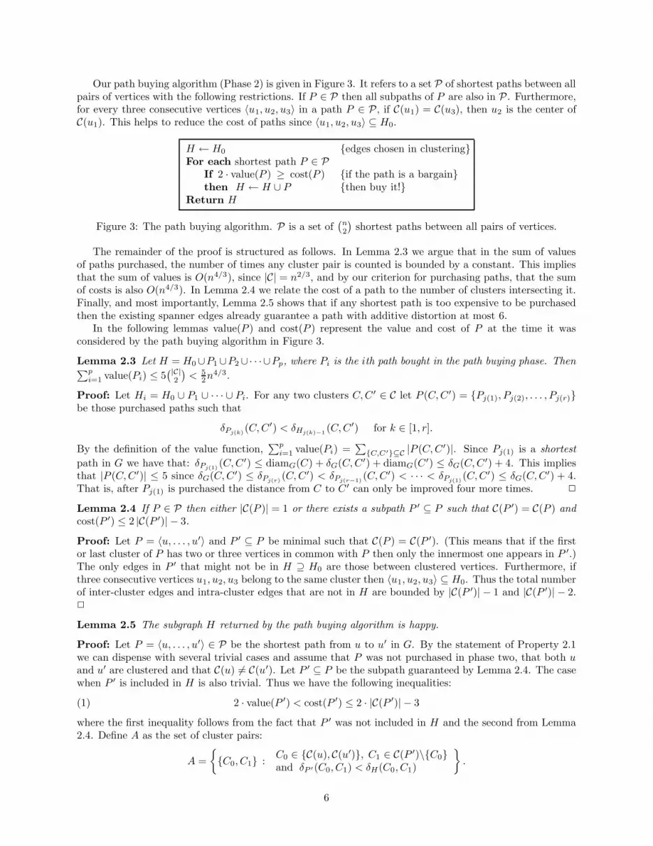
Our path buying algorithm (Phase 2) is given in Figure 3. It refers to a set P of shortest paths between allpairs of vertices with the following restrictions. If P ∈ P then all subpaths of P are also in P . Furthermore,for every three consecutive vertices 〈u1, u2, u3〉 in a path P ∈ P , if C(u1) = C(u3), then u2 is the center ofC(u1). This helps to reduce the cost of paths since 〈u1, u2, u3〉 ⊆ H0.

H ← H0 edges chosen in clusteringFor each shortest path P ∈ P

If 2 · value(P ) ≥ cost(P ) if the path is a bargainthen H ← H ∪ P then buy it!

Return H

Figure 3: The path buying algorithm. P is a set of(

n2

)

shortest paths between all pairs of vertices.

The remainder of the proof is structured as follows. In Lemma 2.3 we argue that in the sum of valuesof paths purchased, the number of times any cluster pair is counted is bounded by a constant. This impliesthat the sum of values is O(n4/3), since |C| = n2/3, and by our criterion for purchasing paths, that the sumof costs is also O(n4/3). In Lemma 2.4 we relate the cost of a path to the number of clusters intersecting it.Finally, and most importantly, Lemma 2.5 shows that if any shortest path is too expensive to be purchasedthen the existing spanner edges already guarantee a path with additive distortion at most 6.

In the following lemmas value(P ) and cost(P ) represent the value and cost of P at the time it wasconsidered by the path buying algorithm in Figure 3.

Lemma 2.3 Let H = H0∪P1∪P2∪· · ·∪Pp, where Pi is the ith path bought in the path buying phase. Then∑p

i=1 value(Pi) ≤ 5(

|C|2

)

< 52n4/3.

Proof: Let Hi = H0 ∪ P1 ∪ · · · ∪ Pi. For any two clusters C, C ′ ∈ C let P (C, C ′) = Pj(1), Pj(2), . . . , Pj(r)be those purchased paths such that

δPj(k)(C, C ′) < δHj(k)−1

(C, C ′) for k ∈ [1, r].

By the definition of the value function,∑p

i=1 value(Pi) =∑

C,C′⊆C |P (C, C ′)|. Since Pj(1) is a shortest

path in G we have that: δPj(1)(C, C ′) ≤ diamG(C) + δG(C, C ′) + diamG(C ′) ≤ δG(C, C ′) + 4. This implies

that |P (C, C ′)| ≤ 5 since δG(C, C ′) ≤ δPj(r)(C, C ′) < δPj(r−1)

(C, C ′) < · · · < δPj(1)(C, C ′) ≤ δG(C, C ′) + 4.

That is, after Pj(1) is purchased the distance from C to C ′ can only be improved four more times. 2

Lemma 2.4 If P ∈ P then either |C(P )| = 1 or there exists a subpath P ′ ⊆ P such that C(P ′) = C(P ) andcost(P ′) ≤ 2 |C(P ′)| − 3.

Proof: Let P = 〈u, . . . , u′〉 and P ′ ⊆ P be minimal such that C(P ) = C(P ′). (This means that if the firstor last cluster of P has two or three vertices in common with P then only the innermost one appears in P ′.)The only edges in P ′ that might not be in H ⊇ H0 are those between clustered vertices. Furthermore, ifthree consecutive vertices u1, u2, u3 belong to the same cluster then 〈u1, u2, u3〉 ⊆ H0. Thus the total numberof inter-cluster edges and intra-cluster edges that are not in H are bounded by |C(P ′)| − 1 and |C(P ′)| − 2.2

Lemma 2.5 The subgraph H returned by the path buying algorithm is happy.

Proof: Let P = 〈u, . . . , u′〉 ∈ P be the shortest path from u to u′ in G. By the statement of Property 2.1we can dispense with several trivial cases and assume that P was not purchased in phase two, that both uand u′ are clustered and that C(u) 6= C(u′). Let P ′ ⊆ P be the subpath guaranteed by Lemma 2.4. The casewhen P ′ is included in H is also trivial. Thus we have the following inequalities:

(1) 2 · value(P ′) < cost(P ′) ≤ 2 · |C(P ′)| − 3

where the first inequality follows from the fact that P ′ was not included in H and the second from Lemma2.4. Define A as the set of cluster pairs:

A =

C0, C1 :C0 ∈ C(u), C(u′), C1 ∈ C(P ′)\C0and δP ′(C0, C1) < δH(C0, C1)

.

6

The cluster pairs counted in A are also counted in value(P ′) so |A| ≤ value(P ′). By the inequalities of Eqn. 1value(P ′) ≤ |C(P ′)| − 2. Notice that the maximum number of cluster pairs counted by A is 2 |C(P ′)| − 3.This means that for at least |C(P ′)| − 1 of these cluster pairs, their distance in the spanner is no worse thantheir distance in P ′. By the pigeonhole principle there must be some cluster C∗ ∈ C(P ′) = C(P ) satisfyingboth

δH(C(u), C∗) ≤ δP ′(C(u′), C∗)

andδH(C∗, C(u′)) ≤ δP ′(C∗, C(u′)).

Since C(P ) = C(P ′) it also follows that P has this property. 2

Lemma 2.6 If H is the subgraph purchased by the path buying algorithm then |H | < 6 · n4/3.

Proof: One can easily see that |H | = |H0|+∑

i cost(Pi). By construction we have |H0| ≤ n4/3. It followsfrom Lemma 2.3 that

∑

i cost(Pi) ≤ 2 ·∑i value(Pi) < 5 · n4/3. 2

Theorem 2.7 There exists an additive 6-spanner of any graph with size O(n4/3).

Proof: Follows from Lemmas 2.2, 2.5, and 2.6. 2

2.1 Parameterizing the Path Buying Algorithm

Our 6-spanner construction can be generalized to larger additive distortion. However, we can only guaranteethat a β-spanner (β > 6) has o(n4/3) edges if the graph satisfies additional requirements. Let Γk(G) be thenumber of edges in G that lie on some cycle with length at most 2k. Theorem 2.8 generalizes Theorem 2.7and provides an efficient construction algorithm.

Theorem 2.8 For any graph G and integer parameters k ≥ 1 and ` ∈ [0, k], there exists an additive

(2k + 4`)-spanner with size O(Γk(G) + n1+ 1k+`+1 ). Furthermore, the spanner can be constructed in time

O(mn1− `k+`+1 ).

Theorem 2.8 says that if the graph is not too far from having girth greater than 2k then we can construct anumber of additive spanners with different size-distortion tradeoffs. Notice that when k = 1, Γ1(G) = 0 sinceall graphs have girth at least 3. As special cases, Theorem 2.8 gives 2- and 6-spanners with size O(n3/2) andO(n4/3). (This 2-spanner construction is slower and more complicated than earlier ones but it does illustratethe applicability of the path buying algorithm.) Figure 4 lists some of the corollaries of Theorem 2.8 forgraphs with girth greater than 4 and greater than 6.

The spanners provided by Theorem 2.8 are constructed with a path buying algorithm, with the followingdifferences. First, it uses a generalized clustering scheme that produces clusters of two radii: k and `. Second,it uses a value function that measures how well the spanner under construction approximates the distancebetween cluster pairs C, C ′, where C has radius ` and C ′ radius k.

Before running the path buying algorithm we compute an appropriate clustering and initial set of edgesHk,`, which plays the same role as H0 in our 6-spanner. This clustering procedure that produces Hk,` is verysimilar to the randomized clustering procedure presented later in Section 3, though the analysis of these twoschemes is sufficiently different to justify two expositions. We begin by selecting vertex sets V` and Vk whereV` is a random sample of V of size n1−`ε and Vk is a random sample of V` of size n1−kε, where ε will bechosen later. We find two clusterings C`, Ck, where Ci consists of a set of disjoint subsets of V . Each C ∈ Ci

is centered at some vertex in Vi and a vertex v is contained in some C ∈ Ci if and only if δ(v, Vi) ≤ i; inparticular, the distance from v to the center of its cluster is at most i. Hk,` consists of a radius-i spanningtree of each C ∈ Ci and i ∈ k, `, as well as every edge incident to a vertex that does not appear in bothclusterings C` and Ck. The number of edges contributed by the spanning trees is only 2n so we are mainlyconcerned with the expected number of the remaining edges.

Lemma 2.9 Given a graph G with m edges, the subgraph Hk,` can be constructed in O(m) time andE[|Hk,`|] = O(Γk(G) + n1+ε).

7

Add. Dist. Spanner Size Construction Time Notes

2 O(n3/2) O(mn) k = 1, ` = 0, cf. [6, 25, 30, 55]

6 O(n4/3) O(mn2/3) k = ` = 1

GRAPHS WITH GIRTH > 4

0 O(n3/2) — [56, 54]4 O(n4/3) O(mn) k = 2, ` = 0

8 O(n5/4) O(mn3/4) k = 2, ` = 112 O(n6/5) O(mn3/5) k = ` = 2

GRAPHS WITH GIRTH > 6

0 O(n4/3) — [56, 54]

6 O(n5/4) O(mn) k = 3, ` = 010 O(n6/5) O(mn4/5) k = 3, ` = 1

14 O(n7/6) O(mn2/3) k = 3, ` = 2

18 O(n8/7) O(mn4/7) k = ` = 3

Figure 4: Additive spanners derived from Theorem 2.8. See [56] for constructions of graphs with girth > 4and > 6, and [54] for references to earlier constructions of high-girth graphs.

Proof: To simplify the analysis we imagine constructing Hk,` by selecting vertex sets V = V0 ⊇ V1 ⊇ · · · ⊇Vk, where Vi is a random sample of Vi−1 of size n1−iε. We construct the clusterings C0, . . . , Ck iteratively.Let c ∈ C ∈ Ci−1, where c ∈ Vi−1 is the center of a cluster C. If c also appears in Vi then every vertexincident to C appears in some cluster in Ci. In particular, c’s cluster in Ci consists of C and some subset ofthe vertices incident to C that join C. (A vertex may be eligible to join multiple clusters and can chooseany one.) Suppose that we decide to include all edges in Hk,` that have at least one endpoint unclustered inany of C0, . . . , Ck. Let v be some vertex that has appeared in all the clusterings C0, . . . , Ci−1 and consider theeffect on v of randomly choosing the subset Vi. Suppose v is incident to s clusters in Ci−1, say C1, . . . , Cs.The probability that v is included in Ci is at least7 1− (1− n−ε)s. The effect of v not appearing in Ci is toinclude in Hk,` all edges incident to v, which could be significantly larger than s and nε. Let C1, . . . , Cs′be those clusters connected to v by at most one edge (this would be exactly one edge, except for the onecluster that actually contains v.) Every edge (v, w) connecting v to a cluster C appearing in Cs′+1, . . . , Cslies on a cycle of length at most 2i ≤ 2k: the one consisting of (v, w), a path from w to w′ ∈ C passingthrough the center of C, and the edge (w′, v). Such a w′ exists because v is connected to C by at leasttwo edges. If v is unclustered in Ci then the contribution of the edges from v to Cs′+1, . . . , Cs is countedin the Γk(G) term. Excluding these edges, the expected number of edges contributed by v is at most(s′ − 1) · Pr[v does not appear in Ci] ≤ (s′ − 1)(1− n−ε)s < nε.8 2

We now turn to the proof of Theorem 2.8.

Proof: (of Theorem 2.8) First notice that the only edges missing from Hk,` are those with both endpointspresent in both clusterings C`, Ck, so we can restrict our attention to shortest paths between clustered vertices.Let Ci(v) be the Ci cluster containing v and Ci(Z) be the set of clusters in Ci intersecting the subgraph Z.After running the path buying algorithm with appropriate cost and value functions we end up with a spannerH that is happy under a new definition of happiness.

Property 2.10 A subgraph H of G that contains Hk,` is happy if for any u, u′ ∈ V`, there is a shortestpath P (w.r.t. G) from u to u′ and a cluster C∗ ∈ Ck(P ) such that: δH(u, C∗) ≤ δP (u, C∗) and δH(u′, C∗) ≤δP (u′, C∗).

7This would be the exact probability if Vi were selected from Vi−1 by sampling each element with probability n−ε. SelectingVi as a random subset of Vi−1 with size n1−iε only improves v’s chance of being clustered in Ci.

8For the last inequality, observe that s′(1 − 1/x)s′ ≤ x(s′/x)e−s′/x ≤ x, for any positive x.

8

It follows that any happy subgraph H is also an additive (2k + 4`)-spanner. To see this, consider ashortest path between any two vertices v, v′ and let u and u′ be the center of the C` clusters containing vand v′, respectively. Let P be the shortest path between u and u′. By the happiness of H there exists acluster C∗ ∈ Ck(P ) such that

δH(u, u′) ≤ δH(u, C∗) + diam(C∗) + δH(C∗, u′) ≤ δ(u, u′) + 2k.

PSfrag replacements

kk

` `

u u′

v v′

C∗

C`(u) C`(u′)

Figure 5: The clusters C`(u), C`(u′), and C∗ ∈ Ck, are indicated by ovals. Dashed curves represent paths inthe spanner H . The shortest paths in G connecting v to v′ and u to u′ are indicated.

Using this bound on the distance from u to u′ in H , we can bound δH(v, v′) as:

δH(v, v′) ≤ δH(v, u) + δH(v′, u′) + δH(u, u′) ≤ 2` + δ(u, u′) + 2k ≤ δ(v, v′) + 2k + 4`.

Let P be a set of shortest paths between all pairs of vertices. We only consider shortest paths inP and insist that it satisfy two properties. First, any subpath of a path in P is also in P . Second, if〈u0, u1, . . . , u2k〉 ∈ P and Ck(u0) = Ck(u2k), then uk is the center of Ck(u0) and 〈u0, . . . , u2k〉 is contained inthe spanning tree of Ck(u0) included in Hk,`. Let P (u, u′) ∈ P be the shortest path between u and u′.

We use the same cost function as before: cost(P ) = |P\H |, where H now represents the spanner underconstruction. However, the value function is only defined on paths connecting vertices in V`. LettingP = P (u, u′), where u, u′ ∈ V`, we define value(P ) as:

value(P ) = |(v, C) : v ∈ u, u′, C ∈ Ck(P ), and δP (v, C) < δH(v, C)| .

The path buying algorithm below has a few differences from the 6-spanner algorithm. We only considershortest paths between vertices in V` and the criterion for purchasing a path P is slightly stronger: 2k ·value(P ) (rather than 2 · value(P )) must be at least cost(P ).

H ← Hk,` edges chosen in clusteringFor each u, u′ ⊆ V` let P = P (u, u′)

If 2k · value(P ) ≥ cost(P ) if the path is a bargainthen H ← H ∪ P then buy it!

Return H

Figure 6: Constructing an additive (2k + 4`)-spanner.

Let P1, . . . , Pp be the paths purchased. It follows that the size of H is exactly |Hk,`| plus∑

1≤i≤p cost(Pi) ≤2k

∑

1≤i≤p value(Pi) ≤ 2µk |V` × Vk| = 2µkn2−(k+`)ε, where µ is the maximum number of times that anypair (v, C), where v ∈ V`, C ∈ Ck could be counted in

∑

i value(Pi). One can see that µ = 2k + 1. When(v, C) is first counted, say when Pi is purchased, we have δPi(v, C) ≤ δ(v, C)+diam(C) = δ(v, C)+2k. After

9

Pi is purchased the distance between v and C in H can only be improved 2k more times. Thus, the size ofH is O(Γk(G) + n1+ε + k2n2−(k+`)ε). Setting nε = (k2n)1/(k+`+1), the total size is O(Γk(G) + n1+1/(k+`+1)).

It only remains to show that H is happy and in particular, that if a path P = P (u, u′) is not purchasedthen δH(u, u′) ≤ δ(u, u′) + 2k. We first bound cost(P ) then show that if P is not purchased, there must besome C∗ ∈ Ck(P ) satisfying Property 2.10

Consider any cluster C ∈ Ck(P ) and let z, z′ be the first and last vertices in P that belong to C. Anedge is internal to C if it lies on the subpath 〈z, . . . , z′〉. (Note that not all vertices between z and z′

are necessarily in C.) It follows from our choice of shortest paths P that either |〈z, . . . , z ′〉| ≤ 2k − 1 or〈z, . . . , z′〉 ⊆ Hk,` ⊆ H . Thus, the total number of internal edges in P\H is at most (2k− 1) |Ck(P )| and thenumber of remaining edges in P\H is at most |Ck(P )| − 1. In total we have cost(P ) ≤ 2k |Ck(P )| − 1. If wefail to purchase P then 2k · value(P ) ≤ cost(P )− 1 ≤ 2k |Ck(P )| − 2, implying that value(P ) ≤ |Ck(P )| − 1.Since there are 2 |Ck(P )| cluster pairs of the form (v, C) where v ∈ u, u′ and C ∈ Ck(P ), our bound onvalue(P ) implies that for at least one C∗ ∈ Ck(P ), δH(u, C∗) ≤ δP (u, C∗) and δH(u′, C∗) ≤ δP (u′, C∗).Therefore H is an additive (2k + 4`)-spanner.

We now turn to an efficient construction algorithm. Recall from Lemma 2.9 that Hk,` can be found in lin-ear time. In the path buying phase it is rather time consuming to maintain the actual distance in H betweenpairs (v, C) ∈ V` × Ck, which would be required to compute the value function exactly. Instead, we keep an

upper bound δH(v, C), which is the minimum distance between v and C in a path already purchased. We alsoignore the cost function and consider the valid upper bound cost(P ) ≤ 2k |Ck(P )|−1. (Clearly these changesdo not affect the correctness of the algorithm.) At the beginning of the path buying phase we construct, inO(m |C`|) time, a shortest path tree originating at each vertex in V`. In such a tree a relevant vertex is one inV` or one that has at least two V` vertices in different subtrees, that is, a branching vertex in the subtree con-necting V` nodes. For u ∈ V` let Ru be the set of relevant vertices in u’s shortest path tree. We consider, innon-decreasing order by length, the shortest paths between pairs (u, u′) where u ∈ V` and u′ ∈ Ru. For a path

P = 〈u0, u1, . . . , uq〉, where u0 ∈ V`, let ν(u0, uq) =∣

∣

∣

(u0, C) : C ∈ Ck(P ) and δP (u0, C) < δH(u0, C)∣

∣

∣.

We assume that after P is considered we have computed ν(u0, ui) and |Ck(〈u0, . . . , ui〉)|, for all relevantvertices ui ∈ Ru0 . When we consider an extension of P , say P ′ = 〈u0, . . . , uq, . . . , uq+r〉, where uq+r is thefirst relevant vertex on the extension, we can easily update |Ck(P ′)| and ν(u0, uq+r) in just O(k + r) time. Ifuq+r ∈ V` then we need to decide whether to purchase P ′. We check if ν(u0, uq+r) + ν(uq+r, u0) ≥ |Ck(P ′)|,which serves the same purpose as checking the inequality 2k · value(P ′) ≥ cost(P ′). If the inequality holdswe buy P ′ and update ν(u, u′) where u ∈ u0, uq+r and u′ ∈ Ru. This amounts to checking, for each pair(u0, C) counted in ν(u0, uq+r) and each path P ′′ = 〈u0, . . . , u

′〉, whether δP ′(u0, C) ≤ δP ′′(u0, C). If so,the pair (u0, C) should no longer be counted in ν(u0, u

′), if it was counted there at all. The total time for

these updates is O(k · |C`|2 · |Ck|) = O(n3− 2`+kk+`+1 ) and the total time for performing breadth first searches

is O(m · |C`|) = O(mn1− `k+`+1 ). We can safely assume that m ≥ n1+ 1

k+`+1 ; if not we could simply returnthe original graph as a trivial additive 0-spanner. For m above this threshold the two time bounds are both

O(mn1− `k+`+1 ). 2

The first obstacle to improving Theorem 2.8 is dealing with graphs with lots of 3- and 4-cycles. It isstrange that short cycles should impede the discovery of more additive spanners since high-girth graphsare the most difficult instances when optimizing for multiplicative distortion. The recent lower bounds ofWoodruff [57] provide some circumstantial evidence that short cycles really do complicate the problem. Hishard instances are actually composed entirely of complete bipartite graphs, where each edge appears on ahuge number of 4-cycles.

Theorem 2.8 generalizes the 6-spanner construction by considering clusterings with wider radii. Anotherdirection for generalization is to consider more hops between clusters. Theorem 2.11 follows from a smalladjustment to the 6-spanner algorithm.

Theorem 2.11 Every graph on n vertices contains an additive O(n1−3ε)-spanner with size O(n1+ε), for anyconstant ε ∈ (0, 1

3 ).

Proof: The algorithm is nearly identical to the 6-spanner construction. We find a radius-1 clustering Ccontaining n1−ε clusters, and let H0 contain all edges incident to at least one unclustered vertex and aspanning tree of each cluster. We run the path buying algorithm from Figure 3 using the same cost function

10

but a different value function:

value(P ) = n−1+3ε · |C, C ′ ⊆ C(P ) : δP (C, C ′) < δH(C, C ′)| .

The rationale for this value function is simple. If there are n1−ε clusters and our desired spanner size isO(n1+ε), each cluster pair can only afford to be charged the cost of buying O(n−1+3ε) edges, that is, asmall fraction of a single edge. Let P be some shortest path and P ′ and P ′′ be the prefix and suffix ofP containing n1−3ε distinct clusters. If P is not purchased then, by the same reasoning used before, theremust be three not necessarily distinct clusters C ′, C∗, C ′′ where C ′ ∈ C(P ′), C ′′ ∈ C(P ′′), and C∗ ∈ C(P )such that δH(C ′, C∗) ≤ δP (C ′, C∗) and δH(C ′′, C∗) ≤ δP (C ′′, C∗). That is, the subpath of P connecting C ′

to C ′′ is approximated by H to within an additive distortion of 6. To get from the first vertex of P to C ′

and from C ′′ to the last vertex of P we use any standard multiplicative O(ε−1)-spanner with size O(n1+ε).The total additive distortion is therefore 6 + O(ε−1(cost(P ′) + cost(P ′′))) = O(n1−3ε). The size of H0 andthe multiplicative spanner is O(n1+ε) and the number of edges included by the path buying algorithm is∑

i cost(Pi) ≤ 2∑

i value(Pi) = O(n−1+3ε ·(

|C|2

)

) = O(n1+ε). 2

Theorem 2.11 is not particularly impressive, but, again, it illustrates the flexible nature of the path buyingtechnique. The previous best additive spanner with size O(n1+ε) had distortion roughly O(n1−2ε) [15] andwas substantially more complicated to construct.

3 A Simple (k, k − 1)-Spanner in Linear Time

In this section we will first show how to construct a (2k − 1, 0)-spanner of size O(kn1+1/k) in O(km)deterministic time. Then we will extend this method to construct a (k, k− 1) spanner of size O(kn1+1/k) inO(km) deterministic time.

The input graph is G = (V, E). A cluster is simply a set of vertices and a clustering is a set of disjointclusters. A vertex is (un)clustered in a clustering C if it appears (does not appear) in some cluster of C. In aclustering C, for any clustered vertex u, denote by C(u) the cluster of C that contains u. For clusters C andC ′, let E(C, C ′) = (C × C ′) ∩ E(G) be the set of edges between C and C ′. Let E(v, C) be the set of edgesbetween the vertex v and vertices in C. A vertex v is adjacent to a cluster C if E(v, C) 6= ∅. In a similarmanner, two clusters C and C ′ are adjacent to each other if E(C, C ′) 6= ∅.

Our constructions in this section are based on a set of k +1 clusterings, C0, C1, . . . , Ck, where C0 = v :v ∈ V (G), Ck = ∅, and |Ci| ≤ n1−i/k. Below, we give two methods for constructing appropriate sequencesof clusterings. The edge set of our (2k − 1)-spanner S is defined by the following two rules:

Rule R1. For each cluster C ∈ Ci, there exists a tree in S that spans C and has radius9 at most i.

Rule R2. For each vertex v that is unclustered in Ci and each cluster C ∈ Ci−1 adjacent to v, some edgefrom E(v, C) appears in S.

The construction of Theorem 3.1 is slightly weaker than that of [38]; however it is the starting point forour (k, k − 1)-spanner.

Theorem 3.1 A (2k − 1)-spanner of size O(kn1+1/k) can be constructed in O(km) deterministic time.

Proof: We first prove that Rules R1 and R2 give a (2k − 1)-spanner; we then prove the size and timebounds. Let (u, v) be an arbitrary edge in the original graph. If δS(u, v) ≤ (2k− 1)δG(u, v) then S is clearlya (2k − 1)-spanner. Let ` be minimum such that either u or v was unclustered in C` and without loss ofgenerality let the unclustered vertex be u. By Rule R2 there must be an edge in S from u to C`−1(v); callthis edge (u, w). By Rule R1 there must be a path in S from w to v of length at most 2(` − 1), twice theradius of C`−1(v). Since ` ≤ k it follows immediately that δS(u, v) ≤ 2k − 1.

Given the clustering Ci we show how to compute Ci+1 such that the number of edges added to the spannerdue to Rules R1 and R2 are at most n and n1+1/k, respectively (This construction is a simplified versionof one described by Elkin [26].) Initially Ci+1 = ∅. We define the priority of a cluster C ∈ Ci to be the

9Recall that maximum distance between any two vertices in a subgraph is at most twice the radius of that subgraph.

11

number of adjacent vertices that are unclustered with respect to Ci+1. We repeatedly choose a cluster C ∈ Ci

with maximum priority. If priority(C) ≥ n(i+1)/k we add a new cluster to Ci+1 consisting of C and allunclustered vertices adjacent to C. (If C has radius i then the cluster added to Ci+1 clearly has radius i+1.)It follows that |Ci+1| ≤ n1−(i+1)/k and that the number of edges included in the spanner due to Rule R2 is∑

C∈Cipriority(C), which is at most |Ci| (n(i+1)/k − 1) < n1+1/k. The number of edges added due to Rule

R1 is at most the number of clustered vertices in Ci+1, i.e. at most n. The clustering Ci+1 can easily begenerated in linear time using a priority queue consisting of n buckets. 2

The randomized construction of [13] constructs the clusterings in an even simpler manner. Rather thancarefully selecting clusters from Ci for inclusion in Ci+1, they randomly sample all clusters from Ci withprobability n−1/k. The alternative (2k− 1)-spanner construction based on this method is given in Figure 7.With this algorithm the expected size of the spanner is O(kn1+1/k).

Initially S = ∅ and C0 = v : v ∈ V (G)

For i from 1 to k

– Let Ci be sampled from Ci−1 with prob. n−1/k (If i = k let Ck = ∅)– For each vertex v which does not belong to any cluster in Ci do (concurrently):

(R1) If v is adjacent to some C ∈ Ci, add v to C and add some edge of E(v, C) to S.

(R2) Otherwise, add to S some edge from E(v, C), for each C ∈ Ci−1 adjacent to v.

Return the (2k − 1)-spanner S

Figure 7: A randomized (2k − 1)-spanner construction.

We next improve our (2k − 1)-spanner construction to obtain a (k, k − 1)-spanner. All the edges thatwe put in the (2k − 1)-spanner S are of the form E(v, C). Now let us also add edges of the form E(C, C ′),which will consist of edges from clusters of one clustering to clusters of another clustering.

Rule R3. For each i with 0 ≤ i ≤ k − 1 and for each pair of adjacent clusters C, C ′ with C ∈ Ci andC ′ ∈ Ck−1−i, some edge from E(C, C ′) appears in S.

Rule R4. For each i ≥ k/2 and each pair of adjacent clusters C, C ′ with C ∈ Ci and C ′ ∈ Ci−1, some edgefrom E(C, C ′) appears in S.

The number of edges included due to Rule R3 is bounded by n1−i/kn1−(k−1−i)/k = n1+1/k, for each i.Similarly, at most n1−i/kn1−(i−1)/k = n2−2i/k+1/k edges are included due to R4, which is at most n1+1/k

since i ≥ k/2. Our entire (k, k − 1)-spanner construction is given in Figure 8. It consists of just those edgesincluded by Rules R1–R4.

(R1–2) Compute a (2k − 1)-spanner S with our construction.

(R3) Add to S one edge from E(C, C ′) for each adjacent pairC ∈ Ci and C ′ ∈ Ck−1−i, for i from 0 to k − 1.

(R4) Add to S one edge from E(C, C ′) for each adjacent pairC ∈ Ci, and C ′ ∈ Ci−1, for i from dk/2e to k − 1.

Figure 8: A simple linear time algorithm for constructing a (k, k − 1)-spanner.

Implementing Rules R3 and R4 takes linear time for any fixed i. Once it is proved that Rules R1–R4yield a (k, k − 1)-spanner we can conclude with the following theorem.

12

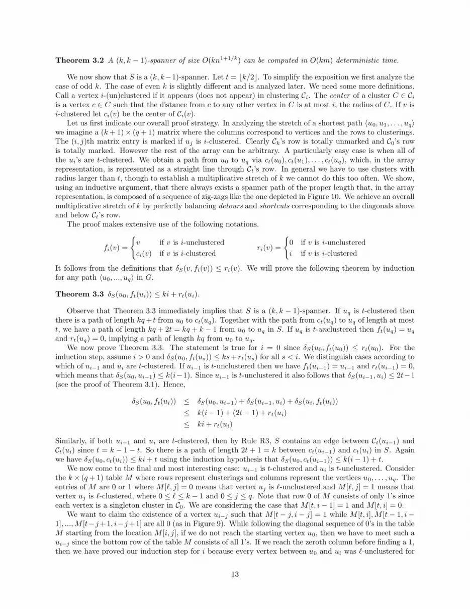
Theorem 3.2 A (k, k − 1)-spanner of size O(kn1+1/k) can be computed in O(km) deterministic time.

We now show that S is a (k, k−1)-spanner. Let t = bk/2c. To simplify the exposition we first analyze thecase of odd k. The case of even k is slightly different and is analyzed later. We need some more definitions.Call a vertex i-(un)clustered if it appears (does not appear) in clustering Ci. The center of a cluster C ∈ Ciis a vertex c ∈ C such that the distance from c to any other vertex in C is at most i, the radius of C. If v isi-clustered let ci(v) be the center of Ci(v).

Let us first indicate our overall proof strategy. In analyzing the stretch of a shortest path 〈u0, u1, . . . , uq〉we imagine a (k + 1)× (q + 1) matrix where the columns correspond to vertices and the rows to clusterings.The (i, j)th matrix entry is marked if uj is i-clustered. Clearly Ck’s row is totally unmarked and C0’s rowis totally marked. However the rest of the array can be arbitrary. A particularly easy case is when all ofthe ui’s are t-clustered. We obtain a path from u0 to uq via ct(u0), ct(u1), . . . , ct(uq), which, in the arrayrepresentation, is represented as a straight line through Ct’s row. In general we have to use clusters withradius larger than t, though to establish a multiplicative stretch of k we cannot do this too often. We show,using an inductive argument, that there always exists a spanner path of the proper length that, in the arrayrepresentation, is composed of a sequence of zig-zags like the one depicted in Figure 10. We achieve an overallmultiplicative stretch of k by perfectly balancing detours and shortcuts corresponding to the diagonals aboveand below Ct’s row.

The proof makes extensive use of the following notations.

fi(v) =

v if v is i-unclustered

ci(v) if v is i-clusteredri(v) =

0 if v is i-unclustered

i if v is i-clustered

It follows from the definitions that δS(v, fi(v)) ≤ ri(v). We will prove the following theorem by inductionfor any path 〈u0, ..., uq〉 in G.

Theorem 3.3 δS(u0, ft(ui)) ≤ ki + rt(ui).

Observe that Theorem 3.3 immediately implies that S is a (k, k − 1)-spanner. If uq is t-clustered thenthere is a path of length kq + t from u0 to ct(uq). Together with the path from ct(uq) to uq of length at mostt, we have a path of length kq + 2t = kq + k − 1 from u0 to uq in S. If uq is t-unclustered then ft(uq) = uq

and rt(uq) = 0, implying a path of length kq from u0 to uq.We now prove Theorem 3.3. The statement is true for i = 0 since δS(u0, ft(u0)) ≤ rt(u0). For the

induction step, assume i > 0 and δS(u0, ft(us)) ≤ ks+ rt(us) for all s < i. We distinguish cases according towhich of ui−1 and ui are t-clustered. If ui−1 is t-unclustered then we have ft(ui−1) = ui−1 and rt(ui−1) = 0,which means that δS(u0, ui−1) ≤ k(i−1). Since ui−1 is t-unclustered it also follows that δS(ui−1, ui) ≤ 2t−1(see the proof of Theorem 3.1). Hence,

δS(u0, ft(ui)) ≤ δS(u0, ui−1) + δS(ui−1, ui) + δS(ui, ft(ui))

≤ k(i− 1) + (2t− 1) + rt(ui)

≤ ki + rt(ui)

Similarly, if both ui−1 and ui are t-clustered, then by Rule R3, S contains an edge between Ct(ui−1) andCt(ui) since t = k − 1− t. So there is a path of length 2t + 1 = k between ct(ui−1) and ct(ui) in S. Againwe have δS(u0, ct(ui)) ≤ ki + t using the induction hypothesis that δS(u0, ct(ui−1)) ≤ k(i− 1) + t.

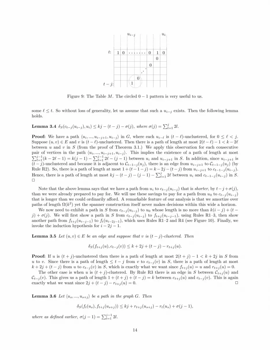
We now come to the final and most interesting case: ui−1 is t-clustered and ui is t-unclustered. Considerthe k× (q + 1) table M where rows represent clusterings and columns represent the vertices u0, . . . , uq. Theentries of M are 0 or 1 where M [`, j] = 0 means that vertex uj is `-unclustered and M [`, j] = 1 means thatvertex uj is `-clustered, where 0 ≤ ` ≤ k − 1 and 0 ≤ j ≤ q. Note that row 0 of M consists of only 1’s sinceeach vertex is a singleton cluster in C0. We are considering the case that M [t, i− 1] = 1 and M [t, i] = 0.

We want to claim the existence of a vertex ui−j such that M [t− j, i− j] = 1 while M [t, i], M [t− 1, i−1], ..., M [t−j +1, i−j +1] are all 0 (as in Figure 9). While following the diagonal sequence of 0’s in the tableM starting from the location M [i, j], if we do not reach the starting vertex u0, then we have to meet such aui−j since the bottom row of the table M consists of all 1’s. If we reach the zeroth column before finding a 1,then we have proved our induction step for i because every vertex between u0 and ui was `-unclustered for

13

...

. . . . . . .PSfrag replacements

0

0

0

000

1

11

uiui−j

t:

t− j:

Figure 9: The Table M . The circled 0− 1 pattern is very useful to us.

some ` ≤ t. So without loss of generality, let us assume that such a ui−j exists. Then the following lemmaholds.

Lemma 3.4 δS(ct−j(ui−j), ui) ≤ kj − (t− j)− σ(j), where σ(j) =∑j

l=1 2l.

Proof: We have a path 〈ui, ..., ui−j+1, ui−j〉 in G, where each ui−` is (t − `)-unclustered, for 0 ≤ ` < j.Suppose (u, v) ∈ E and v is (t− `)-unclustered. Then there is a path of length at most 2(t− `)− 1 < k− 2`between u and v in S (from the proof of Theorem 3.1.) We apply this observation for each consecutivepair of vertices in the path 〈ui, ..., ui−j+1, ui−j〉. This implies the existence of a path of length at most∑j−1

`=1(k − 2`− 1) = k(j − 1)−∑j−1`=1 2`− (j − 1) between ui and ui−j+1 in S. In addition, since ui−j+1 is

(t− j)-unclustered and because it is adjacent to Ct−1−j(uj), there is an edge from ui−j+1 to Ct−1−j(uj) (byRule R2). So, there is a path of length at most 1+ (t− 1− j) = k− 2j− (t− j) from ui−j+1 to ct−1−j(ui−j).

Hence, there is a path of length at most kj − (t− j)− (j − 1)−∑j`=1 2` between ui and ct−1−j(ui−j) in S.

2

Note that the above lemma says that we have a path from ui to ct−j(ui−j) that is shorter, by t−j +σ(j),than we were already prepared to pay for. We will use these savings to pay for a path from u0 to ct−j(ui−j)that is longer than we could ordinarily afford. A remarkable feature of our analysis is that we amortize overpaths of length Ω(k2) yet the spanner construction itself never makes decisions within this wide a horizon.

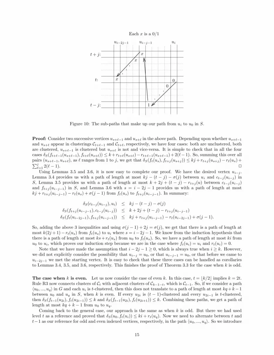
We now need to exhibit a path in S from ct−j(ui−j) to u0 whose length is no more than k(i− j) + (t−j) + σ(j). We will first show a path in S from ct−j(ui−j) to ft+j(ui−j−1), using Rules R1–3, then showanother path from ft+j(ui−j−1) to ft(ui−2j−1), which uses Rules R1–2 and R4 (see Figure 10). Finally, weinvoke the induction hypothesis for i− 2j − 1.

Lemma 3.5 Let (u, v) ∈ E be an edge and suppose that v is (t− j)-clustered. Then

δS(ft+j(u), ct−j(v)) ≤ k + 2j + (t− j)− rt+j(u).

Proof: If u is (t + j)-unclustered then there is a path of length at most 2(t + j) − 1 < k + 2j in S fromu to v. Since there is a path of length ≤ t − j from v to ct−j(v) in S, there is a path of length at mostk + 2j + (t− j) from u to ct−j(v) in S, which is exactly what we want since ft+j(u) = u and rt+j(u) = 0.

The other case is when u is (t + j)-clustered. By Rule R3 there is an edge in S between Ct+j(u) andCt−j(v). This gives us a path of length 1 + (t + j) + (t− j) = k between ct+j(u) and ct−j(v). This is againexactly what we want since 2j + (t− j)− rt+j(u) = 0. 2

Lemma 3.6 Let 〈us, ..., us+j〉 be a path in the graph G. Then

δS(ft(us), ft+j(us+j)) ≤ kj + rt+j(us+j)− rt(us) + σ(j − 1),

where as defined earlier, σ(j − 1) =∑j−1

l=1 2l.

14

.

..

..

.

PSfrag replacements

Each x is a 0/1

00

1

x

x

x

ui

t:

t + j:

t− j:

ui−2j−1 ui−j−1

Figure 10: The sub-paths that make up our path from ui to u0 in S.

Proof: Consider two successive vertices us+`−1 and us+` in the above path. Depending upon whether us+`−1

and us+` appear in clusterings Ct+`−1 and Ct+`, respectively, we have four cases: both are unclustered, bothare clustered, us+`−1 is clustered but us+` is not and vice-versa. It is simple to check that in all the fourcases δS(ft+`−1(us+`−1), ft+`(us+`)) ≤ k + rt+`(us+`)− rt+`−1(us+`−1)+2(`− 1). So, summing this over allpairs (us+`−1, us+`), as ` ranges from 1 to j, we get that δS(ft(us), ft+j(us+j)) ≤ kj + rt+j(us+j)− rt(us) +∑j

`=1 2(`− 1). 2

Using Lemmas 3.5 and 3.6, it is now easy to complete our proof. We have the desired vertex ui−j .Lemma 3.4 provides us with a path of length at most kj − (t − j) − σ(j) between ui and ct−j(ui−j) inS, Lemma 3.5 provides us with a path of length at most k + 2j + (t − j) − rt+j(u) between ct−j(ui−j)and ft+j(ui−j−1) in S, and Lemma 3.6 with s = i − 2j − 1 provides us with a path of length at mostkj + rt+j(ui−j−1)− rt(us) + σ(j − 1) from ft(us) to ft+j(ui−j−1). In summary:

δS(ct−j(ui−j), ui) ≤ kj − (t− j)− σ(j)

δS(ft+j(ui−j−1), ct−j(ui−j)) ≤ k + 2j + (t− j)− rt+j(ui−j−1)

δS(ft(ui−2j−1), ft+j(ui−j−1)) ≤ kj + rt+j(ui−j−1)− rt(ui−2j−1) + σ(j − 1).

So, adding the above 3 inequalities and using σ(j − 1) + 2j = σ(j), we get that there is a path of length atmost k(2j + 1)− rt(us) from ft(us) to ui where s = i− 2j− 1. We know from the induction hypothesis thatthere is a path of length at most ks+ rt(us) from u0 to ft(us). So, we have a path of length at most ki fromu0 to ui, which proves our induction step because we are in the case where ft(ui) = ui and rt(ui) = 0.

Note that we have made the assumption that i− 2j − 1 ≥ 0, which is always true when i ≥ k. However,we did not explicitly consider the possibility that ui−j = u0, or that ui−j−1 = u0, or that before we came toui−2j−1 we met the starting vertex. It is easy to check that these three cases can be handled as corollariesto Lemmas 3.4, 3.5, and 3.6, respectively. This finishes the proof of Theorem 3.3 for the case when k is odd.

The case when k is even. Let us now consider the case of even k. In this case, t = bk/2c implies k = 2t.Rule R3 now connects clusters of Ct with adjacent clusters of Ck−1−t, which is Ct−1. So, if we consider a path〈u0, ..., uq〉 in G and each ui is t-clustered, then this does not translate to a path of length at most kq +k−1between u0 and uq in S, when k is even. If every u2i is (t − 1)-clustered and every u2i−1 is t-clustered,then δS(ft−1(u2i), ft(u2i−1)) ≤ k and δS(ft−1(u2i), ft(u2i+1)) ≤ k. Combining these paths, we get a path oflength at most kq + k − 1 from u0 to uq.

Coming back to the general case, our approach is the same as when k is odd. But there we had usedlevel t as a reference and proved that δS(u0, ft(ui)) ≤ ki + rt(uq). Now we need to alternate between t andt−1 as our reference for odd and even indexed vertices, respectively, in the path 〈u0, ..., uq〉. So we introduce

15

some more notations:

h(i) =

t− 1 if i is even

t if i is oddr′(i) =

t− 1 if ui is h(i)-clustered

0 if ui is h(i)-unclustered

We will show the following theorem here.

Theorem 3.7 δS(u0, fh(i)(ui)) ≤ ki + r′(i).

This theorem immediately implies that S is a (k, k − 1)-spanner because if uq is h(q)-unclustered, thenthere is a path of length at most kq from u0 to uq. If uq is h(q)-clustered, there is a path of length kq + t− 1from u0 to ch(q)(uq) and there is a path of length at most t from ch(q)(uq) to uq. So, we have a path oflength at most kq + t− 1 + t = kq + k − 1 from u0 to uq.

Our proof will follow the same strategy as the proof of Theorem 3.3. We will prove the above theoremby induction. Since h(0) = t − 1, the base case holds. We assume that δS(u0, fh(s)(us)) ≤ ks + r′(s) forall s < i and we will prove the induction step for i. If ui−1 is h(i − 1)-unclustered, then we have a path oflength at most 2h(i− 1) − 1 ≤ 2t− 1 from ui−1 to ui and there is a path of length at most r′(i) + 1 fromui to fh(i)(ui). Hence, using the induction hypothesis for ui−1 and combining it with the above paths to ui

and fh(i)(ui), we get that there is a path of length at most k(i− 1) + 2t− 1 + r′(i) + 1 = ki + r′(i) from u0

to ui.Similarly, if ui−1 is h(i − 1)-clustered and ui is h(i)-clustered, since h(i − 1) + h(i) = k − 1, we would

have put an edge between Ch(i−1)(ui−1) and Ch(i)(ui) (by Rule R3). This gives us a path of length at mosth(i−1)+1+h(i) = 2t = k between ch(i−1)(ui−1) and ch(i)(ui). So, using this path along with the inductionhypothesis, we get a path of length at most ki + t− 1 from u0 to ch(i)(ui).

The non-trivial case is again when ui−1 is h(i − 1)-clustered and ui is h(i)-unclustered. Here, there isone easy sub-case. If h(i) = t, then in the table M (refer Figure 9), we have the desired 1− 0 pattern rightat our doorstep. We have M [t − 1, i − 1] = 1 and M [t, i] = 0. So, this gives us a path of length at most1 + t− 1 from ui to ct−1(ui−1). And the induction hypothesis tells us that there is a path of length at mostk(i − 1) + t − 1 from u0 to ct−1(ui−1). Hence there is a path of length at most ki from u0 to ui, which iswhat we want to show.

So, the only case left is when ui−1 is h(i− 1)-clustered and ui is h(i)-unclustered and h(i) = t− 1. Thenas in the proof of Theorem 3.3, we want to claim that there exists a vertex ui−j such that, in the table M ,M [t−1− j, i− j] = 1 while M [t−1, i], M [t−2, i−1], ..., M [t− j, i− j+1] are all 0. Either such a ui−j exists(since the bottom row of the table M consists of all 1’s) or while following the diagonal path of 0’s in thetable M , we reach the starting vertex u0. In the latter case, we have proved our induction step for i, becauseevery vertex ui−` in 〈u0, ..., ui〉 is (t− 1− `)-unclustered. Then, there is a path of length ≤ 2t− 1 < k in Sbetween every consecutive pair of vertices in 〈u0, ..., ui〉. So, without loss of generality, let us assume thatsuch a ui−j exists.

We need lemmas which are analogous to Lemma 3.4, Lemma 3.5, and Lemma 3.6. The proofs of Lemma3.8 and Lemma 3.9 are identical to those of Lemma 3.4 and Lemma 3.5 respectively.

Lemma 3.8 δS(ct−1−j(ui−j), ui) ≤ kj − (t− j)− σ(j) − (j − 1), where σ(j) =∑j

l=1 2l.

Lemma 3.9 Suppose (u, v) ∈ E. Suppose v is (t− 1− j)-clustered. Then

δS(ft+j(u), ct−1−j(v)) ≤ k + 2j + (t− j)− rt+j(u).

Lemma 3.10 Let 〈us, ..., us+j〉 be a path in the graph G. Then

δS(ft(us), ft+j(us+j)) ≤ kj + j + rt+j(us+j)− rt(us) + σ(j − 1),

If us is t-unclustered, then

δS(us, ft+j(us+j)) ≤ kj + j − 1 + rt+j(us+j) + σ(j − 1).

where as defined earlier, σ(j − 1) =∑j−1

l=1 2l.

16

Proof: 〈us, ..., us+j〉 is a path in G. Consider two successive vertices us+`−1 and us+` in the above path.Depending upon how us+`−1 and us+` appear in clusterings Ct+`−1 and Ct+` respectively, we have four cases:both are unclustered, both are clustered, us+`−1 is clustered but us+` is not and vice-versa. It is simple tocheck that in all the four cases δS(ft+`−1(us+`−1), ft+`(us+`)) ≤ k+1+rt+`(us+`)−rt+`−1(us+`−1)+2(`−1).So, summing this over all pairs (us+`−1, us+`), as ` ranges from 1 to j, we get that δS(ft(us), ft+j(us+j)) ≤kj + j + rt+j(us+j)− rt(us) +

∑j`=1 2(`− 1).

If us is t-unclustered, then there is a path of length at most 2t − 1 from us to us+1 and a path oflength at most rt+1(us+1) from us+1 to ft+1(us+1), which gives us an upper bound of k + rt+1(us+1)for δS(us, ft+1(us+1) instead of k + 1 + rt+1(us+1) for the 〈us, us+1〉 path. This path, when combinedwith the 〈us+1, ..., us+j〉 path obtained from the previous paragraph shows that δS(ft(us), ft+j(us+j)) ≤kj + j − 1 + rt+j(us+j) +

∑j`=1 2(`− 1). 2

So, as in the proof of Theorem 3.3, we use the path given by Lemma 3.8 to go from ui to ct−1−j(ui−j) andthen use the path given by Lemma 3.9 to go from ct−1−j(ui−j) to ft+j(ui−j−1) and then use the path givenby Lemma 3.10 to go from ft+j(ui−j−1) to ft(ui−2j−1). So, if we can show that h(i− 2j − 1) = t, then wecan use the induction hypothesis to claim that there is a path of length at most k(i− 2j− 1)+ r′(i− 2j− 1)from u0 to ft(ui−2j−1).

Lemma 3.11 h(i− 2j − 1) = t.

Proof: This is simple to show. Since h(`) = t if and only if ` is odd, we need to show that i− 2j− 1 is odd.We know that i must be even since h(i) = t− 1. Hence, i− 2j − 1 is odd. 2

So, we can use the induction hypothesis that there is a path of length ≤ k(i−2j−1)+ r′(i−2j−1) fromu0 to ft(ui−2j−1). Suppose ui−2j−1 is h(i−2j−1)-clustered. Then r′(i−2j−1) = t−1. And we get a pathfrom u0 to ui in S of length at most k(i− 2j − 1) + t− 1 + kj + j + rt+j(ui−j−1)− t + σ(j − 1) + k + 2j +(t− j)− rt+j(ui−j−1) + kj− (t− j)−σ(j)− (j− 1) = ki. If ui−2j−1 is t-unclustered, then we use the secondpart of Lemma 3.10 to upper bound the 〈ui−2j−1, ..., ui−j−1〉 path. So, there is a path of length at mostk(i−2j−1)+kj+j−1+rt+j(ui−j−1)+σ(j−1)+k+2j+(t−j)−rt+j(ui−j−1)+kj−(t−j)−σ(j)−(j−1) = kibetween u0 and ui in S. This proves our induction step.

Again, the three cases that ui−j = u0 or ui−j−1 = u0 or before we came to ui−2j−1, we see the startingvertex, can be handled as corollaries to Lemmas 3.8, 3.9, and 3.10 respectively. This finishes the proof ofTheorem 3.7 for the case when k is even. Recall that Theorem 3.3 which shows the correctness for odd kwas already proved. Thus Theorem 3.2 is completely proved.

3.1 Implementation in other models of computations

Our algorithm (Figure 8) for (k, k−1)-spanners can be adapted quite easily to other models of computation.The complexity of each of these algorithms is close to optimal under relevant measures.

• In the external memory model [5] and the cache oblivious model [36], a (k, k−1)-spanner of O(kn1+1/k)size can be computed using the same number of I/O operations as that of sorting km items. Sortingis one of the most primitive tasks in both models and optimal algorithms are known.

• In the CRCW PRAM model [42], a (k, k−1)-spanner of expected size O(kn1+1/k) can be computed inO(k log∗ n) time and O(km) work. The algorithm employs primitive parallel subroutines like computingthe smallest element, semisorting, and multiset hashing.

• In the synchronous distributed model [45], a (k, k − 1)-spanner of expected O(kn1+1/k) size can becomputed in O(k) rounds with total message volume O(k2m).

In order to convey to the reader the ease with which the algorithm is adapted in these models, we providebelow the execution of the (k, k − 1)-spanner construction in distributed environment. Adaptation of thealgorithm in the external-memory and CRCW PRAM environment as mentioned above is similar to theadaptation of (2k − 1)-spanner algorithm of Baswana and Sen [12] in these models.

17

3.2 Distributed algorithm for (k, k − 1)-spanner

Rules R3 and R4 of our algorithm (Figure 8) can be executed in O(k) rounds of communication in adistributed network, and, using the randomized algorithm from Figure 7, Rules R1 and R2 can also beexecuted in O(k) rounds. The main result in this section is Theorem 3.12. Before we prove it, let uselaborate a little on our model of distributed computation. In a synchronized distributed network the nodesof the network solve a problem by exchanging messages in discrete rounds. In each round one message maybe sent across each link in each direction. We are interested in three measures: the number of rounds,the maximum length of any message sent (measured in units of O(log n) bits) and the total length of allmessages sent. Clearly any protocol requiring R rounds, maximum message length L and total volume Vcan be converted to one with parameters RL/U , U , and V , for any any U ≥ 1. That is, Theorem 3.12 canbe adapted to any synchronized network with a fixed maximum message length.

Theorem 3.12 In a synchronized distributed network G, a (k, k − 1)-spanner of G whose expected size isO(kn1+1/k), can be constructed in O(k) rounds of communication. The total message volume is O(k2m) andthe maximum message length is O(n1/2+1/2k).

Proof: We compute the clusters C0, C1, . . . , Ck = ∅ using the randomized algorithm from Figure 7. Eachvertex is the center of its cluster in C0 = v : v ∈ V (G). With probability n−1/k each center in Ci declaresitself to also be a center in Ci+1. These random choices are made before the first round of communication.

After Ci is computed, every vertex tells its neighbors whether it is clustered in Ci and if it is, the identityof its center in Ci and the highest j ≥ i for which that center is also a center in Cj . For each vertex w thathas a neighbor v already clustered in Ci+1, w declares (w, v) to be a spanner edge (Rule R1) and declaresits center in Ci+1 to be that of v. Every vertex w that did not become clustered in Ci+1 declares one edgefrom E(w, C) to be in the spanner (Rule R2), for each C ∈ Ci adjacent to w. Rules R1 and R2 require k− 1rounds of communication, plus one more to let clustered vertices in Ck−1 inform their neighbors of this fact.Each message sent so far has unit length.

Once C0, . . . , Ck−1 are computed, we implement Rules R3 and R4. Consider Rule R3, a fixed i ≥ 0, anda fixed cluster C ∈ C(k−1)/2−i.

10 Rule R1 has created a tree T of spanner edges rooted at the center of C.This tree is used to inform the center of C of all incident clusters in C(k−1)/2+i, and for each such cluster,one connecting edge. Once the center decides which edges to select for Rule R3 it broadcasts its choices backthrough T . The number of rounds for Rule R3 is clearly O(k). The maximum necessary message length(for fixed i) is |C(k−1)/2+i| since duplicate edges connecting the same clusters can be ignored. With high

probability |C(k−1)/2+i| = O(n1/2+1/2k−i/k). Summing over i ≥ 0, the maximum message length is bounded

by O(n1/2+1/2k). For even k, i is always at least 1/2, so in this case the maximum message length is O(√

n).The total message volume for Rule R3 is O(k2m) since each edge can participate for k/2 values of i and foreach, contribute O(k) units of message volume. The implementation and analysis of Rule R4 is very similarto R3.

2

4 Conclusion

The main existential question in the field of spanners is whether, for any given size bound O(n1+ε), there existadditive β(ε)-spanners and if not, which additive spanners do exist? For ε < 1/3 our additive spanners arethe best known, but they have additive distortion that depends heavily on n. In this paper we introduceda general construction technique that might help to resolve the question of additive spanners for generalgraphs.

In Section 3 we addressed the problem of computationally efficient spanner constructions and gave partialanswers to two problems of practical significance: what is the highest quality spanner that can be constructedin linear time? and which spanners can be constructed distributively in O(1) rounds? It seems implausiblethat any additive or (1 + ε, β)-spanners admit such efficient constructions.

One promising direction for future research is to develop approximate distance oracles for unweightedgraphs whose distortion improves with distance. The ultimate goal would be to have oracles with constant

10If k is odd then i is an integer. For even k, i is a half-integer.

18

additive distortion, though any improvement over the purely multiplicative distortion of [54, 13, 43, 11]would be a start. For example, there is no known (3− ε, β)-distance oracle with size O(n3/2) whose querytime is reasonably fast.

Acknowledgment. We would like to thank Uri Zwick, Mikkel Thorup, and Michael Elkin for some helpfulcomments on an earlier draft of this paper.

References

[1] I. Abraham, Y. Bartal, H. T.-H. Chan, K. Dhamdhere, A. Gupta, J. M. Kleinberg, O. Neiman, and A. Slivkins.Metric embeddings with relaxed guarantees. In Proc. 46th Annual IEEE Symposium on Foundations of ComputerScience (FOCS), pages 83–100, 2005.

[2] I. Abraham, Y. Bartal, and O. Neiman. Advances in metric embedding theory. In Proc. 38th Annual ACMSymposium on Theory of Computing (STOC), pages 271–286, 2006.

[3] I. Abraham, Y. Bartal, and O. Neiman. Embedding metrics into ultrametrics and graphs into spanning treeswith constant average distortion. In Proc. 18th ACM-SIAM Symposium on Discrete Algorithms (SODA), pages??–??, 2007.

[4] I. Abraham, C. Gavoille, and D. Malkhi. On space-stretch trade-offs: upper bounds. In Proc. 18th Annual ACMSymposium on Parallel Algorithms and Architectures (SPAA), pages 217–224, 2006.

[5] A. Aggarwal and J. S. Vitter. The input/output complexity of sorting and related problems. Comm. ACM,31(9):1116–1127, 1988.

[6] D. Aingworth, C. Chekuri, P. Indyk, and R. Motwani. Fast estimation of diameter and shortest paths (withoutmatrix multiplication). SIAM J. Comput., 28(4):1167–1181, 1999.

[7] N. Alon, S. Hoory, and N. Linial. The Moore bound for irregular graphs. Graphs and Combinatorics, 18(1):53–57,2002.

[8] N. Alon, R. M. Karp, D. Peleg, and D. B. West. A graph-theoretic game and its application to the k-serverproblem. SIAM J. Comput., 24(1):78–100, 1995.

[9] I. Althofer, G. Das, D. Dobkin, D. Joseph, and J. Soares. On sparse spanners of weighted graphs. Discrete andComputational Geometry, 9:81–100, 1993.

[10] Y. Bartal. Probabilistic approximations of metric spaces and its algorithmic applications. In Proc. 37th AnnualIEEE Symposium on Foundations of Computer Science (FOCS), pages 184–193, 1996.

[11] S. Baswana and T. Kavitha. Faster algorithms for approximate distance oracles and all-pairs small stretch paths.In Proc. 47th IEEE Symposium on Foundations of Computer Science (FOCS), pages 591–602, 2006.

[12] S. Baswana and S. Sen. A simple and linear time randomized algorithm for computing sparse spanners inweighted graphs. J. Random Structures and Algs. to appear. Extended abstract published in Proc. 30th AnnualInt’l Colloq. on Automata, Languages and Programming.

[13] S. Baswana and S. Sen. A simple linear time algorithm for computing a (2k − 1)-spanner of O(n1+1/k) size inweighted graphs. In Proc. 30th Ann. Intl. Colloq. on Automata, Languages and Programming (ICALP), 2003.

[14] S. Baswana and S. Sen. Approximate distance oracles for unweighted graphs in O(n2 log n) time. In Proc. 15thAnnual ACM-SIAM Symp. on Discrete Algorithms, pages 271–280, 2004.

[15] B. Bollobas, D. Coppersmith, and M. Elkin. Sparse distance preservers and additive spanners. In Proc. 14thAnn. ACM-SIAM Symp. on Discrete Algorithms, pages 414–423, 2003.

[16] M. Badoiu, P. Indyk, and A. Sidiropoulos. Approximation algorithms for embedding general metrics into trees.In Proc. 18th ACM-SIAM Symposium on Discrete Algorithms (SODA), 2007.

[17] H. T.-H. Chan, M. Dinitz, and A. Gupta. Spanners with slack. In Proc. 14th Annual European Symposium onAlgorithms (ESA), pages 196–207, 2006.

[18] H. T.-H. Chan and A. Gupta. Small hop-diameter sparse spanners for doubling metrics. In Proc. 17th AnnualACM-SIAM Symposium on Discrete Algorithms (SODA), pages 70–78, 2006.

[19] H. T.-H. Chan, A. Gupta, B. M. Maggs, and S. Zhou. On hierarchical routing in doubling metrics. In Proc. 16thAnnual ACM-SIAM Symposium on Discrete Algorithms (SODA), pages 762–771, 2005.

[20] E. Cohen. Fast algorithms for constructing t-spanners and paths with stretch t. SIAM J. Comput., 28:210–236,1998.

19

[21] E. Cohen. Polylog-time and near-linear work approximation scheme for undirected shortest-paths. J. ACM,47:132–166, 2000.

[22] D. Coppersmith and M. Elkin. Sparse source-wise and pair-wise distance preservers. In Proc. 16th ACM-SIAMSymposium on Discrete Algorithms (SODA), pages 660–669, 2005.

[23] L. J. Cowen. Compact routing with minimum stretch. J. Algor., 28:170–183, 2001.

[24] L. J. Cowen and C. G. Wagner. Compact roundtrip routing in directed networks. J. Algor., 50(1):79–95, 2004.

[25] D. Dor, S. Halperin, and U. Zwick. All-pairs almost shortest paths. SIAM J. Comput., 29(5):1740–1759, 2000.

[26] M. Elkin. Private communication. 2004.

[27] M. Elkin. Computing almost shortest paths. Transactions on Algorithms, 1(2):283–323, 2005.

[28] M. Elkin, Y. Emek, D. A. Spielman, and S.-H. Teng. Lower-stretch spanning trees. In Proc. 37th Annual ACMSymposium on Theory of Computing (STOC), pages 494–503, 2005.

[29] M. Elkin and D. Peleg. (1+ε, β)-Spanner constructions for general graphs. In Proc. 33rd Annual ACM Symposiumon Theory of Computing (STOC), 2001.

[30] M. Elkin and D. Peleg. (1 + ε, β)-spanner constructions for general graphs. SIAM J. Comput., 33(3):608–631,2004.

[31] M. Elkin and D. Peleg. Approximating k-spanner problems for k ≥ 2. Theoretical Computer Science, 337(1–3):249–277, 2005.

[32] M. Elkin and J. Zhang. Efficient algorithms for constructing (1+ ε, β)-spanners in the distributed and streamingmodels. Distributed Computing, 18(5):375–385, 2006.

[33] Y. Emek and D. Peleg. Approximating minimum max-stretch spanning trees on unweighted graphs. In Proc. 15thACM-SIAM Symposium on Discrete Algorithms (SODA), pages 261–270, 2004.

[34] P. Erdos. Extremal problems in graph theory. In Theory of Graphs and its Applications (Proc. Sympos. Smolenice,1963), pages 29–36. Publ. House Czechoslovak Acad. Sci., Prague, 1963.

[35] J. Fakcharoenphol, S. Rao, and K. Talwar. A tight bound on approximating arbitrary metrics by tree metrics.J. Comput. Syst. Sci., 69(3):485–497, 2004.

[36] M. Frigo, C. E. Leiserson, H. Prokop, and S. Ramachandran. Cache-oblivious algorithms. In Proc. 40th AnnualIEEE Symposium on Foundations of Computer Science (FOCS), pages 285–298, 1999.

[37] J. Gudmundsson, C. Levcopoulos, and G. Narasimhan. Fast greedy algorithms for constructing sparse geometricspanners. SIAM J. Comput., 31(5):1479–1500, 2002.

[38] S. Halperin and U. Zwick. Unpublished result, 1996.

[39] S. Har-Peled and M. Mendel. Fast construction of nets in low-dimensional metrics and their applications. SIAMJ. Comput., 35(5):1148–1184, 2006.

[40] P. Indyk. Algorithmic aspects of low-distortion geometric embeddings, 2001. Tutorial, 42nd Annual IEEESymposium on Foundations of Computer Science, URL: http://theory.lcs.mit.edu/˜indyk/tut.html.

[41] P. Indyk and J. Matousek. Low-distortion embedding of finite metric spaces. In Handbook of Discrete andComputational Geometry, Second Edition. CRC Press, 2004.

[42] R. M. Karp and V. Ramachandran. Parallel algorithms for shared-memory machines. In Handbook of ComputerScience, pages 869–942. MIT Press/Elsevier, 1990.

[43] M. Mendel and A. Naor. Ramsey partitions and proximity data structures. In Proc. 47th Annual IEEE Sympo-sium on Foundations of Computer Science (FOCS), pages ??–??, 2006.

[44] G. Narasimhan and M. Smid. Geometric Spanner Networks. Cambridge University Press, 2007.

[45] D. Peleg. Distributed Computing: A Locality-Sensitive Approach. Monographs on Discrete Mathematics andApplications. SIAM, 2000.

[46] D. Peleg and A. A. Schaffer. Graph spanners. Journal of Graph Theory, 13:99–116, 1989.

[47] D. Peleg and J. D. Ullman. An optimal synchronizer for the hypercube. SIAM J. Comput., 18:740–747, 1989.

[48] D. Peleg and E. Upfal. A trade-off between space amd efficiency for routing tables. J. ACM, 36(3):510–530,1989.

[49] L. Roditty, M. Thorup, and U. Zwick. Roundtrip spanners and roundtrip routing in directed graphs. In Proc.13th Ann. ACM-SIAM Symposium On Discrete Algorithms (SODA), pages 844–851, 2002.

20

[50] L. Roditty, M. Thorup, and U. Zwick. Deterministic constructions of approximate distance oracles and spanners.In Proc. 32nd Int’l Colloq. on Automata, Languages, and Programming (ICALP), pages 261–272, 2005.

[51] L. Roditty and U. Zwick. On dynamic shortest paths problems. In Proc. 12th Annual European Symposium onAlgorithms (ESA), pages 580–591, 2004.

[52] D. A. Spielman and S.-H. Teng. Nearly-linear time algorithms for graph partitioning, graph sparsification, andsolving linear systems. In Proc. 36th Annual ACM Symposium on Theory of Computing (STOC), pages 81–90,2004.

[53] M. Thorup and U. Zwick. Compact routing schemes. In Proc. 13th Ann. ACM Symp. on Parallel Algorithmsand Architectures (SPAA), pages 1–10, 2001.

[54] M. Thorup and U. Zwick. Approximate distance oracles. J. ACM, 52(1):1–24, 2005.

[55] M. Thorup and U. Zwick. Spanners and emulators with sublinear distance errors. In Proc. 17th ACM-SIAMSymposium on Discrete Algorithms (SODA), pages 802–809, 2006.

[56] R. Wenger. Extremal graphs with no C4’s, C6’s, or C10’s. J. Combin. Theory Ser. B, 52(1):113–116, 1991.

[57] D. Woodruff. Lower bounds for additive spanners, emulators, and more. In Proc. 47th Annual IEEE Symposiumon Foundations of Computer Science (FOCS), pages ??–??, 2006.

[58] J. Xiao, L. Liu, L. Xia, and T. Jiang. Fast elimination of redundant linear equations and reconstruction ofrecombination-free Mendelian inheritance on a pedigree. In Proc. 18th Annual ACM-SIAM Symposium onDiscrete Algorithms (SODA), pages ??–??, 2007.

21