adaptive embedded and immersed unstructured grid techniques

Arch Comput Methods Eng (2007) 14: 279–301DOI 10.1007/s11831-007-9008-4

Adaptive Embedded/Immersed Unstructured Grid Techniques

Rainald Löhner · Juan R. Cebral ·Fernando F. Camelli · Joseph D. Baum ·Eric L. Mestreau · Orlando A. Soto

Received: 29 November 2006 / Accepted: 29 November 2006 / Published online: 19 July 2007© CIMNE, Barcelona, Spain 2007

Abstract Embedded mesh, immersed body or ficticious do-main techniques have been used for many years as a way todiscretize geometrically complex domains with structuredgrids. The use of such techniques within adaptive, unstruc-tured grid solvers is relatively recent. The combination ofbody-fitted functionality for some portion of the domain,together with embedded mesh or immersed body function-ality for another portion of the domain offers great advan-tages, which are increasingly being exploited. The presentpaper reviews the methodology from an implementationalperspective.

1 Introduction

The numerical solution of Partial Differential Equations(PDEs) is usually accomplished by performing a spatial andtemporal discretization with subsequent solution of a largealgebraic system of equations. The transition from an arbi-trary surface description to a proper mesh still represents adifficult task. This is particularly the case when the surfacedescription is based on data that does not originate fromCAD-systems, such as data from remote sensing, medicalimaging or fluid-structure interaction problems. Consider-ing the rapid advance of computer power, together with the

R. Löhner (�) · J.R. Cebral · F.F. CamelliCenter for Computational Fluid Dynamics, M.S. 6A2, Departmentof Computational and Data Sciences, College of Sciences, GeorgeMason University, Fairfax, VA 22030-4444, USAe-mail: [email protected]

J.D. Baum · E.L. Mestreau · O.A. SotoAdvanced Technology Group, SAIC, SAIC Drive, McLean,VA 22020, USA

perceived maturity of field solvers, an automatic transitionfrom arbitrary surface description to mesh becomes manda-tory.

To date, most of the field solvers based on unstruc-tured grids have only considered body-conforming grids,i.e. grids where the external mesh faces match up with thesurface (body surfaces, external surfaces, etc.) of the do-main [5–8, 52]. The assumption was that one of the per-ceived strengths of field solvers based on unstructured gridswas precisely the ability to mesh arbitrary domains [12, 21].The present paper will consider the case when elements andpoints do not match up perfectly with the body. Solvers ormethods that employ these non body-conforming grids areknown by a variety of names such as: embedded mesh, fic-ticious domain, immersed boundary, Cartesian method etc.The key idea is to place the surface of the CFD domain (i.e.the bodies inside a flow region) inside a large mesh (typi-cally a regular parallelepiped), with special treatment of theelements and points close to the surfaces. If we consider thegeneral case of moving or deforming surfaces with topol-ogy change, as the mesh is not body-conforming, it doesnot have to move. Hence, the PDEs describing the flow canbe left in the simpler Eulerian frame of reference even formoving surfaces. At every timestep, the elements/ edges/points close to the embedded/ immersed surface are iden-tified and proper boundary conditions are applied in theirvicinity. While used extensively [1, 15, 17, 19, 22, 23, 27,30–32, 39, 40, 42, 43, 48–50, 55, 59] this solution strategyalso exhibits some shortcomings:

– The boundary, which, in the absence of field sources hasthe most profound influence on the ensuing physics, isalso the place where the worst elements/approximationsare found;

280 R. Löhner et al.

– Near the boundary, the embedding boundary conditionsneed to be applied, in many cases reducing the local orderof approximation for the PDE;

– No stretched elements can be introduced to resolveboundary layers;

– Adaptivity is essential for most cases;– For problems with moving boundaries the information re-

quired to build the proper boundary conditions for ele-ments close to the surface can take a considerable amountof time; and

– For fluid-structure interaction problems the informationrequired to transfer forces back to the structural surfacecan also take a considerable amount of time.

In nearly all cases reported to date, embedded or im-mersed boundary techniques were developed as a responseto the treatment of problems with:

– ‘Dirty geometries’ [1, 9, 11, 30];– Moving/sliding bodies with thin/vanishing gaps [9, 57];

and– Physics that can be handled with isotropic grids (poten-

tial flow, Euler [1, 9, 17, 27, 30, 31, 48, 50], Euler withBoundary Layer corrections [1], low Reynolds-numberlaminar flow and LES [2, 4, 14, 20, 22, 23, 28, 43, 55, 58].

The human cost of repairing bad input data sets can beoverwhelming in many cases. For some cases, it may evenconstitute an impossible task. Consider, as an example, theclass of fluid-structure interaction problems where surfacesmay rupture and self-contact due to blast damage [8, 9, 38].The contact algorithms of most Computational StructuralDynamics (CSD) codes are based on some form of springanalogy, and hence can not ensure strict no-penetration dur-ing contact. As the surface is self-intersecting, it becomesimpossible to generate a topologically consistent, body fittedvolume mesh. In such cases, embedded or immersed bound-ary techniques represent the only viable solution.

Two basic approaches have been proposed to modify fieldsolvers in order to accommodate embedded surfaces or im-mersed bodies. They are based on either kinetic or kinematicboundary conditions near the surface or inside the bodiesin the fluid. The first type applies an equivalent balanc-ing force to the flowfield in order to achieve the kinematicboundary required at the embedded surface or within theembedded domain [2, 4, 14, 18, 20, 26, 28, 43, 44, 47, 49,56–58]. The second approach is to apply kinematic bound-ary conditions at the nodes close to the embedded surface[1, 17, 30, 39, 40].

At first sight, it may appear somewhat contradictory toeven consider embedded surfaces or immersed bodies in thecontext of a general unstructured grid solver. Indeed, most ofthe work carried out to date was in conjunction with Carte-sian solvers [1, 14, 15, 17, 19, 22, 23, 27, 30, 31, 42, 43, 48,

54], the argument being that flux evaluations could be opti-mized due to coordinate alignment. However, the achievablegains of such coordinate alignment may be limited due to thefollowing mitigating factors:

– For most of the high resolution schemes the cost of limit-ing and the approximate Riemann solver far outweigh thecost of the few scalar products required for arbitrary edgeorientation;

– The fact that any of these schemes (Cartesian, unstruc-tured) requires mesh adaptation in order to be successfulimmediately implies the use of indirect addressing; givencurrent trends in microchip design, indirect addressing,present in both types of solvers, may outweigh all otherfactors;

– Three specialized (x, y, z) edge-loops versus one generaledge-loop, and the associated data reorganization impliesan increase in software maintenance costs.

For a general unstructured grid solver, surface embed-ding represents just another addition in a toolbox of meshhandling techniques (mesh movement, overlapping grids,remeshing, h-refinement, deactivation, etc.), and one thatallows to treat ’dirty geometry’ problems with surprisingease, provided the problem is well represented with isotropicgrids. It also allows for a combination of different surfacetreatment options. A good example where this has beenused very effectively is the modeling of endovascular de-vices such as coils and stents [13]. The arterial vessels aregridded using a body-fitted unstructured grid while the en-dovascular devices are treated via an embedded technique.

This paper is organized as follows: Sect. 2 describes ingeneral terms the treatment of embedded surfaces or im-mersed bodies. The attention then turns to the changes re-quired in a typical flow code to treat embedded surfaces(Sects. 3, 4). Adaptive refinement is considered in Sect. 5,the transfer of loads and fluxes in Sect. 6, and the treat-ment of gaps or cracks in Sect. 7. The direct link to parti-cles and enhancements for visualization of results are men-tioned in Sects. 8, 9, and numerical examples are presentedin Sect. 10. Finally, some conclusions and an outlook forfuture developments are given in Sect. 11.

2 Treatment of Embedded Surfaces or ImmersedBodies

In what follows, we denote by CSD faces the surface of thecomputational domain (or surface) that is embedded. We im-plicitly assume that this information is given by a triangula-tion, which typically is obtained from a CAD package viaSTL files, remote sensing data, medical images or from aCSD code (hence the name) in coupled fluid-structure appli-cations. For immersed body methods we assume that the em-bedded object is given by a tetrahedral mesh. Furthermore,

Adaptive Embedded/Immersed Unstructured Grid Techniques 281

we assume that in both cases in addition to the connectiv-ity and coordinate information, the velocity of the points isgiven.

2.1 Kinetic Treatment of Embedded or Immersed Objects

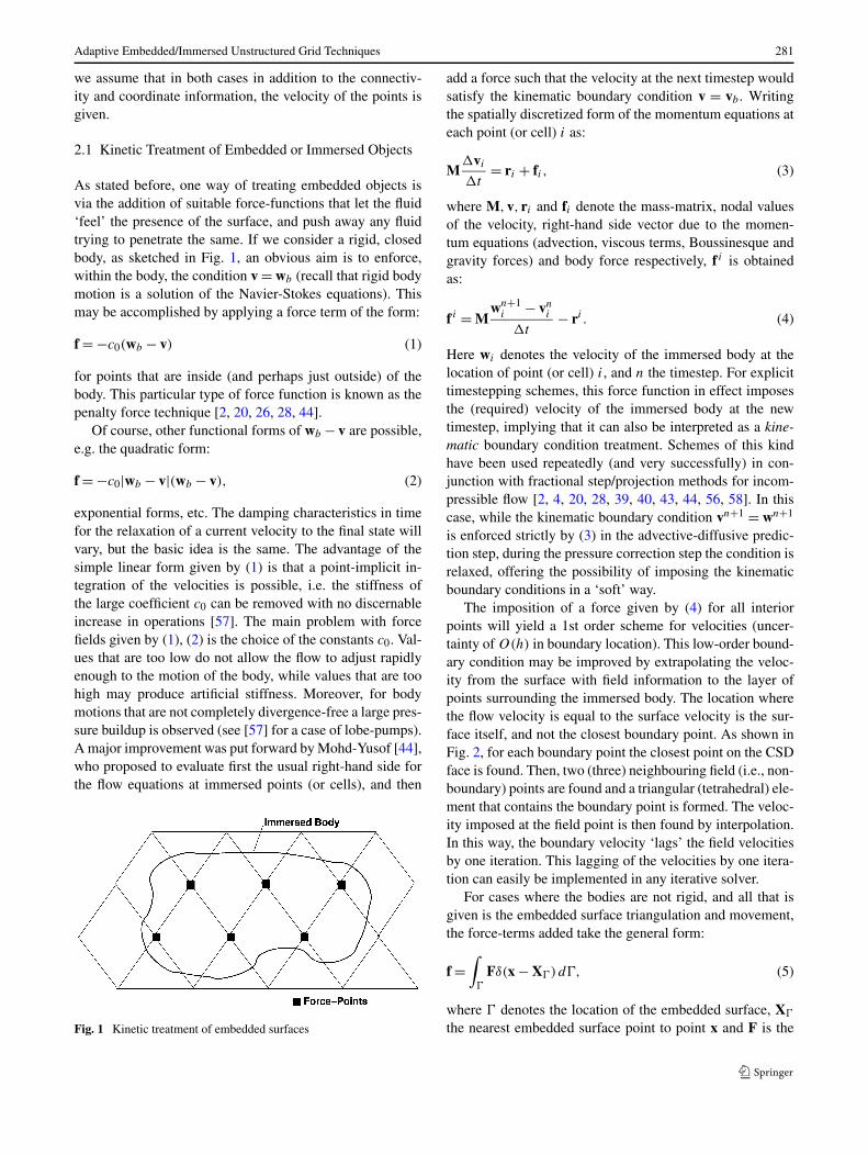
As stated before, one way of treating embedded objects isvia the addition of suitable force-functions that let the fluid‘feel’ the presence of the surface, and push away any fluidtrying to penetrate the same. If we consider a rigid, closedbody, as sketched in Fig. 1, an obvious aim is to enforce,within the body, the condition v = wb (recall that rigid bodymotion is a solution of the Navier-Stokes equations). Thismay be accomplished by applying a force term of the form:

f = −c0(wb − v) (1)

for points that are inside (and perhaps just outside) of thebody. This particular type of force function is known as thepenalty force technique [2, 20, 26, 28, 44].

Of course, other functional forms of wb − v are possible,e.g. the quadratic form:

f = −c0|wb − v|(wb − v), (2)

exponential forms, etc. The damping characteristics in timefor the relaxation of a current velocity to the final state willvary, but the basic idea is the same. The advantage of thesimple linear form given by (1) is that a point-implicit in-tegration of the velocities is possible, i.e. the stiffness ofthe large coefficient c0 can be removed with no discernableincrease in operations [57]. The main problem with forcefields given by (1), (2) is the choice of the constants c0. Val-ues that are too low do not allow the flow to adjust rapidlyenough to the motion of the body, while values that are toohigh may produce artificial stiffness. Moreover, for bodymotions that are not completely divergence-free a large pres-sure buildup is observed (see [57] for a case of lobe-pumps).A major improvement was put forward by Mohd-Yusof [44],who proposed to evaluate first the usual right-hand side forthe flow equations at immersed points (or cells), and then

Fig. 1 Kinetic treatment of embedded surfaces

add a force such that the velocity at the next timestep wouldsatisfy the kinematic boundary condition v = vb . Writingthe spatially discretized form of the momentum equations ateach point (or cell) i as:

M�vi

�t= ri + fi , (3)

where M,v, ri and fi denote the mass-matrix, nodal valuesof the velocity, right-hand side vector due to the momen-tum equations (advection, viscous terms, Boussinesque andgravity forces) and body force respectively, f i is obtainedas:

f i = Mwn+1

i − vni

�t− ri . (4)

Here wi denotes the velocity of the immersed body at thelocation of point (or cell) i, and n the timestep. For explicittimestepping schemes, this force function in effect imposesthe (required) velocity of the immersed body at the newtimestep, implying that it can also be interpreted as a kine-matic boundary condition treatment. Schemes of this kindhave been used repeatedly (and very successfully) in con-junction with fractional step/projection methods for incom-pressible flow [2, 4, 20, 28, 39, 40, 43, 44, 56, 58]. In thiscase, while the kinematic boundary condition vn+1 = wn+1

is enforced strictly by (3) in the advective-diffusive predic-tion step, during the pressure correction step the condition isrelaxed, offering the possibility of imposing the kinematicboundary conditions in a ‘soft’ way.

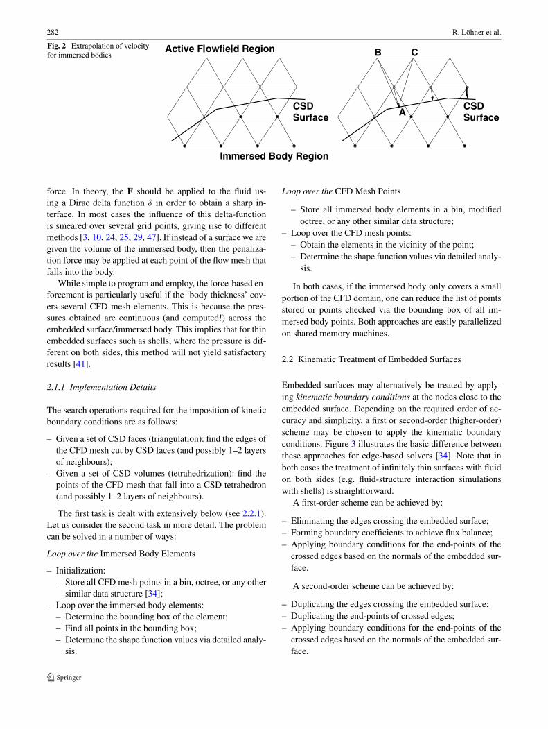
The imposition of a force given by (4) for all interiorpoints will yield a 1st order scheme for velocities (uncer-tainty of O(h) in boundary location). This low-order bound-ary condition may be improved by extrapolating the veloc-ity from the surface with field information to the layer ofpoints surrounding the immersed body. The location wherethe flow velocity is equal to the surface velocity is the sur-face itself, and not the closest boundary point. As shown inFig. 2, for each boundary point the closest point on the CSDface is found. Then, two (three) neighbouring field (i.e., non-boundary) points are found and a triangular (tetrahedral) ele-ment that contains the boundary point is formed. The veloc-ity imposed at the field point is then found by interpolation.In this way, the boundary velocity ‘lags’ the field velocitiesby one iteration. This lagging of the velocities by one itera-tion can easily be implemented in any iterative solver.

For cases where the bodies are not rigid, and all that isgiven is the embedded surface triangulation and movement,the force-terms added take the general form:

f =∫

�

Fδ(x − X�)d�, (5)

where � denotes the location of the embedded surface, X�

the nearest embedded surface point to point x and F is the


Fig. 2 Extrapolation of velocityfor immersed bodies

force. In theory, the F should be applied to the fluid us-ing a Dirac delta function δ in order to obtain a sharp in-terface. In most cases the influence of this delta-functionis smeared over several grid points, giving rise to differentmethods [3, 10, 24, 25, 29, 47]. If instead of a surface we aregiven the volume of the immersed body, then the penaliza-tion force may be applied at each point of the flow mesh thatfalls into the body.

While simple to program and employ, the force-based en-forcement is particularly useful if the ‘body thickness’ cov-ers several CFD mesh elements. This is because the pres-sures obtained are continuous (and computed!) across theembedded surface/immersed body. This implies that for thinembedded surfaces such as shells, where the pressure is dif-ferent on both sides, this method will not yield satisfactoryresults [41].

2.1.1 Implementation Details

The search operations required for the imposition of kineticboundary conditions are as follows:

– Given a set of CSD faces (triangulation): find the edges ofthe CFD mesh cut by CSD faces (and possibly 1–2 layersof neighbours);

– Given a set of CSD volumes (tetrahedrization): find thepoints of the CFD mesh that fall into a CSD tetrahedron(and possibly 1–2 layers of neighbours).

The first task is dealt with extensively below (see 2.2.1).Let us consider the second task in more detail. The problemcan be solved in a number of ways:

Loop over the Immersed Body Elements

– Initialization:– Store all CFD mesh points in a bin, octree, or any other

similar data structure [34];– Loop over the immersed body elements:

– Determine the bounding box of the element;– Find all points in the bounding box;– Determine the shape function values via detailed analy-

sis.

Loop over the CFD Mesh Points

– Store all immersed body elements in a bin, modifiedoctree, or any other similar data structure;

– Loop over the CFD mesh points:– Obtain the elements in the vicinity of the point;– Determine the shape function values via detailed analy-

sis.

In both cases, if the immersed body only covers a smallportion of the CFD domain, one can reduce the list of pointsstored or points checked via the bounding box of all im-mersed body points. Both approaches are easily parallelizedon shared memory machines.

2.2 Kinematic Treatment of Embedded Surfaces

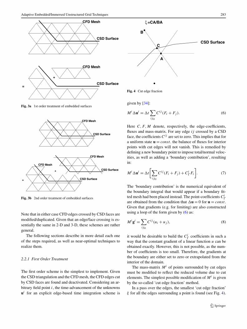
Embedded surfaces may alternatively be treated by apply-ing kinematic boundary conditions at the nodes close to theembedded surface. Depending on the required order of ac-curacy and simplicity, a first or second-order (higher-order)scheme may be chosen to apply the kinematic boundaryconditions. Figure 3 illustrates the basic difference betweenthese approaches for edge-based solvers [34]. Note that inboth cases the treatment of infinitely thin surfaces with fluidon both sides (e.g. fluid-structure interaction simulationswith shells) is straightforward.

A first-order scheme can be achieved by:

– Eliminating the edges crossing the embedded surface;– Forming boundary coefficients to achieve flux balance;– Applying boundary conditions for the end-points of the

crossed edges based on the normals of the embedded sur-face.

A second-order scheme can be achieved by:

– Duplicating the edges crossing the embedded surface;– Duplicating the end-points of crossed edges;– Applying boundary conditions for the end-points of the

crossed edges based on the normals of the embedded sur-face.


Fig. 3a 1st order treatment of embedded surfaces

Fig. 3b 2nd order treatment of embedded surfaces

Note that in either case CFD edges crossed by CSD faces aremodified/duplicated. Given that an edge/face crossing is es-sentially the same in 2-D and 3-D, these schemes are rathergeneral.

The following sections describe in more detail each oneof the steps required, as well as near-optimal techniques torealize them.

2.2.1 First Order Treatment

The first order scheme is the simplest to implement. Giventhe CSD triangulation and the CFD mesh, the CFD edges cutby CSD faces are found and deactivated. Considering an ar-bitrary field point i, the time-advancement of the unknownsui for an explicit edge-based time integration scheme is

Fig. 4 Cut edge fraction

given by [34]:

Mi�ui = �t∑ij�

Cij (Fi + Fj ). (6)

Here C,F,M denote, respectively, the edge-coefficients,fluxes and mass-matrix. For any edge ij crossed by a CSDface, the coefficients Cij are set to zero. This implies that fora uniform state u = const . the balance of fluxes for interiorpoints with cut edges will not vanish. This is remedied bydefining a new boundary point to impose total/normal veloc-ities, as well as adding a ‘boundary contribution’, resultingin:

Mi�ui = �t

[∑ij�

Cij (Fi + Fj ) + Ci�Fi

]. (7)

The ‘boundary contribution’ is the numerical equivalent ofthe boundary integral that would appear if a boundary fit-ted mesh had been placed instead. The point-coefficients Ci

�

are obtained from the condition that �u = 0 for u = const.

Given that gradients (e.g. for limiting) are also constructedusing a loop of the form given by (6) as:

Migi =∑ij�

Cij (ui + uj ), (8)

it would be desirable to build the Ci� coefficients in such a

way that the constant gradient of a linear function u can beobtained exactly. However, this is not possible, as the num-ber of coefficients is too small. Therefore, the gradients atthe boundary are either set to zero or extrapolated from theinterior of the domain.

The mass-matrix Mi of points surrounded by cut edgesmust be modified to reflect the reduced volume due to cutelements. The simplest possible modification of Mi is givenby the so-called ‘cut edge fraction’ method.

In a pass over the edges, the smallest ‘cut edge fraction’ξ for all the edges surrounding a point is found (see Fig. 4).


Fig. 5 Extrapolation of velocity

Fig. 6 Extrapolation of normalpressure gradient

The modified mass-matrix is then given by:

Mi∗ = 1 + ξmin

2Mi. (9)

Note that the value of the modified mass-matrix can neverfall below half of its original value, implying that timestepsizes will always be acceptable.

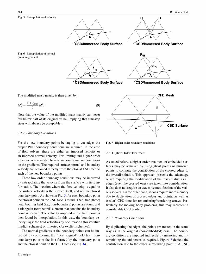
2.2.2 Boundary Conditions

For the new boundary points belonging to cut edges theproper PDE boundary conditions are required. In the caseof flow solvers, these are either an imposed velocity oran imposed normal velocity. For limiting and higher-orderschemes, one may also have to impose boundary conditionson the gradients. The required surface normal and boundaryvelocity are obtained directly from the closest CSD face toeach of the new boundary points.

These low-order boundary conditions may be improvedby extrapolating the velocity from the surface with field in-formation. The location where the flow velocity is equal tothe surface velocity is the surface itself, and not the closestboundary point. As shown in Fig. 5, for each boundary pointthe closest point on the CSD face is found. Then, two (three)neighbouring field (i.e., non-boundary) points are found anda triangular (tetrahedral) element that contains the boundarypoint is formed. The velocity imposed at the field point isthen found by interpolation. In this way, the boundary ve-locity ‘lags’ the field velocities by one iteration (for iterativeimplicit schemes) or timestep (for explicit schemes).

The normal gradients at the boundary points can be im-proved by considering the ‘most aligned’ field (i.e., non-boundary) point to the line formed by the boundary pointand the closest point on the CSD face (see Fig. 6).

Fig. 7 Higher order boundary conditions

2.3 Higher Order Treatment

As stated before, a higher-order treatment of embedded sur-faces may be achieved by using ghost points or mirroredpoints to compute the contribution of the crossed edges tothe overall solution. This approach presents the advantageof not requiring the modification of the mass matrix as alledges (even the crossed ones) are taken into consideration.It also does not require an extensive modification of the vari-ous solvers. On the other hand, it does require more memorydue to duplication of crossed edges and points, as well as(scalar) CPU time for renumbering/reordering arrays. Par-ticularly for moving body problems, this may represent aconsiderable CPU burden.

2.3.1 Boundary Conditions

By duplicating the edges, the points are treated in the sameway as in the original (non-embedded) case. The bound-ary conditions are imposed indirectly by mirroring and in-terpolating the unknowns as required. Figure 7 depicts thecontribution due to the edges surrounding point i. A CSD


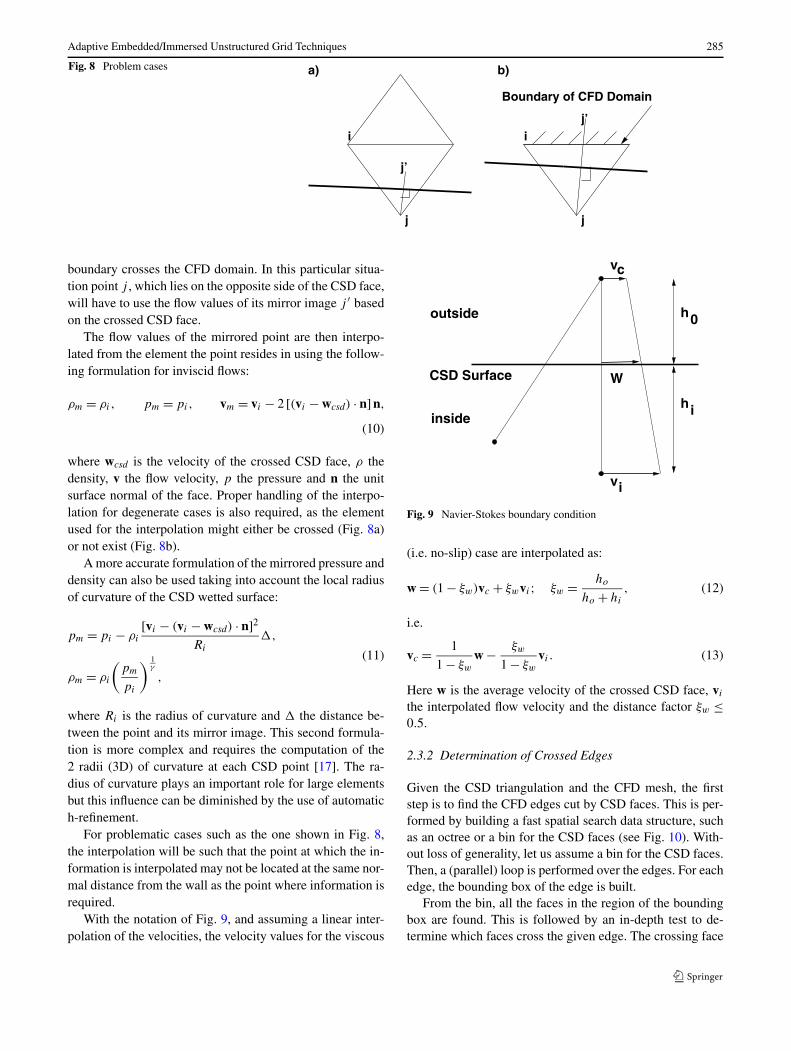
Fig. 8 Problem cases

boundary crosses the CFD domain. In this particular situa-tion point j , which lies on the opposite side of the CSD face,will have to use the flow values of its mirror image j ′ basedon the crossed CSD face.

The flow values of the mirrored point are then interpo-lated from the element the point resides in using the follow-ing formulation for inviscid flows:

ρm = ρi, pm = pi, vm = vi − 2 [(vi − wcsd) · n] n,

(10)

where wcsd is the velocity of the crossed CSD face, ρ thedensity, v the flow velocity, p the pressure and n the unitsurface normal of the face. Proper handling of the interpo-lation for degenerate cases is also required, as the elementused for the interpolation might either be crossed (Fig. 8a)or not exist (Fig. 8b).

A more accurate formulation of the mirrored pressure anddensity can also be used taking into account the local radiusof curvature of the CSD wetted surface:

pm = pi − ρi

[vi − (vi − wcsd) · n]2

Ri

�,

ρm = ρi

(pm

pi

) 1γ

,

(11)

where Ri is the radius of curvature and � the distance be-tween the point and its mirror image. This second formula-tion is more complex and requires the computation of the2 radii (3D) of curvature at each CSD point [17]. The ra-dius of curvature plays an important role for large elementsbut this influence can be diminished by the use of automatich-refinement.

For problematic cases such as the one shown in Fig. 8,the interpolation will be such that the point at which the in-formation is interpolated may not be located at the same nor-mal distance from the wall as the point where information isrequired.

With the notation of Fig. 9, and assuming a linear inter-polation of the velocities, the velocity values for the viscous

Fig. 9 Navier-Stokes boundary condition

(i.e. no-slip) case are interpolated as:

w = (1 − ξw)vc + ξwvi; ξw = ho

ho + hi

, (12)

i.e.

vc = 1

1 − ξw

w − ξw

1 − ξw

vi . (13)

Here w is the average velocity of the crossed CSD face, vi

the interpolated flow velocity and the distance factor ξw ≤0.5.

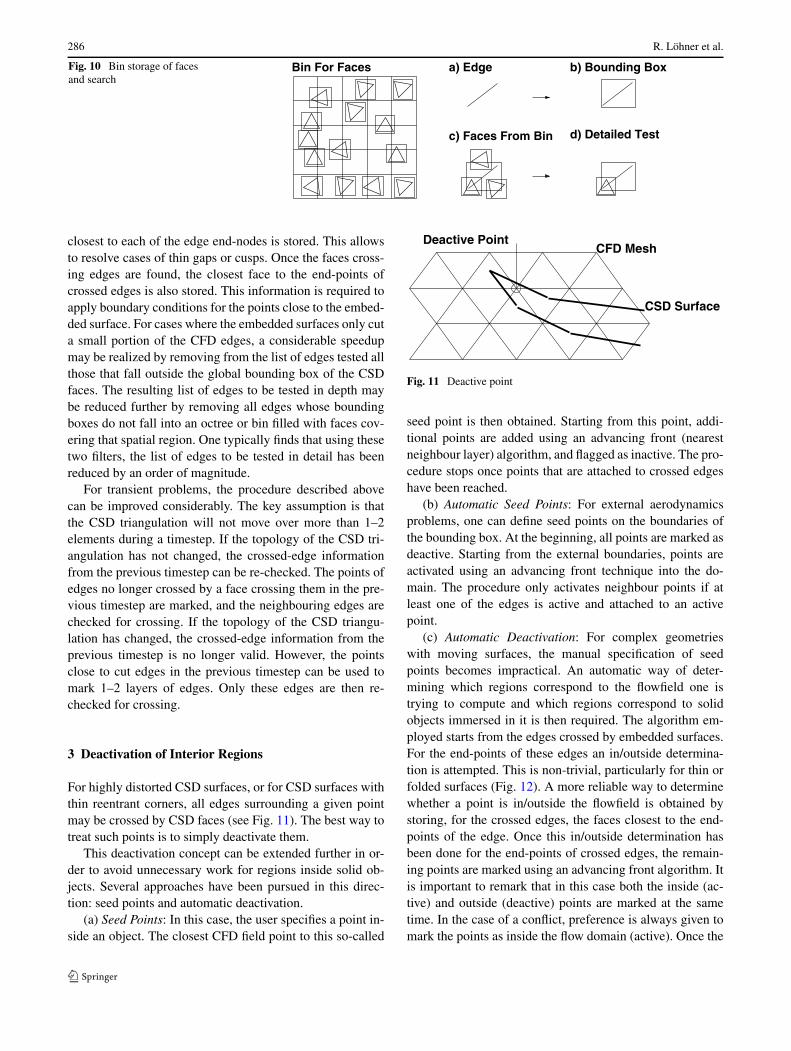
2.3.2 Determination of Crossed Edges

Given the CSD triangulation and the CFD mesh, the firststep is to find the CFD edges cut by CSD faces. This is per-formed by building a fast spatial search data structure, suchas an octree or a bin for the CSD faces (see Fig. 10). With-out loss of generality, let us assume a bin for the CSD faces.Then, a (parallel) loop is performed over the edges. For eachedge, the bounding box of the edge is built.

From the bin, all the faces in the region of the boundingbox are found. This is followed by an in-depth test to de-termine which faces cross the given edge. The crossing face


Fig. 10 Bin storage of facesand search

closest to each of the edge end-nodes is stored. This allowsto resolve cases of thin gaps or cusps. Once the faces cross-ing edges are found, the closest face to the end-points ofcrossed edges is also stored. This information is required toapply boundary conditions for the points close to the embed-ded surface. For cases where the embedded surfaces only cuta small portion of the CFD edges, a considerable speedupmay be realized by removing from the list of edges tested allthose that fall outside the global bounding box of the CSDfaces. The resulting list of edges to be tested in depth maybe reduced further by removing all edges whose boundingboxes do not fall into an octree or bin filled with faces cov-ering that spatial region. One typically finds that using thesetwo filters, the list of edges to be tested in detail has beenreduced by an order of magnitude.

For transient problems, the procedure described abovecan be improved considerably. The key assumption is thatthe CSD triangulation will not move over more than 1–2elements during a timestep. If the topology of the CSD tri-angulation has not changed, the crossed-edge informationfrom the previous timestep can be re-checked. The points ofedges no longer crossed by a face crossing them in the pre-vious timestep are marked, and the neighbouring edges arechecked for crossing. If the topology of the CSD triangu-lation has changed, the crossed-edge information from theprevious timestep is no longer valid. However, the pointsclose to cut edges in the previous timestep can be used tomark 1–2 layers of edges. Only these edges are then re-checked for crossing.

3 Deactivation of Interior Regions

For highly distorted CSD surfaces, or for CSD surfaces withthin reentrant corners, all edges surrounding a given pointmay be crossed by CSD faces (see Fig. 11). The best way totreat such points is to simply deactivate them.

This deactivation concept can be extended further in or-der to avoid unnecessary work for regions inside solid ob-jects. Several approaches have been pursued in this direc-tion: seed points and automatic deactivation.

(a) Seed Points: In this case, the user specifies a point in-side an object. The closest CFD field point to this so-called

Fig. 11 Deactive point

seed point is then obtained. Starting from this point, addi-tional points are added using an advancing front (nearestneighbour layer) algorithm, and flagged as inactive. The pro-cedure stops once points that are attached to crossed edgeshave been reached.

(b) Automatic Seed Points: For external aerodynamicsproblems, one can define seed points on the boundaries ofthe bounding box. At the beginning, all points are marked asdeactive. Starting from the external boundaries, points areactivated using an advancing front technique into the do-main. The procedure only activates neighbour points if atleast one of the edges is active and attached to an activepoint.

(c) Automatic Deactivation: For complex geometrieswith moving surfaces, the manual specification of seedpoints becomes impractical. An automatic way of deter-mining which regions correspond to the flowfield one istrying to compute and which regions correspond to solidobjects immersed in it is then required. The algorithm em-ployed starts from the edges crossed by embedded surfaces.For the end-points of these edges an in/outside determina-tion is attempted. This is non-trivial, particularly for thin orfolded surfaces (Fig. 12). A more reliable way to determinewhether a point is in/outside the flowfield is obtained bystoring, for the crossed edges, the faces closest to the end-points of the edge. Once this in/outside determination hasbeen done for the end-points of crossed edges, the remain-ing points are marked using an advancing front algorithm. Itis important to remark that in this case both the inside (ac-tive) and outside (deactive) points are marked at the sametime. In the case of a conflict, preference is always given tomark the points as inside the flow domain (active). Once the


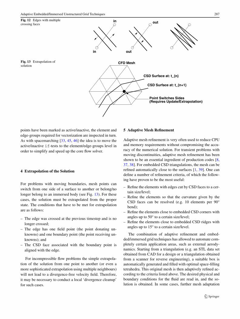
Fig. 12 Edges with multiplecrossing faces

Fig. 13 Extrapolation ofsolution

points have been marked as active/inactive, the element andedge-groups required for vectorization are inspected in turn.As with spacemarching [33, 45, 46] the idea is to move theactive/inactive if-tests to the element/edge-groups level inorder to simplify and speed up the core flow solver.

4 Extrapolation of the Solution

For problems with moving boundaries, mesh points canswitch from one side of a surface to another or belong/nolonger belong to an immersed body (see Fig. 13). For thesecases, the solution must be extrapolated from the properstate. The conditions that have to be met for extrapolationare as follows:

– The edge was crossed at the previous timestep and is nolonger crossed;

– The edge has one field point (the point donating un-knowns) and one boundary point (the point receiving un-knowns); and

– The CSD face associated with the boundary point isaligned with the edge.

For incompressible flow problems the simple extrapola-tion of the solution from one point to another (or even amore sophisticated extrapolation using multiple neighbours)will not lead to a divergence-free velocity field. Therefore,it may be necessary to conduct a local ‘divergence cleanup’for such cases.

5 Adaptive Mesh Refinement

Adaptive mesh refinement is very often used to reduce CPUand memory requirements without compromising the accu-racy of the numerical solution. For transient problems withmoving discontinuities, adaptive mesh refinement has beenshown to be an essential ingredient of production codes [8,37, 38]. For embedded CSD triangulations, the mesh can berefined automatically close to the surfaces [1, 39]. One candefine a number of refinement criteria, of which the follow-ing have proven to be the most useful:

– Refine the elements with edges cut by CSD faces to a cer-tain size/level;

– Refine the elements so that the curvature given by theCSD faces can be resolved (e.g. 10 elements per 90°bend);

– Refine the elements close to embedded CSD corners withangles up to 50° to a certain size/level;

– Refine the elements close to embedded CSD ridges withangles up to 15° to a certain size/level.

The combination of adaptive refinement and embed-ded/immersed grid techniques has allowed to automate com-pletely certain application areas, such as external aerody-namics. Starting from a triangulation (e.g. an STL data setobtained from CAD for a design or a triangulation obtainedfrom a scanner for reverse engineering), a suitable box isautomatically generated and filled with optimal space-fillingtetrahedra. This original mesh is then adaptively refined ac-cording to the criteria listed above. The desired physical andboundary conditions for the fluid are read in, and the so-lution is obtained. In some cases, further mesh adaptation


based on the physics of the problem (shocks, contact discon-tinuities, shear layers, etc.) may be required, but this can alsobe automated to a large extent for a large class of problems.Note that the only user input consists in flow conditions. Themany hours required to obtain a watertight, consistent sur-face description have been eliminated by the use of adaptive,embedded flow solvers.

6 Load/Flux Transfer

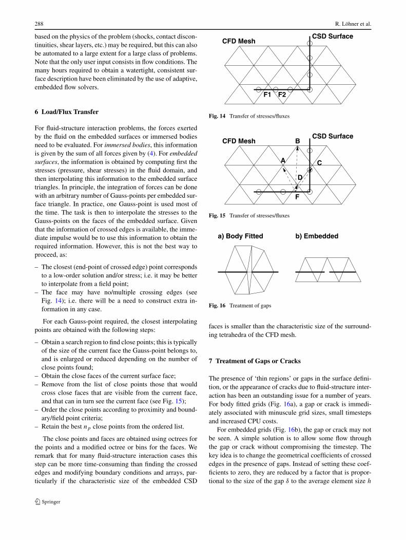
For fluid-structure interaction problems, the forces exertedby the fluid on the embedded surfaces or immersed bodiesneed to be evaluated. For immersed bodies, this informationis given by the sum of all forces given by (4). For embeddedsurfaces, the information is obtained by computing first thestresses (pressure, shear stresses) in the fluid domain, andthen interpolating this information to the embedded surfacetriangles. In principle, the integration of forces can be donewith an arbitrary number of Gauss-points per embedded sur-face triangle. In practice, one Gauss-point is used most ofthe time. The task is then to interpolate the stresses to theGauss-points on the faces of the embedded surface. Giventhat the information of crossed edges is available, the imme-diate impulse would be to use this information to obtain therequired information. However, this is not the best way toproceed, as:

– The closest (end-point of crossed edge) point correspondsto a low-order solution and/or stress; i.e. it may be betterto interpolate from a field point;

– The face may have no/multiple crossing edges (seeFig. 14); i.e. there will be a need to construct extra in-formation in any case.

For each Gauss-point required, the closest interpolatingpoints are obtained with the following steps:

– Obtain a search region to find close points; this is typicallyof the size of the current face the Gauss-point belongs to,and is enlarged or reduced depending on the number ofclose points found;

– Obtain the close faces of the current surface face;– Remove from the list of close points those that would

cross close faces that are visible from the current face,and that can in turn see the current face (see Fig. 15);

– Order the close points according to proximity and bound-ary/field point criteria;

– Retain the best np close points from the ordered list.

The close points and faces are obtained using octrees forthe points and a modified octree or bins for the faces. Weremark that for many fluid-structure interaction cases thisstep can be more time-consuming than finding the crossededges and modifying boundary conditions and arrays, par-ticularly if the characteristic size of the embedded CSD

Fig. 14 Transfer of stresses/fluxes

Fig. 15 Transfer of stresses/fluxes

Fig. 16 Treatment of gaps

faces is smaller than the characteristic size of the surround-ing tetrahedra of the CFD mesh.

7 Treatment of Gaps or Cracks

The presence of ‘thin regions’ or gaps in the surface defini-tion, or the appearance of cracks due to fluid-structure inter-action has been an outstanding issue for a number of years.For body fitted grids (Fig. 16a), a gap or crack is immedi-ately associated with minuscule grid sizes, small timestepsand increased CPU costs.

For embedded grids (Fig. 16b), the gap or crack may notbe seen. A simple solution is to allow some flow throughthe gap or crack without compromising the timestep. Thekey idea is to change the geometrical coefficients of crossededges in the presence of gaps. Instead of setting these coef-ficients to zero, they are reduced by a factor that is propor-tional to the size of the gap δ to the average element size h


in the region:

Cijk = ηC

ij

0k; η = δ/h. (14)

Gaps are detected by considering the edges of elements withmultiple crossed edges. If the faces crossing these edges aredifferent, a test is performed to see if one face can be reachedby the other via a near-neighbour search. If this search issuccessful, the CSD surface is considered watertight. If thesearch is not successful, the gap size δ is determined, andthe edges are marked for modification.

8 Direct Link to Particles

One of the most promising ways to treat discontinua is viaso-called Discrete Element Methods (DEMs) or DiscreteParticle Methods (DPMs). A considerable amount of workhas been devoted to this area in the last two decades, and

Fig. 17 Link to discrete particle method

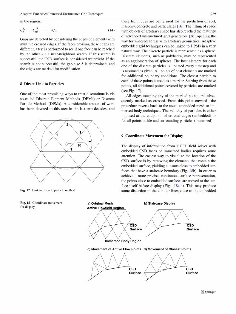
these techniques are being used for the prediction of soil,masonry, concrete and particulates [16]. The filling of spacewith objects of arbitrary shape has also reached the maturityof advanced unstructured grid generators [36] opening theway for widespread use with arbitrary geometries. Adaptiveembedded grid techniques can be linked to DPMs in a verynatural way. The discrete particle is represented as a sphere.Discrete elements, such as polyhedra, may be representedas an agglomeration of spheres. The host element for eachone of the discrete particles is updated every timestep andis assumed as given. All points of host elements are markedfor additional boundary conditions. The closest particle toeach of these points is used as a marker. Starting from thesepoints, all additional points covered by particles are marked(see Fig. 17).

All edges touching any of the marked points are subse-quently marked as crossed. From this point onwards, theprocedure reverts back to the usual embedded mesh or im-mersed body techniques. The velocity of particles is eitherimposed at the endpoints of crossed edges (embedded) orfor all points inside and surrounding particles (immersed).

9 Coordinate Movement for Display

The display of information from a CFD field solver withembedded CSD faces or immersed bodies requires someattention. The easiest way to visualize the location of theCSD surface is by removing the elements that contain theembedded surface, yielding cut-outs close to embedded sur-faces that have a staircase boundary (Fig. 18b). In order toachieve a more precise, continuous surface representation,the points close to embedded surfaces are moved to the sur-face itself before display (Figs. 18c,d). This may producesome distortion in the contour lines close to the embedded

Fig. 18 Coordinate movementfor display


surfaces, but produces a more faithful geometry representa-tion.

Close to corners or ridges multiple surface normals willappear. For each of these multiple normals, a separate direc-tion of movement is determined. The final point movementis obtained as the sum of all of these.

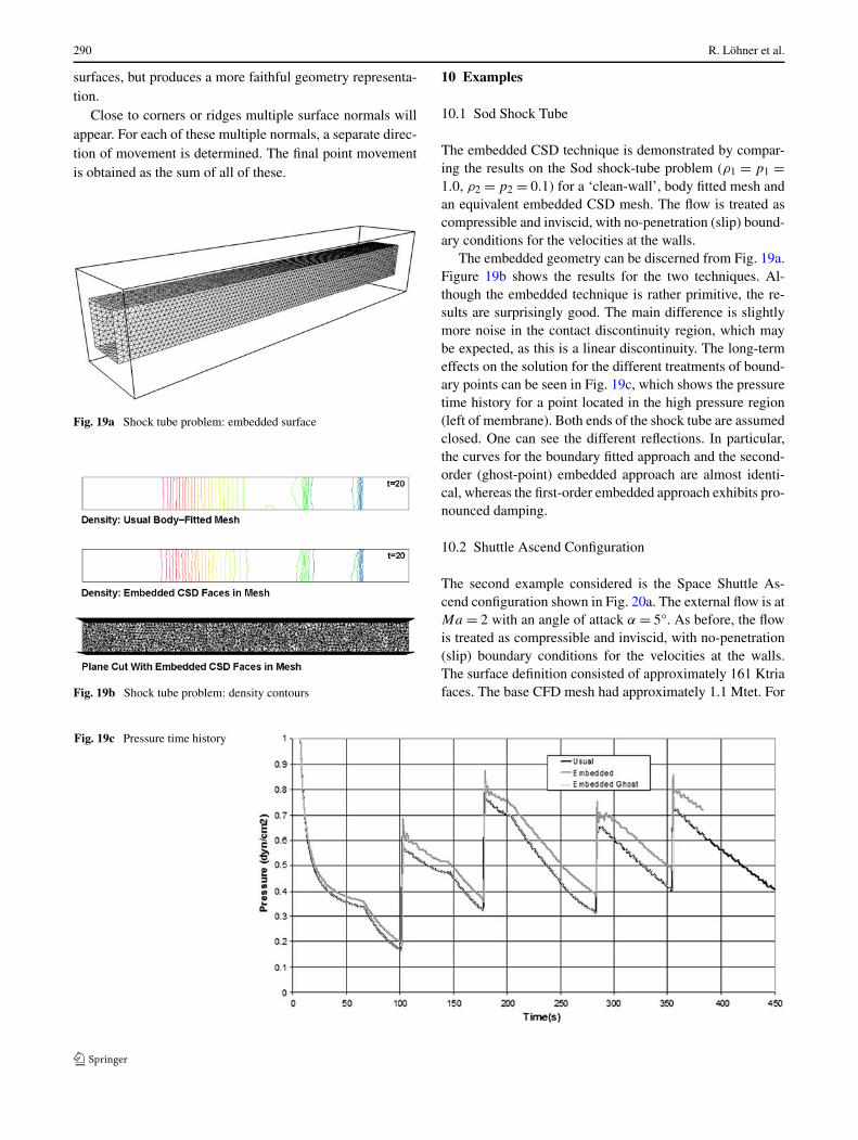
Fig. 19a Shock tube problem: embedded surface

Fig. 19b Shock tube problem: density contours

10 Examples

10.1 Sod Shock Tube

The embedded CSD technique is demonstrated by compar-ing the results on the Sod shock-tube problem (ρ1 = p1 =1.0, ρ2 = p2 = 0.1) for a ‘clean-wall’, body fitted mesh andan equivalent embedded CSD mesh. The flow is treated ascompressible and inviscid, with no-penetration (slip) bound-ary conditions for the velocities at the walls.

The embedded geometry can be discerned from Fig. 19a.Figure 19b shows the results for the two techniques. Al-though the embedded technique is rather primitive, the re-sults are surprisingly good. The main difference is slightlymore noise in the contact discontinuity region, which maybe expected, as this is a linear discontinuity. The long-termeffects on the solution for the different treatments of bound-ary points can be seen in Fig. 19c, which shows the pressuretime history for a point located in the high pressure region(left of membrane). Both ends of the shock tube are assumedclosed. One can see the different reflections. In particular,the curves for the boundary fitted approach and the second-order (ghost-point) embedded approach are almost identi-cal, whereas the first-order embedded approach exhibits pro-nounced damping.

10.2 Shuttle Ascend Configuration

The second example considered is the Space Shuttle As-cend configuration shown in Fig. 20a. The external flow is atMa = 2 with an angle of attack α = 5°. As before, the flowis treated as compressible and inviscid, with no-penetration(slip) boundary conditions for the velocities at the walls.The surface definition consisted of approximately 161 Ktriafaces. The base CFD mesh had approximately 1.1 Mtet. For

Fig. 19c Pressure time history


(a) (b)

(c) (d)

(e) (f)

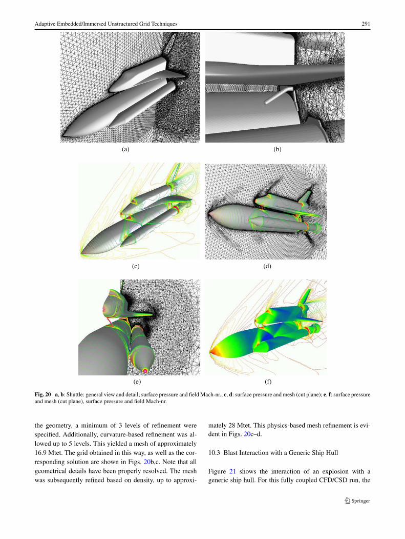
Fig. 20 a, b: Shuttle: general view and detail; surface pressure and field Mach-nr., c, d: surface pressure and mesh (cut plane); e, f: surface pressureand mesh (cut plane), surface pressure and field Mach-nr.

the geometry, a minimum of 3 levels of refinement werespecified. Additionally, curvature-based refinement was al-lowed up to 5 levels. This yielded a mesh of approximately16.9 Mtet. The grid obtained in this way, as well as the cor-responding solution are shown in Figs. 20b,c. Note that allgeometrical details have been properly resolved. The meshwas subsequently refined based on density, up to approxi-

mately 28 Mtet. This physics-based mesh refinement is evi-dent in Figs. 20c–d.

10.3 Blast Interaction with a Generic Ship Hull

Figure 21 shows the interaction of an explosion with ageneric ship hull. For this fully coupled CFD/CSD run, the


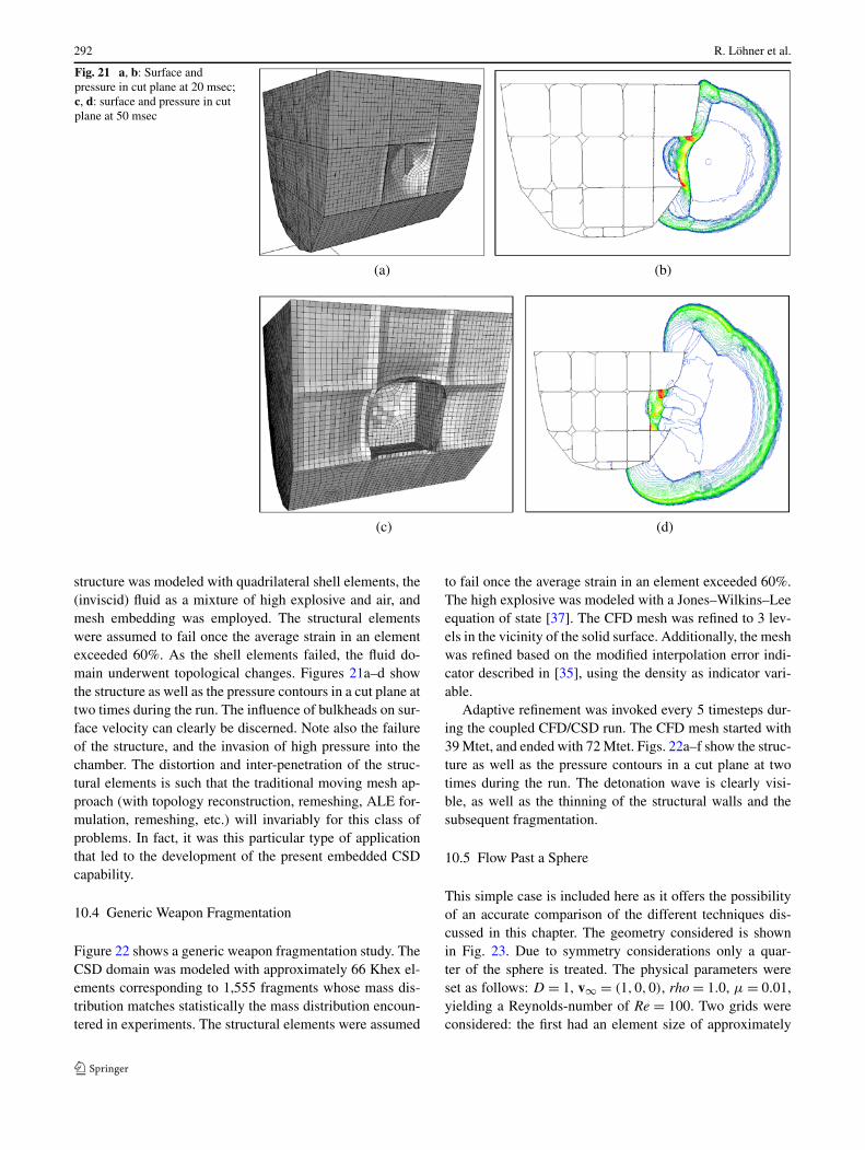
Fig. 21 a, b: Surface andpressure in cut plane at 20 msec;c, d: surface and pressure in cutplane at 50 msec

(a) (b)

(c) (d)

structure was modeled with quadrilateral shell elements, the(inviscid) fluid as a mixture of high explosive and air, andmesh embedding was employed. The structural elementswere assumed to fail once the average strain in an elementexceeded 60%. As the shell elements failed, the fluid do-main underwent topological changes. Figures 21a–d showthe structure as well as the pressure contours in a cut plane attwo times during the run. The influence of bulkheads on sur-face velocity can clearly be discerned. Note also the failureof the structure, and the invasion of high pressure into thechamber. The distortion and inter-penetration of the struc-tural elements is such that the traditional moving mesh ap-proach (with topology reconstruction, remeshing, ALE for-mulation, remeshing, etc.) will invariably for this class ofproblems. In fact, it was this particular type of applicationthat led to the development of the present embedded CSDcapability.

10.4 Generic Weapon Fragmentation

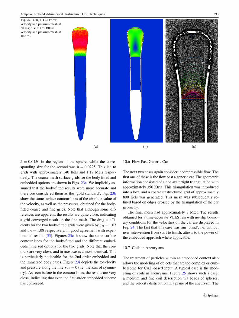
Figure 22 shows a generic weapon fragmentation study. TheCSD domain was modeled with approximately 66 Khex el-ements corresponding to 1,555 fragments whose mass dis-tribution matches statistically the mass distribution encoun-tered in experiments. The structural elements were assumed

to fail once the average strain in an element exceeded 60%.The high explosive was modeled with a Jones–Wilkins–Leeequation of state [37]. The CFD mesh was refined to 3 lev-els in the vicinity of the solid surface. Additionally, the meshwas refined based on the modified interpolation error indi-cator described in [35], using the density as indicator vari-able.

Adaptive refinement was invoked every 5 timesteps dur-ing the coupled CFD/CSD run. The CFD mesh started with39 Mtet, and ended with 72 Mtet. Figs. 22a–f show the struc-ture as well as the pressure contours in a cut plane at twotimes during the run. The detonation wave is clearly visi-ble, as well as the thinning of the structural walls and thesubsequent fragmentation.

10.5 Flow Past a Sphere

This simple case is included here as it offers the possibilityof an accurate comparison of the different techniques dis-cussed in this chapter. The geometry considered is shownin Fig. 23. Due to symmetry considerations only a quar-ter of the sphere is treated. The physical parameters wereset as follows: D = 1, v∞ = (1,0,0), rho = 1.0, μ = 0.01,yielding a Reynolds-number of Re = 100. Two grids wereconsidered: the first had an element size of approximately


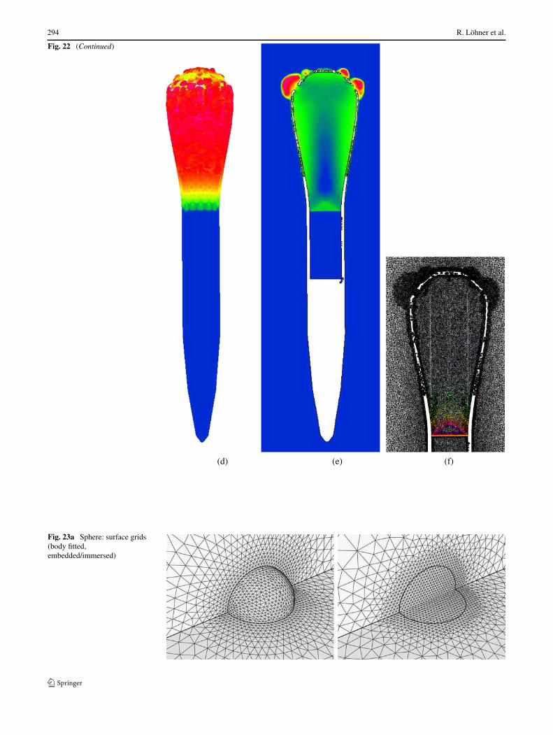
Fig. 22 a, b, c: CSD/flowvelocity and pressure/mesh at68 ms; d, e, f: CSD/flowvelocity and pressure/mesh at102 ms

(a) (b) (c)

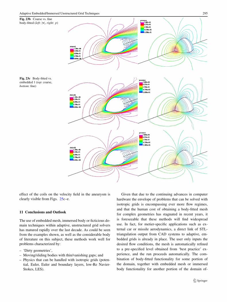
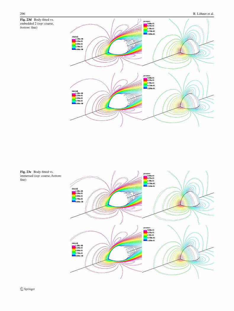
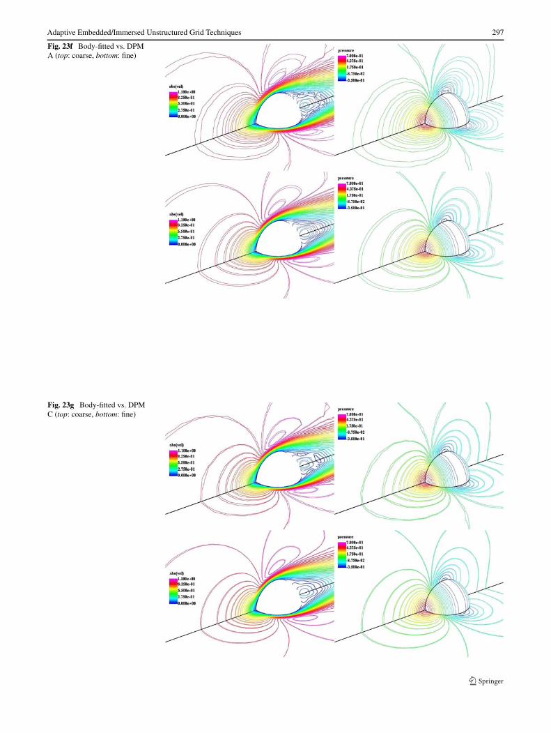
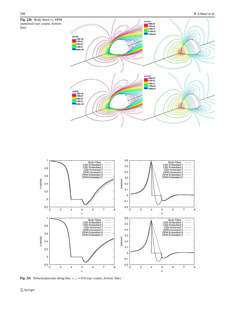
h = 0.0450 in the region of the sphere, while the corre-sponding size for the second was h = 0.0225. This led togrids with approximately 140 Kels and 1.17 Mels respec-tively. The coarse mesh surface grids for the body fitted andembedded options are shown in Figs. 23a. We implicitly as-sumed that the body-fitted results were more accurate andtherefore considered them as the ‘gold standard’. Fig. 23bshow the same surface contour lines of the absolute value ofthe velocity, as well as the pressures, obtained for the body-fitted coarse and fine grids. Note that although some dif-ferences are apparent, the results are quite close, indicatinga grid-converged result on the fine mesh. The drag coeffi-cients for the two body-fitted grids were given by cD = 1.07and cD = 1.08 respectively, in good agreement with exper-imental results [53]. Figures 23c–h show the same surfacecontour lines for the body-fitted and the different embed-ded/immersed options for the two grids. Note that the con-tours are very close, and in most cases almost identical. Thisis particularly noticeable for the 2nd order embedded andthe immersed body cases. Figure 23i depicts the x-velocityand pressure along the line y, z = 0 (i.e. the axis of symme-try). As seen before in the contour lines, the results are veryclose, indicating that even the first-order embedded schemehas converged.

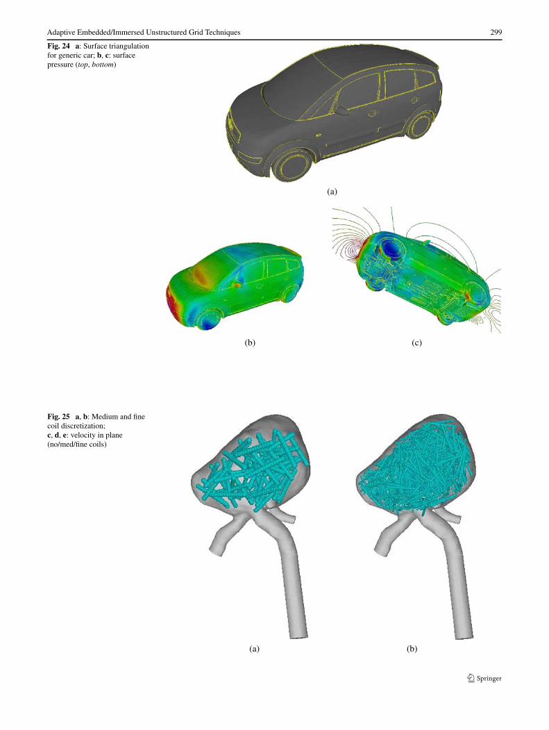
10.6 Flow Past Generic Car

The next two cases again consider incompressible flow. Thefirst one of these is the flow past a generic car. The geometricinformation consisted of a non-watertight triangulation withapproximately 350 Ktria. This triangulation was introducedinto a box, and a coarse unstructured grid of approximately800 Kels was generated. This mesh was subsequently re-fined based on edges crossed by the triangulation of the cargeometry.

The final mesh had approximately 8 Mtet. The resultsobtained for a time-accurate VLES run with no-slip bound-ary conditions for the velocities on the car are displayed inFig. 24. The fact that this case was run ‘blind’, i.e. withoutuser intervention from start to finish, attests to the power ofthe embedded approach where applicable.

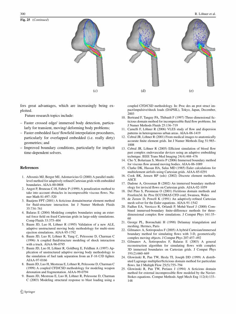
10.7 Coils in Aneurysms

The treatment of particles within an embedded context alsoallows the modeling of objects that are too complex or cum-bersome for CAD-based input. A typical case is the mod-eling of coils in aneurysms. Figure 25 shows such a case:a medium and fine coil description via beads of spheres,and the velocity distribution in a plane of the aneurysm. The


Fig. 22 (Continued)

(d) (e) (f)

Fig. 23a Sphere: surface grids(body fitted,embedded/immersed)


Fig. 23b Coarse vs. finebody-fitted (left: |v|, right: p)

Fig. 23c Body-fitted vs.embedded 1 (top: coarse,bottom: fine)

effect of the coils on the velocity field in the aneurysm isclearly visible from Figs. 25c–e.

11 Conclusions and Outlook

The use of embedded mesh, immersed body or ficticious do-main techniques within adaptive, unstructured grid solvershas matured rapidly over the last decade. As could be seenfrom the examples shown, as well as the considerable bodyof literature on this subject, these methods work well forproblems characterized by:

– ‘Dirty geometries’,– Moving/sliding bodies with thin/vanishing gaps; and– Physics that can be handled with isotropic grids (poten-

tial, Euler, Euler and boundary layers, low-Re Navier-Stokes, LES).

Given that due to the continuing advances in computerhardware the envelope of problems that can be solved withisotropic grids is encompassing ever more flow regimes,and that the human cost of obtaining a body-fitted meshfor complex geometries has stagnated in recent years, itis foreseeable that these methods will find widespreaduse. In fact, for metier-specific applications such as ex-ternal car or missile aerodynamics, a direct link of STL-triangulation output from CAD systems to adaptive, em-bedded grids is already in place. The user only inputs thedesired flow conditions, the mesh is automatically refinedto a pre-specified level obtained from ‘best practice’ ex-perience, and the run proceeds automatically. The com-bination of body-fitted functionality for some portion ofthe domain, together with embedded mesh or immersedbody functionality for another portion of the domain of-


Fig. 23d Body-fitted vs.embedded 2 (top: coarse,bottom: fine)

Fig. 23e Body-fitted vs.immersed (top: coarse, bottom:fine)


Fig. 23f Body-fitted vs. DPMA (top: coarse, bottom: fine)

Fig. 23g Body-fitted vs. DPMC (top: coarse, bottom: fine)


Fig. 23h Body-fitted vs. DPMimmersed (top: coarse, bottom:fine)

Fig. 23i Velocity/pressure along line: y, z = 0.0 (top: coarse, bottom: fine)


Fig. 24 a: Surface triangulationfor generic car; b, c: surfacepressure (top, bottom)

(a)

(b) (c)

Fig. 25 a, b: Medium and finecoil discretization;c, d, e: velocity in plane(no/med/fine coils)

(a) (b)


Fig. 25 (Continued)

(c) (d) (e)

fers great advantages, which are increasingly being ex-ploited.

Future research topics include:

– Faster crossed edge/ immersed body detection, particu-larly for transient, moving/ deforming body problems;

– Faster embedded face/ flowfield interpolation procedures,particularly for overlapped embedded (i.e. really dirty)geometries; and

– Improved boundary conditions, particularly for implicittime-dependent solvers.

References

1. Aftosmis MJ, Berger MJ, Adomavicius G (2000) A parallel multi-level method for adaptively refined Cartesian grids with embeddedboundaries. AIAA-00-0808

2. Angot P, Bruneau C-H, Fabrie P (1999) A penalization method totake into account obstacles in incompressible viscous flows. Nu-mer Math 81:497–520

3. Baaijens FPT (2001) A ficticious domain/mortar element methodfor fluid-structure interaction. Int J Numer Methods Fluids35:734–761

4. Balaras E (2004) Modeling complex boundaries using an exter-nal force field on fixed Cartesian grids in large-eddy simulations.Comp Fluids 33:375–404

5. Baum JD, Luo H, Löhner R (1995) Validation of a new ALE,adaptive unstructured moving body methodology for multi-storeejection simulations. AIAA-95-1792

6. Baum JD, Luo H, Löhner R, Yang C, Pelessone D, Charman C(1996) A coupled fluid/structure modeling of shock interactionwith a truck. AIAA-96-0795

7. Baum JD, Luo H, Löhner R, Goldberg E, Feldhun A (1997) Ap-plication of unstructured adaptive moving body methodology tothe simulation of fuel tank separation from an F-16 C/D fighter.AIAA-97-0166

8. Baum JD, Luo H, Mestreau E, Löhner R, Pelessone D, Charman C(1999) A coupled CFD/CSD methodology for modeling weapondetonation and fragmentation. AIAA-99-0794

9. Baum JD, Mestreau E, Luo H, Löhner R, Pelessone D, CharmanC (2003) Modeling structural response to blast loading using a

coupled CFD/CSD methodology. In: Proc des an prot struct im-pact/impulsive/shock loads (DAPSIL), Tokyo, Japan, December,2003

10. Bertrand F, Tanguy PA, Thibault F (1997) Three-dimensional fic-ticious domain method for incompressible fluid flow problems. IntJ Numer Methods Fluids 25:136–719

11. Camelli F, Löhner R (2006) VLES study of flow and dispersionpatterns in heterogeneous urban areas. AIAA-06-1419

12. Cebral JR, Löhner R (2001) From medical images to anatomicallyaccurate finite element grids. Int J Numer Methods Eng 51:985–1008

13. Cebral JR, Löhner R (2005) Efficient simulation of blood flowpast complex endovascular devices using an adaptive embeddingtechnique. IEEE Trans Med Imaging 24(4):468–476

14. Cho Y, Boluriaan S, Morris P (2006) Immersed boundary methodfor viscous flow around moving bodies. AIAA-06-1089

15. Clarke DK, Hassan HA, Salas MD (1985) Euler calculations formultielement airfoils using Cartesian grids. AIAA-85-0291

16. Cook BK, Jensen RP (eds) (2002) Discrete element methods.ASCE

17. Dadone A, Grossman B (2002) An immersed boundary method-ology for inviscid flows on Cartesian grids. AIAA-02-1059

18. Del Pino S, Pironneau O (2001) Fictitious domain methods andFreefem3d. In: Proc ECCOMAS CFD conf, Swansea, Wales

19. de Zeeuw D, Powell K (1991) An adaptively-refined Cartesianmesh solver for the Euler equations. AIAA-91-1542

20. Fadlun EA, Verzicco R, Orlandi P, Mohd-Yusof J (2000) Com-bined immersed-boundary finite-difference methods for three-dimensional complex flow simulations. J Comput Phys 161:35–60

21. George PL, Borouchaki H (1998) Delaunay triangulation andmeshing. Hermes, Paris

22. Gilmanov A, Sotiropoulos F (2005) A hybrid Cartesian/immersedboundary method for simulating flows with 3-D, geometricallycomplex moving objects. J Comput Phys 207:457–492

23. Gilmanov A, Sotiropoulos F, Balaras E (2003) A generalreconstruction algorithm for simulating flows with complex3D immersed boundaries on Cartesian grids. J Comput Phys191(2):660–669

24. Glowinski R, Pan TW, Hesla TI, Joseph DD (1999) A distrib-uted Lagrange multiplier/ficticious domain method for particulateflows. Int J Multiph Flow 25(5):755–794

25. Glowinski R, Pan TW, Periaux J (1994) A ficticious domainmethod for external incompressible flow modeled by the Navier-Stokes equations. Comput Methods Appl Mech Eng 112(4):133–148


26. Goldstein D, Handler R, Sirovich L (1993) Modeling a no-slip flow boundary with an external force field. J Comput Phys105:354366

27. Karman SL (1995) SPLITFLOW: a 3-D unstructured Carte-sian/prismatic grid CFD code for complex geometries. AIAA-95-0343

28. Kim J, Kim D, Choi H (2001) An immersed-boundary finite-volume method for simulation of flow in complex geometries. JComput Phys 171:132–150

29. Lai MC, Peskin CS (2000) An immersed boundary method withformal second-order accuracy and reduced numerical viscosity. JComput Phys 160:132–150

30. Landsberg AM, Boris JP (1997) The virtual cell embeddingmethod: a simple approach for gridding complex geometries.AIAA-97-1982

31. LeVeque RJ, Calhoun D (2001) Cartesian grid methods for fluidflow in complex geometries. In: Fauci LJ (ed) Computationalmodeling in biological fluid dynamics. IMA volumes in mathe-matics and its applications, vol 124. Springer, New York, pp 117–143

32. LeVeque RJ, Li Z (1994) The immersed interface method for ellip-tic equations with discontinuous coefficients and singular sources.SIAM J Numer Anal 31:1019–1044

33. Löhner R (1998) Computational aspects of space-marching.AIAA-98-0617

34. Löhner R (2001) Applied CFD techniques. Wiley, New York35. Löhner R, Baum JD (1992) Adaptive H-refinement on 3-D un-

structured grids for transient problems. Int J Numer Methods Flu-ids 14:1407–1419

36. Löhner R, Oñate E (2004) A general advancing front techniquefor filling space with arbitrary objects. Int J Numer Methods Eng61:1977–1991

37. Löhner R, Yang C, Baum JD, Luo H, Pelessone D, Charman C(1999) The numerical simulation of strongly unsteady flows withhundreds of moving bodies. Int J Numer Methods Fluids 31:113–120

38. Löhner R, Yang C, Cebral J, Baum JD, Luo H, Mestreau E, Pe-lessone D, Charman C (1999) Fluid-structure interaction algo-rithms for rupture and topology change. In: Proc 1999 JSME com-putational mechanics division meeting, Matsuyama, Japan, No-vember, 1999

39. Löhner R, Baum JD, Mestreau E, Sharov D, Charman C, Pe-lessone D (2004) Adaptive embedded unstructured grid methods.Int J Numer Methods Eng 60:641–660

40. Löhner R, Baum JD, Mestreau EL (2004) Advances in adaptiveembedded unstructured grid methods. AIAA-04-0083

41. Löhner R, Baum JD, Eric EL, Mestreau L, Rice D (2007) Com-parison of body-fitted, embedded and immersed 3-D Euler predic-tions for blast loads on columns. AIAA-07-1133

42. Melton JE, Berger MJ, Aftosmis MJ (1993) 3-D applications of aCartesian grid Euler method. AIAA-93-0853-CP

43. Mittal R, Iaccarino G (2005) Immersed boundary methods. AnnuRev Fluid Mech 37:239–261

44. Mohd-Yusof J (1997) Combined immersed-boundary/B-splinemethods for simulations of flow in complex geometries. In: CTRannual research briefs, NASA Ames Research Center/StanfordUniv, pp 317–327

45. Morino H, Nakahashi K (1999) Space-marching method on un-structured hybrid grid for supersonic viscous flows. AIAA-99-0661

46. Nakahashi K, Saitoh E (1996) Space-marching method on un-structured grid for supersonic flows with embedded subsonic re-gions. AIAA-96-0418; see also AIAA J 35(8):1280–1285 (1997)

47. Patankar NA, Singh P, Joseph DD, Glowinski R, Pan TW (1999) Anew formulation of the distributed Lagrange multiplier/ficticiousdomain method for particulate flows. Int J Multiph Flow. April,1999

48. Pember RB, Bell JB, Colella P, Crutchfield WY, Welcome ML(1995) An adaptive Cartesian grid method for unsteady compress-ible flow in irregular regions. J Comput Phys 120:278

49. Peskin CS (2002) The immersed boundary method. Acta Numer11:479–517

50. Quirk JJ (1994) A Cartesian grid approach with hierarchical re-finement for compressible flows. NASA CR-194938, ICASE Re-port No 94-51

51. Roma AM, Peskin CS, Berger MJ (1995) An adaptive version ofthe immersed boundary method. J Comput Phys 153:509–534

52. Sharov D, Luo H, Baum JD, Löhner R (2000) Time-accurate im-plicit ALE algorithm for shared-memory parallel computers. In:First international conference on computational fluid dynamics,Kyoto, Japan, July 10–14, 2000

53. Schlichting H (1979) Boundary layer theory. McGraw-Hill, NewYork

54. Tsuboi K, Miyakoshi K, Kuwahara K (1991) Incompressible flowsimulation of complicated boundary problems with rectangulargrid system. Theor Appl Mech 40:297–309

55. Turek S (1999) Efficient solvers for incompressible flow problems.Springer lecture notes in computational science and engineering,vol 6. Springer, New York

56. Tyagi M, Acharya S (2005) Large eddy simulation of turbulentflows in complex and moving rigid geometries using the immersedboundary method. Int J Numer Methods Fluids 48:691–722

57. vande Voorde J, Vierendeels J, Dick E (2004) Flow simulationsin rotary volumetric pumps and compressors with the ficticiousdomain method. J Comput Appl Math 168:491–499

58. Yang J, Balaras E (2006) An embedded-boundary formulation forlarge-eddy simulation of turbulent flows interacting with movingboundaries. J Comput Phys 215:12–40

59. Ye T, Mittal R, Udaykumar HS, Shyy W (1999) An accurate Carte-sian grid method for viscous incompressible flows with compleximmersed boundaries. J Comput Phys 156:209–240

adaptive embedded and immersed unstructured grid techniques

Documents