acetone–co enhancement ratios in the upper troposphere
TRANSCRIPT
Atmos. Chem. Phys., 17, 1985–2008, 2017www.atmos-chem-phys.net/17/1985/2017/doi:10.5194/acp-17-1985-2017© Author(s) 2017. CC Attribution 3.0 License.
Acetone–CO enhancement ratios in the upper tropospherebased on 7 years of CARIBIC data: new insightsand estimates of regional acetone fluxesGarlich Fischbeck1, Harald Bönisch1, Marco Neumaier1, Carl A. M. Brenninkmeijer2, Johannes Orphal1, Joel Brito3,Julia Becker1, Detlev Sprung4, Peter F. J. van Velthoven5, and Andreas Zahn1
1Karlsruhe Institute of Technology (KIT), Institute of Meteorology and Climate Research (IMK-ASF), Karlsruhe, Germany2Max Planck Institute for Chemistry (MPIC), Air Chemistry Division, Mainz, Germany3Laboratory for Meteorological Physics (LaMP), University Blaise Pascal, Aubière, France4Fraunhofer Institute of Optronics, System Technologies and Image Exploitation (IOSB), Ettlingen, Germany5Royal Netherlands Meteorological Institute (KNMI), De Bilt, the Netherlands
Correspondence to: Marco Neumaier ([email protected])
Received: 6 September 2016 – Discussion started: 15 September 2016Revised: 22 December 2016 – Accepted: 29 December 2016 – Published: 9 February 2017
Abstract. Acetone and carbon monoxide (CO) are two im-portant trace gases controlling the oxidation capacity of thetroposphere; enhancement ratios (EnRs) are useful in as-sessing their sources and fate between emission and sam-pling, especially in pollution plumes. In this study, we fo-cus on in situ data from the upper troposphere recorded bythe passenger-aircraft-based IAGOS–CARIBIC (In-serviceAircraft for a Global Observing System–Civil Aircraft forthe Regular Investigation of the atmosphere Based on an In-strument Container) observatory over the periods 2006–2008and 2012–2015. This dataset is used to investigate the sea-sonal and spatial variation of acetone–CO EnRs. Further-more, we utilize a box model accounting for dilution, chem-ical degradation and secondary production of acetone fromprecursors. In former studies, increasing acetone–CO EnRsin a plume were associated with secondary production ofacetone. Results of our box model question this commonpresumption and show increases of acetone–CO EnR overtime without taking secondary production of acetone intoaccount. The temporal evolution of EnRs in the upper tro-posphere, especially in summer, is not negligible and im-pedes the interpretation of EnRs as a means for partitioningof acetone and CO sources in the boundary layer. In order toensure that CARIBIC EnRs represent signatures of sourceregions with only small influences by dilution and chem-istry, we limit our analysis to temporal and spatial coherent
events of high-CO enhancement. We mainly focus on NorthAmerica and Southeast Asia because of their different mixof pollutant sources and the good data coverage. For bothregions, we find the expected seasonal variation in acetone–CO EnRs with maxima in summer, but with higher amplitudeover North America. We derive mean (± standard deviation)annual acetone fluxes of (53± 27) 10−13 kg m−2 s−1 and(185± 80) 10−13 kg m−2 s−1 for North America and South-east Asia, respectively. The derived flux for North America isconsistent with the inventories, whereas Southeast Asia ace-tone emissions appear to be underestimated by the invento-ries.
1 Introduction
Acetone (CH3COCH3) is the most abundant small ketone inthe upper troposphere (UT) with mixing ratios occasionallyexceeding 2 ppb in summer (Singh et al., 1994; Pöschl etal., 2001; own measurements). In the dry UT, acetone con-stitutes an important source of HOx radicals and ozone (e.g.Singh et al., 1995; McKeen et al., 1997; Folkins and Chat-field, 2000; Neumaier et al., 2014). At high-NOx levels, ace-tone can form peroxyacetyl nitrate (PAN), which acts as atemporary reservoir for NOx thus enabling long-range trans-port of reactive nitrogen (Singh et al., 1986, 1992; Folkins
Published by Copernicus Publications on behalf of the European Geosciences Union.
1986 G. Fischbeck et al.: Acetone–CO enhancement ratios in the upper troposphere
and Chatfield, 2000; Hansel and Wisthaler, 2000; Fischer etal., 2014). Consequently, acetone is considered to be a keyspecies in the chemistry of the upper troposphere and lowerstratosphere (UTLS) (e.g. Fischer et al., 2012; Neumaier etal., 2014).
Acetone is either directly emitted by anthropogenic andbiogenic sources or formed in the atmosphere by oxidation ofprecursor compounds (e.g. >C2 alkanes). Biogenic sources(including secondary production from biogenic precursors)are believed to account for ∼ 50–70 % of the total acetoneemissions (Jacob et al., 2002; Fischer et al., 2012; Hu et al.,2013; Khan et al., 2015). Until recently, propane was thoughtto be the dominant acetone precursor accounting for ∼ 30 %of the total acetone budget (Fischer et al., 2012). However,the latest STOCHEM-CRI model calculations by Khan etal. (2015) suggest that oxidation of short-lived biogenic com-pounds such as α-pinene and β-pinene could account formore than 60 % of atmospheric acetone with propane oxi-dation being much less important (∼ 12 %). The contributionfrom C4 to C5 alkanes is expected to be 6–7 % (Jacob et al.,2002; Fischer et al., 2012).
Acetone is also directly emitted from biomass burning(BB) (Holzinger et al., 1999; Holzinger et al., 2005) withan estimated contribution of ∼ 4–10 % to the global source(Jacob et al., 2002; Singh et al., 2004; Fischer et al., 2012).The main tropospheric sinks of acetone are oxidation byOH and photolysis, with about equal importance in the mid-latitudes. The resulting overall tropospheric mean lifetime ofacetone is in the range of 14–35 days (Jacob et al., 2002;Schade and Goldstein, 2006; Fischer et al., 2012; Hu et al.,2013; Khan et al., 2015). Despite an increasing number ofUT measurements of acetone (mainly from several researchaircraft campaigns), it is obvious that there continues to bea paucity of representative data of global atmospheric ace-tone. To tackle this problem, efforts have been made to re-trieve acetone from ACE-FTS (Coheur et al., 2007; Harri-son et al., 2011; Tereszchuk et al., 2013; Dufour et al., 2016)and MIPAS (Moore et al., 2012) satellite data, but the signa-ture of acetone is hard to detect (Stiller et al., 2004; Waterfallet al., 2004) and the vertical resolution of the respective in-struments is limited to 2–3 km (Moore et al., 2012; Dufouret al., 2016). Therefore, limited acetone data have been pro-vided this way. Given the poor understanding of the oceansas an acetone reservoir (Marandino et al., 2005; Fischer etal., 2012; Dixon et al., 2013) and the strong temporal andspatial variability of other sources, constraining the globalacetone source clearly requires more extended datasets. Cur-rent global source estimates range from 42.5 Tg a−1 (Arnoldet al., 2005) to 127 Tg a−1 (Elias et al., 2011).
In this study, we adopt the approach of Zahn et al. (2002),who identified correlations between carbon monoxide (CO)and ozone (O3) from small to regional scales in the CARIBIC(Civil Aircraft for the Regular Investigation of the atmo-sphere Based on an Instrument Container) dataset, and in-vestigate the relationship of acetone and CO using 7 years of
IAGOS (In-service Aircraft for a Global Observing System)–CARIBIC measurements covering large parts of the NorthernHemisphere.
The paper is organized as follows. In Sect. 2, we introducethe concept of enhancement ratios (EnRs). The IAGOS–CARIBIC project and the applied measurement techniquesare described in the Sect. 3.1 to 3.3. In Sect. 3.4, we explainhow to analyse the data. The emission inventories used forcomparison with CARIBIC EnRs are described in Sect. 3.5.In Sect. 4.1, we use a box model to examine the tempo-ral evolution of EnR. The results derived from the statisticalanalysis of the full dataset are presented in Sect. 4.2 and 4.3.We summarize the results and give a conclusion in Sect. 5.
2 The concept of enhancement ratios
A powerful tool for quantifying acetone emissions is theanalysis of EnRs in plumes (e.g. Singh et al., 2004; Lai etal., 2011). The EnR is obtained by dividing the plume en-hancement of a species X (above to the background) by theenhancement of another species Y (Lefer et al., 1994; Lee etal., 1997; Mauzerall et al., 1998):
EnR=[X]plume− [X]bgnd
[Y ]plume− [Y ]bgnd. (1)
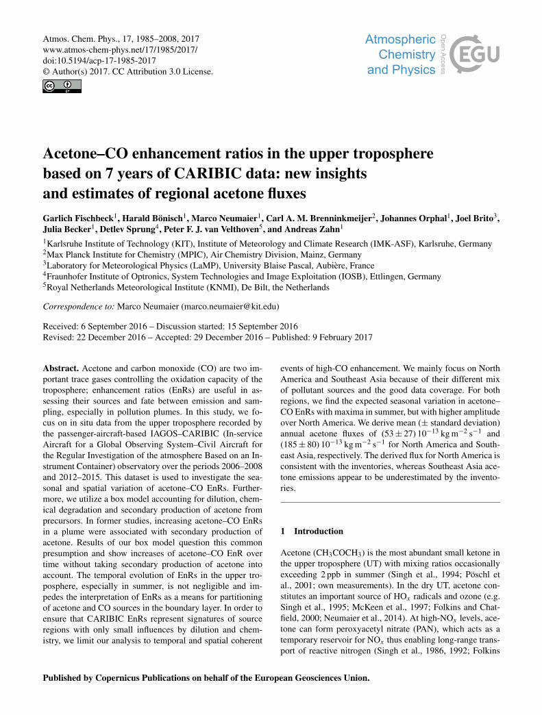
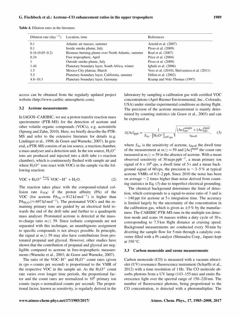
For acetone, it became common practice to use CO as a refer-ence species, because both gases are emitted during incom-plete combustion (Andreae and Merlet, 2001; Wisthaler etal., 2002; Greenberg et al., 2006; Warneke et al., 2011). Inpractice, the EnR is either determined by measuring the vol-ume mixing ratios (VMRs) inside and outside the plume (e.g.Simpson et al., 2011) or from continuous airborne measure-ments during plume passage (see Fig. 1) (Yokelson et al.,2013). In a scatter plot, the data points will ideally lie onthe mixing line that connects the higher concentrations in theplume with the background.
When an EnR is measured at the source, it equals its molaremission ratio (ER) (Yokelson et al., 2013). Downwind fromthe source, the EnR remains equal to the ER as long as pro-duction or removal of X and Y in the plume are negligibleand as long as the plume mixes in the same fixed background(Mauzerall et al., 1998; Yokelson et al., 2013). This is due tothe fact that dividing the enhancement of X by the enhance-ment of Y normalizes for dilution, as both species dilute atthe same rate (Akagi et al., 2012; Yokelson et al., 2013). Weprefer to use EnR whenever it cannot be excluded that theratio has changed since emission. As shown in Fig. 1, this isparticularly the case for measurements in the UT. Plume airinitially mixes with planetary boundary layer (PBL) air andsubsequently enters the “cleaner” UT. Plume ratios observedin the UT significantly differ from the PBL EnR value simplybecause the UT background has a different acetone–CO ratioas the PBL background.
Atmos. Chem. Phys., 17, 1985–2008, 2017 www.atmos-chem-phys.net/17/1985/2017/
G. Fischbeck et al.: Acetone–CO enhancement ratios in the upper troposphere 1987
Table 1. Literature values of acetone–CO emission ratios (ERs) in ppt ppb−1.
ER Air mass, location, time References
0.06–0.25 Biofuel burning Andreae and Merlet (2001)0.84 Vegetation from the southwest USA; laboratory experiment Warneke et al. (2011)1.2 Savanna biomass burning Akagi et al. (2011)1.6 Fresh Canadian boreal biomass burning plumes, June–July 2008 Simpson et al. (2011)1.7–2.05 North American wildfires Friedli et al. (2001)1.9–4.6 Savanna and grassland biomass burning Andreae and Merlet (2001)2.3–2.7 Extratropical forest biomass burning Andreae and Merlet (2001)1.93 Vegetation from the southeast USA; laboratory experiment Warneke et al. (2011)1.94 Pines spruce; laboratory experiment Warneke et al. (2011)2.8 Boreal forest biomass burning Akagi et al. (2011)2.9 Peatland burning Akagi et al. (2011)2.9 Tropical forest biomass burning Andreae and Merlet (2001)2.9 Charcoal burning Andreae and Merlet (2001)2.9 Residential heating Kaltsonoudis et al. (2016)3.0 Extratropical/boreal forest biomass burning Akagi et al. (2011)3.3 Tropical forest biomass burning Akagi et al. (2011)4.8 Fresh savannah fire, Africa Jost et al. (2003)5.4 Savanna grass, laboratory experiment Holzinger et al. (1999)
2.5± 1.3 Mean acetone–CO ER
Table 2. Literature values of acetone–CO enhancement ratios (EnRs) in biomass burning plumes in ppt ppb−1.
EnR Air mass, location, time References
4.7 Fresh biomass burning plume, summer 2008 Singh et al. (2010)5.0 Biomass burning plumes, Canada, June–July 2008 Hornbrook et al. (2011)5.7 Aged boreal biomass burning plumes from North America, July–August 2011 Tereszchuk et al. (2013)6.0 Biomass burning plumes, California, June–July 2008 Hornbrook et al. (2011)6.2 Aged boreal biomass burning plumes from Siberia, July–August 2011 Tereszchuk et al. (2013)6.3 Aged plumes of Alaskan and Canadian forest fire, July 2004 de Gouw et al. (2006);6.6 Aged Biomass burning plumes, Yucatan, March 2006 Yokelson et al. (2009)6.6–22 Aged biomass burning plumes, free troposphere, Pacific, winter/spring 2001 Jost et al. (2002)7.2–10.3 Biomass burning plumes, South Atlantic, September–October 1992 Mauzerall et al. (1998)7.1 Biomass burning plumes, Canada, June–July 2008 Hornbrook et al. (2011)7.5 Biomass burning plumes, Pacific, winter/spring 2001 Singh et al. (2004)7.7 Forest Fire Lake Baikal, April 2008 de Gouw et al. (2009)9.0 Asian biomass burning plumes, June–July 2008 Hornbrook et al. (2011)10.6 Aged (1–5 days) biomass burning and urban plumes, summer 2008 Singh et al. (2010)11.3 Fresh savannah fire plumes (0–125 min plume age), Africa Jost et al. (2003)11.7 Agricultural fires Kazakhstan, April 2008 de Gouw et al. (2009)14.3 Fresh boreal biomass burning plumes from Siberia, July–August 2011 Tereszchuk et al. (2013)16.8 Fresh boreal biomass burning plumes from North America, July–August 2011 Tereszchuk et al. (2013)18 Aged biomass burning plumes, Crete, August 2001 Holzinger et al. (2005)20.4 Young biomass burning plume, Tanzania, October 2005 (using background VMR over Pacific Ocean) Coheur et al. (2007)
9.9± 4.6 Mean acetone–CO EnR
The most comprehensive overview of acetone–CO EnRsto date has been given by de Reus et al. (2003), using dataof five research aircraft campaigns. For each campaign, theauthors split the data into measurements from the marineboundary layer (0–1 km), free troposphere (1–12.5 km) orlower stratosphere (O3> 150 ppb, CO< 60 ppb) and derivedone EnR per layer. Please note, that in this way, data of dif-
ferent flights, i.e. data of “unrelated” measurements in termsof distance and time span, were used to derive a single EnRestimate. The authors found different EnRs for the differentlayers, but, surprisingly, consistent values among the cam-paigns. Since then, EnRs have been frequently reported forindividual plumes and various conditions. In Tables 1–3, wegive an overview of literature acetone–CO ERs and EnRs,
www.atmos-chem-phys.net/17/1985/2017/ Atmos. Chem. Phys., 17, 1985–2008, 2017
1988 G. Fischbeck et al.: Acetone–CO enhancement ratios in the upper troposphere
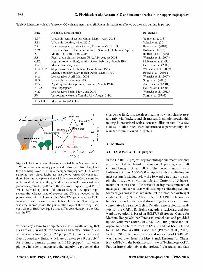
Table 3. Literature values of acetone–CO enhancement ratios (EnRs) in air masses unaffected by biomass burning in ppt ppb−1.
EnR Air mass, location, time References
1.57 Urban air, central eastern China, March–April 2011 Yuan et al. (2013)3.18 Urban air, London, winter 2012 Valach et al. (2014)3.4 Free troposphere, Indian Ocean, February–March 1999 Reiner et al. (2001)3.59 Urban air (with vehicular emissions), Sao Paolo, February–April 2013, Brito et al. (2015)5.0 Mount Tai, China, June 2006 Inomata et al. (2010)5.8 Fresh urban plumes, eastern USA, July–August 2004 Warneke et al. (2007)6.12 High-altitude (> 9km), Pacific Ocean, February–March 1994 McKeen et al. (1997)13–16 Marine boundary layer De Reus et al. (2003)13.4–17.2 Ship measurements, Indian Ocean, March 1999 Whistaler et al. (2002)14 Marine boundary layer, Indian Ocean, March 1999 Reiner et al. (2001);14.2 Los Angeles, April–May 2002 Warneke et al. (2007)18.3 Urban plumes, summer 2008 Singh et al. (2010)19.5 Aged high-altitude plumes, Surinam, March 1998 Andreae et al. (2001)21–25 Free troposphere De Reus et al. (2003)∼ 22 Los Angeles Basin, May–June 2010 Warneke et al. (2012)30 Troposphere, eastern Canada, July–August 1990 Singh et al. (1994)
12.5± 8.6 Mean acetone–CO EnR
0 100 200 300 400
A cet
one
[ppb
]
CO [ppb]
PBL
M ixing lines
[Y]plume-[Y]bgnd
[X]plume-[X]bgnd
M ixing
Plume PBL
0
1
2
3
4
bgnd PBL
bgnd UT
M easurements
Plume UT
UT
Figure 1. Left: schematic drawing (adapted from Mauzerall et al.,1998) of a biomass burning plume and its transport from the plane-tary boundary layer (PBL) into the upper troposphere (UT), wheresampling takes place. Right: acetone plotted versus CO concentra-tions. Black-filled square (plume PBL): acetone–CO concentrationin the fresh plume near the ground, which initially mixes with ad-jacent background (bgnd) air of the PBL (open square, bgnd PBL).When the resulting plume (full circle) rises into the upper tropo-sphere, the enhancement of acetone and CO are reduced as theplume mixes with background air of the UT (open circle, bgnd UT).In an ideal case, measured concentrations lie on the UT mixing linewhen the aircraft passes the plume. The slope of the mixing lines,equivalent to EnR (see Eq. 1), may differ considerably in the PBLand the UT.
without any claim to completeness. It is worth noting thatERs are only available for biomass and biofuel burning andare generally lower (mean: 2.5 ppt ppb−1) than the observedfree-tropospheric EnRs, which are on average 9.9 ppt ppb−1
for biomass burning plumes and 12.5 ppt ppb−1 for otherplumes. In order to understand the underlying processes that
change the EnR, it is worth estimating how fast plumes usu-ally mix with background air masses. In simple models, thismixing is prescribed with a constant dilution rate. In a fewstudies, dilution rates were determined experimentally; theresults are summarized in Table 4.
3 Methods
3.1 IAGOS–CARIBIC project
In the CARIBIC project, regular atmospheric measurementsare conducted on board a commercial passenger aircraft(Brenninkmeijer et al., 2007). The present aircraft is aLufthansa Airbus A340–600 equipped with a multi-line airinlet system (installed below the forward cargo bay) to sup-ply the instruments with sample air. Currently, 15 instru-ments for in situ and 1 for remote sensing measurements oftrace gases and aerosols as well as sample collecting systemsfor trace gas and aerosol are installed in a modified airfreightcontainer (1.6 t). Since May 2005, the CARIBIC laboratoryhas been monthly deployed during regular service for 4–6consecutive long-range flights. Detailed meteorological anal-ysis for the CARIBIC flights (including backward and for-ward trajectories) is based on ECMWF (European Centre forMedium-Range Weather Forecasts) model data and providedby van Velthoven (2016). In 2008, CARIBIC joined the Eu-ropean Research Infrastructure IAGOS and has been referredto as IAGOS–CARIBIC since then (Petzold et al., 2015).In April 2015, the coordination and operation of CARIBICwas handed over from the Max Planck Institute for Chem-istry (MPIC) to the Karlsruhe Institute of Technology (KIT).Further information about the project, flight routes and data
Atmos. Chem. Phys., 17, 1985–2008, 2017 www.atmos-chem-phys.net/17/1985/2017/
G. Fischbeck et al.: Acetone–CO enhancement ratios in the upper troposphere 1989
Table 4. Dilution rates in the literature.
Dilution rate (day−1) Location, time References
0.1 Atlantic air masses, summer Arnold et al. (2007)0.1 Inside smoke plume, July Pisso et al. (2009)0.16 (0.05–0.2) Biomass burning plume over North Atlantic, summer Real et al. (2007)0.24 Free troposphere, April Price et al. (2004)1 Outside smoke plume, July Pisso et al. (2009)1.44 Planetary boundary layer, South Africa, winter Igbafe et al. (2006)1.5 Mexico City plateau, March Voss et al. (2010); Shrivastava et al. (2011)5.5 Planetary boundary layer, California, summer Dillon et al. (2002)4.8–10.3 Planetary boundary layer, Germany Kramp and Volz-Thomas (1997)
access can be obtained from the regularly updated projectwebsite (http://www.caribic-atmospheric.com).
3.2 Acetone measurements
In IAGOS–CARIBIC, we use a proton transfer reaction massspectrometer (PTR-MS) for the detection of acetone andother volatile organic compounds (VOCs), e.g. acetonitrile(Sprung and Zahn, 2010). Here, we briefly describe the PTR-MS and refer to the extensive literature for details (e.g.Lindinger et al., 1998; de Gouw and Warneke, 2007). In gen-eral, a PTR-MS consists of an ion source, a reaction chamber,a mass analyser and a detection unit. In the ion source, H3O+
ions are produced and injected into a drift tube (= reactionchamber), which is continuously flushed with sample air andwhere H3O+ ions react with VOCs in the sample via the fol-lowing reaction:
VOC+H3O+kVOC−→ VOC−H++H2O. (2)
The reaction takes place with the compound-related col-lision rate kVOC if the proton affinity (PA) of theVOC (for acetone PAAc= 812 kJ mol−1) is higher thanPAH2O (≈ 697 kJ mol−1). The protonated VOCs and the re-maining primary ions are guided by an electrical field to-wards the end of the drift tube and further to a quadrupolemass analyser. Protonated acetone is detected at the mass-to-charge ratio m/z 59. Since isobaric compounds are notseparated with this technique, an unambiguous assignmentto specific compounds is not always possible. In principle,the signal at m/z 59 may also have contributions from pro-tonated propanal and glyoxal. However, other studies haveshown that the contribution of propanal and glyoxal are neg-ligible compared to acetone in free-tropospheric measure-ments (Warneke et al., 2003; de Gouw and Warneke, 2007).
The ratio of the VOC–H+ and H3O+ count rates (givenin cps= counts per second) is proportional to the VMR ofthe respective VOC in the sample air. As the H3O+ countrate varies over longer time periods, the proportional fac-tor and the count rates are normalized to 106 primary ioncounts (ncps= normalized counts per second). The propor-tional factor, known as sensitivity, is regularly derived in the
laboratory by sampling a calibration gas with certified VOCconcentrations (Apel-Riemer Environmental, Inc., Colorado,USA) under similar experimental conditions as during flight.The precision of the acetone measurement is mainly deter-mined by counting statistics (de Gouw et al., 2003) and canbe expressed as
1[Ac]ppb =1
SAc ·[H3O+
]106cps
√[Ac]sample
cps + [Ac]bgndcps
tdwell, (3)
where SAc is the sensitivity of acetone, tdwell the dwell timeof the measurement at m/z= 59 and [Ac]bgnd the count ratemeasured atm/z= 59 in the absence of acetone. With a meanobserved sensitivity of 30 ncps ppb−1, a mean primary ionsignal of 6× 10⁶ cps, a dwell time of 5 s and a mean back-ground signal of 60 cps, the precision is ∼ 3–5 % at typicalacetone VMRs of 0.5–2 ppb. Since 2010 the noise has beenon average ∼ 2 times higher than noise derived from count-ing statistics in Eq. (3) due to imperfect electrical grounding.
The chemical background determines the limit of detec-tion, which corresponds to a signal-to-noise ratio of 3 and is∼ 140 ppt for acetone at 5 s integration time. The accuracyis limited largely by the uncertainty of the concentration inthe calibration gas, which is given as ±5 % by the manufac-turer. The CARIBIC PTR-MS runs in the multiple ion detec-tion mode and scans 16 masses within a duty cycle of 30 s,corresponding to 7.5 km flight distance at cruising speed.Background measurements are conducted every 50 min bydiverting the sample flow for 5 min through a catalytic con-verter filled with a Pt catalyst (Shimadzu Corp., Japan) keptat 350 ◦C.
3.3 Carbon monoxide and ozone measurements
Carbon monoxide (CO) is measured with a vacuum ultravi-olet (UV) resonance fluorescence instrument (Scharffe et al.,2012) with a time resolution of 1 Hz. The CO molecule ab-sorbs photons from a UV lamp (143–155 nm) and emits flu-orescence light over the spectral range of 150–220 nm. Thenumber of fluorescence photons, being proportional to theCO concentration, is detected with a photomultiplier. The
www.atmos-chem-phys.net/17/1985/2017/ Atmos. Chem. Phys., 17, 1985–2008, 2017
1990 G. Fischbeck et al.: Acetone–CO enhancement ratios in the upper troposphere
precision of the instrument is 1–2 ppb at an integration timeof 1 s (Scharffe et al., 2012). Ozone (O3) is measured witha fast and precise chemiluminescence detector described inZahn et al. (2012) and calibrated using a likewise installedUV photometer. At typical O3 mixing ratios (10–100 ppb),the precision is 0.3–1.0 % at 10 Hz.
3.4 Data analysis
Data from the individual IAGOS–CARIBIC instruments arecombined into single “merge” files for each flight with a timebinning of 10 s. Data with a sampling frequency > 0.1 Hz,such as the CO measurements (1 Hz), are averaged over the10 s intervals, whereas low-frequency data (< 0.1 Hz), likethe acetone measurements (0.03 Hz), are assigned to the cor-responding 10 s interval. The correlation analysis is restrictedto UT air masses. Data from ascend and descend are rarelyavailable because of the long run-up time of the PTR-MSafter take-off and an automatic equipment shutdown proce-dure well before landing. Stratospheric acetone–CO correla-tions are not well suited for our purpose to investigate sourcepatterns, because of the long transport times. To excludestratospheric data, we use our concomitant CARIBIC ozonedata and apply the definition of the chemical tropopause asproposed by Zahn and Brenninkmeijer (2003) and Zahn etal. (2004) and verified by Thouret et al. (2006). Air masseswith an ozone concentration above the threshold value of
[O3]TPppb = 97+ 26sin
(2π
doy− 30365
), (4)
where doy denotes day of the year, are identified as strato-spheric and excluded. In the rare event of ozone data be-ing unavailable, we use potential vorticity (PV) calculatedfrom the ECMWF model and discard measurements with aPV> 2 pvu, a threshold commonly used to define the dy-namical tropopause (e.g. Hoskins et al., 1985; Holton et al.,1995). In this way, 42 % of the acetone–CO data were iden-tified as stratospheric.
In the remaining dataset, we search for physically mean-ingful correlations in all possible subsets of data fulfilling thefollowing two requirements adapted from Zahn et al. (2002)and Brito, 2012: (i) The subset consists of at least 10 suc-cessive measurements that are no further apart from eachother than 50 km and cover less than 500 km flight path;(ii) The range of CO VMRs in the subset is greater than 10times the average measurement uncertainty of CO. These cri-teria ensure that only temporal and spatial coherent eventswith a “fresh” source signature are considered and will bediscussed in more detail in Sect. 4.1. For each possiblesubset, Pearson’s linear correlation coefficient r and corre-sponding p value are calculated. We assume a good linearcorrelation in the event r > 0.5 and p< 0.05 (5 % signifi-cance level). In such a case, the slope is calculated using thebivariate least-squares method of Williamson–York (York,1966; Williamson, 1968; York et al., 2004) as suggested by
Acet
one
[ppt
]
200
400
600
800
1000
50 100 50 100
AICc,n=1 = 485.1AICc,n=2 = 371.1
AICc,n=1 = 269.0AICc,n=2 = 270.9
r = 0.97
CO [ppb]
( a) ( b)
r = 0.79
n = 1, center c1n = 2, center c1n = 2, center c2
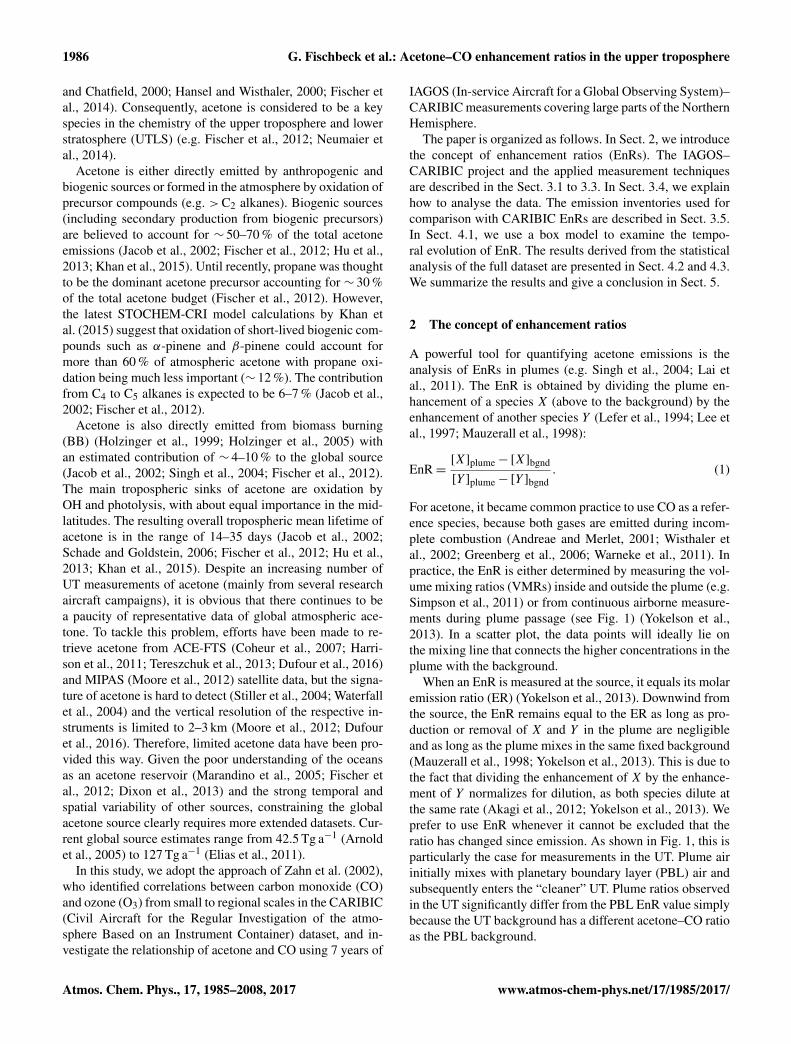
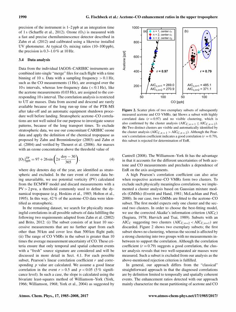
Figure 2. Scatter plots of two exemplary subsets of subsequentlymeasured acetone and CO VMRs. (a) Shows a subset with highlycorrelated data (r = 0.97) and no visible clustering, which isalso confirmed by the cluster analysis (AICC,n= 1≤AICC,n= 2).(b) Two distinct clusters are visible and automatically identified bythe cluster analysis (AICC,n= 1>AICC,n= 2). Although the Pear-son’s correlation coefficient indicates a good correlation (r = 0.79),this subset is rejected for determination of EnR.
Cantrell (2008). The Williamson–York fit has the advantagein that it accounts for the different uncertainties of both ace-tone and CO measurements and precludes a dependence ofEnR on the axis assignments.
A high Pearson’s correlation coefficient can also arisewhen respective acetone–CO VMRs form two clusters. Toexclude such physically meaningless correlations, we imple-mented a cluster analysis based on Gaussian mixture mod-els (GMMs) (Everitt and Hand, 1981; McLachlan and Peel,2000). In our case, two GMMs are fitted to the acetone–COsubset. The first model expects only one cluster and the sec-ond two clusters. In order to choose the best-fitting model,we use the corrected Akaike’s information criterion (AICC)(Sugiura, 1978; Hurvich and Tsai, 1989). Subsets with anAICC suggesting two clusters (AICC,n=2<AICC,n=1) arediscarded. Figure 2 shows two exemplary subsets; the firstsubset shows no clustering, whereas the second is affected bya strong clustering into two groups with no measurements in-between to support the correlation. Although the correlationcoefficient (r = 0.79) suggests a good correlation, the clus-ter analysis reveals that two well-separated air masses weremeasured. Such a subset is excluded from our analysis as theabove-mentioned rejection criterion is fulfilled.
In general, our approach differs from the “classical”straightforward approach in that the diagnosed correlationsare by definition limited to temporally and spatially coherentevents. The enhancement ratios detected with our approachmainly characterize the mean partitioning of acetone and CO
Atmos. Chem. Phys., 17, 1985–2008, 2017 www.atmos-chem-phys.net/17/1985/2017/
G. Fischbeck et al.: Acetone–CO enhancement ratios in the upper troposphere 1991
sources in the boundary layer on a regional scale. The spreadof these source regions depends on the time the analysed airparcel spends in the boundary layer before it is released intothe free and upper troposphere. Therefore, one could inter-pret the correlations derived from our approach as “event-based” EnRs, whereby the “event” is the release of an indi-vidual air parcel out of the boundary layer into the free tro-posphere. In contrast to our analysis, non-coherent correla-tions detected in former studies will often mirror spatial (e.g.latitudinal) gradients of acetone and CO, respectively, or im-ply differences of the trace gas composition of different airmasses, but not enhancement ratios that characterize pollu-tion sources and the chemical processing between emissionin the boundary layer and sampling in the upper troposphere.For this reason, we believe that our approach is best suitedfor the analysis of source patterns with tropospheric EnRs.
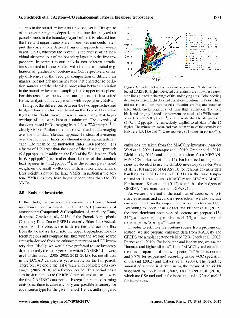
In Fig. 3, the differences between the two approaches andfit algorithms are illustrated based on the data of 17 selectedflights. The flights were chosen in such a way that largeroverlaps of data were kept at a minimum. The diversity ofthe event-based EnRs, ranging from 1.3 to 77.2 ppt ppb−1, isclearly visible. Furthermore, it is shown that initial averagingover the total data (classical approach) instead of averagingover the individual EnRs of coherent events makes a differ-ence. The mean of the individual EnRs (18.6 ppt ppb−1) isa factor of 1.9 larger than the slope of the classical approach(9.8 ppt ppb−1). In addition, the EnR of the Williamson–Yorkfit (9.8 ppt ppb−1) is smaller than the one of the standardleast-squares fit (11.2 ppt ppb−1), as the former puts (more)weight on the small VMRs due to their lower uncertainties.Less weight is put on the large VMRs, in particular the ace-tone VMRs, as they have larger uncertainties than the COVMRs.
3.5 Emission inventories
In this study, we use surface emission data from differentinventories made available in the ECCAD (Emissions ofatmospheric Compounds & Compilation of Ancillary Data)database (Granier et al., 2013) of the French AtmosphericChemistry Data Centre ESPRI (formerly Ether; http://eccad.sedoo.fr/). The objective is to derive the total acetone fluxfrom the boundary layer into the upper troposphere for dif-ferent regions and compare this flux with the acetone sourcestrengths derived from the enhancement ratios and CO inven-tory data. Ideally, we would have preferred to use inventorydata of exactly the same years for which CARIBIC data wereused in this study (2006–2008; 2012–2015), but not all datain the ECCAD database is yet available for the full period.Therefore, we chose the last 6 years with complete data cov-erage (2005–2010) as reference period. This period has asimilar duration as the CARIBIC periods and at least coversthe first CARIBIC data period. Except for biomass burningemissions, there is currently only one possible inventory foreach source type for the given period. Hence, anthropogenic
Figure 3. Scatter plot of tropospheric acetone and CO data of 17 se-lected CARIBIC flights. Detected correlations are shown as regres-sion lines plotted in the range of the underlying data. Colour codingdenotes to which flight data and correlations belong to. Data, whichdid not fall into our event-based correlation criteria, are shown asfilled black circles regardless of their flight affiliation. The solidblack and the grey dashed line represent the results of a Williamson–York fit (EnR: 9.8 ppt ppb−1) and of a standard least-squares fit(EnR: 11.2 ppt ppb−1), respectively, applied to all data of the 17flights. The minimum, mean and maximum value of the event-basedEnRs are 1.3, 18.6 and 77.2, respectively (all values in ppt ppb−1).
emissions are taken from the MACCity inventory (van derWerf et al., 2006; Lamarque et al., 2010; Granier et al., 2011;Diehl et al., 2012) and biogenic emissions from MEGAN-MACC (Sindelarova et al., 2014). For biomass burning emis-sions we decided to use the GFED3 inventory (van der Werfet al., 2010) instead of GFASv1.0 for reasons of easier datahandling, as GFED3 data in ECCAD has the same tempo-ral and spatial resolution as MACCity and MEGAN-MACC.Furthermore, Kaiser et al. (2012) found that the budgets ofGFED3(.1) are consistent with GFASv1.0.
As we are interested in the total flux of acetone, i.e. pri-mary emissions and secondary production, we also includeemission data from the major precursors of acetone and CO.According to Jacob et al. (2002) and Fischer et al. (2012),the three dominant precursors of acetone are propane (13–22 Tg a−1 acetone), higher alkanes (4–7 Tg a−1 acetone) andmonoterpenes (5–6 Tg a−1 acetone).
In order to estimate the acetone source from propane ox-idation, we use propane emission data from MACCity andGFED3 and a molar acetone yield of 72 % (Jacob et al., 2002;Pozzer et al., 2010). For isobutane and isopentane, we use the“butanes and higher alkanes” data of MACCity and calculatethe mass proportion of the two species (5.7 % for isobutaneand 9.7 % for isopentane) according to the VOC speciationof Passant (2002) and Calvert et al. (2009). The resultingamount of acetone is derived using the means of the yieldssuggested by Jacob et al. (2002) and Pozzer et al. (2010),which are 0.96 mol mol−1 for isobutane and 0.72 mol mol−1
for isopentane.
www.atmos-chem-phys.net/17/1985/2017/ Atmos. Chem. Phys., 17, 1985–2008, 2017
1992 G. Fischbeck et al.: Acetone–CO enhancement ratios in the upper troposphere
For the monoterpenes, we use the emission data for thesum of monoterpenes from MEGAN-MACC (Sindelarovaet al., 2014) and the relative contributions provided in Sin-delarova et al. (2014) to calculate the emissions of the fol-lowing individual monoterpene species: α-pinene, β-pinene,limonene, trans-β-ocimene, myrcene, sabinene and 3-carene.For each species, we derive mean acetone yields based on theavailable literature. Here, we consider the two main degrada-tion processes of monoterpenes, reaction with OH and O3,and weight the yields according to the respective reactionrates (i.e. to the importance of the reaction with regard toall degradation processes). All considered yields and calcu-lations are provided as a supplement.
For the secondary production of CO, we only considerprecursors with an annual global contribution of more than25 Tg CO according to Duncan et al. (2007) and an atmo-spheric lifetime shorter than that of acetone, i.e. isoprene,methanol, monoterpenes, (≥C4) alkanes, (≥C3) alkenes andethene. The respective CO production yields are taken fromthe same study and do not account for loss of intermediatetrace gases by deposition, which might over-predict the con-tribution from longer-lived precursors (Duncan et al., 2007).As uncertainties are not provided for all yields and emissioninventory fluxes, we refrain from performing a comprehen-sive uncertainty analysis. However, considerable uncertain-ties might exist and estimates based on these data have to betaken with care. In our analysis, at least the statistical uncer-tainties of fluxes are strongly reduced by averaging over largeregions and time periods.
4 Results and discussions
4.1 Temporal evolution of EnR between emission andsampling
For the CARIBIC measurements in the UT, it is importantto consider the possible temporal evolution of the EnR, be-cause transport timescales and typical tropospheric lifetimesof acetone and CO are of a comparable range. So far, thecombined influence of dilution and chemical transformationon acetone–CO EnRs has not been addressed in previousstudies. In order to better assess their impact, we first exam-ine the temporal evolution of EnRs from a theoretical pointof view. We apply a simple one-box model, in which the boxrepresents the volume of the plume at time t = 0. Whereasthe plume expands with time, the considered box volume isheld constant to take dilution into account. The temporal evo-lution of the mixing ratio of a compound X inside the plumecan then be approximated by (McKeen and Liu, 1993; McK-een et al., 1996)
d[X]plume
dt=−LX[X]plume−D
([X]plume− [X]bgnd
)+PZ,X[Z]plume, (5)
where LX is the overall chemical loss rate of X, D is thefirst-order dilution rate and PZ,X is the production rate ofX from the oxidation of the precursor compound Z. Theoverall chemical loss rate LX is the sum of all loss mech-anisms, which are for acetone reaction with OH and pho-tolysis (LAc = kAc [OH] + JAc) and for CO reaction withOH (LCO = kCO [OH]). As the lifetimes of both species areat least weeks, we simply assume constant reaction and di-lution rates over the considered time period. Consequently,we apply daily averaged photolysis rates obtained from thetropospheric ultraviolet and visible radiation model (TUVversion 5.0; Madronich and Flocke, 1999; Madronich et al.,2010), which uses the quantum yields for acetone by Blitz etal. (2004), and monthly mean OH concentrations from Spi-vakovsky et al. (2000). The OH reaction rates and uncertain-ties thereof are taken from the latest recommendations of theIUPAC (International Union of Pure and Applied Chemistry)Task Group on Atmospheric Chemical Kinetic Data Evalua-tion (Atkinson et al., 2004, 2006). The latter are reported tobe∼ 20 %. The same was assumed for the acetone photolysisrate (see Neumaier et al., 2014).
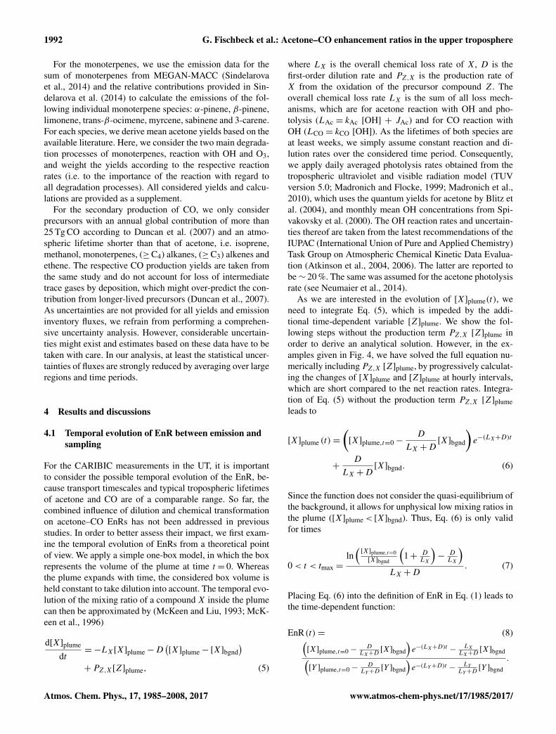
As we are interested in the evolution of [X]plume(t), weneed to integrate Eq. (5), which is impeded by the addi-tional time-dependent variable [Z]plume. We show the fol-lowing steps without the production term PZ,X [Z]plume inorder to derive an analytical solution. However, in the ex-amples given in Fig. 4, we have solved the full equation nu-merically including PZ,X [Z]plume, by progressively calculat-ing the changes of [X]plume and [Z]plume at hourly intervals,which are short compared to the net reaction rates. Integra-tion of Eq. (5) without the production term PZ,X [Z]plumeleads to
[X]plume (t)=
([X]plume,t=0−
D
LX +D[X]bgnd
)e−(LX+D)t
+D
LX +D[X]bgnd. (6)
Since the function does not consider the quasi-equilibrium ofthe background, it allows for unphysical low mixing ratios inthe plume ([X]plume< [X]bgnd). Thus, Eq. (6) is only validfor times
0< t < tmax =ln(
[X]plume,t=0[X]bgnd
(1+ D
LX
)−
DLX
)LX +D
. (7)
Placing Eq. (6) into the definition of EnR in Eq. (1) leads tothe time-dependent function:
EnR(t)= (8)([X]plume,t=0−
DLX+D
[X]bgnd
)e−(LX+D)t − LX
LX+D[X]bgnd(
[Y ]plume,t=0−D
LY+D[Y ]bgnd
)e−(LY+D)t − LY
LY+D[Y ]bgnd
.
Atmos. Chem. Phys., 17, 1985–2008, 2017 www.atmos-chem-phys.net/17/1985/2017/
G. Fischbeck et al.: Acetone–CO enhancement ratios in the upper troposphere 1993
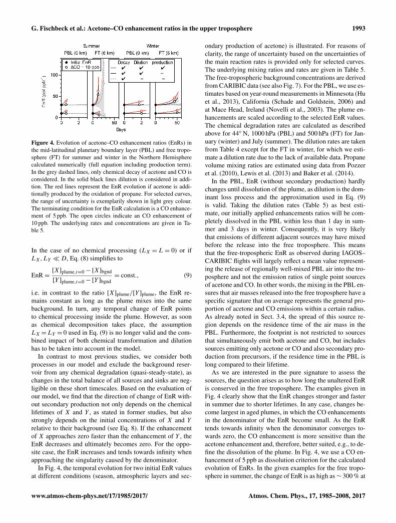
Figure 4. Evolution of acetone–CO enhancement ratios (EnRs) inthe mid-latitudinal planetary boundary layer (PBL) and free tropo-sphere (FT) for summer and winter in the Northern Hemispherecalculated numerically (full equation including production term).In the grey dashed lines, only chemical decay of acetone and CO isconsidered. In the solid black lines dilution is considered in addi-tion. The red lines represent the EnR evolution if acetone is addi-tionally produced by the oxidation of propane. For selected curves,the range of uncertainty is exemplarily shown in light grey colour.The terminating condition for the EnR calculation is a CO enhance-ment of 5 ppb. The open circles indicate an CO enhancement of10 ppb. The underlying rates and concentrations are given in Ta-ble 5.
In the case of no chemical processing (LX = L= 0) or ifLX,LY �D, Eq. (8) simplifies to
EnR=[X]plume,t=0− [X]bgnd
[Y ]plume,t=0− [Y ]bgnd= const., (9)
i.e. in contrast to the ratio [X]plume/[Y ]plume, the EnR re-mains constant as long as the plume mixes into the samebackground. In turn, any temporal change of EnR pointsto chemical processing inside the plume. However, as soonas chemical decomposition takes place, the assumptionLX =LY = 0 used in Eq. (9) is no longer valid and the com-bined impact of both chemical transformation and dilutionhas to be taken into account in the model.
In contrast to most previous studies, we consider bothprocesses in our model and exclude the background reser-voir from any chemical degradation (quasi-steady-state), aschanges in the total balance of all sources and sinks are neg-ligible on these short timescales. Based on the evaluation ofour model, we find that the direction of change of EnR with-out secondary production not only depends on the chemicallifetimes of X and Y , as stated in former studies, but alsostrongly depends on the initial concentrations of X and Yrelative to their background (see Eq. 8). If the enhancementof X approaches zero faster than the enhancement of Y , theEnR decreases and ultimately becomes zero. For the oppo-site case, the EnR increases and tends towards infinity whenapproaching the singularity caused by the denominator.
In Fig. 4, the temporal evolution for two initial EnR valuesat different conditions (season, atmospheric layers and sec-
ondary production of acetone) is illustrated. For reasons ofclarity, the range of uncertainty based on the uncertainties ofthe main reaction rates is provided only for selected curves.The underlying mixing ratios and rates are given in Table 5.The free-tropospheric background concentrations are derivedfrom CARIBIC data (see also Fig. 7). For the PBL, we use es-timates based on year-round measurements in Minnesota (Huet al., 2013), California (Schade and Goldstein, 2006) andat Mace Head, Ireland (Novelli et al., 2003). The plume en-hancements are scaled according to the selected EnR values.The chemical degradation rates are calculated as describedabove for 44◦ N, 1000 hPa (PBL) and 500 hPa (FT) for Jan-uary (winter) and July (summer). The dilution rates are takenfrom Table 4 except for the FT in winter, for which we esti-mate a dilution rate due to the lack of available data. Propanevolume mixing ratios are estimated using data from Pozzeret al. (2010), Lewis et al. (2013) and Baker et al. (2014).
In the PBL, EnR (without secondary production) hardlychanges until dissolution of the plume, as dilution is the dom-inant loss process and the approximation used in Eq. (9)is valid. Taking the dilution rates (Table 5) as best esti-mate, our initially applied enhancements ratios will be com-pletely dissolved in the PBL within less than 1 day in sum-mer and 3 days in winter. Consequently, it is very likelythat emissions of different adjacent sources may have mixedbefore the release into the free troposphere. This meansthat the free-tropospheric EnR as observed during IAGOS–CARIBIC flights will largely reflect a mean value represent-ing the release of regionally well-mixed PBL air into the tro-posphere and not the emission ratios of single point sourcesof acetone and CO. In other words, the mixing in the PBL en-sures that air masses released into the free troposphere have aspecific signature that on average represents the general pro-portion of acetone and CO emissions within a certain radius.As already noted in Sect. 3.4, the spread of this source re-gion depends on the residence time of the air mass in thePBL. Furthermore, the footprint is not restricted to sourcesthat simultaneously emit both acetone and CO, but includessources emitting only acetone or CO and also secondary pro-duction from precursors, if the residence time in the PBL islong compared to their lifetime.
As we are interested in the pure signature to assess thesources, the question arises as to how long the unaltered EnRis conserved in the free troposphere. The examples given inFig. 4 clearly show that the EnR changes stronger and fasterin summer due to shorter lifetimes. In any case, changes be-come largest in aged plumes, in which the CO enhancementsin the denominator of the EnR become small. As the EnRtends towards infinity when the denominator converges to-wards zero, the CO enhancement is more sensitive than theacetone enhancement and, therefore, better suited, e.g., to de-fine the dissolution of the plume. In Fig. 4, we use a CO en-hancement of 5 ppb as dissolution criterion for the calculatedevolution of EnRs. In the given examples for the free tropo-sphere in summer, the change of EnR is as high as∼ 300 % at
www.atmos-chem-phys.net/17/1985/2017/ Atmos. Chem. Phys., 17, 1985–2008, 2017
1994 G. Fischbeck et al.: Acetone–CO enhancement ratios in the upper troposphere
Table 5. Mixing ratios, chemical loss and dilution rates used for the simulation of the temporal evolution of acetone–CO EnRs shown inFig. 4.
Summer Winter
PBL FT PBL FT
Acetone 2.0 0.6 0.5 0.3
Background [ppb] CO 100 70 150 80
Propane 0.1 0.1 1.0 0.2
Acetone 4.2/2.0
Enhancement [ppb] CO 140/200
Propane 0.5
Acetone 0.029± 0.004 0.049± 0.007 0.002± 0.000 0.004± 0.001(5.0± 0.7) (2.9± 0.4) (82.9± 11.8) (37.0± 5.2)
Chemical degradation rate [d−1] CO 0.026± 0.005 0.039± 0.008 0.002± 0.000 0.003± 0.001(lifetime [weeks]) (5.5± 1.1) (3.6± 0.7) (94.0± 18.8) (49.3± 9.9)
Propane 0.111± 0.023 0.154± 0.031 0.005± 0.001 0.009± 0.002(1.3± 0.3) (0.9± 0.2) (26.7± 5.3) (15.2± 3.0)
Dilution rate [d−1] 4.80 0.10 1.44 0.05
Table 6. Mean and median values of EnR frequency distributionsand centre of the fitted Gaussian distributions.
Season Slope/EnR[ppt ppb−1]
JJAS
Arithmetic mean ±σ 27.2± 17.0Median 22.9Gaussian line centre ±σ 19.3± 12.9Number of correlated/ 4747/12 896all measurements
DJFM
Arithmetic mean ±σ 11.6± 7.2Median 9.4Gaussian line centre ±σ 8.5± 3.5Number of correlated/ 4137/10 311all measurements
the time of dissolution, strongly depending on the initial COenhancement and the presence of secondary acetone produc-tion. As we do not have information about the actual age ofthe plumes observed in CARIBIC and thus cannot correctfor the temporal changes, we limit our analysis to plumeswith a CO enhancement greater than 10 ppb (more specif-ically, 10 times the mean measurement uncertainty of CO;see Sect. 3.4). We are aware that this threshold (open cir-cles in Fig. 4) represents a trade-off between maximizingthe number of detected correlations to achieve good statis-tics and minimizing the consideration of aged plumes withEnRs, which have been changed by chemistry and dilutionto such an extent that conclusions about the source signature
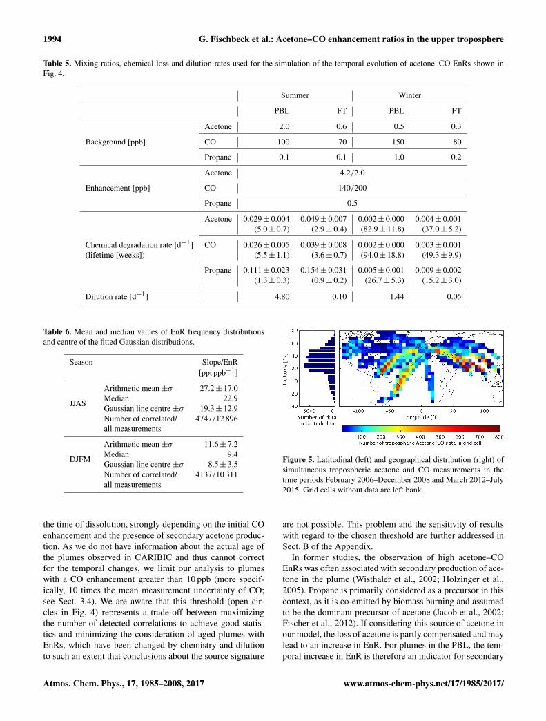
Figure 5. Latitudinal (left) and geographical distribution (right) ofsimultaneous tropospheric acetone and CO measurements in thetime periods February 2006–December 2008 and March 2012–July2015. Grid cells without data are left bank.
are not possible. This problem and the sensitivity of resultswith regard to the chosen threshold are further addressed inSect. B of the Appendix.
In former studies, the observation of high acetone–COEnRs was often associated with secondary production of ace-tone in the plume (Wisthaler et al., 2002; Holzinger et al.,2005). Propane is primarily considered as a precursor in thiscontext, as it is co-emitted by biomass burning and assumedto be the dominant precursor of acetone (Jacob et al., 2002;Fischer et al., 2012). If considering this source of acetone inour model, the loss of acetone is partly compensated and maylead to an increase in EnR. For plumes in the PBL, the tem-poral increase in EnR is therefore an indicator for secondary
Atmos. Chem. Phys., 17, 1985–2008, 2017 www.atmos-chem-phys.net/17/1985/2017/
G. Fischbeck et al.: Acetone–CO enhancement ratios in the upper troposphere 1995
production of acetone. In the free troposphere, the situation ismore complex and our model predicts an increase of EnR inthree of four cases even without the presence of propane, al-though we have to admit that the range of uncertainty is verylarge in one case. Especially in summer, when the curves ofthe higher EnR with and without secondary production donot differ significantly, it seems to be hardly feasible to dis-tinguish between the different reasons of increasing EnRs.
As mentioned earlier, another reason for possible changesin EnR between emission and measurement is the subse-quent mixing with different backgrounds (e.g. Mauzerall etal., 1998; Yokelson et al., 2013). Equation (8) is only valid aslong as the terms [X]bgnd and [Y ]bgnd are constant. Wheneverthe background mixing ratios change, e.g. the plume entersthe free troposphere, the EnR becomes larger under the con-dition(
[X]bgnd,old− [X]bgnd,new)
> EnRold([Y ]bgnd,old− [Y ]bgnd,new
)(10)
and smaller for the reverse inequality. Figure 1 illustrates thiscommon scenario and the resulting change of the slope of themixing line.
4.2 Observation of EnR within IAGOS–CARIBIC
4.2.1 Temporal and spatial distribution of data
The analysis of acetone–CO EnR relies on the availability ofthe simultaneous measurement of acetone and CO in the tro-posphere. At the time of this study, tropospheric acetone datawere available for 105 CARIBIC flights between 20 Febru-ary 2006 and 13 December 2008 and for 109 CARIBICflights between 6 March 2012 and 16 July 2015. The gapis due to a larger modification of the instrument and sub-sequent re-certification. As shown in Fig. 5, about 90 % ofsimultaneous tropospheric acetone and CO measurementswere carried out in the Northern Hemisphere, mainly in thesubtropics and mid-latitudes along the routes between Ger-many and Caracas/Bogota, Sao Paolo, Chennai, Bangkokand Guangzhou/Hong Kong. Although IAGOS–CARIBICflights to North America took place frequently, mainly strato-spheric air was sampled due to the lower tropopause heightsthere. In order to obtain statistically reliable results, we focuson the subtropics and mid-latitudes.
4.2.2 Frequency distribution of EnR
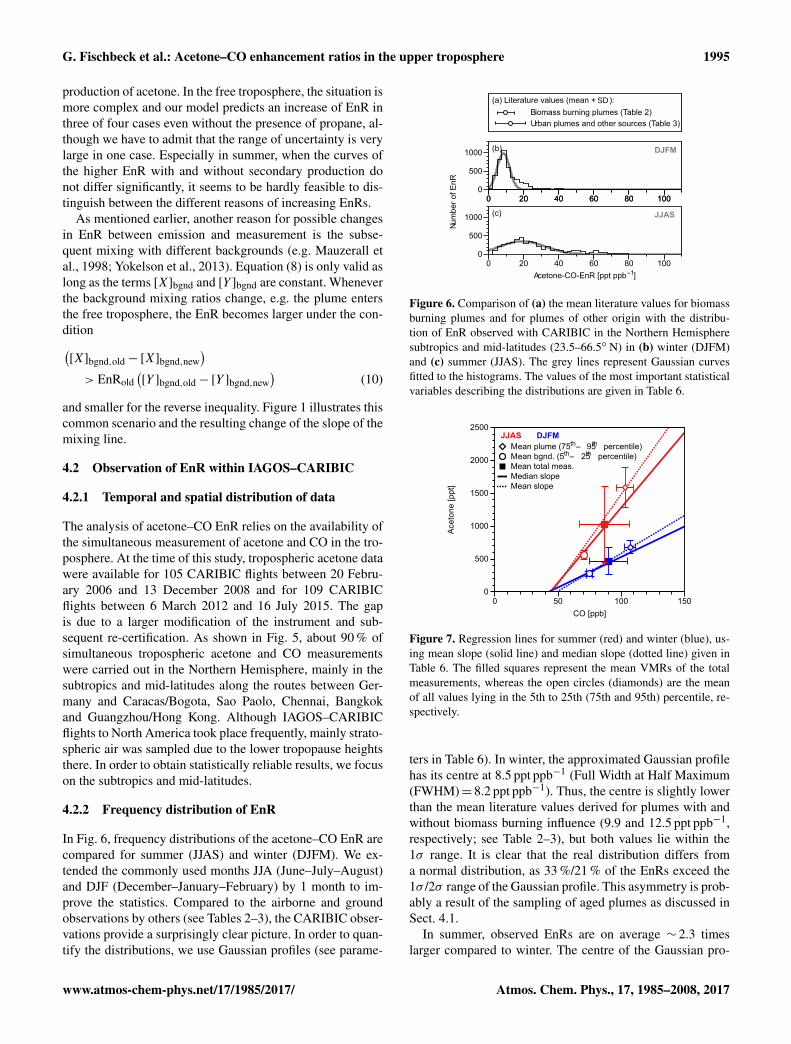
In Fig. 6, frequency distributions of the acetone–CO EnR arecompared for summer (JJAS) and winter (DJFM). We ex-tended the commonly used months JJA (June–July–August)and DJF (December–January–February) by 1 month to im-prove the statistics. Compared to the airborne and groundobservations by others (see Tables 2–3), the CARIBIC obser-vations provide a surprisingly clear picture. In order to quan-tify the distributions, we use Gaussian profiles (see parame-
N um
ber o
f EnR
0 20 40 60 80 100
JJAS
DJFM
0 20 40 60 80 100
(a) L iterature values (mean + ):
U rban plumes and other sources (Table 3)B iomass burning plumes (Table 2)
(b)
(c)
0
500
1000
0
500
1000
A cetone-CO-EnR [ppt ppb ]–10 20 40 60 80 100
SD
Figure 6. Comparison of (a) the mean literature values for biomassburning plumes and for plumes of other origin with the distribu-tion of EnR observed with CARIBIC in the Northern Hemispheresubtropics and mid-latitudes (23.5–66.5◦ N) in (b) winter (DJFM)and (c) summer (JJAS). The grey lines represent Gaussian curvesfitted to the histograms. The values of the most important statisticalvariables describing the distributions are given in Table 6.
JJAS DJFM M ean plume (75 – 95 percentile)th th
M ean bgnd. (5 – 25 percentile)th th
M ean total meas.M edian slopeM ean slope
Acet
one
[ppt
]
0
500
1000
1500
2000
2500
CO [ppb]0 50 100 150
Figure 7. Regression lines for summer (red) and winter (blue), us-ing mean slope (solid line) and median slope (dotted line) given inTable 6. The filled squares represent the mean VMRs of the totalmeasurements, whereas the open circles (diamonds) are the meanof all values lying in the 5th to 25th (75th and 95th) percentile, re-spectively.
ters in Table 6). In winter, the approximated Gaussian profilehas its centre at 8.5 ppt ppb−1 (Full Width at Half Maximum(FWHM)= 8.2 ppt ppb−1). Thus, the centre is slightly lowerthan the mean literature values derived for plumes with andwithout biomass burning influence (9.9 and 12.5 ppt ppb−1,respectively; see Table 2–3), but both values lie within the1σ range. It is clear that the real distribution differs froma normal distribution, as 33 %/21 % of the EnRs exceed the1σ /2σ range of the Gaussian profile. This asymmetry is prob-ably a result of the sampling of aged plumes as discussed inSect. 4.1.
In summer, observed EnRs are on average ∼ 2.3 timeslarger compared to winter. The centre of the Gaussian pro-
www.atmos-chem-phys.net/17/1985/2017/ Atmos. Chem. Phys., 17, 1985–2008, 2017
1996 G. Fischbeck et al.: Acetone–CO enhancement ratios in the upper troposphere
file (19.3 ppt ppb−1) is higher than the mean literature val-ues, but again the values lie within the 1σ range. TheFMHW of the Gaussian profile is even ∼ 3.7 times greater(∼ 30.4 ppt ppb−1), reflecting the larger natural variabilityin summer. As in winter, the real distribution of CARIBICEnRs is shifted towards larger values (mean: 27.2 ppt ppb−1).About 30 %/∼ 16 % of the EnRs exceed the 1σ /2σ range ofthe Gaussian profile. The great majority of high EnRs in sum-mer was sampled in air masses measured above or originat-ing from North America (see next section).
To identify the reason for the considerable seasonal vari-ation of the acetone–CO EnR in the upper troposphere, weplot the regression lines for the mean and median parametersas derived from our EnR distributions (Table 6) alongside theVMRs of the total measurements (Fig. 7). It becomes clearthat the factor of ∼ 2.3 between summer and winter EnR ismainly the consequence of the considerable seasonality ofacetone. The mean CO VMRs between JJAS and DJFM dif-fer by only 6 %, simply as the CO maximum and minimumin the UT occur in March–April and September–October, re-spectively (Zahn et al., 2002; Zbinden et al., 2013; Petetin etal., 2016; Osman et al., 2016).
4.3 Regional differences in EnR and comparison withemission inventories
In this subsection, we use sample location and 5-dayECMWF backwards trajectories calculated every 3 minalong the flight track (van Velthoven, 2016) to assign EnRto selected source regions. If a correlation is found in a sub-set of data (see Sect. 3.4), the derived EnR is assigned to eachacetone–CO data pair of the subset and to the closest 5-dayback trajectory thereof.
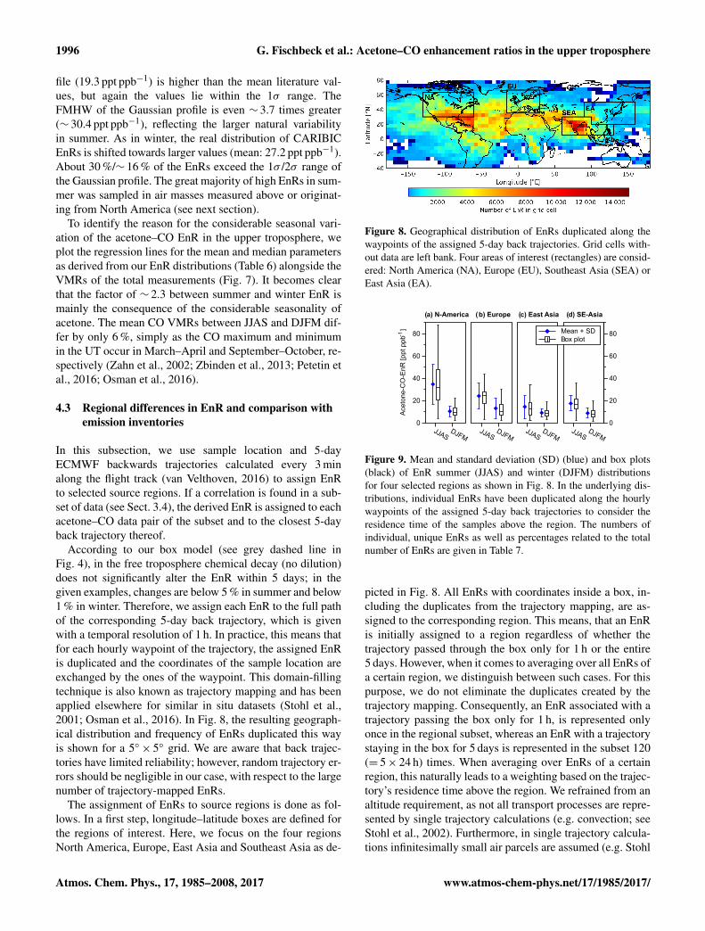
According to our box model (see grey dashed line inFig. 4), in the free troposphere chemical decay (no dilution)does not significantly alter the EnR within 5 days; in thegiven examples, changes are below 5 % in summer and below1 % in winter. Therefore, we assign each EnR to the full pathof the corresponding 5-day back trajectory, which is givenwith a temporal resolution of 1 h. In practice, this means thatfor each hourly waypoint of the trajectory, the assigned EnRis duplicated and the coordinates of the sample location areexchanged by the ones of the waypoint. This domain-fillingtechnique is also known as trajectory mapping and has beenapplied elsewhere for similar in situ datasets (Stohl et al.,2001; Osman et al., 2016). In Fig. 8, the resulting geograph-ical distribution and frequency of EnRs duplicated this wayis shown for a 5◦× 5◦ grid. We are aware that back trajec-tories have limited reliability; however, random trajectory er-rors should be negligible in our case, with respect to the largenumber of trajectory-mapped EnRs.
The assignment of EnRs to source regions is done as fol-lows. In a first step, longitude–latitude boxes are defined forthe regions of interest. Here, we focus on the four regionsNorth America, Europe, East Asia and Southeast Asia as de-
Figure 8. Geographical distribution of EnRs duplicated along thewaypoints of the assigned 5-day back trajectories. Grid cells with-out data are left bank. Four areas of interest (rectangles) are consid-ered: North America (NA), Europe (EU), Southeast Asia (SEA) orEast Asia (EA).
Acet
one-
CO-E
nR [p
pt p
pb]
-1
0
20
40
60
80
JJASDJFM
JJASDJFM
JJASDJFM
JJASDJFM
( a) N-America ( b) Europe ( c) East Asia ( d) SE-Asia
Mean + SDB ox plot
0
20
40
60
80
Figure 9. Mean and standard deviation (SD) (blue) and box plots(black) of EnR summer (JJAS) and winter (DJFM) distributionsfor four selected regions as shown in Fig. 8. In the underlying dis-tributions, individual EnRs have been duplicated along the hourlywaypoints of the assigned 5-day back trajectories to consider theresidence time of the samples above the region. The numbers ofindividual, unique EnRs as well as percentages related to the totalnumber of EnRs are given in Table 7.
picted in Fig. 8. All EnRs with coordinates inside a box, in-cluding the duplicates from the trajectory mapping, are as-signed to the corresponding region. This means, that an EnRis initially assigned to a region regardless of whether thetrajectory passed through the box only for 1 h or the entire5 days. However, when it comes to averaging over all EnRs ofa certain region, we distinguish between such cases. For thispurpose, we do not eliminate the duplicates created by thetrajectory mapping. Consequently, an EnR associated with atrajectory passing the box only for 1 h, is represented onlyonce in the regional subset, whereas an EnR with a trajectorystaying in the box for 5 days is represented in the subset 120(= 5× 24 h) times. When averaging over EnRs of a certainregion, this naturally leads to a weighting based on the trajec-tory’s residence time above the region. We refrained from analtitude requirement, as not all transport processes are repre-sented by single trajectory calculations (e.g. convection; seeStohl et al., 2002). Furthermore, in single trajectory calcula-tions infinitesimally small air parcels are assumed (e.g. Stohl
Atmos. Chem. Phys., 17, 1985–2008, 2017 www.atmos-chem-phys.net/17/1985/2017/
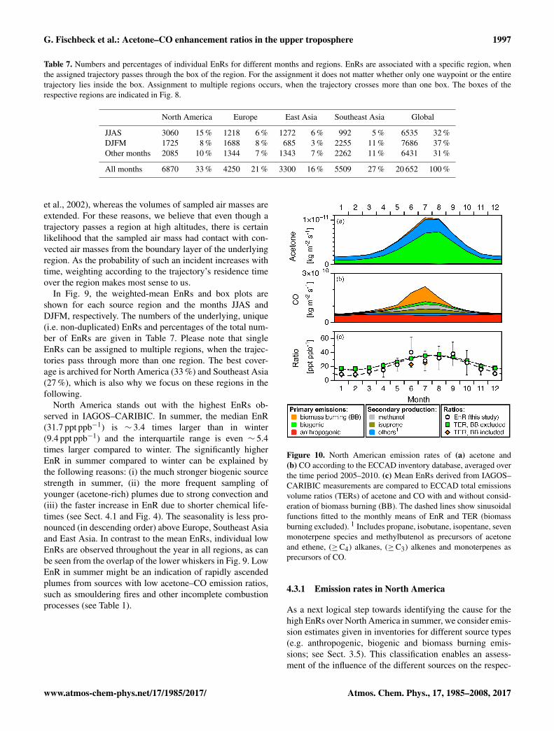
G. Fischbeck et al.: Acetone–CO enhancement ratios in the upper troposphere 1997
Table 7. Numbers and percentages of individual EnRs for different months and regions. EnRs are associated with a specific region, whenthe assigned trajectory passes through the box of the region. For the assignment it does not matter whether only one waypoint or the entiretrajectory lies inside the box. Assignment to multiple regions occurs, when the trajectory crosses more than one box. The boxes of therespective regions are indicated in Fig. 8.
North America Europe East Asia Southeast Asia Global
JJAS 3060 15 % 1218 6 % 1272 6 % 992 5 % 6535 32 %DJFM 1725 8 % 1688 8 % 685 3 % 2255 11 % 7686 37 %Other months 2085 10 % 1344 7 % 1343 7 % 2262 11 % 6431 31 %
All months 6870 33 % 4250 21 % 3300 16 % 5509 27 % 20 652 100 %
et al., 2002), whereas the volumes of sampled air masses areextended. For these reasons, we believe that even though atrajectory passes a region at high altitudes, there is certainlikelihood that the sampled air mass had contact with con-vected air masses from the boundary layer of the underlyingregion. As the probability of such an incident increases withtime, weighting according to the trajectory’s residence timeover the region makes most sense to us.
In Fig. 9, the weighted-mean EnRs and box plots areshown for each source region and the months JJAS andDJFM, respectively. The numbers of the underlying, unique(i.e. non-duplicated) EnRs and percentages of the total num-ber of EnRs are given in Table 7. Please note that singleEnRs can be assigned to multiple regions, when the trajec-tories pass through more than one region. The best cover-age is archived for North America (33 %) and Southeast Asia(27 %), which is also why we focus on these regions in thefollowing.
North America stands out with the highest EnRs ob-served in IAGOS–CARIBIC. In summer, the median EnR(31.7 ppt ppb−1) is ∼ 3.4 times larger than in winter(9.4 ppt ppb−1) and the interquartile range is even ∼ 5.4times larger compared to winter. The significantly higherEnR in summer compared to winter can be explained bythe following reasons: (i) the much stronger biogenic sourcestrength in summer, (ii) the more frequent sampling ofyounger (acetone-rich) plumes due to strong convection and(iii) the faster increase in EnR due to shorter chemical life-times (see Sect. 4.1 and Fig. 4). The seasonality is less pro-nounced (in descending order) above Europe, Southeast Asiaand East Asia. In contrast to the mean EnRs, individual lowEnRs are observed throughout the year in all regions, as canbe seen from the overlap of the lower whiskers in Fig. 9. LowEnR in summer might be an indication of rapidly ascendedplumes from sources with low acetone–CO emission ratios,such as smouldering fires and other incomplete combustionprocesses (see Table 1).
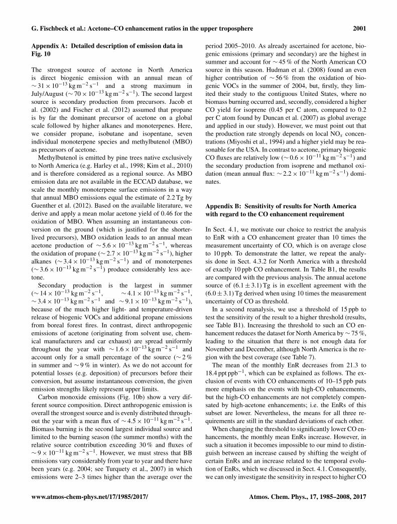
Figure 10. North American emission rates of (a) acetone and(b) CO according to the ECCAD inventory database, averaged overthe time period 2005–2010. (c) Mean EnRs derived from IAGOS–CARIBIC measurements are compared to ECCAD total emissionsvolume ratios (TERs) of acetone and CO with and without consid-eration of biomass burning (BB). The dashed lines show sinusoidalfunctions fitted to the monthly means of EnR and TER (biomassburning excluded). 1 Includes propane, isobutane, isopentane, sevenmonoterpene species and methylbutenol as precursors of acetoneand ethene, (≥C4) alkanes, (≥C3) alkenes and monoterpenes asprecursors of CO.
4.3.1 Emission rates in North America
As a next logical step towards identifying the cause for thehigh EnRs over North America in summer, we consider emis-sion estimates given in inventories for different source types(e.g. anthropogenic, biogenic and biomass burning emis-sions; see Sect. 3.5). This classification enables an assess-ment of the influence of the different sources on the respec-
www.atmos-chem-phys.net/17/1985/2017/ Atmos. Chem. Phys., 17, 1985–2008, 2017
1998 G. Fischbeck et al.: Acetone–CO enhancement ratios in the upper troposphere
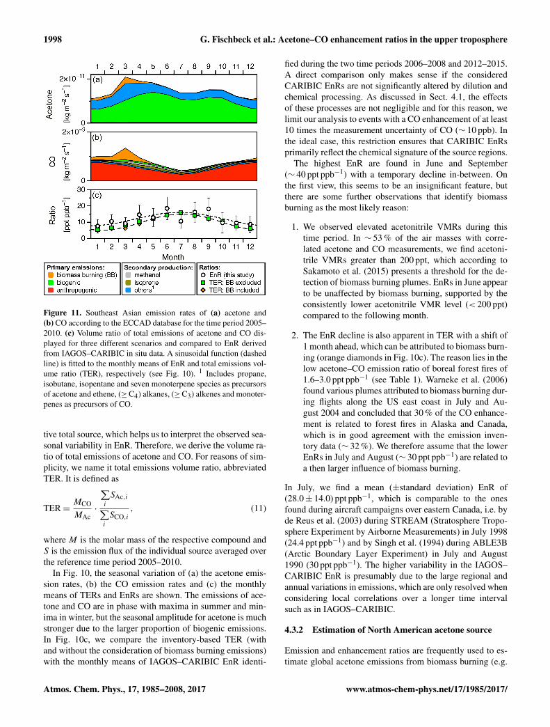
Figure 11. Southeast Asian emission rates of (a) acetone and(b) CO according to the ECCAD database for the time period 2005–2010. (c) Volume ratio of total emissions of acetone and CO dis-played for three different scenarios and compared to EnR derivedfrom IAGOS–CARIBIC in situ data. A sinusoidal function (dashedline) is fitted to the monthly means of EnR and total emissions vol-ume ratio (TER), respectively (see Fig. 10). 1 Includes propane,isobutane, isopentane and seven monoterpene species as precursorsof acetone and ethene, (≥C4) alkanes, (≥C3) alkenes and monoter-penes as precursors of CO.
tive total source, which helps us to interpret the observed sea-sonal variability in EnR. Therefore, we derive the volume ra-tio of total emissions of acetone and CO. For reasons of sim-plicity, we name it total emissions volume ratio, abbreviatedTER. It is defined as
TER=MCO
MAc·
∑i
SAc,i∑i
SCO,i, (11)
where M is the molar mass of the respective compound andS is the emission flux of the individual source averaged overthe reference time period 2005–2010.
In Fig. 10, the seasonal variation of (a) the acetone emis-sion rates, (b) the CO emission rates and (c) the monthlymeans of TERs and EnRs are shown. The emissions of ace-tone and CO are in phase with maxima in summer and min-ima in winter, but the seasonal amplitude for acetone is muchstronger due to the larger proportion of biogenic emissions.In Fig. 10c, we compare the inventory-based TER (withand without the consideration of biomass burning emissions)with the monthly means of IAGOS–CARIBIC EnR identi-
fied during the two time periods 2006–2008 and 2012–2015.A direct comparison only makes sense if the consideredCARIBIC EnRs are not significantly altered by dilution andchemical processing. As discussed in Sect. 4.1, the effectsof these processes are not negligible and for this reason, welimit our analysis to events with a CO enhancement of at least10 times the measurement uncertainty of CO (∼ 10 ppb). Inthe ideal case, this restriction ensures that CARIBIC EnRsprimarily reflect the chemical signature of the source regions.
The highest EnR are found in June and September(∼ 40 ppt ppb−1) with a temporary decline in-between. Onthe first view, this seems to be an insignificant feature, butthere are some further observations that identify biomassburning as the most likely reason:
1. We observed elevated acetonitrile VMRs during thistime period. In ∼ 53 % of the air masses with corre-lated acetone and CO measurements, we find acetoni-trile VMRs greater than 200 ppt, which according toSakamoto et al. (2015) presents a threshold for the de-tection of biomass burning plumes. EnRs in June appearto be unaffected by biomass burning, supported by theconsistently lower acetonitrile VMR level (< 200 ppt)compared to the following month.
2. The EnR decline is also apparent in TER with a shift of1 month ahead, which can be attributed to biomass burn-ing (orange diamonds in Fig. 10c). The reason lies in thelow acetone–CO emission ratio of boreal forest fires of1.6–3.0 ppt ppb−1 (see Table 1). Warneke et al. (2006)found various plumes attributed to biomass burning dur-ing flights along the US east coast in July and Au-gust 2004 and concluded that 30 % of the CO enhance-ment is related to forest fires in Alaska and Canada,which is in good agreement with the emission inven-tory data (∼ 32 %). We therefore assume that the lowerEnRs in July and August (∼ 30 ppt ppb−1) are related toa then larger influence of biomass burning.
In July, we find a mean (±standard deviation) EnR of(28.0± 14.0) ppt ppb−1, which is comparable to the onesfound during aircraft campaigns over eastern Canada, i.e. byde Reus et al. (2003) during STREAM (Stratosphere Tropo-sphere Experiment by Airborne Measurements) in July 1998(24.4 ppt ppb−1) and by Singh et al. (1994) during ABLE3B(Arctic Boundary Layer Experiment) in July and August1990 (30 ppt ppb−1). The higher variability in the IAGOS–CARIBIC EnR is presumably due to the large regional andannual variations in emissions, which are only resolved whenconsidering local correlations over a longer time intervalsuch as in IAGOS–CARIBIC.
4.3.2 Estimation of North American acetone source
Emission and enhancement ratios are frequently used to es-timate global acetone emissions from biomass burning (e.g.
Atmos. Chem. Phys., 17, 1985–2008, 2017 www.atmos-chem-phys.net/17/1985/2017/
G. Fischbeck et al.: Acetone–CO enhancement ratios in the upper troposphere 1999
Holzinger et al., 1999, 2005; Jacob et al., 2002; Wisthaler etal., 2002; Singh et al., 2004; van der Werf et al., 2010; Akagiet al., 2011). Singh et al. (2010) denoted that this top-downapproach is often useful in assessing the accuracy of emis-sion inventories that are generally derived from bottom-updata. Since we did not restrict our analysis to BB plumes,the IAGOS–CARIBIC EnRs should reflect the total acetonesource. In order to derive the total acetone flux SAc fromour observations, the mass-corrected CARIBIC EnR is mul-tiplied by the total flux of CO derived from inventories:
SAc = EnR ·MAc
MCO·
∑i
SCO,i . (12)
For North America, we estimate a mean annual flux of(53± 27) 10−13 kg m−2 s−1 corresponding to total emissionsof (6.0± 3.1) Tg a−1. This is in very good agreement withthe bottom-up estimate of 5.8 Tg a−1, which we derived bysumming up the mean acetone emissions given in the source-specific emission inventories (see Sect. 3.5).
In contrast, Hu et al. (2013) determined a North Americanacetone source of 10.9 Tg a−1 from tall-tower measurementsand inverse modelling, consisting of 5.5 Tg from biogenicsources and 5.4 Tg from anthropogenic sources. Whereas thebiogenic source is similar to our estimate because the a priorisource is equal (4.8 Tg), they assume a much higher anthro-pogenic source based on the US EPA NEI 2005 (NEI-05)inventory (12 % primary, 88 % secondary). We note that an-thropogenic emissions of acetone, propane and CO in NEI-05 are∼ 3,∼ 2 and∼ 1.5 times higher, respectively, than theones given by the MACCity inventory used in this study. Sev-eral studies stated that NEI-05 overestimates anthropogenicemissions of CO and other species (Brioude et al., 2011,2013; Kim et al., 2013; Li et al., 2015), whereas Stein etal. (2014) reported that the anthropogenic emissions of CO inMACCity underestimate the source in Northern Hemisphereindustrialized countries in winter. The latter would be in ac-cordance with our observation of lower EnR compared toTER in winter in Fig. 10c. A larger anthropogenic acetonesource would push EnRs in the opposite direction and is notsupported by IAGOS–CARIBIC EnR results. Further inves-tigations are required to resolve the discrepancy between theabove-mentioned model result of Hu et al. (2013) and thebottom-up and top-down estimates.
4.3.3 Emission rates in Southeast Asia
In this section, we focus our EnR-based approach to assessregional acetone sources to the Southeast Asia region. Be-cause of its increasing role in global air pollution and thecurrent shortage of in situ studies regarding the emissions ofthis region, Southeast Asia stands out as a highly interestingregion (Jaffe et al., 1999; de Laat et al., 2001; Lelieveld etal., 2001, 2015). The rapid industrialization is accompaniedby widespread biomass burning resulting in a significantlydifferent pollution source profile compared to North Amer-
ica (e.g. de Laat et al., 2001). Here we focus on the regionof Southeast Asia (including Pakistan, India, Bangladesh,Bhutan, Myanmar, Thailand, Laos, Cambodia, Vietnam andthe Philippines) as defined in van der Werf et al. (2006). Inthis region, the acetone emission fluxes given in the invento-ries (Fig. 11a) are on average ∼ 3 times higher than in NorthAmerica and show a different seasonality due to the differ-ent (i.e. mainly wet tropical and humid subtropical) climate.Emissions of CO (Fig. 11b) are mainly assigned to anthro-pogenic sources throughout the year, showing a maximum inMarch due to biomass burning emissions and a minimum inJuly.
In Fig. 11c, TER and IAGOS–CARIBIC EnR are plottedfor comparison. As for North America, both are in the samerange and show the same seasonal variation when fitting asinusoidal function to the monthly TER and EnR, but EnR(annual mean: 12.2 ppt ppb−1) are on average ∼ 3 ppt ppb−1
higher than TER (annual mean: 9.2 ppt ppb−1). EnR val-ues derived from the research aircraft campaign INDOEX(INDian Ocean EXperiment) conducted over the IndianOcean in February–March 1999 are even higher than meanCARIBIC EnRs for February and March (9.7 ppt ppb−1).De Reus et al. (2003) found a mean EnR of 21.6 and16.2 ppt ppb−1 when integrating over all flights in the freetroposphere and in the marine boundary layer air, respec-tively. De Gouw et al. (2001) derived an EnR of 14 ppt ppb−1
using data from the same campaign, but averaged acetoneand CO values for level flight tracks before applying the cor-relation analysis. The results are consistent with the EnRsof 13.4–17.2 ppt ppb−1 found in individual plumes in themarine boundary layer over the Indian Ocean (Reiner etal., 2001; Wisthaler et al., 2002). The reasons for the highEnRs in INDOEX compared to the mean TER of South-east Asia (∼ 7.7 ppt ppb−1) and the mean CARIBIC EnR(9.7 ppt ppb−1) can be manifold. Besides this comprehen-sive campaign in 1999, little data have been published onacetone emissions in this region. Based on the IAGOS–CARIBIC EnR and inventory data for CO and its pre-cursors, we derive a mean (± standard deviation) acetoneflux of (185± 80) 10−13 kg m−2 s−1 corresponding to totalemissions of (4.8± 2.1) Tg a−1. Langford et al. (2010) ob-served a mean acetone flux of (33± 181) 10−13 kg m−2 s−1
above a tropical rainforest in Malaysia in 2008, whereasKarl et al. (2004) reported a mean midday flux of250× 10−13 kg m−2 s−1 above a tropical rainforest in CostaRica. All three fluxes are in the same range, but hardlycomparable, because of the different spatial and temporalscopes of the measurements. Whereas the in situ flux mea-surements at individual locations reflect local conditions, themean CARIBIC EnRs are representative of extended het-erogeneous source regions and also capture secondary ace-tone production during transport. The inventory data foracetone and its precursors suggests a mean annual flux of149× 10−13 kg m−2 s−1 and an annual source of 3.7 Tg a−1
www.atmos-chem-phys.net/17/1985/2017/ Atmos. Chem. Phys., 17, 1985–2008, 2017
2000 G. Fischbeck et al.: Acetone–CO enhancement ratios in the upper troposphere
for Southeast Asia, which is lower than our estimates, butwell within the standard deviation.
5 Summary and conclusions
In this study, we give a major update on enhancement ratiosof acetone and CO in the upper troposphere. We present anew method to detect coherent correlations that are physi-cally more meaningful than correlations based on spatiallyor temporally distant measurements. We apply this methodto the IAGOS–CARIBIC dataset of acetone and CO and uti-lize the concept of enhancement ratios for interpretation. Informer studies, free-tropospheric acetone–CO enhancementratios were often compared directly with emission ratios ofindividual sources, although enhancement ratios are onlyequivalent to the emission ratio when measured at the source.For EnRs higher than the ERs, the authors assumed sec-ondary production of acetone in the plume. We show, usinga box model, that an increase in EnR is not inevitably causedby secondary production of acetone, but strongly depends onthe initial quantities of acetone and CO in the plume. Dilutionrates from other studies indicate that common enhancementsare rapidly mixed in the PBL and rather contribute to the PBLbackground than being directly transported into the free tro-posphere. We conclude that an uplift of these air masses leadsto tropospheric EnRs that can be seen as a chemical signatureof the boundary layer air, therefore rather reflecting largerregional source patterns than distinct emissions from singlepoint sources. As the sources vary by season, we investigatethe seasonality of EnR and find that in the Northern Hemi-sphere mid-latitudes they are on average 2.3 times larger insummer than in winter. Given the coverage and representa-tiveness of the IAGOS–CARIBIC dataset, it is also possibleto investigate regional differences in EnR and its seasonal-ity. We compare the seasonality of EnR observed over NorthAmerica, Europe, East Asia and Southeast Asia and find thesame behaviour for all four regions, but with varying de-grees. We assume that these differences are mainly causedby regional differences in acetone and CO sources and there-fore enable the comparison of EnR with emission estimatesof inventories. The monthly ratios of the total acetone andCO bottom-up source estimates lie well within the standard
deviation of mean EnR observed over the respective regionand show the same seasonal course as EnR. We calculate re-gional acetone fluxes by using well-constrained CO emissiondata and monthly averaged EnR. For North America, we es-timate a mean annual acetone flux of 53× 10−13 kg m−2 s−1
and for Southeast Asia 185× 10−13 kg m−2 s−1, reflectingthe dominance of biogenic acetone emissions that are largerin tropical to subtropical Southeast Asia. With our EnR-based approach, it will be also possible to estimate regionalacetone fluxes for other regions in the future. First prelimi-nary evaluations for tropical South America show that EnRsare significantly lower than the monthly total emission ra-tios derived from inventories, except for months with highbiomass burning emissions. It could well be that the largebiogenic source of the Amazon rainforest does not providesufficiently strong regional gradients (plumes) to be capturedby our event-based detection algorithm. However, the de-tected EnRs might be related to biomass burning or pollutedair masses from the highly populated coastal regions. Fur-ther investigations, e.g. analysis of other tracers or evaluationof our box model adapted to the particular conditions, arenecessary to understand this potential discrepancy. In addi-tion, further measurements over this region would be of greatvalue. We conclude that free-tropospheric EnR data with alarge spatial and temporal coverage are a powerful tool to in-vestigate the regional and seasonal differences in sources, toestimate the total acetone flux of specific regions and poten-tially to assess the quality of acetone emission inventories.
6 Data availability
The CARIBIC data and relevant informationare available from the CARIBIC website (http://www.caribic-atmospheric.com) upon signing theCARIBIC data protocol and by contacting theCARIBIC coordinator ([email protected]). Thetrajectory data are available from the websitehttp://projects.knmi.nl/campaign_support/CARIBIC/(van Velthoven, 2016). The underlying emission in-ventory data are available via the ECCAD database(http://eccad.sedoo.fr/) (Granier et al., 2013) upon signingthe data protocol.
Atmos. Chem. Phys., 17, 1985–2008, 2017 www.atmos-chem-phys.net/17/1985/2017/
G. Fischbeck et al.: Acetone–CO enhancement ratios in the upper troposphere 2001
Appendix A: Detailed description of emission data inFig. 10
The strongest source of acetone in North Americais direct biogenic emission with an annual mean of∼ 31× 10−13 kg m−2 s−1 and a strong maximum inJuly/August (∼ 70× 10−13 kg m−2 s−1). The second largestsource is secondary production from precursors. Jacob etal. (2002) and Fischer et al. (2012) assumed that propaneis by far the dominant precursor of acetone on a globalscale followed by higher alkanes and monoterpenes. Here,we consider propane, isobutane and isopentane, sevenindividual monoterpene species and methylbutenol (MBO)as precursors of acetone.
Methylbutenol is emitted by pine trees native exclusivelyto North America (e.g. Harley et al., 1998; Kim et al., 2010)and is therefore considered as a regional source. As MBOemission data are not available in the ECCAD database, wescale the monthly monoterpene surface emissions in a waythat annual MBO emissions equal the estimate of 2.2 Tg byGuenther et al. (2012). Based on the available literature, wederive and apply a mean molar acetone yield of 0.46 for theoxidation of MBO. When assuming an instantaneous con-version on the ground (which is justified for the shorter-lived precursors), MBO oxidation leads to an annual meanacetone production of ∼ 5.6× 10⁻¹³ kg m−2 s−1, whereasthe oxidation of propane (∼ 2.7× 10⁻¹³ kg m−2 s−1), higheralkanes (∼ 3.4× 10⁻¹³ kg m−2 s−1) and of monoterpenes(∼ 3.6× 10⁻¹³ kg m−2 s−1) produce considerably less ace-tone.
Secondary production is the largest in summer(∼ 14× 10−13 kg m−2 s−1, ∼ 4.1× 10⁻¹³ kg m−2 s−1,∼ 3.4× 10⁻¹³ kg m−2 s−1 and ∼ 9.1× 10⁻¹³ kg m−2 s−1),because of the much higher light- and temperature-drivenrelease of biogenic VOCs and additional propane emissionsfrom boreal forest fires. In contrast, direct anthropogenicemissions of acetone (originating from solvent use, chem-ical manufacturers and car exhaust) are spread uniformlythroughout the year with ∼ 1.6× 10⁻¹³ kg m−2 s−1 andaccount only for a small percentage of the source (∼ 2 %in summer and ∼ 9 % in winter). As we do not account forpotential losses (e.g. deposition) of precursors before theirconversion, but assume instantaneous conversion, the givenemission strengths likely represent upper limits.
Carbon monoxide emissions (Fig. 10b) show a very dif-ferent source composition. Direct anthropogenic emission isoverall the strongest source and is evenly distributed through-out the year with a mean flux of ∼ 4.5× 10⁻¹¹ kg m−2 s−1.Biomass burning is the second largest individual source andlimited to the burning season (the summer months) with therelative source contribution exceeding 30 % and fluxes of∼ 9× 10⁻¹¹ kg m−2 s−1. However, we must stress that BBemissions vary considerably from year to year and there havebeen years (e.g. 2004; see Turquety et al., 2007) in whichemissions were 2–3 times higher than the average over the
period 2005–2010. As already ascertained for acetone, bio-genic emissions (primary and secondary) are the highest insummer and account for ∼ 45 % of the North American COsource in this season. Hudman et al. (2008) found an evenhigher contribution of ∼ 56 % from the oxidation of bio-genic VOCs in the summer of 2004, but, firstly, they lim-ited their study to the contiguous United States, where nobiomass burning occurred and, secondly, considered a higherCO yield for isoprene (0.45 per C atom, compared to 0.2per C atom found by Duncan et al. (2007) as global averageand applied in our study). However, we must point out thatthe production rate strongly depends on local NOx concen-trations (Miyoshi et al., 1994) and a higher yield may be rea-sonable for the USA. In contrast to acetone, primary biogenicCO fluxes are relatively low (∼ 0.6× 10⁻¹¹ kg m−2 s−1) andthe secondary production from isoprene and methanol oxi-dation (mean annual flux: ∼ 2.2× 10⁻¹¹ kg m−2 s−1) domi-nates.
Appendix B: Sensitivity of results for North Americawith regard to the CO enhancement requirement
In Sect. 4.1, we motivate our choice to restrict the analysisto EnR with a CO enhancement greater than 10 times themeasurement uncertainty of CO, which is on average closeto 10 ppb. To demonstrate the latter, we repeat the analy-sis done in Sect. 4.3.2 for North America with a thresholdof exactly 10 ppb CO enhancement. In Table B1, the resultsare compared with the previous analysis. The annual acetonesource of (6.1± 3.1) Tg is in excellent agreement with the(6.0± 3.1) Tg derived when using 10 times the measurementuncertainty of CO as threshold.
In a second reanalysis, we use a threshold of 15 ppb totest the sensitivity of the result to a higher threshold (results,see Table B1). Increasing the threshold to such an CO en-hancement reduces the dataset for North America by∼ 75 %,leading to the situation that there is not enough data forNovember and December, although North America is the re-gion with the best coverage (see Table 7).
The mean of the monthly EnR decreases from 21.3 to18.4 ppt ppb−1, which can be explained as follows. The ex-clusion of events with CO enhancements of 10–15 ppb putsmore emphasis on the events with high-CO enhancements,but the high-CO enhancements are not completely compen-sated by high-acetone enhancements; i.e. the EnRs of thissubset are lower. Nevertheless, the means for all three re-quirements are still in the standard deviations of each other.
When changing the threshold to significantly lower CO en-hancements, the monthly mean EnRs increase. However, insuch a situation it becomes impossible to our mind to distin-guish between an increase caused by shifting the weight ofcertain EnRs and an increase related to the temporal evolu-tion of EnRs, which we discussed in Sect. 4.1. Consequently,we can only investigate the sensitivity in respect to higher CO
www.atmos-chem-phys.net/17/1985/2017/ Atmos. Chem. Phys., 17, 1985–2008, 2017
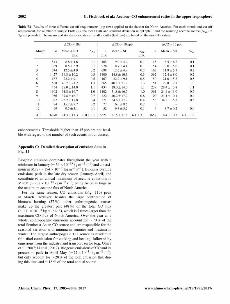
2002 G. Fischbeck et al.: Acetone–CO enhancement ratios in the upper troposphere
Table B1. Results of three different cut-off requirements (top row) applied to the dataset for North America. For each month and cut-offrequirement, the number of unique EnRs (n), the mean EnR and standard deviation in ppt ppb−1 and the resulting acetone source (SAc) inTg are provided. The means and standard deviations for all months (last row) are based on the monthly values.
1CO> 10σ 1CO> 10 ppb 1CO> 15 ppb
Month n Mean+SD SAc n Mean+SD SAc n Mean+SD SAcEnR EnR EnR
1 543 8.8± 4.6 0.1 465 9.0± 4.9 0.1 115 6.5± 6.2 0.12 339 8.5± 3.9 0.1 278 8.7± 4.1 0.1 154 9.0± 5.0 0.13 744 12.5± 4.9 0.2 688 12.6± 4.9 0.2 163 11.8± 5.3 0.24 1427 14.8± 10.2 0.3 1400 14.8± 10.3 0.3 362 12.4± 8.0 0.25 167 22.2± 9.1 0.5 167 22.2± 9.1 0.5 50 21.0± 5.8 0.56 568 40.2± 21.2 1.3 565 40.1± 21.2 1.3 51 29.8± 2.7 1.07 434 28.0± 14.0 1.1 434 28.0± 14.0 1.1 239 28.4± 13.8 1.18 1102 31.8± 16.7 1.0 1102 31.8± 16.7 1.0 361 24.9± 11.0 0.79 956 37.8± 16.7 0.7 722 40.2± 17.2 0.8 100 21.1± 10.1 0.410 397 25.2± 17.8 0.4 371 24.8± 17.9 0.4 53 34.2± 15.3 0.511 94 15.7± 7.7 0.2 77 16.0± 8.6 0.2 0 –12 99 9.5± 3.1 0.1 52 9.3± 3.2 0.1 4 3.7± 0.2 0.0
All 6870 21.3± 11.3 6.0± 3.1 6321 21.5± 11.6 6.1± 3.1 1652 18.4± 10.3 4.8± 1.9
enhancements. Thresholds higher than 15 ppb are not feasi-ble with regard to the number of such events in our dataset.
Appendix C: Detailed description of emission data inFig. 11
Biogenic emission dominates throughout the year with aminimum in January (∼ 64× 10−13 kg m−2 s−1) and a maxi-mum in May (∼ 154× 10−13 kg m−2 s−1). Biomass burningemissions peak in the late dry season (January–April) andcontribute to an annual maximum of acetone emissions inMarch (∼ 208× 10−13 kg m−2 s−1) being twice as large asthe maximum acetone flux of North America.
For the same reason, CO emissions (Fig. 11b) peakin March. However, besides the large contribution ofbiomass burning (37 %), other anthropogenic sourcesmake up the greatest part (48 %) of the total CO flux(∼ 131× 10−11 kg m−2 s−1), which is 7 times larger than themaximum CO flux of North America. Over the year as awhole, anthropogenic emissions account for ∼ 70 % of thetotal Southeast Asian CO source and are responsible for theseasonal variation with minima in summer and maxima inwinter. The largest anthropogenic CO source is residential(bio-)fuel combustion for cooking and heating, followed byemissions from the industry and transport sector (e.g. Oharaet al., 2007; Li et al., 2017). Biogenic emissions of CO and itsprecursors peak in April–May (∼ 22× 10−11 kg m−2 s−1),but only account for ∼ 28 % of the total emission flux dur-ing this time and ∼ 18 % of the total annual source.
Atmos. Chem. Phys., 17, 1985–2008, 2017 www.atmos-chem-phys.net/17/1985/2017/
G. Fischbeck et al.: Acetone–CO enhancement ratios in the upper troposphere 2003
The Supplement related to this article is available onlineat doi:10.5194/acp-17-1985-2017-supplement.
Acknowledgements. The authors wish to thank Lufthansa,Lufthansa Technik and all CARIBIC partners for their ongoingsupport of the IAGOS–CARIBIC laboratory. We especiallyacknowledge D. Scharffe for supplying the CO data and A. Rauthe-Schöch for supplying the merge files. We thank T. Gehrlein,S. Heger, C. Koeppel, A. Petrelli, D. Scharffe and S. Weber fortheir commitment in operating the CARIBIC container. We ac-knowledge the NCAR Atmospheric Chemistry Division (ACD) forproviding the TUV Radiation Model. We thank the Centre Na-tional d’Etudes Spatiales (CNES) and the Centre National de laRecherche Scientifique (CNRS) – Institut National des Sciencesde l’Univers (INSU) for distributing the emission inventory data inthe ECCAD database. ECCAD is part of the ESPRI Data centre(formerly Ether) and the emission database of the GEIA (GlobalEmissions InitiAtive) project, which are gratefully acknowledged.
The article processing charges for this open-accesspublication were covered by a ResearchCentre of the Helmholtz Association.
Edited by: A. PozzerReviewed by: two anonymous referees
References
Akagi, S. K., Yokelson, R. J., Wiedinmyer, C., Alvarado, M. J.,Reid, J. S., Karl, T., Crounse, J. D., and Wennberg, P. O.: Emis-sion factors for open and domestic biomass burning for usein atmospheric models, Atmos. Chem. Phys., 11, 4039–4072,doi:10.5194/acp-11-4039-2011, 2011.
Akagi, S. K., Craven, J. S., Taylor, J. W., McMeeking, G. R., Yokel-son, R. J., Burling, I. R., Urbanski, S. P., Wold, C. E., Seinfeld,J. H., Coe, H., Alvarado, M. J., and Weise, D. R.: Evolution oftrace gases and particles emitted by a chaparral fire in California,Atmos. Chem. Phys., 12, 1397–1421, doi:10.5194/acp-12-1397-2012, 2012.
Andreae, M. O. and Merlet, P.: Emissions of trace gases andaerosols from biomass burning, Global Biogeochem. Cy., 15,955–966, doi:10.1029/2000GB001382, 2001.
Arnold, S. R., Chipperfield, M. P., and Blitz, M. A.: A three-dimensional model study of the effect of new temperature-dependent quantum yields for acetone photolysis, J. Geophys.Res., 110, D22305, doi:10.1029/2005JD005998, 2005.
Arnold, S. R., Methven, J., Evans, M. J., Chipperfield, M. P., Lewis,A. C., Hopkins, J. R., McQuaid, J. B., Watson, N., Purvis, R.M., Lee, J. D., Atlas, E. L., Blake, D. R., and Rappenglück,B.: Statistical inference of OH concentrations and air mass di-lution rates from successive observations of nonmethane hydro-carbons in single air masses, J. Geophys. Res., 112, D10S40,doi:10.1029/2006JD007594, 2007.
Atkinson, R., Baulch, D. L., Cox, R. A., Crowley, J. N., Hamp-son, R. F., Hynes, R. G., Jenkin, M. E., Rossi, M. J., and Troe, J.:
Evaluated kinetic and photochemical data for atmospheric chem-istry: Volume I – gas phase reactions of Ox , HOx , NOx and SOxspecies, Atmos. Chem. Phys., 4, 1461-1738, doi:10.5194/acp-4-1461-2004, 2004.
Atkinson, R., Baulch, D. L., Cox, R. A., Crowley, J. N., Hamp-son, R. F., Hynes, R. G., Jenkin, M. E., Rossi, M. J., and Troe, J.:Evaluated kinetic and photochemical data for atmospheric chem-istry: Volume II – gas phase reactions of organic species, At-mos. Chem. Phys., 6, 3625–4055, doi:10.5194/acp-6-3625-2006,2006.
Baker, A. K., Traud, S., Brenninkmeijer, C. A. M., Hoor, P.,Neumaier, M., Oram, D. E., Rauthe-Schöch, A., Sprung, D.,Schloegl, S., Slemr, F., van Velthoven, P. F. J., Wernli, H., Zahn,A., and Ziereis, H.: Pollution patterns in the upper troposphereover Europe and Asia observed by CARIBIC, Atmos. Environ.,96, 245–256, doi:10.1016/j.atmosenv.2014.06.010, 2014.
Blitz, M. A., Heard, D. E., Pilling, M. J., Arnold, S. R., and Chipper-field, M. P.: Pressure and temperature-dependent quantum yieldsfor the photodissociation of acetone between 279 and 327.5 nm,Geophys. Res. Lett., 31, L06111, doi:10.1029/2003GL018793,2004.
Brenninkmeijer, C. A. M., Crutzen, P., Boumard, F., Dauer, T., Dix,B., Ebinghaus, R., Filippi, D., Fischer, H., Franke, H., Frieβ, U.,Heintzenberg, J., Helleis, F., Hermann, M., Kock, H. H., Koep-pel, C., Lelieveld, J., Leuenberger, M., Martinsson, B. G., Miem-czyk, S., Moret, H. P., Nguyen, H. N., Nyfeler, P., Oram, D.,O’Sullivan, D., Penkett, S., Platt, U., Pupek, M., Ramonet, M.,Randa, B., Reichelt, M., Rhee, T. S., Rohwer, J., Rosenfeld, K.,Scharffe, D., Schlager, H., Schumann, U., Slemr, F., Sprung, D.,Stock, P., Thaler, R., Valentino, F., van Velthoven, P., Waibel, A.,Wandel, A., Waschitschek, K., Wiedensohler, A., Xueref-Remy,I., Zahn, A., Zech, U., and Ziereis, H.: Civil Aircraft for the reg-ular investigation of the atmosphere based on an instrumentedcontainer: The new CARIBIC system, Atmos. Chem. Phys., 7,4953–4976, doi:10.5194/acp-7-4953-2007, 2007.
Brioude, J., Kim, S.-W., Angevine, W. M., Frost, G. J., Lee, S.-H., McKeen, S. A., Trainer, M., Fehsenfeld, F. C., Holloway,J. S., Ryerson, T. B., Williams, E. J., Petron, G., and Fast, J.D.: Top-down estimate of anthropogenic emission inventoriesand their interannual variability in Houston using a mesoscaleinverse modeling technique, J. Geophys. Res., 116, D20305,doi:10.1029/2011JD016215, 2011.
Brioude, J., Angevine, W. M., Ahmadov, R., Kim, S.-W., Evan, S.,McKeen, S. A., Hsie, E.-Y., Frost, G. J., Neuman, J. A., Pol-lack, I. B., Peischl, J., Ryerson, T. B., Holloway, J., Brown, S. S.,Nowak, J. B., Roberts, J. M., Wofsy, S. C., Santoni, G. W., Oda,T., and Trainer, M.: Top-down estimate of surface flux in the LosAngeles Basin using a mesoscale inverse modeling technique: as-sessing anthropogenic emissions of CO, NOx and CO2 and theirimpacts, Atmos. Chem. Phys., 13, 3661–3677, doi:10.5194/acp-13-3661-2013, 2013.
Brito, J.: A Lightweight High-sensitivity Chemical Mass Spectrom-eter for Organic Compounds, Ph.D. thesis, Karlsruhe Institute forTechnology (KIT), 2012.
Brito, J., Wurm, F., Yáñez-Serrano, A. M., de Assunção, J. V.,Godoy, J. M., and Artaxo, P.: Vehicular Emission Ratios of VOCsin a Megacity Impacted by Extensive Ethanol Use: Results ofAmbient Measurements in São Paulo, Brazil, Environ. Sci. Tech-nol., 49, 11381–11387, doi:10.1021/acs.est.5b03281, 2015.
www.atmos-chem-phys.net/17/1985/2017/ Atmos. Chem. Phys., 17, 1985–2008, 2017
2004 G. Fischbeck et al.: Acetone–CO enhancement ratios in the upper troposphere
Calvert, J., Derwent, R., Orlando, J., Tyndall, G., and Walling-ton, T.: Mechanisms of Atmospheric Oxidation of the Alkanes,Angew. Chemie Int., 48, 24–27, doi:10.1002/anie.200901202,2009.
Cantrell, C. A.: Technical Note: Review of methods for linear least-squares fitting of data and application to atmospheric chemistryproblems, Atmos. Chem. Phys., 8, 5477–5487, doi:10.5194/acp-8-5477-2008, 2008.
Coheur, P.-F., Herbin, H., Clerbaux, C., Hurtmans, D., Wespes, C.,Carleer, M., Turquety, S., Rinsland, C. P., Remedios, J., Hauglus-taine, D., Boone, C. D., and Bernath, P. F.: ACE-FTS observationof a young biomass burning plume: first reported measurementsof C2H4, C3H6O, H2CO and PAN by infrared occultation fromspace, Atmos. Chem. Phys., 7, 5437–5446, doi:10.5194/acp-7-5437-2007, 2007.
de Gouw, J. A. and Warneke, C.: Measurements of volatile organiccompounds in the earth’s atmosphere using proton-transfer-reaction mass spectrometry, Mass Spectrom. Rev., 26, 223–257,doi:10.1002/mas.20119, 2007.
de Gouw, J. A., Warneke, C., Scheeren, H. A., van der Veen, C.,Bolder, M., Scheele, M. P., Williams, J., Wong, S., Lange, L.,Fischer, H., and Lelieveld, J.: Overview of the trace gas mea-surements on board the Citation aircraft during the intensive fieldphase of INDOEX, J. Geophys. Res. Atmos., 106, 28453–28467,doi:10.1029/2000JD900810, 2001.
de Gouw, J. A., Goldan, P. D., Warneke, C., Kuster, W. C., Roberts,J. M., Marchewka, M., Bertman, S. B., Pszenny, A. A. P., andKeene, W. C.: Validation of proton transfer reaction-mass spec-trometry (PTR-MS) measurements of gas-phase organic com-pounds in the atmosphere during the New England Air QualityStudy (NEAQS) in 2002, J. Geophys. Res. Atmos., 108, 4682,doi:10.1029/2003JD003863, 2003.
de Laat, A. T. J., de Gouw, J. A., Lelieveld, J., and Hansel, A.:Model analysis of trace gas measurements and pollution impactduring INDOEX, J. Geophys. Res. Atmos., 106, 28469–28480,doi:10.1029/2000JD900821, 2001.
de Reus, M., Fischer, H., Arnold, F., de Gouw, J. A., Holzinger, R.,Warneke, C., and Williams, J.: On the relationship between ace-tone and carbon monoxide in different air masses, Atmos. Chem.Phys., 3, 1709–1723, doi:10.5194/acp-3-1709-2003, 2003.
Diehl, T., Heil, A., Chin, M., Pan, X., Streets, D., Schultz, M.,and Kinne, S.: Anthropogenic, biomass burning, and volcanicemissions of black carbon, organic carbon, and SO2 from 1980to 2010 for hindcast model experiments, Atmos. Chem. Phys.Discuss., 12, 24895–24954, doi:10.5194/acpd-12-24895-2012,2012.
Dixon, J. L., Beale, R., and Nightingale, P. D.: Production ofmethanol, acetaldehyde, and acetone in the Atlantic Ocean, Geo-phys. Res. Lett., 40, 4700–4705, doi:10.1002/grl.50922, 2013.
Dufour, G., Szopa, S., Harrison, J. J., Boone, C. D., andBernath, P. F.: Seasonal variations of acetone in the uppertroposphere–lower stratosphere of the northern midlatitudesas observed by ACE-FTS, J. Mol. Spectrosc., 323, 67–77,doi:10.1016/j.jms.2016.02.006, 2016.
Duncan, B. N., Logan, J. A., Bey, I., Megretskaia, I. A., Yan-tosca, R. M., Novelli, P. C., Jones, N. B., and Rinsland, C. P.:Global budget of CO, 1988–1997: Source estimates and valida-tion with a global model, J. Geophys. Res. Atmos., 112, D22301,doi:10.1029/2007JD008459, 2007.
Elias, T., Szopa, S., Zahn, A., Schuck, T., Brenninkmeijer, C.,Sprung, D., and Slemr, F.: Acetone variability in the upper tro-posphere: analysis of CARIBIC observations and LMDz-INCAchemistry-climate model simulations, Atmos. Chem. Phys., 11,8053–8074, doi:10.5194/acp-11-8053-2011, 2011.
Everitt, B. S. and Hand, D. J.: Mixtures of normal distributions, inFinite Mixture Distributions, Springer Netherlands, Dordrecht,25–57, 1981.
Fischer, E. V., Jacob, D. J., Millet, D. B., Yantosca, R. M.,and Mao, J.: The role of the ocean in the global atmo-spheric budget of acetone, Geophys. Res. Lett., 39, L01807,doi:10.1029/2011GL050086, 2012.
Fischer, E. V., Jacob, D. J., Yantosca, R. M., Sulprizio, M. P., Mil-let, D. B., Mao, J., Paulot, F., Singh, H. B., Roiger, A., Ries, L.,Talbot, R. W., Dzepina, K., and Pandey Deolal, S.: Atmosphericperoxyacetyl nitrate (PAN): a global budget and source attribu-tion, Atmos. Chem. Phys., 14, 2679–2698, doi:10.5194/acp-14-2679-2014, 2014.
Folkins, I. and Chatfield, R.: Impact of acetone on ozone productionand OH in the upper troposphere at high NOx , J. Geophys. Res.Atmos., 105, 11585–11599, doi:10.1029/2000JD900067, 2000.
Granier, C., Bessagnet, B., Bond, T., D’Angiola, A., van der Gon,H., Frost, G. J., Heil, A., Kaiser, J. W., Kinne, S., Klimont, Z.,Kloster, S., Lamarque, J.-F., Liousse, C., Masui, T., Meleux,F., Mieville, A., Ohara, T., Raut, J.-C., Riahi, K., Schultz, M.G., Smith, S. J., Thompson, A., Aardenne, J., Werf, G. R., andVuuren, D. P.: Evolution of anthropogenic and biomass burn-ing emissions of air pollutants at global and regional scalesduring the 1980–2010 period, Clim. Change, 109, 163–190,doi:10.1007/s10584-011-0154-1, 2011.
Granier, C., Boulanger, D., D’Angiola, A., Darras, S., Liousse,C., Marlière, J.-F., Miéville, A., Paulin, M., Pignot, V., and Ze-mankova, K.: Access to Emissions Distributions and Related An-cillary Data through the ECCAD database, EGU General Assem-bly Conference Abstracts, vol. 15, p. 10593, 2013.
Greenberg, J. P., Friedli, H., Guenther, A. B., Hanson, D., Harley,P., and Karl, T.: Volatile organic emissions from the distilla-tion and pyrolysis of vegetation, Atmos. Chem. Phys., 6, 81–91,doi:10.5194/acp-6-81-2006, 2006.
Guenther, A. B., Jiang, X., Heald, C. L., Sakulyanontvittaya, T.,Duhl, T., Emmons, L. K., and Wang, X.: The Model of Emissionsof Gases and Aerosols from Nature version 2.1 (MEGAN2.1): anextended and updated framework for modeling biogenic emis-sions, Geosci. Model Dev., 5, 1471–1492, doi:10.5194/gmd-5-1471-2012, 2012.
Hansel, A. and Wisthaler, A.: A method for real-time detection ofPAN, PPN and MPAN in ambient air, Geophys. Res. Lett., 27,895–898, doi:10.1029/1999GL010989, 2000.
Harley, P., Fridd-Stroud, V., Greenberg, J., Guenther, A., andVasconcellos, P.: Emission of 2-methyl-3-buten-2-ol by pines:A potentially large natural source of reactive carbon to theatmosphere, J. Geophys. Res. Atmos., 103, 25479–25486,doi:10.1029/98JD00820, 1998.
Harrison, J. J., Humpage, N., Allen, N. D. C., Waterfall, A. M.,Bernath, P. F., and Remedios, J. J.: Mid-infrared absorption crosssections for acetone (propanone), J. Quant. Spectrosc. Radiat.Transf., 112, 457–464, doi:10.1016/j.jqsrt.2010.09.002, 2011.
Atmos. Chem. Phys., 17, 1985–2008, 2017 www.atmos-chem-phys.net/17/1985/2017/
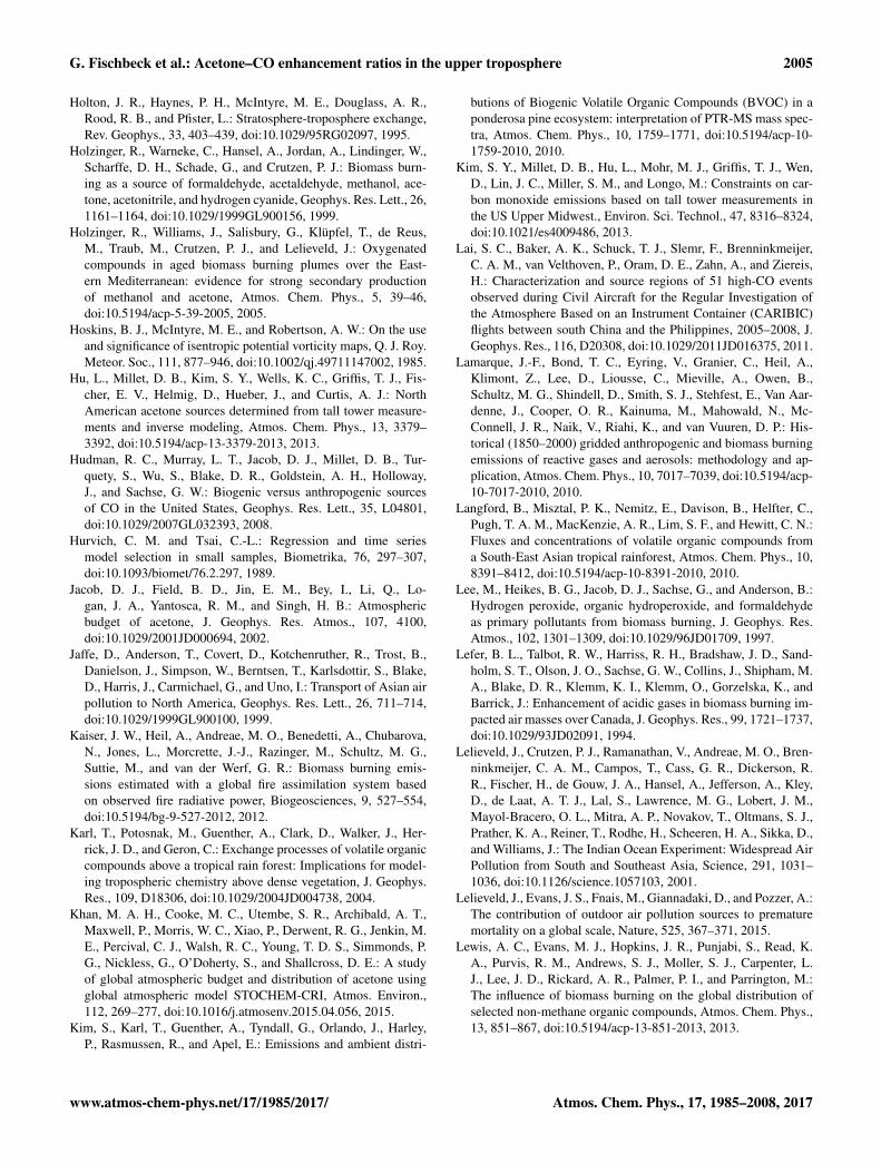
G. Fischbeck et al.: Acetone–CO enhancement ratios in the upper troposphere 2005
Holton, J. R., Haynes, P. H., McIntyre, M. E., Douglass, A. R.,Rood, R. B., and Pfister, L.: Stratosphere-troposphere exchange,Rev. Geophys., 33, 403–439, doi:10.1029/95RG02097, 1995.
Holzinger, R., Warneke, C., Hansel, A., Jordan, A., Lindinger, W.,Scharffe, D. H., Schade, G., and Crutzen, P. J.: Biomass burn-ing as a source of formaldehyde, acetaldehyde, methanol, ace-tone, acetonitrile, and hydrogen cyanide, Geophys. Res. Lett., 26,1161–1164, doi:10.1029/1999GL900156, 1999.
Holzinger, R., Williams, J., Salisbury, G., Klüpfel, T., de Reus,M., Traub, M., Crutzen, P. J., and Lelieveld, J.: Oxygenatedcompounds in aged biomass burning plumes over the East-ern Mediterranean: evidence for strong secondary productionof methanol and acetone, Atmos. Chem. Phys., 5, 39–46,doi:10.5194/acp-5-39-2005, 2005.
Hoskins, B. J., McIntyre, M. E., and Robertson, A. W.: On the useand significance of isentropic potential vorticity maps, Q. J. Roy.Meteor. Soc., 111, 877–946, doi:10.1002/qj.49711147002, 1985.
Hu, L., Millet, D. B., Kim, S. Y., Wells, K. C., Griffis, T. J., Fis-cher, E. V., Helmig, D., Hueber, J., and Curtis, A. J.: NorthAmerican acetone sources determined from tall tower measure-ments and inverse modeling, Atmos. Chem. Phys., 13, 3379–3392, doi:10.5194/acp-13-3379-2013, 2013.
Hudman, R. C., Murray, L. T., Jacob, D. J., Millet, D. B., Tur-quety, S., Wu, S., Blake, D. R., Goldstein, A. H., Holloway,J., and Sachse, G. W.: Biogenic versus anthropogenic sourcesof CO in the United States, Geophys. Res. Lett., 35, L04801,doi:10.1029/2007GL032393, 2008.
Hurvich, C. M. and Tsai, C.-L.: Regression and time seriesmodel selection in small samples, Biometrika, 76, 297–307,doi:10.1093/biomet/76.2.297, 1989.
Jacob, D. J., Field, B. D., Jin, E. M., Bey, I., Li, Q., Lo-gan, J. A., Yantosca, R. M., and Singh, H. B.: Atmosphericbudget of acetone, J. Geophys. Res. Atmos., 107, 4100,doi:10.1029/2001JD000694, 2002.
Jaffe, D., Anderson, T., Covert, D., Kotchenruther, R., Trost, B.,Danielson, J., Simpson, W., Berntsen, T., Karlsdottir, S., Blake,D., Harris, J., Carmichael, G., and Uno, I.: Transport of Asian airpollution to North America, Geophys. Res. Lett., 26, 711–714,doi:10.1029/1999GL900100, 1999.
Kaiser, J. W., Heil, A., Andreae, M. O., Benedetti, A., Chubarova,N., Jones, L., Morcrette, J.-J., Razinger, M., Schultz, M. G.,Suttie, M., and van der Werf, G. R.: Biomass burning emis-sions estimated with a global fire assimilation system basedon observed fire radiative power, Biogeosciences, 9, 527–554,doi:10.5194/bg-9-527-2012, 2012.
Karl, T., Potosnak, M., Guenther, A., Clark, D., Walker, J., Her-rick, J. D., and Geron, C.: Exchange processes of volatile organiccompounds above a tropical rain forest: Implications for model-ing tropospheric chemistry above dense vegetation, J. Geophys.Res., 109, D18306, doi:10.1029/2004JD004738, 2004.
Khan, M. A. H., Cooke, M. C., Utembe, S. R., Archibald, A. T.,Maxwell, P., Morris, W. C., Xiao, P., Derwent, R. G., Jenkin, M.E., Percival, C. J., Walsh, R. C., Young, T. D. S., Simmonds, P.G., Nickless, G., O’Doherty, S., and Shallcross, D. E.: A studyof global atmospheric budget and distribution of acetone usingglobal atmospheric model STOCHEM-CRI, Atmos. Environ.,112, 269–277, doi:10.1016/j.atmosenv.2015.04.056, 2015.
Kim, S., Karl, T., Guenther, A., Tyndall, G., Orlando, J., Harley,P., Rasmussen, R., and Apel, E.: Emissions and ambient distri-
butions of Biogenic Volatile Organic Compounds (BVOC) in aponderosa pine ecosystem: interpretation of PTR-MS mass spec-tra, Atmos. Chem. Phys., 10, 1759–1771, doi:10.5194/acp-10-1759-2010, 2010.
Kim, S. Y., Millet, D. B., Hu, L., Mohr, M. J., Griffis, T. J., Wen,D., Lin, J. C., Miller, S. M., and Longo, M.: Constraints on car-bon monoxide emissions based on tall tower measurements inthe US Upper Midwest., Environ. Sci. Technol., 47, 8316–8324,doi:10.1021/es4009486, 2013.
Lai, S. C., Baker, A. K., Schuck, T. J., Slemr, F., Brenninkmeijer,C. A. M., van Velthoven, P., Oram, D. E., Zahn, A., and Ziereis,H.: Characterization and source regions of 51 high-CO eventsobserved during Civil Aircraft for the Regular Investigation ofthe Atmosphere Based on an Instrument Container (CARIBIC)flights between south China and the Philippines, 2005–2008, J.Geophys. Res., 116, D20308, doi:10.1029/2011JD016375, 2011.
Lamarque, J.-F., Bond, T. C., Eyring, V., Granier, C., Heil, A.,Klimont, Z., Lee, D., Liousse, C., Mieville, A., Owen, B.,Schultz, M. G., Shindell, D., Smith, S. J., Stehfest, E., Van Aar-denne, J., Cooper, O. R., Kainuma, M., Mahowald, N., Mc-Connell, J. R., Naik, V., Riahi, K., and van Vuuren, D. P.: His-torical (1850–2000) gridded anthropogenic and biomass burningemissions of reactive gases and aerosols: methodology and ap-plication, Atmos. Chem. Phys., 10, 7017–7039, doi:10.5194/acp-10-7017-2010, 2010.
Langford, B., Misztal, P. K., Nemitz, E., Davison, B., Helfter, C.,Pugh, T. A. M., MacKenzie, A. R., Lim, S. F., and Hewitt, C. N.:Fluxes and concentrations of volatile organic compounds froma South-East Asian tropical rainforest, Atmos. Chem. Phys., 10,8391–8412, doi:10.5194/acp-10-8391-2010, 2010.
Lee, M., Heikes, B. G., Jacob, D. J., Sachse, G., and Anderson, B.:Hydrogen peroxide, organic hydroperoxide, and formaldehydeas primary pollutants from biomass burning, J. Geophys. Res.Atmos., 102, 1301–1309, doi:10.1029/96JD01709, 1997.
Lefer, B. L., Talbot, R. W., Harriss, R. H., Bradshaw, J. D., Sand-holm, S. T., Olson, J. O., Sachse, G. W., Collins, J., Shipham, M.A., Blake, D. R., Klemm, K. I., Klemm, O., Gorzelska, K., andBarrick, J.: Enhancement of acidic gases in biomass burning im-pacted air masses over Canada, J. Geophys. Res., 99, 1721–1737,doi:10.1029/93JD02091, 1994.
Lelieveld, J., Crutzen, P. J., Ramanathan, V., Andreae, M. O., Bren-ninkmeijer, C. A. M., Campos, T., Cass, G. R., Dickerson, R.R., Fischer, H., de Gouw, J. A., Hansel, A., Jefferson, A., Kley,D., de Laat, A. T. J., Lal, S., Lawrence, M. G., Lobert, J. M.,Mayol-Bracero, O. L., Mitra, A. P., Novakov, T., Oltmans, S. J.,Prather, K. A., Reiner, T., Rodhe, H., Scheeren, H. A., Sikka, D.,and Williams, J.: The Indian Ocean Experiment: Widespread AirPollution from South and Southeast Asia, Science, 291, 1031–1036, doi:10.1126/science.1057103, 2001.
Lelieveld, J., Evans, J. S., Fnais, M., Giannadaki, D., and Pozzer, A.:The contribution of outdoor air pollution sources to prematuremortality on a global scale, Nature, 525, 367–371, 2015.
Lewis, A. C., Evans, M. J., Hopkins, J. R., Punjabi, S., Read, K.A., Purvis, R. M., Andrews, S. J., Moller, S. J., Carpenter, L.J., Lee, J. D., Rickard, A. R., Palmer, P. I., and Parrington, M.:The influence of biomass burning on the global distribution ofselected non-methane organic compounds, Atmos. Chem. Phys.,13, 851–867, doi:10.5194/acp-13-851-2013, 2013.
www.atmos-chem-phys.net/17/1985/2017/ Atmos. Chem. Phys., 17, 1985–2008, 2017
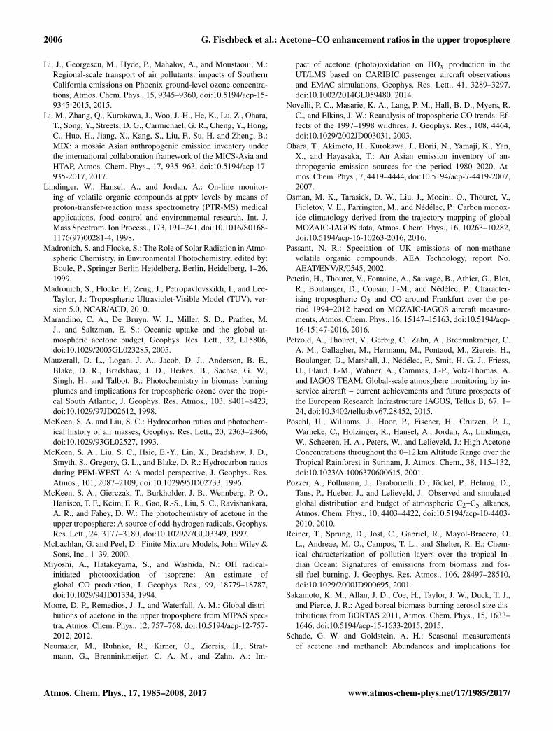
2006 G. Fischbeck et al.: Acetone–CO enhancement ratios in the upper troposphere
Li, J., Georgescu, M., Hyde, P., Mahalov, A., and Moustaoui, M.:Regional-scale transport of air pollutants: impacts of SouthernCalifornia emissions on Phoenix ground-level ozone concentra-tions, Atmos. Chem. Phys., 15, 9345–9360, doi:10.5194/acp-15-9345-2015, 2015.
Li, M., Zhang, Q., Kurokawa, J., Woo, J.-H., He, K., Lu, Z., Ohara,T., Song, Y., Streets, D. G., Carmichael, G. R., Cheng, Y., Hong,C., Huo, H., Jiang, X., Kang, S., Liu, F., Su, H. and Zheng, B.:MIX: a mosaic Asian anthropogenic emission inventory underthe international collaboration framework of the MICS-Asia andHTAP, Atmos. Chem. Phys., 17, 935–963, doi:10.5194/acp-17-935-2017, 2017.
Lindinger, W., Hansel, A., and Jordan, A.: On-line monitor-ing of volatile organic compounds at pptv levels by means ofproton-transfer-reaction mass spectrometry (PTR-MS) medicalapplications, food control and environmental research, Int. J.Mass Spectrom. Ion Process., 173, 191–241, doi:10.1016/S0168-1176(97)00281-4, 1998.
Madronich, S. and Flocke, S.: The Role of Solar Radiation in Atmo-spheric Chemistry, in Environmental Photochemistry, edited by:Boule, P., Springer Berlin Heidelberg, Berlin, Heidelberg, 1–26,1999.
Madronich, S., Flocke, F., Zeng, J., Petropavlovskikh, I., and Lee-Taylor, J.: Tropospheric Ultraviolet-Visible Model (TUV), ver-sion 5.0, NCAR/ACD, 2010.
Marandino, C. A., De Bruyn, W. J., Miller, S. D., Prather, M.J., and Saltzman, E. S.: Oceanic uptake and the global at-mospheric acetone budget, Geophys. Res. Lett., 32, L15806,doi:10.1029/2005GL023285, 2005.
Mauzerall, D. L., Logan, J. A., Jacob, D. J., Anderson, B. E.,Blake, D. R., Bradshaw, J. D., Heikes, B., Sachse, G. W.,Singh, H., and Talbot, B.: Photochemistry in biomass burningplumes and implications for tropospheric ozone over the tropi-cal South Atlantic, J. Geophys. Res. Atmos., 103, 8401–8423,doi:10.1029/97JD02612, 1998.
McKeen, S. A. and Liu, S. C.: Hydrocarbon ratios and photochem-ical history of air masses, Geophys. Res. Lett., 20, 2363–2366,doi:10.1029/93GL02527, 1993.
McKeen, S. A., Liu, S. C., Hsie, E.-Y., Lin, X., Bradshaw, J. D.,Smyth, S., Gregory, G. L., and Blake, D. R.: Hydrocarbon ratiosduring PEM-WEST A: A model perspective, J. Geophys. Res.Atmos., 101, 2087–2109, doi:10.1029/95JD02733, 1996.
McKeen, S. A., Gierczak, T., Burkholder, J. B., Wennberg, P. O.,Hanisco, T. F., Keim, E. R., Gao, R.-S., Liu, S. C., Ravishankara,A. R., and Fahey, D. W.: The photochemistry of acetone in theupper troposphere: A source of odd-hydrogen radicals, Geophys.Res. Lett., 24, 3177–3180, doi:10.1029/97GL03349, 1997.
McLachlan, G. and Peel, D.: Finite Mixture Models, John Wiley &Sons, Inc., 1–39, 2000.
Miyoshi, A., Hatakeyama, S., and Washida, N.: OH radical-initiated photooxidation of isoprene: An estimate ofglobal CO production, J. Geophys. Res., 99, 18779–18787,doi:10.1029/94JD01334, 1994.
Moore, D. P., Remedios, J. J., and Waterfall, A. M.: Global distri-butions of acetone in the upper troposphere from MIPAS spec-tra, Atmos. Chem. Phys., 12, 757–768, doi:10.5194/acp-12-757-2012, 2012.
Neumaier, M., Ruhnke, R., Kirner, O., Ziereis, H., Strat-mann, G., Brenninkmeijer, C. A. M., and Zahn, A.: Im-
pact of acetone (photo)oxidation on HOx production in theUT/LMS based on CARIBIC passenger aircraft observationsand EMAC simulations, Geophys. Res. Lett., 41, 3289–3297,doi:10.1002/2014GL059480, 2014.
Novelli, P. C., Masarie, K. A., Lang, P. M., Hall, B. D., Myers, R.C., and Elkins, J. W.: Reanalysis of tropospheric CO trends: Ef-fects of the 1997–1998 wildfires, J. Geophys. Res., 108, 4464,doi:10.1029/2002JD003031, 2003.
Ohara, T., Akimoto, H., Kurokawa, J., Horii, N., Yamaji, K., Yan,X., and Hayasaka, T.: An Asian emission inventory of an-thropogenic emission sources for the period 1980–2020, At-mos. Chem. Phys., 7, 4419–4444, doi:10.5194/acp-7-4419-2007,2007.
Osman, M. K., Tarasick, D. W., Liu, J., Moeini, O., Thouret, V.,Fioletov, V. E., Parrington, M., and Nédélec, P.: Carbon monox-ide climatology derived from the trajectory mapping of globalMOZAIC-IAGOS data, Atmos. Chem. Phys., 16, 10263–10282,doi:10.5194/acp-16-10263-2016, 2016.
Passant, N. R.: Speciation of UK emissions of non-methanevolatile organic compounds, AEA Technology, report No.AEAT/ENV/R/0545, 2002.
Petetin, H., Thouret, V., Fontaine, A., Sauvage, B., Athier, G., Blot,R., Boulanger, D., Cousin, J.-M., and Nédélec, P.: Character-ising tropospheric O3 and CO around Frankfurt over the pe-riod 1994–2012 based on MOZAIC-IAGOS aircraft measure-ments, Atmos. Chem. Phys., 16, 15147–15163, doi:10.5194/acp-16-15147-2016, 2016.
Petzold, A., Thouret, V., Gerbig, C., Zahn, A., Brenninkmeijer, C.A. M., Gallagher, M., Hermann, M., Pontaud, M., Ziereis, H.,Boulanger, D., Marshall, J., Nédélec, P., Smit, H. G. J., Friess,U., Flaud, J.-M., Wahner, A., Cammas, J.-P., Volz-Thomas, A.and IAGOS TEAM: Global-scale atmosphere monitoring by in-service aircraft – current achievements and future prospects ofthe European Research Infrastructure IAGOS, Tellus B, 67, 1–24, doi:10.3402/tellusb.v67.28452, 2015.
Pöschl, U., Williams, J., Hoor, P., Fischer, H., Crutzen, P. J.,Warneke, C., Holzinger, R., Hansel, A., Jordan, A., Lindinger,W., Scheeren, H. A., Peters, W., and Lelieveld, J.: High AcetoneConcentrations throughout the 0–12 km Altitude Range over theTropical Rainforest in Surinam, J. Atmos. Chem., 38, 115–132,doi:10.1023/A:1006370600615, 2001.
Pozzer, A., Pollmann, J., Taraborrelli, D., Jöckel, P., Helmig, D.,Tans, P., Hueber, J., and Lelieveld, J.: Observed and simulatedglobal distribution and budget of atmospheric C2–C5 alkanes,Atmos. Chem. Phys., 10, 4403–4422, doi:10.5194/acp-10-4403-2010, 2010.
Reiner, T., Sprung, D., Jost, C., Gabriel, R., Mayol-Bracero, O.L., Andreae, M. O., Campos, T. L., and Shelter, R. E.: Chem-ical characterization of pollution layers over the tropical In-dian Ocean: Signatures of emissions from biomass and fos-sil fuel burning, J. Geophys. Res. Atmos., 106, 28497–28510,doi:10.1029/2000JD900695, 2001.
Sakamoto, K. M., Allan, J. D., Coe, H., Taylor, J. W., Duck, T. J.,and Pierce, J. R.: Aged boreal biomass-burning aerosol size dis-tributions from BORTAS 2011, Atmos. Chem. Phys., 15, 1633–1646, doi:10.5194/acp-15-1633-2015, 2015.
Schade, G. W. and Goldstein, A. H.: Seasonal measurementsof acetone and methanol: Abundances and implications for
Atmos. Chem. Phys., 17, 1985–2008, 2017 www.atmos-chem-phys.net/17/1985/2017/
G. Fischbeck et al.: Acetone–CO enhancement ratios in the upper troposphere 2007
atmospheric budgets, Global Biogeochem. Cy., 20, GB1011,doi:10.1029/2005GB002566, 2006.
Scharffe, D., Slemr, F., Brenninkmeijer, C. A. M., and Zahn, A.:Carbon monoxide measurements onboard the CARIBIC pas-senger aircraft using UV resonance fluorescence, Atmos. Meas.Tech., 5, 1753–1760, doi:10.5194/amt-5-1753-2012, 2012.
Simpson, I. J., Akagi, S. K., Barletta, B., Blake, N. J., Choi, Y.,Diskin, G. S., Fried, A., Fuelberg, H. E., Meinardi, S., Rowland,F. S., Vay, S. A., Weinheimer, A. J., Wennberg, P. O., Wiebring,P., Wisthaler, A., Yang, M., Yokelson, R. J., and Blake, D. R.:Boreal forest fire emissions in fresh Canadian smoke plumes:C1-C10 volatile organic compounds (VOCs), CO2, CO, NO2,NO, HCN and CH3CN, Atmos. Chem. Phys., 11, 6445–6463,doi:10.5194/acp-11-6445-2011, 2011.
Sindelarova, K., Granier, C., Bouarar, I., Guenther, A., Tilmes, S.,Stavrakou, T., Müller, J.-F., Kuhn, U., Stefani, P., and Knorr, W.:Global data set of biogenic VOC emissions calculated by theMEGAN model over the last 30 years, Atmos. Chem. Phys., 14,9317–9341, doi:10.5194/acp-14-9317-2014, 2014.
Singh, H. B., Salas, L. J., and Viezee, W.: Global distribution of per-oxyacetyl nitrate, Nature, 321, 588–591, doi:10.1038/321588a0,1986.
Singh, H. B., Herlth, D., O’Hara, D., Zahnle, K., Bradshaw, J.D., Sandholm, S. T., Talbot, R., Crutzen, P. J., and Kanaki-dou, M.: Relationship of peroxyacetyl nitrate to active and to-tal odd nitrogen at northern high latitudes: Influence of reservoirspecies on NOx and O3, J. Geophys. Res., 97, 16523–16530,doi:10.1029/91JD00890, 1992.
Singh, H. B., O’Hara, D., Herlth, D., Sachse, W., Blake, D. R., Brad-shaw, J. D., Kanakidou, M., and Crutzen, P. J.: Acetone in theatmosphere: Distribution, sources, and sinks, J. Geophys. Res.,99, 1805–1819, doi:10.1029/93JD00764, 1994.
Singh, H. B., Kanakidou, M., Crutzen, P. J., and Jacob, D. J.: Highconcentrations and photochemical fate of oxygenated hydrocar-bons in the global troposphere, Nature, 378, 50–54, 1995.
Singh, H. B., Salas, Chatfield, Czech, Fried, Walega, Evans, Field,Jacob, Blake, Heikes, Talbot, Sachse, Crawford, Avery, Sand-holm and Fuelberg: Analysis of the atmospheric distribution,sources, and sinks of oxygenated volatile organic chemicalsbased on measurements over the Pacific during TRACE-P, J.Geophys. Res., 109, D15S07, doi:10.1029/2003JD003883, 2004.
Singh, H. B., Anderson, B. E., Brune, W. H., Cai, C., Cohen, R. C.,Crawford, J. H., Cubison, M. J., Czech, E. P., Emmons, L., andFuelberg, H. E.: Pollution influences on atmospheric composi-tion and chemistry at high northern latitudes: Boreal and Cal-ifornia forest fire emissions, Atmos. Environ., 44, 4553–4564,doi:10.1016/j.atmosenv.2010.08.026, 2010.
Spivakovsky, C. M., Logan, J. A., Montzka, S. A., Balkanski, Y. J.,Foreman-Fowler, M., Jones, D. B. A., Horowitz, L. W., Fusco,A. C., Brenninkmeijer, C. A. M., Prather, M. J., Wofsy, S. C.,and McElroy, M. B.: Three-dimensional climatological distribu-tion of tropospheric OH: Update and evaluation, J. Geophys. Res.Atmos., 105, 8931–8980, doi:10.1029/1999JD901006, 2000.
Sprung, D. and Zahn, A.: Acetone in the upper tropo-sphere/lowermost stratosphere measured by the CARIBIC pas-senger aircraft: Distribution, seasonal cycle, and variability, J.Geophys. Res., 115, D16301, doi:10.1029/2009JD012099, 2010.
Stein, O., Schultz, M. G., Bouarar, I., Clark, H., Huijnen, V.,Gaudel, A., George, M., and Clerbaux, C.: On the wintertime
low bias of Northern Hemisphere carbon monoxide found inglobal model simulations, Atmos. Chem. Phys., 14, 9295–9316,doi:10.5194/acp-14-9295-2014, 2014.
Stiller, G. P., von Clarmann, T., Glatthor, N., Höpfner, M., Kell-mann, S., Kimmich, E., Linden, A., Milz, M., Steck, T., andFischer, H.: Retrievability of Upper Tropospheric Species andParameters from MIPAS/ENVISAT Data, edited by: Borrell, P.,Borrell, P. M., Burrows, J. P., and Platt, U., Springer Berlin Hei-delberg, Berlin, Heidelberg, 167–180, 2004.
Stohl, A., James, P., Forster, C., Spichtinger, N., Marenco,A., Thouret, V., and Smit, H. G. J.: An extension ofMeasurement of Ozone and Water Vapour by Airbus In-service Aircraft (MOZAIC) ozone climatologies using trajec-tory statistics, J. Geophys. Res. Atmos., 106, 27757–27768,doi:10.1029/2001JD000749, 2001.
Stohl, A., Eckhardt, S., Forster, C., James, P., Spichtinger, N., andSeibert, P.: A replacement for simple back trajectory calculationsin the interpretation of atmospheric trace substance measure-ments, Atmos. Environ., 36, 4635–4648, doi:10.1016/S1352-2310(02)00416-8, 2002.
Sugiura, N.: Further analysts of the data by akaike’ s informationcriterion and the finite corrections, Commun. Stat.-Theor. M., 7,13–26, doi:10.1080/03610927808827599, 1978.
Tereszchuk, K. A., González Abad, G., Clerbaux, C., Hadji-Lazaro,J., Hurtmans, D., Coheur, P.-F., and Bernath, P. F.: ACE-FTS ob-servations of pyrogenic trace species in boreal biomass burningplumes during BORTAS, Atmos. Chem. Phys., 13, 4529–4541,doi:10.5194/acp-13-4529-2013, 2013.
Thouret, V., Cammas, J.-P., Sauvage, B., Athier, G., Zbinden, R.,Nédélec, P., Simon, P., and Karcher, F.: Tropopause referencedozone climatology and inter-annual variability (1994–2003) fromthe MOZAIC programme, Atmos. Chem. Phys., 6, 1033–1051,doi:10.5194/acp-6-1033-2006, 2006.
Turquety, S., Logan, J. A., Jacob, D. J., Hudman, R. C., Leung, F.Y., Heald, C. L., Yantosca, R. M., Wu, S., Emmons, L. K., Ed-wards, D. P., and Sachse, G. W.: Inventory of boreal fire emis-sions for North America in 2004: Importance of peat burningand pyroconvective injection, J. Geophys. Res., 112, D12S03,doi:10.1029/2006JD007281, 2007.
van der Werf, G. R., Randerson, J. T., Giglio, L., Collatz, G. J.,Kasibhatla, P. S., and Arellano, A. F.: Interannual variabilityin global biomass burning emissions from 1997 to 2004, At-mos. Chem. Phys., 6, 3423–3441, doi:10.5194/acp-6-3423-2006,2006.
van der Werf, G. R., Randerson, J. T., Giglio, L., Collatz, G. J., Mu,M., Kasibhatla, P. S., Morton, D. C., DeFries, R. S., Jin, Y., andvan Leeuwen, T. T.: Global fire emissions and the contribution ofdeforestation, savanna, forest, agricultural, and peat fires (1997–2009), Atmos. Chem. Phys., 10, 11707–11735, doi:10.5194/acp-10-11707-2010, 2010.
van Velthoven, P. F. J.: Meteorological analysis of CARIBICby KNMI, http://projects.knmi.nl/campaign_support/CARIBIC/,last access: 1 September 2016.
Warneke, C., de Gouw, J. A., Kuster, W. C., Goldan, P. D.,and Fall, R.: Validation of Atmospheric VOC Measurementsby Proton-Transfer- Reaction Mass Spectrometry Using a Gas-Chromatographic Preseparation Method, Environ. Sci. Technol.,37, 2494–2501, doi:10.1021/es026266i, 2003.
www.atmos-chem-phys.net/17/1985/2017/ Atmos. Chem. Phys., 17, 1985–2008, 2017
2008 G. Fischbeck et al.: Acetone–CO enhancement ratios in the upper troposphere
Warneke, C., de Gouw, J. A., Stohl, A., Cooper, O. R., Goldan, P.D., Kuster, W. C., Holloway, J. S., Williams, E. J., Lerner, B.M., McKeen, S. A., Trainer, M., Fehsenfeld, F. C., Atlas, E. L.,Donnelly, S. G., Stroud, V., Lueb, A., and Kato, S.: Biomassburning and anthropogenic sources of CO over New Englandin the summer 2004, J. Geophys. Res. Atmos., 111, D23S15,doi:10.1029/2005JD006878, 2006.
Warneke, C., Roberts, J. M., Veres, P., Gilman, J., Kuster, W. C.,Burling, I., Yokelson, R., and de Gouw, J. A.: VOC identifica-tion and inter-comparison from laboratory biomass burning us-ing PTR-MS and PIT-MS, Int. J. Mass Spectrom., 303, 6–14,doi:10.1016/j.ijms.2010.12.002, 2011.
Waterfall, A. M., Remedios, J. J., Allen, G., and Sembhi, H.: In-frared remote sensing of organic compounds in the upper tro-posphere, Proceedings of the ENVISAT Symposium, Salzburg,September, 2004.
Williamson, J. H.: Least-squares fitting of a straight line, Can. J.Phys., 46, 1845–1847, doi:10.1139/p68-523, 1968.
Wisthaler, A., Hansel, A. Dickerson, R. R., and Crutzen, P.: Organictrace gas measurements by PTR-MS during INDOEX 1999, J.Geophys. Res., 107, 8024, doi:10.1029/2001JD000576, 2002.
Yokelson, R. J., Andreae, M. O., and Akagi, S. K.: Pitfalls withthe use of enhancement ratios or normalized excess mixing ra-tios measured in plumes to characterize pollution sources andaging, Atmos. Meas. Tech., 6, 2155–2158, doi:10.5194/amt-6-2155-2013, 2013.
York, D.: Least-Squares fitting of a straight line, Can. J. Phys., 44,1079–1086, doi:10.1139/p66-090, 1966.
York, D., Evensen, N. M., Martínez, M. L., and De Basabe Del-gado, J.: Unified equations for the slope, intercept, and stan-dard errors of the best straight line, Am. J. Phys., 72, 367,doi:10.1119/1.1632486, 2004.
Zahn, A. and Brenninkmeijer, C. A. M.: New Directions: AChemical Tropopause Defined, Atmos. Environ., 37, 439–440,doi:10.1016/S1352-2310(02)00901-9, 2003.
Zahn, A., Brenninkmeijer, C. A. M., Asman, W. A. H., Crutzen,P. J., Heinrich, G., Fischer, H., Cuijpers, J. W. M., and vanVelthoven, P. F. J.: Budgets of O3 and CO in the upper tro-posphere: CARIBIC passenger aircraft results 1997–2001, J.Geophys. Res. Atmos., 107, 4337, doi:10.1029/2001JD001529,2002.
Zahn, A., Brenninkmeijer, C. A. M., and van Velthoven, P. F. J.:Passenger aircraft project CARIBIC 1997–2002, Part I: the ex-tratropical chemical tropopause, Atmos. Chem. Phys. Discuss.,4, 1091–1117, doi:10.5194/acpd-4-1091-2004, 2004.
Zahn, A., Weppner, J., Widmann, H., Schlote-Holubek, K., Burger,B., Kühner, T., and Franke, H.: A fast and precise chemilumi-nescence ozone detector for eddy flux and airborne application,Atmos. Meas. Tech., 5, 363–375, doi:10.5194/amt-5-363-2012,2012.
Zbinden, R. M., Thouret, V., Ricaud, P., Carminati, F., Cammas, J.-P., and Nédélec, P.: Climatology of pure tropospheric profiles andcolumn contents of ozone and carbon monoxide using MOZAICin the mid-northern latitudes (24◦ N to 50◦ N) from 1994 to2009, Atmos. Chem. Phys., 13, 12363–12388, doi:10.5194/acp-13-12363-2013, 2013.
Atmos. Chem. Phys., 17, 1985–2008, 2017 www.atmos-chem-phys.net/17/1985/2017/