ABSTRACT

GHOLIPOUR BARADARI, MEHDI. Studying Pore Structure of Nonwovens with 3D

Imaging and Modeling Permeability. (Under the direction of Dr. Behnam Pourdeyhimi and

Dr. Benoit Maze).

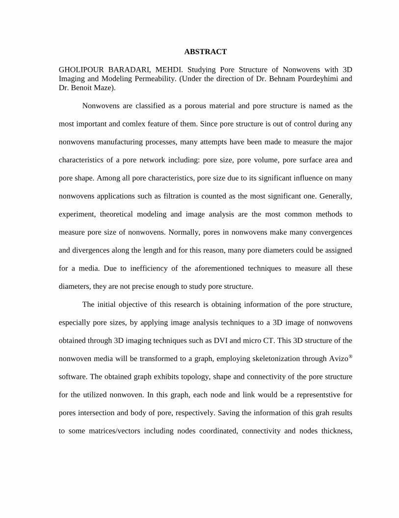
Nonwovens are classified as a porous material and pore structure is named as the

most important and comlex feature of them. Since pore structure is out of control during any

nonwovens manufacturing processes, many attempts have been made to measure the major

characteristics of a pore network including: pore size, pore volume, pore surface area and

pore shape. Among all pore characteristics, pore size due to its significant influence on many

nonwovens applications such as filtration is counted as the most significant one. Generally,

experiment, theoretical modeling and image analysis are the most common methods to

measure pore size of nonwovens. Normally, pores in nonwovens make many convergences

and divergences along the length and for this reason, many pore diameters could be assigned

for a media. Due to inefficiency of the aforementioned techniques to measure all these

diameters, they are not precise enough to study pore structure.

The initial objective of this research is obtaining information of the pore structure,

especially pore sizes, by applying image analysis techniques to a 3D image of nonwovens

obtained through 3D imaging techniques such as DVI and micro CT. This 3D structure of the

nonwoven media will be transformed to a graph, employing skeletonization through Avizo®

software. The obtained graph exhibits topology, shape and connectivity of the pore structure

for the utilized nonwoven. In this graph, each node and link would be a representstive for

pores intersection and body of pore, respectively. Saving the information of this grah results

to some matrices/vectors including nodes coordinated, connectivity and nodes thickness,

which exhibits the pore size. Therefore, all the pore sizes available in the structure will be

extracted through this method.

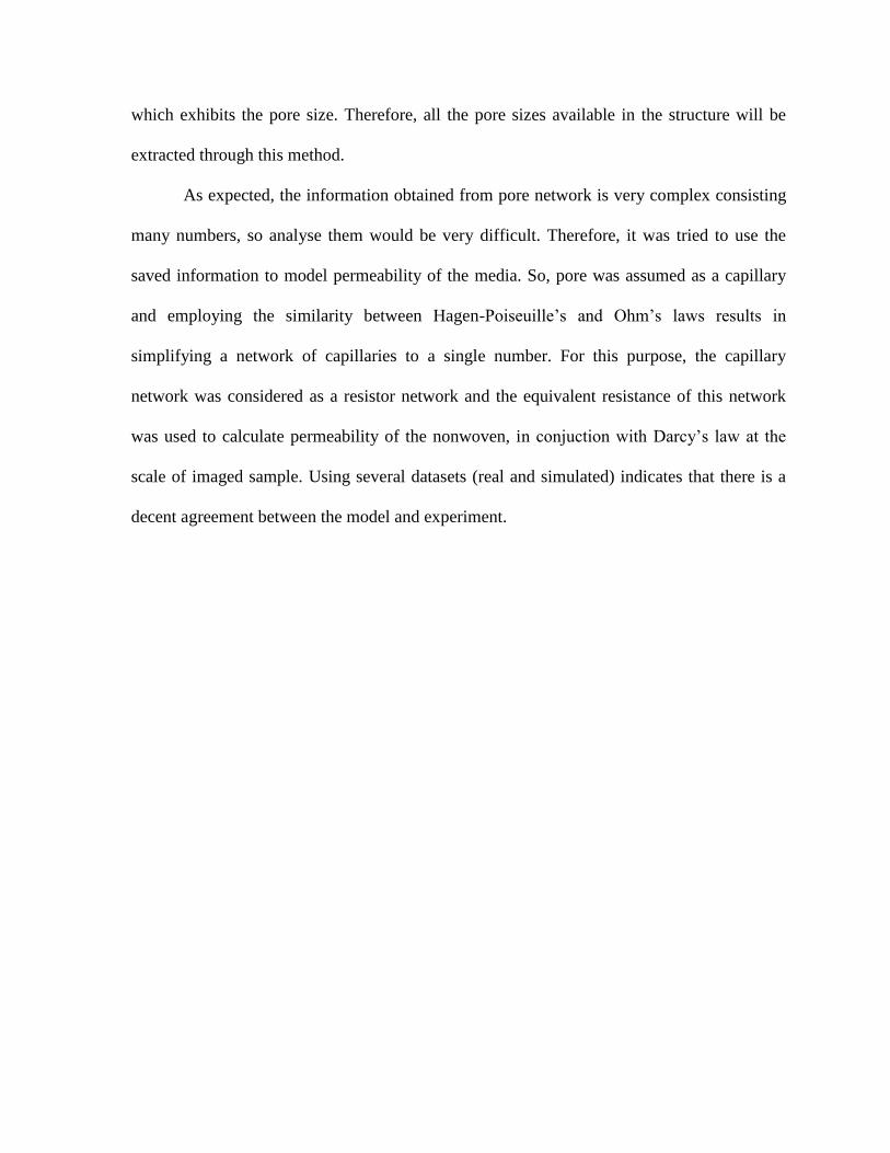
As expected, the information obtained from pore network is very complex consisting

many numbers, so analyse them would be very difficult. Therefore, it was tried to use the

saved information to model permeability of the media. So, pore was assumed as a capillary

and employing the similarity between Hagen-Poiseuille’s and Ohm’s laws results in

simplifying a network of capillaries to a single number. For this purpose, the capillary

network was considered as a resistor network and the equivalent resistance of this network

was used to calculate permeability of the nonwoven, in conjuction with Darcy’s law at the

scale of imaged sample. Using several datasets (real and simulated) indicates that there is a

decent agreement between the model and experiment.

© Copyright 2016 Mehdi Gholipour Baradari

All Rights Reserved

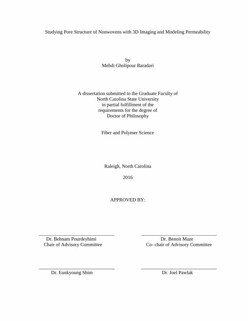
Studying Pore Structure of Nonwovens with 3D Imaging and Modeling Permeability

by

Mehdi Gholipour Baradari

A dissertation submitted to the Graduate Faculty of

North Carolina State University

in partial fulfillment of the

requirements for the degree of

Doctor of Philosophy

Fiber and Polymer Science

Raleigh, North Carolina

2016

APPROVED BY:

_______________________________ _______________________________

Dr. Behnam Pourdeyhimi Dr. Benoit Maze

Chair of Advisory Committee Co- chair of Advisory Committee

_______________________________ _______________________________

Dr. Eunkyoung Shim Dr. Joel Pawlak

ii

DEDICATION

This dissertation is gratefully dedicated to my late parents,

and

my wife, Samaneh, for her constant love, support and motivation.

iii

BIOGRAPHY

Mehdi Gholipour Baradari was born in Babol, Mazandaran, Iran. He completed his bachelor

and master degrees, both in Textile Engineering from Isfahan University of Technology,

Isfahan, Iran in 2005 and 2009, respectively. After finishing his master, he started to work as

a chief engineer for a nonwoven company in conjuction with automotive industry for three

years.

He joined the College of Textile, North Carolina State University in January 2013 to attend

the PhD program in Fiber and Polymer Science. In August 2013, he joined The Nonwovens

Institute as a Graduate Research Assitant to work on pore structure of nonwovens. During his

PhD, he developed a methodology to study pore structure of nonwovens with 3D imaging

and also obtained the graduate certificate in Nonwovens Science and Technology.

iv

ACKNOWLEDGMENTS

Although the PhD is an individual achievement, but it was not possible for me without the

help and inspiration from many amazing people. First and foremost, I have to thank my wife,

Samaneh, for her continuous support, sacrifice and encouregment to pursue my dreams.

I wish to express my deepest gratitude to my advisors, Dr. Pourdeyhimi and Dr. Maze for

their patience, motivation and immense knowledge. This work would not have been done

without their advice. Their guidance helped me a lot in all years of my PhD and made me a

better person in different prespectives.

I also would like to thank the rest of my committee, Dr. Shim and Dr. Pawlak for their

comments and useful suggestions, but also for their tough questions which encouraged me to

think about my research in different aspects.

I would like to thank all the people in The Nonwovens Institute (NWI) who helped me with

this research, especially John Fry, Bradley Scroggins, Amy Minton and Bruce Anderson. I

also need to thank Annette Schenk (MANN+HUMMEL, Raleigh, USA), who contributed in

the simulation part.

Finally, I would like to thank all my groupmates and staffs in the NWI. I had a lot of fun in

this group.

v

TABLE OF CONTENTS

LIST OF TABLES………………………………………………………………………… vii

LIST OF FIGURES ............................................................................................................... ix 1. Introduction ..........................................................................................................................1

1.1 Thesis overview ...............................................................................................................5

2. Literature Review ................................................................................................................6 2.1 Pore definition and characteristics ...................................................................................7 2.2 Parameters affecting pore structure ..................................................................................9

2.3 Pore measurement techniques ........................................................................................11 2.3.1 Pore size and pore size distribution ........................................................................13

2.3.1.1 Bubble point .................................................................................................... 14

2.3.1.2 Extrusion flow porometery (Capillary flow porometry) ................................. 17 2.3.1.3 Extrusion porosimetry ..................................................................................... 21 2.3.1.4 Mercury intrusion porosimetry ....................................................................... 23

2.3.1.5 Non-mercury intrusion porosimetry ............................................................... 24 2.3.1.6 Gas/vapor adsorption (BET) ........................................................................... 24

2.3.1.7 Image analysis technique ................................................................................ 30 2.3.1.8 Other techniques ............................................................................................. 39

2.3.2 Pore volume and pore volume distribution .............................................................41

2.3.3 Pore specific surface area .......................................................................................42 2.4 Theoretical modeling of pore size and pore size distribution ........................................44

2.4.1 Simmonds’s model .................................................................................................44 2.4.2 Abdel-Ghani’s model ..............................................................................................45

2.4.3 Wrotnowski’s model ...............................................................................................46 2.4.4 Goeminne’s model ..................................................................................................47

2.4.5 Giroud’s model .......................................................................................................47 2.4.6 Lifshutz’s model .....................................................................................................48 2.4.7 Faure’s model .........................................................................................................48

2.4.8 Lombard’s model ....................................................................................................50 2.4.9 Rawal’s model ........................................................................................................51

2.5 Permeability ...................................................................................................................53 2.5.1 Empirical techniques to measure permeability of nonwovens ...............................54

2.5.1.1 Determining the flow rate using common pore measurement techniques ...... 54 2.5.2 Theoretical models to predict permeability of nonwovens .....................................55

2.5.2.1 Drag model...................................................................................................... 58 2.5.2.2 Cell model ....................................................................................................... 59

2.5.2.3 Many fibers model .......................................................................................... 61 2.6 Skeletonization (Topological skeleton) .........................................................................62 2.7 Networks and graphs ......................................................................................................65

3. Problem Statement.............................................................................................................68 3.1 Introduction ....................................................................................................................69

vi

3.2 Problem statement ..........................................................................................................70

4. 3D Image Acquisition and Processing ..............................................................................74 4.1 Introduction ....................................................................................................................75 4.2 Digital Volumetric Imaging (DVI) ................................................................................76

4.3 Micro Computed Tomography (micro CT)....................................................................78 4.4 Materials and 2D image acquisition ...............................................................................84

4.4.1 Materials for 2D image acquisition through DVI ...................................................84 4.4.2 Materials for 2D image acquision through micro CT .............................................87

4.4.2.1 Samples with different fiber diameter and constant SVF ............................... 88

4.4.2.2 Samples with constant fiber diameter and different SVF ............................... 90 4.4.2.3 Image pre-processing ...................................................................................... 92

4.5 3D visualization by Avizo® – Standard edition .............................................................96 4.6 Thining process (Skeletonization) through Avizo® .......................................................99

5. Modeling Permeability ....................................................................................................102 5.1 Introduction ..................................................................................................................103

5.2 Analysis of the graph provided by Avizo® ..................................................................103 5.3 Analogy to model permeability ....................................................................................106

5.3.1 Applicability of Hagen-Poiseuille’s equation to model permeability ..................108 5.3.2 Algorithm details to model permeability ..............................................................109

5.3.2.1 Resistance between two connected nodes (pipes resistance) ........................ 112

5.3.2.2 Resistance between two main nodes (capillaries resistance) ........................ 114 5.3.2.3 Calculating the equivalent resistance of the network ................................... 117

5.4 Calculation example .....................................................................................................121 5.5 Algorith outputs for the samples used for micro CT imaging .....................................128 5.6 Calculating the permeability ........................................................................................130

5.7 Analysis the trend of changing permeability for different samples .............................133

5.7.1 Samples with different fiber diameters and same SVFs .......................................133 5.7.2 Samples with same fiber sizes and different SVFs ...............................................134

5.8 Studying pore structure using the dataset obtained through simulation ......................145

6. Experimental Validation .................................................................................................160 6.1 Introduction ..................................................................................................................161

6.2 Measuring permeability through experiment ...............................................................161 6.2.1 Samples with different fiber sizes and same SVFs ...............................................161

6.2.2 Samles with same fiber sizes and different SVFs .................................................165 6.3 Analysis the difference between the results obtained from experiment and model .....172

7. Overall Conclusion and Recommendations for Future Work .....................................176 7.1 Overall conclusion .......................................................................................................177 7.2 Recommendations for future work ..............................................................................179

7.2.1 Using sponbond and meltblown nonwovens as the material ................................179 7.2.2 Using multiple images to model permeability statistically ...................................180

7.2.3 Investigating tortuosity of pores in nonwovens ....................................................180

8. References .........................................................................................................................182

vii

LIST OF TABLES

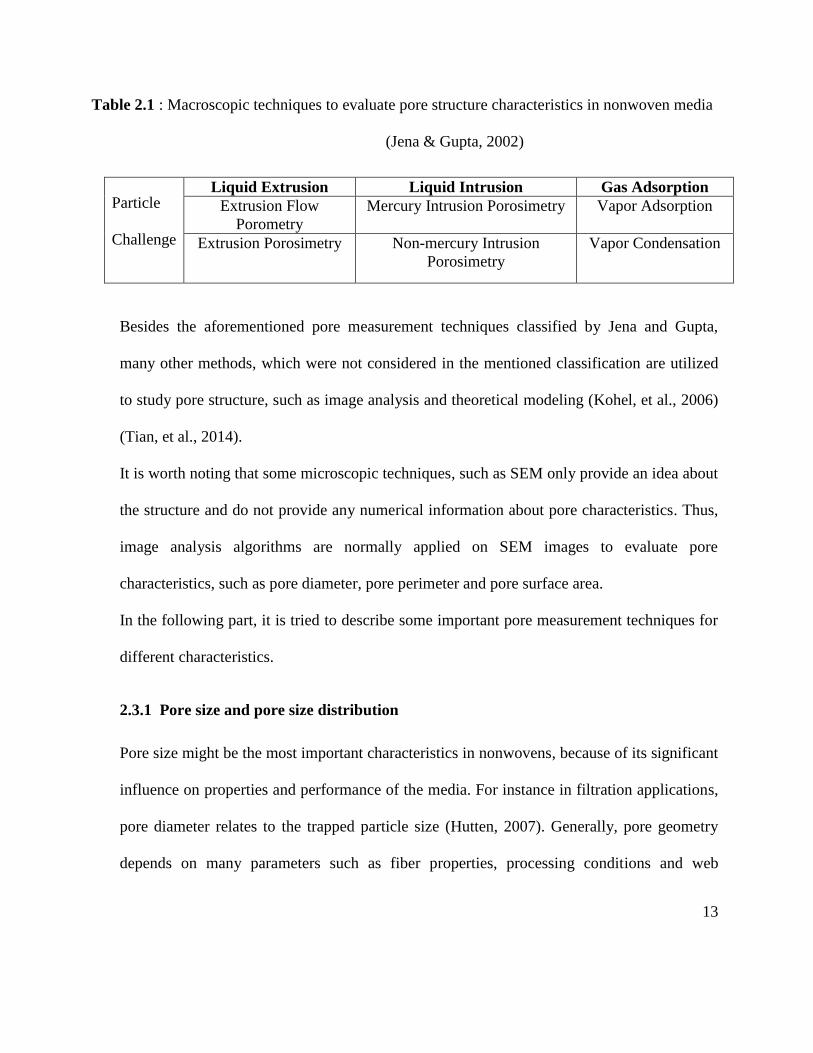
Table 2.1 : Macroscopic techniques to evaluate pore structure characteristics in nonwoven

media (Jena & Gupta, 2002) ........................................................................................... 13

Table 2.2 : Liquids for pore size testing (Hutten, 2007) ........................................................ 16 Table 2.3 : Capability of the extrusion, intrusion and gas adsorption techniques (Hutten,

2007) ............................................................................................................................... 27 Table 4.1 : Samples to study the effect of fiber diameter on pore structurert ........................ 88

Table 4.2 : Samples to study the effect of solidity on pore structure ..................................... 91

Table 5.1 : Matrices/ vectors extracted from the graph shown in Figure 5.7 ...................... 124

Table 5.2 : The equivalent resistance of the samples 1 to 9 based on the designed algorithm

....................................................................................................................................... 129

Table 5.3 : Hagen-Poiseuille’s equation based on algorithm output ................................... 130 Table 5.4 : Voxels size and capillary dimension for each sample provided through software

....................................................................................................................................... 132

Table 5.5 : Permeability for the utilized samples determined from the model .................... 133 Table 5.6 : SVF for samples made from PET 3 denier obtained from real samples and 2D

micro CT images ........................................................................................................... 139 Table 5.7 : SVF for samples made from PET 6 denier obtained from real samples and 2D

micro CT images ........................................................................................................... 141

Table 5.8 : Variables used to generate different structures with different fiber sizes and same

SVFs .............................................................................................................................. 147

Table 5.9 : The algorithm output for the simulated samples with same SVF and different

fiber sizes ...................................................................................................................... 149

Table 5.10 : Modified Hagen-Poiseuille’s equation for simulated dataset .......................... 150 Table 5.11 : The volume of images for the samples with same SVFs and different fiber sizes

....................................................................................................................................... 150 Table 5.12 : Permeability of each sample with same SVFs and different fiber sizes

determined by the model ............................................................................................... 150

Table 5.13 : Permeability coefficients provided by GeoDict® for the samples with different

fiber sizes and same SVFs ............................................................................................ 152

Table 5.14 : Variables used to generate different structures with same fiber sizes and

different SVFs ............................................................................................................... 154

Table 5.15 : The algorithm outputs for the simulated samples with same fiber diameters and

different solidities ......................................................................................................... 156 Table 5.16 : Modified Hagen-Poiseuille’s equation for samples with same fiber sizes and

different SVFs ............................................................................................................... 156

Table 5.17 : Image volume for the simulated samples with same fiber size and different

SVFs .............................................................................................................................. 157 Table 5.18 : Permeability for simulated samples with same fiber diameter and different SVFs

....................................................................................................................................... 157

viii

Table 5.19 : Permeability for simulated samples with same fiber diameter and different SVFs

provided by GeoDict® ................................................................................................... 158 Table 6.1 : Flow rates for samples 1 to 3 measure by experiment ....................................... 162

Table 6.2 : Permeability for the samples with different fiber diameters and same SVFs

measured by experiment ............................................................................................... 163 Table 6.3 : Flow rates for samples 4 to 6 masured by experiment ...................................... 166 Table 6.4 : Permeability for the samples made from PET 3 denier with different SVFs

measured through experiment ....................................................................................... 166 Table 6.5 : Flow rates for samples 7 to 9 measured by experiment ..................................... 169

Table 6.6 : Permeability for the samples made from PET 6 denier and different SVFs...... 169

ix

LIST OF FIGURES

: Different pore types in a porous material (Jena & Gupta, 2002) (Hutten, 2007) . 9 : Different pore cross sections (Jena & Gupta, 2003) ............................................ 9

: Fibrous structure classification based on fiber orientation a) Unidirectional .... 10 : Bubble point sample holder (ASTMF316-03, 2011) ......................................... 17 : Relation between contact angle and surface tensions (Jena & Gupta, 2002) ..... 18 Principle of capillary flow porometry (Jena & Gupta, 2002) (Jena & Gupta, 2001)

......................................................................................................................................... 19

: Scheme of the most constricted pore diameter (Fernando & Chung, 2002) ...... 20 : Determination of mean flow pore size (Yunoki, Matsumoto, & Nakamura,

2004) ............................................................................................................................... 21

: Principle of extrusion porosimetry to evaluate a) pore size b) permeability (Jena

& Gupta, 2002) ............................................................................................................... 22 : Cumulative pore volume of a nanofiber mat (Hutten, 2007) ........................... 23

: Vapor condensation in pores (Jena & Gupta, n.d.) .......................................... 26 : Different diameters of a through pore measured by different methods (Jena &

Gupta, 2002) ................................................................................................................... 28 : Intensity histogram for an image a) with noise b) after noise elimination

(Kohel, Zeng, & Li, 2006) .............................................................................................. 31

: Pore opening diameter distribution (Xu, 1996) ................................................ 34 : a) Ellipse pore b) Pore size distribution (Kohel, Zeng, & Li, 2006) ................ 35

Example of dilation a) the original binary image b) the binary image dilated by

B={(-1, 1)} (Snyder & Qi, 2004). ................................................................................... 37

An imaginary PC board with a crack between two traces (Snyder & Qi, 2004) 38 The image after erosion (Snyder & Qi, 2004) .................................................... 38

Final image after opening procedure (Snyder & Qi, 2004) ................................ 39 : Thermal conductivity of air as a function of pressure for different pore sizes at

300 K (Felix, Jannot, & Degiovanni, 2012).................................................................... 40

: Linear variation of 𝑝/𝑊(𝑝 − 𝑝0) against 𝑝𝑝0 for a nonwoven filter medium

(Jena & Gupta, 2002) ...................................................................................................... 43

: Wrotnowski’s model for pore size (Russel, 2007) ........................................... 46 : Network of straight lines (fibers) obtained by the Poissonian polyhedra model

(Faure, Gource, & Gendrin, 1990) .................................................................................. 49 : Comparison between theoretical and experimental pore size distribution for

samples a, b and c (Tian, et al., 2014)............................................................................. 52

: Schematic of fluid flow direction through fibrous structure a) Unidirectional b)

Layered c) Random (Jaganathan S. , 2008) .................................................................... 57 : Cell model of fibrous structure (Jaganathan S. , 2008) .................................... 60 : Fiber unit cell a) Square array b) Triangular array c) Hexagonal array d)

Staggered array (Jaganathan S. , 2008) ........................................................................... 61

x

: Original image from different objects and their associated skeleton (Abu-Ain,

Sheikh Abdullah, Bataineh, Abu Ain, & Omar, 2013) ................................................... 65 : A binary image (left) and the distance transformed image .............................. 65 : A simple graph with seven vertices and ten edges (Newman, 2010) ............... 66

: A scheme of a direct (left) and indirect (right) graphs (Balakrishnan &

Ranganathan, 2012) ........................................................................................................ 67

Figure 3.1 : Diagram to define Darcy’s law………………………………………………...72

Image acquisition with DVI micro-imager® (Shim, Pourdeyhimi, & Latifi, 2010)

…………………………………………………………………………………………..77

Hydro-entangled 3D image showing exporting of 2D sections (Venu, 2012)... 78 Principal components of a micro CT scanner (Boerckel, Mason, Mc Dermott, &

Alsberg, 2014)…………………………………………………………………………..80 Schematic illustration of back projection (Manitoba, 2015)………………….. 84

The first and the last four sectional images of the PET/Nylon nonwoven

fabric……………………………………………………………………………………86

3D image provided by ResViewTM (Venu, 2012)…………………………….. 87 Images taken through micro CT for the first layer of three samples with same

SVF a) fabric made from 1.5 denier PET b) fabric made from 3 denier PET and c) fabric

made from 6 denier PET………………………………………………………………. 90 The 2D images of the first layer of different samples used for studying the effect

of SVF on pore strcuture………………………………………………………………. 92 Image after applying the median filter………………………………………... 94

The image of first layer of sample 3 after applying the median filter and

thresholding processes………………………………………………………………… 95 Image after cleaning processes………………………………………………. 96

3D image of the PET/Nylon nonwoven sample……………………………... 98

Spatial graph (pore structure) of the PET/Nylon nonwoven sample………. 100 A simple electric circuit (Alexander & Sadiku, 2009) ..................................... 107

A scheme of a resistor between two main nodes (red) including 4 intermediate

nodes (blue). .................................................................................................................. 112 Currents at a node illustrating KCL (Alexander & Sadiku, 2009) ................... 115

Determination of the Y parameters: a) finding Y11, Y21 b) finding Y12, Y22

(Alexander & Sadiku, 2009) ......................................................................................... 116

Nodes on the top and the bottom a) before merging b) after merging ............. 119 The nodes network as an electric circuit .......................................................... 120 An imaginary graph for algorithm description ................................................. 122 The graph shown in Figure 5.7 after merging the nodes .................................. 126 Trend of increasing permeability based on algorithm outputs for the samples

made from different fiber diameters and same SVFs (3.6%) ....................................... 134 Permeability obtained from the model for the samples made of PET 3 denier

with different SVFs ....................................................................................................... 135 The 3D visualization of samples made of PET 3 denier with different SVFs

provided by Avizo® ...................................................................................................... 136

xi

The microscopic images taken from samples made from PET 3 denier and

different SVFs ............................................................................................................... 137 Fiber diameter distribution for a) sample 4 b) sample 5 and c) sample 6 ...... 138 Permeability obtained from model for samples made of PET 6 denier and with

different SVFs ............................................................................................................... 140 The 3D visualization of samples made of PET 6 denier provided by Avizo® 142 The microscopic images taken from samples made from PET 6 denier and

different SVFs ............................................................................................................... 142 Fiber diameter distribution for a) sample 7 b) sample 8 and c) sample 9 ...... 144

Simulated structure for sample 10 (PET 1.5 denier, SVF=3.6%,

resolution=1µm, number of layers = 976) .................................................................... 148 3D visualized structure of sample 10 provided by Avizo® ............................ 148 Trend of increasing the permeability by increasing the fiber diameter for

simulated datasets provided by model .......................................................................... 151 Trend of changing permeability for the samples with different fiber sizes and

same SVFs provided by FlowDict® .............................................................................. 152 The 3D structure generated for sample 15 by GeoDict® (PET 3 denier, ....... 154

3D visualized structure of sample 15 provided by Avizo® ............................ 155 Trend of increasing the permeability by decreasing the solid volume fraction

....................................................................................................................................... 158

Trend of increasing the permeability by decreasing the solid volume fraction

for the values provided by FlowDict® .......................................................................... 159

Figure 6.1 : Trend of increasing permeability for the samples with different fiber diameters

and same SVFs measured by experiment ..................................................................... 163

Figure 6.2 : Comparison between experiment and model for the samples made from different

fiber sizes and same SVF .............................................................................................. 164

Figure 6.3 : Comparison between the results obtained for samples with different fiber

diameters and same SVFs through different methods .................................................. 165 Figure 6.4 : Trend of increasing the permeability for the samples made from PET 3 denier

with different SVFs measured through experiment ...................................................... 167 Figure 6.5 : Comparison between experiment and model values for the samples made from

PET 3 denier and different SVFs .................................................................................. 168 Figure 6.6 : Comparison between the results obtained through different methods for samples

made from PET 3 denier and different SVFs................................................................ 168 Figure 6.7 : Trend of increasing the permeability for the samples made from PET 6 denier

with different SVFs measured through experiment ...................................................... 170 Figure 6.8 : Comparison between experiment and model values for the samples made from

PET 6 denier and different SVFs .................................................................................. 171

Figure 6.9 : Comparison between the results obtained through different methods for samples

made from PET 6 denier and different SVFs................................................................ 172

Figure 6.10 : The effect of assumption on final result for fine fiber and packed structures 174 Figure 6.11 : The effect of assumption on final result for course fiber and open structures 174 Figure 7.1: Tortuosity (Chang & Wang, 2011) ................................................................... 180

1

1. Introduction

2

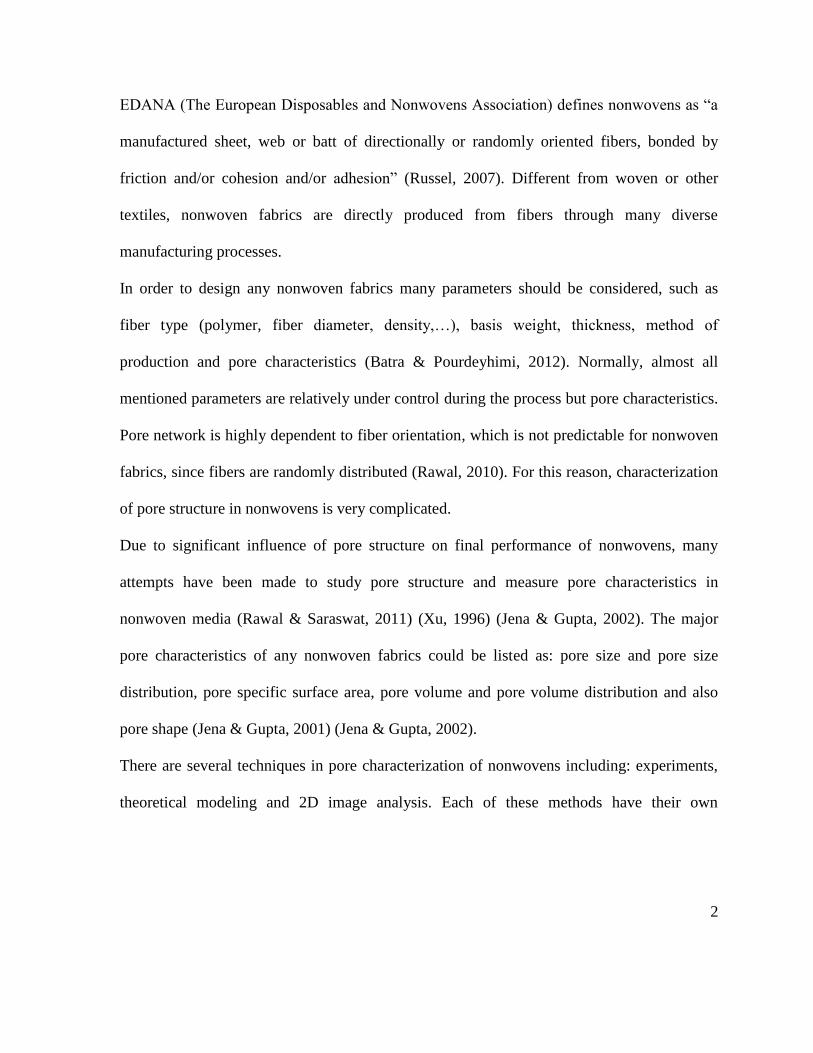
EDANA (The European Disposables and Nonwovens Association) defines nonwovens as “a

manufactured sheet, web or batt of directionally or randomly oriented fibers, bonded by

friction and/or cohesion and/or adhesion” (Russel, 2007). Different from woven or other

textiles, nonwoven fabrics are directly produced from fibers through many diverse

manufacturing processes.

In order to design any nonwoven fabrics many parameters should be considered, such as

fiber type (polymer, fiber diameter, density,…), basis weight, thickness, method of

production and pore characteristics (Batra & Pourdeyhimi, 2012). Normally, almost all

mentioned parameters are relatively under control during the process but pore characteristics.

Pore network is highly dependent to fiber orientation, which is not predictable for nonwoven

fabrics, since fibers are randomly distributed (Rawal, 2010). For this reason, characterization

of pore structure in nonwovens is very complicated.

Due to significant influence of pore structure on final performance of nonwovens, many

attempts have been made to study pore structure and measure pore characteristics in

nonwoven media (Rawal & Saraswat, 2011) (Xu, 1996) (Jena & Gupta, 2002). The major

pore characteristics of any nonwoven fabrics could be listed as: pore size and pore size

distribution, pore specific surface area, pore volume and pore volume distribution and also

pore shape (Jena & Gupta, 2001) (Jena & Gupta, 2002).

There are several techniques in pore characterization of nonwovens including: experiments,

theoretical modeling and 2D image analysis. Each of these methods have their own

3

advantages and disadvantages and the disadvantages associated with each technique

encourage scientists to research more in this area.

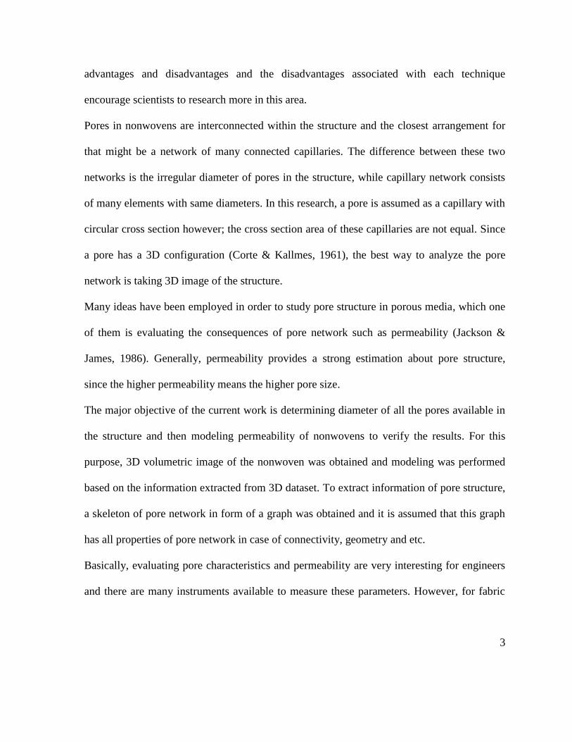
Pores in nonwovens are interconnected within the structure and the closest arrangement for

that might be a network of many connected capillaries. The difference between these two

networks is the irregular diameter of pores in the structure, while capillary network consists

of many elements with same diameters. In this research, a pore is assumed as a capillary with

circular cross section however; the cross section area of these capillaries are not equal. Since

a pore has a 3D configuration (Corte & Kallmes, 1961), the best way to analyze the pore

network is taking 3D image of the structure.

Many ideas have been employed in order to study pore structure in porous media, which one

of them is evaluating the consequences of pore network such as permeability (Jackson &

James, 1986). Generally, permeability provides a strong estimation about pore structure,

since the higher permeability means the higher pore size.

The major objective of the current work is determining diameter of all the pores available in

the structure and then modeling permeability of nonwovens to verify the results. For this

purpose, 3D volumetric image of the nonwoven was obtained and modeling was performed

based on the information extracted from 3D dataset. To extract information of pore structure,

a skeleton of pore network in form of a graph was obtained and it is assumed that this graph

has all properties of pore network in case of connectivity, geometry and etc.

Basically, evaluating pore characteristics and permeability are very interesting for engineers

and there are many instruments available to measure these parameters. However, for fabric

4

engineers during designing and simulating the nonwovens and before any full scale

productions these characteristics would be a concern, since there is no real fabric to test.

This research provides a methodology to find all pores diameter and evaluate permeability of

nonwovens based on 3D dataset of pore network and could be applied for datasets obtained

from real fabrics or simulated ones.

Specific objectives of this study include:

Using 3D imaging to study pore structure of nonwovens and obtain 3D structure of

pore network to determine all pore diameters.

Employing different 3D imaging techniques such as Digital Volumetric Imaging

(DVI) and micro Computed Tomography (micro CT) to visualize the structure of

nonwovens.

Trying to go from a complex network (pore structure) to a single number

(permeability), considering information of all the pores available in the structure.

Designing an algorithm to use the information obtained from 3D pore network to

calculate permeability as a representative value of pore structure in MATLAB.

Investigating the effect of fiber diameter and fabric solidity (solid volume fraction) on

pore structure and permeability employing the designed algorithm.

Verifying the accuracy of model by comparing the algorithm outputs with

experiments.

Studying pore structure and predicting permeability coefficient of simulated

structures using the developed model.

5

1.1 Thesis overview

To meet the aforementioned objectives, this document is organized in the following fashion.

Chapter 2 covers the most relevant concepts and methods in pore structure characterization

and permeability evaluation. Besides, it is tried to explain some theories related to this work,

such as, graph theory and skeletonization. In chapter 3, it is attempted to define the problems

associated with available techniques and the main objective of this research.

As in this study, pore structure was investigated through 3D imaging, in Chapter 4 the most

common methods in 3D imaging of materials as well of image processing technique applied

on the images are explained. Also, the properties of the nonwovens media which are used in

this research will be described.

Chapter 5 includes the details of the model developed to study pore structure of nonwovens,

employing the information obtained from 3D image of the media. Also, in this chapter the

permeability coefficient of each sample will be calculated using the model output.

To verify the results obtained from the model, in Chapter 6 the experimental verification will

be performed to compare experiment and model for the permeability coefficients.

Finally in Chapter 7, some recommendations for future investigations based on findings of

this work will be provided.

6

2. Literature Review

7

2.1 Pore definition and characteristics

Literally, porous materials are encountered everywhere in daily life, such as in technology

and nature. Except metals, some rocks, and some plastics, any other solid and semi- solid

materials are porous to varying degrees (Dullien F. , 1979). Generally, porous materials

consist of multiple phase matter, where at least one of these phases is non-solid that is called

pores or voids (Bear, 1988). Leonhard Euler in 1762 provided a description for pores and

porous bodies probably for the first time, “All bodies in the world are composed of rough and

subtile matter, where of the first is called the characteristic matter whereas the other due to

its nearly infinity small density contributes nothing to the increase of their mass. Since the

mixture of both matters extends to the smallest parts of the space, in which no rough matter

is contained, are called the pores of the bodies,…” (de Boer, 2000).

Porous materials have a unique feature, known as pore structure, which distinguishes them

from other solid bodies. The vast majority of porous media contains an interconnected three-

dimensional network of capillary channels of non-uniform size, shape and length, commonly

referred to as pores (Dullien F. , 1979). Any fluid flows, diffusions and electrical conductions

in porous media take place within very complex microscopic boundaries and any small

changes in pore structure of the media will alter the conditions. This means that convective,

diffusive and interfacial effects, which occur in pores are inseparable from pore structure.

A pore is a minute opening in a system, through which gas, liquid or any microscopic

particles can pass (Jena & Gupta, 2002). Basically, pore structure plays a key role in

performance of nonwoven media, which is not limited to filtration and separation (Rawal &

8

Saraswat, 2011), but several other applications, such as fibrous scaffolds (medical

applications) are directly related to pore structure and many attempts have been made to

investigate that in recent years (Rawal & Saraswat, 2011) (Bagherzadeh, et al., 2013)

(Bagherzadeh, et al., 2014) (Murphy, et al., 2010).In other words, pore characteristics in any

nonwoven materials could be named as the most important structural features that determine

utility of the medium (Xu, 1996). For instance in filtration applications, where particle

trapping represents efficiency, pore structure would be the main parameter. It has been

proven that smaller pore size offers more particle trapping and vice versa.

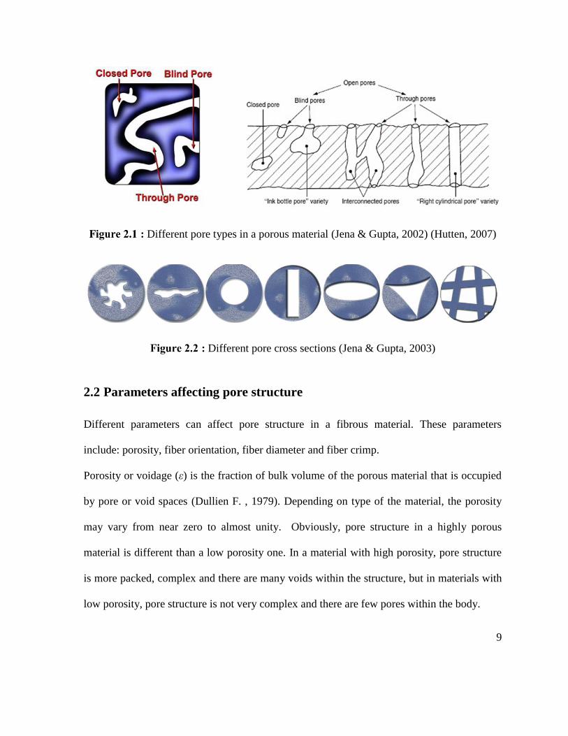
In porous materials, pores are classified into three categories: closed, blind and through pores

(Jena & Gupta, 2002). Closed pores are inside the medium, and are invisible. Blind or dead-

end pores are interconnected only from one side. In contrast, through pores start from one

side of the media and end on the other side, which makes a channel for passing the fluids

(Jena & Gupta, 2002) (Dullien F. , 1979). It is worth noting that in some literature, pores

have been classified into open and closed pores, where the category of open pores includes

blind and through pores (de Boer, 2000) (Hutten, 2007). Figure 2.1 shows the different pore

types.

In nonwovens pores could have different cross sections and this issue makes the pore

characterization more complex (Jena & Gupta, 2003). Figure 2.2 exhibits some possible pore

cross sections.

9

: Different pore types in a porous material (Jena & Gupta, 2002) (Hutten, 2007)

: Different pore cross sections (Jena & Gupta, 2003)

2.2 Parameters affecting pore structure

Different parameters can affect pore structure in a fibrous material. These parameters

include: porosity, fiber orientation, fiber diameter and fiber crimp.

Porosity or voidage (ε) is the fraction of bulk volume of the porous material that is occupied

by pore or void spaces (Dullien F. , 1979). Depending on type of the material, the porosity

may vary from near zero to almost unity. Obviously, pore structure in a highly porous

material is different than a low porosity one. In a material with high porosity, pore structure

is more packed, complex and there are many voids within the structure, but in materials with

low porosity, pore structure is not very complex and there are few pores within the body.

10

Fiber orientation is another important parameter that can affect pore structure. It has been

shown that many nonwoven fabric properties directly relate to fiber arrangement (Hearle &

Stevenson, 1963). In nonwoven materials, fibers are oriented in X- and Y-directions

according to the method of fabric production, and there is limited orientation of fibers in Z-

direction, perpendicular to the plane. Fiber orientation has a significant influence on

geometrical, hydraulic and mechanical properties of fabric especially in terms of anisotropy

(Rawal, Rao, Russel, & Jeganathan, 2010). In many nonwoven applications, such as filters,

hygiene and medical products, the relationship between pore structure and fiber orientation

plays a big role, since the orientation of fibers directly affects fluid flow through fibrous

material.

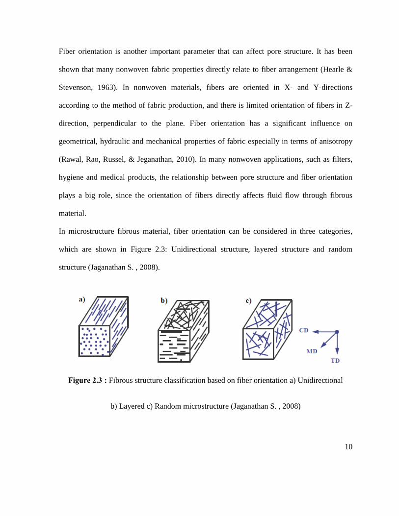
In microstructure fibrous material, fiber orientation can be considered in three categories,

which are shown in Figure 2.3: Unidirectional structure, layered structure and random

structure (Jaganathan S. , 2008).

: Fibrous structure classification based on fiber orientation a) Unidirectional

b) Layered c) Random microstructure (Jaganathan S. , 2008)

11

Image analysis technique is the most common method employed to study fiber orientation

distribution (Pourdeyhimi, et al., 1996) (Pourdeyhimi, et al., 1996) (Pourdeyhimi, et al.,

1997). However, this technique offers fiber orientation based on 2D images and does not

provide any information about fiber orientation for a 3D structure in Z-direction.

Fiber diameter is another parameter that affects pore structure. Free volume between fibers

within the structure could be altered by any changes in fiber diameter. It has been proven that

for a given fabric density and structure, smaller fibers provide smaller pores and in the case

of filtration provide better barrier properties (Kim & Pourdeyhimi, 2000) (Velu, Ghosh, &

Seyam, 2004). In other words, for same web density, if fiber diameter increases, total number

of fibers per unit area and total number of crossovers per unit area will be decreased. This

issue leads to an increase in average pore size in nonwoven medium (Kim & Pourdeyhimi,

2000).

Fiber crimp can also affect pore structure. Observation shows increasing fiber crimp causes

smaller average pore size in materials (Kim & Pourdeyhimi, 2000). Kim and Pourdeyhimi

showed that increasing the crimp leads to an increase in number of crossovers especially in

the direction perpendicular to fiber axis. They also stated that in random oriented nonwovens,

the number of crossovers remains the same and increasing fiber crimp has no significant

effects on pore size (Kim & Pourdeyhimi, 2000).

2.3 Pore measurement techniques

Due to the major influences of pore structure on ultimate performance, pore characterization

is critical in order to design any products. In this regard, many attempts have been made to

12

find accurate methods to evaluate pore parameters. The most important characteristics of

pore structure would be pore size and pore size distribution, pore specific surface area, pore

volume and pore volume distribution, and also pore shape (Jena & Gupta, 2002)

(Charytanowicz, 2014).

Pores are invisible to the naked eye in the majority of porous media, therefore most

techniques use the porous nature of material to study pore structure.

Jena and Gupta classified pore measurement techniques into two main categories:

microscopic and macroscopic (Jena & Gupta, 2002). Microscopic techniques include

methods such as high resolution light, electron microscopy (e.g., SEM) and X-ray scattering.

These techniques can examine very small areas, which could not be measured by

macroscopic techniques. But, it is not possible to evaluate any flow properties through these

techniques. These methods are also time consuming and expensive.

Macroscopic methods can scan large areas of the nonwoven samples including: particle

challenge, liquid extrusion, liquid intrusion and gas adsorption techniques (See Table 2.1). In

the particle challenge test, particles with known size are passed through the media. This test

can evaluate pore size and pore size distribution of the sample, but cannot measure any flow

properties. This method is also time consuming and expensive.

Liquid extrusion, liquid intrusion and gas adsorption techniques can evaluate many pore

structure characteristics. These methods are inexpensive and could be run quickly. So, these

techniques are widely used in order to characterize pore structure (Jena & Gupta, 2002) (Jena

& Gupta, 2003).

13

Table 2.1 : Macroscopic techniques to evaluate pore structure characteristics in nonwoven media

(Jena & Gupta, 2002)

Particle

Challenge

Liquid Extrusion Liquid Intrusion Gas Adsorption

Extrusion Flow

Porometry

Mercury Intrusion Porosimetry Vapor Adsorption

Extrusion Porosimetry Non-mercury Intrusion

Porosimetry

Vapor Condensation

Besides the aforementioned pore measurement techniques classified by Jena and Gupta,

many other methods, which were not considered in the mentioned classification are utilized

to study pore structure, such as image analysis and theoretical modeling (Kohel, et al., 2006)

(Tian, et al., 2014).

It is worth noting that some microscopic techniques, such as SEM only provide an idea about

the structure and do not provide any numerical information about pore characteristics. Thus,

image analysis algorithms are normally applied on SEM images to evaluate pore

characteristics, such as pore diameter, pore perimeter and pore surface area.

In the following part, it is tried to describe some important pore measurement techniques for

different characteristics.

2.3.1 Pore size and pore size distribution

Pore size might be the most important characteristics in nonwovens, because of its significant

influence on properties and performance of the media. For instance in filtration applications,

pore diameter relates to the trapped particle size (Hutten, 2007). Generally, pore geometry

depends on many parameters such as fiber properties, processing conditions and web

14

characteristics and any changes in the mentioned parameters affect pore structure (Rawal,

2010) (Lifshutz, 2005) (Simmonds, et al., 2007) (Savel'eva, et al., 2005).

Basically, the prerequisite parameter to study any transport phenomena in nonwovens is pore

size or pore size distribution (Pan & Zhong, 2006), but it is not easy to evaluate pore

diameter inside the media. As it is known, pore structure is very complex in terms of size,

shape and capillary geometry (Rawal, 2010). Therefore, in almost all available measurement

techniques, pore is assumed to be a cylindrical capillary inside the medium and the diameter

of this capillary is considered as pore size (Hutten, 2007). This assumption is the main

problem associated with these methods because pores are not mostly cylindrical, and do not

have regular diameter along the length.

Pore size could be evaluated through many different approaches, which the most common

ones are provided in next part.

2.3.1.1 Bubble point

Bubble point is mostly used to determine the maximum pore size between 0.1 to 15 µm of

membrane filters (ASTMF316-03, 2011). As stated by the principle, a wetting liquid is held

in pores by capillary attraction and surface tension, also the minimum pressure required to

force liquid is a function of pore diameter (ASTMF316-03, 2011) (Hutten, 2007). This

method is performed by prewetting the sample, increasing gas upstream pressure at a

predetermined rate and observing gas bubbles downstream to indicate gas flow through the

maximum pore size of the medium (Bhatia & Smith, 1995).

15

In this technique, the sample is clamped over a pressurizing chamber. There is a reservoir

above the medium, which is full of test fluid. The pressurizing chamber is connected to a

pressurized air source and to a manometer. Pressure increases when airflow is introduced into

the chamber. Air forces its way through the sample and bubbles through the liquid reservoir.

The manometer records the pressure level at the first bubble generation time (Hutten, 2007)

and the maximum pore diameter can be calculated using equation 1 (ASTMF316-03, 2011),

𝑑 =𝐶𝛾

𝑝 (1)

where:

𝑑: Maximum pore diameter, µm,

𝛾: Surface tension, mN/m,

𝑝: Pressure, Pa or cm Hg, and

𝐶: Constant, 2860 when p is in Pa, 2.15 when p is in cm Hg, and 0.415 when p is in psi units.

As mentioned earlier, the sample should be wetted by floating on a pool of liquid. In Table

2.2, some common liquids used in bubble point technique are cited.

16

Table 2.2 : Liquids for pore size testing (Hutten, 2007)

It is worth noting, some literature recommends to correct the pressure value in equation 1

according to height of the reservoir (See Figure 2.4) however; many companies still prefer

using the old version. Equation 2 shows this correction for the pressure (Hutten, 2007)

(Wang, et al., 2012):

𝑃 = 𝑃0 − 𝜌𝐿𝑔ℎ (2)

where:

𝜌𝐿: Density of the reservoir liquid in 20oC, g/cm3,

ℎ: The height of the reservoir, cm (The reservoir height is normally 0.5 cm), and

𝑔: The gravity constant (981 cm/s2)

17

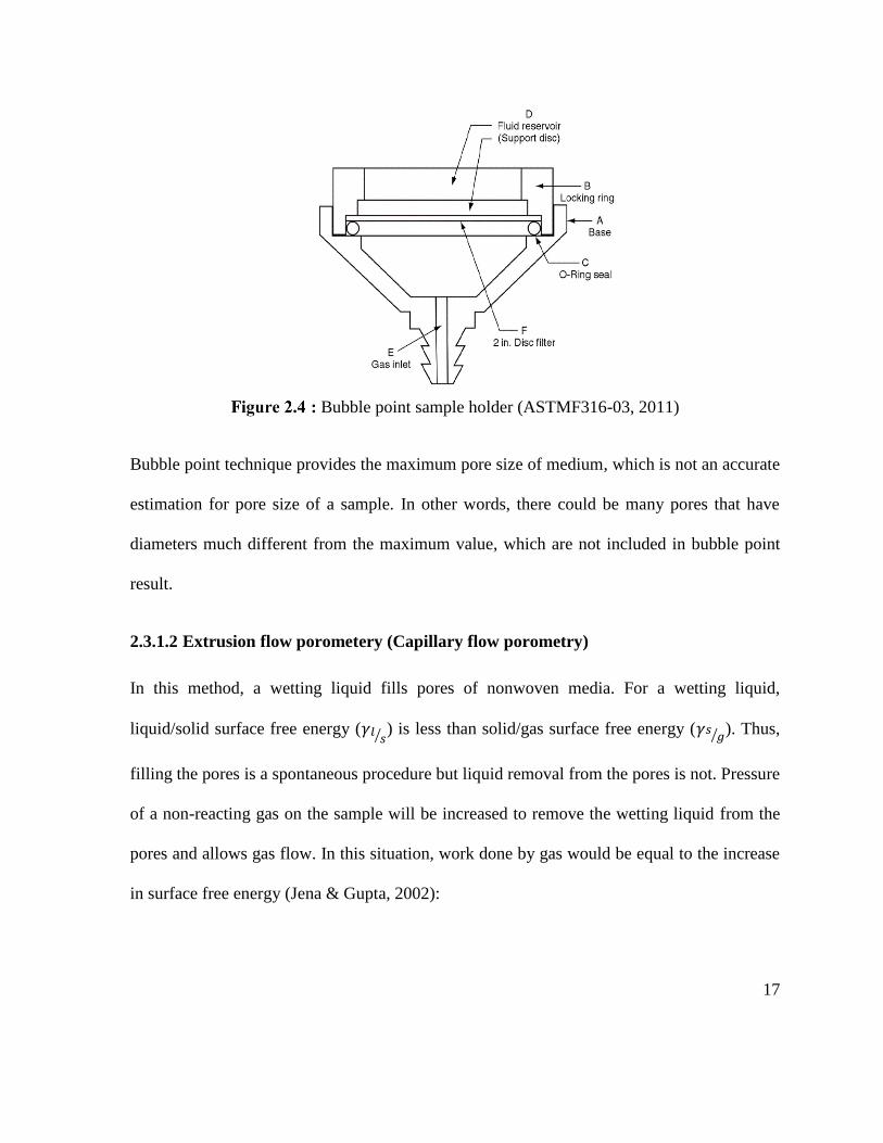
: Bubble point sample holder (ASTMF316-03, 2011)

Bubble point technique provides the maximum pore size of medium, which is not an accurate

estimation for pore size of a sample. In other words, there could be many pores that have

diameters much different from the maximum value, which are not included in bubble point

result.

2.3.1.2 Extrusion flow porometery (Capillary flow porometry)

In this method, a wetting liquid fills pores of nonwoven media. For a wetting liquid,

liquid/solid surface free energy (𝛾𝑙𝑠⁄) is less than solid/gas surface free energy (𝛾𝑠

𝑔⁄). Thus,

filling the pores is a spontaneous procedure but liquid removal from the pores is not. Pressure

of a non-reacting gas on the sample will be increased to remove the wetting liquid from the

pores and allows gas flow. In this situation, work done by gas would be equal to the increase

in surface free energy (Jena & Gupta, 2002):

18

𝑃𝑑𝑉 = (𝛾𝑠𝑔⁄

− 𝛾𝑙𝑠⁄) 𝑑𝑆 (3)

where 𝑃 is differential pressure, 𝑑𝑉 is increase in volume of gas in pore and 𝑑𝑆 is increase in

solid/gas surface area and the corresponding decrease in solid/liquid surface area.

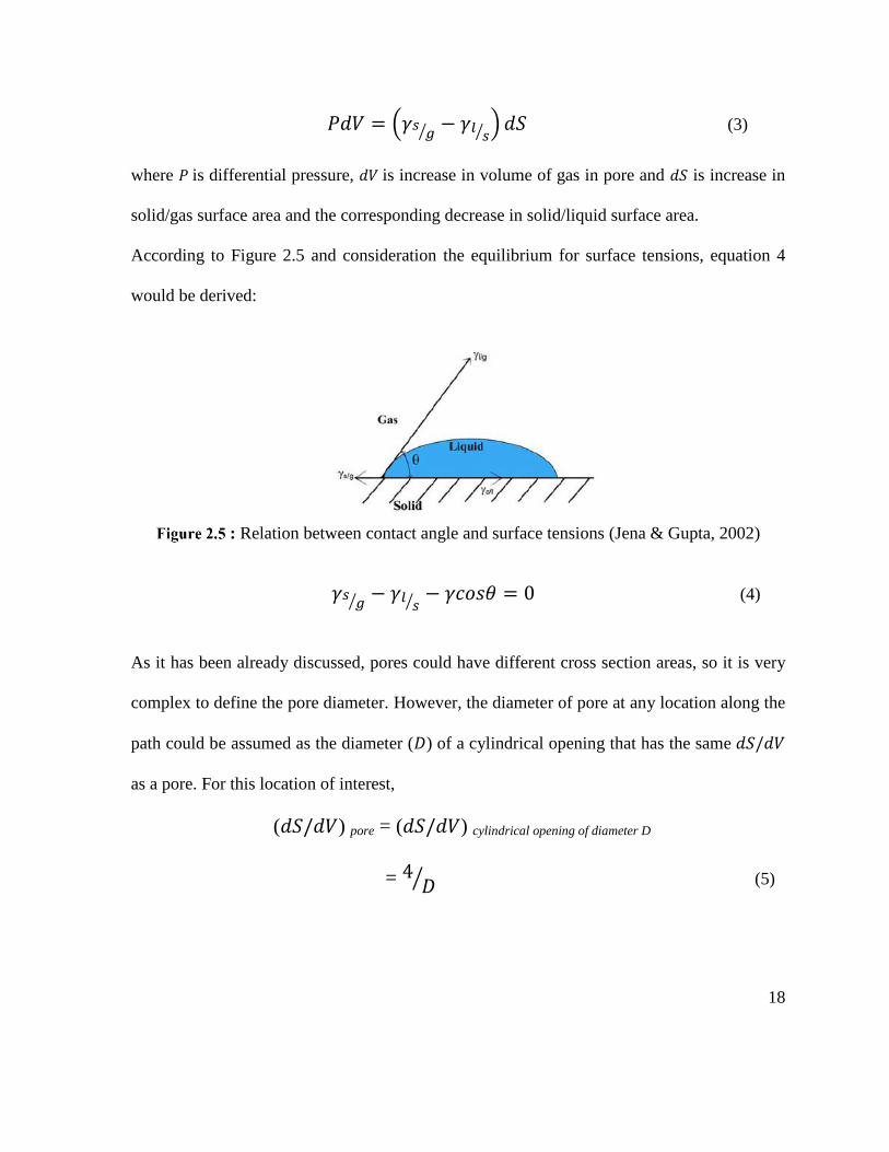
According to Figure 2.5 and consideration the equilibrium for surface tensions, equation 4

would be derived:

: Relation between contact angle and surface tensions (Jena & Gupta, 2002)

𝛾𝑠𝑔⁄

− 𝛾𝑙𝑠⁄− 𝛾𝑐𝑜𝑠𝜃 = 0 (4)

As it has been already discussed, pores could have different cross section areas, so it is very

complex to define the pore diameter. However, the diameter of pore at any location along the

path could be assumed as the diameter (𝐷) of a cylindrical opening that has the same 𝑑𝑆/𝑑𝑉

as a pore. For this location of interest,

(𝑑𝑆/𝑑𝑉) pore = (𝑑𝑆/𝑑𝑉) cylindrical opening of diameter D

= 4 𝐷⁄ (5)

19

The relation between pore diameter and differential pressure, which is needed to displace

wetting liquid in pore, could be derived using equations 3, 4 and 5 (Hutten, 2007) (Jena &

Gupta, 2002):

𝑃 =4γ cos θ

𝐷 (6)

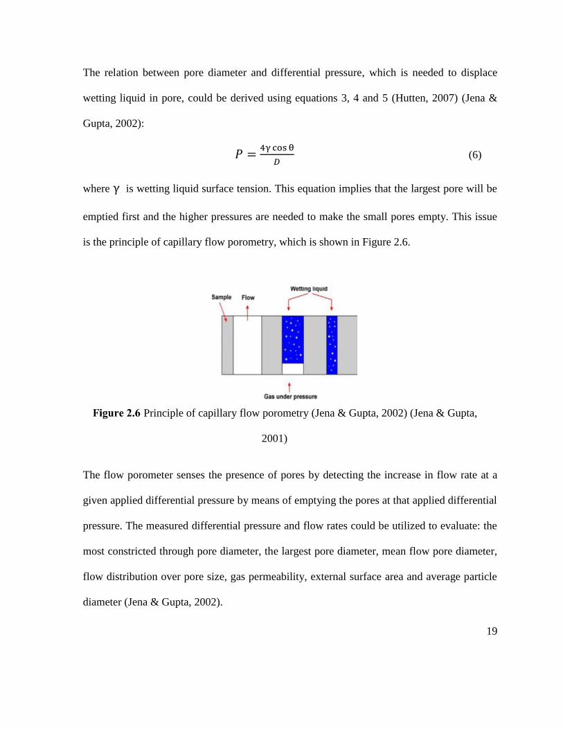
where γ is wetting liquid surface tension. This equation implies that the largest pore will be

emptied first and the higher pressures are needed to make the small pores empty. This issue

is the principle of capillary flow porometry, which is shown in Figure 2.6.

Principle of capillary flow porometry (Jena & Gupta, 2002) (Jena & Gupta,

2001)

The flow porometer senses the presence of pores by detecting the increase in flow rate at a

given applied differential pressure by means of emptying the pores at that applied differential

pressure. The measured differential pressure and flow rates could be utilized to evaluate: the

most constricted through pore diameter, the largest pore diameter, mean flow pore diameter,

flow distribution over pore size, gas permeability, external surface area and average particle

diameter (Jena & Gupta, 2002).

20

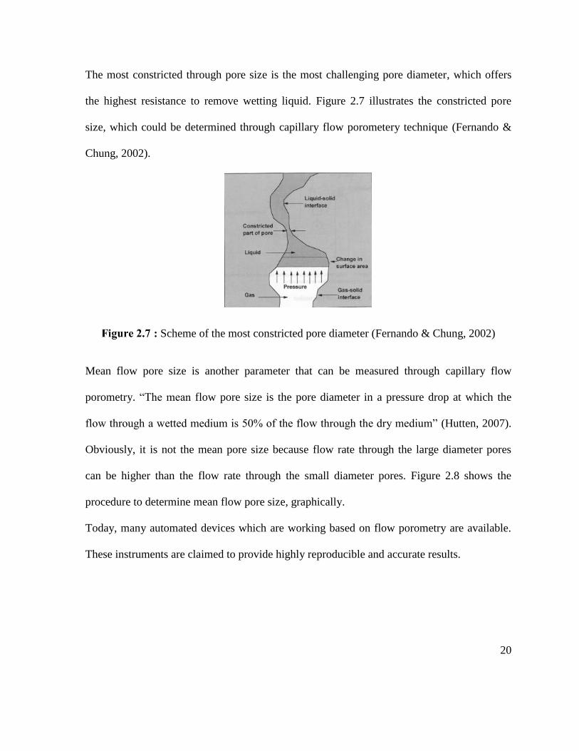
The most constricted through pore size is the most challenging pore diameter, which offers

the highest resistance to remove wetting liquid. Figure 2.7 illustrates the constricted pore

size, which could be determined through capillary flow porometery technique (Fernando &

Chung, 2002).

: Scheme of the most constricted pore diameter (Fernando & Chung, 2002)

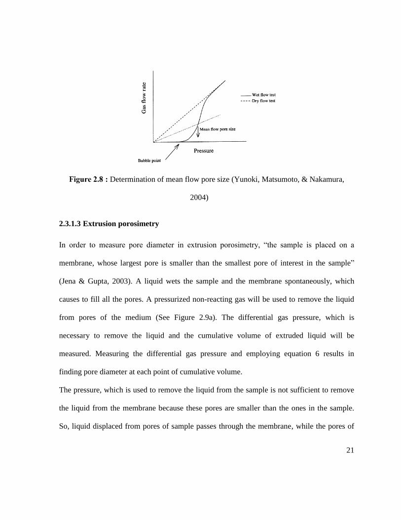
Mean flow pore size is another parameter that can be measured through capillary flow

porometry. “The mean flow pore size is the pore diameter in a pressure drop at which the

flow through a wetted medium is 50% of the flow through the dry medium” (Hutten, 2007).

Obviously, it is not the mean pore size because flow rate through the large diameter pores

can be higher than the flow rate through the small diameter pores. Figure 2.8 shows the

procedure to determine mean flow pore size, graphically.

Today, many automated devices which are working based on flow porometry are available.

These instruments are claimed to provide highly reproducible and accurate results.

21

: Determination of mean flow pore size (Yunoki, Matsumoto, & Nakamura,

2004)

2.3.1.3 Extrusion porosimetry

In order to measure pore diameter in extrusion porosimetry, “the sample is placed on a

membrane, whose largest pore is smaller than the smallest pore of interest in the sample”

(Jena & Gupta, 2003). A liquid wets the sample and the membrane spontaneously, which

causes to fill all the pores. A pressurized non-reacting gas will be used to remove the liquid

from pores of the medium (See Figure 2.9a). The differential gas pressure, which is

necessary to remove the liquid and the cumulative volume of extruded liquid will be

measured. Measuring the differential gas pressure and employing equation 6 results in

finding pore diameter at each point of cumulative volume.

The pressure, which is used to remove the liquid from the sample is not sufficient to remove

the liquid from the membrane because these pores are smaller than the ones in the sample.

So, liquid displaced from pores of sample passes through the membrane, while the pores of

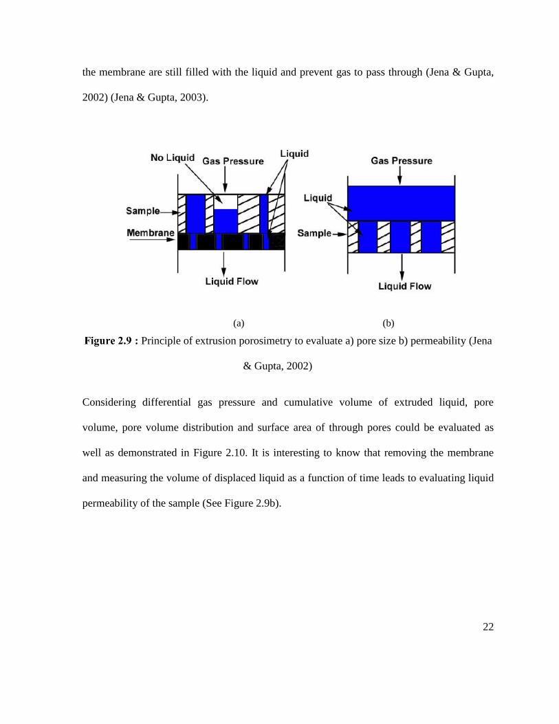
22

the membrane are still filled with the liquid and prevent gas to pass through (Jena & Gupta,

2002) (Jena & Gupta, 2003).

(a) (b)

: Principle of extrusion porosimetry to evaluate a) pore size b) permeability (Jena

& Gupta, 2002)

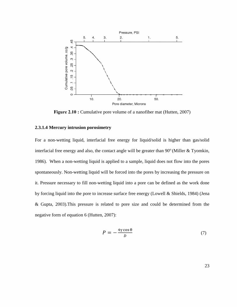
Considering differential gas pressure and cumulative volume of extruded liquid, pore

volume, pore volume distribution and surface area of through pores could be evaluated as

well as demonstrated in Figure 2.10. It is interesting to know that removing the membrane

and measuring the volume of displaced liquid as a function of time leads to evaluating liquid

permeability of the sample (See Figure 2.9b).

23

: Cumulative pore volume of a nanofiber mat (Hutten, 2007)

2.3.1.4 Mercury intrusion porosimetry

For a non-wetting liquid, interfacial free energy for liquid/solid is higher than gas/solid

interfacial free energy and also, the contact angle will be greater than 90o (Miller & Tyomkin,

1986). When a non-wetting liquid is applied to a sample, liquid does not flow into the pores

spontaneously. Non-wetting liquid will be forced into the pores by increasing the pressure on

it. Pressure necessary to fill non-wetting liquid into a pore can be defined as the work done

by forcing liquid into the pore to increase surface free energy (Lowell & Shields, 1984) (Jena

& Gupta, 2003).This pressure is related to pore size and could be determined from the

negative form of equation 6 (Hutten, 2007):

𝑃 = −4γ cosθ

𝐷 (7)

24

Mercury is usually used as the non-wetting liquid. By calculating differential pressure on

mercury and intrusion volume of mercury, it is possible to determine: pore volume, pore

diameter, pore volume distribution and pore surface area (Jena & Gupta, 2002). Because

mercury is a toxic material, instruments with minimum mercury exposure are more popular

in industry. However, it is a destructive procedure and using high pressure may cause to a

change in structure of the material.

2.3.1.5 Non-mercury intrusion porosimetry

This technique is same as mercury intrusion porosimetry, except there is a non-wetting non-

mercury liquid instead of mercury in this method. Water and oil are some of the non-mercury

intrusion liquid that are mostly used. In this technique, there is no toxic material available,

also the pressure is low and small pore sizes could be normally measured (Jena & Gupta,

2002).

2.3.1.6 Gas/vapor adsorption (BET)

Principle of BET (Brunauer, Emmet, Tellet) theory is based on attraction of an inert gas,

which is mostly nitrogen (N2) to the surface area of the sample being tested (Baunauer,

Emmet, & Teller, 1938) (Barrett, Joyner, & Halenda, 1951). Normally, the test is performed

at or near the liquid nitrogen temperature. After exposing a clean surface with a gas, an

adsorbed film generates on the surface and the extent of adsorption will be determined by the

temperature, pressure and the nature of the gas. In this technique, the amount of vapor

adsorbed on pore surface of a sample would be a function of vapor pressure as related to the

25

equilibrium vapor pressure (Lowell & Shields, 1984) (Hutten, 2007). To analyze the data,

BET isotherm equation is utilized as bellow (Allen, 1997):

[𝑝

(𝑝0−𝑝)𝑊] = [

1

𝑊𝑚𝐶] + [

𝐶−1

𝑊𝑚𝐶] (

𝑝

𝑝0) (8)

where 𝑝 is vapor pressure in Pa, 𝑝0 is equilibrium vapor pressure at the temperature of

measurement in Pa, 𝑊 is the amount of adsorbed gas in moles, 𝑊𝑚is amount of gas that can

form a monolayer in moles and 𝐶 is a constant value and depends on the adsorption energy of

the gas to the solid substrate compared to the gas liquefaction energy. High adsorption

energy compared to the liquefaction energy, leads the gas to have a high affinity for the solid

substrate and vice versa (Hutten, 2007).

Vapor condensation is the basic principle to analyze pore size in BET technique. Basically, at

high 𝑝

𝑝0 (relative vapor pressure), vapor tends to be condensed in pores and it is easier for

vapor to condense in small pores than large ones. Vapor condensation at p < p0 into liquid is

guaranteed by an increase in free energy and filling pores with liquid results in replacement

of high free energy vapor/solid interface by the low free energy liquid/solid interface. The

relationship between pore size and vapor pressure is determined by equating two energy

terms. According to Figure 2.11, suppose liquid, l, with volume of dV is condensed in a pore

from vapor, v(p), at pressure, p, and the resulting conversion of the solid/vapor interfacial

area to solid/liquid interfacial area is dS (Jena & Gupta, 2002). Then:

(dV / V ) ΔG [ v(p) → l (bulk) ] + dS ΔGs [ s/v → s/l ] = 0 (9)

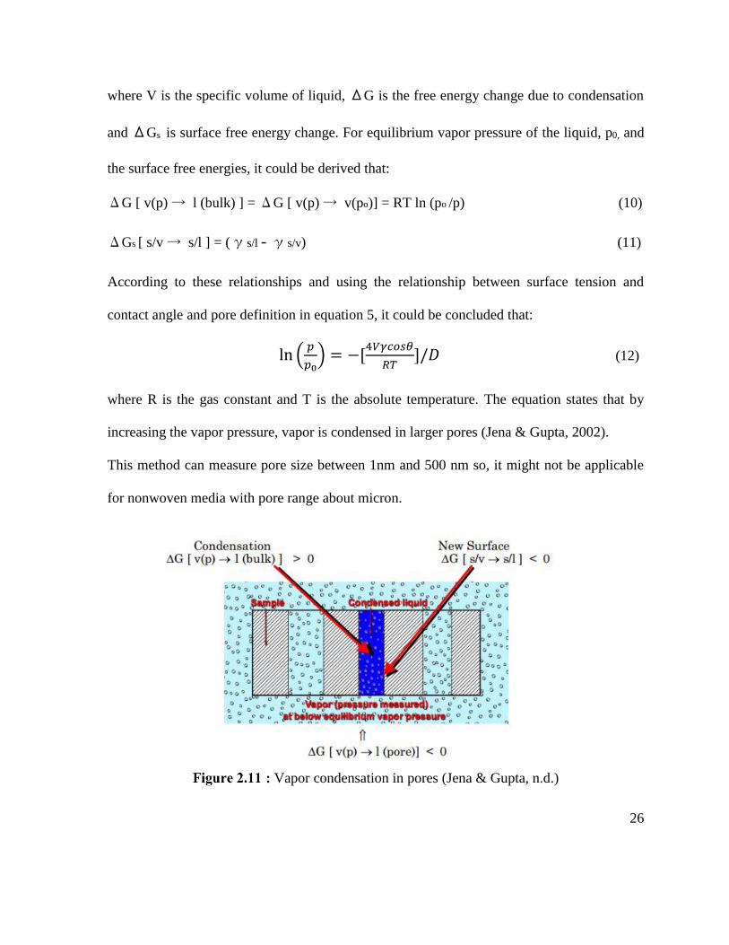
26

where V is the specific volume of liquid, ΔG is the free energy change due to condensation

and ΔGs is surface free energy change. For equilibrium vapor pressure of the liquid, p0, and

the surface free energies, it could be derived that:

ΔG [ v(p) → l (bulk) ] = ΔG [ v(p) → v(po)] = RT ln (po /p) (10)

ΔGs [ s/v → s/l ] = (γs/l - γs/v) (11)

According to these relationships and using the relationship between surface tension and

contact angle and pore definition in equation 5, it could be concluded that:

ln (𝑝

𝑝0) = −[

4𝑉𝛾𝑐𝑜𝑠𝜃

𝑅𝑇]/𝐷 (12)

where R is the gas constant and T is the absolute temperature. The equation states that by

increasing the vapor pressure, vapor is condensed in larger pores (Jena & Gupta, 2002).

This method can measure pore size between 1nm and 500 nm so, it might not be applicable

for nonwoven media with pore range about micron.

: Vapor condensation in pores (Jena & Gupta, n.d.)

27

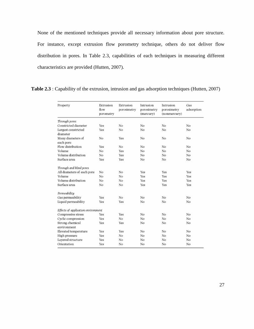
None of the mentioned techniques provide all necessary information about pore structure.

For instance, except extrusion flow porometry technique, others do not deliver flow

distribution in pores. In Table 2.3, capabilities of each techniques in measuring different

characteristics are provided (Hutten, 2007).

Table 2.3 : Capability of the extrusion, intrusion and gas adsorption techniques (Hutten, 2007)

28

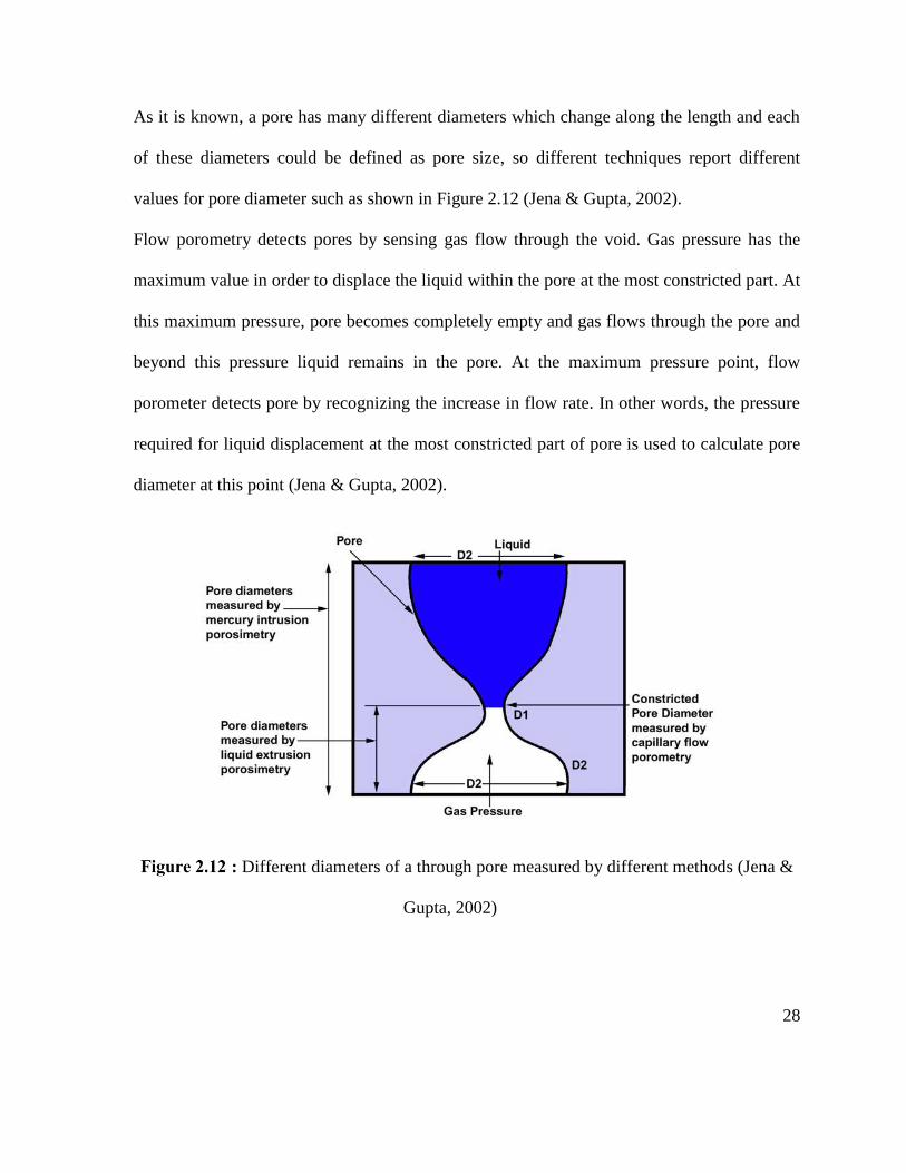
As it is known, a pore has many different diameters which change along the length and each

of these diameters could be defined as pore size, so different techniques report different

values for pore diameter such as shown in Figure 2.12 (Jena & Gupta, 2002).

Flow porometry detects pores by sensing gas flow through the void. Gas pressure has the

maximum value in order to displace the liquid within the pore at the most constricted part. At

this maximum pressure, pore becomes completely empty and gas flows through the pore and

beyond this pressure liquid remains in the pore. At the maximum pressure point, flow

porometer detects pore by recognizing the increase in flow rate. In other words, the pressure

required for liquid displacement at the most constricted part of pore is used to calculate pore

diameter at this point (Jena & Gupta, 2002).

: Different diameters of a through pore measured by different methods (Jena &

Gupta, 2002)

29

In extrusion porosimetry, increasing of gas pressure on one side of sample leads to displace

liquid in pore. In this condition, pore diameter and volume of the part where liquid is

displaced are measured. It is good to say that on attaining the maximum pressure at the most

constricted diameter, the rest of the liquid will be moved from pore beyond the most

constricted part and diameter of pore beyond the most constricted part are not measured.

Therefore, extrusion porosimetry can measure diameter of that part of a pore between the

entry point of the gas and the most constricted point of the through pores (Jena & Gupta,

2003).

In mercury/non-mercury intrusion porosimetry, a non-wetting liquid fills pores from both

sides. By increasing the pressure, liquid enters smaller parts of pore and leads porometer to

measure the diameter and volume of those parts of pore until the most constricted part is

filled. Therefore, a range of pore diameter of all parts of a through pore will be evaluated

(Jena & Gupta, 2002). However, mercury intrusion porosimetry needs a very high pressure,

which may distort the pore structure significantly (Tian, et al., 2014).

In case of measuring through pore diameter by gas adsorption technique, condensation

occurs in narrow parts at low pressure and it expands to wide parts by increasing the

pressure. Thus, pore diameter of all parts could be measured. The problem associated with

BET techniques is, this method is applicable in nanoscale and for measuring pore sizes in

microscale, it is not useful. Meanwhile, the penetrated gas sits on the surface of fibers, so the

measured surface area would be the area of fibers instead of pores.

30

2.3.1.7 Image analysis technique

Image analysis is a popular method to study pore structure using sample images. In this

technique, the image will be processed through an algorithm to provide the requested

information. The accuracy of this technique depends on image quality and the utilized

algorithm. Generally, a typical image processing procedure includes three basic elements: an

image acquisition element, an image analysis element and an image display element (Gong &

Newman, 1992).

Image analysis is normally utilized to study four main pore characteristics in nonwoven

media: pore size, shape, orientation and placement (Xu, 1996). To perform the analysis, the

image could be obtained through three different ways. For pore size in the range of micron,

SEM (scanning electron microscopy) is normally used. The second technique is using a

trinocular microscope with a camera. In this method, the sample should be thin enough and

the obtained image is exactly 2-dimensional. In the third technique, the image will be

provided through a high resolution flatbed scanner. This method is suitable for the samples

with large pores (Doktor & Valach, 2010).

First step in studying pore structure using image analysis is separating the object (pores) from

the background. This procedure is called image segmentation (Snyder & Qi, 2004). It is

worth noting that there is not a standard approach to perform segmentation process because

success of each segmentation process could be judged just based on ultimate result and at the

end of the measurements. In pore characteristics of nonwovens, gray level thresholding is

commonly used as the segmentation procedure. It means, any region, whose brightness is

31

above the threshold will be considered as object and all below the threshold as background

(Ghosh, 2013). For this purpose, image should be transformed to binary image to get fibers

and pores clearly (Kohel, Zeng, & Li, 2006). Binary images are digital images, which have

only two possible values for each pixel. Normally, black and white colors are used in binary

images, where one of them shows the background (black) and the other one shows the

foreground (white) (Gonzalez & Wintz, 1987). Pixels within objects and those within

backgrounds are represented by 1 and 0, respectively (Gong & Newman, 1992).

When an image is taken by any imaging techniques, it is not normally usable because of

variation in intensity, poor contrast and etc. Environmental conditions can affect image

quality and lead to generate noise in the image. This noise results unnecessary pixel

intensities, which makes the ultimate result inaccurate. Thus, before applying any image

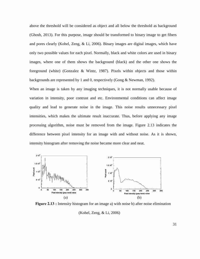
processing algorithm, noise must be removed from the image. Figure 2.13 indicates the

difference between pixel intensity for an image with and without noise. As it is shown,

intensity histogram after removing the noise became more clear and neat.

(a) (b)

: Intensity histogram for an image a) with noise b) after noise elimination

(Kohel, Zeng, & Li, 2006)

32

There are several ways to eliminate the noise in image processing, such as applying filtering

algorithms or using mathematical morphology (Xu, 1996) (Aydilek, et al., 2002) .

In case of filtering, median and mean filters are the most common ones (Jain, 1989). In

mathematical morphology, a structuring element (se) will be defined to modify certain shape

features of the image. Size of the structural element depends on the size of the noise.

Normally, mathematical morphology includes erosion and dilation procedures (Snyder & Qi,

2004) (Wu, van Vlit, Frijlink, & van der Voort Maarschalk, 2007). These concepts will be

described later on.

As discussed, image processing is a very common technique to study pore structure. For

instance, Gong and Newton tried to measure equivalent diameter and hydrodynamic diameter

of a medium using image analysis (Gong & Newman, 1992). They defined equivalent

diameter as:

𝐷𝑒 = 2𝐾/(1.5𝐴

𝑛) (13)

where 𝐾 is the vertical objective length of pixel (pixel width = 1.5×pixel length) and 𝐴 is the

area of a pore in a number of pixels. The result is the diameter of a circular pore with an area

of 𝐴.

In case of hydrodynamic pore diameter, they defined:

𝐷ℎ =6𝐾2𝐴

𝑃 (14)

where 𝑃 is pore perimeter and 𝐴 is pore area.

33

According to their report, to find pore surface area and perimeter it is necessary to assume

pore is circular and then count the pixels of the image. Clearly, assuming pore as a circle

decreases the accuracy, since pores could have different shapes. Meanwhile, to count the

pixels it is required to define the image contours, which needs very precise algorithms for

image processing, noise removal and edge sharpening.

In another investigation, Xu attempted to measure hydrodynamic pore size, pore shape and

pore surface area (Xu, 1996). He defined hydrodynamic diameter as the following:

𝐷ℎ = 4𝐴/𝑃 (15)

where 𝐴 is pore surface area and 𝑃 is pore perimeter. Same as Gong and Newton’s study, it is

necessary to count the pixels to find 𝐴 and 𝑃. The only difference is, Xu used a different

definition for hydrodynamic diameter. This difference between two definitions prevents any

comparisons between these two approaches. He defined another parameter, 𝐷0, as the

opening diameter, which is diameter of the maximum circle that can fit in a pore. Again,

assuming the pore shape as a circle, leads to generate inaccuracy for the results. Figure 2.14

represents the opening diameter distribution for this study.

34

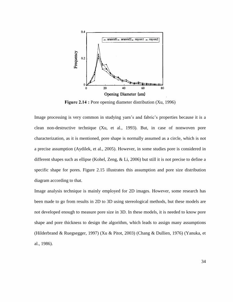
: Pore opening diameter distribution (Xu, 1996)

Image processing is very common in studying yarn’s and fabric’s properties because it is a

clean non-destructive technique (Xu, et al., 1993). But, in case of nonwoven pore

characterization, as it is mentioned, pore shape is normally assumed as a circle, which is not

a precise assumption (Aydilek, et al., 2005). However, in some studies pore is considered in

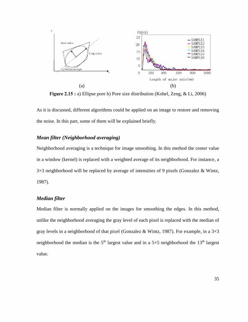
different shapes such as ellipse (Kohel, Zeng, & Li, 2006) but still it is not precise to define a

specific shape for pores. Figure 2.15 illustrates this assumption and pore size distribution

diagram according to that.

Image analysis technique is mainly employed for 2D images. However, some research has

been made to go from results in 2D to 3D using stereological methods, but these models are

not developed enough to measure pore size in 3D. In these models, it is needed to know pore

shape and pore thickness to design the algorithm, which leads to assign many assumptions

(Hilderbrand & Ruegsegger, 1997) (Xu & Pitot, 2003) (Chang & Dullien, 1976) (Yanuka, et

al., 1986).

35

(a) (b)

: a) Ellipse pore b) Pore size distribution (Kohel, Zeng, & Li, 2006)

As it is discussed, different algorithms could be applied on an image to restore and removing

the noise. In this part, some of them will be explained briefly.

Mean filter (Neighborhood averaging)

Neighborhood averaging is a technique for image smoothing. In this method the center value

in a window (kernel) is replaced with a weighted average of its neighborhood. For instance, a

3×3 neighborhood will be replaced by average of intensities of 9 pixels (Gonzalez & Wintz,

1987).

Median filter

Median filter is normally applied on the images for smoothing the edges. In this method,

unlike the neighborhood averaging the gray level of each pixel is replaced with the median of

gray levels in a neighborhood of that pixel (Gonzalez & Wintz, 1987). For example, in a 3×3

neighborhood the median is the 5th largest value and in a 5×5 neighborhood the 13th largest

value.

36

Mathematical morphology

The other approach to improve image quality is employing mathematical morphology, which

is a technique to analyze and process of geometric structures (Najman & Talbot, 2010). The

main morphological operators in mathematical morphology are erosion, dilation, opening and

closing (Snyder & Qi, 2004).

In order to employ the mathematical morphology operators, a structuring element should be

selected to apply the commands on the given image. Basically, structuring element (s.e.) is a

shape that determines how mathematical morphology operator acts on an image (Serra,

1982). Selecting a particular structuring element influences on the obtained information from

the image. Any structuring elements are defined via two major characteristics: shape and

size. Shape of a s.e. could be a ring, ball, square, line, convex, etc. Depending on image, any

of the mentioned shapes could be chosen. The selected shape could have different sizes for

example it could be a 3×3 ball or square. Setting the size of the structuring elements is very

similar to setting the observation scale for an image (Dougherty, 1992).

Dilation means making the boundary of an image a little bit bigger. Normally, dilation effects

on foreground region of image. Consider two images, 𝑓𝐴 and 𝑓𝐵 and let A and B be sets of

ordered pairs, consisting of the coordinates of each foreground pixel in 𝑓𝐴 and 𝑓𝐵,

respectively. Consider one pixel in 𝑓𝐵, and its corresponding element (ordered pair) of B, call

that element b that element 𝑏 ∈ 𝐵. Create a new set by adding the ordered pair b to every

ordered pair in A.

37

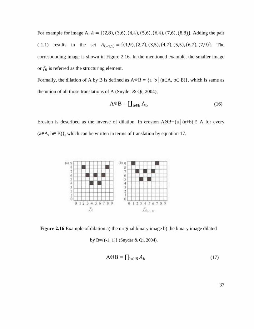
For example for image A, 𝐴 = {(2,8), (3,6), (4,4), (5,6), (6,4), (7,6), (8,8)}. Adding the pair

(-1,1) results in the set 𝐴(−1,1) = {(1,9), (2,7), (3,5), (4,7), (5,5), (6,7), (7,9)}. The

corresponding image is shown in Figure 2.16. In the mentioned example, the smaller image

or 𝑓𝐵 is referred as the structuring element.

Formally, the dilation of A by B is defined as A B = {a+b│(a∈A, b∈ B)}, which is same as

the union of all those translations of A (Snyder & Qi, 2004),

A B = ∐ Abb∈B (16)

Erosion is described as the inverse of dilation. In erosion AΘB={a│(a+b) ∈ A for every

(a∈A, b∈ B)}, which can be written in terms of translation by equation 17.

Example of dilation a) the original binary image b) the binary image dilated

by B={(-1, 1)} (Snyder & Qi, 2004).

AΘB = ∏ 𝐴𝑏b∈ B (17)

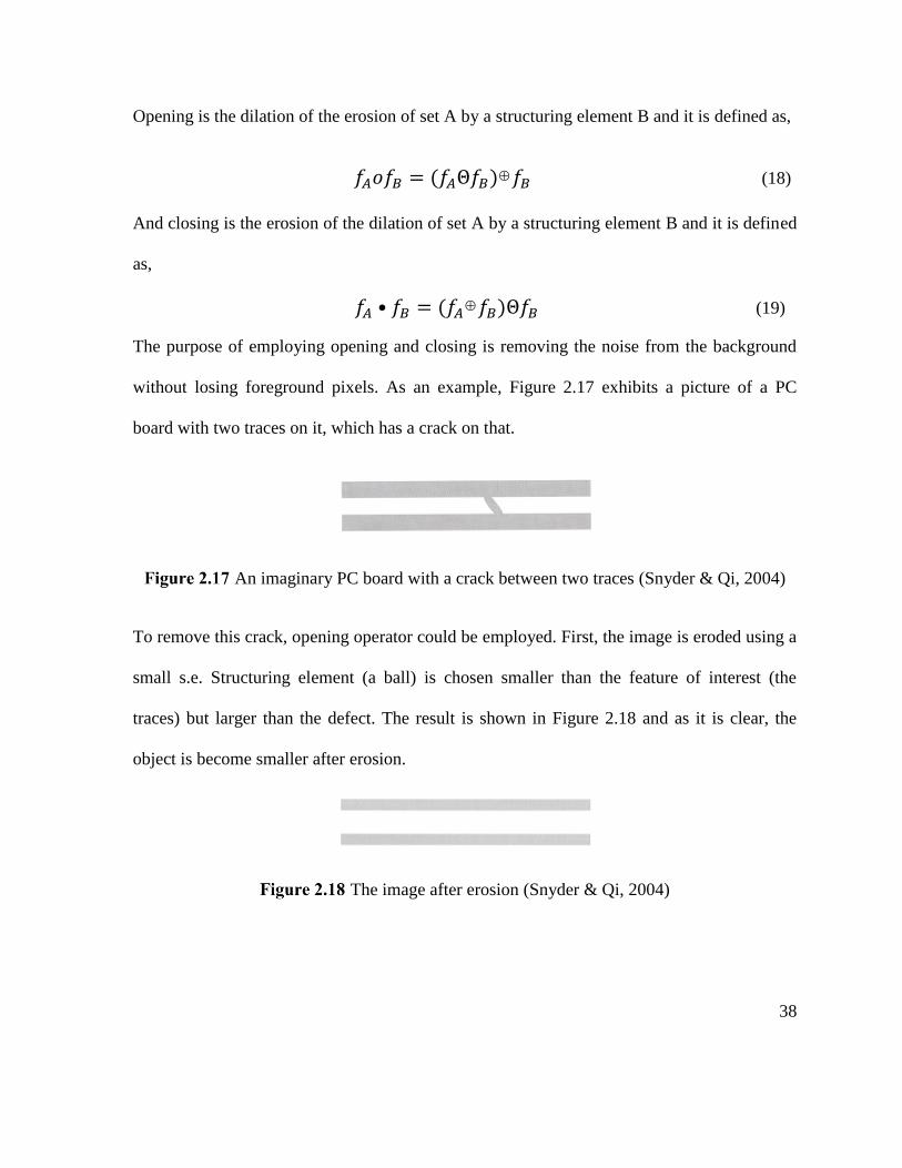
38

Opening is the dilation of the erosion of set A by a structuring element B and it is defined as,

𝑓𝐴𝑜𝑓𝐵 = (𝑓𝐴Θ𝑓𝐵) 𝑓𝐵 (18)

And closing is the erosion of the dilation of set A by a structuring element B and it is defined

as,

𝑓𝐴 • 𝑓𝐵 = (𝑓𝐴 𝑓𝐵)Θ𝑓𝐵 (19)

The purpose of employing opening and closing is removing the noise from the background

without losing foreground pixels. As an example, Figure 2.17 exhibits a picture of a PC

board with two traces on it, which has a crack on that.

An imaginary PC board with a crack between two traces (Snyder & Qi, 2004)

To remove this crack, opening operator could be employed. First, the image is eroded using a

small s.e. Structuring element (a ball) is chosen smaller than the feature of interest (the

traces) but larger than the defect. The result is shown in Figure 2.18 and as it is clear, the

object is become smaller after erosion.

The image after erosion (Snyder & Qi, 2004)

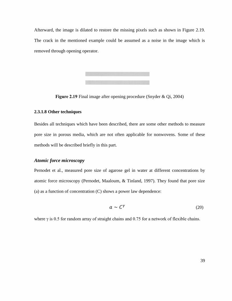
39

Afterward, the image is dilated to restore the missing pixels such as shown in Figure 2.19.

The crack in the mentioned example could be assumed as a noise in the image which is

removed through opening operator.

Final image after opening procedure (Snyder & Qi, 2004)

2.3.1.8 Other techniques

Besides all techniques which have been described, there are some other methods to measure

pore size in porous media, which are not often applicable for nonwovens. Some of these

methods will be described briefly in this part.

Atomic force microscopy

Pernodet et al., measured pore size of agarose gel in water at different concentrations by

atomic force microscopy (Pernodet, Maaloum, & Tinland, 1997). They found that pore size

(a) as a function of concentration (C) shows a power law dependence:

𝑎 ∼ 𝐶𝛾 (20)

where γ is 0.5 for random array of straight chains and 0.75 for a network of flexible chains.

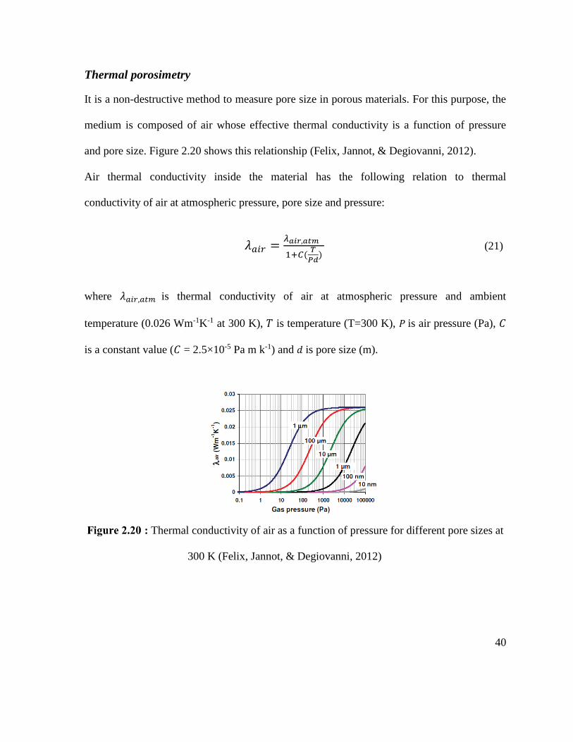
40

Thermal porosimetry

It is a non-destructive method to measure pore size in porous materials. For this purpose, the

medium is composed of air whose effective thermal conductivity is a function of pressure

and pore size. Figure 2.20 shows this relationship (Felix, Jannot, & Degiovanni, 2012).

Air thermal conductivity inside the material has the following relation to thermal

conductivity of air at atmospheric pressure, pore size and pressure:

𝜆𝑎𝑖𝑟 =𝜆𝑎𝑖𝑟,𝑎𝑡𝑚

1+𝐶(𝑇

𝑃𝑑)

(21)

where 𝜆𝑎𝑖𝑟,𝑎𝑡𝑚 is thermal conductivity of air at atmospheric pressure and ambient

temperature (0.026 Wm-1K-1 at 300 K), 𝑇 is temperature (T=300 K), 𝑃 is air pressure (Pa), 𝐶

is a constant value (𝐶 = 2.5×10-5 Pa m k-1) and 𝑑 is pore size (m).

: Thermal conductivity of air as a function of pressure for different pore sizes at

300 K (Felix, Jannot, & Degiovanni, 2012)

41

2.3.2 Pore volume and pore volume distribution

Pore volume could be defined as the ratio of air volume to total volume of a porous medium.

Among the aforementioned pore measurement methods, this parameter could be evaluated

through extrusion porosimetry, intrusion porosimetry and gas adsorption techniques, but flow

porometry cannot measure pore volume (Jena & Gupta, 2002). Each technique provides

different value as pore volume because each of them measure different pore sizes, and pore

dimeter considering in each technique is not identical.

In case of pore volume distribution, it could be defined through the following distribution

function:

𝑓𝑣 = −(𝑑𝑣

𝑑𝑙𝑜𝑔𝐷) (22)

The area under the curve in any pore’s diameter range represents pore volume in that range.

Same as pore volume, each technique provides different volume distribution because of

difference in measuring pore diameter. However, experiments show pore volume

distributions measured by mercury intrusion, non-mercury intrusion and gas adsorption

techniques are very close and extrusion porosimetry provides a higher volume associated

with the constricted pore diameter (Jena & Gupta, 2002).

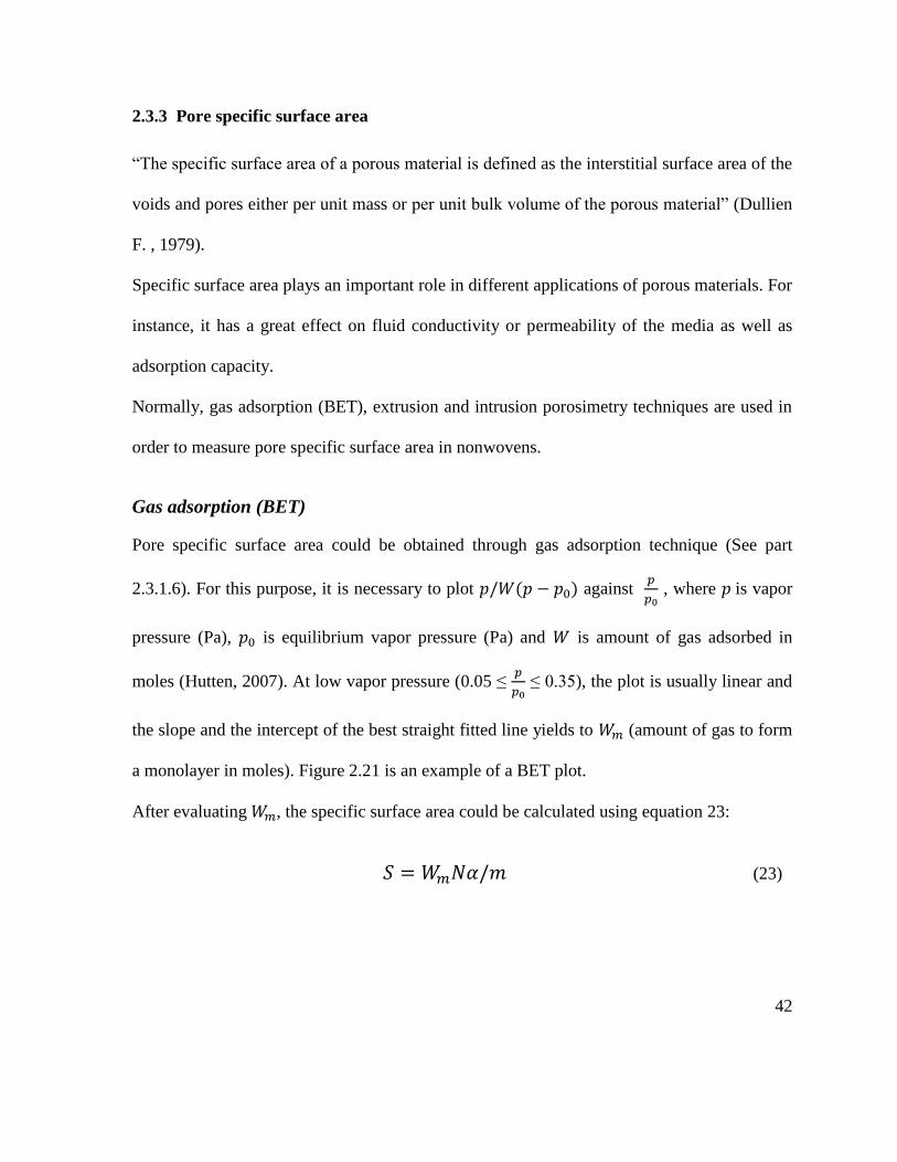
42

2.3.3 Pore specific surface area

“The specific surface area of a porous material is defined as the interstitial surface area of the

voids and pores either per unit mass or per unit bulk volume of the porous material” (Dullien

F. , 1979).

Specific surface area plays an important role in different applications of porous materials. For

instance, it has a great effect on fluid conductivity or permeability of the media as well as

adsorption capacity.

Normally, gas adsorption (BET), extrusion and intrusion porosimetry techniques are used in

order to measure pore specific surface area in nonwovens.

Gas adsorption (BET)

Pore specific surface area could be obtained through gas adsorption technique (See part

2.3.1.6). For this purpose, it is necessary to plot 𝑝/𝑊(𝑝 − 𝑝0) against 𝑝

𝑝0 , where 𝑝 is vapor

pressure (Pa), 𝑝0 is equilibrium vapor pressure (Pa) and 𝑊 is amount of gas adsorbed in

moles (Hutten, 2007). At low vapor pressure (0.05 ≤ 𝑝

𝑝0 ≤ 0.35), the plot is usually linear and

the slope and the intercept of the best straight fitted line yields to 𝑊𝑚 (amount of gas to form

a monolayer in moles). Figure 2.21 is an example of a BET plot.

After evaluating 𝑊𝑚, the specific surface area could be calculated using equation 23:

𝑆 = 𝑊𝑚𝑁𝛼/𝑚 (23)

43

where S is the specific surface area (cm2/g ), N is the Avogadro’s number (6.02 × 1023 atoms

or molecules/mole), 𝛼 is the cross sectional area of the adsorbed gas molecules (cm2) and 𝑚

is the mass of the specimen being tested (g) (Hutten, 2007) (Jena & Gupta, 2002).

: Linear variation of 𝑝/𝑊(𝑝 − 𝑝0) against 𝑝

𝑝0 for a nonwoven filter medium

(Jena & Gupta, 2002)

Extrusion and intrusion porosimetry

The specific pore surface area could be evaluated from the variation of pore volume with

pore diameter measured by extrusion and intrusion porosimetry techniques using equation 34

(Jena & Gupta, 2003):

𝑆 = ∫[ 4 𝐷⁄ ]𝑑𝑉 = 1

𝛾𝑐𝑜𝑠𝜃∫𝑝𝑑𝑉 (24)

where 𝐷 is pore diameter, 𝑑𝑉 is volume differential and 𝛾 is surface tension.

44

It is worth noting that, the result provided by BET is more accurate than intrusion

porosimetry because in intrusion technique, large integration errors are presented by large

changes in pressure due to small changes in volume. So, in this condition the surface area

will be overestimated (Jena & Gupta, 2002).

Surface area could be calculated through flow porometry using the relationship between flow

rate and external surface area (Kraus, Ross, & Girifalco, 1953) based on Kozeny-Carman’s

equation as well.

2.4 Theoretical modeling of pore size and pore size distribution

In order to evaluate pore size in nonwovens, many theoretical models have been developed

and in most of them, pore geometry is illustrated as a 3D pore body network connected by

fibers (Dullien, 1975) (Yanuka, et al., 1986) (Rawal, 2010). Some of the common models for

pore size and pore size distribution of nonwovens are listed below.

2.4.1 Simmonds’s model

Simmonds et al. determined open pore area and total number of pores using an analytical

technique and they succeeded to evaluate the mean pore area using the mentioned parameters

(Simmonds, Bomberger, & Bryner, 2007). In this study, they defined hydrodynamic pore

diameter as the ratio of pore area to pore wetted perimeter and performed the calculations

based on that. According to their analysis, mean pore diameter is directly related to fiber

diameter and inversely proportional to the coverage of fibers in fabric layers. It is worth

noting that in this model, it is assumed that pore shape is circle and regular.

45

𝐷𝑝,𝑚𝑖𝑛 = 2𝑤

𝑐=

2

𝑛𝑓𝑙 (25)

Where 𝐷𝑝,𝑚𝑖𝑛 is mean pore diameter, 𝑤 is fiber diameter, 𝑐 is total projected area of fibers

per unit area (i.e., coverage), 𝑛𝑓 is total number of fibers per unit area and 𝑙 is fiber length.

As noted in the literature, this theory is applicable if 𝑤 << 𝑙.

2.4.2 Abdel-Ghani’s model

Abdel-Ghani and Davis modeled nonwoven fabric network to meet pore size distribution

using Monte-Carlo simulation, numerically (Abdel-Ghani & Davis, 1985). They assumed

nonwoven fabric consists of many layers and cylindrical fibers make random orientation at

each layer and the space between fibers generates pores in each layer of nonwoven. Since, it

is assumed that fibers are straight, pores will be irregular external polygons. Thus, adding

successive layers can form 3D pores that have different cross sections and shapes. However,

assuming fibers as cylinders and nonwoven in homogenous random orientation decrease

accuracy of the model.

𝑛𝑝 = 0.1822 𝑛𝑓2.0458

(26)

where 𝑛𝑝 and 𝑛𝑓 are number of pores and number of fibers, respectively. They also

determined pore area employing fiber diameter:

𝑎𝑝 ≃ 𝜋𝜀𝑑𝑓

2

(1−𝜀)2 (27)

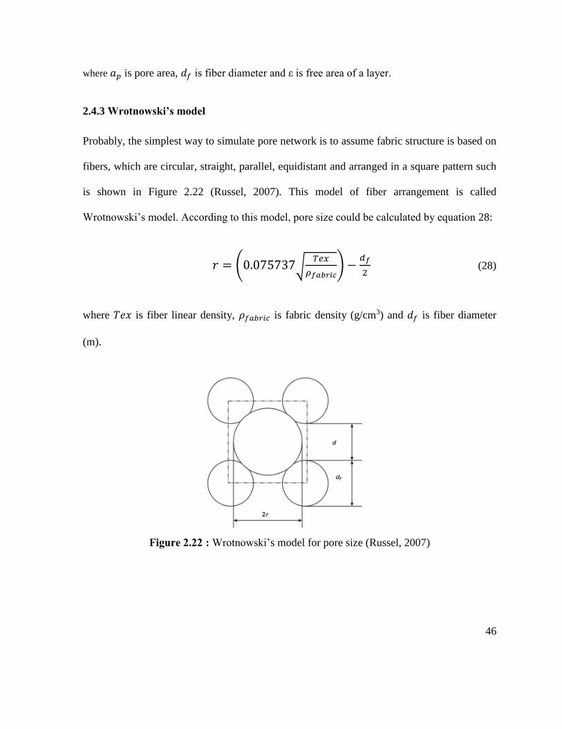
46

where 𝑎𝑝 is pore area, 𝑑𝑓 is fiber diameter and ε is free area of a layer.

2.4.3 Wrotnowski’s model

Probably, the simplest way to simulate pore network is to assume fabric structure is based on

fibers, which are circular, straight, parallel, equidistant and arranged in a square pattern such

is shown in Figure 2.22 (Russel, 2007). This model of fiber arrangement is called

Wrotnowski’s model. According to this model, pore size could be calculated by equation 28:

𝑟 = (0.075737√𝑇𝑒𝑥

𝜌𝑓𝑎𝑏𝑟𝑖𝑐) −

𝑑𝑓

2 (28)

where 𝑇𝑒𝑥 is fiber linear density, 𝜌𝑓𝑎𝑏𝑟𝑖𝑐 is fabric density (g/cm3) and 𝑑𝑓 is fiber diameter

(m).

: Wrotnowski’s model for pore size (Russel, 2007)

47

2.4.4 Goeminne’s model

This model has been established to predict the largest pore size (2𝑟max ) and mean pore size

(2𝑟)using porosity of nonwoven media (ε) (Russel, 2007), which are represented in equations

29 and 30:

Largest pore size: 𝑟𝑚𝑎𝑥 = 𝑑𝑓

2(1−𝜀) (29)

Mean pore size (porosity <0.9): 𝑟 =𝑑𝑓

4(1−𝜀) (30)

Furthermore, pore size (2𝑟) has been obtained using Hagen-Poiseuille’s law in fluid

dynamics for a cylindrical tube (Russel, 2007):

𝑟 = √8𝑘

𝜋

4 (31)

where 𝑘 is the specific permeability (m2).

2.4.5 Giroud’s model

Giroud proposed a theoretical equation to determine the filtration pore size of nonwoven

geotextiles (Russel, 2007),

𝑂𝑓 = [1

√1−𝜀− 1 +

𝜉𝜀𝑑𝑓

(1−𝜀)ℎ]𝑑𝑓 (32)

where 𝑑𝑓 is fiber diameter, 𝜀 is porosity, ℎ is fabric thickness, 𝜉 is an unknown dimensionless

parameter to be obtained by calibration with test data to account for further influence of

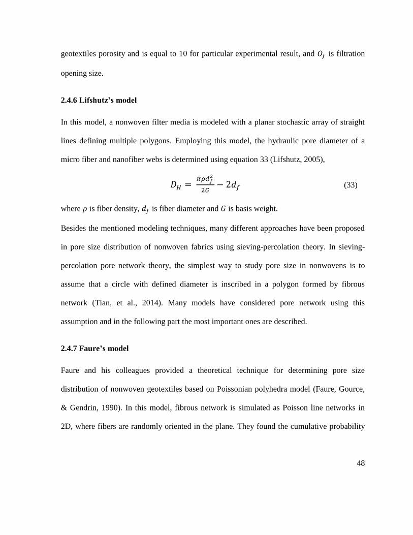
48

geotextiles porosity and is equal to 10 for particular experimental result, and 𝑂𝑓 is filtration

opening size.

2.4.6 Lifshutz’s model

In this model, a nonwoven filter media is modeled with a planar stochastic array of straight

lines defining multiple polygons. Employing this model, the hydraulic pore diameter of a

micro fiber and nanofiber webs is determined using equation 33 (Lifshutz, 2005),

𝐷𝐻 = 𝜋𝜌𝑑𝑓

2

2𝐺− 2𝑑𝑓 (33)

where 𝜌 is fiber density, 𝑑𝑓 is fiber diameter and 𝐺 is basis weight.

Besides the mentioned modeling techniques, many different approaches have been proposed

in pore size distribution of nonwoven fabrics using sieving-percolation theory. In sieving-

percolation pore network theory, the simplest way to study pore size in nonwovens is to

assume that a circle with defined diameter is inscribed in a polygon formed by fibrous

network (Tian, et al., 2014). Many models have considered pore network using this

assumption and in the following part the most important ones are described.

2.4.7 Faure’s model

Faure and his colleagues provided a theoretical technique for determining pore size

distribution of nonwoven geotextiles based on Poissonian polyhedra model (Faure, Gource,

& Gendrin, 1990). In this model, fibrous network is simulated as Poisson line networks in

2D, where fibers are randomly oriented in the plane. They found the cumulative probability

49

(𝐺(𝑑)) of obtaining an inscribed circle (as a pore) between fibers with a diameter equal to or

less than 𝑑 (See Figure 2.23), which is shown as:

𝐺(𝑑) = 1 − {2+𝜒(𝑑+𝐷)

2+𝜒𝐷}𝑒−𝜒𝑑 (34)

and

𝜒 =4𝜇

𝜋𝑇𝐷𝜌 (35)

: Network of straight lines (fibers) obtained by the Poissonian polyhedra model

(Faure, Gource, & Gendrin, 1990)

where 𝜒 is the specific length representing the total length of lines per unit area, 𝑑 is diameter

of inscribed circle, 𝜇 is mass per unit area of fabric, 𝑇 is fabric thickness, 𝐷 is fiber diameter

and 𝜌 is sheet density. It is worth noting that pore is assumed as a disc with axes

perpendicular to the sheet plane and the length of each discs are defined as the fiber diameter.

Thus, the gradation of the conduit offers the cumulative probability of the particle passage

through the nonwoven:

50

𝑄(𝑑) = 1 − [1 − 𝐺(𝑑)]𝑇

𝐷⁄ (36)

where 𝑄(𝑑) is the probability of a particle passing through a pore with diameter 𝑑.

2.4.8 Lombard’s model

In this model, same analogy of Poisson’s polyhedra theory is used to obtain the probability of

diameter distribution of a circle inscribed in a polygon, i.e., 𝐾(𝑑) (Lombard, Rollin, &

Wolff, 1986):

𝐾(𝑑) = (𝜎2𝑑2

4+ 𝜎𝑑 + 1) exp (−𝜎𝑑) (37)

and

𝜎 =8𝜇

𝜋𝑇𝐷𝜌 (38)

where 𝜎 is the specific length, representing the total length of the lines per unit area.

Equation 37, shows the cumulative probability of achieving maximum conduit/particle

diameter (𝑑); however, the particle should travel through the nonwoven layers. Therefore, the

cumulative probability of passage of particles of diameter "𝑑" through the nonwoven layers

(𝐹𝑓(𝑑)) has been defined as:

𝐹𝑓(𝑑) = 1 − [𝐾(𝑑)]𝑇/2𝐷 (39)

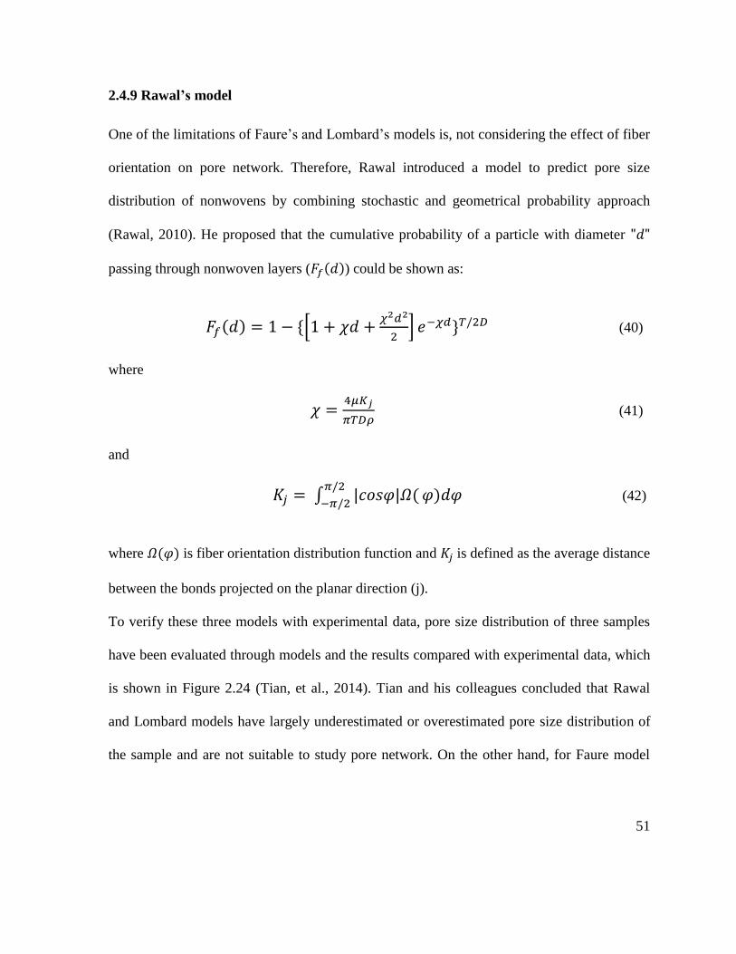
51

2.4.9 Rawal’s model

One of the limitations of Faure’s and Lombard’s models is, not considering the effect of fiber

orientation on pore network. Therefore, Rawal introduced a model to predict pore size

distribution of nonwovens by combining stochastic and geometrical probability approach

(Rawal, 2010). He proposed that the cumulative probability of a particle with diameter "𝑑"

passing through nonwoven layers (𝐹𝑓(𝑑)) could be shown as:

𝐹𝑓(𝑑) = 1 − {[1 + 𝜒𝑑 +𝜒2𝑑2

2] 𝑒−𝜒𝑑}𝑇/2𝐷 (40)

where

𝜒 =4𝜇𝐾𝑗

𝜋𝑇𝐷𝜌 (41)

and

𝐾𝑗 = ∫ |𝑐𝑜𝑠𝜑|𝛺(𝜋/2

−𝜋/2𝜑)𝑑𝜑 (42)

where 𝛺(𝜑) is fiber orientation distribution function and 𝐾𝑗 is defined as the average distance

between the bonds projected on the planar direction (j).

To verify these three models with experimental data, pore size distribution of three samples

have been evaluated through models and the results compared with experimental data, which

is shown in Figure 2.24 (Tian, et al., 2014). Tian and his colleagues concluded that Rawal

and Lombard models have largely underestimated or overestimated pore size distribution of

the sample and are not suitable to study pore network. On the other hand, for Faure model

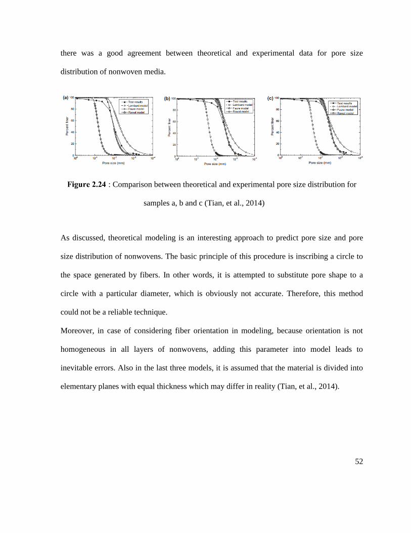
52

there was a good agreement between theoretical and experimental data for pore size

distribution of nonwoven media.

: Comparison between theoretical and experimental pore size distribution for

samples a, b and c (Tian, et al., 2014)

As discussed, theoretical modeling is an interesting approach to predict pore size and pore

size distribution of nonwovens. The basic principle of this procedure is inscribing a circle to

the space generated by fibers. In other words, it is attempted to substitute pore shape to a

circle with a particular diameter, which is obviously not accurate. Therefore, this method

could not be a reliable technique.

Moreover, in case of considering fiber orientation in modeling, because orientation is not

homogeneous in all layers of nonwovens, adding this parameter into model leads to

inevitable errors. Also in the last three models, it is assumed that the material is divided into

elementary planes with equal thickness which may differ in reality (Tian, et al., 2014).

53

2.5 Permeability

Permeability is used for the conductivity of the porous medium regarding to permeation by a

Newtonian fluid (Dullien F. , 1979). Permeability as a general concept leads to some

inaccuracies because its value may vary with the properties of the permeating fluid and the

permeation mechanism in the same porous samples. Therefore, it is more useful and

scientific to use specific permeability, which is not dependent to fluid properties and flow

mechanism. However, in this monograph permeability is used as specific permeability for

short.

In most literature, Darcy and m2 are two main units representing permeability (1 Darcy =

10-12 m2). Also, permeability could be shown by some other units, such as Frazier and Gurley

as well.

There are many structural parameters affecting permeability in nonwoven materials, such as

solidity (Bear, 1988), fiber packing density (Chen & Papathanasiou, 2006) (Chen &

Papathanasiou, 2008),basis weight, thickness, density, fiber diameter, fiber cross section and

fiber crimp frequency (Subramaniam, Madhusoothanan, & Debanth, 1988) (Atwal, 1987)

(Berkalp, 2006) (Cincik & Koc, 2012). It was shown that air permeability decreases by

increasing the basis weight, thickness and density of fabric and decreasing the fiber diameter

(Cincik & Koc, 2012). Web uniformity could be another parameter affecting permeability,

which is not extensively studied yet.

In the following part some empirical and theoretical methods in permeability evaluation of

nonwovens will be provided.

54

2.5.1 Empirical techniques to measure permeability of nonwovens

Generally, to determine permeability, flow rate through the nonwoven media is evaluated and

employing Darcy’s law, permeability could be calculated. In the next part, the common

methods to measure flow rate in nonwovens are explained.

2.5.1.1 Determining the flow rate using common pore measurement techniques

There are many simple devices available for permeability testing of nonwovens. Among the

five common methods which have multiple tests capability, flow porometery is the only

technique which can measure gas permeability (Jena & Gupta, 2002). In this method, flow

porometer can measure permeability of different gases over a wide range of pressure and

temperature.

In case of liquid permeability, flow porometry and extrusion porosimetry are used to measure

liquid permeability of nonwoven media. Flow porometer measures liquid flow rate, when

pressure is increased on excess liquid maintained on the sample in the porometer. In

extrusion porosimetry, the extrusion porometer measures flow rate at similar conditions,

when the membrane is removed from underneath the sample (See Figure 2.9b) (Jena &

Gupta, 2003).

Determining the permeability using Darcy’s law

Darcy through his experimental procedures discovered that the volumetric flow rate 𝑄 within

a porous material (m3/s) is directly proportional to the cross section area 𝐴 (m2), pressure

drop across the porous media Δ𝑃 (Pa) and inversely proportional to thickness 𝑇 (m) of the

55

sample and fluid viscosity 𝜇 (Pa.s). Based on his observations, he proposed the following

equation, which is famously called Darcy’s law:

𝑄 =𝑘

𝜇

𝐴

𝑇Δ𝑃 (43)

The constant value of 𝑘 represents the permeability of the medium (m2). It is worth noting

that considering Darcy’s law using capillary length and surface area leads to another form of

equation 43, such is shown in equation 44,

𝑄 =𝑘

𝜇

𝐴

𝑙 Δ𝑃 (44)

where 𝐴 and 𝑙 are capillary surface area and length, respectively (Russel, 2007) (Dullien,

1979).

As it is shown, Darcy’s law connects permeability to flow rate through the porous material

using the pressure drop within the conduit and capillary geometry. To simplify the

calculations, it is assumed that capillary is a regular cylinder with circular cross sections.

Clearly, measuring flow rate through the medium through experiments in a particular

pressure drop results in determining the permeability, employing surface area and thickness

of the sample in equation 43.

2.5.2 Theoretical models to predict permeability of nonwovens

Many attempts have been performed to develop theoretical models in order to predict

permeability of fibrous structures. A brief review on these developments will be given in this

section.

56

Davies through a dimensional analysis showed that only a function of solid volume fraction

and fiber diameter are the parameters affecting permeability (Davies, 1973):

𝑓 (Δ𝑃

𝑇, 𝑈, 𝑟, 𝜙, 𝜇, 𝜌,

𝜆

𝑟) = 0 (45)

where Δ𝑃 is pressure drop, 𝑇 is thickness, U is superficial velocity (𝑄

𝐴), 𝑟 is fiber radius, 𝜙 is

solid volume fraction, 𝜇 is dynamic viscosity of fluid, 𝜌 is density of fluid and 𝜆 is mean free

path length of molecules. In fluid dynamics, 𝜆

𝑟 is known as knudsen’s number, which is

dimensionless.

According to Buckingham’s theorem (Buckingham, 1914), these seven parameters could be

decreased into four dimensionless units, as shown in equation 46:

𝑓 (𝑈𝑇𝜇

Δ𝑃𝑟2,𝑈𝑟𝜌

𝜇, 𝜙,

𝜆

𝑟) = 0 (46)

The first parameter is the Darcy’s law written in terms of dimensionless permeability( 𝑘

𝑟2 ),

second dimensionless number is Reynold’s number, which could be ignored if the velocity is

low. Knudsen’s number could be also ignored assuming there is no molecular slip on fiber

surface. Therefore, the dimensionless permeability factor could be shown as a function of

solid volume fraction:

𝑘

𝑟2= 𝑓(𝜙) (47)

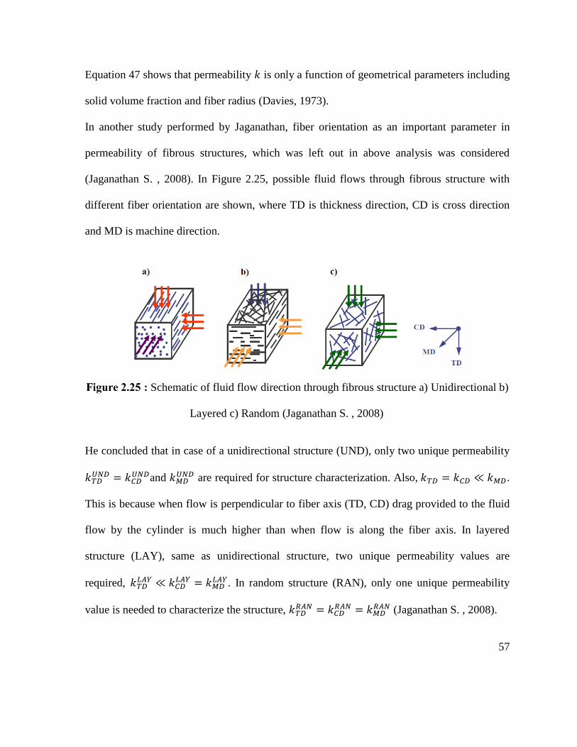
57

Equation 47 shows that permeability 𝑘 is only a function of geometrical parameters including

solid volume fraction and fiber radius (Davies, 1973).

In another study performed by Jaganathan, fiber orientation as an important parameter in

permeability of fibrous structures, which was left out in above analysis was considered

(Jaganathan S. , 2008). In Figure 2.25, possible fluid flows through fibrous structure with

different fiber orientation are shown, where TD is thickness direction, CD is cross direction

and MD is machine direction.

: Schematic of fluid flow direction through fibrous structure a) Unidirectional b)

Layered c) Random (Jaganathan S. , 2008)

He concluded that in case of a unidirectional structure (UND), only two unique permeability

𝑘𝑇𝐷𝑈𝑁𝐷 = 𝑘𝐶𝐷

𝑈𝑁𝐷and 𝑘𝑀𝐷𝑈𝑁𝐷 are required for structure characterization. Also, 𝑘𝑇𝐷 = 𝑘𝐶𝐷 ≪ 𝑘𝑀𝐷.

This is because when flow is perpendicular to fiber axis (TD, CD) drag provided to the fluid

flow by the cylinder is much higher than when flow is along the fiber axis. In layered

structure (LAY), same as unidirectional structure, two unique permeability values are

required, 𝑘𝑇𝐷𝐿𝐴𝑌 ≪ 𝑘𝐶𝐷

𝐿𝐴𝑌 = 𝑘𝑀𝐷𝐿𝐴𝑌. In random structure (RAN), only one unique permeability

value is needed to characterize the structure, 𝑘𝑇𝐷𝑅𝐴𝑁 = 𝑘𝐶𝐷

𝑅𝐴𝑁 = 𝑘𝑀𝐷𝑅𝐴𝑁 (Jaganathan S. , 2008).

58

Several studies have been performed in order to describe fluid flow through porous media

and consequently, many models have been developed. In this part, some of the most

important and the popular ones are described briefly.

2.5.2.1 Drag model

Drag model is based on calculating the force per unit length (F) experienced by a fiber in a

fluid flow. The dimensionless form of permeability should be the referenced in order to

develop the model (Higdon & Ford, 1996):

𝑘

𝑟2=

𝜇𝑄

𝐺𝐴𝑟2 (48)

where 𝐺 is magnitude of mean pressure gradient ∇P. Dimensionless force per unit length of

fiber could be calculated as:

𝐹

𝜇𝑈=

𝐺𝐴𝜋𝑟2

𝜇𝑄𝜙 (49)

where 𝜙 is solid volume fraction. From equations 48 and 49, the relationship between

dimensionless permeability and dimensionless force per unit length will be obtained (Higdon

& Ford, 1996) (Clague & Philips, 1997):

𝑘

𝑟2=

𝜋

𝐹𝜙 (50)

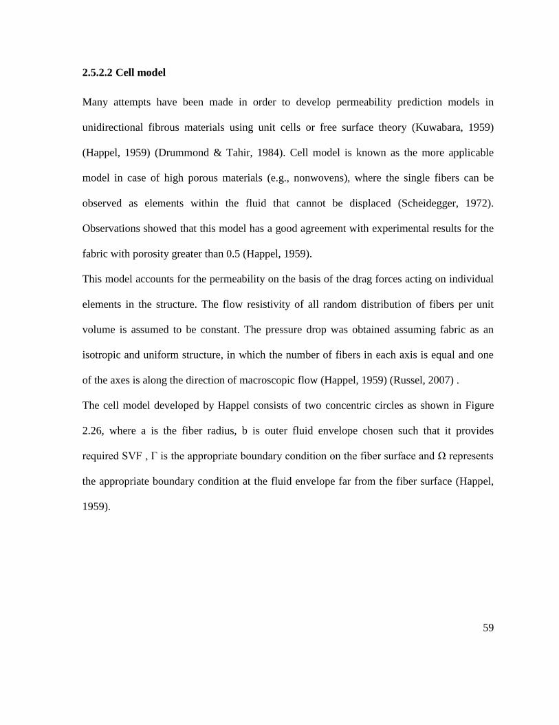
59

2.5.2.2 Cell model

Many attempts have been made in order to develop permeability prediction models in

unidirectional fibrous materials using unit cells or free surface theory (Kuwabara, 1959)

(Happel, 1959) (Drummond & Tahir, 1984). Cell model is known as the more applicable

model in case of high porous materials (e.g., nonwovens), where the single fibers can be

observed as elements within the fluid that cannot be displaced (Scheidegger, 1972).

Observations showed that this model has a good agreement with experimental results for the

fabric with porosity greater than 0.5 (Happel, 1959).

This model accounts for the permeability on the basis of the drag forces acting on individual

elements in the structure. The flow resistivity of all random distribution of fibers per unit

volume is assumed to be constant. The pressure drop was obtained assuming fabric as an

isotropic and uniform structure, in which the number of fibers in each axis is equal and one

of the axes is along the direction of macroscopic flow (Happel, 1959) (Russel, 2007) .

The cell model developed by Happel consists of two concentric circles as shown in Figure

2.26, where a is the fiber radius, b is outer fluid envelope chosen such that it provides

required SVF , Γ is the appropriate boundary condition on the fiber surface and Ω represents

the appropriate boundary condition at the fluid envelope far from the fiber surface (Happel,

1959).

60

: Cell model of fibrous structure (Jaganathan S. , 2008)

Happel, based on these boundary conditions proposed an analytical solution for permeability

for the flow parallel to fiber axis,

𝑘

𝑟2=

1

4𝜙(−𝑙𝑛𝜙 −

3

2+ 2𝜙 −

𝜙2

2) (51)

And the analytical model with the same boundary conditions with zero shear stress at the

perimeter for the flow perpendicular to fiber axis is proposed as:

𝑘

𝑟2=

1

8𝜙(−𝑙𝑛𝜙 +

𝜙2−1

𝜙2+1) (52)

Kuwabara used a similar kind of cell model but changing zero shear stress boundary

condition to zero vorticity boundary condition on Ω (Kuwabara, 1959). The solution for fluid

flow perpendicular to fiber axis is given by:

𝑘

𝑟2=

1

8𝜙(−𝑙𝑛𝜙 −

3

2+ 2𝜙) (53)

Experimental data provided by Fuchs and Krisch showed that Kuwabara’s assumption and

model led to more accurate results than Happel’s (Fuchs & Krisch, 1968).

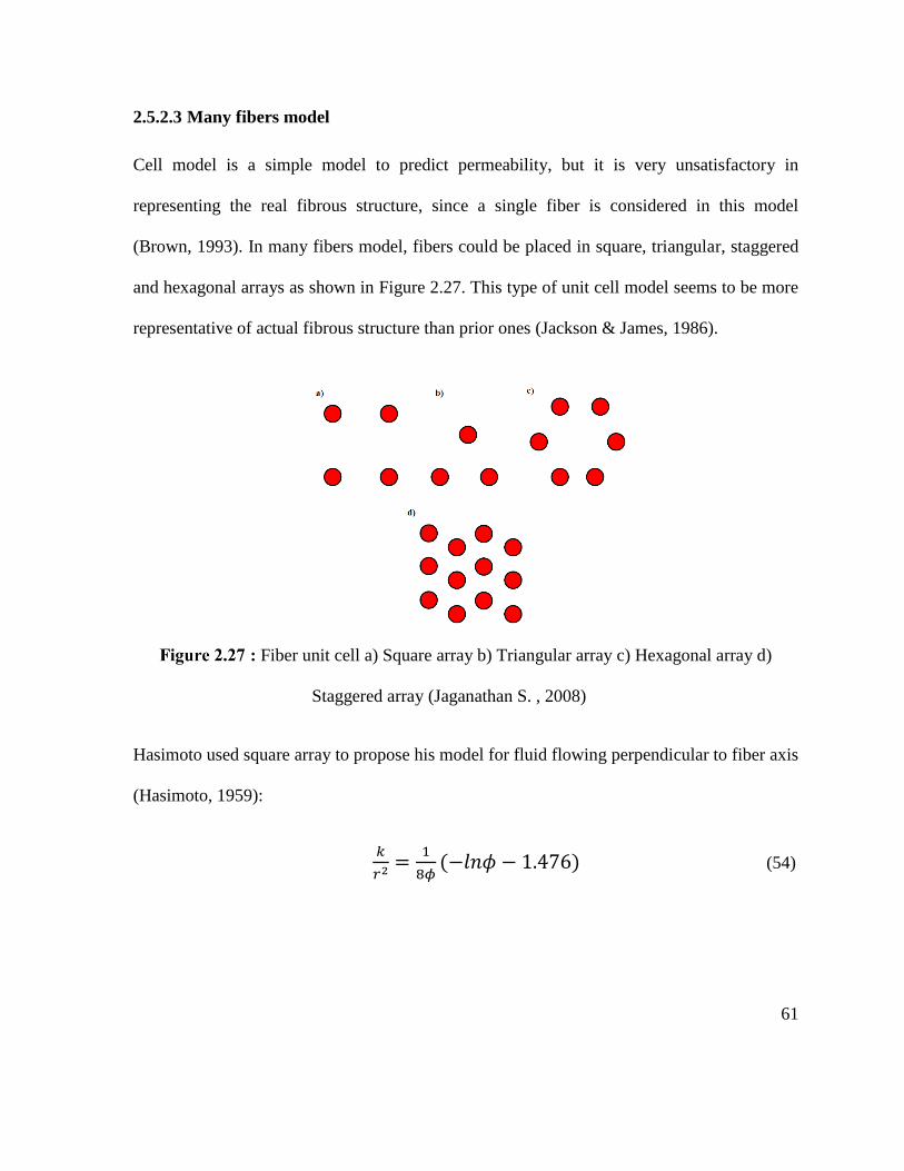
61

2.5.2.3 Many fibers model

Cell model is a simple model to predict permeability, but it is very unsatisfactory in

representing the real fibrous structure, since a single fiber is considered in this model

(Brown, 1993). In many fibers model, fibers could be placed in square, triangular, staggered

and hexagonal arrays as shown in Figure 2.27. This type of unit cell model seems to be more

representative of actual fibrous structure than prior ones (Jackson & James, 1986).

: Fiber unit cell a) Square array b) Triangular array c) Hexagonal array d)

Staggered array (Jaganathan S. , 2008)

Hasimoto used square array to propose his model for fluid flowing perpendicular to fiber axis

(Hasimoto, 1959):

𝑘

𝑟2=

1

8𝜙(−𝑙𝑛𝜙 − 1.476) (54)

62

Drummond and Tahir found equation 55 for flow perpendicular to square array using many

fibers model (Drummond & Tahir, 1984),

𝑘

𝑟2=

1

8𝜙(−𝑙𝑛𝜙 − 1.476 + 2𝜙 − 1.774𝜙2 + 𝑂(𝜙2)) (55)

where 𝑂(𝜙2) is elliptic function.

Jackson and James reported that all mentioned models are almost identical (Jackson &

James, 1986) however; Clague and Philips (Clague & Philips, 1997) proved that these array

type cell models are just valid for 𝜙 < 0.3.

Many different models to predict permeability of fibrous structures have been reviewed in

the literature. However, most of them are based on idealistic fibrous structure, where the

orientation is uniform and fibers are cylindrical. These assumptions are for ease of

calculations but the ultimate results could be far from reality.

2.6 Skeletonization (Topological skeleton)

One of the most important approaches to represent the structural shape of a plane region is

reducing it to a graph. This is usually accomplished by obtaining the skeleton of the region

via skeletonizing (or thinning) algorithm (Gonzalez & Wintz, 1987). The most important

target of skeletonization process is to extract a region-based shape feature representing the

general form of an object.

63

Skeletonization process reduces the foreground regions in a binary image to a skeletal

remnant, which preserves the contour and connectivity of the original region, while most of

the original foreground pixels are thrown away. The skeleton represents the geometrical and

topological properties of the shape such as its connectivity, topology, length, direction and

width. It is worth noting that together with the distance of its point to the boundary, skeleton

can provide shape of the object (Dougherty, 1992). This technique is very important in a

number of applications such as pattern recognition, data compression and data storage

(Saeed, Tabedzki, Rybnik, & Adamski, 2010).

The skeleton of a region could be defined via the medial axis transformation (MAT), which

is proposed by Blum (Gonzalez & Wintz, 1987). MAT determines the closest boundary point

(s) for each point of the object. The inner point is located on the skeleton, if it has at least two

closest boundary points. Figure 2.28 shows some examples of the original images and their

associated skeleton obtained through thinning algorithms.

The skeleton through MAT technique could be achieved through two main ways: First is

using some kind of morphological thinning in order to erode pixels from the boundary, until

no more thinning is possible. In this case, the points which are remained approximate the

skeleton. The second method is applying distance map (distance transform) on the image.

Distance map results the centerlines of the object as the compact representations of the data

(Fouard, Malandian, Prohaska, & Westerhoff, 2006). Distance map algorithm provides a gray

level image, where the value of each object point corresponds to its shortest distance to the

background. The result of the distance transform is similar to the original input image except

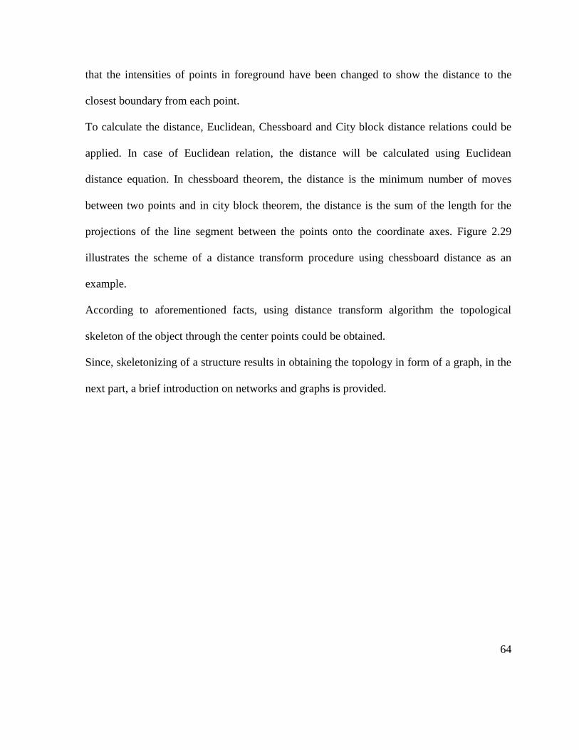
64

that the intensities of points in foreground have been changed to show the distance to the

closest boundary from each point.

To calculate the distance, Euclidean, Chessboard and City block distance relations could be

applied. In case of Euclidean relation, the distance will be calculated using Euclidean

distance equation. In chessboard theorem, the distance is the minimum number of moves

between two points and in city block theorem, the distance is the sum of the length for the

projections of the line segment between the points onto the coordinate axes. Figure 2.29

illustrates the scheme of a distance transform procedure using chessboard distance as an

example.

According to aforementioned facts, using distance transform algorithm the topological

skeleton of the object through the center points could be obtained.

Since, skeletonizing of a structure results in obtaining the topology in form of a graph, in the

next part, a brief introduction on networks and graphs is provided.

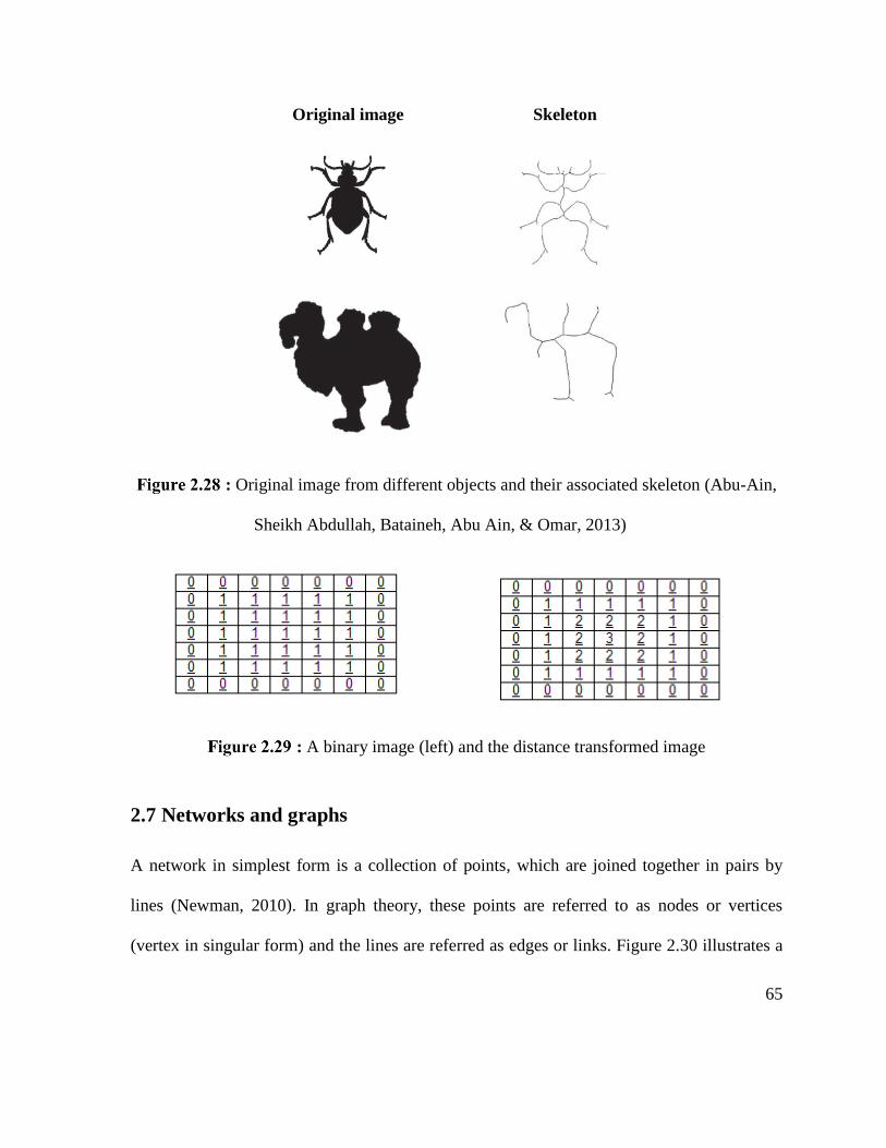
65

Original image Skeleton

: Original image from different objects and their associated skeleton (Abu-Ain,

Sheikh Abdullah, Bataineh, Abu Ain, & Omar, 2013)

: A binary image (left) and the distance transformed image

2.7 Networks and graphs

A network in simplest form is a collection of points, which are joined together in pairs by

lines (Newman, 2010). In graph theory, these points are referred to as nodes or vertices

(vertex in singular form) and the lines are referred as edges or links. Figure 2.30 illustrates a

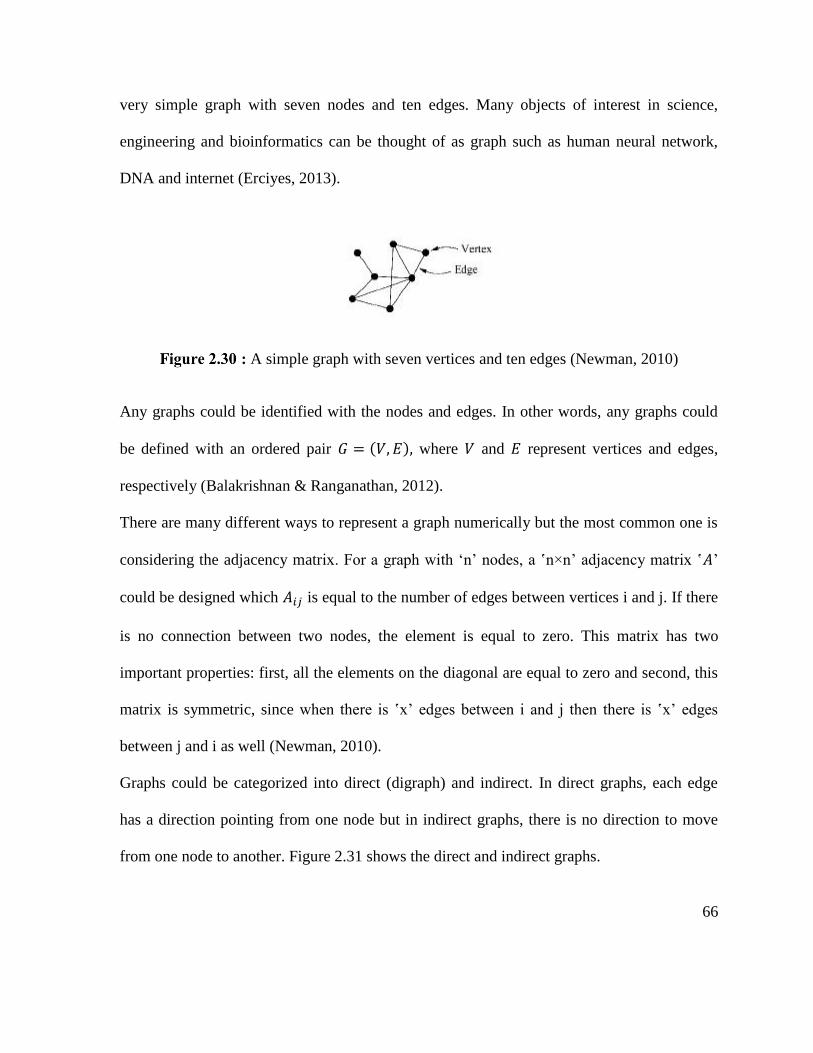
66

very simple graph with seven nodes and ten edges. Many objects of interest in science,

engineering and bioinformatics can be thought of as graph such as human neural network,

DNA and internet (Erciyes, 2013).

: A simple graph with seven vertices and ten edges (Newman, 2010)

Any graphs could be identified with the nodes and edges. In other words, any graphs could

be defined with an ordered pair 𝐺 = (𝑉, 𝐸), where 𝑉 and 𝐸 represent vertices and edges,

respectively (Balakrishnan & Ranganathan, 2012).

There are many different ways to represent a graph numerically but the most common one is

considering the adjacency matrix. For a graph with ‘n’ nodes, a ‛n×n’ adjacency matrix ‛𝐴’

could be designed which 𝐴𝑖𝑗 is equal to the number of edges between vertices i and j. If there

is no connection between two nodes, the element is equal to zero. This matrix has two

important properties: first, all the elements on the diagonal are equal to zero and second, this

matrix is symmetric, since when there is ‛x’ edges between i and j then there is ‛x’ edges

between j and i as well (Newman, 2010).

Graphs could be categorized into direct (digraph) and indirect. In direct graphs, each edge

has a direction pointing from one node but in indirect graphs, there is no direction to move

from one node to another. Figure 2.31 shows the direct and indirect graphs.

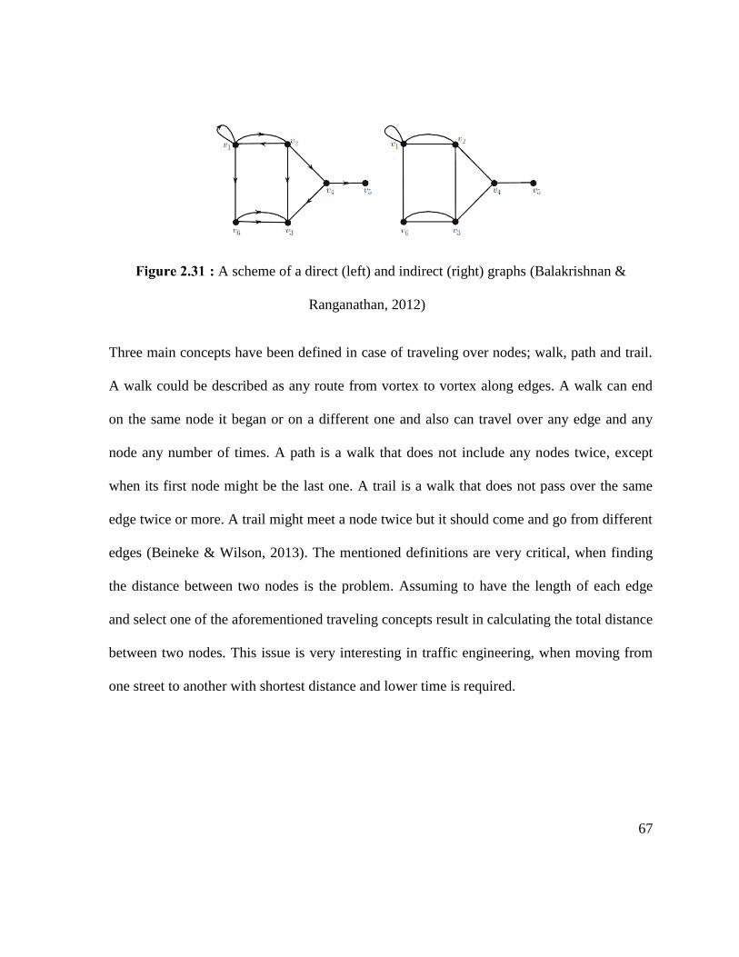
67

: A scheme of a direct (left) and indirect (right) graphs (Balakrishnan &

Ranganathan, 2012)

Three main concepts have been defined in case of traveling over nodes; walk, path and trail.

A walk could be described as any route from vortex to vortex along edges. A walk can end

on the same node it began or on a different one and also can travel over any edge and any

node any number of times. A path is a walk that does not include any nodes twice, except

when its first node might be the last one. A trail is a walk that does not pass over the same

edge twice or more. A trail might meet a node twice but it should come and go from different

edges (Beineke & Wilson, 2013). The mentioned definitions are very critical, when finding

the distance between two nodes is the problem. Assuming to have the length of each edge

and select one of the aforementioned traveling concepts result in calculating the total distance

between two nodes. This issue is very interesting in traffic engineering, when moving from

one street to another with shortest distance and lower time is required.

68

3. Problem Statement

69

3.1 Introduction

Several methods have been developed in order to evaluate pore characteristics of nonwovens.

Pore size, pore volume and pore specific surface area are the most important characteristics

of pore structure in porous materials and many attempts have been made in order to evaluate

these parameters. Among all mentioned characteristics, pore size because of its significant

effects on many properties such as fluid flow and barrier property are more critical and most

of the works have been done to measure this parameter (Jena & Gupta, 2002).

Pore size could be evaluated through different procedures such as experimental techniques,

image analysis and theoretical modeling (Huttenn, 2007) (Gong & Newton, 1992) (Xu, 1996)

(Rawal, 2010). Each method has its own advantages and disadvantages and depends on final

target, one of the mentioned techniques would be selected.

In case of experimental methods, each evaluation technique has a particular definition for

pore especially for pore size. In other words, each technique measures different diameter as

pore size and for this reason, the results are not identical and comparable (See Figure 2.12).

Moreover, a pore has many convergences / divergences along its length and the available

techniques have not this ability to evaluate all pore diameters in the structure, therefore the

reported values are not very accurate.

Besides the experimental methods, 2D image analysis is widely used to determine pore size.

In this technique, image processing algorithms are applied on a 2D image taken from a

porous nonwoven surface. In this method, since all evaluation procedures are performed in

two dimensions (CD and MD) the information of third direction (TD) would be completely

70

missed. Therefore, this method cannot study pore structure in 3D. However, this method is

commonly used to measure pore size of membranes, since a membrane contains many pores

with same diameters.

Theoretical modeling is another approach to study pore size of nonwoven media. In this

method, the space between fibers is mostly defined as a circular area and pore size or pore

size distribution of nonwovens are predicted through different models, which are described in

the previous chapter.

Moreover, to study pore structure of nonwovens experimental and theoretical modeling

methods could be utilized to evaluate permeability of the media, since it is one of the major

consequences of pore structure in nonwovens. In case of experimental techniques flow

porometry is normally employed to measure gas permeability and flow porometry and

extrusion porosimetry are used to evaluate liquid permeability of nonwoven fabrics (Jena &

Gupta, 2002). Since in experimental techniques, real fabric is required for testing procedures

many attempts have been performed to model permeability based on nonwoven structural

parameters to predict permeability. In most of these models such as Drag model and Cell

model, it is tried to define permeability as a function of fiber diameter and solid volume

fraction.

3.2 Problem statement

As it is described, none of the available empirical techniques are accurate enough to evaluate

pore characteristics of nonwovens, since each technique considers different diameter as pore

71

size. Meanwhile, in all mentioned techniques pore is assumed as a cylindrical capillary with

regular diameter along the length with no divergences/convergences.

Moreover, image analysis is not able to study pore structure in 3D and all obtained data is

based on 2D images (e.g. SEM). Therefore, it could not be an accurate technique to

characterize pore structure, since 2D image is not a suitable representative for a 3D structure.

Furthermore, in theoretical modeling a circle or a regular polygon is considered as the space

between fibers and the model tries to calculate the diagonal as pore size. Clearly, the space

between fibers has not a regular shape thus, theoretical models do not provide a reliable

prediction for pore diameter and other pore characteristics.

In case of permeability, experimental techniques find permeability using porous nature of

nonwovens rather than using pore characteristics. In other words, they measure flow rate

through the media and employing thickness and surface area of the sample, permeability

would be calculated using fluid mechanics equations (e.g., Darcy’s law). This means in these

methods, permeability is measured indirectly. In indirect evaluation methods, the desired

characteristic is determined by measuring other parameters and then it is calculated through

some relations.

The goal of this research is studying pore structure of nonwovens with 3D image analysis.

For this purpose, the image acquision is implemented through DVI and micro CT and

applying image analysis technique on the image, all the pores available in the structure will

be obtained. Afterwards, employing the pore information a model will be deveopled to

predict permeability of nonwovens, as the main consequence of the pore structure.

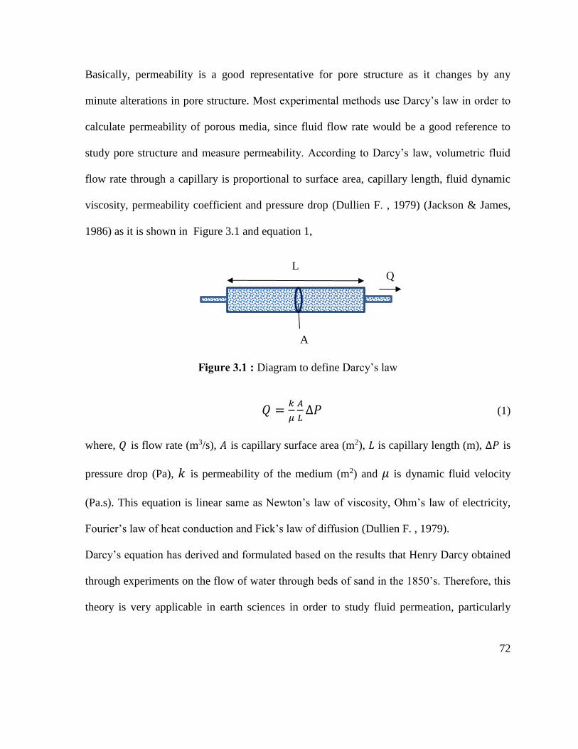
72

Basically, permeability is a good representative for pore structure as it changes by any

minute alterations in pore structure. Most experimental methods use Darcy’s law in order to

calculate permeability of porous media, since fluid flow rate would be a good reference to

study pore structure and measure permeability. According to Darcy’s law, volumetric fluid

flow rate through a capillary is proportional to surface area, capillary length, fluid dynamic

viscosity, permeability coefficient and pressure drop (Dullien F. , 1979) (Jackson & James,

1986) as it is shown in Figure 3.1 and equation 1,

Diagram to define Darcy’s law

𝑄 =𝑘

𝜇

𝐴

𝐿∆𝑃 (1)

where, 𝑄 is flow rate (m3/s), 𝐴 is capillary surface area (m2), 𝐿 is capillary length (m), ∆𝑃 is

pressure drop (Pa), 𝑘 is permeability of the medium (m2) and 𝜇 is dynamic fluid velocity

(Pa.s). This equation is linear same as Newton’s law of viscosity, Ohm’s law of electricity,

Fourier’s law of heat conduction and Fick’s law of diffusion (Dullien F. , 1979).

Darcy’s equation has derived and formulated based on the results that Henry Darcy obtained

through experiments on the flow of water through beds of sand in the 1850’s. Therefore, this

theory is very applicable in earth sciences in order to study fluid permeation, particularly

L Q

A

73

water. In porous materials such as nonwovens, pores configuration is not the same as bed of

sands and the closest arrangement to pore network could be a series of capillaries, which are

interconnected and fluid is flowing through. For that reason, Darcy’s law does not work for

such system in pore scale (micro scale).

Moreover, available theoretical models would not be reliable in prediction of permeability

since many assumptions have been assigned to start modeling of permeability such as

ignoring fibers slippage during flow or regularity of pore size and etc.

According to aforementioned facts, developing a new methodology to find characteristics of

all the pore in the structure looks necessary, since a single number cannot represent whole

network. In the following chapters, a novel method to study pore structure of nonwovens is

provided.

74

4. 3D Image Acquisition and Processing

75

4.1 Introduction

The main goal of this research is characterizing diameter of all the pores available in the

nonwovens structure and in this regard, the 3D structural image of the nonwovens will be

utilized. After obtaining 3D image of nonwoven media, the pore network will be extracted by

skeletonizing the 3D image through Avizo® software. In this circumstance, pore structure is

exhibited in form of a graph and many important information of this graph, such as pores

diameter and pores connectivity will be derermined.

Due to 3D nature of fibrous materials, 2D images would not be a trustworthy reference to

study pore structure. Basically, 3D imaging techniques help to understand the unknown part

of a fibrous structure that is overlooked in 2D methods. Obviously, 3D images provide better

overviews of pore structure than 2D images such as SEM, since in 2D imaging techniques

information of one direction (TD) is totally missed.

To characterize fibrous structures many imaging methods are employed, which limited their

analysis into two directions (X and Y directions) and the third direction (thickness or Z

direction) is left to the observer’s interpretation. Thus, many attempts have been performed

to obtain 3D images from the fibrous structure. Generally, different methods are available in

order to capture 3D image of porous materials, such as serial sectioning imaging of the resin-

impregnated samples (e.g., DVI) (Jaganathan, Tafreshi, & Pourdeyhimi, 2008), magnetic

resonance imaging (MRI) (Lehmann, Hardy, Meyer, & Kasper, 2005) and X-ray computed

tomography (Baruchel, Buffiere, & Maire, 2000) (Montminy, Tannenbaum, & Macosko,

2004).

76

In this study, DVI and micro CT imaging techniques are employed in order to get 2D images

from nonwovens layers. Afterwards, transferring these 2D images to Avizo® results in

getting the 3D structural image of the media. In the following parts, the principles of these

imaging methods will be explained and 3D visualization as well as skeletonization of the 3D

image for obtaining pore network of nonwovens through Avizo® will be described.

4.2 Digital Volumetric Imaging (DVI)

Digital volumetric imaging technique (DVI) is categorized as the serial sectioning methods

and provides data in three dimensions. Generally, serial sectioning techniques offer

microstructural data in three dimensions by removing a layer followed by capturing an image

from the new created layer (Spowart, 2006) (Li, et al., 1998).

DVI has been designed for serial sectioning of biological tissues that are embedded in resins.

Samples are cut with microtome into a series of individual slices and then assembled to

reconstruct three dimensional structure (Knott, Marchman, Wall, & Lich, 2008). Success of

this technique in visualizing and characterizing the structure of biological tissues leads to

develop this method adapting in other areas such as nonwovens. DVI is a fully automated

and continuous technique, which produces hundreds of serial sectional images from the

sample block without any operator involvement.

DVI imaging system consists of three major elements (Venu, 2012):

a) A motion controlled microtome rated for sectioning polymer blocks.

b) Fluorescence epi- illumination microscope optics.

c) A large format CCD array camera.

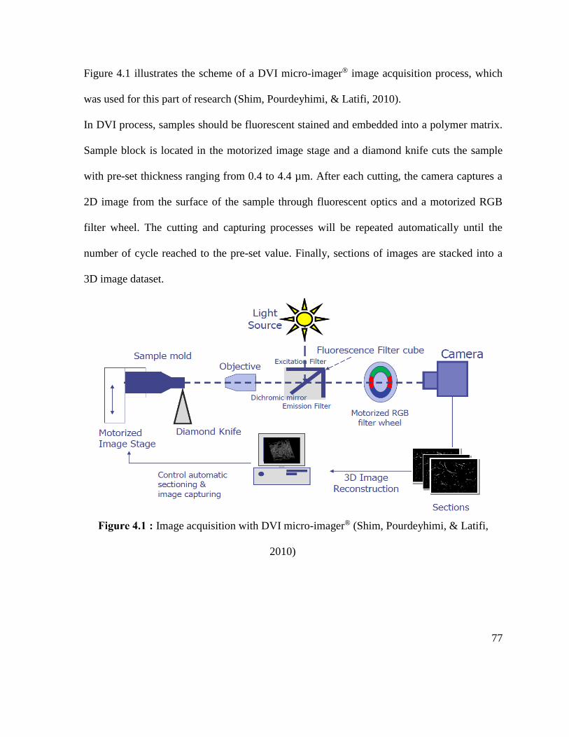
77

Figure 4.1 illustrates the scheme of a DVI micro-imager® image acquisition process, which

was used for this part of research (Shim, Pourdeyhimi, & Latifi, 2010).

In DVI process, samples should be fluorescent stained and embedded into a polymer matrix.

Sample block is located in the motorized image stage and a diamond knife cuts the sample

with pre-set thickness ranging from 0.4 to 4.4 µm. After each cutting, the camera captures a

2D image from the surface of the sample through fluorescent optics and a motorized RGB

filter wheel. The cutting and capturing processes will be repeated automatically until the

number of cycle reached to the pre-set value. Finally, sections of images are stacked into a

3D image dataset.

Image acquisition with DVI micro-imager® (Shim, Pourdeyhimi, & Latifi,

2010)

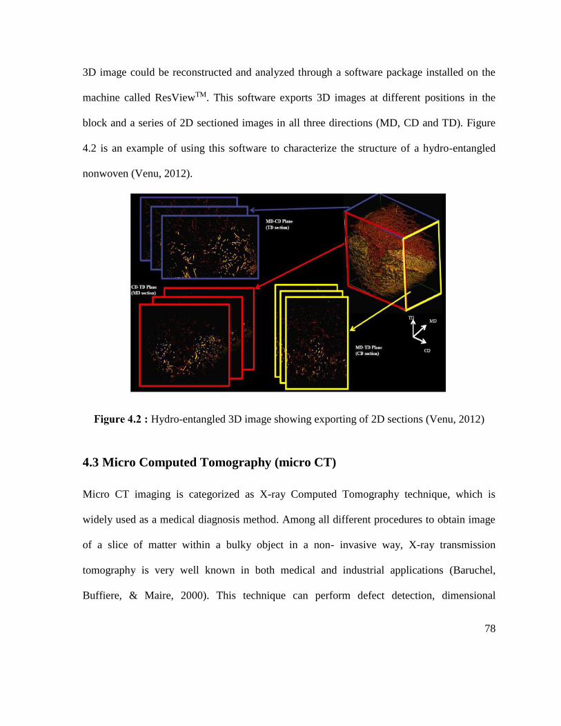
78

3D image could be reconstructed and analyzed through a software package installed on the

machine called ResViewTM. This software exports 3D images at different positions in the

block and a series of 2D sectioned images in all three directions (MD, CD and TD). Figure

4.2 is an example of using this software to characterize the structure of a hydro-entangled

nonwoven (Venu, 2012).

Hydro-entangled 3D image showing exporting of 2D sections (Venu, 2012)

4.3 Micro Computed Tomography (micro CT)

Micro CT imaging is categorized as X-ray Computed Tomography technique, which is

widely used as a medical diagnosis method. Among all different procedures to obtain image

of a slice of matter within a bulky object in a non- invasive way, X-ray transmission

tomography is very well known in both medical and industrial applications (Baruchel,

Buffiere, & Maire, 2000). This technique can perform defect detection, dimensional

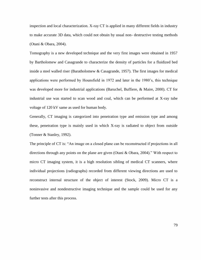
79

inspection and local characterization. X-ray CT is applied in many different fields in industry

to make accurate 3D data, which could not obtain by usual non- destructive testing methods

(Otani & Obara, 2004).

Tomography is a new developed technique and the very first images were obtained in 1957

by Bartholomew and Casagrande to characterize the density of particles for a fluidized bed

inside a steel walled riser (Baratholomew & Casagrande, 1957). The first images for medical

applications were performed by Hounsfield in 1972 and later in the 1980’s, this technique

was developed more for industrial applications (Baruchel, Buffiere, & Maire, 2000). CT for

industrial use was started to scan wood and coal, which can be performed at X-ray tube

voltage of 120 kV same as used for human body.

Generally, CT imaging is categorized into penetration type and emission type and among

these, penetration type is mainly used in which X-ray is radiated to object from outside

(Tonner & Stanley, 1992).

The principle of CT is: “An image on a closed plane can be reconstructed if projections in all

directions through any points on the plane are given (Otani & Obara, 2004).” With respect to

micro CT imaging system, it is a high resolution sibling of medical CT scanners, where

individual projections (radiographs) recorded from different viewing directions are used to

reconstruct internal structure of the object of interest (Stock, 2009). Micro CT is a

noninvasive and nondestructive imaging technique and the sample could be used for any

further tests after this process.

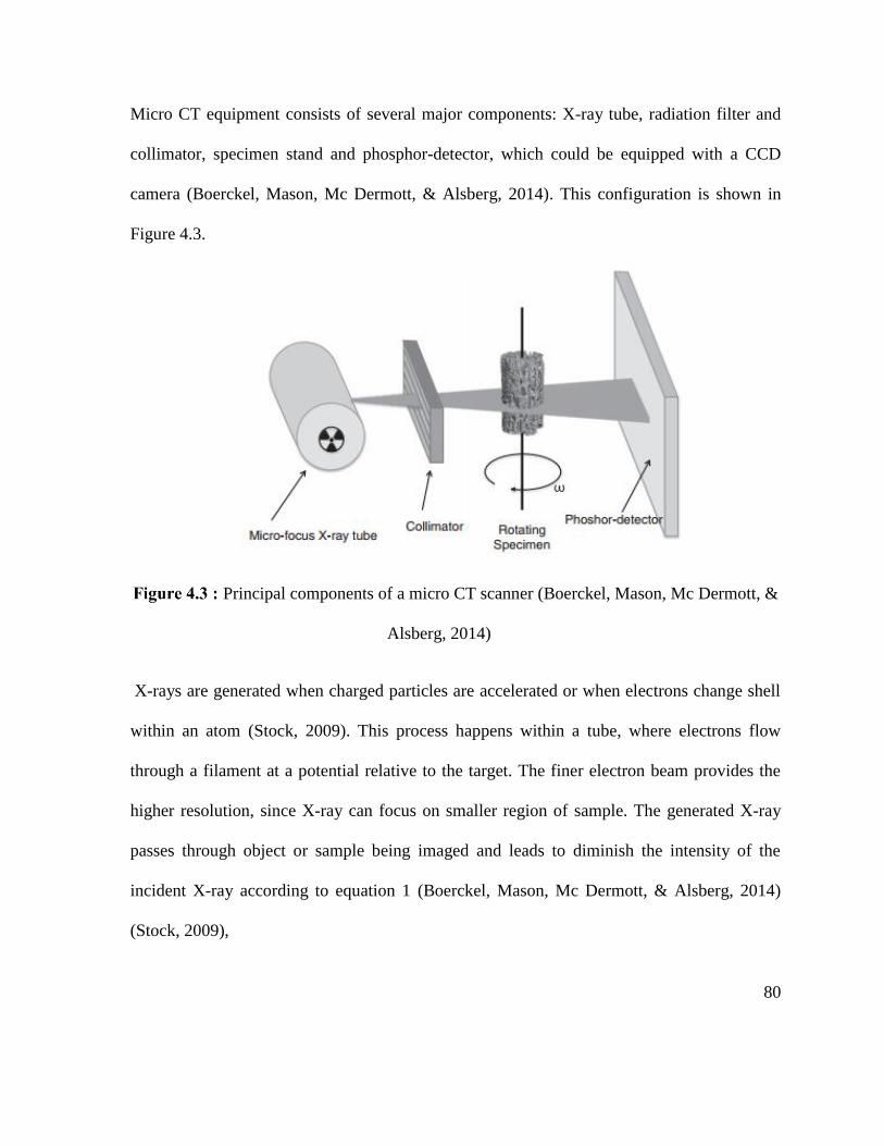
80

Micro CT equipment consists of several major components: X-ray tube, radiation filter and

collimator, specimen stand and phosphor-detector, which could be equipped with a CCD

camera (Boerckel, Mason, Mc Dermott, & Alsberg, 2014). This configuration is shown in

Figure 4.3.

Principal components of a micro CT scanner (Boerckel, Mason, Mc Dermott, &

Alsberg, 2014)

X-rays are generated when charged particles are accelerated or when electrons change shell

within an atom (Stock, 2009). This process happens within a tube, where electrons flow

through a filament at a potential relative to the target. The finer electron beam provides the

higher resolution, since X-ray can focus on smaller region of sample. The generated X-ray

passes through object or sample being imaged and leads to diminish the intensity of the

incident X-ray according to equation 1 (Boerckel, Mason, Mc Dermott, & Alsberg, 2014)

(Stock, 2009),

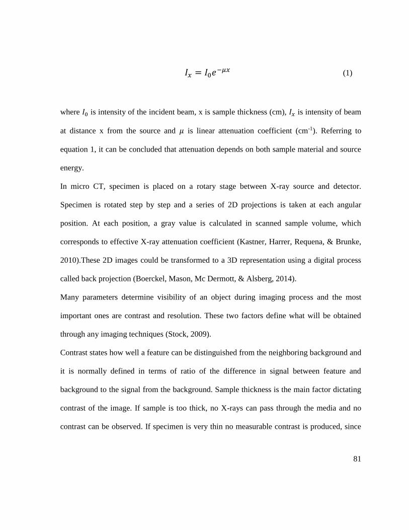
81

𝐼𝑥 = 𝐼0𝑒−𝜇𝑥 (1)

where 𝐼0 is intensity of the incident beam, x is sample thickness (cm), 𝐼𝑥 is intensity of beam

at distance x from the source and 𝜇 is linear attenuation coefficient (cm-1). Referring to

equation 1, it can be concluded that attenuation depends on both sample material and source

energy.

In micro CT, specimen is placed on a rotary stage between X-ray source and detector.

Specimen is rotated step by step and a series of 2D projections is taken at each angular

position. At each position, a gray value is calculated in scanned sample volume, which

corresponds to effective X-ray attenuation coefficient (Kastner, Harrer, Requena, & Brunke,

2010).These 2D images could be transformed to a 3D representation using a digital process

called back projection (Boerckel, Mason, Mc Dermott, & Alsberg, 2014).

Many parameters determine visibility of an object during imaging process and the most

important ones are contrast and resolution. These two factors define what will be obtained

through any imaging techniques (Stock, 2009).

Contrast states how well a feature can be distinguished from the neighboring background and

it is normally defined in terms of ratio of the difference in signal between feature and

background to the signal from the background. Sample thickness is the main factor dictating

contrast of the image. If sample is too thick, no X-rays can pass through the media and no

contrast can be observed. If specimen is very thin no measurable contrast is produced, since

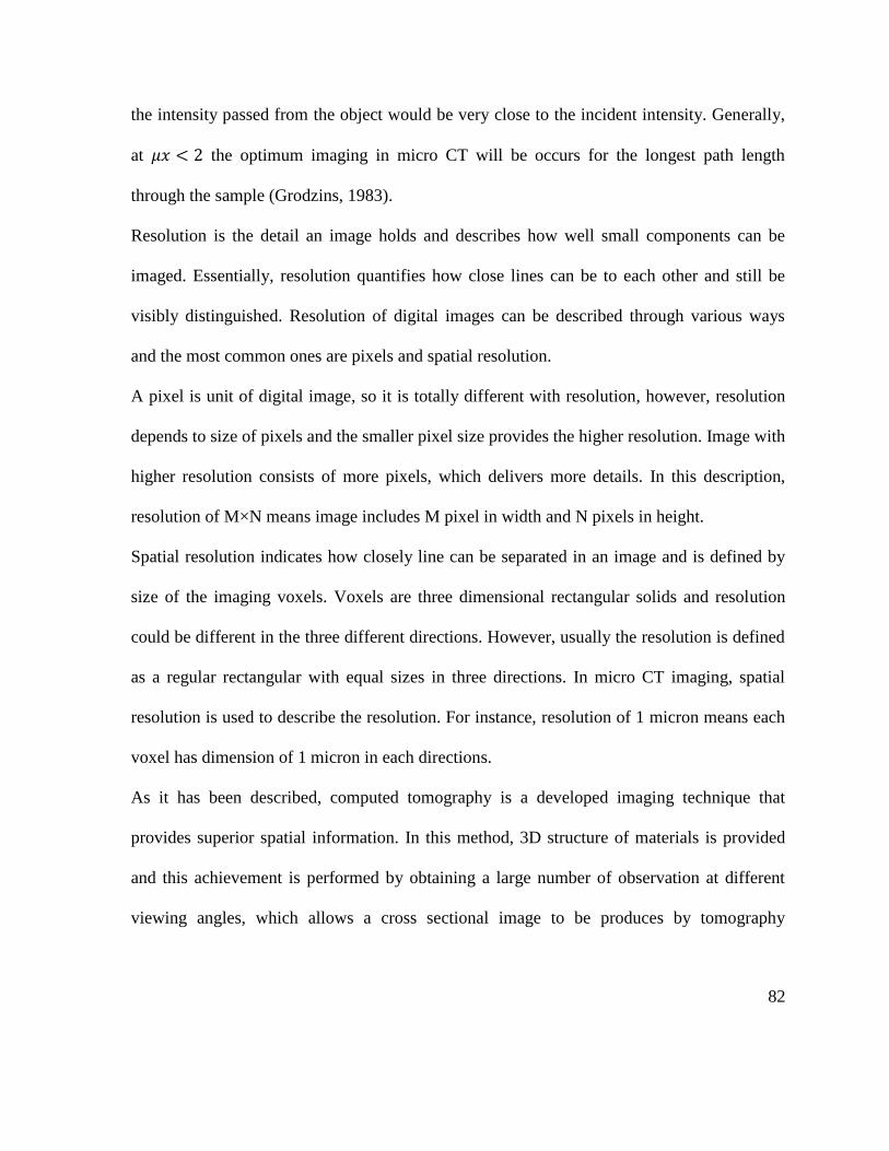
82

the intensity passed from the object would be very close to the incident intensity. Generally,

at 𝜇𝑥 < 2 the optimum imaging in micro CT will be occurs for the longest path length

through the sample (Grodzins, 1983).

Resolution is the detail an image holds and describes how well small components can be

imaged. Essentially, resolution quantifies how close lines can be to each other and still be

visibly distinguished. Resolution of digital images can be described through various ways

and the most common ones are pixels and spatial resolution.

A pixel is unit of digital image, so it is totally different with resolution, however, resolution

depends to size of pixels and the smaller pixel size provides the higher resolution. Image with

higher resolution consists of more pixels, which delivers more details. In this description,

resolution of M×N means image includes M pixel in width and N pixels in height.

Spatial resolution indicates how closely line can be separated in an image and is defined by

size of the imaging voxels. Voxels are three dimensional rectangular solids and resolution

could be different in the three different directions. However, usually the resolution is defined

as a regular rectangular with equal sizes in three directions. In micro CT imaging, spatial

resolution is used to describe the resolution. For instance, resolution of 1 micron means each

voxel has dimension of 1 micron in each directions.

As it has been described, computed tomography is a developed imaging technique that

provides superior spatial information. In this method, 3D structure of materials is provided

and this achievement is performed by obtaining a large number of observation at different

viewing angles, which allows a cross sectional image to be produces by tomography

83

reconstruction (Manitoba, 2015). In order to reconstruct the image in micro CT, back

projection algorithm is normally used. Features buried within a sample detected by X-ray can

be localized in two dimensions through conventional projection method. However, making

many different measurements at different viewing angles, leads to estimate the position of the

objects within the sample employing triangulation process. Figure 4.4 presents a sample

containing two discrete objects. In Figure 4.4.a, a profile of the attenuation of the X-ray beam

by the object is acquired. By projecting data back along a line corresponding to the direction,

in which data was acquired (back projection) a shadow image representing attenuation at this

viewing angle will be delivered. In Figure 4.4.b, this process was repeated at 90o to the first

measurement and the second back projection was calculated. Combining two back projection

results to find an estimation of sample cross section, such as shown in Figure 4.4.c.

(Manitoba, 2015). The accuracy of the back projection process is increased by making

additional viewing angles.

Micro CT imaging technique is a faster method compared to DVI, since it is not necessary to

dye the sample and also image capturing procedure is more rapidly. Meanwhile, it is a non-

destructive process and no sample preparation is needed. The main problem associated with

this technique is images storage due to their large size. Normally, for each sample it is

necessary to assign many gigabytes for data storage.

84

Schematic illustration of back projection (Manitoba, 2015)

4.4 Materials and 2D image acquisition

In order to study pore structure of nonwovens, 2D images of continuous layers of the media

were captured using DVI and micro CT imaging techniques. These 2D images are employed

to visualized the 3D structure of nonwovens. In the following parts the properties of each

samples and the processes applied on them will be discussed.

4.4.1 Materials for 2D image acquisition through DVI

In order to study the pore structure of the nonwovens, a fabric produced by needle punching

of a Nylon and a PET web with basis weights of 40 and 120 g/m2 was utilized. The needling

process was performed by Asselin A.50-RL needle loom with 38 gauge needle, punch

density of 100 strokes/cm2 for both sides needling (face and back) at The Nonwovens

85

Institute, North Carolina State University facility. It is worth noting that this fabric is only

selected for this part of work to demonstrate the capability of the developed methodology

without any considerations on its properties, production conditions and material components.

As it has been described, to obtain 3D image of the sample using DVI technique, it is

necessary to dye the sample. For this purpose, the sample was stained with 10 mg/ml Nile

Red 1-Methyi-2- pyrrolidinone and Sulforhodamine 101 dyes to differently stain the PET and

Nylon components respectively. A 4 mm × 30 mm fabric strip was cut and placed into the

DVI sample mold to produce a sample block. Afterward, the sample mold was filled with an

opaque embedding medium and centrifuged for an hour at 3800 rpm to ensure complete

infiltration and subsequently cured for at least 8 hours in an oven at 70 °C. “The embedding

medium was prepared as outlined below: 5.0 g of Vinylcyclohexene dioxide (VCD), 3.0 g of

Propyleneglycoldiglycidyle ether (DER), and 13.0 g of nonenylsuccinic anhydride (NS) were

mixed with the overhead stirrer (Heidolph Mechanical Overhead Stirrer, RZR 2020) and 2.4

g of Sudan black B (Acros, CAS# 4197-25-5) was then added to achieve opacity.

Dimethylethanolamine (DMAE, 224 μL) was lastly added into the mixture. It was stirred

until the mixture became homogeneous and centrifuged for another 15 min at 5,000 rpm to

remove coagulated Sudan black particles” (Venu, 2012).

The DVI microimager® used in this work has a 4X objective lens, a B2A fluorescent filter

cube (Nikon) with 480/40 nm excitation filter and a beam splitter 505, 510 LP emission filter

and motorized RGB filter wheel were used to capture fluorescent images of sectioned sample

block surfaces. The processes of sectioning and capturing the images were repeated

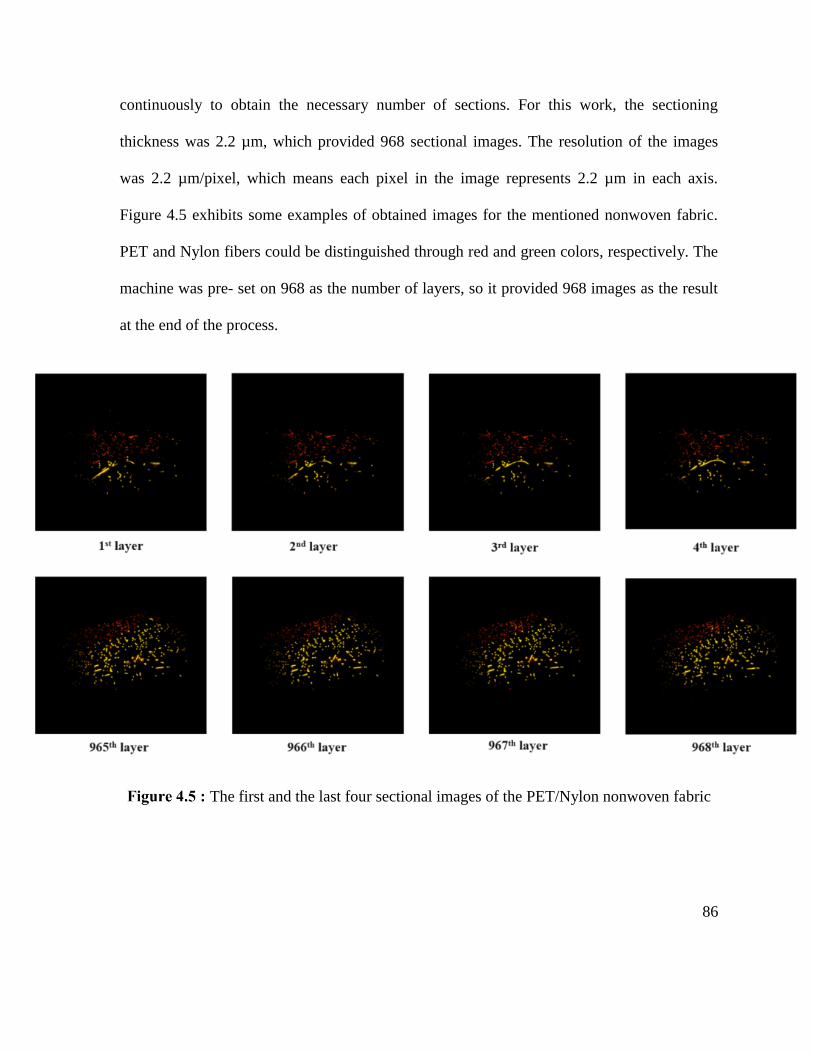
86

continuously to obtain the necessary number of sections. For this work, the sectioning

thickness was 2.2 µm, which provided 968 sectional images. The resolution of the images

was 2.2 µm/pixel, which means each pixel in the image represents 2.2 µm in each axis.

Figure 4.5 exhibits some examples of obtained images for the mentioned nonwoven fabric.

PET and Nylon fibers could be distinguished through red and green colors, respectively. The

machine was pre- set on 968 as the number of layers, so it provided 968 images as the result

at the end of the process.

The first and the last four sectional images of the PET/Nylon nonwoven fabric

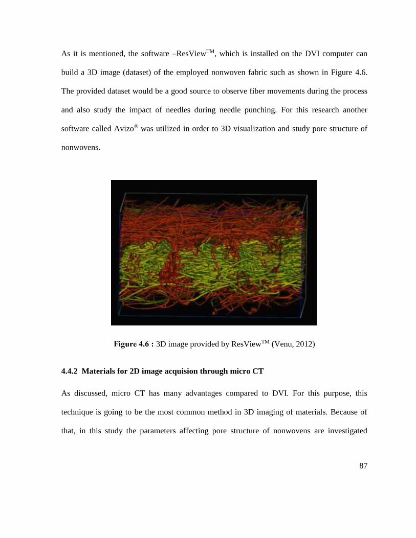
87

As it is mentioned, the software –ResViewTM, which is installed on the DVI computer can

build a 3D image (dataset) of the employed nonwoven fabric such as shown in Figure 4.6.

The provided dataset would be a good source to observe fiber movements during the process

and also study the impact of needles during needle punching. For this research another

software called Avizo® was utilized in order to 3D visualization and study pore structure of

nonwovens.

3D image provided by ResViewTM (Venu, 2012)

4.4.2 Materials for 2D image acquision through micro CT

As discussed, micro CT has many advantages compared to DVI. For this purpose, this

technique is going to be the most common method in 3D imaging of materials. Because of

that, in this study the parameters affecting pore structure of nonwovens are investigated

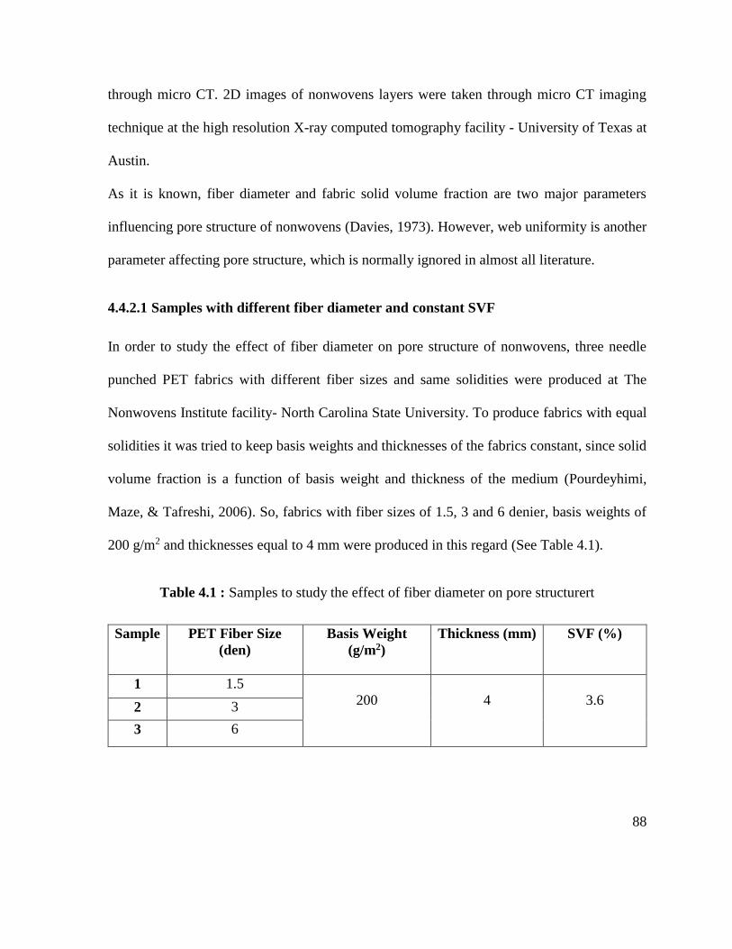
88

through micro CT. 2D images of nonwovens layers were taken through micro CT imaging

technique at the high resolution X-ray computed tomography facility - University of Texas at

Austin.

As it is known, fiber diameter and fabric solid volume fraction are two major parameters

influencing pore structure of nonwovens (Davies, 1973). However, web uniformity is another

parameter affecting pore structure, which is normally ignored in almost all literature.

4.4.2.1 Samples with different fiber diameter and constant SVF

In order to study the effect of fiber diameter on pore structure of nonwovens, three needle

punched PET fabrics with different fiber sizes and same solidities were produced at The

Nonwovens Institute facility- North Carolina State University. To produce fabrics with equal

solidities it was tried to keep basis weights and thicknesses of the fabrics constant, since solid

volume fraction is a function of basis weight and thickness of the medium (Pourdeyhimi,

Maze, & Tafreshi, 2006). So, fabrics with fiber sizes of 1.5, 3 and 6 denier, basis weights of

200 g/m2 and thicknesses equal to 4 mm were produced in this regard (See Table 4.1).

Table 4.1 : Samples to study the effect of fiber diameter on pore structurert

Sample PET Fiber Size

(den)

Basis Weight

(g/m2)

Thickness (mm) SVF (%)

1 1.5

200

4

3.6 2 3

3 6

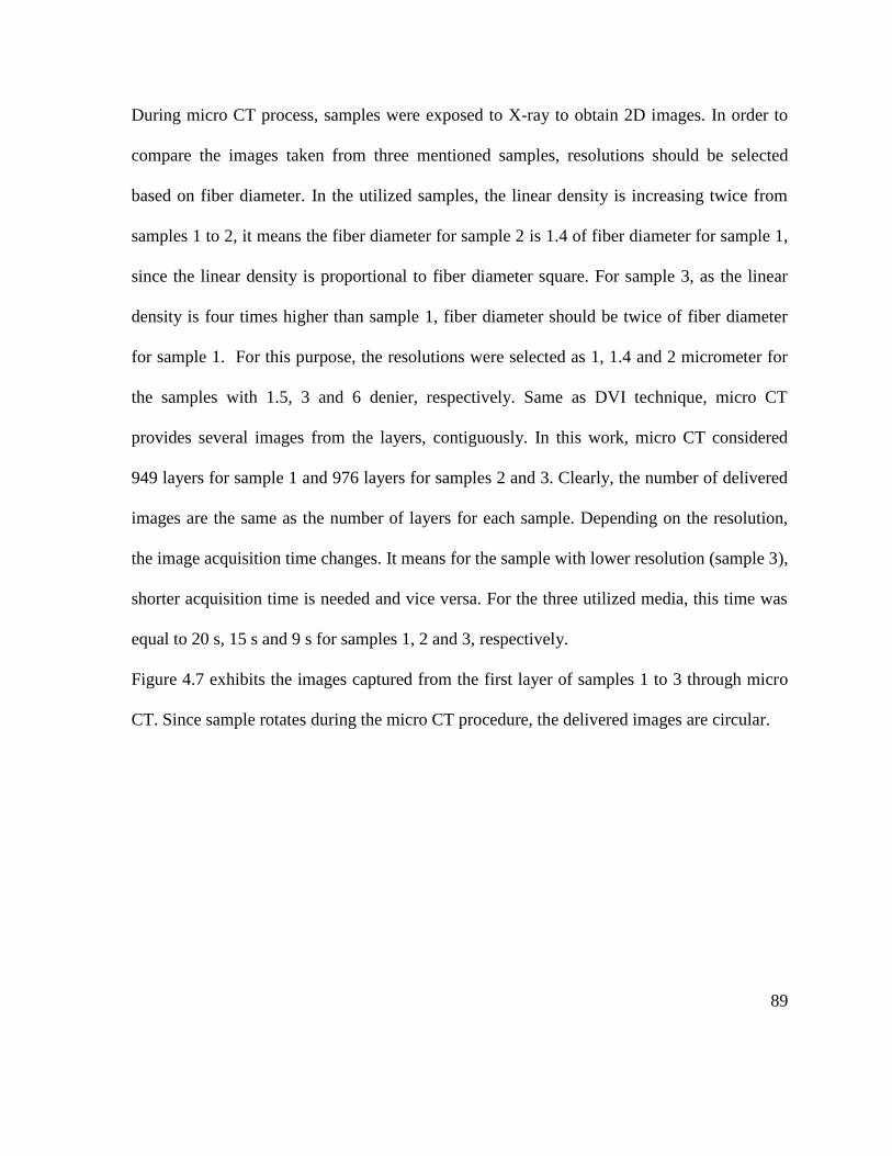
89

During micro CT process, samples were exposed to X-ray to obtain 2D images. In order to

compare the images taken from three mentioned samples, resolutions should be selected

based on fiber diameter. In the utilized samples, the linear density is increasing twice from

samples 1 to 2, it means the fiber diameter for sample 2 is 1.4 of fiber diameter for sample 1,

since the linear density is proportional to fiber diameter square. For sample 3, as the linear

density is four times higher than sample 1, fiber diameter should be twice of fiber diameter

for sample 1. For this purpose, the resolutions were selected as 1, 1.4 and 2 micrometer for

the samples with 1.5, 3 and 6 denier, respectively. Same as DVI technique, micro CT

provides several images from the layers, contiguously. In this work, micro CT considered

949 layers for sample 1 and 976 layers for samples 2 and 3. Clearly, the number of delivered

images are the same as the number of layers for each sample. Depending on the resolution,

the image acquisition time changes. It means for the sample with lower resolution (sample 3),

shorter acquisition time is needed and vice versa. For the three utilized media, this time was

equal to 20 s, 15 s and 9 s for samples 1, 2 and 3, respectively.

Figure 4.7 exhibits the images captured from the first layer of samples 1 to 3 through micro

CT. Since sample rotates during the micro CT procedure, the delivered images are circular.

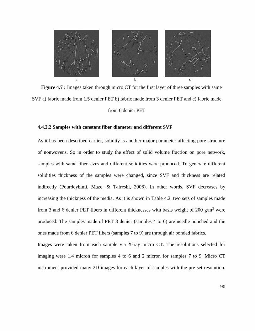
90

a b c

Images taken through micro CT for the first layer of three samples with same

SVF a) fabric made from 1.5 denier PET b) fabric made from 3 denier PET and c) fabric made

from 6 denier PET

4.4.2.2 Samples with constant fiber diameter and different SVF

As it has been described earlier, solidity is another major parameter affecting pore structure

of nonwovens. So in order to study the effect of solid volume fraction on pore network,

samples with same fiber sizes and different solidities were produced. To generate different

solidities thickness of the samples were changed, since SVF and thickness are related

indirectly (Pourdeyhimi, Maze, & Tafreshi, 2006). In other words, SVF decreases by

increasing the thickness of the media. As it is shown in Table 4.2, two sets of samples made

from 3 and 6 denier PET fibers in different thicknesses with basis weight of 200 g/m2 were

produced. The samples made of PET 3 denier (samples 4 to 6) are needle punched and the

ones made from 6 denier PET fibers (samples 7 to 9) are through air bonded fabrics.

Images were taken from each sample via X-ray micro CT. The resolutions selected for

imaging were 1.4 micron for samples 4 to 6 and 2 micron for samples 7 to 9. Micro CT

instrument provided many 2D images for each layer of samples with the pre-set resolution.

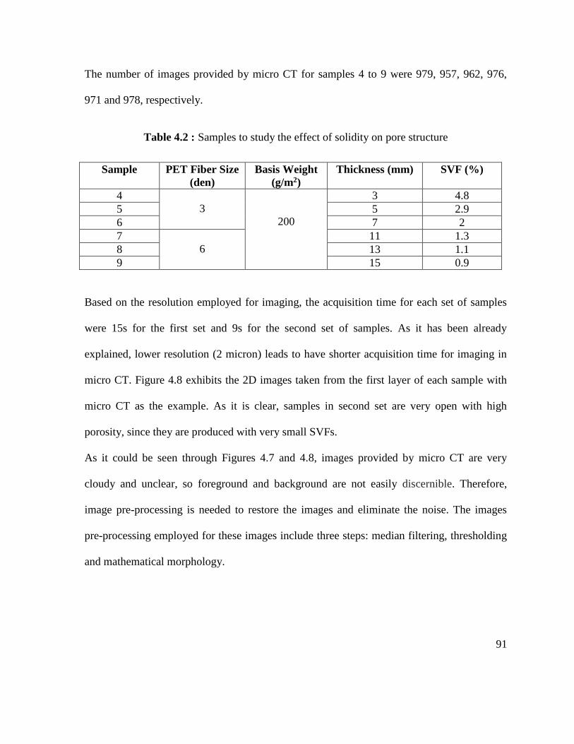
91

The number of images provided by micro CT for samples 4 to 9 were 979, 957, 962, 976,

971 and 978, respectively.

Table 4.2 : Samples to study the effect of solidity on pore structure

Sample PET Fiber Size

(den)

Basis Weight

(g/m2)

Thickness (mm) SVF (%)

4

3

200

3 4.8

5 5 2.9

6 7 2

7

6

11 1.3

8 13 1.1

9 15 0.9

Based on the resolution employed for imaging, the acquisition time for each set of samples

were 15s for the first set and 9s for the second set of samples. As it has been already

explained, lower resolution (2 micron) leads to have shorter acquisition time for imaging in

micro CT. Figure 4.8 exhibits the 2D images taken from the first layer of each sample with

micro CT as the example. As it is clear, samples in second set are very open with high

porosity, since they are produced with very small SVFs.

As it could be seen through Figures 4.7 and 4.8, images provided by micro CT are very

cloudy and unclear, so foreground and background are not easily discernible. Therefore,

image pre-processing is needed to restore the images and eliminate the noise. The images

pre-processing employed for these images include three steps: median filtering, thresholding

and mathematical morphology.

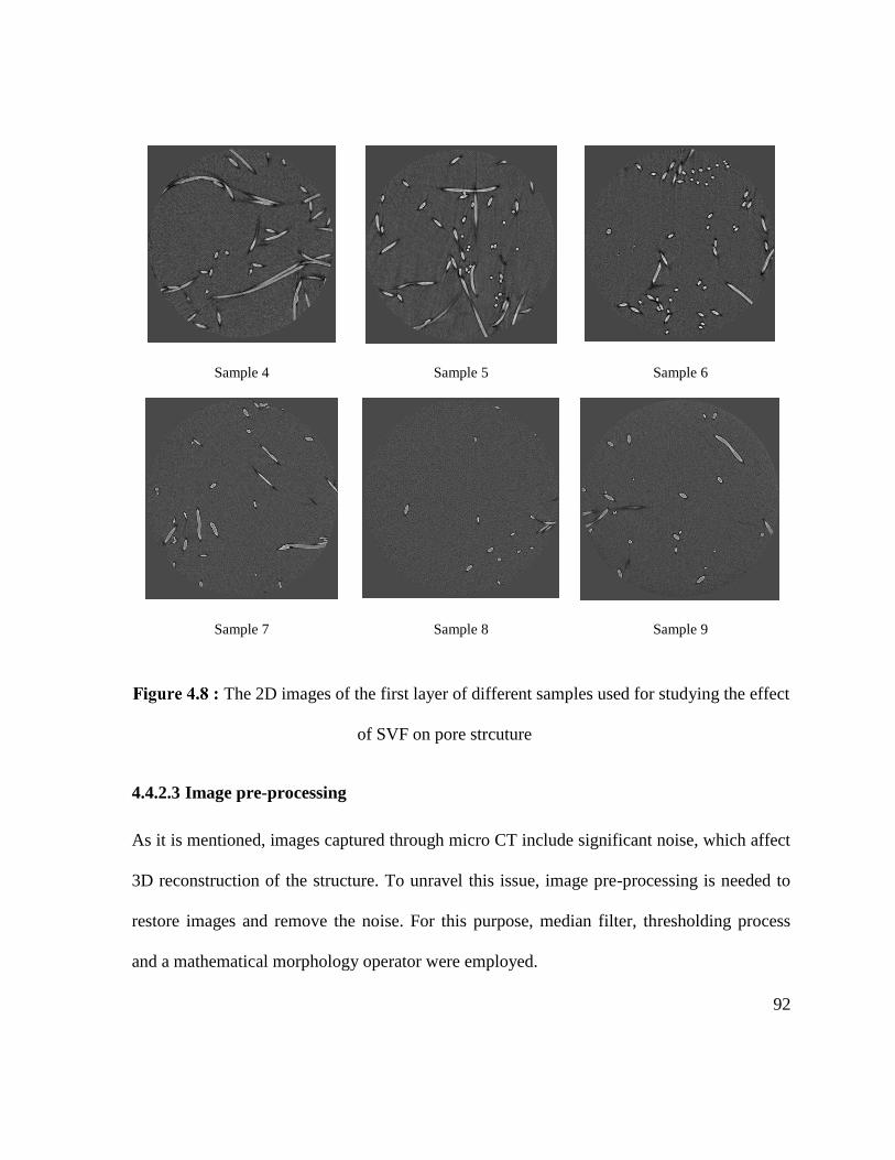
92

Sample 4 Sample 5 Sample 6

Sample 7 Sample 8 Sample 9

The 2D images of the first layer of different samples used for studying the effect

of SVF on pore strcuture

4.4.2.3 Image pre-processing

As it is mentioned, images captured through micro CT include significant noise, which affect

3D reconstruction of the structure. To unravel this issue, image pre-processing is needed to

restore images and remove the noise. For this purpose, median filter, thresholding process

and a mathematical morphology operator were employed.

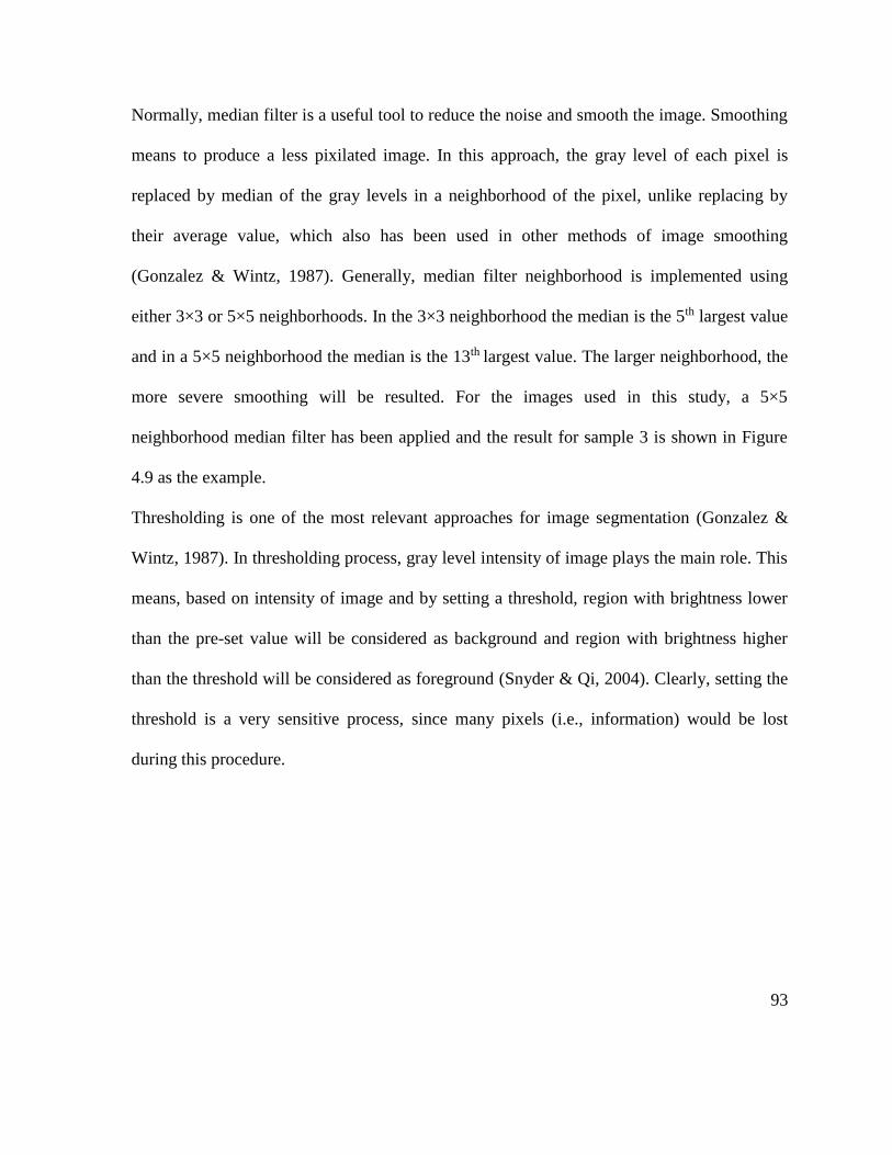
93

Normally, median filter is a useful tool to reduce the noise and smooth the image. Smoothing

means to produce a less pixilated image. In this approach, the gray level of each pixel is

replaced by median of the gray levels in a neighborhood of the pixel, unlike replacing by

their average value, which also has been used in other methods of image smoothing

(Gonzalez & Wintz, 1987). Generally, median filter neighborhood is implemented using

either 3×3 or 5×5 neighborhoods. In the 3×3 neighborhood the median is the 5th largest value

and in a 5×5 neighborhood the median is the 13th largest value. The larger neighborhood, the

more severe smoothing will be resulted. For the images used in this study, a 5×5

neighborhood median filter has been applied and the result for sample 3 is shown in Figure

4.9 as the example.

Thresholding is one of the most relevant approaches for image segmentation (Gonzalez &

Wintz, 1987). In thresholding process, gray level intensity of image plays the main role. This

means, based on intensity of image and by setting a threshold, region with brightness lower

than the pre-set value will be considered as background and region with brightness higher

than the threshold will be considered as foreground (Snyder & Qi, 2004). Clearly, setting the

threshold is a very sensitive process, since many pixels (i.e., information) would be lost

during this procedure.

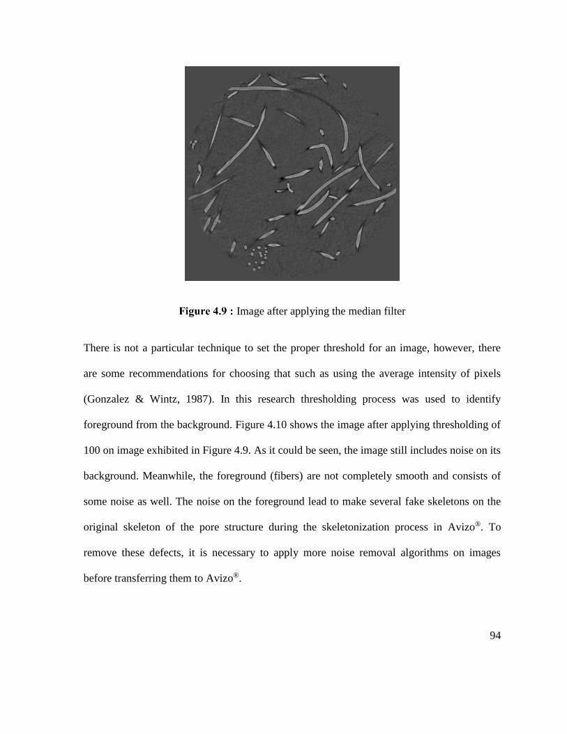
94

Image after applying the median filter

There is not a particular technique to set the proper threshold for an image, however, there

are some recommendations for choosing that such as using the average intensity of pixels

(Gonzalez & Wintz, 1987). In this research thresholding process was used to identify

foreground from the background. Figure 4.10 shows the image after applying thresholding of

100 on image exhibited in Figure 4.9. As it could be seen, the image still includes noise on its

background. Meanwhile, the foreground (fibers) are not completely smooth and consists of

some noise as well. The noise on the foreground lead to make several fake skeletons on the

original skeleton of the pore structure during the skeletonization process in Avizo®. To

remove these defects, it is necessary to apply more noise removal algorithms on images

before transferring them to Avizo®.

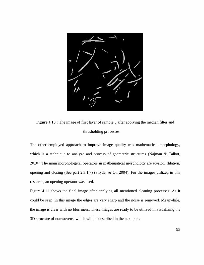
95

The image of first layer of sample 3 after applying the median filter and

thresholding processes

The other employed approach to improve image quality was mathematical morphology,

which is a technique to analyze and process of geometric structures (Najman & Talbot,

2010). The main morphological operators in mathematical morphology are erosion, dilation,

opening and closing (See part 2.3.1.7) (Snyder & Qi, 2004). For the images utilized in this

research, an opening operator was used.

Figure 4.11 shows the final image after applying all mentioned cleaning processes. As it

could be seen, in this image the edges are very sharp and the noise is removed. Meanwhile,

the image is clear with no blurriness. These images are ready to be utilized in visualizing the

3D structure of nonwovens, which will be described in the next part.

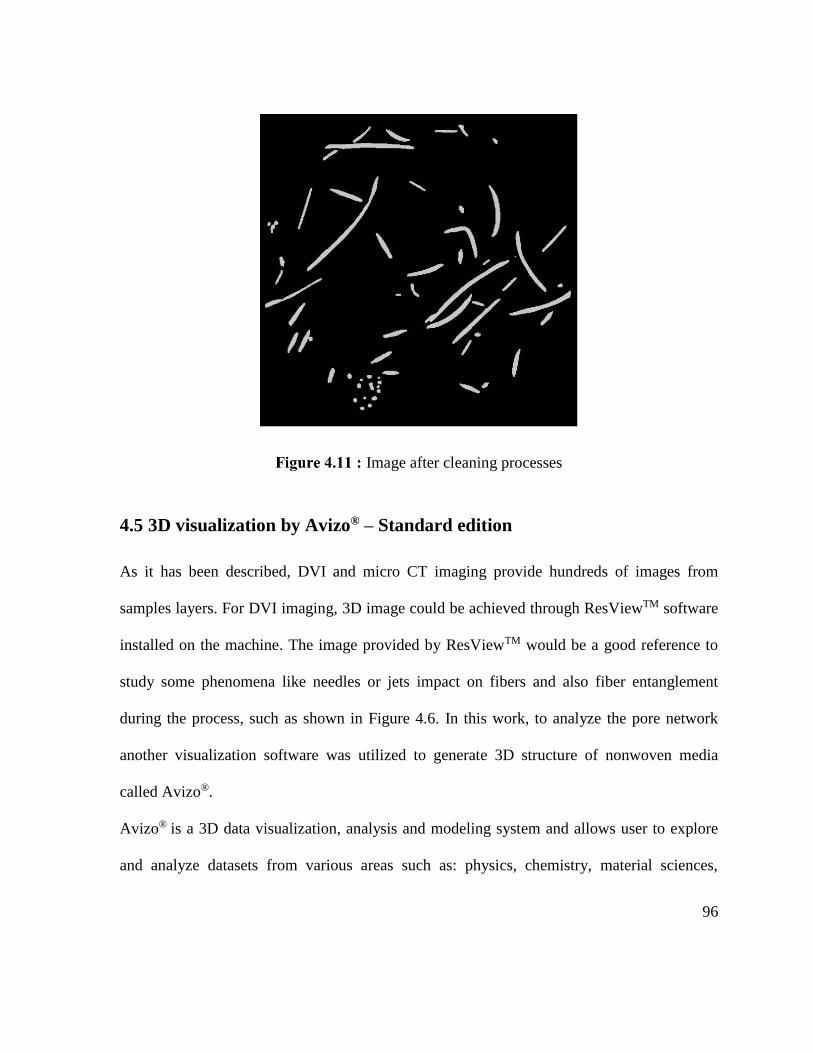
96

Image after cleaning processes

4.5 3D visualization by Avizo® – Standard edition

As it has been described, DVI and micro CT imaging provide hundreds of images from

samples layers. For DVI imaging, 3D image could be achieved through ResViewTM software

installed on the machine. The image provided by ResViewTM would be a good reference to

study some phenomena like needles or jets impact on fibers and also fiber entanglement

during the process, such as shown in Figure 4.6. In this work, to analyze the pore network

another visualization software was utilized to generate 3D structure of nonwoven media

called Avizo®.

Avizo® is a 3D data visualization, analysis and modeling system and allows user to explore

and analyze datasets from various areas such as: physics, chemistry, material sciences,

97

microscopy, computer aided engineering, computational fluid dynamics, numerical solution,

earth science and environment (FEI, 2009).

Avizo® has this ability to explore, analyze, compare and quantify 3D data and provides grids

from voxel data representing an image volume. Generally, Avizo® is a modular and object-

oriented software system, where modules are used to visualize the data object or to perform

some computational operations (FEI, 2009).

Normally, Avizo® can load different types of data including:

-2D and 3D image and volume data,

-Geometric models such as point sets, line sets, surfaces and grids,

- Numerical simulation data and,

-Time series and animations.

In this work, Avizo® -Standard edition is used, which is suitable to visualize 3D volumetric

images. For this purpose, 2D images of the nonwoven media are required to be transferred to

Avizo®.

Regarding DVI process, the 2D images were transferred to Avizo®. These images create a 3D

structure, which represents sample volume. Since the transferred data is RGB images, they

should be converted to gray scale images before applying any processes on them. This

conversion is necessary, since in gray level images each pixel represents a single value.

Same as DVI images, the images captured with micro CT for samples 1 to 9 were transferred

to Avizo® to obtain 3D structural image as well. The only difference between 3D

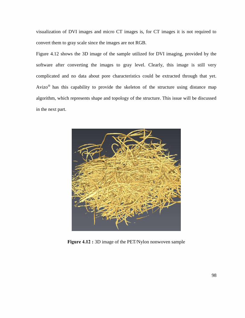
98

visualization of DVI images and micro CT images is, for CT images it is not required to

convert them to gray scale since the images are not RGB.

Figure 4.12 shows the 3D image of the sample utilized for DVI imaging, provided by the

software after converting the images to gray level. Clearly, this image is still very

complicated and no data about pore characteristics could be extracted through that yet.

Avizo® has this capability to provide the skeleton of the structure using distance map

algorithm, which represents shape and topology of the structure. This issue will be discussed

in the next part.

3D image of the PET/Nylon nonwoven sample

99

4.6 Thining process (Skeletonization) through Avizo®

Avizo® has this ability to apply skeletonizing module using distance map algorithm and

provides a graph in order to characterize the structure. This graph represents the shape of the

structure through a connected network (See part 2.6).

Avizo® can recognize voids from fibers by distinguishing bright side and dark side of the

image, where the bright side and dark side represent fibers and voids, respectively. This issue

is called segmentation. Referring to image analysis basics, a thresholding value should be set

for image segmentation that determines the quality of the result. In one hand, adjusting a low

threshold value leads to get an image full of noise, with the unclear border between fibers

and background. On the other hand, setting a high value for threshold casues to remove many

necessary information of the image. For the images used in this work, threshold of 80 was

utilized for image segmentation in Avizo®. After segmentation process, the fiber and void

regions could be distinguished easily.

Since structure of voids is desired, the dark side which indicates the pores should be selected.

The skeletonization process in Avizo® includes three steps: calculating the distance map

using Euclidean distance equation, thinning the data and tracing the line. Once the distance

map and skeleton are computed, software converts the image into a network of the line

segments considering point connectivity. In other words, skeleton module in Avizo® converts

the voxel skeleton to a spatial graph object. A spatial graph consists of nodes and segments,

where nodes represents the branching points and endpoints and segments are the curved lines

connecting the nodes (FEI, 2009). This set of nodes connected by segments is called a graph.

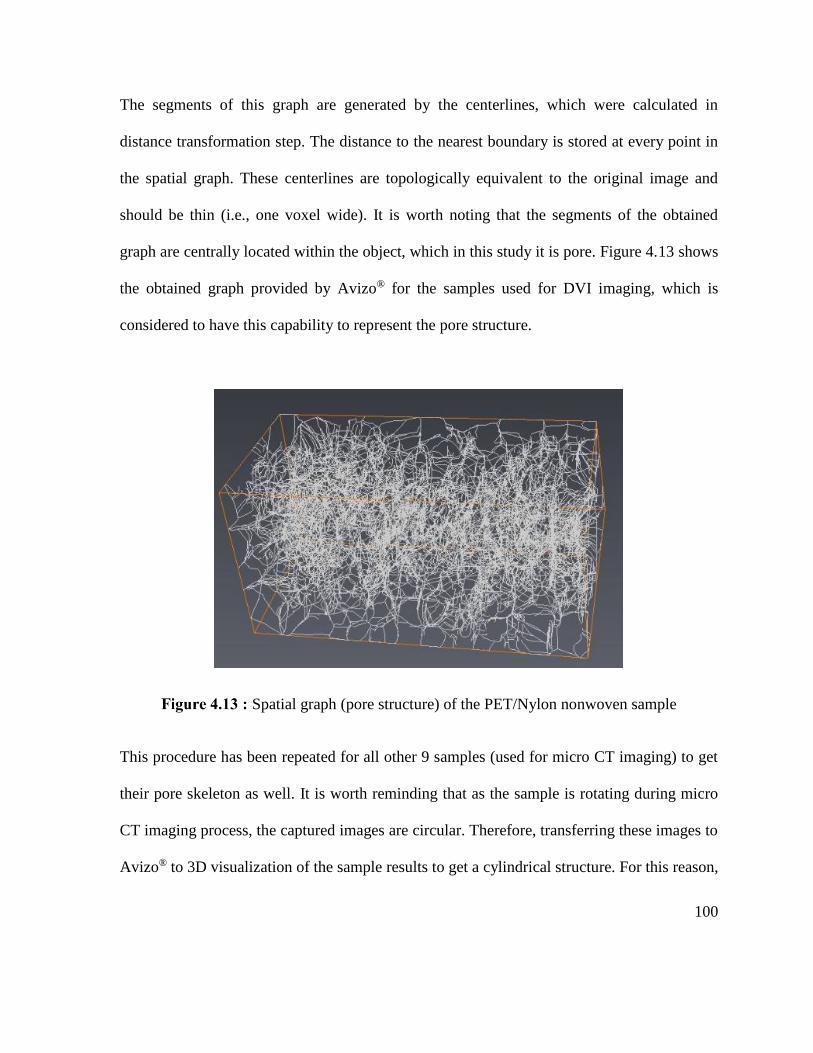
100

The segments of this graph are generated by the centerlines, which were calculated in

distance transformation step. The distance to the nearest boundary is stored at every point in

the spatial graph. These centerlines are topologically equivalent to the original image and

should be thin (i.e., one voxel wide). It is worth noting that the segments of the obtained

graph are centrally located within the object, which in this study it is pore. Figure 4.13 shows

the obtained graph provided by Avizo® for the samples used for DVI imaging, which is

considered to have this capability to represent the pore structure.

Spatial graph (pore structure) of the PET/Nylon nonwoven sample

This procedure has been repeated for all other 9 samples (used for micro CT imaging) to get

their pore skeleton as well. It is worth reminding that as the sample is rotating during micro

CT imaging process, the captured images are circular. Therefore, transferring these images to

Avizo® to 3D visualization of the sample results to get a cylindrical structure. For this reason,

101

to obtain a cubic graph and avoid any inaccuracy in edges, it is necessary to crop the 3D

image and apply the skeletonization on that. Obviosuly, cropping the image results in

changing the dimension and this issue should be considered during the calculations.

The graph obtained through skeletonizing the 3D image of each sample includes many

important information of pore structure, which could be used to characterize that. This

information will be introduced in the following chapter.

102

5. Modeling Permeability

103

5.1 Introduction

As seen in Chapter 4, taking 2D images from continuous layers of a nonwoven media

through DVI or micro CT and transferring the images to Avizo®, after applying any required

image pre-processings, results in obtaining 3D volumetric image of the media. Then,

skeletonizing the 3D image eventuates in getting the pore skeleton, such as exhibited in

Figure 4.13. This graph shows all the pores available in the structure. Since, the target is

evaluating diameter of all the pores, this skeleton would be very helpful as all the pores and

their information are available. However as it could be seen, the graph is very complex and

the pore information could not be extracted without any furtur actions. To tackle this issue,

the graph theory principles and the modules available in the software are used. Referring to

graph theory, each graph consisting many nodes and links, and the connectivity between

nodes determines complexity of the graph. Therefore, eliciting nodes information and

connectivity help to understand the graph and characterize the pore structure, eventually.

It is worth noting that the methodology, which is developed in this work, is applicable for

any media and any claculations explained in the following parts is just for making the model

more clear.

5.2 Analysis of the graph provided by Avizo®

As it has been described, Avizo® provides voids skeleton in form of a graph. Saving the

information of this graph leads to obtain some matrices/vectors, which demonstrate the

graph. This information are listed in the following for the graph shown in Figure 4.13 as the

104

example. Clearly, this information would be same for all other media except the quantity of

each one (length of the matrix/vector), which is different from one sample to another.

- Nodes coordinates (matrix A): One of the important information obtained through the graph

is the total number of nodes in pore skeleton and their positions (coordinates) in X, Y and Z

axes in the form of (x, y, z). These nodes are generated due to voids intersection, where the

nodes located on the top surface of the graph have z equals to zero and the nodes at the

bottom surface have the maximum value of z. The data showed total number of nodes in the

graph (Figure 4.13) is 38203. In other words, to define the pore structure with a skeleton,

38203 nodes are needed to generate the paths and edges. In the dataset, nodes are numbered

from 1 to 38204.

- Connectivity (matrix B): This data shows which nodes are connected. For example in this

work, the dataset indicates that node number 1 is connected to node number 2, node number

2 is connected to node number 3, node number 1 is connected to node number 3 and so on.

The total number of connectivity for the provided graph was 41619. It means, 38203 nodes

make 41619 connectivity to generate the graph. It is worth noting that number of

connectivity illustrates number of edges in the graph. If node number 1 is connected to node

number 2, there should be a link between these two nodes. Therefore, each connectivity

represents an edge.

- Intermediate nodes (matrix C): Two nodes are not connected to each other directly but there

are some intermediate nodes, which determine connection and path tortuosity between two

nodes. Nodes are center points of the skeleton, which are generated during thinning process

105

and in this study the graph consists of 840461 intermediate nodes. It is necessary to note that

this part of dataset covers coordinates of all nodes in the graph including the main and

intermediate nodes. In other words, there are 840461 nodes in the system, that 38203 nodes

are main nodes and the rest are intermediates.

- Number of connectivity (vector D): This data shows number of nodes generating a

connection between two main nodes. For instance according to the dataset, the edge between

nodes number 1 and number 2 was built through 55 nodes. In other words, 55 center points

are generated between nodes number 1 and 2 during the thinning procedure that two of them

are main nodes (nodes 1 and 2) and 53 nodes are intermediate ones.

- Thickness (or node diameter- vector E): As it was already discussed, Avizo® uses thinning

algorithms to provide the skeleton of the pore structure. In the obtained dataset, thickness

illustrates the quantity of thinning for each centerline. In other words, it indicates the distance

between each center point with the associated border. As each center point is shown with a

node (main or intermediate), the thickness values show the thinning quantity for each node.

In pore structure point of view, thickness represents the pore diameter for different points

within the capillary. The saved data provides 840461 values as the thickness or pore size for

the graph. Each of these values corresponds to a node, which shows pores intersection and

indicates the pore diameter at that point.

It is worth noting that elements of A, C and E matrices/vectors are in voxels and it is

necessary to convert them to any conventional units such as SI units for further

investigations.

106

5.3 Analogy to model permeability

It could be concluded from part 5.2 that pore network is very complex including many

connectivity and nodes, so it would be very difficult to analyze them. Also, it is not possible

to compare two pore structures referring to this type of information extracted from pore

skeleton. Therefore the main issue is, how to go from this complex network to a single

number which could be measured experimentally. This single number could be utilized to

define the pore structure and would be an index for comparing pore networks. Since

permeability is directly related to pore size, it is hypothesized that it can play this role. In

order to find the permeability coefficient of the nonwoven media, it is required to obtain the

relationship between pressure and flow rate.

As it has been mentioned, flow rate within a capillary is normally employed in order to study

the pore structure and calculate permeability of the porous media. In nonwovens, since pore

structure is considered as a series of interconnected capillaries with circular cross section,

Hagen-Poiseuille’s law provides more reliable output in permeability evaluation in micro

scale than Darcy’s law, which is normally applicable in larger scales (e.g., bulk nonwovens).

Referring to Hagen-Poiseuille’s equation, fluid flow within a capillary is proportional to

capillary diameter (𝑑), capillary length (𝐿), fluid dynamic viscosity (𝜇) and pressure drop

within the capillary (∆𝑃) such as shown in equation 1 (Kirby, 2010),

∆𝑃 =128𝜇𝐿

𝜋𝑑4𝑄 (1)

As described, in nonwovens a pore could be considered as a capillary, therefore pore

structure is very similar to a system with many interconnected capillaries. However, for such

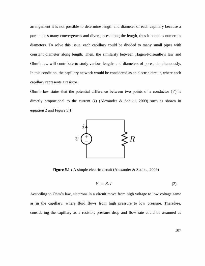
107

arrangement it is not possible to determine length and diameter of each capillary because a

pore makes many convergences and divergences along the length, thus it contains numerous

diameters. To solve this issue, each capillary could be divided to many small pipes with

constant diameter along length. Then, the similarity between Hagen-Poiseuille’s law and

Ohm’s law will contribute to study various lengths and diameters of pores, simultaneously.

In this condition, the capillary network would be considered as an electric circuit, where each

capillary represents a resistor.

Ohm’s law states that the potential difference between two points of a conductor (𝑉) is

directly proportional to the current (𝐼) (Alexander & Sadiku, 2009) such as shown in

equation 2 and Figure 5.1:

A simple electric circuit (Alexander & Sadiku, 2009)

𝑉 = 𝑅. 𝐼 (2)

According to Ohm’s law, electrons in a circuit move from high voltage to low voltage same

as in the capillary, where fluid flows from high pressure to low pressure. Therefore,

considering the capillary as a resistor, pressure drop and flow rate could be assumed as

108

potential difference and current, respectively. Based on this assumption, 128𝜇𝐿

𝜋𝑑4 in Hagen-

Poiseuille’s equation would be equivalent to resistance in Ohm’s law. Using the

aforementioned idea, nonwoven pore network was assumed to be an electric circuit consists

of many resistances “𝑅”, which current of “𝐼” is flowing through when it is connected to a

source with potential difference of “𝑉”. In this condition, calculating the equivalent

resistance (impedance) results in finding a parameter, which illustrates 128𝜇𝐿

𝜋𝑑4 ratio denoted for

all pore geometries within the structure and would be used to calculate permeability.

5.3.1 Applicability of Hagen-Poiseuille’s equation to model permeability

Essentially, Hagen-Poiseuille’s equation is valid for laminar and incompressible flows. A

flow is laminar, when the fluid flows in parallel layers with no disruption between layers.

Basically, at low velocity fluid generates a laminar flow, however, Reynold’s number would

be a good reference in order to recognize the laminar flow, such as shown in equation 3

(Ault, Chen, & Stone, 2015),

𝑅𝑒 =𝜌.𝑑.𝑢

𝜇 (3)

where 𝜌 is fluid density, 𝑑 is capillary diameter, 𝑢 is flow velocity, and 𝜇 is fluid viscosity.

For any porous materials, flow velocity could be replaced with volumetric flow rate (𝑄)

through area of 𝐴, thus, equation 24 will be modified as,

𝑅𝑒 =𝜌.𝑑.𝑄

𝜇.𝐴 (4)

109

where 𝑑 is hydraulic diameter and assuming the pore as a cylinder, it would be equal to pore

diameter, 𝑄 is flow rate and 𝐴 is testing area. In this condition, the flow is laminar for 𝑅𝑒 less

than unity. However, experiments showed that for 𝑅𝑒 up to 10 the flow may still be laminar

(Jackson & James, 1986).

In incompressible flows, there is no significant changes in fluid density during the flow. Flow

is incompressible if it has the Mach number (M) less than 0.3, where Mach number is the

ratio of fluid velocity to the sound velocity. In other words, for the fluid velocity lower than

103 m/s, fluid would be incompressible. The compressibility in M< 0.2-0.3 is very small and

negligible, since flow is steady and isothermal in this range.

In case of nonwoven applications such as filters, fluid could be incompressible like water or

be compressible like air or gas. Since in almost all nonwovens applications fluid flow rate is

not very high and the fluid velocity is much lower than 103 m/s, it could be considered as a

laminar and incompressible flow, therefore, Hagen-Poiseuille’s law would be valid and

applicable.

5.3.2 Algorithm details to model permeability

As discussed, different pore configurations could be existed in a porous media but in

nonwovens almost all are through pores. So, in this study it is assumed that the media

consists of several through pores and fluid enters from top and exists from bottom surface of

that.

110

As it has been already described, Hagen-Poiseuille’s law could be modeled with Ohm’s law.

For this purpose, flow rate and pressure drop are considered as current and potential

difference, respectively. Therefore, based on this assumption 128𝜇𝐿

𝜋𝑑4 illustrates resistance.

According to the aforementioned facts and ideas, finding the equivalent resistance of the

sample using the dataset obtained from the graph, leads to substitute 128𝜇𝐿

𝜋𝑑4 with the resistance

and change Hagen-Poiseuille’s equation.

To determine the mentioned ratio, an algorithm in MATLAB was designed that will be

described in the following sections. This algorithm consists of several parts: in the first

section, the resistance between two continious nodes was determined. In this step the

resistivity of all small resistors (pipes) will be obtained. Then, based on connectivity matrix

(D) resistance between two main nodes was calculated, which shows the resistivity of each

capillary. As the last step, equivalent resistance of the system was determined that indicates

128𝜇𝐿

𝜋𝑑4 for capillary network.

The dataset obtained from the graph is used as the inputs of the algorithm in MATLAB. To

explain the model, the dataset extracted from the graph shown in Figure 4.13 is used (For

other samples, the model works in the same way). For instance, the nodes matrix (A) is a

38203×3 matrix and the columns represent the node in X, Y and Z directions. Because the

coordinates are in voxel, it is necessary to convert them to any metric units. Therefore, based

on DVI setting, where each pixel represents 2.2 µm, the node matrix should be multiplied to

2.2 to have all coordinates in µm. Obviuosley, for the dataset obtained through micro CT

imaging, the dataset should be multiplied by the resolution used for imaging.

111

In case of connectivity matrix (B), it would be a 41619×2 matrix, where the left column

represents the starting node and the right one represents the ending node for a connection.

For example, if node number1 is connected to node number 2, 1 belongs to the left column

and 2 belongs to the right one.

Intermediate nodes are another important information, which should be transferred in the

form of a matrix (C). Same as matrix A it is a matrix with three columns, which represents

each node coordinate in X, Y and Z directions. It is a 840461×3 matrix and it should be

multiplied to 2.2 as well to change the units to micrometer.

The other information obtained through the graph was number of connectivity between two

main nodes, which shows the number of nodes available in a connection. This data could be

transferred in form of a vector (D) with 41619 rows. Each value in this column illustrates the

number of connectivity (small resistors or pipes) between two nodes. For example, according

to matrix B node number 1 is connected to node number 2. Matrix D shows that 55 nodes

generated the connection between nodes number 1 and 2, which two of them are main nodes

and the rest are intermediate. Clearly, the summation of all numbers in matrix D equals to the

total number of present nodes in the system (840461).

The graph provides thickness or pore diameter values through thinning process. These

numbers could be saved in a vector with 840461 rows. Each value in this vector (E) indicates

the thickness of each nodes. Same as matrices A and C, the values in this vector should be

multiplied to 2.2 to change the units into micrometer.

In the next sections the details of the algorithm designed for this study will be explained.

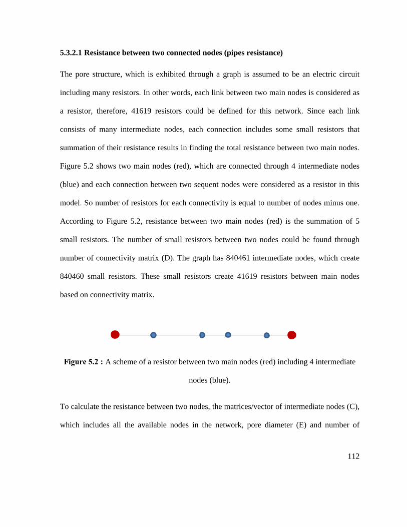
112

5.3.2.1 Resistance between two connected nodes (pipes resistance)

The pore structure, which is exhibited through a graph is assumed to be an electric circuit

including many resistors. In other words, each link between two main nodes is considered as

a resistor, therefore, 41619 resistors could be defined for this network. Since each link

consists of many intermediate nodes, each connection includes some small resistors that

summation of their resistance results in finding the total resistance between two main nodes.

Figure 5.2 shows two main nodes (red), which are connected through 4 intermediate nodes

(blue) and each connection between two sequent nodes were considered as a resistor in this

model. So number of resistors for each connectivity is equal to number of nodes minus one.

According to Figure 5.2, resistance between two main nodes (red) is the summation of 5

small resistors. The number of small resistors between two nodes could be found through

number of connectivity matrix (D). The graph has 840461 intermediate nodes, which create

840460 small resistors. These small resistors create 41619 resistors between main nodes

based on connectivity matrix.

A scheme of a resistor between two main nodes (red) including 4 intermediate

nodes (blue).

To calculate the resistance between two nodes, the matrices/vector of intermediate nodes (C),

which includes all the available nodes in the network, pore diameter (E) and number of

113

connectivity (D) were utilized. Referring to equation 2 and the analogy employed in this

work, the resistance (128𝜇𝐿

𝜋𝑑4 ) is directly proportional to length but has an inverse relationship

with 𝑑4. The 128𝜇

𝜋 ratio is a constant value and could be factored out from the calculation.

Since pore is assumed as a capillary consisting many connected pipes and in the graph it was

represented by a link between two nodes, 𝐿 which is the distance between two consecutive

intermediate nodes illustrates the pipe length. Using the intermediate nodes matrix (C) and

the Euclidean relation for distance this parameter could be achieved. The Euclidean relation

for distance is illustrated in equation 5,

𝐿 = √(𝑥1 − 𝑥2)2 + (𝑦1 − 𝑦2)

2 + (𝑧1 − 𝑧2)2 (5)

where x, y and z are the node position in X, Y and Z directions. Afterwards, a new vector

called distance vector (𝐿) will be generated with 840460 elements. 𝑑 is pore diameter, which

is saved in form of a vector (E) and 𝑑4 means each elements of the pore diameter vector (E)

in power of 4. As vector “E” includes the diameter of each center point and the diameters of

two consecutive nodes are not identical, the average of two diameters was used as the

diameter of the path between two nodes. In this condition, a new vector (𝐸𝑛𝑒𝑤) with 840460

elements will be obtained. Dividing vectors 𝐿 to (𝐸𝑛𝑒𝑤)4 leads to find the resistance (r)

between two sequent nodes by factoring 128𝜇

𝜋 out, which is constant. Vector “r” includes

840460 elements and shows all the resistances between consequent nodes in the network.

114

5.3.2.2 Resistance between two main nodes (capillaries resistance)

After calculating all small resistors in the network (vector r), resistance amid two main nodes

could be determined using vector D (number of connectivity). In vector D, each element

states the number of nodes in each connectivity. For example, based on first row of

matrix/vector B and D node number 1 is connected to node number 3 with 55 nodes, it means

there are 54 small resistors between these two nodes and summation of the first 54 numbers

in the obtained vector (r) results in finding the resistance between two nodes. Or, the second

row states nodes 1 and 3 are connected with 7 nodes, it means there are 6 small resistors and

summation of the next 6 values in vector “r” results the resistance between these two nodes.

Calculating all resistances between main nodes obtains a vector “R” with 41619 elements

that includes 𝐿

𝑑4 values for each connection between two connected main nodes, since the

constant value is factored out from the calculations. After calculating all the resistances, the

equivalent resistance of the network was found using admittance parameter (admittance

matrix).

To calculate the equivalent resistance of the system, the Kirchhoff Circuit Law (KCL) and

the admittance parameter were used. In this part these two rules will be described briefly.

Kirchhoff Circuit Law (KCL)

Kirchhoff Circuit law, which is also known as the Kirchhoff’s first law is based on the law of

conservation of charge, which means the algebraic sum of charges within a system cannot

change (Alexander & Sadiku, 2009). Based on this definition, Kirchhoff Circuit Law states

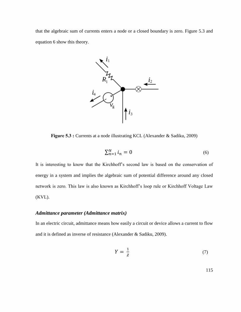
115

that the algebraic sum of currents enters a node or a closed boundary is zero. Figure 5.3 and

equation 6 show this theory.

Currents at a node illustrating KCL (Alexander & Sadiku, 2009)

∑ 𝑖𝑛𝑁𝑛=1 = 0 (6)

It is interesting to know that the Kirchhoff’s second law is based on the conservation of

energy in a system and implies the algebraic sum of potential difference around any closed

network is zero. This law is also known as Kirchhoff’s loop rule or Kirchhoff Voltage Law

(KVL).

Admittance parameter (Admittance matrix)

In an electric circuit, admittance means how easily a circuit or device allows a current to flow

and it is defined as inverse of resistance (Alexander & Sadiku, 2009).

𝑌 = 1

𝑍 (7)

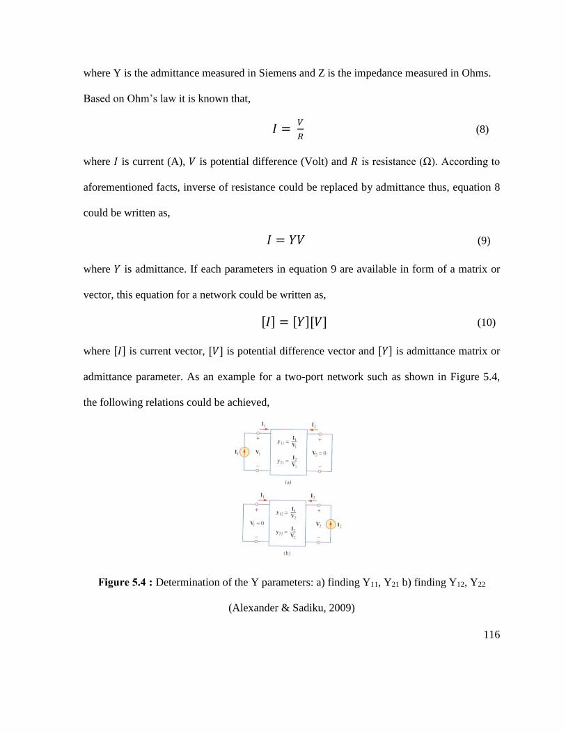
116

where Y is the admittance measured in Siemens and Z is the impedance measured in Ohms.

Based on Ohm’s law it is known that,

𝐼 = 𝑉

𝑅 (8)

where 𝐼 is current (A), 𝑉 is potential difference (Volt) and 𝑅 is resistance (Ω). According to

aforementioned facts, inverse of resistance could be replaced by admittance thus, equation 8

could be written as,

𝐼 = 𝑌𝑉 (9)

where 𝑌 is admittance. If each parameters in equation 9 are available in form of a matrix or

vector, this equation for a network could be written as,

[𝐼] = [𝑌][𝑉] (10)

where [𝐼] is current vector, [𝑉] is potential difference vector and [𝑌] is admittance matrix or

admittance parameter. As an example for a two-port network such as shown in Figure 5.4,

the following relations could be achieved,

Determination of the Y parameters: a) finding Y11, Y21 b) finding Y12, Y22

(Alexander & Sadiku, 2009)

117

𝐼1 = 𝑌11𝑉1 + 𝑌12𝑉2 (11)

𝐼2 = 𝑌21𝑉1 + 𝑌22𝑉2 (12)

These relations could be written in matrix form as well,

[𝐼1𝐼2

] = [𝑌11 𝑌12

𝑌21 𝑌22] [

𝑉1

𝑉2] (13)

The Y terms are known as the admittance parameter or Y parameter.

5.3.2.3 Calculating the equivalent resistance of the network

In admittance matrix (Y) each element represents the admittance between two nodes. This

means Y is a 38203×38203 matrix and 𝑌𝑖𝑗 illustrates the admittance between nodes i and j.

Clearly based on admittance matrix principles, the values of 𝑌𝑖𝑗 could be achieved through

inversing the elements of resistance vector (R) with negative sign. For instance 𝑌12 is the

inverse of resistance between nodes 1 and 2 with negative sign according to vector “R”.

Obviously in matrix Y, if there is no link between two nodes the value in matrix Y would be

zero. For example, if there is no link between node 1 and node 5 then, 𝑌15 = 𝑌51= 0. In

admittance matrix the value of 𝑌𝑖𝑖 is equal to summation of all values in the same row (or

column) multiplied by minus one. In other words, the value of Y’s element on diagonal is

equal to minus of the summation of all elements on that row/column.

It is interesting to know that referring to admittance matrix principles Y is a symmetric

matrix, since the summation of values on each row or column is zero. Also, the value of Y’s

element on diagonal is equal to minus of the summation of all elements on that row/column.

118

To create matrix Y, the connectivity matrix (D) is used to determine which nodes are

connected, then the associated impedance should be extracted from vector “R”.

In this work as it has been described, pores (through pores) start from top surface of the

media and end at the bottom surface. In the graph provided by the software (See Figure 4.13

as the example), node matrix (A) represents pore coordinates. In one hand, the nodes with the

z equals to zero are located on the top surface, since these points have no value in thickness

direction. On the other hand, the nodes with the maximum value of z are located at the

bottom surface, since they passed the maximum distance in thickness direction. Obviously,

other nodes are located in between. Matrix A shows that there are 94 nodes with z equals to

zero on the top and 126 nodes with the maximum value for z at the bottom. The main goal in

this part is to determine the equivalent resistance (impedance) between the top and bottom

surfaces.

As it is discussed, there are 94 nodes on the top and 126 nodes at the bottom surface of the

network. In order to determine the equivalent impedance (resistance) of the sample, the

resistance between top and bottom surface is required. In other words, it is assumed that

current enters the top and goes out from the bottom surface. Knowing the potential difference

and using Ohm’s law, the resistance of the network would be determined. For this purpose, it

is necessary to have one point for entering the current on top and one point for exiting the

current at the bottom. So, it is required to merge the nodes on the top and the bottom into one

node. Afterwards, there is one node at the top and one node at the bottom, which have the

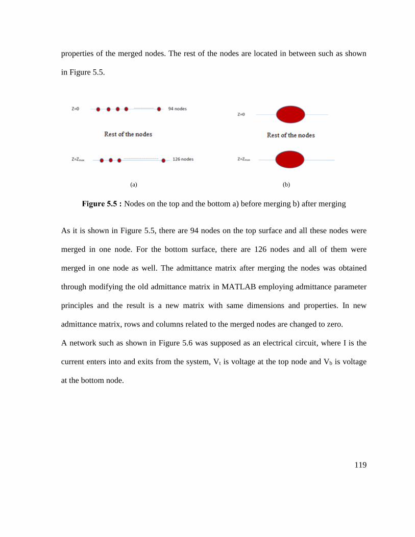
119

properties of the merged nodes. The rest of the nodes are located in between such as shown

in Figure 5.5.

(a) (b)

Nodes on the top and the bottom a) before merging b) after merging

As it is shown in Figure 5.5, there are 94 nodes on the top surface and all these nodes were

merged in one node. For the bottom surface, there are 126 nodes and all of them were

merged in one node as well. The admittance matrix after merging the nodes was obtained

through modifying the old admittance matrix in MATLAB employing admittance parameter

principles and the result is a new matrix with same dimensions and properties. In new

admittance matrix, rows and columns related to the merged nodes are changed to zero.

A network such as shown in Figure 5.6 was supposed as an electrical circuit, where I is the

current enters into and exits from the system, Vt is voltage at the top node and Vb is voltage

at the bottom node.

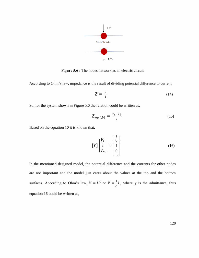
120

The nodes network as an electric circuit

According to Ohm’s law, impedance is the result of dividing potential difference to current,

𝑍 = 𝑉

𝐼 (14)

So, for the system shown in Figure 5.6 the relation could be written as,

𝑍𝑒𝑞(𝑡,𝑏) = 𝑉𝑡−𝑉𝑏

𝐼 (15)

Based on the equation 10 it is known that,

[𝑌] [𝑉𝑡

⋮𝑉𝑏

] =

[

𝐼0

⋮

0−𝐼]

(16)

In the mentioned designed model, the potential difference and the currents for other nodes

are not important and the model just cares about the values at the top and the bottom

surfaces. According to Ohm’s law, 𝑉 = 𝐼𝑅 or 𝑉 =1

𝑦𝐼 , where y is the admittance, thus

equation 16 could be written as,

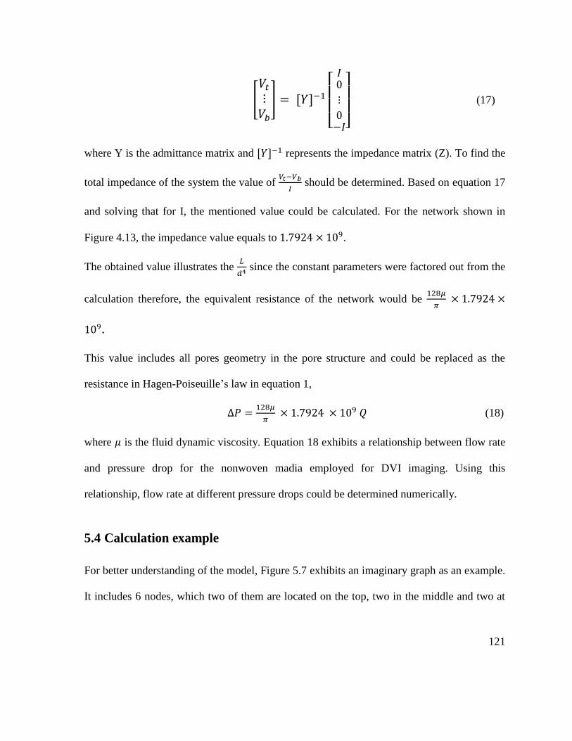
121

[𝑉𝑡

⋮𝑉𝑏

] = [𝑌]−1

[

𝐼0

⋮

0−𝐼]

(17)

where Y is the admittance matrix and [𝑌]−1 represents the impedance matrix (Z). To find the

total impedance of the system the value of 𝑉𝑡−𝑉𝑏

𝐼 should be determined. Based on equation 17

and solving that for I, the mentioned value could be calculated. For the network shown in

Figure 4.13, the impedance value equals to 1.7924 × 109.

The obtained value illustrates the 𝐿

𝑑4 since the constant parameters were factored out from the

calculation therefore, the equivalent resistance of the network would be 128𝜇

𝜋 × 1.7924 ×

109.

This value includes all pores geometry in the pore structure and could be replaced as the

resistance in Hagen-Poiseuille’s law in equation 1,

∆𝑃 =128𝜇

𝜋 × 1.7924 × 109 𝑄 (18)

where 𝜇 is the fluid dynamic viscosity. Equation 18 exhibits a relationship between flow rate

and pressure drop for the nonwoven madia employed for DVI imaging. Using this

relationship, flow rate at different pressure drops could be determined numerically.

5.4 Calculation example

For better understanding of the model, Figure 5.7 exhibits an imaginary graph as an example.

It includes 6 nodes, which two of them are located on the top, two in the middle and two at

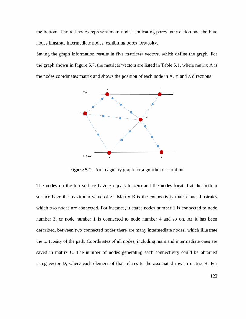
122

the bottom. The red nodes represent main nodes, indicating pores intersection and the blue

nodes illustrate intermediate nodes, exhibiting pores tortuosity.

Saving the graph information results in five matrices/ vectors, which define the graph. For

the graph shown in Figure 5.7, the matrices/vectors are listed in Table 5.1, where matrix A is

the nodes coordinates matrix and shows the position of each node in X, Y and Z directions.

An imaginary graph for algorithm description

The nodes on the top surface have z equals to zero and the nodes located at the bottom

surface have the maximum value of z. Matrix B is the connectivity matrix and illustrates

which two nodes are connected. For instance, it states nodes number 1 is connected to node

number 3, or node number 1 is connected to node number 4 and so on. As it has been

described, between two connected nodes there are many intermediate nodes, which illustrate

the tortuosity of the path. Coordinates of all nodes, including main and intermediate ones are

saved in matrix C. The number of nodes generating each connectivity could be obtained

using vector D, where each element of that relates to the associated row in matrix B. For

123

example according to matrix B, node 1 is connected to node 3 and using vector D there are 4

nodes in this connection, which two of them are main nodes and two are intermediate. Or,

node number 1 is connected to node number 4 with 5 nodes, which two of them are main

nodes and three are intermediate. Vector E is the node diameter vector and shows the

diameter of each intersection or node (pore size vector).

In order to find the equivalent resistance of the designed electric circuit shown in Figure 5.7,

each link between two connected nodes should be considered as a resistor. As it has been

described the resistance is equal to 128𝜇𝐿

𝜋𝑑4, where 𝐿 is length and 𝑑 is diameter of capillary.

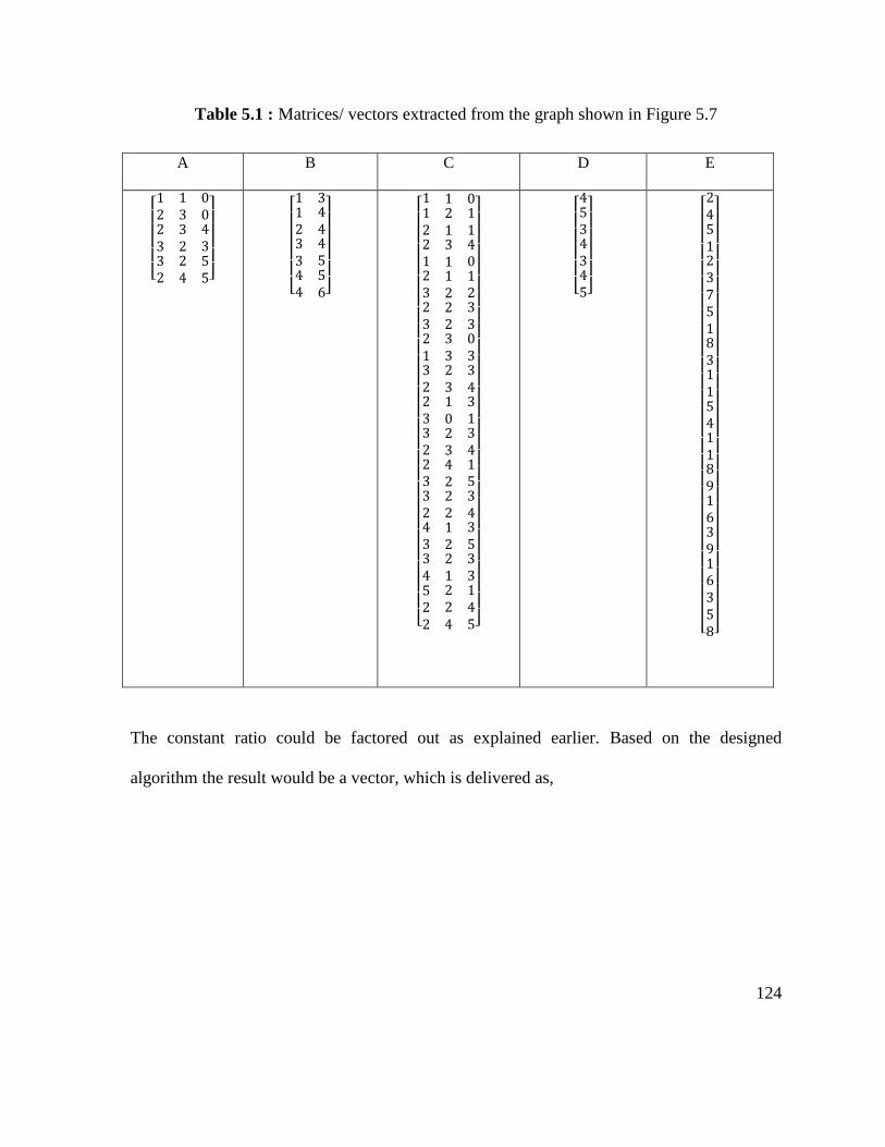
124

Table 5.1 : Matrices/ vectors extracted from the graph shown in Figure 5.7

A B C D E

[ 1 1 02 3 02332

3224

4355]

[ 1 3123344

444556]

[ 1 1 0122123232132233223324334522

213112223323102342221221224

114012330334313415343533145]

[ 4534345]

[ 2451237518311541189163916358]

The constant ratio could be factored out as explained earlier. Based on the designed

algorithm the result would be a vector, which is delivered as,

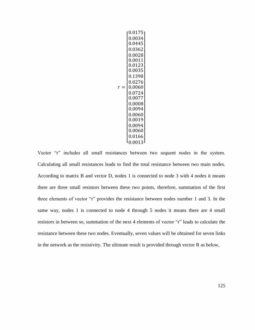
125

𝑟 =

[ 0.01750.00340.04450.03620.00280.00110.01230.00350.13980.02760.00600.07240.00770.00080.00940.00600.00190.00940.00600.01660.0013]

Vector “r” includes all small resistances between two sequent nodes in the system.

Calculating all small resistances leads to find the total resistance between two main nodes.

According to matrix B and vector D, nodes 1 is connected to node 3 with 4 nodes it means

there are three small resistors between these two points, therefore, summation of the first

three elements of vector “r” provides the resistance between nodes number 1 and 3. In the

same way, nodes 1 is connected to node 4 through 5 nodes it means there are 4 small

resistors in between so, summation of the next 4 elements of vector “r” leads to calculate the

resistance between these two nodes. Eventually, seven values will be obtained for seven links

in the network as the resistivity. The ultimate result is provided through vector R as below,

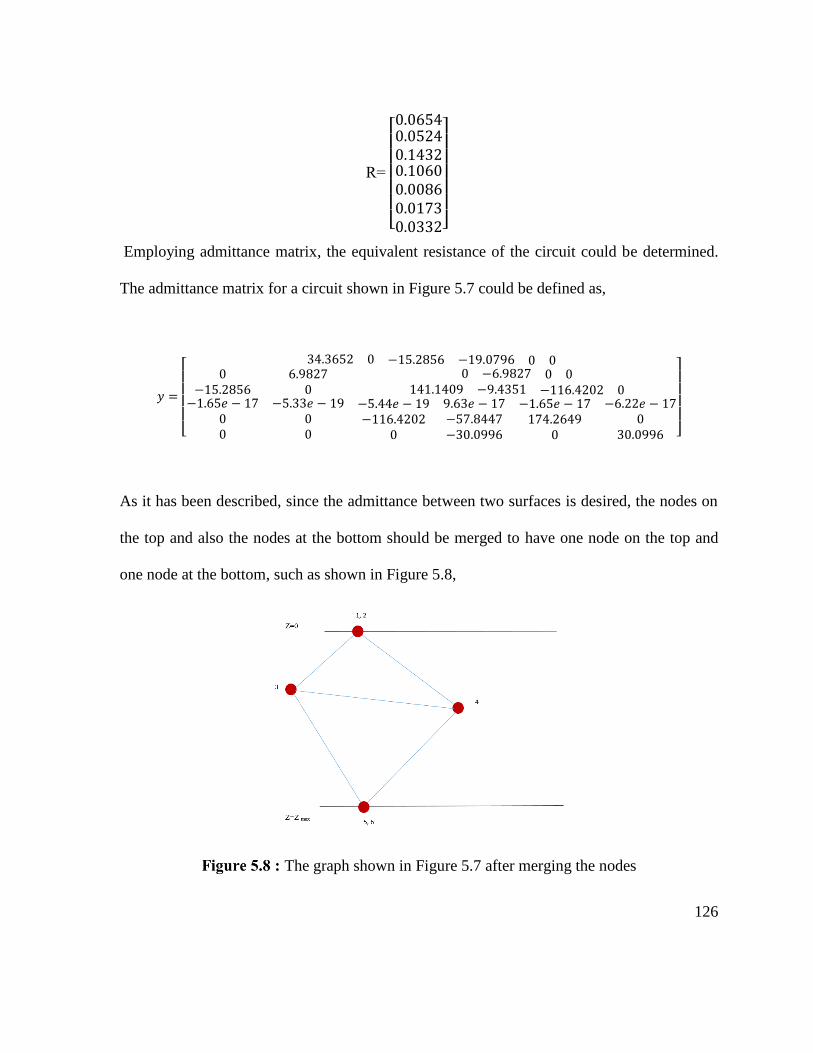
126

Employing admittance matrix, the equivalent resistance of the circuit could be determined.

The admittance matrix for a circuit shown in Figure 5.7 could be defined as,

𝑦 =

[

34.3652 0 −15.2856 −19.0796 0 00

−15.2856−1.65𝑒 − 17

00

6.98270

−5.33𝑒 − 1900

0 −6.9827 0 0141.1409 −9.4351 −116.4202 0

−5.44𝑒 − 19−116.4202

0

9.63𝑒 − 17−57.8447−30.0996

−1.65𝑒 − 17174.2649

0

−6.22𝑒 − 170

30.0996 ]

As it has been described, since the admittance between two surfaces is desired, the nodes on

the top and also the nodes at the bottom should be merged to have one node on the top and

one node at the bottom, such as shown in Figure 5.8,

The graph shown in Figure 5.7 after merging the nodes

R=

[ 0.06540.05240.14320.10600.00860.01730.0332]

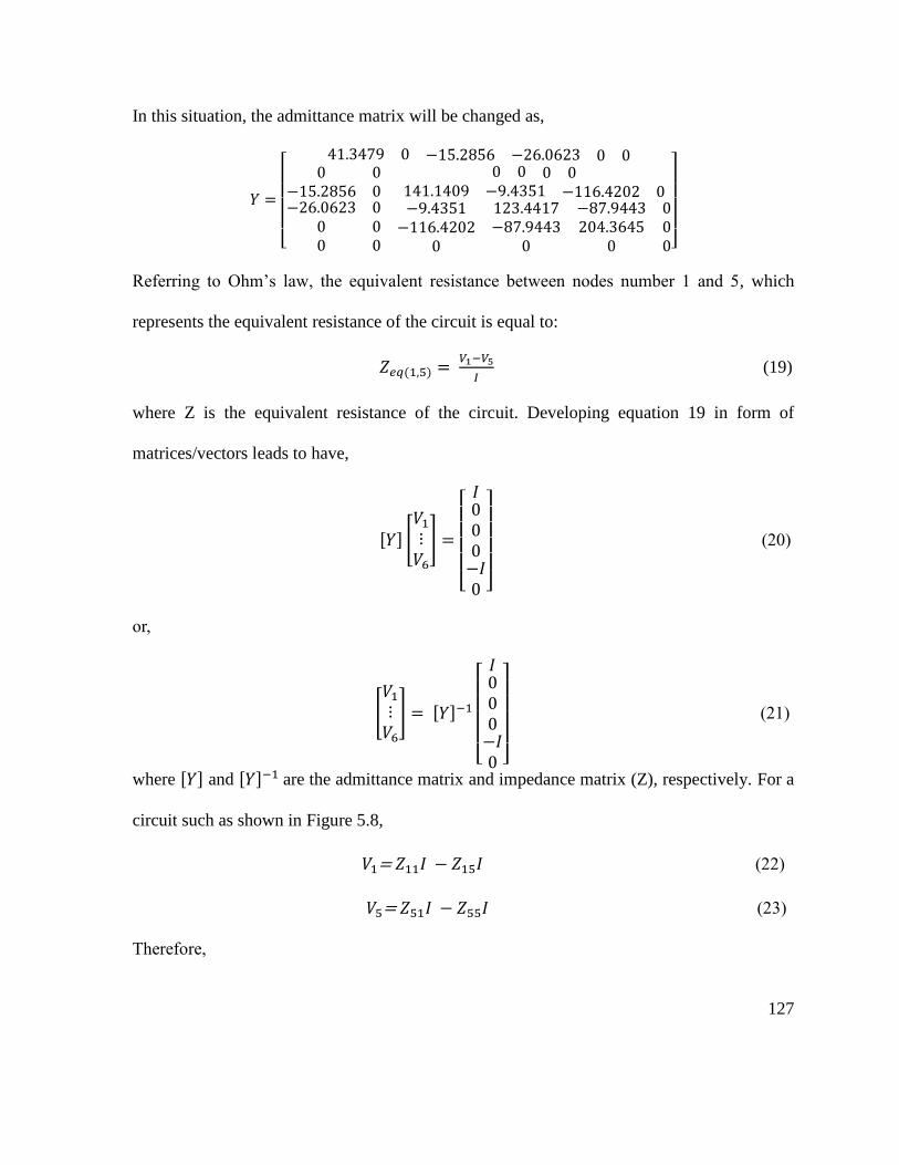
127

In this situation, the admittance matrix will be changed as,

𝑌 =

[

41.3479 0 −15.2856 −26.0623 0 00

−15.2856−26.0623

00

00000

0 0 0 0141.1409 −9.4351 −116.4202 0−9.4351

−116.42020

123.4417−87.9443

0

−87.9443204.3645

0

000]

Referring to Ohm’s law, the equivalent resistance between nodes number 1 and 5, which

represents the equivalent resistance of the circuit is equal to:

𝑍𝑒𝑞(1,5) = 𝑉1−𝑉5

𝐼 (19)

where Z is the equivalent resistance of the circuit. Developing equation 19 in form of

matrices/vectors leads to have,

[𝑌] [𝑉1

⋮𝑉6

] =

[

𝐼000−𝐼0 ]

(20)

or,

[𝑉1

⋮𝑉6

] = [𝑌]−1

[

𝐼000−𝐼0 ]

(21)

where [𝑌] and [𝑌]−1 are the admittance matrix and impedance matrix (Z), respectively. For a

circuit such as shown in Figure 5.8,

𝑉1= 𝑍11𝐼 − 𝑍15𝐼 (22)

𝑉5= 𝑍51𝐼 − 𝑍55𝐼 (23)

Therefore,

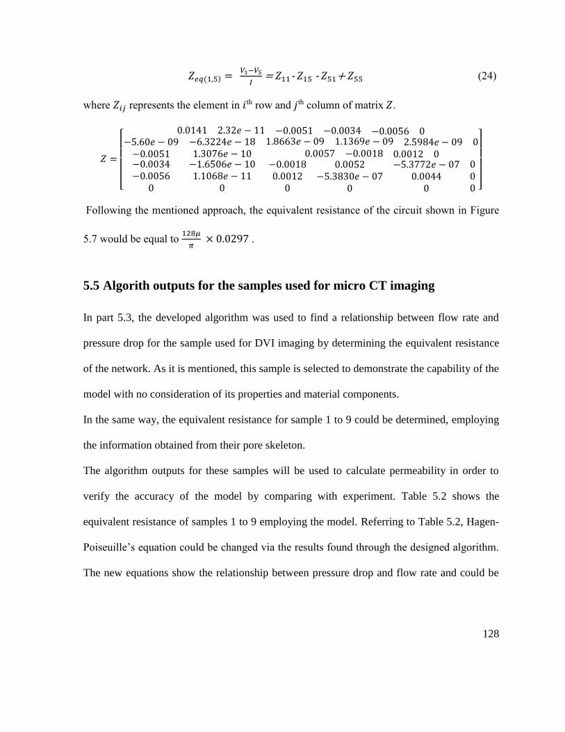
128

𝑍𝑒𝑞(1,5) = 𝑉1−𝑉5

𝐼 = 𝑍11- 𝑍15 - 𝑍51+ 𝑍55 (24)

where 𝑍𝑖𝑗 represents the element in 𝑖th row and 𝑗th column of matrix 𝑍.

𝑍 =

[

0.0141 2.32𝑒 − 11 −0.0051 −0.0034 −0.0056 0−5.60𝑒 − 09

−0.0051−0.0034−0.0056

0

−6.3224𝑒 − 181.3076𝑒 − 10

−1.6506𝑒 − 101.1068𝑒 − 11

0

1.8663𝑒 − 09 1.1369𝑒 − 09 2.5984𝑒 − 09 00.0057 −0.0018 0.0012 0

−0.00180.0012

0

0.0052−5.3830𝑒 − 07

0

−5.3772𝑒 − 070.0044

0

000 ]

Following the mentioned approach, the equivalent resistance of the circuit shown in Figure

5.7 would be equal to 128𝜇

𝜋 × 0.0297 .

5.5 Algorith outputs for the samples used for micro CT imaging

In part 5.3, the developed algorithm was used to find a relationship between flow rate and

pressure drop for the sample used for DVI imaging by determining the equivalent resistance

of the network. As it is mentioned, this sample is selected to demonstrate the capability of the

model with no consideration of its properties and material components.

In the same way, the equivalent resistance for sample 1 to 9 could be determined, employing

the information obtained from their pore skeleton.

The algorithm outputs for these samples will be used to calculate permeability in order to

verify the accuracy of the model by comparing with experiment. Table 5.2 shows the

equivalent resistance of samples 1 to 9 employing the model. Referring to Table 5.2, Hagen-

Poiseuille’s equation could be changed via the results found through the designed algorithm.

The new equations show the relationship between pressure drop and flow rate and could be

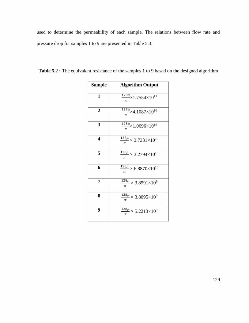
129

used to determine the permeability of each sample. The relations between flow rate and

pressure drop for samples 1 to 9 are presented in Table 5.3.

Table 5.2 : The equivalent resistance of the samples 1 to 9 based on the designed algorithm

Sample Algorithm Output

1 128𝜇

𝜋×1.7554×1011

2 128𝜇

𝜋×4.1087×1010

3 128𝜇

𝜋×1.0696×1010

4 128𝜇

𝜋 × 3.7331×1010

5 128𝜇

𝜋 × 3.2794×1010

6 128𝜇

𝜋 × 6.8870×1010

7 128𝜇

𝜋 × 3.8591×109

8 128𝜇

𝜋 × 3.8095×109

9 128𝜇

𝜋 × 5.2213×109

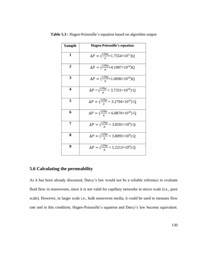
130

Table 5.3 : Hagen-Poiseuille’s equation based on algorithm output

Sample Hagen-Poiseuille’s equation

1 ∆𝑃 = (128𝜇

𝜋×1.7554×1011)Q

2 ∆𝑃 = (128𝜇

𝜋×4.1087×1010)Q

3 ∆𝑃 = (128𝜇

𝜋×1.0696×1010)Q

4 ∆𝑃 = (128𝜇

𝜋 × 3.7331×1010) Q

5 ∆𝑃 = (128𝜇

𝜋 × 3.2794×1010) Q

6 ∆𝑃 = (128𝜇

𝜋 × 6.8870×1010) Q

7 ∆𝑃 = (128𝜇

𝜋 × 3.8591×109) Q

8 ∆𝑃 = (128𝜇

𝜋 × 3.8095×109) Q

9 ∆𝑃 = (128𝜇

𝜋 × 5.2213×109) Q

5.6 Calculating the permeability

As it has been already discussed, Darcy’s law would not be a reliable reference to evaluate

fluid flow in nonwovens, since it is not valid for capillary networks in micro scale (i.e., pore

scale). However, in larger scale i.e., bulk nonwoven media, it could be used to measure flow

rate and in this condition, Hagen-Poiseuille’s equation and Darcy’s law become equivalent.

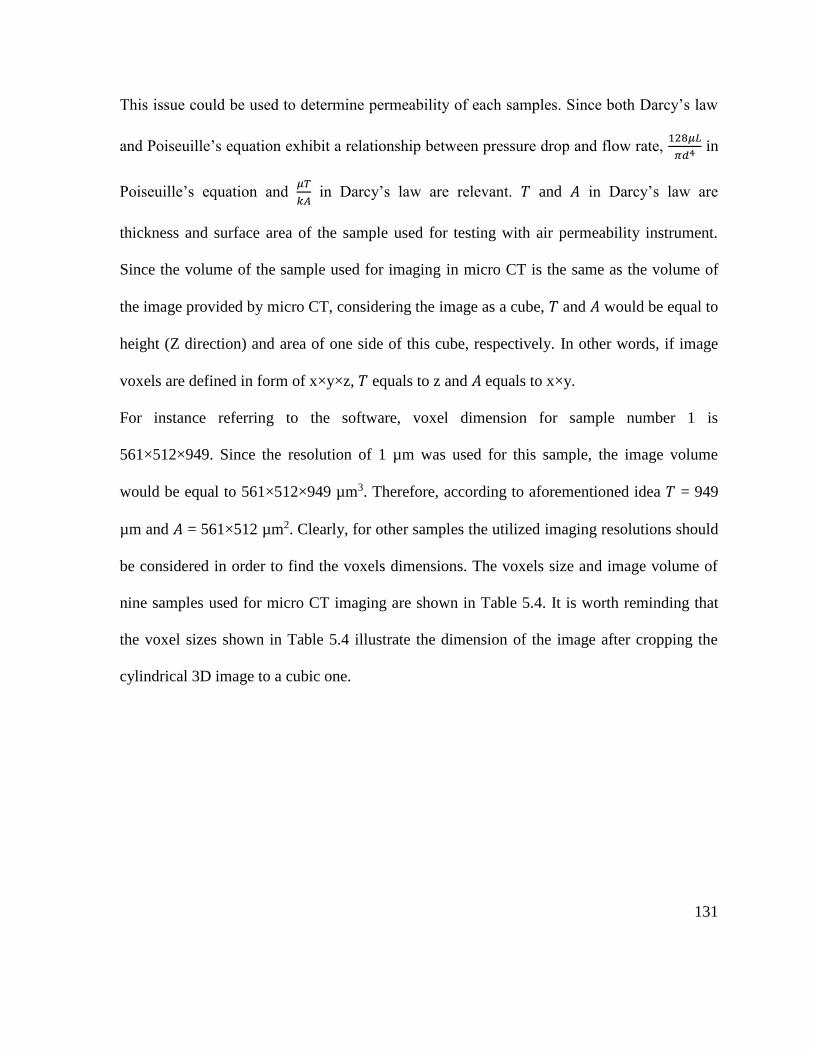
131

This issue could be used to determine permeability of each samples. Since both Darcy’s law

and Poiseuille’s equation exhibit a relationship between pressure drop and flow rate, 128𝜇𝐿

𝜋𝑑4 in

Poiseuille’s equation and 𝜇𝑇

𝑘𝐴 in Darcy’s law are relevant. 𝑇 and 𝐴 in Darcy’s law are

thickness and surface area of the sample used for testing with air permeability instrument.

Since the volume of the sample used for imaging in micro CT is the same as the volume of

the image provided by micro CT, considering the image as a cube, 𝑇 and 𝐴 would be equal to

height (Z direction) and area of one side of this cube, respectively. In other words, if image

voxels are defined in form of x×y×z, 𝑇 equals to z and 𝐴 equals to x×y.

For instance referring to the software, voxel dimension for sample number 1 is

561×512×949. Since the resolution of 1 µm was used for this sample, the image volume

would be equal to 561×512×949 µm3. Therefore, according to aforementioned idea 𝑇 = 949

µm and 𝐴 = 561×512 µm2. Clearly, for other samples the utilized imaging resolutions should

be considered in order to find the voxels dimensions. The voxels size and image volume of

nine samples used for micro CT imaging are shown in Table 5.4. It is worth reminding that

the voxel sizes shown in Table 5.4 illustrate the dimension of the image after cropping the

cylindrical 3D image to a cubic one.

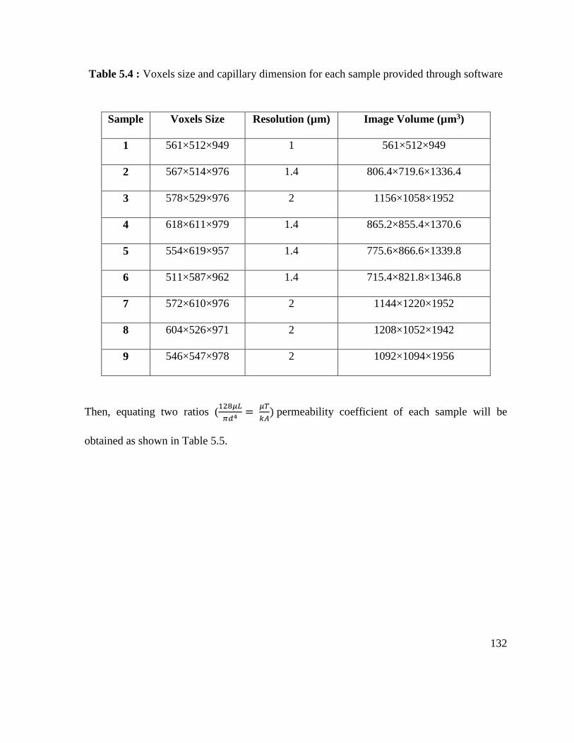
132

Table 5.4 : Voxels size and capillary dimension for each sample provided through software

Sample Voxels Size Resolution (µm) Image Volume (µm3)

1 561×512×949 1 561×512×949

2 567×514×976 1.4 806.4×719.6×1336.4

3 578×529×976 2 1156×1058×1952

4 618×611×979 1.4 865.2×855.4×1370.6

5 554×619×957 1.4 775.6×866.6×1339.8

6 511×587×962 1.4 715.4×821.8×1346.8

7 572×610×976 2 1144×1220×1952

8 604×526×971 2 1208×1052×1942

9 546×547×978 2 1092×1094×1956

Then, equating two ratios (128𝜇𝐿

𝜋𝑑4 = 𝜇𝑇

𝑘𝐴) permeability coefficient of each sample will be

obtained as shown in Table 5.5.

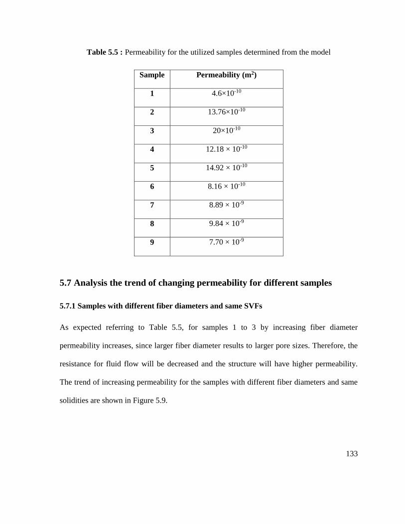
133

Table 5.5 : Permeability for the utilized samples determined from the model

Sample Permeability (m2)

1 4.6×10-10

2 13.76×10-10

3 20×10-10

4 12.18 × 10-10

5 14.92 × 10-10

6 8.16 × 10-10

7 8.89 × 10-9

8 9.84 × 10-9

9 7.70 × 10-9

5.7 Analysis the trend of changing permeability for different samples

5.7.1 Samples with different fiber diameters and same SVFs

As expected referring to Table 5.5, for samples 1 to 3 by increasing fiber diameter

permeability increases, since larger fiber diameter results to larger pore sizes. Therefore, the

resistance for fluid flow will be decreased and the structure will have higher permeability.

The trend of increasing permeability for the samples with different fiber diameters and same

solidities are shown in Figure 5.9.

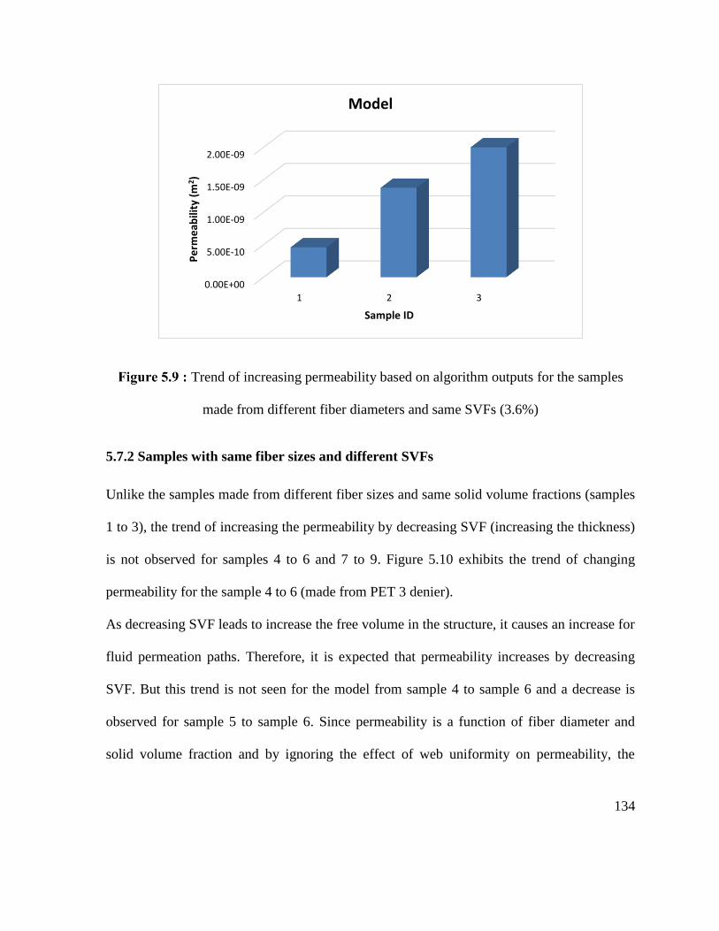
134

Trend of increasing permeability based on algorithm outputs for the samples

made from different fiber diameters and same SVFs (3.6%)

5.7.2 Samples with same fiber sizes and different SVFs

Unlike the samples made from different fiber sizes and same solid volume fractions (samples

1 to 3), the trend of increasing the permeability by decreasing SVF (increasing the thickness)

is not observed for samples 4 to 6 and 7 to 9. Figure 5.10 exhibits the trend of changing

permeability for the sample 4 to 6 (made from PET 3 denier).

As decreasing SVF leads to increase the free volume in the structure, it causes an increase for

fluid permeation paths. Therefore, it is expected that permeability increases by decreasing

SVF. But this trend is not seen for the model from sample 4 to sample 6 and a decrease is

observed for sample 5 to sample 6. Since permeability is a function of fiber diameter and

solid volume fraction and by ignoring the effect of web uniformity on permeability, the

0.00E+00

5.00E-10

1.00E-09

1.50E-09

2.00E-09

1 2 3

Pe

rme

abili

ty (

m2 )

Sample ID

Model

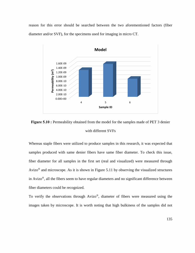
135

reason for this error should be searched between the two aforementioned factors (fiber

diameter and/or SVF), for the specimens used for imaging in micro CT.

Permeability obtained from the model for the samples made of PET 3 denier

with different SVFs

Whereas staple fibers were utilized to produce samples in this research, it was expected that

samples produced with same denier fibers have same fiber diameter. To check this issue,

fiber diameter for all samples in the first set (real and visualized) were measured through

Avizo® and microscope. As it is shown in Figure 5.11 by observing the visualized structures

in Avizo®, all the fibers seem to have regular diameters and no significant difference between

fiber diameters could be recognized.

To verify the observations through Avizo®, diameter of fibers were measured using the

images taken by microscope. It is worth noting that high bulkiness of the samples did not

0.00E+00

2.00E-10

4.00E-10

6.00E-10

8.00E-10

1.00E-09

1.20E-09

1.40E-09

1.60E-09

4 5 6

Pe

rme

abili

ty (

m2)

Sample ID

Model

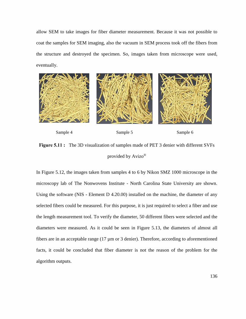
136

allow SEM to take images for fiber diameter measurement. Because it was not possible to

coat the samples for SEM imaging, also the vacuum in SEM process took off the fibers from

the structure and destroyed the specimen. So, images taken from microscope were used,

eventually.

Sample 4 Sample 5 Sample 6

The 3D visualization of samples made of PET 3 denier with different SVFs

provided by Avizo®

In Figure 5.12, the images taken from samples 4 to 6 by Nikon SMZ 1000 microscope in the

microscopy lab of The Nonwovens Institute - North Carolina State University are shown.

Using the software (NIS - Element D 4.20.00) installed on the machine, the diameter of any

selected fibers could be measured. For this purpose, it is just required to select a fiber and use

the length measurement tool. To verify the diameter, 50 different fibers were selected and the

diameters were measured. As it could be seen in Figure 5.13, the diameters of almost all

fibers are in an acceptable range (17 µm or 3 denier). Therefore, according to aforementioned

facts, it could be concluded that fiber diameter is not the reason of the problem for the

algorithm outputs.

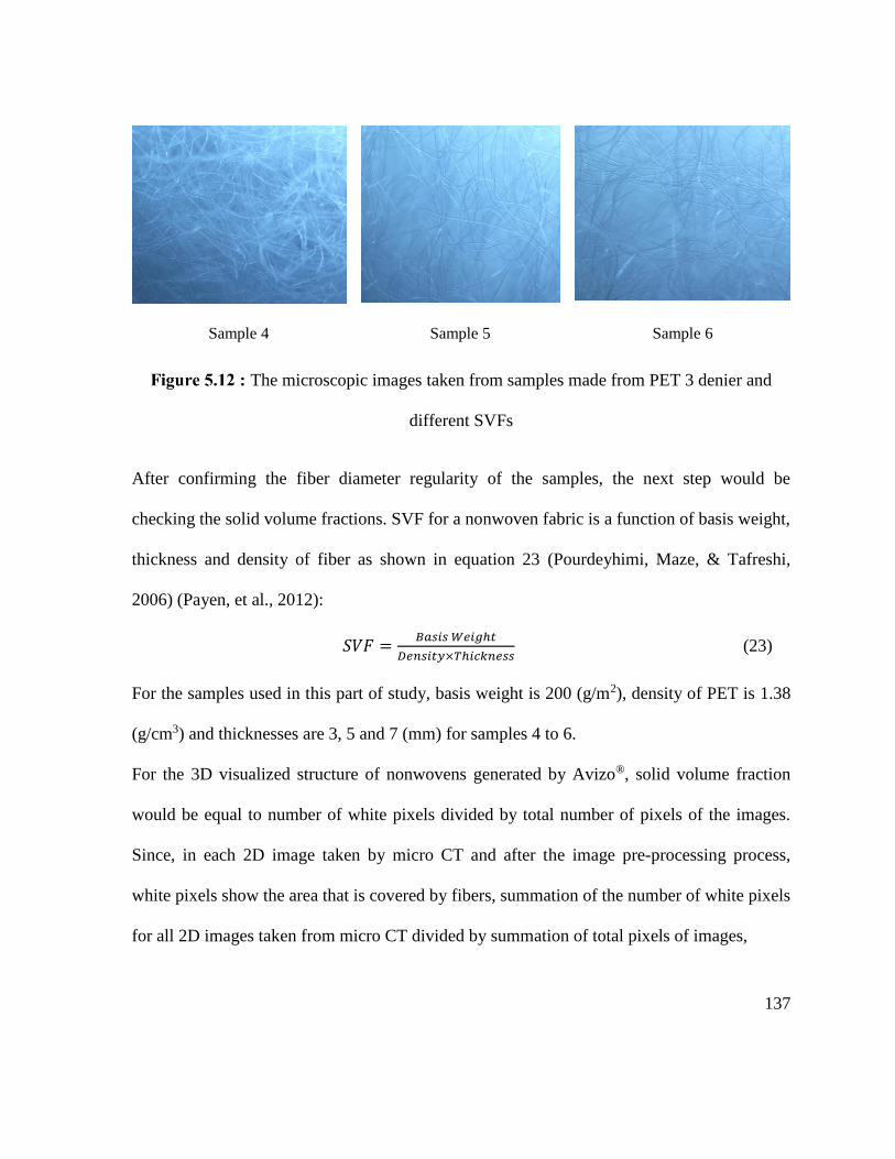
137

Sample 4 Sample 5 Sample 6

The microscopic images taken from samples made from PET 3 denier and

different SVFs

After confirming the fiber diameter regularity of the samples, the next step would be

checking the solid volume fractions. SVF for a nonwoven fabric is a function of basis weight,

thickness and density of fiber as shown in equation 23 (Pourdeyhimi, Maze, & Tafreshi,

2006) (Payen, et al., 2012):

𝑆𝑉𝐹 =𝐵𝑎𝑠𝑖𝑠 𝑊𝑒𝑖𝑔ℎ𝑡

𝐷𝑒𝑛𝑠𝑖𝑡𝑦×𝑇ℎ𝑖𝑐𝑘𝑛𝑒𝑠𝑠 (23)

For the samples used in this part of study, basis weight is 200 (g/m2), density of PET is 1.38

(g/cm3) and thicknesses are 3, 5 and 7 (mm) for samples 4 to 6.

For the 3D visualized structure of nonwovens generated by Avizo®, solid volume fraction

would be equal to number of white pixels divided by total number of pixels of the images.

Since, in each 2D image taken by micro CT and after the image pre-processing process,

white pixels show the area that is covered by fibers, summation of the number of white pixels

for all 2D images taken from micro CT divided by summation of total pixels of images,

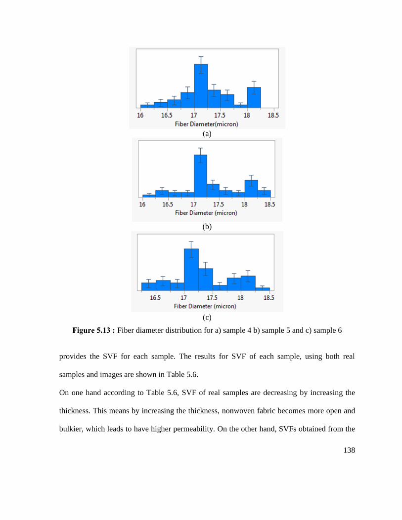
138

(a)

(b)

(c)

Fiber diameter distribution for a) sample 4 b) sample 5 and c) sample 6

provides the SVF for each sample. The results for SVF of each sample, using both real

samples and images are shown in Table 5.6.

On one hand according to Table 5.6, SVF of real samples are decreasing by increasing the

thickness. This means by increasing the thickness, nonwoven fabric becomes more open and

bulkier, which leads to have higher permeability. On the other hand, SVFs obtained from the

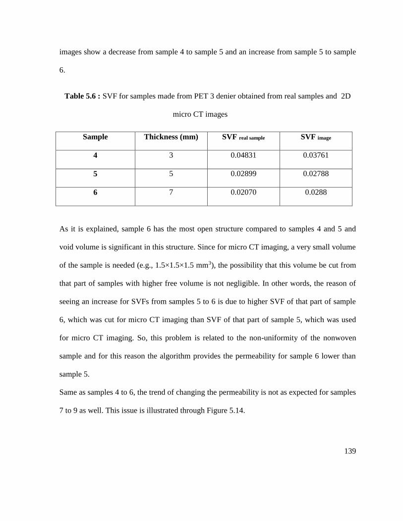
139

images show a decrease from sample 4 to sample 5 and an increase from sample 5 to sample

6.

Table 5.6 : SVF for samples made from PET 3 denier obtained from real samples and 2D

micro CT images

Sample Thickness (mm) SVF real sample SVF image

4 3 0.04831 0.03761

5 5 0.02899 0.02788

6 7 0.02070 0.0288

As it is explained, sample 6 has the most open structure compared to samples 4 and 5 and

void volume is significant in this structure. Since for micro CT imaging, a very small volume

of the sample is needed (e.g., 1.5×1.5×1.5 mm3), the possibility that this volume be cut from

that part of samples with higher free volume is not negligible. In other words, the reason of

seeing an increase for SVFs from samples 5 to 6 is due to higher SVF of that part of sample

6, which was cut for micro CT imaging than SVF of that part of sample 5, which was used

for micro CT imaging. So, this problem is related to the non-uniformity of the nonwoven

sample and for this reason the algorithm provides the permeability for sample 6 lower than

sample 5.

Same as samples 4 to 6, the trend of changing the permeability is not as expected for samples

7 to 9 as well. This issue is illustrated through Figure 5.14.

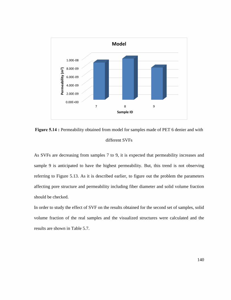
140

Permeability obtained from model for samples made of PET 6 denier and with

different SVFs

As SVFs are decreasing from samples 7 to 9, it is expected that permeability increases and

sample 9 is anticipated to have the highest permeability. But, this trend is not observing

referring to Figure 5.13. As it is described earlier, to figure out the problem the parameters

affecting pore structure and permeability including fiber diameter and solid volume fraction

should be checked.

In order to study the effect of SVF on the results obtained for the second set of samples, solid

volume fraction of the real samples and the visualized structures were calculated and the

results are shown in Table 5.7.

0.00E+00

2.00E-09

4.00E-09

6.00E-09

8.00E-09

1.00E-08

7 8 9

Pe

rme

abili

ty (

m2 )

Sample ID

Model

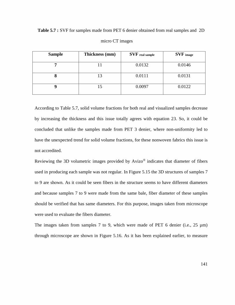
141

Table 5.7 : SVF for samples made from PET 6 denier obtained from real samples and 2D

micro CT images

Sample Thickness (mm) SVF real sample SVF image

7 11 0.0132 0.0146

8 13 0.0111 0.0131

9 15 0.0097 0.0122

According to Table 5.7, solid volume fractions for both real and visualized samples decrease

by increasing the thickness and this issue totally agrees with equation 23. So, it could be

concluded that unlike the samples made from PET 3 denier, where non-uniformity led to

have the unexpected trend for solid volume fractions, for these nonwoven fabrics this issue is

not accredited.

Reviewing the 3D volumetric images provided by Avizo® indicates that diameter of fibers

used in producing each sample was not regular. In Figure 5.15 the 3D structures of samples 7

to 9 are shown. As it could be seen fibers in the structure seems to have different diameters

and because samples 7 to 9 were made from the same bale, fiber diameter of these samples

should be verified that has same diameters. For this purpose, images taken from microscope

were used to evaluate the fibers diameter.

The images taken from samples 7 to 9, which were made of PET 6 denier (i.e., 25 µm)

through microscope are shown in Figure 5.16. As it has been explained earlier, to measure

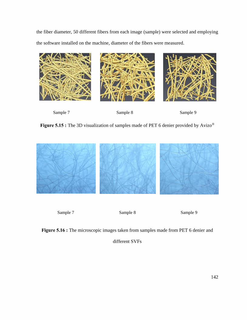
142

the fiber diameter, 50 different fibers from each image (sample) were selected and employing

the software installed on the machine, diameter of the fibers were measured.

Sample 7 Sample 8 Sample 9

The 3D visualization of samples made of PET 6 denier provided by Avizo®

Sample 7 Sample 8 Sample 9

The microscopic images taken from samples made from PET 6 denier and

different SVFs

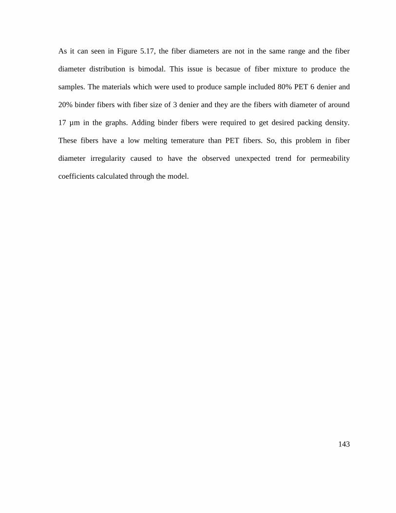
143

As it can seen in Figure 5.17, the fiber diameters are not in the same range and the fiber

diameter distribution is bimodal. This issue is becasue of fiber mixture to produce the

samples. The materials which were used to produce sample included 80% PET 6 denier and

20% binder fibers with fiber size of 3 denier and they are the fibers with diameter of around

17 µm in the graphs. Adding binder fibers were required to get desired packing density.

These fibers have a low melting temerature than PET fibers. So, this problem in fiber

diameter irregularity caused to have the observed unexpected trend for permeability

coefficients calculated through the model.

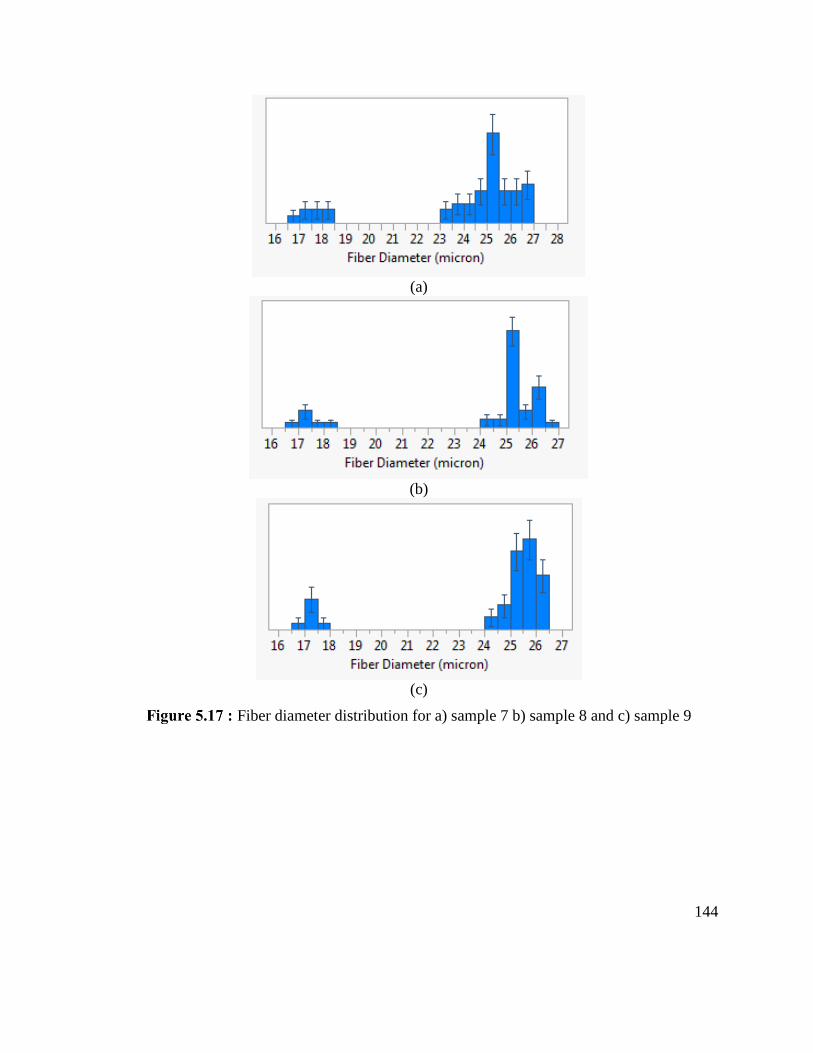
144

(a)

(b)

(c)

Fiber diameter distribution for a) sample 7 b) sample 8 and c) sample 9

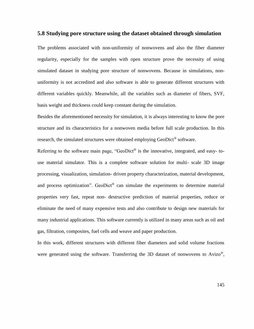
145

5.8 Studying pore structure using the dataset obtained through simulation

The problems associated with non-uniformity of nonwovens and also the fiber diameter

regularity, especially for the samples with open structure prove the necessity of using

simulated dataset in studying pore structure of nonwovens. Because in simulations, non-

uniformity is not accredited and also software is able to generate different structures with

different variables quickly. Meanwhile, all the variables such as diameter of fibers, SVF,

basis weight and thickness could keep constant during the simulation.

Besides the aforementioned necessity for simulation, it is always interesting to know the pore

structure and its characteristics for a nonwoven media before full scale production. In this

research, the simulated structures were obtained employing GeoDict® software.

Referring to the software main page, “GeoDict® is the innovative, integrated, and easy- to-

use material simulator. This is a complete software solution for multi- scale 3D image

processing, visualization, simulation- driven property characterization, material development,

and process optimization”. GeoDict® can simulate the experiments to determine material

properties very fast, repeat non- destructive prediction of material properties, reduce or

eliminate the need of many expensive tests and also contribute to design new materials for

many industrial applications. This software currently is utilized in many areas such as oil and

gas, filtration, composites, fuel cells and weave and paper production.

In this work, different structures with different fiber diameters and solid volume fractions

were generated using the software. Transferring the 3D dataset of nonwovens to Avizo®,

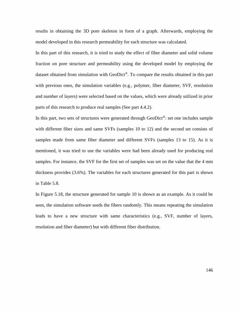
146

results in obtaining the 3D pore skeleton in form of a graph. Afterwards, employing the

model developed in this research permeability for each structure was calculated.

In this part of this research, it is tried to study the effect of fiber diameter and solid volume

fraction on pore structure and permeability using the developed model by employing the

dataset obtained from simulation with GeoDict®. To compare the results obtained in this part

with previous ones, the simulation variables (e.g., polymer, fiber diameter, SVF, resolution

and number of layers) were selected based on the values, which were already utilized in prior

parts of this research to produce real samples (See part 4.4.2).

In this part, two sets of structures were generated through GeoDict®: set one includes sample

with different fiber sizes and same SVFs (samples 10 to 12) and the second set consists of

samples made from same fiber diameter and different SVFs (samples 13 to 15). As it is

mentioned, it was tried to use the variables were had been already used for producing real

samples. For instance, the SVF for the first set of samples was set on the value that the 4 mm

thickness provides (3.6%). The variables for each structures generated for this part is shown

in Table 5.8.

In Figure 5.18, the structure generated for sample 10 is shown as an example. As it could be

seen, the simulation software seeds the fibers randomly. This means repeating the simulation

leads to have a new structure with same characteristics (e.g., SVF, number of layers,

resolution and fiber diameter) but with different fiber distribution.

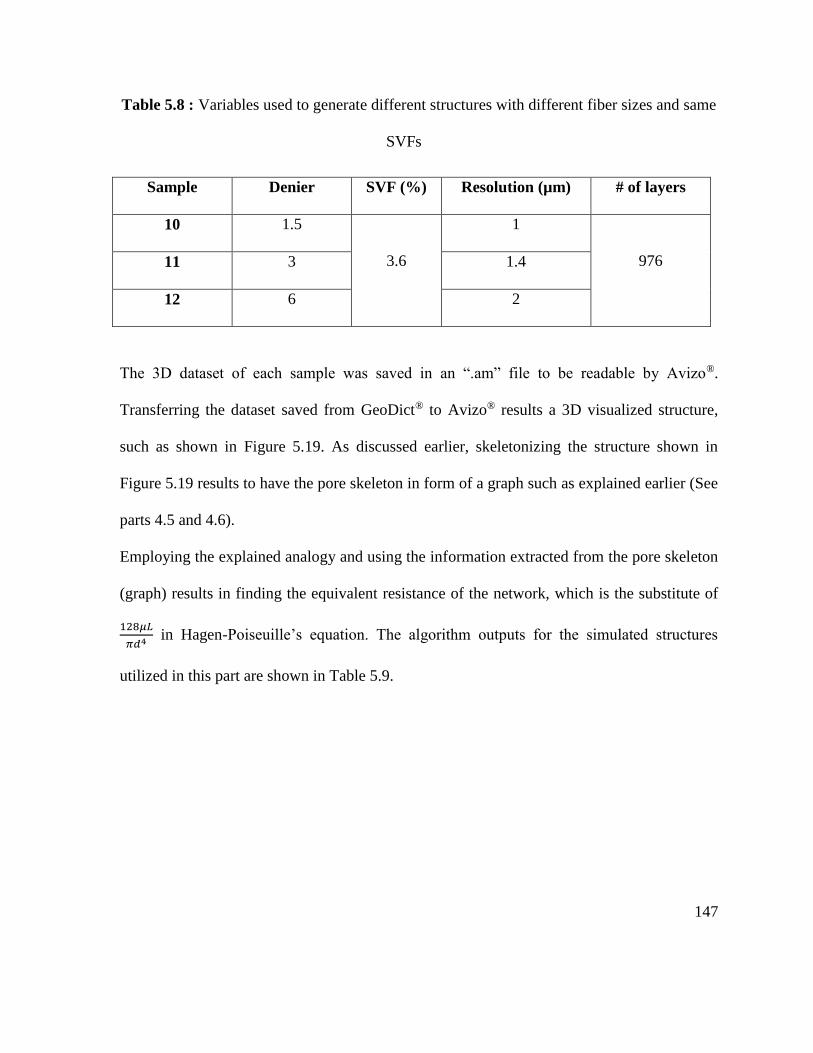
147

Table 5.8 : Variables used to generate different structures with different fiber sizes and same

SVFs

Sample Denier SVF (%) Resolution (µm) # of layers

10 1.5

3.6

1

976 11 3 1.4

12 6 2

The 3D dataset of each sample was saved in an “.am” file to be readable by Avizo®.

Transferring the dataset saved from GeoDict® to Avizo® results a 3D visualized structure,

such as shown in Figure 5.19. As discussed earlier, skeletonizing the structure shown in

Figure 5.19 results to have the pore skeleton in form of a graph such as explained earlier (See

parts 4.5 and 4.6).

Employing the explained analogy and using the information extracted from the pore skeleton

(graph) results in finding the equivalent resistance of the network, which is the substitute of

128𝜇𝐿

𝜋𝑑4 in Hagen-Poiseuille’s equation. The algorithm outputs for the simulated structures

utilized in this part are shown in Table 5.9.

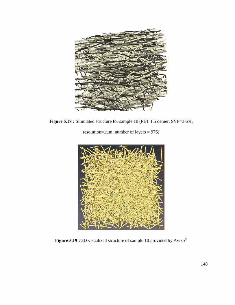
148

Simulated structure for sample 10 (PET 1.5 denier, SVF=3.6%,

resolution=1µm, number of layers = 976)

3D visualized structure of sample 10 provided by Avizo®

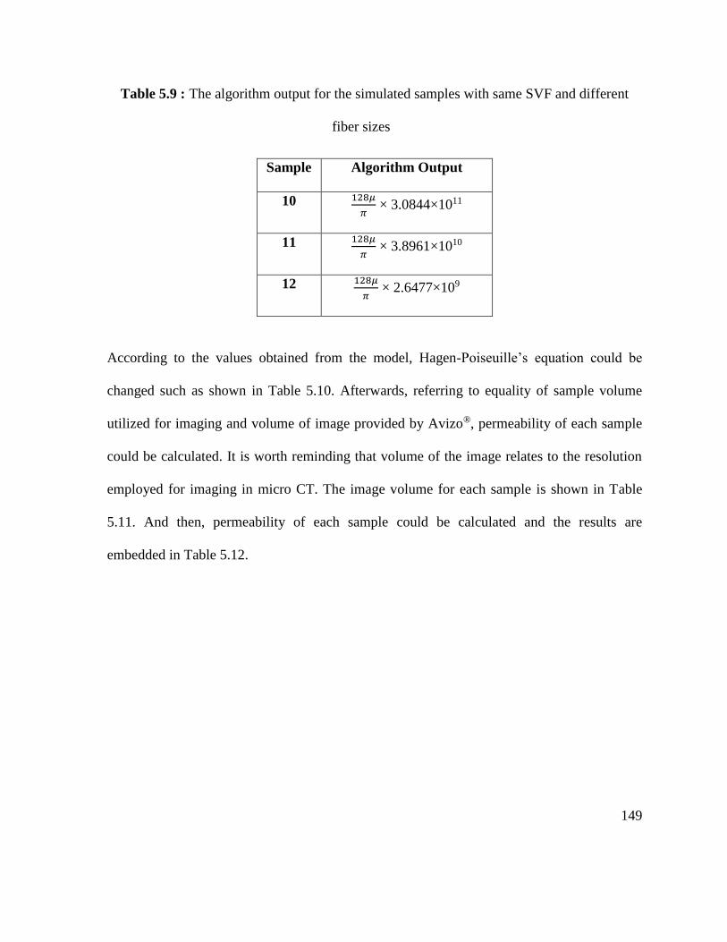
149

Table 5.9 : The algorithm output for the simulated samples with same SVF and different

fiber sizes

Sample Algorithm Output

10 128𝜇

𝜋 × 3.0844×1011

11 128𝜇

𝜋 × 3.8961×1010

12 128𝜇

𝜋 × 2.6477×109

According to the values obtained from the model, Hagen-Poiseuille’s equation could be

changed such as shown in Table 5.10. Afterwards, referring to equality of sample volume

utilized for imaging and volume of image provided by Avizo®, permeability of each sample

could be calculated. It is worth reminding that volume of the image relates to the resolution

employed for imaging in micro CT. The image volume for each sample is shown in Table

5.11. And then, permeability of each sample could be calculated and the results are

embedded in Table 5.12.

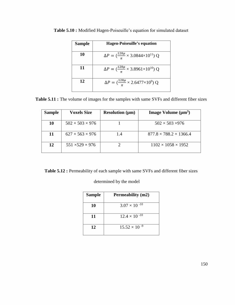
150

Table 5.10 : Modified Hagen-Poiseuille’s equation for simulated dataset

Sample Hagen-Poiseuille’s equation

10 ∆𝑃 = (128𝜇

𝜋 × 3.0844×1011) Q

11 ∆𝑃 = (128𝜇

𝜋 × 3.8961×1010) Q

12 ∆𝑃 = (128𝜇

𝜋 × 2.6477×109) Q

Table 5.11 : The volume of images for the samples with same SVFs and different fiber sizes

Sample Voxels Size Resolution (µm) Image Volume (µm3)

10 502 × 503 × 976 1 502 × 503 ×976

11 627 × 563 × 976 1.4 877.8 × 788.2 × 1366.4

12 551 ×529 × 976 2 1102 × 1058 × 1952

Table 5.12 : Permeability of each sample with same SVFs and different fiber sizes

determined by the model

Sample Permeability (m2)

10 3.07 × 10 -10

11 12.4 × 10 -10

12 15.52 × 10 -9

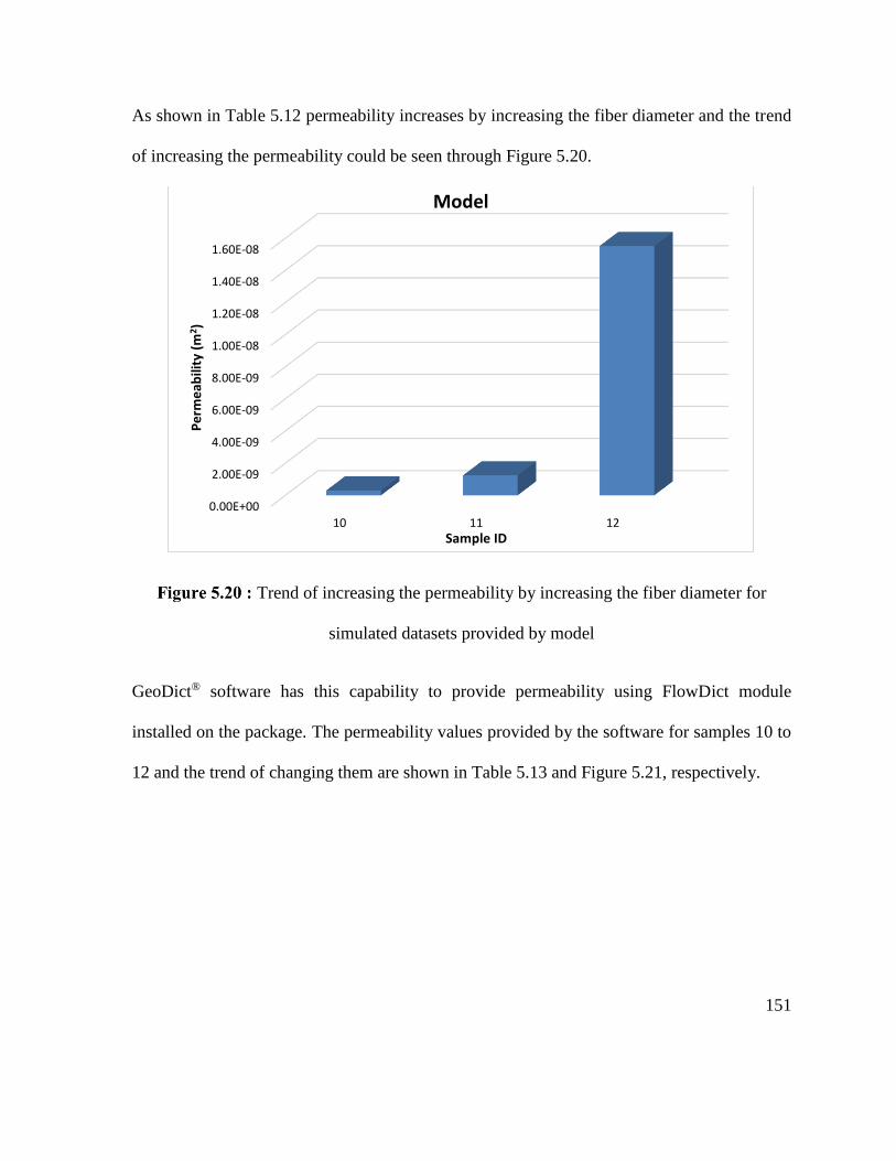
151

As shown in Table 5.12 permeability increases by increasing the fiber diameter and the trend

of increasing the permeability could be seen through Figure 5.20.

Trend of increasing the permeability by increasing the fiber diameter for

simulated datasets provided by model

GeoDict® software has this capability to provide permeability using FlowDict module

installed on the package. The permeability values provided by the software for samples 10 to

12 and the trend of changing them are shown in Table 5.13 and Figure 5.21, respectively.

0.00E+00

2.00E-09

4.00E-09

6.00E-09

8.00E-09

1.00E-08

1.20E-08

1.40E-08

1.60E-08

10 11 12

Pe

rme

abili

ty (

m2)

Sample ID

Model

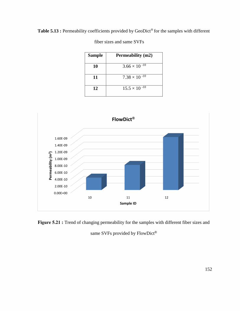
152

Table 5.13 : Permeability coefficients provided by GeoDict® for the samples with different

fiber sizes and same SVFs

Sample Permeability (m2)

10 3.66 × 10 -10

11 7.38 × 10 -10

12 15.5 × 10 -10

Trend of changing permeability for the samples with different fiber sizes and

same SVFs provided by FlowDict®

0.00E+00

2.00E-10

4.00E-10

6.00E-10

8.00E-10

1.00E-09

1.20E-09

1.40E-09

1.60E-09

10 11 12

Pe

rme

abili

ty (

m2 )

Sample ID

FlowDict®

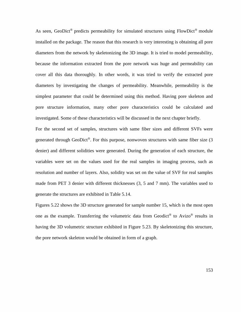
153

As seen, GeoDict® predicts permeability for simulated structures using FlowDict® module

installed on the package. The reason that this research is very interesting is obtaining all pore

diameters from the network by skeletonizing the 3D image. It is tried to model permeability,

because the information extracted from the pore network was huge and permeability can

cover all this data thoroughly. In other words, it was tried to verify the extracted pore

diameters by investigating the changes of permeability. Meanwhile, permeability is the

simplest parameter that could be determined using this method. Having pore skeleton and

pore structure information, many other pore characteristics could be calculated and

investigated. Some of these characteristics will be discussed in the next chapter briefly.

For the second set of samples, structures with same fiber sizes and different SVFs were

generated through GeoDict®. For this purpose, nonwoven structures with same fiber size (3

denier) and different solidities were generated. During the generation of each structure, the

variables were set on the values used for the real samples in imaging process, such as

resolution and number of layers. Also, solidity was set on the value of SVF for real samples

made from PET 3 denier with different thicknesses (3, 5 and 7 mm). The variables used to

generate the structures are exhibited in Table 5.14.

Figures 5.22 shows the 3D structure generated for sample number 15, which is the most open

one as the example. Transferring the volumetric data from Geodict® to Avizo® results in

having the 3D volumetric structure exhibited in Figure 5.23. By skeletonizing this structure,

the pore network skeleton would be obtained in form of a graph.

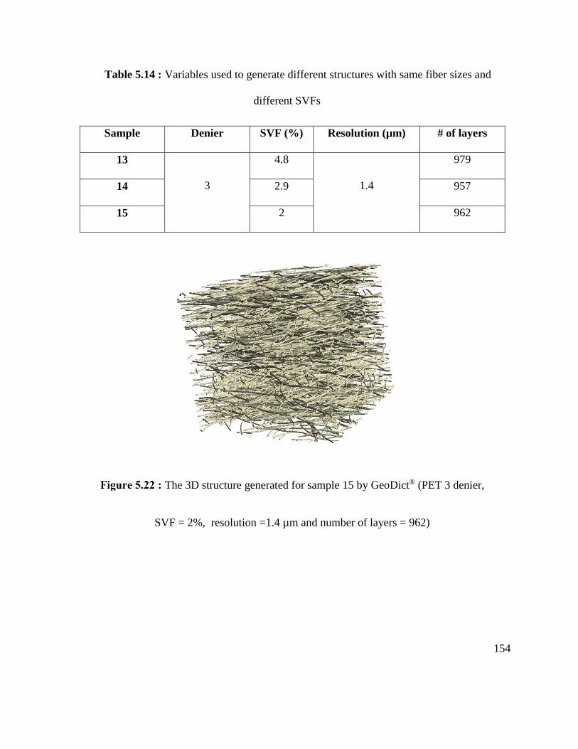
154

Table 5.14 : Variables used to generate different structures with same fiber sizes and

different SVFs

Sample Denier SVF (%) Resolution (µm) # of layers

13

3

4.8

1.4

979

14 2.9 957

15 2 962

The 3D structure generated for sample 15 by GeoDict® (PET 3 denier,

SVF = 2%, resolution =1.4 µm and number of layers = 962)

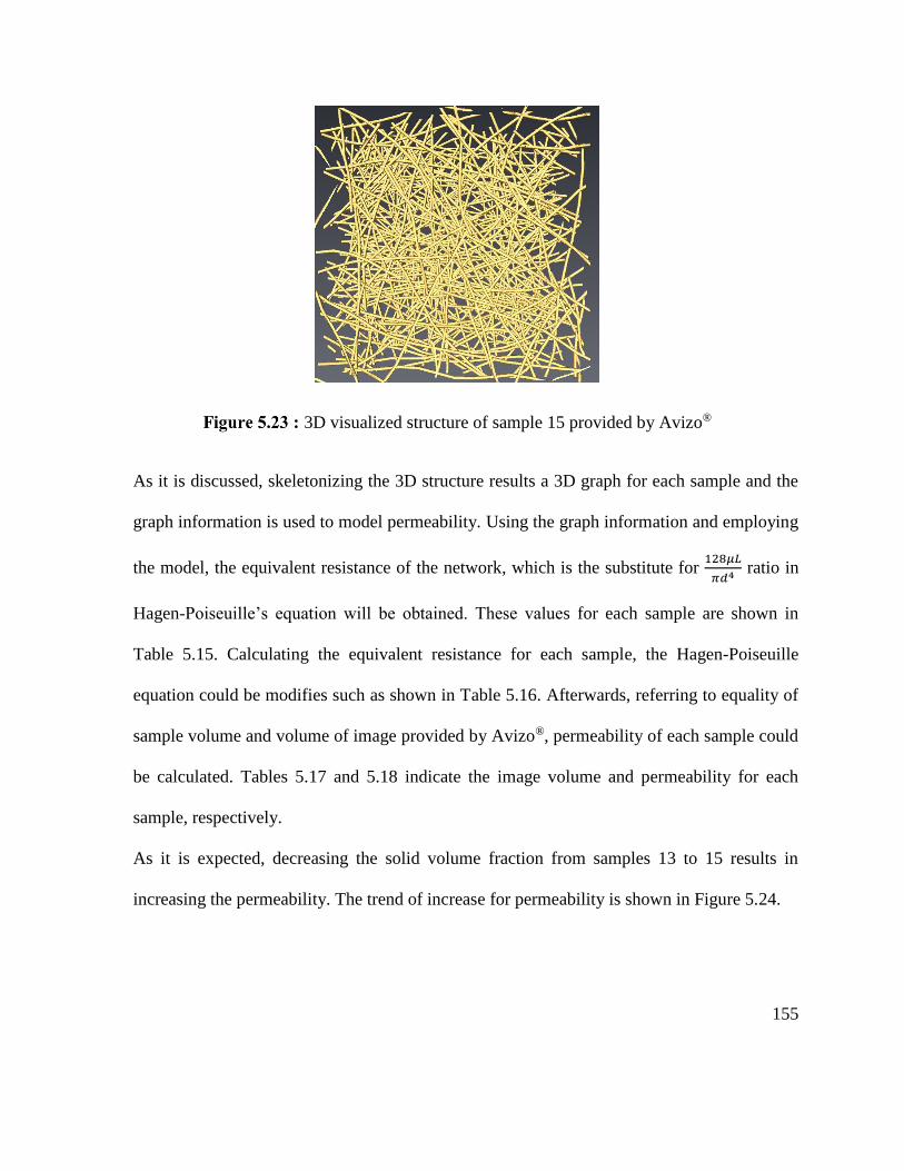
155

3D visualized structure of sample 15 provided by Avizo®

As it is discussed, skeletonizing the 3D structure results a 3D graph for each sample and the

graph information is used to model permeability. Using the graph information and employing

the model, the equivalent resistance of the network, which is the substitute for 128𝜇𝐿

𝜋𝑑4 ratio in

Hagen-Poiseuille’s equation will be obtained. These values for each sample are shown in

Table 5.15. Calculating the equivalent resistance for each sample, the Hagen-Poiseuille

equation could be modifies such as shown in Table 5.16. Afterwards, referring to equality of

sample volume and volume of image provided by Avizo®, permeability of each sample could

be calculated. Tables 5.17 and 5.18 indicate the image volume and permeability for each

sample, respectively.

As it is expected, decreasing the solid volume fraction from samples 13 to 15 results in

increasing the permeability. The trend of increase for permeability is shown in Figure 5.24.

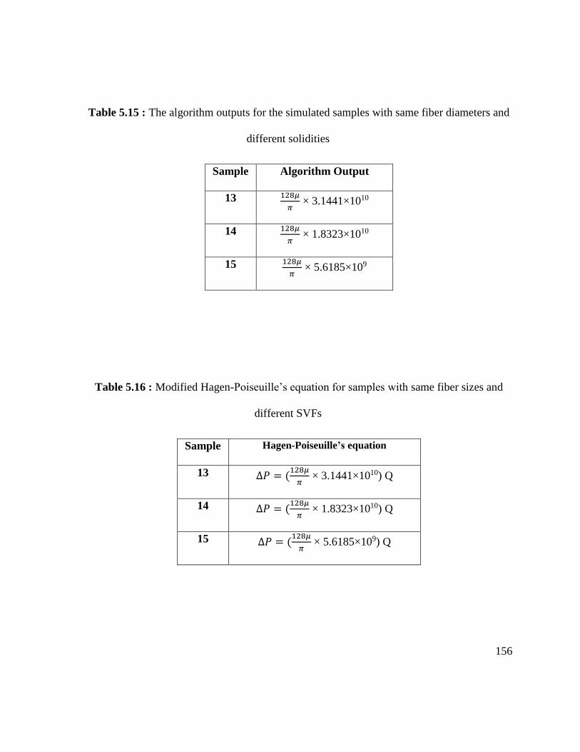
156

Table 5.15 : The algorithm outputs for the simulated samples with same fiber diameters and

different solidities

Sample Algorithm Output

13 128𝜇

𝜋 × 3.1441×1010

14 128𝜇

𝜋 × 1.8323×1010

15 128𝜇

𝜋 × 5.6185×109

Table 5.16 : Modified Hagen-Poiseuille’s equation for samples with same fiber sizes and

different SVFs

Sample Hagen-Poiseuille’s equation

13 ∆𝑃 = (128𝜇

𝜋 × 3.1441×1010) Q

14 ∆𝑃 = (128𝜇

𝜋 × 1.8323×1010) Q

15 ∆𝑃 = (128𝜇

𝜋 × 5.6185×109) Q

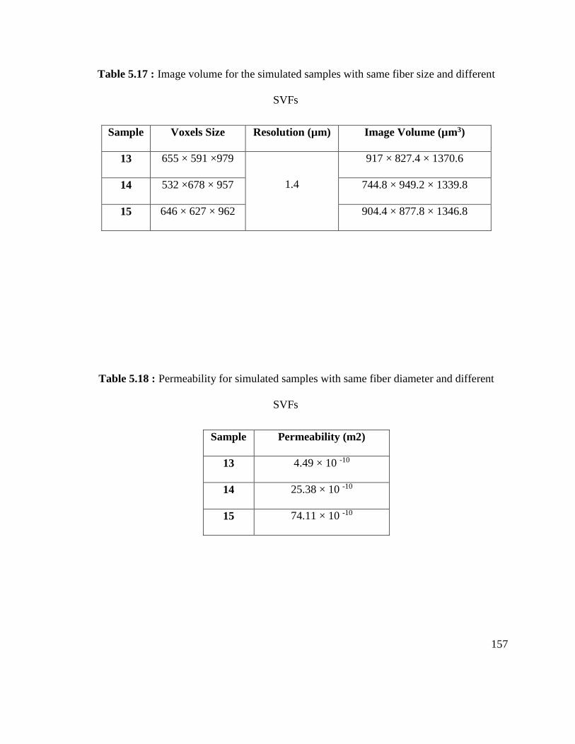
157

Table 5.17 : Image volume for the simulated samples with same fiber size and different

SVFs

Sample Voxels Size Resolution (µm) Image Volume (µm3)

13 655 × 591 ×979

1.4

917 × 827.4 × 1370.6

14 532 ×678 × 957 744.8 × 949.2 × 1339.8

15 646 × 627 × 962 904.4 × 877.8 × 1346.8

Table 5.18 : Permeability for simulated samples with same fiber diameter and different

SVFs

Sample Permeability (m2)

13 4.49 × 10 -10

14 25.38 × 10 -10

15 74.11 × 10 -10

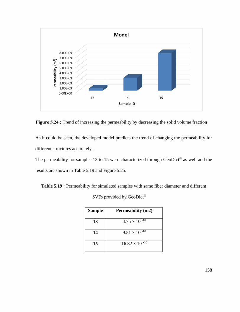
158

Trend of increasing the permeability by decreasing the solid volume fraction

As it could be seen, the developed model predicts the trend of changing the permeability for

different structures accurately.

The permeability for samples 13 to 15 were characterized through GeoDict® as well and the

results are shown in Table 5.19 and Figure 5.25.

Table 5.19 : Permeability for simulated samples with same fiber diameter and different

SVFs provided by GeoDict®

Sample Permeability (m2)

13 4.75 × 10 -10

14 9.51 × 10 -10

15 16.82 × 10 -10

0.00E+00

1.00E-09

2.00E-09

3.00E-09

4.00E-09

5.00E-09

6.00E-09

7.00E-09

8.00E-09

13 14 15

Pe

rme

abili

ty (

m2 )

Sample ID

Model

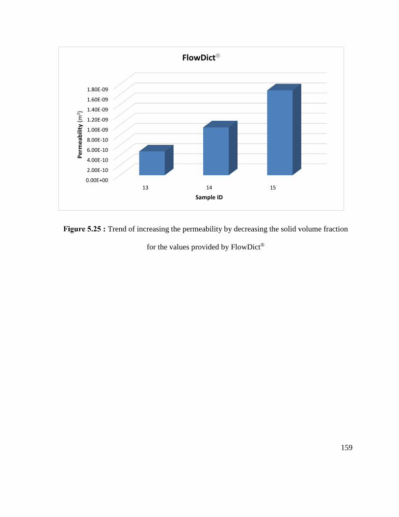
159

Trend of increasing the permeability by decreasing the solid volume fraction

for the values provided by FlowDict®

0.00E+00

2.00E-10

4.00E-10

6.00E-10

8.00E-10

1.00E-09

1.20E-09

1.40E-09

1.60E-09

1.80E-09

13 14 15

Pe

rme

abili

ty(m

2 )

Sample ID

FlowDict®

160

6. Experimental Validation

161

6.1 Introduction

In prior chapters, a methodology to model permeability of nonwovens, employing

information of all the pores available in the structure was explained. Through this model,

permeability of the media, as the main consequence of the pore network, would be evaluated

using 3D image of real or simulated structures.

As seen, permeability changes by changing fiber diameter and solid volume fraction of

nonwoven media, since any alteration in these parameters affect pore size and pore structure.

In other words, increasing the fiber diameter leads to increase pore diameter, therefore fluid

can flow in the capillaries with larger diameter. Decreasing solid volume fraction also results

to have a media with lower packing density, therefore fluid has higher space to flow. Both of

these issues cause the permeability to be increased.

ASTM D737 is normally referred in order to measure permeability og textiles

experimentally. According to this standard and for testing air permeability, flow rate through

area of 38 cm2 of a sample at 125 Pa pressure drop is reported. Then, using Darcy’s equation

permeability coefficient (k) would be evaluated.

In this chapter, the permeability for the samples used for imaging through micro CT will be

measured and the results will be compared with the outputs of the model for permeability.

6.2 Measuring permeability through experiment

6.2.1 Samples with different fiber sizes and same SVFs

Samples which were used to study the effect of fiber diameter on pore structure are shown in

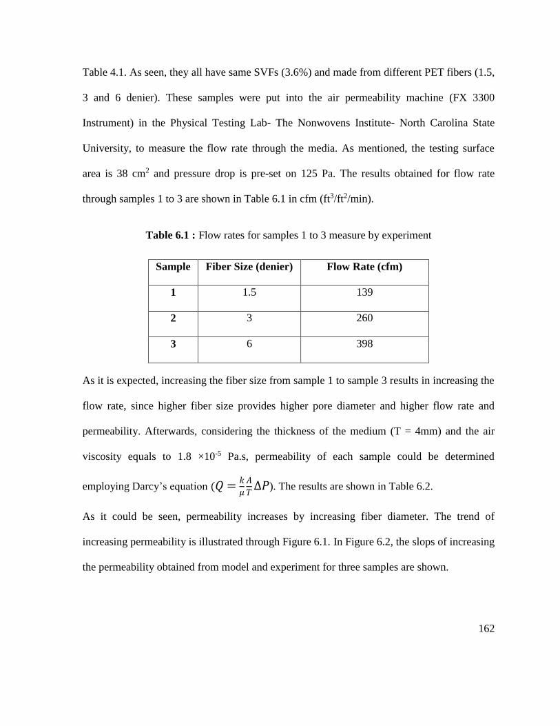
162

Table 4.1. As seen, they all have same SVFs (3.6%) and made from different PET fibers (1.5,

3 and 6 denier). These samples were put into the air permeability machine (FX 3300

Instrument) in the Physical Testing Lab- The Nonwovens Institute- North Carolina State

University, to measure the flow rate through the media. As mentioned, the testing surface

area is 38 cm2 and pressure drop is pre-set on 125 Pa. The results obtained for flow rate

through samples 1 to 3 are shown in Table 6.1 in cfm (ft3/ft2/min).

Table 6.1 : Flow rates for samples 1 to 3 measure by experiment

Sample Fiber Size (denier) Flow Rate (cfm)

1 1.5 139

2 3 260

3 6 398

As it is expected, increasing the fiber size from sample 1 to sample 3 results in increasing the

flow rate, since higher fiber size provides higher pore diameter and higher flow rate and

permeability. Afterwards, considering the thickness of the medium (T = 4mm) and the air

viscosity equals to 1.8 ×10-5 Pa.s, permeability of each sample could be determined

employing Darcy’s equation (𝑄 =𝑘

𝜇

𝐴

𝑇∆𝑃). The results are shown in Table 6.2.

As it could be seen, permeability increases by increasing fiber diameter. The trend of

increasing permeability is illustrated through Figure 6.1. In Figure 6.2, the slops of increasing

the permeability obtained from model and experiment for three samples are shown.

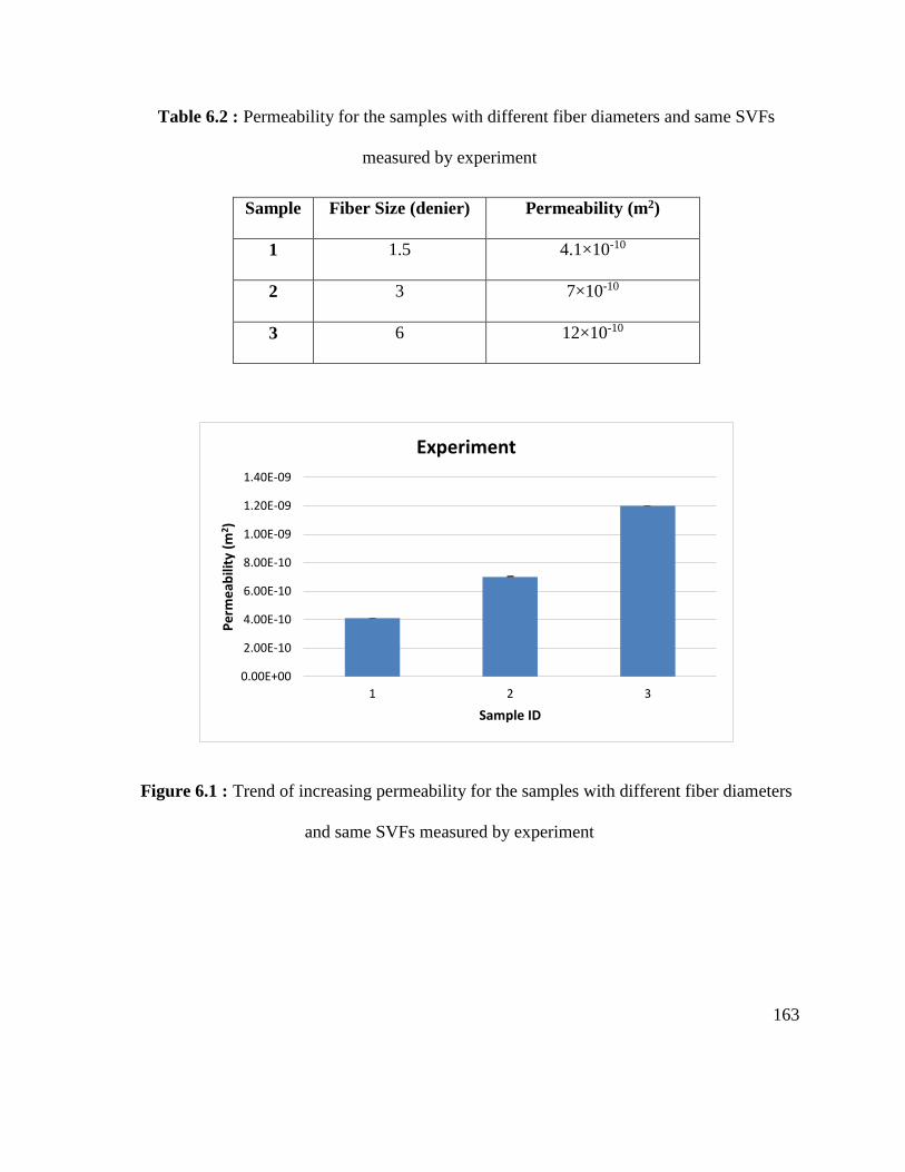
163

Table 6.2 : Permeability for the samples with different fiber diameters and same SVFs

measured by experiment

Sample Fiber Size (denier) Permeability (m2)

1 1.5 4.1×10-10

2 3 7×10-10

3 6 12×10-10

Figure 6.1 : Trend of increasing permeability for the samples with different fiber diameters

and same SVFs measured by experiment

0.00E+00

2.00E-10

4.00E-10

6.00E-10

8.00E-10

1.00E-09

1.20E-09

1.40E-09

1 2 3

Pe

rme

abili

ty (

m2)

Sample ID

Experiment

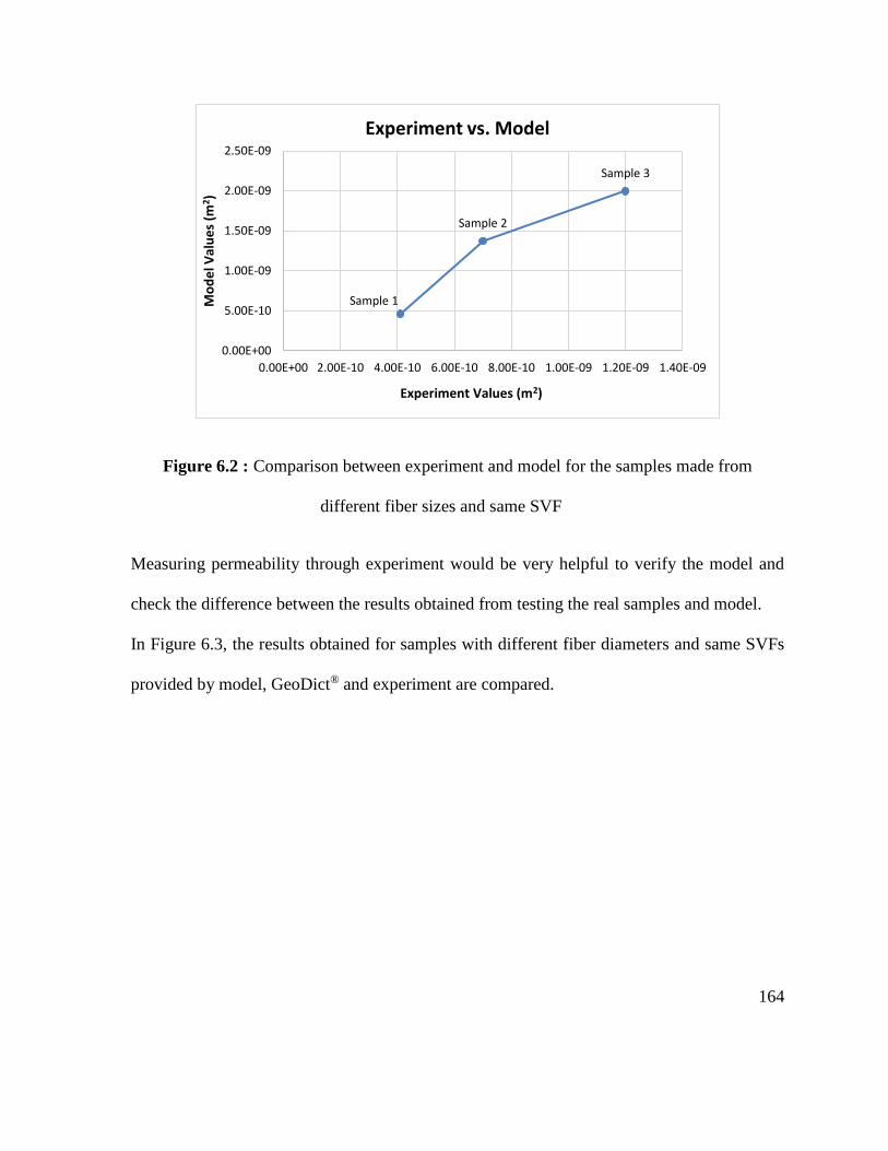
164

Figure 6.2 : Comparison between experiment and model for the samples made from

different fiber sizes and same SVF

Measuring permeability through experiment would be very helpful to verify the model and

check the difference between the results obtained from testing the real samples and model.

In Figure 6.3, the results obtained for samples with different fiber diameters and same SVFs

provided by model, GeoDict® and experiment are compared.

Sample 1

Sample 2

Sample 3

0.00E+00

5.00E-10

1.00E-09

1.50E-09

2.00E-09

2.50E-09

0.00E+00 2.00E-10 4.00E-10 6.00E-10 8.00E-10 1.00E-09 1.20E-09 1.40E-09

Mo

de

l Val

ue

s (m

2 )

Experiment Values (m2)

Experiment vs. Model

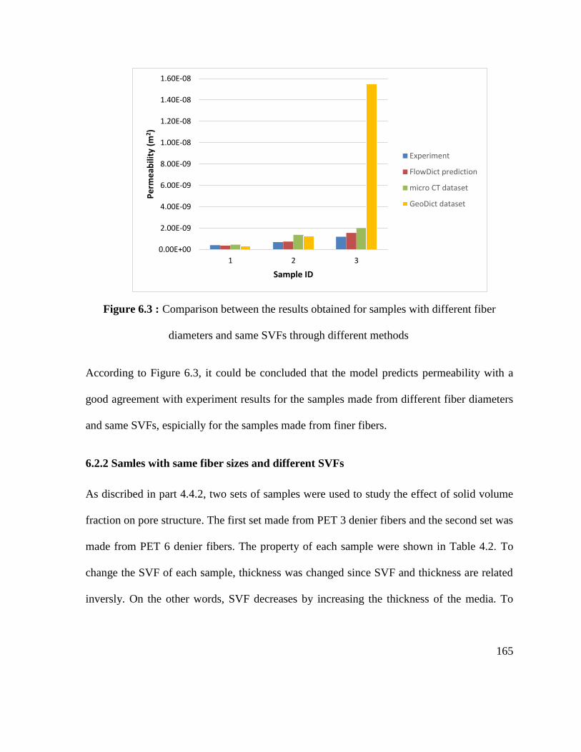
165

Figure 6.3 : Comparison between the results obtained for samples with different fiber

diameters and same SVFs through different methods

According to Figure 6.3, it could be concluded that the model predicts permeability with a

good agreement with experiment results for the samples made from different fiber diameters

and same SVFs, espicially for the samples made from finer fibers.

6.2.2 Samles with same fiber sizes and different SVFs

As discribed in part 4.4.2, two sets of samples were used to study the effect of solid volume

fraction on pore structure. The first set made from PET 3 denier fibers and the second set was

made from PET 6 denier fibers. The property of each sample were shown in Table 4.2. To

change the SVF of each sample, thickness was changed since SVF and thickness are related

inversly. On the other words, SVF decreases by increasing the thickness of the media. To

0.00E+00

2.00E-09

4.00E-09

6.00E-09

8.00E-09

1.00E-08

1.20E-08

1.40E-08

1.60E-08

1 2 3

Pe

rme

abili

ty (

m2)

Sample ID

Experiment

FlowDict prediction

micro CT dataset

GeoDict dataset

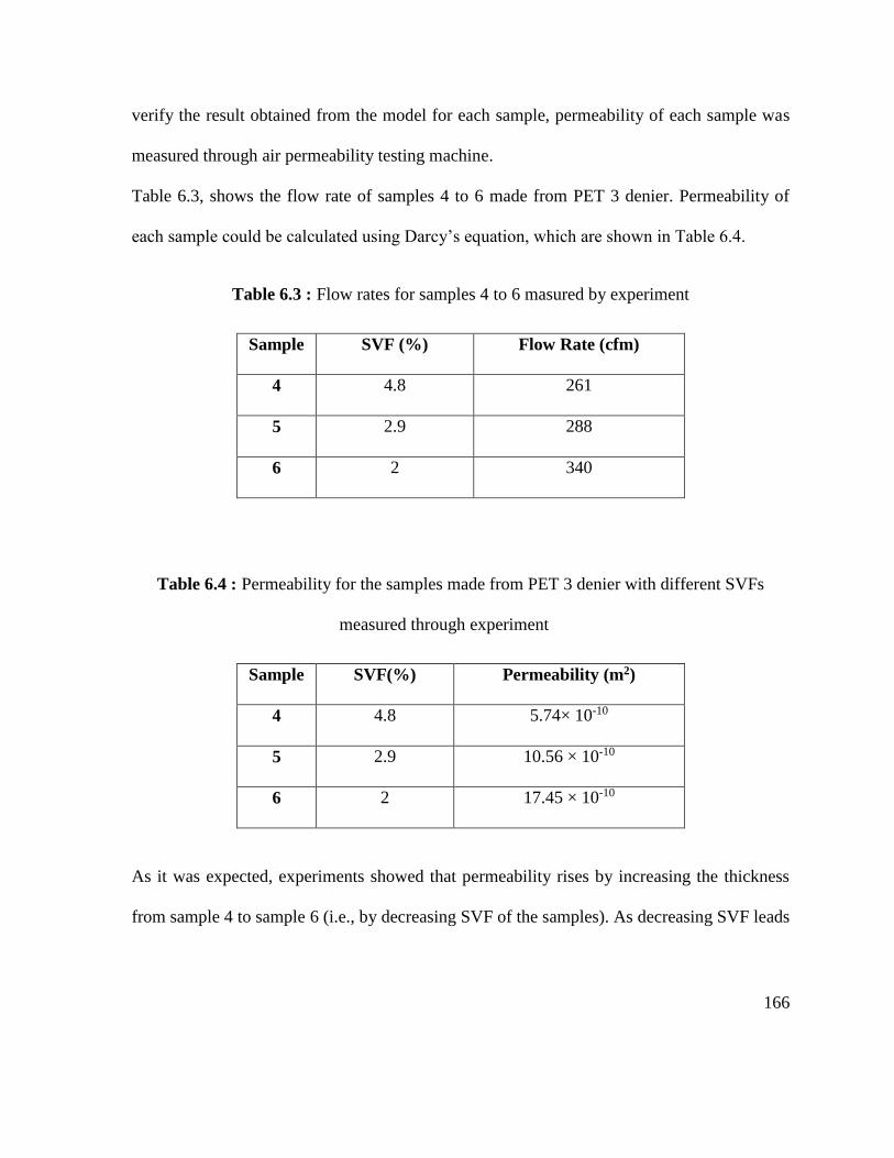
166

verify the result obtained from the model for each sample, permeability of each sample was

measured through air permeability testing machine.

Table 6.3, shows the flow rate of samples 4 to 6 made from PET 3 denier. Permeability of

each sample could be calculated using Darcy’s equation, which are shown in Table 6.4.

Table 6.3 : Flow rates for samples 4 to 6 masured by experiment

Sample SVF (%) Flow Rate (cfm)

4 4.8 261

5 2.9 288

6 2 340

Table 6.4 : Permeability for the samples made from PET 3 denier with different SVFs

measured through experiment

Sample SVF(%) Permeability (m2)

4 4.8 5.74× 10-10

5 2.9 10.56 × 10-10

6 2 17.45 × 10-10

As it was expected, experiments showed that permeability rises by increasing the thickness

from sample 4 to sample 6 (i.e., by decreasing SVF of the samples). As decreasing SVF leads

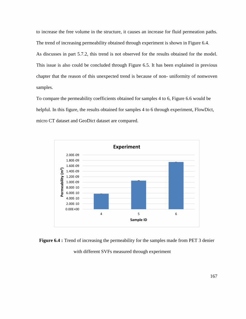
167

to increase the free volume in the structure, it causes an increase for fluid permeation paths.

The trend of increasing permeability obtained through experiment is shown in Figure 6.4.

As discusses in part 5.7.2, this trend is not observed for the results obtained for the model.

This issue is also could be concluded through Figure 6.5. It has been explained in previous

chapter that the reason of this unexpected trend is because of non- uniformity of nonwoven

samples.

To compare the permeability coefficients obtained for samples 4 to 6, Figure 6.6 would be

helpful. In this figure, the results obtained for samples 4 to 6 through experiment, FlowDict,

micro CT dataset and GeoDict dataset are compared.

Figure 6.4 : Trend of increasing the permeability for the samples made from PET 3 denier

with different SVFs measured through experiment

0.00E+00

2.00E-10

4.00E-10

6.00E-10

8.00E-10

1.00E-09

1.20E-09

1.40E-09

1.60E-09

1.80E-09

2.00E-09

4 5 6

Pe

rme

abili

ty (

m2)

Sample ID

Experiment

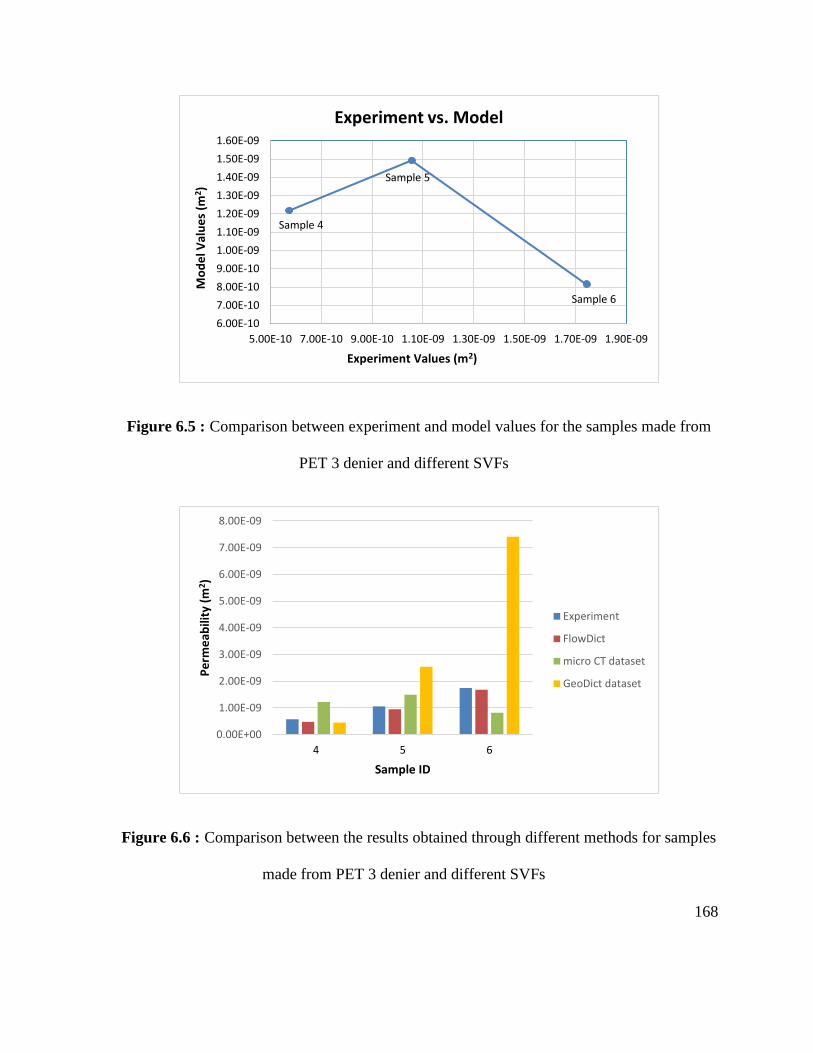
168

Figure 6.5 : Comparison between experiment and model values for the samples made from

PET 3 denier and different SVFs

Figure 6.6 : Comparison between the results obtained through different methods for samples

made from PET 3 denier and different SVFs

Sample 4

Sample 5

Sample 6

6.00E-10

7.00E-10

8.00E-10

9.00E-10

1.00E-09

1.10E-09

1.20E-09

1.30E-09

1.40E-09

1.50E-09

1.60E-09

5.00E-10 7.00E-10 9.00E-10 1.10E-09 1.30E-09 1.50E-09 1.70E-09 1.90E-09

Mo

de

l Val

ue

s (m

2 )

Experiment Values (m2)

Experiment vs. Model

0.00E+00

1.00E-09

2.00E-09

3.00E-09

4.00E-09

5.00E-09

6.00E-09

7.00E-09

8.00E-09

4 5 6

Pe

rme

abili

ty (

m2 )

Sample ID

Experiment

FlowDict

micro CT dataset

GeoDict dataset

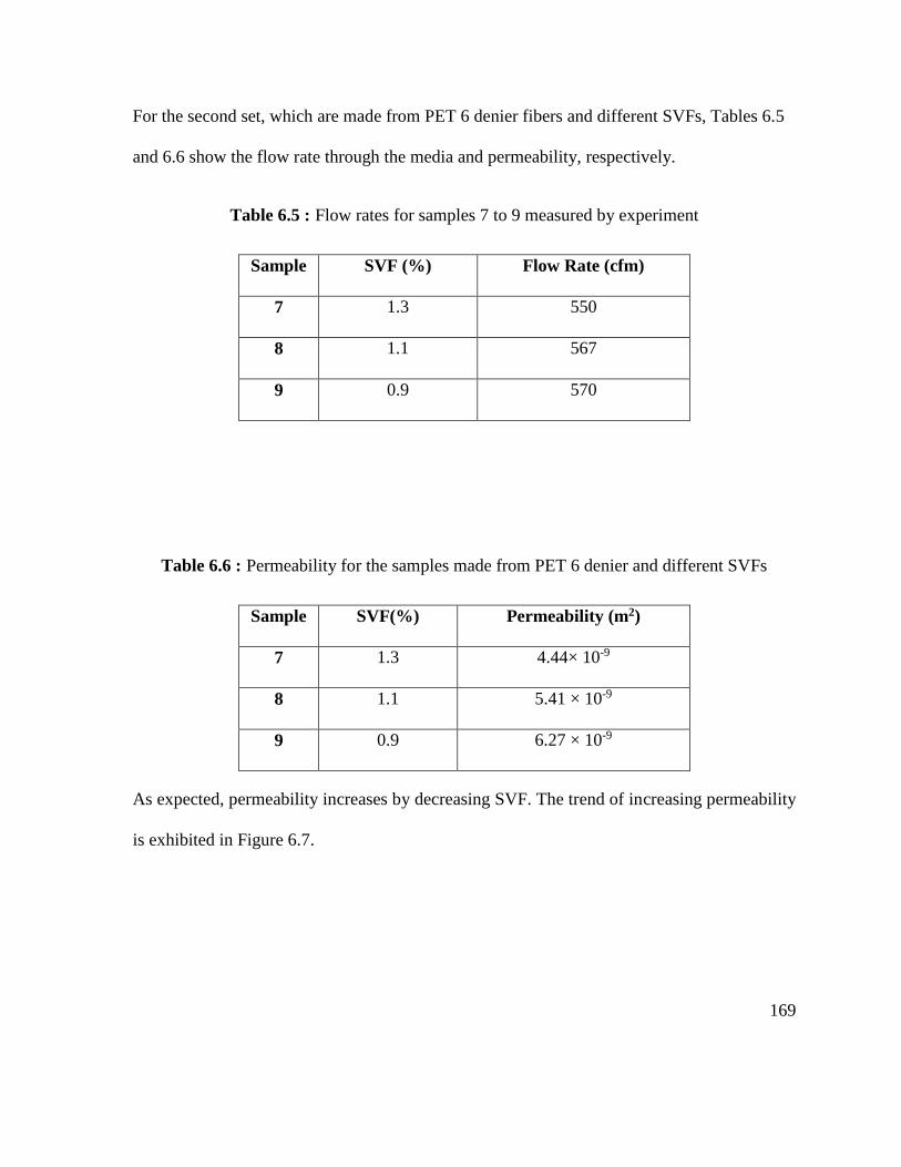
169

For the second set, which are made from PET 6 denier fibers and different SVFs, Tables 6.5

and 6.6 show the flow rate through the media and permeability, respectively.

Table 6.5 : Flow rates for samples 7 to 9 measured by experiment

Sample SVF (%) Flow Rate (cfm)

7 1.3 550

8 1.1 567

9 0.9 570

Table 6.6 : Permeability for the samples made from PET 6 denier and different SVFs

Sample SVF(%) Permeability (m2)

7 1.3 4.44× 10-9

8 1.1 5.41 × 10-9

9 0.9 6.27 × 10-9

As expected, permeability increases by decreasing SVF. The trend of increasing permeability

is exhibited in Figure 6.7.

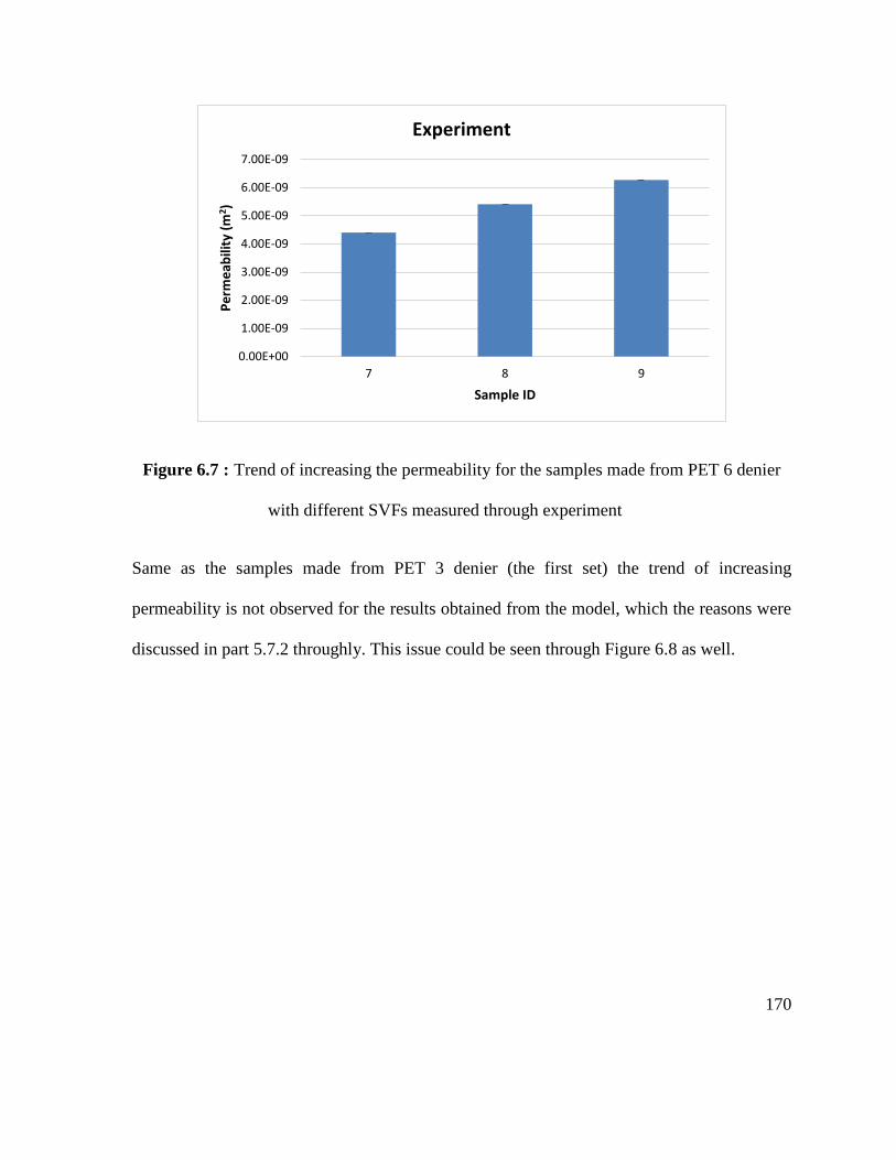
170

Figure 6.7 : Trend of increasing the permeability for the samples made from PET 6 denier

with different SVFs measured through experiment

Same as the samples made from PET 3 denier (the first set) the trend of increasing

permeability is not observed for the results obtained from the model, which the reasons were

discussed in part 5.7.2 throughly. This issue could be seen through Figure 6.8 as well.

0.00E+00

1.00E-09

2.00E-09

3.00E-09

4.00E-09

5.00E-09

6.00E-09

7.00E-09

7 8 9

Pe

rme

abili

ty (

m2)

Sample ID

Experiment

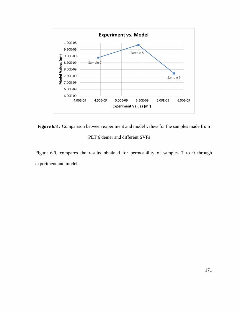
171

Figure 6.8 : Comparison between experiment and model values for the samples made from

PET 6 denier and different SVFs

Figure 6.9, compares the results obtained for permeability of samples 7 to 9 through

experiment and model.

Sample 7

Sample 8

Sample 9

6.00E-09

6.50E-09

7.00E-09

7.50E-09

8.00E-09

8.50E-09

9.00E-09

9.50E-09

1.00E-08

4.00E-09 4.50E-09 5.00E-09 5.50E-09 6.00E-09 6.50E-09

Mo

de

l Val

ue

s (m

2)

Experiment Values (m2)

Experiment vs. Model

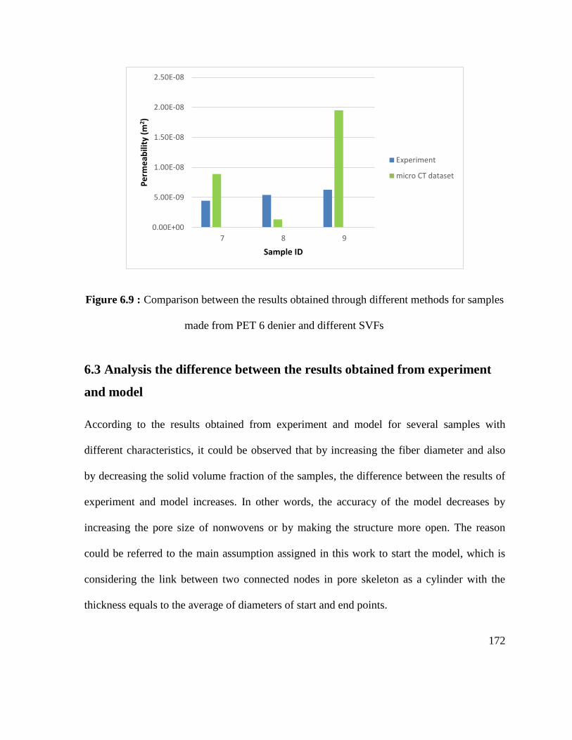
172

Figure 6.9 : Comparison between the results obtained through different methods for samples

made from PET 6 denier and different SVFs

6.3 Analysis the difference between the results obtained from experiment

and model

According to the results obtained from experiment and model for several samples with

different characteristics, it could be observed that by increasing the fiber diameter and also

by decreasing the solid volume fraction of the samples, the difference between the results of

experiment and model increases. In other words, the accuracy of the model decreases by

increasing the pore size of nonwovens or by making the structure more open. The reason

could be referred to the main assumption assigned in this work to start the model, which is

considering the link between two connected nodes in pore skeleton as a cylinder with the

thickness equals to the average of diameters of start and end points.

0.00E+00

5.00E-09

1.00E-08

1.50E-08

2.00E-08

2.50E-08

7 8 9

Pe

rme

abili

ty (

m2 )

Sample ID

Experiment

micro CT dataset

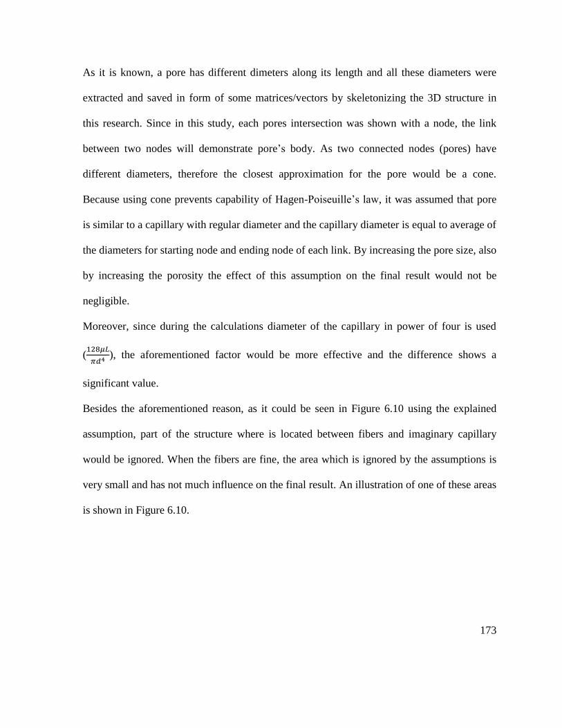
173

As it is known, a pore has different dimeters along its length and all these diameters were

extracted and saved in form of some matrices/vectors by skeletonizing the 3D structure in

this research. Since in this study, each pores intersection was shown with a node, the link

between two nodes will demonstrate pore’s body. As two connected nodes (pores) have

different diameters, therefore the closest approximation for the pore would be a cone.

Because using cone prevents capability of Hagen-Poiseuille’s law, it was assumed that pore

is similar to a capillary with regular diameter and the capillary diameter is equal to average of

the diameters for starting node and ending node of each link. By increasing the pore size, also

by increasing the porosity the effect of this assumption on the final result would not be

negligible.

Moreover, since during the calculations diameter of the capillary in power of four is used

(128𝜇𝐿

𝜋𝑑4 ), the aforementioned factor would be more effective and the difference shows a

significant value.

Besides the aforementioned reason, as it could be seen in Figure 6.10 using the explained

assumption, part of the structure where is located between fibers and imaginary capillary

would be ignored. When the fibers are fine, the area which is ignored by the assumptions is

very small and has not much influence on the final result. An illustration of one of these areas

is shown in Figure 6.10.

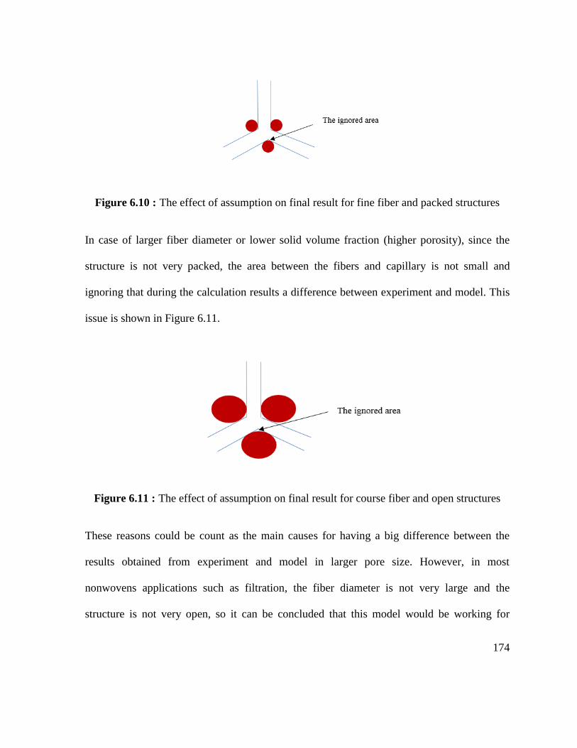
174

Figure 6.10 : The effect of assumption on final result for fine fiber and packed structures

In case of larger fiber diameter or lower solid volume fraction (higher porosity), since the

structure is not very packed, the area between the fibers and capillary is not small and

ignoring that during the calculation results a difference between experiment and model. This

issue is shown in Figure 6.11.

Figure 6.11 : The effect of assumption on final result for course fiber and open structures

These reasons could be count as the main causes for having a big difference between the

results obtained from experiment and model in larger pore size. However, in most

nonwovens applications such as filtration, the fiber diameter is not very large and the

structure is not very open, so it can be concluded that this model would be working for

175

almost all applications thoroughly. In rare applications, where fiber diameter is very large

and porosity is very high, this model may overestimate the permeability.

176

7. Overall Conclusion and Recommendations for

Future Work

177

7.1 Overall conclusion

The main objective of this research is investigating the pore structure of nonwovens and

determining diameter of all the pores available in the structure. For this purpose, 2D images

were captured by DVI and micro CT and it was tried to extract pore information by

skeletonizing the 3D structural image of nonwoven fabric through Avizo®. As it has been

shown in this study, since pore structure is very complex including a lot of connectivity and

numbers, it is not possible to analyze all these numbers to characterize pore structure. Also,

comparison between two different pore networks is not possible referring to the information

that could be extracted from pore structure. Therefore, it was decided to find a parameter,

which covers all pore information to go from a complex network to a single number, which

was permeability. According to the results obtained in this research, the overall conclusions

could be summarized as below:

Current available methods in pore characterization are not accurate enough to study

pore structure of nonwovens and it is necessary to develop new methodologies in

pore characterization due to the problems associated with them.

It is always interesting for industry to understand pore structure of any engineered

nonwoven fabrics before full scale production by using simulated dataset. Since the

real fabric is not available in this step, all the characterizations should be made on

simulated structures rather than experimentation. Predicting properties of simulated

structure is motivating because it is cheap and repeatable.

178

The pore in nonwovens has a 3D configuration with different diameters along its

length. For this reason 3D imaging of nonwovens was selected to study pore

network.

In this research, it is assumed that the pore network contains many through pores.

Also, the pore was assumed as a capillary with circular cross section and pore

network was considered as a network of many interconnected capillaries.

It is concluded that micro CT imaging technique would be a proper method to obtain

3D structure of porous materials, since this technique is growing very fast and

affordable these days. However, because of the quality of the images taken from

micro CT, image pre-processing is required to be applied on the images to get clear

images without any noise.

It is shown that skeletonization would be a good approach to obtain skeleton of the

structure in form of a graph. It is also demonstrated that this graph is a good

representative for the structure of the material and this objective was confirmed by

fit of the model in this research.

In this study it was tried to model permeability of nonwovens using the information

obtained from pore skeleton. For this purpose, the similarity between Hagen-

Poiseuille’s and Ohm’s laws was utilized. On the other words, pore network was

assumed as an electric circuit and each capillary in the network was considered as a

resistor. Afterwards, 128𝜇𝐿

𝜋𝑑4 was considered relevant to equivalent resistance of the

network.

179

The developed model predicts permeability for real and simulated nonwovens with a

good agreement with the results of experiment, specially for the samples made from

fine fibers and high SVF.

The accuracy of the model was verified through experiment for samples with

different fiber sizes and/or solid volume fraction.

7.2 Recommendations for future work

The results of this research encourage us to pursue the investigations in pore characterization

area. Some of these objectives will be explained briefly in the following.

7.2.1 Using sponbond and meltblown nonwovens as the material

In this research, the carded webs made from staple PET fibers were uses for imaging in

micro CT. For staple fibers, as explained earlier, resolution of imaging should be selected

referring to the fiber diameter. In other words, for the samples with larger fiber diameter,

lower resolution swould be selected. It is recommended that for future studies, nonwoven

media produced through different processes such as meltblown and spunbond be employed.

It is worth reminding that, fiber diameter in meltblown and spunbond nonwovens is not

regular and as an example, for a meltbown web plenty of fiber diameters could be assigned.

Normally, a fiber diameter distribution is considered for a meltblown web, so picking a

proper resolution for imaging in micro CT would be very critical.

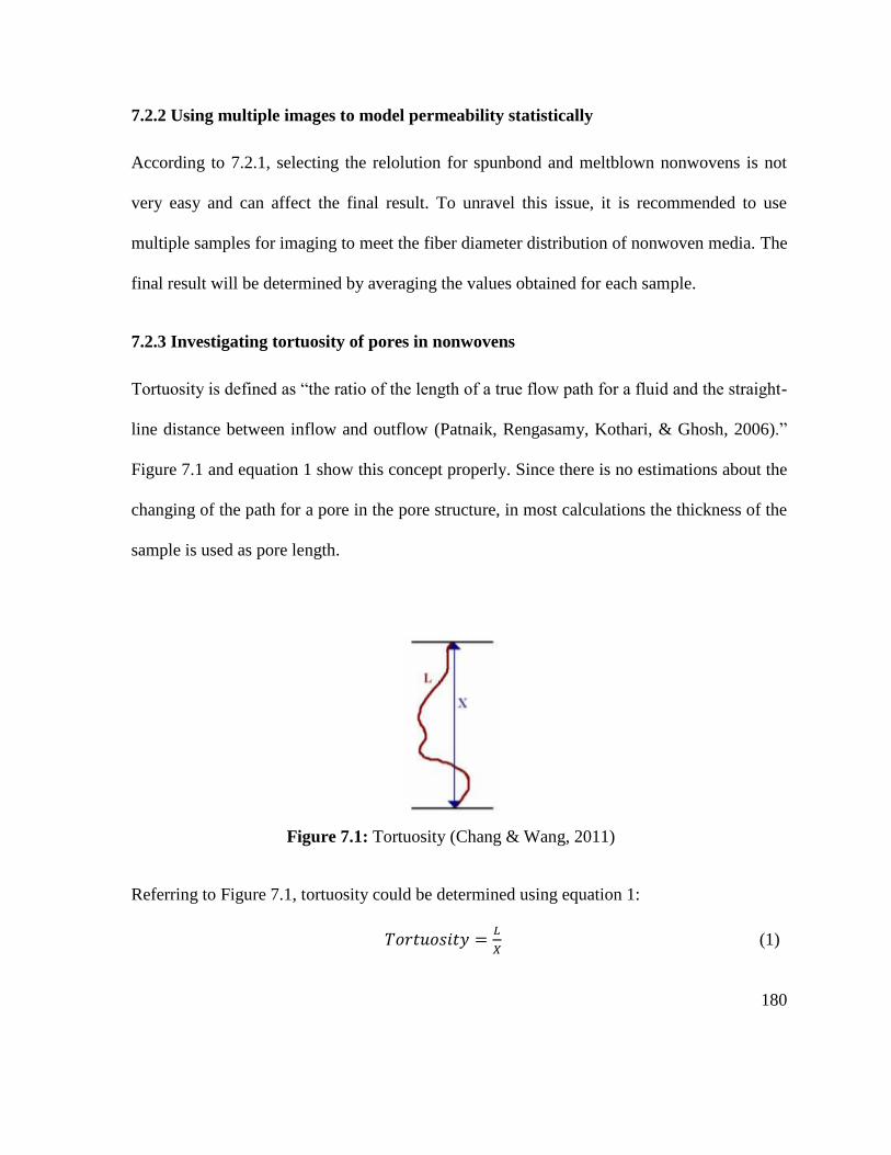
180

7.2.2 Using multiple images to model permeability statistically

According to 7.2.1, selecting the relolution for spunbond and meltblown nonwovens is not

very easy and can affect the final result. To unravel this issue, it is recommended to use

multiple samples for imaging to meet the fiber diameter distribution of nonwoven media. The

final result will be determined by averaging the values obtained for each sample.

7.2.3 Investigating tortuosity of pores in nonwovens

Tortuosity is defined as “the ratio of the length of a true flow path for a fluid and the straight-

line distance between inflow and outflow (Patnaik, Rengasamy, Kothari, & Ghosh, 2006).”

Figure 7.1 and equation 1 show this concept properly. Since there is no estimations about the

changing of the path for a pore in the pore structure, in most calculations the thickness of the

sample is used as pore length.

Figure 7.1: Tortuosity (Chang & Wang, 2011)

Referring to Figure 7.1, tortuosity could be determined using equation 1:

𝑇𝑜𝑟𝑡𝑢𝑜𝑠𝑖𝑡𝑦 =𝐿

𝑋 (1)

181

As mentioned, no conventional techniques can provide tortuosity of a pore. In this study,

skeletonizing the 3D structural image results in obtaining the pore skeleton in form of a

graph, where each node and connectivity represent pores intersection and the path,

respectively (See Figure 4.13). So, focusing on pore skeleton all the paths which demonstrate

the tortuosity of the pores could be studied.

182

8. References

183

Abdel-Ghani, M., & Davis, G. (1985). Simulation of nonwoven fiber mats and the

application to coalescers. Chemical Engineering Science, 40(1), 117-129.

Abu-Ain, W., Sheikh Abdullah, S., Bataineh, B., Abu Ain, T., & Omar, K. (2013).

Skeletonization algorithm for binary images. Procedia Technology, 11, 704-709.

Alexander, C., & Sadiku, M. (2009). Fundamental of electric circuit (4th ed.). New York:

McGraw-Hill.

Allen, T. (1997). Particle size measurement: Volume 2: surface area and pore size

determination (5th ed.). London: Chapman & Hall.

ASTMF316-03. (2011). Standard test method for pore size characteristics of membrane

filters by bubble point and mean flow pore test.

Atwal, M. (1987). Factors affecting the resistance of nonwoven needle punched fabrics.

Textile Research Journal, 57(10), 574-579.

Ault, J., Chen, K., & Stone, H. (2015). Downstream decay of fully developed dean flow.

Journal of Fluid Mechanics, 777, 219-244.

Aydilek, A., Oguz, S., & Edil, T. (2002). Digital image analysis to determine pore opening

size distribution of nonwoven geotextiles. Journal of Computing in Civil Engineering,

16(4), 280-290.

Aydilek, A., Oguz, S., & Edil, T. (2005). Constriction size of geotextile filters. Journal of

Geotechnical and Geoinvironmental Engineering, 131(1), 28-38.

184

Bagherzadeh, R., Latifi, M., & Kong, L. (2014). Three dimensional pore structure analysis of

polycaprolactone nano-microfibrous scaffolds using theoretical and experimantal

approaches. Journal of Biomedical Materials Research Part A, 102(3), 903-910.

Bagherzadeh, R., Latifi, M., Sheikhzadeh Najar, S., Amani Tehran, M., & Kong, L. (2013).

Three dimensional pore structure analysis of nano/microfibrous scaffolds using

confocal laser scanning microscopy. Journal of Biomedical Materials Research Part

A, 101A(3), 765-774.

Balakrishnan, R., & Ranganathan, K. (2012). A textbook of graph theory (2nd ed.). New

York: Springer.

Baratholomew, R., & Casagrande, R. (1957). Measuring solids, concentration in fluidized

system by gamma-ray absorption. Industrial and Engineering Chemistry, 49(3), 428-

431.

Barrett, E., Joyner, L., & Halenda, P. (1951). The determination of pore volume and area

distributions in porous substances,I: Computations from nitrogen isotherm. Journal of

American Chemistry Society, 73(1), 373-380.

Baruchel, J., Buffiere, J., & Maire, E. (2000). X-ray tomography in material science. Paris:

Hermes Science.

Batra, S., & Pourdeyhimi, B. (2012). Introduction to nonwovens technology. Lancaster,PA:

Destech Publications.

Baunauer, S., Emmet, P., & Teller, E. (1938). Adsorption of gases in multimolecular layers.

Journal of American Chemistry Society, 60, 309-319.

185

Bear, J. (1988). Dynamics of fuids in porous media. New York: Dover.

Beineke, L., & Wilson, R. (2013). Topics in structural graph theory. Cambridge: Cambridge

Unversity Press.

Berkalp, O. B. (2006). Air permeability & porosity in spun-laced fabrics. Fibers & Textiles

in Eastern Europe, 14(3), 81-85.

Bhatia, S., & Smith, J. (1995). Application of the bubble point method to the characterization

of the pore size distribution of geotextiles. Geotechnical Testing Journal, 18, 94-105.

Boerckel, J., Mason, D., Mc Dermott, A., & Alsberg, E. (2014). Microcomputed

tomography: approaches and applications in bioengineering. Stem Cell Research &

Therapy, 5(144), 0-12.

Brown, R. (1993). Theory of airflow through filters modeled as arrays of parallel fibers.

Chemical Engineering Science, 48(20), 3535-3543.

Buckingham, E. (1914). On physically similar systems;illustrations of the yse of dimensional

equations. Physical Review, 4(4), 345-376.

Chang, H., & Wang, Y. (2011). Cell response to surface and architecture of tissue

engineering scaffolds. INTECH, 569-588.

Chang, K., & Dullien, F. (1976). Section diameter method for non-spherical objects. Journal

of Microscopy, 18(1), 61-68.

Charytanowicz, M. (2014). An algorithm for the pore size etermination using image analysis.

In E. Pietka, J. Kawa, & W. Wieclawek (Eds.), Information Technologies in

Biomedicine,Volume 3 (pp. 223-234). New York: Springer.

186

Chen, X., & Papathanasiou. (2008). The transverse permeability of disorder fiber arrays: A

statistical correlation in terms of mean nearest interfiber spacing. Transparent in

porous media, 71, 233-251.

Chen, X., & Papathanasiou, T. (2006). On the variability of Kozeny constant for saturated

flow across undirectional disorder fiber array. Composites (part A: applied science

and manufacturing), 37(6), 836-846.

Cincik, E., & Koc, E. (2012). An analysis on air permeability of polyester/viscose blended

needle punched nonwovens. Textile Research Journal, 82(5), 430-442.

Clague, D., & Philips, R. (1997). A numerical calculation of hydraulic permeability of three

dimensional disordered fibrous media. Physics of Fluids, 9(6), 1562-1572.

Corte, H., & Kallmes, O. (1961). The statistical geometry of a fibrous network. Trans,2nd

Fund. Res. Symp (pp. 13-46). Oxford: FRC.

Davies, C. (1973). Air filtration. London: Academic Press.

de Boer, R. (2000). Theory of porous media. New York: Springer.

Doktor, T., & Valach, K. (2010). Assessment of pore size distribution using image analysis.

Trieste,Italy: 9th YSESM.

Dougherty, E. (1992). An introduction to morphological image processing. Bellingham: The

International Society for Optical Engineering.

Drummond, J., & Tahir, M. (1984). Laminar viscous flow through regular arrays of parallel

solid cylinders. International Journal of Multiphase Flow, 10(5), 515-540.

187

Dullien, F. (1975). New network permeability model of porous media. American Institute of

Chemical Engineers Journal, 21, 299-307.

Dullien, F. (1979). Porous media: Fluid transport and pore structure. New York: Academic

Press,Inc.

Erciyes, K. (2013). Distribution graph algorithms for computer networks. London: Springer.

Faure, Y., Gource, J., & Gendrin, P. (1990). Structural study of porometry and filtration

opening size of geotextiles. In I. Peggs (Ed.), Geosynthetics:microstructure and

performance (pp. 102-115). ASTM international.

FEI. (2009). AVIZO user guide. Berlin: Visualization Science group.

Felix, V., Jannot, Y., & Degiovanni, A. (2012). A thermal porosimetry method to estimate

pore size distribution in highly porous insulating materials. Review of Scientific

Instruments, 83, 054903/1-054903/8.

Fernando, J., & Chung, D. (2002). Pore strucutre and permeability of an alumina fiber filter

membrane for hot gas filtration. Journal of Porous Materials, 9, 211-219.

Fouard, C., Malandian, G., Prohaska, S., & Westerhoff, M. (2006). Blockwise processing

applied to brain microvascular network study. IEEE Transactions on Medical

Imaging, 25(10), 1319-1327.

Fuchs, A., & Krisch, N. (1968). Studies on fibrous aerosol filters,III:Diffusional deposition

of aerosols in fibrous filters. Annals of Occupational Hygene, 11, 299-304.

Ghosh, S. (2013). Digital image processing. Oxford: Alpha Science International Ltd.,.

188

Gong, R., & Newman, A. (1992). Image analysis techniques,part 1: the measurement of pore

size distribution. The Journal of Textile Institute, 83(2), 253-268.

Gonzalez, R., & Wintz, P. (1987). Digital image processing (2nd ed.). Reading,MA:

Addison-Wesley Publication Company.

Grodzins, L. (1983). Optimum energies for X-ray transmission tomography of small samples.

Nuclear Instruments and Methods, 206, 541-545.

Happel, J. (1959). Viscous flow relative to arrays of cylinders. A.I.Ch.E Journal, 5(2), 174-

177.

Hasimoto, H. (1959). On the periodic fundamental solutions of the stokes equations and

theirapplication to viscous flow past a cubic array of spheres. Journal of Fluid

Mechanics, 5, 317-328.

Hearle, J., & Stevenson, P. (1963). Nonwoven fabric studies: Part III: The anisotropy of

nonwoven fabrics. Textile research Journal, 33(11), 877-888.

Higdon, J., & Ford, G. (1996). Permeability of three dimensional models of fibrus porous

media. Journal of Fluid Mechanics, 308, 341-361.

Hilderbrand, T., & Ruegsegger, P. (1997). A new method for the model independent

assessment of thickness in three-dimensional images. Journal of Microscopy, 185(1),

67-75.

Hutten, I. M. (2007). Handbook of nonwoven filter media (1st ed.). Burlington,MA: Oxford.

Jackson, G., & James, D. (1986). The permeability of fibrous porous media. The Canadian

Journal of Chemical Engineering, 64, 364-374.

189

Jaganathan, S. (2008). Fluid absorption properties of nonwoven fabric. Raleigh: NCSU PhD

dissertation.

Jaganathan, S., Tafreshi, H., & Pourdeyhimi, B. (2008). Modeling liquid porosimetry in

modeled and imaged 3-D fibrous micorstructures. Jounal of Colloid and Interface

Science, 326, 166-175.

Jain, A. (1989). Fundamental of digital image processing. New Jersey: Prentice-Hall.

Jena, A., & Gupta, K. (2001). An innovative technique for pore structure analysis of fuel

cells and battery components using flow porometry. Journal of Power Sources, 96,

214-219.

Jena, A., & Gupta, K. (2002). Characterization of pore structure of filtration media. Fluid

Particle Separation Journal, 4(3), 227-241.

Jena, A., & Gupta, K. (2003). Liquid extrusion techniques for pore structure evaluation of

nonwovens. International Nonwovens Journal, 45-53.

Jena, A., & Gupta, K. (n.d.). Advanced technology for evaluation of pore structure

characteristics of filtration media to optimize their design and performance.

Ithaca,New York: Porous Materials, Inc.,

(http://pmiappeurope.com/publications/docs/advancedtech.pdf).

Kang, S., & Banerjee, D. (2011). Modeling and simulation of capillary microfluidic network

based on electrical analogies. Journal of Fluid Engineering, 133, 054502/1-054502/6.

190

Kastner, J., Harrer, B., Requena, G., & Brunke, O. (2010). A comprative study of high

resolution cone beam X-ray tomography and synchrotron tomography to Fe- and Al-

alloys. NDT&E international, 43, 599-605.

Kim, H., & Pourdeyhimi, B. (2000). A note on the effect of fiber diameter, fiber crimp and

fiber orientation on pore size in thin webs. International Nonwovens Journal, 9(4),

15-19.

Kirby, B. (2010). Micro-and nano scale fluid mechanics:Transport in microfluidic devices.

New York: Cambridge University Press.

Knott, G., Marchman, H., Wall, D., & Lich, B. (2008). Serial section scanning electron

microscopy of adult brain tissue using focused ion beam milling. The Journal of

Neuroscience, 28(12), 2959-2964.

Kohel, L., Zeng, X., & Li, L. (2006). Digital image analysis to determine pore size

distribution of nonwoven fabrics. Beijing: IMACS Multiconference on

Computational Engineering in System Applications.

Kraus, G., Ross, J., & Girifalco, L. (1953). Surface area analysis by means of gas flow

methods,I:steady state flow in porous media. The Journal of Physical Chemistry,

57(3), 330-333.

Kuwabara, S. (1959). The force experienced by randomly distributed paralled circular

cylinders of spheres in a viscous flow at small Reynolds number. Journal of Fluid

Mechanics, 14(4), 527-532.

191

Lehmann, M., Hardy, E., Meyer, J., & Kasper, G. (2005). MRI as a key tool for

understanding and modeling the filtration kinetics of fibrous media. Magnetic

Resonance Imaging, 23, 341-342.

Li, M., Ghosh, S., Rouns, T., Weiland, H., Richmond, O., & Hunt, W. (1998). Serial

sectioning method in the construction of 3-D microstrucutres for particle-reinforced

MMCs. Materials Characterization, 41, 81-95.

Lifshutz, N. (2005). On the mean flow pore size distribution of microfiber and nanofiber

webs. International Nonwovens Journal, 14, 18-24.

Lombard, G., Rollin, A., & Wolff, C. (1986). Theoretical and experimental opening sizes of

heat bonded geotextiles. Textile Research Journal, 59(4), 208-217.

Lowell, S., & Shields, J. (1984). Powder surface area and porosity. New York: Chapman

Hall Publication.

Manitoba, U. o. (2015). Retrieved from

http://umanitoba.ca/faculties/health_sciences/medicine/units/cacs/sam/micro_ct/8053.

html

Miller, B., & Tyomkin, I. (1986). An extended range liquid extrusion method for determining

pore size distribution. Textile Reseach Journal, 56(1), 35-40.

Montminy, M., Tannenbaum, A., & Macosko, C. (2004). The 3D strucuture of real polymer

foams. Journal of Colloid and Interface Science, 280, 202-211.

192

Murphy, C., Haugh, M., & O'Brien, F. (2010). The effect of mean pore size on cell

attachment, proliferation and migration in collagen-glycosaminologycan scaffolds for

bone tissue engineering. Biomaterials, 31(3), 461-466.

Najman, L., & Talbot, H. (2010). Mathematical morphology. Lavoisier: Wiley.

Newman, M. (2010). Networks: An introduction. New York: Oxford Press.

Otani, J., & Obara, Y. (2004). X-ray CT for geomaterials. Lisse, The Netherlands: Swets&

Zeitlinger B.V.

Pan, N., & Zhong, W. (2006). Fluid transport phenomena in fibrous materials. Textile

Progress, 38(2), 1-93.

Papathanasiou, T., Markicevic, B., & Dendy, E. (2001). A computational evaluation of the

Ergun and Forchheimer equations for fibrous porous media. Physics of Fluids,

13(10), 2795-2804.

Patnaik, A., Rengasamy, R., Kothari, V., & Ghosh, A. (2006). Wetting and wicking in

fibrous materials. Textile Progress, 1754-2278.

Payen, J., Vroman, P., Lewandowski, M., Perwuelz, A., Calle'-Chazelet, S., & Thomas, D.

(2012). Influence of fiber diameter, fiber combinations and solid volume fraction on

air filtration properties in nonwovens. Textile Research Journal, 1948-1959.

Pernodet, N., Maaloum, M., & Tinland, B. (1997). Pore size of agarose gels by atomic force

microscopy. Electrophoresis, 18, 55-58.

Pourdeyhimi, B., Dent, R., & Davis, H. (1997). Measuring fiber orientation in nonwovens:

Part III:Fourier transform. Textile Research Journal, 67(2), 143-151.

193

Pourdeyhimi, B., Maze, B., & Tafreshi, H. V. (2006). Simulation and analysis of unbonded

nonwovens fibrous structures. Journal of Engineered Fibers and Fabrics, 47-65.

Pourdeyhimi, B., Ramanathan, R., & Dent, R. (1996). Measuring fiber orientation in

nonwovens: Part I: Simulation. Textile Research Journal, 66(11), 713-722.

Pourdeyhimi, B., Ramanathan, R., & Dent, R. (1996). Measuring fiber orientation in

nonwovens: Part II: Direct tracking. Textile Research Journal, 66(12), 747-753.

Rawal, A. (2010). Structural analysis of pore size distribution of nonwovens. The Journal of

Textile Institute, 101(4), 350-359.

Rawal, A., & Saraswat, H. (2011). Pore size distribution of hybrid nonwoven geotextiles.

Geotextiles and Geomembranes, 29, 363-367.

Rawal, A., Rao, K., Russel, S., & Jeganathan, A. (2010). Effect of fiber orientation on pore

size characteristics of nonwoven structures. Journal of Applied Polymer Science,

118(5), 2668-2673.

Russel, S. (2007). Handbook of nonwovens. Cambridge: Woodheap Pub.Ltd.

Saeed, A., Tabedzki, M., Rybnik, M., & Adamski, M. (2010). K3M:A universal algorithm

for image skeletonization and a review of thinnnig techniques. International Journal

of Applied Mathematic and Computer Science, 20(2), 317-335.

Savel'eva, E., Bokova, E., & Andrianova, G. (2005). Pore structure of heat-treated

nonwovens materials. Fiber Chemistry, 37(3), 202-204.

Scheidegger, A. (1972). The physics of flow through porous media. Toronto: University of

Toronto Press.

194

Serra, J. (1982). Image analysis and mathematical morphology. London: Academic Press

Inc.

Shim, E., Pourdeyhimi, B., & Latifi, M. (2010). Three-dimensional analysis of segmented pie

bicomponent nonwovens. The Journal of The Textile Institute, 101(9), 773-787.

Simmonds, G., Bomberger, J., & Bryner, M. (2007). Designing nonwovens to meet pore size

specifications. Journal of Engineered Fibers and Fabrics, 2, 1-15.

Snyder, W., & Qi, H. (2004). Machine vision. Cambridge: Cambridge University Press.

Spowart, j. (2006). Automated serial sectioning for 3-D analysis of microstrucutures. Scripta

Materialia, 55, 5-10.

Stock, S. (2009). Micro computed tomography. Boca Raton,FL: CRC Press.

Subramaniam, V., Madhusoothanan, M., & Debanth, C. (1988). Air permeability of blended

nonwoven fabrics. Textile Reserach Journal, 58(11), 677-678.

Tian, Z., Wang, X., & Chen, X. (2014). A new suction method for measurement of pore size

distribution of filter layer in permable formwork. Construction and Building

Materials, 60, 57-62.

Tonner, P., & Stanley, J. (1992). Supervoltage computed tomography for large aerospace

structures. Materials Evaluation, 50(2), 1434-1438.

Velu, Y., Ghosh, T., & Seyam, A. (2004). Meltblown structure formed by robotic and

meltblowning integrated system. International Nonwovens Journal, 8-14.

Venu, L. (2012). A study on hydroentangling mechanisms and structures. Raleigh: PhD

disertation,NCSU.

195

Wang, X., Yan, Z., & Li, C. (2012). A measurment method of pore size evaluation of filter

fabric. Measurment, 45, 184-289.

Wu, Y. S., van Vlit, L. J., Frijlink, H. W., & van der Voort Maarschalk, K. (2007). Pore size

distribution in tablets measured with a morphological sieve. International Journal of

Pharmaceutics, 342(1-2), 176-183.

Xu, B. (1996). Measurement of pore characteristics in nonwoven fabrics using image

analysis. Clothing and Textiles Research Journal, 14(1), 81-88.

Xu, B., Pourdeyhimi, B., & Sobus, J. (1993). Fiber cross sectional shape analysis using

image processing techniques. Textile Research Journal, 63(12), 717-730.

Xu, Y., & Pitot, H. (2003). An improved sterologic method for three-dimensional estimation

of particle size distribution from observations in two dimensions and its application.

Computer Methods and Programs in Biomedicice, 72, 1-20.

Yanuka, M., Dullien, F., & Elrick.D.E. (1986). Percolation process and porous

media,I:Geometrical and topological model of porous media using a three-

dimensional joint pore size distribution. Journal of Colloid and Interface Science,

112(1), 24-41.

Yunoki, T., Matsumoto, K., & Nakamura, K. (2004). Pore size distribution measurements of

nonwovens fibrous filter by differential flow method. Membrane, 29(4), 227-235.