a walk in the statistical mechanical formulation of neural networks - alternative routes to hebb...
TRANSCRIPT
A walk in the statistical mechanical formulation of neural networksAlternative routes to Hebb prescription.
Elena Agliari1, Adriano Barra1, Andrea Galluzzi2, Daniele Tantari2 and Flavia Tavani31Dipartimento di Fisica, Sapienza Universita’ di Roma.
2Dipartimento di Matematica, Sapienza Universita’ di Roma.3Dipartimento SBAI (Ingegneria), Sapienza Universita’ di Roma.
elena.agliari, [email protected], galluzzi, [email protected], [email protected]
Keywords: statistical mechanics, spin-glasses, random graphs.
Abstract: Neural networks are nowadays both powerful operational tools (e.g., for pattern recognition, data mining, errorcorrection codes) and complex theoretical models on the focus of scientific investigation. As for the researchbranch, neural networks are handled and studied by psychologists, neurobiologists, engineers, mathematiciansand theoretical physicists. In particular, in theoretical physics, the key instrument for the quantitative analysisof neural networks is statistical mechanics. From this perspective, here, we first review attractor networks:starting from ferromagnets and spin-glass models, we discuss the underlying philosophy and we recover thestrand paved by Hopfield, Amit-Gutfreund-Sompolinky. One step forward, we highlight the structural equiv-alence between Hopfield networks (modeling retrieval) and Boltzmann machines (modeling learning), hencerealizing a deep bridge linking two inseparable aspects of biological and robotic spontaneous cognition. As asideline, in this walk we derive two alternative (with respect to the original Hebb proposal) ways to recoverthe Hebbian paradigm, stemming from ferromagnets and from spin-glasses, respectively. Further, as thesenotes are thought of for an Engineering audience, we highlight also the mappings between ferromagnets andoperational amplifiers and between antiferromagnets and flip-flops (as neural networks -built by op-amp andflip-flops- are particular spin-glasses and the latter are indeed combinations of ferromagnets and antiferromag-nets), hoping that such a bridge plays as a concrete prescription to capture the beauty of robotics from thestatistical mechanical perspective.
1 Introduction
Neural networks are such a fascinating field of sci-ence that its development is the result of contribu-tions and efforts from an incredibly large variety ofscientists, ranging from engineers (mainly involvedin electronics and robotics) (Hagan et al., 1996;Miller et al., 1995), physicists (mainly involved instatistical mechanics and stochastic processes) (Amit,1992; Hertz and Palmer, 1991), and mathematicians(mainly working in logics and graph theory) (Coolenet al., 2005; Saad, 2009) to (neuro) biologists (Harris-Warrick, 1992; Rolls and Treves, 1998) and (cog-nitive) psychologists (Martindale, 1991; Domhoff,2003).
Tracing the genesis and evolution of neural net-works is very difficult, probably due to the broadmeaning they have acquired along the years1; scien-tists closer to the robotics branch often refer to the
1Seminal ideas regarding automation are already in the
W. McCulloch and W. Pitts model of perceptron (Mc-Culloch and Pitts, 1943) 2, or the F. Rosenblatt ver-sion (Rosenblatt, 1958), while researchers closer tothe neurobiology branch adopt D. Hebb’s work as astarting point (Hebb, 1940). On the other hand, scien-tists involved in statistical mechanics, that joined thecommunity in relatively recent times, usually refer tothe seminal paper by Hopfield (Hopfield, 1982) or tothe celebrated work by Amit Gutfreund Sompolinky(Amit, 1992), where the statistical mechanics analysisof the Hopfield model is effectively carried out.
Whatever the reference framework, at least 30
works of Lee during the XIIX century, if not even back toDescartes, while more modern ideas regarding spontaneouscognition, can be attributed to A. Turing (Turing, 1950) andJ. Von Neumann (Von Neumann, 1951) or to the join effortsof M. Minsky and S. Papert (Minsky and Papert, 1987), justto cite a few.
2Note that the first ”transistor”, crucial to switch fromanalogical to digital processing, was developed only in 1948(Millman and Grabel, 1987).
arX
iv:1
407.
5300
v1 [
cond
-mat
.dis
-nn]
20
Jul 2
014
years elapsed since neural networks entered in thetheoretical physics research and much of the formerresults can now be re-obtained or re-framed in mod-ern approaches and made much closer to the engi-neering counterpart, as we want to highlight in thepresent work. In particular, we show that toy mod-els for paramagnetic-ferromagnetic transition (Ellis,2005) are natural prototypes for the autonomous stor-age/retrieval of information patterns and play as op-erational amplifiers in electronics. Then, we movefurther analyzing the capabilities of glassy systems(ensembles of ferromagnets and antiferromagnets) instoring/retrieving extensive numbers of patterns so torecover the Hebb rule for learning (Hebb, 1940) intwo different ways (the former guided by ferromag-netic intuition, the latter guided by glassy counter-part), both far from the original route contained in hismilestone The Organization of Behavior. Finally, wewill give prescription to map these glassy systems inensembles of amplifiers and inverters (thus flip-flops)of the engineering counterpart so to offer a concretebridge between the two communities of theoreticalphysicists working with complex systems and engi-neers working with robotics and information process-ing.
As these notes are intended for non-theoretical-physicists, we believe that they can constitute a novelperspective on a by-now classical theme and that theycould hopefully excite curiosity toward statistical me-chanics in nearest neighbors scientists like engineerswhom these proceedings are addressed to.
2 Statistical mechanics: Microscopicdynamics obeying entropymaximization
Hereafter we summarize the fundamental stepsthat led theoretical physicists towards artificial intel-ligence; despite this parenthesis may look rather dis-tant from neural network scenarios, it actually allowsus to outline and to historically justify the physicistsperspective.
Statistical mechanics aroused in the last decadesof the XIX century thanks to its founding fathers Lud-wig Boltzmann, James Clarke Maxwell and JosiahWillard Gibbs (Kittel, 2004). Its “solely” scope (atthat time) was to act as a theoretical ground of thealready existing empirical thermodynamics, so to rec-oncile its noisy and irreversible behavior with a de-terministic and time reversal microscopic dynamics.While trying to get rid of statistical mechanics in justa few words is almost meaningless, roughly speaking
its functioning may be summarized via toy-examplesas follows. Let us consider a very simple system,e.g. a perfect gas: its molecules obey a Newton-like microscopic dynamics (without friction -as weare at the molecular level- thus time-reversal as dis-sipative terms in differential equations capturing sys-tem’s evolution are coupled to odd derivatives) and,instead of focusing on each particular trajectory forcharacterizing the state of the system, we define or-der parameters (e.g. the density) in terms of micro-scopic variables (the particles belonging to the gas).By averaging their evolution over suitably probabil-ity measures, and imposing on these averages energyminimization and entropy maximization, it is possibleto infer the macroscopic behavior in agreement withthermodynamics, hence bringing together the micro-scopic deterministic and time reversal mechanics withthe macroscopic strong dictates stemmed by the sec-ond principle (i.e. arrow of time coded in the en-tropy growth). Despite famous attacks to Boltzmanntheorem (e.g. by Zermelo or Poincare) (Castiglioneet al., 2012), statistical mechanics was immediatelyrecognized as a deep and powerful bridge linking mi-croscopic dynamics of a system’s constituents with(emergent) macroscopic properties shown by the sys-tem itself, as exemplified by the equation of state forperfect gases obtained by considering an Hamiltonianfor a single particle accounting for the kinetic contri-bution only (Kittel, 2004).
One step forward beyond the perfect gas, Vander Waals and Maxwell in their pioneering works fo-cused on real gases (Reichl and Prigogine, 1980),where particle interactions were finally considered byintroducing a non-zero potential in the microscopicHamiltonian describing the system. This extensionimplied fifty-years of deep changes in the theoretical-physics perspective in order to be able to face newclasses of questions. The remarkable reward lies ina theory of phase transitions where the focus is nolonger on details regarding the system constituents,but rather on the characteristics of their interactions.Indeed, phase transitions, namely abrupt changes inthe macroscopic state of the whole system, are not dueto the particular system considered, but are primarilydue to the ability of its constituents to perceive inter-actions over the thermal noise. For instance, whenconsidering a system made of by a large number ofwater molecules, whatever the level of resolution todescribe the single molecule (ranging from classicalto quantum), by properly varying the external tunableparameters (e.g. the temperature3), this system even-
3We chose the temperature here (as an example of tun-able parameter) because in neural networks we will dealwith white noise affecting the system. Analogously, in
tually changes its state from liquid to vapor (or solid,depending on parameter values); of course, the sameapplies generally to liquids.
The fact that the macroscopic behavior of a systemmay spontaneously show cooperative, emergent prop-erties, actually hidden in its microscopic descriptionand not directly deducible when looking at its compo-nents alone, was definitely appealing in neuroscience.In fact, in the 70s neuronal dynamics along axons,from dendrites to synapses, was already rather clear(see e.g. the celebrated book by Tuckwell (Tuckwell,2005)) and not too much intricate than circuits thatmay arise from basic human creativity: remarkablysimpler than expected and certainly trivial with re-spect to overall cerebral functionalities like learningor computation, thus the aptness of a thermodynamicformulation of neural interactions -to reveal possibleemergent capabilities- was immediately pointed out,despite the route was not clear yet.
Interestingly, a big step forward to this goal wasprompted by problems stemmed from condensed mat-ter. In fact, quickly theoretical physicists realized thatthe purely kinetic Hamiltonian, introduced for perfectgases (or Hamiltonian with mild potentials allowingfor real gases), is no longer suitable for solids, whereatoms do not move freely and the main energy contri-butions are from potentials. An ensemble of harmonicoscillators (mimicking atomic oscillations of the nu-clei around their rest positions) was the first scenariofor understanding condensed matter: however, as ex-perimentally revealed by crystallography, nuclei arearranged according to regular lattices hence motivat-ing mathematicians in study periodical structures tohelp physicists in this modeling, but merging statis-tical mechanics with lattice theories resulted soon inpractically intractable models4.
As a paradigmatic example, let us consider theone-dimensional Ising model, originally introduced toinvestigate magnetic properties of matter: the generic,out of N, nucleus labeled as i is schematically rep-
condensed matter, disorder is introduced by thermal noise,namely temperature. There is a deep similarity betweenthem. In stochastic processes, prototype for white noisegenerators are random walkers, whose continuous limits areGaussians, namely just the solutions of the Fourier equa-tion for diffusion. However, the same celebrated equationholds for temperature spread too, indeed the latter is relatedto the amount of exchanged heat by the system under con-sideration, necessary for entropy’s growth (Reichl and Pri-gogine, 1980; Kac, 1947). Hence we have the first equiva-lence: white noise in neural networks mirrors thermal noisein structure of matter.
4For instance the famous Ising model (Baxter, 2007),dated 1920 (and curiously invented by Lenz) whose prop-erties are known in dimensions one and two, is still waitingfor a solution in three dimensions.
resented by a spin σi, which can assume only twovalues (σi = −1, spin down and σi = +1, spin up);nearest neighbor spins interact reciprocally throughpositive (i.e. ferromagnetic) interactions Ji,i+1 > 0,hence the Hamiltonian of this system can be written asHN(σ) ∝ −∑
Ni Ji,i+1σiσi+1− h∑
Ni σi, where h tunes
the external magnetic field and the minus sign in frontof each term of the Hamiltonian ensures that spins tryto align with the external field and to get parallel eachother in order to fulfill the minimum energy principle.Clearly this model can trivially be extended to higherdimensions, however, due to prohibitive difficulties infacing the topological constraint of considering near-est neighbor interactions only, soon shortcuts wereproperly implemented to turn around this path. It isjust due to an effective shortcut, namely the so called“mean field approximation”, that statistical mechan-ics approached complex systems and, in particular,artificial intelligence.
3 The route to complexity: The roleof mean field limitations
As anticipated, the “mean field approximation” al-lows overcoming prohibitive technical difficulties ow-ing to the underlying lattice structure. This consistsin extending the sum on nearest neighbor couples(which are O(N)) to include all possible couples inthe system (which are O(N2)), properly rescaling thecoupling (J →J/N) in order to keep thermodynami-cal observables linearly extensive. If we consider aferromagnet built of by N Ising spins σi = ±1 withi ∈ (1, ...,N), we can then write
HN(σ|J) =−1N
N,N
∑i< j
Ji jσiσ j ∼−1
2N
N,N
∑i, j
σiσ j, (1)
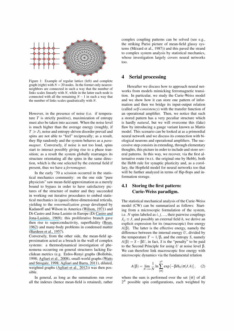
where in the last term we neglected the diagonal term(i = j) as it is irrelevant for large N. From a topolog-ical perspective the mean-field approximation equalsto abandon the lattice structure in favor to a completegraph (see Fig. 1).When the coupling matrix has onlypositive entries, e.g. P(Ji j) = δ(Ji j − J), this modelis named Curie-Weiss model and acts as the sim-plest microscopic Hamiltonian able to describe theparamagnetic-ferromagnetic transitions experiencedby materials when temperature is properly lowered.An external (magnetic) field h can be accounted for byadding in the Hamiltonian an extra term ∝−h∑
Ni σi.
According to the principle of minimum energy,the two-body interaction appearing in the Hamilto-nian in Eq. 1 tends to make spins parallel with eachother and aligned with the external field if present.
sabato 3 maggio 14
Figure 1: Example of regular lattice (left) and completegraph (right) with N = 20 nodes. In the former only nearest-neighbors are connected in such a way that the number oflinks scales linearly with N, while in the latter each node isconnected with all the remaining N− 1 in such a way thatthe number of links scales quadratically with N.
However, in the presence of noise (i.e. if tempera-ture T is strictly positive), maximization of entropymust also be taken into account. When the noise levelis much higher than the average energy (roughly, ifT J), noise and entropy-driven disorder prevail andspins are not able to “feel” reciprocally; as a result,they flip randomly and the system behaves as a para-magnet. Conversely, if noise is not too loud, spinsstart to interact possibly giving rise to a phase tran-sition; as a result the system globally rearranges itsstructure orientating all the spins in the same direc-tion, which is the one selected by the external field ifpresent, thus we have a ferromagnet.
In the early ’70 a scission occurred in the statis-tical mechanics community: on the one side “purephysicists” saw mean-field approximation as a merelybound to bypass in order to have satisfactory pic-tures of the structure of matter and they succeededin working out iterative procedures to embed statis-tical mechanics in (quasi)-three-dimensional reticula,yielding to the renormalization group developed byKadanoff and Wilson in America (Wilson, 1971) andDi-Castro and Jona-Lasinio in Europe (Di Castro andJona-Lasinio, 1969); this proliferative branch gavethen rise to superconductivity, superfluidity (Bean,1962) and many-body problems in condensed matter(Bardeen et al., 1957).Conversely, from the other side, the mean-field ap-proximation acted as a breach in the wall of complexsystems: a thermodynamical investigation of phe-nomena occurring on general structures lacking Eu-clidean metrics (e.g. Erdos-Renyi graphs (Bollobas,1998; Agliari et al., 2008), small-world graphs (Wattsand Strogatz, 1998; Agliari and Barra, 2011), diluted,weighted graphs (Agliari et al., 2012)) was then pos-sible.
In general, as long as the summations run overall the indexes (hence mean-field is retained), rather
complex coupling patterns can be solved (see e.g.,the striking Parisi picture of mean-field glassy sys-tems (Mezard et al., 1987)) and this paved the strandto complex system analysis by statistical mechanics,whose investigation largely covers neural networkstoo.
4 Serial processing
Hereafter we discuss how to approach neural net-works from models mimicking ferromagnetic transi-tion. In particular, we study the Curie-Weiss modeland we show how it can store one pattern of infor-mation and then we bridge its input-output relation(called self-consistency) with the transfer function ofan operational amplifier. Then, we notice that sucha stored pattern has a very peculiar structure whichis hardly natural, but we will overcome this (fake)flaw by introducing a gauge variant known as Mattismodel. This scenario can be looked at as a primordialneural network and we discuss its connection with bi-ological neurons and operational amplifiers. The suc-cessive step consists in extending, through elementarythoughts, this picture in order to include and store sev-eral patterns. In this way, we recover, via the first al-ternative route (w.r.t. the original one by Hebb), boththe Hebb rule for synaptic plasticity and, as a corol-lary, the Hopfield model for neural networks too thatwill be further analyzed in terms of flip-flops and in-formation storage.
4.1 Storing the first pattern:Curie-Weiss paradigm.
The statistical mechanical analysis of the Curie-Weissmodel (CW) can be summarized as follows: Start-ing from a microscopic formulation of the system,i.e. N spins labeled as i, j, ..., their pairwise couplingsJi j ≡ J, and possibly an external field h, we derive anexplicit expression for its (macroscopic) free energyA(β). The latter is the effective energy, namely thedifference between the internal energy U , divided bythe temperature T = 1/β, and the entropy S, namelyA(β) = S−βU , in fact, S is the “penalty” to be paidto the Second Principle for using U at noise level β.We can therefore link macroscopic free energy withmicroscopic dynamics via the fundamental relation
A(β) = limN→∞
1N
ln2N
∑σ
exp [−βHN(σ|J,h)] , (2)
where the sum is performed over the set σ of all2N possible spin configurations, each weighted by
the Boltzmann factor exp[−βHN(σ|J,h)] that tests thelikelihood of the related configuration. From expres-sion (2), we can derive the whole thermodynamicsand in particular phase-diagrams, that is, we are ableto discern regions in the space of tunable parameters(e.g. temperature/noise level) where the system be-haves as a paramagnet or as a ferromagnet.Thermodynamical averages, denoted with the symbol〈.〉, provide for a given observable the expected value,namely the value to be compared with measures inan experiment. For instance, for the magnetizationm(σ)≡ ∑
Ni=1 σi/N we have
〈m(β)〉= ∑σ m(σ)e−βHN(σ|J)
∑σ e−βHN(σ|J). (3)
When β→ ∞ the system is noiseless (zero tempera-ture) hence spins feel reciprocally without errors andthe system behaves ferromagnetically (|〈m〉| → 1),while when β→ 0 the system behaves completely ran-dom (infinite temperature), thus interactions can notbe felt and the system is a paramagnet (〈m〉 → 0). Inbetween a phase transition happens.
In the Curie-Weiss model the magnetizationworks as order parameter: its thermodynamical av-erage is zero when the system is in a paramagnetic(disordered) state (→ 〈m〉 = 0), while it is differentfrom zero in a ferromagnetic state (where it can beeither positive or negative, depending on the sign ofthe external field). Dealing with order parameters al-lows us to avoid managing an extensive number ofvariables σi, which is practically impossible and, evenmore important, it is not strictly necessary.
Now, an explicit expression for the free energy interms of 〈m〉 can be obtained carrying out summationsin eq. 2 and taking the thermodynamic limit N → ∞
as
A(β) = ln2+ lncosh[β(J〈m〉+h)]− βJ2〈m〉2. (4)
In order to impose thermodynamical principles, i.e.energy minimization and entropy maximization, weneed to find the extrema of this expression with re-spect to 〈m〉 requesting ∂〈m(β)〉A(β) = 0. The resultingexpression is called the self-consistency and it readsas
∂〈m〉A(β) = 0⇒ 〈m〉= tanh[β(J〈m〉+h)]. (5)
This expression returns the average behavior of a spinin a magnetic field. In order to see that a phase tran-sition between paramagnetic and ferromagnetic statesactually exists, we can fix h = 0 (and pose J = 1 forsimplicity) and expand the r.h.s. of eq. 5 to get
〈m〉 ∝±√
βJ−1. (6)
0 0.5 1 1.5 20
0.2
0.4
0.6
0.8
1
T
!m" 60 10020
0.05
0.025
0.1
(T # Tc)!1
!m"
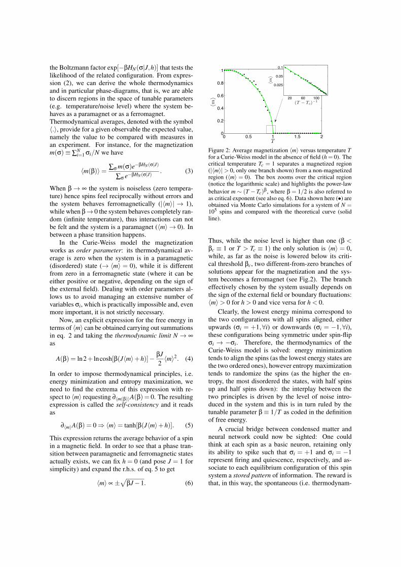
Figure 2: Average magnetization 〈m〉 versus temperature Tfor a Curie-Weiss model in the absence of field (h = 0). Thecritical temperature Tc = 1 separates a magnetized region(|〈m〉|> 0, only one branch shown) from a non-magnetizedregion (〈m〉 = 0). The box zooms over the critical region(notice the logarithmic scale) and highlights the power-lawbehavior m ∼ (T −Tc)
β, where β = 1/2 is also referred toas critical exponent (see also eq. 6). Data shown here (•) areobtained via Monte Carlo simulations for a system of N =105 spins and compared with the theoretical curve (solidline).
Thus, while the noise level is higher than one (β <βc ≡ 1 or T > Tc ≡ 1) the only solution is 〈m〉 = 0,while, as far as the noise is lowered below its criti-cal threshold βc, two different-from-zero branches ofsolutions appear for the magnetization and the sys-tem becomes a ferromagnet (see Fig.2). The brancheffectively chosen by the system usually depends onthe sign of the external field or boundary fluctuations:〈m〉> 0 for h > 0 and vice versa for h < 0.
Clearly, the lowest energy minima correspond tothe two configurations with all spins aligned, eitherupwards (σi = +1,∀i) or downwards (σi = −1,∀i),these configurations being symmetric under spin-flipσi → −σi. Therefore, the thermodynamics of theCurie-Weiss model is solved: energy minimizationtends to align the spins (as the lowest energy states arethe two ordered ones), however entropy maximizationtends to randomize the spins (as the higher the en-tropy, the most disordered the states, with half spinsup and half spins down): the interplay between thetwo principles is driven by the level of noise intro-duced in the system and this is in turn ruled by thetunable parameter β≡ 1/T as coded in the definitionof free energy.
A crucial bridge between condensed matter andneural network could now be sighted: One couldthink at each spin as a basic neuron, retaining onlyits ability to spike such that σi = +1 and σi = −1represent firing and quiescence, respectively, and as-sociate to each equilibrium configuration of this spinsystem a stored pattern of information. The reward isthat, in this way, the spontaneous (i.e. thermodynam-
ical) tendency of the network to relax on free-energyminima can be related to the spontaneous retrieval ofthe stored pattern, such that the cognitive capabilityemerges as a natural consequence of physical princi-ples: we well deepen this point along the whole paper.
4.2 The Curie-Weiss model and the(saturable) operational amplifier
Let us now tackle the problem by another perspec-tive and highlight a structural/mathematical similarityin the world of electronics: the plan is to compareself-consistencies in statistical mechanics and trans-fer functions in electronics so to reach a unified de-scription for these systems. Before proceeding, werecall a few basic concepts. The operational ampli-fier, namely a solid-state integrated circuit (transis-tor), uses feed-back regulation to set its functions assketched in Fig. 3 (insets): there are two signal in-puts (one positive received (+) and one inverted, thusnegative received (-)), two voltage supplies (Vsat , -Vsat ) -where “sat” stands for saturable - and an out-put (Vout ). An ideal amplifier is the linear approxi-mation of the saturable one (technically the voltage atthe input collectors is thought constant so that no cur-rent flows inside the transistor, and Kirchoff rules ap-ply straightforwardly): keeping the symbols of Fig. 3,where Rin stands for the input resistance while R f rep-resents the feed-back resistance, i+ = i− = 0 and as-suming Rin = 1Ω -without loss of generality as onlythe ratio R f /Rin matters- the following transfer func-tion is achieved:
Vout = GVin = (1+R f )Vin, (7)
where G = 1+R f is called gain, therefore as far as0 > R f > ∞ (thus retro-action is present) the device isamplifying.Let us emphasize deep structural analogies with theCurie-Weiss response to a magnetic field h: First, wenotice that all these systems saturate. Whatever themagnitude of the external field for the CW model,once all the spins become aligned, increasing further hwill no longer produce a change in the system; analo-gously, once in the op-amp reached Vout =Vsat , largervalues of Vin will not result in further amplification.Also, notice that both the self-consistency and thetransfer function are two input-output relations (theinput being the external field in the former and theinput-voltage in the latter, the output being the mag-netization in the former and the output-voltage in thelatter), and, once fixed β = 1 for simplicity, expand-ing 〈m〉= tanh(J〈m〉+h)∼ (1+J)h, we can compare
−10 −6 −2 2 6 10−1
−0.6
−0.2
0.2
0.6
1
h
!m"
−10 −5 0 5 10
−1
−0.5
0
0.5
1
Vin
Vout
Vsat
Vsat
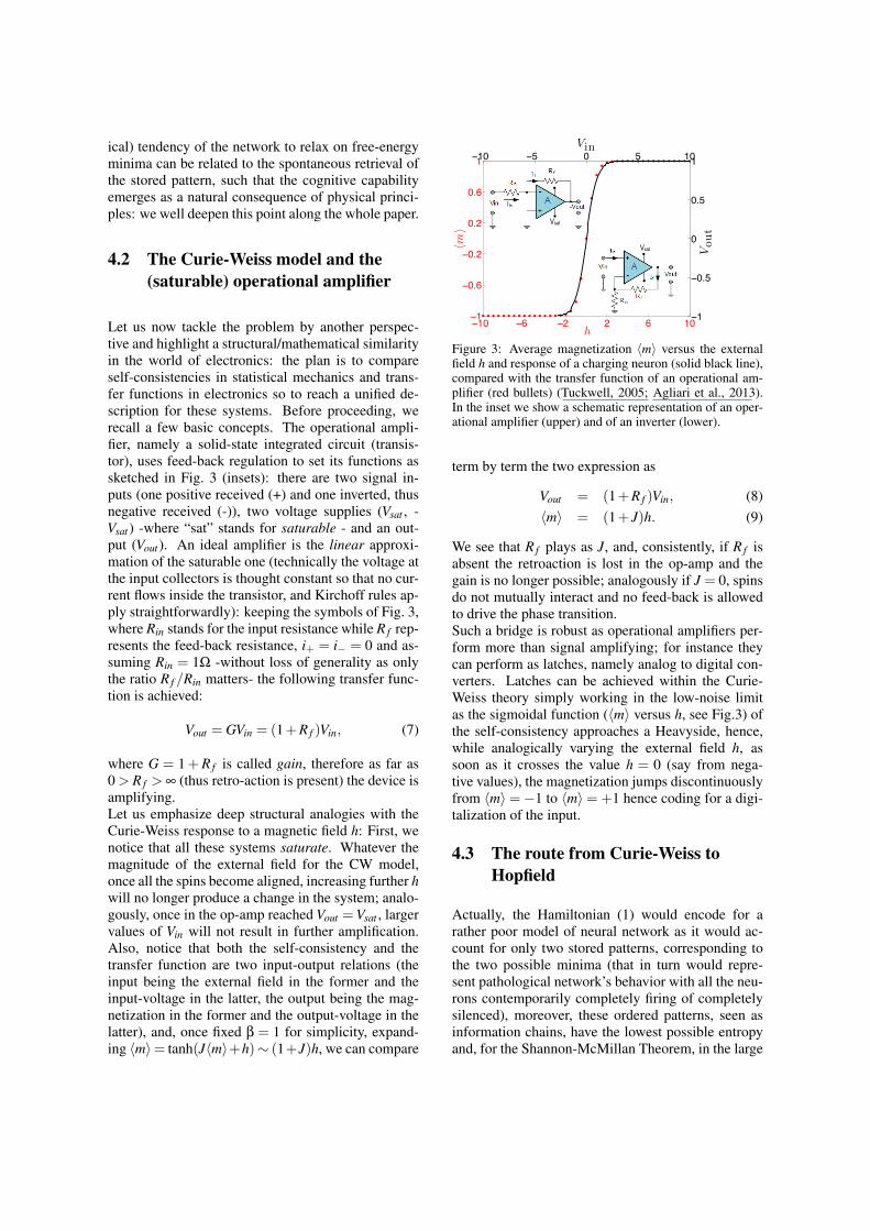
Figure 3: Average magnetization 〈m〉 versus the externalfield h and response of a charging neuron (solid black line),compared with the transfer function of an operational am-plifier (red bullets) (Tuckwell, 2005; Agliari et al., 2013).In the inset we show a schematic representation of an oper-ational amplifier (upper) and of an inverter (lower).
term by term the two expression as
Vout = (1+R f )Vin, (8)〈m〉 = (1+ J)h. (9)
We see that R f plays as J, and, consistently, if R f isabsent the retroaction is lost in the op-amp and thegain is no longer possible; analogously if J = 0, spinsdo not mutually interact and no feed-back is allowedto drive the phase transition.Such a bridge is robust as operational amplifiers per-form more than signal amplifying; for instance theycan perform as latches, namely analog to digital con-verters. Latches can be achieved within the Curie-Weiss theory simply working in the low-noise limitas the sigmoidal function (〈m〉 versus h, see Fig.3) ofthe self-consistency approaches a Heavyside, hence,while analogically varying the external field h, assoon as it crosses the value h = 0 (say from nega-tive values), the magnetization jumps discontinuouslyfrom 〈m〉=−1 to 〈m〉=+1 hence coding for a digi-talization of the input.
4.3 The route from Curie-Weiss toHopfield
Actually, the Hamiltonian (1) would encode for arather poor model of neural network as it would ac-count for only two stored patterns, corresponding tothe two possible minima (that in turn would repre-sent pathological network’s behavior with all the neu-rons contemporarily completely firing of completelysilenced), moreover, these ordered patterns, seen asinformation chains, have the lowest possible entropyand, for the Shannon-McMillan Theorem, in the large
N limit5 they will never be observed.This criticism can be easily overcome thanks to
the Mattis-gauge, namely a re-definition of the spinsvia σi → ξ1
i σi, where ξ1i = ±1 are random entries
extracted with equal probability and kept fixed inthe network (in statistical mechanics these are calledquenched variables to stress that they do not con-tribute to thermalization, a terminology reminiscentof metallurgy (Mezard et al., 1987)). Fixing J ≡ 1 forsimplicity, the Mattis Hamiltonian reads as
HMattisN (σ|ξ) =− 1
2N
N,N
∑i, j
ξ1i ξ
1jσiσ j−h
N
∑i
ξ1i σi. (10)
The Mattis magnetization is defined as m1 = ∑i ξ1i σi.
To inspect its lowest energy minima, we perform acomparison with the CW model: in terms of the (stan-dard) magnetization, the Curie-Weiss model reads asHCW
N ∼ −(N/2)m2 − hm and, analogously we canwrite HMattis
N (σ|ξ) in terms of Mattis magnetizationas HMattis
N ∼−(N/2)m21−hm1. It is then evident that,
in the low noise limit (namely where collective prop-erties may emerge), as the minimum of free energyis achieved in the Curie-Weiss model for 〈m〉 → ±1,the same holds in the Mattis model for 〈m1〉 → ±1.However, this implies that now spins tend to alignparallel (or antiparallel) to the vector ξ1, hence ifthe latter is, say, ξ1 = (+1,−1,−1,−1,+1,+1) ina model with N = 6, the equilibrium configurationsof the network will be σ = (+1,−1,−1,−1,+1,+1)and σ = (−1,+1,+1,+1,−1,−1), the latter due tothe gauge symmetry σi→−σi enjoyed by the Hamil-tonian. Thus, the network relaxes autonomously toa state where some of its neurons are firing whileothers are quiescent, according to the stored patternξ1. Note that, as the entries of the vectors ξ arechosen randomly ±1 with equal probability, the re-trieval of free energy minimum now corresponds to aspin configuration which is also the most entropic forthe Shannon-McMillan argument, thus both the mostlikely and the most difficult to handle (as its informa-tion compression is no longer possible).
Two remarks are in order now. On the one side,according to the self-consistency equation (5) andas shown in Fig. 3, 〈m〉 versus h displays the typi-cal graded/sigmoidal response of a charging neuron(Tuckwell, 2005), and one would be tempted to callthe spins σ neurons. On the other side, it is definitelyinconvenient to build a network via N spins/neurons,which are further meant to be diverging (i.e. N→ ∞)in order to handle one stored pattern of information
5The thermodynamic limit N → ∞ is required forboth mathematical convenience, e.g. it allows saddle-point/stationary-phase techniques, and in order to neglectobservable fluctuations by a central limit theorem argument.
only. Along the theoretical physics route overcomingthis limitation is quite natural (and provides the firstderivation of the Hebbian prescription in this paper):If we want a network able to cope with P patterns, thestarting Hamiltonian should have simply the sum overthese P previously stored6 patterns, namely
HN(σ|ξ) =−1
2N
N,N
∑i, j=1
(P
∑µ=1
ξµi ξ
µj
)σiσ j, (11)
where we neglect the external field (h = 0) for sim-plicity. As we will see in the next section, this Hamil-tonian constitutes indeed the Hopfield model, namelythe harmonic oscillator of neural networks, whosecoupling matrix is called Hebb matrix as encodesthe Hebb prescription for neural organization (Amit,1992).
4.4 The route fromSherrington-Kirkpatrick toHopfield
Despite the extension to the case P > 1 is formallystraightforward, the investigation of the system as Pgrows becomes by far more tricky. Indeed, neuralnetworks belong to the so-called “complex systems”realm. We propose that complex behaviors can be dis-tinguished by simple behaviors as for the latter thenumber of free-energy minima of the system does notscale with the volume N, while for complex systemsthe number of free-energy minima does scale with thevolume according to a proper function of N. For in-stance, the Curie-Weiss/Mattis model has two minimaonly, whatever N (even if N → ∞), and it constitutesthe paradigmatic example for a simple system. Asa counterpart, the prototype of complex system is theSherrington-Kirkpatrick model (SK), originally intro-duced in condensed matter to describe the peculiarbehaviors exhibited by real glasses (Hertz and Palmer,1991; Mezard et al., 1987). This model has an amountof minima that scales ∝ exp(cN) with c 6= f (N), andits Hamiltonian reads as
HSKN (σ|J) = 1√
N
N,N
∑i< j
Ji jσiσ j, (12)
where, crucially, coupling are Gaussian distributed7
as P(Ji j)≡N [0,1]. This implies that links can be ei-
6The part of neural network’s theory we are analyzing ismeant for spontaneous retrieval of already stored informa-tion -grouped into patterns (pragmatically vectors)-. Clearlyit is assumed that the network has already overpass thelearning stage.
7Couplings in spin-glasses are drawn once for all at thebeginning and do not evolve with system’s thermalization,namely they are quenched variables too.
ther positive (hence favoring parallel spin configura-tion) as well as negative (hence favoring anti-parallelspin configuration), thus, in the large N limit, withlarge probability, spins will receive conflicting sig-nals and we speak about “frustrated networks”. In-deed frustration, the hallmark of complexity, is fun-damental in order to split the phase space in severaldisconnected zones, i.e. in order to have several min-ima, or several stored patterns in neural network lan-guage. This mirrors a clear request also in electronics,namely the need for inverters (that once mixed withop-amps) result in flip-flops (crucial for informationstorage as we will see).
The mean-field statistical mechanics for the low-noise behavior of spin-glasses has been first describedby Giorgio Parisi and it predicts a hierarchical orga-nization of states and a relaxational dynamics spreadover many timescales (for which we refer to specifictextbooks (Mezard et al., 1987)). Here we just needto know that their natural order parameter is no longerthe magnetization (as these systems do not magne-tize), but the overlap qab, as we are explaining. Spinglasses are balanced ensembles of ferromagnets andantiferromagnets (this can also be seen mathemati-cally as P(J) is symmetric around zero) and, as a re-sult, 〈m〉 is always equal to zero, on the other hand,a comparison between two realizations of the sys-tem (pertaining to the same coupling set) is meaning-ful because at large temperatures it is expected to bezero, as everything is uncorrelated, but at low temper-ature their overlap is strictly non-zero as spins freezein disordered but correlated states. More precisely,given two “replicas” of the system, labeled as a andb, their overlap qab can be defined as the scalar prod-uct between the related spin configurations, namely asqab = (1/N)∑
Ni σa
i σbi
8, thus the mean-field spin glasshas a completely random paramagnetic phase, with〈q〉 ≡ 0 and a ”glassy phase” with 〈q〉 > 0 split by aphase transition at βc = Tc = 1.
The Sherrington-Kirkpatrick model displays alarge number of minima as expected for a cognitivesystem, yet it is not suitable to act as a cognitivesystem because its states are too ”disordered”. Welook for an Hamiltonian whose minima are not purelyrandom like those in SK, as they must represent or-dered stored patterns (hence like the CW ones), butthe amount of these minima must be possibly exten-sive in the number of spins/neurons N (as in the SKand at contrary with CW), hence we need to retain
8Note that, while in the Curie-Weiss model, whereP(J) = δ(J− 1), the order parameter was the first momen-tum of P(m), in the Sherrington-Kirkpatrick model, whereP(J) = N [0,1], the variance of P(m) (which is roughly qab)is the good order parameter.
0 0.05 0.10
0.2
0.4
0.6
0.8
1
1.2
1.4
0 0.05 0.10
0.2
0.4
0.6
0.8
1
1.2
1.4
0 0.05 0.10
0.2
0.4
0.6
0.8
1
1.2
1.4
0 0.05 0.10
0.2
0.4
0.6
0.8
1
1.2
1.4
↵
T
PM
SG
SG+RR
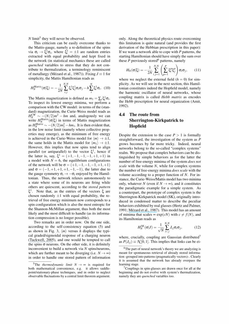
Figure 4: Phase diagram for the Hopfield model (Amit,1992). According to the parameter setting, the system be-haves as a paramagnet (PM), as a spin-glass (SG), or as anassociative neural network able to perform information re-trieval (R). The region labeled (SG+R) is a coexistence re-gion where the system is glassy but still able to retrieve.
a “ferromagnetic flavor” within a “glassy panorama”:we need something in between.
Remarkably, the Hopfield model defined by theHamiltonian (11) lies exactly in between a Curie-Weiss model and a Sherrington-Kirkpatrick model.Let us see why: When P = 1 the Hopfield modelrecovers the Mattis model, which is nothing but agauge-transformed Curie-Weiss model. Conversely,when P → ∞, (1/
√N)∑
Pµ ξ
µi ξ
µj → N [0,1], by the
standard central limit theorem, and the Hopfieldmodel recovers the Sherrington-Kirkpatrick one. Inbetween these two limits the system behaves as an as-sociative network (Barra et al., 2012b).Such a crossover between CW (or Mattis) and SKmodels, requires for its investigation both the P Mat-tis magnetization 〈mµ〉, µ = (1, ...,P) (for quantifyingretrieval of the whole stored patterns, that is the vo-cabulary), and the two-replica overlaps 〈qab〉 (to con-trol the glassyness growth if the vocabulary gets en-larged), as well as a tunable parameter measuring theratio between the stored patterns and the amount ofavailable neurons, namely α = limN→∞ P/N, also re-ferred to as network capacity.
As far as P scales sub-linearly with N, i.e. in thelow storage regime defined by α = 0, the phase dia-gram is ruled by the noise level β only: for β < βc thesystem is a paramagnet, with 〈mµ〉= 0 and 〈qab〉= 0,while for β > βc the system performs as an attractornetwork, with 〈mµ〉 6= 0 for a given µ (selected by theexternal field) and 〈qab〉 = 0. In this regime no dan-gerous glassy phase is lurking, yet the model is ableto store only a tiny amount of patterns as the capacityis sub-linear with the network volume N.Conversely, when P scales linearly with N, i.e. in thehigh-storage regime defined by α > 0, the phase di-agram lives in the α,β plane (see Fig. 4).When α is
−10 −6 −2 2 6 10−1
−0.6
−0.2
0.2
0.6
1
h
!m"
−10 −5 0 5 10
−1
−0.5
0
0.5
1
Vin
VoutR2
Vin
VoutR1
Vin
Vout J<0
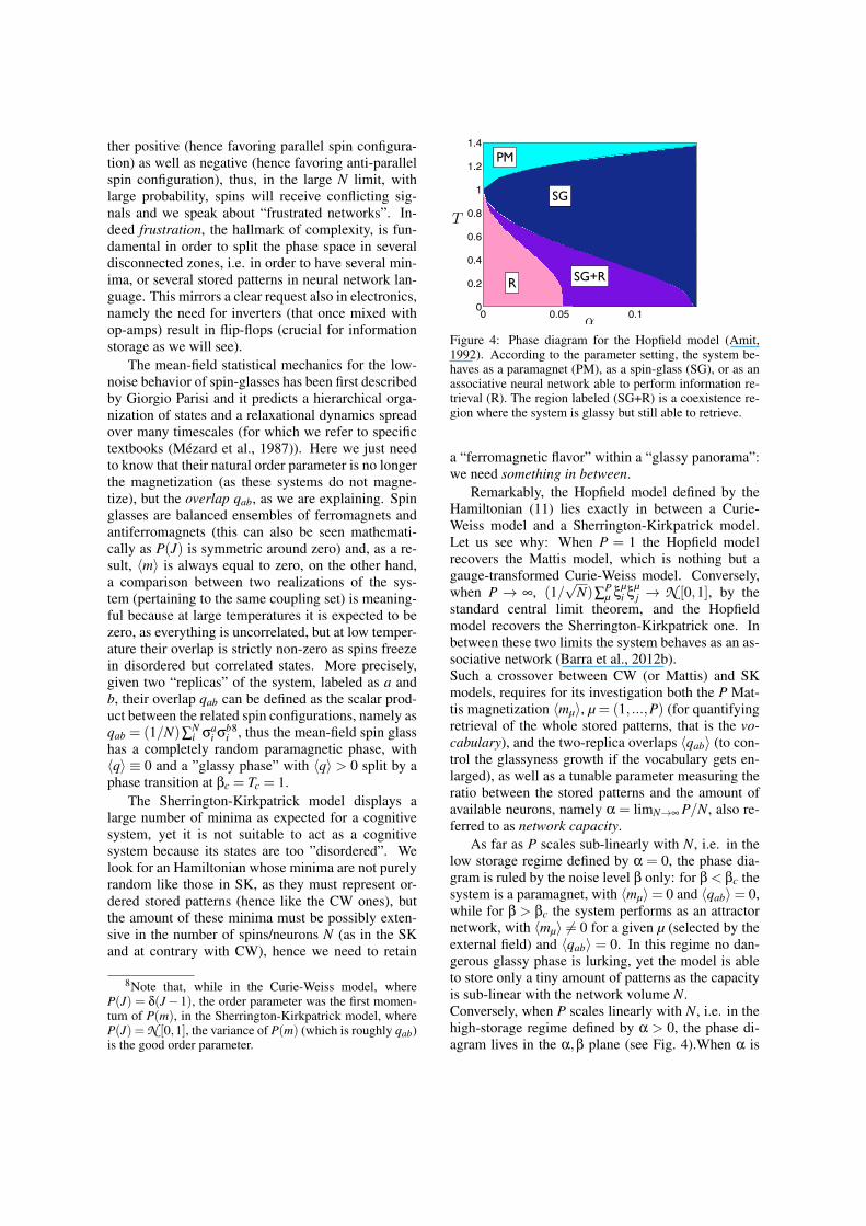
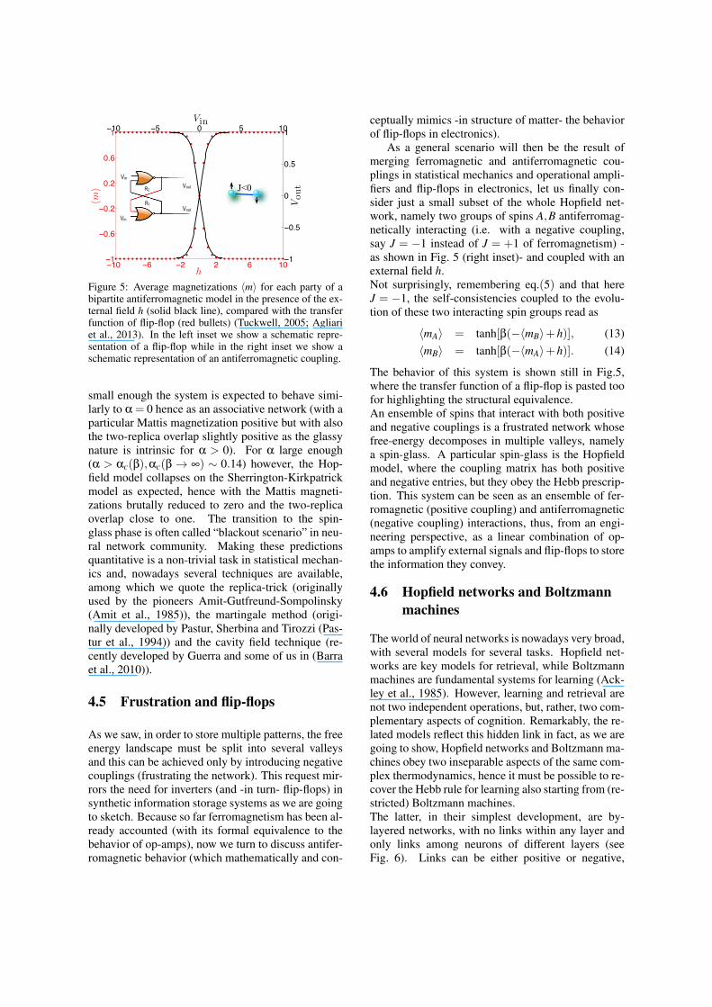
Figure 5: Average magnetizations 〈m〉 for each party of abipartite antiferromagnetic model in the presence of the ex-ternal field h (solid black line), compared with the transferfunction of flip-flop (red bullets) (Tuckwell, 2005; Agliariet al., 2013). In the left inset we show a schematic repre-sentation of a flip-flop while in the right inset we show aschematic representation of an antiferromagnetic coupling.
small enough the system is expected to behave simi-larly to α = 0 hence as an associative network (with aparticular Mattis magnetization positive but with alsothe two-replica overlap slightly positive as the glassynature is intrinsic for α > 0). For α large enough(α > αc(β),αc(β → ∞) ∼ 0.14) however, the Hop-field model collapses on the Sherrington-Kirkpatrickmodel as expected, hence with the Mattis magneti-zations brutally reduced to zero and the two-replicaoverlap close to one. The transition to the spin-glass phase is often called “blackout scenario” in neu-ral network community. Making these predictionsquantitative is a non-trivial task in statistical mechan-ics and, nowadays several techniques are available,among which we quote the replica-trick (originallyused by the pioneers Amit-Gutfreund-Sompolinsky(Amit et al., 1985)), the martingale method (origi-nally developed by Pastur, Sherbina and Tirozzi (Pas-tur et al., 1994)) and the cavity field technique (re-cently developed by Guerra and some of us in (Barraet al., 2010)).
4.5 Frustration and flip-flops
As we saw, in order to store multiple patterns, the freeenergy landscape must be split into several valleysand this can be achieved only by introducing negativecouplings (frustrating the network). This request mir-rors the need for inverters (and -in turn- flip-flops) insynthetic information storage systems as we are goingto sketch. Because so far ferromagnetism has been al-ready accounted (with its formal equivalence to thebehavior of op-amps), now we turn to discuss antifer-romagnetic behavior (which mathematically and con-
ceptually mimics -in structure of matter- the behaviorof flip-flops in electronics).
As a general scenario will then be the result ofmerging ferromagnetic and antiferromagnetic cou-plings in statistical mechanics and operational ampli-fiers and flip-flops in electronics, let us finally con-sider just a small subset of the whole Hopfield net-work, namely two groups of spins A,B antiferromag-netically interacting (i.e. with a negative coupling,say J = −1 instead of J = +1 of ferromagnetism) -as shown in Fig. 5 (right inset)- and coupled with anexternal field h.Not surprisingly, remembering eq.(5) and that hereJ = −1, the self-consistencies coupled to the evolu-tion of these two interacting spin groups read as
〈mA〉 = tanh[β(−〈mB〉+h)], (13)〈mB〉 = tanh[β(−〈mA〉+h)]. (14)
The behavior of this system is shown still in Fig.5,where the transfer function of a flip-flop is pasted toofor highlighting the structural equivalence.An ensemble of spins that interact with both positiveand negative couplings is a frustrated network whosefree-energy decomposes in multiple valleys, namelya spin-glass. A particular spin-glass is the Hopfieldmodel, where the coupling matrix has both positiveand negative entries, but they obey the Hebb prescrip-tion. This system can be seen as an ensemble of fer-romagnetic (positive coupling) and antiferromagnetic(negative coupling) interactions, thus, from an engi-neering perspective, as a linear combination of op-amps to amplify external signals and flip-flops to storethe information they convey.
4.6 Hopfield networks and Boltzmannmachines
The world of neural networks is nowadays very broad,with several models for several tasks. Hopfield net-works are key models for retrieval, while Boltzmannmachines are fundamental systems for learning (Ack-ley et al., 1985). However, learning and retrieval arenot two independent operations, but, rather, two com-plementary aspects of cognition. Remarkably, the re-lated models reflect this hidden link in fact, as we aregoing to show, Hopfield networks and Boltzmann ma-chines obey two inseparable aspects of the same com-plex thermodynamics, hence it must be possible to re-cover the Hebb rule for learning also starting from (re-stricted) Boltzmann machines.The latter, in their simplest development, are by-layered networks, with no links within any layer andonly links among neurons of different layers (seeFig. 6). Links can be either positive or negative,
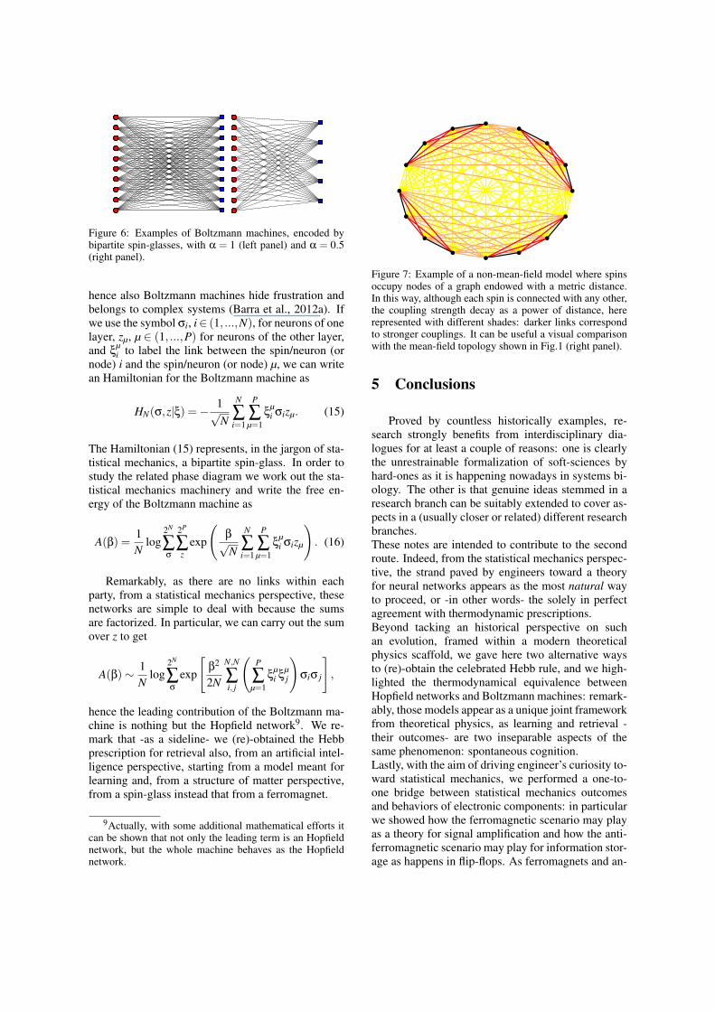
Figure 6: Examples of Boltzmann machines, encoded bybipartite spin-glasses, with α = 1 (left panel) and α = 0.5(right panel).
hence also Boltzmann machines hide frustration andbelongs to complex systems (Barra et al., 2012a). Ifwe use the symbol σi, i∈ (1, ...,N), for neurons of onelayer, zµ, µ ∈ (1, ...,P) for neurons of the other layer,and ξ
µi to label the link between the spin/neuron (or
node) i and the spin/neuron (or node) µ, we can writean Hamiltonian for the Boltzmann machine as
HN(σ,z|ξ) =−1√N
N
∑i=1
P
∑µ=1
ξµi σizµ. (15)
The Hamiltonian (15) represents, in the jargon of sta-tistical mechanics, a bipartite spin-glass. In order tostudy the related phase diagram we work out the sta-tistical mechanics machinery and write the free en-ergy of the Boltzmann machine as
A(β) =1N
log2N
∑σ
2P
∑z
exp
(β√N
N
∑i=1
P
∑µ=1
ξµi σizµ
). (16)
Remarkably, as there are no links within eachparty, from a statistical mechanics perspective, thesenetworks are simple to deal with because the sumsare factorized. In particular, we can carry out the sumover z to get
A(β)∼ 1N
log2N
∑σ
exp
[β2
2N
N,N
∑i, j
(P
∑µ=1
ξµi ξ
µj
)σiσ j
],
hence the leading contribution of the Boltzmann ma-chine is nothing but the Hopfield network9. We re-mark that -as a sideline- we (re)-obtained the Hebbprescription for retrieval also, from an artificial intel-ligence perspective, starting from a model meant forlearning and, from a structure of matter perspective,from a spin-glass instead that from a ferromagnet.
9Actually, with some additional mathematical efforts itcan be shown that not only the leading term is an Hopfieldnetwork, but the whole machine behaves as the Hopfieldnetwork.
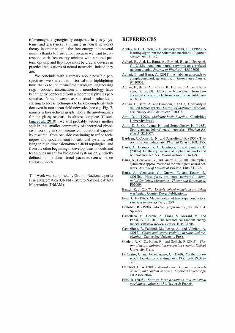
Figure 7: Example of a non-mean-field model where spinsoccupy nodes of a graph endowed with a metric distance.In this way, although each spin is connected with any other,the coupling strength decay as a power of distance, hererepresented with different shades: darker links correspondto stronger couplings. It can be useful a visual comparisonwith the mean-field topology shown in Fig.1 (right panel).
5 Conclusions
Proved by countless historically examples, re-search strongly benefits from interdisciplinary dia-logues for at least a couple of reasons: one is clearlythe unrestrainable formalization of soft-sciences byhard-ones as it is happening nowadays in systems bi-ology. The other is that genuine ideas stemmed in aresearch branch can be suitably extended to cover as-pects in a (usually closer or related) different researchbranches.These notes are intended to contribute to the secondroute. Indeed, from the statistical mechanics perspec-tive, the strand paved by engineers toward a theoryfor neural networks appears as the most natural wayto proceed, or -in other words- the solely in perfectagreement with thermodynamic prescriptions.Beyond tacking an historical perspective on suchan evolution, framed within a modern theoreticalphysics scaffold, we gave here two alternative waysto (re)-obtain the celebrated Hebb rule, and we high-lighted the thermodynamical equivalence betweenHopfield networks and Boltzmann machines: remark-ably, those models appear as a unique joint frameworkfrom theoretical physics, as learning and retrieval -their outcomes- are two inseparable aspects of thesame phenomenon: spontaneous cognition.Lastly, with the aim of driving engineer’s curiosity to-ward statistical mechanics, we performed a one-to-one bridge between statistical mechanics outcomesand behaviors of electronic components: in particularwe showed how the ferromagnetic scenario may playas a theory for signal amplification and how the anti-ferromagnetic scenario may play for information stor-age as happens in flip-flops. As ferromagnets and an-
tiferromagnets synergically cooperate in glassy sys-tems, and glassyness is intrinsic in neural networkstheory in order to split the free energy into severalminima thanks to frustration, because we want to cor-respond each free energy minima with a stored pat-tern, op-amp and flip-flops must be crucial devices inpractical realizations of neural networks: indeed theyare.
We conclude with a remark about possible per-spectives: we started this historical tour highlightinghow, thanks to the mean-field paradigm, engineering(e.g. robotics, automation) and neurobiology havebeen tightly connected from a theoretical physics per-spective. Now, however, as statistical mechanics isstarting to access techniques to tackle complexity hid-den even in non-mean-field networks (see e.g. Fig. 7,namely a hierarchical graph whose thermodynamicsfor the glassy scenario is almost complete (Castel-lana et al., 2010)), we will probably witness anothersplit in this smaller community of theoretical physi-cists working in spontaneous computational capabil-ity research: from one side continuing to refine tech-niques and models meant for artificial systems, welllying in high-dimensional/mean-field topologies, andfrom the other beginning to develop ideas, models andtechniques meant for biological systems only, strictlydefined in finite-dimensional spaces or, even worst, onfractal supports.
This work was supported by Gruppo Nazionale per laFisica Matematica (GNFM), Istituto Nazionale d’AltaMatematica (INdAM).
REFERENCES
Ackley, D. H., Hinton, G. E., and Sejnowski, T. J. (1985). Alearning algorithm for boltzmann machines. Cognitivescience, 9:147–169.
Agliari, E., Asti, L., Barra, A., Burioni, R., and Uguzzoni,G. (2012). Analogue neural networks on correlatedrandom graphs. Journal of Physics A, 45:365001.
Agliari, E. and Barra, A. (2011). A hebbian approach tocomplex-network generation.”. Europhysics Letters,94:10002.
Agliari, E., Barra, A., Burioni, R., Di Biasio, A., and Uguz-zoni, G. (2013). Collective behaviours: from bio-chemical kinetics to electronic circuits. Scientific Re-ports, 3.
Agliari, E., Barra, A., and Camboni, F. (2008). Criticality indiluted ferromagnets. Journal of Statistical Mechan-ics: Theory and Experiment, P10003.
Amit, D. J. (1992). Modeling brain function. CambridgeUniversity Press.
Amit, D. J., Gutfreund, H., and Sompolinsky, H. (1985).Spin-glass models of neural networks. Physical Re-view A, 32:1007.
Bardeen, J., Cooper, L. N., and Schrieffer, J. R. (1957). The-ory of superconductivity. Physical Review, 108:1175.
Barra, A., Bernacchia, A., Contucci, P., and Santucci, E.(2012a). On the equivalence of hopfield networks andboltzmann machines. Neural Networks, 34:1–9.
Barra, A., Genovese, G., and Guerra, F. (2010). The replicasymmetric approximation of the analogical neural net-work. Journal of Statistical Physics, 140:784–796.
Barra, A., Genovese, G., Guerra, F., and Tantari, D.(2012b). How glassy are neural networks?. Jour-nal of Statistical Mechanics: Theory and Experiment,P07009.
Baxter, R. J. (2007). Exactly solved models in statisticalmechanics. Courier Dover Publications.
Bean, C. P. (1962). Magnetization of hard superconductors.Physical Review Letters, 8:250.
Bollobas, B. (1998). Modern graph theory., volume 184.Springer.
Castellana, M., Decelle, A., Franz, S., Mezard, M., andParisi, G. (2010). The hierarchical random energymodel. Physical Review Letters, 104:127206.
Castiglione, P., Falcioni, M., Lesne, A., and Vulpiani, A.(2012). Chaos and coarse graining in statistical me-chanics,. Cambridge University Press.
Coolen, A. C. C., Kuhn, R., and Sollich, P. (2005). The-ory of neural information processing systems. OxfordUniversity Press.
Di Castro, C. and Jona-Lasinio, G. (1969). On the micro-scopic foundation of scaling laws. Phys. Lett, 29:322–323.
Domhoff, G. W. (2003). Neural networks, cognitive devel-opment, and content analysis. American Psychologi-cal Association.
Ellis, R. (2005). Entropy, large deviations, and statisticalmechanics., volume 1431. Taylor & Francis.
Hagan, M. T., Demuth, H. B., and Beale, M. H. (1996).Neural network design. Pws Pub.,, Boston.
Harris-Warrick, R. M., editor (1992). Dynamic biologicalnetworks. MIT press.
Hebb, D. O. (1940). The organization of behavior: A neu-ropsychological theory. Psychology Press.
Hertz, John, A. K. and Palmer, R. (1991). Introduction tothe theory of neural networks. Lecture Notes.
Hopfield, J. J. (1982). Neural networks and physical sys-tems with emergent collective computational abilities.Proc. Natl. A. Sc., 79(8):2554–2558.
Kac, M. (1947). Random walk and the theory of brownianmotion. American Mathematical Monthly, pages 369–391.
Kittel, C. (2004). Elementary statistical physics. CourierDover Publications,.
Martindale, C. (1991). Cognitive psychology: A neural-network approach. Thomson Brooks/Cole PublishingCo.
McCulloch, W. S. and Pitts, W. (1943). A logical calculusof the ideas immanent in nervous activity. The bulletinof mathematical biophysics, 5.4:115–133.
Mezard, M., Parisi, G., and Virasoro, M. A. (1987). Spinglass theory and beyond, volume 9. World scientific,Singapore.
Miller, W. T., Werbos, P. J., and Sutton, R. S., editors(1995). Neural networks for control. MIT press.
Millman, J. and Grabel, A. (1987). Microelectronics.McGraw-Hill.
Minsky, M. L. and Papert, S. A. (1987). Perceptrons - Ex-panded Edition. MIT press, Boston, MA.
Pastur, L., Shcherbina, M., and Tirozzi, B. (1994). Thereplica-symmetric solution without replica trick forthe hopfield model. Journal of Statistical Physics,74:1161–1183.
Reichl, L. E. and Prigogine, I. (1980). A modern coursein statistical physics, volume 71. University of Texaspress, Austin.
Rolls, E. T. and Treves, A. (1998). Neural networks andbrain function.
Rosenblatt, F. (1958). The perceptron: a probabilistic modelfor information storage and organization in the brain.Psychological review, 65(6):386.
Saad, D., editor (2009). On-line learning in neural net-works, volume 17. Cambridge University Press.
Tuckwell, H. C. (2005). Introduction to theoretical neuro-biology., volume 8. Cambridge University Press.
Turing, A. M. (1950). Computing machinery and intelli-gence. Mind, pages 433–460.
Von Neumann, J. (1951). The general and logical theoryof automata. Cerebral mechanisms in behavior, pages1–41.
Watts, D. J. and Strogatz, S. H. (1998). Collective dynamicsof ‘small-world’networks. Nature, 393:440–442.
Wilson, K. G. (1971). Renormalization group and criticalphenomena. Physical Review B, 4:3174.