a three-tiered approach to long term monitoring program optimization

Bioremediation Journal, 8(3–4):147–165, 2004Copyright ©c 2004 Taylor and Francis Inc.ISSN: 1040-8371DOI: 10.1080/10889860490887518

A Three-Tiered Approach to Long TermMonitoring Program Optimization

Carolyn NobelParsons, 1700 Broadway,Suite 900 Denver,CO 80290, USA

John W. AnthonyMitretek Systems,7720 E. Belleview Avenue,Suite BG6, Greenwood Village,CO 80111, USA

ABSTRACT Long term monitoring optimization (LTMO) has proveda valuable method for reducing costs, assuring proper remedial de-cisions are made, and streamlining data collection and managementrequirements over the life of a monitoring program. A three-tieredapproach for LTMO has been developed that combines a qualitativeevaluation with an evaluation of temporal trends in contaminant con-centrations, and a spatial statistical analysis. The results of the threeevaluations are combined to determine the degree to which a mon-itoring program addresses the monitoring program objectives, and adecision algorithm is applied to assess the optimal frequency of mon-itoring and spatial distribution of the components of the monitor-ing network. Ultimately, application of the three-tiered method canbe used to identify potential modifications in sampling locations andsampling frequency that will optimally meet monitoring objectives. Todate, the three-tiered approach has been applied to monitoring pro-grams at 18 sites and has been used to identify a potential average re-duction of over one-third of well sampling events per year. This paperdiscusses the three-tiered approach methodology, including data compi-lation and site screening, qualitative evaluation decision logic, temporaltrend evaluation, and spatial statistical analysis, illustrated using the re-sults of a case study site. Additionally, results of multiple applicationsof the three-tiered LTMO approach are summarized, and future work isdiscussed.

KEYWORDS long term monitoring network optimization, Mann-Kendall tempo-ral trends, geostatistics, kriging

INTRODUCTION

Groundwater monitoring programs have two primary objectives (U.S.Environmental Protection Agency [USEPA], 1994; Gibbons, 1994;USEPA, 2004a):

Address correspondence to CarolynNobel, Parsons, 1700 Broadway, Ste900, Denver, CO 80290, USA. E-mail:[email protected]

147

1. Evaluate long-term temporal trends in contami-nant concentrations at one or more points withinor outside of the remediation zone, as a meansof monitoring the performance of the remedialmeasure (temporal objective); and

2. Evaluate the extent to which contaminant migra-tion is occurring, particularly if a potential expo-sure point for a susceptible receptor exists (spatialobjective).

The relative success of any remediation system andits components (including the monitoring network)must be judged based on the degree to which itachieves the stated objectives of the system. Design-ing an effective groundwater monitoring program in-volves locating monitoring points and developing asite-specific strategy for groundwater sampling andanalysis so as to maximize the amount of relevantinformation that can be obtained while minimiz-ing incremental costs. Relevant information is thatinformation required to effectively address the tem-poral and spatial objectives of monitoring. The ef-fectiveness of a monitoring program in achievingthese two primary objectives can be evaluated quan-titatively using statistical techniques. In addition,there may be other important considerations asso-ciated with a particular monitoring program that aremost appropriately addressed through a qualitativeassessment of the program. The qualitative evalu-ation may consider such factors as hydrostratigra-phy, locations of potential receptor exposure pointswith respect to a dissolved contaminant plume,and the direction(s) and rate(s) of contaminantmigration.

Parsons has developed an approach to evaluatingand optimizing long-term monitoring programs atmature sites (site characterization is complete, anda long-term monitoring program is in place andhas been executed for some period of time) wherethe costs of long-term monitoring represent a sig-nificant fraction of the costs of an environmentalresponse action. Parsons’ three-tiered approach forlong term monitoring optimization (LTMO) consistsof a qualitative evaluation, an evaluation of tem-poral trends in contaminant concentrations, and aspatial statistical analysis. After all three phases (or“tiers”) of the evaluation have been completed, theresults of the three tiers are combined to assess thedegree to which the monitoring network addressesthe primary objectives of monitoring. A decision al-

gorithm is applied to assess the optimal frequencyof monitoring and the spatial distribution of thecomponents of the monitoring network, and to de-velop recommendations for monitoring program op-timization. “Optimization” in this paper refers tothe application of a rule-based procedure (based onprofessional judgment and statistical analysis) that isapplied to recommend a monitoring program that iseffective at meeting the two objectives of monitor-ing while balancing resources and qualitative con-straints, rather than being a formal mathematical op-timization. This paper describes methods that havebeen applied by other investigators to the prob-lem of monitoring-program optimization, presentsParsons’ three-tiered approach, summarizes the re-sults of several sites to which the three-tiered LTMOapproach has been applied, and discusses futurework.

EXAMPLE APPLICATIONS OFMETHODS FOR DESIGNING,

EVALUATING AND OPTIMIZINGMONITORING PROGRAMS

Although monitoring network design has been ex-amined extensively in the past, most previous stud-ies have addressed one of two problems (Reed et al.,2000):

1. application of numerical simulation and opti-mization techniques for screening monitoringplans for detection monitoring at landfills andhazardous-waste sites, and

2. application of ranking methods, including geo-statistics, to augment or design monitoring net-works for site-characterization purposes.

Storck et al. (1995) used a simulation approach toexamine ways to design and evaluate groundwatermonitoring networks for leaking disposal facilities.A Monte Carlo simulator was used to generate alarge number of equally-likely realizations of a ran-dom hydraulic conductivity field and a contami-nant source location. A numerical model simulat-ing groundwater flow and contaminant transport wasused to generate a contaminant plume for each re-alization of the hydraulic-conductivity field. The re-sults of the transport simulations then were used asinput to an optimization model, which generated

148 NOBEL AND ANTHONY

optimal trade-off curves among three conflictingobjectives:

1. maximize probability of contaminant detection,2. minimize cost of monitoring network (i.e., mini-

mum number of monitoring wells), and3. minimize volume of contaminated groundwater.

The model was applied to a hypothetical scenarioin order to examine the sensitivity of the trade-offcurves to various model parameters.

Kelly (1996) applied a numerical model of ground-water flow and contaminant migration together withknowledge of locations of potential contaminantsources, to determine screened-interval elevationsand locations for 75 monitoring wells in 35 clusters,in a network protecting the municipal wellfield ofIndependence, Missouri.

Dresel and Murray (1998) used a ranking approachto assist in the design of a groundwater monitoringnetwork at the U.S. Department of Energy’s Hanfordsite in Washington. A geostatistical model of existingplumes was used to generate a large number of real-izations of contaminant distribution in groundwaterat the facility. Analysis of the realizations provideda quantitative measure of the uncertainties in con-taminant concentrations, and a measure of the prob-ability that a cutoff value (e.g., a regulatory concen-tration standard) would be exceeded at any point. Ametric based on uncertainty measures and declus-tering weights was developed to rank the relativevalue of each monitoring well in the network design.This metric was used, together with hydrogeologicand regulatory considerations in identifying candi-date locations for inclusion in, or removal from thenetwork.

Hudak et al. (1993) applied a ranking method-ology to the design of a detection-monitoring net-work for the Butler County Municipal Landfill insouthwest Ohio. A geographic information system(GIS) was used to assign relative weights to candi-date monitoring locations on the basis of distanceto possible contaminant sources, location relative toprobably contaminant migration pathways, and dis-tance to a potential receptor. The GIS application wasfound to be relatively straightforward to implement,was capable of addressing established regulatory pol-icy, and could be used to address several monitoringobjectives.

Chieniawski et al. (1995) used a simulation ap-proach combined with a ranking approach to exam-ine the problem of optimizing detection monitoringat a waste facility under conditions of uncertainty.A numerical model was used, together with stochas-tic realizations of contaminant transport, to generatenumerous realizations of contaminant movementfor use as input to a multi-objective optimizationmodel. The optimization model was solved usinga genetic algorithm, and generated trade-off curvescomparing the relative cost of a particular monitor-ing network design with the probability that the net-work could detect a leak.

The studies described above dealt primarily withdetection monitoring and global approaches to thedesign of new monitoring networks. By contrast,few investigators have formally addressed the eval-uation and optimization of long-term monitoringprograms at sites having extensive pre-existing mon-itoring networks that were installed during site char-acterization. The primary goal of optimization ef-forts at such sites is to reduce sampling costs byeliminating data redundancy to the extent practi-cable. This type of optimization usually is not in-tended to identify locations for new monitoringwells, and it is assumed that the existing monitoringnetwork sufficiently characterizes the concentrationsand distribution of contaminants being monitored.It also is not intended for use in optimizing detectionmonitoring.

Reed et al. (2000) developed and applied a simu-lation approach for optimizing existing monitoringprograms using a numerical model of groundwaterflow and contaminant transport, several statistically-based plume-interpolation techniques, and a formalmathematical optimization model based on a geneticalgorithm. The optimization approach was used toidentify cost-effective sampling plans that accuratelyquantified the total mass of dissolved contaminantin groundwater. Application of the approach to themonitoring program at Hill Air Force Base (AFB) in-dicated that monitoring costs could be reduced byas much as 60 percent without significant loss in ac-curacy of mass estimates. Reed and Minsker (2004)and Reed et al. (2001 and 2003) extended this workusing several different mathematical optimization al-gorithms to address multiobjective monitoring opti-mization problems.

Cameron and Hunter (2002) applied a spatialand temporal optimization algorithm known as

A THREE-TIERED APPROACH TO LONG TERM MONITORING PROGRAM OPTIMIZATION 149

the Geostatistical Temporal/Spatial (GTS) Optimiza-tion Algorithm to the evaluation and optimiza-tion of two existing monitoring programs at theMassachusetts Military Reservation (MMR), CapeCod, Massachusetts. The GTS algorithm is intendedfor use in optimizing long-term monitoring (LTM)networks using geostatistical methods, and was de-veloped to ensure that only those monitoring datasufficient and necessary to support decisions crucialto monitoring programs are collected and analyzed.The algorithm uses geostatistical methods to opti-mize sampling frequency and to define the networkof essential sampling locations. The algorithm incor-porates a decision pathway analysis that is separatedinto temporal and spatial (i.e., frequency and loca-tion) components, which are used to identify tem-poral and spatial redundancies in existing monitor-ing networks. The results of the temporal analysisapplied to the monitoring programs at MMR indi-cated that sampling frequency could be reduced atmost locations by 40 to 70 percent. The results of thespatial analysis indicated that 109 of the 536 wellsincluded in the two monitoring programs at MMRwere spatially redundant, and could be removed fromthe programs. More recently, Cameron and Hunter(2004) applied the GTS algorithm to monitoring pro-grams at three other sites, and confirmed that use ofthis optimization approach could generate savings

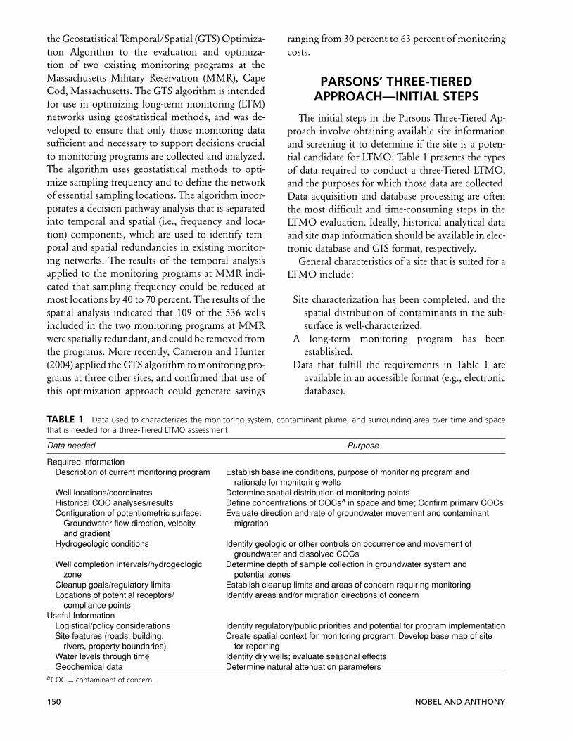
TABLE 1 Data used to characterizes the monitoring system, contaminant plume, and surrounding area over time and spacethat is needed for a three-Tiered LTMO assessment

Data needed Purpose

Required informationDescription of current monitoring program Establish baseline conditions, purpose of monitoring program and

rationale for monitoring wellsWell locations/coordinates Determine spatial distribution of monitoring pointsHistorical COC analyses/results Define concentrations of COCsa in space and time; Confirm primary COCsConfiguration of potentiometric surface:

Groundwater flow direction, velocityand gradient

Evaluate direction and rate of groundwater movement and contaminantmigration

Hydrogeologic conditions Identify geologic or other controls on occurrence and movement ofgroundwater and dissolved COCs

Well completion intervals/hydrogeologiczone

Determine depth of sample collection in groundwater system andpotential zones

Cleanup goals/regulatory limits Establish cleanup limits and areas of concern requiring monitoringLocations of potential receptors/

compliance pointsIdentify areas and/or migration directions of concern

Useful InformationLogistical/policy considerations Identify regulatory/public priorities and potential for program implementationSite features (roads, building,

rivers, property boundaries)Create spatial context for monitoring program; Develop base map of site

for reportingWater levels through time Identify dry wells; evaluate seasonal effectsGeochemical data Determine natural attenuation parameters

aCOC = contaminant of concern.

ranging from 30 percent to 63 percent of monitoringcosts.

PARSONS’ THREE-TIEREDAPPROACH—INITIAL STEPS

The initial steps in the Parsons Three-Tiered Ap-proach involve obtaining available site informationand screening it to determine if the site is a poten-tial candidate for LTMO. Table 1 presents the typesof data required to conduct a three-Tiered LTMO,and the purposes for which those data are collected.Data acquisition and database processing are oftenthe most difficult and time-consuming steps in theLTMO evaluation. Ideally, historical analytical dataand site map information should be available in elec-tronic database and GIS format, respectively.

General characteristics of a site that is suited for aLTMO include:

Site characterization has been completed, and thespatial distribution of contaminants in the sub-surface is well-characterized.

A long-term monitoring program has beenestablished.

Data that fulfill the requirements in Table 1 areavailable in an accessible format (e.g., electronicdatabase).


A long-term monitoring program has beenestablished.

Concentration data are available for more than10 wells (more than 30 wells is preferable), mon-itoring the same contaminant plume and com-pleted in the same water-bearing unit or moni-toring zone.

Analytical results are available from at least four his-torical sampling events over two years or more.

If a system (e.g., site remedy) is in place, it is notexpected to change dramatically during the nextfew years.

The regulatory environment is flexible enough toconsider program modifications.

Monitoring objectives establish the purpose(s) ofmonitoring, but often are poorly defined. Conse-quently, the stated monitoring-program objectivesshould be thoroughly evaluated during the initialstages of LTMO, and modified, if necessary, to re-flect actual program objectives. Additionally, site per-sonnel, regulators, and stakeholders should be in-volved throughout the LTMO process, as they canprovide essential information about regulatory andpolicy issues and other qualitative information thatdrive monitoring priorities that might not be avail-able from other information sources.

PARSONS THREE-TIEREDAPPROACH—METHODOLOGY

Case Study Background

The qualitative, temporal, and spatial analysis tiersare illustrated using the results of an optimization ofa monitoring program that included a subset of theexisting wells at a case study site at the former MatherAir Force Base near Sacramento, California (MatherAFB). The case study results presented in this paperdo not include the entire results for the Mather AFBstudy, and are not intended as a stand-alone casestudy, but rather as example results to demonstratethe Three-Tiered methodology. Complete Three-Tiered case studies are available elsewhere (USEPA,2004b). Various types of contaminants were intro-duced to soil and groundwater in the subsurfaceat Mather AFB during the course of routine Baseoperations that included fuel storage and delivery,fire-fighting training, equipment maintenance, wastedisposal, and other industrial activities conducted

throughout the operational history of the Base. Theprimary contaminants of concern (COCs) at the casestudy site include carbon tetrachloride (CCl4), tetra-chloroethene (PCE), and trichloroethene (TCE). Themonitoring program examined in the case study in-cluded 306 wells completed in multiple hydrogeo-logic zones. Some of the wells are not included inthe current monitoring program; others are sampledat frequencies ranging from quarterly to biennially,for a total of 643 well-sampling events per year. Thesite monitoring program is reviewed annually by theremedial project managers team; the three-tiered ap-proach was applied in 2003 to assess the existing pro-gram and to identify potential additional opportuni-ties for optimization.

In this paper, results from sixteen wells completedin the upper (water-table) aquifer at Mather AFB areused to illustrate the results of each phase of thethree-tiered evaluations. Examination of the resultsobtained from this arbitrary group of wells is notintended to present the comprehensive analysis ofthe case study site, but rather to demonstrate themethodology and types of results produced by theanalysis.

Qualitative Evaluation

The first phase of the three-tiered evaluationinvolves examining the current groundwater mon-itoring program qualitatively, to identify potentialopportunities for LTMO based on factors such as hy-drostratigraphy, locations of potential receptors withrespect to the dissolved plume, and the direction(s)and rate(s) of contaminant migration. An effectivegroundwater monitoring program will provide infor-mation regarding contaminant plume migration andchanges in chemical concentrations through time atappropriate locations, enabling decision-makers toverify that contaminants are not endangering poten-tial receptors, and that remediation is occurring atrates sufficient to achieve remedial action objectiveswithin a reasonable time frame. The design of themonitoring program should therefore include con-sideration of existing receptor exposure pathways, aswell as exposure pathways arising from potential fu-ture use of the groundwater.

Performance monitoring wells located upgradient,within, and immediately downgradient from a plumeprovide a means of evaluating the effectiveness of agroundwater remedy relative to performance criteria.


Long-term monitoring of these wells also providesinformation about migration of the plume and tem-poral trends in chemical concentrations. Groundwa-ter monitoring wells located downgradient from theleading edge of a plume (“sentry wells”) are used toevaluate possible changes in the extent of the plumeand, if warranted, to trigger a contingency responseaction if contaminants are detected.

Primary factors to consider when qualitativelyevaluating a groundwater monitoring program forpotential optimization opportunities include at aminimum:

Aquifer heterogeneity,Types of contaminants,Distance to potential receptor exposure points,Groundwater seepage velocity,Potential surface-water impacts, andThe effects of the remediation system.

These factors will influence the locations and spacingof monitoring points and the sampling frequency.Typically, the greater the seepage velocity and theshorter the distance to receptor exposure points, themore frequently groundwater sampling should beconducted.

The qualitative evaluation considers multiple fac-tors in developing recommendations for continua-tion or cessation of groundwater monitoring at eachwell. In some cases, a recommendation is made tocontinue monitoring a particular well, but at a re-duced frequency. Typical factors considered in de-veloping recommendations to retain a well in, or re-move a well from, a LTM program are summarizedin Table 2. Typical factors considered in develop-ing recommendations for monitoring frequency are

TABLE 2 Decision logic used in the qualitative evaluation phase to determine whether to retain or exclude a well from amonitoring network

Reasons for retaining a well in monitoring network Reasons for removing a well from monitoring network

Well is needed to further characterize the site or monitorchanges in contaminant concentrations through time

Well provides spatially redundant information with aneighboring well (e.g., same constituents, and/orshort distance between wells)

Well is important for defining the lateral or vertical extentof contaminants.

Well has been dry for more than 2 yearsa

Well is needed to monitor water quality at compliancepoint or receptor exposure point (e.g., water supply well)

Contaminant concentrations are consistently belowlaboratory detection limits or cleanup goals

Well is important for defining background water quality Well is completed in same water-bearing zone as nearby well(s)aPeriodic water-level monitoring should be performed in dry wells to confirm that the upper boundary of the saturated zone remains below thewell screen. If the well becomes re-wetted, then its inclusion in the monitoring program should be evaluated. A well that has been dry for morethan two years should be replaced with a new well screened at a deeper interval if groundwater monitoring at that location is deemed to berequired.

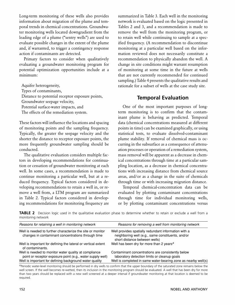
summarized in Table 3. Each well in the monitoringnetwork is evaluated based on the logic presented inTables 2 and 3, and a recommendation is made toremove the well from the monitoring program, orto retain well while continuing to sample at a spec-ified frequency. (A recommendation to discontinuemonitoring at a particular well based on the infor-mation reviewed does not necessarily constitute arecommendation to physically abandon the well. Achange in site conditions might warrant resumptionof monitoring at some time in the future at wellsthat are not currently recommended for continuedsampling.) Table 4 presents the qualitative results andrationale for a subset of wells at the case study site.

Temporal Evaluation

One of the most important purposes of long-term monitoring is to confirm that the contam-inant plume is behaving as predicted. Temporaldata (chemical concentrations measured at differentpoints in time) can be examined graphically, or usingstatistical tests, to evaluate dissolved-contaminantplume stability. If removal of chemical mass is oc-curring in the subsurface as a consequence of attenu-ation processes or operation of a remediation system,mass removal will be apparent as a decrease in chem-ical concentrations through time at a particular sam-pling location, as a decrease in chemical concentra-tions with increasing distance from chemical sourceareas, and/or as a change in the suite of chemicalsthrough time or with increasing migration distance.

Temporal chemical-concentration data can beevaluated by plotting contaminant concentrationsthrough time for individual monitoring wells,or by plotting contaminant concentrations versus


TABLE 3 Decision logic used in the qualitative evaluation phase to determine whether to modify the monitoring frequency ata well

Reasons for increasing sampling frequency Reasons for decreasing sampling frequency

Groundwater velocity is high Groundwater velocity is lowChange in contaminant concentration would

significantly alter a decision or course of actionChange in contaminant concentration would not significantly alter

a decision or course of actionWell is necessary to monitor source area or operating

remedial systemWell is distal from source area and remedial system

Cannot predict whether concentrations will changesignificantly over time

Concentrations are not expected to change significantly over time,or contaminant levels have been below groundwater cleanupobjectives for some prescribed period of time

downgradient distance from the contaminant sourcefor several wells along a particular groundwater flow-path, over several monitoring events. Plotting tempo-ral concentration data is recommended for any anal-ysis of plume stability (Wiedemeier and Haas, 2000);however, visual identification of trends in plotteddata may be a subjective process, particularly if (as islikely) the concentration data do not exhibit a uni-form trend, but are variable through time, as illus-trated in Figure 1.

The possibility of arriving at incorrect conclusionsregarding plume stability on the basis of visual ex-

TABLE 4 Illustration of qualitative evaluation results that shows the pre-optimization (i.e., current) sampling frequency, qual-itative analysis recommendation (exclude, retain, recommended frequency) and the rationale for the recommendation for eachwell

Qualitativeanalysis recommendation

Well ID

Currentsamplingfrequency Exclude Retain Frequency Rationale

MAFB-006 Not sampled√

— Upgradient well, no historical COC detections.MAFB-033 Semi-annual

√Semi-annual Monitors TCE hot spota.

MAFB-037 Annual√

Annual Monitors water quality near southeastern plume boundary.MAFB-047 Annual

√Annual Monitors water quality downgradient of hot spots.

MAFB-048 Annual√

Annual Monitors water quality near western plume boundary.MAFB-085 Semi-annual

√Semi-annual Montiors water quality downgradient.

MAFB-086 Quarterly√

Semi-annual Monitors water quality downgradient of extraction wells.MAFB-087 Quarterly

√Semi-annual Defines extent of hot spot, monitors water near MBS

EW6ABu. Reduce frequency due to COCs consistentlyunder MCLs.

MAFB-088 Semi-annual√

— Redundant with well MAFB-206, which has higher TCEconcentration.

MAFB-089 Annual√

Annual Defines extent of plume.MAFB-090 Semi-annual

√Semi-annual Monitors potential increase in TCE above MCL.

MAFB-091 Not sampled√

— Spatially redundant. MAFB-092 is sampled annually.COCs not detected historically.

MAFB-092 Annual√

Annual Defines plume extent to west.MAFB-093 Not sampled

√— Available in reserve for future sampling if MB-3 becomes

operational.MAFB-095 Quarterly

√Quarterly Monitors hot spot and effects of extraction system near

MBS EW 1A (declining PCE concentrations).MAFB-096 Annual

√Annual Reduce sampling frequency due to COCs consistently

under MCLs. Hydraulically upgradient of plume.a“Hot spots” are defined to be areas where contaminant concentrations exceed the cleanup level by a factor of 10 or more.

amination of temporal concentration data can bereduced by examining temporal trends in chemicalconcentrations using various statistical procedures,including regression analyses and the Mann-Kendalltest for trends. The Mann-Kendall nonparametrictest (Gibbons, 1994) is well-suited for evaluation ofenvironmental data because the sample size can besmall (as few as four data points), no assumptions aremade regarding the underlying statistical distributionof the data, and the test can be adapted to account forseasonal variations in the data. The Mann-Kendalltest involved calculating a trend statistic S at each


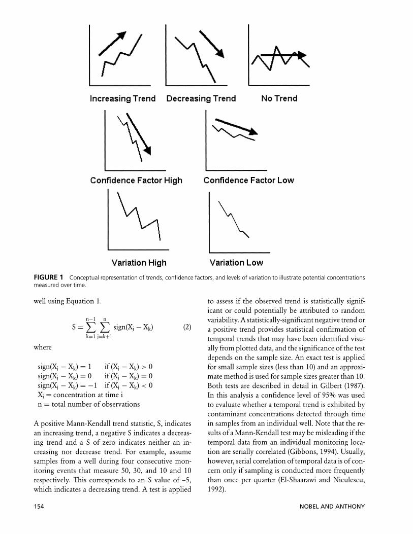
FIGURE 1 Conceptual representation of trends, confidence factors, and levels of variation to illustrate potential concentrationsmeasured over time.

well using Equation 1.

S =n−1∑

k=1

n∑

j=k+1

sign(Xj − Xk) (2)

where

sign(Xj − Xk) = 1 if (Xj − Xk) > 0sign(Xj − Xk) = 0 if (Xj − Xk) = 0sign(Xj − Xk) = −1 if (Xj − Xk) < 0Xi = concentration at time in = total number of observations

A positive Mann-Kendall trend statistic, S, indicatesan increasing trend, a negative S indicates a decreas-ing trend and a S of zero indicates neither an in-creasing nor decrease trend. For example, assumesamples from a well during four consecutive mon-itoring events that measure 50, 30, and 10 and 10respectively. This corresponds to an S value of –5,which indicates a decreasing trend. A test is applied

to assess if the observed trend is statistically signif-icant or could potentially be attributed to randomvariability. A statistically-significant negative trend ora positive trend provides statistical confirmation oftemporal trends that may have been identified visu-ally from plotted data, and the significance of the testdepends on the sample size. An exact test is appliedfor small sample sizes (less than 10) and an approxi-mate method is used for sample sizes greater than 10.Both tests are described in detail in Gilbert (1987).In this analysis a confidence level of 95% was usedto evaluate whether a temporal trend is exhibited bycontaminant concentrations detected through timein samples from an individual well. Note that the re-sults of a Mann-Kendall test may be misleading if thetemporal data from an individual monitoring loca-tion are serially correlated (Gibbons, 1994). Usually,however, serial correlation of temporal data is of con-cern only if sampling is conducted more frequentlythan once per quarter (El-Shaarawi and Niculescu,1992).


The relative value of information obtained fromperiodic monitoring at a particular monitoring wellcan be evaluated by considering the location of thewell with respect to the dissolved contaminant plumeand potential receptor exposure points, and the pres-ence or absence of temporal trends in contaminantconcentrations in samples collected from the well.The degree to which the amount and quality of in-formation that can be obtained at a particular mon-itoring point serve the two primary (i.e., temporaland spatial) objectives of monitoring must be consid-ered in this evaluation. For example, the continuednon-detection of a target contaminant in groundwa-ter at a particular monitoring location provides noinformation about temporal trends in contaminantconcentrations at that location, or about the extentto which contaminant migration is occurring, un-less the monitoring location lies along a groundwaterflowpath between a contaminant source and a po-tential receptor exposure point (e.g., downgradientof a known contaminant plume). Therefore, a mon-itoring well having a history of contaminant con-centrations below detection limits may be provid-ing little or no useful information, depending on itslocation.

A trend of increasing contaminant concentrationsin groundwater at a location between a contaminantsource and a potential receptor exposure point mayrepresent information critical in evaluating whethercontaminants are migrating to the exposure point,thereby completing an exposure pathway. Identifi-cation of a trend of decreasing contaminant con-centrations at the same location may be useful in

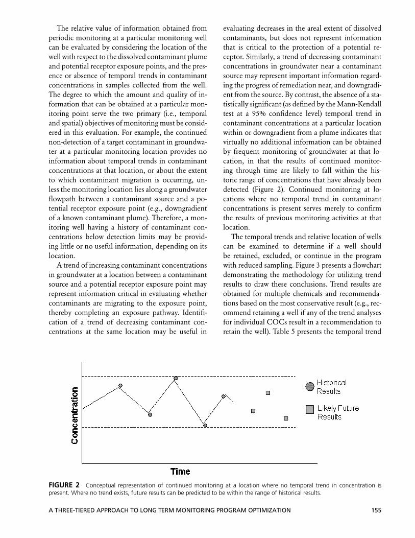
FIGURE 2 Conceptual representation of continued monitoring at a location where no temporal trend in concentration ispresent. Where no trend exists, future results can be predicted to be within the range of historical results.

evaluating decreases in the areal extent of dissolvedcontaminants, but does not represent informationthat is critical to the protection of a potential re-ceptor. Similarly, a trend of decreasing contaminantconcentrations in groundwater near a contaminantsource may represent important information regard-ing the progress of remediation near, and downgradi-ent from the source. By contrast, the absence of a sta-tistically significant (as defined by the Mann-Kendalltest at a 95% confidence level) temporal trend incontaminant concentrations at a particular locationwithin or downgradient from a plume indicates thatvirtually no additional information can be obtainedby frequent monitoring of groundwater at that lo-cation, in that the results of continued monitor-ing through time are likely to fall within the his-toric range of concentrations that have already beendetected (Figure 2). Continued monitoring at lo-cations where no temporal trend in contaminantconcentrations is present serves merely to confirmthe results of previous monitoring activities at thatlocation.

The temporal trends and relative location of wellscan be examined to determine if a well shouldbe retained, excluded, or continue in the programwith reduced sampling. Figure 3 presents a flowchartdemonstrating the methodology for utilizing trendresults to draw these conclusions. Trend results areobtained for multiple chemicals and recommenda-tions based on the most conservative result (e.g., rec-ommend retaining a well if any of the trend analysesfor individual COCs result in a recommendation toretain the well). Table 5 presents the temporal trend


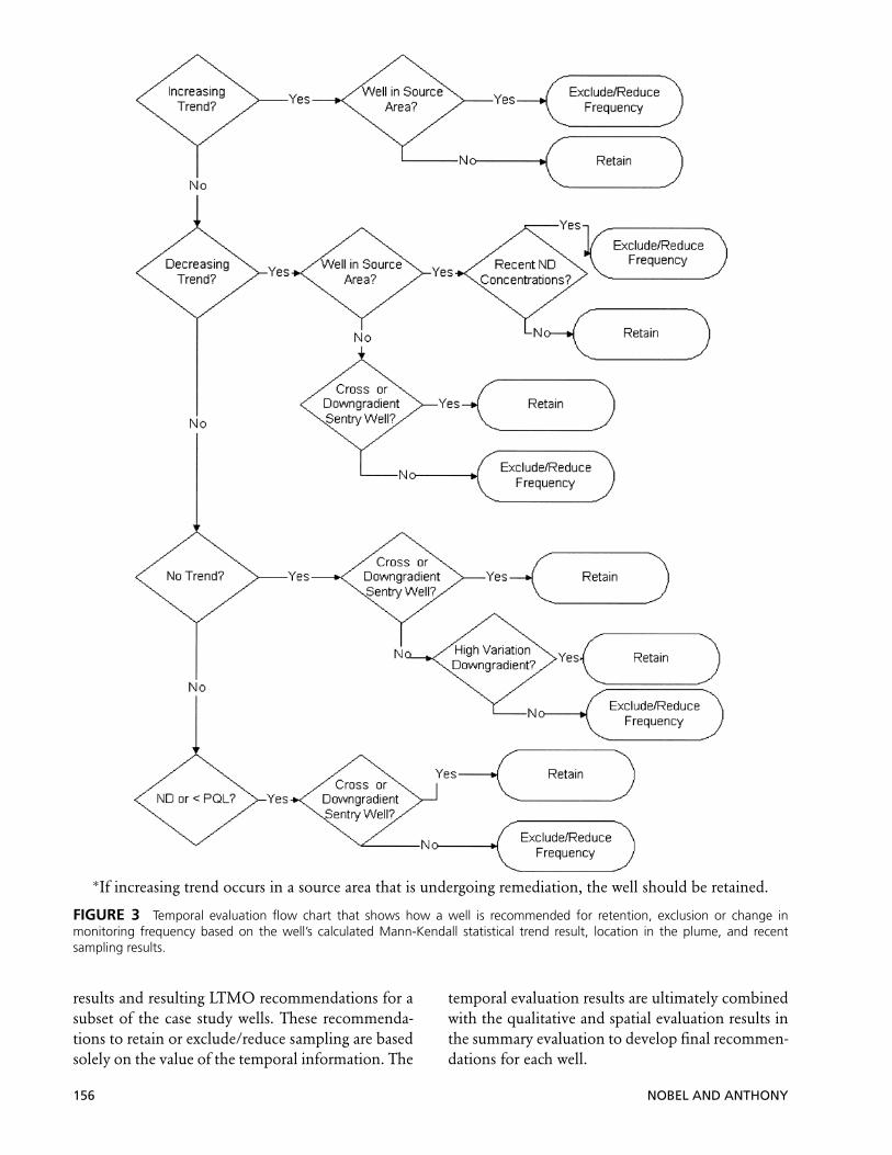
∗If increasing trend occurs in a source area that is undergoing remediation, the well should be retained.

FIGURE 3 Temporal evaluation flow chart that shows how a well is recommended for retention, exclusion or change inmonitoring frequency based on the well’s calculated Mann-Kendall statistical trend result, location in the plume, and recentsampling results.

results and resulting LTMO recommendations for asubset of the case study wells. These recommenda-tions to retain or exclude/reduce sampling are basedsolely on the value of the temporal information. The

temporal evaluation results are ultimately combinedwith the qualitative and spatial evaluation results inthe summary evaluation to develop final recommen-dations for each well.


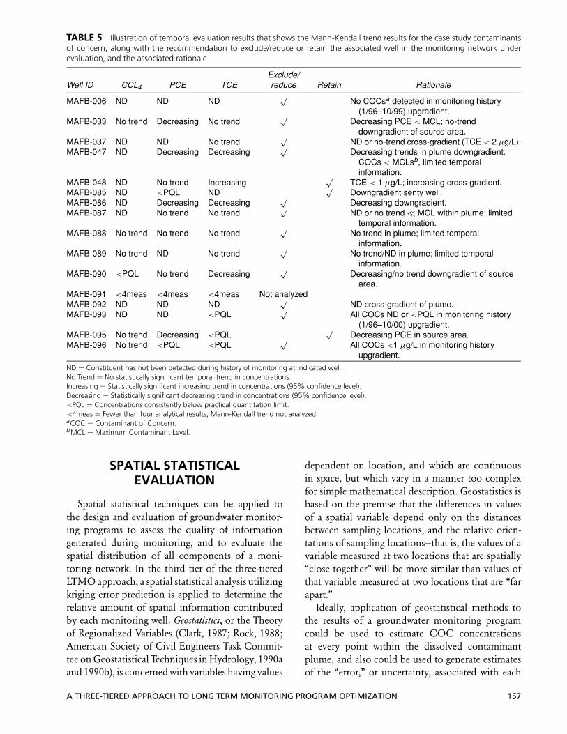
TABLE 5 Illustration of temporal evaluation results that shows the Mann-Kendall trend results for the case study contaminantsof concern, along with the recommendation to exclude/reduce or retain the associated well in the monitoring network underevaluation, and the associated rationale

Exclude/Well ID CCL4 PCE TCE reduce Retain Rationale

MAFB-006 ND ND ND√

No COCsa detected in monitoring history(1/96–10/99) upgradient.

MAFB-033 No trend Decreasing No trend√

Decreasing PCE < MCL; no-trenddowngradient of source area.

MAFB-037 ND ND No trend√

ND or no-trend cross-gradient (TCE < 2 µg/L).MAFB-047 ND Decreasing Decreasing

√Decreasing trends in plume downgradient.

COCs < MCLsb, limited temporalinformation.

MAFB-048 ND No trend Increasing√

TCE < 1 µg/L; increasing cross-gradient.MAFB-085 ND <PQL ND

√Downgradient senty well.

MAFB-086 ND Decreasing Decreasing√

Decreasing downgradient.MAFB-087 ND No trend No trend

√ND or no trend � MCL within plume; limited

temporal information.MAFB-088 No trend No trend No trend

√No trend in plume; limited temporal

information.MAFB-089 No trend ND No trend

√No trend/ND in plume; limited temporal

information.MAFB-090 <PQL No trend Decreasing

√Decreasing/no trend downgradient of source

area.MAFB-091 <4meas <4meas <4meas Not analyzedMAFB-092 ND ND ND

√ND cross-gradient of plume.

MAFB-093 ND ND <PQL√

All COCs ND or <PQL in monitoring history(1/96–10/00) upgradient.

MAFB-095 No trend Decreasing <PQL√

Decreasing PCE in source area.MAFB-096 No trend <PQL <PQL

√All COCs <1 µg/L in monitoring history

upgradient.

ND = Constituent has not been detected during history of monitoring at indicated well.No Trend = No statistically significant temporal trend in concentrations.Increasing = Statistically significant increasing trend in concentrations (95% confidence level).Decreasing = Statistically significant decreasing trend in concentrations (95% confidence level).<PQL = Concentrations consistently below practical quantitation limit.<4meas = Fewer than four analytical results; Mann-Kendall trend not analyzed.aCOC = Contaminant of Concern.bMCL = Maximum Contaminant Level.

SPATIAL STATISTICALEVALUATION

Spatial statistical techniques can be applied tothe design and evaluation of groundwater monitor-ing programs to assess the quality of informationgenerated during monitoring, and to evaluate thespatial distribution of all components of a moni-toring network. In the third tier of the three-tieredLTMO approach, a spatial statistical analysis utilizingkriging error prediction is applied to determine therelative amount of spatial information contributedby each monitoring well. Geostatistics, or the Theoryof Regionalized Variables (Clark, 1987; Rock, 1988;American Society of Civil Engineers Task Commit-tee on Geostatistical Techniques in Hydrology, 1990aand 1990b), is concerned with variables having values

dependent on location, and which are continuousin space, but which vary in a manner too complexfor simple mathematical description. Geostatistics isbased on the premise that the differences in valuesof a spatial variable depend only on the distancesbetween sampling locations, and the relative orien-tations of sampling locations—that is, the values of avariable measured at two locations that are spatially“close together” will be more similar than values ofthat variable measured at two locations that are “farapart.”

Ideally, application of geostatistical methods tothe results of a groundwater monitoring programcould be used to estimate COC concentrationsat every point within the dissolved contaminantplume, and also could be used to generate estimatesof the “error,” or uncertainty, associated with each


estimated concentration value. Thus, the monitoringprogram could be optimized by using available in-formation to identify those areas having the greatestuncertainty associated with the estimated plume ex-tent and configuration. Conversely, sampling pointscould be successively eliminated from simulations,and the resulting uncertainty examined, to evalu-ate if significant loss of information (represented byincreasing error or uncertainty in estimated chem-ical concentrations) occurs as the number of sam-pling locations is reduced. Repeated application ofgeostatistical estimating techniques, using tentativelyidentified sampling locations, then could be used togenerate a sampling program that would provide anacceptable level of uncertainty regarding the distri-bution of COCs with the minimum possible num-ber of samples collected. Furthermore, applicationof geostatistical methods can provide unbiased rep-resentations of the distribution of COCs at differentlocations in the subsurface, enabling the extent ofCOCs to be evaluated more precisely.

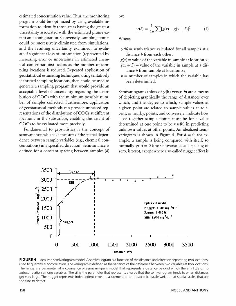
Fundamental to geostatistics is the concept ofsemivariance, which is a measure of the spatial depen-dence between sample variables (e.g., chemical con-centrations) in a specified direction. Semivariance isdefined for a constant spacing between samples (h)

FIGURE 4 Idealized semivariogram model. A semivariogram is a function of the distance and direction separating two locations,used to quantify autocorrelation. The variogram is defined as the variance of the difference between two variables at two locations.The range is a parameter of a covariance or semivariogram model that represents a distance beyond which there is little or noautocorrelation among variables. The sill is the parameter that represents a value that the semivariogram tends to when distancesget very large. The nugget represents independent error, measurement error and/or microscale variation at spatial scales that aretoo fine to detect.

by:

γ (h) = 12n

∑[g(x) − g(x + h)]2 (1)

Where:

γ (h) = semivariance calculated for all samples at adistance h from each other;

g(x) = value of the variable in sample at location x;g(x + h) = value of the variable in sample at a dis-

tance h from sample at location x;n = number of samples in which the variable has

been determined.

Semivariograms (plots of γ (h) versus h) are a meansof depicting graphically the range of distances overwhich, and the degree to which, sample values ata given point are related to sample values at adja-cent, or nearby, points, and conversely, indicate howclose together sample points must be for a valuedetermined at one point to be useful in predictingunknown values at other points. An idealized semi-variogram is shown in Figure 4. For h = 0, for ex-ample, a sample is being compared with itself, sonormally γ (0) = 0 (the semivariance at a spacing ofzero, is zero), except where a so-called nugget effect is


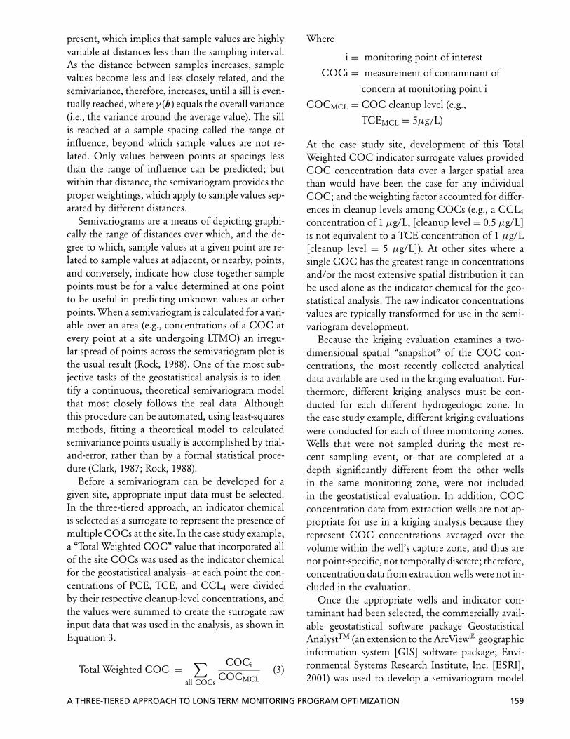
present, which implies that sample values are highlyvariable at distances less than the sampling interval.As the distance between samples increases, samplevalues become less and less closely related, and thesemivariance, therefore, increases, until a sill is even-tually reached, where γ (h ) equals the overall variance(i.e., the variance around the average value). The sillis reached at a sample spacing called the range ofinfluence, beyond which sample values are not re-lated. Only values between points at spacings lessthan the range of influence can be predicted; butwithin that distance, the semivariogram provides theproper weightings, which apply to sample values sep-arated by different distances.

Semivariograms are a means of depicting graphi-cally the range of distances over which, and the de-gree to which, sample values at a given point are re-lated to sample values at adjacent, or nearby, points,and conversely, indicate how close together samplepoints must be for a value determined at one pointto be useful in predicting unknown values at otherpoints. When a semivariogram is calculated for a vari-able over an area (e.g., concentrations of a COC atevery point at a site undergoing LTMO) an irregu-lar spread of points across the semivariogram plot isthe usual result (Rock, 1988). One of the most sub-jective tasks of the geostatistical analysis is to iden-tify a continuous, theoretical semivariogram modelthat most closely follows the real data. Althoughthis procedure can be automated, using least-squaresmethods, fitting a theoretical model to calculatedsemivariance points usually is accomplished by trial-and-error, rather than by a formal statistical proce-dure (Clark, 1987; Rock, 1988).

Before a semivariogram can be developed for agiven site, appropriate input data must be selected.In the three-tiered approach, an indicator chemicalis selected as a surrogate to represent the presence ofmultiple COCs at the site. In the case study example,a “Total Weighted COC” value that incorporated allof the site COCs was used as the indicator chemicalfor the geostatistical analysis—at each point the con-centrations of PCE, TCE, and CCL4 were dividedby their respective cleanup-level concentrations, andthe values were summed to create the surrogate rawinput data that was used in the analysis, as shown inEquation 3.

Total Weighted COCi =∑

all COCs

COCi

COCMCL(3)

Where

i = monitoring point of interest

COCi = measurement of contaminant of

concern at monitoring point i

COCMCL = COC cleanup level (e.g.,

TCEMCL = 5µg/L)

At the case study site, development of this TotalWeighted COC indicator surrogate values providedCOC concentration data over a larger spatial areathan would have been the case for any individualCOC; and the weighting factor accounted for differ-ences in cleanup levels among COCs (e.g., a CCL4

concentration of 1 µg/L, [cleanup level = 0.5 µg/L]is not equivalent to a TCE concentration of 1 µg/L[cleanup level = 5 µg/L]). At other sites where asingle COC has the greatest range in concentrationsand/or the most extensive spatial distribution it canbe used alone as the indicator chemical for the geo-statistical analysis. The raw indicator concentrationsvalues are typically transformed for use in the semi-variogram development.

Because the kriging evaluation examines a two-dimensional spatial “snapshot” of the COC con-centrations, the most recently collected analyticaldata available are used in the kriging evaluation. Fur-thermore, different kriging analyses must be con-ducted for each different hydrogeologic zone. Inthe case study example, different kriging evaluationswere conducted for each of three monitoring zones.Wells that were not sampled during the most re-cent sampling event, or that are completed at adepth significantly different from the other wellsin the same monitoring zone, were not includedin the geostatistical evaluation. In addition, COCconcentration data from extraction wells are not ap-propriate for use in a kriging analysis because theyrepresent COC concentrations averaged over thevolume within the well’s capture zone, and thus arenot point-specific, nor temporally discrete; therefore,concentration data from extraction wells were not in-cluded in the evaluation.

Once the appropriate wells and indicator con-taminant had been selected, the commercially avail-able geostatistical software package GeostatisticalAnalystTM (an extension to the ArcView©R geographicinformation system [GIS] software package; Envi-ronmental Systems Research Institute, Inc. [ESRI],2001) was used to develop a semivariogram model


depicting the spatial variation of the contaminantconcentrations in groundwater. Considerable scatterof the data was apparent during fitting of the modelsto the Total Weighted COC indicator concentrationdata. Several data transformations (including a log-normal transformation) were applied in an attemptto obtain a representative semivariogram model. Ul-timately, the concentration data were transformed to“rank statistics,” in which, for example, the 55 wells inthe upper monitoring zone were ranked from 1 (low-est indicator concentration) to 55 (highest indicatorconcentration) on the basis of the indicator concen-tration most recently detected at each well. Tie valueswere assigned the median rank of the set of rankedvalues, for example, if five wells had nondetectedconcentrations, they each would be ranked “three,”the median of the set of ranks—one, two, three, four,five. Transformations of this type can be less sensitiveto outliers, skewed distributions, or clustered datathan semivariograms based on raw concentration val-ues, and thus may enable recognition and descriptionof the underlying spatial structure of the data in caseswhere ordinary data are too “noisy” (Henley, 1981).The Weighted Total COC rank statistics then wereused to develop semivariograms that most reason-ably modeled the spatial distribution of the data inthe three zones. Anisotropy also was incorporatedinto the models to adjust for the directional influ-ence of groundwater movement from northeast tosouthwest.

After the semivariogram models were developed,they were used in a kriging system as implemented by

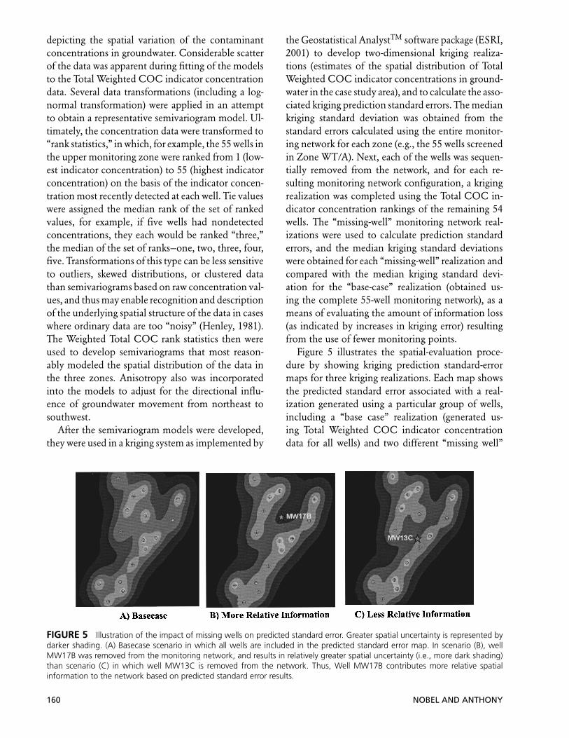
FIGURE 5 Illustration of the impact of missing wells on predicted standard error. Greater spatial uncertainty is represented bydarker shading. (A) Basecase scenario in which all wells are included in the predicted standard error map. In scenario (B), wellMW17B was removed from the monitoring network, and results in relatively greater spatial uncertainty (i.e., more dark shading)than scenario (C) in which well MW13C is removed from the network. Thus, Well MW17B contributes more relative spatialinformation to the network based on predicted standard error results.

the Geostatistical AnalystTM software package (ESRI,2001) to develop two-dimensional kriging realiza-tions (estimates of the spatial distribution of TotalWeighted COC indicator concentrations in ground-water in the case study area), and to calculate the asso-ciated kriging prediction standard errors. The mediankriging standard deviation was obtained from thestandard errors calculated using the entire monitor-ing network for each zone (e.g., the 55 wells screenedin Zone WT/A). Next, each of the wells was sequen-tially removed from the network, and for each re-sulting monitoring network configuration, a krigingrealization was completed using the Total COC in-dicator concentration rankings of the remaining 54wells. The “missing-well” monitoring network real-izations were used to calculate prediction standarderrors, and the median kriging standard deviationswere obtained for each “missing-well” realization andcompared with the median kriging standard devi-ation for the “base-case” realization (obtained us-ing the complete 55-well monitoring network), as ameans of evaluating the amount of information loss(as indicated by increases in kriging error) resultingfrom the use of fewer monitoring points.

Figure 5 illustrates the spatial-evaluation proce-dure by showing kriging prediction standard-errormaps for three kriging realizations. Each map showsthe predicted standard error associated with a real-ization generated using a particular group of wells,including a “base case” realization (generated us-ing Total Weighted COC indicator concentrationdata for all wells) and two different “missing well”


realizations. Lighter colors represent areas withinwhich spatial uncertainty is relatively lower, anddarker colors represent areas within which spatial un-certainty is relatively greater; regions in the immedi-ate vicinity of wells (i.e., data points) have the lowestassociated uncertainty. Map A on Figure 5 shows thepredicted standard error map for the “base-case” real-ization in which all wells are included. Map B showsthe realization in which well MW13C was removedfrom the monitoring network, and Map C shows therealization in which well MC17B was removed. In-terpretation of Figure 5 indicates that when a well isremoved from the network, the predicted standarderror in the vicinity of the missing well increases(as indicated by a darkening of the shading in thevicinity of that well). If a “removed” (missing) well isin an area with several other wells nearby (e.g., wellMW13C; Map B on Figure 5), the predicted stan-dard error may not increase as much as if a well (e.g.,MW17B; Map C) is removed from an area with fewersurrounding wells.

Based on the kriging evaluation, each well was as-signed a “test statistic” describing the relative valueof spatial information obtained from the well, cal-culated from the ratio of the median “missing well”kriging error to the median “base case” error. If re-moval of a particular well from the monitoring net-work caused very little change in the resulting me-dian kriging standard deviation, the test statistic wasequal to 1.0, and that well was regarded as contribut-ing only a limited amount of information to theLTM program. Likewise, if removal of a well fromthe monitoring network produced greater increasesin the kriging standard deviation (greater than 1 per-cent), this was regarded as an indication that the wellcontributes a relatively greater amount of informa-tion, and is relatively more important to the moni-toring network. At the conclusion of the kriging re-alizations for wells in the WT/A zone, each well wasranked from 1 (providing the least information) to55 (the total number of wells included in the anal-ysis of the WT/A zone) (providing the most infor-mation), based on the amount of information (asmeasured by changes in median kriging standard de-viation) the well contributed toward describing thespatial distribution of the concentrations of the TotalWeighted COC indicator. Wells providing the leastamount of information represent possible candidatesfor removal from the monitoring program. The wellsthat contribute the most amount of relative informa-

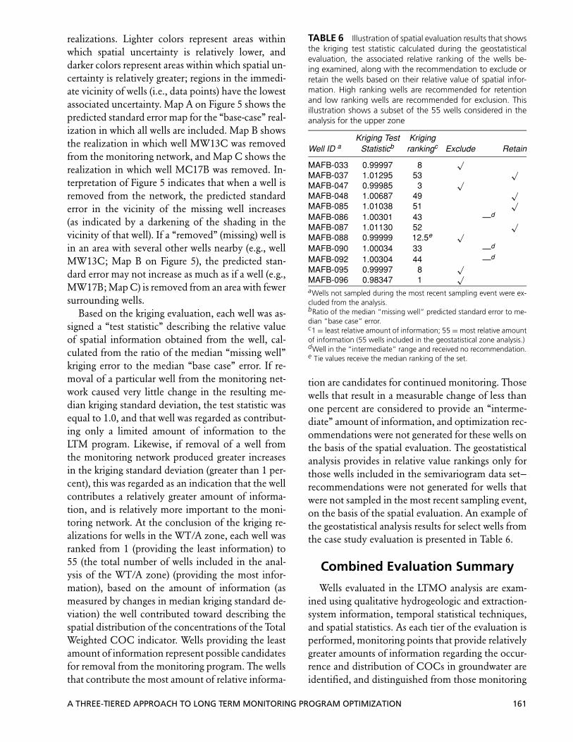
TABLE 6 Illustration of spatial evaluation results that showsthe kriging test statistic calculated during the geostatisticalevaluation, the associated relative ranking of the wells be-ing examined, along with the recommendation to exclude orretain the wells based on their relative value of spatial infor-mation. High ranking wells are recommended for retentionand low ranking wells are recommended for exclusion. Thisillustration shows a subset of the 55 wells considered in theanalysis for the upper zone

Kriging Test KrigingWell ID a Statisticb rankingc Exclude Retain

MAFB-033 0.99997 8√

MAFB-037 1.01295 53√

MAFB-047 0.99985 3√

MAFB-048 1.00687 49√

MAFB-085 1.01038 51√

MAFB-086 1.00301 43 —d

MAFB-087 1.01130 52√

MAFB-088 0.99999 12.5e √MAFB-090 1.00034 33 —d

MAFB-092 1.00304 44 —d

MAFB-095 0.99997 8√

MAFB-096 0.98347 1√

aWells not sampled during the most recent sampling event were ex-cluded from the analysis.bRatio of the median “missing well” predicted standard error to me-dian “base case” error.c1 = least relative amount of information; 55 = most relative amountof information (55 wells included in the geostatistical zone analysis.)dWell in the “intermediate” range and received no recommendation.e Tie values receive the median ranking of the set.

tion are candidates for continued monitoring. Thosewells that result in a measurable change of less thanone percent are considered to provide an “interme-diate” amount of information, and optimization rec-ommendations were not generated for these wells onthe basis of the spatial evaluation. The geostatisticalanalysis provides in relative value rankings only forthose wells included in the semivariogram data set—recommendations were not generated for wells thatwere not sampled in the most recent sampling event,on the basis of the spatial evaluation. An example ofthe geostatistical analysis results for select wells fromthe case study evaluation is presented in Table 6.

Combined Evaluation Summary

Wells evaluated in the LTMO analysis are exam-ined using qualitative hydrogeologic and extraction-system information, temporal statistical techniques,and spatial statistics. As each tier of the evaluation isperformed, monitoring points that provide relativelygreater amounts of information regarding the occur-rence and distribution of COCs in groundwater areidentified, and distinguished from those monitoring


points that provide relatively lesser amounts of infor-mation. Once the three evaluations have been com-pleted, the results are combined to generate a refinedmonitoring program that potentially could provideinformation sufficient to address the primary ob-jectives of monitoring, at reduced cost. Monitoringwells not retained in the refined monitoring networkcould be removed from the monitoring program withrelatively little loss of information. In general, thetemporal and spatial evaluations are used to sup-port and refine the qualitative evaluation; this allowsprofessional judgment and site-specific knowledgedrive the recommendations, but allows for valida-tion and consistency based on the objective statisticalresults.

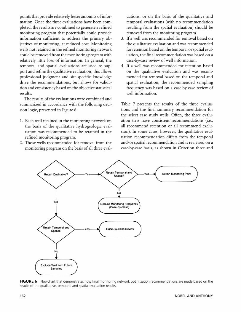
The results of the evaluations were combined andsummarized in accordance with the following deci-sion logic, presented in Figure 6:

1. Each well retained in the monitoring network onthe basis of the qualitative hydrogeologic eval-uation was recommended to be retained in therefined monitoring program.

2. Those wells recommended for removal from themonitoring program on the basis of all three eval-

FIGURE 6 Flowchart that demonstrates how final monitoring network optimization recommendations are made based on theresults of the qualitative, temporal and spatial evaluation results.

uations, or on the basis of the qualitative andtemporal evaluations (with no recommendationresulting from the spatial evaluation) should beremoved from the monitoring program.

3. If a well was recommended for removal based onthe qualitative evaluation and was recommendedfor retention based on the temporal or spatial eval-uation, the final recommendation was based on acase-by-case review of well information.

4. If a well was recommended for retention basedon the qualitative evaluation and was recom-mended for removal based on the temporal andspatial evaluation, the recommended samplingfrequency was based on a case-by-case review ofwell information.

Table 7 presents the results of the three evalua-tions and the final summary recommendation forthe select case study wells. Often, the three evalu-ation tiers have consistent recommendations (i.e.,all recommend retention or all recommend exclu-sion). In some cases, however, the qualitative eval-uation recommendation differs from the temporaland/or spatial recommendation and is reviewed on acase-by-case basis, as shown in Criterion three and


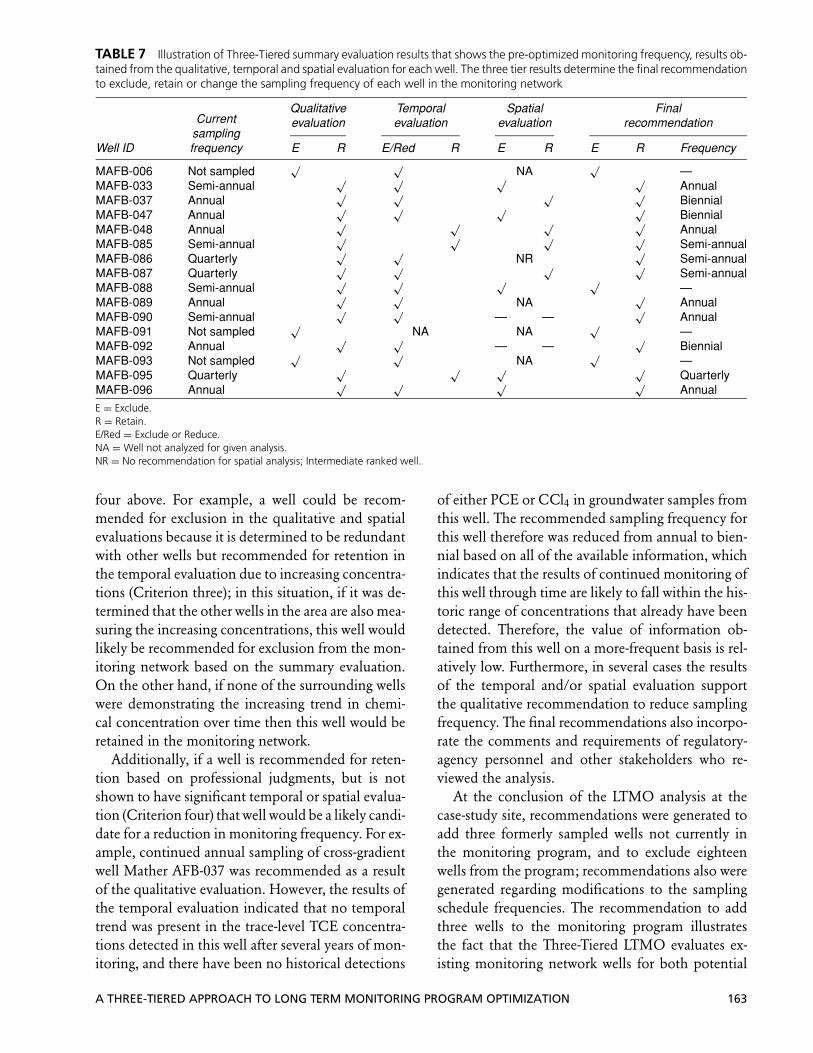
TABLE 7 Illustration of Three-Tiered summary evaluation results that shows the pre-optimized monitoring frequency, results ob-tained from the qualitative, temporal and spatial evaluation for each well. The three tier results determine the final recommendationto exclude, retain or change the sampling frequency of each well in the monitoring network

Qualitative Temporal Spatial Finalevaluation evaluation evaluation recommendation

Well ID

Currentsamplingfrequency E R E/Red R E R E R Frequency

MAFB-006 Not sampled√ √

NA√

—MAFB-033 Semi-annual

√ √ √ √Annual

MAFB-037 Annual√ √ √ √

BiennialMAFB-047 Annual

√ √ √ √Biennial

MAFB-048 Annual√ √ √ √

AnnualMAFB-085 Semi-annual

√ √ √ √Semi-annual

MAFB-086 Quarterly√ √

NR√

Semi-annualMAFB-087 Quarterly

√ √ √ √Semi-annual

MAFB-088 Semi-annual√ √ √ √

—MAFB-089 Annual

√ √NA

√Annual

MAFB-090 Semi-annual√ √

— —√

AnnualMAFB-091 Not sampled

√NA NA

√—

MAFB-092 Annual√ √

— —√

BiennialMAFB-093 Not sampled

√ √NA

√—

MAFB-095 Quarterly√ √ √ √

QuarterlyMAFB-096 Annual

√ √ √ √Annual

E = Exclude.R = Retain.E/Red = Exclude or Reduce.NA = Well not analyzed for given analysis.NR = No recommendation for spatial analysis; Intermediate ranked well.

four above. For example, a well could be recom-mended for exclusion in the qualitative and spatialevaluations because it is determined to be redundantwith other wells but recommended for retention inthe temporal evaluation due to increasing concentra-tions (Criterion three); in this situation, if it was de-termined that the other wells in the area are also mea-suring the increasing concentrations, this well wouldlikely be recommended for exclusion from the mon-itoring network based on the summary evaluation.On the other hand, if none of the surrounding wellswere demonstrating the increasing trend in chemi-cal concentration over time then this well would beretained in the monitoring network.

Additionally, if a well is recommended for reten-tion based on professional judgments, but is notshown to have significant temporal or spatial evalua-tion (Criterion four) that well would be a likely candi-date for a reduction in monitoring frequency. For ex-ample, continued annual sampling of cross-gradientwell Mather AFB-037 was recommended as a resultof the qualitative evaluation. However, the results ofthe temporal evaluation indicated that no temporaltrend was present in the trace-level TCE concentra-tions detected in this well after several years of mon-itoring, and there have been no historical detections

of either PCE or CCl4 in groundwater samples fromthis well. The recommended sampling frequency forthis well therefore was reduced from annual to bien-nial based on all of the available information, whichindicates that the results of continued monitoring ofthis well through time are likely to fall within the his-toric range of concentrations that already have beendetected. Therefore, the value of information ob-tained from this well on a more-frequent basis is rel-atively low. Furthermore, in several cases the resultsof the temporal and/or spatial evaluation supportthe qualitative recommendation to reduce samplingfrequency. The final recommendations also incorpo-rate the comments and requirements of regulatory-agency personnel and other stakeholders who re-viewed the analysis.

At the conclusion of the LTMO analysis at thecase-study site, recommendations were generated toadd three formerly sampled wells not currently inthe monitoring program, and to exclude eighteenwells from the program; recommendations also weregenerated regarding modifications to the samplingschedule frequencies. The recommendation to addthree wells to the monitoring program illustratesthe fact that the Three-Tiered LTMO evaluates ex-isting monitoring network wells for both potential


exclusion (for those wells currently sampled) and forre-inclusion (for those wells in the area of interestthat are not currently sampled). The added wells wererecommended for inclusion based on their histori-cal data. This refined monitoring program would re-sult in an average of 559.5 well-sampling events peryear (where 0.5 events/year represents a well sampledbiannually), as compared with 643 well-samplingevents per year that occur in the current monitor-ing program. Implementing these recommendationsfor optimizing the LTM monitoring program at thecase-study site would reduce the number of well-sampling events per year by approximately 13 per-cent. Although the monitoring program examinedin this case study, at 306 wells and 643 well-samplingevents per year, is among the largest that has beenevaluated to date using the three-tiered approach,the evaluation produced a relatively lower reductionin recommended well-sampling events than haveevaluations at other sites. This may be a result ofthe ongoing internal optimization efforts conductedannually at Mather AFB, and may also reflect in-put from regulatory personnel and other stakeholderswho preferred more conservative sampling frequen-cies (more frequent sampling than recommendedbased on the results of the three-tiered evaluation).

THREE-TIERED LTMO APPLICATIONSAND FUTURE WORK

As of April 2004, the Three-Tiered LTMO ap-proach has been applied to evaluate monitoring pro-grams at eighteen sites. The monitoring programsevaluated with the three-tiered method have rangedin size from programs in which 10 wells are sam-pled, to programs in which more than 300 wells aresampled. COCs addressed by these programs pri-marily have included fuel constituents and volatileorganic compounds. Application of the three-tieredapproach has produced reductions in well-samplingevents ranging from 13 percent to 83 percent per year.On average at all of the sites analyzed, application ofthe three-tiered approach has resulted in reductionsof over one-third of the sampling events per year. Theresults are highly dependent on the site conditions.Typically, application of the approach at sites wheremonitoring is conducted relatively frequently (e.g.,quarterly) and/or to programs that have not beenevaluated in several years resulted in more signifi-

cant optimization opportunities. Although there arefewer opportunities for program optimization at siteswith a smaller number of wells, significant optimiza-tion opportunities can still be identified on a relativescale (i.e., potentially-significant reductions in sam-pling events per year). Additionally, although the fo-cus of three-tiered LTMO applications has been pri-marily on optimizing existing LTM programs, it alsohas been applied successfully to identify optimal lo-cation(s) at which to add new wells to a program, andalso has been used to optimize monitoring programsfor soil-vapor extraction systems.

The three-tiered LTMO method is an evolving ap-proach that is being continuously refined with ad-ditional enhancements, review, and exposure. Themost significant future enhancement to the approachwill be automation of the spatial evaluation. This willenable multiple chemicals and time periods to be in-corporated into the spatial evaluation, if desired, inplace of the “indicator COC single time-period snap-shot” currently utilized.

The three-tiered LTMO approach also is beingprofiled with other LTMO methods in several docu-ments currently in preparation. During the past sev-eral years the US EPA’s Office of Superfund Remedi-ation and Technology Innovation and the Air ForceCenter for Environmental Excellence (AFCEE) havebeen conducting a demonstration project illustratingthe application of the three-tiered approach and theMonitoring and Remediation Optimization System(MAROS) to three case-study sites. MAROS is publicdomain software that was developed for AFCEE byGroundwater Services, Inc., and incorporates opti-mization procedures and decision logic that were de-veloped in the AFCEE Long-Term Monitoring Op-timization guide (AFCEE, 2003). A summary report(USEPA, 2004b), which discusses the results of ap-plication of the two approaches to the evaluationand optimization of groundwater monitoring pro-grams at the three sites, and examines the overallresults obtained using the two LTMO methods, willbe available in mid-2004. The three-tiered LTMO ap-proach also is one of several method included in aRoadmap for LTMO, currently in preparation by theUSEPA and the U.S. Army Corps of Engineers. TheRoadmap is intended to assist managers, regulators,scientists and engineers tasked with reviewing mon-itoring programs in determining whether optimiza-tion is appropriate for their monitoring program, anddescribes available optimization methods that may


be appropriate for application to particular monitor-ing programs.

REFERENCESAir Force Center for Environmental Excellence, Inc. (AFCEE).

2003. Monitoring And Remediation Optimization Sys-tem (MAROS) User’s Guide, Version 2.0. http://www.gsi-net.com/software/Maros.htm. Brooks Air Force Base,Texas. November.

American Society of Civil Engineers (ASCE) Task Committeeon Geostatistical Techniques in Hydrology. 1990a. Reviewof Geostatistics in Geohydrology—I. Basic concepts. Journalof Hydraulic Engineering 116(5):612–632.

ASCE Task Committee on Geostatistical Techniques in Hydrol-ogy. 1990b. Review of Geostatistics in Geohydrology—II.Applications. Journal of Hydraulic Engineering 116(6):633–658.

Cameron, K., and P. Hunter. 2002. Optimization of LTM Net-works Using GTS: Statistical Approaches to Spatial andTemporal Redundancy. Online document available on theWorldwide Web at http://www.afcee.brooks.af.mil/er/rpo/GTSOptPaper.pdf

Cameron, K., and P. Hunter. 2004. Optimizing LTM Net-works with GTS: Three New Case Studies, In AcceleratingSite Closeout, Improving Performance, and Reducing CostsThrough Optimization—Proceedings of the Federal Reme-diation Technologies Roundtable Optimization Conference.June 15–17. Dallas, Texas.

Cieniawski, S. E., J. W. Eheart, and S. Ranjithan. 1995. Usinggenetic algorithms to solve a multiobjective groundwatermonitoring problem. Water Resources Research 31(2):399–409.

Clark, I. 1987. Practical Geostatistics. Elsevier Applied Science,Inc.: London.

Dresel, E. P., and C. Murray. 1998. Groundwater monitoringnetwork design using stochastic simulation. Geological So-ciety of America Abstracts with Programs 30(7):181.

El-Shaarawi, A. H., and S. P. Niculescu. 1992. On Kendall’s tauas a test of trend in time. Environmetrics 3:385–412.

Environmental Systems Research Institute, Inc. (ESRI). 2001.ArcGIS Geostatistical Analyst Extension to ArcGIS 8 Soft-ware. Redlands, CA.

Gibbons, R. D. 1994. Statistical Methods for GroundwaterMonitoring. John Wiley & Sons, Inc.: New York.

Henley, S. 1981. Nonparametric Geostatistics. Applied SciencePublishers, Inc./Halsted Press: London.

Hudak, P. F., H. A. Loaiciga, and F. A. Schoolmaster. 1993.Application of geographic information systems to ground-water monitoring network design. Water Resources Bulletin29(3):383–390.

Kelly, B. P. 1996. Design of a Monitoring Well Network forthe City of Independence, Missouri, Well Field Using Sim-ulated Ground-Water Flow Paths and Travel Times. US Ge-ological Survey Water-Resources Investigation Report 96–4264.

Reed, P. M., and B. S. Minsker. 2004. Striking the balance: Longterm groundwater monitoring design for multiple, conflict-ing objectives. Journal of Water Resources and PlanningManagement 130(2):140–149.

Reed, P. M., B. S. Minsker, and D. E. Goldberg. 2001. A multi-objective approach to cost effective long-term groundwatermonitoring using an elitist nondominated sorted genetic al-gorithm with historical data. Journal of Hydroinformatics3:71–89.

Reed, P. M., B. S. Minsker, and D. E. Goldberg. 2003. Simpli-fying multiobjective optimization II: An automated designmethodology for the nondominated sorted genetic algo-rithm. Water Resources Research 39(7):1196.

Reed, P. M., B. S. Minsker, and A. J. Valocchi. 2000.Cost-effective long-term groundwater monitoringdesign using a genetic algorithm and global mass in-terpolation. Water Resources Research 36(12):3731–3741.

Rock, N. M. S. 1988. Numerical Geology. Springer-Verlag: NewYork.

U.S. Environmental Protection Agency (USEPA). 1994. Meth-ods for Monitoring Pump-and-Treat Performance. Office ofResearch and Development. EPA/600/R-94/123.

USEPA. 2004a. Guidance for Monitoring at Hazardous WasteSites—Framework for Monitoring Plan Development andImplementation. USEPA Office of Solid Waste and Emer-gency Response. OSWER Directive No. 9355. 4–28. January.

USEPA. 2004b. Demonstration of Two Long-Term Ground-water Monitoring Optimization Methods—Report with Ap-pendices. USEPA Office of Solid Waste and Emergency Re-sponse. 542–R–04–001B. July.

Wiedemeier, T. H., and P. E. Haas. 2000. Designing MonitoringPrograms to Effectively Evaluate the Performance of NaturalAttenuation. Air Force Center for Environmental Excellence(AFCEE). August.


a three-tiered approach to long term monitoring program optimization

Documents