a sight for sore eyes
TRANSCRIPT
A Sight for Sore Eyes:
Assessing the Value of View and Land Use in the Housing Market
Andrea Baranzini and Caroline Schaerer
Geneva School of Business Administration (HEG-Ge), Centre for Applied Research in
Management (CRAG), University of Applied Sciences of Western Switzerland (HES-SO)
7 route de Drize, 1227 Carouge – Geneva, Switzerland
[email protected]; [email protected]
phone: +41 22 388 1718; fax: +41 22 388 1701
Abstract
We apply a hedonic model to the Geneva-Switzerland rental market to assess the value of
view from dwellings and of land uses around buildings. Using a geographic information
system, we calculate three-dimensional view variables, accessibility and land use variables. To
our knowledge, this is the first paper to develop precise view measures at the dwelling level,
considering surrounding land uses, in an urban context and with a large sample of 13,000
observations. The results show that view of various environmental amenities and its size has a
significant impact on rents. The estimated rent premium for a dwelling located in a
neighbourhood with an extended surface of water can be as high as 3 percent, and a view of
water-covered area can raise rent up to 57 percent.
JEL classification: Q5, R14, R52, R31, D62
Keywords: Hedonic model; rental market; housing market; view; land use; geographic
information system (GIS)

1
1 Introduction
Urban parks and forests, water resorts, lake shores, farmlands, and land use are
residential amenities that contribute to the wellbeing of urban households. These
amenities provide opportunities for recreation, relief from urban stresses and congestion,
as well as view amenities to the residents of surrounding buildings. A number of studies
have found that tenants and owners are willing to pay a premium for apartments or
houses with a scenic view (e.g., Bond et al. 2002; Seiler et al. 2002) located in proximity
to particular land use features (see McConnel and Walls 2005; Lutzenhiser and Netusil
2001).
Valuing natural land uses, especially in an urban context, can be useful for policy
planning and decisions. Given cities development, there is growing pressure on natural
land uses to satisfy the need for additional housing and commercial spaces. As urban
sprawl is increasingly challenged, emphasis is now placed on city densification. Several
movements have stimulated the debate over reorienting development practices to
support neighbourhood diversity, accessibility of public spaces, and urban design
accounting for pedestrians (e.g., Congress of New Urbanism 2002). Those often
competing demands need to be balanced by city planners, and effective land use
regulation policies should integrate the benefits of preserved open spaces.
The economic literature proposes various valuation methods to assess the value of
urban features. One of the most widespread approaches refers to the hedonic method,
which disentangles market information on house prices or apartment rents in order to
obtain the implicit price of each characteristic of the housing bundle, including
environmental amenities and landscape features. In other words, the hedonic method
quantifies the premium residents are willing to pay to live in a dwelling that offers a
comparatively better view and is located in an area possessing some particular urban
features. However, using the hedonic model to quantify the value of environmental
amenities requires data on the views from the dwellings and on the different land uses in
the vicinity of the buildings. These variables are not particularly easy to characterise and
measure. Traditionally, they are measured by subjective assessments either from direct
site inspection or from household surveys, the disadvantage being that the resulting
samples are relatively small (see Bourassa et al. 2004 for a survey). The extensive

2
functionalities of geographical information systems (GIS) have only recently started to
be used to quantify the size of the land uses and to assess more precisely view variables
(see Bateman et al. 2001; Cavailhès 2008; Lake et al. 1998).
Using GIS capabilities, we develop three-dimensional quantitative measures of view
at the dwelling level. Then, we introduce land use and view measures in a hedonic
model of the Geneva rental market and quantify the premium residents are willing to
pay for those characteristics. We focus on the Canton of Geneva, Switzerland, because
it possesses a large rental market (about 85 percent of the dwellings are rental) with a
relatively dense city and a more dispersed rural area. Moreover, several rich databases are
accessible, including GIS data. In addition, evaluating the impact of view in the Geneva
rental market is of particular interest since a new law that allows raising the height of
the buildings in the city centre has very recently been accepted by popular vote.
Therefore, the impact of the view obstructions on rents and the impact of view from
high-rise buildings is of particular concern.
The paper is organised as follows. In Section 2, we briefly present the hedonic
approach and review the literature focusing on open space and land use valuation in an
urban context. Section 3 explains how we define the variables concerning view, land use,
and diversity. Section 4 presents the dataset, Section 5 details the study’s results, and
Section 6 offers conclusions.
2 Assessing view and land use in the hedonics literature
Rosen’s (1974) seminal work provides the theoretical foundations of the property-
hedonic model by assuming that heterogeneous goods are valued for their utility-
bearing characteristics. Therefore, the implicit prices of house attributes can be revealed
from the observed prices of differentiated products and the quantities of characteristics
associated with them. Given the key assumption that the housing market is competitive,
rent, P, is determined by the implicit vector prices of the dwelling’s characteristics, z,
P = P(z), which is the general form of the hedonic price model. These characteristics are
often decomposed in a vector of structural (e.g., the number of rooms), accessibility
(e.g., proximity to public transportation), environmental quality (such as noise), and
neighbourhood (e.g., proportion of green areas) variables. Hence, the hedonic model is

3
particularly useful for estimating the (implicit) value of a given landscape characteristic
(such as proximity to or view of an urban park) for which there is no explicit market.
Literature surveys of the hedonic approach applied to housing markets are provided by,
for example, Bateman et al. (2001), Day (2001), Palmquist (2005) and Baranzini et al.
(2008).
A relatively recent but fast-growing part of the hedonic literature concentrates on the
value of preserved urban landscape, analysing the recreation use of urban open spaces or
their aesthetic benefits. McConnell and Walls (2005) survey studies on the value of
urban open spaces. Earlier studies often focused on urban parks by using dummy
variables to indicate whether a house is located near them. Other studies characterise
open spaces more precisely, differentiating by types and size. For instance, Lutzenhiser
and Netusil (2001) consider three categories of parks in Portland, Oregon. They show
that houses near natural or speciality parks (the primarily use of which is linked to a
peculiar facility, for example boat ramp facilities) are more expensive, with price
increasing based on park size. In contrast, proximity to an urban park decreases house
prices, although the size of the urban park has a positive impact on prices (for forest
areas, see Tyrväinen 1997; Tyrväinen and Miettinen 2000). In addition to distance, type
and size, open space value may also depend on its status and ownership (on this topic,
see Geoghegan 2002; Irwin 2002).
A quite separated strand of the hedonic literature focuses on the view amenity. A
survey by Bourassa et al. (2004) shows that emphasis is placed on the valuation of water
view (river, lake, sea and ocean), while other types of view, such as mountain or forest,
have been analysed less frequently. This survey also indicates that dummy variables are
frequently used to characterise the view from a property or an apartment. Those
variables can illuminate whether or not a particular feature is visible from the property
(see Bond et al. 2002; Seiler et al. 2002) or may include (see Benson et al. 1998)
dwellers’ subjective assessments of the quality of the view (full-quality view, poor partial
view, and so on. Given that the view may also be interpreted as a proxy for access to a
particular feature, distances are also included in the estimation. Therefore, in their
studies of the impact of a lake view and on land on property values, Bourassa et al.
(2004) and Samarshinghe and Sharp (2006) include indicators for the quality of the

4
view (narrow, medium, and wide) as well as the distance to the coast for the properties
that enjoy a water view. The majority of existing studies conclude that view has a
positive impact on residential values; however, the more distant the view, the smaller
the view premium.
Since most traditional studies on visual amenities generally rely on surveys, they are
often characterised by relatively small samples. More recent literature overcomes this
problem by exploiting the functionalities of GIS to develop sophisticated view indices.
The papers using GIS data are thus not based on individual assessments; rather, they are
based on quantitative measures of view and neighbourhood characteristics.1 For
example, Lake et al. (1998) and Bateman et al. (2001) use the functionalities of GIS to
assess the impact of road development (noise and visual intrusion) on property prices.
Bin et al. (2006) and Yu et al. (2007) used a similar methodology to measure view on
the sea and estimate its impact on real estate prices. Interestingly, Cavailhès et al. (2008)
do not only consider the landscape seen from the house, but also the view that others
have of this house. They find that individuals are willing to pay a premium for a house
with a view, but that being exposed to the view from other houses lowers its price.
Moreover, they conclude that view has a greater influence on real-estate than the mere
land use around the property. Paterson and Boyle (2002) calculate the percentage of
visible land of each land use category within a radius of one kilometre around each
property using GIS technology. However, their visibility measures are based exclusively
on topographic data, i.e. they do not account for the objects that can impede the view.
They find that visibility is an important environmental variable, omission of which
could produce bias in the coefficient of other environmental attributes.
To our knowledge, there are only two studies focusing on the value of view
characteristics on the Swiss housing market. Rieder (2005) considers Switzerland a
single housing market and introduces dummy variables for lake view, river view and
mountain view. He finds that having a view of a lake increases rents by 2.9 percent on
average. Salvi et al. (2004) focus on the Zurich real estate market. They use the
1 The problem of using perceived vs. measured variables is often encountered when using hedonics to
assess environmental impacts. See Baranzini et al. (2010) for an analysis of the relationship between
subjective and scientific noise measures and their use in a hedonic framework.

5
functionalities of GIS to calculate lake view and a general clear view at the hectare level.
Their GIS-based view variables are defined using exclusively topographic data and are
calculated at the hectare level, i.e. the same view value is associated to all buildings in a
given hectare. They find that both general view and lake view have a significant positive
impact on property prices, with the lake view proving to have a greater impact. In the
following Section, we develop original measures of view amenities at the dwelling level
and quantify the scope of different types of view by accounting for view impediments.
3 Constructing GIS-based landscape use and view variables
We calculate multiple variables characterising land uses surrounding each building by
drawing on a very rich and well-developed GIS database – the Information System of
the Geneva Territory (SITG). The SITG provides information on the types of land
uses, topographic data, and height of the surrounding buildings and trees. In order to
limit multicolinearity issues and to reduce the number of variables, we gather similar
land uses into seven categories, sorted into two groups. The first group is called “natural
environment” and is composed of tree-covered areas (trees and forests), agricultural
areas, and water-covered areas (Geneva Lake and Rhone River). The second group
refers to the “built environment” and contains buildings and built areas, urban parks
(including sport courts), transportation areas (roads, railways and airport), and industrial
areas.
Using the previous seven land use categories, we define the following two types of
variables: neighbourhood and view. The neighbourhood variables are computed as the
surface area of each land use type in a radius of one kilometre around each building.
Then, using these surfaces, we refer to Geoghegan et al. (1997) and calculate land use
diversity indices in order to define the land use pattern, i.e. the variety of the land uses
in the vicinity of the buildings. The diversity index is calculated as follows:
)sln(
lnRR
H
K
1kkk
(1)
where Rk is the proportion of the area dedicated to land use k in the neighbourhood of
the building, relative to the total neighbourhood area, and s is the number of different
land use types considered. The value of H varies between 0 and 1, a larger value for H

6
indicating more diverse landscape use. The expected impact of landscape pattern on
house prices is a priori not known. For instance, increasing diversity may be preferred
since it could imply proximity to various activities, such as recreation, shopping, and
workplaces; on the contrary, high diversity can lower housing prices, if it is associated
with chaotic land use planning. Geoghegan et al. (1997) and Acharya and Bennet
(2001) find that landscape diversity in the immediate neighbourhood of the properties
generally has a negative impact on their prices. We have constructed two different
diversity indices, one considering only the natural land uses, i.e. water covered areas,
tree-covered areas, and agricultural land, and another that refers only to the built
environment (built areas, urban parks, transportation and industrial areas).
The calculations of the view variables are complex and time-intensive, since they have
to account for a very large number of factors. We calculate them in accordance with
Lake et al. (1998) and Bateman et al. (2001), but unlike existing literature, we define
our view variables at the dwelling level. We combine a numerical terrain model that
includes the topographic land profile with a surface numerical model, which accounts
for the height of all the objects (e.g., buildings, trees). This allows us to construct a
three-dimensional layer2 that accounts for all the objects that can impede the view.
Then, using complex queries, we are able to calculate the view in a radius of one
kilometre3 around the central point of each building. To be as precise as possible, the
visible surface (the “viewshed”)4 is calculated for three different observer heights – from
the ground floor level (1.8 metres above terrain height), from the middle of the building
(half the difference between the building surface height and the terrain height), and at
the attic level (1 metre less than the building height). By summing up all the visible
cells, we obtain the total number of visible hectares in a radius of one kilometre around
the building at the three different height levels. In Figure 1, we draw the viewshed for a
given building from two different standpoints. The observer, who is symbolized by the
2 The pixel size is 1 m2.
3 Given the enormous amount of information that has to be taken into account in an urban context and
the resulting heavy calculation time, we limited the view variable to the same scale as the land use
variables, i.e. a radius of one kilometre around the building.
4 The viewsheds are calculated using ArcGIS 9.2. For more information on the calculations, see
http://webhelp.esri.com/arcgisdesktop/9.2/index.cfm?TopicName=Performing_a_viewshed_analysis.

7
blue line in the middle of the invisible building, is able to see the entire surface in green.
Then, to determine which and how much of each land use type is visible, we overlay the
visible surface with the seven land use covers. This allows us to calculate natural and
built view diversity indices by applying equation (1). Finally, by using the viewshed
methodology, we determine whether the dwelling has a view of the famous Geneva Jet
d’eau (water fountain) and of the ancient cathedral. Since measuring the visible surface
precisely does not make sense in this case, we define two dummy variables, taking the
value of one if the measured view is positive.
The resulting ground, middle, or attic views are subsequently associated with each
dwelling of a building according to the floor level at which it is located. This is done by
assuming that each floor has a height of 3 metres and then associating the closest view
(ground, middle, or attic).
[Insert Figure 1 about here]
Our view variables are the most precise measures that can be calculated using the
available data. Indeed, our source databases provide information about the floor level at
which the dwellings are located inside the buildings, but they do not indicate the exact
position of the dwelling on each floor level (i.e. we know that the dwelling is situated on
the third floor, but we do not know if it is, for example, on the left or right of the floor
level) or the position of the dwelling’s windows (e.g., backyard or front yard). Therefore,
since our methodology reports all the visible hectares on a 360 degree base, it could well
be that our calculations report a very nice lakefront view, while the dwelling only has a
backyard view. Nevertheless, we have been able to cross-check our GIS-calculated view
variables with a dummy-type view variable, available in the 2003 Survey on the rent
structure from the Federal Statistical Office. In this survey, the respondents were asked
to indicate whether or not they had a view of the lake, river, and/or mountains from
their dwellings. Thus, to make sure that our GIS-calculated view variables are relevant,
we transformed our variables, expressed as the number of hectares visible, into dummy
variables to obtain two variables in comparable dimensions. We found that our GIS-
calculated view variable is only inexact for 10 percent of the 7,395 dwellings in our
database and surveyed by the Federal Statistical Office.

8
4 Dataset and descriptive statistics
Our main data source is the “Statistics on Rents in the Geneva Canton” for the year
2005, issued by the Geneva Cantonal Statistical Office. The sample of this annual
survey covers more than 18,000 apartments in about 7,700 buildings, which represents
almost 1/8 of the total number of dwellings rented out in the canton. It includes data on
rents, year of construction, number of rooms, floor level, status of the apartment (private
rental sector or public rental sector), and it specifies if there was at least one change of
tenant in the last year. The database does not cover owners, individual homes, and
buildings with less than three apartments. Moreover, the dataset does not include
single-family houses. From the original statistics sample, the dwellings that belong to
the public rental sector or to a housing cooperative were excluded, since the rents in
those two sectors are often based on construction costs rather than on market conditions
and therefore evolve in a quite different market segment. After merging all the
information from this dataset with our GIS-calculated variables, we obtain a final
sample of 12,932 complete observations. Our sample is representative of the full sample
of the “Statistics on Rents in the Canton of Geneva”, e.g., in terms of rents, number of
rooms and construction period. The descriptive statistics are reported in Table 1.
The mean monthly rent in 2005 is about CHF 1,1225 for the whole sample with a
large variance. Most of the buildings in our sample were constructed between 1946 and
1970. Note that construction year takes major renovations into account. The mean
number of rooms is about 3.6, which includes the living room, bedrooms and the
kitchen.
We calculate accessibility variables to account for the precise location of the buildings
in the Canton of Geneva. These variables represent the most popular and the relatively
easiest application of GIS. Thus, as in Baranzini and Ramirez (2005), we calculate the
distance from each building to the major public infrastructures, such as primary schools,
public transport stops and the distance to city centre, which approximates the location
of major economic activities. The small means of the accessibility variables illustrate that
the Canton of Geneva is small and dense.
5 In June 2005, CHF 1 = USD 0.80 or EURO 0.65.

9
[Insert Table 1 about here]
The top of Figure 2 shows the mean value of the variable measuring the overall view
of the land use surface in the neighbourhood (which amounts to about 1.5 ha, see the
picture at the top left) and for its maximum value in the sample (about 131 ha, see the
picture at the top right). The bottom of Figure 2 provides a two- and three-dimensional
representation of the view calculated from the ground level (in blue) and from the attic
level (in yellow).
[Insert Figure 2 about here]
From Table 1, we note that only 2 percent of the dwellings have a view of the Geneva
Jet d’eau and 1.4 percent of the ancient cathedral. In addition, there are large differences
between the land use surfaces and the corresponding neighbourhood view variables. For
instance, the mean surface of lake and rivers within one kilometre around the building is
equal to 20 hectares, while the mean view from the dwelling on the lake is 0.09 hectares.
Similarly, the mean surface covered by urban parks within this distance is equal to 17
hectares, while the mean view on them is 0.04 hectares. Given those differences, in the
next section, we will be able to assess whether it is the presence of an environmental
amenity or the view of it that is rewarded in the housing market.
5 Empirical application and results
Since the theoretical literature does not dictate any functional form for the hedonic
equation, it has to be determined empirically. Linear, semi-logarithmic, log-linear, as
well as linear Box-Cox transformations are commonly used functional forms. Box-Cox
transformations of the dependent and independent variables were jointly and
alternatively tested, and the semi-logarithmic functional form appears to be the most
adequate.6 More specifically, we estimate the following hedonic equation:
6 Malpezzi (2002) highlighted the following five major advantages of the semi-logarithmic functional
form: (i) the implicit price of a housing attribute is related to the quantity of the other housing
attributes; (ii) the coefficients are easily interpretable in terms of semi-elasticity; (iii) it mitigates
heteroskedasticity problems; (iv) it can be computed easily; and (v) some flexibility in the specification
of the independent variables can be easily introduced.

10
M
1m
K
1kiiz
Z
1zizjkjkjx
K
1kjximimi
VNASlnP (2)
where lnPi is the natural logarithm of the 2005 monthly rent of dwelling i; Sim the
structural characteristic m of dwelling i; Ajx the accessibility characteristics for building j
to the public infrastructures x; Njk the neighbourhood characteristics k; Viz the view
attributes z from dwelling i; and i is an error term.
To determine which environmental amenities are rewarded in the housing market, we
estimate three different models. The first model, Model 1, is the traditional model,
which contains only the “classic” hedonic variables, i.e. the structural and accessibility
variables. In Model 2, we add the overall neighbourhood and view variables on the
natural and built environments as well as the diversity measures. In Model 3, we
distinguish the different types of land uses. The results of the estimations of these
models are reported in Table 2. There is no significant dependency between the
variables, and the variance inflation factor (vif) test confirms that there are no problems
of multicollinearity. The four models explain about 65 percent of the variance of rents in
the Canton of Geneva.
The comparison of Model 1 coefficients with the two alternative models shows that
the coefficients are remarkably stable across the models.7 Indeed, based on statistical t-
tests, the equality of the coefficients between the three models cannot be rejected.
Therefore, in terms of prediction, we do not expect Models 2 and 3 to be globally more
powerful than Model 1. To test the predictive power of our models, we perform 50 out-
of-sample estimations, each containing 25 percent of the whole sample. We find a mean
absolute value percent error of 21.67 percent with Model 1 and 21.46 with Model 3.
These are error values comparable to those obtained in the literature using OLS (see
Case et al. 2004). In the same vein, based on Bourassa et al. 2010, the percentage of
prediction within 15 percent of the actual price is on average 44.56 with Model 1 and
44.94 with Model 3. However, Models 2 and 3 are better than Model 1 when
7 Note that although the null hypothesis of the absence of spatial correlation is not rejected, the
estimation of the three models using the spatial GMM estimator (Kelejian and Prucha, 1999) gives
similar results as with OLS.

11
predicting rents for the apartments possessing view variables. Indeed, for the latter, the
mean absolute value percent error is 24.14 with Model 1 and 20.19 with Model 3, while
the percentages of prediction within 15 percent of the actual price are 38.12 and 48.62,
respectively.
Almost all the variables are statistically significant and have the expected sign. Given
the semi-logarithmic functional form of the estimated hedonic equation (2), the
coefficients of the continuous variables represent semi-elasticities, i.e. the percentage
change in the rent for a given unit change in the independent variables. For example,
everything else being equal, an increase of 10 metres in the height of the building leads
on average to a 3 percent decrease in the rent. For the dummy and the discrete variables,
the coefficients are not directly interpretable. Indeed, as shown by Halvorsen and
Palmquist (1980), those coefficients must be transformed using the formula (e β − 1) to
obtain the percent change in the dependent variable. Therefore, the rent of an attic
dwelling is, for instance, on average about 7.2 percent higher than a dwelling located on
lower floor levels. The impact of the building’s year of construction behaves peculiarly,
since on average, the rents of buildings built between 1946 and 1970 are lower than
those built before 1946, while the rents of more recent buildings (since 1971) are
higher. This result might arise from the fact that pre-war buildings were more massive
with better sound and thermal insulation and more generous room dimensions than
those that were rapidly built during the post-war housing boom.
[Insert Table 2 about here]
Note also that in case of a change in tenancy between 2004 and 2005, the 2005 rent is
on average about 22 percent higher, which confirms the suspicion that landlords
generally seize the opportunity to raise the rent at changes in tenancy (Thalmann 1987).
Concerning the accessibility variables, proximity to primary school and public transport
stops acts negatively on rent, while proximity to the city centre has a positive influence.
In Model 2, we add the general neighbourhood and view variables on natural and
built environments and the corresponding diversity indices. The results reported in

12
Table 2 show that the surface and view of an additional hectare of natural landscape
increases the rent. The magnitude of these coefficients indicates that the view of natural
environment has a greater impact on rents than the mere presence of natural land use in
the neighbourhood. A possible economic explanation could be that the view on natural
environments is scarcer, as reported in Table 1. While the surface of the built area in the
neighbourhood does not dictate a statistical impact on rents, the view on built land uses
has a negative effect. Moreover, in general, the results of Model 2 show that the
residents do not only value the presence of natural environmental amenities in their
neighbourhood, but also their view of them. In this model, we also introduce diversity
indices related to natural and built land uses. Table 2 reports that the surface and view
diversity indices of the built environment have negative statistically significant
coefficients. This means that, everything else being equal, a greater heterogeneity in the
built environment decreases rent, which is in line with the results by Geoghegan et al.
(1997) and Acharya and Bennet (2001). The diversity indices related to natural land
uses have no significant impact on rents.
In Model 3, we more precisely investigate which type of neighbourhood and views
have an impact on rents. We thus differentiate for the type of land use and view
according to the various land use covers. Note that built and transportation areas are
dropped from the estimation of Model 3, since these variables are highly correlated with
other types of land uses. As expected, both the surface and the view on the water-
covered areas have a positive impact on rents of 0.02 percent and 0.645 percent per
additional hectare of lake/river, respectively. Interestingly, we can observe that while the
coefficient of the view on agricultural land is not statistically significant, the size of this
land use in the neighbourhood adds a premium to rents of 0.043 percent on average by
additional hectare. This suggests that the presence of agricultural land in the
neighbourhood has a positive influence on rents, whether visible or not.
The size of urban parks in the neighbourhood has positive impact on rents, while the
view of these parks acts negatively. Lutzenhiser et al. (2001) and Schultz and King
(2001) obtained the same results and they suggest that busy urban parks might generate
negative externalities. As expected, the impact of industrial areas on rents is clearly
13
negative, since the coefficients of their surface and view possess statistically negative
coefficients.
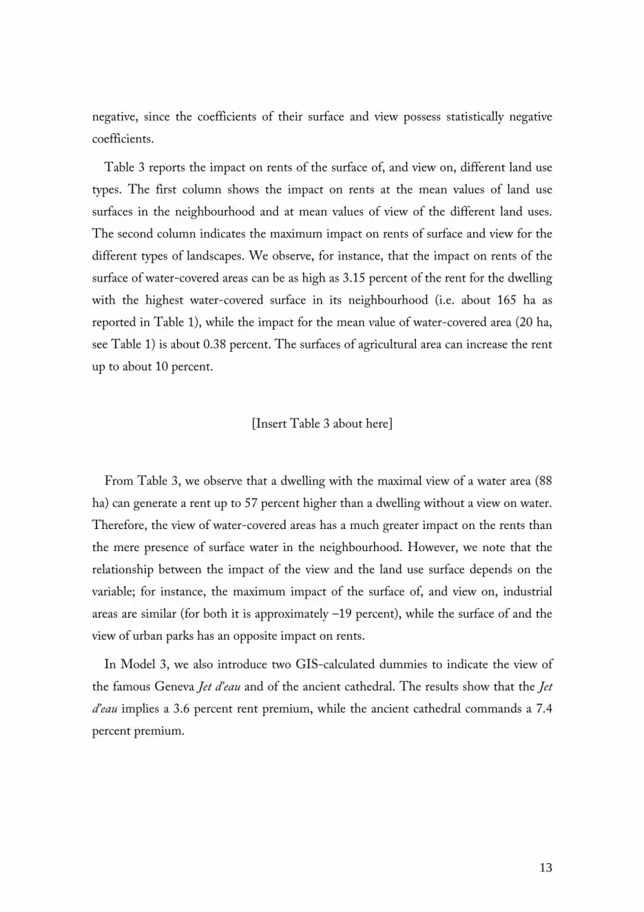
Table 3 reports the impact on rents of the surface of, and view on, different land use
types. The first column shows the impact on rents at the mean values of land use
surfaces in the neighbourhood and at mean values of view of the different land uses.
The second column indicates the maximum impact on rents of surface and view for the
different types of landscapes. We observe, for instance, that the impact on rents of the
surface of water-covered areas can be as high as 3.15 percent of the rent for the dwelling
with the highest water-covered surface in its neighbourhood (i.e. about 165 ha as
reported in Table 1), while the impact for the mean value of water-covered area (20 ha,
see Table 1) is about 0.38 percent. The surfaces of agricultural area can increase the rent
up to about 10 percent.
[Insert Table 3 about here]
From Table 3, we observe that a dwelling with the maximal view of a water area (88
ha) can generate a rent up to 57 percent higher than a dwelling without a view on water.
Therefore, the view of water-covered areas has a much greater impact on the rents than
the mere presence of surface water in the neighbourhood. However, we note that the
relationship between the impact of the view and the land use surface depends on the
variable; for instance, the maximum impact of the surface of, and view on, industrial
areas are similar (for both it is approximately –19 percent), while the surface of and the
view of urban parks has an opposite impact on rents.
In Model 3, we also introduce two GIS-calculated dummies to indicate the view of
the famous Geneva Jet d’eau and of the ancient cathedral. The results show that the Jet
d’eau implies a 3.6 percent rent premium, while the ancient cathedral commands a 7.4
percent premium.

14
6 Conclusions
The aim of this paper is to develop and incorporate original neighbourhood and
aesthetic environmental variables in a hedonic model and to test their impact on
Geneva’s rental market. We compute precise measures of the view and land uses at the
dwelling level in a radius of one kilometre around each building and test three different
hedonic models. To the first “traditional” model, we add in model 2 overall
neighbourhood and view variables as well as the corresponding diversity indices, and
finally, model 3 includes type-specific neighbourhood and view variables. Our results
show that both land use and aesthetic variables significantly affect Geneva rents. In
particular, the size and the view of the natural environment increase rents, while the
view of built environments lowers them. We also find that diversity indices of built
environment land uses and of their views have a negative impact on rents. Looking at
the various land uses more precisely, we find that size and view of water amenities
increase rents. More precisely, the rent premium for a dwelling located in a
neighbourhood with an extended water surface can be as high as 3 percent, while it can
reach up to 57 percent for a view of water-covered areas. In comparison, the surface of
agricultural areas in the neighbourhood of the building can increase rents up to about 10
percent, but a view of them does not have a significant impact. On the contrary, a view
of urban parks affects rents negatively, as does a view of industrial areas. Finally,
dwellings with a view of the famous Geneva Jet d’eau (water fountain) and of the ancient
cathedral generate on average 3.6 and 7.4 percent higher rents, respectively.
This paper highlights the possibility to evaluate the increase of buildings’ value
resulting from an environmental improvement. Moreover, environmental quality, such
as neighbourhood land use composition, their proximity and view, can be precisely
measured at the dwelling and building levels. Therefore, accurate information about
environmental quality would increase market transparency and would reward efforts to

15
improve natural and built environments. Finally, our results can be of particular
relevance in the context of urban densification, since they can be used to assess the
impact of the view obstructions on rents and the impact of view from high-rise
buildings.
Acknowledgements
We are grateful for financial support from the Swiss National Science Foundation,
National Research Programme NRP 54 “Sustainable Development of the Built
Environment”. We thank the Geneva Cantonal Statistical Office for providing the data
on rents and on some dwellings and buildings characteristics; the Geneva Cantonal
Office for Information Systems and Geomatics for providing the GIS data; Alain
Dubois for technical support with the GIS data; and Bengt Kriström, Jon Nelson, José
Ramirez, Philippe Thalmann and two anonymous referees for helpful comments. A
special thank goes to Eva Robinson for her outstanding assistance in calculating GIS
variables.
References
Acharya G, Bennett LL. Valuing open space and land-use patterns in urban watersheds. Journal of Real Estate Finance and Economics 2001; 22(2); 221–237.
Anderson ST, West SE. Open space, residential property values, and spatial context. Regional Science and Urban Economics 2006; 23; 776-789.
Baranzini A, Ramirez JV. Paying for quietness: the impact of noise on Geneva rents. Urban Studies 2005; 42(4); 633-646.
Baranzini A., Schaerer C., Thalmann P. Using measured instead of perceived noise in hedonic models. Transportation Research Part D; Transport and Environment 2010; 15(8); 473-482.
Baranzini A, Schaerer C, Ramirez JV, Thalmann P. (Eds) Hedonic Methods in Housing Markets – Pricing Environmental Amenities and Segregation. New York: Springer; 2008.
Bateman IJ, Jones AP, Lovett AA, Lake IR, Day BH. Applying geographical information systems (GIS) to environmental and resource economics. Environmental and Resource Economics 2001; 22; 219-269.
Benson ED, Hansen JL, Schwartz Jr. AL, Smersh GT. Pricing Residential amenities: The value of a view. Journal of Real Estate Finance and Economics 1998; 16(1); 55-73.

16
Bin OTC, Kruse JB, Landry C. Valuing spatially integrated amenities and risks in coastal housing markets. The Center for Natural Hazards Research 2006; East Carolina University, United States.
Bond MT, Seiler VL, Seiler MJ. Residential real estate prices: A room with a view. Journal of Real Estate Research 2002; 23(1/2); 129-137.
Bourassa SC, Hoesli M, Sun J. What’s in a view ? Environment and Planning A 2004; 36; 1427-1450.
Bourassa SC, Cantoni E, Hoesli M. Predicting house prices with spatial dependence: A comparison of alternative methods. Journal of Real Estate Research 2010; 32; 139-159.
Case B, Clapp J, Dubin R, Rodriguez M. Modeling spatial and temporal house price patterns: A comparison of four models. Journal of Real Estate Finance and Economics 2004; 29; 167-191.
Cavailhès J, Brossard T, Hilal M, Joly D, Tourneux F-P, Tritz C, Wavresky P. Pricing the homebuyer’s countryside view. In: Baranzini A, Schaerer C, Ramirez JV, Thalmann P (Eds), Hedonic Methods in Housing Markets – Pricing Environmental Amenities and Segregation. New York: Springer; 2008. p. 83-98.
Cheshire PC, Sheppard SC. On the price of land and the value of amenities. Economica 1995; 62; 247-267.
Congress of New Urbanism 2002. http://www.cnu.org. Day BH. The theory of hedonic markets: Obtaining welfare measures for changes in environmental
quality using hedonic market data. Economics for the Environment Consultancy 2001; London, United Kingdom.
Des Rosiers F, Thériault M, Kestens Y, Villeneuve P. Landscaping and house values: An empirical investigation. Journal of Real Estate Research 2002; 23; 139-161.
Dumas E, Geniaux G, Napoléone C. Effects of Landscape Ecology Indices on a Real Estate Market. Presented at the 1ère Rencontre du Logement, Marseille, France; 2006.
Geoghegan J, Wainger LA, Bockstael NE. Spatial landscape indices in a hedonic framework: An ecological economics analysis using GIS. Ecological Economics 1997; 23; 251-264.
Geoghegan J. The value of open spaces in residential land use. Land Use Policy 2002; 19(1); 91-98. Halvorsen R, Palmquist R. The interpretation of dummy variables in semilogarithmic equations.
American Economic Review 1980; 70(3); 474-475. Irwin GE. The effects of open space on residential property values. Land Economics 2002; 78(4);
465-480. Kelejian HH, Prucha IR. A generalized moments estimator for the autoregressive parameter in a
spatial model. International Economic Review 1999; 40; 509-533. Lake IR, Lovett AA, Bateman IA, Langford IH. Modelling environmental influences on property
prices in an urban environment. Computers, Environment and Urban Systems 1998; 22(2); 121-136.
Lutzenhiser M, Netusil NR. The effect of open spaces on a home's sale price. Contemporary Economic Policy 2001; 19(3); 291–298.
Malpezzi S. Hedonic pricing models: A selective and applied review. In: Gibbs K, O’Sullivan A (Eds), Housing Economics and Public Policy. London: Blackwell; 2002. p. 67-89.

17
McConnell V, Walls M. The Value of Open Space: Evidence from Studies of Non-Market Benefits. Washington, DC: Resources for the Future; 2005.
Palmquist RB. Property value models. In: Mäler KG, Vincent JR (Eds), Handbook of Environmental Economics, vol. 2. North Holland: Elsevier; 2005. p. 763-819
Paterson RW, Boyle KJ. Out of sight, out of mind? Using GIS to incorporate visibility in hedonic property value models. Land Economics 2002; 78(3); 417-425.
Rieder T. Die Bestimmung des Mieten in der Schweiz. Lizenzarbeit 2005; Volkswirtschfliches Institut; Universität Bern, Switzerland.
Rosen S. Hedonic prices and implicit markets: product differentiation in pure competition. Journal of Political Economy 1974; 82(1); 34-55.
Salvi M, Schellenbauer P, Schmidt H. Preise, Mieten und Renditen: Der Immobilienmarkt transparent gemacht. Zurich Kantonal Bank 2004; Zurich, Switzerland.
Samarshinghe OE, Sharp BMH. The value of a view: A spatial hedonic analysis. Paper presented at the International Conference on Regional and Urban Modelling. Brussels, Belgium; 2006.
Schaerer C, Baranzini A, Ramirez JV, Thalmann P. Using the hedonic approach to value landscape uses in an urban area: An application to Geneva and Zurich. Economie Publique – Public Economics 2007; 20(1); 147-167.
Schultz SD, King DA. The use of census data for hedonic price estimates of open-space amenities and land use. Journal of Real Estate Finance and Economics 2001; 22(2,3); 239-252.
Seiler MJ, Bond MT, Seiler VL. The impact of world class great lakes water views on residential property values. Appraisal Journal 2001; 69; 287-295.
Thalmann P. Explication empirique des loyers lausannois. Swiss Journal of Economics and Statistics 1987; 123(1); 47-69.
Tyrväinen L, Miettinen A. Property prices and urban forest amenities. Journal of Environmental Economics and Management 2000; 39(2); 205-223.
Yu SM, Han SS, Chai CH. Modeling the value of view in real estate valuation: A 3-D GIS Approach. Environment and Planning B: Planning and Design 2007; 34; 139-153.

18
Table 1 Descriptive statistics (N = 12 932)
Variables Mean Std. Dev. Min Max Mean annual net rent 13,462 6,307 2,760 96,000
Structural Variables Built between 1946 & 1960 0.238 0.426 0 1 Built between 1961 & 1970 0.254 0.436 0 1 Built between 1971 & 1980 0.198 0.398 0 1 Built between 1981 & 1990 0.129 0.336 0 1 Built after 1990 0.074 0.261 0 1 Number of rooms 3.602 1.271 2 12 Floor level 3.433 2.568 0 30 Height of the building (x10) [meters] 21.957 8.558 0 91 Attic dwelling 0.028 0.166 0 1 Tenancy change (in the past year) 0.075 0.264 0 1
Accessibility variables Distance to city centre [km] 2.529 1.906 0 13 Distance to nearest primary school [km] 0.213 0.111 0 1 Distance to nearest public transport stops [km] 0.128 0.065 0 0
Neighbourhood variables Surface of natural environment [ha] 120.382 39.132 15 284 Surface of built environment [ha] 173.203 42.204 16 250 Surface of water-covered area [ha] 19.836 30.330 0 165 Surface of agricultural area [ha] 14.912 38.980 0 239 Surface of urban parks [ha] 17.478 7.730 0 50 Surface of industrial area [ha] 7.508 12.034 0 105 Natural land use diversity index 0.476 0.114 0 1 Built land use diversity index 0.569 0.080 0 1
View variables View of natural environment [ha] 0.674 2.873 0 88 View of built environment [ha] 0.797 1.951 0 43 View of water-covered area [ha] 0.087 1.735 0 88 View of agricultural area [ha] 0.198 1.572 0 38 View of urban parks [ha] 0.043 0.223 0 6 View of industrial area [ha] 0.012 0.104 0 4 Natural view diversity index 0.297 0.103 0 1 Built view diversity index 0.366 0.116 0 1 View on Jet d'eau (dummy) 0.020 0.139 0 1 View on ancient cathedral (dummy) 0.014 0.119 0 1
Data source: Calculated using data from the Statistics on Rents 2005 and from SITG.

19
Table 2 Estimation results (N = 12 932)
Model 1 Model 2 Model 3 Dependent variable: ln(net annual rent) Coeff. (Std.err.) Coeff. (Std.err.) Coeff. (Std.err.)
Structural Variables
Built between 1946 & 1960 -0.035 *** (0.008) -0.035 *** (0.008) -0.032 *** (0.008) Built between 1961 & 1970 -0.065 *** (0.009) -0.057 *** (0.009) -0.053 *** (0.009) Built between 1971 & 1980 0.063 *** (0.009) 0.065 *** (0.010) 0.069 *** (0.009) Built between 1981 & 1990 0.186 *** (0.010) 0.185 *** (0.010) 0.190 *** (0.010) Built after 1990 0.272 *** (0.011) 0.273 *** (0.011) 0.277 *** (0.011) Number of rooms 0.238 *** (0.002) 0.238 *** (0.002) 0.238 *** (0.002) Floor level 0.013 *** (0.001) 0.014 *** (0.001) 0.013 *** (0.001) Height of the building (x10) [meters] -0.003 *** (0.000) -0.004 *** (0.000) -0.003 *** (0.000) Attic 0.056 *** (0.014) 0.058 *** (0.014) 0.059 *** (0.014) Tenancy change (in the past year) 0.202 *** (0.009) 0.203 *** (0.008) 0.201 *** (0.008)
Accessibility variables [in km]
Distance to nearest primary school 0.155 *** (0.000) 0.103 *** (0.000) 0.120 *** (0.000) Distance to city centre -0.018 *** (0.000) -0.031 *** (0.000) -0.020 *** (0.000) Distance to nearest public transport stops 0.144 *** (0.000) 0.176 *** (0.000) 0.195 *** (0.000)
Neighbourhood variables [ha]
Surface of natural land use (x 100) 0.065 *** (0.000) Surface of built land use (x 100) -0.013 (0.000) Natural land use diversity index -0.041 (0.029) Built land use diversity index -0.197 *** (0.037) Surface of water-covered area (x 100)
0.019 ** (0.000) Surface of agricultural area (x 100)
0.043 *** (0.000) Surface of urban parks (x 100)
0.062 ** (0.000) Surface of industrial area (x 100)
-0.177 *** (0.000) View variables [ha]
View of natural environment (x 100) 0.194 ** (0.001)
View of built environment (x 100) -0.380 ** (0.002)
Natural view diversity index 0.022 (0.026)
Built view diversity index -0.074 *** (0.020)
View of water-covered areas (x 100) 0.645 *** (0.001)
View of agricultural areas (x 100) 0.041 (0.002)
View of urban parks (x 100) -2.911 ** (0.012)
View of industrial areas (x 100) -5.214 ** (0.023)
View of Jet d'eau (dummy) 0.035 ** (0.017)
View of ancient cathedral (dummy) 0.071 *** (0.019)
Adjusted-R2 0.6345 0.6412 0.6405
F 1101 1003 1003
Mean VIF 1.7 2.2 1.6
Max VIF 2.9 6.9 3.0
Notes: *** significant at the 0.01 level; ** significant at the 0.05 level; * significant at the 0.10 level. The
reference for the period of construction is before 1946. Data sources: Statistics on Rents 2005 and SITG.

20
Table 3 Magnitudes of the impact on rents of different land use surfaces and views
Variables Mean Max Surface of water-covered area [ha] 0.38% 3.15% Surface of agricultural area [ha] 0.64% 10.34% Surface of urban parks [ha] 1.08% 3.07% Surface of industrial area [ha] -1.33% -18.57% View of water-covered area [ha] 0.06% 56.67% View of urban parks [ha] -0.13% -17.70% View of industrial area [ha] -0.06% -19.31%
Note : The magnitude of the view of agricultural area is not reported,
since the estimated impact on rent is not statistically significant.

Figure 1 Illustration of the view measure for a given apartment in our database
Source: Built using data from SITG.
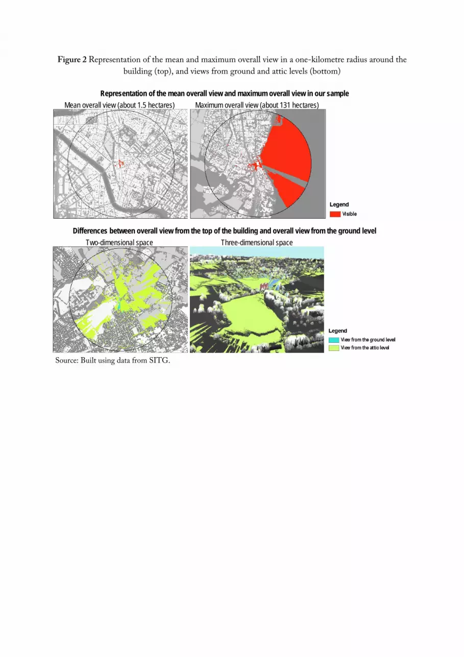
Figure 2 Representation of the mean and maximum overall view in a one-kilometre radius around the
building (top), and views from ground and attic levels (bottom)
Representation of the mean overall view and maximum overall view in our sample
Mean overall view (about 1.5 hectares) Maximum overall view (about 131 hectares)
Differences between overall view from the top of the building and overall view from the ground level
Two-dimensional space Three-dimensional space
Source: Built using data from SITG.