a profit‐maximizing approach to disposition decisions for product returns*
TRANSCRIPT
Decision SciencesVolume 42 Number 3August 2011
C© 2011 The AuthorsDecision Sciences Journal C© 2011 Decision Sciences Institute
A Profit-Maximizing Approach toDisposition Decisions for Product Returns∗Mark E. FergusonMoore School of Business, University of South Carolina, Columbia, SC 29208,e-mail: [email protected]
Moritz FleischmannUniversity of Mannheim, Business School, PO Box 10 34 62, 68131 Mannheim, Germany,e-mail: [email protected]
Gilvan C. Souza†Kelley School of Business, Indiana University, Bloomington, IN 47405,e-mail: [email protected]
ABSTRACT
Motivated by the asset recovery process at IBM, we analyze the optimal dispositiondecision for product returns in electronic products industries. Returns may be eitherremanufactured for reselling or dismantled for spare parts. Reselling a remanufacturedunit typically yields higher unit margins. However, demand is uncertain. A commonpolicy in many firms is to rank disposition alternatives by unit margins. We proposea profit-maximization approach that considers demand uncertainty. We develop singleperiod and multiperiod stochastic optimization models for the disposition problem. An-alyzing these models, we show that the optimal allocation balances expected marginalprofits across the disposition alternatives. A detailed numerical study reveals that ourapproach to the disposition problem outperforms the current practice of focusing exclu-sively on high-margin options, and we identify conditions under which this improvementis the highest. In addition, we show that a simple myopic heuristic in the multiperiodproblem performs well. [Submitted: August 2, 2010. Revisions received: January 18,2011; February 3, 2011. Accepted: February 8, 2011.]
Subject Areas: Closed-Loop Supply Chains, Inventory Management/Coordination, Markovian Decision Processes, and Yield Management.
INTRODUCTION
In this article, we address the disposition decision that a manufacturer has to makefor product returns. We motivate our analysis by describing the asset recoveryprocess at IBM. Information technology products such as personal computers,servers, storage systems, and mainframes coming off of lease are returned to
∗We thank the IBM executives for exposing us to this problem.†Corresponding author.
773
774 Profit-Maximizing Approach to Disposition Decisions for Product Returns
IBM’s remanufacturing facility, where a disposition decision—remanufacture ordismantle for spare parts—is made. The remanufacturing operation involves re-placing all wearable components, testing, cleaning, and reloading of software. Theunits are returned in batches and the current manufacturing process requires that allreturned units start processing immediately upon arrival rather than storing the re-turned units, and remanufacturing or harvesting parts to order. Due to considerablevariety in models and configurations, a remanufacturing-to-order strategy is notfeasible for IBM because fulfilling customer demand is subject to the mix availablein the current supply of used products, which changes from period to period. Thus,IBM remanufactures a particular model/configuration in its current supply of usedproducts, and puts it up for sale. Remanufactured units are advertised on IBM’sWeb site for about one month and, if not sold during this time, are salvaged tothird-party brokers through an auction; the fast obsolescence in the industry makesthese “older” configurations less and less attractive from the customer’s standpoint(we have observed this practice in other firms in the information technology [IT]industry). The price charged for the remanufactured units is severely restricted toprotect the brand image and to minimize the cannibalization of new product salesso it is considered exogenous to our problem. Although remanufactured units soldonline command attractive margins, unsold units salvaged via the auction can, inmost cases, only recover the cost incurred for remanufacturing. Thus, IBM makesa high profit on remanufactured units sold through its regular online channel, andclose to zero profit on remanufactured units salvaged via the auction.
Instead of remanufacturing a unit, IBM can dismantle it to harvest nonwear-able parts, such as memory, video cards, and mother boards, which can be usedas spare parts for service repairs, or even for selling to customers. The traditionalapproach for managing spare parts consists of purchasing new parts from the regu-lar supplier as needed. Moreover, suppliers of new parts (e.g., Intel) often demanda “final buy” from the manufacturer (Cattani & Souza, 2003). In that case, themanufacturer buys a large quantity of parts to last through the period for which ithas service contracts. Because demand for spare parts is uncertain during that longperiod, the firm may run out of inventory and, if the original supplier no longeroffers the part, has to procure the part at an alternative supplier (e.g., distributorsspecializing in hard-to-find parts) at a substantially higher cost. Thus, the disman-tling option offers flexibility to meet demand for spare parts in a less expensive waywhen there are shortages. If a unit has been through the remanufacturing processhowever, the profits from dismantling are not enough to recover the cost of re-manufacturing. Therefore, it is only profitable to select returned units to dismantlebefore they are remanufactured.
The current practice at IBM is to base the disposition decision primarilyon unit margins and on product quality, for products in good technical condition,remanufacturing is prioritized over dismantling. This practice ignores many factors,among which is demand uncertainty. We thus propose a methodology for findingthe optimal disposition decision. Although the problem is motivated by IBM’sasset recovery operations, it is general enough that it can be applied to other firmsin the general electronic products category that deal with product returns, such asfirms in the secondary IT networking industry, for example. In these cases, a returncan be dismantled for recovering nonwearable spare parts without any significantreprocessing.
Ferguson, Fleischmann, and Souza 775
Contributions to the Literature
In specific terms, we make the following contributions:
• We develop and solve a stochastic optimization model for the dispositionproblem that is characteristic of electronic products, and we characterizethe structure of the optimal policy.
• We assess the financial value of the dismantling option. We find that ex-cluding dismantling from the set of dispositions, by always prioritizingthe high-margin remanufacturing option, decreases the firm’s profit by 7%on average, for a six-month planning horizon (this value is higher withlonger planning horizons). In addition, the value of dismantling drops byabout 40% if the final-buy decision does not appropriately anticipate futurestreams of returns and their disposition. This reinforces the view that firmsshould make their operating decisions as a coordinated closed-loop supplychain rather than as separate forward and reverse chains.
• Given the complexity of the optimal disposition policy, we propose a my-opic heuristic based on newsvendor logic, and find that it performs reason-ably well relative to the optimal policy, with an average profit deteriorationof 2%.
The rest of this article is organized as follows: We first position our research in thecontext of the relevant literature. We then list our key assumptions and notation,present our model and provide some analytic results. We follow by presentingnumerical results on the value of dismantling from a study based on realisticparameter values. Finally, we summarize our results and conclude with managerialimplications. All proofs are provided in the Appendix.
LITERATURE REVIEW
Our research draws from three separate streams of the literature: the inventorymanagement of spare parts, revenue management, and closed-loop supply chains.We review each stream and position our research accordingly.
We begin with the literature on multi-echelon spare parts inventory manage-ment. The objective in these models is to find the best allocation of spare partsinventory among different stocking locations to satisfy a target service level orbackorder levels. In his seminal work, Sherbrooke (1968) studies a two-echeloninventory system of spare parts for military aircrafts where the parts are assumedto be repairable, that is, every failed part is sent to the depot for repair andthen put on the shelf once repaired. Under the assumptions of Poisson demand,continuous review, one-for-one ordering policy, full backordering, and indepen-dent and identically distributed (i.i.d.) lead times, he proposes the well-knownmulti-echelon technique for recoverable item control (METRIC) model to calcu-late the expected on-hand inventory and expected backorders at each inventorylocation by using a first moment approximation for the distribution of the out-standing orders. Since then there have been many extensions of the METRICmodel.
Graves (1985) proposes another approximation that fits a negative binomialdistribution to the first two moments of the outstanding orders. He shows that this
776 Profit-Maximizing Approach to Disposition Decisions for Product Returns
approach generally provides a better approximation than METRIC, and it is easierto calculate than the exact solution proposed by Simon (1971). Svoronos and Zipkin(1991) extend the METRIC model to stochastic sequential lead times where ordercrossing is not allowed. Cohen, Zheng, and Wang (1999) and Wang, Cohen, andZheng (2000) argue that the transportation time of defective parts from stockinglocations to the depot repair center might vary significantly for different stockinglocations, especially when the service network is global. They extend the METRICmodel by allowing stocking-center–dependent depot replenishment lead times andshow that the center-independent lead time assumption can lead to significanterrors in the calculation of performance metrics, especially when both the depotstocking level and demand rates are low. Cohen et al. (1999) use two-echelonmodels based on METRIC assumptions to improve the service-parts logisticssystem of electronic testing equipment used in semiconductor and electronicsassembly plants. They demonstrate that the effective use of basic inventory modelscan significantly increase customer service with a reduction (or small increase) ininventory investment.
The main difference in our work from this literature stream is that in theliterature they consider a system where the demand for spare parts and the rateof returns are perfectly correlated (i.e., each demand corresponds to a return andtherefore the number of parts circulating in the system is fixed). In contrast, wefocus on a system where the volumes of demand and returns are large and perfectcorrelation is rarely achieved; as an example, consider the number of laptopsneeding repair versus the number recovered. Moreover, their models primarilypertain to slow moving, expensive items with long life cycles for which an infinitehorizon, continuous review, one-for-one policy seems suitable. Our focus is onshort life cycle products with high demand and return rates and a high risk ofobsolescence; thus a periodic review policy with batch ordering is appropriate.Finally, in our setting the returned products are not solely used for harvestingspare parts—they can also be remanufactured and resold. Thus, we introduce adisposition decision to the theory of spare parts management.
The disposition decision seeks to maximize the benefit generated by a givenset of returned products. This objective is similar to the one of revenue management,and we discuss this analogy. Capacity-based revenue management applications inmanufacturing have mainly focused on customer segments that are heterogeneouson their willingness to wait for a product and can be split between make-to-order (MTO) and make-to-stock environments. Research on MTO environmentshas focused on managing a fixed-capacity system through discounts based onadvance purchase, and delivery time flexibility. Other proposed options includesome type of admissions control policy, where low margin orders may be declinedor quoted a longer lead time in anticipation of future arrivals of higher marginorders. A review of this literature can be found in Keskinocak and Tayur (2004).As previously mentioned, the remanufacturing process is designed for continuousflow and is not suitable for a MTO strategy. For make-to-stock environments, themajority of the research has focused on inventory management policies that includerationing, where a portion of the inventory is reserved for higher margin customerswho may arrive in the future (e.g., Topkis, 1968; Ha, 1997; Deshpande, Cohen, &Donohue, 2003). Our article differs from this literature in that we focus on which

Ferguson, Fleischmann, and Souza 777
type of product to produce (harvesting vs. remanufacturing) from a returned unit,whereas the literature described above considers that the physical characteristicsof the product are the same for all customers but the customer waiting times differ.Ciarallo, Akelia, and Morton (1994) provide a periodic review inventory problemwhere production capacity is uncertain (similar to the uncertain returns in ourmodel). In Ciarallo et al. (1994), however, the production decision is made beforerealizing the random capacity, whereas in our case the remanufacturing decision(and allocation decision) is made after realizing the random number of returns.In addition, our model is inherently different because of the two demand classes:remanufacturing and spare parts.
The recovery of value from used products has triggered the emergence ofclosed-loop supply chains, performing the acquisition and collection of returnedgoods, their inspection, grading, and disposition, reprocessing operations, such asremanufacturing and recycling, and the remarketing of the processed goods (Guide& Van Wassenhove, 2003). For a review of the different streams, see Ferguson andSouza (2010). The stream of research in this large body of literature that is themost related to our article is the disposition decision.
The disposition decision in the reverse supply chain allocates returned prod-ucts to an appropriate processing option. In the simplest case, disposition optionsinclude a form of recovery (e.g., remanufacturing, and disposal). For example,Teunter and Fortuin (1999), and Inderfurth and Mukherjee (2008) suggest reman-ufacturing of end-of-use returns as a way to meet demand for service parts thatare no longer in production. Their case focuses on parts that wear out with useand require some remanufacturing to be used again (e.g., diesel engines). In ourcase, instead, we focus on the electronics industry, where returns can be simplydismantled to meet demand for nonwearable parts, or remanufactured to be sold ata discount relative to comparable new products. A richer setting for the dispositiondecision may include several alternative recovery options, such as remanufactur-ing, harvesting of parts, and material recycling. Most research contributions, aswell as business examples, address the disposition decision by means of a relativelylong-term priority ranking, typically based on contribution margins. This approachassigns a returned product to the highest-ranked option that is technically feasible,given the physical product status (Fleischmann, Bloemhof-Ruwaard, Beullens, &Dekker, 2003). An exception is Guide, Gunes, Souza, and Van Wassenhove (2008),who link the disposition decision to the occupancy rate of the remanufacturing fa-cility, thereby avoiding excessive processing delays.
In this study, we propose that disposition decisions may benefit from adynamic approach that takes into account short-term variations in commercialopportunities. Two main factors drive our argument, namely demand uncertaintyand depreciation. Guide, Souza, Van Wassenhove, and Blackburn (2006) highlightdepreciation as a key issue in closed-loop supply chains and analyze its impacton supply chain design. We address its influence on the short-term dispositiondecisions. The paper that is closest to our analysis is Inderfurth, de Kok, andFlapper (2001), which investigates the allocation of returned products to multiplealternative reuse options, given stochastic demand and return volumes. The authorsanalyze the optimal policy structure and calculate optimal control parameters underthe assumption of a linear allocation of shortages. They propose a heuristic that
778 Profit-Maximizing Approach to Disposition Decisions for Product Returns
makes the allocation (of scarce returns to multiple disposition options) based onmean demands, as opposed to a profit-maximizing approach, which is what wesuggest. Thus, our article is the first to present the argument that the dispositiondecision should be made from a profit-maximizing approach, where profits areto be taken over an expected value form, which includes demand uncertainty,much like some revenue management problems. Kleber, Miner, and Kiesmuller(2002) analyze a related deterministic model and derive optimal disposition rulesunder time-varying return and demand volumes. In contrast to their analysis, ourdisposition strategy is driven by expected opportunity costs, rather than by seasonalfluctuations.
MODEL FORMULATION AND ANALYSIS
Key Assumptions
Motivated by the IBM context introduced before, we consider the situation of afirm that receives recoverable products returned from the market. The firm hastwo options for recovering value from these returns, namely remanufacturing ordismantling for parts. The firm seeks to allocate the returned products to theseoptions so as to maximize expected profits. We make a number of assumptionsthat are specific to the environment of electronic products. The results of this articledo not necessarily carry over to situations where, for example, parts need extensiveremanufacturing after dismantling to be used as a spare part (e.g., engine parts), orwhere products have a relatively long life cycle with low-value depreciation overtime (e.g., engines, transmissions).
Assumption 1: The arrival of returned units is exogenous to the decision maker.
This scenario is common for companies, such as IBM, that lease their prod-ucts with a final return date at the discretion of the customer (the customer canalways choose to continue to pay the lease payments even after the lease term hasended).
Assumption 2: The prices charged for the remanufactured units are exogenous tothe decision maker’s problem and constant over the planning horizon.
In our industry context, remanufactured units are restricted from being pricedbelow a set percentage of the price for the comparable new products to minimizecannibalization. There are also brand image concerns that limit IBM from pricingthe remanufactured units at a market clearing price. Thus, exogenously determinedremanufactured prices are a reasonable assumption in our context.
Assumption 3: Remanufactured units can only be sold during a limited timeperiod. Leftover units at the end of this period are salvaged.
This assumption is related to the previous one. Given pricing inflexibility,a finite selling period counterbalances product depreciation, which is substantialfor electronic products, and keeps product inventory at an acceptable level. This isstandard remanufacturing industry practice for IT equipment, as discussed in theintroduction.
Ferguson, Fleischmann, and Souza 779
Assumption 4: Unsatisfied demand for spare parts entails a per-unit penalty costthat is constant over time.
We consider the firm’s situation after the final buy for parts from the regularsupplier. The price of the component from the alternative and more expensivesupplier is typically constant over time.
Assumption 5: The per unit cost to remanufacture a returned unit is constantacross all units.
Remanufacturing cost depends on a return’s quality, and it is thus (generally)not constant across all units. In the IT industry, however, firms (such as IBM) onlyconsider the highest quality returns for remanufacturing, and demand for reman-ufactured products is considerably smaller than the amount of returns. Therefore,all units considered for remanufacturing have roughly the same quality level and,thus, the same per unit cost.
Assumption 6: Returned units used to produce remanufactured products or usedto disassemble for parts provide 100% yield.
This is a reasonable assumption given that only the highest quality returnsare considered for remanufacturing or parts harvesting. The remainder are sentdirectly to recycling.
Uncoordinated Decision Making and Single-Period Analysis
We begin our analysis with a single-period model where the disposition decisions(quantity to remanufacture versus dismantle) and the spare parts final-buy buydecisions are made independently. We combine these decisions and extend ourmodel to the multiperiod setting in the next subsection. By first presenting thedecisions as independent and single period, we are able to more clearly show thetrade-offs in the disposition decision. We also use the independent decision makingcase as one of our base-line cases in our numerical study where we calculate thevalue of coordinating the decision making.
The disposition decision
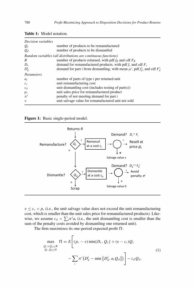
We begin with the disposition decision. Table 1 lists our notation. Using theassumptions outlined above, the disposition problem can be formalized as fol-lows. At the beginning of the period, the firm receives R returns, which is arandom variable with continuous probability density function (pdf) denoted byfR(·), and continuous cumulative distribution function (cdf) denoted by FR(·).Of these, the firm decides upon the number of units to be remanufactured Qr,and the number of units to be dismantled Qd. The remainder units, R − Qr −Qd, are scrapped at a cost normalized to zero. Remanufactured returns that are notsold are salvaged at a unit value of v. Demand for part i that is not met is assesseda unit penalty cost π i, which is the (higher) cost of obtaining the part through analternative supplier. Salvage value for all excess parts is zero; we relax this assump-tion in the multiperiod model, allowing excess parts to be carried over in inventory.This setting is illustrated in Figure 1. To exclude trivial situations, we assume
780 Profit-Maximizing Approach to Disposition Decisions for Product Returns
Table 1: Model notation.
Decision variablesQr number of products to be remanufacturedQd number of products to be dismantled
Random variables (all distributions are continuous functions)R number of products returned, with pdf fR and cdf FR
Dr demand for remanufactured products, with pdf fr and cdf Fr
Did demand for part i from dismantling, with mean μi, pdf f i
d, and cdf F id
Parametersai number of parts of type i per returned unitcr unit remanufacturing costcd unit dismantling cost (includes testing of part(s))pr unit sales price for remanufactured productπ i penalty of not meeting demand for part iv unit salvage value for remanufactured unit not sold
Figure 1: Basic single-period model.
v ≤ cr < pr (i.e., the unit salvage value does not exceed the unit remanufacturingcost, which is smaller than the unit sales price for remanufactured products). Like-wise, we assume cd <
∑iπ
iai (i.e., the unit dismantling cost is smaller than thesum of the penalty costs avoided by dismantling one returned unit).
The firm maximizes its one-period expected profit �:
maxQr+Qd≤RQr,Qd≥0
� = E
[(pr − v) min{Dr, Qr} + (v − cr )Qr
−∑
i
π i(Di
d − min{Di
d, aiQd
})] − cdQd.
(1)
Ferguson, Fleischmann, and Souza 781
Considering that E[min {D, Q}] = Q − ∫ Q0 F(u) du, where F(·) is the cdf of D,
Equation (1) becomes:
maxQr+Qd≤RQr,Qd≥0
� = (pr − v)
(Qr −
∫ Qr
0Fr (u) du
)+ (v − cr )Qr
−∑
i
[πiμi − πi
(aiQd −
∫ aiQd
0F i
d (u) du
)]− cdQd. (2)
The optimal solution of this problem is described in Lemma 1 below:
Lemma 1: Let
�d (Q) =∑
i
π iai
(1 − F i
d(aiQ)) − cd
�r (Q) = (pr − v) (1 − Fr (Q)) + v − cr .
Then the optimal solution to the disposition problem (2) can be written as
(Q∗d, Q
∗r ) =
⎧⎪⎨⎪⎩
(min{R, Q̃d}, 0) if �d (R) > �r (0),
(0, min{R, Q̃r}) if �d (0) < �r (R),
(min{Q̃d, Q̂d}, min{Q̃r , R − Q̂d}) else,
where Q̃d and Q̃r solve �d(Q) = 0 and �r(Q) = 0, respectively, and Q̂d solves�d(Q) = �r(R − Q).
In essence, Lemma 1 indicates that if there are enough returns, the firm cansatisfy demand for dismantling and remanufacturing at the levels Q̃d and Q̃r ,respectively, that set the marginal profit of dismantling and remanufacturing equalto zero. Otherwise, the firm sets the optimal level of dismantling such that themarginal profit of dismantling is equal to the marginal profit of remanufacturing.
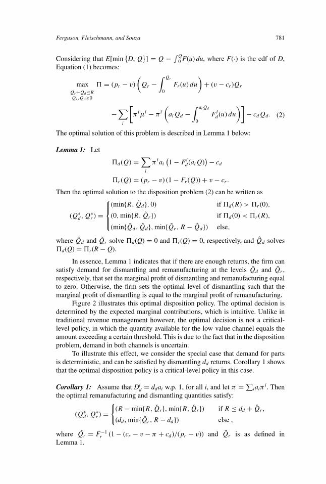
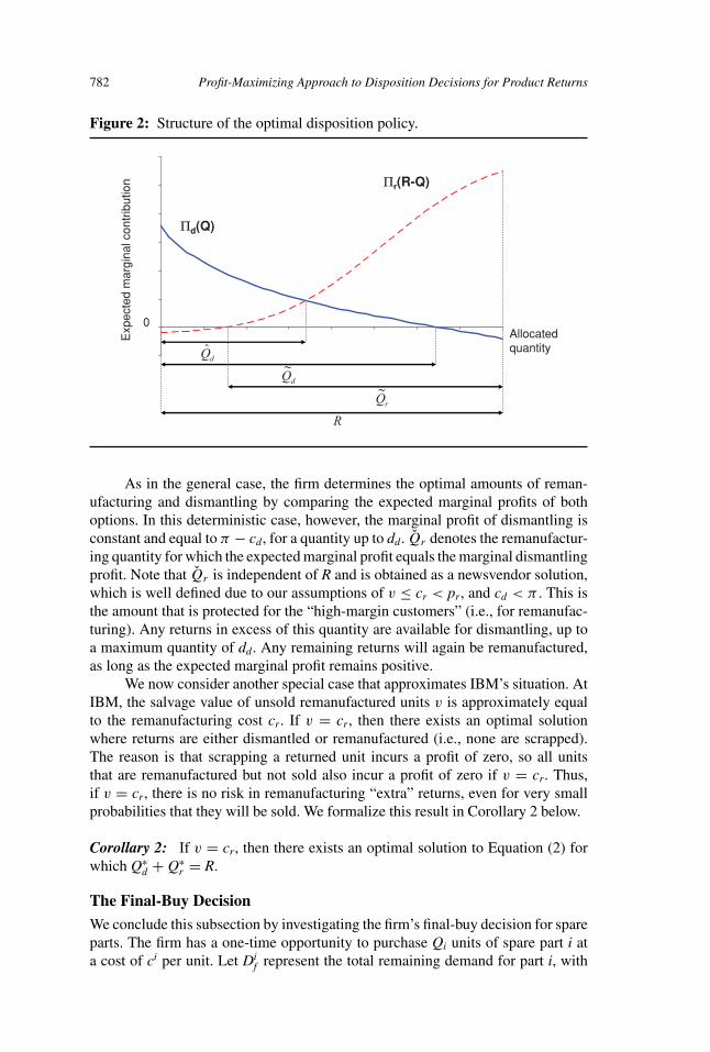
Figure 2 illustrates this optimal disposition policy. The optimal decision isdetermined by the expected marginal contributions, which is intuitive. Unlike intraditional revenue management however, the optimal decision is not a critical-level policy, in which the quantity available for the low-value channel equals theamount exceeding a certain threshold. This is due to the fact that in the dispositionproblem, demand in both channels is uncertain.
To illustrate this effect, we consider the special case that demand for partsis deterministic, and can be satisfied by dismantling dd returns. Corollary 1 showsthat the optimal disposition policy is a critical-level policy in this case.
Corollary 1: Assume that Did = ddai w.p. 1, for all i, and let π = ∑
iaiπi. Then
the optimal remanufacturing and dismantling quantities satisfy:
(Q∗d, Q
∗r ) =
{(R − min{R, Q̌r}, min{R, Q̌r}) if R ≤ dd + Q̌r ,
(dd, min{Q̃r , R − dd}) else ,
where Q̌r = F−1r (1 − (cr − v − π + cd )/(pr − v)) and Q̃r is as defined in
Lemma 1.
782 Profit-Maximizing Approach to Disposition Decisions for Product Returns
Figure 2: Structure of the optimal disposition policy.
Πd(Q)
Πr(R-Q)
0
Expecte
d m
arg
inal contr
ibution
Allocatedquantity
rQ~
dQ~
R
dQ̂
As in the general case, the firm determines the optimal amounts of reman-ufacturing and dismantling by comparing the expected marginal profits of bothoptions. In this deterministic case, however, the marginal profit of dismantling isconstant and equal to π − cd, for a quantity up to dd. Q̌r denotes the remanufactur-ing quantity for which the expected marginal profit equals the marginal dismantlingprofit. Note that Q̌r is independent of R and is obtained as a newsvendor solution,which is well defined due to our assumptions of v ≤ cr < pr, and cd < π . This isthe amount that is protected for the “high-margin customers” (i.e., for remanufac-turing). Any returns in excess of this quantity are available for dismantling, up toa maximum quantity of dd. Any remaining returns will again be remanufactured,as long as the expected marginal profit remains positive.
We now consider another special case that approximates IBM’s situation. AtIBM, the salvage value of unsold remanufactured units v is approximately equalto the remanufacturing cost cr. If v = cr, then there exists an optimal solutionwhere returns are either dismantled or remanufactured (i.e., none are scrapped).The reason is that scrapping a returned unit incurs a profit of zero, so all unitsthat are remanufactured but not sold also incur a profit of zero if v = cr. Thus,if v = cr, there is no risk in remanufacturing “extra” returns, even for very smallprobabilities that they will be sold. We formalize this result in Corollary 2 below.
Corollary 2: If v = cr, then there exists an optimal solution to Equation (2) forwhich Q∗
d + Q∗r = R.
The Final-Buy Decision
We conclude this subsection by investigating the firm’s final-buy decision for spareparts. The firm has a one-time opportunity to purchase Qi units of spare part i ata cost of ci per unit. Let Di
f represent the total remaining demand for part i, with

Ferguson, Fleischmann, and Souza 783
pdf f if (·), and cdf F i
f (·). Assuming the final-buy decision is made independently ofthe dismantling decision, the problem simplifies to a newsvendor problem wherethe cost of underage is π i and the cost of overage is ci. Thus, the optimal final-buydecision is to purchase Q∗
i = (Ffi)−1(π i/(ci + π i)). If we assume that the final-buy
decision occurs before the disposition decision in our single-period model, thenDi
d (used in the disposition problem formulation) represents the remaining demandfor part i after the final-buy quantity has been purchased. Thus, Di
d can also berepresented by the pdf f i
f and cdf F if over the range [Q∗
i , ∞].
Coordinated Decision Making and Multiperiod Analysis
In many examples, such as at IBM, the period during which a firm offers a repairservice, and thus requires spare parts, is much longer than the period during whicha returned unit can be sold—typically many months or years compared to a fewweeks. Firms also typically receive multiple batches of returns during this serviceperiod. To capture the dynamics of this situation, we extend our disposition modelto a multiperiod setting.
The periods are interconnected through the inventory level of spare parts.Any units that are dismantled feed the parts inventory. If demand for parts exceedsthe available inventory, the firm has to procure parts from an expensive backupsupplier, as discussed in the single-period analysis. This corresponds to a “lost-sales” assumption. Our results also extend to the case where unmet demand forparts is backordered, as we discuss at the end of this section. However, given thecriticality of spare parts and thus low willingness to wait, assuming lost sales (i.e.,procuring the part through an alternative and more expensive supplier) is moreappropriate for our setting. Intuitively, the disposition decision depends on theinitial parts inventory level and thereby on the final-buy decision. We thereforeinclude the final-buy decision in our analysis, which is the coordinated setting.
We formalize the multiperiod disposition problem as follows. We assumethat there is only one recoverable part per return (i.e., a1 = 1). One can also thinkof this as an aggregate of multiple parts with similar demands. Modeling multipleparts with very different demands introduces additional complexities, caused bythe interdependence between the dismantling decision and the different inventorieslevels of the different parts, as well by the increasing state space dimensionality.We leave these complexities to future research. We consider a planning horizon ofT periods. Periods are numbered backward, such that period t indicates that thereare t periods until the end of the planning horizon. At the beginning of period t, thefirm observes It, the starting inventory for spare parts, and Rt, the incoming returnsin that period. The firm then decides upon the number of returns to remanufactureQr,t and to dismantle Qd,t. Demand for remanufactured units Dr,t and for spareparts Dd,t is realized. Demand for remanufactured products not met is lost; unsoldremanufactured products are salvaged at a unit value v. Demand for spare partsnot met from inventory is met through an alternative supplier at a cost π per unit;leftover inventory for spare parts is carried over to period t − 1 at a holding costof h per unit. Any left over spare parts at time t = 0 have zero salvage value.
At the start of the planning horizon T , the firm makes a final-buy decision,at a cost of c per part, that brings its inventory of spare parts to IT . The firm aims

784 Profit-Maximizing Approach to Disposition Decisions for Product Returns
to maximize expected discounted profits through the planning horizon, given aone-period discount factor α.
This problem can be formulated as a finite-horizon Markov decision process(MDP) as follows. The state variable is It, the actions are Qd,t and Qr,t, and theone-period profit for t ≥ 1 is:
�t (It , Qd,t , Qr,t ) = (pr − v)
(Qr,t −
∫ Qr,t
0Fr (u) du
)+ (v − cr )Qr,t
− cdQd,t − πμd + π(It + Qd,t ) − (h + π)∫ (It+Qd,t )
0Fd (u) du.
(3)
The state transition is defined by It−1 = (It + Qd,t − Dd,t)+. For It ≥ 0, the Bellmanrecursion of this MDP therefore reads:
Vt (It ) = ERt
⎡⎢⎢⎣ max
Qr,t+Qd,t≤Rt
Qr,t ,Qd,t≥0
(�t (It ,Qd,t ,Qr,t ) + α
∫ ∞
0Vt−1((It + Qd,t − u)+)fd (u) du
)⎤⎥⎥⎦,
(4)
with boundary condition V0 ≡ 0. Equation (4) provides the disposition decision ineach period, given a starting value for inventory. The final buy decision is made atthe beginning of period T , and thus
V ∗T = max
IT
{−cIT + VT (IT )}. (5)
The solution of the above MDP has a similar structure and interpretation as inthe single-period case. The marginal contributions of both disposition alternativesdrive the allocation decision. What is different here is that one also has to takeinto account the impact on future periods through the resulting inventory level. Inaddition, the interplay between disposition and final-buy adds another layer to theproblem. The essential property that drives the structure of the optimal policy isconcavity of the value function in the inventory state variable. We summarize thisresult in the following theorem
Theorem 1: For any t ≥ 1 the MDP defined in Equations (3) and (4) satisfies thefollowing properties:
(i) Vt−1(I) is concave in I.
(ii) V ′t−1(I) ≤ π for any value of I, where V ′
t−1 denotes the first-order derivativeof Vt−1.
(iii) Wt(It, Qd,t, Qr,t) := �t(It, Qd,t, Qr,t) + α∫ ∞
0 Vt−1((It + Qd,t − u)+)fd(u) duis jointly concave in It, Qd,t and Qr,t.
(iv) Let
�d,t (I, Q) = −(h + π)Fd (I + Q)
+ α
∫ I+Q
0V ′
t−1(I + Q − u)fd (u) du − cd + π (6)
Ferguson, Fleischmann, and Souza 785
�r (Q) = (pr − v) (1 − Fr (Q))) + v − cr . (7)
Then, the optimal solution to (4) satisfies
(Q∗d,t , Q
∗r,t ) =
⎧⎪⎪⎨⎪⎪⎩
(min{Rt, Q̃d,t }, 0) if �d,t (It , Rt ) > �r (0),
(0, min{Rt, Q̃r,t }) if �d,t (It , 0) < �r (Rt ),
(min{Q̃d,t , Q̂d,t }, min{Q̃r,t , Rt − Q̂d,t }) else,(8)
where Q̃d,t and Q̃r,t are solutions to �d,t (It , Q̃d,t ) = 0 and �r (Q̃r,t ) = 0,respectively, and Q̂d,t solves �d,t (It , Q̂d,t ) = �r (Rt − Q̂d,t ).
The optimal disposition policy has the same structure as in the single-period case.However, the marginal benefit of dismantling (i.e., �d,t) now depends on the spareparts inventory level. Note from Equation (6) that an additional unit of inventoryshifts the dismantling marginal profit curve in Figure 2 to the left by one unit. Thisalso shifts the intersection point of both marginal profit curves to the left, but notnecessarily by a full unit. Therefore, the optimal policy is not a critical-level policythat replenishes the parts inventory up to a certain fixed target level.
As indicated earlier in this section, the above results extend to the case ofbackordering unmet demand for parts. To this end, one simply drops the (.)+
operator in the argument of Vt−1 in Equation (4) and interprets π as the unitbackorder cost per period.
Note further that as a consequence of the concavity of VT , the optimal final-buy quantity I∗
T can be found through a simple myopic search for the maximum.
NUMERICAL STUDY
In this section, we conduct a detailed numerical analysis to assess the performanceof our approach to product disposition and compare it to current common practice,as well as to a simpler myopic heuristic based on newsvendor logic. Our objectivesare (i) to gain further insight into the characteristics of our profit maximizationapproach and the factors that drive it; and (ii) to determine under which conditionsour approach significantly outperforms the other policies and when, on the contrary,a simpler heuristic will suffice.
Experimental Design
We consider a planning horizon with T = 6 periods, where each period correspondsto one month. Returns arrive randomly in each period according to a Poissonprocess with the mean scaled to μR = 7 (it may be helpful to think of one unit inthis analysis as, say, 1,000 units in real life). There is only one recoverable part perreturn (a1 = 1); again, this can be thought of as an “aggregate” part. We normalizethe remanufactured product’s price to pr = 10. The unit cost of purchasing a sparepart at the beginning of the planning horizon through the final buy is c = 1, or10% of the remanufactured product’s price; this is a realistic number based on ourdiscussions with IBM. The one-period discount factor is α = 0.99, correspondingto an annual cost of capital of 12%; we have experimented with other reasonablediscount factors and concluded that they do not impact our results. Finally, we

786 Profit-Maximizing Approach to Disposition Decisions for Product Returns
assume v = cr, which is in line with IBM’s situation; we relax this assumptionlater and show it does not impact our insights.
We ran a full-factorial experimental design for the remaining parameters ofour model. Each factor in the experimental design is varied at four levels (low,mid-low, mid-high, high) based on observed industrial practice as justified below.The total average demand for spare parts and remanufactured products is expressedas a fraction 1/k of the average number of returns per period: k(μr + μd) = μR. Wechoose k ∈ {0.75, 0.90, 1.05, 1.20}, ranging from the case where average returnsper period are insufficient to meet the average total demand (k = 0.75), to largerthan the average total demand (k = 1.2). We assume that the demand for spare partsin each period follows a Poisson distribution, with its mean expressed as a fractionof the mean demand for remanufactured products μd/μr ∈ {0.5, 1, 1.5, 2}; fromlow to high values found in practice. We consider that demand for remanufacturedproducts follows a gamma distribution with mean μr and a coefficient of variationCVr ∈ {0.1, 0.3, 0.5, 0.7}, from low to high levels of demand variability.
We set remanufacturing cost per unit relative to price cr/pr ∈ {0.1, 0.2,0.3, 0.4}. These choices are justified as follows: Agrawal, Ferguson, and Souza(2008) report values for cr/pr in the range 0.05–0.20 for commercial IT equipment;Hauser and Lund (2003) report average values of cr/pr of 0.45 for industrieswhere remanufacturing is more labor intensive (and thus remanufacturing is moreexpensive). Dismantling cost cd should be lower than c, otherwise dismantling forspare parts is not economically attractive and our problem is not interesting. Wetherefore set cd/c ∈ {0.1, 0.3, 0.5, 0.7}; a wide range from low to high reflectspossible values found in practice.
Regarding holding and penalty costs, inventory theory suggests that therelevant parameter impacting the optimal inventory policy for parts is the ratioπ /h. We assume in this numerical case that demand for spare parts not met is lost(i.e., met with parts from an alternative expensive supplier), which is in line withIBM’s situation. With this in mind, and consistent with inventory theory, we setπ /h ∈ {21, 30, 40, 99}. This range has been used in previous research in inventorytheory for the lost sales case (e.g., Ehrhardt, 1979). We set the unit holding costper period to h = 0.05, corresponding to an annualized holding cost value of 60%,which is typical of components and products in the electronics industry (Guideet al., 2008). We have experimented with lower holding costs, and our insights donot change. With this holding cost value, our experimental design results in π ∈{1.1, 1.5, 2, 5}, which ensures π > c = 1.
Our experimental design is summarized in Table 2. There are 46 = 4,096experimental cells. For each cell, the finite-horizon dynamic program is solved bybackward substitution using a customized code in MATLAB, where the optimiza-tion with respect to Qd,t was performed by myopic enumeration, taking advantageof the result in Theorem 1 that the value to go function Wt(It, Qd,t, Qr,t) is jointlyconcave in (Qd,t, Qr,t) for each state It. Expected sales for the remanufactured prod-uct Qr,t − ∫ Qr,t
0 Fr(u) du were computed numerically using MATLAB’s numericintegration function QUAD. We have used appropriate upper limits for inventoryof parts in the state space (so that the state space is finite for computation). Finally,the computation of the final buy decision I∗
T (Equation (5)) was performed using asimple numerical myopic search for the maximum, as indicated before.
Ferguson, Fleischmann, and Souza 787
Table 2: Experimental design for numerical study (pr = 10, c = 1, α = 0.99,μR = 7).
Factor Description Symbol Factor Levels
Total average demand as a fraction of average returns k 0.75, 0.90, 1.05, 1.20Mean demand for parts relative to remanufactured μd/μr 0.5, 1.0, 1.5, 2.0
productsCV of demand for remanufactured products CVr 0.1, 0.3, 0.5, 0.7Relative remanufacturing cost per unit cr/pr 0.1, 0.2, 0.3, 0.4Relative dismantling cost cd/c 0.1, 0.3, 0.5, 0.7Penalty cost for spare parts (relative to holding cost) π /h 21, 30, 40, 99
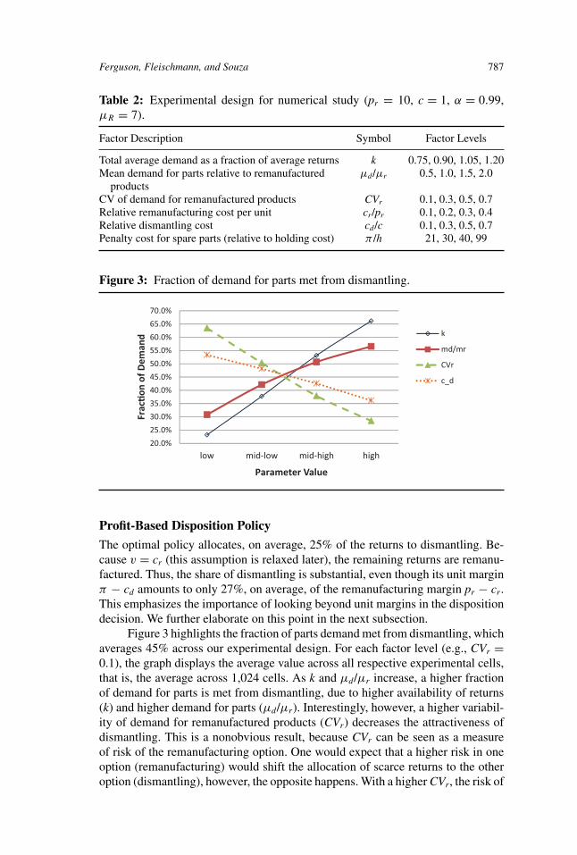
Figure 3: Fraction of demand for parts met from dismantling.
Profit-Based Disposition Policy
The optimal policy allocates, on average, 25% of the returns to dismantling. Be-cause v = cr (this assumption is relaxed later), the remaining returns are remanu-factured. Thus, the share of dismantling is substantial, even though its unit marginπ − cd amounts to only 27%, on average, of the remanufacturing margin pr − cr.This emphasizes the importance of looking beyond unit margins in the dispositiondecision. We further elaborate on this point in the next subsection.
Figure 3 highlights the fraction of parts demand met from dismantling, whichaverages 45% across our experimental design. For each factor level (e.g., CVr =0.1), the graph displays the average value across all respective experimental cells,that is, the average across 1,024 cells. As k and μd/μr increase, a higher fractionof demand for parts is met from dismantling, due to higher availability of returns(k) and higher demand for parts (μd/μr). Interestingly, however, a higher variabil-ity of demand for remanufactured products (CVr) decreases the attractiveness ofdismantling. This is a nonobvious result, because CVr can be seen as a measureof risk of the remanufacturing option. One would expect that a higher risk in oneoption (remanufacturing) would shift the allocation of scarce returns to the otheroption (dismantling), however, the opposite happens. With a higher CVr, the risk of
788 Profit-Maximizing Approach to Disposition Decisions for Product Returns
losing (high margin) sales in the higher-margin remanufacturing channel increases,which motivates a higher allocation of returns to that channel.
Nonoptimal Policies and Heuristics
To find the optimal policy, we solve a dynamic program, whose computationalcomplexity increases significantly in the number of periods T , the mean returnsper period μR, and the mean demand for parts per period μd (as they determine thesize of the state space). We present below three alternative policies to the optimalsolution, which are much less computationally intensive:
• No Dismantling: As discussed before, a common approach in practice is torank dispositions by unit margin and to allocate returns depending on theirquality condition to the highest-ranked option that is technically feasible.In our case, this would mean remanufacturing all returned units (recall thatwe only consider high-quality returns). Demand for parts is then met solelywith inventory from the final buy plus potential emergency supplies. Werefer to this policy as “no dismantling” and denote its expected discountedprofit through the planning horizon by VND
T ; this value is found by solvingEquations (4) and (5) with Qd,t = 0. The quantity of the final buy IND
T isthe critical decision in this policy. We define the value of dismantling as�ND(V∗) = 100%(V∗
T − VNDT )/V∗
T , which is the profit deterioration fromnot using the dismantling option.
• Myopic Heuristic: Given that the no dismantling policy is a relatively crudeheuristic, we construct a myopic heuristic, based on newsvendor logic. Inwhat follows, we denote this approach by the superscript M (for “myopic”).Specifically, our heuristic sets QM
r = min{Q̃Mr , R}, where R is the number
of returns received, and Q̃Mr is the smallest value that satisfies the Equa-
tion Fr (Q̃Mr ) ≥ Cu
Cu+Co, where Cu = pr − cr − (π − cd )(1 − Fd (I + R −
Q̃Mr − 1)) and Co = cr − v + (π − cd )(1 − Fd (I + R − Q̃M
r − 1)). Thecost of underage Cu for our heuristic is the margin of the remanufac-tured product minus the expected unit penalty cost for lack of parts that isavoided by allocating an extra part to dismantling; this penalty occurs ifdemand for parts exceeds current inventory of parts plus parts originatedfrom dismantling. Analogously, the cost of overage Co is the unit loss in-curred for a salvaged remanufactured product plus the expected increase inpenalty costs for lack of parts. The computation of Q̃M
r requires a (simple)numerical search because both left and right-hand sides of the equation thatdefines it are dependent on it. Denote the expected discounted profit forusing this myopic heuristic through the planning horizon by VM
T . Furtherdenote the profit deterioration of using the myopic heuristic relative to theoptimal policy by �M(V∗) = 100%(V∗
T − VMT )/V∗
T .• No Coordination: Our optimal policy assumes that the final buy quantity
I∗T takes into account the forecast for future returns, along with an opti-
mal allocation of returns between dismantling and remanufacturing. Thisassumes a perfect coordination between a purchasing manager, who isresponsible for the supply of a particular part, and the reverse supply chain

Ferguson, Fleischmann, and Souza 789
Figure 4: Value of coordination.
Figure 5: Impact of planning horizon on policy performance.
manager, who is responsible for forecasting and processing returns, whichmay be unrealistic. We now investigate the value of coordination: Whatis the profit deterioration of having the final buy decision made withoutconsideration of a possible supply of parts from dismantling in the future?The final buy quantity without consideration of future dismantling is IND
T .Once that decision is made, however, the firm makes the optimal alloca-tion decision between dismantling and remanufacturing as returns arrive.Thus, the value of coordination is given by �NC(V∗) = 100%(V∗
T (I∗T ) −V∗
T (INDT ))/V∗
T (I∗T ), and this is illustrated in Figure 4.
Results: Policy Performance
Using the experimental design of Table 2, the average value of dismantling�ND(V∗) is 7%, the average profit deterioration of the myopic policy �M(V∗)is 2%, and the average value of coordination �NC(V∗) is 4%. Additional exper-iments indicated that the value of dismantling increases almost linearly with alonger planning horizon T , whereas the performance of the myopic policy andthe value of coordination are both relatively insensitive to T . This is illustrated inFigure 5 for an average case in our experimental design, with k = 1.05, μd/μr =1.5, CVr = 0.3, cr = 3, cd = 1.5, π = 1.5; �ND(V∗) increases from 7.4% to13.6% as T increases from 3 to 15 periods. Firms obtain more benefits from the
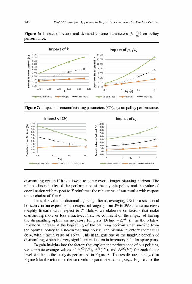
790 Profit-Maximizing Approach to Disposition Decisions for Product Returns
Figure 6: Impact of return and demand volume parameters (k, μd
μr) on policy
performance.
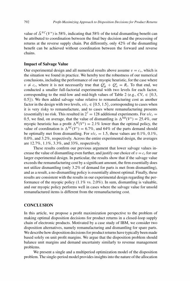
Figure 7: Impact of remanufacturing parameters (CVr, cr) on policy performance.
dismantling option if it is allowed to occur over a longer planning horizon. Therelative insensitivity of the performance of the myopic policy and the value ofcoordination with respect to T reinforces the robustness of our results with respectto our choice of T = 6.
Thus, the value of dismantling is significant, averaging 7% for a six-periodhorizon T in our experimental design, but ranging from 0% to 39%; it also increasesroughly linearly with respect to T . Below, we elaborate on factors that makedismantling more or less attractive. First, we comment on the impact of havingthe dismantling option on inventory for parts. Define −�ND(IT ) as the relativeinventory increase at the beginning of the planning horizon when moving fromthe optimal policy to a no-dismantling policy. The median inventory increase is86%, with a mean value of 169%. This highlights one of the tangible benefits ofdismantling, which is a very significant reduction in inventory held for spare parts.
To gain insights into the factors that explain the performance of our policies,we compute average values of �ND(V∗), �M(V∗), and �NC(V∗) for each factorlevel similar to the analysis performed in Figure 3. The results are displayed inFigure 6 for the return and demand volume parameters k and μd/μr, Figure 7 for the

Ferguson, Fleischmann, and Souza 791
Figure 8: Impact of dismantling parameters (cd, π) on policy performance.
remanufacturing parameters CVr and cr, and Figure 8 for the dismantling param-eters cd and π . Each point in each curve of a chart represents the average of therespective factor across 1,024 experiments; the curves are thus representative ofthe entire design.
The performance of our myopic policy is relatively insensitive to differentfactor levels, with profit deterioration consistently averaging around 2%, exceptfor the factors μd/μr and π . When μd/μr = 2, demand for parts is double that forremanufactured products, and as a result the value of optimally allocating returnsto parts is higher, explaining the relative lower performance of our heuristic (4%).A similar reasoning applies to the cases where penalty values are very high, suchas for π = 5. Across our experimental design, the myopic heuristic deviates fromthe optimal policy, on average, by increasing the final-buy quantity of parts by7%, while at the same time decreasing the dismantling quantity by 40%. Thus,the heuristic tends to underestimate the benefit of dismantling, which is consistentwith its myopic perspective.
As one would expect from intuition, the value of dismantling is higher whenthere are more available returns (higher k); when the demand for parts is higherrelative to remanufacturing (higher μd/μr), the margin of remanufacturing is lower(higher cr), the cost of dismantling (cd) is lower and the penalty cost (π) is higher.Moreover, and not as intuitive, these relationships are quasi-linear as displayedin Figures 6–8. The value of dismantling, however, decreases as the variability ofdemand for the remanufactured product (CVr) increases, which is a nonintuitiveresult explained earlier.
The value of coordination is consistently about 40% lower than the valueof dismantling; the two curves are basically parallel in each of the six fac-tor charts. Thus, accounting for the dismantling option in the final buy hasthe potential to significantly improve profits. Another perspective is to expressthe value of coordination as the fraction of the dismantling benefit that canbe attributed to coordination. This fraction can be expressed as �̃NC(V ∗) =100%(V ∗
T (I ∗T ) − V ∗
T (INDT ))/(V ∗
T (I ∗T ) − V ND
T (INDT )), as shown in Figure 4. The
quantity in the numerator is the dismantling benefit attributable to coordination,whereas the denominator represents the total dismantling benefit. The average
792 Profit-Maximizing Approach to Disposition Decisions for Product Returns
value of �̃NC(V ∗) is 58%, indicating that 58% of the total dismantling benefit canbe attributed to coordination between the final buy decision and the processing ofreturns at the reverse supply chain. Put differently, only 42% of the dismantlingbenefit can be achieved without coordination between the forward and reversechains.
Impact of Salvage Value
Our experimental design and all numerical results above assume v = cr, which isthe situation we found in practice. We hereby test the robustness of our numericalconclusions, including the performance of our myopic heuristic, for the case wherev = cr, where it is not necessarily true that Q∗
dt + Q∗rt = Rt. To that end, we
conducted a smaller full-factorial experimental with two levels for each factor,corresponding to the mid-low and mid-high values of Table 2 (e.g., CVr ∈ {0.3,0.5}). We then added salvage value relative to remanufacturing cost as anotherfactor in the design with two levels, v/cr ∈ {0.5, 1.5}, corresponding to cases whenit is very risky to remanufacture, and to cases where remanufacturing presents(essentially) no risk. This resulted in 27 = 128 additional experiments. For v/cr =0.5, we find, on average, that the value of dismantling is �ND(V∗) = 25.4%, ourmyopic heuristic has a profit �M(V∗) = 2.1% lower than the optimal policy, thevalue of coordination is �NC(V∗) = 6.7%, and 64% of the parts demand shouldbe optimally met from dismantling. For v/cr = 1.5, these values are 0.1%, 0.1%,0.0%, and 3.2%, respectively. Across the entire experimental design, the averagesare 12.7%, 1.1%, 3.3%, and 33%, respectively.
These results confirm our previous argument that lower salvage values in-crease the value of dismantling even further, and justify our choice of v = cr for ourlarger experimental design. In particular, the results show that if the salvage valueexceeds the remanufacturing cost by a significant amount, the firm essentially doesnot utilize dismantling (only 3.2% of demand for parts is met from dismantling),and as a result, a no-dismantling policy is essentially almost optimal. Finally, theseresults are consistent with the results in our experimental design regarding the per-formance of the myopic policy (1.1% vs. 2.0%). In sum, dismantling is valuable,and our myopic policy performs well in cases where the salvage value for unsoldremanufactured items is different from the remanufacturing cost.
CONCLUSION
In this article, we propose a profit maximization perspective to the problem ofmaking optimal disposition decisions for product returns in a closed-loop supplychain of electronic products. Motivated by a case study of IBM, we consider twodisposition alternatives, namely remanufacturing and dismantling for spare parts.We describe how disposition decisions for product returns have typically been madebased solely on unit profit margins. We argue that the disposition problem shouldbalance unit margins and demand uncertainty similarly to revenue managementproblems.
We present a single and a multiperiod optimization model of the dispositionproblem. The single-period model provides insights into the nature of the allocation
Ferguson, Fleischmann, and Souza 793
decision for a given number of returns. We show that the optimal allocation balancesthe expected marginal profits of remanufacturing and dismantling. Our multiperiodmodel links the disposition of returns to the final buy decision for spare parts atthe beginning of the planning horizon, and takes into account uncertainty in thedistribution of returns. We show that the optimal solution has the same structureas the single-period model, although its computation is more complex.
Our results have clear implications for the management of closed-loop supplychains of electronic products. They show that an optimization approach to the dis-position of returns can significantly enhance profitability. Incorporating additionaldisposition options can be very valuable, even if they have lower unit margins thancurrent options. This should encourage managers to explore new product recoveryalternatives. Harvesting of spare parts can be a particularly attractive option giventhe relatively long life cycles of parts. However, careful coordination between for-ward and reverse supply chain decisions is indispensable for reaping these benefits.In our experience, few companies to date have reached this level of integration. Ourmessage is that the current reactive approach to the reverse supply chain missesout on significant opportunities.
Our analysis makes a number of assumptions specific to the recovery systemof electronic products considered here. To further the insight into the role of the dis-position decision in closed-loop supply chains, extensions to other settings wouldbe valuable. This includes the study of dispositions other than remanufacturing anddismantling, and of other industries, where remanufactured products are carriedin inventory over longer periods of time, for example, due to longer life cycles.The incorporation of flexible pricing in the disposition decision would also be ofinterest. In addition, in the multiperiod analysis, we have approximated multipleparts by a single aggregate part. Explicitly modeling multiple parts having differentcharacteristics adds significant complexities, due to the increasing problem size.This is a fertile area for future research, to which our newsvendor heuristic mayserve as a starting point. Finally, another very relevant question for future researchis how to achieve coordination concerning the disposition of returns when deci-sions pertaining to the forward and the reverse supply chain are made by differentorganizational units.
REFERENCES
Agrawal, V., Ferguson, M., & Souza, G. (2008). Trade in rebates for price dis-crimination or product recovery. Working Paper, Kelley School of Business,Indiana University, Bloomington, IN.
Cattani, K., & Souza, G. (2003). Good buy? Delaying end-of-life purchases. Eu-ropean Journal of Operational Research, 146(1), 216–228.
Ciarallo, F., Akelia, R., & Morton, T. (1994). A periodic review, production plan-ning model with uncertain capacity and uncertain demand: Optimality ofextended myopic policies. Management Science, 40(3), 320–332.
Cohen, M., Zheng, Y.-S., & Wang, Y. (1999). Identifying opportunities for im-proving Teradyne’s service-parts logistics system. Interfaces, 29(4), 1–18.

794 Profit-Maximizing Approach to Disposition Decisions for Product Returns
Deshpande, V., Cohen, M., & Donohue, K. (2003). A threshold inventory rationingpolicy for service differentiated demand classes. Management Science, 49(6),683–703.
Ehrhardt, R. (1979). The power approximation for computing (s,S) inventorypolicies. Management Science, 25(8), 777–786.
Ferguson, M., & Souza, G. (2010). Closed loop supply chains: New develop-ments to improve the sustainability of business practices. Boca Raton: CRCPress.
Fleischmann, M., Bloemhof-Ruwaard, J., Beullens, P., & Dekker, R. (2003). Re-verse logistics network design. In R. Dekker, M. Fleischmann, K. Inderfurth,& L. N. Van Wassenhove (Eds.), Reverse logistics: Quantitative models forclosed-loop supply chains. Berlin: Springer Verlag, 65–94.
Graves, S. C. (1985). A multi-echelon inventory model for a repairable item withone-for-one replenishment. Management Science, 31(10), 1247–1256.
Guide, V. D. R., Jr., & Van Wassenhove, L. (2003). Business aspects of closed-loopsupply chains. Pittsburgh, PA: Carnegie Mellon University Press.
Guide, V. D. R., Jr., Souza, G., Van Wassenhove, L., & Blackburn, J. (2006). Timevalue of commercial product returns. Management Science, 52(8), 1200–1214.
Guide, V. D. R., Jr., Gunes, E., Souza, G., & Van Wassenhove, L. (2008). Theoptimal disposition decision for product returns. Operations ManagementResearch, 1(1), 6–14.
Ha, A. Y. (1997). Inventory rationing in a make-to-stock production system withseveral demand classes and lost sales. Management Science, 43(8), 1093–1103.
Hauser, W., & Lund, H. (2003). The remanufacturing industry: Anatomy of a giant.Boston, MA: Boston University.
Inderfurth, K., & Mukherjee, K. (2008). Decision support for spare parts acqui-sition in post product life cycle. Central European Journal of OperationalResearch, 16, 17–42.
Inderfurth, K., de Kok, A., & Flapper, S.-D. (2001). Product recovery in stochasticremanufacturing systems with multiple reuse options. European Journal ofOperational Research, 133(1), 130–152.
Keskinocak, P., & Tayur, S. (2004). Due-date management policies. In D. Simchi-Levi, S. D. Wu, & Z. M. Shen (Eds.), Handbook of quantitative supplychain analysis: Modeling in the e-business era. Norwell, MA: InternationalSeries in Operations Research and Management Science, Kluwer AcademicPublishers, 485–553.
Kleber, R., Miner, S., & Kiesmuller, G. (2002). A continuous time inventory modelfor a product recovery system with multiple reuse options. InternationalJournal of Production Economics, 79, 121–141.
Sherbrooke, C. (1968). METRIC: A multi-echelon technique for recoverable itemcontrol. Operations Research, 16(1), 122–141.
Ferguson, Fleischmann, and Souza 795
Simon, R. M. (1971). Stationary properties of a two-echelon inventory model forlow-demand items. Operations Research, 19(3), 761–773.
Svoronos, A., & Zipkin, P. (1991). Evaluation of the one-for-one replenishmentpolicies for multi-echelon inventory systems. Management Science, 37(1),68–83.
Teunter, R. H., & Fortuin, L. (1999). End-of-life service. International Journal ofProduction Economics, 59, 487–497.
Topkis, D. (1968). Optimal ordering and rationing policies in a nonstationarydynamic inventory model with N classes. Management Science, 15(3), 160–176.
Wang, Y., Cohen, M., & Zheng, Y.-S. (2000). A two-echelon repairable inven-tory system with stocking-center-dependent depot replenishment lead times.Management Science, 46(11), 1441–1453.
APPENDIX: PROOFS
Proof of Lemma 1: The objective function Equation (2) is jointly concave in Qr
and Qd because ∂2�∂Q2
r= −(pr − v)fr (Qr ) ≤ 0, ∂2�
∂Q2d
= − ∑i p
ida
2i f
id (aiQd ) ≤ 0,
and ∂2�∂Qd∂Qr
= 0; thus the Hessian is negative semidefinite. Denoting by L(Qd, Qr,
λR, λd, λr) the Lagrangian of this problem, then the KKT conditions ∂L∂Qi
= 0,i ∈ {r, d}; λR(R − Qr − Qd) = 0, λdQd = 0, λrQr = 0 and λR, λd, λr ≥ 0 arenecessary and sufficient for optimality, because the constraint set is a convex set(both variables Qr and Qd are bounded by R and 0, and there is only a linearconstraint). The Lagrangian for this problem is:
L(Qd, Qr, λR, λd, λr ) = (pr − v)
(Qr −
∫ Qr
0Fr (u) du
)+ (v − cr )Qr
−∑
i
π i
(μi − aiQd +
∫ aiQd
0Fd (u) du
)− cdQd
+ λR(R − Qr − Qd ) + λdQd + λrQr.
The first-order conditions result in
∂L
∂Qr
= −λR + λr + v − cr + (pr − v) (1 − Fr (Qr )) = 0 (A1)
∂L
∂Qd
= −λR + λd − cd +∑
i
π iai
(1 − F i
d (aiQd )) = 0. (A2)
Isolating λR from Equations (A1) and (A2), we obtain:
λr + (pr − v) (1 − Fr (Qr )) + v − cr = λd +∑
i
π iai
(1 − F i
d(aiQd )) − cd.
(A3)
We have two cases to consider:
796 Profit-Maximizing Approach to Disposition Decisions for Product Returns
(i) The constraint Qd + Qr = R is binding. In this case, Qr = R − Qd, andthus Equation (A3) becomes:
(pr − v)(1 − Fr (R − Qd )) + v − cr
−∑
i
π iai
(1 − F i
d (ai(Qd))) + cd = λd − λr .
(A4)
If the left-hand side of Equation (A4) is strictly negative, then λr > 0and, by complementary slackness, Qr = 0 and thus Qd = R. Conversely, astrictly positive left-hand side of Equation (A4) implies Qr = R and Qd =0. Finally, if both Qd and Qr are strictly positive, then λr = λd = 0 and Qd
in Equation (A4) satisfies the condition for Q̂d in Lemma 1. This solutioncan be found using a simple line-search algorithm.
(ii) The constraint Qd + Qr = R is not binding. In this case, by complementaryslackness, λR = 0. For λr = 0, Q̃r defined in Lemma 1 solves Equation (A1),otherwise Qr = 0. Note that Q̃r > 0 because pr > cr. The same argumentapplies for Qd. �
Proof of Corollary 1: The result follows as a special case of Lemma 1. Fordeterministic and equal demand for parts, we have �d(Q) = π − cd for Q ≤ dd
and 0 otherwise. Therefore Q̃d = dd > 0 and Q̌r = R − Q̂d . �
Proof of Corollary 2: For v = cr the expected profit (2) is nondecreasing in Qr.For any solution (Q∗
d, Q∗r ) with Q∗
r + Q∗d < R the disposition decision (Q∗
d, R −Q∗
d) is therefore also optimal. �
Proof of Theorem 1: We show Properties (i)-(iv) by induction. For t = 1 (i) and(ii) hold because V0 ≡ 0 by definition. Assume now that (i) and (ii) hold for t −1. We first show that this implies Properties (iii) and (iv) for t. Subsequently, weshow that (i) and (ii) also hold for t. �
Let
�̃t (X) = πX − π
∫ X
0Fd (u) du
= πE[min{Dd,t , X}],and
�̂t (It , Qd,t , Qr,t ) = �t (It , Qd,t , Qr,t ) − �̃t (It + Qd,t ).
We have ∂2�̂t
∂Q2d,t
= ∂2�̂t
∂I 2t
= ∂2�̂t
∂Qd,t ∂It= −hfdt (It + Qd,t ) ≤ 0, ∂2�̂t
∂Q2r,t
= −(pr −v)frt (Qr,t ) ≤ 0, and ∂2�̂t
∂Qd,tQr,t= ∂2�̂t
∂It ∂Qr,t= 0. Therefore, �̂t is jointly concave
in It, Qd,t and Qr,t. The remainder, Wt (It , Qd,t , Qr,t ) − �̂t (It , Qd,t , Qr,t ) =�̃t (It + Qd,t ) + α
∫ ∞0 Vt−1(It + Qd,t − u)+)fd (u) du depends only on the sum
of It and Qd,t. To complete the proof of (iii) it is therefore sufficient to show that�̃t (X) + α
∫ ∞0 Vt−1((X − u)+)fd (u) du is concave in X. We rewrite this as
Ferguson, Fleischmann, and Souza 797
�̃t (X) + α
∫ ∞
0Vt−1((X − u)+)fd (u) du
= E[π min{X, Dd,t} + αVt−1((X − Dd,t )+)], (A5)
and show that the right-hand side is concave in X for any value of Dd,t. For X =Dd,t concavity follows from the concavity of Vt−1. It remains to show concavityaround X = Dd,t. We have
∂
∂X
(π min{X, Dd,t} + αVt−1((X − Dd,t )
+))
={
π for X < Dd,t ,
αV ′t−1(X − Dd,t ) for X > Dd,t . (A6)
By (ii), the right-hand side term of the second case is bounded by π . This completesthe proof of (iii).
The proof of (iv) is identical to the one of Lemma 1, due to the con-cavity property established in (iii). Note that �dt (I, Q) = ∂Wt
∂Qd,t(I, Q, c) and
�r = ∂Wt
∂Qr,t(I, c, R − Q) for any arbitrary value of c.
We now show that (i) and (ii) hold for t. For (i), it suffices to show thatconcavity holds for any given value of Rt, which implies that it also holds inexpectation. For given Rt the concavity of maxQd,t+Qr,t≤R Wt (I, Qd,t , Qr,t ) in Ifollows from the concavity of Wt shown in (ii) and from the fact that the set offeasible actions Qd,t and Qr,t is convex and independent of I.
Finally, to show (ii) we observe that for any ε > 0
Vt (I + ε) − Vt (I ) = ERt
[Wt (I + ε, Q∗
d,t (I + ε, Rt ), Q∗r,t (I + ε, Rt ))
]− ERt
[Wt (I, Q
∗d,t (I, Rt ), Q
∗r,t (I, Rt ))
]≤ ERt
[Wt (I + ε, Q∗
d,t (I + ε, Rt ), Q∗r,t (I + ε, Rt ))
− Wt (I, Q∗d,t (I + ε, Rt ), Q
∗r,t (I + ε, Rt ))
]≤ επ,
where the first inequality follows from the optimality of Q∗d,t and Q∗
r,t and the factthat the feasible dismantling and remanufacturing quantities are independent of I,and the second inequality follows from Equation (A6). �
Mark Ferguson is the Wilbur S. Smith Professor of Management Science in theMoore School of Business at the University of South Carolina. He received his PhDin business administration, with a concentration in operations management fromDuke University in 2001. He holds a BS in mechanical engineering from VirginiaTech and an MS in industrial engineering from Georgia Tech. His research interestsinvolve many areas of supply chain management including supply chain designfor sustainable operations, contracts that improve overall supply chain efficiency,pricing and revenue management, and the management of perishable products. Heis the coordinator for the focused research area on dynamic pricing and revenuemanagement. Two of his papers have won best paper awards from the Productionand Operations Management Society and several of his research projects have been
798 Profit-Maximizing Approach to Disposition Decisions for Product Returns
funded by the National Science Foundation. He is the co-editor of the book ClosedLoop Supply Chains: New Developments to Improve the Sustainability of BusinessPractices. He currently serves as the president of the POM’s Supply Chain Collegeand the chair for the INFORMS Revenue Management and Pricing Section. Priorto becoming a professor, he had 5 years of experience as a manufacturing engineerand inventory manager with IBM.
Moritz Fleischmann is professor and Chair of Logistics and Supply Chain Man-agement at the University of Mannheim, Germany. Prior to this he was an associateprofessor at the Rotterdam School of Management. He was also a visitor at theTuck School of Business and at INSEAD. He has extensive teaching experiencein the fields of operations management, logistics, supply chain management andmanagement science. His research interests encompass various topics in the field ofsupply chain management. Current focal points include the operations/marketinginterface, coordination of revenue management and operations, e-fulfillment andmulti-channel distribution, and closed-loop and sustainable supply chains.
Gilvan “Gil” Souza is an associate professor of operations management at theKelley School of Business, Indiana University. Prior to Indiana, he was an asso-ciate professor at the Smith School of Business, University of Maryland, and hevisited Georgia Tech’s College of Management during his sabbatical semester in2007. He also worked at Volkswagen of Brazil in new product development andproduct planning prior to entering academia. His research focuses on closed-loopsupply chain management and technology management. Gil is a senior editor forProduction & Operations Management and an associate editor for Decision Sci-ences. He co-edited the book Closed Loop Supply Chains: New Developmentsto Improve the Sustainability of Business Practices (CRC Press, 2010). He wonthe Wickham Skinner Early–Career Research Accomplishments award in 2004,and the Wickham Skinner Best Unpublished Paper Award in 2008, both from theProduction & Operations Management Society. He is the current president of theCollege of Sustainable Operations of POMS.