a probabilistic approach to jointly integrate 3d/4d seismic
TRANSCRIPT
A PROBABILISTIC APPROACH
TO JOINTLY INTEGRATE 3D/4D SEISMIC,
PRODUCTION DATA AND GEOLOGICAL INFORMATION
FOR BUILDING RESERVOIR MODELS
A DISSERTATION
SUBMITTED TO THE DEPARTMENT OF ENERGY
RESOURCES ENGINEERING
AND THE COMMITTEE ON GRADUATE STUDIES
OF STANFORD UNIVERSITY
IN PARTIAL FULFILLMENT OF THE REQUIREMENTS
FOR THE DEGREE OF
DOCTOR OF PHILOSOPHY
Scarlet A. Castro
June 2007

c© Copyright by Scarlet A. Castro 2007
All Rights Reserved
ii
I certify that I have read this dissertation and that, in my opinion, it
is fully adequate in scope and quality as a dissertation for the degree
of Doctor of Philosophy.
Dr. Jef Caers Principal Adviser
I certify that I have read this dissertation and that, in my opinion, it
is fully adequate in scope and quality as a dissertation for the degree
of Doctor of Philosophy.
Dr. Gerald Mavko
I certify that I have read this dissertation and that, in my opinion, it
is fully adequate in scope and quality as a dissertation for the degree
of Doctor of Philosophy.
Dr. Louis Durlofsky
Approved for the University Committee on Graduate Studies.
iii

iv
Abstract
Reservoir modeling aims at understanding important static and dynamic components
of the reservoir in order to make decisions about the future of the surface operations.
The practice of reservoir modeling calls for the integration of expertise from differ-
ent disciplines, as well as the integration of a wide variety of data: geological data,
(core data, well-logs, interpretations, etc.), production data (fluid rates or volumes,
pressure data, etc.), and geophysical data (3D seismic data). Although a single 3D
seismic survey is the most common geophysical data available for most reservoirs, a
suite of several 3D seismic surveys (4D seismic data) acquired for production moni-
toring purposes can be available for mature reservoirs. The main contribution of this
dissertation is to incorporate 4D seismic data within the reservoir modeling workflow
while honoring all other available data.
This dissertation proposes two general approaches to include 4D seismic data
into the reservoir modeling workflow. The Probabilistic Data Integration approach
(PDI), which consists of modeling the information content of 4D seismic through a
spatial probability of facies occurrence; and the Forward Modeling (FM) approach,
which consists of matching 4D seismic along with production data. The reservoir
modeling workflow used in this dissertation, follows the “Parallel Modeling Approach”
of perturbing the high-resolution model directly, and also integrates geological and
production data using a probabilistic data integration approach.
The FM approach requires forward modeling the 4D seismic response, which re-
quires to downscale the flow simulation response. This dissertation introduces a novel
dynamic downscaling method that takes into account both static information (high-
resolution permeability field) and dynamic information in the form of coarsened fluxes
v
and saturations (solution of the global flow simulation).
The two proposed approaches (PDI and FM approaches) are applied to a promi-
nent field in the North Sea, to model the channel facies of a fluvial reservoir. The PDI
approach constrained the reservoir model to the spatial probability of facies occur-
rence (obtained from a calibration between well-log and 4D seismic data) as well as
other static data while satisfactorily history matching only production data; however,
a probabilistic type of match is achieved rather than an quantitative match of the
4D seismic data. The FM approach achieved a partially good quantitative match on
both production and 4D seismic data; however, the history matching of two data of
very different support was considerably more challenging than the PDI approach.
When high quality 4D seismic data are not available or a complicated 4D seismic
forward modeling may not be carried out due to the lack of rock physics data, the
PDI approach may represent a more robust and less difficult to achieve alternative
to include 4D seismic information into the reservoir modeling workflow. However, if
high quality 4D seismic data are available, the FM approach (although practically
more challenging to apply) could help to understand better the dynamic behavior of
the reservoir as well as to identify valuable static information that may need to be
incorporated into the reservoir model.
vi

Acknowledgments
I would like to express my gratitude to the Stanford Center for Reservoir Forecasting
(SCRF) research consortium for providing the financial support during my PhD work
at Stanford.
I feel very lucky to have had Prof. Jef Caers as my adviser during all these
years. He is an outstanding professor and he represented an excellent guide to me as
I transitioned from Geophysics to Petroleum Engineering. I am truly grateful for his
support during these years.
I would like to thank Prof. Andre Journel for all his feedback during my presen-
tations at the SCRF seminars. It has been an honor and a privilege to have learned
Geostats from him.
I would like to thank Prof. Lou Durlofsky for carefully reading my thesis and also
for his guidance during my work on the flow-based downscaling procedure.
Also I would like to thank Prof. Tapan Mukerji for being a member of my com-
mittee, and for his guidance on the creation of the Stanford VI reservoir. He was
always willing to discuss and give his feedback on many geophysical questions I had
during my PhD work; I thank him also for that.
I would like to thank Prof. Gary Mavko for being in my reading committee and
Prof. Jerry Harris for chairing my committee.
Creating the Stanford VI reservoir would have not been possible without the useful
feedback I obtained from Prof. Stephan Graham and Dr. Darryl Fenwick. I thank
them for their time to discuss important geological and flow simulation aspects of
that work.
I am also grateful to Dr. Yuguang Chen who provided the 2D two-phase flow
vii

simulator used by the flow-based downscaling procedure, and also for very useful
discussions.
I appreciate Norsk Hydro and the Oseberg license partners (Statoil, Petoro, Cono-
coPhilips, ExxonMobil and Total) for providing the data I used on testing the two
proposed approaches for incorporating 4D seismic data into reservoir models. Having
the opportunity to work on this data set was invaluable for me; it was a very chal-
lenging project that taught me many things. I would like to thank Eli Zachariassen,
Cecilie Otterlei, Hilde Meisingset, Trond Høye, and Trond Andersen from the Norsk
Hydro Bergen’s Research Center who were always available and willing to help me
with data problems and also with their knowledge about the field. I thank the Norsk
Hydro Bergen’s Research Center for financially supporting part of my trip to Norway
for data collection.
I would also like to thank the ERE staff, especially Ginni Savalli who always help
me through Stanford bureaucratic paper work.
To all SCRF students I am also grateful. During my time at SCRF I always
received help from any SCRF student at any time. In particular I would like to thank
Todd Hoffman and Inanc Tureyen who helped me during my early years at SCRF,
Alex Boucher and Amisha Maharaja who shared with me many difficult times during
the academic life of the PhD.
To my dear officemates and above all extraordinary friends Jenya Polyakova, Lisa
Stright and Whitney Trainor I am deeply grateful. Jenya shared with me the chal-
lenging experience of the first year in the PhD program, I thank her for always being
there to listen. I shared multiple technical discussions about my research with Lisa,
she really knows the details of my work; I thank her for the good feedback and quality
time during those discussions. Also I would like to thank her and Whitney for their
help and sincere support during difficult times of my personal life.
I would like to thank Eddy Romero for convincing me to pursue my PhD in
Petroleum Engineering.
Last but not least I would like to thank my family in Venezuela, especially my
cousin Orglays for her support during tough times, and my parents for have given me
an excellent education and solid moral principles.
viii
Contents
Abstract v
Acknowledgments vii
1 Introduction 1
1.1 Reservoir Modeling and Data Integration . . . . . . . . . . . . . . . . 2
1.2 Incorporating 4D Seismic Data . . . . . . . . . . . . . . . . . . . . . 7
1.2.1 Challenges . . . . . . . . . . . . . . . . . . . . . . . . . . . . . 11
1.2.2 Current Approaches . . . . . . . . . . . . . . . . . . . . . . . 14
1.2.3 Proposed Approach . . . . . . . . . . . . . . . . . . . . . . . . 18
1.3 Dissertation Outline . . . . . . . . . . . . . . . . . . . . . . . . . . . 19
2 Two Workflows for Integrating 4D Seismic Data 21
2.1 Probabilistic Data Integration Approach . . . . . . . . . . . . . . . . 22
2.1.1 The Tau Representation . . . . . . . . . . . . . . . . . . . . . 24
2.1.2 The Probability Perturbation Method . . . . . . . . . . . . . . 28
2.2 Integrating 4D Seismic Data: PDI Approach . . . . . . . . . . . . . . 31
2.2.1 Modeling the Information Content of 4D Seismic Data . . . . 32
2.3 Integrating 4D Seismic Data: FM Approach . . . . . . . . . . . . . . 35
2.3.1 Modeling the 4D Seismic Response . . . . . . . . . . . . . . . 37
2.3.2 Applying the FM Approach to the Stanford V reservoir . . . . 43
3 Downscaling Saturation to Model 4D Seismic Response 52
3.1 State-of-the-Art Downscaling Methods . . . . . . . . . . . . . . . . . 54
ix
3.2 Flow-based Downscaling . . . . . . . . . . . . . . . . . . . . . . . . . 60
3.2.1 Governing equations . . . . . . . . . . . . . . . . . . . . . . . 60
3.2.2 Flow on the high-resolution and coarsened grids . . . . . . . . 61
3.3 2D Synthetic Example . . . . . . . . . . . . . . . . . . . . . . . . . . 63
4 Case Study: The Oseberg Field 68
4.1 Alpha North Segment - Upper Ness Formation . . . . . . . . . . . . . 71
4.2 The Reservoir Modeling Workflow . . . . . . . . . . . . . . . . . . . . 74
4.2.1 The High-resolution 3D Geocellular Model . . . . . . . . . . . 74
4.2.2 The 3D Coarsened Model . . . . . . . . . . . . . . . . . . . . 76
4.2.3 The Flow-Simulation Model . . . . . . . . . . . . . . . . . . . 81
4.2.4 Establishing the History Matching Procedure . . . . . . . . . 83
4.3 Integrating 4D Seismic Data: PDI Approach . . . . . . . . . . . . . . 97
4.4 Integrating 4D Seismic Data: FM Approach . . . . . . . . . . . . . . 106
4.4.1 Forward Modeling the 4D Seismic Response . . . . . . . . . . 107
4.4.2 History Matching Results . . . . . . . . . . . . . . . . . . . . 116
5 Conclusions and Future Research 142
A The Stanford VI Reservoir 151
A.1 Structure and Stratigraphy . . . . . . . . . . . . . . . . . . . . . . . . 155
A.2 Petrophysical Properties . . . . . . . . . . . . . . . . . . . . . . . . . 162
A.2.1 Simulation of Porosity . . . . . . . . . . . . . . . . . . . . . . 162
A.2.2 Simulation of Permeability . . . . . . . . . . . . . . . . . . . . 163
A.2.3 Density . . . . . . . . . . . . . . . . . . . . . . . . . . . . . . 166
A.2.4 P-wave and S-wave Velocities . . . . . . . . . . . . . . . . . . 167
A.2.5 Fluid Substitution . . . . . . . . . . . . . . . . . . . . . . . . 171
A.3 Seismic Attributes . . . . . . . . . . . . . . . . . . . . . . . . . . . . 177
A.3.1 Mathematical Expressions . . . . . . . . . . . . . . . . . . . . 178
A.3.2 Computation of Seismic Attributes . . . . . . . . . . . . . . . 182
A.4 Reservoir Flow Simulation . . . . . . . . . . . . . . . . . . . . . . . . 189
A.4.1 Upscaling of the Reservoir Model . . . . . . . . . . . . . . . . 190
x

A.4.2 Flow Simulation . . . . . . . . . . . . . . . . . . . . . . . . . . 191
A.5 4D Seismic Data . . . . . . . . . . . . . . . . . . . . . . . . . . . . . 208
B Snesim Parameter File 215
C Results of the PDI Approach 218
Bibliography 237
xi
List of Tables
4.1 Variograms used for simulating porosity and permeability for each fa-
cies; ranges are shown in meters. . . . . . . . . . . . . . . . . . . . . . 76
4.2 Density and bulk modulus of the fluids in the Upper Ness reservoir, as
a function of pore pressure (from Norsk Hydro). . . . . . . . . . . . . 108
4.3 Reservoir conditions and other gas, water and oil properties (from
Norsk Hydro). . . . . . . . . . . . . . . . . . . . . . . . . . . . . . . . 108
4.4 P and S-wave velocities as a function of porosity, for a series of effective
pressures (from Norsk Hydro). . . . . . . . . . . . . . . . . . . . . . . 109
4.5 Summary of the behavior of the Objective Function using the FM
approach. . . . . . . . . . . . . . . . . . . . . . . . . . . . . . . . . . 133
4.6 Summary of the matching of production data using the FM approach. 133
4.7 Summary of the matching of 4D seismic data using the FM approach. 133
A.1 Stratigraphic parameters used for the simulation of the facies model
for layer 1. . . . . . . . . . . . . . . . . . . . . . . . . . . . . . . . . . 157
A.2 Stratigraphic parameters used for the simulation of the facies model
for layer 2. . . . . . . . . . . . . . . . . . . . . . . . . . . . . . . . . . 158
A.3 Stratigraphic parameters used for the simulation of the facies model
for layer 3. . . . . . . . . . . . . . . . . . . . . . . . . . . . . . . . . . 159
A.4 Categories for affinity and angle rotation used for simulating the facies
model for layer 3. . . . . . . . . . . . . . . . . . . . . . . . . . . . . . 159
A.5 Variogram used for simulating porosity for each facies. . . . . . . . . 164
A.6 κ-variogram used for simulating permeability for each facies. . . . . . 166
A.7 Rock mineralogy for each facies. . . . . . . . . . . . . . . . . . . . . . 167
xii

A.8 Constant cement model input parameters used in the Stanford VI reser-
voir. . . . . . . . . . . . . . . . . . . . . . . . . . . . . . . . . . . . . 171
A.9 Properties of water and oil obtained using Batzle & Wang [8] relations. 174
A.10 Percentage of random noise added to each property, per facies. . . . . 174
A.11 Parameters used to define the “surface seismic” filter. . . . . . . . . . 183
A.12 Oil and Water PVT properties. . . . . . . . . . . . . . . . . . . . . . 192
A.13 Summary of the production schedule. . . . . . . . . . . . . . . . . . . 196
xiii

List of Figures
1.1 Step-by-step workflow for building a high-resolution geo-cellular model
(from Caers [16]). . . . . . . . . . . . . . . . . . . . . . . . . . . . . . 3
1.2 High resolution model (left) which only matches static data; its flow
response does not match historical water cut at the producer wells. . 4
1.3 Coarsened model (from Figure 1.2) being manually perturbed until
historical water cut at the producer wells is matched. . . . . . . . . . 5
1.4 A facies realization being drawn from a joint conditional probability
distribution which gathers information from all data sources (well-log,
geological information and seismic data) about the unknown sand facies
A. . . . . . . . . . . . . . . . . . . . . . . . . . . . . . . . . . . . . . 8
1.5 The “Parallel Modeling Approach” applied to the initial facies model
(shown in Figure 1.2); where the high-resolution model is perturbed
in a geologically consistent fashion (using PPM) until historical water
cut at the producer wells is matched. . . . . . . . . . . . . . . . . . . 9
1.6 Geologically consistent perturbation of facies using PPM while honor-
ing all other available data. Perturbations are done iteratively on the
conditional probability from which a model is drawn, rather then on
the model itself. . . . . . . . . . . . . . . . . . . . . . . . . . . . . . . 10
xiv
1.7 Change in Vp/Vs versus change in acoustic impedance for each of the
two time-lapse responses: the 1992-1999 time-lapse response (shown in
green) and the 1999-2004 response (shown in red). A change greater
than one means an increase in the attribute over time and a change
smaller that one means a decrease in the attribute over time. The
center of the figure means no change on any of the two attributes. . . 13
2.1 Computation of P (A | D1) for a single grid-block in sequential sim-
ulation with a training image model. The neighboring data (termed
“data event”) near a randomly visited grid-block is extracted. Repli-
cates of this data event are searched for in the training image. The
probability of the central grid-block to be in channel facies (sand) can
be calculated from the set of replicates (modified from Caers [16]). . . 27
2.2 Training image (left), conditional probability P (A | D2) from seismic
data (middle), and an initial realization i0(u) (right). . . . . . . . . . 30
2.3 Realizations simulated using the joint conditional probability distrib-
ution P (A | D1, D2, D3) for rD values of 0.1, 0.3, 0.5, 0.7 and 1. . . . 30
2.4 Reservoir modeling workflow that incorporates the 4D seismic data
through a spatial probability distribution. . . . . . . . . . . . . . . . 32
2.5 Crossplot of Vp/Vs ratio versus acoustic impedance for a typical well
in the field (left). Several logs for this well are shown on the right:
acoustic impedance, gamma-ray, and Vp/Vs. The data points are col-
ored by depth; however, several other color-filled polygons are superim-
posed which correspond to classes defined on the gamma-ray log. The
sands in reservoir are shown inside the red polygon, with low Vp/Vs
and low acoustic impedance (from Andersen et al. [3]). . . . . . . . . 33
2.6 Conceptual sketch of the Base 3D Seismic classification. The green
data points have been obtained from the 3D seismic data, while the
polygons outline the classification of sands into three classes: 5, 10,
and 15 (modified from Andersen et al. [3]). . . . . . . . . . . . . . . . 34
xv
2.7 Crossplot of the change (time-lapse/base) in Vp/Vs versus the change in
acoustic impedance obtained from the 4D response (left). The center
of this crossplot corresponds to “no change”; however a change to
each quadrant is classified as a “physical phenomenon” occurring over
time (shown on the corners). The same crossplot (shown on the right)
shows the polygons outlining the classification of sand (modified from
Andersen et al. [3]). . . . . . . . . . . . . . . . . . . . . . . . . . . . . 35
2.8 Table showing the recording of the classes in the combined 3D and 4D
volumes. The figure to the right shows a smoothed sand probability for
the combined volumes. The pink curve shows probabilities for sand and
the red curve shows probabilities for no-sand lithologies(from Andersen
et al. [3]). . . . . . . . . . . . . . . . . . . . . . . . . . . . . . . . . . 36
2.9 Reservoir modeling workflow that incorporates 4D seismic data by his-
tory matching it along with production data. . . . . . . . . . . . . . . 37
2.10 General procedure and input data needed for creating the Time-lapse
acoustic impedance. . . . . . . . . . . . . . . . . . . . . . . . . . . . . 39
2.11 Petro-elastic model to create Vp, Vs and ρ, taking into account pore
pressure and fluid saturation effects. . . . . . . . . . . . . . . . . . . . 41
2.12 3D reference reservoir facies model, shown in depth slices from top (top
left) to the bottom of the reservoir (bottom right). Floodplain facies
in blue, channel facies in green, crevasse facies in red. . . . . . . . . . 44
2.13 Spatial distribution of water saturation in the reservoir after 6 months
of production, as obtained from flow simulation using the reference
model. Shown in depth slices from top (top left) to the bottom of the
reservoir (bottom right). . . . . . . . . . . . . . . . . . . . . . . . . . 44
2.14 4D seismic response (difference average instantaneous amplitude map)
from reference model. . . . . . . . . . . . . . . . . . . . . . . . . . . . 46
2.15 A slice of the 3D training image used for the facies modeling. Flood-
plain facies in blue, channel facies in green, crevasse facies in red. . . 47
xvi

2.16 The spatial probability distribution of each facies (form left to right:
crevasse, floodplain, channel) obtained from the calibration between
well data and the reference 3D seismic data. . . . . . . . . . . . . . . 47
2.17 3D initial guess model, shown in depth slices from top (top left) to
the bottom of the reservoir (bottom right). Floodplain facies in blue,
channel facies in green, crevasse facies in red. . . . . . . . . . . . . . . 48
2.18 Spatial distribution of water saturation in the reservoir after 6 months
of production, as obtained from flow simulation using the initial guess
model. Shown in depth slices from top (top left) to the bottom of the
reservoir (bottom right). . . . . . . . . . . . . . . . . . . . . . . . . . 48
2.19 4D seismic response (difference average instantaneous amplitude map)
from initial guess reference model. . . . . . . . . . . . . . . . . . . . . 49
2.20 3D best reservoir model found by the history matching algorithm,
shown in depth slices from top (top left) to the bottom of the reser-
voir (bottom right). Floodplain facies in blue, channel facies in green,
crevasse facies in red. . . . . . . . . . . . . . . . . . . . . . . . . . . . 50
2.21 Spatial distribution of water saturation in the reservoir after 6 months
of production, as obtained from flow simulation using the best model
found by the history matching algorithm. Shown in depth slices from
top (top left) to the bottom of the reservoir (bottom right). . . . . . . 50
2.22 4D seismic response (difference average instantaneous amplitude map)
from best model found by the history matching algorithm . . . . . . . 51
2.23 A slice of the water saturation cube after 6 months of production: from
reference model (left), from initial guess model (middle), from history
matched model (right). . . . . . . . . . . . . . . . . . . . . . . . . . . 51
3.1 Traditional approach of sub-sampling the single coarse grid block sat-
uration S(v) to all high-resolution grid cells u. . . . . . . . . . . . . . 54
xvii
3.2 Static downscaling of coarse grid block saturation S(v) through a re-
scaling of sub-grid porosity values Φ(u) to saturation values S(u), while
imposing the average of all sub-grid saturation values within the coarse
block to be equal to the coarse grid block saturation. . . . . . . . . . 55
3.3 Comparing well-log and simulator properties: the red curves corre-
spond to the flow simulator, while the blue curves correspond to the
well logs. Left to right: φ =porosity, k =permeability, Sw =water satu-
ration, and Sg/o =simulator gas saturation and well-log oil saturation.
After Sengupta [75]. . . . . . . . . . . . . . . . . . . . . . . . . . . . . 56
3.4 Downscaling saturations from the flow simulator: (a): Sg taken from
the simulator, (b), (c), (d), (e), (f): Estimations of downscaled Sg.
After Sengupta [75]. . . . . . . . . . . . . . . . . . . . . . . . . . . . . 58
3.5 Cross plot of time-lapse differential AVO attributes from real data
around the well, and from synthetics corresponding to smooth and
downscaled saturation profiles. The error bars represent the uncer-
tainty in synthetic seismic attributes due to the lack of information
about spatial distribution and total amount of gas. Modified from
Sengupta [75]. . . . . . . . . . . . . . . . . . . . . . . . . . . . . . . . 59
3.6 Domains for flow on the coarsened and local high-resolution grids.
Lighter lines represent the high-resolution grid and heavier lines the
coarse grid. . . . . . . . . . . . . . . . . . . . . . . . . . . . . . . . . 62
3.7 High-resolution permeability model (isotropic) for a layered reservoir.
The axe correspond to the grid block number. . . . . . . . . . . . . . 64
3.8 Coarsened effective permeability model (anisotropic) for the layered
reservoir: kx (left) and kz (right). The axe correspond to the grid
block number. . . . . . . . . . . . . . . . . . . . . . . . . . . . . . . . 64
3.9 Saturation profiles (top row) and corresponding forward-modeled 4D
seismic responses (bottom row): coarse scale (left), flow-based down-
scaled (middle), reference high-resolution (right). . . . . . . . . . . . 66
xviii
3.10 Two 4D seismic traces extracted from the modeled 4D seismic re-
sponses obtained using: the coarse scale saturation map (top left),
the downscaled saturation map (top middle), and the high-resolution
saturation map (top right). The seismic trace on the bottom left cor-
responds to a distance of 1000 meters, and the seismic trace on the
bottom right corresponds to a distance of 3500 meters. . . . . . . . . 67
4.1 Structural overview of the northern North Sea and its oil fields. Detail
of the location of the Oseberg field (modified from Smethurst [77]). . 69
4.2 Outline of the Oseberg Field and its major fault blocks: Alpha, Alpha
North, and Gamma (modified from Johnstad et al. [47]). . . . . . . . 72
4.3 West-East Seismic cross-section from the Alpha North segment, show-
ing the top and base of the Brent Group and the Base Cretaceous
erosion (modified from Rutledal et al. [71]. . . . . . . . . . . . . . . . 73
4.4 Conceptual overview of the four-partite compartmentalization (from
top to the bottom of the reservoir) of the channel development of the
UN on Alpha North (modified from Liestøl et al. [55]). . . . . . . . . 73
4.5 Well-log data available for the UN on Alpha North: binary facies clas-
sification (top left), where zero represents floodplain (red) and one
represents channel facies (blue); porosity (top right) and the base 10
logarithm of permeability (bottom). . . . . . . . . . . . . . . . . . . . 77
4.6 Binary training image showing channels facies in blue and floodplain
facies in gray (provided by Norsk Hydro). . . . . . . . . . . . . . . . . 77
4.7 Channel facies probability cubes provided by Norsk Hydro. The prob-
ability cube shown on the left has been obtained from a calibration
between well-log data and the elastic inversion of the Base 3D seismic
survey (acquired in 1992). The probability cube shown on the right
has been obtained from a calibration between well-log data and the
elastic inversion of the 4D seismic data (surveys acquired in 1992, 1999
and 2004) using the procedure presented by Andersen et al. [3]. . . . 78
4.8 Vertical sand proportion curve (modified from Andersen et al. [3]). . 78
xix

4.9 Regions of the reservoir where the training image is rotated for simu-
lation purposes; the rotation angle is measured clockwise with respect
to the North. In the top region, shown in blue, the angle of rotation
corresponds to 0◦. In the bottom region, shown in red, the angle of
rotation corresponds to 72◦. . . . . . . . . . . . . . . . . . . . . . . . 79
4.10 Three conditional facies realizations obtained with the “single normal
equation simulation” (snesim) algorithm. Channels facies is depicted
in blue and floodplain facies in gray. . . . . . . . . . . . . . . . . . . . 79
4.11 Porosity realization, simulated first using “sequential Gaussian simu-
lation” (sgsim), for the floodplain facies (left) and the channel facies
(middle). Using a “cookie-cut” approach, the final porosity realization
is obtained (right). The facies realization used for “cookie-cutting” is
the first one (left) shown in Figure 4.10. . . . . . . . . . . . . . . . . 79
4.12 Permeability realization, co-simulated using “sequential Gaussian co-
simulation” (sgcosim), for the floodplain facies (top left) and the chan-
nel facies (middle). Using a “cookie-cut” approach, the final perme-
ability realization is obtained (right); permeability values are shown
as log10(perm). The facies realization used for “cookie-cutting” is the
first one (left) shown in Figure 4.10. . . . . . . . . . . . . . . . . . . . 80
4.13 View of the flow simulation grid (top), colored by oil saturation, and
the active wells in the flow simulation (bottom). Note the two dedi-
cated, long horizontal UN wells. . . . . . . . . . . . . . . . . . . . . . 81
4.14 Oil and water relative permeability curves for regions where only oil
and water are present (left). Oil and gas relative permeability curves
for regions where only oil, gas and connate water are present (right). . 82
4.15 Drainage water-oil capillary pressure. . . . . . . . . . . . . . . . . . . 82
4.16 Historical field production data from the Upper Ness formation in Al-
pha North. Field pressure shown in black, total field oil production
shown in green and total field water production shown in blue. . . . . 85
xx
4.17 Historical field injection data from the Upper Ness formation in Alpha
North. Total field gas injection shown in red and total field water
injection shown in blue. . . . . . . . . . . . . . . . . . . . . . . . . . 85
4.18 Historical production data from well C-19. Total oil production shown
in green and total water production shown in blue. . . . . . . . . . . 86
4.19 Historical production data from well C-17D. Total oil production shown
in green and total water production shown in blue. . . . . . . . . . . 86
4.20 Results of the elastic inversion of the three seismic surveys of the Alpha
North segment. The top row shows Acoustic Impedance at 1992, 1999
and 2004 respectively. The bottom row shows the Vp/Vs ratio at 1992,
1999 and 2004 respectively. . . . . . . . . . . . . . . . . . . . . . . . . 87
4.21 4D seismic data shown as the ratio between the seismic attribute ob-
tained from the new survey and the same attribute obtained from the
old survey. The top row shows the AI ratios [AI]1999/[AI]1992 and
[AI]2004/[AI]1999 respectively. The bottom row shows the Vp/Vs ratios
[Vp/Vs]1999/[Vp/Vs]1992 and [Vp/Vs]2004/[Vp/Vs]1999 respectively. . . . . . 88
4.22 Summary and classification of the 4D field response (modified from
Andersen et al. [3]). . . . . . . . . . . . . . . . . . . . . . . . . . . . . 90
4.23 Slices of the classified field 4D seismic response from the Alpha North
segment (Upper Ness Formation), from the top to the bottom of the
reservoir (slices shown from left to right). The first row of slices rep-
resents the 4D response between the years 1992 and 1999 (top); the
second row of slices represents the 4D response between the years 1999
and 2004. The colors represent the classes interpreted in Figure 4.22. 93
4.24 Summary and classification of the 4D field response. The circles rep-
resent the percentage of noise (undistinguishable change) used in eval-
uating the reliability of the seismic response in certain areas of the
reservoir (modified from Andersen et al. [3]). . . . . . . . . . . . . . . 94
xxi
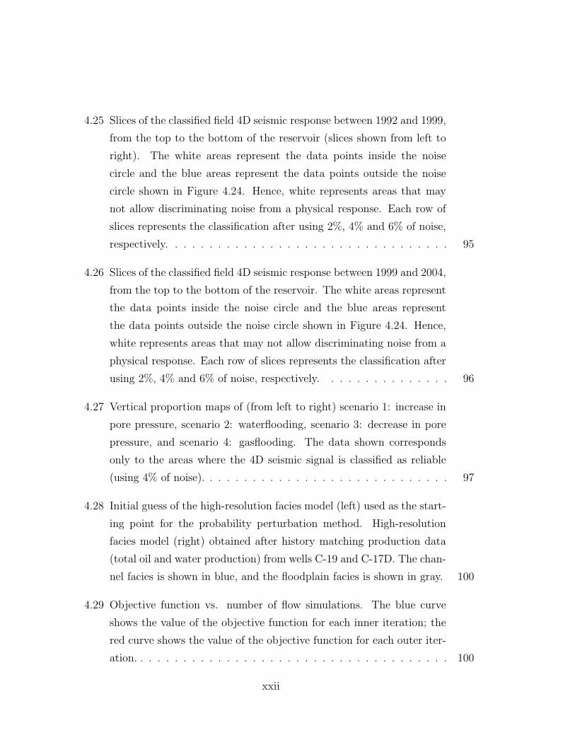
4.25 Slices of the classified field 4D seismic response between 1992 and 1999,
from the top to the bottom of the reservoir (slices shown from left to
right). The white areas represent the data points inside the noise
circle and the blue areas represent the data points outside the noise
circle shown in Figure 4.24. Hence, white represents areas that may
not allow discriminating noise from a physical response. Each row of
slices represents the classification after using 2%, 4% and 6% of noise,
respectively. . . . . . . . . . . . . . . . . . . . . . . . . . . . . . . . . 95
4.26 Slices of the classified field 4D seismic response between 1999 and 2004,
from the top to the bottom of the reservoir. The white areas represent
the data points inside the noise circle and the blue areas represent
the data points outside the noise circle shown in Figure 4.24. Hence,
white represents areas that may not allow discriminating noise from a
physical response. Each row of slices represents the classification after
using 2%, 4% and 6% of noise, respectively. . . . . . . . . . . . . . . 96
4.27 Vertical proportion maps of (from left to right) scenario 1: increase in
pore pressure, scenario 2: waterflooding, scenario 3: decrease in pore
pressure, and scenario 4: gasflooding. The data shown corresponds
only to the areas where the 4D seismic signal is classified as reliable
(using 4% of noise). . . . . . . . . . . . . . . . . . . . . . . . . . . . . 97
4.28 Initial guess of the high-resolution facies model (left) used as the start-
ing point for the probability perturbation method. High-resolution
facies model (right) obtained after history matching production data
(total oil and water production) from wells C-19 and C-17D. The chan-
nel facies is shown in blue, and the floodplain facies is shown in gray. 100
4.29 Objective function vs. number of flow simulations. The blue curve
shows the value of the objective function for each inner iteration; the
red curve shows the value of the objective function for each outer iter-
ation. . . . . . . . . . . . . . . . . . . . . . . . . . . . . . . . . . . . . 100
xxii
4.30 Total oil (top) and water production (bottom) from well C-19. His-
torical data is shown in black, the simulated total oil production from
the initial guess model is shown in magenta, and the best match ob-
tained after several flow simulations is shown in green (on the total oil
production plot), and blue (on the total water production plot). . . . 101
4.31 Total oil (top) and water production (bottom) from well C-17D. His-
torical data is shown in black, the simulated total oil production from
the initial guess model is shown in magenta, and the best match ob-
tained after several flow simulations is shown in green (on the total oil
production plot), and blue (on the total water production plot). . . . 102
4.32 Total oil (top) and water production (bottom) from well C-19. Histor-
ical data is shown in black, the other colors represent the best match
obtained for six reservoir models. . . . . . . . . . . . . . . . . . . . . 103
4.33 Total oil (top) and water production (bottom) from well C-17D. His-
torical data is shown in black, the other colors represent the best match
obtained for six reservoir models. . . . . . . . . . . . . . . . . . . . . 104
4.34 E-type (ensemble average) generated from the six history-matched
reservoir models, using the PDI Approach. . . . . . . . . . . . . . . . 105
4.35 Properties of the fluids in the Upper Ness reservoir as a function of
pore pressure (from Norsk Hydro). . . . . . . . . . . . . . . . . . . . 108
4.36 Seismic velocities of the dry rock as a function of porosity and effective
pressure. Relationships obtained in the lab from measurements made
on cores from the Oseberg Øst field (from Norsk Hydro). . . . . . . . 109
4.37 Seismic velocities of the dry rock as a function of porosity and effective
pressure obtained for Oseberg Øst (black lines) on top of dry rock ve-
locities obtained from Ness well-logs. The color code represents depth
in meters. . . . . . . . . . . . . . . . . . . . . . . . . . . . . . . . . . 111
4.38 Calibrated seismic velocities of the dry rock as a function of porosity
and effective pressure for the Alpha North Ness formation (black lines)
on top of dry rock velocities obtained from Ness well-logs. The color
code represents depth in meters. . . . . . . . . . . . . . . . . . . . . . 112
xxiii
4.39 Slices of the classified modeled 4D seismic response from the Alpha
North segment (Upper Ness Formation), from the top to the bottom
of the reservoir (slices shown from left to right). The colors represent
the classes interpreted in Figure 4.22. . . . . . . . . . . . . . . . . . . 114
4.40 Vertical proportion maps of scenario 3 (decrease in pore pressure) and
scenario 4 (gasflooding), obtained from the classified volume of the
modeled 4D response between 1992-1999 (shown in Figure4.39). . . . 114
4.41 Slices of the flow simulation results used for modeling the 4D response
shown in Figure 4.39 (top); map of the location of injector and pro-
ducer wells (bottom). The results are shown as differences between the
simulation result at year 1999 and the simulation result at year 1992. 115
4.42 Initial guess of the high-resolution facies model (left) used as the start-
ing point for the probability perturbation method. High-resolution
facies model (right) obtained after history matching both production
data (cumulative oil and water production from wells C-19 and C-
17D) and 4D seismic data (proportion maps of scenarios 3 and 4). The
channel facies is shown in blue, and the floodplain facies is shown in
gray. . . . . . . . . . . . . . . . . . . . . . . . . . . . . . . . . . . . . 119
4.43 Objective function vs. number of flow simulations. The blue curve
shows the value of the objective function for each inner iteration; the
red curve shows the value of the objective function for each outer iter-
ation; the black curve shows the production mismatch for each outer
iteration; the green curve shows the 4D seismic mismatch for each outer
iteration. . . . . . . . . . . . . . . . . . . . . . . . . . . . . . . . . . . 119
4.44 Total oil (top) and water production (bottom) from well C-19. His-
torical data is shown in black, the simulated total oil production from
the initial guess model is shown in magenta, and the best match ob-
tained after several flow simulations is shown in green (on the total oil
production plot), and blue (on the total water production plot). . . . 120
xxiv
4.45 Total oil (top) and water production (bottom) from well C-17D. His-
torical data is shown in black, the simulated total oil production from
the initial guess model is shown in magenta, and the best match ob-
tained after several flow simulations is shown in green (on the total oil
production plot), and blue (on the total water production plot). . . . 121
4.46 Vertical proportion maps of scenario 3 (decrease in pore pressure)
shown on the top row and scenario 4 (gasflooding) shown on the bot-
tom row. From left to right: the map obtained from the initial guess
reservoir model, the observed map (field data) and the map obtained
from the reservoir model that best matched both production and 4D
seismic data. . . . . . . . . . . . . . . . . . . . . . . . . . . . . . . . . 122
4.47 Initial guess of the high-resolution facies model (left) used as the start-
ing point for the probability perturbation method. High-resolution
facies model (right) obtained after history matching both production
data (cumulative oil and water production from wells C-19 and C-
17D) and 4D seismic data (proportion maps of scenarios 3 and 4). The
channel facies is shown in blue, and the floodplain facies is shown in
gray. . . . . . . . . . . . . . . . . . . . . . . . . . . . . . . . . . . . . 125
4.48 Objective function vs. number of flow simulations. The blue curve
shows the value of the objective function for each inner iteration; the
red curve shows the value of the objective function for each outer iter-
ation; the black curve shows the production mismatch for each outer
iteration; the green curve shows the value 4D seismic mismatch for
each outer iteration. . . . . . . . . . . . . . . . . . . . . . . . . . . . 125
4.49 Total oil (top) and water production (bottom) from well C-19. His-
torical data is shown in black, the simulated total oil production from
the initial guess model is shown in magenta, and the best match ob-
tained after several flow simulations is shown in green (on the total oil
production plot), and blue (on the total water production plot). . . . 126
xxv
4.50 Total oil (top) and water production (bottom) from well C-17D. His-
torical data is shown in black, the simulated total oil production from
the initial guess model is shown in magenta, and the best match ob-
tained after several flow simulations is shown in green (on the total oil
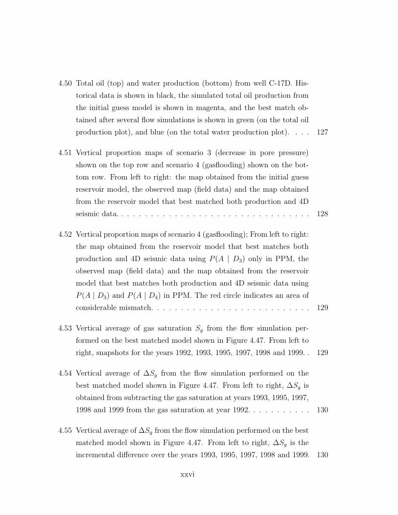
production plot), and blue (on the total water production plot). . . . 127
4.51 Vertical proportion maps of scenario 3 (decrease in pore pressure)
shown on the top row and scenario 4 (gasflooding) shown on the bot-
tom row. From left to right: the map obtained from the initial guess
reservoir model, the observed map (field data) and the map obtained
from the reservoir model that best matched both production and 4D
seismic data. . . . . . . . . . . . . . . . . . . . . . . . . . . . . . . . . 128
4.52 Vertical proportion maps of scenario 4 (gasflooding); From left to right:
the map obtained from the reservoir model that best matches both
production and 4D seismic data using P (A | D3) only in PPM, the
observed map (field data) and the map obtained from the reservoir
model that best matches both production and 4D seismic data using
P (A | D3) and P (A | D4) in PPM. The red circle indicates an area of
considerable mismatch. . . . . . . . . . . . . . . . . . . . . . . . . . . 129
4.53 Vertical average of gas saturation Sg from the flow simulation per-
formed on the best matched model shown in Figure 4.47. From left to
right, snapshots for the years 1992, 1993, 1995, 1997, 1998 and 1999. . 129
4.54 Vertical average of ∆Sg from the flow simulation performed on the
best matched model shown in Figure 4.47. From left to right, ∆Sg is
obtained from subtracting the gas saturation at years 1993, 1995, 1997,
1998 and 1999 from the gas saturation at year 1992. . . . . . . . . . . 130
4.55 Vertical average of ∆Sg from the flow simulation performed on the best
matched model shown in Figure 4.47. From left to right, ∆Sg is the
incremental difference over the years 1993, 1995, 1997, 1998 and 1999. 130
xxvi
4.56 Initial guess of the high-resolution facies model (left) used as the start-
ing point for the probability perturbation method. High-resolution
facies model (right) obtained after history matching both production
data (cumulative oil and water production from wells C-19 and C-
17D) and 4D seismic data (proportion maps of scenarios 3 and 4). The
channel facies is shown in blue, and the floodplain facies is shown in
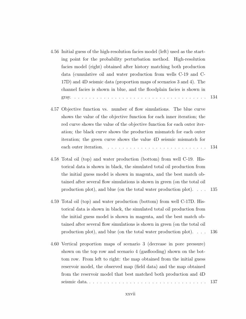
gray. . . . . . . . . . . . . . . . . . . . . . . . . . . . . . . . . . . . . 134
4.57 Objective function vs. number of flow simulations. The blue curve
shows the value of the objective function for each inner iteration; the
red curve shows the value of the objective function for each outer iter-
ation; the black curve shows the production mismatch for each outer
iteration; the green curve shows the value 4D seismic mismatch for
each outer iteration. . . . . . . . . . . . . . . . . . . . . . . . . . . . 134
4.58 Total oil (top) and water production (bottom) from well C-19. His-
torical data is shown in black, the simulated total oil production from
the initial guess model is shown in magenta, and the best match ob-
tained after several flow simulations is shown in green (on the total oil
production plot), and blue (on the total water production plot). . . . 135
4.59 Total oil (top) and water production (bottom) from well C-17D. His-
torical data is shown in black, the simulated total oil production from
the initial guess model is shown in magenta, and the best match ob-
tained after several flow simulations is shown in green (on the total oil
production plot), and blue (on the total water production plot). . . . 136
4.60 Vertical proportion maps of scenario 3 (decrease in pore pressure)
shown on the top row and scenario 4 (gasflooding) shown on the bot-
tom row. From left to right: the map obtained from the initial guess
reservoir model, the observed map (field data) and the map obtained
from the reservoir model that best matched both production and 4D
seismic data. . . . . . . . . . . . . . . . . . . . . . . . . . . . . . . . . 137
xxvii
4.61 Total oil (top) and water production (bottom) from well C-19. His-
torical data is shown in black, the simulated total oil production from
the initial guess model is shown in magenta, and the best match ob-
tained after several flow simulations is shown in green (on the total oil
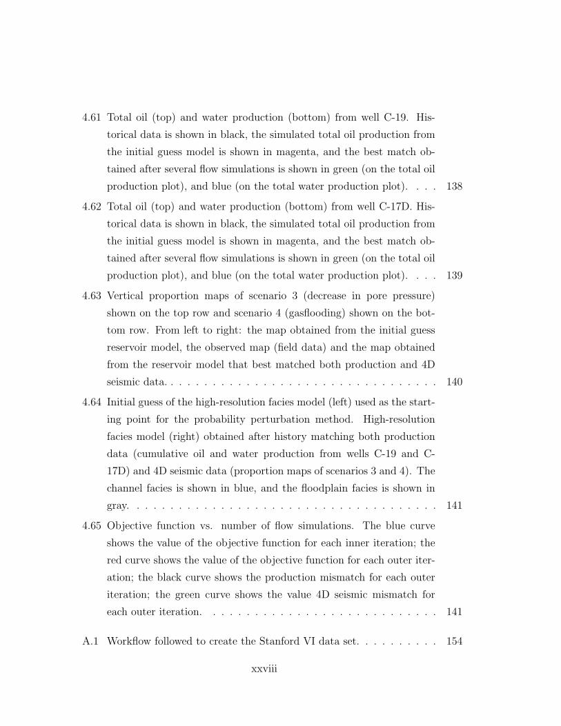
production plot), and blue (on the total water production plot). . . . 138
4.62 Total oil (top) and water production (bottom) from well C-17D. His-
torical data is shown in black, the simulated total oil production from
the initial guess model is shown in magenta, and the best match ob-
tained after several flow simulations is shown in green (on the total oil
production plot), and blue (on the total water production plot). . . . 139
4.63 Vertical proportion maps of scenario 3 (decrease in pore pressure)
shown on the top row and scenario 4 (gasflooding) shown on the bot-
tom row. From left to right: the map obtained from the initial guess
reservoir model, the observed map (field data) and the map obtained
from the reservoir model that best matched both production and 4D
seismic data. . . . . . . . . . . . . . . . . . . . . . . . . . . . . . . . . 140
4.64 Initial guess of the high-resolution facies model (left) used as the start-
ing point for the probability perturbation method. High-resolution
facies model (right) obtained after history matching both production
data (cumulative oil and water production from wells C-19 and C-
17D) and 4D seismic data (proportion maps of scenarios 3 and 4). The
channel facies is shown in blue, and the floodplain facies is shown in
gray. . . . . . . . . . . . . . . . . . . . . . . . . . . . . . . . . . . . . 141
4.65 Objective function vs. number of flow simulations. The blue curve
shows the value of the objective function for each inner iteration; the
red curve shows the value of the objective function for each outer iter-
ation; the black curve shows the production mismatch for each outer
iteration; the green curve shows the value 4D seismic mismatch for
each outer iteration. . . . . . . . . . . . . . . . . . . . . . . . . . . . 141
A.1 Workflow followed to create the Stanford VI data set. . . . . . . . . . 154
xxviii

A.2 Perspective view of the Stanford VI top structure: view from SW (left),
view from SE (right). The color indicates the depth to the top. . . . . 155
A.3 Perspective view of the Stanford VI top and bottom of each of its
layers. The color indicates the depth to the top. . . . . . . . . . . . . 156
A.4 Facies model of Layer 1, which corresponds to sinuous channels: flood-
plain (navy blue), point bar (light blue), channel (yellow), and bound-
ary (red). Stratigraphic grid (left), and cartesian box (right). . . . . . 157
A.5 Facies model of Layer 2, which corresponds to meandering channels:
floodplain (navy blue), point bar (light blue), channel (yellow), and
boundary (red). Stratigraphic grid (left), and Cartesian box (right). . 158
A.6 Facies model of Layer 3 (top), which corresponds to deltaic deposits:
floodplain (navy blue), and channel (yellow). Stratigraphic grid (left),
Cartesian box (right), angle cube (middle), and affinity cube (bottom). 160
A.7 Training Image used for modeling Layer 3. The size of the training
image is 200 × 200 × 5, each slice in the z − direction is shown here
from top to bottom. . . . . . . . . . . . . . . . . . . . . . . . . . . . 161
A.8 Distribution of porosity for each facies in the reservoir. . . . . . . . . 162
A.9 Histogram of porosity for each facies in the reservoir. . . . . . . . . . 163
A.10 Resulting Porosity cube after cookie-cut porosity from each facies’
porosity realization. . . . . . . . . . . . . . . . . . . . . . . . . . . . . 164
A.11 Histogram of the logarithm of permeability, per facies in the reservoir. 165
A.12 Resulting Permeability cube after cookie-cutting permeability from
each facies’ permeability realization. . . . . . . . . . . . . . . . . . . . 166
A.13 Cementing versus sorting trends. . . . . . . . . . . . . . . . . . . . . 168
A.14 P-wave velocity vs. porosity for shales and brine-saturated sandstones. 172
A.15 Resulting density (top), Vp (middle) and Vs (bottom) cubes for the
oil-saturated reservoir. . . . . . . . . . . . . . . . . . . . . . . . . . . 175
A.16 Petrophysical properties crossplots. From left to right: P-wave velocity
vs. porosity, P-wave velocity vs. density, S-wave velocity vs. P-wave
velocity, and porosity vs. density. . . . . . . . . . . . . . . . . . . . . 176
xxix
A.17 P-wave hitting a reflector. The physical properties are different on
either side of the reflector. . . . . . . . . . . . . . . . . . . . . . . . . 179
A.18 Seismic wavefront hitting a reflector. The physical properties are dif-
ferent on either side of the reflector. The part of the P wave striking
at a particular angle-of-incidence (represented by a ray) will have its
energy divided into reflected and transmitted P and S waves. . . . . . 180
A.19 Seismic attributes at the Geostatistical Scale: Acoustic Impedance,
Elastic Impedance, S-wave Impedance, Poisson’s Ratio, Lame coeffi-
cients λ µ. . . . . . . . . . . . . . . . . . . . . . . . . . . . . . . . . . 184
A.20 Seismic attributes crossplots. From left to right: Acoustic impedance
vs. porosity, Elastic impedance vs. porosity, and Acoustic impedance
vs. Elastic impedance. . . . . . . . . . . . . . . . . . . . . . . . . . . 185
A.21 Seismic attributes crossplots. From left to right: Poisson’s Ratio vs.
Acoustic impedance, Poisson’s Ratio vs. Elastic impedance, and Pois-
son’s Ratio vs. porosity. . . . . . . . . . . . . . . . . . . . . . . . . . 185
A.22 Seismic attributes crossplots. From left to right: S-wave impedance
vs. porosity, S-wave impedance vs. Elastic impedance, and Poisson’s
Ratio vs. S-wave impedance. . . . . . . . . . . . . . . . . . . . . . . . 186
A.23 Lame coefficients λ vs. µ. . . . . . . . . . . . . . . . . . . . . . . . . 186
A.24 AVO Intercept vs. Gradient for oil and brine-saturated sandstones. . 187
A.25 Seismic attributes at the Seismic Scale: Acoustic Impedance, Elastic
Impedance, S-wave Impedance, Poisson’s Ratio, Lame coefficients λ µ,
AVO attributes Intercept and Gradient. . . . . . . . . . . . . . . . . . 188
A.26 Porosity at the high-resolution (left), linearly averaged porosity after
upscaling. . . . . . . . . . . . . . . . . . . . . . . . . . . . . . . . . . 190
A.27 Effective Permeability after upscaling: kx (top left), ky (top right), kz
(bottom). . . . . . . . . . . . . . . . . . . . . . . . . . . . . . . . . . 191
A.28 Oil and Water Relative Permeability curves. . . . . . . . . . . . . . . 192
A.29 Location maps of producer wells (left), and injector wells (right). The
color represents horizon top depth (ft). . . . . . . . . . . . . . . . . . 193
xxx
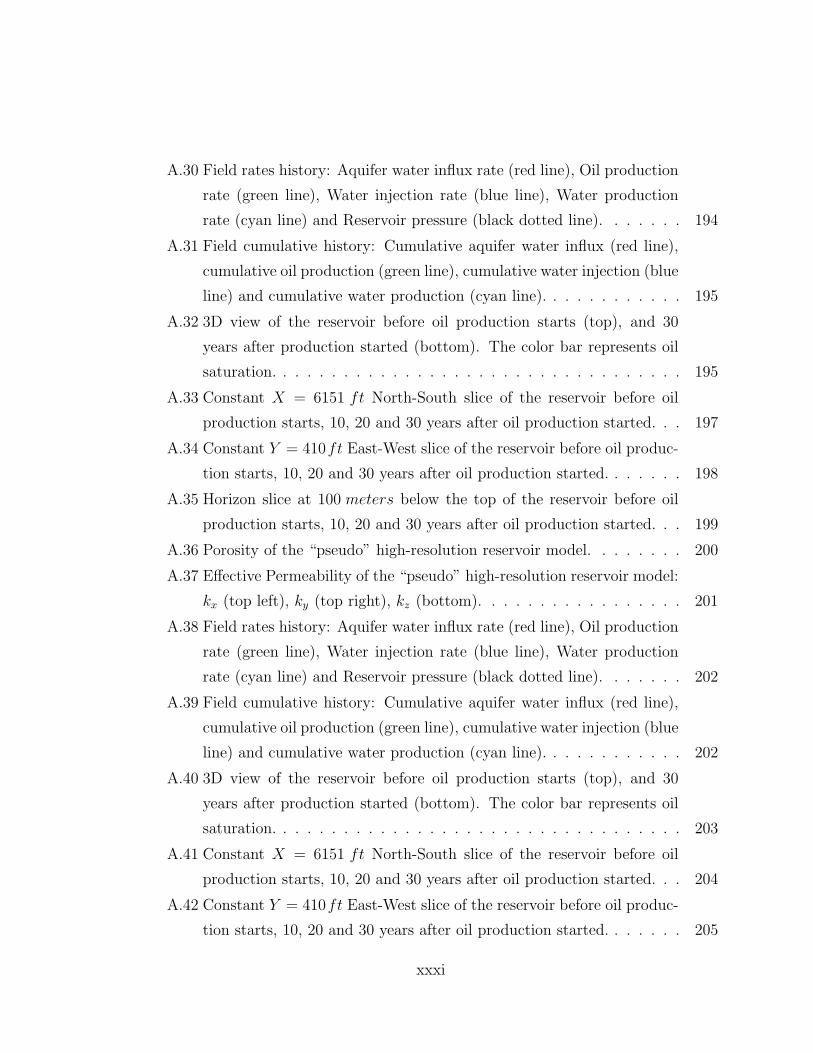
A.30 Field rates history: Aquifer water influx rate (red line), Oil production
rate (green line), Water injection rate (blue line), Water production
rate (cyan line) and Reservoir pressure (black dotted line). . . . . . . 194
A.31 Field cumulative history: Cumulative aquifer water influx (red line),
cumulative oil production (green line), cumulative water injection (blue
line) and cumulative water production (cyan line). . . . . . . . . . . . 195
A.32 3D view of the reservoir before oil production starts (top), and 30
years after production started (bottom). The color bar represents oil
saturation. . . . . . . . . . . . . . . . . . . . . . . . . . . . . . . . . . 195
A.33 Constant X = 6151 ft North-South slice of the reservoir before oil
production starts, 10, 20 and 30 years after oil production started. . . 197
A.34 Constant Y = 410ft East-West slice of the reservoir before oil produc-
tion starts, 10, 20 and 30 years after oil production started. . . . . . . 198
A.35 Horizon slice at 100 meters below the top of the reservoir before oil
production starts, 10, 20 and 30 years after oil production started. . . 199
A.36 Porosity of the “pseudo” high-resolution reservoir model. . . . . . . . 200
A.37 Effective Permeability of the “pseudo” high-resolution reservoir model:
kx (top left), ky (top right), kz (bottom). . . . . . . . . . . . . . . . . 201
A.38 Field rates history: Aquifer water influx rate (red line), Oil production
rate (green line), Water injection rate (blue line), Water production
rate (cyan line) and Reservoir pressure (black dotted line). . . . . . . 202
A.39 Field cumulative history: Cumulative aquifer water influx (red line),
cumulative oil production (green line), cumulative water injection (blue
line) and cumulative water production (cyan line). . . . . . . . . . . . 202
A.40 3D view of the reservoir before oil production starts (top), and 30
years after production started (bottom). The color bar represents oil
saturation. . . . . . . . . . . . . . . . . . . . . . . . . . . . . . . . . . 203
A.41 Constant X = 6151 ft North-South slice of the reservoir before oil
production starts, 10, 20 and 30 years after oil production started. . . 204
A.42 Constant Y = 410ft East-West slice of the reservoir before oil produc-
tion starts, 10, 20 and 30 years after oil production started. . . . . . . 205
xxxi
A.43 Horizon slice at 100 meters below the top of the reservoir before oil
production starts, 10, 20 and 30 years after oil production started. . . 206
A.44 Water cut versus time for well P21: solution from “pseudo” high-
resolution model (red), and solution from upscaled model (blue). Wa-
ter saturation 24 years after oil production started: solution from
“pseudo” high-resolution model (middle), and solution from the up-
scaled model (bottom). . . . . . . . . . . . . . . . . . . . . . . . . . . 207
A.45 Base seismic data set acquired prior to oil production (top left), seismic
data sets acquired after 10 years of oil production (top right), after 25
years of oil production (bottom left), after 30 years of oil production
(bottom right). . . . . . . . . . . . . . . . . . . . . . . . . . . . . . . 209
A.46 Workflow used to create the 4D seismic response at different times
during oil production. . . . . . . . . . . . . . . . . . . . . . . . . . . . 212
A.47 Water saturation from upscaled model after 10 (top left), 25 (top mid-
dle) and 30 (top right) years of oil production. Seismic amplitude
difference from upscaled model for 10 (middle left), 25 (middle mid-
dle) and 30 (middle right) years of oil production. Seismic amplitude
incremental difference from upscaled model for 10 (bottom left), 25
(bottom middle) and 30 (bottom right) years of oil production. . . . . 213
A.48 Water saturation from “pseudo” high-resolution model after 10 (top
left), 25 (top middle) and 30 (top right) years of oil production. Seis-
mic amplitude difference from “pseudo” fine scale model for 10 (middle
left), 25 (middle middle) and 30 (middle right) years of oil produc-
tion. Seismic amplitude incremental difference from “pseudo” high-
resolution model for 10 (bottom left), 25 (bottom middle) and 30 (bot-
tom right) years of oil production. . . . . . . . . . . . . . . . . . . . . 214
B.1 Main window of the program S-GeMS showing the grids and proper-
ties used in the snesim parameter file, the algorithm panel where the
parameters can be manually input, and the visualization panel with a
simulated facies realization. . . . . . . . . . . . . . . . . . . . . . . . 217
xxxii
C.1 History Match # 1. Total oil (top) and water production (bottom)
from well C-19. Historical data is shown in black, the simulated total oil
production from the initial guess model is shown in magenta, and the
best match obtained after several flow simulations is shown in green (on
the total oil production plot), and blue (on the total water production
plot). . . . . . . . . . . . . . . . . . . . . . . . . . . . . . . . . . . . . 219
C.2 Total oil (top) and water production (bottom) from well C-17D. His-
torical data is shown in black, the simulated total oil production from
the initial guess model is shown in magenta, and the best match ob-
tained after several flow simulations is shown in green (on the total oil
production plot), and blue (on the total water production plot). . . . 220
C.3 History Match # 1. Initial guess of the high resolution facies model
(left) used as the starting point for the probability perturbation method.
High resolution facies model (right) obtained after history matching
production data (cumulative oil and water production) from wells C-
19 and C-17D. The channel facies is shown in blue, and the floodplain
facies is shown in gray. . . . . . . . . . . . . . . . . . . . . . . . . . . 221
C.4 History Match # 1. Objective function vs. number of flow simulations.
The blue curve shows the value of the objective function for each inner
iteration; the red curve shows the value of the objective function for
each outer iteration. . . . . . . . . . . . . . . . . . . . . . . . . . . . 221
C.5 History Match # 2. Total oil (top) and water production (bottom)
from well C-19. Historical data is shown in black, the simulated total oil
production from the initial guess model is shown in magenta, and the
best match obtained after several flow simulations is shown in green (on
the total oil production plot), and blue (on the total water production
plot). . . . . . . . . . . . . . . . . . . . . . . . . . . . . . . . . . . . . 222
xxxiii
C.6 History Match # 2. Total oil (top) and water production (bottom)
from well C-17D. Historical data is shown in black, the simulated to-
tal oil production from the initial guess model is shown in magenta,
and the best match obtained after several flow simulations is shown in
green (on the total oil production plot), and blue (on the total water
production plot). . . . . . . . . . . . . . . . . . . . . . . . . . . . . . 223
C.7 History Match # 2. Initial guess of the high resolution facies model
(left) used as the starting point for the probability perturbation method.
High resolution facies model (right) obtained after history matching
production data (cumulative oil and water production) from wells C-
19 and C-17D. The channel facies is shown in blue, and the floodplain
facies is shown in gray. . . . . . . . . . . . . . . . . . . . . . . . . . . 224
C.8 History Match # 2. Objective function vs. number of flow simulations.
The blue curve shows the value of the objective function for each inner
iteration; the red curve shows the value of the objective function for
each outer iteration. . . . . . . . . . . . . . . . . . . . . . . . . . . . 224
C.9 History Match # 3. Total oil (top) and water production (bottom)
from well C-19. Historical data is shown in black, the simulated total oil
production from the initial guess model is shown in magenta, and the
best match obtained after several flow simulations is shown in green (on
the total oil production plot), and blue (on the total water production
plot). . . . . . . . . . . . . . . . . . . . . . . . . . . . . . . . . . . . . 225
C.10 History Match # 3. Total oil (top) and water production (bottom)
from well C-17D. Historical data is shown in black, the simulated to-
tal oil production from the initial guess model is shown in magenta,
and the best match obtained after several flow simulations is shown in
green (on the total oil production plot), and blue (on the total water
production plot). . . . . . . . . . . . . . . . . . . . . . . . . . . . . . 226
xxxiv
C.11 History Match # 3. Initial guess of the high resolution facies model
(left) used as the starting point for the probability perturbation method.
High resolution facies model (right) obtained after history matching
production data (cumulative oil and water production) from wells C-
19 and C-17D. The channel facies is shown in blue, and the floodplain
facies is shown in gray. . . . . . . . . . . . . . . . . . . . . . . . . . . 227
C.12 History Match # 3. Objective function vs. number of flow simulations.
The blue curve shows the value of the objective function for each inner
iteration; the red curve shows the value of the objective function for
each outer iteration. . . . . . . . . . . . . . . . . . . . . . . . . . . . 227
C.13 History Match # 4. Total oil (top) and water production (bottom)
from well C-19. Historical data is shown in black, the simulated total oil
production from the initial guess model is shown in magenta, and the
best match obtained after several flow simulations is shown in green (on
the total oil production plot), and blue (on the total water production
plot). . . . . . . . . . . . . . . . . . . . . . . . . . . . . . . . . . . . . 228
C.14 History Match # 4. Total oil (top) and water production (bottom)
from well C-17D. Historical data is shown in black, the simulated to-
tal oil production from the initial guess model is shown in magenta,
and the best match obtained after several flow simulations is shown in
green (on the total oil production plot), and blue (on the total water
production plot). . . . . . . . . . . . . . . . . . . . . . . . . . . . . . 229
C.15 History Match # 4. Initial guess of the high resolution facies model
(left) used as the starting point for the probability perturbation method.
High resolution facies model (right) obtained after history matching
production data (cumulative oil and water production) from wells C-
19 and C-17D. The channel facies is shown in blue, and the floodplain
facies is shown in gray. . . . . . . . . . . . . . . . . . . . . . . . . . . 230
xxxv
C.16 History Match # 4. Objective function vs. number of flow simulations.
The blue curve shows the value of the objective function for each inner
iteration; the red curve shows the value of the objective function for
each outer iteration. . . . . . . . . . . . . . . . . . . . . . . . . . . . 230
C.17 History Match # 5. Total oil (top) and water production (bottom)
from well C-19. Historical data is shown in black, the simulated total oil
production from the initial guess model is shown in magenta, and the
best match obtained after several flow simulations is shown in green (on
the total oil production plot), and blue (on the total water production
plot). . . . . . . . . . . . . . . . . . . . . . . . . . . . . . . . . . . . . 231
C.18 History Match # 5. Total oil (top) and water production (bottom)
from well C-17D. Historical data is shown in black, the simulated to-
tal oil production from the initial guess model is shown in magenta,
and the best match obtained after several flow simulations is shown in
green (on the total oil production plot), and blue (on the total water
production plot). . . . . . . . . . . . . . . . . . . . . . . . . . . . . . 232
C.19 History Match # 5. Initial guess of the high resolution facies model
(left) used as the starting point for the probability perturbation method.
High resolution facies model (right) obtained after history matching
production data (cumulative oil and water production) from wells C-
19 and C-17D. The channel facies is shown in blue, and the floodplain
facies is shown in gray. . . . . . . . . . . . . . . . . . . . . . . . . . . 233
C.20 History Match # 5. Objective function vs. number of flow simulations.
The blue curve shows the value of the objective function for each inner
iteration; the red curve shows the value of the objective function for
each outer iteration. . . . . . . . . . . . . . . . . . . . . . . . . . . . 233
xxxvi
C.21 History Match # 6. Total oil (top) and water production (bottom)
from well C-19. Historical data is shown in black, the simulated total oil
production from the initial guess model is shown in magenta, and the
best match obtained after several flow simulations is shown in green (on
the total oil production plot), and blue (on the total water production
plot). . . . . . . . . . . . . . . . . . . . . . . . . . . . . . . . . . . . . 234
C.22 History Match # 6. Total oil (top) and water production (bottom)
from well C-17D. Historical data is shown in black, the simulated to-
tal oil production from the initial guess model is shown in magenta,
and the best match obtained after several flow simulations is shown in
green (on the total oil production plot), and blue (on the total water
production plot). . . . . . . . . . . . . . . . . . . . . . . . . . . . . . 235
C.23 History Match # 6. Initial guess of the high resolution facies model
(left) used as the starting point for the probability perturbation method.
High resolution facies model obtained after history matching produc-
tion data (cumulative oil and water production) from wells C-19 and
C-17D. The channel facies is shown in blue, and the floodplain facies
is shown in gray. . . . . . . . . . . . . . . . . . . . . . . . . . . . . . 236
C.24 History Match # 6. Objective function vs. number of flow simulations.
The blue curve shows the value of the objective function for each inner
iteration; the red curve shows the value of the objective function for
each outer iteration. . . . . . . . . . . . . . . . . . . . . . . . . . . . 236
xxxvii

xxxviii
Chapter 1
Introduction
Creating a reservoir model is becoming common practice during several stages of
a reservoir’s life. From exploration to field abandonment, reservoir modeling aims
at understanding and predicting important geological, geophysical and engineering
components of the reservoir.
Our knowledge about the properties of the reservoir changes from one stage to the
other as more data becomes available. During the early exploration stages we may
want to estimate the OOIP in the reservoir; however, during later production stages
we may want to forecast production for the next few years, or plan new wells and/or
surface facilities.
Reservoir modeling calls for the integration of expertise from different disciplines,
as well as the integration of data from various sources. Each type of data provides
information about the reservoir heterogeneity on a different scale; therefore, they have
different degrees of accuracy and may be redundant with each other to certain degrees.
The reservoir model needs to simultaneously (not hierarchically) honor all available
data, both static and dynamic, in order to preserve its predictive capabilities.
Static data includes all data that have been measured or interpreted once in time;
such as:
• Core data: porosity, permeability, relative permeability, wave velocities, etc.
• Well-log data: any suite of logs that indicate lithology and fluid types near the
well-bore.
1
2 CHAPTER 1. INTRODUCTION
• Outcrop analog data.
• Sedimentological and stratigraphic interpretation.
• Stratigraphic horizons and faults interpreted from 3D seismic data.
• Seismic attributes.
• Rock physics data.
• PVT data.
On the contrary, dynamic data includes all data that have been measured or inter-
preted over time; such as:
• Production data: Fluid rates or volumes, pressure data.
• 4D seismic data: any suite of 3D seismic attributes computed from each seismic
survey.
1.1 Reservoir Modeling and Data Integration
The state-of-the-art practice of reservoir modeling starts by creating a high resolution
3D geo-cellular model using static data. A hierarchical approach to build the 3D geo-
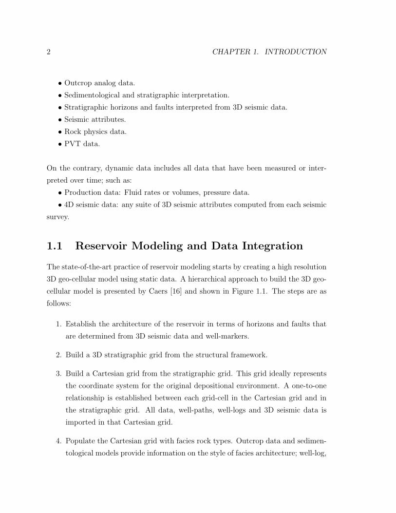
cellular model is presented by Caers [16] and shown in Figure 1.1. The steps are as
follows:
1. Establish the architecture of the reservoir in terms of horizons and faults that
are determined from 3D seismic data and well-markers.
2. Build a 3D stratigraphic grid from the structural framework.
3. Build a Cartesian grid from the stratigraphic grid. This grid ideally represents
the coordinate system for the original depositional environment. A one-to-one
relationship is established between each grid-cell in the Cartesian grid and in
the stratigraphic grid. All data, well-paths, well-logs and 3D seismic data is
imported in that Cartesian grid.
4. Populate the Cartesian grid with facies rock types. Outcrop data and sedimen-
tological models provide information on the style of facies architecture; well-log,
1.1. RESERVOIR MODELING AND DATA INTEGRATION 3
core and seismic data provide local constraints on the spatial distribution of
these facies types.
5. Populate each facies type with porosity and permeability. Porosity is assigned to
each grid cell of the Cartesian grid based on well-log and core data; permeability
is derived from the porosity model. Porosity is usually determined first since
the data on porosity is more reliable and abundant than permeability data.
6. Map back the petrophysical properties into the stratigraphic grid to provide a
high-resolution 3D geo-cellular model.
Figure 1.1: Step-by-step workflow for building a high-resolution geo-cellular model(from Caers [16]).
4 CHAPTER 1. INTRODUCTION
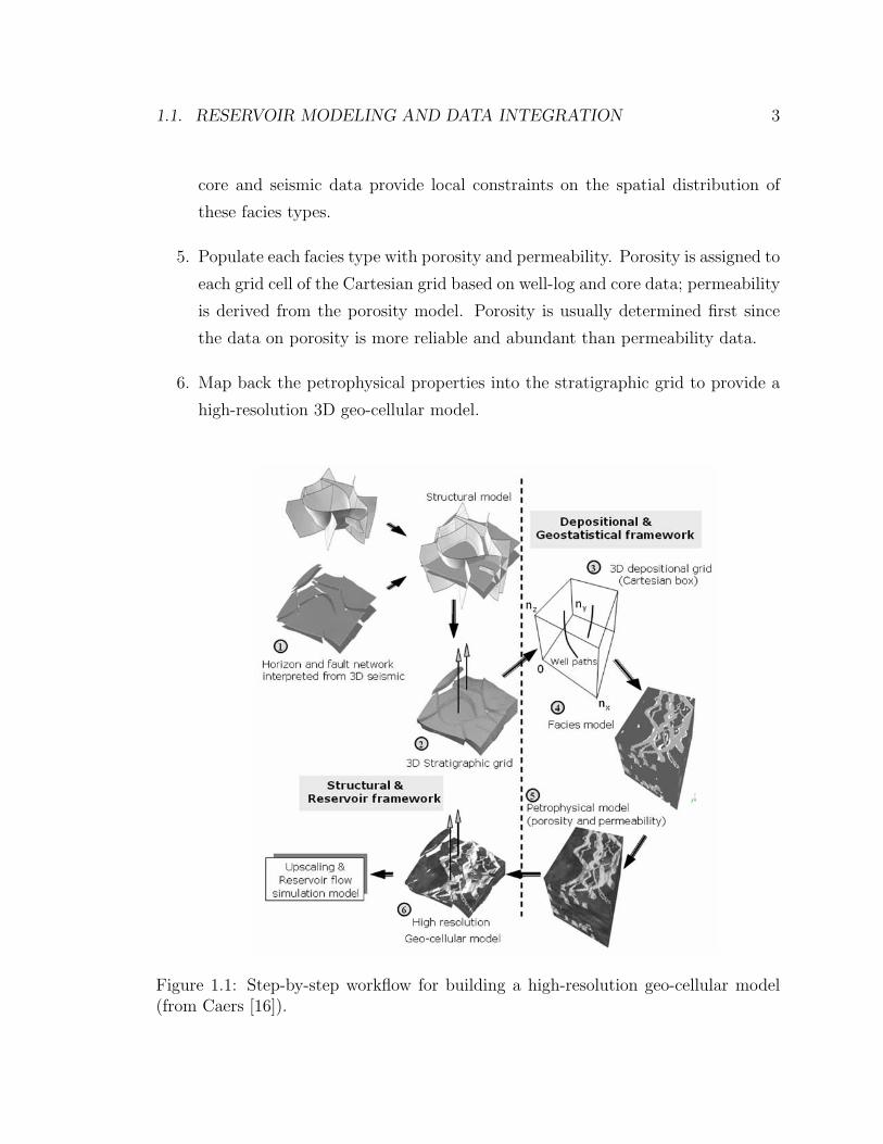
The high-resolution 3D geo-cellular model obtained after following these steps
honors static data but does not match the existing production data (Figure 1.2);
therefore, a history matching procedure is applied to perturb the reservoir model
until the flow response of the model matches the field production data.
Figure 1.2: High resolution model (left) which only matches static data; its flowresponse does not match historical water cut at the producer wells.
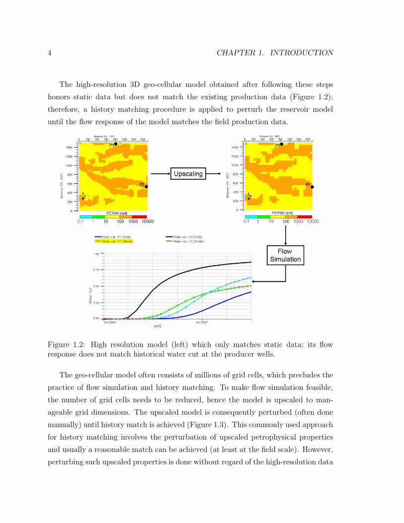
The geo-cellular model often consists of millions of grid cells, which precludes the
practice of flow simulation and history matching. To make flow simulation feasible,
the number of grid cells needs to be reduced, hence the model is upscaled to man-
ageable grid dimensions. The upscaled model is consequently perturbed (often done
manually) until history match is achieved (Figure 1.3). This commonly used approach
for history matching involves the perturbation of upscaled petrophysical properties
and usually a reasonable match can be achieved (at least at the field scale). However,
perturbing such upscaled properties is done without regard of the high-resolution data
1.1. RESERVOIR MODELING AND DATA INTEGRATION 5
and model which honors well-log, geological information and 3D seismic data. The
final result of this approach is a model that only matches production history, but it is
no longer consistent with any data integrated prior to matching; this often precludes
the prediction of future production since the model has lost most if not all geological
realism.
Figure 1.3: Coarsened model (from Figure 1.2) being manually perturbed until his-torical water cut at the producer wells is matched.
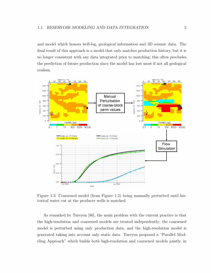
As remarked by Tureyen [86], the main problem with the current practice is that
the high-resolution and coarsened models are treated independently; the coarsened
model is perturbed using only production data, and the high-resolution model is
generated taking into account only static data. Tureyen proposed a “Parallel Mod-
eling Approach” which builds both high-resolution and coarsened models jointly, in
6 CHAPTER 1. INTRODUCTION
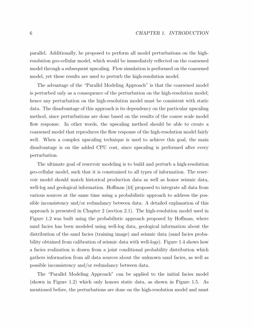
parallel. Additionally, he proposed to perform all model perturbations on the high-
resolution geo-cellular model, which would be immediately reflected on the coarsened
model through a subsequent upscaling. Flow simulation is performed on the coarsened
model, yet these results are used to perturb the high-resolution model.
The advantage of the “Parallel Modeling Approach” is that the coarsened model
is perturbed only as a consequence of the perturbation on the high-resolution model;
hence any perturbation on the high-resolution model must be consistent with static
data. The disadvantage of this approach is its dependency on the particular upscaling
method, since perturbations are done based on the results of the coarse scale model
flow response. In other words, the upscaling method should be able to create a
coarsened model that reproduces the flow response of the high-resolution model fairly
well. When a complex upscaling technique is used to achieve this goal, the main
disadvantage is on the added CPU cost, since upscaling is performed after every
perturbation.
The ultimate goal of reservoir modeling is to build and perturb a high-resolution
geo-cellular model, such that it is constrained to all types of information. The reser-
voir model should match historical production data as well as honor seismic data,
well-log and geological information. Hoffman [44] proposed to integrate all data from
various sources at the same time using a probabilistic approach to address the pos-
sible inconsistency and/or redundancy between data. A detailed explanation of this
approach is presented in Chapter 2 (section 2.1). The high-resolution model used in
Figure 1.2 was built using the probabilistic approach proposed by Hoffman, where
sand facies has been modeled using well-log data, geological information about the
distribution of the sand facies (training image) and seismic data (sand facies proba-
bility obtained from calibration of seismic data with well-logs). Figure 1.4 shows how
a facies realization is drawn from a joint conditional probability distribution which
gathers information from all data sources about the unknown sand facies, as well as
possible inconsistency and/or redundancy between data.
The “Parallel Modeling Approach” can be applied to the initial facies model
(shown in Figure 1.2) which only honors static data, as shown in Figure 1.5. As
mentioned before, the perturbations are done on the high-resolution model and must
1.2. INCORPORATING 4D SEISMIC DATA 7
be geologically consistent with static data. Using a technique called “Probability
Perturbation Method” (PPM), presented by Caers [15], Hoffman proposed to perturb
large scale parameters such as facies distributions while honoring all other available
data. The fundamental principle behind PPM is that perturbations are done on the
conditional probability from which a model is drawn, rather then on the model it-
self (Figure 1.6). The perturbations are done iteratively such that the model’s flow
response is closer to matching the production data.
The reservoir modeling workflow proposed in this dissertation, follows the “Parallel
Modeling Approach” of perturbing the high-resolution model directly, and also uses
the probabilistic data integration approach presented by Hoffman. However, the main
contribution of the workflow proposed here is the inclusion of 4D seismic data, which
had previously not been accounted for.
1.2 Incorporating 4D Seismic Data
Termed “four-dimensional seismology” by Nur [64], 4D seismic data comprise the set
of 3D seismic data acquired at different times over the same area, with the objective
of monitoring changes occurring in a producing hydrocarbon reservoir over time.
4D seismic data record two types of changes: changes in reservoir properties due
to production, and changes in external variables such as ambient noise, recording
equipment, etc. The second type of changes, termed “undesirables” by Jack [45],
represent a research area of its own within the geophysical community; however, it
is out of the scope of this dissertation. The methodology proposed here ignores the
existence of 3D seismic repeatability issues.
Changes in reservoir properties due to production are recorded by 4D seismic data
since seismic velocities and impedance depend on changes in pore fluids, pressure and
temperature [63] [10] [90]. The overall elastic moduli of a rock change with the type
of fluid in the pores, the effective pressure acting on the rock, and the temperature
the rock is subjected to. Due to the change in elastic moduli, the rock becomes more
or less resistant to wave-induced deformations; therefore, seismic velocities experience
an increase or decrease in magnitude. These observations are the basis for using 4D
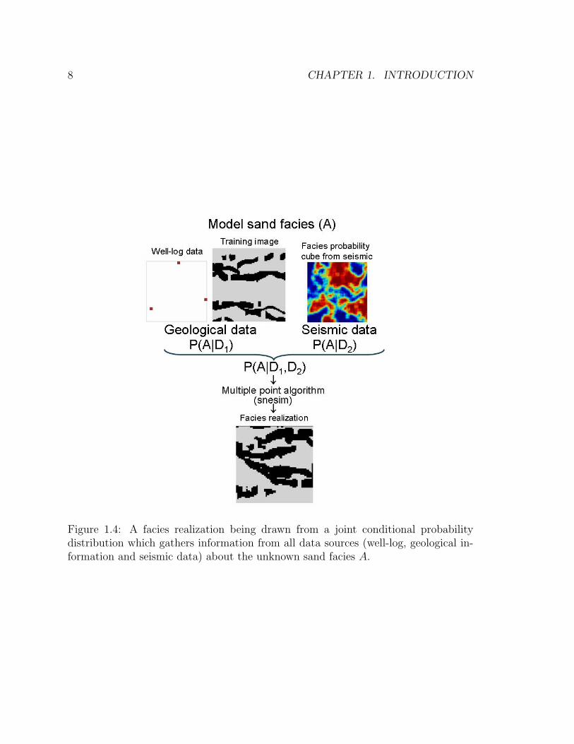
8 CHAPTER 1. INTRODUCTION
Figure 1.4: A facies realization being drawn from a joint conditional probabilitydistribution which gathers information from all data sources (well-log, geological in-formation and seismic data) about the unknown sand facies A.
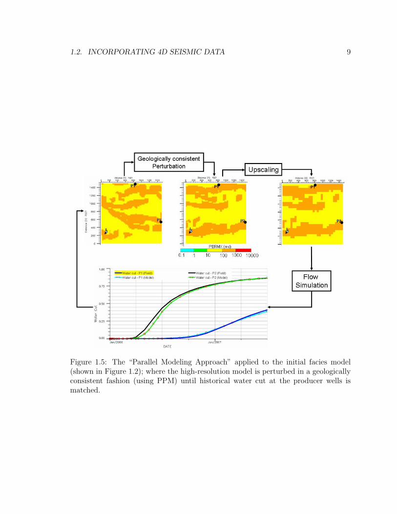
1.2. INCORPORATING 4D SEISMIC DATA 9
Figure 1.5: The “Parallel Modeling Approach” applied to the initial facies model(shown in Figure 1.2); where the high-resolution model is perturbed in a geologicallyconsistent fashion (using PPM) until historical water cut at the producer wells ismatched.
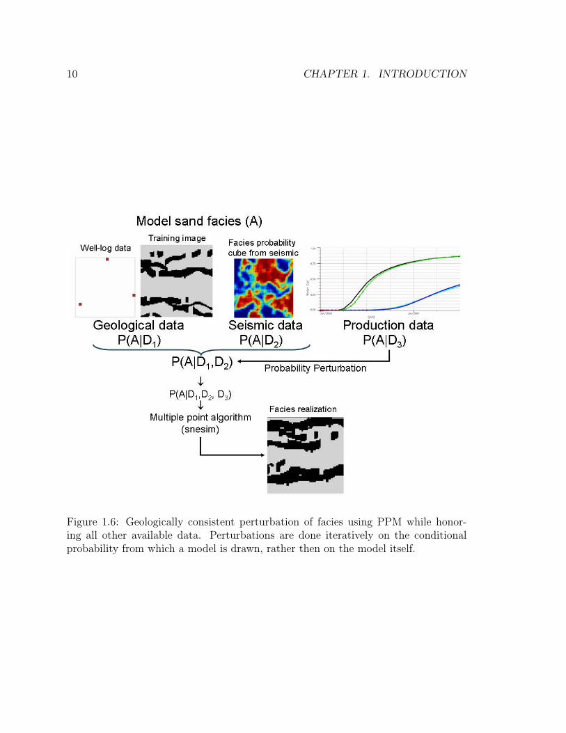
10 CHAPTER 1. INTRODUCTION
Figure 1.6: Geologically consistent perturbation of facies using PPM while honor-ing all other available data. Perturbations are done iteratively on the conditionalprobability from which a model is drawn, rather then on the model itself.
1.2. INCORPORATING 4D SEISMIC DATA 11
seismic data in predicting fluid saturation and pressure changes in the reservoir.
Typically, the difference between two 3D seismic data sets recorded at different
times allows mapping those areas in the reservoir where pressure and/or the distribu-
tion of fluids have changed. Therefore, 4D seismic data not only provides information
about the dynamic process occurring in the reservoir while production takes place; but
also provides information about the spatial lithological heterogeneity where dynamic
changes occur.
1.2.1 Challenges
Providing a spatial distribution of dynamic changes in a producing reservoir, 4D
seismic can be treated as dynamic data, hence can be history matched along with
production data within the reservoir modeling workflow. This quantitative approach
to incorporate 4D seismic data calls for forward modeling the 4D seismic response,
and comparing it with the observed field response.
As production takes place in a reservoir, the spatial distribution of pressure and
saturation in the reservoir changes over time; therefore, the overall elastic moduli of
the reservoir rock changes and 4D seismic is able to record those changes through
“seismic observables”, often called seismic attributes. “Seismic attributes are all the
information obtained from seismic data, either by direct measurements or by logical
or experience based reasoning” [82]. Generally speaking, most seismic attributes are
functions of density, and the velocities of P and S waves as they travel through the
rock; for example, acoustic impedance (a seismic attribute) is the product of density
and P-wave velocity.
Forward modeling the 4D seismic response involves the computation of the seismic
attribute(s) as the spatial distribution of pressure and saturation in the reservoir
changes over time. For the example of acoustic impedance (AI), the change over
time of this seismic attribute can be computed as the set:
[AI]t1 , [AI]t2 , ... [AI]tn
where [AI]ti = [ρVp]ti is the acoustic impedance at time ti, obtained by computing

12 CHAPTER 1. INTRODUCTION
density (ρ) and P-wave velocity (Vp) of the rock subject to the conditions at time
ti, pressure and saturation at that time. The effect of pressure and saturation on
the density of a rock, as well as their effect on the velocity of P and S waves as
they travel through the rock is computed using rock physics models. A detailed
explanation of this procedure is given in Chapter 2 (section 2.3.1); however, for now
it is important to mention that density, P and S-wave velocities for each grid block of
the high-resolution reservoir model are computed first and the conditions - pressure
and saturation - at time ti are imposed later. The spatial distribution of pressure and
saturation is obtained after flow simulation, which is performed on a coarsened grid.
The 4D seismic response is forward modeled using the high-resolution reservoir
properties since seismic waves are often affected by fine scale details below seismic
resolution [58] [74] [75]; therefore, the first challenge encountered is how to port the
coarsened pressure and saturation into the high-resolution grid.
The 4D seismic response is usually due to a combination of both pressure and
saturation effects. A change in pressure often causes a change in saturation in the
reservoir, especially during early stages of production (primary depletion). Sometimes
one effect may dominate the other; therefore, the second challenge encountered is how
to correctly model those effects using rock physics models and lab measurements of
the dependency of P and S wave velocities on pressure.
Comparing the modeled and the field 4D seismic response is an important step
when history matching both production and 4D seismic data. A measure of similarity
or discrepancy must be established, such as a point-to-point correlation coefficient or
an absolute difference between the forward modeled and the observed 4D responses;
however, regardless of the comparison method used, 4D seismic data must be exam-
ined before hand in order to find the “reservoir signal” to be matched.
Chapter 4 of this dissertation shows in detail a case study from a reservoir in the
North Sea where three 3D seismic surveys have been acquired, respectively in the
years of 1992, 1999 and 2004. From each 3D seismic survey, AI and Vp/Vs ratio are
the seismic attributes studied; the change on both attributes over time is summarized
by Figure 1.7. This figure clearly shows that some areas in the reservoir have changed
more significantly than others; in particular, data points located close to the center of
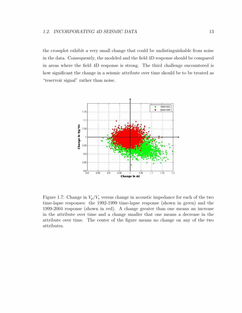
1.2. INCORPORATING 4D SEISMIC DATA 13
the crossplot exhibit a very small change that could be undistinguishable from noise
in the data. Consequently, the modeled and the field 4D response should be compared
in areas where the field 4D response is strong. The third challenge encountered is
how significant the change in a seismic attribute over time should be to be treated as
“reservoir signal” rather than noise.
Figure 1.7: Change in Vp/Vs versus change in acoustic impedance for each of the twotime-lapse responses: the 1992-1999 time-lapse response (shown in green) and the1999-2004 response (shown in red). A change greater than one means an increasein the attribute over time and a change smaller that one means a decrease in theattribute over time. The center of the figure means no change on any of the twoattributes.
14 CHAPTER 1. INTRODUCTION
1.2.2 Current Approaches
A few papers are referenced in the literature for quantitatively matching 4D seismic
along with production data. Basically, two approaches are distinguished:
• The first approach strives to match the change of an interpreted physical prop-
erty from 4D seismic data. Some authors look for matching the change in
saturation and/or pressure [53] [87] [56], while others look for matching the
presence/absence of gas [52]. This approach does not require the forward mod-
eling of the 4D seismic response.
• The second approach pursues the match of the change of a physical seismic
attribute from 4D seismic data [38] [4] [89] [36] [60]; commonly, the change in
acoustic impedance. This approach requires the forward modeling of the 4D
seismic response.
The main difference between the two approaches is the forward modeling of the 4D
seismic response, which is only required by the second approach. Forward modeling
of the 4D seismic response involves the modeling of several 3D seismic data sets, each
one corresponding to the time when the real 3D seismic survey was acquired over the
study area. A full forward modeling of each 3D seismic response is referred in the
Geophysical community to the modeling of the wave propagation that creates seismic
amplitudes as a function of recording time. As explained in more detail in Chapter 2
(section 2.3.1), the simplest process to achieve this goal is termed “the convolutional
model”; however, more rigorous methods, hence computationally expensive, can be
followed such as “3D full wave propagation” which models the entire propagation
and scattering of P and S waves waves as they travel in a 3D earth model. Seismic
amplitudes, however, are functions of several physical attributes such as acoustic
impedance; a procedure called “seismic inversion” is often applied to 3D seismic
amplitude data in order to obtain those physical attributes.
This dissertation considers forward modeling of the 3D seismic response to the
computation of the above mentioned physical attributes. Therefore, when following
the second approach to match the change of a physical seismic attribute from 4D
1.2. INCORPORATING 4D SEISMIC DATA 15
seismic data, the set of observed 3D seismic surveys must be “inverted” to obtain the
physical attribute(s) of interest to be matched.
Some authors that adopt the first approach basically interpret the 4D seismic data
in terms of changes in saturation (and/or pressure), obtaining a map of ∆S. This map
is then compared with the one obtained from the flow simulation in some sense (e.g.
least squares); the reservoir model is perturbed until a satisfactory match is achieved.
This methodology does not require one to forward model the 4D seismic response since
it directly compares saturations (and/or pressure). There are three main drawbacks
with this approach: 1) it is not clear how the coarse-grid saturations from the flow
simulation are compared to the saturations interpreted from the 4D seismic data; 2)
the changes on physical properties interpreted from the 4D seismic data are assumed
“exact”; 3) the influence of other physical properties, such as pressure or the presence
of multiple fluid phases, is ignored.
The changes in saturation (and/or pressure) interpreted from 4D seismic data
are often obtained after some “inversion” process, which is rarely explained by the
reviewed literature. Furthermore, the resolution of the grid on which the physical
properties are obtained is rarely specified; we could assume that it is the grid on
which the seismic inversion is performed, which is not necessarily the high-resolution
geo-cellular grid on which geostatistical modeling takes place. Any of the two grids
mentioned has a higher resolution than the coarsened grid where flow simulation is
performed; therefore, the question is how a flow simulated property (on a coarse grid)
is compared with the “observed” property which is on a higher resolution grid.
The interpretation of changes in saturation and/or pressure from 4D seismic data,
is not an easy task. The observed 4D seismic response is often due to a combination
of changes in pressure and saturation of multiple fluid phases; while in some specific
cases is due changes in temperature (thermal recovery processes), and compaction
(reduction of the pore space as subsidence takes place when fluids are produced)
among others. Ignoring the special cases of temperature and compaction, changes in
pressure and saturation of multiple fluid phases occur at the same time and decoupling
them is a challenging problem to solve. Moreover, assuming an “exact” change on
any of them (interpreted from 4D seismic data) can be considered as an audacious
16 CHAPTER 1. INTRODUCTION
statement.
The second approach pursues the match of the change of a physical seismic at-
tribute from 4D seismic data. As mentioned earlier, physical seismic attributes are
obtained after “seismic inversion”; however, this inversion is simpler and perhaps
more reliable than the one used to obtain pressure and saturation from seismic data.
The second approach requires to forward model the 4D response of the physical seis-
mic attribute(s) considered, such as the change in acoustic impedance. The forward
modeled response is compared with the observed change in acoustic impedance ob-
tained after inversion of the 4D seismic data. The main advantage of this approach
is that no complex/unreliable inversion procedure is applied to 4D seismic data to
obtain pressure/and or saturations changes; therefore, the second two drawbacks of
the first approach do not apply to the second one.
Recalling the discussion in section 1.2.1, forward modeling the 4D seismic response
involves the computation of the seismic attribute(s) as the spatial distribution of
pressure and saturation in the reservoir changes over time. The seismic attribute(s)
is computed first for each grid block of the high-resolution reservoir model and the
conditions - pressure and saturation - are imposed later. The spatial distribution of
pressure and saturation is obtained on a coarsened grid after flow simulation, while
forward modeling the 4D seismic response should be performed on the high-resolution
grid since seismic data are often affected by fine scale details below seismic resolution.
The term “grid resolution” is referred to as the physical dimensions of the grid blocks;
however, seismic resolution is referred to as the minimum size of a geological feature
whose boundaries can be identified by the seismic waves. Some of the reviewed
literature that follows the second approach does not mention clearly on which grid
the forward modeling of the physical seismic attribute(s) is performed; however, some
authors “downscale” the coarse-grid saturation and pressure to the high-resolution
grid where the forward modeling is performed. The commonly used downscaling
procedure is “static” and it does not take the physics of fluid flow into account. In
particular, Mezghani [60] uses a 3D interpolation as downscaling procedure.
In order to compare the 4D seismic attribute computed using rock physics mod-
eling with the observed one, the former is filtered to make it comparable with the
1.2. INCORPORATING 4D SEISMIC DATA 17
observed one. In Mezghani [60], the modeled 4D seismic attribute is computed for
the high-resolution grid, subsequently filtered in the band-width of seismic data and
finally upscaled to the seismic data scale (the upscaling procedure is not described).
The upscaling of 4D seismic attributes implies smoothing of the acoustic contrasts.
Additionally, an upscaled 4D seismic attribute is not comparable with the observed
4D seismic attribute; the observed 4D seismic attribute is affected by fine scale details
below resolution that are not captured by the upscaled 4D seismic attribute.
The reviewed literature that follows the two discussed approaches focus on history
matching dynamic data (4D seismic and production data), and the details of the
optimization algorithm used. The ultimate goal is not only to match dynamic data
but also to honor static data (well-log, geological and geophysical data), since reservoir
models that honor all available data will have a better prediction capabilities of
reservoir behavior than models that only honor some of the available information.
A detailed presentation of the available history matching methods is presented by
Hoffman [44]. He also summarizes their main limitations as follows:
• History matching is often performed without any regard to geologic data. This
limits the predictive capabilities of the “matched” models.
• It is difficult to incorporate important large scale parameters such as NTG, and
reservoir structure in an efficient manner. However, the large scale parameters
often have the most significant impact on production data.
• Most current automatic history matching methods are not practical for real
field applications. They require too many flow simulations or can not handle
the geologic complexity found in most reservoir models.
The alternative method proposed by Hoffman consists of generating reservoir mod-
els constrained to all types of information. The reservoir models will match the his-
torical production data as well as honor 3D/4D seismic data, well log and core data,
and especially large scale geologic information. To achieve this goal reservoir models
are created and perturbed using a data integration approach that takes into account
the possible inconsistency and/or redundancy between data.
18 CHAPTER 1. INTRODUCTION
1.2.3 Proposed Approach
Two general approaches are proposed to include 4D seismic data into the reservoir
modeling workflow. The first approach is the Probabilistic Data Integration approach
(PDI), which consists of modeling the information content of 4D seismic through a
spatial probability of facies occurrence. It has now become a common practice in
geostatistical modeling of facies distribution to constrain such facies modeling to 3D
seismic by means of a facies probability cube [16]. From 3D seismic data, the seismic
observations made along well-paths that contain logs or have been cored are retained.
Using this information, the probabilistic relationship between the facies present and
seismic data is obtained as follows:
Prob(facies k occurs|local seismic data) = φk(local seismic data)
where∑K
k=1 φk = 1 and 0 ≤ φk ≥ 1, ∀ k
Several methods can be used to estimate the functions φk, such as co-located
seismic-to-well calibration. By applying the functions φk to the entire 3D seismic
data set, a 3D facies probability can be obtained for each facies at each grid block
location. More advanced methods for obtaining a facies probability cube look also
into using 4D seismic data by taking advantage of preferential flow through highly
permeable facies. The works of Wu et al. [91] and Andersen et al. [3] are pioneering
on this subject; in particular, the work of Andersen et al. will be explained in Chapter
2 (section 2.2.1).
The second approach, termed Forward Modeling (FM) approach, presented by
Mezghani et al. for petrophysical models using gradual deformation, and extended
to facies models in Castro and Caers [14], consists of matching 4D seismic along with
production data. This approach requires forward modeling the 4D seismic response,
hence requires reasonable quality seismic data and enough rock physics data to make
this modeling feasible. The forward modeling of the 4D seismic data can be very chal-
lenging, especially when the 4D response is due to a combination of both pressure and
saturation effects occurring in the reservoir. Substantial rock physics knowledge from
1.3. DISSERTATION OUTLINE 19
lab-data on the impact of pressure and saturation changes on petrophysical proper-
ties is required and may not always be easily obtainable, or subject to uncertainty.
The quality of the 4D seismic response is also an important factor, since matching a
noisy or ambiguous 4D response may cause inconsistency with other data. The FM
approach is discussed in detail in Chapter 2 (section 2.3).
The PDI approach constrains the reservoir model to the spatial probability of
facies occurrence as well as other static data while history matching only production
data. This approach is explained in detail in Chapter 2 (section 2.2). When high
quality 4D seismic data is not available or a complicated 4D seismic forward modeling
may not be carried out due to the lack of rock physics data, this approach may
represent a more robust and less difficult to achieve alternative to include 4D seismic
information into the reservoir modeling workflow.
1.3 Dissertation Outline
This dissertation is comprised of five chapters. The reservoir modeling workflow
that uses a probabilistic data integration approach and the probability perturbation
method for history matching is presented in Chapter 2. This chapter also introduces
the two proposed approaches for incorporating 4D seismic data into the workflow as
well as synthetic examples illustrating each one of them.
Chapter 3 introduces a new generalized procedure for downscaling coarse-scale
saturations accounting for both static information and the particular flow problem.
The proposed method is illustrated on a 2D synthetic example.
Chapter 4 presents a case study on a North Sea reservoir where the reservoir
modeling workflow has been applied with the purpose of determining the location of
channel sand facies in the reservoir. The two proposed approaches for including 4D
seismic data are evaluated on this case study.
Chapter 5 discusses the major findings of this dissertation, as well as suggestions
for future work.
Among the appendices, a new synthetic reference data set is presented in Appendix
A: The Stanford VI reservoir is introduced with the purpose of extensively testing new

20 CHAPTER 1. INTRODUCTION
algorithms for reservoir modeling, reservoir characterization, and forward 4D seismic
modeling.
Chapter 2
Two Workflows for Integrating 4D
Seismic Data
The set of 3D seismic data acquired at different times over the same area, termed 4D
seismic data, is used for monitoring changes occurring in a hydrocarbon reservoir due
to production. Changes in the type of fluid in the pores of a rock, the effective pressure
acting on a rock, and the temperature a rock is subjected to, can cause changes in the
density of a rock as well as changes in the velocities of seismic waves as they travel
through a rock. 4D seismic data is able to detect those changes in density and seismic
velocities, which are used for predicting fluid saturation and pressure changes in the
reservoir.
The interpretation of the changes observed between the 3D seismic data sets
recorded at different times allows mapping those areas in the reservoir where pres-
sure and/or the distribution of fluids have changed. Therefore, 4D seismic data not
only provides information about the dynamic process occurring in the reservoir while
production takes place; but also provides information about the spatial lithological
heterogeneity where dynamic changes occur.
Providing valuable static and dynamic information, 4D seismic data (when avail-
able) can be incorporated into the reservoir modeling process, whose goal is to build
a model of the reservoir while honoring all types of information. Different sources of
information are used for building reservoir models. Well logs and core data provide
21
22CHAPTER 2. TWO WORKFLOWS FOR INTEGRATING 4D SEISMIC DATA
high resolution information about properties near the well bore, seismic data provides
indirect information about the entire field, but the resolution is much poorer than
well data. Another source of information is the geological setting of the reservoir,
i.e., prior knowledge about the depositional system that created the reservoir rock.
This information, termed “static” data, is used by geostatisticians to create a high
resolution geo-cellular model (Figure 1.1). Although this model honors static data, it
may not be able to reproduce the dynamic response of the reservoir. In other words,
it is not able to reproduce the fluid rates and pressure data observed in producing
wells.
Reservoir engineers follow an iterative procedure, termed “history matching”, that
perturbs the reservoir model until it reproduces the observed production data. In
many practical applications of this procedure, the reservoir model is perturbed with-
out keeping consistency with static data. As remarked by Hoffman [44], the ultimate
goal of reservoir modeling is to create a model of the reservoir that honors simultane-
ously all available information (static and dynamic), since those models would have a
better chance to make realistic predictions about the future production performance
of the reservoir. Hoffman proposed an approach for building and perturbing reservoir
models while simultaneously honoring all available data. He proposed a probabilistic
approach to integrate all data from various sources at the same time, while addressing
the possible inconsistency and/or redundancy between data.
This chapter commences by explaining in detail the probabilistic approach intro-
duced by Hoffman, as it is adopted in this dissertation for building and perturbing
reservoir models. Next, two approaches for incorporating 4D seismic data into the
probabilistic approach will be introduced and discussed. This chapter limits itself to
describing the methodology; a full real field case example is given in Chapter 4.
2.1 Probabilistic Data Integration Approach
Data integration for reservoir modeling has been traditionally applied in a two-step
fashion. First, geostatistics is used to build a model by combining static data; second,
a history matching process is carried out in order to incorporate dynamic data. The
2.1. PROBABILISTIC DATA INTEGRATION APPROACH 23
goal of the Probabilistic Data Integration Approach is to combine both static and
dynamic data in a seamless fashion.
The Probabilistic Data Integration Approach follows the general idea of many
geostatistical algorithms which is to populate a grid with property values using a
set of known data. The property or properties being estimated could be porosity,
permeability, facies indicators or any other geological reservoir property. The property
is estimated using the paradigm of sequential simulation [48]. Each uninformed grid
block is visited randomly, and a conditional probability, P (A | D1), is estimated for
that grid block. P (A | D1) is the probability of the unknown property, A, occurring
given some other information D1. For example, A could stand for “channel facies
occurs” or “porosity is less than 15%” and D1 could be well-log data and/or geologic
knowledge of the reservoir of the same type. Subsequently, the property value for that
grid block is randomly drawn from that probability distribution. Once a grid block
has been simulated, its value is used with the known data to create the conditional
probability for the next grid block. This process is repeated until all grid blocks of
the entire grid are simulated. Three properties of sequential simulation are:
1. the desired statistics are reproduced,
2. multiple realizations can be created by changing the random path in which grid
blocks are visited, and
3. integration of different types of data is possible.
The conditional probability distribution P (A | D1), estimated for the particu-
lar grid block being visited by the algorithm, can be determined in different ways.
The sequential Gaussian simulation algorithm [35], defines P (A | D1) as a Gaussian
distribution with mean equals to the kriging mean and variance equals to the krig-
ing variance, after transforming the property being simulated to the Gaussian space.
The single normal equation simulation [81], however, creates P (A | D1) by scanning a
training image for equivalent multiple-point data events. One of the main differences
between these two algorithms is the way the degree of correlation in the model is
defined; sequential Gaussian simulation relies on the variogram (a measure of corre-
lation between two points in the space, as their separation distance increases) while
24CHAPTER 2. TWO WORKFLOWS FOR INTEGRATING 4D SEISMIC DATA
the single normal equation simulation relies on the training image (an unconditional
and conceptual reservoir analog with the believed geological heterogeneity). Since
the variogram describes the level of correlation between two locations only, it is not
able to model continuous and sinuous patterns such as channels or fractures. For
modeling such geological features a multiple-point approach should be used, where
spatial patterns are inferred from a training image using many spatial locations.
One of the properties of sequential simulation is that it allows for the integration
of different types of data. In other words, the conditional probability distribution
from which the property is drawn can be obtained using other additional types of
data D2, ..., Dn; therefore, instead of drawing from P (A | D1) the algorithm would
draw from the joint conditional P (A | D1, ...Dn).
A conditional probability P (A | Di) can be interpreted as a measure of how
informative the datum Di is about an event A occurring. When dealing with data
from different sources D1, ..., Dn, however, all related to a common event A, the
possible redundancy between data Di must be taken into account. A method to
obtain P (A | D1, ...Dn) from the individual conditional probabilities P (A | Di) while
accounting for redundancy between data is proposed by Journel [49] and is explained
in the following section.
2.1.1 The Tau Representation
The general goal is to model an unknown A (facies or petrophysical property) using
data from different sources D1, ..., Dn. The distance of each datum Di to the unknown
A is defined by Journel [49] as a logistic-type ratio:
xi =1− P (A | Di)
P (A | Di)(2.1)
the joint distance to the unknown is:
x =1− P (A | D1, ..., Dn)
P (A | D1, ..., Dn)(2.2)
Using the paradigm of permanence of ratios, Journel expressed the joint distance x
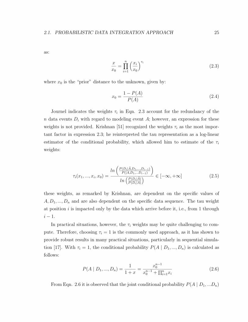
2.1. PROBABILISTIC DATA INTEGRATION APPROACH 25
as:
x
x0
=n∏
i=1
(xi
x0
)τi
(2.3)
where x0 is the “prior” distance to the unknown, given by:
x0 =1− P (A)
P (A)(2.4)
Journel indicates the weights τi in Eqn. 2.3 account for the redundancy of the
n data events Di with regard to modeling event A; however, an expression for these
weights is not provided. Krishnan [51] recognized the weights τi as the most impor-
tant factor in expression 2.3; he reinterpreted the tau representation as a log-linear
estimator of the conditional probability, which allowed him to estimate of the τi
weights:
τi(x1, ..., xi, x0) =ln(
P (Di|A,D1,...,Di−1)P (|A,D1,...Di−1)
)ln(
P (Di|A)P (Di|A)
) ∈ [−∞, +∞] (2.5)
these weights, as remarked by Krishnan, are dependent on the specific values of
A, D1, ..., Dn and are also dependent on the specific data sequence. The tau weight
at position i is impacted only by the data which arrive before it, i.e., from 1 through
i− 1.
In practical situations, however, the τi weights may be quite challenging to com-
pute. Therefore, choosing τi = 1 is the commonly used approach, as it has shown to
provide robust results in many practical situations, particularly in sequential simula-
tion [17]. With τi = 1, the conditional probability P (A | D1, ..., Dn) is calculated as
follows:
P (A | D1, ..., Dn) =1
1 + x=
xn−10
xn−10 +
∏ni=1xi
(2.6)
From Eqn. 2.6 it is observed that the joint conditional probability P (A | D1, ...Dn)
26CHAPTER 2. TWO WORKFLOWS FOR INTEGRATING 4D SEISMIC DATA
can be computed only from the individual conditional probabilities P (A | Di). These
probabilities reveal how informative the datum Di is about the unknown A; therefore,
the procedure followed to extract the information content of each data source depends
on the specific data source itself. For example, suppose the unknown A is channel
facies present or absent at a certain location u = (x, y, z). D1 is geologic data (well-
log and/or core data, and training image), D2 is geophysical data (3D seismic), and
D3 is historical production data.
In this example, the unknown A is an indicator variable I(u) that describes an
event occurring:
I(u) =
1 if channel facies occurs at u
0 else
Following the sequential simulation approach explained earlier, at each uninformed
grid block (visited randomly), P (A | D1) is estimated by the algorithm itself and com-
bined with the other conditional probabilities P (A | D2) and P (A | D3) using Eqn. 2.6
from which a value is drawn for the grid-block. In particular, since simulating channels
requires a multiple-point algorithm, the single normal equation simulation algorithm
computes P (A | D1) after scanning a training image for equivalent multiple-point
data events. Figure 2.1 shows how this process is performed. In the neighborhood
of an uninformed grid-block, the probability of this grid-block being channel facies
given its specific set of neighboring sand and no-sand data values (D1) is calculated
by scanning the training image (Figure 2.1) for “replicates” of this data event: three
such events are found of which one yields a central sand value, hence, the probability
of having sand is 1/3. By random drawing, a facies category is assigned. The set
of neighboring sand and no-sand data values is represented by previously simulated
values and well-log and/or core data, which are assigned (frozen) facies category val-
ues to those grid-blocks that are intersected by wells. The grid-blocks containing well
constraints are never visited and their facies values never re-considered.
Figure 2.1 shows how the single normal equation simulation algorithm computes
P (A | D1); following is a review of how the conditional probabilities P (A | D2) and
P (A | D3) can be computed.
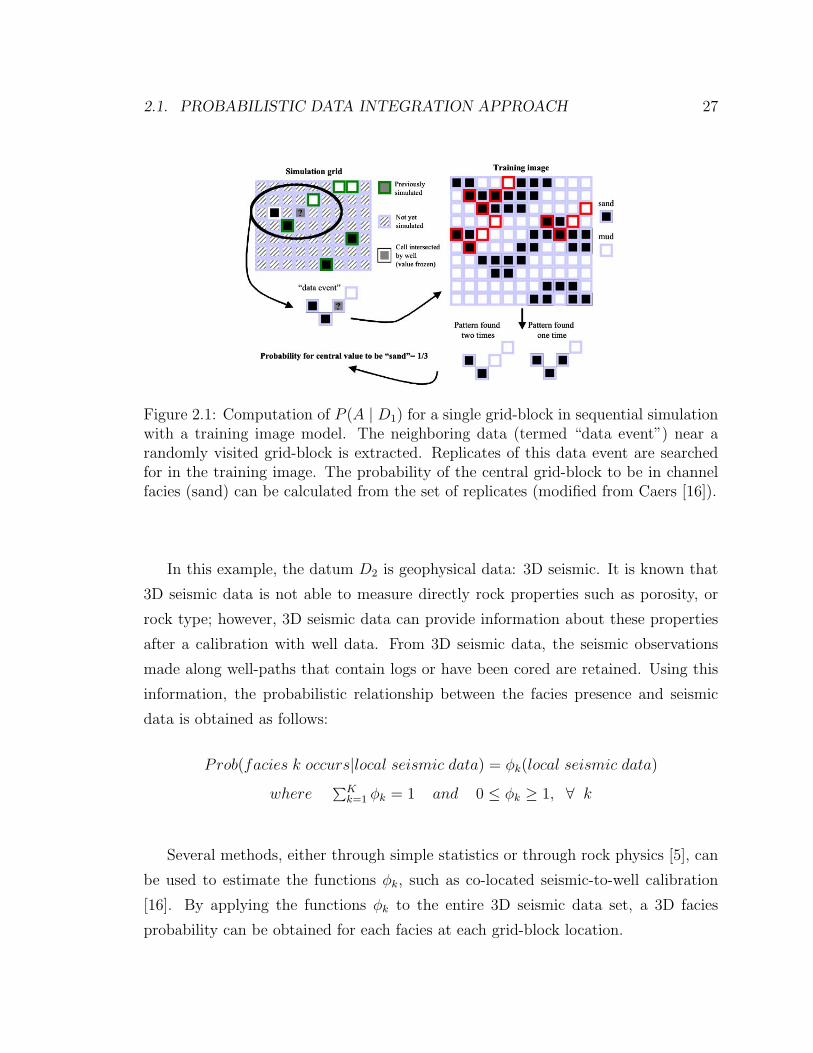
2.1. PROBABILISTIC DATA INTEGRATION APPROACH 27
Figure 2.1: Computation of P (A | D1) for a single grid-block in sequential simulationwith a training image model. The neighboring data (termed “data event”) near arandomly visited grid-block is extracted. Replicates of this data event are searchedfor in the training image. The probability of the central grid-block to be in channelfacies (sand) can be calculated from the set of replicates (modified from Caers [16]).
In this example, the datum D2 is geophysical data: 3D seismic. It is known that
3D seismic data is not able to measure directly rock properties such as porosity, or
rock type; however, 3D seismic data can provide information about these properties
after a calibration with well data. From 3D seismic data, the seismic observations
made along well-paths that contain logs or have been cored are retained. Using this
information, the probabilistic relationship between the facies presence and seismic
data is obtained as follows:
Prob(facies k occurs|local seismic data) = φk(local seismic data)
where∑K
k=1 φk = 1 and 0 ≤ φk ≥ 1, ∀ k
Several methods, either through simple statistics or through rock physics [5], can
be used to estimate the functions φk, such as co-located seismic-to-well calibration
[16]. By applying the functions φk to the entire 3D seismic data set, a 3D facies
probability can be obtained for each facies at each grid-block location.
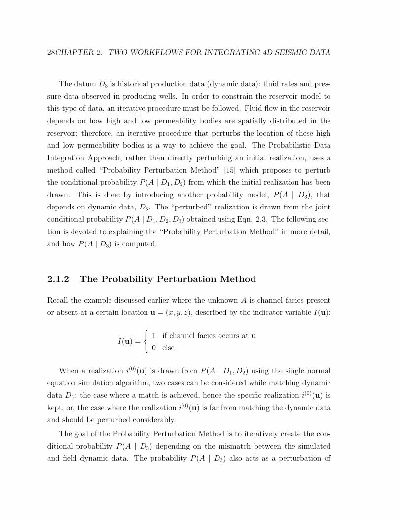
28CHAPTER 2. TWO WORKFLOWS FOR INTEGRATING 4D SEISMIC DATA
The datum D3 is historical production data (dynamic data): fluid rates and pres-
sure data observed in producing wells. In order to constrain the reservoir model to
this type of data, an iterative procedure must be followed. Fluid flow in the reservoir
depends on how high and low permeability bodies are spatially distributed in the
reservoir; therefore, an iterative procedure that perturbs the location of these high
and low permeability bodies is a way to achieve the goal. The Probabilistic Data
Integration Approach, rather than directly perturbing an initial realization, uses a
method called “Probability Perturbation Method” [15] which proposes to perturb
the conditional probability P (A | D1, D2) from which the initial realization has been
drawn. This is done by introducing another probability model, P (A | D3), that
depends on dynamic data, D3. The “perturbed” realization is drawn from the joint
conditional probability P (A | D1, D2, D3) obtained using Eqn. 2.3. The following sec-
tion is devoted to explaining the “Probability Perturbation Method” in more detail,
and how P (A | D3) is computed.
2.1.2 The Probability Perturbation Method
Recall the example discussed earlier where the unknown A is channel facies present
or absent at a certain location u = (x, y, z), described by the indicator variable I(u):
I(u) =
1 if channel facies occurs at u
0 else
When a realization i(0)(u) is drawn from P (A | D1, D2) using the single normal
equation simulation algorithm, two cases can be considered while matching dynamic
data D3: the case where a match is achieved, hence the specific realization i(0)(u) is
kept, or, the case where the realization i(0)(u) is far from matching the dynamic data
and should be perturbed considerably.
The goal of the Probability Perturbation Method is to iteratively create the con-
ditional probability P (A | D3) depending on the mismatch between the simulated
and field dynamic data. The probability P (A | D3) also acts as a perturbation of
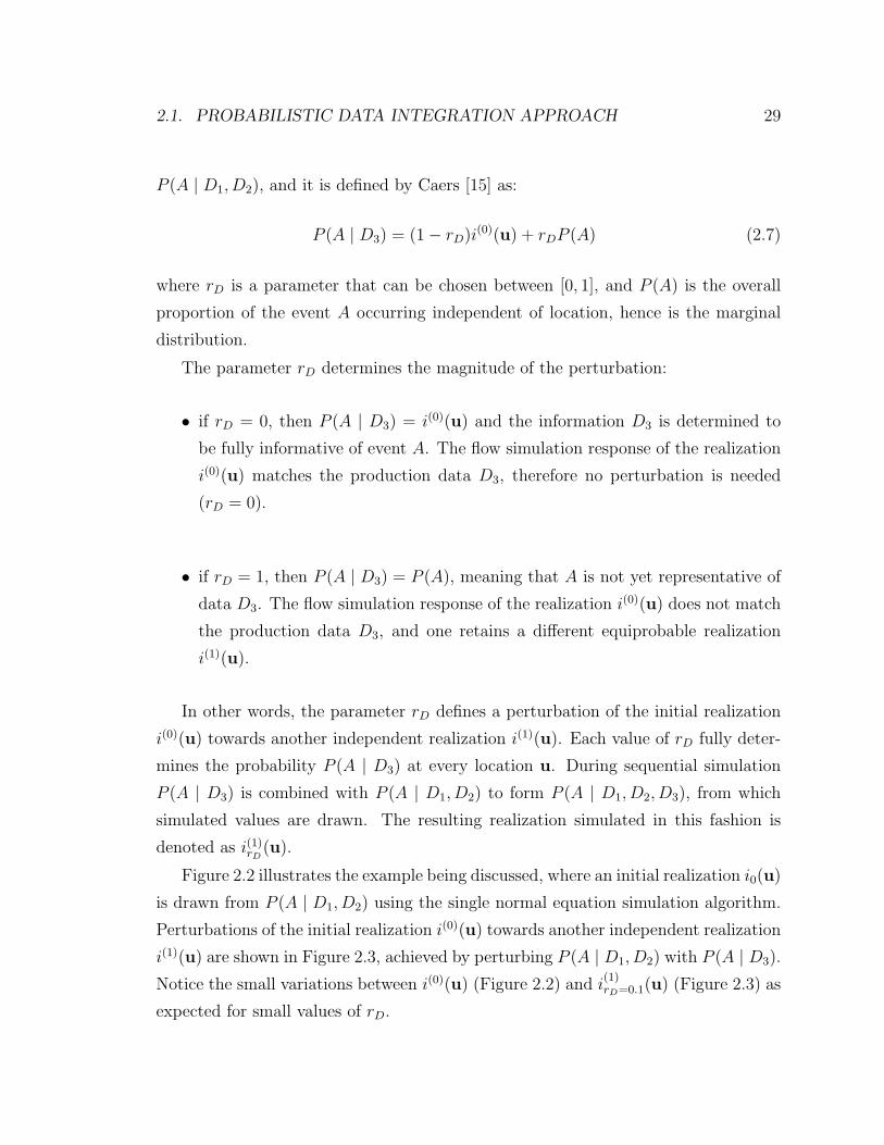
2.1. PROBABILISTIC DATA INTEGRATION APPROACH 29
P (A | D1, D2), and it is defined by Caers [15] as:
P (A | D3) = (1− rD)i(0)(u) + rDP (A) (2.7)
where rD is a parameter that can be chosen between [0, 1], and P (A) is the overall
proportion of the event A occurring independent of location, hence is the marginal
distribution.
The parameter rD determines the magnitude of the perturbation:
• if rD = 0, then P (A | D3) = i(0)(u) and the information D3 is determined to
be fully informative of event A. The flow simulation response of the realization
i(0)(u) matches the production data D3, therefore no perturbation is needed
(rD = 0).
• if rD = 1, then P (A | D3) = P (A), meaning that A is not yet representative of
data D3. The flow simulation response of the realization i(0)(u) does not match
the production data D3, and one retains a different equiprobable realization
i(1)(u).
In other words, the parameter rD defines a perturbation of the initial realization
i(0)(u) towards another independent realization i(1)(u). Each value of rD fully deter-
mines the probability P (A | D3) at every location u. During sequential simulation
P (A | D3) is combined with P (A | D1, D2) to form P (A | D1, D2, D3), from which
simulated values are drawn. The resulting realization simulated in this fashion is
denoted as i(1)rD
(u).
Figure 2.2 illustrates the example being discussed, where an initial realization i0(u)
is drawn from P (A | D1, D2) using the single normal equation simulation algorithm.
Perturbations of the initial realization i(0)(u) towards another independent realization
i(1)(u) are shown in Figure 2.3, achieved by perturbing P (A | D1, D2) with P (A | D3).
Notice the small variations between i(0)(u) (Figure 2.2) and i(1)rD=0.1(u) (Figure 2.3) as
expected for small values of rD.
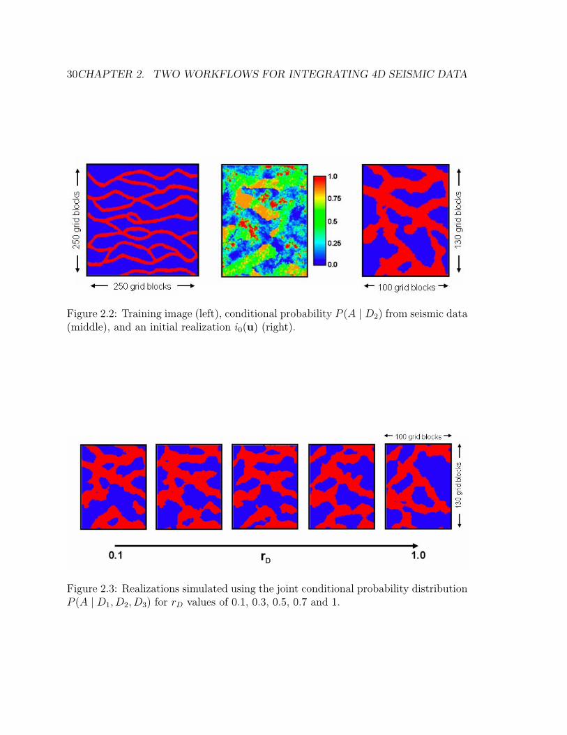
30CHAPTER 2. TWO WORKFLOWS FOR INTEGRATING 4D SEISMIC DATA
Figure 2.2: Training image (left), conditional probability P (A | D2) from seismic data(middle), and an initial realization i0(u) (right).
Figure 2.3: Realizations simulated using the joint conditional probability distributionP (A | D1, D2, D3) for rD values of 0.1, 0.3, 0.5, 0.7 and 1.

2.2. INTEGRATING 4D SEISMIC DATA: PDI APPROACH 31
2.2 Integrating 4D Seismic Data: PDI Approach
This chapter started with a discussion about 4D seismic data and why it should be
incorporated into the reservoir modeling process. 4D seismic data comprise a set of
3D seismic data acquired at different times over the same area. In many cases only
one 3D seismic data set is available: the survey acquired during exploration or early
appraisal of the field, often called “Base 3D seismic data”. Subsequent 3D seismic
surveys, acquired later in time, are called in this dissertation “Time-lapse 3D seismic
data”. The change between surveys, expressed as a ratio, difference or any other
measure of change, is denoted in this dissertation as “4D seismic response”.
4D seismic data provides valuable static and dynamic information about the reser-
voir, since some of the dynamic changes (changes in fluid saturation) occur only in a
certain type of rock with high porosity and permeability. Therefore, 4D seismic data
can be used as a constraint for the facies modeling by means of a facies probability
cube.
Following the Probabilistic Data Integration Approach, the integration of 4D seis-
mic data can now be further explained. Recalling the example discussed in the previ-
ous section, where the unknown A is channel facies presence or absence at a certain
location u = (x, y, z), the new set of data after including 4D seismic data would be:
D1 is geologic data (well-log and/or core data, and training image), D2 is geophysi-
cal data (Base 3D seismic), D3 is 4D seismic data (the set of “Time-lapse 3D seismic
data”), and D4 historical production data. Reservoir models are drawn by the sequen-
tial simulation algorithm from the joint conditional probability P (A | D1, D2, D3, D4),
which is obtained from the individual probabilities P (A | D1), P (A | D2), P (A | D3),
and P (A | D4) using Eqn. 2.6.
Figure 2.4 shows a schematic reservoir modeling workflow where 4D seismic data
is proposed to be included as a spatial probability distribution; the workflow uses
the Probabilistic Data Integration Approach proposed by Hoffman [44] as well as
the Parallel Modeling Approach proposed by Tureyen [86]. The workflow consists of
generating a high resolution 3D geo-cellular model, which is then upscaled and flow
simulation is run to check the match of historical production data. The high resolution
32CHAPTER 2. TWO WORKFLOWS FOR INTEGRATING 4D SEISMIC DATA
model is subsequently perturbed in a fashion that will improve the match and the
entire procedure is repeated until production data are matched. The Probabilistic
Data Integration Approach is used to simulate and perturb the high resolution model,
while simultaneously honoring all static data.
Figure 2.4: Reservoir modeling workflow that incorporates the 4D seismic datathrough a spatial probability distribution.
The information content of 4D seismic data needs to be modeled through a spatial
probability distribution. Although research on this subject is out of the scope of this
dissertation, the works of Wu et al. [91] and Andersen et al. [3] are pioneering on
this matter. In particular, the following section is devoted to explaining the work
of Andersen et al. [3], a particular example of estimating P (A | D2, D3) from rock
physics information.
2.2.1 Modeling the Information Content of 4D Seismic Data
Following the example being discussed in this chapter, when including 4D seismic data
into the Probabilistic Data Integration Approach an additional conditional probability
needs to be computed. The probability P (A | D2), obtained after a calibration of
the Base 3D seismic survey with well-logs [16], summarizes the information that the
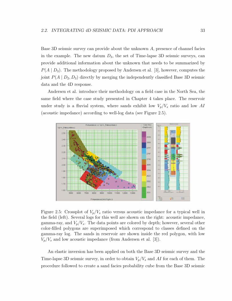
2.2. INTEGRATING 4D SEISMIC DATA: PDI APPROACH 33
Base 3D seismic survey can provide about the unknown A, presence of channel facies
in the example. The new datum D3, the set of Time-lapse 3D seismic surveys, can
provide additional information about the unknown that needs to be summarized by
P (A | D3). The methodology proposed by Andersen et al. [3], however, computes the
joint P (A | D2, D3) directly by merging the independently classified Base 3D seismic
data and the 4D response.
Andersen et al. introduce their methodology on a field case in the North Sea, the
same field where the case study presented in Chapter 4 takes place. The reservoir
under study is a fluvial system, where sands exhibit low Vp/Vs ratio and low AI
(acoustic impedance) according to well-log data (see Figure 2.5).
Figure 2.5: Crossplot of Vp/Vs ratio versus acoustic impedance for a typical well inthe field (left). Several logs for this well are shown on the right: acoustic impedance,gamma-ray, and Vp/Vs. The data points are colored by depth; however, several othercolor-filled polygons are superimposed which correspond to classes defined on thegamma-ray log. The sands in reservoir are shown inside the red polygon, with lowVp/Vs and low acoustic impedance (from Andersen et al. [3]).
An elastic inversion has been applied on both the Base 3D seismic survey and the
Time-lapse 3D seismic survey, in order to obtain Vp/Vs and AI for each of them. The
procedure followed to create a sand facies probability cube from the Base 3D seismic
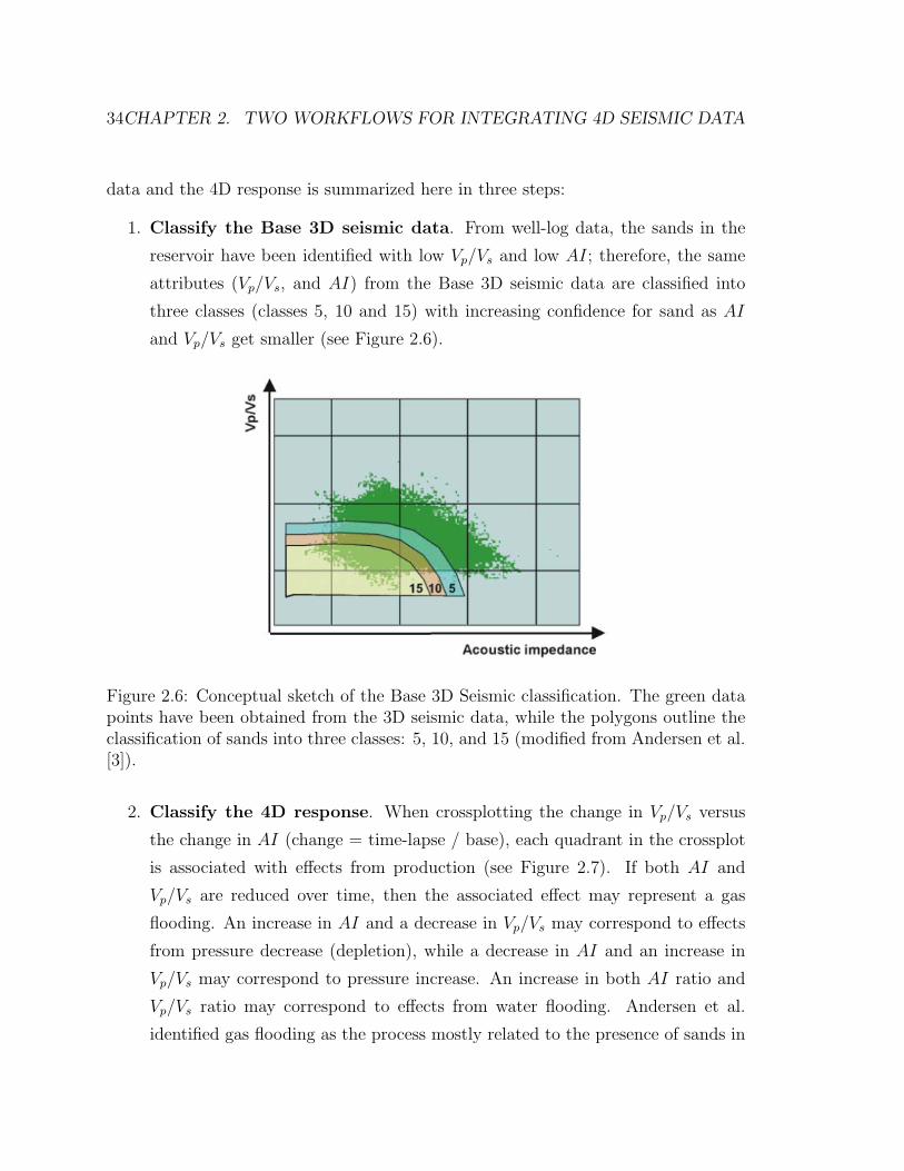
34CHAPTER 2. TWO WORKFLOWS FOR INTEGRATING 4D SEISMIC DATA
data and the 4D response is summarized here in three steps:
1. Classify the Base 3D seismic data. From well-log data, the sands in the
reservoir have been identified with low Vp/Vs and low AI; therefore, the same
attributes (Vp/Vs, and AI) from the Base 3D seismic data are classified into
three classes (classes 5, 10 and 15) with increasing confidence for sand as AI
and Vp/Vs get smaller (see Figure 2.6).
Figure 2.6: Conceptual sketch of the Base 3D Seismic classification. The green datapoints have been obtained from the 3D seismic data, while the polygons outline theclassification of sands into three classes: 5, 10, and 15 (modified from Andersen et al.[3]).
2. Classify the 4D response. When crossplotting the change in Vp/Vs versus
the change in AI (change = time-lapse / base), each quadrant in the crossplot
is associated with effects from production (see Figure 2.7). If both AI and
Vp/Vs are reduced over time, then the associated effect may represent a gas
flooding. An increase in AI and a decrease in Vp/Vs may correspond to effects
from pressure decrease (depletion), while a decrease in AI and an increase in
Vp/Vs may correspond to pressure increase. An increase in both AI ratio and
Vp/Vs ratio may correspond to effects from water flooding. Andersen et al.
identified gas flooding as the process mostly related to the presence of sands in
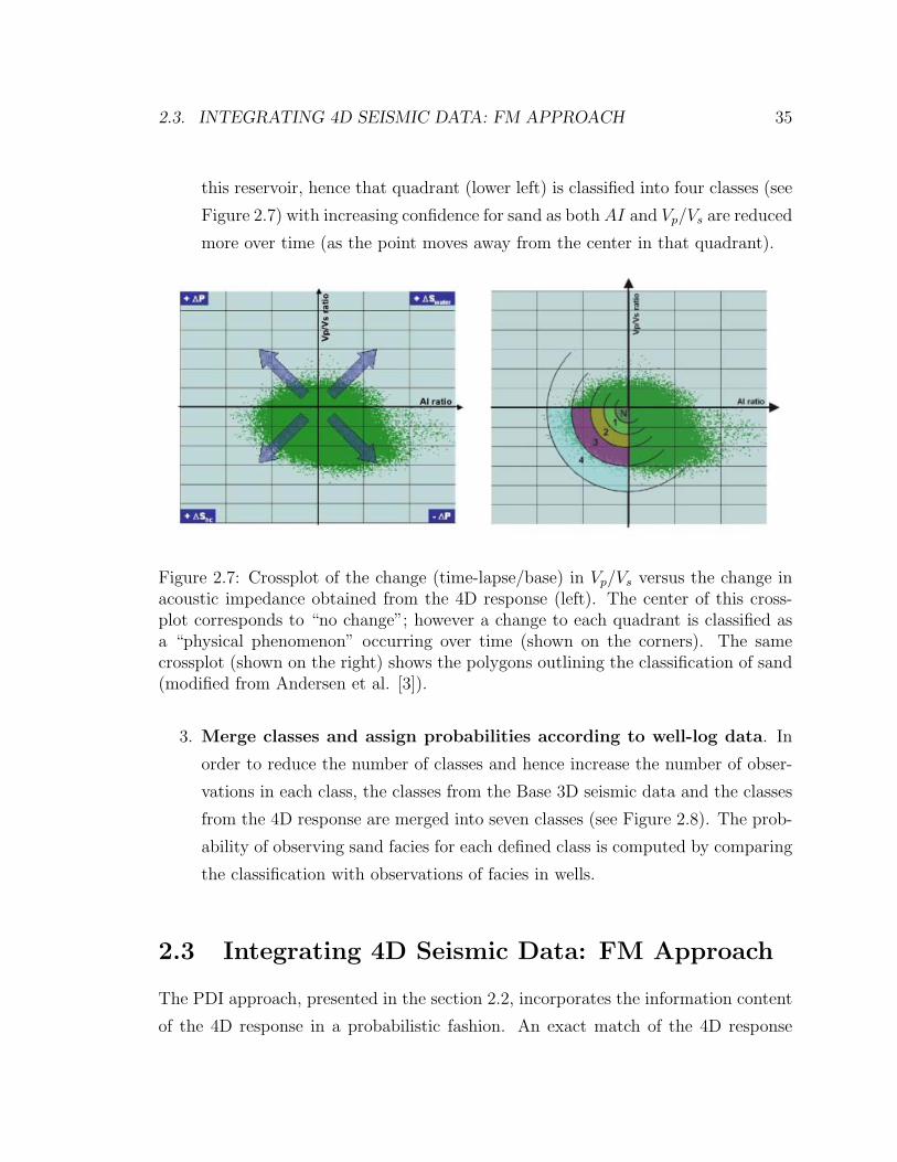
2.3. INTEGRATING 4D SEISMIC DATA: FM APPROACH 35
this reservoir, hence that quadrant (lower left) is classified into four classes (see
Figure 2.7) with increasing confidence for sand as both AI and Vp/Vs are reduced
more over time (as the point moves away from the center in that quadrant).
Figure 2.7: Crossplot of the change (time-lapse/base) in Vp/Vs versus the change inacoustic impedance obtained from the 4D response (left). The center of this cross-plot corresponds to “no change”; however a change to each quadrant is classified asa “physical phenomenon” occurring over time (shown on the corners). The samecrossplot (shown on the right) shows the polygons outlining the classification of sand(modified from Andersen et al. [3]).
3. Merge classes and assign probabilities according to well-log data. In
order to reduce the number of classes and hence increase the number of obser-
vations in each class, the classes from the Base 3D seismic data and the classes
from the 4D response are merged into seven classes (see Figure 2.8). The prob-
ability of observing sand facies for each defined class is computed by comparing
the classification with observations of facies in wells.
2.3 Integrating 4D Seismic Data: FM Approach
The PDI approach, presented in the section 2.2, incorporates the information content
of the 4D response in a probabilistic fashion. An exact match of the 4D response

36CHAPTER 2. TWO WORKFLOWS FOR INTEGRATING 4D SEISMIC DATA
Figure 2.8: Table showing the recording of the classes in the combined 3D and 4Dvolumes. The figure to the right shows a smoothed sand probability for the com-bined volumes. The pink curve shows probabilities for sand and the red curve showsprobabilities for no-sand lithologies(from Andersen et al. [3]).
is not aimed for, rather a probabilistic type match is achieved. Another approach
to incorporate 4D seismic data is by treating it as dynamic data; in other words,
matching it along with production data. When history matching production data
only, the production response of the reservoir model is computed by performing flow
simulation. Therefore, when including the matching of 4D seismic data, the 4D
response of the reservoir model needs to be computed also by performing a “Forward
Modeling” (FM).
When high quality 4D seismic data is not available, or a complicated 4D seismic
forward modeling may not be carried out due to the lack of rock physics data, the
PDI approach may represent a more robust and less difficult to achieve alternative to
include 4D seismic information into the reservoir modeling workflow.
This approach, like the PDI approach, uses the Probabilistic Data Integration
Approach as well as the Parallel Modeling Approach. Recalling the example discussed
through this chapter, where the unknown A is channel facies presence or absence at
a certain location u = (x, y, z), the new set of data after including 4D seismic data
using the FM approach would be: D1 is geologic data (well-log and/or core data,
and training image), D2 is geophysical data (Base 3D seismic), D3 is dynamic data
(historical production data and the 4D response).
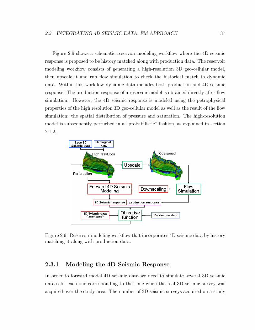
2.3. INTEGRATING 4D SEISMIC DATA: FM APPROACH 37
Figure 2.9 shows a schematic reservoir modeling workflow where the 4D seismic
response is proposed to be history matched along with production data. The reservoir
modeling workflow consists of generating a high-resolution 3D geo-cellular model,
then upscale it and run flow simulation to check the historical match to dynamic
data. Within this workflow dynamic data includes both production and 4D seismic
response. The production response of a reservoir model is obtained directly after flow
simulation. However, the 4D seismic response is modeled using the petrophysical
properties of the high resolution 3D geo-cellular model as well as the result of the flow
simulation: the spatial distribution of pressure and saturation. The high-resolution
model is subsequently perturbed in a “probabilistic” fashion, as explained in section
2.1.2.
Figure 2.9: Reservoir modeling workflow that incorporates 4D seismic data by historymatching it along with production data.
2.3.1 Modeling the 4D Seismic Response
In order to forward model 4D seismic data we need to simulate several 3D seismic
data sets, each one corresponding to the time when the real 3D seismic survey was
acquired over the study area. The number of 3D seismic surveys acquired on a study
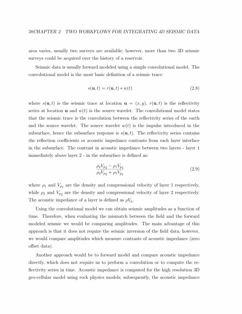
38CHAPTER 2. TWO WORKFLOWS FOR INTEGRATING 4D SEISMIC DATA
area varies, usually two surveys are available; however, more than two 3D seismic
surveys could be acquired over the history of a reservoir.
Seismic data is usually forward modeled using a simple convolutional model. The
convolutional model is the most basic definition of a seismic trace:
s(u, t) = r(u, t) ∗ w(t) (2.8)
where s(u, t) is the seismic trace at location u = (x, y), r(u, t) is the reflectivity
series at location u and w(t) is the source wavelet. The convolutional model states
that the seismic trace is the convolution between the reflectivity series of the earth
and the source wavelet. The source wavelet w(t) is the impulse introduced in the
subsurface, hence the subsurface response is s(u, t). The reflectivity series contains
the reflection coefficients or acoustic impedance contrasts from each layer interface
in the subsurface. The contrast in acoustic impedance between two layers - layer 1
immediately above layer 2 - in the subsurface is defined as:
ρ2Vp2 − ρ1Vp1
ρ2Vp2 + ρ1Vp1
(2.9)
where ρ1 and Vp1 are the density and compressional velocity of layer 1 respectively,
while ρ2 and Vp2 are the density and compressional velocity of layer 2 respectively.
The acoustic impedance of a layer is defined as ρVp.
Using the convolutional model we can obtain seismic amplitudes as a function of
time. Therefore, when evaluating the mismatch between the field and the forward
modeled seismic we would be comparing amplitudes. The main advantage of this
approach is that it does not require the seismic inversion of the field data; however,
we would compare amplitudes which measure contrasts of acoustic impedance (zero
offset data).
Another approach would be to forward model and compare acoustic impedance
directly, which does not require us to perform a convolution or to compute the re-
flectivity series in time. Acoustic impedance is computed for the high resolution 3D
geo-cellular model using rock physics models; subsequently, the acoustic impedance
2.3. INTEGRATING 4D SEISMIC DATA: FM APPROACH 39
is filtered in order to mimic acoustic impedance data from an actual inversion field
data. The main advantage of this approach is that we would be comparing acoustic
impedance of each layer directly; however, the field seismic data needs to be inverted
to obtain acoustic impedance from the amplitude data. When comparing AI we rely
on the result of a seismic inversion which may not be unique.
Using any of the two approaches explained before to forward model seismic data,
we need to compute acoustic impedance at each of the times that real seismic data
is acquired over the study area.
In order to compute the time lapse acoustic impedance we need the petrophysical
properties modeled on the high resolution 3D geo-cellular model as well as the output
from the flow simulation (see Figure 2.10). Using a petro-elastic model (see Figure
2.11) the acoustic impedance at each time is computed on the high resolution grid;
hence, the output from the flow simulation needs to be downscaled. An approach for
downscaling the output from the flow simulation is presented in Chapter 3.
Upscale
Flow Simulation
Downscale[Pp, So, Sw, Sg] @ t1
Downscale[Pp, So, Sw, Sg] @ t2
Downscale[Pp, So, Sw, Sg] @ t3
Downscale[Pp, So, Sw, Sg] @ tn
realization (φ, k)
Petro-ElasticModeling
Acoustic Impedance @ t1
Petro-ElasticModeling
Acoustic Impedance @ t2
Petro-ElasticModeling
Acoustic Impedance @ t3
Petro-ElasticModeling
Acoustic Impedance @ tn
…
Figure 2.10: General procedure and input data needed for creating the Time-lapseacoustic impedance.
40CHAPTER 2. TWO WORKFLOWS FOR INTEGRATING 4D SEISMIC DATA
The petrophysical properties simulated on the high resolution model are typically
porosity and permeability (φ and k); from porosity we are able to compute ρ, Vp and
Vs for the dry rock (no fluids in the pore space) under certain effective pressure Peff
using rock physics relations - Vp(φ, Peff ) and Vs(φ, Peff ) - obtained in the laboratory
for the specific type of rocks in the study area. The effective pressure Peff is defined
as:
Peff = Poverburden − Ppore (2.10)
where Poverburden is the overburden pressure and Ppore is the pore pressure. The pore
pressure is obtained directly from the flow simulator, while the overburden pressure
could be assumed constant for the entire reservoir:
Poverburden = ρgz (2.11)
where ρ is the average density of the overburden, g is the gravitational constant, and
z is the average depth of the reservoir.
Having computed ρ, Vp and Vs for the dry rock under certain effective pressure
Peff , the same properties are updated according to the fluid present in the pore space
using Gassmann’s transformation [32].
Gassmann introduced a mathematical transformation that allows the calculation
of the elastic moduli of the fully-saturated rock from those of the dry rock:
Ksat = KminφKdry − (1 + φ)KfKdry/Kmin + Kf
(1− φ)Kf + φKmin −KfKdry/Kmin
(2.12)
where Ksat is the fully-saturated rock’s bulk modulus, Kf is the bulk modulus of
the fluid in the pore space, φ is the rock’s porosity, Kmin is the bulk modulus of the
mineral, and µ is the rock’s shear modulus.
Using the compressional Vp and shear Vs wave velocities obtained from the lab-
oratory rock physics relations - Vp(φ, Peff ) and Vs(φ, Peff ) - the dry bulk and shear
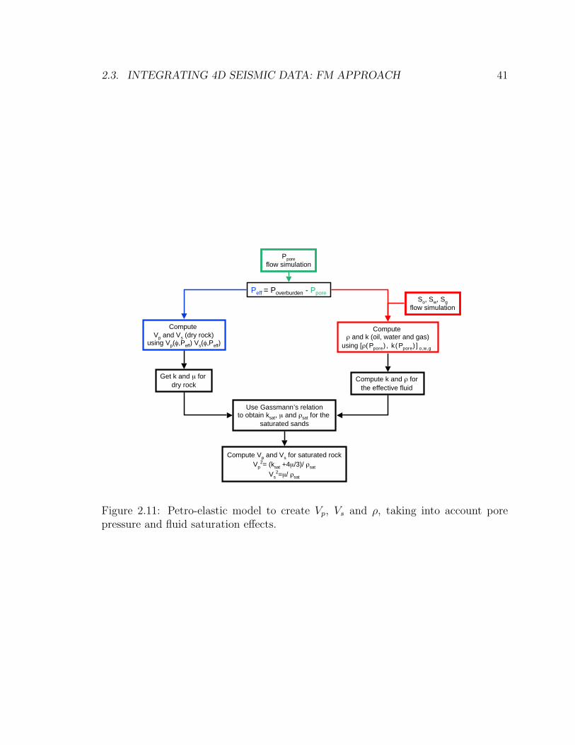
2.3. INTEGRATING 4D SEISMIC DATA: FM APPROACH 41
Peff = Poverburden - Ppore
Compute Vp and Vs (dry rock)
using Vp(φ,Peff) Vs(φ,Peff)
Compute ρ and k (oil, water and gas)
using [ρ(Ppore), k(Ppore)]o,w,g
Get k and µ for dry rock
Compute k and ρ for the effective fluid
Use Gassmann’s relationto obtain ksat, µ and ρsat for the
saturated sands
Compute Vp and Vs for saturated rockVp
2= (ksat +4µ/3)/ ρsat
Vs2=µ/ ρsat
So, Sw, Sgflow simulation
Pporeflow simulation
Figure 2.11: Petro-elastic model to create Vp, Vs and ρ, taking into account porepressure and fluid saturation effects.
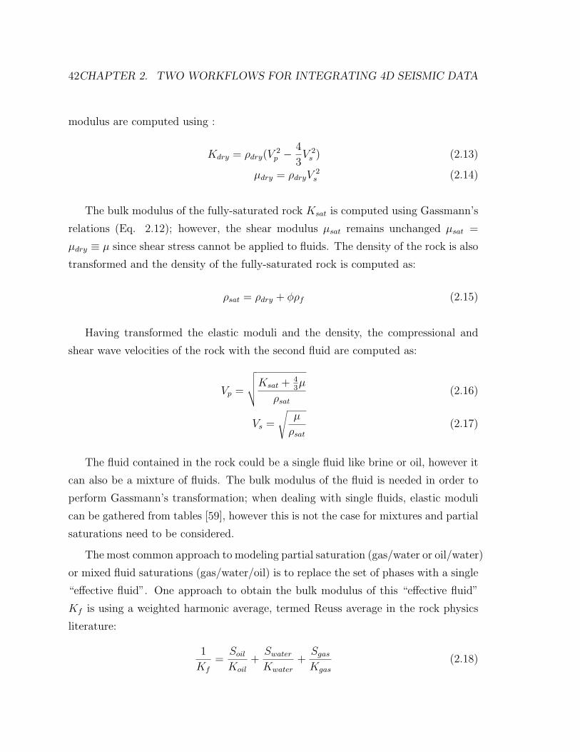
42CHAPTER 2. TWO WORKFLOWS FOR INTEGRATING 4D SEISMIC DATA
modulus are computed using :
Kdry = ρdry(V2p −
4
3V 2
s ) (2.13)
µdry = ρdryV2s (2.14)
The bulk modulus of the fully-saturated rock Ksat is computed using Gassmann’s
relations (Eq. 2.12); however, the shear modulus µsat remains unchanged µsat =
µdry ≡ µ since shear stress cannot be applied to fluids. The density of the rock is also
transformed and the density of the fully-saturated rock is computed as:
ρsat = ρdry + φρf (2.15)
Having transformed the elastic moduli and the density, the compressional and
shear wave velocities of the rock with the second fluid are computed as:
Vp =
√√√√Ksat + 43µ
ρsat
(2.16)
Vs =
õ
ρsat
(2.17)
The fluid contained in the rock could be a single fluid like brine or oil, however it
can also be a mixture of fluids. The bulk modulus of the fluid is needed in order to
perform Gassmann’s transformation; when dealing with single fluids, elastic moduli
can be gathered from tables [59], however this is not the case for mixtures and partial
saturations need to be considered.
The most common approach to modeling partial saturation (gas/water or oil/water)
or mixed fluid saturations (gas/water/oil) is to replace the set of phases with a single
“effective fluid”. One approach to obtain the bulk modulus of this “effective fluid”
Kf is using a weighted harmonic average, termed Reuss average in the rock physics
literature:
1
Kf
=Soil
Koil
+Swater
Kwater
+Sgas
Kgas
(2.18)
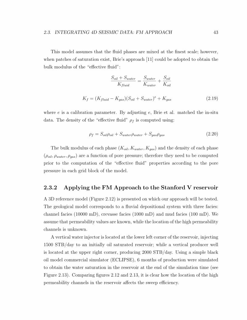
2.3. INTEGRATING 4D SEISMIC DATA: FM APPROACH 43
This model assumes that the fluid phases are mixed at the finest scale; however,
when patches of saturation exist, Brie’s approach [11] could be adopted to obtain the
bulk modulus of the “effective fluid”:
Soil + Swater
Kfluid
=Swater
Kwater
+Soil
Koil
Kf = (Kfluid −Kgas)(Soil + Swater)e + Kgas (2.19)
where e is a calibration parameter. By adjusting e, Brie et al. matched the in-situ
data. The density of the “effective fluid” ρf is computed using:
ρf = Soilρoil + Swaterρwater + Sgasρgas (2.20)
The bulk modulus of each phase (Koil, Kwater, Kgas) and the density of each phase
(ρoil, ρwater, ρgas) are a function of pore pressure; therefore they need to be computed
prior to the computation of the “effective fluid” properties according to the pore
pressure in each grid block of the model.
2.3.2 Applying the FM Approach to the Stanford V reservoir
A 3D reference model (Figure 2.12) is presented on which our approach will be tested.
The geological model corresponds to a fluvial depositional system with three facies:
channel facies (10000 mD), crevasse facies (1000 mD) and mud facies (100 mD). We
assume that permeability values are known, while the location of the high permeability
channels is unknown.
A vertical water injector is located at the lower left corner of the reservoir, injecting
1500 STB/day to an initially oil saturated reservoir; while a vertical producer well
is located at the upper right corner, producing 2000 STB/day. Using a simple black
oil model commercial simulator (ECLIPSE), 6 months of production were simulated
to obtain the water saturation in the reservoir at the end of the simulation time (see
Figure 2.13). Comparing figures 2.12 and 2.13, it is clear how the location of the high
permeability channels in the reservoir affects the sweep efficiency.
44CHAPTER 2. TWO WORKFLOWS FOR INTEGRATING 4D SEISMIC DATA
Figure 2.12: 3D reference reservoir facies model, shown in depth slices from top (topleft) to the bottom of the reservoir (bottom right). Floodplain facies in blue, channelfacies in green, crevasse facies in red.
Figure 2.13: Spatial distribution of water saturation in the reservoir after 6 monthsof production, as obtained from flow simulation using the reference model. Shown indepth slices from top (top left) to the bottom of the reservoir (bottom right).
2.3. INTEGRATING 4D SEISMIC DATA: FM APPROACH 45
Having the reference reservoir model and the water saturation in the reservoir
after 6 months of production, the reference 4D seismic response was created. Using
the facies realization in Figure 2.12, the reference reservoir model was populated
with porosity, compressional velocity and density by using a sequential simulation
algorithm:
• porosity was simulated using a target histogram and variogram.
• compressional velocity was computed using Han’s relations [40] for sandstones
and shaly sandstones, and Gardner’s relation for mudstones [31].
• density was computed from porosity as:
ρ = φρfluid + (1− φ)∑
i
ρmifi
where ρfluid is the density of oil, since the reservoir is initially fully saturated with
oil, ρmiis the density of the mineral mi and fi is the proportion of the mineral mi in
the rock.
Having the reservoir populated with the petrophysical properties as described be-
fore, the 4D seismic response of the reference model was created by forward modeling
two 3D seismic data sets:
• the first 3D seismic data set is forward modeled using the petrophysical prop-
erties of the reservoir fully saturated with oil.
• the second 3D seismic data set is forward modeled using the petrophysical
properties of the reservoir after 6 months of production.
If we were to take the difference of both data sets we would obtain a volume of
the 4D seismic response; however, it has been chosen to take the difference between
a 2D seismic attribute map obtained from each 3D data set. For each seismic trace
the instantaneous amplitude was calculated and the average value was taken. This
process was applied to all traces in each seismic data set (before and after production),
resulting in a map of average instantaneous amplitude for each of them. The difference
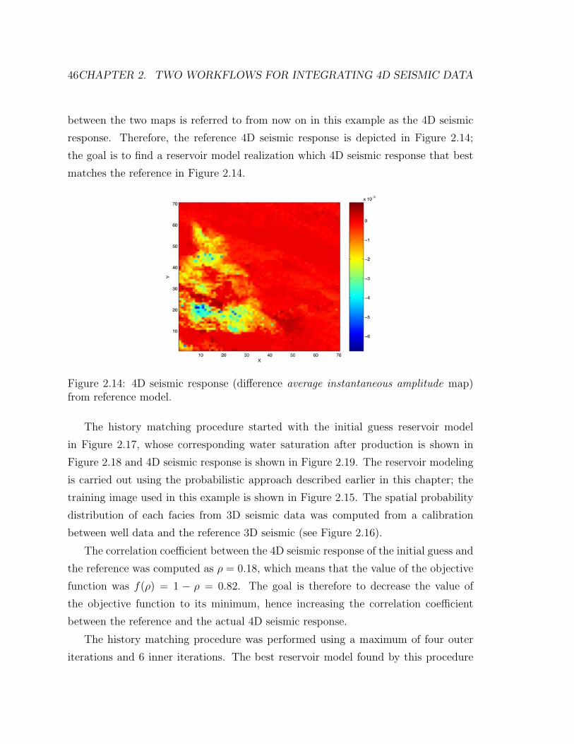
46CHAPTER 2. TWO WORKFLOWS FOR INTEGRATING 4D SEISMIC DATA
between the two maps is referred to from now on in this example as the 4D seismic
response. Therefore, the reference 4D seismic response is depicted in Figure 2.14;
the goal is to find a reservoir model realization which 4D seismic response that best
matches the reference in Figure 2.14.
Figure 2.14: 4D seismic response (difference average instantaneous amplitude map)from reference model.
The history matching procedure started with the initial guess reservoir model
in Figure 2.17, whose corresponding water saturation after production is shown in
Figure 2.18 and 4D seismic response is shown in Figure 2.19. The reservoir modeling
is carried out using the probabilistic approach described earlier in this chapter; the
training image used in this example is shown in Figure 2.15. The spatial probability
distribution of each facies from 3D seismic data was computed from a calibration
between well data and the reference 3D seismic (see Figure 2.16).
The correlation coefficient between the 4D seismic response of the initial guess and
the reference was computed as ρ = 0.18, which means that the value of the objective
function was f(ρ) = 1 − ρ = 0.82. The goal is therefore to decrease the value of
the objective function to its minimum, hence increasing the correlation coefficient
between the reference and the actual 4D seismic response.
The history matching procedure was performed using a maximum of four outer
iterations and 6 inner iterations. The best reservoir model found by this procedure
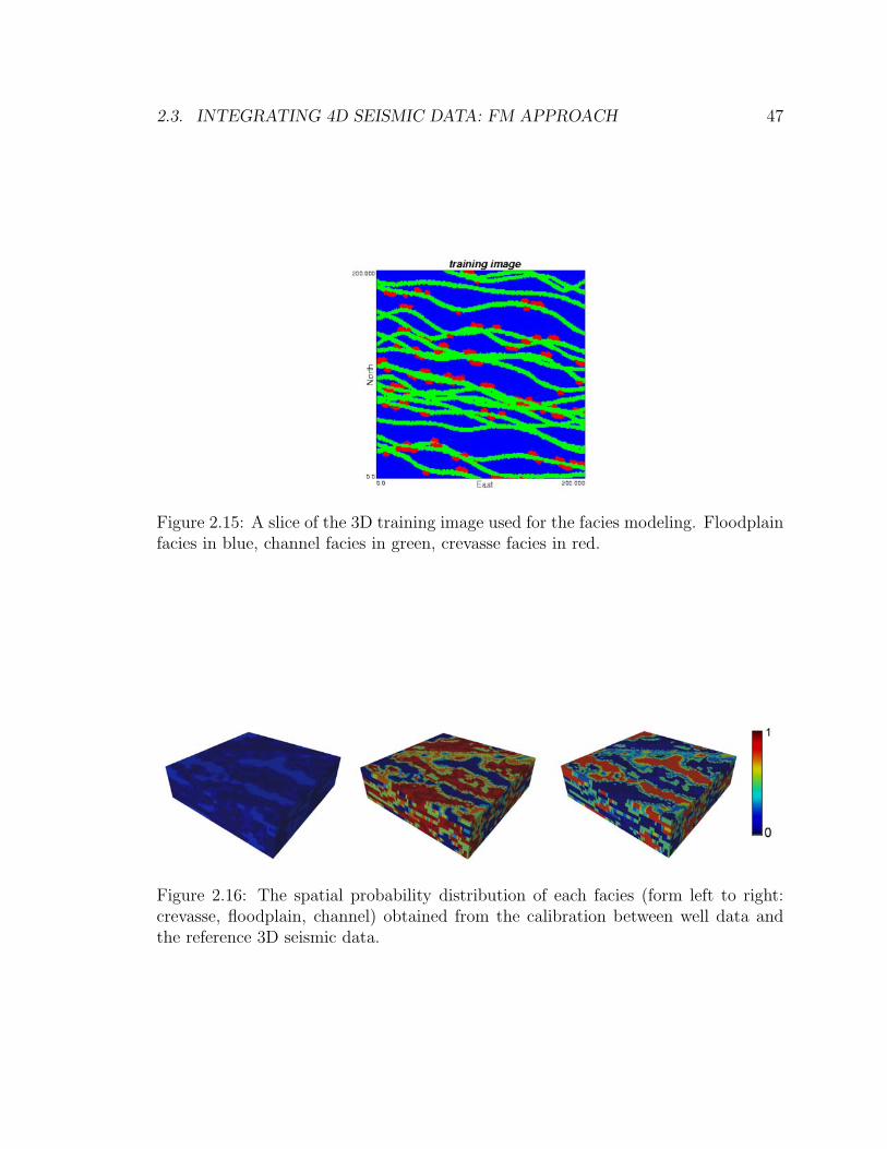
2.3. INTEGRATING 4D SEISMIC DATA: FM APPROACH 47
Figure 2.15: A slice of the 3D training image used for the facies modeling. Floodplainfacies in blue, channel facies in green, crevasse facies in red.
Figure 2.16: The spatial probability distribution of each facies (form left to right:crevasse, floodplain, channel) obtained from the calibration between well data andthe reference 3D seismic data.
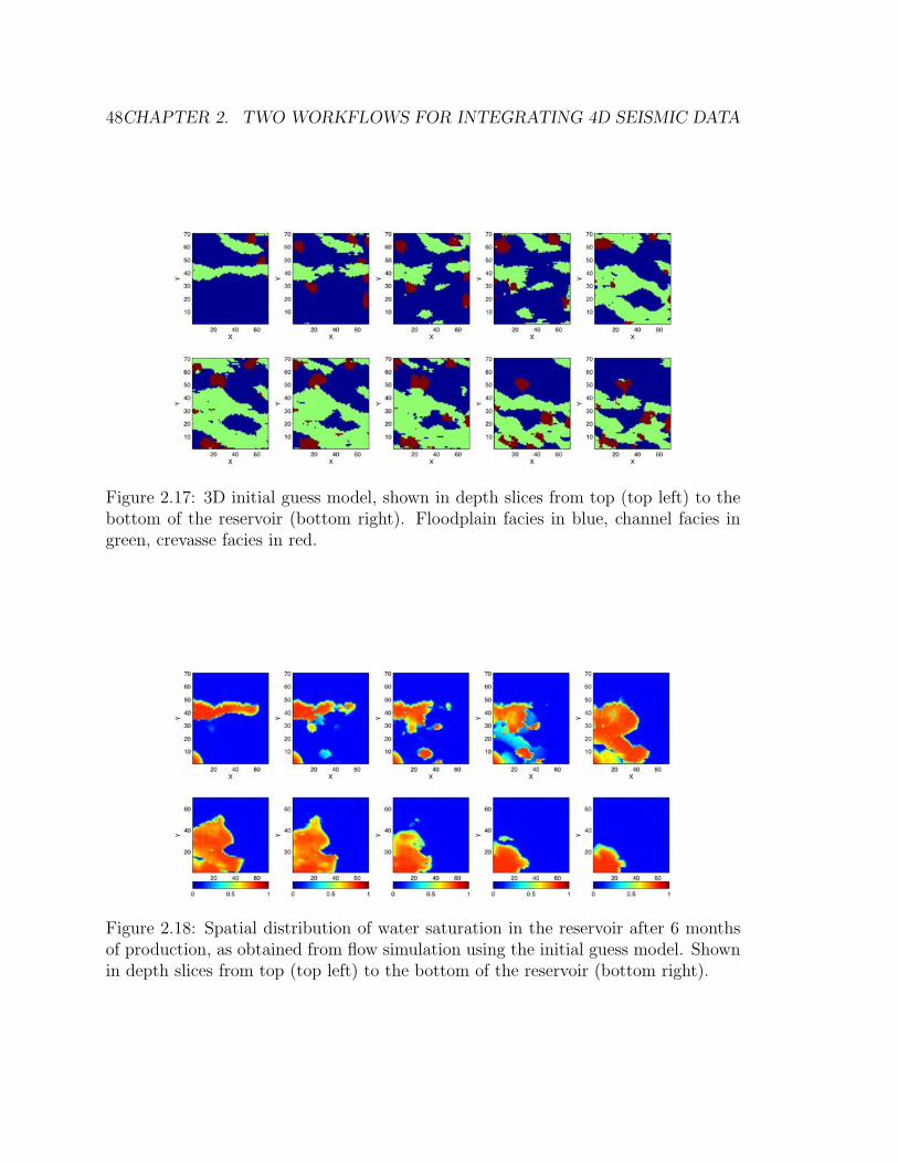
48CHAPTER 2. TWO WORKFLOWS FOR INTEGRATING 4D SEISMIC DATA
Figure 2.17: 3D initial guess model, shown in depth slices from top (top left) to thebottom of the reservoir (bottom right). Floodplain facies in blue, channel facies ingreen, crevasse facies in red.
Figure 2.18: Spatial distribution of water saturation in the reservoir after 6 monthsof production, as obtained from flow simulation using the initial guess model. Shownin depth slices from top (top left) to the bottom of the reservoir (bottom right).
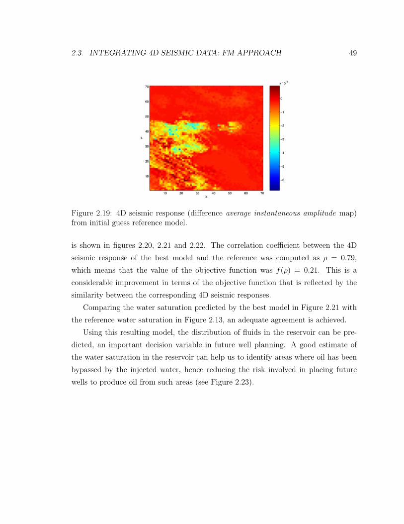
2.3. INTEGRATING 4D SEISMIC DATA: FM APPROACH 49
Figure 2.19: 4D seismic response (difference average instantaneous amplitude map)from initial guess reference model.
is shown in figures 2.20, 2.21 and 2.22. The correlation coefficient between the 4D
seismic response of the best model and the reference was computed as ρ = 0.79,
which means that the value of the objective function was f(ρ) = 0.21. This is a
considerable improvement in terms of the objective function that is reflected by the
similarity between the corresponding 4D seismic responses.
Comparing the water saturation predicted by the best model in Figure 2.21 with
the reference water saturation in Figure 2.13, an adequate agreement is achieved.
Using this resulting model, the distribution of fluids in the reservoir can be pre-
dicted, an important decision variable in future well planning. A good estimate of
the water saturation in the reservoir can help us to identify areas where oil has been
bypassed by the injected water, hence reducing the risk involved in placing future
wells to produce oil from such areas (see Figure 2.23).
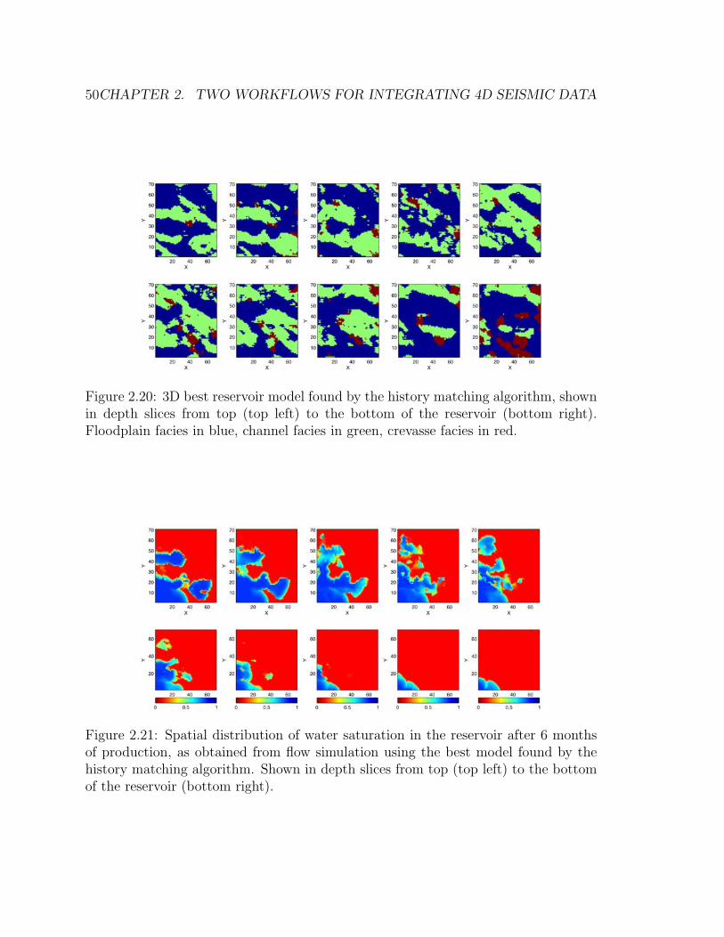
50CHAPTER 2. TWO WORKFLOWS FOR INTEGRATING 4D SEISMIC DATA
Figure 2.20: 3D best reservoir model found by the history matching algorithm, shownin depth slices from top (top left) to the bottom of the reservoir (bottom right).Floodplain facies in blue, channel facies in green, crevasse facies in red.
Figure 2.21: Spatial distribution of water saturation in the reservoir after 6 monthsof production, as obtained from flow simulation using the best model found by thehistory matching algorithm. Shown in depth slices from top (top left) to the bottomof the reservoir (bottom right).
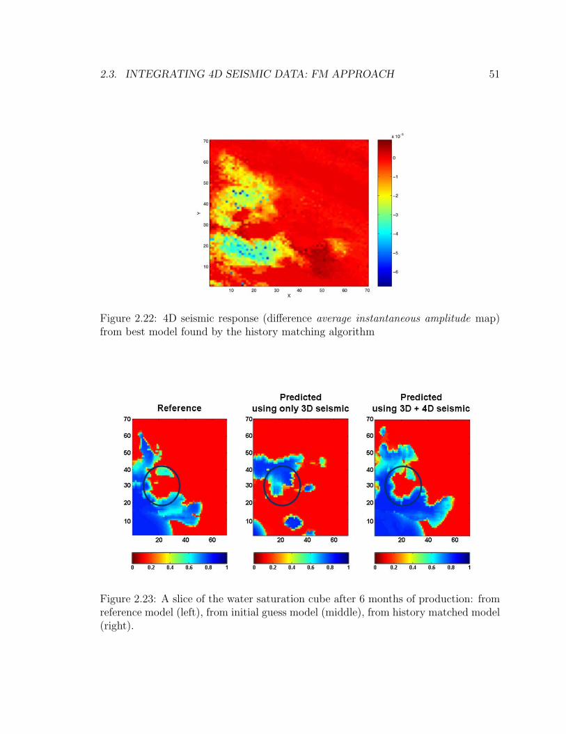
2.3. INTEGRATING 4D SEISMIC DATA: FM APPROACH 51
Figure 2.22: 4D seismic response (difference average instantaneous amplitude map)from best model found by the history matching algorithm
Figure 2.23: A slice of the water saturation cube after 6 months of production: fromreference model (left), from initial guess model (middle), from history matched model(right).
Chapter 3
Downscaling Saturation to Model
4D Seismic Response
4D seismic data can provide a spatial distribution of dynamic changes occurring in a
reservoir due to production. Dynamic changes (changes in pressure and/or saturation)
are inferred from 4D seismic data through changes in reservoir properties since seismic
velocities and impedance depend on changes in pore fluids, pressure and temperature
[63] [10] [90]. Additionally, 4D seismic data can provide static information about the
reservoir, since some of the dynamic changes (changes in fluid saturation) occur only
in a certain type of rock with high porosity and permeability.
Due to the valuable static and dynamic information it carries, 4D seismic data
should be incorporated into the reservoir modeling workflow. Chapter 2 discussed in
detail two approaches to achieve this goal: the PDI approach and the FM approach.
The PDI approach, presented in section 2.2, incorporates the information content
of 4D seismic data in a probabilistic fashion; as a constraint for the modeling of
a static property of the reservoir such as facies. The FM approach, presented in
section 2.3, incorporates 4D seismic data by treating it as dynamic data; in other
words, matching it along with production data. When history matching production
data only, the production response of the reservoir model is computed by performing
flow simulation. Therefore, when including the matching of 4D seismic data, the 4D
response of the reservoir model needs to be computed also by performing a “Forward
52
53
Modeling” (FM).
Forward modeling the 4D seismic response involves the computation of the seismic
attribute(s) as the spatial distribution of pressure and saturation in the reservoir
changes over time. For example, the change over time of acoustic impedance (AI)
can be computed as the set:
[AI]t1 , [AI]t2 , ... [AI]tn
where [AI]ti = [ρVp]ti is the acoustic impedance at time ti, obtained by computing
density (ρ) and P-wave velocity (Vp) of the rock subject to the conditions at time ti,
pressure and saturation at that time. A detailed explanation on the procedure used
to compute the effect of pressure and saturation on the density of a rock, as well as
their effect on the velocity of P and S waves as they travel through the rock was given
in Chapter 2 (section 2.3.1). Density, P and S-wave velocities for each grid block of
the high-resolution reservoir model are computed first and the conditions - pressure
and saturation - at time ti are imposed later. The spatial distribution of pressure and
saturation is obtained after flow simulation, which is performed on a coarsened grid.
The 4D seismic response is forward modeled using the high-resolution reservoir
properties since seismic waves are often affected by fine details below seismic resolu-
tion [58] [74] [75]. Important details such as “patches” of bypassed oil can affect the
seismic signature. Although sometimes seismic waves are not able to “resolve” those
features (i.e., identify their boundaries) they can “detect” them, since they influence
velocity and impedance. Coarse scale saturations from the flow simulator often show
a very smooth version of those “patches” or simply do not show them at all due to
upscaling. Therefore, coarsened saturations need to be ported into the high-resolution
grid through a downscaling procedure.
This chapter is dedicated to investigate the adequacy of state-of-the-art downscal-
ing methods. Additionally, this chapter presents a new dynamic downscaling method,
based on the work of Gautier et al. [33] and Chen et al. [24], that takes into account
both static information (high-resolution permeability field) and dynamic information
in the form of coarsened fluxes and saturations (solution of the global flow simulation).
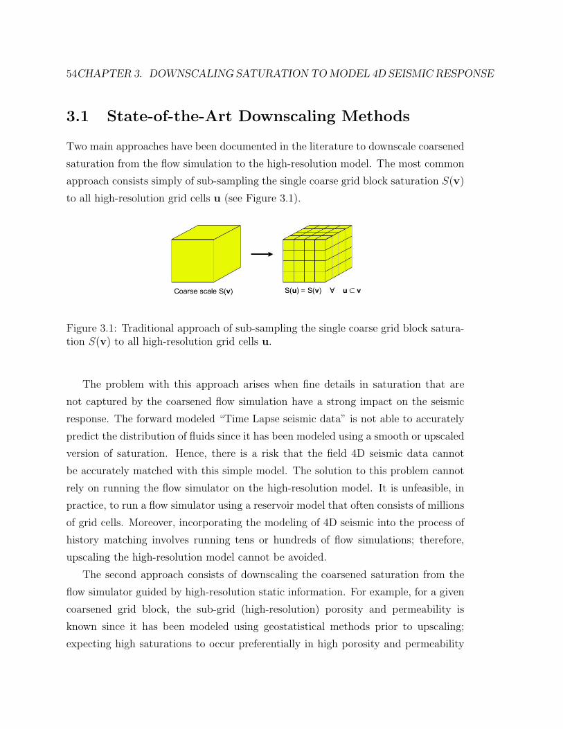
54CHAPTER 3. DOWNSCALING SATURATION TO MODEL 4D SEISMIC RESPONSE
3.1 State-of-the-Art Downscaling Methods
Two main approaches have been documented in the literature to downscale coarsened
saturation from the flow simulation to the high-resolution model. The most common
approach consists simply of sub-sampling the single coarse grid block saturation S(v)
to all high-resolution grid cells u (see Figure 3.1).
Figure 3.1: Traditional approach of sub-sampling the single coarse grid block satura-tion S(v) to all high-resolution grid cells u.
The problem with this approach arises when fine details in saturation that are
not captured by the coarsened flow simulation have a strong impact on the seismic
response. The forward modeled “Time Lapse seismic data” is not able to accurately
predict the distribution of fluids since it has been modeled using a smooth or upscaled
version of saturation. Hence, there is a risk that the field 4D seismic data cannot
be accurately matched with this simple model. The solution to this problem cannot
rely on running the flow simulator on the high-resolution model. It is unfeasible, in
practice, to run a flow simulator using a reservoir model that often consists of millions
of grid cells. Moreover, incorporating the modeling of 4D seismic into the process of
history matching involves running tens or hundreds of flow simulations; therefore,
upscaling the high-resolution model cannot be avoided.
The second approach consists of downscaling the coarsened saturation from the
flow simulator guided by high-resolution static information. For example, for a given
coarsened grid block, the sub-grid (high-resolution) porosity and permeability is
known since it has been modeled using geostatistical methods prior to upscaling;
expecting high saturations to occur preferentially in high porosity and permeability
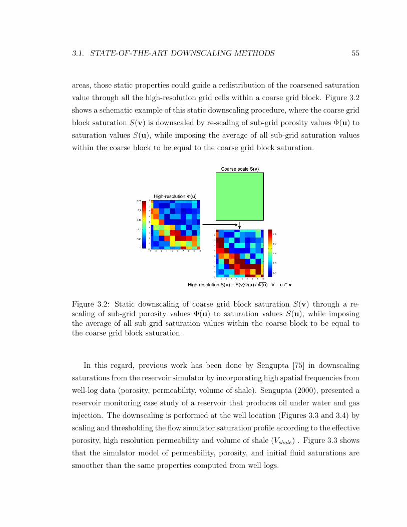
3.1. STATE-OF-THE-ART DOWNSCALING METHODS 55
areas, those static properties could guide a redistribution of the coarsened saturation
value through all the high-resolution grid cells within a coarse grid block. Figure 3.2
shows a schematic example of this static downscaling procedure, where the coarse grid
block saturation S(v) is downscaled by re-scaling of sub-grid porosity values Φ(u) to
saturation values S(u), while imposing the average of all sub-grid saturation values
within the coarse block to be equal to the coarse grid block saturation.
Figure 3.2: Static downscaling of coarse grid block saturation S(v) through a re-scaling of sub-grid porosity values Φ(u) to saturation values S(u), while imposingthe average of all sub-grid saturation values within the coarse block to be equal tothe coarse grid block saturation.
In this regard, previous work has been done by Sengupta [75] in downscaling
saturations from the reservoir simulator by incorporating high spatial frequencies from
well-log data (porosity, permeability, volume of shale). Sengupta (2000), presented a
reservoir monitoring case study of a reservoir that produces oil under water and gas
injection. The downscaling is performed at the well location (Figures 3.3 and 3.4) by
scaling and thresholding the flow simulator saturation profile according to the effective
porosity, high resolution permeability and volume of shale (Vshale) . Figure 3.3 shows
that the simulator model of permeability, porosity, and initial fluid saturations are
smoother than the same properties computed from well logs.
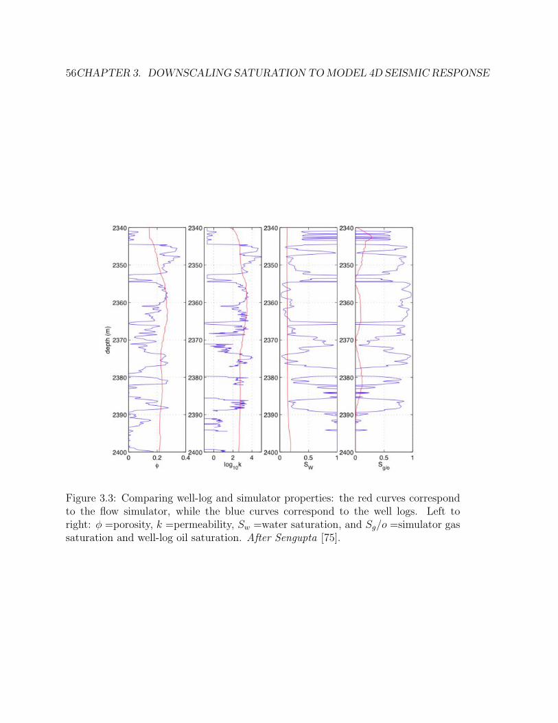
56CHAPTER 3. DOWNSCALING SATURATION TO MODEL 4D SEISMIC RESPONSE
Figure 3.3: Comparing well-log and simulator properties: the red curves correspondto the flow simulator, while the blue curves correspond to the well logs. Left toright: φ =porosity, k =permeability, Sw =water saturation, and Sg/o =simulator gassaturation and well-log oil saturation. After Sengupta [75].
3.1. STATE-OF-THE-ART DOWNSCALING METHODS 57
In order to downscale the saturation from the simulator, Sengupta [75] used the
well-log saturations. Figure 3.4 shows the original profile of the gas saturation (Sg)
taken from the flow simulator, and five estimates of the downscaled Sg, each repre-
senting a variation of the same downscaling approach. These estimates are computed
using the smooth Sg profile from the simulator and the initial oil saturation (1− Sw)
at the well location. Assuming gas is most likely to replace oil in the high porosity,
high permeability sands, the five estimates of Sg presented in Figure 3.4 were created
by Sengupta [75] as follows:
• profile (b) is created by setting to zero the smooth flow simulator profile Sg in
the zones of zero effective porosity,
• profile (c) is obtained by scaling profile (b) according to the high-resolution So
profile at the well, based on the assumption that gas is most likely to replace
oil,
• profiles (d) to (f) are obtained by successive hierarchical thresholding of profile
(c). Although it is not explicitly described, Sengupta mentions the thresholding
can be based on various rock physics parameters such as porosity, Vshale or high-
resolution permeability. As seen in Figure 3.4 an increase in vertical resolution
and Sg is seen from (d) to (f).
Using each of the downscaled 1D saturation profiles, the synthetic time-lapse
differential AVO attributes are computed for each profile (Figure 3.5), from the near
offset (5◦−15◦) and the mid offset (15◦−25◦). The time-lapse differential corresponds
to the percent change in root mean square (RMS) amplitude between the two seismic
surveys. The forward modeling of the 4D seismic response is performed at the well
location, no spatial reservoir modeling using geostatistical methods is done in this
example presented by Sengupta.
Figure 3.5 shows a cross plot between the time-lapse differential for near offsets
and mid offsets, where the color filled dots are values computed from the real seismic
data and the empty circles correspond to the synthetic values obtained from the
downscaled Sg profiles shown in Figure 3.4. From this figure, Sengupta concluded
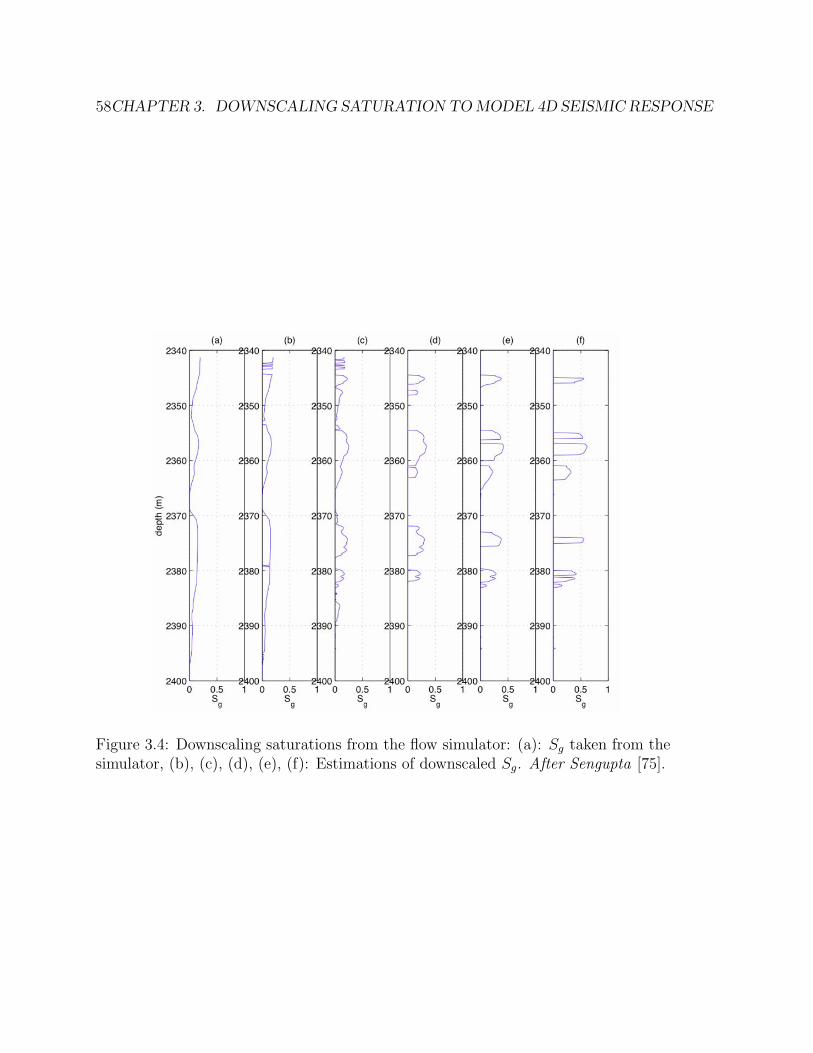
58CHAPTER 3. DOWNSCALING SATURATION TO MODEL 4D SEISMIC RESPONSE
Figure 3.4: Downscaling saturations from the flow simulator: (a): Sg taken from thesimulator, (b), (c), (d), (e), (f): Estimations of downscaled Sg. After Sengupta [75].
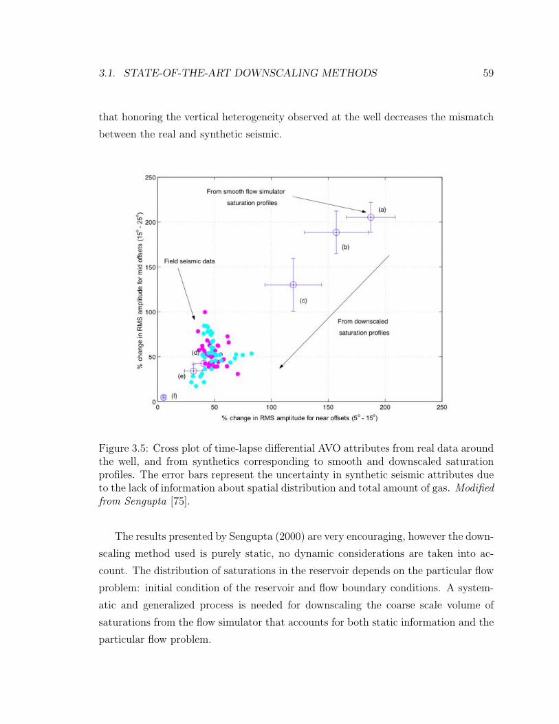
3.1. STATE-OF-THE-ART DOWNSCALING METHODS 59
that honoring the vertical heterogeneity observed at the well decreases the mismatch
between the real and synthetic seismic.
Figure 3.5: Cross plot of time-lapse differential AVO attributes from real data aroundthe well, and from synthetics corresponding to smooth and downscaled saturationprofiles. The error bars represent the uncertainty in synthetic seismic attributes dueto the lack of information about spatial distribution and total amount of gas. Modifiedfrom Sengupta [75].
The results presented by Sengupta (2000) are very encouraging, however the down-
scaling method used is purely static, no dynamic considerations are taken into ac-
count. The distribution of saturations in the reservoir depends on the particular flow
problem: initial condition of the reservoir and flow boundary conditions. A system-
atic and generalized process is needed for downscaling the coarse scale volume of
saturations from the flow simulator that accounts for both static information and the
particular flow problem.
60CHAPTER 3. DOWNSCALING SATURATION TO MODEL 4D SEISMIC RESPONSE
3.2 Flow-based Downscaling
The method proposed in this section for downscaling the coarsened saturations ac-
counts for both static information and the particular flow problem (initial and bound-
ary conditions). This procedure reconstructs the high-resolution saturation map by
simulating the local flow at every coarse grid block using the sub-grid (high-resolution)
permeability field and approximate local boundary conditions that are consistent with
the results of the flow simulation performed on the coarsened grid.
3.2.1 Governing equations
Consider Darcy’s law for two-phase oil-water flow:
uw =kkrw
µw
∇pw (3.1)
uo =kkro
µo
∇po (3.2)
where p is pressure, u is the Darcy velocity, k is permeability, µ is viscosity, and the
subscripts w and o refer to water and oil. The relative permeabilities of water and
oil are designated krw and kro.
Using these equations along with a statement of mass conservation on a control
volume (or grid block) for each phase, i.e., rate of change of mass in the volume equals
the net influx of mass, the following equations describing oil-water flow are obtained:
φ∂Sw
∂t+∇ · (uw) = 0 (3.3)
∇ · (λTk∇p) = 0 (3.4)
where t is time, λT is the total mobility (λT = krw/µw + kro/µo), and all other
variables are as defined previously. Note that here capillary forces and compressibility
effects are neglected. These two equations, referred to as the saturation and pressure
equations, are solved using an IMPES finite difference procedure. Specifically, the
pressure equation is solved first (implicitly) and then the saturation equation is solved

3.2. FLOW-BASED DOWNSCALING 61
explicitly.
3.2.2 Flow on the high-resolution and coarsened grids
Flow on the upscaled/coarsened grid, is performed using a commercial flow simulator.
The following variables are obtained for each coarse grid block v: water saturation
Scw(v), flux in the x direction qc
x(v) at x oriented (normal in the x direction) block
interfaces and flux in the z direction qcz(v) at z oriented block interfaces. Note that
the subscript c denotes a coarse grid quantity. Each coarse block v corresponds to
a region of the underlying high-resolution scale (geological) grid. We designate as
u the nx × ny high-resolution grid blocks that correspond to a particular v. Using
the information from flow on the coarsened grid, for each coarse block v, a flow
problem (Eqns. 3.3 and 3.4) is solved locally over the high-resolution grid blocks
u that correspond to v (Figure 3.6). For this simulation, the local high-resolution
permeability is used. Boundary conditions for the pressure equation are prescribed in
terms of the fluxes at each of the faces of the boundary blocks u, while the saturation
boundary conditions correspond to the saturation value at the inlet faces. The initial
condition is Sfw(u) = 0 for every high-resolution (superscript f) block.
For a particular coarse block, flux boundary conditions are computed for all high-
resolution cells comprising the boundaries of the coarse block. Following the work
of Gautier et al. [33] and Chen et al. [24], these high-resolution fluxes are assigned
in proportion to the high-resolution grid interblock transmissibility. Specifically, the
local high-resolution flux boundary conditions are computed along x = 0 and z = 0
(note that (x, z) = (0, 0) is the origin of the local grid system) as follows:
(qx)0,j =(Tx)1/2,j∑nzj=1(Tx)1/2,j
qcx j = 1, ..., nz (3.5)
(qz)i,0 =(Tz)i,1/2∑nxi=1(Tz)i,1/2
qcz i = 1, ..., nx (3.6)
where Tx and Tz are the high-resolution interblock transmissibilities in the x and z
directions. This reconstruction guarantees flux continuity across high-resolution cells
in neighboring coarse blocks and accounts for sub-grid heterogeneity, in addition to

62CHAPTER 3. DOWNSCALING SATURATION TO MODEL 4D SEISMIC RESPONSE
Figure 3.6: Domains for flow on the coarsened and local high-resolution grids. Lighterlines represent the high-resolution grid and heavier lines the coarse grid.
forcing the sum of the high-resolution grid fluxes to be equal to the corresponding
coarse grid flux.
Saturation boundary conditions are established for the high-resolution grid inlet
boundaries of the coarse block by using the high-resolution saturation of the adja-
cent grid block (which was previously reconstructed). This ensures continuity at the
boundaries of the coarse grid blocks. The reconstruction starts at well blocks and fol-
lows the direction of flow. Local high-resolution boundary conditions are computed
for the target coarse grid block and local flow is performed until the average of the
reconstructed local high-resolution saturations matches the coarse saturation Scw(v).
The process is repeated for each coarse grid block until the high-resolution saturation
field is reconstructed.
This approach for reconstructing the high-resolution saturation field can be ap-
plied in an adaptive fashion, where local high-resolution flow is simulated only in the
areas of the reservoir with high-resolution saturation effects which impact the seismic
signal (e.g., an advancing water front in a region with a high degree of sub-grid per-
meability variability). With this procedure, areas of the reservoir already swept by
3.3. 2D SYNTHETIC EXAMPLE 63
the injected water would not be reconstructed because they exhibit a high constant
saturation value. This approach could be much more efficient computationally than
reconstructing the high-resolution saturation everywhere, particularly in cases where
the important saturation changes occur over relatively small portions of the reservoir.
This technique will however require some modification of the downscaling procedure
described above, for example in the specification of the inlet saturation boundary
conditions. The success of the adaptive flow-based downscaling method proposed
here depends directly on the method used for upscaling as well as the upscaling ratio
applied to the static data prior to the flow simulation. The upscaling method, and
the chosen upscaling ratio, should be able to keep the overall character and posi-
tion of the saturation front, since the adaptive flow-based downscaling method would
identify the front and work on its refinement.
3.3 2D Synthetic Example
To illustrate the overall methodology, a simple example that effectively demonstrates
the importance of downscaling saturation when modeling 4D seismic data is presented.
The 2D (layered) geological model used for the example is shown in Figure 3.7.
Acoustic properties such as impedance (Z = ρVp) are assumed constant within the
layer interval (ρ = 2.3g/cc, and Vp = 2300m/sec). Using a flow-based upscaling
procedure [27], the high-resolution permeability model is upscaled to obtain coarse
scale permeabilities (kx and ky) for each coarse grid block (Figure 3.8).
Using these upscaled permeabilities, we simulate flow driven by a water injector
at the left boundary of the reservoir and an oil producer at the right boundary. The
injection rate is 400STB/day, the production rate is 415STB/day, and 200 days of oil
production are simulated. The resulting water saturation in the reservoir at the end of
the simulation is downscaled to the high-resolution grid (see Figure 3.9). This figure
shows that the fine details of the saturation front are to some extent restored and
the smooth character has been removed. We reiterate that this is achieved without
running a global high-resolution flow simulation.
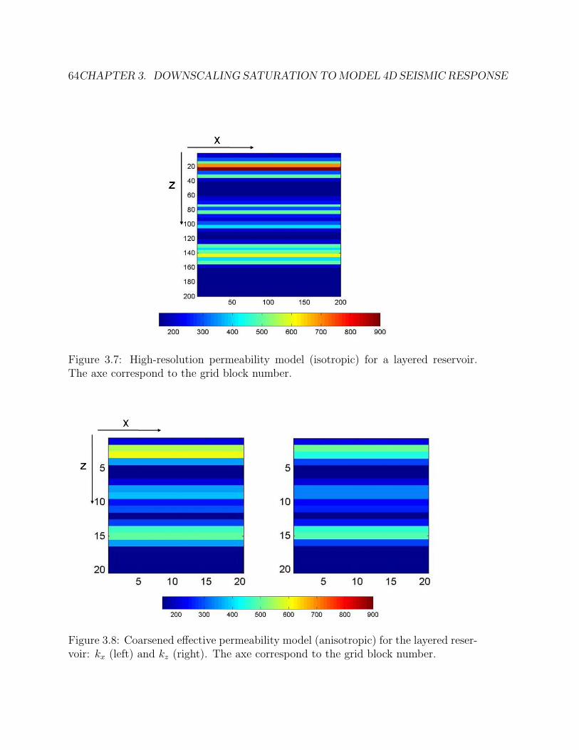
64CHAPTER 3. DOWNSCALING SATURATION TO MODEL 4D SEISMIC RESPONSE
Figure 3.7: High-resolution permeability model (isotropic) for a layered reservoir.The axe correspond to the grid block number.
Figure 3.8: Coarsened effective permeability model (anisotropic) for the layered reser-voir: kx (left) and kz (right). The axe correspond to the grid block number.
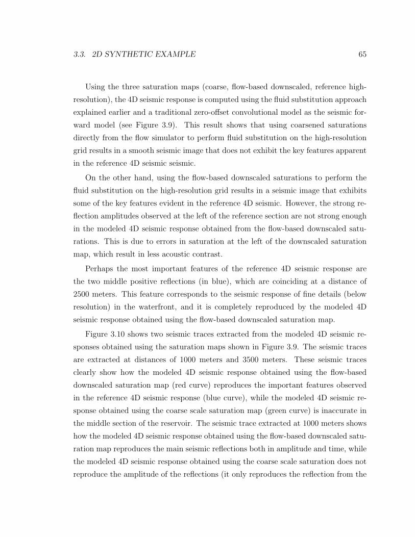
3.3. 2D SYNTHETIC EXAMPLE 65
Using the three saturation maps (coarse, flow-based downscaled, reference high-
resolution), the 4D seismic response is computed using the fluid substitution approach
explained earlier and a traditional zero-offset convolutional model as the seismic for-
ward model (see Figure 3.9). This result shows that using coarsened saturations
directly from the flow simulator to perform fluid substitution on the high-resolution
grid results in a smooth seismic image that does not exhibit the key features apparent
in the reference 4D seismic seismic.
On the other hand, using the flow-based downscaled saturations to perform the
fluid substitution on the high-resolution grid results in a seismic image that exhibits
some of the key features evident in the reference 4D seismic. However, the strong re-
flection amplitudes observed at the left of the reference section are not strong enough
in the modeled 4D seismic response obtained from the flow-based downscaled satu-
rations. This is due to errors in saturation at the left of the downscaled saturation
map, which result in less acoustic contrast.
Perhaps the most important features of the reference 4D seismic response are
the two middle positive reflections (in blue), which are coinciding at a distance of
2500 meters. This feature corresponds to the seismic response of fine details (below
resolution) in the waterfront, and it is completely reproduced by the modeled 4D
seismic response obtained using the flow-based downscaled saturation map.
Figure 3.10 shows two seismic traces extracted from the modeled 4D seismic re-
sponses obtained using the saturation maps shown in Figure 3.9. The seismic traces
are extracted at distances of 1000 meters and 3500 meters. These seismic traces
clearly show how the modeled 4D seismic response obtained using the flow-based
downscaled saturation map (red curve) reproduces the important features observed
in the reference 4D seismic response (blue curve), while the modeled 4D seismic re-
sponse obtained using the coarse scale saturation map (green curve) is inaccurate in
the middle section of the reservoir. The seismic trace extracted at 1000 meters shows
how the modeled 4D seismic response obtained using the flow-based downscaled satu-
ration map reproduces the main seismic reflections both in amplitude and time, while
the modeled 4D seismic response obtained using the coarse scale saturation does not
reproduce the amplitude of the reflections (it only reproduces the reflection from the
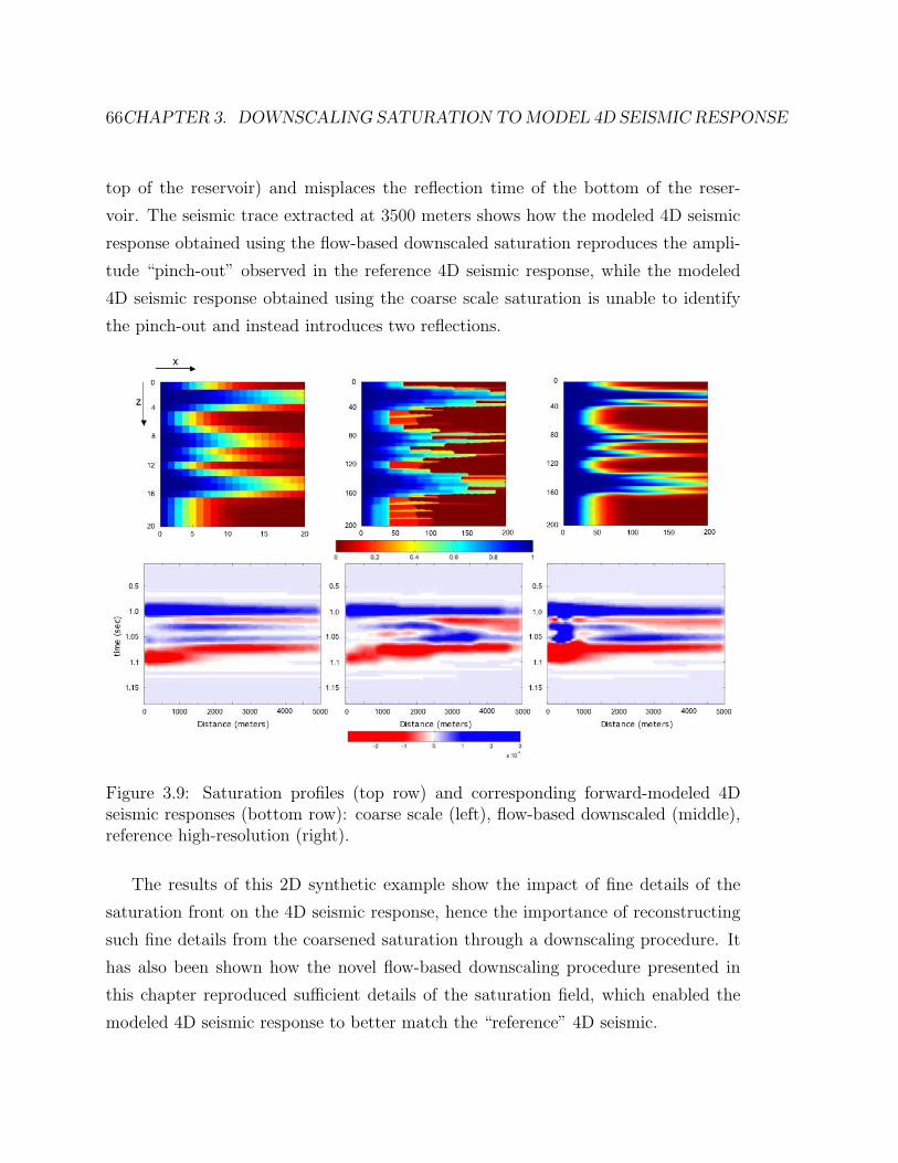
66CHAPTER 3. DOWNSCALING SATURATION TO MODEL 4D SEISMIC RESPONSE
top of the reservoir) and misplaces the reflection time of the bottom of the reser-
voir. The seismic trace extracted at 3500 meters shows how the modeled 4D seismic
response obtained using the flow-based downscaled saturation reproduces the ampli-
tude “pinch-out” observed in the reference 4D seismic response, while the modeled
4D seismic response obtained using the coarse scale saturation is unable to identify
the pinch-out and instead introduces two reflections.
Figure 3.9: Saturation profiles (top row) and corresponding forward-modeled 4Dseismic responses (bottom row): coarse scale (left), flow-based downscaled (middle),reference high-resolution (right).
The results of this 2D synthetic example show the impact of fine details of the
saturation front on the 4D seismic response, hence the importance of reconstructing
such fine details from the coarsened saturation through a downscaling procedure. It
has also been shown how the novel flow-based downscaling procedure presented in
this chapter reproduced sufficient details of the saturation field, which enabled the
modeled 4D seismic response to better match the “reference” 4D seismic.
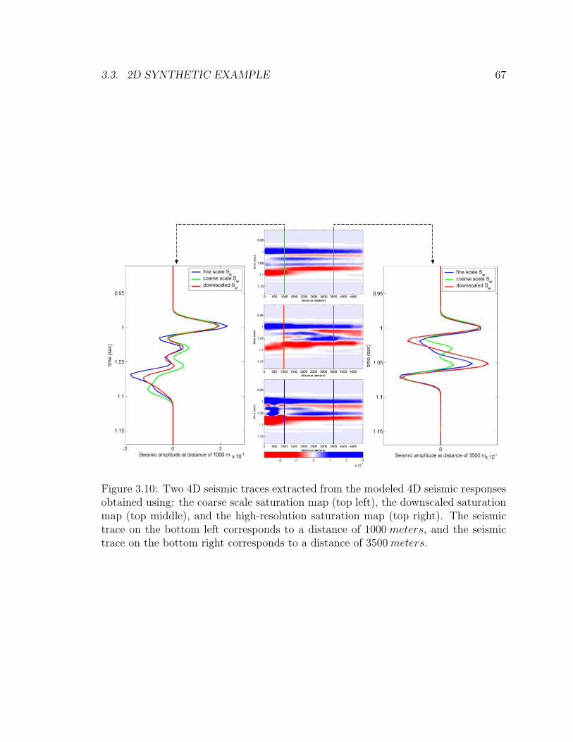
3.3. 2D SYNTHETIC EXAMPLE 67
Figure 3.10: Two 4D seismic traces extracted from the modeled 4D seismic responsesobtained using: the coarse scale saturation map (top left), the downscaled saturationmap (top middle), and the high-resolution saturation map (top right). The seismictrace on the bottom left corresponds to a distance of 1000 meters, and the seismictrace on the bottom right corresponds to a distance of 3500 meters.
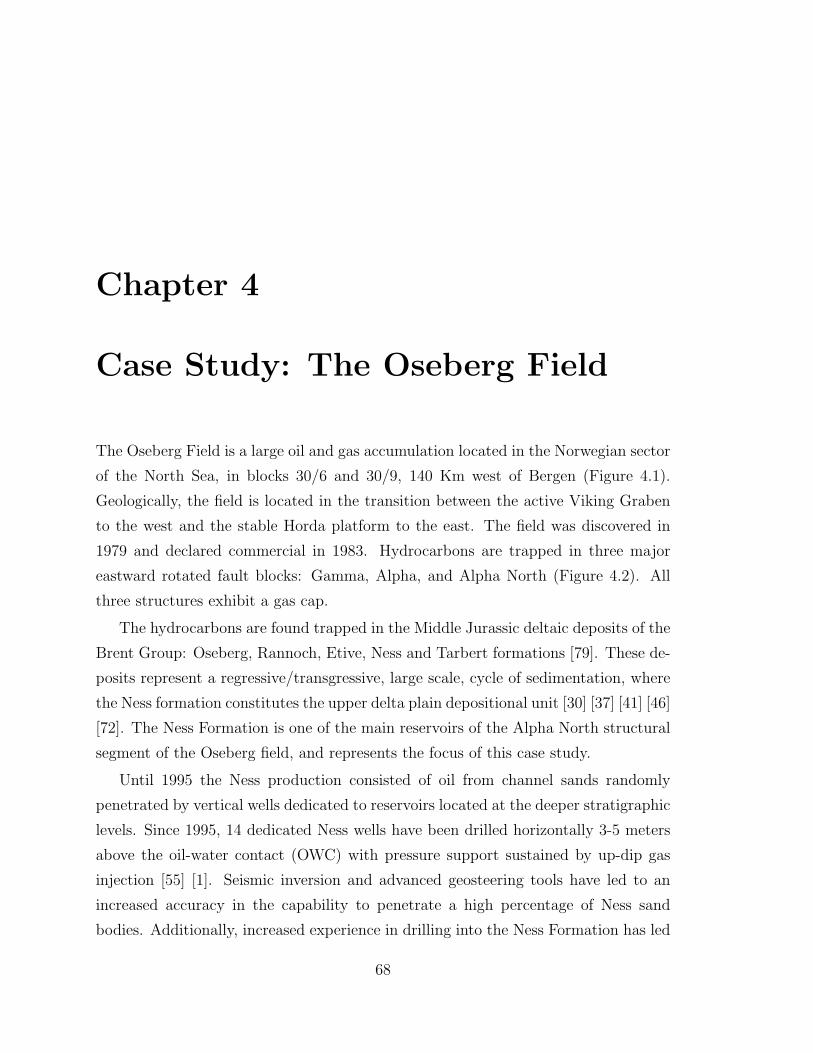
Chapter 4
Case Study: The Oseberg Field
The Oseberg Field is a large oil and gas accumulation located in the Norwegian sector
of the North Sea, in blocks 30/6 and 30/9, 140 Km west of Bergen (Figure 4.1).
Geologically, the field is located in the transition between the active Viking Graben
to the west and the stable Horda platform to the east. The field was discovered in
1979 and declared commercial in 1983. Hydrocarbons are trapped in three major
eastward rotated fault blocks: Gamma, Alpha, and Alpha North (Figure 4.2). All
three structures exhibit a gas cap.
The hydrocarbons are found trapped in the Middle Jurassic deltaic deposits of the
Brent Group: Oseberg, Rannoch, Etive, Ness and Tarbert formations [79]. These de-
posits represent a regressive/transgressive, large scale, cycle of sedimentation, where
the Ness formation constitutes the upper delta plain depositional unit [30] [37] [41] [46]
[72]. The Ness Formation is one of the main reservoirs of the Alpha North structural
segment of the Oseberg field, and represents the focus of this case study.
Until 1995 the Ness production consisted of oil from channel sands randomly
penetrated by vertical wells dedicated to reservoirs located at the deeper stratigraphic
levels. Since 1995, 14 dedicated Ness wells have been drilled horizontally 3-5 meters
above the oil-water contact (OWC) with pressure support sustained by up-dip gas
injection [55] [1]. Seismic inversion and advanced geosteering tools have led to an
increased accuracy in the capability to penetrate a high percentage of Ness sand
bodies. Additionally, increased experience in drilling into the Ness Formation has led
68
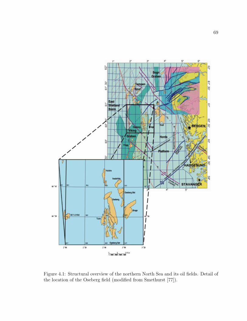
69
Figure 4.1: Structural overview of the northern North Sea and its oil fields. Detail ofthe location of the Oseberg field (modified from Smethurst [77]).
70 CHAPTER 4. CASE STUDY: THE OSEBERG FIELD
to a significant decrease in formation associated drilling problems.
According to Liestøl et al. [55], it is very difficult to predict the reserves associ-
ated with a Ness producer since individual production profiles from Ness wells display
a great variety in production, and low production has been experienced from wells
penetrating up to 70 % channel sands. The best Ness producers have without excep-
tion had some degree of gas-breakthrough, which ensures both pressure support and
efficient sweep of up flank oil. The poorer Ness producers have experienced no gas
or water breakthrough, or only water breakthrough. In addition, some wells struggle
with rapid depletion, reflecting poorly connected volumes.
The main reasons for the production variability and low recovery (26%) experi-
enced from the Ness formation compared to the other shallow-marine reservoirs in the
Oseberg Field are associated with the complexity and heterogeneities of the fluvial
Ness reservoirs [55]. Some of the general observations of Liestøl et al. about the lack
of efficient pressure support from the gas cap in the wells are:
• Large vertical and horizontal heterogeneities in the Ness Formation could cause
nonexistent or poor communication pathways between the channel sands pene-
trated by the well and channel sands in the gas cap.
• The communicating volume around a Ness producer may be so isolated and
limited that the pressure depletion quickly becomes too large to maintain pro-
duction.
• A small part of the sands in the well receives all the pressure support. Pro-
duction from these sands will then dominate and gas flood the well preventing
efficient sweep of sands with poorer pressure support.
As established by Liestøl et al., the distribution of the channel sands in the Ness
reservoir is the parameter that controls production performance in the field. The
distribution of channel sands involves the orientation of the channels, the local pro-
portion of sand and more importantly in this case, the degree of communication
between channel sand bodies. Therefore, the goal of the case study presented in this
chapter is to build several models of the distribution of the channel sands in the Upper

4.1. ALPHA NORTH SEGMENT - UPPER NESS FORMATION 71
Ness Formation of the Alpha North structural segment of the Oseberg field. Each of
these models would be created using the two reservoir modeling workflows, presented
in Chapter 2, to incorporate 4D seismic data: the PDI and FM approaches.
This chapter first introduces the details of the reservoir under study, in the Alpha
North structural segment of the Oseberg field. Subsequently, the available data and
how they are incorporated into the reservoir modeling workflow are presented in
section 4.2. The last two sections of the chapter are devoted to present the results of
the application of the two workflows (PDI and FM approaches) to build a reservoir
model for the Upper Ness in Alpha North; a detailed comparison of the results of the
two approaches is also provided.
4.1 Alpha North Segment - Upper Ness Formation
The Alpha North structural segment, located on the northernmost part of the Oseberg
Field (Figure 4.2), is bounded by normal faults towards the Alpha Main structure in
the South and West and the Theta structure towards north. Cretaceous erosion delin-
eates the western extent of the Brent group reservoirs, while the cap-rock constitutes
late Jurassic and Cretaceous mudstones (Figure 4.3).
One of the main reservoir units of the Alpha North segment is represented by the
Upper Ness Formation (UN). The thickness distribution of the UN on Alpha North
is between 25 and 40 meters TVT (true vertical depth), increasing gently towards
N-NNE, with an average thickness of 33 meters TVT.
The UN corresponds to the upper delta plain depositional unit of the Brent group.
According to Liestøl et al., four sedimentary facies can be identified in the UN: chan-
nel, crevasse, coal and floodplain. The channel facies represent the reservoir unit
in the Ness Formation and is characterized by sharp-based, thick (2.5 - 27 meters)
fining-upwards sandstone units. The properties of the channel sandstones of the UN
on Alpha North gives an average porosity of 24% and and average horizontal perme-
ability of 2600 mD.
Stratigraphically, the distribution of channel-sands forms a four-partition pattern
with two zones of high content of sand alternating with two zones of low sand content
72 CHAPTER 4. CASE STUDY: THE OSEBERG FIELD
shown in Figure 4.4. According to Liestøl et al., paleocurrent measurements show a
main northwards transport direction, with a deviation span ranging from NNW to
NE, throughout the Ness Formation in the Oseberg area; and this is also supported
by seismic data.
The average individual sandstone body thickness is between 4 and 6 meters; how-
ever, amalgamated multistory sandstone bodies average 27 meters thick in central
parts of the Alpha North segment. An average channel width is in the order of 100
to 125 meters, and an average channel belt width is between 250 and 350 meters [55].
Figure 4.2: Outline of the Oseberg Field and its major fault blocks: Alpha, AlphaNorth, and Gamma (modified from Johnstad et al. [47]).
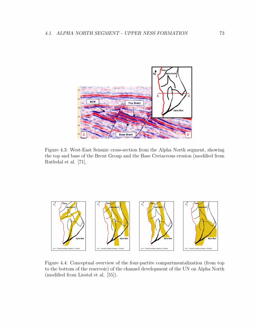
4.1. ALPHA NORTH SEGMENT - UPPER NESS FORMATION 73
Figure 4.3: West-East Seismic cross-section from the Alpha North segment, showingthe top and base of the Brent Group and the Base Cretaceous erosion (modified fromRutledal et al. [71].
Figure 4.4: Conceptual overview of the four-partite compartmentalization (from topto the bottom of the reservoir) of the channel development of the UN on Alpha North(modified from Liestøl et al. [55]).
74 CHAPTER 4. CASE STUDY: THE OSEBERG FIELD
4.2 The Reservoir Modeling Workflow
The Alpha North segment of the Oseberg Field exhibits an excellent variety of data,
which has been provided by the team of geologists, geophysicists, geostatisticians
and reservoir engineers of the company that operates the field (Norsk Hydro). The
available data consists of: well-logs for approximately 15 wells; a training image of
the facies distribution in the reservoir; two facies probability cubes, one created from
the Base 3D seismic survey and another one created from the 4D seismic data; the
properties of the fluids in the reservoir; the relationships (obtained in the lab from core
measurements) between seismic velocities, porosity and effective pressure; 4D seismic
data consisting of the results of an elastic inversion applied to each of the three seismic
surveys acquired in 1992, 1999 and 2004 respectively; historical production data and
a flow simulation model built in ECLIPSE 1.
Using the workflow and methodology presented in Chapter 2, data and procedures
from the Alpha North were provided to each of the main modules of the workflow.
The main modules of the workflow are the following:
• Building a high-resolution 3D geocellular model
• Building a 3D coarsened model
• Building a flow-simulation model
• Establishing the history matching procedure
4.2.1 The High-resolution 3D Geocellular Model
The architecture of the reservoir (structural framework) in terms of horizons and
faults, typically determined from 3D seismic data and well-markers, was established
by the team at Norsk Hydro who constructed the 3D stratigraphic grid used in this
case study. The work presented in this section corresponds solely to the population
of the grid with facies and petrophysical properties.
1 c© Copyright 2005 Schlumberger. All rights reserved.
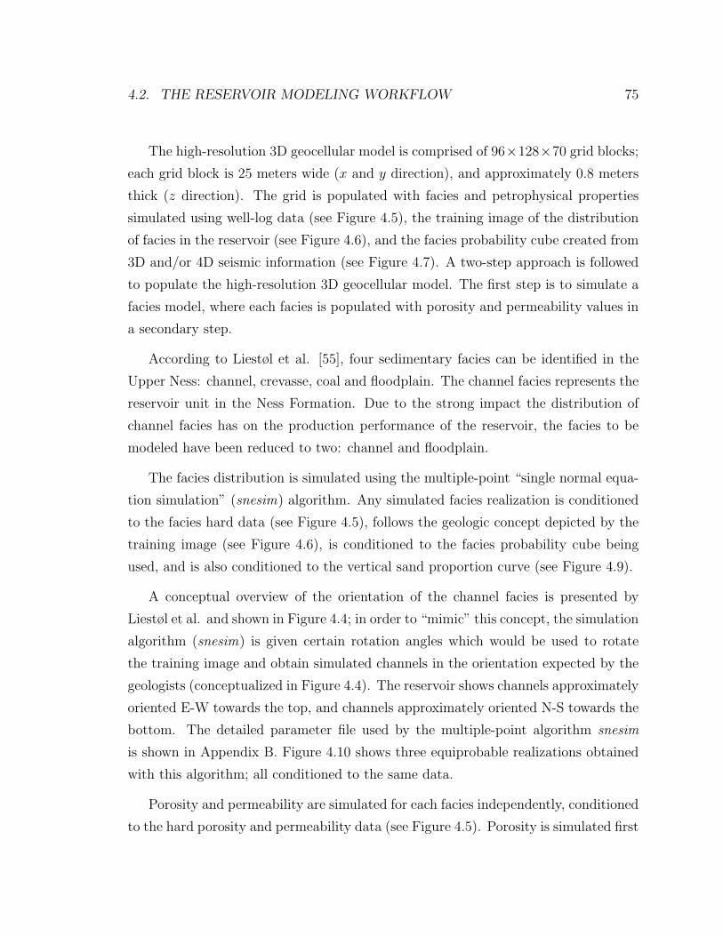
4.2. THE RESERVOIR MODELING WORKFLOW 75
The high-resolution 3D geocellular model is comprised of 96×128×70 grid blocks;
each grid block is 25 meters wide (x and y direction), and approximately 0.8 meters
thick (z direction). The grid is populated with facies and petrophysical properties
simulated using well-log data (see Figure 4.5), the training image of the distribution
of facies in the reservoir (see Figure 4.6), and the facies probability cube created from
3D and/or 4D seismic information (see Figure 4.7). A two-step approach is followed
to populate the high-resolution 3D geocellular model. The first step is to simulate a
facies model, where each facies is populated with porosity and permeability values in
a secondary step.
According to Liestøl et al. [55], four sedimentary facies can be identified in the
Upper Ness: channel, crevasse, coal and floodplain. The channel facies represents the
reservoir unit in the Ness Formation. Due to the strong impact the distribution of
channel facies has on the production performance of the reservoir, the facies to be
modeled have been reduced to two: channel and floodplain.
The facies distribution is simulated using the multiple-point “single normal equa-
tion simulation” (snesim) algorithm. Any simulated facies realization is conditioned
to the facies hard data (see Figure 4.5), follows the geologic concept depicted by the
training image (see Figure 4.6), is conditioned to the facies probability cube being
used, and is also conditioned to the vertical sand proportion curve (see Figure 4.9).
A conceptual overview of the orientation of the channel facies is presented by
Liestøl et al. and shown in Figure 4.4; in order to “mimic” this concept, the simulation
algorithm (snesim) is given certain rotation angles which would be used to rotate
the training image and obtain simulated channels in the orientation expected by the
geologists (conceptualized in Figure 4.4). The reservoir shows channels approximately
oriented E-W towards the top, and channels approximately oriented N-S towards the
bottom. The detailed parameter file used by the multiple-point algorithm snesim
is shown in Appendix B. Figure 4.10 shows three equiprobable realizations obtained
with this algorithm; all conditioned to the same data.
Porosity and permeability are simulated for each facies independently, conditioned
to the hard porosity and permeability data (see Figure 4.5). Porosity is simulated first

76 CHAPTER 4. CASE STUDY: THE OSEBERG FIELD
using “sequential Gaussian simulation” (sgsim), and permeability is subsequently co-
simulated using “sequential Gaussian co-simulation” (sgcosim) with porosity as sec-
ondary information. The histograms of both porosity and permeability are obtained
from the well-log data and the variograms used for sequential simulation (shown in
Table 4.1) are provided by Norsk Hydro. The final porosity and permeability models
are obtained after “cookie-cutting” the porosity and permeability realizations using
the facies realization (see Figures 4.11 and 4.12).
floodplain channeltype Exponential Exponential
nugget 0.0 0.0ranges 1000/1000/10 1000/250/12.5angles 0/0/0 0/90/0
Table 4.1: Variograms used for simulating porosity and permeability for each facies;ranges are shown in meters.
4.2.2 The 3D Coarsened Model
Although the high-resolution 3D geocellular model only consists of 96×128×70 grid
blocks, less than a million cells; the complexity of the flow simulation model (see
section 4.2.3) precluded performing a single flow simulation in a reasonable compu-
tational time for history matching purposes. The reservoir model is to be iteratively
perturbed in a history matching loop until a satisfactory match of dynamic data is
achieved; usually, multiple (often hundreds) flow simulations are required in order to
achieve such a satisfactory match. Hence, it is imperative to reduce the computational
time to obtain useful results for making decisions about the field.
The high-resolution 3D geocellular model was coarsened from 96× 128× 70 grid
blocks to 48 × 64 × 14 grid blocks, using an upscaling ratio of 2 : 2 : 5 and a single-
phase flow-based upscaling procedure developed by Deutsch in 1985 [27]. The single-
phase flow-based upscaling procedure consists of finding the effective permeability of
a coarse grid block comprising fine scale heterogeneities that would give the same flow
through a homogeneous coarse grid block of the same size.
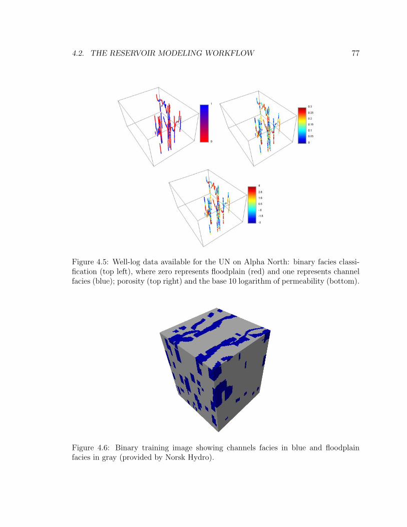
4.2. THE RESERVOIR MODELING WORKFLOW 77
Figure 4.5: Well-log data available for the UN on Alpha North: binary facies classi-fication (top left), where zero represents floodplain (red) and one represents channelfacies (blue); porosity (top right) and the base 10 logarithm of permeability (bottom).
Figure 4.6: Binary training image showing channels facies in blue and floodplainfacies in gray (provided by Norsk Hydro).
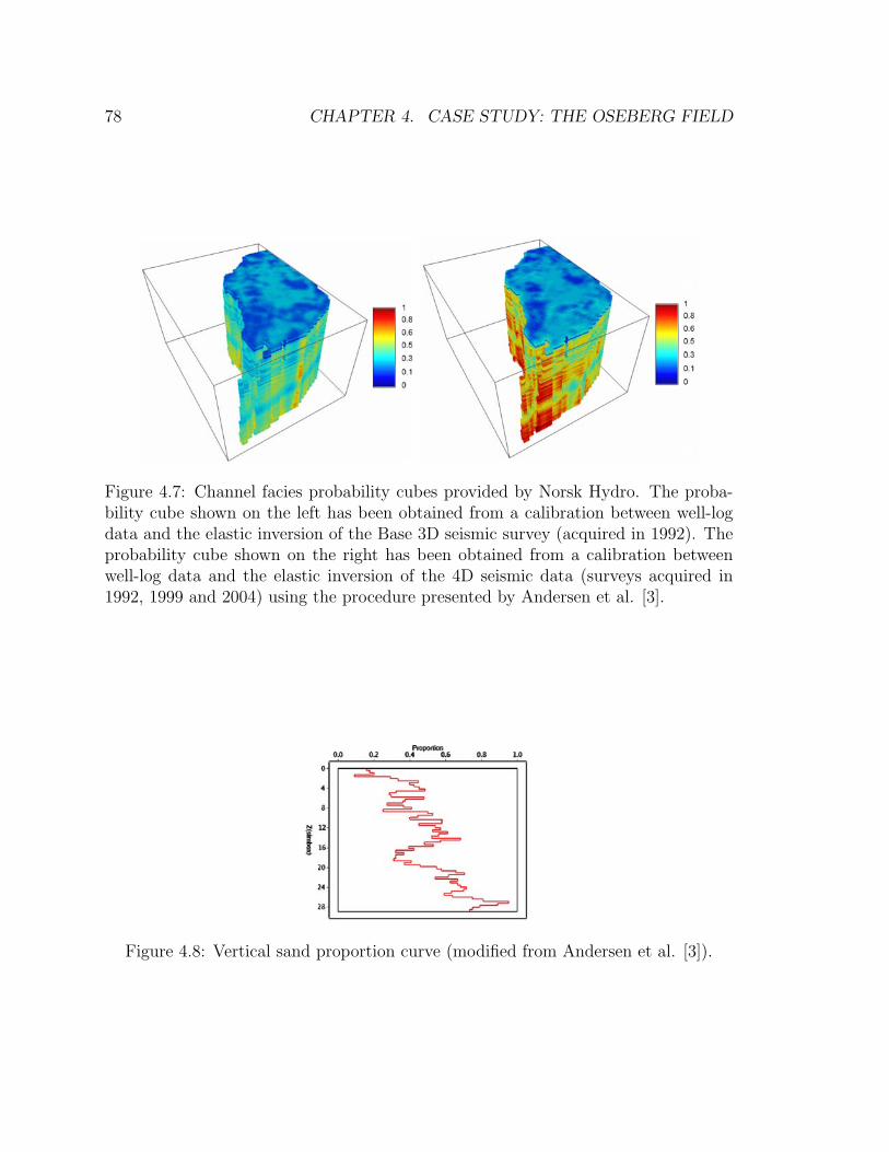
78 CHAPTER 4. CASE STUDY: THE OSEBERG FIELD
Figure 4.7: Channel facies probability cubes provided by Norsk Hydro. The proba-bility cube shown on the left has been obtained from a calibration between well-logdata and the elastic inversion of the Base 3D seismic survey (acquired in 1992). Theprobability cube shown on the right has been obtained from a calibration betweenwell-log data and the elastic inversion of the 4D seismic data (surveys acquired in1992, 1999 and 2004) using the procedure presented by Andersen et al. [3].
Figure 4.8: Vertical sand proportion curve (modified from Andersen et al. [3]).
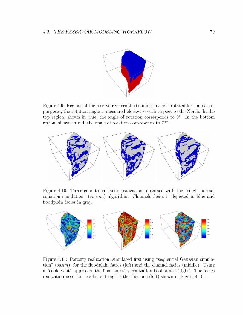
4.2. THE RESERVOIR MODELING WORKFLOW 79
Figure 4.9: Regions of the reservoir where the training image is rotated for simulationpurposes; the rotation angle is measured clockwise with respect to the North. In thetop region, shown in blue, the angle of rotation corresponds to 0◦. In the bottomregion, shown in red, the angle of rotation corresponds to 72◦.
Figure 4.10: Three conditional facies realizations obtained with the “single normalequation simulation” (snesim) algorithm. Channels facies is depicted in blue andfloodplain facies in gray.
Figure 4.11: Porosity realization, simulated first using “sequential Gaussian simula-tion” (sgsim), for the floodplain facies (left) and the channel facies (middle). Usinga “cookie-cut” approach, the final porosity realization is obtained (right). The faciesrealization used for “cookie-cutting” is the first one (left) shown in Figure 4.10.
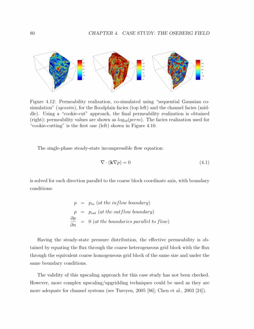
80 CHAPTER 4. CASE STUDY: THE OSEBERG FIELD
Figure 4.12: Permeability realization, co-simulated using “sequential Gaussian co-simulation” (sgcosim), for the floodplain facies (top left) and the channel facies (mid-dle). Using a “cookie-cut” approach, the final permeability realization is obtained(right); permeability values are shown as log10(perm). The facies realization used for“cookie-cutting” is the first one (left) shown in Figure 4.10.
The single-phase steady-state incompressible flow equation:
∇ · (k∇p) = 0 (4.1)
is solved for each direction parallel to the coarse block coordinate axis, with boundary
conditions:
p = pin (at the inflow boundary)
p = pout (at the outflow boundary)
∂p
∂n= 0 (at the boundaries parallel to flow)
Having the steady-state pressure distribution, the effective permeability is ob-
tained by equating the flux through the coarse heterogeneous grid block with the flux
through the equivalent coarse homogeneous grid block of the same size and under the
same boundary conditions.
The validity of this upscaling approach for this case study has not been checked.
However, more complex upscaling/upgridding techniques could be used as they are
more adequate for channel systems (see Tureyen, 2005 [86]; Chen et al., 2003 [24]).
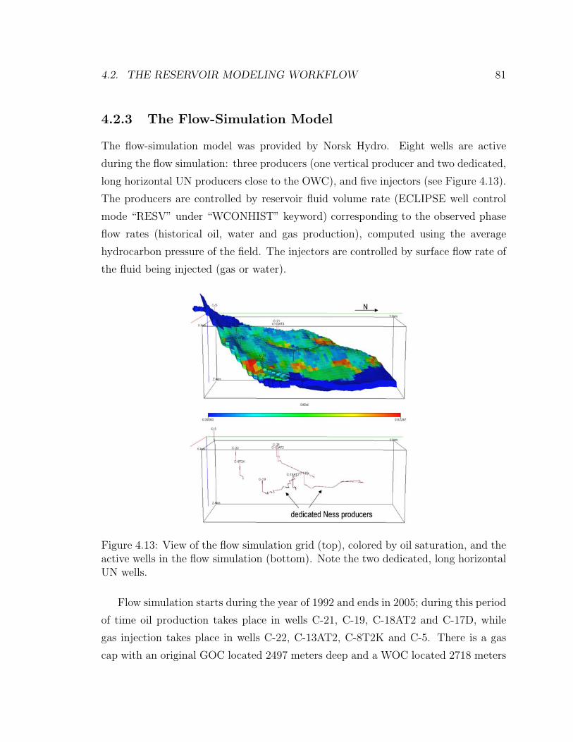
4.2. THE RESERVOIR MODELING WORKFLOW 81
4.2.3 The Flow-Simulation Model
The flow-simulation model was provided by Norsk Hydro. Eight wells are active
during the flow simulation: three producers (one vertical producer and two dedicated,
long horizontal UN producers close to the OWC), and five injectors (see Figure 4.13).
The producers are controlled by reservoir fluid volume rate (ECLIPSE well control
mode “RESV” under “WCONHIST” keyword) corresponding to the observed phase
flow rates (historical oil, water and gas production), computed using the average
hydrocarbon pressure of the field. The injectors are controlled by surface flow rate of
the fluid being injected (gas or water).
Figure 4.13: View of the flow simulation grid (top), colored by oil saturation, and theactive wells in the flow simulation (bottom). Note the two dedicated, long horizontalUN wells.
Flow simulation starts during the year of 1992 and ends in 2005; during this period
of time oil production takes place in wells C-21, C-19, C-18AT2 and C-17D, while
gas injection takes place in wells C-22, C-13AT2, C-8T2K and C-5. There is a gas
cap with an original GOC located 2497 meters deep and a WOC located 2718 meters
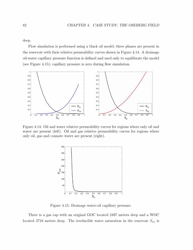
82 CHAPTER 4. CASE STUDY: THE OSEBERG FIELD
deep.
Flow simulation is performed using a black oil model; three phases are present in
the reservoir with their relative permeability curves shown in Figure 4.14. A drainage
oil-water capillary pressure function is defined and used only to equilibrate the model
(see Figure 4.15); capillary pressure is zero during flow simulation.
Figure 4.14: Oil and water relative permeability curves for regions where only oil andwater are present (left). Oil and gas relative permeability curves for regions whereonly oil, gas and connate water are present (right).
Figure 4.15: Drainage water-oil capillary pressure.
There is a gas cap with an original GOC located 2497 meters deep and a WOC
located 2718 meters deep. The irreducible water saturation in the reservoir Swi is
4.2. THE RESERVOIR MODELING WORKFLOW 83
computed as a function of permeability:
Swi = −0.20068 log(k) + 0.02014 log(k)2 + 0.53173
The flow simulation grid consisted originally of the 3D coarsened model with
two additional layers representing the Tarbert reservoir at the top and the ORELN
(Oseberg - Rannoch - Etive - Lower Ness) at the bottom. In order to improve the
flow simulation time, the two additional layers were inactivated since there was no
communication with UN.
4.2.4 Establishing the History Matching Procedure
Establishing the history matching procedure involves defining: the parameter(s) of
the model to be perturbed, the perturbation method to be used, the dynamic data
to be matched, and the objective function to be minimized.
As observed by Liestøl et al. [55], the distribution of the channel sands in the
Ness reservoir is the parameter that controls production performance in the field.
Therefore, the goal of the history matching procedure is no other than to perturb
the distribution of the channel sands in the reservoir model. As thoroughly discussed
in Chapters 1 and 2, our proposed reservoir modeling workflow follows the “Parallel
Modeling Approach” proposed by Tureyen in 2005 [86], and the “Probabilistic Data
Integration Approach” introduced by Hoffman in 2005 [44]. Therefore, the perturba-
tion is performed on the high resolution 3D geocellular model using a method called
“Probability Perturbation Method” [15] which perturbs the conditional probability
from which the initial facies realization has been drawn; the perturbation is done by
introducing another probability model that depends on dynamic data, as explained
in section 2.1.2.
Dynamic data includes all data that have been measured or interpreted over time;
such as: production data (fluid rates or volumes, pressure data), and 4D seismic data
(any suite of 3D seismic attributes computed from each seismic survey). Both produc-
tion and 4D seismic data are available for the reservoir under study in this chapter;
therefore, the application of the two workflows proposed in Chapter 2, pursues either
84 CHAPTER 4. CASE STUDY: THE OSEBERG FIELD
matching production data only (PDI approach) or matching both production and 4D
seismic data (FM approach).
Production and 4D seismic data
The production from Alpha North started in 1991 with a two-front production
drive system; gas injection in the initial gas cap and water injection in the water leg
(see Figure 4.17). Until 1995 the Ness production consisted of oil from channel sands
randomly penetrated by vertical wells dedicated to reservoirs located at the deeper
stratigraphic levels. Since 1995, 14 dedicated Ness wells have been drilled horizontally
3-5 meters above the oil-water contact (OWC) with pressure support sustained by
up-dip gas injection [55] [1]. Two of those wells (C-19 and C-17D) are dedicated
Ness producers in Alpha North (see Figures 4.18 and 4.19). The goal of the history
matching procedure would be matching the total oil and water production for these
two dedicated long horizontal wells.
Production started to decline in 1996 (see Figure 4.16) and as IOR initiative, a
time-lapse seismic survey was acquired in 1999 to be compared with the base survey
from 1992. An elastic inversion procedure was applied by Norsk Hydro to both seismic
data sets, providing acoustic impedance (AI) and Vp/Vs ratio for each seismic survey;
the results were extensively used at that time in defining the location of in-fill wells.
In 2004, a new seismic data set was acquired and Norsk Hydro performed a new
elastic inversion (see Figure 4.20). The results of the elastic inversion on the three
seismic surveys were supplied by Norsk Hydro, sampled in the same grid used for the
high-resolution 3D geocellular model.
The 4D seismic data is shown in Figure 4.21 as ratios between the new survey and
the old survey:
[AI]1999
[AI]1992
[Vp/Vs]1999
[Vp/Vs]1992
[AI]2004
[AI]1999
[Vp/Vs]2004
[Vp/Vs]1999
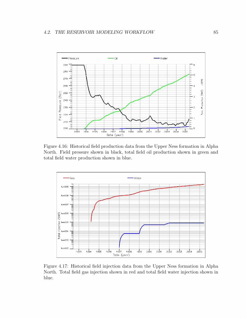
4.2. THE RESERVOIR MODELING WORKFLOW 85
Figure 4.16: Historical field production data from the Upper Ness formation in AlphaNorth. Field pressure shown in black, total field oil production shown in green andtotal field water production shown in blue.
Figure 4.17: Historical field injection data from the Upper Ness formation in AlphaNorth. Total field gas injection shown in red and total field water injection shown inblue.
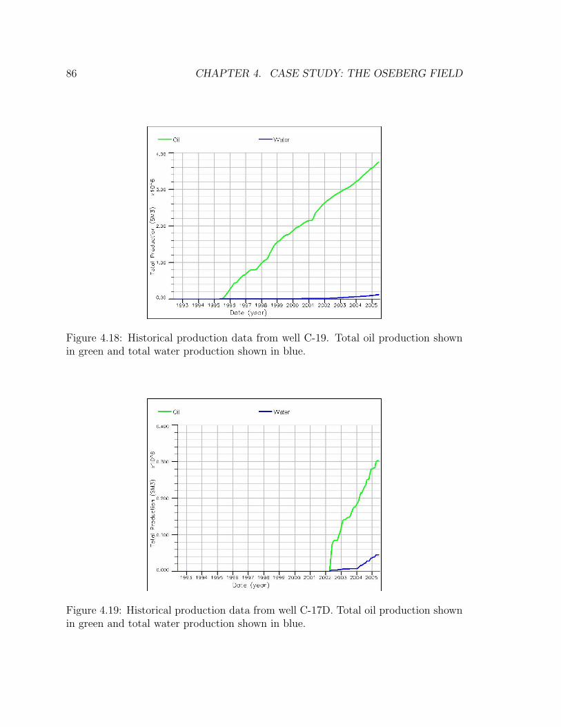
86 CHAPTER 4. CASE STUDY: THE OSEBERG FIELD
Figure 4.18: Historical production data from well C-19. Total oil production shownin green and total water production shown in blue.
Figure 4.19: Historical production data from well C-17D. Total oil production shownin green and total water production shown in blue.
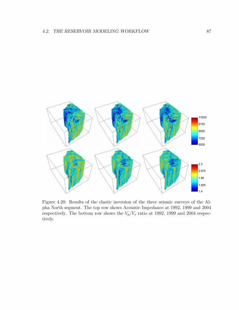
4.2. THE RESERVOIR MODELING WORKFLOW 87
Figure 4.20: Results of the elastic inversion of the three seismic surveys of the Al-pha North segment. The top row shows Acoustic Impedance at 1992, 1999 and 2004respectively. The bottom row shows the Vp/Vs ratio at 1992, 1999 and 2004 respec-tively.
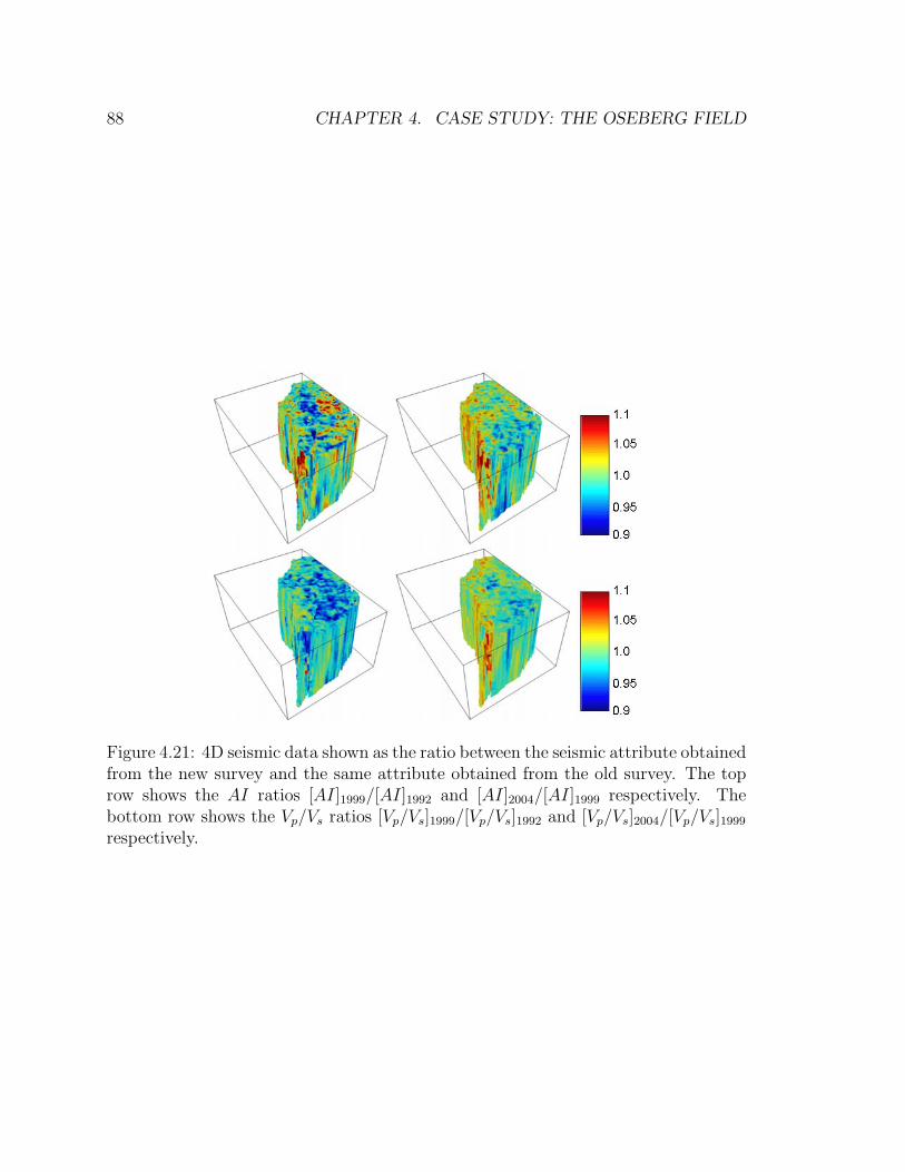
88 CHAPTER 4. CASE STUDY: THE OSEBERG FIELD
Figure 4.21: 4D seismic data shown as the ratio between the seismic attribute obtainedfrom the new survey and the same attribute obtained from the old survey. The toprow shows the AI ratios [AI]1999/[AI]1992 and [AI]2004/[AI]1999 respectively. Thebottom row shows the Vp/Vs ratios [Vp/Vs]1999/[Vp/Vs]1992 and [Vp/Vs]2004/[Vp/Vs]1999
respectively.
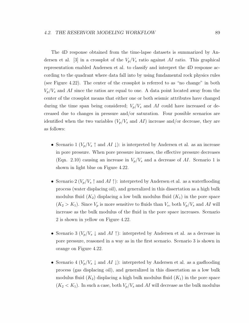
4.2. THE RESERVOIR MODELING WORKFLOW 89
The 4D response obtained from the time-lapse datasets is summarized by An-
dersen et al. [3] in a crossplot of the Vp/Vs ratio against AI ratio. This graphical
representation enabled Andersen et al. to classify and interpret the 4D response ac-
cording to the quadrant where data fall into by using fundamental rock physics rules
(see Figure 4.22). The center of the crossplot is referred to as “no change” in both
Vp/Vs and AI since the ratios are equal to one. A data point located away from the
center of the crossplot means that either one or both seismic attributes have changed
during the time span being considered; Vp/Vs and AI could have increased or de-
creased due to changes in pressure and/or saturation. Four possible scenarios are
identified when the two variables (Vp/Vs and AI) increase and/or decrease, they are
as follows:
• Scenario 1 (Vp/Vs ↑ and AI ↓): is interpreted by Andersen et al. as an increase
in pore pressure. When pore pressure increases, the effective pressure decreases
(Eqn. 2.10) causing an increase in Vp/Vs and a decrease of AI. Scenario 1 is
shown in light blue on Figure 4.22.
• Scenario 2 (Vp/Vs ↑ and AI ↑): interpreted by Andersen et al. as a waterflooding
process (water displacing oil), and generalized in this dissertation as a high bulk
modulus fluid (K2) displacing a low bulk modulus fluid (K1) in the pore space
(K2 > K1). Since Vp is more sensitive to fluids than Vs, both Vp/Vs and AI will
increase as the bulk modulus of the fluid in the pore space increases. Scenario
2 is shown in yellow on Figure 4.22.
• Scenario 3 (Vp/Vs ↓ and AI ↑): interpreted by Andersen et al. as a decrease in
pore pressure, reasoned in a way as in the first scenario. Scenario 3 is shown in
orange on Figure 4.22.
• Scenario 4 (Vp/Vs ↓ and AI ↓): interpreted by Andersen et al. as a gasflooding
process (gas displacing oil), and generalized in this dissertation as a low bulk
modulus fluid (K2) displacing a high bulk modulus fluid (K1) in the pore space
(K2 < K1). In such a case, both Vp/Vs and AI will decrease as the bulk modulus
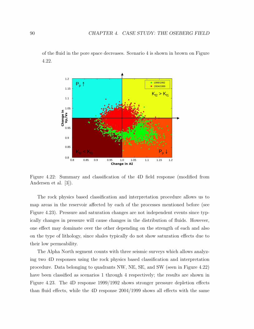
90 CHAPTER 4. CASE STUDY: THE OSEBERG FIELD
of the fluid in the pore space decreases. Scenario 4 is shown in brown on Figure
4.22.
0.8 0.85 0.9 0.95 1.0 1.05 1.1 1.15 1.2
0.9
0.95
0.85
0.8
1.05
1.1
1.15
1.21999/19922004/1999
Pp ↑
Pp ↓Kf2 < Kf1
Kf2 > Kf1
Figure 4.22: Summary and classification of the 4D field response (modified fromAndersen et al. [3]).
The rock physics based classification and interpretation procedure allows us to
map areas in the reservoir affected by each of the processes mentioned before (see
Figure 4.23). Pressure and saturation changes are not independent events since typ-
ically changes in pressure will cause changes in the distribution of fluids. However,
one effect may dominate over the other depending on the strength of each and also
on the type of lithology, since shales typically do not show saturation effects due to
their low permeability.
The Alpha North segment counts with three seismic surveys which allows analyz-
ing two 4D responses using the rock physics based classification and interpretation
procedure. Data belonging to quadrants NW, NE, SE, and SW (seen in Figure 4.22)
have been classified as scenarios 1 through 4 respectively; the results are shown in
Figure 4.23. The 4D response 1999/1992 shows stronger pressure depletion effects
than fluid effects, while the 4D response 2004/1999 shows all effects with the same

4.2. THE RESERVOIR MODELING WORKFLOW 91
strength. This observation shows clearly the reaction of the reservoir to production;
the first time period is associated with primary depletion of the reservoir (pressure
decrease and consequently gas coming out of solution); while the second time period
is associated with the injection of gas and water.
The classification shown in Figure 4.23 has been obtained after applying the cri-
teria shown in Figure 4.22, which is obtained after crossploting the ratios:
[AI]1999
[AI]1992
[Vp/Vs]1999
[Vp/Vs]1992
[AI]2004
[AI]1999
[Vp/Vs]2004
[Vp/Vs]1999
Some data points exhibit AI and Vp/Vs ratios very close to the unit value (“no
change”). However, these data points, located close to the center of the crossplot,
cannot be distinguished from noise related to the seismic surveys, causing non-physical
responses in the amplitudes. Any possible real subtle change that may appear in the
vicinity of the center of the crossplot is very likely to be misclassified due to the noise;
therefore, it is not certain that points within a circular area of the center are actual
physical responses.
Figure 4.24 shows three different assumptions on the magnitude of the noise in
the data (low, medium, high) that could be used to map the areas with reliable field
4D seismic responses (see Figures 4.25 and 4.26). From these figures the following
observations are relevant:
• The first 4D seismic response (1992-1999) has more reliable information than
the second 4D seismic response (1999-2004). Generally, as the level of noise
increases more data points are classified as noise; however, for a constant level of
noise more data points are classified as noise in the second 4D seismic response.
• The data points classified as noise are generally located near the boundaries of
the reservoir.
• A level of noise of 4% is a reasonable value to use, hence only the informative
data from each 4D seismic response is used.

92 CHAPTER 4. CASE STUDY: THE OSEBERG FIELD
The goal of the history matching procedure will be to globally match the overall
proportions of each scenario occurring in the field 4D responses observed in Figure
4.22. If such global match can be obtained then, the reservoir static and flow model
adequately match the overall pressure and saturation changes. Matching the overall
global proportions of each scenario on the two 4D responses implies that the model
should reproduce the contribution of each physical process occurring in the reservoir
during the observed time period. For example, during the period 1992-1999 it is
observed more pressure decline rather than pressure increase; hence, it is expected to
obtain a larger proportion of scenario 3 and a rather low proportion of scenario 1.
Locally matching the occurrence of each physical process is also important since it
may provide us with two very important pieces of information about the reservoir: (1)
local information of the type of facies present and, (2) the connectivity of sand bodies
(flow). Pressure will affect both sand channel and mud floodplain; however, fluid flow
takes place only in sand channels. When pressure decreases as oil is produced, gas
may come out of solution in the sand channels and try to migrate up the gas cap as
other fluids such as oil and water remobilize in the reservoir; however, such sand body
may or may not be connected to provide a flow path for gas to migrate to the gas
cap. These effects have been observed in the modeling of the 4D seismic response (see
section 4.4.1); therefore, locally identifying these interpreted physical processes could
bring important insights to the presence of sand bodies as well as their connectivity.
The resolution of the 4D seismic data is about 25 meters, the thickness distribu-
tion of the reservoir is between 25 and 40 meters TVT with an average thickness of
33 meters, and the average individual sandstone body thickness is between 4 and 6
meters with amalgamated multistory sandstone bodies averaging 27 meters thick in
central parts of Alpha North. Clearly, the resolution of the 4D seismic data precludes
the identification or delineation of individual sandstone bodies in the reservoir (par-
ticularly in the vertical direction); therefore, it is interpreted that only an average
vertical response of the reservoir is what is observed in the 4D data. Rather than
matching the classified 3D volumes shown in Figure 4.23, the goal would be to match
2D proportion maps of each scenario.
The proportion map of each scenario occurring in the field 4D responses should be
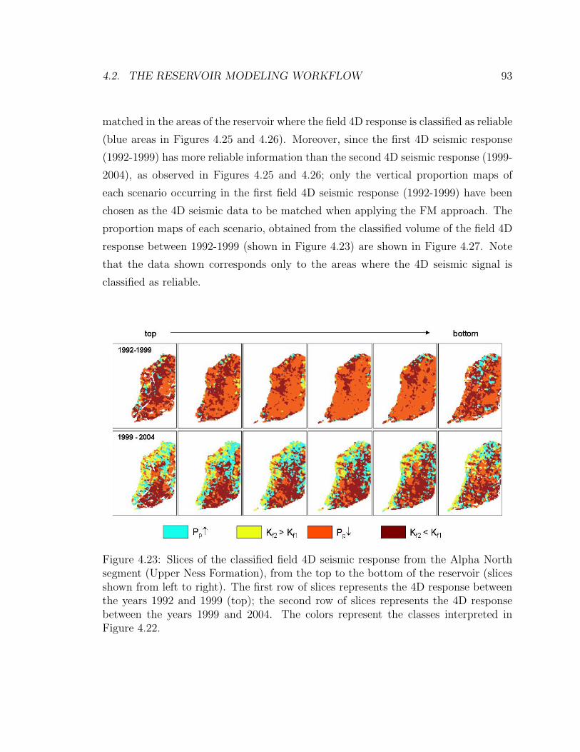
4.2. THE RESERVOIR MODELING WORKFLOW 93
matched in the areas of the reservoir where the field 4D response is classified as reliable
(blue areas in Figures 4.25 and 4.26). Moreover, since the first 4D seismic response
(1992-1999) has more reliable information than the second 4D seismic response (1999-
2004), as observed in Figures 4.25 and 4.26; only the vertical proportion maps of
each scenario occurring in the first field 4D seismic response (1992-1999) have been
chosen as the 4D seismic data to be matched when applying the FM approach. The
proportion maps of each scenario, obtained from the classified volume of the field 4D
response between 1992-1999 (shown in Figure 4.23) are shown in Figure 4.27. Note
that the data shown corresponds only to the areas where the 4D seismic signal is
classified as reliable.
Figure 4.23: Slices of the classified field 4D seismic response from the Alpha Northsegment (Upper Ness Formation), from the top to the bottom of the reservoir (slicesshown from left to right). The first row of slices represents the 4D response betweenthe years 1992 and 1999 (top); the second row of slices represents the 4D responsebetween the years 1999 and 2004. The colors represent the classes interpreted inFigure 4.22.
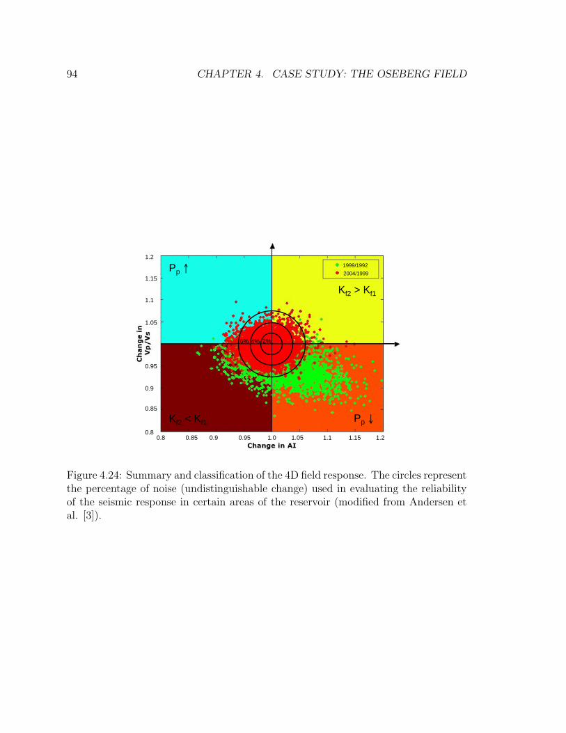
94 CHAPTER 4. CASE STUDY: THE OSEBERG FIELD
0.8 0.85 0.9 0.95 1.0 1.05 1.1 1.15 1.2
0.9
0.95
0.85
0.8
1.05
1.1
1.15
1.21999/19922004/1999
Pp ↑
Pp ↓Kf2 < Kf1
Kf2 > Kf1
2%4%6%
Figure 4.24: Summary and classification of the 4D field response. The circles representthe percentage of noise (undistinguishable change) used in evaluating the reliabilityof the seismic response in certain areas of the reservoir (modified from Andersen etal. [3]).
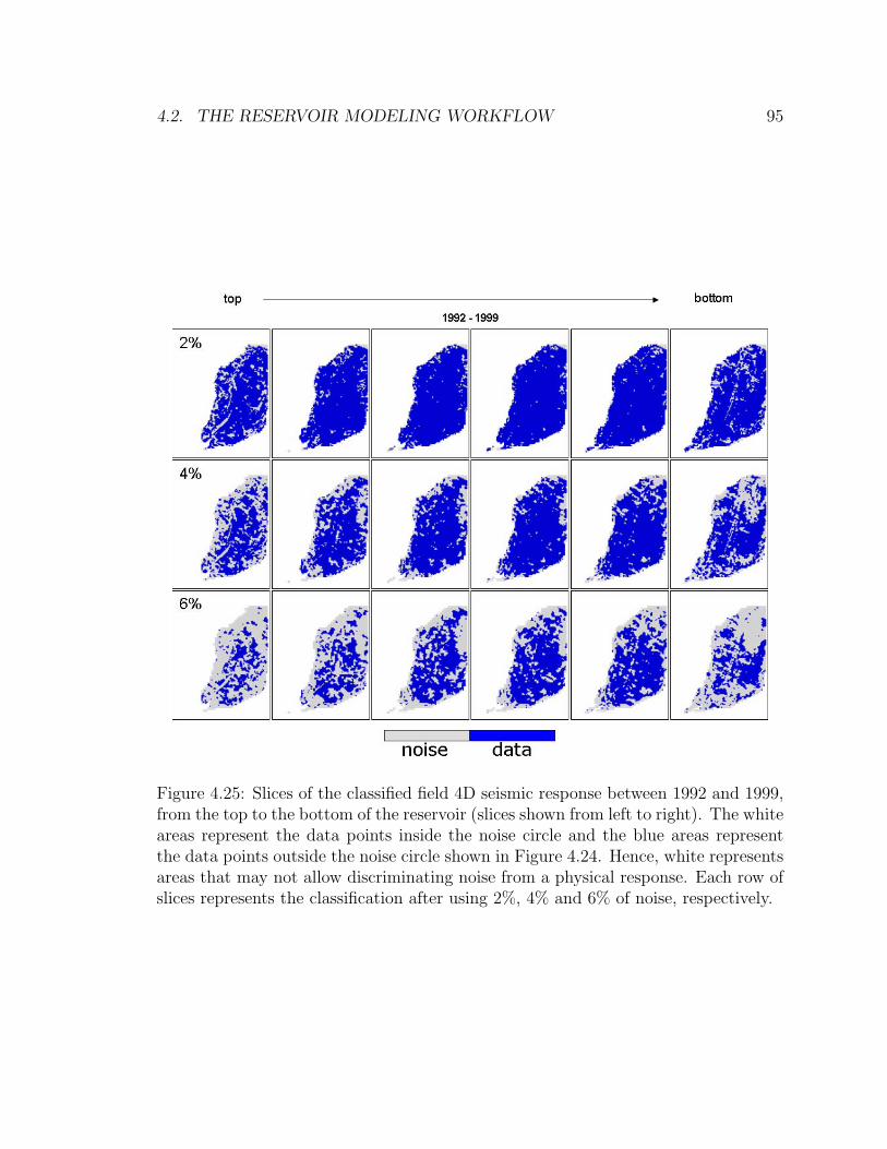
4.2. THE RESERVOIR MODELING WORKFLOW 95
Figure 4.25: Slices of the classified field 4D seismic response between 1992 and 1999,from the top to the bottom of the reservoir (slices shown from left to right). The whiteareas represent the data points inside the noise circle and the blue areas representthe data points outside the noise circle shown in Figure 4.24. Hence, white representsareas that may not allow discriminating noise from a physical response. Each row ofslices represents the classification after using 2%, 4% and 6% of noise, respectively.

96 CHAPTER 4. CASE STUDY: THE OSEBERG FIELD
Figure 4.26: Slices of the classified field 4D seismic response between 1999 and 2004,from the top to the bottom of the reservoir. The white areas represent the datapoints inside the noise circle and the blue areas represent the data points outsidethe noise circle shown in Figure 4.24. Hence, white represents areas that may notallow discriminating noise from a physical response. Each row of slices represents theclassification after using 2%, 4% and 6% of noise, respectively.
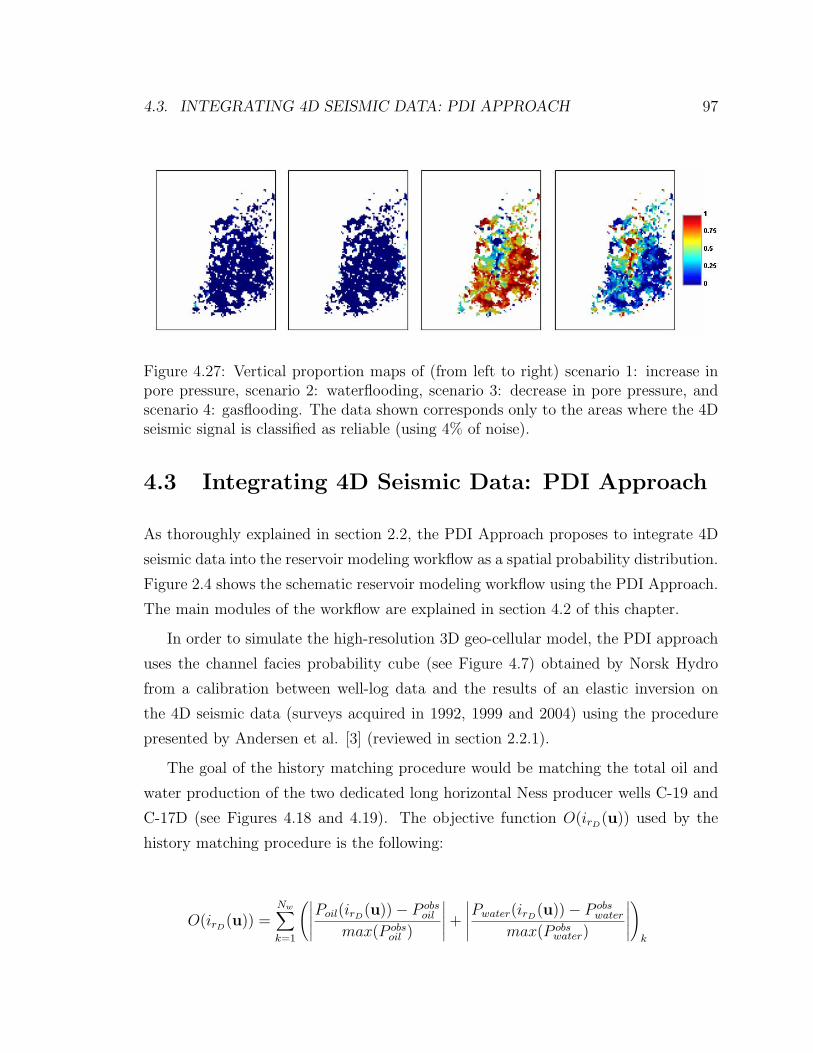
4.3. INTEGRATING 4D SEISMIC DATA: PDI APPROACH 97
Figure 4.27: Vertical proportion maps of (from left to right) scenario 1: increase inpore pressure, scenario 2: waterflooding, scenario 3: decrease in pore pressure, andscenario 4: gasflooding. The data shown corresponds only to the areas where the 4Dseismic signal is classified as reliable (using 4% of noise).
4.3 Integrating 4D Seismic Data: PDI Approach
As thoroughly explained in section 2.2, the PDI Approach proposes to integrate 4D
seismic data into the reservoir modeling workflow as a spatial probability distribution.
Figure 2.4 shows the schematic reservoir modeling workflow using the PDI Approach.
The main modules of the workflow are explained in section 4.2 of this chapter.
In order to simulate the high-resolution 3D geo-cellular model, the PDI approach
uses the channel facies probability cube (see Figure 4.7) obtained by Norsk Hydro
from a calibration between well-log data and the results of an elastic inversion on
the 4D seismic data (surveys acquired in 1992, 1999 and 2004) using the procedure
presented by Andersen et al. [3] (reviewed in section 2.2.1).
The goal of the history matching procedure would be matching the total oil and
water production of the two dedicated long horizontal Ness producer wells C-19 and
C-17D (see Figures 4.18 and 4.19). The objective function O(irD(u)) used by the
history matching procedure is the following:
O(irD(u)) =
Nw∑k=1
(∣∣∣∣∣Poil(irD(u))− P obs
oil
max(P obsoil )
∣∣∣∣∣+∣∣∣∣∣Pwater(irD
(u))− P obswater
max(P obswater)
∣∣∣∣∣)
k
98 CHAPTER 4. CASE STUDY: THE OSEBERG FIELD
where P obsoil and P obs
water are the historical total oil and water production; Poil(irD(u))
and Pwater(irD(u)) are the simulated total oil and water production for realization
irD(u); Nw is the number of wells to be matched (2 wells in this case: C-19 and
C-17D).
An initial guess i(0)(u) of the high-resolution facies model is simulated and shown
in Figure 4.28; using the probability perturbation method, the joint probability dis-
tribution used to simulate the high-resolution facies model is perturbed iteratively.
This perturbation yields a change in the location of the channels; the magnitude of
the perturbation is determined by the parameter rD, described in section 2.1.2. A
one-dimensional optimization is carried out to obtain the rD value that moves the
realization closer to matching production data; the final realization obtained with
the best rD value is denoted as i(1)rD
(u). Using this realization as the initial one, the
process is repeated to obtain i(2)rD
(u) after changing the random seed used for gener-
ating the reservoir model; the process stops when a history match is achieved, hence
the objective function reaches a value below a certain tolerance. The final high-
resolution model obtained with this procedure is shown in Figure 4.28; this model
not only matches production history, but also follows the same geological continuity
model and honors the same well log and 3D/4D seismic probability cube as the initial
model.
The results obtained from the history matching procedure are shown in Figures
4.30 and 4.31; these figures show the actual historical data, the simulated production
from the initial guess model, and the best match obtained after several flow simu-
lations. The decrease of the objective function with the number of flow simulations
(or inner iterations) is shown in Figure 4.29. A maximum of five inner iterations is
performed for each outer iteration; an inner iteration represents an optimization of
the rD value by means of a one-dimensional optimization, while an outer iteration
represents a change in the random seed to generate the high-resolution model.
A satisfactory history match of the total oil and water production is achieved for
well C-19, showing an impressive improvement compared to the simulated production
response of the initial guess model. On the contrary, well C-17D shows a satisfactory
history match on the total oil production only; the factors affecting the mismatch
4.3. INTEGRATING 4D SEISMIC DATA: PDI APPROACH 99
on the total water production for this well should be further investigated. However,
ignoring completion problems, the proximity of well C-17D to the oil-water contact
(see Figure 4.13) and the observed impact of channel compartmentalization on the
production response of the wells in this field could explain a possible water coning
through a drilled channel sand body that continues through the oil-water contact.
The results of the history matching demonstrate that by changing the distribution
of channels, while remaining consistent with other (static) data, a satisfactory match
of production data was achieved. In other words, the location and connectivity of the
channel facies in this reservoir play an important role in the production response of
the wells, as observed by Liestøl et al. from the field production performance.
Due to the stochastic nature of the snesim algorithm, several reservoir models that
match production data while honoring all other available data, can be generated using
the methodology and workflow presented in this dissertation. Figures 4.32 and 4.33
show the results obtained from six history-matched reservoir models. The individual
results from each history-match are presented in appendix C. Figure 4.34 shows the
E-type obtained from the six history-matched reservoir models, which indicates the
probability of each location in the reservoir being channel facies.
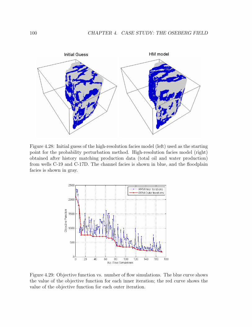
100 CHAPTER 4. CASE STUDY: THE OSEBERG FIELD
Figure 4.28: Initial guess of the high-resolution facies model (left) used as the startingpoint for the probability perturbation method. High-resolution facies model (right)obtained after history matching production data (total oil and water production)from wells C-19 and C-17D. The channel facies is shown in blue, and the floodplainfacies is shown in gray.
Figure 4.29: Objective function vs. number of flow simulations. The blue curve showsthe value of the objective function for each inner iteration; the red curve shows thevalue of the objective function for each outer iteration.

4.3. INTEGRATING 4D SEISMIC DATA: PDI APPROACH 101
Figure 4.30: Total oil (top) and water production (bottom) from well C-19. Historicaldata is shown in black, the simulated total oil production from the initial guess modelis shown in magenta, and the best match obtained after several flow simulationsis shown in green (on the total oil production plot), and blue (on the total waterproduction plot).
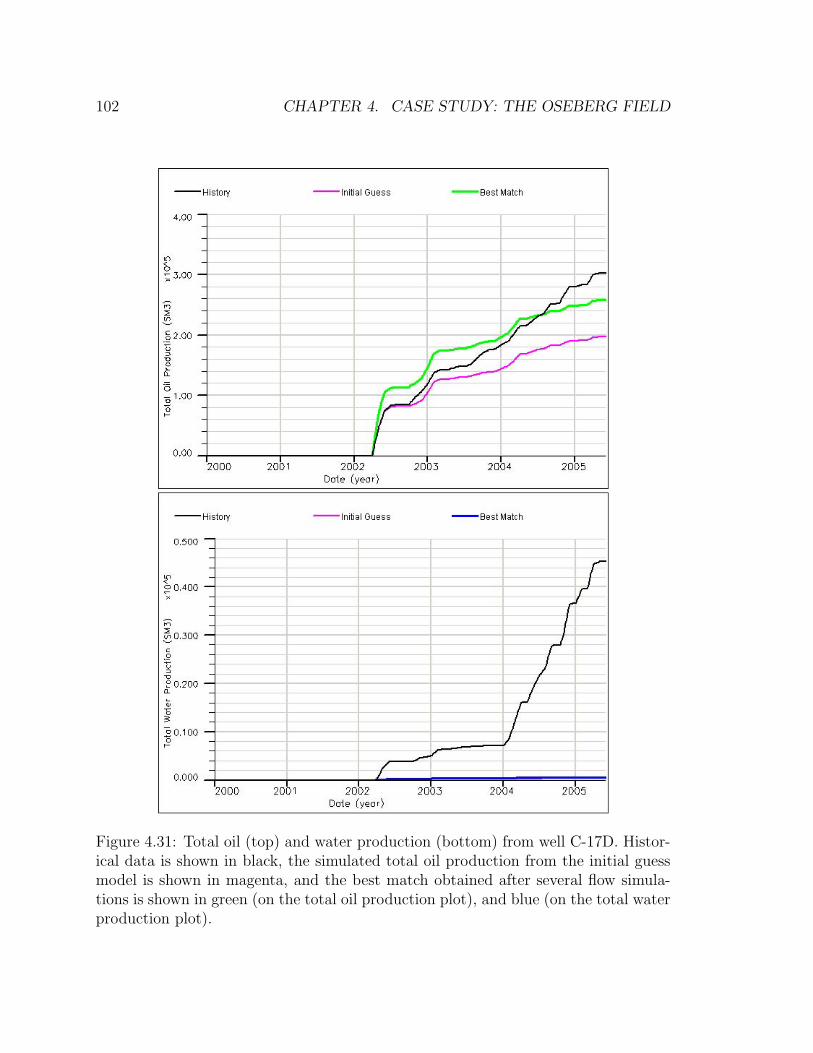
102 CHAPTER 4. CASE STUDY: THE OSEBERG FIELD
Figure 4.31: Total oil (top) and water production (bottom) from well C-17D. Histor-ical data is shown in black, the simulated total oil production from the initial guessmodel is shown in magenta, and the best match obtained after several flow simula-tions is shown in green (on the total oil production plot), and blue (on the total waterproduction plot).
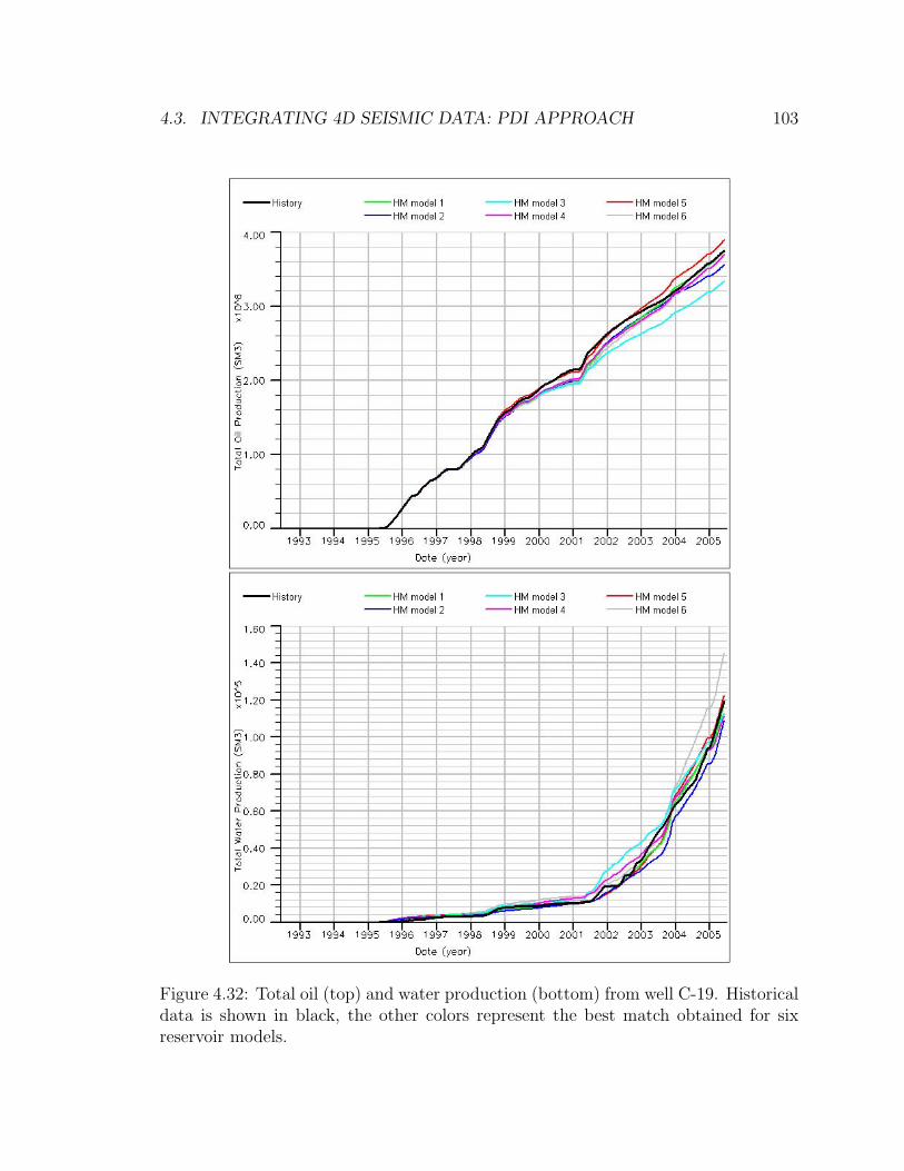
4.3. INTEGRATING 4D SEISMIC DATA: PDI APPROACH 103
Figure 4.32: Total oil (top) and water production (bottom) from well C-19. Historicaldata is shown in black, the other colors represent the best match obtained for sixreservoir models.
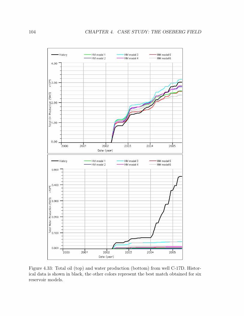
104 CHAPTER 4. CASE STUDY: THE OSEBERG FIELD
Figure 4.33: Total oil (top) and water production (bottom) from well C-17D. Histor-ical data is shown in black, the other colors represent the best match obtained for sixreservoir models.
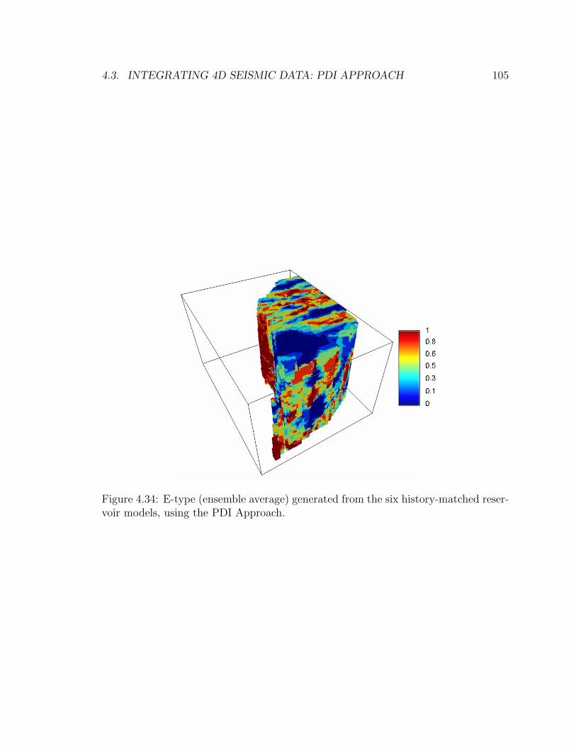
4.3. INTEGRATING 4D SEISMIC DATA: PDI APPROACH 105
Figure 4.34: E-type (ensemble average) generated from the six history-matched reser-voir models, using the PDI Approach.
106 CHAPTER 4. CASE STUDY: THE OSEBERG FIELD
4.4 Integrating 4D Seismic Data: FM Approach
As throughly explained in section 2.3, the FM Approach proposes to integrate 4D
seismic data into the reservoir modeling workflow as dynamic data; in other words,
matching it along with production data. Figure 2.9 shows the schematic reservoir
modeling workflow using the FM Approach. The main modules of the workflow are
explained in section 4.2 of this chapter.
In order to simulate the high-resolution 3D geo-cellular model, the FM approach
uses the channel facies probability cube (see Figure 4.7) obtained by Norsk Hydro
from a calibration between well-log data and the results of an elastic inversion on the
Base 3D seismic data (survey acquired in 1992).
The goal of the history matching procedure would be matching the total oil and
water production of the two dedicated long horizontal Ness producer wells C-19 and
C-17D (see Figures 4.18 and 4.19), as well as 4D seismic data: the proportion maps
of each scenario occurring in the first field 4D seismic response (1992-1999), where
the 4D seismic signal is classified as reliable (shown in Figure 4.27).
The objective function O(irD(u)) used by the history matching procedure is the
following:
O(irD(u)) =
Nw∑j=1
(∣∣∣∣∣Poil(irD(u))− P obs
oil
max(P obsoil )
∣∣∣∣∣+∣∣∣∣∣Pwater(irD
(u))− P obswater
max(P obswater)
∣∣∣∣∣)
j
+ ωNm∑k=1
(1− ρk)
where P obsoil and P obs
water are the historical total oil and water production; Poil(irD(u))
and Pwater(irD(u)) are the simulated total oil and water production for realization
irD(u); Nw is the number of wells to be matched (2 wells in this case: C-19 and C-
17D); ρk is the correlation coefficient between the kth observed and forward modeled
proportion map; ω is a scaling factor that increases the magnitude of the 4D seismic
mismatch to an average order of magnitude of the production mismatch (order of a
thousand); Nm is the number of proportion maps to be matched (2 maps in this case:
maps of scenarios 3 and 4 for period 1992-1999).
When history matching production data only, the production response of the
reservoir model is computed by performing flow simulation. Therefore, when including
4.4. INTEGRATING 4D SEISMIC DATA: FM APPROACH 107
the matching of 4D seismic data, the 4D response of the reservoir model needs to be
computed also by performing a “Forward Modeling” (FM).
4.4.1 Forward Modeling the 4D Seismic Response
In order to forward model the 4D seismic response for the Upper Ness Formation the
petro-elastic model presented in section 2.3.1 was followed. The ratio between the
P-wave and S-wave velocities Vp/Vs as well as acoustic impedance AI were computed
using that procedure. The petro-elastic model uses the pore pressure and the oil,
water and gas saturations obtained from the flow simulation to compute Vp, Vs and
ρ of the rock under certain effective pressure Peff , with a specific oil, water and gas
saturation in the pore space. Due to the complexity of the flow problem in this case
(3D three-phase flow), a simple sub-sampling of coarse grid block pore pressure and
saturation to all high-resolution grid cells was used; however, the potential limitations
of this procedure are very well documented in Chapter 3.
Two important pieces of information need to be supplied to the petro-elastic
model: seismic velocities of the dry rock as a function of porosity and effective pressure
(Vp(φ, Peff ) and Vs(φ, Peff )) and properties of the fluids in the reservoir as a function
of pore pressure (density ρ(Ppore), and bulk modulus K(Ppore)).
The properties of the three fluids in the reservoir (oil, water and gas) as a function
of pore pressure were supplied by Norsk Hydro (see Table 4.2). For each grid block of
the reservoir model the properties of each fluid are computed according to the pore
pressure in that grid block. Using these properties, the “effective fluid” properties are
calculated using the saturations of each fluid and the relationships shown in section
2.3.1 (Eqn. 2.19, and Eqn. 2.20). The equilibration parameter e in Eqn. 2.19 was
supplied by Norsk Hydro e = 3.
Vp(φ, Peff ) and Vs(φ, Peff ) relations were supplied by Norsk Hydro; however, they
corresponded to lab measurements made on cores from the Oseberg Øst field located
further east of the Alpha North segment of the Oseberg Field (see Figure 4.1). The
overburden pressure in this field is about 63.7 MPa, while the computed overburden
pressure for the Alpha North Ness Formation corresponds to 54 MPa; this observation
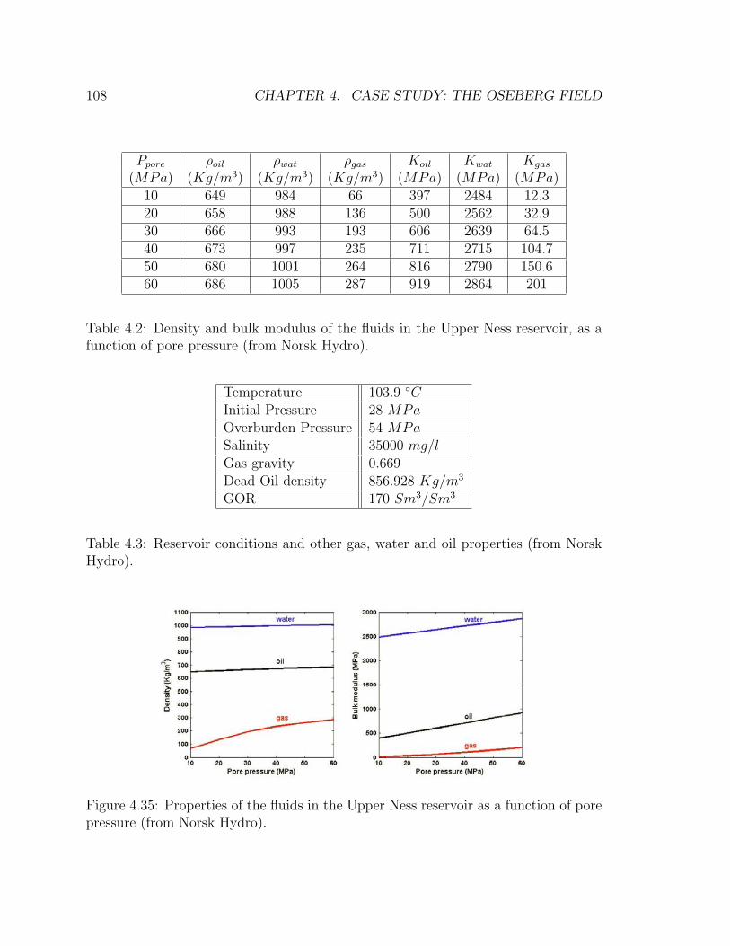
108 CHAPTER 4. CASE STUDY: THE OSEBERG FIELD
Ppore ρoil ρwat ρgas Koil Kwat Kgas
(MPa) (Kg/m3) (Kg/m3) (Kg/m3) (MPa) (MPa) (MPa)10 649 984 66 397 2484 12.320 658 988 136 500 2562 32.930 666 993 193 606 2639 64.540 673 997 235 711 2715 104.750 680 1001 264 816 2790 150.660 686 1005 287 919 2864 201
Table 4.2: Density and bulk modulus of the fluids in the Upper Ness reservoir, as afunction of pore pressure (from Norsk Hydro).
Temperature 103.9 ◦CInitial Pressure 28 MPaOverburden Pressure 54 MPaSalinity 35000 mg/lGas gravity 0.669Dead Oil density 856.928 Kg/m3
GOR 170 Sm3/Sm3
Table 4.3: Reservoir conditions and other gas, water and oil properties (from NorskHydro).
Figure 4.35: Properties of the fluids in the Upper Ness reservoir as a function of porepressure (from Norsk Hydro).
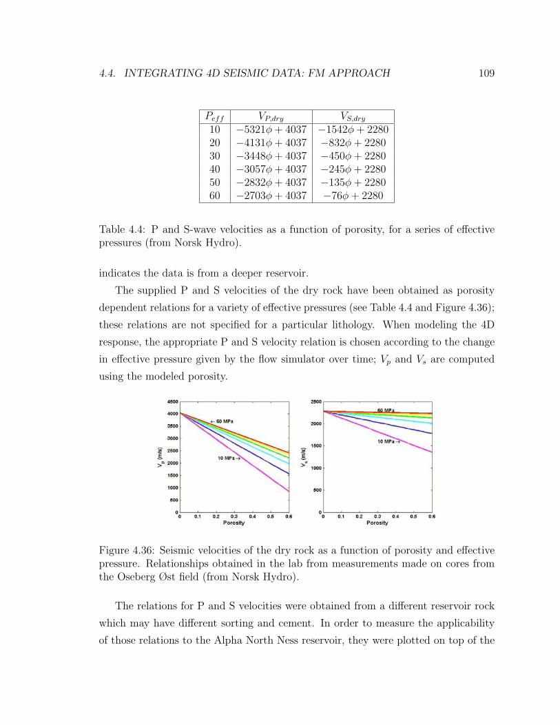
4.4. INTEGRATING 4D SEISMIC DATA: FM APPROACH 109
Peff VP,dry VS,dry
10 −5321φ + 4037 −1542φ + 228020 −4131φ + 4037 −832φ + 228030 −3448φ + 4037 −450φ + 228040 −3057φ + 4037 −245φ + 228050 −2832φ + 4037 −135φ + 228060 −2703φ + 4037 −76φ + 2280
Table 4.4: P and S-wave velocities as a function of porosity, for a series of effectivepressures (from Norsk Hydro).
indicates the data is from a deeper reservoir.
The supplied P and S velocities of the dry rock have been obtained as porosity
dependent relations for a variety of effective pressures (see Table 4.4 and Figure 4.36);
these relations are not specified for a particular lithology. When modeling the 4D
response, the appropriate P and S velocity relation is chosen according to the change
in effective pressure given by the flow simulator over time; Vp and Vs are computed
using the modeled porosity.
Figure 4.36: Seismic velocities of the dry rock as a function of porosity and effectivepressure. Relationships obtained in the lab from measurements made on cores fromthe Oseberg Øst field (from Norsk Hydro).
The relations for P and S velocities were obtained from a different reservoir rock
which may have different sorting and cement. In order to measure the applicability
of those relations to the Alpha North Ness reservoir, they were plotted on top of the
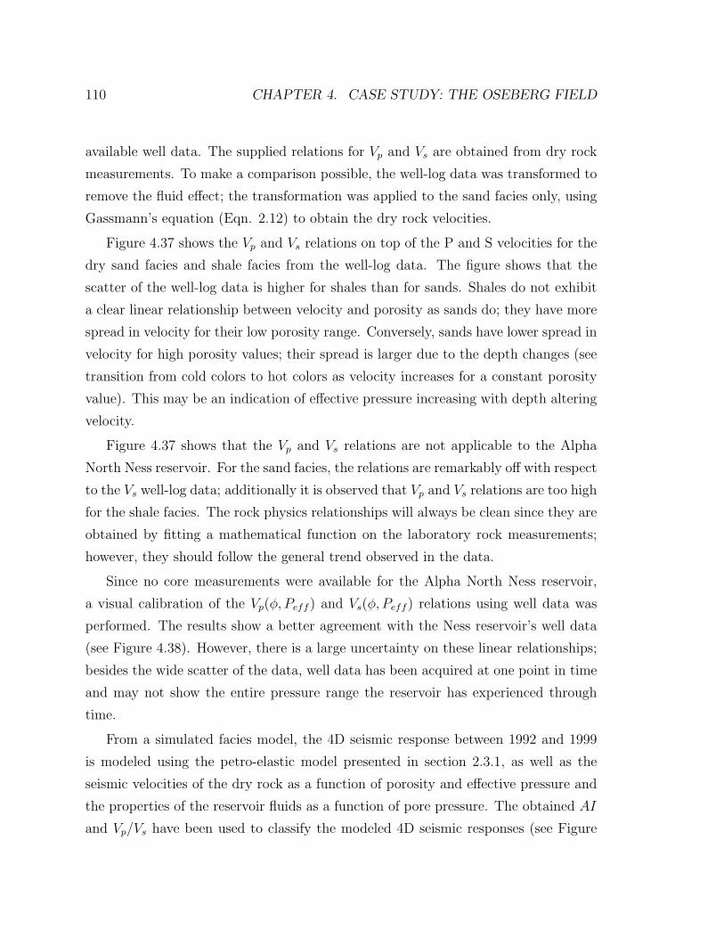
110 CHAPTER 4. CASE STUDY: THE OSEBERG FIELD
available well data. The supplied relations for Vp and Vs are obtained from dry rock
measurements. To make a comparison possible, the well-log data was transformed to
remove the fluid effect; the transformation was applied to the sand facies only, using
Gassmann’s equation (Eqn. 2.12) to obtain the dry rock velocities.
Figure 4.37 shows the Vp and Vs relations on top of the P and S velocities for the
dry sand facies and shale facies from the well-log data. The figure shows that the
scatter of the well-log data is higher for shales than for sands. Shales do not exhibit
a clear linear relationship between velocity and porosity as sands do; they have more
spread in velocity for their low porosity range. Conversely, sands have lower spread in
velocity for high porosity values; their spread is larger due to the depth changes (see
transition from cold colors to hot colors as velocity increases for a constant porosity
value). This may be an indication of effective pressure increasing with depth altering
velocity.
Figure 4.37 shows that the Vp and Vs relations are not applicable to the Alpha
North Ness reservoir. For the sand facies, the relations are remarkably off with respect
to the Vs well-log data; additionally it is observed that Vp and Vs relations are too high
for the shale facies. The rock physics relationships will always be clean since they are
obtained by fitting a mathematical function on the laboratory rock measurements;
however, they should follow the general trend observed in the data.
Since no core measurements were available for the Alpha North Ness reservoir,
a visual calibration of the Vp(φ, Peff ) and Vs(φ, Peff ) relations using well data was
performed. The results show a better agreement with the Ness reservoir’s well data
(see Figure 4.38). However, there is a large uncertainty on these linear relationships;
besides the wide scatter of the data, well data has been acquired at one point in time
and may not show the entire pressure range the reservoir has experienced through
time.
From a simulated facies model, the 4D seismic response between 1992 and 1999
is modeled using the petro-elastic model presented in section 2.3.1, as well as the
seismic velocities of the dry rock as a function of porosity and effective pressure and
the properties of the reservoir fluids as a function of pore pressure. The obtained AI
and Vp/Vs have been used to classify the modeled 4D seismic responses (see Figure
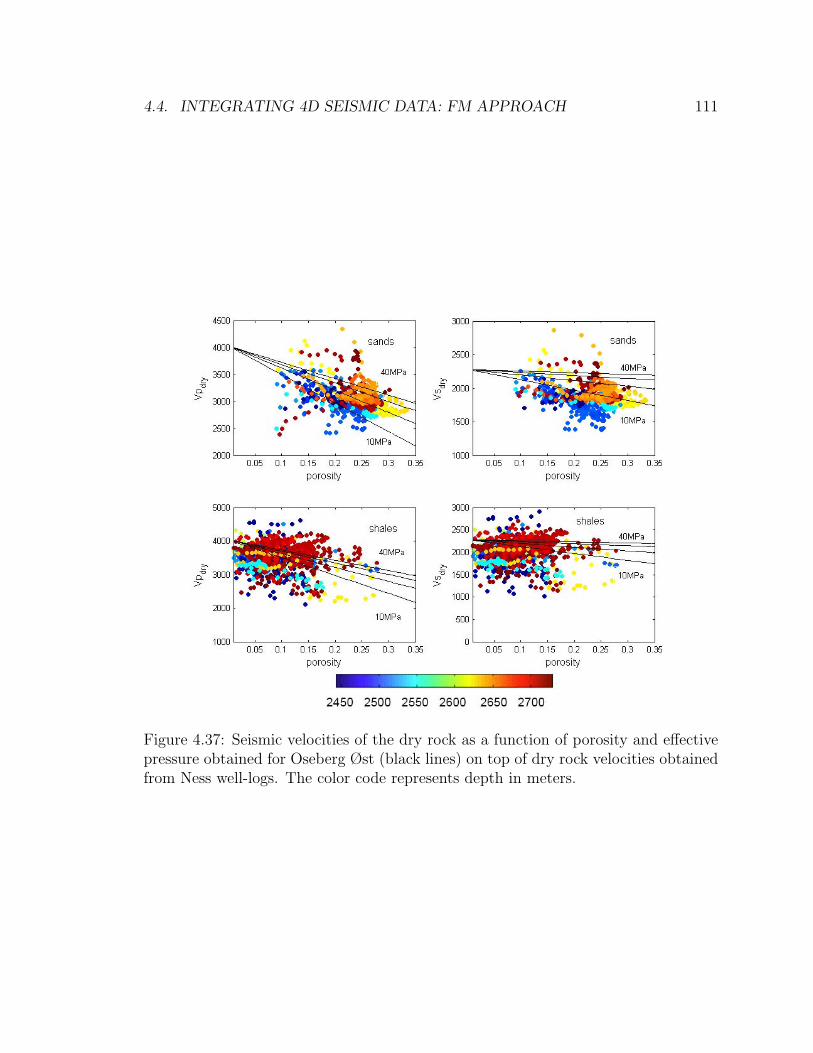
4.4. INTEGRATING 4D SEISMIC DATA: FM APPROACH 111
Figure 4.37: Seismic velocities of the dry rock as a function of porosity and effectivepressure obtained for Oseberg Øst (black lines) on top of dry rock velocities obtainedfrom Ness well-logs. The color code represents depth in meters.
112 CHAPTER 4. CASE STUDY: THE OSEBERG FIELD
Figure 4.38: Calibrated seismic velocities of the dry rock as a function of porosity andeffective pressure for the Alpha North Ness formation (black lines) on top of dry rockvelocities obtained from Ness well-logs. The color code represents depth in meters.
4.4. INTEGRATING 4D SEISMIC DATA: FM APPROACH 113
4.39), using the criteria shown in Figure 4.22.
The classification criterion, based on fundamental rock physics rules, shows that
pressure will affect both sand channel and mud floodplain; however, fluid flow takes
place only in sand channels. Therefore, from Figure 4.39 it is observed that: (1) the
two colors associated with fluid flow (brown and yellow) occur only in sand channel
facies, and (2) the two colors associated with an increase or a decrease in pore pres-
sure (light blue and orange) occur in both sand channel and mud floodplain. The
occurrence of each classification scenario can be explained from the flow simulation
results, shown in Figure 4.41.
Areas of the reservoir shown in brown on Figure 4.39 correspond to areas within
channel facies where ∆So < 0 and ∆Sg > 0 are observed in Figure 4.41; this means
that gas comes out of solution due to the decrease in pore pressure. Areas of the
reservoir shown in yellow on Figure 4.39 correspond to areas within channel facies
where ∆So < 0, ∆Sg ≈ 0, and ∆Sw > 0 are observed in Figure 4.41; this means
that a high bulk modulus fluid displacing a low bulk modulus fluid, in this case water
displacing oil. Figure 4.41 shows that ∆Pp < 0 in the entire reservoir; however,
only some areas in the reservoir are shown in orange on Figure 4.39. Pore pressure
is decreasing in the entire reservoir causing fluid flow; although both pressure and
saturation changes have an effect over the 4D seismic signal, one effect may dominate
the other depending on how strong the dependency of P and S wave velocities on
pressure is modeled.
From the classified modeled 4D seismic response (shown in Figure 4.39), the pro-
portion maps of scenarios 3 and 4 (shown in Figure 4.40) are obtained; the goal of the
history matching procedure is to perturb the model of the reservoir until its modeled
4D seismic response (shown in Figure 4.40) matches the field 4D seismic response
(shown in Figure 4.27).
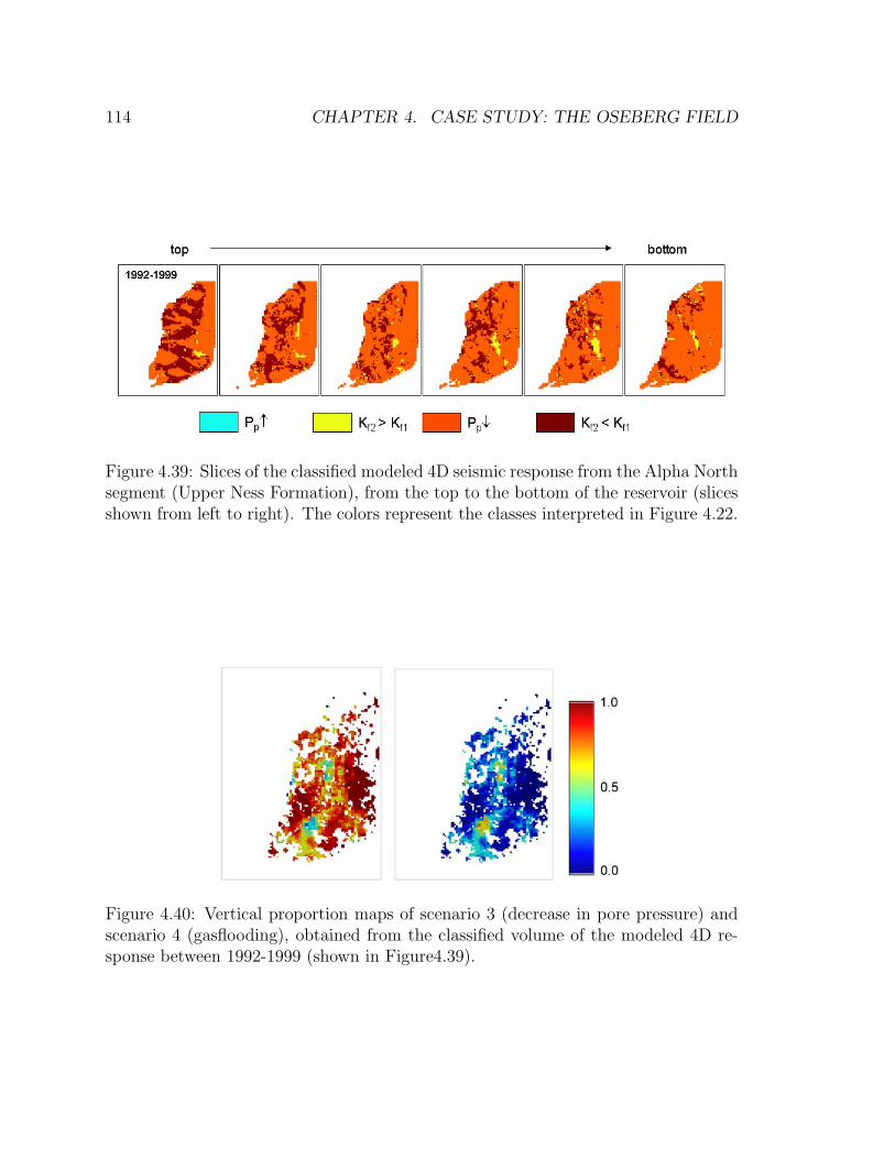
114 CHAPTER 4. CASE STUDY: THE OSEBERG FIELD
Figure 4.39: Slices of the classified modeled 4D seismic response from the Alpha Northsegment (Upper Ness Formation), from the top to the bottom of the reservoir (slicesshown from left to right). The colors represent the classes interpreted in Figure 4.22.
Figure 4.40: Vertical proportion maps of scenario 3 (decrease in pore pressure) andscenario 4 (gasflooding), obtained from the classified volume of the modeled 4D re-sponse between 1992-1999 (shown in Figure4.39).
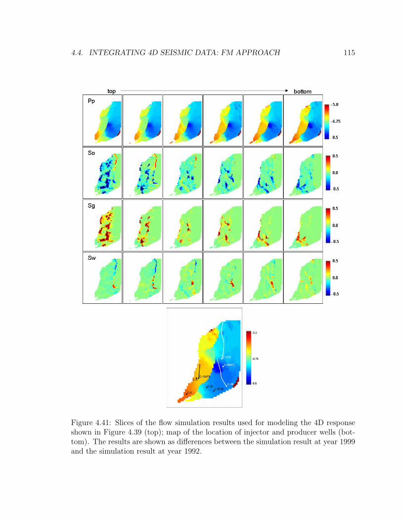
4.4. INTEGRATING 4D SEISMIC DATA: FM APPROACH 115
Figure 4.41: Slices of the flow simulation results used for modeling the 4D responseshown in Figure 4.39 (top); map of the location of injector and producer wells (bot-tom). The results are shown as differences between the simulation result at year 1999and the simulation result at year 1992.
116 CHAPTER 4. CASE STUDY: THE OSEBERG FIELD
4.4.2 History Matching Results
Following the proposed workflow (shown in Figure 2.9) for the FM approach; an
initial guess of the high-resolution facies model is simulated and shown in Figure 4.42;
using the probability perturbation method, the joint probability distribution used to
simulate the high-resolution facies model is perturbed iteratively using P (A | D3),
defined by Eqn. 2.7 in section 2.1.2. Therefore, perturbed facies models are drawn
from P (A | D1, D2, D3), where D1 is geological data (training image and well-log
data), D2 is geophysical data (Base 3D seismic survey), and D3 is dynamic data
(production and 4D seismic data: proportion maps ). The final high-resolution model
obtained with the probability perturbation method (PPM) is shown in Figure 4.42;
this model follows the same geological continuity model (training image), honors the
same well-log data and 3D seismic probability cube as the initial model. Additionally,
this model produced the best match of both historical production data and 4D seismic
data after approximately ninety flow simulations, as seen in Figure 4.43.
The decrease of the total mismatch (production and 4D seismic) is shown by the
red curve in Figure 4.43, while the decrease of the production mismatch and the 4D
seismic mismatch are shown in black and green respectively. These curves show that
the decrease of the total mismatch is mostly driven by the decrease in the production
mismatch, since the decrease in the 4D seismic mismatch is only 13% over the 88 flow
simulations, as opposed to the 90% decrease in production mismatch.
The results obtained from the history matching procedure are shown in Figures
4.44, 4.45 and 4.46; the first two figures show the best match in production data
(wells C-19 and C-17D), while the last figure shows the best match in 4D seismic
data. A satisfactory history match of the total oil and water production is achieved
for well C-19, showing an impressive improvement compared to the simulated pro-
duction response of the initial guess model. On the contrary, well C-17D shows an
unsatisfactory match on the total oil and water production. Figure 4.46 shows an
improvement on the location and magnitude of the main central feature (as indicated
by the ellipse) observed in both maps (high vertical proportion of the “gasflooding”
scenario, low vertical proportion of the “Pore pressure decrease” scenario). The cor-
relation coefficient between the observed and the modeled proportion map of scenario
4.4. INTEGRATING 4D SEISMIC DATA: FM APPROACH 117
3 increased from 0.2 (initial guess) to 0.32 (best match); similarly, the correlation
coefficient between the observed and the modeled vertical proportion map of scenario
4 increased from 0.23 (initial guess) to 0.33 (best match).
These results demonstrate that by changing the distribution of channels, while
remaining consistent with other static data, a satisfactory match on the production
data of well C-19 is achieved. As observed from the results of the PDI approach, the
location and connectivity of the channel facies in this reservoir play an important
role in the production response of the wells; however, perturbing the distribution
of channels only is not enough to obtain a considerable decrease in the 4D seismic
mismatch.
The main central feature observed in the field map of scenario 4 (shown in Figure
4.46, bottom center), corresponds to a high vertical proportion of the “gasflooding”
scenario (low vertical proportion of the “Pore pressure decrease” scenario). This
anomaly is directly related to the local net-to-gross (NTG) since fluid flow occurs
preferentially in sand facies (high permeability); in other words, the high vertical
proportion observed in the field map of scenario 4 is an indicator of high NTG.
Therefore, in addition to the perturbation of the distribution of channels obtained
by using P (A | D3), another conditional probability P (A | D4) can be introduced
to either increase or decrease the local NTG as a function of the local 4D seismic
mismatch.
The local 4D seismic mismatch is translated into an indicator variable I4D(u) that
highlights the areas in the reservoir where the local NTG needs to be either increased
or decreased; the indicator variable is defined as:
I4D(u) =
+1 if τ < Sobs
4 (u) and Sobs4 (u) > S4(u)
0 if Sobs4 (u) = S4(u)
−1 if τ > Sobs4 (u) and Sobs
4 (u) < S4(u)
(4.2)
where Sobs4 (u) is the field proportion map of scenario 4, S4(u) is the forward modeled
proportion map of scenario 4, and τ ∈ [0, 1] is the minimum value of Sobs4 (u) above
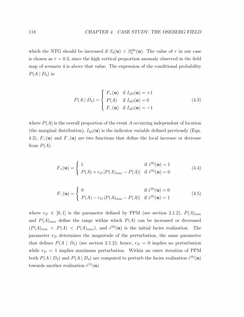
118 CHAPTER 4. CASE STUDY: THE OSEBERG FIELD
which the NTG should be increased if S4(u) < Sobs4 (u). The value of τ in our case
is chosen as τ = 0.3, since the high vertical proportion anomaly observed in the field
map of scenario 4 is above that value. The expression of the conditional probability
P (A | D4) is:
P (A | D4) =
F+(u) if I4D(u) = +1
P (A) if I4D(u) = 0
F−(u) if I4D(u) = −1
(4.3)
where P (A) is the overall proportion of the event A occurring independent of location
(the marginal distribution), I4D(u) is the indicator variable defined previously (Eqn.
4.2), F+(u) and F−(u) are two functions that define the local increase or decrease
from P (A).
F+(u) =
1 if i(0)(u) = 1
P (A) + rD |P (A)max − P (A)| if i(0)(u) = 0(4.4)
F−(u) =
0 if i(0)(u) = 0
P (A)− rD |P (A)min − P (A)| if i(0)(u) = 1(4.5)
where rD ∈ [0, 1] is the parameter defined by PPM (see section 2.1.2), P (A)min
and P (A)max define the range within which P (A) can be increased or decreased
(P (A)min < P (A) < P (A)max), and i(0)(u) is the initial facies realization. The
parameter rD determines the magnitude of the perturbation, the same parameter
that defines P (A | D3) (see section 2.1.2); hence, rD = 0 implies no perturbation
while rD = 1 implies maximum perturbation. Within an outer iteration of PPM
both P (A | D3) and P (A | D4) are computed to perturb the facies realization i(0)(u)
towards another realization i(1)(u).
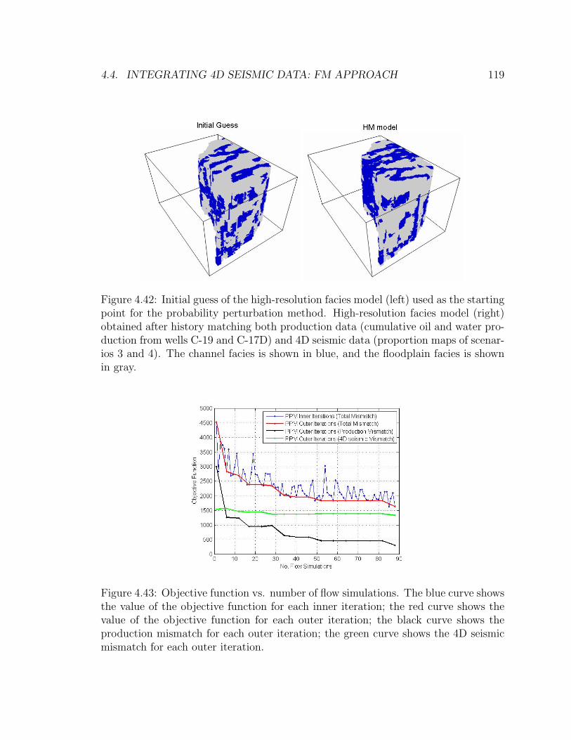
4.4. INTEGRATING 4D SEISMIC DATA: FM APPROACH 119
Figure 4.42: Initial guess of the high-resolution facies model (left) used as the startingpoint for the probability perturbation method. High-resolution facies model (right)obtained after history matching both production data (cumulative oil and water pro-duction from wells C-19 and C-17D) and 4D seismic data (proportion maps of scenar-ios 3 and 4). The channel facies is shown in blue, and the floodplain facies is shownin gray.
Figure 4.43: Objective function vs. number of flow simulations. The blue curve showsthe value of the objective function for each inner iteration; the red curve shows thevalue of the objective function for each outer iteration; the black curve shows theproduction mismatch for each outer iteration; the green curve shows the 4D seismicmismatch for each outer iteration.
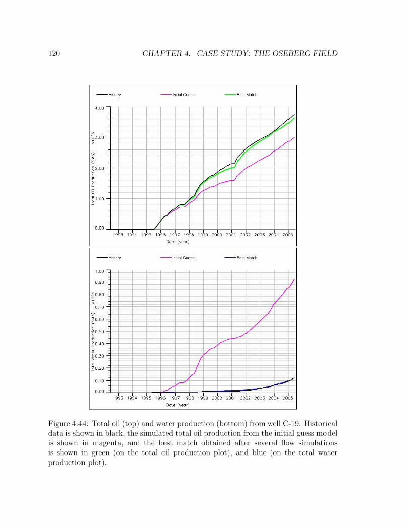
120 CHAPTER 4. CASE STUDY: THE OSEBERG FIELD
Figure 4.44: Total oil (top) and water production (bottom) from well C-19. Historicaldata is shown in black, the simulated total oil production from the initial guess modelis shown in magenta, and the best match obtained after several flow simulationsis shown in green (on the total oil production plot), and blue (on the total waterproduction plot).
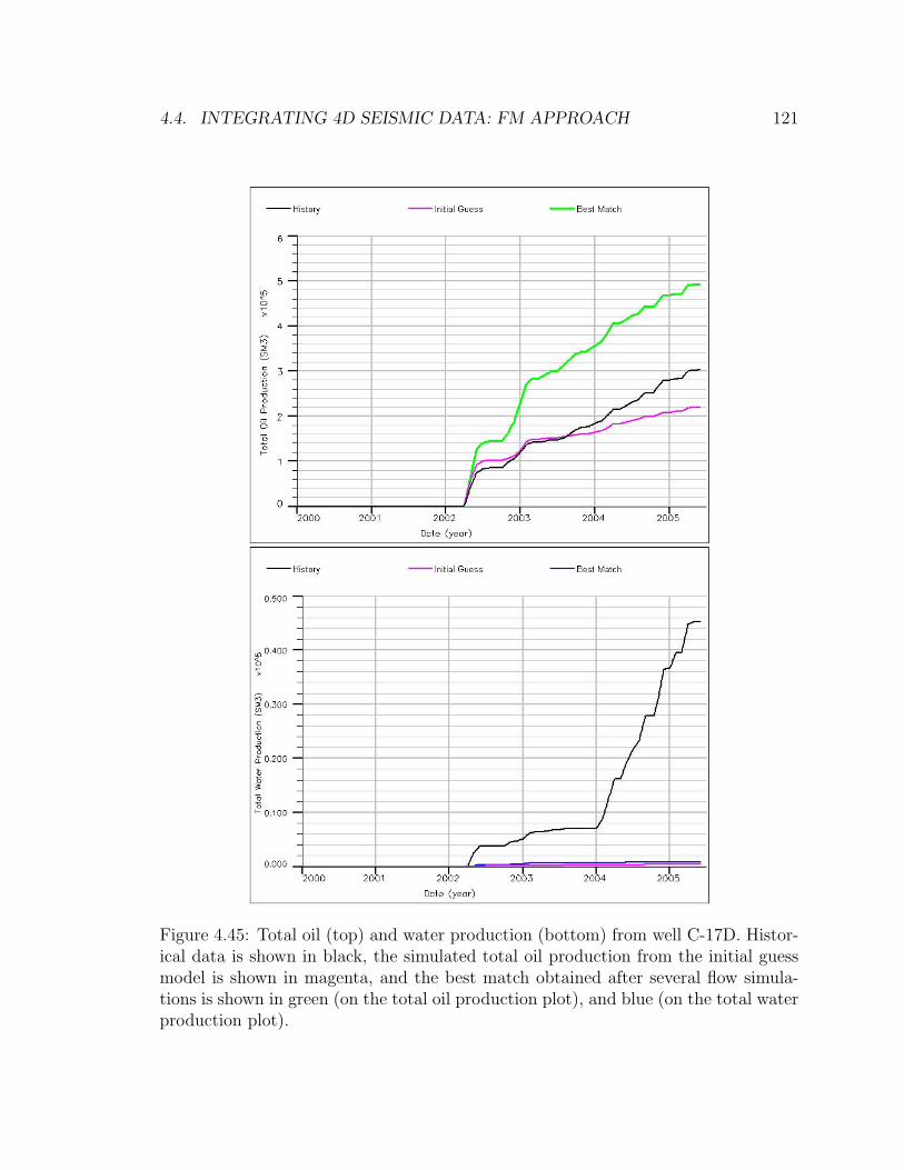
4.4. INTEGRATING 4D SEISMIC DATA: FM APPROACH 121
Figure 4.45: Total oil (top) and water production (bottom) from well C-17D. Histor-ical data is shown in black, the simulated total oil production from the initial guessmodel is shown in magenta, and the best match obtained after several flow simula-tions is shown in green (on the total oil production plot), and blue (on the total waterproduction plot).
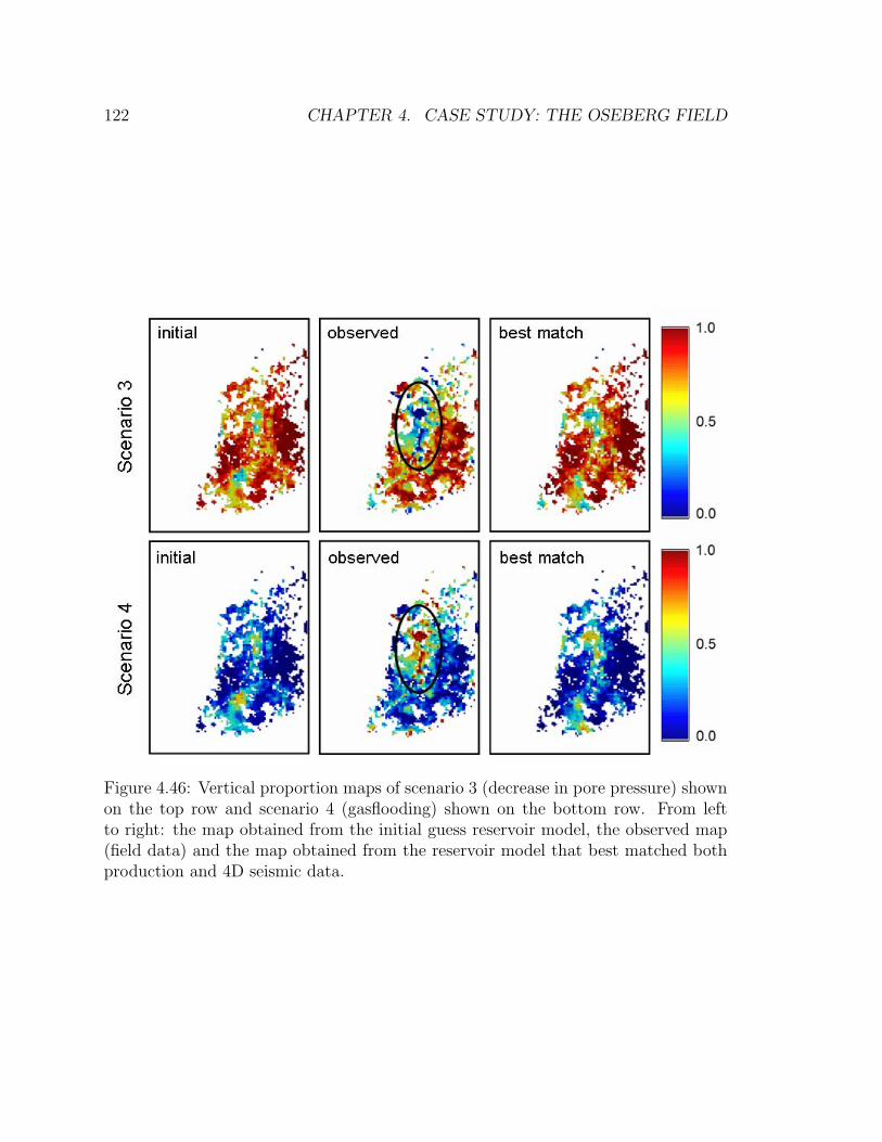
122 CHAPTER 4. CASE STUDY: THE OSEBERG FIELD
Figure 4.46: Vertical proportion maps of scenario 3 (decrease in pore pressure) shownon the top row and scenario 4 (gasflooding) shown on the bottom row. From leftto right: the map obtained from the initial guess reservoir model, the observed map(field data) and the map obtained from the reservoir model that best matched bothproduction and 4D seismic data.
4.4. INTEGRATING 4D SEISMIC DATA: FM APPROACH 123
Following the workflow for the FM approach (shown in Figure 2.9) and starting
from the same initial guess of the high-resolution facies shown in Figure 4.42, the
joint probability distribution used to simulate the high-resolution facies model is
perturbed iteratively using both P (A | D3) (Eqn. 2.7) and P (A | D4) (Eqn. 4.3) After
several flow simulations, the final high-resolution model obtained with the probability
perturbation method (PPM) is shown in Figure 4.47. This model produced the best
match of both historical production data and 4D seismic data after approximately
250 flow simulations, as seen in Figure 4.48. The decrease of the total mismatch
(production and 4D seismic) is shown by the red curve in Figure 4.48, while the
decrease of the production mismatch and the 4D seismic mismatch are shown in
black and green respectively. The decrease in the production mismatch is 86% while
the decrease in the 4D seismic mismatch is 39% over the 250 flow simulations.
The results obtained from the history matching procedure are shown in Figures
4.49, 4.50 and 4.51; the first two figures show the best match in production data
(wells C-19 and C-17D), while the last figure shows the best match in 4D seismic
data. A satisfactory history match of the total oil and water production is achieved
for well C-19, showing an impressive improvement compared to the simulated pro-
duction response of the initial guess model. On the contrary, well C-17D shows an
unsatisfactory match on the total oil and water production. Figure 4.51 shows an
improvement on the location and magnitude of the main central feature observed
in both maps (high vertical proportion of the “gasflooding” scenario. The correla-
tion coefficient between the observed and the modeled proportion map of scenario
3 increased from 0.2 (initial guess) to 0.53 (best match); similarly, the correlation
coefficient between the observed and the modeled vertical proportion map of scenario
4 increased from 0.23 (initial guess) to 0.53 (best match).
Using the additional local perturbation of NTG through P (A | D4), the 4D seismic
mismatch experienced a considerable decrease during the first five outer iterations of
PPM. The final proportion maps of scenarios 3 and 4 from the best matched high-
resolution facies model (Figure 4.51, top and bottom right) show a better agreement
with the observed maps (field data) than the maps obtained without using P (A | D4)
(shown in Figure 4.46). Figure 4.52 shows a comparison between the field data and the
124 CHAPTER 4. CASE STUDY: THE OSEBERG FIELD
the maps obtained from the best matched models (with and without using P (A | D4))
for scenario 4; this figure shows how the map obtained from the best matched model
using P (A | D4) shows a better match with the field data outside the red circled
area. The area inside the red circle shows the greatest mismatch with field data; this
area shows a high vertical proportion of the “gasflooding” scenario which has been
related to a high NTG. However, increasing NTG through P (A | D4) was not enough
to obtain gas coming out of solution in this area. The field data shows that more
than 30% of the thickness of the reservoir in this area is classified as “gasflooding”
scenario; therefore, two phenomena could possibly occur in the model: either no gas
is coming out of solution because it is an isolated area (no pressure depletion), or
gas is coming out of solution but migrating up-dip before the second seismic monitor
survey is forward modeled (before the year 1999).
From the flow simulation performed on the best matched reservoir model shown
in Figure 4.47, it was observed that gas came out of solution in this area by the year
1998 but migrated to other areas in the reservoir before 1999. Figure 4.53 shows
several snapshots in time of the vertical average of Sg where a white circle on the
maps corresponding to years 1998 and 1999 indicates the area of greatest mismatch
between the field and the modeled 4D seismic, the same area where gas came out of
solution and migrated before 1999. Similarly, Figures 4.54 and 4.55 show ∆Sg maps
where the gas migration is more clearly seen, in particular note the negative area
circled on the ∆Sg map between the years of 1998 and 1999 in Figure 4.55.
If the signal from the 4D seismic data is given a high level of certainty, further work
should follow this investigation on the geological feasibility of the presence of a fault
(either not modeled or below the seismic resolution) or any other geological barrier
that prevents the gas from migrating. The area of greatest mismatch between the
field and the modeled 4D seismic (see circled area in Figure 4.52) shows a strong field
4D seismic signal interpreted as “gasflooding”; therefore, it is experiencing pressure
depletion as a consequence of oil production down-dip by wells C-19 and C-17D and
it is not isolated from the rest of the reservoir.
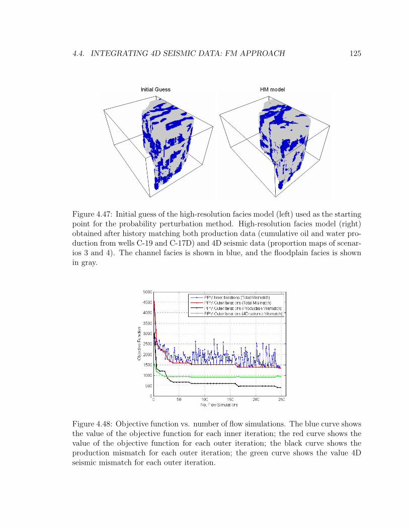
4.4. INTEGRATING 4D SEISMIC DATA: FM APPROACH 125
Figure 4.47: Initial guess of the high-resolution facies model (left) used as the startingpoint for the probability perturbation method. High-resolution facies model (right)obtained after history matching both production data (cumulative oil and water pro-duction from wells C-19 and C-17D) and 4D seismic data (proportion maps of scenar-ios 3 and 4). The channel facies is shown in blue, and the floodplain facies is shownin gray.
Figure 4.48: Objective function vs. number of flow simulations. The blue curve showsthe value of the objective function for each inner iteration; the red curve shows thevalue of the objective function for each outer iteration; the black curve shows theproduction mismatch for each outer iteration; the green curve shows the value 4Dseismic mismatch for each outer iteration.
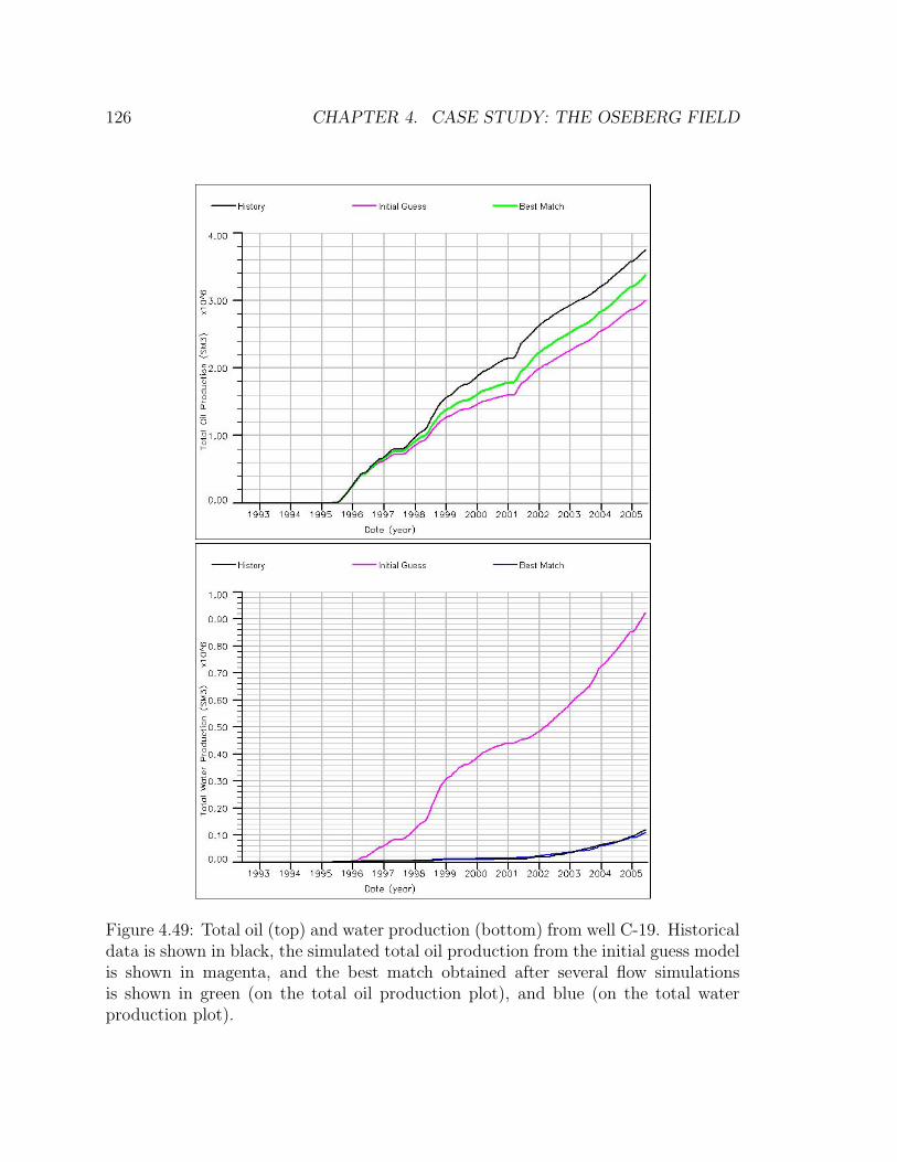
126 CHAPTER 4. CASE STUDY: THE OSEBERG FIELD
Figure 4.49: Total oil (top) and water production (bottom) from well C-19. Historicaldata is shown in black, the simulated total oil production from the initial guess modelis shown in magenta, and the best match obtained after several flow simulationsis shown in green (on the total oil production plot), and blue (on the total waterproduction plot).
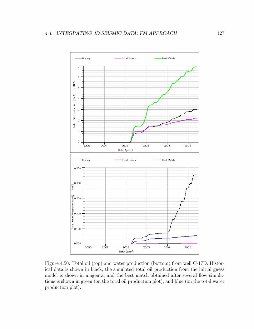
4.4. INTEGRATING 4D SEISMIC DATA: FM APPROACH 127
Figure 4.50: Total oil (top) and water production (bottom) from well C-17D. Histor-ical data is shown in black, the simulated total oil production from the initial guessmodel is shown in magenta, and the best match obtained after several flow simula-tions is shown in green (on the total oil production plot), and blue (on the total waterproduction plot).
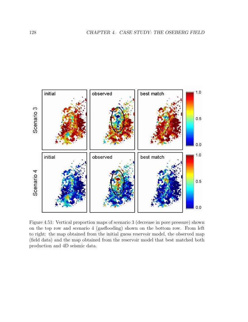
128 CHAPTER 4. CASE STUDY: THE OSEBERG FIELD
Figure 4.51: Vertical proportion maps of scenario 3 (decrease in pore pressure) shownon the top row and scenario 4 (gasflooding) shown on the bottom row. From leftto right: the map obtained from the initial guess reservoir model, the observed map(field data) and the map obtained from the reservoir model that best matched bothproduction and 4D seismic data.
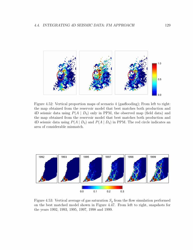
4.4. INTEGRATING 4D SEISMIC DATA: FM APPROACH 129
Figure 4.52: Vertical proportion maps of scenario 4 (gasflooding); From left to right:the map obtained from the reservoir model that best matches both production and4D seismic data using P (A | D3) only in PPM, the observed map (field data) andthe map obtained from the reservoir model that best matches both production and4D seismic data using P (A | D3) and P (A | D4) in PPM. The red circle indicates anarea of considerable mismatch.
Figure 4.53: Vertical average of gas saturation Sg from the flow simulation performedon the best matched model shown in Figure 4.47. From left to right, snapshots forthe years 1992, 1993, 1995, 1997, 1998 and 1999.
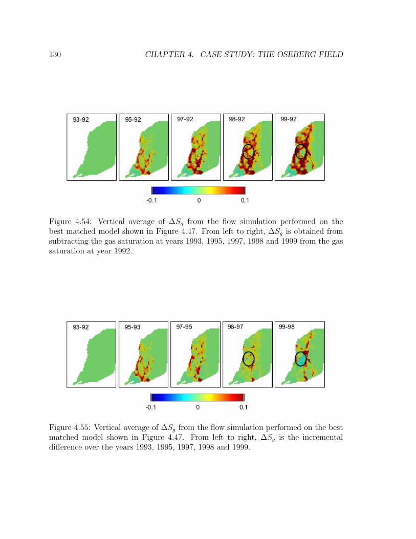
130 CHAPTER 4. CASE STUDY: THE OSEBERG FIELD
Figure 4.54: Vertical average of ∆Sg from the flow simulation performed on thebest matched model shown in Figure 4.47. From left to right, ∆Sg is obtained fromsubtracting the gas saturation at years 1993, 1995, 1997, 1998 and 1999 from the gassaturation at year 1992.
Figure 4.55: Vertical average of ∆Sg from the flow simulation performed on the bestmatched model shown in Figure 4.47. From left to right, ∆Sg is the incrementaldifference over the years 1993, 1995, 1997, 1998 and 1999.
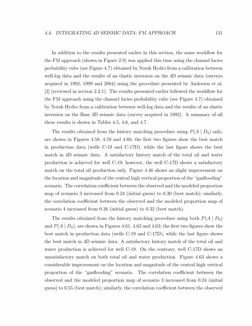
4.4. INTEGRATING 4D SEISMIC DATA: FM APPROACH 131
In addition to the results presented earlier in this section, the same workflow for
the FM approach (shown in Figure 2.9) was applied this time using the channel facies
probability cube (see Figure 4.7) obtained by Norsk Hydro from a calibration between
well-log data and the results of an elastic inversion on the 4D seismic data (surveys
acquired in 1992, 1999 and 2004) using the procedure presented by Andersen et al.
[3] (reviewed in section 2.2.1). The results presented earlier followed the workflow for
the FM approach using the channel facies probability cube (see Figure 4.7) obtained
by Norsk Hydro from a calibration between well-log data and the results of an elastic
inversion on the Base 3D seismic data (survey acquired in 1992). A summary of all
these results is shown in Tables 4.5, 4.6, and 4.7.
The results obtained from the history matching procedure using P (A | D3) only,
are shown in Figures 4.58, 4.59 and 4.60; the first two figures show the best match
in production data (wells C-19 and C-17D), while the last figure shows the best
match in 4D seismic data. A satisfactory history match of the total oil and water
production is achieved for well C-19; however, the well C-17D shows a satisfactory
match on the total oil production only. Figure 4.46 shows an slight improvement on
the location and magnitude of the central high vertical proportion of the “gasflooding”
scenario. The correlation coefficient between the observed and the modeled proportion
map of scenario 3 increased from 0.24 (initial guess) to 0.30 (best match); similarly,
the correlation coefficient between the observed and the modeled proportion map of
scenario 4 increased from 0.26 (initial guess) to 0.32 (best match).
The results obtained from the history matching procedure using both P (A | D3)
and P (A | D4), are shown in Figures 4.61, 4.62 and 4.63; the first two figures show the
best match in production data (wells C-19 and C-17D), while the last figure shows
the best match in 4D seismic data. A satisfactory history match of the total oil and
water production is achieved for well C-19. On the contrary, well C-17D shows an
unsatisfactory match on both total oil and water production. Figure 4.63 shows a
considerable improvement on the location and magnitude of the central high vertical
proportion of the “gasflooding” scenario. The correlation coefficient between the
observed and the modeled proportion map of scenario 3 increased from 0.24 (initial
guess) to 0.55 (best match); similarly, the correlation coefficient between the observed

132 CHAPTER 4. CASE STUDY: THE OSEBERG FIELD
and the modeled vertical proportion map of scenario 4 increased from 0.26 (initial
guess) to 0.55 (best match).
These results were obtained starting from the same random seed as the results
presented earlier (when using the channel facies probability cube obtained from a
calibration between well-log data and the Base 3D seismic data). Similar results are
obtained for the match of production and 4D seismic data; however, figures 4.57 and
4.65 show that a history match is achieved in a shorter number of flow simulations.
When using P (A | D3) only, a history match is obtained in 32 flow simulations,
roughly a third of the number of flow simulation used in the results presented earlier
(88 flow simulations). Similarly, when using P (A | D3) and P (A | D4), a history
match is obtained in 63 flow simulations, roughly a fourth of the number of flow
simulation used in the results presented earlier (250 flow simulations).
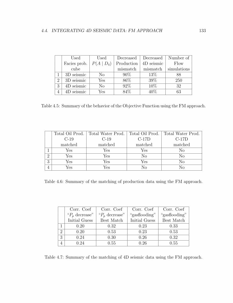
4.4. INTEGRATING 4D SEISMIC DATA: FM APPROACH 133
Used Used Decreased Decreased Number ofFacies prob. P (A | D4) Production 4D seismic Flow
cube mismatch mismatch simulations1 3D seismic No 90% 13% 882 3D seismic Yes 86% 39% 2503 4D seismic No 92% 10% 324 4D seismic Yes 84% 40% 63
Table 4.5: Summary of the behavior of the Objective Function using the FM approach.
Total Oil Prod. Total Water Prod. Total Oil Prod. Total Water Prod.C-19 C-19 C-17D C-17D
matched matched matched matched1 Yes Yes Yes No2 Yes Yes No No3 Yes Yes Yes No4 Yes Yes No No
Table 4.6: Summary of the matching of production data using the FM approach.
Corr. Coef Corr. Coef Corr. Coef Corr. Coef“Pp decrease” “Pp decrease” “gasflooding” “gasflooding”Initial Guess Best Match Initial Guess Best Match
1 0.20 0.32 0.23 0.332 0.20 0.53 0.23 0.533 0.24 0.30 0.26 0.324 0.24 0.55 0.26 0.55
Table 4.7: Summary of the matching of 4D seismic data using the FM approach.

134 CHAPTER 4. CASE STUDY: THE OSEBERG FIELD
Figure 4.56: Initial guess of the high-resolution facies model (left) used as the startingpoint for the probability perturbation method. High-resolution facies model (right)obtained after history matching both production data (cumulative oil and water pro-duction from wells C-19 and C-17D) and 4D seismic data (proportion maps of scenar-ios 3 and 4). The channel facies is shown in blue, and the floodplain facies is shownin gray.
Figure 4.57: Objective function vs. number of flow simulations. The blue curve showsthe value of the objective function for each inner iteration; the red curve shows thevalue of the objective function for each outer iteration; the black curve shows theproduction mismatch for each outer iteration; the green curve shows the value 4Dseismic mismatch for each outer iteration.
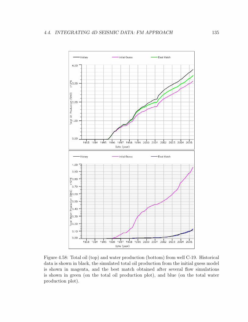
4.4. INTEGRATING 4D SEISMIC DATA: FM APPROACH 135
Figure 4.58: Total oil (top) and water production (bottom) from well C-19. Historicaldata is shown in black, the simulated total oil production from the initial guess modelis shown in magenta, and the best match obtained after several flow simulationsis shown in green (on the total oil production plot), and blue (on the total waterproduction plot).
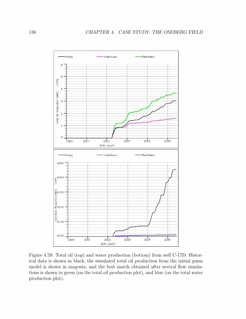
136 CHAPTER 4. CASE STUDY: THE OSEBERG FIELD
Figure 4.59: Total oil (top) and water production (bottom) from well C-17D. Histor-ical data is shown in black, the simulated total oil production from the initial guessmodel is shown in magenta, and the best match obtained after several flow simula-tions is shown in green (on the total oil production plot), and blue (on the total waterproduction plot).
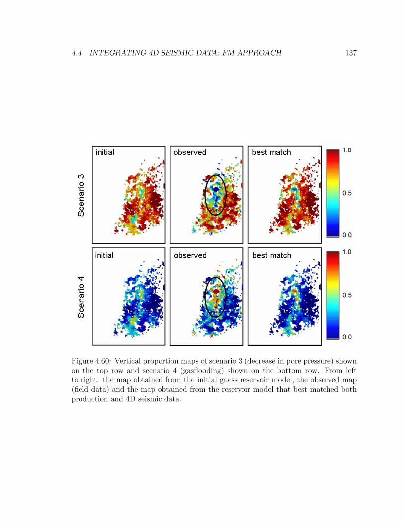
4.4. INTEGRATING 4D SEISMIC DATA: FM APPROACH 137
Figure 4.60: Vertical proportion maps of scenario 3 (decrease in pore pressure) shownon the top row and scenario 4 (gasflooding) shown on the bottom row. From leftto right: the map obtained from the initial guess reservoir model, the observed map(field data) and the map obtained from the reservoir model that best matched bothproduction and 4D seismic data.
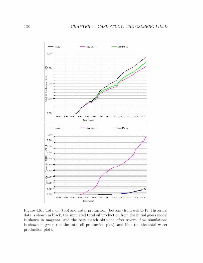
138 CHAPTER 4. CASE STUDY: THE OSEBERG FIELD
Figure 4.61: Total oil (top) and water production (bottom) from well C-19. Historicaldata is shown in black, the simulated total oil production from the initial guess modelis shown in magenta, and the best match obtained after several flow simulationsis shown in green (on the total oil production plot), and blue (on the total waterproduction plot).
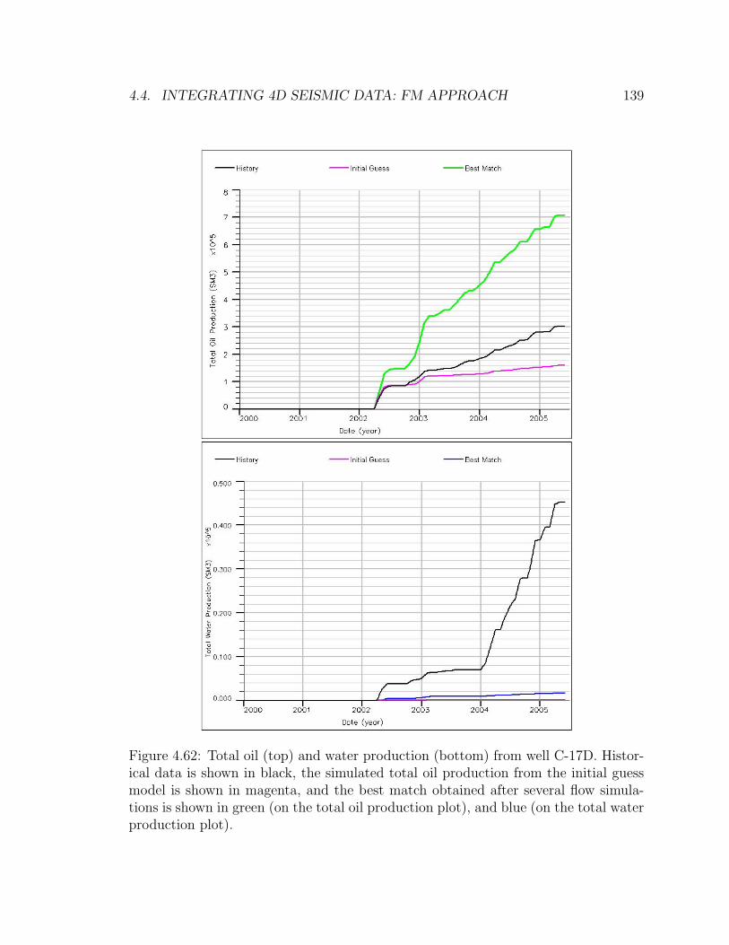
4.4. INTEGRATING 4D SEISMIC DATA: FM APPROACH 139
Figure 4.62: Total oil (top) and water production (bottom) from well C-17D. Histor-ical data is shown in black, the simulated total oil production from the initial guessmodel is shown in magenta, and the best match obtained after several flow simula-tions is shown in green (on the total oil production plot), and blue (on the total waterproduction plot).
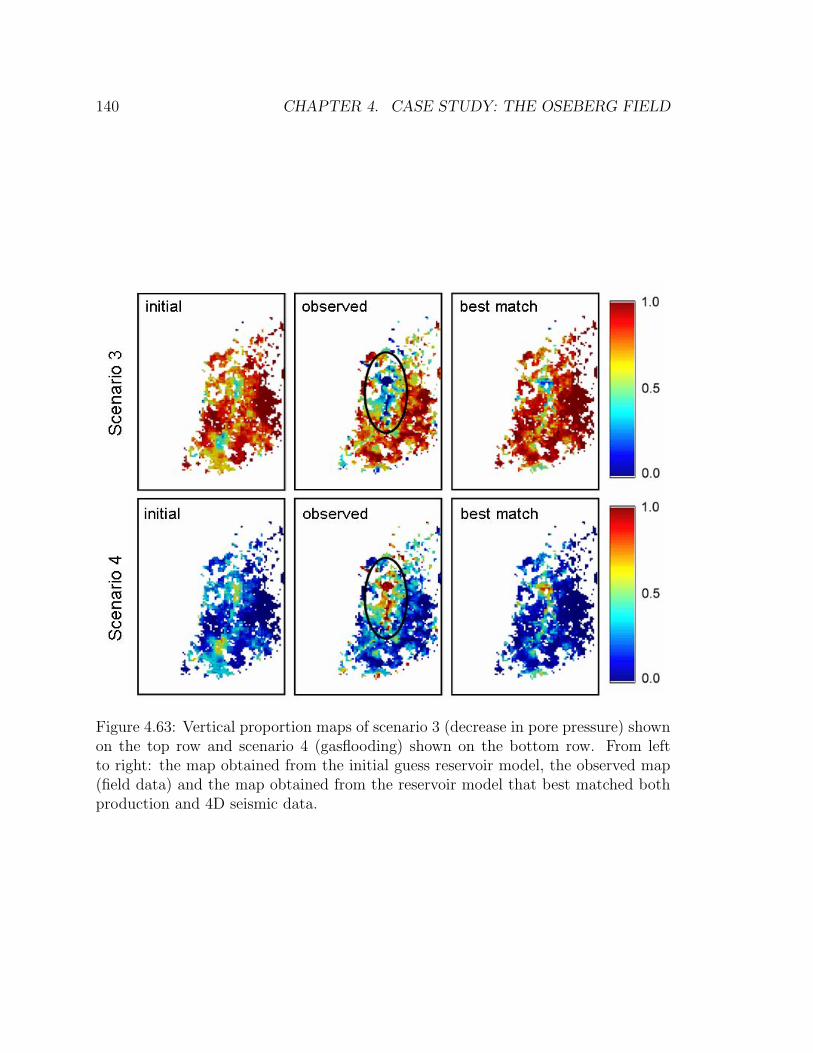
140 CHAPTER 4. CASE STUDY: THE OSEBERG FIELD
Figure 4.63: Vertical proportion maps of scenario 3 (decrease in pore pressure) shownon the top row and scenario 4 (gasflooding) shown on the bottom row. From leftto right: the map obtained from the initial guess reservoir model, the observed map(field data) and the map obtained from the reservoir model that best matched bothproduction and 4D seismic data.
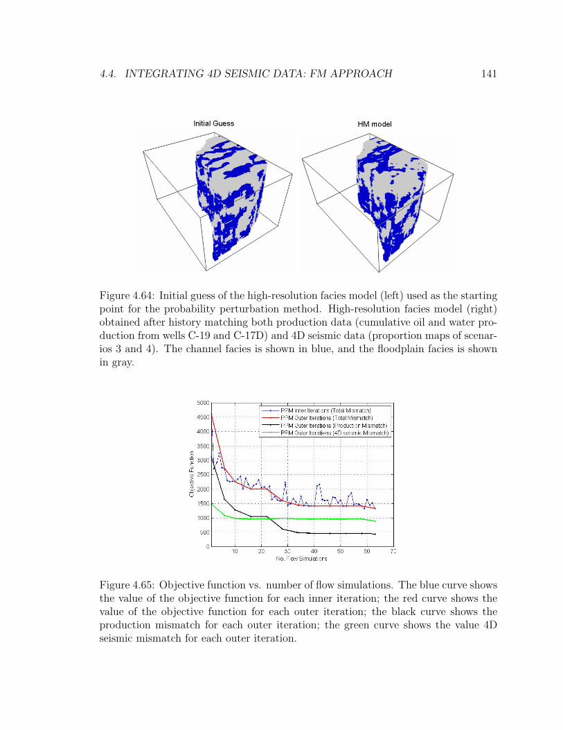
4.4. INTEGRATING 4D SEISMIC DATA: FM APPROACH 141
Figure 4.64: Initial guess of the high-resolution facies model (left) used as the startingpoint for the probability perturbation method. High-resolution facies model (right)obtained after history matching both production data (cumulative oil and water pro-duction from wells C-19 and C-17D) and 4D seismic data (proportion maps of scenar-ios 3 and 4). The channel facies is shown in blue, and the floodplain facies is shownin gray.
Figure 4.65: Objective function vs. number of flow simulations. The blue curve showsthe value of the objective function for each inner iteration; the red curve shows thevalue of the objective function for each outer iteration; the black curve shows theproduction mismatch for each outer iteration; the green curve shows the value 4Dseismic mismatch for each outer iteration.
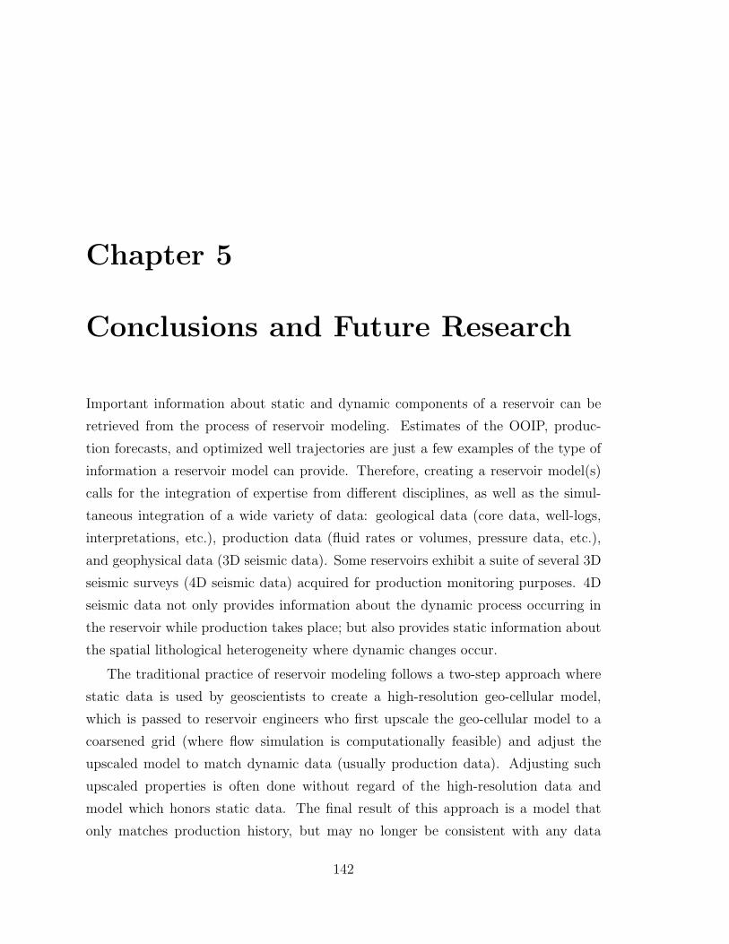
Chapter 5
Conclusions and Future Research
Important information about static and dynamic components of a reservoir can be
retrieved from the process of reservoir modeling. Estimates of the OOIP, produc-
tion forecasts, and optimized well trajectories are just a few examples of the type of
information a reservoir model can provide. Therefore, creating a reservoir model(s)
calls for the integration of expertise from different disciplines, as well as the simul-
taneous integration of a wide variety of data: geological data (core data, well-logs,
interpretations, etc.), production data (fluid rates or volumes, pressure data, etc.),
and geophysical data (3D seismic data). Some reservoirs exhibit a suite of several 3D
seismic surveys (4D seismic data) acquired for production monitoring purposes. 4D
seismic data not only provides information about the dynamic process occurring in
the reservoir while production takes place; but also provides static information about
the spatial lithological heterogeneity where dynamic changes occur.
The traditional practice of reservoir modeling follows a two-step approach where
static data is used by geoscientists to create a high-resolution geo-cellular model,
which is passed to reservoir engineers who first upscale the geo-cellular model to a
coarsened grid (where flow simulation is computationally feasible) and adjust the
upscaled model to match dynamic data (usually production data). Adjusting such
upscaled properties is often done without regard of the high-resolution data and
model which honors static data. The final result of this approach is a model that
only matches production history, but may no longer be consistent with any data
142
143
integrated prior to matching. This dissertation, however, uses a reservoir modeling
workflow that integrates all data from various sources (both static and dynamic)
at the same time using a probabilistic approach. Additionally, it builds both high-
resolution and coarsened models jointly while perturbing the high-resolution model
in a geologically consistent fashion. The main contribution of this dissertation is the
inclusion of 4D seismic data within this reservoir modeling workflow while attempting
to honor all other available data.
Two general approaches are proposed to include 4D seismic data into the reservoir
modeling workflow: the PDI and FM approaches. The Probabilistic Data Integration
approach (PDI), consists of modeling the information content of 4D seismic through
a spatial probability of facies occurrence that is used as a constraint (along with
conditional probabilities from other data) to create a high-resolution facies model
of the reservoir; production data is the only dynamic data included in the iterative
history matching process. The Forward Modeling (FM) approach uses the facies
information content (through a spatial probability) from the base 3D seismic survey
to create a high-resolution facies model of the reservoir; both production and 4D
seismic data are included in the history matching process.
History matching production data only involves modeling the production response
of the reservoir model by performing flow simulation. Therefore, when including the
matching of 4D seismic data, the 4D response of the reservoir model needs to be com-
puted also by performing a “Forward Modeling” (FM). The 4D seismic response of the
reservoir model is forward modeled using the high-resolution reservoir properties and
the downscaled spatial distribution of fluid saturation obtained from flow simulation.
A novel flow-based downscaling method is proposed in this dissertation, the procedure
takes into account both static information (high-resolution permeability field) and dy-
namic information in the form of coarsened fluxes and saturations (solution of the
flow simulation on the coarsened grid). On a synthetic layered example, it was found
that modeling 4D seismic data using flow-based downscaled saturations resulted in a
better match with the “reference” 4D seismic (flow simulation on the high-resolution
grid was possible for this simplified case), because the flow-based downscaled satu-
rations reproduced the sharpness and key details of the saturation field. Modeling
144 CHAPTER 5. CONCLUSIONS AND FUTURE RESEARCH
4D seismic data using the traditional approach of simply projecting the coarse scale
saturation from the flow simulator onto the high resolution grid was shown to result
in a time-lapse response that did not accurately predict the distribution of fluids in
the reservoir.
The two proposed approaches (PDI and FM approaches) to include 4D seismic
data into the reservoir modeling workflow, were successfully applied on the Oseberg
field in the North Sea, to model channel facies of a fluvial reservoir.
The PDI approach constrained the reservoir model to the spatial probability of
facies occurrence (obtained from a calibration between well-log and 4D seismic data)
as well as other static data while history matching production data. A satisfactory
history match of the total oil and water production is achieved for well C-19, showing
an impressive improvement compared to the simulated production response of the
initial guess model. On the contrary, well C-17D shows a satisfactory history match
on the total oil production only; the large mismatch obtained for the total water
production in this well needs to be further investigated through the flow simulation
model. These results demonstrate that by changing the distribution of channels, while
remaining consistent with other (static) data, a satisfactory match of production data
was achieved. However; only a probabilistic matching of 4D seismic data is achieved,
rather than a deterministic physics-based matching of that data.
The FM approach achieved a satisfactory history match of the total oil and water
production for well C-19; on the contrary, well C-17D shows an unsatisfactory match
on the total oil and water production. Changing the distribution of channels, while
remaining consistent with other static data, a satisfactory match on the production
data of well C-19 was achieved; however, perturbing the distribution of channels only
was not enough to obtain a considerable decrease in the 4D seismic mismatch.
The main central feature observed on the field 4D seismic data, related to a high
vertical proportion of the “gasflooding” scenario (low vertical proportion of the “Pore
pressure decrease” scenario), was interpreted to be directly related to the local net-to-
gross (NTG) since fluid flow occurs preferentially in sand facies (high permeability).
Therefore, in addition to the perturbation of the distribution of channels, perturbation
of the local NTG was obtained through the introduction of a second conditional

145
probability in PPM. This results in either an increase or decrease of the local NTG
as a function of the local 4D seismic mismatch.
Using the local perturbation of NTG through a new conditional probability, the
4D seismic mismatch decreased considerably during the first few outer iterations of
PPM. The 4D seismic mismatch decreased three times more than when the local per-
turbation of NTG is not used; however; the production mismatch decreased roughly
the same amount but over a larger number of flow simulations. The final forward
modeled 4D seismic response showed a better agreement with the observed 4D seis-
mic data than the forward modeled 4D seismic response obtained without using the
local perturbation of NTG. Notably was one area in the reservoir, exhibiting a high
vertical proportion of the “gasflooding” scenario (an indicator of high NTG). How-
ever, the model was not able to fully predict this phenomenon. From flow simulation,
it was observed that gas came out of solution in this area by the year 1998 but mi-
grated to other areas in the reservoir before the year 1999, when the second seismic
monitor survey is forward modeled. Two explanations could possibly apply to this
situation: either the 4D seismic data is indicative of a process (not modeled) other
than “gasflooding”, or some geological information is missing in the model such as
the presence of a fault (either not modeled or below the seismic resolution) or any
other geological barrier that prevents the gas from migrating. The feasibility of each
proposed explanation should be further investigated.
The proposed FM approach uses the channel facies probability cube obtained by
Norsk Hydro from a calibration between well-log data and the results of an elastic
inversion on the Base 3D seismic data (survey acquired in 1992). A proposed hybrid
approach would be to use the channel facies probability cube obtained by Norsk
Hydro from a calibration between well-log data and the results of an elastic inversion
on 4D seismic data (surveys acquired in 1992, 1999 and 2004) while at the same time
matching both production and 4D seismic data iteratively. The results obtained from
this hybrid approach showed a similar quality on the match of production and 4D
seismic data; however, it has been noticed that a history match is achieved in a shorter
number of flow simulations. In particular, when using the local perturbation of NTG
the number of flow simulations required to achieve a history match was reduced by a
146 CHAPTER 5. CONCLUSIONS AND FUTURE RESEARCH
factor of four.
When a complicated 4D seismic forward modeling cannot be carried out due to
a lack of rock physics data, the PDI approach may represent a more robust and
less difficult to achieve alternative to include 4D seismic information into the reser-
voir modeling workflow. However, in that case only a probabilistic matching of 4D
seismic data is achieved, rather than a deterministic physics-based matching of that
data. The quality of the 4D seismic data (in terms of signal/noise) is more critical
for the FM approach than for the PDI approach, since a deterministic physics-based
matching of 4D seismic data is pursued. Each approach uses the information content
of 4D seismic data in a different fashion; the PDI approach makes use of the static
information contained in the 4D seismic data, while the FM approach seeks to match
the dynamic information in the 4D seismic data. If high quality 4D seismic data is
available, the FM approach (although practically more challenging to apply) could
help to understand better the dynamic behavior of the reservoir as well as to identify
valuable static information that may need to be incorporated into the reservoir model.
Limitations
Regarding the new flow-based downscaling procedure, it is observed that its suc-
cess depends directly on the method used for upscaling as well as the upscaling ratio
applied to the static data prior to flow simulation. Hence, the upscaling method, and
the chosen upscaling ratio, should maintain the overall character and position of the
saturation front.
This dissertation uses the “Parallel Modeling” approach, introduced by Tureyen
in his PhD dissertation [86], to build both high-resolution and coarsened models
jointly while perturbing the high-resolution model. The limitations of this approach,
as pointed out by Tureyen, also apply to the workflow used here. Perhaps the most
important limitation is the method used for upscaling as well as the upscaling ratio.
If the upscaling procedure is not robust enough to maintain important flow perfor-
mance features from the high-resolution model, the forecast capabilities of the pair
147
high-resolution and coarsened models may be weak. On the other hand, if a sophis-
ticated upscaling procedure is chosen, additional computational cost and complexity
of successive upscaling becomes also a handicap of the approach.
Regarding the two proposed approaches (PDI and FM) to include 4D seismic data
into the reservoir modeling workflow, the following limitations are noticed:
• the PDI approach requires 4D seismic data to be informative about the static
unknown being modeled; facies, for example. This approach uses 4D seismic
data in a “static” fashion where only a probabilistic matching of 4D seismic data
is achieved. The application of this approach to the Alpha North segment of
the Oseberg field was possible because the main dynamic response (gasflooding)
occurs in one particular facies of the binary (channel/no channel) facies model;
hence, the dynamic response was an indicator of the presence of the channel
facies (a static property of the model). In other field applications, it may not
necessarily be possible to translate dynamic changes into information about
static properties.
• the PDI approach only pursues a probabilistic matching of the “static” infor-
mation possibly contained in the 4D seismic data. The PDI approach may not
necessarily achieve a deterministic physics-based matching of the 4D seismic
data since it is not explicitly pursuing that matching like the FM approach
does. This may be of particular relevance in the case where a significant dy-
namic response is observed in the 4D seismic data, and we want the reservoir
model to explicitly reproduce it.
• the FM approach requires forward modeling the 4D seismic response of the
reservoir model. Forward modeling represents a challenge due to several fac-
tors: the joint modeling of pressure and saturation effects while maintaining
the observed dominance of one or the other, the possible lack of rock physics
data (lab measurements on the pressure dependency of the seismic velocities,
for example), the downscaling of the flow response under a complicated flow
scenario (three-phase flow and multiple wells), the forward modeling of the seis-
mic signal (if amplitudes are the seismic attribute being modeled) may imply a
148 CHAPTER 5. CONCLUSIONS AND FUTURE RESEARCH
computationally-costly method being iteratively used.
• the FM approach aims at matching simultaneously both production and 4D
seismic data. Several parameters of the high-resolution and/or flow model may
have a significant effect on the matching of either production or 4D seismic
data. For example, in the case study presented in this dissertation, clearly the
matching of production data was influenced by the distribution of the channel
facies in the reservoir; however, the matching of 4D seismic was influenced by
the local NTG in the reservoir and possibly missing structural complexity in
the flow model. The approach used to perturb these parameters should be such
that improving the matching of one datum does not deteriorate the matching of
the other datum. In addition, a thorough analysis for possible inconsistencies
between the available data should be performed prior to history matching.
• the success of such a complete reservoir modeling workflow involves a multidis-
ciplinary knowledge of all data and processes involved. The modeling of the
dynamic (production and 4D seismic) response of the reservoir depends on the
static description of the reservoir, the modeling of flow boundary conditions
(wells, aquifers), the description of fluids in the reservoir, the modeling of the
seismic response, etc.
Future Research
Regarding the new flow-based downscaling procedure presented in this disserta-
tion, the following areas of future research are identified:
• the application of the procedure in an adaptive fashion, where local high-
resolution flow is simulated only in the areas of the reservoir with high-resolution
saturation effects which impact the seismic signal (e.g., an advancing water front
in a region with a high degree of subgrid permeability variability). With this
procedure, areas of the reservoir already swept (or not yet swept) by the injected
water would not be reconstructed because they exhibit a constant saturation
149
value. This approach could be much more efficient computationally than recon-
structing the high-resolution saturation everywhere, particularly in cases where
the important saturation changes occur over relatively small portions of the
reservoir. This technique will however require some modification of the down-
scaling procedure described in this dissertation, for example in the specification
of the inlet saturation boundary conditions. The success of the proposed adap-
tive flow-based downscaling method depends directly on the method used for
upscaling as well as the upscaling ratio applied to the static data prior to flow
simulation. The upscaling method, and the chosen upscaling ratio, should main-
tain the overall character and position of the saturation front, since the adaptive
flow-based downscaling method would identify the front and work on its refine-
ment. An alternative approach (where downscaling may not be needed) is to
use an upscaling adaptive gridding approach where no upscaling is performed
in the areas of the reservoir with high-resolution saturation effects, such as an
advancing water front in a region with a high degree of subgrid permeability
variability.
• the extension of the method to a 3D three-phase flow-based downscaling pro-
cedure. However, only an approximate method may be sufficient; for example,
in a three-phase situation perhaps the most important feature to reconstruct
would be the presence or absence of gas in a grid block (when modeling seismic
attributes that are not sensitive to the particular value of gas saturation).
Some other areas of future research are the following:
• the inclusion of conditioning to a map of local NTG in multiple-point sequential
simulation algorithms. From the results of the case study presented in this
dissertation, it was observed that the local perturbation of NTG through a new
conditional probability caused partial damage of the geological continuity of the
channel facies.
• related to the case study, the factors affecting the observed mismatch on the
water production of well C-17D should be further investigated. In addition, the
150 CHAPTER 5. CONCLUSIONS AND FUTURE RESEARCH
geological feasibility of the presence of a fault (either not modeled or below the
seismic resolution) or any other geological barrier that prevents the gas from
migrating in the area of largest mismatch with the 4D seismic should also be
investigated.
• the rock physics modeling used in this dissertation assumes no fluid flow oc-
curring in shales (also inactive during flow simulation), but being affected by
changes in pressure. This may not necessarily be an accurate assumption. On
one hand, Gassmann’s fluid substitution is only applicable to sands; on the
other hand, particularly for the case study presented in this dissertation, the
field 4D seismic data (between 1992 and 1999) shows a strong pressure depletion
response that has been interpreted to be experienced by both sand and shales
due to its vast spatial extension. More rock physics laboratory studies on shales
should be carried out in order to understand better their dynamic behavior.
• another area of fascinating research is to model 4D seismic responses due to
compaction and fault(s) reactivation, occurring separately or simultaneously;
in a hydrocarbon producing reservoir. This area may require intensive research
on dynamic re-gridding of the reservoir model as well as the inclusion of geo-
mechanics.
• the application of the PDI and FM approaches to other case studies should
result in setting a criteria for choosing a probabilistic versus a deterministic but
more physics-based use of 4D seismic data.
Appendix A
The Stanford VI Reservoir
With the purpose of extensively testing algorithms for reservoir modeling or reservoir
characterization, Mao and Journel [57] created an exhaustive 3D reference data set
called Stanford V. Although it has been widely used, this data set is too small to
represent current-day reservoir modeling exercises. Several extensions are proposed
here, while incorporated into a new reference reservoir model, termed Stanford VI.
The proposed reference data set (Stanford VI) exhibits a smooth top and bottom
surface representing a trap in the form of an anticline. It provides an exhaustive
sampling of petrophysical properties. The new reservoir model is represented in a 3D
regular grid of 6 million cells (150 × 200 × 200), with more realistic dimensions for
current-day models (25 m in the x and y directions and 1 m in the z direction).
Following Stanford V, the stratigraphic model corresponds to a fluvial channel
system, and the petrophysical properties computed for this reference reservoir corre-
spond to the classical porosity, density, permeability and seismic P-wave and S-wave
velocities. Although most of these properties are calculated following the standard
procedure and algorithms presented by Mao and Journel, a more appropriate Rock
Physics model is used in the new reference reservoir model to compute P-wave velocity
for sandstones.
Traditionally, P-wave velocity is calculated from empirical expressions obtained
from laboratory data as a function of porosity [92] [67] [40] [84]. The former Stanford
151
152 APPENDIX A. THE STANFORD VI RESERVOIR
V reservoir uses one of these expressions, presented by Han [40], to obtain P-wave ve-
locities from porosity. Strictly speaking, Han’s relations are obtained from sandstone
samples collected from different depths, where porosity is controlled by diagenesis and
cementing. In our case porosity is controlled by sorting and clay content, henceforth,
a more appropriate rock physics model is used, namely, the constant cement model
described by Dvorkin and Nur [29].
Besides petrophysical properties, the new reference reservoir model exhibits a
complete set of physical seismic attributes, which are computed from well-known
mathematical expressions and subsequently filtered and smoothed to obtain realistic
looking data as would have been obtained from actual seismic acquisition and mod-
eling. These realistic seismic attributes provide a filtered view of the true spatial
variation of petrophysical properties.
From this new reference reservoir model 4D seismic data is generated. 4D seismic
data is nothing more than three-dimensional (3D) seismic data acquired at different
times over the same area. 4D seismic is used to assess changes in a producing hy-
drocarbon reservoir with time; changes may be observed in fluid location, saturation,
pressure, and temperature. Consequently, one of the main applications of 4D seismic
data is to monitor fluid flow in the reservoir.
In order to create a 4D seismic response, several 3D seismic data sets are forward
modeled using a simple convolutional model. The first seismic data set is created
using the acoustic impedance of the reservoir prior to production, while three more
seismic data sets are created using the acoustic impedance of the reservoir at different
times during oil production.
The acoustic impedance of the reservoir after a certain time t can be computed
by using a fluid substitution approach. Prior to production the reservoir is filled with
oil, while some years after production starts the reservoir contains a mixture of fluids,
typically water oil and gas. In order to use Gassmann’s equations [32] correctly the
saturations of each fluid at every point in space are needed, therefore a flow simulator
is used to obtain them at any point in time during production.
To create the 3D seismic data sets at different times during oil production, a two-
phase flow simulation is performed. Thirty years of oil production are simulated with
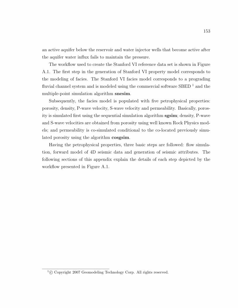
153
an active aquifer below the reservoir and water injector wells that become active after
the aquifer water influx fails to maintain the pressure.
The workflow used to create the Stanford VI reference data set is shown in Figure
A.1. The first step in the generation of Stanford VI property model corresponds to
the modeling of facies. The Stanford VI facies model corresponds to a prograding
fluvial channel system and is modeled using the commercial software SBED 1 and the
multiple-point simulation algorithm snesim.
Subsequently, the facies model is populated with five petrophysical properties:
porosity, density, P-wave velocity, S-wave velocity and permeability. Basically, poros-
ity is simulated first using the sequential simulation algorithm sgsim; density, P-wave
and S-wave velocities are obtained from porosity using well known Rock Physics mod-
els; and permeability is co-simulated conditional to the co-located previously simu-
lated porosity using the algorithm cosgsim.
Having the petrophysical properties, three basic steps are followed: flow simula-
tion, forward model of 4D seismic data and generation of seismic attributes. The
following sections of this appendix explain the details of each step depicted by the
workflow presented in Figure A.1.
1 c© Copyright 2007 Geomodeling Technology Corp. All rights reserved.
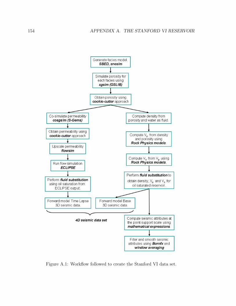
154 APPENDIX A. THE STANFORD VI RESERVOIR
Figure A.1: Workflow followed to create the Stanford VI data set.
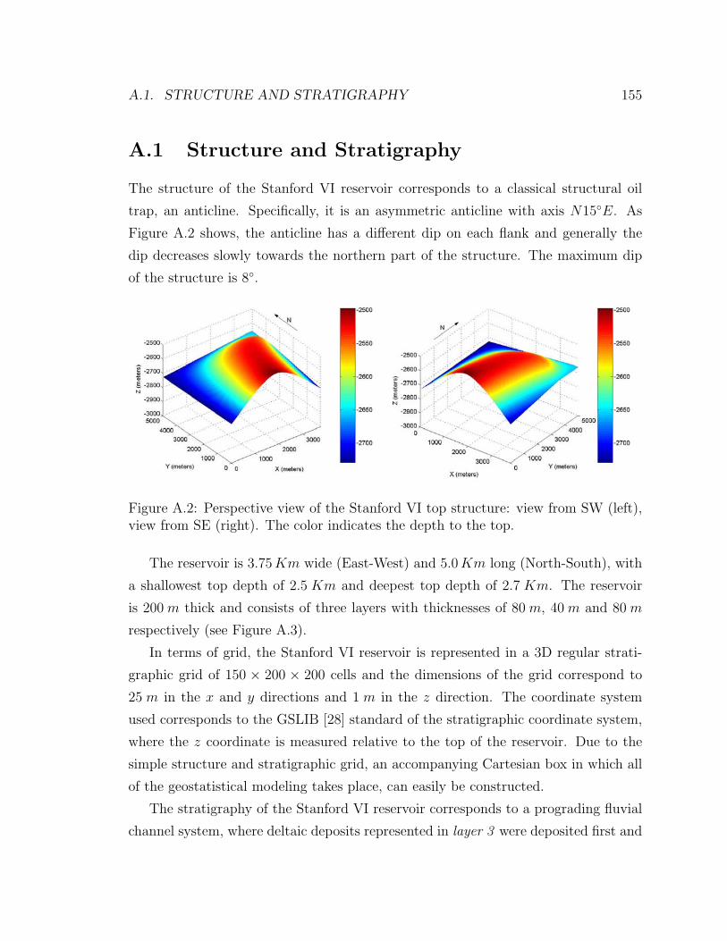
A.1. STRUCTURE AND STRATIGRAPHY 155
A.1 Structure and Stratigraphy
The structure of the Stanford VI reservoir corresponds to a classical structural oil
trap, an anticline. Specifically, it is an asymmetric anticline with axis N15◦E. As
Figure A.2 shows, the anticline has a different dip on each flank and generally the
dip decreases slowly towards the northern part of the structure. The maximum dip
of the structure is 8◦.
Figure A.2: Perspective view of the Stanford VI top structure: view from SW (left),view from SE (right). The color indicates the depth to the top.
The reservoir is 3.75 Km wide (East-West) and 5.0 Km long (North-South), with
a shallowest top depth of 2.5 Km and deepest top depth of 2.7 Km. The reservoir
is 200 m thick and consists of three layers with thicknesses of 80 m, 40 m and 80 m
respectively (see Figure A.3).
In terms of grid, the Stanford VI reservoir is represented in a 3D regular strati-
graphic grid of 150 × 200 × 200 cells and the dimensions of the grid correspond to
25 m in the x and y directions and 1 m in the z direction. The coordinate system
used corresponds to the GSLIB [28] standard of the stratigraphic coordinate system,
where the z coordinate is measured relative to the top of the reservoir. Due to the
simple structure and stratigraphic grid, an accompanying Cartesian box in which all
of the geostatistical modeling takes place, can easily be constructed.
The stratigraphy of the Stanford VI reservoir corresponds to a prograding fluvial
channel system, where deltaic deposits represented in layer 3 were deposited first and
156 APPENDIX A. THE STANFORD VI RESERVOIR
Figure A.3: Perspective view of the Stanford VI top and bottom of each of its layers.The color indicates the depth to the top.
followed by meandering channels in layer 2 and sinuous channels in layer 1. This
sequence of clastic deposits represents a progradation of a fluvial system into the
basin located in this case toward the north of the reservoir.
In order to model the stratigraphy of Stanford VI, the commercial software SBED
is used to model layer 1 and layer 2, while layer 3 is modeled using the multiple-point
simulation algorithm snesim with local rotation and affinity variation to model the
channel meanders.
The first layer of Stanford VI consists of a system of sinuous channels represented
by four facies: the floodplain (shale deposits), the point bar (sand deposits that
occur along the convex inner edges of the meanders of channels), the channel (sand
deposits), and the boundary (shale deposits). The stratigraphic characteristics of
layer 1 are detailed in Table A.1 and Figure A.4 shows the resulting stratigraphic
model for this layer.
The second layer consists of meandering channels also represented by four facies:
the floodplain (shale deposits), the point bar (sand deposits that occur along the
convex inner edges of the meanders of channels), the channel (sand deposits), and
the boundary (shale deposits). The stratigraphic characteristics of layer 2 are detailed
in Table A.2 and Figure A.5 shows the resulting stratigraphic model for this layer.
The last and third layer of the reservoir consist of deltaic deposits and are repre-
sented by two facies: the floodplain (shale deposits), and the channel (sand deposits).
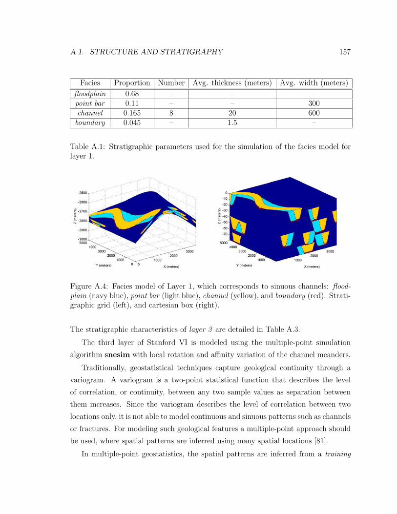
A.1. STRUCTURE AND STRATIGRAPHY 157
Facies Proportion Number Avg. thickness (meters) Avg. width (meters)
floodplain 0.68 – – –point bar 0.11 – – 300channel 0.165 8 20 600boundary 0.045 – 1.5 –
Table A.1: Stratigraphic parameters used for the simulation of the facies model forlayer 1.
Figure A.4: Facies model of Layer 1, which corresponds to sinuous channels: flood-plain (navy blue), point bar (light blue), channel (yellow), and boundary (red). Strati-graphic grid (left), and cartesian box (right).
The stratigraphic characteristics of layer 3 are detailed in Table A.3.
The third layer of Stanford VI is modeled using the multiple-point simulation
algorithm snesim with local rotation and affinity variation of the channel meanders.
Traditionally, geostatistical techniques capture geological continuity through a
variogram. A variogram is a two-point statistical function that describes the level
of correlation, or continuity, between any two sample values as separation between
them increases. Since the variogram describes the level of correlation between two
locations only, it is not able to model continuous and sinuous patterns such as channels
or fractures. For modeling such geological features a multiple-point approach should
be used, where spatial patterns are inferred using many spatial locations [81].
In multiple-point geostatistics, the spatial patterns are inferred from a training
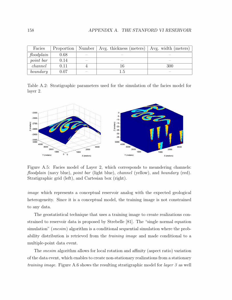
158 APPENDIX A. THE STANFORD VI RESERVOIR
Facies Proportion Number Avg. thickness (meters) Avg. width (meters)
floodplain 0.68 – – –point bar 0.14 – – –channel 0.11 4 16 300boundary 0.07 – 1.5 –
Table A.2: Stratigraphic parameters used for the simulation of the facies model forlayer 2.
Figure A.5: Facies model of Layer 2, which corresponds to meandering channels:floodplain (navy blue), point bar (light blue), channel (yellow), and boundary (red).Stratigraphic grid (left), and Cartesian box (right).
image which represents a conceptual reservoir analog with the expected geological
heterogeneity. Since it is a conceptual model, the training image is not constrained
to any data.
The geostatistical technique that uses a training image to create realizations con-
strained to reservoir data is proposed by Strebelle [81]. The “single normal equation
simulation” (snesim) algorithm is a conditional sequential simulation where the prob-
ability distribution is retrieved from the training image and made conditional to a
multiple-point data event.
The snesim algorithm allows for local rotation and affinity (aspect ratio) variation
of the data event, which enables to create non-stationary realizations from a stationary
training image. Figure A.6 shows the resulting stratigraphic model for layer 3 as well
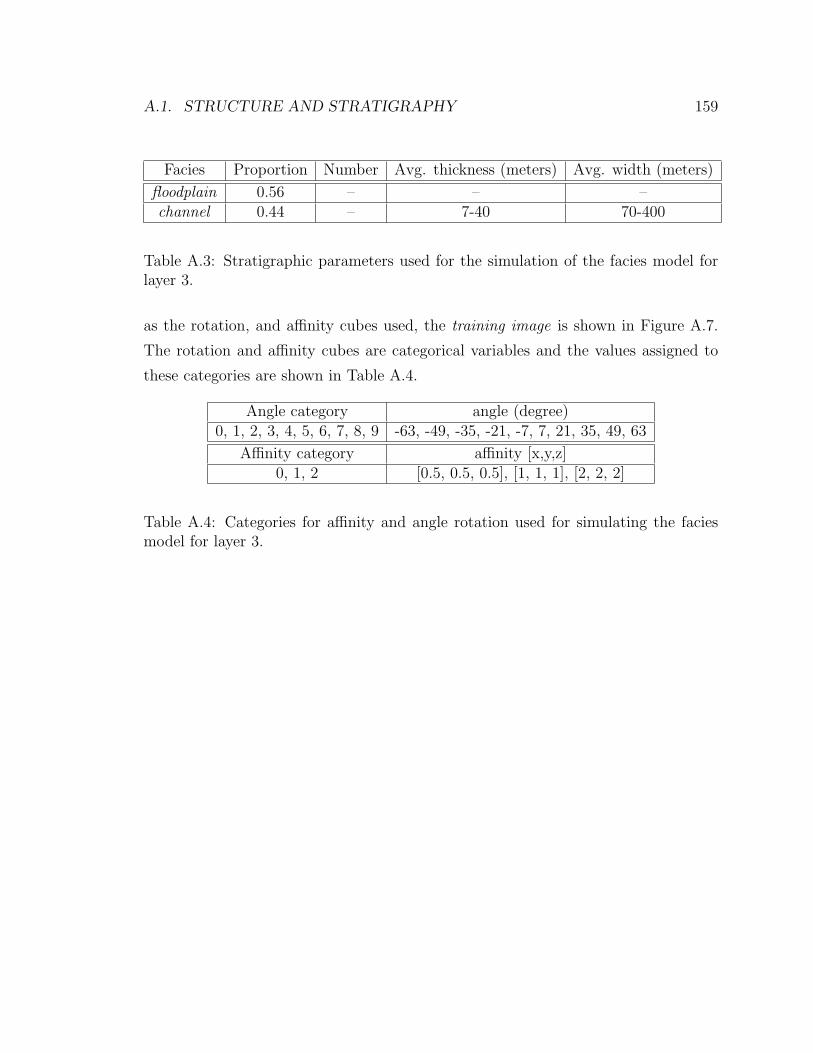
A.1. STRUCTURE AND STRATIGRAPHY 159
Facies Proportion Number Avg. thickness (meters) Avg. width (meters)
floodplain 0.56 – – –channel 0.44 – 7-40 70-400
Table A.3: Stratigraphic parameters used for the simulation of the facies model forlayer 3.
as the rotation, and affinity cubes used, the training image is shown in Figure A.7.
The rotation and affinity cubes are categorical variables and the values assigned to
these categories are shown in Table A.4.
Angle category angle (degree)0, 1, 2, 3, 4, 5, 6, 7, 8, 9 -63, -49, -35, -21, -7, 7, 21, 35, 49, 63
Affinity category affinity [x,y,z]0, 1, 2 [0.5, 0.5, 0.5], [1, 1, 1], [2, 2, 2]
Table A.4: Categories for affinity and angle rotation used for simulating the faciesmodel for layer 3.
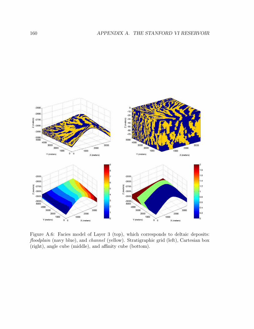
160 APPENDIX A. THE STANFORD VI RESERVOIR
Figure A.6: Facies model of Layer 3 (top), which corresponds to deltaic deposits:floodplain (navy blue), and channel (yellow). Stratigraphic grid (left), Cartesian box(right), angle cube (middle), and affinity cube (bottom).
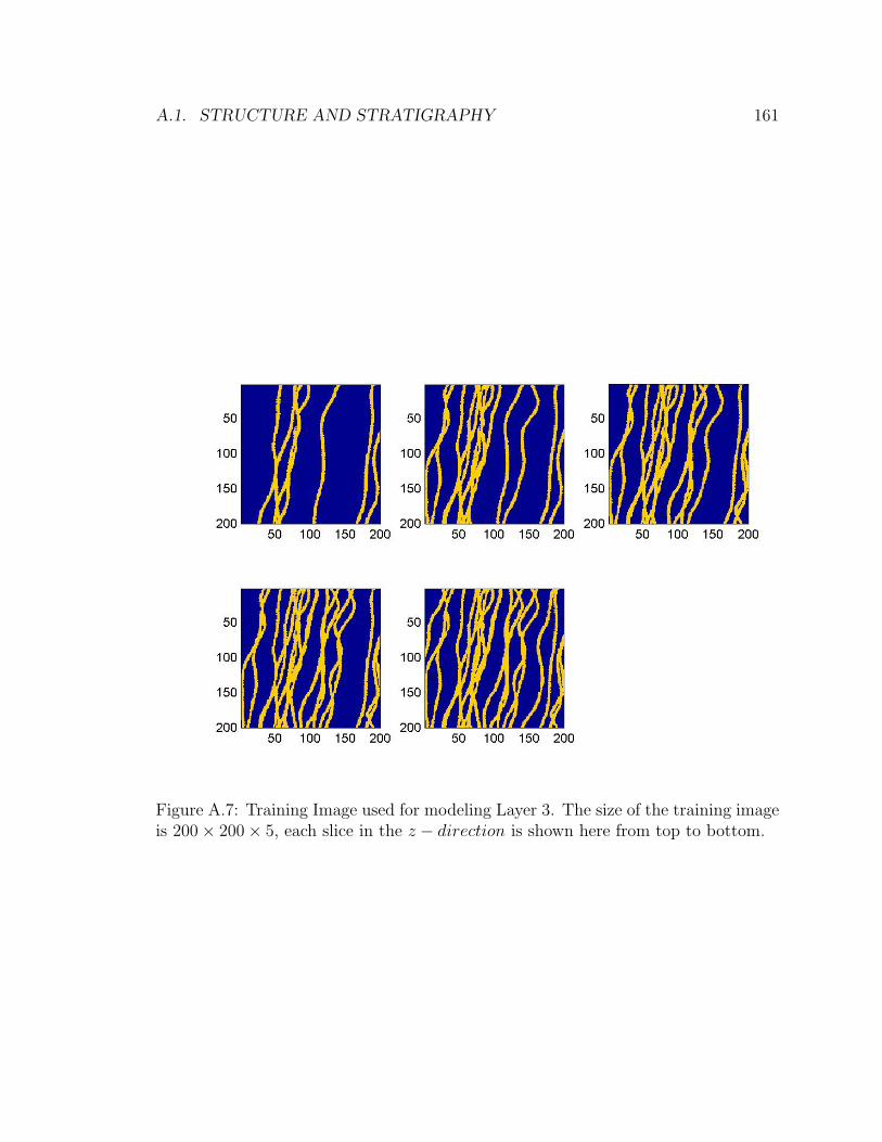
A.1. STRUCTURE AND STRATIGRAPHY 161
Figure A.7: Training Image used for modeling Layer 3. The size of the training imageis 200× 200× 5, each slice in the z − direction is shown here from top to bottom.
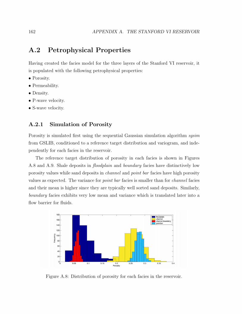
162 APPENDIX A. THE STANFORD VI RESERVOIR
A.2 Petrophysical Properties
Having created the facies model for the three layers of the Stanford VI reservoir, it
is populated with the following petrophysical properties:
• Porosity.
• Permeability.
• Density.
• P-wave velocity.
• S-wave velocity.
A.2.1 Simulation of Porosity
Porosity is simulated first using the sequential Gaussian simulation algorithm sgsim
from GSLIB, conditioned to a reference target distribution and variogram, and inde-
pendently for each facies in the reservoir.
The reference target distribution of porosity in each facies is shown in Figures
A.8 and A.9. Shale deposits in floodplain and boundary facies have distinctively low
porosity values while sand deposits in channel and point bar facies have high porosity
values as expected. The variance for point bar facies is smaller than for channel facies
and their mean is higher since they are typically well sorted sand deposits. Similarly,
boundary facies exhibits very low mean and variance which is translated later into a
flow barrier for fluids.
Figure A.8: Distribution of porosity for each facies in the reservoir.
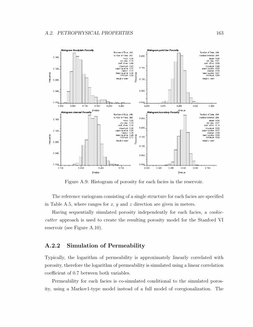
A.2. PETROPHYSICAL PROPERTIES 163
Figure A.9: Histogram of porosity for each facies in the reservoir.
The reference variogram consisting of a single structure for each facies are specified
in Table A.5, where ranges for x, y and z direction are given in meters.
Having sequentially simulated porosity independently for each facies, a cookie-
cutter approach is used to create the resulting porosity model for the Stanford VI
reservoir (see Figure A.10).
A.2.2 Simulation of Permeability
Typically, the logarithm of permeability is approximately linearly correlated with
porosity, therefore the logarithm of permeability is simulated using a linear correlation
coefficient of 0.7 between both variables.
Permeability for each facies is co-simulated conditional to the simulated poros-
ity, using a Markov1-type model instead of a full model of coregionalization. The
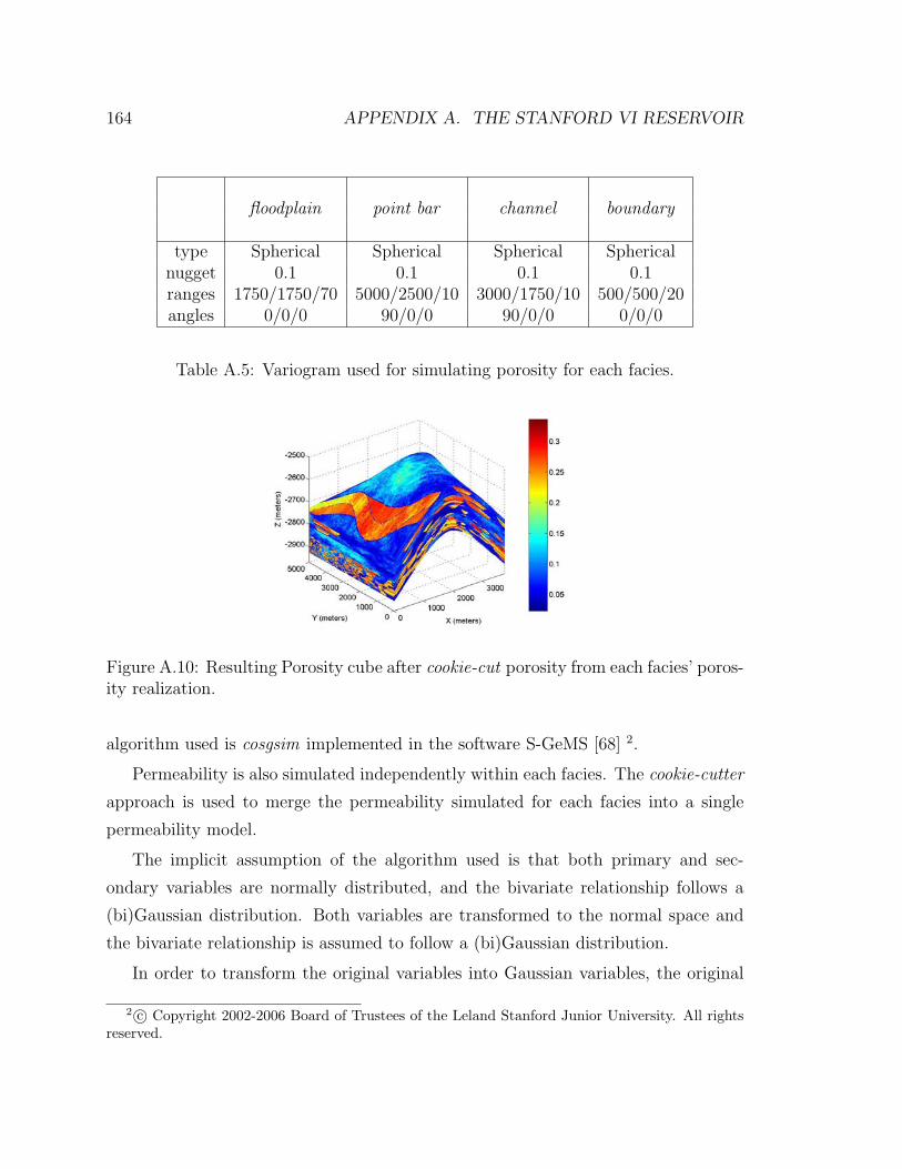
164 APPENDIX A. THE STANFORD VI RESERVOIR
floodplain point bar channel boundary
type Spherical Spherical Spherical Sphericalnugget 0.1 0.1 0.1 0.1ranges 1750/1750/70 5000/2500/10 3000/1750/10 500/500/20angles 0/0/0 90/0/0 90/0/0 0/0/0
Table A.5: Variogram used for simulating porosity for each facies.
Figure A.10: Resulting Porosity cube after cookie-cut porosity from each facies’ poros-ity realization.
algorithm used is cosgsim implemented in the software S-GeMS [68] 2.
Permeability is also simulated independently within each facies. The cookie-cutter
approach is used to merge the permeability simulated for each facies into a single
permeability model.
The implicit assumption of the algorithm used is that both primary and sec-
ondary variables are normally distributed, and the bivariate relationship follows a
(bi)Gaussian distribution. Both variables are transformed to the normal space and
the bivariate relationship is assumed to follow a (bi)Gaussian distribution.
In order to transform the original variables into Gaussian variables, the original
2 c© Copyright 2002-2006 Board of Trustees of the Leland Stanford Junior University. All rightsreserved.
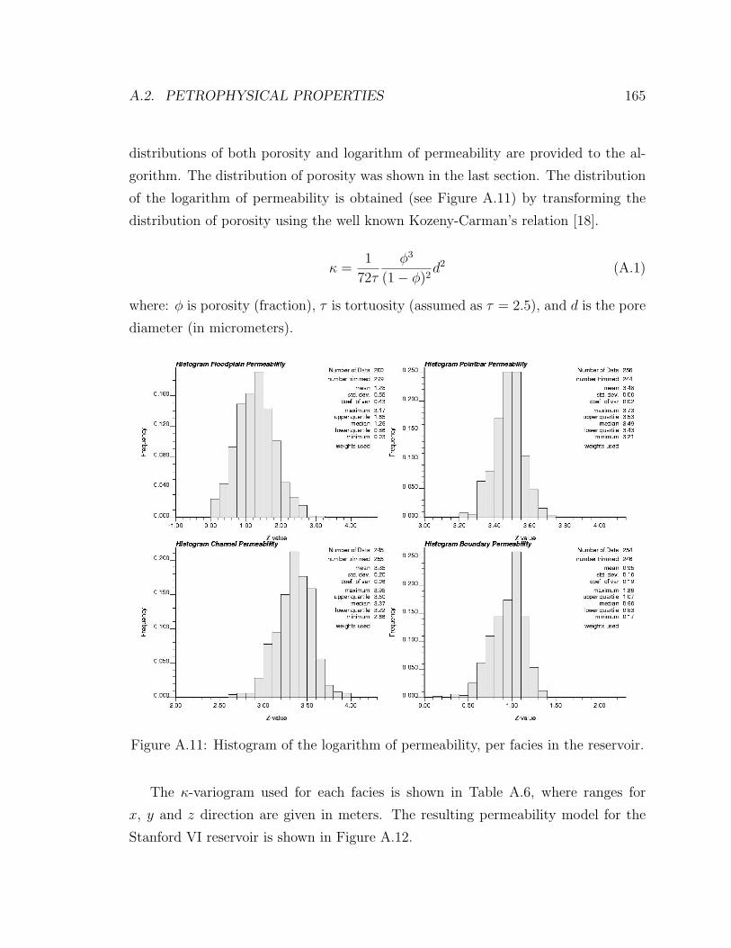
A.2. PETROPHYSICAL PROPERTIES 165
distributions of both porosity and logarithm of permeability are provided to the al-
gorithm. The distribution of porosity was shown in the last section. The distribution
of the logarithm of permeability is obtained (see Figure A.11) by transforming the
distribution of porosity using the well known Kozeny-Carman’s relation [18].
κ =1
72τ
φ3
(1− φ)2d2 (A.1)
where: φ is porosity (fraction), τ is tortuosity (assumed as τ = 2.5), and d is the pore
diameter (in micrometers).
Figure A.11: Histogram of the logarithm of permeability, per facies in the reservoir.
The κ-variogram used for each facies is shown in Table A.6, where ranges for
x, y and z direction are given in meters. The resulting permeability model for the
Stanford VI reservoir is shown in Figure A.12.
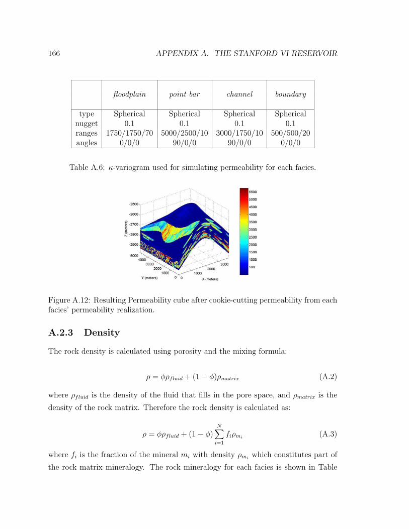
166 APPENDIX A. THE STANFORD VI RESERVOIR
floodplain point bar channel boundary
type Spherical Spherical Spherical Sphericalnugget 0.1 0.1 0.1 0.1ranges 1750/1750/70 5000/2500/10 3000/1750/10 500/500/20angles 0/0/0 90/0/0 90/0/0 0/0/0
Table A.6: κ-variogram used for simulating permeability for each facies.
Figure A.12: Resulting Permeability cube after cookie-cutting permeability from eachfacies’ permeability realization.
A.2.3 Density
The rock density is calculated using porosity and the mixing formula:
ρ = φρfluid + (1− φ)ρmatrix (A.2)
where ρfluid is the density of the fluid that fills in the pore space, and ρmatrix is the
density of the rock matrix. Therefore the rock density is calculated as:
ρ = φρfluid + (1− φ)N∑
i=1
fiρmi(A.3)
where fi is the fraction of the mineral mi with density ρmiwhich constitutes part of
the rock matrix mineralogy. The rock mineralogy for each facies is shown in Table
A.2. PETROPHYSICAL PROPERTIES 167
A.7.
mineralmineral density floodplain point bar channel boundary
(g/cc)clay 2.4 0.7 0.0 0.0 0.8
quartz 2.65 0.2 0.70 0.65 0.15feldspar 2.63 0.1 0.2 0.2 0.05
rock fragments 2.7 0.0 0.1 0.15 0.0
Table A.7: Rock mineralogy for each facies.
Using the mineralogy and the mineral densities shown in Table A.7 the rock matrix
density ρmatrix is computed. The rock bulk density ρ is obtained from Eqn. A.3, using
the simulated porosity and water as the saturating fluid.
Typically, density, P-wave and S-wave velocities are calculated first for water
saturated rocks since the rock physics models used for computing velocities have
been obtained in the lab from water-saturated rocks. Therefore, in order to use these
models correctly, the saturating fluid must be water.
For the generation of this data set density, P-wave and S-wave velocities are com-
puted first for water saturated rocks and using a mathematical transformation termed
fluid substitution these properties are obtained for a rock saturated with oil. This
procedure is explained in section A.2.5 of this appendix.
A.2.4 P-wave and S-wave Velocities
The relationship between P-wave velocity (Vp) and porosity is very well known in
Rock Physics. The higher the porosity of the rock the softer the rock is, and the
smaller the P-wave velocity. In other words, when porosity is high, the rock is more
compressible and less resistant to wave-induced deformations, therefore Vp is small.
Similarly, when porosity is low the rock is less compressible and more resistant to
wave-induced deformations, therefore Vp is high.
Many empirical expressions of Vp as a function of porosity have been obtained from
laboratory data [92] [67] [40] [84], and all of them show the inverse proportionality
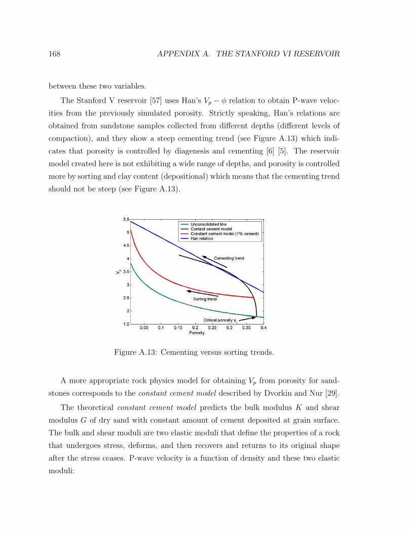
168 APPENDIX A. THE STANFORD VI RESERVOIR
between these two variables.
The Stanford V reservoir [57] uses Han’s Vp − φ relation to obtain P-wave veloc-
ities from the previously simulated porosity. Strictly speaking, Han’s relations are
obtained from sandstone samples collected from different depths (different levels of
compaction), and they show a steep cementing trend (see Figure A.13) which indi-
cates that porosity is controlled by diagenesis and cementing [6] [5]. The reservoir
model created here is not exhibiting a wide range of depths, and porosity is controlled
more by sorting and clay content (depositional) which means that the cementing trend
should not be steep (see Figure A.13).
Figure A.13: Cementing versus sorting trends.
A more appropriate rock physics model for obtaining Vp from porosity for sand-
stones corresponds to the constant cement model described by Dvorkin and Nur [29].
The theoretical constant cement model predicts the bulk modulus K and shear
modulus G of dry sand with constant amount of cement deposited at grain surface.
The bulk and shear moduli are two elastic moduli that define the properties of a rock
that undergoes stress, deforms, and then recovers and returns to its original shape
after the stress ceases. P-wave velocity is a function of density and these two elastic
moduli:
A.2. PETROPHYSICAL PROPERTIES 169
V 2p =
K + 43G
ρ(A.4)
The equations for the Dvorkin’s constant cement model are as follows:
Kdry =
(φ/φb
Kb + 4Gb/3+
1− φ/φb
Kmin + 4Gb/3
)−1
− 4Gb/3 (A.5)
Gdry =
(φ/φb
Gb + z+
1− φ/φb
Gmin + z
)−1
− z (A.6)
z =Gb
6
9Kb + 8Gb
Kb + 2Gb
(A.7)
where φb is porosity (smaller than φc, the initial depositional porosity, sometimes
referred to as critical porosity) at which contact cement trend turns into constant
cement trend (see Figure A.13). Elastic moduli with subscript “min” are the moduli
of the rock mineral and elastic moduli with subscript “b” are the moduli at porosity
φb. These moduli are calculated from the contact cement theory with φ = φb. The
Dvorkin’s contact cement theory is as follows:
Kdry =n(1− φc)McSn
6(A.8)
Gdry =3Kdry
5+
3n(1− φc)GcSτ
20(A.9)
where n is the coordination number, φc is the critical porosity, Mc is the cement’s
P-wave modulus (M = ρV 2p ), and Gc is the cement’s shear modulus. The constants
Sn and Sτ are computed with the following equations:
Sn = Anα2 + Bnα + Cn
An = −0.024153Λ−1.3646n
Bn = 0.20405Λ−0.89008n
170 APPENDIX A. THE STANFORD VI RESERVOIR
Cn = 0.00024649Λ−1.9864n
Sτ = Aτα2 + Bτα + Cτ
Aτ = −10−2(2.26ν2 + 2.07ν + 2.3)Λ0.079ν2+0.175ν−1.342τ
Bτ = (0.0573ν2 + 0.0937ν + 0.202)Λ0.0274ν2+0.0529ν−0.8765τ
Cτ = −10−4(9.654ν2 + 4.945ν + 3.1)Λ0.01867ν2+0.4011ν−1.8186τ
Λn =2Gc
πG
(1− ν)(1− νc)
(1− 2νc)
Λτ =Gc
πG
α = [(2/3)(φc − φ)/(1− φc)]1/2
where G and ν are the shear modulus and the Poisson’s ratio of the grains (matrix),
respectively; Gc and νc are the shear modulus and the Poisson’s ratio of the cement.
The constant cement model input parameters used in this reservoir are summarized
in Table A.8. A 1% calcite cement is added to the sandstone facies (channel and
point bar).
Having computed Kdry and Gdry for dry sandstones using Dvorkin’s constant ce-
ment model, the following equations are used to obtain Ksat and Gsat for water sat-
urated sandstones. These equations correspond to one form of the Gassmann’s fluid
substitution which is explained in more detail in the next section.
Ksat = Kmin
[φKdry − (1 + φ)KwaterKdry/Kmin + Kwater
(1− φ)Kwater + φKmin −KwaterKdry/Kmin
](A.10)
Gsat = Gdry (A.11)
The P-wave velocity Vp for the sandstones is obtained using Eqn. A.4 with Ksat
and Gsat . The rock physics model used for obtaining Vp for shales corresponds to
the empirical Vp − ρ Gardner’s power law [31]:
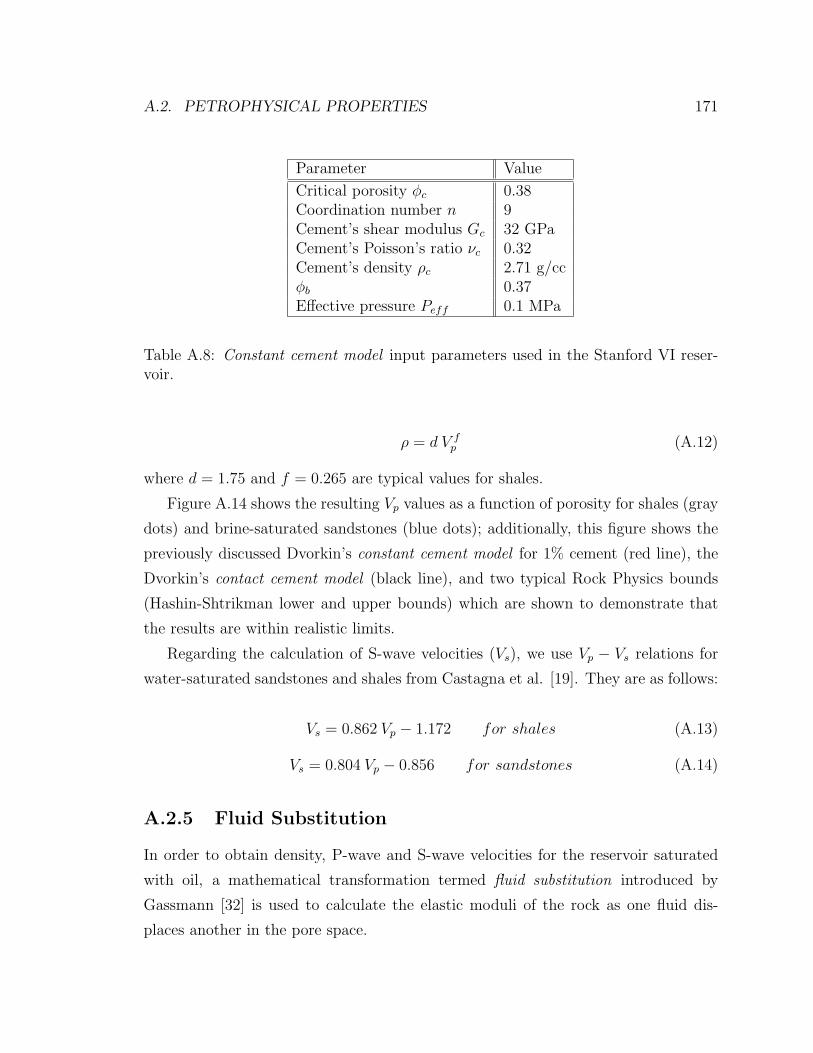
A.2. PETROPHYSICAL PROPERTIES 171
Parameter Value
Critical porosity φc 0.38Coordination number n 9Cement’s shear modulus Gc 32 GPaCement’s Poisson’s ratio νc 0.32Cement’s density ρc 2.71 g/ccφb 0.37Effective pressure Peff 0.1 MPa
Table A.8: Constant cement model input parameters used in the Stanford VI reser-voir.
ρ = d V fp (A.12)
where d = 1.75 and f = 0.265 are typical values for shales.
Figure A.14 shows the resulting Vp values as a function of porosity for shales (gray
dots) and brine-saturated sandstones (blue dots); additionally, this figure shows the
previously discussed Dvorkin’s constant cement model for 1% cement (red line), the
Dvorkin’s contact cement model (black line), and two typical Rock Physics bounds
(Hashin-Shtrikman lower and upper bounds) which are shown to demonstrate that
the results are within realistic limits.
Regarding the calculation of S-wave velocities (Vs), we use Vp − Vs relations for
water-saturated sandstones and shales from Castagna et al. [19]. They are as follows:
Vs = 0.862 Vp − 1.172 for shales (A.13)
Vs = 0.804 Vp − 0.856 for sandstones (A.14)
A.2.5 Fluid Substitution
In order to obtain density, P-wave and S-wave velocities for the reservoir saturated
with oil, a mathematical transformation termed fluid substitution introduced by
Gassmann [32] is used to calculate the elastic moduli of the rock as one fluid dis-
places another in the pore space.
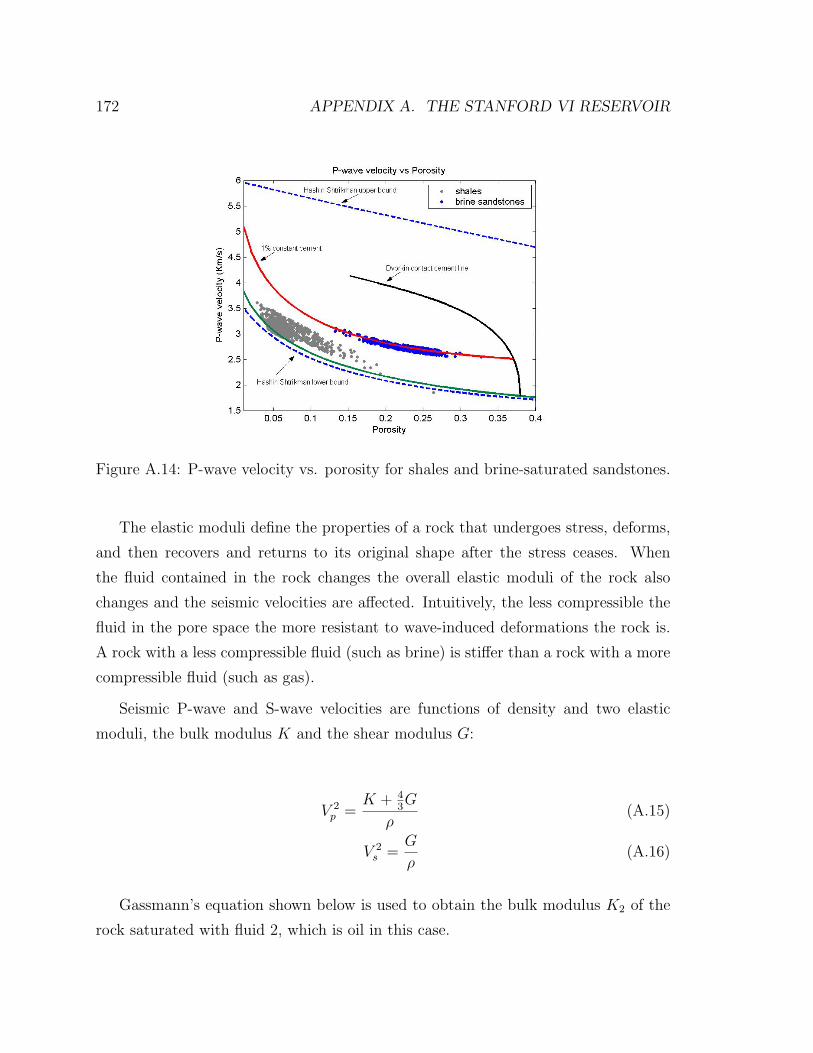
172 APPENDIX A. THE STANFORD VI RESERVOIR
Figure A.14: P-wave velocity vs. porosity for shales and brine-saturated sandstones.
The elastic moduli define the properties of a rock that undergoes stress, deforms,
and then recovers and returns to its original shape after the stress ceases. When
the fluid contained in the rock changes the overall elastic moduli of the rock also
changes and the seismic velocities are affected. Intuitively, the less compressible the
fluid in the pore space the more resistant to wave-induced deformations the rock is.
A rock with a less compressible fluid (such as brine) is stiffer than a rock with a more
compressible fluid (such as gas).
Seismic P-wave and S-wave velocities are functions of density and two elastic
moduli, the bulk modulus K and the shear modulus G:
V 2p =
K + 43G
ρ(A.15)
V 2s =
G
ρ(A.16)
Gassmann’s equation shown below is used to obtain the bulk modulus K2 of the
rock saturated with fluid 2, which is oil in this case.
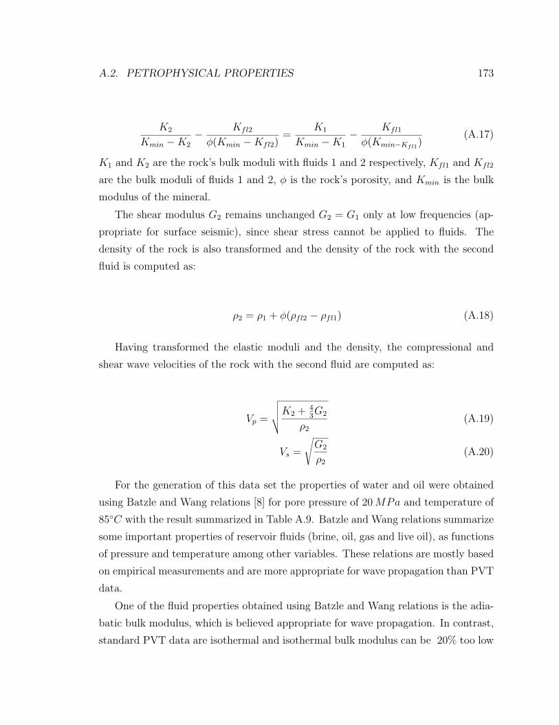
A.2. PETROPHYSICAL PROPERTIES 173
K2
Kmin −K2
− Kfl2
φ(Kmin −Kfl2)=
K1
Kmin −K1
− Kfl1
φ(Kmin−Kfl1)
(A.17)
K1 and K2 are the rock’s bulk moduli with fluids 1 and 2 respectively, Kfl1 and Kfl2
are the bulk moduli of fluids 1 and 2, φ is the rock’s porosity, and Kmin is the bulk
modulus of the mineral.
The shear modulus G2 remains unchanged G2 = G1 only at low frequencies (ap-
propriate for surface seismic), since shear stress cannot be applied to fluids. The
density of the rock is also transformed and the density of the rock with the second
fluid is computed as:
ρ2 = ρ1 + φ(ρfl2 − ρfl1) (A.18)
Having transformed the elastic moduli and the density, the compressional and
shear wave velocities of the rock with the second fluid are computed as:
Vp =
√√√√K2 + 43G2
ρ2
(A.19)
Vs =
√G2
ρ2
(A.20)
For the generation of this data set the properties of water and oil were obtained
using Batzle and Wang relations [8] for pore pressure of 20 MPa and temperature of
85◦C with the result summarized in Table A.9. Batzle and Wang relations summarize
some important properties of reservoir fluids (brine, oil, gas and live oil), as functions
of pressure and temperature among other variables. These relations are mostly based
on empirical measurements and are more appropriate for wave propagation than PVT
data.
One of the fluid properties obtained using Batzle and Wang relations is the adia-
batic bulk modulus, which is believed appropriate for wave propagation. In contrast,
standard PVT data are isothermal and isothermal bulk modulus can be 20% too low
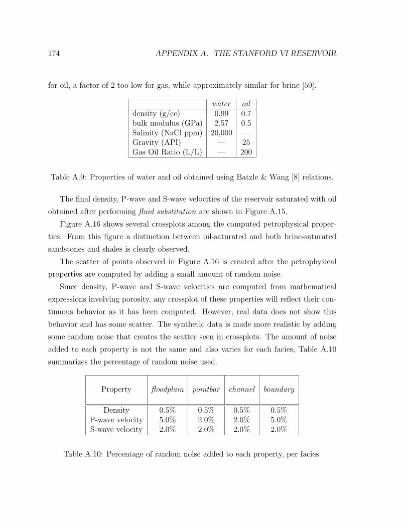
174 APPENDIX A. THE STANFORD VI RESERVOIR
for oil, a factor of 2 too low for gas, while approximately similar for brine [59].
water oildensity (g/cc) 0.99 0.7bulk modulus (GPa) 2.57 0.5Salinity (NaCl ppm) 20,000 —Gravity (API) — 25Gas Oil Ratio (L/L) — 200
Table A.9: Properties of water and oil obtained using Batzle & Wang [8] relations.
The final density, P-wave and S-wave velocities of the reservoir saturated with oil
obtained after performing fluid substitution are shown in Figure A.15.
Figure A.16 shows several crossplots among the computed petrophysical proper-
ties. From this figure a distinction between oil-saturated and both brine-saturated
sandstones and shales is clearly observed.
The scatter of points observed in Figure A.16 is created after the petrophysical
properties are computed by adding a small amount of random noise.
Since density, P-wave and S-wave velocities are computed from mathematical
expressions involving porosity, any crossplot of these properties will reflect their con-
tinuous behavior as it has been computed. However, real data does not show this
behavior and has some scatter. The synthetic data is made more realistic by adding
some random noise that creates the scatter seen in crossplots. The amount of noise
added to each property is not the same and also varies for each facies, Table A.10
summarizes the percentage of random noise used.
Property floodplain pointbar channel boundary
Density 0.5% 0.5% 0.5% 0.5%P-wave velocity 5.0% 2.0% 2.0% 5.0%S-wave velocity 2.0% 2.0% 2.0% 2.0%
Table A.10: Percentage of random noise added to each property, per facies.

A.2. PETROPHYSICAL PROPERTIES 175
Figure A.15: Resulting density (top), Vp (middle) and Vs (bottom) cubes for theoil-saturated reservoir.
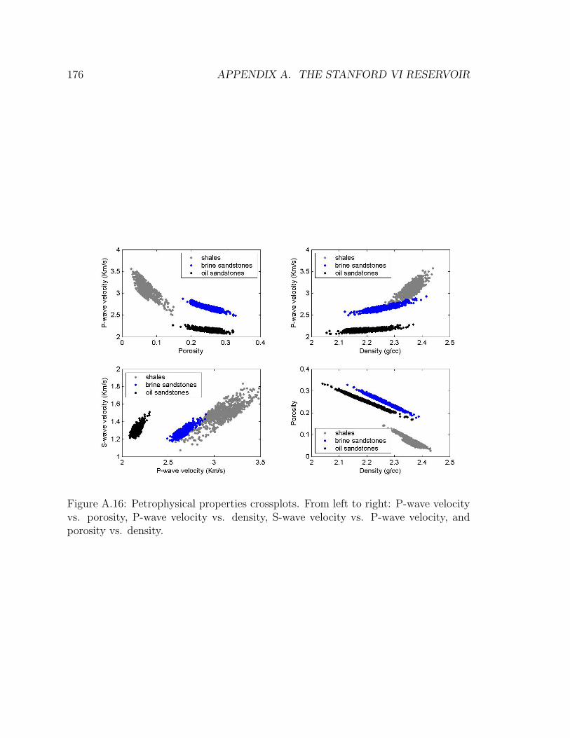
176 APPENDIX A. THE STANFORD VI RESERVOIR
Figure A.16: Petrophysical properties crossplots. From left to right: P-wave velocityvs. porosity, P-wave velocity vs. density, S-wave velocity vs. P-wave velocity, andporosity vs. density.
A.3. SEISMIC ATTRIBUTES 177
A.3 Seismic Attributes
“Seismic attributes are all the information obtained from seismic data, either by
direct measurements or by logical or experience based reasoning” [82]. The principal
objectives of the seismic attributes are to provide accurate and detailed information to
the interpreter on structural, stratigraphic and lithological parameters of the seismic
prospect.
Many attributes can be computed from seismic data, however, only those at-
tributes computed from seismic reflection amplitude carry information about elastic
contrast in the subsurface. Seismic inversion attempts to translate this information
into elastic properties, which are functions of density, P-wave and S-wave velocities.
In a real reservoir characterization situation, seismic inversion is performed on
the seismic reflection amplitudes to obtain the elastic properties, also called physical
attributes.
As mentioned before, from elasticity theory we know that these elastic properties
are functions of density, P-wave and S-wave velocities. Since Stanford VI is a synthetic
data set, the petrophysical properties created before are used to compute a typical
set of physical seismic attributes that could be obtained from seismic inversion in a
real situation, although no explicit inversion is performed.
The following list corresponds to the physical seismic attributes computed:
• Acoustic Impedance.
• S-wave Impedance.
• Elastic Impedance.
• Lame coefficients λ and µ.
• Poisson’s Ratio.
• AVO Intercept and Gradient.
These attributes are computed at the point support using several mathematical
expressions. Subsequently, a surface seismic filtering and smoothing is performed to
obtain the same attributes at the seismic scale. In doing so, more realistic seismic
attributes are created that provide a filtered view of the true spatial variation of
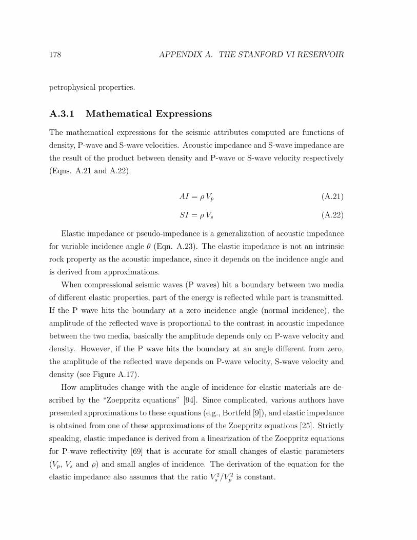
178 APPENDIX A. THE STANFORD VI RESERVOIR
petrophysical properties.
A.3.1 Mathematical Expressions
The mathematical expressions for the seismic attributes computed are functions of
density, P-wave and S-wave velocities. Acoustic impedance and S-wave impedance are
the result of the product between density and P-wave or S-wave velocity respectively
(Eqns. A.21 and A.22).
AI = ρ Vp (A.21)
SI = ρ Vs (A.22)
Elastic impedance or pseudo-impedance is a generalization of acoustic impedance
for variable incidence angle θ (Eqn. A.23). The elastic impedance is not an intrinsic
rock property as the acoustic impedance, since it depends on the incidence angle and
is derived from approximations.
When compressional seismic waves (P waves) hit a boundary between two media
of different elastic properties, part of the energy is reflected while part is transmitted.
If the P wave hits the boundary at a zero incidence angle (normal incidence), the
amplitude of the reflected wave is proportional to the contrast in acoustic impedance
between the two media, basically the amplitude depends only on P-wave velocity and
density. However, if the P wave hits the boundary at an angle different from zero,
the amplitude of the reflected wave depends on P-wave velocity, S-wave velocity and
density (see Figure A.17).
How amplitudes change with the angle of incidence for elastic materials are de-
scribed by the “Zoeppritz equations” [94]. Since complicated, various authors have
presented approximations to these equations (e.g., Bortfeld [9]), and elastic impedance
is obtained from one of these approximations of the Zoeppritz equations [25]. Strictly
speaking, elastic impedance is derived from a linearization of the Zoeppritz equations
for P-wave reflectivity [69] that is accurate for small changes of elastic parameters
(Vp, Vs and ρ) and small angles of incidence. The derivation of the equation for the
elastic impedance also assumes that the ratio V 2s /V 2
p is constant.
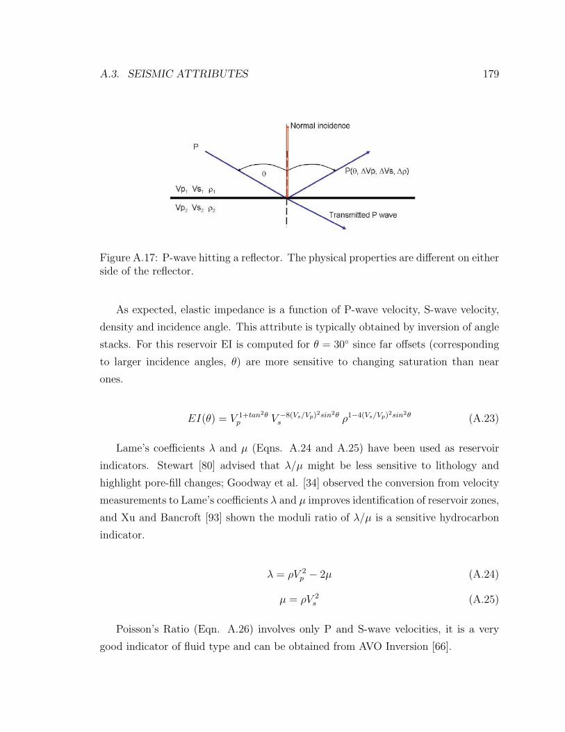
A.3. SEISMIC ATTRIBUTES 179
Figure A.17: P-wave hitting a reflector. The physical properties are different on eitherside of the reflector.
As expected, elastic impedance is a function of P-wave velocity, S-wave velocity,
density and incidence angle. This attribute is typically obtained by inversion of angle
stacks. For this reservoir EI is computed for θ = 30◦ since far offsets (corresponding
to larger incidence angles, θ) are more sensitive to changing saturation than near
ones.
EI(θ) = V 1+tan2θp V −8(Vs/Vp)2sin2θ
s ρ1−4(Vs/Vp)2sin2θ (A.23)
Lame’s coefficients λ and µ (Eqns. A.24 and A.25) have been used as reservoir
indicators. Stewart [80] advised that λ/µ might be less sensitive to lithology and
highlight pore-fill changes; Goodway et al. [34] observed the conversion from velocity
measurements to Lame’s coefficients λ and µ improves identification of reservoir zones,
and Xu and Bancroft [93] shown the moduli ratio of λ/µ is a sensitive hydrocarbon
indicator.
λ = ρV 2p − 2µ (A.24)
µ = ρV 2s (A.25)
Poisson’s Ratio (Eqn. A.26) involves only P and S-wave velocities, it is a very
good indicator of fluid type and can be obtained from AVO Inversion [66].
180 APPENDIX A. THE STANFORD VI RESERVOIR
ν =V 2
p − 2V 2s
2(V 2p − V 2
s )(A.26)
Amplitude variation with offset (AVO) comes from a process called “energy par-
titioning”. When compressional seismic waves (P waves) hit a boundary between
two media of different elastic properties, part of the energy is reflected while part is
transmitted. If the wave hits the boundary at an angle different from zero (incidence
angle), P wave energy is partitioned further into reflected and transmitted P and S
(shear waves) components (see Figure A.18). The amplitudes of the reflected and
transmitted energy depend on the contrast in elastic properties across the boundary,
specifically on P-wave velocity, S-wave velocity and density. But, more importantly
reflection amplitudes also depend on the angle of incidence of compressional seismic
waves.
Figure A.18: Seismic wavefront hitting a reflector. The physical properties are dif-ferent on either side of the reflector. The part of the P wave striking at a particularangle-of-incidence (represented by a ray) will have its energy divided into reflectedand transmitted P and S waves.
How amplitudes change with the angle of incidence for elastic materials are de-
scribed by the “Zoeppritz equations” [94]. One of the most widely used approxima-
tions to the “Zoeppritz equations” is from Shuey [76]:
A.3. SEISMIC ATTRIBUTES 181
R(θ) ≈ R0 + Gsin2θ + F (tan2θ − sin2θ) (A.27)
where
R0 =1
2
[∆Vp
Vp
+∆ρ
ρ
](A.28)
G =1
2
∆Vp
Vp
− 2(Vs/Vp)2
[∆ρ
ρ+ 2
∆Vs
Vs
](A.29)
F =1
2
∆Vp
Vp
(A.30)
The expression for the reflection coefficient given in Eqn. A.27 can be interpreted
in terms of different angular ranges [21]. R0 is the normal incidence reflection coeffi-
cient often referred to as the AVO intercept, G describes the variation at intermediate
offsets and is often referred to as the AVO gradient, whereas F dominates at far offsets
near the critical angle (angle at which all the P-wave incident energy is transmitted).
AVO intercept and gradient have been widely used for hydrocarbon detection,
specially gas, and they are obtained by analyzing the amplitudes of pre-stack seismic
data [65] [23] [70] [78] [2] [20] [73] [54].
Note that AVO intercept and gradient are obtained from an approximation to
the exact P-wave reflection coefficient, that is accurate for small changes of elastic
parameters (Vp, Vs and ρ) and small angles of incidence. Additionally, the mathemat-
ical expression for the P-wave reflection coefficient is obtained originally for a single
interface between two semi-infinite layers; in real cases wave propagation occurs in
more complex multilayered media.
For the Stanford VI reservoir, AVO intercept and gradient are computed using the
above equations and the filtered and smoothed density, P-wave and S-wave velocities,
since the compressional wave reflection coefficient (Eqn. A.27) is obtained for a semi-
infinite two layer media.
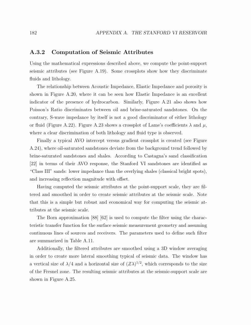
182 APPENDIX A. THE STANFORD VI RESERVOIR
A.3.2 Computation of Seismic Attributes
Using the mathematical expressions described above, we compute the point-support
seismic attributes (see Figure A.19). Some crossplots show how they discriminate
fluids and lithology.
The relationship between Acoustic Impedance, Elastic Impedance and porosity is
shown in Figure A.20, where it can be seen how Elastic Impedance is an excellent
indicator of the presence of hydrocarbon. Similarly, Figure A.21 also shows how
Poisson’s Ratio discriminates between oil and brine-saturated sandstones. On the
contrary, S-wave impedance by itself is not a good discriminator of either lithology
or fluid (Figure A.22). Figure A.23 shows a crossplot of Lame’s coefficients λ and µ,
where a clear discrimination of both lithology and fluid type is observed.
Finally a typical AVO intercept versus gradient crossplot is created (see Figure
A.24), where oil-saturated sandstones deviate from the background trend followed by
brine-saturated sandstones and shales. According to Castagna’s sand classification
[22] in terms of their AVO response, the Stanford VI sandstones are identified as
“Class III” sands: lower impedance than the overlying shales (classical bright spots),
and increasing reflection magnitude with offset.
Having computed the seismic attributes at the point-support scale, they are fil-
tered and smoothed in order to create seismic attributes at the seismic scale. Note
that this is a simple but robust and economical way for computing the seismic at-
tributes at the seismic scale.
The Born approximation [88] [62] is used to compute the filter using the charac-
teristic transfer function for the surface seismic measurement geometry and assuming
continuous lines of sources and receivers. The parameters used to define such filter
are summarized in Table A.11.
Additionally, the filtered attributes are smoothed using a 3D window averaging
in order to create more lateral smoothing typical of seismic data. The window has
a vertical size of λ/4 and a horizontal size of (Zλ)1/2, which corresponds to the size
of the Fresnel zone. The resulting seismic attributes at the seismic-support scale are
shown in Figure A.25.

A.3. SEISMIC ATTRIBUTES 183
minimum signal frequency 10 Hz
maximum signal frequency 40 Hz
source spread -1875 m to 1875 m
receiver spread -1875 m to 1875 m
Table A.11: Parameters used to define the “surface seismic” filter.
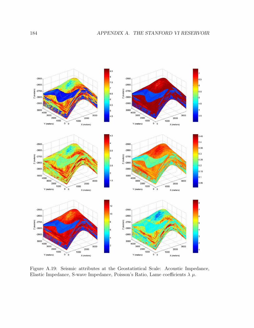
184 APPENDIX A. THE STANFORD VI RESERVOIR
Figure A.19: Seismic attributes at the Geostatistical Scale: Acoustic Impedance,Elastic Impedance, S-wave Impedance, Poisson’s Ratio, Lame coefficients λ µ.
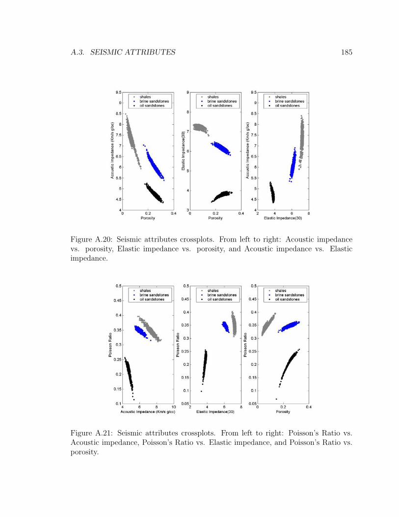
A.3. SEISMIC ATTRIBUTES 185
Figure A.20: Seismic attributes crossplots. From left to right: Acoustic impedancevs. porosity, Elastic impedance vs. porosity, and Acoustic impedance vs. Elasticimpedance.
Figure A.21: Seismic attributes crossplots. From left to right: Poisson’s Ratio vs.Acoustic impedance, Poisson’s Ratio vs. Elastic impedance, and Poisson’s Ratio vs.porosity.
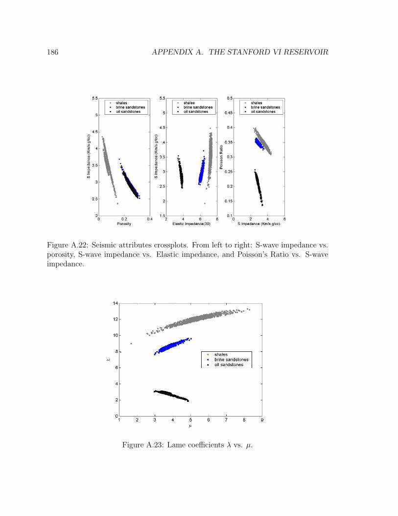
186 APPENDIX A. THE STANFORD VI RESERVOIR
Figure A.22: Seismic attributes crossplots. From left to right: S-wave impedance vs.porosity, S-wave impedance vs. Elastic impedance, and Poisson’s Ratio vs. S-waveimpedance.
Figure A.23: Lame coefficients λ vs. µ.
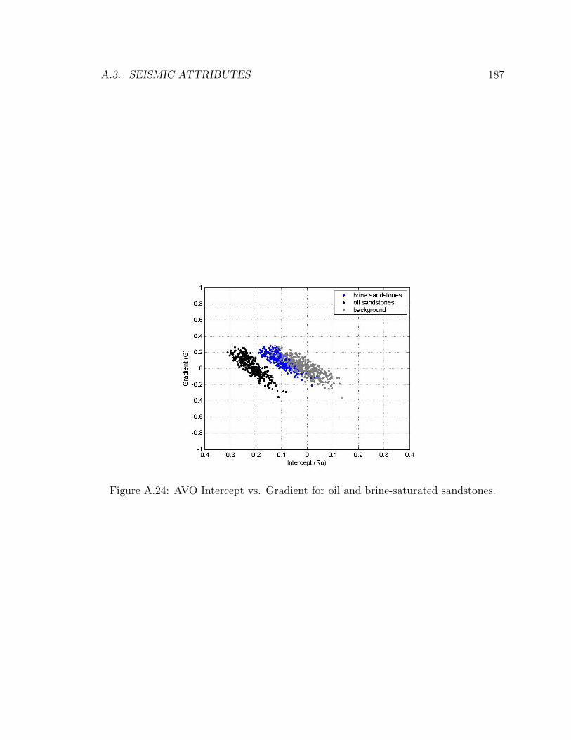
A.3. SEISMIC ATTRIBUTES 187
Figure A.24: AVO Intercept vs. Gradient for oil and brine-saturated sandstones.
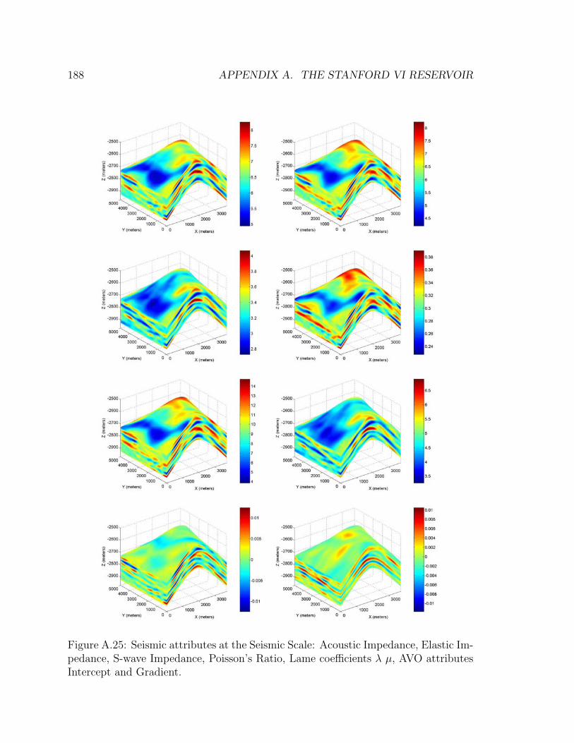
188 APPENDIX A. THE STANFORD VI RESERVOIR
Figure A.25: Seismic attributes at the Seismic Scale: Acoustic Impedance, Elastic Im-pedance, S-wave Impedance, Poisson’s Ratio, Lame coefficients λ µ, AVO attributesIntercept and Gradient.
A.4. RESERVOIR FLOW SIMULATION 189
A.4 Reservoir Flow Simulation
Using the simulated permeability cube for the Stanford VI reservoir model obtained in
section A.2, the next step is to perform a flow simulation. The results from this process
can be potentially used for further research in history matching of both production
and 4D seismic data.
It is well known that reservoir flow simulation provides the means to develop
reservoir management plans to achieve optimal recovery under certain economic con-
straints, since flow simulation allows to predict recovery before production. In order
to do so, flow simulation programs solve mathematical equations that describe the
flow of fluids through a numerical model of the reservoir.
The reservoir model used for solving the flow equations comprises two basic petro-
physical properties: porosity and permeability. Using a discrete 3D reservoir model
with each grid block considered homogeneous and represented by a value of porosity
and permeability, the flow equations often expressed as mass balances are solved for
each grid block under certain boundary conditions.
The number of equations to be solved per block depends on the complexity of the
in situ and injected fluids. Typically, this number varies from 3 (black-oil simulators)
to 15 (compositional simulators). An isothermal black-oil model is used since there
are only two phases in the reservoir (oil and water) and only water is injected at a
certain time during the flow simulation.
Considering two-phase flow (water and oil phases), only 2 equations are to be
solved per grid block; however, the computer work increases rapidly with the number
of blocks in the reservoir model. As mentioned in section A.1 of this appendix, the
size of the high-resolution 3D geo-cellular reservoir model is of 150 × 200 × 200 =
6, 000, 000 grid blocks, which exceeds the capabilities of conventional reservoir simu-
lators.
In order to reduce the size of the simulation model, hence the computational
running time of the flow simulation, upscaling of the reservoir properties is performed
to construct a coarsened reservoir model.
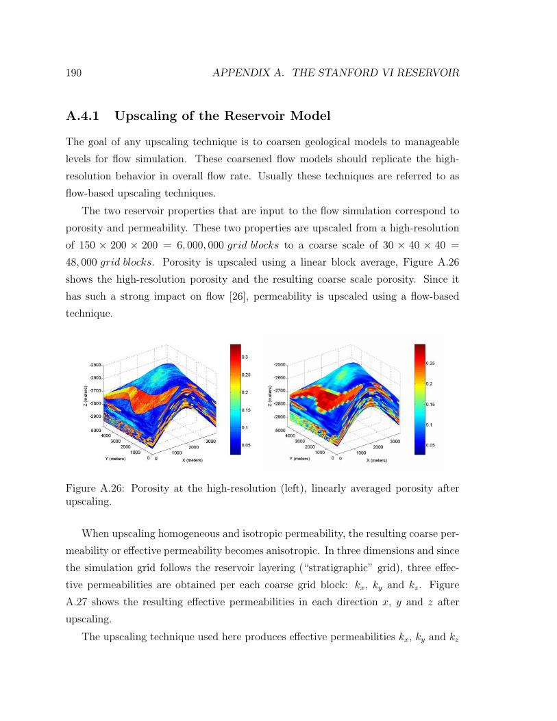
190 APPENDIX A. THE STANFORD VI RESERVOIR
A.4.1 Upscaling of the Reservoir Model
The goal of any upscaling technique is to coarsen geological models to manageable
levels for flow simulation. These coarsened flow models should replicate the high-
resolution behavior in overall flow rate. Usually these techniques are referred to as
flow-based upscaling techniques.
The two reservoir properties that are input to the flow simulation correspond to
porosity and permeability. These two properties are upscaled from a high-resolution
of 150 × 200 × 200 = 6, 000, 000 grid blocks to a coarse scale of 30 × 40 × 40 =
48, 000 grid blocks. Porosity is upscaled using a linear block average, Figure A.26
shows the high-resolution porosity and the resulting coarse scale porosity. Since it
has such a strong impact on flow [26], permeability is upscaled using a flow-based
technique.
Figure A.26: Porosity at the high-resolution (left), linearly averaged porosity afterupscaling.
When upscaling homogeneous and isotropic permeability, the resulting coarse per-
meability or effective permeability becomes anisotropic. In three dimensions and since
the simulation grid follows the reservoir layering (“stratigraphic” grid), three effec-
tive permeabilities are obtained per each coarse grid block: kx, ky and kz. Figure
A.27 shows the resulting effective permeabilities in each direction x, y and z after
upscaling.
The upscaling technique used here produces effective permeabilities kx, ky and kz
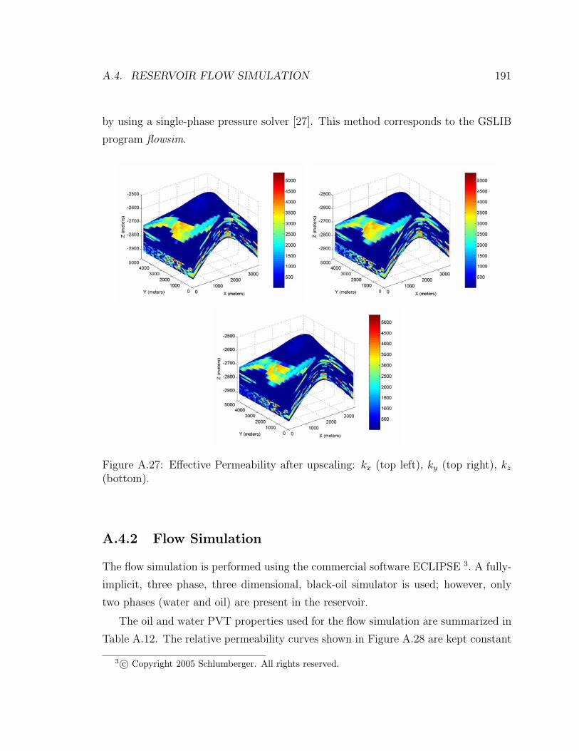
A.4. RESERVOIR FLOW SIMULATION 191
by using a single-phase pressure solver [27]. This method corresponds to the GSLIB
program flowsim.
Figure A.27: Effective Permeability after upscaling: kx (top left), ky (top right), kz
(bottom).
A.4.2 Flow Simulation
The flow simulation is performed using the commercial software ECLIPSE 3. A fully-
implicit, three phase, three dimensional, black-oil simulator is used; however, only
two phases (water and oil) are present in the reservoir.
The oil and water PVT properties used for the flow simulation are summarized in
Table A.12. The relative permeability curves shown in Figure A.28 are kept constant
3 c© Copyright 2005 Schlumberger. All rights reserved.
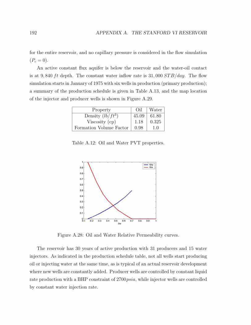
192 APPENDIX A. THE STANFORD VI RESERVOIR
for the entire reservoir, and no capillary pressure is considered in the flow simulation
(Pc = 0).
An active constant flux aquifer is below the reservoir and the water-oil contact
is at 9, 840 ft depth. The constant water inflow rate is 31, 000 STB/day. The flow
simulation starts in January of 1975 with six wells in production (primary production);
a summary of the production schedule is given in Table A.13, and the map location
of the injector and producer wells is shown in Figure A.29.
Property Oil WaterDensity (lb/ft3) 45.09 61.80Viscosity (cp) 1.18 0.325
Formation Volume Factor 0.98 1.0
Table A.12: Oil and Water PVT properties.
Figure A.28: Oil and Water Relative Permeability curves.
The reservoir has 30 years of active production with 31 producers and 15 water
injectors. As indicated in the production schedule table, not all wells start producing
oil or injecting water at the same time, as is typical of an actual reservoir development
where new wells are constantly added. Producer wells are controlled by constant liquid
rate production with a BHP constraint of 2700psia, while injector wells are controlled
by constant water injection rate.
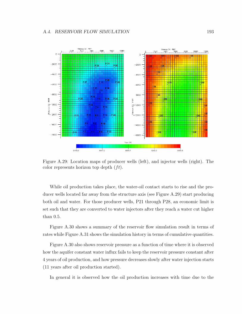
A.4. RESERVOIR FLOW SIMULATION 193
Figure A.29: Location maps of producer wells (left), and injector wells (right). Thecolor represents horizon top depth (ft).
While oil production takes place, the water-oil contact starts to rise and the pro-
ducer wells located far away from the structure axis (see Figure A.29) start producing
both oil and water. For those producer wells, P21 through P28, an economic limit is
set such that they are converted to water injectors after they reach a water cut higher
than 0.5.
Figure A.30 shows a summary of the reservoir flow simulation result in terms of
rates while Figure A.31 shows the simulation history in terms of cumulative quantities.
Figure A.30 also shows reservoir pressure as a function of time where it is observed
how the aquifer constant water influx fails to keep the reservoir pressure constant after
4 years of oil production, and how pressure decreases slowly after water injection starts
(11 years after oil production started).
In general it is observed how the oil production increases with time due to the
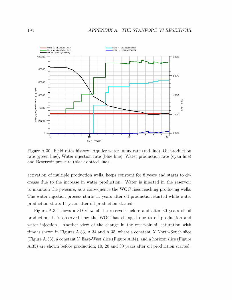
194 APPENDIX A. THE STANFORD VI RESERVOIR
Figure A.30: Field rates history: Aquifer water influx rate (red line), Oil productionrate (green line), Water injection rate (blue line), Water production rate (cyan line)and Reservoir pressure (black dotted line).
activation of multiple production wells, keeps constant for 8 years and starts to de-
crease due to the increase in water production. Water is injected in the reservoir
to maintain the pressure, as a consequence the WOC rises reaching producing wells.
The water injection process starts 11 years after oil production started while water
production starts 14 years after oil production started.
Figure A.32 shows a 3D view of the reservoir before and after 30 years of oil
production; it is observed how the WOC has changed due to oil production and
water injection. Another view of the change in the reservoir oil saturation with
time is shown in Figures A.33, A.34 and A.35, where a constant X North-South slice
(Figure A.33), a constant Y East-West slice (Figure A.34), and a horizon slice (Figure
A.35) are shown before production, 10, 20 and 30 years after oil production started.
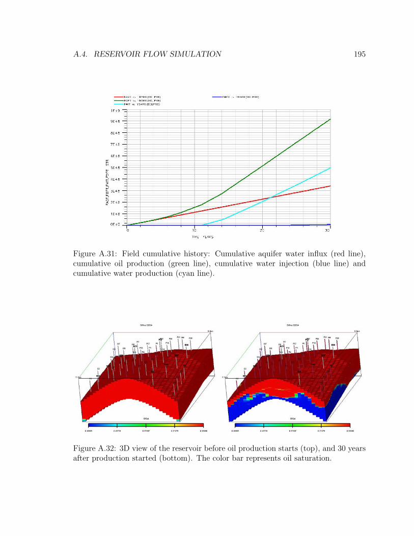
A.4. RESERVOIR FLOW SIMULATION 195
Figure A.31: Field cumulative history: Cumulative aquifer water influx (red line),cumulative oil production (green line), cumulative water injection (blue line) andcumulative water production (cyan line).
Figure A.32: 3D view of the reservoir before oil production starts (top), and 30 yearsafter production started (bottom). The color bar represents oil saturation.
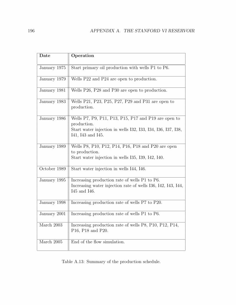
196 APPENDIX A. THE STANFORD VI RESERVOIR
Date Operation
January 1975 Start primary oil production with wells P1 to P6.
January 1979 Wells P22 and P24 are open to production.
January 1981 Wells P26, P28 and P30 are open to production.
January 1983 Wells P21, P23, P25, P27, P29 and P31 are open toproduction.
January 1986 Wells P7, P9, P11, P13, P15, P17 and P19 are open toproduction.Start water injection in wells I32, I33, I34, I36, I37, I38,I41, I43 and I45.
January 1989 Wells P8, P10, P12, P14, P16, P18 and P20 are opento production.Start water injection in wells I35, I39, I42, I40.
October 1989 Start water injection in wells I44, I46.
January 1995 Increasing production rate of wells P1 to P6.Increasing water injection rate of wells I36, I42, I43, I44,I45 and I46.
January 1998 Increasing production rate of wells P7 to P20.
January 2001 Increasing production rate of wells P1 to P6.
March 2003 Increasing production rate of wells P8, P10, P12, P14,P16, P18 and P20.
March 2005 End of the flow simulation.
Table A.13: Summary of the production schedule.
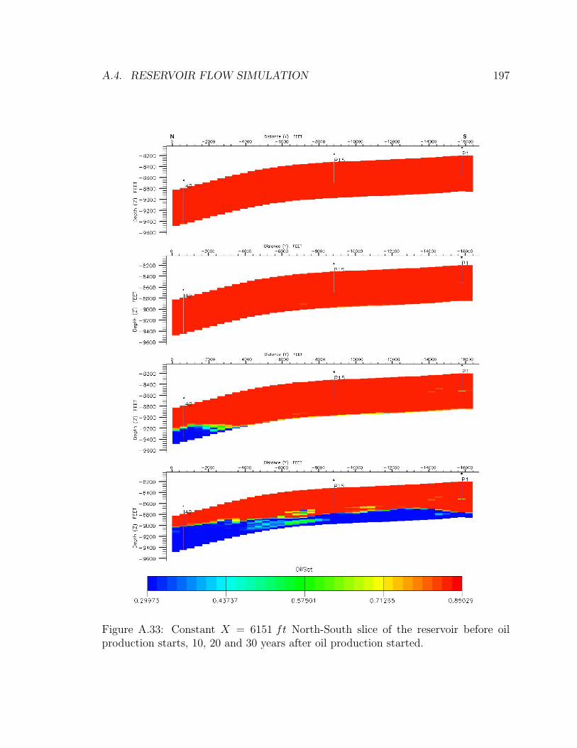
A.4. RESERVOIR FLOW SIMULATION 197
Figure A.33: Constant X = 6151 ft North-South slice of the reservoir before oilproduction starts, 10, 20 and 30 years after oil production started.
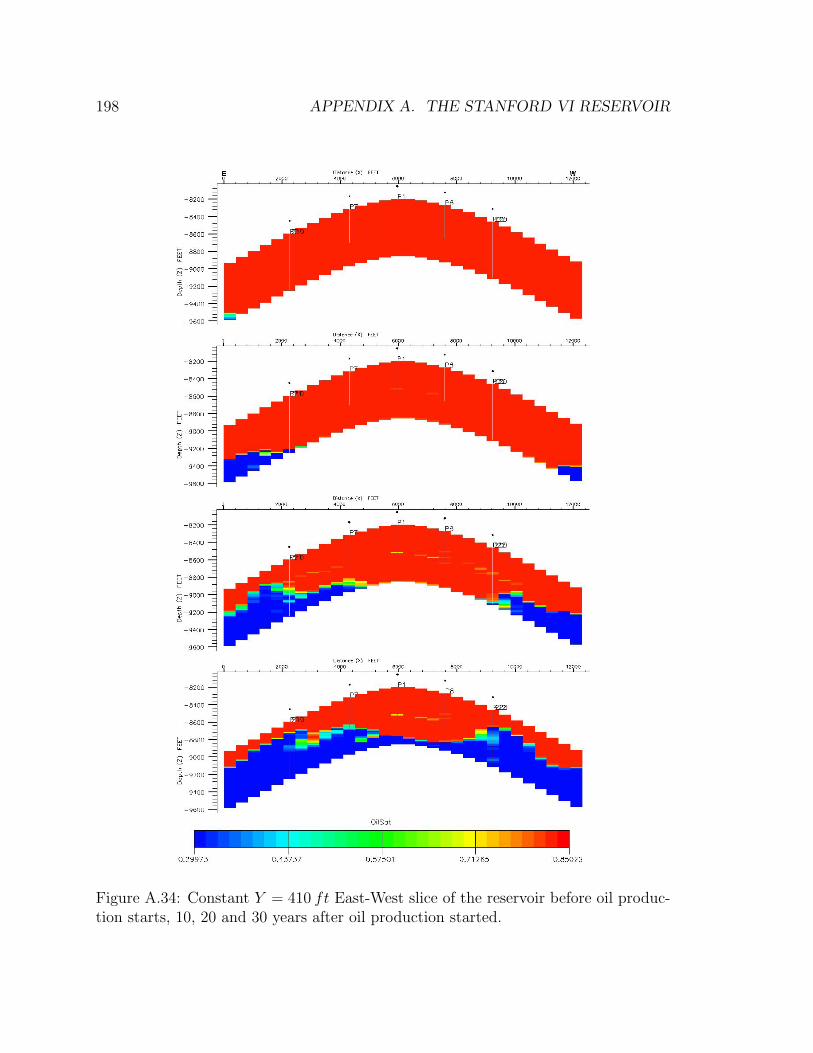
198 APPENDIX A. THE STANFORD VI RESERVOIR
Figure A.34: Constant Y = 410 ft East-West slice of the reservoir before oil produc-tion starts, 10, 20 and 30 years after oil production started.
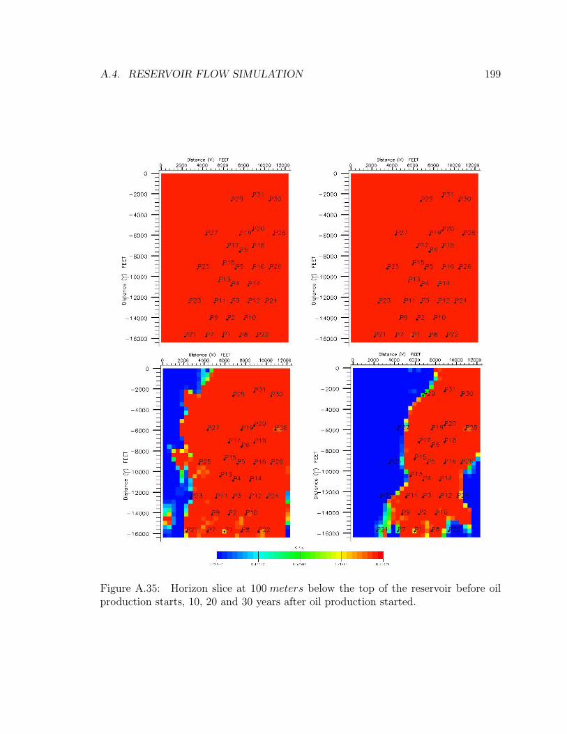
A.4. RESERVOIR FLOW SIMULATION 199
Figure A.35: Horizon slice at 100 meters below the top of the reservoir before oilproduction starts, 10, 20 and 30 years after oil production started.
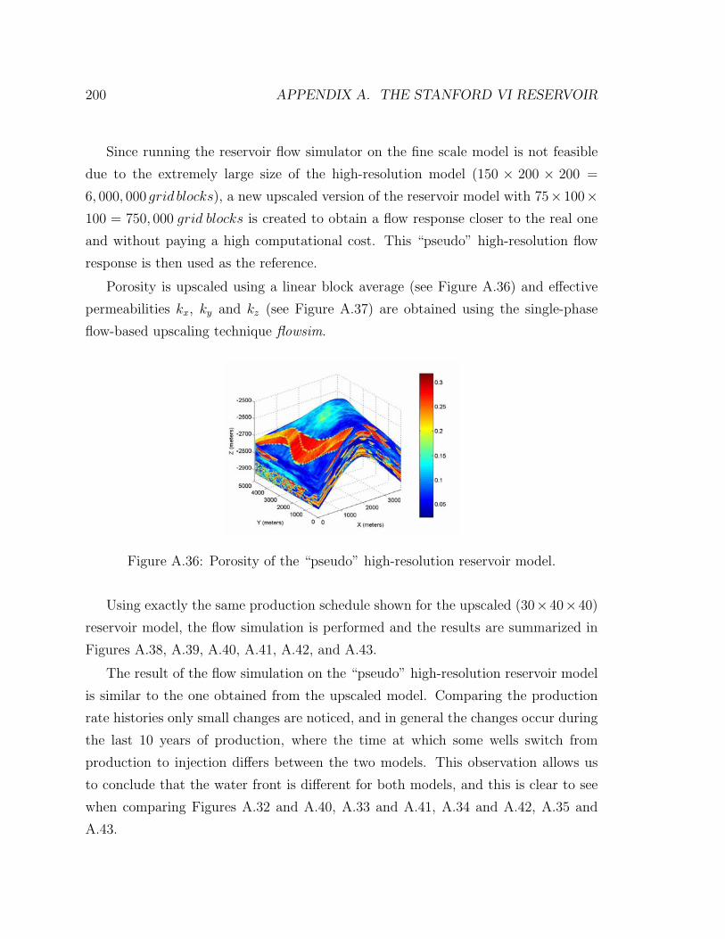
200 APPENDIX A. THE STANFORD VI RESERVOIR
Since running the reservoir flow simulator on the fine scale model is not feasible
due to the extremely large size of the high-resolution model (150 × 200 × 200 =
6, 000, 000 grid blocks), a new upscaled version of the reservoir model with 75×100×100 = 750, 000 grid blocks is created to obtain a flow response closer to the real one
and without paying a high computational cost. This “pseudo” high-resolution flow
response is then used as the reference.
Porosity is upscaled using a linear block average (see Figure A.36) and effective
permeabilities kx, ky and kz (see Figure A.37) are obtained using the single-phase
flow-based upscaling technique flowsim.
Figure A.36: Porosity of the “pseudo” high-resolution reservoir model.
Using exactly the same production schedule shown for the upscaled (30×40×40)
reservoir model, the flow simulation is performed and the results are summarized in
Figures A.38, A.39, A.40, A.41, A.42, and A.43.
The result of the flow simulation on the “pseudo” high-resolution reservoir model
is similar to the one obtained from the upscaled model. Comparing the production
rate histories only small changes are noticed, and in general the changes occur during
the last 10 years of production, where the time at which some wells switch from
production to injection differs between the two models. This observation allows us
to conclude that the water front is different for both models, and this is clear to see
when comparing Figures A.32 and A.40, A.33 and A.41, A.34 and A.42, A.35 and
A.43.
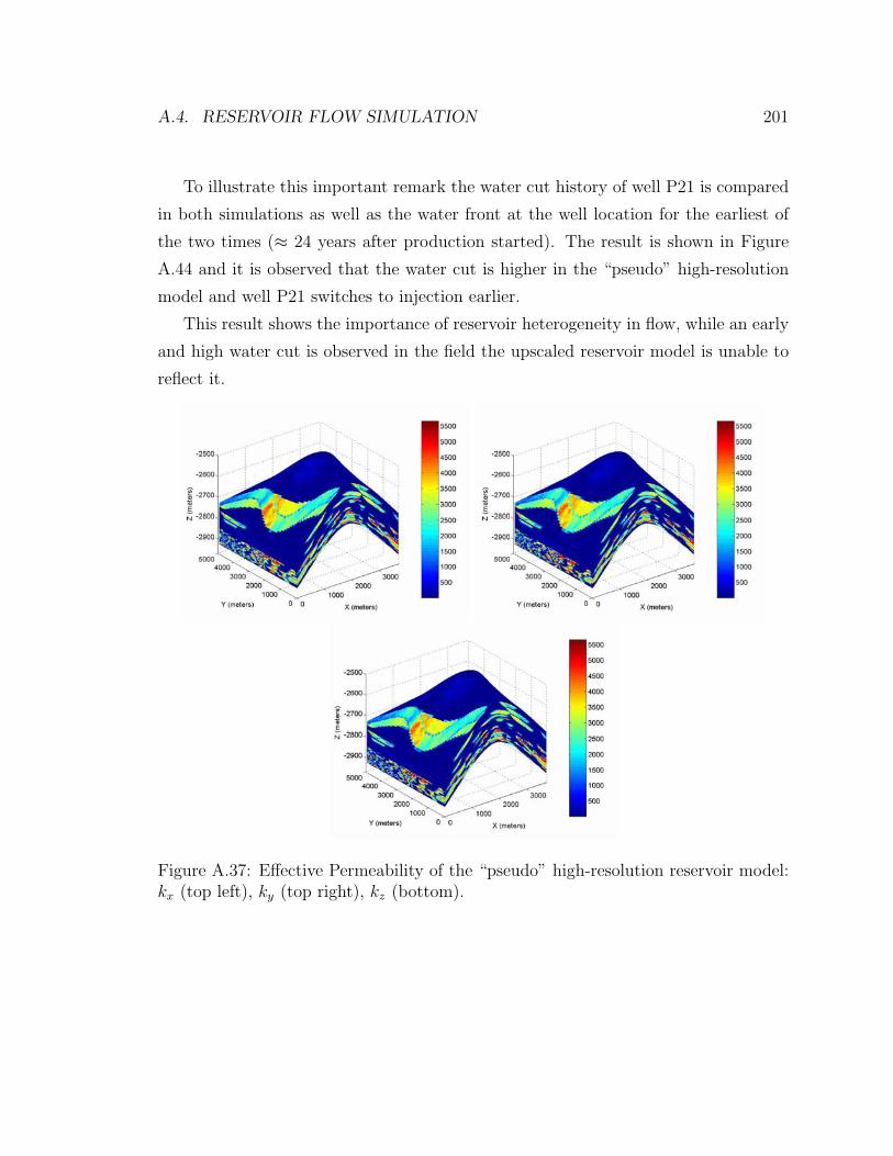
A.4. RESERVOIR FLOW SIMULATION 201
To illustrate this important remark the water cut history of well P21 is compared
in both simulations as well as the water front at the well location for the earliest of
the two times (≈ 24 years after production started). The result is shown in Figure
A.44 and it is observed that the water cut is higher in the “pseudo” high-resolution
model and well P21 switches to injection earlier.
This result shows the importance of reservoir heterogeneity in flow, while an early
and high water cut is observed in the field the upscaled reservoir model is unable to
reflect it.
Figure A.37: Effective Permeability of the “pseudo” high-resolution reservoir model:kx (top left), ky (top right), kz (bottom).
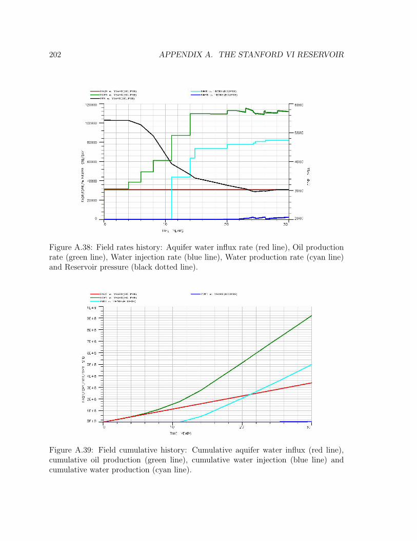
202 APPENDIX A. THE STANFORD VI RESERVOIR
Figure A.38: Field rates history: Aquifer water influx rate (red line), Oil productionrate (green line), Water injection rate (blue line), Water production rate (cyan line)and Reservoir pressure (black dotted line).
Figure A.39: Field cumulative history: Cumulative aquifer water influx (red line),cumulative oil production (green line), cumulative water injection (blue line) andcumulative water production (cyan line).
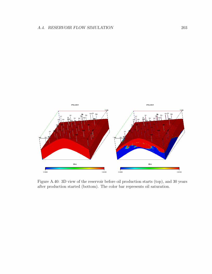
A.4. RESERVOIR FLOW SIMULATION 203
Figure A.40: 3D view of the reservoir before oil production starts (top), and 30 yearsafter production started (bottom). The color bar represents oil saturation.
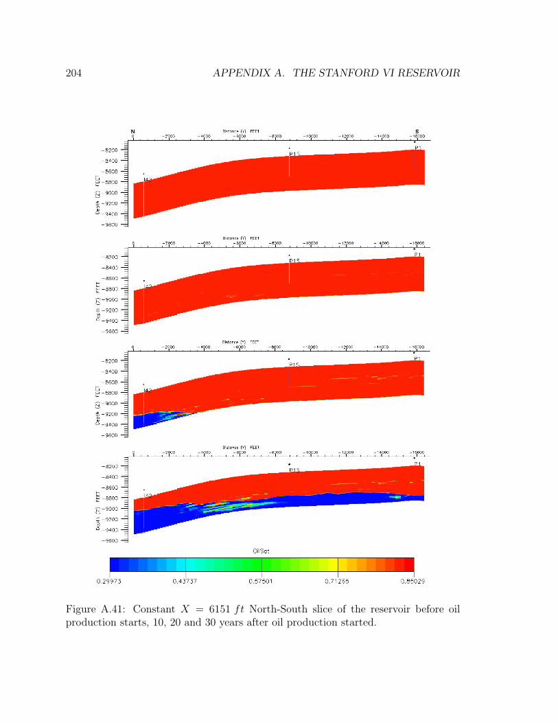
204 APPENDIX A. THE STANFORD VI RESERVOIR
Figure A.41: Constant X = 6151 ft North-South slice of the reservoir before oilproduction starts, 10, 20 and 30 years after oil production started.
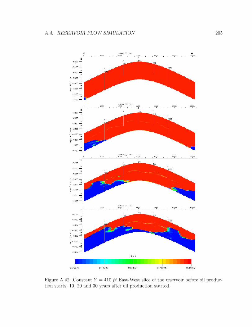
A.4. RESERVOIR FLOW SIMULATION 205
Figure A.42: Constant Y = 410 ft East-West slice of the reservoir before oil produc-tion starts, 10, 20 and 30 years after oil production started.
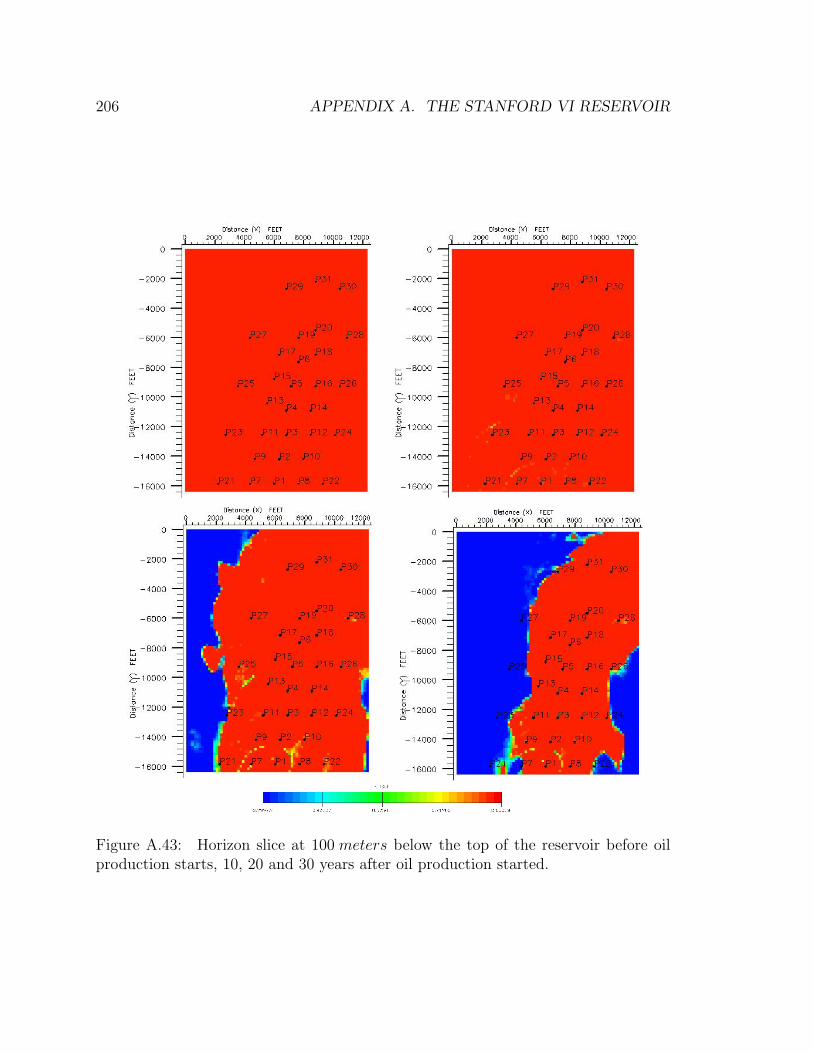
206 APPENDIX A. THE STANFORD VI RESERVOIR
Figure A.43: Horizon slice at 100 meters below the top of the reservoir before oilproduction starts, 10, 20 and 30 years after oil production started.
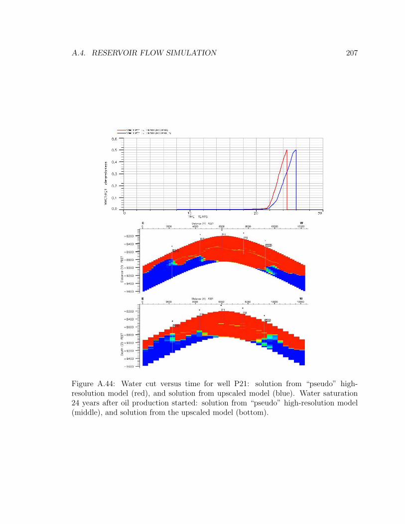
A.4. RESERVOIR FLOW SIMULATION 207
Figure A.44: Water cut versus time for well P21: solution from “pseudo” high-resolution model (red), and solution from upscaled model (blue). Water saturation24 years after oil production started: solution from “pseudo” high-resolution model(middle), and solution from the upscaled model (bottom).
208 APPENDIX A. THE STANFORD VI RESERVOIR
A.5 4D Seismic Data
What is referred to as 4D seismic data is nothing more than three-dimensional (3D)
seismic data acquired at different times over the same area to assess changes in a
producing hydrocarbon reservoir with time; changes may be observed in fluid location,
saturation, pressure, and temperature. Consequently, one of the main applications of
4D seismic data is to monitor fluid flow in the reservoir.
In order to create the 4D seismic response, several 3D seismic data sets s(u, tn)
are forward modeled using the simple convolutional model. It is clear the the first
seismic data set s(u, t0) will be created using the acoustic impedance of the reservoir
prior to production, while the following seismic data set s(u, tn) with n > 0 will be
created using the acoustic impedance of the reservoir as it has changed due to the
movement of fluids in the reservoir.
The acoustic impedance of the reservoir at time tn is obtained using the fluid
substitution procedure explained in section A.2.5. However, this procedure requires
one to know the properties (density and bulk modulus) of the fluid in the rock at time
tn and we know from the flow simulation that two fluids are present with different
partial saturations.
The most common approach to modeling partial saturation (gas/water or oil/water)
or mixed fluid saturations (gas/water/oil) is to replace the set of phases with a sin-
gle “effective fluid”. The bulk modulus of this “effective fluid” is computed with a
weighted harmonic average, termed Reuss average in the rock physics literature:
1
Kfl
=∑
i
Si
Ki
(A.31)
where Kfl is the effective bulk modulus of the fluid mixture, Ki denotes the bulk
moduli of the individual fluid phases, and Si represents their saturations. This model
assumes that the fluid phases are mixed at the finest scale.
The density of the “effective fluid” is computed with the mixing formula:
ρfl =∑
i
Siρi (A.32)
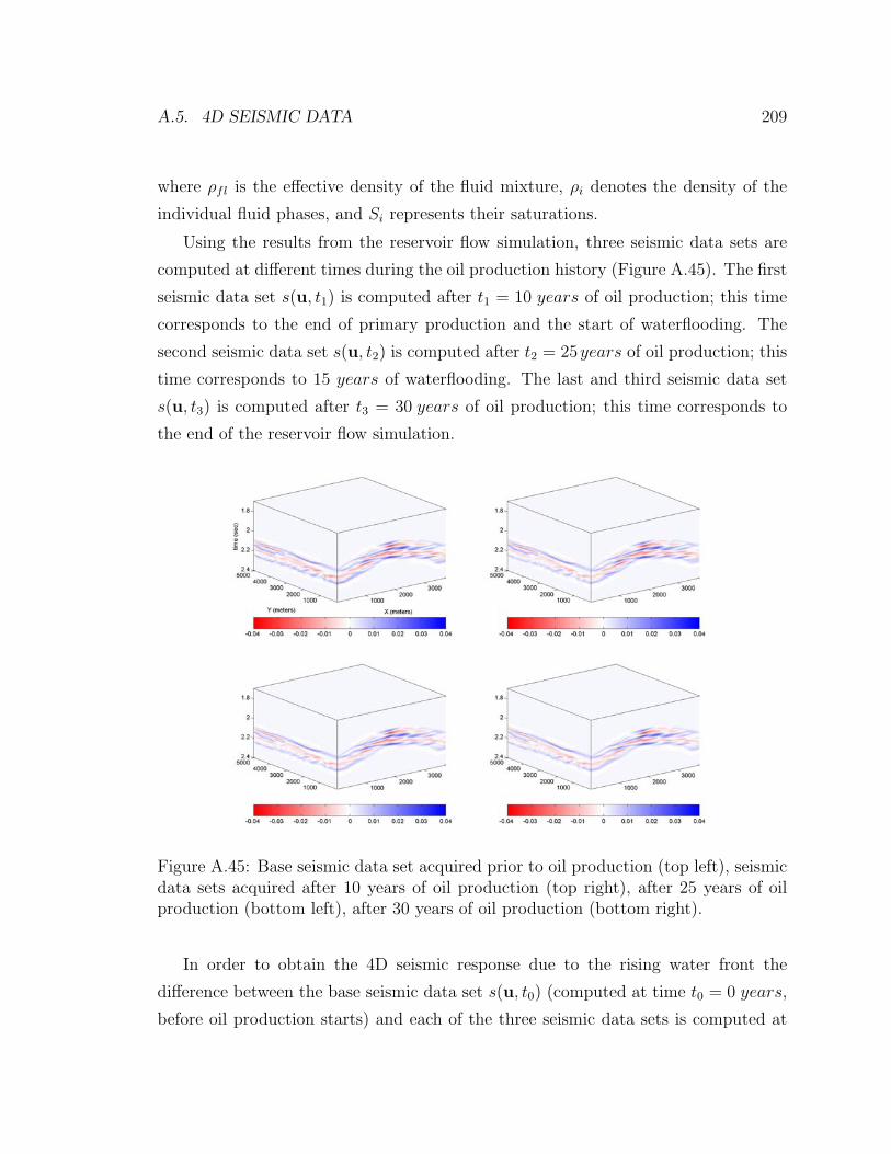
A.5. 4D SEISMIC DATA 209
where ρfl is the effective density of the fluid mixture, ρi denotes the density of the
individual fluid phases, and Si represents their saturations.
Using the results from the reservoir flow simulation, three seismic data sets are
computed at different times during the oil production history (Figure A.45). The first
seismic data set s(u, t1) is computed after t1 = 10 years of oil production; this time
corresponds to the end of primary production and the start of waterflooding. The
second seismic data set s(u, t2) is computed after t2 = 25years of oil production; this
time corresponds to 15 years of waterflooding. The last and third seismic data set
s(u, t3) is computed after t3 = 30 years of oil production; this time corresponds to
the end of the reservoir flow simulation.
Figure A.45: Base seismic data set acquired prior to oil production (top left), seismicdata sets acquired after 10 years of oil production (top right), after 25 years of oilproduction (bottom left), after 30 years of oil production (bottom right).
In order to obtain the 4D seismic response due to the rising water front the
difference between the base seismic data set s(u, t0) (computed at time t0 = 0 years,
before oil production starts) and each of the three seismic data sets is computed at
210 APPENDIX A. THE STANFORD VI RESERVOIR
times tn > 0 (n=1,2,3):
∆sn(u, ∆tn) = s(u, tn)− s(u, t0) n = 1, 2, 3 (A.33)
Additionally, the incremental 4D seismic response is computed to observe the
changes between two consecutive seismic surveys:
[∆sn(u, ∆tn)]∆n = s(u, tn)− s(u, tn−1) n = 1, 2, 3 (A.34)
These differences can be directly obtained by subtracting the originally recorded
amplitudes or any seismic attribute such as acoustic impedance. Generally speaking,
s can be considered as any attribute obtained from the seismic data. The difference
between originally recorded amplitudes are computed assuming small changes in ve-
locity due to the movement of fluids in the reservoir. Subtracting amplitudes can
be a wrong approach when large changes in velocity occur due to the stretching or
shrinking of the time axis.
The workflow used to create each of the 4D seismic responses, at times t1 =
10 years, t2 = 25 years and t3 = 30 years, is summarized in Figure A.46. To obtain
the seismic impedance at time tn fluid substitution on the high-resolution model is
performed using sub-sampling of the coarsened saturations to all high-resolution grid
cells (see section 3.1).
Figure A.47 shows the distribution of fluids in the reservoir after t1 = 10, t2 = 25
and t3 = 30 years of oil production, as well as the 4D seismic response ∆s1(u, ∆t1),
∆s2(u, ∆t2), and ∆s3(u, ∆t3), and the incremental 4D response [∆s1(u, ∆t1)]∆n,
[∆s2(u, ∆t2)]∆n, and [∆s3(u, ∆t3)]∆n. This figure shows how the seismic response
changes due to the rising of the water front. In the areas where oil is still in place,
the seismic data shows no difference. In the areas where water is present, the mag-
nitude of the difference increases with time due to an increase in water saturation.
The incremental difference between two consecutive seismic surveys shows the areas
where the distribution of fluids has changed during that time lapse.
The result obtained in Figure A.47 corresponds to the upscaled reservoir model.
The same procedure is followed for the “pseudo” high-resolution reservoir model, and

A.5. 4D SEISMIC DATA 211
the results are shown in Figure A.48.
Comparing Figures A.47 and A.48 it has been observed that the 4D seismic re-
sponse at late times (25 and 30 years after oil production started) is different from
each model. The 4D seismic response from the upscaled model exhibits stronger dif-
ferences than the 4D seismic response from the “pseudo” high-resolution model, due
to the differences between the coarse and high-resolution water saturation.
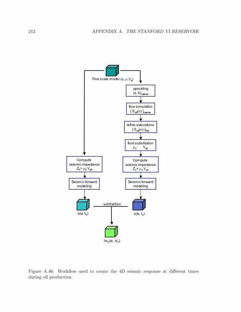
212 APPENDIX A. THE STANFORD VI RESERVOIR
Figure A.46: Workflow used to create the 4D seismic response at different timesduring oil production.
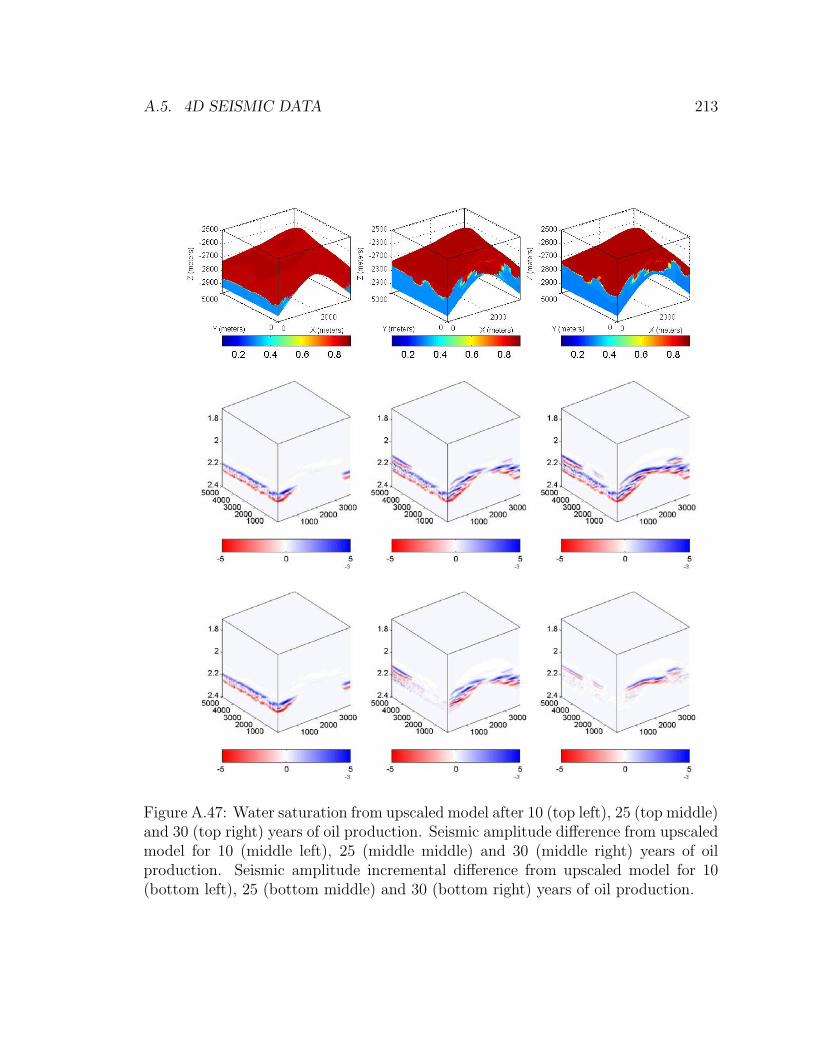
A.5. 4D SEISMIC DATA 213
Figure A.47: Water saturation from upscaled model after 10 (top left), 25 (top middle)and 30 (top right) years of oil production. Seismic amplitude difference from upscaledmodel for 10 (middle left), 25 (middle middle) and 30 (middle right) years of oilproduction. Seismic amplitude incremental difference from upscaled model for 10(bottom left), 25 (bottom middle) and 30 (bottom right) years of oil production.
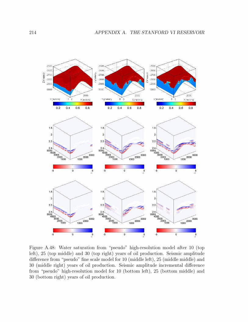
214 APPENDIX A. THE STANFORD VI RESERVOIR
Figure A.48: Water saturation from “pseudo” high-resolution model after 10 (topleft), 25 (top middle) and 30 (top right) years of oil production. Seismic amplitudedifference from “pseudo” fine scale model for 10 (middle left), 25 (middle middle) and30 (middle right) years of oil production. Seismic amplitude incremental differencefrom “pseudo” high-resolution model for 10 (bottom left), 25 (bottom middle) and30 (bottom right) years of oil production.
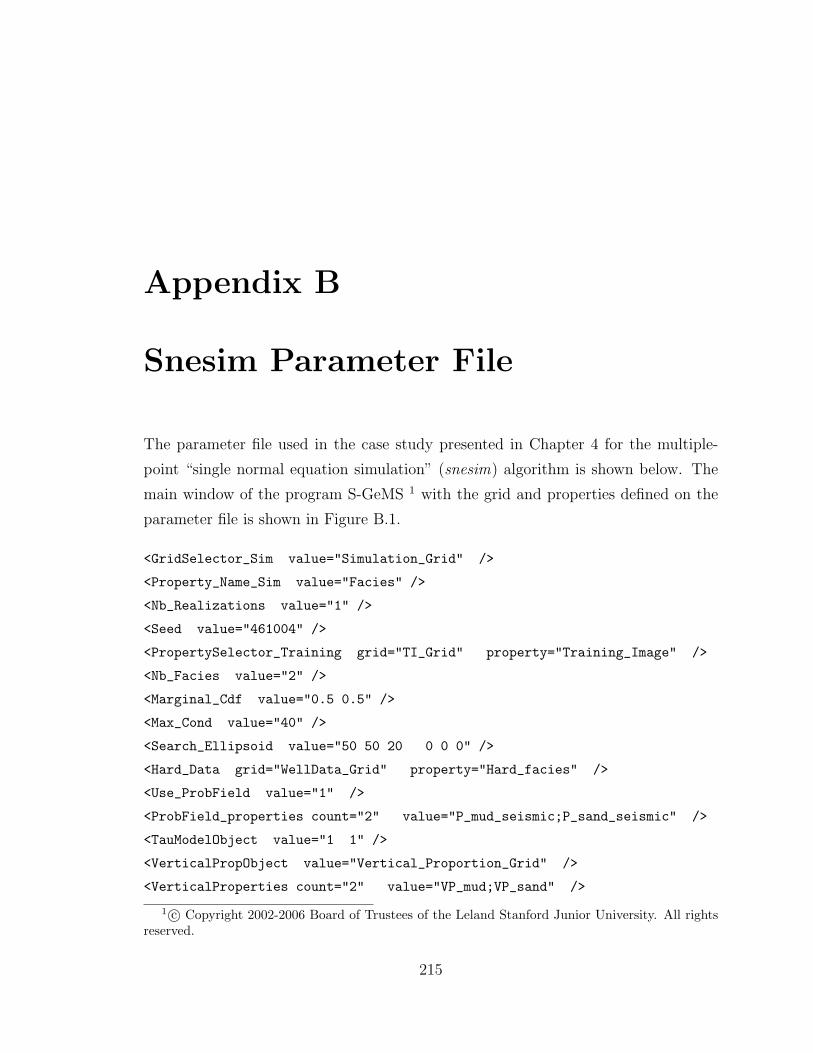
Appendix B
Snesim Parameter File
The parameter file used in the case study presented in Chapter 4 for the multiple-
point “single normal equation simulation” (snesim) algorithm is shown below. The
main window of the program S-GeMS 1 with the grid and properties defined on the
parameter file is shown in Figure B.1.
<GridSelector_Sim value="Simulation_Grid" />
<Property_Name_Sim value="Facies" />
<Nb_Realizations value="1" />
<Seed value="461004" />
<PropertySelector_Training grid="TI_Grid" property="Training_Image" />
<Nb_Facies value="2" />
<Marginal_Cdf value="0.5 0.5" />
<Max_Cond value="40" />
<Search_Ellipsoid value="50 50 20 0 0 0" />
<Hard_Data grid="WellData_Grid" property="Hard_facies" />
<Use_ProbField value="1" />
<ProbField_properties count="2" value="P_mud_seismic;P_sand_seismic" />
<TauModelObject value="1 1" />
<VerticalPropObject value="Vertical_Proportion_Grid" />
<VerticalProperties count="2" value="VP_mud;VP_sand" />
1 c© Copyright 2002-2006 Board of Trustees of the Leland Stanford Junior University. All rightsreserved.
215

216 APPENDIX B. SNESIM PARAMETER FILE
<Use_Rotation value="1" />
<Use_Global_Rotation value="0" />
<Use_Local_Rotation value="1" />
<Global_Angle value="0" />
<Rotation_property value="Regions_Rotation" />
<Rotation_categories value="72 0" />
<Use_Affinity value="0" />
<Cmin value="1" />
<Nb_Multigrids_ADVANCED value="3" />
<Constraint_Marginal_ADVANCED value="0.5" />
<revisit_nodes_prop value="15" />
<Debug_Level value="0" />
<Subgrid_choice value="1" />
<Previously_simulated value="4" />
<Use_Region value="1" />
<Region_Indicator_Prop value="Reservoir_Region" />
<Active_Region_Code value="1" />
<Use_Previous_Simulation value="0" />
<expand_isotropic value="1" />
<expand_anisotropic value="0" />
<aniso_factor value=" " />
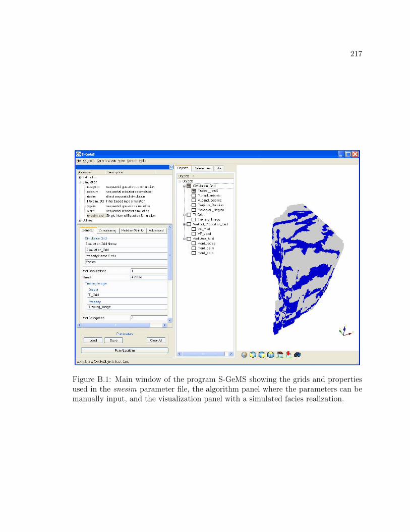
217
Figure B.1: Main window of the program S-GeMS showing the grids and propertiesused in the snesim parameter file, the algorithm panel where the parameters can bemanually input, and the visualization panel with a simulated facies realization.
Appendix C
Results of the PDI Approach
Due to the stochastic nature of the snesim algorithm, several reservoir models that match
production data while honoring all other available data, can be generated using the method-
ology and workflow presented in this dissertation. Section 4.3 has presented the results from
one history-matched reservoir model; however, six history-matched reservoir models have
been obtained using the PDI Approach and the individual results from each history-match
are presented in this appendix.
• The results from the first history-matched reservoir model are shown in Figures C.1
through C.4.
• The results from the second history-matched reservoir model are shown in Figures
C.5 through C.8.
• The results from the third history-matched reservoir model are shown in Figures C.9
through C.12.
• The results from the fourth history-matched reservoir model are shown in Figures
C.13 through C.16.
• The results from the fifth history-matched reservoir model are shown in Figures C.17
through C.20.
• The results from the sixth history-matched reservoir model are shown in Figures C.21
through C.24.
218
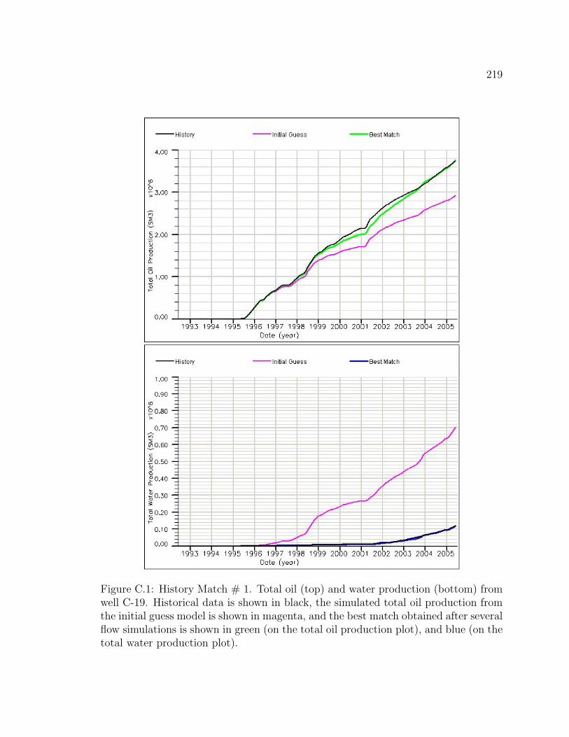
219
Figure C.1: History Match # 1. Total oil (top) and water production (bottom) fromwell C-19. Historical data is shown in black, the simulated total oil production fromthe initial guess model is shown in magenta, and the best match obtained after severalflow simulations is shown in green (on the total oil production plot), and blue (on thetotal water production plot).

220 APPENDIX C. RESULTS OF THE PDI APPROACH
Figure C.2: Total oil (top) and water production (bottom) from well C-17D. Historicaldata is shown in black, the simulated total oil production from the initial guess modelis shown in magenta, and the best match obtained after several flow simulationsis shown in green (on the total oil production plot), and blue (on the total waterproduction plot).
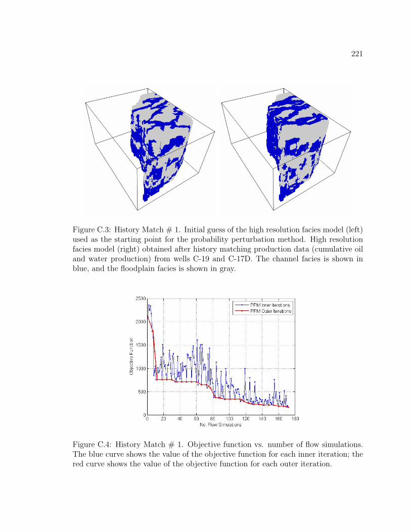
221
Figure C.3: History Match # 1. Initial guess of the high resolution facies model (left)used as the starting point for the probability perturbation method. High resolutionfacies model (right) obtained after history matching production data (cumulative oiland water production) from wells C-19 and C-17D. The channel facies is shown inblue, and the floodplain facies is shown in gray.
Figure C.4: History Match # 1. Objective function vs. number of flow simulations.The blue curve shows the value of the objective function for each inner iteration; thered curve shows the value of the objective function for each outer iteration.

222 APPENDIX C. RESULTS OF THE PDI APPROACH
Figure C.5: History Match # 2. Total oil (top) and water production (bottom) fromwell C-19. Historical data is shown in black, the simulated total oil production fromthe initial guess model is shown in magenta, and the best match obtained after severalflow simulations is shown in green (on the total oil production plot), and blue (on thetotal water production plot).
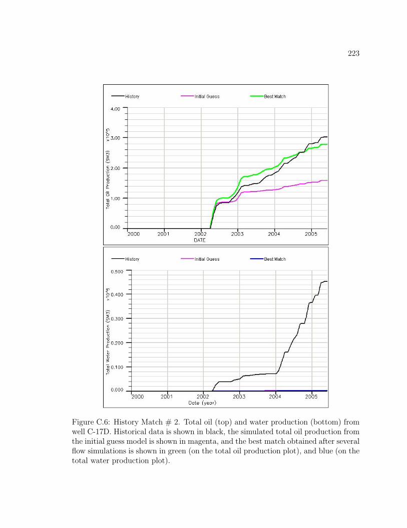
223
Figure C.6: History Match # 2. Total oil (top) and water production (bottom) fromwell C-17D. Historical data is shown in black, the simulated total oil production fromthe initial guess model is shown in magenta, and the best match obtained after severalflow simulations is shown in green (on the total oil production plot), and blue (on thetotal water production plot).
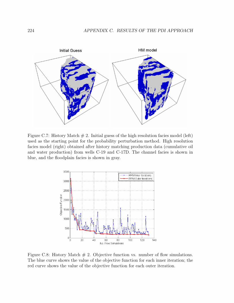
224 APPENDIX C. RESULTS OF THE PDI APPROACH
Figure C.7: History Match # 2. Initial guess of the high resolution facies model (left)used as the starting point for the probability perturbation method. High resolutionfacies model (right) obtained after history matching production data (cumulative oiland water production) from wells C-19 and C-17D. The channel facies is shown inblue, and the floodplain facies is shown in gray.
Figure C.8: History Match # 2. Objective function vs. number of flow simulations.The blue curve shows the value of the objective function for each inner iteration; thered curve shows the value of the objective function for each outer iteration.
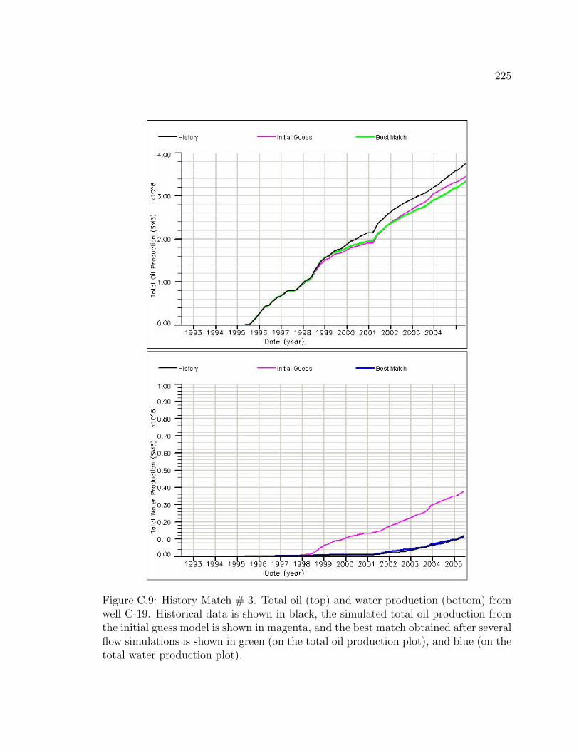
225
Figure C.9: History Match # 3. Total oil (top) and water production (bottom) fromwell C-19. Historical data is shown in black, the simulated total oil production fromthe initial guess model is shown in magenta, and the best match obtained after severalflow simulations is shown in green (on the total oil production plot), and blue (on thetotal water production plot).
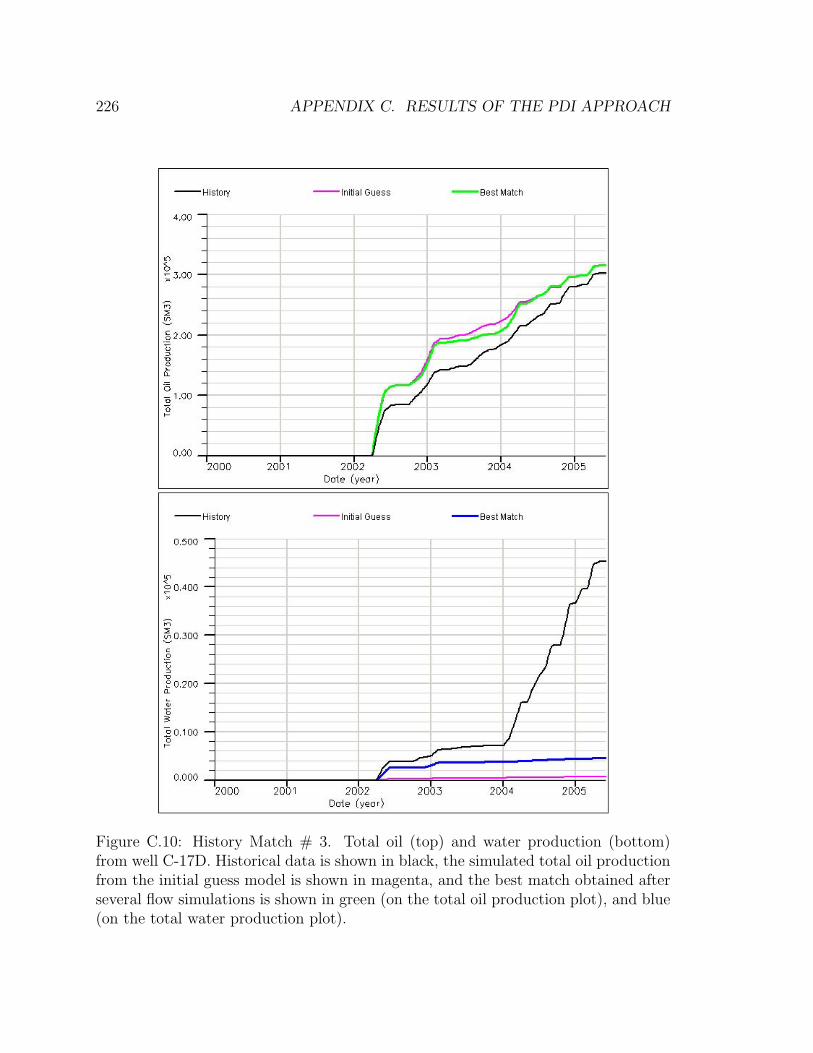
226 APPENDIX C. RESULTS OF THE PDI APPROACH
Figure C.10: History Match # 3. Total oil (top) and water production (bottom)from well C-17D. Historical data is shown in black, the simulated total oil productionfrom the initial guess model is shown in magenta, and the best match obtained afterseveral flow simulations is shown in green (on the total oil production plot), and blue(on the total water production plot).
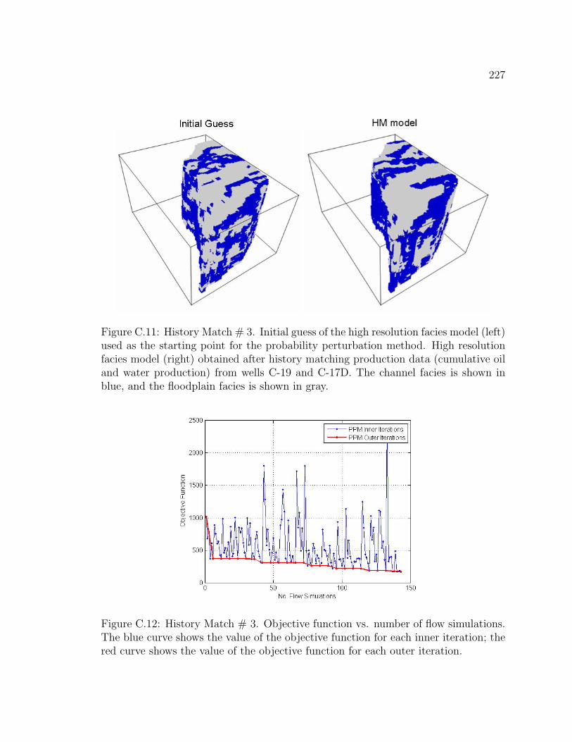
227
Figure C.11: History Match # 3. Initial guess of the high resolution facies model (left)used as the starting point for the probability perturbation method. High resolutionfacies model (right) obtained after history matching production data (cumulative oiland water production) from wells C-19 and C-17D. The channel facies is shown inblue, and the floodplain facies is shown in gray.
Figure C.12: History Match # 3. Objective function vs. number of flow simulations.The blue curve shows the value of the objective function for each inner iteration; thered curve shows the value of the objective function for each outer iteration.
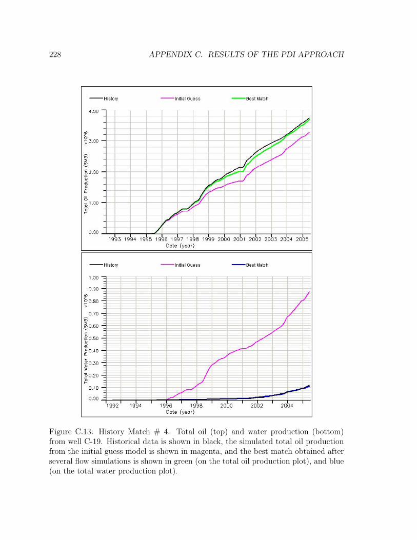
228 APPENDIX C. RESULTS OF THE PDI APPROACH
Figure C.13: History Match # 4. Total oil (top) and water production (bottom)from well C-19. Historical data is shown in black, the simulated total oil productionfrom the initial guess model is shown in magenta, and the best match obtained afterseveral flow simulations is shown in green (on the total oil production plot), and blue(on the total water production plot).
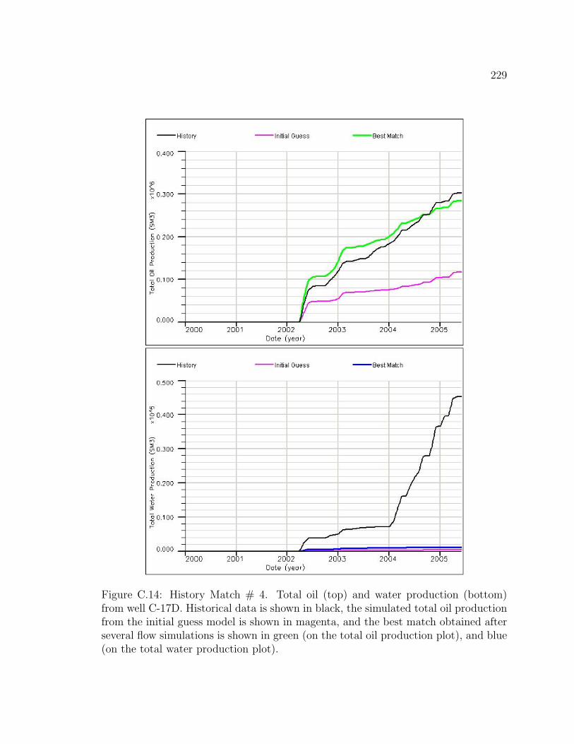
229
Figure C.14: History Match # 4. Total oil (top) and water production (bottom)from well C-17D. Historical data is shown in black, the simulated total oil productionfrom the initial guess model is shown in magenta, and the best match obtained afterseveral flow simulations is shown in green (on the total oil production plot), and blue(on the total water production plot).

230 APPENDIX C. RESULTS OF THE PDI APPROACH
Figure C.15: History Match # 4. Initial guess of the high resolution facies model (left)used as the starting point for the probability perturbation method. High resolutionfacies model (right) obtained after history matching production data (cumulative oiland water production) from wells C-19 and C-17D. The channel facies is shown inblue, and the floodplain facies is shown in gray.
Figure C.16: History Match # 4. Objective function vs. number of flow simulations.The blue curve shows the value of the objective function for each inner iteration; thered curve shows the value of the objective function for each outer iteration.

231
Figure C.17: History Match # 5. Total oil (top) and water production (bottom)from well C-19. Historical data is shown in black, the simulated total oil productionfrom the initial guess model is shown in magenta, and the best match obtained afterseveral flow simulations is shown in green (on the total oil production plot), and blue(on the total water production plot).
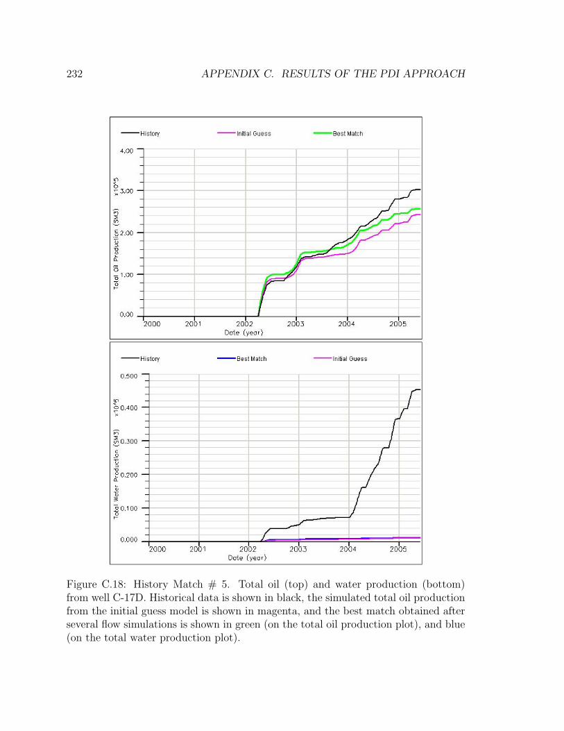
232 APPENDIX C. RESULTS OF THE PDI APPROACH
Figure C.18: History Match # 5. Total oil (top) and water production (bottom)from well C-17D. Historical data is shown in black, the simulated total oil productionfrom the initial guess model is shown in magenta, and the best match obtained afterseveral flow simulations is shown in green (on the total oil production plot), and blue(on the total water production plot).
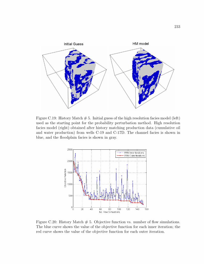
233
Figure C.19: History Match # 5. Initial guess of the high resolution facies model (left)used as the starting point for the probability perturbation method. High resolutionfacies model (right) obtained after history matching production data (cumulative oiland water production) from wells C-19 and C-17D. The channel facies is shown inblue, and the floodplain facies is shown in gray.
Figure C.20: History Match # 5. Objective function vs. number of flow simulations.The blue curve shows the value of the objective function for each inner iteration; thered curve shows the value of the objective function for each outer iteration.
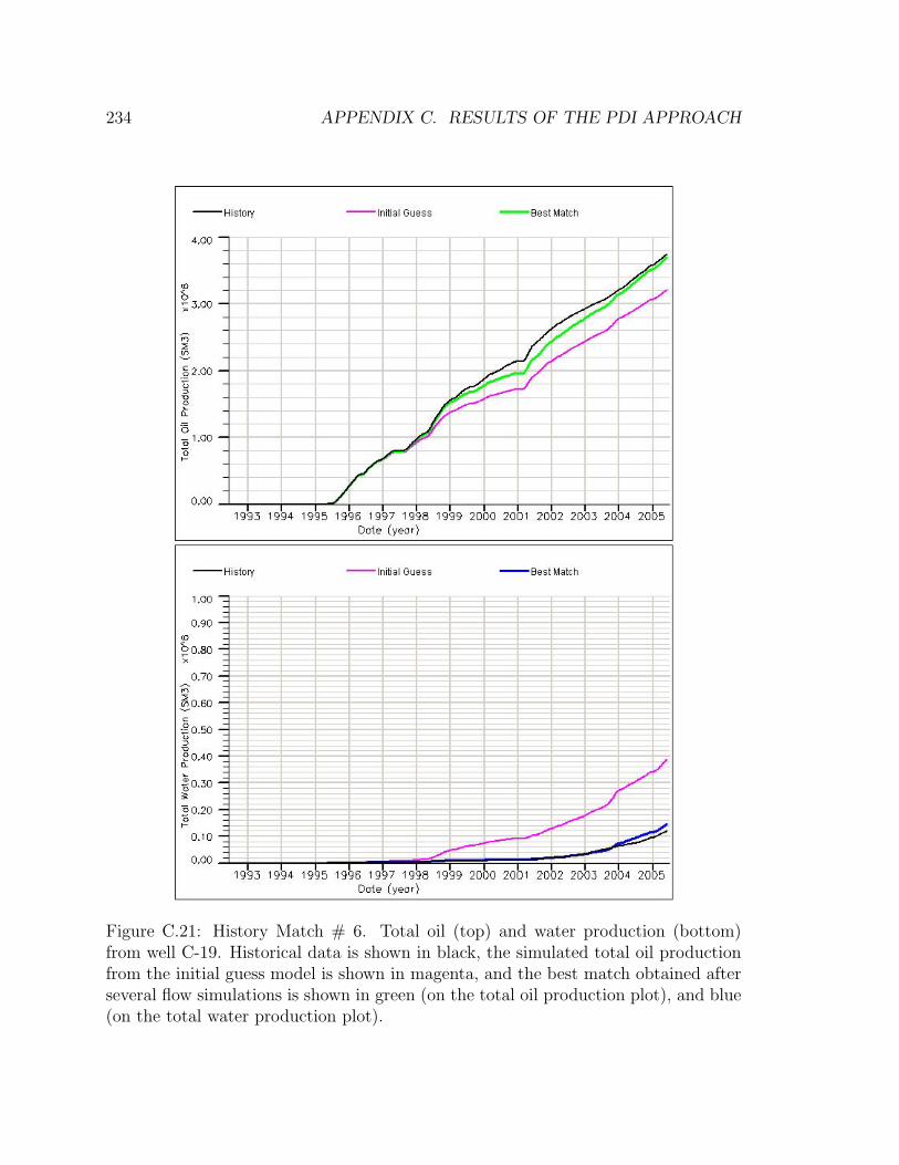
234 APPENDIX C. RESULTS OF THE PDI APPROACH
Figure C.21: History Match # 6. Total oil (top) and water production (bottom)from well C-19. Historical data is shown in black, the simulated total oil productionfrom the initial guess model is shown in magenta, and the best match obtained afterseveral flow simulations is shown in green (on the total oil production plot), and blue(on the total water production plot).
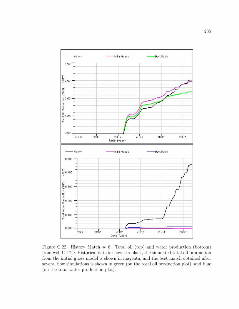
235
Figure C.22: History Match # 6. Total oil (top) and water production (bottom)from well C-17D. Historical data is shown in black, the simulated total oil productionfrom the initial guess model is shown in magenta, and the best match obtained afterseveral flow simulations is shown in green (on the total oil production plot), and blue(on the total water production plot).
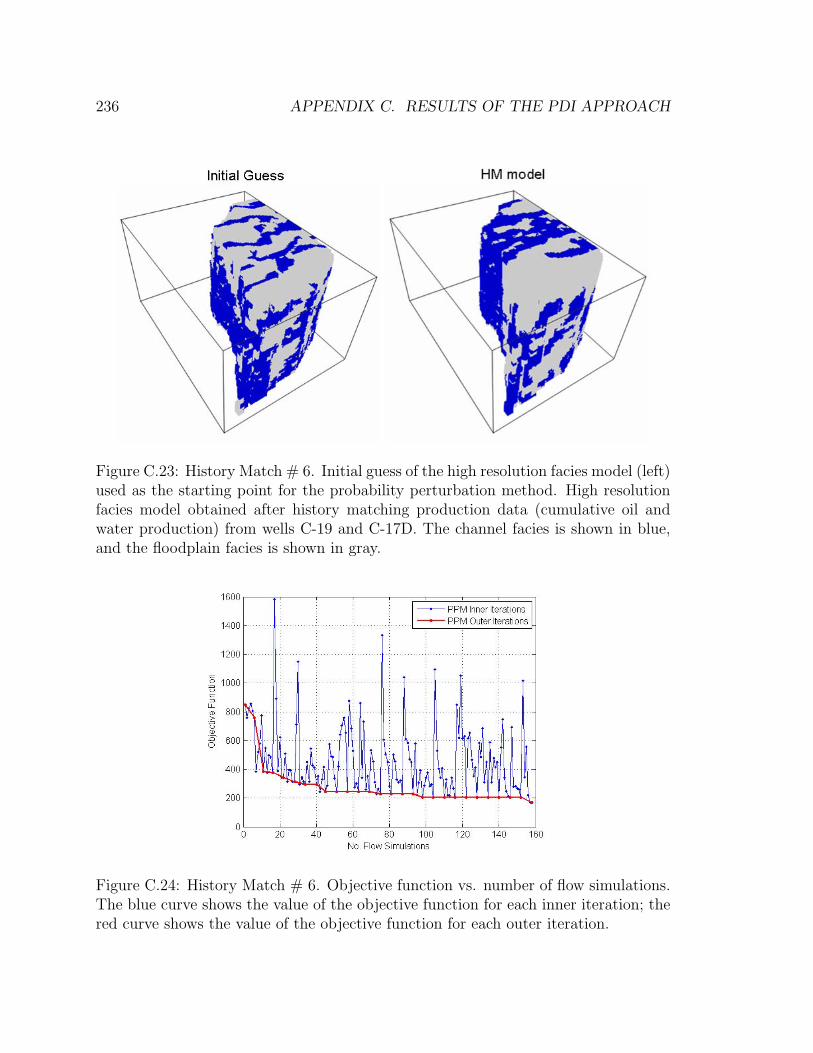
236 APPENDIX C. RESULTS OF THE PDI APPROACH
Figure C.23: History Match # 6. Initial guess of the high resolution facies model (left)used as the starting point for the probability perturbation method. High resolutionfacies model obtained after history matching production data (cumulative oil andwater production) from wells C-19 and C-17D. The channel facies is shown in blue,and the floodplain facies is shown in gray.
Figure C.24: History Match # 6. Objective function vs. number of flow simulations.The blue curve shows the value of the objective function for each inner iteration; thered curve shows the value of the objective function for each outer iteration.
Bibliography
[1] Aasheim, I., 2000: “Oseberg: Increased recoverable resources by optimal reservoir man-
agement and use of new technology”, paper SPE 65163 presented at the SPE European
Petroleum Conference, Paris, France, 24-25 October.
[2] Allen, J. L., and Peddy, C. P., 1993: “Amplitude variation with offset: Gulf Coast case
studies”. Soc. Expl. Geophys., Geophys. Dev. Series 4.
[3] Andersen, T., Zachariassen, E., Høye, T., Meisingset, H. C., Otterlei, C., van Wijn-
gaarden, A. J., Hatland, K., Mangerøy, F., 2006: “Method for conditioning the reservoir
model on 3D and 4D elastic inversion data applied to a fluvial reservoir in the North
Sea”, paper SPE 100190 presented at the SPE Europec/EAGE Annual Conference and
Exhibition, Vienna, Austria, 12-15 June.
[4] Arenas, E., van Kruijsdijk, C., Oldenziel, T., 2001: “Semi-Automatic History Matching
Using the Pilot Point Method Including Time-Lapse Seismic Data”, paper SPE 71634
presented at the SPE Annual Technical Conference and Exhibition, New Orleans, USA,
30 September-3 October.
[5] Avseth, P., Mukerji, T., Mavko, G., 2005:“Quantitative Seismic Interpretation : Apply-
ing Rock Physics Tools to Reduce Interpretation Risk”, Cambridge University Press.
[6] Avseth, P., 2000: “Integrating rock physics and flow simulation to reduce uncertainties
in seismic reservoir monitoring”. Ph.D. dissertation, Stanford University.
[7] Aziz, K., and Settari, A., 1979: “Petroleum Reservoir Simulation”, published by Khalid
Aziz and Antonın Settari.
[8] Batzle, M., Wang, Z., 1992: “Seismic properties of pore fluids”. Geophysics, V. 57, No.
11, 1396-1408.
237

238 BIBLIOGRAPHY
[9] Bortfeld, R., 1961: “Approximation to the reflection and transmission coefficients of
plane longitudinal and transverse waves”. Geophys. Prosp., 9, 485-502.
[10] Bourbie, T., Coussy, O., Zinszner, B., 1987: “Acoustics of Porous Media”. Gulf Pub.
Co.
[11] Brie, A., Pampuri, F., Marsala, A. F., and Meazza, O., 1995: “Shear sonic interpre-
tation in gas-bearing sands”, paper SPE 30595 presented at the SPE Annual Technical
Conference and Exhibition, Dallas, USA, 22-25 October.
[12] Castro, S., and Caers, J., 2004: “Joint integration of 4D seismic and production data
using the probability perturbation method: a proposal”. Stanford Center for Reservoir
Forecasting, 17th Annual Report, Stanford University.
[13] Castro, S., and Caers, J., 2005: “Flow-based downscaling of saturations for modeling
4D seismic data”. Expanded Abstracts, Soc. Expl. Geophys., 75th Annual International
Meeting, 2504-2507.
[14] Castro, S., and Caers, J., 2006: “A probabilistic approach to integration of well log,
geological information, 3D/4D seismic and production data”, paper presented at the 10th
European Conference on the Mathematics of Oil Recovery, Amsterdam, Netherlands, 4-7
September.
[15] Caers, J., 2003: “History matching under a training image-based geological model
constraints”, paper SPE 74716, SPE Journal, 8, 218-226.
[16] Caers, J., 2005: “Petroleum Geostatistics”. Society of Petroleum Engineers, 96p.
[17] Caers, J., Hoffman, B. T., Strebelle, S., Wen, X. W., 2006: “Probabilistic integration
of geologic scenarios, seismic, and production data - a West Africa turbidite reservoir
case study”. The Leading Edge, 25(3), 240-244.
[18] Carman, P. C., 1961: “L’ecoulement des Gaz a Travers les Milieux Poreux”, Bib-
liotheque des Science et Techniques Nucleaires, press Universitaires de France, Paris, 198
p.
[19] Castagna, J. P, Batzle, M. L., and Eastwood, R. L., 1985: “Relationships between
compressional-wave and shear-wave velocities in clastic silicate rocks”. Geophysics, V.
50, No. 4, 571-581.
BIBLIOGRAPHY 239
[20] Castagna, J. P., and Backus, M. M., 1993: “Offset dependent reflectivity: Theory and
practice of AVO analysis”. Soc. Expl. Geophys., Invest. Geophys. 8.
[21] Castagna, J. P., Batzle, M. L., and Kan, T. K.,1993: “Rock physics - the link between
rock properties and AVO response”, in Offset-Dependent Reflectivity - Theory and Prac-
tice of AVO Analysis, J.P Castagna and M. Backus, eds. Investigations in Geophysics,
No. 8, Society of Exploration Geophysicists, Tulsa Oklahoma, 135-171.
[22] Castagna, J. P., Swan, H. W, and Foster, D. J., 1998: “Framework for AVO gradient
and intercept interpretation”. Geophysics, V. 63, No. 3, 948-956.
[23] Chacko, S., 1989: “Porosity identification using amplitude variation with offset: Ex-
amples from South Sumatra”. Geophysics, V. 54, No. 8, 942-951.
[24] Chen, Y., Durlofsky, L. J., Gerritsen, M., and Wen, X. H., 2003: “A coupled local-
global upscaling approach for simulating flow in highly heterogeneous formations”. Ad-
vances in Water Resources, 26, 1041-1060.
[25] Connolly, P., 1999: “Elastic Impedance”. The Leading Edge, 18, 438.
[26] Darcy, H., 1856: “Les Fontaines publiques de la Ville de Dijon”, Dalmount, Paris,
(reprinted in Hubbert, 1969).
[27] Deutsch, C., 1985: “Estimating block effective permeability with geostatistics and
power averaging”, paper SPE 15991 presented at the Unsolicited.
[28] Deutsch, C., Journel, A. G., 1998: “GSLIB Geostatistical Software Library and User’s
Guide”. Oxford University Press.
[29] Dvorkin, J., and Nur, A., 1996: “Elasticity of high-porosity sandstones: Theory for
two North Sea datasets”. Geophysics, V. 61, No. 5, 1363-1370.
[30] Enyon, G., 1981: “Basin development and sedimentation in the Middle Jurassic of the
northern North Sea”, in Illing, L. V., and Hobson, G. D.: Petroleum Geology of the
Continental Shelf of North-west Europe, Heyden, London, 196p.
[31] Gardner, G. H. F., Gardner, L. W., and Gregory, A. R., 1974: “Formation velocity and
density - The diagnostic basis for stratigraphic traps”. Geophysics, V. 39, No. 6, 770-780.
240 BIBLIOGRAPHY
[32] Gassmann, F., 1951: “Uber die Elastizitat poroser Medien”. Vier. der Natur,
Gesellschaft in Zurich, 96, 1-23.
[33] Gautier, Y., Blunt, M. J., and Christie, M. A., 1999: “Nested gridding and streamline-
based simulation for fast reservoir performance prediction”. Computational Geosciences,
3, 295-320.
[34] Goodway, B., Chen, T., and Downton, J., 1997: “Improved AVO fluid detection and
lithology discrimination using Lame petrophysical parameters; λρ, µρ, and λ/µ fluid
stack, from P and S inversions”. Expanded Abstracts, Soc. Expl. Geophys., 67th Annual
International Meeting, 183-186.
[35] Gomez-Hernandez, J. J., and Journel, A. G., 1989: “Conditional simulation of the
Wilmington sand-shale sequence, Los Angeles basin”, in Hydraulic Engineering. ed., M.A.
Ports, publ. American Society of Civil Engineers, NY, 801-806.
[36] Gosselin, O., Cominelli, A., Vand Den Berg, S., and Chowdhury, S. D., 2000: “A
gradient-based approach for history-matching of both production and 4D seismic data”,
paper presented at the 7th European Conference on the Mathematics of Oil Recovery,
Baveno, Italy, 5-8 September.
[37] Graue, E. et al., 1987: “Advance and retreat of the Brent delta system, Norwegian
North Sea”, in Brooks, K. and Glennie, K.: Petroleum Geology of Northwest Europe,
Graham and Trotman, London.
[38] Guerillot, D., and Pianelo, L., 2000: “Simultaneous Matching of Production Data
and Seismic Data for Reducing Uncertainty in Production Forecasts”, paper SPE 65131
presented at the SPE European Petroleum Conference, Paris, France, 24-25 October.
[39] Hubbert, M. K., 1969: “The Theory of Ground-Water Motion and Related Papers”,
Hafner Publishing, New York.
[40] Han, D. H., 1986: “Effects of Porosity and Clay content on Acoustic Properties of
Sandstones and Unconsolidated Sediments”. Ph.D. dissertation, Stanford University.
[41] Helland-Hansen, W. et al., 1992: “Advance and retreat of the Brent delta: recent
contributions to the depositional model”, in Morton, A. C. et al.: Geology of the Brent
Group, Geological Society, London, Special Publication 61.
BIBLIOGRAPHY 241
[42] Hoffman, B. T., and Caers, J., 2003: “Geostatistical history matching using a regional
probability perturbation method”, paper SPE 84409 presented at the SPE Annual Tech-
nical Conference and Exhibition, Denver, USA, 5-8 October.
[43] Hoffman, B. T., Wen, X. H., Strebelle, S., and Caers, J., 2005: “Geologically Consistent
History Matching of a Deepwater Turbidite Reservoir”, paper SPE 95557 presented at
the SPE Annual Technical Conference and Exhibition, Dallas, USA, 9-12 October.
[44] Hoffman, B. T., 2005: “Geologically Consistent History Matching while perturbing
facies”. Ph.D. dissertation, Stanford University.
[45] Jack, I., 1998: “Time-Lapse Seismic in Reservoir Management”. SEG Distinguished
Instructor Short Course.
[46] Johannessen, E. P. et al., 1995: “Northern limit of the ‘Brent delta’ at the Tampen
Spur - a sequence stratigraphic approach for sandstone prediction”, in Steel, R. J. et al.:
Sequence Stratigraphy of the Northwest European Margin, Norwegian Society Special
Publication, 5.
[47] Johnstad, S. E., Seymour, R. H., and Smith, P. J., 1995: “Seismic reservoir monitoring
over the Oseberg field during the period 1989-1992”. First Break, V. 13, No. 05, 169-183.
[48] Journel, A. G., and Alabert, F. A., 1988: “New Method for Reservoir Mapping”, paper
SPE 18324, Journal of Petroleum Technology, V. 42, No. 2, 212-218.
[49] Journel, A. G., 2002: “Combining knowledge form diverse information sources: an
alternative to Bayesian analysis”. Mathematical Geology, V. 34, No. 5, 573-598.
[50] Kim, J., and Caers, J., 2003: “Joint history matching of facies distribution and net-
to-gross”. Stanford Center of Reservoir Forecasting, 16th Annual Report, Stanford Uni-
versity.
[51] Krishnan, S., 2004: “Combining diverse and partially redundant information in the
earth sciences”. Ph.D. dissertation, Stanford University.
[52] Kretz, V., Le Ravalec-Dupin, M., and Roggero, F., 2002: “An Integrated Reservoir
Characterization Study Matching Production and 4D Seismic”, paper SPE 77516 pre-
sented at the SPE Annual Technical Conference and Exhibition, San Antonio, USA, 29
September-2 October.
242 BIBLIOGRAPHY
[53] Landa, J., and Horne, R., 1997: “A procedure to integrate well test data, reservoir
performance history and 4-D seismic information into a reservoir description”, paper SPE
38653 presented at the SPE Annual Technical Conference and Exhibition, San Antonio,
USA, 5-8 October.
[54] Landro, M., Buland, A., and DAngelo, R., 1995: “Target-oriented AVO inversion from
Valhall and Hod fields”. The Leading Edge, V. 14, No. 8, 855861.
[55] Liestøl, F. M., Hodneland, E., Hatland, K., Zachariazzen, E., and Andersen, T., 2005:
“Improved modelling and recovery from fluvial reservoir in the north sea”, paper SPE
10378 presented at the International Petroleum Technology Conference, Doha, Qatar,
21-23 November.
[56] Mantica, S., Cominelli, A., and Mantica, G., 2001: “Combining global and local opti-
mization techniques for automatic history matching production and seismic data”, paper
SPE 66355 presented at the SPE Reservoir Simulation Symposium, Houston, USA, 11-14
February.
[57] Mao, S., and Journel, A. G., 1999: “Generation of a reference petrophysical/seismic
data set: the Stanford V reservoir”. Stanford Center for Reservoir Forecasting, 12th
Annual Report, Stanford University.
[58] Mavko, G., and Mukerji, T., 1998: “Bounds on low-frequency seismic velocities in
partially saturated rocks”. Geophysics, V. 63, No. 3, 918-924.
[59] Mavko, G., Mukerji, T., and Dvorkin, J., 1998: “The Rock Physics Handbook: Tools
for seismic analysis in porous media”. Cambridge University Press.
[60] Mezghani, M., Fornel, A., Langlais, V., and Lucet, N., 2004: “History Matching and
Quantitative Use of 4D Seismic Data for an Improved Reservoir Characterization”, paper
SPE 90420 presented at the SPE Annual Technical Conference and Exhibition, Houston,
USA, 26-29 September.
[61] McCain, W. D., 1989: “The Properties of Petroleum Fluids”. PennWell Publishing Co.
[62] Mukerji, T., Mavko, G., and Rio, P., 1997: “Scales of Reservoir Heterogeneities and
Impact of Seismic Resolution on Geostatistical Integration”. Mathematical Geology, 29,
933-949.
BIBLIOGRAPHY 243
[63] Nur, A., and Simmons, G., 1969: “The effect of saturation on velocity in low porosity
rocks”. Earth and Planetary Sciences Letters, 7, 183-193.
[64] Nur, A., 1989: “Four-dimensional seismology and (true) direct detection of hydrocar-
bon: the petrophysical basis”. The Leading Edge, V. 8, No. 9, 30-36.
[65] Ostrander, W. J., 1984: “Plane-wave reflection coefficients for gas sands at nonnormal
angles of incident”. Geophysics, V. 49, No. 10, 16371648.
[66] Bach, T., Espersen, T. B., Hinkley, R., Pillet, W. R., Pedersen, J. M., and Rasmussen,
K. B., 1999: “Seismic inversion of AVO data”. Expanded Abstracts, EAGE, 61st Meeting,
Session: 6054.
[67] Raymer, L. L., Hunt, E. R., and Gardner, J. S., 1980: “An improved sonic transit-
time-to porosity transform”. Trans. Soc. Prof. Well Log Analysts, 21st Annual Logging
Symposium, Paper P.
[68] Remy, N., Boucher, A., Wu, J., and Journel, A. G., 2007: “Stanford Geostatistical
Modeling Software”. Oxford University Press.
[69] Richards, P. G., and Frasier, C. W., 1976: “Scattering of elastic waves from depth-
dependent inhomogeneities. Geophysics, V. 41, No. 3, 441-458.
[70] Rutherford, S. R., and Williams, H. R., 1989: “Amplitude-versus-offset variations in
gas sands”. Geophysics, V. 54, No. 6, 680-688.
[71] Rutledal, H., Helgesen, J., and Buran, H., 2003: “4D elastic inversion helps locate
in-fill wells at Oseberg field”. First Break, V. 21, No. 8, 43-48.
[72] Ryseth, A., 1989: “Correlation of depositional patterns in the Ness Formation, Oseberg
area”, in Collinson, J. D.: Correlation in Hydrocarbon Exploration, Norwegian Petroleum
Society, Graham and Trotman, London.
[73] Santoso, D., Alam S., Hendraya, L., Alfian, Sulistiyono, and Munadi, S. 1995: “Esti-
mation of limestone reservoir porosity by seismic attribute and AVO analysis”. Expanded
Abstracts, ASEG, 11th Geophysical Conference, V. 26 , No. 2/3, 437-443.
[74] Sengupta, M., and Mavko, G., 1998: “Reducing uncertainties in saturation scales using
fluid flow models’. Expanded Abstracts, Soc. Expl. Geophys., 68th Annual International
Meeting, 1012-1015.
244 BIBLIOGRAPHY
[75] Sengupta, M., 2000: “Integrating rock physics and flow simulation to reduce undcer-
tainties in seismic reservoir monitoring”. Ph.D. dissertation, Stanford University.
[76] Shuey, R. T., 1985: “A simplification of Zoeppritz Equations”. Geophysics, V. 50, No.
4, 609-814.
[77] Smethurst, M. A., 2000: “Land-offshore tectonic links in western Norway and the
northern North Sea”. Journal of Geological Society, London, 157p.
[78] Snyder, A. G., and Wrolstad, K. H., 1992: “Direct detection using AVO, Central
Graben, North Sea”. Geophysics, V. 57, No. 2, 313325.
[79] Spencer, A. M., and Larsen, V. B., 1990: “Fault traps in the Northen North Sea”, in
Hardman, R. F. P. and Brooks, J.: Tectonics Events Responsible for Britain’s Oil and
Gas reserves, Geological Society, London, Special Publication 55.
[80] Stewart, R. R., Zhang, Q., and Guthoff, F., 1995: “Relationships among elastic-wave
values (Rpp, Rps, Rss, Vp, Vs, ρ, σ, κ)”. CREWES Research Report, Chapter 10.
[81] Strebelle, S., 2002: “Conditional Simulation of Complex Geological Structures using
Multiple-point Statistics”. Math. Geol., V. 34, No. 1, 1-26.
[82] Taner, M. T., 2001: “Seismic Attributes”. Recorder, 26 , No.9, 48-56.
[83] Torvund, T., and Nipen, O., 1990: “The Oseberg FIeld: potential for increased oil
recovery by gas injection in a high permeability environment”, in Glennie, K. W.: In-
troduction to the Petroleum Geology of the North Sea, Blackwell Scientific Publications,
Oxford.
[84] Tosaya, C., and Nur, A., 1982: “Effects of diagenesis and clays on compressional
velocities in rocks”. Geophys. Res. Lett., 9, 5-8.
[85] Tureyen, O. I., and Caers, J., 2003. “A two-level optimization method for geostatistical
integration of production data on non-uniform grids”, paper SPE 84368 presented at the
SPE Annual Technical Conference and Exhibition, Denver, USA, 5-8 October.
[86] Tureyen, O. I., 2005: “A parallel modeling approach to reservoir characterization”.
Ph.D. dissertation, Stanford University.
BIBLIOGRAPHY 245
[87] Van Ditzhuijzen, R., Oldenziel, T., and Van Kruijsdijk, C., 2001: “Geological parame-
trization of a reservoir model for history matching incorporating time-lapse seismic based
on a case study of the Stratfjord field”, paper SPE 71318 presented at the SPE Annual
Technical Conference and Exhibition, New Orleans, USA, 30 September-3 October.
[88] von Seggern, D., 1991: “Spatial resolution of acoustic imaging with the Born approxi-
mation”. Geophysics, V. 56, No. 8, 1185-1202.
[89] Waggoner, J. R., Cominelli, A., and Seymour, R. H., 2002: “Improved Reservoir Mod-
eling with Time-Lapse Seismic in a Gulf of Mexico Gas Condensate Reservoir”, paper
SPE 77514 presented at the SPE Annual Technical Conference and Exhibition, San An-
tonio, USA, 29 September-2 October.
[90] Wang, Z., and Nur, A., 1988: “Effect of temperature on wave velocities in sands and
sandstones with heavy hydrocarbons”, paper SPE 15646, SPE Reservoir Engineering,
158-164.
[91] Wu, J., Mukerji, T., and Journel, A. G., 2005: “Seismic time lapse indicators to spot
discrepancies and improve reservoir models”. Stanford Center for Reservoir Forecasting,
18th Annual Report, Stanford University.
[92] Wyllie, M. R. J., Gregory, A. R., and Gardner, L. W., 1956: “Elastic wave velocities
in heterogeneous and porous media”. Geophysics, V. 21, No. 1, 41-70.
[93] Xu, Y., and Bancroft, J. C., 1997: “Joint AVO analysis of PP and PS seismic data”.
CREWES Research Report, V. 9, 34-44.
[94] Zoeppritz, K., 1919: “Erdbebenwellen VIIIB, Ueber Reflexion and Durchgang seismis-
cher Wellen durch Unstetigkeitsflaechen”. Gottinger Nachrichten, I, 66-84.