a novel face recognition approach using normalized
TRANSCRIPT
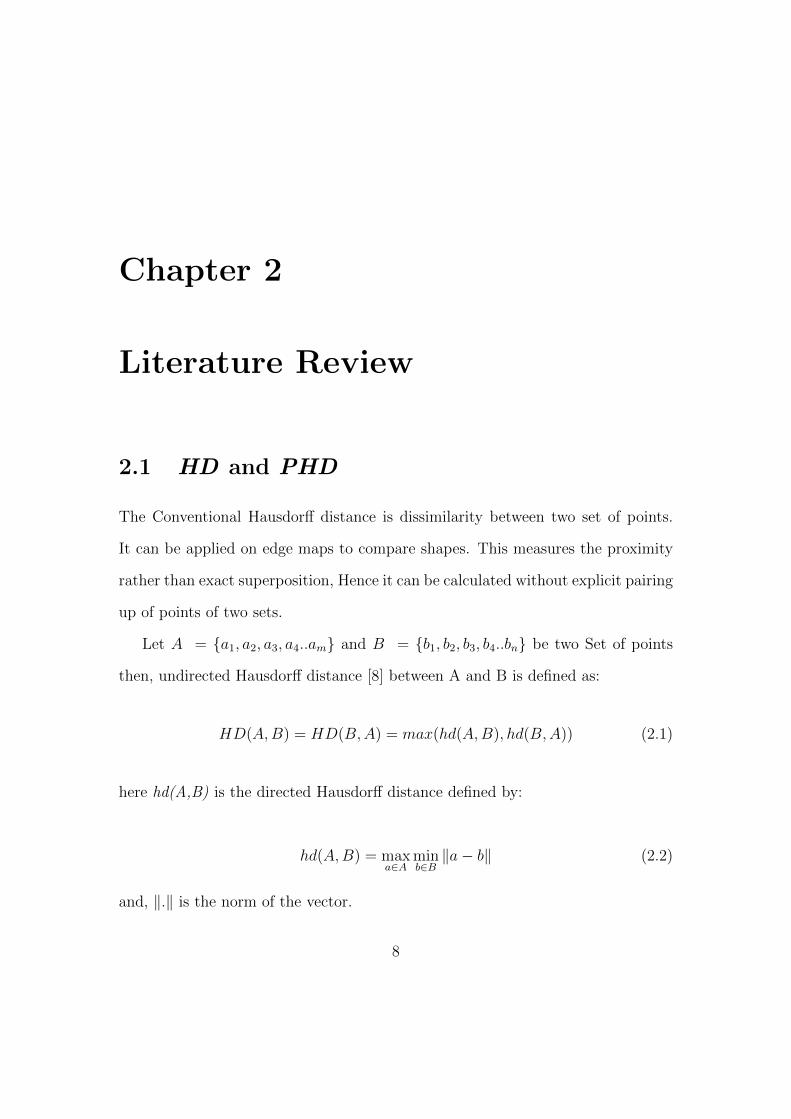
A Novel Face Recognition
Approach using Normalized
Unmatched Points Measure
A Thesis Submitted
in Partial Fulfillment of the Requirements
for the Degree of
Master of Technology
by
Aditya Nigam
Y7111002
to the
DEPARTMENT OF COMPUTER SCIENCE AND ENGINEERING
INDIAN INSTITUTE OF TECHNOLOGY KANPUR
May 2009

CERTIFICATE
This is to certify that the work contained in the thesis entitled “A Novel Face
Recognition Approach using Normalized Unmatched Points Measure” by Aditya
Nigam has been carried out under my supervision and that this work has not been
submitted elsewhere for a degree.
May 2009 Dr. Phalguni Gupta
Department of Computer Science and Engineering
Indian Institute of Technology Kanpur
Kanpur 208016

Contents
Acknowledgements viii
Abstract ix
1 Introduction 1
1.1 Face Recognition System . . . . . . . . . . . . . . . . . . . . . . . . 2
1.2 Motivation . . . . . . . . . . . . . . . . . . . . . . . . . . . . . . . . 4
1.3 Related Work . . . . . . . . . . . . . . . . . . . . . . . . . . . . . . 4
1.4 Organization of the thesis . . . . . . . . . . . . . . . . . . . . . . . 6
2 Literature Review 8
2.1 HD and PHD . . . . . . . . . . . . . . . . . . . . . . . . . . . . . . 8
2.2 MHD and M2HD . . . . . . . . . . . . . . . . . . . . . . . . . . . . 10
2.3 SWHD and SW2HD . . . . . . . . . . . . . . . . . . . . . . . . . . 11
2.4 SEWHD and SEW2HD . . . . . . . . . . . . . . . . . . . . . . . . 11
2.5 Hg and Hpg . . . . . . . . . . . . . . . . . . . . . . . . . . . . . . . 13
2.6 Application in Face Recognition . . . . . . . . . . . . . . . . . . . . 15
3 The Proposed Approach and Implementation Details 16
iii
3.1 Transformation . . . . . . . . . . . . . . . . . . . . . . . . . . . . . 17
3.1.1 gt-Transformation . . . . . . . . . . . . . . . . . . . . . . . . 18
3.2 Defining NUP . . . . . . . . . . . . . . . . . . . . . . . . . . . . . . 21
3.2.1 Definitions . . . . . . . . . . . . . . . . . . . . . . . . . . . . 21
3.3 Efficient computation of NUP . . . . . . . . . . . . . . . . . . . . . 24
3.3.1 Algorithm . . . . . . . . . . . . . . . . . . . . . . . . . . . . 24
3.3.2 Running Time Analysis . . . . . . . . . . . . . . . . . . . . 27
3.3.3 Space Analysis . . . . . . . . . . . . . . . . . . . . . . . . . 28
4 Experimental Results and Analysis 29
4.1 Setup for Face Recognition System . . . . . . . . . . . . . . . . . . 29
4.1.1 Face Detection . . . . . . . . . . . . . . . . . . . . . . . . . 31
4.1.2 Preprocessing and Testing Strategy . . . . . . . . . . . . . . 31
4.1.3 Face image Comparison using NUP measure . . . . . . . . . 31
4.2 Experimental Results . . . . . . . . . . . . . . . . . . . . . . . . . . 32
4.2.1 Parameterized results of NUP based recognition on different
facial databases . . . . . . . . . . . . . . . . . . . . . . . . . 32
4.2.2 Comparative Analysis . . . . . . . . . . . . . . . . . . . . . 40
4.2.3 Overall Analysis . . . . . . . . . . . . . . . . . . . . . . . . . 41
5 Conclusion and Further Work 43
iv

List of Figures
1.1 Face recognition system . . . . . . . . . . . . . . . . . . . . . . . . 2
1.2 Eigenfaces . . . . . . . . . . . . . . . . . . . . . . . . . . . . . . . . 6
2.1 Example hd(A,B) . . . . . . . . . . . . . . . . . . . . . . . . . . . . 9
2.2 Spatial Weighing Function . . . . . . . . . . . . . . . . . . . . . . . 12
2.3 Quantized Images . . . . . . . . . . . . . . . . . . . . . . . . . . . . 14
3.1 Gray-value spectrum. . . . . . . . . . . . . . . . . . . . . . . . . . . 18
3.2 gt-Transformed images . . . . . . . . . . . . . . . . . . . . . . . . . 19
3.3 gt-Transformed images . . . . . . . . . . . . . . . . . . . . . . . . . 20
3.4 Circular Neighborhood . . . . . . . . . . . . . . . . . . . . . . . . . 22
3.5 Data Structure: BLIST . . . . . . . . . . . . . . . . . . . . . . . . . 25
4.1 Images produced after various phases . . . . . . . . . . . . . . . . . 30
4.2 Effect of High gt values under heavy illumination variation . . . . . 33
4.3 ORL Database Results . . . . . . . . . . . . . . . . . . . . . . . . . 35
4.4 YALE Database Results . . . . . . . . . . . . . . . . . . . . . . . . 36
4.5 BERN Database Results . . . . . . . . . . . . . . . . . . . . . . . . 37
4.6 CALTECH Database Results . . . . . . . . . . . . . . . . . . . . . 38
4.7 IITK Database Results . . . . . . . . . . . . . . . . . . . . . . . . . 39
v

4.8 Results of NUP based face recognition on different face databases
considering top n best matches. . . . . . . . . . . . . . . . . . . . . 41
vi
List of Tables
3.1 Notations . . . . . . . . . . . . . . . . . . . . . . . . . . . . . . . . 21
4.1 Databases Information . . . . . . . . . . . . . . . . . . . . . . . . . 32
4.2 Comparative study on ORL and YALE databases when considering
top 1 best match . . . . . . . . . . . . . . . . . . . . . . . . . . . . 40
4.3 Comparative study on BERN database when considering top 1 best
match . . . . . . . . . . . . . . . . . . . . . . . . . . . . . . . . . . 40
4.4 Overall Analysis (considering top-n best matched) . . . . . . . . . . 42
vii

Acknowledgements
I take this immense opportunity to express my sincere gratitude toward my super-
visor Dr. Phalguni Gupta for their invaluable guidance. It would never have been
possible for me to take this project to completion without his innovative ideas and
his relentless support and encouragement.
I also wish to thank whole-heartedly all the faculty members of the Depart-
ment of Computer Science and Engineering for the invaluable knowledge they have
imparted to me and for teaching the principles in the most exciting and enjoyable
way.
My stay at the institute was unforgettable, and the biggest reason being my
classmates. I specially wish to thank Sameer, Ali, Abhay, Sumit, Kamlesh, Tejas,
Manoj, Saket, Sachin and Vishwas for the heated discussions and critiques that
helped in completing this work. Finally, I would like to thank my family for all
the blessings and support that always gave me courage to face all the challenges.
Aditya Nigam
viii
Abstract
The human face is the premier biometric in the field of human recognition; not
only because of its easy acquisition but also since it has been extensively studied
and several good algorithms exist for face recognition. However, there are several
challenges in face recognition like different poses, expressions, backgrounds and
illumination conditions to name a few, because of which the task becomes difficult.
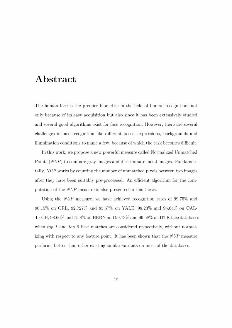
In this work, we propose a new powerful measure called Normalized Unmatched
Points (NUP) to compare gray images and discriminate facial images. Fundamen-
tally, NUP works by counting the number of unmatched pixels between two images
after they have been suitably pre-processed. An efficient algorithm for the com-
putation of the NUP measure is also presented in this thesis.
Using the NUP measure, we have achieved recognition rates of 99.75% and
90.15% on ORL, 92.727% and 85.57% on YALE, 98.23% and 95.64% on CAL-
TECH, 98.66% and 75.8% on BERN and 99.73% and 99.58% on IITK face databases
when top 1 and top 5 best matches are considered respectively, without normal-
izing with respect to any feature point. It has been shown that the NUP measure
performs better than other existing similar variants on most of the databases.
ix
Chapter 1
Introduction
Humans do face recognition on regular basis naturally and so effortlessly that we
never think of what exactly we looked at in the face. Face is a three dimensional
object that is subjected to varying illumination, poses, expressions and so on which
has to be identified based on its two dimensional image. Hence, Face recognition
is an intricate visual pattern recognition problem which can be operated in these
modes -
• Face Verification (or Authentication) that compares a query face image
against a template face image whose identity is being claimed (i.e. one
to one).
• Face Identification (or Recognition) that compares a query face image against
all the template images in the database to determine the identity of the query
face (i.e. one to many).
• Watch List that compares a query face image only to a list of suspects (i.e.
one to few).
1

QueryImage
DetectionFace
NormalizationFace
CroppedFace
- Face FeatureExtraction
AlignedFace -
FeatureVector Face Feature
Matching-
FaceID
DatabaseFace
6
- -
Figure 1.1: Face recognition system
1.1 Face Recognition System
Most of the face recognition methods either rely on detecting local facial feature
(feature extraction), within face as eyes, nose and mouth and use them for recog-
nition or globally analyzing a face as a whole for identifying the person. A face
recognition system [23] generally consist of four modules (as shown in Figure 1.1):
Face Detection, Face Normalization, Face Feature Extraction and Face Feature
Matching.
Some of the conditions that should be accounted for when detecting faces are
[22]:
1. Occlusion: face may be partially occluded by other objects
2. Presence or absence of structural components: beards, mustaches and glasses
3. Facial expression: face appearance is very much affected by a person’s facial
expression
4. Pose (Out-of Plane Rotation): frontal,45 degree,profile,upside down
5. Orientation (In Plane Rotation): face appearance directly varies for different
rotations about the camera’s optical axis
2
6. Imaging conditions: lighting (direction and intensity), camera characteris-
tics, resolution
Face recognition is done after detection, some of the related problems include [23]:
1. Face Localization
(a) Determine face location in the image
(b) Assume single face
2. Face Feature Extraction
(a) Determining location of various facial features as eyes, nose, nostrils,
eyebrow, mouth, lips, ears, etc.
(b) Assume single face
3. Facial expression recognition
4. Human pose estimation and tracking
Human face recognition finds application in a wide range of fields such as auto-
matic video surveillance, criminal identification, credit cards and security systems
to name just a few. The requirements of a good face recognition algorithm are
high recognition rates, tolerance towards various environmental factors such as
illumination, facial poses, facial expressions, image backgrounds, image scales, hu-
man ageing and also good computational and space complexity. The development
of the field of face recognition can be found in [1, 2]. Initial approaches for face
recognition of gray facial images involved the use of PCA [3], EBGM [4], Neural
Networks [5], Support Vector Machines [6] and Hidden Markov Models [7]. How-
ever, these techniques are complex and computationally very expensive as they
3
work on gray scale images and also do not provide too much tolerance to varying
environment.
1.2 Motivation
Face recognition is becoming primary biometric technology because of rapid ad-
vancement in the technology such as digital cameras, the internet and mobile
devices which in turn facilitates its acquisition. Artificially simulating face recog-
nition is required to create intelligent autonomous machines. Face recognition by
machine can contribute in various application in real life such as electronic and
physical access control, biometric authentication, surveillance, human computer
interaction, multimedia management to name just a few. Also, it has many ad-
vantages over other biometric traits as it requires least cooperation, non intrusive,
easy to acquire and use.
1.3 Related Work
The conventional Hausdorff distance was defined on 2 set of points (say A and B)
as :
“The minimum distance between any 2 points a and b such that a ∈ A and
b ∈ B.”
Huttenlocher and Rucklidge et al [8] have proposed the Hausdorff Distance
(HD) and Partial Hausdorff Distance (PHD) measures to compare images. The
HD and PHD measures are not too computation intensive as they treat images
as set of edge points. HD measure is found to be robust for small amount of local
4

non rigid distortions. This property of Hausdorff distance makes it suitable for
face recognition because such distortions occur frequently in facial images and are
usually caused due to slight variation in poses and facial expressions.
Rucklidge [9] has used HD and PHD measures for object localization. HD has
been modified by Dubuisson [15] to MHD, which was less sensitive to noise. The
modified version of PHD named M2HD has been proposed by B.Takacs [10]. It
uses the fact that facial images are assumed to be well cropped and normalized
therefore corresponding points in edge images must be in a ‘neighborhood’ [10].
Hence, M2HD penalizes points matched outside their ‘neighborhood’. Guo, Lam
et al [11] have proposed SWHD and SW2HD which were also based on HD and
M2HD. They give importance to vital facial feature points such as eyes, nose and
mouth, which they approximate by rectangles. Lin, Lam et al [12] have improved
SWHD and SW2HD to SEWHD and SEW2HD by using Eigen faces ∗ (as shown
in Figure 1.2) as weighing functions because regions having larger variations are
known to be important for facial discrimination.
The three-dimensional information of facial features plays vital role in discrim-
inating faces. Unfortunately by creating edge maps we may lose most of this
crucial information. HD and all its variant measures are defined on edge maps.
They may work well for object detection and face recognition on some illumination-
varying facial image databases. However their performance on pose-varying and
expression-varying facial image databases is limited and cannot be improved be-
yond a certain level since edge maps change drastically with pose and expression
variance. Vivek and Sudha [13] have proposed Hg and Hpg measures which work
∗Eigenfaces appears as light and dark areas arranged in a specific pattern. Regions wherethe difference among the training images is large, the corresponding regions at the eigenfaceswill have large magnitude.
5
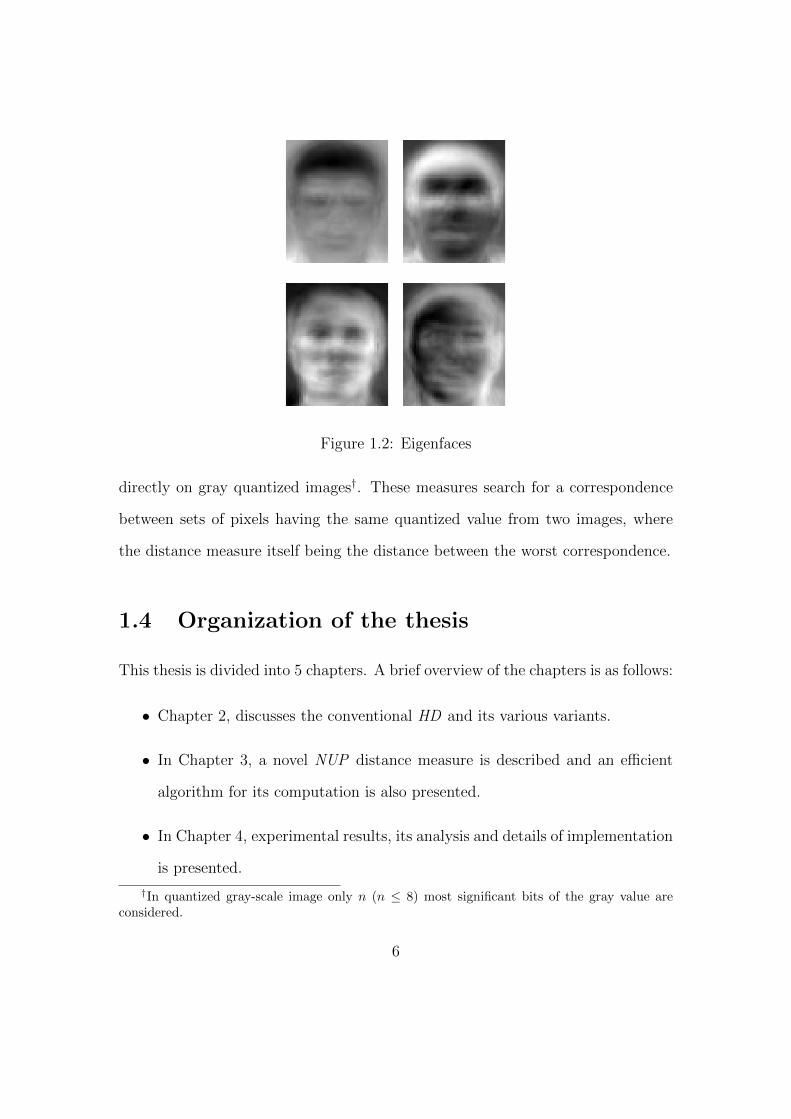
Figure 1.2: Eigenfaces
directly on gray quantized images†. These measures search for a correspondence
between sets of pixels having the same quantized value from two images, where
the distance measure itself being the distance between the worst correspondence.
1.4 Organization of the thesis
This thesis is divided into 5 chapters. A brief overview of the chapters is as follows:
• Chapter 2, discusses the conventional HD and its various variants.
• In Chapter 3, a novel NUP distance measure is described and an efficient
algorithm for its computation is also presented.
• In Chapter 4, experimental results, its analysis and details of implementation
is presented.
†In quantized gray-scale image only n (n ≤ 8) most significant bits of the gray value areconsidered.
6

• In Chapter 5, future work is presented and conclusion is given.
7
Chapter 2
Literature Review
2.1 HD and PHD
The Conventional Hausdorff distance is dissimilarity between two set of points.
It can be applied on edge maps to compare shapes. This measures the proximity
rather than exact superposition, Hence it can be calculated without explicit pairing
up of points of two sets.
Let A = {a1, a2, a3, a4..am} and B = {b1, b2, b3, b4..bn} be two Set of points
then, undirected Hausdorff distance [8] between A and B is defined as:
HD(A,B) = HD(B,A) = max(hd(A,B), hd(B,A)) (2.1)
here hd(A,B) is the directed Hausdorff distance defined by:
hd(A,B) = maxa∈A
minb∈B‖a− b‖ (2.2)
and, ‖.‖ is the norm of the vector.
8
and CorrespondanceMin Value
10(1-a)
1 corresponds to a
2 corresponds to a8(2-a)
3 corresponds to a12(3-a)
'
&
$
%
'
&
$
%
1
2
3
a
b
Distances Max Value
10
14
8
10
12
15
[Most Dissimilar Points]
12(3-a)
This is the worstcorrespondance
1-a
1-b
2-a
2-b
3-a
3-b
Pairs of Points
SET A SET B
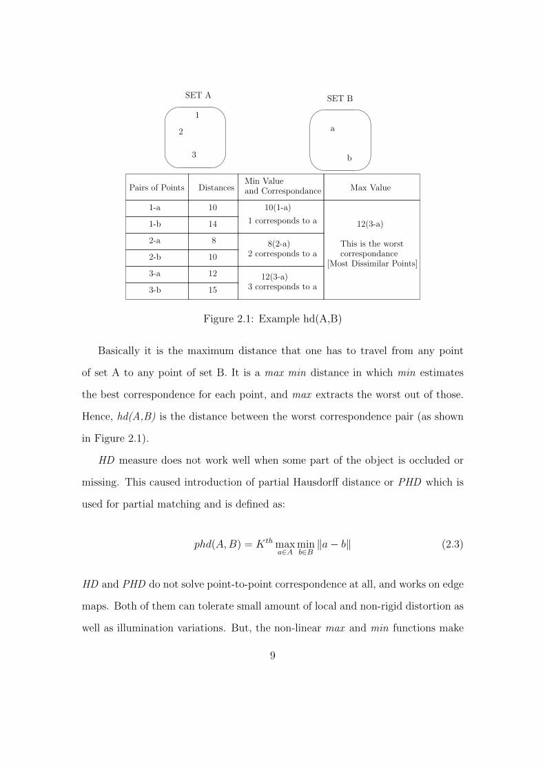
Figure 2.1: Example hd(A,B)
Basically it is the maximum distance that one has to travel from any point
of set A to any point of set B. It is a max min distance in which min estimates
the best correspondence for each point, and max extracts the worst out of those.
Hence, hd(A,B) is the distance between the worst correspondence pair (as shown
in Figure 2.1).
HD measure does not work well when some part of the object is occluded or
missing. This caused introduction of partial Hausdorff distance or PHD which is
used for partial matching and is defined as:
phd(A,B) = Kth maxa∈A
minb∈B‖a− b‖ (2.3)
HD and PHD do not solve point-to-point correspondence at all, and works on edge
maps. Both of them can tolerate small amount of local and non-rigid distortion as
well as illumination variations. But, the non-linear max and min functions make
9
HD and PHD very sensitive to noise.
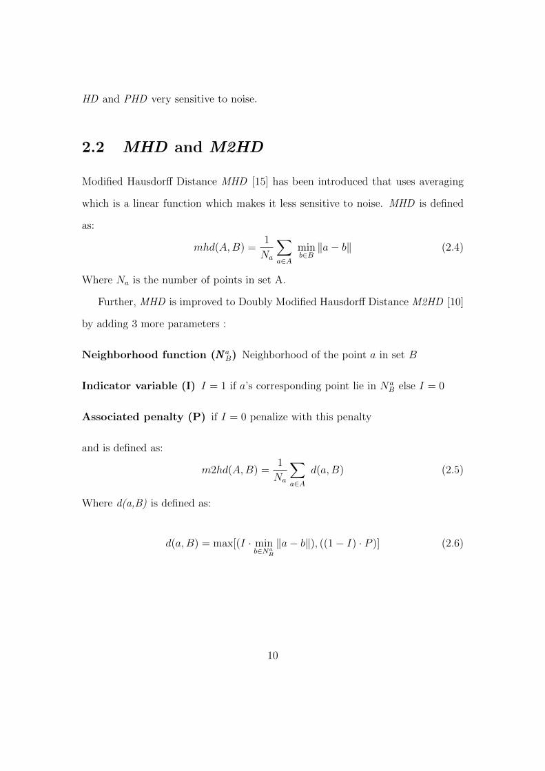
2.2 MHD and M2HD
Modified Hausdorff Distance MHD [15] has been introduced that uses averaging
which is a linear function which makes it less sensitive to noise. MHD is defined
as:
mhd(A,B) =1
Na
∑a∈A
minb∈B‖a− b‖ (2.4)
Where Na is the number of points in set A.
Further, MHD is improved to Doubly Modified Hausdorff Distance M2HD [10]
by adding 3 more parameters :
Neighborhood function (NNNaB) Neighborhood of the point a in set B
Indicator variable (I) I = 1 if a’s corresponding point lie in NaB else I = 0
Associated penalty (P) if I = 0 penalize with this penalty
and is defined as:
m2hd(A,B) =1
Na
∑a∈A
d(a,B) (2.5)
Where d(a,B) is defined as:
d(a,B) = max[(I · minb∈Na
B
‖a− b‖), ((1− I) · P )] (2.6)
10
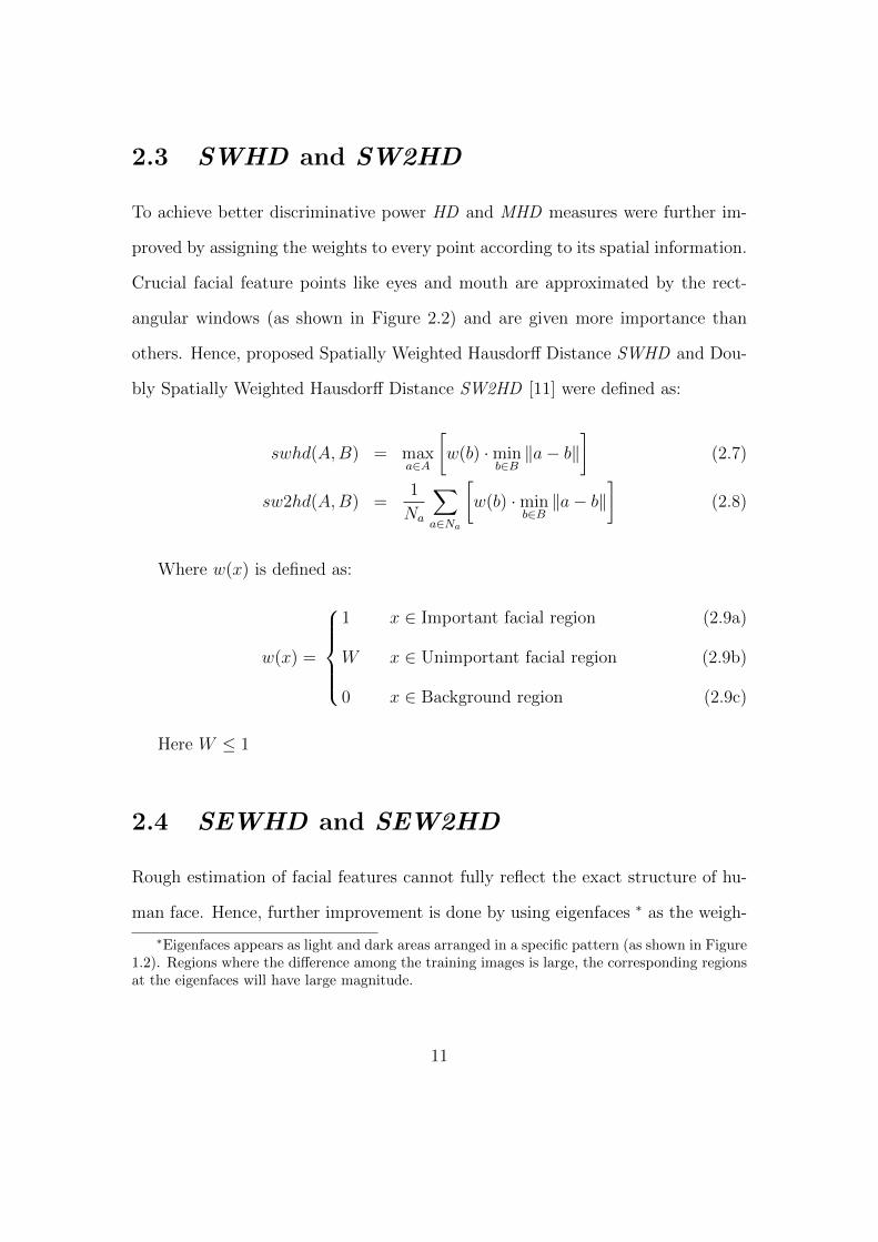
2.3 SWHD and SW2HD
To achieve better discriminative power HD and MHD measures were further im-
proved by assigning the weights to every point according to its spatial information.
Crucial facial feature points like eyes and mouth are approximated by the rect-
angular windows (as shown in Figure 2.2) and are given more importance than
others. Hence, proposed Spatially Weighted Hausdorff Distance SWHD and Dou-
bly Spatially Weighted Hausdorff Distance SW2HD [11] were defined as:
swhd(A,B) = maxa∈A
[w(b) ·min
b∈B‖a− b‖
](2.7)
sw2hd(A,B) =1
Na
∑a∈Na
[w(b) ·min
b∈B‖a− b‖
](2.8)
Where w(x) is defined as:
w(x) =
1 x ∈ Important facial region (2.9a)
W x ∈ Unimportant facial region (2.9b)
0 x ∈ Background region (2.9c)
Here W ≤ 1
2.4 SEWHD and SEW2HD
Rough estimation of facial features cannot fully reflect the exact structure of hu-
man face. Hence, further improvement is done by using eigenfaces ∗ as the weigh-
∗Eigenfaces appears as light and dark areas arranged in a specific pattern (as shown in Figure1.2). Regions where the difference among the training images is large, the corresponding regionsat the eigenfaces will have large magnitude.
11
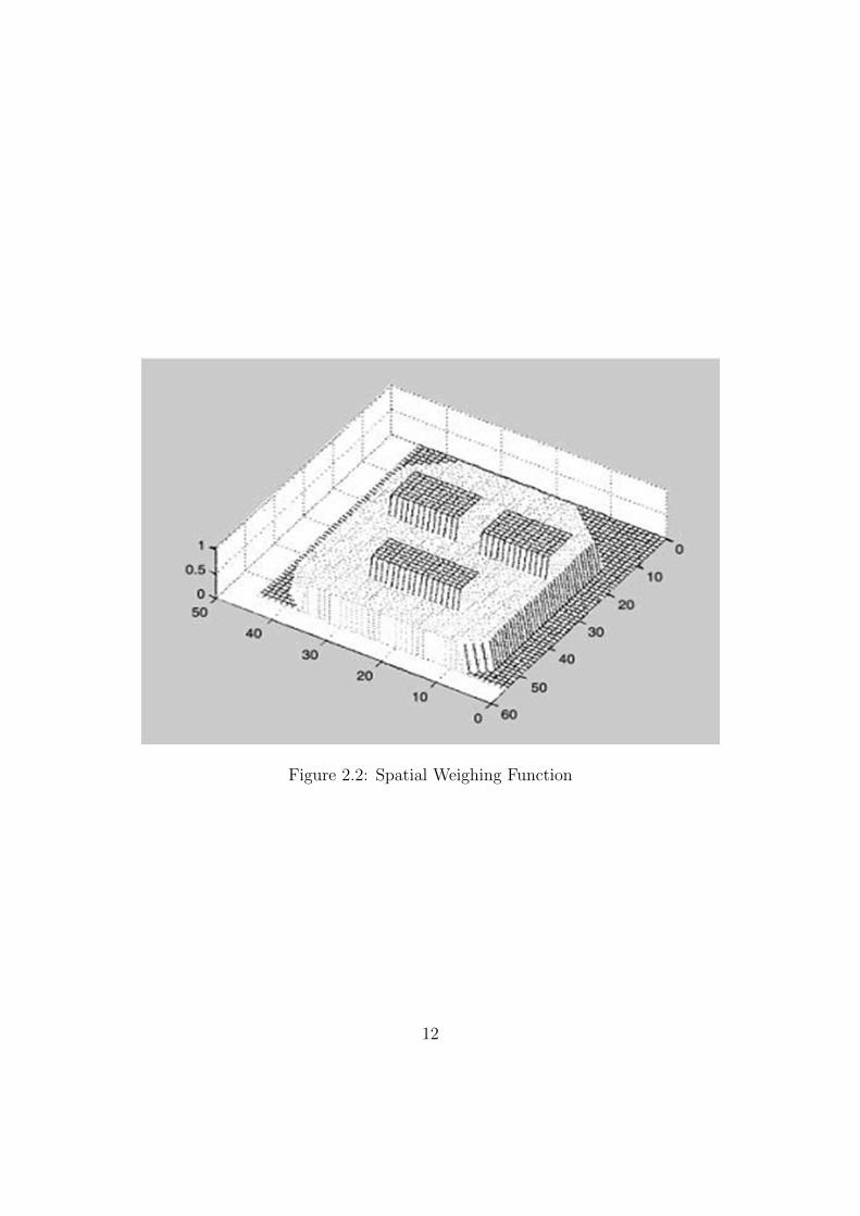
Figure 2.2: Spatial Weighing Function
12
ing function because they represents the most significant variations in the set of
training face images. Proposed Spatially Eigen Weighted Hausdorff Distance SE-
WHD and Doubly Spatially Eigen Weighted Hausdorff Distance SEW2HD [12]
are defined as:
sewhd(A,B) = maxa∈A
[we(b) · min
b∈B‖a− b‖
](2.10)
sew2hd(A,B) =1
Na
∑a∈Na
[we(b) ·min
b∈B‖a− b‖
](2.11)
where we(x) is defined as:
we(x) = The eigen weight function generated by the first eigen vector (2.12)
2.5 Hg and Hpg
Till 2006 Hausdorff distance measure was being explored only on edge maps but
unfortunately on edge images most of the important facial features are lost which
are very useful for facial discrimination. Gray Hausdorff Distance Hg and Partial
Gray Hausdorff Distance Hpg [13] measures works on quantized images and are
found robust to slight variation in poses, expressions and illumination. It is seen
that quantized image with n ≥ 5 retains the perceptual appearance and the in-
trinsic facial feature information that resides in gray values (as shown in Figure
2.3).
Hg and Hpg are defined as :
13

(a) top 1 bit (b) top 2 bits (c) top 3 bits (d) top 4 bits
(e) top 5 bits (f) top 6 bits (g) top 7 bits (h) top 8 bits
Figure 2.3: Quantized Images
hg(A,B) = maxi=0..2n−1
a∈Ai
d(a,Bi) (2.13)
hpg(A,B) = Kth maxi=0..2n−1
a∈Ai
d(a,Bi) (2.14)
where d(a,Bi) is defined as :
d(a,Bi) =
{minb∈Bi
‖a− b‖ if Bi is non-empty (2.15a)
L otherwise (2.15b)
Here, Ai and Bi are the set of pixels in A and B images having quantized gray
value i. L is a large value can be√r2 + c2 + 1 for r× c images. Both Hg and Hpg
search for a correspondence between sets of pixels having the same quantized value
from two images where the distance measure itself being the distance between the
14

worst correspondence.
2.6 Application in Face Recognition
All of the measures discussed before Hg and Hpg works on edge images. They treat
an image as a set of edge points and then calculates the value of the measure using
its mathematical formula as defined above (in their respective section).
Hg and Hpg works on quantized images. They treat a gray-scale image A
as 256 sets of points (say {A0, A1, A2, ..A255} ), where Ai is the set of pixels in
image A having quantized gray value i. Then Hg and Hpg are calculated using its
mathematical formula as defined above.
15
Chapter 3
The Proposed Approach and
Implementation Details
We define a new Normalized Unmatched Points measure NUP that can be applied
on gray-scale facial images. It is similar to the Hausdorff distance based mea-
sures but is computationally less expensive and more accurate. NUP also shows
robustness against slight variation in poses, expressions and illumination.
In a gray-scale image, each pixel has an 8-bit gray value that lies in between 0
to 255 which is very sensitive to the environmental conditions. In varying uncon-
trolled environment, it becomes very difficult for a measure to capture any useful
information about the image. Hence face recognition is very challenging using
gray-scale images.
16

3.1 Transformation
Sudha and Wong [14] describe a transformation (referred hereafter as SK-transformation)
which provides some robustness against illumination variation and local non-rigid
distortions by converting gray scale images into transformed images that preserve
intensity distribution.
A pixel’s relative gray value in its neighborhood can be more stable than its
own gray value. Hence in an SK-transformed image, every pixel is represented
by an 8-element vector which in itself can store the sign of first-order derivative
with respect to its 8-neighborhood. Each SK-transformed images hold a property
that even if the gray value of the pixels are being changed in different poses of the
same subject, their corresponding vector (i.e. its contribution in the transformed
image) do not change by a great extent.
The above property holds when gray values of neighborhood pixels are not too
close to each other. But usually, we have small variations in the gray values (e.g.
in background, facial features etc.), where the above property fails to hold.
The problem is caused by our comparator function, which assumes for any gray
level X that:
X
= X (3.1a)
< α ∈ (X, 255] (3.1b)
> α ∈ [0, X) (3.1c)
where X is a gray level not merely a number.
Practically a gray level X is neither greater than gray level (X − 1) nor less
than gray level (X + 1); ideally they should be considered as equal. Gray levels
17
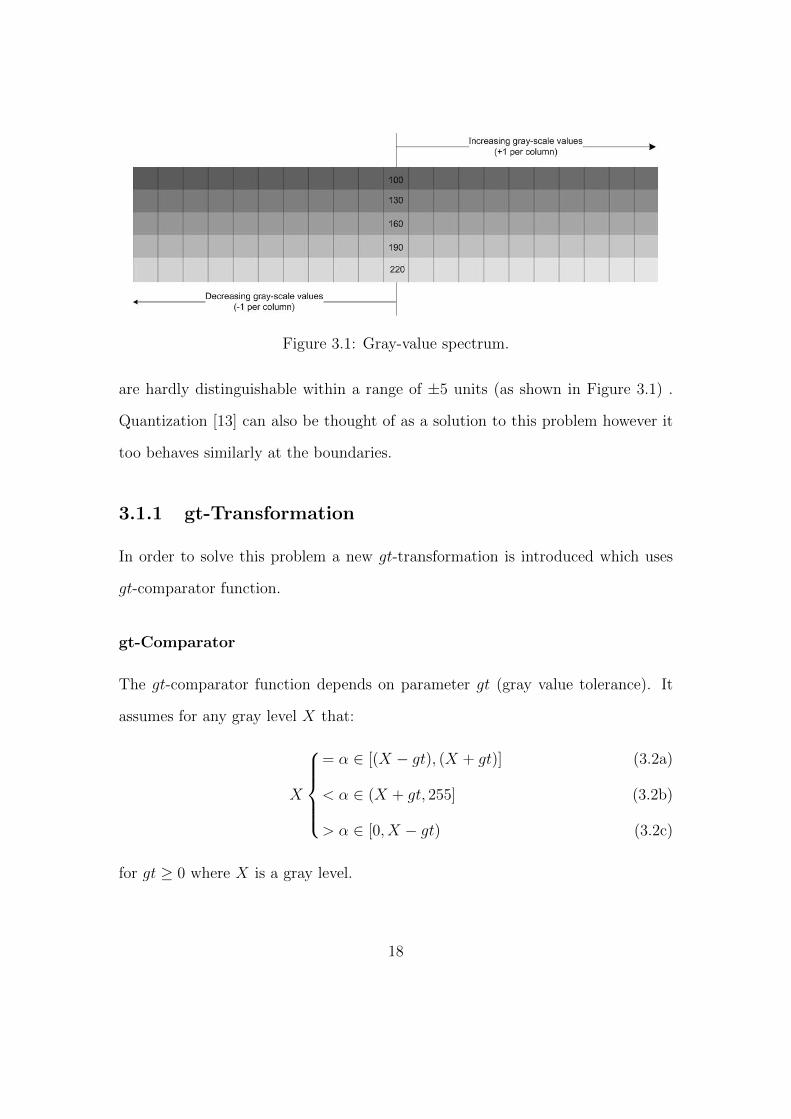
Figure 3.1: Gray-value spectrum.
are hardly distinguishable within a range of ±5 units (as shown in Figure 3.1) .
Quantization [13] can also be thought of as a solution to this problem however it
too behaves similarly at the boundaries.
3.1.1 gt-Transformation
In order to solve this problem a new gt-transformation is introduced which uses
gt-comparator function.
gt-Comparator
The gt-comparator function depends on parameter gt (gray value tolerance). It
assumes for any gray level X that:
X
= α ∈ [(X − gt), (X + gt)] (3.2a)
< α ∈ (X + gt, 255] (3.2b)
> α ∈ [0, X − gt) (3.2c)
for gt ≥ 0 where X is a gray level.
18

As shown in the Figure 3.2, with big gt values important facial features are
lost.
(a) Original (b) gt = 0 (c) gt = 1 (d) gt = 2
(e) gt = 3 (f) gt = 4 (g) gt = 5 (h) gt = 6
(i) gt = 7 (j) gt = 8 (k) gt = 9 (l) gt = 10
Figure 3.2: gt-Transformed images
If there is limited variation in illumination and lighting conditions, then gt = 5
can be useful (as shown in Figure 3.1). The value of gt depends on the database
that is being tested; however it cannot be chosen to be very large; otherwise
19
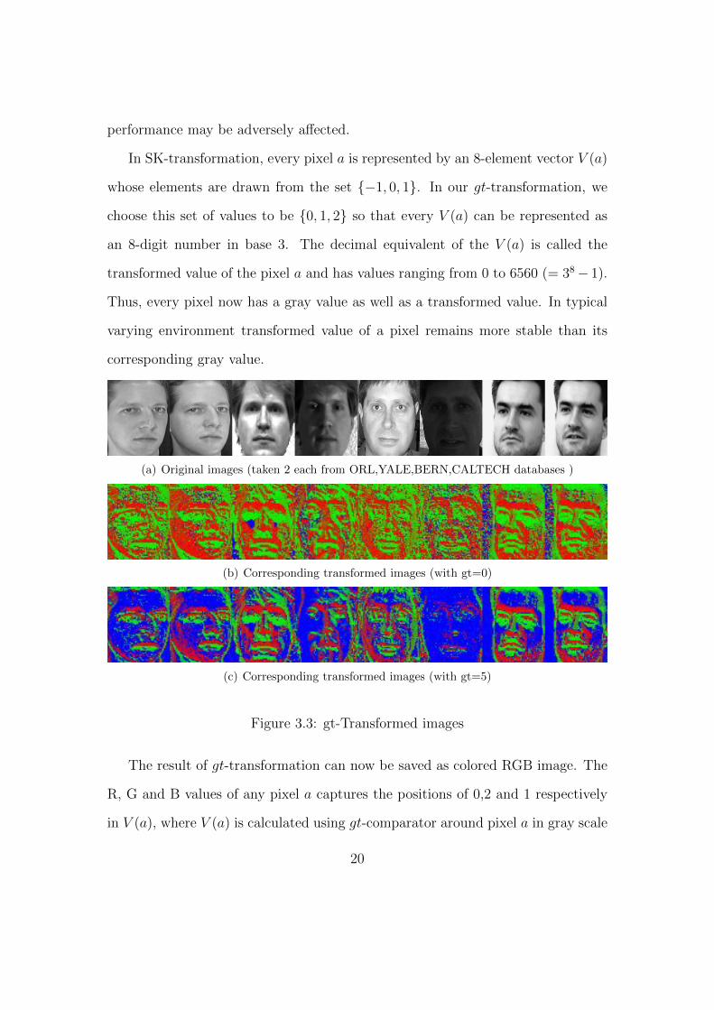
performance may be adversely affected.
In SK-transformation, every pixel a is represented by an 8-element vector V (a)
whose elements are drawn from the set {−1, 0, 1}. In our gt-transformation, we
choose this set of values to be {0, 1, 2} so that every V (a) can be represented as
an 8-digit number in base 3. The decimal equivalent of the V (a) is called the
transformed value of the pixel a and has values ranging from 0 to 6560 (= 38− 1).
Thus, every pixel now has a gray value as well as a transformed value. In typical
varying environment transformed value of a pixel remains more stable than its
corresponding gray value.
(a) Original images (taken 2 each from ORL,YALE,BERN,CALTECH databases )
(b) Corresponding transformed images (with gt=0)
(c) Corresponding transformed images (with gt=5)
Figure 3.3: gt-Transformed images
The result of gt-transformation can now be saved as colored RGB image. The
R, G and B values of any pixel a captures the positions of 0,2 and 1 respectively
in V (a), where V (a) is calculated using gt-comparator around pixel a in gray scale
20
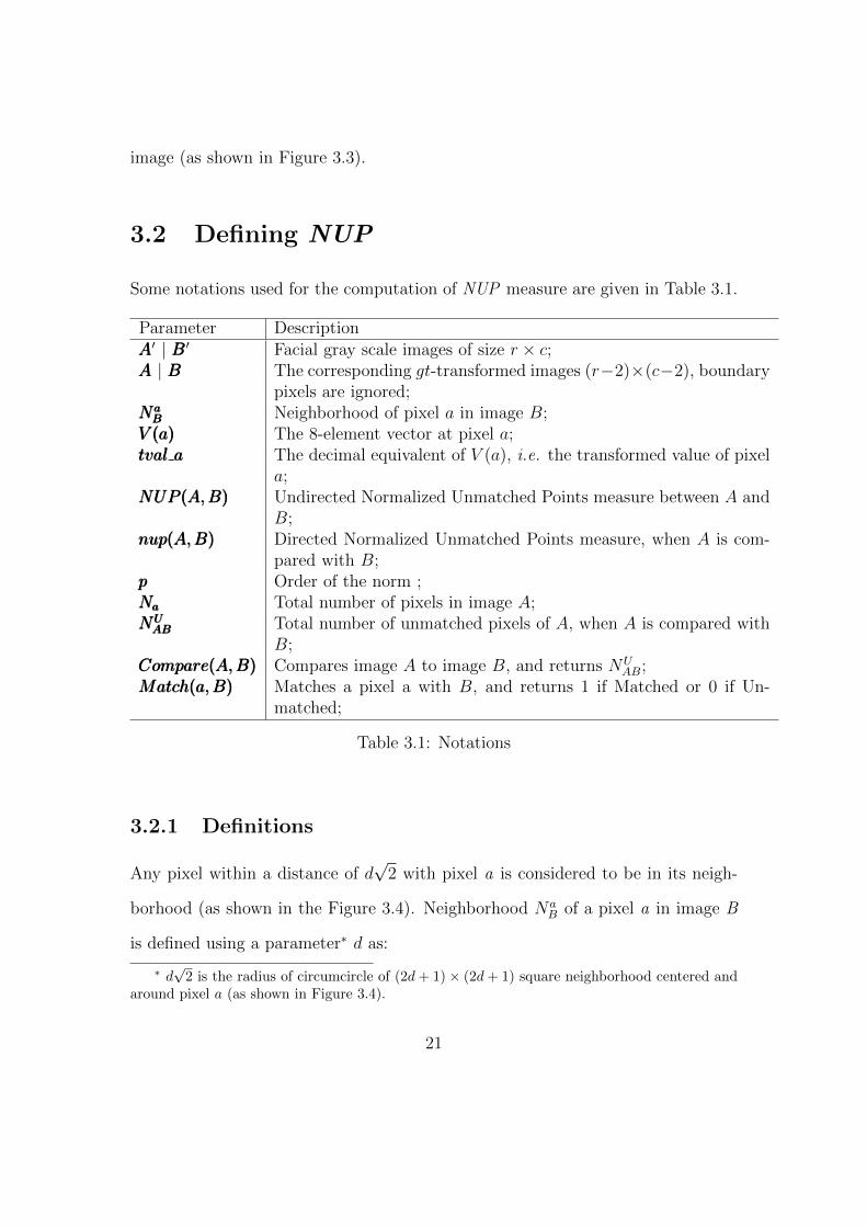
image (as shown in Figure 3.3).
3.2 Defining NUP
Some notations used for the computation of NUP measure are given in Table 3.1.
Parameter DescriptionAAA′ | BBB′ Facial gray scale images of size r × c;AAA | BBB The corresponding gt-transformed images (r−2)×(c−2), boundary
pixels are ignored;Na
BNaBNaB Neighborhood of pixel a in image B;
V (a)V (a)V (a) The 8-element vector at pixel a;tval atval atval a The decimal equivalent of V (a), i.e. the transformed value of pixel
a;NUP (A,B)NUP (A,B)NUP (A,B) Undirected Normalized Unmatched Points measure between A and
B;nup(A,B)nup(A,B)nup(A,B) Directed Normalized Unmatched Points measure, when A is com-
pared with B;ppp Order of the norm ;NaNaNa Total number of pixels in image A;NU
ABNUABNUAB Total number of unmatched pixels of A, when A is compared with
B;Compare(A,B)Compare(A,B)Compare(A,B) Compares image A to image B, and returns NU
AB;Match(a,B)Match(a,B)Match(a,B) Matches a pixel a with B, and returns 1 if Matched or 0 if Un-
matched;
Table 3.1: Notations
3.2.1 Definitions
Any pixel within a distance of d√
2 with pixel a is considered to be in its neigh-
borhood (as shown in the Figure 3.4). Neighborhood NaB of a pixel a in image B
is defined using a parameter∗ d as:
∗ d√
2 is the radius of circumcircle of (2d + 1)× (2d + 1) square neighborhood centered andaround pixel a (as shown in Figure 3.4).
21

Figure 3.4: Circular Neighborhood
NaB = {b ∈ B | ‖a− b‖ ≤ d
√2} (3.3)
Compare(A,B) compares image A to image B, and returns NUAB (i.e. number
of unmatched points), which can be defined as:
NUAB =
∑a∈A
(1−Match(a,B)) (3.4)
22
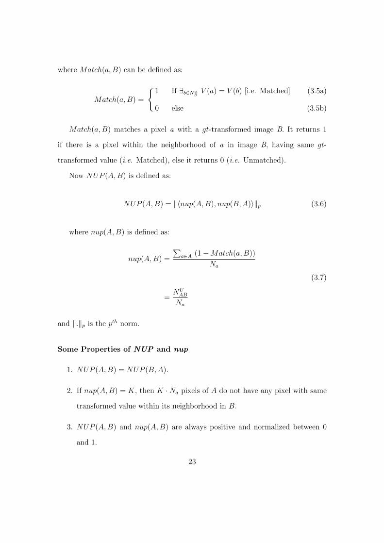
where Match(a,B) can be defined as:
Match(a,B) =
{1 If ∃b∈Na
BV (a) = V (b) [i.e. Matched] (3.5a)
0 else (3.5b)
Match(a,B) matches a pixel a with a gt-transformed image B. It returns 1
if there is a pixel within the neighborhood of a in image B, having same gt-
transformed value (i.e. Matched), else it returns 0 (i.e. Unmatched).
Now NUP (A,B) is defined as:
NUP (A,B) = ‖〈nup(A,B), nup(B,A)〉‖p (3.6)
where nup(A,B) is defined as:
nup(A,B) =
∑a∈A (1−Match(a,B))
Na
=NU
AB
Na
(3.7)
and ‖.‖p is the pth norm.
Some Properties of NUP and nup
1. NUP (A,B) = NUP (B,A).
2. If nup(A,B) = K, then K ·Na pixels of A do not have any pixel with same
transformed value within its neighborhood in B.
3. NUP (A,B) and nup(A,B) are always positive and normalized between 0
and 1.
23

4. NUP (A,B) and nup(A,B) are parameterized by gt, d and p.
3.3 Efficient computation of NUP
Compare(A,B) and Match(a,B) operations are required to compute NUP (A,B).
Both of these operations take O(rc) time for r× c sized images. Hence, computing
NUP (A,B) using naive method requires O(r2c2) time , which is prohibitively
computationally intensive. Hence an efficient algorithm is required to compute
the NUP measure.
3.3.1 Algorithm
Flow Control of the Algorithm
Algorithm to compute NUP(A,B) (Algorithm 1) computes Normalized Unmatched
Points measure between two gt-transformed images. It calls the function Com-
pare(A,B) (Algorithm 2) that computes directional unmatched points, which itself
calls Matched(a,B) (Algorithm 3) which only checks whether a pixel a got a Match
in image B or not.
Discussion of the Algorithms
In Algorithm 1, two gt-transformed images are passed. Compare(A,B) function is
called to calculate the directional unmatched points, which is further normalized
by total number of pixels in the image.
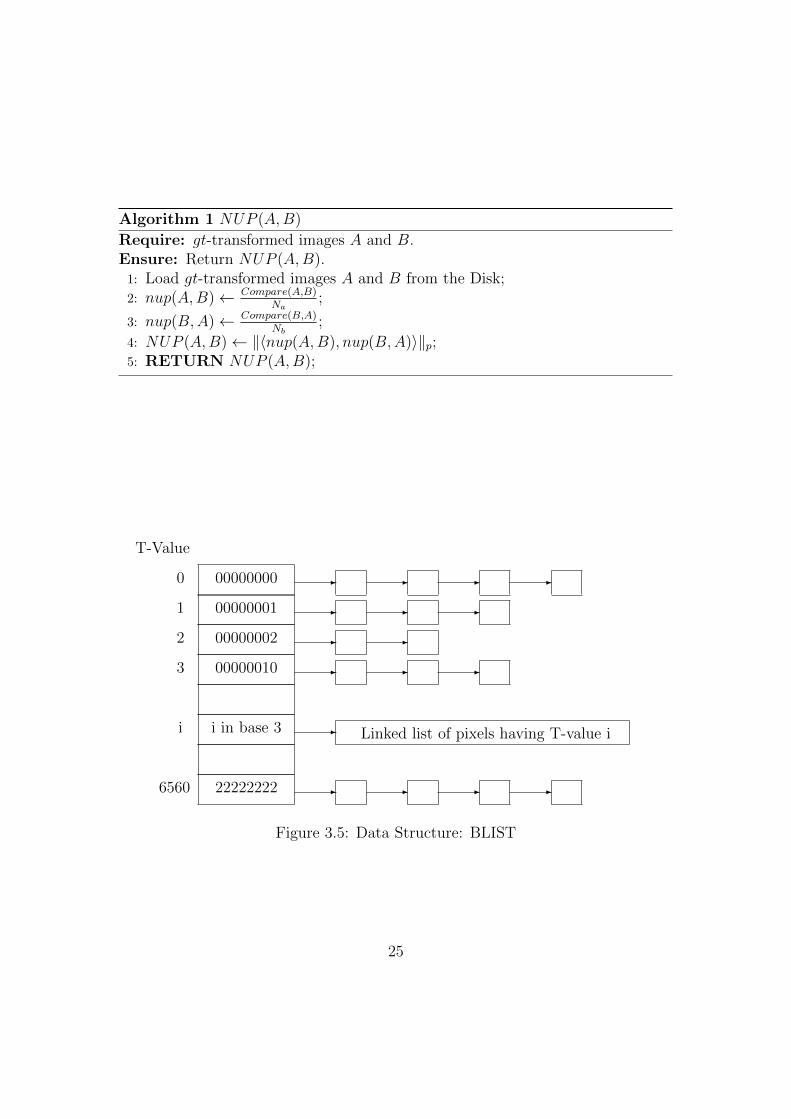
To perform the Match(a,B) operation efficiently an array of pointers to linked
list BLIST (as shown in Figure 3.5) is created. BLIST will have 38 elements such
24
Algorithm 1 NUP (A,B)
Require: gt-transformed images A and B.Ensure: Return NUP (A,B).
1: Load gt-transformed images A and B from the Disk;2: nup(A,B)← Compare(A,B)
Na;
3: nup(B,A)← Compare(B,A)Nb
;
4: NUP (A,B)← ‖〈nup(A,B), nup(B,A)〉‖p;5: RETURN NUP (A,B);
-
-
-
-
-
- - -
- - -
- -
-
- -
-
2
1
0
22222222
00000010
00000002
00000001
00000000
i i in base 3
6560
Linked list of pixels having T-value i
3
T-Value
Figure 3.5: Data Structure: BLIST
25
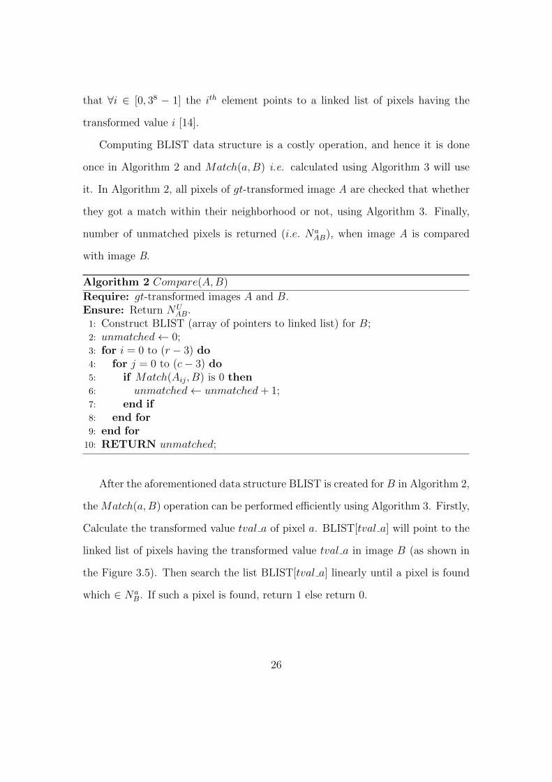
that ∀i ∈ [0, 38 − 1] the ith element points to a linked list of pixels having the
transformed value i [14].
Computing BLIST data structure is a costly operation, and hence it is done
once in Algorithm 2 and Match(a,B) i.e. calculated using Algorithm 3 will use
it. In Algorithm 2, all pixels of gt-transformed image A are checked that whether
they got a match within their neighborhood or not, using Algorithm 3. Finally,
number of unmatched pixels is returned (i.e. NaAB), when image A is compared
with image B.
Algorithm 2 Compare(A,B)
Require: gt-transformed images A and B.Ensure: Return NU
AB.1: Construct BLIST (array of pointers to linked list) for B;2: unmatched← 0;3: for i = 0 to (r − 3) do4: for j = 0 to (c− 3) do5: if Match(Aij, B) is 0 then6: unmatched← unmatched+ 1;7: end if8: end for9: end for
10: RETURN unmatched;
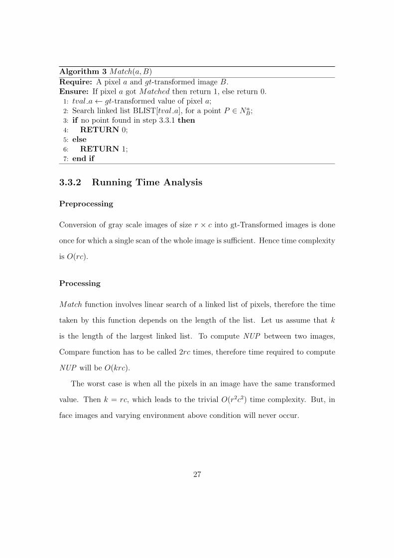
After the aforementioned data structure BLIST is created for B in Algorithm 2,
the Match(a,B) operation can be performed efficiently using Algorithm 3. Firstly,
Calculate the transformed value tval a of pixel a. BLIST[tval a] will point to the
linked list of pixels having the transformed value tval a in image B (as shown in
the Figure 3.5). Then search the list BLIST[tval a] linearly until a pixel is found
which ∈ NaB. If such a pixel is found, return 1 else return 0.
26
Algorithm 3 Match(a,B)
Require: A pixel a and gt-transformed image B.Ensure: If pixel a got Matched then return 1, else return 0.
1: tval a← gt-transformed value of pixel a;2: Search linked list BLIST[tval a], for a point P ∈ Na
B;3: if no point found in step 3.3.1 then4: RETURN 0;5: else6: RETURN 1;7: end if
3.3.2 Running Time Analysis
Preprocessing
Conversion of gray scale images of size r × c into gt-Transformed images is done
once for which a single scan of the whole image is sufficient. Hence time complexity
is O(rc).
Processing
Match function involves linear search of a linked list of pixels, therefore the time
taken by this function depends on the length of the list. Let us assume that k
is the length of the largest linked list. To compute NUP between two images,
Compare function has to be called 2rc times, therefore time required to compute
NUP will be O(krc).
The worst case is when all the pixels in an image have the same transformed
value. Then k = rc, which leads to the trivial O(r2c2) time complexity. But, in
face images and varying environment above condition will never occur.
27
3.3.3 Space Analysis
Space requirement of an gray image is O(rc). The same space can be utilized for
storing gt-transformed images as original images are not used for further compu-
tation.
The array of pointers to the linked list of pixels (BLIST), is of size (38). This
is constant independent of image size. As all the pixels in both the images will
be added once to lists of pixels the total memory used in constructing the data
structure for the images is 2 · (38 + rc) units.
28

Chapter 4
Experimental Results and
Analysis
4.1 Setup for Face Recognition System
Our face recognition system consists of 3 phases. In first phase face detection is
done, in second phase some preprocessing is performed (i.e. gt-transformation),
and finally in third phase face comparison using NUP measure is performed.
In this system, face normalization is optional because for big databases a lot
of manual work is required to gather the ground truth information. Neighborhood
function will take care of this normalization. Also face feature extraction and
matching is not required as suggested in Figure 1.1, because our approach relies
on globally analysing a face as a whole for the recognition purpose.
29

(a) Input Face images
(b) Cropped Face images
(c) Normalized Face images
(d) gt-Transformed images(gt=0)
(e) gt-Transformed images(gt=5)
Figure 4.1: Images produced after various phases
30
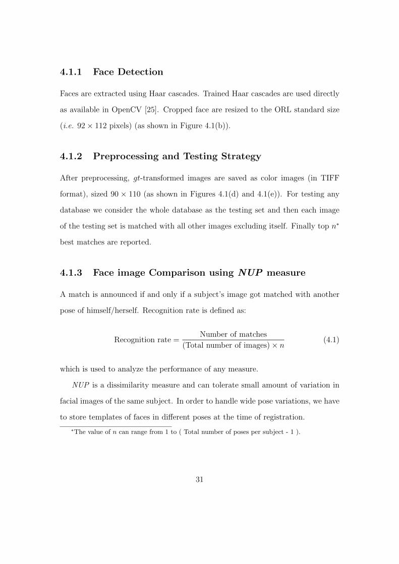
4.1.1 Face Detection
Faces are extracted using Haar cascades. Trained Haar cascades are used directly
as available in OpenCV [25]. Cropped face are resized to the ORL standard size
(i.e. 92× 112 pixels) (as shown in Figure 4.1(b)).
4.1.2 Preprocessing and Testing Strategy
After preprocessing, gt-transformed images are saved as color images (in TIFF
format), sized 90 × 110 (as shown in Figures 4.1(d) and 4.1(e)). For testing any
database we consider the whole database as the testing set and then each image
of the testing set is matched with all other images excluding itself. Finally top n∗
best matches are reported.
4.1.3 Face image Comparison using NUP measure
A match is announced if and only if a subject’s image got matched with another
pose of himself/herself. Recognition rate is defined as:
Recognition rate =Number of matches
(Total number of images)× n(4.1)
which is used to analyze the performance of any measure.
NUP is a dissimilarity measure and can tolerate small amount of variation in
facial images of the same subject. In order to handle wide pose variations, we have
to store templates of faces in different poses at the time of registration.
∗The value of n can range from 1 to ( Total number of poses per subject - 1 ).
31

Database Subjects Poses Total Images VaryingORL 40 10 400 Poses and Expressions
YALE 15 11 165 Illumination and ExpressionsBERN 30 10 300 Poses and Expressions
CALTECH 17 20 340 Poses and IlluminationIITK 149 10 1490 Poses and Scale
Table 4.1: Databases Information
4.2 Experimental Results
The performance evaluation of NUP measure was done on some standard bench-
mark facial image databases such as ORL [17], YALE [18], BERN [19], CALTECH
[20], and IITK (as shown in Table 4.1). Under varying lighting conditions, poses
and expressions NUP measure has demonstrated very good recognition rates.
4.2.1 Parameterized results of NUP based recognition on
different facial databases
NUP measure is parameterized primarily by two parameters gt and d, the third
parameter p (order of norm) is set to 20 for this work. Gray value Tolerance gt
can vary within range [0, 5] and Neighborhood parameter d can vary within range
[1, 15].
Discussion for gt (Gray Value Tolerance)
From the definition of gt (as shown in Equation 3.2a) it is clear that more and
more elements of V (a) start acquiring value 1 with higher gt values. This will
boost the blue value of pixels in the gt-transformed images. In the presence of
directional lights and heavy illumination condition variations some of the facial
32

(a) Original
(b) gt = 0
(c) gt = 5
Figure 4.2: Effect of High gt values under heavy illumination variation
33

regions becomes significantly dark. High gt values in these conditions may further
lift up the blue value upto an extent that blue color starts dominating in gt-
transformed image (as shown in Figure 4.2). This results in deterioration of the
performance.
NUP measure performs well on illumination varying databases such as YALE
and CALTECH (as shown in Table 4.1) with lower gt values (as shown in Figures
4.4 and 4.6). Databases like ORL, BERN and IITK where illumination is not
varying too much and directional lighting is also absent, higher gt values will yield
better discrimination (as shown in Figures 4.3, 4.5 and 4.7).
Discussion for d (Neighborhood parameter)
From the definition of d (as shown in Equation 3.3), on unnormalized †, pose and
expression varying images of ORL, BERN and IITK databases, bigger neighbor-
hood yield good performance as also suggested by the plots (as shown in Figures
4.3, 4.5 and 4.7).
On databases like YALE and CALTECH smaller neighborhood is expected
because they contain fairly normalized images without too much pose and expres-
sion variations (as shown in Table 4.1), as also suggested by the plots (as shown
in Figures 4.4 and 4.6).
†Images not normalized with respect to any of the facial features.
34

(a) ORL, Considering top 1 best matched
(b) ORL, Considering top 5 best matched
Figure 4.3: ORL Database Results
35

(a) YALE, Considering top 1 best matched
(b) YALE, Considering top 5 best matched
Figure 4.4: YALE Database Results
36

(a) BERN, Considering top 1 best matched
(b) BERN, Considering top 5 best matched
Figure 4.5: BERN Database Results
37

(a) CALTECH, Considering top 1 best matched
(b) CALTECH, Considering top 5 best matched
Figure 4.6: CALTECH Database Results
38
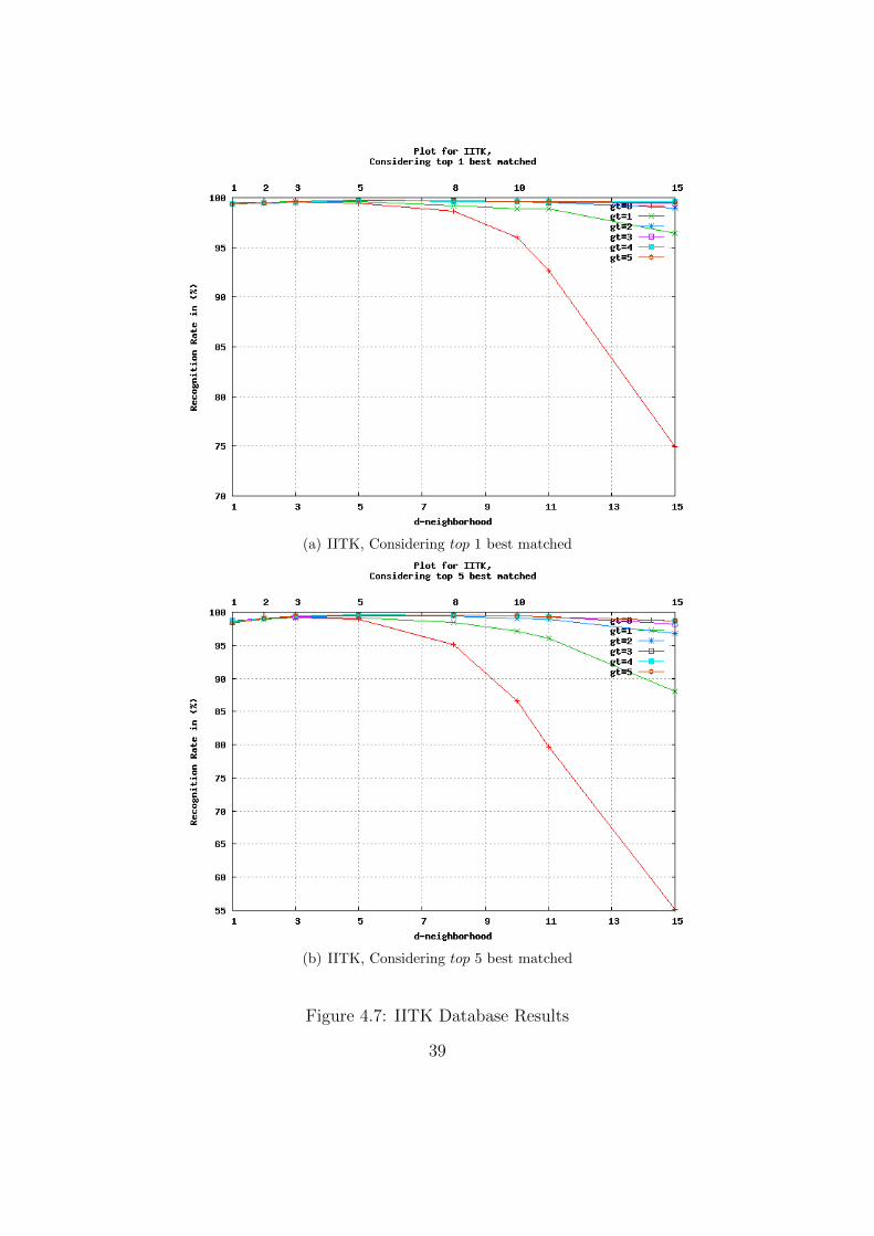
(a) IITK, Considering top 1 best matched
(b) IITK, Considering top 5 best matched
Figure 4.7: IITK Database Results
39
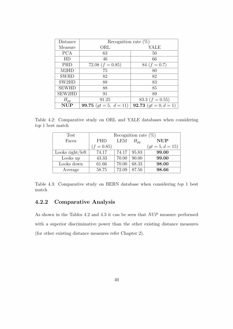
Distance Recognition rate (%)Measure ORL YALE
PCA 63 50HD 46 66
PHD 72.08 (f = 0.85) 84 (f = 0.7)M2HD 75 80SWHD 82 82SW2HD 88 83SEWHD 88 85SEW2HD 91 89
Hpg 91.25 83.3 (f = 0.55)NUP 99.75 (gt = 5, d = 11) 92.73 (gt = 0, d = 1)
Table 4.2: Comparative study on ORL and YALE databases when consideringtop 1 best match
Test Recognition rate (%)Faces PHD LEM Hpg NUP
(f = 0.85) (gt = 5, d = 15)Looks right/left 74.17 74.17 95.83 99.00
Looks up 43.33 70.00 90.00 99.00Looks down 61.66 70.00 68.33 98.00
Average 58.75 72.09 87.50 98.66
Table 4.3: Comparative study on BERN database when considering top 1 bestmatch
4.2.2 Comparative Analysis
As shown in the Tables 4.2 and 4.3 it can be seen that NUP measure performed
with a superior discriminative power than the other existing distance measures
(for other existing distance measures refer Chapter 2).
40

Figure 4.8: Results of NUP based face recognition on different face databasesconsidering top n best matches.
4.2.3 Overall Analysis
The overall performance of NUP is evaluated by testing it over various standard
face databases with respect to n (as shown in Figure 4.8). For n = 1, 2 recognition
rates are very good(as shown in Figure 4.8 and Table 4.4). With increasing n the
recognition rate falls which is obvious.
41
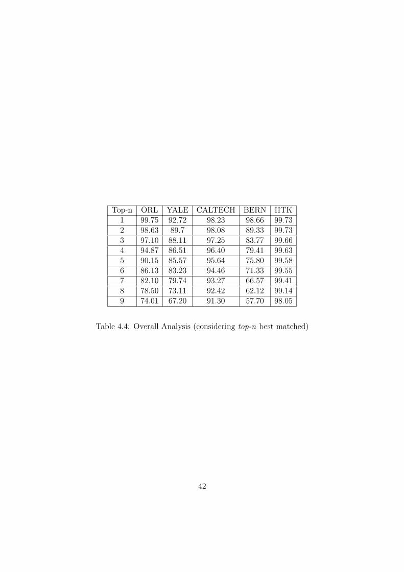
Top-n ORL YALE CALTECH BERN IITK1 99.75 92.72 98.23 98.66 99.732 98.63 89.7 98.08 89.33 99.733 97.10 88.11 97.25 83.77 99.664 94.87 86.51 96.40 79.41 99.635 90.15 85.57 95.64 75.80 99.586 86.13 83.23 94.46 71.33 99.557 82.10 79.74 93.27 66.57 99.418 78.50 73.11 92.42 62.12 99.149 74.01 67.20 91.30 57.70 98.05
Table 4.4: Overall Analysis (considering top-n best matched)
42

Chapter 5
Conclusion and Further Work
In this work, a new measure Normalized Unmatched Points (NUP) has been pro-
posed to compare gray facial images. The face recognition approach based on
NUP measure is different from existing Hausdorff distance based methods as it
works on gt-transformed images that are obtained from gray images rather than
edge images. Thus, this approach can achieve the appearance based comparison
of faces. An algorithm is also presented to efficiently compute the NUP measure.
The NUP measure is primarily controlled by two parameters, gt and d. The
values for the parameters are set taking into account the illumination variation and
the nature of the images in the face database. NUP measure has shown tolerance
to varying poses, expressions and illumination conditions. Experiments on ORL,
YALE, BERN and CALTECH benchmark face databases with the NUP measure
have achieved recognition rates of 95% and above.
In a constrained environment which is uniformly well illuminated NUP mea-
sure could also be used for video surveillance, scene segmentation in videos, face
detection, face authentication. The NUP measure is computationally inexpensive
43

and provides good performance levels. For recognition in complex varying envi-
ronments with big images it can also be used as fast first level scanner, working
on re-sampled∗ images providing assistance to the higher levels. This measure can
also be extended to other biometric traits as iris and ear.
Experimental results have shown that the NUP measure has a better discrim-
inative power as it can achieve a higher recognition rate than HD, PHD, MHD,
M2HD, SWHD, SW2HD, SEWHD, SEW2HD, Hg and Hpg.
∗A n × n sized image can be re-sampled as considering every kth scan line, and on it every
lth pixel. Hence n× n pixels, are reduced to only[n2
k·l
]pixels.
44
Bibliography
[1] A.Samal and P.A.Iyengar, Automatic recognition and analysis of human facesand facial expressions; a survey, Pattern recognition 25 (1) (1992) 65-77.
[2] R.Chellappa, C.L.Wilson and S.Sircohey, Human and machine recognition offaces: a survey, Proc. IEEE 83 (5) (1995) 705-740.
[3] M.Turk and A.Pentland, Eigenfaces for recognition, Journal of cognitive Neu-roscience, March 1991.
[4] L.Wiskott, J.-M.Fellous, N.Kuiger and C.Von der Malsburg, Face recognitionby elastic bunch graph matching, IEEE Tran. on Pattern Anal.Mach.Intell., 19:775-779.
[5] S.Lawrence, C.L.Giles, A.C.Tsoi, and A. D. Back, Face recognition: A con-volutional neural network approach, IEEE Trans. Neural Networks, 8:98-113,1997.
[6] Guodong Guo, Stan Z. Li, and Kapluk Chan, Face Recognition by SupportVector Machines, Automatic Face and Gesture Recognition, 2000.Proc. FourthIEEE Inter.Conf. on Volume,Issue,2000 Page(s):196-201
[7] F.S.Samaria, Face recognition using Hidden Markov Models. PhD thesis, Trin-ity College, University of Cambridge,Cambridge,1994.
[8] D.P.Huttenlocher, G.A.Klanderman and W.A.Rucklidge, Comparing imagesusing the Hausdorff distance, IEEE Trans.Pattern Anal.Mach.Intell,vol.15,no.9,pp.850-863, sep.1993.
[9] W.J.Rucklidge, Locating objects using the Hausdorff distance, ICCV 95: Proc.5th Int. Conf. Computer Vision, Washington, D.C, June 1995, pp. 457-464.
[10] B.Takacs, Comparing face images using the modified Hausdorff distance, Pat-tern Recognit,vol.31, no.12,pp.1873-1881, 1998.
45
[11] B.Guo, K.-M.Lam, K.-H.Lin and W.-C.Siu, Human face recognition based onspatially weighted Hausdorff distance, Pattern Recognit. Lett., vol. 24,pp.499-507, Jan. 2003.
[12] K.-H.Lin, K.-M.Lam and W.-C.Siu, Spatially eigen-weighted Hausdorff dis-tances for human face recognition, Pattern Recognit.,vol.36,pp.1827-1834, Aug.2003.
[13] E.P.Vivek and N.Sudha, Gray Hausdorff distance measure for comparing faceimages, IEEE Trans. Inf. Forensics and Security, vol.1, no. 3, Sep. 2006.
[14] N.Sudha and Y.Wong, Hausdorff distance for iris recognition, Proc. of 22ndIEEE Int. Symp. on Intelligent Control ISIC 2007,pages 614-619,Singapore,October 2007.
[15] M.Dubuisson and A.K.Jain, A modified Hausdorff distance for object Match-ing, Proc. 12th Int. conf. on Pattern Recognition (ICPR), Jerusalem, Israel,(1994).
[16] Y.Gao and M.K.Leung, Face recognition using line edgemap, IEEE Trans.Pattern Anal. Machine Intell.,vol.24, pp.764-779, Jun. 2002.
[17] The ORL Database of Faces[Online], Available:http://www.uk.research.att.com/facedatabase.html.
[18] The Yale University Face Database[Online], Available:http://cvc.yale.edu/projects/yalefaces/yalefaces.html.
[19] The Bern University Face Database[Online], Available:ftp://ftp.iam.
unibe.ch/pub/images/faceimages/.
[20] The Caltech University Face Database[Online], Available:http://www.
vision.caltech.edu/html-files/archive.html.
[21] David A. Forsyth and Jean Ponce, Computer Vision - A Modern Approach,Pearson Education, 2003.
[22] Yang,M.H.;Kriegman,D.J. and Ahuja, N, Detecting Faces in Images: A Sur-vey, IEEE Transaction (PAMI), Vol.24, No. 1, (2002),(34-58).
[23] Li,S.Z and Jain, A.K Handbook of Face Recognition, Springer-Verlag, (2005)
[24] Yuankui Hu and Zengfu Wang, A Similarity Measure Based on Hausdorff Dis-tance for Human Face Recognition, 18th International Conference on PatternRecognition (ICPR06), IEEE (2006).
46

[25] Gary Bradski, Adrian Kaehler Learning OpenCV: Computer Vision withthe OpenCV Library, [ONLINE ], Available at http://www.amazon.com/
Learning-OpenCV-Computer-Vision-Library/dp/0596516134
47