A new 3D finite element model of the IEC 60318-1 artificial ear Agustin Bravo , Richard Barham , Mariano Ruiz1, Juan Manuel Lopez , Guillermo De Areas and Manuel Recuero

Grupo de Investigation en Instrumentation y Acustica Aplicada, Universidad Politecnica de Madrid; Ctra Valencia Km-7, Madrid 28031, Spain

Acoustics and Ionising Radiation Team, National Physical Laboratory, Hampton Road, Teddington TW11 8QH, UK

Abstract The artificial ear specified in IEC 60318-1 is used for the measurement of headphones and has been designed to present an acoustic load equivalent to that of normal human ears. In this respect it is specified in terms of an acoustical impedance, and modelled by a lumped parameter approach. However, this has some inherent frequency limitations and becomes less valid as the acoustic wavelength approaches the characteristic dimensions within the device. In addition, when sound propagates through structures such as narrow tubes, annular slits or over sharp corners, noticeable thermal and viscous effects take place causing further departure from the lumped parameter model. A new numerical model has therefore been developed, which gives proper consideration to the aforementioned effects. Both kinds of losses can be simulated by means of the LMS Virtual Lab acoustic software which facilitates finite and boundary element modelling of the whole artificial ear. A full 3D model of the artificial ear has therefore been developed based on key dimensional data found in IEC 60318-1. The model has been used to calculate the acoustical impedance, and the results compared with the corresponding data determined from the lumped parameter model. The numerical simulation of the artificial ear has been shown to provide realistic results, and is a powerful tool for developing a detailed understanding of the device. It is also proving valuable in the revision of IEC 60318-1 that is currently in progress.

Nomenclature

Symbol i

Ks

Jo Ji

y Po

Meaning

angular frequency Stokes' wave number, according to the formula

Ks = {—icopa/ix)112 where \x is air viscosity coefficient with a value of 1.86 x 10~5 N s i r r 2

zero Bessel order function first order Bessel function air adiabatic constant static air pressure at a barometric pressure of

0.76 m Hg and a temperature of 0 °C Bk = ( - i&>/A)0'5, where A is the thermal

diffusivity of air (m2 s_ 1) with a value of 1.9 x l O ^ n ^ s " 1

h length of a narrow tube in metres r0 radius of a narrow tube in metres ts thickness of rectangular slit in metres ws width of rectangular slit in metres ls length of rectangular slit in metres Po ambient density of the air according to

the formula po = 1-29 x [273/(t + 273)] (To/0.76) kgrrr3, where t is the temperature in °C and Po is the barometric pressure in metres of mercury

c speed of sound in air in m s_1, given by the formula c 331.5Vl+?/273, where t is the temperature in °C

pi

1. Introduction A revision of IEC 60318-1 is currently in progress and some of the issues being considered include

The International Electrotechnical Commission (IEC) pub­lishes standards relating to audiometric equipment. The latest version of the standard specifying performance requirements for pure-tone audiometers was published in 2001 This is used by manufacturers of equipment, and in many countries forms the basis for the regulation of equipment used in hearing assessment. The standard includes calibration considerations and refers to other devices known as ear simulators, which are covered in a further series of IEC standards. An ear simulator is a device for measuring the acoustical output of headphones (and similar devices). Strictly, an ear simulator aims to provide a realistic simulation of the acoustical impedance for the part of the ear to be simulated. However, there is a sub-class of devices that only provide simple volumetric coupling. These are known generically as acoustic couplers. This distinction and the wide range of ear simulators that are available present a number of technical challenges and usability issues. Many examples exist in the literature showing the range of issues associated with the use of ear simulators. Some of the key problems are

1. The use of different types of ear simulator usually leads to different measured acoustic levels for the device being tested. This has resulted in a situation where the type of ear simulator to be used and its specific configuration has to be fully specified for a given application. Of course not all applications can be covered by such an approach, leading to ambiguity in many instances

2. Intercomparisons of measurements using ear simulators, while generally demonstrating good levels of consis­tency have also highlighted limitations in the specifi­cations that make the expected level of agreement unclear. One example is that the expected or allowed variation in acoustical impedance is not stated. Such issues should be addressed to make the calibration process more reliable and enable suitable models for uncertainty estimation to be developed.

3. The models to allow uncertainty estimates for air- and bone-conduction calibrations are currently not given in IEC 60645-1 Some supporting data are becoming available in the literature

IEC has a policy of regularly reviewing its standards, which provides a good opportunity to consider some of the limitations highlighted above.

The ear simulator specified in IEC 60318-1 sometimes known as the artificial ear, is a device intended for measuring supra-aural headphones (i.e. devices intended to be placed on the external pinna) having a particular geometric form, and for circumaural headphones (i.e. devices intended to be placed on the head so as to surround the pinna). The same device forms the basis of recommendations from the International Telecommunications Union (ITU-T) for the measurement of telephony equipment.

- The introduction of a test method for the measurement of the acoustical impedance.

- A review and revision of the specification of the acoustical impedance based on new data derived from measurements of actual devices.

- Specification of a realistic tolerance for the acoustical impedance to enable actual devices to be tested periodically for conformance.

- Review and revision of the lumped parameter model to align with the revised specification derived from measurement data.

This paper aims to contribute to the understanding that supports the development of the standard, by developing a finite element (FE) model of the artificial ear. This is considered essential for understanding the acoustic behaviour of the device beyond what is possible with the lumped parameter model.

An earlier attempt to construct a 2D FE model focused mostly on the problems in accurately modelling the behaviour of narrow tubes and slits within the device, in which the usual assumptions about the medium being lossless become invalid.

This paper describes a new 3D FE model for studying the behaviour of the artificial ear and for calculating the acoustical impedance. The model has been formulated based on the detailed geometric information provided in Annex B of IEC 60318-1 which gives an example design that is the basis for the majority of the devices available commercially.

2. Structure of coupler IEC 60318

The IEC 60318-1 artificial ear consists of three interconnected cavities, two of which are not visible externally. Figure 1 shows the generalized form, but practical devices have a more elegant design. The key features are

• The main cavity, denoted V\, has a conical form and houses a microphone at its base. The upper opening and the surrounding external surface match the form of the earphones it is designed to measure and allows for effective and reproducible placement. The distance between the opening and the plane of the microphone is also specified as this has an implication on the longitudinal resonance frequency. These requirements lead to the geometrical form, as well as the volume of cavity V\ to be fully specified.

• The secondary cavities, denoted V2 and V3, have volumes of 1800 mm3 and 7500 mm3, respectively. However, no further geometrical specification is given in IEC 60318-1 so this becomes a matter of commercial design and implementation.

• The three cavities are connected by specified acoustical masses and resistances, denoted by L2 and R2 (connecting Vi and V2) and L3 and R3 (connecting V\ and V3). The elements are specified by their acoustical impedance rather than by precise dimensions, and manufacturers have their own ways of implementing the requirements.

1.00E+08

1 Ear simulator 2 Removable section / E C efi 3 Microphone

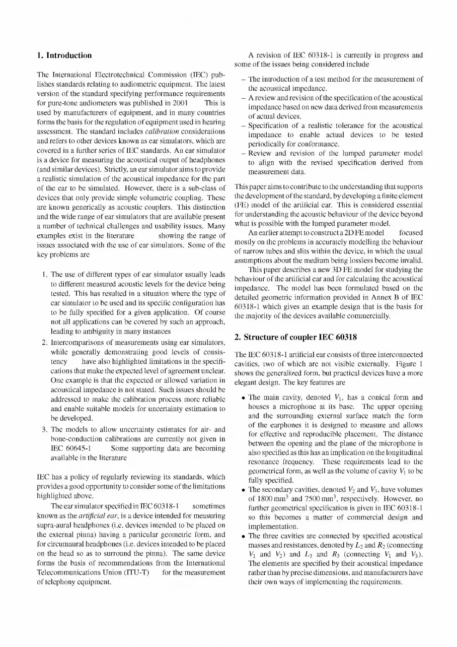
Figure 1. Schematic 1EC proposal: geometric shape and mechanical dimensions of a type I coupler under the IEC 60318 standard normative, wherein the following acoustic parameters have been defined: L2 = 5 x 102 Pas2 irT3, L3 = 1 R? =6 .5 x 106Pasirr3 and R* = 2 x 107Pasirr3 .

ACOUSTIC PRESSURE

R1 5K V1 •

1.76UF

.2 5m H

R2 35

V2 -1.27uF

L3 100mH

R3 200

V3 5.2SuF

Figure 2. Lumped parameter model of a IEC 60318 type I coupler proposed in the IEC standard normative.

• A further acoustical resistance Ri is specified, connecting Vi to the external surroundings. This is for static pressure equalization within the device and has no influence over frequency response.

To summarize, IEC 60318-1 only specified essential geometrical features to establish the correct acoustical impedance and operating frequency range. Thus many dimensional details are left unspecified, to be addressed by specific implementations. However, an example design is also given for information in Annex B of the Standard.

3. Traditional approach: the lumped parameter model LPM

IEC 60318-1:1998 adopts a lumped parameter approach, for specifying the acoustical impedance of the artificial ear. It also includes an equivalent circuit, shown in figure 2, having an electrical impedance analogous to the specified acoustical impedance, where one electrical ohm corresponds to 1 x 105 Pa s irT3. Figure 3 shows the acoustical impedance calculated from this lumped parameter model.

1.00E+05 1

-30.00

-40.00

-50.00

(A % S, -60.00 o Q

-70.00

-80.00

-90.00

a) Mod

•

jlus of m pedance

»— • •

-̂ * i s

Hz

-*— (b) Phase of impec ance

Hz

Figure 3. Impedance of the lumped parameter model defined in the IEC 60318 standard normative: (a) modulus of impedance in the IEC lumped parameter model and (b) phase of impedance in the IEC lumped parameter model.

1.00E+09

1.00E+08

10000

- X - Modulus of impedance of Complete coupler

k Modulus of impedance R2L2C2 branch

Modulus of impedance for V1

Modulus of impedance for V2

n Modulus of impedance R3L3C3 branch

Modulus of impedance for V3

Figure 4. Modulus of impedance of R2L2C2, RiL3C3 branch, cavity V\, V2 and V3 IEC 60318 coupler elements.

The total effective acoustical impedance shown in figure 3 can be broken down to illustrate the contribution of the individual elements. Figure 4 shows these individual contributions as a function of frequency, from which the following is evident:

• Branches R2L2C2 and R3L3C3 form Helmholtz res­onators with resonance frequencies of around 2 kHz and 220 Hz, respectively.

• Away from the transition regions associated with these resonance frequencies, the overall acoustical impedance

Figure 5. Type I artificial ear according to the IEC 60318 normative: (a) coupler, (b) internal blind cavities, (c) external geometry and (d) cross-section.

is dominated by the compliance of the effective volume of the artificial ear. Below approximately 150 Hz this is given by the sum of all three cavities, between 500 Hz and 1 kHz the effective volume is the sum of V\ and V2, and above approximately 4 kHz, only V\ is active.

• The R-C branches have an inherent time constant that effectively closes off the associated cavity above its cut­off frequency.

4. FE approach: FEM-BEM model

In developing a numerical model of the artificial ear, it is necessary to consider the detailed internal geometry of the device. The geometric implementation considered is shown in figure 5. Figure 5(a) shows the outer form of the device and figure 5(c) the internal cavities. Figure 5(b) shows the location of the cavities within the device and figure 5(d) shows how these cavities are interconnected.

The artificial ear therefore has three different types of element to be simulated; the cavities themselves, the narrow tubes linking V\ to V3 and the annual slit linking V\ to V2. Due to the different nature of these elements, a mixed finite element (FEM) and boundary element (BEM) approach has been chosen to model the complete device.

The commercial software tool, CATIA V5 (releases 15 to 17), has been used to produce a 3D capture of the internal elements of the artificial ear, and to perform meshing using its built-in 'advanced meshing tools' The commercial software tool, LMS Virtual Lab (version 5.6B), which is based on Synnoise, was used for acoustic simulation, and provided additional modules for the numerical computation of acoustic-type FEM and BEM

FEM calculation was the fastest and most efficient approach for simple cavities such as V\, V2 and V3, while a BEM approach was necessary for modelling the interconnecting elements, including the viscous and thermal loss mechanisms that are vital to correctly describing their behaviour. Unfortunately, the BEM approach comes at the expense of a significantly longer calculation time.

Given that different approaches were necessary, an analysis of each element has been made separately, and connected with appropriate boundary conditions according to the construction of the device (see figure 5). This was partly necessary because the LMS Virtual Lab simulation environment could not be used to create a single model, where there are orders of magnitude differences in the geometric scale. In each case then, the acoustical impedance is calculated as the ratio of the average pressure on a piston source to its volume velocity.

The FE models for each type of element are described below, together with the associated results for the acoustical impedance. The results are compared with those obtained using the traditional LPM.

4.1. Cavities FEM modelling

In the LPM, the acoustical impedance of a cavity is given by l/i&>CA, where CA is its acoustical compliance [13]. When the acoustic wavelength is large compared with the cavity dimensions, the sound pressure is uniformly distributed within the cavity. In this case, and under adiabatic conditions, the acoustical compliance is given by

CA V

p0c2

V

y-Po (1)

10000

Modulus of impedance in LUMPED Model Modulus of impedance in FEM Model

Figure 6. The developed and simulated V\ FEM model results versus the lumped IEC model: (a) FEM model with 3156 nodes and 13703 TE4 elements and (b) the modulus of acoustic impedance simulated for cavity V\ versus the modulus of impedance in the lumped IEC model.

0.00

-0.25

-0.50

m -0.75

-1.00

-1.25

-1.50

. 1 1 T ^ f r & A

A

A A

10 100 Hz 1000 10000

A Detail Modulus of acoustic impedance difference FEM vs Lumped model in V1 Cavity

Figure 7. Differences between the modulus of acoustic impedance in the FEM model versus the IEC lumped model for the V\ cavity.

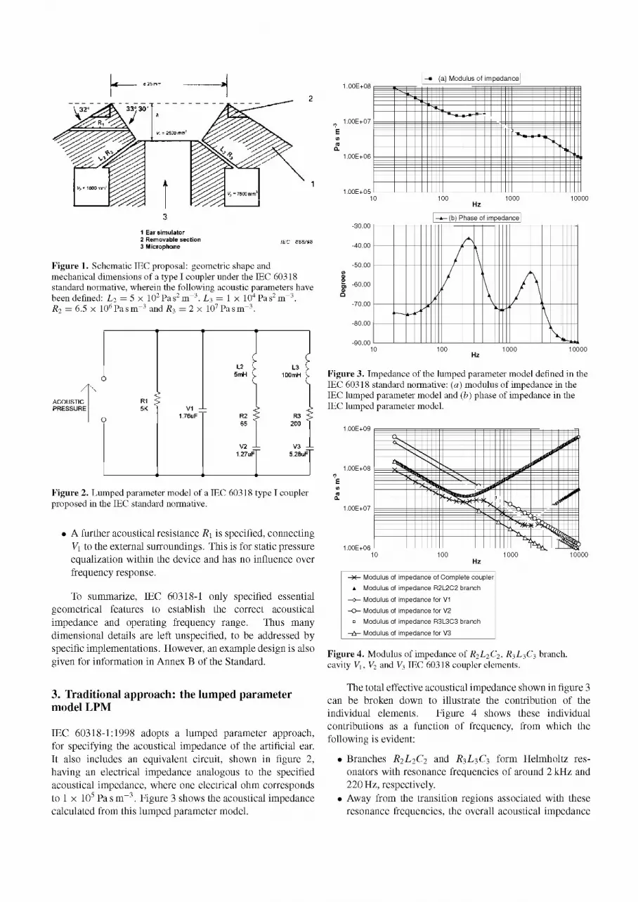
The FEM modelling of the cavities for the artificial ear is formed by a three-dimensional structure, modelled by linear tetrahedron elements (CATIA V5 Advanced meshing methods' type TE4 isoparametric solid element ). The number of elements used was a function of the volume and geometry of the specific cavity being modelled.

During the calculations the density of air was taken as 1.2 kg irr3 and the speed of sound as 340 m s 4 . These values are appropriate for the reference environmental conditions specified in IEC 60318-1.

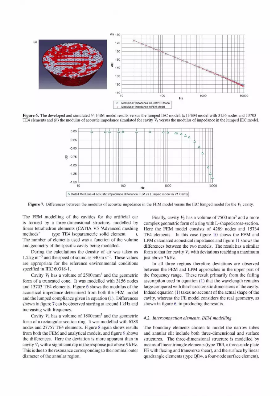
Cavity V\ has a volume of 2500 mm3 and the geometric form of a truncated cone. It was modelled with 3156 nodes and 13703 TE4 elements. Figure 6 shows the modulus of the acoustical impedance determined from both the FEM model and the lumped compliance given in equation (1). Differences shown in figure 7 can be observed starting at around 1 kHz and increasing with frequency.

Cavity V2 has a volume of 1800 mm3 and the geometric form of a rectangular section ring. It was modelled with 6788 nodes and 27757 TE4 elements. Figure 8 again shows results from both the FEM and analytical models, and figure 9 shows the differences. Here the deviation is more apparent than in cavity Vi with a significant dip in the responsejust above 9 kHz. This is due to the resonance corresponding to the nominal outer diameter of the annular region.

Finally, cavity V3 has a volume of 7500 mm3 and a more complex geometric form of a ring with L-shaped cross-section. Here the FEM model consists of 4289 nodes and 15734 TE4 elements. In this case figure 10 shows the FEM and LPM calculated acoustical impedance and figure 11 shows the differences between the two models. The result has a similar form to that for cavity V2 with deviations reaching a maximum just above 7 kHz.

In all three regions therefore deviations are observed between the FEM and LPM approaches in the upper part of the frequency range. These result primarily from the failing assumption used in equation (1) that the wavelength remains large compared with the characteristic dimensions of the cavity. Indeed equation (1) takes no account of the actual shape of the cavity, whereas the FE model considers the real geometry, as shown in figure 6, in producing the results.

4.2. Interconnection elements. BEM modelling

The boundary elements chosen to model the narrow tubes and annular slit include both three-dimensional and surface structures. The three-dimensional structure is modelled by means of linear triangle elements (type TR3, a three-node plate FE with flexing and transverse shear), and the surface by linear quadrangle elements (type QD4, a four-node surface element).

10000

Hz -x- Modulus of impedance in LUMPED Model - ° - Modulus of impedance in FEM Model

Figure 8. The developed and simulated V2 FEM model results versus the lumped IEC model: (a) FEM model with 6788 nodes and 27757 TE4 elements and (b) the modulus of acoustic impedance simulated for the cavity V2 versus the modulus of impedance in the lumped IEC model.

0 -1 -2 -3 -4 -5

A-Y ± \ L i L i 1 \ " * A A

A •-

A

-9 -10 -11 -12 -13 -14

10 100 1000 Hz

10000

A Detail Modulus of acoustic impedance difference FEM vs Lumped model in V2 Cavity

Figure 9. Differences between the modulus of acoustic impedance in the FEM model versus the IEC lumped model for the V2 cavity.

Modulus of impedance in LUMPED model - Modulus of impedance in FEM Model

Figure 10. The developed and simulated V3 FEM model results versus the lumped IEC model: (a) FEM model with 4289 nodes and 15734 TE4 elements and (b) the modulus of acoustic impedance simulated for the cavity V3 versus the modulus of impedance in the lumped IEC model.

Both types of element are based on the Reissner/Mindlin theory

4.2.1. Thermalandviscositylossesinnarrowstructures. The propagation of acoustic waves through very narrow elements results in energy losses due to the close proximity of the boundary. The energy loss mechanism can be modelled generically by the Navier-Stokes equations. These effects

are widely documented in the bibliography . The two predominant loss mechanisms are

• Losses due to viscosity. This is the main loss mechanism and it is produced by friction phenomena within the tube.

• Thermal losses. Caused by heat conduction between the fluid and the wall.

Accounting for these losses analytically introduces complex density and speed of sound parameters into the analysis. Using

12

10

A A A A A A A A A A 1 A A A * A A * A AA A A

100 Hz

1000 10000

A Detail Modulus of acoustic impedance difference FEM vs Lumped model in V3 Cavity

Figure 11. Differences between the modulus of acoustic impedance in the FEM model versus the IEC lumped model for the V3 cavity.

(a) (b) 175

- ^ - Acoustic resistance in Lumped Model -o- Acoustic resistance in BEM model

u ^ F XT' u r

*c

Jf^f4

Jftr^ ; '

>r-

, j r ^ rn^

W^

#E .*<#

W "

Hz

- Acoustic mass in Lumped Model - Acoustic mass in BEM model

Figure 12. The developed and simulated L3R3 BEM model versus the lumped IEC model: (a) FEM model and geometry with 3156 nodes and 13703 TR3 elements and (b) acoustic resistance and mass obtained in the BEM model versus modulus of impedance in the lumped IEC model for the L3R3 narrow tube.

these modified complex parameters, both types of losses can be simulated in the LMS Virtual Lab FE module over the range of frequencies from 20 Hz to 10 kHz. That these phenomena can be accounted for in the modelling represents an improvement over the lumped parameter model where viscous and thermal losses are considered, but not fully accounted for. It is also not common for such effects to be included in FEM analysis.

4.2.2. Narrow tube elements, L3R3. For a narrow tube, the acoustical impedance is, to a first approximation, given by

Jnarrow_tube

8 • yu • h 4 • po • h • co r + i~2 —' (2)

where the radius of the tube satisfies r0 -< 0 .002/vJ and end correction effects are neglected. Equation (2) is then seen to have the form ZA = R\+ i«MA from which the acoustical

resistance and mass can be deduced. The artificial ear design being considered here includes four narrow tubes that act in parallel to connect volumes V\ and V3. Each tube is modelled individually. The dimensions of the tubes are taken directly from IEC 60318-1 as r0 = 0.225 mm and h = 3.8 mm. Figure 12 shows the meshing of the narrow tube using the CATIA V5 software tool. The complex density and speed of sound parameters are introduced during the calculations to enable the loss mechanisms to be simulated. Viscosity losses are modelled by means of complex density of air where

Pnarrow_tube — PO 2-J i (g„To)

Ks-r0- Jo(ks -r0) (3)

and the impedance of the tube is assumed to be independent of the incident sound pressure, Ks is Stokes' wave number, J0 and

1

0.8

0.6

0.4

0.2 m •a

0 » (A

-0.2 |

-0.4

-0.6

Hz

- X - Detail Acoustic resistance difference BEM vs Lumped model in L3R3 narrow tube

—•— Detail Acoustic mass difference BEM vs Lumped model in L3R3 narrow tube

Figure 13. Comparison between the BEM modei and the fumped modef for the acoustic resistance R3 and for acoustic mass L3.

> s i — •O &(r.< >0'XX)

1/ \ V \

Figure 14. Rectangular slit geometry.

can be modelled using a complex density of air under linear assumption, are given by

and,

J\ are, respectively, the zero and first order Bessel functions, Po is the normal density of the air and h, r0 are tube dimensions.

Thermal losses are modelled using a complex speed of sound where

^narrow-tube y^ narrow_tube / P§ /A)

and the bulk modulus according to is given by

K narrow_tube y-Po 1 + 2 . ( y - l ) . / i ( B t T 0 ) - i - i

(4)

(5) Bk-r0- J0(Bk -r0)

where y is the air adiabatic constant, p> is the static air pressure and Bk accounts for the thermal diffusivity of the air.

4.2.2.1. Results of narrow tube BEM analysis with losses. Figure 12 shows the acoustical resistance and mass for the narrow tube derived from BEM FEs analysis (with 3156 nodes and 13703 TR3 elements) described above and from the lumped parameter model given by equation (2).

The differences are shown in figure 13 for the acoustical resistance and for the acoustical mass, indicating significant variation, especially in the acoustical resistance. The difference in the acoustical resistance results because the lumped parameter model does not fully account for the viscosity or thermal losses which are significant in this type of acoustic element.

4.2.3. Annular slit, L2R2- For a narrow slit with parallel sides, the acoustical impedance is, to a first approximation, given by [13] in the form of

12 • p • ls . 6 • po • 4 Alit = —n + 1-

Ws 5 • ws • ts (6)

where end corrections are neglected and ts -< 0.003/^/f. The acoustical resistance and mass can be inferred from equation (6) as they were in equation (2).

In the artificial ear design under consideration, an annular slit connects the volumes V\ and V2, providing the appropriate acoustical resistance and mass. The geometry of the slit and the meshing is shown in figure 14. In this case, viscosity losses

Pslit = PO tanh(Vi-A.siit)

V i - A , slit

where 'po-co\1/2

•"•slit — ls ' I I p. )

(7)

(8)

As before, the thermal losses are modelled by a complex speed of sound according to

Cslit = V^sl i t /PO, (9)

where, for this geometry, the bulk modulus is given by [18,21] and produces

^"sl Y • P0 l + (y - l) tanh(Vi-A.siit)

Vi-A. slit , (10)

where y is the air adiabatic constant, Po is the standard air pressure, po is the normal density of the air and ts is slit dimension.

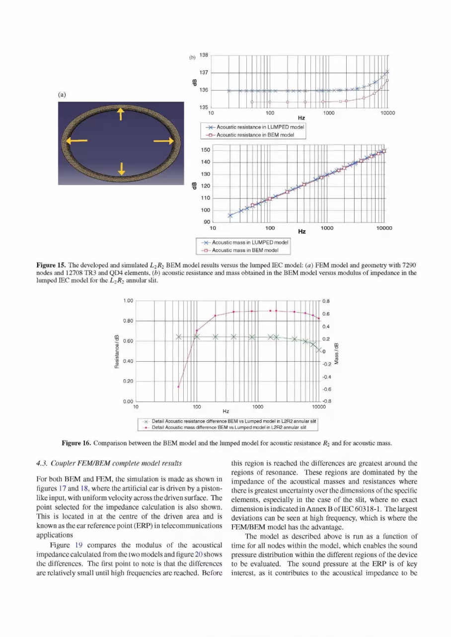
4.2.3.1. Results ofannular slit BEM analysis with losses. The results of the BEM (with 7290 nodes and 12708 TR3 and QD4 elements) and LPM can be seen in figure 15, and the differences for the derived acoustical resistance and mass in figure 16. As before, the BEM deviates from the LPM. This time the deviation is a similar order of magnitude for both the mass and resistance.

It is interesting to note the critical dependence of the lumped parameter impedance values on the dimensions of the interconnecting elements equations (2) and (6). In practice the slit width dimension ts is made adjustable, so that the desired impedance can be set during manufacture, from direct measurements of the flow resistance (which is related to the acoustical resistance), rather than aiming to establish a specific setting for the width, which would require very precise control over mechanical tolerances.

(b) 138

137

136

135

"" -H- - H-

10 100 1000 10000 Hz

-Acoustic resistance in LUMPED model

-Acoustic resistance in BEM model

40

30

10

on

X* 9 £ * i. r

10 100 Hz 1000 10000

-Acoustic mass in LUMPED model

-Acoustic mass in BEM model

Figure 15. The developed and simulated L2R2 BEM model results versus the lumped IEC model: (a) FEM model and geometry with 7290 nodes and 12708 TR3 and QD4 elements, (b) acoustic resistance and mass obtained in the BEM model versus modulus of impedance in the lumped IEC model for the L2R2 annular slit.

1.00

10000

Detail Acoustic resistance difference BEM vs Lumped model in L2R2 annular slit Detail Acoustic mass difference BEM vs Lumped model in L2R2 annular slit

Figure 16. Comparison between the BEM model and the lumped model for acoustic resistance R2 and for acoustic mass.

4.3. Coupler FEM/BEM complete model results

For both BEM and FEM, the simulation is made as shown in figures 17 and 18, where the artificial ear is driven by a piston­like input, with uniform velocity across the driven surface. The point selected for the impedance calculation is also shown. This is located in at the centre of the driven area and is known as the ear reference point (ERP) in telecommunications applications

Figure 19 compares the modulus of the acoustical impedance calculated from the two models and figure 20 shows the differences. The first point to note is that the differences are relatively small until high frequencies are reached. Before

this region is reached the differences are greatest around the regions of resonance. These regions are dominated by the impedance of the acoustical masses and resistances where there is greatest uncertainty over the dimensions of the specific elements, especially in the case of the slit, where no exact dimension is indicated in Annex B of IEC 60318-1. The largest deviations can be seen at high frequency, which is where the FEM/BEM model has the advantage.

The model as described above is run as a function of time for all nodes within the model, which enables the sound pressure distribution within the different regions of the device to be evaluated. The sound pressure at the ERP is of key interest, as it contributes to the acoustical impedance to be

2.25

2.00

1.75

1.50

1.25

1.00

S 0.75

0.50

0.25

0.00

-0.25

-0.50

-0.75

l i t f

Figure 17. Set-up for complete FEM/BEM model.

V2 vi

Figure 18. Complete FEM/BEM artificial ear model.

1 .OE+08

1 .OE+07

1 .OE+06

1 .OE+05 10000

-Modulus of impedance of lumped IEC model

Modulus of impedance BEM/FEM model

Figure 19. Acoustic impedance comparison for IEC 60318 couplers: lumped model and FEM/BEM model proposed.

calculated. However, it is also possible to examine the acoustical behaviour in the other regions. This provides additional information on the physical phenomena that take place inside the coupler, and the sound pressure distributions within the different cavities, as a function of frequency. For instance, the viscosity and thermal losses that take place in narrow conduits can be seen. Such analysis and visualization of the sound field are not possible using the lumped model.

Hz

- o - Difference in Modulus of impedance Lumped-BEM/FEM model

Figure 20. Difference in modulus of impedance of lumped IEC model versus BEM/FEM model.

4.4. Verification and discussion

IEC 60318-1 does not currently specify the overall acoustical impedance of the artificial ear as a function of frequency. It merely states the lumped parameters that the elements within the device should have. The LPM is very useful for developing a physical understanding of the artificial ear, but it has limitations arising from the assumptions used to derive the lumped parameters. Primarily these are that adiabatic conditions exist, and that the acoustical wavelength is considerably smaller than characteristic dimensions within the elements described by the lumped parameters. Unfortunately the inherent limitations, particularly regarding the wavelength, are not mentioned in IEC 60318-1:1998. The acoustical impedance calculated from the lumped parameter model is given in an informative part of the Standard (and then only graphically) and is therefore not mandatory. Yet there is an expectation that these values represent the impedance of actual devices over the given frequency range (up to 10 kHz). Results presented here indicate that the requirement for the wavelength to be large compared with the physical dimension within the device is becoming invalid in the upper part of the frequency range. They also appear to indicate that the assumption about adiabatic conditions is also partially invalidated by the high ratio of surface area to volume in some of the cavities, leading to a small degree of heat conduction. So while the relative simplicity of the LPM brings advantages, some knowledge of the constraints within which it is valid is needed in order to use it appropriately. The new numerical model presented here is not constrained by the same assumptions as the LPM, so it is able to provide some insight into its limitations. It remains for the numerical model to be validated with measurements on actual devices to confirm the findings here. However, such measurements are only just being realized, and the methodology being introduced into the current revision of IEC 60318-1. Such experimental validation will therefore be the subject of further research.

However, the mixed FEM/BEM simulation presented here offers a number of advantages over the LPM and can be extremely valuable in helping to understand further

the physical phenomena governing the performance of the artificial ear. These advantages include

• The possibility of the model to yield the direction of sound propagation, which is helpful in calculating the acoustical impedance.

• The FEM/BEM model can be used to study the precise effect of geometry on the acoustical impedance, providing scope to consider potential improvement for this type of ear simulator.

• The model enables the dependence of the acoustical impedance on critical dimensions to be specified more precisely.

5. Conclusions

A complete three-dimensional FEs model for E C 60318-1 ear simulator has been developed using a mixed FEM/BEM approach. The model is thought to be the first of its kind to take full account of viscosity and thermal effects throughout the relevant sections of the device, with a unified theory based on the Navier-Stokes equation.

Results from the new FEM/BEM model have been com­pared with the traditional lumped parameter model based on the equivalent electrical circuit given in IEC 60318-1 [8]. The FEM/BEM model presented here is considered to better rep­resent the performance of actual devices, especially at high frequencies, because it takes full account of the underlying physics, including elements neglected by the lumped param­eter approach. The effects, in some components, become noticeable at frequencies above 1 kHz, where the limitations in the lumped parameter begin to occur, but the real advantages of the FEM/BEM model are realized at high frequencies. There is even the possibility to investigate performance beyond the currently specified upper frequency limit of 10 kHz.

It remains to be shown that the measured acoustical impedance of real artificial ears agrees more closely with this new FEM/BEM model than with the model in the current ver­sion of IEC 60318-1. A recent experimental investigation, for which only preliminary reports have appeared in the litera­ture [22], has already shown that there are differences between the published specification and the data measured in practice. Further work is planned to investigate the level of agreement between measurement data and the FEM/BEM model.

Acknowledgments

The authors would like to thank Comunidad de Madrid Government and Universidad Politecnica de Madrid for the grant CCG06-UPM/FI-312 received to develop the project and the Instrumentation and Applied Acoustic Research UPM group (I2A2), Spain, and the National Physical Laboratory (NPL), UK, for supporting this investigation.

References

IEC 60645-1 Ed. 1.0 b 1992 Audiometers—Part 1: Pure-tone Audiometers (Geneva: International Electrotechnical Commission)

Goncalves A A Jr, Pedroso M A and Gerges S N Y 2004 Uncertainty in audiometer calibration Metrologia 41 1-7

Ruiz M, Feuereisen B, Machon D and Recuero M 2002 Conf. Forum Acousticum: A Model of Uncertainty Calculation for the Calibration of Audiometers (Sevilla, Spain)

Lightfoot G 2000 Audiometer calibration: interpreting and applying the standards Br. J. Audiol. 34 311-6

Smith P A and Foster J R 1997 Audiometer calibration: two neglected areas Br. J. Audiol. 31 359-64

Sherwood T R 1997 Final Report: Euromet Project 363 Harmonisation of Audiometry Measurements within Europe National Physical Laboratory Report CMAM 001

Hart A 2000 Co-operation in the Standardisation of Ear Simulator (Cambridge: National Measurement System Policy Unit, Department of Trade and Industry and Scientific Generics Limited)

IEC 60318-1 Ed. 1.0 1998 Electroacoustics—Simulators of human head and ear—Part 1: Ear Simulator for the Calibration of Supra-aural Earphones (Geneva: International Electrotechnical Commission)

ITU-T Recommendation P.57 Series P: Telephone Transmission Quality Artificial ears (Geneva: International Telecommunication Union)

Gelat P and Barham R G 2001 Internoise: Int. Conf. on Noise Control Engineering: Finite Element Model of the IEC 60318-1 Artificial Ear (The Hague, The Netherlands)

Dassault Systemes 2005-2007 Catia V5 Manuals (Suresnes, France: Dassault Systemes)

LMS International LMS Virtual Lab REv6B Manuals (Leuven, Belgium: LMS International)

Beranek L L 1993 Acoustics (New York: Acoustical Society of America)

Dassault Systemes 2005 Finite Element Reference Guide V5R16 (Suresnes, France: Dassault Systemes)

Beltman W M 1999 Viscothermal wave propagation including acousto-elastic interaction: I. Theory /. Sound Vib. Ill 555-86

Ingard U 1953 On the theory and design of acoustic resonators /. Acoust. Soc. Am. 25 1037-61

Ingard U 1967 Acoustic non linearity of an orifice /. Acoust. Soc. Am. 42 1-17

Silvian L J 1935 Acoustic impedance of small orifice /. Acoust. Soc. Am. 7 94-101

Cutanda V 2002 Numerical transducer modelling PhD Thesis Technical University of Denmark, Department of Acoustic Technology

Ahuja K K and Gaeta R J Jr 2002 Report: Active Control of Liner Impedance by Varying Perforate Orifice Geometry Georgia Institute of Technology Atlanta, GA, NASA STI Program (NASA/CR-2000-210663)

Zwickker C and Kosten C V 1949 Sound Absorbing Material (Amsterdam: Elsevier) pp 25-40

Barham R G 2008 Proc. Institute of Acoustics Spring Conf.: Acoustical Impedance of Ear Simulators and the Revision of IEC 60318-1 (University of Reading)