a neural population selective for song in human auditory cortex

Article

A neural population select
ive for song in humanauditory cortex
Highlights

d Neural population responsive to singing, but not instrumental

music or speech

d New statistical method infers neural populations from human

intracranial responses

d fMRI used to map the spatial distribution of intracranial

responses

d Intracranial responses replicate distinct music- and speech-

selective populations

Norman-Haignere et al., 2022, Current Biology 32, 1–15April 11, 2022 ª 2022 Elsevier Inc.https://doi.org/10.1016/j.cub.2022.01.069

Authors

Sam V. Norman-Haignere,

Jenelle Feather, Dana Boebinger, ...,

Josh H. McDermott, Gerwin Schalk,

Nancy Kanwisher

[email protected]

In brief

Using human intracranial recordings,

Norman-Haignere et al. reveal a neural

population that responds to singing, but

not instrumental music or speech. This

neural population was uncovered by

modeling electrode responses as a

weighted sum of canonical response

components. The spatial distribution of

each intracranial component was

mapped using fMRI.

ll

mailto:[email protected]


https://doi.org/10.1016/j.cub.2022.01.069

Please cite this article in press as: Norman-Haignere et al., A neural population selective for song in human auditory cortex, Current Biology (2022),https://doi.org/10.1016/j.cub.2022.01.069

ll

Article

A neural population selective for songin human auditory cortexSam V. Norman-Haignere,1,2,3,4,5,6,7,15,20,* Jenelle Feather,7,8,9,16 Dana Boebinger,7,8,10,17 Peter Brunner,11,12,13

Anthony Ritaccio,11,14 Josh H. McDermott,7,8,9,10,18 Gerwin Schalk,11 and Nancy Kanwisher7,8,9,191Zuckerman Institute, Columbia University, New York, NY, USA2HHMI Fellow of the Life Sciences Research Foundation, Chevy Chase, MD, USA3Laboratoire des Sytemes Perceptifs, D�epartement d’Etudes Cognitives, ENS, PSL University, CNRS, Paris, France4Department of Biostatistics & Computational Biology, University of Rochester Medical Center, Rochester, NY, USA5Department of Neuroscience, University of Rochester Medical Center, Rochester, NY, USA6Department of Biomedical Engineering, University of Rochester, Rochester, NY, USA7Department of Brain and Cognitive Sciences, Massachusetts Institute of Technology, Cambridge, MA, USA8McGovern Institute for Brain Research, Massachusetts Institute of Technology, Cambridge, MA, USA9Center for Brains, Minds and Machines, Cambridge, MA, USA10Program in Speech and Hearing Biosciences and Technology, Harvard University, Cambridge, MA, USA11Department of Neurology, Albany Medical College, Albany, NY, USA12National Center for Adaptive Neurotechnologies, Albany, NY, USA13Department of Neurosurgery, Washington University School of Medicine, St. Louis, MO, USA14Department of Neurology, Mayo Clinic, Jacksonville, FL, USA15Twitter: @SamNormanH16Twitter: @jenellefeather17Twitter: @dlboebinger18Twitter: @JoshHMcDermott19Twitter: @Nancy_Kanwisher20Lead contact

*Correspondence: [email protected]


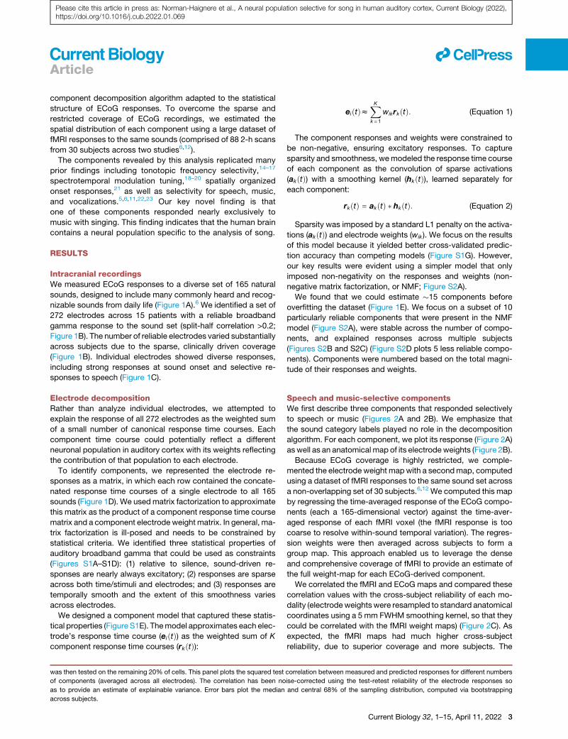
SUMMARY

How is music represented in the brain? While neuroimaging has revealed some spatial segregation betweenresponses tomusic versus other sounds, little is known about the neural code formusic itself. To address thisquestion, we developed a method to infer canonical response components of human auditory cortex usingintracranial responses to natural sounds, and further used the superior coverage of fMRI to map their spatialdistribution. The inferred components replicated many prior findings, including distinct neural selectivity forspeech and music, but also revealed a novel component that responded nearly exclusively to music withsinging. Song selectivity was not explainable by standard acoustic features, was located near speech-andmusic-selective responses, andwas also evident in individual electrodes. These results suggest that rep-resentations ofmusic are fractionated into subpopulations selective for different types ofmusic, one of whichis specialized for the analysis of song.

INTRODUCTION

Music is a quintessentially human capacity: it is present in some

form in nearly every society1,2 and differs substantially from its

closest analogs in non-human animals.3 Researchers have

long debated whether the human brain has mechanisms dedi-

cated to music, and if so, what computations those mechanisms

perform.4 These questions have important implications for un-

derstanding the organization of auditory cortex,5,6 the neural ba-

sis of sensory deficits such as amusia,7,8 the consequences of

auditory expertise,9 and the computational underpinnings of

auditory behavior.10

Neuroimaging studies have suggested that representations of

music diverge from those of other sound categories in human

non-primary auditory cortex. Prior studies have observed non-

primary voxels with partial selectivity for music compared with

other categories,5,11 and recent studies from our lab, which

modeled fMRI voxels as weighted sums of multiple response

components, inferred a component with clear music selec-

tivity6,12 that was distinct from nearby speech-selective re-

sponses. However, little is known about how neural responses

are organized within the domain of music, such as whether

distinct subpopulations exist that are selective for particular

types or features of music.13

Here, we examined the neural representation of music, and of

natural sounds more broadly, using intracranial recordings from

the human brain (ECoG, or electrocorticography), which have

substantially better spatiotemporal resolution than non-invasive

neuroimaging methods. We measured ECoG responses to a

diverse set of 165 natural sounds (Figure 1A) and developed a

Current Biology 32, 1–15, April 11, 2022 ª 2022 Elsevier Inc. 1

https://twitter.com/SamNormanH

https://twitter.com/jenellefeather

https://twitter.com/dlboebinger

https://twitter.com/JoshHMcDermott

https://twitter.com/Nancy_Kanwisher



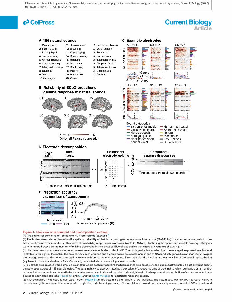
Figure 1. Overview of experiment and decomposition method(A) The sound set consisted of 165 commonly heard sounds (each 2 s).6

(B) Electrodes were selected based on the split-half reliability of their broadband gamma response time course (70–140 Hz) to natural sounds (correlation be-

tween odd versus even repetitions). This panel plots reliability maps for six example subjects (of 15 total), illustrating the sparse and variable coverage. Subjects

were numbered based on the number of reliable electrodes in their dataset. Blue circles outline the example electrodes shown in (C).

(C) The broadband gamma response time course of several example electrodes to all 165 sounds, plotted as a raster. The time-averaged response to each sound

is plotted to the right of the raster. The sounds have been grouped and colored based on membership in one of 12 sound categories. Below each raster, we plot

the average response time course to each category with greater than 5 exemplars. Error bars plot the median and central 68% of the sampling distribution

(equivalent to one standard error for a Gaussian), computed via bootstrapping across sounds.

(D) Electrode time courses were compiled in amatrix, where each row contains the full response time course of each electrode (from 0 to 3 s post-stimulus onset),

concatenated across all 165 sounds tested. The data matrix was approximated as the product of a response time course matrix, which contains a small number

of canonical response time courses that are shared across all electrodes, with an electrode weight matrix that expresses the contribution of each component time

course to each electrode (see Figures S1 and S7 and the STAR Methods for additional modeling details).

(E) Cross-validation was used to compare models (Figure S1G) and determine the number of components. The data matrix was divided into cells, with one

cell containing the response time course of a single electrode to a single sound. The model was trained on a randomly chosen subset of 80% of cells and

(legend continued on next page)

ll

2 Current Biology 32, 1–15, April 11, 2022


Article

ll


Article

component decomposition algorithm adapted to the statistical

structure of ECoG responses. To overcome the sparse and

restricted coverage of ECoG recordings, we estimated the

spatial distribution of each component using a large dataset of

fMRI responses to the same sounds (comprised of 88 2-h scans

from 30 subjects across two studies6,12).

The components revealed by this analysis replicated many

prior findings including tonotopic frequency selectivity,14–17

spectrotemporal modulation tuning,18–20 spatially organized

onset responses,21 as well as selectivity for speech, music,

and vocalizations.5,6,11,22,23 Our key novel finding is that

one of these components responded nearly exclusively to

music with singing. This finding indicates that the human brain

contains a neural population specific to the analysis of song.

RESULTS

Intracranial recordingsWe measured ECoG responses to a diverse set of 165 natural

sounds, designed to include many commonly heard and recog-

nizable sounds from daily life (Figure 1A).6 We identified a set of

272 electrodes across 15 patients with a reliable broadband

gamma response to the sound set (split-half correlation >0.2;

Figure 1B). The number of reliable electrodes varied substantially

across subjects due to the sparse, clinically driven coverage

(Figure 1B). Individual electrodes showed diverse responses,

including strong responses at sound onset and selective re-

sponses to speech (Figure 1C).

Electrode decompositionRather than analyze individual electrodes, we attempted to

explain the response of all 272 electrodes as the weighted sum

of a small number of canonical response time courses. Each

component time course could potentially reflect a different

neuronal population in auditory cortex with its weights reflecting

the contribution of that population to each electrode.

To identify components, we represented the electrode re-

sponses as a matrix, in which each row contained the concate-

nated response time courses of a single electrode to all 165

sounds (Figure 1D). We usedmatrix factorization to approximate

this matrix as the product of a component response time course

matrix and a component electrode weight matrix. In general, ma-

trix factorization is ill-posed and needs to be constrained by

statistical criteria. We identified three statistical properties of

auditory broadband gamma that could be used as constraints

(Figures S1A–S1D): (1) relative to silence, sound-driven re-

sponses are nearly always excitatory; (2) responses are sparse

across both time/stimuli and electrodes; and (3) responses are

temporally smooth and the extent of this smoothness varies

across electrodes.

We designed a component model that captured these statis-

tical properties (Figure S1E). Themodel approximates each elec-

trode’s response time course (eiðtÞ) as the weighted sum of K

component response time courses (rkðtÞ):

was then tested on the remaining 20% of cells. This panel plots the squared test

of components (averaged across all electrodes). The correlation has been no

as to provide an estimate of explainable variance. Error bars plot the median

across subjects.

eiðtÞzXKk = 1

wikrkðtÞ: (Equation 1)

The component responses and weights were constrained to

be non-negative, ensuring excitatory responses. To capture

sparsity and smoothness, wemodeled the response time course

of each component as the convolution of sparse activations

(akðtÞ) with a smoothing kernel (hkðtÞ), learned separately for

each component:

rkðtÞ = akðtÞ � hkðtÞ: (Equation 2)

Sparsity was imposed by a standard L1 penalty on the activa-

tions (akðtÞ) and electrode weights (wik ). We focus on the results

of this model because it yielded better cross-validated predic-

tion accuracy than competing models (Figure S1G). However,

our key results were evident using a simpler model that only

imposed non-negativity on the responses and weights (non-

negative matrix factorization, or NMF; Figure S2A).

We found that we could estimate �15 components before

overfitting the dataset (Figure 1E). We focus on a subset of 10

particularly reliable components that were present in the NMF

model (Figure S2A), were stable across the number of compo-

nents, and explained responses across multiple subjects

(Figures S2B and S2C) (Figure S2D plots 5 less reliable compo-

nents). Components were numbered based on the total magni-

tude of their responses and weights.

Speech and music-selective componentsWe first describe three components that responded selectively

to speech or music (Figures 2A and 2B). We emphasize that

the sound category labels played no role in the decomposition

algorithm. For each component, we plot its response (Figure 2A)

aswell as an anatomical map of its electrodeweights (Figure 2B).

Because ECoG coverage is highly restricted, we comple-

mented the electrode weight mapwith a secondmap, computed

using a dataset of fMRI responses to the same sound set across

a non-overlapping set of 30 subjects.6,12 We computed this map

by regressing the time-averaged response of the ECoG compo-

nents (each a 165-dimensional vector) against the time-aver-

aged response of each fMRI voxel (the fMRI response is too

coarse to resolve within-sound temporal variation). The regres-

sion weights were then averaged across subjects to form a

group map. This approach enabled us to leverage the dense

and comprehensive coverage of fMRI to provide an estimate of

the full weight-map for each ECoG-derived component.

We correlated the fMRI and ECoG maps and compared these

correlation values with the cross-subject reliability of each mo-

dality (electrodeweights were resampled to standard anatomical

coordinates using a 5 mm FWHM smoothing kernel, so that they

could be correlated with the fMRI weight maps) (Figure 2C). As

expected, the fMRI maps had much higher cross-subject

reliability, due to superior coverage and more subjects. The

correlation between measured and predicted responses for different numbers

ise-corrected using the test-retest reliability of the electrode responses so

and central 68% of the sampling distribution, computed via bootstrapping

Current Biology 32, 1–15, April 11, 2022 3

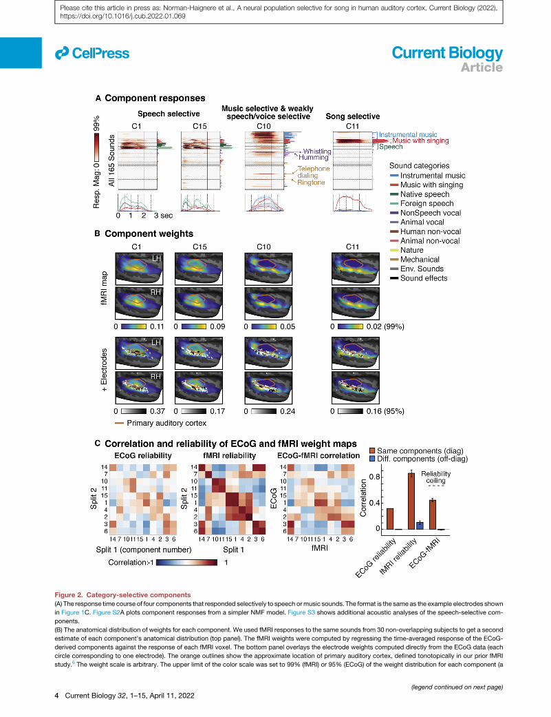
Figure 2. Category-selective components

(A) The response time course of four components that responded selectively to speech ormusic sounds. The format is the same as the example electrodes shown

in Figure 1C. Figure S2A plots component responses from a simpler NMF model. Figure S3 shows additional acoustic analyses of the speech-selective com-

ponents.

(B) The anatomical distribution of weights for each component. We used fMRI responses to the same sounds from 30 non-overlapping subjects to get a second

estimate of each component’s anatomical distribution (top panel). The fMRI weights were computed by regressing the time-averaged response of the ECoG-

derived components against the response of each fMRI voxel. The bottom panel overlays the electrode weights computed directly from the ECoG data (each

circle corresponding to one electrode). The orange outlines show the approximate location of primary auditory cortex, defined tonotopically in our prior fMRI

study.6 The weight scale is arbitrary. The upper limit of the color scale was set to 99% (fMRI) or 95% (ECoG) of the weight distribution for each component (a

(legend continued on next page)

ll



Article

ll


Article

correlation between fMRI and ECoG maps for corresponding

components was slightly higher than the reliability of the ECoG

maps themselves and much higher than that for mismatching

components (p < 0.001 via bootstrapping across the fMRI sub-

jects). These findings suggest a close correspondence between

the fMRI and ECoG maps that is primarily limited by the sparse

coverage of ECoG recordings and thus demonstrates the utility

of combining the precision of ECoG recordings with the spatial

coverage of fMRI. We primarily used the fMRI maps to test for

laterality effects, due to its dense bilateral coverage across

many subjects.

Two components (C1 and C15) responded nearly exclusively

to speech, with virtually no response to all other sounds including

non-speech vocalizations. These components responded simi-

larly to native and foreign speech sounds (all subjects were

native English speakers), consistent with prior work showing

that speech selectivity in STG is not driven by linguistic mean-

ing.6,23 C1 and C15 responded at different time points within

each speech utterance. Some of this response pattern to speech

could be predicted by a linear spectrotemporal receptive

field (STRF) (p < 0.01; see STAR Methods for details) with

C15 showing a higher frequency STRF compared with C1

(Figures S3A and S3B). However, the overall predictions of a

STRF model across the full sound set were poor and failed to

capture these components’ selectivity for speech (Figure S3C).

These results suggest that C1 and C15 are nonlinearly tuned

for distinct speech-specific features or classes that happen to

have distinct frequency spectra (e.g., low-frequency voiced pho-

nemes versus high-frequency fricatives).24–27

The weights for the speech-selective components were pri-

marily clustered in middle STG, with no significant difference be-

tween the two hemispheres (p > 0.73 uncorrected for the number

of components; via bootstrapping across subjects), consistent

with prior studies.5,12,23 The time-averaged response of C1

and C15 was very similar, which limited our ability to anatomi-

cally distinguish these two components with fMRI.

One component (C10) responded strongly to both instrumental

music and music with singing (average[instrumental music, sung

music] > average[all non-music categories]: p < 0.001 via boot-

strapping, Bonferroni-corrected for the number of components)

and produced an intermediate response to speech and other hu-

man vocalizations. The intermediate response to speech/voice

could reflect imperfect disentangling of speech andmusic selec-

tivity by our component model, potentially due to limited

coverage of the superior temporal plane where music selectivity

is prominent and speech selectivity isweak.C10 also showed the

longest response latency of all the inferred components (708ms),

higher threshold for fMRI because of its greater coverage). The lower limit was set

were in practice mostly positive). Figures S2B and S2C show how the electrode

(C) This panel quantifies the similarity of the fMRI and ECoG weight maps relative

modality. The leftmost two matrices show the correlation between all pairs of co

from the samemodality (left matrix, ECoG; middle, fMRI). The right matrix plots th

the average correlation for corresponding (matrix diagonal) and non-correspond

should be higher for corresponding components. The dashed line shows an estim

the reliability of the twomodalities. All 10 reliable components are shown, including

arranged by the similarity of their response profiles since components with more

butions. ECoG electrode weights were resampled to standard anatomical coordin

across subjects and with the fMRI maps (smoothed with a 5-mm FWHM kernel). E

strapping across fMRI subjects. Bootstrapping across ECoG subjects was not fe

suggesting a longer integrationwindow28 (latencieswere defined

as the time needed for the response to reach half its maximum).

The weights for C10 showed three hotspots in posterior, middle,

and anterior STG, with no difference between the two hemi-

spheres (p = 0.63 uncorrected). This anatomical profile is similar

to the music-selective component we previously inferred using

just fMRI data,6,12 but the cluster in middle STGwas more prom-

inent here likely due to stronger speech responses. These results

replicate our prior fMRI findings, showing distinct clusters of

speech and music selectivity in non-primary auditory cortex.

Song selectivityOur key novel finding is that one component (C11) responded

nearly exclusively to sung music: every music stimulus with

singing produced a high response whereas all other sounds,

including both speech and instrumental music, produced little

to no response (sung music always had instrumental backing).

Because our component model approximates electrodes as

weighted sums of multiple components, the model should not

have needed a separate song-selective component if song

selectivity simply reflected a sum of speech and music selec-

tivity. The component response confirmed this expectation: the

response to sung music was substantially and significantly

higher than the sum of the response to speech and instrumental

music (sung music > max[English speech, foreign speech] +

instrumental music: p < 0.001 via bootstrapping, Bonferroni-cor-

rected). Moreover, the response of C11 could not be explained

as a linear combination of our previously reported fMRI compo-

nents that showed clear selectively for music and speech indi-

vidually (Figures S4A and S4B). C11 had a relatively long latency

(298ms), and its weightswere concentrated in non-primary audi-

tory cortex, nearby to both speech- and music-selective re-

sponses in middle and anterior STG, respectively. C11 was not

significantly lateralized in the fMRI weight map (p = 0.48 uncor-

rected), and although the electrode weights appear somewhat

right lateralized, this difference was also not significant (p =

0.09 uncorrected), though we note that laterality comparisons

with ECoG data are generally underpowered.

Hypothesis-driven component analysisAre statistical assumptions like non-negativity and sparsity

necessary to detect speech, music, and song selectivity? To

answer this question, we performed a simpler analysis, where

we attempted to learn a weighted sum of electrode responses

that approximated a binary preference for speech, music, or

singing (via regularized regression), using cross-validation

across sounds to prevent overfitting. This analysis successfully

to 0 (ECoGweights were constrained to be non-negative, and the fMRI weights

weights are distributed across subjects.

to the maximum possible similarity given the across-subject reliability of each

mponent weight maps, measured using two non-overlapping sets of subjects

e correlation between ECoG and fMRI weight maps. The bar plots at right show

ing components (off-diagonal). If the modalities are consistent, the correlation

ate of the maximum possible correlation between ECoG and fMRI maps given

those without strong category selectivity (see Figure 5). The components were

similar response profiles also tended to have more similar anatomical distri-

ates (using a 5-mm FWHM smoothing kernel) so that they could be compared

rror bars show the central 68% of the sampling distribution, computed by boot-

asible because of variable coverage.


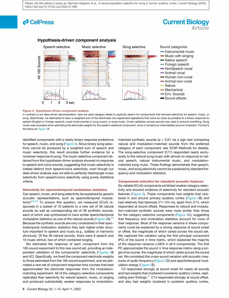
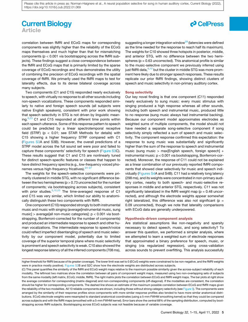
Figure 3. Hypothesis-driven component analysis

In contrast to our data-driven decomposition, here we used category labels to explicitly search for components that showed selectivity for speech, music, or

song. Specifically, we attempted to learn a weighted sum of the electrodes (via regularized regression) that came as close as possible to a binary response to

speech (English or Foreign speech), music (instrumental or sung music), or sung music. Cross-validation across sounds was used to prevent overfitting. Sung

music was excluded when estimating the electrode weights for the speech-selective component, since it contains an intermediate amount of speech. Format is

the same as Figure 2A.

ll


Article

identified components with a nearly binary response preference

for speech, music, and song (Figure 3). Since binary song selec-

tivity cannot be produced by a weighted sum of speech and

music selectivity, this result provides further evidence for a

nonlinear response to song. Themusic-selective component ob-

tained from this hypothesis-driven analysis showed no response

to speech and voice sounds, suggesting that music selectivity is

indeed distinct from speech/voice selectivity, even though our

data-driven analysis was not able to perfectly disentangle music

selectivity from speech/voice selectivity using purely statistical

criteria.

Selectivity for spectrotemporal modulation statisticsCan speech, music, and song selectivity be explained by generic

acoustic representations, such as spectrotemporal modula-

tions?18–20 To answer this question, we measured ECoG re-

sponses in a subset of 10 patients to a new set of 36 natural

sounds as well as corresponding set of 36 synthetic sounds,

each of which was synthesized to have similar spectrotemporal

modulation statistics as one of the natural sounds (Figure 4A).29

Because the synthetic sounds are only constrained in their spec-

trotemporal modulation statistics they lack higher-order struc-

ture important to speech and music (e.g., syllabic or harmonic

structure). Of the 36 natural sounds, there were 8 speech and

10 music stimuli, two of which contained singing.

We estimated the response of each component from the

165-sound experiment to this new sound set, providing an inde-

pendent validation of the components’ selectivity (Figures 4B

and 4C). Specifically, we fixed the component electrode weights

to those estimated from the 165-sound experiment, and we esti-

mated a new set of component response time courses that best

approximated the electrode responses from the modulation-

matching experiment. All of the category-selective components

replicated their selectivity for natural speech, music, or singing

and produced substantially weaker responses to modulation-


matched synthetic sounds (p < 0.01 via a sign test comparing

natural and modulation-matched sounds from the preferred

category of each component; see STAR Methods for details).

The song-selective component (C11) responded nearly exclu-

sively to the natural sung music with almost no response to nat-

ural speech, natural instrumental music, and modulation-

matched sung music. These findings demonstrate that speech,

music, and song selectivity cannot be explained by standard fre-

quency and modulation statistics.

Components selective for standard acoustic featuresSix reliable ECoG components exhibited weaker category selec-

tivity and showed evidence of selectivity for standard acoustic

features (Figure 5). These components had weights that clus-

tered in and around primary auditory cortex (Figure 5B) and

had relatively fast latencies (71–124 ms, apart from C14, which

responded at sound offset). Responses to natural and modula-

tion-matched synthetic sounds were more similar than those

for the category-selective components (Figure 5C), suggesting

that frequency and modulation statistics account for more of

their response. Most of the response variance in these compo-

nents could be explained by a strong response at sound onset

or offset, the magnitude of which varied across the sound set.

We captured this variation using the first principal component

(PC) of the sound 3 time matrix, which explained the majority

of the response variance (>58% in all 6 components). The first

PC approximates the sound3 time response matrix using a sin-

gle time course, the magnitude of which varies across the sound

set. We correlated this cross-sound variation with acoustic mea-

sures of audio frequency (Figure 5D) and spectrotemporal mod-

ulation energy (Figure 5E).

C3 responded strongly at sound onset for nearly all sounds

and had weights that clustered in posterior auditory cortex, repli-

cating prior findings.21 C14 responded strongly at sound offset,

and also had weights clustered in posterior auditory cortex,

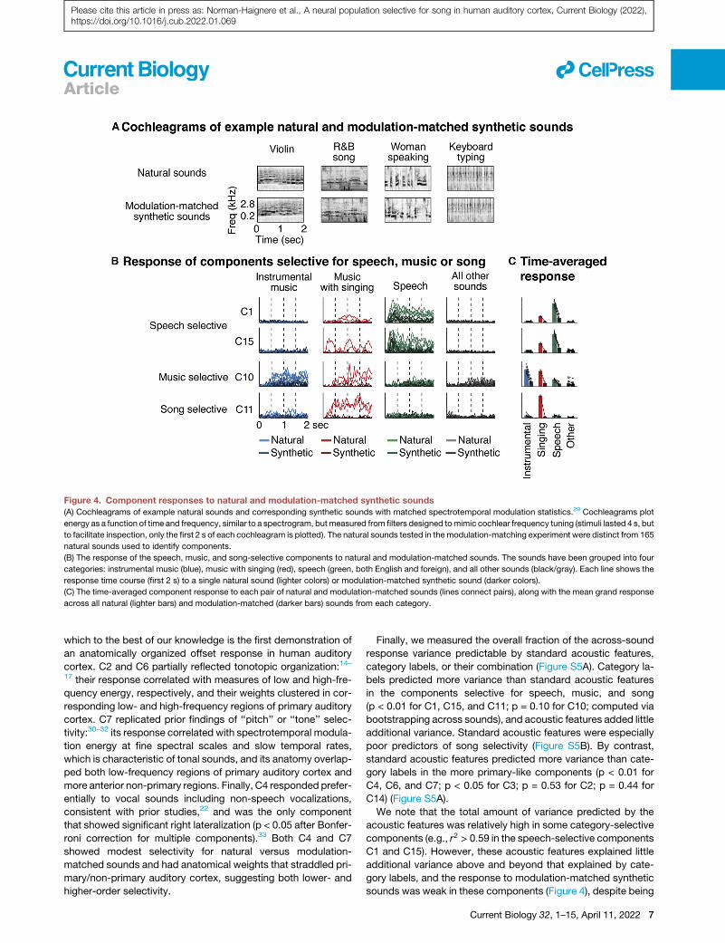
Figure 4. Component responses to natural and modulation-matched synthetic sounds

(A) Cochleagrams of example natural sounds and corresponding synthetic sounds with matched spectrotemporal modulation statistics.29 Cochleagrams plot

energy as a function of time and frequency, similar to a spectrogram, butmeasured from filters designed tomimic cochlear frequency tuning (stimuli lasted 4 s, but

to facilitate inspection, only the first 2 s of each cochleagram is plotted). The natural sounds tested in the modulation-matching experiment were distinct from 165

natural sounds used to identify components.

(B) The response of the speech, music, and song-selective components to natural and modulation-matched sounds. The sounds have been grouped into four

categories: instrumental music (blue), music with singing (red), speech (green, both English and foreign), and all other sounds (black/gray). Each line shows the

response time course (first 2 s) to a single natural sound (lighter colors) or modulation-matched synthetic sound (darker colors).

(C) The time-averaged component response to each pair of natural and modulation-matched sounds (lines connect pairs), along with the mean grand response

across all natural (lighter bars) and modulation-matched (darker bars) sounds from each category.

ll


Article

which to the best of our knowledge is the first demonstration of

an anatomically organized offset response in human auditory

cortex. C2 and C6 partially reflected tonotopic organization:14–

17 their response correlated with measures of low and high-fre-

quency energy, respectively, and their weights clustered in cor-

responding low- and high-frequency regions of primary auditory

cortex. C7 replicated prior findings of ‘‘pitch’’ or ‘‘tone’’ selec-

tivity:30–32 its response correlated with spectrotemporal modula-

tion energy at fine spectral scales and slow temporal rates,

which is characteristic of tonal sounds, and its anatomy overlap-

ped both low-frequency regions of primary auditory cortex and

more anterior non-primary regions. Finally, C4 responded prefer-

entially to vocal sounds including non-speech vocalizations,

consistent with prior studies,22 and was the only component

that showed significant right lateralization (p < 0.05 after Bonfer-

roni correction for multiple components).33 Both C4 and C7

showed modest selectivity for natural versus modulation-

matched sounds and had anatomical weights that straddled pri-

mary/non-primary auditory cortex, suggesting both lower- and

higher-order selectivity.

Finally, we measured the overall fraction of the across-sound

response variance predictable by standard acoustic features,

category labels, or their combination (Figure S5A). Category la-

bels predicted more variance than standard acoustic features

in the components selective for speech, music, and song

(p < 0.01 for C1, C15, and C11; p = 0.10 for C10; computed via

bootstrapping across sounds), and acoustic features added little

additional variance. Standard acoustic features were especially

poor predictors of song selectivity (Figure S5B). By contrast,

standard acoustic features predicted more variance than cate-

gory labels in the more primary-like components (p < 0.01 for

C4, C6, and C7; p < 0.05 for C3; p = 0.53 for C2; p = 0.44 for

C14) (Figure S5A).

We note that the total amount of variance predicted by the

acoustic features was relatively high in some category-selective

components (e.g., r2 > 0:59 in the speech-selective components

C1 and C15). However, these acoustic features explained little

additional variance above and beyond that explained by cate-

gory labels, and the response to modulation-matched synthetic

sounds was weak in these components (Figure 4), despite being


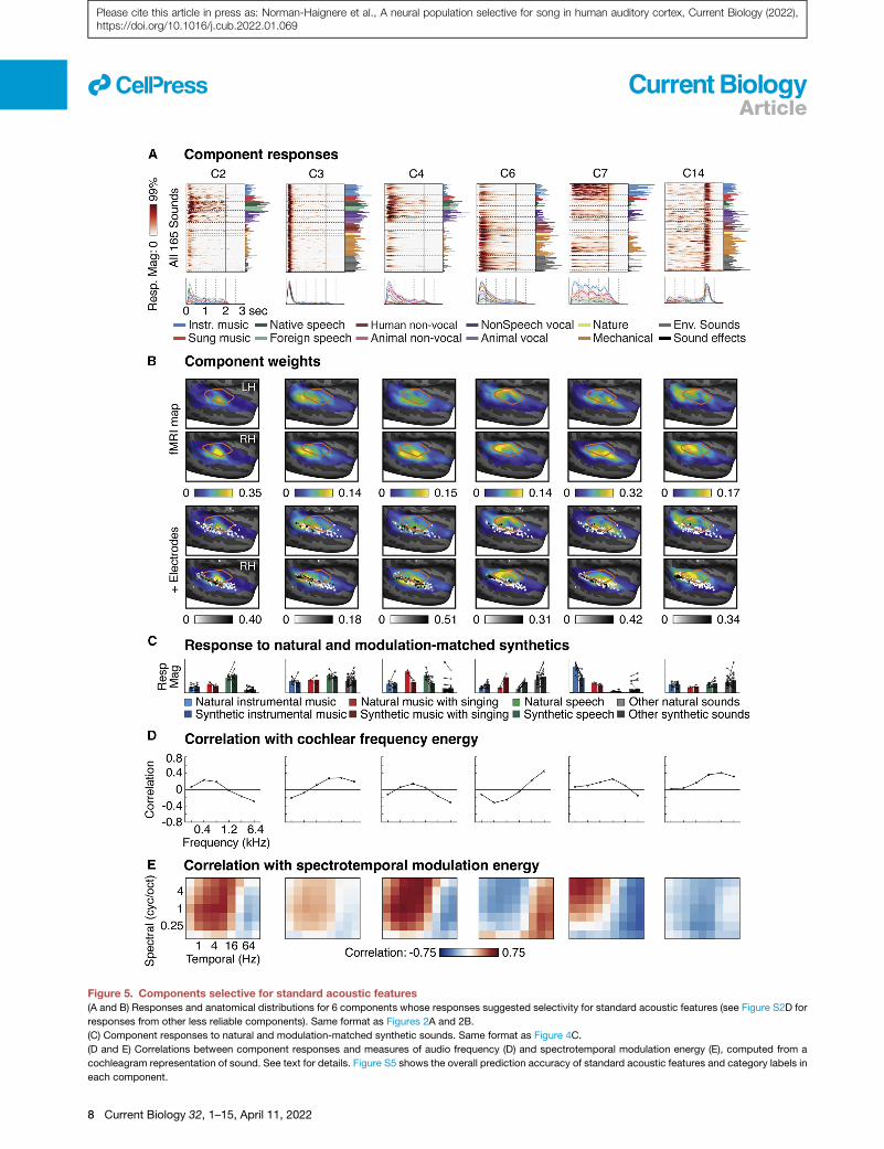
Figure 5. Components selective for standard acoustic features(A and B) Responses and anatomical distributions for 6 components whose responses suggested selectivity for standard acoustic features (see Figure S2D for

responses from other less reliable components). Same format as Figures 2A and 2B.

(C) Component responses to natural and modulation-matched synthetic sounds. Same format as Figure 4C.

(D and E) Correlations between component responses and measures of audio frequency (D) and spectrotemporal modulation energy (E), computed from a

cochleagram representation of sound. See text for details. Figure S5 shows the overall prediction accuracy of standard acoustic features and category labels in

each component.

ll



Article

ll


Article

matched on the same features used to compute the predictions.

Thus, these seemingly good predictions may be driven by

spurious correlations across natural sounds between standard

acoustic features and higher-order, category-specific features

(e.g., phonemic structure).34 Our synthesis approach addresses

this problem because the synthetic sounds are only constrained

by frequency and modulation features, effectively decoupling

them from higher-order features of sound.29

Single-electrode analysesWe tested whether we could also observe speech, music, and

song selectivity in individual electrodes without any component

modeling.Basedonprior studies,weexpected that speechselec-

tivity would be prominent in individual electrodes, but it was un-

clear if music or song selectivity would be robustly present, given

that music selectivity is weak in individual fMRI voxels.6,12 We

identified electrodes selective for speech, music, or song using

a subset of data and then measured their response in left-out, in-

dependent data. Electrode identification involved three steps.

First, we measured the average response across time and stimuli

to all soundcategorieswithmore thanfiveexemplars.Second,we

identified a pool of electrodes with a highly selective (selec-

tivity > 0.6) and significant (p < 0.001 via bootstrapping) response

to either speech, music, or song compared with all other cate-

gories. Selectivity was measured by contrasting the maximum

response across all speech and music categories (English

speech, foreign speech, sung music, instrumental music) with

the maximum response across all other non-music and non-

speech categories (we used the selectivity index [A�B]/A, where

A and B are the categories being contrasted; the [A� B] contrast

was bootstrapped and compared against 0 to assess signifi-

cance). Third, from this pool of electrodes, we formed three

groups: those that responded significantly more to speech than

all else (max[English speech, foreign speech] > max[non-speech

categories except sung music]), music than all else (instrumental

music > max[non-music categories]), or that exhibited super-ad-

ditive selectivity for singing (sung music > max[English speech,

foreign speech] + instrumental music) (using a threshold of

p < 0.01, via bootstrapping).

We show the top electrodes most significantly responsive to

speech, music, or singing as well as the average response

across all electrodes from each group (Figure 6). As expected,

we observed many speech-selective electrodes (173 electrodes

across 14 subjects). Notably, we also observed a small number

of music and song-selective electrodes (11 music-selective

electrodes across 4 subjects, and 7 song-selective electrodes

across 3 subjects). Despite their small number, each music-

and song-selective electrode replicated their selectivity for mu-

sic or song in independent data (p < 0.05 via bootstrapping for

every electrode individually; p < 0.001 for responses averaged

across all music and song-selective electrodes; selectivity was

measured using the same contrasts described above). More-

over, modulation-matched synthetic sounds produced much

weaker responses than natural sounds from the preferred cate-

gory in these electrodes (p < 0.01 via a sign test between re-

sponses to natural and model-matched sounds, applied to the

average response of speech, music, and song-selective elec-

trodes). The three subjects (S1, S3, and S4) with song-selective

electrodes had more sound-responsive electrodes than all but

one other subject (S2; subjects were ordered based on the num-

ber of sound-responsive electrodes they showed) and did not

have unusually high levels of musical training (S1 reported no

musical training, and S3 and S4 both reported 4 years of music

classes in elementary/middle school). Thus, it seems likely that

these subjects showed song-selective electrodes simply

because we had better coverage of their auditory cortex.

The presence of song selectivity in individual electrodes dem-

onstrates that our component analysis did not infer a form of

selectivity that is not present in the data. At the same time, only

a handful of electrodes showed song selectivity, and the selec-

tivity of these electrodes was substantially weaker than the

song-selective component we identified using purely statistical

criteria (p < 0.001 via bootstrap, using the super-additive song

selectivity metric). This observation suggests that our component

method isolated selectivity for singing by de-mixing weak song

selectivity present in individual electrodes. To test this hypothesis,

we re-ran both our data-driven (Figure 2) and hypothesis-driven

(Figure 3) component analyses after discarding all song-selective

electrodes. These analyses revealed a nearly identical song-se-

lective component (Figure S6A). This finding demonstrates that

we can infer song selectivity using two non-overlapping sets of

electrodes and two different analysis approaches.

The uneven distribution of electrodes across subjects made us

wonder whether our findings were driven by individual subjects.

The electrodes from just S1, for example, comprised �25% of

the dataset (70 of 272 electrodes). To address this question, we

repeated our data-driven and hypothesis-driven component ana-

lyses 15 times, each time excluding all the electrodes from one

subject. We observed a clear song-selective component in every

case (the correlation between the response of the song-selective

component derived from all subjects and those derived from

reduced datasets was greater than 0.9 in all cases) (Figure S6B

plots the song-selective components inferred when excluding

data fromS1).Whenwediscardedall of thedata fromall three sub-

jects with song-selective electrodes, thus discarding nearly half

the dataset (122 of 272 electrodes), we still recovered a song-se-

lective component using our hypothesis-driven method, but not

using our data-drivenmethod (FigureS6C).Wenote that detecting

song selectivity using our hypothesis-driven approach is highly

non-trivial: when we applied the same approach to a standard

acoustic representation or to our previously inferred fMRI compo-

nents, we did not recover a song-selective component

(Figures S4A, S4B, and S5B). Thus, the failure of our data-driven

method is not because song selectivity is absent, but instead re-

flects the inherent challenge of unmixing different response pat-

terns using purely statistical criteria, particularly with a modestly

sizeddataset.Overall, thesefindingsdemonstrate thatsongselec-

tivity is robustly present across multiple subjects.

Prediction of music and speech selectivity detectedwith fMRIWhy were we able to observe a song-selective component that

was not evident in prior fMRI studies? One natural hypothesis is

that ECoG is a finer-grained measure of neural activity and thus

allowed us to resolve finer-grained selectivity. If this hypothesis

were true, we might expect coarser fMRI response patterns to

be predictable from finer-grained ECoG responses, but not vice

versa. We have already shown that the song-selective ECoG


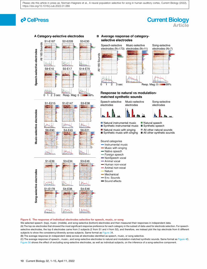
Figure 6. The response of individual electrodes selective for speech, music, or song

We selected speech- (top), music- (middle), and song-selective (bottom) electrodes and then measured their responses in independent data.

(A) The top six electrodes that showed the most significant response preference for each category in the subset of data used for electrode selection. For speech-

selective electrodes, the top 6 electrodes came from 2 subjects (2 from S1 and 4 from S2), and therefore, we instead plot the top electrode from 6 different

subjects to show the consistency/diversity across subjects. Same format as Figure 2A.

(B) The average response (in independent data) across all electrodes identified as speech, music, or song selective.

(C) The average response of speech-, music-, and song-selective electrodes to natural and modulation-matched synthetic sounds. Same format as Figure 4C.

Figure S6 shows the effect of excluding song-selective electrodes, as well as individual subjects, on the inference of a song-selective component.

ll



Article

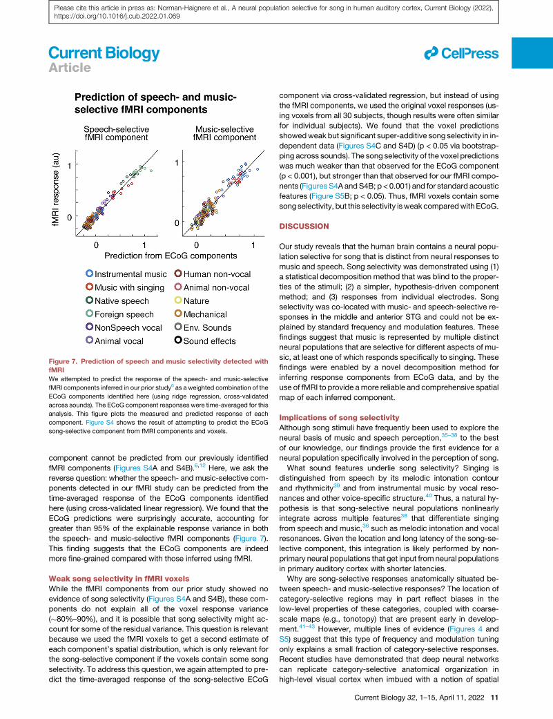
Figure 7. Prediction of speech and music selectivity detected with

fMRI

We attempted to predict the response of the speech- and music-selective

fMRI components inferred in our prior study6 as a weighted combination of the

ECoG components identified here (using ridge regression, cross-validated

across sounds). The ECoG component responses were time-averaged for this

analysis. This figure plots the measured and predicted response of each

component. Figure S4 shows the result of attempting to predict the ECoG

song-selective component from fMRI components and voxels.

ll


Article

component cannot be predicted from our previously identified

fMRI components (Figures S4A and S4B).6,12 Here, we ask the

reverse question: whether the speech- and music-selective com-

ponents detected in our fMRI study can be predicted from the

time-averaged response of the ECoG components identified

here (using cross-validated linear regression). We found that the

ECoG predictions were surprisingly accurate, accounting for

greater than 95% of the explainable response variance in both

the speech- and music-selective fMRI components (Figure 7).

This finding suggests that the ECoG components are indeed

more fine-grained compared with those inferred using fMRI.

Weak song selectivity in fMRI voxelsWhile the fMRI components from our prior study showed no

evidence of song selectivity (Figures S4A and S4B), these com-

ponents do not explain all of the voxel response variance

(�80%–90%), and it is possible that song selectivity might ac-

count for some of the residual variance. This question is relevant

because we used the fMRI voxels to get a second estimate of

each component’s spatial distribution, which is only relevant for

the song-selective component if the voxels contain some song

selectivity. To address this question, we again attempted to pre-

dict the time-averaged response of the song-selective ECoG

component via cross-validated regression, but instead of using

the fMRI components, we used the original voxel responses (us-

ing voxels from all 30 subjects, though results were often similar

for individual subjects). We found that the voxel predictions

showedweak but significant super-additive song selectivity in in-

dependent data (Figures S4C and S4D) (p < 0.05 via bootstrap-

ping across sounds). The song selectivity of the voxel predictions

was much weaker than that observed for the ECoG component

(p < 0.001), but stronger than that observed for our fMRI compo-

nents (Figures S4A andS4B; p < 0.001) and for standard acoustic

features (Figure S5B; p < 0.05). Thus, fMRI voxels contain some

song selectivity, but this selectivity isweak comparedwithECoG.

DISCUSSION

Our study reveals that the human brain contains a neural popu-

lation selective for song that is distinct from neural responses to

music and speech. Song selectivity was demonstrated using (1)

a statistical decomposition method that was blind to the proper-

ties of the stimuli; (2) a simpler, hypothesis-driven component

method; and (3) responses from individual electrodes. Song

selectivity was co-located with music- and speech-selective re-

sponses in the middle and anterior STG and could not be ex-

plained by standard frequency and modulation features. These

findings suggest that music is represented by multiple distinct

neural populations that are selective for different aspects of mu-

sic, at least one of which responds specifically to singing. These

findings were enabled by a novel decomposition method for

inferring response components from ECoG data, and by the

use of fMRI to provide amore reliable and comprehensive spatial

map of each inferred component.

Implications of song selectivityAlthough song stimuli have frequently been used to explore the

neural basis of music and speech perception,35–38 to the best

of our knowledge, our findings provide the first evidence for a

neural population specifically involved in the perception of song.

What sound features underlie song selectivity? Singing is

distinguished from speech by its melodic intonation contour

and rhythmicity39 and from instrumental music by vocal reso-

nances and other voice-specific structure.40 Thus, a natural hy-

pothesis is that song-selective neural populations nonlinearly

integrate across multiple features38 that differentiate singing

from speech and music,36 such as melodic intonation and vocal

resonances. Given the location and long latency of the song-se-

lective component, this integration is likely performed by non-

primary neural populations that get input from neural populations

in primary auditory cortex with shorter latencies.

Why are song-selective responses anatomically situated be-

tween speech- and music-selective responses? The location of

category-selective regions may in part reflect biases in the

low-level properties of these categories, coupled with coarse-

scale maps (e.g., tonotopy) that are present early in develop-

ment.41–43 However, multiple lines of evidence (Figures 4 and

S5) suggest that this type of frequency and modulation tuning

only explains a small fraction of category-selective responses.

Recent studies have demonstrated that deep neural networks

can replicate category-selective anatomical organization in

high-level visual cortex when imbued with a notion of spatial


ll


Article

topography and a simple wiring constraint,44,45 providing a func-

tional hypothesis for why this organization emerges. Speech-

and music-trained DNNs have shown promise in predicting

non-primary auditory cortical responses,10 and future research

could test whether these networks can explain the functional

and anatomical organization uncovered here.

How do song-selective populations interact with regions

beyondauditory cortex?Thereare reports of responses to singing

and other types of music in motor/premotor regions,46–48 which

could in principle influence responses in auditory cortex through

feedback, and there is broad consensus that auditory circuits

play a critical role in the production of speech and other vocal

sounds such as singing.48–51 Listening to singing can induce

strong emotions52 andmemories53 that plausibly dependupon in-

teractions between song-selective neural populations and re-

gions of the medial temporal lobe and basal forebrain.54,55 Our

study opens the door to studying such interactions with greater

precision, for example, by stimulating auditory electrodes that

project strongly on music- or song-selective components and

measuring the impact on downstream regions, as well as any

concomitant changes in patients’ subjective perception.56,57

How might song selectivity have arisen in the first place? The

visual word form area demonstrates that category-selective neu-

ral populations can arise purely from experience, since reading is

a recent cultural invention.58 Music could similarly arise from in-

dividual experience, particularly since it engages reward-related

circuits in the basal forebrain,54,55 whose activity can induce

long-term plasticity in the auditory cortex.59 However, unlike

reading, singing could plausibly have shaped neural circuits

over the course of evolution,60 since it appears to be a natural

and instinctive behavior that is widely present across human so-

cieties2 and does not require technology. Indeed, we observed

music- and song-selective electrodes in a subject with no re-

ported musical training (S1), consistent with a recent finding

from our lab that music selectivity does not depend on explicit

training.12 On the other hand, almost all listeners have extensive

implicit knowledge of music and song gained through listening

over the lifetime.61,62 Thus, many questions remain about the or-

igins of song and music selectivity in auditory cortex.

What are the perceptual consequences of neural song selec-

tivity? Vocal melodies are better remembered than instrumental

melodies,53 which may reflect greater salience for sung

compared with instrumental music.63 The neural basis of this

increased salience remains unclear, but one possibility is that

more salient stimuli might have more distinctive representations

in high-level sensory regions.64 We hope our study will catalyze

research that focuses specifically on the perception of song,

distinct from music and speech perception more generally.

Music selectivityOur findings validate our prior fMRI studies, which reported a mu-

sic-selective component with substantially greater selectivity than

that present in individual voxels,6,12 which we hypothesized was

due to the overlap of neural populations within voxels. Consistent

with thishypothesis, someof theelectrodes thatshowed thestron-

gestmusic selectivity (e.g., S1-E147, S1-E215) were sampled by a

high-densitygridwithparticularlysmall electrodes (1-mmexposed

diameter), suggesting that high spatial resolution is indeed impor-

tant for detecting music selectivity in individual electrodes.


Voice and speech selectivityPrior studies have identified a large region within the STG that re-

sponds preferentially to non-speech voice sounds (the ‘‘tempo-

ral voice area’’).65 However, the extent to which speech- and

voice-selective responses are distinct in the brain has remained

unclear: speech-selective responses typically show above base-

line responses to non-speech vocalizations,6 and the temporal

voice area responds more strongly to speech than other non-

speech vocalizations.65 By contrast, the speech-selective com-

ponents (C1, C15) identified in this study showed virtually no

response to non-speech vocalizations, and C4 responded

strongly to a wide range of speech and non-speech vocaliza-

tions. This finding suggests that speech and voice indeed have

spatially distinct representations. The apparent overlap of

speech and voice responses in prior studies may be due to

coarse neuroimaging methods and analyses.

Component modeling: Strengths, limitations, andrelationship to prior methodsComponent modeling provides a way to (1) infer prominent

response patterns,21,66 (2) suggest novel hypotheses, and (3)

disentangle spatially overlapping responses.67 Our results illus-

trate each of these benefits. We inferred a small number of com-

ponents that explained much of the response variation across

hundreds of electrodes. We uncovered a novel form of music

selectivity (song selectivity) that we did not a priori expect. And

the song-selective component showed clearer selectivity for

singing than that present in individual electrodes, many of which

appeared to reflect a mixture of music, speech, and song

selectivity.

Thekeychallengeofcomponentmodeling is thatmatrixapprox-

imation is ill-posed, and hence, the solution depends on statistical

assumptions. Many component methods rely on just one of the

following three assumptions: (1) non-negativity,68 (2) sparsity

across time or space,69,70 or (3) temporal smoothness.71,72 We

showedthatall of thesepropertiesareevident inauditoryECoGre-

sponses, and themodel we developed to embody these assump-

tions predicted ECoG responses better thanbaselinemodels. Our

key finding of song selectivity was nonetheless robust to these as-

sumptions: song selectivity was observed in a model that only

imposed non-negativity on the responses (Figure S2A), as well

as a simpler, regression-based analysis (Figure 3) and in re-

sponses of individual electrodes (Figure 6), neither of which

depend on statistical assumptions like non-negativity or sparsity.

Our fMRI decomposition method placed statistical constraints

on the voxel weights because we had thousands of voxels

(>10,000) with which to estimate statistics. Here, we additionally

constrained the component responses because we had many

fewer electrodes and high-dimensional response time courses.

Ourmethod is distinct from a variety of other relevant component

models. Unlike many sparse convolutional models,73 each

component in our model is defined by a single time course and

a single pattern of electrode weights rather than by a time-vary-

ing spatial pattern. As a result, our components can be more

easily interpreted as the response of an underlying neuronal pop-

ulation. Unlike clustering methods (or convex NMF21), our

method can disentangle responses that overlap within individual

electrodes. And unlike many tensor decomposition methods,74

our method does not require the shape of a component’s

ll


Article

response time course to be identical across different stimuli,

which is critical when modeling responses to sensory features

that are not necessarily aligned to stimulus onset.

Combining the strengths of fMRI and ECoG datafMRI and ECoG data have different strengths and weaknesses.

fMRI data are coarse due to the indirect sampling of neural activ-

ity via blood flow but are non-invasive and can provide dense,

comprehensive coverage from many subjects. By contrast,

ECoG coverage is sparse and driven by clinical demands, but

has much better spatiotemporal precision. Our study introduces

amethod for combining the strengths of ECoGand fMRI, by infer-

ring a set of canonical response patterns with ECoG and then

mapping their spatial distribution with fMRI. This approach

cannot spatially distinguish two components with similar time-

averaged responses (e.g., the speech-selective components

C1 and C15), but empirically, most components had distinct

time-averaged responses, andwe foundaclose correspondence

between fMRI and ECoG maps, which was primarily limited by

the sparse coverage of ECoG recordings (Figure 2C).

CONCLUSIONS

By revealing a neural population selective for song, our study be-

gins to unravel the neural code for music, raising many questions

for future research. Do music- and song-selective responses

reflect note-level structure (e.g., pitch and timbre)75 or the way

notes are patterned (e.g., melodies and rhythms)?76 How can

music and song selectivity be described in computational terms,

given that standard acoustic features appear insufficient?10 And

how did music and song selectivity arise over the course of

development or evolution?1,2 Our study represents an initial

step toward answering these longstanding questions.

STAR+METHODS

Detailed methods are provided in the online version of this paper

and include the following:

d KEY RESOURCES TABLE

d RESOURCE AVAILABILITY

B Lead contact

B Materials availability

B Data and code availability

d EXPERIMENTAL MODEL AND SUBJECT DETAILS

B Subjects

d METHOD DETAILS

B Electrode grids

B Natural sounds

B Modulation-matched synthetic sounds

B Sound category assignments

B Music ratings

d QUANTIFICATION AND STATISTICAL ANALYSIS

B Preprocessing

B Session effects

B Electrode selection

B Electrode localization

B Response statistics relevant to component modeling

B Component model

B Constraining the smoothing kernel

B Cross-validation analyses

B Assessing component robustness

B fMRI weight maps

B Tonotopic definition of primary auditory cortex

B Component responses to modulation-matched

sounds

B Acoustic correlations and predictions

B Calculating latencies

B Speech STRFs

B Predicting ECoG components from fMRI and vice

versa

B Hypothesis-driven component analysis

B Single electrode analyses

B Statistics

B Noise correction

SUPPLEMENTAL INFORMATION

Supplemental information can be found online at https://doi.org/10.1016/j.

cub.2022.01.069.

ACKNOWLEDGMENTS

This work was supported by the National Institutes of Health (DP1 HD091947

to N.K., P41-EB018783 to P.B. and G.S., P50-MH109429 to G.S., R01-

EB026439 to P.B. and G.S., U24-NS109103 to P.B. and G.S., U01-

NS108916 to P.B. and G.S., R25-HD088157 to G.S., and K99DC018051-

01A1 to S.V.N.-H.), the US Army Research Office (W911NF-15-1-0440 to

G.S.), the National Science Foundation (grant BCS-1634050 to J.H.M.), the

NSF Science and Technology Center for Brains, Minds, and Machines (CCF-

1231216), Fondazione Neurone (grant to P.B. and G.S.), the Howard Hughes

Medical Institute (LSRF Postdoctoral Fellowship to S.V.N.-H.), and the Kristin

R. Pressman and Jessica J. Pourian ’13 Fund at MIT.

AUTHOR CONTRIBUTIONS

Conceptualization, S.V.N.-H., J.F., P.B., A.R., J.H.M., G.S., and N.K.; method-

ology, S.V.N.-H., J.F., P.B., and A.R.; software, S.V.N.-H. and J.F.; validation,

S.V.N.-H.; formal analysis, S.V.N.-H.; investigation, S.V.N.-H., D.B., P.B., and

A.R.; resources, P.B. and A.R.; data curation, S.V.N.-H., J.F., D.B., and P.B.;

writing – original draft, S.V.N.-H.; writing – review & editing, S.V.N.-H., J.F.,

D.B., P.B., A.R., J.H.M., G.S., and N.K.; visualization, S.V.N.-H.; supervision,

A.R., J.H.M., G.S., and N.K.; project administration, N.K.; funding acquisition,

S.V.N.-H., P.B., A.R., J.H.M., G.S., and N.K.

DECLARATION OF INTERESTS

N.K. was recently on the Current Biology advisory board. The other authors

declare no competing interests.

Received: February 23, 2021

Revised: October 26, 2021

Accepted: January 24, 2022

Published: February 22, 2022

REFERENCES

1. Wallin, N.L., Merker, B., and Brown, S. (2001). The Origins of Music (MIT

Press).

2. Mehr, S.A., Singh, M., Knox, D., Ketter, D.M., Pickens-Jones, D., Atwood,

S., Lucas, C., Jacoby, N., Egner, A.A., Hopkins, E.J., et al. (2019).

Universality and diversity in human song. Science 366, eaax0868.




http://refhub.elsevier.com/S0960-9822(22)00131-2/sref1





ll


Article

3. Patel, A.D. (2019). Evolutionary music cognition: cross-species studies. In

Foundations in Music Psychology: Theory and Research, P.J. Rentfrow,

and D.J. Levitin, eds. (MIT Press), pp. 459–501.

4. Peretz, I., Vuvan, D., Lagrois, M.E., and Armony, J.L. (2015). Neural over-

lap in processing music and speech. Philos. Trans. R. Soc. Lond. B Biol.

Sci. 370, 20140090.

5. Leaver, A.M., andRauschecker, J.P. (2010). Cortical representation of nat-

ural complex sounds: effects of acoustic features and auditory object

category. J. Neurosci. 30, 7604–7612.

6. Norman-Haignere, S.V., Kanwisher, N.G., and McDermott, J.H. (2015).

Distinct cortical pathways for music and speech revealed by hypothe-

sis-free voxel decomposition. Neuron 88, 1281–1296.

7. Peretz, I. (2016). Neurobiology of congenital amusia. Trends Cogn. Sci. 20,

857–867.

8. Peterson, R.L., and Pennington, B.F. (2015). Developmental dyslexia.

Annu. Rev. Clin. Psychol. 11, 283–307.

9. Herholz, S.C., and Zatorre, R.J. (2012). Musical training as a framework for

brain plasticity: behavior, function, and structure. Neuron 76, 486–502.

10. Kell, A.J.E., Yamins, D.L.K., Shook, E.N., Norman-Haignere, S.V., and

McDermott, J.H. (2018). A task-optimized neural network replicates hu-

man auditory behavior, predicts brain responses, and reveals a cortical

processing hierarchy. Neuron 98, 630–644.e16.

11. Angulo-Perkins, A., Aub�e, W., Peretz, I., Barrios, F.A., Armony, J.L., and

Concha, L. (2014). Music listening engages specific cortical regions within

the temporal lobes: differences between musicians and non-musicians.

Cortex 59, 126–137.

12. Boebinger, D., Norman-Haignere, S.V., McDermott, J.H., and Kanwisher,

N. (2021). Music-selective neural populations arise without musical

training. J. Neurophysiol. 125, 2237–2263.

13. Casey, M.A. (2017). Music of the 7Ts: predicting and decoding multivoxel

fMRI responses with acoustic, schematic, and categorical music features.

Front. Psychol. 8, 1179.

14. Humphries, C., Liebenthal, E., and Binder, J.R. (2010). Tonotopic organi-

zation of human auditory cortex. NeuroImage 50, 1202–1211.

15. Da Costa, S.D., Zwaag, W. van der, Marques, J.P., Frackowiak, R.S.J.,

Clarke, S., and Saenz, M. (2011). Human primary auditory cortex follows

the shape of heschl’s gyrus. J. Neurosci. 31, 14067–14075.

16. Moerel, M., DeMartino, F., and Formisano, E. (2012). Processing of natural

sounds in human auditory cortex: tonotopy, spectral tuning, and relation to

voice sensitivity. J. Neurosci. 32, 14205–14216.

17. Baumann, S., Petkov, C.I., andGriffiths, T.D. (2013). A unified framework for

the organization of the primate auditory cortex. Front. Syst. Neurosci. 7, 11.

18. Schonwiesner, M., and Zatorre, R.J. (2009). Spectro-temporal modulation

transfer function of single voxels in the human auditory cortex measured

with high-resolution fMRI. Proc. Natl. Acad. Sci. USA 106, 14611–14616.

19. Barton, B., Venezia, J.H., Saberi, K., Hickok, G., and Brewer, A.A. (2012).

Orthogonal acoustic dimensions define auditory field maps in human cor-

tex. Proc. Natl. Acad. Sci. USA 109, 20738–20743.

20. Santoro, R., Moerel, M., De Martino, F., Goebel, R., Ugurbil, K., Yacoub,

E., and Formisano, E. (2014). Encoding of natural sounds at multiple spec-

tral and temporal resolutions in the human auditory cortex. PLoS Comp.

Biol. 10, e1003412.

21. Hamilton, L.S., Edwards, E., and Chang, E.F. (2018). A spatial map of

onset and sustained responses to speech in the human superior temporal

gyrus. Curr. Biol. 28, 1860–1871.e4.

22. Belin, P., Zatorre, R.J., Lafaille, P., Ahad, P., and Pike, B. (2000). Voice-se-

lective areas in human auditory cortex. Nature 403, 309–312.

23. Overath, T., McDermott, J.H., Zarate, J.M., and Poeppel, D. (2015). The

cortical analysis of speech-specific temporal structure revealed by re-

sponses to sound quilts. Nat. Neurosci. 18, 903–911.

24. Mesgarani, N., Cheung, C., Johnson, K., and Chang, E.F. (2014). Phonetic

feature encoding in human superior temporal gyrus. Science 343, 1006–

1010.


25. Di Liberto, G.M., O’Sullivan, J.A., and Lalor, E.C. (2015). Low-frequency

cortical entrainment to speech reflects phoneme-level processing. Curr.

Biol. 25, 2457–2465.

26. de Heer, W.A., Huth, A.G., Griffiths, T.L., Gallant, J.L., and Theunissen,

F.E. (2017). The hierarchical cortical organization of human speech pro-

cessing. J. Neurosci. 37, 6539–6557.

27. Brodbeck, C., Hong, L.E., and Simon, J.Z. (2018). Rapid transformation

from auditory to linguistic representations of continuous speech. Curr.

Biol. 28, 3976–3983.e5.

28. Norman-Haignere, S.V., Long, L.K., Devinsky, O., Doyle, W., Irobunda, I.,

Merricks, E.M., Feldstein, N.A., McKhann, G.M., Schevon, C.A., Flinker,

A., et al. (2022). Multiscale temporal integration organizes hierarchical

computation in human auditory cortex. Preprint at. Nat. Hum. Behav.

Published online February 10, 2022. https://doi.org/10.1038/s41562-

021-01261-y.

29. Norman-Haignere, S.V., and McDermott, J.H. (2018). Neural responses to

natural andmodel-matched stimuli reveal distinct computations in primary

and nonprimary auditory cortex. PLoS Biol 16, e2005127.

30. Patterson, R.D., Uppenkamp, S., Johnsrude, I.S., and Griffiths, T.D.

(2002). The processing of temporal pitch and melody information in audi-

tory cortex. Neuron 36, 767–776.

31. Penagos, H., Melcher, J.R., and Oxenham, A.J. (2004). A neural represen-

tation of pitch salience in nonprimary human auditory cortex revealed with

functional magnetic resonance imaging. J. Neurosci. 24, 6810–6815.

32. Norman-Haignere, S., Kanwisher, N., and McDermott, J.H. (2013).

Cortical pitch regions in humans respond primarily to resolved harmonics

and are located in specific tonotopic regions of anterior auditory cortex.

J. Neurosci. 33, 19451–19469.

33. Roswandowitz, C., Kappes, C., Obrig, H., and von Kriegstein, K. (2018).

Obligatory and facultative brain regions for voice-identity recognition.

Brain 141, 234–247.

34. Groen, I.I., Greene, M.R., Baldassano, C., Fei-Fei, L., Beck, D.M., and

Baker, C.I. (2018). Distinct contributions of functional and deep neural

network features to representational similarity of scenes in human brain

and behavior. eLife 7, e32962.

35. Merrill, J., Sammler, D., Bangert, M., Goldhahn, D., Lohmann, G., Turner,

R., and Friederici, A.D. (2012). Perception of words and pitch patterns in

song and speech. Front. Psychol. 3, 76.

36. Tierney, A., Dick, F., Deutsch, D., and Sereno, M. (2013). Speech versus

song: multiple pitch-sensitive areas revealed by a naturally occurring

musical illusion. Cereb. Cortex 23, 249–254.

37. Whitehead, J.C., and Armony, J.L. (2018). Singing in the brain: neural rep-

resentation of music and voice as revealed by fMRI. Hum. Brain Mapp 39,

4913–4924.

38. Sammler, D., Baird, A., Valabregue, R., Cl�ement, S., Dupont, S., Belin, P.,

and Samson, S. (2010). The relationship of lyrics and tunes in the process-

ing of unfamiliar songs: a functional magnetic resonance adaptation study.

J. Neurosci. 30, 3572–3578.

39. Patel, A.D. (2011). In Language, music, and the brain: a resource-sharing

framework, , P. Rebuschat, M. Rohmeier, J.A. Hawkins, and I. Cross, eds.,

pp. 204–223, Oxford.

40. Sundberg, J. (1999). The perception of singing. In The Psychology of

Music (Elsevier), pp. 171–214.

41. Arcaro, M.J., and Livingstone, M.S. (2021). On the relationship between

maps and domains in inferotemporal cortex. Nat. Rev. Neurosci. 22,

573–583.

42. Levy, I., Hasson, U., Avidan, G., Hendler, T., and Malach, R. (2001).

Center-periphery organization of human object areas. Nat. Neurosci. 4,

533–539.

43. Conway, B.R. (2018). The organization and operation of inferior temporal

cortex. Annu. Rev. Vis. Sci. 4, 381–402.

44. Lee, H., Margalit, E., Jozwik, K.M., Cohen, M.A., Kanwisher, N., Yamins,

D.L., and DiCarlo, J.J. (2020). Topographic deep artificial neural networks

reproduce the hallmarks of the primate inferior temporal cortex face










































































https://doi.org/10.1038/s41562-021-01261-y

https://doi.org/10.1038/s41562-021-01261-y
















































ll


Article

processing network. Preprint at bioRxiv. https://doi.org/10.1101/2020.07.

09.185116.

45. Blauch, N.M., Behrmann, M., and Plaut, D.C. (2022). A connectivity-con-

strained computational account of topographic organization in primate

high-level visual cortex. Proc. Natl. Acad. Sci. USA 119, e2112566119.

46. Callan, D.E., Tsytsarev, V., Hanakawa, T., Callan, A.M., Katsuhara, M.,

Fukuyama, H., and Turner, R. (2006). Song and speech: brain regions

involvedwithperceptionandcovert production.Neuroimage31, 1327–1342.

47. L�eveque, Y., and Schon, D. (2015). Modulation of the motor cortex during

singing-voice perception. Neuropsychologia 70, 58–63.

48. Zatorre, R.J., Chen, J.L., and Penhune, V.B. (2007). When the brain plays

music: auditory–motor interactions in music perception and production.

Nat. Rev. Neurosci. 8, 547–558.

49. Kleber, B.A., and Zarate, J.M. (2014). The Neuroscience of Singing (Oxford

University Press).

50. Hickok, G., Houde, J., and Rong, F. (2011). Sensorimotor integration in

speech processing: computational basis and neural organization.

Neuron 69, 407–422.

51. Guenther, F.H., and Vladusich, T. (2012). A neural theory of speech acqui-

sition and production. J. Neurolinguistics 25, 408–422.

52. Bainbridge, C.M., Bertolo, M., Youngers, J., Atwood, S., Yurdum, L.,

Simson, J., Lopez, K., Xing, F., Martin, A., and Mehr, S.A. (2021). Infants

relax in response to unfamiliar foreign lullabies. Nat. Hum. Behav. 5,

256–264.

53. Weiss, M.W., Trehub, S.E., and Schellenberg, E.G. (2012). Something in

the way she sings: enhanced memory for vocal melodies. Psychol. Sci.

23, 1074–1078.

54. Blood, A.J., and Zatorre, R.J. (2001). Intensely pleasurable responses to

music correlate with activity in brain regions implicated in reward and

emotion. Proc. Natl. Acad. Sci. USA 98, 11818–11823.

55. Salimpoor, V.N., van denBosch, I., Kovacevic, N., McIntosh, A.R., Dagher,

A., and Zatorre, R.J. (2013). Interactions between the nucleus accumbens

and auditory cortices predict music reward value. Science 340, 216–219.

56. Parvizi, J., Jacques, C., Foster, B.L., Witthoft, N., Rangarajan, V., Weiner,

K.S., and Grill-Spector, K. (2012). Electrical stimulation of human fusiform

face-selective regions distorts face perception. J. Neurosci. 32, 14915–

14920.

57. Schalk, G., Kapeller, C., Guger, C., Ogawa, H., Hiroshima, S., Lafer-

Sousa, R., Saygin, Z.M., Kamada, K., and Kanwisher, N. (2017).

Facephenes and rainbows: causal evidence for functional and anatomical

specificity of face and color processing in the human brain. Proc. Natl.

Acad. Sci. USA 114, 12285–12290.

58. Dehaene, S., and Cohen, L. (2011). The unique role of the visual word form

area in reading. Trends Cogn. Sci. 15, 254–262.

59. Froemke, R.C., Merzenich, M.M., and Schreiner, C.E. (2007). A synaptic

memory trace for cortical receptive field plasticity. Nature 450, 425–429.

60. Mehr, S.A., and Krasnow, M.M. (2017). Parent-offspring conflict and the

evolution of infant-directed song. Evol. Hum. Behav. 38, 674–684.

61. Tillmann, B. (2005). Implicit investigations of tonal knowledge in nonmusi-

cian listeners. Ann. N. Y. Acad. Sci. 1060, 100–110.

62. Bigand, E., and Poulin-Charronnat, B. (2006). Are we ‘‘experienced lis-

teners’’? A review of the musical capacities that do not depend on formal

musical training. Cognition 100, 100–130.

63. Weiss, M.W., Schellenberg, E.G., Peng, C., and Trehub, S.E. (2019).

Contextual distinctiveness affects the memory advantage for vocal mel-

odies. Auditory Percept. Cogn. 2, 47–66.

64. Cohen, M.A., Alvarez, G.A., Nakayama, K., and Konkle, T. (2017). Visual

search for object categories is predicted by the representational architec-

ture of high-level visual cortex. J. Neurophysiol. 117, 388–402.

65. Belin, P., Zatorre, R.J., and Ahad, P. (2002). Human temporal-lobe

response to vocal sounds. Brain Res. Cogn. Brain Res. 13, 17–26.

66. Chen, P.-H.C., Chen, J., Yeshurun, Y., Hasson, U., Haxby, J., and

Ramadge, P.J. (2015). A reduced-dimension fMRI shared response

model. Advances in Neural Information Processing Systems 28, 460–468.

67. de Cheveign�e, A., and Parra, L.C. (2014). Joint decorrelation, a versatile

tool for multichannel data analysis. Neuroimage 98, 487–505.

68. Lee, D.D., and Seung, H.S. (1999). Learning the parts of objects by non-

negative matrix factorization. Nature 401, 788–791.

69. Olshausen, B.A., and Field, D.J. (1997). Sparse coding with an overcom-

plete basis set: a strategy employed by V1? Vis. Res. 37, 3311–3325.

70. Hyv€arinen, A. (1999). Fast and robust fixed-point algorithms for indepen-

dent component analysis. IEEE Trans. Neural Netw. 10, 626–634.

71. Wiskott, L., and Sejnowski, T.J. (2002). Slow feature analysis: unsuper-

vised learning of invariances. Neural Comput 14, 715–770.

72. Byron, M.Y., Cunningham, J.P., Santhanam, G., Ryu, S.I., Shenoy, K.V.,

and Sahani, M. (2009). Gaussian-process factor analysis for low-dimen-

sional single-trial analysis of neural population activity. Advances in

Neural Information Processing Systems 21, 1881–1888.

73. Bouchard, K.E., Bujan, A.F., Chang, E.F., and Sommer, F.T. (2017). Sparse

coding of ECoG signals identifies interpretable components for speech

control in human sensorimotor cortex. Annu. Int. Conf. IEEE Eng. Med.

Biol. Soc. 39th Annual International Conference of the IEEE Engineering

in Medicine and Biology Society (EMBC) 2017, 3636–3639.

74. Williams, A.H., Kim, T.H., Wang, F., Vyas, S., Ryu, S.I., Shenoy, K.V.,

Schnitzer, M., Kolda, T.G., and Ganguli, S. (2018). Unsupervised discovery

of demixed, low-dimensional neural dynamics across multiple timescales

through tensor component analysis. Neuron 98, 1099–1115.e8.

75. Casey, M., Thompson, J., Kang, O., Raizada, R., and Wheatley, T. (2012).

Population codes representing musical timbre for high-level fMRI catego-

rization of music genres. In Machine Learning and Interpretation in

Neuroimaging (Springer), pp. 34–41.

76. Schindler, A., Herdener, M., and Bartels, A. (2013). Coding of melodic

gestalt in human auditory cortex. Cereb. Cortex 23, 2987–2993.

77. Schalk, G., and Mellinger, J. (2010). A Practical Guide to Brain–Computer

Interfacing with BCI2000: General-Purpose Software for Brain-Computer

Interface Research, Data Acquisition, Stimulus Presentation, and Brain

Monitoring (Springer Science & Business Media).

78. Schalk, G., McFarland, D.J., Hinterberger, T., Birbaumer, N., andWolpaw,

J.R. (2004). BCI2000: a general-purpose brain-computer interface (BCI)

system. IEEE Trans. Biomed. Eng. 51, 1034–1043.

79. Chi, T., Ru, P., and Shamma, S.A. (2005). Multiresolution spectrotemporal

analysis of complex sounds. J. Acoust. Soc. Am. 118, 887–906.

80. Nichols, T.E., and Holmes, A.P. (2002). Nonparametric permutation tests

for functional neuroimaging: a primer with examples. Hum. Brain Mapp.

15, 1–25.

81. Norman-Haignere, S.V., Albouy, P., Caclin, A., McDermott, J.H.,

Kanwisher, N.G., and Tillmann, B. (2016). Pitch-responsive cortical re-

gions in congenital amusia. J. Neurosci. 36, 2986–2994.

82. Kuhn, H.W. (1955). The Hungarian method for the assignment problem.

Nav. Res. Logist. Q. 2, 83–97.

83. Murphy, K.P. (2012). Machine Learning: a Probabilistic Perspective (MIT

Press).

84. Daube, C., Ince, R.A.A., andGross, J. (2019). Simple acoustic features can

explain phoneme-based predictions of cortical responses to speech. Curr.

Biol. 29, 1924–1937.e9.

85. Efron, B. (1982). The Jackknife, the Bootstrap, and Other Resampling

Plans (Siam).

86. Loftus, G.R., and Masson, M.E. (1994). Using confidence intervals in

within-subject designs. Psychon. Bull. Rev. 1, 476–490.

87. Schoppe, O., Harper, N.S., Willmore, B.D., King, A.J., and Schnupp, J.W.

(2016). Measuring the performance of neural models. Front. Comp.

Neurosci. 10, 10.

88. Spearman, C. (1910). Correlation calculated from faulty data. Br. J.

Psychol. 3, 271–295.


https://doi.org/10.1101/2020.07.09.185116

https://doi.org/10.1101/2020.07.09.185116
































































































































ll


Article

STAR+METHODS

KEY RESOURCES TABLE

REAGENT or RESOURCE SOURCE IDENTIFIER

Deposited data

fMRI dataset of 165 natural sounds (10

subjects), Norman-Haignere et al.6McDermott, Kanwisher, and Norman-

Haignere labs

https://github.com/snormanhaignere/

natsound165-neuron2015

Software and algorithms

Freesurfer MGH https://surfer.nmr.mgh.harvard.edu

Other

165 natural sounds, Norman-Haignere

et al.6McDermott, Kanwisher, and Norman-

Haignere labs

http://mcdermottlab.mit.edu/svnh/

Natural-Sound/Stimuli.html

RESOURCE AVAILABILITY

Lead contactRequests for additional information or resources related to the study should be directed to Sam Norman-Haignere

([email protected]).

Materials availabilityThis study did not generate new unique reagents.

Data and code availability

d Source data is available in this repository: https://github.com/snormanhaignere/song-ecog-current-biology

d Code implementing the component decomposition is in this repository: https://github.com/snormanhaignere/ecog-

component-model

EXPERIMENTAL MODEL AND SUBJECT DETAILS

SubjectsFifteen epilepsy patients participated in our study (mean age: 35 years, age standard deviation: 14 years; 8 right-handed; 8 female).

All subjects were native English speakers, born in the US, who did not speak a second language. These subjects underwent tempo-

rary implantation of subdural electrode arrays at Albany Medical College to localize the epileptogenic zones and to delineate these

zones from eloquent cortical areas before brain resection. All subjects gave informed written consent to participate in the study,

which was approved by the Institutional Review Board of Albany Medical College.

METHOD DETAILS

Electrode gridsMost subjects had electrodes implanted in a single hemisphere, and STG coverage wasmuch better in one of the two hemispheres in

all subjects (8 right hemisphere patients and 7 left hemisphere patients). Inmost subjects, electrodes had a 2.3mmexposed diameter

with a 6mm center-to-center spacing for temporal lobe grids (10 mm spacing for grids in frontal, parietal and occipital lobe, but elec-

trodes from these grids typically did not show reliable sound-driven responses; electrodes were embedded in silicone; PMT Corp.,

Chanhassen, MN). Two subjects were implanted with a higher-density grid (1 mm exposed diameter, 3 mm center-to-center

spacing). One subject was implanted with stereotactic electrodes instead of grids.

Natural soundsThe sound set was the same as in our prior study.6 To generate the stimulus set, we began with a set of 280 everyday sounds for

which we could find a recognizable, 2-second recording. Using an online experiment (via Amazon’s Mechanical Turk), we excluded

sounds that were difficult to recognize (below 80% accuracy on a ten-way multiple-choice task; 55–60 subjects for each sound),

yielding 238 sounds. We then selected a subset of 160 sounds that were rated as most frequently heard in everyday life (in a second

Mechanical Turk study; 38–40 ratings per sound). Five additional ‘‘foreign speech’’ sounds were included (‘‘German,’’ ‘‘French,’’

e1 Current Biology 32, 1–15.e1–e11, April 11, 2022


https://github.com/snormanhaignere/song-ecog-current-biology

https://github.com/snormanhaignere/ecog-component-model

https://github.com/snormanhaignere/ecog-component-model

https://github.com/snormanhaignere/natsound165-neuron2015

https://github.com/snormanhaignere/natsound165-neuron2015

https://surfer.nmr.mgh.harvard.edu

http://mcdermottlab.mit.edu/svnh/Natural-Sound/Stimuli.html


ll


Article

‘‘Italian,’’ ‘‘Russian,’’ ‘‘Hindi’’) to distinguish responses to acoustic speech structure from responses to linguistic structure (the

160-sound set included only two foreign speech stimuli: ‘‘Spanish’’ and ‘‘Chinese’’). In total, there were 10 English speech stimuli,

7 foreign speech stimuli, 21 instrumental music stimuli, and 11 music stimuli with singing (see sound category assignments). Sounds

were RMS-normalized and presented by BCI200077,78 at a comfortable volume using sound-isolating over-the-ear headphones

(Panasonic RP-HTX7, 10 dB isolation). The sound set is freely available: http://mcdermottlab.mit.edu/svnh/Natural-Sound/Stimuli.

html

Subjects completed between three and seven runs of the experiment (S11, S13: 3 runs, S6, S14: 4 runs, S15: 5 runs, S1: 7 runs; all

other subjects: 6 runs). In each run, each natural sound was presented at least once. Between 14 and 17 of the sounds were repeated

exactly back-to-back, and subjectswere asked to press a buttonwhen they detected this repetition. This second instance of the sound

was excluded from the analysis because the presence of a target could otherwise bias responses in favor of the repeated stimuli. Each

run used a different random ordering of stimuli. There was a 1.4-2 second gap (randomly chosen) between consecutive stimuli.

Modulation-matched synthetic soundsIn ten subjects, we also measured responses to a distinct set of 36 natural sounds and 36 corresponding synthetic sounds that were

individually matched to each natural sound in their spectrotemporal modulations statistics using the approach described in our prior

study.29 The synthesis algorithm starts with an unstructured noise stimulus and iteratively modifies the noise tomatch themodulation

statistics of a natural sound. Modulations are measured using a standard model of auditory cortical responses79 in which a cochlea-

gram is passed through a set of linear filters tuned to modulations at a particular audio frequency, temporal rate, and spectral scale

(i.e. how coarse vs fine themodulations are in frequency). The spectrotemporal filters were created by crossing 9 temporal rates (0.5,

1, 2, 4, 8, 16, 32, 128 Hz) with 7 spectral scales (0.125, 0.25, 0.5, 1, 2, 4, 8 cycles per octave) and replicating each filter at each audio

frequency. The synthesis procedure alters the noise stimulus to match the histogram of response magnitudes across time for each

filter in themodel, which implicitly matches all time-averaged statistics of the filter responses (e.g., mean, variance, skew). The stimuli

and synthesis procedures were very similar to those used in our prior study with a few minor exceptions that are noted next.

All stimuli were 4 seconds. We used shorter stimuli than the 10-second stimuli in our prior fMRI study due to limitations in the

recording time. Because the stimuli were shorter, we did not include the very low-rate filters (0.125 and 0.25 Hz), which were neces-

sary for longer stimuli to prevent energy from clumping unnaturally at particular moments in the synthetic recording. We also did not

include ‘‘DC filters’’ but instead simplymatched themean value of the cochleagram across time and frequency at each iteration of the

algorithm. Our prior paper described two versions of the algorithm: one in which the histogram-matching procedure was applied to

the raw filter outputs and one where the matching procedure was applied to the envelopes of the filter responses. We found that the

resulting stimuli were very similar, both perceptually and in terms of the cortical response. The stimuli tested here were created by

applying the histogram matching procedure to the envelopes.

The stimuli were presented in random order with a 1.4- to 1.8-second gap between stimuli (for the first subject tested, a 2- to

2.2-second gap was used). The natural sounds were repeated to make it possible to assess the reliability of stimulus-driven re-

sponses. For all analyses, we simply averaged responses across the two repetitions. The sound set was presented across 4 runs.

In one subject (S1), the entire experiment was repeated once.

Sound category assignmentsIn an online experiment, Mechanical Turk subjects chose the category that best described each of the 165 sounds tested, and we

assigned each sound to its most frequently chosen category (30–33 subjects per sound).6 Category assignments were highly reliable

(split-half kappa = 0.93). We chose to re-assign three sounds (‘‘cymbal crash’’, ‘‘horror film sound effects’’, and ‘‘drum roll’’) from the

‘‘instrumental music’’ category to a new ‘‘sound effects’’ category. There were twomotivations for this re-assignment: (1) these three

sounds were the only sounds assigned to themusic category that produced weak fMRI responses in the music-selective component

we inferred in our prior study,6 presumably because they lack canonical types of musical structure (i.e. clear notes, melody, rhythm,

harmony, key, etc.); and (2) excluding these sounds made our song selectivity contrast (sung music – (instrumental music + speech))

more conservative as it is not biased upwards by the presence of instrumental music sounds that lack rich musical structure.

Music ratingsWe used a large collection of online ratings (188 subjects) collected in a prior study12 to compare the instrumental and sung music in

our study in terms of familiarity, musicality, and likeability. We found that the distributions of these ratings were highly overlapping for

instrumental and sungmusic, with no significant difference between the categories (p > 0.05 via bootstrapping across sounds). Since

the song-selective component responded strongly to every sungmusic stimulus and weakly to every instrumental music stimulus, its

response is unlikely to reflect these variables.

QUANTIFICATION AND STATISTICAL ANALYSIS

PreprocessingPreprocessing was implemented in MATLAB. The scripts used to implement the preprocessing steps are available here (we refer-

ence specific scripts within these directories in describing our analyses): https://github.com/snormanhaignere/ecog-analysis-

code and https://github.com/snormanhaignere/general-analysis-code

Current Biology 32, 1–15.e1–e11, April 11, 2022 e2



https://github.com/snormanhaignere/ecog-analysis-code

https://github.com/snormanhaignere/ecog-analysis-code

https://github.com/snormanhaignere/general-analysis-code

ll


Article

The responses from all electrodes were common-average referenced to the grand mean across all electrodes (separately for each

subject). We excluded noisy electrodes from the common-average reference by detecting anomalies in the 60 Hz power (see chan-

nel_selection_from_60Hz_noise.m; an IIR resonance filter with a 3dB down bandwidth of 0.6 Hz was used to measure the RMS po-

wer). Specifically, we excluded electrodes whose 60 Hz power exceeded 5 standard deviations of the median across electrodes.

Because the standard deviation is itself sensitive to outliers, we estimated the standard deviation using the central 20% of samples,

which are unlikely to be influenced by outliers (by dividing the range of the central 20% of samples by that which would be expected

from aGaussian of unit variance; see zscore_using_central_samples.m). After common-average referencing, we used a notch filter to

remove 60 Hz noise and its harmonics (60, 120, 180, and 240 Hz; see notch_filt.m; an IIR notch filter with a 3dB down bandwidth of

1 Hz was used to remove individual frequency components; the filter was applied forward and backward using filtfilt.m).

We computed broadband gamma power by measuring the envelope of the preprocessed signal filtered between 70 and 140 Hz

(see bandpass_envelopes.m; bandpass filtering was implemented using a 6th order Butterworth filter with 3dB down cutoffs of 70

and 140 Hz; the filter was applied forward and backward using filtfilt.m). The envelope was measured as the absolute value of the

analytic signal after bandpassing. For single-electrode analyses (Figure 6), we downsampled the envelopes to 100 Hz (from the

1200 Hz recording rate) and smoothed the time courses with a 50 ms FWHM kernel to reduce noise and make it easier to distinguish

the time courses for different categories in the plots. For component analyses, we downsampled the envelopes to 25 Hz, because

this enabled us to fit the data in the limitedmemory available on theGPU used to perform the optimization. No smoothing was applied

since the model inferred an appropriate smoothing kernel for each component.

Occasionally, we observed visually obvious artifacts in the broadband gamma power for a small number of timepoints. To detect

these artifacts, we computed the 90th percentile of each electrode’s responsemagnitudes across all timepoints, which is by definition

near the upper end of that electrode’s response distribution, but which should also be unaffected by outliers assuming the number of

outliers accounts for less than 10%of time points (which we generally found to be the case). We classified a timepoint as an outlier if it

exceeded 5 times the 90th percentile value for each electrode. We found this value to be relatively conservative in that only a small

number of timepoints were excluded (<1% of timepoints for all sound-responsive electrodes), and the vast majority of the excluded

timepoints were artifactual based on visual inspection of the broadband gamma time courses. Because there were only a small num-

ber of outlier timepoints, we replaced the outliers with interpolated values from nearby non-outlier timepoints. We also manually

excluded 2 electrodes and one to three runs from 9 other electrodes where there were a large number of visually obvious artifacts.

For each 2-second stimulus, we measured the response of each electrode during a three-second window locked to sound onset

(for the 4-second natural and modulation-matched stimuli we used a 5-second window). We detected the onset of sound in each

stimulus by computing the waveform power in 10 ms bins (with a 2 ms hop) and selecting the first bin in which the audio power ex-

ceeded 50 dB of the maximum power across all windows and stimuli. Following standard practice, the audio and ECoG data were

synced by sending a copy of the audio signal to the same system used to record ECoG signals. This setup allowed us to measure the

time delay between when the system initiated a trial and the onset of sound (which we measured using pure tones).

Responses were converted to units of percent signal change relative to silence by subtracting and then dividing the response of

each electrode by the average response during the 300 ms before each stimulus.

Session effectsFor six of the 15 subjects, runs were collected across two sessions with a gap in between (typically a day; the 7th run of S1 was

collected in a third session). For the vast majority of electrodes, we found that their response properties were stable across sessions.

Occasionally, weobservedelectrodes that substantially changed their selectivity, potentially due to small changes in thepositioningof

the electrodes over the cortex. To identify such changes, we measured the time-averaged response of each electrode to each of the

165 sounds tested for each runof data.We thendetected electrodes forwhich the test-retest correlation from runsof the samesession

was significantly greater than the test-retest correlation from runs of different sessions (p < 10-5; we used time-averaged response

profiles rather than the raw time courses because we found them to bemore reliable, and thus a better target for detecting selectivity

changes across sessions; for S1 we grouped the runs from the 2nd and 3rd session together since there was only a single run in the 3rd

session). Significance was evaluated via a permutation test80 in which we permuted the correspondence between stimuli across runs

(10,000 permutations).We used this approach to build up a null distribution for our test statistic (the difference between the correlation

within and across sessions), fit this null distribution with a Gaussian (so that we could estimate small p-values that would have been

impossible to estimate via counting), andused thenull to calculate a two-sidedp-value (bymeasuring the tail probability that exceeded

the test statistic andmultiplying by2). Seven electrodespassedour conservative significance threshold. For these electrodes,we sim-

ply treated the data from different sessions as coming from different electrodes, since they likely sampled distinct neural populations.

Electrode selectionWe selected electrodes with a reliable response across the 165 natural sounds tested. Specifically, we separately measured each

electrode’s broadband gamma response time course using odd vs. even runs/repetitions (each sound was presented once per

run, ignoring 1-back repetitions which were discarded; see natural sounds above). We then correlated each electrode’s full response

time course across all sounds between these two repeatedmeasurements. We kept all electrodes with a split-half correlation greater

than 0.2 (electrodes with a test-retest correlation less than 0.2 were quite noisy upon inspection). Results were similar using a more

liberal threshold of 0.1.


ll


Article

Electrode localizationWe localized electrodes in order to visualize the electrode weights for each component. Electrode locations played no role in the

identification of components or category-selective electrodes.

Following standard practice, we identified electrodes as bright spots on a post-operative computer tomography (CT) image. The

CT was aligned to a high-resolution, pre-operative magnetic resonance image (MRI) using a rigid-body transformation. We then

projected each electrode onto the cortical surface, computed by Freesurfer from the MRI scan. This projection is error-prone

because far-away points on the cortical surface can be spatially nearby due to cortical folding. As a consequence, it was not un-

common for electrodes very near STG, where sound-driven responses are common, to be projected to a spatially nearby point on

the middle temporal or supramarginal/inferior frontal gyrus, where sound-driven responses are much less common (Figures S7A

and S7B). To minimize gross errors, we preferentially localized sound-driven electrodes to regions where sound-driven responses

are likely to occur28 (Figure S7C). Specifically, using a recently collected fMRI dataset,12 where responses were measured to the

same 165 sounds in a large cohort of 20 subjects with whole-brain coverage (our prior published study only had partial brain

coverage6), we calculated the fraction of subjects that showed a significant response to sound at each point in the brain

(p < 10-5, measured using a permutation test81). We treated this map as a prior and multiplied it by a likelihood map, computed

separately for each electrode based on the distance of that electrode to each point on the cortical surface (using a Gaussian error

distribution; 10 mm FWHM). We then assigned each electrode to the point on the cortical surface where the product of the prior

and likelihood was greatest (which can be thought of as the maximum posterior probability solution). We smoothed the prior prob-

ability map so that it would only affect the localization of electrodes at a coarse level (10 mm FWHM kernel), and not bias the

location of electrodes locally, and we set the minimum prior probability to be 0.05 to ensure every point had non-zero prior

probability.

Response statistics relevant to component modelingOur component model approximated the response of each electrode as the weighted sum of a set of canonical response time

courses (‘‘components’’). The component time courses are shared across all electrodes, but the weights are unique. We modeled

each electrode as the weighted sum of multiple components because each electrode reflects the pooled activity of many neurons.

Our analysis is a form of matrix factorization in which the data matrix, consisting of all the electrode responses, is approximated as a

product of a component response matrix and a component weight matrix.

Matrix factorization is inherently ill-posed in that there exist many equally good approximations. Thus, we constrained our

factorization by additional statistical criteria. Most component methods rely on one of three statistical assumptions: (1) non-nega-

tivity;68 (2) a non-Gaussian (typically sparse) distribution of response magnitudes across time or space;69,70 or (3) temporal

smoothness of the component responses.71,72 We investigated each of these statistical properties in broadband gamma re-

sponses to sound (Figures S1A–S1D) in order to determine which statistics might be useful in designing an appropriate factoriza-

tion method.

To evaluate non-negativity, we measured the percent of the total RMS power accounted for by positive vs. negative responses

during the presentation of sound (measured relative to 300 ms of silence preceding the onset of each sound):

100 �ffiffiffiffiffiffiffiffiffiffiffiffiffiffiffiffiffiffiffiffiffiffiffiffiffiffiffiP

ip2iP

ip2i +P

jn2j

s(Equation 3)

where fpig and fnjg indicate the set of all positive and negative values for a given collection of response time courses. We

applied the above equation to the pooled response time courses of all sound-responsive electrodes (pooling across all time-

points, sounds, and electrodes) (Figure S1A). To minimize the effect of measurement noise, which could create negative values

even if none are present (since measurement noise will not depend on the stimulus and thus noise fluctuations will be symmetric

around the silent baseline), we measured the response of all electrodes in two splits of data (the average across odd and even

runs). We then: (1) created an ordered list of response magnitudes, with the order determined by responses from the first split

and the magnitudes given by the responses in the second split (2) applied a median filter to the ordered response magnitudes

thus suppressing unreliable response variation (filter size = 10,000 datapoints) (see Figure S1A). Noise will cause the ordering of

response magnitudes to change across splits and the median filter will suppress this variation. When Equation 3 was applied to

these de-noised response distributions, we found that positive responses accounted for greater than 99.9% of the RMS power

across all sound-responsive electrodes. Note that sound-responsive electrodes were selected based on the reliability of their

responses, not based on a greater response to sounds compared with silence, and thus our analysis is not biased by our se-

lection criterion.

To investigatewhether and how the distribution of responsesmight differ from aGaussian, wemeasured the skewness (normalized

3rd moment) and sparsity (excess kurtosis relative to a Gaussian, logarithmically transformed) of the responses:

skewness =1N

PNi = 1ðxi � xÞ3�

1N

PNi = 1ðxi � xÞ2

�3=2 (Equation 4)


ll


Article

sparsity = log

2664 1

N

PNi = 1ðxi � xÞ4�

1N

PNi = 1ðxi � xÞ2

�2 � 3

3775 (Equation 5)

We applied the above equations to the response distribution of each electrode (pooling across all timepoints and sounds),

denoised using the same procedure described in the preceding paragraph (median filter size = 100 bins). Figure S1C plots a histo-

gram of these skewness and sparsity values across all electrodes. We found that all electrodes were skewed and sparse relative to a

Gaussian, and relative to what would be expected given the statistics of ECoG noise (p < 0.001 via a sign test; see statistics for de-

tails). This observation implies that the response distribution of each electrode across time/stimuli has a heavy rightward tail, with a

relatively small fraction of timepoints yielding large responses for any given electrode.

We also tested the skewness and sparsity of responses across electrodes. Specifically, we measured the average response of

each electrode to each sound, and then for each sound, we applied Equations 4 and 5 to the distribution of responses across the

271 sound-responsive electrodes. Figure S1D plots histograms of these skewness and sparsity measures across all 165 sounds.

We did not apply our de-noising procedure since we only had 271 electrodes which made the sorting/median-filtering procedure

infeasible (in contrast, for each electrode we had 12,375 timepoints across all sounds); moreover, time-averaging the response of

each electrode to each sound helped to reduce noise. We again found that this distribution was significantly skewed and sparse rela-

tive to a Gaussian and relative to what would be expected given just noise in the data (p < 0.001 via sign test).

Finally, to investigate the temporal smoothness of auditory ECoG responses, wemeasured the normalized autocorrelation of each

electrode’s response (Figure S1B). To prevent noise from influencing the result, we correlated responses measured in independent

runs (odd and even runs). This analysis revealed substantial long-term dependencies over more than a second, the strength of which

varied substantially across electrodes.

Together, the results from our analysis revealed three key properties of auditory ECoG: (1) nearly all responses are positive/excit-

atory relative to sound onset; (2) responses are skewed/sparse across time/stimuli and electrodes; (3) responses are temporally

smooth and the extent of this smoothness varies across electrodes. We sought to design a simple component model that captures

these three essential properties.

Component modelIn this section, we give a complete description of our componentmodel, repeating some of the text and equations from theResults for

completeness. Each electrode is represented by its response time course across all sounds (eiðtÞ) (Figure S1E). We approximate this

response time course as the weighted sum of K component response time courses (rkðtÞ) (this is the same as Equation 1 in the main

text):

eiðtÞzXKk =1

wikrkðtÞ

The component time courses are shared across all electrodes, but theweights are specific to each electrode, allowing themodel to

approximate different response patterns. We constrain all of the component responses and weights to be positive. To encourage the

components to be both sparse and smooth, we model the response time course of each component as the convolution of a set of

sparse activations (akðtÞ) with a smoothing kernel (hkðtÞ) (this is the same as Equation 2 in the main text):

rkðtÞ = akðtÞ � hkðtÞThe activations effectively determine when responses occur and the kernel determines their shape and smoothness. The activa-

tions, smoothing kernel, and electrodeweights are all inferred from the data. The inference algorithm proceeds byminimizing the cost

function in Equation 6, which has two parts: (1) a reconstruction penalty that encourages the model to be close to the data (the first

term); and (2) an L1 penalty that encourages the component activations and weights to be sparse (the second term).

minfwikg; fak ðtÞg;fhk ðtÞg

Xi;t

eiðtÞ �

XKk = 1

wikrkðtÞ!2

+ l

Xi

XKk = 1

wik +XKk =1

Xt

akðtÞ!

(Equation 6)

We allowed the smoothing kernel to vary across components to capture the fact that different electrodes have variable levels of

smoothness (Figure S1B).We forced the kernel to be smooth by constraining it to be unimodal (see constraining the smoothing kernel

below). The learned smoothing kernels for each component are shown in Figure S7D. The kernels vary substantially in their extent/

duration, thus capturing varying levels of smoothness across components. The model has two hyper-parameters: the number of

components (K) and the strength of the sparsity penalty (l), which we chose using cross-validation (see next section).

We implemented and optimized the model in TensorFlow (version 1.1.0), which provides efficient, general-purpose routines for

optimizing models composed of common mathematical operations. We used the built-in ADAM optimizer to minimize the loss.

We ran the optimizer for 10,000 iterations, decreasing the step size after every 2,000 iterations (in logarithmically spaced intervals;

from 0.01 to 0.0001). Positivity of the activations and electrode weights was enforced by representing each element as the absolute

value of a real-valued latent variable.


ll


Article

The components were numbered based on their total contribution to explaining the data matrix, measured by summing the

response time course and electrode weights for each component, and then multiplying them together: Xi

wik

! Xt

rkðtÞ!

(Equation 7)

Constraining the smoothing kernelWe investigated three methods for constraining the kernel to be smooth: (1) using a parametric kernel (e.g., Gamma distribution); (2)

placing a penalty on the derivative of the kernel; and (3) constraining the kernel to be unimodal. We found that the optimizer had dif-

ficulty minimizing the loss when using parametric kernels. We found that penalizing the derivative and constraining the kernel to be

unimodal were both effective (yielding similar cross-validated prediction accuracy), but penalizing the derivative requires a third hy-

per-parameter that must be chosen with cross-validation, so we chose the unimodal constraint.

We constrained the kernel to be unimodal by placing two constraints on its derivative (approximated as the difference between

adjacent samples): (1) the first N points of the derivative must be positive and the remaining points must be negative (which forces

the kernel to go up and then down, but not oscillate; where N is any integer less than the total number of timepoints in the kernel) (2)

the sumof the derivativemust equal 0 (ensuring that the kernel starts and ends at zero). The set of operations used to implement these

constraints in TensorFlow is illustrated in Figure S7E.Many of the learned smoothing kernels were asymmetric, with a rapid rise and a

slower falloff (Figure S7D). There is nothing in the constraints that encourages asymmetry and so this property must reflect an asym-

metry in the neural responses.

Cross-validation analysesWe used cross-validated prediction accuracy to determine the number of components and the sparsity parameter (Figures 1E and

S1F), as well as to compare our model with several baseline models (Figure S1G). For the purposes of cross-validation, we divided

the time courses for different sounds into cells, thus creating an electrode x sound matrix of cells, each with a single time course

(Figure 1E). We then trained the model on a random subset of 80% of cells and measured the model’s prediction accuracy in the

left-out 20% of cells (squared Pearson correlation between measured and predicted responses). We trained models starting from

10 different random initializations and selected the model (out of these 10) with the lowest error in the training data. We repeated

our analyses using 5 different random splits of train and test data, averaging the test correlations across splits. For each split, we

ensured an even and broad sampling of train and test stimuli using the following procedure: (1) we created a random ordering of stim-

uli and electrodes (2) we assigned the first 20% of sounds to be test sounds for the first electrode, the next 20% of sounds to be test

sounds for electrodes 2, and so on. After using up all 165 sounds, we refreshed the pool of available test sounds using a new random

ordering of stimuli.

To prevent correlated noise across electrodes from influencing the results, we used non-overlapping sets of runs (odd and even

runs) for the training and test data (i.e., training on odd runs and testing on even runs, and vice-versa; again, averaging test corre-

lations across the two splits in addition to averaging across the 5 splits of train/test cells described above). For a given set of

hyper-parameters, we then averaged the test correlations across all electrodes to arrive at a summary measure of that model’s per-

formance (Figures 1E and S1F). We noise-corrected these correlations using the test-retest correlation of each electrode’s response

(see noise correction below).

We considered several baseline models that did not use the convolutional decomposition described above. We tested four base-

line models: (1) we removed the sparseness and smoothness constraints entirely but maintained the non-negativity constraint (i.e.

non-negative matrix factorization / NMF68); (2) we imposed sparsity but not smoothness via an L1 penalty on the component re-

sponses and weights (3) we imposed smoothness but not sparsity via an L2 penalty on the derivative of the component responses

(the first-order difference of adjacent time-points); and (4) we applied both the L1 sparsity and L2 smoothness constraint. To prevent

the number of hyper-parameters from biasing the results, for each electrode, we selected the hyper-parameters that led to the best

performance across electrodes from other subjects. We used grid-search over the following range of hyper-parameters: K (number

of components) = ½5;10;15; 20;25;30�, l (sparsity) = ½0; 0:033; 0:1; 0:33; 1; 3:3�,u (smoothness) = ½0; 0:033; 0:1; 0:33� (we verified

that the best-performing models were not on the boundary of these values, except in cases where the best-performing model had a

parameter value of 0). We found that all of the baseline models performed significantly worse than our primary model (Figure S1G)

(p < 0.001 via bootstrapping across subjects, see statistics; including themodel with both an L1 sparsity and L2 smoothness penalty,

which had more hyper-parameters). This result suggests that our convolutional decomposition is an effective way of capturing both

the smoothness and sparsity of auditory broadband gamma responses and is more effective than simply imposing sparsity and

smoothing penalties directly on the component responses (and has fewer parameters).

Assessing component robustnessWe first assessed if the components inferred by our main model were also present in a simpler model that only imposed non-nega-

tivity on the responses (using a 15-component model in both cases). We greedily matched components acrossmodels by correlating

their electrode weights (results were the same if matching was performed using response profiles). The matching process started by

matching the pair of components with the highest correlation, removing those two components, and then repeating this process until


ll


Article

nomore components were left. For the 10most reliable components, the response profiles were qualitatively very similar (Figure S2A)

and the correlation of response profiles and weights for corresponding components was high (all correlations > 0.84). Four compo-

nents (C3, C5, C9, C13) were not included in the main figures because their responses or weights showed more substantial differ-

ences between models, leading to lower response or weight correlations (response correlations for these components: C5=0.69,

C8=0.32, C9=0.13, C13=0.86; weight correlations: C5=0.79, C8=0.09, C9=-0.08, C13=0.82). These components are shown in

Figure S2D.

To evaluate whether the components were robust across the number of model components, we tested if the same components

were present in a 20-component model. We found that most of the components present in the 15-component model were also pre-

sent in a 20-component model, demonstrating that the model primarily added new components without altering existing compo-

nents. For the 10 most reliable components, the response profile and weight correlations between the components obtained for

the 15- and 20-component models were always higher than 0.88. Reducing the number of components from 15 inevitably elimi-

nated/merged some of the components from the 15-component model (which had the best cross-validated prediction accuracy),

though we note that a song-selective component was still evident in a 10-component model.

For the 15-component model, we found that most components had weights that were broadly distributed across many electrodes

and subjects. As we increased the number of components in the model, we found that the additional components began to weigh

heavily on a small number of electrodes, often from a single subject, whichmay help explain why cross-validated prediction accuracy

dropped for higher numbers of components (Figure 1E). One component (C12) from the 15-component model was not included in the

main figures because much of its weight was concentrated in a single subject (Figures S2B and S2C). The response of this compo-

nent is also plotted in Figure S2D.

As with any sparse component model, our cost function is not convex, and the optimization algorithm could potentially arrive at

local optima, leading to unstable results across different random initializations of the algorithm. To address this issue, we ran the anal-

ysis many times (1,000 times), using different random initializations (activations and electrode weights were initialized with random

samples from a truncated normal distribution; see Figure S7E for the structure and initialization of the smoothing kernels). One would

hope to obtain components that are stable, i.e., that are consistently present for all solutions with low cost, which we quantified by

correlating the component response profiles for the solution with the lowest cost with those for the 99 next-best solutions (using the

‘‘Hungarian algorithm’’ to determine the correspondence between components from different solutions82). As a measure of stability,

we computed the median correlation value for each component across the 99 next-best solutions. For all of the components, even

those that were less reliable by other metrics, the median correlation was greater than 0.93, indicating that the algorithm was able to

find a stable minimum.

fMRI weight mapsWe took advantage of a relatively large dataset of fMRI responses to the same 165 sounds in order to get a second and more reliable

estimate of the anatomical weight map for our ECoG components (Figures 2B and 5B), thus combining the broader and denser sam-

pling available in fMRI with the more precise functional components derived from ECoG. The dataset consisted of responses from 30

subjects collected across two studies.6,12 The subjects had a wide range of musical expertise from almost none to many years of

training. We have found that fMRI responses to natural sounds, including selective responses to music, are similar in subjects

with and without musical training.12 We thus pooled data across all 30 subjects unless otherwise noted. We limited our analyses

to the same anatomical region of sound-responsive voxels that we used in our prior study.6

The fMRI weights were computed by approximating each voxel’s response as the weighted sum of the ECoG components after

time-averaging their response. The weights were computed using ordinary linear regression, implemented by multiplying the fMRI

response profile of each voxel by the pseudoinverse of the time-averaged ECoG component response matrix. The time-averaged

responses of the speech-selective components (C1&C15) were highly correlated (r=0.91) which would havemade the pseudoinverse

unstable, and thus when calculating the weights for each speech-selective component we excluded the other speech-selective

component from the calculation of the pseudoinverse. We averaged the weights across subjects to arrive at our group maps.

To evaluate the correspondence between theweight maps for the ECoG components derived from the ECoG versus fMRI data, we

correlated weight maps for corresponding components and compared this correlation to that for mismatching components, as well

as to the split-half reliability across subjects of the fMRI and ECoG maps alone (Figure 2C). Because ECoG coverage varies from

patient to patient, we split the patients into two groups with a similar number of electrodes that were evenly distributed between

the left and right hemisphere when evaluating split-half reliability (for fMRI analyses we simply used a random split with an equal num-

ber of subjects from each of the two studies). Specifically, we considered all possible splits of the 15 ECoG patients into two groups.

For each split, we computed the absolute difference between the total number of electrodes in each group as well as the absolute

difference between the total number of electrodes between the left and right hemisphere of each group. We then selected the split

where the sum of these two difference scores was minimal. For the optimal split, the first group had 78 right hemisphere electrodes

and 58 left hemisphere electrodes across 5 patients. The second group had 68 right hemisphere electrodes and 68 left hemisphere

electrodes across 10 patients.

In order to compare the fMRI and ECoGmaps, we resampled both to a common anatomical grid on the cortical surface (1.5 mm x

1.5 mm spacing). Because ECoG coverage varies, some grid positions are much better sampled than others. To account for this, we

weighted each grid position by a measure of the total number of electrodes near to it when computing correlations. We did this for all

correlations including the fMRI split-half correlations, where this is not necessary, so that the results would be comparable. The


ll


Article

weighted Pearson correlation was computed by simply replacing the standard covariance, variance, and mean statistics with their

weighted counterparts:

corrw =covwðx; yÞffiffiffiffiffiffiffiffiffiffiffiffiffiffiffiffiffiffiffiffiffiffiffiffiffiffiffiffiffiffiffivarwðxÞvarwðyÞ

p (Equation 8)

covwðx; yÞ =P

iwiðxi �meanwðxÞÞðyi �meanwðyÞÞPiwi

(Equation 9)

varwðxÞ =P

iwiðxi �meanwðxÞÞ2Piwi

(Equation 10)

meanwðxÞ =P

iwixiPiwi

(Equation 11)

The grid weights (wi) were computed using the following equation:

wi =XNj =1

GðdijÞ (Equation 12)

where dij is the distance between grid position i and electrode j and G(.) is a Gaussian kernel (5 mm FWHM). A high grid weight in-

dicates there were many nearby electrodes, while a low weight indicates there were no nearby electrodes. We excluded grid posi-

tions with a very small weight from the analysis (wi<0.1).

We bootstrapped across the fMRI subjects to get error bars for all correlations involving fMRI data (Figure 2C). To compute split-

half correlations, we separately bootstrapped the subjects within each split. It was not feasible to bootstrap the ECoG subjects,

because the spatial coverage was so variable. For the correlation matrices in Figure 2C, the components were arranged such

that components with more similar response profiles were next to each other. The arrangement was computed using a hierarchical

clustering algorithm (MATLAB’s linkage function using a correlation distance metric).

Tonotopic definition of primary auditory cortexWe used tonotopic maps from a prior study6 to define primary auditory cortex at the group level. Specifically, we outlined by hand the

tonotopic regions spanned by the high-low-high gradient characteristic of primary auditory cortex.14–17 Tonotopy was measured us-

ing responses to pure tones from one of six frequency ranges (center frequencies: 200, 400, 800, 1600, 3200, and 6400 Hz). We

measured the frequency range that produced the maximum response in voxels significantly modulated by frequency (p < 0.05 in

a 1-way ANOVA across the 6 ranges). These best-frequency maps were averaged across subjects to form group maps.

Component responses to modulation-matched soundsThe components were inferred using responses to just the 165 natural sounds from the main experiment. But since a subset of ten

subjects were tested in both experiments, we could estimate the response of these same components to the natural and synthetic

sounds from our control experiment. Specifically, we fixed the component electrode weights to the values inferred from the re-

sponses in our main experiment and learned a new set of component response time courses that best approximated the measured

responses in the modulation-matching experiment. Since the electrode weights are known, this analysis is no longer ill-posed, and

we thus removed all of the additional sparsity and smoothness constraints and simply estimated a set of non-negative response pro-

files that minimized the squared error between the measured and predicted response time courses (we left the non-negativity

constraint because we found that nearly all of the measured responses were non-negative).

Acoustic correlations and predictionsWe evaluated acoustic selectivity for the ECoG components that showed weak category selectivity and relatively similar re-

sponses to natural and modulation-matched sounds (Figure 5). Most of the response variance of these components could be ex-

plained by the first PC of the sound x time component response matrix, which for many of the components reflected a strong

response at sound onset or offset, the magnitude of which varied across the sound set. We correlated the stimulus weights of

the first PC (i.e., a measure of the response magnitude) with measures of frequency and spectrotemporal modulation energy.

The frequency measures were the same as those used in Norman-Haignere et al.6 and were computed by summing energy in

a cochleagram representation of sound across both time and frequency (within 6 coarse bands with center frequencies shown

in Figure 5D), yielding one number per sound and frequency band. The modulation measures were the same as those used in

Norman-Haignere and McDermott29 and were computed using a standard bank of spectrotemporal modulation filters applied


ll


Article

to a cochleagram representation of sound.29,79 This analysis yielded a 5D tensor (time x audio frequency x temporal modulation x

spectral modulation x orientation). We measured the standard deviation across time of each filter’s response and then averaged

across audio frequency and orientation, yielding one number per sound and spectrotemporal modulation rate. We partialled out

the contribution of the frequency measures from the modulation measures to ensure they could not explain any modulation cor-

relations (using ordinary least squares regression).

Wealsomeasured the overall predictionaccuracyof themodulation-basedacoustic features, category labels, and the combination of

the two (FigureS5).Weagain summarized the responseofeachECoGcomponent using its firstPCandattempted topredict its response

variation across stimuli. For the category-selective components, the first PC captured its selectivity for categories, allowing us to test

whether this selectivity could be accounted for by standard acoustic features. We used all of the modulation features without averaging

across frequencyororientation inorder togive them thebest possible chance topredict thedata.Weused ridge regularization toprevent

overfittingandnestedcross-validation toselect the ridgeparameter (5 folds;eachcategoryhada roughlyequalnumberofsounds ineach

fold). The category labels were binary features indicating for each sound the category that it belonged to. We discarded two categories

with fewer than 5 exemplars (‘‘nature sounds’’ and ‘‘sound effects’’). Acoustic features were z-scored and we equalized the norm of

the acoustic and category features before combining them in our joint prediction model. For computational efficiency, the acoustic

modulation features were compressed using the singular value decomposition. Given the SVD decomposition of the feature matrix:

F = USVT (Equation 13)

The compressed matrix is given by:

Fcompressed = US (Equation 14)

Since the number of acoustic features was greater than the number of sounds, this operation reduces the dimensionality of the

feature set without losing any expressive power. Multiplying by S is important because it preserves the variance of each dimension,

which plays an important role in regularizing the regression model.83

Calculating latenciesWe also calculated component latencies using the first PC of the sound x time response matrix for each component. Latencies were

calculated as the time needed for the time course of the first PC to reach half of its maximum value.

Speech STRFsThe speech-selective components appeared to respond at different moments within each speech stimulus. To test if this variation

was related to the stimulus, we used a traditional spectrotemporal receptive field (STRF) analysis (Figure S3). We estimated a

linear mapping between the cochleagram for each sound and the ECoG component time course, fit in the standard way by re-

gressing the response against delayed copies of each frequency channel. For each frequency regressor, we also included its

half-wave rectified temporal derivative (difference between adjacent samples), which we found improved predictions, consistent

with prior work.84 The linear mapping was estimated using ridge regression, with 5-fold nested cross-validation across stimuli.

Figures S3A and S3B plot the STRFs estimated for the speech-selective components (C1, C15) in response to just the speech

stimuli (both English and foreign speech). Figure S3C shows the prediction of a STRF model trained to predict each component’s

response to all 165 sounds.

Predicting ECoG components from fMRI and vice versaWe tested if we could predict the response of the ECoG song-selective component from our previously inferred fMRI components

(Figures S4A and S4B), and whether we could predict the response of the speech and music-selective fMRI components from our

ECoG components (using all of the components from a 15-component model) (Figure 7). For these analyses, we averaged electrode

responses across time. Predictions were made using ridge regression with five-fold cross-validation across the sound set. The reg-

ularization parameter was chosen using cross-validation within each training fold. The folds were chosen to include a roughly equal

number of sounds from each category.

We used two independent measures of each fMRI and ECoG component to noise-correct the predictions and get a measure of

explainable variance (see noise correction below). The two independent measurements were computed by first getting three inde-

pendent measurements of each voxel or electrode response (from different stimulus repetitions). We used one measurement to es-

timate a set of reconstruction weights that best approximated the component response (again using ridge regression). We then

applied these reconstruction weights to the other two measurements of each electrode/voxel.

We also attempted to predict the response of the song-selective ECoG component (C11) from voxel responses to test if there was

any song selectivity present in the original fMRI data that was not captured by components (Figures S4C and S4D). Analysis details

were the same as described above, but the input was the response of all voxels from our two studies.6,12

Hypothesis-driven component analysisWe used a hypothesis-driven regression analysis to directly test if there were components selective for speech, music, and singing in

the data set (Figure 3). Specifically, we used ridge regression to try and learn aweighted sumof the electrode responses that yielded a

binary response of 1 for all sounds from the target category and 0 for all other sounds.We used cross-validation across the sound set


ll


Article

to prevent statistical circularity (nested 5-fold cross-validation with the ridge regularization parameter selected within the train set).

We used time-averaged electrode responses to learn the weights since we only needed one number per sound to learn the mapping.

We then multiplied the full time courses of the electrodes by the learned weights in order to be able to compare the component in-

ferred by this analysis with the component inferred by our decomposition method.

Single electrode analysesTo identify electrodes selective for music, speech, and song, we defined a number of contrasts based on the average response to

different categories. For example, to assess super-additive song selectivity we subtracted the summed response to instrumental mu-

sic and speech from the response to sungmusic, and to be conservative we used themaximum response across English and foreign

speech as our measure of the response to speech, yielding the following contrast: sung music – (max[English speech, foreign

speech] + instrumental music). All of the individual contrasts tested are described in the Results (a greater-than sign is used instead

of subtraction since we selected voxels where the contrast was greater than 0). We divided each contrast by the maximum response

across all categories to compute a measure of selectivity.

In all cases, we used independent data to identify electrodes and measure their response. Specifically, we used two runs (first and

last) to select electrodes and the remaining runs to evaluate their response. We note that we did not pre-select electrodes based on

reliability, as was done for our decomposition analyses, in order to ensure that the data used to identify electrodes andmeasure their

response was fully independent.

StatisticsThe significance of all category contrasts was evaluated using bootstrapping.85 Specifically, we sampled sounds from each category

with replacement (100,000 times), averaged responses across the sampled sounds for each category, and then recomputed the

contrast of interest (all of the contrasts tested are specified in the Results). We then counted the fraction of samples that fell below

zero and multiplied by 2 to compute a two-sided p-value. For p-values smaller than 0.001, counting becomes unreliable, and so we

instead fit the distribution of bootstrapped samples with a Gaussian and measured the tail probability that fell below zero (and multi-

plied by 2 to compute a two-sided p-value). For the component analyses, we corrected for multiple comparisons bymultiplying these

p-values by the number of components (i.e., Bonferroni correction).

We compared the song-selective component (C11) with the average response of all song-selective electrodes by counting the

fraction of bootstrapped samples where the component showed greater super-additive selectivity for singing than the average

response of the song-selective electrodes. The same approach was used to compare the song selectivity of the fMRI voxel predic-

tions (Figures S4C and S4D) to (1) the song-selective ECoG component (2) the fMRI component predictions (Figures S4A and S4B)

and (3) the acoustic feature predictions (Figure S5B).

We used fMRI to test for laterality effects because we had a large number of subjects with complete, bilateral coverage, unlike ECoG

where each patient had sparse coverage from a single hemisphere. For each ECoG component, we computed the average weight of

the top 100 voxels from the left and right hemisphere with the greatest weights along that component, corresponding to about 10% of

sound responsive voxels (1040 voxels in the right hemisphere, 991 sound-responsive voxels in the left hemisphere). We focused on the

top 100 voxels because component weights were generally concentrated in a small fraction of voxels. Results were robust to the spe-

cific number of voxels selected. We then subtracted the average weight for the left and right hemisphere and bootstrapped this differ-

ence score by sampling subjects with replacement (100,000 samples). We computed a p-value by counting the fraction of samples

falling below or above zero (whichever was smaller) and multiplying by 2. We Bonferroni-corrected this p-value by multiplying by

the number of components. We also tested if the song-selective component was significantly lateralized in the ECoG electrodes since

there appeared to be a trend towards right lateralization. The number of electrodes in each hemisphere varied widely across subjects,

so for this analysis, we simply bootstrapped the averageweight difference between the two hemispheres (as opposed to trying to select

the top N voxels). Laterality comparisons with ECoG are inevitably underpowered due to limited and variable coverage.

We also used bootstrapping across subjects to place error bars on the component model prediction scores. Specifically, we (1)

sampled subjects with replacement (10,000 times); (2) averaged the correlation values across the electrodes from the sampled sub-

jects; and (3) noise-corrected the correlation using the test-retest reliability of the sampled electrodes. We tested whether our

component model outperformed our baseline models by counting the fraction of bootstrapped samples where the average predic-

tions were lower than each baseline model and multiplying by 2 to arrive at a two-sided p-value. When plotting the predictions for

different models (Figure S1G), we used ‘‘within-subject’’ error bars,86 computed by subtracting off the mean of each bootstrapped

sample across all models beforemeasuring the central 68%of the sampling distribution.Wemultiplied the central 68% interval by the

correction factor shown below to account for a downward bias in the standard error induced by mean-subtraction86:ffiffiffiffiffiffiffiffiffiffiffiffiN

N� 1

r(Equation 15)

We used a sign test to evaluate whether the response to natural sounds was consistently greater than responses to corresponding

modulation-matched sounds. A sign test is a natural choice, because the natural and modulation-matched sounds are organized as

pairs (Figure 4A). For components selective for speech or music (song-selective component described in the next paragraph), we

compared the time-averaged response to natural speech/music with the corresponding modulation-matched controls (there were


ll


Article

eight speech stimuli and eight instrumental music stimuli, and twomusic stimuli with singing). We performed the same analysis on the

average response of speech- andmusic-selective electrodes (Figure 6C). For both components and electrodes, the response to nat-

ural sounds of the preferred category was always greater than the response tomodulation-matched sounds, and thus significant with

a sign test (p < 0.01).

Although therewere only twomusic stimuli with singing in themodulation-matching experiment, the stimuli were relatively long (4 sec-

onds). We thus subdivided the response to each stimulus into seven 500 ms segments (discarding the first 500 ms to account for the

build-up in the response) and measured the average response to each segment. For both the song-selective component and the

average response of song-selective electrodes, we found that for all fourteen 500-ms segments (7 segments across 2 stimuli), the

response to natural sung music was higher than the response to the modulation-matched controls, and thus is significant with a

sign test (p < 0.01).

To determine whether the electrode responses were significantly more skewed and sparse than would be expected given noise

(i.e. to evaluate the significance of the skewness/sparsity measures described in response statistics relevant to component

modeling), we computed the skewness/sparsity of two data quantities: (1) the residual error after subtracting the response to

even and odd runs; and (2) the summed response across even and odd runs. The properties of the noise should be the same for these

two quantities, but the second quantity will also contain the reliable stimulus-driven component of the response. Thus, if the second

quantity (summed response) ismore skewed/sparse than the first quantity (residual error), then the stimulus-driven responsemust be

more skewed/sparse than the noise. To assess skewness/sparsity across time and stimuli, we measured the skewness and sparsity

(Equations 4 and 5) separately for each electrode using the residual error and summed response (pooling responses across all time-

points and stimuli). In every subject, we found that the average skewness/sparsity of the summed responses was greater than the

skewness/sparsity of the residual error, and thus significant with a sign test (p < 0.001). We used the same approach to evaluate the

skewness/sparsity of responses across electrodes, measured separately for each sound. Using a sign test across sounds, we found

both the skewness and sparsity of the summed response to be significantly greater than that for the residual error (p < 0.001).

We used bootstrapping across sounds to place error bars on themeasured prediction accuracies for themodulation-based acous-

tic features and category labels (as well as their combination) (Figure S5A). Specifically, we sampled sounds with replacement

100,000 times and re-measured the correlation between the measured and predicted response (significance and error bars were

computed as already described).

We used a permutation test to evaluate if the speech STRFs (Figure S3) captured unique variance in the response of the two

speech-selective components (C1 & C15). First, we calculated the Pearson correlation between the measured and STRF-predicted

component response across all speech sounds (C1: r = 0:79, C15: r = 0:82). We then compared this correlation value with a null

distribution, computed by permuting the correspondence across stimuli between the measured and predicted response (100,000

permutations). We also measured the correlation drop when we swapped the predictions across components (correlating the

STRF for C1 with C15 and vice versa) and bootstrapped this drop score to test if it was significantly different from 0 (sampling sounds

with replacement 100,000 times). P-values were computed by counting the fraction of permuted null samples that exceeded the

target statistic or the fraction of bootstrapped drop scores that fell below 0. All tested comparisons were significant (p < 0.01).

Noise correctionWe used standard noise correction procedures to provide a ceiling on our measured correlations and provide an estimate of explain-

able variance. In general, the correlation between two variables can be noise-corrected by dividing by the geometric mean of the

reliability of the variables10,87:

corrðx; yÞffiffiffiffiffiffiffiffiffiffiffiffiffiffiffiffiffiffiffiffiffiffiffiffiffiffiffiffiffiffiffiffiffiffiffiffiffiffiffiffiffiffiffiffiffiffiffiffifficorrðx1; x2Þcorrðy1; y2Þ

p (Equation 16)

where x1 and x2 are two independent measures of the same variable (same for y1 and y2). The numerator was computed by averaging

the cross-variable correlations for two independent measurements:

corrðx; yÞ = 0:5 corrðx1; y1Þ+ 0:5corrðx2; y2Þ (Equation 17)

The correlations in Figure 2C are not noise-corrected and instead we explicitly plot the reliability ceiling (i.e., the denominator of

Equation 16). When comparing ECoG and fMRI weight maps, we used all of the available data for computing the ECoG-fMRI corre-

lations (Figure 2C), and we, therefore, Spearman-Brown corrected the test-retest correlations that went into the reliability ceiling

calculation since only half the data could be used to measure reliability88:

2r

1+ r(Equation 18)

where r is the uncorrected split-half correlation.

For simplicity, whenmeasuring the response variance explained by the components (Figures 1E, S1F, and S1G), we only corrected

for the reliability of the individual electrodes and not the component predictions, since the component predictions were much more

reliable than the individual electrodes (i.e. we set the reliability of the component predictions to 1 in Equation 16).

We used the squared and noise-corrected Pearson correlation as a measure of explainable variance.


a neural population selective for song in human auditory cortex

Documents