A neural network algorithm for the traveling salesman problem

with backhauls

Hassan Ghaziri*, Ibrahim H. Osman

School of Business, Center for Advanced Mathematical Studies, American University of Beirut, P.O. Box 11-0236, Bliss Street,

Beirut, Lebanon

Abstract

This paper introduces a new heuristic based on Kohonen’s self-organizing feature map for the traveling

salesman problem with backhauls (TSPB). The TSPB is an extension of the traveling salesman problem in which a

set of customers is partitioned into a set of linehaul customers to be visited contiguously at the beginning of the

route and a set of backhaul customers to be visited once all linehaul customers have been visited. The major

innovation of the proposed heuristic is based on the design of a new network architecture, which consists of two

separate chains of neurons. The network evolves into a feasible TSPB tour using four types of interactions: (1) the

first chain interacts with the linehaul customers, (2) the second chain interacts with the backhaul customers, (3) the

tails of the chains interacts together, and (4) the heads of the two chains interact with the depot. The generated tour

is then improved using the 2-opt procedure. The new heuristic is compared to the best available TSPB heuristics in

the literature on medium to large-sized instances up to 1000 customers. The computational results demonstrate that

the proposed approach is comparable in terms of solution quality and computational requirements.

q 2002 Published by Elsevier Science Ltd.

Keywords: Asymmetric traveling salesman problem; Traveling salesman problem with backhaul; Competitive neural network;

Meta-heuristics; Self-organizing feature maps; Variable neighborhood search

1. Introduction

We consider an extension of the traveling salesman problem (TSP) known as the traveling salesman

problem with backhauls (TSPB), in which a set of customers is partitioned into two subsets: linehaul and

backhaul customers. Each linehaul customer requires the delivery of a certain quantity of products from

the depot, whereas each backhaul customer requires the collection of a certain quantity of products to the

depot. The partition of the set of customers is frequently arising in many practical situations, such as the

grocery industry, in which, supermarkets and shops are the linehaul customers, and grocery suppliers are

0360-8352/03/$ - see front matter q 2002 Published by Elsevier Science Ltd.

PII: S0360-8352(02)00179-1

Computers & Industrial Engineering 44 (2003) 267–281www.elsevier.com/locate/dsw

* Corresponding author.E-mail addresses: ghaziri@aub.edu.lb (H. Ghaziri), ibrahim.osman@aub.edu.lb (I.H. Osman).

the backhauls customers. The Interstate Commerce Commission estimated a yearly savings of $160

millions in the USA grocery industry due to the introduction of the backhaul customers (Casco, Golden,

& Wasil, 1988). Other TSPB applications arise in the automated warehouse routing (Chisman, 1975); in

operation sequencing on numerically controlled machines (Lotkin, 1978); in quality stores (Yano et al.,

1987) and in children bus transportation (Mosheiov, 1994).

The TSPB can be defined as follows. Let G ¼ ðV ;AÞ be a graph, where V ¼ {v0;…; vn} is the set of

nodes and A ¼ {ðvi; vjÞ : vi – vj=vi and vj [ V} is the set of arcs. It is assumed that the arc ðvi; vjÞ is

undirected and associated with a cost Cij representing the travel cost/time or distance between customers

i and j located at nodes vi and vj; respectively. The node set is partitioned into V ¼ {{v0};L;B} where

v0 is the depot, L is the set of linehaul customers and B is the set of backhaul customers. The objective

of the TSPB is to find the least cost Hamiltonian cycle on G that starts from v0 visiting contiguously all

customers in L and followed by all customers of B before returning to the depot.

The TSPB belongs to the general class of TSP with precedence constraints. First, it is a special case of

the pickup and delivery TSP in which each pickup customer is associated with exactly one delivery

customer, the number of pickups equals to the number of deliveries and each pickup must be visited

before its associated delivery customer (Kalantari, Hill, & Arora, 1985; Renaud, Boctor, & Quenniche,

2000). Second, it is a special case of the clustered TSP in which V is partitioned into clusters V1;…;Vm

and the clusters, Vi’s can be visited in any order, but the customers in each cluster must be visited

contiguously (Chisman, 1975; Jongens & Volgenant, 1985; Potvin & Guertin, 1996). Last, it is a sub-

problem in the vehicle routing problem with backhauls in which capacity/time restrictions are imposed

on the vehicle visiting the linehaul and backhaul customers (Anily, 1996; Osman & Wassan, 2002;

Thangiah, Potvin, & Sung, 1996; Toth & Vigo, 1999). For an extensive bibliography on routing

problems and their applications, we refer to Laporte and Osman (1995).

The TSPB is NP-hard in the strong sense, since it generalizes the TSP when B ¼ B: The TSPB can be

transformed into a standard asymmetric TSP by adding an arbitrarily large constant to each Cij where

ðvi; vjÞ is any arc linking any two sets, {v0}; B and L (Chisman, 1975). Therefore, the asymmetric TSP

exact algorithm of Fischetti and Toth (1992) can be used to solve TSPB. However, when n is large

solving the TSPB exactly becomes impractical and approximate methods (heuristics/meta-heuristics)

must be used (Osman, 1995).

In the literature, there are a few heuristics for the TSPB. They are modifications of the TSP

approaches. For example, Gendreau, Hertz, and Laporte (1992) developed a heuristic for the TSP and

called it GENUIS. It consists of a tour construction phase (GENI) and a tour improvement phase (US).

Gendreau, Hertz, and Laporte (1996) stated that “the current state of knowledge on the TSPB is still

unsatisfactory and more powerful algorithms must be designed”. They modified GENUIS to generate six

heuristics for the TSPB: H1, GENIUS is applied to the transformed cost matrix by adding a large

constant to solve the TSPB as an asymmetric TSP; H2, a double-cycle approach, which applies GENIUS

separately to the set nodes L and B, then joining these two cycles and the depot to construct a TSPB

solution; H3 is H2 but applied to the sets L< {v0} and B< {v0}; H4 is the cheapest-insertion with the

US post-optimization; H5 is the GENI followed by Or-Opt tour improvement procedure and H6 is the

cheapest-insertion followed by the Or-Opt procedure. It was found that H1 is the best performing

heuristic. Recently, Mladenovic and Hansen (1997) used GENIUS within a variable neighborhood

search framework (GENIUS-VNS) to solve the TSPB. They found that the GENIUS-VNS is better than

the original GENIUS by an average of 0.40% with an increase of 30% in running time.

To our knowledge, no work has been published using the neural networks (NN) approach for the

H. Ghaziri, I.H. Osman / Computers & Industrial Engineering 44 (2003) 267–281268

TSPB. In this article, we attempt to fill in this gap by designing a self-organizing feature map (SOFM)

for the TSPB. We also show that this heuristic produces good results when compared to the exact TSPB

solutions obtained by the asymmetric algorithm of Fischetti and Toth (1992) on small-sized instances

and comparable results when compared to the recent heuristics and meta-heuristics on large-sized

instances. The remaining part of the paper is organized as follows. In Section 2, we present a brief review

of NN on routing problems. In Section 3, we describe our implementation of the SOFM algorithm to the

TSPB. Computational results are reported in Section 4 with a comparison to the best in the literature on

randomly generated instances of sizes up to 1000 cities. In Section 5, we conclude with some remarks.

2. Neural networks for routing problems

In this section, we give highlight of the most promising NN applications for routing problems. The

reader is referred to the following NN surveys for more details on routing problems (Burke, 1994; Looi,

1992; Potvin, 1993; Smith, 1999). The idea of using NN to provide solutions to difficult NP-hard

optimization problems originated with the work of Hopfield and Tank (HT) on the TSP (Hopfield &

Tank, 1985). It has been widely recognized that the HT formulation is not ideal for problems other than

TSP. The HT method also utilizes a nature of energy function, which causes infeasible solutions to occur

most of the time. However, Aiyer, Niranjan, and Fallside (1990) introduced a subspace approach, where

a single term is used to represent all constraints into the energy function. As a result, the HT feasibility

can now be guaranteed. However, difficulty with the HT approach still exists, it is the convergence to

local optima of the energy function. Recently, an investigation into the improvement of the local optima

of the HT network to the TSP was conduced by Peng, Gupta, and Armitage (1996). They obtained good

results for improving the local minima on small-sized TSP of less than 14 cities. But it was very difficult

to obtain similar results for larger-sized instances. Another recent application to the generalized TSP

(GTSP) by Andresol, Gendreau, and Potvin (1999) found that the HT is competitive to a recent heuristic

for the GTSP with respect to solution quality. But it was computationally more expensive and failed to

find feasible solutions when the search space is too large. In our view, much more research is still needed

to make the HT network competitive with meta-heuristics (Osman & Laporte, 1996).

The other more promising NN approach for routing problems is based on the Kohonen’s SOFM

(Kohonen, 1982, 1995). The SOFM is an unsupervised NN, which does not depend on any energy

function. It simply inspects the input data for regularities and patterns and organizes itself in such a way

to form an ordered description of the input data. Kohonen’s SOFM converts input patterns of arbitrary

dimensions into the responses of a one- or two-dimensional array of neurons. Learning is achieved

through adaptation of the weights connecting the input pattern (layer) to the array on neurons. The

learning process comprises a competitive stage of identifying a winning neuron, which is closest to the

input data, and an adaptive stage, where the weights of the winning neuron and its neighboring neurons

are adjusted in order to approach the presented input data.

Applications of the SOFM to the TSP started with the work of Fort (1988). In this approach, one-

dimensional circular array of neurons is generated, and mapped onto the TSP cities in such a way that

two neighboring points on the array are also neighbors in distance. Durbin and Willshaw (1987) already

introduced a similar idea for the TSP and called it an elastic network. The elastic network starts with k

nodes (k is greater than n ) lying on an artificial ‘elastic band’. The nodes are then moved in the Euclidean

space, thus stretching the elastic band, in such a way to minimize an energy function. The main

H. Ghaziri, I.H. Osman / Computers & Industrial Engineering 44 (2003) 267–281 269

difference between the two approaches is that Fort’s approach incorporates stochasticities into the

weight adaptations, whereas the elastic network is completely deterministic. Also there is no energy

function in Fort’s approach.

Encouraged by the improved NN results, researchers began combining features of both elastic

network and SOFM to derive better algorithms for solving TSPs including: Angeniol, De-La-Croix, and

Le-Texier (1988), Burke (1994) and Vakhutinsky and Golden (1995). It should be noted that the best NN

results for TSP instances taken from the TSPLIB literature were obtained by Aras, Oommen, and Altinel

(1999) using a modified SOFM algorithm. Finally, there are also few SOFM applications extended to the

vehicle routing problems by Ghaziri (1991, 1996), Modares, Somhom, and Enkawa (1999) and Potvin

and Robillard (1995).

3. SOFM for the TSP with backhauls

In this section, we first describe briefly the application of the SOFM algorithm to the TSP. Next, the

SOFM approach to the TSPB is explained, followed by its algorithmic steps.

3.1. The SOFM for the TSP

The SOFM approach is applied to the Euclidian TSP, where cities are defined by their coordinates in

the two-dimensional Euclidian space. The SOFM algorithm starts by specifying the architecture of the

network, which consists of a one ring upon which the artificial neurons are spatially distributed. The

coordinates in the Euclidian space and the position on the ring identify each neuron. The positions are

initially created as follows. Assuming a ring of m neurons, the neurons are equally positioned on a circle

of radius equal to 1/2 for TSP instances uniformly generated in the unit square, and the angle between

two consecutive neurons is equal to 3608 divided by m. The Euclidian distance will be used to compare

the positions of neurons with the positions of cities. The lateral distance will be used to define the

distance on the ring between two neurons. The lateral distance between any two neurons is defined to be

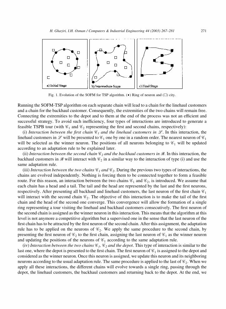
the smallest number of neurons separating them plus one. In the first step, a city is randomly picked up;

its position is compared to all positions of neurons on the ring. The nearest neuron to the city is then

selected and moved towards the city. The neighbors of the selected neuron move also towards the city

with a decreasing intensity controlled by the lateral distance. Fig. 1 illustrates the evolution of the

algorithm starting from the initial state of the ring, (a) reaching an intermediate stage after some

iterations (b) and stopping at the final state (c). The number of neurons should be greater than the number

of cities (m is greater or equal to 3n ) to avoid the oscillation of a neuron between different neighboring

cities. An extensive analysis of this algorithm could be found in the works published by Angeniol et al.

(1988), Fort (1988) and Smith (1999).

3.2. The SOFM for the TSPB

In this section, we will explain how to extend the SOFM-TSP algorithm to the TSPB. The basic idea is

to design a new architecture in which the TSP ring is replaced by two chains: one for the linehauls and

one for the backhauls. The linehaul customers will interact exclusively with the first chain, the backhaul

customers will interact exclusively with the second chain and the depot will interact with both chains.

H. Ghaziri, I.H. Osman / Computers & Industrial Engineering 44 (2003) 267–281270

Running the SOFM-TSP algorithm on each separate chain will lead to a chain for the linehaul customers

and a chain for the backhaul customer. Consequently, the extremities of the two chains will remain free.

Connecting the extremities to the depot and to them at the end of the process was not an efficient and

successful strategy. To avoid such inefficiency, four types of interactions are introduced to generate a

feasible TSPB tour (with C1 and C2 representing the first and second chains, respectively):

(i) Interaction between the first chain C1 and the linehaul customers in L. In this interaction, the

linehaul customers in L will be presented to C1 one by one in a random order. The nearest neuron of C1

will be selected as the winner neuron. The positions of all neurons belonging to C1 will be updated

according to an adaptation rule to be explained later.

(ii) Interaction between the second chain C2 and the backhaul customers in B. In this interaction, the

backhaul customers in B will interact with C2 in a similar way to the interaction of type (i) and use the

same adaptation rule.

(iii) Interaction between the two chains C1 and C2. During the previous two types of interactions, the

chains are evolved independently. Nothing is forcing them to be connected together to form a feasible

route. For this reason, an interaction between the two chains C1 and C2; is introduced. We assume that

each chain has a head and a tail. The tail and the head are represented by the last and the first neurons,

respectively. After presenting all backhaul and linehaul customers, the last neuron of the first chain C1

will interact with the second chain C2: The objective of this interaction is to make the tail of the first

chain and the head of the second one converge. This convergence will allow the formation of a single

ring representing a tour visiting the linehaul and backhaul customers consecutively. The first neuron of

the second chain is assigned as the winner neuron in this interaction. This means that the algorithm at this

level is not anymore a competitive algorithm but a supervised one in the sense that the last neuron of the

first chain has to be attracted by the first neuron of the second chain. After this assignment, the adaptation

rule has to be applied on the neurons of C2: We apply the same procedure to the second chain, by

presenting the first neuron of C2 to the first chain, assigning the last neuron of C1 as the winner neuron

and updating the positions of the neurons of C1 according to the same adaptation rule.

(iv) Interaction between the two chains C1, C2 and the depot. This type of interaction is similar to the

last one, where the depot is presented to the first chain. The first neuron of C1 is assigned to the depot and

considered as the winner neuron. Once this neuron is assigned, we update this neuron and its neighboring

neurons according to the usual adaptation rule. The same procedure is applied to the last of C2: When we

apply all these interactions, the different chains will evolve towards a single ring, passing through the

depot, the linehaul customers, the backhaul customers and returning back to the depot. At the end, we

Fig. 1. Evolution of the SOFM for TSP algorithm. (†) Ring of neuron and (A) city.

H. Ghaziri, I.H. Osman / Computers & Industrial Engineering 44 (2003) 267–281 271

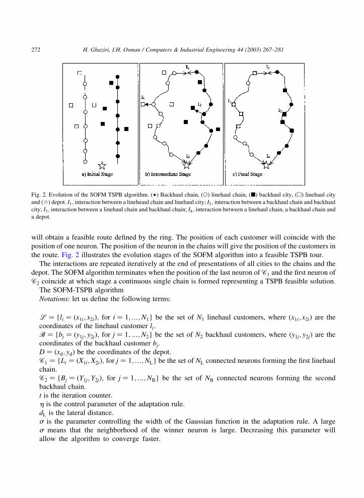
will obtain a feasible route defined by the ring. The position of each customer will coincide with the

position of one neuron. The position of the neuron in the chains will give the position of the customers in

the route. Fig. 2 illustrates the evolution stages of the SOFM algorithm into a feasible TSPB tour.

The interactions are repeated iteratively at the end of presentations of all cities to the chains and the

depot. The SOFM algorithm terminates when the position of the last neuron of C1 and the first neuron of

C2 coincide at which stage a continuous single chain is formed representing a TSPB feasible solution.

The SOFM-TSPB algorithm

Notations: let us define the following terms:

L ¼ {li ¼ ðx1i; x2iÞ; for i ¼ 1;…;N1} be the set of N1 linehaul customers, where ðx1i; x2iÞ are the

coordinates of the linehaul customer li:B ¼ {bj ¼ ðy1j; y2jÞ; for j ¼ 1;…;N2} be the set of N2 backhaul customers, where ðy1j; y2jÞ are the

coordinates of the backhaul customer bj:D ¼ ðxd; ydÞ be the coordinates of the depot.

C1 ¼ {Li ¼ ðX1i;X2iÞ; for j ¼ 1;…;NL} be the set of NL connected neurons forming the first linehaul

chain.

C2 ¼ {Bj ¼ ðY1j;Y2jÞ; for j ¼ 1;…;NB} be the set of NB connected neurons forming the second

backhaul chain.

t is the iteration counter.

h is the control parameter of the adaptation rule.

dL is the lateral distance.

s is the parameter controlling the width of the Gaussian function in the adaptation rule. A large

s means that the neighborhood of the winner neuron is large. Decreasing this parameter will

allow the algorithm to converge faster.

Fig. 2. Evolution of the SOFM TSPB algorithm. (†) Backhaul chain, (W) linehaul chain, (B) backhaul city, (A) linehaul city

and (q) depot. I1; interaction between a lineheaul chain and linehaul city; I2; interaction between a backhaul chain and backhaul

city; I3; interaction between a linehaul chain and backhaul chain; I4; interaction between a linehaul chain, a backhaul chain and

a depot.

H. Ghaziri, I.H. Osman / Computers & Industrial Engineering 44 (2003) 267–281272

SOFM algorithmic steps:

Step 1. Initialization

a. Read the input data for the linehaul and backhaul customers.

b. Generate the positions of NL neurons located on the first chain C1; where NL ¼ 3N1:c. Generate the positions of NB neurons located on the first chain C2; where NB ¼ 3N2:d. Set the initial state of each chain to a vertical line, see Fig. 2.

e. Set t ¼ 0; sð0Þ ¼ 1 and hð0Þ ¼ 3:

Step 2. Select an input

a. Select randomly a customer C [ L<B: Every customer will be selected exactly once

during one iteration.

b. Let us define the city to be represented by C ¼ ðx1c; x2cÞ or C ¼ ðy1c; y2cÞ depending on

whether it belongs to L or B.

Step 3. Select the winner neuron

If (C belongs to L) Thena. Selection of the nearest neuron. Let Lp be the winning neuron belonging to C1; i.e. Lp ¼ ðX1p ;X2pÞ

such that ðx1c 2 X1pÞ2 þ ðx2c 2 X2pÞ

2 # ðx1c 2 X1iÞ2 þ ðx2c 2 X2iÞ

2; ;i ¼ 1;…;NL:b. Adaptation rule. Update the coordinates of each linehaul neurons, Li ¼ ðX1i;X2iÞ: For example, the

update of the X-coordinate of Li is done as follows

X1iðt þ 1Þ ¼ X1iðtÞ þ hðtÞ £ GðLi; LpÞ £ ðx1c 2 X1iðtÞÞ; ;i ¼ 1;…;NL:

where

GðLi;LpÞ ¼

1ffiffi2

p exp2d2

LðLi; LpÞ

2s2

!:

Else (C belongs to B)

c. Selection of the nearest neuron. Let Bp be the winning neuron belonging to C2; i.e. Bp ¼ ðY1p ; Y2pÞ

such that ðy1c 2 Y1pÞ2 þ ðy2c 2 Y2pÞ

2 # ðy1c 2 Y1jÞ2 þ ðy2c 2 Y2jÞ

2; ;j ¼ 1;…;NB

d. Adaptation rule. Update the coordinates of each backhaul neurons, Bj ¼ ðY1j; Y2jÞ: For example, the

update of the Y-coordinate of Bj is done as follows

Y1jðt þ 1Þ ¼ Y1jðtÞ þ hðtÞ £ GðBj;BpÞ £ ðy1c 2 Y1jðtÞÞ; ;j ¼ 1;…;NB

where

GðBj;BpÞ ¼1ffiffi2

p exp2d2

LðBj;BpÞ

2s2

!:

Step 4. Extremities interactions

H. Ghaziri, I.H. Osman / Computers & Industrial Engineering 44 (2003) 267–281 273

a. Interaction with the Depot. Consider the depot as a customer that should be served by both

chains. Assign the heads of both chins as the winning neuron. Apply Step 3.b or 3.d.

b. Interaction of the two chains. Consider the tail of each chain as a customer for the other

chain and apply step 3 accordingly.

Step 5. End-iteration test

If Not {all customers are selected at the current iteration} Then go to Step 2.

Step 6. Stopping criterion

If {all customers are within 1024 of their nearest neurons in the Euclidean space}

Then Stop

Elsea. Update sðt þ 1Þ ¼ 0:99sðtÞ and hðt þ 1Þ ¼ 0:99hðtÞ:b. Set ðt ¼ t þ 1Þ and Go to Step 2.

If the SOFM algorithm is followed by the post-improvement phase using the 2-opt improvement

procedure applied separately to the TSP segments associated with the backhaul and linehaul customers

of the TSPB, then the new variant is denoted by SOFMp. It will be shown that the solution quality of

SOFM algorithm can be improved substantially by SOFMp with a little extra effort.

4. Computational experience

Our computational experience is designed to analysis the performance of the SOFM heuristic and its

variant SOFMp in terms of solution quality and computational requirements. The experimental design

consists of two experiments. The first experiment is designed to compare the performance of the

proposed heuristics with a branch and bound (B&B) tree search procedure for the asymmetric TSP

developed by Fischetti and Toth (1992) on small-sized instances. The second experiment is designed to

compare their performance with the best existing heuristics in the literature on medium to large-sized

instances.

4.1. Test instances and performance measure

The first experiment uses a set of 100 test instances. Each instance involves 50 backhaul and linehaul

customers to be served from a single depot. The customers and depot coordinates are randomly

generated in the unit square ½0; 1�2 according to a continuous uniform distribution. The set of 100 test

instances is divided into five groups. Each group contains 20 instances with a given ratio for randomly

selecting the backhaul customers. The ratio is computed by r ¼ lB=V l; the number of backhaul

customers over the total number of backhaul and linehaul customers. The r values are given in the set

V ¼ {0:1; 0:2; 0:3; 0:4; 0:5}:The second experiment uses a set of 750 test instances, which are generated according to the

experimental design defined by Gendreau et al. (1996), used by Mladenovic and Hansen (1997) and

H. Ghaziri, I.H. Osman / Computers & Industrial Engineering 44 (2003) 267–281274

explained as follows. The coordinates of the customers and the depots are generated in the interval

½0; 100�2 according to a continuous distribution. For each pair ðn; rÞ where n ¼ 100; 200; 300; 500 and

1000 and r [ V; 30 instances are generated.

The quality of an algorithm is measured by the relative percentage deviation (RPD) of the solution

value from its lower bound, optimal solution, or best-found value depending on whatever available. For

each given pair of ðn; rÞ; the average of solutions and the average of RPD values (ARPD) over the set of

instances in the group are reported.

4.2. Comparison with the B&B tree search algorithm

The objective of this section is to analyze the quality of the SOFM and SOFMp heuristics, and the

effect of backhaul ratio (r ) on the performance all compared algorithms. For a given instance, the

associated cost matrix of the TSPB is converted into an equivalent cost matrix associated with an

asymmetric TSP by adding large distances to arcs connecting the subsets {D}, L and B. The modified

cost matrix is then solved by the B&B tree search algorithm to obtain its exact optimal solution.

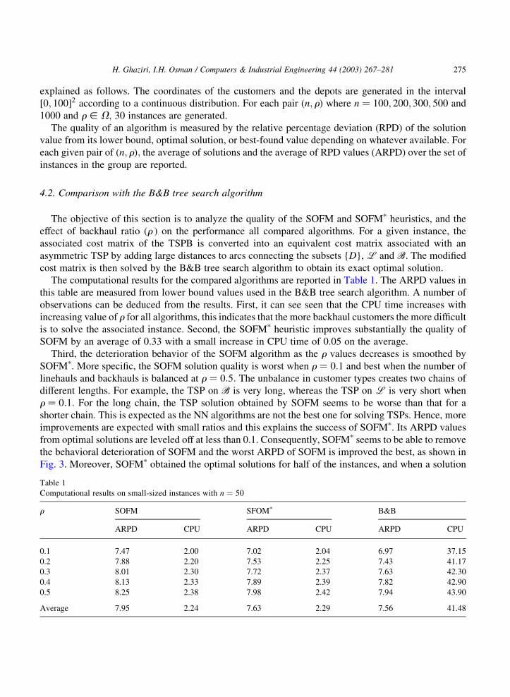
The computational results for the compared algorithms are reported in Table 1. The ARPD values in

this table are measured from lower bound values used in the B&B tree search algorithm. A number of

observations can be deduced from the results. First, it can see seen that the CPU time increases with

increasing value of r for all algorithms, this indicates that the more backhaul customers the more difficult

is to solve the associated instance. Second, the SOFMp heuristic improves substantially the quality of

SOFM by an average of 0.33 with a small increase in CPU time of 0.05 on the average.

Third, the deterioration behavior of the SOFM algorithm as the r values decreases is smoothed by

SOFMp. More specific, the SOFM solution quality is worst when r ¼ 0:1 and best when the number of

linehauls and backhauls is balanced at r ¼ 0:5: The unbalance in customer types creates two chains of

different lengths. For example, the TSP on B is very long, whereas the TSP on L is very short when

r ¼ 0:1: For the long chain, the TSP solution obtained by SOFM seems to be worse than that for a

shorter chain. This is expected as the NN algorithms are not the best one for solving TSPs. Hence, more

improvements are expected with small ratios and this explains the success of SOFMp. Its ARPD values

from optimal solutions are leveled off at less than 0.1. Consequently, SOFMp seems to be able to remove

the behavioral deterioration of SOFM and the worst ARPD of SOFM is improved the best, as shown in

Fig. 3. Moreover, SOFMp obtained the optimal solutions for half of the instances, and when a solution

Table 1

Computational results on small-sized instances with n ¼ 50

r SOFM SFOMp B&B

ARPD CPU ARPD CPU ARPD CPU

0.1 7.47 2.00 7.02 2.04 6.97 37.15

0.2 7.88 2.20 7.53 2.25 7.43 41.17

0.3 8.01 2.30 7.72 2.37 7.63 42.30

0.4 8.13 2.33 7.89 2.39 7.82 42.90

0.5 8.25 2.38 7.98 2.42 7.94 43.90

Average 7.95 2.24 7.63 2.29 7.56 41.48

H. Ghaziri, I.H. Osman / Computers & Industrial Engineering 44 (2003) 267–281 275

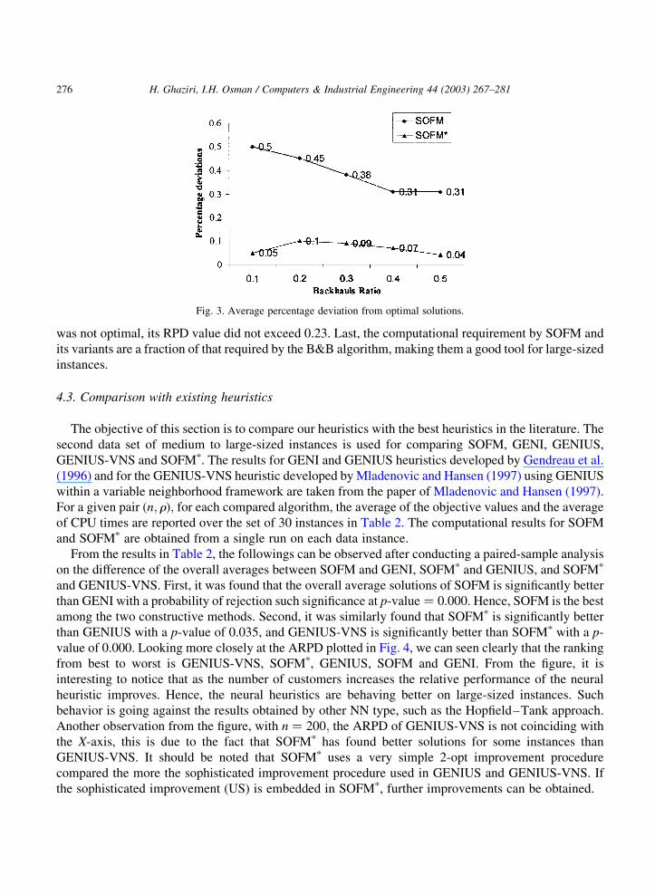
was not optimal, its RPD value did not exceed 0.23. Last, the computational requirement by SOFM and

its variants are a fraction of that required by the B&B algorithm, making them a good tool for large-sized

instances.

4.3. Comparison with existing heuristics

The objective of this section is to compare our heuristics with the best heuristics in the literature. The

second data set of medium to large-sized instances is used for comparing SOFM, GENI, GENIUS,

GENIUS-VNS and SOFMp. The results for GENI and GENIUS heuristics developed by Gendreau et al.

(1996) and for the GENIUS-VNS heuristic developed by Mladenovic and Hansen (1997) using GENIUS

within a variable neighborhood framework are taken from the paper of Mladenovic and Hansen (1997).

For a given pair ðn; rÞ; for each compared algorithm, the average of the objective values and the average

of CPU times are reported over the set of 30 instances in Table 2. The computational results for SOFM

and SOFMp are obtained from a single run on each data instance.

From the results in Table 2, the followings can be observed after conducting a paired-sample analysis

on the difference of the overall averages between SOFM and GENI, SOFMp and GENIUS, and SOFMp

and GENIUS-VNS. First, it was found that the overall average solutions of SOFM is significantly better

than GENI with a probability of rejection such significance at p-value ¼ 0.000. Hence, SOFM is the best

among the two constructive methods. Second, it was similarly found that SOFMp is significantly better

than GENIUS with a p-value of 0.035, and GENIUS-VNS is significantly better than SOFMp with a p-

value of 0.000. Looking more closely at the ARPD plotted in Fig. 4, we can seen clearly that the ranking

from best to worst is GENIUS-VNS, SOFMp, GENIUS, SOFM and GENI. From the figure, it is

interesting to notice that as the number of customers increases the relative performance of the neural

heuristic improves. Hence, the neural heuristics are behaving better on large-sized instances. Such

behavior is going against the results obtained by other NN type, such as the Hopfield–Tank approach.

Another observation from the figure, with n ¼ 200; the ARPD of GENIUS-VNS is not coinciding with

the X-axis, this is due to the fact that SOFMp has found better solutions for some instances than

GENIUS-VNS. It should be noted that SOFMp uses a very simple 2-opt improvement procedure

compared the more the sophisticated improvement procedure used in GENIUS and GENIUS-VNS. If

the sophisticated improvement (US) is embedded in SOFMp, further improvements can be obtained.

Fig. 3. Average percentage deviation from optimal solutions.

H. Ghaziri, I.H. Osman / Computers & Industrial Engineering 44 (2003) 267–281276

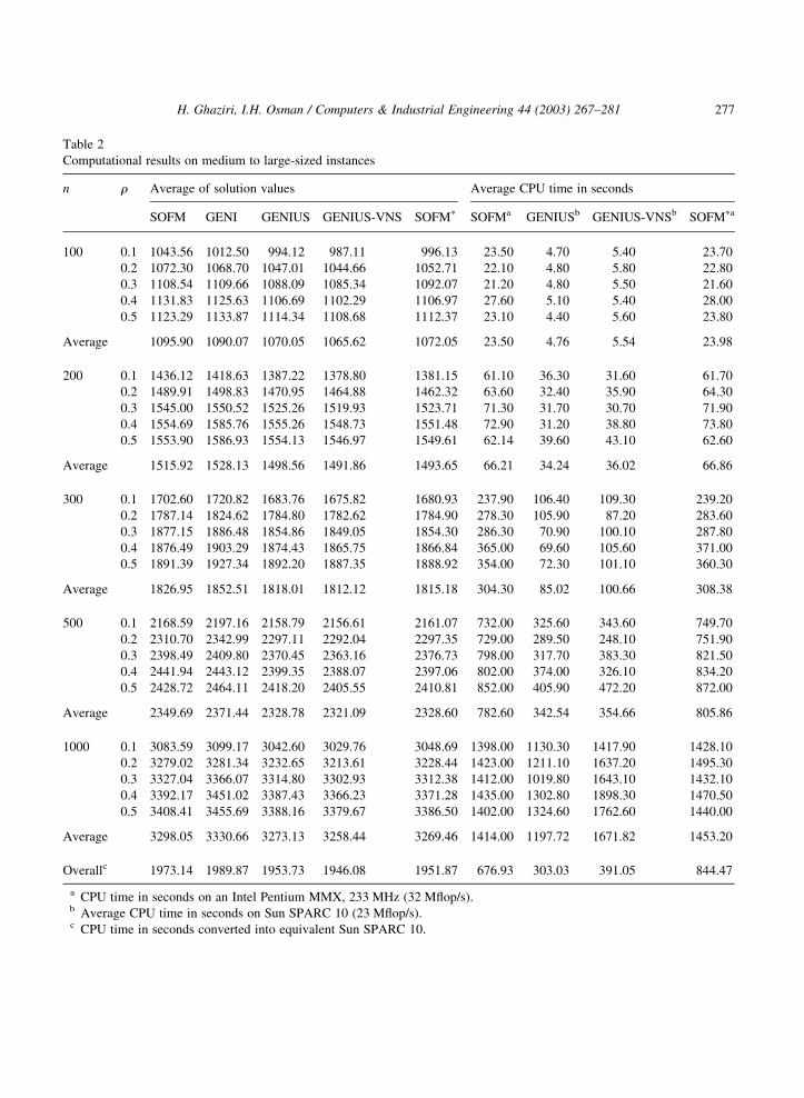
Table 2

Computational results on medium to large-sized instances

n r Average of solution values Average CPU time in seconds

SOFM GENI GENIUS GENIUS-VNS SOFMp SOFMa GENIUSb GENIUS-VNSb SOFMpa

100 0.1 1043.56 1012.50 994.12 987.11 996.13 23.50 4.70 5.40 23.70

0.2 1072.30 1068.70 1047.01 1044.66 1052.71 22.10 4.80 5.80 22.80

0.3 1108.54 1109.66 1088.09 1085.34 1092.07 21.20 4.80 5.50 21.60

0.4 1131.83 1125.63 1106.69 1102.29 1106.97 27.60 5.10 5.40 28.00

0.5 1123.29 1133.87 1114.34 1108.68 1112.37 23.10 4.40 5.60 23.80

Average 1095.90 1090.07 1070.05 1065.62 1072.05 23.50 4.76 5.54 23.98

200 0.1 1436.12 1418.63 1387.22 1378.80 1381.15 61.10 36.30 31.60 61.70

0.2 1489.91 1498.83 1470.95 1464.88 1462.32 63.60 32.40 35.90 64.30

0.3 1545.00 1550.52 1525.26 1519.93 1523.71 71.30 31.70 30.70 71.90

0.4 1554.69 1585.76 1555.26 1548.73 1551.48 72.90 31.20 38.80 73.80

0.5 1553.90 1586.93 1554.13 1546.97 1549.61 62.14 39.60 43.10 62.60

Average 1515.92 1528.13 1498.56 1491.86 1493.65 66.21 34.24 36.02 66.86

300 0.1 1702.60 1720.82 1683.76 1675.82 1680.93 237.90 106.40 109.30 239.20

0.2 1787.14 1824.62 1784.80 1782.62 1784.90 278.30 105.90 87.20 283.60

0.3 1877.15 1886.48 1854.86 1849.05 1854.30 286.30 70.90 100.10 287.80

0.4 1876.49 1903.29 1874.43 1865.75 1866.84 365.00 69.60 105.60 371.00

0.5 1891.39 1927.34 1892.20 1887.35 1888.92 354.00 72.30 101.10 360.30

Average 1826.95 1852.51 1818.01 1812.12 1815.18 304.30 85.02 100.66 308.38

500 0.1 2168.59 2197.16 2158.79 2156.61 2161.07 732.00 325.60 343.60 749.70

0.2 2310.70 2342.99 2297.11 2292.04 2297.35 729.00 289.50 248.10 751.90

0.3 2398.49 2409.80 2370.45 2363.16 2376.73 798.00 317.70 383.30 821.50

0.4 2441.94 2443.12 2399.35 2388.07 2397.06 802.00 374.00 326.10 834.20

0.5 2428.72 2464.11 2418.20 2405.55 2410.81 852.00 405.90 472.20 872.00

Average 2349.69 2371.44 2328.78 2321.09 2328.60 782.60 342.54 354.66 805.86

1000 0.1 3083.59 3099.17 3042.60 3029.76 3048.69 1398.00 1130.30 1417.90 1428.10

0.2 3279.02 3281.34 3232.65 3213.61 3228.44 1423.00 1211.10 1637.20 1495.30

0.3 3327.04 3366.07 3314.80 3302.93 3312.38 1412.00 1019.80 1643.10 1432.10

0.4 3392.17 3451.02 3387.43 3366.23 3371.28 1435.00 1302.80 1898.30 1470.50

0.5 3408.41 3455.69 3388.16 3379.67 3386.50 1402.00 1324.60 1762.60 1440.00

Average 3298.05 3330.66 3273.13 3258.44 3269.46 1414.00 1197.72 1671.82 1453.20

Overallc 1973.14 1989.87 1953.73 1946.08 1951.87 676.93 303.03 391.05 844.47

a CPU time in seconds on an Intel Pentium MMX, 233 MHz (32 Mflop/s).b Average CPU time in seconds on Sun SPARC 10 (23 Mflop/s).c CPU time in seconds converted into equivalent Sun SPARC 10.

H. Ghaziri, I.H. Osman / Computers & Industrial Engineering 44 (2003) 267–281 277

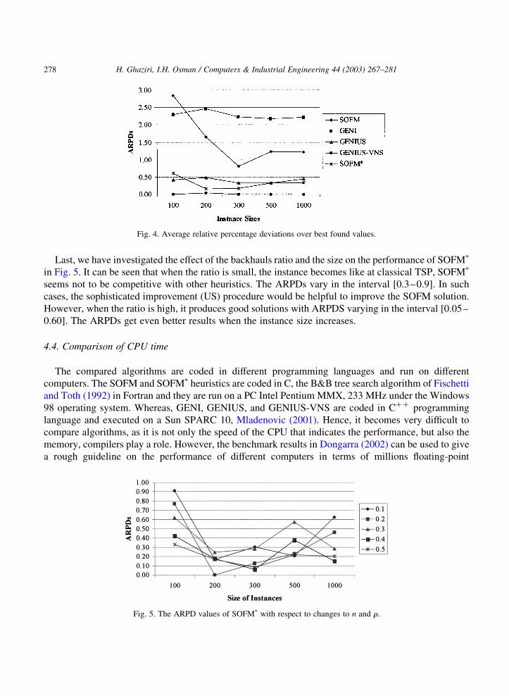
Last, we have investigated the effect of the backhauls ratio and the size on the performance of SOFMp

in Fig. 5. It can be seen that when the ratio is small, the instance becomes like at classical TSP, SOFMp

seems not to be competitive with other heuristics. The ARPDs vary in the interval [0.3–0.9]. In such

cases, the sophisticated improvement (US) procedure would be helpful to improve the SOFM solution.

However, when the ratio is high, it produces good solutions with ARPDS varying in the interval [0.05–

0.60]. The ARPDs get even better results when the instance size increases.

4.4. Comparison of CPU time

The compared algorithms are coded in different programming languages and run on different

computers. The SOFM and SOFMp heuristics are coded in C, the B&B tree search algorithm of Fischetti

and Toth (1992) in Fortran and they are run on a PC Intel Pentium MMX, 233 MHz under the Windows

98 operating system. Whereas, GENI, GENIUS, and GENIUS-VNS are coded in Cþþ programming

language and executed on a Sun SPARC 10, Mladenovic (2001). Hence, it becomes very difficult to

compare algorithms, as it is not only the speed of the CPU that indicates the performance, but also the

memory, compilers play a role. However, the benchmark results in Dongarra (2002) can be used to give

a rough guideline on the performance of different computers in terms of millions floating-point

Fig. 4. Average relative percentage deviations over best found values.

Fig. 5. The ARPD values of SOFMp with respect to changes to n and r.

H. Ghaziri, I.H. Osman / Computers & Industrial Engineering 44 (2003) 267–281278

operations completed per second, Mflop/s. The Sun SPARC 10 performance is 23 Mflops, whereas the

Intel Pentium MMX 233 MHz performance is 32 Mflops. Hence, our CPU time must be multiplied by a

factor of 1.39 to get an equivalent Sun SPARC 10 time. Our Mflop/s is estimated from Kennedy (1998)

and Dongarra’s results. Looking at the results in Table 2, it can be seen that GENIUS-VNS improves

over SOFMp by 0.29% and it is also 46% faster, on the average. However, looking at the large-sized

instances with n ¼ 1000; SOFMp uses 20% more CPU time than GENIUS-VNS with comparable

results. This indicates that the speed gap might be further reduced for larger sized instances. However,

larger sized instances were not considered due to the lack of comparative benchmark results.

5. Conclusion

The SOFM heuristic and its variant with 2-opt post-optimization SOFMp are designed and

implemented for the TSPB. Their comparisons with the branch and bound exact method and the best

existing heuristics show that they are competitive with respect to solution quality, but they require more

computational effort, similar to other NN in the literature. In particular, the constructive SOFM heuristic

gives better results than GENI constructive heuristic. Moreover, SOFMp produces better results than

GENIUS and very comparable to the later variant GENIUS-VNS, which is based a variable

neighborhood framework. From the experimental analysis, the B&B exact method must be

recommended for small-sized instances, GENUIS-VNS for medium-sized instances and SOFMp for

large-sized instances.

Our neural approach is by far more powerful, flexible and simple to implement than the Hopfield–

Tank NN method. The major limitation of the SOFM algorithm is its inability to address non-Euclidean

instances. Further research can be conducted by applying the SOFM heuristic on the modified cost

matrix associated with the equivalent asymmetric TSP to find out whether better results can be obtained.

In addition, the effect of replacing the 2-opt post-optimization procedure by a more sophisticated one

similar to one used in the competitive heuristics should be investigated.

Acknowledgments

We thank Professor Poalo Toth for making the exact method code available and the four referees for

their comments that improved the clarity of the paper. We also thank Mr Iyad Wehbe from RCAM

(Research and Computer Aided Management Company, Lebanon) for helping us in coding and running

the various experiments.

References

Aiyer, S. V. B., Niranjan, M., & Fallside, F. (1990). A theoretical investigation into the performance of the Hopfield model.

IEEE Transactions on Neural Networks, 1, 204–215.

Andresol, R., Gendreau, M., & Potvin, J.-Y. (1999). A Hopfield–Tank neural network model for the generalized traveling

salesman problem. In S. Voss, S. Martello, I. H. Osman, & C. Roucairol (Eds.), Meta-heuristics advances and trends in local

search paradigms for optimization (pp. 393–402). Boston: Kluwer Academic Publishers.

H. Ghaziri, I.H. Osman / Computers & Industrial Engineering 44 (2003) 267–281 279

Angeniol, B., De-La-Croix, G., & Le-Texier, J.-Y. (1988). Self-organizing feature maps and the traveling salesman problem.

Neural Networks, 1, 289–293.

Anily, S. (1996). The vehicle routing problem with delivery and backhaul options. Naval Research Logistics, 43, 415–434.

Aras, N., Oommen, B. J., & Altinel, I. K. (1999). The Kohonen network incorporating explicit statistics and its application to

the traveling salesman problem. Neural Networks, 12, 1273–1284.

Burke, L. I. (1994). Adaptive neural networks for the traveling salesman problem: Insights from operations research. Neural

Networks, 7, 681–690.

Casco, D., Golden, B. L., & Wasil, E. (1988). Vehicle routing with backhauls: Models algorithms and cases studies. In B. L.

Golden, & A. A. Assad (Eds.), (Vol. 16) (pp. 127–148). Vehicle routing: Methods and studies, studies in management

science and systems, Amsterdam: North Holland.

Chisman, J. A. (1975). The clustered traveling salesman problem. Computers and Operations Research, 2, 115–119.

Dongarra, J. J (2002). Performance of various computers using standard linear equation software. Technical Report, Computer

Science Department, University of Tennessee, USA. http://www.netlib.org/benchmark/performance.ps.

Durbin, R., & Willshaw, D. (1987). An analogue approach to the traveling salesman problem using elastic net method. Nature,

326, 689–691.

Fischetti, M., & Toth, P. (1992). An additive bounding procedure for the asymmetric traveling salesman problem.

Mathematical Programming, 53, 173–197.

Fort, J. C. (1988). Solving a combinatorial problem via self-organizing process: An application to the traveling salesman

problem. Biological Cybernetics, 59, 33–40.

Gendreau, G., Hertz, A., & Laporte, G. (1992). New insertion and post-optimization procedures for the traveling salesman

problem. Operations Research, 40, 1086–1094.

Gendreau, G., Hertz, A., & Laporte, G. (1996). The traveling salesman problem with backhauls. Computers and Operations

Research, 23, 501–508.

Ghaziri, H. (1991). Solving routing problem by self-organizing maps. In T. Kohonen, K. Makisara, O. Simula, & J. Kangas

(Eds.), Artificial neural networks (pp. 829–834). Amsterdam: North Holand.

Ghaziri, H. (1996). Supervision in the self-organizing feature map: Application to the vehicle routing problem. In I. H.

Osman, & J. P. Kelly (Eds.), Meta-heuristics: Theory and applications (pp. 651–660). Boston: Kluwer Academic

Publishers.

Hopfield, J. J., & Tank, D. W. (1985). Neural computation of decisions in optimization problem. Biological Cybernetics, 52,

141–152.

Jongens, K., & Volgenant, T. (1985). The symmetric clustered traveling salesman problem. European Journal of Operational

Research, 19, 68–75.

Kalantari, B., Hill, A. V., & Arora, S. R. (1985). An algorithm for the traveling salesman with pickup and delivery customers.

European Journal of Operational Research, 22, 377–386.

Kennedy, P (1998). RISC benchmark scores. http://kennedyp.iccom.com/riscscore.htm.

Kohonen, T. (1982). Self-organized formation of topologically correct feature maps. Biological Cybernetics, 43, 59–69.

Kohonen, T. (1995). Self-organizing maps. Berlin: Springer.

Laporte, G., & Osman, I. H. (1995). Routing problems: A bibliography. Annals of Operations Research, 61, 227–262.

Looi, C.-K. (1992). Neural network methods in combinatorial optimization. Computers and Operations Research, 19,

191–208.

Lotkin, F. C. J. (1978). Procedures for traveling salesman problems with additional constraints. European Journal of

Operational Research, 3, 135–141.

Mladenovic, N (2001). Personal communication.

Mladenovic, N., & Hansen, P. (1997). Variable neighborhood search. Computers and Operations Research, 24, 1097–1100.

Modares, A., Somhom, S., & Enkawa, T. (1999). A self-organizing neural network approach for multiple traveling salesman

and vehicle routing problems. International Transactions in Operational Research, 6, 591–606.

Mosheiov, G. (1994). The traveling salesman problem with pickup and delivery. European Journal of Operational Research,

72, 299–310.

Osman, I. H. (1995). An introduction to meta-heuristics. In M. M. Lawrence, & C. Wilsdon (Eds.), Operational research

tutorial 1995 (pp. 92–122). Birmingham, UK: Operational Research Society.

Osman, I. H., & Laporte, G. (1996). Meta-heuristics: A bibliography. Annals of Operations Research, 63, 513–623.

H. Ghaziri, I.H. Osman / Computers & Industrial Engineering 44 (2003) 267–281280

Osman, I. H., & Wassan, N. A. (2002). A reactive tabu search for the vehicle routing problem with Backhauls. Journal of

Scheduling, 5(4) 263–285.

Peng, E., Gupta, K. N. K., & Armitage, A. F. (1996). An investigation into the improvement of local minima of the Hopfield

network. Neural Networks, 9, 1241–1253.

Potvin, J.-Y. (1993). The traveling salesman problem: A neural network perspective. ORSA Journal on Computing, 5, 328–348.

Potvin, J. Y., & Guertin, F. (1996). The clustered traveling salesman problem: A genetic approach. In I. H. Osman, & J. P. Kelly

(Eds.), Meta-heuristics theory and applications (pp. 619–631). Boston: Kluwers Academic Publishers.

Potvin, J.-Y., & Robillard, C. (1995). Clustering for vehicle routing with a competitive neural network. Neurocomputing, 8,

125–139.

Renaud, J., Boctor, F. F., & Quenniche, J. (2000). A heuristic for the pickup and delivery traveling problem. Computers and

Operations Research, 27, 905–916.

Smith, K. A. (1999). Neural network for combinatorial optimization: A review of more than a decade of research. INFORMS

Journal on Computing, 11, 15–34.

Thangiah, S. R., Potvin, J. Y., & Sung, T. (1996). Heuristic approaches to the vehicle routing with backhauls and time windows.

Computers and Operations Research, 1043–1057.

Toth, P., & Vigo, D. (1999). A heuristic algorithm for the symmetric and asymmetric vehicle routing problems with backhauls.

European Journal of Operational Research, 113, 528–543.

Vakhutinsky, A. I., & Golden, B. L. (1995). A hierarchical strategy for solving traveling salesman problems using elastic nets.

Journal of Heuristics, 1, 67–76.

Yano, C., Chan, T., Richter, L., Culter, L., Murty, K., & McGettigan, D. (1987). Vehicle routing at quality stores. Interfaces, 17,

52–63.

H. Ghaziri, I.H. Osman / Computers & Industrial Engineering 44 (2003) 267–281 281