a mixed groundwater system at midway, ut: discriminating superimposed local and regional discharge

A mixed groundwater system at Midway, UT: discriminating

superimposed local and regional discharge

Concepcion Carreon-Diazcontia,*, Stephen T. Nelsonb, Alan L. Mayob,David G. Tingeyb, Maren Smithb

aInstituto de Ingenierıa, Universidad Autonoma de Baja California, Blvd. B. Juarez s/n, Mexicali, Baja California 21280, MexicobDepartment of Geology, S389 ESC, Brigham Young University, Provo, UT 84602, USA

Received 19 September 2001; revised 1 November 2002; accepted 8 November 2002

Abstract

Mixed thermal and cold water groundwater occurs in the Midway area, UT. Midway is located in the western Heber Valley,

an alluvial-filled intermontane basin behind the crest of the Wasatch Mountains. In addition to streams and thermal springs,

groundwater discharges from alluvium, bedrock, and karstified tufa. Evaluation of the thermal system reveals that it has been

circulated to depths of ,2 km and temperatures of ,150 8C. Most groundwater characteristics of the area can be explained by

subsurface mixing between isotopically depleted, Pleistocene-aged thermal water and isotopically enriched, cold, modern, low

TDS groundwater. Because the entire system exhibits evidence of mixing, it is possible to define the regional extent of

upwelling of thermal water, as well as mixing fractions between the two end-members. The subsurface mixing of thermal and

non-thermal waters is highly controlled by the superimposition of local irrigation recharge.

q 2003 Elsevier Science B.V. All rights reserved.

Keywords: Hydrogeology; Hydrochemistry; Stable isotopes; Mixing; Groundwater; Water End-members

1. Introduction

Subsurface mixing of diverse waters is a natural

process that, due to its influence on groundwater

evolution, may be the source of serious concerns

regarding groundwater as a resource. Considerable

research has been carried out examining

surface water – groundwater interaction to

evaluate the impact of irrigation practices on

aquifers (Davisson and Criss, 1995; Chaouni-Alia

et al., 1999), to determine the sources of water

contamination (Roback et al., 1997; Green et al.,

1998), to assess ecological risks (Hayashi

and Rosenberry, 2001), and even to

delineate water rights (Schellpeper and Harvey,

1998).

The purpose of this investigation is to evaluate

the subsurface mixing of thermal and non-thermal

groundwaters and, superimposed upon this, the

effects of local irrigation recharge in Midway, the

western portion of the Heber Valley, UT,

using traditional hydrochemical tools. We employ

0022-1694/03/$ - see front matter q 2003 Elsevier Science B.V. All rights reserved.

PII: S0 02 2 -1 69 4 (0 2) 00 3 59 -1

Journal of Hydrology 273 (2003) 119–138

www.elsevier.com/locate/jhydrol

* Corresponding author. Present address: Department of Geology

and Geophysics, College of Mines and Earth Sciences, University of

Utah, 135 S. 1460 E., Room 719, Salt Lake City, UT 84112-0111,

USA. Tel.: þ1-801-582-1923; fax: þ1-801-581-7065.

E-mail address: [email protected] (C. Carreon-Diazconti).

http://www.elsevier.com/locate/jhydrol

multiple lines of evidence to converge upon a fairly

rigorous assessment of subsurface mixing, and

mixing between irrigation recharge and

groundwater.

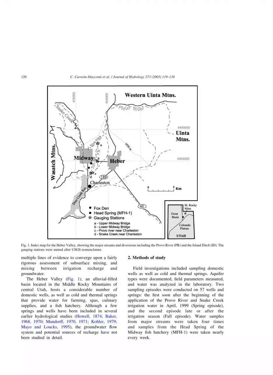
The Heber Valley (Fig. 1), an alluvial-filled

basin located in the Middle Rocky Mountains of

central Utah, hosts a considerable number of

domestic wells, as well as cold and thermal springs

that provide water for farming, spas, culinary

supplies, and a fish hatchery. Although a few

springs and wells have been included in several

earlier hydrological studies (Howell, 1874; Baker,

1968, 1970; Mundorff, 1970, 1971; Kohler, 1979;

Mayo and Loucks, 1995), the groundwater flow

system and potential sources of recharge have not

been studied in detail.

2. Methods of study

Field investigations included sampling domestic

wells as well as cold and thermal springs. Aquifer

types were documented, field parameters measured,

and water was analyzed in the laboratory. Two

sampling episodes were conducted on 57 wells and

springs: the first soon after the beginning of the

application of the Provo River and Snake Creek

irrigation water in April, 1999 (Spring episode),

and the second episode late or after the

irrigation season (Fall episode). Water samples

from major streams were taken four times

and samples from the Head Spring of the

Midway fish hatchery (MFH-1) were taken nearly

every week.

Fig. 1. Index map for the Heber Valley, showing the major streams and diversions including the Provo River (PR) and the Island Ditch (ID). The

gauging stations were named after USGS nomenclature.

C. Carreon-Diazconti et al. / Journal of Hydrology 273 (2003) 119–138120

Field parameters, major ions, and stable isotope

measurements (dDVSMOW, d 18OVSMOW) were com-

pleted on most samples except for samples taken at

frequent intervals at the hatchery Head Spring

where only d 18OVSMOW and dDVSMOW were

determined. Temperature, pH, and conductivity

were measured in the field. Waters for complete

analysis were collected in acid-washed 5-gallon

high-density polyethylene containers, and 1 l bot-

tles, returned to the laboratory, and processed. As a

cross check, alkalinity (HCO32) determined by field

titration and laboratory titration were observed to

agree to within a few percent for a few samples

with a broad range of HCO32 activities.

Cation abundances were measured using a Perkin

Elmer Atomic Absorption Spectrometer, whereas

anions were measured with Dionex Ion Chromato-

graph. HCO32 was determined by acid titration to a pH

of 4.5. The acceptable error on charge balance was

#5%. dDVSMOW, d 18OVSMOW and d 13CPDB were

determined by isotope ratio mass spectrometry with

methods similar to Gehre et al. (1996), Epstein and

Mayeda (1953), and McCrea (1950), respectively. All

d 18OVSMOW and dDVSMOW values were normalized

to the VSMOW/SLAP scale (Coplen, 1988; Nelson,

2000). Precision was determined by replicate analysis

of a laboratory quality control standard. The uncer-

tainly is about ^1‰ for dDVSMOW. Precision for

d 18OVSMOW is listed in Table 1. A continuous flow

method was used for oxygen isotopes; if there is a

dependence of d 18OVSMOW on beam current, this can

add uncertainty to the analysis as high PCO2waters can

outgas in the sample vial, producing considerable

variability in beam current between samples. How-

ever, similar to Fessenden et al. (2002), we have found

little dependence on beam current. Samples for

d 13CPDB were analyzed against reference gases

calibrated to NBS-19. Stable isotope data are reported

in Tables 1 and 2.3H and 14C measurements were conducted by

liquid scintillation counting at the University of

Miami Tritium Laboratory and Beta Analytical,

respectively. 14C values are reported as percent

modern carbon (pmc) and 3H values are reported

in tritium units (TU) (Tables 1 and 2). Concen-

trations of fluorescent dye for tracer tests

were measured at Ozark Underground Laboratory

in Arkansas.

Methods used to determine hydrostratigraphy, net

geochemical mass balance reactions and

mixing proportions, and groundwater residence

times are described elsewhere in this paper and by

Carreon-Diazconti (2000). All isotope, solute and

field parameter data are reported in Tables 1–3.

3. Geological setting

The Heber Valley is surrounded and underlain

predominantly by faulted and folded Mississippian to

Jurassic sedimentary rocks of the Wasatch Range

(Bromfield et al., 1970; Hintze, 2000), which for the

purposes of this paper have been grouped into

siliciclastic dominated and carbonate dominated bed-

rocks (Fig. 2). Oligocene rhyodacite to andesite tuff

and breccias of the Keetley Volcanics (Baker, 1976),

and Oligocene porphyry intrusions (Bromfield et al.,

1970) have been included in the geological map

(Fig. 2) as igneous bedrock.

Primary geological structures are the Charleston

thrust fault (Baker, 1976; Hintze, 2000), and

several local thrust and reverse faults to the north

and northeast of the area, including the Dutch

Hollow Fault and Pine Creek Faults (Bromfield

et al., 1970). However, it is not clear how these

faults may influence flow in the Midway area. Step

faulting from west to east along normal faults is

inferred from gravity data (Peterson in Baker,

1970; Benson, 2000).

Quaternary alluvial sand and gravel (unconsoli-

dated deposits) overlie the bedrock in the Heber

Valley. Lithologic logs from temperature gradient

wells located in the Midway thermal zone show at

least 76 m of basin-fill sediments (Kohler, 1979),

whereas estimated depth for the alluvium deposits is

between 150 and 245 m (Benson, 2000). These

sediments underlie or are intercalated with a platform

of calcareous spring deposits (karstic tufa deposits) in

the Midway area (Bromfield et al., 1970). Although

not mapped separately on Fig. 2, surface exposures of

these spring deposits underlie the town of Midway

and large areas to the north and west. The Head

Spring, as well as most other sampled hatchery

springs, discharges from tufa at the base of the

embankment.

C. Carreon-Diazconti et al. / Journal of Hydrology 273 (2003) 119–138 121

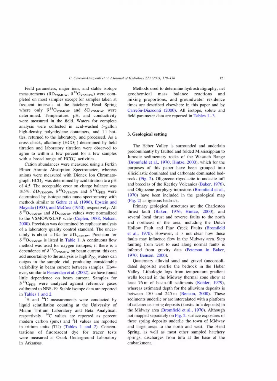
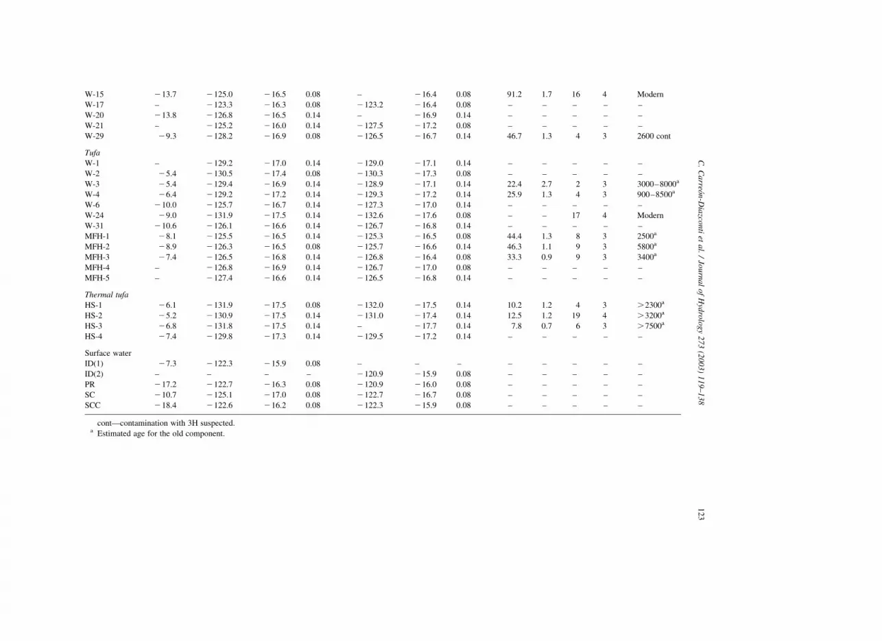
Table 1

Isotope concentration and model ages

ID and aquifer

type

Spring sampling episode Fall sampling episode Spring episode Modeled age

(years)

d 13CPDB

(‰)

dDVSMOW

(‰)

d 18OVSMOW dDVSMOW

(‰)

d 18OVSMOW14C Tritium

‰ Precision ‰ Precision pmc ^ TU eTU

Alluvium

CS-1 211.3 2129.8 217.5 0.14 2129.8 217.3 0.14 – – – – –

CS-4 29.5 2125.4 216.6 0.14 2124.2 216.3 0.08 74 1.1 7 3 Modern

CS-6 215.4 2123.3 216.2 0.14 2126.1 216.6 0.14 – – – – –

CS-7 212.9 2122.8 216.0 0.08 – – – – – – – –

CS-8 212.7 2127.2 217.3 0.14 – – – – – – – –

W-8 26.5 2129.6 216.7 0.14 2129.1 217.2 0.14 34.3 2 1 3 5000 cont

W-9 – 2128.8 217.2 0.08 2128.7 216.9 0.14 – – – – –

W-10 – 2127.8 216.8 0.14 2128.2 216.9 0.14 – – – – –

W-11 – 2128.1 215.3 0.08 2128.5 217.1 0.08 – – – – –

W-12 – 2124.7 216.4 0.08 2124.3 216.6 0.14 – – – – –

W-13 – 2121.8 216.1 0.08 2123.5 216.3 0.14 – – – – –

W-16 – 2129.6 216.8 0.14 2128.9 217.4 0.14 – – – – –

W-18 – 2126.8 217.0 0.08 2126.2 216.8 0.14 – – – – –

W-19 27.1 2128.5 217.1 0.14 2127.1 216.8 0.14 45.9 1.2 6 3 .3000a

W-22 – 2124.3 216.4 0.14 2125.0 216.6 0.14 – – – – –

W-23 – 2125.7 216.4 0.14 2125.7 216.8 0.14 – – – – –

W-25 – 2125.8 216.7 0.08 2126.3 216.9 0.14 – – – – –

W-26 210.8 2130.2 217.7 0.08 2129.8 216.8 0.08 55.7 1.3 2 3 900 cont

W-27 214.6 2128.1 216.9 0.14 2127.8 217.0 0.14 – – – – –

W-28 – 2128.3 217.5 0.08 2128.3 217.0 0.14 – – – – –

W-30 28.4 2125.6 216.5 0.14 2125.9 216.7 0.14 43.5 2.1 8 3 –

W-32 216.9 2123.6 216.1 0.08 2125.2 216.6 0.08 – – – – –

W-33 216.2 2122.9 215.9 0.08 2122.2 216.4 0.08 – – – – –

W-34 211.6 2127.8 216.8 0.14 2128.1 217.1 0.14 – – – – –

W-35 – 2129.9 217.1 0.14 – – – – – – – –

Bedrock

CS-2 – 2127.5 217.2 0.08 2127.3 217.2 0.14 58.5 0.9 16 4 ,50

CS-3 – 2125.1 216.6 0.14 2125.2 216.6 0.14 – – – – –

CS-5 28.8 2128.1 217.3 0.14 2127.8 217.3 0.14 58.9 1.2 13 4 Modern

W-5 – 2125.8 216.7 0.08 2125.9 216.7 0.14 – – – – –

W-7 – 2126.1 216.8 0.14 2127.3 216.8 0.14 – – – – –

W-14 – 2128.9 217.3 0.17 2130.3 217.1 0.08 – – – – –

C.

Ca

rreon

-Dia

zcon

tiet

al.

/Jo

urn

al

of

Hyd

rolo

gy

27

3(2

00

3)

11

9–

13

81

22

W-15 213.7 2125.0 216.5 0.08 – 216.4 0.08 91.2 1.7 16 4 Modern

W-17 – 2123.3 216.3 0.08 2123.2 216.4 0.08 – – – – –

W-20 213.8 2126.8 216.5 0.14 – 216.9 0.14 – – – – –

W-21 – 2125.2 216.0 0.14 2127.5 217.2 0.08 – – – – –

W-29 29.3 2128.2 216.9 0.08 2126.5 216.7 0.14 46.7 1.3 4 3 2600 cont

Tufa

W-1 – 2129.2 217.0 0.14 2129.0 217.1 0.14 – – – – –

W-2 25.4 2130.5 217.4 0.08 2130.3 217.3 0.08 – – – – –

W-3 25.4 2129.4 216.9 0.14 2128.9 217.1 0.14 22.4 2.7 2 3 3000–8000a

W-4 26.4 2129.2 217.2 0.14 2129.3 217.2 0.14 25.9 1.3 4 3 900–8500a

W-6 210.0 2125.7 216.7 0.14 2127.3 217.0 0.14 – – – – –

W-24 29.0 2131.9 217.5 0.14 2132.6 217.6 0.08 – – 17 4 Modern

W-31 210.6 2126.1 216.6 0.14 2126.7 216.8 0.14 – – – – –

MFH-1 28.1 2125.5 216.5 0.14 2125.3 216.5 0.08 44.4 1.3 8 3 2500a

MFH-2 28.9 2126.3 216.5 0.08 2125.7 216.6 0.14 46.3 1.1 9 3 5800a

MFH-3 27.4 2126.5 216.8 0.14 2126.8 216.4 0.08 33.3 0.9 9 3 3400a

MFH-4 – 2126.8 216.9 0.14 2126.7 217.0 0.08 – – – – –

MFH-5 – 2127.4 216.6 0.14 2126.5 216.8 0.14 – – – – –

Thermal tufa

HS-1 26.1 2131.9 217.5 0.08 2132.0 217.5 0.14 10.2 1.2 4 3 .2300a

HS-2 25.2 2130.9 217.5 0.14 2131.0 217.4 0.14 12.5 1.2 19 4 .3200a

HS-3 26.8 2131.8 217.5 0.14 – 217.7 0.14 7.8 0.7 6 3 .7500a

HS-4 27.4 2129.8 217.3 0.14 2129.5 217.2 0.14 – – – – –

Surface water

ID(1) 27.3 2122.3 215.9 0.08 – – – – – – – –

ID(2) – – – – 2120.9 215.9 0.08 – – – – –

PR 217.2 2122.7 216.3 0.08 2120.9 216.0 0.08 – – – – –

SC 210.7 2125.1 217.0 0.08 2122.7 216.7 0.08 – – – – –

SCC 218.4 2122.6 216.2 0.08 2122.3 215.9 0.08 – – – – –

cont—contamination with 3H suspected.a Estimated age for the old component.

C.

Ca

rreon

-Dia

zcon

tiet

al.

/Jo

urn

al

of

Hyd

rolo

gy

27

3(2

00

3)

11

9–

13

81

23

4. Climate

Located about 1700 m above the sea level, the

Heber Valley annual average temperature is 7 8C with

monthly average temperature ranging from 213 8C in

January to 30.6 8C in July. Total annual precipitation

for the 1999 water year was 39.7 cm (about

45.2 m3 £ 106), which represents 14% of the valley

total estimated inflow (Carreon-Diazconti, 2000),

with a minimum of 1.01 m3 £ 106 in September and

the maximum of 7.12 m3 £ 106 in January as snow-

fall. Evaporation data are not available for the area;

however, records from the nearby Provo Brigham

Young University climatological station show an

annual pan evaporation rate of 126.24 cm for a period

of 20 years (National Weather Service, 2000).

5. Hydrology

5.1. Subsurface hydrology

The area of study is a 114 km2 valley that forms

part of the Provo River drainage system, which

discharges into the Great Basin. The Provo River and

the Snake Creek are ‘gaining streams’ (Baker, 1970);

therefore, they should not contribute to groundwater

by infiltration in the Heber Valley. Comparison

Table 2

Time-series isotope composition for the Head Spring and related surface water

Head Spring Provo River Snake Creek

Collection

date

d 18OVSMOW

(‰)

dDVSMOW

(‰)

Collection

date

d 18OVSMOW

(‰)

dDVSMOW

(‰)

Collection date d 18OVSMOW

(‰)

dDVSMOW

(‰)

03/30/99 216.6 2125.5 06/15/99 216.3 2122.7 06/14/99 217.0 2125.1

04/05/99 216.6 2125.5 08/11/99 216.3 2120.9 08/11/99 217.0 2124.3

04/12/99 216.6 2126.0 09/08/99 216.0 2120.9 09/08/99 216.7 2122.7

04/19/99 216.6 2126.5 10/14/99 215.6 2119.0 10/14/99 216.8 2125.7

04/26/99 216.5 2125.8

05/10/99 216.5 2125.5

05/17/99 216.5 2125.9

05/24/99 216.6 2125.2

05/31/99 216.5 2125.7

06/14/99 216.5 2124.9

06/22/99 216.7 2126.0

06/28/99 216.5 2125.8

07/06/99 216.6 2124.3

07/19/99 216.7 2125.0

08/26/99 216.3 2125.3

08/30/99 216.6 2125.1

09/09/99 216.5 2125.0

09/13/99 216.6 2125.2

09/21/99 215.9 2123.6

09/27/99 216.5 2125.5

09/28/99 216.5 –

10/04/99 216.6 2125.0

10/12/99 216.4 2125.5

10/15/99 216.7 2125.4

10/18/99 216.3 2124.8

10/25/99 216.4 2125.5

11/01/99 216.4 2124.5

11/24/99 – 2124.9

12/07/99 216.5 2124.5

12/12/99 216.2 2125.1

01/10/00 216.5 2125.2


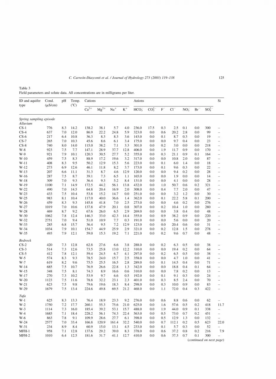
Table 3

Field parameters and solute data. All concentrations are in milligrams per liter.

ID and aquifer

type

Cond.

(mS/cm)

pH Temp.

(8C)

Cations Anions Si

Ca2þ Mg2þ Naþ Kþ HCO32 CO3

22 F2 Cl2 NO32 Br2 SO4

22

Spring sampling episode

Alluvium

CS-1 776 8.3 14.2 138.2 38.1 5.7 4.0 236.0 17.5 0.3 2.5 0.1 0.0 300 –

CS-4 637 7.0 12.0 86.9 22.2 24.8 5.9 323.0 0.0 0.6 20.2 2.8 0.0 99 –

CS-6 217 6.4 10.8 36.3 8.3 8.3 3.6 143.0 0.0 0.1 8.7 0.3 0.0 19 –

CS-7 265 7.0 10.3 45.6 8.6 6.1 3.4 175.0 0.0 0.0 9.7 0.4 0.0 23 –

CS-8 740 8.0 14.0 115.0 38.2 7.1 3.3 301.0 0.0 0.2 3.0 0.0 0.0 218 –

W-8 923 7.5 7.7 147.1 28.9 37.7 12.8 406.0 0.0 1.9 11.7 0.9 0.0 170 –

W-9 921 7.9 10.1 120.3 30.5 27.7 5.2 355.0 0.0 0.3 21.1 0.9 0.1 164 –

W-10 459 7.5 8.3 88.9 17.2 19.6 3.2 317.0 0.0 0.0 10.8 2.0 0.0 87 –

W-11 408 8.3 9.5 50.2 12.9 15.3 5.6 223.0 0.0 0.1 6.0 1.4 0.0 18 –

W-12 273 6.9 12.6 46.1 11.8 8.2 3.7 173.0 0.0 0.1 9.6 0.3 0.0 22 –

W-13 207 6.6 11.1 31.3 8.7 4.6 12.9 120.0 0.0 0.0 9.4 0.2 0.0 28 –

W-16 287 7.5 8.7 39.1 7.3 6.5 1.1 165.0 0.0 0.0 1.9 0.0 0.0 14 –

W-18 309 7.0 9.3 36.4 9.3 5.2 8.4 131.0 0.0 0.0 4.1 0.0 0.0 28 –

W-19 1100 7.1 14.9 172.5 44.2 56.1 13.8 432.0 0.0 1.0 50.7 0.6 0.2 321 –

W-22 490 7.0 14.5 64.8 20.4 16.9 2.0 308.0 0.0 0.4 7.7 2.0 0.0 47 –

W-23 433 7.5 10.4 53.8 15.2 14.7 0.0 251.0 0.0 0.0 3.2 1.2 0.0 30 –

W-25 983 8.1 10.4 117.0 40.0 36.6 1.4 362.0 0.0 0.1 22.2 5.8 0.1 200 –

W-26 459 8.3 9.3 145.8 41.8 7.0 2.5 273.0 0.0 0.0 4.6 0.2 0.0 276 –

W-27 1019 7.0 10.6 137.8 47.9 20.1 0.8 307.0 0.0 0.2 10.4 1.0 0.0 280 –

W-28 469 8.7 9.2 67.6 26.0 6.5 2.9 269.0 0.0 0.0 3.8 0.4 0.0 48 –

W-30 1062 7.8 12.4 146.3 33.0 42.3 14.4 355.0 0.0 0.9 38.2 0.9 0.0 220 –

W-32 2751 7.0 9.4 51.0 10.9 7.7 0.3 191.0 0.0 0.0 5.6 0.0 0.0 20 –

W-33 285 6.8 15.7 36.4 9.5 7.2 12.9 123.0 0.0 0.0 20.4 0.6 0.0 31 –

W-34 1034 7.9 10.1 154.7 44.9 25.9 2.9 321.0 0.0 0.2 12.8 1.5 0.0 278 –

W-35 493 7.9 12.1 59.0 15.3 19.2 7.1 221.0 0.0 0.2 9.6 0.7 0.0 48 –

Bedrock

CS-2 420 7.3 12.8 62.8 27.6 6.6 3.8 288.0 0.0 0.2 6.3 0.5 0.0 38 –

CS-3 514 7.3 12.6 73.5 25.8 13.0 12.2 310.0 0.0 0.0 19.4 0.2 0.0 64 –

CS-5 412 7.8 12.1 59.4 24.5 6.7 4.1 297.0 0.0 0.2 6.5 0.5 0.0 38 –

W-5 574 8.3 9.3 78.5 24.0 15.7 2.5 358.0 0.0 0.0 4.7 1.0 0.0 41 –

W-7 619 8.2 9.6 75.5 25.5 16.5 2.8 289.0 0.0 0.1 14.5 0.4 0.0 71 –

W-14 685 7.5 10.7 76.9 26.6 22.8 1.3 342.0 0.0 0.0 18.8 0.4 0.1 64 –

W-15 348 7.5 8.1 74.3 8.9 16.6 0.6 310.0 0.0 0.0 7.8 0.2 0.0 13 –

W-17 270 7.3 10.2 53.9 9.7 6.6 0.5 192.0 0.0 0.1 9.1 0.3 0.0 24 –

W-20 1123 7.5 11.6 78.8 32.2 23.1 2.3 401.0 0.0 0.3 8.5 2.4 0.0 70 –

W-21 623 7.5 9.8 79.6 19.6 18.3 8.4 298.0 0.0 0.3 10.0 0.9 0.0 83 –

W-29 1679 7.5 13.4 224.6 49.8 69.5 21.2 468.0 0.0 1.1 72.0 0.4 0.3 422 –

Tufa

W-1 625 8.3 13.3 76.4 18.9 23.3 9.2 276.0 0.0 0.6 8.8 0.6 0.0 62 –

W-2 1750 7.2 17.7 260.1 55.3 75.6 21.0 625.0 0.0 1.6 57.6 0.5 0.2 418 11.7

W-3 1114 7.3 16.0 185.4 39.2 53.1 15.7 488.0 0.0 1.9 44.0 0.9 0.1 338 –

W-4 1685 7.1 18.4 228.2 56.1 74.3 22.4 563.0 0.0 0.5 73.0 0.7 0.2 451 –

W-6 863 7.8 9.1 109.9 28.6 27.7 6.1 398.0 0.0 0.5 12.9 1.3 0.0 132 –

W-24 2577 7.0 33.4 166.8 120.9 161.4 32.2 540.0 0.0 0.7 112.1 0.2 0.5 623 22.0

W-31 234 8.9 8.4 60.9 15.0 13.1 4.5 233.0 0.0 0.1 5.7 0.3 0.0 52 –

MFH-1 958 7.1 12.8 137.6 29.2 39.0 8.3 378.0 0.0 0.6 37.2 0.8 0.2 216 7.9

MFH-2 1010 6.4 12.5 181.6 31.7 41.1 12.7 410.0 0.0 0.6 37.3 0.7 0.1 300 –

(continued on next page)


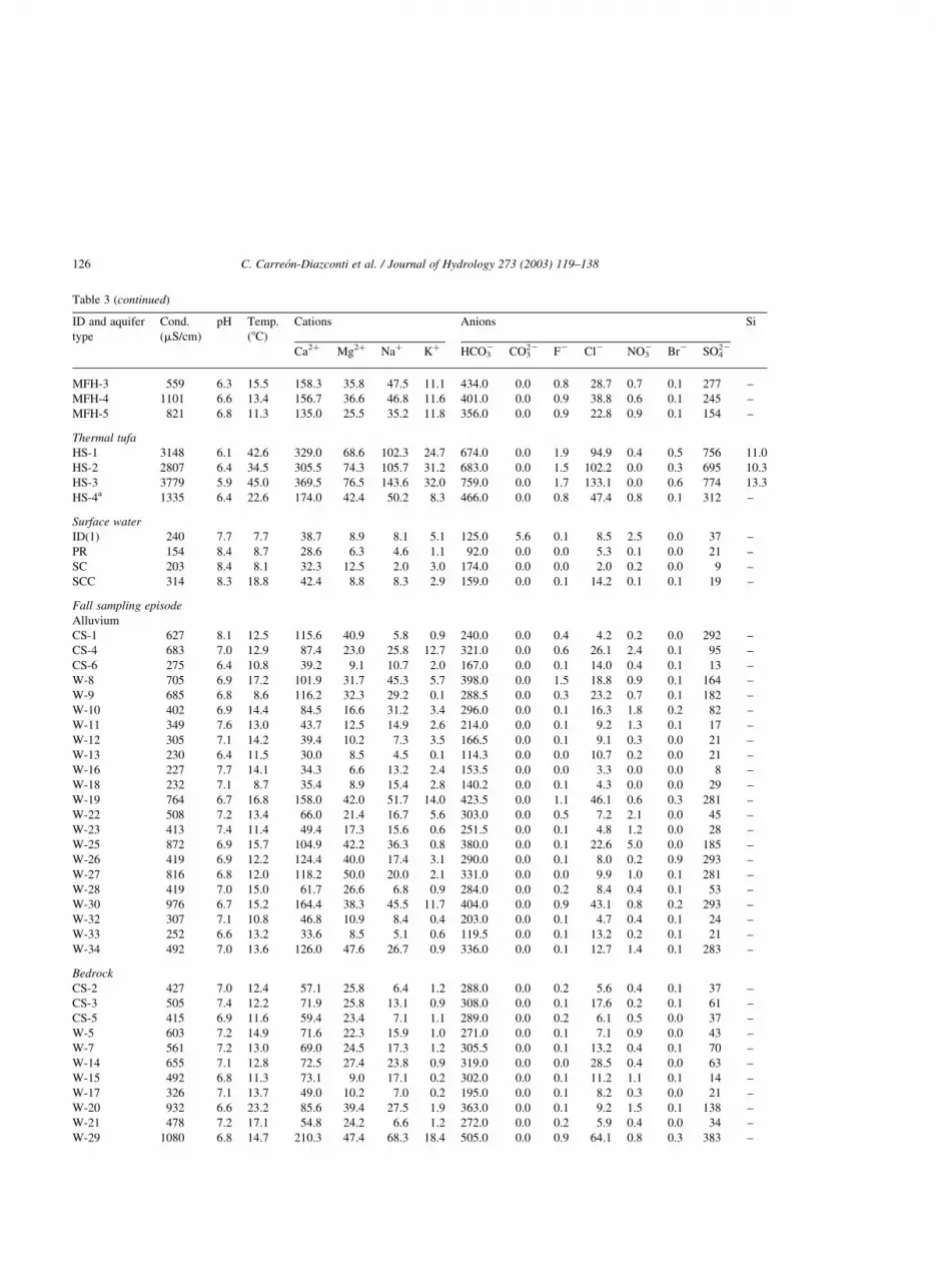
Table 3 (continued)

ID and aquifer

type

Cond.

(mS/cm)

pH Temp.

(8C)

Cations Anions Si



22

MFH-3 559 6.3 15.5 158.3 35.8 47.5 11.1 434.0 0.0 0.8 28.7 0.7 0.1 277 –

MFH-4 1101 6.6 13.4 156.7 36.6 46.8 11.6 401.0 0.0 0.9 38.8 0.6 0.1 245 –

MFH-5 821 6.8 11.3 135.0 25.5 35.2 11.8 356.0 0.0 0.9 22.8 0.9 0.1 154 –

Thermal tufa

HS-1 3148 6.1 42.6 329.0 68.6 102.3 24.7 674.0 0.0 1.9 94.9 0.4 0.5 756 11.0

HS-2 2807 6.4 34.5 305.5 74.3 105.7 31.2 683.0 0.0 1.5 102.2 0.0 0.3 695 10.3

HS-3 3779 5.9 45.0 369.5 76.5 143.6 32.0 759.0 0.0 1.7 133.1 0.0 0.6 774 13.3

HS-4a 1335 6.4 22.6 174.0 42.4 50.2 8.3 466.0 0.0 0.8 47.4 0.8 0.1 312 –

Surface water

ID(1) 240 7.7 7.7 38.7 8.9 8.1 5.1 125.0 5.6 0.1 8.5 2.5 0.0 37 –

PR 154 8.4 8.7 28.6 6.3 4.6 1.1 92.0 0.0 0.0 5.3 0.1 0.0 21 –

SC 203 8.4 8.1 32.3 12.5 2.0 3.0 174.0 0.0 0.0 2.0 0.2 0.0 9 –

SCC 314 8.3 18.8 42.4 8.8 8.3 2.9 159.0 0.0 0.1 14.2 0.1 0.1 19 –

Fall sampling episode

Alluvium

CS-1 627 8.1 12.5 115.6 40.9 5.8 0.9 240.0 0.0 0.4 4.2 0.2 0.0 292 –

CS-4 683 7.0 12.9 87.4 23.0 25.8 12.7 321.0 0.0 0.6 26.1 2.4 0.1 95 –

CS-6 275 6.4 10.8 39.2 9.1 10.7 2.0 167.0 0.0 0.1 14.0 0.4 0.1 13 –

W-8 705 6.9 17.2 101.9 31.7 45.3 5.7 398.0 0.0 1.5 18.8 0.9 0.1 164 –

W-9 685 6.8 8.6 116.2 32.3 29.2 0.1 288.5 0.0 0.3 23.2 0.7 0.1 182 –

W-10 402 6.9 14.4 84.5 16.6 31.2 3.4 296.0 0.0 0.1 16.3 1.8 0.2 82 –

W-11 349 7.6 13.0 43.7 12.5 14.9 2.6 214.0 0.0 0.1 9.2 1.3 0.1 17 –

W-12 305 7.1 14.2 39.4 10.2 7.3 3.5 166.5 0.0 0.1 9.1 0.3 0.0 21 –

W-13 230 6.4 11.5 30.0 8.5 4.5 0.1 114.3 0.0 0.0 10.7 0.2 0.0 21 –

W-16 227 7.7 14.1 34.3 6.6 13.2 2.4 153.5 0.0 0.0 3.3 0.0 0.0 8 –

W-18 232 7.1 8.7 35.4 8.9 15.4 2.8 140.2 0.0 0.1 4.3 0.0 0.0 29 –

W-19 764 6.7 16.8 158.0 42.0 51.7 14.0 423.5 0.0 1.1 46.1 0.6 0.3 281 –

W-22 508 7.2 13.4 66.0 21.4 16.7 5.6 303.0 0.0 0.5 7.2 2.1 0.0 45 –

W-23 413 7.4 11.4 49.4 17.3 15.6 0.6 251.5 0.0 0.1 4.8 1.2 0.0 28 –

W-25 872 6.9 15.7 104.9 42.2 36.3 0.8 380.0 0.0 0.1 22.6 5.0 0.0 185 –

W-26 419 6.9 12.2 124.4 40.0 17.4 3.1 290.0 0.0 0.1 8.0 0.2 0.9 293 –

W-27 816 6.8 12.0 118.2 50.0 20.0 2.1 331.0 0.0 0.0 9.9 1.0 0.1 281 –

W-28 419 7.0 15.0 61.7 26.6 6.8 0.9 284.0 0.0 0.2 8.4 0.4 0.1 53 –

W-30 976 6.7 15.2 164.4 38.3 45.5 11.7 404.0 0.0 0.9 43.1 0.8 0.2 293 –

W-32 307 7.1 10.8 46.8 10.9 8.4 0.4 203.0 0.0 0.1 4.7 0.4 0.1 24 –

W-33 252 6.6 13.2 33.6 8.5 5.1 0.6 119.5 0.0 0.1 13.2 0.2 0.1 21 –

W-34 492 7.0 13.6 126.0 47.6 26.7 0.9 336.0 0.0 0.1 12.7 1.4 0.1 283 –

Bedrock

CS-2 427 7.0 12.4 57.1 25.8 6.4 1.2 288.0 0.0 0.2 5.6 0.4 0.1 37 –

CS-3 505 7.4 12.2 71.9 25.8 13.1 0.9 308.0 0.0 0.1 17.6 0.2 0.1 61 –

CS-5 415 6.9 11.6 59.4 23.4 7.1 1.1 289.0 0.0 0.2 6.1 0.5 0.0 37 –

W-5 603 7.2 14.9 71.6 22.3 15.9 1.0 271.0 0.0 0.1 7.1 0.9 0.0 43 –

W-7 561 7.2 13.0 69.0 24.5 17.3 1.2 305.5 0.0 0.1 13.2 0.4 0.1 70 –

W-14 655 7.1 12.8 72.5 27.4 23.8 0.9 319.0 0.0 0.0 28.5 0.4 0.0 63 –

W-15 492 6.8 11.3 73.1 9.0 17.1 0.2 302.0 0.0 0.1 11.2 1.1 0.1 14 –

W-17 326 7.1 13.7 49.0 10.2 7.0 0.2 195.0 0.0 0.1 8.2 0.3 0.0 21 –

W-20 932 6.6 23.2 85.6 39.4 27.5 1.9 363.0 0.0 0.1 9.2 1.5 0.1 138 –

W-21 478 7.2 17.1 54.8 24.2 6.6 1.2 272.0 0.0 0.2 5.9 0.4 0.0 34 –

W-29 1080 6.8 14.7 210.3 47.4 68.3 18.4 505.0 0.0 0.9 64.1 0.8 0.3 383 –


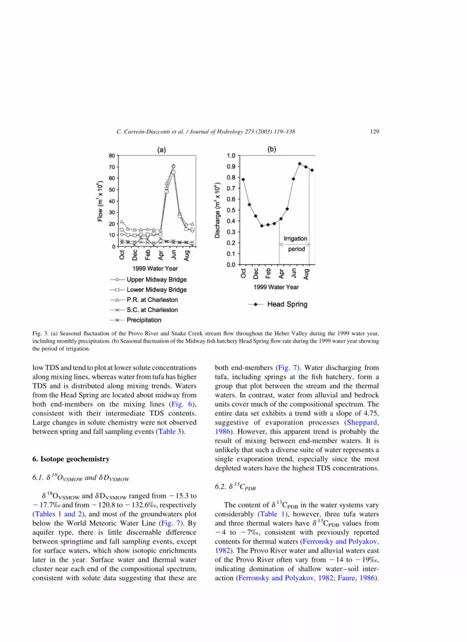
between the Provo River Upper Midway Bridge and

Provo River Lower Midway Bridge stream-flow

records for the 1999 water year (Fig. 3) demonstrates

that during periods of base flow in the winter months,

the stream gains about 10–20% water as it flows

through this stretch of the Heber Valley, whereas

water loss during spring and summer, when snow

melts and runoff takes place, reflects water removal

for irrigation. Making a similar comparison between

the Provo River Upper Midway Bridge and the Provo

River near the Charleston gauging station, the stream

gains about 50% from groundwater throughout the

winter season. A summer gain–loss stream-flow

analysis for Snake Creek showed that only in its

northwestern stretch as it enters the valley is water lost

to the subsurface. Otherwise it gains flow along most

of the rest of its course when water diversions are

accounted for.

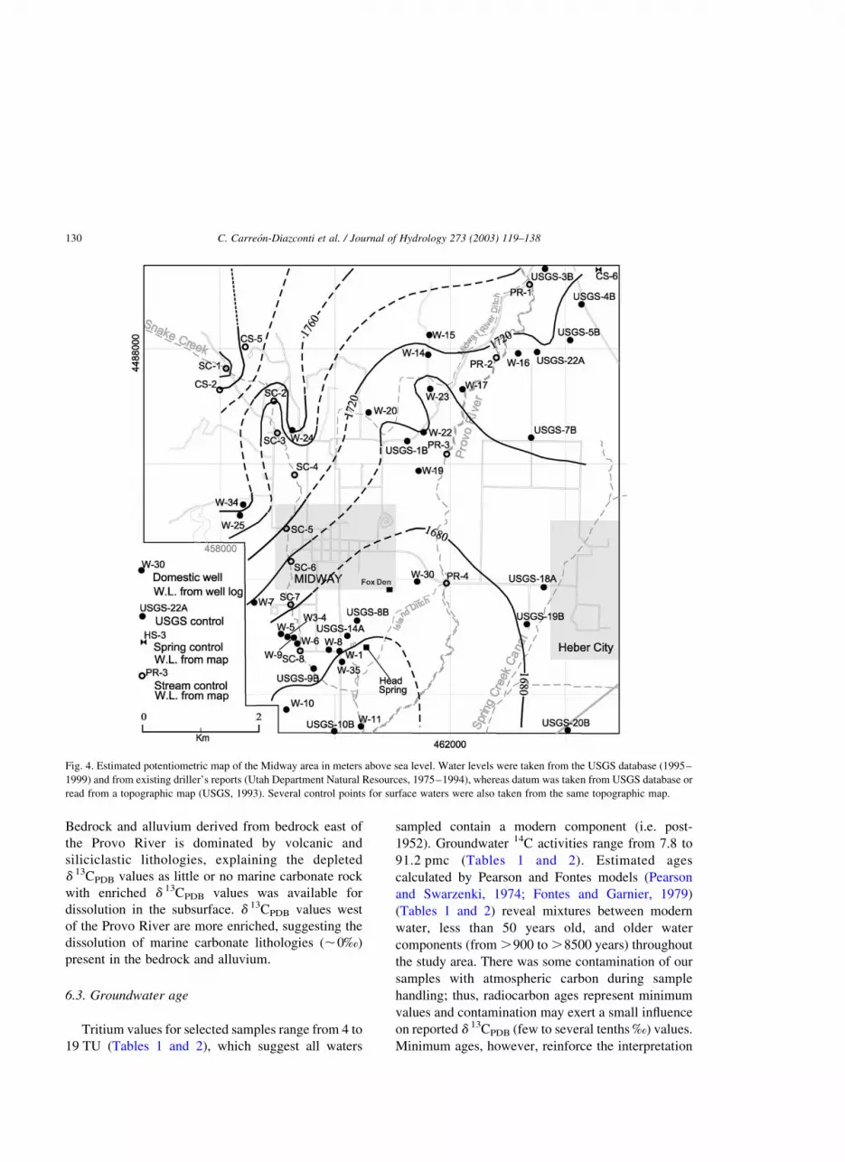
5.2. Groundwater movement

A preliminary potentiometric map (Fig. 4) was

constructed using the best water level data available

to us (US Geological Survey monitoring wells,

1995–1999; well driller’s reports, Utah Department

of Natural Resources, 1975–1994). Several control

points for surface waters were taken from a USGS

topographic map (1993). Potentiometric contours

wrap around to the south in the study area, west of

the Provo River, suggesting that groundwater flow is

focused toward the hatchery, including Head Spring,

which averages 0.7 m3/s. Thus, the simplest

interpretations of potentiometric map are: (1)

groundwater from both sides of Provo River is

migrating toward the stream, consistent with water

gains in the Provo River, and (2) the hatchery area

is a locus of focused discharge, consistent with

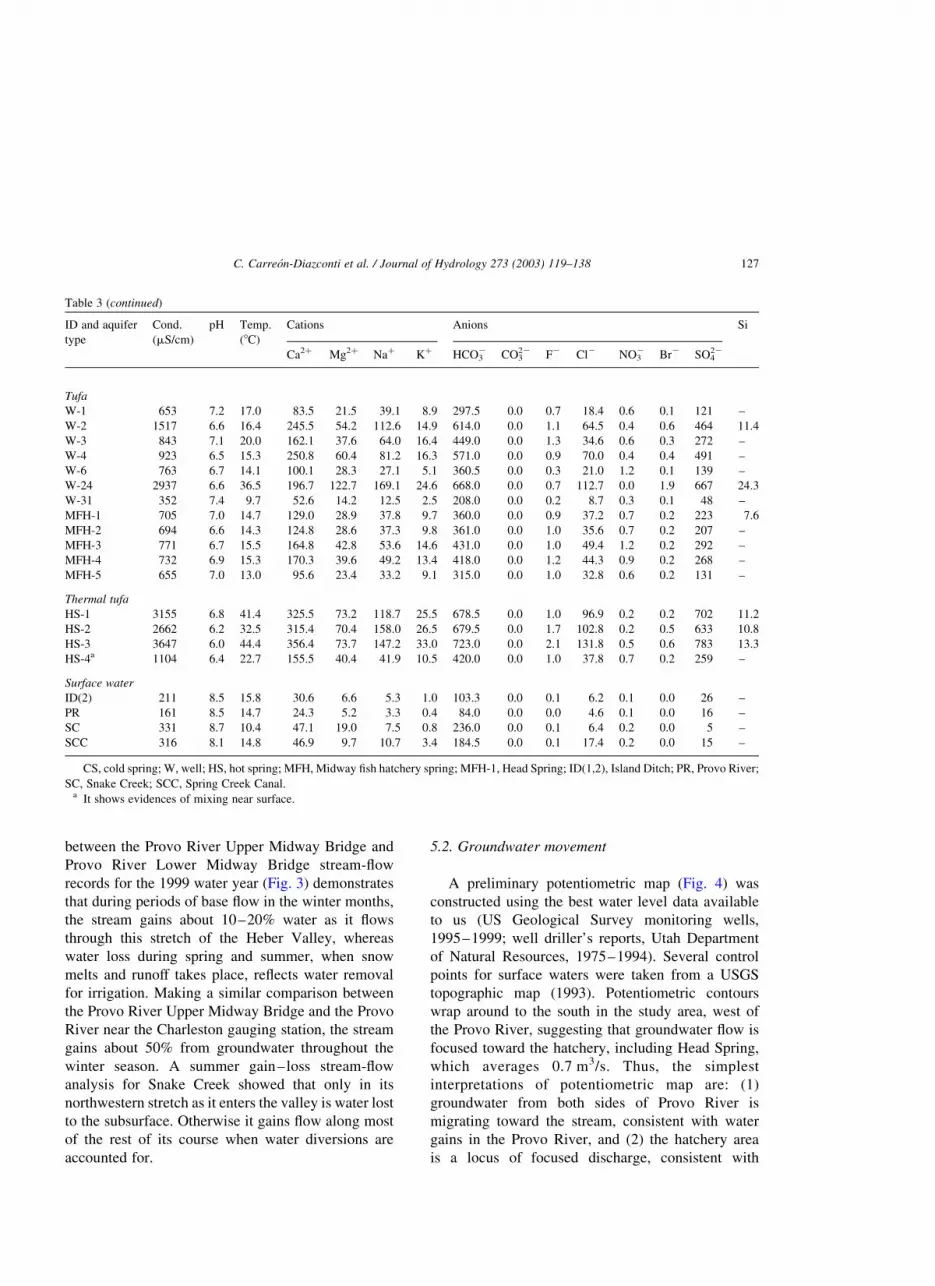
Table 3 (continued)

ID and aquifer

type

Cond.

(mS/cm)

pH Temp.

(8C)

Cations Anions Si



22

Tufa

W-1 653 7.2 17.0 83.5 21.5 39.1 8.9 297.5 0.0 0.7 18.4 0.6 0.1 121 –

W-2 1517 6.6 16.4 245.5 54.2 112.6 14.9 614.0 0.0 1.1 64.5 0.4 0.6 464 11.4

W-3 843 7.1 20.0 162.1 37.6 64.0 16.4 449.0 0.0 1.3 34.6 0.6 0.3 272 –

W-4 923 6.5 15.3 250.8 60.4 81.2 16.3 571.0 0.0 0.9 70.0 0.4 0.4 491 –

W-6 763 6.7 14.1 100.1 28.3 27.1 5.1 360.5 0.0 0.3 21.0 1.2 0.1 139 –

W-24 2937 6.6 36.5 196.7 122.7 169.1 24.6 668.0 0.0 0.7 112.7 0.0 1.9 667 24.3

W-31 352 7.4 9.7 52.6 14.2 12.5 2.5 208.0 0.0 0.2 8.7 0.3 0.1 48 –

MFH-1 705 7.0 14.7 129.0 28.9 37.8 9.7 360.0 0.0 0.9 37.2 0.7 0.2 223 7.6

MFH-2 694 6.6 14.3 124.8 28.6 37.3 9.8 361.0 0.0 1.0 35.6 0.7 0.2 207 –

MFH-3 771 6.7 15.5 164.8 42.8 53.6 14.6 431.0 0.0 1.0 49.4 1.2 0.2 292 –

MFH-4 732 6.9 15.3 170.3 39.6 49.2 13.4 418.0 0.0 1.2 44.3 0.9 0.2 268 –

MFH-5 655 7.0 13.0 95.6 23.4 33.2 9.1 315.0 0.0 1.0 32.8 0.6 0.2 131 –

Thermal tufa

HS-1 3155 6.8 41.4 325.5 73.2 118.7 25.5 678.5 0.0 1.0 96.9 0.2 0.2 702 11.2

HS-2 2662 6.2 32.5 315.4 70.4 158.0 26.5 679.5 0.0 1.7 102.8 0.2 0.5 633 10.8

HS-3 3647 6.0 44.4 356.4 73.7 147.2 33.0 723.0 0.0 2.1 131.8 0.5 0.6 783 13.3

HS-4a 1104 6.4 22.7 155.5 40.4 41.9 10.5 420.0 0.0 1.0 37.8 0.7 0.2 259 –

Surface water

ID(2) 211 8.5 15.8 30.6 6.6 5.3 1.0 103.3 0.0 0.1 6.2 0.1 0.0 26 –

PR 161 8.5 14.7 24.3 5.2 3.3 0.4 84.0 0.0 0.0 4.6 0.1 0.0 16 –

SC 331 8.7 10.4 47.1 19.0 7.5 0.8 236.0 0.0 0.1 6.4 0.2 0.0 5 –

SCC 316 8.1 14.8 46.9 9.7 10.7 3.4 184.5 0.0 0.1 17.4 0.2 0.0 15 –

CS, cold spring; W, well; HS, hot spring; MFH, Midway fish hatchery spring; MFH-1, Head Spring; ID(1,2), Island Ditch; PR, Provo River;

SC, Snake Creek; SCC, Spring Creek Canal.a It shows evidences of mixing near surface.


the numerous springs and artesian monitoring wells

found on hatchery property.

5.3. Groundwater flow system and hydrochemistry

In addition to surface water, four groundwater

systems have been identified on the basis of rock

type, discharge temperature, and discharge location.

They include: (1) thermal water (.30 8C), (2)

alluvium water, (3) shallow tufa water, and (4)

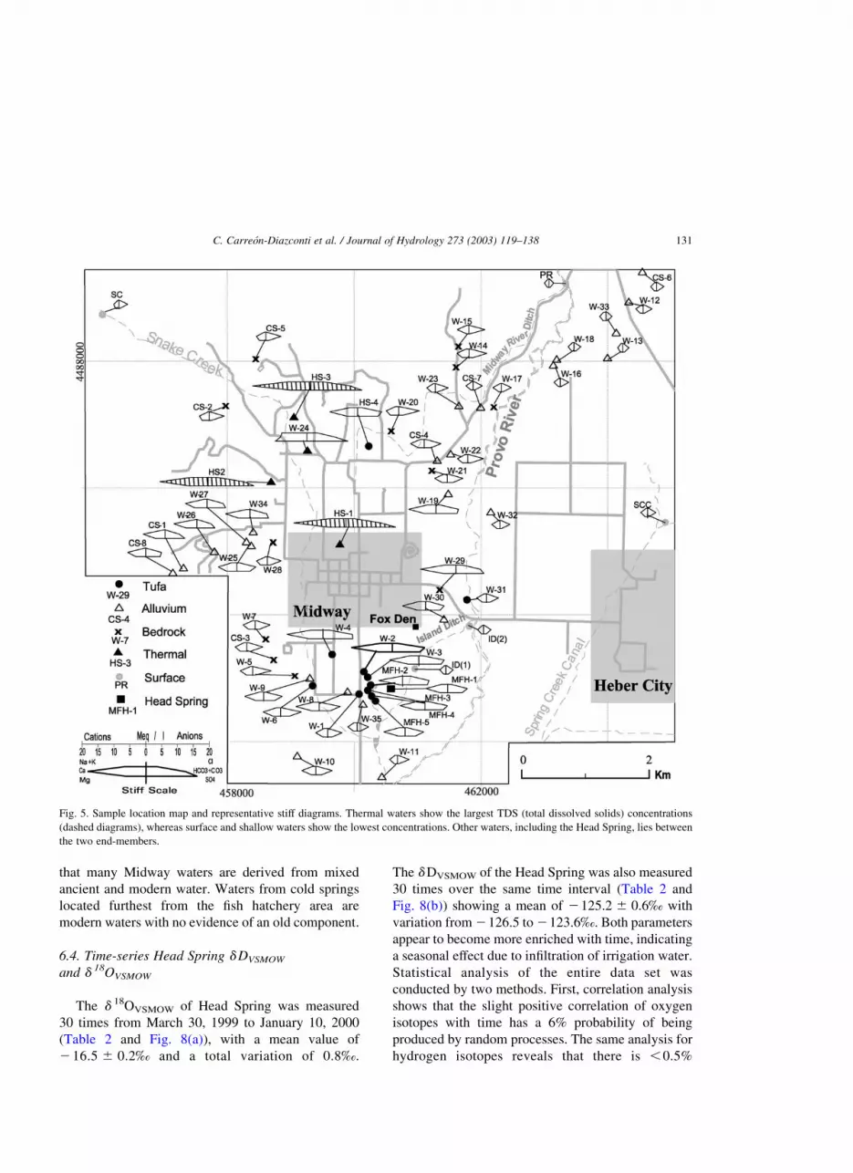
bedrock water. Chemically, two end-member waters

can be identified (Figs. 5 and 6). One is comprised

of cold, low TDS calcium bicarbonate waters from

surface as well as some alluvial and bedrock

sources. By contrast, thermal springs discharge

calcium sulfate water and have much higher TDS

contents as stiff diagrams illustrate (Fig. 5).

Other waters exhibit chemical characteristics that

are transitional between the end-members (Figs. 5 and

6).Waters discharging from bedrockand alluvium have

Fig. 2. Geological map of the Heber Valley (modified from Hintze (2000)).


low TDS and tend to plot at lower solute concentrations

along mixing lines, whereas water from tufa has higher

TDS and is distributed along mixing trends. Waters

from the Head Spring are located about midway from

both end-members on the mixing lines (Fig. 6),

consistent with their intermediate TDS contents.

Large changes in solute chemistry were not observed

between spring and fall sampling events (Table 3).

6. Isotope geochemistry

6.1. d 18OVSMOW and dDVSMOW

d 18OVSMOW and dDVSMOW ranged from 215.3 to

217.7‰ and from 2120.8 to 2132.6‰, respectively

(Tables 1 and 2), and most of the groundwaters plot

below the World Meteoric Water Line (Fig. 7). By

aquifer type, there is little discernable difference

between springtime and fall sampling events, except

for surface waters, which show isotopic enrichments

later in the year. Surface water and thermal water

cluster near each end of the compositional spectrum,

consistent with solute data suggesting that these are

both end-members (Fig. 7). Water discharging from

tufa, including springs at the fish hatchery, form a

group that plot between the stream and the thermal

waters. In contrast, water from alluvial and bedrock

units cover much of the compositional spectrum. The

entire data set exhibits a trend with a slope of 4.75,

suggestive of evaporation processes (Sheppard,

1986). However, this apparent trend is probably the

result of mixing between end-member waters. It is

unlikely that such a diverse suite of water represents a

single evaporation trend, especially since the most

depleted waters have the highest TDS concentrations.

6.2. d 13CPDB

The content of d 13CPDB in the water systems vary

considerably (Table 1), however, three tufa waters

and three thermal waters have d 13CPDB values from

24 to 27‰, consistent with previously reported

contents for thermal waters (Ferronsky and Polyakov,

1982). The Provo River water and alluvial waters east

of the Provo River often vary from 214 to 219‰,

indicating domination of shallow water–soil inter-

action (Ferronsky and Polyakov, 1982; Faure, 1986).

Fig. 3. (a) Seasonal fluctuation of the Provo River and Snake Creek stream flow throughout the Heber Valley during the 1999 water year,

including monthly precipitation. (b) Seasonal fluctuation of the Midway fish hatchery Head Spring flow rate during the 1999 water year showing

the period of irrigation.


Bedrock and alluvium derived from bedrock east of

the Provo River is dominated by volcanic and

siliciclastic lithologies, explaining the depleted

d 13CPDB values as little or no marine carbonate rock

with enriched d 13CPDB values was available for

dissolution in the subsurface. d 13CPDB values west

of the Provo River are more enriched, suggesting the

dissolution of marine carbonate lithologies (,0‰)

present in the bedrock and alluvium.

6.3. Groundwater age

Tritium values for selected samples range from 4 to

19 TU (Tables 1 and 2), which suggest all waters

sampled contain a modern component (i.e. post-

1952). Groundwater 14C activities range from 7.8 to

91.2 pmc (Tables 1 and 2). Estimated ages

calculated by Pearson and Fontes models (Pearson

and Swarzenki, 1974; Fontes and Garnier, 1979)

(Tables 1 and 2) reveal mixtures between modern

water, less than 50 years old, and older water

components (from .900 to .8500 years) throughout

the study area. There was some contamination of our

samples with atmospheric carbon during sample

handling; thus, radiocarbon ages represent minimum

values and contamination may exert a small influence

on reported d 13CPDB (few to several tenths ‰) values.

Minimum ages, however, reinforce the interpretation

Fig. 4. Estimated potentiometric map of the Midway area in meters above sea level. Water levels were taken from the USGS database (1995–

1999) and from existing driller’s reports (Utah Department Natural Resources, 1975–1994), whereas datum was taken from USGS database or

read from a topographic map (USGS, 1993). Several control points for surface waters were also taken from the same topographic map.


that many Midway waters are derived from mixed

ancient and modern water. Waters from cold springs

located furthest from the fish hatchery area are

modern waters with no evidence of an old component.

6.4. Time-series Head Spring dDVSMOW

and d 18OVSMOW

The d 18OVSMOW of Head Spring was measured

30 times from March 30, 1999 to January 10, 2000

(Table 2 and Fig. 8(a)), with a mean value of

216.5 ^ 0.2‰ and a total variation of 0.8‰.

The dDVSMOW of the Head Spring was also measured

30 times over the same time interval (Table 2 and

Fig. 8(b)) showing a mean of 2125.2 ^ 0.6‰ with

variation from 2126.5 to 2123.6‰. Both parameters

appear to become more enriched with time, indicating

a seasonal effect due to infiltration of irrigation water.

Statistical analysis of the entire data set was

conducted by two methods. First, correlation analysis

shows that the slight positive correlation of oxygen

isotopes with time has a 6% probability of being

produced by random processes. The same analysis for

hydrogen isotopes reveals that there is ,0.5%

Fig. 5. Sample location map and representative stiff diagrams. Thermal waters show the largest TDS (total dissolved solids) concentrations

(dashed diagrams), whereas surface and shallow waters show the lowest concentrations. Other waters, including the Head Spring, lies between

the two end-members.


probability that the positive slope was produced

randomly. Second, there is a significant gap in data

extending from mid-July to late-August. dDVSMOW

average before mid-July is 2125.5‰ and after mid-

July is 2125.0‰. If the data before and after this gap

are treated as groups, a t-test comparison of means

shows that there is only a 1% probability that they

represent the same population.

6.5. Dye tracer data

In September of 2000, dye tracer tests were

conducted. Rhodamine WT dye was injected into

the Fox Den, a karst feature in the tufa platform

located 1 km to the northeast of the Head Spring.

Within the sinkhole, water flows both in and out

through fractured tufa, but only in the summer months

when the application of irrigation water locally raises

the water table. Simultaneously, fluorescein dye was

injected into flood irrigation water that was being

turned into a pasture adjacent to the Fox Den. Because

of the potential for large degrees of dilution, dye

concentrations were not measured directly at the

hatchery. Instead, dye was allowed to accumulate on

charcoal packets and was subsequently desorbed and

measured in the resulting solution. Fig. 9 illustrates

the breakthrough of these dyes at the Head

Spring. Maximum concentrations were reached for

Fig. 7. d 18OVSMOW versus dDVSMOW plot for waters of the Midway

area, including the World Meteoric Water Line (Rosanski et al.,

1993). Once again, cold, low TDS and thermal waters appear to

represent end-members waters. See text for discussion.

Fig. 6. Solute and field parameter cross-plots of Midway waters for

(a) temperature versus conductivity, (b) chloride versus sulfate, and

(c) sodium versus calcium concentrations. For ease of reading, only

data for the spring sampling episode were plotted since no large

differences were observed between the two sampling episodes. Note

that cold, low TDS (surface and shallow waters) and thermal waters

(of higher TDS) appear to represent potential mixing end-members

for the other waters throughout the area.


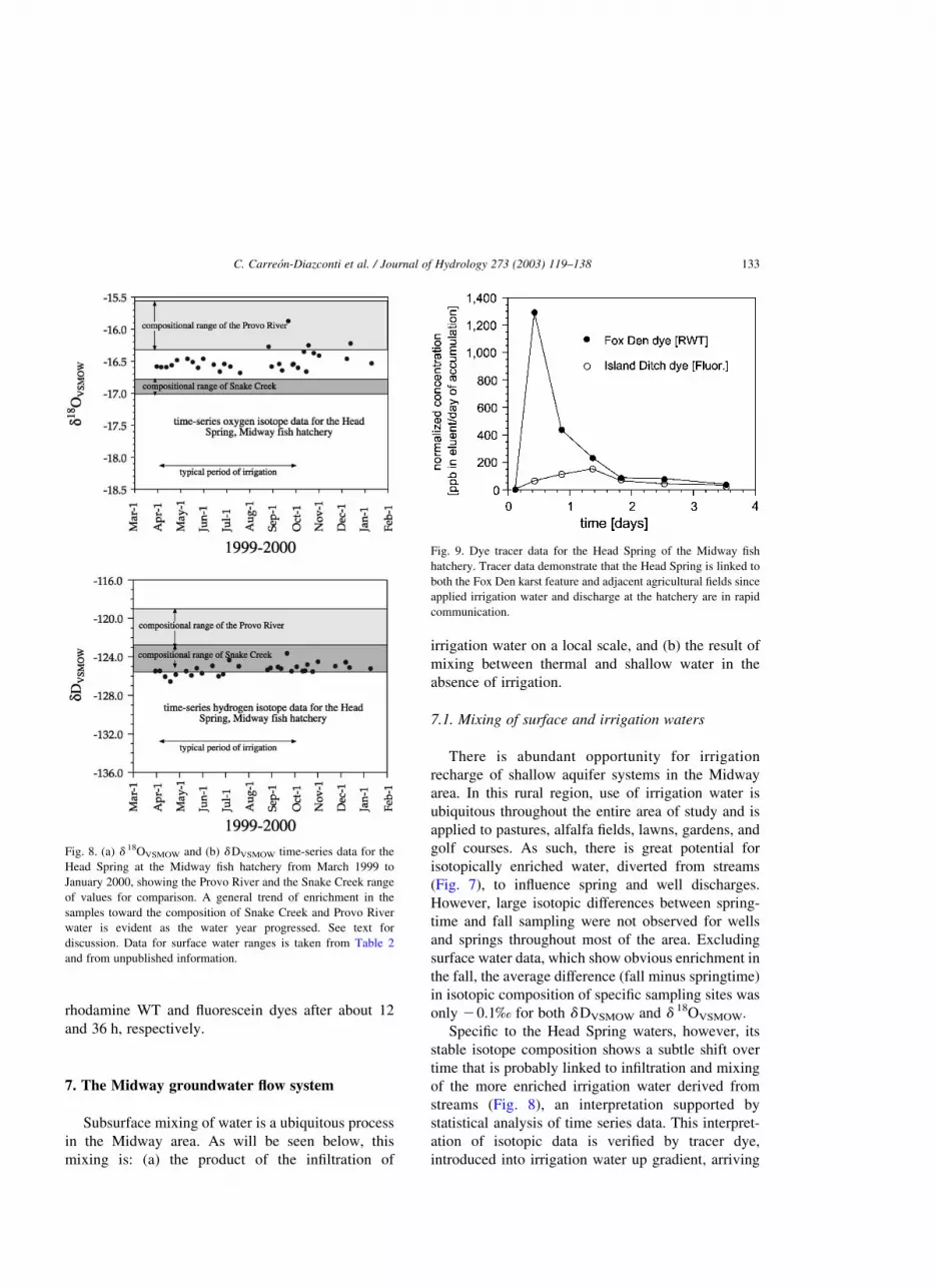
rhodamine WT and fluorescein dyes after about 12

and 36 h, respectively.

7. The Midway groundwater flow system

Subsurface mixing of water is a ubiquitous process

in the Midway area. As will be seen below, this

mixing is: (a) the product of the infiltration of

irrigation water on a local scale, and (b) the result of

mixing between thermal and shallow water in the

absence of irrigation.

7.1. Mixing of surface and irrigation waters

There is abundant opportunity for irrigation

recharge of shallow aquifer systems in the Midway

area. In this rural region, use of irrigation water is

ubiquitous throughout the entire area of study and is

applied to pastures, alfalfa fields, lawns, gardens, and

golf courses. As such, there is great potential for

isotopically enriched water, diverted from streams

(Fig. 7), to influence spring and well discharges.

However, large isotopic differences between spring-

time and fall sampling were not observed for wells

and springs throughout most of the area. Excluding

surface water data, which show obvious enrichment in

the fall, the average difference (fall minus springtime)

in isotopic composition of specific sampling sites was

only 20.1‰ for both dDVSMOW and d 18OVSMOW.

Specific to the Head Spring waters, however, its

stable isotope composition shows a subtle shift over

time that is probably linked to infiltration and mixing

of the more enriched irrigation water derived from

streams (Fig. 8), an interpretation supported by

statistical analysis of time series data. This interpret-

ation of isotopic data is verified by tracer dye,

introduced into irrigation water up gradient, arriving

Fig. 8. (a) d 18OVSMOW and (b) dDVSMOW time-series data for the

Head Spring at the Midway fish hatchery from March 1999 to

January 2000, showing the Provo River and the Snake Creek range

of values for comparison. A general trend of enrichment in the

samples toward the composition of Snake Creek and Provo River

water is evident as the water year progressed. See text for

discussion. Data for surface water ranges is taken from Table 2

and from unpublished information.

Fig. 9. Dye tracer data for the Head Spring of the Midway fish

hatchery. Tracer data demonstrate that the Head Spring is linked to

both the Fox Den karst feature and adjacent agricultural fields since

applied irrigation water and discharge at the hatchery are in rapid

communication.


at the hatchery. The fractured karstified tufa is

probably in direct communication with the Head

Spring, as reflected in the rapid transport of

rhodamine WT dye from the Fox Den (Fig. 9). The

injection point was a pool of water in the bottom of the

sinkhole. Thus, there was no opportunity for irrigation

return flows to transport dye to the hatchery.

The adjacent flood-irrigated field also indicates a

strong hydrologic connection to the hatchery,

although the relatively broadened peak for fluorescein

dye (Fig. 9) probably represents hydrodynamic

dispersion in the soil/alluvial system prior to the

infiltrating water reaching highly transmissive frac-

tured tufa known to exist in the subsurface as

evidenced in well logs. It should be noted that the

application of irrigation water in this field results in

increased flux rates at the hatchery as mentioned in

Section 1 and illustrated in Fig. 3(b). There is some

chance that fluorescein dye was brought close to the

hatchery by irrigation returns confined in drainage

ditches. However, it can be reasonably demonstrated

that the irrigation water does, in fact, rapidly infiltrate

and reach the hatchery from the Fox Den area.

Waters sampled to the east of the Provo River

probably reflect underflow whereas water to the west

reflects complex mixing processes with the thermal

end-member. Water discharging from alluvium and

bedrock show variable mixing according to proximity

to the sources of end-member waters. Similarly, much

of the water discharging from the tufa platform shows

characteristics that cluster between the end-members.

7.2. Mixing between cold and thermal components

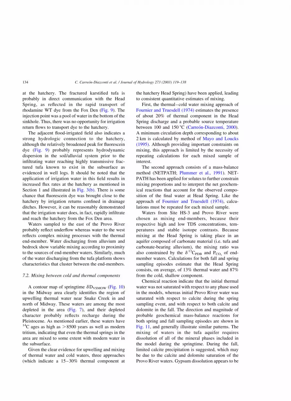
A contour map of springtime dDVSMOW (Fig. 10)

in the Midway area clearly identifies the region of

upwelling thermal water near Snake Creek in and

north of Midway. These waters are among the most

depleted in the area (Fig. 7), and their depleted

character probably reflects recharge during the

Pleistocene. As mentioned earlier, these waters have14C ages as high as .8500 years as well as modern

tritium, indicating that even the thermal springs in the

area are mixed to some extent with modern water in

the subsurface.

Given the clear evidence for upwelling and mixing

of thermal water and cold waters, three approaches

(which indicate a 15–30% thermal component at

the hatchery Head Spring) have been applied, leading

to consistent quantitative estimates of mixing.

First, the thermal–cold water mixing approach of

Fournier and Truesdell (1974) estimates the presence

of about 20% of thermal component in the Head

Spring discharge and a probable source temperature

between 100 and 150 8C (Carreon-Diazconti, 2000).

A minimum circulation depth corresponding to about

2 km is calculated by method of Mayo and Loucks

(1995). Although providing important constraints on

mixing, this approach is limited by the necessity of

repeating calculations for each mixed sample of

interest.

The second approach consists of a mass-balance

method (NETPATH; Plummer et al., 1991). NET-

PATH has been applied for solutes to further constrain

mixing proportions and to interpret the net geochem-

ical reactions that account for the observed compo-

sition of the final water at Head Spring. Like the

approach of Fournier and Truesdell (1974), calcu-

lations must be repeated for each mixed sample.

Waters from Site HS-3 and Provo River were

chosen as mixing end-members, because their

respective high and low TDS concentrations, tem-

peratures and stable isotope contrasts. Because

mixing at the Head Spring is taking place in an

aquifer composed of carbonate material (i.e. tufa and

carbonate-bearing alluvium), the mixing ratio was

also constrained by the d 13CPDB and PCO2of end-

member waters. Calculations for both fall and spring

sampling episodes estimate that the Head Spring

consists, on average, of 13% thermal water and 87%

from the cold, shallow component.

Chemical reaction indicate that the initial thermal

water was not saturated with respect to any phase used

in the models, whereas initial Provo River water was

saturated with respect to calcite during the spring

sampling event, and with respect to both calcite and

dolomite in the fall. The direction and magnitude of

probable geochemical mass-balance reactions for

both spring and fall sampling episodes are shown in

Fig. 11, and generally illustrate similar patterns. The

mixing of waters in the tufa aquifer requires

dissolution of all of the mineral phases included in

the model during the springtime. During the fall,

limited calcite precipitation is suggested, which may

be due to the calcite and dolomite saturation of the

Provo River waters. Gypsum dissolution appears to be


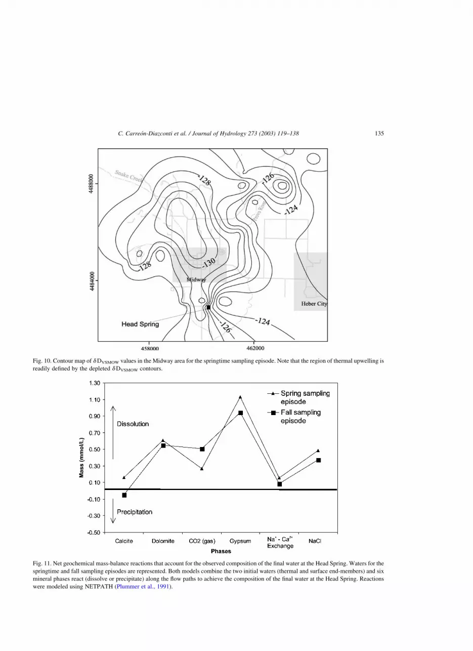
Fig. 10. Contour map of dDVSMOW values in the Midway area for the springtime sampling episode. Note that the region of thermal upwelling is

readily defined by the depleted dDVSMOW contours.

Fig. 11. Net geochemical mass-balance reactions that account for the observed composition of the final water at the Head Spring. Waters for the

springtime and fall sampling episodes are represented. Both models combine the two initial waters (thermal and surface end-members) and six

mineral phases react (dissolve or precipitate) along the flow paths to achieve the composition of the final water at the Head Spring. Reactions

were modeled using NETPATH (Plummer et al., 1991).


the predominant reaction along this flowpath because

it is the only phase that controls the activity of SO422.

Other sources of sulfur are not anticipated in this

system.

The final approach relies on applying simple

mixing relationships (Clark and Fritz, 1997) to stable

isotopes. Using the composition of end-member

waters (HS-3 and Provo River), mixing fractions

were calculated in a spreadsheet for all samples,

permitting the construction of a contour map that

quantifies mixing fractions on the basis of dDVSMOW

compositions (Fig. 12). Hydrogen isotopes were

chosen because they are unlikely to undergo signifi-

cant isotopic exchange within the aquifer. This is

especially important when mixing involves a thermal

component because oxygen isotope composition is

much more likely to be affected by water–rock

isotopic exchange reactions at elevated temperature.

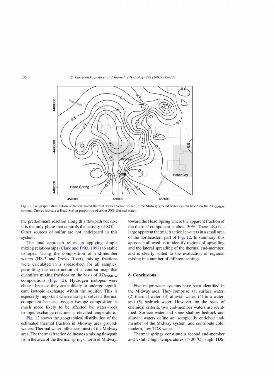
Fig. 12 shows the geographical distribution of the

estimated thermal fraction in Midway area ground-

waters. Thermal water influences most of the Midway

area. The thermal fraction delineates a mixing flowpath

from the area of the thermal springs, north of Midway,

toward the Head Spring where the apparent fraction of

the thermal component is about 30%. There also is a

large apparent thermal fraction in waters in a small area

of the northeastern part of Fig. 12. In summary, this

approach allowed us to identify regions of upwelling

and the lateral spreading of the thermal end-member,

and is clearly suited to the evaluation of regional

mixing in a number of different settings.

8. Conclusions

Five major water systems have been identified in

the Midway area. They comprise: (1) surface water,

(2) thermal water, (3) alluvial water, (4) tufa water,

and (5) bedrock water. However, on the basis of

chemical criteria, two end-member waters are ident-

ified. Surface water and some shallow bedrock and

alluvial waters define an isotopically enriched end-

member of the Midway system, and contribute cold,

modern, low TDS water.

Thermal springs constitute a second end-member

and exhibit high temperatures (.30 8C), high TDS,

Fig. 12. Geographic distribution of the estimated thermal water fraction mixed in the Midway ground water system based on the dDVSMOW

content. Curves indicate a Head Spring proportion of about 30% thermal water.


and depleted dDVSMOW and d 18OVSMOW values.

However, even these waters exhibit clear evidence

of mixing. 14C and 3H data indicate that even the

thermal component consists of a mixture between

ancient (.8500 years) and modern water and that the

ancient component of this end-member was recharged

during cold climatic conditions. This water infiltrated

at high elevations, circulated to depths on the order of

2 km into sedimentary rocks and has been heated to

100–150 8C in temperature. After ascending through

fractures and along normal faults it mixes in varying

proportions with modern water in the shallow

subsurface.

With few exceptions, the entire groundwater

system in the Midway area is the result, to some

degree, of mixing between the two end-members,

whether it be in bedrock, alluvial, or tufa aquifers.

For example, isotopic and chemical mixing models

show that Head Spring discharging water is the

result of mixing about 13–30% thermal water and

70–87% cold, low TDS water.

Three approaches have been employed to

evaluate mixing. Application of the thermodynamic

(Fournier and Truesdell, 1974) and mass balance

approaches (Plummer et al. 1991) employ rigorous

constraints on mixing and associated physical and

chemical processes, although each mixed waters

must be evaluated separately. Mixing calculations

based on isotopic composition, on the other hand,

can be employed simultaneously for an entire data

set once reasonable end-member waters have been

identified. This allows the construction of regional

contours maps of mixing fractions. Although not as

rigorous as other approaches, it nonetheless ident-

ifies the extent of mixing over a large region and

allows for the identification of features that may

warrant further investigation by mass balance or

geothermal methods.

Evidences of infiltration of water from irrigation

into the Midway groundwater system are: (1) the

hydraulic response (increased flux) at the Head Spring

just hours after the onset of flood irrigation due to

communication through karstified tufa underneath

nearby fields, (2) the isotopic enrichment of water at

the hatchery Head Spring during the irrigation season,

and (3) preliminary results from dye tracer studies

showing that tracers injected in both fractured tufa

and alluvial deposits approximately 1 km from

the hatchery took less than 2 days to reach the Head

Spring.

Acknowledgements

The Utah Division of Wildlife generously sup-

ported this study. Particular thanks are extended to Joe

Valentine, Dan Aubrey, Chuck Bobo, and the staff of

the Midway Fish hatchery. We also thank our

Katherine Anderson and Chris Bexfield for extensive

support in data acquisition. Special thanks are given to

Dr Colin Neal and Dr Gideon Tredoux for their

valuable reviews.

References

Baker Jr., C.H., 1968. Thermal springs near Midway, Utah.

US Geological Survey, Professional Paper 600-D, pp. D63–

D70.

Baker Jr., C., 1970. Water resources of the Heber-Kamas-Park City

area north-central Utah. State of Utah, Department of Natural

Resources, Technical Publication No. 27, p. 79.

Baker, A.A., 1976. Geologic map of the west half of the Strawberry

Valley Quadrangle. US Geological Survey, Department of the

Interior.

Benson, A., 2000. Written communication. Department of Geology,

Brigham Young University, Provo, Utah.

Bromfield, C.S., Baker, A.A., Crittenden Jr., M.D., 1970.

Geologic map of the Heber Quadrangle, Wasatch and

Summit counties, Utah. US Geological Survey, Department

of the Interior.

Carreon-Diazconti, C., 2000. Evaluation of the groundwater system

in Midway, Utah, with emphasis on the spring supplying the

Midway fish hatchery. Unpublished MS Thesis, Brigham Young

University, Provo Utah.

Chaouni-Alia, A., El-Halimi, N., van-Camp, M., Walraevens, K.,

1999. Groundwater quality and freshening processes in the

aquifer of the Bou-Areg plain. Natuurwetenschappelijk Tijds-

chrift 79 (1–4), 145–153.

Clark, I.D., Fritz, P., 1997. Environmental Isotopes in Hydrogeol-

ogy, CRC Press, Boca Raton, p. 328.

Coplen, T.B., 1988. Normalization of oxygen and hydrogen isotope

data. Chemical Geology 72, 293–297.

Davisson, M.L., Criss, R.E., 1995. Stable isotopes and groundwater

flow dynamics of agricultural irrigation recharge into ground-

water resources of the Central Valley, California.

Lawrence Livermore National Laboratory, Contract W-7405-

ENG-48, p. 18.

Epstein, S., Mayeda, T.K., 1953. Variations in the 18O/16O ratio

in natural waters. Geochimica et Cosmochimica Acta 4,

213–224.


Faure, G., 1986. Principles of Isotope Geology, 2nd ed, Wiley,

London.

Ferronsky, V.I., Polyakov, V.A., 1982. Environmental Isotopes in

the Hydrosphere, Wiley, London, p. 466.

Fessenden, J.E., Cook, C.S., Lott, M.J., Ehleringer, J.R., 2002. Rapid18O analysis of small water and CO2 samples using a continuous-

flow isotope ratio mass spectrometer. Rapid Communications in

Mass Spectrometry 16, 1257–1260.

Fontes, J.Ch., Garnier, J.M., 1979. Determination of initial 14C

activity of the total dissolved carbon: a review of the existing

models and a new approach. American Geophysical Union,

Water Resources Research 15 (2), 399–413.

Fournier, R.O., Truesdell, A.H., 1974. Geochemical indicators

of subsurface temperature—Part 2, estimation of

temperature and fraction of hot water mixed with cold

water. US Geological Survey, Journal of Research 2 (3),

263–270.

Gehre, M., Hoefling, R., Kowski, P., 1996. Sample preparation

device for quantitative hydrogen isotope analysis using chro-

mium metal. Analytical Chemistry 68, 4414–4417.

Green, A.R., Feast, N.A., Hiscock, K.M., Dennis, P.F., 1998.

Identification of the source and fate of nitrate

contamination of the Jersey bedrock aquifer using stable

nitrogen isotopes. Groundwater pollution, aquifer recharge

and vulnerability. Geological Society Special Publications

130.

Hayashi, M., Rosenberry, D.O., 2001. Effects of groundwater

exchange on the hydrology and ecology of surface waters.

Journal of Hydrology 43 (4), 327–341.

Hintze, L.F., 2000. Digital geologic map of Utah. US Geological

Survey, computer file.

Howell, E.E., 1874. Report on the geology of portions of Utah,

Nevada, Arizona, and New Mexico. Part III, Chapter VIII, The

basin and range system of Southwestern Utah; Chapter IX,

Plateau system of portions of Eastern Utah, Northern Arizona,

and Western Central New Mexico.

Kohler, J.F., 1979. Geology, characteristics, and resource potential

of the low-temperature geothermal system near Midway,

Wasatch County, Utah. Utah Geological and Mineral Survey,

Report of Investigation No. 142, p. 45.

Mayo, A.L., Loucks, M.D., 1995. Solute and isotopic geochemistry

and groundwater flow in the central Wasatch Range, Utah.

Journal of Hydrology 172, 31–59.

McCrea, J.M., 1950. On the isotopic chemistry of carbonates and a

paleotemperature scale. Journal of Physical Chemistry 18,

849–857.

Mundorff, J.C., 1970. Major thermal springs of Utah. US Geological

Survey and Utah Geological and Mineralogical Survey, Water

Resources Bulletin 13, 70.

Mundorff, J.C., 1971. Nonthermal springs of Utah. US Geological

Survey and Utah Geological and Mineralogical Survey, Water-

Resources Bulletin 16, 70.

National Weather Service, 2000. Western Regional Climate Center

web site: http://www.wrcc.dri.edu.

Nelson, S.T., 2000. A simple, practical methodology for routine

VSMOW/SLAP normalization of water samples analyzed by

continuous flow methods. Rapid Communications in Mass

Spectrometry 14, 1044–1046.

Pearson, F.J. Jr., Swarzenki, W.W., 1974. Carbon-14 evidence for

the origin and arid region groundwater Northeastern Province,

Kenya. Isotope techniques in groundwater. IAEA, Professional

Symposium, Monaco, 95–108.

Plummer, L.N., Prestemon, E.C., Parkhurst, D.L., 1991. An

interactive code (NETPATH) for modeling Net geochemical

reactions along a flow path. US Geological Survey, Water

Resources Investigations, Report 91-4078.

Roback, R.C., Murrell, M., Nunn, A., Johnson, T., McCling, T.,

Luo, S., Ku, R., 1997. Groundwater mixing, flow-paths and

water/rock interaction at INEEL; evidences from uranium

isotopes. Abstracts with Programs, Geological Society of

America 29 (6), 308.

Rosanski, K., Araguas-Araguas, L., Gonfiantini, R., 1993. Isotopic

patterns in modern global precipitation. Climatic change in

continental isotopic records. American Geophysical Union,

Geophysical Monograph 78, 1–36.

Schellpeper, J.J., Harvey, F.E., 1998. Chemical

and isotopic characterization of ground and surface waters

in the Republican River basin of Nebraska as a

means to assess the impact of irrigation practices.

Abstracts with Programs, Geological Society of America 30

(7), 67.

Sheppard, S.M.F., 1986. Characteristics and isotopic variations in

natural water. Stable isotopes in high temperature geological

processes. Mineralogical Society of America, Reviews in

Mineralogy 6, 165–183.


http://www.wrcc.dri.edu

a mixed groundwater system at midway, ut: discriminating superimposed local and regional discharge

Documents