a mathematical model of vowel identification by users of cochlear implants

A mathematical model of vowel identification by users ofcochlear implants

Elad Sagia�

Department of Otolaryngology, New York University School of Medicine, New York, New York 10016

Ted A. MeyerDepartment of Otolaryngology–HNS, Medical University of South Carolina, Charleston, South Carolina29425

Adam R. Kaiser and Su Wooi TeohDepartment of Otolaryngology, Head and Neck Surgery, DeVault Otologic Research Laboratory, IndianaUniversity School of Medicine, Indianapolis, Indiana 46202

Mario A. SvirskyDepartment of Otolaryngology, New York University School of Medicine, New York, New York 10016

�Received 1 January 2009; revised 25 November 2009; accepted 30 November 2009�

A simple mathematical model is presented that predicts vowel identification by cochlear implantusers based on these listeners’ resolving power for the mean locations of first, second, and/or thirdformant energies along the implanted electrode array. This psychophysically based model provideshypotheses about the mechanism cochlear implant users employ to encode and process the inputauditory signal to extract information relevant for identifying steady-state vowels. Using one freeparameter, the model predicts most of the patterns of vowel confusions made by users of differentcochlear implant devices and stimulation strategies, and who show widely different levels of speechperception �from near chance to near perfect�. Furthermore, the model can predict results from theliterature, such as Skinner, et al. ��1995�. Ann. Otol. Rhinol. Laryngol. 104, 307–311� frequencymapping study, and the general trend in the vowel results of Zeng and Galvin’s ��1999�. Ear Hear.20, 60–74� studies of output electrical dynamic range reduction. The implementation of the modelpresented here is specific to vowel identification by cochlear implant users, but the framework of themodel is more general. Computational models such as the one presented here can be useful foradvancing knowledge about speech perception in hearing impaired populations, and for providing aguide for clinical research and clinical practice.© 2010 Acoustical Society of America. �DOI: 10.1121/1.3277215�

PACS number�s�: 43.71.An, 43.66.Ts, 43.71.Es, 43.71.Ky �MSS� Pages: 1069–1083

I. INTRODUCTION

Cochlear implants �CIs� represent the most successfulexample of a neural prosthesis that restores a human sense.The last two decades have been witness to systematic im-provements in technology and clinical outcomes, yet sub-stantial individual differences remain. The reference to theindividual CI user is important because typical fitting proce-dures for CIs are guided primarily by the listener’s prefer-ence, by what “sounds better,” independent of their speechperception �which does not always correlate perfectly withsubjective preference; Skinner et al., 2002�. Several re-searchers have suggested that one of the factors limiting per-formance in many CI users is precisely this lack ofperformance-based fitting. If CI users were fit according totheir specific perceptual and physiological strengths andweaknesses clinical outcomes might improve significantly�Shannon, 1993�. Yet, assessing the effect of all possible fit-ting parameters on a given CI user’s speech perception is not

a�Author to whom correspondence should be addressed. Electronic mail:
[email protected]
J. Acoust. Soc. Am. 127 �2�, February 2010 0001-4966/2010/127�2

feasible. In this regard, quantitative models may prove a use-ful aid to clinical practice. In the present study we propose amathematical model that explains a CI user’s vowel identifi-cation based on their ability to identify average formant cen-ter frequency values, and assess this model’s ability to pre-dict vowel identification performance under two CI devicesetting manipulations.

One example that demonstrates how such a model mightguide clinical practice relates to the CI user’s “frequencymap,” i.e., the frequency bands assigned to each stimulationchannel. More than 20 years after the implantation of the firstmultichannel CIs the optimal frequency map remains un-known, either on average or for each specific CI user. Thelack of evidence in this case is not total, however. Skinneret al. �1995� reported that a certain frequency map �fre-quency allocation table or FAT No. 7� used with theNucleus-22 device resulted in better speech perceptionscores for a group of CI users than the frequency map thatwas the default for the clinical fitting software, and also themost widely used map at the time �FAT No. 9�. Skinneret al.’s �1995� study resulted in a major shift and FAT No. 7
became much more commonly used by CI audiologists. Yet,
© 2010 Acoustical Society of America 1069�/1069/15/$25.00

with the large number of possible combinations, testing thewhole parametric space of frequency map manipulations isboth time and cost prohibitive. A possible alternative wouldbe to use a model that provides reasonable predictions ofspeech perception under each FAT, and test a listener’s per-formance using only the subset of FATs that the model deemsmost promising.

Several acoustic cues have been shown to influencevowel perception by listeners with normal hearing, includingsteady-state formant center frequencies �Peterson and Bar-ney, 1952�, formant frequency ratios �Chistovich and Lublin-skaya, 1979�, fundamental frequency, formant trajectoriesduring the vowel, and vowel duration �Hillenbrand et al.,1995; Syrdal and Gopal, 1986; Zahorian and Jagharghi,1993�, as well as formant transitions from and into adjacentphonemes �Jenkins et al., 1983�. That is, listeners with nor-mal hearing can utilize the more subtle, dynamic changes informant content available in the acoustic signal. Supportingthis notion is the observation that listeners with normal hear-ing are highly capable of discriminating small changes informant frequency. Kewley-Port and Watson �1994� foundthat listeners with normal hearing could detect differences informant frequency of about 14 Hz in the range of F1 andabout 1.5% in the range of F2. Hence, when two vowelsconsist of similar steady-state formant values, listeners withnormal hearing have sufficient acuity to differentiate be-tween these vowels based on small differences in formanttrajectories.

In contrast, due to device and/or sensory limitations, lis-teners with CIs may only be able to utilize a subset of theseacoustic cues �Chatterjee and Peng, 2008; Fitzgerald et al.,2007; Hood et al., 1987; Iverson et al., 2006; Kirk et al.,1992; Teoh et al., 2003�. For example, in terms of formantfrequency discrimination, Fitzgerald et al. �2007� found thatusers of the Nucleus-24 device could discriminate about 50–100 Hz in the F1 frequency range and about 10% in the F2frequency range, i.e., roughly five times worse than the nor-mal hearing data reported by Kewley-Port and Watson�1994�. Hence, some of the smaller formant changes thathelp listeners with normal hearing identify vowels may notbe perceptible to CI users. Indeed, Kirk et al. �1992� demon-strated that when static formant cues were removed fromvowels, normal hearing listeners were able to identify thesevowels at levels significantly above chance whereas CI userscould not. Furthermore, little or no improvement in vowelscores was found for the CI users when dynamic formantcues were added to static formant cues. In more recentlyimplanted CI users, Iverson et al. �2006� found that CI userscould utilize the larger dynamic formant changes that occurin diphthongs in order to differentiate these vowels frommonophthongs, but it was also found that normal hearinglisteners could utilize this cue to a far greater extent than CIusers.

CI users’ limited access to these acoustic cues gives usthe opportunity to test a very simple model of vowel identi-fication that relies only on steady-state formant center fre-quencies. Clearly, such a simple model would be insufficientto explain vowel identification in listeners with normal hear-
ing, but it may be adequate to explain vowel identification in
1070 J. Acoust. Soc. Am., Vol. 127, No. 2, February 2010

current CI users. The model employed in the present study isan application of the multidimensional phoneme identifica-tion or MPI model �Svirsky, 2000, 2002�, which was devel-oped as a general framework to predict phoneme identifica-tion based on measures of a listener’s resolving power for agiven set of speech cues. In the present study, the model istested on four experiments related to vowel identification byCI users. The first two were conducted by us and consist ofvowel and first-formant identification data from CI listeners.The purpose of these two data sets was to test the model’sability to account for vowel identification by CI users, and toassess the model’s account of relating vowel identification tolisteners’ ability to resolve steady-state formant center fre-quencies. The third and fourth data sets were extracted fromSkinner et al., 1995 and Zeng and Galvin, 1999, respectively.These two data sets were used to test the MPI model’s abilityto make predictions about how changes in two CI devicefitting parameters �FAT and electrical dynamic range, respec-tively� affect vowel identification in these listeners.

II. GENERAL METHODS

A. MPI model

The mathematical framework of the MPI model is amultidimensional extension of Durlach and Braida’s single-dimensional model of loudness perception �Durlach andBraida, 1969; Braida and Durlach, 1972�, which is in turnbased on earlier work by Thurstone �1927a, 1927b� amongothers. The MPI model is more general than the Durlach–Braida model not only due to the fact that it is multidimen-sional, but also because loudness need not be one of themodel’s dimensions. Let us first define some terms and as-sumptions that underlie the MPI model. We assume that aphoneme �vowel or consonant� is identified based on severalacoustic cues. A given acoustic cue assumes characteristicvalues for each phoneme along the respective perceptual di-mension. A subject’s resolving power, or just-noticeable-difference �JND�, along this perceptual dimension can bemeasured with appropriate psychophysical tests. The JNDsfor all dimensions are subject-specific inputs to the MPImodel. Because listeners have different JND values alongany given dimension, the model’s predictions can be differ-ent for each subject.

1. General implementation: Three steps

The implementation of the MPI model in the presentstudy can be summarized in three steps. First, we must hy-pothesize what the relevant perceptual dimensions are. Thesehypotheses are informed by knowledge about acoustic-phonetic properties of speech, and about the auditory psy-chophysical capabilities of CI users �Teoh et al., 2003�. Sec-ond, we have to measure the mean location of each phonemealong each postulated perceptual dimension. These locationsare uniquely determined by the physical characteristics of thestimuli and the selected perceptual dimensions. Third, wemust measure the subjects’ JNDs along each perceptual di-mension using appropriate psychophysical tests, or leave theJNDs as free parameters to determine how well the model
could fit the experimental data. Because there are several
Sagi et al.: Modeling cochlear implant users’ vowel confusions

ways to measure JNDs, these two approaches could yieldJND values that are related, but not necessarily the same.

Step 1. The proposed set of relevant perceptual dimen-sions for the present study of vowel identification by CI us-ers is the mean locations along the implanted electrode arrayof stimulation pulses corresponding to the first three formantfrequencies, i.e., F1, F2, and F3. These dimensions are mea-sured in units of distance along the electrode array �e.g., mmfrom most basal electrode� rather than frequency �Hz�. Inexperiment 1, different combinations of these dimensions areexplored to determine a set of dimensions that best describeeach CI subject’s vowel confusion matrix. In experiments 3and 4, the F1F2F3 combination is used exclusively.

Step 2. Locations of mean formant energy along theelectrode array were obtained from “electrodograms” ofvowel tokens. The details of how electrodograms were ob-tained are in Sec. II B. An electrodogram is a graph thatincludes information about which electrode is stimulated at agiven time, and at what current amplitude and pulse duration.Depending on the allocation of frequency bands to elec-trodes, an electrodogram depicts how formant energy be-comes distributed over a subset of electrodes. The left panelof Fig. 1 is an example of an electrodogram of the vowel“had” obtained with the Nucleus device where higher elec-trode numbers refer to more apical or low-frequency encod-ing electrodes. For each pulse, the amount of electricalcharge �i.e., current times pulse duration� is depicted as agray-scale from 0% �light� to 100% �dark� of the dynamicrange, where 0% represents threshold stimulation level and100% represents the maximum comfortable level. We areparticularly concerned with how formant energies F1, F2,and F3 are distributed along the array over a time windowcentered at the middle portion of the vowel stimulus �rect-angle in Fig. 1�. The right panel of Fig. 1 is a histogram ofthe number of times each electrode was stimulated over thistime window, weighted by the amount of electrical chargeabove threshold for each current pulse �measured with thepercentage of the dynamic range described above�. The his-togram’s vertical axis is in units of millimeters from the most

FIG. 1. Electrodogram of the vowel in ‘‘had’’ obtained with the Nucleusdevice. Higher electrode numbers refer to more apical or low-frequencyencoding electrodes. Charge magnitude is depicted as a gray-scale from 0%�light� to 100% �dark� of dynamic range. Rectangle centered at 200 msrepresents the time window used to compile histogram on the right, whichrepresents a weighted count of the number of times each electrode wasstimulated. Locations of mean formant energies �F1, F2, and F3 in millime-ters from most basal electrode� extracted from histogram.

basal electrode as measured along the length of the electrode

J. Acoust. Soc. Am., Vol. 127, No. 2, February 2010 S

array. These units are inferred from the inter-electrode dis-tance of a given CI device �e.g., 0.75 mm for the Nucleus-22and Nucleus-24 CIs and 2 mm for the Advanced BionicsClarion 1.2 CI�. To obtain the location of mean formant en-ergy along the array for each formant, the histogram was firstpartitioned into regions of formant energies �one for eachformant� and then the mean location for each formant wascalculated from the portion of the histogram within each re-gion. The frequency ranges selected to partition histogramsinto formant regions, based on the average formant measure-ments of Peterson and Barney �1952� for male speakers,were F1�800 Hz�F2�2250 Hz�F3�3000 Hz for allvowels except for “heard,” for which F1�800 Hz�F2�1700 Hz�F3�3000 Hz. In Fig. 1, the locations of meanformant energies are indicated to the right of the histogram.Whereas each electrode is located at discrete points along thearray, the mean location of formant energy varies continu-ously along the array.

Step 3. JND was varied as a free parameter with onedegree of freedom until a predicted matrix was obtained that“best-fit” the observed experimental matrix. That is, in agiven best-fit model matrix, JND was assumed to be equalfor each perceptual dimension.

2. MPI model framework

Qualitative description. The MPI model is comprised oftwo sub-components, an internal noise model and a decisionmodel. The internal noise model postulates that a phonemeproduces percepts that are represented by a Gaussian prob-ability distribution in a multidimensional perceptual space.For the sake of simplicity it is assumed that perceptual di-mensions are independent �orthogonal� and distances are Eu-clidean. These distributions represent the assumption thatsuccessive presentations of the same stimulus result in some-what different percepts, due to imperfections in the listener’sinternal representation of the stimulus �i.e., sensory noise andmemory noise�. The center of the Gaussian distribution cor-responding to a given phoneme is determined by the physicalcharacteristics of the stimulus along each dimension. Thestandard deviation along each dimension is equal to the lis-tener’s JND for the stimulus’ physical characteristic alongthat dimension. Smaller JNDs produce narrower Gaussiandistributions and can result in fewer confusions among dif-ferent sounds.

The decision model employed in the present study issimilar to the approach employed by Braida �1991� and Ro-nan et al. �2004�, and describes how subjects categorizespeech sounds based on the perceptual input. According tothe decision model, the multidimensional perceptual space issubdivided into non-overlapping response regions, one foreach phoneme. Within each response region there is a re-sponse center, which represents the listener’s expectationabout how a given phoneme should sound. One interpreta-tion of the response center concept is that it reflects a sub-ject’s expected sensation in response to a stimulus �e.g., aprototype or “best exemplar” of the subject’s phoneme cat-egory�. When a percept �generated by the internal noisemodel� falls in the response region corresponding to a given
phoneme �or, in other words, when the percept is closer to
agi et al.: Modeling cochlear implant users’ vowel confusions 1071

�

the response center of that phoneme than to any other re-sponse center�, then the decision model predicts that the sub-ject will select that phoneme as the one that she/he heard.The ideal experienced listener would have response centersthat are equal to the stimulus centers, which we define as theaverage location of tokens for a particular phoneme in theperceptual space. In other words, this listener’s expectationsmatch the actual physical stimuli. When this is not the case,one can implement a bias parameter to accommodate fordifferences between stimulus and response centers. In thepresent study, all listeners are treated as ideal experiencedlisteners so that stimulus and response centers are equal.

Using a Monte Carlo algorithm that implements eachcomponent of the MPI model, one can simulate vowel iden-tifications to any desired number of iterations, and compilethe results into a confusion matrix. Each iteration can besummarized as a two-step process. First, one uses the inter-nal noise model to generate a sample percept for a givenphoneme. Second, one uses the decision model to select thephoneme that has the response center closest to the percept.Figure 2 illustrates a block diagram of the two-step iterationinvolved in a three-dimensional MPI model for vowel iden-tification, where the three dimensions are the average loca-tions along the electrode array stimulated in response to thefirst three formants: F1, F2, and F3.

Mathematical formulation. The Gaussian distributionthat underlies the internal noise model for the F1F2F3 per-ceptual dimension combination can be described as follows.Let Ei represent the ith vowel out of the nine possible vowelsused in the present study. Let Eij represent the jth token ofEi, out of the five possible tokens used for this vowel in thepresent study. Each token is described as a point in the threedimensional F1F2F3 perceptual space. Let this point T bedescribed by the set T= �TF1 ,TF2 ,TF3�, so that TF2�Eij� repre-sents the F2 value of the vowel token Eij. Let J= �JF1 ,JF2 ,JF3� represent the subject’s set of JNDs across perceptualdimensions so that JF2 represents the JND along the F2 di-mension. Now let X= �xF1 ,xF2 ,xF3� be a set of random vari-

FIG. 2. Summary of the two-step iteration involved in a three-dimensionalF1F2F3 MPI model for vowel identification. Internal noise model generatesa percept by adding noise �proportional to input JNDs� to the formant loca-tions of a given vowel. Decision model selects response center �i.e., bestexemplar of a given vowel� with formant locations closest to those of per-cept.

ables across perceptual dimensions, so that xF2 is a random


variable describing any possible location along the F2 di-mension. Since perceptual dimensions are assumed to be in-dependent, the normal probability density describing thelikelihood of the location of a percept that arises from voweltoken Eij can be defined as P�X �Eij� where

P�X�Eij� =1

JF1JF2JF3��2��3e−�xF1 − TF1�Eij��

2/2JF12

�e−�xF2 − TF2�Eij��2/2JF2

2e−�xF3 − TF3�Eij��

2/2JF32. �1�

Each presentation of Eij results in a sensation that ismodeled as a point that varies stochastically in the three di-mensional F1F2F3 space following the Gaussian distributionP�X �Eij�. This point, or “percept,” can be defined as X�= �x�F1 ,x�F2 ,x�F3�, where x�F2 is the coordinate of X� alongthe F2 dimension. The prime script is used here to distin-guish X� as a point in X. The stochastic variation of X� arisesfrom a combination of “sensation noise,” which is a measureof the observer’s sensitivity to stimulus differences along therelevant dimension, and “memory noise,” which is related touncertainty in the observer’s internal representation of thephonemes within the experimental context.

In the decision model, the percept X� is categorized byfinding the closest response center. Let R�Ek�= �RF1�Ek� ,RF2�Ek� ,RF3�Ek�� be the location of the response center forthe kth vowel so that RF2�Ek� represents the location of theresponse center for this vowel along the F2 perceptual di-mension. For vowel Ek, the stimulus center can be repre-sented as S�Ek�= �SF1�Ek� ,SF2�Ek� ,SF3�Ek��, where SF2�Ek� isthe location of the stimulus center for vowel Ek along the F2perceptual dimension. SF2�Ek� is equal to the average F2value across the five tokens of Ek �i.e., the average ofTF2�Ekj� for j=1, . . . ,5�. When a listener’s expected sensa-tion in response to a given phoneme is unbiased, then we saythat the response center is equal to the stimulus center; i.e.,R�Ek�=S�Ek�. Conversely, if the listener’s expectations �rep-resented by the response centers� are not in line with thephysical characteristics of the stimulus �represented by thestimulus centers�, then we say that the listener is a biasedobserver. In the present study, all listeners are treated as un-biased observers so that response centers are equal to stimu-lus centers.

The closest response center to the percept X� can bedetermined by comparing X� with all response centers R�Ez�for z=1, . . . ,n using the Euclidean measure

Dz =

x�F1 − RF1�Ez�JF1

2

+ x�F2 − RF2�Ez�JF2

2

+ x�F3 − RF3�Ez�JF3

2

. �2�

If R�Ek� is the closest response center to the percept X� �inother words, if Dz is minimized when z=k�, then the pho-neme that gave rise to the percept �i.e., Ei� was identified asphoneme Ek and one can update Cellik in the confusion ma-trix accordingly. Using a Monte Carlo algorithm, the processof generating a percept with Eq. �1� and categorizing thispercept using Eq. �2� can be continued for all vowel tokensto any desired number of iterations. It is important to note
that the JNDs that appear in the denominator of Eq. �2� are

used to ensure that all distances are measured as multiples ofthe relevant just-noticeable-difference along each perceptualdimension.

B. Stimulus measurements

Electrodograms of the vowel tokens used in the presentstudy were obtained for two types of Nucleus device and onetype of Advanced Bionics device using specialized hardwareand software. In both cases, vowel tokens were presentedover loudspeaker to the device’s external microphone in asound attenuated room. The microphone was placed approxi-mately 1 m from the loudspeaker and stimuli were presentedat 70 dB C-weighted sound pressure level �SPL� as measurednext to the speech processor’s microphone.

Depending on the experiment conducted in the presentstudy, measurements were obtained from either a standardNucleus-22 device with a Spectra body-worn processor or astandard Nucleus-24 device with a Sprint body-worn proces-sor. In either case, the radio frequency �RF� informationtransmitted by the processor �through its transmitter coil�was sent to a Nucleus dual-processor interface �DPI�. TheDPI, which was connected to a PC, captured and decoded theRF signal, which was then read by a software package calledsCILab �Bögli et al., 1995; Wai et al., 2003�. The speechprocessor was programmed with the spectral peak �SPEAK�stimulation strategy where the thresholds and maximumstimulation levels were fixed to 100 and 200 clinical units,respectively. Depending on the experiment, the frequency al-location table was set to FAT No. 7 and/or FAT No. 9.

For the Advanced Bionics device, electrodograms wereobtained by measuring current amplitude and pulse durationdirectly from the electrode array of an eight-channel Clarion1.2 “implant-in-a-box” connected to an external speech pro-cessor �provided by Advanced Bionics Corporation, Valen-cia, CA, USA�. The processor was programmed with thecontinuous interleaved sampling �CIS� stimulation strategyand with the standard frequency-to-electrode assigned by theprocessor’s programming software. For each electrode, thesignal was passed through a resistor and recorded to PC byone channel of an eight-channel IOtech WaveBook/512HData Acquisition System �12-bit analogue to digital �A/D�conversion sampled at 1 MHz�.

C. Comparing predicted and observed confusionmatrices

Two measures were used to assess the ability of the MPImodel to generate a matrix that best predicted a listener’sobserved vowel confusion matrix. The first method providesa global measure of how a model matrix generated with theMPI model differs from an experimental matrix. The secondmethod examines how the MPI model accounts for the spe-cific error patterns observed in the experimental matrix. Forboth measures, matrix elements are expressed in units ofpercentage so that each row sums to 100%.

1. Root-mean-square difference

The first measure is the root-mean-square �rms� differ-
ence between the predicted and observed matrices. With this

measure, the differences between each element of the ob-served matrix and each element of the predicted matrix aresquared and summed. The sum is divided by the total num-ber of elements in the matrix �e.g., 9�9=81� to give themean-square, and its square-root the rms difference in unitsof percent. With this measure, the predicted matrix that mini-mized rms was defined as the best-fit to the observed matrix.

2. Error patterns

The second measure examines the extent to which theMPI model predicts the pattern of vowel pairs that were con-fused �or not confused� more frequently than a predefinedpercentage of the time. Vowel pairs were analyzed withoutmaking a distinction as to the direction of the confusionwithin a pair, e.g., “had” confused with “head” vs “head”confused with “had.” That is, in a given confusion matrix,the percentage of time the ith and jth vowel pair was con-fused is equal to �Cellij +Cellji� /2. This approach wasadopted to simplify the fitting criteria between observed andpredicted matrices and should not be taken to mean that con-fusions within a vowel pair are assumed to be symmetric. Infact, there is considerable evidence that vowel confusion ma-trices are not symmetric either for normal hearing listeners�Phatak and Allen, 2007�, or for the CI users in the presentstudy.

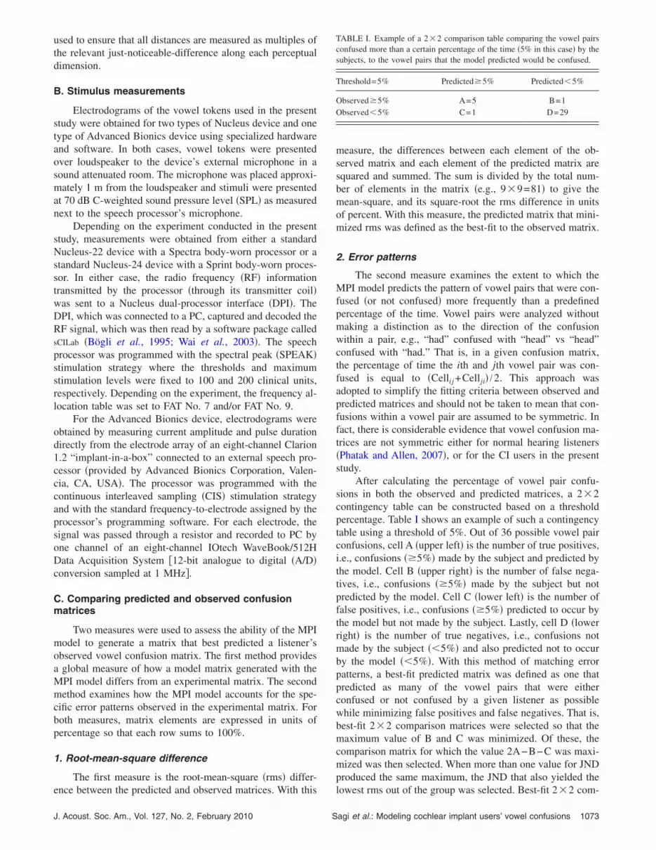
After calculating the percentage of vowel pair confu-sions in both the observed and predicted matrices, a 2�2contingency table can be constructed based on a thresholdpercentage. Table I shows an example of such a contingencytable using a threshold of 5%. Out of 36 possible vowel pairconfusions, cell A �upper left� is the number of true positives,i.e., confusions ��5%� made by the subject and predicted bythe model. Cell B �upper right� is the number of false nega-tives, i.e., confusions ��5%� made by the subject but notpredicted by the model. Cell C �lower left� is the number offalse positives, i.e., confusions ��5%� predicted to occur bythe model but not made by the subject. Lastly, cell D �lowerright� is the number of true negatives, i.e., confusions notmade by the subject ��5%� and also predicted not to occurby the model ��5%�. With this method of matching errorpatterns, a best-fit predicted matrix was defined as one thatpredicted as many of the vowel pairs that were eitherconfused or not confused by a given listener as possiblewhile minimizing false positives and false negatives. That is,best-fit 2�2 comparison matrices were selected so that themaximum value of B and C was minimized. Of these, thecomparison matrix for which the value 2A−B−C was maxi-mized was then selected. When more than one value for JNDproduced the same maximum, the JND that also yielded the

TABLE I. Example of a 2�2 comparison table comparing the vowel pairsconfused more than a certain percentage of the time �5% in this case� by thesubjects, to the vowel pairs that the model predicted would be confused.

Threshold=5% Predicted�5% Predicted�5%

Observed�5% A=5 B=1Observed�5% C=1 D=29

lowest rms out of the group was selected. Best-fit 2�2 com-


parison matrices were obtained at three values for threshold:3%, 5%, and 10%. Different thresholds were necessary toassess errors made by subjects with very different perfor-mance levels. A best-fit 2�2 comparison matrix was labeled“satisfactory” if both A and D were greater than �or at leastequal to� B and C. According to this definition a satisfactorycomparison matrix is one where the model was able to pre-dict at least one-half of the vowel pairs confused by an indi-vidual listener, and do so with a number of false positives nogreater than the number of true positives �vowel pairs accu-rately predicted to be confused by the individual�.

III. EXPERIMENT 1: VOWEL IDENTIFICATION

A. Methods

1. CI listeners

Twenty-five postlingually deafened adult users of CIswere recruited for this study. Participants were compensatedfor their time and provided informed consent. All partici-pants were over 18 years of age at the time of testing, and themean age at implantation was 50 years ranging from 16 to 75years. Participants were profoundly deaf �PTA�90 dB� andhad at least 1 year of experience with their implant beforetesting, with the exception of N17 who had 11 months ofpost-implant experience when tested. The demographics for

TABLE II. Demographics of CI users tested for this study: 7 users of theAdvanced Bionics device �C� and 18 users of the Nucleus device �N�. Age atimplantation and experience with implant are stated in years. Speech pro-cessing strategies are CIS, ACE �Advanced Combination Encoder�, andSPEAK.

SubjectImplanted

ageImplant

experienceImplanted

device Strategy

No.of

channels

C1 66 3.4 Clarion 1.2 CIS 8C2 32 3.4 Clarion 1.2 CIS 8C3 61 5.9 Clarion 1.2 CIS 8C4 23 5.5 Clarion 1.2 CIS 8C5 53 6.1 Clarion 1.2 CIS 5C6 39 2.7 Clarion 1.2 CIS 6C7 43 2.2 Clarion 1.2 CIS 8N1 31 5.2 Nucleus CI22M SPEAK 18N2 59 11.2 Nucleus CI22M SPEAK 13N3 71 3 Nucleus CI22M SPEAK 14N4 67 2.9 Nucleus CI22M SPEAK 19N5 45 3.9 Nucleus CI22M SPEAK 20N6 48 9.1 Nucleus CI22M SPEAK 16N7 16 4.6 Nucleus CI22M SPEAK 18N8 66 2.3 Nucleus CI22M SPEAK 18N9 48 1.7 Nucleus CI24M ACE 20N10 42 2.3 Nucleus CI24M SPEAK 16N11 44 3.1 Nucleus CI24M SPEAK 20N12 75 1.7 Nucleus CI24M SPEAK 19N13 65 2.2 Nucleus CI24M SPEAK 20N14 53 1.9 Nucleus CI24M SPEAK 20N15 45 4.2 Nucleus CI24M SPEAK 20N16 45 3.2 Nucleus CI24M SPEAK 20N17 37 0.9 Nucleus CI24M SPEAK 20N18 68 1.2 Nucleus CI24M SPEAK 20

this group at time of testing are presented in Table II, includ-


ing age at implantation, duration of post-implant experience,type of CI device and speech processing strategy, as well asnumber of active channels.

2. Stimuli and general procedures

Vowel stimuli consisted of nine vowels in /hVd/context,i.e., heed, hawed, heard, hood, who’d, hid, hud, had, andhead. Stimuli included three tokens of each vowel recordedfrom the same male speaker. Vowel tokens would be pre-sented over loudspeaker to CI subjects seated 1 m away in asound attenuated room. The speaker was calibrated beforeeach experimental session so that stimuli would register avalue of 70 dB C-weighted SPL on a sound level meterplaced at the approximate location of a user’s ear-level mi-crophone. In a given session listeners would be presentedwith one to three lists of the same 45 stimuli �i.e., up to 135presentations� where each list comprised a different random-ization of presentation order. In each list, two tokens of eachvowel were presented twice and one token was presentedonce. Before the testing session, listeners were presentedwith each vowel token at least once knowing in advance thevowel to be presented for practice. During the testing ses-sion, no feedback was provided. All three lists were pre-sented on the same day, and a listener was allowed a breakbetween lists if required.

3. Application of the MPI model

Step 1. All seven possible combinations of one, two, orthree dimensions consisting of mean locations of formantenergies F1, F2, and F3 along the electrode array weretested.

Step 2. Mean locations of formant energies along theelectrode array were obtained from electrodograms of eachvowel token that was presented to CI subjects. A set of for-mant location measurements was obtained for each CI lis-tener. Obtaining these measurements directly from each sub-ject’s external device would have been optimal, but timeconsuming. Instead, four generic sets of formant locationmeasurements were obtained. One set was obtained for theNucleus-24 spectra body-worn processor with the SPEAKstimulation strategy using FAT No. 9, and three sets wereobtained for the Clarion 1.2 processor with the CIS stimula-tion strategy using the standard FAT imposed by the device’sfitting software. The three sets of formant locations forClarion users were obtained with the speech processor pro-grammed using eight, six, and five channels. One Clarionsubject had five active channels in his FAT, another one hadsix channels, and the remaining five had all eight channelsactivated. Two out of 18 of the Nucleus subjects and 4 out of7 of the Clarion subjects used these standard FATs, whereasthe other subjects used other FATs with slight modifications.For example, a Nucleus subject may have used FAT No. 7instead of FAT No. 9, or one or more electrodes may havebeen turned off, or a Clarion subject may have used extendedfrequency boundaries for the lowest or the highest frequencychannels. For these other subjects, each generic set of for-mant location measurements that we obtained was then
modified to generate a unique set of measurements. Using

linear interpolation, the generic data set was first transformedinto hertz using the generic set’s frequency allocation tableand then transformed back into millimeters from the mostbasal electrode using the frequency allocation table that wasprogrammed into a given subject’s speech processor at thetime of testing. This method provided a unique set of for-mant location measurements even for those subjects with oneor more electrodes shut off, typically to avoid facial twitchand/or dizziness.

Step 3. Using a CI listener’s set of formant location mea-surements for a given perceptual dimension combination,MPI model-predicted matrices were generated while JNDwas varied using one degree of freedom from 0.03 to 6 mmin steps of 0.005 mm �i.e., a total of 1195 predicted matri-ces�. The lower bound of 0.03 mm was selected as it repre-sents a reasonable estimate of the lowest JND for place ofstimulation in the cochlea achievable with present day CIdevices �Firszt et al., 2007; Kwon and van den Honert,2006�. Each predicted matrix �one for each value of JND�consisted of 5 000 iterations per vowel token, i.e., 225 000entries in total. Predicted matrices were compared with thelistener’s observed vowel confusion matrix to obtain the JNDthat provided the best-fit between predicted matrices and theCI listener’s observed vowel matrix. A best-fit JND valueand predicted matrix was obtained for each CI listener, foreach of the seven perceptual dimension combinations, bothin terms of the lowest rms difference and in terms of the best2�2 comparison matrix using thresholds of 3%, 5%, and10%. The combination of perceptual dimensions that pro-vided the best-fit to the data was then examined, both fromthe point of view of rms difference and of error patterns.

B. Results

Vowel identification percent correct scores for the CIlisteners tested in the present study are listed in the secondcolumn of Table III. The scores ranged from near chance tonear perfect.

1. rms differences between observed and predictedmatrices

Also listed in Table III are the minimum rms differencesbetween predicted and observed matrices as a function ofseven possible perceptual dimension combinations. The per-ceptual dimension combination that produced the lowestminimum rms is highlighted in bold, and rms values greaterthan 1% above the lowest minimum rms have been omitted.As one can observe, the perceptual dimension combinationthat produced the lowest minimum rms was F1F2F3 for 15out of 25 listeners. For eight of the remaining ten listeners,the F1F2F3 perceptual dimension combination provided a fitthat was not the best, but was within 1% of the best-fit. Ofthese remaining ten listeners, six were best fitted by the F1F2combination, three by the F2 combination, and one by theF1F3 combination.

The third column of Table III contains the rms differ-ence between each listener’s observed vowel confusion ma-trix and a purely random matrix, i.e., one where all matrix
elements are equal. Any good model should yield a rms dif-

ference that is much smaller than the values that appear inthis column. Indeed, this is true for 20 out of 25 CI users forwhich the lowest minimum rms values achieved with theMPI model �highlighted in bold� are at least 10% lower thanthose for a purely random matrix �i.e., third column of TableIII�. The remaining five CI users �C5, C6, N2, N8, and N12�had the lowest vowel identification scores in the group �be-tween 21% and 44% correct�. For these subjects, the MPImodel does not do much better than a purely random matrix,especially for the three subjects whose scores were onlyabout twice chance levels.

A repeated measures analysis of variance �ANOVA� onranks was conducted on the rms values we obtained for allsubjects. Perceptual dimension combinations, as well as therandom matrix comparison, were considered as differenttreatment groups applied to the same CI subjects. A signifi-cant difference was found across treatment groups �p�0.001�. Using the Student–Newman–Keuls method formultiple post-hoc comparisons, the following significant

TABLE III. Minimum rms difference between CI users’ observed and pre-dicted vowel confusion matrices for seven perceptual dimension combina-tions comprising F1, F2, and/or F3. The lowest rms values across perceptualdimensions are highlighted in bold and only values within 1% of this mini-mum were reported. The second and third columns list observed vowelpercent correct and the rms difference between observed matrices and apurely random matrix.

CIUser

Vowel�%�

rms

Random F1F2F3 F1F2 F1F3 F2F3 F1 F2 F3

C1 72.6 25.2 9.9 10.0 ¯ 10.1 ¯ ¯ ¯

C2 98.5 31.0 5.2 5.4 ¯ 16.0 ¯ ¯ ¯

C3 94.1 29.7 6.3 6.7 ¯ ¯ ¯ ¯ ¯

C4 80.0 26.3 9.1 9.5 ¯ ¯ ¯ ¯ ¯

C5 21.5 11.0 14.9 15.0 14.5 ¯ ¯ ¯ 15.5C6 43.7 16.5 10.8 11.1 11.4 ¯ ¯ ¯ ¯

C7 83.7 27.0 6.0 6.1 ¯ ¯ ¯ ¯ ¯

N1 80.0 28.2 14.9 15.3 ¯ 15.7 ¯ ¯ ¯

N2 22.2 11.5 ¯ 13.8 ¯ ¯ ¯ 14.1 14.7N3 73.3 24.6 8.0 ¯ ¯ 8.1 ¯ ¯ ¯

N4 70.4 26.7 13.3 ¯ ¯ 13.3 ¯ 12.7 ¯

N5 95.6 30.0 5.4 4.4 ¯ ¯ ¯ ¯ ¯

N6 81.7 27.2 11.4 12.0 ¯ 12.4 ¯ ¯ ¯

N7 72.6 23.5 ¯ 10.4 ¯ ¯ ¯ ¯ ¯

N8 26.1 11.6 11.9 11.6 ¯ 12.2 ¯ 12.4 ¯

N9 80.0 26.7 9.0 ¯ ¯ ¯ ¯ ¯ ¯

N10 81.5 26.3 10.7 10.1 ¯ ¯ ¯ ¯ ¯

N11 85.0 27.9 10.2 ¯ ¯ ¯ ¯ ¯ ¯

N12 42.2 16.4 11.9 12.7 ¯ 12.1 ¯ 12.5 ¯

N13 79.3 25.4 8.4 9.2 ¯ ¯ ¯ ¯ ¯

N14 81.5 26.9 10.0 ¯ ¯ ¯ ¯ ¯ ¯

N15 91.1 29.5 9.7 9.2 ¯ ¯ ¯ ¯ ¯

N16 59.3 24.7 15.3 ¯ ¯ 15.8 ¯ 14.8 ¯

N17 71.1 24.3 10.2 ¯ ¯ ¯ ¯ 9.8 ¯

N18 66.7 24.2 12.1 ¯ ¯ 13.0 ¯ ¯ ¯

Mean 70.1 24.1 10.5 11.1 14.9 12.7 17.7 13.7 19.7No. of

best rms15 6 1 0 0 3 0

group differences were found at p�0.01: F1F2F3 rms


�F1F2 rms�F2F3 rms�F2 rms�F1F3 rms�F1, F3 andrandom rms. No significant differences were found betweenF1, F3, and the random case.

2. Prediction of error patterns

Table IV shows the extent to which the MPI model canfit the patterns of vowel confusions made by individual CIusers. The table lists one example of a best 2�2 comparisonmatrix for each subject. At the bottom of Table IV is a keythat identifies where to find for each comparison matrix thesubject identifier, the perceptual dimension from which thebest comparison matrix was selected, the threshold �3%, 5%,or 10%�, the p-value obtained from a Fisher exact test, andelements A–D of the comparison matrix as outlined in TableI of Sec. II. The following criteria were used for selecting thematrices listed in Table IV: �1� a satisfactory 2�2 compari-son matrix with F1F2F3 at the 5% threshold, �2� a satisfac-tory matrix with F1F2F3 at any threshold, and �3� a satisfac-tory matrix at any perceptual dimension. Under thesecriteria, satisfactory matrices were obtained for 24 out of 25subjects. The only exception was subject C2 who confusedvery few vowel pairs and for whom a satisfactory compari-son matrix could not be obtained. On the lower right of TableIV is an average of elements A–D for all 25 exemplars listedin Table IV. On average, the MPI model predicted the pattern

TABLE IV. Best 2�2 comparison matrices between observed vowel confucomparison matrices is on bottom: dim=perceptual dimension combinatio=result of Fisher exact test; A, B, C, and D, as in Table I. Bottom right, av

C1 F1F2F3 C2 F1F2F3 C35% �0.001 5% 1.00 10%7 0 0 0 31 28 2 34 3

C6 F1F2F3 C7 F1F2F3 N15% 0.002 5% 0.013 10%12 3 3 2 25 16 2 29 2

N4 F1F2F3 N5 F1F2 N65% �0.001 3% 0.005 10%4 2 4 1 20 30 4 27 2

N9 F1F2F3 N10 F1F2F3 N115% 0.010 3% 0.024 10%3 1 5 5 23 29 3 23 2

N14 F1F2F3 N15 F1F2F3 N1610% 0.027 10% 0.010 5%

2 1 2 0 52 31 2 32 4

KSubject

thrAC

of vowel confusions in 31 out of 36 possible vowel pair


confusions. As for the Fisher exact tests, the comparison ma-trices in Table IV were significant at p�0.05 for 24 out of25 subjects �again subject C2 was the exception�, half ofwhich were significant at p�0.01.

Table V shows the number of satisfactory best-fit 2�2comparison matrices obtained for each listener at each per-ceptual dimension combination. As comparison matriceswere obtained at thresholds of 3%, 5%, and 10%, the maxi-mum number of satisfactory comparison matrices at eachperceptual dimension combination is 3. The bottom row ofTable V lists the total number of satisfactory comparisonmatrices at each perceptual dimension combination. As onecan observe, the F1F2F3 combination produced the largestnumber of satisfactory best-fit 2�2 comparison matrices,corroborating the result obtained with the best-fit rms crite-ria.

C. Discussion

It is not surprising that a model based on the ability todiscriminate formant center frequencies can explain at leastsome aspects of vowel identification. Rather, what is novelabout the results of the present study is that the MPI modelproduced confusion matrices that closely matched CI users’vowel confusion matrices, including the general pattern oferrors between vowels, despite differences in age at implan-

matrices from CI users and those predicted from MPI model. Key for bestr=threshold at which best comparison matrix was obtained, and p-valuebest 2�2 comparison matrix.

F2F3 C4 F1F2F3 C5 F1F2F3.024 5% 0.003 5% 0.026

2 4 2 23 428 2 28 4 5

F2 N2 F1F2F3 N3 F1F2F3.027 10% 0.015 5% 0.003

1 11 7 4 231 3 15 2 28

2F3 N7 F1F2F3 N8 F1F2F3.027 10% 0.013 5% 0.041

1 3 2 16 531 2 29 6 9

F2F3 N12 F1F2F3 N13 F1F2F3.010 5% �0.001 5% 0.030

0 14 4 4 432 2 16 3 25

F2F3 N17 F1F2F3 N18 F1F2F3.026 3% 0.002 5% 0.003

4 11 4 9 423 4 17 4 19

imvalue AverageB 6.20 2.44D 2.76 24.60

sionn, therage

F10

0

F0

F10

F10

eyD

p-

tation, implant experience, device and simulation strategy


used �Table II�, as well as overall vowel identification level�Table III�. It is important to stress that these results wereachieved with only one degree of freedom. The ability todemonstrate how a model accounts for experimental data isstrengthened when the model can capture the general trendof the data while using fewer instead of more degrees offreedom �Pitt and Navarro, 2005�. With one degree of free-dom, when a model with F1F2F3 does better than a modelwith F1F2, or when a model with F1F2 does better than amodel with F2 alone, one can interpret the value of an addedperceptual dimension without having to account for the pos-sibility that the improvement was due to an added fittingparameter.

Whether in terms of rms differences �Table III� or pre-diction of error patterns �Table V� it is clear that F1F2F3 wasthe most successful formant combination in accounting forCI users’ vowel identification. Upon inspection of the otherformant dimension combinations, both Tables III and V sug-gest that models that included the F2 dimension tended to dobetter than models without F2, and Table III suggests that theF1F2 combination was a close second to the F1F2F3 combi-nation. The implication may be that F2, and perhaps F1, areimportant for identifying vowels in most listeners, whereasF3 may be an important cue for some implanted listeners,particularly for r-colored vowels such as heard, but perhapsnot for others �Skinner et al., 1996�.

The model was able to explain most of the confusions

TABLE V. Number of “satisfactory” 2�2 comparison matrices at thresh-olds of 3%, 5%, and 10% for each perceptual dimension.

Subject F1F2F3 F1F2 F1F3 F2F3 F1 F2 F3

C1 3 3 0 3 0 3 0C2 0 0 0 0 0 0 0C3 1 0 0 0 0 0 0C4 2 2 0 2 0 2 0C5 1 1 1 0 1 0 0C6 3 3 3 3 3 3 0C7 3 2 0 1 0 1 0N1 0 0 0 0 0 1 0N2 2 3 1 3 1 3 2N3 2 2 0 2 0 2 0N4 3 3 0 3 0 3 0N5 0 1 0 0 0 0 0N6 0 0 0 1 0 0 0N7 2 3 0 2 0 3 0N8 2 1 1 2 1 2 0N9 3 0 0 2 0 1 0N10 1 2 0 1 0 2 0N11 1 0 0 1 0 0 0N12 3 3 3 3 3 3 3N13 2 2 0 2 0 2 0N14 2 0 0 1 0 0 0N15 1 0 0 1 0 0 0N16 3 3 0 2 0 3 0N17 1 3 1 2 0 3 1N18 3 2 2 3 0 3 0

Total 44 39 12 40 9 40 6

made by most of the individual listeners, while making few


false positive predictions. This is an important result becauseone degree of freedom is always sufficient to fit one inde-pendent variable, such as percent correct, but it is not suffi-cient to predict a data set that includes 36 pairs of vowels. Itshould come as no surprise that percent correct scores in apredicted vowel matrix drop as the JND parameter is in-creased. Any model that employs a parameter to move dataaway from the main diagonal would accomplish the sameresult. However, the MPI model succeeds in the sense thatincreasing the JND moves data away from the main diagonaltoward a specific vowel confusion pattern determined by theset of perceptual dimensions proposed. Although the fit be-tween predicted and observed data was not perfect, it wasstrong enough to suggest that the proposed model capturessome of the mechanisms CI users employ to identify vowels.

IV. EXPERIMENT 2: F1 IDENTIFICATION

A. Methods

One of the premises underlying the MPI model of vowelidentification by CI users in the present study is that a rela-tionship exists between these listeners’ ability to identifyvowels and their ability to identify steady-state formant fre-quencies. To test this premise, 18 of the 25 CI users testedfor our vowel identification task were also tested for first-formant �F1� identification.

1. Stimuli and general procedures

The testing conditions for this experiment were the sameas for the vowel identification experiment in Sec. III A 2,differing only in the type and number of stimuli to identify.For F1 identification, stimuli were seven synthetic three-formant steady-state vowels created with the Klatt 88 speechsynthesizer �Klatt and Klatt, 1990�. The synthetic vowels dif-fered from each other only in steady-state first-formant cen-ter frequencies, which ranged between 250 and 850 Hz inincrements of 100 Hz. The fundamental, second, and thirdformant frequencies were fixed at 100, 1500, and 2500 Hz,respectively. Steady-state F1 values were verified with anacoustic waveform editor. The spectral envelope was ob-tained from the middle portion of each stimulus, and thefrequency value of the F1 spectral peak was confirmed. Eachstimulus was 1 s in duration and the onset and offset of thevowel envelope occurred over a 10 ms interval, this transi-tion being linear in dB. The stimuli were digitally storedusing a sampling rate of 11 025 Hz at 16 bits of resolution.Listeners were tested using a seven-alternative, one intervalforced choice absolute identification task. During each blockof testing stimuli were presented ten times in random order�i.e., 70 presentations per block�. Prior to testing, participantswould familiarize themselves with each stimulus �numbered1–7� using an interactive software interface. During testing,participants would cue the interface to play a stimulus andthen select the most appropriate stimulus number. After eachselection, feedback about the correct response was displayedon the computer monitor before moving on to the next stimu-lus. Subjects completed seven to ten testing blocks �with theexception of listeners N6 and N7 who completed six and fivetesting blocks, respectively�. This number of testing blocks
was chosen as it was typically sufficient for most listeners to

provide at least two runs representative of asymptotic, orbest, performance.

2. Cumulative-d� „��… analysis

For each block of testing a sensitivity index d� �Durlachand Braida, 1969� was calculated for each pair of adjacentstimuli �1 vs 2, 2 vs 3, …, 6 vs 7� and then summed to obtainthe total sensitivity, i.e., ��, which is the cumulative-d�across the range of first-formant frequencies between 250and 850 Hz �i.e., from stimuli 1 to 7�. For a given pair ofadjacent stimuli, d� was calculated by subtracting the meanresponses for the two stimuli and dividing by the averagestandard deviation of the responses to the two stimuli. Foreach CI user, the two highest �� among all testing blockswere averaged to arrive at the final score for this task. Theaverage of the highest two �� scores represents an estimateof asymptotic performance, i.e., failure to improve ��.Asymptotic performance was sought as it provides a measureof sensory discrimination performance after factoring inlearning effects and factoring out fatigue. As is customary for�� calculations, any d� score greater than 3 was set to d�=3 �Tong and Clark, 1985�. We defined the JND as occurringat d�=1, so that �� equals the number of JNDs across therange of first-formant frequencies between 250 and 850 Hz.We then divided this range �i.e., 600 Hz� by �� to obtain theaverage JND in Hz.

To test the premise that a relationship exists between CIlisteners’ ability to identify vowels and their ability to dis-criminate steady-state formant frequencies, two correlationanalyses were made using the average JNDs �in hertz� mea-sured in the F1 identification task. One comparison was be-tween JNDs �in hertz� and vowel identification percent cor-rect scores. The other comparison was between JNDs �inhertz� and the F1F2F3 MPI model input JNDs �in millime-ters� that yielded best-fit predicted matrices in terms of low-est rms difference.

B. Results

Listed in Table VI are CI subjects’ observed percent cor-rect scores for vowel identification and observed averageJNDs �in hertz� for first-formant identification �F1 ID�. Alsolisted in Table VI are CI subjects’ predicted vowel identifi-cation percent correct and input JNDs �in millimeters� thatprovided best-fit model matrices using the F1F2F3 MPImodel. Comparing the observed scores, a scatter plot ofvowel scores and JNDs for the 18 CI users tested on bothtasks �Fig. 3, top panel� yields a correlation of r=−0.654�p=0.003�. This result suggests that in our group of CI users,the ability to correctly identify vowels was significantly cor-related with the ability to identify first-formant frequency.Furthermore, for the same 18 CI users, a scatter plot of theMPI model input JNDs in millimeters against the observedJNDs in hertz from F1 identification �Fig. 3, bottom panel�yields a correlation of r=0.635, p=0.005 �without the datapoint with the highest predicted JND in millimeters, r=0.576 and p=0.016�. Hence, a significant correlation existsbetween the JNDs obtained from first-formant identificationand the JNDs obtained indirectly by optimizing model ma-
trices to fit the vowel identification matrices obtained from

the same listeners. That is, fitting the MPI model to one dataset �vowel identification� produced JNDs that are consistentwith JNDs obtained with the same listeners from a com-pletely independent data set �F1 identification�.

C. Discussion

The significant correlations in Fig. 3 lend support to thehypothesis that CI users’ ability to discriminate the locationsof steady-state mean formant energies along the electrodearray contributes to vowel identification, and also provides adegree of validation for the manner in which the MPI modelof the present study connects these two variables. Neverthe-less, the correlations were not very large, accounting for ap-proximately 40% of the variability observed in the scatterplots. One important difference between identification ofvowels and identification of formant center frequencies isthat the former involves the assignment of lexically mean-ingful labels stored in long-term memory whereas the latterdoes not. Hence, if a CI user has very good formant centerfrequency discrimination, their ability to identify vowelscould still be poor if their vowel labels are not sufficientlyresolved in long-term memory. That is, good formant centerfrequency discrimination is necessary but not sufficient forgood vowel identification.

As a side note, the observed JNDs in Table VI were

TABLE VI. Observed percent correct scores for vowel identification andaverage JNDs �in hertz� for first-formant identification, and F1F2F3 MPImodel-predicted vowel percent correct scores and input JNDs that mini-mized rms difference between predicted and observed vowel confusion ma-trices for CI users tested in this study �NA=not available�.

Subject

Observed Predicted �F1F2F3�

Vowel�%�

JND�Hz�

Vowel�%�

JND�mm�

C1 72.6 279 72.6 0.095C2 98.5 144 91.6 0.040C3 94.1 138 89.5 0.040C4 80.0 NA 77.8 0.080C5 21.5 359 24.1 0.685C6 43.7 111 45.9 0.125C7 83.7 88 84.9 0.060N1 80.0 NA 70.9 0.280N2 22.2 NA 28.8 1.575N3 73.3 141 71.6 0.230N4 70.4 247 70.6 0.280N5 95.6 NA 91.8 0.070N6 81.7 131 75.5 0.225N7 72.6 123 80.7 0.150N8 26.1 324 29.0 1.725N9 80.0 NA 76.9 0.270N10 81.5 NA 72.6 0.175N11 85.0 159 80.8 0.220N12 42.2 224 45.8 0.820N13 79.3 116 80.4 0.225N14 81.5 138 79.4 0.235N15 91.1 NA 87.3 0.140N16 59.3 185 52.8 0.645N17 71.1 141 72.7 0.315N18 66.7 311 64.1 0.430

larger than those reported by Fitzgerald et al. �2007�.


However, this is to be expected as their F1 discriminationtask measured the JND above an F1 center frequency of 250Hz, whereas our measure represented the average JND for F1center frequencies between 250 and 850 Hz.

V. EXPERIMENT 3: FREQUENCY ALLOCATIONTABLES

A. Methods

Skinner et al. �1995� examined the effect of FAT Nos. 7and 9 on speech perception with seven postlingually deaf-ened adult users of the Nucleus-22 device and SPEAKstimulation strategy. Although FAT No. 9 was the defaultclinical map, Skinner et al. �1995� found that their listeners’speech perception improved with FAT No. 7. The speechbattery they used included a vowel identification task with 19medial vowels in /hVd/context, 3 tokens each, comprising 9pure vowels, 5 r-colored vowels, and 5 diphthongs. Thevowel confusion matrices they obtained �and recordings ofthe stimuli they used� were provided to us for the presentstudy.

1. Application of MPI model

The MPI model was applied to the vowel identificationdata of Skinner et al. �1995� in order to test the model’sability to explain the improvement in performance that oc-

FIG. 3. Top panel: scatter plot of vowel identification percent correct scoresagainst observed JND �in hertz� from first-formant identification obtainedfrom 18 CI users �r=−0.654, p=0.003�. Bottom panel: scatter plot ofF1F2F3 MPI model’s input JNDs �in millimeters� that produced best-fit tosubjects’ observed vowel matrices �minimized rms� against these subjects’observed JND �in hertz� from first-formant identification �r=0.635 and p=0.005�.

curred when listener’s used FAT No. 7 instead of FAT No. 9.


As a demonstration of how the MPI model can be used toexplore the vast number of possible settings for a given CIfitting parameter in a very short amount of time, the MPImodel was also used to provide a projection of vowel percentcorrect scores as a function of ten different frequency allo-cation tables and JND.

Step 1. One perceptual dimension combination was usedto model the data of Skinner et al. �1995� and to generatepredictions at other FATs. Namely, mean locations of for-mant energies along the electrode array for the first threeformants combined, i.e., F1F2F3, in units of millimetersfrom the most basal electrode.

Step 2. Because our MPI model predicts identification ofand confusions among vowels based on CI users’ discrimi-nation of mean formant energy locations, only ten of thevowels used by Skinner et al. �1995� were used in ourmodel; i.e., the nine purely monophthongal vowels and ther-colored vowel heard. Using the original vowel recordingsused by Skinner et al. �1995� and sCILab software �Bögliet al., 1995; Wai et al., 2003�, two sets of formant locationmeasurements were obtained from a Nucleus-22 spectrabody-worn processor programmed with the SPEAK stimula-tion strategy. One set of measurements was obtained whilethe processor was programmed with FAT No. 7, and theother while the processor was programmed with FAT No. 9.Both sets of measurements were used for fitting Skinneret al.’s �1995� data, and for the MPI model’s projection ofvowel percent correct as a function of JND. For the model’sprojection at other FATs, formant location measurementswere obtained using linear interpolation from FAT No. 9. Theother frequency allocation tables explored in this projectionwere FAT Nos. 1, 2, and 6–13.

Step 3. For Skinner et al.’s �1995� data, the MPI modelwas run while allowing JND to vary as a free parameter untilmodel matrices were obtained that best-fit the observedgroup vowel confusion matrices at FAT Nos. 7 and 9. TheJND parameter was varied from 0.1 to 1 mm of electrodedistance in increments of 0.01 mm using one degree of free-dom; i.e., JND was the same for each perceptual dimension.Only one value of JND was used to find a best-fit to both setsof observed matrices in terms of minimum rms combined forboth matrices. For the MPI model’s projection of vowelidentification as a function of the various FATs, model ma-trices were obtained for JND values of 0.1, 0.2, 0.4, 0.8, and1.0 mm of electrode distance, where JND was assumed to bethe same for each perceptual dimension. Percent correctscores were then calculated from the resulting model matri-ces. In all of the above simulations, the MPI model was runusing 5000 iterations per vowel token.

B. Results

1. Application of MPI model to Skinner et al. „1995…

For the ten vowels we included in our modeling, theaverage vowel identification percent correct scores for thegroup of listeners tested by Skinner et al. �1995� were 84.9%with FAT No. 7 and 77.5% with FAT No. 9. For the MPImodel of Skinner et al.’s �1995� data, a JND of 0.24 mmproduced best-fit model matrices. The rms differences be-
tween observed and predicted matrices were 4.3% for FAT

No. 7 and 6.2% for FAT No. 9. The predicted matrices hadpercent correct scores equal to 85.1% with FAT No. 7 and79.4% with FAT No. 9. Thus, the model predicted that FATNo. 7 should result in better vowel identification �which wastrue for all JND values between 0.1 and 1 mm� and it alsopredicted the size of the improvement. The 2�2 comparisonmatrices that demonstrate the extent to which model matricesaccount for the error pattern in Skinner et al.’s �1995� matri-ces are presented in Table VII. The comparison matriceswere compiled using a threshold of 3%. With one degree offreedom, the MPI model produced model matrices that ac-count for 40 out of 45 vowel pair confusions in the case ofFAT No. 7 and 39 out of 45 vowel pair confusions in the caseof FAT No. 9. For both comparison matrices, a Fisher’s exacttest yields p�0.001.

TABLE VII. 2�2 comparison matrices for MPI model matrices producedwith JND=0.24 mm and Skinner et al.’s �1995� vowel matrices obtainedwith FAT Nos. 7 and 9. The data follow the key at the bottom of Table IV.

FAT No. 7 F1F2F3 FAT No. 9 F1F2F33% p�0.001 3% p�0.0016 3 6 52 34 1 33

TABLE VIII. Frequency allocation table numbers �FAT No.� 1, 2, and 6–stimulated electrode and indicate the lower frequency boundary �in hertz� ashighest frequency channel. Approximate range of formant frequency regio�2000–3000 Hz�.

Channel 1 2 6 7 8

1 75 80 109 120 13

2 175 186 254 280 31

3 275 293 400 440 48

4 375 400 545 600 66

5 475 506 690 760 84

6 575 613 836 920 10

7 675 720 981 1080 12

8 775 826 1127 1240 13

9 884 942 1285 1414 15

10 1015 1083 1477 1624 18

11 1166 1244 1696 1866 20

12 1340 1429 1949 2144 23

13 1539 1642 2239 2463 27

14 1785 1904 2597 2856 31

15 2092 2231 3042 3347 3716 2451 2614 3565 3922 43

17 2872 3063 4177 4595 51

18 3365 3589 4894 5384 5919 3942 4205 5734 6308 7020 4619 4926 6718 7390 82

Upper 5411 5772 7871 8658 96


2. MPI model projection at various FATs

The FAT determines the frequency band assigned to agiven electrode. The ten FATs used to produce MPI modelprojections of vowel percent correct scores are summarizedin Table VIII, which depicts the FAT number �1, 2, and6–13�, channel number �starting from the most apicallystimulating electrode�, and the lower frequency boundary �inhertz� assigned to a given channel �the upper frequencyboundary for a given channel is equal to the lower frequencyboundary of the next highest channel number, and the upperboundary for the highest channel number is provided in thebottom row�. The percent correct scores obtained from MPImodel matrices at each FAT, and as a function of JND aresummarized in Fig. 4. Two observations are worth noting.First, a lower JND for a given frequency map results in ahigher predicted percent correct score. That is, a lower JNDwould provide better discrimination between formant valuesand hence a smaller chance of confusing formant values be-longing to different vowels. Second, for a fixed JND, percentcorrect scores begin to gradually decrease as the FAT numberis increased to higher FAT numbers beyond FAT No. 7, withthe exception of JND=0.1 mm where a ceiling effect isobserved. As FAT number increases from No. 1 to No. 9,a larger frequency range is assigned to the same set of

or the Nucleus-22 device. Channel numbers begin with the most apicallyd to a given electrode. Bottom row indicates upper frequency boundary fordicated by text in bold: F1 �300–1000 Hz�, F2 �1000–2000 Hz�, and F3

FAT No.

9 10 11 12 13

150 171 200 240 150

350 400 466 560 300

550 628 733 880 700

750 857 1 000 1 200 1100

950 1 085 1 266 1 520 1500

1 150 1 314 1 533 1 840 1900

1 350 1 542 1 800 2 160 2300

1 550 1 771 2 066 2 480 2700

1 768 2 020 2 357 2 828 3100

2 031 2 321 2 708 3 249 3536

2 333 2 666 3 110 3 732 4062

2 680 3 062 3 573 4 288 4666

3 079 3 518 4 105 4 926 5360

3 571 4 081 4 761 5 713 6158

4 184 4 781 5 578 6 694 71424 903 5 603 6 537 7 844 8368

5 744 6 564 7 658 9 190 ¯

6 730 7 691 8 973 ¯ ¯

7 885 9 011 ¯ ¯ ¯

9 238 ¯ ¯ ¯ ¯

10 823 10 557 10 513 10 768 9806

13 fsignens in

3

1

8

6

4

22

00

77

71

05

73

82

36

74

1958

05

820811

20


electrodes. For FAT Nos. 10–13, the relatively large fre-quency span is maintained while the number of electrodesassigned is gradually reduced. Hence, the MPI model pre-dicts that vowel identification will be deleteriously affectedby assigning too large of a frequency span to the CI elec-trodes. In Fig. 4, the two filled circles joined by a solid linerepresent the vowel identification percent correct scores ob-tained by Skinner et al. �1995� for the ten vowel tokens weincluded in our modeling.

C. Discussion

The very first thing to point out is the economy withwhich the MPI model can be used to project estimates of CIusers’ performance. The simulation routine implementing theMPI model produced all of the outputs in Fig. 4 in a matterof minutes. Contrast this with the time and resources re-quired to obtain data such as that of Skinner et al. �1995�,which amounts to two data points in Fig. 4. It would befinancially and practically impossible to obtain these dataexperimentally for all the frequency maps available with agiven cochlear implant, let alone for the theoretically infinitenumber of possible frequency maps.

Without altering any model assumptions, the model pre-dicts the increase in percent correct vowel identification at-tributable to changing the frequency map from FAT No. 9 toFAT No. 7 with the Nucleus-22 device. In retrospect, Skinneret al. �1995� hypothesized that FAT No. 7 might result inimproved speech perception because it encodes a more re-stricted frequency range onto the electrodes of the implantedarray. Encoding a larger frequency range onto the array in-volves a tradeoff: The locations of mean formant energiesfor different vowels are squeezed closer together. With lessspace between mean formant energies, the vowels becomemore difficult to discriminate, at least in terms of this par-ticular set of perceptual dimensions, resulting in a lower per-cent correct score.

How does this concept apply to the MPI model projec-tions at different FATs displayed in Fig. 4? The effect ofdifferent FAT frequency ranges on mean formant locationsalong the electrode array is depicted in Table VIII whereapproximate formant regions are indicated in bold. The fre-quency boundaries defined for each formant are 300–1000

FIG. 4. F1F2F3 MPI model prediction of vowel identification percent cor-rect scores as a function of FAT No. and JND �in millimeters�. Filled circles:Skinner et al.’s �1995� mean group data when CI subjects’ used FAT Nos. 7and 9.

Hz for F1, 1000–2000 Hz for F2, and 2000–3000 Hz for F3.


Under this definition of formant regions, five or more elec-trodes are available for each of F1 and F2 for all maps up toFAT No. 8, and progressively decrease for higher map num-bers. In Fig. 4, percent correct changes very little betweenFAT Nos. 1 and 8, suggesting that F1 and F2 are sufficientlyresolved, and then drops progressively for higher map num-bers. Indeed, FAT No. 9 has one less electrode available forF2 in comparison to FAT No. 7, which may explain the smallbut significant drop in percent correct scores with FAT No. 9observed by Skinner et al. �1995�.

Apparently, the changes in the span of electrodes formean formant energies in FAT Nos. 7 and 9 are of a magni-tude that will not contribute to large differences in vowelpercent correct score for JND values that are very small �lessthan 0.2 mm� or very high �more than 0.8 mm�, but arerelevant for JND values that are in between these two ex-tremes.

Although the prediction of the MPI model in Fig. 4 sug-gests that there is not much to be gained �or lost, for thatmatter� by shifting the frequency map from FAT No. 7 toFAT No. 1, there is strong evidence to suggest that such achange could be detrimental. Fu et al. �2002� found a signifi-cant drop in vowel identification scores in three postlinguallydeafened subjects tested with FAT No. 1 in comparison totheir clinically assigned maps �FAT Nos. 7 and 9�, even afterthese subjects used FAT No. 1 continuously for three months.Out of all the maps in Table VIII, FAT No. 1 encodes thelowest frequency range to the electrode array, and potentiallyhas the largest frequency mismatch to the characteristic fre-quency of the neurons stimulated by the implanted elec-trodes; particularly for postlingually deafened adults who re-tained the tonotopic organization of the cochlea before theylost their hearing. The results of Fu et al. �2002� suggest thatthe use of FAT No. 1 in postlingually deafened adults resultsin an excessive amount of frequency shift, i.e., an amount offrequency mismatch that precludes complete adaptation. InFig. 4, response bias was assumed to be zero �see Sec. IIA2�so that no mismatch occurred between percepts elicited bystimuli and the expected locations of those percepts. Thecontribution of a nonzero response bias to lowering vowelpercent correct scores for the type of frequency mismatchimposed by FAT No. 1 is addressed in Sagi et al., �2010�wherein the MPI model was applied to the vowel data of Fuet al. �2002�.

VI. EXPERIMENT 4: ELECTRICAL DYNAMIC RANGEREDUCTION

A. Methods

The electrical dynamic range is the range between theminimum stimulation level for a given channel, typically setat threshold, and the maximum stimulation level, typicallyset at the maximum comfortable loudness. Zeng and Galvin�1999� systematically decreased the electrical dynamic rangeof four adult users of the Nucleus-22 device with SPEAKstimulation strategy from 100% to 25% and then to 1% ofthe original dynamic range. In the 25% condition, dynamicrange was set from 75% to 100% of the original dynamicrange. In the 1% condition, dynamic range was set from 75%
to 76% of the original dynamic range. CI users were then

tested on several speech perception tasks including vowelidentification in quiet. One result of Zeng and Galvin �1999�was that even though the electrical dynamic range was re-duced to almost zero, the average percent correct score foridentification of vowels in quiet dropped by only 9%. Wesought to determine if the MPI model could explain thisresult by assessing the effect of dynamic range reduction onformant location measurements. If reducing the dynamicrange has a small effect on formant location measurements,then the MPI model would predict a small change in vowelpercent correct scores.

1. Application of MPI model

Step 1. One perceptual dimension combination was usedto model the data of Zeng and Galvin �1999�. Namely, meanlocations of formant energies along the electrode array forthe first three formants, i.e., F1F2F3, in units of millimetersfrom the most basal electrode.

Step 2. Three sets of formant location measurementswere obtained, one for each dynamic range condition. Forthe 100% dynamic range condition, sCILab recordings wereobtained for the vowel tokens used in experiment 1 of thepresent study, using a Nucleus-22 spectra body-worn proces-sor programmed with the SPEAK stimulation strategy andFAT No. 9. The minimum and maximum stimulation levelsin the output of the speech processor were set to 100 and 200clinical units, respectively, for each electrode. For the othertwo dynamic range conditions, the stimulation levels in thesesCILab recordings were adjusted in proportion to the desireddynamic range. That is, the charge amplitude of stimulationpulses, which spanned from 100 to 200 clinical units in theoriginal recordings, was proportionally mapped to 175–200clinical units for the 25% dynamic range condition, and to175–176 clinical units for the 1% dynamic range condition.Formant locations were then obtained from electrodogramsof the original and modified sCILab recordings.

Step 3. In Zeng and Galvin, 1999, the average vowelidentification score in quiet for the 25% dynamic range con-dition was 69% correct. Using the formant measurements forthis condition, the MPI model was run while varying JND,until a JND was found that produced a model matrix withpercent correct equal to 69%. This value of JND was thenused to run the MPI model with the other two sets of formantmeasurements for the 100% and 1% dynamic range condi-tions. In each case, the MPI model was run with 5000 itera-tions per vowel token, and the percent correct of the resultingmodel matrices was compared with the scores observed inZeng and Galvin, 1999.

B. Results

With the MPI model, a JND of 0.27 mm provided avowel percent correct score of 69% using the formant mea-surements obtained for the 25% dynamic range condition.With the same value of JND, the formant measurements ob-tained for the 100% and 1% dynamic range conditionsyielded vowel matrices with 71% and 68% correct, i.e., adrop of 3%. The observed scores obtained by Zeng andGalvin �1999� for these two conditions were 76% and 67%,
respectively, i.e., a drop of 9%. On one hand, the MPI model

employed here explains how a large reduction in electricaldynamic range results in a small drop in the identification ofvowels under quiet listening conditions. On the other hand,the MPI model underestimated the magnitude of the dropobserved by Zeng and Galvin �1999�.

C. Discussion

It should not come as a surprise that the F1F2F3 MPImodel employed here predicts that a large reduction in theoutput dynamic range would have a negligible effect onvowel identification scores in quiet. After all, reducing theoutput dynamic range �even 100-fold� causes a negligibleshift in the location of mean formant energy along the elec-trode array. More importantly, why did this model underes-timate the observed results of Zeng and Galvin �1999�? Oneexplanation may be that the model does not account for therelative amplitudes of formant energies, which can affectpercepts arising from F1 and F2 center frequencies in closeproximity �Chistovich and Lublinskaya, 1979�. Reducing theoutput dynamic range can affect the relative amplitudes offormant energies without changing their locations along theelectrode array. This effect may explain why Zeng andGalvin �1999� found a larger drop in vowel identificationscores than those predicted by the MPI model. Hence, theMPI model employed in the present study may be sufficientto explain the vowel identification data of experiments 1 and3, but may need to be modified to more accurately predictthe data of Zeng and Galvin �1999�.

Of course, the prediction that reducing the dynamicrange will not largely affect vowel identification scores inquiet only applies to users of stimulation strategies such asSPEAK, ACE, and n-of-m. This effect would be completelydifferent for a stimulation strategy like CIS, where all elec-trodes are activated in cycles, and the magnitude of eachstimulation pulse is determined in proportion to the electricdynamic range. For example, in a CI user with CIS, the 1%dynamic range condition used by Zeng and Galvin �1999�would result in continuous activation of all electrodes at thesame level regardless of input, thus obliterating all spectralinformation about vowel identity.

VII. CONCLUSIONS

A very simple model predicts most of the patterns ofvowel confusions made by users of different cochlear im-plant devices �Nucleus and Clarion� who use different stimu-lation strategies �CIS or SPEAK�, who show widely differentlevels of speech perception �from near chance to near per-fect�, and who vary widely in age of implantation and im-plant experience �Tables II and III�. The model’s accuracy inpredicting confusion patterns for an individual listener is sur-prisingly robust to these variations despite the use of a singledegree of freedom. Furthermore, the model can predict someimportant results from the literature, such as Skinner et al.’s�1995� frequency mapping study, and the general trend �butnot the size of the effect� in the vowel results of Zeng andGalvin’s �1999� studies of output electrical dynamic rangereduction.

The implementation of the model presented here is spe-
cific to vowel identification by CI users, dependent on

discrimination of mean formant energy along the electrodearray. However, the framework of the model is general. Al-ternative models of vowel identification within the MPIframework could use dynamic measures of formant fre-quency �i.e., formant trajectories and co-articulation�, orother perceptual dimensions such as formant amplitude orvowel duration. One alternative to the MPI framework mightinvolve the comparison of phonemes based on time-averagedelectrode activation across the implanted array, treated as asingle object rather than breaking it down into specific“cues” or perceptual dimensions �cf. Green and Birdsall,1958; Müsch and Buus, 2001�. Regardless of the specificform they might take, computational models like the onepresented here can be useful for advancing our understandingabout speech perception in hearing impaired populations,and for providing a guide for clinical research and clinicalpractice.

ACKNOWLEDGMENTS

Norbert Dillier from ETH �Zurich� provided us with hissCILab computer program, which we used to record stimula-tion patterns generated by the Nucleus speech processors.Advanced Bionics Corporation provided an implant-in-a-boxso we could monitor stimulation patterns generated by theirimplant. Margo Skinner �may she rest in peace� provided theoriginal vowel tokens used in her study as well as the con-fusion matrices from that study. This study was supported byNIH-NIDCD Grant Nos. R01-DC03937 �P.I.: Mario Svirsky�and T32-DC00012 �PI: David B. Pisoni� as well as by grantsfrom the Deafness Research Foundation and the NationalOrganization for Hearing Research.

Bögli, H., Dillier, N., Lai, W. K., Rohner, M., and Zillus, B. A. �1995�.Swiss Cochlear Implant Laboratory �Version 1.4� ��computer software��,Zürich, Switzerland.

Braida, L. D. �1991�. “Crossmodal integration in the identification of con-sonant segments,” Q. J. Exp. Psychol. 43A, 647–677.

Braida, L. D., and Durlach, N. I. �1972�. “Intensity perception. II. Reso-lution in one-interval paradigms,” J. Acoust. Soc. Am. 51, 483–502.

Chatterjee, M., and Peng, S. C. �2008�. “Processing F0 with cochlear im-plants: Modulation frequency discrimination and speech intonation recog-nition,” Hear. Res. 235, 143–156.

Chistovich, L. A., and Lublinskaya, V. V. �1979�. “The ‘center of gravity’effect in vowel spectra and critical distance between the formants: Psy-choacoustical study of the perception of vowel-like stimuli,” Hear. Res. 1,185–195.

Durlach, N. I., and Braida, L. D. �1969�. “Intensity perception. I. Prelimi-nary theory of intensity resolution,” J. Acoust. Soc. Am. 46, 372–383.

Firszt, J. B., Koch, D. B., Downing, M., and Litvak, L. �2007�. “Currentsteering creates additional pitch percepts in adult cochlear implant recipi-ents,” Otol. Neurotol. 28, 629–636.

Fitzgerald, M. B., Shapiro, W. H., McDonald, P. D., Neuburger, H. S.,Ashburn-Reed, S., Immerman, S., Jethanamest, D., Roland, J. T., and Svir-sky, M. A. �2007�. “The effect of perimodiolar placement on speech per-ception and frequency discrimination by cochlear implant users,” ActaOto-Laryngol. 127, 378–383.

Fu, Q. J., Shannon, R. V., and Galvin, J. J., III �2002�. “Perceptual learningfollowing changes in the frequency-to-electrode assignment with theNucleus-22 cochlear implant,” J. Acoust. Soc. Am. 112, 1664–1674.

Green, D. M., and Birdsall, T. G. �1958�. “The effect of vocabulary size onarticulation score,” Technical Memorandum No. 81 and Technical NoteNo. AFCRC-TR-57-58, University of Michigan, Electronic DefenseGroup.

Hillenbrand, J., Getty, L. A., Clark, M. J., and Wheeler, K. �1995�. “Acous-tic characteristics of American English vowels,” J. Acoust. Soc. Am. 97,3099–3111.

Hood, L. J., Svirsky, M. A., and Cullen, J. K. �1987�. “Discrimination of


complex speech-related signals with a multichannel electronic cochlearimplant as measured by adaptive procedures,” Ann. Otol. Rhinol. Laryn-gol. 96, 38–41.

Iverson, P., Smith, C. A., and Evans, B. G. �2006�. “Vowel recognition viacochlear implants and noise vocoders: Effects of formant movement andduration,” J. Acoust. Soc. Am. 120, 3998–4006.

Jenkins, J. J., Strange, W., and Edman, T. R. �1983�. “Identification of vow-els in ‘vowelless’ syllables,” Percept. Psychophys. 34, 441–450.

Kewley-Port, D., and Watson, C. S. �1994�. “Formant-frequency discrimi-nation for isolated English vowels,” J. Acoust. Soc. Am. 95, 485–496.

Kirk, K. I., Tye-Murray, N., and Hurtig, R. R. �1992�. “The use of static anddynamic vowel cues by multichannel cochlear implant users,” J. Acoust.Soc. Am. 91, 3487–3497.

Klatt, D. H., and Klatt, L. C. �1990�. “Analysis, synthesis, and perception ofvoice quality variations among female and male talkers,” J. Acoust. Soc.Am. 87, 820–857.

Kwon, B. J., and van den Honert, C. �2006�. “Dual-electrode pitch discrimi-nation with sequential interleaved stimulation by cochlear implant users,”J. Acoust. Soc. Am. 120, EL1–EL6.

Müsch, H., and Buus, S. �2001�. “Using statistical decision theory to predictspeech intelligibility. I. Model structure,” J. Acoust. Soc. Am. 109, 2896–2909.

Peterson, G. E., and Barney, H. L. �1952�. “Control methods used in a studyof the vowels,” J. Acoust. Soc. Am. 24, 175–184.

Phatak, S. A., and Allen, J. B. �2007�. “Consonant and vowel confusions inspeech-weighted noise,” J. Acoust. Soc. Am. 121, 2312–2326.

Pitt, M. A., and Navarro, D. J. �2005�. in Twenty-First Century Psycholin-guistics: Four Cornerstones, edited by A. Cutler �Lawrence Erlbaum As-sociates, Mahwah, NJ�, pp. 347–362.

Ronan, D., Dix, A. K., Shah, P., and Braida, L. D. �2004�. “Integrationacross frequency bands for consonant identification,” J. Acoust. Soc. Am.116, 1749–1762.

Sagi, E., Fu, Q.-J., Galvin, J. J., III, and Svirsky, M. A. �2010�. “A model ofincomplete adaptation to a severely shifted frequency-to-electrode map-ping by cochlear implant users,” J. Assoc. Res. Otolaryngol. �in press�.

Shannon, R. V. �1993�. in Cochlear Implants: Audiological Foundations,edited by R. S. Tyler �Singular, San Diego, CA�, pp. 357–388.

Skinner, M. W., Arndt, P. L., and Staller, S. J. �2002�. “Nucleus 24 advancedencoder conversion study: Performance versus preference,” Ear Hear. 23,2S–17S.

Skinner, M. W., Fourakis, M. S., Holden, T. A., Holden, L. K., and Demor-est, M. E. �1996�. “Identification of speech by cochlear implant recipientswith the multipeak �MPEAK� and spectral peak �SPEAK� speech codingstrategies I. vowels,” Ear Hear. 17, 182–197.

Skinner, M. W., Holden, L. K., and Holden, T. A. �1995�. “Effect of fre-quency boundary assignment on speech recognition with the SPEAKspeech-coding strategy,” Ann. Otol. Rhinol. Laryngol. 104, �Suppl. 166�,307–311.

Svirsky, M. A. �2000�. “Mathematical modeling of vowel perception byusers of analog multichannel cochlear implants: Temporal and channel-amplitude cues,” J. Acoust. Soc. Am. 107, 1521–1529.

Svirsky, M. A. �2002�. in Etudes et Travaux, edited by W. Serniclaes �Insti-tut de Phonetique et des Langues Vivantes of the ULB, Brussels�, Vol. 5,pp. 143–186.

Syrdal, A. K., and Gopal, H. S. �1986�. “A perceptual model of vowelrecognition based on the auditory representation of American Englishvowels,” J. Acoust. Soc. Am. 79, 1086–1100.

Teoh, S. W., Neuburger, H. S., and Svirsky, M. A. �2003�. “Acoustic andelectrical pattern analysis of consonant perceptual cues used by cochlearimplant users,” Audiol. Neuro-Otol. 8, 269–285.

Thurstone, L. L. �1927a�. “A law of comparative judgment,” Psychol. Rev.34, 273–286.

Thurstone, L. L. �1927b�. “Psychophysical analysis,” Am. J. Psychol. 38,368–389.

Tong, Y. C., and Clark, G. M. �1985�. “Absolute identification of electricpulse rates and electrode positions by cochlear implant subjects,” J.Acoust. Soc. Am. 77, 1881–1888.

Wai, K. L., Bögli, H., and Dillier, N. �2003�. “A software tool for analyzingmultichannel cochlear implant signals,” Ear Hear. 24, 380–391.

Zahorian, S. A., and Jagharghi, A. J. �1993�. “Spectral-shape features versusformants as acoustic correlates for vowels,” J. Acoust. Soc. Am. 94, 1966–1982.

Zeng, F. G., and Galvin, J. J., III �1999�. “Amplitude mapping and phoneme
recognition in cochlear implant listeners,” Ear Hear. 20, 60–74.

a mathematical model of vowel identification by users of cochlear implants

Documents