105

ISSN 1648-4142 print / ISSN 1648-3480 online TRANSPORTwww.transport.vtu.lt

TRANSPORT – 2006, Vol XXI, No 2, 105–111

A MATHEMATICAL MODEL FOR EVALUATING ACCELERATEDWEAR DUE TO INEFFICIENT MAINTENANCE

Sunday Ayoola Oke, Ayokunle Bamigbaiye, Oluwafemi Isaac Oyedokun

Department of Mechanical Engineering, University of Lagos, Akoka-Lagos, Nigeria,E-mail: sa_oke@yahoo.com

Received 5 December 2005; accepted 28 March 2006

Abstract. This paper examines accelerated wear due to inefficient maintenance practice in the engineering orga-nization, with a special focus on plant machinery. It considers some important parameters, mathematical rela-tions and how to reduce the effect of poor maintenance practices on plant machinery. Mathematical tools ofcalculus, series, statistics, and variation were utilized in the development of the model. The result shows thatpoor maintenance practices increase accelerated wear in plant machinery while good maintenance is aided byplanned maintenance, well-stocked inventory of spare parts, good production procedures, extended plant life,etc. This work is limited in scope since it considers a limited number of parameters as measures of wear. Thepaper is valuable to the maintenance manager and practitioners who intend to produce/manufacture and at thesame time minimize the accelerated wear in production machinery by close monitoring, and using the model asa tool. The work is of immense benefits to managers in process industries, particularly in oil and gas explorationactivities. The work is new, presenting a simple approach for easy adaptation in the industry. The approachutilized is not yet documented in the maintenance engineering literature. Thus, a new area of research is openedup for research explorations for the members of the maintenance engineering community.

Keywords: wear rate, maintenance engineering, inefficient maintenance, manufacturing system, accelerated wear.

1. Introduction

Manufacturing generally involves the combina-tion of tools, equipment, and processes to convert rawmaterials into a finished product through the mostefficient and cost-effective means [1, 2]. Manufactur-ing, however, will either be very slow and inefficientor altogether impossible without the use of machines.These machines are usually mechanical devices withseveral mechanisms to create the effects of a motionor power transmission from one point to another.Other mechanisms include the conversion of onemotion to another (e.g. rotational to reciprocating),increasing the speed of motion, changing the direc-tion of rotation or even the plane of a motion.

Machines in operation generally involve mechani-cal actions of bodies (linkages) moving relative to oneanother. This causes heat to be generated, thus re-sulting in the removal of layers of machine parts in arelative motion. Although this seems natural in plantmachinery maintenance, its effects could take alarm-ing dimensions when the maintenance practice de-signed to minimize wear is poorly done; hence we have

accelerated wear [3, 4]. Maintenance, which is a set ofactivities aimed at ensuring that plants operate opti-mally can be broadly classified into two: planned andunplanned maintenance. Accelerated wear is reducedby operating planned maintenance while unplannedmaintenance is a corrective measure aimed at restor-ing broken down machines (plant parts) to normaloperating capacity.

Accelerated wear among other effects, leads tothe reduction of plant life, unexpected machine break-down (shut downs), breaks in the production chain,failure to meet production targets, disappointment ofcompany customers, loss of patronage through brandswitching (change in loyalty of one’s customer to othermore reliable operators within the same business),decline in profit, and consequently, the growth of thebusiness [5–7]. This model considers several measuresof wear i.e. parameters used to evaluate the plant-ac-celerated wear). These include skill of the operatorsof the plant machinery (expertise), duration of plantoperation, wear function of each machine, the leak-age rate (that is, the rate of loss of liquid from thepiping system due to leaks). Since the life of the plant

106

depends on the wear rate, it is of the utmost impor-tance to undertake this study on accelerated wear as afunction of maintenance practice [6–8].

The paper is organized as follows: Section 2 dis-cusses the methodology used while presenting theframework under a number of stated assumptions. Insection 3, a case study is provided in order to illus-trate the practical relevance of the model proposed insection 2. Section 4 presents the analysis of resultswhile in section 5, the conclusions are presented witha brief discussion of the lessons learnt and future ex-tension of this study.

2. Methodology

2.1. The theoretical framework

The mathematical theories applied in the modelare calculus, statistics, arithmetic sequence and varia-tion. Variation was used in the model design so thatwear and other parameters such as a manpower fac-tor, volume rate of fluid cost from joints, etc. can berelated and expressed mathematically. The wear pa-rameters are represented as continuous functions oftime. The motivation for this is that time is an essen-tial parameter on which other parameters depend.Making a function continuous makes it easier to workwith as mathematical operations of differentiation andintegration over duration will be carried out easily.Another important reason for utilizing calculus is thatparametric variation (say with time) is made possibleand useful as a measure of wear using calculus.

The mean of a particular variable is at times ob-tained so as to get a representative value for all thedata at hand. This is a statistical tool. The machineryin a plant will wear at different rates due to differentconditions and duration of use that they are exposedto. By taking the mean we would have more meaning-ful representation of the wear for the whole plant thanusing total wear. The wear in each machine is also notfixed; it can be expressed as a continuous function oftime (this is called the machine wear function fit). Itenables flexibility in the mathematical behaviour ofeach machine run over the same period of time. Themean of the wear obtained is then taken as a repre-sentative value for the plant wear.

The motivation for utilizing an arithmetic se-quence as a tool for the model design is that for partA of the analysis, it is assumed that even when theplant is given planned maintenance, operated as speci-fied by the manufacturer, loaded appropriately, it willstill wear steadily. It wears by amount ( )w∆ whichvalue will later be assumed for every t hour day ofplant operation.

If for the first day of plant operation (t hours),the wear is 0w , then, for the next day it will be

ww ∆+0 , the 3rd day it will be( ) wwwww ∆+=∆+∆+ 200 . For the 4th day, the plantwear will be ww ∆+ 30 .

Therefore, for n days of plant operation, we willhave ( )( )wnw ∆−+ 10 as the amount of wear. This issimilar to the formula for the n th term of an arith-metic sequence which first term is a , having commondifference d and a value:

( )dnan 1−+=τ . (1)

Also,

( )( )wnwwn ∆−+= 10 . (2)

By comparing equations (1) and (2), we note thatnnw τ= ; and 0wa = . Also, ( )1−n is the number of

days of plant operation. We also note that w∆ = addi-tional wear due to a day of plant operation, nw = wearin the machine after n days of operation.

0w is made different from the incremental valueof the wear ( )w∆ so that the initial wear on the plantcan, if desired, be made a value different from that ofincremental wear ( )w∆ . The justification for this ap-proach is that machinery always has a measure of fric-tion no matter how well maintained. This has wearassociated with it. Moreover, using an arithmetic se-quence to represent it will give the slowest wear rate(which is desired as a mathematical representation/model for good maintenance).

Using of geometric sequence, exponential func-tion, or similar mathematical tools will give wear val-ues that will build up rapidly. This will make it impos-sible to merge the concept (good maintenance) andthe mathematical implication (slow wear rate) forplanned maintenance.

2.2. Assumptions

It may be difficult to find a very effective way ofmeasuring wear in a plant in view of the complexityinvolved. Many machines operating on different prin-ciples consequently will exhibit wear by differentmeans. The effect of plant acquisition or downsizingon the wear measurement put in place, maintenance(planned and unplanned), shut downs, changes in pre-vailing technology of production, etc. makes the prob-lem of measuring wear and its relationship to mainte-nance practice very complex. However, in order toobtain a realistic solution, certain assumptions had tobe made.

These include:• We are considering a situation outside the plant

expansion or downsizing programmes. That is,there is no acquisition of new plant machinery ordisposal of the old one.

• There is no change in the production procedureof the plant (i.e. no adoption of new production

S. A. Oke et al. / TRANSPORT – 2006, Vol XXI, No 2, 105–111

107

patterns, technology, etc.). The reason is that theadoption of a new production procedure will mostlikely evolve a more efficient method of produc-tion, consequently we have less wear. This willdistort the result of the study, as the present sys-tem in place is what should be our concern.

• The plant operates on a limited number ( )m ofmechanical machines. This is to restrict the sizeof the plant and the scope of the problems to sys-tems that can be analyzed using mathematics ofrigid and fluid mechanics (i.e. excluding electri-cal and chemical effects).

• The plant piping system will have its wear pro-portional to the rate of volume lost from leaks,joints, etc. with respect to time. The justificationfor this is that except using high technology prin-ciples such as intelligent pigging (used for pipe-line maintenance in oil exploration companies),an easy way to observe/model wear in a pipe is toconsider the rate of leakage. This can easily bemodeled as a continuous function of time ( )tv .

• That the wear in each machine has its own wearfunction ( )tf defining it. It is expressed as a con-tinuous function of time to allow for mathemati-cal operations of integration and differentiationto be performed easily on it. Also, each machineis allowed to have its own wear function ( )tfi forflexibility since it will wear depending on its par-ticular condition of operation and duration of use.Time is used as the independent variable for thewear function because wear depends on long (du-ration) use.

• The model will give results with units in millime-ters (mm). This is assumed basically for dimen-sional homogeneity so that all the parameters con-sidered will be adjusted with appropriate constantsto give values of wear in the same dimension. Sec-ondly, it is customary to measure in millimeters.

2.3. Model development

The model developed here considers a produc-tion plant having a number of machines on which itoperates. The model can be broken down to two parts:Part A and B. Part A considers an ideal situation inwhich:

1. The machines are operated by the right per-sonnel (that is, skilled manpower).

2. The machines are operated strictly accordingto the manufacturer’s manual.

3. Plant is given good maintenance when due.4. Plant is loaded as specified by a manufacturer.5. Plant is run for periods as specified by a manu-

facturer.6. There is a well-stocked inventory of spare parts.

7. Running maintenance is done to avoid unnec-essary down time/shut down.

8. There is before-breakdown-replacement(BBR) of worn-out parts of the plant machinery.

Part B considers the effect of inefficient main-tenance on the plant machinery (i.e. the additionalwear occurring in the machines due to poor mainte-nance practice).

Part A of the model frameworkIn this part of the model, we assume that a plant

operates ideally. That is, a good maintenance prac-tice is in place. Let the plant machinery operate foronly t hours by the day. For this period, let the plantincremental wear be w∆ . If the plant wear for the firstday during the hours of operation is 0w , then for thesecond day the plant will have the wear ww ∆+0 . Onthe 3rd day, the wear would be ( )( )www ∆+∆+0 i.e.( )ww ∆+ 20 . For the 4th day, the wear would be( )( )www ∆+∆+ 20 i.e. ( )ww ∆+ 30 . It follows that for

n days of operation, the plant will have the wear of( )( )( )wnwwn ∆−+= 10 .

This is an arithmetic way by which the wear ofthe plant increases. The justification for this is that aplant (which is composed of machines) will always haveits efficiency less than one (i.e. 1<η ). This is due tothe friction that comes into play when there is a rela-tive motion between bodies. Mechanical systems arecomposed mainly of these linkages (having frictionalforces acting). Therefore, there will be steady, thoughgradual wear that is here defined as nw by the for-mula for the n th value of an arithmetic sequence.

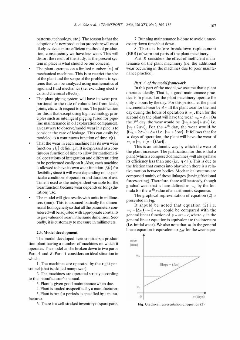
The graphical representation of equation (2) ispresented in Fig.

It should be noted that equation (2) i.e.( )( ) 01 wnwwn +−∆= could be compared with the

general linear function of cmxy += , where c in thegeneral linear equation is equivalent to the intercept(i.e. initial wear). We also note that m in the generallinear equation is equivalent to w∆ for the wear equa-

Fig. Graphical representation of equation (2)

S. A. Oke et al. / TRANSPORT – 2006, Vol XXI, No 2, 105–111

108

tion, i.e. additional day of plant operation. It shouldalso be noted that ( )mfy = is the same as nw , i.e.wear in plant after running for n days. The wear graphabove shows the linear variation of the wear withduration ( )n in days of plant operation.

Part B of the model frameworkThis part deals with an inefficiently maintained

plant. The section considers the additional wear to thatin equation (2). This is due to the effect of lack ofefficient maintenance of plant wear. Let us follow astepwise approach in the development of the formulato represent this additional wear. Let the wear in eachmachine, say turbine, pump, compressor, etc. each bedefined by their particular wear function ( )tfi suchthat the total plant wear owing to these machines willbe given by xw , stated below:

( )∑=

=m

1iix tf w , (3)

where m is the number of machines in the plant underconsideration. The mean wear, which is a repre-sentative value for the plant machinery will thereforebe given by:

( )∑=

==m

1ii

xy tf

m

1

m

w w . (4)

Another measure of wear considered is the vol-ume rate of leaks from joints, gaskets, or the plantpiping system generally. Let the wear in the pipingsystem be proportional to the rate of drops of volumesof the fluid conveyed with respect to time. Therefore,representing this wear by zw we will obtain:

( )dt

dv t wz = , (5)

where ( )tv is the time-dependent volumetric wearfunction. Putting a constant of proportionality intoequation (7) (for dimensional homogeneity) we willobtain:

( )dt

tkdv wz = , (6)

where k = wear constant for the plant piping system(network). It is important to note that wear in plantpiping system depends on:• Material of construction of the pipe.• The material (or fluid) conveyed.• Whether or not the pipe is submerged (subsea

piping) or protected from corrosion.Combining equations (4) and (6) to obtain com-

bined wear ( )pw , which is expressed as:

( )( )

dt

tkv tf

m

1 m

1ii ++= ∑

=

zyp www . (7)

In considering the effect of the individuals oper-

ating the machines, let us introduce the reciprocal

α1

into equation (5). The range of values of α will

depend on the expertise (training/competence level)of each machine operator (or say a mean value to rep-resent the competence level for the plant operators).We therefore, have a new expression for weargiven by:

α=

pQ

w

w . (8)

Again,

( )( )

+

α= ∑

= dt

tkdv tf

m

11 w

m

1iiQ , (9)

where α = manpower competence factor.Equation (9) gives an expression that can be used

to evaluate the additional wear in plant machinery dueto inefficient maintenance. Adding equations (1) and(9) to obtain a general wear equation represented by

Rw , we have:

QnR www += ,

and

( )( ) ( )( )

+

α+∆−+= ∑

= dt

tkdv tf

m

11w1nww

m

1ii0R . (10)

Equation (10) above gives an expression that canbe used to determine/evaluate plant wear. It can beviewed as a sum of:• Normal wear (good maintenance practice): nw .• Additional wear (poor maintenance practice): Qw .

3. Case study

Let us consider a hypothetical multinational oiland gas company with over two decades of operationin the oil rich Niger-Delta region of southern, Nige-ria. This is a production plant which goal is to pro-duce energy products such as PMS (premium motorspirit gasoline), among other petroleum derivatives.The plant operation will involve the exploration andprocessing of petroleum before it takes a form suit-able for consumption. The plant will therefore requireamong other things, a complex network of piping, dif-ferent machines operating at different stages of pro-cessing the crude oil. These machines involve com-pressors, turbines, cooling towers, throttle valves, con-densers, evaporators, boilers, burners, nozzles, diffus-ers, etc. For the purpose of simplifying the problem,let us assume that a plant operates on only 4 machines:turbine, compressor, pump and evaporator. Let usfurther assume that each of these machines has its wear

S. A. Oke et al. / TRANSPORT – 2006, Vol XXI, No 2, 105–111

109

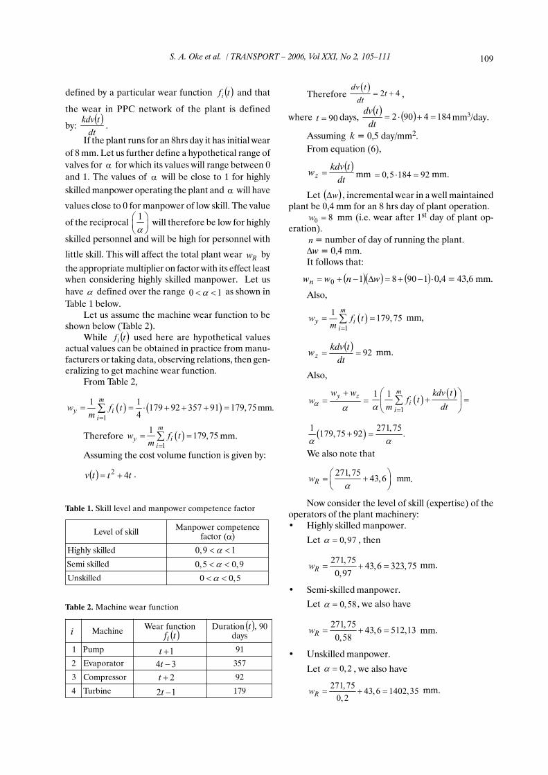
defined by a particular wear function ( )tfi and that

the wear in PPC network of the plant is defined

by: ( )

dt

tkdv.

If the plant runs for an 8hrs day it has initial wearof 8 mm. Let us further define a hypothetical range ofvalves for α for which its values will range between 0and 1. The values of α will be close to 1 for highlyskilled manpower operating the plant and α will have

values close to 0 for manpower of low skill. The value

of the reciprocal 1

α

will therefore be low for highly

skilled personnel and will be high for personnel with

little skill. This will affect the total plant wear Rw by

the appropriate multiplier on factor with its effect leastwhen considering highly skilled manpower. Let ushave α defined over the range 0 1α< < as shown inTable 1 below.

Let us assume the machine wear function to beshown below (Table 2).

While ( )tfi used here are hypothetical valuesactual values can be obtained in practice from manu-facturers or taking data, observing relations, then gen-eralizing to get machine wear function.

From Table 2,

( ) ( )1

1 1179 92 357 91 179,75mm.

4

m

y ii

w f tm

=

= = ⋅ + + + =∑

Therefore ( )1

1179,75

m

y ii

w f tm

=

= =∑ mm.

Assuming the cost volume function is given by:

( ) tttv 42 += .

Table 1. Skill level and manpower competence factor

Table 2. Machine wear function

Therefore ( )

2 4dv t

tdt

= + ,

where 90=t days, ( )

( ) 1844902 =+⋅=dt

tdvmm3/day.

Assuming k = 0,5 day/mm2.From equation (6),

( )dt

tkdvwz = mm 0,5 184 92= ⋅ = mm.

Let ( )w∆ , incremental wear in a well maintainedplant be 0,4 mm for an 8 hrs day of plant operation.

80 =w mm (i.e. wear after 1st day of plant op-eration).

n = number of day of running the plant.∆w = 0,4 mm.It follows that:

( )( ) ( )190810 ⋅−+=∆−+= wnwwn 0,4 = 43,6 mm.

Also,

( )1

1179,75

m

y ii

w f tm

=

= =∑ mm,

( )92==

dt

tkdvwz mm.

Also,

y zw wwα

α

+= = ( )

( )

1

1 1 m

ii

kdv tf t

m dtα =

+ =

∑

( )1 271,75

179,75 92 .α α

+ =

We also note that

271,7543,6 mmRw

α

= +

.

Now consider the level of skill (expertise) of theoperators of the plant machinery:• Highly skilled manpower.

Let 0,97α = , then

271,7543,6 323,75

0,97Rw = + = mm.

• Semi-skilled manpower.

Let 0,58α = , we also have

271,7543,6 512,13

0,58Rw = + = mm.

• Unskilled manpower.

Let 0, 2α = , we also have

271,7543,6 1402,35

0, 2Rw = + = mm.

S. A. Oke et al. / TRANSPORT – 2006, Vol XXI, No 2, 105–111

enihcaM noitcnufraeW 09,noitaruDsyad

1 pmuP 19

2 rotaropavE 753

3 rosserpmoC 29

4 enibruT 971

i ( )tfi

( )t

1+t

34 −t

2+t

12 −t

lliksfoleveL ecnetepmocrewopnaM)(rotcaf

delliksylhgiH

delliksimeS

delliksnU

α

0,9 1α< <

0,5 0,9α< <

0 0,5α< <

110

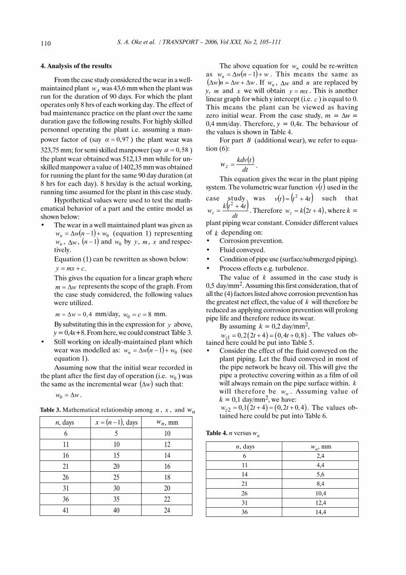
4. Analysis of the results

From the case study considered the wear in a well-maintained plant Aw was 43,6 mm when the plant wasrun for the duration of 90 days. For which the plantoperates only 8 hrs of each working day. The effect ofbad maintenance practice on the plant over the sameduration gave the following results. For highly skilledpersonnel operating the plant i.e. assuming a man-power factor of (say 0,97α = ) the plant wear was

323,75 mm; for semi skilled manpower (say 0,58α = )the plant wear obtained was 512,13 mm while for un-skilled manpower a value of 1402,35 mm was obtainedfor running the plant for the same 90 day duration (at8 hrs for each day). 8 hrs/day is the actual working,running time assumed for the plant in this case study.

Hypothetical values were used to test the math-ematical behavior of a part and the entire model asshown below:• The wear in a well maintained plant was given as

( ) 01 wnwwn +−∆= (equation 1) representingnw , w∆ , ( )1−n and 0w by y , m , x and respec-

tively.Equation (1) can be rewritten as shown below:

cmxy += .This gives the equation for a linear graph where

wm ∆= represents the scope of the graph. Fromthe case study considered, the following valueswere utilized.

0, 4m w= ∆ = mm/day, 80 == cw mm.

By substituting this in the expression for y above,y = 0,4x+8. From here, we could construct Table 3.

• Still working on ideally-maintained plant whichwear was modelled as: ( ) 01 wnwwn +−∆= (seeequation 1).Assuming now that the initial wear recorded in

the plant after the first day of operation (i.e. 0w ) wasthe same as the incremental wear ( )w∆ such that:

ww ∆=0 .

Table 3. Mathematical relationship among n , x , and nw

syad, syad, mm,

6 5 01

11 01 21

61 51 41

12 02 61

62 52 81

13 03 02

63 53 22

14 04 42

n ( )1−= nx nw

The above equation for nw could be re-writtenas ( ) wnwwn +−∆= 1 . This means the same as( ) wwnw ∆+∆=∆ . If nw , w∆ and n are replaced byy, m and x we will obtain mxy = . This is anotherlinear graph for which y intercept (i.e. c ) is equal to 0.This means the plant can be viewed as havingzero initial wear. From the case study, m = ∆w =0,4 mm/day. Therefore, y = 0,4x. The behaviour ofthe values is shown in Table 4.

For part B (additional wear), we refer to equa-tion (6):

( )dt

tkdvwz = .

This equation gives the wear in the plant pipingsystem. The volumetric wear function ( )tv used in the

case study was ( ) ( )tttv 42 += such that( )

dt

ttkwz

42 += . Therefore ( )42 += tkwz , where k =

plant piping wear constant. Consider different valuesof k depending on:• Corrosion prevention.• Fluid conveyed.• Condition of pipe use (surface/submerged piping).• Process effects e.g. turbulence.

The value of k assumed in the case study is0,5 day/mm2. Assuming this first consideration, that ofall the (4) factors listed above corrosion prevention hasthe greatest net effect, the value of k will therefore bereduced as applying corrosion prevention will prolongpipe life and therefore reduce its wear.

By assuming k = 0,2 day/mm2,( ) ( )1 0,2 2 4 0,4 0,8zw t t= + = + . The values ob-

tained here could be put into Table 5.• Consider the effect of the fluid conveyed on the

plant piping. Let the fluid conveyed in most ofthe pipe network be heavy oil. This will give thepipe a protective covering within as a film of oilwill always remain on the pipe surface within. k

will therefore be ww . Assuming value ofk = 0,1 day/mm2, we have:

( ) ( )2 0,1 2 4 0,2 0,4zw t t= + = + . The values ob-tained here could be put into Table 6.

S. A. Oke et al. / TRANSPORT – 2006, Vol XXI, No 2, 105–111

n syad, wn mm,

6 4,2

11 4,4

41 6,5

12 4,8

62 4,01

13 4,21

63 4,41

Table 4. n versus wn

111

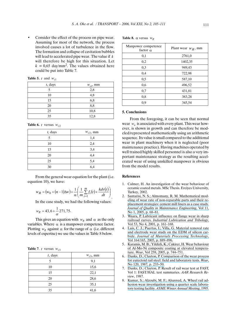
• Consider the effect of the process on pipe wear.Assuming for most of the network, the processinvolved causes a lot of turbulence in the flow.The formation and collapse of cavitation bubbleswill lead to accelerated pipe wear. The value if kwill therefore be high for this situation. Letk = 0,65 day/mm2. The values obtained herecould be put into Table 7.

From the general wear equation for the plant (i.e.equation 10), we have:

( )( ) ( )( )

+

α+∆−+= ∑

=

m

iiR

dt

tkdvtf

mwnww

10

111

.In the case study, we had the following values:

143,6 271,75Rw

α= + .

This gives an equation with Rw and α as the onlyvariables. Where α is a manpower competence factor.Plotting Rw against α for the range of α (i.e. differentlevels of expertise) we use the values in Table 8 below.

5. Conclusions

From the foregoing, it can be seen that normalwear nw is associated with every plant. This wear how-ever, is shown in growth and can therefore be mod-eled/represented mathematically using an arithmeticsequence. Its value is small compared to the additionalwear in plant machinery when it is neglected (poormaintenance practice). Having machines operated bywell trained/highly skilled personnel is also a very im-portant maintenance strategy as the resulting accel-erated wear of using unskilled manpower is obviousfrom the model results.

References

1. Calmer, H. An investigation of the wear behaviour ofceramic coated metals. MSc Thesis. Erciyes University,Turkey, 2002.

2. Santarisi, N. S.; Almomany, R. M. Mathematical mod-eling of wear rate of non-reparable parts and their re-placement strategies: cement mill liners as a case study.Journal of Quality in Maintenance Engineering, Vol 11,No 1, 2005, p. 68–81.

3. Waara, P. Lubricant influence on flange wear in sharprailroad curves. Industrial Lubrication and Tribology,Vol 53, No 4, 2001, p. 161–168.

4. Luis, C. J.; Puertas, I.; Villa, G. Material removal rateand electrode wear study on the EDM of silicon car-bide. Journal of Materials Processing Technology,Vol 164/165, 2005, p. 889–896.

5. Karamis, M. B.; Yildizli, K.; Cakirer, H. Wear behaviourof Al-Mo-Ni composite coating at elevated tempera-ture. Wear, Vol 258, 2005, p. 744–751.

6. Danks, D.; Clayton, P. Comparison of the wear processfor eutectoid rail steel: field and laboratory tests. Wear,No 120, 1987, p. 233–50.

7. Danks, D.; Clayton, P. Result of rail wear test at FAST,Vol 1: FAST/HAL test summaries. AAR Research Re-view, 1987.

8. Kumar, S.; Alzoubi, M. F.; Alsayyed, A. Wheel rail ad-hesion wear investigation using a quarter scale labora-tory testing facility. ASME Winter Annual Meeting, 1995.

Table 6. t versus 2zw

Table 7. t versus 3zw

Table 8. α versus Rw

S. A. Oke et al. / TRANSPORT – 2006, Vol XXI, No 2, 105–111

2zwsyad, mm,

5 4,1

01 4,2

51 4,3

02 4,4

52 4,5

03 4,6

t

ecnetepmocrewopnaMrotcaf mm,raewtnalP

1,0 0,1672

2,0 53,2041

3,0 34,949

4,0 89,227

5,0 01,785

6,0 25,694

7,0 18,134

8,0 82,383

9,0 45,543

αRw

Table 5. t and 1zw

t syad, wz1 mm,

5 8,2

01 8,4

51 8,6

02 8,8

52 8,01

53 8,21

syad, mm,

5 1,9

01 6,51

51 1,22

02 6,82

52 1,53

53 6,14

t 3zw