1

A High-Order-Accurate 3D Surface IntegralEquation Solver for Uniaxial Anisotropic Media

Jin Hu, Student Member, IEEE and Constantine Sideris, Member, IEEE

Abstract—This paper introduces a high-order accurate surfaceintegral equation method for solving 3D electromagnetic scatter-ing for dielectric objects with uniaxially anisotropic permittivitytensors. The N-Muller formulation is leveraged resulting in asecond-kind integral formulation, and a finite-difference-basedapproach is used to deal with the strongly singular terms resultingfrom the dyadic Green’s functions for uniaxially anisotropicmedia while maintaining the high-order accuracy of the dis-cretization strategy. The integral operators are discretized viaa Nystrom-collocation approach, which represents the unknownsurface densities in terms of Chebyshev polynomials on curvilin-ear quadrilateral surface patches. The convergence is investigatedfor various geometries, including a sphere, cube, a complicatedNURBS geometry imported from a 3D CAD modeler software,and a nanophotonic silicon waveguide, and results are comparedagainst a commercial finite element solver. To the best of ourknowledge, this is the first demonstration of high-order accuracyfor objects with uniaxially anisotropic materials using surfaceintegral equations.

Index Terms—Integral equations, high-order accuracy, N-Muller formulation, spectral methods, scattering.

I. INTRODUCTION

Boundary Integral Equations (BIE) are a powerful approachfor numerically solving Maxwell’s equations and have beenapplied to solve a plethora of scattering problems, includ-ing antennas [1], radar scattering [2], and most recentlynanophotonics [3]–[5]. Traditionally known as open boundaryproblems due to satisfying the Sommerfeld radiation conditionby design, BIE’s have also recently been successfully appliedfor solving dielectric waveguiding problems, which requiresimulating waveguides extending to and from infinity, in bothtwo [3], [6] and three [5] dimensions. Unlike other volumetriccomputational approaches, such as Finite Difference (FD)and Finite Element (FE) methods, which require generatingcomplicated volume meshes, BIE methods only mesh thesurfaces between material regions. Since BIE methods solvefor unknowns over surface rather than volume meshes, theymay also result in significantly smaller problems compared tousing volumetric approaches in scenarios with high volume tosurface area ratios. BIE’s have predominantly been used forsolving problems with homogeneous, isotropic dielectrics dueto the availability of closed-form Dyadic Green’s functions,which can be readily discretized using suitable numericalquadrature and singularity treatment approaches. For example,our recent work in [7] demonstrates high-order convergencediscretizing the Magnetic Field Integral Equation (MFIE) and

The authors gratefully acknowledge support by the Air Force Office ofScientific Research (FA9550-20-1-0087) and the National Science Foundation(CCF-1849965, CCF-2047433).

J. Hu and C. Sideris are with the Department of Electrical and ComputerEngineering, University of Southern California, Los Angeles, CA 90089, USA(e-mails: jinhu@usc.edu, csideris@usc.edu).

the N-Muller formulation for modeling metals and dielectricsrespectively using a Chebyshev-based Nystrom method. Onthe other hand, many anisotropic materials are commonlyused in engineering applications, such as anisotropic dielectricsubstrates for antennas [8], [9] and liquid crystal claddings fordesigning reconfigurable nanophotonic devices [10]. However,despite the fact that closed-form Green’s functions have beenderived for uniaxially anisotropic media, there is a dearth ofwork available using BIE methods to solve problems withthese materials. In fact, the only discretization approach in theliterature is [11], which presents compelling results comparingagainst volumetric methods but does not report on error orconvergence properties.

Indeed, although closed form expressions for the dyadicGreen’s functions for materials with uniaxially anisotropicpermittivity and permeability do exist [12], they are signif-icantly more complex and challenging to discretize than thecorresponding expressions for the isotropic material case (e.g.,see eq. 24). The PMCHWT [13] formulation is used in [11]and discretized using the Method-of-Moments (MoM) andRWG basis functions [14], [15]. The strongly singular partof the Gee operator (known as the T operator in the literaturefor the isotropic case) is dealt with in the usual manner byusing integration by parts to decrease the kernel singularityby moving a derivative to the testing function. However, theGem ∝

(∇×Gee

)operator (known as the K operator in

the literature for the isotropic case) also contains a strongsingularity which cannot be easily reduced. [11] approximatesintegrals with Gem by shifting the target point r slightly offthe surface. Unfortunately, this approach is expected to resultin poor accuracy since the operator is evaluated on a differenttarget point than the original intended one on the surface, andfurthermore because the kernel remains nearly singular and istherefore very challenging to numerically integrate even withthe target point being shifted off the surface.

In this work, we present an new discretization strategy,which when combined with the singular integration approachusing Chebhyshev polynomials to represent the unknowndensities introduced in [7] achieves high-order accuracy forscattering from objects composed of uniaxially anisotropicmaterials. To the best of our knowledge, this is the very firstdemonstration of a boundary integral solver for anisotropicmedia which achieves high-order accuracy. Note that in allof our examples we assume that only the permittivity tensoris anisotropic and that µr = 1; however, the approach pre-sented can readily be extended to support materials with bothpermittivity and permeability tensors having anisotropy. Thepaper is organized as follows. Section II briefly introduces thesurface integral formulation under consideration for dielectricscatterers. Section III reviews the Dyadic Green’s functions

arX

iv:2

203.

0579

5v1

[ph

ysic

s.co

mp-

ph]

11

Mar

202

2

2

for uniaxial anisotropic media and sets up a system of in-tegral equations for a scenario with an anisotropic scattererinside an isotropic exterior medium based on the N-Mullerformulation. Section IV analyzes the singular behavior of eachanisotropic kernel operator. Section V presents our Chebyshev-based discretization and singular integration approach foraccurate evaluation of the integral operators. Finally, SectionVI demonstrates error convergence and both near and far-fieldnumerical results for four different example cases.

II. SURFACE INTEGRAL EQUATION FORMULATION

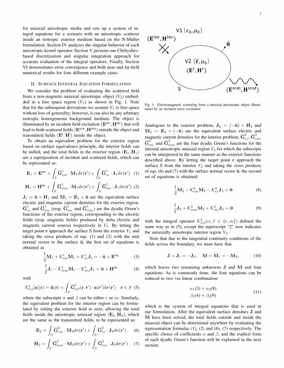
We consider the problem of evaluating the scattered fieldfrom a non-magnetic uniaxial anisotropic object (V2) embed-ded in a free space region (V1) as shown in Fig. 1. Notethat for the subsequent derivations we assume V1 is free-spacewithout loss of generality; however, it can also be any arbitraryisotropic homogeneous background medium. The object isilluminated by an incident field excitation

(Einc,Hinc

)that will

lead to both scattered fields (Escat,Hscat) outside the object andtransmitted fields (Et,Ht) inside the object.

To obtain an equivalent problem for the exterior regionbased on surface equivalence principle, the interior fields canbe nulled, and the total fields in the exterior region (E1,H1)are a superposition of incident and scattered fields, which canbe represented as:

E1 = Einc +

∫S

G1

em ·M1dσ(r′) +

∫S

G1

ee · J1dσ(r′) (1)

H1 = Hinc +

∫S

G1

mm ·M1dσ(r′) +

∫S

G1

me · J1dσ(r′) (2)

J1 = n ×H1 and M1 = E1 × n are the equivalent surfaceelectric and magnetic current densities for the exterior region.G

1

ee and G1

em (resp. G1

me and G1

mm) are the dyadic Green’sfunctions of the exterior region, corresponding to the electricfields (resp. magnetic fields) produced by delta electric andmagnetic current sources respectively in V1. By letting thetarget point r approach the surface S from the exterior V1 andtaking the cross products of eqs. (1) and (2) with the unitnormal vector to the surface n, the first set of equations isobtained as

1

2M1 +K1

emM1 +K1eeJ1 = −n×Einc (3)

1

2J1 −K1

mmM1 −K1meJ1 = n×Hinc (4)

with

K1αβ [a](r) = n(r)×

∫S

G1

αβ(r, r′) · a(r′)dσ(r′) r ∈ S (5)

where the subscripts α and β can be either e or m. Similarly,the equivalent problem for the interior region can be formu-lated by setting the exterior field to zero, allowing the totalfields inside the anisotropic uniaxial region (E2,H2), whichare the same as the transmitted fields, to be represented as:

E2 =

∫S

G2

em ·M2dσ(r′) +

∫S

G2

ee · J2dσ(r′) (6)

H2 =

∫S

G2

mm ·M2dσ(r′) +

∫S

G2

me · J2dσ(r′) (7)

Fig. 1. Electromagnetic scattering from a uniaxial anisotropic object illumi-nated by an incident wave excitation

Analogous to the exterior problem, J2 = (−n) × H2 andM2 = E2 × (−n) are the equivalent surface electric andmagnetic current densities for the interior problem, G

2

ee, G2

em,G

2

me and G2

mm are the four dyadic Green’s functions for theinternal anisotropic uniaxial region V2 for which the subscriptscan be interpreted in the same manner as the exterior functionsdescribed above. By letting the target point r approach thesurface S from the interior V2 and taking the cross productsof eqs. (6) and (7) with the surface normal vector n, the secondset of equations is obtained:

1

2M2 −K2

emM2 −K2eeJ2 = 0 (8)

1

2J2 +K2

mmM2 +K2meJ2 = 0 (9)

with the integral operator K2αβ(α, β ∈ {e,m}) defined the

same way as in (5), except the superscript “2” now indicatesthe uniaxially anisotropic interior region V2.

Note that due to the tangential continuity conditions of thefields across the boundary, we must have that

J = J1 = −J2, M = M1 = −M2, (10)

which leaves two remaining unknowns J and M and fourequations. As is commonly done, the four equations can bereduced to two via linear combination:

α1(3) + α2(8)β1(4) + β2(9)

(11)

which is the system of integral equations that is used inour formulation. After the equivalent surface densities J andM have been solved, the total fields outside and inside theuniaxial object can be determined anywhere by evaluating therepresentation formulas (1), (2) and (6), (7) respectively. Thespecific choice of coefficients α and β, and the explicit formof each dyadic Green’s function will be explained in the nextsection.

3

III. DYADIC GREEN’S FUNCTIONS FOR UNIAXIALANISOTROPIC MEDIA

The interior region V2 in the formulation is filled with auniaxially anisotropic dielectric, which can characterized bythe relative permittivity tensor:

ε = ε⊥I+ (ε‖ − ε⊥)cc (12)

where c is a unit vector parallel to the distinguished axis, ε‖is the relative permittivity along the direction of c, ε⊥ is therelative permittivity along the directions perpendicular to cand I represents the unit dyadic. It has been shown in [11],[12] that closed-form expressions exist for the dyadic Green’sfunctions for this type of material, which we reproduce herefor completeness:

G2

ee =iωµ0

4π

{∇∇k2⊥

eik⊥Re

Re+ ε‖

eik⊥Re

Reε−1

−

[ε‖e

ik⊥Re

ε⊥Re− eik⊥R

R

] [(R× c)(R× c)

(R× c)2

]−[ε‖ − ε⊥ε⊥

eik⊥(Re+R)/2

Re +R

sin (k⊥(Re − R)/2)

(k⊥(Re − R)/2)

]×[I− cc− 2

(R× c)(R× c)

(R× c)2

]}(13)

G2

mm =iωε04π

{∇∇k20

eik⊥R

R+ ε⊥

eik⊥R

RI

+

[ε‖e

ik⊥Re

Re− ε⊥e

ik⊥R

R

] [(R× c)(R× c)

(R× c)2

]+

[(ε‖ − ε⊥)

eik⊥(Re+R)/2

Re +R

sin (k⊥(Re − R)/2)

(k⊥(Re − R)/2)

]×[I− cc− 2

(R× c)(R× c)

(R× c)2

]}(14)

G2

em =i

ωε0ε−1 · ∇ ×G

2

mm (15)

G2

me =1

iωµ0∇×G

2

ee (16)

where ε0 and µ0 are the permittivity and permeability of freespace respectively, ω is the angular frequency of the incidentfield, k0 = ω

√ε0µ0 is the wavenumber in free space, R =

r − r′ and R = |R| are the relative position vector and thedistance respectively from a source point to an observationpoint, ε−1 = ε−1⊥ I+(ε−1‖ − ε

−1⊥ )cc is the inverse of ε and Re,

and k⊥ are given by:

Re =√ε‖(R · ε−1 ·R), k⊥ = k0

√ε⊥ (17)

Note that if the permittivity tensor is set to ε = I, the aboveuniaxially anisotropic Green’s functions simplify to the well-known isotropic dyadic Green’s functions for free-space:

G1

ee =iωµ0

4π

[∇∇k20

eik0R

R+eik0R

RI

](18)

G1

mm =iωε04π

[∇∇k20

eik0R

R+eik0R

RI

](19)

G1

em =i

ωε0∇×G

1

mm (20)

G1

me =1

iωµ0∇×G

1

ee (21)

The linear combination coefficients in the integral equationsystem (11) are chosen according to the N-Muller formulationto be: α1 = εr1 = 1, α2 = εr2 = ε⊥, β1 = µr1 = β2 =µr2 = 1, which cancel the singularity of the hypersingular partof the G

1

ee operator and result in a well-conditioned second-kind integral equation formulation [16]. The resulting integralequations can be represented in matrix form as follows:

[K1em − ε⊥K2

em + 1+ε⊥2 I K1

ee − ε⊥K2ee

K2mm −K1

mm K2me −K1

me + I

] [MJ

]=

[−n×Einc

n×Hinc

](22)

where I is the identity operator and the expressions fordyadic Green’s functions G

i

αβ involved in each of the integraloperators Kiαβ(i ∈ {1, 2};α, β ∈ {e,m}) are given by (13)–(16) and (18)– (21).

IV. SINGULARITY ANALYSIS OF INTEGRAL OPERATORS

In order to evaluate the action of each of the integraloperators Kiαβ on the densities with high accuracy, care mustbe taken to analyze and properly handle the singular behaviorof each operator.

A. Singularity of K2ee

At first glance, the Kiee and Kimm(i ∈ {1, 2}) operators ap-pear to both be hypersingular with O(1/R3) singularities dueto the ∇∇ operator acting on a term with O(1/R) singularity.However, vector identities can be utilized to transfer the one ofthe ∇ operators to the density term and the other ∇, which canbe made to not depend on the source integration coordinate,can be pulled outside of the integral1. For example, taking the

1Note: Moving the gradient (∇) outside the integral is not strictly necessarywhen using the Muller formulation since its coefficients are designed to cancelthe singularity.

4

K2ee operator with a target point approaching the surface from

the inside,

K2eeJ = n(r)×

∫S

G2

ee(r, r′) · J(r′)dσ(r′)

∣∣∣∣r∈S

= n(r)×∫S

G2

ee(r, r′) · J(r′)dσ(r′)

∣∣∣∣r→r−

=iωµ0

4πn(r)×

∫S

{∇∇k2⊥

eik⊥Re

Re+D

}· J(r′)dσ(r′)

∣∣∣∣r→r−

=iωµ0

4πn(r)×

{1

k2⊥∇∫S

∇eik⊥Re

Re· J(r′)dσ(r′)

+

∫S

D · J(r′)dσ(r′)}∣∣∣∣

r→r−

=iωµ0

4πn(r)×

{1

k2⊥∇∫S

eik⊥Re

Re∇′s · J(r′)dσ(r′)

+

∫S

D · J(r′)dσ(r′)}∣∣∣∣

r→r−

(23)where

D = ε‖eik⊥Re

Reε−1 −

[ε‖e

ik⊥Re

ε⊥Re− eik⊥R

R

] [(R× c)(R× c)

(R× c)2

]−[ε‖ − ε⊥ε⊥

eik⊥(Re+R)/2

Re +R

sin (k⊥(Re − R)/2)

(k⊥(Re − R)/2)

]×[I− cc− 2

(R× c)(R× c)

(R× c)2

](24)

and r → r− indicates that operator is evaluated for atarget point that is approaching r ∈ S along −n from V2.Since the kernels of both integrals, D and eik⊥Re/Re, haveO(1/R) singularity, the integral operator K2

ee in this formis weakly singular. K2

mm,K1ee and K1

mm can also be readilytransformed into weakly singular operators by following thesame procedure as K2

ee.

B. Singularity of K2me

The action of the ∇× operator on weakly singular kernelswith O(1/R) singularities makes the dyadic Green’s functionsof the Kime and Kiem(i ∈ {1, 2}) operators strongly singularwith O(1/R2) type singularity. Nevertheless, these operatorscan also be manipulated to become weakly singular whenacting on densities by applying vector identities. For exam-ple, consider the K2

me acting on J, with the target point r

approaching the surface from the inside as before,

K2meJ = n(r)×

∫S

G2

me(r, r′) · J(r′)dσ(r′)

∣∣∣∣r∈S

= n(r)×∫S

G2

me(r, r′) · J(r′)dσ(r′)

∣∣∣∣r→r−

+1

2J

= n(r)×∫S

1

iωµ0∇×G

2

ee · J(r′)dσ(r′)∣∣∣∣r→r−

+1

2J

=1

4πn(r)×

{∫S

∇× ∇∇k2⊥

eik⊥Re

Re· J(r′)dσ(r′)

∣∣∣∣r→r−

+

∫S

∇×D(r, r′) · J(r′)dσ(r′)∣∣∣∣r→r−

}+

1

2J

=1

4πn(r)×∇×

∫S

D(r, r′) · J(r′)dσ(r′)∣∣∣∣r→r−

+1

2J

(25)where D is given in (24) and the second equality followsfrom the jump condition. Note that the ∇∇ term can beremoved since ∇ × ∇ ≡ 0. It can be seen that the kernelinside the integral (D(r, r′)) is now weakly singular since thecurl operation has been factored out of the integral. The sameprocedure can be used to also transform K2

em, K1me and K1

em

into weakly singular forms.These operators in their weakly singular form can now be

discretized with high-order accuracy using the Chebyshev-based Nystrom method that was first introduced in [7] forperfect conductors and isotropic dielectric materials. The fol-lowing section briefly reviews the key points of the Chebyshevmethod and discusses our adaptation and application of it tothe present anisotropic formulation.

V. EVALUATION OF ACTION OF INTEGRAL OPERATORSKiαβ USING CHEBYSHEV EXPANSION BASED METHOD

According to the analysis in section IV, two types ofweakly-singular integrals as well as their gradient and curlneed to be evaluated to compute the action of the integraloperators K2

ee and K2me on the current density J:

φ(r) =

∫S

eik⊥Re

Re∇′s · J(r′)dσ(r′), n(r)×∇φ(r)|r=r−

A(r) =

∫S

D(r, r′) · J(r′)dσ(r′), n(r)×∇×A(r)|r=r−

(26)where φ(r) and A(r) are scalar and vector functions of thetarget point r respectively and D is defined in (24). Note thatwe focus on the operators acting on J since the same procedurecan be used to discretize the K2

mm and K2em operators which

act on M.

A. Evaluation of φ(r) and A(r)

In order to compute φ(r) and A(r), the whole surfaceS is split into M non-overlapping curvilinear quadrilateralpatches Sp, p = 1, 2, ...,M . A parametric mapping is definedfrom the unit square [−1, 1] × [−1, 1] in UV space to eachsurface Sp in Cartesian coordinates. Specifically, we introduceparameterization r = rp(u, v) = (xp(u, v), yp(u, v), zp(u, v))

5

for patch Sp. The tangential covariant basis vectors and normalvectors on Sp can then be defined as

apu =∂rp(u, v)

∂u, apv =

∂rp(u, v)

∂v, np =

apu × apv||apu × apv||

. (27)

The tangential electric current density vector J on the surfaceSp can be expanded in terms of the local tangential coordinatebasis as

Jp(u, v) = Jp,u(u, v)apu(u, v) + Jp,v(u, v)apv(u, v) (28)

where Jp(u, v) ≡ J(rp(u, v)), Jp,u and Jp,v are the con-travariant components of the surface current density J. Forsufficiently smooth surface geometries, Jp,u and Jp,v aresmooth functions of u and v and can be approximated withspectral convergence by using Chebyshev polynomials as

Jp,a =

Npv−1∑m=0

Npu−1∑n=0

γp,an,mTn(u)Tm(v), for a = u, v (29)

where the Chebyshev coefficients γp,an,m can be computed fromthe values of Jp,a on Sp at the Chebyshev nodes, which iswhere the discretized set of unknowns are located, by usingthe discrete orthogonality property of Chebyshev polynomials:

γp,an,m =αnαmNpuN

pv

Npv−1∑k=0

Npu−1∑l=0

Jp,a(ul, vk)Tn(ul)Tm(vk), (30)

After the Chebyshev coefficients are obtained from the densityvalues on Chebyshev nodes, we are able to compute the den-sity values Jp,a(u, v) for arbitrary (u, v) by interpolating via(29), and the Cartesian components Jpi (u, v) can be computedby taking dot product of Cartesian basis vectors ei(i = x, y, z)and Jp(u, v). Thus, φ(r) and the i-th Cartesian component ofthe integral A(r) can be represented as

φ(r) =

M∑p=1

∫Sp

eik⊥Re

Re∇′s · J(r′)dσ(r′)

=M∑p=1

∫ 1

−1

∫ 1

−1

eik⊥Re

Re

(∂(√|Gp|Jp,u)∂u

+∂(√|Gp|Jp,v)∂v

)dudv

(31)

Ai(r) =

M∑p=1

∫Sp

ei ·D(r, r′) · J(r′)dσ(r′)

=

M∑p=1

∫ 1

−1

∫ 1

−1(DixJ

px +DiyJ

py +DizJ

pz )√|Gp|dudv

(32)where Dij = Dij(r, r

p(u, v))(i, j = x, y, z) is the Cartesiancomponent of the dyadic D(r, r′), Jpj = Jpj (u, v) is theCartesian component of current density J and

√|Gp| =√

|Gp(u, v)| is the surface element Jacobian on the sourcepatch Sp. If the target point r is far away from Sp, the kernelsDij and eik⊥Re/Re are smooth and Fejer’s first quadraturerule can be used directly on the discrete densities at theChebyshev nodes to evaluate the integrals numerically withhigh-order accuracy. When the target point r is on the source

patch Sp itself or nearby, the integrals become singular ornearly singular and require special treatment. Since the densityon each patch can be expanded in terms of a Chebyshevpolynomial basis via (29), the action of these integrals onthe density J can be computed by first precomputing theiraction on each Chebyshev basis polynomial, followed bymultiplying the resulting values against the expanded Cheby-shev coefficients of the density and accumulating over all nand m indices. Since all of the kernels involved have beenmanipulated to be weakly singular, we adopt the change ofvariables proposed in [7], [17] [18, Sec. 3.5] to regularizethe integrals by annihilating the singularity with the surfaceJacobian, allowing the precomputations to be computed withvery high accuracy using a standard Fejer quadrature rule. TheChebyshev discretization and singular integration approachesfor the Nystrom method are described in depth in [7].

B. Evaluation of n(r)×∇φ(r)|r=r−

In view of the surface representation in terms of non-overlapping patches, for a target point r on pth patch Sp, wefirst expand the ∇ operator in the local coordinate frame as

∇ = ap,u∂

∂u+ ap,v

∂

∂v+ np

∂

∂np(33)

where ap,u and ap,v are contravariant basis vectors that satisfythe orthogonality relation

ap,a · apb =

{1 a = b

0 a 6= b. (34)

The operator can then be expanded as

n(r)×∇φ(r)|r→r−

= np × (ap,u∂φ

∂u+ ap,v

∂φ

∂v+ np

∂φ

∂np)

∣∣∣∣r→r−

=∂φ

∂u

∣∣∣∣r→r−

np × ap,u +∂φ

∂v

∣∣∣∣r→r−

np × ap,v

=∂φ

∂u

∣∣∣∣r∈Sp

np × ap,u +∂φ

∂v

∣∣∣∣r∈Sp

np × ap,v

(35)

Note that the third equality follows from the fact that φ(r) hascontinuous tangential derivatives across the surface withoutany jump condition. As in section V-A, φ(r) is first computedat each Chebyshev node (ul, vk) on Sp and then expandedwith a Chebyshev transform as

φ(rp(u, v)) =

Npv−1∑m=0

Npu−1∑n=0

ζpn,mTn(u)Tm(v) (36)

where ζpn,m are the Chebyshev coefficients obtained by using(30) and replacing Jp,a(ul, vk) with φ(rp(ul, vk)). The partialderivatives with respect to u and v can then be readilycomputed by taking the derivatives of Chebyshev polynomialsTn(u) and Tm(v) respectively as

∂φ

∂u(rp(u, v)) =

Npv−1∑m=0

Npu−1∑n=0

ζpn,mT′n(u)Tm(v)

∂φ

∂v(rp(u, v)) =

Npv−1∑m=0

Npu−1∑n=0

ζpn,mTn(u)T′m(v)

(37)

6

for all target points r = rp(u, v) ∈ Sp and n(r)×∇φ(r)|r=r−

can then be computed by substituting into expansion (35).

C. Evaluation of n(r)×∇×A(r)|r=r−

By using the same expansion for ∇ operator as in (33), wecan expand this operator as

n(r)×∇×A(r)|r→r−

= np × (ap,u × ∂A

∂u+ ap,v × ∂A

∂v+ np × ∂A

∂np)

∣∣∣∣r→r−

= np × (ap,u × ∂A

∂u

∣∣∣∣r→r−

) + np × (ap,v × ∂A

∂v

∣∣∣∣r→r−

)

+ np × (np × ∂A

∂np

∣∣∣∣r→r−

)

= ap,u(np · ∂A∂u

∣∣∣∣r∈Sp

) + ap,v(np · ∂A∂v

∣∣∣∣r∈Sp

)− ∂A

∂np

∣∣∣∣r→r−

+ np(np · ∂A∂np

∣∣∣∣r→r−

)

(38)where the tangential derivatives for each Cartesian componentof A, ∂A

∂u and ∂A∂v , on Sp can be evaluated in the same way

as ∂φ∂u and ∂φ

∂v in section V-B.According to the limit definition of the directional deriva-

tive, the normal derivative of each Cartesian component i ofA, ∂Ai

∂np |r→r− , can be written as:

∂Ai∂np

∣∣∣∣r→r−

= limδ→0+

Ai(r)−Ai(r− δnp)δ

i = x, y, z (39)

The normal derivative can be transformed into a derivative ofa univariate function by definining auxiliary function, g(δ) =Ai(r+ δnp):

∂Ai∂np

∣∣∣∣r=r−

= limδ→0+

Ai(r)−Ai(r− δnp)δ

= limδ→0+

g(0)− g(−δ)δ

= g′−(0)

(40)

In order to approximate the derivative g′−(0) numerically withhigh accuracy without requiring very close off-surface evalua-tion, we use the following backward difference approximation:

∂Ai∂np

∣∣∣∣r=r−

= g′−(0) ≈3g(0)− 4g(−δ) + g(−2δ)

δ

=3Ai(r)− 4Ai(r− δnp) + Ai(r− 2δnp)

δ

(41)

which results in second order accuracy O(δ2) as δ → 0+.Note that the weakly singular integrals Ai(r), Ai(r − δnp)and Ai(r−2δnp) in the numerator can be evaluated with highaccuracy using the rectangular-singular integration methoddiscussed in section V-A.

After the two weakly singular integrals φ(r) and A(r) andtheir gradient and curl have been evaluated respectively, K2

eeJand K2

meJ can be obtained by substituting into (23) and (25).The same approach can be used to compute the actions of theother integral operators required since the kernels of K2

mmM,K1eeJ and K1

mmM are similar to that of K2eeJ and the kernels

of K2emM, K1

meJ and K1emM are similar to that of K2

meJ

as discussed in section IV. Therefore, the LHS of the wholesystem (22) can be evaluated for an arbitrary target point r ∈S. As is done in a typical Nystrom method, the operatorsare evaluated at the same targets points as the unknowns; i.e.,at the Chebyshev nodes on each patch, and each equation istested with the two tangential contravariant basis vectors. Thisresults in a full-rank linear system with the same number ofequations as unknowns, which can readily be solved using asuitable linear solver of choice. In this work, we use GMRESto solve the discretized systems iteratively.

VI. NUMERICAL RESULTS

We first study the convergence of the forward map withrespect to the number of Chebyshev nodes per side of thepatch: N = Np

u = Npv of the forward map. This can be

done numerically by applying the whole system (22) operator,which includes the actions of all the integral operators, onreference current densities J and M on a sphere and compar-ing against an analytical Mie series solution [19]. Followingthis, we present several examples demonstrating scatteringfrom a uniaxially anisotropic dielectric sphere and cube tohighlight the high order accuracy which can be achieved withour method. We also solve a scattering example from a 3DNURBS model generated by a commercial CAD softwareto demonstrate the ability of our method to handle objectswith complicated geometrical features and curvature. Finally,we apply our method to a silicon nanophotonic phase-shifterwaveguiding structure and compare the results against a com-mercial FDTD solver to showcase the potential of our methodfor simulating nanophotonic devices with high accuracy.

A. Forward Map Convergence

We evaluate convergence of the forward map (applicationof the integral operator to a prescribed density) on a uni-axially anisotropic dielectric sphere with diameter D = 2λ0,anisotropic permittivity ε⊥ = 2, ε‖ = 3 and distinguished axisc = (0, 0, 1). Fig. 2(a) and (b) plot the forward mapping errorversus N for increasing Nβ and decreasing finite differencestep size δ in (41) respectively. Note that a sufficiently smallδ = 10−5 is used for the plot versus Nβ and a sufficienlylarge Nβ = 600 is used for the plot versus δ such thatthe convergence is dominated by the parameter that is underconsideration in each plot. An analytical Mie series solutionfor scattering from a uniaxially anisotropic dielectric spheredue to an incident plane wave [19] is used for the referencedensities. As expected and discussed in Section V, both the δand Nβ parameters affect the overall accuracy significantly andshould be chosen judiciously according to the desired overallsolution accuracy.

B. Uniaxially Anisotropic Sphere

Next we investigate solving the full scattering problem forthe same sphere considered in section VI-A. The electric fieldof the incident plane wave is given by Einc = exe

ik0z . Toverify the correctness and accuracy of our results, the resultof our solver is compared with the analytical Mie seriessolution [19].

7

(a)

(b)

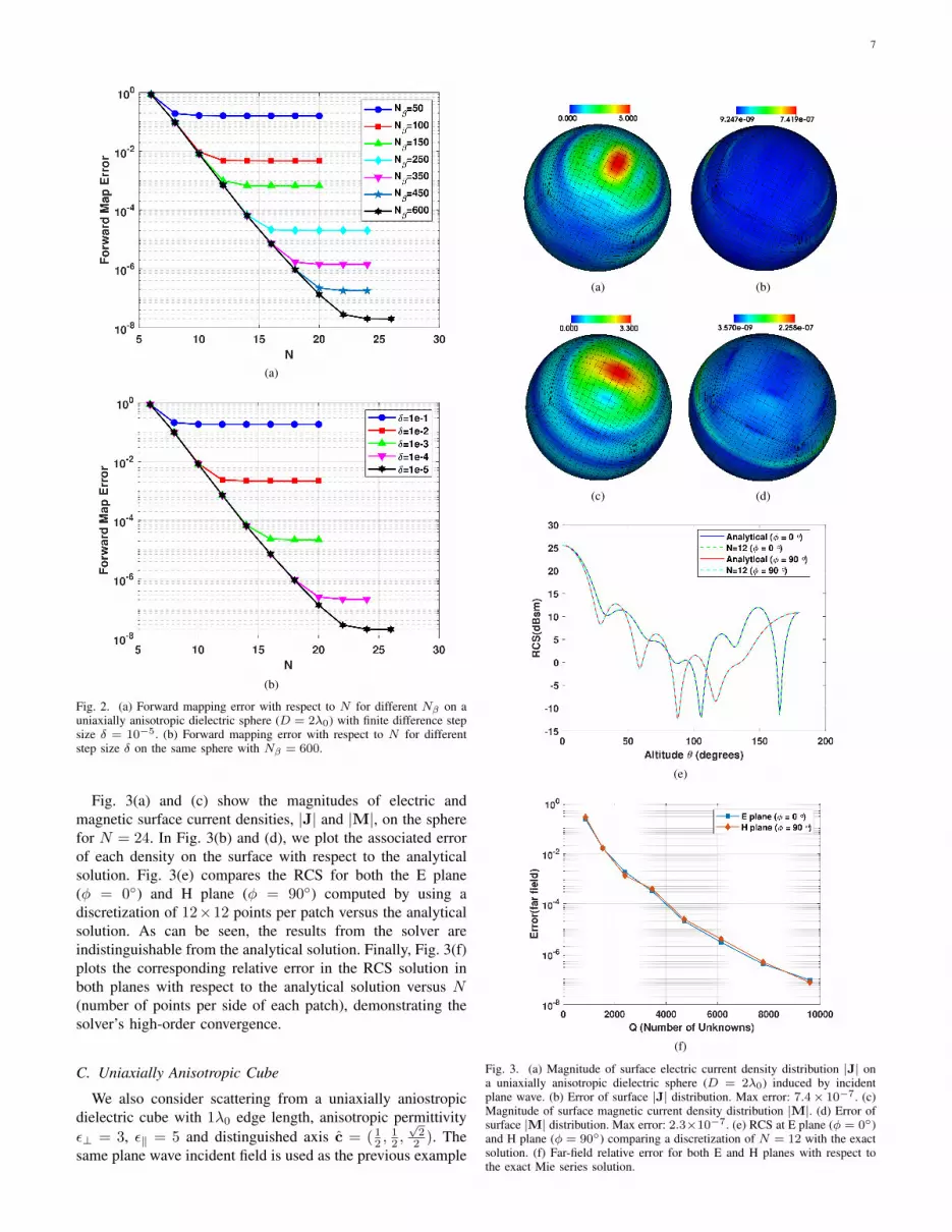
Fig. 2. (a) Forward mapping error with respect to N for different Nβ on auniaxially anisotropic dielectric sphere (D = 2λ0) with finite difference stepsize δ = 10−5. (b) Forward mapping error with respect to N for differentstep size δ on the same sphere with Nβ = 600.

Fig. 3(a) and (c) show the magnitudes of electric andmagnetic surface current densities, |J| and |M|, on the spherefor N = 24. In Fig. 3(b) and (d), we plot the associated errorof each density on the surface with respect to the analyticalsolution. Fig. 3(e) compares the RCS for both the E plane(φ = 0◦) and H plane (φ = 90◦) computed by using adiscretization of 12×12 points per patch versus the analyticalsolution. As can be seen, the results from the solver areindistinguishable from the analytical solution. Finally, Fig. 3(f)plots the corresponding relative error in the RCS solution inboth planes with respect to the analytical solution versus N(number of points per side of each patch), demonstrating thesolver’s high-order convergence.

C. Uniaxially Anisotropic Cube

We also consider scattering from a uniaxially aniostropicdielectric cube with 1λ0 edge length, anisotropic permittivityε⊥ = 3, ε‖ = 5 and distinguished axis c = (12 ,

12 ,√22 ). The

same plane wave incident field is used as the previous example

(a) (b)

(c) (d)

(e)

(f)

Fig. 3. (a) Magnitude of surface electric current density distribution |J| ona uniaxially anisotropic dielectric sphere (D = 2λ0) induced by incidentplane wave. (b) Error of surface |J| distribution. Max error: 7.4× 10−7. (c)Magnitude of surface magnetic current density distribution |M|. (d) Error ofsurface |M| distribution. Max error: 2.3×10−7. (e) RCS at E plane (φ = 0◦)and H plane (φ = 90◦) comparing a discretization of N = 12 with the exactsolution. (f) Far-field relative error for both E and H planes with respect tothe exact Mie series solution.

8

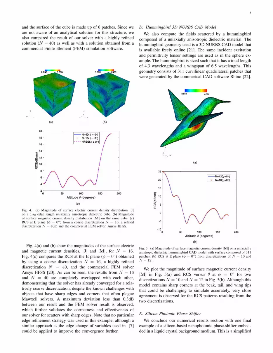
and the surface of the cube is made up of 6 patches. Since weare not aware of an analytical solution for this structure, wealso compared the result of our solver with a highly refinedsolution (N = 40) as well as with a solution obtained from acommercial Finite Element (FEM) simulation software.

(a) (b)

(c)

Fig. 4. (a) Magnitude of surface electric current density distribution |J|on a 1λ0 edge length uniaxially anisotropic dielectric cube. (b) Magnitudeof surface magnetic current density distribution |M| on the same cube. (c)RCS at E plane (φ = 0◦) from a coarse discretization N = 16, a refineddiscretization N = 40m and the commercial FEM solver, Ansys HFSS.

Fig. 4(a) and (b) show the magnitudes of the surface electricand magnetic current densities, |J| and |M|, for N = 16.Fig. 4(c) compares the RCS at the E plane (φ = 0◦) obtainedby using a coarse discretization N = 16, a highly refineddiscretization N = 40, and the commercial FEM solverAnsys HFSS [20]. As can be seen, the results from N = 16and N = 40 are completely overlapped with each other,demonstrating that the solver has already converged for a rela-tively coarse discretization, despite the known challenges withobjects that have sharp edges and corners that often plagueMawxell solvers. A maximum deviation less than 0.3dBbetween our result and the FEM solver result is observed,which further validates the correctness and effectiveness ofour solver for scatters with sharp edges. Note that no particularedge refinement strategy was used in this example, although asimilar approach as the edge change of variables used in [7]could be applied to improve the convergence further.

D. Hummingbird 3D NURBS CAD Model

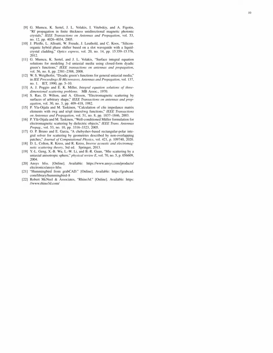
We also compute the fields scattered by a hummingbirdcomposed of a uniaxially anisotropic dielectric material. Thehummingbird geometry used is a 3D NURBS CAD model thatis available freely online [21]. The same incident excitationand permittivity tensor settings are used as in the sphere ex-ample. The hummingbird is sized such that it has a total lengthof 4.3 wavelengths and a wingspan of 6.5 wavelengths. Thisgeometry consists of 311 curvilinear quadrilateral patches thatwere generated by the commerical CAD software Rhino [22].

(a)

(b)

Fig. 5. (a) Magnitude of surface magnetic current density |M| on a uniaxiallyanistropic dielectric hummingbird CAD model with surface composed of 311patches. (b) RCS at E plane (φ = 0◦) from discretizations of N = 10 andN = 12 .

We plot the magnitude of surface magnetic current density|M| in Fig. 5(a) and RCS versus θ at φ = 0◦ for twodiscretizations N = 10 and N = 12 in Fig. 5(b). Although thismodel contains sharp corners at the beak, tail, and wing tipsthat could be challenging to simulate accurately, very closeagreement is observed for the RCS patterns resulting from thetwo discretizations.

E. Silicon Photonic Phase Shifter

We conclude our numerical results section with one finalexample of a silicon-based nanophotonic phase-shifter embed-ded in a liquid crystal background medium. This is a simplified

9

design inspired by [10] and consists of two parallel rectangularsilicon waveguides embedded within a uniaxially anisotropicliquid crystal cladding. The orientation of the distinguishedaxis c of the liquid crystal media can be electrically controlledby an external voltage. By altering the amplitude of this volt-age, the distinguished axis is rotated, causing the permittivityexperienced by the dominant field component to change andleading to a different corresponding propagation constant. Thischanges the phase-shift experienced by light propagating in thefundamental mode of the waveguide over a certain distance asdiscussed in [10].

In our example, the width and the height of the rectangularcross sections of both waveguides are 0.24µm and 0.22µmrespectively, and the spacing between the two silicon rodsis 0.12µm. The anisotropic permittivity of the liquid crystalcladding is set to be ε⊥ = 2.3409, ε‖ = 2.9241, thedistinguished axis c is set to either x or z, and the siliconwaveguide has permittivity εSi = 12.11. We use an electricdipole polarized along (1, 0, 0) direction with unit amplitudeand 1.55µm free space wavelength placed at (0, 0,−1) asthe source excitation. The Windowed Green Function (WGF)method is used to simulate the waveguides extending intoinfinity from both directions [3], [5], [6].

(a)

(b)

Fig. 6. (a) Phase variation of Ex along the propagation direction for bothc = x and c = z. (b) Real part of Ex on the planar cross section −0.4µm ≤x ≤ 0.4µm,−2µm ≤ z ≤ 2µm

Fig. 6(a) shows the phase variation of the dominant fieldcomponent Ex along the propagation direction for both c = x

and c = z obtained by using our solver as well as acommercial FDTD solver. The results of the two solversmatch very closely with each other. As expected, due to thedifference in the propagation constants of the propagatingmodes caused by rotating the distinguished axis of the liquidcrystal cladding from c = x to c = z, the slopes of thephase versus position for the two scenarios are different.The real part of the Ex field on the planar cross section−0.4µm ≤ x ≤ 0.4µm,−2µm ≤ z ≤ 2µm is depictedin Fig. 6(b), indicating single mode propagation along thewaveguide.

VII. CONCLUSION

We introduced a high-order accurate approach to solve the3D Maxwell surface integral equation formulation for scatter-ing from uniaxially anisotropic objects and media. Specifically,we utilized vector identities to represent the integral operatorsin terms of weakly singular integrals and their gradients andcurls. A Chebyshev polynomial expansion based approachsimilar to the one used in our previous work for isotropicdielectric and metallic objects [7] is applied for discretizingand evaluating these operators numerically. The high accuracyof the method is verified by comparing the convergence of thesolution for scattering from a uniaxial anisotropic dielectricsphere to an analytical solution. Other examples were alsopresented, including scattering from a uniaxially anisotropiccube, a 3D NURBS model generated by a commercial CADsoftware, and a silicon photonic phase-shifter embedded ina liquid crystal background medium, which demonstrate theeffectiveness and versatility of the solver for handling manydifferent scenarios. Future work includes using the solver to in-verse design high-performance radio-frequency and nanopho-tonic devices using uniaxially anisotropic materials, such asliquid crystals, which can be dynamically reconfigured byswitching their polarization states.

REFERENCES

[1] S. Makarov, “Mom antenna simulations, with matlab: Rwg basis func-tions,” IEEE Antennas and Propagation Magazine, vol. 43, no. 5, pp.100–107, 2001.

[2] P. Yla-Oijala and M. Taskinen, “Application of combined field integralequation for electromagnetic scattering by dielectric and compositeobjects,” IEEE transactions on antennas and propagation, vol. 53, no. 3,pp. 1168–1173, 2005.

[3] C. Sideris, E. Garza, and O. P. Bruno, “Ultrafast simulation andoptimization of nanophotonic devices with integral equation methods,”ACS Photonics, vol. 6, no. 12, pp. 3233–3240, 2019.

[4] E. Garza, J. Hu, and C. Sideris, “High-order chebyshev-based nystrommethods for electromagnetics,” in 2021 International Applied Computa-tional Electromagnetics Society Symposium (ACES). IEEE, 2021, pp.1–4.

[5] E. Garza, C. Sideris, and O. P. Bruno, “A boundary integral method for3d nonuniform dielectric waveguide problems via the windowed greenfunction,” arXiv preprint arXiv:2110.11419, 2021.

[6] O. P. Bruno, E. Garza, and C. Perez-Arancibia, “Windowed greenfunction method for nonuniform open-waveguide problems,” IEEETransactions on Antennas and Propagation, vol. 65, no. 9, pp. 4684–4692, 2017.

[7] J. Hu, E. Garza, and C. Sideris, “A chebyshev-based high-order-accurateintegral equation solver for maxwell’s equations,” IEEE Transactions onAntennas and Propagation, vol. 69, no. 9, pp. 5790–5800, 2021.

[8] D. Pozar, “Radiation and scattering from a microstrip patch on a uniaxialsubstrate,” IEEE Transactions on Antennas and Propagation, vol. 35,no. 6, pp. 613–621, 1987.

10

[9] G. Mumcu, K. Sertel, J. L. Volakis, I. Vitebskiy, and A. Figotin,“Rf propagation in finite thickness unidirectional magnetic photoniccrystals,” IEEE Transactions on Antennas and Propagation, vol. 53,no. 12, pp. 4026–4034, 2005.

[10] J. Pfeifle, L. Alloatti, W. Freude, J. Leuthold, and C. Koos, “Silicon-organic hybrid phase shifter based on a slot waveguide with a liquid-crystal cladding,” Optics express, vol. 20, no. 14, pp. 15 359–15 376,2012.

[11] G. Mumcu, K. Sertel, and J. L. Volakis, “Surface integral equationsolutions for modeling 3-d uniaxial media using closed-form dyadicgreen’s functions,” IEEE transactions on antennas and propagation,vol. 56, no. 8, pp. 2381–2388, 2008.

[12] W. S. Weiglhofer, “Dyadic green’s functions for general uniaxial media,”in IEE Proceedings H-Microwaves, Antennas and Propagation, vol. 137,no. 1. IET, 1990, pp. 5–10.

[13] A. J. Poggio and E. K. Miller, Integral equation solutions of three-dimensional scattering problems. MB Assoc., 1970.

[14] S. Rao, D. Wilton, and A. Glisson, “Electromagnetic scattering bysurfaces of arbitrary shape,” IEEE Transactions on antennas and prop-agation, vol. 30, no. 3, pp. 409–418, 1982.

[15] P. Yla-Oijala and M. Taskinen, “Calculation of cfie impedance matrixelements with rwg and n/spl times/rwg functions,” IEEE Transactionson Antennas and Propagation, vol. 51, no. 8, pp. 1837–1846, 2003.

[16] P. Yla-Oijala and M. Taskinen, “Well-conditioned Muller formulation forelectromagnetic scattering by dielectric objects,” IEEE Trans. AntennasPropag., vol. 53, no. 10, pp. 3316–3323, 2005.

[17] O. P. Bruno and E. Garza, “A chebyshev-based rectangular-polar inte-gral solver for scattering by geometries described by non-overlappingpatches,” Journal of Computational Physics, vol. 421, p. 109740, 2020.

[18] D. L. Colton, R. Kress, and R. Kress, Inverse acoustic and electromag-netic scattering theory, 3rd ed. Springer, 2013.

[19] Y.-L. Geng, X.-B. Wu, L.-W. Li, and B.-R. Guan, “Mie scattering by auniaxial anisotropic sphere,” physical review E, vol. 70, no. 5, p. 056609,2004.

[20] Ansys hfss. [Online]. Available: https://www.ansys.com/products/electronics/ansys-hfss

[21] “Hummingbird from grabCAD.” [Online]. Available: https://grabcad.com/library/hummingbird-8

[22] Robert McNeel & Associates, “Rhino3d.” [Online]. Available: https://www.rhino3d.com/