a game theoretic approach - computer science

Journal of Computer and System Sciences 117 (2021) 130–153

Contents lists available at ScienceDirect

Journal of Computer and System Sciences

www.elsevier.com/locate/jcss

On the profits of competing cloud service providers: A game

theoretic approach

Keqin Li

Department of Computer Science, State University of New York, New Paltz, NY 12561, USA

a r t i c l e i n f o a b s t r a c t

Article history:Received 18 September 2019Received in revised form 28 September 2020Accepted 28 October 2020Available online 20 November 2020

Keywords:Competing cloud service providersCompetitive cloud computing marketExpected customer satisfactionNash equilibriumNon-cooperative gameProfit maximization

The main contributions of the paper are summarized as follows. We take an analytical approach in the sense that the quality of service and the price of service as well as the revenue, cost, and profit of a cloud service provider (CSP) can all be quantitatively available based on well established analytical models. We argue that the satisfaction of a customer includes two aspects, i.e., satisfaction on the price of service and satisfaction on the quality of service. We are able to derive a closed-form expression of the expected customer satisfaction of a CSP. We develop a non-cooperative game formulation for a competitive cloud computing market with competing CSPs. We discuss the market stability mechanism which creates interaction among the CSPs, give the best response of a CSP based on the other CSPs’ strategies, mention the existence of the Nash equilibrium, and develop an algorithm to find the Nash equilibrium.

© 2020 Elsevier Inc. All rights reserved.

1. Introduction

1.1. Background

Cloud computing has created new business models [53], with various cloud service delivery models such as infrastructure-as-a-service, platform-as-a-service, software-as-a-service, storage-as-a-service, database-as-a-service, security-as-a-service, communication-as-a-service, integration-as-a-service, testing-as-a-service, process-as-a-service, and so on [13]. It is not a secret that cloud computing has the potential to be one of today’s biggest business opportunities for cloud service providers throughout the world [8]. According to Gartner, the worldwide public cloud services market is projected to grow from USD 182.4 billion in 2018 to USD 331.2 billion in 2022, attaining a compound annual growth rate (CAGR) of 16% [16]. In another report, the global cloud computing market size is expected to grow from USD 272.0 billion in 2018 to USD 623.3 billion by 2023, at a CAGR of 18% during the forecast period [43]. 74% of Tech Chief Financial Officers (CFOs) have said that cloud computing will have the most measurable impact on their business, higher than Internet of things, artificial intelligence, 3D printing, virtual reality, and blockchain [9].

Like all businesses, cloud computing has competitive markets with competing cloud service providers. From the eco-nomics point of view,1 a competitive cloud computing market is an imperfectly competitive market, where all the cloud service providers can set service prices or take other actions,2 as opposed to a perfectly competitive market, where every

E-mail address: [email protected] https://en .wikipedia .org /wiki /Competition _(economics).2 https://en .wikipedia .org /wiki /Imperfect _competition.

https://doi.org/10.1016/j.jcss.2020.10.0080022-0000/© 2020 Elsevier Inc. All rights reserved.

https://doi.org/10.1016/j.jcss.2020.10.008

http://www.ScienceDirect.com/

http://www.elsevier.com/locate/jcss

http://crossmark.crossref.org/dialog/?doi=10.1016/j.jcss.2020.10.008&domain=pdf

mailto:[email protected]

https://en.wikipedia.org/wiki/Competition_(economics)

https://en.wikipedia.org/wiki/Imperfect_competition

https://doi.org/10.1016/j.jcss.2020.10.008

K. Li Journal of Computer and System Sciences 117 (2021) 130–153

participant is a passive price taker, i.e., no participant has the market power to set prices.3 In particular, a competitive cloud computing market takes the form of oligopoly (from Greek oλιγ oζ (oligos, meaning “few”) and πωλειν (polein, meaning “to sell”)) [15,36], which is a market form wherein a market or industry is dominated by a small number of oligopolists (e.g., cloud service providers/sellers).4 There are two to ten firms competing on the basis of service quality, service price, technological innovations, and reputation. Each oligopolist (i.e., a cloud service provider) is so large that its actions affect market conditions, i.e., each oligopolist is a proactive price setter or action taker. With just a few opponents, each oligopolist is aware of the actions of the others. The decisions of one company influence other companies and are influenced by deci-sions of other companies. Strategic planning by oligopolists needs to take into account the likely responses of other market participants.

The purpose of the oligopolists is to maximize their profits (i.e., revenue minus cost). The profit of a cloud service provider is determined by its share of market, revenue of business, and cost of operation. A cloud service provider should take an appropriate action to maximize its profit. Notice that the market share is actually determined by the cloud service consumers/buyers, who choose the cloud service provider that has the highest customer satisfaction, which depends on quality of service and price of service, two most important considerations of cloud service customers [47]. Therefore, an action taken by a cloud service provider (e.g., increasing or decreasing the number of servers, the speed of servers, and the charge of services) will change its quality of service, price of service, and customer satisfaction, which causes some cloud service users to re-consider their cloud service providers. The flow of users in a competitive cloud computing market results in re-distribution of market share among the competing cloud service providers, whose revenue and profit will be changed accordingly. Eventually, the market becomes stable, i.e., all the cloud service providers have the same customer satisfaction, and no consumer wants to change his cloud service provider anymore. A cloud service provider should take the best action to make the most profit from a stable market. However, since each cloud service provider is making his best effort, the ultimate profit of a cloud service provider in a competitive cloud computing market becomes an interesting question.

Due to the competitive nature of cloud service providers, the most effective way to study an oligopoly market is to treat the market as a non-cooperative game involving two or more selfish players, each attempts to maximize his own profit and payoff. The competition of the oligopolists eventually reaches a Nash equilibrium. If each player has decided a strategy and no player can benefit by changing his strategy while other players keep their strategies unchanged, then the current set of strategies and the corresponding payoffs reach a Nash equilibrium.5 The Nash equilibrium is one of the fundamental concepts in game theory. The Nash equilibrium concept can be used to analyze the outcome of the strategic interaction of several decision makers. In other words, it provides an effective way to predict what will happen if several competing cloud service providers are making decisions at the same time to maximize their profits, where the best action for a cloud service provider to take depends on the actions of the others. A fundamental difficulty in analyzing the Nash equilibrium of a competitive cloud computing market is that the interaction among the competing cloud service providers is achieved by floating cloud service consumers who are looking for the best cloud service provider. These cloud service customers will stabilize the market by making all cloud service providers equally preferred. Therefore, the action of a cloud service provider depends on the actions of the others in an analytically very obscure and mysterious way.

1.2. Key contributions

While profit maximization of cloud service providers has been studied extensively in the literature (see Section 2), there has been little analytical investigation of the profits of competing cloud service providers in a competitive cloud computing market. The motivation of this paper is to make some efforts in this direction. The main contributions of the paper are summarized as follows.

• First, as a unique feature of our study, we take an analytical approach in the sense that the quality of service and the price of service as well as the revenue, cost, and profit of a cloud service provider can all be quantitatively available based on well established analytical models (i.e., multiserver model, power consumption models, and profit model).

• Second, we argue that the satisfaction of a customer includes two aspects, i.e., satisfaction on the price of service and satisfaction on the quality of service. We are able to derive a closed-form expression of the expected customer satisfaction of a cloud service provider, which gives a solid foundation for our further discussion.

• Third, we develop a non-cooperative game formulation for a competitive cloud computing market with competing cloud service providers. We discuss the market stability mechanism which creates interaction among the cloud service providers, give the best response of a cloud service provider based on the other cloud service providers’ strategies, mention the existence of the Nash equilibrium, and develop an algorithm to find the Nash equilibrium.

To the best of the author’s knowledge, there has been no such analytical study on the profits of competing cloud service providers in a competitive cloud computing market in the existing literature. Our investigation in this paper has made significant contributions in this direction.

3 https://en .wikipedia .org /wiki /Perfect _competition.4 https://en .wikipedia .org /wiki /Oligopoly.5 https://en .wikipedia .org /wiki /Nash _equilibrium.

131

https://en.wikipedia.org/wiki/Perfect_competition

https://en.wikipedia.org/wiki/Oligopoly

https://en.wikipedia.org/wiki/Nash_equilibrium


Table 0Summary of related research.

Research aspect Related reference

Comprehensive survey [5,11,12,25,54]

Profit maximization for service providers [3,7,19,26,35,42,51]

Profit maximization using dynamic pricing [10,48,52,55,58–60]

Various queueing models [1,14,21,38–40]

Profit maximization with other issues [6,17,24,37]

Profit maximization for geo-distributed data centers [18,22,33,41,44,49,57]

Competitive cloud computing market [15,20,30,50]

The rest of the paper is organized as follows. In Section 2, we review related research in profit maximization of cloud service providers. In Section 3, we present the preliminaries, including a multiserver model, two power consumption models, and a profit model. In Section 4, we discuss customer satisfaction by quantitatively defining the concept and analytically calculating the expected customer satisfaction. In Section 5, we study the non-cooperative game for competing cloud service providers, discuss the market stability mechanism, give the best response of a cloud service provider, mention the existence of the Nash equilibrium, and develop an algorithm to find the Nash equilibrium. In Section 6, we demonstrate numerical examples for Nash equilibrium. In Section 7, we conclude the paper.

2. Related research

While substantial research is currently taking place in the technology-related issues of cloud computing, there is an equally urgent need for understanding the business-related issues surrounding cloud computing. Cloud computing eco-nomics, e.g., pricing strategies and profit maximization for cloud service providers, has been listed in the top of a suggested research agenda [34]. The reader is referred to [5,11,12,25,54] for recent comprehensive surveys. Table 0 gives a summary of related research.

Profit maximization for service providers has been extensively studied in recent years. Chaisiri et al. proposed a stochastic programming model for a cloud provider to find an optimal computing resources subscription plan which maximizes the profit under uncertain customer demand [3]. Chiang and Ouyang proposed an optimal profit control policy which allows a cloud provider to make the optimal decision in the number of servers and system capacity, so as to maximize profit [7]. Goudarzi and Pedram presented a distributed solution to an SLA-based resource allocation problem (which determines the profit) by performing optimizations in three dimensions of processing, storage, and communication [19]. Lee et al. developed two sets of service request scheduling algorithms attempting to maximize profit within the satisfactory level of service quality specified by service consumers [26]. Mazzucco and Dyachuk addressed the problem of maximizing the revenues of cloud providers by trimming down their electricity costs and dynamically powering servers on and off [35]. Ren and van der Schaar proposed a joint optimization of scheduling and pricing decisions for delay-tolerant batch services to maximize a service provider’s long-term profit [42]. Tsakalozos et al. employed microeconomics to direct the allotment of cloud resources for a cloud administration to maximize per-user financial profit [51].

Profit maximization using dynamic pricing has been considered by several researchers. Cong et al. and Wang et al. developed a dynamic pricing strategy based on the customer perceived value [10,52]. Thanakornworakij et al. proposed an economic model for cloud service providers to maximize profit based on right pricing and rightsizing in the cloud data centers [48]. Xu and Li adopted a market-driven dynamic pricing mechanism to maximize the expected long-term revenue [55]. Zhao et al. designed an efficient online algorithm for dynamic pricing of VM resources across datacenters in a geo-distributed cloud to maximize the profit of a cloud provider over a long run [58]. Zheng and Veeravalli considered a joint treatment of load balancing and pricing, studied the relationship between price, load, and revenue, and found that there exists an optimal price which maximizes the revenue [59]. Attempting to dynamically adjust the virtual resource rental strategy according to price distribution and task urgency, Zhou et al. introduced a dynamic virtual resource renting approach [60].

Various queueing models have been employed for studying profit maximization. Cao et al. studied the problem of optimal multiserver configuration for profit maximization in a cloud computing environment [1]. Feng et al. addressed the problem of maximizing a provider’s revenue through SLA-based dynamic resource allocation, formalized the resource allocation prob-lem using queuing theory, and proposed optimal solutions considering pricing mechanisms, arrival rates, service rates, and available resources [14]. Jaiganesh et al. proposed a priority based queuing model to evaluate the services leased by a cloud service provider, which schedules services to result in maximum profit [21]. Mei et al. addressed a fund-constrained profit maximization problem, i.e., for a service provider to select appropriate application domains for investment and to allocate the available funding, such that the total profit is maximized [38]. Mei et al. also defined and solved the virtual machine configuring and pricing problem which is an optimization problem to maximize the profit of a cloud broker [39]. Mei et al. further considered profit maximization with guaranteed quality of service in cloud computing [40].

Profit maximization has been discussed together with other issues, e.g., customer satisfaction and energy efficiency. Chen et al. investigated the interaction of service profit and customer satisfaction, and presented two scheduling algorithms that can effectively bid for different types of VM instances to make tradeoffs between profit and customer satisfaction [6].

132


Ghamkhari and Mohsenian-Rad proposed a novel optimization-based profit maximization strategy for green data centers, taking into account service-level agreements and availability of local renewable power generation at data centers [17]. Aim-ing at achieving the minimum service delay while taking into account a provider’s profit, Koutsandria et al. investigated the problem of efficient resource allocation strategies for time-varying traffic, and also proposed an energy-efficient approach for CPU-intensive tasks in cloud systems [24]. Mei et al. considered customer-satisfaction-aware optimal multiserver config-uration for profit maximization in cloud computing by incorporating the impact of customer satisfaction on profit into their model [37].

Profit maximization for geo-distributed data centers has also been investigated extensively. Goiri et al. presented ways for a provider to enhance its profit in cloud federation [18]. Jing et al. proposed a customer satisfaction-aware algorithm based on ant-colony optimization for geo-distributed data centers, by formulating profit maximization as an optimization problem under customer satisfaction and data center constraints [22]. Liu et al. proposed an energy-efficient, profit- and cost-aware request dispatching and resource allocation algorithm to maximize the net profit of a cloud service provider operating geographically distributed data centers [33]. Patel and Sarje proposed an algorithm for VM provisioning in a federated cloud environment, attempting to improve a cloud provider’s profit [41]. Roh et al. formulated a problem for cloud service providers owning multiple geo-distributed clouds to decide their computing resource prices as a game of resource pricing [44]. Toosi et al. proposed policies that help in the decision-making process to enhance profit, utilization, and QoS in a cloud federation environment [49]. Yang et al. proposed and developed a business-oriented federated cloud computing model to maximize customer satisfaction, business benefits, and resources usage [57].

Several researchers have considered a competitive cloud computing market with competing cloud service providers. Feng et al. conducted an in-depth game theoretic study of a competition market with multiple competing cloud providers [15]. Hu et al. proposed a price bidding mechanism for multi-attribute cloud-computing resource provision from the perspective of a non-cooperative game [20]. Liu et al. focused on request migration strategies among multiple servers for load balancing and considered the problem from a game theoretic perspective [30]. Truong-Huu and Tham formulated the competition among cloud providers as a non-cooperative stochastic game [50]. The game theory approach has also been applied to study various other aspects of cloud computing [2,27,29,31,32,56].

As mentioned earlier, there has been little analytical investigation of the profits of competing cloud service providers in a competitive cloud computing market using a game theoretic approach.

3. The preliminaries

In this section, we present our multiserver model, power consumption models, and profit model. (The material in this section is essentially from [1] and included here for the sake of completeness.) A summary of notations and definitions is given in the appendix.

3.1. A multiserver model

By using a multiserver system, a cloud service provider (CSP) can process users’ service requests. Such a multiserver system can be implemented by various architectures, such as blade servers and blade centers where each server is a server blade, clusters of traditional servers where each server is an ordinary processor, and multicore server processors where each server is a single core. These blades, processors, and cores are all called servers. In a cloud computing environment, when a cloud service provider receives service requests (i.e., applications and tasks) submitted by users (i.e., customers and consumers of cloud computing), the cloud service provider serves the requests (i.e., runs the applications and performs the tasks) on its multiserver system and returns the required results.

Assume that there are n competing cloud service providers 1, 2, ..., n in the market, who operate n heterogeneous multiserver systems with different sizes, speeds, power consumption models, workloads, performance, revenues, costs, and profits. The multiserver system of the ith cloud service provider (CSPi ) has mi identical servers, where mi is the size of the system. We treat a multiserver system as an M/M/m queueing system with the following standard assumptions. (1) Service requests arrive according to a Poisson stream with arrival rate λi (measured by the number of arrival tasks per unit of time, e.g., second), i.e., the inter-arrival times are independent and identically distributed (i.i.d.) exponential random variables with mean 1/λi . (2) There is a queue with infinite capacity for waiting tasks when all the mi servers are busy, which adopts the first-come-first-served (FCFS) queueing discipline. (3) The task execution requirements (measured by the number of processor cycles or the number of billion instructions to be executed) are i.i.d. exponential random variables r with mean r̄. (4) The mi servers of the ith cloud service provider have identical execution speed si (measured by GHz or the number of billion instructions that can be executed in one second). Hence, the task execution times on the servers of the ith cloud service provider are i.i.d. exponential random variables xi = r/si with mean x̄i = r̄/si (measured by seconds).

Based on the above assumptions, we know that the average service rate (i.e., the average number of service requests that can be finished by a server in one second) of the ith cloud service provider is μi = 1/x̄i = si/r̄. The server utilization (i.e., the average percentage of time that a server is busy) of the ith cloud service provider is ρi = λi/miμi = λi x̄i/mi = λi r̄/mi si . Let pi,k denote the probability that there are k service requests (waiting or being processed) in the M/M/m queueing system for the ith cloud service provider. From the classic queueing theory, we have ([23], p. 102)

133


pi,k =

⎧⎪⎪⎪⎪⎨⎪⎪⎪⎪⎩

pi,0(miρi)

k

k! , k ≤ mi;

pi,0mmi

i ρki

mi ! , k ≥ mi;where

pi,0 =⎛⎝mi−1∑

k=0

(miρi)k

k! + (miρi)mi

mi ! · 1

1 − ρi

⎞⎠

−1

.

The probability of queueing (i.e., the probability that a newly submitted service request must wait because all servers are busy) is

Pq,i =∞∑

k=mi

pi,k = pi,mi

1 − ρi= pi,0

(miρi)mi

mi ! · 1

1 − ρi.

3.2. Power consumption models

It is well known that power dissipation and circuit delay in digital CMOS circuits can be accurately modeled by simple equations, even for complex microprocessor circuits. Power consumption in CMOS circuits have several components, includ-ing dynamic, static, and short-circuit power dissipation. However, in a well designed circuit, the dominant component is dynamic power consumption Pi (i.e., the switching component of power) of the multiserver system of the ith cloud service provider, which is approximately Pi = ai Ci V 2

i f i , where ai is an activity factor, Ci is the loading capacitance, V i is the supply voltage, and f i is the clock frequency [4]. In the ideal case, the supply voltage and the clock frequency are related in such a way that V i ∝ f φi

i for some constant φi > 0. The server execution speed si is usually linearly proportional to the clock frequency, namely, si ∝ f i . For ease of modeling, it is assumed that V i = bi f φi

i and si = ci f i , where bi and ci are some constants. Hence, we know that the dynamic power consumption is Pi = ξi s

αii , where ξi = aib

2i Ci/c2φi+1

i and αi = 2φi + 1. We use P∗

i to represent base power consumption of the multiserver system of the ith cloud service provider, which includes static power dissipation, short circuit power dissipation, and other leakage and wasted power [28].

Two types of server speed and power consumption models will be considered in this paper.

• In the idle-speed model, we have Pi = λi r̄ξi sαi−1i + mi P∗

i .• In the constant-speed model, we have Pi = mi(ξi s

αii + P∗

i ).

3.3. A profit model

The service charge to a service request is determined by multiple factors, including the amount of a service (reflected by the parameter r), the service level agreement (reflected by the parameter ci), the expectation and satisfaction of a consumer (reflected by the parameter s0,i ), the quality of a service (reflected by the parameter Ti ), the penalty of a low quality service (reflected by the parameter di ), and a service provider’s margin and profit (reflected by the parameter ai ). The ith cloud service provider chooses s0,i (the baseline speed of CSPi ), ai (the service charge per unit amount of service of CSPi ), ci (a parameter indicating the service level agreement of CSPi ), and di (a parameter indicating the degree of penalty of breaking the service level agreement of CSPi ).

The service charge function for a service request processed by the ith cloud service provider with execution requirement r and response time Ti is defined as follows:

Ci(r, Ti) =

⎧⎪⎪⎨⎪⎪⎩

air, if 0 ≤ Ti ≤ (ci/s0,i)r;air − di(Ti − (ci/s0,i)r), if (ci/s0,i)r < Ti ≤ (ai/di + ci/s0,i)r;0, if Ti > (ai/di + ci/s0,i)r.

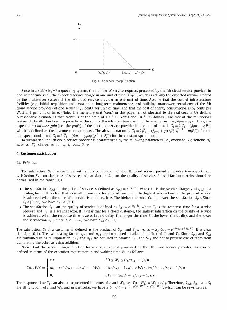
The above service charge function is illustrated in Fig. 1, whose rationals can be found in [1].It is clear that Ci(r, Ti) is a random variable, since both r and Ti are random variables. It has been proven in [1] that the

expected charge to a service request processed by the ith cloud service provider is

C i = Ci(r, Ti) = air̄

(1 − Pq,i

((mi si − λi r̄)(ci/s0,i − 1/si) + 1)((mi si − λi r̄)(ai/di + ci/s0,i − 1/si) + 1)

),

where Pq,i = pi,m /(1 − ρi) and pi,m = pi,0(miρi)mi /mi !.
i i
134


Fig. 1. The service charge function.

Since in a stable M/M/m queueing system, the number of service requests processed by the ith cloud service provider in one unit of time is λi , the expected service charge in one unit of time is λi C i , which is actually the expected revenue created by the multiserver system of the ith cloud service provider in one unit of time. Assume that the cost of infrastructure facilities (e.g., initial acquisition and installation, long-term maintenance, and building, manpower, rental cost of the ith cloud service provider) of one server is βi cents per unit of time, and that the cost of energy consumption is γi cents per Watt and per unit of time. (Note: The monetary unit “cent” in this paper is not identical to the real cent in US dollars. A reasonable estimate is that “cent” is at the scale of 10−4 US cents and 10−6 US dollars.) The cost of the multiserver system of the ith cloud service provider is the sum of the infrastructure cost and the energy cost, i.e., βimi +γi P i . Then, the expected net business gain (i.e., the profit) of the ith cloud service provider in one unit of time is Gi = λi C i − (βimi + γi P i), which is defined as the revenue minus the cost. The above equation is Gi = λi C i − (βimi + γi(λi r̄ξi s

αi−1i + mi P∗

i )) for the idle-speed model, and Gi = λi C i − (βimi + γimi(ξi s

αii + P∗

i )) for the constant-speed model.To summarize, the ith cloud service provider is characterized by the following parameters, i.e., workload: λi ; system: mi ,

si , ξi , αi , P∗i ; charge: s0,i , ai , ci , di ; cost: βi , γi .

4. Customer satisfaction

4.1. Definition

The satisfaction Si of a customer with a service request r of the ith cloud service provider includes two aspects, i.e., satisfaction S p,i on the price of service and satisfaction Sq,i on the quality of service. All satisfaction metrics should be normalized in the range [0, 1].

• The satisfaction S p,i on the price of service is defined as S p,i = e−ηp,i Ci , where Ci is the service charge, and ηp,i is a scaling factor. It is clear that as in all businesses, for a cloud consumer, the highest satisfaction on the price of service is achieved when the price of a service is zero, i.e., free. The higher the price Ci , the lower the satisfaction S p,i . Since Ci ∈ [0, ∞), we have S p,i ∈ (0, 1].

• The satisfaction Sq,i on the quality of service is defined as Sq,i = e−ηq,i T i , where Ti is the response time for a service request, and ηq,i is a scaling factor. It is clear that for a cloud customer, the highest satisfaction on the quality of service is achieved when the response time is zero, i.e., no delay. The longer the time Ti , the lower the quality, and the lower the satisfaction Sq,i . Since Ti ∈ (0, ∞), we have Sq,i ∈ (0, 1).

The satisfaction Si of a customer is defined as the product of S p,i and Sq,i , i.e., Si = S p,i Sq,i = e−(ηp,i Ci+ηq,i T i) . It is clear that Si ∈ (0, 1). The two scaling factors ηp,i and ηq,i are introduced to adapt the effect of Ci and Ti . Since S p,i and Sq,iare combined using multiplication, ηp,i and ηq,i are not used to balance S p,i and Sq,i and not to prevent one of them from dominating the other as using addition.

Notice that the service charge function for a service request processed on the ith cloud service provider can also be defined in terms of the execution requirement r and waiting time W i as follows:

Ci(r, W i) =

⎧⎪⎪⎨⎪⎪⎩

air, if 0 ≤ W i ≤ (ci/s0,i − 1/si)r;(ai + cidi/s0,i − di/si)r − di W i, if (ci/s0,i − 1/si)r < W i ≤ (ai/di + ci/s0,i − 1/si)r;0, if W i > (ai/di + ci/s0,i − 1/si)r.

The response time Ti can also be represented in terms of r and W i , i.e., Ti(r, W i) = W i + r/si . Therefore, S p,i , Sq,i , and Si

are all functions of r and W i , and in particular, we have Si(r, W i) = e−(ηp,i Ci(r,W i)+ηq,i T i(r,W i)) , which can be rewritten as:

135


Si(r, W i) =⎧⎪⎪⎨⎪⎪⎩

e−(ηp,iair+ηq,i(W i+r/si)), if 0 ≤ W i ≤ (ci/s0,i − 1/si)r;e−(ηp,i((ai+cidi/s0,i−di/si)r−di W i)+ηq,i(W i+r/si)), if (ci/s0,i − 1/si)r < W i ≤ (ai/di + ci/s0,i − 1/si)r;e−ηq,i(W i+r/si), if W i > (ai/di + ci/s0,i − 1/si)r.

Since both r and W i are random variables, Si = Si(r, W i) is also a random variable. We are interested in its expectation, i.e., Si . In the following, we calculate Si .

4.2. Derivation

In this section, we derive a closed-form expression of the expected customer satisfaction of a cloud service provider.We define a unit impulse function uz(t) as follows [1]:

uz(t) =

⎧⎪⎨⎪⎩

z, 0 ≤ t ≤ 1

z;

0, t >1

z.

Let z → ∞ and define u(t) = limz→∞ uz(t). It has been proved in [1] that the pdf of the waiting time W i of a newly arrived

service request is

f W i (t) = (1 − Pq,i)u(t) + miμi pi,mi e−(1−ρi)miμi t, 0 ≤ t < ∞,

where Pq,i = pi,mi /(1 − ρi) and pi,mi = pi,0(miρi)mi /mi !.

The expected satisfaction Si(r) of a customer with a service request r is

Si(r) = Si(r, W i)

=∞∫

0

f W i (t)Si(r, t)dt

=∞∫

0

((1 − Pq,i)u(t) + miμi pi,mi e

−(1−ρi)miμi t)

Si(r, t)dt

= (1 − Pq,i)

∞∫0

u(t)Si(r, t)dt + miμi pi,mi

∞∫0

e−(1−ρi)miμi t Si(r, t)dt

= (1 − Pq,i)e−(ηp,iai+ηq,i/si)r + miμi pi,mi

( (ci/s0,i−1/si)r∫0


+(ai/di+ci/s0,i−1/si)r∫

(ci/s0,i−1/si)r

e−(1−ρi)miμi t Si(r, t)dt +∞∫

(ai/di+ci/s0,i−1/si)r


)


( (ci/s0,i−1/si)r∫0

e−(1−ρi)miμi te−(ηp,iair+ηq,i(t+r/si))dt

+(ai/di+ci/s0,i−1/si)r∫

(ci/s0,i−1/si)r

e−(1−ρi)miμi te−(ηp,i((ai+cidi/s0,i−di/si)r−dit)+ηq,i(t+r/si))dt

+∞∫

(ai/di+ci/s0,i−1/si)r

e−(1−ρi)miμi te−ηq,i(t+r/si)dt

)


(e−(ηp,iai+ηq,i/si)r

(ci/s0,i−1/si)r∫e−((1−ρi)miμi+ηq,i)tdt

0

136


+e−(ηp,i(ai+cidi/s0,i−di/si)+ηq,i/si)r

(ai/di+ci/s0,i−1/si)r∫(ci/s0,i−1/si)r

e−((1−ρi)miμi−ηp,idi+ηq,i)tdt

+e−(ηq,i/si)r

∞∫(ai/di+ci/s0,i−1/si)r

e−((1−ρi)miμi+ηq,i)tdt

)


(e−(ηp,iai+ηq,i/si)r · 1 − e−((1−ρi)miμi+ηq,i)(ci/s0,i−1/si)r

(1 − ρi)miμi + ηq,i

+e−(ηp,i(ai+cidi/s0,i−di/si)+ηq,i/si)r

·e−((1−ρi)miμi−ηp,idi+ηq,i)(ci/s0,i−1/si)r − e−((1−ρi)miμi−ηp,idi+ηq,i)(ai/di+ci/s0,i−1/si)r

(1 − ρi)miμi − ηp,idi + ηq,i

+e−(ηq,i/si)r · e−((1−ρi)miμi+ηq,i)(ai/di+ci/s0,i−1/si)r


)


(e−(ηp,iai+ηq,i/si)r − e−((1−ρi)miμi(ci/s0,i−1/si)+ηp,iai+ηq,i ci/s0,i)r


+e−((1−ρi)miμi(ci/s0,i−1/si)+ηp,iai+ηq,i ci/s0,i)r − e−((1−ρi)miμi(ai/di+ci/s0,i−1/si)+ηq,i(ai/di+ci/s0,i))r


+e−((1−ρi)miμi(ai/di+ci/s0,i−1/si)+ηq,i(ai/di+ci/s0,i))r


).

To finish the computation, we notice that the pdf of task execution requirement r is

fr(z) = 1

r̄e−z/r̄, 0 ≤ z < ∞.

Hence, the expected customer satisfaction of the ith cloud service provider is

Si = Si(r)

=∞∫

0

fr(z)Si(z)dz

= 1

r̄

∞∫0

e−z/r̄

((1 − Pq,i)e−(ηp,iai+ηq,i/si)z

+miμi pi,mi

(e−(ηp,iai+ηq,i/si)z − e−((1−ρi)miμi(ci/s0,i−1/si)+ηp,iai+ηq,i ci/s0,i)z


+e−((1−ρi)miμi(ci/s0,i−1/si)+ηp,iai+ηq,i ci/s0,i)z − e−((1−ρi)miμi(ai/di+ci/s0,i−1/si)+ηq,i(ai/di+ci/s0,i))z


+e−((1−ρi)miμi(ai/di+ci/s0,i−1/si)+ηq,i(ai/di+ci/s0,i))z


))dz

= 1

r̄

∞∫0

((1 − Pq,i)e−(ηp,iai+ηq,i/si+1/r̄)z

+miμi pi,mi

(e−(ηp,iai+ηq,i/si+1/r̄)z − e−((1−ρi)miμi(ci/s0,i−1/si)+ηp,iai+ηq,i ci/s0,i+1/r̄)z


+e−((1−ρi)miμi(ci/s0,i−1/si)+ηp,iai+ηq,i ci/s0,i+1/r̄)z − e−((1−ρi)miμi(ai/di+ci/s0,i−1/si)+ηq,i(ai/di+ci/s0,i)+1/r̄)z

(1 − ρ )m μ − η d + η
i i i p,i i q,i
137


Fig. 2. The expected customer satisfaction Si vs. task arrival rate λi .

+e−((1−ρi)miμi(ai/di+ci/s0,i−1/si)+ηq,i(ai/di+ci/s0,i)+1/r̄)z


))dz

= 1

r̄

(1 − Pq,i

ηp,iai + ηq,i/si + 1/r̄+ miμi pi,mi

(1


(1

ηp,iai + ηq,i/si + 1/r̄− 1

(1 − ρi)miμi(ci/s0,i − 1/si) + ηp,iai + ηq,ici/s0,i + 1/r̄

)

+ 1


(1

(1 − ρi)miμi(ci/s0,i − 1/si) + ηp,iai + ηq,ici/s0,i + 1/r̄

− 1

(1 − ρi)miμi(ai/di + ci/s0,i − 1/si) + ηq,i(ai/di + ci/s0,i) + 1/r̄

)

+ 1

(1 − ρi)miμi + ηq,i· 1

(1 − ρi)miμi(ai/di + ci/s0,i − 1/si) + ηq,i(ai/di + ci/s0,i) + 1/r̄

)).

4.3. Data

Consider a cloud service provider whose multiserver system has the following parameter setting: λi = 8.0, r̄ = 1.0, mi =7, si = 1.5, ξi = 4.0, αi = 3.0, P∗

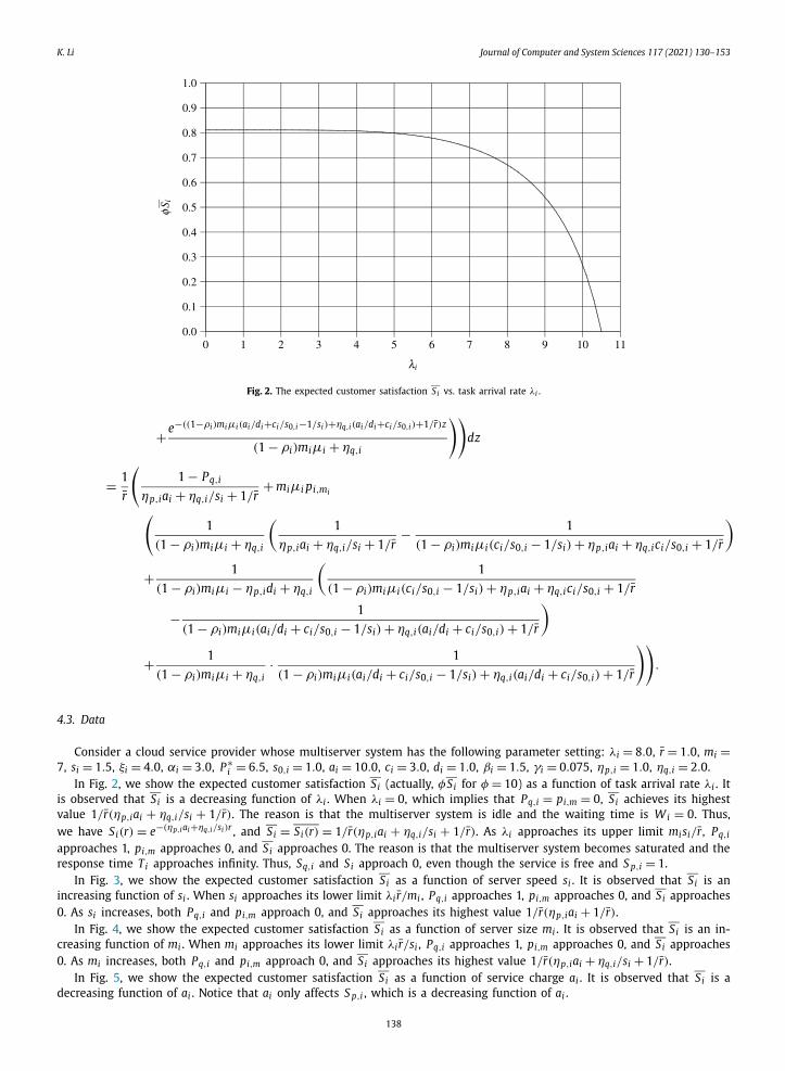
i = 6.5, s0,i = 1.0, ai = 10.0, ci = 3.0, di = 1.0, βi = 1.5, γi = 0.075, ηp,i = 1.0, ηq,i = 2.0.In Fig. 2, we show the expected customer satisfaction Si (actually, φSi for φ = 10) as a function of task arrival rate λi . It

is observed that Si is a decreasing function of λi . When λi = 0, which implies that Pq,i = pi,m = 0, Si achieves its highest value 1/r̄(ηp,iai + ηq,i/si + 1/r̄). The reason is that the multiserver system is idle and the waiting time is W i = 0. Thus, we have Si(r) = e−(ηp,iai+ηq,i/si)r , and Si = Si(r) = 1/r̄(ηp,iai + ηq,i/si + 1/r̄). As λi approaches its upper limit mi si/r̄, Pq,i

approaches 1, pi,m approaches 0, and Si approaches 0. The reason is that the multiserver system becomes saturated and the response time Ti approaches infinity. Thus, Sq,i and Si approach 0, even though the service is free and S p,i = 1.

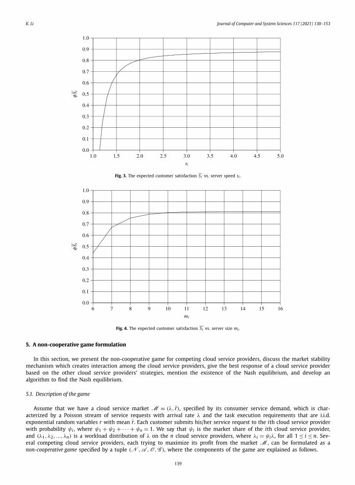
In Fig. 3, we show the expected customer satisfaction Si as a function of server speed si . It is observed that Si is an increasing function of si . When si approaches its lower limit λi r̄/mi , Pq,i approaches 1, pi,m approaches 0, and Si approaches 0. As si increases, both Pq,i and pi,m approach 0, and Si approaches its highest value 1/r̄(ηp,iai + 1/r̄).

In Fig. 4, we show the expected customer satisfaction Si as a function of server size mi . It is observed that Si is an in-creasing function of mi . When mi approaches its lower limit λi r̄/si , Pq,i approaches 1, pi,m approaches 0, and Si approaches 0. As mi increases, both Pq,i and pi,m approach 0, and Si approaches its highest value 1/r̄(ηp,iai + ηq,i/si + 1/r̄).

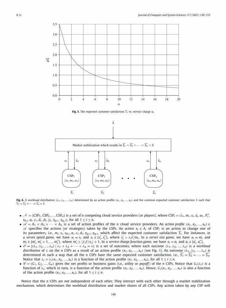
In Fig. 5, we show the expected customer satisfaction Si as a function of service charge ai . It is observed that Si is a decreasing function of ai . Notice that ai only affects S p,i , which is a decreasing function of ai .

138


Fig. 3. The expected customer satisfaction Si vs. server speed si .

Fig. 4. The expected customer satisfaction Si vs. server size mi .

5. A non-cooperative game formulation

In this section, we present the non-cooperative game for competing cloud service providers, discuss the market stability mechanism which creates interaction among the cloud service providers, give the best response of a cloud service provider based on the other cloud service providers’ strategies, mention the existence of the Nash equilibrium, and develop an algorithm to find the Nash equilibrium.

5.1. Description of the game

Assume that we have a cloud service market M = (λ, ̄r), specified by its consumer service demand, which is char-acterized by a Poisson stream of service requests with arrival rate λ and the task execution requirements that are i.i.d. exponential random variables r with mean r̄. Each customer submits his/her service request to the ith cloud service provider with probability ψi , where ψ1 + ψ2 + · · · + ψn = 1. We say that ψi is the market share of the ith cloud service provider, and (λ1, λ2, ..., λn) is a workload distribution of λ on the n cloud service providers, where λi = ψiλ, for all 1 ≤ i ≤ n. Sev-eral competing cloud service providers, each trying to maximize its profit from the market M , can be formulated as a non-cooperative game specified by a tuple (N , A , O, G ), where the components of the game are explained as follows.

139


Fig. 5. The expected customer satisfaction Si vs. service charge ai .

Fig. 6. A workload distribution (λ1, λ2, ..., λn) determined by an action profile (x1, x2, ..., xn) and the common expected customer satisfaction S such that S1 = S2 = · · · = Sn = S .

• N = {CSP1, CSP2, ..., CSPn} is a set of n competing cloud service providers (or players), where CSPi = (λi, mi, si, ξi, αi, P∗i ,

s0,i, ai, ci, di, βi, γi, ηp,i, ηq,i), for all 1 ≤ i ≤ n.• A = A1 × A2 × · · · × An is a set of action profiles of the n cloud service providers. An action profile (x1, x2, ..., xn) ∈

A specifies the actions (or strategies) taken by the CSPs. An action xi ∈ Ai of CSPi is an action to change one of its parameters, i.e., mi, si, s0,i, ai, ci, di, ηp,i, ηq,i , which affect the expected customer satisfaction Si . For instances, in a server speed game, we have xi = si and si ∈ [s′

i, s′′i ], where s′

i > λi r̄/mi . In a server size game, we have xi = mi and mi ∈ {m′

i, m′i + 1, ..., m′′

i }, where m′i ≥ λi r̄/si� + 1. In a service charge function game, we have xi = ai and ai ∈ [a′

i, a′′i ].

• O = {(λ1, λ2, ..., λn) | λ1 + λ2 + · · · + λn = λ} is a set of outcomes, where each outcome (λ1, λ2, ..., λn) is a workload distribution of λ on the n CSPs as a result of an action profile (x1, x2, ..., xn) (see Fig. 6). An outcome (λ1, λ2, ..., λn) is determined in such a way that all the n CSPs have the same expected customer satisfaction, i.e., S1 = S2 = · · · = Sn . Notice that λi = λi(x1, x2, ..., xn) is a function of the action profile (x1, x2, ..., xn), for all 1 ≤ i ≤ n.

• G = (G1, G2, ..., Gn) gives the net profits or business gains (i.e., utility or payoff ) of the n CSPs. Notice that Gi(λi) is a function of λi , which in turn, is a function of the action profile (x1, x2, ..., xn). Hence, Gi(x1, x2, ..., xn) is also a function of the action profile (x1, x2, ..., xn), for all 1 ≤ i ≤ n.

Notice that the n CSPs are not independent of each other. They interact with each other through a market stabilization mechanism, which determines the workload distribution and market shares of all CSPs. Any action taken by any CSP will

140


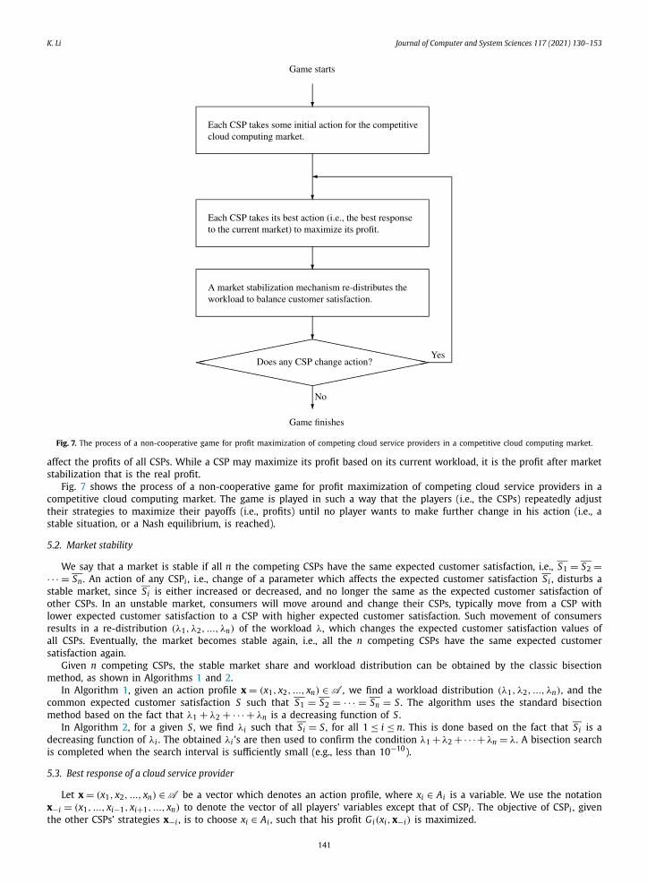
Fig. 7. The process of a non-cooperative game for profit maximization of competing cloud service providers in a competitive cloud computing market.

affect the profits of all CSPs. While a CSP may maximize its profit based on its current workload, it is the profit after market stabilization that is the real profit.

Fig. 7 shows the process of a non-cooperative game for profit maximization of competing cloud service providers in a competitive cloud computing market. The game is played in such a way that the players (i.e., the CSPs) repeatedly adjust their strategies to maximize their payoffs (i.e., profits) until no player wants to make further change in his action (i.e., a stable situation, or a Nash equilibrium, is reached).

5.2. Market stability

We say that a market is stable if all n the competing CSPs have the same expected customer satisfaction, i.e., S1 = S2 =· · · = Sn . An action of any CSPi , i.e., change of a parameter which affects the expected customer satisfaction Si , disturbs a stable market, since Si is either increased or decreased, and no longer the same as the expected customer satisfaction of other CSPs. In an unstable market, consumers will move around and change their CSPs, typically move from a CSP with lower expected customer satisfaction to a CSP with higher expected customer satisfaction. Such movement of consumers results in a re-distribution (λ1, λ2, ..., λn) of the workload λ, which changes the expected customer satisfaction values of all CSPs. Eventually, the market becomes stable again, i.e., all the n competing CSPs have the same expected customer satisfaction again.

Given n competing CSPs, the stable market share and workload distribution can be obtained by the classic bisection method, as shown in Algorithms 1 and 2.

In Algorithm 1, given an action profile x = (x1, x2, ..., xn) ∈ A , we find a workload distribution (λ1, λ2, ..., λn), and the common expected customer satisfaction S such that S1 = S2 = · · · = Sn = S . The algorithm uses the standard bisection method based on the fact that λ1 + λ2 + · · · + λn is a decreasing function of S .

In Algorithm 2, for a given S , we find λi such that Si = S , for all 1 ≤ i ≤ n. This is done based on the fact that Si is a decreasing function of λi . The obtained λi ’s are then used to confirm the condition λ1 +λ2 +· · ·+λn = λ. A bisection search is completed when the search interval is sufficiently small (e.g., less than 10−10).

5.3. Best response of a cloud service provider

Let x = (x1, x2, ..., xn) ∈ A be a vector which denotes an action profile, where xi ∈ Ai is a variable. We use the notation x−i = (x1, ..., xi−1, xi+1, ..., xn) to denote the vector of all players’ variables except that of CSPi . The objective of CSPi , given the other CSPs’ strategies x−i , is to choose xi ∈ Ai , such that his profit Gi(xi, x−i) is maximized.

141


Algorithm 1: Stabilizing market.

Input: M = (λ, ̄r), N = {CSP1, CSP2, ..., CSPn}, and an action profile x = (x1, x2, ..., xn) ∈ A .

Output: A workload distribution (λ1, λ2, ..., λn), such that S1 = S2 = · · · = Sn .

Initialize the search interval of S to be (0, 1); (1)

while (the length of the search interval is not less than ε) do (2)

S ← the middle point of the search interval; (3)

for i ← 1 to n do (4)

Obtain λi by using algorithm Finding λi with parameters CSPi and S; (5)

end do; (6)

if (λ1 + λ2 + · · · + λn < λ) then (7)

Change the search interval to the left half; (8)

else (9)

Change the search interval to the right half; (10)

end if (11)

end do; (12)

S ← the middle point of the search interval; (13)


Obtain λi by using algorithm Finding λi ; (15)

end do; (16)

return (λ1, λ2, ..., λn). (17)

Algorithm 2: Finding λi .

Input: CSPi and S .

Output: λi such that Si = S .

Initialize the search interval of λi to be [0, mi si/r̄]; (1)

while (the length of the search interval is not less than ε) do (2)

λi ← the middle point of the search interval; (3)

Calculate Si ; (4)

if (Si < S) then (5)

Change the search interval to the left half; (6)

else (7)

Change the search interval to the right half; (8)

end if (9)

end do; (10)

λi ← the middle point of the search interval; (11)

return λi . (12)

When xi changes, it results in a new stable market, where all the n competing CSPs have the same expected customer satisfaction S , which can be viewed as a function S(xi) of xi . The value of S then determines a workload distribution (λ1, λ2, ..., λn), and in particular, λi can be viewed as a function λi(S) of S . The value of λi finally decides the profit Gi of CSPi , and Gi can be viewed as a function Gi(λi) of λi . Therefore, we have Gi = Gi(λi, xi) = Gi(λi(S), xi) = Gi(λi(S(xi)), xi), i.e., Gi can be viewed as a function Gi(xi) of xi .

Essentially, we need to find xi such that ∂Gi(xi)/∂xi = 0. Notice that ∂Gi(xi)/∂xi involves ∂Gi/∂λi , ∂λi/∂ S , and ∂ S/∂xi . The main challenge here is that there is no explicit closed-form expressions for the two functions λi(S) and S(xi). From an implicit equation Si(λi) = S , where Si is viewed as a function of λi , we still cannot derive ∂λi/∂ S , because a closed-

form expression for Si−1

(S), i.e., the inverse function to find λi for a given S , is not available. Although from the condition λ1 + λ2 + · · · + λn = λ and the implicit equation

S1−1

(S) + S2−1

(S) + · · · + Sn−1

(S) = λ,

we can find S for a given xi numerically, there is no way to find ∂ S/∂xi , since no closed-form expression for S(xi) is available.

Our algorithm for the best response of a cloud service provider is given in Algorithm 3. We consider the case when Ai(i.e., the set of actions for CSPi ) is discrete. The algorithm finds xi such that Gi(xi) is maximized, i.e., Gi(xi) = max

x∈Ai

(Gi(x)).

This can be realized by traversing through the discrete set Ai . As mentioned above, the best response of CSPi with continu-ous Ai remains unknown and needs further investigation.

142


Algorithm 3: Finding xi (best response of CSPi with discrete Ai ).

Input: M = (λ, ̄r), N = {CSP1, CSP2, ..., CSPn}, an action profile x = (x1, x2, ..., xn) ∈ A , index i.Output: xi such that Gi(xi) is maximized, i.e., Gi(xi) = max

x∈Ai

(Gi(x)).

Gopt ← 0; (1)

for (each x ∈ Ai ) do (2)

Find λi by using algorithm Stabilizing Market with parameters M , N , and x′ = (x, x−i); (3)

Calculate Gi(x); (4)

if (Gi(x) > Gopt) then (5)

xi ← x; (6)

end if (7)

end do; (8)

return xi . (9)

Algorithm 4: Calculating the Nash equilibrium.

Input: M = (λ, ̄r) and N = {CSP1, CSP2, ..., CSPn}.

Output: The Nash equilibrium x∗ = (x∗1, x∗

2, ..., x∗n).

Initialize x = (x1, x2, ..., xn) to some appropriate vector; (1)

repeat (2)


Obtain x′i by using algorithm Finding xi (4)

with parameters M , N , x′ = (x′1, ..., x′

i−1, xi , xi+1, ..., xn), and i; (5)

end do; (6)

x′ ← (x′1, x′

2, ..., x′n); (7)

if (x′ = x) then (8)

x ← x′; (9)

else (10)

x∗ ← x′; (11)

return x∗; (12)

end if (13)

forever. (14)

Fig. 8. The net profit G4 vs. server speed s4.

143


Fig. 9. The net profit G4 vs. server size m4.

Fig. 10. The net profit G4 vs. service charge a4.

5.4. Existence of the Nash equilibrium

A (pure strategy) Nash equilibrium is a vector x∗ = (x∗1, x

∗2, ..., x

∗n), which satisfies

Gi(x∗i ,x∗

−i) ≥ Gi(xi,x∗−i), for all xi ∈ Ai, and for all 1 ≤ i ≤ n.

In words, a Nash equilibrium is a strategy profile x∗ with the property that no single CSPi can benefit from a unilateral deviation from x∗

i , if all the other CSPs act according to it.The most important issues of a non-cooperative game are an analytical issue, i.e., the existence (and even uniqueness) of

the Nash equilibrium, and an algorithmic issue, i.e., the convergence of an iterative best-response-based algorithm.Let F : A →Rn be a mapping:

F(x) = (∂G1(x)/∂x1, ∂G2(x)/∂x2, ..., ∂Gn(x)/∂xn).

The following result is from [45,46].

Theorem 1. If A ⊆ Rn is convex and compact (closed and bounded), and Gi(x) is continuously differentiable in x and Gi(xi, x−i) is concave (i.e., Fi(x) = ∂Gi(x)/∂xi) is monotonically decreasing) in xi for each fixed x−i , then there exists a Nash equilibrium.

144


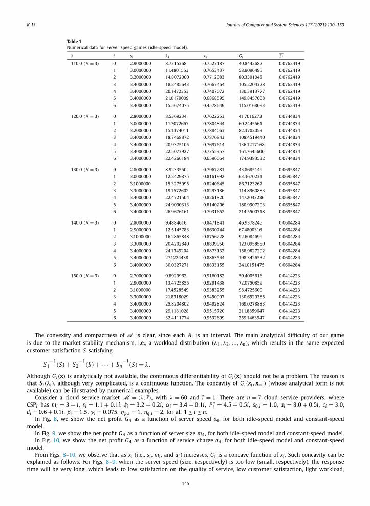
Table 1Numerical data for server speed games (idle-speed model).

λ i si λi ρi Gi Si

110.0 (K = 3) 0 2.9000000 8.7315368 0.7527187 40.8442682 0.0762419

1 3.0000000 11.4801553 0.7653437 58.9096495 0.0762419

2 3.2000000 14.8072000 0.7712083 80.3391048 0.0762419

3 3.4000000 18.2485643 0.7667464 105.2204328 0.0762419

4 3.4000000 20.1472353 0.7407072 130.3913777 0.0762419

5 3.4000000 21.0179009 0.6868595 149.8457008 0.0762419

6 3.4000000 15.5674075 0.4578649 115.0168093 0.0762419

120.0 (K = 3) 0 2.8000000 8.5369234 0.7622253 41.7016273 0.0744834

1 3.0000000 11.7072667 0.7804844 60.2445561 0.0744834

2 3.2000000 15.1374011 0.7884063 82.3702053 0.0744834

3 3.4000000 18.7468872 0.7876843 108.4519440 0.0744834

4 3.4000000 20.9375105 0.7697614 136.1217168 0.0744834

5 3.4000000 22.5073927 0.7355357 161.7645600 0.0744834

6 3.4000000 22.4266184 0.6596064 174.9383532 0.0744834

130.0 (K = 3) 0 2.8000000 8.9233550 0.7967281 43.8685149 0.0695847

1 3.0000000 12.2429875 0.8161992 63.3670231 0.0695847

2 3.1000000 15.3275995 0.8240645 86.7123267 0.0695847

3 3.3000000 19.1572602 0.8293186 114.8960883 0.0695847

4 3.4000000 22.4721504 0.8261820 147.2033236 0.0695847

5 3.4000000 24.9090313 0.8140206 180.9307203 0.0695847

6 3.4000000 26.9676161 0.7931652 214.5500318 0.0695847

140.0 (K = 3) 0 2.8000000 9.4884616 0.8471841 46.9378245 0.0604284

1 2.9000000 12.5145783 0.8630744 67.4800316 0.0604284

2 3.1000000 16.2865848 0.8756228 92.6084699 0.0604284

3 3.3000000 20.4202840 0.8839950 123.0958580 0.0604284

4 3.4000000 24.1349204 0.8873132 158.9827292 0.0604284

5 3.4000000 27.1224438 0.8863544 198.3426532 0.0604284

6 3.4000000 30.0327271 0.8833155 241.0151475 0.0604284

150.0 (K = 3) 0 2.7000000 9.8929962 0.9160182 50.4005616 0.0414223

1 2.9000000 13.4725855 0.9291438 72.0750859 0.0414223

2 3.1000000 17.4528549 0.9383255 98.4725600 0.0414223

3 3.3000000 21.8318029 0.9450997 130.6529385 0.0414223

4 3.4000000 25.8204802 0.9492824 169.0278883 0.0414223

5 3.4000000 29.1181028 0.9515720 211.8859647 0.0414223

6 3.4000000 32.4111774 0.9532699 259.1463947 0.0414223

The convexity and compactness of A is clear, since each Ai is an interval. The main analytical difficulty of our game is due to the market stability mechanism, i.e., a workload distribution (λ1, λ2, ..., λn), which results in the same expected customer satisfaction S satisfying

S1−1

(S) + S2−1

(S) + · · · + Sn−1

(S) = λ.

Although Gi(x) is analytically not available, the continuous differentiability of Gi(x) should not be a problem. The reason is that Si(λi), although very complicated, is a continuous function. The concavity of Gi(xi, x−i) (whose analytical form is not available) can be illustrated by numerical examples.

Consider a cloud service market M = (λ, ̄r), with λ = 60 and r̄ = 1. There are n = 7 cloud service providers, where CSPi has mi = 3 + i, si = 1.1 + 0.1i, ξi = 3.2 + 0.2i, αi = 3.4 − 0.1i, P∗

i = 4.5 + 0.5i, s0,i = 1.0, ai = 8.0 + 0.5i, ci = 3.0, di = 0.6 + 0.1i, βi = 1.5, γi = 0.075, ηp,i = 1, ηq,i = 2, for all 1 ≤ i ≤ n.

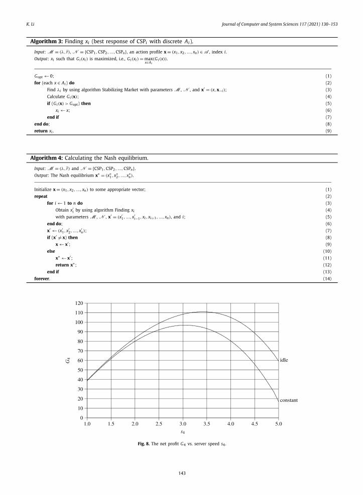
In Fig. 8, we show the net profit G4 as a function of server speed s4, for both idle-speed model and constant-speed model.

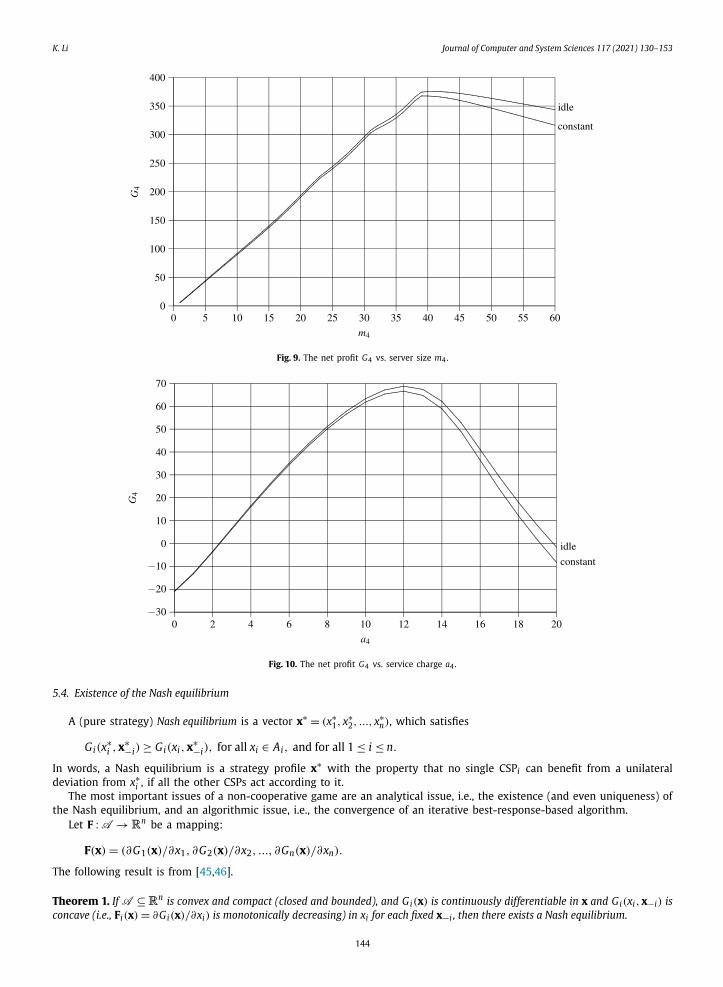
In Fig. 9, we show the net profit G4 as a function of server size m4, for both idle-speed model and constant-speed model.In Fig. 10, we show the net profit G4 as a function of service charge a4, for both idle-speed model and constant-speed

model.From Figs. 8–10, we observe that as xi (i.e., si , mi , and ai ) increases, Gi is a concave function of xi . Such concavity can be

explained as follows. For Figs. 8–9, when the server speed (size, respectively) is too low (small, respectively), the response time will be very long, which leads to low satisfaction on the quality of service, low customer satisfaction, light workload,

145


Table 2Numerical data for server speed games (constant-speed model).

λ i si λi ρi Gi Si

110.0 (K = 3) 0 2.6000000 7.9087990 0.7604614 35.7211541 0.0735022

1 2.7000000 10.4715781 0.7756724 52.1461436 0.0735022

2 2.9000000 13.6669256 0.7854555 71.6296263 0.0735022

3 3.0000000 16.4387423 0.7827973 93.6791942 0.0735022

4 3.2000000 19.8539530 0.7755450 118.6860447 0.0735022

5 3.3000000 22.3230123 0.7516166 142.8851955 0.0735022

6 2.9000000 19.3369897 0.6667927 140.2268513 0.0735022

120.0 (K = 2) 0 2.6000000 8.1702010 0.7855962 37.8968179 0.0700138

1 2.7000000 10.8278420 0.8020624 55.2987844 0.0700138

2 2.9000000 14.1640928 0.8140283 76.2930250 0.0700138

3 3.0000000 17.1346889 0.8159376 100.5766641 0.0700138

4 3.2000000 20.8811874 0.8156714 129.4100236 0.0700138

5 3.3000000 23.9233543 0.8055001 160.4317672 0.0700138

6 3.2000000 24.8986337 0.7780823 185.5232594 0.0700138

130.0 (K = 2) 0 2.6000000 8.5279306 0.8199933 40.8368441 0.0643938

1 2.7000000 11.2982726 0.8369091 59.4128039 0.0643938

2 2.9000000 14.7927081 0.8501556 82.1276673 0.0643938

3 3.0000000 17.9670285 0.8555728 108.7517816 0.0643938

4 3.2000000 22.0203293 0.8601691 141.2148045 0.0643938

5 3.4000000 26.3573242 0.8613505 179.7163252 0.0643938

6 3.4000000 29.0364066 0.8540120 218.7726667 0.0643938

140.0 (K = 3) 0 2.6000000 9.0795308 0.8730318 45.1763980 0.0531795

1 2.7000000 11.9898079 0.8881339 65.2067150 0.0531795

2 2.9000000 15.6675539 0.9004341 89.9264587 0.0531795

3 3.1000000 19.7300845 0.9092205 119.9266014 0.0531795

4 3.3000000 24.1721132 0.9156103 156.2840465 0.0531795

5 3.4000000 28.1123912 0.9187056 198.3162207 0.0531795

6 3.4000000 31.2485183 0.9190741 243.4833860 0.0531795

150.0 (K = 3) 0 2.6000000 9.7010278 0.9327911 48.8764199 0.0348202

1 2.8000000 13.2146110 0.9439008 70.1546493 0.0348202

2 3.0000000 17.1308001 0.9517111 96.0951374 0.0348202

3 3.2000000 21.4483048 0.9575136 127.7202034 0.0348202

4 3.4000000 26.1662353 0.9619939 166.2466975 0.0348202

5 3.4000000 29.5020654 0.9641198 209.4477416 0.0348202

6 3.4000000 32.8369556 0.9657928 257.1498553 0.0348202

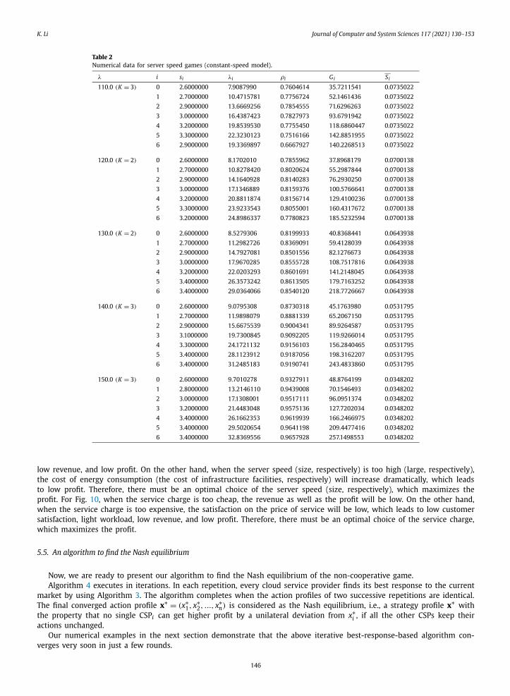
low revenue, and low profit. On the other hand, when the server speed (size, respectively) is too high (large, respectively), the cost of energy consumption (the cost of infrastructure facilities, respectively) will increase dramatically, which leads to low profit. Therefore, there must be an optimal choice of the server speed (size, respectively), which maximizes the profit. For Fig. 10, when the service charge is too cheap, the revenue as well as the profit will be low. On the other hand, when the service charge is too expensive, the satisfaction on the price of service will be low, which leads to low customer satisfaction, light workload, low revenue, and low profit. Therefore, there must be an optimal choice of the service charge, which maximizes the profit.

5.5. An algorithm to find the Nash equilibrium

Now, we are ready to present our algorithm to find the Nash equilibrium of the non-cooperative game.Algorithm 4 executes in iterations. In each repetition, every cloud service provider finds its best response to the current

market by using Algorithm 3. The algorithm completes when the action profiles of two successive repetitions are identical. The final converged action profile x∗ = (x∗

1, x∗2, ..., x

∗n) is considered as the Nash equilibrium, i.e., a strategy profile x∗ with

the property that no single CSPi can get higher profit by a unilateral deviation from x∗i , if all the other CSPs keep their

actions unchanged.Our numerical examples in the next section demonstrate that the above iterative best-response-based algorithm con-

verges very soon in just a few rounds.

146


Table 3Numerical data for server size games (idle-speed model).

λ i mi λi ρi Gi Si

110.0 (K = 2) 0 20 37.5407990 0.8532000 222.8245121 0.0866674

1 20 37.4928218 0.8150613 235.8914060 0.0866674

2 20 34.9663792 0.7284662 230.5208550 0.0866674

3 1 0.0000000 0.0000000 -1.9875000 —

4 1 0.0000000 0.0000000 -2.0250000 —

5 1 0.0000000 0.0000000 -2.0625000 —

6 1 0.0000000 0.0000000 -2.1000000 —

120.0 (K = 2) 0 20 38.2045328 0.8682848 227.3981315 0.0846704

1 20 38.6445170 0.8400982 244.2890126 0.0846704

2 20 37.9203932 0.7900082 253.2747341 0.0846704

3 7 5.2305570 0.2988890 28.5857128 0.0846704

4 1 0.0000000 0.0000000 -2.0250000 —

5 1 0.0000000 0.0000000 -2.0625000 —

6 1 0.0000000 0.0000000 -2.1000000 —

130.0 (K = 2) 0 20 38.2497401 0.8693123 227.7091738 0.0845190

1 20 38.7185454 0.8417075 244.8282565 0.0845190

2 20 38.0749608 0.7932283 254.4646503 0.0845190

3 12 14.9567538 0.4985585 97.6731935 0.0845190

4 1 0.0000000 0.0000000 -2.0250000 —

5 1 0.0000000 0.0000000 -2.0625000 —

6 1 0.0000000 0.0000000 -2.1000000 —

140.0 (K = 2) 0 20 38.2612587 0.8695741 227.7884149 0.0844801

1 20 38.7373292 0.8421159 244.9650704 0.0844801

2 20 38.1137310 0.7940361 254.7631012 0.0844801

3 17 24.8876811 0.5855925 168.4241996 0.0844801

4 1 0.0000000 0.0000000 -2.0250000 —

5 1 0.0000000 0.0000000 -2.0625000 —

6 1 0.0000000 0.0000000 -2.1000000 —

150.0 (K = 2) 0 20 38.3977234 0.8726755 228.7268423 0.0840082

1 20 38.9575267 0.8469028 246.5684852 0.0840082

2 20 38.5556781 0.8032433 258.1646807 0.0840082

3 20 34.0890717 0.6817814 237.2207003 0.0840082

4 1 0.0000000 0.0000000 -2.0250000 —

5 1 0.0000000 0.0000000 -2.0625000 —

6 1 0.0000000 0.0000000 -2.1000000 —

6. Numerical examples

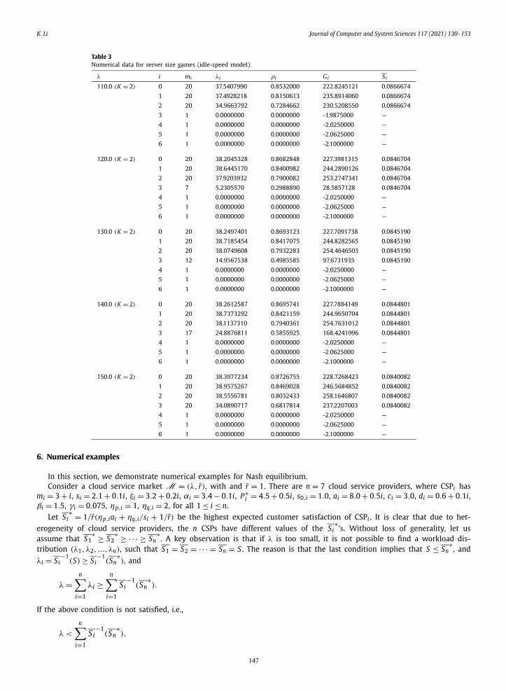
In this section, we demonstrate numerical examples for Nash equilibrium.Consider a cloud service market M = (λ, ̄r), with and r̄ = 1. There are n = 7 cloud service providers, where CSPi has

mi = 3 + i, si = 2.1 + 0.1i, ξi = 3.2 + 0.2i, αi = 3.4 − 0.1i, P∗i = 4.5 + 0.5i, s0,i = 1.0, ai = 8.0 + 0.5i, ci = 3.0, di = 0.6 + 0.1i,

βi = 1.5, γi = 0.075, ηp,i = 1, ηq,i = 2, for all 1 ≤ i ≤ n.Let Si

∗ = 1/r̄(ηp,iai + ηq,i/si + 1/r̄) be the highest expected customer satisfaction of CSPi . It is clear that due to het-erogeneity of cloud service providers, the n CSPs have different values of the Si

∗’s. Without loss of generality, let us

assume that S1∗ ≥ S2

∗ ≥ · · · ≥ Sn∗

. A key observation is that if λ is too small, it is not possible to find a workload dis-tribution (λ1, λ2, ..., λn), such that S1 = S2 = · · · = Sn = S . The reason is that the last condition implies that S ≤ Sn

∗, and

λi = Si−1

(S) ≥ Si−1

(Sn∗), and

λ =n∑

i=1

λi ≥n∑

i=1

Si−1

(Sn∗).

If the above condition is not satisfied, i.e.,

λ <

n∑Si

−1(Sn

∗),

i=1

147


Table 4Numerical data for server size games (constant-speed model).

λ i mi λi ρi Gi Si

110.0 (K = 2) 0 20 37.5407990 0.8532000 212.7252151 0.0866674

1 20 37.4928218 0.8150613 221.5381466 0.0866674

2 20 34.9663792 0.7284662 207.1672704 0.0866674

3 1 0.0000000 0.0000000 -6.6750000 —

4 1 0.0000000 0.0000000 -7.0569146 —

5 1 0.0000000 0.0000000 -7.3876578 —

6 1 0.0000000 0.0000000 -7.6609089 —

120.0 (K = 2) 0 20 38.3577999 0.8717682 219.6304981 0.0841483

1 20 38.8935450 0.8455118 234.1127029 0.0841483

2 20 38.4295455 0.8006155 240.0456639 0.0841483

3 5 4.3191097 0.3455288 9.8154498 0.0841483

4 1 0.0000000 0.0000000 -7.0569146 —

5 1 0.0000000 0.0000000 -7.3876578 —

6 1 0.0000000 0.0000000 -7.6609089 —

130.0 (K = 2) 0 20 38.4374599 0.8735786 220.3026446 0.0838669

1 20 39.0208595 0.8482796 235.2543412 0.0838669

2 20 38.6788122 0.8058086 242.4105740 0.0838669

3 10 13.8628684 0.5545147 71.8765313 0.0838669

4 1 0.0000000 0.0000000 -7.0569146 —

5 1 0.0000000 0.0000000 -7.3876578 —

6 1 0.0000000 0.0000000 -7.6609089 —

140.0 (K = 2) 0 20 38.4281335 0.8733667 220.2239637 0.0839002

1 20 39.0060257 0.8479571 235.1213405 0.0839002

2 20 38.6501212 0.8052109 242.1383868 0.0839002

3 15 23.9157196 0.6377525 139.0293256 0.0839002

4 1 0.0000000 0.0000000 -7.0569146 —

5 1 0.0000000 0.0000000 -7.3876578 —

6 1 0.0000000 0.0000000 -7.6609089 —

150.0 (K = 2) 0 20 38.5140226 0.8753187 220.9484170 0.0835897

1 20 39.1419293 0.8509115 236.3397119 0.0835897

2 20 38.9097054 0.8106189 244.6008428 0.0835897

3 19 33.4343427 0.7038809 207.5131447 0.0835897

4 1 0.0000000 0.0000000 -7.0569146 —

5 1 0.0000000 0.0000000 -7.3876578 —

6 1 0.0000000 0.0000000 -7.6609089 —

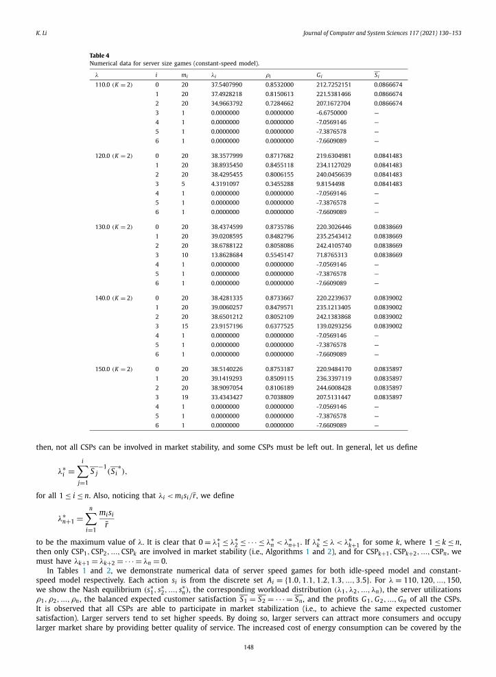
then, not all CSPs can be involved in market stability, and some CSPs must be left out. In general, let us define

λ∗i =

i∑j=1

S j−1

(Si∗),

for all 1 ≤ i ≤ n. Also, noticing that λi < mi si/r̄, we define

λ∗n+1 =

n∑i=1

mi si

r̄

to be the maximum value of λ. It is clear that 0 = λ∗1 ≤ λ∗

2 ≤ · · · ≤ λ∗n < λ∗

n+1. If λ∗k ≤ λ < λ∗

k+1 for some k, where 1 ≤ k ≤ n, then only CSP1, CSP2, ..., CSPk are involved in market stability (i.e., Algorithms 1 and 2), and for CSPk+1, CSPk+2, ..., CSPn , we must have λk+1 = λk+2 = · · · = λn = 0.

In Tables 1 and 2, we demonstrate numerical data of server speed games for both idle-speed model and constant-speed model respectively. Each action si is from the discrete set Ai = {1.0, 1.1, 1.2, 1.3, ..., 3.5}. For λ = 110, 120, ..., 150, we show the Nash equilibrium (s∗

1, s∗2, ..., s

∗n), the corresponding workload distribution (λ1, λ2, ..., λn), the server utilizations

ρ1, ρ2, ..., ρn , the balanced expected customer satisfaction S1 = S2 = · · · = Sn , and the profits G1, G2, ..., Gn of all the CSPs. It is observed that all CSPs are able to participate in market stabilization (i.e., to achieve the same expected customer satisfaction). Larger servers tend to set higher speeds. By doing so, larger servers can attract more consumers and occupy larger market share by providing better quality of service. The increased cost of energy consumption can be covered by the

148


Table 5Numerical data for service charge function games (idle-speed model).

λ i ai λi ρi Gi Si

80.0 (K = 12) 0 3.5000000 5.0211914 0.5705899 2.2092155 0.1678751

1 3.5000000 7.3429953 0.6385213 3.7277767 0.1678751

2 3.5000000 9.9322083 0.6897367 5.2366216 0.1678751

3 4.0000000 9.7592078 0.5576690 6.8214878 0.1678751

4 4.0000000 12.7098419 0.6110501 10.0346180 0.1678751

5 4.0000000 15.9032987 0.6544567 13.6752179 0.1678751

6 4.0000000 19.3312567 0.6904020 17.9191394 0.1678751

90.0 (K = 8) 0 9.0000000 5.5743117 0.6334445 33.9174716 0.0796446

1 9.0000000 7.9349743 0.6899978 48.4137078 0.0796446

2 9.5000000 9.8408769 0.6833942 64.1182641 0.0796446

3 9.5000000 12.6140291 0.7208017 82.2207212 0.0796446

4 9.5000000 15.6224772 0.7510806 101.9167088 0.0796446

5 10.0000000 17.5210261 0.7210299 122.0569434 0.0796446

6 10.0000000 20.8923046 0.7461537 146.3876470 0.0796446

100.0 (K = 4) 0 15.0000000 5.8917928 0.6695219 71.6078666 0.0499211

1 15.0000000 8.2980510 0.7215697 100.8272744 0.0499211

2 15.0000000 10.9478833 0.7602697 132.7937386 0.0499211

3 15.0000000 13.8307587 0.7903291 167.4763804 0.0499211

4 15.0000000 16.9400003 0.8144231 204.9393059 0.0499211

5 15.0000000 20.2710238 0.8341985 245.3063160 0.0499211

6 15.0000000 23.8204901 0.8507318 288.7372253 0.0499211

110.0 (K = 3) 0 15.0000000 6.9386222 0.7884798 85.5015005 0.0417008

1 15.0000000 9.4955072 0.8256963 116.5286405 0.0417008

2 15.0000000 12.2787221 0.8526890 150.0518070 0.0417008

3 15.0000000 15.2817285 0.8732416 186.1080739 0.0417008

4 15.0000000 18.5003323 0.8894391 224.8063553 0.0417008

5 15.0000000 21.9316233 0.9025359 266.3017147 0.0417008

6 15.0000000 25.5734644 0.9133380 310.7762493 0.0417008

120.0 (K = 2) 0 15.0000000 8.1073095 0.9212852 99.3555763 0.0232192

1 15.0000000 10.7752334 0.9369768 130.9748683 0.0232192

2 15.0000000 13.6513625 0.9480113 164.7133981 0.0232192

3 15.0000000 16.7334281 0.9561959 200.6682420 0.0232192

4 15.0000000 20.0199693 0.9624985 238.9843602 0.0232192

5 15.0000000 23.5099772 0.9674888 279.8388111 0.0232192

6 15.0000000 27.2027200 0.9715257 323.4264782 0.0232192

increased revenue, and eventually more profits are made. All CSPs have about the same server utilization and definitely the same expected customer satisfaction.

In Tables 3 and 4, we demonstrate numerical data of server size games for both idle-speed model and constant-speed model respectively. Each action mi is from the discrete set Ai = {1, 2, 3, 4, ..., 20}. For λ = 110, 120, ..., 150, we show the Nash equilibrium (m∗

1, m∗2, ..., m

∗n), the corresponding workload distribution (λ1, λ2, ..., λn), the server utilizations

ρ1, ρ2, ..., ρn , the balanced expected customer satisfaction S1 = S2 = · · · = Sn , and the profits G1, G2, ..., Gn of all the CSPs. It is observed that smaller servers tend to set their maximum sizes. By doing so, small servers can attract more consumers and occupy larger market share by providing better quality of service. Furthermore, the above situation makes larger servers unable to participate in market stabilization (i.e., to achieve the same expected customer satisfaction), and eventually decide to set their server sizes to 1 (i.e., to quit the market) to minimize business loss.

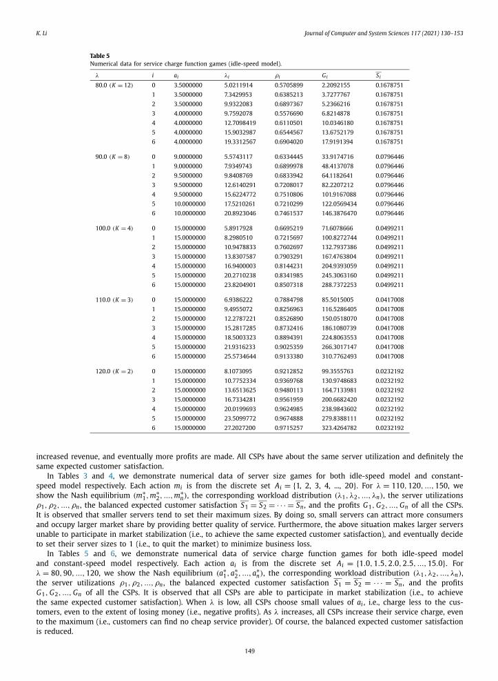
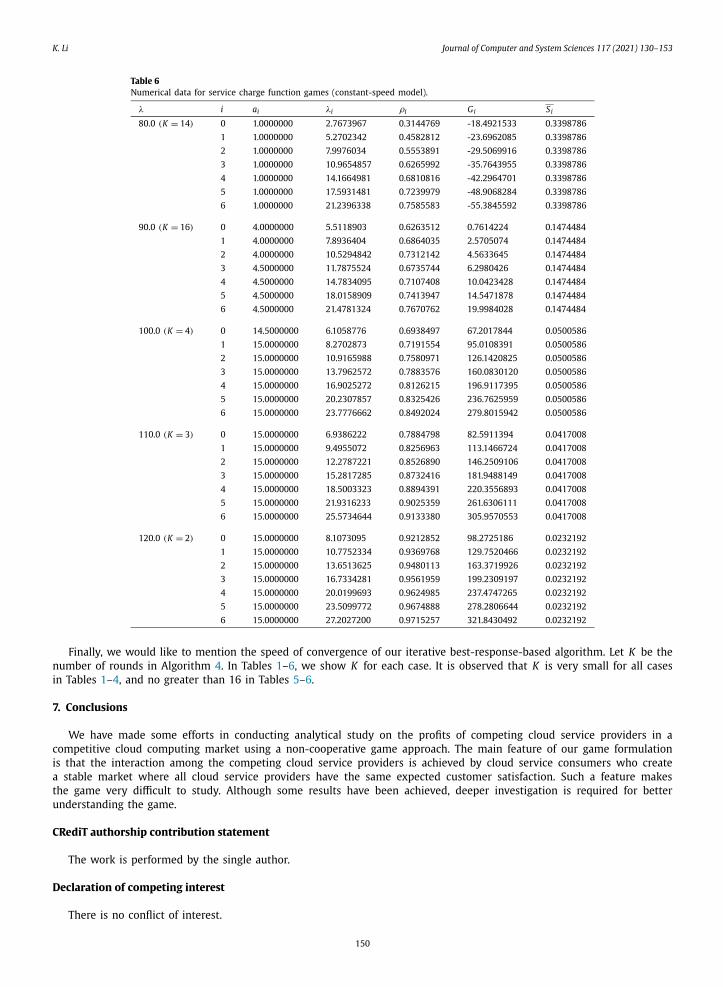
In Tables 5 and 6, we demonstrate numerical data of service charge function games for both idle-speed model and constant-speed model respectively. Each action ai is from the discrete set Ai = {1.0, 1.5, 2.0, 2.5, ..., 15.0}. For λ = 80, 90, ..., 120, we show the Nash equilibrium (a∗

1, a∗2, ..., a

∗n), the corresponding workload distribution (λ1, λ2, ..., λn),

the server utilizations ρ1, ρ2, ..., ρn , the balanced expected customer satisfaction S1 = S2 = · · · = Sn , and the profits G1, G2, ..., Gn of all the CSPs. It is observed that all CSPs are able to participate in market stabilization (i.e., to achieve the same expected customer satisfaction). When λ is low, all CSPs choose small values of ai , i.e., charge less to the cus-tomers, even to the extent of losing money (i.e., negative profits). As λ increases, all CSPs increase their service charge, even to the maximum (i.e., customers can find no cheap service provider). Of course, the balanced expected customer satisfaction is reduced.

149


Table 6Numerical data for service charge function games (constant-speed model).

λ i ai λi ρi Gi Si

80.0 (K = 14) 0 1.0000000 2.7673967 0.3144769 -18.4921533 0.3398786

1 1.0000000 5.2702342 0.4582812 -23.6962085 0.3398786

2 1.0000000 7.9976034 0.5553891 -29.5069916 0.3398786

3 1.0000000 10.9654857 0.6265992 -35.7643955 0.3398786

4 1.0000000 14.1664981 0.6810816 -42.2964701 0.3398786

5 1.0000000 17.5931481 0.7239979 -48.9068284 0.3398786

6 1.0000000 21.2396338 0.7585583 -55.3845592 0.3398786

90.0 (K = 16) 0 4.0000000 5.5118903 0.6263512 0.7614224 0.1474484

1 4.0000000 7.8936404 0.6864035 2.5705074 0.1474484

2 4.0000000 10.5294842 0.7312142 4.5633645 0.1474484

3 4.5000000 11.7875524 0.6735744 6.2980426 0.1474484

4 4.5000000 14.7834095 0.7107408 10.0423428 0.1474484

5 4.5000000 18.0158909 0.7413947 14.5471878 0.1474484

6 4.5000000 21.4781324 0.7670762 19.9984028 0.1474484

100.0 (K = 4) 0 14.5000000 6.1058776 0.6938497 67.2017844 0.0500586

1 15.0000000 8.2702873 0.7191554 95.0108391 0.0500586

2 15.0000000 10.9165988 0.7580971 126.1420825 0.0500586

3 15.0000000 13.7962572 0.7883576 160.0830120 0.0500586

4 15.0000000 16.9025272 0.8126215 196.9117395 0.0500586

5 15.0000000 20.2307857 0.8325426 236.7625959 0.0500586

6 15.0000000 23.7776662 0.8492024 279.8015942 0.0500586

110.0 (K = 3) 0 15.0000000 6.9386222 0.7884798 82.5911394 0.0417008

1 15.0000000 9.4955072 0.8256963 113.1466724 0.0417008

2 15.0000000 12.2787221 0.8526890 146.2509106 0.0417008

3 15.0000000 15.2817285 0.8732416 181.9488149 0.0417008

4 15.0000000 18.5003323 0.8894391 220.3556893 0.0417008

5 15.0000000 21.9316233 0.9025359 261.6306111 0.0417008

6 15.0000000 25.5734644 0.9133380 305.9570553 0.0417008

120.0 (K = 2) 0 15.0000000 8.1073095 0.9212852 98.2725186 0.0232192

1 15.0000000 10.7752334 0.9369768 129.7520466 0.0232192

2 15.0000000 13.6513625 0.9480113 163.3719926 0.0232192

3 15.0000000 16.7334281 0.9561959 199.2309197 0.0232192

4 15.0000000 20.0199693 0.9624985 237.4747265 0.0232192

5 15.0000000 23.5099772 0.9674888 278.2806644 0.0232192

6 15.0000000 27.2027200 0.9715257 321.8430492 0.0232192

Finally, we would like to mention the speed of convergence of our iterative best-response-based algorithm. Let K be the number of rounds in Algorithm 4. In Tables 1–6, we show K for each case. It is observed that K is very small for all cases in Tables 1–4, and no greater than 16 in Tables 5–6.

7. Conclusions

We have made some efforts in conducting analytical study on the profits of competing cloud service providers in a competitive cloud computing market using a non-cooperative game approach. The main feature of our game formulation is that the interaction among the competing cloud service providers is achieved by cloud service consumers who create a stable market where all cloud service providers have the same expected customer satisfaction. Such a feature makes the game very difficult to study. Although some results have been achieved, deeper investigation is required for better understanding the game.

CRediT authorship contribution statement

The work is performed by the single author.

Declaration of competing interest

There is no conflict of interest.

150


Acknowledgments

The author appreciates the anonymous reviewers for their constructive comments.

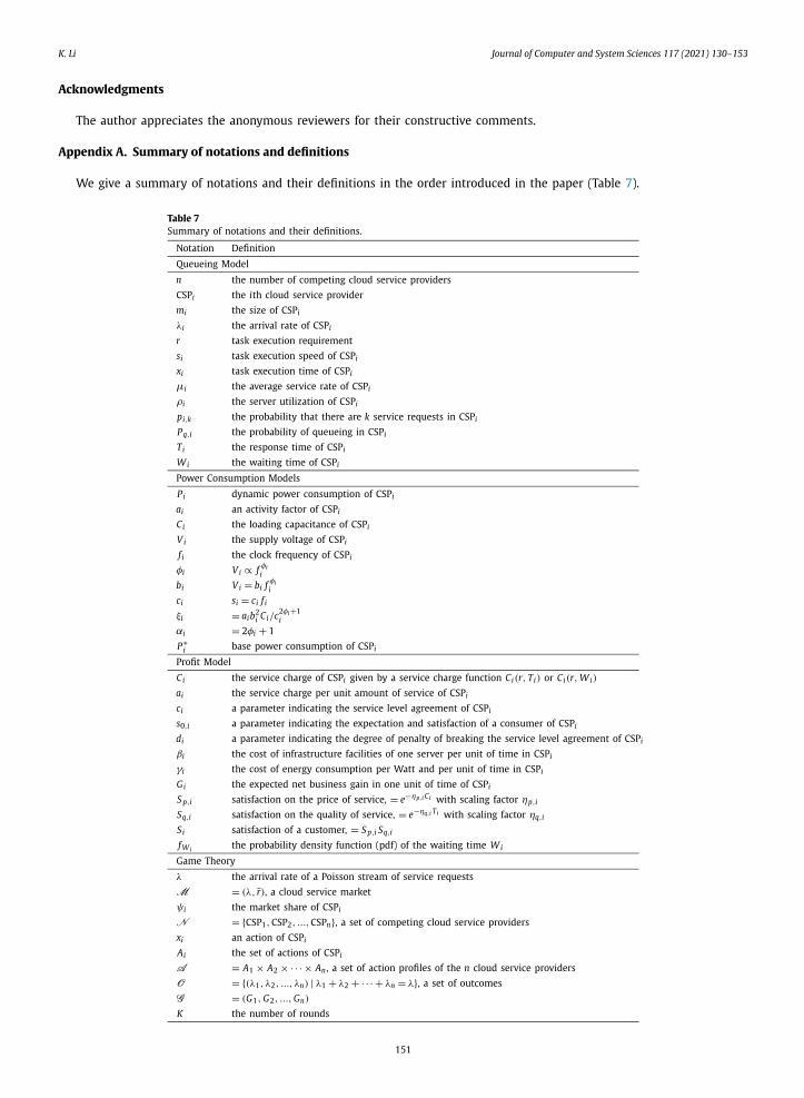
Appendix A. Summary of notations and definitions

We give a summary of notations and their definitions in the order introduced in the paper (Table 7).

Table 7Summary of notations and their definitions.

Notation Definition

Queueing Model

n the number of competing cloud service providers

CSPi the ith cloud service provider

mi the size of CSPi

λi the arrival rate of CSPi

r task execution requirement

si task execution speed of CSPi

xi task execution time of CSPi

μi the average service rate of CSPi

ρi the server utilization of CSPi

pi,k the probability that there are k service requests in CSPi

Pq,i the probability of queueing in CSPi

T i the response time of CSPi

W i the waiting time of CSPi

Power Consumption Models

Pi dynamic power consumption of CSPi

ai an activity factor of CSPi

Ci the loading capacitance of CSPi

V i the supply voltage of CSPi

f i the clock frequency of CSPi

φi V i ∝ f φii

bi V i = bi f φii

ci si = ci f i

ξi = aib2i Ci/c2φi+1

i

αi = 2φi + 1

P∗i base power consumption of CSPi

Profit Model

Ci the service charge of CSPi given by a service charge function Ci(r, Ti) or Ci(r, W i)

ai the service charge per unit amount of service of CSPi

ci a parameter indicating the service level agreement of CSPi

s0,i a parameter indicating the expectation and satisfaction of a consumer of CSPi

di a parameter indicating the degree of penalty of breaking the service level agreement of CSPi

βi the cost of infrastructure facilities of one server per unit of time in CSPi

γi the cost of energy consumption per Watt and per unit of time in CSPi

Gi the expected net business gain in one unit of time of CSPi

S p,i satisfaction on the price of service, = e−ηp,i Ci with scaling factor ηp,i

Sq,i satisfaction on the quality of service, = e−ηq,i T i with scaling factor ηq,i

Si satisfaction of a customer, = S p,i Sq,i

f Wi the probability density function (pdf) of the waiting time W i

Game Theory

λ the arrival rate of a Poisson stream of service requests

M = (λ, r̄), a cloud service market

ψi the market share of CSPi

N = {CSP1,CSP2, ...,CSPn}, a set of competing cloud service providers

xi an action of CSPi

Ai the set of actions of CSPi

A = A1 × A2 × · · · × An , a set of action profiles of the n cloud service providers

O = {(λ1, λ2, ..., λn) | λ1 + λ2 + · · · + λn = λ}, a set of outcomes

G = (G1, G2, ..., Gn)

K the number of rounds

151


References

[1] J. Cao, K. Hwang, K. Li, A. Zomaya, Optimal multiserver configuration for profit maximization in cloud computing, IEEE Trans. Parallel Distrib. Syst. 24 (6) (2013) 1087–1096.

[2] X.-R. Cao, H.-X. Shen, R. Milito, P. Wirth, Internet pricing with a game theoretical approach: concepts and examples, IEEE/ACM Trans. Netw. 10 (2) (2002) 208–216.

[3] S. Chaisiri, B.-S. Lee, D. Niyato, Profit maximization model for cloud provider based on Windows Azure platform, in: 9th International Conference on Electrical Engineering/Electronics, Computer, Telecommunications and Information Technology, May 2012, 4 pp.

[4] A.P. Chandrakasan, S. Sheng, R.W. Brodersen, Low-power CMOS digital design, IEEE J. Solid-State Circuits 27 (4) (1992) 473–484.[5] S.S. Chauhan, E.S. Pilli, R.C. Joshi, G. Singh, M.C. Govil, Brokering in interconnected cloud computing environments: a survey, J. Parallel Distrib. Comput.

133 (2019) 193–209.[6] J. Chen, C. Wang, B.B. Zhou, L. Sun, Y.C. Lee, A.Y. Zomaya, Tradeoffs between profit and customer satisfaction for service provisioning in the cloud, in:

Proceedings of the 20th International Symposium on High Performance Distributed Computing, June 2011, pp. 229–238.[7] Y.-J. Chiang, Y.-C. Ouyang, Profit optimization in SLA-aware cloud services with a finite capacity queuing model, Math. Probl. Eng. 2014 (2014) 534510.[8] Cisco, An innovative business model for cloud providers, whitepaper, available at https://www.cisco .com /c /dam /en _us /solutions /trends /cloud /docs /an _

innovative _business _whitepaper.pdf.[9] L. Columbus, Roundup of cloud computing forecasts, 2017, available at https://www.forbes .com /sites /louiscolumbus /2017 /04 /29 /roundup -of -cloud -

computing -forecasts -2017 /#ec8a3a231e87.[10] P. Cong, L. Li, J. Zhou, K. Cao, T. Wei, M. Chen, S. Hu, Developing user perceived value based pricing models for cloud markets, IEEE Trans. Parallel

Distrib. Syst. 29 (12) (2018) 2742–2756.[11] P. Cong, G. Xu, T. Wei, K. Li, A survey of profit optimization techniques for cloud providers, ACM Comput. Surv. 53 (2) (2020) 26.[12] A. Elhabbash, F. Samreen, J. Hadley, Y. Elkhatib, Cloud brokerage: a systematic survey, ACM Comput. Surv. 51 (6) (2019) 119.[13] T. Erl, Z. Mahmood, R. Puttini, Cloud Computing: Concepts, Technology & Architecture, Prentice Hall, Upper Saddle River, NJ, 2015.[14] G. Feng, S. Garg, R. Buyya, W. Li, Revenue maximization using adaptive resource provisioning in cloud computing environments, in: ACM/IEEE 13th

International Conference on Grid Computing, Sept. 2012, pp. 192–200.[15] Y. Feng, B. Li, B. Li, Price competition in an oligopoly market with multiple IaaS cloud providers, IEEE Trans. Comput. 63 (1) (2014) 59–73.[16] Gartner, https://www.gartner.com /en /newsroom /press -releases /2019 -04 -02 -gartner-forecasts -worldwide -public -cloud -revenue -to -g.[17] M. Ghamkhari, H. Mohsenian-Rad, Energy and performance management of green data centers: a profit maximization approach, IEEE Trans. Smart

Grid 4 (2) (2013) 1017–1025.[18] I. Goiri, J. Guitart, J. Torres, Characterizing cloud federation for enhancing providers’ profit, in: IEEE 3rd International Conference on Cloud Computing,

July 2010, pp. 123–130.[19] H. Goudarzi, M. Pedram, Maximizing profit in cloud computing system via resource allocation, in: 31st International Conference on Distributed Com-

puting Systems Workshops, June 2011, pp. 1–6.[20] J. Hu, K. Li, C. Liu, K. Li, A game-based price bidding algorithm for multi-attribute cloud resource provision, IEEE Trans. Serv. Comput. (2018), https://

doi .org /10 .1109 /TSC .2018 .2860022, in press.[21] M. Jaiganesh, B. Ramadoss, A.V.A. Kumar, S. Mercy, Performance evaluation of cloud services with profit optimization, Proc. Comput. Sci. 54 (2015)

24–30.[22] C. Jing, Y. Zhu, M. Li, Customer satisfaction-aware scheduling for utility maximization on geo-distributed cloud data centers, in: IEEE 10th International

Conference on High Performance Computing and Communications & 2013 IEEE International Conference on Embedded and Ubiquitous Computing, Nov. 2013, pp. 218–225.

[23] L. Kleinrock, Queueing Systems, Volume 1: Theory, John Wiley and Sons, New York, 1975.[24] G. Koutsandria, E. Skevakis, A.A. Sayegh, P. Koutsakis, Can everybody be happy in the cloud? Delay, profit and energy-efficient scheduling for cloud

services, J. Parallel Distrib. Comput. 96 (2016) 202–217.[25] D. Kumar, G. Baranwal, Z. Raza, D.P. Vidyarthi, A survey on spot pricing in cloud computing, J. Netw. Syst. Manag. 26 (4) (2018) 809–856.[26] Y.C. Lee, C. Wang, A.Y. Zomaya, B.B. Zhou, Profit-driven scheduling for cloud services with data access awareness, J. Parallel Distrib. Comput. 72 (4)

(2012) 591–602.[27] K. Li, C. Liu, K. Li, A. Zomaya, A framework of price bidding configurations for resource usage in cloud computing, IEEE Trans. Parallel Distrib. Syst.

27 (8) (2016) 2168–2181.[28] W. Lin, F. Shi, W. Wu, K. Li, G. Wu, A.-A. Mohammed, A taxonomy and survey of power models and power modeling for cloud servers, ACM Comput.

Surv. 53 (5) (October 2020) 100, pp. 1–41.[29] C. Liu, K. Li, K. Li, Bargaining game based scheduling for performance guarantees in cloud computing, ACM Trans. Model. Perform. Eval. Comput. Syst.

3 (1) (2018) 1.[30] C. Liu, K. Li, K. Li, A game approach to multi-servers load balancing with load-dependent server availability consideration, IEEE Trans. Cloud Comput.

(2018), https://doi .org /10 .1109 /TCC .2018 .2790404, in press.[31] C. Liu, K. Li, K. Li, R. Buyya, A new service mechanism for profit maximization of a cloud provider and its users, IEEE Trans. Cloud Comput. (2017),

https://doi .org /10 .1109 /TCC .2017.2701793, in press.[32] C. Liu, K. Li, C. Xu, K. Li, Strategy configurations of multiple users competition for cloud service reservation, IEEE Trans. Parallel Distrib. Syst. 27 (2)

(2016) 508–520.[33] S. Liu, S. Ren, G. Quan, M. Zhao, S. Ren, Profit aware load balancing for distributed cloud data centers, in: IEEE 27th International Symposium on

Parallel & Distributed Processing, May 2013, pp. 611–622.[34] S. Marston, Z. Li, S. Bandyopadhyay, J. Zhang, A. Ghalsasi, Cloud computing – the business perspective, Decis. Support Syst. 51 (1) (2011) 176–189.[35] M. Mazzucco, D. Dyachuk, Optimizing Cloud providers revenues via energy efficient server allocation, Sustain. Comput. Inform. Syst. 2 (1) (2012) 1–12.[36] J. McKendrick, Cloud computing market may become an oligopoly of high-volume vendors, available at https://www.forbes .com /sites /joemckendrick /

2013 /07 /11 /cloud -computing -market -may-become -an -oligopoly-of -high -volume -vendors /#7353d65c6a23.[37] J. Mei, K. Li, K. Li, Customer-satisfaction-aware optimal multiserver configuration for profit maximization in cloud computing, IEEE Trans. Sustain.

Comput. 2 (1) (2017) 17–29.[38] J. Mei, K. Li, K. Li, A fund constrained investment scheme for profit maximization in cloud computing, IEEE Trans. Serv. Comput. 11 (6) (2018) 893–907.[39] J. Mei, K. Li, K. Li, Profit maximization for cloud brokers in cloud computing, IEEE Trans. Parallel Distrib. Syst. 30 (1) (2019) 190–203.[40] J. Mei, K. Li, A. Ouyang, K. Li, A profit maximization scheme with guaranteed quality of service in cloud computing, IEEE Trans. Comput. 64 (11) (2015)

3064–3078.[41] K.S. Patel, A.K. Sarje, VM provisioning policies to improve the profit of cloud infrastructure service providers, in: Third International Conference on

Computing Communication & Networking Technologies, July 2012.[42] S. Ren, M. van der Schaar, Dynamic scheduling and pricing in wireless cloud computing, IEEE Trans. Mob. Comput. 13 (10) (2014) 2283–2292.[43] Research Markets, https://www.prnewswire .com /news -releases /623 -bn -cloud -computing -market -–global -forecast -to -2023 -increase -in -adoption -of -

hybrid -cloud -services -300820321.html.

152

http://refhub.elsevier.com/S0022-0000(20)30101-X/bibEFBEF4BD5CBEF3A8D7471A4BE183FF5Fs1

http://refhub.elsevier.com/S0022-0000(20)30101-X/bibEFBEF4BD5CBEF3A8D7471A4BE183FF5Fs1

http://refhub.elsevier.com/S0022-0000(20)30101-X/bibCF2ACA7ACBE9C54A7609EDA92A19C45Cs1

http://refhub.elsevier.com/S0022-0000(20)30101-X/bibCF2ACA7ACBE9C54A7609EDA92A19C45Cs1

http://refhub.elsevier.com/S0022-0000(20)30101-X/bibD03820ECF9D58B756AF08E61207BB60Es1

http://refhub.elsevier.com/S0022-0000(20)30101-X/bibD03820ECF9D58B756AF08E61207BB60Es1

http://refhub.elsevier.com/S0022-0000(20)30101-X/bibEBCD706079D9C58C000E6C717E740502s1

http://refhub.elsevier.com/S0022-0000(20)30101-X/bib52F35170ABC5EE65E678A7AA4A6571BCs1

http://refhub.elsevier.com/S0022-0000(20)30101-X/bib52F35170ABC5EE65E678A7AA4A6571BCs1

http://refhub.elsevier.com/S0022-0000(20)30101-X/bib0DBC54F242C1A009746874E52635A004s1

http://refhub.elsevier.com/S0022-0000(20)30101-X/bib0DBC54F242C1A009746874E52635A004s1

http://refhub.elsevier.com/S0022-0000(20)30101-X/bib42983B05E2F2CC22822E30BEB7BDD668s1

https://www.cisco.com/c/dam/en_us/solutions/trends/cloud/docs/an_innovative_business_whitepaper.pdf

https://www.cisco.com/c/dam/en_us/solutions/trends/cloud/docs/an_innovative_business_whitepaper.pdf

https://www.forbes.com/sites/louiscolumbus/2017/04/29/roundup-of-cloud-computing-forecasts-2017/#ec8a3a231e87

https://www.forbes.com/sites/louiscolumbus/2017/04/29/roundup-of-cloud-computing-forecasts-2017/#ec8a3a231e87

http://refhub.elsevier.com/S0022-0000(20)30101-X/bib466D5046B1F77BD832C92C26CCE94D66s1

http://refhub.elsevier.com/S0022-0000(20)30101-X/bib466D5046B1F77BD832C92C26CCE94D66s1

http://refhub.elsevier.com/S0022-0000(20)30101-X/bibFD6701E73C22C9FDC8123DC97D48F0EEs1

http://refhub.elsevier.com/S0022-0000(20)30101-X/bib931E34F2126D2B9D502E2D95012713CAs1

http://refhub.elsevier.com/S0022-0000(20)30101-X/bibEFA0BFF183DA4BC574DC82011291F87As1

http://refhub.elsevier.com/S0022-0000(20)30101-X/bibC4F58CEFBA9D90137D10D12AF8556883s1

http://refhub.elsevier.com/S0022-0000(20)30101-X/bibC4F58CEFBA9D90137D10D12AF8556883s1

http://refhub.elsevier.com/S0022-0000(20)30101-X/bib41BF80D3FFE05D483FF2A339F8EAC566s1

https://www.gartner.com/en/newsroom/press-releases/2019-04-02-gartner-forecasts-worldwide-public-cloud-revenue-to-g

http://refhub.elsevier.com/S0022-0000(20)30101-X/bib64F3BD1741AB8D6BA545A1AE09BB8728s1

http://refhub.elsevier.com/S0022-0000(20)30101-X/bib64F3BD1741AB8D6BA545A1AE09BB8728s1

http://refhub.elsevier.com/S0022-0000(20)30101-X/bibB5BA08E857E316ED7E0778E3EC40225Fs1

http://refhub.elsevier.com/S0022-0000(20)30101-X/bibB5BA08E857E316ED7E0778E3EC40225Fs1

http://refhub.elsevier.com/S0022-0000(20)30101-X/bibAD2D8EE7D788DCF41F399818F639CB64s1

http://refhub.elsevier.com/S0022-0000(20)30101-X/bibAD2D8EE7D788DCF41F399818F639CB64s1

https://doi.org/10.1109/TSC.2018.2860022

https://doi.org/10.1109/TSC.2018.2860022

http://refhub.elsevier.com/S0022-0000(20)30101-X/bibF2A81EA403828365544CA3CE7718DCC3s1

http://refhub.elsevier.com/S0022-0000(20)30101-X/bibF2A81EA403828365544CA3CE7718DCC3s1

http://refhub.elsevier.com/S0022-0000(20)30101-X/bibA8AAABE023B7E22EE7058406BA7BDE5Bs1



http://refhub.elsevier.com/S0022-0000(20)30101-X/bibB9B04ABCAE5BC357FCF85E066184C1C6s1

http://refhub.elsevier.com/S0022-0000(20)30101-X/bibABF4EF5F3AFBFFD00A8086195CCA3D28s1

http://refhub.elsevier.com/S0022-0000(20)30101-X/bibABF4EF5F3AFBFFD00A8086195CCA3D28s1

http://refhub.elsevier.com/S0022-0000(20)30101-X/bib22932A4A55948C6E19456C9D3EFFBE45s1

http://refhub.elsevier.com/S0022-0000(20)30101-X/bibC0B72315CDD623D3ECEAD245512C20C7s1

http://refhub.elsevier.com/S0022-0000(20)30101-X/bibC0B72315CDD623D3ECEAD245512C20C7s1

http://refhub.elsevier.com/S0022-0000(20)30101-X/bibEDFA3FCC173813FB3C5FB7B8803445B3s1

http://refhub.elsevier.com/S0022-0000(20)30101-X/bibEDFA3FCC173813FB3C5FB7B8803445B3s1

http://refhub.elsevier.com/S0022-0000(20)30101-X/bib44694B727EE1B467EF518098675E237Es1

http://refhub.elsevier.com/S0022-0000(20)30101-X/bib44694B727EE1B467EF518098675E237Es1

http://refhub.elsevier.com/S0022-0000(20)30101-X/bib32A7C7AEF91D1AE3F3684704FD5FACEEs1

http://refhub.elsevier.com/S0022-0000(20)30101-X/bib32A7C7AEF91D1AE3F3684704FD5FACEEs1

https://doi.org/10.1109/TCC.2018.2790404

https://doi.org/10.1109/TCC.2017.2701793

http://refhub.elsevier.com/S0022-0000(20)30101-X/bib7B86174209823B32261274050FBA0277s1

http://refhub.elsevier.com/S0022-0000(20)30101-X/bib7B86174209823B32261274050FBA0277s1

http://refhub.elsevier.com/S0022-0000(20)30101-X/bib6EC7E996C36CBEA0920D4825945E6BADs1

http://refhub.elsevier.com/S0022-0000(20)30101-X/bib6EC7E996C36CBEA0920D4825945E6BADs1

http://refhub.elsevier.com/S0022-0000(20)30101-X/bibF0CD1117869EF9DECB4768074522C1F7s1

http://refhub.elsevier.com/S0022-0000(20)30101-X/bib7DC10E66DA5549D351765BD940B81BE9s1

https://www.forbes.com/sites/joemckendrick/2013/07/11/cloud-computing-market-may-become-an-oligopoly-of-high-volume-vendors/#7353d65c6a23

https://www.forbes.com/sites/joemckendrick/2013/07/11/cloud-computing-market-may-become-an-oligopoly-of-high-volume-vendors/#7353d65c6a23

http://refhub.elsevier.com/S0022-0000(20)30101-X/bibB371A9E7A5D02A0A567D960EF277B22As1

http://refhub.elsevier.com/S0022-0000(20)30101-X/bibB371A9E7A5D02A0A567D960EF277B22As1

http://refhub.elsevier.com/S0022-0000(20)30101-X/bib84B94C9AB55EFE4D09125A104BB7172Cs1

http://refhub.elsevier.com/S0022-0000(20)30101-X/bib8AC68C912F6566B8192BF1152B41D4D9s1

http://refhub.elsevier.com/S0022-0000(20)30101-X/bib56C28D179A04987204604DC42A1ED0A0s1

http://refhub.elsevier.com/S0022-0000(20)30101-X/bib56C28D179A04987204604DC42A1ED0A0s1

http://refhub.elsevier.com/S0022-0000(20)30101-X/bibD3D4C5DEB455AC79DD5FF47C88BD65D9s1

http://refhub.elsevier.com/S0022-0000(20)30101-X/bibD3D4C5DEB455AC79DD5FF47C88BD65D9s1

http://refhub.elsevier.com/S0022-0000(20)30101-X/bib3DF8A820012C09FD73447AB491A0C15Cs1

http://www.prnewswire.com/news-releases/623-bn-cloud-computing-market---global-forecast-to-2023-increase-in-adoption-of-hybrid-cloud-services-300820321.html

http://www.prnewswire.com/news-releases/623-bn-cloud-computing-market---global-forecast-to-2023-increase-in-adoption-of-hybrid-cloud-services-300820321.html


[44] H. Roh, C. Jung, W. Lee, D.-Z. Du, Resource pricing game in geo-distributed clouds, in: Proceedings of the 32nd IEEE Conference on Computer Commu-nications, July 2013, pp. 1519–1527.

[45] J.B. Rosen, Existence and uniqueness of equilibrium points for concave N-person games, Econometrica 33 (3) (1965) 520–534.[46] G. Scutari, D.P. Palomar, F. Facchinei, J.-S. Pang, Convex optimization, game theory, and variational inequality theory, IEEE Signal Process. Mag. 27 (3)

(2010) 35–49.[47] M. Tanaka, Y. Murakami, Strategy-proof pricing for cloud service composition, IEEE Trans. Cloud Comput. 4 (3) (2016) 363–375.[48] T. Thanakornworakij, R. Nassar, C.B. Leangsuksun, M. Paun, An economic model for maximizing profit of a cloud service provider, in: Seventh Interna-

tional Conference on Availability, Reliability and Security, Aug. 2012, pp. 274–279.[49] A.N. Toosi, R.N. Calheiros, R.K. Thulasiram, R. Buyya, Resource provisioning policies to increase IaaS provider’s profit in a federated cloud environment,

in: IEEE 13th International Conference on High Performance Computing and Communications, Sept. 2011, pp. 279–287.[50] T. Truong-Huu, C.-K. Tham, A novel model for competition and cooperation among cloud providers, IEEE Trans. Cloud Comput. 2 (3) (2014) 251–265.[51] K. Tsakalozos, H. Kllapi, E. Sitaridi, M. Roussopoulos, D. Paparas, A. Delis, Flexible use of cloud resources through profit maximization and price

discrimination, in: IEEE 27th International Conference on Data Engineering, April 2011, pp. 75–86.[52] T. Wang, J. Zhou, G. Zhang, T. Wei, S. Hu, Customer perceived value- and risk-aware multiserver configuration for profit maximization, IEEE Trans.

Parallel Distrib. Syst. 31 (5) (2020) 1074–1088.[53] C. Weinhardt, A. Anandasivam, B. Blau, N. Borissov, T. Meinl, W. Michalk, J. Stößer, Cloud computing – a classification, business models, and research

directions, Bus. Inf. Syst. Eng. 1 (5) (2009) 391–399.[54] C. Wu, R. Buyya, K. Ramamohanarao, Cloud pricing models: taxonomy, survey and interdisciplinary challenges, ACM Comput. Surv. 52 (6) (2019) 108.[55] H. Xu, B. Li, Dynamic cloud pricing for revenue maximization, IEEE Trans. Cloud Comput. 1 (2) (2013) 158–171.[56] B. Yang, Z. Li, S. Chen, T. Wang, K. Li, A Stackelberg game approach for energy-aware resource allocation in data centers, IEEE Trans. Parallel Distrib.

Syst. 27 (12) (2016) 3646–3658.[57] X. Yang, B. Nasser, M. Surridge, S. Middleton, A business-oriented Cloud federation model for real-time applications, Future Gener. Comput. Syst. 28 (8)

(2012) 1158–1167.[58] J. Zhao, H. Li, C. Wu, Z. Li, Z. Zhang, F.C.M. Lau, Dynamic pricing and profit maximization for the cloud with geo-distributed data centers, in: Proceedings

of the 33rd IEEE Conference on Computer Communications, May 2014, pp. 118–126.[59] Q. Zheng, B. Veeravalli, On the design of mutually aware optimal pricing and load balancing strategies for grid computing systems, IEEE Trans. Comput.

63 (7) (2014) 1802–1811.[60] A. Zhou, Q. Sun, L. Sun, J. Li, F. Yang, Maximizing the profits of cloud service providers via dynamic virtual resource renting approach, EURASIP J. Wirel.

Commun. Netw. 2015 (2015) 71.

153

http://refhub.elsevier.com/S0022-0000(20)30101-X/bibF45541887B3B7CAF327F564C696DBB4As1

http://refhub.elsevier.com/S0022-0000(20)30101-X/bibF45541887B3B7CAF327F564C696DBB4As1

http://refhub.elsevier.com/S0022-0000(20)30101-X/bibA448FFA969E691CD387EB7DEAC4F453Bs1

http://refhub.elsevier.com/S0022-0000(20)30101-X/bibDEC15B02D547B17ABF73D123BC0D25F5s1

http://refhub.elsevier.com/S0022-0000(20)30101-X/bibDEC15B02D547B17ABF73D123BC0D25F5s1

http://refhub.elsevier.com/S0022-0000(20)30101-X/bibAC7A4FBD0D788D94F43454817E1C208Cs1

http://refhub.elsevier.com/S0022-0000(20)30101-X/bib90DEEC787C16D02830A25A0E48A10B3Ds1

http://refhub.elsevier.com/S0022-0000(20)30101-X/bib90DEEC787C16D02830A25A0E48A10B3Ds1

http://refhub.elsevier.com/S0022-0000(20)30101-X/bibC8B43FF535D146F31A96C68D5CD29DFFs1

http://refhub.elsevier.com/S0022-0000(20)30101-X/bibC8B43FF535D146F31A96C68D5CD29DFFs1

http://refhub.elsevier.com/S0022-0000(20)30101-X/bibDF1F3EDB9115ACB0A1E04209B7A9937Bs1

http://refhub.elsevier.com/S0022-0000(20)30101-X/bib0DC224C1C7F1E2E61FCFC22B33FB0F73s1

http://refhub.elsevier.com/S0022-0000(20)30101-X/bib0DC224C1C7F1E2E61FCFC22B33FB0F73s1

http://refhub.elsevier.com/S0022-0000(20)30101-X/bib5CAEA9742D0E61D6B213EBF3CB4914A2s1

http://refhub.elsevier.com/S0022-0000(20)30101-X/bib5CAEA9742D0E61D6B213EBF3CB4914A2s1

http://refhub.elsevier.com/S0022-0000(20)30101-X/bibCF7D09FC44E2E8D68BEEEBFE294B9AC2s1

http://refhub.elsevier.com/S0022-0000(20)30101-X/bibCF7D09FC44E2E8D68BEEEBFE294B9AC2s1

http://refhub.elsevier.com/S0022-0000(20)30101-X/bib23DC75D4D9E14953C8D67913DA178DBBs1

http://refhub.elsevier.com/S0022-0000(20)30101-X/bibA7A4CCC5E1A068D87F4965E014329201s1

http://refhub.elsevier.com/S0022-0000(20)30101-X/bibF4F349E6D090D9CB83EB5E2BB155D48Fs1

http://refhub.elsevier.com/S0022-0000(20)30101-X/bibF4F349E6D090D9CB83EB5E2BB155D48Fs1

http://refhub.elsevier.com/S0022-0000(20)30101-X/bib10DD33F842F7AF46E047648A0423F0E4s1

http://refhub.elsevier.com/S0022-0000(20)30101-X/bib10DD33F842F7AF46E047648A0423F0E4s1

http://refhub.elsevier.com/S0022-0000(20)30101-X/bib4FE66EA86A73DC5A7903A31818288835s1

http://refhub.elsevier.com/S0022-0000(20)30101-X/bib4FE66EA86A73DC5A7903A31818288835s1

http://refhub.elsevier.com/S0022-0000(20)30101-X/bib310E0A4E72F1F2DCEE6682B027940A82s1

http://refhub.elsevier.com/S0022-0000(20)30101-X/bib310E0A4E72F1F2DCEE6682B027940A82s1

http://refhub.elsevier.com/S0022-0000(20)30101-X/bib49463037134D44A9F9CF905294865A82s1

http://refhub.elsevier.com/S0022-0000(20)30101-X/bib49463037134D44A9F9CF905294865A82s1

a game theoretic approach - computer science

Documents