a fourier method for the fractional diffusion equation describing sub-diffusion
TRANSCRIPT

QUT Digital Repository: http://eprints.qut.edu.au/
Chen, Chang-Ming and Liu, Fawang and Turner, Ian W. and Anh, Vo V. (2007) A Fourier method for the fractional diffusion equation describing sub-diffusion. Journal of Computational Physics 227(2):pp. 886-897.
© Copyright 2007 Elsevier
A Fourier method for the fractional diffusion
equation describing sub-diffusion ?
Chang-Ming Chen a, F. Liu a,b,∗, I. Turner b, V. Anh b
aSchool of Mathematical Sciences, Xiamen University, Xiamen 361005, ChinabSchool of Mathematical Sciences, Queensland University of Technology, GPO Box
2434, Brisbane, Qld. 4001, Australia
Abstract
In this paper, a fractional partial differential equation (FPDE) describing sub-
diffusion is considered. An implicit difference approximation scheme (IDAS) forsolving a FPDE is presented. We propose a Fourier method for analyzing the sta-bility and convergence of the IDAS, derive the global accuracy of the IDAS, anddiscuss the solvability. Finally, numerical examples are given to compare with theexact solution for the order of convergence, and simulate the fractional dynamicalsystems.
Key words: fractional diffusion equation, sub-diffusion, implicit differenceapproximation, Fourier method, stability, convergence.
1 Introduction
Fractional diffusion equations have attracted in recent years a considerableinterest both in mathematics and in applications. These equations containderivatives of fractional order in space, time or space-time [1]. They wereused in modelling of many physical and chemical processes and in engineering[2],[3],[4]. Such evolution equations imply a fractional Fick’s law for the flux
? This research has been supported by the National Natural Science Foundation ofChina grant 10271098 and the Australian Research Council grant LP0348653.∗ Corresponding author.
Email address: [email protected] or [email protected] (F. Liu).
Preprint submitted to Elsevier Preprint 8 February 2007

that accounts for spatial and temporal non-locality [5]. Fractional calculusprovides a powerful instrument for the description of memory and hereditaryproperties of substances [4]. Fractional-order differential equations have beenthe subject of worldwide attention by many research groups. In particular, thefocus of Gorenflo, Mainardi and their co-authors’ works on fractional calculusmodelling (both deterministic and stochastic) and the derivation of fundamen-tal solutions of the time, space and space-time fractional diffusion equations.They also presented discrete random walk models [6],[7] and found that thefundamental solution can be interpreted as a probability density evolving intime of a self-similar stochastic process that can be viewed as a generaliseddiffusion process. Benson et al. [8],[9] used a fractional advection-dispersionequation to simulate transport processes with heavy tails and demonstratedthe equivalence between these heavy-tailed motions and transport equationsthat use fractional-order derivatives. Already in 1986 Wyss [10] considered thetime fractional diffusion equation and gave the solution in closed form in termsof Fox functions. Then in 1989 Schneider and Wyss [11] considered the timefractional diffusion and wave equations, and the corresponding Green func-tions were obtained in closed form for arbitrary space dimensions in termsof Fox functions and their properties were exhibited. However, an explicitrepresentation of the Green functions for the problem in a half-space was dif-ficult to determine, except in the special cases α = 1 (i.e., the first-order timederivative) with arbitrary n, or n=1 with arbitrary α (i.e., the fractional-ordertime derivative). Huang and Liu [12] considered the time-fractional diffusionequations in an n-dimensional whole-space and half-space. They investigatedthe explicit relationships between the problems in whole-space with the cor-responding problems in half-space by the Fourier-Laplace transform.
Fractional kinetic equations have proved particularly useful in the contextof anomalous slow diffusion (sub-diffusion) [1]. The theoretical justificationfor the fractional diffusion equation, together with the abundance of phys-ical and biological experiments demonstrating the prevalence of anomaloussub-diffusion, has led to an intensive effort in recent years to find accurateand stable methods of solution that are also straightforward to implement[13]. It has been suggested that the probability density function (pdf) u(x, t)that describes anomalous sub-diffusive particles follows the fractional diffusionequation [1],[13],[14]:
∂u(x, t)
∂t=0 D1−γ
t
[∂2u(x, t)
∂x2
]+ f(x, t), t ≥ 0, (1)
where 0D1−γt u (0 < γ ≤ 1) denotes the Riemann-Liouville fractional derivative
2

of order 1− γ of the function u(x, t):
0D1−γt u(x, t) =
1
Γ(γ)
∂
∂t
t∫
0
u(x, τ)
(t− τ)1−γdτ, (2)
with 0 < γ < 1. For γ = 1 one recovers the identity operator and for γ = 0the ordinary first-order derivative.
Some numerical methods for solving the space or time, or time-space frac-tional partial differential equations have been proposed [15],[16],[17], [18], [19],[20], [21], [22], [23], [24]. However, the stability and convergence of numericalmethods for fractional partial differential equations are deserve further inves-tigations.
In this paper, we consider the initial-boundary value problem of the fractionaldiffusion equation describing sub-diffusion (FDE-sub) [13], [25]:
∂u(x, t)
∂t=0 D1−γ
t
[∂2u(x, t)
∂x2
]+ f(x, t), 0 < t ≤ T, 0 < x < L, (3)
u(0, t) = ϕ(t), 0 ≤ t ≤ T, (4)
u(L, t) = ψ(t), 0 ≤ t ≤ T, (5)
u(x, 0) = w(x), 0 ≤ x ≤ L, (6)
where 0 < γ ≤ 1; f(x, t), ϕ(t), ψ(t) and w(x) are sufficiently smooth functions.
Langlands and Henry [13] have investigated this problem. They proposed animplicit numerical scheme (L1 approximation), and discussed the accuracy andstability of this scheme. However, the global accuracy of the implicit numericalscheme has not been derived and it is apparent that the unconditional stabilityfor all γ in the range 0 < γ ≤ 1 has not been established. The main purposeof this paper is to solve this problem via Fourier method.
The structure of the paper is as follows. In Section 2, we present an implicitdifference approximation scheme. Sections 3 and 4 investigate the stability andconvergence of the IDAS respectively, using Fourier method. We prove thatthe IDAS is unconditionally stable for all γ in the range 0 < γ ≤ 1, derivethe global accuracy of the IDAS, analyze the convergence of the IDAS , anddiscuss the solvability. Finally, some numerical examples are provided.
3

2 An implicit difference approximation scheme for FDE-sub
In this section, we first let
tk = kτ, k = 0, 1, . . . , N
andxj = jh, j = 0, 1, . . . , M
respectively, where τ = T/N and h = L/M . For every 1 − γ, the Riemann-Liouville fractional derivative exists and coincides with the Grunwald-Letnikovfractional derivative. The relationship between the Riemann-Liouville andGrunwald-Letnikov definitions is also another consequence that is importantfor numerical approximation of FDE-sub; the formulation of applied prob-lems; the manipulation with fractional derivatives; and the formulation ofphysically meaningful initial and boundary value problems. This allows theuse of the Riemann-Liouville definition during problem formulation, and thenthe Grunwald-Letnikov definition for obtaining the numerical solution [15].In proposing an approximation for FDE-sub, the key point is how to ap-proximate the Riemann-Liouville fractional derivative. Using the relationshipbetween Grunwald-Letnikov and Riemann-Liouville fractional derivatives [4],we have
0D1−γt f(t) = lim
τ→0τ γ−1∆1−γ
τ f(t) = limτ→0
τ γ−1[t/τ ]∑
l=0
(−1)l
(1− γ
l
)f(t− lτ).
Then the initial-boundary value problem of FDE-sub (3)− (6) can be approx-imated by the following implicit difference approximation scheme:
ukj − uk−1
j
τ=
τ γ−1
h2
k∑
l=0
λl
(uk−l
j−1 − 2uk−lj + uk−l
j+1
)+ fk
j , (7)
(k = 1, 2, . . . , N, j = 1, 2, . . . , M − 1),
uk0 = ϕ(tk), (k = 0, 1, . . . , N), (8)
ukm = ψ(tk), (k = 0, 1, . . . , N), (9)
u0j = w(xj), (j = 0, 1, . . . , M) (10)
where λl = (−1)l
1− γ
l
, l = 0, 1, . . . , k, and fk
j = f(xj, tk).
4

3 Stability of the implicit difference approximation scheme
In this section, we will analyze the stability of the IDAS (7)-(10). We firstrewrite (7) as
ukj = uk−1
j + µk∑
l=0
λl
(uk−l
j−1 − 2uk−lj + uk−l
j+1
)+ τfk
j , (11)
(k = 1, 2, . . . , N, j = 1, 2, . . . , M − 1)
where µ = τγ
h2 .
Let Ukj be the approximate solution of IDAS (7)-(10), and define
ρkj = uk
j − Ukj , (k = 0, 1, . . . , N, j = 1, 2, . . . , M − 1)
and
ρk =[ρk
1, ρk2, . . . , ρ
kM−1
]T
respectively. We obtain the following roundoff error equations:
ρkj = ρk−1
j + µk∑
l=0
λl
(ρk−l
j−1 − 2ρk−lj + ρK−l
j+1
), (12)
(k = 1, 2, . . . , N, j = 1, 2, . . . , M − 1).
We will analyze the stability of IDAS (7)-(10) by using Fourier method. Basedon this, we define grid functions:
ρk(x) =
ρkj , when xj − h
2< x ≤ xj + h
2, j = 1, 2, · · · ,M − 1,
0, when 0 ≤ x ≤ h2or L− h
2< x ≤ L,
(k = 1, 2, · · · , N),
then ρk(x) can be expanded in a Fourier series:
ρk(x) =∞∑
m=−∞dk(m)ei2πmx/L, (k = 1, 2, . . . , N),
where
dk(m) =1
L
L∫
0
ρk(x)e−i2πmx/Ldx.
Noticing, with the natural definition of the discrete 2-norm,
5

‖ρk‖2 =
M−1∑
j=1
h|ρkj |2
12
(13)
=
h2∫
0
|ρk(x)|2dx +M−1∑
j=1
xj+h2∫
xj−h2
|ρk(x)|2dx +
L∫
L−h2
|ρk(x)|2dx
12
=
L∫
0
|ρk(x)|2dx
12
and applying the Parseval equality:
L∫
0
|ρk(x)|2dx =∞∑
m=−∞|dk(m)|2,
we obtain
‖ρk‖22 =
∞∑
m=−∞|dk(m)|2. (14)
Based on the above analysis, we can suppose that the solution of equation(12) has the following form:
ρkj = dke
iσjh,
where σ = 2πm/L. Substituting the above expression into (12), we obtain
(1 + 4 sin2 σh
2
)dk =
(1− 4µλ1 sin2 σh
2
)dk−1 − 4µ sin2 σh
2
k∑
l=2
λldk−l,(15)
(k = 1, 2, . . . , N).
Lemma 1: The coefficients λl (l = 0, 1, . . .) satisfy
(1)λ0 = 1, λ1 = γ − 1, λl < 0, l = 1, 2, . . .
(2)∞∑l=0
λl = 1, and ∀n ∈ N+,− n∑l=1
λl < 1.
Applying Lemma 1, Eq. (15) can be written as
dk =1 + 4µ(1− γ) sin2 σh
2
1 + 4µ sin2 σh2
dk−1 −4µ sin2 σh
2
1 + 4µ sin2 σh2
k∑
l=2
λldk−l, (16)
(k = 1, 2, . . . , N).
6

Proposition 1: Supposing that dk (k = 1, 2 . . . , N) be the solution of Eq.(16), we have
|dk| ≤ |do|, (k = 1, 2, . . . , N).
Proof: We will use mathematical induction to complete the proof.
For k=1, from Eq. (16) we have
d1 =1 + 4µ(1− γ) sin2 σh
2
1 + 4µ sin2 σh2
d0.
Noticing that 0 < γ < 1, we obtain
|d1| ≤ |d0|.
Supposing that|dn| ≤ |d0|, (n = 1, 2, . . . , k − 1),
applying Lemma 1, from Eq. (16), we have
|dk| ≤ 1+4µ(1−γ) sin2 σh2
1+4µ sin2 σh2
|dk−1|+ 4µ sin2 σh2
1+4µ sin2 σh2
k∑l=2|λl||dk−l|
≤[
1+4µ(1−γ) sin2 σh2
1+4µ sin2 σh2
+4µ sin2 σh
2
1+4µ sin2 σh2
(k∑
l=1|λl| − |λ1|
)]|d0|
=
{1+4µ(1−γ) sin2 σh
2
1+4µ sin2 σh2
+4µ sin2 σh
2
1+4µ sin2 σh2
[− k∑
l=1λl − (1− γ)
]}|d0|
≤{
1+4µ(1−γ) sin2 σh2
1+4µ sin2 σh2
+4µ sin2 σh
2
1+4µ sin2 σh2
[1− (1− γ)]}|d0|
= |d0|.
This completes the proof.
Theorem 1: The implicit difference approximation scheme (7)-(10) is uncon-ditionally stable .
Proof: Applying Proposition 1, and noticing (14), we obtain
‖ρk‖2 ≤ ‖ρ0‖2, k = 1, 2, . . . , N,
which proves that IDAS (7-10) is unconditionally stable.
4 Convergence of the implicit difference approximation scheme
In this section,we first introduce the following lemma.
Lemma 2: τ γ−1k∑
l=0λl = 1
Γ(γ)+ 0(τ).
7

Proof: Because
0D1−γt g(t) = τ γ−1
[t/τ ]∑
l=0
λlg(t− lτ) + 0(τ),
then
0D1−γt g(t)|t=tk = τ γ−1
k∑
l=0
λlg(tk − lτ) + 0(τ). (17)
Taking g(t) = 1 and tk = 1 in (17), we have
0D1−γt (1)|t=1 = τ γ−1
k∑
l=0
λl + 0(τ).
Therefore
τ γ−1k∑
l=0
λl =0 D1−γt (1)|t=1 + 0(τ) =
1
Γ(γ)+ 0(τ).
This completes the proof.
We now define
Rkj =
u(xj, tk)− u(xj, tk−1)
τ(18)
−τ γ−1
h2
k∑
l=0
λl [u(xj−1, tk−l)− 2u(xj, tk−l) + u(xj+1, tk−l)] ,
(k = 1, 2, . . . , N, j = 1, 2, . . . , M − 1).
Applying Lemma 2 and (17), we have
τγ−1
h2
k∑l=0
λl [u(xj−1, tk−l)− 2u(xj, tk−l) + u(xj+1, tk−l)]
= 0D1−γt
[∂2u(xj ,tk)
∂x2
]+ O(τ) + O(h2)
On the other hand,
u(xj, tk)− u(xj, tk−1)
τ=
∂u(xj, tk)
∂t+ O(τ).
Consequently
Rkj = O(τ + h2), (k = 1, 2, . . . , N, j = 1, 2, . . . , M − 1).
Therefore, there is a positive constant c1, such that
|Rkj | ≤ c1(τ + h2), k = 1, 2, . . . , N, (j = 1, 2, . . . , M − 1). (19)
8

Letek
j = u(xj, tk)− ukj , (k = 1, 2, . . . , N, , i = 1, 2, . . . , M − 1)
andek =
[ek1, e
k2, . . . , e
kM−1
]T, Rk =
[Rk
1 , Rk2 , . . . , R
kM−1
]T
respectively. From (18), we have
u(xj, tk) = u(xj, tk−1) + τγ
h2
k∑l=0
λl [u(xj−1, tk−l)− 2u(xj, tk−l) + u(xj+1, tk−l)]
+τf(xj, tk) + τRkj ,
k = 1, 2, . . . , N, j = 1, 2, . . . , M − 1.
Subtracting the above equation from (11), we obtain
ekj = ek−1
j + µk∑
l=0
λl
(ek−l
j−1 − 2ek−lj + ek−l
j+1
)+ τRk
j , (20)
(k = 1, 2 . . . , N, j = 1, 2, . . . , M − 1).
We now analyze the convergence of IDAS (7)-(10) by using Fourier method.Using the same idea to the stability analysis in Section 3, we first define gridfunctions
ek(x) =
ekj , when xj − h
2< x ≤ xj + h
2, j = 1, 2, . . . , M − 1,
0, when 0 ≤ x ≤ h2
or L− h2
< x ≤ L,
(k = 0, 1, · · · , N)
and
Rk(x) =
Rkj , when xj − h
2< x ≤ xj + h
2, j = 1, 2, . . . , M − 1,
0, when 0 ≤ x ≤ h2or L− h
2< x ≤ L,
(k = 1, 2, · · · , N),
respectively. Then ek(x) and Rk(x) have Fourier series expansions, respec-tively:
ek(x) =∞∑
m=−∞ξk(m)ei2πmx/L, (k = 0, 1, . . . , N)
and
Rk(x) =∞∑
m=−∞ηk(m)ei2πmx/L, (k = 1, 2, . . . , N)
where
ξk(m) =1
L
L∫
0
ek(x)e−i2πmx/Ldx,
9

and
ηk(m) =1
L
L∫
0
Rk(x)e−i2πmx/Ldx.
Similarly, we also have
‖ek‖22 =
M−1∑
j=1
h|ekj |2
12
=∞∑
m=−∞|ξk(m)|2, (k = 0, 1, . . . , N) (21)
and
‖Rk‖22 =
M−1∑
j=1
h|Rkj |2
12
=∞∑
m=−∞|ηk(m)|2, (k = 1, 2, . . . , N), (22)
respectively. Based on the above analysis, we can suppose that
ekj = ξke
iσjh
and
Rkj = ηke
iσjh,
respectively. Substituting the above expressions into (20), we obtain
(1 + 4µ sin2 σh
2
)ξk =
(1− 4µλ1 sin2 σh
2
)ξk−1 (23)
− 4µ sin2 σh
2
k∑
l=2
λlξk−l + τηk,
(k = 1, 2, . . . , N).
Applying Lemma 1, equations (23) can be written as
ξk =1 + 4µ(1− γ) sin2 σh
2
1 + 4µ sin2 σh2
ξk−1 −4µ sin2 σh
2
1 + 4µ sin2 σh2
k∑
l=2
λlξk−l (24)
+τηk
1 + 4µ sin2 σh2
, (k = 1, 2, . . . , N).
Proposition 2: Suppose the ξk(k = 1, 2, . . . , N) be the solution of the equa-tions (24), then there is a positive constant c2 such that
|ξk| ≤ kτc2|η1|, k = 1, 2, . . . , N.
10

proof. First, noticing that e0 = 0, we have
ξ0 ≡ ξ0(m) = 0.
In addition, from (19) and the left hand side of (22),we have
‖Rk‖2 ≤ c1
√L(τ + h2), k = 1, 2, . . . , N. (25)
Again, based on the convergence of the series in the right hand side of (22),then there is a positive constant c2 such that
|ηk| ≡ |ηk(m)| ≤ c2|η1| ≡ c2|η1(m)|, k = 1, 2, . . . , N. (26)
We will complete the proof using mathematical induction. For k = 1, from(24),we have
ξ1 =1+4µ(1−γ) sin2 σh
2
1+4µ sin2 σh2
ξ0 + τη1
1+4µ sin2 σh2
= τη1
1+4µ sin2 σh2
.
From (26), we obtain|ξ1| ≤ τ |η1| ≤ c2τ |η1|.
Suppose that|ξn| ≤ c2nτ |η1|, n = 1, 2, . . . , k − 1.
Applying lemma 1, and noticing that 0 < γ < 1 and (26), from (24), we have
|ξk| ≤ 1+4µ(1−γ) sin2 σh2
1+4µ sin2 σh2
|ξk−1|+ 4µ sin2 σh2
1+4µ sin2 σh2
k∑l=2|λl||ξk−l|+ τ |ηk|
1+4µ sin2 σh2
≤ c2kτ |η1|.
This completes the proof.
Theorem 2: The implicit difference approximation scheme (7-10) is L2- con-vergent, and the order of convergence is O(τ + h2).
Proof: Applying Proposition 2 and (25), and noticing (21) and (22), we obtain
‖ek‖2 ≤ c2kτ‖R1‖2 ≤ c1c2kτ√
L(τ + h2).
Because kτ ≤ T, we have
‖ek‖2 < c(τ + h2),
where c = c1c2T√
L.
This completes the proof.
11

5 The solvability of the implicit difference approximation scheme
We letu0 = [w(x1), w(x2), . . . , w(xM−1)]
T
anduk =
[uk
1, uk2, . . . , u
kM−1
]T, k = 1, 2, . . . , N
respectively, then the implicit difference approximation scheme (7)− (10) canbe written in matrix from :
Auk =k−1∑
i=0
Biui + F, k = 1, 2, . . . , N (27)
where
A =
1 + 2µ −µ
−µ 1 + 2µ −µ. . . . . . . . .
−µ 1 + 2µ −µ
−µ 1 + 2µ
,
Bi = µλk−i
−2 1
1 −2 1. . . . . . . . .
1 −2 1
1 −2
,
i = 0, 1, . . . , k − 2,
Bk−1 =
1− 2µλ1 µλ1
µλ1 1− 2µλ1 µλ1
. . . . . . . . .
µλ1 1− 2µλ1 −µλ1
µλ1 1− 2µλ1
,
12

F =
µk∑
i=0λk−iϕ(ti) + τf(x1, tk)
τf(x2, tk)...
τf(xM−2, tk)
µk∑
i=0λk−iψ(ti) + τf(xM−1, tk)
.
Theorem 3: The difference equations (27) is uniquely solvable.
Proof: Because µ > 0, then the coefficient matrix of the difference equations(27) is a strictly diagonally dominant matrix. Therefore A is a nonsingularmatrix; this proves Theorem 3.
6 Numerical examples
In this section, some numerical examples are presented which confirm ourtheoretical results.
Example 1: Fractional diffusion equation describing sub-diffusion with a non-homogeneous term:
∂u(x, t)
∂t= 0D
1−γt
[∂2u(x, t)
∂x2
](28)
+ ex
[(1 + γ)tγ − Γ(2 + γ)
Γ(1 + 2γ)t2γ
], 0 < t ≤ 1, 0 < x < 1,
u(0, t) = t1+γ, 0 ≤ t ≤ 1, (29)
u(1, t) = et1+γ, 0 ≤ t ≤ 1, (30)
u(x, 0) = 0, 0 ≤ x ≤ 1. (31)
The exact solution of the problem (28)-(31) is
u(x, t) = ext1+γ.
The maximum error of the exact solution and IDAS is defined as follows:
E∞ = max0≤k≤N
max0≤j≤M
{|uk
j − u(xj, tk)|}
.
13
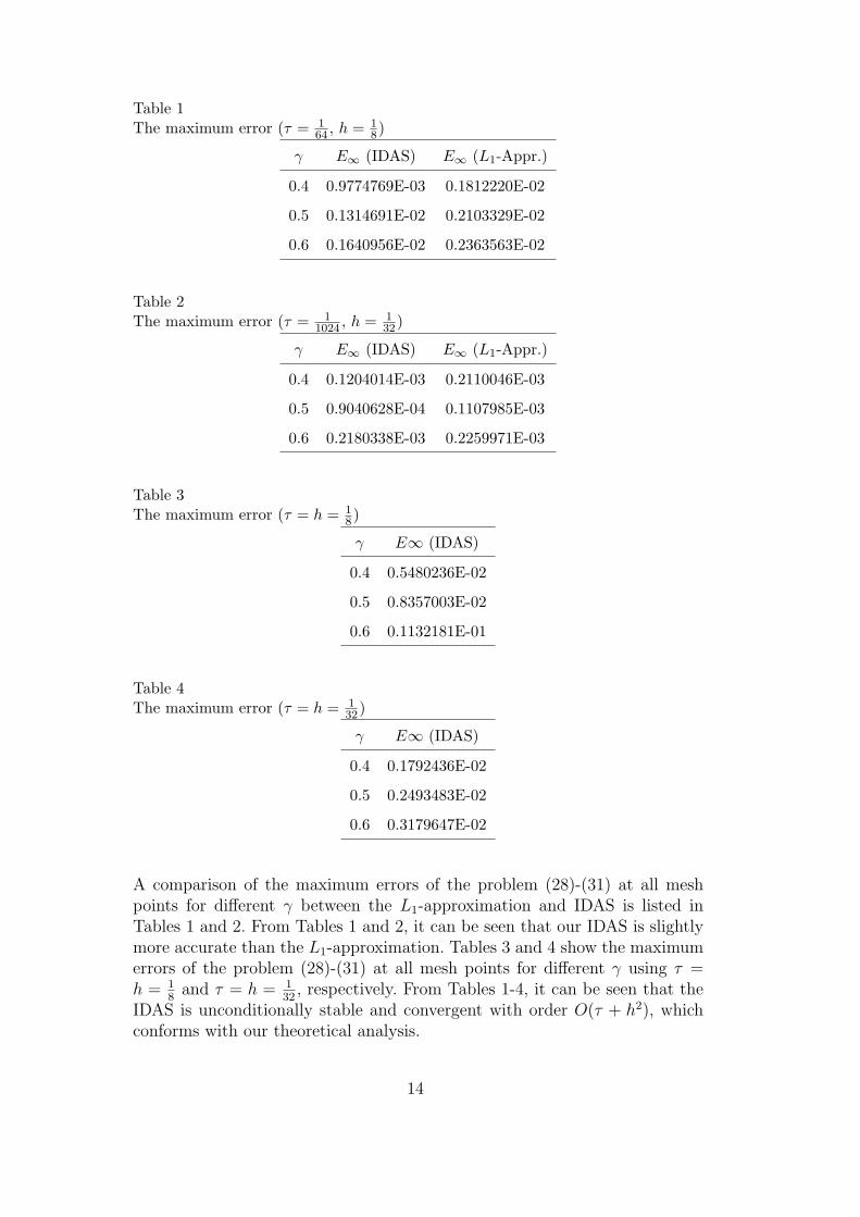
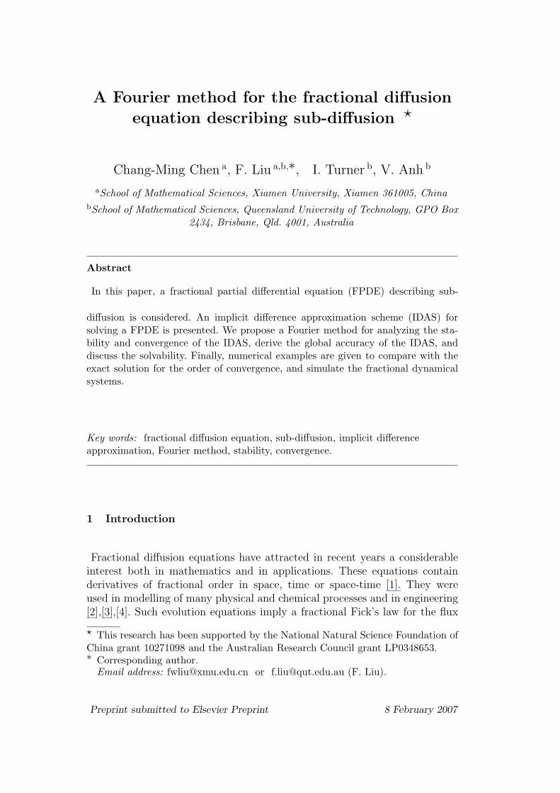
Table 1The maximum error (τ = 1
64 , h = 18)
γ E∞ (IDAS) E∞ (L1-Appr.)
0.4 0.9774769E-03 0.1812220E-02
0.5 0.1314691E-02 0.2103329E-02
0.6 0.1640956E-02 0.2363563E-02
Table 2The maximum error (τ = 1
1024 , h = 132)
γ E∞ (IDAS) E∞ (L1-Appr.)
0.4 0.1204014E-03 0.2110046E-03
0.5 0.9040628E-04 0.1107985E-03
0.6 0.2180338E-03 0.2259971E-03
Table 3The maximum error (τ = h = 1
8)
γ E∞ (IDAS)
0.4 0.5480236E-02
0.5 0.8357003E-02
0.6 0.1132181E-01
Table 4The maximum error (τ = h = 1
32)
γ E∞ (IDAS)
0.4 0.1792436E-02
0.5 0.2493483E-02
0.6 0.3179647E-02
A comparison of the maximum errors of the problem (28)-(31) at all meshpoints for different γ between the L1-approximation and IDAS is listed inTables 1 and 2. From Tables 1 and 2, it can be seen that our IDAS is slightlymore accurate than the L1-approximation. Tables 3 and 4 show the maximumerrors of the problem (28)-(31) at all mesh points for different γ using τ =h = 1
8and τ = h = 1
32, respectively. From Tables 1-4, it can be seen that the
IDAS is unconditionally stable and convergent with order O(τ + h2), whichconforms with our theoretical analysis.
14
Example 2: Fractional diffusion equation describing sub-diffusion with a ho-mogeneous term:
∂u(x, t)
∂t=0 D1−γ
t
[∂2u(x, t)
∂x2
], 0 < t, 0 < x < 2, (32)
u(0, t) = 0, 0 ≤ t, (33)
u(2, t) = 0, 0 ≤ t ≤ 1, (34)
u(x, 0) = w(x) =
2x, 0 ≤ x ≤ 12,
4−2x3
, 12≤ x ≤ 2.
(35)
The function w(x) represents the temperature distribution in a bar generatedby a point heat source kept at the point x = 1
2for sufficiently long time.
Figures 1 and 2 compare the response of the diffusion system for different realnumber 0 < γ < 1 at t = 0.4 and different x, and at x = 0.5 and different t,respectively. In the example, we take τ = 0.01, h = 0.1. From Figures 1 and 2,it is seen that IDAS can be applied to simulate fractional dynamical systems.
00.4
0.81.2
1.62
0.0
0.2
0.4
0.6
0.8
1.00
0.1
0.2
0.3
0.4
0.5
0.6
0.7
0.8
xγ
u(x,
t=0.
4)
Fig. 1. The numerical solution of problem (32)-(35) when t = 0.4 for various γ.
7 Conclusion
In this paper, we presented an implicit difference approximation scheme forsolving a fractional diffusion equation describing sub-diffusion. Fourier methodhas been has been used to successfully analyze the stability and the conver-gence of the IDAS. This technique can also be extended to analyze otherfractional partial differential equations.
15

0
0.1
0.2
0.3
0.4
0
0.2
0.4
0.6
0.8
1 0.2
0.3
0.4
0.5
0.6
0.7
0.8
0.9
1
t
γ
u(x=
0.5,
t)
Fig. 2. The numerical solution of problem (32)-(35) when x = 12 for various γ.
References
[1] R.Metzler and J.Klafter, The random walk’s guide to anomalous diffusion: afractional dynamics approach, Phys. Rep. 339 (2000) 1-77.
[2] R. Gorenflo and F. Mainardi, Fractional calulus: integral and differentialequations of fractional order, in: Fractals and Fractional Caluculus in ContinuunMechanics (eds. A Carpinteri and F. Mainardi), Springer Verlag Verlag, Wienand New York, 1997, 223-276.
[3] F. Mainardi, Fractional relaxation-oscillation and fractional diffusion-wavephenomena, Chaos, Solitons and Fractals, 7(9) (1996) 1461-1477.
[4] I. Podlubny, Fractional Differential Equations, Academic, Press, New York, 1999.
[5] R. Gorenflo, F. Mainardi, D. Moretti and P. Paradisi, Time Fractional Diffusion:A Discrete Random Walk Approach, Nonlinear Dynamics, 29 (2002) 129-143.
[6] R. Gorenflo and Mainardi,F., Random Walk Models for Space FractionalDiffusion Processes, Fractional Calculus & Applied Analysis, 1 (1998) 167-191.
[7] F. Mainardi, Yu. Luchko and G. Pagnini, The fundanental solution of the space-time fractional diffusion equation, Fractional Calculus and Applied Analysis, 4(2)(2001) 153-192.
[8] D.A. Benson, S.W. Wheatcraft and M.M Meerschaert, Application of a fractionaladvection-despersion equation, Water Resour. Res., 36(6) (2000a) 1403-1412.
[9] D.A. Benson, S.W. Wheatcraft and M.M. Meerschaert, The fractional-ordergoverning equation of Levy motion, Water Resour. Res. 36(6) (2000b) 1413-1423.
[10] W. Wyss, The fractional diffusion equation, J. Math. Phys., 27 (1986) 2782-2785.
[11] W.R. Schneider and W. Wyss, Fractional diffusion and wave equations, J. Math.Phys., 30 (1989) 134-144.
16

[12] F. Huang and F. Liu, The time fractional diffusion and advection-dispersionequation, ANZIAM J., 46 (2005) 317-330.
[13] T.A.M. Langlands and B.I. Henry, The accuracy and stability of an implicitsolution method for the fractional diffusion equation, J. Comp. Phys, 205 (2005)719-736.
[14] S.B. Yuste and L. Acedo, An explicit finite difference method and a newVon neumman-type stability analysis for fractional diffusion equations, SIAMJ. Numer. Anal. 42(5) (2005) 1862-1874.
[15] F. Liu, V. Anh, I. Turner, Numerical Solution of the Space Fractional Fokker-Planck Equation, J. Comp. Appl. Math., 166 (2004) 209-219.
[16] F. Liu, V. Anh, I. Turner and P. Zhuang, Numerical simulation for solutetransport in fractal porous media, ANZIAM J., 45(E) (2004) 461-473.
[17] M. Meerschaert and C. Tadjeran, Finite difference approximations for fractionaladvection-dispersion flow equations, J. Comp. and Appl. Math., 172 (2004) 65-77.
[18] S. Shen and F. Liu, Error analysis of an explicit finite difference approximationfor the space fractional diffusion, ANZIAM J., 46(E) (2005) 871-887.
[19] F. Liu, S. Shen, V. Anh and I. Turner, Analysis of a discrete non-Markovianrandom walk approximation for the time fractional diffusion equation, ANZIAMJ., 46(E) (2005) 488-504.
[20] J.P. Roop, Computational aspects of FEM approximation of fractionaladvection dispersion equations on boundary domains in R2, J. Comput. Appl.Math., (2006) in press.
[21] Q. Liu, F. Liu, I. Turner and V. Anh, Approximation of the Levy-Felleradvection-dispersion process by random walk and finite difference method, J.Phys. Comp., (2006), in press.
[22] P. Zhuang and F. Liu, Implicit difference approximation for the time fractionaldiffusion equation, J. Appl. Math. Computing, 22(3) (2006) 87-99.
[23] F. Liu, P. Zhuang, V. Anh, I. Turner and K. Burrage , Stability and Convergenceof the difference Methods for the Space-Time Fractional Advection-DiffusionEquation, Appl. Math. and Comput., (2007), in press.
[24] H. Zhang, F. Liu and V. Anh, Numerical approximation of Lvy-Feller diffusionequation and its probability interpretation, J. Comput. Appl. Math., (2007), inpress.
[25] F. So, K.L. Liu, A study of the subdiffusive fractional Fokker-Plank equationof bistable systems, Physica A, 331 (2004) 378-390.
17