arX

iv:1

007.

1388

v1 [

cs.D

C]

8 Ju

l 201

0

A Flexible Patch-Based Lattice BoltzmannParallelization Approach for Heterogeneous GPU–CPU Clusters

Christian Feichtingera,∗, Johannes Habichb, Harald Kostlera, Georg Hagerb, Ulrich Rudea,Gerhard Welleinb

aChair for System SimulationUniversity of Erlangen-Nuremberg

bRegional Computing Center ErlangenUniversity of Erlangen-Nuremberg

Abstract

Sustaining a large fraction of single GPU performance in parallel computations is considered tobe the major problem of GPU-based clusters. In this article,this topic is addressed in the contextof a lattice Boltzmann flow solver that is integrated in the WaLBerla software framework. Wepropose a multi-GPU implementation using a block-structured MPI parallelization, suitable forload balancing and heterogeneous computations on CPUs and GPUs. The overhead required formulti-GPU simulations is discussed in detail and it is demonstrated that the kernel performancecan be sustained to a large extent. With our GPU implementation, we achieve nearly perfectweak scalability on InfiniBand clusters. However, in strongscaling scenarios multi-GPUs makeless efficient use of the hardware than IBM BG/P and x86 clusters. Hence, a cost analysis mustdetermine the best course of action for a particular simulation task. Additionally, weak scalingresults of heterogeneous simulations conducted on CPUs andGPUs simultaneously are presentedusing clusters equipped with varying node configurations.

Keywords: Lattice Boltzmann Method, MPI, CUDA, Heterogeneous Computations

1. Introduction

In the field of computational fluid dynamics (CFD), flow solvers based on the lattice Boltzmannmethod (LBM) have become a well-established alternative for solving the Navier-Stokes equa-tions directly. The LBM algorithm is a cellular automaton derived from the Boltzmann equation;each node (cell) on the computational grid exchanges information with its neighbors, which makesmemory bandwidth the performance-limiting bottleneck of the LBM in most cases. Modeling realsystems requires large computational effort, therefore performance optimization and paralleliza-tion of LBM codes are very active fields of research. GPU architectures offer the highest memory

∗Corresponding authorEmail address:Christian.Feichtinger@informatik.uni-erlangen.de (Christian Feichtinger)

Preprint submitted to Parallel Computing July 9, 2010

to processor chip bandwidth available today in commodity hardware and promise a big perfor-mance gain for memory-bound applications. However, tremendous effort has to be put into highlyefficient LBM codes even on single GPUs [1, 2, 3]. First promising results of nonregular imple-mentations [4] show that the LBM is applicable to nonuniformdomains and multi-GPU clustersas well.

In order to push these experimental efforts into real production CFD applications it is crucial toestablish scalable LBM codes on GPU clusters. Still the current Top500 list [5] contains only afew GPU clusters, since the nonstandard programming paradigm and the rather slow CPU-to-GPUconnection are obstacles that hamper their general applicability. The main contribution of this pa-per is to show that it is possible to exploit the full computational power of currently emergingGPU–CPU clusters. We start by applying low-level optimizations to the GPU kernels to improvesingle-GPU performance, then move to multiple GPUs using MPI-based distributed memory par-allelization, and finally establish load-balanced heterogeneous GPU–CPU parallelism by incorpo-rating the otherwise idle multicore CPUs and GPU-less compute nodes into the flow solver.

To bring together high performance and high productivity weapply aPatch and Blockdesign,which divides the computational domain into subregions that are distributed to thecompute units(GPUs or teams of CPU threads in a multicore node). This is a choice as to how many subre-gions are assigned to each compute unit instead of individual cells, simplifying static load balanc-ing. Ghost layers are exchanged between neighboring subregions using the appropriate data paths(shared memory, PCIe bus, InfiniBand interconnect). A simulation is thus able to run in parallelon a heterogeneous cluster comprising various different architectures. The whole code is includedin the WaLBerla (Widely applicable lattice Boltzmann solver from Erlangen) software framework,which is employed in many CFD applications. We can show that high computational performancecan be sustained within WaLBerla and therefore only very small application management andcommunication overhead is added.

This paper is organized as follows. We start with a brief description of the architectures used formeasurements and the LBM method in Sec. 2. Code optimizations and performance models areshown in Sec. 3. Section 4 describes the WaLBerla software framework and the heterogeneousparallelization approach. In Sec. 5 we finally analyze the performance behavior of our code onsingle CPUs, single GPUs, and heterogeneous CPU–GPU clusters in strong and weak scalingscenarios.

2. Methods and Architectures

2.1. The Lattice Boltzmann Method

The LBM has evolved over the last two decades and is today widely accepted in academia andindustry for solving incompressible flows. Coming from a simplified gas-kinetic description, i.e.a velocity discrete Boltzmann equation with an appropriatecollision term, it satisfies the Navier-Stokes equations in the macroscopic limit with second orderaccuracy [6, 7]. In contrast to conven-tional computational fluid dynamic methods, the LBM uses a set of particle distribution functions(PDF) in each cell to describe the fluid flow. A PDF is defined as the expected value of particlesin a volume located at the lattice position~x with the lattice velocity~ei . Computationally, the LBM

2

is based on a uniform grid of cubic cells that are updated in each time step using an informa-tion exchange with nearest neighbor cells only. Structurally, this is equivalent to an explicit timestepping for a finite difference scheme. For the LBM the lattice velocities~ei determine the finitedifference stencil, wherei represents an entry in the stencil. Here, we use the so-called D3Q19model resulting in a 19 point stencil and 19 PDFs in each cell.The evolution of a single PDFfi isdescribed by

fi(~x+~ei∆t, t+∆t) = f colli (~x, t) =

fi(~x, t)−1τ[

fi(~x, t)− f eqi (ρ(~x, t),~u(~x, t))

]

(1)

f eqi (ρ(~x, t),~u(~x, t)) = wi

[

ρ +ρ0(

3~ei~u+4.5(~ei~u)2−1.5~u2

)]

(2)

i = 0. . .19,

and can be split into two steps: A collision step applying thecollision operator and a propagationstep advecting the PDFs to the neighboring cells. In this article, we use the single relaxation timecollision operator [7]. In Eq. 1,f coll

i denotes the intermediate state after collision but before prop-agation. The relaxation timeτ can be determined from the kinematic viscosityν = (τ − 1

2)c2sδ t,

with cs as the speed of sound. Further,f eqi is a Taylor expanded version of the Maxwell-Boltzmann

equilibrium distribution function [7] optimized for incompressible flows [8]. For the isothermalcase, f eq

i depends on the macroscopic velocity~u(~x, t) and the macroscopic densityρ(~x, t), andthe lattice weightswi are 1

3, 118 or 1

36. The macroscopic quantitiesρ and~u are determined fromthe 0th and 1st order moment of the distribution functionsρ(~x, t) = ρ0+ δρ(~x, t) = ∑18

i=0 fi(~x, t),and ρ0~u(~x, t) = ∑18

i=0~ei fi(~x, t), whereρ is split into a constant partρ0 and a slightly changingperturbationδρ . The equation of state of an ideal gas provides the pressurep(~x, t) = c2

sρ(~x, t).Usually, the PDFs are initialized tof eq

i (ρ0,0). To increase the accuracy of simulations in singleprecision we usefi(~x, t) = fi(~x, t)− f eq

i (ρ0,0) and f eqi (ρ(~x, t),~u(~x, t)) = f eq

i (ρ(~x, t),~u(~x, t))−f eqi (ρ0,0) as proposed by [8] resulting in PDF values centered around 0.According to [1], it is

possible with the LBM scheme described above to achieve accurate single precision results, whichis important for GPU implementations.

A further important issue is the implementation of the propagation, for which there exist twoschemes: First a pushing and second a pulling. For the first case, the PDFs in a cell are firstcollided and then pushed to the neighborhood. In the second case, the neighboring PDFs are firstpulled into the lattice cell and then collided. Additionally, the propagation step introduces datadependencies to the LBM, which commonly result in an implementation of the LBM using twoPDF grids. However, these dependencies are of local type, asonly PDFs of neighboring cells areaccessed. Hence, the LBM is particularly well suited for massively parallel simulations [9, 10, 11].In WaLBerla, we use thepull approach as it is better suited for our parallelization (seeSec. 4 fordetails on the parallelization).

The most common approach for implementing solid wall boundaries in the LBM is the bounce-back (BB) rule [6, 7], i.e. if a distribution is about to be propagated into a solid cell, the dis-tribution’s direction is reversed into the original cell. BB generally assumes that the wall is inthe middle between the two cell centers, i.e. half-way. Thisformulation leads to:fi(~x, t +∆t) =

3

fi(~x, t)+6wiρ0~ei~uw with~ei =−~ei anduw being the velocity prescribed at the wall.

2.2. Hardware Environments

2.2.1. CPU-based Cluster Systems

In general, current clusters based on dual-socket Intel quad-core processors offer a peak node per-formance in the range of 60 to 100 GFLOPS. The on-chip memory controllers with up to threeDDR3 memory channels per socket provide a theoretical peak node bandwidth of 64 GB/s. Theclusters introduced in the following table all share this common architecture:

Nodes Processor Interconnect Clock Speed Memory nVIDIA GPUs per NodeXeon [GHz] [GB]

TinyGPU [12] 8 X5550 DDR IB 2.66 24 2 x TESLA C1060JUROPA [13] 2208 X5570 QDR IB 2.93 24NEC Nehalem [14] 700 X5560 DDR IB∗ 2.8 12 2 x TESLA S1070∗ Oversubscribed IB backbone (30 nodes)

The IBM BlueGene/P-based cluster JUGENE [15] comprises 73728 compute nodes, each equippedwith one 850 MHz PowerPC 450 quad-core processor and 4 GB memory, which are connected viaa proprietary high speed interconnect offering 850 MB/s perlink direction.

2.2.2. nVIDIA Graphic Processing Units

The GT–200-based GPUs are the second generation of nVIDIA graphics cards capable of GPGPUcomputing using theCompute Unified Device Architecture(CUDA) [16]. A GPU has several mul-tiprocessors (MP), each with 8 processor cores. Computations are executed by so-called threads,whereas up to 1024 threads are concurrently running on one MPin order to hide memory latencyby efficient scheduling. Threads are organized in GPU-blocks, which are pinned to an MP overthe whole runtime. Each MP has 16384 registers and 16 kB of shared memory available, i.e. thereare only 16 registers and about 16 bytes per thread if 1024 threads are running in parallel. Hence,the concurrency is limited if kernels allocate more than 16 registers, which has a severe impact onperformance. See [17] for further details on CUDA and nVIDIAGPU hardware.

2.3. Interconnects

Most of today’s high performance systems use InfiniBand (IB)for the connection of the computenodes. Heterogeneous computations on CPUs and GPUs requirePCI-Express (PCIe) transfers forboth IB and CPU–GPU communication. In order to develop a sensible performance model, allinvolved communication paths must be considered.

PCIe 2.0 x16 is currently the fastest peripheral bus with a peak transfer bandwidth of 8 GB/s perdirection. Figure 1 shows that one can maintain about 6 GB/s bandwidth if the transfered data islarger than 2 MB and the CUDA callcudahostallocis used to allocate so-calledpinned memoryon the host. Pinned memory in contrast to memory allocated bymallocwill not be paged out, isprivate to the process allocating it, and is local to the physical socket of the allocating process.The advantage of pinned memory results from the possibilityto use fast direct-memory-accesses

4

1/8

1/8

1/4

1/4

1/2

1/2

1

1

2

2

4

4

8

8

16

16

32

32

64

64

128

128

256

256

512

512

Data transferred [MB]0 0

1 1

2 2

3 3

4 4

5 5

6 6

Ban

dwid

th [G

B/s

]

PCIe Device to Host copy PCIe Host to Device copyPCIe Device to Host copy pinnedPCIe Host to Device copy pinnedDDR InfiniBand PingPongQDR InfiniBand PingPong

Figure 1: Host–GPU and MPI PingPong bandwidth measurementson TinyGPU. The functioncudaMemcpyimple-menting a vector copy is used for all PCIe copy operations.

(DMA). With our current LBM implementation packets in the range of 250 kB to 500 kB areexchanged per PCIe data transfer, leading to an effective bandwidth between about 5 GB/s and6 GB/s. Please note that two GPUs on the NEC Nehalem cluster have to share the same PCIe bus,which is capable of transferring 12.8 GB/s.

IB host adapters are connected to the host via the PCIe x8 interface. IB bandwidth measurementsof the Intel IMBPingPongbenchmark [18] for quad-(QDR) and double-(DDR) data rate IBcan befound in Fig. 1. The measurements show that QDR (3.0 GB/s) doubles the bandwidth comparedto DDR (1.5 GB/s) and that the GPU’s PCIe operates with at least twice the bandwidth.

The performance of LBM codes is usually given in terms ofmillion fluid lattice cell updates persecond(MFLUPS) instead of GFlops, as the actual executed GFlops cannot be determined pre-cisely. Table 1 gives an estimate for the minimal impact of the data transfer over all interconnectson performance. The compute time of the kerneltk and the IB and PCIe data transfer timestt canhereby be determined by

tk =n3

cell

Pand tt =

2 ·n2cell ·nPDF ·nplane·sPDF

B,

whereP is the performance,nCell the number of lattice cells per dimension,nPDF the number ofPDFs communicated per boundary cell,nplane the number of planes to be communicated,sPDF thesize in bytes of a PDF andB is the bandwidth of the corresponding interconnect. It was assumedthat all domain boundaries have to be communicated, which results in the transfer of 6 boundaryplanes with 5 PDFs per cell.

3. CPU and GPU Kernel Implementation

3.1. Upper Bound Performance Estimation

The performance of our LBM implementation is like most scientific codes dominated by memorybandwidth. To estimate an upper bound for the obtainable LBMbandwidth on CPUs, we employ

5

Steps Tesla C1060 (∼ 300 MFLUPS)

Compute Time 3.3 msPCIe: 5 GB/s (I) 0.48 msIB: 3.0 GB/s (II) 0.8 ms

Total Time: (I) 3.78 ms→ 264 MFLUPS(I+II) 4.58 ms→ 218 MFLUPS

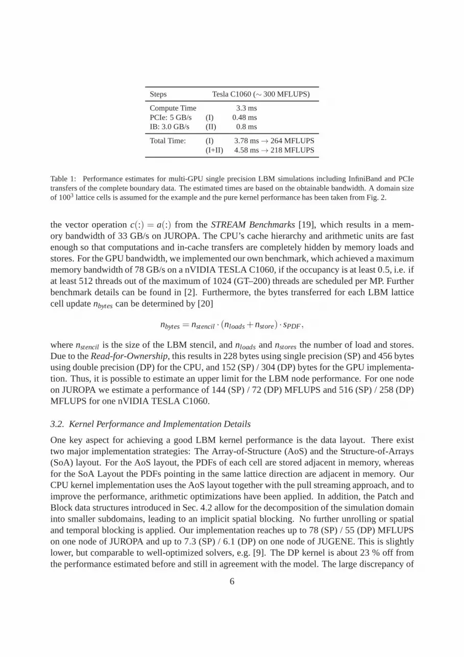
Table 1: Performance estimates for multi-GPU single precision LBM simulations including InfiniBand and PCIetransfers of the complete boundary data. The estimated times are based on the obtainable bandwidth. A domain sizeof 1003 lattice cells is assumed for the example and the pure kernel performance has been taken from Fig. 2.

the vector operationc(:) = a(:) from theSTREAM Benchmarks[19], which results in a mem-ory bandwidth of 33 GB/s on JUROPA. The CPU’s cache hierarchyand arithmetic units are fastenough so that computations and in-cache transfers are completely hidden by memory loads andstores. For the GPU bandwidth, we implemented our own benchmark, which achieved a maximummemory bandwidth of 78 GB/s on a nVIDIA TESLA C1060, if the occupancy is at least 0.5, i.e. ifat least 512 threads out of the maximum of 1024 (GT–200) threads are scheduled per MP. Furtherbenchmark details can be found in [2]. Furthermore, the bytes transferred for each LBM latticecell updatenbytescan be determined by [20]

nbytes= nstencil· (nloads+nstore) ·sPDF,

wherenstencil is the size of the LBM stencil, andnloads andnstoresthe number of load and stores.Due to theRead-for-Ownership, this results in 228 bytes using single precision (SP) and 456 bytesusing double precision (DP) for the CPU, and 152 (SP) / 304 (DP) bytes for the GPU implementa-tion. Thus, it is possible to estimate an upper limit for the LBM node performance. For one nodeon JUROPA we estimate a performance of 144 (SP) / 72 (DP) MFLUPS and 516 (SP) / 258 (DP)MFLUPS for one nVIDIA TESLA C1060.

3.2. Kernel Performance and Implementation Details

One key aspect for achieving a good LBM kernel performance isthe data layout. There existtwo major implementation strategies: The Array-of-Structure (AoS) and the Structure-of-Arrays(SoA) layout. For the AoS layout, the PDFs of each cell are stored adjacent in memory, whereasfor the SoA Layout the PDFs pointing in the same lattice direction are adjacent in memory. OurCPU kernel implementation uses the AoS layout together withthe pull streaming approach, and toimprove the performance, arithmetic optimizations have been applied. In addition, the Patch andBlock data structures introduced in Sec. 4.2 allow for the decomposition of the simulation domaininto smaller subdomains, leading to an implicit spatial blocking. No further unrolling or spatialand temporal blocking is applied. Our implementation reaches up to 78 (SP) / 55 (DP) MFLUPSon one node of JUROPA and up to 7.3 (SP) / 6.1 (DP) on one node of JUGENE. This is slightlylower, but comparable to well-optimized solvers, e.g. [9].The DP kernel is about 23 % off fromthe performance estimated before and still in agreement with the model. The large discrepancy of

6

0 50 100 150 200Cubic Domain Size

0 0

50 50

100 100

150 150

200 200

250 250

300 300

350 350

400 400

450 450

MF

LUP

S

SPDP

Figure 2: Single-GPU measurements of the pure GPU kernel performance for SP and DP on a nVIDIA TESLAC1060.

nearly 50 % for the SP kernel can be attributed to the computational intensity of the nonvectorizedLBM kernel, making the code essentially not memory, but computationally bound.

In contrast to the CPU implementation, the GPU implementation uses the SoA layout, becausein combination with the pull streaming approach it is possible to align the memory writes. Inaddition, the scattered loads that occur in our implementation can be efficiently coalesced bythe memory subsystem. Hence, we do not have to use the shared memory of the GPU. For thescheduling of the threads, we adopted a scheme first proposedin [1], where each GPU threadupdates one lattice cell and one GPU block is assigned one rowof the simulation domain. In orderto improve the kernel performance, we reduced the number of registers used for each thread byprefetching the PDFs into temporal variables and also by modifying the array accesses as describedin [2]. With these optimizations, we can achieve a maximum occupancy of 0.5. The maximumperformance for some domain sizes has been around 500 (SP) / 250 (DP), which agrees well withour performance estimates and also with the results in [3]. Acomparison to [1] is rather difficultas they used a different LBM stencil and hardware has evolved. Still, the sustained memorybandwidth of both implementations on the particular hardware is around 70 % of peak bandwidth.A detailed kernel performance analysis for cubic domain sizes is depicted in Fig. 2. The measuredperformance fluctuations for varying domain sizes result from the different numbers of scheduledthreads per MP and from memory alignment issues.

4. The WaLBerla Framework

WaLBerla is a massively parallel multiphysics software framework that is originally centeredaround the LBM, but whose applicability is not limited to this algorithm. Its main design goals areto provide excellent application performance across a widerange of computing platforms and theeasy integration of new functionality. In this context additional functionality can either extend theframework for new simulation tasks, or optimize existing algorithms by adding special-purposehardware-dependent kernels or new concepts such as load balancing strategies. In order to achieve

7

this flexibility, WaLBerla has been designed utilizing software engineering concepts such as thespiral model and prototyping [21, 22], and also using commondesign patterns [23]. Several re-searchers and cooperation partners have already used the software framework to solve variouscomplex simulation tasks. Amongst others, free-surface flows [24] using a localized parallel algo-rithm for bubbles coalescence, free-surface flows with floating objects [25], flows through porousmedia, clotting processes in blood vessels [26], particulate flows for several million volumetricparticles [27] on up to 8192 cores, and a fluctuating lattice Boltzmann [28] for nano fluids havebeen included. In addition to the strictly Eulerian view of field equations and their discretization,WaLBerla also supports Lagrangian representations of physical phenomena, such as e.g. particu-late flows. Currently, the prototype WaLBerla 2.0 is under development extending the frameworkfor heterogeneous simulations on CPUs and GPUs, and load balancing strategies. Heterogeneouscomputations are already supported, but the designs for dynamic load balancing strategies are cur-rently under development, although the underlying data structures can already be used for staticload balancing.

In WaLBerla, all simulation tasks are broken down into several basic steps, so-calledSweeps. ASweep can be divided into two parts: a communication step fulfilling the boundary conditions forparallel simulations by nearest neighbor communication and a communication independent workstep traversing the process-local grid and performing operations on all cells. The work step usuallyconsists of a kernel call, which is realized for instance by afunction object or a function pointer.As for each work step there may exist a list of possible (hardware dependent) kernels, the executedkernel is selected by our functionality management (see below). For pure LBM simulations onlyone Sweep is needed exchanging PDF boundary data during the communication phase and execut-ing one of the kernels that have been described in Sec. 3. The functionality management in WaL-Berla 2.0 selects the required kernels according to meta data provided with each kernel. This dataallows the selection of different kernels for different simulation runs, processes and subregions ofthe simulation domain, so-calledBlocks(see Sec. 4.2). Hence, it is possible to specifically select,for heterogeneous computations even on each single process, hardware optimized kernels. Furtherdetails on the functionality management can be found in Sec.4.1.

A further fundamental design of the whole software framework is ourPatchandBlockdata struc-ture, which is a specific version of block-structured grids.Besides forming the basis for theparallelization and load balancing strategies, Blocks arealso essential to configure the domainsubregions with regard to the simulated task and the utilized hardware. More information on thePatch and Block data structure can be found in Sec. 4.2. Further, WaLBerla enables parallel MPIsimulations of various simulation tasks. In order to do so, the process-to-process communicationsupports messages, containing data from any kind of data structure conforming to a documentedinterface, of arbitrary length and data type as well as the serialization of messages to the sameprocess. Using our parallelization it is possible to represent even complex communication pat-terns, such as our localized bubble merge algorithm [24] or our parallel multigrid solver portedfrom [29]. The general parallelization design is describedin Sec. 4.3. For parallel simulationson GPUs, the boundary data of the GPU has first to be copied by a PCIe transfer to the CPU andthen be communicated via the MPI parallelization. Therefore, the data structures of the single coreimplementation are extended by buffers on GPU and CPU in order to achieve fast PCIe transfers.

8

In addition, on-GPU copy kernels are added to fill these buffers. In Sec. 4.4 the details of ourparallel GPU implementation are introduced. To support heterogeneous simulations on GPUs andCPUs, we execute different kernels on CPU and GPU and also define a common interface for thecommunication buffers, so that an abstraction from the hardware is possible. Additionally, thework load of the CPU and the GPU processes has to be balanced. In our approach this is achievedby allocating several Blocks on each GPU and only one on each CPU-only process.

4.1. Functionality Management

The functionality management in WaLBerla 2.0 allows to select different functionality (e.g. ker-nels, communication functions) for different granularities, e.g. for the whole simulation, for indi-vidual processes, and for individual Blocks. This is realized by adding meta data to each function-ality consisting of three unique identifiers (UID).

UID Name Granularity Example

fs Functionality Selector Simulation Gravity on/offhs Hardware Selector Process CPU and/or GPUbs Block Selector Block LBM

On the basis of these UIDs the kernels can be selected according to the requirements of the sim-ulated scenarios. Hence, physical effects can be turned on/off in an efficient well-defined mannerby means of thefsselector. Hardware-dependent kernels can be selected for different architecturesdepending on thehsselector and simulation tasks can be selected via thebsselector. A complexexample for the capabilities of our concept are heterogeneous LBM simulations on CPUs andGPUs described in Sec. 4.5.

4.2. Patch and Block Concept

In WaLBerla the simulation domain is described with our Patch and Block design, which is il-lustrated in Fig. 3. It has been developed in order to supportmassively parallel simulations, loadbalancing strategies and the configuration to simulation tasks and hardware. A Patch hereby is arectangular cuboid describing a region in the simulation that is discretized with the same resolu-tion. In principal, these Patches can be arranged hierarchically for grid refinement techniques, butin this work we are using only one Patch covering the whole simulation domain. This Patch isfurther subdivided into a Cartesian grid of Blocks, again ofcuboidal shape, containing the actualgrid-based data for the simulation (simulation data). Withthe aid of these Blocks the simula-tion domain can be partitioned for parallel simulation. It is hereby possible to allocate severalBlocks on a process in order to support load balancing strategies. Additionally, with the help ofthe functionality management the Blocks’ data can be configured for the simulated scenario. Inparticular, each Block contains two kinds of data: management information and simulation data.The management data contains arank parameter, which decides on which process the simulationdata of the Block is allocated. Additionally, a hardware selector (hs) describes the hardware onwhich the Block is allocated, whereby all Blocks on the same process have the same hardwareselector assigned to them. Further, the management data contains a block selector (bs) deciding

9

Figure 3: Patch and Block Design. Each Block stores management information consisting of a block and a hardwareselector, a MPI rank, an axis aligned bounding box (AABB), and a Block identifier (BlockID) required for the identi-fication of individual Blocks. The Blocks’ management information is stored on all processes, but simulation data isonly allocated on processes which are responsible for that particular Block.

which task is simulated on a Block. For the simulation data each block stores a dynamic list ofbase class pointers. For multiphysics simulations this allows to store an arbitrary number of datafields, e.g. grid-based data for velocity, temperature or potential values or unstructured particledata for particulate flows. Hence, each block can be configured in the following way: Duringthe initialization of a simulation WaLBerla creates lists of possible simulation tasks, kernels foreach Sweep and several simulation data types, whereby each entry in a list is connected to metadata for the functionality management. With the help of the selectors stored in the managementinformation it is possible to select which task has to be simulated, which simulation data has to beallocated, and which kernels have to be selected for the Sweeps from these lists.

4.3. General Design of the MPI Communication

The parallelization of WaLBerla, which is depicted in Fig. 4, can be broken down into three steps:a data extraction step, a MPI communication step and a data insertion step. During the data extrac-tion step, the data that has to be communicated is copied fromthe simulation data structures of thecorresponding Blocks. Therefore, we distinguish between process-local and MPI communicationfor Blocks lying on the same or different processes. Local communication directly copies fromthe sending Block to the receiving Block, whereas for the MPIcommunication the data has first tobe copied into buffers. For each process to which data has to be sent, one buffer is allocated. Withthe buffers, all messages from Blocks (block message) on thesame process to another process areserialized. Additionally, the buffers are of data typebyteand thus the MPI messages can containany data type that can be converted into bytes. To extract thedata to be communicated from thesimulation data, extraction function objects are used. Foreach communication step and for eachsimulation data type several possible function objects areprovided during the configuration ofthe communication. These are again selected via the functionality management. During the MPI

10

Figure 4: Design for parallel simulations. In the Figure, the MPI communication from process I to process II isdepicted. First, the data to be communicated is extracted with provided functions from each Block and stored in sendbuffers. For pure fluid flows only PDFs have to be sent. On the sending side an MPIIsend is scheduled and on thereceiving side the message is either received with a MPIProbe, MPIGetCount and a MPIRecv, or a MPIIrecv.Note, that we attach a header to each Block message containing the BlockID and a communication direction. This isrequired in order to determine the Block to which the data hasto be copied on the receiving side.

communication one MPI message is sent to each process waiting for data from the current process.Therefore, nonblocking MPI functions are used, if the message size can be determined a priori.The data insertion step is similar to the data extraction, only here we traverse the block messagesin the communication buffers instead of the Blocks.

Figure 5: Multi-GPU design.

4.4. Multi GPU Implementation

For parallel GPU simulations part of the data stored on the GPU has to be transferred to theCPU via PCIe transfers before it can be communicated by meansof the MPI communication. Anefficient implementation of this transfer is important in order to sustain a large portion of the kernelperformance. Hence, we only transfer the minimum amount of data necessary, the boundary valuesof the PDFs. Our parallel GPU implementation is depicted in Fig. 5 for one process having two

11

Blocks. It can be seen that we extended the data structures byadditional buffers on the GPU and onthe CPU side. In 3D, we add 6 planes and 12 edge buffers. To update the ghost layer of the PDFsand to prepare the GPU buffers for the MPI communication additional on-GPU copy operationsare needed. The data of the buffers is copied to the ghost layer of the Blocks before the kernel calland the PDF boundary values of the PDF data are copied into theGPU buffers afterwards. Forparallel simulations, the MPI implementation of Sec. 4.3 isused. Here, the only difference to theCPU implementation are the extraction and insertion functions, which for the local communicationsimply swap the GPU buffers, whereas the functioncudaMemcpyis used to copy the data directlyfrom the GPU buffers into the MPI buffers and vice versa for the MPI communication. To treatthe boundary conditions at the domain boundary, the corresponding GPU buffers are transferredvia cudaMemcpyto the CPU buffers. Next, the boundary conditions are applied and the data iscopied back into the GPU buffers. The boundary conditions are fulfilled before the on-GPU copyoperations.

4.5. Heterogeneous GPU / CPU Implementation

Figure 6: Heterogeneous simulation on GPU and CPU. The illustrated simulation is executed on two processes eachhaving one Block covering half of the simulation domain. A standard LBM simulation is chosen asfs and on allBlocks thebspure LBM is activated. Further, the first process runs on a CPU(hsCPU), whereas the second uses aGPU (hsGPU). According to these UIDs, the simulation data is allocatedand the kernels, the extraction and insertionfunctions are selected. For the communication, extractionfunctionscopyToBufare selected by the UIDs of the cor-responding Block to copy the communicated data in the specified format into the MPI send buffers. After the MPIcommunication, the insertion functionscopyFromBufcopy the data from the MPI buffers back into the receiving datastructures.

For parallel heterogeneous simulations, the information which Block runs on which hardware hasto be known on all processes in our implementation. Hence, during the initialization we set on eachprocess thehsof all Blocks to thehsof the process on which they are allocated. To determine thehs of each process, the input for the simulation describes all possible node configurations and alist which node belongs to which configuration. A node configuration defines how many processescan be executed on a particular node and whichhsshould be used for each process. Using thesehardware selectors, it is now possible to utilize differentLBM kernels and simulation data on

12

0 25 50 75 100 125 150 175200 225 250 275Cubic Domain Size

0 0

50 50

100 100

150 150

200 200

250 250

300 300

350 350

MF

LUP

S

1 Block8 Blocks64 Blocks

(a) SP

0 25 50 75 100 125 150 175 200 225Cubic Domain Size

0 0

25 25

50 50

75 75

100 100

125 125

150 150

175 175

200 200

MF

LUP

S

1 Block8 Blocks64 Blocks

(b) DP

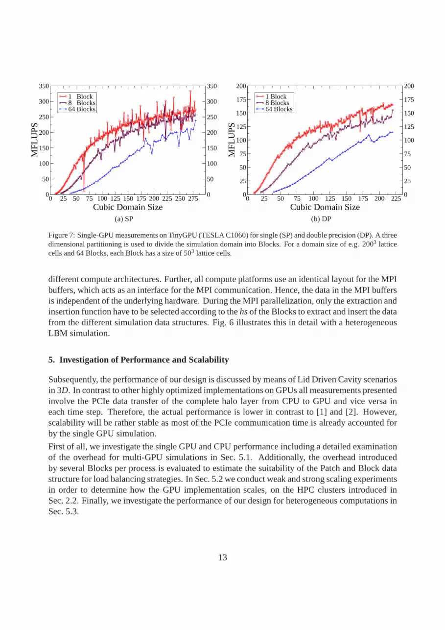
Figure 7: Single-GPU measurements on TinyGPU (TESLA C1060)for single (SP) and double precision (DP). A threedimensional partitioning is used to divide the simulation domain into Blocks. For a domain size of e.g. 2003 latticecells and 64 Blocks, each Block has a size of 503 lattice cells.

different compute architectures. Further, all compute platforms use an identical layout for the MPIbuffers, which acts as an interface for the MPI communication. Hence, the data in the MPI buffersis independent of the underlying hardware. During the MPI parallelization, only the extraction andinsertion function have to be selected according to thehsof the Blocks to extract and insert the datafrom the different simulation data structures. Fig. 6 illustrates this in detail with a heterogeneousLBM simulation.

5. Investigation of Performance and Scalability

Subsequently, the performance of our design is discussed bymeans of Lid Driven Cavity scenariosin 3D. In contrast to other highly optimized implementations on GPUs all measurements presentedinvolve the PCIe data transfer of the complete halo layer from CPU to GPU and vice versa ineach time step. Therefore, the actual performance is lower in contrast to [1] and [2]. However,scalability will be rather stable as most of the PCIe communication time is already accounted forby the single GPU simulation.

First of all, we investigate the single GPU and CPU performance including a detailed examinationof the overhead for multi-GPU simulations in Sec. 5.1. Additionally, the overhead introducedby several Blocks per process is evaluated to estimate the suitability of the Patch and Block datastructure for load balancing strategies. In Sec. 5.2 we conduct weak and strong scaling experimentsin order to determine how the GPU implementation scales, on the HPC clusters introduced inSec. 2.2. Finally, we investigate the performance of our design for heterogeneous computations inSec. 5.3.

13

5.1. Single GPU and CPU Performance

Our performance results for a single GPU having 1 to 64 local Blocks are depicted in Fig. 7. Theperformance increases with the domain size and saturates ata domain size of around 2003 latticecells for a single Block. This is in contrast to the pure kernel measurements of Fig. 2, where themaximum performance is already reached for a domain size of around 703 lattice cells. Fig. 8shows that this results from the additional overhead of the on-GPU and BC copy operations. Thesame holds for the drop in performance using several Blocks,as the pure kernel runtime of 1 and64 Blocks is nearly identical. For large domain sizes we loose about 5 % for 8 Blocks and 25 % for64 Blocks compared to the runtime of one Block. Hence, if several small Blocks are required, e.g.for load balancing strategies, the performance of our GPU implementation will be reduced. Themaximum achieved performance is 340 (SP) / 167 (DP) MFLUPS. Compared to the pure kernelperformance we sustain around 80 % using large domains for both SP and DP. For small domainsizes, e.g. 1003 lattice cells, we estimated in Tab. 1 a drop in performance from around 300 to 264MFLUPS (SP), taking only the PCIe transfer into account. Themeasurements in Fig. 7 show aperformance of around 190 MFLUPS. As can be seen in Fig. 8, this discrepancy again results fromthe, in this case dominating, overheads of the on-GPU copiesand the BC treatment. This clearlyindicates that the PCIe transfer, which is included in the BCtreatment, is not the only componentcrucial to sustain a large portion of the kernel performance. The on-GPU copy operations arehereby unavoidable, but the BC could be treated directly on the GPUs for further performanceimprovement. This will be investigated in future work.

The single node performance on JUROPA and JUGENE is presented in Fig. 9. Compared to themaximum single GPU performance the CPU performance corresponds to about 25 % in SP and33 % in DP on JUROPA and 2 % in SP and 3.5 % in DP on JUGENE. Usually, we use domain sizesranging from 903 to 1303 in DP on one CPU core. For these sizes, the CPU measurements show a

100 150 200 250Cubic Domain Size

10 10

20 20

30 30

40 40

50 50

60 60

70 70

80 80

Tim

e pe

r ite

ratio

n [m

s] BC 1 Block PinnedBC 64 Blocks Pinnedon-GPU Copy 1 Blockon-GPU Copy 64 BlocksKernel 1 BlockKernel 64 Blocks

(a) Runtime

50 100 150 200 250Cubic Domain Size

0.25 0.25

0.5 0.5

0.75 0.75

1 1

1.25 1.25

1.5 1.5

1.75 1.75

2 2

GP

U O

verh

ead

Rat

io on-GPU Copy 1 Blockon-GPU Copy 64 BlocksBC 1 Block PinnedBC 64 Blocks Pinned

(b) Overhead Ratios

Figure 8: Single-GPU time measurements on TinyGPU(TESLA C1060) in SP. Fig. (a) shows the runtimes of differentparts of the algorithm and Fig. (b) shows the ratio of the times for on-GPU copy operations and boundary conditionhandling (BC) to the kernel execution time. In both Figures results are given for 1 and 64 Blocks. Pinned memorydenotes host memory allocated by the CUDA callcudaHostAlloc.

14

0 25 50 75 100 125Cubic Domain Size per Core

0 0

10 10

20 20

30 30

40 40

50 50

60 60

70 70

80 80

MF

LUP

S p

er N

ode

1 Block per Core SP8 Blocks per Core SP27 Blocks per Core SP1Block per Core DP8 Blocks per Core DP27 Blocks per Core DP

(a) JUROPA

0 25 50 75 100Cubic Domain Size per Core

0 0

1 1

2 2

3 3

4 4

5 5

6 6

7 7

8 8

MF

LUP

S p

er N

ode

1 Block per Core SP27 Blocks per Core SP1 Block per Core DP27 Blocks per Core DP

(b) JUGENE

Figure 9: Single node CPU measurements on JUROPA (Xeon X5570) and JUGENE (BlueGene/P) for different Blocknumbers per core. For JUROPA 8 and for JUGENE 4 cores are used.

superior performance for multi-Block simulations compared to single Block simulations. This is incontrast to the GPU implementation, where multiple Blocks cause a degradation in performance.This results from an efficient utilization of the cache due toblocking effects occurring especiallyfor the AoS data layout. Hence, for the investigated architectures block-structured grids are wellsuited for load balancing strategies.

5.2. Multi-CPU and GPU Performance

0 2 4 6 8 10 12 14 16 18 20 22 24 26 28 30Nodes (2 GPUs per Node)

0 0

1 1

2 2

3 3

4 4

5 5

6 6

7 7

GF

LUP

S

360^3 SP240^3 DP

(a) Absolute performance

0 2 4 6 8 10 12 14 16 18 20 22 24 26 28 30Nodes (2 GPUs per Node)

0 0

100 100

200 200

300 300

400 400

500 500

MF

LUP

S p

er N

ode 360^3 SP

240^3 DP

(b) Relative performance

Figure 10: Multi-GPU strong scaling experiments on the NEC Nehalem cluster (TESLA S1070) with a domain sizeof 3603 lattice cells in SP and 2403 lattice cells in DP. The block decomposition is three dimensional. Figure (a) showsthe absolute performance values, whereas Figure (b) shows the relative performance, i.e. the absolute performancedivided by the number of compute nodes.

15

There are two basic scenarios to investigate parallel performance: weak scaling and strong scaling.In weak scaling experiments, the work load per compute node is kept constant for an increasingnumber of nodes. With this scenario the scalability and the overall manageable parallelism of thecode is evaluated. Strong scaling experiments answer the question how much the time to solutioncan be reduced for a given problem. Therefore, the work load of all nodes is kept constant leadingto a dominating communication overhead and thus a drop in speedup with an increasing numberof nodes. An important point for the scalability of multi-GPU simulations is whether the perfor-mance scales if using two GPUs on the same node. On TinyGPU andthe NEC Nehalem clusterthis has been the case, as we achieved around 95 % parallel efficiency for two GPUs. Further,weak scaling experiments on the NEC Nehalem cluster showed anearly linear scaling up to 60GPUs for the domain size 2223 resulting in a maximum performance of around 16 GFLUPS in SP.In comparison to todays CPUs, single GPUs offer a superior performance. Hence, on the one handthey should be well suited to reduce the time to solution in parallel simulations as less internodeparallelism is required. On the other hand, the multi-GPU performance is not only hampered bythe MPI communication, but also by the PCIe transfers, the on-GPU copies, and, in contrast tothe CPU, the missing cache effect for small domains. In our GPU strong scaling experiments,depicted in Fig. 10, it can be seen that the relative performance for 1 to 30 compute nodes dropsfrom around 500 to 235 MFLUPS in SP and from around 250 to 100 MFLUPS in DP. Comparedto the CPU strong scaling experiments in Fig. 11, we need around 6 (SP & DP) compute nodeson JUROPA and 75 (SP) / 50 (DP) on JUGENE to achieve the performance of a single GPU nodeon the NEC Nehalem cluster. To achieve the performance of 30 GPU compute nodes, we needaround 137 (SP) / 70 (DP) compute nodes on JUROPA and 1275 (SP)/ 750 (DP) on JUGENE.The corresponding parallel efficiencies are: 46 (SP) / 37 (DP) % for the GPU implementationon NEC Nehalem cluster, 65 (SP) / 93 (DP) % for the CPU implementation on JUROPA and90 (SP) / 98 (DP) % on JUGENE. Hence, to achieve the same time tosolution our GPU imple-

0 2000 4000 6000 8000 10000 12000 14000Cores

0 0

1 1

2 2

3 3

4 4

5 5

6 6

7 7

8 8

9 9

10 10

11 11

GF

LUP

S

512

1024

2048

4096

JUGENE 360^3 SPJUGENE 240^3 DPJUROPA 360^3 SPJUROPA 240^3 DP

(a) Absolute performance

16 32 64 128 256 512 1024 2048 4096 8192Cores

0 0

10 10

20 20

30 30

40 40

50 50

60 60

70 70

80 80

MF

LUP

S p

er N

ode

JUGENE 360^3 SPJUGENE 240^3 DPJUROPA 360^3 SPJUROPA 240^3 DP

(b) Relative performance

Figure 11: Multi-CPU strong scaling performance on JUROPA (Xeon X5570) and JUGENE (BlueGene/P). The blockdecomposition is three dimensional.

16

mentation makes less efficient use of the utilized hardware,but also requires fewer nodes.

5.3. Heterogeneous GPU–CPU Performance

0 5 10 15 20 25Blocks on each GPU

0 0

100 100

200 200

300 300

400 400

500 500

MF

LUP

S

(a) Investigation of the load balance with 6 CPU-only pro-cesses each working on one Block and 2 GPU processeswith varying block counts. The Block size is 903 latticecells.

Block Size 703 713 903 913

Blocks 44 44 50 50

Processes2 x GPU 379.1 341.6 422.6 404.32 x GPU + 6 x CPU 423.2 382.6 466.7 446.1

Block Size 703 713 903 913

Processes6 x CPU (6 Blocks) 58.5 58.6 58.1 58.12 x GPU (2 Blocks) 388.2 431.2 495.3 469.2

(b) Performance comparison between homogeneous andheterogeneous setups depending on the Block size.

Figure 12: Heterogeneous performance on one compute node ofTinyGPU (TESLA C1060) in SP.

To discuss the capabilities of heterogeneous simulations on GPUs and CPUs we first investigate theperformance on a single compute node of TinyGPU. Here, best performance results are achievedwith 6 CPU only processes and 2 for the GPUs. Additionally, the work load for each process has tobe adjusted. This is depicted in Fig. 12a, where each CPU process has one Block with 903 latticecells, whereas the number of blocks allocated on each GPU process is increased until the workload is balanced. Note that in the load-balanced case of 22 Blocks on each GPU, the runtime ofthe GPU kernel is still 33 % lower than the runtime of the CPU kernel, as on the GPU side a largercommunication overhead is added to overall runtime. Further, in Tab. 12b the node performance ofheterogeneous simulations is compared to simulations using only GPUs having the same numberof Blocks or just one Block on each GPU. Hereby, the number of Blocks is chosen so that theheterogeneous simulations are load balanced. It can be seenthat the heterogeneous simulationsyield an increase in performance of around 42 MFLUPS for all Block sizes, whereas the maximumfor 6 CPU processes would be around 58 MFLUPS. Compared to simulations running on two GPUprocesses, which have only one Block on each process we loosearound 5−12 % performancedue to the increased overhead. For the 703 Block size the kernel performance is overly high dueto padding effects and hence we gain around 10 % in performance. Summarizing, for the merepurpose of a performance increase our current heterogeneous implementation is not suitable, butfor simulations requiring several blocks on each process, e.g. for load balancing strategies or otheroptimizations, it is possible to improve the performance. Additionally, with our implementationthe memory of GPU and CPU can be utilized, which allows for larger simulation setups. So far,we have only considered heterogeneous simulations on a single compute node. In Tab. 2 weak

17

Blocks GPU: 1 GPU: 22, CPU: 1

Nodes 1 30 1 30 60 90Processes 2 x GPU 60 x GPU 2 x GPU + 60 x GPU + 60 GPU + 60 GPU +

6 x CPU 180 x CPU 420 x CPU 660 x CPU

MFLUPS 476 14480 459 13267 15684 17846

Table 2: Heterogeneous weak scaling experiments using up to90 compute nodes on the NEC Nehalem cluster. Thesimulation domain for nodes with GPUs is 90x4500x90 and for CPU-only nodes 90x540x90. All presented results arein SP and the load for the heterogeneous simulations is balanced.

scaling experiments up to 90 compute nodes are depicted. Theweak scaling experiment using 60GPUs on 30 compute nodes shows a perfect parallel efficiency and the heterogeneous experimentrunning on 60 GPUs and 180 CPU only processes has a parallel efficiency of 96 %. In addition, wehave conducted scaling experiments using different kind ofcompute nodes, e.g. compute nodeshaving only a CPU and nodes having additional GPUs. It can be seen that the performance scaleswell from 30 up to 90 compute nodes. Hence, with our implementation it is possible to efficientlyutilize all nodes on clusters having heterogeneous node configurations. A further improvementof our heterogeneous design for multiphysics simulations could be the simulation of complexspatially contained functionality, e.g. a rising bubble, on processes running on CPUs and to onlysimulate pure fluid regions on the GPUs, for which they are currently suited best.

6. Conclusion

A fundamental requirement for the utilization of GPUs in HPCclusters are scalable multi-GPUimplementations. In this article, we have shown that this ispossible for the LBM. Additionally,by means of our Patch and Block design, and our functionalitymanagement we have presentedan approach for heterogeneous simulation on clusters equipped with varying node configurations.Further, we have shown that with our WaLBerla framework goodruntime performance resultscan be achieved on various compute platforms despite the overhead for flexibility and its suitabil-ity for multiphysics simulations. In future work, we will optimize the memory accesses of ourGPU implementation with the help of padding strategies as well as implement arbitrary bound-ary conditions, directly computed on the GPU. We will also investigate hybrid OpenMP and MPIparallelization in combination with heterogeneous simulations.

Acknowledgments

This work is partially funded by the European Commission with DECODE, CORDIS projectno. 213295, by the Bundesministerium fur Bildung und Forschung under theSKALBproject, no.01IH08003A, as well as by the “Kompetenznetzwerk fur Technisch-Wissenschaftliches Hoch- undHochstleistungsrechnen in Bayern” (KONWIHR) via waLBerlaMC. Compute resources on JU-GENE and JUROPA were provided by the John-von-Neumann Institute (Research Centre Julich)under the HER12 project. We thank the DEISA Consortium, co-funded through the EU FP6

18

project RI-031513 and the FP7 project RI-222919, for support and access to Juropa within theDEISA Extreme Computing Initiative. Access to the systems at HLRS was granted throughBun-desprojekt LBA-Diff.

References

[1] J. Tolke, M. Krafczyk, Teraflop Computing on a Desktop PCwith GPUs for 3D CFD, Int. J. Comput. FluidDyn. 22 (7) (2008) 443–456.

[2] J. Habich, T. Zeiser, G. Hager, G. Wellein, Speeding up a Lattice Boltzmann Kernel on nVIDIA GPUs, in:Proceedings of the First International Conference on Parallel, Distributed and Grid Computing for Engineering,Civil-Comp Press, 2009, p. 17.

[3] C. Obrecht, F. Kuznik, B. Tourancheau, J.-J. Roux, A New Approach to the Lattice Boltzmann Method forGraphics Processing Units, Computers & Mathematics with Applications In Press, Corrected Proof.

[4] M. Bernaschi, M. Fatica, S. Melchionna, S. Succi, E. Kaxiras, A Flexible High-Performance Lattice BoltzmannGPU Code for the Simulations of Fluid Flows in Complex Geometries, Concurrency and Computation: Practiceand Experience 22 (1) (2010) 1–14.

[5] TOP500 Supercomputer Sites,http://www.top500.org/ (Mar. 2010).[6] S. Chen, G. D. Doolen, Lattice Boltzmann Method for FluidFlows, Annual Review of Fluid Mechanics 30 (1)

(1998) 329–364.[7] S. Succi, The Lattice Boltzmann Equation for Fluid Dynamics and Beyond (Numerical Mathematics and Scien-

tific Computation), Oxford University Press, USA, 2001.[8] X. He, L.-S. Luo, Lattice Boltzmann Model for the Incompressible NavierStokes Equation, Stat. Phys. 88 (3-4)

(1997) 927–944.[9] T. Zeiser, G. Hager, G. Wellein, Benchmark Analysis and Application Results for Lattice Boltzmann Simulations

on NEC SX Vector and Intel Nehalem Systems, Parallel Processing Letters 19 (4) (2009) 491–511.[10] C. K. Aidun, J. R. Clausen, Lattice-Boltzmann Method for Complex Flows, Annual Review of Fluid Mechanics

42 (1) (2010) 439–472.[11] C. Feichtinger, J. Gotz, S. Donath, K. Iglberger, U. R¨ude, WaLBerla: Exploiting Massively Parallel Systems for

Lattice Boltzmann Simulations, in: R. Trobec, M. Vajtersic, P. Zinterhof (Eds.), Parallel Computing. Numerics,Applications, and Trends, Springer-Verlag, Berlin, Heidelberg, New York, 2009, pp. 240–259.

[12] Regionales Rechenzentrum Erlangen,http://www.rrze.de/dienste/arbeiten-rechnen/hpc/systeme/tinygpu-clus

(May 2010).[13] JUROPA Cluster ForschungszentrumJulich,http://www.fz-juelich.de/portal/forschung/information/supercomp

(May 2010).[14] NEC Nehalem Cluster HochstleistungsrechenzentrumStuttgart,http://www.hlrs.de/systems/platforms/nec-nehalem-

(May 2010).[15] JUGENE Cluster ForschungszentrumJulich,http://www.fz-juelich.de/portal/forschung/information/supercomput

(May 2010).[16] nVIDIA Cuda Toolkit 2.3,http://www.nvidia.com/object/cuda_get.html (Sep. 2009).[17] nVIDIA Cuda Programming Guide 2.3.1,http://developer.download.nvidia.com/compute/cuda/2_3/toolkit/docs

(Aug. 2009).[18] Intel MPI Benchmarks,http://software.intel.com/en-us/articles/intel-mpi-benchmarks/ (May

2010).[19] The Stream Benchmark,http://www.streambench.org/ (Mar. 2010).[20] G. Wellein, T. Zeiser, G. Hager, S. Donath, On the SingleProcessor Performance of Simple Lattice Boltzmann

Kernels, Computers & Fluids 35 (8-9) (2006) 910–919.[21] B. Boehm, A Spiral Model of Software Development and Enhancement, ACM SIGSOFT Software Engineering

Notes 11 (4) (1986) 14–24.[22] H. van Vliet, Software Engineering: Principles and Practice, 3rd Edition, John Wiley & Sons, Inc. New York,

NY, USA, 2008.

19

[23] E. Gamma, R. Helm, R. Johnson, J. Vlissides, Design Patterns: Elements of Reusable Object-Oriented Software,Addison-Wesley Longman Publishing Co., Inc. Boston, MA, USA, 1995.

[24] S. Donath, C. Feichtinger, T. Pohl, J. Gotz, U. Rude, Localized Parallel Algorithm for Bubble Coalescence inFree Surface Lattice-Boltzmann Method, in: Lecture Notes in Computer Science, Euro-Par 2009, Vol. 5704,Springer, 2009, pp. 735–746.

[25] S. Bogner, Simulation of Floating Objects in Free-Surface Flow, Diploma Thesis (2009).URL http://www10.informatik.uni-erlangen.de/Publications/Theses/2009/Bogner_DA09.pdf

[26] D. Haspel, Simulation of Clotting Processes using Non-Newtonian Blood Models and the Lattice Boltzmann Method,Master’s Thesis (2009).URL http://www10.informatik.uni-erlangen.de/Publications/Theses/2009/Haspel_MA09.pdf

[27] J. Gotz, K. Iglberger, C. Feichtinger, S. Donath, U. R¨ude, Coupling Multibody Dynamics and ComputationalFluid Dynamics on 8192 Processor Cores, Parallel Computing36 (2-3) (2010) 142 – 151.

[28] B. Dunweg, U. Schiller, A. J. C. Ladd, Statistical Mechanics of the Fluctuating Lattice Boltzmann Equation,Phys. Rev. E 76 (3) (2007) 036704.

[29] H. Kostler, A Multigrid Framework for Variational Approaches in Medical Image Processing and ComputerVision, Verlag Dr. Hut, Munchen, 2008.

20