a finite element dynamical nonlinear subscale approximation for the low mach number flow equations

Journal of Computational Physics 230 (2011) 7988–8009

Contents lists available at ScienceDirect

Journal of Computational Physics

journal homepage: www.elsevier .com/locate / jcp

A finite element dynamical nonlinear subscale approximationfor the low Mach number flow equations

Matias Avila a, Javier Principe b,⇑, Ramon Codina b

a Centre Internacional de Mètodes Numèrics en Enginyeria (CIMNE), Jordi Girona 1-3, Edifici C1, 08034 Barcelona, Spainb Universitat Politècnica de Catalunya, Jordi Girona 1-3, Edifici C1, 08034 Barcelona, Spain

a r t i c l e i n f o

Article history:Received 9 February 2011Received in revised form 21 June 2011Accepted 30 June 2011Available online 19 August 2011

Keywords:Thermally coupled flowLow Mach number flowVariational multiscale methodDynamic subscale

0021-9991/$ - see front matter � 2011 Elsevier Incdoi:10.1016/j.jcp.2011.06.032

⇑ Corresponding author.E-mail addresses: [email protected] (M. Av

a b s t r a c t

In this work we propose a variational multiscale finite element approximation of thermallycoupled low speed flows. The physical model is described by the low Mach number equa-tions, which are obtained as a limit of the compressible Navier–Stokes equations in thesmall Mach number regime. In contrast to the commonly used Boussinesq approximation,this model permits to take volumetric deformation into account. Although the former ismore general than the latter, both systems have similar mathematical structure and theirnumerical approximation can suffer from the same type of instabilities.

We propose a stabilized finite element approximation based on the variational multi-scale method, in which a decomposition of the approximating space into a coarse scaleresolvable part and a fine scale subgrid part is performed. Modeling the subscale and takingits effect on the coarse scale problem into account results in a stable formulation. The qual-ity of the final approximation (accuracy, efficiency) depends on the particular model.

The distinctive features of our approach are to consider the subscales as transient and tokeep the scale splitting in all the nonlinear terms. The first ingredient permits to obtain animproved time discretization scheme (higher accuracy, better stability, no restrictions onthe time step size). The second ingredient permits to prove global conservation properties.It also allows us to approach the problem of dealing with thermal turbulence from a strictlynumerical point of view.

Numerical tests show that nonlinear and dynamic subscales give more accurate solutionsthan classical stabilized methods.

� 2011 Elsevier Inc. All rights reserved.

1. Introduction

The general description of a fluid flow involves the solution of the compressible Navier–Stokes equations. It is widelyaccepted that these equations provide an accurate description of any problem in fluid mechanics which may present manydifferent nonlinear physical mechanisms. Depending on the physics of the problem under consideration, different simplifiedmodels describing some of these mechanisms can be derived from the compressible Navier–Stokes equations.

Our application is directed to low speed strongly thermally coupled flows which are described by the compressibleNavier–Stokes equations in the low-Mach number limit. This limit is derived by an asymptotic expansion of the problemvariables as power series of the small parameter cMa2� 1, where c denotes the specific heat ratio and Ma the Mach numberof the problem. For details of this asymptotic expansion procedure, see [27,29,33]. As a particular result of this process, thetotal pressure is split into two parts, the thermodynamic part pth(t) which is uniform in space, and the hydrodynamic part

. All rights reserved.

ila), [email protected] (J. Principe), [email protected] (R. Codina).

http://dx.doi.org/10.1016/j.jcp.2011.06.032

mailto:[email protected]



http://dx.doi.org/10.1016/j.jcp.2011.06.032

http://www.sciencedirect.com/science/journal/00219991

http://www.elsevier.com/locate/jcp

M. Avila et al. / Journal of Computational Physics 230 (2011) 7988–8009 7989

p(x, t) which is several orders of magnitude smaller than pth and is therefore omitted in the state and energy equations. Thisleads to a removal of the acoustic modes but large variations of density due to temperature variations are allowed. This sys-tem of equations is commonly used to describe problems of combustion in the form of deflagrations (i.e., flames at lowspeed).

Despite this important difference in the treatment of the incompressibility, the low Mach number equations present thesame mathematical structure as the incompressible Navier–Stokes equations, in the sense that the mechanical pressure isdetermined from the mass conservation constraint. Consequently the same type of numerical instabilities can be found,namely the problem of compatibility conditions between the velocity and pressure finite element spaces, and the instabilitiesdue to convection dominated flows. These instabilities can be avoided by the use of stabilization techniques. A Galerkin finiteelement method can be used with mixed LBB stable elements, avoiding stabilization techniques when convection is not dom-inant [18,30]. Stabilized finite element methods (FEM) have been initially developed for the Stokes [22] and for the convectiondiffusion reaction (CDR) problems [6]. Later they have been extended to incompressible Navier–Stokes equations [7,26] , andfor the low Mach approximation [32] but the nonlinearity of the problem was not considered in their design. These extensionswere essentially the application to nonlinear transient problems of a technique developed for linear steady ones.

The design of stabilization techniques considering the transient nonlinear nature of the problems began with the intro-duction of dynamic nonlinear subscales in [8,12]. Developed in the context of the variational multiscale (VMS) concept intro-duced by Hughes [21] , the idea is to consider the subgrid scale time dependent and to consider its effect on all the nonlinearterms, resulting in extra terms in the final discrete scheme. Important improvements in the discrete formulation of theincompressible Navier–Stokes problem have been observed. From a theoretical point of view, the use of transient subgridscales explains how the stabilization parameter should depend on the time step size and makes space and time discretiza-tions commutative. The tracking of the subscales along the nonlinear process provides global momentum conservation forincompressible flows. From a practical point of view, the use of time dependent nonlinear subscales results in a more robustand more accurate method (an unusual combination) as shown by numerical experiments [8,12].

These developments also opened the door to the use of numerical techniques to cope with the potential instabilities andto model turbulence at the same time, as pointed out in [8,12]. This is a natural step as turbulence is originated by the pres-ence of the nonlinear convective term, as it is well known. The idea of a large eddy simulation (LES) approach to turbulencemodeling using only numerical ingredients actually goes back at least to [5], and the possibility to use the VMS frameworkfor that purpose to [8]. It was fully developed for incompressible flows in [3] and for low Mach number flows recently in [15],where quantitative comparisons against direct numerical simulations are presented. It is important to point out, however,that not all the terms arising from the nonlinear scale splitting are considered in these works. Apart from these results, acareful analysis of the dissipative structure of the variational multiscale method with nonlinear time dependent subscaleswas presented in [17,34], showing the physical interpretation of the method. This analysis was extended to thermally cou-pled flows using the Boussinesq approximation in [10].

In this article we consider time dependent subscales and their effect in all the nonlinear terms in the low Mach numberflow equations. It is shown that the method does not only provide the necessary stabilization of the formulation but alsoenables to obtain more accurate solutions than the classical linear approach for an equivalent mesh as it happened forincompressible flows. It is also shown that global conservation properties for mass, momentum and energy are obtainedfrom the final discrete scheme.

The paper is organized as follows. In Section 2, the Low Mach number equations and their variational formulation aregiven. Afterwards the VMS formulation through dynamic scale splitting is derived in Section 3. It is shown in Section 4 thatthis formulation provides global mass, momentum and energy conservation when using equal interpolation spaces for thevelocity, pressure and temperature equations. Time integration schemes are discussed in Section 5. The treatment of thenonlinear terms is described in detail in Section 6. The formulation is tested for both stationary and dynamic problems inSection 7. Conclusions are drawn in Section 8.

2. The low Mach number equations

2.1. Initial and boundary value problem

Let X � Rd, with d = 2,3 be the computational domain in which the flow takes place during the time interval [0, tend], andlet @X be its boundary. The initial and boundary value problem to be considered consists of finding a velocity field u, a hydro-dynamic pressure field p, a temperature field T, and the thermodynamic pressure pth such that

@q@tþr � ðquÞ ¼ 0 in X; t 2 ð0; tendÞ ð1Þ

q@u@tþ qu � ru�r � ð2le0ðuÞÞ þ rp ¼ qg in X; t 2 ð0; tendÞ ð2Þ

qcp@T@tþ qcpu � rT �r � ðkrTÞ � aT

dpth

dt¼ Q in X; t 2 ð0; tendÞ ð3Þ

7990 M. Avila et al. / Journal of Computational Physics 230 (2011) 7988–8009

where q denotes the density, l the viscosity, e0ðuÞ ¼ eðuÞ � 13 ðr � uÞI the deviatoric part of the rate of deformation tensor

e uð Þ ¼ rsu ¼ 12 ðruþruTÞ; I the identity tensor, g the gravity force vector, cp the specific heat coefficient at constant pres-

sure, k the thermal conductivity, Q the heat source, and a ¼ � 1q@q@T jp the thermal expansion coefficient. Eqs. (1)–(3) represent

the mass, momentum and energy conservation respectively. Additionally the system must be closed by a state equationrelating density q, thermodynamic pressure pth and temperature T of the form

q ¼ qðT; pthÞ ð4Þ

These equations must be supplied with initial and boundary conditions. Initial conditions are

u ¼ u0 in X; t ¼ 0T ¼ T0 in X; t ¼ 0

pth ¼ pth0 in X; t ¼ 0

whereas Dirichlet and Neumann boundary conditions for Eqs. (2) and (3) are

u ¼ u on CuD

T ¼ bT on CTD

ð�pI þ 2le0ðuÞÞ � n ¼ tn on CuN

krT � n ¼ qn on CTN

where n is the outer unit normal on the boundary and it is assumed that CfD [ Cf

N ¼ @X, and CfD \ Cf

N ¼ ; for f = T, u.Determination of the thermodynamic pressure. The time dependence of thermodynamic pressure pth(t) has to be

determined independently of Eqs. (1)–(3). For open flows CuN – ;

� �the thermodynamic pressure is given by the boundary

conditions. For closed flows CuN ¼ ;

� �the thermodynamic pressure is determined through global conservation equations over

domain X, taking advantage of the uniformity of pth.In a closed system without inflow–outflow, the total mass remains constant over time, and pth may be obtained at each

time subject to an integral form of the state equation
ZXqðT;pthÞdX ¼
ZXq0dX ð5Þ

where q0 ¼ q T0; pth0

� �is the initial density field.

In a closed system with inflow–outflow, the thermodynamic pressure may be determined by an equation obtained as aresult of combining Eqs. (1), (3) and (4), given by

aTc� 1

dpth

dtþ c

c� 1aTKr � u�r � ðkrTÞ ¼ Q ð6Þ

where c, a and the compressibility coefficient K ¼ 1q@q@p jT are thermodynamic functions, depending on pth and T. Integrating

Eq. (6) over domain X yields an ordinary differential equation for pth as

dpth

dt

ZX

aTc� 1

dXþZ

X

cc� 1

aTKr � udX ¼

ZX

QdXþZ@X

n � krTdC ð7Þ

which is subject to the initial condition pthðt ¼ 0Þ ¼ pth0 .

Ideal gases. For ideal gases, the state equation is q = pth/RT , with R ¼ RM , where R is the universal gas constant and M the

mean molecular mass. The thermal expansion and the compressibility coefficients for ideal gases are a = 1/T and K = 1/pth,respectively. Considering also uniform mean molecular mass (no combustion), Eqs. (5) and (7) take the form

pth ¼ pth0

RX

1T0

dXRX

1T dX

and

jXjðc� 1Þ

dpth

dtþ c

c� 1pthZ@X

n � udC ¼Z

XQdXþ

Z@X

n � krTdC ð8Þ

respectively, jXj being the measure of X.

2.2. Variational formulation

To obtain a variational formulation for the system (1)–(3), let us denote by V, Q, W the functional spaces where the solu-tion is sought. When the Boussinesq approximation is considered they are given by V ¼ L2ð0; T; H1ðXÞdÞ; Q ¼ D0ð0; T; L2ðXÞÞ,and W = L2(0,T;H1(X)) [10], where D0ð0; T; L2ðXÞÞ is the set of L2(X) functions in space which are distributions in time. For the


low Mach number equations, the minimum regularity required is only known in very particular cases [27]. The correspond-ing space of (time independent) test functions will be denoted by V0, Q0, W0. Functions belonging to these spaces vanish onthe part of the boundary where Dirichlet conditions are imposed. We also introduce the notation (�, �)�(�, �)X and (�, �)C for theL2-inner product on X and C, respectively, or for the integral of the product of two functions if they are not square integrablebut their product can be integrated (the product of two functions becomes the contraction when vectors or tensors areconsidered).

Using this notation the weak form of the problem consists of finding (u,p,T) 2 (V,Q,W) such that

@q@t; q

� �þ ðr � ðquÞ; qÞ ¼ 0 8q 2 Q 0 ð9Þ

q@u@t;v

� �þ ðqu � ru;vÞ þ ð2le0ðuÞ;rsvÞ � ðp;r � vÞ ¼ ðqg;vÞ þ ðtn;vÞCu

N8v 2 V0 ð10Þ

qcp@T@t;w

� �þ ðqcpu � rT;wÞ þ ðkrT;rwÞ � aT

dpth

dt;w

!¼ ðQ ;wÞ þ ðqn;wÞCT

N8w 2W0 ð11Þ

3. Space discretization by scale splitting

Let us consider a finite element partition {K} with ne elements of the computational domain X, from which we can con-struct finite element spaces for the velocity, pressure and temperature in the usual manner. We will denote them by Vh � V,Qh � Q and Wh �W, respectively. We will assume that they are all built from continuous piecewise polynomials of the samedegree k. In this section we assume zero Dirichlet boundary conditions to simplify the presentation.

Let us split the continuous space Y = V � Q �W as Y ¼ Y h � eY , where eY ¼ eV � eQ � fW is the subgrid space, that can be inprinciple any space to complete Yh = Vh � Qh �Wh in Y. The continuous unknowns are split as

u ¼ uh þ ~u ð12Þp ¼ ph þ ~p ð13ÞT ¼ Th þ eT ð14Þ

where the components with subscripts h belong to the corresponding finite element spaces, and the components with the ~correspond to the subgrid space. These additional components are what we will call subscales.

Each particular variational multiscale method will depend on the way the subscales are approximated. As presented in[21], there are many possibilities such as hierarchical order refinement, (residual free) bubbles or approximation to the ele-ment Green functions. In fact, two level schemes in which the subscales themselves are expanded in terms of bases functionshave also been used to model turbulent flows [23–25]. However, it is also common to perform approximations to the differ-ential operator in the subscale equations in order to obtain closed expressions for them, usually in terms of the residuals ofthe finite element equations, as will be explained in Section 3. This way permits to recover classical stabilized methodsdeveloped for linear equations (e.g. the Douglas–Wang, method originally developed for the Stokes problem in [14]). Our par-ticular approach is to keep time dependency of these subscales and keep the previous decompositions (12)–(14) in all theterms of the variational problem (9)–(11) even if the differential operator is approximated.

The only approximation we will make for the moment is to assume that the subscales vanish on the interelement bound-aries, @K. This happens for example if one assumes subscales as bubble functions, or that their Fourier modes correspond tohigh wave numbers, as it is explained in [8]. Ideas in the direction of relaxing this condition can be found in [11].

Substituting decompositions (12)–(14) in the variational problem (9)–(11), taking the tests functions in the correspondingfinite element spaces and integrating some terms by parts, the problem consists in finding (uh,Th,ph) 2 Vh � Qh �Wh such that

@qh

@t; qh

� �� ðqhuh;rqhÞ þ ðqhn � uh; qhÞ@X � ðqh ~u;rqhÞ ¼ 0 ð15Þ

qh @uh

@t;vh

� �þ ðqhðuh þ ~uÞ � ruh;vhÞ þ ð2le0ðuhÞ;rsvhÞ � ðph;r � vhÞ þ qh @~u

@t;vh

� �� ~u;� @q

h

@tvh þ qhðuh þ ~uÞ � rvh þrh � ð2leðvhÞÞ

� �� ð~p;r � vhÞ ¼ ðqhg;vhÞ þ ðtn;vhÞCu

Nð16Þ

qhcp@Th

@t;wh

� �þ ðqhcpðuh þ ~uÞ � rTh;whÞ þ ðkrTh;rwhÞ � aðTh þ eT Þdpth

dt;wh

!þ qhcp

@eT@t;wh

!

� eT ;�cp@qh

@twh þ qhcpðuh þ ~uÞ � rwh þrh � ðkrwhÞ

� �¼ ðQ ;whÞ þ ðqn;whÞCT

Nð17Þ


for any test functions (vh,qh,wh) 2 (V0,h,Q0,h,W0,h), where

qh ¼ qðTh þ eT ;pthÞ ð18Þ

is obtained applying the scale splitting to the state Eq. (4). Notation qh indicates that the obtained density for the discreteproblem is different from that in the continuous problem. The use of a superscript instead of a subscript is because densitydoes not belong to any of the introduced finite element spaces but it is a nonlinear function evaluated using the finite ele-ment and subgrid temperatures (and it therefore depends, indirectly, on the mesh). The symbolrh in Eqs. (16) and (17) indi-cates that the integral is carried over the finite element interiors, and not over the edges, for example

ðeT ;rh � ðkrwhÞÞ ¼X

K

ðeT ;r � ðkrwhÞÞK

where (�, �)K is the L2(K) inner product.In order to give a closure to system (15)–(18) we need to define how the subscales ~u; ~p and eT are computed, which will be

discussed in the rest of the section. As mentioned before, we will finally provide closed expressions for them in terms of theresiduals of the finite element equations at each (integration point of each) element, and therefore this will provide an im-plicit definition of the spaces of subscales (in terms of the finite element spaces). However, we would like to point out that,once the velocity subscale is approximated in the momentum Eq. (16), it provides additional terms than those that appear inclassical stabilized finite element methods. These are non standard terms in the sense that they are usually neglected andappear because we keep the scale splitting also in nonlinear terms. The terms involving the velocity subgrid scale arisingfrom the convective term in the momentum equation ðqh ~u � ruh;vhÞ � ð~u;qhðuh þ ~uÞ � rvhÞ can be understood as the con-tribution from the Reynolds- and cross-stress terms of a LES approach. Therefore, modeling ~u implies modeling the subgridscale tensor. The last row in (16) comes from the contribution of the pressure subscale, that reinforces mass balance, and thecontribution from the external forces. Similar comments to those made for the momentum equation apply to the energy Eq.(17). Once the temperature subscale is approximated it provides additional terms than those that appear in classical stabi-lized methods. The terms involving the velocity and temperature subgrid scale arising from the convective termðqhcp ~u � rTh;whÞ � ðeT ;qhcpðuh þ ~uÞ � rwhÞ can be understood as the contribution from the Reynolds- and cross-stress termsof a LES approach, see [10]. In the mass conservation Eq. (15) the fourth term provides pressure stability once the velocitysubscale is approximated.

To get the final numerical scheme we approximate the subscales in the element interiors. We do that below, but let usfirst write the subgrid equations before any approximation (apart from assuming that the subscales vanish on the interel-ement boundaries). In the same way the finite element equations can be understood as the projection of the original equa-tions onto the finite element spaces, the equations for the subscales are obtained by projecting the original equations ontotheir corresponding spaces eY . If eP denotes the projection onto any of these spaces, the subscale equations are written as

ePðqhr � ~u� qhaðuh þ ~uÞ � reT Þ ¼ ePðRcÞ ð19Þ

eP qh @~u@tþ qhðuh þ ~uÞ � r~u�r � ð2le0ð~uÞÞ þ r~p

� �¼ ePðRmÞ ð20Þ

eP qhcp@eT@tþ qhcpðuh þ ~uÞ � reT �r � ðkreT Þ !

¼ ePðReÞ ð21Þ

where

Rc ¼ �@qh

@t� qhr � uh þ qhaðuh þ ~uÞ � rTh ð22Þ

Rm ¼ qhg � qh @uh

@t� qhðuh þ ~uÞ � ruh þr � ð2le0ðuhÞÞ � rph ð23Þ

Re ¼ Q þ aðTh þ eT Þdpth

dt� qhcp

@Th

@t� qhcpðuh þ ~uÞ � rTh þr � ðkrThÞ ð24Þ

are the residuals of the finite element unknowns in the momentum, continuity and heat equation, respectively.Let us remark that writing some terms in the left or right-hand-side we are not assuming that they are known or un-

known but just introducing a definition of the residuals (22)–(24). Eqs. (19)–(21) are actually coupled to the finite elementEqs. (15)–(18) forming a system whose linearization will be discussed in Section 6 after performing the approximationsneeded to obtain a numerical method. This definition of the residuals is motivated by the following observation: modelingthe gradients of the subscales is much more involved than modeling the subscales themselves. Note that although all theunknowns are being split in Eqs. (15)–(18), those equations do not contain any subscale gradient nor any density gradient.This has been purposely achieved by a proper integration by parts of the continuous problem (9)–(11).


Approximation of the subscales. Up to this point the only approximation introduced is to assume that the subscales van-ish on the element boundaries. This approximation is not sufficient to obtain a numerical method because the space of sub-scales is still infinite dimensional (the ‘‘broken’’ space [K H1

0ðKÞ, for example) and therefore the subscale problem (19)–(21) isas difficult as the original continuous problem. To overcome this problem we adopt a simple approximation which consistsin replacing the (spatial) differential operator by an algebraic operator which can be easily inverted. This old strategy, whichcan be understood as an approximation of the element Green’s function by a Dirac distribution [21], has been already used,for example, in [8,31] and references therein, and it is briefly described below.

The differential Eqs. (19)–(21) over each element domain K can be written in vectorial form as

eP M@ eU@tþ L eU !

¼ ePðRÞ in K

where eU � ½~u; ~p; eT ; L is a spacial differential vector operator, M is the (d + 2) � (d + 2) diagonal matrix M = diag(qhId,0,qhcp),where Id is the d � d identity matrix, and R � [Rm,Rc,Re]. In the present work we will consider the space of subscales as that of

the residuals, that is, we will consider eP ¼ I (the identity) when applied to the finite element residuals. Another possibility,

advocated in [8], consists in taking eP as the projection onto the space orthogonal to the finite element space. Even though thismethod presents some advantages like better accuracy, a clear identification of the energy transfer mechanisms between thefinite element scales and the subscales [34], as well as improved stability and convergence estimates for transient Stokes andincompressible flows [1,2], its use in the case of low Mach number equations requires further developments. Among them wecan mention the problem of approximating a weighted projection that would guarantee exact L2(X) orthogonality by thestandard L2(X) projection, an issue discussed in [8] in the case of incompressible flows, as well as the approximation of theL2(X) projection by a lumped mass matrix inversion. Both problems can be circumvented introducing an appropriate iterativeprocedure but this procedure would interact with the linearization scheme which is one of the points in which we are inter-

ested herein. We will therefore restrict our attention to the choice eP ¼ I, which is what can be considered as the standardapproach in stabilized finite element methods.

We consider the algebraic approximation L s�1 in each K, where s is an (d + 2) � (d + 2) diagonal matrix. Takings = diag(smId,sc,se) the approximation to the subscales Eqs. (19)–(21) within each element of the finite element partitionreads

1sc

~p ¼ Rc ð25Þ

qh @~u@tþ 1

sm~u ¼ Rm ð26Þ

qhcp@eT@tþ 1

se

eT ¼ Re ð27Þ

It is important to remark that, after the approximation L s�1, Eqs. (25)–(27) become a set of ordinary differential equationsat each integration point. Nevertheless, we keep the notation @

@t for the temporal derivative to emphasize the fact that thesubscales depend on the position.

The stabilization parameters can be motivated by an approximated Fourier analysis performed in [8], but they are usuallyobtained by scaling arguments. The same analysis can be performed for the present variable-density equation system toobtain

sc ¼h2

c1qhsm¼ l

qhþ c2

c1juh þ ~ujh ð28Þ

sm ¼ c1lh2 þ c2

qhjuh þ ~ujh

� ��1

ð29Þ

se ¼ c1k

h2 þ c2qhcpjuh þ ~uj

h

� ��1

ð30Þ

where h is the element size and c1 and c2 are algorithmic constants whose values are c1 = 4 and c2 = 2 in the numerical exper-iments of Section 7 using linear elements.

It is important to remark that (26) and (27) are nonlinear equations as the velocity subscale contributes to the advectionvelocity in momentum and energy residuals and also in the stabilization parameters sc, sm, se. The temperature subscale con-tributes through qh to the residuals and to the coefficients of the stabilization parameters.

When the time derivative of the subscales is neglected, we will call them quasi-static, whereas otherwise we will callthem dynamic. However, using quasi-static subscales in combination with the nonlinear model presented here is an ap-proach we do not favor for the following reason. Solutions of the nonlinear Eqs. (26) and (27) display a dynamic behaviorwhich may be radically different from the linear one. The values of ~u and eT for which these equations are satisfied when@~u=@t ¼ 0 and @eT=@t ¼ 0 constitute the equilibria or fixed points of the dynamical system, which can be one or more, stable


or unstable. Therefore, quasi-static subscales can only be considered when solving linear subscale equations. To solve the nonlin-ear subscale Eqs. (26) and (27) the subscales must be dynamic in order to avoid possible lack of uniqueness in their calculations.

The space discretized formulation is now complete, but contrarily to what happens with linear quasi-static subscales it isnot possible to obtain a closed-form expression for dynamic subscales and insert them into (15)–(17) to obtain a problem forthe finite element unknowns only. Before discretizing in time we cannot go any further than saying that the problem consistsin solving (15)–(17) together with (25)–(27). This final semidiscrete system of equations is highly nonlinear, even more whennonlinear subscales are considered. Some possibilities to linearize the (fully discrete) problem are described in Section 6.

4. Global conservation properties

The aim of this section is to obtain global conservation statements similar to those holding for the continuous problem(1)–(3), but for the semidiscrete one. To do that it is necessary to consider the finite element spaces without Dirichlet bound-ary conditions and an augmented problem that also contains the tractions at the Dirichlet boundaries as unknowns [20]. Thispermits to take constant test functions (see below) and to arrive to conservation statements in terms of the tractions andflows at the boundaries. We shall see that the following conservation statements hold when equal interpolation is used forall variables.

4.1. Mass conservation

Taking the test function qh = 1 in the mass Eq. (15) global mass conservation follows immediately:
ZX
@qh

@tdX ¼ �

Z@X

n � qhuhdC ð31Þ

4.2. Momentum conservation

Suppose that a canonical Cartesian coordinate system is used. Taking the tests function vh = (1,0,0), (0,1,0) and (0,0,1) in(the augmented problem corresponding to) the finite element momentum Eq. (16), we get
Z
Xqh @

@tðuh þ ~uÞdXþ

ZXqhðuh þ ~uÞ � ruhdXþ

ZX

~u@qh

@tdX ¼

ZXqhgdXþ

Z@X

tndC ð32Þ

When using equal interpolation spaces for the velocity components and pressure equations, we can take the test functionequal to velocity components qh = uh,i, i = 1, . . . ,d, in the discrete mass Eq. (15). Therefore, we get the relation
Z
Xqhðuh þ ~uÞ � ruhdX ¼

ZX

@qh

@t

� �uhdXþ

Z@Xðn � uhÞqhuhdC

Replacing in (32) we arrive to
ZXqh @
@tðuh þ ~uÞdXþ

ZXðuh þ ~uÞ @q

h

@tdX ¼

ZXqhgdXþ

Z@Xðtn � ðn � uhÞqhuhÞdC

If momentum is defined as p ¼ qhuh þ qh ~u, with the contributions due to the finite element and the subscale components,we arrive to the following conservation statement
Z
X

@p@t

dX ¼Z

XqhgdXþ

Z@Xðtn � ðn � uhÞqhuhÞdC ð33Þ

This equality indicates that the change of the total momentum over the system is equal to the total force over the systemplus the traction and momentum fluxes over the boundary oX. Note that Eq. (33) holds independently of the subscaleapproximation. If, as we have formally assumed, it is zero on the element boundaries, qhuhjoX = pjoX. Otherwise, boundarysubscale terms would need to be added.

4.3. Energy conservation

Taking the test function wh = 1 in (the augmented problem corresponding to) the finite element energy Eq. (17) we get
ZX
qhcp@

@tðTh þ eT Þ þ qhcpðuh þ ~uÞ � rTh þ eTcp

@qh

@t

� �dX ¼

ZX

Q þ aðTh þ eT Þ dpth

dt

!dXþ

Z@X

qndC ð34Þ

When using equal interpolation spaces for the temperature and pressure equations (Wh = Qh), we can take qh = Th in the dis-crete mass Eq. (15) to obtain

ZXqhðuh þ ~uÞ � rThdX ¼
ZX

@qh

@t

� �ThdXþ

Z@X

qhn � uhThdC

Replacing this equality in (34) we get the relation
ZX
cp@

@tðqhðTh þ eT ÞÞdX ¼

ZX

Q þ aðTh þ eT Þdpth

dt

!dXþ

Z@Xðqn � n � uhqhcpThÞdC ð35Þ

which is the discrete counterpart of energy conservation Eq. (3) integrated over domain X. So, Eq. (35) implies energyconservation.

In the case of ideal gases (taking pth ¼ qhRðTh þ eT Þ with R ¼ c�1c cp and a ¼ 1=ðTh þ eT Þ) Eq. (35) can be written as

jXjc� 1

dpth

dtþ cpth

c� 1

Z@X

n � uhdC ¼Z

XQdXþ

Z@X

qndC ð36Þ

which is the discrete version of Eq. (8), implying global energy conservation. For ideal gases the internal energy per unit massis e ¼ cvT ¼ 1

c�1 pth=q, where cv � cp/c. So, for the low Mach approximation internal energy per unit volume qe is uniform anddirectly proportional to thermodynamic pressure pth. According to that, we define at the discrete level, the discrete internalenergy per unit volume as qheh ¼ 1

c�1 pth ¼ qhcv ðTh þ eT Þ. Replacing this definition in Eq. (36), we arrive to the first law of ther-modynamics for open systems in terms of the internal energy
Z
X

@ qheh

� �@t

dX ¼Z

XQdXþ

Z@Xðqn � n � uhðqheh þ pthÞÞdC ð37Þ

that indicates that the change of internal energy of the system is equal to the heat power added to the system plus the workdone over the system W ¼ �

R@X n � uhpthdC ¼ �pth

RXr � uhdX

� �plus the boundary fluxes of heat and internal energy qn and

n �uhqheh. It has been proved recently in [10] that for the Boussinesq approximation global conservation of energy is obtainedwhen nonlinear and orthogonal subscales are used.

5. Time discretization

Any time integration scheme could now be applied to discretize in time the finite element Eqs. (15)–(17), together withEqs. (25)–(27). As it is discussed in [12] the time integration for the subscales could be one order less accurate than for thefinite element equations without affecting the accuracy of the scheme. To be specific we will consider backward differencingschemes, of second order for the finite element functions and of first order for subscale functions. The choice of a lower orderaccurate scheme for the subscales results in important memory savings.

Let dt be the time step size of a uniform partition of the time interval [0, tend], 0 = t0 < t1 < � � � < tN = tend. Functions approx-imated at time tn will be identified with the superscript n. Temporal derivatives in Eqs. (15)–(17) and (25)–(27) as well as in(22)–(24), will be approximated by

@/@t

��tnþ1 3/nþ1 � 4/n þ /n�1

2dt:¼ dt/

nþ1

@u@t

��tnþ1 unþ1 �un

dt:¼ ~dtunþ1

where operator dt/ indicates discrete temporal derivatives over functions / = uh, / = Th, / = qh, / = pth and the operator ~dtuindicates discrete temporal derivatives over the subscales u ¼ ~u and u ¼ eT whereas, as usual, all the rest of the terms inthese equations are evaluated at tn+1 (eventually ~dt ¼ dt if the same integration scheme is wished to be used for both thefinite element and subscale component of an unknown). After doing this, the subscale Eqs. (25)–(27) yield

~pnþ1 ¼ snþ1c Rnþ1

c ð38Þ

~unþ1 ¼ qh

dtþ 1

snþ1m

� ��1

Rnþ1m þ qh ~un

dt

� �ð39Þ

eT nþ1 ¼ qhcp

dtþ 1

snþ1e

� ��1

Rnþ1e þ qhcp

eT n

dt

!ð40Þ

From these expressions, we see that the residual of the momentum and energy equations are multiplied respectively by

stm ¼qh

dtþ 1

snþ1m

� ��1

ð41Þ


ste ¼qhcp

dtþ 1

snþ1e

� ��1

ð42Þ

These can be considered the effective stabilization parameters for the transient Low Mach equations. Expressions withasymptotic behavior similar to coefficients stm, ste in terms of h; l; juh þ ~uj, and dt can often be found in the literature(see e.g. [16]). It is important to note that if the stabilization parameter depends on dt and subscales are not considered timedependent, the steady-state solution will depend on the time step size. This does not happen if expressions (39) and (40) areused. It can be checked that, when steady state is reached the usual expressions employed for stationary problems are recov-ered, namely ~u ¼ smRm, and eT ¼ seRe.

After introducing the temporal discretization described above one faces a coupled nonlinear problem forunþ1

h ; pnþ1h ; Tnþ1

h ; ~unþ1; ~pnþ1 and eT nþ1 which consists of the time discrete version of (15)–(18), (38)–(40) together with thedefinition of the residuals (22)–(24). The linearization of this system is described in the following section.

6. Linearization strategy

In order to solve the strongly coupled nonlinear problem given by the time discrete version of (15)–(18), (38)–(40)together with the definition of the residuals (22)–(24), we perform an iterative loop of index i, at each time step n. In this

loop, given unþ1;ih ; Tnþ1;i

h ; ~unþ1;i and eT nþ1;i, we first compute the finite element unknowns unþ1;iþ1h ; pnþ1;iþ1

h and Tnþ1;iþ1h from

the equations obtained when replacing the subscale expressions (38)–(40) into the time discretized finite element Eqs.(15)–(17). Likewise, temporal derivatives of velocity and temperature subscales are written in terms of known iterates ofsubscales and residuals using (26) and (27) and replaced into the time discretized finite element Eqs. (15)–(17). Finally, itis worth noting that the fourth term in (17) (the one involving the thermodynamic pressure) is treated differently: the tem-

perature subscale is evaluated as eT nþ1;i because in this way, when an ideal gas is considered, ai Tnþ1;ih þ eT nþ1;i

� �¼ 1, where

ai ¼ �1q@q@T

��T¼Tnþ1;i

hþeT nþ1;i

The thermodynamic pressure itself is also evaluated at the end of each iteration, so this term can be considered as part of theright-hand-side.

In order to write the equations obtained in this way, we also introduce the notation

ai ¼ unþ1;ih þ ~unþ1;i

qi ¼ q Tnþ1;ih þ eT nþ1;i;pth;nþ1;i

� �
and we use these expressions to compute snþ1;i
c ; snþ1;im ; snþ1;i

e using (28)–(30) and snþ1;itm ; snþ1;i

te using (41) and (42). Let us alsodefine perturbations of test functions as

PicðqhÞ ¼ snþ1;i

tm qirqh

PimðvhÞ ¼ snþ1;i

tm �qi

dtvh � dtqivh þ qiai � rvh þrh � ð2leðvhÞÞ

Pi

tmðvhÞ ¼ snþ1;itm

1

snþ1;im

vh � dtqivh þ qiai � rvh þrh � ð2leðvhÞÞ

PieðwhÞ ¼ snþ1;i

te �qicp

dtwh � cpdtqiwh þ qicpai � rwh þrh � ðkrwhÞ

Pi

teðwhÞ ¼ snþ1;ite

1

snþ1;ie

wh � cpdtqiwh þ qicpai � rwh þrh � ðkrwhÞ

Using these definitions we can write mass conservation as

� qiunþ1;iþ1h ;rqh

� �þ qin � unþ1;iþ1

h ; qh

� �@X

þ qidtunþ1;iþ1h þ qiai � runþ1;iþ1

h þrpnþ1;iþ1h �rh � 2le0 unþ1;iþ1

h

� �� ; Pi

cðqhÞ� �

¼ � dtqi; qh

� �þ qig þ qi ~un

dt; Pi

cðqhÞ� �

ð43Þ

momentum conservation as

qidtunþ1;iþ1h þ qiai � runþ1;iþ1

h ;vh þ PimðvhÞ

� �� pnþ1;iþ1

h ;r � vh

� �þ 2le0 unþ1;iþ1

h

� �;rsvh

� �þ rpnþ1;iþ1

h �rh � 2le0 unþ1;iþ1h

� �� ;Pi

mðvhÞ� �

þ qir � unþ1;iþ1h � qiaiai � rTnþ1;i

h ; snþ1;ic r � vh

� �¼ ðtn;vhÞCu

N� dtqi; snþ1;i

c r � vh

� �þ qig;vh þ Pi

mðvhÞ� �

þ qi

dt~un;Pi

tmðvhÞ� �

ð44Þ


and energy conservation as

qicpdtTnþ1;iþ1h þ qicpai � rTnþ1;iþ1

h ;wh þ PieðwhÞ

� �� rh � krTnþ1;iþ1

h

� �; Pi

eðwhÞ� �

þ krTnþ1;iþ1h ;rwh

� �¼ qn;whð ÞCT

Nþ Q þ ai Tnþ1;i

h þ eT nþ1;i� �

dtpth;nþ1;i;wh þ PieðwhÞ

� �þ qicp

dteT n; Pi

teðwhÞ� �

ð45Þ

After solving these equations, the finite element unknowns unþ1;iþ1h ; pnþ1;iþ1

h and Tnþ1;iþ1h are obtained.

Now we proceed to solve (38)–(40) together with the definition of the residuals (22)–(24) to obtain the subscales ~unþ1;iþ1

and eT nþ1;iþ1. Note that Eqs. (38)–(40) are nonlinear in ~unþ1;iþ1 (through the stabilization parameters) and in eT nþ1;iþ1 (throughthe density). These dependencies are made explicit by rewriting (39) and (40) as

qhðeT Þ~dt ~uþ s�1m ð~u; eT Þ~uþ qhðeT Þ~u � ruh ¼ RmlðeT Þ ð46Þ

qhðeT Þcp~dteT þ s�1

e ð~u; eT ÞeT þ qhðeT Þcp ~u � rTh ¼ RelðeT Þ ð47Þ

where all variables are evaluated at time step n + 1 iteration i + 1 and the residuals Rml and Rel (not depending on ~u) are given by

RmlðeT Þ ¼ qhg � qhdtuh � qhuh � ruh þr � ð2le0ðuhÞÞ � rph

RelðeT Þ ¼ Q þ aðTh þ eT Þdtpth � qhcpdtTh � qhcpuh � rTh þr � ðkrThÞ

The difference between Rml and Rm (resp. Re and Rel) is precisely the last term of the left-hand-side in (46) (resp. (47)). Toobtain ~unþ1;iþ1 and eT nþ1;iþ1 at each integration point of each element we need to solve Eqs. (46) and (47) iteratively. Theirlinearization will be discussed in the following, considering either fixed point (Picard) or Newton–Raphson’s methods,and also either a monolithic or a segregated calculation of the velocity and temperature subscales. We will present the dif-ferent methods and then their performance will be evaluated in a simple test case in Section 7.

The final time evolution and iterative scheme is presented in Algorithm 1.

Algorithm 1. Time evolution and iterative strategy

1: Set u0h and ~u0.

2: Set n = 0.3: for n < N do

4: Set unþ1;0h ¼ un

h and Tnþ1;0h ¼ Tn

h

5: Set ~unþ1;0 ¼ ~un and eT nþ1;0 ¼ eT n

6: Set i = 0.7: while not converged do

8: Solve (43)–(45) to obtain unþ1;iþ1h ; Tnþ1;iþ1

h and pnþ1;iþ1h

9: for each integration point do

10: Solve iteratively (46) and (47) to obtain ~unþ1;iþ1 and eT nþ1;iþ1

11: end for12: Solve (5) or (7) to obtain pth,n+1,i+1

13: i = i + 1.14: end while15: end for

6.1. Picard’s linearization

Let us denote with a superscript k or k + 1 the iteration counter for the subscales (remember that all unknowns need to becomputed at time step n + 1 and global iteration i + 1). The finite element unknowns are assumed to be given as we need tosolve problem (46) and (47). If the subscales are known at iteration k, the simplest way to approximate them at iterationk + 1 is by solving

qh~dt ~ukþ1 þ s�1m ð~uk; eT kÞ~ukþ1 þ qh ~ukþ1 � ruh ¼ RmlðeT kÞ ð48Þ

qhcp~dteT kþ1 þ s�1

e ð~uk; eT kÞeT kþ1 þ qhcp ~ukþ1 � rTh ¼ RelðeT kÞ ð49Þ

where qh ¼ q pth; Th þ eT k� �

is computed from the unknowns at the last iteration. Note that solving (48) implies the solution

of a d � d linear system at each integration point. This is due to the last term in the left-hand-side of (48) which was eval-uated in iteration k in [9,12,19] (doing that permits to obtain a closed expression for ~ukþ1, but the iterative scheme may fail toconverge).


6.2. Picard’s linearization, Gauss–Seidel-type ~u� eT calculation

It is observed that Eq. (48) does not depend on eT kþ1, and therefore this equation may be used to compute ~ukþ1. Once it isknown, instead of using ~uk in Eq. (49) we could think of using this updated value, ~ukþ1, that is to say, using a Gauss-Seidel-type coupling of (48) and (49). The resulting problem is

qh~dt ~ukþ1 þ s�1m ð~uk; eT kÞ~ukþ1 þ qh ~ukþ1 � ruh ¼ RmlðeT kÞ


e ð~ukþ1; eT kÞeT kþ1 þ qhcp ~ukþ1 � rTh ¼ RelðeT kÞ

This scheme has been proved to converge faster than (48) and (49). Note that the only difference between both methods isthe way to evaluate se.

6.3. Newton–Raphson’s linearization, monolithic ~u� eT calculation

An alternative to fixed point schemes is to use the Newton–Raphson method. When applied to (46) and (47), the problemto be solved at each iteration is

qh~dt ~ukþ1 þ qh ~ukþ1 � ruh þ s�1m ð~uk; eT kÞ~ukþ1 þ c2qh

hðuh þ ~ukÞjuh þ ~ukj � ð

~ukþ1 � ~ukÞ

~uk

� c2

hjuh þ ~ukj~uk þ ðuh þ ~ukÞ � ruh � g þ dtðuh þ ~ukÞ

� �qhðeT kþ1 � eT kÞTh þ eT k

¼ RmlðeT kÞ


e ð~uk; eT kÞeT kþ1 þ qhcp ~ukþ1 � rTh þc2qhcp


~ukþ1 � ~ukÞ eT k

� c2

hjuh þ ~ukjeT k þ ðuh þ ~ukþ1Þ � rTh þ dtðTh þ eT kÞ

� �qhcpðeT kþ1 � eT kÞTh þ eT k

¼ RelðeT kÞ

In our numerical tests we have observed that this scheme is the most robust, always achieving convergence but needing some-times more iterations than the other schemes. Note that it implies to solve for ~ukþ1 and eT kþ1 in a monolithic (coupled) way.

6.4. Newton–Raphson’s linearization, segregated ~u� eT calculation

An alternative to the monolithic scheme presented above would be to use eT k in the equation for ~ukþ1, so as to allow for asegregated calculation of ~ukþ1 and eT kþ1. The result is

qh~dt ~ukþ1 þ qh ~ukþ1 � ruh þ s�1m ð~uk; eT kÞ~ukþ1 þ c2qh


~ukþ1 � ~ukÞ

~uk ¼ RmlðeT kÞ

qhcp~dteT kþ1 þ qhcp ~ukþ1 � rTh þ s�1

e ð~ukþ1; eT kÞeT kþ1

� c2

hjuh þ ~ukþ1jeT k þ ðuh þ ~ukþ1Þ � rTh þ dtðTh þ eT kÞ

� �qhcpeT kþ1 � eT k� �Th þ eT k

¼ RelðeT kÞ

Note that ~ukþ1 is used in the evaluation of se, using the same Gauss–Seidel-type update as for Picard’s method.

7. Numerical examples

In this section we present three examples. The first example, extensively studied in the literature, is a stationary flow in adifferentially heated cavity and permits us to perform a detailed study of the behavior of the nonlinear subscale models andtheir iterative solution. The second one is a transient bidimensional closed flow with increasing thermodynamic pressureand permits us to test the temporal accuracy of the proposed scheme. The third one is a transient three dimensional fire com-partment room in which, apart from testing the accuracy of the method we also present some preliminary conclusions on itscomputational efficiency.

Whereas in the first example different subscale models are compared, in the second and third we compare the formula-tion presented in this paper against the algebraic subgrid scale (ASGS) method, as presented in [32] , which is reduced to theGalerkin least squares method (GLS) [18] when linear elements are used. Bilinear (2D) and trilinear (3D) interpolated Q1 ele-ments are used in all the numerical examples for velocity, pressure and temperature. In the first two examples the algebraicsystem corresponding to the finite element problem (line 6 in Algorithm 1) is solved using a direct method whereas in the


last one it is solved using an iterative one (GMRES) whose convergence criteria is that any residual (for mass, momentum orenergy equations) cannot be bigger than 10�6 of the initial one. The convergence criteria for the nonlinear iterations (loop

starting at line 7 in Algorithm 1) was set as /nþ1;iþ1h � /nþ1;i

h

�� < �1 /nþ1;iþ1h

�� for any finite element unknown /h, where the tol-

erance �1 was set to 10�9 in the first example and to 5�10�4 in the second and third ones. The subscales were computed ateach integration point until j~/nþ1;iþ1;kþ1 � ~/nþ1;iþ1;kj < �2j~/nþ1;iþ1;kþ1j, for any subscale ~/. The tolerance was set to

�2 ¼ 10�3 /nþ1;iþ1h � /nþ1;i

h

�� = /nþ1;iþ1h

�� in all the examples.

In all examples we consider an ideal gas with constant values of R = 287.0 J kg�1 K�1 and cp = 1004.5 J kg�1 K�1.

7.1. Natural convection in a cavity

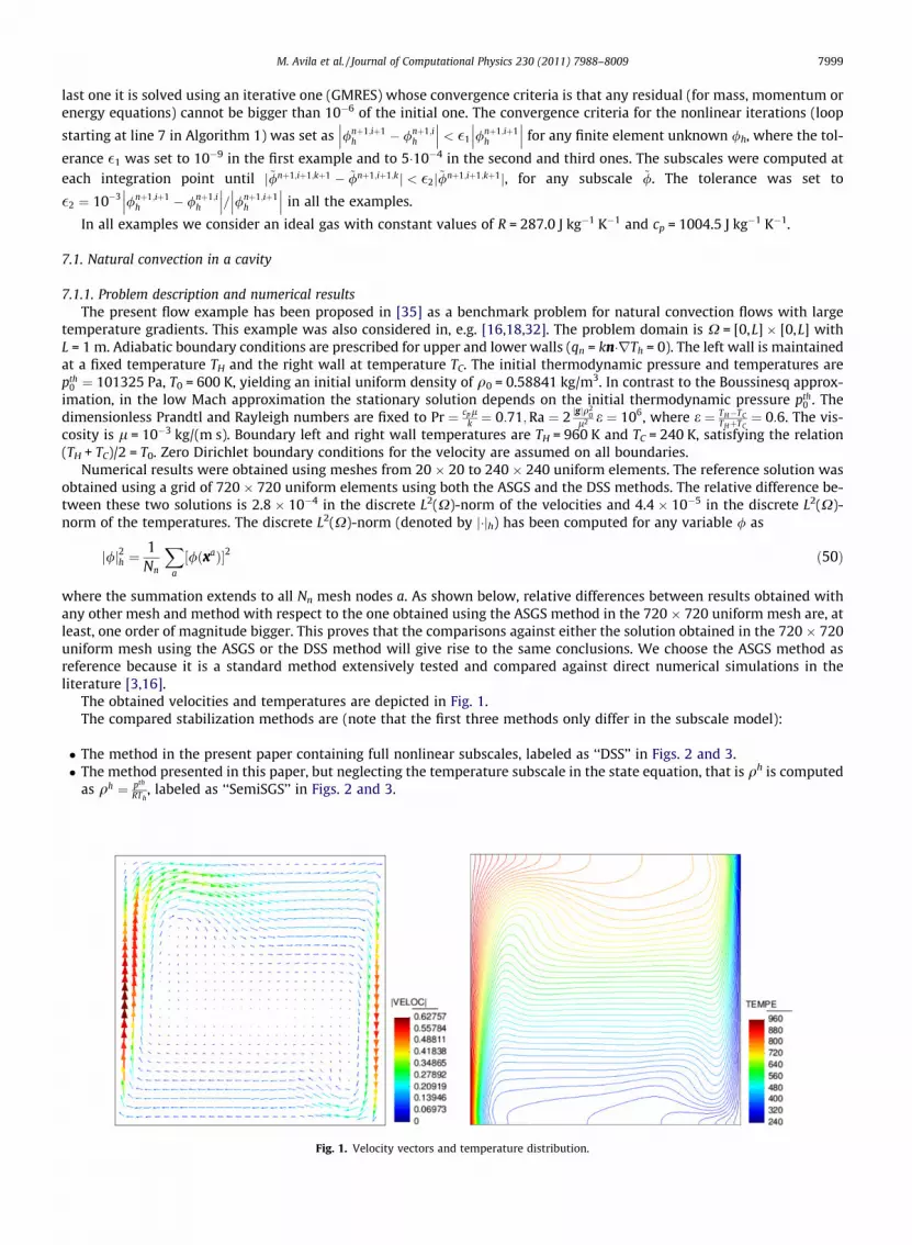
7.1.1. Problem description and numerical resultsThe present flow example has been proposed in [35] as a benchmark problem for natural convection flows with large

temperature gradients. This example was also considered in, e.g. [16,18,32]. The problem domain is X = [0,L] � [0,L] withL = 1 m. Adiabatic boundary conditions are prescribed for upper and lower walls (qn = kn�rTh = 0). The left wall is maintainedat a fixed temperature TH and the right wall at temperature TC. The initial thermodynamic pressure and temperatures arepth

0 ¼ 101325 Pa, T0 = 600 K, yielding an initial uniform density of q0 = 0.58841 kg/m3. In contrast to the Boussinesq approx-imation, in the low Mach approximation the stationary solution depends on the initial thermodynamic pressure pth

0 . Thedimensionless Prandtl and Rayleigh numbers are fixed to Pr ¼ cpl

k ¼ 0:71;Ra ¼ 2 jgjq20

l2 e ¼ 106, where e ¼ TH�TCTHþTC

¼ 0:6. The vis-cosity is l = 10�3 kg/(m s). Boundary left and right wall temperatures are TH = 960 K and TC = 240 K, satisfying the relation(TH + TC)/2 = T0. Zero Dirichlet boundary conditions for the velocity are assumed on all boundaries.

Numerical results were obtained using meshes from 20 � 20 to 240 � 240 uniform elements. The reference solution wasobtained using a grid of 720 � 720 uniform elements using both the ASGS and the DSS methods. The relative difference be-tween these two solutions is 2.8 � 10�4 in the discrete L2(X)-norm of the velocities and 4.4 � 10�5 in the discrete L2(X)-norm of the temperatures. The discrete L2(X)-norm (denoted by j�jh) has been computed for any variable / as

j/j2h ¼1

Nn

Xa

½/ðxaÞ2 ð50Þ

where the summation extends to all Nn mesh nodes a. As shown below, relative differences between results obtained withany other mesh and method with respect to the one obtained using the ASGS method in the 720 � 720 uniform mesh are, atleast, one order of magnitude bigger. This proves that the comparisons against either the solution obtained in the 720 � 720uniform mesh using the ASGS or the DSS method will give rise to the same conclusions. We choose the ASGS method asreference because it is a standard method extensively tested and compared against direct numerical simulations in theliterature [3,16].

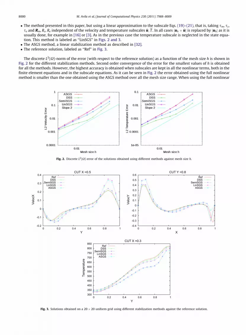
The obtained velocities and temperatures are depicted in Fig. 1.The compared stabilization methods are (note that the first three methods only differ in the subscale model):

� The method in the present paper containing full nonlinear subscales, labeled as ‘‘DSS’’ in Figs. 2 and 3.� The method presented in this paper, but neglecting the temperature subscale in the state equation, that is qh is computed

as qh ¼ pth

RTh, labeled as ‘‘SemiSGS’’ in Figs. 2 and 3.

Fig. 1. Velocity vectors and temperature distribution.


� The method presented in this paper, but using a linear approximation to the subscale Eqs. (19)–(21), that is, taking sm, sc,se and Rm, Rc, Re independent of the velocity and temperature subscales ~u; eT . In all cases juh þ ~uj is replaced by juhj as it isusually done, for example in [16] or [3]. As in the previous case the temperature subscale is neglected in the state equa-tion. This method is labeled as ‘‘LinSGS’’ in Figs. 2 and 3.� The ASGS method, a linear stabilization method as described in [32].� The reference solution, labeled as ‘‘Ref’’ in Fig. 3.

The discrete L2(X)-norm of the error (with respect to the reference solution) as a function of the mesh size h is shown inFig. 2 for the different stabilization methods. Second order convergence of the error for the smallest values of h is obtainedfor all the methods. However, the highest accuracy is obtained when subscales are kept in all the nonlinear terms, both in thefinite element equations and in the subscale equations. As it can be seen in Fig. 2 the error obtained using the full nonlinearmethod is smaller than the one obtained using the ASGS method over all the mesh size range. When using the full nonlinear

Fig. 2. Discrete L2(X) error of the solutions obtained using different methods against mesh size h.

-0.2

-0.1

0

0.1

0.2

0.3

0.4

0 0.2 0.4 0.6 0.8 1

Velo

cX

Y

CUT X =0.5Ref

DSSSemiSGS

LinSGSASGS

-0.4

-0.3

-0.2

-0.1

0

0.1

0.2

0.3

0.4

0.5

0.6

0 0.2 0.4 0.6 0.8 1

Velo

cY

X

CUT Y =0.8Ref

DSSSemiSGS

LinSGSASGS

300

350

400

450

500

550

600

650

700

750

800

850

0 0.2 0.4 0.6 0.8 1

Tem

pera

ture

Y

CUT X =0.3Ref

DSSSemiSGS

LinSGSASGS

Fig. 3. Solutions obtained on a 20 � 20 uniform grid using different stabilization methods against the reference solution.


method a convergence rate of order greater than 2 is observed on the coarsest meshes. As will be justified in the next Section7.1.2 the full nonlinear method will converge to the ASGS method for h small enough and this implies the there must be aregion in which this slope decreases below 2. When the temperature subscale is neglected in the state equation the solutionis less accurate, the gain in accuracy respect to the ASGS method is lower, becoming negligible over the finer grids. Finally,when a linear approximation to the subscale Eqs. (25)–(27) is considered, even less accurate solutions are obtained, the gainin accuracy respect to the ASGS method being negligible over all the mesh size range. A possible explanation for this phe-nomenon arises from the analysis of the subgrid velocity and temperature fields given in the following Section 7.1.2.

The higher accuracy of the fully nonlinear approximation for the subscales is further illustrated in Fig. 3 where the var-iation of the velocity and temperature solutions for different stabilization methods are depicted along three different linescutting the domain.

Another quantity of interest is the heat transfer from the hot to the cold wall, represented by the Nusselt number, definedas

Fig. 4

NuðxÞ ¼ LTH � TC

n � rTðxÞ; x 2 @X

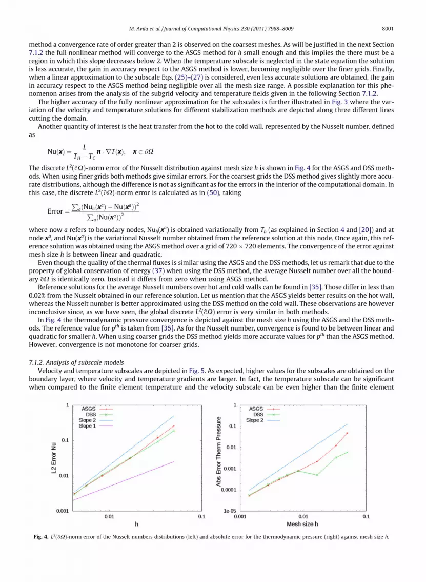
The discrete L2(oX)-norm error of the Nusselt distribution against mesh size h is shown in Fig. 4 for the ASGS and DSS meth-ods. When using finer grids both methods give similar errors. For the coarsest grids the DSS method gives slightly more accu-rate distributions, although the difference is not as significant as for the errors in the interior of the computational domain. Inthis case, the discrete L2(oX)-norm error is calculated as in (50), taking

Error ¼P

a NuhðxaÞ � NuðxaÞð Þ2Pa NuðxaÞð Þ2

where now a refers to boundary nodes, Nuh(xa) is obtained variationally from Th (as explained in Section 4 and [20]) and atnode xa, and Nu(xa) is the variational Nusselt number obtained from the reference solution at this node. Once again, this ref-erence solution was obtained using the ASGS method over a grid of 720 � 720 elements. The convergence of the error againstmesh size h is between linear and quadratic.

Even though the quality of the thermal fluxes is similar using the ASGS and the DSS methods, let us remark that due to theproperty of global conservation of energy (37) when using the DSS method, the average Nusselt number over all the bound-ary oX is identically zero. Instead it differs from zero when using ASGS method.

Reference solutions for the average Nusselt numbers over hot and cold walls can be found in [35]. Those differ in less than0.02% from the Nusselt obtained in our reference solution. Let us mention that the ASGS yields better results on the hot wall,whereas the Nusselt number is better approximated using the DSS method on the cold wall. These observations are howeverinconclusive since, as we have seen, the global discrete L2(oX) error is very similar in both methods.

In Fig. 4 the thermodynamic pressure convergence is depicted against the mesh size h using the ASGS and the DSS meth-ods. The reference value for pth is taken from [35]. As for the Nusselt number, convergence is found to be between linear andquadratic for smaller h. When using coarser grids the DSS method yields more accurate values for pth than the ASGS method.However, convergence is not monotone for coarser grids.

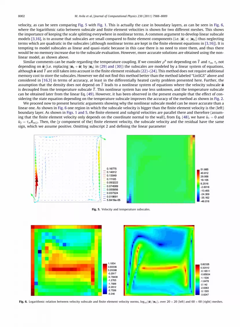
7.1.2. Analysis of subscale modelsVelocity and temperature subscales are depicted in Fig. 5. As expected, higher values for the subscales are obtained on the

boundary layer, where velocity and temperature gradients are larger. In fact, the temperature subscale can be significantwhen compared to the finite element temperature and the velocity subscale can be even higher than the finite element

. L2(@X)-norm error of the Nusselt numbers distributions (left) and absolute error for the thermodynamic pressure (right) against mesh size h.


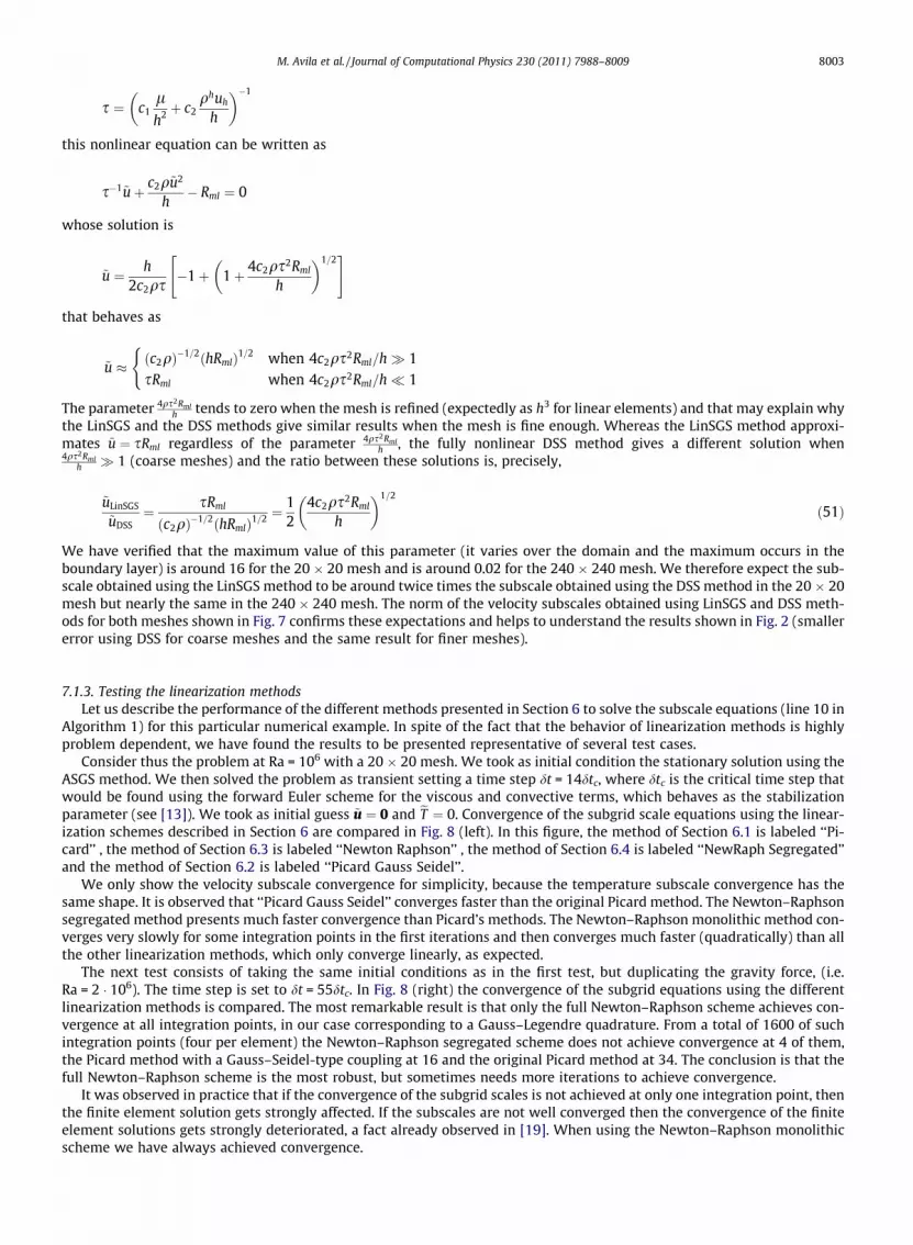
velocity, as can be seen comparing Fig. 5 with Fig. 1. This is actually the case in boundary layers, as can be seen in Fig. 6,where the logarithmic ratio between subscale and finite element velocities is shown for two different meshes. This showsthe importance of keeping the scale splitting everywhere in nonlinear terms. A common argument to develop linear subscalemodels [3,16], is to assume that subscales are small compared to finite element components (i.e. j~uj � juhj) thus neglectingterms which are quadratic in the subscales (although nonlinear terms are kept in the finite element equations in [3,16]). It istempting to model subscales as linear and quasi-static because in this case there is no need to store them, and thus therewould be no memory increase due to the subscale evaluation. However, more accurate solutions are obtained using the non-linear model, as shown above.

Similar comments can be made regarding the temperature coupling. If we consider qh not depending on eT and sm, se notdepending on ~u (i.e. replacing juh þ ~uj by juhj in (29) and (30)) the subscales are modeled by a linear system of equations,although ~u and eT are still taken into account in the finite element residuals (22)–(24). This method does not require additionalmemory cost to store the subscales. However we did not find this method better than the method labeled ‘‘LinSGS’’ above andconsidered in [16,3] in terms of accuracy, at least in the differentially heated cavity problem presented here. Further, theassumption that the density does not depend on eT leads to a nonlinear system of equations where the velocity subscale ~uis decoupled from the temperature subscale eT . This nonlinear system has one less unknown, and the temperature subscalecan be obtained later from the linear Eq. (49). However, it has been observed in the present example that the effect of con-sidering the state equation depending on the temperature subscale improves the accuracy of the method as shown in Fig. 2.

We proceed now to present heuristic arguments showing why the nonlinear subscale model can be more accurate than alinear one. As shown in Fig. 6 one region in which the subscale velocity is bigger than the finite element velocity is the (left)boundary layer. As shown in Figs. 1 and 5, the finite element and subgrid velocities are parallel there and therefore (assum-ing that the finite element velocity only depends on the coordinate normal to the wall), from Eq. (48), we have ~u1 ¼ 0 and~u2 ¼ smRml;2. Then, the (y component of the) finite element velocity, the subscale velocity and the residual have the samesign, which we assume positive. Omitting subscript 2 and defining the linear parameter

Fig. 5. Velocity and temperature subscales.

Fig. 6. Logarithmic relation between velocity subscale and finite element velocity norms, log10ðj~uj=juhjÞ, over 20 � 20 (left) and 60 � 60 (right) meshes.


s ¼ c1lh2 þ c2

qhuh

h

� ��1

this nonlinear equation can be written as

s�1~uþ c2q~u2

h� Rml ¼ 0

whose solution is

~u ¼ h2c2qs

�1þ 1þ 4c2qs2Rml

h

� �1=2" #

that behaves as

~u ðc2qÞ�1=2ðhRmlÞ1=2 when 4c2qs2Rml=h� 1sRml when 4c2qs2Rml=h� 1

(
The parameter 4qs2Rml
h tends to zero when the mesh is refined (expectedly as h3 for linear elements) and that may explain whythe LinSGS and the DSS methods give similar results when the mesh is fine enough. Whereas the LinSGS method approxi-mates ~u ¼ sRml regardless of the parameter 4qs2Rml

h , the fully nonlinear DSS method gives a different solution when4qs2Rml

h � 1 (coarse meshes) and the ratio between these solutions is, precisely,

~uLinSGS

~uDSS¼ sRml

ðc2qÞ�1=2ðhRmlÞ1=2 ¼12

4c2qs2Rml

h

� �1=2

ð51Þ

We have verified that the maximum value of this parameter (it varies over the domain and the maximum occurs in theboundary layer) is around 16 for the 20 � 20 mesh and is around 0.02 for the 240 � 240 mesh. We therefore expect the sub-scale obtained using the LinSGS method to be around twice times the subscale obtained using the DSS method in the 20 � 20mesh but nearly the same in the 240 � 240 mesh. The norm of the velocity subscales obtained using LinSGS and DSS meth-ods for both meshes shown in Fig. 7 confirms these expectations and helps to understand the results shown in Fig. 2 (smallererror using DSS for coarse meshes and the same result for finer meshes).

7.1.3. Testing the linearization methodsLet us describe the performance of the different methods presented in Section 6 to solve the subscale equations (line 10 in

Algorithm 1) for this particular numerical example. In spite of the fact that the behavior of linearization methods is highlyproblem dependent, we have found the results to be presented representative of several test cases.

Consider thus the problem at Ra = 106 with a 20 � 20 mesh. We took as initial condition the stationary solution using theASGS method. We then solved the problem as transient setting a time step dt = 14dtc, where dtc is the critical time step thatwould be found using the forward Euler scheme for the viscous and convective terms, which behaves as the stabilizationparameter (see [13]). We took as initial guess ~u ¼ 0 and eT ¼ 0. Convergence of the subgrid scale equations using the linear-ization schemes described in Section 6 are compared in Fig. 8 (left). In this figure, the method of Section 6.1 is labeled ‘‘Pi-card’’ , the method of Section 6.3 is labeled ‘‘Newton Raphson’’ , the method of Section 6.4 is labeled ‘‘NewRaph Segregated’’and the method of Section 6.2 is labeled ‘‘Picard Gauss Seidel’’.

We only show the velocity subscale convergence for simplicity, because the temperature subscale convergence has thesame shape. It is observed that ‘‘Picard Gauss Seidel’’ converges faster than the original Picard method. The Newton–Raphsonsegregated method presents much faster convergence than Picard’s methods. The Newton–Raphson monolithic method con-verges very slowly for some integration points in the first iterations and then converges much faster (quadratically) than allthe other linearization methods, which only converge linearly, as expected.

The next test consists of taking the same initial conditions as in the first test, but duplicating the gravity force, (i.e.Ra = 2 � 106). The time step is set to dt = 55dtc. In Fig. 8 (right) the convergence of the subgrid equations using the differentlinearization methods is compared. The most remarkable result is that only the full Newton–Raphson scheme achieves con-vergence at all integration points, in our case corresponding to a Gauss–Legendre quadrature. From a total of 1600 of suchintegration points (four per element) the Newton–Raphson segregated scheme does not achieve convergence at 4 of them,the Picard method with a Gauss–Seidel-type coupling at 16 and the original Picard method at 34. The conclusion is that thefull Newton–Raphson scheme is the most robust, but sometimes needs more iterations to achieve convergence.

It was observed in practice that if the convergence of the subgrid scales is not achieved at only one integration point, thenthe finite element solution gets strongly affected. If the subscales are not well converged then the convergence of the finiteelement solutions gets strongly deteriorated, a fact already observed in [19]. When using the Newton–Raphson monolithicscheme we have always achieved convergence.

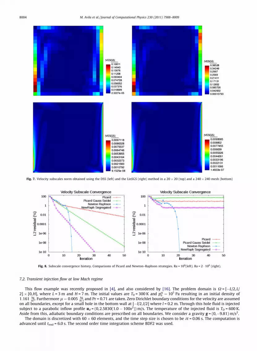
Fig. 8. Subscale convergence history. Comparisons of Picard and Newton–Raphson strategies. Ra = 106(left). Ra = 2 � 106 (right).

Fig. 7. Velocity subscales norm obtained using the DSS (left) and the LinSGS (right) method in a 20 � 20 (top) and a 240 � 240 mesh (bottom)


7.2. Transient injection flow at low Mach regime

This flow example was recently proposed in [4], and also considered by [16]. The problem domain is X = [�L/2,L/2] � [0,H], where L = 3 m and H = 7 m. The initial values are T0 = 300 K and pth

0 ¼ 105 Pa resulting in an initial density of1:161 kg

m3. Furthermore l ¼ 0:005 kgm s and Pr = 0.71 are taken. Zero Dirichlet boundary conditions for the velocity are assumed

on all boundaries, except for a small hole in the bottom wall at [�l/2, l/2] where l = 0.2 m. Through this hole fluid is injectedsubject to a parabolic inflow profile ud = (0,2.5830(1.0 � 100x2)) m/s. The temperature of the injected fluid is TD = 600 K.Aside from this, adiabatic boundary conditions are prescribed on all boundaries. We consider a gravity g = (0,�9.81) m/s2.

The domain is discretized with 60 � 60 elements, and the time step size is chosen to be dt = 0.06 s. The computation isadvanced until tend = 6.0 s. The second order time integration scheme BDF2 was used.


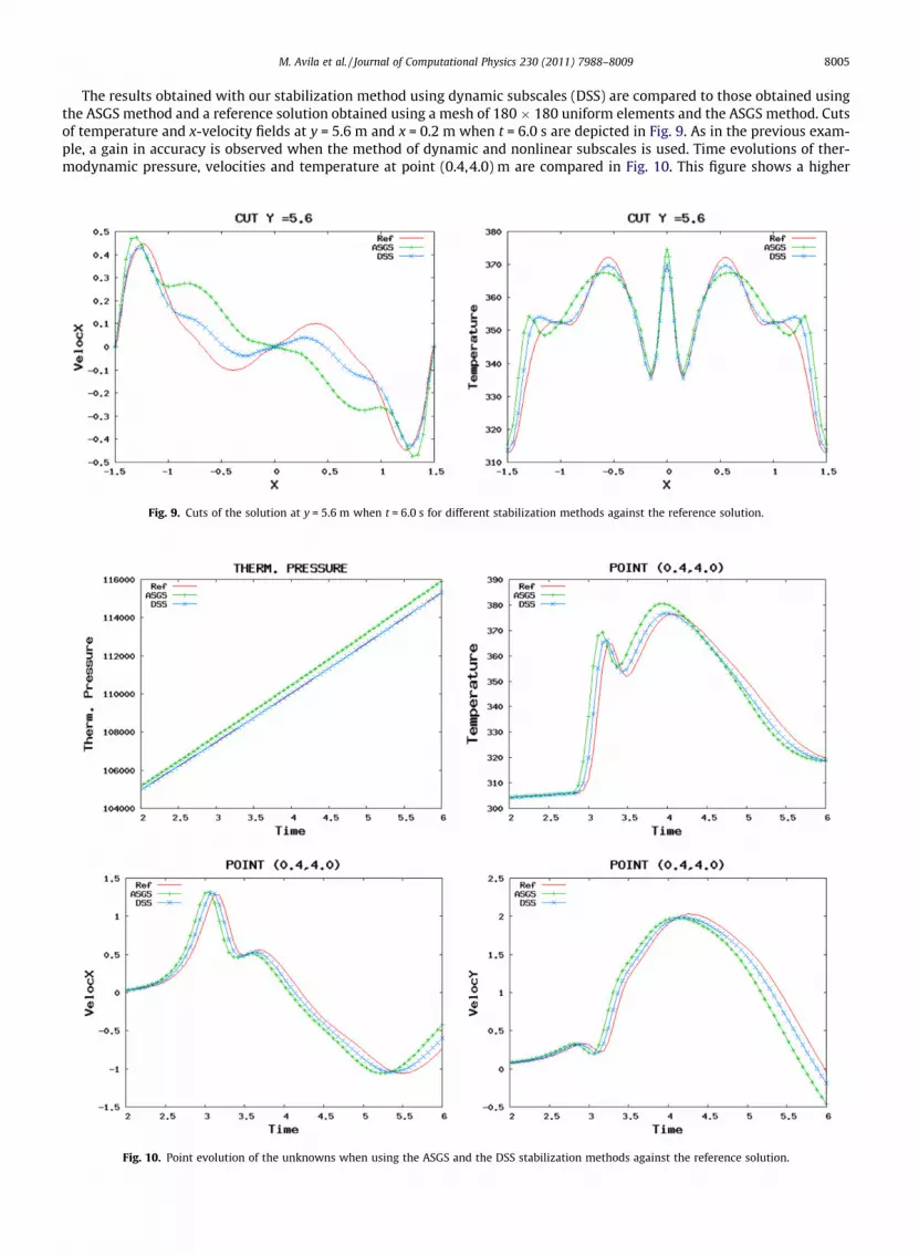
The results obtained with our stabilization method using dynamic subscales (DSS) are compared to those obtained usingthe ASGS method and a reference solution obtained using a mesh of 180 � 180 uniform elements and the ASGS method. Cutsof temperature and x-velocity fields at y = 5.6 m and x = 0.2 m when t = 6.0 s are depicted in Fig. 9. As in the previous exam-ple, a gain in accuracy is observed when the method of dynamic and nonlinear subscales is used. Time evolutions of ther-modynamic pressure, velocities and temperature at point (0.4,4.0) m are compared in Fig. 10. This figure shows a higher

Fig. 9. Cuts of the solution at y = 5.6 m when t = 6.0 s for different stabilization methods against the reference solution.

Fig. 10. Point evolution of the unknowns when using the ASGS and the DSS stabilization methods against the reference solution.

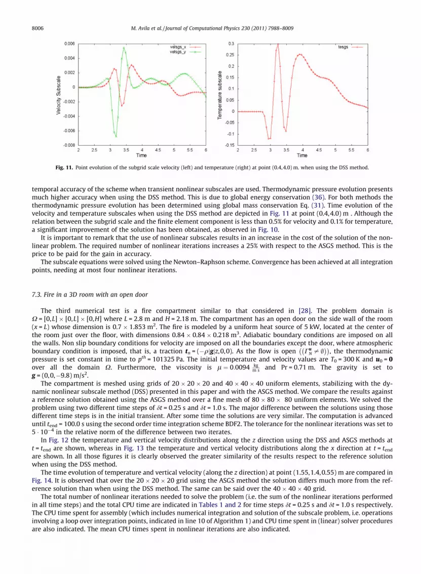
Fig. 11. Point evolution of the subgrid scale velocity (left) and temperature (right) at point (0.4,4.0) m. when using the DSS method.


temporal accuracy of the scheme when transient nonlinear subscales are used. Thermodynamic pressure evolution presentsmuch higher accuracy when using the DSS method. This is due to global energy conservation (36). For both methods thethermodynamic pressure evolution has been determined using global mass conservation Eq. (31). Time evolution of thevelocity and temperature subscales when using the DSS method are depicted in Fig. 11 at point (0.4,4.0) m . Although therelation between the subgrid scale and the finite element component is less than 0.5% for velocity and 0.1% for temperature,a significant improvement of the solution has been obtained, as observed in Fig. 10.

It is important to remark that the use of nonlinear subscales results in an increase in the cost of the solution of the non-linear problem. The required number of nonlinear iterations increases a 25% with respect to the ASGS method. This is theprice to be paid for the gain in accuracy.

The subscale equations were solved using the Newton–Raphson scheme. Convergence has been achieved at all integrationpoints, needing at most four nonlinear iterations.

7.3. Fire in a 3D room with an open door

The third numerical test is a fire compartment similar to that considered in [28]. The problem domain isX = [0,L] � [0,L] � [0,H] where L = 2.8 m and H = 2.18 m. The compartment has an open door on the side wall of the room(x = L) whose dimension is 0.7 � 1.853 m2. The fire is modeled by a uniform heat source of 5 kW, located at the center ofthe room just over the floor, with dimensions 0.84 � 0.84 � 0.218 m3. Adiabatic boundary conditions are imposed on allthe walls. Non slip boundary conditions for velocity are imposed on all the boundaries except the door, where atmosphericboundary condition is imposed, that is, a traction tn = (�qjgjz,0,0). As the flow is open Cu

N – ;� ��

, the thermodynamicpressure is set constant in time to pth = 101325 Pa. The initial temperature and velocity values are T0 = 300 K and u0 = 0over all the domain X. Furthermore, the viscosity is l ¼ 0:0094 kg

m s and Pr = 0.71 m. The gravity is set tog = (0,0,�9.8) m/s2.

The compartment is meshed using grids of 20 � 20 � 20 and 40 � 40 � 40 uniform elements, stabilizing with the dy-namic nonlinear subscale method (DSS) presented in this paper and with the ASGS method. We compare the results againsta reference solution obtained using the ASGS method over a fine mesh of 80 � 80 � 80 uniform elements. We solved theproblem using two different time steps of dt = 0.25 s and dt = 1.0 s. The major difference between the solutions using thosedifferent time steps is in the initial transient. After some time the solutions are very similar. The computation is advanceduntil tend = 100.0 s using the second order time integration scheme BDF2. The tolerance for the nonlinear iterations was set to5 � 10�4 in the relative norm of the difference between two iterates.

In Fig. 12 the temperature and vertical velocity distributions along the z direction using the DSS and ASGS methods att = tend are shown, whereas in Fig. 13 the temperature and vertical velocity distributions along the x direction at t = tend

are shown. In all those figures it is clearly observed the greater similarity of the results respect to the reference solutionwhen using the DSS method.

The time evolution of temperature and vertical velocity (along the z direction) at point (1.55,1.4,0.55) m are compared inFig. 14. It is observed that over the 20 � 20 � 20 grid using the ASGS method the solution differs much more from the ref-erence solution than when using the DSS method. The same can be said over the 40 � 40 � 40 grid.

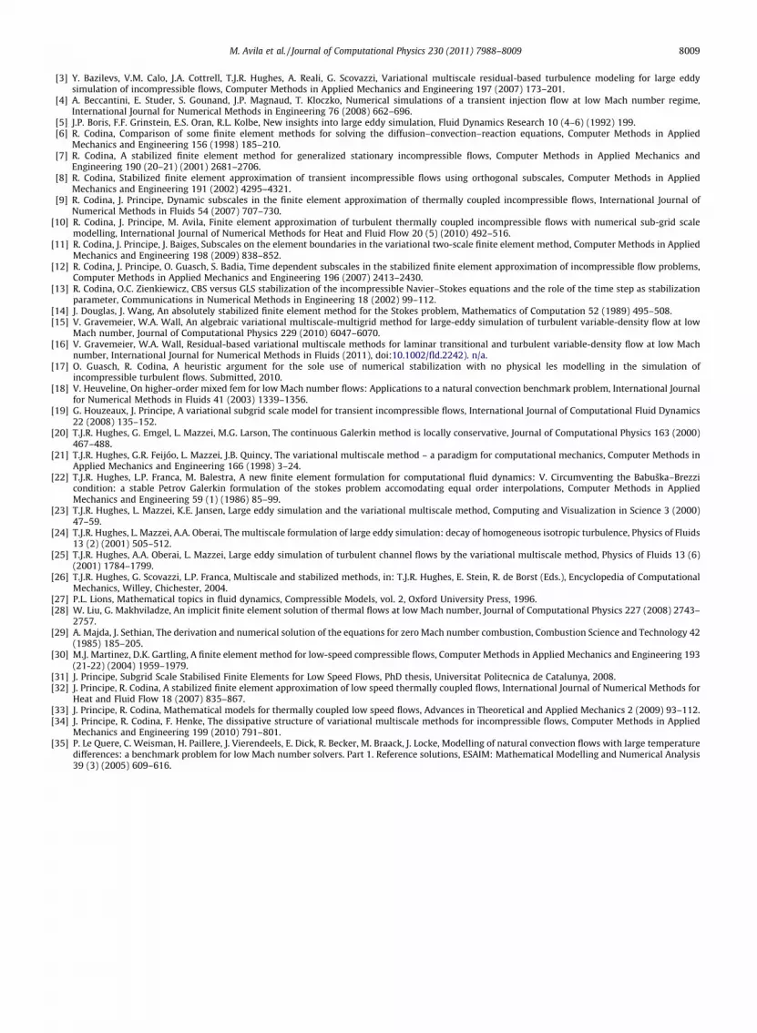
The total number of nonlinear iterations needed to solve the problem (i.e. the sum of the nonlinear iterations performedin all time steps) and the total CPU time are indicated in Tables 1 and 2 for time steps dt = 0.25 s and dt = 1.0 s respectively.The CPU time spent for assembly (which includes numerical integration and solution of the subscale problem, i.e. operationsinvolving a loop over integration points, indicated in line 10 of Algorithm 1) and CPU time spent in (linear) solver proceduresare also indicated. The mean CPU times spent in nonlinear iterations are also indicated.

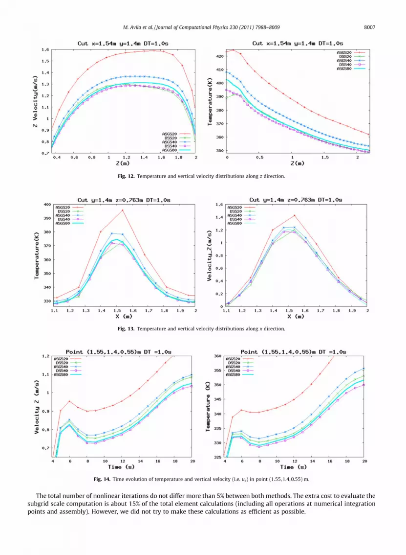
Fig. 12. Temperature and vertical velocity distributions along z direction.

Fig. 13. Temperature and vertical velocity distributions along x direction.

Fig. 14. Time evolution of temperature and vertical velocity (i.e. uz) in point (1.55,1.4,0.55) m.


The total number of nonlinear iterations do not differ more than 5% between both methods. The extra cost to evaluate thesubgrid scale computation is about 15% of the total element calculations (including all operations at numerical integrationpoints and assembly). However, we did not try to make these calculations as efficient as possible.

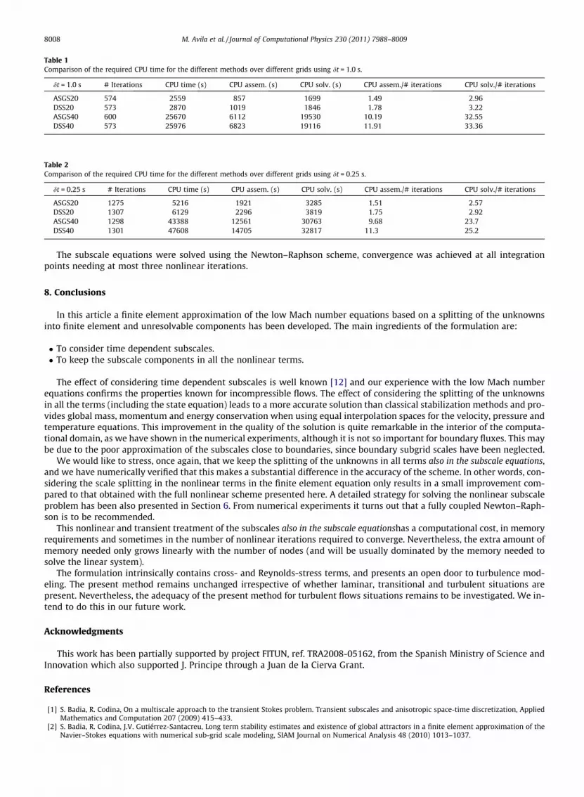
Table 1Comparison of the required CPU time for the different methods over different grids using dt = 1.0 s.

dt = 1.0 s # Iterations CPU time (s) CPU assem. (s) CPU solv. (s) CPU assem./# iterations CPU solv./# iterations

ASGS20 574 2559 857 1699 1.49 2.96DSS20 573 2870 1019 1846 1.78 3.22ASGS40 600 25670 6112 19530 10.19 32.55DSS40 573 25976 6823 19116 11.91 33.36

Table 2Comparison of the required CPU time for the different methods over different grids using dt = 0.25 s.

dt = 0.25 s # Iterations CPU time (s) CPU assem. (s) CPU solv. (s) CPU assem./# iterations CPU solv./# iterations

ASGS20 1275 5216 1921 3285 1.51 2.57DSS20 1307 6129 2296 3819 1.75 2.92ASGS40 1298 43388 12561 30763 9.68 23.7DSS40 1301 47608 14705 32817 11.3 25.2


The subscale equations were solved using the Newton–Raphson scheme, convergence was achieved at all integrationpoints needing at most three nonlinear iterations.

8. Conclusions

In this article a finite element approximation of the low Mach number equations based on a splitting of the unknownsinto finite element and unresolvable components has been developed. The main ingredients of the formulation are:

� To consider time dependent subscales.� To keep the subscale components in all the nonlinear terms.

The effect of considering time dependent subscales is well known [12] and our experience with the low Mach numberequations confirms the properties known for incompressible flows. The effect of considering the splitting of the unknownsin all the terms (including the state equation) leads to a more accurate solution than classical stabilization methods and pro-vides global mass, momentum and energy conservation when using equal interpolation spaces for the velocity, pressure andtemperature equations. This improvement in the quality of the solution is quite remarkable in the interior of the computa-tional domain, as we have shown in the numerical experiments, although it is not so important for boundary fluxes. This maybe due to the poor approximation of the subscales close to boundaries, since boundary subgrid scales have been neglected.

We would like to stress, once again, that we keep the splitting of the unknowns in all terms also in the subscale equations,and we have numerically verified that this makes a substantial difference in the accuracy of the scheme. In other words, con-sidering the scale splitting in the nonlinear terms in the finite element equation only results in a small improvement com-pared to that obtained with the full nonlinear scheme presented here. A detailed strategy for solving the nonlinear subscaleproblem has been also presented in Section 6. From numerical experiments it turns out that a fully coupled Newton–Raph-son is to be recommended.

This nonlinear and transient treatment of the subscales also in the subscale equationshas a computational cost, in memoryrequirements and sometimes in the number of nonlinear iterations required to converge. Nevertheless, the extra amount ofmemory needed only grows linearly with the number of nodes (and will be usually dominated by the memory needed tosolve the linear system).

The formulation intrinsically contains cross- and Reynolds-stress terms, and presents an open door to turbulence mod-eling. The present method remains unchanged irrespective of whether laminar, transitional and turbulent situations arepresent. Nevertheless, the adequacy of the present method for turbulent flows situations remains to be investigated. We in-tend to do this in our future work.

Acknowledgments

This work has been partially supported by project FITUN, ref. TRA2008-05162, from the Spanish Ministry of Science andInnovation which also supported J. Principe through a Juan de la Cierva Grant.

References

[1] S. Badia, R. Codina, On a multiscale approach to the transient Stokes problem. Transient subscales and anisotropic space-time discretization, AppliedMathematics and Computation 207 (2009) 415–433.

[2] S. Badia, R. Codina, J.V. Gutiérrez-Santacreu, Long term stability estimates and existence of global attractors in a finite element approximation of theNavier–Stokes equations with numerical sub-grid scale modeling, SIAM Journal on Numerical Analysis 48 (2010) 1013–1037.


[3] Y. Bazilevs, V.M. Calo, J.A. Cottrell, T.J.R. Hughes, A. Reali, G. Scovazzi, Variational multiscale residual-based turbulence modeling for large eddysimulation of incompressible flows, Computer Methods in Applied Mechanics and Engineering 197 (2007) 173–201.

[4] A. Beccantini, E. Studer, S. Gounand, J.P. Magnaud, T. Kloczko, Numerical simulations of a transient injection flow at low Mach number regime,International Journal for Numerical Methods in Engineering 76 (2008) 662–696.

[5] J.P. Boris, F.F. Grinstein, E.S. Oran, R.L. Kolbe, New insights into large eddy simulation, Fluid Dynamics Research 10 (4–6) (1992) 199.[6] R. Codina, Comparison of some finite element methods for solving the diffusion–convection–reaction equations, Computer Methods in Applied

Mechanics and Engineering 156 (1998) 185–210.[7] R. Codina, A stabilized finite element method for generalized stationary incompressible flows, Computer Methods in Applied Mechanics and

Engineering 190 (20–21) (2001) 2681–2706.[8] R. Codina, Stabilized finite element approximation of transient incompressible flows using orthogonal subscales, Computer Methods in Applied

Mechanics and Engineering 191 (2002) 4295–4321.[9] R. Codina, J. Principe, Dynamic subscales in the finite element approximation of thermally coupled incompressible flows, International Journal of

Numerical Methods in Fluids 54 (2007) 707–730.[10] R. Codina, J. Principe, M. Avila, Finite element approximation of turbulent thermally coupled incompressible flows with numerical sub-grid scale

modelling, International Journal of Numerical Methods for Heat and Fluid Flow 20 (5) (2010) 492–516.[11] R. Codina, J. Principe, J. Baiges, Subscales on the element boundaries in the variational two-scale finite element method, Computer Methods in Applied

Mechanics and Engineering 198 (2009) 838–852.[12] R. Codina, J. Principe, O. Guasch, S. Badia, Time dependent subscales in the stabilized finite element approximation of incompressible flow problems,

Computer Methods in Applied Mechanics and Engineering 196 (2007) 2413–2430.[13] R. Codina, O.C. Zienkiewicz, CBS versus GLS stabilization of the incompressible Navier–Stokes equations and the role of the time step as stabilization

parameter, Communications in Numerical Methods in Engineering 18 (2002) 99–112.[14] J. Douglas, J. Wang, An absolutely stabilized finite element method for the Stokes problem, Mathematics of Computation 52 (1989) 495–508.[15] V. Gravemeier, W.A. Wall, An algebraic variational multiscale-multigrid method for large-eddy simulation of turbulent variable-density flow at low

Mach number, Journal of Computational Physics 229 (2010) 6047–6070.[16] V. Gravemeier, W.A. Wall, Residual-based variational multiscale methods for laminar transitional and turbulent variable-density flow at low Mach

number, International Journal for Numerical Methods in Fluids (2011), doi:10.1002/fld.2242). n/a.[17] O. Guasch, R. Codina, A heuristic argument for the sole use of numerical stabilization with no physical les modelling in the simulation of

incompressible turbulent flows. Submitted, 2010.[18] V. Heuveline, On higher-order mixed fem for low Mach number flows: Applications to a natural convection benchmark problem, International Journal

for Numerical Methods in Fluids 41 (2003) 1339–1356.[19] G. Houzeaux, J. Principe, A variational subgrid scale model for transient incompressible flows, International Journal of Computational Fluid Dynamics

22 (2008) 135–152.[20] T.J.R. Hughes, G. Emgel, L. Mazzei, M.G. Larson, The continuous Galerkin method is locally conservative, Journal of Computational Physics 163 (2000)

467–488.[21] T.J.R. Hughes, G.R. Feijóo, L. Mazzei, J.B. Quincy, The variational multiscale method – a paradigm for computational mechanics, Computer Methods in

Applied Mechanics and Engineering 166 (1998) 3–24.[22] T.J.R. Hughes, L.P. Franca, M. Balestra, A new finite element formulation for computational fluid dynamics: V. Circumventing the Babuška–Brezzi

condition: a stable Petrov Galerkin formulation of the stokes problem accomodating equal order interpolations, Computer Methods in AppliedMechanics and Engineering 59 (1) (1986) 85–99.

[23] T.J.R. Hughes, L. Mazzei, K.E. Jansen, Large eddy simulation and the variational multiscale method, Computing and Visualization in Science 3 (2000)47–59.

[24] T.J.R. Hughes, L. Mazzei, A.A. Oberai, The multiscale formulation of large eddy simulation: decay of homogeneous isotropic turbulence, Physics of Fluids13 (2) (2001) 505–512.

[25] T.J.R. Hughes, A.A. Oberai, L. Mazzei, Large eddy simulation of turbulent channel flows by the variational multiscale method, Physics of Fluids 13 (6)(2001) 1784–1799.

[26] T.J.R. Hughes, G. Scovazzi, L.P. Franca, Multiscale and stabilized methods, in: T.J.R. Hughes, E. Stein, R. de Borst (Eds.), Encyclopedia of ComputationalMechanics, Willey, Chichester, 2004.

[27] P.L. Lions, Mathematical topics in fluid dynamics, Compressible Models, vol. 2, Oxford University Press, 1996.[28] W. Liu, G. Makhviladze, An implicit finite element solution of thermal flows at low Mach number, Journal of Computational Physics 227 (2008) 2743–

2757.[29] A. Majda, J. Sethian, The derivation and numerical solution of the equations for zero Mach number combustion, Combustion Science and Technology 42

(1985) 185–205.[30] M.J. Martinez, D.K. Gartling, A finite element method for low-speed compressible flows, Computer Methods in Applied Mechanics and Engineering 193

(21-22) (2004) 1959–1979.[31] J. Principe, Subgrid Scale Stabilised Finite Elements for Low Speed Flows, PhD thesis, Universitat Politecnica de Catalunya, 2008.[32] J. Principe, R. Codina, A stabilized finite element approximation of low speed thermally coupled flows, International Journal of Numerical Methods for

Heat and Fluid Flow 18 (2007) 835–867.[33] J. Principe, R. Codina, Mathematical models for thermally coupled low speed flows, Advances in Theoretical and Applied Mechanics 2 (2009) 93–112.[34] J. Principe, R. Codina, F. Henke, The dissipative structure of variational multiscale methods for incompressible flows, Computer Methods in Applied

Mechanics and Engineering 199 (2010) 791–801.[35] P. Le Quere, C. Weisman, H. Paillere, J. Vierendeels, E. Dick, R. Becker, M. Braack, J. Locke, Modelling of natural convection flows with large temperature

differences: a benchmark problem for low Mach number solvers. Part 1. Reference solutions, ESAIM: Mathematical Modelling and Numerical Analysis39 (3) (2005) 609–616.

http://dx.doi.org/10.1002/fld.2242)

a finite element dynamical nonlinear subscale approximation for the low mach number flow equations

Documents