a feynman-kac solution to a random impulsive equation of schrödinger type
TRANSCRIPT
RESEARCH Real Analysis Exchange
Vol. 36(1), 2010/2011, pp. 107–148
E. M. Bonotto,⇤ Instituto de Ciencias Matematicas e de Computacao,Universidade de Sao Paulo-Campus de Sao Carlos, Caixa Postal 668,13560-970 Sao Carlos SP, Brazil. email: [email protected]
M. Federson, Instituto de Ciencias Matematicas e de Computacao,Universidade de Sao Paulo-Campus de Sao Carlos, Caixa Postal 668,13560-970 Sao Carlos SP, Brazil. email: [email protected]
P. Muldowney, Magee College, University of Ulster, Derry, BT48 7JL,Northern Ireland. email: [email protected]
A FEYNMAN-KAC SOLUTION TO ARANDOM IMPULSIVE EQUATION OF
SCHRODINGER TYPE
Abstract
If a force is applied to a particle undergoing Brownian motion, the
resulting motion has a state function which satisfies a di↵usion or Schro-
dinger-type equation. We consider a process in which Brownian motion
is replaced by a process which has Brownian transitions at all times
other than random times at which the transitions have an additional
“impulsive” displacement. Using a Feynman-Kac formulation based on
generalized Riemann integration, we examine the resulting equation of
motion.
1 Introduction.
As an introduction, we give a broad outline of the underlying ideas andmethodology of the paper.
Mathematical Reviews subject classification: Primary: 28C20, 35R12; Secondary: 46G12,46T12
Key words: Henstock integral, Feynman-Kac formula, partial di↵erential equations,impulse, Brownian motion
Received by the editors October 10, 2010Communicated by: Luisa Di Piazza
⇤Supported by CNPq (140326/2005-7) and CAPES (BEX 4681/06-1).
107
108 E. M. Bonotto, M. Federson and P. Muldowney
1.1 Some Underlying Ideas.
When some system parameter has a discontinuity, the term “impulse” or“jump” can be a vivid way of describing this characteristic of the system.
Sometimes the state of a system can be described by a di↵erential equation.For instance, a di↵usion can be described by a parabolic partial di↵erentialequation satisfied by some function of displacement and time.
The purpose of this paper is to examine the relationship between discon-tinuities in the state function which characterizes the di↵usion, and impulsivechanges in the underlying di↵usion itself. We use a Feynman-Kac formulationto show the connection between these two classes of discontinuities.
Our method of analysis is based on the generalized Riemann approachof Henstock. In e↵ect, our Feynman-Kac formulation of the problem is ageneralized Riemann (or Henstock) integral.
The generalized Riemann integral is an adaptation of the standard Rie-mann integral such that Riemann sums can be used to give results for whichLebesgue methods are usually required. The general idea of this is as follows.We have some domain which is partitioned by means of a finite collection {I}of disjoint sets, which we can think of as “intervals”, with |I| denoting themeasure of an interval I. By “shrinking” the partitions, we can estimate theRiemann integral of a function f(x) of values x in the domain by forming theRiemann sums
Pf(x)|I|.
In the standard Riemann integral, in any term f(x)|I| of the Riemann sum,the only restriction on the choice of the evaluation point x is that it shouldbelong to the corresponding partitioning interval I. The generalized Riemannadaptation is to make the selection of each interval I in the partition dependon the choice of each corresponding evaluation point x in
Pf(x)|I|. What
di↵erence does this make? It means that we can form the Riemann sums in away which is sensitive to, or responsive to, the local behavior of the integrand.For instance, if f is highly oscillatory in a particular neighborhood, takingvery large positive and negative values there, we can force the local terms ofthe Riemann sum to correspond to the local behavior of f . So in a scenariowhere f has a positive value at x and a negative value at the nearby pointx0, the partitioning intervals I, I 0 can be chosen so that the Riemann sum. . .+f(x)|I|+f(x0)|I 0|+. . . captures the variation of f ; so that, in this scenario,we produce in the Riemann sum a cancellation e↵ect from the neighboring x,x0.
In this way it is found that we can define an integral of f which is equalto the Lebesgue integral of f whenever the latter exists. We call this thegeneralized Riemann integral (also known as Henstock integral or Henstock-Kurzweil integral).
A random impulsive equation of Schr
¨
odinger type 109
Instead of using the Lebesgue measure |I|, we can use arbitrary interval
functions µ(I), and the resulting definition of an integral
Zf(x)µ(I) by Rie-
mann sums remains valid. More generally, instead of integrating a productf(x)µ(I), we can integrate functions h(x, I) by taking Riemann sum estimatesP
h(x, I) over x-dependent partitions {I} of the domain of integration.The discussion above can be read in a way which assumes that the domain
of integration is a bounded real interval [a, b], so that each of the partition-ing intervals I is itself a bounded real interval. But the points made in thediscussion remain valid if the domain of integration is a more general, multi-dimensional space, such as Rn, in which some of the partitioning intervals arenot bounded or compact.
The scenario we tackle in this paper requires us to consider displacementsxt at various times t in some time interval (⌧ 0, ⌧), and also to consider thepossibility that, at arbitrary times ⌧ 0 < t
1
< · · · < tn�1
< ⌧ , the displacementsxt
j
satisfy uj xtj
vj for 1 j n � 1; or xj 2 Cl(Ij) (closure of Ij),where we write Ij = [uj , vj) and xj = xt
j
for each j.Writing
x = (xt)t2(⌧ 0,⌧) and I = {x : xj 2 Ij , 1 j n� 1}we are led to consider Riemann sums such as
Pf(x)µ(I). The corresponding
integrals are
Zf(x)µ(I). The domain of integration is the set {x}, where each
x is a mapping of the form
x : (⌧ 0, ⌧) 7! R, with xt = x(t) 2 R for ⌧ 0 < t < ⌧.
We denote this domain by R(⌧ 0,⌧), which can be viewed as a Cartesian prod-uct of R by itself uncountably many times. The partitioning intervals I arecylindrical subsets of R(⌧ 0,⌧).
The framework of generalized Riemann integration outlined above can beadapted to this scenario, and this is explained in more detail in [8].
Treating the elements x as sample paths in some version of the Brownianmotion, we develop a Feynman-Kac representation
u(⇠, ⌧) =
Z
R(⌧0,⌧)
f(x)µ(I),
with ⇠ := x(⌧), of the solutions u(⇠, ⌧) of a partial di↵erential equation
@u
@⌧� 1
2
@2u
@⇠2+ V (⇠)u = 0,
110 E. M. Bonotto, M. Federson and P. Muldowney
where V is a potential function.With the aid of this theoretical framework, we can relate discontinuities in
u(⇠, ⌧) to “impulses” in the sample paths x.
1.2 Outline of the Theory.
To begin, we define the di↵erent kinds of cylindrical intervals
I = P�1
N (I1
⇥ · · ·⇥ In�1
)
which are used to partition the domain of integration R(⌧ 0,⌧). Given
N = {t1
, . . . , tn} ⇢ (⌧ 0, ⌧), with ⌧ 0 = t0
< t1
< · · · < tn�1
< tn = ⌧,
PN is the projection function which maps R(⌧ 0,⌧) to the n-dimensional productspace RN or Rn.
In general, if we want to define an integral
Z
R(⌧0,⌧)
f(x)µ(I), we must show
how the approximating Riemann sumsP
f(x)µ(I) are constructed, and thatis done in [8].
We are especially interested in volume functions (or measures) µ on the setsI which are related to the Brownian motion function in which each di↵erencex(tj)� x(tj�1
) is normally distributed with mean zero and variance tj � tj�1
,giving
µ(I) =
Z
I1
· · ·Z
In�1
nY
j=1
0
B@e� 1
2
(yj
�y
j�1)2
t
j
�t
j�1
p2⇡(tj � tj�1
)
1
CA dy1
. . . dyn�1
(1)
as the joint probability that the motion takes a value xj in Ij at time tj , for1 j n� 1. (There is a technical, notational reason for having 1, . . . , n� 1,rather than 1, . . . , n, as the range of j). The finite-dimensional expressionon the right hand side of (1) is used to give meaning to the function on theleft which has an infinite-dimensional domain. The essential simplicity ofthe expression on the right helps to simplify the analysis, in comparison withother formulations of the theory which introduce measurable sets at this point,instead of the simpler cylindrical intervals I. Because if the integrand f(x)
takes the value 1 for all x, then
Z
R(⌧0,⌧)
f(x)µ(I) is approximated by Riemann
sumsP
µ(I) whose value, in every case, turns out to be
Z+1
�1· · ·Z
+1
�1
mY
j=1
0
B@e� 1
2
(yj
�y
j�1)2
t
j
�t
j�1
p2⇡(tj � tj�1
)
1
CA dy1
. . . dym�1
,
A random impulsive equation of Schr
¨
odinger type 111
where {t1
, . . . , tm�1
} is the maximal of the sets of times {· · · , tj , · · · } whichappear, as variable sets, in each of the terms µ(I) of the Riemann sum.
The latter integral can be evaluated by iterated integration, and this isdemonstrated in [8]. Alternatively, with x
0
= x(t0
) = x(⌧ 0) and xn = x(tn) =x(⌧), basic probability theory tells us that this integral gives the probabilitydensity function of a normal random variable x(⌧)�x(⌧ 0) with mean zero andvariance ⌧ � ⌧ 0, so the value of the integral is
e� (x(⌧)�x(⌧0))2
2(⌧�⌧
0)
p2⇡(⌧ � ⌧ 0)
.
Some of these ideas occur in the analysis of Brownian motion, but are oftenexpressed somewhat di↵erently.
1.3 Impulsive Processes with Drift.
When the underlying Brownian process undergoes impulsive changes of amountsJk at specified times ⌧k, then we get a process
z = {zt} = {z(t) : t 2 (⌧ 0, ⌧)}, where z(t) = x(t) +X
⌧k
t
Jk.
From this we are led to consider a measure
µ(I) =
Z
I1
· · ·Z
In�1
nY
j=1
0
B@e� 1
2
(zj
�y
j�1)2
t
j
�t
j�1
p2⇡(tj � tj�1
)
1
CA dy1
. . . dyn�1
,
where zj = yj + Jj , if tj is one of the instants ⌧k, and zj = yj otherwise.Our purpose is to investigate systems in which the impulsive process is sub-
ject to some external force which produces a further manifestation of driftingmotion in the process, represented by a potential function V which, at anytime t, depends on the displacement x(t). The study of systems of this kindleads to examination of the function
f(x) = exp
0
@�nX
j=1
V (z(tj))(tj � tj�1
)
1
A
= exp
0
@�nX
j=1
V
0
@x(tj) +X
⌧i
tj
Ji
1
A (tj � tj�1
)
1
A
112 E. M. Bonotto, M. Federson and P. Muldowney
defined for x 2 R(⌧ 0,⌧). (Indeed, f depends also on the choice of the set{t
1
, . . . , tn} which, like x, is a variable in successive terms of a Riemann sum.Suitable notation for this dependence is presented in a later section.)
The state function u(⇠, ⌧) describing the evolution of this system, with⇠ = x(⌧), is often obtained as a solution to an appropriate parabolic di↵usionequation, and sometimes this has a Feynman-Kac representation
u(⇠, ⌧) =
Z
R(⌧0,⌧)
f(x)µ(I).
We investigate each of these methods of determining u(⇠, ⌧) and, by examin-ing Riemann sum estimates of u, we show how discontinuities in u are relatedto impulsive phenomena in the underlying process z. The latter can be re-garded as initial conditions or boundary conditions for the constitutive partialdi↵erential equation.
Our investigation is restricted to impulses J which are functions of thedisplacement x(t), at random times. In the concluding section of the paper,we illustrate the theory by explicit evaluation of u when each of the impulsefunctions is a constant.
2 The Henstock Integral in Function Space.
In this section we present the basic definitions and notation of the theoryof Henstock Integral in Function Spaces. We also include some fundamentalresults which are necessary for understanding the basis of the theory.
Let R denote the set of real numbers and let R+
denote the set of positivereal numbers. Let I be a real interval of the form:
(�1, v), [u, v) or [u, +1). (2)
A partition of R is a finite collection of disjoint intervals I whose union is R.We say that I is attached to x (or associated with x) if
x = �1, x = u or v, x = +1,
respectively.Let R denote the union of the domain of integration R with the set of
associated points x of the intervals I of R, so that R = R [ {�1, +1}.In generalized Riemann integration, the convention is that the domain of
integration is the space which is partitioned by intervals. A point x is notalways an element of the associated interval I to which it is attached. Thusthe set of associated points x may constitute a set which di↵ers from the
A random impulsive equation of Schr
¨
odinger type 113
domain of integration. In our case, the domain of integration is R and the setof associated points is R.
Let � : R ! R+
be a positive function defined for x 2 R. If I is attachedto x, we say that (x, I) is �-fine if
v < � 1
�(x), v � u < �(x), or u >
1
�(x), (3)
respectively.In this version of the integral, the attached or associated points x of an
interval I are its vertices. In another version (see [9]), they are chosen fromthe union of I with the vertices: that is, the closure of I in the open-intervaltopology. These two versions are equivalent whenever the integrator (measureor interval function) is finitely additive, because if x is an interior point of[u, v), then f(x)m([u, v)) = f(x)m([u, x)) + f(x)m([x, v)), see [9]. In yetanother version (see [7]), an equivalent of the Lebesgue integral is produced ifthe associated or attached intervals of a point x are the intervals I satisfyingI ✓ (x��(x), x+�(x)). In this case, the attached points of an interval may beoutside the closure of I in the open-interval topology. In all cases, the domainof integration is the space which is partitioned by the intervals.
If N = {t1
, ..., tn} is a finite set, with Rtj
= R and Rtj
= R, let x =(x(t
1
), ..., x(tn)) denote any element of
Y{Rt
j
: tj 2 N} = RN.
Denote x(tj) by xj , 1 j n. For each tj 2 N , let Ij = I(tj) denotean interval of form (2). Then I = I
1
⇥ ... ⇥ In is an interval ofQ{Rt
j
: tj 2N} = RN . A pair (x, I) is associated, or attached, in RN if each (xj , Ij)
is associated in R, 1 j n, that is, x is a vertex of I in RN. Given a
function � : RN ! R+
, an associated pair (x, I) of the domain RN is �-fineif each (xj , Ij) satisfies one of the inequalities in (3), depending on the kindof interval Ij (see (2)). A finite collection E = {(xj , Ij)} of associated pairs(xj , Ij), where each (xj , Ij) is associated in RN , is a division of RN if theintervals Ij are disjoint with union RN , and the division is �-fine if each of thepairs (xj , Ij), 1 j n, is �-fine. A proof of the existence of such a �-finedivision is given in [9], Theorem 4.1.
Let B denote any infinite set, and let F(B) denote the family of finitesubsets of B. In what follows, we consider the product space
Qt2B Rt with
Rt = R for each t 2 B, that is, the set of all functions on B to R. We prefer touse, for this product, the notation RB which is usual in the theory of stochasticprocesses.
114 E. M. Bonotto, M. Federson and P. Muldowney
Let x = xB denote any element of RB. With
N = NB = {t1
, ..., tn} 2 F(B),
let x(N) = x(NB) denote a point (x1
, ..., xn) = (x(t1
), ..., x(tn)) of RN. Con-
sider the projection
PN : RB ! RN , PN (x) = (x(t1
), ..., x(tn)),
and similarly we define the projection PN : RB ! RN. Then, to each interval
I1
⇥ ... ⇥ In of RN there corresponds a cylindrical interval I[N ] := P�1
N (I1
⇥...⇥ In), which is a subset of RB . It is often convenient to denote I
1
⇥ ...⇥ Inby I(t
1
)⇥ ...⇥ I(tn) or I(N), so I[N ] = I(N)⇥ RB\N . Similarly,
PN (xB) = x(N) 2 RN, for x = xB 2 RB
.
Given x 2 RBand I[N ] ⇢ RB , we say that (x, I[N ]) is associated in RB ,
if (x(N), I(N)) is an associated pair in RN . Our domain of integration is RB
and the set of associated points is RB.
Definition 2.1. A finite collection E = {(x, I[N ]) : x 2 RBand N 2 F(B)}
of associated pairs is said to be a division of RB, if the intervals I[N ] aredisjoint and have union RB.
Divisions of cylindrical intervals in RB are defined similarly.We now address the question of a gauge for RB , that is, a rule which
determines which associated point-interval pairs (x, I[N ]) are admissible, aselements of a division, in forming a Riemann sum approximation of an integralin the infinite dimensional space RB . To do this, we define mappings LB on the
sets of associated points RBof the domain of integration RB , and mappings
�B on RB ⇥ F(B), which give us an e↵ective class of gauges. Let
LB : RB ! F(B), LB(x) 2 F(B);
�B : RB ⇥ F(B) ! R+
, 0 < �B(x, N) < +1.
A choice of LB and �B gives us a representative member of this class of gauges:
�B := (LB , �B). (4)
We say that an associated point-interval pair (x, I[N ]) is �B-fine if
N ◆ LB(x), and (x(N), I(N)) is �B-fine in RN .
A random impulsive equation of Schr
¨
odinger type 115
Definition 2.2. A division E = {(x, I[N ]) : x 2 RBand N 2 F(B)} of
the domain of integration is �B-fine, or is a �B-division, if each of the pairs(x, I[N ]) is �B-fine. In this case, we denote E by E�
B
.
The space RB admits a �B-division. This result is stated next and a proofof it can be found in [8], Theorem 1.
Theorem 2.1. For any infinite set B and for any given gauge �B, there existsa �B-fine division of RB.
The generalized Riemann integral of a function h of an associated pair(x, I[N ]) is defined as follows (see [14]).
Definition 2.3. The function h is generalized Riemann integrable over RB,
with integral ↵ =
Z
RB
h, if, given ✏ > 0, there exists a gauge �B such that
������
X
(x, I[N ])2E�
B
h(x, I[N ])� ↵
������< ✏
for every �B-division E�B
of RB.
Sometimes we integrate functions h(I[N ]) which do not depend on theassociated point x of the variable I[N ]. In generalized Riemann integra-tion, this must be handled carefully. We should think of the integrand ash(x, I[N ]) = h(I[N ]) for every x associated with I[N ]. Thus, even though thevariable x does not appear explicitly in the integrand, the terms
Ph(I[N ])
of the Riemann sum still depend on the x’s of the division {(x, I[N ])} whichdetermines the Riemann sum.
Definition 2.4. Two functions h1
(x, I[N ]) and h2
(x, I[N ]) are variationallyequivalent in RB if, given ✏ > 0, there exists �B such that, for all divisionsE�
B
, X
(x, I[N ])2E�
B
|h1
(x, I[N ])� h2
(x, I[N ])| < ✏.
If h1
is integrable in X ✓ RB and if h2
is variationally equivalent to h1
,
then h2
is integrable in X and
Z
X
h1
=
Z
X
h2
(see [14], Proposition 18, page
32 for a proof). This result is important because sometimes, when we want to
establish a property of
Z
X
h1
, it is easier to demonstrate it first for an integralZ
X
h2
, where h2
is “equivalent”, in the variational sense, to h1
.
116 E. M. Bonotto, M. Federson and P. Muldowney
3 Additional definitions.
The following result is a version of the Tonelli theorem for generalized Riemannintegrals and it will be useful in the main results. See [22], Theorem 6.6.5, fora proof of it.
Theorem 3.1. Let J be an interval in Rn, with J = H ⇥K, where H and K
belong to Rland Rm
, n = l +m. Let f be a function defined on Rn. If
i) f is measurable on J ;
ii) there is a function g such that |f | g on J and either
A1
=
Z
H
✓Z
K
g(x, y)dy
◆dx < 1
or
A2
=
Z
K
✓Z
H
g(x, y)dx
◆dy < 1.
Then, f is generalized Riemann integrable (or Henstock-Kurzweil inte-grable) on J and
Z Z
J
f =
Z
H
✓Z
K
f(x, y)dy
◆dx.
The next result can be found in [22], Corollary 6.6.7.
Corollary 3.1. If f is measurable and non-negative, thenZ Z
J
f =
Z
H
✓Z
K
f(x, y)dy
◆dx =
Z
K
✓Z
H
f(x, y)dx
◆dy,
provided that at least one of the three integrals exists and is finite.
The following result corresponds to Lebesgue’s dominated convergence the-orem. A proof of it can be found in [14], Proposition 33.
Theorem 3.2. Suppose hj(x, N, I) is integrable in RB, j = 1, 2, 3, ..., andfor each associated pair (x, I[N ]), the sequence {hj(x, I, N)}j�1
converges toa value h(x, N, I). Suppose, if ✏ > 0 is given, there exists a gauge �
1
suchthat, whenever (x, I[N ]) is �
1
-fine, there exists j0
= j0
(x, I[N ]) > 0 such thatj > j
0
implies
|h(x, N, I)� hj(x, N, I)| < ✏g0
(x, N, I),
A random impulsive equation of Schr
¨
odinger type 117
where g0
is a positive function, integrable in RB. Suppose there exist functionsg1
(x, N, I) and g2
(x, N, I), integrable in RB, and a gauge �2
satisfying
g1
(x, N, I) hj(x, N, I) g2
(x, N, I)
for each j and each �2
-fine (x, I[N ]). Then h is generalized Riemann integrablein RB and
limj!+1
Z
RB
hj(x, N, I) =
Z
RB
h(x, N, I).
4 The Main Results.
We divide this section into two parts. The first part is concerned with theproperties of the volume function of a process with random impulses and withthe integrability of this volume function. In the second part, we present animpulsive partial di↵erential equation of Schrodinger type and we show that itssolution can be represented by an integral with respect to the volume functionof an underlying impulsive process. This is the Feynman-Kac representation.
4.1 The Volume Function of a Random Impulsive Process.
Let {xt}t�0
be a Brownian motion. Suppose at time tj�1
> 0, the displace-ment is xj�1
= x(tj�1
). For the later time tj , the increment xj � xj�1
isnormally distributed, with mean zero and variance tj � tj�1
. Therefore, theprobability that xj = x(tj) 2 [uj , vj [ (uj < vj) is
1p2⇡(tj � tj�1
)
Z vj
uj
exp
✓�1
2
(yj � xj�1
)2
tj � tj�1
◆dyj .
Thus, given x(t0
) = ⇠0 (t0
� 0 and ⇠0 2 R), the joint probability that x1
2I1
,..., xn 2 In, where Ij = [uj , vj [, 1 j n, is
Z v1
u1
...
Z vn
un
nY
j=1
exp⇣� 1
2
(yj
�yj�1)
2
tj
�tj�1
⌘
p2⇡(tj � tj�1
)dy
1
...dyn. (5)
Therefore, in Brownian motion, we are lead to consider expressions of the form
nY
j=1
exp⇣� 1
2
(yj
�yj�1)
2
tj
�tj�1
⌘
p2⇡(tj � tj�1
). (6)
118 E. M. Bonotto, M. Federson and P. Muldowney
In the sequel, we shall present a version for the expressions (5) and (6),when the underlying Brownian process undergoes impulsive changes at somemoments of time.
We start by giving some notations in order to define the impulsive process.Let {!i : i = 1, 2, . . .} be a series of random variables with !i 2 (0, T ),0 < T +1, where !i is independent of !j when i 6= j for all i, j = 1, 2, . . ..Let Ji : R ! R, i = 1, 2, . . . , be a collection of continuous functions. Let ⌧ 0, ⌧be real numbers such that 0 < ⌧ 0 < ⌧ . Now, let
⌧j = ⌧ 0 +jX
i=1
!i,
j = 1, 2, . . .. We also assume that for any bounded interval [a, b] ✓ R the set{⌧i}i�1
\ [a, b] is finite.
Given x 2 R(⌧ 0, ⌧), suppose ⌧ 0 < ⌧1
< . . . < ⌧p < ⌧ < ⌧p+1
. Consider thefunction z 2 R(⌧ 0, ⌧) such that
z(t) = x(t), for ⌧ 0 < t < ⌧1
,
z(t) = x(t) +X
⌧j
t
Jj(x(⌧j)), ⌧j t < ⌧j+1
, j = 1, 2, ..., p� 1,
z(t) = x(t) +X
⌧j
t
Jj(x(⌧j)), ⌧p t < ⌧.
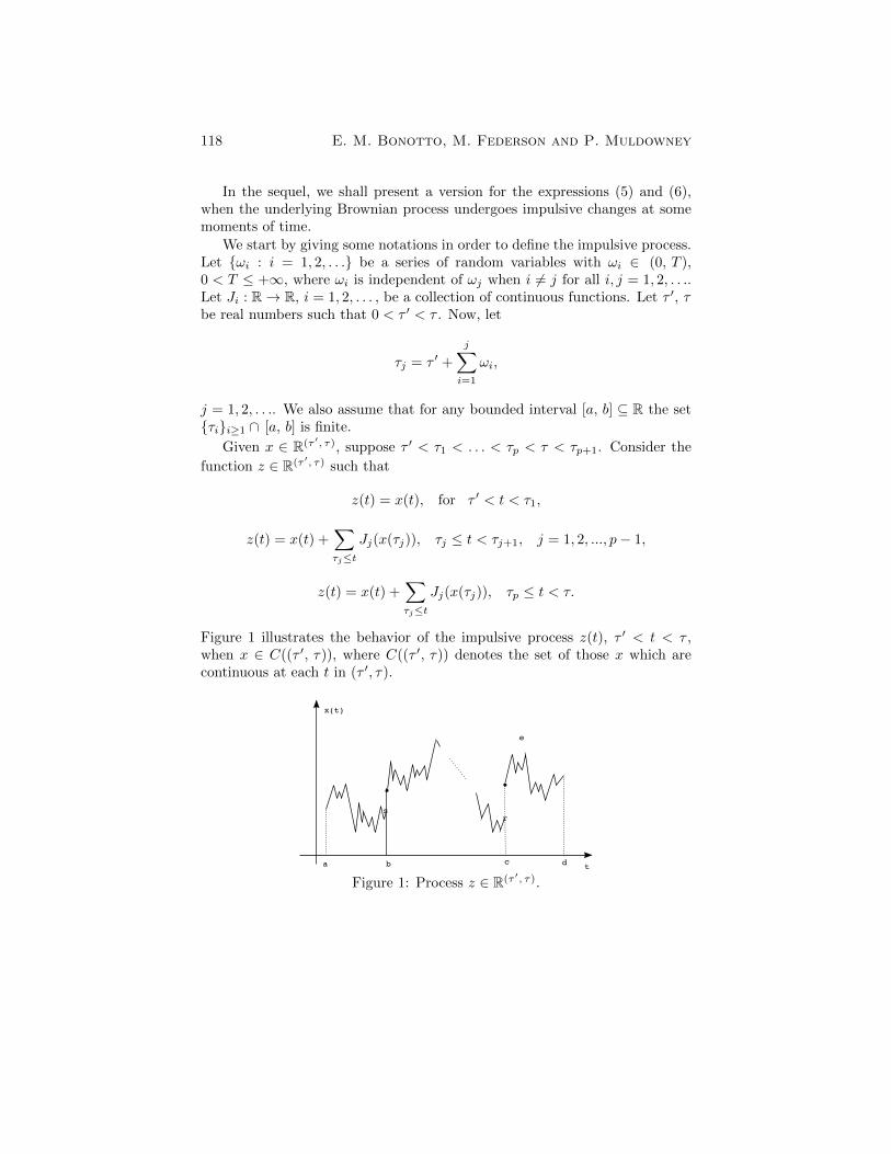
Figure 1 illustrates the behavior of the impulsive process z(t), ⌧ 0 < t < ⌧ ,when x 2 C((⌧ 0, ⌧)), where C((⌧ 0, ⌧)) denotes the set of those x which arecontinuous at each t in (⌧ 0, ⌧).
t
x(t)
a b c d
e
sr
Figure 1: Process z 2 R(⌧ 0, ⌧).
A random impulsive equation of Schr
¨
odinger type 119
Given the interval (⌧ 0, ⌧) ⇢ R let N = {t1
, ..., tr�1
} ⇢ (⌧ 0, ⌧), where⌧ 0 = t
0
and ⌧ = tr. We define N! by
N! = N [{⌧1
, . . . , ⌧p} whenever ⌧1
, . . . , ⌧p 2 (⌧ 0, ⌧) with ⌧p < ⌧ < ⌧p+1
.
Note that N! = N if ⌧1
> ⌧ . If {⌧1
, ⌧2
, ..., ⌧p} ⇢ (⌧ 0, ⌧), p � 1, we enu-merate N! = {t
1
, t2
, . . . , tn�1
}, where ⌧ 0 = t0
, ⌧ = tn and {⌧1
, ⌧2
, ..., ⌧p} ={ti1 , ti2 , ..., tip} with ij 2 {1, 2, ..., n � 1} for 1 j p. Let N = N (N!) ={1, 2, ..., n} and J = J (N!) = {i
1
, i2
, ..., ip}.We now define a volume function for the impulsive process. First, corre-
sponding to w(y, N) in the Brownian motion, that is
w(y, N) =nY
j=1
exp⇣� 1
2
(yj
�yj�1)
2
tj
�tj�1
⌘
p2⇡(tj � tj�1
),
(see [14], chapter 3, for more details), we define gI(y, N!) for the impulsiveprocess by
Y
j2N\J
exp⇣� 1
2
(yj
�yj�1)
2
tj
�tj�1
⌘
p2⇡(tj � tj�1
)
Y
j2J
exp⇣� 1
2
(yj
�(yj�1�J
j
(yj
)))
2
tj
�tj�1
⌘
p2⇡(tj � tj�1
)
which is equal to
Y
j2N\J
exp⇣� 1
2
(yj
�yj�1)
2
tj
�tj�1
⌘
p2⇡(tj � tj�1
)
Y
j2J
exp⇣� 1
2
(Jj
(yj
)+yj
�yj�1)
2
tj
�tj�1
⌘
p2⇡(tj � tj�1
). (7)
Note that if ⌧1
> ⌧ then gI(y, N!) = w(y, N).Let I(tj) = Ij = [uj , vj) ⇢ R and �Ij = vj � uj , 1 j n � 1. Recall
that I(N) = I1
⇥ ...⇥ In�1
.A volume function for the impulsive process is then given by
QI(I[N!]) = QI(I[N!]; ⌧0, ⌧, ⇠0, ⇠) =
Z
I(N!
)
gI(y, N!)dy(N!),
where ⇠0, ⇠ 2 R and 0 < ⌧ 0 < ⌧ .Let
Z =
8<
:Jj 2 C(R, R) :Z
+1
�1
exp⇣� 1
2
(Jj
(yj
)+yj
�yj�1)
2
tj
�tj�1
⌘
p2⇡(tj � tj�1
)dyj = 1, for j = 1, 2, . . .
9=
;
120 E. M. Bonotto, M. Federson and P. Muldowney
where C(R, R) = {g : R ! R : g is continuous}. In particular, if Jj areconstant functions for all j = 1, 2, . . ., then clearly Z 6= ;.
If Jj 2 Z, j = 1, 2, . . ., then QI(I[N!]) is the probability distributionfunction for the impulsive process which gives the probability that xj 2 Ij for1 j n� 1.
If (x, I) is an associated pair, where I = I[N!], let
GI(x, I[N!]) := GI(x, I[N!]; ⌧0, ⌧, ⇠0, ⇠) = QI(I[N!]). (8)
Now we shall prove that GI(x, I[N!]) is generalized Riemann integrable inR(⌧ 0, ⌧). In order to do that, we need to prove an auxiliary result. So, let usstart by introducing some auxiliary functions.
Suppose that ⌧ 0 < ⌧1
< . . . < ⌧p < ⌧ < ⌧p+1
, where ⌧j = ⌧ 0 +jX
i=1
!i,
j = 1, 2, . . . as defined before. Then, we define �1
, �2
: R⇥ (⌧ 0, ⌧) �! R and�j : R⇥ R⇥ (⌧ 0, ⌧)⇥ (⌧ 0, ⌧) �! R, j = 1, 2, ..., p� 1, by
�1
(yk, tk) =1p
2⇡(tk � ⌧ 0)exp
✓�1
2
(yk � ⇠0)2
tk � ⌧ 0
◆,
for k 2 {1, 2, ..., i1
� 1},
�2
(yip
, tip
) =1p
2⇡(⌧ � tip
)exp
✓�1
2
(⇠ � yip
)2
⌧ � tip
◆
and
�j(yij
, yij+1�1
, tij
, tij+1�1
) =1p
2⇡(tij+1�1
� tij
)exp
✓�1
2
(yij+1�1
� yij
)2
tij+1�1
� tij
◆,
j = 1, 2, ..., p� 1.Analogously, define �
1
(Jk(yk), tk), for k 2 J , replacing yk by Jk(yk) + ykin the expression of �
1
(yk, tk), and define �j(yij
, Jij+1(yij+1), tij , tij+1) re-
placing yij+1�1
by Jij+1(yij+1)+ yi
j+1 and tij+1�1
by tij+1 in the expression of
�j(yij
, yij+1�1
, tij
, tij+1�1
), for j 2 {1, 2, ..., p� 1}.We can prove the next lemma by completing the square in the exponential.
Lemma 4.1. If a, b, u, v 2 R, with a > 0 and b > 0, then the function
h(↵) =
ra
⇡e�a(u�↵)2
rb
⇡e�b(↵�v)2
A random impulsive equation of Schr
¨
odinger type 121
is Riemann integrable and
Z+1
�1
ra
⇡e�a(u�↵)2
rb
⇡e�b(↵�v)2d↵ =
sab
⇡(a+ b)exp
✓� ab
a+ b(u� v)2
◆.
Proposition 4.1 in the sequel says that, for y = (y1
, . . . , yn�1
) 2 Rn�1, thefunction gI(y, N!) defined by equation (7) is generalized Riemann integrablewith respect to y in Rn�1.
Proposition 4.1. Let N! = {t1
, t2
, ..., tn�1
} ⇢ (⌧ 0, ⌧) be given with ⌧ 0 = t0
and ⌧ = tn. Let gI be the function defined in (7), where y(⌧ 0) = y(t0
) = ⇠0
and y(⌧) = y(tn) = ⇠ (⇠0, ⇠ 2 R). Then, gI is generalized Riemann integrablewith respect to y in Rn�1 and
Z
Rn�1
gI(y, N!)dy1dy2...dyn�1
=1p
2⇡(⌧ � ⌧ 0)exp
✓�1
2
(⇠ � ⇠0)2
⌧ � ⌧ 0
◆
whenever ⌧1
> ⌧ . AlsoZ
Rn�1
gI(y, N!)dy1dy2...dyn�1
=
Z+1
�1�1
(Ji1(yi1), ti1)�2(yi1 , ti1)dyi1
whenever ⌧ 0 < ⌧1
< ⌧ < ⌧2
, andZ
Rn�1
gI(y, N!)dy1dy2...dyn�1
=
=
Z+1
�1...
Z+1
�1�1
(Ji1(yi1), ti1)
0
@p�1Y
j=1
�j(yij
, Jij+1(yij+1), tij , tij+1)
1
A⇥
⇥�2
(yip
, tip
)pY
j=1
dyij
whenever ⌧ 0 < ⌧1
< . . . < ⌧p < ⌧ < ⌧p+1
, p � 2.
Proof. If ⌧1
> ⌧ the result is proved in [14] (see Proposition 36). Let usprove the case when J = {i
1
, . . . , ip}, p � 2. Indeed, let I = {⌧1
, ⌧2
, ..., ⌧p} ={ti1 , ti2 , ..., tip} ⇢ (⌧ 0, ⌧) with ij 2 {1, 2, ..., n� 1} for 1 j p, p � 2. Let
N = {1, 2, ..., i1
� 1, i1
, i1
+ 1, ...., ip � 1, ip, ip + 1, ..., n� 1, n}.Define
j(yj , yj�1
) =1p
2⇡(tj � tj�1
)exp
✓�1
2
(yj � yj�1
)2
tj � tj�1
◆, j 2 N \ J ,
122 E. M. Bonotto, M. Federson and P. Muldowney
and
'j(yj , yj�1
) =1p
2⇡(tj � tj�1
)exp
✓�1
2
(Jj(yj) + yj � yj�1
)2
tj � tj�1
◆, j 2 J .
By Lemma 4.1, we obtain
Z+1
�1...
Z+1
�1 1
(y1
, y0
)... i1�1
(yi1�1
, yi1�2
)dy1
...dyi1�2
=
=1p
2⇡(ti1�1
� ⌧ 0)exp
✓�1
2
(yi1�1
� ⇠0)2
ti1�1
� ⌧ 0
◆= �
1
(yi1�1
, ti1�1
), (9)
Z+1
�1...
Z+1
�1 i
j
+1
(yij
+1
, yij
)... ij+1�1
(yij+1�1
, yij+1�2
)dyij
+1
...dyij+1�2
=
=1p
2⇡(tij+1�1
� tij
)exp
✓�1
2
(yij+1�1
� yij
)2
tij+1�1
� tij
◆= �j(yi
j
, yij+1�1
, tij
, tij+1�1
),
(10)j = 1, 2, ..., p� 1, and also
Z+1
�1...
Z+1
�1 i
p
+1
(yip
+1
, yip
)... n(yn, yn�1
)dyip
+1
...dyn�1
=
=1p
2⇡(⌧ � tip
)exp
✓�1
2
(⇠ � yip
)2
⌧ � tip
◆= �
2
(yip
, tip
). (11)
Thus, taking tip
+` := tn�1
, ` 2 N, from equations (9), (10) and (11), we have
Z+1
�1...
Z+1
�1gI(y, N!)
0
@i1�2Y
j=1
dyj
1
A
0
@p�1Y
j=1
dyij
+1
...dyij+1�2
1
AY
j=1
dyip
+j =
(12)
= �1
(yi1�1
, ti1�1
)
0
@p�1Y
j=1
'ij
(yij
, yij
�1
)�j(yij
, yij+1�1
, tij
, tij+1�1
)
1
A⇥
⇥'ip
(yip
, yip
�1
)�2
(yip
, tip
).
Using Lemma 4.1, we have
Z+1
�1�1
(yi1�1
, ti1�1
)'i1(yi1 , yi1�1
)dyi1�1
= �1
(Ji1(yi1), ti1) (13)
A random impulsive equation of Schr
¨
odinger type 123
andZ
+1
�1�j(yi
j
, yij+1�1
, tij
, tij+1�1
)'ij+1(yij+1 , yij+1�1
)dyij+1�1
= (14)
= �j(yij
, Jij+1(yij+1), tij , tij+1), j = 1, ..., p� 1.
Then, from (12), (13) and (14), it follows that
Z+1
�1...
Z+1
�1gI(y, N!)
Y
j2N\Jdyj =
= �1
(Ji1(yi1), ti1)
0
@p�1Y
j=1
�j(yij
, Jij+1(yij+1), tij , tij+1)
1
A�2
(yip
, tip
). (15)
Define the functions f, F : Rp ! R by
f(yi1 , ..., yip) =
0
@p�1Y
j=1
�j(yij
, Jij+1(yij+1), tij , tij+1)
1
A�2
(yip
, tip
)
andF (yi1 , ..., yip) = �
1
(Ji1(yi1), ti1)f(yi1 , ..., yip).
Thus F is a continuous function, |F (yi1 , ..., yip)| f(yi1 , ..., yip)p2⇡(ti1 � ⌧ 0)
and
Z+1
�1...
Z+1
�1
f(yi1 , ..., yip)p2⇡(ti1 � ⌧ 0)
dyi1 ...dyip =1p
2⇡(ti1 � ⌧ 0).
By the Tonelli theorem (Theorem 3.1), the function F is generalized Riemannintegrable in Rp and
Z
Rp
F (yi1 , ..., yip)dyi1 ...dyip =
Z+1
�1...
Z+1
�1F (yi1 , ..., yip)dyi1 ...dyip
is finite. Hence, from (15),
Z+1
�1...
Z+1
�1gI(y, N!)dy1dy2...dyn�1
=
=
Z+1
�1...
Z+1
�1F (yi1 , ..., yip)dyi1 ...dyip < 1.
124 E. M. Bonotto, M. Federson and P. Muldowney
Using Corollary 3.1, gI(y, N!) is generalized Riemann integrable with respectto y in Rn�1 and Z
Rn�1
gI(y, N!)dy1...dyn�1
=
=
Z+1
�1...
Z+1
�1gI(y, N!)dy1dy2...dyn�1
=
=
Z+1
�1...
Z+1
�1�1
(Ji1(yi1), ti1)
0
@p�1Y
j=1
�j(yij
, Jij+1(yij+1), tij , tij+1)
1
A⇥
⇥�2
(yip
, tip
)pY
j=1
dyij
,
which completes the proof.
The next result says that GI(x, I[N!]) given by (8) is generalized Riemannintegrable in the function space R(⌧ 0, ⌧).
Theorem 4.1. The generalized Riemann integral
Z
R(⌧0, ⌧)
GI(x, I[N!])
exists.
Proof. If ⌧1
> ⌧ the result is proved in [14] (see Proposition 36). SupposeJ = {i
1
, . . . , ip}, p � 1. Then, consider a division E = {(x, I[N!])} of R(⌧ 0, ⌧),with each N! chosen so that I = {⌧
1
, . . . , ⌧p} ✓ N! 2 F((⌧ 0, ⌧)), p � 1. Thenthe Riemann sum of GI is given by
X
(x, I[N!
])2EGI(x, I[N!]) =
X
(x, I[N!
])2EQI(I[N!]).
Let M! = [{N! : (x, I[N!]) 2 E} and enumerate M! as {t1
, ..., tm�1
}, where⌧ 0 = t
0
, ⌧ = tm and t0
< t1
< ... < tm�1
< tm. Each term QI(I[N!]) of theRiemann sum can be rewritten as QI(I[M!]) by inserting additional yj ’s inthe expression of gI , j 2 N \J , and integrating from �1 to +1 on the extrayj ’s. Then the Riemann sum becomes
X
(x, I[M!
])2EQI(I[M!]).
A random impulsive equation of Schr
¨
odinger type 125
with M! a fixed set of dimensions. So we are now dealing, in e↵ect, withsome Riemann sum estimate of an integral in m � 1 dimensions. Then eachterm of the Riemann sum is an integral over I[M!] ⇢ Rm�1, and, by the finiteadditivity of these integrals in Rm�1,
X
(x, I[M!
])2EQI(I([M!]) =
Z+1
�1...
Z+1
�1gI(y, M!)dy1...dym�1
. (16)
By Proposition 4.1, the integral (16) exists and we can rewrite
X
(x, I[M!
])2EQI(I[M!])
as Z+1
�1�1
(Ji1(yi1), ti1)�2(yi1 , ti1)dyi1 (17)
if p = 1, and
Z+1
�1...
Z+1
�1�1
(Ji1(yi1), ti1)
0
@p�1Y
j=1
�j(yij
, Jij+1(yij+1), tij , tij+1)
1
A⇥
⇥�2
(yip
, tip
)pY
j=1
dyij
(18)
if p � 2. Let �1
be the integral in (17) and �2
be the integral in (18). Thus,given ✏ > 0, for any gauge � chosen so that L(x) ◆ I, we have that for every(x, I[N!]) 2 E� , I ✓ L(x) ✓ N! implies
������
X
(x, I[N!
])2E�
GI(x, I[N!])� �1
������< ✏ if p = 1
and ������
X
(x, I[N!
])2E�
GI(x, I[N!])� �2
������< ✏ if p � 2.
Therefore,
Z
R(⌧0, ⌧)
GI(x, I[N!]) = �1
if p = 1 or
Z
R(⌧0, ⌧)
GI(x, I[N!]) = �2
if
p � 2 and the proof is complete.
126 E. M. Bonotto, M. Federson and P. Muldowney
Let us show that the expressions gI(x, N!)n�1Y
j=1
�Ij and GI(x, I[N!]) are
variationally equivalent in R(⌧ 0, ⌧). This result is a consequence of the nextproposition.
If (x, I) is an associated pair, where I = I[N!], define the auxiliary functionqI(x, I[N!]) by
qI(x, I[N!]) = gI(x, N!)n�1Y
j=1
�Ij .
Proposition 4.2. Let k(x(N!)) = k(x(t1
), ..., x(tn�1
)) be a real-valued func-tion which depends on (x(t
1
), ..., x(tn�1
)). If k is jointly continuous in xj,1 j n � 1, then the expressions k(x(N!))qI(x, I[N!]) andZ
I(N!
)
k(y(N!))gI(y, N!)dy(N!) are variationally equivalent in R(⌧ 0, ⌧), pro-
vided at least one the two integrals exists.
Proof. Let ✏ > 0 be given. Let us consider the case when ⌧1
2 (⌧ 0, ⌧). Aproof for the case when ⌧
1
> ⌧ can be found in [14], Proposition 37. Since Jj ,
j = 1, 2, . . ., are continuous functions, given x 2 R(⌧ 0,⌧), we can choose L(x)
and �(x, N!) such that, ifN! ◆ L(x) ◆ I = {⌧1
, . . . , ⌧p}, then (I(N!), x(N!))is ��fine, and if y 2 I(N!), then
|k(x(N!))gI(x, N!)� k(y(N!))gI(y, N!)| < ✏
4
p2⇡(ti1 � ⌧ 0)gI(x, N!)
and
gI(y, N!) >1
2gI(x, N!).
Thus,�����k(x(N!))qI(x, I[N!])�
Z
I(N!
)
k(y(N!))gI(y, N!)dy(N!)
����� =
=
������k(x(N!))gI(x, N!)
n�1Y
j=1
�Ij �Z
I(N!
)
k(y(N!))gI(y, N!)dy(N!)
������=
=
�����
Z
I(N!
)
[k(x(N!))gI(x, N!)� k(y(N!))gI(y, N!)] dy(N!)
�����
✏
2
p2⇡(ti1 � ⌧ 0)
Z
I(N!
)
gI(y, N!)dy(N!).
A random impulsive equation of Schr
¨
odinger type 127
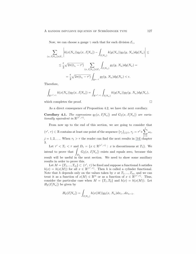
Now, we can choose a gauge � such that for each division E� ,
X
(x, I[N!
])2E�
�����k(x(N!))qI(x, I[N!])�Z
I(N!
)
k(y(N!))gI(y, N!)dy(N!)
�����
✏
2
p2⇡(ti1 � ⌧ 0)
X
(x, I[N!
])2E�
Z
I(N!
)
gI(y, N!)dy(N!) =
=✏
2
p2⇡(ti1 � ⌧ 0)
Z
Rn�1
gI(y, N!)dy(N!) < ✏.
Therefore,Z
R(⌧0,⌧)
k(x(N!))qI(x, I[N!]) =
Z
R(⌧0,⌧)
Z
I(N!
)
k(y(N!))gI(y, N!)dy(N!),
which completes the proof.
As a direct consequence of Proposition 4.2, we have the next corollary.
Corollary 4.1. The expressions qI(x, I[N!]) and GI(x, I[N!]) are varia-tionally equivalent in R(⌧ 0, ⌧).
From now up to the end of this section, we are going to consider that
(⌧ 0, ⌧) ⇢ R contains at least one point of the sequence {⌧j}j�1
, ⌧j = ⌧ 0+jX
i=1
!i,
j = 1, 2, . . .. When ⌧1
> ⌧ the reader can find the next results in [14] chapter3.
Let ⌧ 0 < T1
< ⌧ and D1
= {x 2 R(⌧ 0, ⌧) : x is discontinuous at T1
}. We
intend to prove that
Z
D1
GI(x, I[N!]) exists and equals zero, because this
result will be useful in the next section. We need to show some auxiliaryresults in order to prove this.
LetM = {T1
, ..., Tm} ⇢ (⌧ 0, ⌧) be fixed and suppose a functional h satisfiesh(x) = h(x(M)) for all x 2 R(⌧ 0, ⌧). Then h is called a cylinder functional.Note that h depends only on the values taken by x at T
1
, ..., Tm, and we cantreat it as a function of x(M) 2 Rm or as a function of x 2 R(⌧ 0,⌧). Thus,consider the particular case when M = {T
1
, T2
} and h(x) = h(x(M)). LetHI(I[N!]) be given by
HI(I[N!]) =
Z
I(N!
)
h(x(M))gI(x, N!)dx1
...dxn�1
.
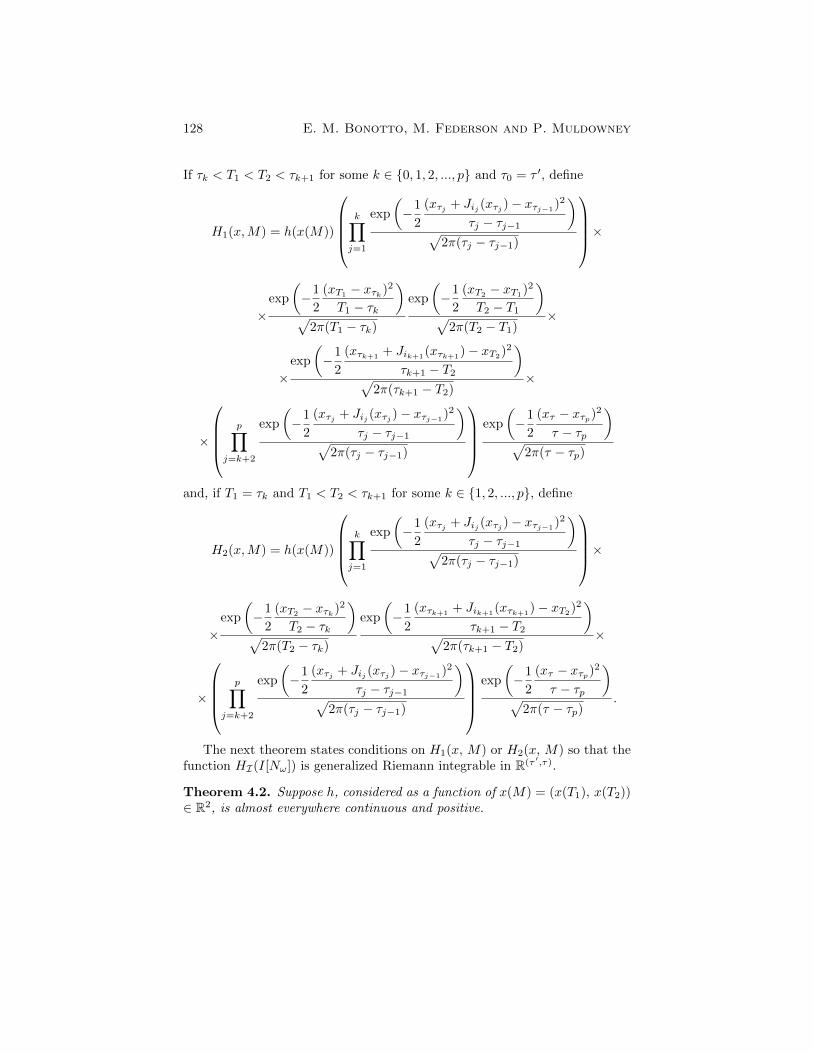
128 E. M. Bonotto, M. Federson and P. Muldowney
If ⌧k < T1
< T2
< ⌧k+1
for some k 2 {0, 1, 2, ..., p} and ⌧0
= ⌧ 0, define
H1
(x,M) = h(x(M))
0
BBB@
kY
j=1
exp
✓�1
2
(x⌧j
+ Jij
(x⌧j
)� x⌧j�1)
2
⌧j � ⌧j�1
◆
p2⇡(⌧j � ⌧j�1
)
1
CCCA⇥
⇥exp
✓�1
2
(xT1 � x⌧k
)2
T1
� ⌧k
◆
p2⇡(T
1
� ⌧k)
exp
✓�1
2
(xT2 � xT1)2
T2
� T1
◆
p2⇡(T
2
� T1
)⇥
⇥exp
✓�1
2
(x⌧k+1 + Ji
k+1(x⌧k+1)� xT2)2
⌧k+1
� T2
◆
p2⇡(⌧k+1
� T2
)⇥
⇥
0
BBB@
pY
j=k+2
exp
✓�1
2
(x⌧j
+ Jij
(x⌧j
)� x⌧j�1)
2
⌧j � ⌧j�1
◆
p2⇡(⌧j � ⌧j�1
)
1
CCCA
exp
✓�1
2
(x⌧ � x⌧p
)2
⌧ � ⌧p
◆
p2⇡(⌧ � ⌧p)
and, if T1
= ⌧k and T1
< T2
< ⌧k+1
for some k 2 {1, 2, ..., p}, define
H2
(x,M) = h(x(M))
0
BBB@
kY
j=1
exp
✓�1
2
(x⌧j
+ Jij
(x⌧j
)� x⌧j�1)
2
⌧j � ⌧j�1
◆
p2⇡(⌧j � ⌧j�1
)
1
CCCA⇥
⇥exp
✓�1
2
(xT2 � x⌧k
)2
T2
� ⌧k
◆
p2⇡(T
2
� ⌧k)
exp
✓�1
2
(x⌧k+1 + Ji
k+1(x⌧k+1)� xT2)2
⌧k+1
� T2
◆
p2⇡(⌧k+1
� T2
)⇥
⇥
0
BBB@
pY
j=k+2
exp
✓�1
2
(x⌧j
+ Jij
(x⌧j
)� x⌧j�1)
2
⌧j � ⌧j�1
◆
p2⇡(⌧j � ⌧j�1
)
1
CCCA
exp
✓�1
2
(x⌧ � x⌧p
)2
⌧ � ⌧p
◆
p2⇡(⌧ � ⌧p)
.
The next theorem states conditions on H1
(x, M) or H2
(x, M) so that thefunction HI(I[N!]) is generalized Riemann integrable in R(⌧ 0,⌧).
Theorem 4.2. Suppose h, considered as a function of x(M) = (x(T1
), x(T2
))2 R2, is almost everywhere continuous and positive.
A random impulsive equation of Schr
¨
odinger type 129
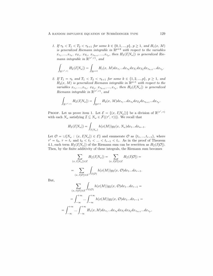
1. If ⌧k < T1
< T2
< ⌧k+1
for some k 2 {0, 1, ..., p}, p � 1, and H1
(x, M)is generalized Riemann integrable in Rp+2 with respect to the variablesx⌧1 , ..., x⌧k , xT1 , xT2 , x⌧k+1 , ..., x⌧p , then HI(I[N!]) is generalized Rie-
mann integrable in R(⌧ 0,⌧), andZ
R(⌧0,⌧)
HI(I[N!]) =
Z
Rp+2
H1
(x, M)dx⌧1 ...dx⌧kdxT1dxT2dx⌧k+1 ...dx⌧p .
2. If T1
= ⌧k and T1
< T2
< ⌧k+1
for some k 2 {1, 2, ..., p}, p � 1, andH
2
(x, M) is generalized Riemann integrable in Rp+1 with respect to thevariables x⌧1 , ..., x⌧k , xT2 , x⌧
k+1 , ..., x⌧p , then HI(I[N!]) is generalized
Riemann integrable in R(⌧ 0,⌧), andZ
R(⌧0,⌧)
HI(I[N!]) =
Z
Rp+1
H2
(x, M)dx⌧1 ...dx⌧kdxT2dx⌧k+1 ...dx⌧p .
Proof. Let us prove item 1. Let E = {(x, I[N!])} be a division of R(⌧ 0, ⌧)
with each N! satisfying I ✓ N! 2 F((⌧ 0, ⌧))}. We recall that
HI(I[N!]) =
Z
I(N!
)
h(x(M))gI(x, N!)dx1
...dxn�1
.
Let O = [{N! : (x, I[N!]) 2 E} and enumerate O as {t1
, ..., tr�1
}, where⌧ 0 = t
0
, ⌧ = tr and t0
< t1
< ... < tr�1
< tr. As in the proof of Theorem4.1, each term HI(I[N!]) of the Riemann sum can be rewritten as HI(I[O]).Then, by the finite additivity of these integrals, the Riemann sum becomes
X
(x, I[N!
])2EHI(I[N!]) =
X
(x, I[O])2EHI(I[O]) =
=X
(x, I[O])2E
Z
I(O)
h(x(M))gI(x, O)dx1
...dxr�1
.
But,X
(x, I[O])2E
Z
I(O)
h(x(M))gI(x, O)dx1
...dxr�1
=
=
Z+1
�1...
Z+1
�1h(x(M))gI(x, O)dx
1
...dxr�1
=
=
Z+1
�1...
Z+1
�1H
1
(x,M)dx⌧1 ...dx⌧kdxT1dxT2dx⌧k+1 ...dx⌧p ,
130 E. M. Bonotto, M. Federson and P. Muldowney
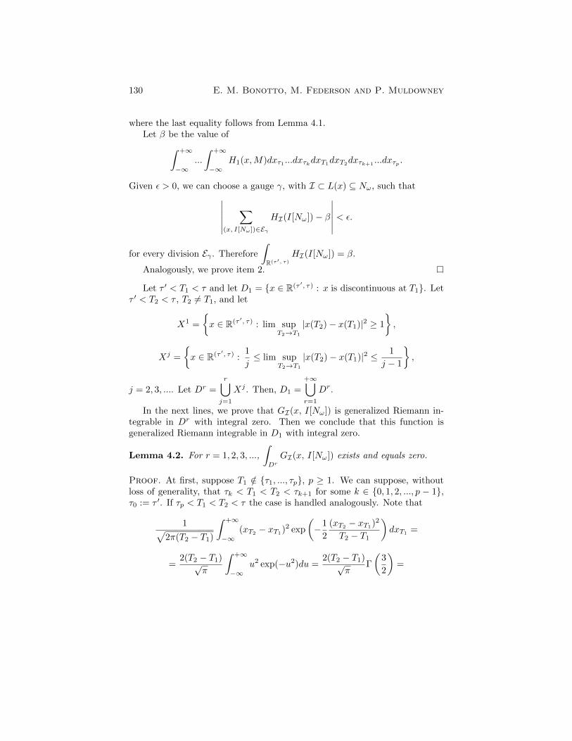
where the last equality follows from Lemma 4.1.Let � be the value of
Z+1
�1...
Z+1
�1H
1
(x,M)dx⌧1 ...dx⌧kdxT1dxT2dx⌧k+1 ...dx⌧p .
Given ✏ > 0, we can choose a gauge �, with I ⇢ L(x) ✓ N!, such that������
X
(x, I[N!
])2E�
HI(I[N!])� �
������< ✏.
for every division E� . ThereforeZ
R(⌧0, ⌧)
HI(I[N!]) = �.
Analogously, we prove item 2.
Let ⌧ 0 < T1
< ⌧ and let D1
= {x 2 R(⌧ 0, ⌧) : x is discontinuous at T1
}. Let⌧ 0 < T
2
< ⌧ , T2
6= T1
, and let
X1 =
⇢x 2 R(⌧ 0, ⌧) : lim sup
T2!T1
|x(T2
)� x(T1
)|2 � 1
�,
Xj =
⇢x 2 R(⌧ 0, ⌧) :
1
j lim sup
T2!T1
|x(T2
)� x(T1
)|2 1
j � 1
�,
j = 2, 3, .... Let Dr =r[
j=1
Xj . Then, D1
=+1[
r=1
Dr.
In the next lines, we prove that GI(x, I[N!]) is generalized Riemann in-tegrable in Dr with integral zero. Then we conclude that this function isgeneralized Riemann integrable in D
1
with integral zero.
Lemma 4.2. For r = 1, 2, 3, ...,
Z
Dr
GI(x, I[N!]) exists and equals zero.
Proof. At first, suppose T1
/2 {⌧1
, ..., ⌧p}, p � 1. We can suppose, withoutloss of generality, that ⌧k < T
1
< T2
< ⌧k+1
for some k 2 {0, 1, 2, ..., p � 1},⌧0
:= ⌧ 0. If ⌧p < T1
< T2
< ⌧ the case is handled analogously. Note that
1p2⇡(T
2
� T1
)
Z+1
�1(xT2 � xT1)
2 exp
✓�1
2
(xT2 � xT1)2
T2
� T1
◆dxT1 =
=2(T
2
� T1
)p⇡
Z+1
�1u2 exp(�u2)du =
2(T2
� T1
)p⇡
�
✓3
2
◆=
A random impulsive equation of Schr
¨
odinger type 131
=2(T
2
� T1
)p⇡
p⇡
2= T
2
� T1
= |T2
� T1
|.
Then,
Z+1
�1...
Z+1
�1
|xT2 � xT1 |2p2⇡(⌧
1
� ⌧ 0)
kY
j=2
exp
✓�1
2
(x⌧j
+ Jij
(x⌧j
)� x⌧j�1)
2
⌧j � ⌧j�1
◆
p2⇡(⌧j � ⌧j�1
)⇥
⇥exp
✓�1
2
(xT1 � x⌧k
)2
T1
� ⌧k
◆
p2⇡(T
1
� ⌧k)
exp
✓�1
2
(xT2 � xT1)2
T2
� T1
◆
p2⇡(T
2
� T1
)⇥
⇥exp
✓�1
2
(x⌧k+1 + Ji
k+1(x⌧k+1)� xT2)2
⌧k+1
� T2
◆
p2⇡(⌧k+1
� T2
)⇥
⇥pY
j=k+2
exp
✓�1
2
(Jij
(x⌧j
) + x⌧j
� x⌧j�1)
2
⌧j � ⌧j�1
◆
p2⇡(⌧j � ⌧j�1
)⇥
⇥exp
✓�1
2
(x⌧ � x⌧p
)2
⌧ � ⌧p
◆
p2⇡(⌧ � ⌧p)
dx⌧1 ...dx⌧kdxT1dxT2dx⌧k+1 ...dx⌧p =|T
2
� T1
|p2⇡(⌧
1
� ⌧ 0).
Let & be the last integral. Let h(x(M)) = (xT2 � xT1)2 in the expression
of H1
(x, M). Then, by Theorem 4.2, item 1., we haveZ
R(⌧0, ⌧)
HI(I[N!]) =
=
Z+1
�1...
Z+1
�1|xT2 � xT1 |2
kY
j=1
0
BBB@
exp
✓�1
2
(x⌧j
+ Jij
(x⌧j
)� x⌧j�1)
2
⌧j � ⌧j�1
◆
p2⇡(⌧j � ⌧j�1
)
1
CCCA⇥
⇥exp
✓�1
2
(xT1 � x⌧k
)2
T1
� ⌧k
◆
p2⇡(T
1
� ⌧k)
exp
✓�1
2
(xT2 � xT1)2
T2
� T1
◆
p2⇡(T
2
� T1
)⇥
⇥exp
✓�1
2
(x⌧k+1 + Ji
k+1(x⌧k+1)� xT2)2
⌧k+1
� T2
◆
p2⇡(⌧k+1
� T2
)⇥
132 E. M. Bonotto, M. Federson and P. Muldowney
⇥pY
j=k+2
0
BBB@
exp
✓�1
2
(x⌧j
+ Jij
(x⌧j
)� x⌧j�1)
2
⌧j � ⌧j�1
◆
p2⇡(⌧j � ⌧j�1
)
1
CCCA⇥
⇥exp
✓�1
2
(x⌧ � x⌧p
)2
⌧ � ⌧p
◆
p2⇡(⌧ � ⌧p)
dx⌧1 ...dx⌧kdxT1dxT2dx⌧k+1 ...dx⌧p
& =|T
2
� T1
|p2⇡(⌧
1
� ⌧ 0),
where the last inequality follows from the Tonelli theorem (Theorem 3.1).Given ✏ > 0 and j 2 N, we can choose T
2
and a division E� such that
✏
j>
X
(x, I[N!
])2E�
HI(I[N!]) =
(⇤)=
X
(x, I(O))2E�
Z
I(O)
(xT2 � xT1)2gI(x, O)dx
1
...dxr�1
�
�X
(x, I[O])2E�
�(Xj , x)
Z
I(O)
(xT2 � xT1)2gI(x, O)dx
1
...dxr�1
�
� 1
j
X
(x, I[O])2E�
�(Xj , x)
Z
I(O)
gI(x, O)dx1
...dxr�1
=
=1
j
X
(x, I[O])2E�
�(Xj , x)GI(x, I[O]).
The symbol O after the first equality (⇤) denotes O = [{N! : (x, I[N!]) 2E�}. Since ✏ > 0 is arbitrary,
Z
R(⌧0, ⌧)
�(Xj , x)GI(x, I[N!]) = 0
for every j = 1, 2, .... Then, by the finite additivity of the integral,
Z
R(⌧0, ⌧)
�(Dr, x)GI(x, I[N!]) = 0.
A random impulsive equation of Schr
¨
odinger type 133
If T1
2 {⌧1
, ..., ⌧p}, then T1
= ⌧k for some k 2 {1, 2, ..., p}. ConsideringT1
< T2
< ⌧k+1
(denote in this case ⌧ := ⌧p+1
), since
1p2⇡(T
2
� ⌧k)
Z+1
�1|xT2 � x⌧
k
|2 exp✓�1
2
(xT2 � x⌧k
)2
T2
� ⌧k
◆dx⌧
k
= |T2
� T1
|,
then
Z+1
�1...
Z+1
�1
|xT2 � xT1 |2p2⇡(⌧
1
� ⌧ 0)
kY
j=2
0
BBB@
exp
✓�1
2
(x⌧j
+ Jij
(x⌧j
)� x⌧j�1)
2
⌧j � ⌧j�1
◆
p2⇡(⌧j � ⌧j�1
)
1
CCCA⇥
⇥exp
✓�1
2
(xT2 � x⌧k
)2
T2
� ⌧k
◆
p2⇡(T
2
� ⌧k)
exp
✓�1
2
(Jik+1(x⌧k+1) + x⌧
k+1 � xT2)2
⌧k+1
� T2
◆
p2⇡(⌧k+1
� T2
)⇥
⇥pY
j=k+2
exp
✓�1
2
(x⌧j
+ Jij
(x⌧j
)� x⌧j�1)
2
⌧j � ⌧j�1
◆
p2⇡(⌧j � ⌧j�1
)
exp
✓�1
2
(x⌧ � x⌧p
)2
⌧ � ⌧p
◆
p2⇡(⌧ � ⌧p)
⇥
⇥dx⌧1 ...dx⌧kdxT2dx⌧k+1 ...dx⌧p =|T
2
� T1
|p2⇡(⌧
1
� ⌧).
Thus, Z
R(⌧0, ⌧)
HI(I[N!]) |T2
� T1
|p2⇡(⌧
1
� ⌧ 0),
whereZ
R(⌧0,⌧)
HI(I[N!]) =
Z
Rp+1
H2
(x, M)dx⌧1 ...dx⌧kdxT2dx⌧k+1 ...dx⌧p
with h(x(M)) = (xT2 � xT1)2 in the expression of H
2
(x, M).The rest of the proof follows by analogous argument.
Theorem 4.3. The integral
Z
D1
GI(x, I[N!]) exists and equals zero.
Proof. We have D1
=+1[
r=1
Dr and Dr ⇢ Dr+1. For each associated pair
(x, I[N!]), define
fk(x, I[N!]) = �(Dk, x)GI(x, I[N!]), k = 1, 2, 3....
134 E. M. Bonotto, M. Federson and P. Muldowney
Given x 2 D1
, there exists a positive integer k0
such that x 2 Dk for k � k0
.Thus, �(Dk, x) = �(D
1
, x) for k � k0
. Consequently, for each associated pair(x, I[N!]), we have
fk(x, I[N!])k!+1�! f
0
(x, I[N!]),
where f0
(x, I[N!]) = �(D1
, x)GI(x, I[N!]). Note that
|f0
(x, I[N!])| GI(x, I[N!]) and |fk(x, I[N!])| GI(x, I[N!]),
k = 1, 2, 3, . . ..Given ✏ > 0, there exists k
1
> 0 such that
|f0
(x, I[N!])� fk(x, I[N!])| < ✏GI(x, I[N!]),
for k > k1
and all associated pairs (x, I[N!]). By Theorem 4.1, GI(x, I[N!])is generalized Riemann integrable in R(⌧ 0, ⌧). By Theorem 3.2, f
0
is generalizedRiemann integrable in R(⌧ 0, ⌧) and
Z
R(⌧0, ⌧)
f0
(x, I[N!]) = limk!+1
Z
R(⌧0, ⌧)
fk(x, I[N!]).
Using Lemma 4.2, we obtainZ
R(⌧0, ⌧)
�(D1
, x)GI(x, I[N!]) = 0
and the proof is complete.
4.2 An equation of Schrodinger type random with impulses.
We start by defining the solution of an impulsive partial di↵erential equation.The idea of this definition is inspired by [13].
Suppose 0 = ⌧0
< ⌧1
< ⌧2
< ... < ⌧p < ⌧ are given numbers and ⌧ 2]0, +1[. Define
� = R⇥ [0, ⌧ ],
�k = {( , t) : 2 R, t 2 (⌧k, ⌧k+1
)} , 0 k p� 1,
�k = {( , t) : 2 R, t 2 [⌧k, ⌧k+1
)} , 0 k p� 1,
�p = {( , t) : 2 R, t 2 (⌧p, ⌧)} ,�p = {( , t) : 2 R, t 2 [⌧p, ⌧)} ,
� =p[
k=0
�k and � =p[
k=0
�k.
Let K(�, R) be the class of all functions u : � ! R such that
A random impulsive equation of Schr
¨
odinger type 135
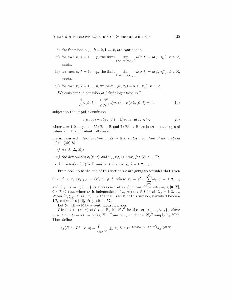
i) the functions u|�
k
, k = 0, 1, ..., p, are continuous.
ii) for each k, k = 1, ..., p, the limit lim(⌫, t)!( , ⌧�
k
)
u(⌫, t) = u( , ⌧�k ), 2 R,
exists.
iii) for each k, k = 1, ..., p, the limit lim(⌫, t)!( , ⌧+
k
)
u(⌫, t) = u( , ⌧+k ), 2 R,
exists.
iv) for each k, k = 1, ..., p, we have u( , ⌧k) = u( , ⌧+k ), 2 R.
We consider the equation of Schrodinger type in �
@
@tu( , t)� 1
2
@2
@ 2
u( , t) + V ( )u( , t) = 0, (19)
subject to the impulse condition
u( , ⌧k)� u( , ⌧�k ) = I( , ⌧k, u( , ⌧k)), (20)
where k = 1, 2, ..., p, and V : R ! R and I : R3 ! R are functions taking realvalues and I is not identically zero.
Definition 4.1. The function u : � ! R is called a solution of the problem(19)� (20) if:
i) u 2 K(�, R);
ii) the derivatives ut( , t) and u ( , t) exist, for ( , t) 2 �;
iii) u satisfies (19) in � and (20) at each ⌧k, k = 1, 2, ..., p.
From now up to the end of this section we are going to consider that given
0 < ⌧ 0 < ⌧ , {⌧p}p�1
\ (⌧ 0, ⌧) 6= ;, where ⌧j = ⌧ 0 +jX
i=1
!i, j = 1, 2, . . .,
and {!i : i = 1, 2, . . .} is a sequence of random variables with !i 2 ]0, T [,0 < T +1, where !i is independent of !j when i 6= j for all i, j = 1, 2, . . ..When {⌧p}p�1
\ (⌧ 0, ⌧) = ; the main result of this section, namely Theorem4.7, is found in [14], Proposition 57.
Let UI : R ! R be a continuous function.Given s 2 (⌧ 0, ⌧) and & 2 R, let N
(s)! be the set {t
1
, ...., tr�1
}, where
t0
= ⌧ 0 and tr = s (r = r(s) 2 N). From now, we denote N(s)! simply by N (s).
Then define
vI(N (s), I(s); &, s) =
Z
I(N(s))
gI(y, N (s))e�UI(xr(s)�1)(s�⌧ 0
)dy(N (s))
136 E. M. Bonotto, M. Federson and P. Muldowney
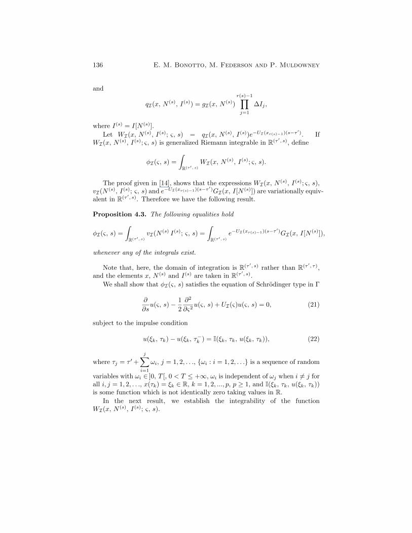
and
qI(x, N (s), I(s)) = gI(x, N (s))
r(s)�1Y
j=1
�Ij ,
where I(s) = I[N (s)].Let WI(x, N (s), I(s); &, s) = qI(x, N (s), I(s))e�UI(x
r(s)�1)(s�⌧ 0). If
WI(x, N (s), I(s); &, s) is generalized Riemann integrable in R(⌧ 0, s), define
�I(&, s) =Z
R(⌧0, s)
WI(x, N (s), I(s); &, s).
The proof given in [14], shows that the expressions WI(x, N (s), I(s); &, s),vI(N (s), I(s); &, s) and e�UI(x
r(s)�1)(s�⌧ 0)GI(x, I[N (s)]) are variationally equiv-
alent in R(⌧ 0, s). Therefore we have the following result.
Proposition 4.3. The following equalities hold
�I(&, s) =Z
R(⌧0, s)
vI(N (s) I(s); &, s) =
Z
R(⌧0, s)
e�UI(xr(s)�1)(s�⌧ 0
)GI(x, I[N (s)]),
whenever any of the integrals exist.
Note that, here, the domain of integration is R(⌧ 0, s) rather than R(⌧ 0, ⌧),and the elements x, N (s) and I(s) are taken in R(⌧ 0, s).
We shall show that �I(&, s) satisfies the equation of Schrodinger type in �
@
@su(&, s)� 1
2
@2
@&2u(&, s) + UI(&)u(&, s) = 0, (21)
subject to the impulse condition
u(⇠k, ⌧k)� u(⇠k, ⌧�k ) = I(⇠k, ⌧k, u(⇠k, ⌧k)), (22)
where ⌧j = ⌧ 0 +jX
i=1
!i, j = 1, 2, . . ., {!i : i = 1, 2, . . .} is a sequence of random
variables with !i 2 ]0, T [, 0 < T +1, !i is independent of !j when i 6= j forall i, j = 1, 2, . . ., x(⌧k) = ⇠k 2 R, k = 1, 2, ..., p, p � 1, and I(⇠k, ⌧k, u(⇠k, ⌧k))is some function which is not identically zero taking values in R.
In the next result, we establish the integrability of the functionWI(x, N (s), I(s); &, s).
A random impulsive equation of Schr
¨
odinger type 137
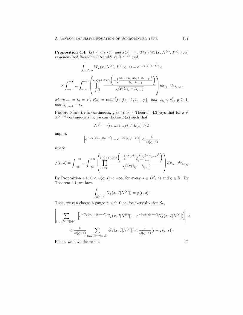
Proposition 4.4. Let ⌧ 0 < s < ⌧ and x(s) = &. Then WI(x, N (s), I(s); &, s)is generalized Riemann integrable in R(⌧ 0, s) and
Z
R(⌧0, s)
WI(x, N (s), I(s); &, s) = e�UI(&)(s�⌧ 0)⇥
⇥Z
+1
�1...
Z+1
�1
0
BB@
r(s)+1Y
j=1
exp
✓� 1
2
(xi
j
+Ji
j
(xi
j
)�xi
j�1 )2
ti
j
�ti
j�1
◆
p2⇡(ti
j
� tij�1)
1
CCA dxi1 ...dxir(s)
,
where ti0 = t0
= ⌧ 0, r(s) = max�j : j 2 {1, 2, ..., p} and ti
j
< s , p � 1,
and tir(s)+1
= s.
Proof. Since UI is continuous, given ✏ > 0, Theorem 4.3 says that for x 2R(⌧ 0, s) continuous at s, we can choose L(x) such that
N (s) = {t1
, ..., tr�1
} ◆ L(x) ◆ Iimplies ���e�UI(xr�1)(s�⌧ 0
) � e�UI(&)(s�⌧ 0)
��� <✏
'(&, s),
where
'(&, s) =
Z+1
�1...
Z+1
�1
0
BB@
r(s)+1Y
j=1
exp
✓� 1
2
(xi
j
+Ji
j
(xi
j
)�xi
j�1 )2
ti
j
�ti
j�1
◆
p2⇡(ti
j
� tij�1)
1
CCA dxi1 ...dxir(s)
.
By Proposition 4.1, 0 < '(&, s) < +1, for every s 2 (⌧ 0, ⌧) and & 2 R. ByTheorem 4.1, we have
Z
R(⌧0, s)
GI(x, I[N (s)]) = '(&, s).
Then, we can choose a gauge � such that, for every division E� ,������
X
(x,I[N(s)])2E
�
he�UI(xr�1)(s�⌧ 0
)GI(x, I[N (s)])� e�UI(&)(s�⌧ 0)GI(x, I[N (s)])
i������<
<✏
'(&, s)
X
(x,I[N(s)])2E
�
GI(x, I[N (s)]) <✏
'(&, s)(✏+ '(&, s)).
Hence, we have the result.
138 E. M. Bonotto, M. Federson and P. Muldowney
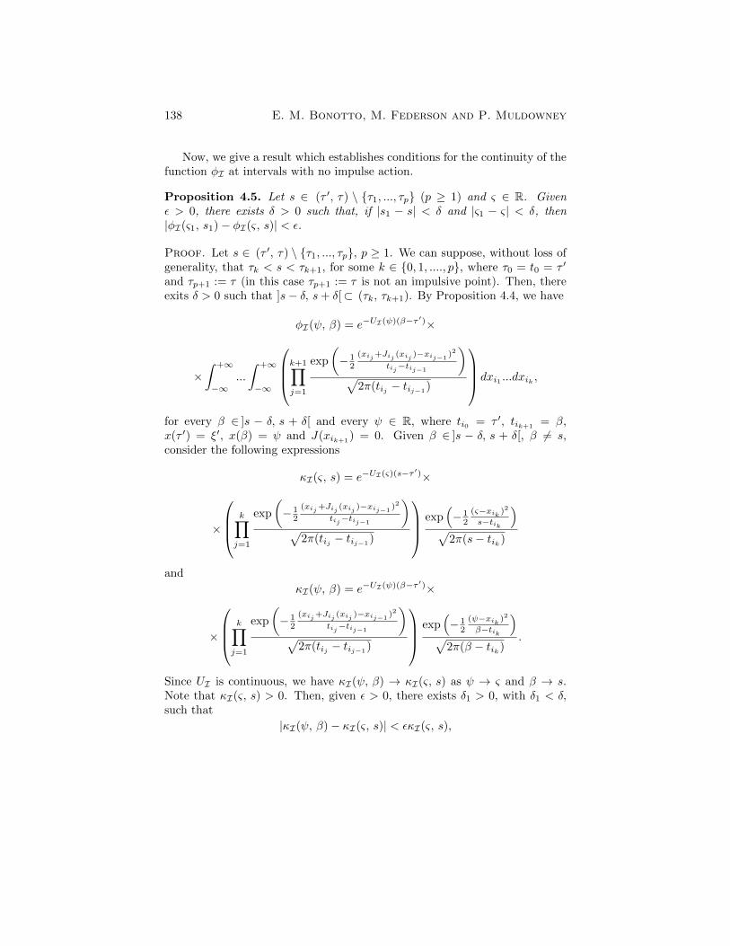
Now, we give a result which establishes conditions for the continuity of thefunction �I at intervals with no impulse action.
Proposition 4.5. Let s 2 (⌧ 0, ⌧) \ {⌧1
, ..., ⌧p} (p � 1) and & 2 R. Given✏ > 0, there exists � > 0 such that, if |s
1
� s| < � and |&1
� &| < �, then|�I(&1, s1)� �I(&, s)| < ✏.
Proof. Let s 2 (⌧ 0, ⌧) \ {⌧1
, ..., ⌧p}, p � 1. We can suppose, without loss ofgenerality, that ⌧k < s < ⌧k+1
, for some k 2 {0, 1, ...., p}, where ⌧0
= t0
= ⌧ 0
and ⌧p+1
:= ⌧ (in this case ⌧p+1
:= ⌧ is not an impulsive point). Then, thereexits � > 0 such that ]s� �, s+ �[⇢ (⌧k, ⌧k+1
). By Proposition 4.4, we have
�I( , �) = e�UI( )(��⌧ 0)⇥
⇥Z
+1
�1...
Z+1
�1
0
BB@k+1Y
j=1
exp
✓� 1
2
(xi
j
+Ji
j
(xi
j
)�xi
j�1 )2
ti
j
�ti
j�1
◆
p2⇡(ti
j
� tij�1)
1
CCA dxi1 ...dxik
,
for every � 2 ]s � �, s + �[ and every 2 R, where ti0 = ⌧ 0, tik+1 = �,
x(⌧ 0) = ⇠0, x(�) = and J(xik+1) = 0. Given � 2 ]s � �, s + �[, � 6= s,
consider the following expressions
I(&, s) = e�UI(&)(s�⌧ 0)⇥
⇥
0
BB@kY
j=1
exp
✓� 1
2
(xi
j
+Ji
j
(xi
j
)�xi
j�1 )2
ti
j
�ti
j�1
◆
p2⇡(ti
j
� tij�1)
1
CCAexp
⇣� 1
2
(&�xi
k
)
2
s�ti
k
⌘
p2⇡(s� ti
k
)
and
I( , �) = e�UI( )(��⌧ 0)⇥
⇥
0
BB@kY
j=1
exp
✓� 1
2
(xi
j
+Ji
j
(xi
j
)�xi
j�1 )2
ti
j
�ti
j�1
◆
p2⇡(ti
j
� tij�1)
1
CCAexp
⇣� 1
2
( �xi
k
)
2
��ti
k
⌘
p2⇡(� � ti
k
).
Since UI is continuous, we have I( , �) ! I(&, s) as ! & and � ! s.Note that I(&, s) > 0. Then, given ✏ > 0, there exists �
1
> 0, with �1
< �,such that
|I( , �)� I(&, s)| < ✏I(&, s),
A random impulsive equation of Schr
¨
odinger type 139
whenever 0 < |��s| < �1
and 0 < | �&| < �1
. By the dominated convergencetheorem (Theorem 3.2, see also [9], Theorem 9.2), we have
�I( , �) ! �I(&, s)
as ! & and � ! s. Therefore the result is proved.
Theorem 4.4 below says the lateral limits of the function �I at the moments{⌧
1
, ..., ⌧p}, p � 1, exist.
Theorem 4.4. Let x(⌧k) = ⇠k 2 R, k = 1, 2, ..., p, p � 1. Then, the limits
lim(&, s)!(⇠
k
, ⌧+k
)
�I(&, s) and lim(&, s)!(⇠
k
, ⌧�k
)
�I(&, s)
exist for k = 1, 2, ..., p, p � 1.
Proof. Let ⌧k where k 2 {1, 2, ...} and ⌧ 0 < ⌧k < ⌧ . Let � > 0 be arbitrarilysmall. By Proposition 4.4, we have
�I(&, ⌧k + �) = e�UI(&)(⌧k+��⌧ 0)⇥
⇥Z
+1
�1...
Z+1
�1
0
BB@kY
j=1
exp
✓� 1
2
(xi
j
+Ji
j
(xi
j
)�xi
j�1 )2
ti
j
�ti
j�1
◆
p2⇡(ti
j
� tij�1)
1
CCA⇥
⇥exp
⇣� 1
2
(&�⇠k
)
2
�
⌘
p2⇡�
dxi1 ...dxik
.
Now, note that
0
BB@kY
j=1
exp
✓� 1
2
(xi
j
+Ji
j
(xi
j
)�xi
j�1 )2
ti
j
�ti
j�1
◆
p2⇡(ti
j
� tij�1)
1
CCAexp
⇣� 1
2
(&�⇠k
)
2
�
⌘
p2⇡�
1p2⇡(ti1 � ti0)
!0
BB@kY
j=2
exp
✓� 1
2
(xi
j
+Ji
j
(xi
j
)�xi
j�1 )2
ti
j
�ti
j�1
◆
p2⇡(ti
j
� tij�1)
1
CCAexp
⇣� 1
2
(&�⇠k
)
2
�
⌘
p2⇡�
.
140 E. M. Bonotto, M. Federson and P. Muldowney
Define ↵ as being the righthand side of the inequality above. Then, the
integral
Z+1
�1...
Z+1
�1↵dxi1 ...dxi
k
exists and it is equal to
1p2⇡(ti1 � ti0)
=1p
2⇡(⌧1
� ⌧ 0).
Then,
�I(&, ⌧k + �) e�UI(&)(⌧k+��⌧ 0)
p2⇡(⌧
1
� ⌧ 0).
Hence the limit lim(&, s)!(⇠
k
, ⌧+k
)
�I(&, s) exists.
Now, we note that
�I(&, ⌧k � �) = e�UI(&)(⌧k���⌧ 0)⇥
⇥Z
+1
�1...
Z+1
�1
0
BB@k�1Y
j=1
exp
✓� 1
2
(xi
j
+Ji
j
(xi
j
)�xi
j�1 )2
ti
j
�ti
j�1
◆
p2⇡(ti
j
� tij�1)
1
CCA⇥
⇥exp
⇣� 1
2
(&�⇠k�1)
2
(⌧k
���⌧k�1)
⌘
p2⇡(⌧k � � � ⌧k�1
)dxi1 ...dxi
k�1 .
Analogously, we have
�I(&, ⌧k � �) e�UI(&)(⌧k���⌧ 0)
p2⇡(⌧
1
� � � ⌧ 0)if k = 1,
and
�I(&, ⌧k � �) e�UI(&)(⌧k���⌧ 0)
p2⇡(⌧
1
� ⌧ 0)if k = 2, 3, ..., p, p � 2.
Thus, the limit lim(&, s)!(⇠
k
, ⌧�k
)
�I(&, s) also exists.
As a consequence of Proposition 4.4 and Theorem 4.4, we have the followingresult.
Theorem 4.5. Let ⌧k, k 2 {1, 2, ...}, such that ⌧ 0 < ⌧k < ⌧ and x(⌧k) = ⇠k.The function �I satisfies the condition given by (22) where I(⇠k, ⌧k, �I(⇠k, ⌧k))= �I(⇠k, ⌧k)� �I(⇠k, ⌧�k ) and �I is given by Proposition 4.4.
A random impulsive equation of Schr
¨
odinger type 141
Now, let us denote WI(x, N (s), I(s); &, s) by !I(&, s), where
WI(x, N (s), I(s); &, s) = qI(x, N (s), I(s))e�UI(xr�1)(s�⌧ 0)
and
qI(x, N (s), I(s)) = gI(x, N (s))r�1Y
j=1
�Ij .
By di↵erentiation, for s 6= ⌧j , j = 1, 2, . . ., we get
@!I(&, s)@s
= �UI(xr�1
)!I(&, s)� 1
2(s� tir
)!I(&, s)+
1
2
✓& � xi
r
s� tir
◆2
!I(&, s),
@!I(&, s)@&
= � (& � xir
)
s� tir
!I(&, s)
and@2!I(&, s)
@&2= � 1
s� tir
!I(&, s) +✓& � xi
r
s� tir
◆2
!I(&, s).
Thus,@!I(&, s)
@s� 1
2
@2!I(&, s)@&2
+ UI(xr�1
)!I(&, s) = 0. (23)
The next result says that UI(xr�1
)!I(&, s) is generalized Riemann inte-grable. Since UI is continuous the proof of Proposition 4.6 is analogously tothe proof of Proposition 4.4.
Proposition 4.6. Let ⌧ 0 < s < ⌧ , s 6= ⌧j for every j = 1, 2, ..., p and x(s) = &.Then the function UI(xr�1
)!I(&, s) is generalized Riemann integrable and
Z+1
�1...
Z+1
�1UI(xr�1
)!I(&, s)dxi1 ...dxir
= UI(&)�I(&, s).
By Proposition 4.6, the expression@!I(&, s)
@s� 1
2
@2!I(&, s)@&2
in equation
(23) is generalized Riemann integrable and
Z+1
�1...
Z+1
�1
✓@!I(&, s)
@s� 1
2
@2!I(&, s)@&2
◆dxi1 ...dxi
r
= �UI(&)�I(&, s).
The problem now is to prove the following equalities
Z+1
�1...
Z+1
�1
@!I(&, s)@s
dxi1 ...dxir
=@
@s
Z+1
�1...
Z+1
�1!I(&, s)dxi1 ...dxi
r
142 E. M. Bonotto, M. Federson and P. Muldowney
andZ
+1
�1...
Z+1
�1
@2!I(&, s)@&2
dxi1 ...dxir
=@2
@&2
Z+1
�1...
Z+1
�1!I(&, s)dxi1 ...dxi
r
and to conclude that
@�I@s
(&, s)� 1
2
@2�I@&2
(&, s) + UI(&)�I(&, s) = 0
for (&, s) 2 �. Thus, in order to prove the equalities, we introduce someadditional notations below.
Given f(&, s), let
Dabcf(&, s) =1
afa(&, s)� 1
2bcfbc(&, s),
wherefa(&, s) = f(&, s+ a)� f(&, s)
and
fbc(&, s) = f(& + b+ c, s)� f(& + b, s)� f(& + c, s) + f(&, s)
for non-zero real numbers a, b, c. Then the limit
lima,b,c!0
Dabcf(&, s)
exists and equals@f
@s(&, s)� 1
2
@2f
@&2(&, s),
if and only if the partial derivatives
@f
@s,@2f
@&2
exist.
In our case, since the derivatives@!I@s
(&, s) and@2!I@&2
(&, s) exist, we have
lima,b,c!0
Dabc!I(&, s) =@!I@s
(&, s)� 1
2
@2!I@&2
(&, s) = �UI(xr�1
)!I(&, s). (24)
By Proposition 4.6, the limit lima,b,c!0
Dabc!I(&, s) is generalized Riemann in-
tegrable andZ
+1
�1...
Z+1
�1lim
a,b,c!0
Dabc!I(&, s)dxi1 ...dxir
= �UI(&)�I(&, s). (25)
A random impulsive equation of Schr
¨
odinger type 143
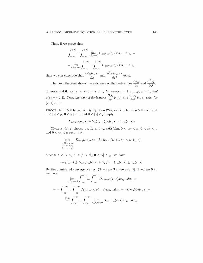
Thus, if we prove that
Z+1
�1...
Z+1
�1lim
a,b,c!0
Dabc!I(&, s)dxi1 ...dxir
=
= lima,b,c!0
Z+1
�1...
Z+1
�1Dabc!I(&, s)dxi1 ...dxi
r
,
then we can conclude that@�I(&, s)
@sand
@2�I(&, s)@&2
exist.
The next theorem shows the existence of the derivatives@�I@s
and@2�I@&2
.
Theorem 4.6. Let ⌧ 0 < s < ⌧ , s 6= ⌧j for every j = 1, 2, ..., p, p � 1, and
x(s) = & 2 R. Then the partial derivatives@�I@s
(&, s) and@2�I@&2
(&, s) exist for
(&, s) 2 �.
Proof. Let ✏ > 0 be given. By equation (24), we can choose µ > 0 such that0 < |↵| < µ, 0 < |�| < µ and 0 < |�| < µ imply
|D↵��!I(&, s) + UI(xr�1
)!I(&, s)| < !I(&, s)✏.
Given x, N , I, choose ↵0
, �0
and �0
satisfying 0 < ↵0
< µ, 0 < �0
< µand 0 < �
0
< µ such that
sup0<|↵|<↵0
0<|�|<�0
0<|�|<�0
|D↵��!I(&, s) + UI(xr�1
)!I(&, s)| < !I(&, s).
Since 0 < |↵| < ↵0
, 0 < |�| < �0
, 0 < |�| < �0
, we have
�!I(&, s) D↵��!I(&, s) + UI(xr�1
)!I(&, s) !I(&, s).
By the dominated convergence test (Theorem 3.2, see also [9], Theorem 9.2),we have
lim↵, �, �!0
Z+1
�1...
Z+1
�1D↵��!I(&, s)dxi1 ...dxi
r
=
= �Z
+1
�1...
Z+1
�1UI(xr�1
)!I(&, s)dxi1 ...dxir
= �UI(&)�I(&, s) =
(25)
=
Z+1
�1...
Z+1
�1lim
↵, �, �!0
D↵��!I(&, s)dxi1 ...dxir
.
144 E. M. Bonotto, M. Federson and P. Muldowney
Then, since
lim↵, �, �!0
Z+1
�1...
Z+1
�1D↵��!I(&, s)dxi1 ...dxi
r
=@�I(&, s)
@s� 1
2
@2�I(&, s)@&2
,
the result is proved.
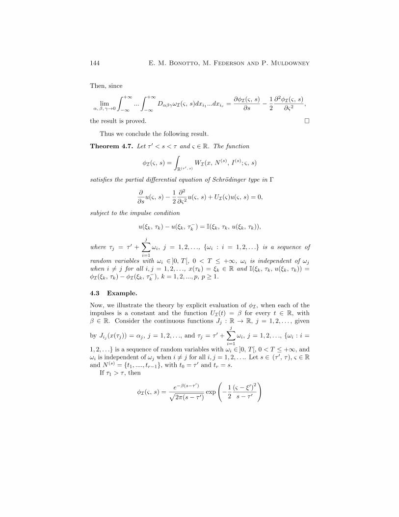
Thus we conclude the following result.
Theorem 4.7. Let ⌧ 0 < s < ⌧ and & 2 R. The function
�I(&, s) =Z
R(⌧0, s)
WI(x, N (s), I(s); &, s)
satisfies the partial di↵erential equation of Schrodinger type in �
@
@su(&, s)� 1
2
@2
@&2u(&, s) + UI(&)u(&, s) = 0,
subject to the impulse condition
u(⇠k, ⌧k)� u(⇠k, ⌧�k ) = I(⇠k, ⌧k, u(⇠k, ⌧k)),
where ⌧j = ⌧ 0 +jX
i=1
!i, j = 1, 2, . . ., {!i : i = 1, 2, . . .} is a sequence of
random variables with !i 2 ]0, T [, 0 < T +1, !i is independent of !j
when i 6= j for all i, j = 1, 2, . . ., x(⌧k) = ⇠k 2 R and I(⇠k, ⌧k, u(⇠k, ⌧k)) =�I(⇠k, ⌧k)� �I(⇠k, ⌧�k ), k = 1, 2, ..., p, p � 1.
4.3 Example.
Now, we illustrate the theory by explicit evaluation of �I , when each of theimpulses is a constant and the function UI(t) = � for every t 2 R, with� 2 R. Consider the continuous functions Jj : R ! R, j = 1, 2, . . . , given
by Jij
(x(⌧j)) = ↵j , j = 1, 2, . . ., and ⌧j = ⌧ 0 +jX
i=1
!i, j = 1, 2, . . ., {!i : i =
1, 2, . . .} is a sequence of random variables with !i 2 ]0, T [, 0 < T +1, and!i is independent of !j when i 6= j for all i, j = 1, 2, . . .. Let s 2 (⌧ 0, ⌧), & 2 Rand N (s) = {t
1
, ...., tr�1
}, with t0
= ⌧ 0 and tr = s.If ⌧
1
> ⌧ , then
�I(&, s) =e��(s�⌧
0)
p2⇡(s� ⌧ 0)
exp
�1
2
(& � ⇠0)2
s� ⌧ 0
!
A random impulsive equation of Schr
¨
odinger type 145
is a solution of the partial di↵erential equation of Schrodinger type
@
@su(&, s)� 1
2
@2
@&2u(&, s) + �u(&, s) = 0
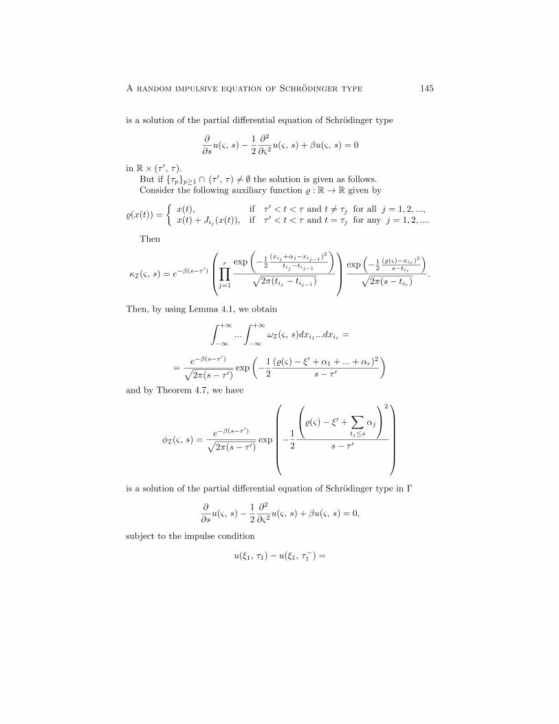
in R⇥ (⌧ 0, ⌧).But if {⌧p}p�1
\ (⌧ 0, ⌧) 6= ; the solution is given as follows.Consider the following auxiliary function % : R ! R given by
%(x(t)) =
⇢x(t), if ⌧ 0 < t < ⌧ and t 6= ⌧j for all j = 1, 2, ...,x(t) + Ji
j
(x(t)), if ⌧ 0 < t < ⌧ and t = ⌧j for any j = 1, 2, ....
Then
I(&, s) = e��(s�⌧0)
0
BB@rY
j=1
exp
✓� 1
2
(xi
j
+↵j
�xi
j�1 )2
ti
j
�ti
j�1
◆
p2⇡(ti
j
� tij�1)
1
CCAexp
⇣� 1
2
(%(&)�xi
r
)
2
s�ti
r
⌘
p2⇡(s� ti
r
).
Then, by using Lemma 4.1, we obtain
Z+1
�1...
Z+1
�1!I(&, s)dxi1 ...dxi
r
=
=e��(s�⌧
0)
p2⇡(s� ⌧ 0)
exp
✓�1
2
(%(&)� ⇠0 + ↵1
+ ...+ ↵r)2
s� ⌧ 0
◆
and by Theorem 4.7, we have
�I(&, s) =e��(s�⌧
0)
p2⇡(s� ⌧ 0)
exp
0
BBBBBBB@
�1
2
0
@%(&)� ⇠0 +X
tj
s
↵j
1
A2
s� ⌧ 0
1
CCCCCCCA
is a solution of the partial di↵erential equation of Schrodinger type in �
@
@su(&, s)� 1
2
@2
@&2u(&, s) + �u(&, s) = 0,
subject to the impulse condition
u(⇠1
, ⌧1
)� u(⇠1
, ⌧�1
) =
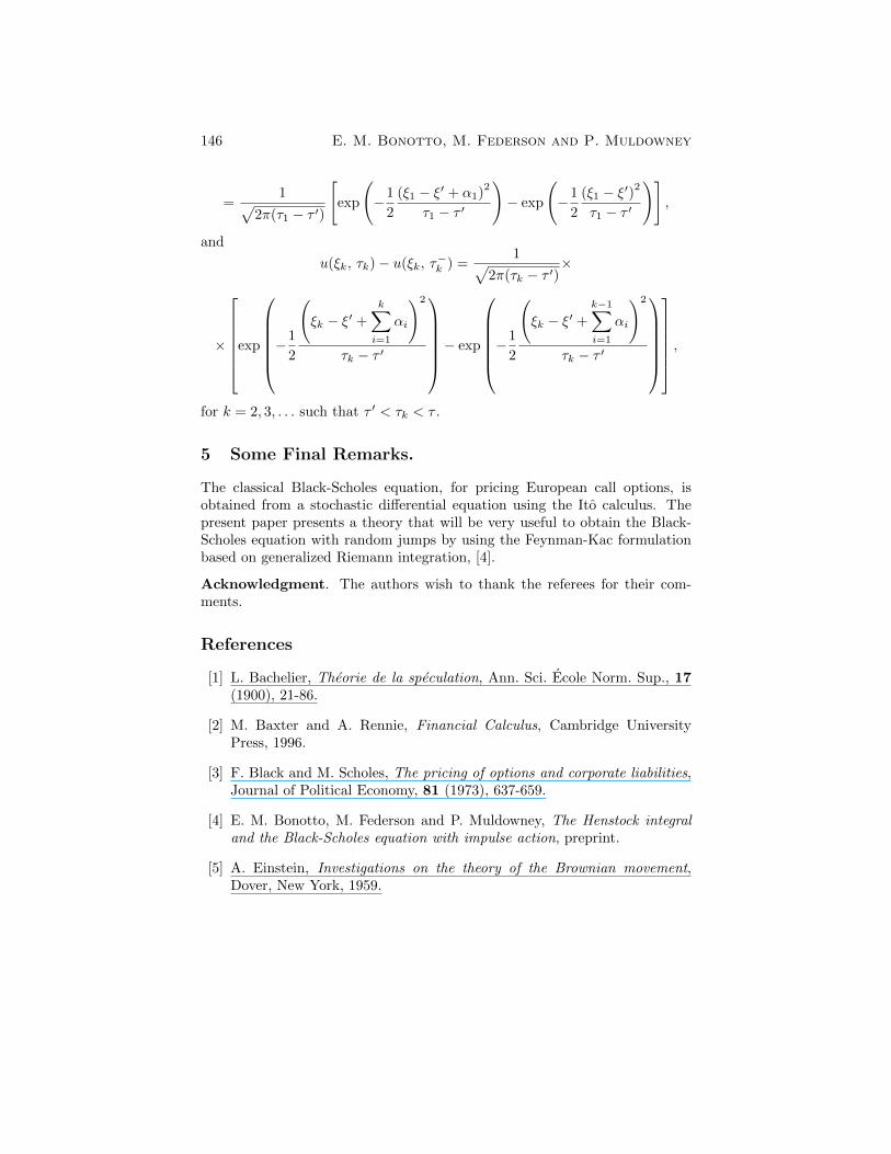
146 E. M. Bonotto, M. Federson and P. Muldowney
=1p
2⇡(⌧1
� ⌧ 0)
"exp
�1
2
(⇠1
� ⇠0 + ↵1
)2
⌧1
� ⌧ 0
!� exp
�1
2
(⇠1
� ⇠0)2
⌧1
� ⌧ 0
!#,
and
u(⇠k, ⌧k)� u(⇠k, ⌧�k ) =
1p2⇡(⌧k � ⌧ 0)
⇥
⇥
2
666664exp
0
BBBBB@�1
2
⇠k � ⇠0 +
kX
i=1
↵i
!2
⌧k � ⌧ 0
1
CCCCCA� exp
0
BBBBB@�1
2
⇠k � ⇠0 +
k�1X
i=1
↵i
!2
⌧k � ⌧ 0
1
CCCCCA
3
777775,
for k = 2, 3, . . . such that ⌧ 0 < ⌧k < ⌧ .
5 Some Final Remarks.
The classical Black-Scholes equation, for pricing European call options, isobtained from a stochastic di↵erential equation using the Ito calculus. Thepresent paper presents a theory that will be very useful to obtain the Black-Scholes equation with random jumps by using the Feynman-Kac formulationbased on generalized Riemann integration, [4].
Acknowledgment. The authors wish to thank the referees for their com-ments.
References
[1] L. Bachelier, Theorie de la speculation, Ann. Sci. Ecole Norm. Sup., 17(1900), 21-86.
[2] M. Baxter and A. Rennie, Financial Calculus, Cambridge UniversityPress, 1996.
[3] F. Black and M. Scholes, The pricing of options and corporate liabilities,Journal of Political Economy, 81 (1973), 637-659.
[4] E. M. Bonotto, M. Federson and P. Muldowney, The Henstock integraland the Black-Scholes equation with impulse action, preprint.
[5] A. Einstein, Investigations on the theory of the Brownian movement,Dover, New York, 1959.
A random impulsive equation of Schr
¨
odinger type 147
[6] A. Etheridge, A course in financial calculus, Cambridge University Press,2002.
[7] R. Gordon, The integrals of Lebesgue, Denjoy, Perron and Henstock,Amer. Math. Soc., Providence, RI, 1994.
[8] R. Henstock, P. Muldowney and V. A. Skvortsov, Partitioning infinite-dimensional spaces for generalized Riemann integration, Bull. LondonMath. Soc., 38 (2006), 795-803.
[9] R. Henstock, Lectures on the theory of integration, World Scientific, Sin-gapore, 1988.
[10] M. Kac, Probability and related topics in the Physical Sciences, Inter-science, New York, 1957.
[11] I. Karatzas and S. E. Shreve, Brownian motion and stochastic calculus,Graduate texts in Mathematics, Springer-Verlag, 113, 1991.
[12] D. Lamberton and B. Lapeyre, Introduction to stochastic calculus appliedto finance, Chapman & Hall/CRC, 2000.
[13] J. Luo, Oscillation of hyperbolic partial di↵erential equations with im-pulses, Appl. Math. Comput, 133(2-3) (2002), 309-318.
[14] P. Muldowney, A general theory of integration in function spaces, PitmanResearch Notes in Mathematics, no. 153, Longman, 1987.
[15] P. Muldowney, Financial valuation and the Henstock integral, SeminarioBrasileiro de Analise, 60 (2000), 79-108.
[16] P. Muldowney, Introduction to Feynman integration, J. Math. Study,27(1) (1994), 127-132.
[17] P. Muldowney, Topics in probability using generalised Riemann integra-tion, Math. Proc. R. Ir. Acad., 99A(1) (1999), 39-50.
[18] P. Muldowney, Feynman’s path integrals and Henstock’s non-absolute in-tegration, J. Appl. Anal., 6(1) (2000), 1-24.
[19] P. Muldowney, The Henstock integral and the Black-Scholes theory ofderivative asset pricing, Real Anal. Exchange, 26(1) (2001), 117-132.
[20] P. Muldowney, Lebesgue integrability implies generalized Riemann inte-grability in R]0,1], Real Anal. Exchange, 27(1) (2001/2002), 223-234.
148 E. M. Bonotto, M. Federson and P. Muldowney
[21] N. Wiener, Generalised harmonic analysis, Acta Math., 55 (1930), 117-258.
[22] L. P. Yee and R. Vyborny, The integral: An easy approach after Kurzweiland Henstock, Austral. Math. Soc. Lect. Ser., Cambridge UniversityPress, 14, 2000.