A-contrario approach for outlier detection in GNSS positioning

Salim Zair, Sylvie Le Hegarat-Mascle and Emmanuel Seignez

Abstract—The localization, that allows to precisely know theorientation and position of a system in the environment, is stillchallenging in urban environments due to satellite occlusion.This phenomenon reduces the data redundancy and providesbad satellite geometry and reflected signals, called multipaths,that distort the measurements and make them erroneous. TheRAIM method, integrated in most GPS receivers, deals with oneoutlier per instant. This assumption is not longer valid in urbanareas where more than one outlier have to be considered. Thispaper proposes a new approach for the detection and exclusion ofthe outliers in the GPS pseudo-distance observations. From twoassumed models representing the distribution of inconsistent data(naive models), two criteria are proposed to partition the datasetbetween inliers and outliers. Two algorithms implementing thesecriteria are presented and evaluated on two datasets respectivelyacquired in an open environment and in an urban environment.The results are compared with methods classically used forsuch problems. We show that the proposed outliers detectionalgorithms improve the estimation of the receiver location and,in the presence of 30% or more outliers, outperform the classicalapproaches.

I. INTRODUCTION

Nowadays, Global Navigation Satellite System (GNSS)represents a crucial service for many applications in agricul-ture, robotics and telecommunication, providing a high preci-sion localization with large coverage. In an urban environment,positioning still represents a big issue due to high buildings,reducing data redundancy and distorting the measurements ofpseudo-ranges (PR). These multipath phenomena and non-line-of-sight (NLOS) propagation appear when the signals reflectedby the buildings are observed.

In order to robustify the GNSS location estimation, threemain strategies have been proposed. The first one bases onthe use of complementary information/sensors (e.g. inertialmeasurement unit or inertial navigation systems [1] or cam-era [2]), geographical information (e.g. digital maps or by priorinformation) that are fused with GNSS data using varioustechniques (e.g. Kalman filter [3] or particle filter [4]). Thesecond class of approaches bases on estimation of the satellitereliability. This latter may be derived from signal power [5] orfrom context estimation (e.g. detecting the satellites not in lineof sight [6], [7] using additional information). In both cases,the data provided by NLOS satellites are discarded.

The third class of approaches bases on robust estimation,i.e. methods that are able to bear with some erroneous mea-surements, called ‘outliers’ in the following. An commonlyused assumption is that the number of outliers at a giveninstant is lower than one (as in Receiver Autonomous Integrity

Institute of Fundamental Electronics, department Autonomous SystemsUniversity of Paris-Sud, 91405 Orsay, France{salim.zair, sylvie.le-hegarat,

emmanuel.seignez}@u-psud.fr

Monitoring algorithm [8]) or bounded with known bounds (asin practical implementation of the q-relaxation technique in In-terval Analysis [9]). However, such an assumption is not validfor urban navigation [10]. Besides, with the commissioning offuture navigation systems, the number of available satellitesat a given time will increase making statistical approachesparticularly relevant. Their basic principle is to estimate theconsistency of some subsets of data in order to both detectthe outliers in the whole set of data and to remove or reducetheir impact on the estimate of the parameters (location inour case). For GNSS positioning, M-estimators [11] havebeen investigated by [12] and RANSAC [13] was proposedby [14]. The RANSAC approach (called RANCO for RangeConsensus) uses subsampling of the space of solutions, suchthat the only examined solutions correspond to the exactsolutions of the set of equations modelling the consideredproblem. The main drawback of RANSAC criterion is theexistence of an a priori threshold (the inliers and the outliersare separated by thresholding the error relative to the examinedsolution). Then, in ([15], [16], [17]) some authors investigatedthe coupling of the subsampling of the solution space (likein the original RANSAC) with an free-parameter criterion,namely a Number of False Alarm (NFA) criterion derived froma-contrario modelling [18]. Following these works, this studyfocuses on a-contrario modelling for simultaneous detection ofthe outliers and estimation of the receiver location.

The paper is organized as follows. Section 2 presents theproblem of location estimation using GNSS measurements.Section 3 proposes two NFA criteria for outlier detection in thecontext of GNSS. Simulations and results with raw GPS dataare discussed in Section 4. Section 5 gathers our conclusionsand perspectives.

II. GNSS POSITIONING PROBLEM

The basic signal provided by one GNSS satellite Si isthe PR ρi that, in absence of noise, corresponds to thedistance between the receiver and the satellite. Assuming thereceiver is located at position (xr, yr, zr) (in an Earth CenteredEarth Fixed Cartesian coordinate system) and Si is located atposition (xSi

, ySi, zSi

),

ρi =

√(xr − xSi)

2+ (yr − ySi)

2+ (zr − zSi)

2+ cδt. (1)

In Eq. (1), δt is the time bias (difference) between the satel-lite clock and the receiver clock (they are not synchronized)and c is the speed of light.

In positioning problem, the observations are the PR mea-surements associated to a satellite, denoted (ρi, xSi , ySi , zSi),and the parameters to estimate are the receiver position andthe time bias, denoted X = (xr, yr, zr, δt). Then, at leastfour observations are required to estimate the 4−tuple X ofunknown parameters [19]. The resolution of the system can bedone either using the Gauss-Newton algorithm or linearizing978-1-4799-9858-6/15/$31.00 c©2015 IEEE

and using the Singular Value Decomposition (SVD) that allowsrobust inversion.

Different physical phenomena may affect the signal, suchas tropospheric and ionospheric effects, or multipaths thatappear as additive noises corrupting the ρi measurements. Tocope with these noises, more than four satellites are consideredif possible. Indeed, about nine to eleven satellites are visiblesimultaneously in open area, whereas in urban environment thenumber of visible satellites is often between two and six. Then,the idea is to exploit the redundancy between observations todetect the outliers and to filter the noise on the inliers. Forinstance, in the RAIM algorithm a statistical test is performedon the measurements (assuming Gaussian noise so that theSum Squared Errors (SSE) follows a chi-squared) to detecta ‘fault’, to remove the corresponding measurement from thedataset and to compute the receiver position according to theLeast Square Error criterion. However, as already pointed out,there is a need to investigate some approaches allowing moreimportant rates of outliers.

III. A-CONTRARIO APPROACH FOR OUTLIER DETECTION

Using an a-contrario approach, the inliers will be detectedas too regular to appear ‘by chance’. In order to instantiate thisperception concept through a Number of False Alarm (NFA)criterion, two elements have to be defined. First, we defineone (or several) measurement(s) characterizing the inliers andsecond, we define a ‘naive’ model that represents the statisticsin the case of the outliers (the H0 hypothesis in statisticaldecision theory). Note that, in the perspective of a-contrariodetection, the naive model can be rather rough since it has onlyto be contradicted by the inliers. In the case of the GNSS data,the main feature characterizing the inliers is the consistencyof the PR measurements. In this study, we investigate twomeasurements of their consistency.

A. Gaussian criterion

Let us assume a subset of inliers noted D: D is a setof indices (in the whole set of observations). The first mea-surement of D consistency is the sum of the squared errors(called residual errors or residues) between the observed PRand the computed PR. The more consistent subsets of inliersshould present particularly low values of squared residuesum. Then, M1 models the distribution of the residues incase of inconsistency. It is as follows: the set of residuesis a random process of |D| independent centered Gaussianvariables N (0, σ) with σ being the standard deviation of acompletely unstructured set and |.| denoting the cardinality setoperator.

Denoting(xr, yr, zr, δt

)the estimated parameter tuple

(time bias and coordinates of the receiver), the residue riassociated to the observation (ρi, xSi

, ySi, zSi

) is

ri =ρi−[√

(xr− xSi)2+ (yr− ySi

)2+ (zr− zSi

)2

+ cδt

].

(2)

In order to measure the consistency of the subset D, wecompute δ2

D: the sum of the r2i values for indices i belonging

to D. To interpret the value of δ2D, we consider the probability

Algorithm 1: NFA based on M1 with inputs: M obser-vations, σ, t and outputs: X and D1 Initialize the vectors δmin [i] and NFA [i] and the

scalar NFAmin to +∞;2 for 1 to t do3 Draw randomly d observations (xSi

, ySi, zSi

, ρi)denoted by {o1, ..., od};

4 Estimate X the d-tuple of the unknown parametersfrom {o1, ..., od} constraints, e.g. usingGauss-Newton algorithm for non-linear case;

5 Compute the vector of residues according to Eq. (2);6 Sort it by increasing values into a vector

Wr = (wi)i∈{1...M} with j the index permutationfunction such that ∀i ∈ {1...M} , wi = rj(i);

7 Initialize δ2D = 0;

8 for i← d+ 1 to M do9 δ2

D ← δ2D + w2

i ;10 if δ2

D < δmin [i] then11 δmin [i] = δ2

D;12 Compute NFA [i] according to Eq. (3);13 if NFA [i] < NFAmin then14 NFAmin = NFA [i];

D = {j (1) ...j (i)};15 X = X;16 end17 end18 end19 end

of observing δ2D by chance, denoted PM1

(δ2D). Hence, the

NFA for subset D is:

NFA1 (D) = η1PM1

(δ2D, σ

),

= η11

Γ( |D|2 )

∫ δ2D/2σ2

0e−tt

|D|2 −1dt,

(3)

where Γ is the Gamma function and η1 is a normalization term(equivalent to the number of tests) that controls the averagenumber of false alarms [20]. The χ2 function employed inthe classical RAIM method [8] differs from the Gaussiancriterion Eq. (3) by its use and interpretation. For the RAIM,the probability of false alarm PFA and the decision thresholdT have to be set according to a priori knowledge. The inputsof Eq. (3) are used to calculate the NSSE (Normalized Sumof Squared Errors) in order to find the most consistent subsetD, without any knowledge or prior information. The parameterσ, calculated from the dataset, is not a strict parameter, sinceit has an influence in the NFA1 value but no influence on thesubset cardinality |D| and the data chosen.

B. Binomial criterion

The second measurement of D consistency is the size ofthe spatial volume validating D PR constraints. Specifically,the receiver locations validating a PR constraint from Si arelocated on a sphere Si (see Eq. (1)). The spatial boundingvolume VD validatingD PR constraints is the smallest ellipsoid(in our case) that intersects all Si spheres for indices ibelonging to D. The more consistent subsets of inliers shouldpresent particularly small volumes VD.

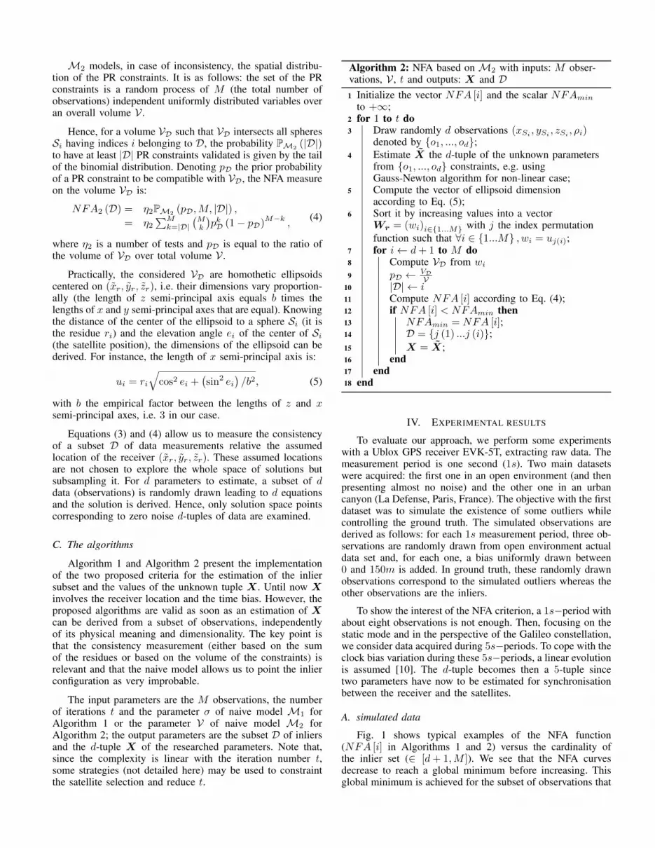
M2 models, in case of inconsistency, the spatial distribu-tion of the PR constraints. It is as follows: the set of the PRconstraints is a random process of M (the total number ofobservations) independent uniformly distributed variables overan overall volume V .

Hence, for a volume VD such that VD intersects all spheresSi having indices i belonging to D, the probability PM2 (|D|)to have at least |D| PR constraints validated is given by the tailof the binomial distribution. Denoting pD the prior probabilityof a PR constraint to be compatible with VD, the NFA measureon the volume VD is:

NFA2 (D) = η2PM2 (pD,M, |D|) ,= η2

∑Mk=|D|

(Mk

)pkD (1− pD)

M−k,

(4)

where η2 is a number of tests and pD is equal to the ratio ofthe volume of VD over total volume V .

Practically, the considered VD are homothetic ellipsoidscentered on (xr, yr, zr), i.e. their dimensions vary proportion-ally (the length of z semi-principal axis equals b times thelengths of x and y semi-principal axes that are equal). Knowingthe distance of the center of the ellipsoid to a sphere Si (it isthe residue ri) and the elevation angle ei of the center of Si(the satellite position), the dimensions of the ellipsoid can bederived. For instance, the length of x semi-principal axis is:

ui = ri

√cos2 ei +

(sin2 ei

)/b2, (5)

with b the empirical factor between the lengths of z and xsemi-principal axes, i.e. 3 in our case.

Equations (3) and (4) allow us to measure the consistencyof a subset D of data measurements relative the assumedlocation of the receiver (xr, yr, zr). These assumed locationsare not chosen to explore the whole space of solutions butsubsampling it. For d parameters to estimate, a subset of ddata (observations) is randomly drawn leading to d equationsand the solution is derived. Hence, only solution space pointscorresponding to zero noise d-tuples of data are examined.

C. The algorithms

Algorithm 1 and Algorithm 2 present the implementationof the two proposed criteria for the estimation of the inliersubset and the values of the unknown tuple X . Until now Xinvolves the receiver location and the time bias. However, theproposed algorithms are valid as soon as an estimation of Xcan be derived from a subset of observations, independentlyof its physical meaning and dimensionality. The key point isthat the consistency measurement (either based on the sumof the residues or based on the volume of the constraints) isrelevant and that the naive model allows us to point the inlierconfiguration as very improbable.

The input parameters are the M observations, the numberof iterations t and the parameter σ of naive model M1 forAlgorithm 1 or the parameter V of naive model M2 forAlgorithm 2; the output parameters are the subset D of inliersand the d-tuple X of the researched parameters. Note that,since the complexity is linear with the iteration number t,some strategies (not detailed here) may be used to constraintthe satellite selection and reduce t.

Algorithm 2: NFA based on M2 with inputs: M obser-vations, V , t and outputs: X and D1 Initialize the vector NFA [i] and the scalar NFAmin

to +∞;2 for 1 to t do3 Draw randomly d observations (xSi

, ySi, zSi

, ρi)denoted by {o1, ..., od};

4 Estimate X the d-tuple of the unknown parametersfrom {o1, ..., od} constraints, e.g. usingGauss-Newton algorithm for non-linear case;

5 Compute the vector of ellipsoid dimensionaccording to Eq. (5);

6 Sort it by increasing values into a vectorWr = (wi)i∈{1...M} with j the index permutationfunction such that ∀i ∈ {1...M} , wi = uj(i);

7 for i← d+ 1 to M do8 Compute VD from wi9 pD ← VD

V10 |D| ← i11 Compute NFA [i] according to Eq. (4);12 if NFA [i] < NFAmin then13 NFAmin = NFA [i];14 D = {j (1) ...j (i)};15 X = X;16 end17 end18 end

IV. EXPERIMENTAL RESULTS

To evaluate our approach, we perform some experimentswith a Ublox GPS receiver EVK-5T, extracting raw data. Themeasurement period is one second (1s). Two main datasetswere acquired: the first one in an open environment (and thenpresenting almost no noise) and the other one in an urbancanyon (La Defense, Paris, France). The objective with the firstdataset was to simulate the existence of some outliers whilecontrolling the ground truth. The simulated observations arederived as follows: for each 1s measurement period, three ob-servations are randomly drawn from open environment actualdata set and, for each one, a bias uniformly drawn between0 and 150m is added. In ground truth, these randomly drawnobservations correspond to the simulated outliers whereas theother observations are the inliers.

To show the interest of the NFA criterion, a 1s−period withabout eight observations is not enough. Then, focusing on thestatic mode and in the perspective of the Galileo constellation,we consider data acquired during 5s−periods. To cope with theclock bias variation during these 5s−periods, a linear evolutionis assumed [10]. The d-tuple becomes then a 5-tuple sincetwo parameters have now to be estimated for synchronisationbetween the receiver and the satellites.

A. simulated data

Fig. 1 shows typical examples of the NFA function(NFA [i] in Algorithms 1 and 2) versus the cardinality ofthe inlier set (∈ [d+ 1,M ]). We see that the NFA curvesdecrease to reach a global minimum before increasing. Thisglobal minimum is achieved for the subset of observations that

(a) M1 naive model (b) M2 naive model

Fig. 1: Functions log(NFA) versus the number of inliers:(a) NFA criterion 1, (b) NFA criterion 2.

is the ‘more’ consistent according to the NFA criterion. TheNFA curves have global minima clear and accurate converselyto the monotonically increasing functions representing eitherthe sum of the square residues or the number of satisfiedconstraints versus the inlier set cardinality. Note that the NFAvalues cannot be compared between the two models M1 andM2 since they do not base the consistency measure on thesame information (residue values or geometric constraints).In our study, the naive model parameters, σ for M1 and Vfor M2 have been set proportional to σM and VM that arerespectively the variance of the whole data set and the areaincluding all constraints. To check the robustness versus thenaive model parameter, the NFA curves obtained using twodifferent values of σ for M1 and of V for M2 have beenplotted. Fig. 1a and Fig. 1b show that, in both cases, thecardinality of the inlier set that achieves the global minimumis the same. It is |D| = 28 according to NFA1 and |D| = 27according to NFA2 whereas the actual number of inliers is25. This small difference may be explained as follows: sincethe added noise to the drawn measurements is between 0 and150m, some simulated outliers present very low noise.

To quantify the ability of the proposed algorithms toestimate the inlier and outlier subsets, we compute the numbersof True Positives (TP ), False Positives (FP ), False Negatives(FN ) and True Negatives (TN ) out of the simulation dataset.In our application, actual inliers are measurements not drawnto add them a simulated bias and actual outliers are mea-surements drawn to add them a simulated bias. The wholesimulation dataset includes 70000 observations (43750 inliersand 26250 simulated outliers) partitioned in 1750 5s−periods.For each period, 40 observations are considered and classifiedbetween inliers and outliers. Table I shows the obtained values.Comparing the two criteria, the results are very close butNFA1 criterion appears slightly more cautious than NFA2

criterion (it leads to a lower number of FP and higher FNnumber). In Table I, the accuracy ( (TP+TN)

(TP+TN+FP+FN) ) and

precision ( (TP )(TP+FP ) ) values are also shown, confirming the

very good ability of NFA criteria to detect the outliers. Thevalues in Tab. I were computed according to ground truth(any observation drawn to add a bias is a simulated outlier,not taking into account the added bias value), since it seemsrather arbitrary to fix a threshold on the added bias to decidewhich drawn observations are effective outliers. Nevertheless,let us just specify that, using a threshold equal to 50m (severemultipath effects) to define ground truth outliers, the obtainedaccuracy and precision values are greater than 99.5% (accuracyequal to 99.68% and 99.91% and precision equal to 99.98%and 99.96%, for NFA1 and NFA2 respectively).

TABLE I: Performance of NFA1 and NFA2 criteria foroutlier diagnostic.

TP FP FN TN Accuracy PrecisionNFA1 43536 2957 214 23293 95.47% 93.63%NFA2 43706 2977 44 23273 95.68% 93.62%

Fig. 2: Cluster of 1750 points representing the estimatedpositions with different methods.

Focusing now on the localization accuracy, Tab. II showsthe statistical performance computed on the 1750 5s−periodsof the simulation set, in terms of L1 norm that is the average ofthe absolute value of the residues, L2 norm that is the averageof the squared residues and Linf norm that is the maximumof the residues. The proposed algorithms are compared to theclassical M estimator and the LS estimator. Tab. II clearlyshows the interest of removing the outliers from the observa-tions in order to get an accurate receiver location since NFA1

and NFA2 location error is divided by a factor greater than3 relatively to the LS estimator performance and by a factorgreater than 2 relatively to the M estimator one. Fig. 2 showsthe 1750 estimated 2D locations (bird-view, ground truth in(0, 0)) by the LS estimator, the M estimator and the proposedalgorithms. We note that the clusters of the LS estimatorand the M estimator are much more spread than the clusterscorresponding to the NFA1 and NFA2 criteria. Specifically97% of the location errors are lower than 10m for NFA1 and96.51% for NFA2, respectively. The high errors that remainare due to bad satellite configuration.

B. Experimental data

Considering now the second data set, Fig. 3 presents abird’s-eye view of the urban environment where data havebeen acquired. The receiver remained static during the wholeexperiment (approximately 40 minutes), while the seven GPSsatellites slightly move. Their tracks are plotted in orange withpositions at the beginning of the experiment indicated withblack points close to the satellite name.

Table III presents the exclusion rates for each satellitecomputed during two time periods (2mn) respectively at thebeginning and at the end of the experiment (T1 = [100− 220]and T2 = [1750−1870], with time unit being the second). Theexclusion rate of a given satellite Si is equal to the number ofoutlier measurements among the total number of measurementsprovided by Si over the considered period. Depending on

TABLE II: Localization errors (in m) of simulated data in(East,North,Up) coordinates.

norm L1 L2 Linf

LS estimator (13, 15, 32) (16, 19, 40) (52, 70, 153)M estimator (9, 11, 24) (13, 17, 34) (64, 90, 199)NFA1 (1, 2, 3) (2, 3, 5) (18, 41, 59)NFA2 (2, 3, 3) (3, 4, 7) (37, 43, 101)

Fig. 3: Skyplot of the satellites during experiment (trajectoriesare plotted in orange) superimposed on a bird’s-eye view.

the considered satellite, the exclusion rates are more or lessvariable during the experiment. For instance, during T1, thesatellite G2 is very often excluded (both according to NFA1

and NFA2 criteria) but not are the other satellites. DuringT2, the highest exclusion rates are achieved for satellitesG12 and G24. We also note that G25 exclusion rates differconsidering either NFA1 criterion or NFA2 criterion. Indeed,it is located at 80.5◦ elevation inducing a low precision on theUp coordinate and NFA2 criterion has a greater tolerancetoward the error on the Up coordinate since we defined thehomothetic ellipsoids with z dimension equal to three timesthe x and y dimensions.

Fig. 4 shows the signed errors for East and North coor-dinates versus time, using different approaches: LS estimator,M estimator, NFA criteria (1 and 2), particle filter and set-membership method [21] using q-relaxation (q = 2). As previ-ously, the receiver location is estimated every 5s−period. Thefact that the precision of the location is time varying is clearlyillustrated on Fig. 4a: until t = 500s, LS and M estimatorspresent a strong bias (about 80m) on East coordinate, then Mestimator location shows a strong improvement. NFA criteria(1 or 2) provide very precise estimations of receiver locationexcept at some particular instants (e.g. t = 30s, t = 950s)where the other methods also fail because of the very poorsatellite configuration. Particle filter method estimates the threeENU coordinates with 3000 particles, the North coordinatecurve is smooth conversely to the East coordinate curve (noisymost of the time). Now, to obtain such results, the filter pa-rameters (re-sampling threshold, prior probability distribution)have been manually adjusted knowing the ground truth. Theset-membership method [21] only provides an estimation of

TABLE III: Satellite exclusion rates during periods T1 and T2.

Satellite G2 G12 G14 G24 G25 G29 G31T1, M1 0.91 0 0 0 0.0083 0 0.058T1, M2 0.73 0.14 0.04 0.066 0.015 0.12 0.16T2, M1 0.155 0.425 0.135 0.32 0.34 0.05 0.01T2, M2 0.145 0.375 0.135 0.38 0.095 0.14 0.015

TABLE IV: Localization errors (in m) of actual data in(East,North,Up) coordinates.

norm L1 L2 Linf

LS estimator (30, 15, 50) (41, 22, 104) (94, 104, 1684)M estimator (17, 10, 33) (29, 18, 95) (89, 119, 1672)Particle Filter (15, 6, 14) (19, 9, 19) (45, 45, 54)NFA1 (5, 6, 17) (7, 11, 30) (59, 55, 159)NFA2 (5, 6, 15) (6, 11, 27) (58, 61, 164)

the box (compact) within which the solution should be. Thebounds of these boxes are plotted on Fig. 4. Even if the solution(error equal to zero) is within the plotted bounds for (almost)all epochs, in most cases the set-membership method is ratherimprecise. Not to increase the imprecision box, one has to keepa sufficient number of data. Hence, in our case we set q equalto 2 in the q-relaxation even if, with this dataset, the actualnumber of outliers may be greater (according a posteriorianalysis of the NFA algorithm results).

Like for first dataset, the global precision of the localisationis measured in terms of L1, L2 and Linf norms. Table IVshows the obtained values for (East, North, Up) coordinatesand different methods, LS estimator, M estimator, NFA criteria(1 and 2) and particle filter. It appears that, thanks to parameterfitting, particle filter provides the best estimations for the Northand Up coordinates according to the three norms, NFA criteriaprovide the best East estimation (norms L1 and L2) and best2D accuracy (13m for both NFA1 and NFA2 and 21m forparticle filter).

V. CONCLUSION

In this paper, a new approach able to cope with a significantnumber of outliers was presented for GNSS positioning. It isbased on a-contrario modelling so that it detects the inliersubset as ‘too’ consistent or regular to appear by chance(under the naive model representing the unstructured data).Two models and derived algorithms have been proposed. Thefirst one assumes Gaussian distribution of the residues. Thesecond one assumes binomial distribution for the number ofconstraints consistent with a given location area. From thesemodels, NFA criteria have been derived. Minimizing theseNFA criteria allows us to get the subset of the outliers andthe location of the receiver. Tests have been performed in thecase of a static receiver showing very promising results.

Future work deals with the dynamic case. First tests havebeen performed (not presented in this paper) and have shownthat proposed algorithms can be extended to the dynamiccase as follows. We model the trajectory of the receiverby a parametrized curve and we add the curve parametersinto the researched d-tuple. Controlling the trajectory solution(parametrized curve) also allows for smoothing the receivertrajectory. More tests in various environments (urban canyon,forest) will be held. Another future work will deal with

(a) Location error on East coordinate

(b) Location error on North coordinate

Fig. 4: Location error versus time, case of urban environmentdataset. The NFA1 and NFA2 criteria are superimposed mostof the time and close to the y = 0 axis (ground truth).

the use of data provided by satellites from various GNSS,e.g. GPS/GALILEO and GLONASS. The heterogeneity ofthe data implies several issues. For instance, depending onthe clock synchronization between the considered GNSS, onemore parameter should be introduced in the tuple of unknownparameters X . Depending on the receiver position and thefeatures of the different GNSS, the satellites may presentdifferent levels of reliability. We will investigate the analysisof the historic of the outliers to derive some confidence orintegrity values associated to the different satellites.

REFERENCES

[1] K. Saadeddin, M. Abdel-Hafez, and M. Jarrah, Estimating vehicle stateby GPS/IMU fusion with vehicle dynamics, Journal of Intelligent &Robotic Systems, vol.74, no.1–2, pp.147–172, 2014.

[2] D. Won, E. Lee, M. Heo, S. Sung, J. Lee, and J. Young Jae, GNSSintegration with vision-based navigation for low GNSS visibility con-ditions, GPS Solutions, vol.18, no.2, pp.177–187, 2014.

[3] S. Sukkarieh, E. M. Nebot, and H. F. Durrant-Whyte, A high integrityIMU/GPS navigation loop for autonomous land vehicle applications,IEEE Trans. on Robotics & Automation, vol.15, no.3, pp.572–578,1999.

[4] F. Gustafsson, F. Gunnarsson, N. Bergman, U. Forssell, J. Jansson,R. Karlsson, R., and P. J. Nordlund, Particle filters for positioning,navigation, and tracking, IEEE Trans. on Signal Processing, vol.50,no.2, pp.425–437, 2002.

[5] M. Obst, and G. Wanielik, Probabilistic non-line-of-sight detection inreliable urban GNSS vehicle localization based on an empirical sensormodel, Proc. IEEE Intelligent Vehicles Symposium, pp.363–368, 2013.

[6] M. Obst, S. Bauer, and G. Wanielik, Urban multipath detection andmitigation with dynamic 3D maps for reliable land vehicle localiza-tion, Proc. IEEE/ION Position Location and Navigation Symposium(PLANS), pp.685–691, 2012.

[7] J. Marais, C. Meurie, D. Attia, Y. Ruichek, and A. Flancquart, Towardaccurate localization in guided transport: combining GNSS data andimaging information, Transportation Research Part C: Emerging Tech-nologies, vol.43, pp.188–197, 2013.

[8] R. Brown, A baseline GPS RAIM scheme and a note on the equivalenceof three RAIM methods, Navigation, vol.39, no.3, pp.301–316, 1992.

[9] E. Seignez, M. Kieffer, A. Lambert, E. Walter, and T. Maurin, Real-time bounded-error state estimation for vehicle tracking, Int. Journal ofRobotics Research, vol. 28, no.1, pp.34–48, 2009.

[10] O. Le Marchand, P. Bonnifait, J. Banez-Guzman, F. Peyret, F., and D.Betaille, Performance evaluation of fault detection algorithms as appliedto automotive localisation, Proc. European Navigation Conference-GNSS, 2008.

[11] P. J. Huber, Robust estimation of a location parameter, The Annals ofMathematical Statistics, vol.35, no.1, pp.73–101, 1964.

[12] N. L. Knight, and J. Wang, A comparison of outlier detection proce-dures and robust estimation methods in GPS positioning, Journal ofNavigation, vol.62, no.4, pp.699–709, 2009.

[13] M. A. Fischler, and R. C. Bolles, Random sample consensus: a paradigmfor model fitting with applications to image analysis and automatedcartography, Comm. of the ACM, vol.24, no.6, pp.381–395, 1981.

[14] G. Schroth, A. Ene, J. Blanch, T. Walter, and P. Enge, P., Failuredetection and exclusion via range consensus, Proc. European NavigationConference, 2008.

[15] L. Moisan, and B. Stival, A probabilistic criterion to detect rigid pointmatches between two images and estimate the fundamental matrix, Int.Journal of Computer Vision, vol.57, no.3, pp.201–218, 2004.

[16] J. Rabin, J. Delon, and Y. Gousseau, A statistical approach to thematching of local features, SIAM Journal on Imaging Sciences, vol.2,no.3, pp.931–958, 2009.

[17] A. Robin, L. Moisan, and S. Le Hegarat-Mascle, An a-contrarioapproach for subpixel change detection in satellite imagery, IEEE Trans.on Pattern Analysis and Machine Intelligence, vol.32, no.11, pp.1977–1993, 2010.

[18] A. Desolneux, L. Moisan, and J. M. Morel, Meaningful alignments, Int.Journal of Computer Vision, vol.40, no.1, pp.7–23, 2000.

[19] E. D. Kaplan, and C. J. Hegarty, Understanding GPS: Principles AndApplications, Artech house, 2006.

[20] A. Desolneux, L. Moisan, L., and J. M. Morel, From Gestalt TheoryTo Image Analysis: A Probabilistic Approach, Springer, 2007.

[21] V. Drevelle, and P. Bonnifait, A set-membership approach for highintegrity height-aided satellite positioning, GPS solutions, vol.15, no.4,pp.357–368, 2011.