Pat

tern

Rec

ogni

tion

Let

ters

.

A Class-Dependent Weighted Dissimilarity Measure

for Nearest Neighbor Classification Problems

Roberto Paredes and Enrique Vidal

Instituto Tecnológico de Informática,

Universidad Politécnica de Valencia, Spain.

rparedes@iti.upv.es, evidal@iti.upv.es

Abstract

A class-dependent weighted (CDW) dissimilarity measure invector spaces is proposed

to improve the performance of the nearest neighbor classifier. In order to optimize the

required weights, an approach based on Fractional Programming is presented. Experiments

with several standard benchmark data sets show the effectiveness of the proposed technique.

Keywords: Nearest Neighbour Classification, Weighted DissimilarityMeasures, Itera-

tive Optimization, Fractional Programming.

1 Introduction

Let P be a finite set ofprototypes, which are class-labelled points in a vector spaceE and

let d(�; �) be a dissimilarity measure defined inE. For any given pointx 2 E, the Nearest

Neighbor(NN) classification rule assigns the label of a prototypep 2 P to x such thatd(p; x)is minimum. The NN rule can be extended to thek-NN rule by classifyingx in the class which

is more heavily represented by the labels of itsk nearest neighbours. The great effectiveness of

these rules when the number of prototypes is growing to infinity is well known [Cover (1967)].

However, in most real situations, the number of available prototypes is usually very small, which

often leads to dramatic degradations of (k-)NN classification accuracy.

Consider the following general statistical statement of a two-class Pattern Recognition clas-

sification problem: LetDn = f(X1; Y1); : : : ; (Xn; Yn)g be a training data set of independent,

identically distributed random variable pairs, whereYi 2 f0; 1g; 1 � i � n, are classification

labels, and letX be an observation from the same distribution. LetY be the true label ofX andgn(�) a classification rule based onDn. The probability of error isRn = PfY 6= gn(X)g. De-

vroye et al. show that, for any integern and classification rulegn, there exists a distribution of(X; Y ) with Bayes riskR� = 0 such that the expectation ofRn isE(Rn) � 12 � ", where" > 0is an arbitrary small number [Devroye (1996)]. This theoremstates that even though we have

rules, such as thek-NN rule, that are universally consistent (that is, theyasymptoticallyprovide

optimal performance for any distribution), theirfinitesample performance can be extremely bad

for some distributions.

This reason explains the increasing interest in finding variants of the NN rule and adequate

distance measures that help improve the NN classification performance in small data set situa-

tions [Tomek (1976), Fukunaga (1985), Luk (1986), Urahama (1995), Short (1980), Short (1981),

Fukunaga (1982), Fukunaga (1984), Myles (1990].

Here we propose a weighted measure which can be seen as a generalization of the simple

weightedL2 dissimilarity in a d-dimensional space:d(y; x) =vuut dXj=1 �j2(xj � yj)2 (1)

where�j is the weight of the j-th dimension. Assuming am-class classification problem, our

proposed generalization is just a natural extension of (1):d(y; x) =vuut dXj=1 �2 j(xj � yj)2 (2)

where = lass(x). We will refer to this extension as“Class-Dependent Weighted (CDW)”

measure. If�ij = 1, 1 < i < m, 1 < j < d, the weighted measure is just theL2 metric.

On the other hand, if the weights are the inverse of the variances in each dimension, theMaha-

lanobis distance (MD)is obtained. Weights can also be computed as class-dependent inverse

variances, leading to a measure that will be referred to asclass-dependent Mahalanobis (CDM)

dissimilarity.

In the general case, (2) is not a metric, sinced(x; y) can be different fromd(y; x) if lass(x) 6= lass(y), which would not satisfy the symmetry property.

In this most general setting, we are interested in finding anm� d weight matrix,M , which

optimizes the CDW-based NN classification performance:

2

M = 0BBB� �11 : : : �1d...

...�m1 : : : �md 1CCCA (3)

2 Approach

In order to find a matrixM that results in a low error rate of the NN classifier with the CDW

dissimilarity measure, we propose the minimization of a specific criterion index.

Under the proposed framework, we expect NN accuracy to improve by using a dissimilarity

measure such that distances between points belonging to thesame class are small while inter-

class distances are large. This simple idea suggests the following criterion index:J(M) = Px2S d(x; x=nn)Px2S d(x; x6=nn) (4)

wherex=nn is the nearest neighbor ofx in the same class( lass(x) = lass(x=nn)) andx6=nn is the

nearest neighbor ofx in a different class( lass(x) 6= lass(x 6=nn)). In the sequel,P

x2S d(x; x=nn)will be denoted asf(M), and

Px2S d(x; x6=nn) asg(M). That is:J(M) = f(M)g(M)

Minimizing this index amounts to minimizing aratio between sums of distances, a problem

which is difficult to solve by conventional gradient descent. In fact, the gradient with respect to

a�ij takes the form:�J(M)��ij = (�f(M)=��ij)g(M)� f(M)(�g(M)=��ij)g(M)2Taking into account thatf(M) =Px2S d(x; x=nn) andg(M) =Px2S d(x; x 6=nn) this leads to an

exceedingly complex expression. Clearly, an alternative technique for minimizing (4) is needed.

2.1 Fractional Programming

In order to find a matrixM that minimizes (4), a Fractional Programming procedure [Sniedovich (1992)]

is proposed. Fractional programming aims at solving problems of the following type:1ProblemQ : q = minz2Z v(z)w(z)1As in [Vidal (1995)], where another application of Fractional Programming in Pattern Recognition is de-

scribed, her we considerminimizationproblems rather thanmaximizationproblems as in [Sniedovich (1992)]. It

can be easily verified that the same results of [Sniedovich (1992)] also hold in our formulation.

3

wherev andw are real-valued functions on some setZ, andw(z) > 0; 8z 2 Z. Let Z�denote the set of optimal solutions to this problem. An optimal solution can be obtained via the

solution of a parametric problem of the following type:ProblemQ(�) : q(�) = minz2Z(v(z)� �w(z)); � 2 <:LetZ�(�) denote the set of optimal solutions to the problemQ(�). The justification for seeking

the solution ofProblem Qvia Problem Q(�) is that a� 2 < exists such that every optimal solu-

tion to the problemProblem Q(�) is also an optimal solution to theProblem Q. The algorithm

for finding this� 2 < is known asDinkelbach’s Algorithm[Sniedovich (1992)].

Dinkelbach’s Algorithm

Step–1: Selectz 2 Z and setk = 1 and �(k) = v(z)w(z)Step–2: Set�0 = �(k);

solve the problemQ(�(k)) and selectz 2 Z�(�(k))Step–3: Setk = k + 1 and �(k) = v(z)w(z)

if �0 = �(k) stop, else go to step 2.

Step 2 requires an optimal solution to the problemQ(�) : q(�) = minz2z(v(z)��w(z)). If

this optimal solution can be found2, then the algorithm finds a� (in a finite number of iterations)

for which every optimal solution toQ(�) is an optimal solution toQ as well. Unfortunately,

however, ifQ(�) cannot be solved optimally (only local solutions can be found), then the algo-

rithm does not guarantee that the global optimal solution can be found for the original problemQ. Since we will use gradient descent techniques to solveQ(�) which do not guarantee a glob-

ally optimal solution, in general we will not find the optimalsolution to the problemQ, but we

expect to find a good local optimum.

In our case,Z is a setM of matrices of sizem� d as in (3) andz is one of these matrices,M 2 M. Thus, using gradient descent to obtain a locally optimal solution to the problemQ(�) = minM2M(f(M)� �g(M)) leads to the following equations:�0ij = �ij � �ij �(f(M)� �g(M))��ij 1 � i � m; 1 � j � d (5)

where�ij is a component ofM at a certain iteration of the descent algorithm,�0ij is the value of

this component at the next iteration and�ij is a step factor (or “learning rate”) for dimensionj2and other basic conditions are met [Sniedovich (1992)]

4

and classi (typically�ij = � 8i; j). By developing the partial derivatives in (5) for ourm-class

classification problem and definingSi = fx 2 S : lass(x) = ig, 1 � i � m, the following

update equations are obtained:�0ij = �ij �Xx2Si �ij�ij(x=nnj � xj)2d(x; x=nn) (6)�0ij = �ij + X

x62Si^x6=nn2Si ��ij�ij(x 6=nnj � xj)2d(x; x6=nn) (7)

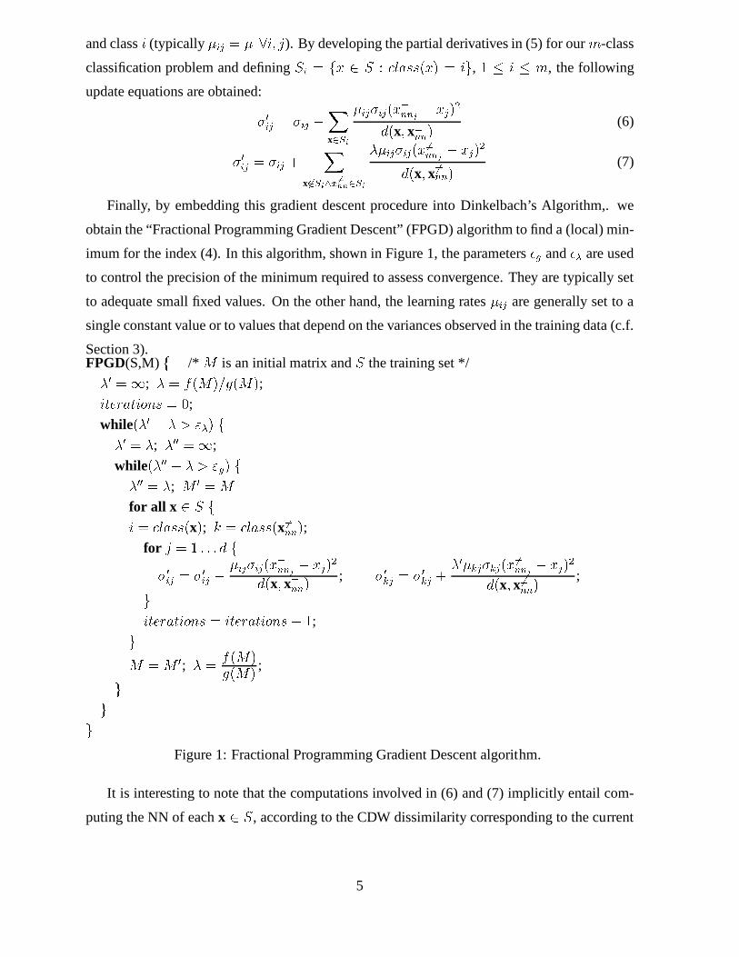
Finally, by embedding this gradient descent procedure intoDinkelbach’s Algorithm,. we

obtain the “Fractional Programming Gradient Descent” (FPGD) algorithm to find a (local) min-

imum for the index (4). In this algorithm, shown in Figure 1, the parameters�g and�� are used

to control the precision of the minimum required to assess convergence. They are typically set

to adequate small fixed values. On the other hand, the learning rates�ij are generally set to a

single constant value or to values that depend on the variances observed in the training data (c.f.

Section 3).FPGD(S,M)f /* M is an initial matrix andS the training set */�0 =1; � = f(M)=g(M);iterations = 0;

while(�0 � � > "�) f�0 = �; �00 =1;

while(�00 � � > "g) f�00 = �; M 0 = Mfor all x 2 S fi = lass(x); k = lass(x 6=nn);

for j = 1 : : : d f�0ij = �0ij � �ij�ij(x=nnj � xj)2d(x; x=nn) ; �0kj = �0kj + �0�kj�kj(x 6=nnj � xj)2d(x; x6=nn) ;giterations = iterations + 1;gM = M 0; � = f(M)g(M) ;gggFigure 1: Fractional Programming Gradient Descent algorithm.

It is interesting to note that the computations involved in (6) and (7) implicitly entail com-

puting the NN of eachx 2 S, according to the CDW dissimilarity corresponding to the current

5

0

2

4

6

8

10

12

14

0 50 100 150 2000

0.2

0.4

0.6

0.8

1

Iterations

FPGD evolution in the Monkey ProblemError estimation Index

Error estimationIndex

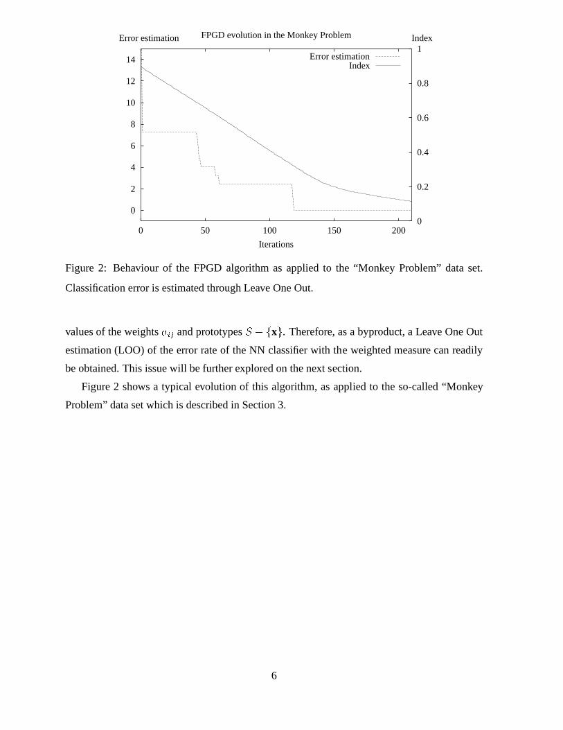
Figure 2: Behaviour of the FPGD algorithm as applied to the “Monkey Problem” data set.

Classification error is estimated through Leave One Out.

values of the weights�ij and prototypesS � fxg. Therefore, as a byproduct, a Leave One Out

estimation (LOO) of the error rate of the NN classifier with the weighted measure can readily

be obtained. This issue will be further explored on the next section.

Figure 2 shows a typical evolution of this algorithm, as applied to the so-called “Monkey

Problem” data set which is described in Section 3.

6

2.2 Finding adequate solutions in adverse situations.

A negative side effect of the fact that only locally optimal solutions can be obtained in each

step of the Fractional Programming procedure is that, if thethe additive factor in (7) is not

sufficiently large, the algorithm may tend to set�-values to zero.

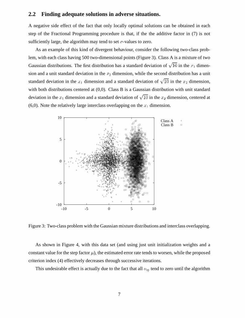
As an example of this kind of divergent behaviour, consider the following two-class prob-

lem, with each class having 500 two-dimensional points (Figure 3). Class A is a mixture of two

Gaussian distributions. The first distribution has a standard deviation ofp10 in thex1 dimen-

sion and a unit standard deviation in thex2 dimension, while the second distribution has a unit

standard deviation in thex1 dimension and a standard deviation ofp10 in thex2 dimension,

with both distributions centered at (0,0). Class B is a Gaussian distribution with unit standard

deviation in thex1 dimension and a standard deviation ofp10 in thex2 dimension, centered at

(6,0). Note the relatively large interclass overlapping onthex1 dimension.

-10

-5

0

5

10

-10 -5 0 5 10

Class AClass B

Figure 3: Two-class problem with the Gaussian mixture distributions and interclass overlapping.

As shown in Figure 4, with this data set (and using just unit initialization weights and a

constant value for the step factor�), the estimated error rate tends to worsen, while the proposed

criterion index (4) effectively decreases through successive iterations.

This undesirable effect is actually due to the fact that all�ij tend to zero until the algorithm

7

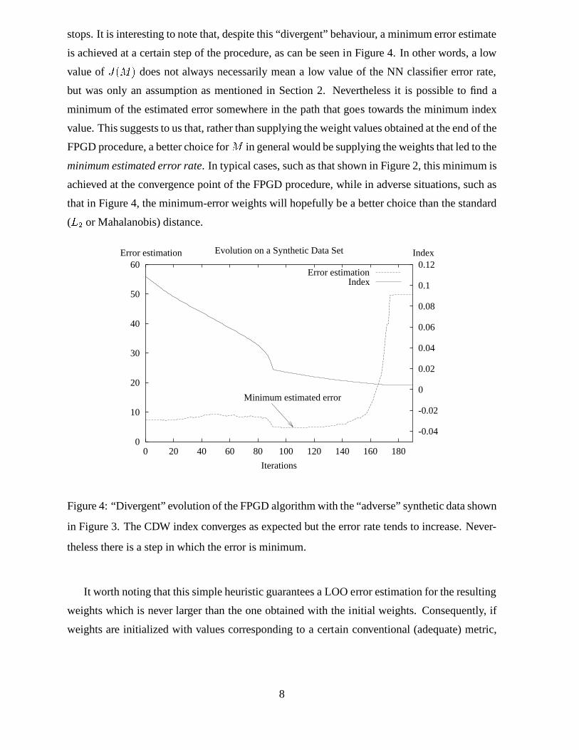
stops. It is interesting to note that, despite this “divergent” behaviour, a minimum error estimate

is achieved at a certain step of the procedure, as can be seen in Figure 4. In other words, a low

value ofJ(M) does not always necessarily mean a low value of the NN classifier error rate,

but was only an assumption as mentioned in Section 2. Nevertheless it is possible to find a

minimum of the estimated error somewhere in the path that goes towards the minimum index

value. This suggests to us that, rather than supplying the weight values obtained at the end of the

FPGD procedure, a better choice forM in general would be supplying the weights that led to the

minimum estimated error rate. In typical cases, such as that shown in Figure 2, this minimum is

achieved at the convergence point of the FPGD procedure, while in adverse situations, such as

that in Figure 4, the minimum-error weights will hopefully be a better choice than the standard

(L2 or Mahalanobis) distance.

0

10

20

30

40

50

60

0 20 40 60 80 100 120 140 160 180

-0.04

-0.02

0

0.02

0.04

0.06

0.08

0.1

0.12

Iterations

Evolution on a Synthetic Data SetError estimation Index

Minimum estimated error

Error estimationIndex

Figure 4: “Divergent” evolution of the FPGD algorithm with the “adverse” synthetic data shown

in Figure 3. The CDW index converges as expected but the errorrate tends to increase. Never-

theless there is a step in which the error is minimum.

It worth noting that this simple heuristic guarantees a LOO error estimation for the resulting

weights which is never larger than the one obtained with the initial weights. Consequently, if

weights are initialized with values corresponding to a certain conventional (adequate) metric,

8

the final weights are expected to behave at least as well as this metric would.

2.3 Asymptotic behaviour.

The previous section introduce a essential feature of our approach, namely, the estimation of

the error rate of the classifier by LOO using the weights at each step of the process. At the end

of the process, the weights with the best estimation are selected.

Let n be the size of the training set. IfM is initialized to the unit matrix, in the first step of

the process a LOO error estimation,�nnn, of the standard Nearest Neighbor classifier is obtained.

At the end of the process the weight matrix with the best errorestimation,�nw, is selected.

Therefore�nw � �nnn.

It’s well known that, under suitable conditions [Devroye (1996)], whenn tends to infinity

the LOO error estimation of a NN classifier tends to the error rate of this classifier. Therefore:�nw � �nnnlimn!1 �nnn = �nnlimn!1 �nw = �w9>>>=>>>;! �w � �nn (8)

In conclusion, the classifier using the optimal weight matrix is guaranteed to produce less

than or equal error rate than the standard Nearest Neighbor,in this asymptotic case.

3 Experiments

Several standard benchmark corpora from the UCI Repositoryof Machine Learning Databases

and Domain Theories [UCI] and the Statlog Project [Statlog]have been used. A short descrip-

tion of these corpora is given below:� Statlog Australian Credit Approval (Australian): 690 prototypes, 14 features, 2 classes. Dividedinto 10 sets for cross-validation.� UCI Balance (Balance): 625 prototypes, 4 features, 3 classes. Divided into 10 sets for cross-validation. A different design of the experiment was made in[Shultz (1994)].� Statlog Pima Indians Diabetes (Diabetes): 768 prototypes, 8 features, 2 classes. Divided into 11sets for cross-validation.� Statlog DNA (DNA): Training set of 2000 prototypes. Test set of 1186 vectors,180 features, 3classes.

9

� Statlog German Credit Data (German): 1000 prototypes, 20 features, 2 classes. Divided into 10sets for cross-validation.� Statlog Heart (Heart): 270 prototypes, 13 features, 2 classes. Divided into 9 sets for cross-validation.� UCI Ionosphere (Ionosphere): Training set of 200 prototypes (the first 200 as in [Sigilito (1989)]),Testset 151 vectors, 34 features, 2 classes.� Statlog Letter Image Recognition Letter (Letter): Training set of 15000 prototypes, Test set of5000 vectors, 16 features, 26 classes.� UCI Monkey-Problem-1 (Monkey): Training set of 124 prototypes, Test set of 432 vectors, 6features, 2 classes.� Statlog Satellite Image (Satimage): Training set of 4435 prototypes, Test set of 2000 prototypes,36 features, 6 classes.� Statlog Image Segmentation (Segmen): 2310 prototypes, 19 features, 7 classes. Divided into 10sets for cross-validation.� Statlog Shuttle (Shuttle): Training set of 43,500 prototypes, Test set of 14,500 vectors, 9 features,7 classes.� Statlog Vehicle (Vehicle): 846 prototypes, 18 features, 4 classes. Divided into 9 sets for cross-validation.

Most of these data sets involve bothnumericandcategoricalfeatures. In our experiments,

each categorical feature has been replaced byn binary features, wheren is the number of

different values allowed for the categorical feature. For example, in a hypothetical set of data

with two features: Age (Continuous) and Sex (Categorical: M,F), the categorical feature would

be replaced by two binary features; i.e., Sex=M will be represented as (1,0) and Sex=F as (0,1).

The continuous feature will not undergo any change, leadingto an overall three-dimensional

representation.

Many UCI and Statlog data sets are small. In these cases,N-Fold Cross-Validation[Raudys (1991)]

has been applied to obtain the classification results. Each corpus is divided intoN blocks usingN � 1 blocks as a training set and the remaining block as a test set.Therefore, each block

is used exactly once as a test set. The number of cross validation blocks,N , is specified for

each corpus in the UCI and Statlog documentation. For theDNA, Letter, Monkey, Satimageand

Shuttle, which are relatively larger corpora, a single specific partition into training and test sets

was provided by Statlog and, in these cases, no cross validation was carried out. It should be

finally mentioned that, although classification-cost penalties are available in a few cases, for the

sake of presentation homogeneity, we have decided not to make use of them; neither for training

nor for classification.

10

4 Results

Experiments with both the NN and the k-NN rules were carried out using theL2 metric, the

Mahalanobis distance (MD), the“class-dependent”Mahalanobis (CDM), and our CDW dis-

similarity measures. As mentioned in Section 1, CDM consists in weighting each dimension by

the inverse of the variance of this dimension in each class.

In the case of the CDM dissimilarity, computation singularities can appear when dealing

with categorical features, which often exhibitnull class-dependent variances. This problem was

solved by using the overall variance as a “back-off” for smoothing the null values.

Initialization values for training the CDW weights were selected according to the following

simple rule, which is based on LOO NN performance of conventional methods on the training

data: If rawL2 outperforms CDM, then set all initial�ij = 1; otherwise, set them to the inverse

of the corresponding training data standard deviations. Similarly, the step factors,�ij, are set

to a small constant (0.001) in the former case and to the inverse of the standard deviation in

the latter. Tables 1 and 2 summarize the results for NN and K-NN classification, respectively.

In the case of k-NN, only the results for the optimal value ofk; 1 < k < 21 observed in each

method are reported.

For the NN classification rule (Table 1) CDW outperforms conventional methods in most of

the corpora. The greatest improvement (+13%) was obtained in theMonkey-Problem, a categor-

ical corpus with a small number of features and only two classes. Similarly, good improvement

(+9.2%) was obtained for theDNAcorpus, which is also a corpus with categorical data, but with

far more features (180) and 3 classes. CDW has only been slightly outperformed (by less than

1.6%) by other methods in a few cases:Australian, IonosphereandShuttle.

For the K-NN classification rule (Table 2), CDW outperforms conventional methods in

many corpora:DNA, Ionosphere, Letter, Monkey, SegmenandVehicle; againMonkeyandDNA

yielded the most significant improvements (+12.7% and +7.7%, respectively). Also, in this K-

NN case, in the corpora where CDW is outperformed by some other method, the difference in

accuracy was generally small.

Error estimation 95% Confidence Intervals3 [Duda (1973)] for the best method are also

shown in Tables 1 and 2. It is interesting to note that in the few cases where CDW is outper-

formed by other methods, the difference is generally well within the corresponding confidence3Computed by numerically solving the equations:

Pk�K P (k; n; p1) = 1�A2 andPk�K P (k; n; p0) = 1�A2 ,

where P(k,n,p) is the binomial distribution, A=0.95 is the confidence value and[p0; p1℄ the confidence interval.

11

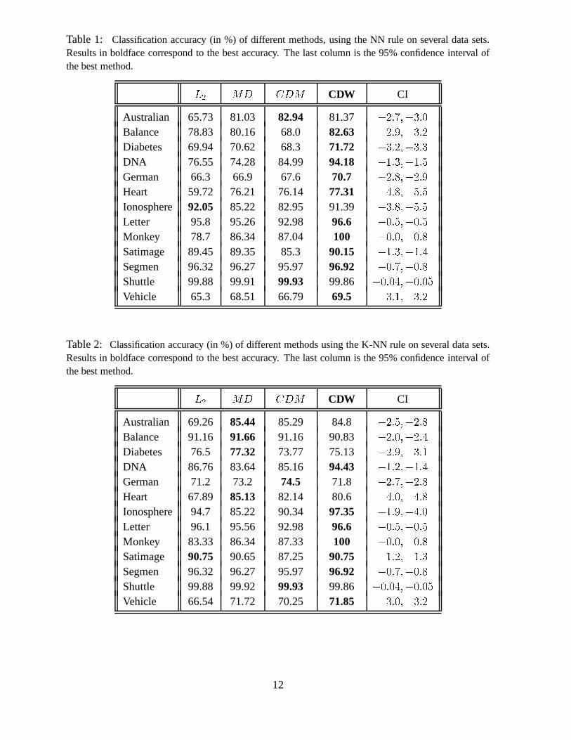
Table 1: Classification accuracy (in %) of different methods, using the NN rule on several data sets.Results in boldface correspond to the best accuracy. The last column is the 95% confidence interval ofthe best method. L2 MD CDM CDW CI

Australian 65.73 81.03 82.94 81.37 +2:7;�3:0Balance 78.83 80.16 68.0 82.63 +2:9;�3:2Diabetes 69.94 70.62 68.3 71.72 +3:2;�3:3DNA 76.55 74.28 84.99 94.18 +1:3;�1:5German 66.3 66.9 67.6 70.7 +2:8;�2:9Heart 59.72 76.21 76.14 77.31 +4:8;�5:5Ionosphere 92.05 85.22 82.95 91.39 +3:8;�5:5Letter 95.8 95.26 92.98 96.6 +0:5;�0:5Monkey 78.7 86.34 87.04 100 +0:0;�0:8Satimage 89.45 89.35 85.3 90.15 +1:3;�1:4Segmen 96.32 96.27 95.97 96.92 +0:7;�0:8Shuttle 99.88 99.91 99.93 99.86 +0:04;�0:05Vehicle 65.3 68.51 66.79 69.5 +3:1;�3:2

Table 2: Classification accuracy (in %) of different methods using the K-NN rule on several data sets.Results in boldface correspond to the best accuracy. The last column is the 95% confidence interval ofthe best method. L2 MD CDM CDW CI

Australian 69.26 85.44 85.29 84.8 +2:5;�2:8Balance 91.16 91.66 91.16 90.83 +2:0;�2:4Diabetes 76.5 77.32 73.77 75.13 +2:9;�3:1DNA 86.76 83.64 85.16 94.43 +1:2;�1:4German 71.2 73.2 74.5 71.8 +2:7;�2:8Heart 67.89 85.13 82.14 80.6 +4:0;�4:8Ionosphere 94.7 85.22 90.34 97.35 +1:9;�4:0Letter 96.1 95.56 92.98 96.6 +0:5;�0:5Monkey 83.33 86.34 87.33 100 +0:0;�0:8Satimage 90.75 90.65 87.25 90.75 +1:2;�1:3Segmen 96.32 96.27 95.97 96.92 +0:7;�0:8Shuttle 99.88 99.92 99.93 99.86 +0:04;�0:05Vehicle 66.54 71.72 70.25 71.85 +3:0;�3:2

12

intervals. On the other hand, in many cases where CDW was the best method, confidence in-

tervals were small (notably DNA, Monkey and Letter), thus indicating a statistically significant

advantage of CDW.

Comparisons with the best method known for each corpus [UCI,Statlog, Sigilito (1989)] are

summarized in Table 3, while Table 4 shows the results achieved by several methods in a few

corpora4. From these comparisons and the previously discussed results (Tables 1,2) it can be

seen that CDW exhibits auniformly good behaviourfor all the corpora, while other procedures

may work very well for some corpora (usually only one corpus)but typically tend to worsen

(dramatically in many cases) for the rest.

5 Concluding remarks

A weighted dissimilarity measure for NN classification has been presented. The required matrix

of weights is obtained through Fractional-Programming-based minimization of an appropriate

criterion index. Results obtained for several standard benchmark data sets are promising.

Current results using the CDW index and the FPGD algorithm are uniformly better than

those achieved by other more traditional methods. This alsoapplies to comparing FPGD with

the direct Gradient Descent technique previously proposedin [Paredes (1998)] to minimize a

simpler criterion index.

Other more sofisticated optimization methods can be devisedto minimize the proposed in-

dex (4) and new indexes can be proposed which would probably lead to improved performance.

In this sense, an index which computes the relation between the K-NN distances to the proto-

types of the same class and the K-NN to the prototypes in the nearest class (rather than the plain

NN as in (4)), would be expected to improve current CDW K-NN results.

Another new weighting scheme that deserves to be studied is one in which weights are as-

signed to eachprototype–rather than (or in addition to) eachclass. This “Prototype-Dependent

Weighted (PDW)” measure would involve a more “local” configuration of the dissimilarity

function and is expected to lead to an overall behaviour of the corresponding k-NN classifiers

which is even more data-independent.4Corpora that make use of classification-cost penalties (Section 3), (such asHeart andGerman), other corpora

which are not comparable because of other differences in experiment design, are excluded. Only those methods

which have results in many corpora, and corpora for which results with many methods are available have been

chosen for the comparisons in Table 4

13

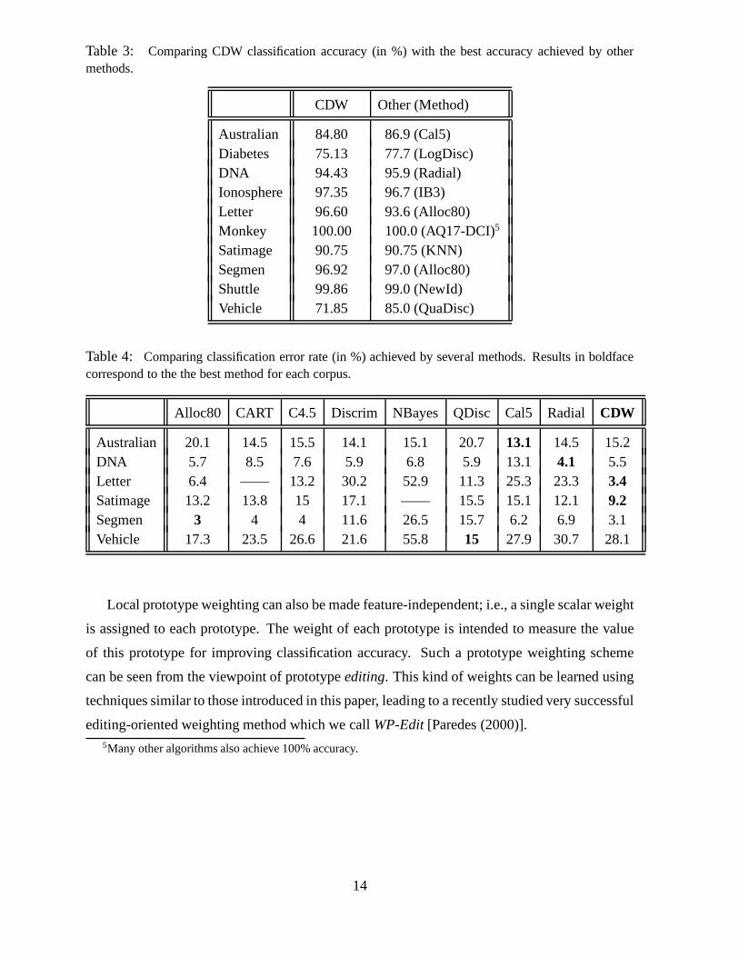
Table 3: Comparing CDW classification accuracy (in %) with the best accuracy achieved by othermethods.

CDW Other (Method)

Australian 84.80 86.9 (Cal5)Diabetes 75.13 77.7 (LogDisc)DNA 94.43 95.9 (Radial)Ionosphere 97.35 96.7 (IB3)Letter 96.60 93.6 (Alloc80)Monkey 100.00 100.0 (AQ17-DCI)5

Satimage 90.75 90.75 (KNN)Segmen 96.92 97.0 (Alloc80)Shuttle 99.86 99.0 (NewId)Vehicle 71.85 85.0 (QuaDisc)

Table 4: Comparing classification error rate (in %) achieved by several methods. Results in boldfacecorrespond to the the best method for each corpus.

Alloc80 CART C4.5 Discrim NBayes QDisc Cal5 Radial CDW

Australian 20.1 14.5 15.5 14.1 15.1 20.7 13.1 14.5 15.2DNA 5.7 8.5 7.6 5.9 6.8 5.9 13.1 4.1 5.5Letter 6.4 —— 13.2 30.2 52.9 11.3 25.3 23.3 3.4Satimage 13.2 13.8 15 17.1 —— 15.5 15.1 12.1 9.2Segmen 3 4 4 11.6 26.5 15.7 6.2 6.9 3.1Vehicle 17.3 23.5 26.6 21.6 55.8 15 27.9 30.7 28.1

Local prototype weighting can also be made feature-independent; i.e., a single scalar weight

is assigned to each prototype. The weight of each prototype is intended to measure the value

of this prototype for improving classification accuracy. Such a prototype weighting scheme

can be seen from the viewpoint of prototypeediting. This kind of weights can be learned using

techniques similar to those introduced in this paper, leading to a recently studied very successful

editing-oriented weighting method which we callWP-Edit[Paredes (2000)].5Many other algorithms also achieve 100% accuracy.

14

References[Cover (1967)] T.M. Cover and P.E. Hart. 1967 Nearest neighbor pattern classification. IEEE Transac-

tions on Infromation Theory, 13(1), 21–27.

[Devroye (1996)] L. Györfi, L. Devroye and G. Lugosi. 1996. A probabilistic theory of pattern recog-nition. Springer-Verlag New York, Inc.

[Tomek (1976)] I. Tomek. 1976. A generalization of the k-nn rule. IEEE Transactions on Systems, Man,and Cybernetics 6(2), 121–126.

[Fukunaga (1985)] K. Fukunaga and T.E. Flick. 1985. The 2-nnrule for more accurate nn risk estima-tion. IEEE Transactions on Pattern Analysis and Machine Intelligence, 7(1), 107–112.

[Luk (1986)] A. Luk and J.E. Macleod. 1986. An alternative nearest neighbour classification scheme.Pattern Recognition Letters, 4, 375–381.

[Urahama (1995)] K. Urahama and Y. Furukawa. 1995. Gradientdescent learning of nearest neighborclassifiers with outlier rejection. Pattern Recognition, 28(5), 761–768.

[Short (1980)] R.D. Short and K. Fukunaga. 1980. A new nearest neighbor distance measure. In Proc.5th IEEE Int. Conf. Pattern Recognition. Miami Beach, FL.

[Short (1981)] R.D. Short and K. Fukunaga. 1981. An optimal distance measure for nearest neighbourclassification. IEEE Trans. Info. Theory, 27, 622–627.

[Fukunaga (1982)] K. Fukunaga and T.E.Flick. 1892. A parametrically defined nearest neighbour mea-sure. Patter Recognition Letters, 1, 3–5.

[Fukunaga (1984)] K. Fukunaga and T.E.Flick. 1984. An optimal global nearest neighbour metric. IEEETrans. Pattern Recognition Mach. Intell. PAMI, 6, 314–318.

[Myles (1990] J.P. Myles and D.J. Hand. 1990. The multi-class metric problem in nearest neighbourdiscrimination rules. Pattern Recognition, 23(11), 1291–1297.

[Paredes (1998)] R. Paredes and E. Vidal. 1998. A nearest neighbor weighted measure in classificationproblems. VIII Simposium Nacional de Reconocimiento de Formas y Análisis de Imágenes, Proc.,Bilbao, Spain. July 1998.

[Paredes (2000)] R. Paredes and E. Vidal. 2000. Weighting prototypes. A new editing approach. 15thInternational Conference on Pattern Recognition, ICPR2000. Barcelona, Spain. September 2000.

[Sniedovich (1992)] M. Sniedovich. 1992. Dynamic Programming. Marcel Dekker Inc.

[Vidal (1995)] E. Vidal, A. Marzal and P. Aibar. 1995. Fast Computation of Normalized Edit Distances”.IEEE Trans. on Pattern Analysis and Machine Intelligence, 17(9), 899-902.

[UCI] C. Blake, E. Keogh and C.J. Merz. UCI Repository of machine learning databases.http://www.ics.uci.edu/�mlearn/MLRepository.html. University of California, Irvine, Dept. of In-formation and Computer Sciences.

[Statlog] Statlog Corpora. Dept. Statistics and Modellong Science (Stams). Stratchclyde University.ftp.strath.ac.uk

[Sigilito (1989)] V.G. Sigilito, S. P. Wing, L. V. Hutton andK. B. Baker. 1989. Classification of radarreturns from the ionosphere using neural networks. Johns Hopkins APL Technical Digest, 10,262-266.

[Shultz (1994)] T.R. Shultz, D. Mareschal and W.C. Schmidt.1994. Modeling Cognitive Developmenton Balance Scale Phenomena. Machine Learning, 16, 57–86.

[Raudys (1991)] S.J. Raudys and A.K Jain. 1991. Small SampleEffects in Statistical Pattern Recogni-tion: Recomendations for Practitioners". IEEE Trans on PAMI, 13(3), 252-264.

[Duda (1973)] R.Duda and P.Hart. 1973. Pattern Recognitionand Scene Analisys. John Wiley. NewYork.

15