431 1 development of different methods and their efficiencies
TRANSCRIPT
V.A. Baheti, A. Paul / Acta Materialia 156 (2018) 420– 431
1
Development of different methods and their efficiencies for the estimation of diffusion
coefficients following the diffusion couple technique
Varun A. Baheti 1,2 and Aloke Paul 1,* 1 Department of Materials Engineering, Indian Institute of Science, Bangalore 560012, India
2 Department of Metallurgical and Materials Engineering, Indian Institute of Technology, Kharagpur 721302, India*Corresponding author e–mail: [email protected]
Abstract
The interdiffusion coefficients are estimated either following the Wagner’s method expressed
with respect to the composition (mol or atomic fraction) normalized variable after
considering the molar volume variation or the den Broeder’s method expressed with respect
to the concentration (composition divided by the molar volume) normalized variable. On the
other hand, the relations for estimation of the intrinsic diffusion coefficients of components as
established by van Loo and integrated diffusion coefficients in a phase with narrow
homogeneity range as established by Wagner are currently available with respect to the
composition normalized variable only. In this study, we have first derived the relation
proposed by den Broeder following the line of treatment proposed by Wagner. Further, the
relations for estimation of the intrinsic diffusion coefficients of the components and
integrated interdiffusion coefficient are established with respect to the concentration
normalized variable, which were not available earlier. The veracity of these methods is
examined based on the estimation of data in Ni–Pd, Ni–Al and Cu–Sn systems. Our analysis
indicates that both the approaches are logically correct and there is small difference in the
estimated data in these systems although a higher difference could be found in other systems.
The integrated interdiffusion coefficients with respect to the concentration (or concentration
normalized variable) can only be estimated considering the ideal molar volume variation.
This might be drawback in certain practical systems.
Keywords:
Interdiffusion; Bulk diffusion; Diffusion coefficient estimation.
1. Introduction
Diffusion couple technique is a tool to study diffusion in inhomogeneous materials by
coupling dissimilar materials at the temperature of interest [1]. As an added advantage, one
can mimic the heterogeneous material systems in application for understanding the phase
transformations and the growth of product phases by diffusion–controlled process, which
control the various physico–mechanical properties and reliability of the structure [1]. This is
even emerged as a research tool to screen a very wide range of compositions optimizing
physical and mechanical properties for the development of a new material from only very few
samples, which otherwise would need a large volume of samples and unusually high man–
time [2].
The two major developments to establish this method as an efficient research tool for
diffusion studies can be stated as: (i) The relation developed by Matano [3] for the estimation
2
of composition dependent interdiffusion coefficients. It was developed by simplifying the
partial differential equation of Fick’s second law [4] to ordinary differential equation utilizing
the Boltzmann parameter [5]. This is known as the Matano–Boltzmann analysis. (ii) The
Darken–Manning relation [6, 7] developed based on the Kirkendall effect [8] for the
estimation of the intrinsic diffusion coefficients (influenced by thermodynamic driving force)
and tracer diffusion coefficients (indicating the self–diffusion coefficients) of components
[1].
However, the use of Matano–Boltzmann method for the estimation of the
interdiffusion coefficients �̃�(𝐶𝐵∗) as a function of concentration (𝐶𝐵) introduces error in
calculations in most of the practical systems. This relation is expressed as
�̃�(𝐶𝐵∗) = −
1
2𝑡(𝑑𝐶𝐵
∗
𝑑𝑥)
[𝑥∗(𝐶𝐵∗ − 𝐶𝐵
−) − ∫ (𝐶𝐵 − 𝐶𝐵−)
𝑥∗
𝑥−∞ 𝑑𝑥] (1)
where 𝑡 is the annealing time and 𝑥∗ = (𝑥∗ − 𝑥𝑜) since the location parameter is measured
with respect to 𝑥𝑜, i.e., the location of Matano (or initial contact) plane. The asterisk (∗)
represents the location of interest. Therefore, one of the very important pre–requisites for the
use of Matano–Boltzmann analysis is the need to locate the Matano plane. This can be
followed only when the molar volume varies ideally with composition or if we consider it as
constant. However, it does not fulfill in most of the practical systems and hence, it is almost
impossible to locate 𝑥𝑜 exactly. As explained mathematically in Ref. [9], it gives different
values of 𝑥𝑜 when estimated using different components and the difference between them is
exactly the same as expansion (for the positive deviation of molar volume) or shrinkage (for
the negative deviation of molar volume) of the diffusion couple in a binary system.
To circumvent this problem, mainly two relations are established independently:
(i) The relation developed by Wagner [10] following an analytical approach based on simple
algebraic equations, which is expressed as
�̃�(𝑌𝑁𝐵
∗ ) =𝑉𝑚
∗
2𝑡(𝑑𝑌𝑁𝐵
∗
𝑑𝑥)
[(1 − 𝑌𝑁𝐵
∗ ) ∫𝑌𝑁𝐵
𝑉𝑚𝑑𝑥
𝑥∗
𝑥−∞ + 𝑌𝑁𝐵
∗ ∫(1−𝑌𝑁𝐵
)
𝑉𝑚𝑑𝑥
𝑥+∞
𝑥∗ ] (2)
where 𝑌𝑁𝐵=
𝑁𝐵−𝑁𝐵−
𝑁𝐵+−𝑁𝐵
− is the composition normalized variable. 𝑁𝐵 is the composition in mol (or
atomic) fraction of component B. 𝑉𝑚 is the molar volume. “–” and “+” represents the un–
reacted left– and right–hand side of the diffusion couple.
(ii) The relation developed by den Broeder [11] by extending the Matano–Boltzmann analysis
following a graphical approach, which is expressed as
�̃�(𝑌𝐶𝐵
∗ ) =1
2𝑡(𝑑𝑌𝐶𝐵
∗
𝑑𝑥)
[(1 − 𝑌𝐶𝐵
∗ ) ∫ 𝑌𝐶𝐵
𝑥∗
𝑥−∞ 𝑑𝑥 + 𝑌𝐶𝐵
∗ ∫ (1 − 𝑌𝐶𝐵)
𝑥+∞
𝑥∗ 𝑑𝑥] (3)
where 𝑌𝐶𝐵=
𝐶𝐵−𝐶𝐵−
𝐶𝐵+−𝐶𝐵
− is the concentration normalized variable. 𝐶𝐵 (=𝑁𝐵
𝑉𝑚) is the concentration
of component B. The main advantage of using any of the above two relations can be
understood immediately that there is no need to locate the Matano plane, and hence it can
also consider the actual variation of molar volume with composition.
Out of all the methods, the Wagner’s method [10] draws a special attention, since in
the same manuscript, the author established the concept of the integrated interdiffusion
coefficient (�̃�𝑖𝑛𝑡) for the estimation of the diffusion coefficients in line compounds or the
3
phases with narrow homogeneity range in which concentration gradient cannot be measured.
Immediately after that, van Loo [12, 13] proposed the relations for intrinsic 𝐷𝑖 (or tracer 𝐷𝑖∗)
diffusion coefficients of components, in which the Matano plane is not necessary to locate.
Much later, Paul [9] derived these relations by extending the Wagner’s approach. Both of
these relations are derived with the composition normalized variable 𝑌𝑁𝐵.
To summarize, the relations for the estimation of interdiffusion and integrated
diffusion coefficients (derived by Wagner [10]), and intrinsic diffusion coefficients (derived
by van Loo [13] and Paul [9]) are expressed with respect to composition (mol or atomic
fraction) normalized variable 𝑌𝑁𝐵 although the molar volume term to consider the change in
total volume of the sample is included correctly during the derivation of these relations (for
example, see Equation 2). On the other hand, den Broeder’s relation [11] for the
interdiffusion coefficient is derived based on concentration (composition divided by molar
volume) normalized variable 𝑌𝐶𝐵 in which the molar volume term is automatically included,
see Equation 3. The relations for the estimation of other diffusion parameters (integrated and
intrinsic diffusion coefficients) with respect to the variable 𝑌𝐶𝐵 are not available. For a
constant molar volume, it is easy to visualize from Equations 2 and 3 that both the relations
of the interdiffusion coefficients lead to the same equation and therefore will give the same
value.
These two methods (den Broeder and Wagner) are compared based on the estimated
data only since these are derived completely differently (den Broeder: graphical and Wagner:
algebraic formulations). Therefore, with the aim of examining the veracity of these two
approaches, we do the following:
(i) For the sake of efficient comparison, we follow the line of treatment proposed by Wagner
to check if we can arrive at the den Broeder’s relation following Wagner’s line of treatment.
(ii) This will then help to extend it to derive the relations for the estimation of the intrinsic
diffusion coefficients of components and the integrated interdiffusion coefficient (for the
phases with narrow homogeneity range) with respect to 𝑌𝐶𝐵 which are not available at
present.
(iii) Following, we consider the experimental results in Ni–Pd (a system with solid solution),
Ni–Al (in –NiAl, a phase with the wide homogeneity range of composition) and Cu–Sn (a
system with the narrow homogeneity range phases) to discuss efficiencies/limitations of the
approaches.
2. Interdiffusion and intrinsic diffusion coefficients with respect to 𝒀𝑪𝑩
The derivation of relations for the interdiffusion coefficients by Wagner [10] and the
intrinsic diffusion coefficients by Paul [9] after extending the same line of treatment with
respect to composition normalized variable 𝑌𝑁𝐵 can be found in the respective references as
mentioned or in the text book as mentioned in Ref. [1]. In this section, we follow the
Wagner’s line of treatment to find if we can arrive at the den Broeder's relation with respect
to 𝑌𝐶𝐵. Then we extend it further to derive the relations for the intrinsic and tracer diffusion
coefficients. These will then allow us to compare the data of a particular diffusion parameter
when estimated following different relations utilizing 𝑌𝑁𝐵 and 𝑌𝐶𝐵
. It should be noted here
4
that the estimation of the tracer diffusion coefficients following the diffusion couple
technique is considered indirect but reliable [14],[15],[16],[17],[18]. These are important to
correlate the diffusion data with defects assisting the diffusion process in the absence of
thermodynamic driving forces.
2.1 Derivation of the Interdiffusion Coefficient with respect to 𝒀𝑪𝑩
Interdiffusion coefficients are related to the interdiffusion fluxes following the Fick’s first
law with respect to component B as [4]
𝐽𝐵 = −�̃�𝜕𝐶𝐵
𝜕𝑥 (4)
From the standard thermodynamic relation 𝐶𝐴�̅�𝐴 + 𝐶𝐵�̅�𝐵 = 1 [1], we can write
�̃�𝜕𝐶𝐵
𝜕𝑥= −𝐽𝐵 = −(𝐶𝐴�̅�𝐴 + 𝐶𝐵�̅�𝐵)𝐽𝐵 (5)
where �̅�𝑖 are the partial molar volumes of components A and B.
Using another standard thermodynamic equation �̅�𝐴𝑑𝐶𝐴 + �̅�𝐵𝑑𝐶𝐵 = 0 [1], we can relate the
interdiffusion fluxes with respect to components A and B as
𝐽𝐵 = −�̃�𝜕𝐶𝐵
𝜕𝑥=
�̅�𝐴
�̅�𝐵�̃�
𝜕𝐶𝐴
𝜕𝑥= −
�̅�𝐴
�̅�𝐵𝐽𝐴
�̅�𝐵𝐽𝐵 = −�̅�𝐴𝐽𝐴 (6)
Note here that the interdiffusion fluxes and the concentration gradients are different at one
particular composition (with respect to a particular location in a diffusion couple) in a system
with non–ideal molar volume variation. For a constant molar volume �̅�𝐴 = �̅�𝐵 = 𝑉𝑚, these are
equal but with opposite sign [19]. On the other hand, the interdiffusion coefficient is the
material constant and one will find the same value irrespective of any component considered
for the estimation of the data.
Combining Equations (5) and (6), we can write
�̃� =−𝐽𝐵
(𝜕𝐶𝐵𝜕𝑥
)=
−(𝐶𝐴�̅�𝐴+𝐶𝐵�̅�𝐵)𝐽𝐵
(𝜕𝐶𝐵𝜕𝑥
)
�̃� =�̅�𝐴(𝐶𝐵𝐽𝐴−𝐶𝐴𝐽𝐵)
(𝜕𝐶𝐵𝜕𝑥
)
𝐽𝐵 = −�̅�𝐴(𝐶𝐵𝐽𝐴 − 𝐶𝐴𝐽𝐵) (7)
Following Boltzmann [5], compositions in an interdiffusion zone can be related to its position
and annealing time by an auxiliary variable as
𝜆 = 𝜆(𝐶𝐵) =𝑥−𝑥𝑜
√𝑡=
𝑥
√𝑡 (8)
where 𝑥𝑜 = 0 is the location of the initial contact plane (Matano plane).
After differentiating Boltzmann parameter in Equation (8) with respect to t and then utilizing
the same relation again, we get dλ
𝑑𝑡= −
1
2
𝑥
𝑡3/2 = −𝜆
2𝑡
−1
𝑑𝑡=
𝜆
2𝑡𝑑𝜆 (9)
The concentration normalized variable introduced by den Broeder [11] is expressed as
𝑌𝐶𝐵=
𝐶𝐵−𝐶𝐵−
𝐶𝐵+−𝐶𝐵
− (10)
5
where 𝐶𝐵− and 𝐶𝐵
+ are the concentration of B at the un–affected left– and right–hand side of
the diffusion couple.
It can be rearranged to
𝐶𝐵 = 𝐶𝐵+𝑌𝐶𝐵
+ 𝐶𝐵−(1 − 𝑌𝐶𝐵
) (11a)
Using standard thermodynamic relation 𝐶𝐴�̅�𝐴 + 𝐶𝐵�̅�𝐵 = 1, Equation (11a) can be written as 1−𝐶𝐴�̅�𝐴
�̅�𝐵= 𝐶𝐵
+𝑌𝐶𝐵+ 𝐶𝐵
−(1 − 𝑌𝐶𝐵)
1 − 𝐶𝐴�̅�𝐴 = �̅�𝐵𝐶𝐵+𝑌𝐶𝐵
+ �̅�𝐵𝐶𝐵−(1 − 𝑌𝐶𝐵
)
𝐶𝐴�̅�𝐴 = 1 − �̅�𝐵𝐶𝐵+𝑌𝐶𝐵
− �̅�𝐵𝐶𝐵−(1 − 𝑌𝐶𝐵
)
𝐶𝐴�̅�𝐴 = (1 − 𝑌𝐶𝐵) + 𝑌𝐶𝐵
− �̅�𝐵𝐶𝐵+𝑌𝐶𝐵
− �̅�𝐵𝐶𝐵−(1 − 𝑌𝐶𝐵
)
𝐶𝐴 =(1−�̅�𝐵𝐶𝐵
+)𝑌𝐶𝐵+(1−�̅�𝐵𝐶𝐵
−)(1−𝑌𝐶𝐵)
�̅�𝐴 (11b)
From Fick’s second law [4], we know that 𝜕𝐶𝑖
𝜕𝑡=
𝜕
𝜕𝑥(�̃�
𝜕𝐶𝑖
𝜕𝑥) = −
𝜕𝐽𝑖
𝜕𝑥. Therefore, with
respect to components A and B and with the help of Equation (9), we can write 𝜕𝐽𝐵
𝜕𝑥= −
𝜕𝐶𝐵
𝜕𝑡=
𝜆
2𝑡
𝑑(𝐶𝐵)
𝑑𝜆 (12a)
𝜕𝐽𝐴
𝜕𝑥= −
𝜕𝐶𝐴
𝜕𝑡=
𝜆
2𝑡
𝑑(𝐶𝐴)
𝑑𝜆 (12b)
Note here that in Equations (11a) and (11b), the concentrations of component B and A, i.e.,
𝐶𝐵 and 𝐶𝐴 are expressed in terms of the concentration normalized variable (𝑌𝐶𝐵). So, next we
aim to rewrite Fick’s second law, i.e., Equations (12a) and (12b) with respect to 𝑌𝐶𝐵.
Replacing Equation (11a) in (12a) and Equation (11b) in (12b), we get
𝜕𝐽𝐵
𝜕𝑥=
𝜆
2𝑡[𝐶𝐵
+ 𝑑𝑌𝐶𝐵
𝑑𝜆+ 𝐶𝐵
− 𝑑(1−𝑌𝐶𝐵)
𝑑𝜆]
(13a)
𝜕𝐽𝐴
𝜕𝑥=
𝜆
2𝑡[(
1−�̅�𝐵𝐶𝐵+
�̅�𝐴)
𝑑𝑌𝐶𝐵
𝑑𝜆+ (
1−�̅�𝐵𝐶𝐵−
�̅�𝐴)
𝑑(1−𝑌𝐶𝐵)
𝑑𝜆] (13b)
Now, we aim to write the above equations with respect to 𝑌𝐶𝐵 and (1 − 𝑌𝐶𝐵
) separately.
Operating [𝐶𝐵−× Eq. (13b)] − [(
1−�̅�𝐵𝐶𝐵−
�̅�𝐴) ×Eq. (13a)] leads to
𝐶𝐵− 𝜕𝐽𝐴
𝜕𝑥− (
1−�̅�𝐵𝐶𝐵−
�̅�𝐴)
𝜕𝐽𝐵
𝜕𝑥=
𝜆
2𝑡(
𝐶𝐵−−𝐶𝐵
+
�̅�𝐴)
𝑑𝑌𝐶𝐵
𝑑𝜆 (14a)
Operating [𝐶𝐵+× Eq. (13b)] − [(
1−�̅�𝐵𝐶𝐵+
�̅�𝐴) ×Eq. (13a)] leads to
𝐶𝐵+ 𝜕𝐽𝐴
𝜕𝑥− (
1−�̅�𝐵𝐶𝐵+
�̅�𝐴)
𝜕𝐽𝐵
𝜕𝑥=
𝜆
2𝑡(
𝐶𝐵+−𝐶𝐵
−
�̅�𝐴)
𝑑(1−𝑌𝐶𝐵)
𝑑𝜆 (14b)
After differentiating Boltzmann parameter in Equation (8) with respect to x, we get
𝑑𝜆 =𝑑𝑥
√𝑡 (15)
Multiplying left–hand side by 𝑑𝑥
√𝑡 and right–hand side by 𝑑𝜆 of the Equation (14a) and (14b),
respectively, we get
�̅�𝐴𝐶𝐵− 𝑑𝐽𝐴−(1−�̅�𝐵𝐶𝐵
−) 𝑑𝐽𝐵
√𝑡= (
𝐶𝐵−−𝐶𝐵
+
2𝑡) 𝜆 𝑑(𝑌𝐶𝐵
) (16a)
�̅�𝐴𝐶𝐵+ 𝑑𝐽𝐴−(1−�̅�𝐵𝐶𝐵
+) 𝑑𝐽𝐵
√𝑡= (
𝐶𝐵+−𝐶𝐵
−
2𝑡) 𝜆 𝑑(1 − 𝑌𝐶𝐵
) (16b)
Equation (16a) is integrated for a fixed annealing time t from un–affected left–hand side of
the diffusion couple, i.e., = 𝜆−∞ (corresponds to 𝑥 = 𝑥−∞) to the location of interest =
6
* (corresponds to 𝑥 = 𝑥∗) for estimation of the diffusion coefficient. Following, we
rearrange, with respect to integration by parts [∫ 𝑢𝑑𝑣 = 𝑢𝑣 − ∫(𝑣𝑑𝑢)]. 1
√𝑡[�̅�𝐴𝐶𝐵
− ∫ 𝑑𝐽𝐴𝐽𝐴
∗
0− (1 − �̅�𝐵𝐶𝐵
−) ∫ 𝑑𝐽𝐵𝐽𝐵
∗
0] = (
𝐶𝐵−−𝐶𝐵
+
2𝑡) ∫ 𝜆 𝑑(𝑌𝐶𝐵
)𝜆∗
𝜆−∞
(𝑉𝐴∗𝐶𝐵
−)𝐽𝐴∗ −(1−�̅�𝐵
∗𝐶𝐵−)𝐽𝐵
∗
√𝑡= (
𝐶𝐵−−𝐶𝐵
+
2𝑡) [𝜆∗𝑌𝐶𝐵
∗ − ∫ 𝑌𝐶𝐵 𝑑𝜆
𝜆∗
𝜆−∞ ] (17a)
Similarly, Equation (16b) is integrated from the location of interest = * to the un–affected
right–hand side of the diffusion couple, i.e., = 𝜆+∞ (corresponds to 𝑥 = 𝑥+∞).
1
√𝑡[�̅�𝐴𝐶𝐵
+ ∫ 𝑑𝐽𝐴0
𝐽𝐴∗ − (1 − �̅�𝐵𝐶𝐵
+) ∫ 𝑑𝐽𝐵0
𝐽𝐵∗ ] = (
𝐶𝐵+−𝐶𝐵
−
2𝑡) ∫ 𝜆 𝑑(1 − 𝑌𝐶𝐵
)𝜆+∞
𝜆∗
−(�̅�𝐴∗𝐶𝐵
+)𝐽𝐴∗ +(1−�̅�𝐵
∗𝐶𝐵+)𝐽𝐵
∗
√𝑡= (
𝐶𝐵+−𝐶𝐵
−
2𝑡) [−𝜆∗(1 − 𝑌𝐶𝐵
∗ ) − ∫ (1 − 𝑌𝐶𝐵) 𝑑𝜆
𝜆+∞
𝜆∗ ] (17b)
Note here that the interdiffusion fluxes 𝐽𝑖 is equal to zero at the un–affected parts of the
diffusion couple, 𝑥 = 𝑥−∞ and 𝑥 = 𝑥+∞, while 𝐽𝑖∗ is the fixed value (for certain annealing
time t) at the location of interest 𝑥 = 𝑥∗ in the above Equations (17). Next, we aim to rewrite
the above equations with respect to interdiffusion fluxes 𝐽𝑖 of both components to get an
expression for the interdiffusion coefficient �̃�.
Operating [𝑌𝐶𝐵
∗ × Eq. (17b)] − [(1 − 𝑌𝐶𝐵
∗ ) × Eq. (17a)] leads to
�̅�𝐴∗(𝐶𝐵
∗ 𝐽𝐴∗ −𝐶𝐴
∗ 𝐽𝐵∗ )
√𝑡= (
𝐶𝐵+−𝐶𝐵
−
2𝑡) [(1 − 𝑌𝐶𝐵
∗ ) ∫ 𝑌𝐶𝐵 𝑑𝜆 + 𝑌𝐶𝐵
∗ ∫ (1 − 𝑌𝐶𝐵) 𝑑𝜆
𝜆+∞
𝜆∗
𝜆∗
𝜆−∞ ] (18)
Numerator on the left–hand side can be derived, by using 𝐶𝐵∗ = 𝐶𝐵
+𝑌𝐶𝐵
∗ + 𝐶𝐵−(1 − 𝑌𝐶𝐵
∗ )
following Equation (11a) and standard thermodynamic relation �̅�𝐴∗𝐶𝐴
∗ = 1 − �̅�𝐵∗𝐶𝐵
∗ , following
the steps:
𝑌𝐶𝐵
∗ {−(�̅�𝐴∗𝐶𝐵
+)𝐽𝐴∗ + (1 − �̅�𝐵
∗𝐶𝐵+)𝐽𝐵
∗ } − (1 − 𝑌𝐶𝐵
∗ ){(�̅�𝐴∗𝐶𝐵
−)𝐽𝐴∗ − (1 − �̅�𝐵
∗𝐶𝐵−)𝐽𝐵
∗ }
= {−�̅�𝐴∗𝐶𝐵
+𝑌𝐶𝐵
∗ − �̅�𝐴∗𝐶𝐵
−(1 − 𝑌𝐶𝐵
∗ )}𝐽𝐴∗ + {(1 − �̅�𝐵
∗𝐶𝐵+)𝑌𝐶𝐵
∗ + (1 − 𝑌𝐶𝐵
∗ )(1 − �̅�𝐵∗𝐶𝐵
−)}𝐽𝐵∗
= −�̅�𝐴∗{𝐶𝐵
+𝑌𝐶𝐵
∗ + 𝐶𝐵−(1 − 𝑌𝐶𝐵
∗ )}𝐽𝐴∗ + {𝑌𝐶𝐵
∗ − �̅�𝐵∗𝐶𝐵
+𝑌𝐶𝐵
∗ + 1 − �̅�𝐵∗𝐶𝐵
− − 𝑌𝐶𝐵
∗ + �̅�𝐵∗𝐶𝐵
−𝑌𝐶𝐵
∗ }𝐽𝐵∗
= −�̅�𝐴∗{𝐶𝐵
+𝑌𝐶𝐵
∗ + 𝐶𝐵−(1 − 𝑌𝐶𝐵
∗ )}𝐽𝐴∗ + [1 − �̅�𝐵
∗{𝐶𝐵+𝑌𝐶𝐵
∗ + 𝐶𝐵−(1 − 𝑌𝐶𝐵
∗ )}]𝐽𝐵∗
= −�̅�𝐴∗(𝐶𝐵
∗𝐽𝐴∗ − 𝐶𝐴
∗𝐽𝐵∗ ).
Utilizing 𝑑𝜆 =𝑑𝑥
√𝑡 from Equation (15), we get
�̅�𝐴∗(𝐶𝐵
∗𝐽𝐴∗ − 𝐶𝐴
∗𝐽𝐵∗ ) = (
𝐶𝐵+−𝐶𝐵
−
2𝑡) [(1 − 𝑌𝐶𝐵
∗ ) ∫ 𝑌𝐶𝐵 𝑑𝑥 + 𝑌𝐶𝐵
∗ ∫ (1 − 𝑌𝐶𝐵) 𝑑𝑥
𝑥+∞
𝑥∗
𝑥∗
𝑥−∞ ] (19)
For 𝐶𝐵 = 𝐶𝐵∗ , from Equation (7) we know that 𝐽𝐵
∗ = −�̅�𝐴∗(𝐶𝐵
∗𝐽𝐴∗ − 𝐶𝐴
∗𝐽𝐵∗ ) and hence the
interdiffusion flux with respect to component B can be expressed as
𝐽𝐵∗ = 𝐽𝐵(𝐶𝐵
∗) = − (𝐶𝐵
+−𝐶𝐵−
2𝑡) [(1 − 𝑌𝐶𝐵
∗ ) ∫ 𝑌𝐶𝐵
𝑥∗
𝑥−∞ 𝑑𝑥 + 𝑌𝐶𝐵
∗ ∫ (1 − 𝑌𝐶𝐵)
𝑥+∞
𝑥∗ 𝑑𝑥] (20a)
Similarly, one can derive the interdiffusion flux with respect to component A as
𝐽𝐴∗ = 𝐽𝐴(𝐶𝐴
∗) = (𝐶𝐴
−−𝐶𝐴+
2𝑡) [𝑌𝐶𝐴
∗ ∫ (1 − 𝑌𝐶𝐴)
𝑥∗
𝑥−∞ 𝑑𝑥 + (1 − 𝑌𝐶𝐴
∗ ) ∫ 𝑌𝐶𝐴
𝑥+∞
𝑥∗ 𝑑𝑥] (20b)
where 𝑌𝐶𝐴=
𝐶𝐴−𝐶𝐴+
𝐶𝐴−−𝐶𝐴
+. Note opposite sign of interdiffusion fluxes when estimated with respect
to component A and B because of opposite direction of diffusion of these components.
From Equation (11a) we know that 𝐶𝐵 = 𝐶𝐵+𝑌𝐶𝐵
+ 𝐶𝐵−(1 − 𝑌𝐶𝐵
). By differentiating it with
respect to x, we can write
(𝑑𝐶𝐵
𝑑𝑥)
𝑥=𝑥∗= 𝐶𝐵
+ 𝑑𝑌𝐶𝐵
𝑑𝑥− 𝐶𝐵
− 𝑑𝑌𝐶𝐵
𝑑𝑥= (𝐶𝐵
+ − 𝐶𝐵−) (
𝑑𝑌𝐶𝐵
𝑑𝑥)
𝑥=𝑥∗ (21)
7
From Equation (7) for 𝐶𝐵 = 𝐶𝐵∗ , we know
�̃�(𝐶𝐵∗) =
−𝐽𝐵∗
(𝑑𝐶𝐵𝑑𝑥
)𝑥=𝑥∗
(22)
Substituting for flux [Eq. (20a)] and gradient [Eq. (21)] in Fick’s first law [Eq. (22)], we get
the expression for the estimation of interdiffusion coefficient as
�̃�(𝑌𝐶𝐵
∗ ) =1
2𝑡(𝑑𝑌𝐶𝐵
∗
𝑑𝑥)
[(1 − 𝑌𝐶𝐵
∗ ) ∫ 𝑌𝐶𝐵
𝑥∗
𝑥−∞ 𝑑𝑥 + 𝑌𝐶𝐵
∗ ∫ (1 − 𝑌𝐶𝐵)
𝑥+∞
𝑥∗ 𝑑𝑥] (23)
den Broeder [11] derived this relation with respect to 𝑌𝐶𝐵 following the graphical approach. It
should be noted here that the interdiffusion coefficients (�̃�(𝑌𝐶𝐴
∗ ) and �̃�(𝑌𝐶𝐵
∗ )) estimated with
respect to component A and B are the same [19]. In this study, we arrive at the same relation
(see Equation 3) following the Wagner’s [10] line of treatment, although Wagner derived the
relation as expressed in Equation 2 with respect to 𝑌𝑁𝐵. Therefore, in a sense, both the
relations are logically correct. Additionally, for a constant molar volume (𝑉𝑚 = 𝑉𝑚− = 𝑉𝑚
+),
both the den Broeder and the Wagner relations lead to
�̃�(𝑌𝑁𝐵
∗ ) =1
2𝑡(𝑑𝑌𝑁𝐵
∗
𝑑𝑥)
[(1 − 𝑌𝑁𝐵
∗ ) ∫ 𝑌𝑁𝐵
𝑥∗
𝑥−∞ 𝑑𝑥 + 𝑌𝑁𝐵
∗ ∫ (1 − 𝑌𝑁𝐵)𝑑𝑥
𝑥+∞
𝑥∗ ] (44)
Since, 𝑌𝐶𝐵=
𝐶𝐵−𝐶𝐵−
𝐶𝐵+−𝐶𝐵
− =
𝑁𝐵𝑉𝑚
−𝑁𝐵
−
𝑉𝑚
𝑁𝐵+
𝑉𝑚−
𝑁𝐵−
𝑉𝑚
=𝑁𝐵−𝑁𝐵
−
𝑁𝐵+−𝑁𝐵
− = 𝑌𝑁𝐵
2.2 Derivation of the intrinsic and tracer diffusion coefficients with respect to 𝒀𝑪𝑩
As already mentioned, the relations for the intrinsic diffusion coefficients are
available only with respect to 𝑌𝑁𝐵. Therefore, these relations should be derived with respect
𝑌𝐶𝐵 to examine the differences in the data when estimated following these different
approaches, i.e., with respect to 𝑌𝐶𝐵 and 𝑌𝑁𝐵
. Previously, Paul [9] derived these relations with
respect to 𝑌𝑁𝐵 by extending the Wagner’s line of treatment to derive the same relations as
developed earlier by van Loo [13] differently. We now, extend the analysis to develop the
relations for the intrinsic diffusion coefficients with respect to 𝑌𝐶𝐵.
When the location of interest is the position of the Kirkendall marker plane (K), i.e.,
𝑥∗ = 𝑥𝐾, we can write Equations (17a) and (17b), respectively as
(𝑉𝐴𝐾𝐶𝐵
−)𝐽𝐴𝐾−(1−�̅�𝐵
𝐾𝐶𝐵−)𝐽𝐵
𝐾
√𝑡= (
𝐶𝐵+−𝐶𝐵
−
2𝑡) [−𝜆𝐾𝑌𝐶𝐵
𝐾 + ∫ 𝑌𝐶𝐵 𝑑𝜆
𝜆𝐾
𝜆−∞ ] (25a)
−(𝑉𝐴𝐾𝐶𝐵
+)𝐽𝐴𝐾+(1−�̅�𝐵
𝐾𝐶𝐵+)𝐽𝐵
𝐾
√𝑡= (
𝐶𝐵+−𝐶𝐵
−
2𝑡) [−𝜆𝐾(1 − 𝑌𝐶𝐵
𝐾 ) − ∫ (1 − 𝑌𝐶𝐵) 𝑑𝜆
𝜆+∞
𝜆𝐾 ] (25b)
Now, we aim to rewrite the above equations with respect to 𝐽𝐵𝐾 and 𝐽𝐴
𝐾 such that we can get an
expression for intrinsic diffusion coefficient of component B and A, i.e., 𝐷𝐵 and 𝐷𝐴,
respectively, at the Kirkendall maker plane utilizing the Darken’s equation [6] relating the
interdiffusion flux (𝐽𝑖) with the intrinsic flux (𝐽𝑖) of component.
Operating [�̅�𝐴𝐾𝐶𝐵
+ × Eq. (25a)] + [�̅�𝐴𝐾𝐶𝐵
− × Eq. (25b)] leads to
−(𝐶𝐵+−𝐶𝐵
−)𝐽𝐵𝐾
√𝑡= (
𝐶𝐵+−𝐶𝐵
−
2𝑡) [−𝜆𝐾{𝐶𝐵
+𝑌𝐶𝐵
𝐾 + 𝐶𝐵−(1 − 𝑌𝐶𝐵
𝐾 )} + 𝐶𝐵+ ∫ 𝑌𝐶𝐵
𝑑𝜆𝜆𝐾
𝜆−∞ − 𝐶𝐵− ∫ (1 − 𝑌𝐶𝐵
) 𝑑𝜆𝜆+∞
𝜆𝐾 ]
Note that �̅�𝐴𝐾 has been cancelled on both sides, since numerator on the left–hand side is
8
{−(�̅�𝐴𝐾𝐶𝐵
+)(1 − �̅�𝐵𝐾𝐶𝐵
−) + �̅�𝐴𝐾𝐶𝐵
−(1 − �̅�𝐵𝐾𝐶𝐵
+)}𝐽𝐵𝐾 = −�̅�𝐴
𝐾(𝐶𝐵+ − 𝐶𝐵
−)𝐽𝐵𝐾
Utilizing 𝐶𝐵𝐾 = 𝐶𝐵
+𝑌𝐶𝐵
𝐾 + 𝐶𝐵−(1 − 𝑌𝐶𝐵
𝐾 ) from Equation (11a) and after rearranging, we get
𝐽𝐵𝐾 =
√𝑡
2𝑡[𝜆𝐾𝐶𝐵
𝐾 − 𝐶𝐵+ ∫ 𝑌𝐶𝐵
𝑑𝜆𝜆𝐾
𝜆−∞ + 𝐶𝐵− ∫ (1 − 𝑌𝐶𝐵
) 𝑑𝜆𝜆+∞
𝜆𝐾 ] (26a)
Similarly, operating [(1 − �̅�𝐵𝐾𝐶𝐵
+) × Eq. (25a)] + [(1 − �̅�𝐵𝐾𝐶𝐵
−) × Eq. (25b)] and utilizing
�̅�𝐴𝐾𝐶𝐴
𝐾 = (1 − �̅�𝐵𝐾𝐶𝐵
+)𝑌𝐶𝐵
𝐾 + (1 − �̅�𝐵𝐾𝐶𝐵
−)(1 − 𝑌𝐶𝐵
𝐾 ) from Equation (11b), we get
−𝑉𝐴𝐾(𝐶𝐵
+−𝐶𝐵−)𝐽𝐴
𝐾
√𝑡= (
𝐶𝐵+−𝐶𝐵
−
2𝑡) [−𝜆𝐾�̅�𝐴
𝐾𝐶𝐴𝐾 + (1 − �̅�𝐵
𝐾𝐶𝐵+) ∫ 𝑌𝐶𝐵
𝑑𝜆𝜆𝐾
𝜆−∞ − (1 − �̅�𝐵𝐾𝐶𝐵
−) ∫ (1 − 𝑌𝐶𝐵) 𝑑𝜆
𝜆+∞
𝜆𝐾 ]
since numerator on the left–hand side is
{�̅�𝐴𝐾𝐶𝐵
−(1 − �̅�𝐵𝐾𝐶𝐵
+) − �̅�𝐴𝐾𝐶𝐵
+(1 − �̅�𝐵𝐾𝐶𝐵
−)}𝐽𝐴𝐾 = −�̅�𝐴
𝐾(𝐶𝐵+ − 𝐶𝐵
−)𝐽𝐴𝐾
Dividing both sides of equation by a factor of �̅�𝐴𝐾 and after rearranging, we get
𝐽𝐴𝐾 =
√𝑡
2𝑡[𝜆𝐾𝐶𝐴
𝐾 − (1−𝑉𝐵
𝐾𝐶𝐵+
�̅�𝐴𝐾 ) ∫ 𝑌𝐶𝐵
𝑑𝜆𝜆𝐾
𝜆−∞ + (1−𝑉𝐵
𝐾𝐶𝐵−
𝑉𝐴𝐾 ) ∫ (1 − 𝑌𝐶𝐵
) 𝑑𝜆𝜆+∞
𝜆𝐾 ] (26b)
From Boltzmann parameter in Equation (8), we know that 𝜆𝐾 =𝑥𝐾
√𝑡 or 𝑥𝐾 = 𝜆𝐾√𝑡.
Therefore, the velocity of the Kirkendall marker plane can be expressed as
𝑣𝐾 =𝑑𝑥𝐾
𝑑𝑡=
𝑑(𝜆𝐾√𝑡)
𝑑𝑡= 𝜆𝐾 𝑑(√𝑡)
𝑑𝑡=
𝜆𝐾
2√𝑡=
𝜆𝐾√𝑡
2𝑡
Also, differentiating Boltzmann parameter with respect to x, from Equation (15) we know
that √𝑡 𝑑𝜆 = 𝑑𝑥.
Putting 𝜆𝐾√𝑡
2𝑡= 𝑣𝐾 and √𝑡 𝑑𝜆 = 𝑑𝑥 in Equations (26), we get
𝐽𝐵𝐾 = 𝑣𝐾𝐶𝐵
𝐾 −1
2𝑡[𝐶𝐵
+ ∫ 𝑌𝐶𝐵
𝑥𝐾
𝑥−∞ 𝑑𝑥 − 𝐶𝐵− ∫ (1 − 𝑌𝐶𝐵
)𝑥+∞
𝑥𝐾 𝑑𝑥] (27a)
𝐽𝐴𝐾 = 𝑣𝐾𝐶𝐴
𝐾 −1
2𝑡[(
1−𝑉𝐵𝐾𝐶𝐵
+
�̅�𝐴𝐾 ) ∫ 𝑌𝐶𝐵
𝑑𝑥𝑥𝐾
𝑥−∞ − (1−𝑉𝐵
𝐾𝐶𝐵−
𝑉𝐴𝐾 ) ∫ (1 − 𝑌𝐶𝐵
) 𝑑𝑥𝑥+∞
𝑥𝐾 ] (27b)
Following Darken’s Analysis [6], we know that 𝐽𝐵𝐾 = 𝐽𝐵 + 𝑣𝐾𝐶𝐵
𝐾 and 𝐽𝐴𝐾 = 𝐽𝐴 + 𝑣𝐾𝐶𝐴
𝐾.
Therefore, we can get an expression for intrinsic flux of component B and A, i.e., 𝐽𝐵 and 𝐽𝐴,
respectively, as follows:
𝐽𝐵 = 𝐽𝐵𝐾 − 𝑣𝐾𝐶𝐵
𝐾
𝐽𝐵 = −1
2𝑡[𝐶𝐵
+ ∫ 𝑌𝐶𝐵
𝑥𝐾
𝑥−∞ 𝑑𝑥 − 𝐶𝐵− ∫ (1 − 𝑌𝐶𝐵
)𝑥+∞
𝑥𝐾 𝑑𝑥] (28a)
𝐽𝐴 = 𝐽𝐴𝐾 − 𝑣𝐾𝐶𝐴
𝐾
𝐽𝐴 = −1
2𝑡[(
1−�̅�𝐵𝐾𝐶𝐵
+
�̅�𝐴𝐾 ) ∫ 𝑌𝐶𝐵
𝑥𝐾
𝑥−∞ 𝑑𝑥 − (1−�̅�𝐵
𝐾𝐶𝐵−
�̅�𝐴𝐾 ) ∫ (1 − 𝑌𝐶𝐵
)𝑥+∞
𝑥𝐾 𝑑𝑥] (28b)
Using Fick’s first law [4], we can write 𝐷𝐵 =−𝐽𝐵
(𝜕𝐶𝐵𝜕𝑥
)𝑥𝐾
and 𝐷𝐴 =−𝐽𝐴
(𝜕𝐶𝐴𝜕𝑥
)𝑥𝐾
. Therefore, we can
write an expression for intrinsic diffusion coefficient of component B and A, i.e., 𝐷𝐵 and 𝐷𝐴,
respectively, as follows:
𝐷𝐵 =1
2𝑡(
𝜕𝑥
𝜕𝐶𝐵)
𝐾[𝐶𝐵
+ ∫ 𝑌𝐶𝐵
𝑥𝐾
𝑥−∞ 𝑑𝑥 − 𝐶𝐵− ∫ (1 − 𝑌𝐶𝐵
)𝑥+∞
𝑥𝐾 𝑑𝑥] (29a)
𝐷𝐴 =1
2𝑡(
𝜕𝑥
𝜕𝐶𝐴)
𝐾[(
1−�̅�𝐵𝐾𝐶𝐵
+
�̅�𝐴𝐾 ) ∫ 𝑌𝐶𝐵
𝑥𝐾
𝑥−∞ 𝑑𝑥 − (1−�̅�𝐵
𝐾𝐶𝐵−
�̅�𝐴𝐾 ) ∫ (1 − 𝑌𝐶𝐵
)𝑥+∞
𝑥𝐾 𝑑𝑥] (29b)
The same relation of 𝐷𝐴 with respect to 𝑌𝐶𝐴 can be derived as
𝐷𝐴 =1
2𝑡(
𝜕𝑥
𝜕𝐶𝐴)
𝐾[𝐶𝐴
− ∫ 𝑌𝐶𝐴
𝑥𝐾
𝑥+∞ 𝑑𝑥 − 𝐶𝐴+ ∫ (1 − 𝑌𝐶𝐴
)𝑥−∞
𝑥𝐾 𝑑𝑥] (29c)
9
Compared to Equation 29b, Equation 29c avoids the need for partial molar volumes and
hence the error associated with the estimation of these values, as shown later in Section 2.3.
Using �̅�𝐴𝑑𝐶𝐴 + �̅�𝐵𝑑𝐶𝐵 = 0, we get 𝜕𝐶𝐵
𝜕𝑥= −
�̅�𝐴
�̅�𝐵
𝜕𝐶𝐴
𝜕𝑥⟹
𝜕𝑥
𝜕𝐶𝐵= −
�̅�𝐵
�̅�𝐴
𝜕𝑥
𝜕𝐶𝐴.
Utilizing (𝜕𝑥
𝜕𝐶𝐵)
𝐾= −
�̅�𝐵𝐾
�̅�𝐴𝐾 (
𝜕𝑥
𝜕𝐶𝐴)
𝐾 in Equations (29), the ratio of intrinsic diffusivities can be
written as
𝐷𝐵
𝐷𝐴=
�̅�𝐵𝐾
�̅�𝐴𝐾 [
𝐶𝐵+ ∫ 𝑌𝐶𝐵
𝑥𝐾
𝑥−∞ 𝑑𝑥−𝐶𝐵− ∫ (1−𝑌𝐶𝐵
)𝑥+∞
𝑥𝐾 𝑑𝑥
−𝐶𝐴− ∫ 𝑌𝐶𝐴
𝑥𝐾
𝑥+∞ 𝑑𝑥+𝐶𝐴+ ∫ (1−𝑌𝐶𝐴
)𝑥−∞
𝑥𝐾 𝑑𝑥 ] (29d)
This is derived, extending the den Broeder approach for the first time using 𝑌𝐶𝐵. The similar
equations with respect to 𝑌𝑁𝐵 as derived by van Loo [13] and Paul [9] are expressed as
𝐷𝐵 =1
2𝑡(
𝜕𝑥
𝜕𝐶𝐵)
𝐾[𝑁𝐵
+ ∫𝑌𝑁𝐵
𝑉𝑚
𝑥𝐾
𝑥−∞ 𝑑𝑥 − 𝑁𝐵− ∫
(1−𝑌𝑁𝐵)
𝑉𝑚
𝑥+∞
𝑥𝐾 𝑑𝑥] (30a)
𝐷𝐴 =1
2𝑡(
𝜕𝑥
𝜕𝐶𝐴)
𝐾[𝑁𝐴
+ ∫𝑌𝑁𝐵
𝑉𝑚
𝑥𝐾
𝑥−∞ 𝑑𝑥 − 𝑁𝐴− ∫
(1−𝑌𝑁𝐵)
𝑉𝑚
𝑥+∞
𝑥𝐾 𝑑𝑥] (30b)
𝐷𝐵
𝐷𝐴=
�̅�𝐵𝐾
�̅�𝐴𝐾 [
𝑁𝐵+ ∫
𝑌𝑁𝐵𝑉𝑚
𝑥𝐾
𝑥−∞ 𝑑𝑥−𝑁𝐵− ∫
(1−𝑌𝑁𝐵)
𝑉𝑚
𝑥+∞
𝑥𝐾 𝑑𝑥
−𝑁𝐴+ ∫
𝑌𝑁𝐵𝑉𝑚
𝑥𝐾
𝑥−∞ 𝑑𝑥+𝑁𝐴− ∫
(1−𝑌𝑁𝐵)
𝑉𝑚
𝑥+∞
𝑥𝐾 𝑑𝑥
] (30c)
If a constant molar volume is considered (such that the molar volume and the partial molar
volumes at every composition are equal, i.e., 𝑉𝑚 = �̅�𝐴 = �̅�𝐵, both the Equations (29) and (30)
will be reduced to the same equation
𝐷𝐵 =1
2𝑡(
𝜕𝑥
𝜕𝑁𝐵)
𝐾[𝑁𝐵
+ ∫ 𝑌𝑁𝐵
𝑥𝐾
𝑥−∞ 𝑑𝑥 − 𝑁𝐵− ∫ (1 − 𝑌𝑁𝐵
)𝑥+∞
𝑥𝐾 𝑑𝑥] (31a)
𝐷𝐴 =1
2𝑡(
𝜕𝑥
𝜕𝑁𝐴)
𝐾[𝑁𝐴
+ ∫ 𝑌𝑁𝐵
𝑥𝐾
𝑥−∞ 𝑑𝑥 − 𝑁𝐴− ∫ (1 − 𝑌𝑁𝐵
)𝑥+∞
𝑥𝐾 𝑑𝑥] (31b)
Following Darken–Manning Analysis [6, 7], the intrinsic (𝐷𝑖) and tracer (𝐷𝑖∗) diffusion
coefficients are related as
𝐷𝐴 =𝑉𝑚
�̅�𝐵𝐷𝐴
∗Φ(1 + 𝑊𝐴) (32a)
𝐷𝐵 =𝑉𝑚
�̅�𝐴𝐷𝐵
∗ Φ(1 − 𝑊𝐵) (32b)
where the terms 𝑊𝑖 =2𝑁𝑖(𝐷𝐴
∗ −𝐷𝐵∗ )
𝑀0(𝑁𝐴𝐷𝐴∗ +𝑁𝐵𝐷𝐵
∗ ) arise from the vacancy–wind effect, a constant 𝑀0
depends on the crystal structure. Φ =dln𝑎A
dlnNA=
dln𝑎B
dlnNB is the thermodynamic factor which
(according to the Gibbs–Duhem relation) is same for both the components A and B in a
binary system. 𝑎𝑖 is the activity of component i. Therefore, the tracer diffusion coefficients
can be estimated from the known thermodynamic parameters following Equations 29 or 30
and 32.
2.3 Comparison of the interdiffusion and intrinsic diffusion coefficients estimated
following the relations established with respect to 𝒀𝑪𝑩 and 𝒀𝑵𝑩
We compare the estimated values based on the estimation of diffusion coefficients in
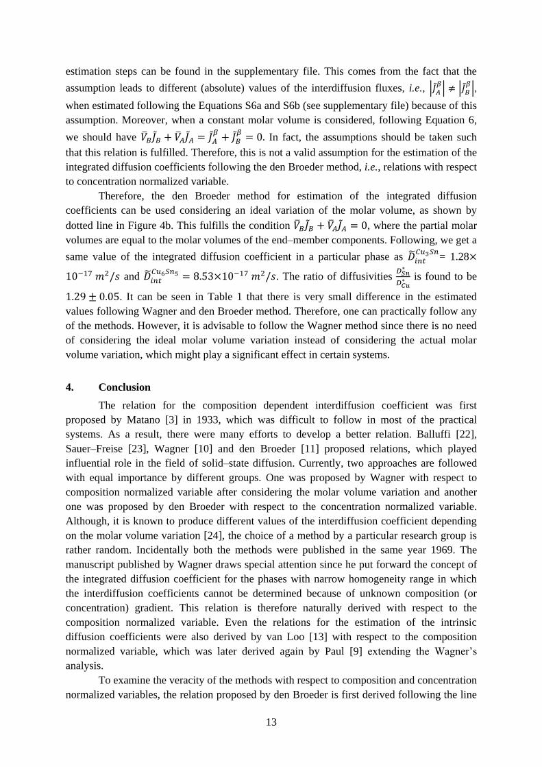
the Ni–Pd system [20]. The interdiffusion zone developed after annealing Ni and Pd at 1100
°C for 196 hrs is shown in Figure 1a. The location of the Kirkendall marker plane is
10
identified by the ThO2 particles, at 40.3 at% Ni. The composition profile developed in the
interdiffusion zone is shown in Figure 1b. This is measured in a direction perpendicular to the
Kirkendall marker plane following the diffusion direction of the components. The variation
of molar volume used for the estimation of diffusion coefficients is shown in Figure 1c. The
partial molar volumes of the components at the composition of the Kirkendall marker plane
(𝑁𝑁𝑖𝐾 = 0.403) are shown. Since this diffusion couple is prepared with pure components as
the end–members, the composition normalized variables are the same as composition of the
respective components, as shown in Figure 1b. The concentration normalized variables for
component A and B are shown in Figure 1d. The estimated data are shown in Figure 2. To
compare the data, the different parts of the den Broeder’s and the Wagner’s relations are
plotted. Gradients of concentration normalized variable (𝑑𝑌𝐶𝐵
∗
𝑑𝑥) and composition normalized
variable (𝑑𝑌𝑁𝐵
∗
𝑑𝑥) are shown in Figure 2a. The bracketed terms [(1 − 𝑌𝐶𝐵
∗ ) ∫ 𝑌𝐶𝐵
𝑥∗
𝑥−∞ 𝑑𝑥 +
𝑌𝐶𝐵
∗ ∫ (1 − 𝑌𝐶𝐵)
𝑥+∞
𝑥∗ 𝑑𝑥] = 2𝑡×�̃�(𝑌𝐶𝐵
∗ )× (𝑑𝑌𝐶𝐵
∗
𝑑𝑥) and 𝑉𝑚
∗ [(1 − 𝑌𝑁𝐵
∗ ) ∫𝑌𝑁𝐵
𝑉𝑚𝑑𝑥
𝑥∗
𝑥−∞ +
𝑌𝑁𝐵
∗ ∫(1−𝑌𝑁𝐵
)
𝑉𝑚𝑑𝑥
𝑥+∞
𝑥∗ ] = 2𝑡×�̃�(𝑌𝑁𝐵
∗ )× (𝑑𝑌𝑁𝐵
∗
𝑑𝑥) are shown in Figure 2b. Following, �̃�(𝑌𝐶𝐵
∗ )
and �̃�(𝑌𝑁𝐵
∗ ) are shown in Figure 2c. As expected based on the definition of terms 𝑌𝐶𝐵 and
𝑌𝑁𝐵, although there is difference in the slope and the bracket terms; however, a very minor
difference in the estimated diffusion coefficients with respect to 𝑌𝐶𝐵 and 𝑌𝑁𝐵
is evident.
Following, the intrinsic diffusion coefficients of components following den Broeder
and Wagner methods are estimated. Since pure end–members are used, considering the
composition profile in Figure 1b, we can write 𝑁𝐵−(= 𝑁𝑁𝑖
− ) = 0, 𝑁𝐴+(= 𝑁𝑃𝑑
+ ) = 0, 𝑁𝐵+(=
𝑁𝑁𝑖+ ) = 1, and 𝑁𝐴
−(= 𝑁𝑃𝑑− ) = 1. Therefore, we have 𝐶𝐴
−(= 𝐶𝑃𝑑− ) =
𝑁𝑃𝑑−
𝑉𝑚− =
1
𝑉𝑃𝑑, 𝐶𝐵
−(= 𝐶𝑁𝑖− ) =
𝑁𝑁𝑖−
𝑉𝑚− =
0
𝑉𝑃𝑑= 0, 𝐶𝐴
+(= 𝐶𝑃𝑑+ ) =
𝑁𝑃𝑑+
𝑉𝑚+ =
0
𝑉𝑁𝑖= 0 and 𝐶𝐵
+(= 𝐶𝑁𝑖+ ) =
𝑁𝑁𝑖+
𝑉𝑚+ =
1
𝑉𝑁𝑖. Therefore, we can
simplify the Equation 29a, b and c in the case of Ni–Pd diffusion couple as
𝐷𝐵(= 𝐷𝑁𝑖) =1
2𝑡(
𝜕𝑥
𝜕𝐶𝐵)
𝐾[𝐶𝐵
+ ∫ 𝑌𝐶𝐵
𝑥𝐾
𝑥−∞ 𝑑𝑥] =1
2𝑡(
𝜕𝑥
𝜕𝐶𝑁𝑖)
𝐾[
1
𝑉𝑁𝑖∫ 𝑌𝐶𝑁𝑖
𝑥𝐾
𝑥−∞ 𝑑𝑥] = 2.6×10⁻¹⁴ 𝑚2/𝑠,
𝐷𝐴(= 𝐷𝑃𝑑) =1
2𝑡(
𝜕𝑥
𝜕𝐶𝐴)
𝐾[(
1−�̅�𝐵𝐾𝐶𝐵
+
�̅�𝐴𝐾 ) ∫ 𝑌𝐶𝐵
𝑥𝐾
𝑥−∞ 𝑑𝑥 − (1
�̅�𝐴𝐾) ∫ (1 − 𝑌𝐶𝐵
)𝑥+∞
𝑥𝐾 𝑑𝑥] =
1
2𝑡(
𝜕𝑥
𝜕𝐶𝑃𝑑)
𝐾[(
1−�̅�𝑁𝑖
𝐾
𝑉𝑁𝑖
�̅�𝑃𝑑𝐾 ) ∫ 𝑌𝐶𝑁𝑖
𝑥𝐾
𝑥−∞ 𝑑𝑥 − (1
�̅�𝑃𝑑𝐾 ) ∫ (1 − 𝑌𝐶𝑁𝑖
)𝑥+∞
𝑥𝐾 𝑑𝑥] = 5.2×10⁻¹⁴ 𝑚2/𝑠,
𝐷𝐴(= 𝐷𝑃𝑑) =1
2𝑡(
𝜕𝑥
𝜕𝐶𝐴)
𝐾[𝐶𝐴
− ∫ 𝑌𝐶𝐴
𝑥𝐾
𝑥+∞ 𝑑𝑥] =1
2𝑡(
𝜕𝑥
𝜕𝐶𝑃𝑑)
𝐾[
1
𝑉𝑃𝑑∫ 𝑌𝐶𝑃𝑑
𝑥𝐾
𝑥+∞ 𝑑𝑥] = 4.9×10⁻¹⁴ 𝑚2/𝑠.
The same can be estimated following the Wagner’s method modifying the Equations 30a and
b for the Ni–Pd diffusion couple at the Kirkendall marker plane as
𝐷𝐵(= 𝐷𝑁𝑖) =1
2𝑡(
𝜕𝑥
𝜕𝐶𝐵)
𝐾[∫
𝑌𝑁𝐵
𝑉𝑚𝑑𝑥
𝑥𝐾
𝑥−∞ ] =1
2𝑡(
𝜕𝑥
𝜕𝐶𝑁𝑖)
𝐾[∫
𝑌𝑁𝑁𝑖
𝑉𝑚𝑑𝑥
𝑥𝐾
𝑥−∞ ] = 2.6×10⁻¹⁴ 𝑚2/𝑠,
𝐷𝐴(= 𝐷𝑃𝑑) =1
2𝑡(
𝜕𝑥
𝜕𝐶𝐴)
𝐾[− ∫
(1−𝑌𝑁𝐵)
𝑉𝑚𝑑𝑥
𝑥+∞
𝑥𝐾 ] =1
2𝑡(
𝜕𝑥
𝜕𝐶𝑃𝑑)
𝐾[− ∫
(1−𝑌𝑁𝑁𝑖)
𝑉𝑚𝑑𝑥
𝑥+∞
𝑥𝐾 ] =
4.9×10⁻¹⁴ 𝑚2/𝑠.
11
Therefore, there is no difference in the estimated intrinsic diffusion coefficients following
den Broeder and Wagner methods. A small difference in values of intrinsic diffusion
coefficient of Pd is found following the den Broeder method when estimated with respect to
𝑌𝐶𝑁𝑖 and 𝑌𝐶𝑃𝑑
. This must be because of error associated with the calculation of partial molar
volumes while estimating the data utilizing 𝑌𝐶𝑁𝑖.
Following, we estimate the interdiffusion coefficients in the –NiAl phase. The
composition profile of a diffusion couple Ni0.46Al0.54 / Ni0.575Al0.425 after annealing at 1200 °C
for 24 hrs is shown in Figure 3a. The molar volume variation in this intermetallic compound
is shown in Figure 3b [9]. The estimated interdiffusion coefficients by two methods are
shown in Figure 3c. The difference between the data estimated using both the methods in this
system is higher compared to the Ni–Pd system.
3. Integrated Interdiffusion Coefficient
Wagner, in his seminal contribution [10], introduced the concept of the integrated
interdiffusion coefficient in a phase with narrow homogeneity range since the
concentration/composition gradient in such a phase cannot be determined. This is expressed
with respect to 𝑌𝑁𝐵 or 𝑁𝐵 as
�̃�𝑖𝑛𝑡𝛽
= 𝑉𝑚𝛽
∆𝑥𝛽 (𝑁𝐵
+ − 𝑁𝐵−
2𝑡) [
𝑌𝑁𝐵
𝛽(1 − 𝑌𝑁𝐵
𝛽)
𝑉𝑚𝛽
∆𝑥𝛽 + (1 − 𝑌𝑁𝐵
𝛽) ∫
𝑌𝑁𝐵
𝑉𝑚
𝑥𝛽1
𝑥−∞
𝑑𝑥 + 𝑌𝑁𝐵
𝛽∫
(1 − 𝑌𝑁𝐵)
𝑉𝑚
𝑥+∞
𝑥𝛽2
𝑑𝑥]
(33a)
�̃�𝑖𝑛𝑡𝛽
=(𝑁𝐵
𝛽− 𝑁𝐵
−)(𝑁𝐵+ − 𝑁𝐵
𝛽)
(𝑁𝐵+ − 𝑁𝐵
−)
(∆𝑥𝛽)
2𝑡
2
+𝑉𝑚
𝛽∆𝑥𝛽
2𝑡[(𝑁𝐵
+ − 𝑁𝐵𝛽
)
(𝑁𝐵+ − 𝑁𝐵
−)∫
(𝑁𝐵 − 𝑁𝐵−)
𝑉𝑚
𝑑𝑥
𝑥𝛽1
𝑥−∞
+(𝑁𝐵
𝛽− 𝑁𝐵
−)
(𝑁𝐵+ − 𝑁𝐵
−)∫
(𝑁𝐵+ − 𝑁𝐵)
𝑉𝑚
𝑑𝑥
𝑥+∞
𝑥𝛽2
]
(33b)
At present, the relation to estimate the same diffusion parameter with respect to 𝑌𝐶𝐵 or 𝐶𝐵 is
not available. Therefore, as given in the supplementary file, we derived this relation by
extending the den Broeder’s relation for the interdiffusion coefficient. This is expressed with
respect to 𝑌𝐶𝐵 or 𝐶𝐵 as
�̃�𝑖𝑛𝑡𝛽
=(𝑉𝑚
𝛽)
2
�̅�𝐴𝛽 ∆𝑥𝛽 (
𝐶𝐵+−𝐶𝐵
−
2𝑡) [𝑌𝐶𝐵
𝛽(1 − 𝑌𝐶𝐵
𝛽)∆𝑥𝛽 + (1 − 𝑌𝐶𝐵
𝛽) ∫ 𝑌𝐶𝐵
𝑥𝛽1
𝑥−∞ 𝑑𝑥 + 𝑌𝐶𝐵
𝛽∫ (1 −
𝑥+∞
𝑥𝛽2
𝑌𝐶𝐵) 𝑑𝑥] (34a)
�̃�𝑖𝑛𝑡𝛽
=(𝑉𝑚
𝛽)
2
�̅�𝐴𝛽
(𝐶𝐵𝛽
−𝐶𝐵−)(𝐶𝐵
+−𝐶𝐵𝛽
)
(𝐶𝐵+−𝐶𝐵
−)
(∆𝑥𝛽)2
2𝑡+
(𝑉𝑚𝛽
)2
�̅�𝐴𝛽
∆𝑥𝛽
2𝑡[
𝐶𝐵+−𝐶𝐵
𝛽
𝐶𝐵+−𝐶𝐵
− ∫ (𝐶𝐵 − 𝐶𝐵−)
𝑥𝛽1
𝑥−∞ 𝑑𝑥 +
𝐶𝐵𝛽
−𝐶𝐵−
𝐶𝐵+−𝐶𝐵
− ∫ (𝐶𝐵+ − 𝐶𝐵)
𝑥+∞
𝑥𝛽2𝑑𝑥]
(34b)
12
It can be seen that an additional term of partial molar volume is present in the relation
expressed with respect to 𝑌𝐶𝐵 or 𝐶𝐵 as compared to the relation expressed with respect to 𝑌𝑁𝐵
or 𝑁𝐵.
Now we compare the efficiencies and difficulties of estimation of the data utilizing the
growth of the product phases, as shown in Figure 4a, in the Cu–Sn system. The Cu/Sn
diffusion couple was annealed at 200 °C for 81 hrs (i.e., 2𝑡 = 2×81×3600 s) in which two
phases Cu3Sn and Cu6Sn5 grows in the interdiffusion zone [16]. The average thicknesses of
the phases are estimated as 3.5 m (= ∆𝑥𝐶𝑢3𝑆𝑛) for Cu3Sn and 13 m (= ∆𝑥𝐶𝑢6𝑆𝑛5) for
Cu6Sn5. The marker plane, detected by the presence of duplex morphology, in the Cu6Sn5
phase is found at a distance of 7m from the Cu3Sn/Cu6Sn5 interface. The actual molar
volumes of these phases are estimated as 𝑉𝑚𝐶𝑢3𝑆𝑛
= 8.59×10⁻⁶ and 𝑉𝑚𝐶𝑢6𝑆𝑛5 = 10.59×10⁻⁶
m3/mol. From the knowledge of the molar volumes of the end–member components 𝑉𝑚− =
𝑉𝑚𝐶𝑢 = 7.12×10⁻⁶ and 𝑉𝑚
+ = 𝑉𝑚𝑆𝑛 = 16.24×10⁻⁶ m3/mol, we can estimate the ideal molar
volume of the product phase of interest (𝛽) following the Vegard’s law 𝑉𝑚𝛽
= 𝑁𝐶𝑢𝛽
𝑉𝑚𝐶𝑢 +
𝑁𝑆𝑛𝛽
𝑉𝑚𝑆𝑛. This is estimated as 𝑉𝑚
𝐶𝑢3𝑆𝑛(𝑖𝑑𝑒𝑎𝑙) = 9.4×10⁻⁶ m3/mol for the Cu3Sn phase
(𝑁𝐶𝑢𝐶𝑢3𝑆𝑛
=3
4, 𝑁𝑆𝑛
𝐶𝑢3𝑆𝑛=
1
4) and 𝑉𝑚
𝐶𝑢6𝑆𝑛5(𝑖𝑑𝑒𝑎𝑙) = 11.3×10⁻⁶ m3/mol for the Cu6Sn5 phase
(𝑁𝐶𝑢𝐶𝑢6𝑆𝑛5 =
6
11, 𝑁𝑆𝑛
𝐶𝑢6𝑆𝑛5 =5
11). Therefore, as shown in Figure 4b, the negative deviations of
the molar volumes are 8.6% for the Cu3Sn phase and 6.3% for the Cu6Sn5 phase.
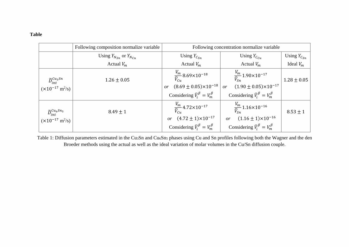
The detailed estimation procedure following the Wagner method can be found in
books as mentioned in Refs. [1, 21]. As explained in detail in the supplementary file, the
integrated diffusion coefficients of the phases following this method are estimated as
�̃�𝑖𝑛𝑡𝐶𝑢3𝑆𝑛
= 1.26 × 10⁻¹⁷ 𝑚2/𝑠 and �̃�𝑖𝑛𝑡𝐶𝑢6𝑆𝑛5 = 8.49 × 10⁻¹⁷ 𝑚2/𝑠. As it should be, the same
values are estimated considering the components A and B following Equations S10 or S11 in
the supplementary file. The ratio of diffusivities in the Cu6Sn5 phase is estimated as 𝐷𝑆𝑛
∗
𝐷𝐶𝑢∗ =
1.30 ± 0.05. It should be noted here that a different value of this ratio was reported in Ref.
[16], which was an average of data estimated at different locations in different diffusion
couples, compared to the data reported in this study estimated based on the micrograph, as
shown in Figure 4a.
Compared to the Wagner method (Equations S10 or S11 in the supplementary file),
den Broeder method (Equations S7 or S8 in the supplementary file) has an additional
complication because of the presence of partial molar volume terms in them. In a compound
with narrow homogeneity range, the variation of the lattice parameter with respect to the
composition is not known. The variation in such a small composition range might be small;
however, the difference between the partial molar volumes could still be very high. To
circumvent this problem, there could be two options: (i) consider 𝑉𝑚𝛽
= �̅�𝐴𝛽
= �̅�𝐵𝛽
, i.e., a
constant molar volume in the phase of interest or (ii) an ideal variation of the molar volume
in the whole A–B system. To discuss the pros and cons of these two assumptions, we extend
our analysis based on the estimated data in the Cu–Sn system. Following the first assumption,
as listed in column number 2 and 3 of Table 1, we estimate two different values of the data
when estimated following the composition/concentration profile of component A and B. The
13
estimation steps can be found in the supplementary file. This comes from the fact that the
assumption leads to different (absolute) values of the interdiffusion fluxes, i.e., |𝐽𝐴𝛽
| ≠ |𝐽𝐵𝛽
|,
when estimated following the Equations S6a and S6b (see supplementary file) because of this
assumption. Moreover, when a constant molar volume is considered, following Equation 6,
we should have �̅�𝐵𝐽𝐵 + �̅�𝐴𝐽𝐴 = 𝐽𝐴𝛽
+ 𝐽𝐵𝛽
= 0. In fact, the assumptions should be taken such
that this relation is fulfilled. Therefore, this is not a valid assumption for the estimation of the
integrated diffusion coefficients following the den Broeder method, i.e., relations with respect
to concentration normalized variable.
Therefore, the den Broeder method for estimation of the integrated diffusion
coefficients can be used considering an ideal variation of the molar volume, as shown by
dotted line in Figure 4b. This fulfills the condition �̅�𝐵𝐽𝐵 + �̅�𝐴𝐽𝐴 = 0, where the partial molar
volumes are equal to the molar volumes of the end–member components. Following, we get a
same value of the integrated diffusion coefficient in a particular phase as �̃�𝑖𝑛𝑡𝐶𝑢3𝑆𝑛
= 1.28×
10−17 𝑚2/𝑠 and �̃�𝑖𝑛𝑡𝐶𝑢6𝑆𝑛5 = 8.53×10⁻¹⁷ 𝑚2/𝑠. The ratio of diffusivities
𝐷𝑆𝑛∗
𝐷𝐶𝑢∗ is found to be
1.29 ± 0.05. It can be seen in Table 1 that there is very small difference in the estimated
values following Wagner and den Broeder method. Therefore, one can practically follow any
of the methods. However, it is advisable to follow the Wagner method since there is no need
of considering the ideal molar volume variation instead of considering the actual molar
volume variation, which might play a significant effect in certain systems.
4. Conclusion
The relation for the composition dependent interdiffusion coefficient was first
proposed by Matano [3] in 1933, which was difficult to follow in most of the practical
systems. As a result, there were many efforts to develop a better relation. Balluffi [22],
Sauer–Freise [23], Wagner [10] and den Broeder [11] proposed relations, which played
influential role in the field of solid–state diffusion. Currently, two approaches are followed
with equal importance by different groups. One was proposed by Wagner with respect to
composition normalized variable after considering the molar volume variation and another
one was proposed by den Broeder with respect to the concentration normalized variable.
Although, it is known to produce different values of the interdiffusion coefficient depending
on the molar volume variation [24], the choice of a method by a particular research group is
rather random. Incidentally both the methods were published in the same year 1969. The
manuscript published by Wagner draws special attention since he put forward the concept of
the integrated diffusion coefficient for the phases with narrow homogeneity range in which
the interdiffusion coefficients cannot be determined because of unknown composition (or
concentration) gradient. This relation is therefore naturally derived with respect to the
composition normalized variable. Even the relations for the estimation of the intrinsic
diffusion coefficients were also derived by van Loo [13] with respect to the composition
normalized variable, which was later derived again by Paul [9] extending the Wagner’s
analysis.
To examine the veracity of the methods with respect to composition and concentration
normalized variables, the relation proposed by den Broeder is first derived following the line
14
of treatment followed by Wagner. Following, this is extended to derive the relations for the
intrinsic diffusion coefficients and the integrated diffusion coefficients to develop the
relations with respect to the concentration normalized variable, which were not available
earlier. We have shown further that an additional assumption of the ideal molar volume
variation is required for the estimation of the integrated diffusion coefficient with respect to
the concentration normalized variable when compared to the relation developed by Wagner
with respect to the composition normalized variable, which can be used with actual molar
volume variation.
Acknowledgement
We acknowledge the financial support from ARDB, India (Project number
ARDB/GTMAP/01/2031786/M/1, DT. 11/1/2016).
References
[1] A. Paul, T. Laurila, V. Vuorinen, S.V. Divinski, Thermodynamics, Diffusion and the
Kirkendall Effect in Solids, 1st ed., Springer, Switzerland, 2014.
[2] A. Kodentsov, A. Paul, Chapter 6 - Diffusion Couple Technique: A Research Tool in
Materials Science, Handbook of Solid State Diffusion, Editors: A. Paul and S. Divinsky,
Volume 2: Diffusion Analysis and Material Applications, Elsevier 2017, pp. 207-275.
[3] C. Matano, On the relation between the diffusion-coefficients and concentrations of
solid metals (the nickel-copper system), Japanese Journal of Physics 8 (1933) 109-113.
[4] A. Fick, Ueber Diffusion, Annalen der Physik 170 (1855) 59-86.
[5] L. Boltzmann, Zur Integration der Diffusionsgleichung bei variabeln Diffusions-
coefficienten, Annalen der Physik 289 (1894) 959-964.
[6] L.S. Darken, Diffusion, Mobility and Their Interrelation through Free Energy in
Binary Metallic Systems, Transactions of the American Institute of Mining and Metallurgical
Engineers 175 (1948) 184-201.
[7] J.R. Manning, Diffusion and the Kirkendall shift in binary alloys, Acta Metallurgica
15 (1967) 817-826.
[8] A.D. Smigelskas, E.O. Kirkendall, Zinc Diffusion in Alpha-Brass, Transactions of the
American Institute of Mining and Metallurgical Engineers 171 (1947) 130-142.
[9] A. Paul, PhD Thesis, The Kirkendall effect in solid state diffusion, Eindhoven
University of Technology, The Netherlands, 2004. Available at
alexandria.tue.nl/extra2/200412361.pdf.
[10] C. Wagner, The evaluation of data obtained with diffusion couples of binary single-
phase and multiphase systems, Acta Metallurgica 17 (1969) 99-107.
[11] F.J.A. den Broeder, A general simplification and improvement of the Matano-
Boltzmann method in the determination of the interdiffusion coefficients in binary systems,
Scripta Metallurgica 3 (1969) 321-325.
[12] F.J.J. Van Loo, On the determination of diffusion coefficients in a binary metal
system, Acta Metallurgica 18 (1970) 1107-1111.
[13] F.J.J. van Loo, Multiphase diffusion in binary and ternary solid-state systems,
Progress in Solid State Chemistry 20 (1990) 47-99.
15
[14] V.A. Baheti, S. Roy, R. Ravi, A. Paul, Interdiffusion and the phase boundary
compositions in the Co–Ta system, Intermetallics 33 (2013) 87-91.
[15] V.A. Baheti, R. Ravi, A. Paul, Interdiffusion study in the Pd–Pt system, Journal of
Materials Science: Materials in Electronics 24 (2013) 2833-2838.
[16] V.A. Baheti, S. Kashyap, P. Kumar, K. Chattopadhyay, A. Paul, Bifurcation of the
Kirkendall marker plane and the role of Ni and other impurities on the growth of Kirkendall
voids in the Cu–Sn system, Acta Materialia 131 (2017) 260-270.
[17] V.A. Baheti, S. Kashyap, P. Kumar, K. Chattopadhyay, A. Paul, Solid–state
diffusion–controlled growth of the phases in the Au–Sn system, Philosophical Magazine
98(1) (2018) 20-36.
[18] A. Paul, C. Ghosh, W.J. Boettinger, Diffusion Parameters and Growth Mechanism of
Phases in the Cu–Sn System, Metallurgical and Materials Transactions A 42 (2011) 952-963.
[19] A. Paul, Comments on “Sluggish diffusion in Co–Cr–Fe–Mn–Ni high-entropy alloys”
by K.Y. Tsai, M.H. Tsai and J.W. Yeh, Acta Materialia 61 (2013) 4887–4897, Scripta
Materialia 135 (2017) 153-157.
[20] M.J.H. van Dal, PhD Thesis, Microstructural stability of the Kirkendall plane,
Eindhoven University of Technology, The Netherlands, 2001.
[21] A. Paul, Chapter 3 - Estimation of Diffusion Coefficients in Binary and Pseudo-
Binary Bulk Diffusion Couples, in: Handbook of Solid State Diffusion, Editors: A. Paul and
S. Divinsky, Volume 1: Diffusion Fundamentals and Techniques, Elsevier 2017, pp. 79-201.
[22] R.W. Balluffi, On the determination of diffusion coefficients in chemical diffusion,
Acta Metallurgica 8 (1960) 871-873.
[23] F. Sauer, V. Freise, Diffusion in binären Gemischen mit Volumenänderung,
Zeitschrift für Elektrochemie, Berichte der Bunsengesellschaft für physikalische Chemie 66
(1962) 353-362.
[24] S. Santra, A. Paul, Role of the Molar Volume on Estimated Diffusion Coefficients,
Metallurgical and Materials Transactions A 46 (2015) 3887-3899.
Figure 1: (a) Micrograph of the Ni/Pd diffusion couple annealed at 1100 °C for 196 hrs [20].
ThO2 particles identifies the location of the Kirkendall marker plane, (b) the corresponding
composition profile [20] (equal to the composition normalize variable, 𝑌𝑁𝐵) developed in the
interdiffusion zone, (c) Molar volume variation in the Ni–Pd solid solution [20], (d) the
concentration normalized variables.
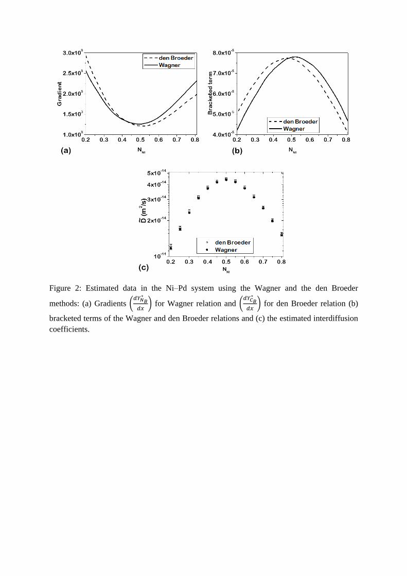
Figure 2: Estimated data in the Ni–Pd system using the Wagner and the den Broeder
methods: (a) Gradients (𝑑𝑌𝑁𝐵
∗
𝑑𝑥) for Wagner relation and (
𝑑𝑌𝐶𝐵∗
𝑑𝑥) for den Broeder relation (b)
bracketed terms of the Wagner and den Broeder relations and (c) the estimated interdiffusion
coefficients.
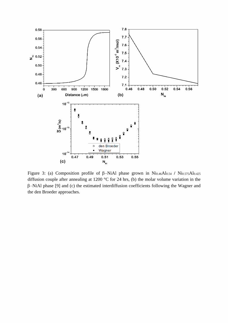
Figure 3: (a) Composition profile of –NiAl phase grown in Ni0.46Al0.54 / Ni0.575Al0.425
diffusion couple after annealing at 1200 °C for 24 hrs, (b) the molar volume variation in the
–NiAl phase [9] and (c) the estimated interdiffusion coefficients following the Wagner and
the den Broeder approaches.
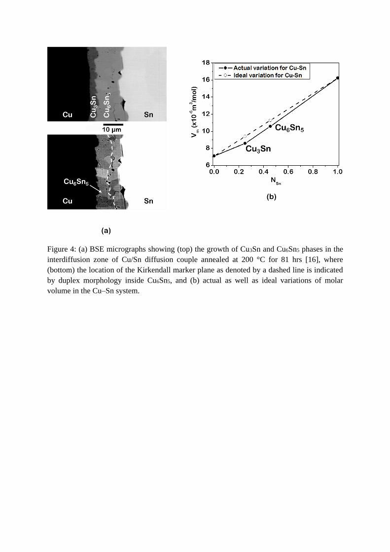
Figure 4: (a) BSE micrographs showing (top) the growth of Cu3Sn and Cu6Sn5 phases in the
interdiffusion zone of Cu/Sn diffusion couple annealed at 200 °C for 81 hrs [16], where
(bottom) the location of the Kirkendall marker plane as denoted by a dashed line is indicated
by duplex morphology inside Cu6Sn5, and (b) actual as well as ideal variations of molar
volume in the Cu–Sn system.
Table
Following composition normalize variable Following concentration normalize variable
Using 𝑌𝑁𝑆𝑛 or 𝑌𝑁𝐶𝑢
Actual 𝑉𝑚
Using 𝑌𝐶𝑆𝑛
Actual 𝑉𝑚
Using 𝑌𝐶𝐶𝑢
Actual 𝑉𝑚
Using 𝑌𝐶𝑆𝑛
Ideal 𝑉𝑚
�̃�𝑖𝑛𝑡𝐶𝑢3𝑆𝑛
(×10−17 m2/s)
1.26 ± 0.05
𝑉𝑚�̅�𝐶𝑢
8.69×10⁻¹⁸
or (8.69 ± 0.05)×10−18
Considering �̅�𝑖𝛽= 𝑉𝑚
𝛽
𝑉𝑚�̅�𝑆𝑛
1.90×10⁻¹⁷
or (1.90 ± 0.05)×10−17
Considering �̅�𝑖𝛽= 𝑉𝑚
𝛽
1.28 ± 0.05
�̃�𝑖𝑛𝑡𝐶𝑢6𝑆𝑛5
(×10−17 m2/s)
8.49 ± 1
𝑉𝑚�̅�𝐶𝑢
4.72×10⁻¹⁷
or (4.72 ± 1)×10−17
Considering �̅�𝑖𝛽= 𝑉𝑚
𝛽
𝑉𝑚�̅�𝑆𝑛
1.16×10⁻¹⁶
or (1.16 ± 1)×10−16
Considering �̅�𝑖𝛽= 𝑉𝑚
𝛽
8.53 ± 1
Table 1: Diffusion parameters estimated in the Cu3Sn and Cu6Sn5 phases using Cu and Sn profiles following both the Wagner and the den
Broeder methods using the actual as well as the ideal variation of molar volumes in the Cu/Sn diffusion couple.
Supplementary File
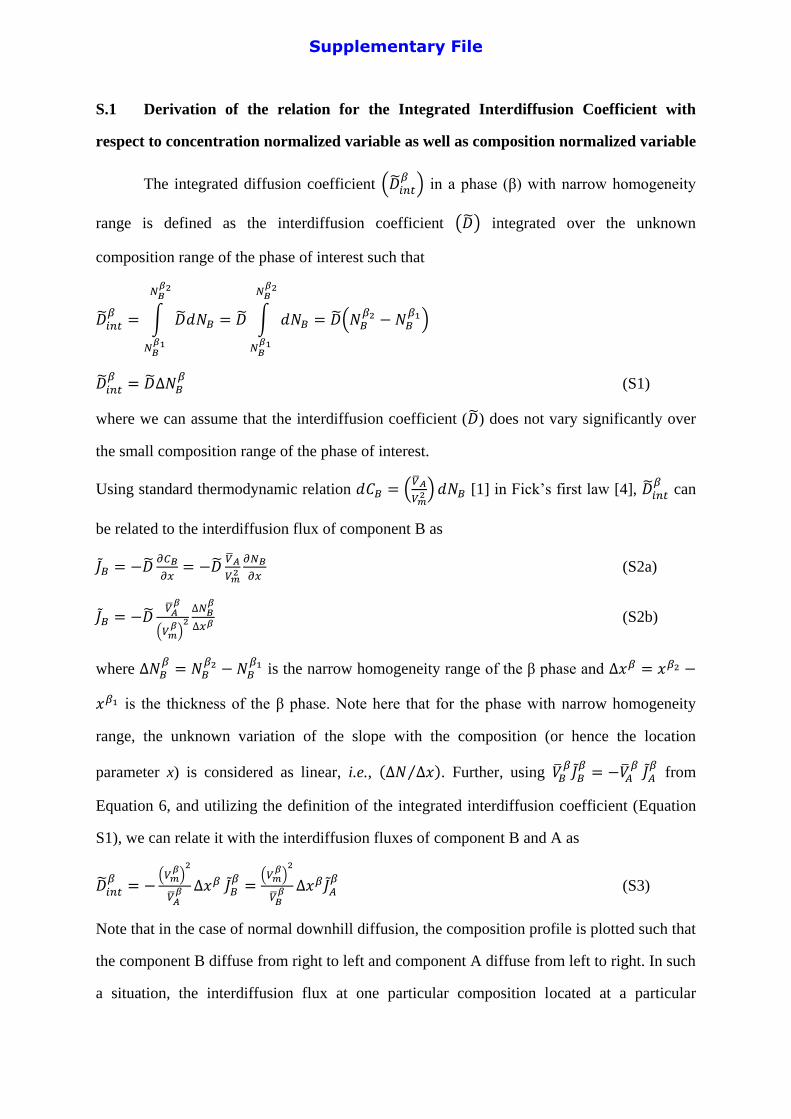
S.1 Derivation of the relation for the Integrated Interdiffusion Coefficient with
respect to concentration normalized variable as well as composition normalized variable
The integrated diffusion coefficient (�̃�𝑖𝑛𝑡𝛽
) in a phase (β) with narrow homogeneity
range is defined as the interdiffusion coefficient (�̃�) integrated over the unknown
composition range of the phase of interest such that
�̃�𝑖𝑛𝑡𝛽
= ∫ �̃�𝑑𝑁𝐵
𝑁𝐵𝛽2
𝑁𝐵𝛽1
= �̃� ∫ 𝑑𝑁𝐵
𝑁𝐵𝛽2
𝑁𝐵𝛽1
= �̃�(𝑁𝐵𝛽2 − 𝑁𝐵
𝛽1)
�̃�𝑖𝑛𝑡𝛽
= �̃�∆𝑁𝐵𝛽
(S1)
where we can assume that the interdiffusion coefficient (�̃�) does not vary significantly over
the small composition range of the phase of interest.
Using standard thermodynamic relation 𝑑𝐶𝐵 = (�̅�𝐴
𝑉𝑚2 ) 𝑑𝑁𝐵 [1] in Fick’s first law [4], �̃�𝑖𝑛𝑡
𝛽 can
be related to the interdiffusion flux of component B as
𝐽𝐵 = −�̃�𝜕𝐶𝐵
𝜕𝑥= −�̃�
�̅�𝐴
𝑉𝑚2
𝜕𝑁𝐵
𝜕𝑥 (S2a)
𝐽𝐵 = −�̃��̅�𝐴
𝛽
(𝑉𝑚𝛽
)2
∆𝑁𝐵𝛽
∆𝑥𝛽 (S2b)
where ∆𝑁𝐵𝛽
= 𝑁𝐵𝛽2 − 𝑁𝐵
𝛽1 is the narrow homogeneity range of the β phase and ∆𝑥𝛽 = 𝑥𝛽2 −
𝑥𝛽1 is the thickness of the β phase. Note here that for the phase with narrow homogeneity
range, the unknown variation of the slope with the composition (or hence the location
parameter x) is considered as linear, i.e., (∆𝑁 ∆𝑥⁄ ). Further, using �̅�𝐵𝛽
𝐽𝐵𝛽
= −�̅�𝐴𝛽
𝐽𝐴𝛽
from
Equation 6, and utilizing the definition of the integrated interdiffusion coefficient (Equation
S1), we can relate it with the interdiffusion fluxes of component B and A as
�̃�𝑖𝑛𝑡𝛽
= −(𝑉𝑚
𝛽)
2
�̅�𝐴𝛽 ∆𝑥𝛽 𝐽𝐵
𝛽=
(𝑉𝑚𝛽
)2
�̅�𝐵𝛽 ∆𝑥𝛽𝐽𝐴
𝛽 (S3)
Note that in the case of normal downhill diffusion, the composition profile is plotted such that
the component B diffuse from right to left and component A diffuse from left to right. In such
a situation, the interdiffusion flux at one particular composition located at a particular
Supplementary File
location of the diffusion couple after annealing for time 𝑡, 𝐽𝐵 will have a negative sign and 𝐽𝐴
will have a positive sign leading equal and positive value of �̃�𝑖𝑛𝑡𝛽
irrespective of the
composition profile considered for the estimation. With respect the concentration profiles of
components B and A, following the Equations 20, we have
𝐽𝐵𝛽
= 𝐽𝐵(𝐶𝐵𝛽
) = − (𝐶𝐵
+−𝐶𝐵−
2𝑡) [(1 − 𝑌𝐶𝐵
𝛽) ∫ 𝑌𝐶𝐵
𝑥∗
𝑥−∞ 𝑑𝑥 + 𝑌𝐶𝐵
𝛽∫ (1 − 𝑌𝐶𝐵
)𝑥+∞
𝑥∗ 𝑑𝑥] (S4a)
𝐽𝐴𝛽
= 𝐽𝐴(𝐶𝐴𝛽
) = − (𝐶𝐴
−−𝐶𝐴+
2𝑡) [(1 − 𝑌𝐶𝐴
𝛽) ∫ 𝑌𝐶𝐴
𝑥∗
𝑥+∞ 𝑑𝑥 + 𝑌𝐶𝐴
𝛽∫ (1 − 𝑌𝐶𝐴
)𝑥−∞
𝑥∗ 𝑑𝑥] (S4b)
where 𝑌𝐶𝐵
𝛽=
𝐶𝐵𝛽
−𝐶𝐵−
𝐶𝐵+−𝐶𝐵
− and 𝑌𝐶𝐴
𝛽=
𝐶𝐴𝛽
−𝐶𝐴+
𝐶𝐴−−𝐶𝐴
+.
The term inside square bracket is separated into 3 parts in the interdiffusion zone as the
thickness related to the phase of interest and the other two parts for the interdiffusion zone
before and after that:
𝐽𝐵𝛽
= − (𝐶𝐵
+−𝐶𝐵−
2𝑡) [(1 − 𝑌𝐶𝐵
𝛽) ∫ 𝑌𝐶𝐵
𝑥𝛽1
𝑥−∞ 𝑑𝑥 + 𝑌𝐶𝐵
𝛽∫ (1 − 𝑌𝐶𝐵
)𝑥𝛽2
𝑥𝛽1𝑑𝑥 + 𝑌𝐶𝐵
𝛽∫ (1 − 𝑌𝐶𝐵
)𝑥+∞
𝑥𝛽2𝑑𝑥] (S5a)
𝐽𝐴𝛽
= − (𝐶𝐴
−−𝐶𝐴+
2𝑡) [(1 − 𝑌𝐶𝐴
𝛽) ∫ 𝑌𝐶𝐴
𝑥𝛽2
𝑥+∞ 𝑑𝑥 + 𝑌𝐶𝐴
𝛽∫ (1 − 𝑌𝐶𝐴
)𝑥𝛽1
𝑥𝛽2𝑑𝑥 + 𝑌𝐶𝐴
𝛽∫ (1 − 𝑌𝐶𝐴
)𝑥−∞
𝑥𝛽1𝑑𝑥] (S5b)
In the phase of interest 𝑌𝐶𝐵
𝛽 (or 𝑌𝐶𝐴
𝛽) is constant because of the growth of the phase with very
narrow homogeneity range, i.e., with almost a fixed composition 𝐶𝐵𝛽
(or 𝐶𝐴𝛽
). Therefore, after
rearranging, we can write
𝐽𝐵𝛽
= − (𝐶𝐵
+−𝐶𝐵−
2𝑡) [𝑌𝐶𝐵
𝛽(1 − 𝑌𝐶𝐵
𝛽) ∆𝑥𝛽 + (1 − 𝑌𝐶𝐵
𝛽) ∫ 𝑌𝐶𝐵
𝑥𝛽1
𝑥−∞ 𝑑𝑥 + 𝑌𝐶𝐵
𝛽∫ (1 − 𝑌𝐶𝐵
)𝑥+∞
𝑥𝛽2𝑑𝑥] (S6a)
𝐽𝐴𝛽
= (𝐶𝐴
−−𝐶𝐴+
2𝑡) [𝑌𝐶𝐴
𝛽(1 − 𝑌𝐶𝐴
𝛽)∆𝑥𝛽 + (1 − 𝑌𝐶𝐴
𝛽) ∫ 𝑌𝐶𝐴
𝑥+∞
𝑥𝛽2𝑑𝑥 + 𝑌𝐶𝐴
𝛽∫ (1 − 𝑌𝐶𝐴
)𝑥𝛽1
𝑥−∞ 𝑑𝑥] (S6b)
where ∆𝑥𝛽 = 𝑥𝛽2 − 𝑥𝛽1 is the thickness of the β phase. It should be noted there that the
minus sign in 𝐽𝐴𝛽
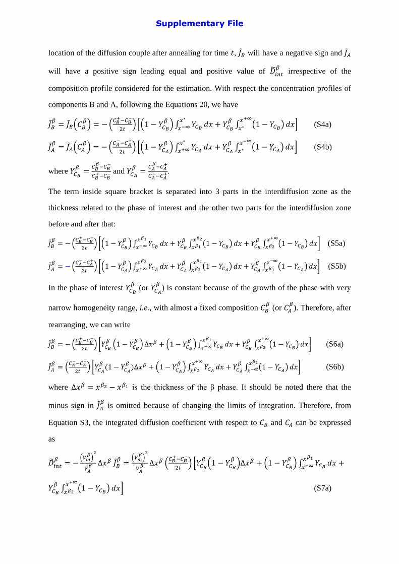
is omitted because of changing the limits of integration. Therefore, from
Equation S3, the integrated diffusion coefficient with respect to 𝐶𝐵 and 𝐶𝐴 can be expressed
as
�̃�𝑖𝑛𝑡𝛽
= −(𝑉𝑚
𝛽)
2
�̅�𝐴𝛽 ∆𝑥𝛽 𝐽𝐵
𝛽=
(𝑉𝑚𝛽
)2
�̅�𝐴𝛽 ∆𝑥𝛽 (
𝐶𝐵+−𝐶𝐵
−
2𝑡) [𝑌𝐶𝐵
𝛽(1 − 𝑌𝐶𝐵
𝛽)∆𝑥𝛽 + (1 − 𝑌𝐶𝐵
𝛽) ∫ 𝑌𝐶𝐵
𝑥𝛽1
𝑥−∞ 𝑑𝑥 +
𝑌𝐶𝐵
𝛽∫ (1 − 𝑌𝐶𝐵
)𝑥+∞
𝑥𝛽2𝑑𝑥] (S7a)
Supplementary File
�̃�𝑖𝑛𝑡𝛽
=(𝑉𝑚
𝛽)
2
�̅�𝐵𝛽 ∆𝑥𝛽𝐽𝐴
𝛽=
(𝑉𝑚𝛽
)2
�̅�𝐵𝛽 ∆𝑥𝛽 (
𝐶𝐴−−𝐶𝐴
+
2𝑡) [𝑌𝐶𝐴
𝛽(1 − 𝑌𝐶𝐴
𝛽)∆𝑥𝛽 + (1 − 𝑌𝐶𝐴
𝛽) ∫ 𝑌𝐶𝐴
𝑥+∞
𝑥𝛽2𝑑𝑥 +
𝑌𝐶𝐴
𝛽∫ (1 − 𝑌𝐶𝐴
)𝑥𝛽1
𝑥−∞ 𝑑𝑥] (S7b)
Further, expanding 𝑌𝐶𝐵 and 𝑌𝐶𝐴
(from Equation S4) with respect to 𝐶𝐵 and 𝐶𝐴, we get
�̃�𝑖𝑛𝑡𝛽
=(𝑉𝑚
𝛽)
2
�̅�𝐴𝛽
(𝐶𝐵𝛽
− 𝐶𝐵−)(𝐶𝐵
+ − 𝐶𝐵𝛽
)
(𝐶𝐵+ − 𝐶𝐵
−)
(∆𝑥𝛽)2
2𝑡
+(𝑉𝑚
𝛽)
2
�̅�𝐴𝛽
∆𝑥𝛽
2𝑡[𝐶𝐵
+ − 𝐶𝐵𝛽
𝐶𝐵+ − 𝐶𝐵
− ∫ (𝐶𝐵 − 𝐶𝐵−)
𝑥𝛽1
𝑥−∞
𝑑𝑥 +𝐶𝐵
𝛽− 𝐶𝐵
−
𝐶𝐵+ − 𝐶𝐵
− ∫ (𝐶𝐵+ − 𝐶𝐵)
𝑥+∞
𝑥𝛽2
𝑑𝑥]
(S8a)
�̃�𝑖𝑛𝑡𝛽
=(𝑉𝑚
𝛽)
2
�̅�𝐵𝛽
(𝐶𝐴𝛽
− 𝐶𝐴+)(𝐶𝐴
− − 𝐶𝐴𝛽
)
(𝐶𝐴− − 𝐶𝐴
+)
(∆𝑥𝛽)2
2𝑡
+(𝑉𝑚
𝛽)
2
�̅�𝐵𝛽
∆𝑥𝛽
2𝑡[𝐶𝐴
− − 𝐶𝐴𝛽
𝐶𝐴− − 𝐶𝐴
+ ∫ (𝐶𝐴 − 𝐶𝐴+)
𝑥+∞
𝑥𝛽2
𝑑𝑥 +𝐶𝐴
𝛽− 𝐶𝐴
+
𝐶𝐴− − 𝐶𝐴
+ ∫ (𝐶𝐴− − 𝐶𝐴)
𝑥𝛽1
𝑥−∞
𝑑𝑥]
(S8b)
Note that 𝐶𝐴 + 𝐶𝐵 =1
𝑉𝑚 and 𝐶𝐵
+ > 𝐶𝐵−, 𝐶𝐴
− > 𝐶𝐴+.
Therefore, Equations S7 or S8 are relations for the estimation of �̃�𝑖𝑛𝑡𝛽
with respect to 𝑌𝐶𝐵 (and
𝑌𝐶𝐴) or 𝐶𝐵 (and 𝐶𝐴), which was not available earlier. Previously, Wagner [10] derived the
relation with respect to 𝑌𝑁𝐵 or 𝑁𝐵 considering non–ideal variation of the molar volume,
which can be expressed as [1]
The interdiffusion fluxes from the composition profiles of components B and A are
𝐽𝐵𝛽
= −𝑉𝐴
𝛽
𝑉𝑚𝛽 (
𝑁𝐵+−𝑁𝐵
−
2𝑡) [
𝑌𝑁𝐵
𝛽(1−𝑌𝑁𝐵
𝛽)
𝑉𝑚𝛽 ∆𝑥𝛽 + (1 − 𝑌𝑁𝐵
𝛽) ∫
𝑌𝑁𝐵
𝑉𝑚
𝑥𝛽1
𝑥−∞ 𝑑𝑥 + 𝑌𝑁𝐵
𝛽∫
(1−𝑌𝑁𝐵)
𝑉𝑚
𝑥+∞
𝑥𝛽2𝑑𝑥] (S9a)
𝐽𝐴𝛽
=�̅�𝐵
𝛽
𝑉𝑚𝛽 (
𝑁𝐴−−𝑁𝐴
+
2𝑡) [
𝑌𝑁𝐴
𝛽(1−𝑌𝑁𝐴
𝛽)
𝑉𝑚𝛽 ∆𝑥𝛽 + (1 − 𝑌𝑁𝐴
𝛽) ∫
𝑌𝑁𝐴
𝑉𝑚
𝑥+∞
𝑥𝛽2𝑑𝑥 + 𝑌𝑁𝐴
𝛽∫
(1−𝑌𝑁𝐴)
𝑉𝑚
𝑥𝛽1
𝑥−∞ 𝑑𝑥] (S9b)
where 𝑌𝑁𝐵
𝛽=
𝑁𝐵𝛽
−𝑁𝐵−
𝑁𝐵+−𝑁𝐵
−. and 𝑌𝑁𝐴
𝛽=
𝑁𝐴𝛽
−𝑁𝐴+
𝑁𝐴−−𝑁𝐴
+.
Therefore, from Equation S3, the �̃�𝑖𝑛𝑡𝛽
with respect to 𝑁𝐵 and 𝑁𝐴 can be expressed as
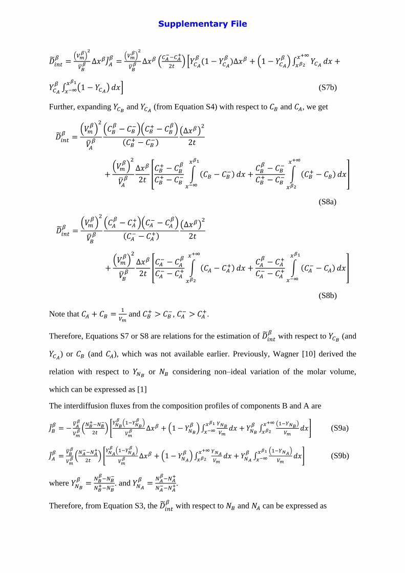
Supplementary File
�̃�𝑖𝑛𝑡𝛽
= −(𝑉𝑚
𝛽)
2
𝑉𝐴𝛽 ∆𝑥𝛽 𝐽𝐵
𝛽= 𝑉𝑚
𝛽∆𝑥𝛽 (
𝑁𝐵+−𝑁𝐵
−
2𝑡) [
𝑌𝑁𝐵
𝛽(1−𝑌𝑁𝐵
𝛽)
𝑉𝑚𝛽 ∆𝑥𝛽 + (1 − 𝑌𝑁𝐵
𝛽) ∫
𝑌𝑁𝐵
𝑉𝑚
𝑥𝛽1
𝑥−∞ 𝑑𝑥 +
𝑌𝑁𝐵
𝛽∫
(1−𝑌𝑁𝐵)
𝑉𝑚
𝑥+∞
𝑥𝛽2𝑑𝑥] (S10a)
�̃�𝑖𝑛𝑡𝛽
=(𝑉𝑚
𝛽)
2
𝑉𝐵𝛽 ∆𝑥𝛽𝐽𝐴
𝛽= 𝑉𝑚
𝛽∆𝑥𝛽 (
𝑁𝐴−−𝑁𝐴
+
2𝑡) [
𝑌𝑁𝐴
𝛽(1−𝑌𝑁𝐴
𝛽)
𝑉𝑚𝛽 ∆𝑥𝛽 + (1 − 𝑌𝑁𝐴
𝛽) ∫
𝑌𝑁𝐴
𝑉𝑚
𝑥+∞
𝑥𝛽2𝑑𝑥 +
𝑌𝑁𝐴
𝛽∫
(1−𝑌𝑁𝐴)
𝑉𝑚
𝑥𝛽1
𝑥−∞ 𝑑𝑥] (S10b)
Further, expanding 𝑌𝑁𝐵 and 𝑌𝑁𝐴
(from Equation S9) with respect to 𝑁𝐵 and 𝑁𝐴, we get
�̃�𝑖𝑛𝑡𝛽
=(𝑁𝐵
𝛽− 𝑁𝐵
−)(𝑁𝐵+ − 𝑁𝐵
𝛽)
(𝑁𝐵+ − 𝑁𝐵
−)
(∆𝑥𝛽)
2𝑡
2
+𝑉𝑚
𝛽∆𝑥𝛽
2𝑡[(𝑁𝐵
+ − 𝑁𝐵𝛽
)
(𝑁𝐵+ − 𝑁𝐵
−)∫
(𝑁𝐵 − 𝑁𝐵−)
𝑉𝑚
𝑑𝑥
𝑥𝛽1
𝑥−∞
+(𝑁𝐵
𝛽− 𝑁𝐵
−)
(𝑁𝐵+ − 𝑁𝐵
−)∫
(𝑁𝐵+ − 𝑁𝐵)
𝑉𝑚
𝑑𝑥
𝑥+∞
𝑥𝛽2
]
(S11a)
�̃�𝑖𝑛𝑡𝛽
=(𝑁𝐴
𝛽− 𝑁𝐴
+)(𝑁𝐴− − 𝑁𝐴
𝛽)
(𝑁𝐴− − 𝑁𝐴
+)
(∆𝑥𝛽)
2𝑡
2
+𝑉𝑚
𝛽∆𝑥𝛽
2𝑡[(𝑁𝐴
− − 𝑁𝐴𝛽
)
(𝑁𝐴− − 𝑁𝐴
+)∫
(𝑁𝐴 − 𝑁𝐴+)
𝑉𝑚
𝑑𝑥
𝑥+∞
𝑥𝛽2
+(𝑁𝐴
𝛽− 𝑁𝐴
+)
(𝑁𝐴− − 𝑁𝐴
+)∫
(𝑁𝐴− − 𝑁𝐴)
𝑉𝑚
𝑑𝑥
𝑥𝛽1
𝑥−∞
]
(S11b)
Note that 𝑁𝐴 + 𝑁𝐵 = 1 and 𝑁𝐵+ > 𝑁𝐵
−, 𝑁𝐴− > 𝑁𝐴
+. Equations S10 or S11 was derived by
Wagner [10], which is expressed with respect to 𝑌𝑁𝐵 (and 𝑌𝑁𝐴
) or 𝑁𝐵 (and 𝑁𝐴).
In an intermetallic compound with narrow homogeneity range, we cannot estimate the
composition or concentration gradients. Even we do not know the partial molar volumes of
the components in a phase. Therefore, instead of following the Equation 29b, we can estimate
the ratio of the tracer diffusion coefficients by neglecting the vacancy wind effect following
Equations 29a, c and 32 as
𝐷𝐵∗
𝐷𝐴∗ = [
𝐶𝐵+ ∫ 𝑌𝐶𝐵
𝑥𝐾
𝑥−∞ 𝑑𝑥−𝐶𝐵− ∫ (1−𝑌𝐶𝐵
)𝑥+∞
𝑥𝐾 𝑑𝑥
−𝐶𝐴− ∫ 𝑌𝐶𝐴
𝑥𝐾
𝑥+∞ 𝑑𝑥+𝐶𝐴+ ∫ (1−𝑌𝐶𝐴
)𝑥−∞
𝑥𝐾 𝑑𝑥] (S12)
Note here that the contribution of the vacancy wind effect does not contribute very
significantly in most of the systems and the difference in estimated data could fall within the
Supplementary File
limit of experimental error [1]. The same relation with respect to 𝑌𝑁𝐵 and 𝑁𝐵 (following
Equations 30 and 32) can be expressed as
𝐷𝐵∗
𝐷𝐴∗ = [
𝑁𝐵+ ∫
𝑌𝑁𝐵𝑉𝑚
𝑥𝐾
𝑥−∞ 𝑑𝑥−𝑁𝐵− ∫
(1−𝑌𝑁𝐵)
𝑉𝑚
𝑥+∞
𝑥𝐾 𝑑𝑥
−𝑁𝐴+ ∫
𝑌𝑁𝐵𝑉𝑚
𝑥𝐾
𝑥−∞ 𝑑𝑥+𝑁𝐴− ∫
(1−𝑌𝑁𝐵)
𝑉𝑚
𝑥+∞
𝑥𝐾 𝑑𝑥
] (S13)
Since these relations are free from partial molar volume terms, there data can be estimated
straightforwardly.
Estimation of the integrated diffusion coefficients following different methods in the
Cu–Sn system
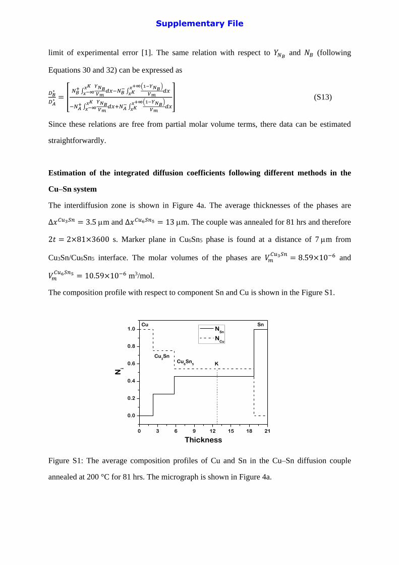
The interdiffusion zone is shown in Figure 4a. The average thicknesses of the phases are
∆𝑥𝐶𝑢3𝑆𝑛 = 3.5m and ∆𝑥𝐶𝑢6𝑆𝑛5 = 13 m. The couple was annealed for 81 hrs and therefore
2𝑡 = 2×81×3600 s. Marker plane in Cu6Sn5 phase is found at a distance of 7m from
Cu3Sn/Cu6Sn5 interface. The molar volumes of the phases are 𝑉𝑚𝐶𝑢3𝑆𝑛
= 8.59×10⁻⁶ and
𝑉𝑚𝐶𝑢6𝑆𝑛5 = 10.59×10⁻⁶ m3/mol.
The composition profile with respect to component Sn and Cu is shown in the Figure S1.
0 3 6 9 12 15 18 21
0.0
0.2
0.4
0.6
0.8
1.0
K
Ni
Thickness
NSn
NCu
Cu6Sn
5
Cu3Sn
Cu Sn
Figure S1: The average composition profiles of Cu and Sn in the Cu–Sn diffusion couple
annealed at 200 °C for 81 hrs. The micrograph is shown in Figure 4a.
Supplementary File
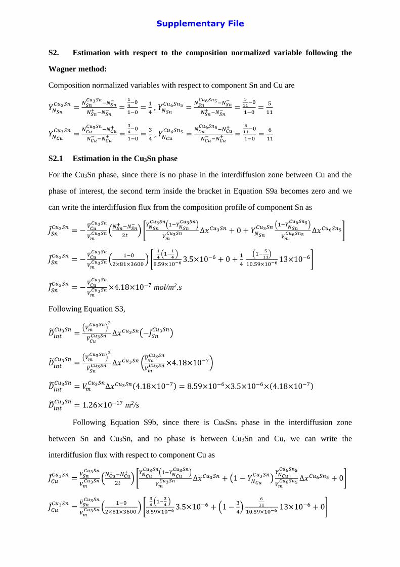
S2. Estimation with respect to the composition normalized variable following the
Wagner method:
Composition normalized variables with respect to component Sn and Cu are
𝑌𝑁𝑆𝑛
𝐶𝑢3𝑆𝑛=
𝑁𝑆𝑛𝐶𝑢3𝑆𝑛
−𝑁𝑆𝑛−
𝑁𝑆𝑛+ −𝑁𝑆𝑛
− =1
4−0
1−0=
1
4 , 𝑌𝑁𝑆𝑛
𝐶𝑢6𝑆𝑛5 =𝑁𝑆𝑛
𝐶𝑢6𝑆𝑛5−𝑁𝑆𝑛−
𝑁𝑆𝑛+ −𝑁𝑆𝑛
− =5
11−0
1−0=
5
11
𝑌𝑁𝐶𝑢
𝐶𝑢3𝑆𝑛=
𝑁𝐶𝑢𝐶𝑢3𝑆𝑛
−𝑁𝐶𝑢+
𝑁𝐶𝑢− −𝑁𝐶𝑢
+ =3
4−0
1−0=
3
4 , 𝑌𝑁𝐶𝑢
𝐶𝑢6𝑆𝑛5 =𝑁𝐶𝑢
𝐶𝑢6𝑆𝑛5−𝑁𝐶𝑢+
𝑁𝐶𝑢− −𝑁𝐶𝑢
+ =6
11−0
1−0=
6
11
S2.1 Estimation in the Cu3Sn phase
For the Cu3Sn phase, since there is no phase in the interdiffusion zone between Cu and the
phase of interest, the second term inside the bracket in Equation S9a becomes zero and we
can write the interdiffusion flux from the composition profile of component Sn as
𝐽𝑆𝑛𝐶𝑢3𝑆𝑛
= −�̅�𝐶𝑢
𝐶𝑢3𝑆𝑛
𝑉𝑚𝐶𝑢3𝑆𝑛 (
𝑁𝑆𝑛+ −𝑁𝑆𝑛
−
2𝑡) [
𝑌𝑁𝑆𝑛
𝐶𝑢3𝑆𝑛(1−𝑌𝑁𝑆𝑛
𝐶𝑢3𝑆𝑛)
𝑉𝑚𝐶𝑢3𝑆𝑛 ∆𝑥𝐶𝑢3𝑆𝑛 + 0 + 𝑌𝑁𝑆𝑛
𝐶𝑢3𝑆𝑛 (1−𝑌𝑁𝑆𝑛
𝐶𝑢6𝑆𝑛5)
𝑉𝑚𝐶𝑢6𝑆𝑛5
∆𝑥𝐶𝑢6𝑆𝑛5]
𝐽𝑆𝑛𝐶𝑢3𝑆𝑛
= −�̅�𝐶𝑢
𝐶𝑢3𝑆𝑛
𝑉𝑚𝐶𝑢3𝑆𝑛 (
1−0
2×81×3600 ) [
1
4 (1−
1
4 )
8.59×10⁻⁶ 3.5×10⁻⁶ + 0 +1
4
(1−5
11)
10.59×10⁻⁶ 13×10−6]
𝐽𝑆𝑛𝐶𝑢3𝑆𝑛
= −�̅�𝐶𝑢
𝐶𝑢3𝑆𝑛
𝑉𝑚𝐶𝑢3𝑆𝑛 ×4.18×10−7 mol/m2.s
Following Equation S3,
�̃�𝑖𝑛𝑡𝐶𝑢3𝑆𝑛
=(𝑉𝑚
𝐶𝑢3𝑆𝑛)
2
�̅�𝐶𝑢𝐶𝑢3𝑆𝑛 ∆𝑥𝐶𝑢3𝑆𝑛(−𝐽𝑆𝑛
𝐶𝑢3𝑆𝑛)
�̃�𝑖𝑛𝑡𝐶𝑢3𝑆𝑛
=(𝑉𝑚
𝐶𝑢3𝑆𝑛)
2
�̅�𝑆𝑛𝐶𝑢3𝑆𝑛 ∆𝑥𝐶𝑢3𝑆𝑛 (
�̅�𝑆𝑛𝐶𝑢3𝑆𝑛
𝑉𝑚𝐶𝑢3𝑆𝑛 ×4.18×10−7)
�̃�𝑖𝑛𝑡𝐶𝑢3𝑆𝑛
= 𝑉𝑚𝐶𝑢3𝑆𝑛
∆𝑥𝐶𝑢3𝑆𝑛(4.18×10⁻⁷) = 8.59×10−6×3.5×10−6×(4.18×10−7)
�̃�𝑖𝑛𝑡𝐶𝑢3𝑆𝑛
= 1.26×10⁻¹⁷ m2/s
Following Equation S9b, since there is Cu6Sn5 phase in the interdiffusion zone
between Sn and Cu3Sn, and no phase is between Cu3Sn and Cu, we can write the
interdiffusion flux with respect to component Cu as
𝐽𝐶𝑢𝐶𝑢3𝑆𝑛
=�̅�𝑆𝑛
𝐶𝑢3𝑆𝑛
𝑉𝑚𝐶𝑢3𝑆𝑛 (
𝑁𝐶𝑢− −𝑁𝐶𝑢
+
2𝑡) [
𝑌𝑁𝐶𝑢
𝐶𝑢3𝑆𝑛(1−𝑌𝑁𝐶𝑢
𝐶𝑢3𝑆𝑛)
𝑉𝑚𝐶𝑢3𝑆𝑛 ∆𝑥𝐶𝑢3𝑆𝑛 + (1 − 𝑌𝑁𝐶𝑢
𝐶𝑢3𝑆𝑛)
𝑌𝑁𝐶𝑢
𝐶𝑢6𝑆𝑛5
𝑉𝑚𝐶𝑢6𝑆𝑛5
∆𝑥𝐶𝑢6𝑆𝑛5 + 0]
𝐽𝐶𝑢𝐶𝑢3𝑆𝑛
=�̅�𝑆𝑛
𝐶𝑢3𝑆𝑛
𝑉𝑚𝐶𝑢3𝑆𝑛 (
1−0
2×81×3600 ) [
3
4 (1−
3
4 )
8.59×10⁻⁶ 3.5×10⁻⁶ + (1 −3
4)
6
11
10.59×10⁻⁶ 13×10−6 + 0]
Supplementary File
𝐽𝐶𝑢𝐶𝑢3𝑆𝑛
=�̅�𝑆𝑛
𝐶𝑢3𝑆𝑛
𝑉𝑚𝐶𝑢3𝑆𝑛 ×4.18×10−7 mol/m2.s
Following Equation S3,
�̃�𝑖𝑛𝑡𝐶𝑢3𝑆𝑛
=(𝑉𝑚
𝐶𝑢3𝑆𝑛)
2
�̅�𝐶𝑢𝐶𝑢3𝑆𝑛 ∆𝑥𝐶𝑢3𝑆𝑛(𝐽𝐶𝑢
𝐶𝑢3𝑆𝑛)
�̃�𝑖𝑛𝑡𝐶𝑢3𝑆𝑛
=(𝑉𝑚
𝐶𝑢3𝑆𝑛)
2
�̅�𝑆𝑛𝐶𝑢3𝑆𝑛 ∆𝑥𝐶𝑢3𝑆𝑛 (
�̅�𝑆𝑛𝐶𝑢3𝑆𝑛
𝑉𝑚𝐶𝑢3𝑆𝑛 ×4.18×10−7)
�̃�𝑖𝑛𝑡𝐶𝑢3𝑆𝑛
= 𝑉𝑚𝐶𝑢3𝑆𝑛
∆𝑥𝐶𝑢3𝑆𝑛(4.18×10⁻⁷) = 8.59×10−6×3.5×10−6×(4.18×10−7)
�̃�𝑖𝑛𝑡𝐶𝑢3𝑆𝑛
= 1.26×10⁻¹⁷ m2/s
Therefore, as it should be, the exactly same value is estimated following the composition
profiles of Sn and Cu. Most importantly, one has to make sure that Equation 6 is fulfilled.
This is indeed fulfilled since
�̅�𝐶𝑢𝐶𝑢3𝑆𝑛
𝐽𝐶𝑢𝐶𝑢3𝑆𝑛
+ �̅�𝑆𝑛𝐶𝑢3𝑆𝑛
𝐽𝑆𝑛𝐶𝑢3𝑆𝑛
= �̅�𝐶𝑢𝐶𝑢3𝑆𝑛 𝑉𝑆𝑛
𝐶𝑢3𝑆𝑛
𝑉𝑚𝐶𝑢3𝑆𝑛 ×4.18×10−7 − �̅�𝑆𝑛
𝐶𝑢3𝑆𝑛 𝑉𝐶𝑢𝐶𝑢3𝑆𝑛
𝑉𝑚𝐶𝑢3𝑆𝑛 ×4.18×10−7 = 0
S2.2 Estimation in the Cu6Sn5 phase
Following Equation S9a, since there is no phase in the interdiffusion zone between Cu6Sn5
and Sn, we can write the interdiffusion flux with respect to component Sn
𝐽𝑆𝑛𝐶𝑢6𝑆𝑛5 = −
𝑉𝐶𝑢𝐶𝑢6𝑆𝑛5
𝑉𝑚𝐶𝑢6𝑆𝑛5
(𝑁𝑆𝑛
+ −𝑁𝑆𝑛−
2𝑡) [
𝑌𝑁𝑆𝑛
𝐶𝑢6𝑆𝑛5(1−𝑌𝑁𝑆𝑛
𝐶𝑢6𝑆𝑛5)
𝑉𝑚𝐶𝑢6𝑆𝑛5
∆𝑥𝐶𝑢6𝑆𝑛5 + (1 − 𝑌𝑁𝑆𝑛
𝐶𝑢6𝑆𝑛5)𝑌𝑁𝑆𝑛
𝐶𝑢3𝑆𝑛
𝑉𝑚𝐶𝑢3𝑆𝑛 ∆𝑥𝐶𝑢3𝑆𝑛 + 0]
𝐽𝑆𝑛𝐶𝑢6𝑆𝑛5 = −
�̅�𝐶𝑢𝐶𝑢6𝑆𝑛5
𝑉𝑚𝐶𝑢6𝑆𝑛5
(1−0
2×81×3600 ) [
5
11(1−
5
11)
10.59×10⁻⁶ 13×10−6 + (1 −5
11)
1
4
8.59×10⁻⁶ 3.5×10⁻⁶ + 0]
𝐽𝑆𝑛𝐶𝑢6𝑆𝑛5 = −
�̅�𝐶𝑢𝐶𝑢6𝑆𝑛5
𝑉𝑚𝐶𝑢6𝑆𝑛5
6.17×10⁻⁷ mol/m2.s
Following Equation S3,
�̃�𝑖𝑛𝑡𝐶𝑢6𝑆𝑛5 =
(𝑉𝑚𝐶𝑢6𝑆𝑛5)
2
�̅�𝐶𝑢𝐶𝑢6𝑆𝑛5
∆𝑥𝐶𝑢6𝑆𝑛5(−𝐽𝑆𝑛𝐶𝑢6𝑆𝑛5)
�̃�𝑖𝑛𝑡𝐶𝑢6𝑆𝑛5 =
(𝑉𝑚𝐶𝑢6𝑆𝑛5)
2
�̅�𝐶𝑢𝐶𝑢6𝑆𝑛5
∆𝑥𝐶𝑢6𝑆𝑛5 (�̅�𝐶𝑢
𝐶𝑢6𝑆𝑛5
𝑉𝑚𝐶𝑢6𝑆𝑛5
6.17×10⁻⁷)
�̃�𝑖𝑛𝑡𝐶𝑢6𝑆𝑛5 = 𝑉𝑚
𝐶𝑢6𝑆𝑛5∆𝑥𝐶𝑢6𝑆𝑛5(6.17×10⁻⁷) = 10.59×10−6×13×10−6×(6.17×10−7)
�̃�𝑖𝑛𝑡𝐶𝑢6𝑆𝑛5 = 8.49 ×10⁻¹⁷ m2/s
Supplementary File
Following Equation S9b, since there is no phase in the interdiffusion zone between Sn
and Cu6Sn5, and Cu3Sn phase is between Cu6Sn5 and Cu, we can write the interdiffusion flux
with respect to component Cu as
𝐽𝐶𝑢𝐶𝑢6𝑆𝑛5 =
�̅�𝑆𝑛𝐶𝑢6𝑆𝑛5
𝑉𝑚𝐶𝑢6𝑆𝑛5
(𝑁𝐶𝑢
− −𝑁𝐶𝑢+
2𝑡) [
𝑌𝑁𝐶𝑢
𝐶𝑢6𝑆𝑛5(1−𝑌𝑁𝐶𝑢
𝐶𝑢6𝑆𝑛5)
𝑉𝑚𝐶𝑢6𝑆𝑛5
∆𝑥𝐶𝑢6𝑆𝑛5 + 0 + 𝑌𝑁𝐶𝑢
𝐶𝑢6𝑆𝑛5(1−𝑌𝑁𝐶𝑢
𝐶𝑢3𝑆𝑛)
𝑉𝑚𝐶𝑢3𝑆𝑛 ∆𝑥𝐶𝑢3𝑆𝑛]
𝐽𝐶𝑢𝐶𝑢6𝑆𝑛5 =
�̅�𝑆𝑛𝐶𝑢6𝑆𝑛5
𝑉𝑚𝐶𝑢6𝑆𝑛5
(1−0
2×81×3600 ) [
6
11(1−
6
11)
10.59×10⁻⁶ 13×10−6 + 0 +6
11
(1−3
4)
8.59×10⁻⁶ 3.5×10⁻⁶]
𝐽𝐶𝑢𝐶𝑢6𝑆𝑛5 =
�̅�𝑆𝑛𝐶𝑢6𝑆𝑛5
𝑉𝑚𝐶𝑢6𝑆𝑛5
6.17×10⁻⁷ mol/m2.s
Following Equation S3,
�̃�𝑖𝑛𝑡𝐶𝑢6𝑆𝑛5 =
(𝑉𝑚𝐶𝑢6𝑆𝑛5)
2
�̅�𝑆𝑛𝐶𝑢6𝑆𝑛5
∆𝑥𝐶𝑢6𝑆𝑛5(𝐽𝐶𝑢𝐶𝑢6𝑆𝑛5)
�̃�𝑖𝑛𝑡𝐶𝑢6𝑆𝑛5 =
(𝑉𝑚𝐶𝑢6𝑆𝑛5)
2
�̅�𝑆𝑛𝐶𝑢6𝑆𝑛5
∆𝑥𝐶𝑢6𝑆𝑛5 (�̅�𝑆𝑛
𝐶𝑢6𝑆𝑛5
𝑉𝑚𝐶𝑢6𝑆𝑛5
6.17×10⁻⁷)
�̃�𝑖𝑛𝑡𝐶𝑢6𝑆𝑛5 = 𝑉𝑚
𝐶𝑢6𝑆𝑛5∆𝑥𝐶𝑢6𝑆𝑛5(6.17×10⁻⁷) = 10.59×10−6×13×10−6×(6.17×10−7)
�̃�𝑖𝑛𝑡𝐶𝑢6𝑆𝑛5 = 8.49 ×10⁻¹⁷ m2/s
Therefore, again we have the same values when estimated with respect to component Sn and
Cu. We can also verify the Equation 6 following
�̅�𝐶𝑢𝐶𝑢6𝑆𝑛5𝐽𝐶𝑢
𝐶𝑢6𝑆𝑛5 + �̅�𝑆𝑛𝐶𝑢6𝑆𝑛5𝐽𝑆𝑛
𝐶𝑢6𝑆𝑛5 = �̅�𝐶𝑢𝐶𝑢6𝑆𝑛5 𝑉𝑆𝑛
𝐶𝑢6𝑆𝑛5
𝑉𝑚𝐶𝑢6𝑆𝑛5
6.17×10⁻⁷ − �̅�𝑆𝑛𝐶𝑢6𝑆𝑛5 𝑉𝐶𝑢
𝐶𝑢6𝑆𝑛5
𝑉𝑚𝐶𝑢6𝑆𝑛5
6.17×10−7 = 0
It is to be noted there that although the partial molar volume terms are unknown, we could
still verify the condition in Equation 6 is indeed fulfill. However, the same is not true with
respect to the concentration normalized variable, as shown in the next section.
S3. Estimation with respect to the concentration normalized variable following the
relations derived in the present work:
Since the partial molar volumes of components in the 𝛽 phase are unknown, it is evident from
Equations S7 or S8 that we cannot estimate �̃�𝑖𝑛𝑡𝛽
directly with respect to 𝑌𝐶𝐵 (and 𝑌𝐶𝐴
) or 𝐶𝐵
(and 𝐶𝐴). To facilitate the discussion on one of the important points as discussed in the
manuscript, we estimate data for both the actual and the ideal molar volume of the phase of
interest
Supplementary File
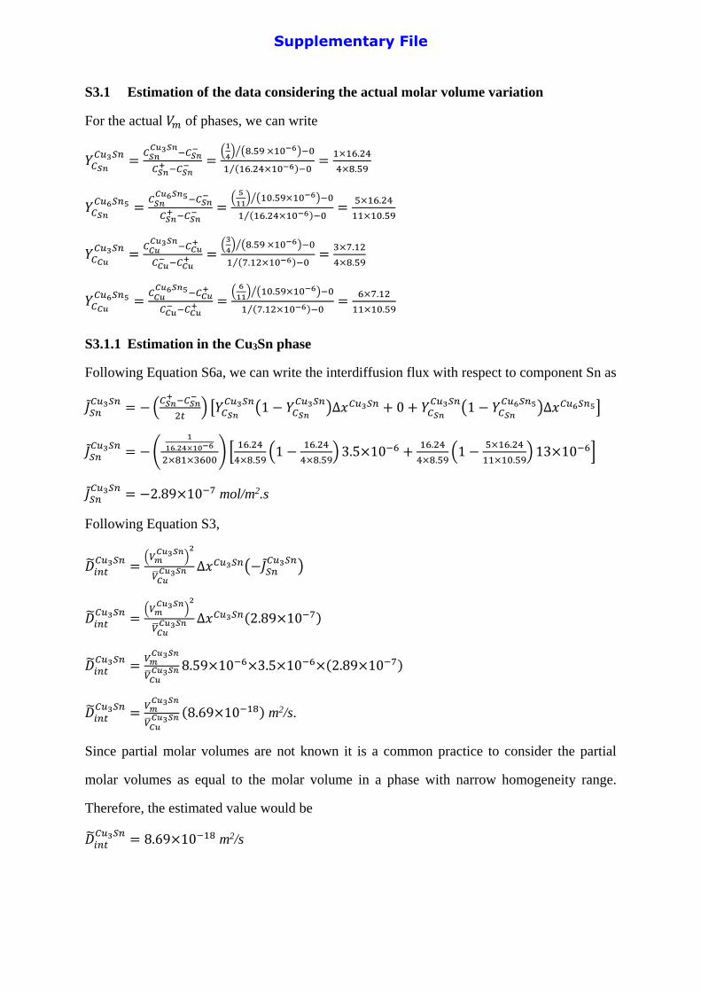
S3.1 Estimation of the data considering the actual molar volume variation
For the actual 𝑉𝑚 of phases, we can write
𝑌𝐶𝑆𝑛
𝐶𝑢3𝑆𝑛=
𝐶𝑆𝑛𝐶𝑢3𝑆𝑛
−𝐶𝑆𝑛−
𝐶𝑆𝑛+ −𝐶𝑆𝑛
− =(
1
4) (8.59 ×10⁻⁶)⁄ −0
1 (16.24×10⁻⁶)⁄ −0=
1×16.24
4×8.59
𝑌𝐶𝑆𝑛
𝐶𝑢6𝑆𝑛5 =𝐶𝑆𝑛
𝐶𝑢6𝑆𝑛5−𝐶𝑆𝑛−
𝐶𝑆𝑛+ −𝐶𝑆𝑛
− =(
5
11) (10.59×10⁻⁶)−0⁄
1 (16.24×10⁻⁶)⁄ −0=
5×16.24
11×10.59
𝑌𝐶𝐶𝑢
𝐶𝑢3𝑆𝑛=
𝐶𝐶𝑢𝐶𝑢3𝑆𝑛
−𝐶𝐶𝑢+
𝐶𝐶𝑢− −𝐶𝐶𝑢
+ =(
3
4) (8.59 ×10⁻⁶)⁄ −0
1 (7.12×10⁻⁶)⁄ −0=
3×7.12
4×8.59
𝑌𝐶𝐶𝑢
𝐶𝑢6𝑆𝑛5 =𝐶𝐶𝑢
𝐶𝑢6𝑆𝑛5−𝐶𝐶𝑢+
𝐶𝐶𝑢− −𝐶𝐶𝑢
+ =(
6
11) (10.59×10⁻⁶)⁄ −0
1 (7.12×10⁻⁶)⁄ −0=
6×7.12
11×10.59
S3.1.1 Estimation in the Cu3Sn phase
Following Equation S6a, we can write the interdiffusion flux with respect to component Sn as
𝐽𝑆𝑛𝐶𝑢3𝑆𝑛
= − (𝐶𝑆𝑛
+ −𝐶𝑆𝑛−
2𝑡) [𝑌𝐶𝑆𝑛
𝐶𝑢3𝑆𝑛(1 − 𝑌𝐶𝑆𝑛
𝐶𝑢3𝑆𝑛)∆𝑥𝐶𝑢3𝑆𝑛 + 0 + 𝑌𝐶𝑆𝑛
𝐶𝑢3𝑆𝑛(1 − 𝑌𝐶𝑆𝑛
𝐶𝑢6𝑆𝑛5)∆𝑥𝐶𝑢6𝑆𝑛5]
𝐽𝑆𝑛𝐶𝑢3𝑆𝑛
= − (1
16.24×10⁻⁶
2×81×3600) [
16.24
4×8.59(1 −
16.24
4×8.59) 3.5×10⁻⁶ +
16.24
4×8.59(1 −
5×16.24
11×10.59) 13×10−6]
𝐽𝑆𝑛𝐶𝑢3𝑆𝑛
= −2.89×10⁻⁷ mol/m2.s
Following Equation S3,
�̃�𝑖𝑛𝑡𝐶𝑢3𝑆𝑛
=(𝑉𝑚
𝐶𝑢3𝑆𝑛)
2
�̅�𝐶𝑢𝐶𝑢3𝑆𝑛 ∆𝑥𝐶𝑢3𝑆𝑛(−𝐽𝑆𝑛
𝐶𝑢3𝑆𝑛)
�̃�𝑖𝑛𝑡𝐶𝑢3𝑆𝑛
=(𝑉𝑚
𝐶𝑢3𝑆𝑛)
2
�̅�𝐶𝑢𝐶𝑢3𝑆𝑛 ∆𝑥𝐶𝑢3𝑆𝑛(2.89×10⁻⁷)
�̃�𝑖𝑛𝑡𝐶𝑢3𝑆𝑛
=𝑉𝑚
𝐶𝑢3𝑆𝑛
�̅�𝐶𝑢𝐶𝑢3𝑆𝑛 8.59×10−6×3.5×10−6×(2.89×10−7)
�̃�𝑖𝑛𝑡𝐶𝑢3𝑆𝑛
=𝑉𝑚
𝐶𝑢3𝑆𝑛
�̅�𝐶𝑢𝐶𝑢3𝑆𝑛 (8.69×10⁻¹⁸) m2/s.
Since partial molar volumes are not known it is a common practice to consider the partial
molar volumes as equal to the molar volume in a phase with narrow homogeneity range.
Therefore, the estimated value would be
�̃�𝑖𝑛𝑡𝐶𝑢3𝑆𝑛
= 8.69×10⁻¹⁸ m2/s
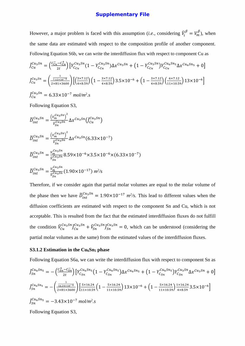
Supplementary File
However, a major problem is faced with this assumption (i.e., considering �̅�𝑖𝛽
= 𝑉𝑚𝛽
), when
the same data are estimated with respect to the composition profile of another component.
Following Equation S6b, we can write the interdiffusion flux with respect to component Cu as
𝐽𝐶𝑢𝐶𝑢3𝑆𝑛
= (𝐶𝐶𝑢
− −𝐶𝐶𝑢+
2𝑡) [𝑌𝐶𝐶𝑢
𝐶𝑢3𝑆𝑛(1 − 𝑌𝐶𝐶𝑢
𝐶𝑢3𝑆𝑛)∆𝑥𝐶𝑢3𝑆𝑛 + (1 − 𝑌𝐶𝐶𝑢
𝐶𝑢3𝑆𝑛)𝑌𝐶𝐶𝑢
𝐶𝑢6𝑆𝑛5∆𝑥𝐶𝑢6𝑆𝑛5 + 0]
𝐽𝐶𝑢𝐶𝑢3𝑆𝑛
= (1
7.12×10⁻⁶
2×81×3600) [(
3×7.12
4×8.59) (1 −
3×7.12
4×8.59) 3.5×10⁻⁶ + (1 −
3×7.12
4×8.59) (
6×7.12
11×10.59) 13×10−6]
𝐽𝐶𝑢𝐶𝑢3𝑆𝑛
= 6.33×10⁻⁷ mol/m2.s
Following Equation S3,
�̃�𝑖𝑛𝑡𝐶𝑢3𝑆𝑛
=(𝑉𝑚
𝐶𝑢3𝑆𝑛)
2
�̅�𝑆𝑛𝐶𝑢3𝑆𝑛 ∆𝑥𝐶𝑢3𝑆𝑛(𝐽𝐶𝑢
𝐶𝑢3𝑆𝑛)
�̃�𝑖𝑛𝑡𝐶𝑢3𝑆𝑛
=(𝑉𝑚
𝐶𝑢3𝑆𝑛)
2
�̅�𝑆𝑛𝐶𝑢3𝑆𝑛 ∆𝑥𝐶𝑢3𝑆𝑛(6.33×10⁻⁷)
�̃�𝑖𝑛𝑡𝐶𝑢3𝑆𝑛
=𝑉𝑚
𝐶𝑢3𝑆𝑛
�̅�𝑆𝑛𝐶𝑢3𝑆𝑛 8.59×10−6×3.5×10−6×(6.33×10−7)
�̃�𝑖𝑛𝑡𝐶𝑢3𝑆𝑛
=𝑉𝑚
𝐶𝑢3𝑆𝑛
�̅�𝑆𝑛𝐶𝑢3𝑆𝑛 (1.90×10⁻¹⁷) m2/s
Therefore, if we consider again that partial molar volumes are equal to the molar volume of
the phase then we have �̃�𝑖𝑛𝑡𝐶𝑢3𝑆𝑛
= 1.90×10⁻¹⁷ m2/s. This lead to different values when the
diffusion coefficients are estimated with respect to the component Sn and Cu, which is not
acceptable. This is resulted from the fact that the estimated interdiffusion fluxes do not fulfill
the condition �̅�𝐶𝑢𝐶𝑢3𝑆𝑛
𝐽𝐶𝑢𝐶𝑢3𝑆𝑛
+ �̅�𝑆𝑛𝐶𝑢3𝑆𝑛
𝐽𝑆𝑛𝐶𝑢3𝑆𝑛
= 0, which can be understood (considering the
partial molar volumes as the same) from the estimated values of the interdiffusion fluxes.
S3.1.2 Estimation in the Cu6Sn5 phase
Following Equation S6a, we can write the interdiffusion flux with respect to component Sn as
𝐽𝑆𝑛𝐶𝑢6𝑆𝑛5 = − (
𝐶𝑆𝑛+ −𝐶𝑆𝑛
−
2𝑡) [𝑌𝐶𝑆𝑛
𝐶𝑢6𝑆𝑛5(1 − 𝑌𝐶𝑆𝑛
𝐶𝑢6𝑆𝑛5)∆𝑥𝐶𝑢6𝑆𝑛5 + (1 − 𝑌𝐶𝑆𝑛
𝐶𝑢6𝑆𝑛5)𝑌𝐶𝑆𝑛
𝐶𝑢3𝑆𝑛∆𝑥𝐶𝑢3𝑆𝑛 + 0]
𝐽𝑆𝑛𝐶𝑢6𝑆𝑛5 = − (
1
16.24×10⁻⁶
2×81×3600) [
5×16.24
11×10.59(1 −
5×16.24
11×10.59) 13×10−6 + (1 −
5×16.24
11×10.59)
1×16.24
4×8.593.5×10−6]
𝐽𝑆𝑛𝐶𝑢6𝑆𝑛5 = −3.43×10⁻⁷ mol/m2.s
Following Equation S3,
Supplementary File
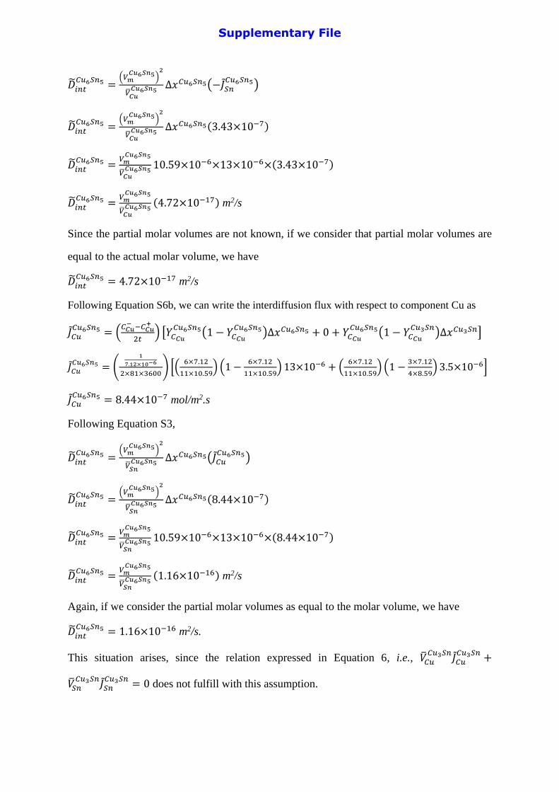
�̃�𝑖𝑛𝑡𝐶𝑢6𝑆𝑛5 =
(𝑉𝑚𝐶𝑢6𝑆𝑛5)
2
�̅�𝐶𝑢𝐶𝑢6𝑆𝑛5
∆𝑥𝐶𝑢6𝑆𝑛5(−𝐽𝑆𝑛𝐶𝑢6𝑆𝑛5)
�̃�𝑖𝑛𝑡𝐶𝑢6𝑆𝑛5 =
(𝑉𝑚𝐶𝑢6𝑆𝑛5)
2
�̅�𝐶𝑢𝐶𝑢6𝑆𝑛5
∆𝑥𝐶𝑢6𝑆𝑛5(3.43×10⁻⁷)
�̃�𝑖𝑛𝑡𝐶𝑢6𝑆𝑛5 =
𝑉𝑚𝐶𝑢6𝑆𝑛5
�̅�𝐶𝑢𝐶𝑢6𝑆𝑛5
10.59×10−6×13×10−6×(3.43×10−7)
�̃�𝑖𝑛𝑡𝐶𝑢6𝑆𝑛5 =
𝑉𝑚𝐶𝑢6𝑆𝑛5
�̅�𝐶𝑢𝐶𝑢6𝑆𝑛5
(4.72×10⁻¹⁷) m2/s
Since the partial molar volumes are not known, if we consider that partial molar volumes are
equal to the actual molar volume, we have
�̃�𝑖𝑛𝑡𝐶𝑢6𝑆𝑛5 = 4.72×10⁻¹⁷ m2/s
Following Equation S6b, we can write the interdiffusion flux with respect to component Cu as
𝐽𝐶𝑢𝐶𝑢6𝑆𝑛5 = (
𝐶𝐶𝑢− −𝐶𝐶𝑢
+
2𝑡) [𝑌𝐶𝐶𝑢
𝐶𝑢6𝑆𝑛5(1 − 𝑌𝐶𝐶𝑢
𝐶𝑢6𝑆𝑛5)∆𝑥𝐶𝑢6𝑆𝑛5 + 0 + 𝑌𝐶𝐶𝑢
𝐶𝑢6𝑆𝑛5(1 − 𝑌𝐶𝐶𝑢
𝐶𝑢3𝑆𝑛)∆𝑥𝐶𝑢3𝑆𝑛]
𝐽𝐶𝑢𝐶𝑢6𝑆𝑛5 = (
1
7.12×10⁻⁶
2×81×3600) [(
6×7.12
11×10.59) (1 −
6×7.12
11×10.59) 13×10−6 + (
6×7.12
11×10.59) (1 −
3×7.12
4×8.59) 3.5×10⁻⁶]
𝐽𝐶𝑢𝐶𝑢6𝑆𝑛5 = 8.44×10⁻⁷ mol/m2.s
Following Equation S3,
�̃�𝑖𝑛𝑡𝐶𝑢6𝑆𝑛5 =
(𝑉𝑚𝐶𝑢6𝑆𝑛5)
2
�̅�𝑆𝑛𝐶𝑢6𝑆𝑛5
∆𝑥𝐶𝑢6𝑆𝑛5(𝐽𝐶𝑢𝐶𝑢6𝑆𝑛5)
�̃�𝑖𝑛𝑡𝐶𝑢6𝑆𝑛5 =
(𝑉𝑚𝐶𝑢6𝑆𝑛5)
2
�̅�𝑆𝑛𝐶𝑢6𝑆𝑛5
∆𝑥𝐶𝑢6𝑆𝑛5(8.44×10⁻⁷)
�̃�𝑖𝑛𝑡𝐶𝑢6𝑆𝑛5 =
𝑉𝑚𝐶𝑢6𝑆𝑛5
�̅�𝑆𝑛𝐶𝑢6𝑆𝑛5
10.59×10−6×13×10−6×(8.44×10−7)
�̃�𝑖𝑛𝑡𝐶𝑢6𝑆𝑛5 =
𝑉𝑚𝐶𝑢6𝑆𝑛5
�̅�𝑆𝑛𝐶𝑢6𝑆𝑛5
(1.16×10⁻¹⁶) m2/s
Again, if we consider the partial molar volumes as equal to the molar volume, we have
�̃�𝑖𝑛𝑡𝐶𝑢6𝑆𝑛5 = 1.16×10⁻¹⁶ m2/s.
This situation arises, since the relation expressed in Equation 6, i.e., �̅�𝐶𝑢𝐶𝑢3𝑆𝑛
𝐽𝐶𝑢𝐶𝑢3𝑆𝑛
+
�̅�𝑆𝑛𝐶𝑢3𝑆𝑛
𝐽𝑆𝑛𝐶𝑢3𝑆𝑛
= 0 does not fulfill with this assumption.
Supplementary File
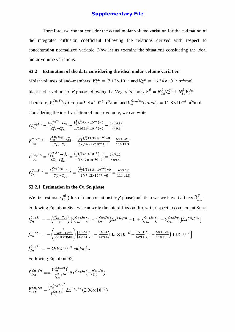
Therefore, we cannot consider the actual molar volume variation for the estimation of
the integrated diffusion coefficient following the relations derived with respect to
concentration normalized variable. Now let us examine the situations considering the ideal
molar volume variations.
S3.2 Estimation of the data considering the ideal molar volume variation
Molar volumes of end–members: 𝑉𝑚𝐶𝑢 = 7.12×10⁻⁶ and 𝑉𝑚
𝑆𝑛 = 16.24×10⁻⁶ m3/mol
Ideal molar volume of 𝛽 phase following the Vegard’s law is 𝑉𝑚𝛽
= 𝑁𝐶𝑢𝛽
𝑉𝑚𝐶𝑢 + 𝑁𝑆𝑛
𝛽𝑉𝑚
𝑆𝑛
Therefore, 𝑉𝑚𝐶𝑢3𝑆𝑛
(𝑖𝑑𝑒𝑎𝑙) = 9.4×10⁻⁶ m3/mol and 𝑉𝑚𝐶𝑢6𝑆𝑛5(𝑖𝑑𝑒𝑎𝑙) = 11.3×10⁻⁶ m3/mol
Considering the ideal variation of molar volume, we can write
𝑌𝐶𝑆𝑛
𝐶𝑢3𝑆𝑛=
𝐶𝑆𝑛𝐶𝑢3𝑆𝑛
−𝐶𝑆𝑛−
𝐶𝑆𝑛+ −𝐶𝑆𝑛
− =(
1
4) (9.4 ×10⁻⁶)⁄ −0
1 (16.24×10⁻⁶)⁄ −0=
1×16.24
4×9.4
𝑌𝐶𝑆𝑛
𝐶𝑢6𝑆𝑛5 =𝐶𝑆𝑛
𝐶𝑢6𝑆𝑛5−𝐶𝑆𝑛−
𝐶𝑆𝑛+ −𝐶𝑆𝑛
− =(
5
11) (11.3×10⁻⁶)⁄ −0
1 (16.24×10⁻⁶)⁄ −0=
5×16.24
11×11.3
𝑌𝐶𝐶𝑢
𝐶𝑢3𝑆𝑛=
𝐶𝐶𝑢𝐶𝑢3𝑆𝑛
−𝐶𝐶𝑢+
𝐶𝐶𝑢− −𝐶𝐶𝑢
+ =(
3
4) (9.4 ×10⁻⁶)⁄ −0
1 (7.12×10⁻⁶)⁄ −0=
3×7.12
4×9.4
𝑌𝐶𝐶𝑢
𝐶𝑢6𝑆𝑛5 =𝐶𝐶𝑢
𝐶𝑢6𝑆𝑛5−𝐶𝐶𝑢+
𝐶𝐶𝑢− −𝐶𝐶𝑢
+ =(
6
11) (11.3 ×10⁻⁶)⁄ −0
1 (7.12×10⁻⁶)⁄ −0=
6×7.12
11×11.3
S3.2.1 Estimation in the Cu3Sn phase
We first estimate 𝐽𝑖𝛽
(flux of component inside 𝛽 phase) and then we see how it affects �̃�𝑖𝑛𝑡𝛽
.
Following Equation S6a, we can write the interdiffusion flux with respect to component Sn as
𝐽𝑆𝑛𝐶𝑢3𝑆𝑛
= − (𝐶𝑆𝑛
+ −𝐶𝑆𝑛−
2𝑡) [𝑌𝐶𝑆𝑛
𝐶𝑢3𝑆𝑛(1 − 𝑌𝐶𝑆𝑛
𝐶𝑢3𝑆𝑛)∆𝑥𝐶𝑢3𝑆𝑛 + 0 + 𝑌𝐶𝑆𝑛
𝐶𝑢3𝑆𝑛(1 − 𝑌𝐶𝑆𝑛
𝐶𝑢6𝑆𝑛5)∆𝑥𝐶𝑢6𝑆𝑛5]
𝐽𝑆𝑛𝐶𝑢3𝑆𝑛
= − (1
16.24×10⁻⁶
2×81×3600) [
16.24
4×9.4(1 −
16.24
4×9.4) 3.5×10⁻⁶ +
16.24
4×9.4(1 −
5×16.24
11×11.3) 13×10−6]
𝐽𝑆𝑛𝐶𝑢3𝑆𝑛
= −2.96×10⁻⁷ mol/m2.s
Following Equation S3,
�̃�𝑖𝑛𝑡𝐶𝑢3𝑆𝑛
==(𝑉𝑚
𝐶𝑢3𝑆𝑛)
2
�̅�𝐶𝑢𝐶𝑢3𝑆𝑛 ∆𝑥𝐶𝑢3𝑆𝑛(−𝐽𝑆𝑛
𝐶𝑢3𝑆𝑛)
�̃�𝑖𝑛𝑡𝐶𝑢3𝑆𝑛
=(𝑉𝑚
𝐶𝑢3𝑆𝑛)
2
�̅�𝐶𝑢𝐶𝑢3𝑆𝑛 ∆𝑥𝐶𝑢3𝑆𝑛(2.96×10⁻⁷)
Supplementary File
�̃�𝑖𝑛𝑡𝐶𝑢3𝑆𝑛
=(9.4×10⁻⁶)
2
7.12×10−6 ×3.5×10−6×(2.96×10−7)
�̃�𝑖𝑛𝑡𝐶𝑢3𝑆𝑛
≈ 1.28×10⁻¹⁷ m2/s.
Following Equation S6b, we can write the interdiffusion flux with respect to component Cu as
𝐽𝐶𝑢𝐶𝑢3𝑆𝑛
= (𝐶𝐶𝑢
− −𝐶𝐶𝑢+
2𝑡) [𝑌𝐶𝐶𝑢
𝐶𝑢3𝑆𝑛(1 − 𝑌𝐶𝐶𝑢
𝐶𝑢3𝑆𝑛)∆𝑥𝐶𝑢3𝑆𝑛 + (1 − 𝑌𝐶𝐶𝑢
𝐶𝑢3𝑆𝑛)𝑌𝐶𝐶𝑢
𝐶𝑢6𝑆𝑛5∆𝑥𝐶𝑢6𝑆𝑛5 + 0]
𝐽𝐶𝑢𝐶𝑢3𝑆𝑛
= (1
7.12×10⁻⁶
2×81×3600) [(
3×7.12
4×9.4) (1 −
3×7.12
4×9.4) 3.5×10⁻⁶ + (1 −
3×7.12
4×9.4) (
6×7.12
11×11.3) 13×10−6]
𝐽𝐶𝑢𝐶𝑢3𝑆𝑛
= 6.71×10⁻⁷ mol/m2.s
Following Equation S3,
�̃�𝑖𝑛𝑡𝐶𝑢3𝑆𝑛
=(𝑉𝑚
𝐶𝑢3𝑆𝑛)
2
�̅�𝑆𝑛𝐶𝑢3𝑆𝑛 ∆𝑥𝐶𝑢3𝑆𝑛(𝐽𝐶𝑢
𝐶𝑢3𝑆𝑛)
�̃�𝑖𝑛𝑡𝐶𝑢3𝑆𝑛
=(𝑉𝑚
𝐶𝑢3𝑆𝑛)
2
�̅�𝑆𝑛𝐶𝑢3𝑆𝑛 ∆𝑥𝐶𝑢3𝑆𝑛(6.71×10⁻⁷)
�̃�𝑖𝑛𝑡𝐶𝑢3𝑆𝑛
=(9.4×10⁻⁶)
2
16.24×10−6 ×3.5×10−6×(6.71×10−7)
�̃�𝑖𝑛𝑡𝐶𝑢3𝑆𝑛
≈ 1.28×10⁻¹⁷ m2/s.
Therefore, we get the same value when estimated with respect to the component Sn and Cu,
since the relation expressed in Equation 6 is also fulfilled
�̅�𝐶𝑢𝐶𝑢3𝑆𝑛
𝐽𝐶𝑢𝐶𝑢3𝑆𝑛
+ �̅�𝑆𝑛𝐶𝑢3𝑆𝑛
𝐽𝑆𝑛𝐶𝑢3𝑆𝑛
= 7.12×10−6 ×6.71×10−7 − 16.24×10−6×2.96×10−7 ≈ 0
S3.2.2 Estimation in the Cu6Sn5 phase
Following Equation S6a, we can write the interdiffusion flux with respect to component Sn as
𝐽𝑆𝑛𝐶𝑢6𝑆𝑛5 = − (
𝐶𝑆𝑛+ −𝐶𝑆𝑛
−
2𝑡) [𝑌𝐶𝑆𝑛
𝐶𝑢6𝑆𝑛5(1 − 𝑌𝐶𝑆𝑛
𝐶𝑢6𝑆𝑛5)∆𝑥𝐶𝑢6𝑆𝑛5 + (1 − 𝑌𝐶𝑆𝑛
𝐶𝑢6𝑆𝑛5)𝑌𝐶𝑆𝑛
𝐶𝑢3𝑆𝑛∆𝑥𝐶𝑢3𝑆𝑛 + 0]
𝐽𝑆𝑛𝐶𝑢6𝑆𝑛5 = − (
1
16.24×10⁻⁶
2×81×3600) [
5×16.24
11×11.3(1 −
5×16.24
11×11.3) 13×10−6 + (1 −
5×16.24
11×11.3)
16.24
4×9.43.5×10−6]
𝐽𝑆𝑛𝐶𝑢6𝑆𝑛5 = −3.66×10⁻⁷ mol/m2.s
Following Equation S3,
�̃�𝑖𝑛𝑡𝐶𝑢6𝑆𝑛5 =
(𝑉𝑚𝐶𝑢6𝑆𝑛5)
2
�̅�𝐶𝑢𝐶𝑢6𝑆𝑛5
∆𝑥𝐶𝑢6𝑆𝑛5(−𝐽𝑆𝑛𝐶𝑢6𝑆𝑛5)
Supplementary File
�̃�𝑖𝑛𝑡𝐶𝑢6𝑆𝑛5 =
(𝑉𝑚𝐶𝑢6𝑆𝑛5)
2
�̅�𝐶𝑢𝐶𝑢6𝑆𝑛5
∆𝑥𝐶𝑢6𝑆𝑛5(3.66×10⁻⁷)
�̃�𝑖𝑛𝑡𝐶𝑢6𝑆𝑛5 =
(11.3×10⁻⁶)2
7.12×10−6 ×13×10−6×(3.66×10−7)
�̃�𝑖𝑛𝑡𝐶𝑢6𝑆𝑛5 ≈ 8.53×10⁻¹⁷ m2/s
Following Equation S6b, we can write the interdiffusion flux with respect to component Cu as
𝐽𝐶𝑢𝐶𝑢6𝑆𝑛5 = (
𝐶𝐶𝑢− −𝐶𝐶𝑢
+
2𝑡) [𝑌𝐶𝐶𝑢
𝐶𝑢6𝑆𝑛5(1 − 𝑌𝐶𝐶𝑢
𝐶𝑢6𝑆𝑛5)∆𝑥𝐶𝑢6𝑆𝑛5 + 0 + 𝑌𝐶𝐶𝑢
𝐶𝑢6𝑆𝑛5(1 − 𝑌𝐶𝐶𝑢
𝐶𝑢3𝑆𝑛)∆𝑥𝐶𝑢3𝑆𝑛]
𝐽𝐶𝑢𝐶𝑢6𝑆𝑛5 = (
1
7.12×10⁻⁶
2×81×3600) [(
6×7.12
11×11.3) (1 −
6×7.12
11×11.3) 13×10−6 + (
6×7.12
11×11.3) (1 −
3×7.12
4×9.4) 3.5×10⁻⁶]
𝐽𝐶𝑢𝐶𝑢6𝑆𝑛5 = 8.31×10⁻⁷ mol/m2.s
Following Equation S3,
�̃�𝑖𝑛𝑡𝐶𝑢6𝑆𝑛5 =
(𝑉𝑚𝐶𝑢6𝑆𝑛5)
2
�̅�𝑆𝑛𝐶𝑢6𝑆𝑛5
∆𝑥𝐶𝑢6𝑆𝑛5(𝐽𝐶𝑢𝐶𝑢6𝑆𝑛5)
�̃�𝑖𝑛𝑡𝐶𝑢6𝑆𝑛5 =
(𝑉𝑚𝐶𝑢6𝑆𝑛5)
2
�̅�𝑆𝑛𝐶𝑢6𝑆𝑛5
∆𝑥𝐶𝑢6𝑆𝑛5(8.31×10⁻⁷)
�̃�𝑖𝑛𝑡𝐶𝑢6𝑆𝑛5 =
(11.3×10⁻⁶)2
16.24×10−6 ×13×10−6×(8.31×10−7)
�̃�𝑖𝑛𝑡𝐶𝑢6𝑆𝑛5 ≈ 8.53×10⁻¹⁷ m2/s
Therefore, we have the same value when estimated with respect to the component Sn and Cu,
since Equation 6 fulfills following
�̅�𝐶𝑢𝐶𝑢6𝑆𝑛5𝐽𝐶𝑢
𝐶𝑢6𝑆𝑛5 + �̅�𝑆𝑛𝐶𝑢6𝑆𝑛5𝐽𝑆𝑛
𝐶𝑢6𝑆𝑛5 = 7.12×10−6 ×8.31×10−7 − 16.24×10−6×3.66×10−7 ≈ 0
Therefore, we can conclude that if the relation with respect to the concentration normalized
variable is used for the estimation of the interdiffusion coefficient, we need to consider the
ideal molar volume. We cannot consider the actual molar volumes of the phases.
One important fact should be noted here that
For pure end–members, 𝑁𝐵− = 0, 𝑁𝐴
+ = 0, 𝑁𝐵+ = 1 and 𝑁𝐴
− = 1.
Therefore, we have 𝐶𝐵− = 0, 𝐶𝐴
+ = 0, 𝐶𝐵+ =
1
𝑉𝑚+ and 𝐶𝐴
− =1
𝑉𝑚− such that
𝑌𝐶𝐵=
𝐶𝐵−𝐶𝐵−
𝐶𝐵+−𝐶𝐵
− =𝐶𝐵
𝐶𝐵+ =
𝑁𝐵
𝑉𝑚×𝑉𝑚
+ =𝑌𝑁𝐵
𝑉𝑚×𝑉𝑚
+
Supplementary File
𝑌𝐶𝐴=
𝐶𝐴−𝐶𝐴+
𝐶𝐴−−𝐶𝐴
+ =𝐶𝐴
𝐶𝐴− =
𝑁𝐴
𝑉𝑚×𝑉𝑚
− =𝑌𝑁𝐴
𝑉𝑚×𝑉𝑚
−
While using the relations with respect to the composition normalized variables, only the
molar volumes of phases is considered irrespective of the choice of diffusion profile of
component A or B; however, the same is not true while using the relations with respect to the
concentration normalized variables, since depending on the choice of diffusion profile, the
molar volume (𝑉𝑚+ or 𝑉𝑚
−) of one of the end–members along with that of the phases is always
being considered for the estimation of a particular diffusion parameter, leading to very minor
difference in the estimated values.